Quantum theory of wave propagation and linear amplification in free electron lasers
Upload
khangminh22Category
view
0download
0
Universitat Politècnica de CatalunyaBarcelonaTech
Escola Tècnica Superior d’Enginyers de Camins, Canals i Portsde Barcelona
Doctoral Program in Civil Engineering
Doctoral Thesis
Wave Propagation Problems
with Aeroacoustic Applications
Author:Hector Espinoza
Supervisors:Prof. Ramon CodinaProf. Santiago Badia
2015


i
Acta de Calificación de Tesis Doctoral
Curso Académico: 2014-2015Nombres y Apellidos: Héctor Gabriel, Espinoza RománPrograma de doctorado: Ingeniería CivilUnidad estructural responsable del programa: ETSECCPB
Resolución del tribunalReunido el Tribunal designado a tal efecto, el doctorando / la doctoranda expone
el tema de la su tesis doctoral titulada: Wave Propagation Problems with AeroacousticApplications.
Acabada la lectura y después de dar respuesta a las cuestiones formuladas por losmiembros titulares del tribunal, éste otorga la calificación:
NO APTO APROBADO NOTABLE SOBRESALIENTE
(Nombre, apellidos y firma) (Nombre, apellidos y firma)
Presidente/a Secretario/a(Nombre, apellidos y firma) (Nombre, apellidos y firma) (Nombre, apellidos y firma)
Vocal Vocal Vocal
El resultado del escrutinio de los votos emitidos por los miembros titulares del tribunal,efectuado por la Escuela de Doctorado, a instancia de la Comisión de Doctorado de laUPC, otorga la MENCIÓN CUM LAUDE:
SÍ NO
(Nombre, apellidos y firma) (Nombre, apellidos y firma)
Presidente de la Comisión Permanente dela Escuela de Doctorado
Secretario de la Comisión Permanente dela Escuela de Doctorado
a de de .


to my family
iii


Acknowledgement
I would like to acknowledge the help and constant support of my advisors Ramon Codinaand Santiago Badia. Their guidance, scientific rigor and valuable suggestions made thiswork possible.
Additionally, I appreciate the opportune help from my workmates Joan Baiges, MatíasÁvila and Christian Muñoz in various code implementation aspects. In addition, I wouldlike to mention Ernesto, Fermin, Ester, Arnau and Alexis with whom I shared office duringmy doctoral period.
Likewise, I would like to mention Oscar Fruitos, Alberto Ferriz, Martí Coma and LuisFernández from CIMNE-TTS where I worked in many interesting projects.
In addition, I would like to thank the support received from the EUNISON project(EU-FET grant 308874), specially from Oriol Guasch and Marc Arnela regarding the voicesimulation cases.
Moreover, I would like to acknowledge Johan Hoffman and Niyazi Cem Degirmencifor their support during my short stay at Kungliga Tekniska Högskolan (Royal Instituteof Technology) in Stockholm, Sweden. Additionally, I would like to mention Aurélien,Jeannette, Bärbel and Rodrigo whom I met at KTH.
Not to mention the support of my family that despite the distance is always with mein many ways.
Finally, I would like to acknowledge the Formación de Profesorado Universitario pro-gram from the Spanish Ministry of Education for their support through the doctoral grantAP2010-0563.
v


Abstract
The present work is a compilation of the research produced in the field of wave propagationmodeling. It contains in-depth analysis of stability, convergence, dispersion and dissipationof spatial, temporal and spatial-temporal discretization schemes. Space discretization isdone using stabilized finite element methods denoted with the acronyms ASGS and OSS.Time discretization is done using finite difference methods including backward Euler (BE),2nd order backward differentiation formula (BDF2) and Crank-Nicolson (CN).
Firstly, we propose two stabilized finite element methods for different functional frame-works of the wave equation in mixed form. These stabilized finite element methods arestable for any pair of interpolation spaces of the unknowns. The variational forms cor-responding to different functional settings are treated in a unified manner through theintroduction of length scales related to the unknowns. Stability and convergence analysisis performed together with numerical experiments. It is shown that modifying the lengthscales allows one to mimic at the discrete level the different functional settings of thecontinuous problem and influence the stability and accuracy of the resulting methods.
Then, we develop numerical approximations of the wave equation in mixed form supple-mented with non-reflecting boundary conditions (NRBCs) of Sommerfeld-type on artificialboundaries for truncated domains. Stability and convergence analyses of these stabilizedformulations including the NRBC are presented. Additionally, numerical convergence testsare evaluated for various polynomial interpolations, stabilization methods and variationalforms. Finally, several benchmark problems are solved to determine the accuracy of thesemethods in 2D and 3D.
Afterwards, we analyze time marching schemes for the wave equation in mixed form.The problem is discretized in space using stabilized finite elements. On the one hand,stability and convergence analyses of the fully discrete numerical schemes are presented.On the other hand, we use Fourier techniques (also known as von Neumann analysis) inorder to analyze stability, dispersion and dissipation. Additionally, numerical convergencetests are presented for various time integration schemes, polynomial interpolations (for thespatial discretization), stabilization methods and variational forms. Finally, a 1D exampleis solved to analyze the behavior of the different schemes considered.
Later, we present various application examples and compare the numerical results of thedifferent algorithms i.e. ASGS or OSS stabilization and BE, BDF2 or CN time marchingschemes. Additionally, comparison with experiments is performed in some cases.
Finally, conclusions are drawn including the research achievements and future work.
vii


Resumen
El presente trabajo es una compilación de la investigación producida en el campo demodelado de propagación de ondas. Contiene análisis de estabilidad, convergencia, dis-persión y disipación de discretizaciones espaciales, temporales y espacio-temporales. Ladiscretización espacial se hace usando elementos finitos estabilizados denotados por losacrónimos ASGS y OSS. La discretización temporal se hace usando métodos de diferenciasfinitas incluyendo backward Euler (BE), backward differentiation formula de 2do orden(BDF2) y Crank-Nicolson (CN).
En primer lugar, proponemos dos métodos de elementos finitos estabilizados paradiferentes marcos funcionales de la ecuación de ondas en forma mixta. Estos métodos deelementos finitos estabilizados son estables para cualquier par de espacios de interpolaciónde las incógnitas. Las formas variacionales que corresponden a los diferentes marcosfuncionales son tratadas de manera unificada a través de la introducción de longitudes deescalado relacionadas con las incógnitas. Estabilidad y convergencia son analizadas juntocon experimentos numéricos. Se muestra como modificando las longitudes de escalado sepuede reproducir a nivel discreto los diferentes marcos funcionales del problema continuoy como influencian la estabilidad y precisión de los métodos resultantes.
Luego, desarrollamos aproximaciones numéricas de la ecuación de ondas en forma mixtacomplementadas con condiciones de frontera de no-reflexión (NRBCs) de tipo Sommerfeldsobre fronteras artificiales para dominios truncados. Análisis de estabilidad y convergenciade estas formulaciones estabilizadas incluyendo la NRBC son presentados. Adicionalmente,pruebas de convergencia son llevadas a cabo para varias interpolaciones polinomiales, méto-dos de estabilización y formas variacionales. Finalmente, varios problemas de referenciason resueltos para determinar la precisión de estos métodos en 2D y 3D.
Después, analizamos esquemas de discretización temporal para la ecuación de ondas enforma mixta. El problema es discretizado en el espacio utilizando elementos finitos esta-bilizados. Por un lado, análisis de convergencia y estabilidad de los esquemas numéricostotalmente discretos son presentados. Por otro lado, usamos técnicas de Fourier (tambiénconocidas como análisis de von Neumann) con el fin de analizar estabilidad, dispersión ydisipación. Adicionalmente, pruebas numéricas de convergencia son presentadas para var-ios esquemas de integración temporal, interpolaciones polinomiales (para la discretizaciónespacial), métodos de estabilización y formas variacionales. Finalmente, un ejemplo 1D esresuelto para analizar el comportamiento de los diferentes esquemas numéricos considera-dos.
Más tarde, presentamos varios ejemplos de aplicación y comparamos los resultadosnuméricos de los diferentes algoritmos. Por ejemplo estabilización ASGS/OSS y esque-mas de integración temporal BD/BDF2/CN. Adicionalmente, se compara los resultados
ix

x
numéricos con resultados experimentales en algunos casos.Por último, las conclusiones son presentadas incluyendo los logros obtenidos en esta
investigación y el trabajo futuro.

Contents
1 Introduction 11.1 Motivation . . . . . . . . . . . . . . . . . . . . . . . . . . . . . . . . . . . . 11.2 Overview . . . . . . . . . . . . . . . . . . . . . . . . . . . . . . . . . . . . . 21.3 Wave Equations . . . . . . . . . . . . . . . . . . . . . . . . . . . . . . . . . 2
1.3.1 Introduction . . . . . . . . . . . . . . . . . . . . . . . . . . . . . . . 21.3.2 Wave Equations in time domain and frequency domain . . . . . . . 31.3.3 Nyquist Frequency . . . . . . . . . . . . . . . . . . . . . . . . . . . 61.3.4 Acoustic Waves in Fluids . . . . . . . . . . . . . . . . . . . . . . . . 71.3.5 Wave Energy . . . . . . . . . . . . . . . . . . . . . . . . . . . . . . 7
1.4 Non-Reflecting Boundaries (NRB) . . . . . . . . . . . . . . . . . . . . . . . 81.4.1 Introduction . . . . . . . . . . . . . . . . . . . . . . . . . . . . . . . 81.4.2 Impedance . . . . . . . . . . . . . . . . . . . . . . . . . . . . . . . . 91.4.3 Reflection and Refraction . . . . . . . . . . . . . . . . . . . . . . . 101.4.4 Sommerfeld Boundary Condition . . . . . . . . . . . . . . . . . . . 121.4.5 Other NRBC . . . . . . . . . . . . . . . . . . . . . . . . . . . . . . 131.4.6 Perfectly Matched Layer . . . . . . . . . . . . . . . . . . . . . . . . 131.4.7 Other NRBL . . . . . . . . . . . . . . . . . . . . . . . . . . . . . . 151.4.8 NRB performance evaluation . . . . . . . . . . . . . . . . . . . . . 15
1.5 Aeroacoustics . . . . . . . . . . . . . . . . . . . . . . . . . . . . . . . . . . 181.5.1 Overview . . . . . . . . . . . . . . . . . . . . . . . . . . . . . . . . 181.5.2 Concepts . . . . . . . . . . . . . . . . . . . . . . . . . . . . . . . . . 191.5.3 Navier-Stokes Equations . . . . . . . . . . . . . . . . . . . . . . . . 201.5.4 Acoustic Analogy . . . . . . . . . . . . . . . . . . . . . . . . . . . . 21
1.6 Structure . . . . . . . . . . . . . . . . . . . . . . . . . . . . . . . . . . . . 241.7 Research diffusion . . . . . . . . . . . . . . . . . . . . . . . . . . . . . . . . 24
1.7.1 Publications . . . . . . . . . . . . . . . . . . . . . . . . . . . . . . . 241.7.2 Conferences . . . . . . . . . . . . . . . . . . . . . . . . . . . . . . . 25
2 Stability, Convergence and Accuracy of Stabilized Finite Element Meth-ods for the Wave Equation in Mixed Form 272.1 Introduction . . . . . . . . . . . . . . . . . . . . . . . . . . . . . . . . . . . 272.2 Problem Statement . . . . . . . . . . . . . . . . . . . . . . . . . . . . . . . 28
2.2.1 Initial and Boundary Value Problem . . . . . . . . . . . . . . . . . 282.2.2 Variational Problem . . . . . . . . . . . . . . . . . . . . . . . . . . 29
2.3 Stabilized Finite Element Methods . . . . . . . . . . . . . . . . . . . . . . 31
xi
xii CONTENTS
2.3.1 The Variational Multiscale Framework . . . . . . . . . . . . . . . . 312.3.2 Algebraic Sub-Grid Scale Method (ASGS) . . . . . . . . . . . . . . 322.3.3 Orthogonal Sub-scale Stabilization Method (OSS) . . . . . . . . . . 322.3.4 The Stabilization Parameters . . . . . . . . . . . . . . . . . . . . . 33
2.4 Stability Analysis . . . . . . . . . . . . . . . . . . . . . . . . . . . . . . . . 342.4.1 Λ-Coercivity . . . . . . . . . . . . . . . . . . . . . . . . . . . . . . . 342.4.2 Stability . . . . . . . . . . . . . . . . . . . . . . . . . . . . . . . . . 38
2.5 Convergence Analysis . . . . . . . . . . . . . . . . . . . . . . . . . . . . . . 422.5.1 ASGS Method . . . . . . . . . . . . . . . . . . . . . . . . . . . . . . 432.5.2 OSS Method . . . . . . . . . . . . . . . . . . . . . . . . . . . . . . . 452.5.3 Accuracy of ASGS and OSS Methods . . . . . . . . . . . . . . . . . 482.5.4 Numerical Tests . . . . . . . . . . . . . . . . . . . . . . . . . . . . . 49
2.6 Conclusions . . . . . . . . . . . . . . . . . . . . . . . . . . . . . . . . . . . 52
3 A Sommerfeld non-reflecting boundary condition for the wave equationin mixed form 533.1 Introduction . . . . . . . . . . . . . . . . . . . . . . . . . . . . . . . . . . . 533.2 Problem statement . . . . . . . . . . . . . . . . . . . . . . . . . . . . . . . 56
3.2.1 Wave equation in time and frequency domain . . . . . . . . . . . . 563.2.2 Sommerfeld Boundary Condition . . . . . . . . . . . . . . . . . . . 573.2.3 Initial and Boundary Value Problem . . . . . . . . . . . . . . . . . 583.2.4 Internal energy and power flux . . . . . . . . . . . . . . . . . . . . . 593.2.5 Variational Problem . . . . . . . . . . . . . . . . . . . . . . . . . . 60
3.3 Stabilized Finite Element Methods . . . . . . . . . . . . . . . . . . . . . . 623.3.1 Algebraic Sub-Grid Scale (ASGS) method . . . . . . . . . . . . . . 633.3.2 Orthogonal Sub-scale Stabilization (OSS) method . . . . . . . . . . 633.3.3 The stabilization parameters . . . . . . . . . . . . . . . . . . . . . . 64
3.4 Numerical analysis . . . . . . . . . . . . . . . . . . . . . . . . . . . . . . . 643.4.1 Stability analysis . . . . . . . . . . . . . . . . . . . . . . . . . . . . 643.4.2 Convergence Analysis . . . . . . . . . . . . . . . . . . . . . . . . . . 673.4.3 Accuracy of ASGS and OSS Methods . . . . . . . . . . . . . . . . . 69
3.5 Numerical experiments . . . . . . . . . . . . . . . . . . . . . . . . . . . . . 703.5.1 Convergence tests . . . . . . . . . . . . . . . . . . . . . . . . . . . . 703.5.2 NRB Performance Evaluation . . . . . . . . . . . . . . . . . . . . . 71
3.6 Conclusions . . . . . . . . . . . . . . . . . . . . . . . . . . . . . . . . . . . 83
4 On some time marching schemes for the stabilized finite element approx-imation of the mixed wave equation 854.1 Introduction . . . . . . . . . . . . . . . . . . . . . . . . . . . . . . . . . . . 854.2 Problem statement and numerical approximation . . . . . . . . . . . . . . 87
4.2.1 Initial and boundary value problem . . . . . . . . . . . . . . . . . . 874.2.2 Variational problem . . . . . . . . . . . . . . . . . . . . . . . . . . . 884.2.3 Stabilized finite element formulations . . . . . . . . . . . . . . . . . 894.2.4 Full discretization . . . . . . . . . . . . . . . . . . . . . . . . . . . . 90
4.3 Stability and convergence results . . . . . . . . . . . . . . . . . . . . . . . 914.3.1 Preliminaries . . . . . . . . . . . . . . . . . . . . . . . . . . . . . . 91

CONTENTS xiii
4.3.2 Analysis strategy . . . . . . . . . . . . . . . . . . . . . . . . . . . . 924.3.3 Forms, norms and error functions . . . . . . . . . . . . . . . . . . . 934.3.4 A sample of the proofs: ASGS-BE method . . . . . . . . . . . . . . 934.3.5 Accuracy of the fully discrete methods . . . . . . . . . . . . . . . . 100
4.4 Fourier analysis . . . . . . . . . . . . . . . . . . . . . . . . . . . . . . . . . 1024.4.1 Time semi-discretization . . . . . . . . . . . . . . . . . . . . . . . . 1024.4.2 Space semi-discretization . . . . . . . . . . . . . . . . . . . . . . . . 1064.4.3 Space-time discretization . . . . . . . . . . . . . . . . . . . . . . . . 109
4.5 Numerical results . . . . . . . . . . . . . . . . . . . . . . . . . . . . . . . . 1134.5.1 Convergence tests . . . . . . . . . . . . . . . . . . . . . . . . . . . . 1144.5.2 Numerical comparison . . . . . . . . . . . . . . . . . . . . . . . . . 114
4.6 Conclusions . . . . . . . . . . . . . . . . . . . . . . . . . . . . . . . . . . . 120
5 Applications 1215.1 Concentric Tubes . . . . . . . . . . . . . . . . . . . . . . . . . . . . . . . . 121
5.1.1 Space and time domains . . . . . . . . . . . . . . . . . . . . . . . . 1215.1.2 Boundary and Initial conditions . . . . . . . . . . . . . . . . . . . . 1225.1.3 Experimental setup . . . . . . . . . . . . . . . . . . . . . . . . . . . 1225.1.4 Spatial and temporal discretization . . . . . . . . . . . . . . . . . . 1225.1.5 Results . . . . . . . . . . . . . . . . . . . . . . . . . . . . . . . . . . 125
5.2 Eccentric Tubes . . . . . . . . . . . . . . . . . . . . . . . . . . . . . . . . . 1315.2.1 Space and time domains . . . . . . . . . . . . . . . . . . . . . . . . 1315.2.2 Boundary and Initial conditions . . . . . . . . . . . . . . . . . . . . 1315.2.3 Experimental setup . . . . . . . . . . . . . . . . . . . . . . . . . . . 1315.2.4 Spatial and temporal discretization . . . . . . . . . . . . . . . . . . 1315.2.5 Results . . . . . . . . . . . . . . . . . . . . . . . . . . . . . . . . . . 133
5.3 Vowel generation in 3D . . . . . . . . . . . . . . . . . . . . . . . . . . . . . 1395.3.1 Space and time domains . . . . . . . . . . . . . . . . . . . . . . . . 1395.3.2 Boundary and Initial conditions . . . . . . . . . . . . . . . . . . . . 1395.3.3 Spatial and temporal discretization . . . . . . . . . . . . . . . . . . 1425.3.4 Results . . . . . . . . . . . . . . . . . . . . . . . . . . . . . . . . . . 142
5.4 Diphthong generation in 3D . . . . . . . . . . . . . . . . . . . . . . . . . . 1465.4.1 Problem statement . . . . . . . . . . . . . . . . . . . . . . . . . . . 1465.4.2 Space and time domains . . . . . . . . . . . . . . . . . . . . . . . . 1485.4.3 Boundary and Initial conditions . . . . . . . . . . . . . . . . . . . . 1485.4.4 Spatial and temporal discretization . . . . . . . . . . . . . . . . . . 1485.4.5 Results . . . . . . . . . . . . . . . . . . . . . . . . . . . . . . . . . . 148
6 Conclusions 1516.1 Achievements . . . . . . . . . . . . . . . . . . . . . . . . . . . . . . . . . . 1516.2 Concluding Remarks . . . . . . . . . . . . . . . . . . . . . . . . . . . . . . 1516.3 Future Work . . . . . . . . . . . . . . . . . . . . . . . . . . . . . . . . . . . 152
References 153


List of Figures
1.1 Wave equations in time/frequency domain . . . . . . . . . . . . . . . . . . 31.2 Nyquist frequency . . . . . . . . . . . . . . . . . . . . . . . . . . . . . . . . 61.3 NRB families: NRBC and NRBL . . . . . . . . . . . . . . . . . . . . . . . 91.4 Plane Wave Reflection . . . . . . . . . . . . . . . . . . . . . . . . . . . . . 101.5 Plane Wave Refraction . . . . . . . . . . . . . . . . . . . . . . . . . . . . . 111.6 PML concept . . . . . . . . . . . . . . . . . . . . . . . . . . . . . . . . . . 131.7 Big Domain Benchmark . . . . . . . . . . . . . . . . . . . . . . . . . . . . 171.8 Big Domain Benchmark Energy Evolution . . . . . . . . . . . . . . . . . . 181.9 Speaker generating sound . . . . . . . . . . . . . . . . . . . . . . . . . . . 181.10 Acoustic Waves Generation . . . . . . . . . . . . . . . . . . . . . . . . . . 19
2.1 Mesh Sample . . . . . . . . . . . . . . . . . . . . . . . . . . . . . . . . . . 50
3.1 Mesh Sample . . . . . . . . . . . . . . . . . . . . . . . . . . . . . . . . . . 713.2 Contours of ph for the benchmark problem with analytical solution (ASGS
method, VF I, h = 5) . . . . . . . . . . . . . . . . . . . . . . . . . . . . . . 733.3 Contours of the exact p for the benchmark problem with analytical solution 733.4 Cut at y = 0 of p for the benchmark problem with analytical solution (ASGS
method, VF I, h = 5, Q1 elements, Cτ = 0.05). Results shown at t = 50,100 and 150. . . . . . . . . . . . . . . . . . . . . . . . . . . . . . . . . . . . 74
3.5 Cut at x = y of p for the benchmark problem with analytical solution (ASGSmethod, VF I, h = 5, Q1 elements, Cτ = 0.05). Results shown at t = 50,100 and 150. . . . . . . . . . . . . . . . . . . . . . . . . . . . . . . . . . . . 74
3.6 Contours of ph in the small domain for the big/small domain benchmarkproblem in 2D. From the left to the right: t = 8, t = 16 and t = 24. . . . . 75
3.7 Contours of pR,h in the big domain for the big/small domain benchmarkproblem in 2D. From the left to the right: t = 8, t = 16 and t = 24. . . . . 76
3.8 Cut at y = 0 of ph and pR,h for the big/small domain benchmark problemin 2D. From the left to the right: t = 8, t = 16 and t = 24. . . . . . . . . . 76
3.9 Cut at x = y of ph and pR,h for the big/small domain benchmark problemin 2D. From the left to the right: t = 8, t = 16 and t = 24. . . . . . . . . . 76
3.10 Evolution of total energy E for the big/small domain benchmark problemin 2D. . . . . . . . . . . . . . . . . . . . . . . . . . . . . . . . . . . . . . . 77
3.11 Contours of ph in the small domain for the big/small domain benchmarkproblem in 3D. From the left to the right: t = 0, 8 and 16 (ASGS method,VF I, h = 200, Q1 elements). . . . . . . . . . . . . . . . . . . . . . . . . . 78
xv

xvi LIST OF FIGURES
3.12 Contours of pR,h in the big domain for the big/small domain benchmarkproblem in 3D. From the left to the right: t = 0, 8 and 16 (ASGS method,VF I, h = 200, Q1 elements). . . . . . . . . . . . . . . . . . . . . . . . . . 78
3.13 Cut at y = 0 of p for the big/small domain benchmark problem in 3D (ASGSmethod, VF I, h = 200, Q1 elements). From the left to the right: t = 8, 16and 24. . . . . . . . . . . . . . . . . . . . . . . . . . . . . . . . . . . . . . . 79
3.14 Evolution of total energy E for the big/small domain benchmark problemin 3D . . . . . . . . . . . . . . . . . . . . . . . . . . . . . . . . . . . . . . . 79
3.15 Contours of |uh| in the small domain for the showcase problem with NRBC.From the left to the right: t = 0, t = 0.3 and t = 0.6. . . . . . . . . . . . . 80
3.16 Contours of |uR,h| in the big domain for the showcase problem with NRBC.From the left to the right: t = 0, t = 0.3 and t = 0.6. . . . . . . . . . . . . 81
3.17 Evolution of total energy E for the showcase problem with NRBC . . . . . 813.18 Evolution of ph at r = 1 for the showcase problem with NRBL. . . . . . . . 823.19 Contours of ph in the small domain for the the showcase problem with NRBL.
From the left to the right: t = 0, t = 0.5 and t = 1.0. . . . . . . . . . . . . 823.20 Contours of pR,h in the big domain for the the showcase problem with NRBL.
From the left to the right: t = 0, t = 0.5 and t = 1.0. . . . . . . . . . . . . 833.21 Evolution of total energy E for the showcase problem with NRBL. . . . . . 83
4.1 θ-method time semi-discretization . . . . . . . . . . . . . . . . . . . . . . . 1034.2 BDF2 time semi-discretization . . . . . . . . . . . . . . . . . . . . . . . . . 1034.3 Time semi-discretization comparison . . . . . . . . . . . . . . . . . . . . . 1034.4 ASGS space semi-discretization: real part of the wavenumber ratio (the right
picture is a zoom of the left) . . . . . . . . . . . . . . . . . . . . . . . . . . 1054.5 ASGS space semi-discretization: imaginary part of the wavenumber ratio
(the right picture is a zoom of the left) . . . . . . . . . . . . . . . . . . . . 1054.6 OSS space semi-discretization: real part of the wavenumber ratio (the right
picture is a zoom of the left) . . . . . . . . . . . . . . . . . . . . . . . . . . 1054.7 OSS space semi-discretization: imaginary part of the wavenumber ratio (the
right picture is a zoom of the left) . . . . . . . . . . . . . . . . . . . . . . . 1064.8 ASGS + θ for r = 1 and Cτ = 0.2 . . . . . . . . . . . . . . . . . . . . . . . 1084.9 ASGS + θ for r = 1 and θ = 0.5 . . . . . . . . . . . . . . . . . . . . . . . 1084.10 ASGS + θ for Cτ = 0.2 and θ = 0.5 . . . . . . . . . . . . . . . . . . . . . . 1084.11 ASGS + BDF2 for r = 1 . . . . . . . . . . . . . . . . . . . . . . . . . . . 1094.12 ASGS + BDF2 for Cτ = 0.2 . . . . . . . . . . . . . . . . . . . . . . . . . . 1094.13 Fully discrete ASGS with Cτ = 0.2 and r = 1 . . . . . . . . . . . . . . . . 1114.14 OSS + θ for r = 1 and Cτ = 0.2 . . . . . . . . . . . . . . . . . . . . . . . 1124.15 OSS + θ for r = 1 and θ = 0.5 . . . . . . . . . . . . . . . . . . . . . . . . 1124.16 OSS + θ for Cτ = 0.2 and θ = 0.5 . . . . . . . . . . . . . . . . . . . . . . 1124.17 OSS + BDF2 for r = 1 . . . . . . . . . . . . . . . . . . . . . . . . . . . . 1134.18 OSS + BDF2 for Cτ = 0.2 . . . . . . . . . . . . . . . . . . . . . . . . . . . 1134.19 Numerical solution using the ASGS formulation and different time marching
schemes . . . . . . . . . . . . . . . . . . . . . . . . . . . . . . . . . . . . . 1184.20 Comparison of ASGS and OSS using BE as time integration . . . . . . . . 1184.21 Comparison of ASGS and OSS using BDF2 as time integration . . . . . . . 119

LIST OF FIGURES xvii
4.22 Comparison of ASGS and OSS using CN as time integration . . . . . . . . 119
5.1 Concentric tubes spatial domain . . . . . . . . . . . . . . . . . . . . . . . . 1225.2 Concentric tubes boundary conditions . . . . . . . . . . . . . . . . . . . . . 1235.3 Concentric tubes experiment model . . . . . . . . . . . . . . . . . . . . . . 1235.4 Experiment setup . . . . . . . . . . . . . . . . . . . . . . . . . . . . . . . . 1245.5 Cut on the plane z = 0 showing the tetrahedral mesh used . . . . . . . . . 1245.6 Contour fill of the acoustic pressure at t = 0.003 . . . . . . . . . . . . . . . 1265.7 Contour fill of the acoustic velocity magnitude at t = 0.003 . . . . . . . . . 1265.8 Contour fill of the x-component of the acoustic velocity at t = 0.003 . . . . 1275.9 Contour fill of the y-component of the acoustic velocity at t = 0.003 . . . . 1275.10 Transfer function H12 using ASGS-BE . . . . . . . . . . . . . . . . . . . . 1285.11 Transfer function H12 using ASGS-BDF2 . . . . . . . . . . . . . . . . . . . 1285.12 Transfer function H12 using ASGS-CN . . . . . . . . . . . . . . . . . . . . 1295.13 Transfer function H12 using ASGS . . . . . . . . . . . . . . . . . . . . . . . 1295.14 Transfer function H12 using BDF2 . . . . . . . . . . . . . . . . . . . . . . . 1305.15 Transfer function H12 using CN . . . . . . . . . . . . . . . . . . . . . . . . 1305.16 Eccentric tubes spatial domain . . . . . . . . . . . . . . . . . . . . . . . . . 1315.17 Eccentric tubes boundary conditions . . . . . . . . . . . . . . . . . . . . . 1325.18 Eccentric tubes experiment model . . . . . . . . . . . . . . . . . . . . . . . 1325.19 Cut on the plane z = 0 showing the tetrahedral mesh used . . . . . . . . . 1335.20 Contour fill of the acoustic pressure at t = 0.003 . . . . . . . . . . . . . . . 1345.21 Contour fill of the acoustic velocity magnitude at t = 0.003 . . . . . . . . . 1345.22 Contour fill of the x-component of the acoustic velocity at t = 0.003 . . . . 1355.23 Contour fill of the y-component of the acoustic velocity at t = 0.003 . . . . 1355.24 Transfer function H12 using ASGS-BE . . . . . . . . . . . . . . . . . . . . 1365.25 Transfer function H12 using ASGS-BDF2 . . . . . . . . . . . . . . . . . . . 1365.26 Transfer function H12 using ASGS-CN . . . . . . . . . . . . . . . . . . . . 1375.27 Transfer function H12 using ASGS . . . . . . . . . . . . . . . . . . . . . . . 1375.28 Transfer function H12 using BDF2 . . . . . . . . . . . . . . . . . . . . . . . 1385.29 Transfer function H12 using CN . . . . . . . . . . . . . . . . . . . . . . . . 1385.30 Vocal tract in 3D . . . . . . . . . . . . . . . . . . . . . . . . . . . . . . . . 1395.31 Head and vocal tract in 3D . . . . . . . . . . . . . . . . . . . . . . . . . . 1405.32 Head in 3D . . . . . . . . . . . . . . . . . . . . . . . . . . . . . . . . . . . 1405.33 Head in 3D embedded into a sphere . . . . . . . . . . . . . . . . . . . . . . 1415.34 Vowel generation in 3D: boundary conditions . . . . . . . . . . . . . . . . . 1415.35 Rosenberg glottal pulse model . . . . . . . . . . . . . . . . . . . . . . . . . 1425.36 Cut on the plane y = 0 showing the tetrahedral mesh used . . . . . . . . . 1435.37 Vowel generation in 3D: contour fill of the acoustic pressure . . . . . . . . 1435.38 Vowel generation in 3D: acoustic velocity magnitude . . . . . . . . . . . . . 1445.39 Vowel generation in 3D: x-component of the acoustic velocity . . . . . . . . 1445.40 Vowel generation in 3D: z-component of the acoustic velocity . . . . . . . . 1455.41 Vowel generation in 3D: spectrum comparison . . . . . . . . . . . . . . . . 1465.42 Simplified vocal tract in 3D: /a/ position and /i/ position . . . . . . . . . 1485.43 Diphthong generation in 3D: contour fill of the acoustic pressure . . . . . . 1495.44 Diphthong generation in 3D: pressure evolution at the vocal tract outlet . . 150

xviii LIST OF FIGURES
5.45 Diphthong generation in 3D: pressure spectrogram for diphthong /ai/ . . . 150

Chapter 1
Introduction
1.1 Motivation
Nowadays, aeroacoustics is a research topic of considerable interest with many practicalapplications. One application is in transport such as aeronautics and automotive design. Inaeronautics there is trailing edge, landing gear and high lift systems sound. In automotiveapplications there are car/motorcycle body and helmet sound. Another application is voicesimulation in which the vocal folds and vocal tract are taken into account in order to modelthe human voice.
Stringent regulation imposes the reduction of the perceived sound of automobiles andaircraft. For instance, the Advisory Council for Aeronautics Research in Europe includesa 50% cut in CO2 emission per passenger-kilometer, an 80% cut in NOx emissions, and ahalving of perceived aircraft noise [1]. Additionally, NASA’s Environmentally ResponsibleAviation Project (ERA) has set goals for noise and emissions reduction and fuel perfor-mance improvements. This includes the N+1, N+2 and N+3 goals for the years 2015, 2020and 2025 which set sound reduction levels of -32 dB, -42 dB and -71 dB with respect tothe sound emitted by a Boeing 737-800 [2].
The advent of quieter jet engines has made noticeable the sound generated aerody-namically from landing gear and high lift systems. In new electric or efficient internalcombustion engines for automotive applications it will probably happen something similarand other sources of sound will gain importance such as aerodynamic generated sound,contact sound (tyre-road contact) and frame/bodywork vibration sound.
Voice simulation can have medical applications to understand how voice problemsarise and how they can be treated. Additionally, understanding the human phonationprocess can contribute to vocal training and development of new speech compression andsynthesis algorithms and prosthetic larynges [3]. A research project directly related tovoice simulation is the project Extensive Unified-Domain Simulation of the Human Voice(EUNISON) [4] in which we are currently participating.
Some publications where the reader is referred for voice simulation also known as humanphonation simulation are [3, 5–7].
The sound produced in the applications described is broadband. It means it includesmany frequencies. In some cases, one frequency or some frequencies can be dominant.Simulation methods include frequency domain and time domain methods. Time domain
1

2 CHAPTER 1. INTRODUCTION
methods are intrinsically broadband while frequency domain methods are single-band.Aeroacoustics can be modeled using direct or indirect/hybrid computation. Hybrid
computation involves an acoustic analogy, a flow solver and a wave propagation solver.Direct computation does not introduce any approximation but can be more computation-ally expensive. Wave propagation is modeled in time domain either with the irreduciblewave equation or the mixed wave equation. The mixed wave equation becomes a naturaloption in problems involving moving domains because the equation can be set in an arbi-trary Lagrangian-Eulerian frame of reference [5]. The present research focuses on the wavepropagation part of hybrid aeroacoustic computation using the wave equation in mixedform. Spatial and temporal discretization is analyzed extensively and several applicationexamples are shown.
1.2 Overview
Several methods have been used for the study of aeroacoustics and wave propagation. Thesemethods vary from purely analytical to numerical methods. Among numerical methods,finite element methods (FEM), finite volume methods (FV), finite difference methods (FD)and boundary element methods (BEM) have been used for the study of wave propagation.
With respect to finite element methods, inf-sup stable elements and stabilized finiteelements have been used in aeroacoustics and wave propagation.
The mathematical models used in aeroacoustics and wave propagation are diverse,among them we have: the classical scalar wave equation, the scalar Helmholtz equation,the linearized Euler equations, the wave equation in mixed form, the incompressible Navier-Stokes equations and the full Navier-Stokes equations.
In wave propagation non-reflecting boundaries (NRB) are needed. Several non-reflectingboundary conditions (NRBC) and non-reflecting boundary layers (NRBL) have been de-vised. Among NRBC, the Sommerfeld radiation condition is a classical example. AmongNRBL, the Perfectly Matched Layer (PML) is very popular.
1.3 Wave Equations
1.3.1 Introduction
A wave equation is a PDE (Partial Differential Equation) that describes waves. Wavesare commonly found in many physical phenomena such as: acoustics, fluid dynamics,elastodynamics and electromagnetics. We will focus on waves propagating in fluids.
A wave propagating in air is historically known as sound because, for a certain frequencyrange, human beings are able to hear it when the wave reaches our auditory system. Someauthors refer to noise propagation but we prefer to call it sound propagation for generality.
Waves can be described in time domain or frequency domain. Time is denoted ast ∈ (0, T ) and angular frequency is denoted as ω. Both time and frequency domainanalysis involve a spatial domain Ω ⊂ Rd, where d is the dimension of the spatial domain(d = 1, 2, 3). Let x ∈ Ω be any point of the spatial domain Ω and let Γ be the boundaryof the spatial domain Ω. From hereafter, we will refer to vectors in Rd simply as vectors.
1.3. WAVE EQUATIONS 3
Mixed time
Mixed frequency
Irreducible time
Irreducible frequency
Fourier Transform
Elimination of u/p
(Helmholtz Eq.)
Figure 1.1: Wave equations in time/frequency domain
Given that complex numbers will appear at some point, we will refer to complex numbersor real numbers explicitly, but whenever we omit the complex or real specification realvalues have to be assumed.
Named after Leonhard Euler, Euler’s Formula establishes a relationship between trigono-metric functions and the complex exponential function. For any x ∈ R it holds:
eix = cosx+ i sinx, (1.1)
where e is the base of the natural logarithm, i is the imaginary unit, cos(·) and sin(·) arethe trigonometric functions cosine and sine respectively and x is given in radians. Theformula is still valid if x is a complex number but across this document we will restrict xto real numbers.
1.3.2 Wave Equations in time domain and frequency domain
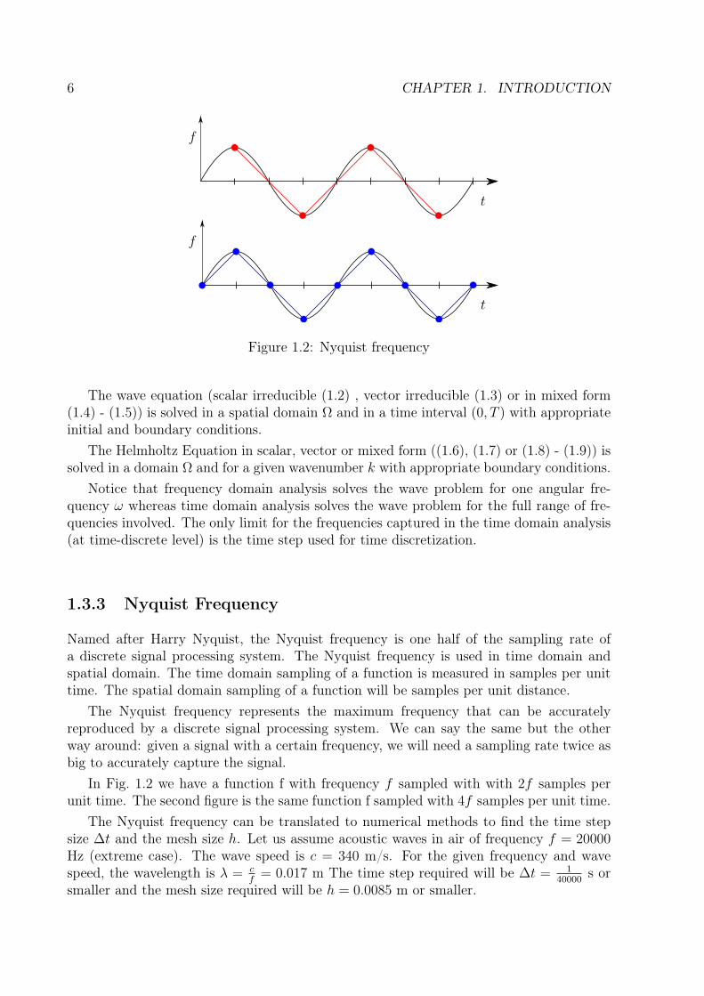
Fig. 1.1 shows a sketch of the relationship of the wave equations in time and frequencydomain.
Time domain analysis uses the scalar wave equation in its irreducible form (1.2):
1
c2∂ttp
′ −∆p′ = f ′, (1.2)
where p′(x, t) is the unknown (real valued scalar function), f ′ is a forcing term and c is thewave speed.
Additionally, time domain analysis can involve the vector wave equation in irreducibleform (1.3):
1
c2∂ttu
′ −∆u′ = f ′, (1.3)
where u′(x, t) is the unknown (real valued vector function) and f ′ is a forcing term.Notice that the vector wave equation in irreducible form (1.3) has no practical interest
since the regularity requirement for the vector unknown u′ is the same as the regularityrequirement for the scalar unknown p′ in the scalar wave equation in irreducible form (1.2)but the number of unknowns is d times bigger in the vector wave equation with respect tothe scalar wave equation.

4 CHAPTER 1. INTRODUCTION
Furthermore, time domain analysis can involve the wave equation in mixed form (1.4)-(1.5):
µp∂tp′ +∇·u′ = fp, (1.4)
µu∂tu′ +∇p′ = fu, (1.5)
where p′(x, t) and u′(x, t) are the unknowns, with p′ real valued scalar function and u′ realvalued vector function, µp > 0 and µu > 0 are the parameters of the equation and [fp,fu]are forcing terms.
Notice that the number of unknowns in the wave equation in mixed form is d+ 1 timesthe number of unknowns in the scalar wave equation in irreducible form, but the regularityrequirements in space and time are less stringent for both p′ and u′.
On the contrary, frequency domain analysis involves using the Scalar Helmholtz Equa-tion (1.6):
∆p+ k2p = fk, (1.6)
where p(x) is the unknown (complex valued scalar function), k is the wavenumber corre-sponding to a certain angular frequency ω and fk is a forcing term.
Additionally, frequency domain analysis can involve the Vector Helmholtz Equation(1.7):
∆u+ k2u = fk, (1.7)
where u(x) is the unknown (complex valued vector function), k is the wavenumber corre-sponding to a certain angular frequency ω and fk is a forcing term.
Notice that the Vector Helmholtz equation (1.7) has no practical interest since theregularity required for the vector unknown u is the same as the regularity required for thescalar unknown p in the Scalar Helmholtz equation (1.6) but the number of unknowns is dtimes bigger.
Additionally, frequency domain analysis can involve the Helmholtz Equation in mixedform (1.8) - (1.9):
−iµpωp+∇·u = fp, (1.8)
−iµuωu+∇p = fu, (1.9)
where p(x) and u(x) are the unknowns, ω is the angular frequency, µp > 0 and µu > 0 areparameters of the equation and fp and fu are forcing terms.
Notice that the number of unknowns in the Mixed Helmholtz equation is d+1 times thenumber of unknowns in the Scalar Helmholtz Equation, but the regularity requirements(in space) are less stringent for both p and u.
Until now, we have expressed wave equations in terms of either p′ or u′ or both.Additionally we have used their complex counterparts p or u. There is one more approachwhich uses the Velocity Potential ψ. The velocity potential wave equation is written as:
1
c2∂ttψ −∆ψ = fψ, (1.10)

1.3. WAVE EQUATIONS 5
from which we can extract p′ or u′ as follows:
p′ = −µu∂tψ + fψ,p, (1.11)u′ = ∇ψ, (1.12)
where ∇fψ,p = fu.Notice that the wave equation in mixed form is in agreement with the velocity potential
wave equation taking fψ = µp∂tfψ,p − fp.Now let us consider the complex counterpart ψ and let us write the Helmholtz Equation
in terms of the complex velocity potential:
∆ψ + k2ψ = fψ, (1.13)
from which we can extract p or u as follows:
p = iµuωψ + fψ,p, (1.14)
u = ∇ψ, (1.15)
where ∇fψ,p = fu.Wave equations in time domain or frequency domain are related to each other. Un-
knowns, coefficients and forcing terms of the equations are related. In the next paragraphswe show these relationships for the unknowns and coefficients only. The relationship be-tween forcing terms is trivial.
The coefficients µp and µu that characterize the mixed wave equation (1.4) - (1.5) arerelated to the wave speed c appearing in irreducible form of the scalar wave equation (1.2)or vector wave equation (1.3) as follows:
c2 = (µpµu)−1 . (1.16)
The wavenumber k characterizes the Scalar Helmholtz equation (1.6) and the VectorHelmholtz Equation (1.7) and is related to the wave speed c appearing in irreducible formof the wave equation (1.2) as follows:
ω = kc = 2πf , (1.17)
where ω is the angular frequency and f is the frequency.Assuming harmonic behavior of p′ with angular frequency ω and phase angle φ, we can
write:
p′ (x, t) = <(p (x) e−iωt
)= < (p) cos (ωt) + = (p) sin (ωt) = |p| cos (ωt− φ) , (1.18)
where <() and =() stand for real part and imaginary part respectively, |p| is the magnitudeof p defined as |p| :=
√(<(p))2 + (=(p))2 and φ := arctan
(=(p)<(p)
)is the argument of p.
Similarly, we can write:
u′ (x, t) = <(u (x) e−iωt
)= < (u) cos (ωt) + = (u) sin (ωt) . (1.19)
6 CHAPTER 1. INTRODUCTION
t
f
t
f
Figure 1.2: Nyquist frequency
The wave equation (scalar irreducible (1.2) , vector irreducible (1.3) or in mixed form(1.4) - (1.5)) is solved in a spatial domain Ω and in a time interval (0, T ) with appropriateinitial and boundary conditions.
The Helmholtz Equation in scalar, vector or mixed form ((1.6), (1.7) or (1.8) - (1.9)) issolved in a domain Ω and for a given wavenumber k with appropriate boundary conditions.
Notice that frequency domain analysis solves the wave problem for one angular fre-quency ω whereas time domain analysis solves the wave problem for the full range of fre-quencies involved. The only limit for the frequencies captured in the time domain analysis(at time-discrete level) is the time step used for time discretization.
1.3.3 Nyquist Frequency
Named after Harry Nyquist, the Nyquist frequency is one half of the sampling rate ofa discrete signal processing system. The Nyquist frequency is used in time domain andspatial domain. The time domain sampling of a function is measured in samples per unittime. The spatial domain sampling of a function will be samples per unit distance.
The Nyquist frequency represents the maximum frequency that can be accuratelyreproduced by a discrete signal processing system. We can say the same but the otherway around: given a signal with a certain frequency, we will need a sampling rate twice asbig to accurately capture the signal.
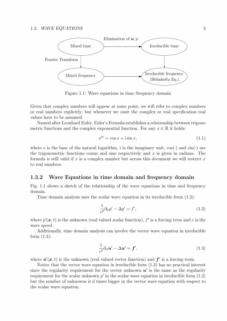
In Fig. 1.2 we have a function f with frequency f sampled with with 2f samples perunit time. The second figure is the same function f sampled with 4f samples per unit time.
The Nyquist frequency can be translated to numerical methods to find the time stepsize ∆t and the mesh size h. Let us assume acoustic waves in air of frequency f = 20000Hz (extreme case). The wave speed is c = 340 m/s. For the given frequency and wavespeed, the wavelength is λ = c
f= 0.017 m The time step required will be ∆t = 1
40000s or
smaller and the mesh size required will be h = 0.0085 m or smaller.

1.3. WAVE EQUATIONS 7
1.3.4 Acoustic Waves in Fluids
Wave propagation in fluids is known as Acoustics. The wave speed is a property of thefluid media. It can be computed as:
c2 =∂p
∂ρ
∣∣∣∣s
, (1.20)
where p is the thermodynamical pressure (absolute pressure) and ρ is the mass density.The s indicates a process with constant entropy.
An ideal gas has a simple equation of state defined as:
p = ρRsT, (1.21)
where Rs is the specific ideal gas constant and T is the absolute temperature. The specificideal gas constant is related to the universal ideal gas constant Ru through:
Rs =Ru
M, (1.22)
where M is the molar mass of the gas and Ru = 8.3144 m3 Pa K−1 mol−1.Then, for an ideal gas the equation defining the speed of sound is:
c2 = γp
ρ= γRsT, (1.23)
where γ is the specific heat ratio (1.4 for air).In air, the sound speed can be considered constant for any wave frequency. That brings
us to the concept of dispersive and non-dispersive media. In dispersive media the wavespeed is dependent of the frequency of the wave. On the other hand, in non-dispersivemedia the wave speed is independent of the frequency.
In a fluid the parameters of the wave equation in mixed form are taken as:
µp =1
ρ0c2, µu = ρ0, (1.24)
where ρ0 is the mass density and c is the speed of sound, with both ρ0 and c in the referencestate.
1.3.5 Wave Energy
The wave equation in mixed form has an internal structure of energy conservation.Let us define e as the energy density (energy per unit volume) in a point of a domain
as:
e =1
2
(µpp
′2 + µu|u′|2), (1.25)
where ep = 12µpp
′2 is the potential energy density and ek = 12µu|u′|2 is the kinetic energy
density. For a plane wave the kinetic and potential energy are the same.

8 CHAPTER 1. INTRODUCTION
Let E be the total energy of the domain in consideration:
E =
∫Ω
e dΩ, (1.26)
let i be the wave intensity in a given point of the domain:
i = p′u′, (1.27)
let Ib be the total power going from the domain to the outside through the boundary Γ:
Ib =
∫Γ
n · i dΓ, (1.28)
let if be the energy per unit time per unit volume added by the forcing terms:
if = p′fp + u′ · fu, (1.29)
and, finally, let If be the total power added to the domain by the forcing terms:
If =
∫Ω
if dΩ. (1.30)
Then, the energy conservation statement can be written as:
dE
dt+ Ib = If . (1.31)
Additionally, it holds:
∂te+∇ · i = if . (1.32)
1.4 Non-Reflecting Boundaries (NRB)
1.4.1 Introduction
Partial Differential Equations (PDE) involve a domain where the unknowns have to bedetermined. The domain can be space (Ωf ⊆ Rd), time (0, T ) or space-time (Ωf × (0, T )).
Let us concentrate in the spatial part of the domain and let us consider a numericalapproximation method to solve the PDE. We are interested in Finite Elements, but thenumerical method can be Finite Differences or Finite Volumes. Recall that we have used⊆ to define Ωf , this means that some PDEs might need infinite or semi-infinite spatialdomains in order to be solved. That brings a problem since we cannot discretize all Rd
with a finite number of elements of finite size h. So, instead of solving the PDE in Ωf , wesolve it in Ω ⊂ Ωf such that meas(Ω) is finite. Obviously, the boundary Γ of Ω is designedsmooth enough and with a convenient shape. Then, another question arises: we know theboundary condition to impose on the boundary Γf of Ωf but we do not know what toimpose on Γ.
In some problems the unknowns or their gradients decay fast enough in space, so thatimposing the same boundary condition of Γf on Γ and choosing Ω sufficiently large is

1.4. NON-REFLECTING BOUNDARIES (NRB) 9
Ωf
Ω
Ωf
Ω
Figure 1.3: NRB families: NRBC and NRBL
good enough. But, some other problems such as wave propagation problems in which theunknown decays with distance r as r−
(d−1)2 can require prohibitively big spatial domains in
order that the imposition of the same boundary condition of Γf on Γ is good enough.Furthermore, energy will bounce back when it reflects on Γ and it will remain inside
Ω perturbing the solution thereafter. The boundary solution is obvious but not trivial:not imposing the same condition of Γf on Γ. The ideal non reflecting boundary conditionshould be such that the solution in Ωf restricted to Ω is the same as the solution obtainedin Ω.
This leads to the introduction of Non-Reflecting Boundary Conditions (NRBC) andNon-Reflecting Boundary Layers (NRBL). We will refer to NRBC and NRBL simply asNon-Reflecting Boundaries (NRB).
Throughout this document, we denote as NRBC to boundary conditions applied on Γand as NRBL to an added layer of material after Γ (see Fig. 1.3).
NRBC are also known as Absorbing Boundary Conditions (ABC), Artificial BoundaryConditions (ABC) or Open Boundary Conditions (OBC).
Acoustic wave propagation problems often involve the calculation of acoustic intensityat a given point due to a given set of acoustic sources. Using a perfect NRB we obtain anintensity if at each spatial point. Using an approximate NRB we obtain an intensity i. Agood NRB will lead to an intensity i close to if .
In what follows, we will describe the Sommerfeld boundary condition (a type of NRBC),some other NRBCs and finally the Perfectly Matched Layer (PML) which is a type ofNRBL. But first let us start with some basic concepts of impedance, reflection and refrac-tion.
1.4.2 Impedance
Let us consider an harmonic force (perfect sine or cosine variation in time). The ratio ofthe complex amplitude of the force to the complex amplitude of the velocity at a givenpoint on a surface is called mechanical impedance at the point:
Z =p
un, (1.33)
where Z is the mechanical impedance and un is the normal component of u in the directiontowards the surface (pointing outside of the fluid). Obviously, Z is a complex number

10 CHAPTER 1. INTRODUCTION
α
Wall
y
α
Figure 1.4: Plane Wave Reflection
since p and u are complex. The real part of Z is called Resistance and its imaginary partReactance. The inverse 1/Z is known as Admittance.
In acoustics the definition of characteristic impedance is:
Zchar =
(µuµp
) 12
. (1.34)
The characteristic impedance is inherent to the propagation media. Let us assume wedivide a domain with an artificial boundary of impedance Z. Now we require that theartificial boundary has no effect on the wave field on both sides of the boundary. Then,the impedance needed for this artificial boundary is the characteristic impedance.
The power per unit surface through a surface of impedance Z is:
iZ = <(Z)|n · u|2, (1.35)
where n is the unit outward normal to the surface. Notice that when <(Z) > 0 the surfaceis passive and absorbs energy, but when <(Z) < 0 the surface is active and produces energy.
1.4.3 Reflection and Refraction
Before describing NRB, let us first describe the reflection and refraction phenomena.
Wave Reflection
Let us consider a plane wave in the x− y plane incident in the y − z plane (see Fig. 1.4).Assuming a perfect reflection (zero absorption), the reflected wave will have identicalwavenumber and angle α as the incident wave [8].
Now, let us consider the surface has a finite impedance Z and that the incident wavehas the following form:
pin = Aei(kxx+kyy), (1.36)

1.4. NON-REFLECTING BOUNDARIES (NRB) 11
α1
Medium 1 Medium 2
α2
α1
y
Figure 1.5: Plane Wave Refraction
where kx and ky are the wavenumber components in the x and y direction respectively andA is the complex amplitude of the incident wave.
The reflected wave will have the following form:
pre = RAei(−kxx+kyy), (1.37)
where R is the reflection coefficient that can be computed as:
R =ξ cos(α)− 1
ξ cos(α) + 1, (1.38)
with
ξ =Z
Zchar
. (1.39)
In the wave equation in mixed form, the condition of perfect reflection on a segment Γuof the boundary Γ can be modeled imposing n · u′ = 0. On the other hand, the boundarycondition p′ = 0 on a segment Γp of the boundary Γ represents a pressure released surface.This is an idealization of the interface water-air when considering wave propagation in thewater [9].
Wave Refraction
Now, let us consider a wave impacting at the interface between two fluids with wavevelocities c1 and c2 (see Fig. 1.5). The compatibility condition required in this case is thatthe trace velocity at the interface of both mediums match. This is known as the tracevelocity matching [10]. The trace velocity is the tangent component of the velocity at theinterface.
There are two cases: the trace velocity is higher than c2 or lower than c2. Let usconsider the first case (trace velocity higher than c2):
c2 <c1
sinα1
. (1.40)

12 CHAPTER 1. INTRODUCTION
There is a transmitted wave in medium 2 with the form:
ptr = T Aei(kxx+k2y cosα2), (1.41)
where k2 is the wavenumber in the second medium and α2 is the refraction or transmissionangle.
The requirement that the pressure is continuous at the interface yields:
1 +R = T , (1.42)
and the trace velocity matching yields:
cosα1
Zchar,1
(1−R) =cosα2
Zchar,2
T . (1.43)
In the second case, when the wave speed at the second medium c2 is greater than thetrace velocity at the interface, the transmission depends on the incidence angle. Obviously,it can only occur when c2 > c1. Let us define the critical angle as:
αcr = arcsinc1
c2
. (1.44)
If the incidence angle α1 is greater than the critical angle αcr, all the energy is reflected inthe interface. If the incidence angle α1 is less than the critical angle αcr, there is a wavetransmitted and a wave reflected [8].
1.4.4 Sommerfeld Boundary Condition
The Sommerfeld boundary condition is a type of NRBC and gets its name from ArnoldSommerfeld who was a German theoretical physicist. Sommerfeld mentions it in [11] as:
“The sources must be sources, not sinks, of energy. The energy which isradiated from the sources must scatter to infinity; no energy may be radiatedfrom infinity into the prescribed singularities of the field”.
The Sommerfeld radiation condition is applicable when the sources are concentratedin a region of space and the exterior boundary is a sphere surrounding it and centered atthe source region. Additionally, the spherical surface has to be sufficiently far away to thesources in order that the impinging waves only have radial component.
In spherical coordinates and for the Helmholtz equation in 3D, the Sommerfeld radiationcondition can be expressed as:
limr→∞
(r (∂rp− ikp)) = 0, (1.45)
where r is radial component in the spherical coordinate system. Some authors write theSommerfeld radiation condition with a + sign, but that depends on the time variationassumption. Throughout this document we have assumed a time variation e−iωt whichgives the minus sign.

1.4. NON-REFLECTING BOUNDARIES (NRB) 13
PML
Physical media
Figure 1.6: PML concept
In 2D or 3D (d = 2, 3) the Sommerfeld radiation condition can be expressed as:
limr→∞
(rd−1
2 (∂rp− ikp))
= 0. (1.46)
In time domain and for the scalar wave equation in 3D the Sommerfeld radiationcondition can be written as:
limr→∞
(r
(∂rp′ +
1
c∂tp′))
= 0. (1.47)
1.4.5 Other NRBC
NRBCs impose a boundary condition that mimics a non-reflecting boundary withoutneeding to add an absorbing boundary layer. From the computational cost point of viewNRBC do not add extra degrees of freedom to the problem being solved and that is a veryappealing feature.
Before, we described the Sommerfeld Radiation condition, which is a well known NRBC,but there are many other NRBC. Some authors have proposed Dirichlet-to Neumannmappings [12, 13] from domain decomposition methods, others proposed High OrderBoundary Conditions [14–17] while others proposed simpler approaches [18–20].
NRBC formulations have been formulated for the irreducible form of the wave equationin [14–16, 21–28], for the scalar Helmholtz equation in [12, 13, 29, 30], for the wave equationin mixed form in [17–20] and for flow problems in [31–33].
1.4.6 Perfectly Matched Layer
The concept of perfectly matched layer (PML) was first developed by Berenger in 1994for electromagnetic waves [34]. It consists in an artificial absorbing boundary layer placednext to the wave propagating media with the property of absorbing waves incident to it.A graphical representation of the absorbing layer can be seen in Fig. 1.6. PML has beenused since its appearance in many problems such as the scalar wave equation in irreducibleform [35–37], scalar Helmholtz equation [38–40], mixed form of the wave equation [41–44]and electromagnetic waves [34, 45–47].
Theoretically, PML absorbs waves at any angle of incidence but since we are not solvingthe exact problem (continuous) its absorptivity properties are not perfect. Therefore, in

14 CHAPTER 1. INTRODUCTION
practical terms, PML has the ability to absorb incident waves in a wide range of anglesof incidence. Another feature is that absorbing properties are good for a wide range offrequencies. When comparing PML with the Sommerfeld Radiation condition, the mainadvantage of PML is the absorptivity in a wide range of angles of incidence because theSommerfeld radiation condition assumes (or requires) a normal angle of incidence in orderto be accurate.
The original Berenger’s formulation of PML is called split field PML because he splitthe solution into two artificial fields whose sum is the physical field. Nowadays, it is morepopular the Uniaxial PML formulation (UPML) in which the wave equation is expressedas the combination of artificial anisotropic absorbing materials. Anyway, both PML andUPML are equivalent and can be derived from complex coordinate stretching.
Let us now refer to Fig. 1.6. The wave equation (in time or frequency domain) is solvedin the Physical media and the PML equations are solved in the PML absorbing layer.
Now, let us describe the formulation of PML applied to the wave equation in mixed form.For simplicity we will consider the 2D case, but the extension to 3D is straightforward.The formulation we describe here appears in [42] and was implemented and tested usingthe finite difference method.
Let us split p such that:
p = pa + pb, (1.48)
then, the governing equations in the PML layer are:
∂tu1 + q1u1 + ∂1 (pa + pb) = 0, (1.49)∂tu2 + q2u2 + ∂2 (pa + pb) = 0, (1.50)∂tpa + q1pa + ∂1u1 = 0, (1.51)∂tpb + q2pb + ∂2u2 = 0, (1.52)
with the following boundary condition on the boundary Γ of the PML layer:
p = 0 on Γ. (1.53)
The attenuation parameters qi can be taken as constant or variable. Linear and quadraticprofiles have been tested, for instance:
qi = qδ
(rPML
δPML
)nPML
, (1.54)
where δPML is the thickness of the PML layer, qδ is the attenuation factor and rPML is anormal coordinate with value zero on the boundary of the physical media and value δPML
at the end of the PML layer. The exponent nPML can be taken as 1 or 2 to obtain a linearor quadratic attenuation parameter.
Notice that the PML formulation presented increases the number of unknowns of theproblem. The cost increase is not so big since it is only an extra scalar unknown. Forthe scalar wave equation in irreducible form the relative cost increase is higher for obviousreasons.
1.4. NON-REFLECTING BOUNDARIES (NRB) 15
Later, in 2001, Hu presented a stable and well-posed PML formulation in unsplitphysical variables [48]. The avoidance of splitting facilitates the implementation. Butstill there is an auxiliary variable and thus the number of unknowns in the PML region isincreased.
PML features exponential decay of waves propagating inside the absorbing layer. Com-monly, a hard wall condition is applied on the exterior boundary of the PML layer, thatmeans energy can still reflect on that boundary and go back to the physical domain. Inthe way back, the PML layer still absorbs energy of the wave, so the effective attenuationof the PML layer is 2δPML. The exponential decay inside the PML layer is governed by theattenuation parameters qi. Higher attenuation parameters mean faster decay.
The design of a PML layer for a given problem involves setting the thickness δPML
and the parameters qi. We might be tempted to choose the attenuation parameters ashigh as possible and a small PML thickness but it is not that simple. An abrupt changeof properties from physical media to PML media might induce reflection on the PMLmedia/physical media interface. So we cannot choose the attenuation parameters so high.Additionally, a good practice is to choose the attenuation parameters as zero in the interiorof the PML layer and maximum in the exterior of the PML layer so that the change ofproperties from physical media to PML media is smooth. A common practice is to chooseδPML as a fraction of the wavelength. Cohen [49] recommends choosing δPML as one thirdof the wavelength for acoustic problems, meanwhile the study of Oskooi [50] in photonicssuggests choosing it as one half of the wavelength. This half-wavelength thickness criteriafor acoustic waves in air means thicknesses ranging from 8 to 0.01 m for the range of audiblefrequencies 20 - 20000 Hz.
1.4.7 Other NRBL
PML is a very popular NRBL but there are other NRBL. Richards et al proposes in [51]a NRBL based on damping the solution in time with a factor σ to a desired target value.In that publication they claim better performance than PML.
1.4.8 NRB performance evaluation
Many benchmark problems have been devised in order to evaluate the performance ofNRBC and NRBL.
Some procedures compare an analytical solution with the numerical solution in thetruncated domain using the NRB. For example Problems 1 and 2 in Category 3 of [52].Another example are the Parts 1, 2 and 3 of Problem 3 in Category 1 of [53].
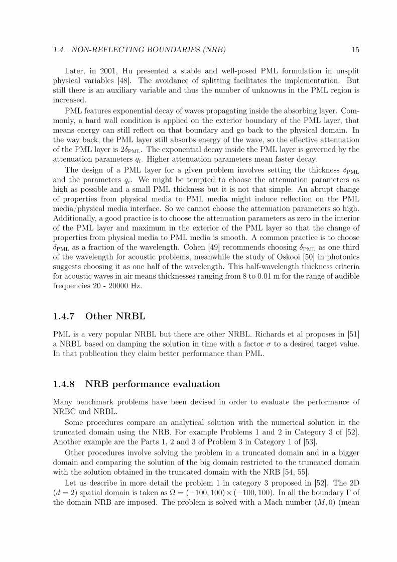
Other procedures involve solving the problem in a truncated domain and in a biggerdomain and comparing the solution of the big domain restricted to the truncated domainwith the solution obtained in the truncated domain with the NRB [54, 55].
Let us describe in more detail the problem 1 in category 3 proposed in [52]. The 2D(d = 2) spatial domain is taken as Ω = (−100, 100)× (−100, 100). In all the boundary Γ ofthe domain NRB are imposed. The problem is solved with a Mach number (M, 0) (mean

16 CHAPTER 1. INTRODUCTION
flow in the x direction). The initial condition is:
p = exp
[−(ln 2)
(x2 + y2
9
)], (1.55)
u1 = 0.04y exp
[−(ln 2)
((x− 67)2 + y2
25
)], (1.56)
u2 = −0.04(x− 67) exp
[−(ln 2)
((x− 67)2 + y2
25
)]. (1.57)
The problem consists in finding the unknowns at t = 30, 40, 50, 60, 70, 80, 100, 100 and600.
The analytical solution to that problem is the following. Let α1 = ln 29, α2 = ln 2
25and
η =√
(x−Mt)2 + y2. The exact solution is:
p =1
2α1
∫ ∞0
e−ξ24α1 cos(ξt)J0(ξη)ξ dξ, (1.58)
u1 =x−Mt
2α1η
∫ ∞0
e−ξ24α1 sin(ξt)J1(ξη)ξ dξ + 0.04ye−α2[(x−67−Mt)2+y2], (1.59)
u2 =y
2α1η
∫ ∞0
e−ξ24α1 sin(ξt)J1(ξη)ξ dξ − 0.04(x− 67−Mt)e−α2[(x−67−Mt)2+y2], (1.60)
where Jα are the Bessel functions of order α.One problem with this benchmark is that it does not specify the mesh to use. Another
problem are the benchmark results in the original document, as they are quite old, thedocument is not clear to read.
The benchmark problem 3 in category 1 of [53] is more specific and specifies the meshto use. It involves periodic boundary conditions and the results can be easily comparedthrough the error at each time step. The unsuitability of this benchmark is that the errorresults are not purely due to the non-reflective properties of the NRB used, but includepropagation error ( due to temporal and spatial discretization).
In my opinion, the best NRB benchmark should only include the non-reflective prop-erties of the NRB. So, the big domain/small domain seems the most appropriate methodin the time domain. I have no idea what would be the equivalent in the frequency domain.The big domain benchmark is sketched in Fig. 1.7. The red zone represents the initial wavepulse. The time interval used in the big and small domain is the same. The time intervalis chosen such that the initial pulse has touched all the surrounding NRB. The big domainis chosen such that along the previously selected time interval, the initial pulse does notreach the big boundary.
The comparison criteria in the Big Domain Benchmark is multiple and it has twocomponents. The first component is the time domain norm and the second component isthe spatial domain norm.
For the time domain norm we have many options An instant of time tc ∈ (0, T ) can bechosen for comparison. Other option can be comparing in the whole time interval (0, T )with an L∞(0, T ) norm or with an L2(0, T ) norm.
The spatial domain norm has many options too. A point xc ∈ Ω or the whole domain Ωcan be chosen for computing the norm. Additionally, the quantity of interest together with

1.4. NON-REFLECTING BOUNDARIES (NRB) 17
Big Domain NRBC
NRBL
Figure 1.7: Big Domain Benchmark
its norm has multiple options. Among the options we have the energy ||e||L2 , the potentialenergy ||ep||L2 , the kinetic energy ||ek||L2 , the H1(Ω) norm of the pressure fluctuation||p′||H1(Ω), the H(div,Ω) norm of the velocity fluctuation ||u′||H(div,Ω) and a composite normcombining some or all the norms of the above in space and time |||·|||. Obviously, the choiceof a point xc does not make any sense in variational formulations.
The comparison criteria (see Chapter 2 or Chapter 3) can be taken as:
|||[p′,u′]|||2A := µp||p′||2L∞(Υ,L2(Ω)) + µu||u′||2L∞(Υ,L2(Ω)), (1.61)
or
|||[p′,u′]|||2B := |||[p′,u′]|||2A + τp||∇p′||2L2(Υ,L2(Ω)) + τu||∇·u′||2L2(Υ,L2(Ω)), (1.62)
where τp and τu are the stabilization parameters containing length scales of the waveproblem.
A typical plot of the total energy in Ω versus time for the Big Domain Benchmarkshould look like 1.8. In that plot the big domain solution is plotted in black and the smalldomain solution is plotted in blue. The imperfection of the NRB is seen because the curvesdo not match exactly.

18 CHAPTER 1. INTRODUCTION
t
E
Figure 1.8: Big Domain Benchmark Energy Evolution
1.5 Aeroacoustics
1.5.1 Overview
Acoustic waves can be produced from the unsteady motion of a solid boundary in contactwith a fluid (See Fig. 1.9). This field is known as simply Acoustics and it is not the mainconcern of Aeroacoustics. Aeroacoustics is the study of sound generation by turbulent flowor aerodynamic forces interacting with surfaces and the subsequent propagation of soundthrough the fluid (See Fig. 1.10). Aerodynamic forces interacting with surfaces can beregarded as Aeroelasticity. Computational Aeroacoustics is the use of numerical methodsto solve aeroacoustics problems [7].
Aeroacoustics problems can be approached in two forms: direct computation andindirect or hybrid approach. The first approach consist in solving the flow problem atthe same time as the acoustic problem. The advantage of the direct approach is theavoidance approximations in the model. The disadvantage is its high computational costbecause a fine enough mesh and time step has to be used [56].
On the other hand, the hybrid approach solves first the flow problem, then uses theinformation from the flow in order to predict the sound sources (using acoustic analogies)and finally solves the acoustic problem. The main assumption of the hybrid approach isthat the flow produces sound and the sound propagating does not affect in any way the
Figure 1.9: Speaker generating sound

1.5. AEROACOUSTICS 19
Flow
Acoustic Waves
Figure 1.10: Acoustic Waves Generation
flow (there is not two way coupling). This assumption is valid because the propagation ofsound involves small pressure fluctuations while fluid flow involves big pressure fluctuations.Additionally, at low Mach numbers, the fluid can be considered incompressible for the flowcalculation and the acoustic sources will be accurate enough for the acoustic calculation.
For the hybrid approach the type of fluid dynamics simulation used can be Reynolds-Averaged Navier-Stokes (RANS), Large Eddy Simulation (LES) or Direct Numerical Sim-ulation (DNS). When RANS is used, the approach is known as stochastic. The stochasticapproach uses RANS, which is not computationally expensive, and from that informationconstructs the sound sources.
Aeroacoustics is very challenging from the computational point of view because it re-quires solving a unsteady flow problem with a fine enough spatial and temporal discretiza-tion in order to capture all the flow details responsible of generating sound which is verycostly.
Additionally, there is an enormous disparity between the flow velocity/pressure and theacoustic velocity/pressure because for low Mach numbers the energy generated as soundwaves is of order Ma4 [57]. In the case of sound generated by a turbulent jet, the ratiobetween the power of the waves generated and the power of the jet is of order Ma5. Thisdisparity makes the direct approach very challenging because the simulation has to be ableto detect the small perturbations with enough accuracy. For the hybrid approach, thedisparity is less important because the acoustic problem is solved separately.
1.5.2 Concepts
The time-average value p of a given property p is defined as [58]:
p(x) =1
T
∫ T
0
p(x, t) dt, (1.63)
and its fluctuation p′ is defined as:
p(x, t) = p(x) + p′(x, t). (1.64)

20 CHAPTER 1. INTRODUCTION
The root mean square value RMS is defined as:
prms(x) =
(1
T
∫ T
0
(p′(x, t))2dt
) 12
. (1.65)
For a cosinusoidal wave of amplitude A described as A cos(ωt− φ) the RMS value can becalculated as:
prms =A√2. (1.66)
In acoustics in general and in aeroacoustics in particular we need a way of measuringthe loudness of sound in a given point. Thus, the Sound Pressure level SPL is introduced.Sound pressure level is a measure of the deviation of the pressure around the ambientpressure. It is commonly measured in decibels (dB). A dB is a tenth of a Bel. A Belis a rarely used unit named after Alexander G. Bell. The sound pressure level in dB iscalculated as:
SPL = 10 log10
p2rms
p2ref
, (1.67)
where pref is the reference pressure and is taken as pref = 20 × 10−6 Pa for air andpref = 1× 10⁻⁶ Pa for water.
The pressure fluctuations prms contain all the frequency spectrum. Sometimes it can beadvantageous to split the spectrum and consider the contribution of a given frequency tothe total. Assuming the frequency spectrum is discrete and has N frequency contributions(the idea readily extends to continuum frequency spectrum), the pressure fluctuations canbe split as:
p′(x, t) =N∑n=1
p′n(x, t), (1.68)
where p′n is the pressure component with angular frequency ωn. Its complex amplitude pnis defined as:
p′n(x, t) = <(pn(x)e−iωnt
), (1.69)
and the pressure level at the angular frequency ωn is defined as:
SPLn = 10 log10
12|pn|2
p2ref
. (1.70)
1.5.3 Navier-Stokes Equations
The Navier-Stokes equations describe the movement of a fluid and are named after Claude-Louis Navier and George Gabriel Stokes. The equations are:
∂tρ+∇ · (ρu) = 0, (1.71)

1.5. AEROACOUSTICS 21
ρ (∂tu+ (u · ∇)u)−∇ · σ = fmom, (1.72)
where ρ is the fluid density, u is the fluid velocity, σ is the stress tensor and fmom is thebody force per unit volume. Obviously, we need to add to the Navier-Stokes equations theconstitutive equation of the fluid, the state equation and the energy equation in order tobe able to solve the problem.
The equations are solved in a spatial domain Ω ∈ Rd (d = 1, 2, 3) with boundary Γ andin a time interval (0, T ) with appropriate boundary and initial conditions.
Equation (1.71) is known as mass conservation equation or continuity equation. Equa-tion (1.72) is known as the momentum equation because it is a momentum conservationstatement.
The range of applicability of the equations presented includes: compressible or incom-pressible flows, laminar or turbulent flows and viscous or inviscid flows.
Newtonian fluids are fluids that behave according to the following equation:
σij = −p δij + τij, (1.73)
τij = µ (∂jui + ∂iuj) +
(λ− 2
3µ
)δij∂kuk, (1.74)
where p is the pressure (thermodynamic pressure), δ is the Kronecker delta, τij is thedeviatoric part of the stress tensor, µ is the dynamic viscosity of the fluid and λ is thebulk viscosity (also known as volume viscosity or second viscosity expansion viscosity).Thermodynamics second-law arguments show that λ must be positive. The effect of theterm involving ∇·u is very small even in compressible flows and it is usual to assume λ = 0or λ− 2
3µ = 0.
Recall that:
(∇ · σ)i = ∂jσji = ∂jσij, (1.75)
as σ is symmetric.Navier-Stokes equations can be written in conservative form as:
∂tρ+∇ · (ρu) = 0, (1.76)∂t(ρu) +∇ · (ρuu)−∇ · σ = fmom. (1.77)
1.5.4 Acoustic Analogy
In the hybrid approach to aeroacoustics, an acoustic analogy is needed in order to translatethe flow results into acoustic sources. The first to develop this concept was Lighthill in1952 [59, 60], then Curle considered solid walls in 1955 [61], afterwards Phillips in 1960studied sound generated at high Mach numbers [62]. In 1969 Williams and Hawkings [63]proposed a new acoustic analogy in order to consider solid surfaces moving arbitrarily.Recently, in 2003 Goldstein proposed a generalized acoustic analogy [64].
Lighthill Acoustic Analogy
It was proposed by Michael James Lighthill who was a British applied mathematician. Hepublished his results in two famous papers in 1952 and 1954 [59, 60]. The sound generated

22 CHAPTER 1. INTRODUCTION
is represented by quadrupole volume sources. It assumes the medium is stationary andit does not consider solid walls. The reference density is taken as ρ0 and the densityfluctuation is defined as:
ρ′ = ρ− ρ0 (1.78)
The Lighthill acoustic analogy can be obtained from the Navier-Stokes equations inconservative form with fmom = 0 differentiating with respect to time the mass conservationequation and subtracting the divergence of the momentum conservation equation:
∂ttρ+ ∂t(∇·(ρu))−∇·(∂t(ρu))−∇·(∇·(ρuu− σ)) = 0, (1.79)
then subtracting c2∆ρ′ to both sides we get:
∂ttρ− c2∆ρ′ = ∇·(∇·(ρuu− σ))− c2∆ρ′, (1.80)
finally, as time derivatives only see ρ′:
∂ttρ′ − c2∆ρ′ = ∂i∂jTij, (1.81)
where ∂i∂jTij is the acoustic source. Tij is known as the Lighthill stress tensor and isdefined as:
Tij = ρuiuj + δij[(p− p0)− c2 (ρ− ρ0)
]− τij, (1.82)
where δij is the Kronecker delta, p0 is the reference pressure, ρ0 is the reference density, cis the speed of sound at the reference density and pressure and τij is the deviatoric part ofthe stress tensor.
The Lighthill tensor can be neglected in the far field region, because the sound isgenerated in the near field region. In the near field region, the Lighthill tensor can beapproximated by neglecting τij because viscosity is known to cause a small damping dueto the conversion of acoustic energy into heat.
Another approximation can be made to the Lighthill tensor for isentropic flows and theterm (p− p0)− c2 (ρ− ρ0) can be neglected, thus:
T ≈ ρu⊗ u. (1.83)
The Lighthill stress tensor can be calculated from a computational fluid dynamicssimulation and then serve as input for the wave equation in the propagation stage.
Before we have written the density fluctuation scalar wave equation in irreducible form.We can write an equivalent equation in terms of pressure as:
1
c2∂ttp
′ −∆p′ = ∂i∂jTij. (1.84)
In the case of the wave equation in mixed form (1.4)-(1.5), we can take the forcingterms from the Lighthill acoustic analogy as:
fp = 0 , (1.85)fu = −∇ · T = −∂jTji = −∂jTij. (1.86)
1.5. AEROACOUSTICS 23
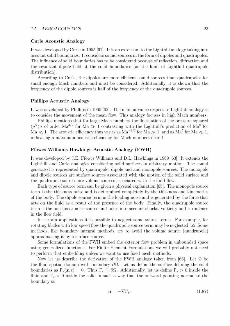
Curle Acoustic Analogy
It was developed by Curle in 1955 [61]. It is an extension to the Lighthill analogy taking intoaccount solid boundaries. It considers sound sources in the form of dipoles and quadrupoles.The influence of solid boundaries has to be considered because of reflection, diffraction andthe resultant dipole field at the solid boundaries (as the limit of Lighthill quadrupoledistribution).
According to Curle, the dipoles are more efficient sound sources than quadrupoles forsmall enough Mach numbers and must be considered. Additionally, it is shown that thefrequency of the dipole sources is half of the frequency of the quadrupole sources.
Phillips Acoustic Analogy
It was developed by Phillips in 1960 [62]. The main advance respect to Lighthill analogy isto consider the movement of the mean flow. This analogy focuses in high Mach numbers.
Phillips mentions that for large Mach numbers the fluctuation of the pressure squared(p′2)is of order Ma3/2 for Ma 1 contrasting with the Lighthill’s prediction of Ma8 forMa 1. The acoustic efficiency thus varies as Ma−3/2 for Ma 1, and as Ma5 for Ma 1,indicating a maximum acoustic efficiency for Mach numbers near 1.
Ffowcs Williams-Hawkings Acoustic Analogy (FWH)
It was developed by J.E. Ffowcs Williams and D.L. Hawkings in 1969 [63]. It extends theLighthill and Curle analogies considering solid surfaces in arbitrary motion. The soundgenerated is represented by quadrupole, dipole and and monopole sources. The monopoleand dipole sources are surface sources associated with the motion of the solid surface andthe quadrupole sources are volume sources associated with the fluid flow.
Each type of source term can be given a physical explanation [65]. The monopole sourceterm is the thickness noise and is determined completely by the thickness and kinematicsof the body. The dipole source term is the loading noise and is generated by the force thatacts on the fluid as a result of the presence of the body. Finally, the quadrupole sourceterm is the non-linear noise source and takes into account shocks, vorticity and turbulencein the flow field.
In certain applications it is possible to neglect some source terms. For example, forrotating blades with low speed flow the quadrupole source term may be neglected [65].Somemethods, like boundary integral methods, try to avoid the volume source (quadrupole)approximating it by a surface source.
Some formulations of the FWH embed the exterior flow problem in unbounded spaceusing generalized functions. For Finite Element Formulations we will probably not needto perform that embedding unless we want to use fixed mesh methods.
Now let us describe the derivation of the FWH analogy taken from [66]. Let Ω bethe fluid spatial domain with boundary ∂Ω. Let us define the surface defining the solidboundaries as Γs(x, t) = 0. Thus Γs ⊆ ∂Ω. Additionally, let us define Γs > 0 inside thefluid and Γs < 0 inside the solid in such a way that the outward pointing normal to theboundary is:
n = −∇Γs. (1.87)

24 CHAPTER 1. INTRODUCTION
The time dependence means that solid boundaries can move arbitrarily (rigid or flexiblebody motion). The mass and momentum equations can be written as:
∂tρ+ ∂i(ρui) = ρ0uiδ(Γs)∂iΓs, (1.88)∂t(ρui) + ∂j(ρuiuj + τij) = τijδ(Γs)∂jΓs, (1.89)
where δ(·) is the Dirac delta function. For a static surface the source term in the massconservation equation vanishes.
Then, the wave equation in irreducible form is:
∂ttρ′ − c2∇ρ′ = ∂ijTij − ∂i (τijδ(Γs)∂jΓs) + ∂t (ρouiδ(Γs)∂iΓs) , (1.90)
where Tij is the Lighthill stress tensor. The first term of the right hand side of the equationrepresents a quadrupole volume source. The second term represents a dipole surface source.Finally, the third term represents a monopole surface source.
Goldstein Acoustic Analogy
It was developed by Goldstein in 2003 [64]. His contribution was to rewrite Navier-Stokesequations (in conservative form) as inhomogeneous linearized Euler equations. The soundsource terms are a result of shear stress and energy flux perturbations.
1.6 StructureThe document is organized as follows: in Chapter 2 the wave equation is discretized inspace using stabilized finite element methods. Additionally, stability and convergence ofthe semi-discrete schemes is analyzed. In Chapter 3 a non-reflecting boundary conditionis added to the stabilized finite element formulation of the wave equation in mixed form.Stability and convergence is analyzed as well as the non-reflective properties of the non-reflective boundary condition. In Chapter 4 time marching schemes for the mixed waveequation are analyzed, with emphasis in stability, convergence, dissipation and dispersion.In Chapter 5 various wave propagation problems are solved and some of them are comparedwith experimental results. Finally, in Chapter 6 conclusions are drawn and future researchlines are mentioned.
1.7 Research diffusionThe research work contained in this thesis has been disseminated in the format of articlesin peer-reviewed scientific journals and in the form of oral presentations in scientificconferences and congresses.
1.7.1 Publications
Some chapters of this thesis are based on or include the following publications:Chapter 2:

1.7. RESEARCH DIFFUSION 25
Santiago Badia, Ramon Codina, and Hector Espinoza. “Stability, Convergence, andAccuracy of Stabilized Finite Element Methods for the Wave Equation in Mixed Form”.In: SIAM Journal on Numerical Analysis 52.4 (May 2014), pp. 1729–1752. doi: 10.1137/130918708
Chapter 3:Hector Espinoza, Ramon Codina, and Santiago Badia. “A Sommerfeld non-reflecting
boundary condition for the wave equation in mixed form”. In: Computer Methods inApplied Mechanics and Engineering 276 (July 2014), pp. 122–148. issn: 0045-7825. doi:10.1016/j.cma.2014.03.015. url: http://www.sciencedirect.com/science/article/pii/S0045782514001017
Chapter 4:Hector Espinoza, Ramon Codina, and Santiago Badia. “On some time marching
schemes for the stabilized finite element approximation of the mixed wave equation”. In:Computer Methods in Applied Mechanics and Engineering (Dec. 2014). Submitted.
Chapter 5:Oriol Guasch, Marc Arnela, Ramon Codina, and Hector Espinoza. “A stabilized finite
element method for the mixed wave equation in an ALE framework with application todiphthong production”. In: Journal of Computational Physics (Oct. 2014). Submitted.
1.7.2 Conferences
Research results had been presented in the following conferences:Ramon Codina, Hector Espinoza, and Santiago Badia. “Linear waves in mixed form:
functional settings and stabilized finite element approximation”. In: 6th Scientific Com-puting Seminar / VMS 2012. Christian-Albrechts-Universität zu Kiel. June 2012. url:http://www.math.uni-kiel.de/numerik/braack/conf/vms2012/
Hector Espinoza, Ramon Codina, and Santiago Badia. “Wave Equation in MixedForm: Stability and Convergence Estimates using Stabilized Finite Element Methods”.In: Congress on Numerical Methods in Engineering CNM 2013. Sociedad Española deMétodos Numéricos en Ingeniería (SEMNI). June 2013. url: http://congress.cimne.com/metnum2013/
Oriol Guasch, Marc Arnela, Ramon Codina, and Hector Espinoza. “A stabilizedarbitrary Lagrangian Eulerian finite element method for the mixed wave equation withapplication to diphthong production”. In: WCCM XI. IACM and ECCOMAS. July 2014.url: http://www.wccm-eccm-ecfd2014.org/
Hector Espinoza, Ramon Codina, and Santiago Badia. “Numerical analysis and bench-marking of a Sommerfeld-type non-reflecting boundary condition for the wave equation inmixed form”. In: WCCM XI. IACM and ECCOMAS. July 2014. url: http://www.wccm-eccm-ecfd2014.org/
Marc Arnela, Oriol Guasch, Ramon Codina, and Hector Espinoza. “Finite elementcomputation of diphthong sounds using tuned two-dimensional vocal tracts”. In: 7thForum Acusticum. Polish Acoustics Society and European Acoustics Association. Sept.2014. url: http://www.fa2014.pl/
Oriol Guasch, Marc Arnela, Ramon Codina, and Hector Espinoza. “Stabilized finiteelement formulation for the mixed convected wave equation in domains with driven flex-

26 CHAPTER 1. INTRODUCTION
ible boundaries”. In: NOVEM 2015. INSA. Apr. 2015. url: http : / / novem2015 .sciencesconf.org/
Ramon Codina, Marc Arnela, Oriol Guasch, and Hector Espinoza. “Waves in timedependent domains”. In: 10th International Workshop on Variational Multiscale andStabilized Finite Elements (VMS2015). German Association for Computational Mechanics(GACM). Garching, Germany, Feb. 2015. url: http://www.lnm.mw.tum.de/vms2015/
Ramon Codina, Oriol Guasch, Marc Arnela, and Hector Espinoza. “Approximationof waves written in mixed form in time dependent domains”. In: Congresso de MétodosNuméricos em Engenharia. Instituto Superior Técnico. June 2015. url: http://www.dem.ist.utl.pt/cmn2015/

Chapter 2
Stability, Convergence and Accuracy ofStabilized Finite Element Methods forthe Wave Equation in Mixed Form
This chapter is based on the material in:Santiago Badia, Ramon Codina, and Hector Espinoza. “Stability, Convergence, and Ac-curacy of Stabilized Finite Element Methods for the Wave Equation in Mixed Form”. In:SIAM Journal on Numerical Analysis 52.4 (May 2014), pp. 1729–1752. doi: 10.1137/130918708with the notation modified to make it fit with the other chapters.
In this chapter we propose two stabilized finite element methods for different functionalframeworks of the wave equation in mixed form. These stabilized finite element methodsare stable for any pair of interpolation spaces of the unknowns. The variational formscorresponding to different functional settings are treated in an unified manner through theintroduction of length scales related to the unknowns. Stability and convergence analysisis performed together with numerical experiments. It is shown that modifying the lengthscales allows one to mimic at the discrete level the different functional settings of thecontinuous problem and influence the stability and accuracy of the resulting methods.
2.1 Introduction
When applied to approximate differential equations with several unknowns, and partic-ularly saddle point problems, standard Galerkin mixed finite element (FE) formulationsoften require the use of inf-sup stable interpolations for the unknowns in order to be stable[78]. Inf-sup stable FE formulations have been formulated for several mixed problems,e.g. [79] for the Stokes problem, [80] for the Darcy problem, [81] for the Maxwell prob-lem, [82, 83] for the Stokes-Darcy problem, [84] for the wave equation and [85, 86] forelastodynamics.
On the contrary, stabilized FE methods [87] allow one to avoid inf-sup compatibilityconstraints. As a result, we can deal with different saddle-point problems by using the sameequal interpolation for all the unknowns; see e.g. the unified framework for Stokes, Darcyand Maxwell problems in [88]. This way, we can certainly ease implementation issues,
27

28 CHAPTER 2. STABILIZED FEM FOR THE MIXED WAVE EQUATION
specially for multiphysics simulations. Stabilized FE methods can nicely be motivated inthe Variational Multi-Scale (VMS) framework, as shown in [89].
This work is a follow-up of [90] for the wave equation in mixed form. The mixedwave equation is approximated in [90] using the Orthogonal Sub-scale Stabilization (OSS)method. In the present work, the OSS method is extended and the Algebraic Sub-GridScale Method (ASGS) is also considered. Additionally, length scales associated to theunknowns are introduced, allowing one to treat different functional settings in a unifiedmanner. A similar approach for the stationary Stokes-Darcy problem can be found in [91].
We focus on three variational forms of the mixed wave equation and the functionalsetting for each case. We obtain the different functional settings by transferring regularityfrom the scalar to the vector unknowns or vice-versa. More about functional settings forwave propagation problems of first and second order can be found in [92].
A priori error estimates for the mixed wave equation can be found in the literature.Some only bound L2 norms of the error of the unknowns [93, 94], whereas others, such as[84], take into account the divergence of the vector unknown too. In this work we boundboth the the gradient of the scalar unknown and the divergence of the vector unknownusing stabilized FEs.
Several stability and convergence analysis have been done so far for the irreducibleform of the wave equation (second order space and time derivatives) [95, 96] but not muchattention has been paid to the first order in time and space wave equation. As far as theauthors are aware, the present work is the first to analyze the convergence properties ofstabilized FEs applied to the mixed form of the wave equation.
The organization of the chapter is as follows. In Section 2.2 we describe the continuousproblem and its variational forms. In Section 2.3 we describe the stabilized discrete problemusing the ASGS and the OSS methods. In Section 2.4 we state and prove the stability ofthe discrete formulations. In Section 2.5 we state and prove the convergence of the discreteformulations, including numerical tests. Finally, in Section 2.6 the conclusions of the workare presented.
2.2 Problem Statement
2.2.1 Initial and Boundary Value Problem
The problem we consider is an initial and boundary value problem posed in a time interval(0, T ) and in a spatial domain Ω ⊂ Rd, (d = 1, 2 or 3). The long term behavior T → ∞will not be considered in this work.
Let Γ be the boundary of the domain Ω. We split this boundary into two disjoint setsdenoted as Γp and Γu, where the boundary conditions corresponding to the unknowns pand u will be respectively enforced.
The problem consists in finding p : Ω × (0, T ) −→ R and u : Ω × (0, T ) −→ Rd suchthat:
µp∂tp+∇·u = fp , (2.1)µu∂tu+∇p = fu , (2.2)

2.2. PROBLEM STATEMENT 29
with the following initial conditions:
p (x, 0) = 0, u (x, 0) = 0, x ∈ Ω, (2.3)
and with the following boundary conditions:
p = 0 on Γp, n · u = 0 on Γu, t ∈ (0, T ), (2.4)
where µp > 0 and µu > 0 are coefficients such that c2 = (µpµu)−1, c is the wave speed, fp
and fu are forcing terms and n is the unit outward normal to the boundary of the domain.Notice that any general problem with non-homogeneous initial and boundary conditionscan be cast in the form (2.1)-(2.4) properly modifying the forcing terms.
In the previous equations and in what follows, we use the following convention: boldface italic letters represent vectors in Rd, (d = 1, 2 or 3), bold face regular upper-case lettersrepresent matrices, and non-bold letters represent scalars.
Let L2(Ω) be the space of square integrable functions defined on the domain Ω, L2(Ω)d
the space of vector valued functions with components in L2(Ω), H1(Ω) the space offunctions in L2(Ω) with derivatives in L2(Ω), H1(Ω)
d the space of vector valued functionswith components in H1(Ω), and H(div,Ω) the space of vector functions with componentsand divergence in L2(Ω). Any of the spaces defined previously will be denoted genericallyas X. Additionally, given X, a space of (scalar or vector) functions defined over Ω, itsspatial norm will be denoted as ‖ · ‖X and the space of functions whose X-norm is Ck
continuous in the time interval [0, T ] will be denoted by Ck ([0, T ];X). We will only beinterested in the cases k = 0, k = 1 and k = 2. In the case of L2(Ω) or L2(Ω)
d the L2-normwill be simply denoted as ||·||. Functions whose X-norm is Lp in [0, T ] will be denoted byLp(0, T ;X); when X = L2(Ω) or X = L2(Ω)
d, the simplification Lp(L2) will be sometimesused.
Furthermore, let Vp, Vu be spaces associated with p and u respectively. These spaceswill be defined afterwards because they depend on the functional setting. Additionally, letus define V := Vp × Vu and L := L2(Ω)× L2(Ω)
d.Problem (2.1)-(2.2) will be well posed for
p ∈ C1(
[0, T ] ;L2(Ω))∩ C0
([0, T ] ;Vp
), (2.5)
u ∈ C1(
[0, T ] ;L2(Ω)d) ∩ C0
([0, T ] ;Vu
), (2.6)
with fp and fu in regular enough spaces.
2.2.2 Variational Problem
The variational form of problem (2.1)-(2.4) can be expressed in three different ways. Eachone requires a certain regularity on the unknowns p and u, which is equivalent to say thatp and u should belong to a particular space of functions.
The problem reads: find [p,u] ∈ C1 ([0, T ];L) ∩ C0 ([0, T ];V ) such that
B ([p,u] , [q,v]) = L ([q,v]) , (2.7)
for all test functions [q,v] ∈ C0 ([0, T ];V ) and the respective initial conditions. Here,we require that p(x, 0) = q(x, 0) = 0 and u(x, 0) = v(x, 0) = 0. The bilinear form B,

30 CHAPTER 2. STABILIZED FEM FOR THE MIXED WAVE EQUATION
the linear form L and the space V are defined in three different ways depending on thevariational form into consideration.
Let us denote as ( · , · ) the L2(Ω) inner product. For simplicity, we will assume that theforcing terms fp and fu are square integrable, although we could relax the this regularityrequirement and assume they belong to the dual space of Vp and Vu, respectively.
The variational formulation of problem (2.1)-(2.4) can be posed in three different forms,essentially differing in the way integration by parts from the strong form of the problemis performed and in the regularity required for the unknowns. In the problem statementgiven below, variational form I (2.8)-(2.11) is obtained not integrating by parts any term.Variational form II (2.12)-(2.15) is obtained integrating by parts the term (∇p,v). Finally,variational form III (2.16)-(2.19) is obtained integrating by parts the term (∇·u, q). Noticethat integration by parts leads to a boundary term. The treatment of the boundary termis explained in each case.
Variational Form I
Vp =q ∈ H1(Ω)| q = 0 on Γp
, Vu = v ∈ H(div,Ω)| n · v = 0 on Γu
B ([p,u] , [q,v]) = µp (∂tp, q) + (∇·u, q) + µu (∂tu,v) + (∇p,v) (2.8)L ([q,v]) = (fp, q) + (fu,v) (2.9)
p = 0 on Γp, Strongly imposed (2.10)n · u = 0 on Γu, Strongly imposed (2.11)
Variational Form II
Vp = L2(Ω), Vu = v ∈ H(div,Ω)| n · v = 0 on Γu
B ([p,u] , [q,v]) = µp (∂tp, q) + (∇·u, q) + µu (∂tu,v)− (p,∇·v) (2.12)L ([q,v]) = (fp, q) + (fu,v) (2.13)
p = 0 on Γp, Weakly imposed (2.14)n · u = 0 on Γu, Strongly imposed (2.15)
Notice that the boundary integral that appears after integration by parts of (∇p,v)vanishes due to (2.14)-(2.15).
Variational Form III
Vp =q ∈ H1(Ω)| q = 0 on Γp
, Vu = L2(Ω)
d
B ([p,u] , [q,v]) = µp (∂tp, q)− (u,∇q) + µu (∂tu,v) + (∇p,v) (2.16)

2.3. STABILIZED FINITE ELEMENT METHODS 31
L ([q,v]) = (fp, q) + (fu,v) (2.17)
p = 0 on Γp, Strongly imposed (2.18)n · u = 0 on Γu, Weakly imposed (2.19)
Notice that the boundary integral that appears after integration by parts of (∇·u, q)vanishes due to (2.18)-(2.19).
2.3 Stabilized Finite Element Methods
In this section, we present two stabilized FE methods, which we will denote by the acronymsASGS and OSS, aimed to overcome the instability problems of the standard Galerkinmethod. In general, stabilized FE methods can be used with any type of interpolationfor p and u. In particular, we focus on equal and continuous interpolations for p and uand therefore conforming FE spaces. For conciseness we will consider quasi-uniform FEpartitions of size h. For stabilized formulations in general non-uniform non-degeneratecases, see [97].
Let Vp,h and Vu,h be the FE spaces to approximate p and u, respectively, with Vp,h ⊂ Vpand Vu,h ⊂ Vu. Additionally, let us define Vh = Vp,h × Vu,h. For any of these spaces wewill make frequent use of the classical inverse inequality ‖∇vh‖ ≤ Cinvh
−1‖vh‖, with Cinv
a constant independent of the FE function vh and the mesh size h.
2.3.1 The Variational Multiscale Framework
It is not our purpose here to describe in detail the heuristic design of the stabilized finiteelement methods we will consider, for which [90] can be consulted. We shall only sketchthe idea of how the method can be motivated.
Let us write the wave equation as
M∂tU + AU = F, (2.20)
where M is a diagonal matrix with entries µp, µu, U = [p,u] is the unknown, A is thedifferential operator of the problem and F groups the forcing terms. The weak form of theproblem can now be written as
〈AU, V 〉 = B(U, V ) = (F, V ), (2.21)
where 〈·, ·〉 is an appropriate duality depending on the functional setting being chosen.The idea of the Variational Multiscale (VMS) framework to approximate problem (2.21)
is as follows [89]. Let X be the space where U belongs, and consider X = Xh ⊕ X, whereXh is a finite element approximation space and X a complement to be specified. It canbe thought as the space where the components of U which cannot be reproduced by thefinite element mesh live. Functions U ∈ X will be called sub-grid scales or sub-scales. Asa first approximation, we assume that all terms involving U evaluated on inter elementboundaries vanish.

32 CHAPTER 2. STABILIZED FEM FOR THE MIXED WAVE EQUATION
Using the splitting U = Uh + U in (2.21), taking first the test function as Vh ∈ Xh andthen considering the test function in X yields:
B(Uh, Vh) + 〈U , A∗Vh〉 = (F, Vh), (2.22)
P (M∂tU + AU) = P (F −M∂tUh − AUh), (2.23)
where A∗ is the adjoint operator of A and P stands for the L2 projection onto X. We shallintroduce now two approximations. The first is that P (M∂tU) ≈ 0. This is not crucial,and in fact it can be relaxed, yielding what we call dynamic sub-scales [98]. The secondapproximation is to replace PA by a diagonal algebraic operator τ−1, with entries τ−1
p ,τ−1u . Using these approximations in (2.23) yields
U = τ P (F −M∂tUh − AUh).
When introduced in (2.22) we obtain the stabilized finite element method we were seeking.When applied to our problem, this method will be of the form: Find a pair [ph,uh] ∈C1([0, T ];Vh) satisfying the initial conditions ph(x, 0) = 0, uh(x, 0) = 0 and such that
Bs ([ph,uh] , [qh,vh]) = Ls ([qh,vh]) , (2.24)
for all test functions [qh,vh] ∈ C0 ([0, T ];Vh) such that qh(x, 0) = 0, vh(x, 0) = 0, where itcan be readily checked that the bilinear form Bs and the linear form Ls are given by
Bs ([ph,uh] , [qh,vh]) = B ([ph,uh] , [qh,vh]) + (P (µp∂tph +∇·uh), τp∇·vh)+ (P (µu∂tuh +∇ph), τu∇qh),
Ls ([qh,vh]) = L ([qh,vh]) + (P (fp), τp∇·vh) + (P (fu), τu∇qh). (2.25)
Depending on the choice of X or, equivalently, on the projection P , different stabilizedmethods arise. The two analyzed in this chapter are described in the following.
2.3.2 Algebraic Sub-Grid Scale Method (ASGS)
In this case we take X as the space of finite element residuals, so that P is the identitywhen acting on those residuals. Thus, the problem consists in solving (2.24) with
Bs ([ph,uh] , [qh,vh]) = B ([ph,uh] , [qh,vh]) + (µp∂tph +∇·uh, τp∇·vh)+ (µu∂tuh +∇ph, τu∇qh) , (2.26)
Ls ([qh,vh]) = L ([qh,vh]) + (fp, τp∇·vh) + (fu, τu∇qh) . (2.27)
2.3.3 Orthogonal Sub-scale Stabilization Method (OSS)
This method is an extension to the wave equation in mixed form of the method proposedin [98, 99]. Space X is taking as the orthogonal in the L2 sense to Xh. Thus, the problemconsists in solving problem (2.24) and taking the bilinear form Bs and the linear form Lsas:
Bs ([ph,uh] , [qh,vh]) = B ([ph,uh] , [qh,vh]) +(P⊥p (∇·uh) , τp∇·vh
)

2.3. STABILIZED FINITE ELEMENT METHODS 33
+(P⊥u (∇ph) , τu∇qh
), (2.28)
Ls ([qh,vh]) = L ([qh,vh]) +(P⊥p (fp) , τp∇·vh
)+(P⊥u (fu) , τu∇qh
), (2.29)
where P⊥p (·) = I(·) − Pp(·) and P⊥u (·) = I(·) − Pu(·), Pp(·) being the L2(Ω) projection onVp,h and Pu(·) the L2(Ω) projection on Vu,h. This in particular implies that Pp(·) = 0 onΓp for variational forms I and III and that n · Pu(·) = 0 on Γu for variational forms I andII.
From the implementation point of view, the terms P⊥p (∇·uh) and P⊥u (∇ph) obviouslyimply an augmented stencil in the matrix of the final algebraic system of equations to besolved. However, using iterative methods it is possible to deal with this without increasingthe memory storage and at a very low computation cost, as shown in [97]. In the timediscrete problem, it is also possible to approximate P⊥p (∇·unh) ≈ ∇·unh − Pp
(∇·un−1
h
)(and likewise for P⊥u (∇pnh)), where the superscript denotes the time step counter. Otherpossibilities are discussed in [100], and a modified projection with lower sparsity is proposedin [101]. In any case, the increase in computational effort because of the projections canbe made very low.
2.3.4 The Stabilization Parameters
An important component of stabilized formulations are the stabilization parameters. Fol-lowing the motivation presented in Subsection 3.1, they appear when trying to approximatePAU ≈ τ−1U in a certain sense, which in our case is [∇·u,∇p] ≈ [τ−1
p p, τ−1u u]. Again, the
details of the arguments for this approximation can be found in [90, 102], and here we willonly describe the essential ideas.
Consider equation (2.20). In general, the dimensions of the components of F areheterogeneous. Let S be a positive-definite scaling matrix such that the product F tSF =:|F |2S is dimensionally well defined. Within each element K of the finite element partition,we assume that the Fourier transform of U is dominated by wave numbers of the formh−1k, with h the diameter of K and k dimensionless and of order one. We may thentake the Fourier transform F of PAU and get F(PAU) = h−1S(k)F(U), where S(k) is acomplex matrix.
Let ‖F‖K,S be the L2(K)-norm of |F |S. The way we propose to approximate PAU ≈τ−1U is to choose τ−1 such that ‖h−1S(k)F(U)‖K,S = ‖τ−1U‖K,S. This in particular canbe accomplished by imposing that the spectrum of h−1S(k)F(U) and of τ−1U with respectto the scaling matrix S coincide. Choosing S as diagonal, with entries
Sp = µu`p, Su = µp`u,
with `p, `u length scales corresponding to p and u, respectively, it can be shown that
τp = Cτ
√µuµph
√`p`u, τu = Cτ
√µpµuh
√`u`p, (2.30)
where Cτ is a dimensionless algorithmic constant that corresponds to the norm of S(k)evaluated at a certain wave number k. See [90, 102] for the details of the derivation.

34 CHAPTER 2. STABILIZED FEM FOR THE MIXED WAVE EQUATION
Table 2.1: Stabilization Parameters Order and Length Scales Definition
Variational Form I II IIIτp O(h) O(1) O(h2)τu O(h) O(h2) O(1)`p `p = `u L2
0/h h`u `p = `u h L2
0/h
As it will be shown in the analysis to be presented, in order to mimic at the discretelevel the proper functional setting of the continuous problem the length scales `p and `ushould be taken as shown in Table 2.1, where L0 is a fixed length scale of the problem thatcan be fixed a priori. The motivation for designing the stabilization parameters can befound in [90, 91].
2.4 Stability Analysis
In this section, we state and prove stability for the ASGS and the OSS methods. Firstly,we use the concept of Λ-Coercivity, which will aid us in the proof of stability and later inthe convergence analysis.
2.4.1 Λ-Coercivity
In this section, we state and prove Λ-coercivity in the same sense as in [103] for the ASGSmethod and with some modifications for the OSS method. The results obtained apply toany of the variational forms defined in (2.8)-(2.19). We only prove Λ-coercivity for thevariational form I (2.8)-(2.11) because variational forms II and III only differ in two of theGalerkin terms, namely (∇ph,vh) and (∇·uh, qh). That difference makes the proof justslightly different among the three variational forms. Therefore we only include the prooffor the variational form I.
In what follows, C denotes a positive constant, independent of µp, µu, `p and `u, butwhich might depend on the computational domain Ω. In the discrete formulation C will beindependent of the mesh size h. The value of C may be different at different occurrences.Additionally, we will use the notation A & B and A . B to indicate that A ≥ CB andA ≤ CB respectively, where A and B are two quantities that might depend on the solutionor mesh size.
The previous methods are not coercive in the norms of interest. The well-posednessis proved via an inf-sup condition. Let V be a normed space with norm | · |V and ζ :V ×V −→ R a bilinear form. The inf-sup condition implies that ∀u ∈ V ∃ v ∈ V such thatζ(u, v) & |u|V |v|V with |v|V . |u|V .
For the subsequent analysis we want to prove a more descriptive property than theinf-sup condition. We will define an operator Λ : V −→ V such that ζ(u,Λ(u)) &|u|V |Λ(u)|V ∀u ∈ V , with |Λ(u)|V . |u|V . This property has been defined as Λ-Coercivityin [103]. It implies the inf-sup condition for a particular definition of norms but it alsoprovides additional information on how to choose a v such that the inf-sup condition holds.

2.4. STABILITY ANALYSIS 35
Definition 2.4.1. Let us define the following norm in C1([0, T ];Vh):
||| [qh,vh] |||2W,h := µp‖qh‖2L∞(Υ,L2(Ω)) + µu‖vh‖2
L∞(Υ,L2(Ω))
+ τp‖µp∂tqh +∇·vh‖2L2(Υ,L2(Ω)) + τu‖µu∂tvh +∇qh‖2
L2(Υ,L2(Ω)). (2.31)
The way the norm ||| · |||W,h is written and the spaces to which [ph,uh] belong allow usto determine the expression of the length scales `p and `u. In particular, the terms thatcontain ∇ph and ∇·uh are the ones that allow us to define the length scales. For instance,in the case of Variational Form II, as ph ∈ L2(Ω), the term containing the ∇ph shouldinclude a factor h2, that means we choose τu = O(h2). Following the same reasoning, for∇·uh ∈ L2(Ω) we arrive to τp = O(1). In Table 2.1 we have summarized this reasoningand extended it to the remaining variational forms.
Note that some of the results to be presented hold even in the case τp = 0, τu =0. However, in this case the norm in (2.31) only contains L∞(Υ, L2(Ω)) norms, andthis is not enough to avoid point-to-point oscillations. This stability would be found inmost first-order-in-time problems using the standard Galerkin method, even if the spatialapproximation is completely unstable.
ASGS Method
Here we state and prove Λ-Coercivity for the ASGS method.
Lemma 2.4.1. (Weak Λ-Coercivity, ASGS) The bilinear form (2.26) satisfies
||| [qh,vh] |||2W,h .∫ T
0
Bs ([qh,vh] ,Λ ([qh,vh])) dt ∀ [qh,vh] , (2.32)
where the norm ||| · |||W,h is defined in (2.31) and
Λ ([qh,vh]) := [qh + τpµp∂tqh,vh + τuµu∂tvh] . (2.33)
Proof. Let us test (2.26) with (2.33):
Bs ([qh,vh] ,Λ ([qh,vh]))
= (µp∂tqh +∇·vh, qh) + (µp∂tqh +∇·vh, τpµp∂tqh + τp∇·vh)+ (µu∂tvh +∇qh,vh) + (µu∂tvh +∇qh, τuµu∂tvh + τu∇qh) (2.34)+ (µp∂tqh +∇·vh, τp∇·(τuµu∂tvh)) + (µu∂tvh +∇qh, τu∇ (τpµp∂tqh)) ,
using the divergence theorem, recalling that qh(n ·vh) = 0 and ∂tqh∂t(n ·vh) = 0 on Γ dueto (2.4), we get:
Bs ([qh,vh] ,Λ ([qh,vh])) =1
2µp
d
dt‖qh‖2 +
1
2µu
d
dt‖vh‖2 +
1
2µpτpτu
d
dt‖∇qh‖2
+1
2µuτpτu
d
dt‖∇·vh‖2 + τp‖µp∂tqh +∇·vh‖2 + τu‖µu∂tvh +∇qh‖2, (2.35)
and integrating (2.35) from t = 0 up to any t = t∗ ≤ T we get:∫ t∗
0
Bs ([qh,vh] ,Λ ([qh,vh])) dt

36 CHAPTER 2. STABILIZED FEM FOR THE MIXED WAVE EQUATION
=1
2µp‖qh(t∗)‖2 +
1
2µu‖vh(t∗)‖2 +
1
2τpτuµp‖∇qh(t∗)‖2 +
1
2τpτuµu‖∇·vh(t∗)‖2
+ τp
∫ t∗
0
‖µp∂tqh(t) +∇·vh(t)‖2 dt+ τu
∫ t∗
0
‖µu∂tvh(t) +∇qh(t)‖2 dt,
from where L∞(Υ, L2(Ω)) stability follows. Choosing t∗ = T we complete the proof.
OSS Method
Here we state and prove Λ-Coercivity for the OSS method. In this case we express Λ-Coercivity in two norms: a weak norm defined in (2.31) and a stronger norm defined in(2.42) below. The norm in (2.42) is stronger, since it provides full control over ∇ph and∇·uh.
Lemma 2.4.2. (Weak Λ-Coercivity, OSS) The bilinear form (2.28) satisfies:
||| [qh,vh] |||2W,h .∫ T
0
Bs ([qh,vh] ,Λ ([qh,vh])) dt ∀ [qh,vh] , (2.36)
where the norm ||| · |||W,h is defined in (2.31) and
Λ ([qh,vh]) = [qh,vh] +β [τp(µp∂tqh + Pp(∇·vh)), τu(µu∂tvh + Pu(∇qh))] , (2.37)
with a small enough β > 0.
Proof. Let us test (2.28) against Λa([qh,vh]) = [qh,vh]. Using the divergence theorem, theboundary condition qh(n ·vh) = 0 and integrating from t = 0 to t = T , we can readily get:∫ T
0
Bs ([qh,vh] ,Λa ([qh,vh])) dt ≥ 1
2µp‖qh‖2
L∞(L2) +1
2µu‖vh‖2
L∞(L2)
+ τp‖P⊥p (∇·vh) ‖2L2(L2) + τu‖P⊥u (∇qh) ‖2
L2(L2). (2.38)
Now, let Λb([qh,vh]) =[τp(µp∂tqh + Pp (∇·vh)), τu(µu∂tvh +Pu (∇qh))
]and let us test
(2.28) against Λb([qh,vh]):
Bs ([qh,vh] ,Λb ([qh,vh])) = (µp∂tqh +∇·vh, τp(µp∂tqh + Pp (∇·vh)))+ (µu∂tvh +∇qh, τu(µu∂tvh + Pu (∇qh)))+(P⊥p (∇·vh), τp∇·(τu(µu∂tvh + Pu (∇qh)))
)+(P⊥u (∇qh), τu∇ (τp(µp∂tqh + Pp (∇·vh)))
). (2.39)
Using the Cauchy-Schwarz inequality, the inverse inequality, the fact that τpτu = C2τh
2 andYoung’s inequality, we get:
Bs ([qh,vh] ,Λb ([qh,vh]))
≥ τp‖µp∂tqh + Pp (∇·vh) ‖2 + τu‖µu∂tvh + Pu (∇qh) ‖2
− 1
2α1
τp‖µp∂tqh + Pp (∇·vh) ‖2 − α1
2C2τC
2invτu‖P⊥u (∇qh)‖2

2.4. STABILITY ANALYSIS 37
− 1
2α2
τu‖µu∂tvh + Pu (∇qh) ‖2 − α2
2C2τC
2invτp‖P⊥p (∇·vh)‖2, (2.40)
for any α1, α2 > 0. Next, we integrate (2.40) in time from 0 to T and multiply it by apositive constant β. The resulting inequality is added to (2.38). Taking β small enoughand αi large enough, we prove the lemma.
As was explained before, now we introduce a norm stronger than (2.31). Using thisnorm we establish a new Λ-coercivity result.
Lemma 2.4.3. (Strong Λ-Coercivity, OSS) The bilinear form (2.28) satisfies:
||| [qh,vh] |||2S,h .∫ T
0
Bs ([qh,vh] ,Λ1 ([qh,vh])) dt
+
∫ T
0
Bs ([∂tqh, ∂tvh] ,Λ2 ([qh,vh])) dt (2.41)
+ Bs ([qh,vh] ,Λ2 ([qh,vh]))∣∣t=0
,
∀ [qh,vh], where
||| [qh,vh] |||2S,h :=µp‖qh‖2L∞(Υ,L2(Ω)) + µu‖vh‖2
L∞(Υ,L2(Ω))
+ τp‖∇·vh‖2L2(Υ,L2(Ω)) + τu‖∇qh‖2
L2(Υ,L2(Ω)), (2.42)
and
Λ1 ([qh,vh]) = [qh + β1τpPp(∇·vh),vh + β1τuPu(∇qh)] , (2.43)Λ2 ([qh,vh]) = β2 [∂tqh, ∂tvh] , (2.44)
with β1 > 0 small enough,
β2 = µpγp + µuγu, γp =α
2T
(τp + τu
µuµp
), γu =
α
2T
(τu + τp
µpµu
), (2.45)
and α > 0 large enough.
Proof. Let us test (2.28) with (2.43):
Bs ([qh,vh] ,Λ1 ([qh,vh]))
= (µp∂tqh +∇·vh, qh + β1τpPp(∇·vh)) + (µu∂tvh +∇qh,vh + β1τuPu(∇qh))+(P⊥p (∇·vh), τp∇·(vh + β1τuPu(∇qh))
)+(P⊥u (∇qh), τu∇(qh + β1τpPp(∇·vh))
). (2.46)
Using the divergence theorem, the fact that qh(n · vh) = 0 on the boundary, the Cauchy-Schwarz inequality, Young’s inequality and integrating in time from 0 to T , we readilyget: ∫ T
0
Bs ([qh,vh] ,Λ1 ([qh,vh])) dt ≥ 1
2µp‖qh‖2
L∞(L2) +1
2µu‖vh‖2
L∞(L2)

38 CHAPTER 2. STABILIZED FEM FOR THE MIXED WAVE EQUATION
+ β3τp‖∇·vh‖2L2(L2) −
α1
2τp‖µp∂tqh‖2
L2(L2)
+ β3τu‖∇qh‖2L2(L2) −
α1
2τu‖µu∂tvh‖2
L2(L2), (2.47)
with
β3 = min
β1
(1− β1
2α1
− β1C2τC
2inv
2
),1
2
. (2.48)
and β1 small enough, so that β3 is positive.Now, let us take Λ2 as defined in (2.44). Using the fact that ∂tqh∂t(n · vh) = 0 on the
boundary and integrating in time, we get:∫ T
0
Bs ([∂tqh, ∂tvh] ,Λ2 ([qh,vh])) dt ≥ γp
(‖µp∂tqh‖2
L∞(L2) − ‖µp∂tqh(0)‖2)
+ γu
(‖µu∂tvh‖2
L∞(L2) − ‖µu∂tvh(0)‖2). (2.49)
Additionally, we take α large enough so that γp and γu are large enough and the combina-tion of (2.47) and (2.49) results in a positive factor multiplying both ‖µp∂tqh‖L∞(L2) and‖µu∂tuh‖L∞(L2).
Now, let us test (2.28) with (2.44) and evaluate it at t = 0:
Bs ([qh,vh] ,Λ2 ([qh,vh]))∣∣t=0
= (µp∂tqh(0) +∇·vh(0), β2∂tqh(0)) + (µu∂tvh(0) +∇qh(0), β2∂tvh(0))
+(P⊥p (∇·vh(0)), τp∇·(β2∂tvh(0))
)+(P⊥u (∇qh(0)), τu∇(β2∂tqh(0))
). (2.50)
Noticing that ∇qh(0) = 0 and ∇·vh(0) = 0, we get:
Bs ([qh,vh] ,Λ2 ([qh,vh]))∣∣t=0≥ 2γp‖µp∂tqh(0)‖2 + 2γu‖µu∂tvh(0)‖2. (2.51)
Combining (2.47), (2.49) and (2.51) the proof is complete.
2.4.2 Stability
Here, using the previous Λ-coercivity lemmata, we state and prove stability for the ASGSand the OSS methods, i.e. we prove that the solution is bounded by the initial conditionsand forcing terms. The results obtained apply to any of the variational forms defined in(2.8)-(2.19).
ASGS Method
In this section we define the external forces norm and prove stability for the ASGS method.
Theorem 2.4.1. (ASGS Stability) The solution [ph,uh] of (2.24) obtained with the ASGSmethod (2.26) - (2.27) satisfies
||| [ph,uh] |||2W,h . ‖ [fp,fu] ‖2W,h, (2.52)

2.4. STABILITY ANALYSIS 39
with the norm ||| · |||W,h defined in (2.31) and with
‖ [fp,fu] ‖2W,h :=
1
µp‖fp‖2
L1(Υ,L2(Ω)) +1
µu‖fu‖2
L1(Υ,L2(Ω))
+ τp‖fp‖2L2(Υ,L2(Ω)) + τu‖fu‖2
L2(Υ,L2(Ω))
+ τpτuµu‖∂tfp‖2L1(Υ,L2(Ω)) + τpτuµp‖∂tfu‖2
L1(Υ,L2(Ω))
+ τpτuµu‖fp‖2L∞(Υ,L2(Ω)) + τpτuµp‖fu‖2
L∞(Υ,L2(Ω)). (2.53)
Proof. Using weak Λ-Coercivity for the ASGS method (2.32) and the definition of theoperator Λ in (2.33) we arrive to:
||| [ph,uh] |||2W,h .∫ T
0
[(fp, ph + τpµp∂tph) + τp (fp,∇·(uh + τuµu∂tuh))
+ (fu,uh + τuµu∂tuh) + τu (fu,∇ (ph + τpµp∂tph))]
dt. (2.54)
Combining some terms and using Cauchy-Schwarz inequality, we get
||| [ph,uh] |||2W,h .∫ T
0
[‖fp‖‖ph‖+ τp‖fp‖‖µp∂tph +∇·uh‖
+ (fp, τpτuµu∇·∂tuh) + (fu, τpτuµp∇∂tph)
+ ‖fu‖‖uh‖+ τu‖fu‖‖µu∂tuh +∇ph‖]
dt. (2.55)
Most of the terms of (2.55) are easy to bound, the only ones that require special treatmentare the ones containing ∇·∂tuh and ∇∂tph. Those terms can be bounded as:
(fp, τpτuµu∇·∂tuh) + (fu, τpτuµp∇∂tph)
= −∫ T
0
(∂tfp, τpτuµu∇·uh) dt+ (fp (T ) , τpτuµu∇·uh (T ))
−∫ T
0
(∂tfu, τpτuµp∇ph) dt+ (fu (T ) , τpτuµp∇ph (T ))
≤ α1
2τpτuµu‖∂tfp‖2
L1(L2) +1
2α1
τpτuµu‖∇·uh‖2L∞(L2)
+α2
2τpτuµu‖fp‖2
L∞(L2) +1
2α2
τpτuµu‖∇·uh‖2L∞(L2)
+α3
2τpτuµp‖∂tfu‖2
L1(L2) +1
2α3
τpτuµp‖∇ph‖2L∞(L2)
+α4
2τpτuµp‖fu‖2
L∞(L2) +1
2α4
τpτuµp‖∇ph‖2L∞(L2). (2.56)
Finally, taking αi sufficiently large in (2.56) and replacing it in (2.55), it is easy to arriveto (2.52), which is what we wanted to prove.
OSS Method
In this section we define the external forces norm and prove stability for the OSS method.

40 CHAPTER 2. STABILIZED FEM FOR THE MIXED WAVE EQUATION
Theorem 2.4.2. (Weak OSS Stability) The solution [ph,uh] of (2.24) obtained with theOSS method (2.28)-(2.29) satisfies
||| [ph,uh] |||2W,h . ‖ [fp,fu] ‖2W,h, (2.57)
with the norm ||| · |||W,h defined in (2.31) and with
‖ [fp,fu] ‖2W,h :=
1
µp‖fp‖2
L1(Υ,L2(Ω)) +1
µu‖fu‖2
L2(Υ,L2(Ω))
+ τp‖fp‖2L2(Υ,L2(Ω)) + τu‖fu‖2
L2(Υ,L2(Ω)). (2.58)
Proof. Using the weak Λ-Coercivity for the OSS method (2.36) with Λ as in (2.37) wearrive to:
||| [ph,uh] |||2W,h .∫ T
0
[(fp, ph + βτp (µp∂tph + Pp(∇·uh)))
+ (fu,uh + βτu (µu∂tuh + Pu(∇ph)))+(P⊥p (fp), τp∇·(uh + βτu (µu∂tuh + Pu(∇ph)))
)+(P⊥u (fu), τu∇ (ph + βτp (µp∂tph + Pp(∇·uh)))
) ]dt
.α1
2
1
µp‖fp‖2
L1(L2) +1
2α1
µp‖ph‖2L∞(L2)
+α2
2τp‖fp‖2
L2(L2) +β2
2α2
τp‖µp∂tph +∇·uh‖2L2(L2)
+α3
2
1
µu‖fu‖2
L1(L2) +1
2α3
µu‖uh‖2L∞(L2)
+α4
2τu‖fu‖2
L2(L2) +β2
2α4
τu‖µu∂tuh +∇ph‖2L2(L2)
+α5
2τp‖P⊥p (fp)‖2
L2(L2) +β2
2α5
τp‖P⊥p (∇·uh)‖2L2(L2)
+α6
2τp‖P⊥p (fp)‖2
L2(L2) +β2C2
τC2inv
2α6
τu‖µu∂tuh + Pu(∇ph)‖2L2(L2)
+α7
2τu‖P⊥u (fu)‖2
L2(L2) +β2
2α7
τu‖P⊥u (∇ph)‖2L2(L2)
+α8
2τu‖P⊥u (fu)‖2
L2(L2) +β2C2
τC2inv
2α8
τp‖µp∂tph + Pp(∇·uh)‖2L2(L2).
We complete the proof choosing αi large enough.
Theorem 2.4.3. (Strong OSS Stability) The solution [ph,uh] of (2.24) obtained with theOSS method (2.28)-(2.29) satisfies
||| [ph,uh] |||2S,h . ‖ [fp,fu] ‖2S,h, (2.59)
with the norm ||| · |||S,h defined in (2.42) and with
‖ [fp,fu] ‖2S :=
1
µp‖fp‖2
L1(Υ,L2(Ω)) +1
µu‖fu‖2
L1(Υ,L2(Ω))

2.4. STABILITY ANALYSIS 41
+ τp‖fp‖2L2(Υ,L2(Ω)) + τu‖fu‖2
L2(Υ,L2(Ω))
+ γp
(‖∂tfp‖2
L1(Υ,L2(Ω)) + ‖fp(0)‖2)
+ γu
(‖∂tfu‖2
L1(Υ,L2(Ω)) + ‖fu(0)‖2)
+γuµuτp‖∂tfp‖2
L2(Υ,L2(Ω)) +γpµpτu‖∂tfu‖2
L2(Υ,L2(Ω))
+ γuτp‖fp(0)‖+ γpτu‖fu(0)‖, (2.60)
and the parameters γp and γu are given in (2.45).
Proof. Using the strong Λ-Coercivity for the OSS method (2.41) and the definitions of Λi
from (2.43)-(2.44), we arrive to:
||| [ph,uh] |||2S,h .∫ T
0
Ls (Λ1 ([ph,uh])) dt+
∫ T
0
Lt (Λ2 ([ph,uh])) dt
+ Ls (Λ2 ([ph,uh]))∣∣t=0, (2.61)
where Lt is Ls with the time derivative of the forces. The first term of (2.61) can be writtenand bounded as follows:∫ T
0
Ls (Λ1 ([ph,uh])) dt
=
∫ T
0
[(fp, ph+β1τpPp(∇·uh)) + (fu,uh+β1τuPu(∇ph))
]dt
+
∫ T
0
(P⊥p (fp), τp∇·(uh + β1τuPu(∇ph))
)dt
+
∫ T
0
(P⊥u (fu), τu∇ (ph + β1τpPp(∇·uh))
)dt
≤ α1
2
1
µp‖fp‖2
L1(L2) +( β2
1
2α2
+1
2α5
+β2
1C2τC
2inv
2α8
)τp‖∇·uh‖2
L2(L2)
+α2 + α5 + α6
2τp‖fp‖2
L2(L2) +1
2α1
µp‖ph‖2L∞(L2)
+α3
2
1
µu‖fu‖2
L1(L2) +( β2
1
2α4
+1
2α7
+β2
1C2τC
2inv
2α6
)τu‖∇ph‖2
L2(L2)
+α4 + α7 + α8
2τu‖fu‖2
L2(L2) +1
2α3
µu‖uh‖2L∞(L2). (2.62)
The second term of (2.61) can be written and bounded as follows:∫ T
0
Lt (Λ2 ([ph,uh])) dt
=
∫ T
0
[(∂tfp, β2∂tph) +
(P⊥p (∂tfp), τp∇·(β2∂tuh)
) ]dt
+
∫ T
0
[(∂tfu, β2∂tuh) +
(P⊥u (∂tfu), τu∇ (β2∂tph)
) ]dt

42 CHAPTER 2. STABILIZED FEM FOR THE MIXED WAVE EQUATION
≤ α9γp‖∂tfp‖2L1(L2) +
γpα9
‖µp∂tph‖2L∞(L2)
+α10γuµu
τp‖∂tfp‖2L2(L2) +
γuα10µu
τp‖P⊥p (∇·µu∂tuh)‖2L2(L2)
+ α11γu‖∂tfu‖2L1(L2) +
γuα11
‖µu∂tuh‖2L∞(L2)
+α12γpµp
τu‖∂tfu‖2L2(L2) +
γpα12µp
τu‖P⊥u (∇µp∂tph)‖2L2(L2). (2.63)
The third term of (2.61) can be written and bounded as follows:
Ls (Λ2 ([ph,uh]))∣∣t=0
= (fp(0), β2∂tph(0)) + (fu(0), β2∂tuh(0))
+(P⊥p (fp(0)), τp∇·β2∂tuh(0)
)+(P⊥u (fu(0)), τu∇β2∂tph(0)
)≤ α13γp‖fp(0)‖2 +
γpα13
‖µp∂tph(0)‖2 + α15γuτp‖fp(0)‖2
+ α14γu‖fu(0)‖2 +γuα14
‖µu∂tuh(0)‖2 + α16γpτu‖fu(0)‖2
+γuα15
τp‖P⊥p (∇·µu∂tuh)(0)‖2 +γpα16
τu‖P⊥u (∇µp∂tph)(0)‖2. (2.64)
Finally, combining (2.62), (2.63) and (2.64) and taking αi large enough, the proof iscomplete.
Remark 2.4.1. From Theorems 4.5, 4.6 and 4.7, two conclusions can be drawn. First,in the case of the weaker norm (2.31) both the ASGS and the OSS methods are stable, butthe latter requires less regularity on the forcing terms than the former. But, secondly, theOSS method allows one to obtain convergence in the stronger norm (2.42) (at the expenseof more regularity on the forcing terms), and thus to control all the gradient of ph and allthe divergence of uh, not in combination with temporal derivatives.
2.5 Convergence AnalysisIn this section we state and prove convergence of the stabilized finite element methodsproposed: ASGS and OSS. The results obtained apply to any of the variational formsdefined in (2.8)-(2.19). We only prove convergence for the variational form I becausevariational forms II and III only differ in two of the Galerkin terms (∇ph,vh) and (∇·uh, qh)with respect to the variational form I.
Let us define pI as the Pp projection of the exact solution p on Vp,h and uI as the Puprojection of the exact solution u on Vu,h.
Lemma 2.5.1. (Optimality of Pp and Pu) Let Pp : Vp −→ Vp,h and Pu : Vu −→ Vu,h be twoprojections defined as:
(Pp(q), χh) = (q, χh) ∀χh ∈ Vp,h, (2.65)Pp(q) = 0 on Γp, (2.66)
(Pu(v),wh) = (v,wh) ∀wh ∈ Vu,h, (2.67)n · Pu(v) = 0 on Γu. (2.68)

2.5. CONVERGENCE ANALYSIS 43
Let k and l be the polynomial interpolation order for Vp,h and Vu,h respectively. Then, Ppand Pu are optimal in L2(Ω) and H1(Ω). That is:
‖q − Pp(q)‖0 . hk+1|q|k+1, ‖q − Pp(q)‖1 . hk|q|k+1, (2.69)‖v − Pu(v)‖0 . hl+1|v|l+1, ‖v − Pu(v)‖1 . hl|v|l+1. (2.70)
for smooth enough q ∈ Vp and v ∈ Vu.
Proof. Let Zp,h and Zu,h be the Scott-Zhang projection operators that satisfy the boundaryconditions of Vp and Vu, respectively [104]. By the definition of Pp in (2.65) we have:
(q − Pp(q), q − Pp(q)) = (q − Pp(q), q − Zp,h(q)) , (2.71)‖q − Pp(q)‖ ≤ ‖q − Zp,h(q)‖ . hk+1|q|k+1. (2.72)
Now, let us consider the approximation error in the H1 norm:
‖q − Pp(q)‖1 ≤ ‖q − Zp,h(q)‖1 + ‖Zp,h(q)− Pp(q)‖1 (2.73)≤ ‖q − Zp,h(q)‖1 + Cinvh
−1‖Zp,h(q)− Pp(q)‖0 (2.74)≤ ‖q − Zp,h(q)‖1 + Cinvh
−1 (‖Zp,h(q)− q‖0 + ‖q − Pp(q)‖0) (2.75). hk|q|k+1, (2.76)
where we have used the inverse inequality. The proof for Pu is similar to the proof for Ppand we omit it.
Let us define two types of error. The error of the approximate solution (obtained usingASGS or OSS) with respect to the projected exact solution is defined as:
ep := ph − pI , eu := uh − uI , (2.77)
and the error of the exact solution with respect to the projected exact solution is definedas:
εp := p− pI , εu := u− uI . (2.78)
Notice that [ep, eu] belongs to the FE space and [εp, εu] is orthogonal to the FE spacewith respect to the L2(Ω) inner product. We shall make frequent use of this orthogonalityproperty.
Additionally, let us define the projection error in the H i (Ω) norm:
εi(p) = ||εp||Hi(Ω), εi(u) = ||εu||Hi(Ω), i = 0, 1. (2.79)
2.5.1 ASGS Method
Let us consider problem (2.24) with Bs and Ls defined in (2.26) and (2.27), respectively.The approximate solution to that problem converges as stated in the following result:
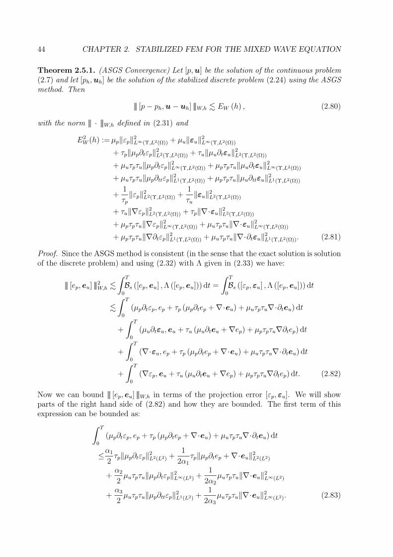
44 CHAPTER 2. STABILIZED FEM FOR THE MIXED WAVE EQUATION
Theorem 2.5.1. (ASGS Convergence) Let [p,u] be the solution of the continuous problem(2.7) and let [ph,uh] be the solution of the stabilized discrete problem (2.24) using the ASGSmethod. Then
||| [p− ph,u− uh] |||W,h . EW (h) , (2.80)
with the norm ||| · |||W,h defined in (2.31) and
E2W (h) :=µp‖εp‖2
L∞(Υ,L2(Ω)) + µu‖εu‖2L∞(Υ,L2(Ω))
+ τp‖µp∂tεp‖2L2(Υ,L2(Ω)) + τu‖µu∂tεu‖2
L2(Υ,L2(Ω))
+ µuτpτu‖µp∂tεp‖2L∞(Υ,L2(Ω)) + µpτpτu‖µu∂tεu‖2
L∞(Υ,L2(Ω))
+ µuτpτu‖µp∂ttεp‖2L1(Υ,L2(Ω)) + µpτpτu‖µu∂ttεu‖2
L1(Υ,L2(Ω))
+1
τp‖εp‖2
L2(Υ,L2(Ω)) +1
τu‖εu‖2
L2(Υ,L2(Ω))
+ τu‖∇εp‖2L2(Υ,L2(Ω)) + τp‖∇·εu‖2
L2(Υ,L2(Ω))
+ µpτpτu‖∇εp‖2L∞(Υ,L2(Ω)) + µuτpτu‖∇·εu‖2
L∞(Υ,L2(Ω))
+ µpτpτu‖∇∂tεp‖2L1(Υ,L2(Ω)) + µuτpτu‖∇·∂tεu‖2
L1(Υ,L2(Ω)). (2.81)
Proof. Since the ASGS method is consistent (in the sense that the exact solution is solutionof the discrete problem) and using (2.32) with Λ given in (2.33) we have:
||| [ep, eu] |||2W,h .∫ T
0
Bs ([ep, eu] ,Λ ([ep, eu])) dt =
∫ T
0
Bs ([εp, εu] ,Λ ([ep, eu])) dt
.∫ T
0
(µp∂tεp, ep + τp (µp∂tep +∇·eu) + µuτpτu∇·∂teu) dt
+
∫ T
0
(µu∂tεu, eu + τu (µu∂teu +∇ep) + µpτpτu∇∂tep) dt
+
∫ T
0
(∇·εu, ep + τp (µp∂tep +∇·eu) + µuτpτu∇·∂teu) dt
+
∫ T
0
(∇εp, eu + τu (µu∂teu +∇ep) + µpτpτu∇∂tep) dt. (2.82)
Now we can bound ||| [ep, eu] |||W,h in terms of the projection error [εp, εu]. We will showparts of the right hand side of (2.82) and how they are bounded. The first term of thisexpression can be bounded as:∫ T
0
(µp∂tεp, ep + τp (µp∂tep +∇·eu) + µuτpτu∇·∂teu) dt
≤α1
2τp‖µp∂tεp‖2
L2(L2) +1
2α1
τp‖µp∂tep +∇·eu‖2L2(L2)
+α2
2µuτpτu‖µp∂tεp‖2
L∞(L2) +1
2α2
µuτpτu‖∇·eu‖2L∞(L2)
+α3
2µuτpτu‖µp∂ttεp‖2
L1(L2) +1
2α3
µuτpτu‖∇·eu‖2L∞(L2). (2.83)

2.5. CONVERGENCE ANALYSIS 45
The third term of (2.82) can be bounded as:∫ T
0
(∇·εu, ep + τp (µp∂tep +∇·eu) + µuτpτu∇·∂teu) dt
≤α4
2τ−1u ‖εu‖2
L2(L2) +1
2α4
τu‖µu∂teu +∇ep‖2L2(L2)
+α5
2τp‖∇·εu‖2
L2(L2) +1
2α5
τp‖µp∂tep +∇·eu‖2L2(L2)
+α6
2µuτpτu‖∇·εu‖2
L∞(L2) +1
2α6
µuτpτu‖∇·eu‖2L∞(L2)
+α7
2µuτpτu‖∇·∂tεu‖2
L1(L2) +1
2α7
µuτpτu‖∇·eu‖2L∞(L2). (2.84)
The second and fourth terms of (2.82) can be bounded similarly as the first and thirdterms as shown in (2.83)-(2.84). Taking αi big enough, it follows that ||| [ep, eu] |||2W,h .E2W (h). Additionally, ||| [p− ph,u− uh] |||2W,h . ||| [ep, eu] |||2W,h + ||| [εp, εu] |||2W,h. Furthermore,
by definition ||| [εp, εu] |||2W,h . E2W (h), which completes the proof.
The inequality ||| [εp, εu] |||2W,h . E2W (h) is precisely the way of determining E2
W (h).
2.5.2 OSS Method
As we have defined two norms for the OSS method, one weaker than the other, we willprove convergence in both, starting with the weaker one.
Theorem 2.5.2. (OSS Convergence in the weak norm) Let [p,u] be the solution of thecontinuous problem (2.7) and let [ph,uh] be the solution of the stabilized discrete problem(2.24) using the OSS method. Then
||| [p− ph,u− uh] |||W,h . EW (h) , (2.85)
with the norm ||| · |||W,h defined in (2.31) and
E2W (h) :=µp‖εp‖2
L∞(Υ,L2(Ω)) + µu‖εu‖2L∞(Υ,L2(Ω))
+ τp‖µp∂tεp‖2L2(Υ,L2(Ω)) + τu‖µu∂tεu‖2
L2(Υ,L2(Ω))
+1
τp‖εp‖2
L2(Υ,L2(Ω)) +1
τu‖εu‖2
L2(Υ,L2(Ω))
+ τu‖∇εp‖2L2(Υ,L2(Ω)) + τp‖∇·εu‖2
L2(Υ,L2(Ω)). (2.86)
Proof. Since the OSS method is consistent (in the sense that the exact solution is solutionof the discrete problem) because the OSS method uses the projections Pp and Pu, we canuse the weak Λ-coercivity of the OSS method (2.36) with Λ given in (2.37) and we get:
||| [ep, eu] |||2W,h .∫ T
0
(µp∂tεp +∇·εu, ep + βτp (µp∂tep + Pp (∇·eu))) dt
+
∫ T
0
(µu∂tεu +∇εp, eu + βτu (µu∂teu + Pu (∇ep))) dt

46 CHAPTER 2. STABILIZED FEM FOR THE MIXED WAVE EQUATION
+
∫ T
0
(τpP
⊥p (∇·εu),∇·(eu + βτu (µu∂teu + Pu (∇ep)))
)dt
+
∫ T
0
(τuP
⊥u (∇εp),∇ (ep + βτp (µp∂tep + Pp (∇·eu)))
)dt. (2.87)
Now we can bound ||| [ep, eu] |||W,h in terms of the projection error [εp, εu]. We will showparts of the right hand side of (2.87) and how they are bounded. The first term of thisexpression can be bounded as:∫ T
0
(µp∂tεp +∇·εu, ep + βτp (µp∂tep + Pp (∇·eu))) dt
≤ α1
2τp‖µp∂tεp + Pp(∇·εu)‖2
L2(L2) +α2
2τ−1u ‖εu‖2
L2(L2) (2.88)
+β2
2α1
τp‖µp∂tep + Pp(∇·eu)‖2L2(L2) +
τu2α2
‖µu∂teu + Pu(∇ep)‖2L2(L2).
The third term of (2.87) can be bounded as:∫ T
0
(τpP
⊥p (∇·εu),∇·(eu + βτu (µu∂teu + Pu (∇ep)))
)dt
≤ α3
2τp‖P⊥p (∇·εu)‖2
L2(L2) +1
2α3
τp‖P⊥p (∇·eu)‖2L2(L2)
+β2
2α3
τuC2τC
2inv‖µu∂teu + Pu(∇ep)‖2
L2(L2). (2.89)
The second and fourth terms of (2.87) can be bounded similarly as we did for the first andthird terms in (2.88)-(2.89). Taking αi big enough, it follows that ||| [ep, eu] |||2W,h . E2
W (h).Using the same reasoning as for the ASGS method, we complete the proof for the OSSmethod.
Let us examine each term of E2W,h from (2.86) with respect to ‖p−ph‖2
L∞(Υ,L2(Ω)) (or theequivalent norm for u). The first and second terms are optimal for any of the variationalforms I, II and III (2.8)-(2.17). The third and fourth terms are at least optimal for I, IIor III. The fifth and seventh terms are quasi-optimal for I, optimal for II and sub-optimalfor III. The sixth and eighth terms are quasi-optimal for I, sub-optimal for II and optimalfor III. A similar analysis can be carried out for the error of ∇ph and ∇·uh. Results aresummarized in Table 2.2.
Now, let us examine the convergence of the OSS method in the strong norm (2.42).
Theorem 2.5.3. (OSS Convergence in the strong norm) Let [p,u] be the solution of thecontinuous problem (2.7) and let [ph,uh] be the solution of the stabilized discrete problem(2.24) using the OSS method. Then
||| [p− ph,u− uh] |||S,h . ES (h) , (2.90)
with the norm ||| · |||S,h defined in (2.42) and
E2S(h) :=µp‖εp‖2
L∞(Υ,L2(Ω)) + µu‖εu‖2L∞(Υ,L2(Ω))

2.5. CONVERGENCE ANALYSIS 47
+ τu‖∇εp‖L2(Υ,L2(Ω)) + τp‖∇·εu‖L2(Υ,L2(Ω))
+ τp‖µp∂tεp‖2L2(Υ,L2(Ω)) + τu‖µu∂tεu‖2
L2(Υ,L2(Ω))
+1
τp‖εp‖2
L2(Υ,L2(Ω)) +1
τu‖εu‖2
L2(Υ,L2(Ω))
+ γp‖µp∂ttεp +∇·∂tεu‖2L1(Υ,L2(Ω)) + γu‖µu∂ttεu +∇∂tεp‖2
L1(Υ,L2(Ω))
+ β2τp‖∇·∂tεu‖2L2(Υ,L2(Ω)) + β2τu‖∇∂tεp‖2
L2(Υ,L2(Ω))
+ γp‖µp∂tεp(0)‖2 + γu‖µu∂tεu(0)‖2. (2.91)
Proof. Since the OSS method is consistent (in the sense that the exact solution is solutionof the discrete problem) , using the strong Λ-coercivity (2.41) with Λi given in (2.43)-(2.44),i = 1, 2, we get:
||| [ep, eu] |||2W,h .∫ T
0
Bs ([εp, εu] ,Λ1 ([ep, eu])) dt
+
∫ T
0
Bs ([∂tεp, ∂tεu] ,Λ2 ([ep, eu])) dt
+ Bs ([εp, εu] ,Λ2 ([ep, eu]))∣∣t=0. (2.92)
Now we can bound each term of (2.92) in terms of the interpolation error [εp, εu]. The firstterm of (2.92) can be written as:∫ T
0
Bs ([εp, εu] ,Λ1 ([ep, eu])) dt =
∫ T
0
(µp∂tεp +∇·εu, ep + β1τpPp(∇·eu)) dt
+
∫ T
0
(µu∂tεu +∇εp, eu +β1τuPu(∇ep)) dt
+
∫ T
0
(P⊥p (∇·εu), τp∇·(eu + β1τuPu(∇ep))
)dt
+
∫ T
0
(P⊥u (∇εp), τu∇(ep + β1τpPp(∇·eu))
)dt. (2.93)
The first term (and similarly the second term) of (2.93) can be bounded as:∫ T
0
(µp∂tεp +∇·εu, ep + β1τpPp(∇·eu)) dt
≤α1
2τ−1u ‖εu‖2
L2(L2) +1
2α1
τu‖∇ep‖2L2(L2)
+α2
2τp‖µp∂tεp +∇·εu‖2
L2(L2) +β2
1
2α2
τp‖∇·eu‖2L2(L2). (2.94)
The third term (and similarly the fourth term) of (2.93) can be bounded as:∫ T
0
(P⊥p (∇·εu), τp∇·(eu + β1τuPu(∇ep))
)dt
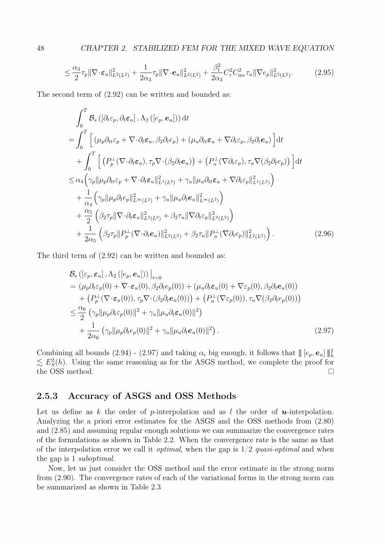
48 CHAPTER 2. STABILIZED FEM FOR THE MIXED WAVE EQUATION
≤ α3
2τp‖∇·εu‖2
L2(L2) +1
2α3
τp‖∇·eu‖2L2(L2) +
β21
2α3
C2τC
2invτu‖∇ep‖2
L2(L2). (2.95)
The second term of (2.92) can be written and bounded as:∫ T
0
Bs ([∂tεp, ∂tεu] ,Λ2 ([ep, eu])) dt
=
∫ T
0
[(µp∂ttεp +∇·∂tεu, β2∂tep) + (µu∂ttεu +∇∂tεp, β2∂teu)
]dt
+
∫ T
0
[ (P⊥p (∇·∂tεu), τp∇·(β2∂teu)
)+(P⊥u (∇∂tεp), τu∇(β2∂tep)
) ]dt
≤α4
(γp‖µp∂ttεp +∇·∂tεu‖2
L1(L2) + γu‖µu∂ttεu +∇∂tεp‖2L1(L2)
)+
1
α4
(γp‖µp∂tep‖2
L∞(L2) + γu‖µu∂teu‖2L∞(L2)
)+α5
2
(β2τp‖∇·∂tεu‖2
L2(L2) + β2τu‖∇∂tεp‖2L2(L2)
)+
1
2α5
(β2τp‖P⊥p (∇·∂teu)‖2
L2(L2) + β2τu‖P⊥u (∇∂tep)‖2L2(L2)
). (2.96)
The third term of (2.92) can be written and bounded as:
Bs ([εp, εu] ,Λ2 ([ep, eu]))∣∣t=0
= (µp∂tεp(0) +∇·εu(0), β2∂tep(0)) + (µu∂tεu(0) +∇εp(0), β2∂teu(0))
+(P⊥p (∇·εu(0)), τp∇·(β2∂teu(0))
)+(P⊥u (∇εp(0)), τu∇(β2∂tep(0))
)≤ α6
2
(γp‖µp∂tεp(0)‖2 + γu‖µu∂tεu(0)‖2
)+
1
2α6
(γp‖µp∂tep(0)‖2 + γu‖µu∂teu(0)‖2
). (2.97)
Combining all bounds (2.94) - (2.97) and taking αi big enough, it follows that ||| [ep, eu] |||2h. E2
S(h). Using the same reasoning as for the ASGS method, we complete the proof forthe OSS method.
2.5.3 Accuracy of ASGS and OSS Methods
Let us define as k the order of p-interpolation and as l the order of u-interpolation.Analyzing the a priori error estimates for the ASGS and the OSS methods from (2.80)and (2.85) and assuming regular enough solutions we can summarize the convergence ratesof the formulations as shown in Table 2.2. When the convergence rate is the same as thatof the interpolation error we call it optimal, when the gap is 1/2 quasi-optimal and whenthe gap is 1 suboptimal.
Now, let us just consider the OSS method and the error estimate in the strong normfrom (2.90). The convergence rates of each of the variational forms in the strong norm canbe summarized as shown in Table 2.3
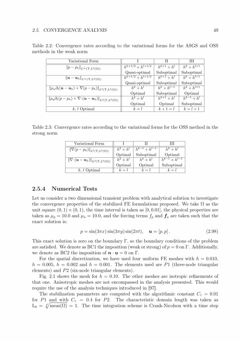
2.5. CONVERGENCE ANALYSIS 49
Table 2.2: Convergence rates according to the variational forms for the ASGS and OSSmethods in the weak norm
Variational Form I II III||p− ph||L∞(Υ,L2(Ω)) hk+1/2 + hl+1/2 hk+1 + hl hk + hl+1
Quasi-optimal Suboptimal Suboptimal||u− uh||L∞(Υ,L2(Ω)) hk+1/2 + hl+1/2 hk+1 + hl hk + hl+1
Quasi-optimal Suboptimal Suboptimal||µu∂t(u− uh) +∇(p− ph)||L2(Υ,L2(Ω)) hk + hl hk + hl−1 hk + hl+1
Optimal Suboptimal Optimal||µp∂t(p− ph) +∇·(u− uh)||L2(Υ,L2(Ω)) hk + hl hk+1 + hl hk−1 + hl
Optimal Optimal Suboptimalk, l Optimal k = l k + 1 = l k = l + 1
Table 2.3: Convergence rates according to the variational forms for the OSS method in thestrong norm
Variational Form I II III||∇(p− ph)||L2(Υ,L2(Ω)) hk + hl hk−1 + hl−1 hk + hl
Optimal Suboptimal Optimal||∇·(u− uh)||L2(Υ,L2(Ω)) hk + hl hk + hl hk−1 + hl−1
Optimal Optimal Suboptimalk, l Optimal k = l k = l k = l
2.5.4 Numerical Tests
Let us consider a two dimensional transient problem with analytical solution to investigatethe convergence properties of the stabilized FE formulations proposed. We take Ω as theunit square (0, 1)× (0, 1), the time interval is taken as [0, 0.01], the physical properties aretaken as µp = 10.0 and µu = 10.0, and the forcing terms fp and fu are taken such that theexact solution is:
p = sin(3πx) sin(3πy) sin(2πt), u = [p, p] . (2.98)
This exact solution is zero on the boundary Γ, so the boundary conditions of the problemare satisfied. We denote as BC1 the imposition (weak or strong) of p = 0 on Γ. Additionally,we denote as BC2 the imposition of n · u = 0 on Γ.
For the spatial discretization, we have used four uniform FE meshes with h = 0.010,h = 0.005, h = 0.002 and h = 0.001. The elements used are P1 (three-node triangularelements) and P2 (six-node triangular elements).
Fig. 2.1 shows the mesh for h = 0.10. The other meshes are isotropic refinements ofthat one. Anisotropic meshes are not encompassed in the analysis presented. This wouldrequire the use of the analysis techniques introduced in [97].
The stabilization parameters are computed with the algorithmic constant Cτ = 0.01for P1 and with Cτ = 0.4 for P2. The characteristic domain length was taken asL0 = d
√meas(Ω) = 1. The time integration scheme is Crank-Nicolson with a time step

50 CHAPTER 2. STABILIZED FEM FOR THE MIXED WAVE EQUATION
Figure 2.1: Mesh Sample
Table 2.4: Experimental convergence rates for the ASGS method using P1/P1 interpola-tion.
Variational Form I II IIIBoundary Cond. BC1 BC2 min BC1 BC2 min BC1 BC2 min||p− ph||L∞(Υ,L2(Ω)) 2.15 2.38 1.5 1.99 1.79 1 2.13 2.20 1||u− uh||L∞(Υ,L2(Ω)) 2.19 2.09 1.5 1.43 1.59 1 1.84 1.79 1||∇(p− ph)||L2(Υ,L2(Ω)) 1.03 1.18 1 0.99 0.84 0 1.04 1.07 1||∇·(u− uh)||L2(Υ,L2(Ω)) 1.48 1.10 1 1.10 1.13 1 0.81 0.71 0
size of 10−5. We have used a very small time step to avoid any interference of the timemarching algorithm into the spatial error since we are only interested in this spatial error.With that time step size the difference between the error of the scalar unknown in thenorm ||·||L∞(Υ,L2(Ω)) and the error in the same norm with a time step size twice as bigwas less than 1% in the finest mesh. This of course depends on the time interval chosen(T = 0.01), which has been taken small enough to avoid long term effects which wouldrequire a carefully designed time integration scheme, but large enough to obtain significantspatial errors.
In Tables 2.4 to 2.7 the experimental convergence rates for the ASGS and the OSSmethods are shown. BC1 and BC2 are the results obtained using BC1 and BC2 asboundary conditions and min stands for the minimum expected convergence rate based ontheoretical analysis. All these numerical results match with the convergence rates predictedtheoretically, in the sense that the convergence rate is always at least as fast as the worstpredicted by the analysis. It would be perhaps possible to improve the convergence ratesobtained using some sort of duality arguments, although we have not pursued this in thiswork (see [91]). It is noteworthy that the convergence rates for both the ASGS and theOSS method are surprisingly similar, although the absolute errors are not. For example,for BC1 and the Variational Form III using linear elements, the slope of the convergencecurve of ph in L∞(Υ, L2(Ω)) is 2.13 for both the ASGS and the OSS methods, but theabsolute errors are different. For h = 0.1, 0.05 and 0.025 the errors for the ASGS methodare 2.92 × 10⁻², 6.60 × 10⁻³ and 1.38 × 10⁻³, respectively, whereas for the OSS methodthese are 2.61× 10⁻², 6.15× 10⁻³ and 1.36× 10⁻³.

2.5. CONVERGENCE ANALYSIS 51
Table 2.5: Experimental convergence rates for the OSS method using P1/P1 interpolation.
Variational Form I II IIIBoundary Cond. BC1 BC2 min BC1 BC2 min BC1 BC2 min||p− ph||L∞(Υ,L2(Ω)) 2.16 2.43 1.5 1.99 1.79 1 2.13 2.20 1||u− uh||L∞(Υ,L2(Ω)) 2.18 2.18 1.5 1.41 1.59 1 1.84 1.79 1||∇(p− ph)||L2(Υ,L2(Ω)) 1.04 1.18 1 0.99 0.84 0 1.04 1.07 1||∇·(u− uh)||L2(Υ,L2(Ω)) 1.48 1.10 1 1.10 1.13 1 0.81 0.71 0
Table 2.6: Experimental convergence rates for the ASGS method using P2/P2 interpola-tion.
Variational Form I II IIIBoundary Cond. BC1 BC2 min BC1 BC2 min BC1 BC2 min||p− ph||L∞(Υ,L2(Ω)) 3.03 3.03 2.5 2.67 2.67 2 3.41 3.40 2||u− uh||L∞(Υ,L2(Ω)) 3.01 3.01 2.5 2.50 2.54 2 2.76 2.76 2||∇(p− ph)||L2(Υ,L2(Ω)) 2.06 2.07 2 1.79 1.79 1 2.54 2.54 2||∇·(u− uh)||L2(Υ,L2(Ω)) 2.07 2.06 2 2.55 2.55 2 1.79 1.79 1
Table 2.7: Experimental convergence rates for the OSS method using P2/P2 interpolation.
Variational Form I II IIIBoundary Cond. BC1 BC2 min BC1 BC2 min BC1 BC2 min||p− ph||L∞(Υ,L2(Ω)) 3.03 3.02 2.5 2.66 2.66 2 3.30 3.29 2||u− uh||L∞(Υ,L2(Ω)) 2.99 3.00 2.5 2.48 2.52 2 2.76 2.76 2||∇(p− ph)||L2(Υ,L2(Ω)) 2.06 2.06 2 1.79 1.79 1 2.53 2.53 2||∇·(u− uh)||L2(Υ,L2(Ω)) 2.06 2.06 2 2.55 2.54 2 1.79 1.79 1

52 CHAPTER 2. STABILIZED FEM FOR THE MIXED WAVE EQUATION
2.6 ConclusionsIn the present work, we have presented two stabilized FE methods (ASGS and OSS) for thewave equation in mixed form. Additionally, these stabilized methods have been applied tothree variational forms of the problem. We normally use the stabilized FE formulations forequal interpolation of the unknowns, but the analysis is not restricted to that and allowsany continuous interpolation pair. Extension to discontinuous approximations would beeasy to analyze, but this would require the introduction of terms evaluated on the interelement boundaries.
Length scales related to the unknowns were introduced in order to treat all variationalforms in a unified manner. The way length scales are computed is determined by the norm|||·||| in order to have control over the gradient of the scalar unknown or the divergence ofthe vector unknown if it is the case. Furthermore, length scales obviously influence thestability and accuracy of the methods.
Stability was proven for both the ASGS and the OSS methods applied to the waveequation in mixed form. According to those results, we have control over the L2-normof these unknowns. Moreover, depending on the variational form into consideration,additional control over the gradient of the scalar unknown and/or over the divergenceof the vector unknown is attained, and therefore we can guarantee that no numericalpoint-to-point oscillations will occur.
Theoretical convergence rates were found for both the ASGS and the OSS methods, andfor all the variational forms analyzed. Both stabilization methods exhibit at least the sameconvergence properties based on theoretical analysis. Additionally, there is no numericalevidence that the ASGS method has convergence superiority over the OSS method or vice-versa. One interesting feature of the convergence analysis applied to the three variationalforms of the wave equation in mixed form is the guideline given to which variational formto use. That said, for a balanced accuracy for both unknowns and equal interpolation,variational form I is the best choice.

Chapter 3
A Sommerfeld non-reflecting boundarycondition for the wave equation inmixed form
This chapter is based on the material in:Hector Espinoza, Ramon Codina, and Santiago Badia. “A Sommerfeld non-reflectingboundary condition for the wave equation in mixed form”. In: Computer Methods inApplied Mechanics and Engineering 276 (July 2014), pp. 122–148. issn: 0045-7825. doi:10.1016/j.cma.2014.03.015. url: http://www.sciencedirect.com/science/article/pii/S0045782514001017with the notation modified to make it fit with the other chapters. Some content is repeatedfrom Chapter 1 and Chapter 2 so it is self-contained.
In this chapter we develop numerical approximations of the wave equation in mixedform supplemented with non-reflecting boundary conditions (NRBCs) of Sommerfeld-typeon artificial boundaries for truncated domains. We consider three different variationalforms for this problem, depending on the functional space for the solution, in particular,in what refers to the regularity required on artificial boundaries. Then, stabilized finite el-ement methods that can mimic these three functional settings are described. Stability andconvergence analyses of these stabilized formulations including the NRBC are presented.Additionally, numerical convergence tests are evaluated for various polynomial interpola-tions, stabilization methods and variational forms. Finally, several benchmark problemsare solved to determine the accuracy of these methods in 2D and 3D.
3.1 Introduction
Many engineering problems dealing with waves involve infinite domains. Usually, theinfinite domain is truncated for computational purposes and the wave problem is solvedin a finite domain [105, 106]. Non-reflecting boundaries (NRBs) have to be considered,which must allow the waves to leave the truncated domain avoiding spurious reflectionsthat may pollute the solution in the interior of the computational domain of interest. Thereare many types of NRBs, which can be classified into two groups, namely, Non-ReflectingBoundary Conditions (NRBCs) and Non-Reflecting Boundary Layers (NRBLs). NRBCs
53

54 CHAPTER 3. NRBC FOR THE MIXED WAVE EQUATION
are boundary conditions on the artificial boundary that absorb impinging waves. On theother hand, NRBLs have the property of absorbing waves that are traveling inside thelayer.
NRBL techniques have been applied to the time-domain wave equation in irreducible[35, 36, 107] and mixed form [42, 43, 51], and to the linearized Euler equations [108–110]. Perhaps the most popular among the NRBL techniques is the Perfectly MatchedLayer (PML). The PML concept was developed by Berenger in 1994 for electromagneticscattering [34]. The idea is to add an absorbing layer to the domain designed to have zeroreflection for any plane wave and to make the solution decay exponentially inside the layer[111].
A classical example of NRBC is the so-called Sommerfeld boundary (or radiation)condition [11]. It relates the temporal derivative and the normal derivative of the unknownin the case of boundaries far away from sources and normal to the propagating wave.Thus, it is inexact for non-perpendicular wave incidence and boundaries close to sources,and therefore it has to be understood as an approximate boundary condition to avoidwave reflection in these cases. NRBCs have also been applied to the time-domain waveequation in irreducible [16, 112–114] and mixed form [20], as well as for the linearized Eulerequations in [17, 20].
The error E introduced by a NRBC is the difference between the exact solution in theunbounded domain and the solution in the truncated domain with the artificial boundary.Let J be the order of the NRBC, R the distance of the artificial boundary to the wavesource, kt the tangential wave number and ω the wave angular frequency. The error Eintroduced by a NRBC of order J [106] behaves as
E = O(k2t
ω2
)J= O
(1
R2
)J. (3.1)
For a fixed location of the artificial boundary, increasing the order J reduces the errorintroduced by the NRBC. If the error approaches zero as J increases the NRBC is exact,whereas if the error does not approach zero the NRBC is asymptotic [105].
Many NRBCs have been developed and can be classified as classical, exact non-localand local high-order. Among classical NRBCs we have those proposed by Engquist-Majda[14], Bayliss-Turkel [115] and Higdon [116]. Classical NRBCs appeared as an improvementof Sommerfeld NRBC and can be high-order in theory, but in practice only low-orderversions are used because of the presence of high-order derivatives which are difficult tohandle numerically [111]. Among exact non-local NRBCs we have Dirichlet-to-Neumannformulations [117] and the Difference Potential Method [118]. Exact non-local NRBCsinvolve a boundary integral operator which couples all the points on the boundary [111].Among local high-order NRBCs we have those due to Collino [119], Grote-Keller [23],Rowley-Colonius [120], Guddati-Tassoulas [121], Givoli-Neta [16] and Hagstrom-Warburton[122]. Local high-order NRBCs are high-order in theory and can be implemented up toany desired order in practice, which can be achieved introducing auxiliary variables [111].
The wave equations can be posed in irreducible form, leading to a second-order (in spaceand time) scalar partial differential equation. Many applications require the vector-valuedunknown of the problem, which can be computed by the solution of the irreducible formplus a post-processing step, but leads to a poor approximation of it. In order to improve

3.1. INTRODUCTION 55
the convergence rate for the vector field, we can consider the problem as a first-order (inspace and time) hyperbolic system, that involves both the scalar and vector unknowns. Thewave equation in mixed form is in fact mandatory for some applications in solid mechanicsor in nonlinear waves in shallow waters.
The finite element (FE) approximation in space of this hyperbolic problem is notstraightforward, since its well-posedness relies on an inf-sup condition. Thus, Galerkin FEschemes require mixed interpolations that satisfy a discrete version of this compatibilitycondition [78]. Inf-sup stable FE formulations have been developed for several mixedproblems, e.g., [79] for the Stokes problem, [80] for the Darcy problem, [81] for the Maxwellproblem, [82, 83] for the Stokes-Darcy problem, [84] for the wave equation, and [85, 86] forelastodynamics. As an alternative to inf-sup stable formulations, we can consider stabilizedFE formulations [90]. Stabilized FEs add new terms to the Galerkin formulation, whichprovide the required stability for well-posedness (without the need to rely on a discreteinf-sup condition) keeping optimal convergence properties. This way, we are able to useequal interpolation for the scalar and vector unknowns of the wave equation in mixed form.
In this work, we develop novel stabilized FE formulations for wave scattering problemson unbounded domains truncated via Sommerfeld-type boundary conditions as the simplestexample of NRBC. Our starting point is the formulation recently presented and analyzedin [67]. It is a stabilized FE method with the important feature of allowing for differentfunctional settings. This is accomplished by transferring regularity from the scalar to thevector unknowns or vice-versa [67] through an appropriate integration by parts and designof the stabilization parameters. Summarizing, the main contributions are:
• Statement of the mixed form of the wave equation with Sommerfeld artificial bound-ary conditions in three different functional settings. It is an extension of the work in[67], in which the functional setting has to be properly modified in order to give senseto the Sommerfeld terms; extra regularity is required on the artificial boundary forthe vector unknown. One of the resulting formulations has already been proposedin [20], whereas the other two problem settings are new. We observe that the newfunctional spaces are in fact complete.
• Extension of the stabilized FE formulations in [67] to deal with Sommerfeld boundaryconditions. We design stabilized FE formulations that can mimic the three functionalsettings proposed at the continuous level. Stability and convergence results arepresented, and their proof is sketched. A set of numerical experiments is performedto check the convergence of the formulations, as well as the error introduced by theSommerfeld boundary condition.
The organization of the chapter is as follows. In Section 3.2, we present the waveequation in irreducible and mixed form and in time and frequency domain. Additionally,we describe the Sommerfeld boundary condition applied to the wave equation. We alsopropose three different functional settings for the time-domain wave problem in mixed formtruncated with Sommerfeld boundary conditions. In Section 3.3, we describe the spatialdiscretization we propose, which is a stabilized FE method (in two different versions),and show how to mimic the three functional settings by properly integrating by partsand choosing the stabilization parameters. Section 3.4 is devoted to the stability and

56 CHAPTER 3. NRBC FOR THE MIXED WAVE EQUATION
convergence analysis of these formulations, respectively. In all these sections, time is leftcontinuous, concentrating the exposition only in the spatial approximation. In Section 3.5we carry out convergence tests and evaluate the performance of the NRBC through variousbenchmark problems in 2D and 3D. Finally, we draw some conclusions in Section 3.6.
3.2 Problem statementIn this section, we state the wave equation in mixed form in time and frequency domain.Further, we state the Sommerfeld artificial boundary conditions in both cases. The useof Sommerfeld-type boundary conditions for the mixed form of the wave equation hasbeen used in [20] (without using this terminology). Waves are commonly found in manyphysical phenomena such as acoustic and electromagnetic scattering, fluid dynamics, andelastodynamics. To fix ideas, we will use the terminology of waves propagating in fluids,although our approach is obviously general.
3.2.1 Wave equation in time and frequency domain
Waves can be described in time domain or frequency domain. In both cases, the probleminvolves a spatial domain Ω ⊂ Rd, where d is the space dimension (d = 1, 2, 3). Let Γbe its boundary and x ∈ Ω any spatial point. From hereafter, we will refer to vectorsin Rd simply as vectors. Further, we use the following convention: lower-case bold italicletters represent vectors in Rd, and non-bold letters represent scalars. Both complex andreal numbers are used in this section. We implicitly assume real numbers unless otherwisespecified.
In the time domain, the problem is posed in Ξ := Ω×Υ, where t ∈ Υ := (0, T ) denotesa time value. The long term behavior, i.e. T → ∞, will not be considered in this work.The time-domain wave equation in its irreducible form reads as:
1
c2∂ttp
′ −∆p′ = f ′, (3.2)
where p′(x, t) is the unknown (real-valued scalar function), f ′ is a forcing term and c is thewave speed. Alternatively, we can consider the wave equation in mixed form:
µp∂tp′ +∇·u′ = fp, (3.3)
µu∂tu′ +∇p′ = fu, (3.4)
where the unknowns p′(x, t) and u′(x, t) are real-valued scalar and vector functions, re-spectively, µp > 0 and µu > 0 are the physical parameters of the equation and [fp,fu]are forcing terms. The coefficients µp and µu that characterize the mixed wave equation(3.3)-(3.4) are related to the wave speed c appearing in irreducible form of the scalar waveequation (3.2) as follows:
c2 = (µpµu)−1 .
Time domain analysis solves the wave problem for the full range of frequencies involved.The only limit for the frequencies captured at time-discrete level is the size of the time

3.2. PROBLEM STATEMENT 57
step used for the time discretization. Frequency domain analysis results from a Fouriertransform in time of the time-domain problem and solves the wave problem for one angularfrequency ω. In the irreducible case, it leads to the scalar Helmholtz equation:
∆p+ k2p = fk, (3.5)
where p(x) is now the unknown (complex-valued scalar function), and k = ω/c is thewavenumber corresponding to a certain angular frequency ω. As in the time domain case,we can also make use of the Helmholtz equation in mixed form:
−iµpωp+∇·u = fp, (3.6)
−iµuωu+∇p = fu, (3.7)
where p(x) and u(x) are complex unknowns, ω is the angular frequency, fp and fu areforcing terms and i =
√−1.
Notice that the number of unknowns in the wave equation in mixed form (both in thetime and frequency domain) is d+ 1 times the ones in irreducible form, but the regularityrequirements in space and time can be made less stringent for p′. In all cases, the waveequation has to be supplemented with appropriate initial and boundary conditions. In thecase of the mixed form, boundary conditions also depend on the functional setting of theproblem.
3.2.2 Sommerfeld Boundary Condition
The Sommerfeld boundary condition is a type of NRBC, that takes its name from theGerman theoretical physicist Arnold Sommerfeld, applicable when the sources are concen-trated in a region of the space and the exterior boundary is a sphere surrounding it andcentered at the source region. Additionally, the spherical surface has to be far away fromthe source, so that one can assume that the impinging waves only have radial compo-nent when they reach the artificial boundary. In spherical coordinates and for the scalarHelmholtz equation in 3D (frequency domain), the Sommerfeld radiation condition can beexpressed as:
limr→∞
(r (∂rp− ikp)) = 0,
where r is radial component in the spherical coordinate system and ∂r is the derivativein the radial direction.1 In spherical coordinates and for the scalar wave equation inirreducible form in 3D (time domain) the Sommerfeld radiation condition can be writtenas:
limr→∞
(r
(∂rp′ +
1
c∂tp′))
= 0.
1Some authors write the Sommerfeld radiation condition with a + sign, but that depends on the timevariation assumption. In this work, we have assumed a harmonic time variation with harmonics of theform e−iωt, which gives the minus sign.
58 CHAPTER 3. NRBC FOR THE MIXED WAVE EQUATION
On the other hand, when considering the mixed form of these equations, the Sommerfeldradiation condition can be written in two different ways:
limr→∞
(r(√
µp ∂rp′ −√µu ∇·u′
))= 0,
limr→∞
(r(√
µp ∂tp′ −√µu ∂tu′r
))= 0. (3.8)
In the frequency domain, these Sommerfeld boundary conditions lead to:
limr→∞
(r(√
µp ∂rp−√µu ∇·u
))= 0,
limr→∞
(r(√
µp p−√µu ur
))= 0.
Condition (3.8) can be simplified taking out the temporal derivative, which yields
limr→∞
(r(√
µp p′ −√µu u′r + C(x)
))= 0.
C(x) is a time-independent function defined on Γ, which can be determined from initialconditions. Assuming that√µp p′(x, 0)−√µu u′r(x, 0) = 0 holds on the artificial boundary,we get C(x) = 0. It leads to the final expression
limr→∞
(r(√
µp p′ −√µu u′r
))= 0.
This Sommerfeld radiation condition is a limit for r →∞, and establishes a fast decay of√µp p
′−√µu u′r. If R <∞, the approximation that we may consider is√µp p′−√µu u
′r = 0
at r = R. Moreover, if the boundary is not a sphere, we may replace u′r by n ·u′, n beingthe unit normal exterior to the boundary. Thus, we may consider the approximation
õp p
′ −√µu n · u′ = 0. (3.9)
Because of its simplicity, this is the boundary condition we propose to enforce on theartificial boundary for the mixed wave equation in time domain. In the following sections,we show that this boundary condition has good non-reflecting properties and is stable, inspite of having been superseded in accuracy by high order NRBCs. The analysis of itsperformance in combination with the FE method we propose is the subject of this chapter.
3.2.3 Initial and Boundary Value Problem
Let us split Γ into three disjoint sets denoted as Γp, Γu and Γo. The scalar unknown p isenforced on Γp, the normal trace of the vector unknown γnu on Γu (γn denotes the normaltrace operator), and the NRBC we wish to analyze on Γo (the artificial boundary). Theproblem consists in finding p : Ξ −→ R and u : Ξ −→ Rd such that:
µp∂tp+∇·u = fp , (3.10)µu∂tu+∇p = fu , (3.11)
with the initial conditions
p(x, 0) = 0, u (x, 0) = 0, (3.12)

3.2. PROBLEM STATEMENT 59
and with the boundary conditions
p = 0 on Γp, γnu := n · u = 0 on Γu, µ12p p = µ
12uγnu on Γo. (3.13)
Let us define two auxiliary variables denoted as κp and κu defined as:
κp :=
(µpµu
) 12
, κu :=
(µuµp
) 12
.
Let Ψ be a generic spatial domain, i.e., Ω or Γ or part of them. Let L2(Ψ) be thespace of square integrable functions defined on Ψ, and L2(Ψ)
d the space of vector functionswith components in L2(Ψ). H1(Ψ) is the space of functions in L2(Ψ) with derivatives inL2(Ψ), H(div,Ψ) the space of vector functions with components and divergence in L2(Ψ).Any of the spaces defined previously will be denoted generically as X. Additionally, foran arbitrary functional space X, its norm will be denoted as ||·||X. In the case of L2(Ω)
or L2(Ω)d, the L2-norm will simply be denoted as ||·|| and the L2-inner-product as (· , ·).
Furthermore, the space of functions whose X-norm is Cr continuous in the time interval Υwill be denoted by Cr(Υ; X). (We will only be interested in the cases r = 0 and r = 1.)Functions whose X-norm is Lp in Υ will be denoted by Lp(Υ; X).
Furthermore, let Vp, Vu be the functional spaces associated with p and u, respectively.These spaces will be defined afterwards because they depend on the functional setting.Additionally, let us define V := Vp × Vu and L := L2(Ω)× L2(Ω)
d.Problem (3.10)-(3.11) with appropriate initial and boundary conditions will be stated
for
p ∈ C1(Υ;L2(Ω)
)∩ C0
(Υ;Vp
),
u ∈ C1(Υ;L2(Ω)
d) ∩ C0(Υ;Vu
),
with fp and fu in regular enough spaces.
3.2.4 Internal energy and power flux
Let us multiply (3.10) against p, (3.11) against u, add the resulting equations and integrateover Ω. Applying the divergence theorem, we get the energy balance equation:
1
2µp
d
dt||p||2 +
1
2µu
d
dt||u||2 = −
∫Γ
n · pu dΓ + (fp, p) + (fu,u) .
The total internal energy E is defined as:
E :=1
2
(µp||p||2 + µu||u||2
),
which contains the potential energy 12µp||p||2 and the kinetic energy 1
2µu||u||2. The energy
per unit time, i.e. the power added through the boundary, is defined as:
Pb := −∫
Γ
n · pu dΓ,

60 CHAPTER 3. NRBC FOR THE MIXED WAVE EQUATION
whereas the power of the external forces is defined as:
Pf := (fp, p) + (fu,u) .
The power flux (energy per unit time per unit surface) at any given point of the boundaryis n · pu. The Sommerfeld boundary condition prescribed on Γo is the one that ensuresthat energy always flows out of the boundary because n ·pu ≥ 0 everywhere at any instantof time, i.e., Pb ≤ 0. It makes the problem well-posed, since the solution is bounded bythe data. With these definitions we can write the energy balance equation as:
dE
dt= Pb + Pf . (3.14)
Our interest in equation (3.14) relies in the fact that it represents the power balance of thesystem and it reveals the interaction of the forces and boundaries with the domain.
3.2.5 Variational Problem
The variational form of problem (3.10)-(3.13) can be expressed in three different ways.Each one requires a certain regularity on the unknowns p and u, which amounts to saythat p and u should belong to a particular space of functions. In all cases the problemreads: find [p,u] ∈ C1 (Υ;L) ∩ C0 (Υ;V ) such that
B ([p,u] , [q,v]) = L ([q,v]) , (3.15)
for all test functions [q,v] ∈ V and the respective initial conditions. The bilinear form B,the linear form L and the space V are defined in three different ways depending on thevariational form into consideration. For simplicity, we will assume that the forcing termsfp and fu are square integrable, although we could relax this regularity requirement andassume they belong to the dual space of Vp and Vu, respectively.
The three different variational formulations of problem (3.10)-(3.13) essentially differ inthe way integration-by-parts from the strong form of the problem is performed and in theregularity required for the unknowns. In the problem statement given below, variationalform I (3.16)-(3.20) is obtained without integrating by parts any term. Thus, boundaryconditions on both scalar and vector quantities have to be imposed strongly. Pressuresin H1(Ω) have well-defined traces in L2(Γ), and the pressure boundary condition on Γphas sense. The velocity space H(div,Ω) does not have a continuous γn operator ontoL2(Γ). Thus, in order for the Sommerfeld condition p = κuγnu to have sense in L2(Ω)(which is required for p ∈ H1(Ω)), we consider a more regular velocity space, viz., thespace of H(div,Ω) with normal traces in L2(Ω). We can easily check that the resultingbilinear/linear forms in (3.16)-(3.17) are continuous in this functional setting.
The introduction of the NRBC motivated a slight modification of the functional frame-work and working norms with respect to Chapter 2. The modifications are reflected below.
Variational Form I
Vp =q ∈ H1(Ω)| q = 0 on Γp
,

3.2. PROBLEM STATEMENT 61
Vu =v ∈ H(div,Ω)| γnv = 0 on Γu and γnv ∈ L2(Γo)
,
B ([p,u] , [q,v]) = µp (∂tp, q) + (∇·u, q) + µu (∂tu,v) + (∇p,v) , (3.16)L ([q,v]) = (fp, q) + (fu,v) , (3.17)
p = 0 on Γp, strongly imposed, (3.18)γnu = 0 on Γu, strongly imposed, (3.19)
µ12p p = µ
12uγnu on Γo, strongly imposed. (3.20)
The variational form II (3.21)-(3.25) is obtained integrating by parts the term (∇p,v),and using the Sommerfeld condition (3.9) on Γo:
(∇p,v) = −(p,∇·v) +
∫Γo
γnvp = −(p,∇·v) + κu
∫Γo
γnuγnv.
The boundary integral on Γp∪Γu vanishes due to (3.23)-(3.24) below; the pressure conditionon Γp is weakly enforced and the velocity condition on Γu is strongly enforced. In this case,pressures only need to be in L2(Ω), whereas velocities should belong to the same space asin the previous variational form. We observe that the normal trace γn of velocity functionshave to be in L2(Γo) in order to give sense to the Sommerfeld term on Γo. In this functionalsetting, the bilinear/linear forms (3.21)-(3.22) are continuous. 2
Variational Form II
Vp = L2(Ω),
Vu =v ∈ H(div,Ω)| γnv = 0 on Γu and γnv ∈ L2(Γo)
,
B ([p,u] , [q,v]) = µp (∂tp, q) + (∇·u, q) + µu (∂tu,v)− (p,∇·v) + κu
∫Γo
γnvγnu dΓ,
(3.21)L ([q,v]) = (fp, q) + (fu,v) , (3.22)
p = 0 on Γp, weakly imposed, (3.23)γnu = 0 on Γu, strongly imposed, (3.24)
µ12p p = µ
12uγnu on Γo, weakly imposed. (3.25)
Finally, the variational form III (3.26)-(3.30) is obtained integrating by parts the term(∇·u, q) and proceeding analogously on the boundary:
(∇·u, q) = −(u,∇q) +
∫Γo
γnuq = −(u,∇q) + κp
∫Γo
pq.
2This formulation has already been proposed in [20], but the functional setting was incorrect; onlyH(div,Ω) regularity was assumed for the vector unknowns and the Sommerfeld terms were ill-posed. Inany case, the authors explicitly say that this is not the goal of their paper.

62 CHAPTER 3. NRBC FOR THE MIXED WAVE EQUATION
In this case, the velocity condition on Γu is weakly enforced, whereas the pressure conditionon Γp is strongly enforced. The functional setting in this third case is standard.
Variational Form III
Vp =q ∈ H1(Ω)| q = 0 on Γp
, Vu = L2(Ω)
d,
B ([p,u] , [q,v]) = µp (∂tp, q)− (u,∇q) + µu (∂tu,v) + (∇p,v) + κp
∫Γo
pq dΓ, (3.26)
L ([q,v]) = (fp, q) + (fu,v) , (3.27)
p = 0 on Γp, strongly imposed, (3.28)γnu = 0 on Γu, weakly imposed, (3.29)
µ12p p = µ
12uγnu on Γo, weakly imposed. (3.30)
Let us note that the Sommerfeld condition on Γo is strongly enforced for the firstvariational form, whereas it is weakly enforced in the other two cases. On the other hand,the introduction of the Sommerfeld boundary conditions requires a more regular functionalsetting (see [67] for comparison).
Notice the way we have defined Vu for variational forms I and II. When we move fromthe continuous level to the discrete level we have to ensure the spaces we are working withare complete. The completeness of Vu is proved in the following lemma. A similar resultwith a similar proof but involving u ∈ H(curl,Ω) and u×n ∈ L2(Γ) can be found in [123,p. 69, p. 84].
Lemma 3.2.1. (Completeness of Vu) The space Vu for the variational forms I and II iscomplete when it is endowed with the following norm:
|||u|||2Vu :=1
L20
||u||2 + ||∇·u||2 +1
L0
||γnu||2L2(Γo). (3.31)
Proof. Let un be a Cauchy sequence in Vu. Since H(div,Ω) is complete, un −→ w inH(div,Ω). Additionally, γnun −→ v in L2(Γo) since L2(Γo) is complete. Furthermore,γnun −→ γnw in H−1/2(Γ) since the normal trace operator γn goes from H(div,Ω) toH−1/2(Γ). Since the limits must be the same, we conclude that γnw = v in L2(Γo) andtherefore Vu is complete.
3.3 Stabilized Finite Element MethodsIn this section, we present two stabilized FE methods, which we will denote by the acronymsASGS and OSS, aimed to overcome the instability problems of the standard Galerkinmethod. In general, the stabilized FE methods we propose can be used with any type ofcontinuous interpolation for p and u. In particular, we focus on equal order continuousinterpolations. For conciseness, we consider quasi-uniform FE partitions of size h. Forstabilized formulations in general non-uniform non-degenerate cases, see [97].
3.3. STABILIZED FINITE ELEMENT METHODS 63
Let Vp,h and Vu,h be the FE spaces to approximate p and u, respectively, with Vp,h ⊂ Vpand Vu,h ⊂ Vu. Additionally, let us define Vh = Vp,h × Vu,h. For any of these spaces wewill make frequent use of the classical inverse inequality ‖∇vh‖ ≤ Cinvh
−1‖vh‖, with Cinv
a constant independent of the FE function vh and the mesh size h.Stabilized FE methods deal with the following problem: Find a pair [ph,uh] ∈ C1(Υ;Vh)
satisfying the initial conditions ph(x, 0) = 0, uh(x, 0) = 0 and such that
Bs ([ph,uh] , [qh,vh]) = Ls ([qh,vh]) , (3.32)
for all test functions [qh,vh] ∈ Vh, where the bilinear form Bs and the linear form Ls includethe Galerkin terms and additional stabilization terms. Depending on how the stabilizationpart is designed, a different stabilization method arises. Below, we propose two differenttypes of methods, namely ASGS and OSS. The stabilization terms depend on the choiceof the so-called stabilization parameters τp and τu.
3.3.1 Algebraic Sub-Grid Scale (ASGS) method
The ASGS-type stabilization was originally proposed in [87, 89]. The ASGS stabilizationterms have the same expression for the three variational forms introduced above. For thewave equation in mixed form, the ASGS stabilized problem (3.32) is obtained by takingBs and Ls as:
Bs ([ph,uh] , [qh,vh]) = B ([ph,uh] , [qh,vh])
+ (µp∂tph +∇·uh, τp∇·vh) + (µu∂tuh +∇ph, τu∇qh) , (3.33)Ls ([qh,vh]) = L ([qh,vh]) + (fp, τp∇·vh) + (fu, τu∇qh) . (3.34)
It consists in subtracting to the Galerkin terms the integral of the residual of the equationtimes the adjoint of the spatial differential operator and a stabilization parameter. (τu, τp)are the stabilization parameters, which will be different for every variational formulation.The additional terms provide stability without harming consistency and a priori errorestimates.
3.3.2 Orthogonal Sub-scale Stabilization (OSS) method
The OSS stabilization technique was designed in [98, 99]. Instead of considering the wholeresidual (as in ASGS), it only includes quantities that provide stabilization. However, sinceit would spoil accuracy, the FE projection of these quantities is subtracted, recoveringoptimal convergence. It consists in solving problem (3.32) taking Bs and Ls as:
Bs ([ph,uh] , [qh,vh]) = B ([ph,uh] , [qh,vh])
+(P⊥p (∇·uh) , τp∇·vh
)+(P⊥u (∇ph) , τu∇qh
), (3.35)
Ls ([qh,vh]) = L ([qh,vh]) +(P⊥p (fp) , τp∇·vh
)+(P⊥u (fu) , τu∇qh
), (3.36)
where P⊥p (·) = I(·) − Pp(·) and P⊥u (·) = I(·) − Pu(·), Pp(·) being the L2(Ω) projection onVp,h and Pu(·) the L2(Ω) projection on Vu,h. This in particular implies that Pp(·) = 0 onΓp for variational forms I and III and that n · Pu(·) = 0 on Γu for variational forms I andII.

64 CHAPTER 3. NRBC FOR THE MIXED WAVE EQUATION
Table 3.1: Stabilization Parameters Order and Length Scales Definition
Variational Form I II IIIτp O(h) O(1) O(h2)τu O(h) O(h2) O(1)`p `p = `u L2
0/h h`u `p = `u h L2
0/h
3.3.3 The stabilization parameters
An important component of stabilized formulations are the stabilization parameters. Inour case, we compute them in all formulations as:
τp = Cτ
√µuµph
√`p`u, τu = Cτ
√µpµuh
√`u`p, (3.37)
where Cτ is a dimensionless algorithmic constant and `p, `u are length scales correspondingto p and u respectively. As it was shown in the analysis presented in [67], in order to mimicat the discrete level the proper functional setting of the continuous problem, the lengthscales `p and `u should be taken as shown in Table 3.1, where L0 is a fixed length scaleof the problem that can be fixed a priori. The motivation for designing the stabilizationparameters can be found in [90, 91].
3.4 Numerical analysis
3.4.1 Stability analysis
In this section, we present stability results for the ASGS and the OSS methods. We usethe concept of Λ-coercivity, originally introduced in [103], which aids us in the proof ofstability and convergence analyses. The proofs of the stability lemmata and theorems arevery similar to the proofs shown in [67], the only difference being the new terms on Γo, dueto the Sommerfeld artificial boundary condition. Since these terms have required a moreregular functional setting than the one in [67], the working norms now contain the newterms κp||qh||2L2(Υ,L2(Γo)) and κu||γnvh||
2L2(Υ,L2(Γo)). These working norms are defined next:
Definition 3.4.1 (Working norms). Let
|||[qh,vh]|||20,h := µp||qh||2L∞(Υ;L2(Ω)) + µu||vh||2L∞(Υ;L2(Ω))
+ (1 + σ)κp||qh||2L2(Υ,L2(Γo)) + (1− σ)κu||γnvh||2L2(Υ,L2(Γo)),
with σ = 0,−1, 1 for variational forms I, II and III, respectively. We define:i) Weak norm:
|||[qh,vh]|||2W,h := |||[qh,vh]|||20,h + τp||µp∂tqh +∇·vh||2L2(Υ;L2(Ω))
+ τu||µu∂tvh +∇qh||2L2(Υ;L2(Ω)). (3.38)

3.4. NUMERICAL ANALYSIS 65
ii) Strong norm:
|||[qh,vh]|||2S,h := |||[qh,vh]|||20,h + τp||∇·vh||2L2(Υ,L2(Ω)) + τu||∇qh||2L2(Υ,L2(Ω)). (3.39)
We state a first stability result in the form of Λ-coercivity. This concept is used herein the same sense as in [67, 103] for the ASGS and OSS methods. The results obtainedapply to any of the variational forms, defined in (3.16), (3.21), and (3.26).
In what follows, C denotes a positive constant, independent of µp, µu, `p and `u. Inthe discrete formulation C will be independent of the mesh size h. The value of C may bedifferent at different occurrences. Additionally, we will use the notation A & B and A . Bto indicate that A ≥ CB and A ≤ CB respectively, where A and B are two quantities thatmight depend on the solution or mesh size.
The ASGS and OSS methods are not coercive in the norms of interest and therefore theirwell-posedness needs to be proved via an inf-sup condition. For the subsequent analysiswe use a more descriptive property than the inf-sup condition. This property has beendefined as Λ-coercivity in [103].
Definition 3.4.2 (Λ-coercivity). Let V be a normed space and ζ : V × V −→ R abilinear form. ζ is Λ-coercive if we can define a continuous operator Λ : V −→ V, i.e.,‖Λ(u)‖V . ‖u‖V ∀u ∈ V, such that
ζ(u,Λ(u)) & ‖u‖V‖Λ(u)‖V ∀u ∈ V .
Let us recall that the inf-sup condition for ζ implies that ∀u ∈ V ∃ v ∈ V such thatζ(u, v) & ‖u‖V‖v‖V with ‖v‖V . ‖u‖V . Thus, Λ-coercivity implies the inf-sup conditionfor a particular definition of norms but it is stronger, since it also provides a continuousoperator Λ that for every function u in V gives a function v = Λ(u) such that the inf-supcondition holds.
In the case of the OSS method we can state Λ-coercivity in two norms: the weak normdefined in (3.38) and the strong norm defined in (3.39); ASGS stability can only be provedwith the weak norm. The norm in (3.39) is stronger, since it provides full control over∇ph and ∇·uh. The proof is just a slight modification of the one in [67] to account forthe boundary terms and we omit it. We detail the expressions of Λ that allow us to proveΛ-coercivity because they in fact provide information about the stabilization mechanismof every method.
Lemma 3.4.1 (Λ-coercivity). Both the ASGS and the OSS methods are Λ-coercive in thenorm defined in (3.38), i.e., their associated bilinear form satisfies
|||[qh,vh]|||2W,h .∫
Υ
Bs ([qh,vh] ,Λ ([qh,vh])) dt ∀ [qh,vh] ,
whit the following choices of Λ(·):
i) ASGS method:Λ ([qh,vh]) := [qh + τpµp∂tqh,vh + τuµu∂tvh] ,
ii) OSS method:
Λ ([qh,vh]) := [qh,vh] + β[τp(µp∂tqh + Pp(∇·vh)), τu(µu∂tvh + Pu(∇qh))
],

66 CHAPTER 3. NRBC FOR THE MIXED WAVE EQUATION
with a small enough β > 0. Moreover, the OSS method is also Λ-coercive in the normdefined in (3.39), i.e., its bilinear form satisfies
|||[qh,vh]|||2S,h .∫
Υ
Bs ([qh,vh] ,Λ1 ([qh,vh])) dt+
∫Υ
Bs ([∂tqh, ∂tvh] ,Λ2 ([qh,vh])) dt
+ Bs ([qh,vh] ,Λ2 ([qh,vh]))∣∣t=0
,
for all [qh,vh], where
Λ1 ([qh,vh]) = [qh + β1τpPp(∇·vh),vh + β1τuPu(∇qh)] ,Λ2 ([qh,vh]) = β2 [∂tqh, ∂tvh] ,
with β1 > 0 small enough, β2 = µpγp + µuγu,
γp =α
2T
(τp + τu
µuµp
), γu =
α
2T
(τu + τp
µpµu
), (3.40)
and α > 0 large enough.
Now, we state stability of the ASGS and the OSS methods. The results obtained applyto any of the variational forms defined in (3.16)-(3.30). We start defining the norms inwhich the external forces need to be bounded in order to obtain stability. Again, it providesinformation about the behavior of the two formulations considered and, obviously, theregularity requirements on the data in order to have well-posedness.
Definition 3.4.3 (External Forces Norms). Let us consider the following norms of thedata:
i) External forces weak norm for the OSS method:
||[fp,fu]||2W-OSS,h :=1
µp||fp||2L1(Υ,L2(Ω)) +
1
µu||fu||2L1(Υ,L2(Ω))
+ τp||fp||2L2(Υ,L2(Ω)) + τu||fu||2L2(Υ,L2(Ω)). (3.41)
ii) External forces weak norm for the ASGS method:
||[fp,fu]||2W-ASGS,h :=||[fp,fu]||2W-OSS,h
+ τpτuµu||∂tfp||2L1(Υ,L2(Ω)) + τpτuµp||∂tfu||2L1(Υ,L2(Ω))
+ τpτuµu||fp||2L∞(Υ,L2(Ω)) + τpτuµp||fu||2L∞(Υ,L2(Ω)). (3.42)
iii) External forces strong norm for the OSS method:
||[fp,fu]||2S-OSS,h :=||[fp,fu]||2W-OSS,h + γp
(||∂tfp||2L1(Υ,L2(Ω)) + ||fp(0)||2
)+ γu
(||∂tfu||2L1(Υ,L2(Ω)) + ||fu(0)||2
)+ β2τp||∂tfp||2L2(Υ,L2(Ω)) + β2τu||∂tfu||2L2(Υ,L2(Ω)), (3.43)
with γp and γu given in (3.40).

3.4. NUMERICAL ANALYSIS 67
Next, we state the stability properties of the different methods. Their proof is verysimilar to the ones in [67], the only modification being the boundary terms arising fromthe Sommerfeld boundary condition.
Theorem 3.4.1 (Stability). The solution [ph,uh] of the ASGS-stabilized FE formulation(3.32) with (3.33)-(3.34) satisfies
|||[ph,uh]|||2W,h . ||[fp,fu]||2W-ASGS,h, (3.44)
with the norms defined in (3.38) and (3.42). On the other hand, the solution of the OSS-stabilized FE formulation (3.32) with (3.35)-(3.36) satisfies
|||[ph,uh]|||2W,h . ||[fp,fu]||2W-OSS,h, (3.45)
with the (weak) norms defined in (3.38) and (3.41), as well as
|||[ph,uh]|||2S,h . ||[fp,fu]||2S-OSS,h, (3.46)
with the (strong) norms defined in (3.39) and (3.43).
3.4.2 Convergence Analysis
In this section we present convergence results for the stabilized FE methods proposed.The results obtained apply to any of the variational forms defined in (3.16)-(3.30). Onceagain, the proof is omitted because it is very similar to the proofs presented in [67], theonly difference being the treatment of the boundary terms arising from the Sommerfeldcondition. The way to deal with them is shown in the following lemma.
Let us define pI as the Pp projection of the exact solution p on Vp,h and uI as the Puprojection of the exact solution u on Vu,h. This projection, which, contrary to the classicalL2 projection, incorporates boundary conditions, turns out to be optimal:
Lemma 3.4.2 (Optimality of Pp and Pu,h). Let Pp : Vp −→ Vp,h and Pu : Vu −→ Vu,h betwo projections defined as:
(Pp(q), χh) = (q, χh) ∀χh ∈ Vp,h, Pp(q) = 0 on Γp,
(Pu(v),wh) = (v,wh) ∀wh ∈ Vu,h, n · Pu(v) = 0 on Γu.
Let k and l be the polynomial interpolation order for Vp,h and Vu,h respectively. Then, Ppand Pu are optimal in L2(Ω), H1(Ω) and L2(Γ), that is to say:
||q − Pp(q)||L2(Ω) . hk+1|q|Hk+1(Ω), ||v − Pu(v)||L2(Ω) . hl+1|v|Hl+1(Ω),
||q − Pp(q)||H1(Ω) . hk|q|Hk+1(Ω), ||v − Pu(v)||H1(Ω) . hl|v|Hl+1(Ω),
||q − Pp(q)||L2(Γ) . hk+ 12 |q|
Hk+ 12 (Γ)
, ||γnv − γnPu(v)||L2(Γ) . hl+12 |v|
Hl+ 12 (Γ)
,
for smooth enough q ∈ Vp and v ∈ Vu.
Proof. The proof follows the one in [67]. The additional ingredient is the error estimatefor the boundary terms, whose proof is a straightforward consequence of the classicalinterpolation estimates for traces of functions on boundaries. Note that Pp(q) = q on Γpand γnPu(v) = γnv on Γu.

68 CHAPTER 3. NRBC FOR THE MIXED WAVE EQUATION
Let us define two types of error functions. The error of the approximate solution(obtained using the ASGS or the OSS methods) with respect to the projected exact solutionis defined as:
ep := ph − pI , eu := uh − uI ,
whereas the error of the exact solution with respect to the projected exact solution isdefined as:
εp := p− pI , εu := u− uI .
Notice that [ep, eu] belongs to the FE space and [εp, εu] is orthogonal to the FE space withrespect to the L2(Ω) inner product.
Definition 3.4.4 (Error Functions). Let us define the following error functions:
i) OSS weak error function:
E2W-OSS(h) :=µp||εp||2L∞(Υ,L2(Ω)) + µu||εu||2L∞(Υ,L2(Ω))
+ τu||∇εp||2L2(Υ,L2(Ω)) + τp||∇·εu||2L2(Υ,L2(Ω))
+ τp||µp∂tεp||2L2(Υ,L2(Ω)) + τu||µu∂tεu||2L2(Υ,L2(Ω))
+1
τp||εp||2L2(Υ,L2(Ω)) +
1
τu||εu||2L2(Υ,L2(Ω))
+ (1 + σ)κp||εp||2L2(Υ,L2(Γo)) + (1− σ)κu||γnεu||2L2(Υ,L2(Γo)). (3.47)
ii) ASGS error function:
E2W-ASGS(h) :=E2
W-OSS(h)
+ µuτpτu||µp∂tεp||2L∞(Υ,L2(Ω)) + µpτpτu||µu∂tεu||2L∞(Υ,L2(Ω))
+ µuτpτu||µp∂ttεp||2L1(Υ,L2(Ω)) + µpτpτu||µu∂ttεu||2L1(Υ,L2(Ω))
+ µpτpτu||∇εp||2L∞(Υ,L2(Ω)) + µuτpτu||∇·εu||2L∞(Υ,L2(Ω))
+ µpτpτu||∇∂tεp||2L1(Υ,L2(Ω)) + µuτpτu||∇·∂tεu||2L1(Υ,L2(Ω)). (3.48)
iii) OSS strong error function:
E2S-OSS(h) :=E2
W-OSS(h)
+ γp||µp∂ttεp +∇·∂tεu||2L1(Υ,L2(Ω)) + γu||µu∂ttεu +∇∂tεp||2L1(Υ,L2(Ω))
+ β2τp||∇·∂tεu||2L2(Υ,L2(Ω)) + β2τu||∇∂tεp||2L2(Υ,L2(Ω))
+ γp||µp∂tεp(0)||2 + γu||µu∂tεu(0)||2. (3.49)
The following theorem shows that the previous error functions are in fact the upperbounds for the error of the methods we consider. The proof follows the same lines as in[67].

3.4. NUMERICAL ANALYSIS 69
Table 3.2: Convergence rates according to the variational forms for the ASGS and OSSmethods in the weak norm
Variational Form I II III||p− ph||L∞(Υ,L2(Ω)) hk+1/2 + hl+1/2 hk+1/2 + hl hk + hl+1/2
Quasi-optimal Suboptimal Suboptimal||u− uh||L∞(Υ,L2(Ω)) hk+1/2 + hl+1/2 hk+1/2 + hl hk + hl+1/2
Quasi-optimal Suboptimal Suboptimal||µu∂t(u− uh) +∇(p− ph)||L2(Υ,L2(Ω)) hk + hl hk−1/2 + hl−1 hk + hl+1/2
Optimal Suboptimal Optimal||µp∂t(p− ph) +∇·(u− uh)||L2(Υ,L2(Ω)) hk + hl hk+1/2 + hl hk−1 + hl−1/2
Optimal Optimal Suboptimalk, l Optimal k = l k + 1/2 = l k = l + 1/2
Theorem 3.4.2 (Convergence). Let [p,u] be the solution of the continuous problem (3.15)and let [ph,uh] be the solution of the stabilized discrete problem (3.32). For the ASGSformulation (3.33)-(3.34), the discrete solution satisfies the following error estimate:
|||[p− ph,u− uh]|||W,h . EW-ASGS (h) , (3.50)
with the norm defined in (3.38) and the error function (3.48). On the other hand, the OSSformulation (3.35)-(3.36) satisfies
|||[p− ph,u− uh]|||W,h . EW-OSS (h) , (3.51)
with the norm defined in (3.38) and the error function (3.47), as well as
|||[p− ph,u− uh]|||S,h . ES-OSS (h) , (3.52)
with the norm (3.39) and the error function (3.49).
3.4.3 Accuracy of ASGS and OSS Methods
Let k be the order of p-interpolation and l the order of u-interpolation. Analyzing thea priori error estimates for the ASGS and the OSS methods from (3.50) and (3.51)and assuming regular enough solutions, we can summarize the convergence rates of theformulations as shown in Table 3.2. Further, the OSS method also satisfies the errorestimate in the strong norm (3.52), summarized in Table 3.3. We stress the fact that theconvergence rates do depend on the choice of the stabilization parameters, and differentconvergence orders are obtained for the three discrete variational formulations above. Wenote that the introduction of Sommerfeld artificial boundary conditions does not spoil theconvergence rates in [67].

70 CHAPTER 3. NRBC FOR THE MIXED WAVE EQUATION
Table 3.3: Convergence rates according to the variational forms for the OSS method in thestrong norm
Variational Form I II III||∇(p− ph)||L2(Υ,L2(Ω)) hk + hl hk−1 + hl−1 hk + hl
Optimal Suboptimal Optimal||∇·(u− uh)||L2(Υ,L2(Ω)) hk + hl hk + hl hk−1 + hl−1
Optimal Optimal Suboptimalk, l Optimal k = l k = l k = l
3.5 Numerical experimentsIn this section we perform numerical experiments with the finite element formulationspresented. First, in Section 3.5.1, we test convergence in h. To achieve that, we choose ananalytical solution that satisfies the boundary conditions. This experiment shows theconvergence of the discrete solution to the analytical solution. The intention of thisexperiment is just to check the convergence in h of the stabilization methods for allvariational forms. Additionally, the intention is not to evaluate the accuracy of the NRBCbecause that is done later on in Section 3.5.2.
Then, in Section 3.5.2, we evaluate the accuracy of the NRBC. The main objective isto evaluate how good is the NRBC compared to the solution obtained in an unboundeddomain. As the NRBC is not exact, we show that the error of the discrete solution using theNRBC with respect to the solution in the unbounded domain does not approach zero as werefine the mesh. This is the error introduced by the NRBC. Additionally, in Section 3.5.2,we evaluate the error as a function of the NRBC location.
3.5.1 Convergence tests
Let us consider a two-dimensional transient problem with analytical solution to investigatethe convergence properties of the stabilized FE formulations proposed. We take Ω =(0, 1)× (0, 1), the time interval [0, 0.01], physical properties µp = 10.0 and µu = 10.0, andthe forcing terms fp and fu such that the exact solution is:
p = sin(3
2πx)
sin(3πy) sin(2πt), u = [p, p] .
We impose p = 0 on x = 0, y = 0 and y = 1. The NRBC is imposed on x = 1.For the spatial discretization, we have used four uniform FE meshes with h = 0.010,
h = 0.005, h = 0.002 and h = 0.001. The elements used are P1 (three-node triangularelements) and P2 (six-node triangular elements). Fig. 3.1 shows the mesh for h = 0.10.The other meshes are isotropic refinements of that one.
The stabilization parameters are computed with the algorithmic constant Cτ = 0.01for P1 elements and with Cτ = 0.4 for P2 elements. The characteristic domain length wastaken as L0 = d
√meas(Ω) = 1. The time integration scheme is Crank-Nicolson with a time
step size of 10−5. We have used a very small time step to avoid any interference of thetime marching algorithm into the spatial error since we are only interested in the spatial

3.5. NUMERICAL EXPERIMENTS 71
Figure 3.1: Mesh Sample
Table 3.4: Experimental convergence rates for the ASGS method using P1/P1 interpola-tion.
Variational Form I II IIIBoundary Cond. Num Min Num Min Num Min||p− ph||L∞(Υ,L2(Ω)) 2.01 1.5 1.97 1 1.98 1||u− uh||L∞(Υ,L2(Ω)) 2.01 1.5 1.99 1 2.01 1||∇(p− ph)||L2(Υ,L2(Ω)) 1.00 1 1.00 0 1.00 1||∇·(u− uh)||L2(Υ,L2(Ω)) 1.00 1 1.00 1 1.00 0
error. With that time step size, the difference between the error of the scalar unknown inthe norm ||·||L∞(Υ,L2(Ω)) and the error in the same norm with a time step size twice as bigwas less than 1% in the finest mesh.
In Tables 3.4 to 3.7 the experimental convergence rates for the ASGS and the OSSmethods are shown. In the tables, the word Num stands for the numerical result andthe word Min stands for the minimum expected convergence rate based on theoreticalanalysis. All these numerical results match or are better than the convergence ratespredicted theoretically.
3.5.2 NRB Performance Evaluation
Many benchmark problems have been devised in order to evaluate the performance ofNRBC and NRBL formulations. Some procedures compare an analytical solution withthe numerical solution in the truncated domain using the NRB, e.g., Problems 1 and 2 in
Table 3.5: Experimental convergence rates for the OSS method using P1/P1 interpolation.
Variational Form I II IIIBoundary Cond. Num Min Num Min Num Min||p− ph||L∞(Υ,L2(Ω)) 2.01 1.5 1.97 1 1.98 1||u− uh||L∞(Υ,L2(Ω)) 2.01 1.5 1.99 1 2.01 1||∇(p− ph)||L2(Υ,L2(Ω)) 1.00 1 1.00 0 1.00 1||∇·(u− uh)||L2(Υ,L2(Ω)) 1.00 1 1.00 1 1.00 0

72 CHAPTER 3. NRBC FOR THE MIXED WAVE EQUATION
Table 3.6: Experimental convergence rates for the ASGS method using P2/P2 interpola-tion.
Variational Form I II IIIBoundary Cond. Num Min Num Min Num Min||p− ph||L∞(Υ,L2(Ω)) 3.04 2.5 2.67 2 3.41 2||u− uh||L∞(Υ,L2(Ω)) 3.01 2.5 2.62 2 2.77 2||∇(p− ph)||L2(Υ,L2(Ω)) 2.07 2 1.78 1 2.56 2||∇·(u− uh)||L2(Υ,L2(Ω)) 2.08 2 2.57 2 1.78 1
Table 3.7: Experimental convergence rates for the OSS method using P2/P2 interpolation.
Variational Form I II IIIBoundary Cond. Num Min Num Min Num Min||p− ph||L∞(Υ,L2(Ω)) 3.00 2.5 2.64 2 3.17 2||u− uh||L∞(Υ,L2(Ω)) 3.00 2.5 2.48 2 2.75 2||∇(p− ph)||L2(Υ,L2(Ω)) 2.06 2 1.78 1 2.54 2||∇·(u− uh)||L2(Υ,L2(Ω)) 2.06 2 2.53 2 1.78 1
Category 3 of [52]. Other examples are the Parts 1, 2 and 3 of Problem 3 in Category 1 of[53]. Other procedures involve solving the problem in a truncated domain and in a biggerdomain, and compare the solution of the big domain restricted to the truncated domainwith the solution obtained in the truncated domain with the NRB [17, 42].
Benchmark problem with analytical solution
Let us consider Problem 1-Category 3 proposed in [52]. This problem has also appearedin [110]. The 2D (d = 2) spatial domain is taken as Ω = (−100, 100) × (−100, 100) Thephysical parameters are taken as µu = 1, µp = 1. In all the boundary Γ of the domainNRBCs are imposed. In the references mentioned, the problem is solved with a Machnumber (M, 0) (mean flow in the x direction). In this work we have considered the non-convected wave equation and therefore we take M = 0 (zero mean flow). The simulationtime is T = 150. The time step is taken as 1.0 and the time integration scheme used isBDF2. The initial condition is:
p = exp
[−(ln 2)
(x2 + y2
δ2a
)], u1 = 0, u2 = 0,
where δa = 20 is the radius of the acoustic pulse. The problem consists in finding theunknowns at various instants of time.
Let α1 = ln 2δ2a
and η =√x2 + y2. The exact solution is:
p =1
2α1
∫ ∞0
e−ξ24α1 cos(ξt)J0(ξη)ξ dξ,
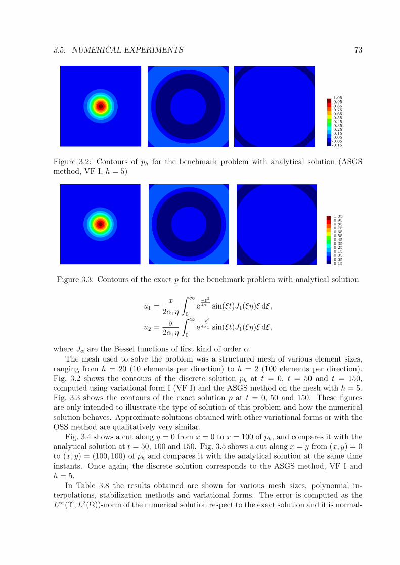
3.5. NUMERICAL EXPERIMENTS 73
-0.15-0.050.050.150.250.350.450.550.650.750.850.951.05
Figure 3.2: Contours of ph for the benchmark problem with analytical solution (ASGSmethod, VF I, h = 5)
-0.15-0.050.050.150.250.350.450.550.650.750.850.951.05
Figure 3.3: Contours of the exact p for the benchmark problem with analytical solution
u1 =x
2α1η
∫ ∞0
e−ξ24α1 sin(ξt)J1(ξη)ξ dξ,
u2 =y
2α1η
∫ ∞0
e−ξ24α1 sin(ξt)J1(ξη)ξ dξ,
where Jα are the Bessel functions of first kind of order α.The mesh used to solve the problem was a structured mesh of various element sizes,
ranging from h = 20 (10 elements per direction) to h = 2 (100 elements per direction).Fig. 3.2 shows the contours of the discrete solution ph at t = 0, t = 50 and t = 150,computed using variational form I (VF I) and the ASGS method on the mesh with h = 5.Fig. 3.3 shows the contours of the exact solution p at t = 0, 50 and 150. These figuresare only intended to illustrate the type of solution of this problem and how the numericalsolution behaves. Approximate solutions obtained with other variational forms or with theOSS method are qualitatively very similar.
Fig. 3.4 shows a cut along y = 0 from x = 0 to x = 100 of ph, and compares it with theanalytical solution at t = 50, 100 and 150. Fig. 3.5 shows a cut along x = y from (x, y) = 0to (x, y) = (100, 100) of ph and compares it with the analytical solution at the same timeinstants. Once again, the discrete solution corresponds to the ASGS method, VF I andh = 5.
In Table 3.8 the results obtained are shown for various mesh sizes, polynomial in-terpolations, stabilization methods and variational forms. The error is computed as theL∞(Υ, L2(Ω))-norm of the numerical solution respect to the exact solution and it is normal-

74 CHAPTER 3. NRBC FOR THE MIXED WAVE EQUATION
-0.20
-0.15
-0.10
-0.05
0.00
0.05
0.10
0.15
0.20
0 20 40 60 80 100
p(5
0)
x
ExactThis Work
-0.10
-0.05
0.00
0.05
0.10
0.15
0 20 40 60 80 100
p(1
00)
x
-0.04
-0.04
-0.04
-0.03
-0.03
-0.02
-0.01
-0.01
0 20 40 60 80 100
p(1
50)
x
Figure 3.4: Cut at y = 0 of p for the benchmark problem with analytical solution (ASGSmethod, VF I, h = 5, Q1 elements, Cτ = 0.05). Results shown at t = 50, 100 and 150.
-0.20
-0.15
-0.10
-0.05
0.00
0.05
0.10
0.15
0.20
0 20 40 60 80 100 120 140 160
p(5
0)
d
ExactThis Work
-0.10
-0.05
0.00
0.05
0.10
0.15
0 20 40 60 80 100 120 140 160
p(1
00)
d
-0.08
-0.06
-0.04
-0.02
0.00
0.02
0.04
0.06
0 20 40 60 80 100 120 140 160p(1
50)
d
Figure 3.5: Cut at x = y of p for the benchmark problem with analytical solution (ASGSmethod, VF I, h = 5, Q1 elements, Cτ = 0.05). Results shown at t = 50, 100 and 150.
ized by the L∞(Υ, L2(Ω))-norm of the exact solution. For VF II and III, the characteristiclength is taken as L0 = 100. The algorithmic constant is taken as Cτ = 0.05 for linearelements and Cτ = 0.1 for quadratic elements in 2D and Cτ = 0.1 for linear elements in3D. We have found experimentally that these values yield good results, and are the valuesused in all the examples. Note that in all cases the error behaves as expected. When theerror does not decrease as the mesh is refined or the polynomial order is increased, it isbecause of the error introduced by the NRBC.
Table 3.8: Error of the NRBC for the benchmark problem with analytical solution
h Element Method VF Error in p Error in u20 Q1 ASGS I 0.2166 0.257120 Q2 ASGS I 0.1120 0.13985 Q1 ASGS I 0.0385 0.08945 Q2 ASGS I 0.0379 0.09032 Q1 ASGS I 0.0383 0.09122 Q2 ASGS I 0.0384 0.09165 Q1 ASGS II 0.0439 0.09345 Q1 ASGS III 0.0443 0.09355 Q1 OSS I 0.0386 0.0897

3.5. NUMERICAL EXPERIMENTS 75
-150-5050
150250350450550650750850950
1050
Figure 3.6: Contours of ph in the small domain for the big/small domain benchmarkproblem in 2D. From the left to the right: t = 8, t = 16 and t = 24.
Big/small domain benchmark problem in 2D
A very interesting NRB performance test appeared in [17]. Using SI units throughout, theproblem proposed is defined on a square domain of side 10 000 centered at the origin ofcoordinates and divided into 100× 100 Q1 elements, with the NRB condition on the foursides. The reference state properties are density ρ0 = 1.2, pressure p0 = 1.01 × 10⁵ andheat capacity ratio γ = 1.4. We take µp = 1
γp0, µu = ρ0 and the initial condition is
p(x, 0) =
0.01 p0 cos
(πr2R
)if r < R,
0 otherwise,
with R = 1 000 and r =√x2 + y2. The simulation time is T = 24.
For comparison, a reference solution is obtained in a bigger domain, namely, a squareof side 30 000 with the region of interest in its center. The boundary condition used in thebig domain is p = 0 everywhere. The big domain is discretized with a mesh of 300 × 300Q1 elements.
Let us denote as [ph,uh] the solution in the small domain and as [pR,h,uR,h] the solutionin the big domain. The error is computed as:
ep =
maxt
√√√√ N∑n=1
(pR,h(xn, t)− ph(xn, t))2
maxt
√√√√ N∑n=1
(pR,h(xn, t))2
−1
, (3.53)
where N is the number of nodes of the problem in the small domain, with coordinates xn,n = 1, ..., N . The error for the x-component and y-component of u (eu and ev, respectively)is computed similarly.
To get an qualitative impression of the type of solution we are looking for and how theNRBC behaves, Fig. 3.6 shows the contours of ph in the small domain at t = 0, 8 and16, whereas Fig. 3.7 shows the contours of pR,h in the same region and at the same timeinstants. As in the previous example, these solutions have been computed using VF I andthe ASGS method.
Fig. 3.8 shows a cut at y = 0 for 0 ≤ x ≤ 5000 of ph and compares it with the solutionpR,h obtained in the big domain at t = 8, 16 and 24. Fig. 3.9 shows a similar cut and at

76 CHAPTER 3. NRBC FOR THE MIXED WAVE EQUATION
-150-5050
150250350450550650750850950
1050
Figure 3.7: Contours of pR,h in the big domain for the big/small domain benchmark problemin 2D. From the left to the right: t = 8, t = 16 and t = 24.
-150
-100
-50
0
50
100
150
200
0E0 1E3 2E3 3E3 4E3 5E3
p(8
)
x
BigSma
-90
-80
-70
-60
-50
-40
-30
-20
-10
0
0E0 1E3 2E3 3E3 4E3 5E3
p(1
6)
x
-7
-6
-5
-4
-3
-2
-1
0E0 1E3 2E3 3E3 4E3 5E3
p(2
4)
x
Figure 3.8: Cut at y = 0 of ph and pR,h for the big/small domain benchmark problem in2D. From the left to the right: t = 8, t = 16 and t = 24.
the same time instants, but along x = y from (x, y) = (0, 0) to (x, y) = (5000, 5000). It isobserved that the solutions in the big and small domains only differ significantly at t = 24,where a certain reflection is observed in spite of using the Sommerfeld boundary condition.However, these reflections are very small. To see this, Fig. 3.10 shows the evolution intime of the energy E in the region of interest. It can be seen that the solution in the smalldomain with the NRBC behaves as the big domain solution.
The results obtained with the NRBC are presented in Table 3.9 for various mesh sizes(100 and 50), polynomial order (P1 and P2), stabilization methods (ASGS and OSS),
-150
-100
-50
0
50
100
150
200
0E0 1E3 2E3 3E3 4E3 5E3 6E3 7E3 8E3
p(8
)
d
BigSma
-100
-50
0
50
100
150
0E0 1E3 2E3 3E3 4E3 5E3 6E3 7E3 8E3
p(1
6)
d
-60
-50
-40
-30
-20
-10
0
10
20
0E0 1E3 2E3 3E3 4E3 5E3 6E3 7E3 8E3
p(2
4)
d
Figure 3.9: Cut at x = y of ph and pR,h for the big/small domain benchmark problem in2D. From the left to the right: t = 8, t = 16 and t = 24.

3.5. NUMERICAL EXPERIMENTS 77
0
0.5e+6
1.0e+6
1.5e+6
2.0e+6
2.5e+6
3.0e+6
3.5e+6
0 5 10 15 20 25
E
t
BigSma
Figure 3.10: Evolution of total energy E for the big/small domain benchmark problem in2D.
Table 3.9: Error of the NRBC for the big/small domain benchmark problem in 2D
h Element Method VF L0 tsche δt ep eu ev100 P1 ASGS I - CN 0.16 0.057 0.081 0.081100 P1 ASGS I - BDF2 0.16 0.058 0.081 0.081100 P2 ASGS I - BDF2 0.16 0.058 0.081 0.081100 P1 OSS I - BDF2 0.16 0.058 0.081 0.081100 P1 ASGS I - BDF2 0.08 0.057 0.081 0.08150 P1 ASGS I - BDF2 0.08 0.056 0.081 0.081100 P1 ASGS II 100 BDF2 0.16 0.058 0.082 0.082100 P1 ASGS II 1000 BDF2 0.16 0.058 0.082 0.082100 P1 ASGS II 10 BDF2 0.16 0.058 0.082 0.082100 P1 ASGS III 100 BDF2 0.16 0.058 0.082 0.082
variational forms (I, II and III), domain length scales (10, 100 and 1000), time marchingschemes (Crank Nicolson and 2nd order BDF) and time step sizes (δt = 0.16 and 0.08).It can be seen that the error for p is around 5.8% and the error for u is around 8.2% forall cases, independently of the numerical strategy. It can therefore be concluded that thiserror comes exclusively from the truncation of the domain with the NRBC. In [17] theerrors reported are ep = 2.9% and eu = ev = 6.2% for a NRBC of order J = 10, slightlysmaller than those we have found. Additionally, the errors obtained with our formulationare similar to the ones obtained with J = 7. A second order finite difference formulationwith a node spacing of 100 per direction and a second order explicit time integration schemeis used in this reference, with a time step size equal to the critical time step needed forstability multiplied by 0.9.
Big/small domain benchmark problem in 3D
To test the NRBC in 3D, we solve a similar problem to the one in [17] extended to 3D. Wechoose the small domain as a cube of side 10 000 centered at the origin. The small domain

78 CHAPTER 3. NRBC FOR THE MIXED WAVE EQUATION
-65-55-45-35-25-15-55
1525354555
Figure 3.11: Contours of ph in the small domain for the big/small domain benchmarkproblem in 3D. From the left to the right: t = 0, 8 and 16 (ASGS method, VF I, h = 200,Q1 elements).
-65-55-45-35-25-15-55
1525354555
Figure 3.12: Contours of pR,h in the big domain for the big/small domain benchmarkproblem in 3D. From the left to the right: t = 0, 8 and 16 (ASGS method, VF I, h = 200,Q1 elements).
is divided in 50 × 50 × 50 Q1 elements (h = 200) with the NRBC applied on the wholeboundary. The simulation time is T = 24, the time step size is taken as 0.16 and the timescheme used is BDF2. The equation coefficients µp and µu, as well as the initial condition,are chosen to be the same as before, in the 2D case. The only change is that the initialcondition is in a sphere of radius R, so now r is computed as r =
√x2 + y2 + z2.
For comparison, a reference solution pR,h is obtained in a bigger domain, namely, acube of side 20 000 with the region of interest in its center. The big domain is dividedin 100 × 100 × 100 Q1 elements and the boundary condition pR,h = 0 is imposed. Theerror is computed as in the 2D version of the case with equation (3.53). Fig. 3.11 showsthe contours of p in the plane z = 0 for the small domain at t = 0, t = 8 and t = 16,whereas Fig. 3.12 shows the contours of p in the plane z = 0 for the big domain at thesame instants. A good qualitative agreement is observed.
Fig. 3.13 shows a cut at y = z = 0 for 0 ≤ x ≤ 5000 of ph and pR,h at t = 8, 16 and 24.Significant discrepancies are only observed at t = 24. However, they have small energy, asshown below.
The results obtained with our NRBC are presented in Table 3.10 for various meshsizes (500, 250 and 200), polynomial order (Q1 and Q2), stabilization methods (ASGS andOSS), variational forms (I, II and III) and domain length scales (25, 250 and 2500). It can

3.5. NUMERICAL EXPERIMENTS 79
-80
-60
-40
-20
0
20
40
60
0E0 1E3 2E3 3E3 4E3 5E3
p(8
)
x
BigSma
-35
-30
-25
-20
-15
-10
-5
0
5
10
0E0 1E3 2E3 3E3 4E3 5E3
p(1
6)
x
-0.4
-0.2
0.0
0.2
0.4
0.6
0.8
0E0 1E3 2E3 3E3 4E3 5E3
p(2
4)
x
Figure 3.13: Cut at y = 0 of p for the big/small domain benchmark problem in 3D (ASGSmethod, VF I, h = 200, Q1 elements). From the left to the right: t = 8, 16 and 24.
Table 3.10: Error of the NRBC for the big/small domain benchmark problem in 3D
h Element Method VF L0 ep eu500 Q1 ASGS I - 0.077 0.084250 Q1 ASGS I - 0.078 0.085200 Q1 ASGS I - 0.077 0.085250 Q2 ASGS I - 0.081 0.090250 Q1 OSS I - 0.078 0.086250 Q1 ASGS II 100 0.081 0.090250 Q1 ASGS III 100 0.081 0.090250 Q1 ASGS II 25 0.081 0.090250 Q1 ASGS II 2500 0.081 0.090
be seen that the error for p is around 7.9% and the error for u is around 8.6% for all cases.Fig. 3.14 shows the evolution in time of the energy E in the region of interest for the
case with mesh size 250 m, the ASGS method, Q1 elements and VF I. It can be seen thatthe solution obtained with the NRBC behaves as the big domain solution.
0
0.5e+9
1.0e+9
1.5e+9
2.0e+9
2.5e+9
3.0e+9
0 5 10 15 20 25
E
t
BigSma
Figure 3.14: Evolution of total energy E for the big/small domain benchmark problem in3D

80 CHAPTER 3. NRBC FOR THE MIXED WAVE EQUATION
00.51.01.52.02.53.03.54.04.55.05.56.0
Figure 3.15: Contours of |uh| in the small domain for the showcase problem with NRBC.From the left to the right: t = 0, t = 0.3 and t = 0.6.
Showcase problem with NRBC in 2D
An illustrative NRBC showcase appeared in [20] by Glowinski et al. Although it is not abenchmark of the NRBC, a plot of the evolution in time of the total energy of the systemillustrates that the energy goes out of the region of interest and never enters again becausethe total energy decreases monotonically. The problem is defined in a square domainΩ = (−0.5, 0.5)× (−0.5, 0.5), with µp = 1 and µu = 1. The simulation time is T = 1. Theinitial solution is p(x, 0) = 0 and
u(x, 0) =
−4πr
sin(2πr) cos(2πr)
[x
y
]r ≤ R,
0 otherwise,
with r =√x2 + y2, R = 0.25. In all the boundary the NRBC is applied. The problem
is solved with a mesh size h = 0.01, a time step of δt = 0.002 and the time integrationscheme is BDF2.
Additionally, we have defined a big domain to compare the results of the NRBC inthe small domain. The big domain is taken as Ω = (−1.5, 1.5) × (−1.5, 1.5). Fig. 3.15shows the contours of |uh| computed in the small domain at t = 0, t = 0.3 and t = 0.6.Fig. 3.16 shows the contours of |uR,h|, the solution computed in the big domain, at thesame instants. It is observed that there is a certain distortion of the wave at t = 0.6 closeto the boundary in the small domain case, which is not observed in the solution computedin the big domain.
The evolution of total energy inside the domain of interest is shown in Fig. 3.17. Theagreement between the energy computed in both the big and the small domains is verygood, indicating that the wave distortion close to the boundary of the solution computedin the small domain has low energy.
The error of the small domain with respect to the big domain in L∞(Υ, L2(Ω)) normfor VF I, the ASGS method and P1 elements was 6.8% for p and 5.3% for u.

3.5. NUMERICAL EXPERIMENTS 81
00.51.01.52.02.53.03.54.04.55.05.56.0
Figure 3.16: Contours of |uR,h| in the big domain for the showcase problem with NRBC.From the left to the right: t = 0, t = 0.3 and t = 0.6.
0.00.20.40.60.81.01.21.41.61.82.0
0.0 0.2 0.4 0.6 0.8 1.0
E
t
BigSma
Ref. [20]
Figure 3.17: Evolution of total energy E for the showcase problem with NRBC
Showcase problem with NRBL in 2D
A NRBL example appeared in [42] by Qi et al. It uses PML as NRBL. We solve the sameexample using our NRBC and compare the results. The domain is a hollow cylinder thatextends from r = 1 to r = 1 + H, with H = 1. The mesh size is h = 0.01 in the radialdirection and has 720 divisions in the circumferential direction. The coefficients of theequation are taken as µp = 1 and µu = 1. The simulation time is T = 4, the time stepsize is δt = 0.005 and the time integration algorithm is BDF2. The initial condition is zerofor both p and u. The boundary condition at r = 1 changes from a prescription in p to aprescription in γnu, and is given by:
p = cos(2πt) 0 < t ≤ 1, r = 1,
γnu = 0 1 < t < 4, r = 1.
At r = 1 + H the NRB is prescribed. In the case of [42], as a PML strategy is used, thedomains extends from r = 1 +H to r = 1 +H + δ to include the absorbing PML. The casewith δ = 2 from [42] was chosen as it is the one that provides less reflection according totheir results. In Fig. 3.18 it is shown the evolution of p at r = 1 with our method and thecomparison with the results obtained using PML by [42].

82 CHAPTER 3. NRBC FOR THE MIXED WAVE EQUATION
-1
-0.5
0
0.5
1
0 0.5 1 1.5 2 2.5 3 3.5 4
p
t
Ref. [42] (PML)SmaBig
Figure 3.18: Evolution of ph at r = 1 for the showcase problem with NRBL.
-0.7-0.5-0.3-0.10.10.30.50.70.9
Figure 3.19: Contours of ph in the small domain for the the showcase problem with NRBL.From the left to the right: t = 0, t = 0.5 and t = 1.0.
In addition to the results presented in [42], we followed the big/small domain approachas in the previous examples, taking 1 < r < 2(1 + H) as the big domain. Fig. 3.19 showsthe contours of ph in the small domain at t = 0, 0.5 and 1.0, whereas Fig. 3.20 shows thecontours of the solution computed in the big domain, pR,h, at the same time instants.
Fig. 3.21 shows the energy evolution inside the domain of interest. As in the previousexamples, the differences between the solutions in the small and the big domains have lowenergy.
The error of the small domain with NRBC respect to the big domain in L∞(Υ, L2(Ω))norm for VF I, the ASGS method and Q1 elements was 5.3% for p and 3.8% for u.
In addition to the Big/Small domain analysis, we performed a Big/Medium/Smalldomain analysis. The idea is to compare the solutions in the medium and small domainswith respect to the solution in the big domain. The medium domain was taken with H =1.83 and the error in the medium domain with respect to the big domain in L∞(Υ, L2(Ω))norm for VF I, the ASGS method and Q1 elements was 3.4% for p and 2.3% for u. Thesmall domain corresponds to a location of the NRBC of R = 2, whereas the mediumdomain has R = 2.83. With the errors obtained we can infer that the error is proportionalto (1/R2)J with J ≈ 0.66.

3.6. CONCLUSIONS 83
-0.7-0.5-0.3-0.10.10.30.50.70.9
Figure 3.20: Contours of pR,h in the big domain for the the showcase problem with NRBL.From the left to the right: t = 0, t = 0.5 and t = 1.0.
0
0.5
1
1.5
2
2.5
3
0 0.5 1 1.5 2 2.5 3 3.5 4 4.5
E
t
BigSma
Figure 3.21: Evolution of total energy E for the showcase problem with NRBL.
3.6 Conclusions
In this work, we have described a NRBC for the wave equation in mixed form in timedomain. In particular, we have considered Sommerfeld-type artificial boundary conditions.The resulting system of equations has been stated in three different functional settings,based on the regularity required for the scalar and vector unknowns. The introduction ofthe NRBC terms require to increase the regularity of the functional setting for problems inbounded domains [67]. The extra regularity required is somehow small because the set offunctions in H(div,Ω) with normal trace in L2(Γo) is close to H(div,Ω), considering thatH
12
+ε(Ω) has trace in L2(Γ) for any ε > 0 and that H1(Ω) has trace in H12 (Γ).
We have presented two stabilized FE methods (ASGS and OSS) including the NRBC.Additionally, the stabilized methods can mimic the three variational forms of the problem,which require different regularity of the unknowns, via a proper design of the stabilizationparameters. Stability and convergence results have been presented for these stabilized FEformulations. The NRBC does not affect previous results proved in [67] for Dirichlet-typeboundary conditions, although it requires extra regularity on the boundary for the vectorunknown in variational forms I and II. We normally use the stabilized FE formulations for

84 CHAPTER 3. NRBC FOR THE MIXED WAVE EQUATION
equal interpolation of the unknowns, but the analysis is not restricted to that and allowsany continuous interpolation pair.
Numerical experiments have been carried out to check the accuracy of the methods andthe results obtained are in agreement with the accuracy predicted theoretically. Benchmarkproblems have been solved using the NRBCs proposed and good results have been obtainedwhen compared with other NRBCs or NRBLs. The main practical advantage of the NRBCdescribed over other NRBCs is its simplicity and the fact that no nonlinear or iterativemethods are required. Further, for NRBC schemes, the truncated domain does not needto be extended with an absorbing layer. Additionally, when compared to PML techniques,it avoids extra degrees of freedom per node and avoids the solution of other governingequations in the absorbing layer.

Chapter 4
On some time marching schemes for thestabilized finite element approximationof the mixed wave equation
This chapter is based on the material in:Hector Espinoza, Ramon Codina, and Santiago Badia. “On some time marching schemesfor the stabilized finite element approximation of the mixed wave equation”. In: ComputerMethods in Applied Mechanics and Engineering (Dec. 2014). SubmittedSome content is repeated from Chapter 1 and Chapter 3 so it is self-contained.
In this chapter we analyze time marching schemes for the wave equation in mixed form.The problem is discretized in space using stabilized finite elements. On the one hand,stability and convergence analyses of the fully discrete numerical schemes are presented.On the other hand, we use Fourier techniques (also known as von Neumann analysis) inorder to analyze stability, dispersion and dissipation. Additionally, numerical convergencetests are presented for various time integration schemes, polynomial interpolations (for thespatial discretization), stabilization methods, and variational forms. Finally, a 1D exampleis solved to analyze the behavior of the different schemes considered.
4.1 Introduction
Finite difference time marching schemes are mostly used for the time integration of evo-lution problems because of their efficiency and ease of implementation. In the case ofpartial differential equations (PDEs) in space and time, even if a given finite differencescheme has some general properties regarding stability and accuracy, the precise behaviorof the scheme needs to be analyzed together with the spatial discretization employed. Inthis chapter we aim at analyzing classical first and second order schemes for the hyperbolicwave equation, with the particularity that we write it in mixed form and discretize in spaceusing stabilized finite element (FE) methods.
For the analysis of time discretization schemes for wave propagation problems it iscustomary to split the total discretization error into two parts: dispersion error and dissi-pation error. Dispersion is the dependency of the phase velocity on the frequency and thedispersion error is the deviation of the phase velocity with respect to the expected one for
85

86 CHAPTER 4. TIME MARCHING SCHEMES FOR THE WAVE EQUATION
a given frequency. On the other hand, dissipation error is the decrease in amplitude withrespect to the expected one. In general, dispersion and dissipation errors are higher forpoorly resolved frequencies, which occurs mainly for small frequencies. The wave equationwe aim to analyze is non-dispersive and non-dissipative. Therefore, it would be desirableto have non-dispersive and non-dissipative discretization schemes. This sometimes cannotbe achieved, thus one just aims to have low-dispersion low-dissipation schemes [124, 125].Dispersion and/or dissipation of numerical schemes can be evaluated using Fourier tech-niques (see [126, 127]), energy methods (see [128]), or modified equation analysis (see [127,129]). Fourier analysis can be carried out for semi-discretizations or full discretizations.Dispersion/dissipation analysis methods have been used to optimize numerical schemes[126, 129]. Other properties of the continuous wave equation, such as the preservation ofsymplecticity, some invariants or some symmetries are even more difficult to inherit fordiscrete schemes. This is the motivation of the so-called geometric numerical integrators,which we will not consider in this chapter (see [130], for example).
Contrary to the irreducible hyperbolic wave equation, which is of second order inspace and time, the mixed wave equation is of first order in space and time. We willconsider the case of a single scalar unknown, which in the mixed format unfolds into twounknowns, namely, this scalar field and a vector unknown. With regard to the spaceapproximation, the Galerkin FE discretization of this mixed wave equation requires tosatisfy a compatibility condition between the spaces of the two unknowns (scalar andvector), i.e., to use so-called inf-sup compatible interpolations. Alternatively, we canconsider stabilized FE methods, which provide much more flexibility when choosing theinterpolation spaces [67, 68, 90]. In particular, we can consider equal interpolation forthe unknowns. Stability and convergence of the stabilized FE spatial semi-discretizationof the mixed wave equation has been presented in [67, 68]. Stability and convergence offully discrete schemes has also been analyzed for the convection-diffusion equation and theStokes equations in [103, 131, 132] using spatial and temporal approximations related tothose used in the present work.
In this work, we analyze the stability and convergence properties for the mixed waveequation, after time semi-discretization, space semi-discretization, and full discretization,and perform their Fourier analyses. For the time discretization, we consider backwardEuler (BE), Crank-Nicolson1 (CN) and the second order backward differentiation formula(BDF2). We will see how a symplectic time integrator (CN) compares to non-symplectictime integrators (BE and BDF2). Dispersion and dissipation of discretization methodswill be evaluated through numerical experiments. This consists in solving a given problemand evaluating the solution obtained [126, 134, 135]. We will solve a 1D wave propaga-tion problem to show qualitatively dispersion and dissipation of the proposed numericalschemes.
The organization of the chapter is as follows. In Section 4.2 we present the problemstatement and its space-time discretization. In Section 4.3 we present stability and con-
1The original CN discretization scheme was devised to solve numerically PDEs of heat-conduction type;it is a space-time discretization based on finite differences. Sometimes CN is used to refer to the implicitmidpoint method or the (implicit) trapezoidal rule and there is no agreement in the literature [133]. Wehave to mention that for linear operators (which is the the case of the mixed wave equation) the trapezoidalrule and the implicit midpoint method are equivalent.

4.2. PROBLEM STATEMENT AND NUMERICAL APPROXIMATION 87
vergence results of the fully discrete problem obtained using variational techniques. Weprovide results for all the methods considered, even though we only present one sample ofthe proofs of these results. In Section 4.4 we present a complete Fourier analysis for the1D wave equation in mixed form, from which precise information on the behavior of thedifferent schemes can be drawn. Numerical results are presented in Section 4.5 and, finally,in Section 4.6 the conclusions of the work are summarized. This chapter is a continuationof our work on the approximation of the mixed form of the wave equation presented in [67,68] which correspond to Chapter 2 and Chapter 3 respectively. Frequent reference is madeto these two papers/chapters, to which the reader is addressed for details.
4.2 Problem statement and numerical approximation
4.2.1 Initial and boundary value problem
The problem we consider is an initial and boundary value problem posed in a time intervalΥ := (0, T ) and in a spatial domain Ω ⊂ Rd, (d = 1, 2 or 3). Let t ∈ Υ be a given timeinstant in the temporal domain and x ∈ Ω a given point in the spatial domain. We definethe space-time domain as Ξ := Ω×Υ. Let Γ be the boundary of the domain Ω. We split Γinto three disjoint sets denoted as Γp, Γu and Γo. The scalar unknown p is enforced on Γp,the normal trace of the vector unknown γnu on Γu, and a simple non reflecting boundarycondition (NRBC) on Γo. Although the boundary conditions are irrelevant for the vonNeumann analysis, we just mention them for completeness.
The problem consists in finding p : Ξ −→ R and u : Ξ −→ Rd such that
µp∂tp+∇·u = fp , (4.1)µu∂tu+∇p = fu , (4.2)
with the following initial conditions
p(x, 0) = 0, u (x, 0) = 0, (4.3)
and with the following boundary conditions
p = 0 on Γp, γnu := n · u = 0 on Γu, µ12p p = µ
12uγnu on Γo, (4.4)
where µp > 0 and µu > 0 are physical coefficients such that c2 = (µpµu)−1, c is the wave
speed, fp and fu are forcing terms, n is the unit outward normal to the boundary ofthe domain and γn is the normal trace operator. In the previous equations and in whatfollows, we use the following convention: lower-case bold italic letters represent vectors inRd, lower-case non-bold italic letters represent scalars, whereas upper-case non-bold italicletters may be arrays or matrices.
Let Ψ be a generic spatial domain, i.e. Ω or Γ or part of them. Whenever they arewell defined, we denote by L2(Ψ) the space of square integrable functions defined on Ψ,by H1(Ψ) the space of functions in L2(Ψ) with derivatives in L2(Ψ), by H(div,Ψ) thespace of vector functions with components and divergence in L2(Ψ), and by L2(Ψ)
d thespace of vector functions with components in L2(Ψ). Additionally, for an arbitrary normed

88 CHAPTER 4. TIME MARCHING SCHEMES FOR THE WAVE EQUATION
functional space X, its norm will be denoted as ||·||X. In the case of L2(Ω) or L2(Ω)d the
L2-norm will simply be denoted as ||·|| and the L2-inner-product as (· , ·) Furthermore, thespace of functions whose X-norm is Cr continuous in the time interval Υ will be denotedby Cr(Υ; X). We will only be interested in the cases r = 0 and r = 1. Functions whoseX-norm is Lp in Υ will be denoted by Lp(Υ; X); when X = L2(Ω) or X = L2(Ω)
d, the compactnotation Lp(L2) will sometimes be used. Furthermore, let Vp, Vu be spaces associated withp and u respectively. These spaces will be defined afterwards because they depend on thefunctional setting. Additionally, let us define V := Vp × Vu and L := L2(Ω)× L2(Ω)
d.Problem (4.1)-(4.2) with appropriate initial and boundary conditions will be well-posed
for:
p ∈ C1(Υ;L2(Ω)
)∩ C0
(Υ; Vp
), u ∈ C1
(Υ;L2(Ω)
d) ∩ C0(Υ; Vu
),
with fp and fu regular enough.
4.2.2 Variational problem
The variational form of problem (4.1)-(4.4) can be expressed in three different ways. Eachone requires a certain regularity on the unknowns p and u. The problem reads: find[p,u] ∈ C1 (Υ; L) ∩ C0 (Υ; V) such that
B ([p,u] , [q,v]) = L ([q,v]) ,
for all test functions [q,v] ∈ V, and satisfying the initial conditions. The bilinear form B,the linear form L and the space V are defined in three different ways depending on thevariational form into consideration. For simplicity, we will assume that the forcing termsfp and fu are square integrable, although we could relax this regularity requirement andassume they belong to the dual space of Vp and Vu, respectively. Let us also define twoauxiliary variables denoted as κp and κu:
κp :=
(µpµu
) 12
, κu :=
(µuµp
) 12
.
The possible variational formulations of the problem are the following [67, 68]:
Variational Form I
Vp =q ∈ H1(Ω)| q = 0 on Γp
,
Vu =v ∈ H(div,Ω)| γnv = 0 on Γu and γnv ∈ L2(Γo)
B ([p,u] , [q,v]) = µp (∂tp, q) + (∇·u, q) + µu (∂tu,v) + (∇p,v) (4.5)L ([q,v]) = (fp, q) + (fu,v) (4.6)p = 0 on Γp, Strongly imposed (4.7)γnu = 0 on Γu, Strongly imposed (4.8)
µ12p p = µ
12uγnu on Γo, Strongly imposed (4.9)

4.2. PROBLEM STATEMENT AND NUMERICAL APPROXIMATION 89
Variational Form II
Vp = L2(Ω), Vu =v ∈ H(div,Ω)| γnv = 0 on Γu and γnv ∈ L2(Γo)
B ([p,u] , [q,v]) = µp (∂tp, q) + (∇·u, q) + µu (∂tu,v)− (p,∇·v) + κu
∫Γo
(γnv)(γnu) dΓ
(4.10)L ([q,v]) = (fp, q) + (fu,v) (4.11)p = 0 on Γp, Weakly imposed (4.12)γnu = 0 on Γu, Strongly imposed (4.13)
µ12p p = µ
12uγnu on Γo, Weakly imposed (4.14)
Variational Form III
Vp =q ∈ H1(Ω)| q = 0 on Γp
, Vu = L2(Ω)
d
B ([p,u] , [q,v]) = µp (∂tp, q)− (u,∇q) + µu (∂tu,v) + (∇p,v) + κp
∫Γo
pq dΓ (4.15)
L ([q,v]) = (fp, q) + (fu,v) (4.16)p = 0 on Γp, Strongly imposed (4.17)γnu = 0 on Γu, Weakly imposed (4.18)
µ12p p = µ
12uγnu on Γo, Weakly imposed (4.19)
4.2.3 Stabilized finite element formulations
Here we present two stabilized FE methods, which we will denote by the acronyms ASGS(Algebraic Sub-Grid Scales) and OSS (Orthogonal Sub-grid Scales), aimed to overcomethe instability problems of the standard Galerkin method found when the interpolatingspaces do not satisfy an appropriate inf-sup condition. We focus on equal and continuousinterpolations for p and u and therefore, conforming FE spaces. For conciseness, we willconsider quasi-uniform FE partitions K of size h. For stabilized formulations in generalnon-uniform non-degenerate cases, see [97].
Let Vp,h and Vu,h be the FE spaces constructed from the FE partition K to approx-imate p and u, respectively, with Vp,h ⊂ Vp and Vu,h ⊂ Vu. Additionally, let us defineVh = Vp,h × Vu,h. Stabilized FE methods deal with the following problem: find a pair[ph,uh] ∈ C1(Υ; Vh) with initial conditions ph(x, 0) = 0, uh(x, 0) = 0 such that
Bs ([ph,uh] , [qh,vh]) = Ls ([qh,vh]) , (4.20)
for all test functions [qh,vh] ∈ Vh, where the bilinear form Bs and the linear form Ls includethe Galerkin terms and additional stabilization terms. Depending on how the stabilizationpart is designed, a different stabilization method arises. Below, we present two methods,namely ASGS and OSS. The stabilization terms depend on the choice of the so-calledstabilization parameters τp and τu.

90 CHAPTER 4. TIME MARCHING SCHEMES FOR THE WAVE EQUATION
Table 4.1: Stabilization Parameters Order and Length Scales Definition
Variational Form I II III`p `p = `u L2
0/h h`u `p = `u h L2
0/hτp O(h) O(1) O(h2)τu O(h) O(h2) O(1)
The ASGS method is an extension to the mixed form of the wave equation of themethod proposed in [87, 89]. It consists in solving problem (4.20) and taking the bilinearform Bs and the linear form Ls as:
Bs ([ph,uh] , [qh,vh]) = B ([ph,uh] , [qh,vh]) + (µp∂tph +∇·uh, τp∇·vh)+ (µu∂tuh +∇ph, τu∇qh) , (4.21)
Ls ([qh,vh]) = L ([qh,vh]) + (fp, τp∇·vh) + (fu, τu∇qh) . (4.22)
The OSS method is an extension to the wave equation in mixed form of the methodproposed in [98, 99]. It consists in solving problem (4.20) and taking the bilinear form Bsand the linear form Ls as:
Bs ([ph,uh] , [qh,vh]) = B ([ph,uh] , [qh,vh]) +(P⊥p (∇·uh) , τp∇·vh
)+(P⊥u (∇ph) , τu∇qh
), (4.23)
Ls ([qh,vh]) = L ([qh,vh]) +(P⊥p (fp) , τp∇·vh
)+(P⊥u (fu) , τu∇qh
), (4.24)
where P⊥p (·) = I(·) − Pp(·) and P⊥u (·) = I(·) − Pu(·), Pp(·) being the L2(Ω) projectionon Vp,h and Pu(·) the L2(Ω) projection on Vu,h. This in particular implies that Pp(·) = 0on Γp for variational forms I and III and that n · Pu(·) = 0 on Γu for variational forms Iand II. Let us remark that for the sake of conciseness we will not consider in this chapterthe so-called dynamic subscales introduced in [98], even if we favor them and their use iscrucial in the case of very small time steps (see also [136, 137]).
An important ingredient of stabilized formulations are the stabilization parameters. Inour case, we compute them in all formulations as:
τp = Cτh
√µuµp
√`p`u, τu = Cτh
√µpµu
√`u`p, (4.25)
where Cτ is a dimensionless algorithmic constant and `p, `u are length scales correspondingto p and u, respectively. As it was shown in the analysis presented in [67], in orderto mimic at the discrete level the proper functional setting of the continuous problemthe length scales `p and `u should be taken as shown in Table 4.1, where L0 is a fixedlength scale of the problem that can be fixed a priori. The motivation for designing thestabilization parameters can be found in [90, 91].
4.2.4 Full discretization
To discretize in time we will use standard finite difference schemes of first and second order,namely, the BE, the CN and the BDF2 schemes. Let 0 = t0 < . . . < tn < . . . tN = T be a
4.3. STABILITY AND CONVERGENCE RESULTS 91
finite difference partition of Υ of size δt, , that we take constant for the sake of simplicity.Let U be the sequence of exact solutions U := UnNn=0 := [p(x, tn),u(x, tn)]Nn=0. Wewill often abbreviate pn := p(x, tn) and un := u(x, tn); the same symbol will be used for atime approximation to these unknowns. Let Uh be the sequence of approximate solutionsof the fully discrete problem, that is Uh := Un
h Nn=0 := [pnh,unh]Nn=0. This fully discrete
problem reads: find the sequence Uh such that
Bh (Uh, Vh) = Lh (Vh) , (4.26)
for all Vh. The definitions of Bh and Lh depend on the combination of space and timediscretization and will be given in the next section, where the stability and convergenceproperties of the fully discrete methods are presented.
To simplify notation we will use the backward (DrB,q,s) central (Dr
C,q,s) and forward(Dr
F,q,s) difference operators for the r-th derivative, of order q and in a time interval of sizesδt. For instance, the BE and BDF2 approximations of the time derivative for the scalarunknown will be
D1B,1,1p
n =pn − pn−1
δt, D1
B,2,1pn =
3pn − 4pn−1 + pn−2
2δt.
4.3 Stability and convergence results
4.3.1 Preliminaries
We present here the results of stability and convergence of the fully discrete methodsarising from the combination of time marching schemes (BE, CN and BDF2) and spatialstabilized FE methods (ASGS and OSS). We provide stability and convergence resultsfor each fully discrete method. In order to do that, we use the concept of Λ-coercivity,used for the first time in [103], which aids us in the proof of stability and later in theconvergence analysis. The proofs are similar to the ones shown in [67, 68], but consideringnow the time-discretization also. Only one of such proofs will be developed here, the othersfollowing very similar strategies.
As usual, we use C for a generic constant independent of the mesh size h and time stepδt. The value of C may be different at different occurrences. Additionally, we will use thenotation A & B and A . B to indicate that A ≥ CB and A ≤ CB for any A and Bdepending on the solution and the data. All our results are presented in such a way thatC is independent of the dimensional system, i.e., C is dimensionless.
Let UI be the sequence of projected solutions UI := [pnI ,unI ]Nn=0, where pnI := Πn
p (pn)and unI := Πn
u (un), where Πnp (·) and Πn
u (·) are adequate interpolants onto the FE spaces,taken to be projections. Notice that this notation allows us to take different interpolantsat different time steps.
Let us define some auxiliary norms to ease notation in the following:
|||V n|||20 := µp||qn||2 + µu||vn||2, (4.27)
|||V |||2B := (1 + σ)κp||q||2`2(Υ,L2(Γo)) + (1− σ)κu||γnv||2`2(Υ,L2(Γo)), (4.28)
92 CHAPTER 4. TIME MARCHING SCHEMES FOR THE WAVE EQUATION
|||F |||2F :=1
µp||fp||2`1(Υ,L2(Ω)) +
1
µu||fu||2`1(Υ,L2(Ω)) + τp||fp||2`2(Υ,L2(Ω)) + τu||fu||2`2(Υ,L2(Ω)),
(4.29)
with σ = −1, 0, 1 for variational forms I, II and III respectively, and ‖ · ‖`p(Υ,X) stands forthe `p-norm of a sequence of X-norms associated to the time discretization of Υ. WhenX = Lq(Ω), we will use the abbreviation `p(Υ, Lq(Ω)) ≡ `p(Lq).
For the convergence analysis we need to define three types of errors: the projection error,the discretization error, and the total error. The projection error is the error betweenthe exact solution and the projected exact solution and is defined as ε := εnNn=0 :=
[εnp , εnu]Nn=0
:= U−UI . The discretization error is the error between the discrete solutionand the projected exact solution and is defined as e := enNn=0 :=
[enp , e
nu]Nn=0
:= Uh−UI .Finally, the total error is the error between the exact solution and the discrete solutionand is defined as ξ := ξnNn=0 :=
[ξnp , ξ
nu ]Nn=0
:= U − Uh.
4.3.2 Analysis strategy
As mentioned above, all the methods considered have the form (4.26). We have provedthat all of them (ASGS and OSS for the spatial discretization, considering the threepossible variational formulations, and BE, CN and BDF2 for the time integration) arestable and optimally convergent, with the convergence order in space and time that shouldbe expected. However, including all the proofs would be extremely long and tedious.Rather than this, we explain in what follows the analysis strategy that we have employed,give the details of the terms involved for each method in the following subsection andpresent then the proof of the simplest case.
For all methods we have proved Λ-coercivity, stability and convergence in an appropriatenorm |||·||| that depends on the method. More precisely, we have shown that
1. Λ-coercivity. If V is a sequence of functions, either continuous or discrete in space,there exist a map Λ(V ) such that
Bh(V,Λ(V )) & |||V |||2, |||Λ(V )||| . |||V |||, (4.30)
for all V . From this property one easily gets stability in the form of an inf-supcondition (see [103]).
2. Stability. The discrete solution Uh satisfies
|||Uh||| . |||F |||∗, (4.31)
for an appropriate norm |||F |||∗ of the data (the forcing terms).
3. Convergence. Of course, the final objective is to provide an estimate for the totalerror ξ in some norm. We can show that if U is the sequence of continuous solutionsand Uh the sequence of discrete solutions, then
|||U − Uh||| . E(h, δt), (4.32)

4.3. STABILITY AND CONVERGENCE RESULTS 93
for a certain error function E(h, δt). At this point, let us remark that convergence isnot a more or less straightforward consequence of stability, since the discrete problemis not consistent in the variational sense. To prove convergence we need to deal withthe consistency error
C(U, Vh) := Lh(Vh)− Bh(U, Vh). (4.33)
From this definition it is easy to arrive to
Bh(e, Vh) = Bh(ε, Vh) + C(U, Vh). (4.34)
4.3.3 Forms, norms and error functions
Recalling that we have taken as zero the initial conditions, all methods are solely defined bythe bilinear form Bh and the linear form Lh. These are given for all methods in Table 4.2.The only comment that needs to be made is that in practice BDF2 can be started eitherwith BE or CN. Numerical experiments show no difference in the convergence rate, evenif theoretical error estimates are not optimal for convergence in terms of δt when BDF2 isstarted with BE for variational forms II and III.
The stability analysis of the different methods relies on the expression of map Λ(V )satisfying (4.30), the norm of the unknown |||V ||| and the norm of the forcing terms |||F |||∗.These are all given in Table 4.3. Note that in this table use is made of abbreviations (4.27)-(4.29). The expressions of |||F |||∗ determine the regularity required for the data in each case.
Finally, Tables 4.4 and 4.5 provide the error functions of the error estimates (4.32) forthe ASGS and the OSS methods, respectively. There are many terms in these expressionswith the same convergence order. However, including all of them gives an indication of thepossible sources of error, as well as of the required regularity of the continuous solution toobtain optimal convergence rates.
4.3.4 A sample of the proofs: ASGS-BE method
As an example of how to prove (4.30), (4.31) and (4.32), we present now the proof ofthese results for the simplest of the six methods considered, namely, ASGS for the spacediscretization and BE for the time integration. The proof of the rest of methods is moreor less involved, but follows the same ideas.
Proof of Λ-coercivity (4.30)
From the definition of Bh in Table 4.2 and of Λ(V ) in Table 4.3 for the ASGS-BE methodwe get
Bh (V,Λ (V )) =N∑n=1
δt(µpD
1B,1,1q
n, qn)
+N∑n=1
δt(µuD
1B,1,1v
n,vn)
+ τpτuµu
N∑n=1
δt(∇·vn,∇·
(D1
B,1,1vn))
+ τpτuµp
N∑n=1
δt(∇qn,∇
(D1
B,1,1qn))

94 CHAPTER 4. TIME MARCHING SCHEMES FOR THE WAVE EQUATION
Table 4.2: Forms that define the methods
Method Bh and Lh
ASGS-BEBh (Uh, Vh) =
∑Nn=1 δt
[(µpD1
B,1,1pnh +∇·unh , q
nh + τp∇·vnh
)+(µuD1
B,1,1unh +∇pnh ,v
nh + τu∇qnh
)]Lh (Vh) =
∑Nn=1 δt
(fpn, qnh + τp∇·vnh
)+∑Nn=1 δt
(fun,vnh + τu∇qnh
)
ASGS-CN
Bh (Uh, Vh) =∑Nn=1 δt
[(µpD1
B,1,1pnh +∇·un−
12
h , qnh + τp∇·vnh)
+(µuD1
B,1,1unh +∇pn−
12
h ,vnh + τu∇qnh)]
Lh (Vh) =∑Nn=1 δt
(fpn− 1
2 , qnh + τp∇·vnh)
+∑Nn=1 δt
(fun− 1
2 ,vnh + τu∇qnh)
ASGS-BDF2
Bh (Uh, Vh) = δt
[(µpD1
B,1,1p1h +∇·u1− 1
2h , q1
h + τp∇·v1h
)+(µuD1
B,1,1u1h +∇p1− 1
2h ,v1
h + τu∇q1h
)]+∑Nn=2 δt
[(µpD1
B,2,1pnh +∇·unh , q
nh + τp∇·vnh
)+(µuD1
B,2,1unh +∇pnh ,v
nh + τu∇qnh
)]Lh (Vh) = δt
(fp
1− 12 , q1
h + τp∇·v1h
)+∑Nn=2 δt
(fpn, qnh + τp∇·vnh
)+δt
(fu
1− 12 ,v1
h + τu∇q1h
)+∑Nn=2 δt
(fun,vnh + τu∇qnh
)OSS-BE
Bh (Uh, Vh) =∑Nn=1 δt
[(µpD1
B,1,1pnh +∇·unh , q
nh
)+ τp
(P⊥p
(∇·unh
),∇·vnh
)]+∑Nn=1 δt
[(µuD1
B,1,1unh +∇pnh ,v
nh
)+ τu
(P⊥u
(∇pnh
),∇qnh
)]Lh (Vh) =
∑Nn=1 δt
[(fpn, qnh
)+ τp
(P⊥p (fp
n) ,∇·vnh)]
+∑Nn=1 δt
[(fun,vnh
)+ τu
(P⊥u (fu
n) ,∇qnh)]
OSS-CN
Bh (Uh, Vh) =∑Nn=1 δt
[(µpD1
B,1,1pnh +∇·un−
12
h , qnh
)+ τp
(P⊥p
(∇·un−
12
h
),∇·vnh
)]+∑Nn=1 δt
[(µuD1
B,1,1unh +∇pn−
12
h ,vnh
)+ τu
(P⊥u
(∇pn−
12
h
),∇qnh
)]Lh (Vh) =
∑Nn=1 δt
[(fpn− 1
2 , qnh
)+ τp
(P⊥p
(fpn− 1
2
),∇·vnh
)]+∑Nn=1 δt
[(fun− 1
2 ,vnh
)+ τu
(P⊥u
(fun− 1
2
),∇qnh
)]
OSS-BDF2
Bh (Uh, Vh) = δt
[(µpD1
B,1,1p1h +∇·u
12h , q
1h + τp∇·v1
h
)+(P⊥p
(∇·u
12h
), τp∇·v1
h
)]+∑Nn=2 δt
[(µpD1
B,2,1pnh +∇·unh , q
nh
)+ τp
(P⊥p
(∇·unh
),∇·vnh
)]+δt
[(µuD1
B,1,1u1h +∇p
12h ,v
1h
)+(P⊥u
(∇p
12h
), τu∇q1
h
)]+∑Nn=2 δt
[(µuD1
B,2,1unh +∇pnh ,v
nh
)+ τu
(P⊥u
(∇pnh
),∇qnh
)]Lh (Vh) = δt
[(fp
12 , q1
h
)+ τp
(P⊥p
(fp
12
),∇·v1
h
)]+ δt
[(fu
12 ,v1
h
)+ τu
(P⊥u
(fu
12
),∇q1
h
)]+∑Nn=2 δt
[(fpn, qnh
)+ τp
(P⊥p (fp
n) ,∇·vnh)]
+∑Nn=2 δt
[(fun,vnh
)+ τu
(P⊥u (fu
n) ,∇qnh)]
+N∑n=1
δt [(∇·vn, qn) + (∇qn,vn)]
+N∑n=1
δtτp∣∣∣∣µpD1
B,1,1qn +∇·vn
∣∣∣∣2 +N∑n=1
δtτu∣∣∣∣µuD1
B,1,1vn +∇qn
∣∣∣∣2+ τpτuµpµu
N∑n=1
δt[(D1
B,1,1qn,∇·
(D1
B,1,1vn))
+(D1
B,1,1vn,∇
(D1
B,1,1qn))]
.
(4.35)
Now we show how each term is bounded. The first four terms of (4.35) can be bounded asN∑n=1
δt(µpD
1B,1,1q
n, qn)
+N∑n=1
δt(µuD
1B,1,1v
n,vn)
+ τpτuµu
N∑n=1
δt(∇·vn,∇·
(D1
B,1,1vn))
+ τpτuµp
N∑n=1
δt(∇qn,∇
(D1
B,1,1qn))&∣∣∣∣∣∣V N
∣∣∣∣∣∣20. (4.36)
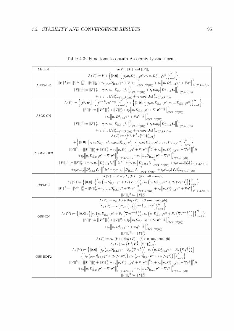
4.3. STABILITY AND CONVERGENCE RESULTS 95
Table 4.3: Functions to obtain Λ-coercivity and norms
Method Λ(V ), |||V ||| and |||F |||∗
ASGS-BE
Λ (V ) := V +
[0,0] ,
[τpµpD1
B,1,1qn, τuµuD1
B,1,1vn]Nn=1
|||V |||2 :=
∣∣∣∣∣∣V N ∣∣∣∣∣∣20
+ |||V |||2B + τp
∣∣∣∣∣∣µpD1B,1,1q
n +∇·vn∣∣∣∣∣∣2`2(Υ,L2(Ω))
+ τu
∣∣∣∣∣∣µuD1B,1,1v
n +∇qn∣∣∣∣∣∣2`2(Υ,L2(Ω))
|||F |||∗2 := |||F |||2F + τpτuµu
∣∣∣∣∣∣D1B,1,1fp
∣∣∣∣∣∣2`1(Υ,L2(Ω))
+ τpτuµp
∣∣∣∣∣∣D1B,1,1fu
∣∣∣∣∣∣2`1(Υ,L2(Ω))
+τpτuµu||fp||2`∞(Υ,L2(Ω)) + τpτuµp||fu||2`∞(Υ,L2(Ω))
ASGS-CN
Λ (V ) :=
[p0,u0
],[pn−
12 ,un−
12
]Nn=1
+
[0,0] ,
[τpµpD1
B,1,1qn, τuµuD1
B,1,1vn]Nn=1
|||V |||2 :=
∣∣∣∣∣∣V N ∣∣∣∣∣∣20
+ |||V |||2B + τp
∣∣∣∣∣∣µpD1B,1,1q
n +∇·vn−12
∣∣∣∣∣∣2`2(Υ,L2(Ω))
+τu
∣∣∣∣∣∣µuD1B,1,1v
n +∇qn−12
∣∣∣∣∣∣2`2(Υ,L2(Ω))
|||F |||∗2 := |||F |||2F + τpτuµu
∣∣∣∣∣∣D1B,1,1fp
∣∣∣∣∣∣2`1(Υ,L2(Ω))
+ τpτuµp
∣∣∣∣∣∣D1B,1,1fu
∣∣∣∣∣∣2`1(Υ,L2(Ω))
+τpτuµu||fp||2`∞(Υ,L2(Ω)) + τpτuµp||fu||2`∞(Υ,L2(Ω))
ASGS-BDF2
Λ (V ) :=V 0, V
12 , V nNn=2
+
[0,0] ,
[τpµpD1
B,1,1q1, τuµuD1
B,1,1v1],[τpµpD1
B,2,1qn, τuµuD1
B,2,1vn]Nn=2
|||V |||2 :=
∣∣∣∣∣∣V N ∣∣∣∣∣∣20
+ |||V |||2B + τp
∣∣∣∣∣∣µpD1B,1,1q
1 +∇·v12
∣∣∣∣∣∣2δt+ τu
∣∣∣∣∣∣µuD1B,1,1v
1 +∇q12
∣∣∣∣∣∣2δt+τp
∣∣∣∣∣∣µpD1B,2,1q
n +∇·vn∣∣∣∣∣∣2`2(Υ,L2(Ω))
+ τu
∣∣∣∣∣∣µuD1B,2,1v
n +∇qn∣∣∣∣∣∣2`2(Υ,L2(Ω))
|||F |||∗2 := |||F |||2F + τpτuµu
∣∣∣∣∣∣D1B,1,1fp
1∣∣∣∣∣∣2δt2 + τpτuµu
∣∣∣∣∣∣D1B,2,1fp
∣∣∣∣∣∣2`1(Υ,L2(Ω))
+ τpτuµu||fp||2`∞(Υ,L2(Ω))
+τpτuµp
∣∣∣∣∣∣D1B,1,1fu
1∣∣∣∣∣∣2δt2 + τpτuµp
∣∣∣∣∣∣D1B,2,1fu
∣∣∣∣∣∣2`1(Υ,L2(Ω))
+ τpτuµp||fu||2`∞(Υ,L2(Ω))
OSS-BE
Λ (V ) := V + βΛb (V ) (β small enough)
Λb (V ) :=
[0,0] ,[τp(µpD1
B,1,1qn + Pp (∇·vn)
), τu
(µuD1
B,1,1vn + Pu (∇qn)
)]Nn=1
|||V |||2 :=
∣∣∣∣∣∣V N ∣∣∣∣∣∣20
+ |||V |||2B + τp
∣∣∣∣∣∣µpD1B,1,1q
n +∇·vn∣∣∣∣∣∣2`2(Υ,L2(Ω))
+ τu
∣∣∣∣∣∣µuD1B,1,1v
n +∇qn∣∣∣∣∣∣2`2(Υ,L2(Ω))
|||F |||∗2 := |||F |||2F
OSS-CN
Λ (V ) := Λa (V ) + βΛb (V ) (β small enough)
Λa (V ) :=
[p0,u0
],[pn−
12 ,un−
12
]Nn=1
Λb (V ) :=
[0,0] ,
[τp(µpD1
B,1,1qn + Pp
(∇·vn−
12
)), τu
(µuD1
B,1,1vn + Pu
(∇qn−
12
))]Nn=1
|||V |||2 :=
∣∣∣∣∣∣V N ∣∣∣∣∣∣20
+ |||V |||2B + τp
∣∣∣∣∣∣µpD1B,1,1q
n +∇·vn−12
∣∣∣∣∣∣2`2(Υ,L2(Ω))
+τu
∣∣∣∣∣∣µuD1B,1,1v
n +∇qn−12
∣∣∣∣∣∣2`2(Υ,L2(Ω))
|||F |||∗2 := |||F |||2F
OSS-BDF2
Λ (V ) := Λa (V ) + βΛb (V ) (β > 0 small enough)
Λa (V ) :=V 0, V
12 , V nNn=2
Λb (V ) :=
[0,0] ,
[τp(µpD1
B,1,1q1 + Pp
(∇·v
12
)), τu
(µuD1
B,1,1v1 + Pu
(∇q
12
))][τp(µpD1
B,2,1qn + Pp (∇·vn)
), τu
(µuD1
B,2,1vn + Pu (∇qn)
)]Nn=2
|||V |||2 :=
∣∣∣∣∣∣V N ∣∣∣∣∣∣20
+ |||V |||2B + τp
∣∣∣∣∣∣µpD1B,1,1q
1 +∇·v12
∣∣∣∣∣∣2δt+ τu
∣∣∣∣∣∣µuD1B,1,1v
1 +∇q12
∣∣∣∣∣∣2δt+τp
∣∣∣∣∣∣µpD1B,2,1q
n +∇·vn∣∣∣∣∣∣2`2(Υ,L2(Ω))
+ τu
∣∣∣∣∣∣µuD1B,2,1v
n +∇qn∣∣∣∣∣∣2`2(Υ,L2(Ω))
|||F |||∗2 := |||F |||2F

96 CHAPTER 4. TIME MARCHING SCHEMES FOR THE WAVE EQUATION
Table 4.4: Error functions I: ASGS formulation
Method E(h, δt)
BE
E2(h, δt) := µp||εp||2`∞(L2) + µu||εu||2`∞(L2) + τpτuµu||∇·εu||2`∞(L2) + τpτuµp||∇εp||2`∞(L2)
+ 1τu||εu||2`2(L2) + τp
∣∣∣∣µpD1B,1,1εp
∣∣∣∣2`2(L2)
+ τp||∇·εu||2`2(L2) + (1 + σ)κp||εp||2`2(Υ,L2(Γo))
+ 1τp||εp||2`2(L2) + τu
∣∣∣∣µuD1B,1,1εu
∣∣∣∣2`2(L2)
+ τu||∇εp||2`2(L2) + (1− σ)κu||εu||2`2(Υ,L2(Γo))
+τpτuµu∣∣∣∣µpD1
B,1,1εp∣∣∣∣2`∞(L2)
+ τpτuµu∣∣∣∣µpD2
C,2,1εp∣∣∣∣2`1(L2)
+ τpτuµu∣∣∣∣∇·D1
B,1,1εu∣∣∣∣2`1(L2)
+τpτuµp∣∣∣∣µuD1
B,1,1εu∣∣∣∣2`∞(L2)
+ τpτuµp∣∣∣∣µuD2
C,2,1εu∣∣∣∣2`1(L2)
+ τpτuµp∣∣∣∣∇D1
B,1,1εp∣∣∣∣2`1(L2)
+ δt2
µp||µp∂ttp||2`1(L2) + δt2τp||µp∂ttp||2`2(L2) + τpτuµuδt
2(||µp∂ttp||2`∞(L2) + ||µp∂tttp||2`1(L2)
)+ δt2
µu||µu∂ttu||2`1(L2) + δt2τu||µu∂ttu||2`2(L2) + τpτuµpδt
2(||µu∂ttu||2`∞(L2) + ||µu∂tttu||2`1(L2)
)
CN
E2(h, δt) := µp||εp||2`∞(Υ,L2(Ω)) + µu||εu||2`∞(Υ,L2(Ω))
+(1 + σ)κp||εp||2`2(Υ,L2(Γo)) + (1− σ)κu||εu||2`2(Υ,L2(Γo))
+ 1τu||εu||2`2(L2) + τp
∣∣∣∣µpD1B,1,1εp
∣∣∣∣2`2(L2)
+ τp||∇·εu||2`2(L2) + τpτuµu∣∣∣∣∇·D1
B,1,1εu∣∣∣∣2`1(L2)
+ 1τp||εp||2`2(L2) + τu
∣∣∣∣µuD1B,1,1εu
∣∣∣∣2`2(L2)
+ τu||∇εp||2`2(L2) + τpτuµp∣∣∣∣∇D1
B,1,1εp∣∣∣∣2`1(L2)
+τpτuµu∣∣∣∣µpD1
B,1,1εp∣∣∣∣2`∞(L2)
+ τpτuµu∣∣∣∣µpD2
C,2,1εp∣∣∣∣2`1(L2)
+τpτuµp∣∣∣∣µuD1
B,1,1εu∣∣∣∣2`∞(L2)
+ τpτuµp∣∣∣∣µuD2
C,2,1εu∣∣∣∣2`1(L2)
+ δt4
µp||µp∂tttp||2`1(L2) + δt4τp||µp∂tttp||2`2(L2) + τpτuµuδt
4[||µp∂tttp||2`∞(L2) + ||µp∂ttttp||2`1(L2)
]+ δt4
µu||µu∂tttu||2`1(L2) + δt4τu||µu∂tttu||2`2(L2) + τpτuµpδt
4[||µu∂tttu||2`∞(L2) + ||µu∂ttttu||2`1(L2)
]
BDF2
E2(h, δt) := µp||εp||2`∞(L2) + µu||εu||2`∞(L2)
+(1 + σ)κp||εp||2`2(Υ,L2(Γo)) + (1− σ)κu||εu||2`2(Υ,L2(Γo))
+ 1τu||εu||2`2(Υ,L2(Ω)) + τp
∣∣∣∣µpD1B,1,1ε
1p
∣∣∣∣2δt+ τp∣∣∣∣µpD1
B,2,1εp∣∣∣∣2`2(L2)
+ τp||∇·εu||2`2(L2)
+ 1τp||εp||2`2(L2) + τu
∣∣∣∣µuD1B,1,1ε
1u
∣∣∣∣2δt+ τu∣∣∣∣µuD1
B,2,1εu∣∣∣∣2`2(L2)
+ τu||∇εp||2`2(Υ,L2(Ω))
+τpτuµu
∣∣∣∣∣∣µpD2C,2, 12
ε12p
∣∣∣∣∣∣2δt2 + τpτuµp
∣∣∣∣∣∣µuD2C,2, 12
ε12u
∣∣∣∣∣∣2δt2+τpτuµu
(∣∣∣∣µpD1B,2,1ε
2p
∣∣∣∣2 +∣∣∣∣µp (D1
B,2,1ε3p − 4D1
B,2,1ε2p
)∣∣∣∣2)+τpτuµp
(∣∣∣∣µuD1B,2,1ε
2u
∣∣∣∣2 +∣∣∣∣µu (D1
B,2,1ε3u − 4D1
B,2,1ε2u
)∣∣∣∣2)+τpτuµu
∣∣∣∣µp(3D2C,4,1 − 2D2
C,2,2)εnp∣∣∣∣2`1(L2)
+ τpτuµp∣∣∣∣µu(3D2
C,4,1 − 2D2C,2,2)εnu
∣∣∣∣2`1(L2)
+τpτuµu
(∣∣∣∣µpD1B,2,1ε
Np
∣∣∣∣2 +∣∣∣∣µp (3D1
B,2,1εN−1p − 4D1
B,2,1εNp
)∣∣∣∣2)+τpτuµp
(∣∣∣∣µuD1B,2,1ε
Nu
∣∣∣∣2 +∣∣∣∣µu (3D1
B,2,1εN−1u − 4D1
B,2,1εNu
)∣∣∣∣2)+τpτuµu
(∣∣∣∣∇·D1B,1,1ε
1u
∣∣∣∣2δt2 +∣∣∣∣∇·D1
F,2,1εu∣∣∣∣2`1(L2)
)+τpτuµp
(∣∣∣∣∇D1B,1,1ε
1p
∣∣∣∣2δt2 +∣∣∣∣∇D1
F,2,1εp∣∣∣∣2`1(L2)
)+ δt4
µp
∣∣∣∣∣∣µp∂tttp 12
∣∣∣∣∣∣2δt2 + δt4
µp||µp∂tttpn||2`1(L2) + δt4
µu
∣∣∣∣∣∣µu∂tttu 12
∣∣∣∣∣∣2δt2 + δt4
µu||µu∂tttun||2`1(L2)
+δt4τp
∣∣∣∣∣∣µp∂tttp 12
∣∣∣∣∣∣2δt+ δt4τp||µp∂tttpn||2`2(L2) + δt4τu
∣∣∣∣∣∣µu∂tttu 12
∣∣∣∣∣∣2δt+ δt4τu||µu∂tttun||2`2(L2)
+δt4τpτuµu
(∣∣∣∣∣∣µp∂tttp 12
∣∣∣∣∣∣2 + ||µp∂ttttp||2`1(L2) + ||µp∂tttp||2L∞(L2)
)+δt4τpτuµp
(∣∣∣∣∣∣µu∂tttu 12
∣∣∣∣∣∣2 + ||µu∂ttttu||2`1(L2) + ||µu∂tttu||2L∞(L2)
)
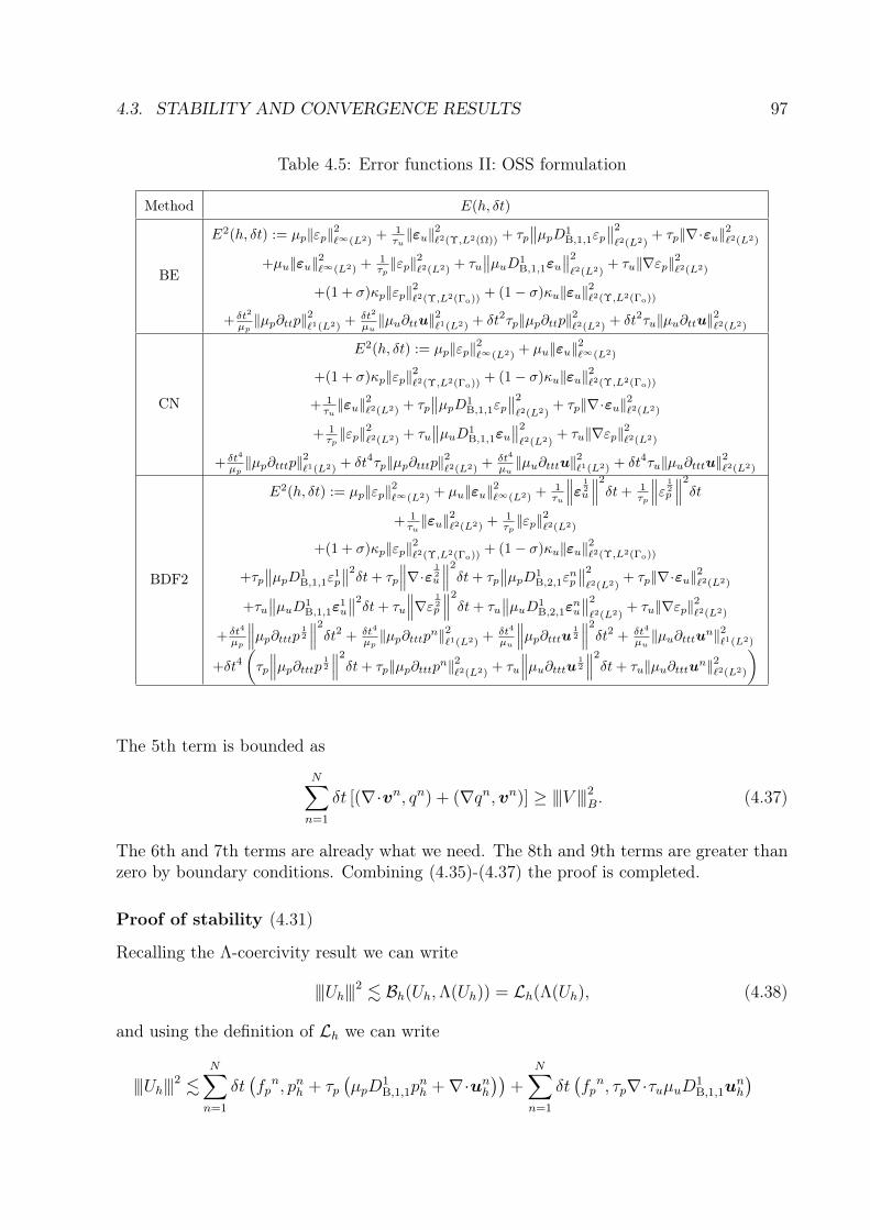
4.3. STABILITY AND CONVERGENCE RESULTS 97
Table 4.5: Error functions II: OSS formulation
Method E(h, δt)
BE
E2(h, δt) := µp||εp||2`∞(L2) + 1τu||εu||2`2(Υ,L2(Ω)) + τp
∣∣∣∣µpD1B,1,1εp
∣∣∣∣2`2(L2)
+ τp||∇·εu||2`2(L2)
+µu||εu||2`∞(L2) + 1τp||εp||2`2(L2) + τu
∣∣∣∣µuD1B,1,1εu
∣∣∣∣2`2(L2)
+ τu||∇εp||2`2(L2)
+(1 + σ)κp||εp||2`2(Υ,L2(Γo)) + (1− σ)κu||εu||2`2(Υ,L2(Γo))
+ δt2
µp||µp∂ttp||2`1(L2) + δt2
µu||µu∂ttu||2`1(L2) + δt2τp||µp∂ttp||2`2(L2) + δt2τu||µu∂ttu||2`2(L2)
CN
E2(h, δt) := µp||εp||2`∞(L2) + µu||εu||2`∞(L2)
+(1 + σ)κp||εp||2`2(Υ,L2(Γo)) + (1− σ)κu||εu||2`2(Υ,L2(Γo))
+ 1τu||εu||2`2(L2) + τp
∣∣∣∣µpD1B,1,1εp
∣∣∣∣2`2(L2)
+ τp||∇·εu||2`2(L2)
+ 1τp||εp||2`2(L2) + τu
∣∣∣∣µuD1B,1,1εu
∣∣∣∣2`2(L2)
+ τu||∇εp||2`2(L2)
+ δt4
µp||µp∂tttp||2`1(L2) + δt4τp||µp∂tttp||2`2(L2) + δt4
µu||µu∂tttu||2`1(L2) + δt4τu||µu∂tttu||2`2(L2)
BDF2
E2(h, δt) := µp||εp||2`∞(L2) + µu||εu||2`∞(L2) + 1τu
∣∣∣∣∣∣ε 12u
∣∣∣∣∣∣2δt+ 1τp
∣∣∣∣∣∣ε 12p
∣∣∣∣∣∣2δt+ 1τu||εu||2`2(L2) + 1
τp||εp||2`2(L2)
+(1 + σ)κp||εp||2`2(Υ,L2(Γo)) + (1− σ)κu||εu||2`2(Υ,L2(Γo))
+τp∣∣∣∣µpD1
B,1,1ε1p
∣∣∣∣2δt+ τp
∣∣∣∣∣∣∇·ε 12u
∣∣∣∣∣∣2δt+ τp∣∣∣∣µpD1
B,2,1εnp
∣∣∣∣2`2(L2)
+ τp||∇·εu||2`2(L2)
+τu∣∣∣∣µuD1
B,1,1ε1u
∣∣∣∣2δt+ τu
∣∣∣∣∣∣∇ε 12p
∣∣∣∣∣∣2δt+ τu∣∣∣∣µuD1
B,2,1εnu
∣∣∣∣2`2(L2)
+ τu||∇εp||2`2(L2)
+ δt4
µp
∣∣∣∣∣∣µp∂tttp 12
∣∣∣∣∣∣2δt2 + δt4
µp||µp∂tttpn||2`1(L2) + δt4
µu
∣∣∣∣∣∣µp∂tttu 12
∣∣∣∣∣∣2δt2 + δt4
µu||µu∂tttun||2`1(L2)
+δt4(τp
∣∣∣∣∣∣µp∂tttp 12
∣∣∣∣∣∣2δt+ τp||µp∂tttpn||2`2(L2) + τu
∣∣∣∣∣∣µu∂tttu 12
∣∣∣∣∣∣2δt+ τu||µu∂tttun||2`2(L2)
)
The 5th term is bounded as
N∑n=1
δt [(∇·vn, qn) + (∇qn,vn)] ≥ |||V |||2B. (4.37)
The 6th and 7th terms are already what we need. The 8th and 9th terms are greater thanzero by boundary conditions. Combining (4.35)-(4.37) the proof is completed.
Proof of stability (4.31)
Recalling the Λ-coercivity result we can write
|||Uh|||2 . Bh(Uh,Λ(Uh)) = Lh(Λ(Uh), (4.38)
and using the definition of Lh we can write
|||Uh|||2 .N∑n=1
δt(fpn, pnh + τp
(µpD
1B,1,1p
nh +∇·unh
))+
N∑n=1
δt(fpn, τp∇·τuµuD1
B,1,1unh
)

98 CHAPTER 4. TIME MARCHING SCHEMES FOR THE WAVE EQUATION
+N∑n=1
δt(fu
n,unh + τu(µuD
1B,1,1u
nh +∇pnh
))+
N∑n=1
δt(fu
n, τu∇τpµpD1B,1,1p
nh
).
(4.39)
The 1st and 3rd terms can be bounded asN∑n=1
δt(fpn, pnh + τp
(µpD
1B,1,1p
nh +∇·unh
))+
N∑n=1
δt(fu
n,unh + τu(µuD
1B,1,1u
nh +∇pnh
)). α1|||F |||2F +
1
α1
|||Uh|||2, (4.40)
where here and in what follows αi > 0 are reals appearing from Young’s inequality. The2nd and 4th terms are bounded in a similar manner and we just show how we bound the2nd term:
N∑n=1
δt(fpn, τp∇·τuµuD1
B,1,1unh
)=−
N∑n=1
δt(D1
B,1,1fpn, τpτuµu∇·un−1
h
)+(fpN , τpτuµu∇·uNh
).α2τpτuµu
∣∣∣∣D1B,1,1fp
∣∣∣∣2`1(Υ,L2(Ω))
+ α3τpτuµu||fp||2`∞(Υ,L2(Ω))
+1
α2
τpτuµu||∇·uh||2`∞(Υ,L2(Ω)) +1
α3
τpτuµu||∇·uh||2`∞(Υ,L2(Ω)). (4.41)
Combining (4.38)-(4.41) and taking αi large enough the proof is complete.
Proof of convergence (4.32)
Combining Λ-coercivity with V = e and (4.34) we can arrive to
|||e|||2 . Bh(e,Λ(e)) = Bh(ε,Λ(e)) + C(U,Λ(e)).
The aim is to bound e in terms of ε and U . We first analyze the term containing Bh andthen the term associated to the consistency error (4.33):
Bh(ε,Λ(e)) =N∑n=1
δt(µpD
1B,1,1ε
np +∇·εnu, enp + τp
(µpD
1B,1,1e
np +∇·enu
)+ τpτuµu∇·D1
B,1,1enu
)+
N∑n=1
δt(µuD
1B,1,1ε
nu +∇εnp , enu + τu
(µuD
1B,1,1e
nu +∇enp
)+ τpτuµp∇D1
B,1,1enp
)≤
N∑n=1
δt
[α1
2τp
∣∣∣∣εnp ∣∣∣∣2 +τp
2α1
∣∣∣∣µpD1B,1,1e
np +∇·enu
∣∣∣∣2]
+N∑n=1
δt
[α2
2τu||εnu||
2 +τu
2α2
∣∣∣∣µuD1B,1,1e
nu +∇enp
∣∣∣∣2]

4.3. STABILITY AND CONVERGENCE RESULTS 99
+N∑n=1
δtτp
[α3
2
∣∣∣∣µpD1B,1,1ε
np +∇·εnu
∣∣∣∣2 +1
2α3
∣∣∣∣µpD1B,1,1e
np +∇·enu
∣∣∣∣2]
+N∑n=1
δtτu
[α4
2
∣∣∣∣µuD1B,1,1ε
nu +∇εnp
∣∣∣∣2 +1
2α4
∣∣∣∣µuD1B,1,1e
nu +∇enp
∣∣∣∣2]
+N∑n=1
δt(µpD
1B,1,1ε
np +∇·εnu, τpτuµu∇·D1
B,1,1enu
)+
N∑n=1
δt(µuD
1B,1,1ε
nu +∇εn+1
p , τpτuµp∇D1B,1,1e
np
).
The only terms missing to bound are the last two ones. Both are bound similarly and wewill only show how the first one is bounded. The first part is bounded as
N∑n=1
δt(µpD
1B,1,1ε
np , τpτuµu∇·D1
B,1,1enu
)=τpτuµu
[(µpD
1B,1,1ε
Np ,∇·eNu
)−(µpD
1B,1,1ε
1p,∇·e0
u
)]−
N−1∑n=1
δtτpτuµu(µpD
2C,2,1ε
np ,∇·enu
)≤τpτuµu
[α5
2
∣∣∣∣µpD1B,1,1ε
Np
∣∣∣∣2 +1
2α5
∣∣∣∣∇·eNu ∣∣∣∣2]+ τpτuµu
[α6
2
∣∣∣∣µpD2C,2,1εp
∣∣∣∣2`1(L2)
+1
2α6
||∇·eu||2`∞(L2)
],
and the second part is bounded as
N∑n=1
δt(∇·εnu, τpτuµu∇·D1
B,1,1enu
)=τpτuµu
[(∇·εNu ,∇·eNu
)−(∇·ε0
u,∇·e0u
)]−
N∑n=1
δt(∇·D1
B,1,1εnu, τpτuµu∇·enu
)≤τpτuµu
[α7
2
∣∣∣∣∇·εNu ∣∣∣∣2 +1
2α7
∣∣∣∣∇·eNu ∣∣∣∣2 +α8
2
∣∣∣∣∇·D1B,1,1εu
∣∣∣∣2`1(L2)
+1
2α8
||∇·eu||2`∞(L2)
].
This completes the bounding of Bh. Now let us bound the consistency error (4.33):
C(U,Λ(e)) = Lh(Λ(e))− Bh(U,Λ(e))
=−N∑n=1
δt(µpD
1B,1,1p
n +∇·un, enp + τp(µpD
1B,1,1e
np +∇·enu
)+ τpτuµu∇·D1
B,1,1enu
)−
N∑n=1
δt(µuD
1B,1,1u
n +∇pn, enu + τu(µuD
1B,1,1e
nu +∇enp
),+τpτuµp∇D1
B,1,1enp
).

100 CHAPTER 4. TIME MARCHING SCHEMES FOR THE WAVE EQUATION
Both terms are bounded similarly and we only show how it is bounded the first one. Letus start with its first part
−N∑n=1
δt(µpD
1B,1,1p
n +∇·un, enp)≤α9
2
δt2
µp
[N∑n=1
∣∣∣∣µpD1B,1,1p
n +∇·un∣∣∣∣]2
+1
2α9
µp||ep||2`∞(L2)
≤α9
2
δt2
µp
[N∑n=1
∣∣∣∣µpD1B,1,1p
n − µp∂tpn∣∣∣∣]2
+1
2α9
µp||ep||2`∞(L2)
≤α9
2
δt2
µp||µp∂ttpn||2`1(L2) +
1
2α9
µp||ep||2`∞(L2).
The second part can be bounded as
−N∑n=1
δt(µpD
1B,1,1p
n +∇·un, τp(µpD
1B,1,1e
np +∇·enu
))≤α10
2
N∑n=1
δtτp∣∣∣∣µpD1
B,1,1pn − µp∂tpn
∣∣∣∣2 +1
2α10
N∑n=1
δtτp∣∣∣∣µpD1
B,1,1enp +∇·enu
∣∣∣∣2≤α10
2δt2τp||µp∂ttpn||2`2(Υ,L2(Ω)) +
1
2α10
τp∣∣∣∣µpD1
B,1,1enp +∇·enu
∣∣∣∣2`2(Υ,L2(Ω))
.
The third part can be bounded as
−N∑n=1
δt(µpD
1B,1,1p
n +∇·un, τpτuµu∇·D1B,1,1e
nu
)=τpτuµu
[(µpD
1B,1,1p
N +∇·uN ,∇·eNu)−(µpD
1B,1,1p
1 +∇·u0,∇·e0u
)]− τpτuµu
[N−1∑n=1
δt(µpD
2C,2,1p
n +∇·D1B,1,1u
n,∇·enu)
+ δt(∇·D1
B,1,1u1,∇·e0
u
)]
≤τpτuµu[α11
2
∣∣∣∣µpD1B,1,1p
N +∇·uN∣∣∣∣2 +
1
2α11
∣∣∣∣∇·eNu ∣∣∣∣2]+ τpτuµu
α12
2
[N−1∑n=1
δt∣∣∣∣µpD2
C,2,1pn +∇·D1
B,1,1un∣∣∣∣]2
+ τpτuµu1
2α12
||∇·eu||2
≤τpτuµu[α11
2δt2∣∣∣∣µp∂ttpN ∣∣∣∣2 +
1
2α11
∣∣∣∣∇·eNu ∣∣∣∣2]+ τpτuµu
[α12
2δt2||µp∂tttp||2`1(Υ,L2(Ω)) +
1
2α12
||∇·eu||2`∞(Υ,L2(Ω))
].
Combining all bounds the proof is complete.
4.3.5 Accuracy of the fully discrete methods
Let k be the order of p-interpolation and l the order of u-interpolation. Analyzing thea priori error estimates (4.32) for the fully discrete methods with the error functions

4.3. STABILITY AND CONVERGENCE RESULTS 101
Table 4.6: Convergence rates for ASGS-BE and OSS-BE according to variational form
Variational Form I II III∣∣∣∣ξnp ∣∣∣∣`∞(L2), ||ξnu ||`∞(L2) hk+ 1
2 + hl+12 + δt+ h
12 δt hk+ 1
2 + hl + δt hk + hl+12 + δt∣∣∣∣µuD1
B,1,1ξnu +∇ξnp
∣∣∣∣`2(L2)
hk + hl + h−12 δt+ δt hk−
12 + hl−1 + h−1δt hk + hl+
12 + δt∣∣∣∣µpD1
B,1,1ξnp +∇·ξnu
∣∣∣∣`2(L2)
hk + hl + h−12 δt+ δt hk+ 1
2 + hl + δt hk−1 + hl−12 + h−1δt
Best k, l, h-δt k = l, δt ∼ hk+ 12 k + 1
2 = l, δt ∼ hl k = l + 12 , δt ∼ h
k
k = l, δt ∼ hl k = l, δt ∼ hk
k + 1 = l, δt ∼ hl− 12 k = l + 1, δt ∼ hk− 1
2
Table 4.7: Convergence rates for ASGS-CN and OSS-CN according to variational form
Variational Form I II III∣∣∣∣ξnp ∣∣∣∣`∞(L2), ||ξnu ||`∞(L2) hk+ 1
2 + hl+12 + δt2 + h
12 δt2 hk+ 1
2 + hl + δt2 hk + hl+12 + δt2∣∣∣∣∣∣∣∣µuD1
B,1,1ξnu +∇ξn−
12
p
∣∣∣∣∣∣∣∣`2(L2)
hk + hl + h−12 δt2 + δt2 hk−
12 + hl−1 + h−1δt2 hk + hl+
12 + δt2∣∣∣∣∣∣∣∣µpD1
B,1,1ξnp +∇·ξn−
12
u
∣∣∣∣∣∣∣∣`2(L2)
hk + hl + h−12 δt2 + δt2 hk+ 1
2 + hl + δt2 hk−1 + hl−12 + h−1δt2
Best k, l, h-δt k = l, δt2 ∼ hk+ 12 k + 1
2= l, δt2 ∼ hl k = l + 1
2, δt2 ∼ hk
k = l, δt2 ∼ hl k = l, δt2 ∼ hk
k + 1 = l, δt2 ∼ hl−12 k = l + 1, δt2 ∼ hk−
12
given in Tables 4.4 and 4.5 and assuming regular enough solutions, we can summarizethe convergence rates as shown in Tables 4.6-4.8. We stress the fact that the convergencerates do depend on the choice of the stabilization parameters, and different convergenceorders are obtained for the three discrete variational formulations above. Let us note thatthe time discretization schemes do not spoil the spatial convergence rates obtained in [67,68] for the time-continuous case.
Table 4.8: Convergence rates for ASGS-BDF2 and OSS-BDF2 according to variationalform
Variational Form I II III∣∣∣∣ξnp ∣∣∣∣`∞(L2), ||ξnu ||`∞(L2) hk+ 1
2 + hl+12 + δt2 hk+ 1
2 + hl + δt2 hk + hl+12 + δt2∣∣∣∣µuD1
B,2,1ξnu +∇ξnp
∣∣∣∣`2(L2)
hk + hl + h−12 δt2 hk−
12 + hl−1 + h−1δt2 hk + hl+
12 + δt2∣∣∣∣µpD1
B,2,1ξnp +∇·ξnu
∣∣∣∣`2(L2)
hk + hl + h−12 δt2 hk+ 1
2 + hl + δt2 hk−1 + hl−12 + h−1δt2
Best k, l, h-δt k = l, δt2 ∼ hk+ 12 k + 1
2 = l, δt2 ∼ hl k = l + 12 , δt
2 ∼ hk
k = l, δt2 ∼ hl k = l, δt2 ∼ hk
k + 1 = l, δt2 ∼ hl− 12 k = l + 1, δt2 ∼ hk− 1
2

102 CHAPTER 4. TIME MARCHING SCHEMES FOR THE WAVE EQUATION
4.4 Fourier analysisWe show now the results of a Fourier analysis (or von Neumann analysis) in 1D using linear(P1) elements, which serves to study dispersion, dissipation, and stability of the numericalschemes. The analysis is done in an unbounded domain with no forcing terms, but withnon-zero initial conditions. The mesh is taken uniform, of size h, and the time step is δt.We focus on variational form I because it has the best convergence properties, as shown inthe previous analysis.
Let us consider a solution of the form p = Cpei(kx−ωt) and u = Cpµ
1/2p µ
−1/2u ei(kx−ωt),
where Cp is an arbitrary constant such that [p] = [Cp], [·] standing for dimensional group, ωis the angular frequency (temporal frequency) and k is the (angular) wavenumber (spatialfrequency). It can be checked that this plane wave is solution of the wave equation inmixed form. The angular frequency and wavenumber are related through the wave speedas ω = kc.
For 1D P1 elements of size diamK = h we will need the following element matrices:∫K
NiNj
∣∣∣i,j=1,2
=h
6
(2 11 2
),
∫K
Ni∂xNj
∣∣∣i,j=1,2
=1
2
(−1 1−1 1
),∫
K
∂xNiNj
∣∣∣i,j=1,2
=1
2
(−1 −11 1
),
∫K
∂xNi∂xNj
∣∣∣i,j=1,2
=1
h
(1 −1−1 1
),
where Ni is the shape function of node i (in element K). When assembled for just twoelements sharing a generic node they give, respectively,
Mp = Mu =h
6
2 1 01 4 10 2 1
, Kp = Ku =1
2
−1 1 0−1 0 10 −1 1
,
MS,p = MS,u =1
2
−1 −1 01 0 −10 1 1
, KS,p = KS,u =1
h
1 −1 0−1 2 −10 −1 1
.
Additionally, we define the lumped mass matrices
Mp = Mu =h
2
1 0 00 2 00 0 1
.
First we will analyze the time semi-discretization, then the space semi-discretizationand finally the full discretization. The time discretizations to be considered are the θ andBDF2 methods, whereas the space discretizations to be analyzed are stabilized FE methods(ASGS and OSS). We will often take tn = nδt and xj = jh, where n is the time step andj is the mesh point.
4.4.1 Time semi-discretization
Let us start considering the effect of the time discretization only, without discretizing inspace. Let us take ωδt = kδtcδt and kδt = k, where the subscript δt denotes temporal

4.4. FOURIER ANALYSIS 103
0
0.5
1
1.5
2
0 0.2 0.4 0.6 0.8 1
<(ωδt)/ω
ωδt/π
θ = 0 and θ = 1θ = 0.25 and θ = 0.75
θ = 0.50
-0.4
-0.2
0
0.2
0.4
0 0.2 0.4 0.6 0.8 1
=(ωδt)/ω
ωδt/π
θ = 0θ = 0.25θ = 0.5θ = 0.75θ = 1
Figure 4.1: θ-method time semi-discretization
0.6
0.8
1
1.2
1.4
0 0.2 0.4 0.6 0.8 1
<(ωδt)/ω
ωδt/π
minus root
-0.4
-0.2
0
0.2
0.4
0 0.2 0.4 0.6 0.8 1
=(ωδt)/ω
ωδt/π
minus root
Figure 4.2: BDF2 time semi-discretization
0.6
0.8
1
1.2
1.4
0 0.2 0.4 0.6 0.8 1
<(ωδt)/ω
ωδt/π
θ = 0.5BDF2
-0.4
-0.2
0
0.2
0.4
0 0.2 0.4 0.6 0.8 1
=(ωδt)/ω
ωδt/π
θ = 0.5BDF2
Figure 4.3: Time semi-discretization comparison
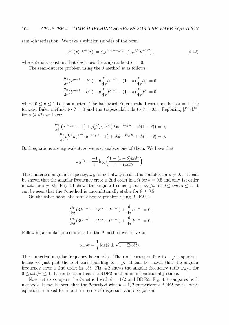
104 CHAPTER 4. TIME MARCHING SCHEMES FOR THE WAVE EQUATION
semi-discretization. We take a solution (mode) of the form
[P n(x), Un(x)] = φkei(kx−ωδttn)
[1, µ1/2
p µ−1/2u
], (4.42)
where φk is a constant that describes the amplitude at tn = 0.The semi-discrete problem using the θ method is as follows:
µpδt
(P n+1 − P n) + θd
dxUn+1 + (1− θ) d
dxUn = 0,
µuδt
(Un+1 − Un) + θd
dxP n+1 + (1− θ) d
dxP n = 0,
where 0 ≤ θ ≤ 1 is a parameter. The backward Euler method corresponds to θ = 1, theforward Euler method to θ = 0 and the trapezoidal rule to θ = 0.5. Replacing [P n, Un]from (4.42) we have:
µpδt
(e−iωδtδt − 1
)+ µ1/2
p µ−1/2u
(ikθe−iωδtδt + ik(1− θ)
)= 0,
µuδtµ1/2p µ−1/2
u
(e−iωδtδt − 1
)+ ikθe−iωδtδt + ik(1− θ) = 0.
Both equations are equivalent, so we just analyze one of them. We have that
ωδtδt =−1
ilog
(1− (1− θ)iωδt
1 + iωδtθ
).
The numerical angular frequency, ωδt, is not always real, it is complex for θ 6= 0.5. It canbe shown that the angular frequency error is 2nd order in ωδt for θ = 0.5 and only 1st orderin ωδt for θ 6= 0.5. Fig. 4.1 shows the angular frequency ratio ωδt/ω for 0 ≤ ωδt/π ≤ 1. Itcan be seen that the θ-method is unconditionally stable for θ ≥ 0.5.
On the other hand, the semi-discrete problem using BDF2 is:
µp2δt
(3P n+1 − 4P n + P n−1) +d
dxUn+1 = 0,
µu2δt
(3Un+1 − 4Un + Un−1) +d
dxP n+1 = 0.
Following a similar procedure as for the θ method we arrive to
ωδtδt =1
ilog(2±
√1− 2iωδt).
The numerical angular frequency is complex. The root corresponding to +√ is spurious,
hence we just plot the root corresponding to −√. It can be shown that the angularfrequency error is 2nd order in ωδt. Fig. 4.2 shows the angular frequency ratio ωδt/ω for0 ≤ ωδt/π ≤ 1. It can be seen that the BDF2 method is unconditionally stable.
Now, let us compare the θ-method with θ = 1/2 and BDF2. Fig. 4.3 compares bothmethods. It can be seen that the θ-method with θ = 1/2 outperforms BDF2 for the waveequation in mixed form both in terms of dispersion and dissipation.

4.4. FOURIER ANALYSIS 105
0.6
0.8
1
1.2
1.4
0 0.2 0.4 0.6 0.8 1
<(kh/k)
kh/π
Cτ = 0.0Cτ = 0.1Cτ = 0.2Cτ = 0.3Cτ = 0.4
0.96
0.98
1
1.02
1.04
0 0.1 0.2 0.3 0.4 0.5
<(kh/k
)
kh/π
Cτ = 0.0Cτ = 0.1Cτ = 0.2Cτ = 0.3Cτ = 0.4
Figure 4.4: ASGS space semi-discretization: real part of the wavenumber ratio (the rightpicture is a zoom of the left)
-0.4
-0.2
0
0.2
0.4
0 0.2 0.4 0.6 0.8 1
=(kh/k
)
kh/π
Cτ = 0.0Cτ = 0.1Cτ = 0.2Cτ = 0.3Cτ = 0.4
-0.04
-0.02
0
0.02
0.04
0 0.1 0.2 0.3 0.4 0.5
=(kh/k
)
kh/π
Cτ = 0.0Cτ = 0.1Cτ = 0.2Cτ = 0.3Cτ = 0.4
Figure 4.5: ASGS space semi-discretization: imaginary part of the wavenumber ratio (theright picture is a zoom of the left)
0.6
0.8
1
1.2
1.4
0 0.2 0.4 0.6 0.8 1
<(kh/k
)
kh/π
Cτ = 0.0Cτ = 0.1Cτ = 0.2Cτ = 0.3Cτ = 0.4
0.96
0.98
1
1.02
1.04
0 0.1 0.2 0.3 0.4 0.5
<(kh/k
)
kh/π
Cτ = 0.0Cτ = 0.1Cτ = 0.2Cτ = 0.3Cτ = 0.4
Figure 4.6: OSS space semi-discretization: real part of the wavenumber ratio (the rightpicture is a zoom of the left)

106 CHAPTER 4. TIME MARCHING SCHEMES FOR THE WAVE EQUATION
-0.4
-0.2
0
0.2
0.4
0 0.2 0.4 0.6 0.8 1
=(kh/k
)
kh/π
Cτ = 0.0Cτ = 0.1Cτ = 0.2Cτ = 0.3Cτ = 0.4
-0.04
-0.02
0
0.02
0.04
0 0.1 0.2 0.3 0.4 0.5
=(kh/k)
kh/π
Cτ = 0.0Cτ = 0.1Cτ = 0.2Cτ = 0.3Cτ = 0.4
Figure 4.7: OSS space semi-discretization: imaginary part of the wavenumber ratio (theright picture is a zoom of the left)
4.4.2 Space semi-discretization
We analyze now the wave equation in mixed form when the spatial discretization is doneusing the ASGS and the OSS methods. We take ωh = khch and ωh = ω, where the subscripth denotes spatial semi-discretization. We take now
[Pj(t), Uj(t)] = φωei(khxj−ωt)[1, µ1/2
p µ−1/2u
], (4.43)
where φω is a constant that describes the amplitude at t = 0.For the ASGS method, the semi-discrete problem has the matrix structure:
µpMpdP
dt+KuU + τuµuMS,u
dU
dt+ τuKS,pP = 0,
µuMudU
dt+KpP + τpµpMS,p
dP
dt+ τpKS,uU = 0,
where a subscript S has been introduced in the matrices with contributions from thestabilization terms. In these equations, P and U do not denote the sequence of solutionsin time, but the array of nodal unknowns with time-continuous components. The meaningof P and U in what follows will be determined by the context. We just analyze one ofthe previous equations because they are equivalent. The j-th row of the first system ofequations is
µph
6
(d
dtPj−1 + 4
d
dtPj +
d
dtPj+1
)+
1
2(−Uj−1 + Uj+1)
+ τuµu1
2
(d
dtUj−1 −
d
dtUj+1
)+ τu
1
h(−Pj−1 + 2Pj − Pj+1) = 0.
Replacing [Pj, Uj] from (4.43) we have:
−iωµph
6
(e−ikhh + 4 + eikhh
)+
1
2µ1/2p µ−1/2
u
(−e−ikhh + eikhh
)− 1
2iωτuµ
1/2p µ1/2
u
(e−ikhh − eikhh
)+
1
hτu(−e−ikhh + 2− eikhh
)= 0,

4.4. FOURIER ANALYSIS 107
khk
= − i
khlog
(−(4kh+ 12iCτ )±
√36(kh)2C2
τ + 72ikhCτ + 12(kh)2 − 36
2(kh+ 3i− 3khCτ − 6iCτ )
).
The Maclaurin series for the real and imaginary parts are:
<(kh)
k= 1− 15C2
τ − 1
180(kh)4 +
126C4τ − 63C2
τ + 1
1512(kh)6 + ... ,
=(kh)
k=Cτ12
(kh)3 − 6C3τ − Cτ72
(kh)5 + ... .
It can be shown that kh is complex and that <(kh) is of order (kh)4 for any Cτ and of order(kh)6 for Cτ = 1/
√15 ≈ 0.2582. Additionally, =(kh) is of order (kh)3 for any Cτ > 0.
Fig. 4.4 and Fig. 4.5 show the real and imaginary parts of the wavenumber ratio as afunction of kh/π. It can be seen that the Galerkin method (Cτ = 0) is unstable whereasthe ASGS method is always stable.
Next, we analyze an OSS method in which a lumped mass matrix (diagonal) is usedto project the residual. Additionally, as the projection with a lumped mass matrix isnot exactly an L2 projection, we keep the time derivatives in the residual. Non-lumped(consistent) mass matrices are used for time derivatives. Better than lumped mass matrixapproximations to the L2 projection can be used, but the results obtained are very similar.For instance we could use the family of banded approximate mass matrices from [138].
The matrix form of the semi-discrete problem is:
µpMpdP
dt+KuU + τuµuMS,u
dU
dt+ τuKS,pP − τuMS,uRu = 0,
MuRu = µuMud
dtU +KpP,
µuMudU
dt+KpP + τpµpMS,p
dP
dt+ τpKS,uU − τpMS,pRp = 0,
MpRp = µpMpd
dtP +KuU.
As we use a lumped projection, the semi-discrete problem reduces to:
µpMpdP
dt+KuU + τuµuMS,u
dU
dt+ τuKS,pP − τuMS,uM
−1u
(µuMu
d
dtU +KpP
)= 0,
µuMudU
dt+KpP + τpµpMS,p
dP
dt+ τpKS,uU − τpMS,pM
−1p
(µpMp
d
dtP +KuU
)= 0.
Following similar steps as for the ASGS method, we arrive to the expression which relateskhh with kh:
2kh(eikhh + 4e2ikhh + e3ikhh
)+ khCτ
(−1 + 2eikhh − 2e3ikhh + e4ikhh
)+ 6i
(−eikhh + e3ikhh
)+ 3iCτ
(1− 4eikhh + 6e2ikhh − 4e3ikhh + e4ikhh
)= 0.
Fig. 4.6 and Fig. 4.7 show the real and imaginary parts of the wavenumber ratio as afunction of kh/π. As before, the Galerkin method (Cτ = 0) is unstable whereas the OSSmethod is always stable.

108 CHAPTER 4. TIME MARCHING SCHEMES FOR THE WAVE EQUATION
0.6
0.8
1
1.2
1.4
0 0.2 0.4 0.6 0.8 1
<(ω
∗/ω
)
kh/π
θ = 1θ = 0.5θ = 0
-0.4
-0.2
0
0.2
0.4
0 0.2 0.4 0.6 0.8 1
=(ω
∗/ω
)
kh/π
θ = 1θ = 0.5θ = 0
Figure 4.8: ASGS + θ for r = 1 and Cτ = 0.2
0.6
0.8
1
1.2
1.4
0 0.2 0.4 0.6 0.8 1
<(ω
∗/ω
)
kh/π
Cτ = 0.1Cτ = 0.2Cτ = 0.3Cτ = 0.4Cτ = 0.5
-0.4
-0.2
0
0.2
0.4
0 0.2 0.4 0.6 0.8 1
=(ω
∗/ω
)
kh/π
Cτ = 0.1Cτ = 0.2Cτ = 0.3Cτ = 0.4Cτ = 0.5
Figure 4.9: ASGS + θ for r = 1 and θ = 0.5
0.6
0.8
1
1.2
1.4
0 0.2 0.4 0.6 0.8 1
<(ω
∗/ω
)
kh/π
r = 0.1r = 0.5r = 1.0r = 2.0r = 10.0
-0.4
-0.2
0
0.2
0.4
0 0.2 0.4 0.6 0.8 1
=(ω
∗/ω
)
kh/π
r = 0.1r = 0.5r = 1.0r = 2.0r = 10.0
Figure 4.10: ASGS + θ for Cτ = 0.2 and θ = 0.5

4.4. FOURIER ANALYSIS 109
0.6
0.8
1
1.2
1.4
0 0.2 0.4 0.6 0.8 1
<(ω
∗/ω
)
kh/π
Cτ = 0.1Cτ = 0.2Cτ = 0.3Cτ = 0.4Cτ = 0.5
-0.4
-0.2
0
0.2
0.4
0 0.2 0.4 0.6 0.8 1
=(ω
∗/ω
)
kh/π
Cτ = 0.1Cτ = 0.2Cτ = 0.3Cτ = 0.4Cτ = 0.5
Figure 4.11: ASGS + BDF2 for r = 1
0.6
0.8
1
1.2
1.4
0 0.2 0.4 0.6 0.8 1
<(ω
∗/ω
)
kh/π
r = 0.1r = 0.5r = 1.0r = 2.0r = 10.0
-0.4
-0.2
0
0.2
0.4
0 0.2 0.4 0.6 0.8 1
=(ω
∗/ω
)
kh/π
r = 0.1r = 0.5r = 1.0r = 2.0r = 10.0
Figure 4.12: ASGS + BDF2 for Cτ = 0.2
4.4.3 Space-time discretization
Finally, we analyze the fully discrete problems arising from the combination of timediscretizations (θ and BDF2) and space discretizations (ASGS and OSS). Thus, in totalwe will analyze four fully discrete problems. We take ω∗ = k∗c∗ and k∗ = k. The subscript∗ denotes full discretization. We take a mode of the form[
P nj , U
nj
]= φke
i(kxj−ω∗tn)[1, µ1/2
p µ−1/2u
], (4.44)
where φk describes the amplitude at tn = 0.Let us define r as the Courant or CFL number as
r := cδt/h. (4.45)
First, we consider the ASGS formulation for the space discretization. With regard tothe time integration, we first consider the θ-method. The fully discrete problem is:
µpδtMp
(P n+1 − P n
)+τu
µuδtMS,u
(Un+1 − Un
)+ θ
(KuU
n+1 + τuKS,pPn+1)
+ (1− θ) (KuUn + τuKS,pP
n) = 0,

110 CHAPTER 4. TIME MARCHING SCHEMES FOR THE WAVE EQUATION
µuδtMu
(Un+1 − Un
)+τp
µpδtMS,p
(P n+1 − P n
)+ θ
(KpP
n+1 + τpKS,uUn+1)
+(1− θ) (KpPn + τpKS,uU
n) = 0.
We concentrate in one of the equations because both will be equivalent for the currentanalysis. The j-th row of the system of equations is
µph
6δt
(P n+1j−1 + 4P n+1
j + P n+1j+1 − P n
j−1 − 4P nj − P n
j+1
)+τuµu2δt
(Un+1j−1 − Un+1
j+1 − Unj−1 + Un
j+1
)+ θ
(1
2
(−Un+1
j−1 + Un+1j+1
)+ τu
1
h
(−P n+1
j−1 + 2P n+1j − P n+1
j+1
))+ (1− θ)
(1
2
(−Un
j−1 + Unj+1
)+ τu
1
h
(−P n
j−1 + 2P nj − P n
j+1
))= 0,
and replacing[P nj , U
nj
]from (4.44) we get
µph
6δt
(ei(−kh−ω∗δt) + 4ei(−ω∗δt) + ei(kh−ω∗δt) − ei(−kh) − 4− ei(kh)
)+
1
2δtτuµ
12p µ
12u
(ei(−kh−ω∗δt) − ei(kh−ω∗δt) − ei(−kh) + ei(kh)
)+ θ
(1
2µ
12p µ− 1
2u
(−ei(−kh−ω∗δt) + ei(kh−ω∗δt)
)+
1
hτu(−ei(−kh−ω∗δt) + 2ei(−ω∗δt) − ei(kh−ω∗δt)
))+ (1− θ)
(1
2µ
12p µ− 1
2u
(−ei(−kh) + ei(kh)
)+
1
hτu(−ei(−kh) + 2− ei(kh)
))= 0.
Using the definition of r from (4.45) we arrive to:
ω∗ω
=−1
irkhlog
(2 + cos(kh)− 3iCτ sin(kh)− (1− θ)(3ir sin(kh) + 6rCτ (1− cos(kh)))
2− 3iCτ sin(kh) + cos(kh) + 3irθ sin(kh) + 6rθCτ (1− cos(kh))
).
Fig. 4.8, Fig. 4.9, and Fig. 4.10 show the real and imaginary parts of the angularfrequency ratio keeping two parameters fixed. It can be seen that θ = 0 (forward Euler orexplicit Euler scheme) is unconditionally unstable. This is similar to what happens withforward in time-centered in space finite differences (FTCS) applied to the pure advectionequation in 1D.
Next, we consider the ASGS with the BDF2 time integration. The fully discrete problemis:
µp2δt
Mp
(3P n+2 − 4P n+1 + P n
)+τu
µu2δt
MS,u
(3Un+2 − 4Un+1 + Un
)+KuU
n+2 + τuKS,pPn+2 = 0,
µu2δt
Mu
(3Un+2 − 4Un+1 + Un
)+τp
µp2δt
MS,p
(3P n+2 − 4P n+1 + P n
)+KpP
n+2 + τpKS,uUn+2 = 0.
Following a similar procedure as before, we arrive to(3e−2iω∗δt − 4e−iω∗δt + 1
)((2 + cos(kh))− 3iCτ (sin(kh)))

4.4. FOURIER ANALYSIS 111
0.6
0.8
1
1.2
1.4
0 0.2 0.4 0.6 0.8 1
<(ω
∗/ω
)
kh/π
ASGS + θ = 1ASGS + θ = 1/2ASGS + BDF2
-0.4
-0.2
0
0.2
0.4
0 0.2 0.4 0.6 0.8 1
=(ω
∗/ω
)
kh/π
ASGS + θ = 1ASGS + θ = 1/2ASGS + BDF2
Figure 4.13: Fully discrete ASGS with Cτ = 0.2 and r = 1
+e−2iω∗δt (6ir (sin(kh)) + 12rCτ (1− cos(kh))) = 0.
Fig. 4.11 and Fig. 4.12 show the angular frequency ratio for the fully discrete problem. Itcan be seen that this combination of spatial and temporal discretization is stable.
Fig. 4.13 compares the fully discrete ASGS method with the two time integrationschemes shown previously. It can be seen that the θ method performs better than BDF2for small enough kh.
Next, we aim to analyze the properties of the OSS stabilized formulation. When usingthe θ-method for the time integration, the fully discrete problem is:
µpδtMp
(P n+1 − P n
)+ τu
µuδtMS,u
(Un+1 − Un
)− τuMS,uM
−1u
µuδtMu
(Un+1 − Un
)+ θ
(KuU
n+1 + τuKS,pPn+1 − τuMS,uM
−1u KpP
n+1)
+ (1− θ)(KuU
n + τuKS,pPn − τuMS,uM
−1u KpP
n)
= 0,
µuδtMu
(Un+1 − Un
)+ τp
µpδtMS,p
(P n+1 − P n
)− τpMS,pM
−1p
µpδtMp
(P n+1 − P n
)+ θ
(KpP
n+1 + τpKS,uUn+1 − τpMS,pM
−1p KuU
n+1)
+ (1− θ)(KpP
n + τpKS,uUn − τpMS,pM
−1p KuU
n)
= 0.
Following a similar procedure as before we arrive to(e−iω∗δt − 1
)(2 (2 + cos(kh)) + iCτ (−2 sin(kh) + sin(2kh)))
+(θe−iω∗δt + 1− θ
)(6ir (sin(kh)) + 3rCτ (3− 4 cos(kh) + cos(2kh))) = 0.
Fig. 4.14, Fig. 4.15, and Fig. 4.16 show the angular frequency ratio for this fully discretizedproblem.
Next, we consider the OSS-BDF2 fully discrete problem:µp2δt
Mp
(3P n+2 − 4P n+1 + P n
)+ τu
µu2δt
MS,u
(3Un+2 − 4Un+1 + Un
)+KuU
n+2
+ τuKS,pPn+2 − τuMS,uM
−1u
( µu2δt
Mu
(3Un+2 − 4Un+1 + Un
)+KpP
n+2)
= 0,

112 CHAPTER 4. TIME MARCHING SCHEMES FOR THE WAVE EQUATION
0.6
0.8
1
1.2
1.4
0 0.2 0.4 0.6 0.8 1
<(ω
∗/ω
)
kh/π
θ = 1θ = 0.5θ = 0
-0.4
-0.2
0
0.2
0.4
0 0.2 0.4 0.6 0.8 1
=(ω
∗/ω
)
kh/π
θ = 1θ = 0.5θ = 0
Figure 4.14: OSS + θ for r = 1 and Cτ = 0.2
0.6
0.8
1
1.2
1.4
0 0.2 0.4 0.6 0.8 1
<(ω
∗/ω
)
kh/π
Cτ = 0.1Cτ = 0.2Cτ = 0.3Cτ = 0.4Cτ = 0.5
-0.4
-0.2
0
0.2
0.4
0 0.2 0.4 0.6 0.8 1
=(ω
∗/ω
)
kh/π
Cτ = 0.1Cτ = 0.2Cτ = 0.3Cτ = 0.4Cτ = 0.5
Figure 4.15: OSS + θ for r = 1 and θ = 0.5
0.6
0.8
1
1.2
1.4
0 0.2 0.4 0.6 0.8 1
<(ω
∗/ω
)
kh/π
r = 0.1r = 0.5r = 1.0r = 2.0r = 10.0
-0.4
-0.2
0
0.2
0.4
0 0.2 0.4 0.6 0.8 1
=(ω
∗/ω
)
kh/π
r = 0.1r = 0.5r = 1.0r = 2.0r = 10.0
Figure 4.16: OSS + θ for Cτ = 0.2 and θ = 0.5

4.5. NUMERICAL RESULTS 113
0.6
0.8
1
1.2
1.4
0 0.2 0.4 0.6 0.8 1
<(ω
∗/ω
)
kh/π
Cτ = 0.1Cτ = 0.2Cτ = 0.3Cτ = 0.4Cτ = 0.5
-0.4
-0.2
0
0.2
0.4
0 0.2 0.4 0.6 0.8 1
=(ω
∗/ω
)
kh/π
Cτ = 0.1Cτ = 0.2Cτ = 0.3Cτ = 0.4Cτ = 0.5
Figure 4.17: OSS + BDF2 for r = 1
0.6
0.8
1
1.2
1.4
0 0.2 0.4 0.6 0.8 1
<(ω
∗/ω
)
kh/π
r = 0.1r = 0.5r = 1.0r = 2.0r = 10.0
-0.4
-0.2
0
0.2
0.4
0 0.2 0.4 0.6 0.8 1
=(ω
∗/ω
)
kh/π
r = 0.1r = 0.5r = 1.0r = 2.0r = 10.0
Figure 4.18: OSS + BDF2 for Cτ = 0.2
µu2δt
Mu
(3Un+2 − 4Un+1 + Un
)+ τp
µp2δt
MS,p
(3P n+2 − 4P n+1 + P n
)+KpP
n+2
+ τpKS,uUn+2 − τpMS,pM
−1p
( µp2δt
Mp
(3P n+2 − 4P n+1 + P n
)+KuU
n+2)
= 0.
Following a similar procedure as before we get(3e−2iω∗δt − 4e−iω∗δt + 1
)(2 (2 + cos(kh)) + iCτ (−2 sin(kh) + sin(2kh)))
+ e−2iω∗δt (12ir (sin(kh)) + 6rCτ (3− 4 cos(kh) + cos(2kh))) = 0.
Fig. 4.17 and Fig. 4.18 show the real and imaginary parts of the angular frequency ratio.The plots comparing time marching schemes for the OSS method are very similar to
the ones for ASGS and are not shown for succinctness. The fully discrete ASGS and OSSmethods perform similarly according to this analysis, so we do not show a side by sidecomparison of both methods.
4.5 Numerical resultsIn this section we present two sets of numerical results. First, convergence tests arepresented and compared with the predicted convergence rates obtained from convergence

114 CHAPTER 4. TIME MARCHING SCHEMES FOR THE WAVE EQUATION
Table 4.9: Experimental δt convergence rates for ASGS-BE method using Q1/Q1 spatialinterpolation
Variational Form I II III Iδt vs. h δt ∼ 0.5h δt ∼ 4.5h1.5
Num Min Num Min Num Min Num Min||pn − pnh||`∞(L2) 1.00 1 1.00 1 1.01 1 1.00 1||un − unh||`∞(L2) 1.02 1 1.02 1 1.02 1 1.01 1||∇(pn − pnh)||`2(L2) 1.00 0.5 1.00 0 1.00 1 0.66 2/3||∇·(un − unh)||`2(L2) 1.00 0.5 1.00 1 1.00 0 0.66 2/3
analysis. Then, numerical solutions of a wave propagation problem are compared in orderto see the differences of the fully discrete methods.
4.5.1 Convergence tests
Let us consider a two dimensional transient problem with analytical solution to investigatethe convergence properties of the stabilized FE formulations proposed. The spatial domainis the unit square (0, 1)×(0, 1) and the temporal domain is (0, 1). The forcing terms [fp,fu]are chosen such that the exact solution is p = sin(πx) sin(πy) cos
(π3t)and u = [p, p] with
µp = µu = 1. On the boundary we prescribe p = 0 (Γ = Γp). The initial condition is takenas the exact solution at t = 0. Various mesh sizes and time step sizes have been used togenerate the results. We have used isotropic bilinear (Q1) and biquadratic (Q2) meshes ofsizes h = 0.05, 0.025, 0.01, 0.005 and 0.002. The stabilization algorithmic constant Cτ hasbeen taken as 0.05 for Q1 elements and 0.4 for Q2 elements. The the length scale of theproblem has been taken as L0 = d
√meas(Ω) = 1.
In Tables 4.9-4.20 we show the convergence rates with respect to the time step sizeδt for various stabilization methods (ASGS and OSS), time integrators (BE/CN/BDF2)and spatial interpolations (Q1 and Q2). The numerical experiments have been carriedout modifying the time step size and the mesh size at the same time. The relationship(δt, h) is shown in each table for each variational form with the respective proportionalityconstant and power, δt ∼ Csh
s. The power constant s has been chosen as s = 1 for all thevariational forms and, additionally, it has been chosen such that the best convergence isachieved for equal interpolation of the unknowns (k = l). It is observed than in all casesthe numerical rate of convergence obtained (Num) is greater than or equal to the minimumone predicted by the convergence analysis (Min).
4.5.2 Numerical comparison
In Section 4.4 we analyzed dispersion and dissipation analytically through Fourier tech-niques. We present now a simple test to verify experimentally the predictions of the Fourieranalysis. Let us consider a 1D problem in Ω = (0, L) = (0, 1) and Υ = (0, 0.8), and let ussolve the mixed wave equation with µp = 1, µu = 1, zero initial conditions and boundaryconditions p(0, t) = sin (ωt) and p(L, t) = 0. We compare the solutions obtained with thefully discrete methods at t = 0.6.

4.5. NUMERICAL RESULTS 115
Table 4.10: Experimental δt convergence rates for OSS-BE method using Q1/Q1 spatialinterpolation
Variational Form I II III Iδt vs. h δt ∼ 0.5h δt ∼ 4.5h1.5
Num Min Num Min Num Min Num Min||pn − pnh||`∞(L2) 1.00 1 1.00 1 1.01 1 1.00 1||un − unh||`∞(L2) 1.02 1 1.02 1 1.02 1 1.01 1||∇(pn − pnh)||`2(L2) 1.00 0.5 1.00 0 1.00 1 0.66 2/3||∇·(un − unh)||`2(L2) 1.00 0.5 1.00 1 1.00 0 0.66 2/3
Table 4.11: Experimental δt convergence rates for ASGS-BE method using Q2/Q2 spatialinterpolation
Variational Form I II III I II IIIδt vs. h δt ∼ 0.5h δt ∼ 894h2.5 δt ∼ 40h2 δt ∼ 40h2
Num Min Num Min Num Min Num Min Num Min Num Min∣∣∣∣pn − pnh∣∣∣∣`∞(L2)0.98 1 0.98 1 0.98 1 0.99 1 0.99 1 0.99 1∣∣∣∣un − unh∣∣∣∣`∞(L2)0.99 1 0.99 1 0.99 1 1.00 1 1.00 1 1.00 1∣∣∣∣∇(pn − pnh)
∣∣∣∣`2(L2)
0.99 0.5 0.99 0 0.99 1 0.98 4/5 0.50 0.5 1.00 1∣∣∣∣∇·(un − unh)∣∣∣∣`2(L2)
0.99 0.5 0.99 1 0.99 0 0.99 4/5 1.00 1 0.50 0.5
Table 4.12: Experimental δt convergence rates for OSS-BE method using Q2/Q2 spatialinterpolation
Variational Form I II III I II IIIδt vs. h δt ∼ 0.5h δt ∼ 894h2.5 δt ∼ 40h2 δt ∼ 40h2
Num Min Num Min Num Min Num Min Num Min Num Min∣∣∣∣pn − pnh∣∣∣∣`∞(L2)0.98 1 0.98 1 0.98 1 0.99 1 0.99 1 0.99 1∣∣∣∣un − unh∣∣∣∣`∞(L2)0.99 1 0.99 1 0.99 1 1.00 1 1.00 1 1.00 1∣∣∣∣∇(pn − pnh)
∣∣∣∣`2(L2)
0.99 0.5 1.02 0 0.99 1 0.98 4/5 0.51 0.5 1.00 1∣∣∣∣∇·(un − unh)∣∣∣∣`2(L2)
0.99 0.5 0.99 1 1.03 0 0.99 4/5 0.99 1 0.52 0.5
Table 4.13: Experimental δt convergence rates for ASGS-CN method using Q1/Q1 spatialinterpolation
Variational Form I II III I II IIIδt vs. h δt ∼ 0.5h δt ∼ 0.2h0.75 δt ∼ 0.1h0.5 δt ∼ 0.1h0.5
Num Min Num Min Num Min Num Min Num Min Num Min∣∣∣∣pn − pnh∣∣∣∣`∞(L2)2.00 1.5 2.00 1 2.00 1 2.60 2 3.38 2 3.39 2∣∣∣∣un − unh∣∣∣∣`∞(L2)2.00 1.5 2.00 1 2.00 1 2.64 2 3.72 2 3.72 2∣∣∣∣∇(pn − pnh)
∣∣∣∣`2(L2)
1.00 1 1.00 0 1.00 1 1.33 4/3 1.99 0 1.99 2∣∣∣∣∇·(un − unh)∣∣∣∣`2(L2)
1.00 1 1.00 1 1.00 0 1.33 4/3 1.99 2 1.99 0

116 CHAPTER 4. TIME MARCHING SCHEMES FOR THE WAVE EQUATION
Table 4.14: Experimental δt convergence rates for OSS-CN method using Q1/Q1 spatialinterpolation
Variational Form I II III I II IIIδt vs. h δt ∼ 0.5h δt ∼ 0.2h0.75 δt ∼ 0.1h0.5 δt ∼ 0.1h0.5
Num Min Num Min Num Min Num Min Num Min Num Min∣∣∣∣pn − pnh∣∣∣∣`∞(L2)2.00 1.5 2.00 1 2.00 1 2.60 2 3.38 2 3.39 2∣∣∣∣un − unh∣∣∣∣`∞(L2)2.00 1.5 2.00 1 2.00 1 2.64 2 3.72 2 3.72 2∣∣∣∣∇(pn − pnh)
∣∣∣∣`2(L2)
1.00 1 1.00 0 1.00 1 1.33 4/3 1.99 0 1.99 2∣∣∣∣∇·(un − unh)∣∣∣∣`2(L2)
1.00 1 1.00 1 1.00 0 1.33 4/3 1.99 2 1.99 0
Table 4.15: Experimental δt convergence rates for ASGS-CN method using Q2/Q2 spatialinterpolation
Variational Form I II III Iδt vs. h δt ∼ 0.5h δt ∼ 2h1.25
Num Min Num Min Num Min Num Min||pn − pnh||`∞(L2) 2.01 2 2.00 2 2.00 2 2.00 2||un − unh||`∞(L2) 2.26 2 2.00 2 2.00 2 2.13 2||∇(pn − pnh)||`2(L2) 1.99 1.5 1.00 1 2.00 2 1.60 1.6||∇·(un − unh)||`2(L2) 1.99 1.5 2.00 2 1.00 1 1.60 1.6
Table 4.16: Experimental δt convergence rates for OSS-CN method using Q2/Q2 spatialinterpolation
Variational Form I II III Iδt vs. h δt ∼ 0.5h δt ∼ 2h1.25
Num Min Num Min Num Min Num Min||pn − pnh||`∞(L2) 2.01 2 1.99 2 2.00 2 2.00 2||un − unh||`∞(L2) 2.04 2 1.99 2 2.03 2 2.00 2||∇(pn − pnh)||`2(L2) 2.00 1.5 1.00 1 2.00 2 1.60 1.6||∇·(un − unh)||`2(L2) 2.02 1.5 1.98 2 1.02 1 1.62 1.6
Table 4.17: Experimental δt convergence rates for ASGS-BDF2 method using Q1/Q1spatial interpolation
Variational Form I II III I II IIIδt vs. h δt ∼ 0.5h δt ∼ 0.2h0.75 δt ∼ 0.1h0.5 δt ∼ 0.1h0.5
Num Min Num Min Num Min Num Min Num Min Num Min∣∣∣∣pn − pnh∣∣∣∣`∞(L2)2.00 1.5 2.00 1 2.00 1 2.66 2 3.93 2 3.93 2∣∣∣∣un − unh∣∣∣∣`∞(L2)2.00 1.5 2.00 1 2.00 1 2.67 2 4.04 2 4.04 2∣∣∣∣∇(pn − pnh)
∣∣∣∣`2(L2)
1.00 1 1.00 0 1.00 1 1.32 4/3 1.99 0 1.99 2∣∣∣∣∇·(un − unh)∣∣∣∣`2(L2)
1.00 1 1.00 1 1.00 0 1.32 4/3 1.99 2 1.99 0

4.5. NUMERICAL RESULTS 117
Table 4.18: Experimental δt convergence rates for OSS-BDF2 method using Q1/Q1 spatialinterpolation
Variational Form I II III I II IIIδt vs. h δt ∼ 0.5h δt ∼ 0.2h0.75 δt ∼ 0.1h0.5 δt ∼ 0.1h0.5
Num Min Num Min Num Min Num Min Num Min Num Min∣∣∣∣pn − pnh∣∣∣∣`∞(L2)2.00 1.5 2.00 1 2.00 1 2.66 2 3.93 2 3.93 2∣∣∣∣un − unh∣∣∣∣`∞(L2)2.00 1.5 2.00 1 2.00 1 2.67 2 4.04 2 4.04 2∣∣∣∣∇(pn − pnh)
∣∣∣∣`2(L2)
1.00 1 1.00 0 1.00 1 1.32 4/3 1.99 0 1.99 2∣∣∣∣∇·(un − unh)∣∣∣∣`2(L2)
1.00 1 1.00 1 1.00 0 1.32 4/3 1.99 2 1.99 0
Table 4.19: Experimental δt convergence rates for ASGS-BDF2 method using Q2/Q2spatial interpolation
Variational Form I II III Iδt vs. h δt ∼ 0.5h δt ∼ 2h1.25
Num Min Num Min Num Min Num Min||pn − pnh||`∞(L2) 2.17 2 2.00 2 2.13 2 2.41 2||un − unh||`∞(L2) 2.19 2 2.00 2 2.00 2 2.34 2||∇(pn − pnh)||`2(L2) 1.99 1.5 1.00 1 2.00 2 1.59 1.6||∇·(un − unh)||`2(L2) 1.99 1.5 2.00 2 1.00 1 1.59 1.6
For ω = 10π a quite coarse pair of mesh and time step sizes is (h, δt) = (0.05, 0.05).This allows us to see dispersion and dissipation in the numerical solution when comparedwith the exact solution sin(ωt−kx)(1−H(x−ct)), where H is the Heaviside step function.The algorithmic constant is taken as Cτ = 0.1 and the elements used are P1.
Fig. 4.19 shows the numerical solutions obtained with ASGS and three time marchingschemes. CN is the least dissipative while BE is the most dissipative and BDF2 issomewhere in the middle. These numerical results are in agreement with the previousFourier analysis. OSS behaves similarly and we do not show those results. Figs. 4.20-4.22compare the ASGS method with the OSS method for the same time integration scheme,showing a very similar numerical behavior.
Table 4.20: Experimental δt convergence rates for OSS-BDF2 method using Q2/Q2 spatialinterpolation
Variational Form I II III Iδt vs. h δt ∼ 0.5h δt ∼ 2h1.25
Num Min Num Min Num Min Num Min||pn − pnh||`∞(L2) 2.18 2 2.02 2 2.14 2 2.42 2||un − unh||`∞(L2) 2.03 2 2.00 2 2.03 2 2.24 2||∇(pn − pnh)||`2(L2) 2.00 1.5 1.01 1 2.00 2 1.60 1.6||∇·(un − unh)||`2(L2) 2.02 1.5 2.00 2 1.03 1 1.64 1.6

118 CHAPTER 4. TIME MARCHING SCHEMES FOR THE WAVE EQUATION
-1
-0.5
0
0.5
1
0 0.2 0.4 0.6 0.8 1
p
x
Exact
BE
BDF2
CN
Figure 4.19: Numerical solution using the ASGS formulation and different time marchingschemes
-1
-0.5
0
0.5
1
0 0.2 0.4 0.6 0.8 1
p
x
Exact
ASGS
OSS
Figure 4.20: Comparison of ASGS and OSS using BE as time integration

4.5. NUMERICAL RESULTS 119
-1
-0.5
0
0.5
1
0 0.2 0.4 0.6 0.8 1
p
x
Exact
ASGS
OSS
Figure 4.21: Comparison of ASGS and OSS using BDF2 as time integration
-1
-0.5
0
0.5
1
0 0.2 0.4 0.6 0.8 1
p
x
Exact
ASGS
OSS
Figure 4.22: Comparison of ASGS and OSS using CN as time integration

120 CHAPTER 4. TIME MARCHING SCHEMES FOR THE WAVE EQUATION
4.6 ConclusionsIn this work we have presented fully discrete methods arising from the combination ofspatial discretization methods, namely stabilized FE methods, and temporal discretizationmethods (backward Euler, Crank-Nicolson and 2nd order backward differentiation for-mula) for the mixed wave equation in three different variational forms. The stabilizationparameters have been designed such that they mimic the continuous setting.
Stability and convergence has been proved for all combinations of space discretizationand time discretization. Stability, dispersion and dissipation of the fully discrete methods in1D for equal interpolation of [p,u] has been analyzed using Fourier techniques. Accordingto this analysis, CN performs better than BE and BDF2. Additionally, ASGS and OSSperform similarly.
Numerical convergence tests have been performed and the results obtained in thenumerical experiments are in agreement with the theoretical predictions. Additionally,the fully discrete methods have been compared qualitatively. This comparison shows thedifferences in dispersion and dissipation of the methods and is in agreement with the Fourieranalysis.

Chapter 5
Applications
This chapter includes material in:Oriol Guasch, Marc Arnela, Ramon Codina, and Hector Espinoza. “A stabilized finiteelement method for the mixed wave equation in an ALE framework with application todiphthong production”. In: Journal of Computational Physics (Oct. 2014). Submittedas well as additional unpublished numerical application examples.
Here we present various wave propagation examples. The examples include a concentrictube wave propagation problem, an eccentric tube problem, vowel generation and diph-thong generation. Some of the results are compared with experiments [139]. All examplesinvolve acoustic wave propagation where the propagation media is air with properties µp =7.083E-6 m s2/Kg and µu = 1.20 Kg/m3 which correspond to a sound speed c = 343 m/sand a density ρ0 = 1.20 Kg/m3.
The algorithmic constant for the stabilization parameters was taken as Cτ = 0.1 in allcases. The element size h is based on the volume of the element h = d
√Ve.
5.1 Concentric Tubes
This is a 3D example of wave propagation inside of two concentric tubes of different diam-eter. In the context of voice simulation, this geometry corresponds to a very rudimentaryapproximation of the vocal tract in vowel /a/ position. A pressure pulse at the smalldiameter tube is the input signal and the end of the big diameter tube is the output tofree space. Two reference points denoted as 1 and 2 will be used for comparison withexperimental results using the concept of transfer function [139].
5.1.1 Space and time domains
The time interval for the simulation is 25 ms. The spatial domain consists of two concentrictubes: one 85 mm long with a diameter of 14 mm and another tube of the same length anda diameter of 29.5 mm as shown in Fig. 5.1. The smaller diameter tube is the sound inletthrough a 2 mm diameter hole. Acoustic pressure and velocity are measured at points 1and 2 for comparison with experimental results.
121
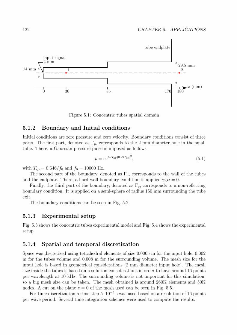
122 CHAPTER 5. APPLICATIONS
1 2
0 30 85 180170x (mm)
14 mm29.5 mm
2 mminput signal
tube endplate
Figure 5.1: Concentric tubes spatial domain
5.1.2 Boundary and Initial conditions
Initial conditions are zero pressure and zero velocity. Boundary conditions consist of threeparts. The first part, denoted as Γp, corresponds to the 2 mm diameter hole in the smalltube. There, a Gaussian pressure pulse is imposed as follows
p = e[(t−Tgp)0.29Tgp]2 , (5.1)
with Tgp = 0.646/f0 and f0 = 10000 Hz.The second part of the boundary, denoted as Γu, corresponds to the wall of the tubes
and the endplate. There, a hard wall boundary condition is applied γnu = 0.Finally, the third part of the boundary, denoted as Γo, corresponds to a non-reflecting
boundary condition. It is applied on a semi-sphere of radius 150 mm surrounding the tubeexit.
The boundary conditions can be seen in Fig. 5.2.
5.1.3 Experimental setup
Fig. 5.3 shows the concentric tubes experimental model and Fig. 5.4 shows the experimentalsetup.
5.1.4 Spatial and temporal discretization
Space was discretized using tetrahedral elements of size 0.0005 m for the input hole, 0.002m for the tubes volume and 0.008 m for the surrounding volume. The mesh size for theinput hole is based in geometrical considerations (2 mm diameter input hole). The meshsize inside the tubes is based on resolution considerations in order to have around 16 pointsper wavelength at 10 kHz. The surrounding volume is not important for this simulation,so a big mesh size can be taken. The mesh obtained is around 260K elements and 50Knodes. A cut on the plane z = 0 of the mesh used can be seen in Fig. 5.5.
For time discretization a time step 5 ·10−6 s was used based on a resolution of 16 pointsper wave period. Several time integration schemes were used to compute the results.

5.1. CONCENTRIC TUBES 123
1 2
Γo
Γu
150 mm
Γp
Figure 5.2: Concentric tubes boundary conditions
Figure 5.3: Concentric tubes experiment model

124 CHAPTER 5. APPLICATIONS
Figure 5.4: Experiment setup
x
y
z
Figure 5.5: Cut on the plane z = 0 showing the tetrahedral mesh used
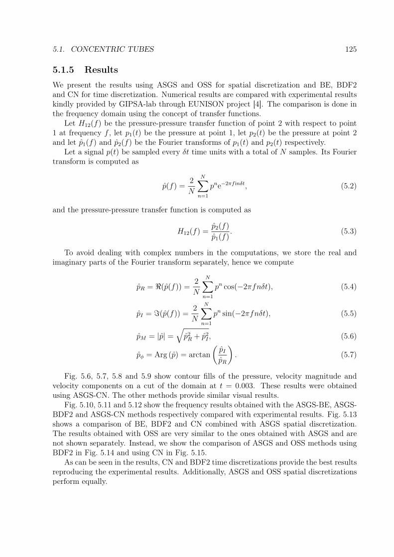
5.1. CONCENTRIC TUBES 125
5.1.5 Results
We present the results using ASGS and OSS for spatial discretization and BE, BDF2and CN for time discretization. Numerical results are compared with experimental resultskindly provided by GIPSA-lab through EUNISON project [4]. The comparison is done inthe frequency domain using the concept of transfer functions.
Let H12(f) be the pressure-pressure transfer function of point 2 with respect to point1 at frequency f , let p1(t) be the pressure at point 1, let p2(t) be the pressure at point 2and let p1(f) and p2(f) be the Fourier transforms of p1(t) and p2(t) respectively.
Let a signal p(t) be sampled every δt time units with a total of N samples. Its Fouriertransform is computed as
p(f) =2
N
N∑n=1
pne−2πf inδt, (5.2)
and the pressure-pressure transfer function is computed as
H12(f) =p2(f)
p1(f). (5.3)
To avoid dealing with complex numbers in the computations, we store the real andimaginary parts of the Fourier transform separately, hence we compute
pR = <(p(f)) =2
N
N∑n=1
pn cos(−2πfnδt), (5.4)
pI = =(p(f)) =2
N
N∑n=1
pn sin(−2πfnδt), (5.5)
pM = |p| =√p2R + p2
I , (5.6)
pφ = Arg (p) = arctan
(pIpR
). (5.7)
Fig. 5.6, 5.7, 5.8 and 5.9 show contour fills of the pressure, velocity magnitude andvelocity components on a cut of the domain at t = 0.003. These results were obtainedusing ASGS-CN. The other methods provide similar visual results.
Fig. 5.10, 5.11 and 5.12 show the frequency results obtained with the ASGS-BE, ASGS-BDF2 and ASGS-CN methods respectively compared with experimental results. Fig. 5.13shows a comparison of BE, BDF2 and CN combined with ASGS spatial discretization.The results obtained with OSS are very similar to the ones obtained with ASGS and arenot shown separately. Instead, we show the comparison of ASGS and OSS methods usingBDF2 in Fig. 5.14 and using CN in Fig. 5.15.
As can be seen in the results, CN and BDF2 time discretizations provide the best resultsreproducing the experimental results. Additionally, ASGS and OSS spatial discretizationsperform equally.

126 CHAPTER 5. APPLICATIONS
Figure 5.6: Contour fill of the acoustic pressure at t = 0.003
Figure 5.7: Contour fill of the acoustic velocity magnitude at t = 0.003

5.1. CONCENTRIC TUBES 127
Figure 5.8: Contour fill of the x-component of the acoustic velocity at t = 0.003
Figure 5.9: Contour fill of the y-component of the acoustic velocity at t = 0.003

128 CHAPTER 5. APPLICATIONS
-35
-30
-25
-20
-15
-10
-5
0
0 1 2 3 4 5 6 7 8 9 10
H12(dB)
f (kHz)
ASGS-BEExp
Figure 5.10: Transfer function H12 using ASGS-BE
-35
-30
-25
-20
-15
-10
-5
0
5
0 1 2 3 4 5 6 7 8 9 10
H12(dB)
f (kHz)
ASGS-BDF2Exp
Figure 5.11: Transfer function H12 using ASGS-BDF2

5.1. CONCENTRIC TUBES 129
-35
-30
-25
-20
-15
-10
-5
0
5
0 1 2 3 4 5 6 7 8 9 10
H12(dB)
f (kHz)
ASGS-CNExp
Figure 5.12: Transfer function H12 using ASGS-CN
-35
-30
-25
-20
-15
-10
-5
0
5
0 1 2 3 4 5 6 7 8 9 10
H12(dB)
f (kHz)
CNBDF2
BE
Figure 5.13: Transfer function H12 using ASGS

130 CHAPTER 5. APPLICATIONS
-35
-30
-25
-20
-15
-10
-5
0
5
0 1 2 3 4 5 6 7 8 9 10
H12(dB)
f (kHz)
ASGSOSS
Figure 5.14: Transfer function H12 using BDF2
-35
-30
-25
-20
-15
-10
-5
0
5
0 1 2 3 4 5 6 7 8 9 10
H12(dB)
f (kHz)
ASGSOSS
Figure 5.15: Transfer function H12 using CN

5.2. ECCENTRIC TUBES 131
5.2 Eccentric TubesThis case is very similar to the concentric tubes case. In the context of voice simulation,this geometry corresponds to a rudimentary approximation of the vocal tract in vowel /a/position and it is regarded as a better approximation than the concentric tubes becausethe eccentricity mimics the distribution of cross-sections along the vocal tract. As in thecase of the concentric tubes, a pressure pulse at the small diameter tube is the input signaland the end of the big diameter tube is the output to free space.
5.2.1 Space and time domains
The time interval for the simulation is 25 ms. The spatial domain consists of two eccentrictubes: one 85 mm long with a diameter of 14 mm and another tube of the same length anda diameter 29.5 mm as shown in Fig. 5.16. The smaller diameter tube is the sound inletthrough a 2 mm diameter hole. Acoustic pressure and velocity are measured at points 1and 2 for comparison with experimental results [139].
5.2.2 Boundary and Initial conditions
The boundary and initial conditions for this case are the same used in the concentric tubescase. The boundary conditions can be seen in Fig. 5.17.
5.2.3 Experimental setup
Fig. 5.18 shows the eccentric tubes experimental model. The experimental setup is thesame as in the concentric tubes case and can be seen in Fig. 5.4.
5.2.4 Spatial and temporal discretization
Space was discretized using tetrahedral elements of size 0.0005 m for the input hole, 0.002m for the tubes volume and 0.008 m for the surrounding volume. The mesh size for theinput hole is based in geometrical considerations (2 mm diameter input hole). The mesh
1 2
0 30 85 180170x (mm)
14 mm29.5 mm
2 mminput signal
tube endplate
Figure 5.16: Eccentric tubes spatial domain

132 CHAPTER 5. APPLICATIONS
1 2
Γo
Γu
150 mm
Γp
Figure 5.17: Eccentric tubes boundary conditions
Figure 5.18: Eccentric tubes experiment model

5.2. ECCENTRIC TUBES 133
x
y
z
Figure 5.19: Cut on the plane z = 0 showing the tetrahedral mesh used
size inside the tubes is based on resolution considerations in order to have around 16 pointsper wavelength at 10 kHz. The surrounding volume is not important for this simulation,so a big mesh size can be taken. The mesh obtained is around 260K elements and 50Knodes. A cut on the plane z = 0 of the mesh used can be seen in Fig. 5.19.
For time discretization a time step 5 ·10−6 s was used based on a resolution of 16 pointsper wave period. Several time integration schemes were used to compute the results.
5.2.5 Results
We present the results using ASGS and OSS for spatial discretization and BE, BDF2and CN for time discretization. Numerical results are compared with experimental resultskindly provided by GIPSA-lab through EUNISON project [4]. The comparison is done inthe frequency domain using the concept of transfer functions explained before.
Fig. 5.20, 5.21, 5.22 and 5.23 show contour fills of the pressure, velocity magnitude andvelocity components on a cut of the domain at t = 0.003. These results were obtainedusing ASGS-CN. The other methods provide similar visual results.
Fig. 5.24, 5.25 and 5.26 show the frequency results obtained with the ASGS-BE, ASGS-BDF2 and ASGS-CN methods respectively compared with experimental results. Fig. 5.27shows a comparison of BE, BDF2 and CN combined with ASGS spatial discretization.The results obtained with OSS are very similar to the ones obtained with ASGS and arenot shown separately. Instead, we show the comparison of ASGS and OSS methods usingBDF2 in Fig. 5.28 and using CN in Fig. 5.29.

134 CHAPTER 5. APPLICATIONS
Figure 5.20: Contour fill of the acoustic pressure at t = 0.003
Figure 5.21: Contour fill of the acoustic velocity magnitude at t = 0.003

5.2. ECCENTRIC TUBES 135
Figure 5.22: Contour fill of the x-component of the acoustic velocity at t = 0.003
Figure 5.23: Contour fill of the y-component of the acoustic velocity at t = 0.003

136 CHAPTER 5. APPLICATIONS
-40
-35
-30
-25
-20
-15
-10
-5
0
0 1 2 3 4 5 6 7 8 9 10
H12(dB)
f (kHz)
ASGS-BE
Exp
Figure 5.24: Transfer function H12 using ASGS-BE
-40
-35
-30
-25
-20
-15
-10
-5
0
0 1 2 3 4 5 6 7 8 9 10
H12(dB)
f (kHz)
ASGS-BDF2
Exp
Figure 5.25: Transfer function H12 using ASGS-BDF2

5.2. ECCENTRIC TUBES 137
-40
-35
-30
-25
-20
-15
-10
-5
0
0 1 2 3 4 5 6 7 8 9 10
H12(dB)
f (kHz)
ASGS-CN
Exp
Figure 5.26: Transfer function H12 using ASGS-CN
-40
-35
-30
-25
-20
-15
-10
-5
0
0 1 2 3 4 5 6 7 8 9 10
H12(dB)
f (kHz)
CN
BDF2
BE
Figure 5.27: Transfer function H12 using ASGS

138 CHAPTER 5. APPLICATIONS
-40
-35
-30
-25
-20
-15
-10
-5
0
0 1 2 3 4 5 6 7 8 9 10
H12(dB)
f (kHz)
ASGS
OSS
Figure 5.28: Transfer function H12 using BDF2
-35
-30
-25
-20
-15
-10
-5
0
0 1 2 3 4 5 6 7 8 9 10
H12(dB)
f (kHz)
ASGS
OSS
Figure 5.29: Transfer function H12 using CN

5.3. VOWEL GENERATION IN 3D 139
As can be seen in the results and as happened before in the concentric tubes case, CNand BDF2 provide the best results. Additionally, ASGS and OSS perform equally.
5.3 Vowel generation in 3D
This example consists in the wave propagation inside a realistic vocal tract in /a/ position.The geometry starts at the glottis, extends to the lips and goes onwards to free space. Arealistic shape head (without hair) is included in the simulation. The 3D geometry appearsin [140] and was kindly provided by the authors.
An input signal is imposed at the glottis (vocal tract inlet). This signal consists in aglottal pulse model of Rosenberg type [5].
Sound is captured in front of the lips and transformed to an audio file that can be heardand compared to the real sounding vowel /a/.
5.3.1 Space and time domains
The time interval for the simulation is 1 s. This time domain was chosen in order to obtaina long enough time series to generate an audio file.
The spatial domain is composed of the vocal tract, the head with all details (lips, nose,eyes, ears) and the open space. Fig. 5.30-5.33 show the various parts of the spatial domain.The open space is modeled by an sphere of radius 0.3 m centered at the mouth.
5.3.2 Boundary and Initial conditions
The initial conditions are zero for both pressure and velocity. The boundary conditions areapplied on three different regions of the spatial domain. The first region is the vocal tractinlet where a Rosenberg glottal pulse is imposed in the normal velocity component. The
Figure 5.30: Vocal tract in 3D

140 CHAPTER 5. APPLICATIONS
Figure 5.31: Head and vocal tract in 3D
Figure 5.32: Head in 3D
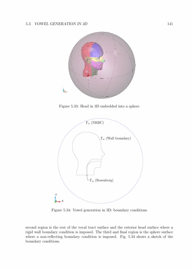
5.3. VOWEL GENERATION IN 3D 141
Figure 5.33: Head in 3D embedded into a sphere
y
z
x
Γu (Rosenberg)
Γu (Wall boundary)
Γo (NRBC)
Figure 5.34: Vowel generation in 3D: boundary conditions
second region is the rest of the vocal tract surface and the exterior head surface where arigid wall boundary condition is imposed. The third and final region is the sphere surfacewhere a non-reflecting boundary condition is imposed. Fig. 5.34 shows a sketch of theboundary conditions.

142 CHAPTER 5. APPLICATIONS
0
0.2
0.4
0.6
0.8
1
0 0.005 0.01 0.015 0.02 0.025 0.03
f(t
)
t
Figure 5.35: Rosenberg glottal pulse model
The Rosenberg glottal pulse model is a train of pulses. Each pulse is defined as follows
f(t) =
A2
(1− cos(π t
Tp)), 0 ≤ t < Tp
A cos(π t−Tp
2Tn
), Tp ≤ t < Tn
0, Tn ≤ t < T0
, (5.8)
where A is the amplitude, T0 is the period of the signal, Tp is the time where the signalstops increasing and Tn is the time where the signal reaches zero again.
We will use A = 1, T0 = 0.01s, Tp = 0.4T0 and Tn = 0.56T0. A plot of the Rosenbergglottal pulse can be seen in Fig. 5.35. Jitter and shimmer can be added to the input signalto make it sound more natural.
5.3.3 Spatial and temporal discretization
Space was discretized using tetrahedral elements of size 0.001 m for the vocal tract andlips, 0.005 m for the head surface and 0.02 m for the surrounding volume. The mesh sizeinside the vocal tract is governed by geometric details of the vocal tract, which measureless than 3 mm. The surrounding volume is not important for this simulation, so a bigmesh size can be taken. Of course there is a slow transition from small size to big size.The mesh obtained is around 1M elements and 170K nodes. A cut on the plane y = 0 ofthe mesh used can be seen in Fig. 5.36.
For time discretization a BDF2 scheme with time step 2.5 · 10−5 s was used.
5.3.4 Results
Figures 5.37, 5.38, 5.39 and 5.40 show contour fills of the pressure, velocity magnitudeand velocity components on a cut at y = 0 of the domain. The y-velocity component isnot shown because it is zero as the plane y = 0 is a symmetry plane. These results wereobtained using ASGS-BDF2. OSS-BDF2 provides similar visual results.

5.3. VOWEL GENERATION IN 3D 143
y
z
x
Figure 5.36: Cut on the plane y = 0 showing the tetrahedral mesh used
Figure 5.37: Vowel generation in 3D: contour fill of the acoustic pressure

144 CHAPTER 5. APPLICATIONS
Figure 5.38: Vowel generation in 3D: acoustic velocity magnitude
Figure 5.39: Vowel generation in 3D: x-component of the acoustic velocity

5.3. VOWEL GENERATION IN 3D 145
Figure 5.40: Vowel generation in 3D: z-component of the acoustic velocity
From the pressure field obtained, it is possible to extract the sound at each point. Onepoint of interest is in front of the mouth, where an audio file can be generated and thevowel /a/ can be heard.
Additionally, we can compare the spectrum of a human-generated vowel /a/ with theone obtained from our FEM model. Fig. 5.41 shows the comparison. Notice that we havenot used any filter for any of the signals. In the next section, specifically in Fig. 5.45 youcan see the effects of signal processing techniques.

146 CHAPTER 5. APPLICATIONS
-80
-70
-60
-50
-40
-30
-20
-10
0
10
20
0 1 2 3 4 5
pdB
f kHz
humanFEM
Figure 5.41: Vowel generation in 3D: spectrum comparison
5.4 Diphthong generation in 3DThis example consists in the generation of a diphthong in a 3D domain. The diphthong tobe generated is /ai/. The formulation is set in an Arbitrary Lagrangian-Eulerian framework[5]. The mesh is deformed from vowel /a/ position to vowel /i/ position using linearinterpolation in time. For an extended version of this example the reader is referred to [5].There is some signal processing terminology that is not defined anywhere in the thesis butthat goes beyond scope.
An input signal is imposed at the glottis (vocal tract inlet). This signal consists in aglottal pulse model of Rosenberg type. Sound is captured near the vocal tract output andcompared to the real sounding diphthong /ai/.
5.4.1 Problem statement
The most natural option to deal with wave propagation in moving domains is the mixedwave equation with ALE. The mixed wave equation can be expressed in ALE formulationas:
µp∂tp− µpuD ·∇p+∇·u = fp, (5.9)µu∂tu− µuuD ·∇u+∇p = fu, (5.10)
where uD is the domain velocity. In the discrete setting uD will be the mesh velocity. Theproblem is supplemented with the initial conditions
p(x, 0) = 0, u(x, 0) = 0, (5.11)
and with the boundary conditions
p = 0 on Γp, γnu = 0 on Γu. (5.12)
5.4. DIPHTHONG GENERATION IN 3D 147
The variational problem can be formulated as finding p ∈ C1(Υ, L2(Ω))∩C0(Υ, Vp) andu ∈ C1(Υ, L2(Ω)) ∩ C0(Υ, Vu) such that
B([p,u] , [q,v]) = L([q,v]), (5.13)
for all [q,v] ∈ [Vp, Vu] with Vp = q ∈ H1(Ω)|q = 0 on Γp, Vu = v ∈ H(div,Ω)|γnv =
0 on Γu, uD ·∇u ∈ L2(Ω)d and
B([p,u] , [q,v]) = (µp∂tp− µpuD ·∇p+∇·u, q) + (µu∂tu− µuuD ·∇u+∇p,v) , (5.14)L([q,v]) = (fp, q) + (fu,v) . (5.15)
Using stabilized finite elements the space-discrete problem reads: find [ph,uh] such that
Bs([ph,uh] , [qh,vh]) = Ls([qh,vh]), (5.16)
for all test functions [qh,vh] ∈ [Vp,h, Vu,h] where
Bs([ph,uh] , [qh,vh]) = B([ph,uh] , [qh,vh]) + (P ′ (µp∂tph − µpuD ·∇ph +∇·uh) , τu∇·uh)+ (P ′ (µu∂tuh − µuuD ·∇uh +∇ph) , τp∇ph) , (5.17)
Ls([qh,vh]) = L([qh,vh]) + (P ′(fp), τu∇·vh) + (P ′(fu), τp∇qh) , (5.18)
with the stabilization parameters τp and τu defined as
τp =h
C1(µpµu)2|uD|+ C2
√µuµp, τu =
h
C1(µpµu)2|uD|+ C2
√µpµu. (5.19)
The projection operator P ′(·) can be chosen as either the identity to obtain the ASGSmethod or the L2(Ω)-orthogonal projection to obtain the OSS method.
The time discretization is straightforward and BE, CN and BDF2 methods can beapplied.
With regard to the motion of the computational mesh, it will be prescribed by theknown displacement at the domain boundaries. The motion of the boundary nodes becomessmoothly transmitted to the inner mesh nodes through diffusion, i.e. using the standardstrategy of solving the Laplacian equation for the node displacements w(x, t). Therefore,at each time step n+1 we will solve the additional equation
∇2wn+1 = 0 in Ω (5.20)
with boundary conditions
wn+1 = xmn+1 − xm
n on Γm, γnwn+1 = 0 on Γf , (5.21)
and the mesh node positions being updated according to
xDn+1 = xD
n +wn+1. (5.22)
Γm represents the boundary of Ω evolving with prescribed displacement xm(x, t), whereasΓf denotes a fixed boundary of Ω. From the displacements w(x, t) one can compute themesh velocity using an appropriate time integration scheme (e.g. BE).

148 CHAPTER 5. APPLICATIONS
Figure 5.42: Simplified vocal tract in 3D: /a/ position and /i/ position
5.4.2 Space and time domains
The time interval for the simulation is 0.2 s. The spatial domain is is a simplified 3D modelof the vocal tract consisting in circular concentric cross-sections as shown in Fig. 5.42.
5.4.3 Boundary and Initial conditions
The initial conditions are zero for both pressure and velocity. The initial mesh condition isan average between the two extreme positions in order to avoid excessive mesh distortion.The boundary conditions are applied on three different regions of the spatial domain. Thefirst region is the vocal tract inlet where a Rosenberg glottal pulse is imposed. The secondregion is the rest of the vocal tract surface where a rigid wall boundary condition is imposed.The third and final region is the vocal tract output where p = 0 is imposed.
To increase the naturalness of the diphthong, the glottal pulses have been enhancedintroducing a pitch curve for the fundamental frequency, adding some shimmer to the signalamplitude and applying a fade in/out to the global signal.
5.4.4 Spatial and temporal discretization
Space was discretized using tetrahedral elements of size 0.002 m for the whole vocal tract.The mesh can be seen in Fig. 5.42. The stabilization parameters were taken as C1 = 0.01and C2 = 10. For time discretization a BDF2 scheme with time step 1.25 ·10−5 s was used.
5.4.5 Results
Fig. 5.43 shows a contour fill of the pressure at different time steps together with the meshmovement. These results were obtained using ASGS-BDF2.
From the pressure field obtained, it is possible to extract the sound at each point. Onepoint of interest is near the vocal tract outlet, where an audio file can be generated andthe diphthong /ai/ can be heard.

5.4. DIPHTHONG GENERATION IN 3D 149
Figure 5.43: Diphthong generation in 3D: contour fill of the acoustic pressure
Fig. 5.44 shows the pressure evolution at the vocal tract outlet.Fig. 5.45 shows the spectrogram corresponding to the acoustic pressure in Fig. 5.44.
This has been computed using a Hamming window with a frame width of 20 ms and anoverlap of 1 ms. As usually done in speech processing, a pre-emphasis FIR filter withcoefficients [1 -0.97] has been applied to enhance the visualization of the high frequencyrange. In the first curve of the spectrogram, corresponding to vowel /a/, we can clearlyidentify the two formants of vowel /a/. Similarly, the last curve of the spectrogramcorresponds to vowel /i/ and its two formants an also be clearly recognized. The trajectoriesof the two formants F1 and F2, which separate apart from /a/ to /i/, have been highlightedto appreciate clearly their evolution.

150 CHAPTER 5. APPLICATIONS
Figure 5.44: Diphthong generation in 3D: pressure evolution at the vocal tract outlet
Figure 5.45: Diphthong generation in 3D: pressure spectrogram for diphthong /ai/

Chapter 6
Conclusions
6.1 AchievementsOne achievement of this work is the formulation and analysis of two stabilized finite elementmethods for solving the wave equation in mixed form. The variational problem can becast in three different variational forms, each one requiring a certain regularity on theunknowns. The formulation includes ASGS and OSS methods taylored to work in threedifferent functional frameworks in which the regularity requirements of the scalar space aretransferred to the vector one or vice-versa. The analysis includes stability and convergencefor both stabilization methods and for all variational forms. Additionally, numerical testswere performed to compare numerical results with theoretical predictions.
Another achievement is the formulation and analysis of a non-reflecting boundarycondition (NRBC) that fits into the stabilization methods and functional settings. Theintroduction of the NRBC motivated a slight modification of the functional frameworkand working norms in which we were able to prove stability and convergence of theformulations. Numerical convergence tests were performed to compare with theoreticalconvergence predictions. Finally, many numerical examples were solved in 2D and 3D toshow the capabilities of the NRBC.
Moreover, time marching schemes applied to the mixed wave equation were imple-mented and analyzed. One part of the analysis includes stability and convergence of thefully discrete schemes. The other part involves stability, dispersion and dissipation analysiswith the aid of Fourier techniques. A 1D example was solved to compare numerical resultswith Fourier predictions which yielded good agreement between both.
Furthermore, various wave propagation problems were solved and some of them com-pared simulation results with experimental results. These problems are mainly 3D andinclude realistic geometries. One of the main results is voice simulation inside the vocaltract and open space in order to reproduce a vowel /a/ starting from a glottal signal asinput. Another main result is diphthong simulation using an ALE formulation.
6.2 Concluding RemarksThe implementation of the mixed wave equation with the discretization methods describedin this thesis is not difficult. The only implementation difficulty for time-dependent-
151

152 CHAPTER 6. CONCLUSIONS
only problems as this one is that space/time discretization is always coupled. In otherwords, when implementing a (full) discretization method from zero and it does not work asexpected, the implementation error can be anywhere. Finding the error cannot be tackledby first solving a steady-state version of the problem, then making it work and finallysolving the time-dependent version.
The implementation of the non-reflecting boundary condition described in this thesis isstraightforward. It only involves terms on the boundary. There is no need of an additionallayer of absorbing material which introduces extra degrees of freedom. Anyway, I havenot worked with absorbing layers to give a more informed comparison of both. In theapplication examples the NRBC has worked very well when using a smooth NRBC-surface.This is reflected in the close agreement between numerical simulations and experiments.In the benchmark cases, despite using square geometries in 2D or cubes in 3D, the NRBChas given good results in the sense of monotonous energy dissipation.
Let us consider the stability of the spatial discretization methods (ASGS and OSS).Both methods are stable with respect to their respective working norm(s)/external forcesnorm(s) pairs. I have to mention that the regularity requirements of the external forces forstability differs for ASGS and OSS. Nevertheless, for the same value of the stabilizationalgorithmic constant, both ASGS and OSS exhibit the same stability in practice. That is,there are no node-to-node oscillations and the results look visually similar.
Let us consider the accuracy of the spatial discretization methods with respect to theerror in the unknowns in their respective norm(s). The spatial discretization methodspresented, namely ASGS and OSS, can exhibit up to optimal convergence rates dependingon the variational form. However, the convergence proofs presented are not sharp enoughleaving the theoretical convergence rates as quasi-optimal at best.
6.3 Future WorkThe wave equation in mixed form was solved using stabilized finite element methodsallowing us to use equal interpolation spaces for both the scalar and vector unknownsand avoiding inf-sup stable elements. Additional stabilization sophistications still need tobe formulated, implemented and analyzed such as dynamic sub-scales. Furthermore, afractional step scheme for the formulation needs to be developed in order to solve biggerproblems more efficiently.
More accurate non-reflective boundary conditions applied to the mixed wave equationneed to be researched. It is said that the Sommerfeld boundary condition is zero-orderaccurate (J = 0), although we found it is order J = 0.66 in 2D.
In this work we analyzed and implemented up to 2nd order time marching schemes(BE, BDF2 and CN). Higher order schemes should be explored such as Runge-Kutta andsymplectic Runge-Kutta. Additional energy-preserving or momentum-preserving schemesshould be considered and analyzed as well.
The wave equation in mixed form has proven useful for dealing with moving domainsin ALE formulation since it is not possible to express the irreducible wave equation ina moving domain. Stability and convergence of the ALE formulation has yet to beanalyzed. Additionally, aeroacoustics in moving domains has to be developed throughthe computation of source terms from the incompressible flow solver.

References
[1] Nigel Peake and Anthony B. Parry. “Modern Challenges Facing TurbomachineryAeroacoustics”. In: Annual Review of Fluid Mechanics 44 (2012), pp. 227–228. doi:10.1146/annurev-fluid-120710-101231 (cit. on p. 1).
[2] Edward M. Greitzer and H. N. Slater. N+3 Aircraft Concept Designs and TradeStudies. Tech. rep. tech report. MIT, Aurora Flight Sciences, and Pratt & WhitneyTeam, Mar. 2010 (cit. on p. 1).
[3] Rajat Mittal, Byron D. Erath, and Michael W. Plesniak. “Fluid Dynamics of HumanPhonation and Speech”. In: Annual Review of Fluid Mechanics 45.1 (2013), pp. 437–467. doi: 10.1146/annurev-fluid-011212-140636 (cit. on p. 1).
[4] Extensive UNIfied-domain SimulatiON of the human voice (EUNISON). FP7-ICT-2011-C 308874. 2015. url: http://fp7eunison.com/ (cit. on pp. 1, 125, 133).
[5] Oriol Guasch, Marc Arnela, Ramon Codina, and Hector Espinoza. “A stabilizedfinite element method for the mixed wave equation in an ALE framework withapplication to diphthong production”. In: Journal of Computational Physics (Oct.2014). Submitted (cit. on pp. 1, 2, 25, 121, 139, 146).
[6] Manfred Kaltenbacher, Stefan Zörner, and Andreas Hüppe. “On the importanceof strong fluid-solid coupling with application to human phonation”. In: Progressin Computational Fluid Dynamics, an International Journal 14.1 (2014), pp. 2–13(cit. on p. 1).
[7] Manfred Kaltenbacher. “Computational acoustics in multi-field problems”. In: Jour-nal of Computational Acoustics 19.01 (2011), pp. 27–62. doi: 10.1142/S0218396X11004286. eprint: http://www.worldscientific.com/doi/pdf/10.1142/S0218396X11004286. url: http://www.worldscientific.com/doi/abs/10.1142/S0218396X11004286 (cit. on pp. 1, 18).
[8] Peter Hagedorn and Anirvan DasGupta. Vibration and Waves in Continuous Me-chanical Systems. John Wiley & Sons, 2007 (cit. on pp. 10, 12).
[9] Nikolaos Kampanis, Vassilios Dougalis, and John Ekaterinaris. Effective Computa-tional Methods for Wave Propagation. Chapman & Hall, 2008 (cit. on p. 11).
[10] Thomas Rossing. Handbook of Acoustics. Springer, 2007 (cit. on p. 11).
[11] Arnold Sommerfeld. Partial differential equations in physics. Elsevier, 1949 (cit. onpp. 12, 54).
153

154 REFERENCES
[12] Marcus J. Grote and Christoph Kirsch. “Dirichlet-to-Neumann boundary condi-tions for multiple scattering problems”. In: Journal of Computational Physics 201.2(2004), pp. 630–650. issn: 0021-9991. doi: 10.1016/j.jcp.2004.06.012. url:http://www.sciencedirect.com/science/article/pii/S002199910400258X(cit. on p. 13).
[13] David P. Nicholls and Nilima Nigam. “Exact non-reflecting boundary conditionson general domains”. In: Journal of Computational Physics 194.1 (2004), pp. 278–303. issn: 0021-9991. doi: 10.1016/j.jcp.2003.09.006. url: http://www.sciencedirect.com/science/article/pii/S0021999103004832 (cit. on p. 13).
[14] Bjorn Engquist and Andreq Majda. “Absorbing boundary conditions for numericalsimulation of waves”. In: Mathematics of Computation 31.139 (1977), pp. 629–651(cit. on pp. 13, 54).
[15] Robert L. Higdon. “Absorbing boundary conditions for difference approximationsto the multidimensional wave equation”. In: Mathematics of computation 47.176(1986), pp. 437–459 (cit. on p. 13).
[16] Dan Givoli and Beny Neta. “High-order non-reflecting boundary scheme for time-dependent waves”. In: Journal of Computational Physics 186.1 (2003), pp. 24–46.issn: 0021-9991. doi: 10.1016/S0021- 9991(03)00005- 6. url: http://www.sciencedirect.com/science/article/pii/S0021999103000056 (cit. on pp. 13,54).
[17] John R. Dea, Francis X. Giraldo, and Beny Neta. “High-order non-reflecting bound-ary conditions for the linearized 2-D Euler equations: No mean flow case”. In: WaveMotion 46.3 (2009), pp. 210–220. issn: 0165-2125. doi: 10.1016/j.wavemoti.2008.11.002. url: http://www.sciencedirect.com/science/article/pii/S0165212508001029 (cit. on pp. 13, 54, 72, 75, 77).
[18] Edward Dean and Roland Glowinski. “Domain decomposition methods for mixedfinite element approximations of wave problems”. In: Computers and Mathematicswith Applications 38.7-8 (1999), pp. 207–214. doi: 10.1016/S0898-1221(99)00251-5 (cit. on p. 13).
[19] Christophe Bogey and Christophe Bailly. “Three-dimensional non-reflective bound-ary conditions for acoustic simulations: far field formulation and validation testcases”. In: Acta Acustica 88.4 (2002), pp. 463–471 (cit. on p. 13).
[20] Roland Glowinski and Serguei Lapin. “Solution of a Wave Equation by a MixedFinite Element - Fictitious Domain Method”. In: Computational Methods in AppliedMathematics 4.4 (2004), pp. 431–444. doi: 10.2478/cmam- 2004- 0024 (cit. onpp. 13, 54–56, 61, 80, 81).
[21] Zhenpeng Liao, Huang L. Wong, Yan Baipo, and Yifan Yang. “A transmittingboundary for transient wave analyses”. In: Sientia Sinica 27.10 (1984), pp. 1063–1076 (cit. on p. 13).

REFERENCES 155
[22] Alan Bamberger, Patrick Joly, and Jean E. Roberts. “Second-order absorbingboundary conditions for the wave equation: a solution for the corner problem”.In: SIAM Journal on Numerical Analysis 27.2 (1990), pp. 323–352. doi: 10.1137/0727021 (cit. on p. 13).
[23] Marcus Grote and Joseph Keller. “Exact Nonreflecting Boundary Conditions for theTime Dependent Wave Equation”. In: SIAM Journal on Applied Mathemathics 55.2(1995), pp. 280–297. doi: 10.1137/S0036139993269266 (cit. on pp. 13, 54).
[24] Andrzej J. Safjan. “Highly accurate non-reflecting boundary conditions for finiteelement simulations of transient acoustics problems”. In: Computer Methods inApplied Mechanics and Engineering 152.1-2 (1998), pp. 175–193. issn: 0045-7825.doi: 10.1016/S0045-7825(97)00188-6. url: http://www.sciencedirect.com/science/article/pii/S0045782597001886 (cit. on p. 13).
[25] Bradley Alpert, Leslie Greengard, and Thomas Hagstrom. “Nonreflecting BoundaryConditions for the Time-Dependent Wave Equation”. In: Journal of ComputationalPhysics 180.1 (2002), pp. 270–296. doi: 10.1006/jcph.2002.7093 (cit. on p. 13).
[26] Steen Krenk. “Unified formulation of radiation conditions for the wave equation”. In:International Journal for Numerical Methods in Engineering 53.2 (2002), pp. 275–295. issn: 1097-0207. doi: 10.1002/nme.268 (cit. on p. 13).
[27] ZhenHuan Teng. “Exact boundary condition for time-dependent wave equationbased on boundary integral”. In: Journal of Computational Physics 190.2 (2003),pp. 398–418. issn: 0021-9991. doi: 10.1016/S0021-9991(03)00281-X. url: http://www.sciencedirect.com/science/article/pii/S002199910300281X (cit. onp. 13).
[28] Thomas Hagstrom, Assaf Mar-Or, and Dan Givoli. “High-order local absorbingconditions for the wave equation: Extensions and improvements”. In: Journal ofComputational Physics 227.6 (2008), pp. 3322–3357. issn: 0021-9991. doi: 10.1016/j.jcp.2007.11.040. url: http://www.sciencedirect.com/science/article/pii/S0021999107005360 (cit. on p. 13).
[29] Isaac Harari, Igor Patlashenko, and Dan Givoli. “Dirichlet-to-Neumann Maps forUnbounded Wave Guides”. In: Journal of Computational Physics 143.1 (1998),pp. 200–223. doi: 10.1006/jcph.1998.5960 (cit. on p. 13).
[30] Ata Mugan and Gregory M. Hulbert. “Nonreflecting boundary conditions in acous-tics for finite element methods based upon off-surface boundary integral equa-tions”. In: Computer Methods in Applied Mechanics and Engineering 188.1-3 (2000),pp. 289–306. issn: 0045-7825. doi: 10.1016/S0045-7825(99)00153-X. url: http://www.sciencedirect.com/science/article/pii/S004578259900153X (cit. onp. 13).
[31] Tasos Papanastasiou, Nikos Malamataris, and Kevin Ellwood. “A New OutflowBoundary Condition”. In: International Journal for Numerical Methods in Fluids14 (1992), pp. 587–608. doi: 10.1002/fld.1650140506 (cit. on p. 13).

156 REFERENCES
[32] Morten Wang and Tony Sheu. “Implementation of a free boundary condition toNavier-Stokes equations”. In: International Journal of Numerical Methods for Heat& Fluid Flow 7.1 (1997), pp. 95–111. doi: 10.1108/09615539710156228 (cit. onp. 13).
[33] Maxim Ol’shanskii and Vladimir M. Staroverov. “On simulation of outflow boundaryconditions in finite difference calculations for incompressible fluid”. In: InternationalJournal for Numerical Methods in Fluids 33.4 (2000), pp. 499–534. doi: 10.1002/1097-0363(20000630)33:4<499::AID-FLD19>3.0.CO;2-7 (cit. on p. 13).
[34] Jean-Pierre Berenger. “A perfectly matched layer for the absorption of electromag-netic waves”. In: Journal of Computational Physics 114.2 (1994), pp. 185–200. issn:0021-9991. doi: 10.1006/jcph.1994.1159. url: http://www.sciencedirect.com/science/article/pii/S0021999184711594 (cit. on pp. 13, 54).
[35] Barbara Kaltenbacher, Manfred Kaltenbacher, and Imbo Sim. “A modified andstable version of a perfectly matched layer technique for the 3-d second orderwave equation in time domain with an application to aeroacoustics”. In: Journalof Computational Physics 235 (2013), pp. 407–422. issn: 0021-9991. doi: 10.1016/j.jcp.2012.10.016. url: http://www.sciencedirect.com/science/article/pii/S0021999112006055 (cit. on pp. 13, 54).
[36] Julen Diaz and Patrick Joly. “A time domain analysis of PML models in acoustics”.In: Computer Methods in Applied Mechanics and Engineering 195.29-32 (2006),pp. 3820–3853. doi: 10.1016/j.cma.2005.02.031 (cit. on pp. 13, 54).
[37] YangQing Zeng, JianQi He, and QingHuo Liu. “The application of the perfectlymatched layer in numerical modeling of wave propagation in poroelastic media”. In:Geophysics 66.4 (2001), pp. 1258–1266. doi: 10.1190/1.1487073 (cit. on p. 13).
[38] Eliane Bécache, Dhia Bonnet-Ben, and Legendre Guillaume. “Perfectly matchedlayers for time-harmonic acostics in the presence of a uniform flow”. In: SIAMJournal on Numerical Analysis 44.3 (2006), pp. 1191–1217. doi: 10.1137/040617741 (cit. on p. 13).
[39] Alfredo Bermúdez, Luis Hervella-Nieto, Andrés Prieto, and Rodolfo Rodríguez.“An optimal perfectly matched layer with unbounded absorbing function for fime-harmonic acoustic stattering problems”. In: Journal of Computational Physics 223.2(2007), pp. 469–488. doi: j.jcp.2006.09.018 (cit. on p. 13).
[40] Isaac Harari and Michael Slavutin. “Analytical and Numerical Studies of a FiniteElement PML for the Helmholtz Equation”. In: Journal of Computational Acoustics8.1 (2000), pp. 121–137. doi: 10.1142/S0218396X0000008X (cit. on p. 13).
[41] Quing-Huo Liu and Jianping Tao. “The perfectly matched layer for acoustic wavesin absorptive media”. In: Journal of the Acoustical Society of America 102.4 (1997),pp. 2072–2082. doi: 10.1121/1.419657 (cit. on p. 13).
[42] Quan Qi and Thomas L. Geers. “Evaluation of the Perfectly Matched Layer for Com-putational Acoustics”. In: Journal of Computational Physics 139 (1998), pp. 166–183. doi: 10.1006/jcph.1997.5868 (cit. on pp. 13, 14, 54, 72, 81, 82).

REFERENCES 157
[43] Andreas Hüppe and Manfred Kaltenbacher. “Stable matched layer for the acousticconservation equations in the time domain”. In: Journal of Computational Acoustics20.01 (2012), p. 1250004. doi: 10.1142/S0218396X11004511. eprint: http://www.worldscientific.com/doi/pdf/10.1142/S0218396X11004511. url: http://www.worldscientific.com/doi/abs/10.1142/S0218396X11004511 (cit. onpp. 13, 54).
[44] Xiaojuen Yuan, David Borup, James W. Wiskin, Michael Berggren, Rick Eidens,and Steven A. Johnson. “Formulation and Validation of Berenger’s PML absorbingboundary for the FTDT simulation of acoustic scattering”. In: IEE Transactions onUltrasonics, Ferroelectrics and Frequency Control 44.4 (1997), pp. 816–822. url:http : / / ieeexplore . ieee . org / stamp / stamp . jsp ? tp = &arnumber = 655197&isnumber=14267 (cit. on p. 13).
[45] Jean-Pierre Berenger. “Three-Dimensional Perfectly Matched Layer for the Absorp-tion of Electromagnetic Waves”. In: Journal of Computational Physics 127.2 (1996),pp. 363–379. doi: jcph.1996.0181 (cit. on p. 13).
[46] Raj Mittra and Umit Pekel. “A new look at the perfectly matched layer (PML)concept for the reflectionless absorption of electromagnetic waves”. In: Microwaveand Guided Wave Letters, IEEE 5.3 (1995), pp. 84–86. doi: 10.1109/75.366461.url: http://ieeexplore.ieee.org/stamp/stamp.jsp?tp=&arnumber=366461&isnumber=8397 (cit. on p. 13).
[47] Steven Cummer. “A simple, nearly perfectly matched layer for general electromag-netic media”. In: Microwave and Wireless Components Letters, IEEE 13.3 (2003),pp. 128–130. doi: 10.1109/LMWC.2003.810124 (cit. on p. 13).
[48] Fang Q. Hu. “A stable, perfectly matched layer for linearized Euler equations inunsplit physical variables”. In: Journal of Computational Physics 173.2 (2001),pp. 455–480. doi: 10.1006/jcph.2001.6887 (cit. on p. 15).
[49] Steffen Marburg and Bodo Nolte. Computational Acoustics of Noise Propagation inFluids. Springer, 2008 (cit. on p. 15).
[50] Ardavan F. Oskooi, Lei Zhang, Avniel Yehuda, and Steven Johnson. “The failure ofperfectly matched layers, and towards their redemption by adiabatic absorbers”. In:Optics Express 16.15 (2008), pp. 11376–11392. doi: 10.1364/OE.16.011376. url:http://www.opticsexpress.org/abstract.cfm?URI=oe-16-15-11376 (cit. onp. 15).
[51] Simon K. Richards, Xin Zhang, Xiaoxian Chen, and Philip A. Nelson. “The eval-uation of non-reflecting boundary conditions for duct acoustic computation”. In:Journal of Sound and Vibration 270.3 (2004), pp. 539–557. doi: 10.1016/j.jsv.2003.09.042 (cit. on pp. 15, 54).
[52] Jay C. Hardin, J. Raymond Ristorcelli, and Christopher K.W. Tam, eds. ICASE/LaRCWorkshop on Benchmark Problems in Computational Aeroacoustics (CAA). Na-tional Aeronautics and Space Administration, Langley Research Center, 1995 (cit.on pp. 15, 72).

158 REFERENCES
[53] Milo D. Dahl, ed. Fourth Computational Aeroacoustics (CAA) Workshop on Bench-mark Problems. NASA, Glenn Research Center, 2004 (cit. on pp. 15, 16, 72).
[54] Gianluca Lazzi and Om P. Gandhi. “On the optimal design of the PML absorbingboundary condition for the FDTD code”. In: IEEE Transactions on Antennas andPropagation 45.5 (1997), pp. 914–917. doi: 10.1109/8.575651 (cit. on p. 15).
[55] Ching-Lie Li, Chien-Wei Liu, and Shao-Hon Chen. “Optimization of a PML ab-sorber’s conductivity profile using FDTD”. In: Microwave and Optical TechnologyLetters 37.5 (2003), pp. 380–383. doi: 10.1002/mop.10924 (cit. on p. 15).
[56] Tim Colonius and Sanjiva Lele. “Computational aeroacoustics: progress on nonlinearproblems of sound generation”. In: Progress in Aerospace Sciences 40.6 (2004),pp. 345–416. doi: 10.1016/j.paerosci.2004.09.001 (cit. on p. 18).
[57] Meng Wang, Jonathan B. Freund, and Sanjiva K. Lele. “Computational Predictionof Flow-Generated Sound”. In: Annual Reviews of Fluid Mechanics 38.1 (2006),pp. 483–512. doi: 10.1146/annurev.fluid.38.050304.092036 (cit. on p. 19).
[58] Andreas Hüppe and Manfred Kaltenbacher. “Spectral finite elements for computa-tional aeroacoustics using acoustic perturbation equations”. In: Journal of Compu-tational Acoustics 20.02 (2012), p. 1240005. doi: 10.1142/S0218396X1240005X.eprint: http://www.worldscientific.com/doi/pdf/10.1142/S0218396X1240005X. url: http://www.worldscientific.com/doi/abs/10.1142/S0218396X1240005X (cit. on p. 19).
[59] Michael J. Lighthill. “On sound generated aerodynamically I. General Theory”. In:Proceedings of the Royal Society of London 211 (1952), pp. 564–587 (cit. on p. 21).
[60] Michael J. Lighthill. “On Sound Generated Aerodynamically. II. Turbulence as aSource of Sound”. In: Proceedings of the Royal Society of London (1954), pp. 1–32(cit. on p. 21).
[61] N. Curle. “The influence of solid boundaries upon aerodynamic sound”. In: Proceed-ings of the Royal Society of London 231.1187 (1955), pp. 505–514. doi: 10.1098/rspa.1955.0191 (cit. on pp. 21, 23).
[62] Owen M. Phillips. “On the generation of sound by supersonic turbulent shear layers”.In: Journal of Fluid Mechanics 9 (01 Aug. 1960), pp. 1–28. issn: 1469-7645. doi: 10.1017/S0022112060000888. url: http://journals.cambridge.org/article_S0022112060000888 (cit. on pp. 21, 23).
[63] John E. Ffowcs-Williams and David L. Hawkings. “Sound generation by turbulenceand surfaces in arbitrary motion”. In: Philosophical Transactions of the Royal Societyof London. Series A, Mathematical and Physical Sciences 264.1151 (1969), pp. 321–342 (cit. on pp. 21, 23).
[64] Marvin Goldstein. “A generalized acoustic analogy”. In: Journal of Fluid Mechanics488 (June 2003), pp. 315–333. issn: 1469-7645. doi: 10.1017/S0022112003004890.url: http://journals.cambridge.org/article_S0022112003004890 (cit. onpp. 21, 24).
REFERENCES 159
[65] Kenneth S. Brentner and Feri Farassat. “Analytical comparison of the acousticanalogy and Kirchhoff formulation for moving surfaces”. In: AIAA journal 36.8(1998), pp. 1379–1386. doi: 10.2514/2.558 (cit. on p. 23).
[66] Siegfried Wagner, Rainer Bareiß, and Gianfranco Guidati. Wind Turbine Noise.Springer-Verlag, 1996 (cit. on p. 23).
[67] Santiago Badia, Ramon Codina, and Hector Espinoza. “Stability, Convergence, andAccuracy of Stabilized Finite Element Methods for the Wave Equation in MixedForm”. In: SIAM Journal on Numerical Analysis 52.4 (May 2014), pp. 1729–1752.doi: 10.1137/130918708 (cit. on pp. 25, 27, 55, 62, 64, 65, 67–69, 83, 86–88, 90,91, 101).
[68] Hector Espinoza, Ramon Codina, and Santiago Badia. “A Sommerfeld non-reflectingboundary condition for the wave equation in mixed form”. In: Computer Methods inApplied Mechanics and Engineering 276 (July 2014), pp. 122–148. issn: 0045-7825.doi: 10.1016/j.cma.2014.03.015. url: http://www.sciencedirect.com/science/article/pii/S0045782514001017 (cit. on pp. 25, 53, 86–88, 91, 101).
[69] Hector Espinoza, Ramon Codina, and Santiago Badia. “On some time marchingschemes for the stabilized finite element approximation of the mixed wave equa-tion”. In: Computer Methods in Applied Mechanics and Engineering (Dec. 2014).Submitted (cit. on pp. 25, 85).
[70] Ramon Codina, Hector Espinoza, and Santiago Badia. “Linear waves in mixed form:functional settings and stabilized finite element approximation”. In: 6th ScientificComputing Seminar / VMS 2012. Christian-Albrechts-Universität zu Kiel. June2012. url: http://www.math.uni-kiel.de/numerik/braack/conf/vms2012/(cit. on p. 25).
[71] Hector Espinoza, Ramon Codina, and Santiago Badia. “Wave Equation in MixedForm: Stability and Convergence Estimates using Stabilized Finite Element Meth-ods”. In: Congress on Numerical Methods in Engineering CNM 2013. Sociedad Es-pañola de Métodos Numéricos en Ingeniería (SEMNI). June 2013. url: http://congress.cimne.com/metnum2013/ (cit. on p. 25).
[72] Oriol Guasch, Marc Arnela, Ramon Codina, and Hector Espinoza. “A stabilizedarbitrary Lagrangian Eulerian finite element method for the mixed wave equationwith application to diphthong production”. In: WCCM XI. IACM and ECCOMAS.July 2014. url: http://www.wccm-eccm-ecfd2014.org/ (cit. on p. 25).
[73] Hector Espinoza, Ramon Codina, and Santiago Badia. “Numerical analysis andbenchmarking of a Sommerfeld-type non-reflecting boundary condition for the waveequation in mixed form”. In: WCCM XI. IACM and ECCOMAS. July 2014. url:http://www.wccm-eccm-ecfd2014.org/ (cit. on p. 25).
[74] Marc Arnela, Oriol Guasch, Ramon Codina, and Hector Espinoza. “Finite elementcomputation of diphthong sounds using tuned two-dimensional vocal tracts”. In: 7thForum Acusticum. Polish Acoustics Society and European Acoustics Association.Sept. 2014. url: http://www.fa2014.pl/ (cit. on p. 25).

160 REFERENCES
[75] Oriol Guasch, Marc Arnela, Ramon Codina, and Hector Espinoza. “Stabilized finiteelement formulation for the mixed convected wave equation in domains with drivenflexible boundaries”. In: NOVEM 2015. INSA. Apr. 2015. url: http://novem2015.sciencesconf.org/ (cit. on p. 25).
[76] Ramon Codina, Marc Arnela, Oriol Guasch, and Hector Espinoza. “Waves in timedependent domains”. In: 10th International Workshop on Variational Multiscaleand Stabilized Finite Elements (VMS2015). German Association for ComputationalMechanics (GACM). Garching, Germany, Feb. 2015. url: http://www.lnm.mw.tum.de/vms2015/ (cit. on p. 26).
[77] Ramon Codina, Oriol Guasch, Marc Arnela, and Hector Espinoza. “Approximationof waves written in mixed form in time dependent domains”. In: Congresso deMétodos Numéricos em Engenharia. Instituto Superior Técnico. June 2015. url:http://www.dem.ist.utl.pt/cmn2015/ (cit. on p. 26).
[78] Franco Brezzi and Michel Fortin. Mixed and hybrid finite element methods. NewYork, NY, USA: Springer-Verlag New York, Inc., 1991. isbn: 0-387-97582-9 (cit. onpp. 27, 55).
[79] Douglas Arnold, Franco Brezzi, and Michel Fortin. “A stable finite element for theStokes equations”. In: Calcolo 21 (4 1984), pp. 337–344. issn: 0008-0624. doi: 10.1007/BF02576171 (cit. on pp. 27, 55).
[80] Franco Brezzi, Jim Douglas Jr, and L. Donatella Marini. “Two families of mixedfinite elements for second order elliptic problems”. In: Numerische Mathematik 47.2(June 1985), pp. 217–235. issn: 0029-599X, 0945-3245. doi: 10.1007/BF01389710.url: http://link.springer.com/article/10.1007/BF01389710 (visited on03/20/2013) (cit. on pp. 27, 55).
[81] Jean-Claude Nédélec. “A new family of mixed finite elements in R3”. In: NumerischeMathematik 50.1 (Jan. 1986), pp. 57–81. issn: 0029-599X, 0945-3245. doi: 10.1007/BF01389668. url: http://link.springer.com/article/10.1007/BF01389668(visited on 03/20/2013) (cit. on pp. 27, 55).
[82] Todd Arbogast and Dana Brunson. “A computational method for approximating aDarcy-Stokes system governing a vuggy porous medium”. In: Computational Geo-sciences 11 (3 2007), pp. 207–218. issn: 1420-0597. doi: 10.1007/s10596-007-9043-0 (cit. on pp. 27, 55).
[83] Kent-Andre Mardal, Xue-Cheng Tai, and Ragnar Winther. “A Robust Finite El-ement Method for Darcy-Stokes Flow”. In: SIAM Journal on Numerical Analy-sis 40.5 (2002), pp. 1605–1631. doi: 10.1137/S0036142901383910. eprint: http://epubs.siam.org/doi/pdf/10.1137/S0036142901383910. url: http://epubs.siam.org/doi/abs/10.1137/S0036142901383910 (cit. on pp. 27, 55).
[84] Eliane Bécache, Patrick Joly, and Chrysoula Tsogka. “An Analysis of New MixedFinite Elements for the Approximation of Wave Propagation Problems”. In: SIAMJournal on Numerical Analysis 37.4 (2000), pp. 1053–1084. doi: 10.1137/S0036142998345499 (cit. on pp. 27, 28, 55).

REFERENCES 161
[85] Eliane Bécache, Patrick Joly, and Chrysoula Tsogka. “A New Family of Mixed FiniteElements for the Linear Elastodynamic Problem”. In: SIAM Journal on NumericalAnalysis 39.6 (2002), pp. 2109–2132. doi: 10.1137/S0036142999359189. eprint:http://epubs.siam.org/doi/pdf/10.1137/S0036142999359189. url: http://epubs.siam.org/doi/abs/10.1137/S0036142999359189 (cit. on pp. 27, 55).
[86] Charalambos Makridakis. “On mixed finite element methods for linear elastody-namics”. In: Numerische Mathematik 61 (1 1992), pp. 235–260. issn: 0029-599X.doi: 10.1007/BF01385506 (cit. on pp. 27, 55).
[87] Thomas J.R. Hughes. “Multiscale phenomena: Green’s functions, the Dirichlet-to-Neumann formulation, subgrid scale models, bubbles and the origins of stabilizedmethods”. In: Computer Methods in Applied Mechanics and Engineering 127.1-4(1995), pp. 387–401. issn: 0045-7825. doi: 10.1016/0045-7825(95)00844-9. url:http://www.sciencedirect.com/science/article/pii/0045782595008449(cit. on pp. 27, 63, 90).
[88] Santiago Badia and Ramon Codina. “Stokes, Maxwell and Darcy: A single finite ele-ment approximation for three model problems”. In: Applied Numerical Mathematics62.4 (2012), pp. 246–263. issn: 0168-9274. doi: 10.1016/j.apnum.2011.07.001.url: http://www.sciencedirect.com/science/article/pii/S0168927411001097 (cit. on p. 27).
[89] Thomas J.R. Hughes, Gonzalo R. Feijoo, Luca Mazzei, and Jean-Baptiste Quincy.“The variational multiscale method-A paradigm for computational mechanics”. In:Computer Methods in Applied Mechanics and Engineering 166.1-2 (1998), pp. 3–24.issn: 0045-7825. doi: 10.1016/S0045- 7825(98)00079- 6. url: http://www.sciencedirect.com/science/article/pii/S0045782598000796 (cit. on pp. 28,31, 63, 90).
[90] Ramon Codina. “Finite element approximation of the hyperbolic wave equation inmixed form”. In: Computer Methods in Applied Mechanics and Engineering 197.13-16 (2008), pp. 1305–1322. issn: 0045-7825. doi: 10.1016/j.cma.2007.11.006.url: http://www.sciencedirect.com/science/article/pii/S0045782507004550 (cit. on pp. 28, 31, 33, 34, 55, 64, 86, 90).
[91] Santiago Badia and Ramon Codina. “Unified Stabilized Finite Element Formula-tions for the Stokes and the Darcy Problems”. In: SIAM Journal on NumericalAnalysis 47.3 (2009), pp. 1971–2000. doi: 10 . 1137 / 08072632X. eprint: http ://epubs.siam.org/doi/pdf/10.1137/08072632X. url: http://epubs.siam.org/doi/abs/10.1137/08072632X (cit. on pp. 28, 34, 50, 64, 90).
[92] Patrick Joly. “Variational Methods for Time-Dependent Wave Propagation Prob-lems”. In: Topics in Computational Wave Propagation. Ed. by Mark Ainsworth et al.Vol. 31. Lecture Notes in Computational Science and Engineering. Springer BerlinHeidelberg, 2003, pp. 201–264. isbn: 978-3-642-55483-4. doi: 10.1007/978-3-642-55483-4\_6 (cit. on p. 28).
162 REFERENCES
[93] Tunc Geveci. “On the application of mixed finite element methods to the wave equa-tions”. In: Modélisation mathématique et analyse numérique 22.2 (1988), pp. 243–250. issn: 0764-583X. url: http://cat.inist.fr/?aModele=afficheN%5C&cpsidt=7795462 (cit. on p. 28).
[94] Eleanor Jenkins, Béatrice Rivière, and Mary Wheeler. “A Priori Error Estimates forMixed Finite Element Approximations of the Acoustic Wave Equation”. In: SIAMJournal on Numerical Analysis 40.5 (2002), pp. 1698–1715. doi: 10.1137/S0036142901388068 (cit. on p. 28).
[95] Donald A. French. “A space-time finite element method for the wave equation”. In:Computer Methods in Applied Mechanics and Engineering 107.1-2 (1993), pp. 145–157. issn: 0045-7825. doi: 10.1016/0045-7825(93)90172-T. url: http://www.sciencedirect.com/science/article/pii/004578259390172T (cit. on p. 28).
[96] Ohannes Karakashian and Charalambos Makridakis. “Convergence of a Continu-ous Galerkin Method with Mesh Modification for Nonlinear Wave Equations”. In:Mathematics of Computation 74.249 (2005), pp. 85–102. issn: 00255718. url: http://www.jstor.org/stable/4100238 (cit. on p. 28).
[97] Ramon Codina. “Analysis of a stabilized finite element approximation of the Oseenequations using orthogonal subscales”. In: Applied Numerical Mathematics 58.3(2008), pp. 264–283. issn: 0168-9274. doi: 10.1016/j.apnum.2006.11.011. url:http://www.sciencedirect.com/science/article/pii/S0168927406002194(cit. on pp. 31, 33, 49, 62, 89).
[98] Ramon Codina. “Stabilized finite element approximation of transient incompressibleflows using orthogonal subscales”. In: Computer Methods in Applied Mechanics andEngineering 191.39-40 (2002), pp. 4295–4321. issn: 0045-7825. doi: 10.1016/S0045-7825(02)00337-7. url: http://www.sciencedirect.com/science/article/pii/S0045782502003377 (cit. on pp. 32, 63, 90).
[99] Ramon Codina. “Stabilization of incompressibility and convection through orthog-onal sub-scales in finite element methods”. In: Computer Methods in Applied Me-chanics and Engineering 190.13-14 (2000), pp. 1579–1599. issn: 0045-7825. doi:10.1016/S0045- 7825(00)00254- 1. url: http://www.sciencedirect.com/science/article/pii/S0045782500002541 (cit. on pp. 32, 63, 90).
[100] Ramon Codina, Jordi Blasco, Gustavo Buscaglia, and Antonio Huerta. “Implemen-tation of a stabilized finite element formulation for the incompressible Navier-Stokesequations based on a pressure gradient projection”. In: International Journal forNumerical Methods in Fluids 37 (2001), pp. 419–444 (cit. on p. 33).
[101] Santiago Badia. “On stabilized finite element methods based on the Scott-Zhang pro-jector. Circumventing the inf-sup condition for the Stokes problem”. In: ComputerMethods in Applied Mechanics and Engineering 247-248 (2012), pp. 65–72. issn:0045-7825. doi: 10.1016/j.cma.2012.07.020. url: http://www.sciencedirect.com/science/article/pii/S0045782512002435 (cit. on p. 33).

REFERENCES 163
[102] Santiago Badia and Ramon Codina. “Stabilized continuous and discontinuous Galer-kin techniques for Darcy flow”. In: Computer Methods in Applied Mechanics and En-gineering 199.25-28 (2010), pp. 1654–1667. issn: 0045-7825. doi: 10.1016/j.cma.2010.01.015. url: http://www.sciencedirect.com/science/article/pii/S0045782510000241 (cit. on p. 33).
[103] Santiago Badia and Ramon Codina. “Analysis of a Stabilized Finite Element Ap-proximation of the Transient Convection-Diffusion Equation Using an ALE Frame-work”. In: SIAM Journal on Numerical Analysis 44.5 (2006), pp. 2159–2197. doi:10.1137/050643532. eprint: http://epubs.siam.org/doi/pdf/10.1137/050643532. url: http://epubs.siam.org/doi/abs/10.1137/050643532 (cit. on pp. 34,64, 65, 86, 91, 92).
[104] L. Ridgway Scott and Shangyou Zhang. “Finite element interpolation of nonsmoothfunctions satisfying boundary conditions”. In: Mathematics of Computation 54.190(1990), pp. 483–493. doi: 10.1090/S0025-5718-1990-1011446-7 (cit. on p. 43).
[105] Dan Givoli. “High-order local non-reflecting boundary conditions: a review”. In:Wave Motion 39.4 (2004), pp. 319–326. issn: 0165-2125. doi: 10 . 1016 / j .wavemoti . 2003 . 12 . 004. url: http : / / www . sciencedirect . com / science /article/pii/S0165212503001203 (cit. on pp. 53, 54).
[106] Semyon V. Tsynkov. “Numerical solution of problems on unbounded domains. Areview”. In: Applied Numerical Mathematics 27.4 (1998), pp. 465–532. issn: 0168-9274. doi: 10.1016/S0168-9274(98)00025-7. url: http://www.sciencedirect.com/science/article/pii/S0168927498000257 (cit. on pp. 53, 54).
[107] Daniel Appelö and Gunilla Kreiss. “Application of a perfectly matched layer tothe nonlinear wave equation”. In: Wave Motion 44.7-8 (2007), pp. 531–548. issn:0165-2125. doi: 10 . 1016 / j . wavemoti . 2007 . 01 . 004. url: http : / / www .sciencedirect.com/science/article/pii/S0165212507000145 (cit. on p. 54).
[108] Ying Zhou and Zhijian Wang. “Absorbing boundary conditions for the Euler andNavier-Stokes equations with the spectral difference method”. In: J. Comput. Phys.229.23 (Nov. 2010), pp. 8733–8749. issn: 0021-9991. doi: 10.1016/j.jcp.2010.08.007 (cit. on p. 54).
[109] Fang Q. Hu. “A Perfectly Matched Layer absorbing boundary condition for lin-earized Euler equations with a non-uniform mean flow”. In: Journal of Computa-tional Physics 208.2 (2005), pp. 469–492. issn: 0021-9991. doi: 10.1016/j.jcp.2005.02.028. url: http://www.sciencedirect.com/science/article/pii/S0021999105001117 (cit. on p. 54).
[110] Jan S. Hesthaven. “On the Analysis and Construction of Perfectly Matched Layersfor the Linearized Euler Equations”. In: Journal of Computational Physics 142.1(1998), pp. 129–147. issn: 0021-9991. doi: 10.1006/jcph.1998.5938. url: http://www.sciencedirect.com/science/article/pii/S0021999198959381 (cit. onpp. 54, 72).

164 REFERENCES
[111] Dan Givoli. “Computational Absorbing Boundaries”. In: Computational Acousticsof Noise Propagation in Fluids. Ed. by Steffen Marburg and Bodo Nolte. Vol. 31.Springer Berlin Heidelberg, 2008, pp. 145–166. isbn: 978-3-540-77447-1. doi: 10.1007/978-3-540-77448-8_6 (cit. on p. 54).
[112] Mi Zhao, Xiuli Du, Jingbo Liu, and Heng Liu. “Explicit finite element artificialboundary scheme for transient scalar waves in two-dimensional unbounded waveg-uide”. In: International Journal for Numerical Methods in Engineering 87.11 (2011),pp. 1074–1104. issn: 1097-0207. doi: 10.1002/nme.3147 (cit. on p. 54).
[113] Eliane Bécache, Dan Givoli, and Thomas Hagstrom. “High-order Absorbing Bound-ary Conditions for anisotropic and convective wave equations”. In: Journal of Com-putational Physics 229.4 (2010), pp. 1099–1129. issn: 0021-9991. doi: 10.1016/j.jcp.2009.10.012. url: http://www.sciencedirect.com/science/article/pii/S0021999109005579 (cit. on p. 54).
[114] Julen Diaz and Patrick Joly. “An Analysis of Higher Order Boundary Conditionsfor the Wave Equation”. In: SIAM Journal of Applied Mathematics 65.5 (2005),pp. 1547–1575. doi: 10.1137/S0036139903436145 (cit. on p. 54).
[115] Alvin Bayliss and Eli Turkel. “Radiation boundary conditions for wave-like equa-tions”. In: Communications on Pure and Applied Mathematics 33.6 (1980), pp. 707–725. issn: 1097-0312. doi: 10.1002/cpa.3160330603 (cit. on p. 54).
[116] Robert L. Higdon. “Numerical absorbing boundary conditions for the wave equa-tion”. In: Mathematics of computation 49.179 (1987), pp. 65–90 (cit. on p. 54).
[117] Joseph B. Keller and Dan Givoli. “Exact non-reflecting boundary conditions”. In:Journal of Computational Physics 82.1 (1989), pp. 172–192. issn: 0021-9991. doi:10.1016/0021-9991(89)90041-7 (cit. on p. 54).
[118] Viktor S. Ryaben’Kii and Semyon V. Tsynkov. “Artificial boundary conditions forthe numerical solution of external viscous flow problems”. In: SIAM journal onnumerical analysis 32.5 (1995), pp. 1355–1389 (cit. on p. 54).
[119] Francis Collino. “High order absorbing boundary conditions for wave propagationmodels: straight line boundary and corner cases”. In: Second International Confer-ence on Mathematical and Numerical Aspects of Wave Propagation. SIAM, 1993,pp. 161–171 (cit. on p. 54).
[120] Clarence W. Rowley and Tim Colonius. “Discretely Nonreflecting Boundary Condi-tions for Linear Hyperbolic Systems”. In: Journal of Computational Physics 157.2(2000), pp. 500–538. issn: 0021-9991. doi: 10.1006/jcph.1999.6383. url: http://www.sciencedirect.com/science/article/pii/S0021999199963830 (cit. onp. 54).
[121] Murthy N. Guddati and John L. Tassoulas. “Continued-Fraction absorbing bound-ary conditions for the wave equation”. In: Journal of Computational Acoustics 08.01(2000), pp. 139–156. doi: 10 . 1142 / S0218396X00000091. url: http : / / www .worldscientific.com/doi/abs/10.1142/S0218396X00000091 (cit. on p. 54).

REFERENCES 165
[122] Thomas Hagstrom and Timothy Warburton. “A new auxiliary variable formulationof high-order local radiation boundary conditions: corner compatibility conditionsand extensions to first-order systems”. In: Wave Motion 39.4 (2004), pp. 327–338(cit. on p. 54).
[123] Peter Monk. Finite element methods for Maxwell’s equations. Oxford UniversityPress, 2003 (cit. on p. 62).
[124] Julien Berland, Christophe Bogey, and Christophe Bailly. “Low-dissipation andlow-dispersion fourth-order Runge–Kutta algorithm”. In: Computers & Fluids 35.10(2006), pp. 1459–1463. issn: 0045-7930. doi: 10.1016/j.compfluid.2005.04.003.url: http://www.sciencedirect.com/science/article/pii/S0045793005000575 (cit. on p. 86).
[125] Kostas Tselios and Theodore E. Simos. “Runge-Kutta methods with minimal disper-sion and dissipation for problems arising from computational acoustics”. In: Journalof Computational and Applied Mathematics 175.1 (2005), pp. 173–181. issn: 0377-0427. doi: 10.1016/j.cam.2004.06.012. url: http://www.sciencedirect.com/science/article/pii/S0377042704002511 (cit. on p. 86).
[126] Hui Xu and Pierre Sagaut. “Optimal low-dispersion low-dissipation LBM schemesfor computational aeroacoustics”. In: Journal of Computational Physics 230.13(2011), pp. 5353–5382. issn: 0021-9991. doi: 10.1016/j.jcp.2011.03.040. url:http://www.sciencedirect.com/science/article/pii/S0021999111002014(cit. on p. 86).
[127] Jiequan Li and Zhicheng Yang. “The von Neumann analysis and modified equationapproach for finite difference schemes”. In: Applied Mathematics and Computation225 (2013), pp. 610–621. issn: 0096-3003. doi: 10.1016/j.amc.2013.09.046. url:http://www.sciencedirect.com/science/article/pii/S0096300313010254(cit. on p. 86).
[128] Jan Nordström. “Conservative Finite Difference Formulations, Variable Coefficients,Energy Estimates and Artificial Dissipation”. In: Journal of Scientific Computing29.3 (2006), pp. 375–404. issn: 0885-7474. doi: 10.1007/s10915-005-9013-4(cit. on p. 86).
[129] Patrick Joly and Jerónimo Rodríguez. “Optimized higher order time discretizationof second order hyperbolic problems: Construction and numerical study”. In: Journalof Computational and Applied Mathematics 234.6 (2010), pp. 1953–1961. issn: 0377-0427. doi: 10.1016/j.cam.2009.08.046. url: http://www.sciencedirect.com/science/article/pii/S037704270900524X (cit. on p. 86).
[130] Yajuan Sun and PSP Tse. “Symplectic and multisymplectic numerical methods forMaxwell’s equations”. In: Journal of Computational Physics 230.5 (2011), pp. 2076–2094 (cit. on p. 86).

166 REFERENCES
[131] Erik Burman and Miguel A. Fernández. “Galerkin Finite Element Methods withSymmetric Pressure Stabilization for the Transient Stokes Equations: Stabilityand Convergence Analysis”. In: SIAM Journal on Numerical Analysis 47.1 (2008),pp. 409–439. doi: 10.1137/070707403. eprint: http://epubs.siam.org/doi/pdf/10.1137/070707403. url: http://epubs.siam.org/doi/abs/10.1137/070707403 (cit. on p. 86).
[132] Erik Burman. “Consistent SUPG-method for transient transport problems: Stabilityand convergence”. In: Computer Methods in Applied Mechanics and Engineering199.17-20 (2010), pp. 1114–1123. issn: 0045-7825. doi: 10.1016/j.cma.2009.11.023. url: http://www.sciencedirect.com/science/article/pii/S0045782509003983 (cit. on p. 86).
[133] Juan C. López-Marcos. “Crank-Nicolson method”. In: Encyclopedia of Mathematics.Springer, 2012, p. 1 (cit. on p. 86).
[134] Gunwoo Noh, Seounghyun Ham, and Klaus-Jürgen Bathe. “Performance of an im-plicit time integration scheme in the analysis of wave propagations”. In: Computers &Structures 123 (2013), pp. 93–105. issn: 0045-7949. doi: 10.1016/j.compstruc.2013.02.006. url: http://www.sciencedirect.com/science/article/pii/S0045794913000540 (cit. on p. 86).
[135] Alexander V. Idesman, Himadri Samajder, Eugenio Aulisa, and Padmanabhan Se-shaiyer. “Benchmark problems for wave propagation in elastic materials”. In: Com-putational Mechanics 43.6 (2009), pp. 797–814. issn: 0178-7675. doi: 10.1007/s00466-008-0346-3 (cit. on p. 86).
[136] Ramon Codina, Javier Principe, Oriol Guasch, and Santiago Badia. “Time depen-dent subscales in the stabilized finite element approximation of incompressible flowproblems”. In: Computer Methods in Applied Mechanics and Engineering 196.21-24(2007), pp. 2413–2430. issn: 0045-7825. doi: 10.1016/j.cma.2007.01.002. url:http://www.sciencedirect.com/science/article/pii/S0045782507000035(cit. on p. 90).
[137] Santiago Badia and Ramon Codina. “On a multiscale approach to the transientStokes problem: Dynamic subscales and anisotropic space-time discretization”. In:Applied Mathematics and Computation 207.2 (2009), pp. 415–433. issn: 0096-3003.doi: 10.1016/j.amc.2008.10.059. url: http://www.sciencedirect.com/science/article/pii/S0096300308008291 (cit. on p. 90).
[138] Jean-Luc Guermond and Richard Pasquetti. “A correction technique for the dis-persive effects of mass lumping for transport problems”. In: Computer Methods inApplied Mechanics and Engineering 253 (2013), pp. 186–198. issn: 0045-7825. doi:10.1016/j.cma.2012.08.011. url: http://www.sciencedirect.com/science/article/pii/S0045782512002630?v=s5 (cit. on p. 107).
[139] Rémi Blandin, Marc Arnela, Rafael Laboissière, Xavier Pelorson, Oriol Guasch,Annemie Van Hirtum, and Xavier Laval. “Effects of higher order propagation modesin vocal tract like geometries”. In: The Journal of the Acoustical Society of America137.2 (2015), pp. 832–843 (cit. on pp. 121, 131).

REFERENCES 167
[140] Marc Arnela, Oriol Guasch, and Francesc Alías. “Effects of head geometry simplifi-cations on acoustic radiation of vowel sounds based on time-domain finite-elementsimulations”. In: The Journal of the Acoustical Society of America 134.4 (2013),pp. 2946–2954. doi: 10.1121/1.4818756. url: http://scitation.aip.org/content/asa/journal/jasa/134/4/10.1121/1.4818756 (cit. on p. 139).
[141] TeX Live. 2014. url: https://www.tug.org/texlive/.
[142] biblatex - Bibliographies in LaTeX using BibTeX for sorting only. 2014. url: https://www.ctan.org/pkg/biblatex.
[143] biber - A BibTeX replacement for users of biblatex. 2014. url: https://www.ctan.org/pkg/biber.
[144] LATEX. 2015. url: http://en.wikibooks.org/wiki/LaTeX.
[145] TEX. 2015. url: http://en.wikibooks.org/wiki/TeX.
[146] Library of Congress Recommended Format Specifications. LOC RFS. 2015. url:http://www.loc.gov/preservation/resources/rfs/.
[147] Fedora Workstation. 2015. url: https://getfedora.org/en/.
[148] GCC, the GNU Compiler Collection. 2014. url: https://gcc.gnu.org/.
[149] Open MPI: Open Source High Performance Computing. 2014. url: http://www.open-mpi.org/.
[150] PETSc: Portable, Extensible Toolkit for Scientific Computation. 2014. url: http://www.mcs.anl.gov/petsc/.
Copyright © 2022 FDOKUMEN