Measurement and prediction of soil erosion in dry field using portable wind erosion tunnel
Upload
khangminh22Category
view
0download
0
Design of a Small Aeroacoustic Wind Tunnel
Master Thesis
DTU Wind EnergyDepartment of Wind Energy


Design of a Small Aeroacoustic Wind Tunnel
Master ThesisJuly, 2018
ByPerrin Vendrig
Copyright: Reproduction of this publication in whole or in part must include the cus-tomary bibliographic citation, including author attribution, report title, etc.
Cover photo: Vibeke Hempler, 2012Published by: DTU, Department of Wind Energy, Nils Koppels Alle, Building 403, 2800
Kgs. Lyngby Denmarkwww.vindenergi.dtu.dk

Approval
This thesis has been prepared over nine months at the Department of Wind Energy, atthe Technical University of Denmark, DTU, in partial fulfilment for the degree Master ofScience in Engineering, MSc Eng.
It is assumed that the reader has a basic knowledge in the areas of aerodynamics, com-putational fluid dynamics and acoustics.
Perrin Vendrig - s145174
Signature
Date
ii Design of a Small Aeroacoustic Wind Tunnel

Student ID: s145174 Danmarks Tekniske Universitet
Summary
In this master thesis project the initial steps for the design of a new wind tunnelfor aeroacoustic measurements are made. Well-documented sizing methods fordifferent wind tunnel parts were found in a literature study and were usedtogether with 2D CFD simulations to create a new wind tunnel design. Thickcorner vanes were used in this design with the purpose of using them as bafflemufflers to create a better environment for aeroacoustic measurements inside thetest section. The performance of the wind tunnel was evaluated thereafter by 3DCFD simulations. The 3D simulations provide an idea of the flow velocities, theflow uniformity, turbulence intensities, pressure losses and noise sources insidethe wind tunnel. Since an existing wind tunnel fan and 42 kW motor was tobe reused, noise measurements were done to find the noise characteristics of thefan-motor combination and to have an idea of how noise would propogate inthe environment were the new wind tunnel would be placed. After the noisemeasurements, predictions of the transmission loss through the corner vaneswere made by using finite element analyses.
The main findings were that a redesign of the first diffuser of the windtunnel design might be needed as large flow separation was found there. Thisflow separation also generated a lot of noise and would likely affect aeroacousticmeasurements inside the test section. The first diffusers also spoilt the flowcharacteristics downstream. Whether this separation would truly occur in a realsituation is uncertain as the Boussinesq simplification in the SST k − ω modelthat was used may have predicted the existence of separation incorrectly. Otherthan that, it was found that the flow characteristics inside the test section weredecent and that the fan and motor were good enough to move the flow to decentvelocities inside the test section. From the noise measurement it became evidentthat the fan produces significant noise and after the predictions of transmissionlosses through the wind tunnel (corners), it could be concluded that the additionof porous lining inside the corners does not attenuate the noise sufficiently for thecurrent design. In order to be able to find the transmission losses numerically,a lot of simplifications had to be made to save on computational resources.
Because of the simplifications and the choice of CFD models, there is anuncertainty of the validity of the current results and findings. Verification andvalidation is therefore needed before it would be recommended to start con-structing the wind tunnel. The first important step that should be taken incontinuation of this project would be the verification of the CFD results by uti-lizing a different model and/or using a Kato-Launder limiter for the used k−ωmodel. Then a more precise estimation of the effect of the screens, exit diffuserand inlet/filter should be made. Thereafter, the transmission loss through oneof the corners should be measurement for validating the 2D simplification madein the predictions and whether predicting numerically the transmission loss atthe center frequencies of the octave-bands holds in real situations. Noise predic-

Student ID: s145174 Danmarks Tekniske Universitet
tions with a higher resolution of the frequency range may be required otherwise.Furthermore, it is recommended to find the foremost causes of the fan noise andmake improvements based on those findings in order to lower to production ofnoise and find additional ways to attenuate the noise through the tunnel.
The report is limited to simple design methods and simulations. Aerody-namic optimisation programs for, for example, corner vanes were not availableand neither was it attempted to do strong iterative design process which includesboth the aerodynamic and acoustic aspects of a wind tunnel. The use of CFD islimited to finding steady-state solutions. Even though transient solutions maygive a better understanding of the flow inside the wind tunnel, it is not con-sidered as something necessary to find a good design. Neither the direct andintegral method, that require an unsteady solution for finding time-dependent(tonal) noise sources in a flow, can be used, because of the wall bounded flowand the boundary conditions inside a wind tunnel. Furthermore, the lack ofcomputational resources also limits the depth of analysis of the noise. Con-struction and detailed design are not included in this project either. The designthat is found and evaluated in this project can be considered as a concept.


Student ID: s145174 Danmarks Tekniske Universitet
Contents
List of Figures 4
List of Tables 11
1 Introduction 12
2 Literature Study 142.1 Relevance of Aeroacoustic Research . . . . . . . . . . . . . . . . . 142.2 Aeroacoustic Experiments . . . . . . . . . . . . . . . . . . . . . . 142.3 Wind Tunnel Types for Aeroacoustic Measurements . . . . . . . 15
2.3.1 Closed Test Section . . . . . . . . . . . . . . . . . . . . . 152.3.2 Open-jet Test Section . . . . . . . . . . . . . . . . . . . . 152.3.3 Hybrid Test Section . . . . . . . . . . . . . . . . . . . . . 16
2.4 Aeroacoustic Measurements . . . . . . . . . . . . . . . . . . . . . 172.5 Noise Sources of Wind Tunnels . . . . . . . . . . . . . . . . . . . 18
2.5.1 Fan and Drive-System . . . . . . . . . . . . . . . . . . . . 182.5.2 Microphones and Microphone Arrays . . . . . . . . . . . . 192.5.3 Testing Hardware . . . . . . . . . . . . . . . . . . . . . . . 192.5.4 boundary layer . . . . . . . . . . . . . . . . . . . . . . . . 19
2.6 The Anechoic Environment . . . . . . . . . . . . . . . . . . . . . 202.6.1 The Anechoic Chamber . . . . . . . . . . . . . . . . . . . 202.6.2 Acoustic Lining . . . . . . . . . . . . . . . . . . . . . . . . 212.6.3 Fan Improvements . . . . . . . . . . . . . . . . . . . . . . 222.6.4 Mufflers . . . . . . . . . . . . . . . . . . . . . . . . . . . . 22
2.7 Wind Tunnel Design . . . . . . . . . . . . . . . . . . . . . . . . . 222.7.1 The Settling Chamber, Honeycomb Structure and Screens 232.7.2 The Contraction . . . . . . . . . . . . . . . . . . . . . . . 242.7.3 The Diffuser . . . . . . . . . . . . . . . . . . . . . . . . . 252.7.4 Corner Vanes . . . . . . . . . . . . . . . . . . . . . . . . . 26
2.8 Conclusion and Discussion . . . . . . . . . . . . . . . . . . . . . . 26
3 Outline and Research Statement 30
4 Sizing of the Wind Tunnel 314.1 Settling Chamber . . . . . . . . . . . . . . . . . . . . . . . . . . . 314.2 Contraction . . . . . . . . . . . . . . . . . . . . . . . . . . . . . . 314.3 test section . . . . . . . . . . . . . . . . . . . . . . . . . . . . . . 354.4 Diffuser . . . . . . . . . . . . . . . . . . . . . . . . . . . . . . . . 364.5 Corners and Corner Vanes . . . . . . . . . . . . . . . . . . . . . . 37

Student ID: s145174 Danmarks Tekniske Universitet
5 2D CFD Evaluations 435.1 Geometry . . . . . . . . . . . . . . . . . . . . . . . . . . . . . . . 435.2 Meshing . . . . . . . . . . . . . . . . . . . . . . . . . . . . . . . . 44
5.2.1 Flow Regime and Wall Distance . . . . . . . . . . . . . . 445.2.2 The Turbulent boundary layer . . . . . . . . . . . . . . . 455.2.3 Application for Meshing . . . . . . . . . . . . . . . . . . . 465.2.4 Mesh for Case with Wall Treatment . . . . . . . . . . . . 465.2.5 Mesh for Case without Wall Treatment . . . . . . . . . . 495.2.6 Meshes for Convergence Study . . . . . . . . . . . . . . . 52
5.3 Fluent . . . . . . . . . . . . . . . . . . . . . . . . . . . . . . . . . 525.4 Results . . . . . . . . . . . . . . . . . . . . . . . . . . . . . . . . . 535.5 Discussion of 2D CFD Results . . . . . . . . . . . . . . . . . . . . 66
6 3D CFD Simulations 696.1 Geometry . . . . . . . . . . . . . . . . . . . . . . . . . . . . . . . 696.2 Meshing . . . . . . . . . . . . . . . . . . . . . . . . . . . . . . . . 70
6.2.1 Mesh for the Lower Velocity Limit . . . . . . . . . . . . . 706.2.2 Mesh for the Lower Velocity Limit with Refined Grid . . 716.2.3 Mesh for the Upper Velocity Limit . . . . . . . . . . . . . 716.2.4 Mesh for the Upper Velocity Limit with Refined Grid . . 716.2.5 Mesh for the Cases with Wall Treatment . . . . . . . . . . 716.2.6 Mesh for the Cases with Wall Treatment and Refined Grid 72
6.3 Solver Settings . . . . . . . . . . . . . . . . . . . . . . . . . . . . 726.4 Solution Monitors . . . . . . . . . . . . . . . . . . . . . . . . . . 736.5 Boundary Conditions . . . . . . . . . . . . . . . . . . . . . . . . . 746.6 Results . . . . . . . . . . . . . . . . . . . . . . . . . . . . . . . . . 746.7 Aerodynamic Noise Sources . . . . . . . . . . . . . . . . . . . . . 876.8 Discussion of 3D CFD Results . . . . . . . . . . . . . . . . . . . . 89
7 Noise Measurements 927.1 Experiment Setup . . . . . . . . . . . . . . . . . . . . . . . . . . 927.2 Noise Recordings . . . . . . . . . . . . . . . . . . . . . . . . . . . 987.3 Noise Post-Processing . . . . . . . . . . . . . . . . . . . . . . . . 1007.4 Results . . . . . . . . . . . . . . . . . . . . . . . . . . . . . . . . . 1017.5 Conclusion and Discussion of Measurement Results . . . . . . . . 112
8 Transmission Losses 1178.1 Methodology . . . . . . . . . . . . . . . . . . . . . . . . . . . . . 1178.2 Models . . . . . . . . . . . . . . . . . . . . . . . . . . . . . . . . . 1188.3 Geometry . . . . . . . . . . . . . . . . . . . . . . . . . . . . . . . 1208.4 Meshing and Analysis Settings . . . . . . . . . . . . . . . . . . . 1218.5 Results . . . . . . . . . . . . . . . . . . . . . . . . . . . . . . . . . 1278.6 Discussion of Transmission Loss Results . . . . . . . . . . . . . . 135
9 General Conclusion and Discussion 138

Student ID: s145174 Danmarks Tekniske Universitet
10 Recommendations 141
11 Bibliography 143

Student ID: s145174 Danmarks Tekniske Universitet
List of Figures
1 Schematic of the red wind tunnel located on the Lyngby DTUCampus. . . . . . . . . . . . . . . . . . . . . . . . . . . . . . . . . 13
2 Fifth-order polynomial for the shape of the contraction edges(from MatLab). . . . . . . . . . . . . . . . . . . . . . . . . . . . . 33
3 First-order derivative of the polynomial (from MatLab). . . . . . 334 Second-order derivative of the polynomial (from MatLab). . . . . 345 Shape of the contraction in a 3D domain (from MatLab). . . . . 356 Sketch of the side-view of the first wind tunnel corner with con-
straints (from CATIA V5). . . . . . . . . . . . . . . . . . . . . . 397 Sketch of the side-view of the second wind tunnel corner with
contstraints (from CATIA V5). . . . . . . . . . . . . . . . . . . . 398 Sketch of the side-view of the first corner-vane with contstraints
(from CATIA V5). . . . . . . . . . . . . . . . . . . . . . . . . . . 409 Sketch of the side-view of the second corner-vane with contstraints
(from CATIA V5). . . . . . . . . . . . . . . . . . . . . . . . . . . 4010 Assembly of the wind tunnel parts (from CATIA V5). . . . . . . 4111 A simple American-projection with dimensions of the wind tunnel
contours (from CATIA V5). . . . . . . . . . . . . . . . . . . . . . 4212 Zero-thickness model of the wind tunnel geometry (from Ansys). 4413 Mesh of the zero-thickness model of the wind tunnel (from Ansys
Fluent). . . . . . . . . . . . . . . . . . . . . . . . . . . . . . . . . 4714 Mesh of the zero-thickness model of the wind tunnel at the first
corner (from Ansys Fluent). . . . . . . . . . . . . . . . . . . . . . 4715 Mesh of the zero-thickness model of the wind tunnel at a corner-
vane of the first corner (from Ansys Fluent). . . . . . . . . . . . . 4816 Mesh of the zero-thickness model of the wind tunnel at the outlet
of the contraction (from Ansys Fluent). . . . . . . . . . . . . . . 4817 Mesh of the zero-thickness model of the wind tunnel (from Ansys
Fluent). . . . . . . . . . . . . . . . . . . . . . . . . . . . . . . . . 5018 Mesh of the zero-thickness model of the wind tunnel at the first
corner (from Ansys Fluent). . . . . . . . . . . . . . . . . . . . . . 5019 Mesh of the zero-thickness model of the wind tunnel at a corner-
vane of the first corner (from Ansys Fluent). . . . . . . . . . . . . 5120 Mesh of the zero-thickness model of the wind tunnel at the outlet
of the contraction (from Ansys Fluent). . . . . . . . . . . . . . . 5121 The convergence history of residuals for the simulation with stan-
dard grid and wall treatment at pressure difference of 25 Pa (fromAnsys Fluent). . . . . . . . . . . . . . . . . . . . . . . . . . . . . 53
22 The convergence history of scaled residuals for the simulationwith standard grid and wall treatment at pressure difference of725 Pa (from Ansys Fluent). . . . . . . . . . . . . . . . . . . . . 54

Student ID: s145174 Danmarks Tekniske Universitet
23 The convergence history of scaled residuals for the simulationwith standard grid and no wall treatment at pressure differenceof 25 Pa (from Ansys Fluent). . . . . . . . . . . . . . . . . . . . . 54
24 The convergence history of scaled residuals for the simulationwith standard grid and no wall treatment at pressure differenceof 725 Pa (from Ansys Fluent). . . . . . . . . . . . . . . . . . . . 55
25 The convergence history of velocity at inlet, outlet and inside thetest section for simulation with standard grid and wall treatmentat pressure difference of 25 Pa (from Ansys Fluent). . . . . . . . 55
26 The convergence history of velocity at inlet, outlet and inside testsection for simulation with standard grid and wall treatment atpressure difference of 725 Pa (from Ansys Fluent). . . . . . . . . 56
27 The convergence history of velocity at inlet, outlet and inside testsection for simulation with standard grid and no wall treatmentat pressure difference of 25 Pa (from Ansys Fluent). . . . . . . . 56
28 The convergence history of velocity at inlet, outlet and inside testsection for simulation with standard grid and no wall treatmentat pressure difference of 725 Pa (from Ansys Fluent). . . . . . . . 57
29 Contour plot of static pressure inside the duct for simulation withstandard grid and no wall treatment at pressure difference of 25Pa (from Ansys Fluent). . . . . . . . . . . . . . . . . . . . . . . 57
30 Contour plot of static pressure inside the duct for simulation withstandard grid and no wall treatment at pressure difference of 725Pa (from Ansys Fluent). . . . . . . . . . . . . . . . . . . . . . . 58
31 Contour plot of static pressure in the first corner for simulationwith standard grid and no wall treatment at pressure differenceof 25 Pa (from Ansys Fluent). . . . . . . . . . . . . . . . . . . . . 58
32 Contour plot of static pressure in the first corner for simulationwith standard grid and no wall treatment at pressure differenceof 725 Pa (from Ansys Fluent). . . . . . . . . . . . . . . . . . . . 59
33 The contour plot of the static pressure in the second corner forthe simulation with the standard grid and no wall treatment ata pressure difference of 25 Pa (from Ansys Fluent). . . . . . . . . 59
34 The contour plot of the static pressure in the second corner forthe simulation with the standard grid and no wall treatment ata pressure difference of 725 Pa (from Ansys Fluent). . . . . . . . 60
35 The velocity vectors in the first corner for the simulation withthe standard grid and no wall treatment at a pressure differenceof 25 Pa (from Ansys Fluent). . . . . . . . . . . . . . . . . . . . . 60
36 The velocity vectors in the first corner for the simulation withthe standard grid and no wall treatment at a pressure differenceof 725 Pa (from Ansys Fluent). . . . . . . . . . . . . . . . . . . . 61
37 The velocity vectors in the second corner for the simulation withthe standard grid and no wall treatment at a pressure differenceof 25 Pa (from Ansys Fluent). . . . . . . . . . . . . . . . . . . . . 61

Student ID: s145174 Danmarks Tekniske Universitet
38 The velocity vectors in the second corner for the simulation withthe standard grid and no wall treatment at a pressure differenceof 725 Pa (from Ansys Fluent). . . . . . . . . . . . . . . . . . . . 62
39 The streamlines in the first corner for the simulation with thestandard grid and no wall treatment at a pressure difference of25 Pa (from Ansys Fluent). . . . . . . . . . . . . . . . . . . . . . 62
40 The streamlines in the first corner for the simulation with thestandard grid and no wall treatment at a pressure difference of725 Pa (from Ansys Fluent). . . . . . . . . . . . . . . . . . . . . 63
41 The streamlines in the second corner for the simulation with thestandard grid and no wall treatment at a pressure difference of25 Pa (from Ansys Fluent). . . . . . . . . . . . . . . . . . . . . . 63
42 The streamlines in the second corner for the simulation with thestandard grid and no wall treatment at a pressure difference of725 Pa (from Ansys Fluent). . . . . . . . . . . . . . . . . . . . . 64
43 Velocity plotted against the gauge pressure at outlet for the twomeshes where wall treatment was used (from MatLab). . . . . . . 64
44 The velocity profile over the duct-height in the middle of the testsection for all of the four meshes at a pressure difference of 25 Pa(from MatLab). . . . . . . . . . . . . . . . . . . . . . . . . . . . . 65
45 The velocity profile over the duct-height in the middle of the testsection for all of the four meshes at a pressure difference of 725Pa (from MatLab). . . . . . . . . . . . . . . . . . . . . . . . . . . 65
46 Symmetry model of the wind tunnel geometry (from Ansys). . . 7047 Convergence history of the velocity inside the test section. Wall
treatment indicated by WT (from MatLab). . . . . . . . . . . . . 7548 Residuals of the simulation with standard grid and no wall treat-
ment (from Ansys Fluent). . . . . . . . . . . . . . . . . . . . . . . 7649 Residuals of the simulation with standard grid and wall treatment
(from Ansys Fluent). . . . . . . . . . . . . . . . . . . . . . . . . . 7650 Contour plots of the velocity on the symmetry-plane (from Ansys
Fluent). . . . . . . . . . . . . . . . . . . . . . . . . . . . . . . . . 7751 Contour plots of the vv+2 Reynolds stresses on the symmetry-
plane (from Ansys Fluent). . . . . . . . . . . . . . . . . . . . . . 7752 Velocity vector plots of the cross-section at different locations in
the first diffuser (from Ansys Fluent). . . . . . . . . . . . . . . . 7853 Velocity vector plots of the cross-section at different locations in
the second diffuser (from Ansys Fluent). . . . . . . . . . . . . . . 7854 Contour plots of the vv+2 Reynolds stresses over the cross-sections
at different locations in the first diffuser (from Ansys Fluent). . . 7955 Contour plot of the vv+2 Reynolds stresses over the cross-sections
at different locations in the second diffuser (from Ansys Fluent). 7956 Contour plot of the static pressure over the cross-sections at dif-
ferent locations in the first diffuser (from Ansys Fluent). . . . . . 8057 Contour plot of the static pressure over the cross-sections at dif-
ferent locations in the second diffuser (from Ansys Fluent). . . . 80

Student ID: s145174 Danmarks Tekniske Universitet
58 Streamline plot of the wind tunnel (from Ansys Fluent). . . . . . 8159 Velocity contour plot of the cross-section at different locations in
the test section (from Ansys Fluent). . . . . . . . . . . . . . . . . 8160 Contour plot of the vv+2 Reynolds stresses over the cross-sections
at different locations in the test section (from Ansys Fluent). . . 8261 Contour plot of the static pressure over the cross-sections at dif-
ferent locations in the test section (from Ansys Fluent). . . . . . 8262 Pressure losses (from MatLab). . . . . . . . . . . . . . . . . . . . 8563 Pressure losses (from MatLab) . . . . . . . . . . . . . . . . . . . 8564 Contour plots of the acoustic power level in Decibels found in the
wind tunnel diffusers (from Ansys Fluent). . . . . . . . . . . . . . 8865 Contour plots of the acoustic power level in Decibels emitted by
the surfaces in the wind tunnel (from Ansys Fluent). . . . . . . . 8866 The first microphone, which can be found near the tunnel outlet. 9467 The second microphone, which is located next to the tunnel outlet. 9468 The third microphone, which is placed next to the fan and motor
outside of the tunnel. . . . . . . . . . . . . . . . . . . . . . . . . . 9569 The fourth microphone, which is placed in a separate compart-
ment underneath the test section. . . . . . . . . . . . . . . . . . . 9570 The fifth microphone, which stands next to the test section of the
tunnel. . . . . . . . . . . . . . . . . . . . . . . . . . . . . . . . . . 9671 The sixth microphone, which is placed directly in front of the
inlet of the tunnel. . . . . . . . . . . . . . . . . . . . . . . . . . . 9672 The seventh microphone, which is located some distance away
from the inlet. . . . . . . . . . . . . . . . . . . . . . . . . . . . . . 9773 Schematic of the microphones that are placed around the wind
tunnel. . . . . . . . . . . . . . . . . . . . . . . . . . . . . . . . . . 9774 Periodogram of the measured noise for when the wind tunnel is
switched off (from MatLab). . . . . . . . . . . . . . . . . . . . . . 10175 Periodogram of the measured noise at a flow velocity of 10 me-
ters per second in the test section and the background noise sub-tracted (from MatLab). . . . . . . . . . . . . . . . . . . . . . . . 102
76 Periodogram of the measured noise at a flow velocity of 20 me-ters per second in the test section and the background noise sub-tracted (from MatLab). . . . . . . . . . . . . . . . . . . . . . . . 102
77 Periodogram of the measured noise at a flow velocity of 30 me-ters per second in the test section and the background noise sub-tracted (from MatLab). . . . . . . . . . . . . . . . . . . . . . . . 103
78 Periodogram of the measured noise at a flow velocity of 40 me-ters per second in the test section and the background noise sub-tracted (from MatLab). . . . . . . . . . . . . . . . . . . . . . . . 103
79 Periodogram of the measured noise at a flow velocity of 50 me-ters per second in the test section and the background noise sub-tracted (from MatLab). . . . . . . . . . . . . . . . . . . . . . . . 104

Student ID: s145174 Danmarks Tekniske Universitet
80 Periodogram of the measured noise at a flow velocity of 60 me-ters per second in the test section and the background noise sub-tracted (from MatLab). . . . . . . . . . . . . . . . . . . . . . . . 104
81 The noise for when the wind tunnel is switched off, shown in 1/3octave-bands (from MatLab). . . . . . . . . . . . . . . . . . . . . 105
82 The noise at a flow velocity of 10 meters per second, with thebackground noise subtracted, shown in 1/3 octave-bands (fromMatLab). . . . . . . . . . . . . . . . . . . . . . . . . . . . . . . . 105
83 The noise at a flow velocity of 20 meters per second, with thebackground noise subtracted, shown in 1/3 octave-bands (fromMatLab). . . . . . . . . . . . . . . . . . . . . . . . . . . . . . . . 106
84 The noise at a flow velocity of 30 meters per second, with thebackground noise subtracted, shown in 1/3 octave-bands (fromMatLab). . . . . . . . . . . . . . . . . . . . . . . . . . . . . . . . 106
85 The noise at a flow velocity of 40 meters per second, with thebackground noise subtracted, shown in 1/3 octave-bands (fromMatLab). . . . . . . . . . . . . . . . . . . . . . . . . . . . . . . . 107
86 The noise at a flow velocity of 50 meters per second, with thebackground noise subtracted, shown in 1/3 octave-bands (fromMatLab). . . . . . . . . . . . . . . . . . . . . . . . . . . . . . . . 107
87 The noise at a flow velocity of 60 meters per second, with thebackground noise subtracted, shown in 1/3 octave-bands (fromMatLab). . . . . . . . . . . . . . . . . . . . . . . . . . . . . . . . 108
88 Periodogram of the noise recorded by the first microphone andthe background noise subtracted for different flow velocities (fromMatLab). . . . . . . . . . . . . . . . . . . . . . . . . . . . . . . . 108
89 Periodogram of the noise recorded by the second microphone andthe background noise subtracted for different flow velocities (fromMatLab). . . . . . . . . . . . . . . . . . . . . . . . . . . . . . . . 109
90 Periodogram of the noise recorded by the third microphone andthe background noise subtracted for different flow velocities (fromMatLab). . . . . . . . . . . . . . . . . . . . . . . . . . . . . . . . 109
91 Periodogram of the noise recorded by the fourth microphone andthe background noise subtracted for different flow velocities (fromMatLab). . . . . . . . . . . . . . . . . . . . . . . . . . . . . . . . 110
92 Periodogram of the noise recorded by the fifth microphone andthe background noise subtracted for different flow velocities (fromMatLab). . . . . . . . . . . . . . . . . . . . . . . . . . . . . . . . 110
93 Periodogram of the noise recorded by the sixth microphone andthe background noise subtracted for different flow velocities (fromMatLab). . . . . . . . . . . . . . . . . . . . . . . . . . . . . . . . 111
94 Periodogram of the noise recorded by the seventh microphoneand the background noise subtracted for different flow velocities(from MatLab). . . . . . . . . . . . . . . . . . . . . . . . . . . . . 111
95 Simplified geometry of the second corner with perforated plateand porous material (from Ansys). . . . . . . . . . . . . . . . . . 121

Student ID: s145174 Danmarks Tekniske Universitet
96 Close-up of the corner vane of the second corner with perforatedplate and porous material (from Ansys). . . . . . . . . . . . . . . 121
97 Simplified geometry of the complete geometry with perforatedplates and porous material (from Ansys). . . . . . . . . . . . . . 122
98 Mesh of the first corner, perforated plate and porous materialassembly with a cell-size of 2.5 millimeter (from Ansys). . . . . . 123
99 Mesh of the first corner, perforated plate and porous materialassembly with a cell-size of 1.75 millimeter (from Ansys). . . . . 124
100 Mesh of the second corner, perforated plate and porous materialassembly with a cell-size of 2.5 millimeter (from Ansys). . . . . . 124
101 Mesh of the second corner, perforated plate and porous materialassembly with a cell-size of 1.75 millimeter (from Ansys). . . . . 125
102 Mesh of the first corner, perforated plate and porous material as-sembly as in the complete geometry with a cell-size of 7 millimeter(from Ansys). . . . . . . . . . . . . . . . . . . . . . . . . . . . . . 125
103 Mesh of the first corner, perforated plate and porous material as-sembly as in the complete geometry with a cell-size of 5 millimeter(from Ansys). . . . . . . . . . . . . . . . . . . . . . . . . . . . . . 126
104 Mesh of the second corner, perforated plate and porous mate-rial assembly as in the complete geometry with a cell-size of 7millimeter (from Ansys). . . . . . . . . . . . . . . . . . . . . . . . 126
105 Mesh of the second corner, perforated plate and porous mate-rial assembly as in the complete geometry with a cell-size of 5millimeter (from Ansys). . . . . . . . . . . . . . . . . . . . . . . . 127
106 Transmission losses through the corners (from MatLab). . . . . . 128107 Transmission losses from fan to test section (from MatLab). . . . 128108 Noise reduction by applying porous material for the two corners
and complete configuration (from MatLab). . . . . . . . . . . . . 129109 Contour plot of transmission losses through the second corner
with the JCA model (from Ansys). . . . . . . . . . . . . . . . . . 129110 Contour plot of transmission losses through the second corner
with the Miki model (from Ansys). . . . . . . . . . . . . . . . . . 130111 Contour plot of transmission losses through the second corner
with no porous lining (from Ansys). . . . . . . . . . . . . . . . . 130112 Contour plot of transmission losses through the first corner with
the JCA model (from Ansys). . . . . . . . . . . . . . . . . . . . . 131113 Contour plot of transmission losses through the first corner with
the Miki model (from Ansys). . . . . . . . . . . . . . . . . . . . . 131114 Contour plot of transmission losses through the first corner with
no porous lining (from Ansys). . . . . . . . . . . . . . . . . . . . 132115 Contour plot of transmission losses from fan to test section with
the JCA model (from Ansys). . . . . . . . . . . . . . . . . . . . . 132116 Contour plot of transmission losses from fan to test section with
the Miki model (from Ansys). . . . . . . . . . . . . . . . . . . . . 133117 Contour plot of transmission losses from fan to the test section
with no porous lining (from Ansys). . . . . . . . . . . . . . . . . 133

Student ID: s145174 Danmarks Tekniske Universitet
118 The transmission losses found in the two corners deducted fromthe noise measurements made with the first microphone at a flowvelocity of 40 meters per second (from MatLab). . . . . . . . . . 136

Student ID: s145174 Danmarks Tekniske Universitet
List of Tables
1 Flow uniformity within the test section . . . . . . . . . . . . . . . 662 Overview of the area-averaged flow velocities found in the test
section and total pressure losses for different simulation cases. . . 683 Overview of the flow velocities, turbulence intensities and flow
uniformities at different locations in the wind tunnel. . . . . . . . 834 Overview of the wind tunnel parts with their respective number
in Figure 63b. . . . . . . . . . . . . . . . . . . . . . . . . . . . . . 865 Number and time of the recordings. . . . . . . . . . . . . . . . . 986 Recording log. . . . . . . . . . . . . . . . . . . . . . . . . . . . . . 997 Correlation coefficients between all microphones from the com-
plete range of velocities. . . . . . . . . . . . . . . . . . . . . . . . 1158 Distances in meters from cross-correlations between all the mi-
crophones at a velocity of 10 meters per second in the test section.1169 Number of cells found in each geometry. . . . . . . . . . . . . . . 12210 Average transmission losses for the corners. . . . . . . . . . . . . 13411 Results of grid-convergence study for the corners. . . . . . . . . . 13412 Average transmission losses for the complete configuration. . . . 13413 Results of grid-convergence study for the complete configuration. 134

Student ID: s145174 Danmarks Tekniske Universitet
1 Introduction
This master thesis projects presents the first steps made for the design of anew small wind tunnel for aeroacoustic measurements on the DTU LyngbyCampus. The new wind tunnel is intended to replace the old red wind tunnellocated on the Lyngby Campus of DTU. Besides aeroacoustic measurements,the wind tunnel is also intended to be used for general educational purposes.Since resources are limited, the methods used in the design-process should becost- and time-effective as well. Therefore, the first criteria for the new windtunnel will be the re-use of the fan, inlet, and possibly the 4 screens of the oldred wind tunnel that are located on the DTU Lyngby campus. The fan is anaxial fan with a 42 kW drive-system. The fan has a diameter of 1 meter, alarge hub with a diffuser at the outlet and the fan blades intersect the innerboundaries of the duct.
Other requirements for the wind tunnel were the dimensions of the testsection with a width of 750 millimeters, a height of 500 millimeters and a lengthof 2000 millimeters. At the same time, the test section should be closed andhave interchangeable walls depending on whether the experiment primarily hasaerodynamics or acoustic purposes. Further criteria that were specified, includethat the wind tunnel should have an open-circuit and be fitted in the same areaas the old red wind tunnel is located now. The test section of the open redwind tunnel is located on the ground floor, whilst the fan-duct is located in thebasement as can be seen in the schematic in Figure 1. This means, of course,that there are bends that that direct the flow down as both the test section andfan-duct are placed horizontally. Even though there is a so-called elephant-holebetween the ground floor and the basement present, that vents the excessiveair from the basement up, there is no possibility of using a closed-circuit tunneldue to the fact that the elephant-hole and the hole that accommodates the ductleading the air downstairs are located too closely together. Accommodating thewhole tunnel on the ground floor, which would imply elimination of bends, isimpossible due to the lack of space.
Page 12 of 147

Student ID: s145174 Danmarks Tekniske Universitet
Figure 1: Schematic of the red wind tunnel located on the Lyngby DTU Campus.
Page 13 of 147

Student ID: s145174 Danmarks Tekniske Universitet
2 Literature Study
2.1 Relevance of Aeroacoustic Research
The industry of renewable energy sources is becoming larger with new climateagreements. Wind energy is gaining in popularity and governments are widelyinvesting in new large wind turbines and wind parks. Even small-scale pri-vate projects are started up more often than ever. At the same time, growingeconomies around the world are leading to more air-traffic. Activity aroundairports is rapidly increasing. Both air-traffic and wind energy produce aerody-namic noise, which falls right into the field of aeroacoustic studies.
(Janssen et al. 2010) compares two Swedish studies and one Dutch studyabout the annoyance and health effects of wind turbines on people. The paperreanalyzed the data of these three aforementioned studies and used the samemethodology on each of them to reach a conclusion about health effects. Thefindings of the studies were consistent with each other and annoyance by windturbine noise increased with the measure sound pressure levels. Increased sleepdisturbance, stress and lowered well-being were found among the test subjects.(Boes et al. 2013) presents a study where noise measurements of flight operationsat Zurich Airport are compared with medical data from residents at the samelocation. Here too, it indicates increased annoyance in the form of headachesand sleep disruption among the people that were included in the study. Thesefindings are backed up by a literature study by (Kaltenbach et al. 2013), where10 different studies are reviewed and noise is also associated with hypertensionand decreased cognitive ability.
These examples of consequences by wind turbines and aircraft operationsmake aeroacoustics an interesting and desired field of studies. Comparing thestudies presented at the first AIAA Aeroacoustic Conferences mid-20th centurywith topics of recent conferences, indicates that the focus in aeroacoustics hasshifted from jet- and turbofan-noise to airframe-noise, annoyance and studiesabout noise and high-lift devices. This shift corresponds with the aforemen-tioned developments in wind energy and increased airport operations.
2.2 Aeroacoustic Experiments
Most aeroacoustic experiments are conducted in wind tunnels as it offers acheaper solution than field tests and the controlled environment allows to get adeeper understanding behind the physics of the noise. There are numerous fieldsof studies where anechoic wind tunnels can be applied to, such as airfoil studiespresented by (Migliore & Oerlemans 2003) and (Lopes et al. 2006), for example,airframe noise and fields that are not related to the aerospace industry, like caracoustics and trains as suggested by (Brouwer 1997). Since this literature studywill focus itself on the design of a small anechoic wind tunnel, it can be assumed
Page 14 of 147

Student ID: s145174 Danmarks Tekniske Universitet
that the test section as well as the power source are of limited size. The lattermay imply that flow velocities that can be attained would not be very high. Withsmall models and low flow velocities, the Reynolds numbers that can be achievedin the test environment are not likely to exceed 5·105. Since real flows conditionsare reconstructed in wind tunnels by merely altering the Mach and Reynoldsnumber, the applications of a small wind tunnel will be limited (Anderson 2008).Because of the range of low Reynolds and Mach numbers, it could be used formodel validation, tests on individual parts, (2D) airfoil measurements, naturalflyers, unmanned aerial systems, some wind turbine applications and propellers(Selig et al. 2011).
2.3 Wind Tunnel Types for Aeroacoustic Measurements
(Glegg & Devenport 2017) distinguishes between three different types of ane-choic wind tunnels by the kind of test section they have: Closed, open-jet andhybrid test sections.
2.3.1 Closed Test Section
The physics and interference of aerodynamics in closed test section are well-known and require few corrections. Acoustic measurements can be done bymicrophones in fairings that are placed in the flow area or those embedded inthe wall of the test section. (Jaeger et al. 2000) found an improved method forreducing the flow interaction for embedded microphone array in the wall, by cov-ering the cavities in which the arrays were placed with acoustically-transmissiveKevlar material. This material would allow the noise to pass, whilst it shieldedthe array from the flow. However, the noise of the boundary layer over thewall of the test section and reflections of the same solid walls are high, causeinterference and may therefore spoil aeroacoustic measurements as shown in (Lvet al. 2018). (Soderman & Allen 2002) argues that anechoic wind tunnels witha closed test section require large dimensions where the noise can reach the far-field within the test section. Noise in the near-field, close to the source, is verydifferent to noise from the far-field, which is most often the point of interest. Ittakes about one to two acoustic wavelengths for noise to reach the far-field.
2.3.2 Open-jet Test Section
Anechoic wind tunnels with an open-jet as a test section can avoid problemswith reverberation spoiling the measurements what may happen when doingaeroacoustic measurements in wind tunnels with closed test sections. In anechoicopen-jet wind tunnels, the flow from the contraction is directed into an anechoicchamber. The model will then be placed inside the jet that travels through thechamber, whilst microphone arrays can be placed outside of there in order toavoid any flow interaction. However, for the noise to reach the microphone array,it must travel through free shear layer of the flow, where effects like spectralbroadening and refraction will play a role. Open-jet anechoic wind tunnels are
Page 15 of 147

Student ID: s145174 Danmarks Tekniske Universitet
considered to be a good option for smaller wind tunnels as it relatively easyto place a microphone array in the far-field with a sufficiently large anechoicchamber. Undesired noise may arise, however, from the interaction between thecontraction nozzle or the collector and the flow.
Noise Refraction Noise from a source inside a jet will refract in the freeshear layer and will leave the jet and enter the ambient air under a differentangle than it came from. This refraction will pose problems when using thebeamforming method, when using microphone arrays to identify noise sourceson a body that is exposed to the flow of a jet. Since refraction, as well as theamplitude change through the free shear layer, is independent of frequency andthickness of the free shear layer, simple corrections, as presented by (Amiet1975), can be done to account for this. When these corrections were validatedby NASA, however, they were only valid for moderate angles between the sourceand the shear layer, noise entering the shear layer in the far-field and distanceslarger than one jet-radius between source and shear layer.
Spectral Broadening Spectral broadening is another effect that occurs whennoise goes through the turbulent shear layer of an open-jet wind tunnel. Asdescribed in (Sijtsma et al. 2014), where a model is derived and validated toaccount for spectral broadening, spectral broadening is the scattering of peaksfrom tonal noise. This tonal noise inside the jet will be recorded as sound froma frequency-band in the ambient air of an open-jet wind tunnel. The extentof spectral broadening is dependent on flow velocity, noise frequency and thethickness of the shear layer.
Aerodynamic interference Besides the two aforementioned phenomena, aero-dynamic interference effects are significant in open wind tunnels and thereforemany corrections are required for aeroacoustic measurements in this type ofwind tunnel. In some cases, depending on the model size and type, anotherseries of aerodynamic measurements are required in another wind tunnel to ac-count for the interference effects in aeoacoustic experiments as mentioned by(Soderman & Allen 2002).
2.3.3 Hybrid Test Section
The third type is a hybrid wind tunnel, where the hard walls of a closed testsection are replaced by acoustic transmissive material. Such walls contain theair flow and therefore limit the amount of aerodynamic interference that isoften found in open-jet wind tunnels. The Virginia Tech stability wind tunnelis an example of such a hybrid wind tunnel, where two of the hard test sectionwalls are switched out with acoustic permeable Kevlar. The idea of an acoustictransparent wall was first tested by (Bauer 1976), where a perforated steel platecovered with a fine stainless-steel mesh was used as a substitute for a regulartest section wall. One meter behind this wall, a microphone was placed that
Page 16 of 147

Student ID: s145174 Danmarks Tekniske Universitet
only recorded a 1dB transmission loss from noise from the flow through thewall, while adversive effects of the free shear layer were prevented at the sametime. (Jaeger et al. 2000) found in his study that Kevlar cloth was very muchsuited to shield microphones from the flow in hard-walled test sections and incontrast to the perforated plate from (Bauer 1976), it would not fail due to(metal) fatigueness. This study by (Jaeger et al. 2000) led to the Virginia Techstability wind tunnel, where, as mentioned in the previous, Kevlar is stretchedover large cut-outs in the wind tunnel walls, behind which microphones arraysare placed in anechoic chambers on either side. Since hybrid anechoic windtunnels generally combine the benefits of the hard-walled and open-jet tunnels,they have gotten more populair recently. Other wind tunnels that make useof this configuration are the JAXA tunnel, the NSWCCD tunnel and the newPoul la Cour wind tunnel.
Because of material flexibility, resulting in deforming walls at the hand ofthe pressure distribution around the model placed inside the test section, andporosity (flow leakage), there will still be a need to account for aerodynamicinterference as explained in (Remillieux et al. 2008). (Ito et al. 2008) showedthat the aerodynamic corrections that are required for hybrid anechoic windtunnels are less than the hard-walled and open-jet types. Simple CFD or panel-methods may assist in finding the right corrections to each situation. A downsideof hybrid anechoic wind tunnels, is that the test section is relatively expensive.Acoustic transparent walls have high manufacturing costs and there is a specialclamping system required in case Kevlar will be used as explained in (Remillieuxet al. 2008) and (Devenport et al. 2017).
2.4 Aeroacoustic Measurements
(Soderman & Allen 2002) gives a good overview of common measurement tech-niques in wind tunnels. Acoustic measurements inside the wind tunnel caneither be done by single microphones or a phased microphone array. Condensermicrophones are commonly used in aeroacoustic experiments because of theirreliability and characteristics. They can be selected upon their characteristics(e.g. microphone diameter) in order to have a specific frequency range or sen-sitivity. Electret microphones are a cheaper option, but require calibration foreach new experiment.
It is recommended to keep microphones outside of the flow and as close aspossible to the model at the same time in order to have the largest possiblesignal-to-noise ratio. At the same time the microphone should be placed inthe acoustic far-field, approximately one wavelength away, in order to avoidcontamination by pressure fluctuations (of turbulence) in the near-field. Whenmicrophones are placed inside an anechoic chamber, it is recommended to keepthem one-quarter wavelength away from the wedge-tips. Keeping the micro-phone (array) out of the flow, prevents parasitic noise for when it would be
Page 17 of 147

Student ID: s145174 Danmarks Tekniske Universitet
exposed directly to the flow. In some experiments, it may be required to exposemicrophones in the flow after all in order to get a better angle on a noise source.In such occasions, an aerodynamic fairing, which would minimize the amountof noise generated by the exposure, is required as well in order to boost thissignal-to-noise ratio.
(Wagner 1996) is a book that functions as an introduction to wind turbinenoise. Based on research conducted in the past, the book summarizes differenttypes of aerodynamic noise and noise sources, which are not excluded to onlywind turbine cases, but occur in most aerodynamic situations. It comes clearlyforward that the intensity of aerodynamic noise is strongly dependent on the flowvelocity and that turbulent fluctuations and the boundary layer are prominentnoise sources. (Glegg & Devenport 2017) points out the importance of aero-dynamic measurements in parallel with acoustic recordings during aeroacousticexperiments. In a study by (Kolb et al. 2007) to noise produced by 2D high-liftdevices, aerodynamic properties were measured by pressure tabs and hot-wireanemometry. Aerodynamic measurements are both important for getting a bet-ter understanding of the physics behind the noise and corrections applied to thenoise measurements during post-processing. In the ONERA CEPRA19 windtunnel PIV is used as mentioned by (Piccin 2009).
2.5 Noise Sources of Wind Tunnels
(Soderman & Allen 2002) is a paper that discusses the acoustic characteristicsof wind tunnels and aeroacoustic measurement techniques in wind tunnels. Itstates that the quality of acoustic measurements are highly dependent on thesignal-to-noise ratio. It is said that the signal requires to be at least 6 dB largerthan the background noise of the wind tunnel in order to retrieve accurate datafrom measurements, even though it is mentioned that (Jacob & Talotte 2000)presents a technique were aeroacoustic sound below the background level canbe measured. (Soderman & Allen 2002) presents the drive fan, wall boundarylayer, test supporting hardware and microphone self-noise as the four sources ofwind tunnel back ground noise.
2.5.1 Fan and Drive-System
According to (Soderman & Allen 2002), the noise from a common axial drivefan is dominant in the low-frequency range, where the first two tone harmonicsof the fan are usually highest. Just like for wind turbines, the noise and tonesstems from the blade passage rate. Since best efficiencies of fans are attained atlow RPM, the frequency of the tones are low as well. (Santana et al. 2014), apaper on the acoustic treatment of a wind tunnel at the university of Sao Paolo,and (Donald A. Dietrich & Abbott 1977), a study into the noise characteristicsof axial fans by NASA, both confirm the dominance of the noise in the lowerfrequency range with their results of their own fan noise measurements duringexperiments. The first mentioned shows the first tonal peaks between 100 and
Page 18 of 147

Student ID: s145174 Danmarks Tekniske Universitet
1000 Hertz and for the second study they are located between 0 and 2000 Hertz.(Donald A. Dietrich & Abbott 1977) showed furthermore that fan-noise is in-creased with increased inflow velocity and angle of attack, blade-loading androtational speed.
2.5.2 Microphones and Microphone Arrays
Microphone self-noise is another source of background noise in wind tunnels.Microphones directly inserted into the flow, often the case with aeroacousticmeasurements in wind tunnel with hard-walled test sections, are shielded fromthe total pressure by aerodynamic forebodies in order to expose it to just thestatic pressure. (Allen & Soderman 1993) is a study to a new design of suchforebodies by NASA, where it is shown that the self-noise is specifically domi-nant below frequencies of 5kHertz. From (Allen & Olsen 1998), a study into theeffect of turbulence intensity on the self-noise of microphones, also by NASA,shows that the increase of turbulence intensity results in higher self-noise lev-els. The decrease of turbulence intensity from 1 percent to a tenth of a percentshows already a decrease of 20 dB in almost the complete audible spectrum forthis study. In the previous, (Jaeger et al. 2000) was already mentioned, wherea study to microphones attached or embedded in the wall are subjected to theboundary layer turbulence. Recessed microphones in this study show a decreaseof almost 20 dB compared to flush mounted microphones between 2 kHertz and10 kHertz.
In (Ross et al. 1983) microphone arrays for open-jet aeroacoustic wind tun-nels were placed far away from the jet center-line and significant lower back-ground noise was measured as there was, of course, no self-noise of the micro-phones as well as the nozzle and collector of the wind tunnel may have shieldedthe microphones from noise sources elsewhere in the wind tunnel duct, suchas the fan. The anechoic chamber may play a role here too as there is soundabsorption by the walls and therefore no reverberation.
2.5.3 Testing Hardware
Cables, probes, models, supports, corner vanes and other hardware that is ex-posed to the flow inside the wind tunnel duct, may also generate significantnoise. (Williamson 1996) is a review on the vortex dynamics of cylinder wakes,where is shown that wires and struts may cause aeolian tones from vortex shed-ding. The study (Hersh et al. 1974) shows that airfoils with specific shapes maygenerate noise in a similar fashion unless the boundary layer is tripped at theleading-edge.
2.5.4 boundary layer
The boundary layer inside the wind tunnel is another source of background noisein aeroacoustic experiments. According to (Grissom et al. 2006), where several
Page 19 of 147

Student ID: s145174 Danmarks Tekniske Universitet
studies into boundary layer noise and new experiments into boundary layernoise are discussed, it is related to the wall roughness, but the precise mechanicsbehind the noise are relatively unknown. Three theories are mentioned in thispaper, where either the noise stems from the unsteady fluctuations due to eitherthe height elements or the number of roughness elements per unit area or itis described as dipoles sources as a result of the unsteady loading roughnesselements are subjected.
In (Duell et al. 2004) the boundary layer background noise of different windtunnels used in the automotive and aerospace industry are compared, discussedand used to validate a prediction model for boundary layer noise. From thisstudy, it followed that boundary layer noise becomes dominant over fan-noiseand other noise sources above 1000 Hertz at test section inflow velocities of 140km/h. The dominance of boundary layer noise in the test section diminishesbetween 7 and 10 kHertz in this study. boundary layer noise in hard-walled testsections reach sound levels up to 20 to 30 dB higher than open-jet wind tunnelsat 1000 Hertz because of reverberance. In (Soderman et al. 2000), a study tothe development of a new acoustic lining for the test section of the NASA 40-80wind tunnel, background noise of the boundary layer lies roughly between 5kHertz and 10 kHertz. In the same studies, a reduction in background noisebelow 5 kHertz is attributed to a lower flow turbulence and above 5 kHertzamongst others to a thinner boundary layer.
2.6 The Anechoic Environment
From papers on the design of new aeroacoustic testing facilities, such as (Mathewet al. 2005), (Winkler et al. 2007), (Pascioni et al. 2014) and (Devenport et al.2017), the criteria on flow quality are presented as a maximum flow non-uniformityof 1 percent and a turbulence intensity below 0.1 percent. These numbers cor-respond with what is recommended in later mentioned papers dedicated to thedesign of regular wind tunnels such as (Jewel B. Barlow 1999) and (Mehta &Bredshaw 1979). From (Mehta & Bredshaw 1979) it also becomes evident thatthe flow quality is of great importance in aeroacoustic measurements as theeffect of free-stream turbulence on the leading-edge of a test object may con-taminate the results. Reduced flow uniformity may pose difficulties in placingmodels inside the test section, as well as the thickness of the shear layer will beincreased for open-jet tunnels. (Glegg & Devenport 2017) writes that withoutclear knowledge of the flow quality, it would be a difficult task to put aeroacous-tic measurements into perspective, understand the physics behind them andapply the required corrections for both the aerodynamics and the acoustics.
2.6.1 The Anechoic Chamber
An anechoic environment is key for conducting aeroacoustic measurements. Foropen-jet and hybrid anechoic wind tunnels, the microphone arrays are placedinside anechoic chambers, which are characterized by rock wool or polyurethane
Page 20 of 147

Student ID: s145174 Danmarks Tekniske Universitet
wedges. The arrays are shielded from background noise and protected fromnoise reflections in this environment. In (Pascioni et al. 2014), a report onthe construction of a new anechoic facility in Australia, it is recommended tohave an airtight chamber and tightly packed wedges with tip-to-valley lengthsof quarter of the wavelength that corresponds to the desired cut-off frequency.
2.6.2 Acoustic Lining
As was mentioned in the previous, the range of relevant frequencies that couldbe recorded during aeroacoustic experiments is large with scaled models andmay also lie outside the audible spectrum of humans. The aforementioned self-noise sources of wind tunnels, emit noise within this relevant frequency rangeand may therefore spoil aeroacoustic measurements inside the test section. Itis therefore also important that self-noise of the wind tunnel is limited anddoes not propagate to the test section. (Santana et al. 2014) states that ratherthan addressing all the noise sources individually, it is easier to prevent noisepropagating towards the test section.
In (Leclercq et al. 2007) and (Pascioni et al. 2014), two papers on the designof new open-jet facilities, the fan-ducts are disconnected to the rest of the windtunnel-duct to avoid further effects from vibrations generated by fan and motor.On top of that, the fan-ducts and motors are shielded with acoustic lining. In(Santana et al. 2014) acoustic improvements are done for a closed-circuit windtunnel, where the ducts before and after the fan-section are equipped withacoustic lining. Diffusers are not given acoustic lining in order to avoid flowseparation - With adverse pressure gradients already present, the roughness ofthe porous surface accompanied by such lining makes the flow more prone toseparation. (Johansson 1992) uses a special dampening platform to place thecomplete motor-fan combination upon on top of it in order to avoid vibrationsmaking finding their way to elsewhere in the tunnel-duct. The hub and thecentral aft-body of the fan are also lined with sound absorbing material inthis study. Experiments with a new wedge-shaped acoustic lining from (Allen& Olsen 1998) show that low frequencies are generally well-absorbed by thickacoustic lining, but require a large thickness. mid- to high-range frequencies areabsorbed less well in this study.
The protective layer of the lining, which can be a perforated or porous sur-face, affects the characteristics of the acoustic lining. In (Munjal 2014) it isshown that the porous surface affects the transmission loss of noise through thelining. A porosity of 20% does not change the characteristics of the lining interms of transmission loss, whilst a 5% porosity increases its effect somewhat forthe lower frequencies and has a poorer performance for a broad range of higherfrequencies.
Page 21 of 147

Student ID: s145174 Danmarks Tekniske Universitet
2.6.3 Fan Improvements
(Remillieux et al. 1986) makes use of a microphone array placed in front of thefan to identify the noise sources of the fan. It was found that tip-clearancebetween the fan-tips and the fan-duct is a prominent noise source and that ex-tensions and fillings reduce the noise produced by the fan. Besides improvingthe inflow quality, as suggested by (Donald A. Dietrich & Abbott 1977), (Remil-lieux et al. 1986) also makes use of a low-rpm fan with high solidity and specialdesigned aeroacoustic stator-vanes. (Soderman & Allen 2002) suggest the useof the M-H airfoil for stator-vanes and/or the support structure of the fan thatis exposed to the flow.
2.6.4 Mufflers
(Santana et al. 2014) uses baffle mufflers to stop noise propagating towardsthe test section. In this study it is shown that it has particularly positiveeffects in the range above 4000 Hertz. Blockage will play a role, however, andpressure losses will be increased with this type of muffler. (Munjal 2014) statesthat baffle mufflers are particularly effective for lower frequencies. Togetherwith the application acoustic lining on the tunnel walls, the sound pressurelevels found in the test section were 5 dB lower in the study of (Santana et al.2014). (Bergmann 2012) by the dnw institute in Braunschweig for improvementsof the tunnel, uses thick corner-vanes with acoustic lining to stop noise frompropagating further down the duct. Using thick vanes with long extensions issince recently a popular trend for new anechoic wind tunnels and will, amongstothers, also be used for the new Poul La Cour wind tunnel at the Risø facilityof DTU as shown in (Devenport et al. 2017). (Devenport et al. 2017) alsomentions that corner-vanes, besides acting like a baffle muffler that is effectiveagainst lower frequencies, are also expected to be effective for absorbing higherfrequencies because of their curvature. The acoustic performance of the cornersis evaluated with an insertion loss model in (Devenport et al. 2017). In (Leclercqet al. 2007) and (Piccin 2009), two papers on the update of anechoic windtunnels, there are silencers placed at the inlet of open-circuit wind tunnels. Inthese papers, the silencers are either straight vanes or baffle mufflers as describedin the previous.
2.7 Wind Tunnel Design
(Mehta & Bredshaw 1979), (Bell & Mehta 1988b), (Jewel B. Barlow 1999) and(Bradshaw & Pankhurst 1964) are works that are dedicated to the design oflow speed wind tunnels and are often referenced to in other papers on the con-struction of new low speed wind tunnels such as (Hernandez et al. 2013), wherethey were used for the design of wind tunnels for the Spanish national council ofsports and the technical institute of renewable energy on Tenerife, for example.The aforementioned papers share recommendations for the sizing and designstandard components of wind tunnels, which are the screens, honeycombs, set-tling chamber, contraction, test section, diffusers, corners and drive fan. From
Page 22 of 147

Student ID: s145174 Danmarks Tekniske Universitet
the papers it becomes evident that in particular the contraction requires in thedesign process. Although, the diffusers and corners also deserve extra attentionin the design process.
2.7.1 The Settling Chamber, Honeycomb Structure and Screens
According to (Mehta & Hoffmann 1986), an experimental investigation to theeffect of screens on the flow, screens remove turbulence in the flow and improveflow uniformity by creating a static pressure drop. They are also a tool toreduce the boundary layer thickness in a wind tunnel. By refracting the flowthrough the screen to the local normal, the turbulence-intensity will be reducedin every direction. Screens with an open-area ratio of less than 0.5−0.6 producean unstable flow, as random jets from the screen pores collide downstream.Currently, open-area ratios are β ∼ 0.6 for wind tunnels.
Screens of the same solidity and shape are more effective with larger spac-ing of the wiring. Though, simulations in the study (Kulkarni et al. 2010)showed that wires require to have a Reynolds number of less than 50 in orderto avoid vortex shedding. Combinations of screens in series, where the meshbecomes finer for every screen, have proven to be very effective in turbulencereduction. These effective combinations however, are at the cost of a higherpower-factor/larger pressure loss of the wind tunnel.
Honeycomb structures in wind tunnels both suppress and generate turbu-lence in a wind tunnel flow and remove swirl. (Loerke & Nagib 1976) showsthat the generated turbulence is a result of a laminar flow instability in thedirect wake of the structure. The mechanics behind the turbulence generationof honeycomb structures is largely unknown and it is therefore hard to makeany predictions on how self-turbulence will show itself for a given structure.(Scheiman & Brooks 1980) showed experimentally and (Kulkarni et al. 2010)numerically that the effectiveness of honeycombs structures can be increased byplacing a fine-meshed screen downstream of the honeycomb. There is no clearmethod in predicting the effects of their configuration together. Honeycombsare especially effects against lateral turbulence, whilst screens are better forremoving axial turbulence.
(Mehta & Bredshaw 1979) advises on how the honeycombs and screens arecommonly implemented in the tunnel. The settling chamber usually housesthe honeycomb structure and/or one or multiple screens. The spacing betweenthe honeycombs and screens should be such that the pressure is fully recovered(i.e. the rate of change of pressure w.r.t. distance from the wall is zero) afterthe perturbation, before it reaches the next screen. This guarantees that theperturbations of each component are independent of each other. It has beenshown that honeycomb/screen combinations with a spacing of 0.2 times thesettling chamber diameter performs adequately. This is also the distance that
Page 23 of 147

Student ID: s145174 Danmarks Tekniske Universitet
is suggested for letting the flow recover before it enters the contraction.
2.7.2 The Contraction
The contraction is one of the most important components of a wind tunnel andmust be designed with care, as it directly determines the flow quality in the testsection. From (Batchelor 1953) it was found that the contraction reduces tur-bulence and non-uniform flow components. The total pressure remains constantthrough the contraction and therefore mean and fluctuating velocities becomea smaller fraction of the total velocity through the contraction.
(Mehta & Bredshaw 1979) argues that the contraction ratio should ideally beas large as possible, but there is a preferred ratio between 6 and 9. A too largecontraction would result in very large dimensions of the inlet and flow noise. Acontraction that is too small would result in large pressure losses in the settlingchamber. The latter is a direct result of high flow velocities through the screensand honeycombs. The non-uniformities and longitudinal turbulence should bebelow 1% and non-uniformity should be below 0.5%. These numbers may beachieved with 2 or 3 screens in the settling chamber with such a contractionratio.
Circular cross-sections are ideal for contractions as cross flows and bound-ary layer separation in corners are avoided. With the absence of boundary layerseparation, the flows in the corners do not necessarily have any effect on thequality of the flow in the test section and remain localized according to (Su1991). Cross flow-effects can be reduced by reducing asymmetry and reducingvelocity extrema in the contraction. (Bell & Mehta 1988b) explains how separa-tion occurs due to adverse pressure gradients along the walls of a cross-section.These adverse pressure gradients can be avoided by infinitely-long contractions,which is of course impossible. Because contractions require a finite length,adverse pressure gradients occur. Longer contractions would have less severeadverse pressure gradients and the flow would be less likely to separate, but be-cause of the increased length of the contraction, the boundary layer may growtoo much, resulting in a flow of poor quality through the test section. In gen-eral, boundary layers are less likely to separate at the contraction-exit due toan increased skin friction coefficient and the stabilizing convex wall-shape. Theconcave wall-shape at the inlet however, has a destabilizing effect on the bound-ary layer. Separation at the inlet can be avoided by having large contractionratios, because of the strong flow acceleration that follows. Low curvature atthe end of the contraction, reduces variations in axial velocity across the cross-section and chances on separation. Generally, it is advised to have both at thein- and outlet of the contraction low curvature, whilst there is a steep slope inthe central region of the contraction to avoid negative consequences for the flowin the test section.
Page 24 of 147

Student ID: s145174 Danmarks Tekniske Universitet
There are multiple methods to design a wind tunnel contraction. The mostpopular methods are solving the streamline equation for an axi-symmetric windtunnel as presented in (Morel 1975), or, for square cross-sections, from (Bell& Mehta 1988a), using a fifth-order polynomial of which the first and secondderivative are set to zero to guarantee a slope of zero at both ends of the con-traction. For the polynomial method, there are variations to the polynomialpresented by (Abbaspour & Shojaee 2009) that improve certain flow character-istics at the cost of other characteristics. Curves described by 3rd and 4th orderpolynomials may also result in adequate flow characteristics, but will be lesser(although simpler) options. Other methods are connecting two elliptical arcs aspresented by (J. H. Downie 1984) or simulation driven design optimization by(Leifsson et al. 2012), for example, where a surrogate-based optimization for acontraction is done by using a lo-fi CFD model.
2.7.3 The Diffuser
As mentioned earlier, the diffuser is another important part of the wind tunnel.A wind tunnel may lose a lot of its efficiency if there is separation inside adiffuser. This is either the consequence of a too thick boundary layer entering thediffuser inlet or a too large divergence-angle. Wind tunnels often use multiplediffusers with moderate area-ratios and low expansion angles, in order to preventseparation due to adverse pressure gradients. The paper (Patterson 1938), areview of multiple papers on the design of diffusers, also saw separation happenoften in long diffusers with very low expansion angles.
According to (Patterson 1938) and (Mehta & Bredshaw 1979) splitter platesor deflectors can eliminate the onset of boundary layer separation and reducethe boundary layer thickness by diverting flow from the core to the regions nearthe wall. Other effects are reducing flow asymmetry and unsteadiness and itsdrag and create a more uniform velocity profile. When these are implementedat the diffuser-exit, they may also bring velocity variations down from 30% toa mere 5%.
(Bradshaw & Pankhurst 1964) says that smaller expansion angles should beconsidered for diffusers for open-circuit wind tunnels as boundary layer thicknessis relatively larger for these wind tunnels compared to closed-circuit tunnelsas the length-to-diameter of the test sections of open-circuit wind tunnels areusually higher. As a result, a boundary layer is more likely to separate in adiffuser.
The optimum divergence angle for a diffuser is dependent on the cross-sectional shape. In (Patterson 1938) axi-symmetric diffusers are presented asthe most efficient in terms of flow-expansion efficiency at the same rate of expan-sion and have an optimum expansion angle somewhere between 5◦ and 8◦. Forsquare cross-sections with two diverging walls this angle is 11◦ between them.
Page 25 of 147

Student ID: s145174 Danmarks Tekniske Universitet
For square cross-sections throughout, this angle is 6◦. The pressure of the flowcontinues to rise after the flow exits the diffuser. Depending on the divergence-angle of the diffuser, the pressure of the flow can continue to rise for about 2 to6 times after exiting the diffuser. Depending on the turbulence of the flow atthe inlet of the diffuser, a straight duct to settle after the diffuser can increasethe efficiency of flow expansion from 5 to 17 percent. In general, the efficiencygain is decreased for larger area ratios. (Johansson 1992) mentions that squareand symmetric diffusers are more efficient than those expanding over one plane.
2.7.4 Corner Vanes
(Mehta & Bredshaw 1979) presents a universal method of designing corner vanesvanes from thin metal sheets. In common practice, the vanes are circular arcswith straight extensions at the outer end. The downstream end here is alignedwith the duct, whilst the upstream end makes a 4◦ incidence angle with the flow.The arcs turn 86◦ in total. For very large wind tunnels however, airfoil shapedvanes are used instead. Even though these vanes could be applied in smallerwind tunnels too in order to reduce pressure losses by about 5 times accordingto (Sahlin & Johansson 1991), where a study was done to mimic the flow arounda corner vane to that of an airfoil in the free stream at a low Reynolds number.An increase in the amount of vanes would decrease pressure losses, but increasefriction losses.
Corners may contribute for more than 50% of the total pressure loss, of whichthe first two corners after the test section are most critical, in a wind tunneland must therefore be designed with care. While the use of vanes ahead of thetest section only improves the flow uniformity in the test section for about 10%,corner vanes after the test section increase the uniformity with 36% as shown in(Calautit et al. 2014). When vanes are used for both corners, the study showedthat the uniformity may increase by 65%.
In order to build a more compact wind tunnel, expanding bends could beused, where the corners have wider areas at the outlet. Such corners wouldlower the criteria for the diffuser. It does require a more careful design of thevanes to guarantee in order to limit the increase of pressure losses, however.(Lindgren et al. 1998), a study to the performance of expanding bends, showsthat three-dimensional secondary flow effects are limited if the expansion ratiosare kept beneath 1.33. For expanding bends, the location of the vanes w.r.t.the tunnel walls and themselves differ to those of non-expanding bends. Thismeans that an optimisation is required for the geometry of the corner vanes.
2.8 Conclusion and Discussion
From the consulted literature it becomes apparent that the design of a newwind tunnel is rather straightforward. So is applying the modifications thatare required to make the wind tunnel fit for aeroacoustic measurements, unless
Page 26 of 147

Student ID: s145174 Danmarks Tekniske Universitet
each noise source inside the wind tunnel is treated separately. It must be keptin mind, however, that most of the consulted literature regarded bigger andcommercial projects, where the budgets are also larger. This has obviouslyconsequences for this design process, as the availability of resources that can beused for the new small wind tunnel at DTU are clearly much lower.
When looking at both the given requirements for the new wind tunnel andthe literature from this study, a hybrid wind tunnel would in the end be thebest configuration. A hard-walled test section with the given requirements onthe dimensions of the test section would likely be too small to produce qualityresults. Besides that, microphones would directly act as extra noise sources. Anopen-jet tunnel would require a large anechoic chamber, which will drive up costsand there is no guarantee that such a large and static room can accommodatedin the hall where the new wind tunnel will be placed. On top of that, it will bemore difficult to conduct regular aerodynamic experiments with an open windtunnel and the lay-out with the anechoic chamber may impose extra difficultiesin accessing the testing area. In short, it is expected that a hybrid configurationwill have a higher degree of convenience and has a higher potential to producequality results.
Because of limited space, the wind tunnel is required to have two bends sothe tunnel can make use of the space available on the ground floor and in thebasement. From an aerodynamic perspective bends are not ideal and if therewas a freedom of choice baffle mufflers would be a better option as, for example,baffle mufflers in (Santana et al. 2014) only resulted in a 2 percent performanceloss. However, literature shows that acoustically lined bends are a solid methodin stopping noise to propagate to the test section and these should be includedin the design as bends are a necessity nevertheless. There will also be a silencerrequired at the inlet of the tunnel, but this will not be treated further in thisstudy.
From the literature it also became evident that flow quality is key for both be-ing able to understand the physics behind the acoustics and keep lower noise lev-els. Literature showed that the turbulence intensities found inside the test sec-tions of several wind tunnels was between 0.1-0.3 percent. Flow non-uniformitywas found to be below 1 percent. Not just the flow quality inside the test sectionmatters, but also elsewhere in the tunnel. At the inlet of the fan in particularas a lowered quality of the inflow conditions for the fan can result in decreasedefficiency and increased noise. Separation noise may propagate upstream andspoil measurements. Screens, aerodynamic stator fairings and blade-tip fills,as suggested in (Soderman & Allen 2002) and (Donald A. Dietrich & Abbott1977), may improve inflow conditions for the fan. It may be required to haveslightly diverging walls in the rather long test section in order to compensatefor the boundary layer growth. In short, it can be concluded that the ductof the tunnel should have the focus first and that the initial task in designing
Page 27 of 147
Student ID: s145174 Danmarks Tekniske Universitet
an anechoic wind tunnel is guaranteeing good flow conditions. Modifications toimprove the anechoic environment and acoustic properties of the tunnel come insecond and do not necessarily have to be included in the initial design process.They could easily be installed at a later stage.
With the limited resources, time and space at hand, common and proventechniques should be used as much as possible. This would mean following therecommendations for the design of all the wind tunnel parts. (Calautit et al.2014), (Leifsson et al. 2012), (Johansson 1992) and (Bergmann 2012) presentsimulation-driven design of either wind tunnel parts or of the complete windtunnel. Optimizing the corners and contraction numerically would be ideal,especially because of the asymmetrical contraction shape and the use of thickcorner vanes, but, as said, it would be time consuming with writing code andbesides that, for example, software, like MISES from MIT made by Drela for theoptimization for wind tunnel vanes, is not widely available for use. CFD, as usedby (Calautit et al. 2014)and (Bergmann 2012) however, can be very valuablewithin the design process by doing quick evaluations of the configuration. CFDwould be a practical tool that can identify areas that deserve attention in thedesign and give an idea of the flow quality and characteristics that can be foundin- and outside of the test section. All in all, it will help in preventing unforeseenthings happening such as flow separation, rotation and so on.
The fan of the old wind tunnel, including the motor and the duct, are tobe re-used for the new design. The settling chamber is to be re-used as well.Whether screens can be used for the new design, depend, as implied earlier, onthe flow conditions that can be found inside the new duct as the current screenmeshes may result in adverse effects. The 5th order polynomial-shape for thecontraction is the more common and a more compact option compared to theshape presented by (J. H. Downie 1984). Space and costs should be prioritizedover a potential loss in efficiency and increased pressure losses with the strongercurvature of the polynomial-shape. The design of the diffuser may not follow therecommendations from literature completely. In the previous, it was stated by(Patterson 1938) that symmetrical expansions are the most efficient. However,from (Johansson 1992) and (Wagner 1996) it is known that thick corner vanescan be considered as strongly cambered airfoils and that flow-induced noiseincreases with the fifth power of the flow velocity. Therefore the flow velocity,especially at the first corner, should be kept as low as possible. The diffusers,while honoring and staying below the recommended maximum expansion angles,cannot have symmetric expansions as the flow from a rectangular test sectionmust be expanded to the circular cross-section of the fan-duct eventually anda large expansion over a limit length is desired before the first corner on topof that. With the general recommendations for corner vanes and their multipleroles in mind, they are together with the bends expected to be the most difficultparts of the wind tunnel to design and to eventually build at a later stage.Optimisation of corner vanes has already been determined to be out of the
Page 28 of 147

Student ID: s145174 Danmarks Tekniske Universitet
scope of this project. Considering the resources available, construction and thedesire to use thick vanes to control the noise, it is implied that a certain degreeof simplicity is required and that trial-and-error, in order to see ”what works”,may be needed in the initial stages of designing the vanes and bends.
Page 29 of 147

Student ID: s145174 Danmarks Tekniske Universitet
3 Outline and Research Statement
The methods from literature for sizing and shaping a regular wind tunnel as wellas for the acoustic treatment of a wind tunnel are well-proven. Little simulation-driven design has been done for individual wind tunnel parts and completetunnels in earlier studies. For the design of a small anechoic wind tunnel in thiscontext, simulations of noise propagation could be an important factor for theacoustic treatment in this project. The research statement is therefore ”TheSimulation-Driven Design of a Small Aerocoustic Wind Tunnel”.
In this project, the sizing of wind tunnel parts and aerodynamic evaluationwill be presented first. CATIA V5 will be used to create a concept of the windtunnel design. The wind tunnel parts will be designed, sized and assembledfollowing the recommendations from literature, while keeping aeroacoustic per-formance in the back of the head. These geometries could then be exported toan external application for CFD evaluations. The prefered application wouldbe Ansys Fluent. Using this application would ease the process of evaluatinggeometries and whenever necessary, it will allow for quickly adjusting certaincharacteristics of the geometry to eventually find a final design of the wind tun-nel that shows acceptable flow conditions. 2D simulations will primarily be doneto evaluate the performance of the corners and its vanes before investing in 3Dsimulations, which would be used for evaluating the performance of the com-plete tunnel in terms of, amongst others, power requried, pressure losses, flowuniformity and turbulence intensity. Furthermore, aerodynamically generatednoise in the tunnel will be identified and could be done by the built-in methodsof Fluent employing Lighthill’s acoustic analogy and the data acquired fromthe 3D simulations. The CFD results will be limited to steady-state solutions.Even though transient solutions from Fluent would allow for finding spectra of(tonal) noise sources, generating the right input data for simulations, it wouldrequire a lot of time and (computational) resources to find such numbers. Notto mention that such simulations are only possible under a very limited set ofconditions.
After aerodynamic analyses, acoustic measurements will be done on the cur-rent site of the red wind tunnel in order to find the noise spectra of the fan andthe power-source that will both be re-used for the new wind tunnel. Addition-ally, any specifics of the noise propagation from the basement to the ground floorare sought after during these measurements - whether the noise would mostlypropagate in through the wind tunnel or through the elephant hole in the currentsituation. At the same time, transmission loss through the corners will predictedby doing simulations in Ansys Mechanical. The acoustic measurements and theprediction of the transmission losses will be put side to side in order to make aprediction about the acoustic environment inside the test section. This projectwill concluded with a general conclusion and recommendations for future work.
Page 30 of 147

Student ID: s145174 Danmarks Tekniske Universitet
4 Sizing of the Wind Tunnel
In this section, a conceptual design of the wind tunnel duct will be made. Thismodel must be in line with the aforementioned criteria. The designs of a set-tling chamber, contraction, test section, two diffusers and two corners will bepresented. The assembly of the components that will be designed in this sectionwill be used for CFD simulations at a later stage to evaluate the performanceof the wind tunnel design.
4.1 Settling Chamber
As mentioned in the previous, the screens of the old red wind tunnel, dependingon their characteristics, will be re-used for the new aeroacoustic tunnel. Thecharacteristics of these screens will not be evaluated and their effect will notbe evaluated in this study, but the general effect on screens on the flow will beincluded in pressure loss estimations later on in this study. Also, the screenswill not be taken into account for the CFD evaluations for the sake of simplicity.At this point, only the dimensions of the settling chamber will be determined.A spacing of 0.2 times the (hydraulic) diameter of the settling chamber is rec-ommended by (Mehta & Bredshaw 1979). With a wall-height and width of 1.78meter for a square cross-section, the length of the settling chamber is 0.356 me-ter long. It must be kept in mind that with the inclusion of screens, the settlingchamber will increase in length as the flow needs to settle with approximately0.2∗ times the hydraulic diameter of the settling chamber after each screen.
4.2 Contraction
With a square settling chamber and the rectangular test section, the contrac-tion will have an aspect-ratio. A contraction with cross-sectional dissimilaritymay have some disadvantages - The aspect-ratio does make the flow more two-dimensional and flow-extrema will be increased on the narrow side, whilst theyare decreased on the wide side. These effects mostly appear in the corners ofthe cross-section from a study by (J. H. Downie 1984).
The most straightforward and mentioned method to design the contraction,is following the curve of a polynomial of the fifth order as it is a good compro-mise that minimises the chances of separation occurring over the curves and iscompact at the same time. The cross-section of both the settling chamber andtest section have surface areas that were determined to be 3.1684 m2 and 0.375m2, respectively. These areas result in a contraction ratio of 8.45. The sameliterature that recommended the fifth-order polynomial method to design thecontraction, also recommended an optimum contraction ratio that lies between8 and 9.
Besides changing the surface area of the duct, the contraction also acts as a
Page 31 of 147

Student ID: s145174 Danmarks Tekniske Universitet
transition from a square cross-section to a rectangular shape. The applicationof the fifth-order method in this project will therefore differ somewhat from the(axi-)symmetric cases widely presented in the literature. Since both the cross-sections are symmetric about the horizontal- and vertical-axis, a diagonal fromone corner of the square cross-section to the closest corner of the rectangularcross-section will have the shape of the fifth-order polynomial. This approachacts as a compromise of the polynomial shape between the vertical and hor-izontal sides of the contraction. With sides a of the square cross-section andwidth b and height h from the rectangular cross-section, the envelope of thepolynomial then must have a ”height” hp that can be calculated with Equation1 as followed
hp =
√
(1
2
(
a− b))2
+(1
2
(
a− c))2
(1)
Resulting in a height of 0.8215 meter for hp.
As mentioned in the previous, the contraction shape can be found by using afifth-order polynomial fit. The conditions of both ends are known: Both ends areclamped (second-order derivative is 0), with zero slope (first-order derivativesare 0) and the ends lie at 0 and hp height. From Equations 2, 3 and 4, the firststep in finding the coefficients for the polynomial can be found. In Equation 4it can be seen that the first 3 terms are nonzero and the last three disappear.
y = x5 + x4 + x3 + x2 + x+ C = 0 or hp (2)
y = 5x4 + 4x3 + 3x2 + 2x+ 1 = 0 (3)
y = 20x3 + 12x2 + 6x+ 2 = 0 (4)
The coefficients of the polynomial can be found by taking the cross-product ofthe first 3 terms of Equations 2, 3 and 4, which results into Equation 5.
h = 6x5 − 15x4 + 10x3 (5)
The envelope of the polynomial was determined by a discretization between thenumbers 0 and 1 of 100 steps first. This vector for x as well as the outcome forh, can be multiplied by xs and hs, respectively, to find the exact coordinates ofthe envelope. In Figure 2 the polynomial can be seen. In Figure 3 and 4, thefirst- and second-order derivatives, respectively, of the polynomial are shown.
Page 32 of 147

Student ID: s145174 Danmarks Tekniske Universitet
Figure 2: Fifth-order polynomial for the shape of the contraction edges (fromMatLab).
Figure 3: First-order derivative of the polynomial (from MatLab).
Page 33 of 147

Student ID: s145174 Danmarks Tekniske Universitet
Figure 4: Second-order derivative of the polynomial (from MatLab).
In Figures 2, 3 and 4 it can be seen that the maximum slope is halfwaythrough the contraction, the outer-ends do not have a slope and they areclamped and maximum curvature is just after and before, the contraction-inletand outlet, respectively. The next step in the contraction design is determiningthe coordinates of the edges of the contraction in a 3D domain. This can bedone by taking the sine and cosine of the angle the edges make with the vertical-axis of one of the cross-sectional planes. In the 3D domain, the x coordinatesof the polynomial become the z coordinates. hp can be decomposed into x andy coordinates as shown in Equations 6 and 7.
x = h · sin
(
tan
(
1
2
(a− b)
(a− h)
))
− C (6)
y = h · cos
(
tan
(
1
2
(a− b)
(a− h)
))
−K (7)
For Equations 6 and 7, the signs change depending on which corners of thesquare and rectangular cross-sections on the xy-plane the polynomial connects.Constants C and K indicate the coordinates of the corners of the square cross-section. For C as well as K, these values can be either −0.89 or 0.89 meter. InFigure 5 the shape of the contraction in a 3D domain can be seen. xp is chosento be 1.60, which makes the contraction-length .160 meter and gives a 0.89factor when it is divided by the side-length of the contraction-inlet. A factorbetween 0.667 and 1.79 is recommended in order to either avoid separation dueto strong curvature or growth of the boundary layer as mentioned by (Bell &Mehta 1988a). The contraction is therefore rather short, which was mostly donein order to save space at the place where it is located.
Page 34 of 147

Student ID: s145174 Danmarks Tekniske Universitet
Figure 5: Shape of the contraction in a 3D domain (from MatLab).
For the sake of flow uniformity, a duct with a length of 0.2 times the width ofthe cross-section at the contraction-inlet is placed between the contraction-exitand the start of the test section to let the flow settle. This helps the flow settleto a uniform velocity-profile and pressure distribution in the test section and isrecommended by (Mehta & Bredshaw 1979).
4.3 test section
The prefered dimensions of the test section were 2×0.5×0.75 meter. This resultsin a cross-sectional area of 0.375 m2. It is suggested that the cross-sectional areaof the fan should be about 2 to 3 times as large as the cross-section of the testsection according to (Bradshaw & Pankhurst 1964). A too small area-ratiowould require a high rotational speed of the fan resulting in more vibrations(and therefore more noise) and implies increased overall dimensions of the windtunnel, whilst a too large ratio would result in turbulence and a poor velocity-profile at the fan-inlet (which implies a worse fan efficiency). With a fan areaof 0.785 meter, this would result in a ratio of 2.09. A ratio of 2 is recommendedto keep the wind tunnel dimensions small.
The hydraulic diameter of the test section can be determined by Equation 8
Dh = 2ab
a+ b(8)
Page 35 of 147

Student ID: s145174 Danmarks Tekniske Universitet
With a = 0.50 and b = 0.75, the hydraulic diameter becomes 0.60 meter. It isrecommended that the length of the test section is kept between 0.5 and 3 timesthe hydraulic diameter in order to let the flow from the contraction recover andbecome uniform over a minimal length and avoid severe boundary layer growthand/or flow separation in the test section according to (Jewel B. Barlow 1999).With a test section length of 2 meter, the test section is 3.33 times the hydraulicdiameter. And 4 times if the duct between the contraction and the test sectionis taken into account as well. It may therefore be necessary to have slightlydiverging walls in the test section on the narrow side. Whether such measuresmust be taken for the wind tunnel design, should become evident by CFD lateron.
4.4 Diffuser
Even though it is desired to keep the wind tunnel dimensions limited, the dif-fuser and maximum expansion angles, as well as the fact that the available areafor placing the wind tunnel is divided between two floor-levels, limit possibili-ties of keeping the tunnel compact. Since the corners of the wind tunnel willhave guide-vanes, it is important that the flow is sufficiently expanded beforeit reaches these vanes in order to limit the self-noise and spoiling future noise-measurements as a consequence Besides that, significant pressure losses mayoccur in the corners with a high flow-velocity. With an area of 0.785 m2 forthe fan-inlet, it means that the duct, before changing the cross-sectional shapefrom square to circular, will have sides with a width of 0.886 meter.
In (Wagner 1996) it is mentioned that sound power levels increases with afactor of the fifth-order of flow velocity. It is assumed that 60% of the flow-velocity in the test section at the start of the first corner is enough to keep theself-noise (and also pressure losses) sufficiently low . From continuity, the areaof the diffuser-exit should then be 0.625 m2, if the test section dimensions are0.50 meter in height 0.75 meter in width. From literature, such as (Mehta &Bredshaw 1979) and (Patterson 1938), the most efficient expansion angles fordiffusers range between 6 and 11 for square and rectangular ducts. From quick2D CFD evaluations and trial and error at a later stage in this project, however,it became evident that the maximum expansion angle for the ducts was about6 degrees only. In order to reach an area of 0.625 m2, the wide side of the testsection expanded to a width of 0.8862 meter, whilst the narrow side expandedto a height of 0.705 meter. This results in a length of 1.950 meters for the firstdiffuser with an expansion angle of 6 degrees on the narrow side. On the wideside, it resulted in an expansion angle of 3.995 degrees.
The second diffuser lies between the first and the second corner and has alength of 2.2 meters. The second diffuser is placed vertically and the length of 2.2meters guarantees that the test section has a sufficient height to do experimentsand work with models inside. The second diffuser only expands two opposing
Page 36 of 147

Student ID: s145174 Danmarks Tekniske Universitet
walls from a width of 0.705 meter to 0.886 meter. This results in an expansionangle of 4.72 degrees.
4.5 Corners and Corner Vanes
The design of the corners and the corner-vanes for this wind tunnel were inspiredby the German WindGuard wind tunnel. Rather than a 90 degree bend, thecorners consist out of two 45 degree bend with a straight part in between.This does not necessarily have any direct aerodynamic advantages, but it doessimplify manufacturing and the addition of acoustic lining at a later point inthe designing process. Additionally, no impermeable boundary to prevent theflow from leaking through the porous lining would be needed for the vanes. Thecorners play an important role in noise propagation and the design of them is,amongst others, a trade-off between aerodynamic and acoustic characteristics.
The design of the corners, together with its vanes, was mostly a trial-and-error approach, where the configuration of the corners were modified at thehand of the results from quick 2D CFD evaluations of the whole wind tunnelconfiguration. The setup of the 2D CFD simulations and the final results willbe discussed later in Section 5.5. While the length of the straight connectionbetween the two bends of each corner was kept at 300 millimeters, the radiiof the first and second bend of each corner, which correspond with the center-line of the leading- and trailing-edge of the corner-vanes, respectively, werevaried until CFD results did not show any severe flow distortion or separationfor different flow velocities. This generally meant increasing the radius of thesecond bend of each corner, adjusting the first bend-radius so that it wouldfollow the streamlines of the flow and fitting half of an ellipse, where the major-axis is approximately six times the length of the minor-axis, as a leading-edge.This was done to get an airfoil-shape for the corner vanes as recommended by(Johansson 1992). The ellipse was made by a standard ellipse shaper-functionwithin the sketch-environment of CATIA V5. The co-vertices were tangent toand coincided with the two arcs of the first bend of the vane. The vertex wasplaced on the center-line/chord of the vane and its position was fixed withinthe tunnel-corner by coinciding this point on the straight construction-line thatconnected the start of the first inner-bend with the first outer-bend. The minor-axis of this ellipse-shaped leading-edge tilted because of the sketch constraintsit was subjected to. Giving this axis a length that equals the vane-thickness(30 and 60 millimeter for the vanes in the first and second corner respectively)proved to work properly during CFD simulations. For the trailing-edge, the twoarcs tangent to their respective wall of the vane met on the construction linebetween the two ends of the second inner- and outer-bend.
The dimensions of the first corner-inlet and - outlet were 0.886 meter in widthand 0.705 meter in height. For the first corner, a thickness of 30 millimeters forthe corner vanes gave good aerodynamic results. The first bend of 45 degrees
Page 37 of 147

Student ID: s145174 Danmarks Tekniske Universitet
had a radius of 210 millimeter and for the second bend it was 350 millimeter.As mentioned in the previous, the bends were connection by a straight wall of300 millimeter in between. The first inner-bend is tangent with the wall-angleof the first diffuser and therefore the angle is only 42 degrees, whilst there isa 42.65 degree angle between the second inner-bend and the second diffuser.The straight outer-walls before the first bend and after the second bend areconnected by an angle that is equal to the wall-angle of the first and seconddiffuser, respectively. The vane-spacing (wall-to-wall) in the first corner is 98millimeter with 7 vanes in total.
The second corner was designed similarly to the first corner. The in- andoutlet dimensions were 0.886 meter for both the width and height. The radiiof the first and second bends were 320 and 540 millimeter, respectively. Thethickness of the vanes was doubled w.r.t. the first corner to 60 millimeters. Atthe end of the second diffuser the velocity of the flow is approximately 48% of theflow velocity in the test section. self-noise would therefore be less significant andthe aerodynamic distortion, because of a greater thickness, is unlikely to affectthe flow quality in the test section significantly so far downstream. The firstinner-bend of the second corner is tangent with the wall-angle of 2.35 degreesof the second diffuser and therefore the bend only makes a total angle of 42.65degrees. The three other bends of the corner make a 45 degree angle betweenthe straight walls they are located. The outer-wall of the second-corner at theinlet makes a 2.35 degree angle with the outlet of the second diffuser. Thevane-spacing of the second corner is 96 millimeter with 7 vanes in total.
The second corner is followed by a straight duct with a square cross-section.The sides are 0.886 meter in width and the length o the duct is 0.6 times thewidth of the cross-section. This part was included to improve the flow conditionsat the outlet for better CFD results. Ansys Fluent may experience trouble withconverging when there are a lot of flow irregularities and distortion at the outletof the flow-domain. The factor of 0.6 is rather arbitrary, but assumed to be highenough to not let the flow distortion at the corner affect the conditions at theoutlet. For the final design, this part of the tunnel should be a gradual changefrom the square cross-section to the circular cross-section with a diameter of 1meter that matches the fan-duct. For now, this cross-section is kept as a squarefor the sake of simplicity during the CFD simulations. Figure 6 and 7 are side-views of the first and second corner, respectively. Figure 8 and 9 present theirrespective vanes. Figure 10 shows the assembly of all the wind tunnel parts.With the dimensions shown in Figure 11, the test section of the new tunnelwould approximately be at chest-height on the ground floor.
Page 38 of 147

Student ID: s145174 Danmarks Tekniske Universitet
Figure 6: Sketch of the side-view of the first wind tunnel corner with constraints(from CATIA V5).
Figure 7: Sketch of the side-view of the second wind tunnel corner with con-tstraints (from CATIA V5).
Page 39 of 147

Student ID: s145174 Danmarks Tekniske Universitet
Figure 8: Sketch of the side-view of the first corner-vane with contstraints (fromCATIA V5).
Figure 9: Sketch of the side-view of the second corner-vane with contstraints(from CATIA V5).
Page 40 of 147

Student ID: s145174 Danmarks Tekniske Universitet
Figure 10: Assembly of the wind tunnel parts (from CATIA V5).
Page 41 of 147

Student ID: s145174 Danmarks Tekniske Universitet
Figure 11: A simple American-projection with dimensions of the wind tunnelcontours (from CATIA V5).
Page 42 of 147

Student ID: s145174 Danmarks Tekniske Universitet
5 2D CFD Evaluations
2D CFD evaluations were used to investigate the flow through the conceptualdesign of the wind tunnel from the settling chamber to the inlet of the fan-duct. From the 2D evaluation it should become evident whether the tunnel canachieve acceptable flow conditions for experiments in the future. This mostlymeans preventing separation, investigate the effects of the corner-vanes on theflow and attain good levels of flow uniformity inside the test section. For theseevaluations, Fluent of Ansys 18.0 was used.
These CFD evaluations were divided up in two stages: The first part usedquick evaluations to determine the average flow velocity found in the test sectionas a result from the pressure difference between the inlet and outlet of the duct.These evaluations were also used to investigate the influence of the corner shapeand corner vanes on the flow quality. The wall treatment in Fluent was helpfulhere, as they allowed the cell count of the mesh, and therefore the computa-tional effort, low. In the second part the complete boundary layer was resolvedthroughout the duct for the lower and upper velocity limit as determined in theprevious. These evaluations were expected to show boundary layer growth andwhether separation would occur in the wind tunnel more precisely. For all thesimulations, simulations are run again with a refined grid in order to find outwhether the solutions are grid-dependent or not.
The following sections will give insight in importing the geometry in Ansys,meshing and solver settings. Whereafter the 2D CFD results are shown anddiscussed.
5.1 Geometry
For the 2D evaluations, a section-cut of the wind tunnel model on the symmetry-plane was made in CATIA V5. The test section of the conceptual design wasdivided up in four equal parts of 0.5 meter in length before that, in order to helpsetting up the simulation. The section-cut contained only the contour lines ofthe geometry and the separation lines of the different components in a sketch.For use later on in Ansys as a zero thickness model, fills were added to createfaces along the complete geometry. The model was then exported to Ansys. InFigure 12, the geometry is shown as it is displayed in the design modeler. It canclearly be seen that the components that were designed in the previous sectionmatch with the faces of the model and are divided by edges. The inlet, outletand all the other edges that separated the different components received namedselections that would simplify meshing and setting up the solver at a later stage.
Page 43 of 147

Student ID: s145174 Danmarks Tekniske Universitet
Figure 12: Zero-thickness model of the wind tunnel geometry (from Ansys).
5.2 Meshing
The next step was importing the geometry in the standard mesher of Ansys.Here was virtual topology used to join multiple discontinued edges of each sin-gle component. The curved contours of, for example, the contraction and thecorner-vanes consisted out of multiple (straight) edges, that were joined to onesingle edge, which was done for the sake of simplicity in meshing and using thesolver as well. Actual meshing was the next task. Since there were differentevaluations, the meshes required different criteria. Therefore, there should bean idea of the expected flow velocities that can be attained in the test sectionof the new wind tunnel with the current power source and fan.
5.2.1 Flow Regime and Wall Distance
Currently, the red wind tunnel at DTU can achieve a flow velocity of 65 metersper second in the test section, where the surface area of the cross-section is0.25 square meters. Since the cross-sectional area of the new wind tunnel issupposed the 0.375 meters squared, continuity tells that the maximum speedshould theoretically be 43.3 meters per second. With some margin, it is assumedthat a flow velocity of 50 meters per second can be achieved. The lower velocitylimit is set to approximately 10 meters per second. The lower limit is ratherarbitrary and merely used to evaluate performance at low flow velocities.
There is no such thing as creating the perfect mesh and it is rather a trade-offbetween different criteria to reach an acceptable solution to the problem. Firstof all, the mesh needs to fulfill the requirements of the model in terms of wall
Page 44 of 147

Student ID: s145174 Danmarks Tekniske Universitet
distance in order to find an accurate solution. A turbulent boundary layer canbe divided up into three regimes: the viscous sub-layer, the buffer layer and thelog-law layer. Moving away from the object placed in a turbulent flow, theseregimes follow each other up in the same order they have been mentioned, untilthe log-law regime transitions to the free-stream region. The distance away fromthe wall to which each region extends can be expressed in the non-dimensionalwall-distance y+. The non-dimensional wall-distance can be calculated by usingEquations 9 through 12.
Cf = (2log10(Re)− 0.65)−2.3 for Re < 109 (9)
τw =1
2Cfρv
2 (10)
u⋆ =
√
τwρ
(11)
y =y+µ
ρu⋆
(12)
Where Cf is the skin-friction coefficient, τw is the wall shear stress, u⋆ is thefriction velocity and y the wall-distance.
5.2.2 The Turbulent boundary layer
The viscous sub-layer, also called the laminar layer, goes according to turbulencetheory from the wall, where both the flow velocity (zero-slip) and the non-dimensional wall-distance are zero, to about a wall-height where y+ is 5. Fromhere on the boundary layer moves into the region of the buffer layer, where theflow is not fully turbulent yet. This region is where the transition from laminarto turbulent flow takes place and when the flow is fully turbulent, the logarithmiclayer starts. This region lies between a y+ of 30 and 300. In turbulence theorythe upper limit of this layer is not set and depends on the flow characteristics.The logarithmic layer extends as far as where the log-law still governs the flowcharacteristics better than the free-stream properties, which can even be upto the point where y+ lies around 500 or more as stated in (Sumer 2003). InFluent however, this is set upper-limit is set to 300 according to the FluentUser’s Guide.
The SST k − ω model can be used to solve the complete flow field. This,however, requires a y+ of at least 1 for the cell at the wall together with a slowcell growth-rate in order to capture all the four regimes accurately. This resultsin a very fine mesh and the cell count would bring up the computational effortgreatly. This cell number can be brought down by using the wall treatment thatthe k − ω models in Fluent have by default. Fluent provides a y+-insensitivewall treatment for all the k − ω models. This wall treatment will be discussedin greater detail later on in the project. This wall treatment means also that
Page 45 of 147

Student ID: s145174 Danmarks Tekniske Universitet
the mesh can be used safely for a range of velocities and would make a grid-convergence study easier.
5.2.3 Application for Meshing
The Ansys Mesher was used to mesh the section-cut. The built-in mesherof Ansys was preferred over block-meshing in programs such as ICEM CFD,because of its user-friendliness and the ease of generating and changing a propermesh quickly for a relatively complex geometry. The mesh was unstructured,because of the complex geometry. It was also believed that a structured meshwas not per se needed to get a converged solution.
5.2.4 Mesh for Case with Wall Treatment
From inlet to outlet, the walls of the geometry were divided up in parts of 0.0125meter in length. This was a soft edge-sizing constraint, meaning that thesedivisions could become finer near the curvature and corners of, for example,the corners vanes and the angle the diffusers make with straight walls. Thisconstraint was put in place in order to have a smoother transition (volumewise) between the inflation-layer and the triangles of the mesh. An inflation oftwelve layers was created, where the first layer-height was 0.0007 meter frominlet until the end of the test section, 0.001 meter from the first diffuser untilthe first corner and 0.0013 meter from the second diffuser until the outlet. Thegrowth-rate through the inflation-layers was set to 1.1. Even though the walltreatment is insensitive to the wall-distance, the inflation-layer was set up insuch a manner that the cells adjacent to the wall lied between about 30 and 100for the velocity range that was discussed in the previous. For the lower-limitof the velocity range, the ten of the twelve layers fell within a y+ value of 300as recommended by Fluent. The number that covers the boundary layer wouldbecome less with increasing flow velocity. The decision to not follow up on theten-layer recommendation by the Fluent User’s Guide for the higher velocitieswas made, since it would result in a drastic increase of the number of cells forthe mesh. The cell-count would approach numbers for the meshes where no walltreatment would used and because of computational effort, part of the purposeof this series of simulations would be lost. The numbers of y+ correspondingwith first-layer height are expected to be lower, because of the velocity-gradientnear the wall. The theoretical values should therefore be a safe approximation.Twelve layers in combination with the other settings, gave size-wise a smoothtransition between the inflation-layer and the unstructured mesh. In the end, atriangle-method was selected for meshing this geometry. Figures 13, 14, 15 and16, show screen captures of the mesh of the complete wind tunnel, first corner,a corner-vane in the first corner and of the wall at outlet of the contraction,respectively. The limited amount of cells that make up the inflation-layer canbe seen very in these figures.
Page 46 of 147

Student ID: s145174 Danmarks Tekniske Universitet
Figure 13: Mesh of the zero-thickness model of the wind tunnel (from AnsysFluent).
Figure 14: Mesh of the zero-thickness model of the wind tunnel at the firstcorner (from Ansys Fluent).
Page 47 of 147

Student ID: s145174 Danmarks Tekniske Universitet
Figure 15: Mesh of the zero-thickness model of the wind tunnel at a corner-vaneof the first corner (from Ansys Fluent).
Figure 16: Mesh of the zero-thickness model of the wind tunnel at the outlet ofthe contraction (from Ansys Fluent).
Page 48 of 147

Student ID: s145174 Danmarks Tekniske Universitet
The application had its default settings set to CFD with a solver preferencecompletely set for Fluent. The mid-side element nodes were set to dropped. Thesize function was set to proximity and curvature with a fine relevance center.The initial size seed was on the active assembly and the smoothing of the meshwas selected to be high. The span angle center was fine and the number ofcells across the gap was set to 10. Both the faces and edges were selected asthe sources of the proximity size function. The growth-rate was 1.2 and theother settings remained untouched and were left to their default values. Thisresulted in a mesh with 89159 cells. The maximum skewness was 0.9993 withan average of 0.09826. The cells with this maximum skewness were only a veryfew present on the trailing-edges of the corner-vanes and are not expected toeffect the solution in any way.
5.2.5 Mesh for Case without Wall Treatment
This mesh was made in order to let the solver integrate through the viscoussublayer and resolve the complete boundary layer. The y+ value of the cellsadjacent to the wall should therefore be less than 1. Unlike the previous case,this y+ criterium should be met for the complete velocity-range. The wallswere divided up in parts of 0.002 meter in order to hold an adequate transitionbetween the inflation-layer and the unstructured mesh without requiring a highgrowth-factors between the inflations.The inflation-layers were set up in similarfashion to the previous mesh, where the first-layer heights where 4 · 10−6 meterfrom inlet until the end of the test section, 5 · 10−6 meter from the first diffuseruntil the first corner and 7 ·10−6 meter from the second diffuser until the outlet.The growth-rate of both the inflation-layer and the rest of the mesh was set to1.2 and a number 32 layers was chosen. This inflation-layer would cover theboundary layer for the given velocity-range with more than ten cells as well.The relevance center for this mesh was set to coarse and the number of cellsacross a gap was 9. This resulted in a mesh with 628829 cells. The maximumskewness was 0.9999 with an average of 0.06124. The cells with this maximumskewness were only a very few present on the trailing-edges of the corner-vanesand are not expected to effect the solution in any way. Figures 17, 18, 19 and20, show screen captures of the mesh of the complete wind tunnel, first corner,a corner-vane in the first corner and of the wall at outlet of the contraction,respectively. The refined inflation-layer for resolving the complete boundarylayer can be observed very well in these figures.
Page 49 of 147

Student ID: s145174 Danmarks Tekniske Universitet
Figure 17: Mesh of the zero-thickness model of the wind tunnel (from AnsysFluent).
Figure 18: Mesh of the zero-thickness model of the wind tunnel at the firstcorner (from Ansys Fluent).
Page 50 of 147

Student ID: s145174 Danmarks Tekniske Universitet
Figure 19: Mesh of the zero-thickness model of the wind tunnel at a corner-vaneof the first corner (from Ansys Fluent).
Figure 20: Mesh of the zero-thickness model of the wind tunnel at the outlet ofthe contraction (from Ansys Fluent).
Page 51 of 147

Student ID: s145174 Danmarks Tekniske Universitet
5.2.6 Meshes for Convergence Study
For the cases with wall treatment, the first layer-heights were left alone. Theedge-sizing at the walls was lowered 0.0075 meter, the number of cells acrossthe gap was increased to 15 and the growth-rate of the cells was lowered, again,to 1.1. This resulted in a mesh with 138500 cells. The maximum skewness was0.99943 with an average of 0.08124. The cells with this maximum skewness wereonly a very few present on the trailing-edges of the corner-vanes and are notexpected to effect the solution in any way.
The edge-sizing along the walls was decreased to 0.0015 meter for the caseswithout wall treatment. The number of cells across gaps was 15 and the rel-evance center medium. The growth-rate of the cells in the mesh was loweredto 1.1. This resulted in a mesh of 940159 cells with a maximum skewness of1. The cells with this maximum skewness were only a very few present on thetrailing-edges of the corner-vanes and are not expected to effect the solution inany way.
5.3 Fluent
As mentioned in the previous SST k − ω model was chosen to do the CFDevaluations. The SST k − ω model is two-equation eddy-viscosity model thatsolves the turbulent kinetic energy k and the specific rate of dissipation of kineticenergy ω. Eddy-viscosity models also use the eddy-viscosity µt in order tocalculate the Reynolds stresses. Fluent implements this model as formulatedby (Menter 1994). The curvature correction and production-limiter that Fluentoffers for the SST k − ω model were also selected.
The driving force will be pressure difference between the in- and outlet.The turbulence-intensity was set to the default value of 5%. The hydraulicdiameters of the in- and outlet correspond with the duct-height that is normalto the flow direction. For the in- and outlet, this would be 1.78 and 0.8862meter, respectively. The gauge pressure at the inlet of the wind tunnel was keptat 0 Pascal, whilst the gauge pressure at the outlet would be set and −25 Pascaland would subsequently be decreased with increments of 25 Pascal until a flowvelocity of 50 meters per second would be reached inside the test section of thewind tunnel. This was later on found to be at −725 Pascal.
For the simulations, the SIMPLE algorithm was used - A semi-implicitmethod that solves the momentum equation implicitly and the velocity equationexplicitly. For the spatial discretization, the default settings of Fluent were used.The under-relaxation factors were set to the default values as well, except forthe pressure, which was set to 0.2. The under-relaxation factor for pressure waslowered for the sake of stability. Convergence would be met if all the residualswould fall below 1e-5 and the flow velocity inside the test section was monitored
Page 52 of 147

Student ID: s145174 Danmarks Tekniske Universitet
at the same time. Before running the simulations, a standard initialization wasused.
5.4 Results
Figure 21: The convergence history of residuals for the simulation with standardgrid and wall treatment at pressure difference of 25 Pa (from Ansys Fluent).
Page 53 of 147

Student ID: s145174 Danmarks Tekniske Universitet
Figure 22: The convergence history of scaled residuals for the simulation withstandard grid and wall treatment at pressure difference of 725 Pa (from AnsysFluent).
Figure 23: The convergence history of scaled residuals for the simulation withstandard grid and no wall treatment at pressure difference of 25 Pa (from AnsysFluent).
Page 54 of 147

Student ID: s145174 Danmarks Tekniske Universitet
Figure 24: The convergence history of scaled residuals for the simulation withstandard grid and no wall treatment at pressure difference of 725 Pa (from AnsysFluent).
Figure 25: The convergence history of velocity at inlet, outlet and inside thetest section for simulation with standard grid and wall treatment at pressuredifference of 25 Pa (from Ansys Fluent).
Page 55 of 147

Student ID: s145174 Danmarks Tekniske Universitet
Figure 26: The convergence history of velocity at inlet, outlet and inside testsection for simulation with standard grid and wall treatment at pressure differ-ence of 725 Pa (from Ansys Fluent).
Figure 27: The convergence history of velocity at inlet, outlet and inside testsection for simulation with standard grid and no wall treatment at pressuredifference of 25 Pa (from Ansys Fluent).
Page 56 of 147

Student ID: s145174 Danmarks Tekniske Universitet
Figure 28: The convergence history of velocity at inlet, outlet and inside testsection for simulation with standard grid and no wall treatment at pressuredifference of 725 Pa (from Ansys Fluent).
Figure 29: Contour plot of static pressure inside the duct for simulation withstandard grid and no wall treatment at pressure difference of 25 Pa (from AnsysFluent).
Page 57 of 147

Student ID: s145174 Danmarks Tekniske Universitet
Figure 30: Contour plot of static pressure inside the duct for simulation withstandard grid and no wall treatment at pressure difference of 725 Pa (from AnsysFluent).
Figure 31: Contour plot of static pressure in the first corner for simulation withstandard grid and no wall treatment at pressure difference of 25 Pa (from AnsysFluent).
Page 58 of 147

Student ID: s145174 Danmarks Tekniske Universitet
Figure 32: Contour plot of static pressure in the first corner for simulationwith standard grid and no wall treatment at pressure difference of 725 Pa (fromAnsys Fluent).
Figure 33: The contour plot of the static pressure in the second corner for thesimulation with the standard grid and no wall treatment at a pressure differenceof 25 Pa (from Ansys Fluent).
Page 59 of 147

Student ID: s145174 Danmarks Tekniske Universitet
Figure 34: The contour plot of the static pressure in the second corner for thesimulation with the standard grid and no wall treatment at a pressure differenceof 725 Pa (from Ansys Fluent).
Figure 35: The velocity vectors in the first corner for the simulation with thestandard grid and no wall treatment at a pressure difference of 25 Pa (fromAnsys Fluent).
Page 60 of 147

Student ID: s145174 Danmarks Tekniske Universitet
Figure 36: The velocity vectors in the first corner for the simulation with thestandard grid and no wall treatment at a pressure difference of 725 Pa (fromAnsys Fluent).
Figure 37: The velocity vectors in the second corner for the simulation withthe standard grid and no wall treatment at a pressure difference of 25 Pa (fromAnsys Fluent).
Page 61 of 147

Student ID: s145174 Danmarks Tekniske Universitet
Figure 38: The velocity vectors in the second corner for the simulation with thestandard grid and no wall treatment at a pressure difference of 725 Pa (fromAnsys Fluent).
Figure 39: The streamlines in the first corner for the simulation with the stan-dard grid and no wall treatment at a pressure difference of 25 Pa (from AnsysFluent).
Page 62 of 147

Student ID: s145174 Danmarks Tekniske Universitet
Figure 40: The streamlines in the first corner for the simulation with the stan-dard grid and no wall treatment at a pressure difference of 725 Pa (from AnsysFluent).
Figure 41: The streamlines in the second corner for the simulation with thestandard grid and no wall treatment at a pressure difference of 25 Pa (fromAnsys Fluent).
Page 63 of 147

Student ID: s145174 Danmarks Tekniske Universitet
Figure 42: The streamlines in the second corner for the simulation with thestandard grid and no wall treatment at a pressure difference of 725 Pa (fromAnsys Fluent).
Figure 43: Velocity plotted against the gauge pressure at outlet for the twomeshes where wall treatment was used (from MatLab).
Page 64 of 147

Student ID: s145174 Danmarks Tekniske Universitet
Figure 44: The velocity profile over the duct-height in the middle of the testsection for all of the four meshes at a pressure difference of 25 Pa (from MatLab).
Figure 45: The velocity profile over the duct-height in the middle of the testsection for all of the four meshes at a pressure difference of 725 Pa (from Mat-Lab).
Page 65 of 147

Student ID: s145174 Danmarks Tekniske Universitet
5.5 Discussion of 2D CFD Results
Figure 21 and 22 show the residuals for the simulations with the standard gridand the use of the wall treatment for pressure differences at 25 and 725 Pa,respectively, at which the upper and lower limits of the earlier specified velocity-range would be reached. Figure 23 and 24 show the same plots for the standardgrid where no wall treatment was used for pressure differences at 25 and 725 Pa,respectively. The wavy trend of the solutions for the first couple of iterationscan be a results of sensitivity of the SST k − ω model to the initial conditions.The fact that the oscillating behaviour does not continue until convergence,indicates that a steady RANS model can be used adequately for these cases.
Figure 25 and 26 show the convergence of the average velocity found at theinlet, outlet and inside the test section for the simulations with the standardgrid and the use of the wall treatment for pressure differences at 25 and 725 Pa,respectively. Whereas Figure 27 and 28 show the same plots for the standardgrid with no wall treatment for pressure differences at 25 and 725 Pa, respec-tively. The plots show that the velocity hardly changes when convergence isreached and are, therefore, a good indication that the solution is acceptable.
Figure 43 shows the average velocity inside the test section plotted againstthe gauge pressure from 25 until 725 Pa for the standard mesh and refinedmesh were wall treatment was used. It can be seen that the velocities rangefrom approximately 10 to 50 m/s. In the same Figure, the velocities that werefound at 25 and 725 Pa can be observed for the standard and refined meshwithout wall treatment. The results from the cases with the refined grids areoverlapping with those from the standard grids.
Figures 44 and 45 show the velocity profiles seen in the duct at pressuredifferences of 25 and 725 Pa, respectively. It can be seen that the flow is uniformfor a large part of the cross-section and the velocity profiles do not show anystrange behaviour. Table 1 shows the flow uniformity for the four differentmeshes at a pressure difference at 25 and 725 Pa. It can be seen that sufficientlevels of uniformity are reached.
Table 1: Flow uniformity within the test section
GaugePressureat Outlet
No Wall-Treatment
Std.
No Wall-Treatment
CS
Wall-Treatment
Std.
Wall-Treatment
CS25 0.9912 0.9918 0.9884 0.9900725 0.9912 0.9918 0.9882 0.9899
Figures 29 to 34 show the static pressure in the complete tunnel and thecorners for a solution where no wall treatment was used for pressure differences
Page 66 of 147

Student ID: s145174 Danmarks Tekniske Universitet
of 25 and 725 Pa. From these Figures, it can be seen that the flow that has gonethrough the contraction requires some distance for the pressure to settle andremain largely unchanged throughout the test section. This was, as mentionedin the previous, already taken into account during the sizing of the new windtunnel duct. Pressure recovery can be seen inside the diffusers and corners assoon as the flow has left the test section. The recovery is gradual and thereseems not to be any strange behaviour throughout the duct. The rapid changeof static pressure inside the contraction is because of the flow acceleration andthe two small low pressure regions at the end of the test section in Figure 29 area consequence of the angle that the first diffuser makes with the test section.A closer look at the corners, shows, as expected, low pressure regions overthe outside of the corner-vane and high pressure regions at the leading edge(stagnation) and along the inside of the corner-vane. The absence of severechanges in variations of static pressure may already hint that there will not beany flow separation present.
Figures 39 to 42 show the streamlines in the corners. Figures 39 and 40 showthe streamlines at a pressure difference of 25 Pa in the first and second corner,respectively. Figures 41 and 42 show the streamlines at a pressure difference of725 Pa in the first and second corner, respectively. If separation would occur,the corners would be the most likely areas for where it would take place. Frominspecting Figures 39 to 42, it can be concluded that separation cannot be foundin the corners. The streamlines that are discontinued in the corners, indicatelow velocities and at these locations separation or flow reversal may occur afterall. It is therefore important to inspect the vector plots at these locations aswell.
Figures 35 to 38 show vector plots of critical locations inside the wind tunnel,where separation or flow reversal may occur. These locations were consideredcritical after inspection of the streamline plots. Figures 35 and 37 show theouter part of first bend of the first and second corner, respectively. Figures 36and 38 show the same, except that the second bend is shown for the first andsecond corner, respectively. None of the above mentioned phenomena occur atany of the four locations, even though flow velocity becomes rather low.
The results of the 2D CFD evaluations show that the wind tunnel has ac-ceptable characteristics. From Figures 43, 44 and 45 it can already be seen thatthe results vary very little with a refined grid. Even though the number of cellswas only increased once by a factor of approximately 1.5 and the refining of theinflation-layer may not have been the right way to go in a convergence-study, itis not expected that outcomes would drastically change when an additional con-verged grid was used. In Table 2 an overview of the area-averaged flow velocitiesinside the test section and total pressure losses of the simulations can be seen.it can be seen that the numbers are consistent with continuity and Bernoulli’sprinciple at the outlet. Even though the set-up of the simulations were not ideal
Page 67 of 147

Student ID: s145174 Danmarks Tekniske Universitet
and did not always follow the Fluent User’s Guide recommendations, the resultsare considered good enough. The next step is to evaluate the 3D geometry ofthe wind tunnel.
Table 2: Overview of the area-averaged flow velocities found in the test sectionand total pressure losses for different simulation cases.
Gauge Pressure [Pa] Flow Velocity [m/s] Pressure Loss [Pa]
No WT Std.25 8.63 9.80725 51.8 189
No WT Rfd.25 8.85 9.25725 51.7 192
WT Std.25 8.73 9.49725 51.0 204
WT Rfd.25 8.68 9.67725 51.2 199
Page 68 of 147

Student ID: s145174 Danmarks Tekniske Universitet
6 3D CFD Simulations
The 3D CFD simulations in Ansys were setup in a similar fashion as the 2Dsimulations. In total, 20 initial simulations were done. The first 2 simulationswere to resolve the complete boundary layer at the aforementioned lower andupper velocity boundaries of approximately 10 and 50 meters per second, re-spectively, inside the test section of the wind tunnel. These simulations wereto give a clear insight in the flow quality of the wind tunnel and were used tofind the most prominent broadband noise sources. The following 8 simulationsused wall treatment. These simulations were used to make velocity and pressureloss distributions of the wind tunnel. These distributions could later be usedto evaluate whether the current power source and fan are sufficient for the newdesign. The last 10 simulations were the same as the aforementioned cases, butwith a refined grid for a small convergence study.
In this section, the geometry will be evaluated and treated first, then themeshes for the 3D cases are created, where after the solver settings are discussed.Then the aerodynamic results are presented and the foremost flow-induced noisesources are shown. This section will be concluded with a discussion about theresults.
6.1 Geometry
The 3D model was first given 30 millimeter chamfers that made a 45 degreeangle with the wall on the corners of the cross-section. Then, before exportingthe geometry, the angles the diffusers make with the other parts at the inlet,were rounded off with an arch with a radius of 200 millimeter. After exportingthe model from Catia V5 and importing the 3D model into the Ansys DesignModeler, the adjacent faces of all parts of the wind tunnel were given namedselections for the sake of post-processing the results of the CFD evaluationsat a later stage. The next step was creating a symmetry-plane along the flowdirection of the wind tunnel in order to reduce cell-count after meshing and min-imizing computational effort during the evaluations as only half of the geometrywas required to be meshed. This symmetry-plane would not affect the solutionsas the 3D effects were not expected to be asymmetrical in a symmetrical duct.If rotation were to occur around the axis of the flow-direction however, this maybe more difficult to identify because of the asymmetrical motion and the natureof the set-up with the symmetry plane. In Figure 46 the geometry is as it willbe seen by the mesher and the solver in the subsequent steps of finding a 3DCFD solution.
Page 69 of 147

Student ID: s145174 Danmarks Tekniske Universitet
Figure 46: Symmetry model of the wind tunnel geometry (from Ansys).
6.2 Meshing
For the 20 different cases, or simulations, 6 meshes were required, of which 4were needed for the cases where the boundary layer was resolved completelyand 2 were needed for the cases with wall treatment. Again, the Ansys Mesherwas used.
6.2.1 Mesh for the Lower Velocity Limit
For this mesh, with the assumption of a flow velocity of approximately 10 metersper second inside the test section, a first layer height of 2e-5 m for the inflation-layer between the inlet and the end of the first diffuser was chosen. For the firstcorner and the second diffuser, this first layer height was increased to 3.3e−5 mbecause of the increased cross-section. From the start of the second corner untilthe outlet, the first layer height was set to 4.2e− 5. All the inflation-layers had28 layers and a growth factor of 1.2. Whilst fewer layers would be suffice to reacha y+ value of 300, which Fluent considers as the point where the free-streamregion begins, layers were added to secure a better volume-wise transition to thetetrahedron mesh. A later check in Fluent, after reaching a converged solution,it was found that the y+ value would not exceed 0.822, which is well under therecommended value of 1 for resolving the complete boundary layer.
Further settings for the mesh were a proximity and curvature size function,of which the proximity size function had the faces and edges as its source, witha coarse relevance center. The transition was set to be fast and a fine span anglewas selected. The number of cells across a gap was set to 4. The initial sizeseed was selected to be on the active assembly, the growth rate was 1.2 and theautomatic mesh based defeaturing was turned on. All the other options had itsdefault values. A face sizing of 0.02 m was given to the outer walls of the wind
Page 70 of 147

Student ID: s145174 Danmarks Tekniske Universitet
tunnel. The faces of the trailing edges of the corner vanes were given a facesizing of 0.01 m. Both sizings were done with the soft sizing option.
These settings resulted in a mesh with 10799471 cells with a maximum andaverage skewness of 0.96132 and 0.31015, respectively.
6.2.2 Mesh for the Lower Velocity Limit with Refined Grid
For the refined grid, with respect to the standard grid, the following changeswere made: the relevance center was set to medium, the number of cells across agap was 5 and the growth rate was lowered to 1.15. The face sizing of the outerwalls and trailing-edges of the corner vanes were lowered to 0.015 m and 0.0075m, respectively. This resulted in a mesh of 21057436 cells with a maximumand average skewness of 0.96104 and 0.28549, respectively. Even though theinflation layer did not change, the maximum y+ value found in this grid was0.971.
6.2.3 Mesh for the Upper Velocity Limit
The first layer height of the inflation layer from the inlet until the end of thefirst diffuser was 6e− 6 m, from the start of the first corner until the end of thesecond diffuser this height was increased to 1e− 5 m and from the start of thesecond corner until the outlet to 1.25e−5 m. The amount of inflation layers was35 with a growth rate of 1.2. During post-processing, the maximum y+ valuefound was 0.969.
The general mesh settings, together with the face sizings, were identical tothe case with the standard grid of the lower velocity limit. An edge sizingoption was added for the trailing edges of all the corner vanes. The hard sizingoption was selected with an element size of 0.0025 m. In order to avoid stair-step meshing, the gap factor of the inflation layer was decreased to 0.2 and themaximum angle was increased to 180◦. With these option, a mesh with 14855129cells was generated and had a maximum and average skewness of 0.96195 and0.20355, respectively.
6.2.4 Mesh for the Upper Velocity Limit with Refined Grid
For this refined grid, the exact same changes were made as done for the refinedgrid of the mesh for the lower velocity limit. The edge sizing on the trailing-edgewas lowered to 2e-3 m with a growth-rate of 1.15. This resulted in a mesh of28094966 cells with a maximum and average skewness of 0.96341 and 0.29959,respectively. The maximum y+ value found for this grid was 0.981.
6.2.5 Mesh for the Cases with Wall Treatment
As mentioned in the previous, Fluent provides a wall treatment to solve theboundary layer independent of the non-dimensional wall distance. It is recom-
Page 71 of 147

Student ID: s145174 Danmarks Tekniske Universitet
mended however to keep cover the boundary layer with at least 10 cells in orderproduce accurate results. Since this mesh will be used for different flow veloc-ities ranging from the lower until the upper limit, it has to fulfill the 10 layercriterium in each case. With first layer heights of 4e-5 m, 7e-5 m and 8e-5 m forthe aforementioned regions of the wind tunnel, 24 inflation layers and a growthrate of 1.2, the 10 layer criterium would be fulfilled for flow velocities lyingapproximately between 10 and 50 meters per second inside the test section.
The general meshing settings were identicial to those of the mesh for thelower velocity limit – the first presented meshing case, with the face sizingoptions included. Along with the inflation layer, this resulted in a mesh with9367840 cells and a maximum and average skewness of 0.95857 and 0.31321,respectively.
6.2.6 Mesh for the Cases with Wall Treatment and Refined Grid
For this mesh, the settings of the standard mesh for the cases with wall treat-ment have undergone the same changes as done for the refined grid of the firstpresented case in this subsection. This resulted in a mesh of 1833485 cells anda maximum and average skewness of 0.957 and 0.287, respectively
6.3 Solver Settings
It was desired that a solution as found for a 3D model with double precision.From the relatively large face sizing compared to the low first layer heights ofthe inflation layer, it can be assumed that the aspect-ratio of the cells are highand the double precision, at the costs of extra memory, would be helpful. TheSST k − ω model was preferred for its favorable characteristics close and awayfrom the wall. For all the simulations, besides the default settings, the regularproduction limiter and curvature correction were selected too.
In contrast to the 2D simulations, the pressure based coupled-solver wasused instead of the SIMPLE algorithm that uses a pressure based segregatedalgorithm. The use of the SIMPLE algorithm resulted in a strong oscillationof the residuals and difficulties in converging in trial simulations. Especiallywhen a more accurate solution was desired by using a second order upwindscheme for spatial discretization of the flow variables. The difficulty of reachinga converged solution is likely to be a consequence of the highly skewed cells foundin the meshes and the number of them. The pressure-based coupled solver isconsidered more robust and superior to the SIMPLE solver by Ansys. Thecoupled solver is a full implicit coupling method that couples the pressure andmomentum continuity equations and solves these simultaneously by introducinga time-step in the form of the Courant number. It was therefore believed thatthe coupled solver would give the desired performance. The Courant numberwill replace the under-relaxation factors for pressure and momentum and localize
Page 72 of 147

Student ID: s145174 Danmarks Tekniske Universitet
the advancement of the solution with a localized time-step. This localized time-step is superior to one single time-step over the whole domain as a universaltime-step may either be too low and result in slow convergence or too high andresult in solution divergence. The full implicit coupled method is, of course,faster than the semi-implicit segregated method, but is at the cost of usingapproximately twice as much memory according to the Fluent User’s Guide.Turbulence kinetic energy and specific dissipation rate are still segregated forthis method.
Along with the coupled scheme, second order upwind spatial discretizationwas selected for pressure, momentum, turbulence kinetic energy and turbulencespecific dissipation rate. The gradient had its least-squares cell based defaultoption. A High order term relaxation for all the flow variables with a defaultvalue of 0.25 was used to improve the start-up of the simulation and preventthe convergence from stagnating. This form of relaxation should also minimizethe need for modifications during the simulation, such as changing the courantnumber and/or the residuals. For the same reason choosing the double precision,the warped-face gradient correction was also used.
The flow courant number was lowered from the default 200 to 10 in orderto guarantee stability and convergence at the cost of speed as a minimal inter-action with the simulations was desired once the simulations were initiated. Asthe turbulence kinetic energy showed difficulties converging when the SIMPLEscheme was used, the under relaxation factors of pressure, momentum, density,turbulence kinetic energy and turbulence specific dissipation rate were loweredto 0.2, 0.2, 0.4, 0.35 and 0.35, respectively. Turbulence kinetic energy and tur-bulence specific dissipation rate are not coupled and still required the underrelaxation factors to converge.
6.4 Solution Monitors
The static pressure, velocity and volume rate were monitored at the inlet, inthe test section and at the outlet during the simulations in order to see whetherthe solution would converge. The convergence set to be reached when the conti-nuity, momentum, turbulence kinetic energy and turbulence specific dissipationrate residuals were below 5e-5. In comparison with the 2D simulations, the con-vergence criterium was lowered slightly. This was done first when the SIMPLEsolver was still used in order to see whether the turbulence kinetic energy couldconverge before the continuity started to oscillate. It was not expected that thecriterium of 5e-5 would have any large effects and have a drastically changedoutcome compared to when lower criteria were used instead. Moreover, therewere insufficient resources available that would allow for lengthy simulations.
Page 73 of 147

Student ID: s145174 Danmarks Tekniske Universitet
6.5 Boundary Conditions
The driving force through the wind tunnel was a pressure difference and madeby selecting a pressure-inlet and pressure-outlet in Fluent. Whilst the gaugepressure at the inlet was kept zero, the gauge pressure at the pressure outlet wasvaried for the cases. For the cases without wall treatment, the gauge pressurewas set at -25 Pa for the lower velocity limit and -725 Pa for the upper velocitylimit, which would result in a flow velocity of approximately 10 and 50 m/sinside the test section, respectively. For the cases with wall treatment, the gaugepressure at the outlet was decreased from -25 Pa to -725 Pa with increments of100 Pa. For the inlet as well as the outlet, the turbulence intensity was kept atis default value of 5 % whilst the hydraulic diameter was set to the respectivehydraulic diameters of the duct found at the inlet and outlet.
6.6 Results
In Figure 47, the convergence of the velocity halfway through the test sectioncan be seen for different simulation cases, where WT indicates the use of walltreatment. Figures 48a to 49b show the residuals of the simulations with thestandard grids at 25 and 725 Pa. Figures 50a and 50b show contour plots ofthe velocity over the symmetry-plane. In this figure, regions of low velocity canbe observed in the second diffuser. The vv+2 Reynolds stresses, determinedby the Boussinesq approximation are plotted in Figures 51a and 51b. The lowvelocities found in Figures 50a and 50b and the regions with increased Reynoldsstresses seen in Figures 51a and 51b may imply separation or other adverse floweffects in the diffusers. In Figures 52a and 52b, velocity vector plots of thecross-section can be seen at different locations in the first diffuser. Figures 53aand 53b are velocity vector plots over the cross-section at diffirent locations inthe second diffuser. Figures 54a to 55b and Figures 56a to 57b are identical toFigures 52a to 53b, but with the contours of the vv+2 Reynolds stresses andstatic pressure, respectively. Figures 58a and 58b are streamline plots throughthe wind tunnel.
The vector plots clearly show the presence of flow reversal or separationin the first and second diffuser. In the static pressure plots, a strong adversepressure gradient developing from the corner of the first diffuser and present inthe bottom of the second diffuser can be identified as the cause of the separation.In Figures 58a and 58b, some of the streamlines in the diffusers can be seendrifting. This also implies separation.
In Figures 59a and 59b velocity vector plots over cross-sections of the testsection and the straight duct after the exit of the contraction. Figures 60a and60b and Figures 61a and 61b are similar plots, but with the contours of theReynolds stresses and static pressure, respectively, instead. A first glance atFigures 59a to 61b tells that the flow characteristics seem acceptable inside thetest section.
Page 74 of 147

Student ID: s145174 Danmarks Tekniske Universitet
Figure 47: Convergence history of the velocity inside the test section. Walltreatment indicated by WT (from MatLab).
A further inspection of the flow inside the test section and the rest of thetunnel could be done by looking at the uniformity index of the velocity-profileand the turbulence intensity. Whilst the default definition of the area-weightedflow uniformity was good to go, the turbulence intensity had to be re-defined inFluent as a user defined formula. From the Fluent Theory Guide, Equation 13was taken
I0≡
√
2
3k
|U |(13)
where I is the turbulence intensity, k is the turbulent kinetic energy and U isthe velocity magnitude. In Table 3, the area-weighted average of the turbulenceintensity and the area-weighted uniformity-index of the velocity and the area-weighted velocity at different locations inside the wind tunnel can be found. InTable 3 it can be seen that, the turbulence intensity at the inlet corresponds withthe value given as the boundary condition and that the turbulence intensitiesfound inside the test section generally stay low, the uniformity-indices of thevelocity are high throughout the tunnel and that the velocity of the flow at thestart of the first corner has reduced to 60% with respect to the test section aswas desired during the design of the tunnel.
Page 75 of 147

Student ID: s145174 Danmarks Tekniske Universitet
(a) Pressure difference of 25 Pa. (b) Pressure difference of 725 Pa.
Figure 48: Residuals of the simulation with standard grid and no wall treatment(from Ansys Fluent).
(a) Pressure difference of 25 Pa. (b) Pressure difference of 725 Pa.
Figure 49: Residuals of the simulation with standard grid and wall treatment(from Ansys Fluent).
Page 76 of 147

Student ID: s145174 Danmarks Tekniske Universitet
(a) Pressure difference of 25 Pa. (b) Pressure difference of 725 Pa.
Figure 50: Contour plots of the velocity on the symmetry-plane (from AnsysFluent).
(a) Pressure difference of 25 Pa. (b) Pressure difference of 725 Pa.
Figure 51: Contour plots of the vv+2 Reynolds stresses on the symmetry-plane(from Ansys Fluent).
Page 77 of 147

Student ID: s145174 Danmarks Tekniske Universitet
(a) Pressure difference of 25 Pa. (b) Pressure difference of 725 Pa.
Figure 52: Velocity vector plots of the cross-section at different locations in thefirst diffuser (from Ansys Fluent).
(a) Pressure difference of 25 Pa. (b) Pressure difference of 725 Pa.
Figure 53: Velocity vector plots of the cross-section at different locations in thesecond diffuser (from Ansys Fluent).
Page 78 of 147

Student ID: s145174 Danmarks Tekniske Universitet
(a) Pressure difference of 25 Pa. (b) Pressure difference of 725 Pa.
Figure 54: Contour plots of the vv+2 Reynolds stresses over the cross-sectionsat different locations in the first diffuser (from Ansys Fluent).
(a) Pressure difference of 25 Pa. (b) Pressure difference of 725 Pa.
Figure 55: Contour plot of the vv+2 Reynolds stresses over the cross-sectionsat different locations in the second diffuser (from Ansys Fluent).
Page 79 of 147

Student ID: s145174 Danmarks Tekniske Universitet
(a) Pressure difference of 25 Pa. (b) Pressure difference of 725 Pa.
Figure 56: Contour plot of the static pressure over the cross-sections at differentlocations in the first diffuser (from Ansys Fluent).
(a) Pressure difference of 25 Pa. (b) Pressure difference of 725 Pa.
Figure 57: Contour plot of the static pressure over the cross-sections at differentlocations in the second diffuser (from Ansys Fluent).
Page 80 of 147

Student ID: s145174 Danmarks Tekniske Universitet
(a) Pressure difference of 25 Pa.
(b) Pressure difference of 725 Pa.
Figure 58: Streamline plot of the wind tunnel (from Ansys Fluent).
(a) Pressure difference of 25 Pa. (b) Pressure difference of 725 Pa.
Figure 59: Velocity contour plot of the cross-section at different locations in thetest section (from Ansys Fluent).
Page 81 of 147

Student ID: s145174 Danmarks Tekniske Universitet
(a) Pressure difference of 25 Pa. (b) Pressure difference of 725 Pa.
Figure 60: Contour plot of the vv+2 Reynolds stresses over the cross-sectionsat different locations in the test section (from Ansys Fluent).
(a) Pressure difference of 25 Pa. (b) Pressure difference of 725 Pa.
Figure 61: Contour plot of the static pressure over the cross-sections at differentlocations in the test section (from Ansys Fluent).
Page 82 of 147

Student ID: s145174 Danmarks Tekniske Universitet
Table 3: Overview of the flow velocities, turbulence intensities and flow unifor-mities at different locations in the wind tunnel.
Velocity [m/s]Uniformity-Index [-]
TurbulenceIntensity [%]
25 Pa 725 Pa 25 Pa 725 Pa 25 Pa 725 PaInlet 1.04 6.08 0.976 0.978 1.00 1.00Start
Contraction1.05 6.10 0.955 0.958 1.16 1.13
ExitContraction
8.86 51.6 0.988 0.991 0.478 0.372
Start TestSection
8.86 51.6 0.983 0.989 0.719 0.526
Mid TestSection
8.86 51.6 0.971 0.980 1.25 0.876
Exit TestSection
8.69 51.6 0.960 0.972 1.69 1.21
Start 1stCorner
5.41 31.5 0.830 0.861 16.9 14.4
Exit 1stCorner
2.28 13.3 0.587 0.589 2.77 2.35
Start 2ndCorner
4.23 24.6 0.868 0.898 6.94 5.10
Exit 2ndCorner
4.24 24.7 0.923 0.939 5.63 4.62
Outlet 4.23 24.6 0.918 0.939 4.83 4.06
Page 83 of 147

Student ID: s145174 Danmarks Tekniske Universitet
In Figure 62a the pressure loss as a function of the gauge pressure or staticpressure rise is shown. Figures 62b and 63a show the pressure losses as a functionof the flow velocity in the test section and the gauge pressure or static pressurerise as a function of volumetric flow rate in the test section, respectively.
In Figures 62a to 63a, pressure loss estimations derived from empirical datapresented by (Eckert et al. 1976) are added. Besides the dimensions of the com-ponents that were determined in the previous, standard atmospheric conditionsat sea level for density and dynamic viscosity and the theoretical flow velocitiesfrom continuity w.r.t. the flow velocity in the test section found by CFD wereused. Contributions of the straight duct after the fan, the exit-diffuser and thefour screens and its duct, as shown in Figure 1, along with the pressure lossfrom recovery at the exit were added to the CFD results and the already exist-ing empirical estimations by using the same method and are shown as separateplots in Figures 62a to 63a too. For the screens, a porosity of 0.6 was assumed,along with wire radii of 0.7, 0.52, 0.33 and 0.15 millimeter. For extra compari-son, measurements from pressure-tabs from the red wind tunnel are also shownin Figure 63a. It can be seen that the CFD results have the lowest estimationof the required pressure rise. The estimations from empirical data are slightlyhigher in term of pressure rise. The measurements in the red wind tunnel, onthe other hand, show that a very high pressure rise is required compared to theother curves to attain the same flow velocities inside the test section. Figure 63bshows the cumulative pressure loss through the wind tunnel from inlet to outlet.Table 4 names the parts and as what number they can be found in Figure 63b.The largest differences in pressure losses from the two methods can be found inthe contraction and the two diffusers.
Page 84 of 147

Student ID: s145174 Danmarks Tekniske Universitet
(a) Total pressure loss of the wind tunnel as a func-tion of static pressure rise.
(b) Total pressure loss of the wind tunnel as a func-tion of flow velocity inside the test section.
Figure 62: Pressure losses (from MatLab).
(a) Required static pressure rise for the wind tunnelas a function of volumetric flow rate inside the testsection.
(b) Cumulative pressure loss for all the separatewind tunnel parts from inlet to outlet.
Figure 63: Pressure losses (from MatLab).
Page 85 of 147

Student ID: s145174 Danmarks Tekniske Universitet
Table 4: Overview of the wind tunnel parts with their respective number inFigure 63b.
Number Wind Tunnel Part1-2 Settling Chamber2-3 Contraction3-4 Settling Duct4-5 Test Section5-6 First Diffuser6-7 First Corner7-8 Second Diffuser8-9 Second Corner9-10 Straight Duct
Page 86 of 147

Student ID: s145174 Danmarks Tekniske Universitet
6.7 Aerodynamic Noise Sources
From a steady RANS solution, a prediction of the aerodynamically generatednoise can be made in Fluent by using Lighthill’s acoustic analogy. As a steady-state solution does not solve over time, the predictions are considered as broad-band noise, where it is assumed that the acoustic energy is evenly distributedover a frequency-range, and does not, for example, allow for the identification oftonal noise. As stated in the Fluent User’s Guide, the broadband noise sourcemodels purely identify the noise sources in, for example, terms of power andcannot predict how the noise would propagate up- or downstream. In the Flu-ent Theory Guide further information about the physics behind the acousticbroadband noise models can be found.
The first approximation of the aerodynamically generated noise was done byusing Proudman’s formula as formulated in the Fluent Theory Guide, where interms of k and ω the acoustic power per unit isotropic turbulence is calculated.The power of the noise sources can be shown in Decibels by using the default1e-12 W/m3 reference acoustic power in Fluent. In Figures 64a and 64b, thesound power level over different cross-sections between the first and seconddiffuser can be seen for gauge pressures of 25 Pa and 725 Pa, respectively. Onlythe two diffusers are shown as the turbulence kinetic energy and/or turbulenceintensity are most significant in these parts. For the second approximation,a boundary layer noise source model was employed. Here, Fluent uses Curlesintegral in the form as shown in the Fluent Theory Guide to determine the localcontribution of the wind tunnel surface to approximate the acoustic power ineither W/m2 or Decibels after normalizing it with the default reference value ofW/m2. In Figures 65a and 65b the acoustic power level can be seen over thewind tunnel surfaces. In these Figures, the leading-edges of the corner vanesand the contraction exit are the most prominent noise sources.
Page 87 of 147

Student ID: s145174 Danmarks Tekniske Universitet
(a) Pressure difference of 25 Pa. (b) Pressure difference of 725 Pa.
Figure 64: Contour plots of the acoustic power level in Decibels found in thewind tunnel diffusers (from Ansys Fluent).
(a) Pressure difference of 25 Pa. (b) Pressure difference of 725 Pa.
Figure 65: Contour plots of the acoustic power level in Decibels emitted by thesurfaces in the wind tunnel (from Ansys Fluent).
Page 88 of 147

Student ID: s145174 Danmarks Tekniske Universitet
6.8 Discussion of 3D CFD Results
At the points of convergence, figure 47 shows that the velocities inside the testsection hardly change. Along with trend of the residual plots shown in figures48a to 49b, it can be concluded that a steady-state solution adequately addressesthe problem. The other cases converged in similar fashion.
The flow exiting the contraction can be seen settling in the short sectionbefore entering the test section. The flow conditions inside the test section ap-pear to be acceptable, even though the uniformity indices of the flow velocityfound inside the test section and turbulence intensities do not meet the desirednumbers found in literature. The former can perhaps be explained by the factthat the consulted literature generally regarded big wind tunnels, where thearea-ratio of the core-flow is relatively larger compared to the velocity profilenear the wall. Whereas for the latter, it is expected that whenever turbulencescreens are installed before the contraction the intensities will lower under theaforementioned 1% throughout the complete test section. The turbulence in-tensity is increasing along the length of the of the test section and is likely aresult of the thickening of the boundary layer, which can be seen from boththe plots where either velocity or Reynolds stresses over the cross-sections areshown. Walls with a slight divergence-angle should therefore be considered forthe test section in order to compensate for this growth.
Whilst the flow from the inlet to end of the test section does not showany undesired effects, separation can be found in the first and second diffuser.Separation, especially in the first diffuser, is a problem as it generates noiseand can propagate attenuated to the test section. Furthermore, the increasedturbulence caused by the separation in the first diffuser will generate even morenoise by its interaction with the leading-edges of the corner vanes as described in(Wagner 1996). In Figures 52a to 58b, it can be seen that the separation can benoticed halfway through the first diffuser. It is therefore likely that separation iscaused by a combination of the increasing boundary layer thickness, an adversepressure gradient and corner effects as can be seen in Figures 56a and 56b.Before chamfers were added to the corners over the cross-section of the windtunnel and the transition edges were softened at the diffuser inlets, separationalready started in the corner of the cross-section over the angle the first diffusermade with test section. For the second diffuser, increased Reynolds stresses anda pressure gradient can be seen to result in separation. Unlike before, the causesare less pronounced here than for the first diffuser. However, it is assumed thatit is combination of the distorted flow from the separation in the first diffuserand the first corner and the pressure gradient result in separation in the seconddiffuser too.
In Figures 62a to 63a it can be seen that the CFD has lower estimationthan the empirical prediction method presented in (Eckert et al. 1976), even
Page 89 of 147

Student ID: s145174 Danmarks Tekniske Universitet
though the numbers are close and have generally the same trend in Figure63b. Measurements showed that the red wind tunnel requires a much higherpressure rise than is predicted for the new tunnel to attain the same volumetricflow rates. The filter has been neglected in any of the estimations, as well asa conversion from a square to circular cross-section, stator vanes of the fanand obstructions subjected to the flow such as measurement equipment in thetest section. However, the measurements showed pressure rises almost twice aslarge and it is not expected that the neglected aspects would account for thatdifference. It is therefore assumed that the high pressure rises are, amongstothers a result of a somewhat inefficient wind tunnel design that causes highpressure losses. Improper screens and corner vanes design and placement andseparation may have contributed to this. Other factors may be dust build-upinside the wind tunnel. As mentioned in the previous, the fan is powered bya motor of 42 kW. If the trend of the measurements is extrapolated to themaximum flow velocity of 65 m/s, which corresponds with a volumetric flowrate of 16.25 m3/s inside the test section of the wind tunnel, a pressure riseof over 2000 Pa would be required. This translates to a plausible efficiency ofapproximately 0.8 - 0.9 for the current motor-fan combination. Unless the fanis limited by the volume of air it can move, which is unlikely as axial fans areusually bounded by maximum pressure rise performance-wise, higher velocitiesthan the aforementioned 43.3 meters per second or even 50 meters per secondshould be attainable inside the test section.
The interpretation of the sound power levels in these cases is not as straight-forward as it would be for a receiver and sound pressure levels. From TheEngineering Toolbox online, the boundary layer noise, that lies approximatelyat 40 and 70 dB for the low and high velocity cases, respectively, could becompared to the noise that a refrigerator and a vacuum cleaner produce at thelower and higher end, respectively.For the noise that the turbulence in the flowproduces, the estimates lie between a refrigerator and a noisy shopping street oran air chisel, respectively. The comparison of sound power levels for the lattercase, make the results somewhat unlikely and seem to be high approximations.However, it must not be forgotten that very small areas or volumes are seen toproduce this sound power level. The effect and meaning it has on the receiverin terms of, for example, sound pressure level is not known. Then it must betaken into account that the models assume isotropic turbulence, that the flow isin stand still and the parameters are directly calculated from properties such ask and ω. The fact that there is a mean flow present that has been acceleratedthrough a contraction, would already oppose the assumption of isotropic turbu-lence. Then there is chance of excessive approximation of turbulence becauseof the Boussinesq approximation, where the reynolds stresses are proportionalto the strain rate. Strong curvature, acceleration or deceleration may resultin excessive production of turbulence kinetic energy. Even with the use of thecurvature correction and production limiter, of which the latter only addressesthe kinetic energy build-up at stagnation points according to the Fluent User’s
Page 90 of 147

Student ID: s145174 Danmarks Tekniske Universitet
Guide, the strong strain rates, and therefore turbulence kinetic energy build-,could still be found in the diffusers because of the expansion. It may thereforebe an idea to use a different model for the 3D evaluation to see how those resultswould compare to the k-ω SST model, or to use the k-ω SST again with theKato-launder limiter selected. It is needless to say that the separation seen inthe diffusers may just be an over-prediction. When it turns out that there isstill separation present after new evaluations or experiments, one or both dif-fusers require a redesign. All in all, the separation found in the second diffuseris most likely a consequence of the separation in the first. Meaning that thefirst diffuser is the key-point of interest. At the same time, it could be assumedthat the corners function well enough in a 3D situation too, and that the lesserdrifting of streamlines that is seen over the vanes of the first corner is also aconsequence of the separation seen in the first diffuser.
Page 91 of 147

Student ID: s145174 Danmarks Tekniske Universitet
7 Noise Measurements
In order to have a better understanding about noise propagation through a duct,an experiment was conducted where noise recordings were made at differentlocations along the duct of the red wind tunnel. Even though this wind tunnelwould be removed from service, the results would still be able to tell somethingabout noise propagation in general and the noise that the fan and motor produce,which will both be re-used for the new acoustic wind tunnel that will be built inthis same study. The experiment may also give information about how the noiseleaks through from one floor to the other. This is also of importance as the newwind tunnel, like the old tunnel, will also be built over two floors. The noiserecordings are done at a range of velocities. These recordings were processedand used to create periodograms that would show the sound pressure level overa range of frequencies. Aditionally, the noise in 1/3 octave spectra will be shownand correlations between measurements will be investigated. It is expected thatlow frequencies noise that stems from the motor and fan will be dominant atfirst. Higher frequency noise was expected to become increasingly prominentas aerodynamic induced noise increases drastically for higher flow velocities aswritten in (Wagner 1996).
7.1 Experiment Setup
In this experiment, seven microphones were used and the first step was placingthem at different locations around the duct. The first microphone was placedone meter behind the outlet of the wind tunnel as can be seen in Figure 66. Itwas placed as such, that it would not be directly in the flow in order to avoidnoise contamination from the air interacting with the microphone head. Thesecond microphone was located just outside of the outlet as shown in Figure 67.Similarly to the first microphone, it was set up so that it would not interfere withthe flow. The third microphone in Figure 68 was placed one half meter outside ofthe duct at the height of the fan. The fourth microphone was placed in a closedcompartment adjacent to the test section. The microphone would be separatedfrom the flow, but noise would still be able to propagate through the wall of thetest section. Figure 69 shows the location of the fourth microphone. The fifthmicrophone was placed outside of the wind tunnel directly on the right side ofthe test section as can be seen in Figure 70. The sixth and seventh microphone,of which the location can be seen in Figures 71 and 72, respectively, were placedin the vicinity of the tunnel inlet. The sixth microphone was directly placedin the middle of the inlet, whilst the seventh was placed a meter away fromthe inlet on the right side. Figure 73 shows a simple schematic with all themicrophone locations with respect to the tunnel.
The noise that is picked up by the microphones, is directed to a computerwhere the signal is sampled with a sample frequency of 25600 Hertz. Thesampling is done for each microphone-channel separately. The samples of all
Page 92 of 147

Student ID: s145174 Danmarks Tekniske Universitet
separate channels would be saved in one data-file and made up one recording.MatLab would be able to read and play back these sound files later on.
Page 93 of 147

Student ID: s145174 Danmarks Tekniske Universitet
Figure 66: The first microphone, which can be found near the tunnel outlet.
Figure 67: The second microphone, which is located next to the tunnel outlet.
Page 94 of 147

Student ID: s145174 Danmarks Tekniske Universitet
Figure 68: The third microphone, which is placed next to the fan and motoroutside of the tunnel.
Figure 69: The fourth microphone, which is placed in a separate compartmentunderneath the test section.
Page 95 of 147

Student ID: s145174 Danmarks Tekniske Universitet
Figure 70: The fifth microphone, which stands next to the test section of thetunnel.
Figure 71: The sixth microphone, which is placed directly in front of the inletof the tunnel.
Page 96 of 147

Student ID: s145174 Danmarks Tekniske Universitet
Figure 72: The seventh microphone, which is located some distance away fromthe inlet.
Figure 73: Schematic of the microphones that are placed around the wind tun-nel.
Page 97 of 147

Student ID: s145174 Danmarks Tekniske Universitet
7.2 Noise Recordings
The purpose of the experiment was to generate noise spectra for the recordingsat each microphone at flow velocities running from 0 to 60 meters per secondwith intervals of 10 meters per second. At each velocity, 4 recordings of 2minutes were made. In order to process these recordings, the recordings hadto be played back first. The experiments were conducted in the day time andthe hall was, of course, open and free to use. It was therefore required tolisten back to all the microphone channels of the recording in order to checkwhether any noise, like opening and closing doors for example, would affect therecordings and spoil the subsequent noise spectra. Since listening back to allthe channels and recordings separately would be very time consuming, Onlythe first and fifth microphone were used or this playback evaluation as theycover they basement and ground floor, respectively, on which the wind tunnelis located. Here it was assumed that these two microphones would pick upall significant irregularities from the background and account for all the otherchannels too. Table 6 shows the experiment log and Table 5 recording times.In order to be certain about the presence of a velocity-equilibrium, recordingssamples were chosen for initial playback that lied well in the velocity intervalduring the experiment. This corresponded with recordings 6, 10, 14, 18, 22, 26and 30. From playback it turned out that all recordings were not spoiled andcould be used for further evaluation. The playback was done with the Soundfunction in MatLab.
Table 5: Number and time of the recordings.
Recording Number and Initiation TimeNumber Time Number Time Number Time Number Time
1 12:16 9 12:32 17 12:48 25 13:042 12:18 10 12:34 18 12:50 26 13:063 12:20 11 12:36 19 12:52 27 13:084 12:22 12 12:38 20 12:54 28 13:105 12:24 13 12:40 21 12:56 29 13:126 12:26 14 12:42 22 12:58 30 13:147 12:28 15 12:44 23 13:00 31 13:168 12:30 16 12:46 24 13:02 32 13:18
Page 98 of 147

Student ID: s145174 Danmarks Tekniske Universitet
Table 6: Recording log.
Wind Tunnel Status and TimeTime Wind Tunnel Status12:16 Background Noise12:17 Closed Tunnel Window- Wind Tunnel Start
12:23 Idle12:31 Test Section 10 m/s12:40 Test Section 20 m/s12:48 Test Section 30 m/s12:56 Test Section 40 m/s13:04 Test Section 50 m/s13:12 Test Section 60 m/s13:19 Idle
Page 99 of 147

Student ID: s145174 Danmarks Tekniske Universitet
7.3 Noise Post-Processing
The Welch method was used to do the spectrum analysis as it could be usedto estimate the sound pressure level at different frequencies and offer a bettersolution (less variance) than Bartlett’s method at the cost of a lower frequencyresolution as in (Fowler n.d.). The Welch method estimates the power spectraldensity by dividing the audio-signal up in different segments, which overlap eachother as explained in (Mathworks n.d.). Then, periodograms of each segmentare made by doing a discrete Fourier transform. After which, ultimately, theaverage of the power spectral densities are found. In MatLab, this can be doneby the built-in pwelch function, which returns the power spectral density perfrequency as a function of the audio-signal, window-size, overlap, discretizationrefinement and sample frequency. By inserting the output of the power spectraldensity function with Equation 14, the sound pressure level over the frequencyrange could be found.
SPL = 20 log
(
p
pref
)
dB (14)
Where p is the registered pressure by the microphones and pref is the refer-ence pressure of 2 · 10−5, which is the lowest noticeable pressure difference bythe human ear. With a sampling frequency of 25600 Hertz, a overlap of 0.5 andthe number of discrete Fourier points at 512, the Welch method would returnspectra up to 12800 Hertz (Nyquist frequency) with instances of 25 Hertz.
Page 100 of 147

Student ID: s145174 Danmarks Tekniske Universitet
7.4 Results
Figure 74 shows the sound pressure levels for when the wind tunnel was switchedoff and it is the periodogram of the first recording listed in Table 6. Figures75 to 80 show the periodograms of the wind tunnel noise with the backgroundnoise subtracted for flow velocities from 10 to 60 meters per second. Figures81 to 87 show the frequency band-spectra, where the frequency-range is splitup into 1/3 octave-bands for when the wind tunnel is switched off and thenfor flow velocities from 10 to 60 meters per second. Figures 88 to 94 show thenoise spectra at different velocities for microphones 1 to 7, respectively. Alsofor the band-spectra and the periodograms of each separate microphone, thebackground noise was subtracted from the measurements for when the windtunnel was in operation. For clarity, this subtraction was done by subtractingpressures and not sound pressure levels.
Figure 74: Periodogram of the measured noise for when the wind tunnel isswitched off (from MatLab).
Page 101 of 147

Student ID: s145174 Danmarks Tekniske Universitet
Figure 75: Periodogram of the measured noise at a flow velocity of 10 meters persecond in the test section and the background noise subtracted (from MatLab).
Figure 76: Periodogram of the measured noise at a flow velocity of 20 meters persecond in the test section and the background noise subtracted (from MatLab).
Page 102 of 147

Student ID: s145174 Danmarks Tekniske Universitet
Figure 77: Periodogram of the measured noise at a flow velocity of 30 meters persecond in the test section and the background noise subtracted (from MatLab).
Figure 78: Periodogram of the measured noise at a flow velocity of 40 meters persecond in the test section and the background noise subtracted (from MatLab).
Page 103 of 147

Student ID: s145174 Danmarks Tekniske Universitet
Figure 79: Periodogram of the measured noise at a flow velocity of 50 meters persecond in the test section and the background noise subtracted (from MatLab).
Figure 80: Periodogram of the measured noise at a flow velocity of 60 meters persecond in the test section and the background noise subtracted (from MatLab).
Page 104 of 147

Student ID: s145174 Danmarks Tekniske Universitet
Figure 81: The noise for when the wind tunnel is switched off, shown in 1/3octave-bands (from MatLab).
Figure 82: The noise at a flow velocity of 10 meters per second, with the back-ground noise subtracted, shown in 1/3 octave-bands (from MatLab).
Page 105 of 147

Student ID: s145174 Danmarks Tekniske Universitet
Figure 83: The noise at a flow velocity of 20 meters per second, with the back-ground noise subtracted, shown in 1/3 octave-bands (from MatLab).
Figure 84: The noise at a flow velocity of 30 meters per second, with the back-ground noise subtracted, shown in 1/3 octave-bands (from MatLab).
Page 106 of 147

Student ID: s145174 Danmarks Tekniske Universitet
Figure 85: The noise at a flow velocity of 40 meters per second, with the back-ground noise subtracted, shown in 1/3 octave-bands (from MatLab).
Figure 86: The noise at a flow velocity of 50 meters per second, with the back-ground noise subtracted, shown in 1/3 octave-bands (from MatLab).
Page 107 of 147

Student ID: s145174 Danmarks Tekniske Universitet
Figure 87: The noise at a flow velocity of 60 meters per second, with the back-ground noise subtracted, shown in 1/3 octave-bands (from MatLab).
Figure 88: Periodogram of the noise recorded by the first microphone and thebackground noise subtracted for different flow velocities (from MatLab).
Page 108 of 147

Student ID: s145174 Danmarks Tekniske Universitet
Figure 89: Periodogram of the noise recorded by the second microphone andthe background noise subtracted for different flow velocities (from MatLab).
Figure 90: Periodogram of the noise recorded by the third microphone and thebackground noise subtracted for different flow velocities (from MatLab).
Page 109 of 147

Student ID: s145174 Danmarks Tekniske Universitet
Figure 91: Periodogram of the noise recorded by the fourth microphone and thebackground noise subtracted for different flow velocities (from MatLab).
Figure 92: Periodogram of the noise recorded by the fifth microphone and thebackground noise subtracted for different flow velocities (from MatLab).
Page 110 of 147

Student ID: s145174 Danmarks Tekniske Universitet
Figure 93: Periodogram of the noise recorded by the sixth microphone and thebackground noise subtracted for different flow velocities (from MatLab).
Figure 94: Periodogram of the noise recorded by the seventh microphone andthe background noise subtracted for different flow velocities (from MatLab).
Page 111 of 147

Student ID: s145174 Danmarks Tekniske Universitet
7.5 Conclusion and Discussion of Measurement Results
Microphones 4 and 5 record higher sound pressure levels over the audible fre-quency range for when the wind tunnel is idle. This may be a result of theincreased activity in the main hall. The other microphones are shielded fromthis in this case by (movable) walls. It can be observed that the microphonesrecord a similar envelope the frequency-range. A ‘’bucket” can be observed inthe periodogram of the fourth microphone, where noise of frequencies between200 and 500 appear to be rather low. The fifth microphone registers lower soundpressure levels than all the other microphones for when the wind tunnel is inoperation. An explanation for this could be the fact that it is not placed closeto both the in- and outlet, nor in an adjacent chamber to the duct. It has tobe kept in mind, again, that the inlet is shielded off by movable walls and theoutlet is placed in a small basement, whilst the fifth microphone is placed ratherisolated from places where the noise can easily reach to. Between 200 and 500Hertz again, the fourth microphone registers significantly lower sound pressurelevels. This may be a consequence of the test section wall that works as a filterfor those noise frequencies. The sixth and seventh microphone generally havethe same envelope as the first, second and third microphone, but they recordsomewhat lower sound pressure levels.
It can also be seen in Figures 75 to 80 that the noise shows itself primarilyin three to five peaks between 300 and 2000 Hertz and one cluster of peaksaround 8000 Hertz at first. These noise peaks are likely to stem from the motorand fan combination as the first three microphones record the highest soundpressure levels for these peaks. With increased flow velocity, smaller peaksappear for frequencies over 1000 Hertz. The sound pressure levels for the fourthchannel increase for the mid- to high-frequency range. The sound pressurelevels of the sixth and seventh channel also increase for higher frequencies, butnot as strongly. The erratic behaviour the envelope of the periodogram of thefourth channel may be a consequence of the fact that it is located in a tightcompartment adjecent to the test section. Reverberation is likely to play a rolehere. In general, the rise of higher frequency noise with increased flow velocity inthe tunnel is possibly to be a result of self-noise inside the tunnel duct, from theflow going over the corner vanes for example, as (Thomas F. Brooks & Marcolini1989) and (H. Arbey 1983) have shown that (untripped) airfoils mostly producenoise of higher frequencies too for low angles of attack. Another argument forthis, is that the third microphone, next to the motor and fan on the outsideof the wind tunnel, records much lower sound pressure levels for these highfrequencies and the envelope of the periodogram there is quite dissimilar.
Figures 81 to 87 show the 1/3 octave spectra, where the frequency range issplit up into 1/3 octave-bands. The spectra should be easier to analyse this wayas the individual peaks are filtered out and not every frequency requires to beanalysed individually. In Figure 81 it can be seen as well that the fourth andfifth microphone show higher sound pressure levels. The other five microphones
Page 112 of 147

Student ID: s145174 Danmarks Tekniske Universitet
show the same trend over the bands with a small peak at a center frequencyof 315 Hertz. For when the wind tunnel is in operation, the fifth microphonerecords the lowest sound pressure levels and generally follows the envelope of thefirst three and last two microphones over the bands for the different velocities.The last two microphones initially record lower sound pressure levels than thefirst three channels, but for increased velocity this will turn around for the verylow and higher octave bands. Also the fourth microphone records higher soundpressure levels for the octave bands with higher center frequencies. Furthermore,it can be noticed that for the first three and two last microphones peaks at centerfrequencies of 160, 630 and 1250 Hertz start to appear besides the one at 315Hertz when the wind tunnel is in operation. These peaks seem to shift to higherfrequencies with increased flow velocity.
Figures 88 to 94 show the noise spectra at different velocities for microphones1 to 7, respectively. It can be clearly seen that the sound pressure levels recordedby all the microphones increase for increased flow velocities. Whilst the enve-lope of the perdiodograms of the fourth and fifth microphones remain largelyunchanged, the periodograms for the first, third, sixth and seventh microphonesshow that some of the peaks change significantly for different flow velocities. Formicrophone one and three in particular, there are two strong peaks just over a1000 Hertz that appear rather suddenly at a velocity of 20 meters per secondin the test section. These weaken somewhat and become stronger again forvelocities of 50-60 meters per second. This may indicate resonance. For thesame two microphones, many small peaks appear from 50 meters per second onbetween 2000 and 5000 Hertz. For the first three and the last two microphones,the peaks seem to shift slightly to higher frequencies with higher flow velocities.
(Donald A. Dietrich & Abbott 1977) and (L.D. Santana 2014) made similarnoise measurements. The first paper regards a study to the acoustic signaturesof a turbofan engine. The second paper is a report on the acoustic treatmentfor an anechoic wind tunnel. In both papers, multiple peaks can be observedthroughout the spectra, similarly to the peaks found in this study. In thesepapers, there is a similar shift to higher frequencies for higher flow velocitiesor, analogically, an increase in revolutions per minute of the fan. The peaksare the tonal noise from the fan, which is a consequence of the blades passingthe struts of the fan as explained in (Wagner 1996). The amount of peaks andtheir respective frequency are dependent on the amount of blades, struts andthe revolutions per minute. Naturally, the frequency of the noise increases ifthe frequency of rotation is increased, which is, of course, the case for higherflow velocities. The fact that this frequency shift was only visible for higherflow velocities, may be a consequence of the fan operating beyond its designrotational speed where the loss in efficiency is compensated by a high rpm. All inall, judging from the comparison with other measurements, it can be concludedat this point that the dominant noise source during the measurements of thisproject was the fan.
Page 113 of 147

Student ID: s145174 Danmarks Tekniske Universitet
(L.D. Santana 2014) presents plots of the noise spectrum at a flow velocityof 15, 31 and 37 meters per second. The second plot shows a very strong peak atapproximately 200 Hertz, which is over 20 dB less strong in the first plot and isalmost completely faded away in the third. This may, just like at the peaks foundat a flow velocity of 20 meters per second in this experiment, indicate resonance.However, due to the lack of additional information, an explicit conclusion cannotbe made regarding this. The acoustic treatment presented in (L.D. Santana2014) shows that acoustic lining inside the fan-duct is effective for frequenciesabove 400 Hertz at 15 meters per second and frequencies above 700 Hertz at 37meters per second. Baffle mufflers are used as extra treatment in this study andfind their effectiveness mostly at lower flow velocities. In all presented situations,the combination of acoustic treatment used in this study is unable to counter thesignificant tonal noise from the first three peaks, but the sound pressure levelsof the peaks above the aforementioned frequencies are successfully lowered. Itmay also be worth mentioned that also in (L.D. Santana 2014) a cluster ofpeaks can be found around 7-8 kHertz, similarly to the measurements in thisstudy. These clusters remain present in the three periodograms, but the bafflemufflers appear to be very effective in damping these specific peaks. Since thefan is the foremost noise source, it would be worthwhile to find its performanceparameters, such as rpm, and place those next to the noise measurements.
The noise going through the elephant-hole also remains a point of interestand it is important to know how the noise propagates from the basement tothe ground floor. In other words, what share of the noise that is recorded trav-elled through the duct upstream or went up through the elephant-hole. The fifthmicrophone shows periodograms that have an envelope that is similar to the mi-crophones in the basement. The sound pressure levels are much lower however.Also the sixth and seventh microphone have similar envelopes to those in thebasement. Whether the noise traveled through the duct or went up through theelephant-hole, could possibly be determent by calculating correlation-coefficientsand the cross-correlation between the microphones. The correlation-coefficientsbetween the periodograms of the microphones, could tell the degree of similaritybetween the measurements of each microphone.
Table 7 shows a table of correlation-coefficients between all the microphones.For these coefficients, the whole range of flow velocities have been taken intoaccount. It can clearly be seen that the microphones closest to each othershare the highest coefficients. The fourth microphone has the lowest correlationcoefficients and this is likely a consequence of the reverberation in its tight com-partment in combination with its physical separation from the fan and motor.Another explanation is that the noise it records comes mostly from the flowafter all. In general, the coefficients for the seventh microphone are low andare even lower than for the fifth, despite the remote location of the microphone.For the sixth microphone they’re rather high, which was unexpected as it wasbelieved, with its location right in front of the inlet, that self-noise and noise
Page 114 of 147

Student ID: s145174 Danmarks Tekniske Universitet
propagating through the duct would have had a considerable effect.
The cross-correlation of the measured time-signals could be used to findthe lag between the microphones in their recordings and in turn be used tocalculate a distance between the microphones (which is the cause of this lag)by dividing the lag by the sampling frequency and multiplying it again by thespeed of sound. This distance may be able to assist in determining whetherthe noise traveled through the duct or went up through the elephant-hole. Forexample, if the cross-correlation between the first and seventh microphone is onthe order of ten meters and not meters, it is likely that the noise has propagatedthrough the duct. Table 8 shows the distances that are calculated from the lagin the time-signals. Short distances of a couple of meters between the first threeand last two microphone do correspond with the setup that is used. Distancesbetween first three microphones and the fourth or fifth microphone are way toolarge however and there is no real consistency between the numbers in general.It could be that the noise reaches the fifth and fourth microphone only after acouple of reflections, hence the calculated distances appear to be so high, butthis explanation seems to be rather far-fetched. With multiple noise sourcespresent, reverberation etc. it was already expected that the noise would mostlikely turn out to be uncorrelated. The measurements of the low velocity of 10meters per second in the test section was already used to anticipate possiblenoise reflections, but then it still proved to be no help in finding some morevaluable numbers. Also with the correlation-coefficients from the periodograms,frequency-shifts may have contaminated the numbers. It is somewhat likely thata large part of the noise from the basement leaks through the elephant-hole tothe ground floor and propagation to the duct is limited.
Table 7: Correlation coefficients between all microphones from the completerange of velocities.
Microphone1 2 3 4 5 6 7
Micro
phone
1 1.00 0.85 0.81 0.19 0.61 0.73 0.472 0.85 1.00 0.68 0.14 0.68 0.83 0.563 0.81 0.68 1.00 0.09 0.75 0.58 0.334 0.19 0.14 0.09 1.00 0.12 0.14 0.135 0.61 0.68 0.75 0.12 1.00 0.63 0.426 0.73 0.83 0.58 0.14 0.63 1.00 0.747 0.47 0.56 0.33 0.13 0.42 0.74 1.00
Page 115 of 147
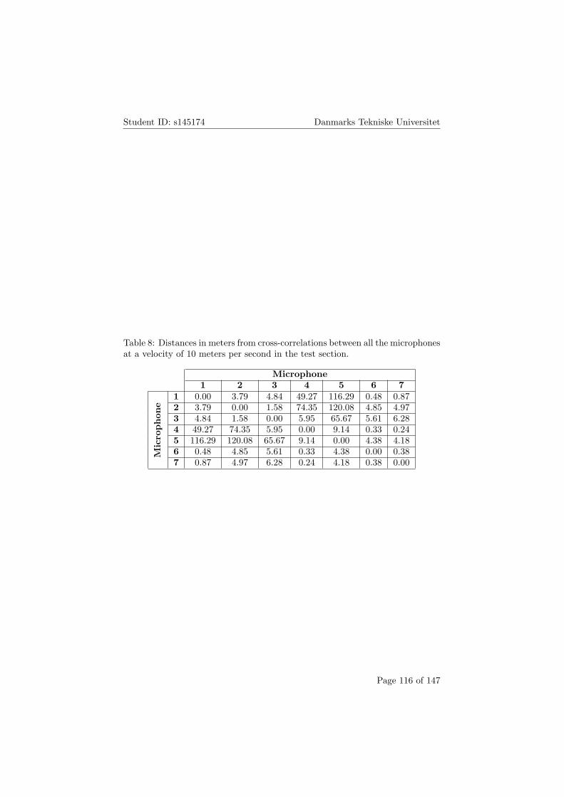
Student ID: s145174 Danmarks Tekniske Universitet
Table 8: Distances in meters from cross-correlations between all the microphonesat a velocity of 10 meters per second in the test section.
Microphone1 2 3 4 5 6 7
Micro
phone
1 0.00 3.79 4.84 49.27 116.29 0.48 0.872 3.79 0.00 1.58 74.35 120.08 4.85 4.973 4.84 1.58 0.00 5.95 65.67 5.61 6.284 49.27 74.35 5.95 0.00 9.14 0.33 0.245 116.29 120.08 65.67 9.14 0.00 4.38 4.186 0.48 4.85 5.61 0.33 4.38 0.00 0.387 0.87 4.97 6.28 0.24 4.18 0.38 0.00
Page 116 of 147

Student ID: s145174 Danmarks Tekniske Universitet
8 Transmission Losses
The design of the new wind tunnel design requires two bends. From an aerody-namic perspective, the bends are not ideal because of pressure losses. However,their necessity can be exploited for the acoustic treatment of the wind tunnelin order to make the wind tunnel fit for aeroacoustic measurements. As men-tioned and seen in the previous, the design of the corners allows them to be usedas baffle mufflers. The thick corner vanes of the design allows for the housingof porous lining, which can aid in the attenuation of the motor- and fan-noisethrough the corners. The use of porous lining in corner vanes is, amongst others,presented in (Devenport et al. 2017) and (Bergmann 2012).
In the previous it was mentioned that the design of the corners as well asthe vanes were inspired by the WindGuard anechoic wind tunnel in Germany.The motivation for the corners and vanes with a double bend with a straightsection is between was for design simplicity – adding porous material inside astraight section would be placed easier than in an arch or heavily camberedairfoil-shaped vane. On top of that, an impermeable barrier is believed to notbe required as air is unlikely to leak from one side of the vane to the other overa straight section.
(Soderman & Allen 2002) stated that aeroacoustic measurements will bepossible when the background noise is 6 dB less than flow-induced noise by themodel. From noise measurements it became evident that the sound pressurelevels produced by the motor and fan combination at the maximum rotationalspeed is approximately 80 dB for frequencies below 2 kHertz. (Munjal 2014)mentions that an acoustically lined corner can attenuate noise for as much as 10dB. (Munjal 2014) states that at least a thickness of a tenth of the wavelengthfor the porous lining is required for it to work effectively. This already impliesa difficulty in attenuating the lower frequency range of the noise.
In this section, a prediction of the transmission and insertion loss throughthe acoustically lined corners are made by using a finite element analysis. Theeffect of the complete wind tunnel configuration from the start of the fan-ductuntil the end of the test section will also be evaluated. In the following, themethodology and some background information regarding the used models andits inputs will be given first. Then the geometry, mesh and model set-up willbe discussed. The results will be presented and discussed thereafter.
8.1 Methodology
The methodology for finding these losses is straightforward. The different partsof the tunnel have been designed earlier and these will, of course, be unchangedfor the transmission loss predictions. The goal is to model the propagation ofnoise through each corner and calculate the attenuation. For each corner, two
Page 117 of 147

Student ID: s145174 Danmarks Tekniske Universitet
cases will be presented: One where porous material is applied and one withoutporous material. The ratio of the attenuation between the cases, gives theinsertion loss of the tunnel. The evaluations of the complete configuration willbe done in a similar fashion.
The Ansys Mechanical APDL of Ansys 18.0 and the corresponding Acous-tics ACT plugin were used for the simulations of noise propagation through thecorners (with porous lining). After the geometries and meshes have been cre-ated, the ACT allows to set up acoustic boundary conditions and excitations aswell as the option to define acoustic and material characteristics for each partof the model. Visualisations of the sound pressure levels found in the enclosedenvironment as well as of the transmission losses are possible with the sameplugin. In this particular case, the noise propagation is found by an acousticfull harmonic analysis and without structural interaction.
In order to maintain simplicity and reduce computational effort for theseevaluations, a thin model, where it is aimed to have a thickness of just one cell,will be used for the simulations. 2D simulations are not possible with the Me-chanical APDL. The geometries with a thickness of one cell limits the degreesof freedom and the cell or node count of the model is kept within bounds. Thisalmost 2D representation is identical to the 3D corner models apart from itsthickness. It is assumed that results will be close to a full 3D representationas acoustic excitation and propagation are normalized to surface area. Themethodology is similar to the simulations presented in (Acoustic Simulation ofa Silencer n.d.). A 3D evaluation over a large frequency range is not possi-ble, because it would require unavailable computational power with any of theavailable solvers.
8.2 Models
It is desired to do the analysis over an as wide as possible frequency-range andgiven that the flow resistivity, which will be discussed in more detail in latersections, is rather high for porous materials, as can be seen in (Mareze et al.2012) and (Doutres et al. n.d.), the documentation for the Ansys MechanicalAPDL implies that it would leave the JCA and Miki models as the only com-monly used methods for the simulations with acoustic lining because of the ratiobetween frequency and flow resistivity.
In (Miki 1990) an improvement of the Delany-Bazley model is presented .The Delany-Bazley model is an empirical model that determines the character-istic impedance and the propagation coefficient of porous materials as a functionof the ratio between the frequency of the noise and the flow resistivity of theporous material. Since the function by the power-law regression of the Delany-Bazley model would sometimes provide negative impedances, Miki improvedthe model with new regressions that would that would give only positive and
Page 118 of 147

Student ID: s145174 Danmarks Tekniske Universitet
real values for the characteristic impedances. This automatically improved theperformance at lower frequencies. Whereas the original Delany-Bazley modelpeformed poorly at lower frequencies, the Miki model provides good resultsacross the whole frequency range even though it is still bound to an upper-limitof the frequency and flow resistivity ratio of less than one. In the documenta-tion for Ansys Mechanical APDL it is shown how the Miki model affects theimpedance and propogation constant in an acoustic full harmonic analysis.
The JCA model stems from an improvement in (Champoux & Allard 1990)on the work presented in (Johnson et al. 1987). In Johnson, the acoustic behav-ior in porous media is described in terms of dynamic permeability and dynamictortuosity. The model is derived from Biot’s theory and attempts to solely de-termine the noise propagation in a porous medium by using macroscopic charac-teristics. The high-frequency behavior of the dynamic tortuosity is determinedby the characteristic viscous length in (Champoux & Allard 1990): a parameterthat is directly related to the geometry of the pores in the medium. Anotherparameter was determined in the same paper, the thermal characteristic length,defines the high frequency behavior of the dynamic permeability and is a resultof the excess temperature caused by the compression of air inside the porousmedium. The porosity, flow resistivity and tortuosity are the three remainingparameters required for the model. The JCA model is mentioned and used inmultiple papers and is considered as a good method for estimating the noisepropagation through porous material, even though its accuracy may diminishfor lower frequencies as mentioned in Fluent Theory Guide. For a acousticfull harmonic analysis in Ansys, the JCA model alters the effective density (re-lated to the dynamic permeability) and the effective bulk modulus (related tothe dynamic tortuosity) in a full harmonic analysis in Ansys as written by thedocumentation for the Ansys Mechanical APDL.
In the previous subsection, the two models use a total of five parameters:flow resistivity, porosity, tortuosity, viscous characteristic length and thermalcharacteristic length. The first named is the only input parameters requiredfor the Miki model. (Shravage et al. 2010b) is a study to the parameters ofthe JCA model, where the definition of each parameter and its effect on noisepropagation is determined. The flow resistivity is the force required for the flowgoing through porous material. Increased flow resistivity increases transmissionlosses. Increased porosity also has a positive effect on transmission losses. Tor-tuosity is a measure of difference between the length of a straight path of a poreand the actual path of a pore. High values of tortuosity is subject to resonanceeffects in transmission losses throughout the frequency range as the speed ofsound of the fluid is directly affected. Low values of tortuosity increase trans-mission losses for higher frequencies and shows itself to be the most effective.Porosity and Tortuosity often have values close to 1 for porous media. Lowviscous characteristic lengths will result in higher transmission losses for midand high frequencies. The thermal characteristic length has a minimum effect
Page 119 of 147

Student ID: s145174 Danmarks Tekniske Universitet
on the transmission loss, except for very low values where it results in modifiedvalues for flow resistivity and tortuosity and will increase losses in the mid andhigh frequency range. In general, it becomes evident that the parameters influ-ence the mid and high frequency range the most and this may ultimately resultin poor quality of aeroacoustic mesurements for low frequencies. It is thereforelikely that the lower limit for the anechoic conditions for wind tunnels, besideslimited lining thickness, is also a result of the inability to effectively manipulatethe transmission loss for low frequencies material-wise.
8.3 Geometry
Even though a detailed design of the corner could be used for the evaluations,a simplified case is believed to suffice. This means, in addition to the duct, thelining and perforated plate/protective layer have to be added to the completegeometry of the corners. The thickness of the perforated plate should in any casebe thin and was chosen to be an arbitrary 1.27 millimeter or 1/20th of an inch.This specific thickness was arbitrary. When a detailed design of the cornerswill be made and built in order to experimentally validate the numbers fromthese predictions, these thicknesses may have to be updated and the simulationsmay have to be run again. By leaving the geometry of duct untouched, thethicknesses of the sections with the porous material inside the vanes will become27.46 and 57.46 millimeter thick, for the first and second corner, respectively.The length of the plate and lining sections are 300 millimeter, correspondingwith the straight section of the corner vanes as can be seen in Figures 95 - 97.
In Catia V5, the geometries of the perforated plates and lining were createdand assembled with their respective corners. The thickness of the whole assem-bled geometry was set to 1 millimeter, which would allow for a reduced cell sizeof the while maintaining a single-cell thickness of the mesh. The outer walls ofthe bend have lining-plate combinations with just one plate instead of two forthe corner vane combinations. Since Ansys has a built-in model to simulate aperforated plate at the hand of several parameters, the holes did not have to bespecified in the geometry. This also eases meshing at a later stage. In Figures95 and 96 the assembly of the second corner can be seen. The first corner is, ofcourse, assembled in a similar fashion.
For the complete geometry, the cross-section on the symmetry-plane of theduct was given a thickenss of 1 millimeter. The geometries of the porous materialand the perforated plates were added in the same fashion as for the separatecorners. In Figure 97 the geometry of the complete configuration can be seen.For this geometry, the corners are, of course, identical to the two separatecorners.
Page 120 of 147

Student ID: s145174 Danmarks Tekniske Universitet
Figure 95: Simplified geometry of the second corner with perforated plate andporous material (from Ansys).
Figure 96: Close-up of the corner vane of the second corner with perforatedplate and porous material (from Ansys).
8.4 Meshing and Analysis Settings
The next step was meshing the geometry. The refinement of the mesh is largelydependent on the frequency-range. For linear elements, 12 elements per wave-length are required and for quadratic elements, only 6 elements are needed. Forthe two corners, a multi-zone method was used with quadratic elements of asize of 2.5 millimeter. This cell-size would meet the requirements of at least 6elements per wavelength up to a frequency of 20000 Hertz. For the convergence
Page 121 of 147

Student ID: s145174 Danmarks Tekniske Universitet
Figure 97: Simplified geometry of the complete geometry with perforated platesand porous material (from Ansys).
studies, the cell-size was reduced to 1.75 millimeters, which increased the cell-count by a factor of approximately. In order to model a perforated plate, thequadratic elements need to have exactly opposing faces and this was guaran-teed by using the multi-zone method. The evaluations of the full configurationwere done with cell-sizes of 7 and 5 millimeters for the standard and refinedgrid, respectively. The standard size would be sufficient for evaluations up to8000 Hertz and the refined size would increase the cell-count by approximatelya factor of two. Figures 98 to 105 show a part of the two corners for the 4different meshes. An analysis up to 20000 Hertz would not be possible for thefull geometry as the graphical user interface of Ansys Mechanical does not workproperly on the cluster and the other available systems do not provide enoughmemory to generate the required mesh and input files or read the results files.Table 9 shows the number of cells in each model and case.
Table 9: Number of cells found in each geometry.
Cell CountStandard Grid Refined Grid
Geometry 1st Corner 184105 375330Geometry 2nd Corner 282421 576447Complete Geometry 132493 259106
The fluid region, perforated plate and the porous material were selectedas different acoustic bodies which held different acoustic properties. The fluidproperties of air, found in the documentation for the Ansys Mechanical APDL,were given to all the acoustic bodies. The perforated plate was modelled by
Page 122 of 147

Student ID: s145174 Danmarks Tekniske Universitet
adding a square grid model that uses a 2 × 2 transmittance matrix to modelthe holes in the body at the hand of plate thickness, hole spacing, hole radiusand hole radius-ratio. (Munjal 2014) states that the acoustic properties of theporous material does not change with a porosity of 20%. This porosity of20% was achieved with a ratio of 1 and a spacing and radius of 5 millimeterand 1.25 millimeter, respectively. (Mareze et al. 2012) provided all the relevantparameters of rock wool needed for the model to function with either the JCA orthe Miki model. In this paper, rock wool has a flow resistivity of 20600 kNs/m4,a porosity of 0.98, tortuosity of 1.01, thermal characteristic length of 85 µm anda viscous characteristic length of 90 µm. The numbers in (Mareze et al. 2012)follow the statements made in (Shravage et al. 2010b), where it is mentionedthat porous media for acoustic treatment have often a porosity and tortuosityclose to 1 and a high flow resistivity. For analyses without porous materialapplied, the acoustic bodies with the porous material and the perforated plateswere simply suppressed.
An arbitrary normal surface velocity of -0.0024 m/s was chosen as the ex-citation for this particular solution. Radiation boundaries were given to thein- and outlet of the corner. Additional boundary conditions were the externalports given to the faces of the perforated plates adjacent to the air-line andporous material. The physical boundaries to which no boundary conditionswere applied, had fully reflective walls by default. The analysis was set up togive a solution for all the center frequencies of the octave bands from 16 Hertzto 20000 Hertz for the corners and from 16 Hertz to 8000 Hertz for the completeconfigurations.
Figure 98: Mesh of the first corner, perforated plate and porous material as-sembly with a cell-size of 2.5 millimeter (from Ansys).
Page 123 of 147

Student ID: s145174 Danmarks Tekniske Universitet
Figure 99: Mesh of the first corner, perforated plate and porous material as-sembly with a cell-size of 1.75 millimeter (from Ansys).
Figure 100: Mesh of the second corner, perforated plate and porous materialassembly with a cell-size of 2.5 millimeter (from Ansys).
Page 124 of 147

Student ID: s145174 Danmarks Tekniske Universitet
Figure 101: Mesh of the second corner, perforated plate and porous materialassembly with a cell-size of 1.75 millimeter (from Ansys).
Figure 102: Mesh of the first corner, perforated plate and porous material as-sembly as in the complete geometry with a cell-size of 7 millimeter (from Ansys).
Page 125 of 147

Student ID: s145174 Danmarks Tekniske Universitet
Figure 103: Mesh of the first corner, perforated plate and porous material as-sembly as in the complete geometry with a cell-size of 5 millimeter (from Ansys).
Figure 104: Mesh of the second corner, perforated plate and porous materialassembly as in the complete geometry with a cell-size of 7 millimeter (fromAnsys).
Page 126 of 147

Student ID: s145174 Danmarks Tekniske Universitet
Figure 105: Mesh of the second corner, perforated plate and porous materialassembly as in the complete geometry with a cell-size of 5 millimeter (fromAnsys).
8.5 Results
The transmission losses through each corner with and without porous materialcan be seen in Figure 106. The results with a refined grid can also be seen here.In Figure 107 a similar Plot can be seen for the complete configuration. Figure108 shows the noise reduction per corner, of the corners added together and thecomplete configuration, where the transmission loss without porous material isdeducted from the transmission loss with porous material. Figures 109 to 114show the contour Plots of the corners for the two different models that wereand without porous material applied from the simulations with the standardmesh. Figures 115 to 117 show the same Plots for the complete configuration.Table 10 shows the average transmission losses through each corner with andwithout porous material. Table 12 shows the average transmission losses for thecomplete configuration. Table 11 shows the percentual difference between theoutcomes of the standard and their respective refined grids of the corners. Table13 shows the percentual differences between the outcomes of the convergencestudy for the complete configuration.
Page 127 of 147

Student ID: s145174 Danmarks Tekniske Universitet
Figure 106: Transmission losses through the corners (from MatLab).
Figure 107: Transmission losses from fan to test section (from MatLab).
Page 128 of 147

Student ID: s145174 Danmarks Tekniske Universitet
Figure 108: Noise reduction by applying porous material for the two cornersand complete configuration (from MatLab).
Figure 109: Contour plot of transmission losses through the second corner withthe JCA model (from Ansys).
Page 129 of 147

Student ID: s145174 Danmarks Tekniske Universitet
Figure 110: Contour plot of transmission losses through the second corner withthe Miki model (from Ansys).
Figure 111: Contour plot of transmission losses through the second corner withno porous lining (from Ansys).
Page 130 of 147

Student ID: s145174 Danmarks Tekniske Universitet
Figure 112: Contour plot of transmission losses through the first corner withthe JCA model (from Ansys).
Figure 113: Contour plot of transmission losses through the first corner withthe Miki model (from Ansys).
Page 131 of 147

Student ID: s145174 Danmarks Tekniske Universitet
Figure 114: Contour plot of transmission losses through the first corner with noporous lining (from Ansys).
Figure 115: Contour plot of transmission losses from fan to test section withthe JCA model (from Ansys).
Page 132 of 147

Student ID: s145174 Danmarks Tekniske Universitet
Figure 116: Contour plot of transmission losses from fan to test section withthe Miki model (from Ansys).
Figure 117: Contour plot of transmission losses from fan to the test section withno porous lining (from Ansys).
Page 133 of 147

Student ID: s145174 Danmarks Tekniske Universitet
Table 10: Average transmission losses for the corners.
Average Transmission Loss [dB]Standard Grid Refined Grid
1st Corner JCA 12.6361 12.64841st Corner Miki 12.9110 12.9633
1st Corner 8.6176 8.67262nd Corner JCA 14.489 14.54282nd Corner Miki 14.5074 14.5608
2nd Corner 10.5222 10.5768
Table 11: Results of grid-convergence study for the corners.
Difference [%]1st Corner JCA 0.09661st Corner Miki 0.6339
1st Corner 0.40372nd Corner JCA 0.36732nd Corner Miki 0.5166
2nd Corner 0.3667
Table 12: Average transmission losses for the complete configuration.
Average Transmission Loss [dB]Standard Grid Refined Grid
JCA 27.3044 27.3706MIKI 27.0434 27.1121
No PorousMaterial
13.8539 13.9184
Table 13: Results of grid-convergence study for the complete configuration.
Difference [%]JCA 0.2416MIKI 0.2535
No PorousMaterial
0.4634
Page 134 of 147

Student ID: s145174 Danmarks Tekniske Universitet
8.6 Discussion of Transmission Loss Results
From Figures 106 and 107 it can be seen that the corners with porous materialare particularly effective for the mid-range frequencies between 1 kHertz and4 kHertz. Figure 108 shows that the low frequencies are difficult to controland that the effect of the porous material diminishes for higher frequencies,even though the transmission loss is steadily going up in this range. The lowerperformance for the lower frequencies is explained in a parametric study by(Shravage et al. 2010b) and the book by (Munjal 2014), where in the former itis implied that the parameters of porous material have hardly any effect on thelower frequencies and in the latter it is stated that porous material is effectivewith a module-thickness of at least a 10th of the wavelength. The absorptivematerial is relatively thin compared to the long wavelengths of low frequencynoise. For the high frequency range, it can be observed that even withoutporous material the transmission loss is high. In (Munjal 2014), there is alsoan estimate of 10 dB is given as an achievable transmission loss for a corneror baffle muffler. This 10 dB corresponds with the order of the numbers foundby the simulations. The simulations of the noise propagation from the fan tothe end of the test section showed that the transmission loss were only slightlyhigher than the losses found by adding up the transmission losses of the twoseparate corners and indicate that the diffusers and straight ducts only have aminor effect in attenuating the noise. In Figures 109 to 117, the contour plotsshow very well the plane waves through the corners where no porous lining isused. For the corners where porous material is applied, the attenuation of noisecan clearly be observed. In these contour Plots, the differences between theJCA and Miki model can hardly be seen. The refined grid shows no drasticchanges in results. The Miki model was used as a verification method for theJCA model as the two models are drastically different. Even though there aresome noticeable differences of only a couple percent between the outcomes, theresults are of the same order and follow the same trend.
In the previous, it was mentioned that aeroacoustic measurements are viableif the noise of the test subject is exceeds the background noise by 6 dB. In Figure118 the transmission loss of both corners is deducted from the 1/3 octave bandspectrum of the noise captured by the first microphone at a flow velocity of 40meters per second in the previous section. The decuction of the transmissionloss found for the complete configuration is also shown in the same figure. Itcan be seen that the first real difference with applying porous material in thecorner vanes is observable at 200 Hertz and becomes significant after 500 Hertz.In the mid and high frequency range thereafter, the effect of the lining can beseen to be as much as 20 dB and the deductions leave sound pressure levels tolie between 40 and 50 dB up to the band with a center frequency of 8000 Hertz.The complete geometry generally performs better than the two separate cornersin the mid and high frequency range. This difference may be the results of theincorporation of the straight ducts and diffusers for the analysis. The effect canbe observed for both the cases with and without porous material applied. By
Page 135 of 147

Student ID: s145174 Danmarks Tekniske Universitet
looking at (Brooks et al. 1989), the noise spectrum of different kind of airfoilsis still found to lie around 50 dB. The same can be seen in (Arbey & Bataille1983) for measurements at flow velocities of 35 meters per second. This, plusthe fact that the lower frequencies are unattenuated, imply that the lined cornervanes may not be enough to guarantee an adequate environment for aeroacousticmeasurements.
Figure 118: The transmission losses found in the two corners deducted fromthe noise measurements made with the first microphone at a flow velocity of 40meters per second (from MatLab).
Validation is key and required to find out whether the 2D simulations of thecorners give a good representation of the 3D problem. By constructing one ofthe corners and experimentally find the transmission loss in a setup that is sim-ilar to how the simulations setup, the value of this, in fact, prediction methodcan be shown. Another validation in a full wind tunnel setup, where the noisesource would be a real fan, can show whether the simplification by using a nor-mal velocity excitation is sufficient. In (Shravage et al. 2010a) and (Doutreset al. n.d.) methods are presented to find the acoustic properties of the mate-rial for when they are not known beforehand. This would mean that after thevalidation-process, simulations may need to be run again with altered parame-ters. The prediction of the noise that could be expected inside the test sectionmay have been lacking in the sense that not the complete transmission lossof one octave-band has been calculated. Instead determining the octave-bandfrom a range of frequencies with an identical resolution as the measurements(25 Hertz), simulations were run for just the center frequencies. This could be
Page 136 of 147

Student ID: s145174 Danmarks Tekniske Universitet
a problematic simplification. However, doing simulations for frequencies up to12800 or 20000 Hertz with a better frequency resolution results in large input-files, the need for loads of RAM and access to a lot of free disk-space (on theorder of tens of terabytes). What can be concluded so far, is that the acousticlining is not sufficient to allow for proper aeroacoustic measurements.
Page 137 of 147

Student ID: s145174 Danmarks Tekniske Universitet
9 General Conclusion and Discussion
The first steps in designing a new aeroacoustic wind tunnel could be madein this study. From the literature study it could be concluded that there arestraightforward and proven methods to design a wind tunnel. The design ofaeroacoustic wind tunnels largely follow the same principles as regular windtunnels do. Even though there is noise as an additional aspect that has to betaken into account in the design of such a wind tunnel, the focus should stillbe on the aerodynamics and the flow quality. The reason for this is, is that aclear understanding of the physics behind the noise is needed and a controllableenvironment is desired and bad flow quality may generate noise elsewhere in thetunnel. Rather than addressing noise sources inside the wind tunnel individuallythat may stand in the way of a proper anechoic environment for aeroacousticmeasurements in the test section, simple and effective solutions such as (baffle)mufflers are recommended.
A design of the wind tunnel was made by following recommendations in lit-erature. The corners however, were made with the philosophy that they wouldeventually be used as baffle-mufflers to attenuate noise. A trial-and-error pro-cess was done to find corner and thick corner vane geometries that would givegood aerodynamic results in 2D simulations of the new wind tunnel design. Thecorner vanes were given a thickness beforehand for the placement of porous ma-terial later on. The 2D simulations gave good results for the current wind tunneldesign. The methodology and the set up of these simulations however, did notexactly follow the Fluent User’s Guide recommendations and may not have beenideal. The default inlet turbulence intensity was set at its default value of 5%as a boundary condition, whilst lower turbulence intensities could be expectedin a true indoor environment with stationary air. Then the inflation-layer maynot have been fine enough for some of the simulations were wall treatment wasused. The convergence study may have been insufficient as well and even thoughthe cases where the boundary layer was completely resolved showed favorablecharacteristics, an additional convergence study with an additional refinementmay have shown different results.
The 2D solutions were considered good enough and 3D evaluations were donenext. The 3D simulations followed much closer the Fluent recommendationsand used a more robust solver that is available in Fluent. The quality insidethe test section appeared to be good after the 3D simulations. The outcomesof the CFD simulations were also close to those from empirical predictions. Itturned out that the new design has a better performance compared to the oldred wind tunnel. Even though favorable characteristics were found inside thetest section, mostly the first diffuser was giving problems. Separation was seenhere and resulted in non-ideal flow characteristics in the first corner and seconddiffuser downstream. It was argued however, that this separation is incorrectlypredicted by the model that was employed because of Boussinesq’s assumption
Page 138 of 147

Student ID: s145174 Danmarks Tekniske Universitet
of proportional production of turbulence kinetic energy to the strain rate. Thisseparation, also predicted a large sound power level generated by the air. Itssignificance is somewhat unknown as it is not clear what amount or what volumeof air produces these high levels of noise. At the same time, nothing is knownabout the propagation of the noise. It does occur close to the test section andmay spoil aeroacoustic measurements. A reevaluation is needed where eitherthe Kato-Launder limiter in order to limit the over-production of turbulencethat is characteristic of the SST k − ω model and/or another model will beused, before a redesign of the first diffuser should be considered. The boundarylayer noise on the other hand, was limited and only visible in regions with highvelocity such as the contraction-exit and the leading-edges of the corner vanes.Also here it is not clear what the significance of the sources are for the receiver.However, it becomes clear what the benefit is from the long contraction-typeswith very moderate curvature designed by methods presented by (J. H. Downie1984), for example, as the velocity extrema at the walls are low. The area ofthe noise sources of the leading-edges of the corner vanes is very small and thecorner vanes themselves are a considerable distance away from the test section,making the boundary layer noise of less importance.
The noise measurements of the fan of the red wind tunnel showed that thenoise of the fan was highest between 1000 and 2000 Hertz. The tonal noise wasalso visible as strong peaks in the spectra. The propagation of noise stemmingfrom the fan in the basement to the ground floor did not become visible afterusing the (cross-)correlation of the time and frequency signal.
The transmission loss of the corners and the part of the wind tunnel goingfrom the fan-inlet to the exit of the test section found in the simulations gaveconsistent results with refined grids and the use of different models. It remainsunclear however if these numbers translate to real-life situations because of the2D simplification. A validation is therefore required. The 2D simplification,the use of a plane-wave as a noise source and the assumption of fully reflectiveboundaries may have given unrealistic results. The prediction of the noise thatcould be expected inside the test section may have been lacking in the sensethat not the complete transmission loss of one octave-band has been calculated.Instead determining the octave-band from a range of frequencies with an identi-cal resolution as the measurements (25 Hertz), simulations were run for just thecenter frequencies. This could be problematic simplification as the behaviourfor other frequencies in that band is unknown. However, doing simulations forfrequencies up to 12800 or 20000 Hertz with instances of 25 Hertz requires largeinput-files, loads of RAM and a lot of free disk-space (on the order of tens ofterabytes). An extensive study into the transmission loss by doing simulationsrequires, all in all, a lot of resources and is therefore in most cases a limiting fac-tor. What is hinted in the noise measurements and transmission loss predictionsso far, is that the acoustic lining may not be sufficient for proper aeroacousticmeasurements.
Page 139 of 147

Student ID: s145174 Danmarks Tekniske Universitet
The HPC services of DTU were used for the CFD and FEA simulations. Forthis, input files had to be created, which proved to be rather difficult at timesas the Ansys geometrical, meshing and Fluent interfaces, did not work properlyon the server computers. Hence, a personal computer had to be used to createinput files. This was time-consuming with limited RAM and processing power.On top of that, the post-processing was also difficult on the HPC computers.Post-processing exported solution files on a personal computer was necessaryand had a risk of crashing Ansys or the computer, because of the size of theexported solution files. This limited, amongst others, the amount and qualityof figures and log files that could be extracted and presented in the report.
Page 140 of 147

Student ID: s145174 Danmarks Tekniske Universitet
10 Recommendations
While the initial steps have been made for the design of a new wind tunnel,there is still room for improvement and there are additional steps to be taken. Incontinuation of this project, it is recommended that the 3D CFD simulations aredone with another turbulence model or that a Kato-Launder limiter is used withthe current one. A redesign of the first diffuser may be needed depending on theresults. For any new simulation, whether it is CFD or FEA, it is recommendedto work on a computer with strong performance in order to ease pre- and post-processing.
Extra analyses with a higher frequency resolution could aid in better predic-tions of transmission losses. As was mentioned earlier, the effect of the corners isthen easier to compare and to interpreted with noise measurements as it allowsfor a sounder picture of the losses in octave bands. The noise simulations needto be validated, however, in order to see whether the 2D simplification holdsfor real-life situations. This could possibly be done by placing a mock-up of thecorners in an anechoic chamber. On the upstream side of the model, there is amicrophone placed. On the downstream side of the corner a noise source thateither emits a certain tone or white noise is placed. The transmission loss couldthen be found by subtracted the microphone readings from the pressure levelsof the emitted noise.
Since the screens, inlet-filter, inlet-muffler, exit-diffuser and the square tocircular transition have not been treated so far, these should also be investigated.Especially the cross-sectional transition may be important to model for CFDand evaluate before building as it will also determine the inflow conditions ofthe fan. Turbulence intensities in the test section appeared to be a bit high, butcould be addressed together with the placement of screens and determining thewind tunnel characteristics in testing.
Parametric studies by using different porous linings and porosities of theperforated plates during propagation simulations, may give new insights or givebetter results in calculating transmission losses. Additionally, new evaluationswith filling up the arcs of the corner vane’s trailing-edges with porous materialcould be done in order to see whether it has a positive effect on the anechoicenvironment in the test section of the current wind tunnel configuration. Theinclusion of the fan-duct in this analysis, where the fan-hub and walls are linedwith porous material, is also recommended. The single plane-wave, could bereplaced with two sources on planes on either side of the hub here if there areno better alternatives to model the noise sources for such an analysis.
Then, to have a better understanding of the fan as a noise source and to makean attempt to make it quieter in operation, noise measurements upstream of thefan inside the wind tunnel could be done by using a microphone array. (virtual)
Page 141 of 147

Student ID: s145174 Danmarks Tekniske Universitet
noise sources on the fan could then be identified and possibly be eliminated in asimilar fashion as described in (Remillieux et al. 1986). For such measurements,it is also recommended to use a higher sampling frequency in order to find thepower spectral density at higher frequencies - In the literature study earlier, itwas already mentioned that scaled models will emit noise of higher frequencies.During calibration for aeroacoustic measurements in the tunnel, it may be usefulto have knowledge of the noise characteristics of the fan in this range.
Finally, detailed designs and engineering drawings of the new wind tunnelare required for construction and it might be of interest to find the pressures andforces on the wind tunnel walls during operation from the CFD results beforethat as it can be a help in selecting materials.
Additional things that might be of interest are, if the computational re-sources are available, modelling the propagation from the fan to the test sectionand the adjacent anechoic chamber. Similarly, the new design placed in theenvironment with two floors could be modelled in order to see how the noisepropagates through the wind tunnel and elephant hole.
More in-depth noise analyses from the flow are difficult and unnecessary.Even though Fluent provides a direct method and an integral method based onacoustic analogy, which both use an unsteady/transient solution, they are oflimited use in this situation according to the Fluent User’s Guide. The integralmethod only calculates far-field noise to the free-stream. It is impossible tofind the propagation in wall-bounded flows here. The direct method is limitedto near-field noise, requires a lot of computational resources and non-reflectiveboundary conditions. What is possible, however, is a study to structural vibra-tion and Helmholtz resonance. From a transient solution, the pressure fluctua-tions on surfaces and walls can be extracted and imported in Ansys Mechanical.These fluctuations can be implemented as excitations. The propagation of noiseproduced by these excitations can then be modeled.
Page 142 of 147

Student ID: s145174 Danmarks Tekniske Universitet
11 Bibliography
Abbaspour, M. & Shojaee, M. N. (2009), ‘Innovative approach to design a newnational low speed wind tunnel’.
Acoustic Simulation of a Silencer (n.d.).URL: https://www.simutechgroup.com/tips-and-tricks/fea-articles/379-acoustic-simulation-of-a-silencer
Allen, C. S. & Olsen, L. E. (1998), ‘Effect of free stream turbulence on theflow-induced background noise of in-flow microphones’.
Allen, C. S. & Soderman, P. T. (1993), ‘Aeroacoustic probe design for micro-phone to reduce flow-induced self-noise’.
Amiet, R. K. (1975), ‘Correction of open jet wind tunnel measurements for shearlayer refraction’.
Anderson, J. D. (2008), Introduction to Flight.
Arbey, H. & Bataille, J. (1983), ‘Noise generated by airfoil profiles placed in auniform laminar flow’.
Batchelor, G. K. (1953), The Theory of Homogeneous Turbulence.
Bauer, A. B. (1976), ‘Acoustically transparent walls for wind-tunnel applica-tions’.
Bell, J. H. & Mehta, R. D. (1988a), ‘Contraction design for small low-speedwind tunnels’.
Bell, J. H. & Mehta, R. D. (1988b), ‘Design and calibration o the mixing layerand wind tunnel’.
Bergmann, A. (2012), ‘The aeroacoustic wind tunnel dnw-nwb’.
Boes, S., Nuesch, S. & Stillman, S. (2013), ‘Aircraft noise, health and residentialsorting: Evidence from two quasi-experiments’, Health Economics 22, 1037–1051.
Bradshaw, P. & Pankhurst, R. C. (1964), ‘The design of low-speed wind tunnels’,NPL Aero REport .
Brooks, T. F., Pope, D. S. & Marcolini, M. A. (1989), ‘Airfoil self-noise andprediction’.
Brouwer, H. H. (1997), ‘Anechoic wind tunnels’.
Calautit, J. K., Chaudhry, A. N., Hughes, B. R. & Sim, L. F. (2014), ‘A validateddesign methodology for a closed-loop subsonic wind tunnel’.
Page 143 of 147

Student ID: s145174 Danmarks Tekniske Universitet
Champoux, Y. & Allard, J. F. (1990), ‘Dynamic tortuosity and bulk modulusin air-saturated porous media’.
Devenport, W., Bak, C., Brown, K., Borgoltz, A., Oesterlund, J. & Davidsson,P. (2017), ‘Design and operation of hybrid aeroacoustic wind tunnels’.
Donald A. Dietrich, M. F. H. & Abbott, J. M. (1977), ‘Fan acoustic signaturesin an anechoic wind tunnel’.
Doutres, O., Salissou, Y., Atalla, N. & Panneton, R. (n.d.), ‘Evaluation of theacoustic and non-acoustic properties of sound absorbing materials using athree-microphone impedance tube’.
Duell, E., Yen, J., Walter, J. & Arnette, S. (2004), ‘Boundary layer noise inaeroacoustic wind tunnels’.
Eckert, W. T., Mort, K. W. & Jope, J. (1976), ‘Aerodynamic design guidelinesand computer program for estimation of subsonic wind tunnel performance’.
Fowler, P. M. (n.d.), ‘Practical classical methods’.URL: http://www.ws.binghamton.edu/fowler/
Glegg, S. & Devenport, W. (2017), Aeroacoustics of Low Mach Number Flows.
Grissom, D. L., Smith, B., Devenport, W. J. & Stewart, G. A. L. (2006), ‘Rough-wall boundary layer noise’.
H. Arbey, J. B. (1983), ‘Noise generated by airfoil profiles placed in a uniformlaminar flow’, J. Fluid Mech 134, 33–47.
Hernandez, M. A. G., Lopez, A. I. M., Jarzabek, A. A., Perales, J. M. P., Wu,Y. & Xiaoxiao, S. (2013), ‘Design methodology for a quick and low-cost windtunnel’.
Hersh, A. S., Soderman, P. T. & Hayden, R. E. (1974), ‘Investigation of acousticeffects of leading edge serrations on airfoils’.
Ito, T., Ura, H. & Yokokawa, Y. (2008), ‘Aeroacoustic noise measurements inaerodynamic low-speed wind tunnels’.
J. H. Downie, R. Jordinson, F. B. (1984), ‘On the design of three-dimensionalwind tunnel contractions’.
Jacob, M. C. & Talotte, C. (2000), ‘Numerical prediction methods for the as-sessment of aerodynamic sound generation on high speed trains’.
Jaeger, S. M., Horne, W. C. & Allen, C. S. (2000), ‘Effect of surface treatmenton array microphone self-noise’.
Janssen, S. A., Vos, H., Eisses, A. R. & Pedersen, E. (2010), ‘Predicting annoy-ance by wind turbine noise’.
Page 144 of 147

Student ID: s145174 Danmarks Tekniske Universitet
Jewel B. Barlow, William H. Rae Jr., A. P. (1999), Low-Speed Wind TunnelTesting, John Wiley Sons Inc.
Johansson, A. V. (1992), ‘Low speed wind-tunnel with extrame flow quality -design and tests’.
Johnson, D. L., Koplik, J. & Dashen, R. (1987), ‘Theory of dynamic permeabil-ity and tortuosity in fluid-sarturated porous media’.
Kaltenbach, M., Maschke, C., Hess, F., Niemann, H. & Fuehr, M. (2013),‘Health impairments, annoyance and learning disorders by aircraft noise’, In-ternational Journal of Environmental Protection 6, 15–46.
Kolb, A., nd Roger Drobietz, P. F. & Graenewald, M. (2007), ‘Aeroacousticwind measurements on a 2d high-lift configuration’.
Kulkarni, V., Sahoo, N. & Chavan, S. D. (2010), ‘Simulation of honeycomb-screen combinations for turbulence management in a subsonic wind tunnel’.
L.D. Santana, M. Carmo, F. C. (2014), ‘The update of an aerodynamicwind-tunnel for aeroacoustic testing’, J. Aerospace Technology Management6(2), 111–118.
Leclercq, D., Doolan, C. & Reichl, J. (2007), ‘Development and validation of asmall-scale anechoic wind tunnel’.
Leifsson, L., Koziel, S., Andrason, F., Magnusson, K. & Gylfason, A. (2012),‘Numerical optimization and experimental validation of a low-speed wind tun-nel contraction’.
Lindgren, B., Oesterlund, J. & Johansson, A. V. (1998), ‘Measurement andcalculation of guide vane performance in expanding bends for wind tunnels’.
Loerke, R. I. & Nagib, H. M. (1976), ‘Control of free-stream turbulence bymeans of honeycombs: A balance between suppresion and generation’.
Lopes, L. V., Brentner, K. S., Morris, P. J. & Lockard, D. P. (2006), ‘Increasedfidelty in prediction methods for landing gear noise’.
Lv, J., Wang, N., Liao, D., Yu, Y. & Gao, X. (2018), ‘Study on acousticallytransparent test section of aeroacoustic wind tunnel’.
Mareze, P. H., Lenzi, A. & Pellegrini, C. (2012), ‘Rigid-frame porous materialacoustic attenuation on compressor discharge’.
Mathew, J., Bahr, C. J., Sheplak, M. & Cattafesta, L. (2005), ‘Design, fabrica-tion and characterization of an anechoic wind tunnel facility’.
Mathworks (n.d.), ‘Welch’s method’.URL: https://www.mathworks.com/examples/signal/mw/signal-ex45136368-welch-s-method
Page 145 of 147

Student ID: s145174 Danmarks Tekniske Universitet
Mehta, R. D. & Bredshaw, P. (1979), ‘Design rules or small low speed windtunnels’, The Aeronautical Journal o the Royal Aeronautical Society .
Mehta, R. D. & Hoffmann, P. H. (1986), ‘A study of the factors affecting bound-ary layer two-dimensionality in wind tunnels’.
Menter, F. R. (1994), ‘Two-equation eddy-viscosity turbulence models for engi-neering applications’, AIAA Journal. 32(8).
Migliore, P. & Oerlemans, S. (2003), ‘Wind tunnel aeroacoustic tests of sixairfoils for use on small wind turbines’.
Miki, Y. (1990), ‘Acoustical properties of porous materials - modifications ofdelany-bazley models’.
Morel, T. (1975), ‘The comprehensive design of axisymmetric wind tunnel con-tractions’.
Munjal, M. (2014), Acoustics of Ducts and Mufflers, John Wiley and Sons Ltd.
Pascioni, K., Reger, R., Edstrand, A. & Cattafesta, L. (2014), ‘Characterizationof an aeroacoustic wind tunnel facility’.
Patterson, G. N. (1938), ‘Modern diffuser design’.
Piccin, O. (2009), ‘Cepra19: The onera large anechoic facility’.
Remillieux, M. C., Crede, E. D., Camargo, H. E., Burdisso, R. A. & Devenport,W. J. (1986), ‘The virginia tech stability wind tunnel from an aerodynamicinto an aeroacoustic facility’.
Remillieux, M. C., Crede, E. D., Camargo, H. E., Burdisso, R. A., Deven-port, W. J., Rasnick, M., Seeters, P. V. & Chou, A. (2008), ‘Calibration anddemonstration of the new virginia tech anechoic wind tunnel’.
Ross, R., YOung, K. J., Allen, R. M. & van Ditshuizen, J. C. A. (1983), ‘Acous-tic wave propagation through the shear layer of the dnw large open jet windtunnel’.
Sahlin, A. & Johansson, A. V. (1991), ‘Design of guide vanes for minimizing thepressure loss in sharp bends’.
Santana, L. D., Carno, M. & Catalano, F. M. (2014), ‘The update of an aero-dynamic wind tunnelforaeroacoustictesting
′.
Scheiman, J. & Brooks, J. D. (1980), ‘Comparison of experimental and theoreticalturbulence reduction from screens, honeycomb, and honeycomb-screen combi-nations’.
Selig, M. S., Deters, R. W. & Williamson, G. A. (2011), ‘Wind tunnel testingairfoils at low reynolds numbers’.
Page 146 of 147

Student ID: s145174 Danmarks Tekniske Universitet
Shravage, P., Jain, S. & Karanth, N. (2010a), ‘A comparison of analytical andoptimization inverse techniques for characterizing intrinsic parameters of porousmaterials’.
Shravage, P., Jain, S. & Karanth, N. (2010b), ‘Effect of intrinsic parameters onsound absorption and transmission loss - a parametric study’.
Sijtsma, P., Oerlemans, S., Tibbe, T. G., Berkefeld, T. & Spehr, C. (2014), ‘Spec-tral broadening by shear layers of open jet wind tunnels’.
Soderman, P. T. & Allen, C. S. (2002), ‘Microphone measurements in and out ofairstream’.
Soderman, P. T., Jaeger, S. M., Hayes, J. A. & Allen, C. (2000), ‘Acoustic perfor-mance of the 40- by 80-foot wind tunnel test setion deep acoustic lining’.
Su, Y.-X. (1991), ‘Flow analysis and desigh of three-dimensional wind tunnelcontractions’.
Sumer, B. M. (2003), ‘Lecture notes on turbulence’.
Thomas F. Brooks, D. S. P. & Marcolini, M. A. (1989), ‘Airfoil self-noise andprediction’, NASA Referebce Publication (1218).
Wagner, Bareiss, G. (1996), Wind Turbine Noises, Springer.
Williamson, C. H. K. (1996), ‘Vortex dynamics in the cylinder wake’.
Winkler, J., Temel, F. Z. & Carolus, T. (2007), ‘Concept, design and characteri-zation of a small aeroacoustic wind tunnel facility’.
Page 147 of 147

In this master thesis project, the initial steps for the design of a new wind tunnel for aeroacousticmeasurements are made. A literature study and 2D CFD simulations are used to create a new windtunnel design. Thick corner vanes will be a characteristic feature of the design with the purposeof using them as bae muers to create a better environment for aeroacoustic measurements.The performance of the wind tunnel is evaluated by 3D CFD simulations. Noise measurements areused to find the noise characteristics of the fan-motor combination and to see how it propogates.Furthermore, predictions of the transmission loss through the corner vanes are made by using finiteelement analyses.
TechnicalUniversity ofDenmark
Nils Koppels Alle, Building 4032800 Kgs. LyngbyTlf. 4525 1700
www.vindenergi.dtu.dk
Copyright © 2022 FDOKUMEN