A spectrally formulated plate element for wavepropagation analysis in anisotropic material

A. Chakraborty, S. Gopalakrishnan *

Department of Aerospace Engineering, Indian Institute of Science, Bangalore, 560 012, India

Abstract

A new spectrally formulated plate element is developed to study wave propagation in composite structures. The ele-

ment is based on the classical lamination plate theory. Recently developed method based on singular value decompo-

sition (SVD) is used in the element formulation. Along with this, a new strategy based on the method of solving

polynomial eigenvalue problem (PEP) is proposed in this paper, which significantly reduces human intervention

(and thus human error), in the element formulation. The developed element has an exact dynamic stiffness matrix,

as it uses the exact solution of the governing elastodynamic equation of plate in frequency–wavenumber domain as

the interpolating functions. Due to this, the mass distribution is modeled exactly, and as a result, a single element cap-

tures the exact frequency response of a regular structure, and it suffices to model a plate of any dimension. Thus, the

cost of computation is dramatically reduced compared to the cost of conventional finite element analysis. The fast Fou-

rier transform (FFT) and Fourier series are used for inversion to time–space domain. This element is used to model

plate with ply drops and to capture the propagation of Lamb waves.

Keywords: CLPT; SVD; PEP; High frequency; Ply-drop; Lamb wave

1. Introduction

Fibre reinforced composite materials are currently occupying the centre stage of structural materials,

especially in aerospace and automobile industries and defense applications. The extensive usage of thesematerials demand accurate prediction of their behavior for all kind of loadings. Probably, the most impor-

tant of them is the impact loading, caused by high velocity impact, (say) of flying debris, bird hit or tool

* Corresponding author. Tel.: +91 80 22933019; fax: +91 80 23600134.

E-mail address: krishnan@aero.iisc.ernet.in (S. Gopalakrishnan).

drop, which normally all composite structures experience in their life time. These loads are of very short

duration, but contain high energy, which can cause severe damage to the structure in the shortest notice.

Although, there is a wealth of literature in the development of composite plate element, not much is re-

ported on transient dynamic analysis in general and wave propagation analysis in particular. Few related

works on the numerical modeling of impact behavior of composite materials published so far are givenhere, and the list is no way exhaustive. Modeling of particulate-loaded composite material is given by Arias

et al. [1], where a new model is implemented in a code, which validates experimental results. Closed form

solutions for peak load and response due to small mass impact is given in [2], where the analysis is based on

the Hertzian contact. Response of laminated composite plate under low velocity impact is studied by per-

forming experiment and the result is validated by commercial software packages [3]. Similar experiments

are conducted on glass/epoxy laminated composite plates for low velocity impact in [4]. Dynamic response

of laminated composite plate is obtained by the strip element method, where the effect of rotary inertia is

included [5]. Using effective laminate stiffness, an analytical model for wave propagation in multi-direc-tional composite is proposed in [6]. Analysis of symmetric laminate to obtain the nature of impact response

is done in [7]. Dynamic behavior of folded plate for isotropic material was obtained by Danial et al. [8],

which was also implemented in parallel computers (see [9,10]). Lee et al. [11] analysed composite folded

plate structure, where third-order plate theory was used. There are other studies on wave propagation in

laminates due to low-velocity impact, mostly carried out by Mal and Lih [12–16]. Further, wave propaga-

tion in composite laminate for antiplane loading was studied by Ma and Huang [17], where closed form

expressions were found for displacements and stresses.

Analysis of structures subjected to impact load (a load of very small duration compared to the naturaltime periods of the system) by conventional FE analysis is difficult because of restricted computational re-

sources. This takes us to the realm of frequency domain analysis and in particular, Spectral analysis, which

as outlined by Chatfield [18], is the synthesis of waveforms from the superposition of many frequency com-

ponents. This spectral analysis is used to construct a frequency domain based matrix methodology by

Doyle [19], which is called the spectral finite element method (SFEM).

Spectral plate element (SPE) for isotropic material was formulated by Doyle [19] following the same pro-

cedures as in 1-D case. Here, nodal displacements are related to nodal tractions through frequency–wave-

number dependent stiffness matrix. However, the elements are essentially semi-infinite i.e., they arebounded only in one directions and thus the effect of one parallel lateral boundary cannot be captured.

However, contribution from distributed mass can be represented exactly and consequently, elements need

not to be small, and they can model a planform of any length, as long as one dimension is larger than the

other. SPE for isotropic material was formulated by Rizzi [20–22], where only inplane motions were con-

sidered. Recently, two new SPEs for the analysis in-plane motion is developed by the present authors, one

for anisotropic material [23] and another for inhomogeneous material [24]. In these new elements, the ear-

lier limitation of spectral element (SE) formulation, like the necessity of doing apriori Helmholtz decom-

position of the displacement field, is removed. The elements are formulated based upon the most generalmethod of treating the propagation of elastic waves in anisotropic media, i.e., the partial wave technique

(PWT) [25]. This method is extended towards formulating the SPE, where out of plane motion is considered

in addition to the in-plane motion. The analysis is based on the concept of superposing forward and back-

ward moving waves, which together will result in the complete wave solution and finding the optimum

weight factor is the sole objective of the analysis. Here, a new SPE is formulated for anisotropic media,

where, in the element formulation, we propose a simplified way of finding the wavenumbers and wave

amplitudes numerically, which together construct the partial waves.

In the formulation of SPE for in-plane motion, the wavenumbers were computed by the method of com-panion matrix and then the singular value decomposition (SVD) method was employed to compute the

wave amplitudes. Although this method is quite efficient, as the previous elements demonstrate, formula-

tion of the companion matrix proves to be cumbersome and prone to human error, especially when the sys-

tem size is large, (plates and shells). Thus there is a need to automate the whole procedure of finding the

wavenumbers and wave amplitudes. In this work, we use the concept of the latent roots and right latent

eigenvector of the system matrix (called the wave matrix) for computing the wavenumber and the amplitude

ratio matrix as the whole problem is posed as a polynomial eigenvalue problem (PEP). As algorithms are

available now for solving any PEP, even when it is not regular, the method is implemented in the spectralelement formulation and tested for its performance in terms of speed and accuracy. Thus, significant

changes are made in the element level stiffness matrix formulation, which sets path for the formulation

of other higher order SEs, e.g., higher order plates and shells. It must be mentioned that the present method

is similar to the Stroh formalism [26–29], which is used for static and dynamic analysis of anisotropic

materials.

The manuscript is organised as follows. In Section 2, detail of the SPE formulation is given. In Section 3,

several numerical examples are discussed. First, the efficiency and accuracy of the present element is dem-

onstrated. Next, plate with ply-drop is analyzed. Finally, propagation of Lamb waves is studied. In Section4, conclusions are drawn.

2. Mathematical formulation

According to the classical lamination plate theory (CLPT), the displacement field is

Uðx; y; z; tÞ ¼ uðx; y; tÞ � zow=ox;

V ðx; y; z; tÞ ¼ vðx; y; tÞ � zow=oy;

W ðx; y; z; tÞ ¼ wðx; y; tÞ;

where u, v and w are the displacement components of the reference plane in x, y and z direction, respectively

and z is measured downward positive (see Fig. 1). The associated nonzero strains are

�xx

�yy

�xy

8><>:

9>=>; ¼

ou=ox

ov=oy

ou=oy þ ov=ox

8><>:

9>=>;þ

�zo2w=oxx

�zo2w=oyy

�2zo2w=oxy

8><>:

9>=>; ¼ f�0g þ f�1g ð1Þ

L

X, u, Nx

Y, v, Ny

Z, w, V

θ

L

, M

u1, Nx1

w2, V2w1, V1

u1, Nx1

v1, Ny1 v2, Ny2θ1, M1 θ2, M2

Fig. 1. The plate element and the associated d.o.fs.

where �xx and �yy are the normal strains in x and y directions, respectively, and �xy is the in-plane shear

strain. The corresponding normal and shear stresses are related to these strains by the relation

rxx

ryy

rxy

8><>:

9>=>; ¼

Q11 Q12 0

Q12 Q22 0

0 0 Q66

264

375

�xx

�yy

�xy

8><>:

9>=>;; ð2Þ

where Qij are the elements of the anisotropic constitutive matrix, where the effect of ply-angle is taken into

consideration. The expressions of Qijs are given in [30]. The force resultants are defined in terms of thesestresses as

Nxx

Nyy

Nxy

8><>:

9>=>; ¼

ZA

rxx

ryy

rxy

8><>:

9>=>;dA;

Mxx

Myy

Mxy

8><>:

9>=>; ¼

ZAz

rxx

ryy

rxy

8><>:

9>=>;dA: ð3Þ

Substituting Eqs. (2) and (1) in Eq. (3) the relation between the force resultants and the displacement field is

obtained as

Nxx

Nyy

Nxy

8><>:

9>=>; ¼

A11 A12 0

A12 A22 0

0 0 A66

264

375f�0g þ

B11 B12 0

B12 B22 0

0 0 B66

264

375f�1g;

Mxx

Myy

Mxy

8><>:

9>=>; ¼

B11 B12 0

B12 B22 0

0 0 B66

264

375f�0g þ

D11 D12 0

D12 D22 0

0 0 D66

264

375f�1g;

where the elements Aij, Bij and Dij are defined as

½Aij;Bij;Dij� ¼ZAQij½1; z; z2�dA:

The kinetic energy (K) and the potential energy (P) are defined in terms of the displacement filed and

stresses as

K ¼ ð1=2ÞZVqð _U 2 þ _V

2 þ _W2ÞdV ;

P ¼ ð1=2ÞZVðrxx�xx þ ryy�yy þ rxy�xyÞdV ;

Applying Hamilton�s principle, the governing equations can be written in terms of these force resultants

as

oNxx=oxþ oNxy=oy ¼ I0€u� I1o€w=ox; ð4Þ

oNxy=oxþ oNyy=oy ¼ I0€v� I1o€w=oy; ð5Þ

o2Mxx=oxxþ 2o2Mxy=oxy þ o2Myy=oyy ¼ I0€w� I2ðo2€w=oxxþ o2€w=oyyÞ þ I1ðo _u=oxþ o _v=oyÞ; ð6Þ

where the mass moments are defined as

½I0; I1; I2� ¼ZAq½1; z; z2�dA:

The governing equations can be further expanded in terms of the displacement components. However,

because of their complexity, they are not given here and can be found in [30]. The associated boundary con-

ditions are

Nxx ¼ Nxxnx þ Nxyny ; Nyy ¼ Nxynx þ Nyyny ; ð7Þ

Mxx ¼ �Mxxnx �Mxyny ; ð8Þ

V x ¼ ðoMxx=oxþ 2oMxy=oy � I1€uþ I2o€w=oxÞnx þ ðoMxy=oxþ 2oMyy=oy � I1€vþ I2o€w=oyÞny ; ð9Þ

where Nxx and Nyy are the applied normal forces in the x and y direction, Mxx and Myy are the applied mo-

ments about Y and X axes and V x is the applied shear force in Z direction.

The SE formulation begins by assuming a solution of the displacement field. In particular, time har-

monic waves are sought and it is assumed that the model is unbounded in Y direction (although bounded

in X direction). Thus the assumed form is a combination of Fourier series in Y direction and Fourier trans-form in time

uðx; y; tÞ ¼XNn¼1

XMm¼1

uðxÞcosðgmyÞsinðgmyÞ

� �e�jxnt; ð10Þ

vðx; y; tÞ ¼XNn¼1

XMm¼1

vðxÞsinðgmyÞcosðgmyÞ

� �e�jxnt; ð11Þ

wðx; y; tÞ ¼XNn¼1

XMm¼1

wðxÞcosðgmyÞsinðgmyÞ

� �e�jxnt; ð12Þ

where the cosine or sine dependency is chosen based upon the symmetry or anti-symmetry of the load

about x-axis. The xn and the gm are the circular frequency at nth sampling point and the wavenumber

in y direction at the mth sampling point, respectively. The N is the index corresponding to the Nyquist

frequency in fast Fourier transform (FFT), which is used for computer implementation of the Fouriertransform.

Substituting Eqs. (10)–(12) in Eqs. (4)–(6), a set of ODEs are obtained for the unknowns uðxÞ; vðxÞ andwðxÞ. Since these ODEs are having constant coefficients, their solutions can be written as ~ue�jkx; ~ve�jkx and~we�jkx, where k is the wavenumber in x direction, yet to be determined and ~u; ~v and ~w are the unknown

constants. Substituting these assumed forms in the set of ODEs, a polynomial eigenvalue problem (PEP)

is posed as to find (v,k), such that

WðkÞv ¼ ðk4A4 þ k3A3 þ k2A2 þ kA1 þ A0Þv ¼ 0; v 6¼ 0; ð13Þ

where Ai 2 C3�3, k is an eigenvalue and v is the corresponding right eigenvector. The matrices Ai are given

in Appendix A. It can be noticed that A4 is singular, thus the lambda matrix W(k) is not regular [31] and

admits infinite eigenvalues [32].

It is to be noted that, considerable efforts have been made earlier for the computation of eigenvalues (thewavenumber k) and the eigenvectors (called amplitude ratio) in different directions, which is evident in the

existing literature of SFEM. However, none of these methods is robust, generally applicable and easily

implementable through computer programming. For example, a k-space averaging method was adopted

by considering the submatrices of the wave matrix, W(k), and Muller�s method was applied on the reduced

equations in the formulation of composite tube element [33]. However, the most difficult task was the com-

putation of the amplitude ratios. This vectors were computed by allowing them to satisfy the matrix-vector

equation, Eq. (13), and thus solving a homogeneous system of equations, much like finding the eigenvector

of a matrix when the corresponding eigenvalue is known. This method, however, becomes very tedious for

higher order SEs and it is difficult to choose the pivot element, apriori.

However, all these strategies are redundant in the light of the new formulations shown in this work.

There are two different ways of solving this problem.

2.1. Method 1: the companion matrix and SVD technique

In the first method, it is noted that the desired eigenvalues are the latent roots, which satisfy the condi-

tion det(W(k)) = 0, (see [34]). Further, if ki is any such root, then there is atleast one non-trivial solution for

v, which is known as the latent eigenvector. To find the latent root, the determinant is expanded in a poly-

nomial of k, p(k), and solved by the companion matrix method (see [24]). In this method, the companion

matrix L(p), corresponding to p(k) is formed, which is defined as

LðpÞ ¼

0 1 0 � � � 0

0 0 1 �... ..

. ... . .

. ...

0 0 0 1

�am �am�1 � � � �a2 �a1

26666664

37777775;

where p(k) is given by

pðkÞ ¼ km þ a1km�1 þ � � � þ am:

One of the many important properties of the companion matrix is that the characteristic polynomial l(p)

is p(k) itself [31]. Thus, eigenvalues of L(p) are the roots of p(k), which are obtained readily using standard

subroutines of LAPACK (xGEEV group). In the present problem, the governing polynomial for m = k2

can be written as

pðkÞ ¼ m4 þ C1m3 þ C2m2 þ C3mþ C4; Ci 2 C ð14Þ

which generates a companion matrix of order 4.

Once the eigenvalues are obtained they can be used to obtain the eigenvectors. To do so, it is to be notedthat the eigenvectors are the elements of the null space of W(k) and the eigenvalues make this null space

non-trivial by rendering W(k) singular. Hence, computation of the eigenvectors is equivalent to the compu-

tation of the null space of a matrix. To this end, the singular value decomposition (SVD) method is most

effective. Any matrix A 2 Cm�n can be decomposed in terms of unitary matrices U and V and diagonal ma-

trix S as A = USVH, where �H� in the superscript denotes the Hermitian conjugate (see [35]). The S is the

matrix of singular values. For singular matrices, one or more of the singular values will be zero and the

required property of the unitary matrix V is that the columns of V that correspond to zero singular values

(zero diagonal elements of S) are the elements of the null space of A. The SVD can be performed by theefficient and economic LAPACK subroutines (xGESVD group).

2.2. Method 2: linearization of PEP

In this method if the PEP is posed as

WðkÞx ¼ ðk‘A‘ þ k‘�1A‘�1 þ � � � þ kA1 þ A0Þx ¼ 0; A‘ 2 Cm�m

then the problem is linearized to

Az ¼ kBz; A;B 2 C‘m�‘m ð15Þ

where

A ¼

0 I 0 � � � 0

0 0 I � � � 0

..

. ... . .

. . .. ..

.

..

. ... . .

. . ..

I

�A0 �A1 A2 � � � �Al�1

266666664

377777775; B ¼

I

I

� � �I

�A‘

26666664

37777775

and the relation between x and z is given by z = (xT,kxT, . . . ,kl�1xT)T. B�1A is a block companion matrix of

the PEP. The generalized eigenvalue problem of Eq. (15) can be solved by the QZ algorithm, iterative

method, Jacobi–Davidson method or the rational Krylov method. Each one of these has its own advanta-ges and deficiencies, however, the QZ algorithm is the most powerful method for small to moderate sized

problems and hence for the present problem, as the order of the matrices A and B is not large (‘ = 4,m = 3).

The computation can be performed by the subroutines available in LAPACK (xGGEV and xGGES

group).

In both of these methods, eigenvalue solver is employed, where for QZ algorithm the cost of computation

is �30n3 and extra �16n3 for eigenvector computation (n is the order of the matrix). Since, the order of the

companion matrix in the second method is three times that of first method, the cost is 27 times more, which is

significant as this computation is to be performed N · M times. Further, since W(k) is not regular, there areinfinite eigenvalues and caution should be exercised in rejecting those roots. However, the second method is

advantageous because it obviates the necessity of obtaining the lengthy expressions of Ci in Eq. (14).

In the subsequent computation, both the methods are investigated for their effectiveness. It is found that

for a single computation, the companion matrix method takes 0.03 s of CPU time, 0.0661 s of real time and

6991 floating point operations (flops), whereas, the PEP method takes 0.02 s of CPU time, 0.0686 s of real

time and 27,6735 flops, where all this computation is done in SUN Solaris workstation. Thus, the PEP

method is faster than the companion matrix method although significantly large flops are involved. In

the present SPE formulation, wavenumbers can be computed by any one of the discussed methods, whichdepends upon users choice. However, in the companion matrix method, although the expressions of Ci are

manageable, they are not given here because of their complexity.

2.3. Computation of wavenumber

The polynomial governing the wavenumbers (Eq. (14)) is solved by considering a graphite–epoxy (Gr.–

Ep.) (AS/3501) plate of following material properties.

E1 ¼ 144:48 GPa; E2 ¼ 9:63 GPa; E3 ¼ 9:63 GPa;

G23 ¼ 4:128 GPa; G13 ¼ 4:128 GPa; G12 ¼ 4:128 GPa;

m23 ¼ 0:3; m13 ¼ 0:02; m12 ¼ 0:02

q ¼ 1389 kg=m3 h0 ¼ 1:0 mm N ‘ ¼ 10;

where h0 is the thickness of each layer and N‘ is the total number of layers. Further, an asymmetric ply-stacking sequence is considered ([05/905]). The Y wavenumber, gm is fixed at 50 for all the wavenumber com-

putation. The real and imaginary part of the wavenumbers are shown in Figs. 2 and 3, respectively. The

points in the abscissa marked by 1, 2 and 3 denote the frequencies where real wavenumbers become imag-

inary and vice-versa. These frequencies are called the cut-off frequencies and they are at 5.3, 13.8 and

60 kHz. Two roots are equal before point 1, and they are denoted by k1,2. Thus, before point 1, there

are only four nonzero real roots (±k1,2) and eight nonzero imaginary roots (±k1,2, ±k3 and ±k4). After point

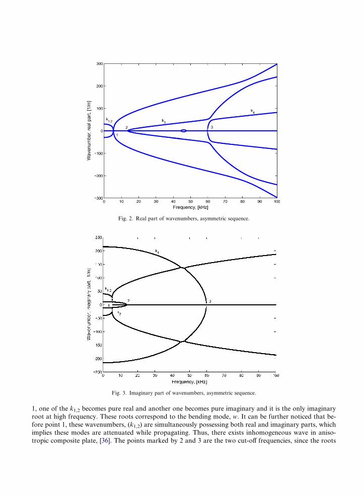
Fig. 2. Real part of wavenumbers, asymmetric sequence.

Fig. 3. Imaginary part of wavenumbers, asymmetric sequence.

1, one of the k1,2 becomes pure real and another one becomes pure imaginary and it is the only imaginary

root at high frequency. These roots correspond to the bending mode, w. It can be further noticed that be-

fore point 1, these wavenumbers, (k1,2) are simultaneously possessing both real and imaginary parts, which

implies these modes are attenuated while propagating. Thus, there exists inhomogeneous wave in aniso-

tropic composite plate, [36]. The points marked by 2 and 3 are the two cut-off frequencies, since the roots

k3 and k4 become real at this point from their imaginary values. These roots correspond to the inplane

motion, i.e., u and v displacements.

The cut-off frequencies can be obtained from Eq. (14) by letting k = 0 and solving for xn.

The governing equation for the cut-off frequency becomes

a0w6n þ a1w4

n þ a2w2n þ a3 ¼ 0; ð16Þ

where ai are material property and wavenumber gm dependent coefficients and are given in Appendix A.

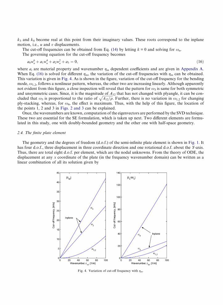
When Eq. (16) is solved for different gm, the variation of the cut-off frequencies with gm can be obtained.

This variation is given in Fig. 4. As is shown in the figure, variation of the cut-off frequency for the bendingmode, x1,2, follows a nonlinear pattern, whereas, the other two are increasing linearly. Although apparently

not evident from this figure, a close inspection will reveal that the pattern for x3 is same for both symmetric

and unsymmetric cases. Since, it is the magnitude of A12 that has not changed with plyangle, it can be con-

cluded that x3 is proportional to the ratio offfiffiffiffiffiffiffiffiffiffiffiffiA12=q

p. Further, there is no variation in x1,2 for changing

ply-stacking, whereas, for x4, the effect is maximum. Thus, with the help of this figure, the location of

the points 1, 2 and 3 in Figs. 2 and 3 can be explained.

Once, the wavenumbers are known, computation of the eigenvectors are performed by the SVD technique.

These two are essential for the SE formulation, which is taken up next. Two different elements are formu-lated in this study, one with doubly-bounded geometry and the other one with half-space geometry.

2.4. The finite plate element

The geometry and the degrees of freedom (d.o.f.) of the semi-infinite plate element is shown in Fig. 1. It

has four d.o.f., three displacement in three coordinate direction and one rotational d.o.f. about the Y-axis.

Thus, there are total eight d.o.f. per element, which are the nodal unknowns. From the theory of ODE, the

displacement at any x coordinate of the plate (in the frequency wavenumber domain) can be written as alinear combination of all its solution given by

Fig. 4. Variation of cut-off frequency with gm.

~u ¼X8i¼1

ai/ie�jkix; ~u ¼ f~u;~v; ~wgT; /i 2 C3�1;

where /is are the elements of the null space of the W, obtained by the SVD method. Also note that,

/ie�jkix; i ¼ 1; . . . ; 8 are the partial waves as discussed in Section 1. The ais are the unknown constants,

which must be expressed in terms of the nodal variables. This step can be viewed as the transformation

from the generalized coordinate to the physical coordinate.

To do so, let us write the displacement field in a matrix-vector multiplication form

~u ¼uðx;xnÞvðx;xnÞwðx;xnÞ

8><>:

9>=>; ¼

/11 � � � /18

/21 � � � /28

/31 � � � /38

264

375

e�jk1x 0 . . . 0

0 e�jk2x . . . 0

..

. . .. . .

. ...

0 . . . . . . e�jk8x

266664

377775fag;

where kp+4 = �kp, (p = 1,. . .,4) and the elements of /i are written as /pi, (p = 1,. . .,3). In concise notation

above equation becomes

f~ugn;m ¼ ½U�n;m½KðxÞ�n;mfagn;m; ð17Þ

where n, m is introduced in the subscript to remind that all these expressions are evaluated at a particular

value of xn and gm. The [K(x)]nm is a diagonal matrix of order 8 · 8 whose ith element is e�jkix . The

[U]n,m = [/1 � � � /8] is also called the amplitude ratio matrix. The an,m is a vector of eight unknown constants

to be determined. These unknown constants are expressed in terms of the nodal displacements by evaluat-

ing Eq. (17) at the two nodes i.e., at x = 0 and x = L. In doing so, we get

fugn;m ¼~u1

~u2

� �n

¼ ½T1�n;mfagn;m; ð18Þ

where ~u1 and ~u2 are the nodal displacements of node 1 and node 2, respectively. The expression for [T1]n,m is

given in Appendix B.

Before advancing, it is to be noted that the element has edges parallel to the Y-axis, hence at the plate

boundary nx = ±1 and ny = 0. These relations are to be utilized in the force–displacement relation. Usingthe force boundary conditions Eqs. (7)–(9), the force vector ffgnm ¼ fNxx;Nyy ; V x;Mxxgn;m can be written

in terms of the unknown constants {a}n,m as {f}n,m = [P]n,m {a}n,m. When the force vector is evaluated at

node 1 and node 2, (substituting nx = ±1) nodal force vectors are obtained and can be related to {a}n,m as

ffgn;m ¼~f1~f2

( )n;m

¼Pð0ÞPðLÞ

� �n;m

fagn;m ¼ ½T2�n;mfagn;m: ð19Þ

Eqs. (18) and (19) together yield the relation between the nodal force and nodal displacement vector at fre-

quency xn and wavenumber gm as

ffgn;m ¼ ½T2�n;m½T1��1

n;mfugn;m ¼ ½K�n;mfugn;m; ð20Þ

where [K]n,m is the dynamic stiffness matrix at frequency xn and wavenumber gm of order 8 · 8. Explicitform of the matrix [T2]n,m is given in Appendix B.

2.5. Semi-infinite or throw-off plate element

For the infinite domain element, only the forward propagating modes are considered. The displacement

field (at frequency xn and wavenumber gm) becomes

f~ugn;m ¼X4m¼1

/me�jkmxam ¼ ½U�n;m½KðxÞ�n;mfagn;m;

where [U]n,m and [K(x)]n,m is now of order 4 · 4. The {a}n,m is a vector of four unknown constants. Eval-

uating above expression at node 1 (x = 0), nodal displacements are related to these constants through the

matrix [T1]n,m as

fugn;m ¼ f~u1gn;m ¼ ½U�n;m½Kð0Þ�n;mfagn;m ¼ ½T1�n;mfagn;m; ð21Þ

where [T1]n,m is now a matrix of dimension 4 · 4. Similarly, the nodal forces at node 1 can be related to theunknown constants as

ffgn;m ¼ f~fgn;m ¼ ½P ð0Þ�nfagn;m ¼ ½T2�n;mfagn;m: ð22Þ

Using Eqs. (21) and (22), nodal forces at node 1 are related to the nodal displacements at node 1 as

ffgn;m ¼ ½T2�n;m½T1��1

n;mfugn;m ¼ ½K�n;mfugn;m; ð23Þ

where [K]n,m is the element dynamic stiffness matrix of dimension 4 · 4 at frequency xn and wavenumber

gm. The [T1]n,m and [T2]n,m are the first 4 · 4 truncated part of the matrices [T1]n,m and [T2]n,m of the finite

plate element.

2.6. Prescription of boundary conditions

Essential boundary conditions are prescribed in the usual way of FE methods, where simply the nodal

displacements are arrested or released depending upon the nature of the boundary conditions. The appliedforces or moments are to be prescribed at the nodes. It is assumed that the forcing function (for symmetric

loading) can be written as

F ðx; y; tÞ ¼ dðx� xjÞXMm¼1

am cosðgmyÞ ! XN�1

n¼0

f neð�jwntÞ

!;

where d denotes the Dirac delta function, xj is the X coordinate of the point where load is applied and the x

dependency is fixed by suitably choosing the node where the load is prescribed. No variation of load along

X direction is allowed in this analysis. The f n are the Fourier transform coefficients of the time dependent

part of the load, which are computed by FFT and the am are the Fourier series coefficients of the y-depen-

dent part of the load.

There are two summations involved in the solution and two associated windows, one in time, T and onein space, LY. The discrete frequencies xn and discrete horizontal wavenumber gm are related to these win-

dows by the number of data N and M chosen in each summation, i.e.

wn ¼ 2np=T ¼ 2np=ðNDtÞ; gm ¼ 2ðm� 1Þp=LY ¼ 2ðm� 1Þp=ðMDxÞ;

where Dt and Dx are the temporal and spatial sample rate, respectively.

3. Numerical examples

The developed spectral element is validated first by comparing its accuracy with conventional 2D plate

FE. ply-angle on the mechanical response is studied. Next, a plate with ply-drop is studied to show the effi-

ciency of the present element in modeling complex and computationally expensive structures. Finally,

Lamb wave propagation in anisotropic plate is captured and effect of axial–flexural coupling on Lamb wave

is demonstrated.

3.1. Verification of the SPE

The same material, Gr.–Ep. (AS/3501), which was taken earlier in the study of wavenumber is taken in

this example. Both symmetric and asymmetric ply-sequences are considered in this study. The plate is 1.0 m

long in Y direction (LY) and 0.3 m in X direction (i.e., the propagation direction). Each laminae is 1 mm

thick and 10 such layers are taken. The beam is fixed at one edge and free at the other edge, where an

impact load is applied both in axial (X) and transverse (Z) direction (see Fig. 5). The load is of unit mag-

nitude and very short duration (150 ls) and has a high frequency content of about 46 kHz. The load pat-

tern, both in time and frequency domain, is shown in Fig. 6.

When the plate is modeled by the developed SPE, only one element is required, which generates a dy-namic stiffness matrix of size [4 · 4]. The load is transformed in frequency domain by the FFT, where

8192 sampling points are used. This large number of FFT points is taken to avoid wrap around problem,

which induces periodicity in the solution and thus, hinders decrement of the wave amplitude at the edge of

time window. This problem is inherent to FFT as finite number of points is used. Although 8192 sample

points are taken, analysis is performed only up to the Nyquist frequency as the time domain data is real.

Hence, the dynamic stiffness matrix is formulated and the system of four equations is solved for 4096 times.

In comparison, the FE model of the plate requires atleast 3000 four noded plate element. This mesh renders

a system size of [18,300 · 312], where 18,300 is the number of equations and 312 is the half-bandwidth. Toget the time history data, the Newmark time integration is adopted with a time increment of 1 ls. The sys-tem matrix is decomposed (LU factorization) at the beginning of the time integration and is back-substi-

tuted at each time step. Thus, to get a time history upto 5000 ls, 500 back substitutions need to be

performed on this large matrix and the requirement of the computational resource is many times larger

than the requirement of the SE analysis.

For symmetric ply sequence, [010], there is no coupling between the axial and bending motions. The load

is first applied in axial direction and axial velocity at the impact point is measured and plotted in Fig. 7

along with the FE response. As the figure suggests the response matches well with the FE solution. Theinitial waveform is the incident pulse, which travels 0.3 m distance and gets reflected and shows up again

at around 160 ls (the inverted peak). Subsequently there are multiple reflections from the free and fixed

end. It is to be noted that the reflected wave from the free end maintains its sign, whereas, in the case of

fixed end sign change occurs. At large time, however, difference between the SPE response and the FE res-

ponse increases, which is due to the approximate nature of the mass distribution in the FE model.

Fig. 5. Model for verification study.

Fig. 6. Load applied to the examples 1–4 (Sections 3.1–3.4).

Fig. 7. Axial velocity for symmetric layup: (solid line) SPE and (dashed line) 2D FEM.

The same load is applied again at the free end in transverse direction and the transverse velocity at the

impact point is measured and plotted in Fig. 8. In this case also, good agreement between SPE and FE

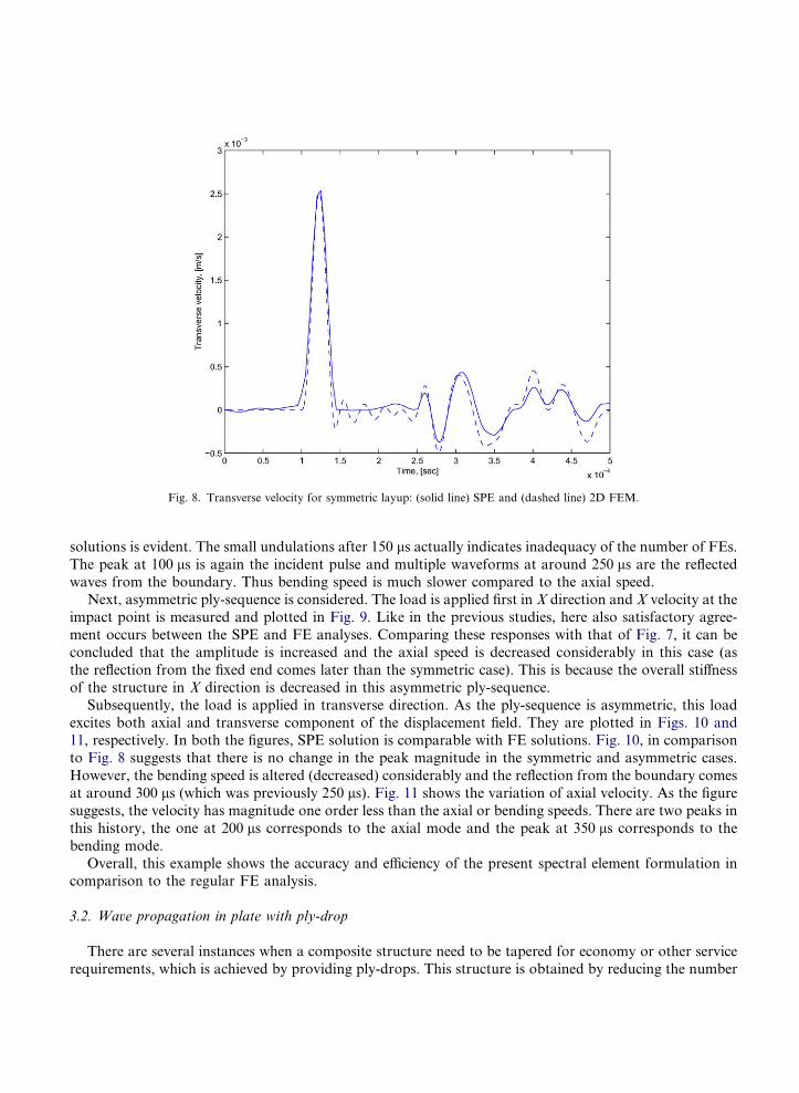
Fig. 8. Transverse velocity for symmetric layup: (solid line) SPE and (dashed line) 2D FEM.

solutions is evident. The small undulations after 150 ls actually indicates inadequacy of the number of FEs.

The peak at 100 ls is again the incident pulse and multiple waveforms at around 250 ls are the reflected

waves from the boundary. Thus bending speed is much slower compared to the axial speed.Next, asymmetric ply-sequence is considered. The load is applied first in X direction and X velocity at the

impact point is measured and plotted in Fig. 9. Like in the previous studies, here also satisfactory agree-

ment occurs between the SPE and FE analyses. Comparing these responses with that of Fig. 7, it can be

concluded that the amplitude is increased and the axial speed is decreased considerably in this case (as

the reflection from the fixed end comes later than the symmetric case). This is because the overall stiffness

of the structure in X direction is decreased in this asymmetric ply-sequence.

Subsequently, the load is applied in transverse direction. As the ply-sequence is asymmetric, this load

excites both axial and transverse component of the displacement field. They are plotted in Figs. 10 and11, respectively. In both the figures, SPE solution is comparable with FE solutions. Fig. 10, in comparison

to Fig. 8 suggests that there is no change in the peak magnitude in the symmetric and asymmetric cases.

However, the bending speed is altered (decreased) considerably and the reflection from the boundary comes

at around 300 ls (which was previously 250 ls). Fig. 11 shows the variation of axial velocity. As the figure

suggests, the velocity has magnitude one order less than the axial or bending speeds. There are two peaks in

this history, the one at 200 ls corresponds to the axial mode and the peak at 350 ls corresponds to the

bending mode.

Overall, this example shows the accuracy and efficiency of the present spectral element formulation incomparison to the regular FE analysis.

3.2. Wave propagation in plate with ply-drop

There are several instances when a composite structure need to be tapered for economy or other service

requirements, which is achieved by providing ply-drops. This structure is obtained by reducing the number

Fig. 9. Axial velocity for asymmetric layup: (solid line) SPE and (dashed line) 2D FEM.

Fig. 10. Transverse velocity for asymmetric layup: (solid line) SPE and (dashed line) 2D FEM 27.

of laminaes at certain intervals, which depend upon the load distribution through the structure. The present

SPE can model this kind of structure easily and thus analysis of ply-dropped plate subjected to impulse

loading is quite viable.

Fig. 11. Axial velocity for asymmetric layup: (solid line) SPE and (dashed line) 2D FEM.

Fig. 12. Plate with ply-drop.

To this end the plate configuration shown in Fig. 12 is taken. The plate is made up of Gr.–Ep. (AS/3501)fibre composites and is 3.0 m long in Y direction and 0.9 m in X direction. It is fixed at one end and free at

the other edge. The material properties are as taken before and each laminae is 1.0 mm thick. The plate is

divided into three regions along X direction. From the fixed end to 0.3 m, there are 10 layers in the plate.

For the next 0.3 m, the plate is having eight laminaes and the last 0.3 m is having six laminaes. The plate is

modeled with three finite SPEs, which results in a system size of 12 · 12.

The plate is impacted at the mid-point of the free end by a concentrated load whose time dependency is

same as taken previously, i.e., as given in Fig. 6. The load is first applied in X direction and the X velocity is

measured at the impact point. The measured velocity history is plotted in Fig. 13. The same structure is alsoanalysed for uniform ply-stacking (10 layers) and the result is superimposed in the same figure. It is evident

from the figure that ply-drop affects the stiffness of the plate considerably, as there is an increment in the

maximum amplitude of about 90%. This reduction of stiffness is also visible in the reflection from the

Fig. 13. Variation of axial velocity: (solid line) plydrop and (dashed line) uniform plate.

boundary. The reflection from the boundary appears at the same instance in both the cases, which indicates

that there is not much alteration in group speed due to ply-drop. However, there are two extra reflections

(inverted peaks at around 175 ls and 240 ls) in the response from the ply-drop plate before the arrival of

the boundary reflection, which are originated at the ply-drop junctions due to mismatch in impedance.

Next, the plate is impacted at the same point in the Z direction and the Z velocity is measured at the

same point. Simultaneously, the response of the uniform plate is also plotted in Fig. 14. As noticed before,there is considerable difference in the peak amplitudes (almost a factor of 2), which follows the same pattern

of axial velocity history. The extra reflections originated at the interfaces are also visible (starting at around

250 ls), which are not present in the uniform plate response. However, there is no deviation in the arrival

time of the boundary reflection, which is denoting the closeness of the bending group speed of in both the

cases.

Overall, this example shows the efficiency of the present element in modeling structures with discontinu-

ity and bringing out the essential dynamic characteristics.

3.3. Propagation of Lamb wave

The final example is the propagation of Lamb wave in a Gr.–Ep. (AS/3501) plate with the same material

properties as taken before. The propagating distance is taken as 2.0 m and to get rid of the boundary reflec-

tions, two throw-off SPEs are used. In between, the finite plate is modeled with four SPEs, which together

with the throw-off elements generate a system size of [16 · 16]. Lamb waves are generated in this plate by

applying a tone burst signal with centre frequency of 50 kHz. Three laminae sequences are considered, one

symmetric, [010], and two asymmetric, [05/455] and [05/905].First the load is applied in X direction and both X and Z velocity histories are plotted in Fig. 15. The

figure shows that the first symmetric (s0) and anti-symmetric (a0) modes are captured by the plate element.

This is expected, since the plate is formulated based on the CLPT. For the symmetric laminate, there is no

Fig. 14. Variation of transverse velocity: (solid line) plydrop and (dashed line) uniform plate.

Fig. 15. Lamb wave due to X-load, profiles are shifted for clarity.

axial bending coupling and the X velocity history shows only the axial mode (s0). However, for increasing

coupling, the bending mode, a0, appears in the X velocity history, as is shown in the left subfigure. The fig-

Fig. 16. Lamb wave due to Z-load, profiles are shifted for clarity.

ure also shows the relative movement of the modes, which clearly shows that the Lamb wave speed is max-

imum for [010] sequence and minimum for [05/905] sequence, for both s0 and a0 modes. The change in the s0mode speed is more between [010] and [05/455] case, compared to the change between [05/455] and [05/905]

case. For transverse velocity history (plotted in the right subfigure), as expected, there is no response for

symmetric ply-sequence (since there is no coupling). However, for asymmetric lay-up, both the bending

and stretching modes are present. Further, variation of the group speed for a0 mode (shown by the move-ment of the a0 blobs) is easily detectable for varying asymmetry.

Next the load is applied in Z direction and both X and Z velocity histories are plotted in Fig. 16. The left

subfigure shows the variation of X velocity. Again in this case, symmetric laminate generates no axial res-

ponse, which starts coming only for asymmetric ply-sequences. As the figure suggests, for asymmetric lay-

up, energy is concentrated more in s0 mode (higher amplitude). Also, the group speed variation is nominal

for s0 mode, whereas, detectable variation can be observed for the a0 mode. The right subfigure shows the

variation of the Z velocity. As is seen in the figure, symmetric laminates are devoid of s0 mode, which shows

up only at the asymmetric ply-stacking. The wave energy is now concentrated more in the bending mode(a0), as the relatively large amplitude suggests.

This example shows the possible application of the present SPE for modeling and simulation of Lamb

wave propagation in composite laminate.

4. Conclusion

A spectral element is developed by exactly solving the governing partial differential equations of CLPTin frequency–wavenumber domain. The element is formulated using robust algorithms of SVD and PEP,

which minimize human intervention and reduce the possibility of human error. The variation of wavenum-

ber is obtained which reveals the inhomogeneous nature of the propagating wave in CLPT. The element

efficiently captures the wave solution of layered anisotropic plate subjected to impact loading. The cost of

computation is many order less than what any conventional FE analysis incurs. The element is used to

model complex structures like folded plate and plate with ply-drop, where the responses are capturing

the essential features of the propagating wave. Effect of ply-sequence is demonstrated in the simple plate

and folded plate structure. Lamb waves are captured and variation of the first symmetric and anti-symmet-ric modes with laminae sequence is demonstrated.

Appendix A

The matrices, A‘ in Eq. (13) are

A0 ¼�A66g2m þ I0w2

n 0 0

0 �A22g2m þ I0w2n �B22g3m þ I1w2

ngm0 �B22g3m þ I1w2

ngm �D22g4m þ I0w2n þ I2w2

ng2m

264

375;

A1 ¼0 �jgmðA12 þ A66Þ �jg2mðB12 þ 2B66Þ þ jI1w2

n

jgmðA12 þ A66Þ 0 0

jg2mðB12 þ 2B66Þ � jI1w2n 0 0

264

375;

A2 ¼�A11 0 0

0 �A66 �gmðB12 þ 2B66Þ0 �gmðB12 þ 2B66Þ �g2mð2D12 þ 4D66Þ þ I2w2

n

264

375;

A3 ¼0 0 �jB11

0 0 0

jB11 0 0

264

375;

A4 ¼0 0 0

0 0 0

0 0 �D11

264

375:

The coefficients in Eq. (16) (g = gm) are

a0 ¼ I20I2g2 þ I30 � I0I21I2;

a1 ¼ �I20D22g4 � I20ðA22 þ A66Þg2 � I0I2g4ðA66 þ A22Þ þ A66g

4I21 þ 2I0B22g4I1;

a2 ¼ �I0B222g

6 þ A66g4A22I0 þ A66g

6I0D22 � 2A66g6B22I1 þ I0A22g

6D22 þ A66g6A22I2;

a3 ¼ A66g8ð�A22D22 þ B2

22Þ:

Appendix B

The matrix [T1]n,m in Eq. (18) is given as

T 1ðm; nÞ ¼ Uðm; nÞ; m ¼ 1; . . . ; 3; n ¼ 1; . . . ; 8

T 1ðm; nÞ ¼ �jkpUðm� 4; pÞe�jknL; m ¼ 5; . . . ; 7; n ¼ 1; . . . ; 8

T 1ð4; nÞ ¼ �jknUð3; nÞ; n ¼ 1; . . . ; 8

T 1ð8; nÞ ¼ �jknUð7; nÞ; n ¼ 1; . . . ; 8

The matrix [T2]n,m in Eq. (18) is given as (n = 1, . . ., 8)

T 2ð1; nÞ ¼ jknA11Uð1; nÞ � gA12Uð2; nÞ � k2nB11Uð3; nÞ � g2B12Uð3; nÞ;T 2ð2; nÞ ¼ gA66Uð1; nÞ þ jknA66Uð2; nÞ þ 2jB66kngUð3; nÞ;T 2ð3; nÞ ¼ k2nB11Uð1; nÞ þ jB12kngUð2; nÞ þ jk3nD11Uð3; nÞ þ jD12kng2Uð3; nÞ;þ2g2B66Uð1; nÞ

þ 2jkngB66Uð2; nÞ þ 4jkng2D66Uð3; nÞT 2ð4; nÞ ¼ �jknB11Uð1; nÞ þ gB12Uð2; nÞ þ k2nD11Uð3; nÞ þ g2D12Uð3; nÞT 2ðm; nÞ ¼ �T 2ðm� 4; nÞe�jknL; m ¼ 5; . . . ; 8:

References

[1] A. Arias, R. Zaera, J. Lopez-Puente, C. Navarro, Numerical modeling of the impact behavior of new particulate-loaded

composite materials, Compos. Struct. 61 (2003) 151–159.

[2] R. Olsson, Closed form prediction of peak load and delamination onset under small mass impact, Compos. Struct. 59 (2003) 341–

349.

[3] Z. Aslan, R. Karakuzu, B. Okutan, The response of laminated composite plates under low-velocity impact loading, Compos.

Struct. 59 (2003) 119–127.

[4] F. Mili, B. Necib, Impact behavior of cross-ply laminated composite plates under low velocities, Compos. Struct. 51 (2001) 237–

244.

[5] Y. Wang, K. Lam, G. Liu, The effect of rotary inertia on the dynamic response of laminated composite plate, Compos. Struct. 48

(2000) 265–273.

[6] J. Lee, Plate waves in multi-directional composite laminates, Compos. Struct. 46 (1999) 289–297.

[7] A. Christoforou, A.S. Yigit, Characterization of impact in composite plates, Compos. Struct. 43 (1998) 15–24.

[8] A.N. Danial, J.F. Doyle, S.A. Rizzi, Dynamic analysis of folded plate structures, J. Vibrat. Acoust. 118 (4) (1996) 591–598.

[9] A.N. Danial, J.F. Doyle, Dynamic analysis of folded plate structures on a massively parallel computer, Comput. Struct. 54 (3)

(1995) 521–529.

[10] A.N. Danial, J.F. Doyle, Massively parallel implementation of the spectral element method for impact problems in plate

structures, Comput. Syst. Eng. 5 (4–6) (1994) 375–388.

[11] S. Lee, S. Wooh, S. Yhim, Dynamic behavior of folded composite plates analyzed by the third-order plate theory, Int. J. Solid.

Struct. 41 (2004) 1879–1892.

[12] A. Mal, S. Lih, Elastodynamic response of a unidirectional composite laminate to concentrated surface loads: Part i, J. Appl.

Mech. 59 (1992) 878–886.

[13] A. Mal, S. Lih. Elastodynamic response of a unidirectional composite laminate to concentrated surface loads: Part ii, J. Appl.

Mech. 59 (1992) 887–892.

[14] S. Lih, A. Mal, On the accuracy of approximate plate theories for wave field calculation in composite laminates, Wave Motion 21

(1995) 17–34.

[15] S. Lih, A. Mal, Response of multilayered composites to dynamic surface loads, Composites B 29B (1996) 633–641.

[16] A. Mal, Elastic waves from localized sources in composite laminates, Int. J. Solid Struct. 39 (21–22) (2002) 5481–5494.

[17] C. Ma, K. Huang, Wave propagation in layered elastic media for antiplane deformation, Int. J. Solid Struct. 32 (5) (1995) 665–

678.

[18] C. Chatfield, The Analysis of Time Series, Chapman and Hall, London, 1984.

[19] J.F. Doyle, Wave Propagation in Structures, Springer, Berlin, 1997.

[20] S.A. Rizzi, A spectral analysis approach to wave propagation in layered solids, Ph.D. Dissertation Purdue University.

[21] S.A. Rizzi, J. Doyle, Force identification for impact problem on a half plane, Computational Techniques for Contact, Impact,

Penetration and Perforation of Solids 103 (1989) 163–182.

[22] S.A. Rizzi, J. Doyle, Force identification for impact of a layered system, Comput. Aspects Contact, Impact Penetrat., Elmepress

Int. (1991) 222–241.

[23] A. Chakraborty, S. Gopalakrishnan, A spectrally formulated finite element for wave propagation analysis in layered composite

media, Int. J. Solid Struct. 41 (18) (2004) 5155–5183.

[24] A. Chakraborty, S. Gopalakrishnan, Wave propagation in inhomogeneous layered media: Solution of forward and inverse

problems, Acta Mech. 169 (1–4) (2004) 153–185.

[25] L. Solie, B. Auld, Elastic waves in free anisotropic plates, J. Acoust. Soc. Am. 54 (1) (1973).

[26] A. Stroh, Dislocations and cracks in anisotropic elasticity, Philos. Mag. 7 (1958) 625–646.

[27] T. Ting, Anisotropic Elasticity: Theory and Applications, Oxford University Press, New York, 1996.

[28] T. Ting, A unified formalism for elastostatics or steady state motion of compressible or incompressible anisotropic elastic material,

Int. J. Solid Struct. 39 (2002) 5427–5445.

[29] C. Hwu, Stroh-like formalism for the coupled stretching–bending analysis of composite laminates, Int. J. Solid Struct. 40 (2003)

3681–3705.

[30] J. Reddy, Mechanics of Laminated Plates, CRC Press, Boca Raton, FL, 1997.

[31] P. Lancaster, Theory of Matrices, Academic Press, New York, 1969.

[32] F. Tisseur, N.J. Higham, Structured pseudospectra for polynomial eigenvalue problems, with applications, SIAM J. Matrix Anal.

Appl. 23 (1) (2001) 187–208.

[33] D.R. Mahapatra, S. Gopalakrishnan, A spectral finite element for analysis of wave propagation in uniform composite tubes, J.

Sound Vibrat. 268 (3) (2003) 429–463.

[34] P. Lancaster, Lambda Matrices and Vibrating Systems, Pergamon Press, Oxford, 1966.

[35] G. Golub, C.V. Loan, Matrix Computation, The John Hopkins University Press, 1989.

[36] G. Caviglia, A. Morro, Inhomogeneous Waves in Solids and Fluids, World Scientific Press, Singapore, 1992.