Statistical adaptive sensing by detectors with spectrallyoverlapping bands

Ünal Sakoglu, Majeed M. Hayat, J. Scott Tyo, Philip Dowd, Senthil Annamalai, Kalyan T. Posani,and Sanjay Krishna

It has recently been reported that by using a spectral-tuning algorithm, the photocurrents of multipledetectors with spectrally overlapping responsivities can be optimally combined to synthesize, withincertain limits, the response of a detector with an arbitrary responsivity. However, it is known that thepresence of noise in the photocurrent can degrade the performance of this algorithm significantly,depending on the choice of the responsivity spectrum to be synthesized. We generalize this algorithm toaccommodate noise. The results are applied to quantum-dot mid-infrared detectors with bias-dependentspectral responses. Simulation and experiment are used to show the ability of the algorithm to reduce theadverse effect of noise on its spectral-tuning capability. © 2006 Optical Society of America

OCIS codes: 040.0040, 040.3060, 040.5570, 020.6580, 160.6000, 280.0280.

1. Introduction

Modern hyperspectral sensor systems, such as theAirborne Visible�Infrared Imaging Spectrometer(AVIRIS) or Hyperspectral Digital Imaging CollectionExperiment (HYDICE), are capable of sensing thespectrum of a source in upwards of 200 bands of width10–20 nm.1–3 These systems are sophisticated andcostly; they either use a dispersive optic element tospread the spectral content for each pixel to multipleline arrays3 or use interferometric techniques thatinvolve computation of the interference pattern andFourier transform to obtain the spectral content.4–8

In these systems, the spectrum or the interferogramcorresponding to each pixel is captured on a singlecolumn of the array, leaving only one dimension ofthe array for gathering the spatial information. Multi-spectral systems, such as the Multispectral ThermalImager,9 are different from hyperspectral systems inthat they use much fewer but wider bands, whichresults in reduced spectral resolution. However, mul-

tispectral sensing systems are simpler and easier torealize than hyperspectral sensing systems, as theyrequire far less sophisticated optical front ends.

A key characteristic common to existing hyperspec-tral and multispectral sensors is that they cannotoffer spectral resolutions below the resolution of theirbands, which is a consequence of the spectrally non-overlapping nature of the bands. On the other hand,multispectral detectors often have much wider re-sponsivities than the desired resolution. Nonetheless,one can extract higher spectral resolution informa-tion from multiple detectors provided that the detec-tors exhibit spectrally overlapping responsivities.10

Indeed, the use of spectral overlap in detectors toextract higher spectral resolution information is seenin nature. For example, the human eye uses overlap-ping spectral bands of three (in some cases four) dif-ferent kinds of cone cells to sense color. Also, it hasbeen shown that the use of overlapping spectral fil-tering in technology can improve performance ofspectral sensing systems.11

An example of a class of detectors that can be uti-lized to produce spectrally overlapping bands is asubclass of the quantum-dot infrared photodetector(QDIP).12–15 A QDIP may display a bias-dependentspectral responsivity due to the quantum-confinedStark effect, which is caused by an asymmetric po-tential profile. As the operating bias is varied, theresponsivity changes by exhibiting a shift in its peakand, to a lesser extent, a variation in its shape. Forthis type of QDIP, a single detector can be operated atmultiple biases sequentially, whereby the detector’s

U. Sakoglu (sakoglu@ece.unm.edu), M. M. Hayat, and J. S. Tyoare with the Department of Electrical and Computer Engineering,University of New Mexico, Albuquerque, New Mexico 87131. P.Dowd, S. Annamalai, K. T. Posani, and S. Krishna are with theCenter for High Technology Materials and Department of Electri-cal and Computer Engineering, University of New Mexico, Albu-querque, New Mexico 87131.

Received 13 January 2006; revised 17 May 2006; accepted 17May 2006; posted 17 May 2006 (Doc. ID 67214).

0003-6935/06/287224-11$15.00/0© 2006 Optical Society of America

7224 APPLIED OPTICS � Vol. 45, No. 28 � 1 October 2006

responsivity changes each time the bias is varied.Therefore, a single QDIP can be exploited as differentdetectors.

Recently, Sakoglu et al.10 reported a postprocessingalgorithm that exploits the spectral overlap in mul-tiple detectors in QDIPs to perform spectral sensingin the range of 3–8 �m with a resolution down to0.50 �m, which is one fourth of the spectral resolu-tion of the detector. It has also been shown theoreti-cally that this technique is capable of performingsome level of multispectral sensing.10,16 The idea ofthe algorithm can be described as follows. Supposethat we operate the detector at K different biases andassume that for the kth bias the detector responsivityis Rk��� �A�W�. Now suppose that we are interested incombining the outputs of the detectors at variousbiases so as to mimic the response of a desired spec-tral filter, or band, which we denote by rc���. The firststep of the algorithm is to form a weighted superpo-sition of K responsivities to optimally approximatethe multispectral band represented by rc��� (in theminimum mean-square sense). Then, by exploitingthe linearity of the detector, these very weights canbe used to form a weighted sum of the individualphotocurrents from the detector, one for each operat-ing bias. The resulting superposition would yield thebest approximation of the output of the sought-afterband represented by rc���. Synthesized responsivitiesobtained in this fashion can be continuously varied,within certain limits, in shape (unimodal or multimo-dal), width (narrowband or wideband), and location,depending on the requirements of each application.In other words, continuous spectral tuning is ob-tained.10

On the basis of the spectral overlap and diversity ofQDIPs, approaches that use principal componentsanalysis and canonical correlation analysis have beendeveloped to study the performance of sensing.17–22

The detectors’ responsivities, which are functions ofwavelength, are transformed into an uncorrelatedfunction space. Since the spectra are practically sam-pled in wavelength, they have viewed sensing as aninner product between the sampled scene spectrumvector and the detector responsivity vector. Theyhave transformed the vectors into an uncorrelatedvector space in which the detectors’ responsivities aredecorrelated, and only the principal contributers arechosen to be used in sensing. Then, inner productoutputs for each transformed detector constitute anew space. They have shown that sensing in this newspace can give comparable results with a reduceddata set. The new responsivities in the transformedspace can still be overlapping in wavelength. In thiswork, however, instead of projecting the detectors’responsivities onto an uncorrelated space, we are in-terested in projecting them onto a new responsivityspace that has certain properties: It is desired thatthe new responsivity functions have a certain centerwavelength and certain resolution, as well as a cer-tain shape. These properties might be wanted forcertain applications in which the spectral informa-tion from certain bands is desired.

From a practical standpoint, however, the successof the aforementioned postprocessing-based tunablesensing strategy depends upon the level of noise in themeasured current, which is attributable to dark cur-rent and the associated generation–recombination(shot) noise.23–25 Since the algorithm is based on form-ing a weighted sum of photocurrents (usually withpositive and negative signs), the noise variances cor-responding to each weighted photocurrent accumu-late, resulting in approximation error and poor signal-to-noise ratio (SNR).16 Moreover, the effect of noise onthe performance is shown to vary with the spectralwidth of the desired responsivity. In particular, as thefull width at half-maximum (FWHM) of the desiredresponsivity decreases, the degradation due to noiseeffect becomes more severe. Intuitively, this is becausethe magnitudes of the weights needed to approximatea narrow responsivity become large and the noise ac-cumulation becomes more pronounced; more specifi-cally, the ratio of the sum of weights to the sum of theirabsolute values approachs zero. Therefore, there is afundamental trade-off between the spectral resolutionsought by the spectral-tuning algorithm and the noise-induced error.

In this paper we derive a generalization of thespectral-tuning algorithm10,16 reported earlier to ac-commodate noise in the photocurrent. More gener-ally, this work provides a framework for using acollection of sensors that have overlapping bands anddifferent noise characteristics to synthesize outputscorresponding to a desired arbitrary band. The theoryis applied to mid-infrared QDIPs fabricated by ourgroup.

2. Theory

A. Photocurrent Model

The total current produced by a detector (labeled byk) can generally be written as

Yk � yp,k � dk � Nk, (1)

where Nk is the total noise (comprising one or more ofthe following components depending on the operatingconditions: generation–recombination noise, signal-induced shot noise, Johnson noise, 1�f noise, etc.), dk

is the dark current representing the dc component ofthe current in the absence of illumination, and yp,k isthe true photocurrent resulting from illumination.Both the dark current and the noise statistics aredependent upon temperature, the type of detector, aswell as the operating bias of the detector. However,the noise components are assumed to be statisticallyindependent from detector to detector. We denote themean and variance of the noise by �N,k and �N,k

2 re-spectively. Moreover, we define the measurementSNR as the ratio of the photocurrent to the standarddeviation of the noise,

SNRk –yp,k

�N,k. (2)

1 October 2006 � Vol. 45, No. 28 � APPLIED OPTICS 7225

For a linear detector, the relationship among thedetector’s spectral response, the source spectrum,and the photocurrent can be cast as

yp,k � Ae��min

�max

Rk���g��, Z�d�, (3)

where g��, Z� �W cm�2 �m�1� is the spectral irradi-ance of the source (combined with any other filtersand�or effects in the scene) at temperature Z (kelvin)and Ae is the effective source-to-detector area thatcombines all the coupling factors. For simplicity weassume that Ae does not vary from detector to detec-tor. For the sake of the analysis to follow, it would beconvenient to embed the noise into the integral aboveand obtain an equivalent expression for the noisyphotocurrent. By using Eqs. (2) and (3), we can write

Yp,k – yp,k � Nk

�Ae��min

�max

�Rk��� �Nk

Ae��min

�max

g���, Z�d��� g��, Z�d�,

(4)

�Ae��min

�max

�Rk��� �Rk���Nk

Ae��min

�max

Rk����g���, Z�d���� g��, Z�d�, (5)

�Ae��min

�max

Rk����1 �Nk

�N,kSNRkg��, Z�d�. (6)

In Eq. (6), we can identify the noisy responsivity as

Rk��� – Rk����1 �Nk

�N,kSNRk. (7)

We introduce the approximation in Eq. (5) to get ridof the dependence on source irradiance, g��, Z�, i.e., tomake the algorithm source independent, since thegoal of the algorithm is to sense the source irradiance.This approximation turns into an equality when thevariation in Rk��� is negligible over the integrationrange. However, in that case it would not serve ouralgorithm since there would not be any spectral di-versity.

The above approximation can be equivalentlyrestated as Rk�����min

�max g����d�' � �min

�max Rk����g����d��.From the first mean value theorem for integration,we know that at least one � satisfies equality in theapproximation. The theorem states that if R���� :��min, �max� → � is continuous and g���� : ��min, �max�→ � is a integrable positive function, then there

exists a number � in ��min, �max� such that�

�min�max Rk����g����d�� � Rk������min

�max g����d��. Moreover,since the detectors’ responses are close to 0 near �minand �max, and have peak(s) in between, there exist atleast two � values for which the equality holds sincethis condition leads to the existance of a set of� � �1, �2, . . .� such that Rk��1� � Rk��2� � . . .�.Furthermore, due to nature of our spectral-tuningalgorithm, which combines (with positive and nega-tive weights) the detectors’ spectral response, the as-sociated approximation error also gets averaged.Thus, when we compare the spectral-tuning results ofthe original and the noise-modified algorithm, we seethat this approximation does not seem to affect thenoise-modified algorithm so badly as to make itworse, as we present in Section 3.

B. Algorithm Development

As described in Section 1, the goal of the algorithm isto synthesize the photocurrent response of an arbi-trary desired responsivity, rc��� associated with cen-ter wavelength �c, by utilizing the outputs of multipledetectors with spectrally overlapping responsivities.The shape and width of rc��� and the location of thefilter centers, �c �c � 1, . . . , C�, all depend on theapplication. Let us assume that we have a collectionof K detectors, � � D1, . . . , DK�, each having spec-tral responsivity Rk���, k � 1, . . . , K. By combiningthe detector-dependent responsivities Rk���, thedesired responsivity rc��� can be approximatedlinearly as

rc��� � �k�1

K

wc,kRk���. (8)

Our goal is to find the set of weights, wc –�wc,1, . . . , wc,K�T, so that we can best approximate theideal response

yc � Ae��min

�max

g��, Z�rc���d� (9)

by means of the synthesized response Yc �

�k�1K wk,cYp,k. It has been shown10 that in the absence

of noise, the best approximate response Yc, in theminimum mean-square error sense, is equivalent tothe response of the detector whose spectral responseis rc��� � �k�1

K wc,kRk��� that best approximates thedesired rc���, in which case

Yc � Ae��min

�max

g��, Z���k�1

K

wc,kRk����d�. (10)

We now incorporate noise into the algorithm byseeking the vector wc that minimizes the averageof the mean-square error �2�rc, �� – E�yc � Yc2�,where E denotes ensemble averaging. By substitutingEqs. (9) and (10) in this definition, we obtain

7226 APPLIED OPTICS � Vol. 45, No. 28 � 1 October 2006

�2�rc, �� � E��Ae��min

�max

g��, Z��rc��� � �k�1

K

wc,kRk���

� �1 �Nk

�N,kSNRk�d��2�. (11)

To remove the dependence of the error expression onthe spectral irradiance g���, we compute an upperbound to this expression using the Schwarz inequal-ity.26 We assume that the noise Nk has zero mean forall detectors and that noise for different detectors isindependent. We then discretize the integral and con-vert Eq. (11) into matrix form (see Appendix A for adetailed derivation) and obtain the expression to beminimized as

�

L �j�1

L �rc2��j� � 2rc��j���

k�1

K

wc,kRk��j��� ��

k�1

K

wc,kRk��j��2

���k�1

K

wc,k2

Rk2��j�

SNRk2��. (12)

In the above, L is the number of wavelength loca-tions at which the spectrum was sampled, �1 ��min, �L � �max, and � � �max � �min. Defining thevector forms of the discretized spectrum as Rk –�Rk��1�, . . . , Rk��L��T and rc – �rc��1�, . . . , rc��L��T,and the matrix of spectral response A –�R1, . . . , RK�, the weight vector that minimizes thediscretized mean-square error is found to be (seeAppendix A for derivation)

wc � �ATA � ���1�c, (13)

where

��

R1

TR1

SNR12

0 . . . 0

0R2

TR2

SNR22

. . . 0

É É Ì É

0 0 . . .RK

TRK

SNRK2

, (14)

�c � ATrc. (15)

It can be seen from expression (12) that in theabsence of noise, the minimization problem reducesto the minimization of the error in the approximationof the filter rc��� (or equivalently rc). However, suchminimization can produce a solution that is highlyfluctuating as a function of �; therefore, it is desirableto include a regularization term that penalizes non-smoothness in the approximation.10 As such, we in-clude a regularization term, ��QAwc�

2, in the mean-square error, so that the regularized version of

expression (12) becomes

�L�1��rc � Awc�2 � wc

T�wc � ��QAwc�2�, (16)

where Q is a regularization matrix (typically a high-pass filter). As in our earlier work, we take

Q � �1 �1

�1 2 �1Ì

�1 2 �1�1 1

�, (17)

which is the Laplacian operator, and � is the corre-sponding weight for the penalization term and can beadjusted according to the desired level of roughnesspenalization.10 (In our applications, � � 0.04 gavegood results.) We finally obtain an expression for theweights that minimize expression (16):

wc � �ATA � � � �QTATAQ��1�c. (18)

A flow chart summarizing the entire algorithm isshown in Fig. 1.

3. Application to Quantum-dot Infrared Detectors

In this section we apply the noise-modified spectral-tuning algorithm developed in Subsection 2.B toQDIPs that have been recently fabricated and char-acterized at the Center for High Technology Materi-als at the University of New Mexico. The QDIP deviceused in our application has an asymmetric dots-in-a-well (DWELL) structure, sandwiched between highly

Fig. 1. Flow chart of the entire noise-modified spectral-tuningalgorithm.

1 October 2006 � Vol. 45, No. 28 � APPLIED OPTICS 7227

n-doped GaAs layers and grown on a semi-insulatingGaAs substrate. A simple schematic of the device isshown in Fig. 2. The active region of the detectorconsists of 15 layers of InAs quantum dots in anIn0.15Ga0.85As well.27 The well is asymmetric in thesense that the width of the top and bottom well layersare different (60 and 50 Å), which leads to photore-sponsivities that can be spectrally tuned by changingthe applied bias voltage. The width of the quantum-dot layer is only 5–8 Å, and the total thickness of thedetector is �3.5 �m. Devices with different diameterapertures, ranging from 25 to 300 �m, were fabri-cated on a 6-by-6 array. Data from a 300 �m diame-ter aperture detector were chosen for our application.This was done due to the large aperture area, whichyields a large photocurrent.

A. Experiment and Measurement Process

The spectral response of the QDIP was measured ata temperature of 50 K by using a Fourier-transforminfrared spectrometer and was averaged over 64measurements for each bias voltage, �V1, . . . , V17�� �4, 3.75, . . . , 2, �1.75, �2.25, . . . , �3.5� V. Theset of responses was obtained in a wavenumber do-main ranging from 500 to 5000 cm�1, correspondingto 2–20 �m. The responses were resampled to fit in alinear wavelength grid, with 0.01 �m intervals in therange of 2.51–11.00 �m. The parameters L and �,used in the algorithm, are therefore 850 and 8.5 �m,respectively. The spectral response was also normal-ized so that the peak value is equal to unity, and theresulting peak-normalized spectral responses, de-noted by fk���, were obtained. The average total cur-rent yk and average dark current dk of the detector forthe same set of voltages were also measured. Theaverage photocurrents yp,k were then computed bytaking the difference between the measured total cur-rent and the dark current, under unfiltered black-body source illumination. In total, 30 and 110measurements were used for the average total anddark-current response, respectively. The standarddeviation of the current noise �N,k was also estimatedempirically from the dark-current measurements.

Next, the bias-dependent peak responsivity Rkp of

the device was calculated by using the relation28,29

yp,k � Ae��min

�max

Rkpfk���g��, Z�d�. (19)

In our devices, the effective source-to-detector areawas found to be Ae � 10�6 cm2. The responsivity of thedetector can now be obtained by multiplying the peakresponsivity with the peak-normalized spectral re-sponse

Rk��� � Rkpfk���. (20)

We define the transmittance of the source-to-detector optical system, or the relative spectrum(with respect to a blackbody source), as

G��, Z� �g��, Z�W��, Z�

, (21)

where W��, Z� � �2 hc2��5���exp�hc��kBZ� � 1��W cm�2 �m�1� is the blackbody spectral density de-termined by Planck’s law at the source temperature Z(h is Planck’s constant, kB is the Boltzmann constant,and c is the speed of light). One can pick either g���,the total irradiance, or G���, the transmittance, asthe spectrum to be reconstructed, since one can becalculated from the other (as long as the source tem-perature is known). In our application, we considertwo cases: (1) placing no filter in front of the detectorso that G��� � 1, or equivalently g��, Z� is the black-body irradiance at the temperature Z; and (2) placinga 3 mm polystyrene filter in front of the detector sothat G��� is the transmittance of the filter. In ourexperiment, the blackbody source incident on the de-tector was at room temperature �300 K�.

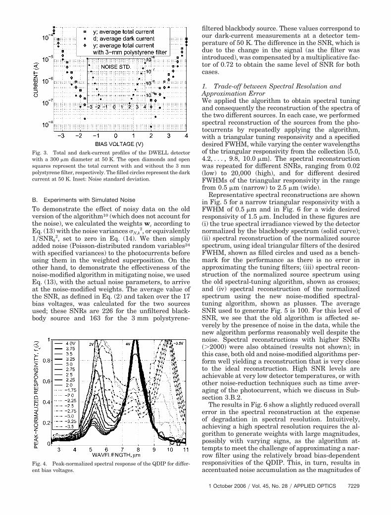
The bias-dependent total current profile, yk, k �1, . . . , K � 17, with and without the 3 mm polysty-rene filter in the view of the detector and the dark-current profile, dk, and its standard deviation are allshown in Fig. 3. These were measured at the detectortemperature of 50 K. The peak-normalized spectralresponses of the device, fk���, measured at the sametemperature for the prescribed set of bias voltages,are shown in Fig. 4. It can be seen in Fig. 4 that, as thebias voltage is varied, the shape of the spectral re-sponse changes, by means of the change in the heightof dominant and secondary peaks. Also note that theFWHM of the main peaks of the response change from1.5 �m (at 4 V) to 2 �m (at �2 V). The narrower theFWHM of the responsivities, the better the algorithmcan approximate narrower responsivities rc.

For the devices considered, much of the range ofthe spectral tuning lays in the atmospheric absorb-tion region; however, we will ignore this limitation inthis paper since our focus is to prove the concept ofalgorithmic spectral tuning. We have recently dem-onstrated QDIPs with peaks of the bias-dependentspectral responses spanning the range 8–12 �m.

Fig. 2. Schematic of the 15-layer asymmetric InAs�In0.15Ga0.85AsDWELL detector structure sandwiched between two highly dopedn-GaAs contact layers, grown on a semi-insulating GaAs sub-strate.27

7228 APPLIED OPTICS � Vol. 45, No. 28 � 1 October 2006

B. Experiments with Simulated Noise

To demonstrate the effect of noisy data on the oldversion of the algorithm10 (which does not account forthe noise), we calculated the weights wc according toEq. (13) with the noise variances �N,k

2, or equivalently1�SNRk

2, set to zero in Eq. (14). We then simplyadded noise (Poisson-distributed random variables24

with specified variances) to the photocurrents beforeusing them in the weighted superposition. On theother hand, to demonstrate the effectiveness of thenoise-modified algorithm in mitigating noise, we usedEq. (13), with the actual noise parameters, to arriveat the noise-modified weights. The average value ofthe SNR, as defined in Eq. (2) and taken over the 17bias voltages, was calculated for the two sourcesused; these SNRs are 226 for the unfiltered black-body source and 163 for the 3 mm polystyrene-

filtered blackbody source. These values correspond toour dark-current measurements at a detector tem-perature of 50 K. The difference in the SNR, which isdue to the change in the signal (as the filter wasintroduced), was compensated by a multiplicative fac-tor of 0.72 to obtain the same level of SNR for bothcases.

1. Trade-off between Spectral Resolution andApproximation ErrorWe applied the algorithm to obtain spectral tuningand consequently the reconstruction of the spectra ofthe two different sources. In each case, we performedspectral reconstruction of the sources from the pho-tocurrents by repeatedly applying the algorithm,with a triangular tuning responsivity and a specifieddesired FWHM, while varying the center wavelengthsof the triangular responsivity from the collection {5.0,4.2, . . . , 9.8, 10.0 �m}. The spectral reconstructionwas repeated for different SNRs, ranging from 0.02(low) to 20,000 (high), and for different desiredFWHMs of the triangular responsivity in the rangefrom 0.5 �m (narrow) to 2.5 �m (wide).

Representative spectral reconstructions are shownin Fig. 5 for a narrow triangular responsivity with aFWHM of 0.5 �m and in Fig. 6 for a wide desiredresponsivity of 1.5 �m. Included in these figures are(i) the true spectral irradiance viewed by the detectornormalized by the blackbody spectrum (solid curve);(ii) spectral reconstruction of the normalized sourcespectrum, using ideal triangular filters of the desiredFWHM, shown as filled circles and used as a bench-mark for the performance as there is no error inapproximating the tuning filters; (iii) spectral recon-struction of the normalized source spectrum usingthe old spectral-tuning algorithm, shown as crosses;and (iv) spectral reconstruction of the normalizedspectrum using the new noise-modified spectral-tuning algorithm, shown as plusses. The averageSNR used to generate Fig. 5 is 100. For this level ofSNR, we see that the old algorithm is affected se-verely by the presence of noise in the data, while thenew algorithm performs reasonably well despite thenoise. Spectral reconstructions with higher SNRs��2000� were also obtained (results not shown); inthis case, both old and noise-modified algorithms per-form well yielding a reconstruction that is very closeto the ideal reconstruction. High SNR levels areachievable at very low detector temperatures, or withother noise-reduction techniques such as time aver-aging of the photocurrent, which we discuss in Sub-section 3.B.2.

The results in Fig. 6 show a slightly reduced overallerror in the spectral reconstruction at the expenseof degradation in spectral resolution. Intuitively,achieving a high spectral resolution requires the al-gorithm to generate weights with large magnitudes,possibly with varying signs, as the algorithm at-tempts to meet the challenge of approximating a nar-row filter using the relatively broad bias-dependentresponsivities of the QDIP. This, in turn, results inaccentuated noise accumulation as the magnitudes of

Fig. 3. Total and dark-current profiles of the DWELL detectorwith a 300 �m diameter at 50 K. The open diamonds and opensquares represent the total current with and without the 3 mmpolystyrene filter, respectively. The filled circles represent the darkcurrent at 50 K. Inset: Noise standard deviation.

Fig. 4. Peak-normalized spectral response of the QDIP for differ-ent bias voltages.

1 October 2006 � Vol. 45, No. 28 � APPLIED OPTICS 7229

the weights increase. Thus, there is a fundamentaltrade-off between synthesized spectral resolution androbustness to noise. Indeed, calculations confirm thatthere is a strong trend of increase in the sum ofabsolute values of the weights (over all bias voltages)as the desired FWHM is decreased. For example, inthe case of the old algorithm with a triangular filtercentered at �c � 6.0 �m, the sum of absolute values ofthe weights takes the values of 55,751, 62,666, and246,340 for FWHM values of 2.5, 1.5, and 0.5 �m,respectively, which directly translates to an increasein noise accumulation in the weighted superpositionas the FWHM is reduced. In contrast, the noise-modified algorithm shows a similar trend in the mag-

nitudes of the weights only at high photocurrentSNRs ��200�, but the trend weakens and eventuallydisappears as the SNR decreases. For example, for anSNR value of 0.2, the noise-modified algorithm ren-ders the values of 4604, 4897, and 4763, for the sumof the absolute values of the weights, for FWHM val-ues of 2.5, 1.5, and 0.5 �m, respectively. The decreasein the weights’ magnitudes in the noise-modified al-gorithm is a direct consequence of the algorithm’sattempt to combat noise. The sample standard devi-ation of the weights, which is another measure of themagnitude of the weights, also shows a similar trendas the sum of absolute values of the weights (resultsnot shown).

2. Role of Photocurrent Signal-to-Noise RatioFor each SNR level, the tuning algorithm was applied1000 times, with the noise in the photocurrent varyingrandomly from trial to trial. The errors of the spectralreconstruction, normalized with respect to the truevalue of the target spectrum, were then calculated andaveraged over the 1000 trials and over the construction

Fig. 5. Performance of the algorithm in synthesizing the relativepower spectrum of (a) a blackbody source and (b) a 3 mm polysty-rene filter by using the desired responsivity of ideal triangularfilters of FWHM of 0.5 �m, under moderately low noise (with aSNR of 100). The crosses and plusses represent the original tuningalgorithm that does not accommodate the noise and the new noise-modified tuning algorithm, respectively. The filled circles repre-sent the reconstruction by using ideal responsivity. Under very lownoise (for a SNR of more than �2000), the ideal reconstruction(filled circles) and algorithms’ reconstruction (plusses and crosses)overlap.

Fig. 6. Same as Fig. 5 but with a wider desired triangular re-sponsivity with a FWHM of 1.5 �m.

7230 APPLIED OPTICS � Vol. 45, No. 28 � 1 October 2006

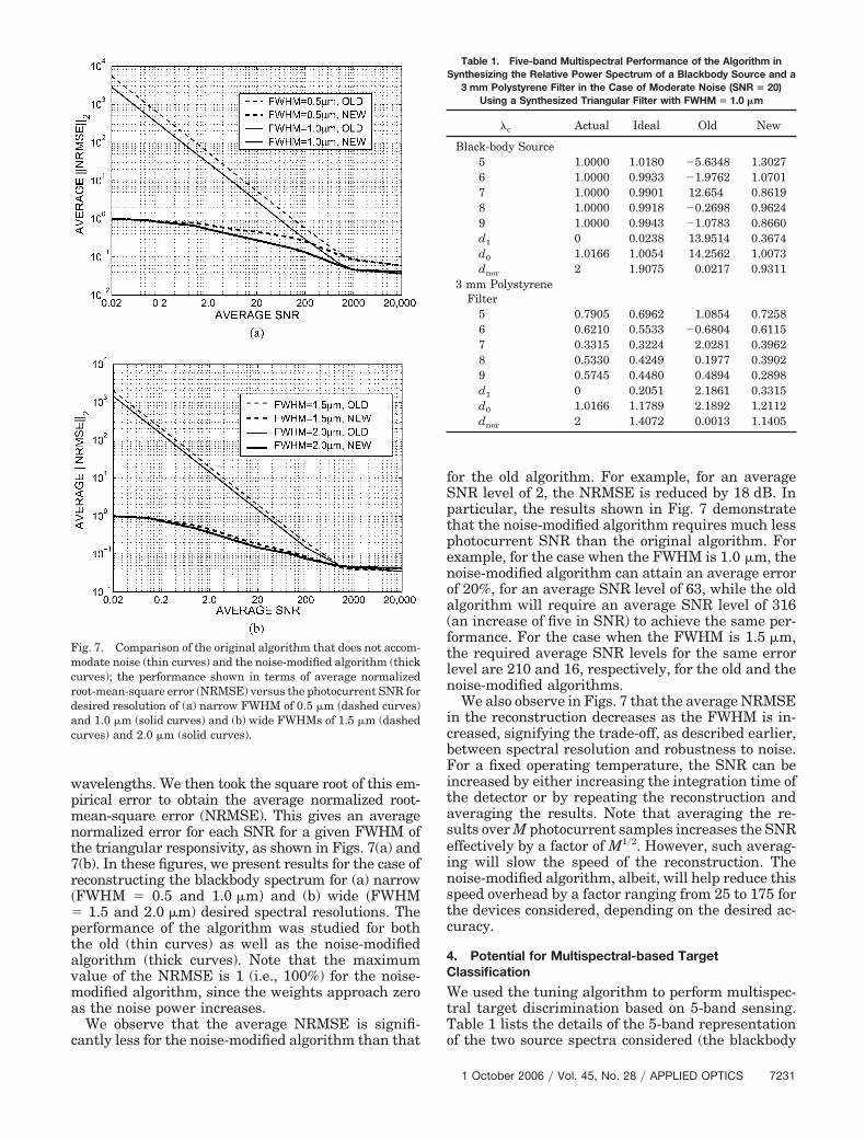
wavelengths. We then took the square root of this em-pirical error to obtain the average normalized root-mean-square error (NRMSE). This gives an averagenormalized error for each SNR for a given FWHM ofthe triangular responsivity, as shown in Figs. 7(a) and7(b). In these figures, we present results for the case ofreconstructing the blackbody spectrum for (a) narrow�FWHM � 0.5 and 1.0 �m) and (b) wide �FWHM� 1.5 and 2.0 �m) desired spectral resolutions. Theperformance of the algorithm was studied for boththe old (thin curves) as well as the noise-modifiedalgorithm (thick curves). Note that the maximumvalue of the NRMSE is 1 (i.e., 100%) for the noise-modified algorithm, since the weights approach zeroas the noise power increases.

We observe that the average NRMSE is signifi-cantly less for the noise-modified algorithm than that

for the old algorithm. For example, for an averageSNR level of 2, the NRMSE is reduced by 18 dB. Inparticular, the results shown in Fig. 7 demonstratethat the noise-modified algorithm requires much lessphotocurrent SNR than the original algorithm. Forexample, for the case when the FWHM is 1.0 �m, thenoise-modified algorithm can attain an average errorof 20%, for an average SNR level of 63, while the oldalgorithm will require an average SNR level of 316(an increase of five in SNR) to achieve the same per-formance. For the case when the FWHM is 1.5 �m,the required average SNR levels for the same errorlevel are 210 and 16, respectively, for the old and thenoise-modified algorithms.

We also observe in Figs. 7 that the average NRMSEin the reconstruction decreases as the FWHM is in-creased, signifying the trade-off, as described earlier,between spectral resolution and robustness to noise.For a fixed operating temperature, the SNR can beincreased by either increasing the integration time ofthe detector or by repeating the reconstruction andaveraging the results. Note that averaging the re-sults over M photocurrent samples increases the SNReffectively by a factor of M1�2. However, such averag-ing will slow the speed of the reconstruction. Thenoise-modified algorithm, albeit, will help reduce thisspeed overhead by a factor ranging from 25 to 175 forthe devices considered, depending on the desired ac-curacy.

4. Potential for Multispectral-based TargetClassification

We used the tuning algorithm to perform multispec-tral target discrimination based on 5-band sensing.Table 1 lists the details of the 5-band representationof the two source spectra considered (the blackbody

Fig. 7. Comparison of the original algorithm that does not accom-modate noise (thin curves) and the noise-modified algorithm (thickcurves); the performance shown in terms of average normalizedroot-mean-square error (NRMSE) versus the photocurrent SNR fordesired resolution of (a) narrow FWHM of 0.5 �m (dashed curves)and 1.0 �m (solid curves) and (b) wide FWHMs of 1.5 �m (dashedcurves) and 2.0 �m (solid curves).

Table 1. Five-band Multispectral Performance of the Algorithm inSynthesizing the Relative Power Spectrum of a Blackbody Source and a

3 mm Polystyrene Filter in the Case of Moderate Noise (SNR � 20)Using a Synthesized Triangular Filter with FWHM � 1.0 �m

�c Actual Ideal Old New

Black-body Source5 1.0000 1.0180 �5.6348 1.30276 1.0000 0.9933 �1.9762 1.07017 1.0000 0.9901 12.654 0.86198 1.0000 0.9918 �0.2698 0.96249 1.0000 0.9943 �1.0783 0.8660d1 0 0.0238 13.9514 0.3674d0 1.0166 1.0054 14.2562 1.0073dnor 2 1.9075 0.0217 0.9311

3 mm PolystyreneFilter

5 0.7905 0.6962 1.0854 0.72586 0.6210 0.5533 �0.6804 0.61157 0.3315 0.3224 2.0281 0.39628 0.5330 0.4249 0.1977 0.39029 0.5745 0.4480 0.4894 0.2898d1 0 0.2051 2.1861 0.3315d0 1.0166 1.1789 2.1892 1.2112dnor 2 1.4072 0.0013 1.1405

1 October 2006 � Vol. 45, No. 28 � APPLIED OPTICS 7231

source with and without the polystyrene film) withthe old and noise-modified spectral-tuning algo-rithms. Individual bands correspond to triangular fil-ters with a FWHM of 1 �m, centered at variouswavelengths. The SNR is assumed as 200. The firstcolumn of the table shows the centers of the fivebands, ranging from 5 to 9 �m. The second columndepicts the actual values of the target spectrum, sam-pled at the center wavelengths, while the third col-umn is the ideal reconstruction using the triangularfilters with a FWHM of 1 �m. The fourth and fifthcolumns are the reconstruction results using the oldalgorithm and the noise-modified algorithm. Separa-bility between the two target spectra can be exam-ined by comparing the Euclidean distance betweenthe 5-band reconstruction (columns four or five inTable 1) and the actual samples of the spectra(column 2 in Table 1) in the five-dimensional multi-spectral feature space, comprising the reconstructedoutputs of each band. More precisely, we haveadopted a simple performance metric, defined by30

dnor �d0 � d1

0.5�d0 � d1�, (22)

where d1 is the distance between the reconstructed5-band feature vector and the true spectrum samples,and d0 is the distance between the reconstructed5-band feature vector and the wrong spectrum. Notethat the best separation is achieved when dnor � 2,which corresponds to d1 � 0. On the other hand, theworst performance occurs when dnor � 0, which cor-responds to the case when separation is impossibleunder this simple distance-based metric.

Table 1 corresponds to the cases for which the truehypothesis is the unfiltered blackbody source and the3 mm polystyrene-filtered blackbody source. The re-sults are for a noisy case in which the SNR � 20 (lowSNR). We can see that the noise-modified algorithmresults in much less distance to the true spectrum,and hence larger dnor. For example, as shown in Table1 for a blackbody source, the noise-modified algo-rithm yields dnor � 0.9311, which is much closer tothat of the ideal reconstruction (for which dnor �1.9075) than that of the old algorithm (for whichdnor � 0.0217). These results show that under lowSNR conditions, only the noise-modified algorithmcan be used for successful target discrimination, andthe separation offered by the noise-modified algo-rithm is quite close to an ideal multispectral sensor.When the noise power is small (e.g., when the SNR isgreater than 2000), the reconstruction results for theold and new algorithm become comparable (resultsnot shown here).

The error in the reconstructed spectra dependsupon the reconstruction wavelength, which, in turn,is mainly governed by (1) the shapes of the basisdetector spectra Rk���, (2) the target spectrum g���,and (3) the shape of the desired target responsivityrc���. Near the wavelength regions where the basisspectra have well-defined peaks, the reconstruction

error decreases since the associated ideal filterapproximation error is low. For example, if we con-sider the blackbody spectrum reconstruction resultsshown in Table 1 [also shown in Fig. 5(a)] to see theeffect of the location of the peaks, we see that theerror is least around 8 �m, where some of basis spec-tra corresponding to the bias range 4–2.5 V� havepeaks according to Fig. 4. On the other hand, theerror is worse around 5 and 7 �m where the basisspectra do not exhibit major peaks. From the poly-styrene reconstruction in Table 1 [also shown in Figs.5(b) and 6(b)], we observe how the accuracy of thereconstruction is also dictated by the shape of thesource spectrum; fine features of the spectrum (nar-row dips and peaks) cannot be reconstructed well dueto the limited resolution of the basis spectra. Fromour experience, we observed that we cannot go belowthe target resolution of FWHM � 0.5 �m with theresolution of the basis spectra of the current QDIPsproduced, which have a FWHM of approximately2 �m. In addition to tuning in the 3–8 �m range re-ported earlier,10 the device used in this paper allowsus to tune in the range of 5–10 �m. We have recentlydeveloped a QDIP that would allow us to have tuningin the 8–12 �m range.

5. Conclusions

We have developed a spectral-tuning algorithm thatis based on exploiting the presence of spectral overlapand spectral diversity in the responsivities of a col-lection of detectors to synthesize the output of adesired arbitrary band. This work is an importantgeneralization of an earlier version of the algorithmto accommodate and compensate for noise in the out-put of the detectors. We have applied the algorithmto quantum-dot mid-infrared photodetectors (QDIPs)developed by our group, and have shown approxi-mate, continuous spectral tuning for two differentsource spectra, namely, a blackbody source with andwithout a 3 mm polystyrene filter in the range of5–10 �m. As a measure of performance, we used thenormalized root-mean-square error as a function ofdifferent noise levels and desired tuning resolutions.We have shown that the SNR requirements for thenoise-modified algorithm are significantly reducedwhen compared with the old algorithm, which did notaccommodate photocurrent noise. This promises ro-bustness to photocurrent noise with certain limita-tions depending on the spectral diversity in thedetectors’ responsivities. Also, as the desired spectralresolution of the tuning is reduced, the required SNRbecomes less. Therefore, as the desired width of thetuning filter is increased, which is the case in manywideband applications, the algorithm becomes morerobust to noise and the overall tuning error de-creases. This shows a fundamental trade-off betweenthe resolution of spectral tuning and robustness tonoise.

Appendix A

The expectation of the square of the error betweenthe actual and the approximated outputs can be writ-

7232 APPLIED OPTICS � Vol. 45, No. 28 � 1 October 2006

ten as [see Eqs. (9), (10), and (11) in Section 2]

E�yc � Yc2��E��Ae��min

�max

g��, Z��rc���

� �k�1

K

wc,kRk����1 �Nk

SNRk�N,k�d��2�.

(A1)

After applying the Schwarz inequality,26 we canwrite

E�yc � Yc2� � E�Ae��min

�max

g��, Z�2d�����

�min

�max �rc��� � �k�1

K

wc,kRk���

� �1 �Nk

SNRk�N,kd��2�. (A2)

Since the term in the first set of brackets is a con-stant, the minimization reduces to the minimiza-tion of

E���min

�max �rc��� � �k�1

K

wc,kRk����1 �Nk

SNRk�N,kd��2�.

(A3)

Expanding the equation and moving the expectationthrough the deterministic variables, we obtain

��min

�max �rc2��� � 2rc��� �

k�1

K

wc,kRk����1 �E�Nk�

SNRk�N,k�d�

���min

�max

E���k�1

K

wc,kRk����1 �Nk

SNRk�N,k�2�d�. (A4)

To complete the terms in the first integral into aquadratic, we add and subtract

��k�1

K

wc,kRk����1 �E�Nk�

SNRk�N,kd��2

,

expand the square of summation into multiplicationof double summation, and obtain

Since we assume independence among noise compo-nents from different detectors, the term inside theparentheses in the second integral reduces to

��k�1

K

wc,k2

Rk2���

SNRk2�, (A6)

and the discretized minimization problem then be-comes

�

L �j�1

L ��rc��j� � �k�1

K

wc,kRk��j��1 �E�Nk�

SNRk�N,k�2

� ��k�1

K

wc,k2

Rk2��j�

SNRk2��. (A7)

By invoking the assumption E�Nk� � 0 for all k, theabove quantity simplifies to

�

L �j�1

L �rc2��j� � 2rc��j���

k�1

K

wc,kRk��j��� ��

k�1

K

wc,kRk��j��2

� ��k�1

K

wc,k2

Rk2��j�

SNRk2��. (A8)

We now differentiate with respect to wc,s, set theresult to zero, and obtain

�j�1

L

rc��j�Rs��j���j�1

L �Rs��j���k�1

K

wc,kRk��j��� wc,s

Rs2��j�

SNRs2�. (A9)

Moving Rk��j� into the summation and interchangingthe order of summations, we have

�j�1

L

rc��j�Rs��j� � ��k�1

K

wc,k �j�1

L

Rs��j�Rk��j���

wc,s

SNRs2 ��

j�1

L

Rs2��j��. (A10)

Defining �c,s – rcTRs � �j�1

L rc��j�Rs��j�, and �s,k –Rs

TRk � �j�1L Rs��j�Rk��j�, we can write the equation as

�c,s � ��k�1

K

wc,k�s,k�wc,s

SNRs2 �s,s. (A11)

If we repeat this equation for s � 1, . . . , K, we havea linear system of K equations with K unknowns wc,k,which can be stated in matrix form as

��min

�max�rc�����k�1

K

wc,kRk����1 �E�Nk�

SNRk�N,k�2

d� ���min

�max��k�1

K

�l�1

K

wc,kwc,l�E�NkNl� � E�Nk�E�Nl��Rk���Rl���

�N,k�N,lSNRkSNRl�d�. (A5)

1 October 2006 � Vol. 45, No. 28 � APPLIED OPTICS 7233

�c � �ATA � ��wc, (A12)

where A, �, and �c are defined in Eqs. (13), (14), and(15). From linear algebra, the solution to Eq. (A12) isEq. (13).

We thank Biliana Paskaleva, Zhipeng Wang, andAmtout Abdenour at the University of New Mexicofor many valuable discussions. This work was sup-ported by the National Science Foundation underaward IIS-0434102.

References1. G. Vane and A. F. H. Goetz, “Terrestrial imaging spectros-

copy,” Remote Sens. Environ. 24, 1–29 (1988).2. G. Vane, R. Green, T. Chrien, H. Enmark, E. Hansen, and W.

Porter, “The airborne visible infrared imaging spectrometer,”Remote Sens. Environ. 44, 127–143 (1993).

3. R. W. Basedow, D. C. Carmer, and M. E. Anderson, “HYDICEsystem: implementation and performance,” in Imaging Spec-trometry V, M. R. Descour, J. M. Mooney, D. L. Perry, and L. R.Illing, eds., Proc. SPIE 2480, 258–267 (1995).

4. T. H. Barnes, “Photodiode array Fourier transform spectrom-eter with improved dynamic range,” Appl. Opt. 24, 3702–3706(1985).

5. G. B. Rafert, R. G. Sellar, and L. J. Otten III, “An interactiveperformance model for spatially modulated Fourier transformspectrometers,” in Imaging Spectrometry, M. R. Descour, J. M.Mooney, D. L. Perry, and L. R. Illing, eds., Proc. SPIE 2480,410–417 (1995).

6. L. J. Otten III, G. B. Rafert, and R. G. Sellar, “The design of anairborne Fourier transform visible hyperspectral imaging sys-tem for light aircraft environmental remote sensing,” in Imag-ing Spectrometry, M. R. Descour, J. M. Mooney, D. L. Perry,and L. R. Illing, eds., Proc. SPIE 2480, 418–424 (1995).

7. L. J. Otten III, A. D. Meigs, A. Franklin, R. D. Sears, M. W.Robinson, J. B. Rafert, and D. S. Fronterhouse, “On boardspectral imager data processor,” in Imaging Spectrometry V,M. R. Descour and S. S. Shen, eds., Proc. SPIE 3753, 86–94(1995).

8. J. S. Tyo and T. S. Turner, “Variable retardance, Fourier trans-form imaging spectropolarimeters for visible spectrum remotesensing,” Appl. Opt. 40, 1450–1458 (2001).

9. W. R. Bell, “Multispectral Thermal Imager—overview,” in Al-gorithms for Multispectral, Hyperspectral, and UltraspectralImagery VII, S. S. Shen and M. R. Descour, eds., Proc. SPIE4381, 173–183 (2001).

10. U. Sakoglu, J. S. Tyo, M. M. Hayat, S. Raghavan, and S.Krishna, “Spectrally adaptive infrared photodetectors withbias-tunable quantum dots,” J. Opt. Soc. Am. B 21, 7–17(2004).

11. H. J. Caulfield, “Artificial color,” Neurocomputing 51, 463–465(2003).

12. P. Bhattacharya, S. Krishna, J. D. Phillips, D. Klotzkin, andP. J. McCann, “Quantum dot carrier dynamics and far infrareddevices,” in Optoelectronics Materials and Devices II, Y.-K. Suand P. Bhattacharya, eds., Proc. SPIE 4078, 84–89 (2000).

13. P. Bhattacharya, S. Krishna, J. Phillips, P. J. McCann, and K.Namjou, “Carrier dynamics in self-organized quantum dotsand their application to long-wavelength sources and detec-tors,” J. Cryst. Growth 227, 27–35 (2001).

14. S. Krishna, P. Rotella, S. Raghavan, A. Stintz, M. M. Hayat,J. S. Tyo, and S. W. Kennerly, “Bias-dependent tunable re-sponse of normal incidence long wave infrared quantum-dot

photodetectors,” in Proceedings of the IEEE�LEOS AnnualMeeting (Institute of Electrical and Electronics Engineers,2002) Vol. 2, pp. 754–755.

15. S. Krishna, “Quantum dots-in-a-well infrared photodetectors,”J. Phys. D 38, 2142–2150 (2005).

16. U. Sakoglu, Z. Wang, M. M. Hayat, J. S. Tyo, S. Annamalai, P.Dowd, and S. Krishna, “Quantum dot detectors for infraredsensing: bias-controlled spectral tuning and matched filter-ing,” in Nanosensing: Materials and Devices, M. Saif Islam andA. K. Dutta, eds., Proc. SPIE 5593, 396–407 (2004).

17. Z. Wang, U. Sakoglu, S. Annamalai, N.-R. Weisse-Bernstein,P. Dowd, J. S. Tyo, M. M. Hayat, and S. Krishna, “Real-timeimplementation of spectral matched filtering algorithms usingadaptive focal plane array technology,” in Imaging Spectrom-etry X, A. G. Tescher, ed., Proc. SPIE 5546, 73–83 (2004).

18. Z. Wang, B. Paskaleva, J. S. Tyo, and M. M. Hayat, “Canonicalcorrelations analysis for assessing the performance of adaptivespectral imagers,” in Defense and Security Symposium, Algo-rithms and Technologies for Multispectral, Hyperspectral, andUltraspectral Imagery XI, S. S. Shen and P. E. Lewis, eds.,Proc. SPIE 5806, 23–34 (2005).

19. Z. Wang, B. Paskaleva, M. M. Hayat, and J. S. Tyo, “Analyzingspectral sensors with highly overlapping bands,” presented atthe Twelfth SPIE Defense and Security Symposium on Algo-rithms and Technologies for Multispectral, Hyperspectral,and Ultraspectral Imagery, Orlando, Fla., 18–20 April2006.

20. B. Paskaleva, M. M. Hayat, M. M. Moya, and R. J. Fogler,“Multispectral rock type separation and classification,” inInfrared Spaceborne Remote Sensing XII, M. Strojnik, ed.,Proc. SPIE 5543, 152–163 (2004).

21. B. Paskaleva and M. M. Hayat, “Optimized algorithm for spec-tral band selection for rock-type classification,” in Defense andSecurity Symposium, Algorithms and Technologies for Multi-spectral, Hyperspectral, and Ultraspectral Imagery XI, S. S.Shen and P. E. Lewis, eds., Proc. SPIE 5806, 131–138 (2005).

22. B. Paskaleva, M. M. Hayat, S. Tyo, Z. Wang, and M. Martinez,“Feature selection for spectral sensors with overlapping noisyspectral bands,” presented at the Twelfth SPIE Defense andSecurity Symposium on Algorithms and Technologies forMultispectral, Hyperspectral, and Ultraspectral Imagery,Orlando, Fla., 18–20 April 2006.

23. V. Ryzhii, “Physical model and analysis of quantum-dot infra-red photodetectors with blocking layer,” J. Appl. Phys. 89,5117–5124 (2001).

24. P. Bhattacharya, Semiconductor Optoelectronic Devices, 2nded. (Prentice-Hall, 1996).

25. E. L. Dereniak and G. D. Boreman, Infrared Detectors andSystems (Wiley, 1996).

26. H. Stark and J. Woods, Probability and Random Processes withApplications to Signal Processing, 3rd ed. (Prentice-Hall, 2002).

27. S. Krishna, D. Forman, S. Annamalai, P. Dowd, P. Varangis, T.Tumolillo, Jr., A. Gray, J. Zilko, K. Sun, M. Liu, J. Campbell,and D. Carothers, “Demonstration of a 320 � 256 two-colorfocal plane array using InAs�InGaAs quantum dots in welldetectors,” Appl. Phys. Lett. 86, 193501–3 (2005).

28. B. F. Levine, “Quantum-well infrared photodetectors,” J. Appl.Phys. 74, R1–R81 (1993).

29. J. Phillips, P. Bhattacharya, S. W. Kennerly, D. W. Beekman,and M. Dutta, “Self-assembled InAs-GaAs quantum-dot inter-subband detectors,” IEEE J. Quantum Electron. 35, 936–942(1999).

30. F. F. Sabins, Remote Sensing: Principles and Interpretation,3rd ed. (Freeman, 1997).

7234 APPLIED OPTICS � Vol. 45, No. 28 � 1 October 2006