First joint gravitational wave search by the AURIGA EXPLORER NAUTILUS Virgo Collaboration
Upload
khangminh22Category
view
3download
0
Living Rev Relativ (2016) 19:1DOI 10.1007/s41114-016-0002-8
REVIEW ARTICLE
Interferometer techniques for gravitational-wavedetection
Charlotte Bond1 · Daniel Brown1 ·Andreas Freise1 · Kenneth A. Strain2
Published online: 16 December 2016© The Author(s) 2016. This article is published with open access at Springerlink.com
Abstract Several km-scale gravitational-wave detectors have been constructed world-wide. These instruments combine a number of advanced technologies to push the limitsof precision length measurement. The core devices are laser interferometers of a newkind; developed from the classical Michelson topology these interferometers integrateadditional optical elements, which significantly change the properties of the opticalsystem. Much of the design and analysis of these laser interferometers can be per-formed using well-known classical optical techniques; however, the complex opticallayouts provide a new challenge. In this review, we give a textbook-style introductionto the optical science required for the understanding of modern gravitational wavedetectors, as well as other high-precision laser interferometers. In addition, we pro-
This article is a revised version of http://dx.doi.org/10.12942/lrr-2010-1.Change summary Major revision, updated and expanded. The number of references has increased from58 to 185.Change details Added new Sects. 6, 7, 11, and a new Appendix “Advanced LIGO optical layout”.Expanded Sect. 5 on “Basic interferometers”, Sect. 8 on “Interferometric length sensing and control”, andSect. 9 on “Beam shapes: Beyond the plane wave approximation”.
B Andreas [email protected]://www.gwoptics.org
Charlotte [email protected]
Daniel [email protected]
Kenneth A. [email protected]
1 School of Physics and Astronomy, University of Birmingham, Birmingham B15 2TT, UK
2 School of Physics and Astronomy, University of Glasgow, Glasgow G12 8QQ, UK
123
1 Page 2 of 221 Living Rev Relativ (2016) 19:1
vide a number of examples for a freely available interferometer simulation softwareand encourage the reader to use these examples to gain hands-on experience with thediscussed optical methods.
Keywords Gravitational waves · Gravitational-wave detectors · Laser interferometry ·Optics · Simulations · Finesse
Contents
1 Introduction . . . . . . . . . . . . . . . . . . . . . . . . . . . . . . . . . . . . . . . . . . . . . 41.1 The scope and style of the review . . . . . . . . . . . . . . . . . . . . . . . . . . . . 41.2 Overview of the goals of interferometer design for gravitational-wave detection . . . . 51.3 Plane-wave analysis . . . . . . . . . . . . . . . . . . . . . . . . . . . . . . . . . . . 81.4 Frequency domain analysis . . . . . . . . . . . . . . . . . . . . . . . . . . . . . . . . 10
2 Optical components: coupling of field amplitudes . . . . . . . . . . . . . . . . . . . . . . . . . 102.1 Mirrors and spaces: reflection, transmission and propagation . . . . . . . . . . . . . . 112.2 The two-mirror resonator . . . . . . . . . . . . . . . . . . . . . . . . . . . . . . . . . 122.3 Coupling matrices . . . . . . . . . . . . . . . . . . . . . . . . . . . . . . . . . . . . 132.4 Phase relation at a mirror or beam splitter . . . . . . . . . . . . . . . . . . . . . . . . 152.5 Lengths and tunings: numerical accuracy of distances . . . . . . . . . . . . . . . . . . 192.6 Revised coupling matrices for space and mirrors . . . . . . . . . . . . . . . . . . . . 222.7 Finesse examples . . . . . . . . . . . . . . . . . . . . . . . . . . . . . . . . . . . . . 232.7.1 Mirror reflectivity and transmittance . . . . . . . . . . . . . . . . . . . . . . . . . . 232.7.2 Length and tunings . . . . . . . . . . . . . . . . . . . . . . . . . . . . . . . . . . . 24
3 Light with multiple frequency components . . . . . . . . . . . . . . . . . . . . . . . . . . . . . 263.1 Modulation of light fields . . . . . . . . . . . . . . . . . . . . . . . . . . . . . . . . . 263.2 Phase modulation . . . . . . . . . . . . . . . . . . . . . . . . . . . . . . . . . . . . . 273.3 Frequency modulation . . . . . . . . . . . . . . . . . . . . . . . . . . . . . . . . . . 293.4 Amplitude modulation . . . . . . . . . . . . . . . . . . . . . . . . . . . . . . . . . . 303.5 Sidebands as phasors in a rotating frame . . . . . . . . . . . . . . . . . . . . . . . . . 303.6 Phase modulation through a moving mirror . . . . . . . . . . . . . . . . . . . . . . . 313.7 Coupling matrices for beams with multiple frequency components . . . . . . . . . . . 333.8 Finesse examples . . . . . . . . . . . . . . . . . . . . . . . . . . . . . . . . . . . . . 343.8.1 Modulation index . . . . . . . . . . . . . . . . . . . . . . . . . . . . . . . . . . . . 343.8.2 Mirror modulation . . . . . . . . . . . . . . . . . . . . . . . . . . . . . . . . . . . 34
4 Optical readout . . . . . . . . . . . . . . . . . . . . . . . . . . . . . . . . . . . . . . . . . . . 354.1 Detection of optical beats . . . . . . . . . . . . . . . . . . . . . . . . . . . . . . . . . 364.2 Signal demodulation . . . . . . . . . . . . . . . . . . . . . . . . . . . . . . . . . . . 384.3 Finesse examples . . . . . . . . . . . . . . . . . . . . . . . . . . . . . . . . . . . . . 404.3.1 Optical beat . . . . . . . . . . . . . . . . . . . . . . . . . . . . . . . . . . . . . . . 40
5 Basic interferometers . . . . . . . . . . . . . . . . . . . . . . . . . . . . . . . . . . . . . . . . 415.1 The two-mirror cavity: a Fabry–Perot interferometer . . . . . . . . . . . . . . . . . . 415.2 Michelson interferometer . . . . . . . . . . . . . . . . . . . . . . . . . . . . . . . . . 445.3 Michelson interferometer and the sideband picture . . . . . . . . . . . . . . . . . . . 475.4 Michelson interferometer signal readout with DC offset, or RF modulation . . . . . . 495.5 Response of the Michelson interferometer to a gravitational waves signal . . . . . . . 515.6 Finesse examples . . . . . . . . . . . . . . . . . . . . . . . . . . . . . . . . . . . . . 555.6.1 Cavity power . . . . . . . . . . . . . . . . . . . . . . . . . . . . . . . . . . . . . . 555.6.2 Michelson power . . . . . . . . . . . . . . . . . . . . . . . . . . . . . . . . . . . . 565.6.3 Michelson gravitational wave response . . . . . . . . . . . . . . . . . . . . . . . . 57
6 Radiation pressure and quantum fluctuations of light . . . . . . . . . . . . . . . . . . . . . . . 586.1 Quantum noise sidebands . . . . . . . . . . . . . . . . . . . . . . . . . . . . . . . . . 586.2 Vacuum noise and gravitational-wave detector readout schemes . . . . . . . . . . . . 626.3 Quantum noise with non-linear optical effects or squeezed states . . . . . . . . . . . . 676.4 Radiation pressure coupling at a suspended mirror . . . . . . . . . . . . . . . . . . . 68
123

Living Rev Relativ (2016) 19:1 Page 3 of 221 1
6.5 Semi-classical Schottky shot-noise formula . . . . . . . . . . . . . . . . . . . . . . . 716.6 Optical springs . . . . . . . . . . . . . . . . . . . . . . . . . . . . . . . . . . . . . . 726.7 Finesse examples . . . . . . . . . . . . . . . . . . . . . . . . . . . . . . . . . . . . . 766.7.1 Optical spring . . . . . . . . . . . . . . . . . . . . . . . . . . . . . . . . . . . . . . 766.7.2 Homodyne detector and squeezed light . . . . . . . . . . . . . . . . . . . . . . . . 776.7.3 Quantum-noise limited interferometer sensitivity . . . . . . . . . . . . . . . . . . . 78
7 Advancing the interferometer layout . . . . . . . . . . . . . . . . . . . . . . . . . . . . . . . . 797.1 Michelson interferometers with power recycling . . . . . . . . . . . . . . . . . . . . . 807.2 Michelson interferometers with arm cavities . . . . . . . . . . . . . . . . . . . . . . . 827.3 Signal recycling, dual recycling and resonant sideband extraction . . . . . . . . . . . 847.4 Sagnac interferometer . . . . . . . . . . . . . . . . . . . . . . . . . . . . . . . . . . 867.5 Finesse examples . . . . . . . . . . . . . . . . . . . . . . . . . . . . . . . . . . . . . 877.5.1 Michelson interferometer with arm cavities . . . . . . . . . . . . . . . . . . . . . . 877.5.2 Michelson interferometer with signal recycling . . . . . . . . . . . . . . . . . . . . 887.5.3 Sagnac interferometer . . . . . . . . . . . . . . . . . . . . . . . . . . . . . . . . . 89
8 Interferometric length sensing and control . . . . . . . . . . . . . . . . . . . . . . . . . . . . . 908.1 An overview of the control problem . . . . . . . . . . . . . . . . . . . . . . . . . . . 918.2 Linear time-invariant control theory: introductory concepts . . . . . . . . . . . . . . . 938.3 Digital signal processing for control . . . . . . . . . . . . . . . . . . . . . . . . . . . 958.4 Degrees of freedom and operating points . . . . . . . . . . . . . . . . . . . . . . . . 978.5 Error signals and transfer functions . . . . . . . . . . . . . . . . . . . . . . . . . . . 998.6 Bode plots: traditional control theory for SISO loops . . . . . . . . . . . . . . . . . . 1018.7 Separating mixtures of the degrees of freedom: control matrices . . . . . . . . . . . . 1048.8 Modern control methods in gravitational-wave detectors . . . . . . . . . . . . . . . . 1058.9 Fabry–Perot length sensing . . . . . . . . . . . . . . . . . . . . . . . . . . . . . . . . 1068.10 The Pound–Drever–Hall length sensing scheme . . . . . . . . . . . . . . . . . . . . . 1078.11 Michelson length sensing . . . . . . . . . . . . . . . . . . . . . . . . . . . . . . . . . 1098.12 Advanced LIGO: an example of a complex interferometer . . . . . . . . . . . . . . . 1118.13 The Schnupp modulation scheme . . . . . . . . . . . . . . . . . . . . . . . . . . . . 1138.14 Extending the Pound–Drever–Hall technique to more complicated optical systems . . 1148.15 Complementary techniques: internal modulation, external modulation and dithering . . 1188.16 Circumstances in which offset locking is favoured over modulationbased techniques . 1198.17 Finesse examples . . . . . . . . . . . . . . . . . . . . . . . . . . . . . . . . . . . . . 1218.17.1 Michelson modulation . . . . . . . . . . . . . . . . . . . . . . . . . . . . . . . . . 1218.17.2 Cavity power and slope . . . . . . . . . . . . . . . . . . . . . . . . . . . . . . . . . 1228.17.3 Michelson with Schnupp modulation . . . . . . . . . . . . . . . . . . . . . . . . . 123
9 Beam shapes: beyond the plane wave approximation . . . . . . . . . . . . . . . . . . . . . . . 1249.1 A typical laser beam: the fundamental Gaussian mode . . . . . . . . . . . . . . . . . 1259.2 Describing beam distortions with higher-order modes . . . . . . . . . . . . . . . . . . 1259.3 The paraxial approximation . . . . . . . . . . . . . . . . . . . . . . . . . . . . . . . 1269.4 Transverse electromagnetic modes . . . . . . . . . . . . . . . . . . . . . . . . . . . . 1289.5 Properties of Gaussian beams . . . . . . . . . . . . . . . . . . . . . . . . . . . . . . 1299.6 Astigmatic beams: the tangential and sagittal plane . . . . . . . . . . . . . . . . . . . 1319.7 Higher-order Hermite–Gauss modes . . . . . . . . . . . . . . . . . . . . . . . . . . . 1329.8 The Gaussian beam parameter . . . . . . . . . . . . . . . . . . . . . . . . . . . . . . 1339.9 Properties of higher-order Hermite–Gauss modes . . . . . . . . . . . . . . . . . . . . 1349.10 Gouy phase . . . . . . . . . . . . . . . . . . . . . . . . . . . . . . . . . . . . . . . . 1359.11 Laguerre–Gauss modes . . . . . . . . . . . . . . . . . . . . . . . . . . . . . . . . . . 1369.12 Tracing a Gaussian beam through an optical system . . . . . . . . . . . . . . . . . . . 1409.13 ABCD matrices . . . . . . . . . . . . . . . . . . . . . . . . . . . . . . . . . . . . . . 1419.14 Computing a cavity eigenmode and stability . . . . . . . . . . . . . . . . . . . . . . . 1449.15 Round-trip Gouy phase and higher-order-mode separation . . . . . . . . . . . . . . . 1459.16 Coupling of higher-order-modes . . . . . . . . . . . . . . . . . . . . . . . . . . . . . 1469.17 Finesse examples . . . . . . . . . . . . . . . . . . . . . . . . . . . . . . . . . . . . . 1499.17.1 Beam parameter tracing . . . . . . . . . . . . . . . . . . . . . . . . . . . . . . . . 1499.17.2 Telescope and Gouy phase . . . . . . . . . . . . . . . . . . . . . . . . . . . . . . . 1509.17.3 LG33 mode . . . . . . . . . . . . . . . . . . . . . . . . . . . . . . . . . . . . . . . 151
123
1 Page 4 of 221 Living Rev Relativ (2016) 19:1
10 Imperfect interferometers . . . . . . . . . . . . . . . . . . . . . . . . . . . . . . . . . . . . . . 15210.1 Spatial modes in optical cavities . . . . . . . . . . . . . . . . . . . . . . . . . . . . . 15310.2 Cavity alignment in the mode picture . . . . . . . . . . . . . . . . . . . . . . . . . . 15410.3 Mode mismatch . . . . . . . . . . . . . . . . . . . . . . . . . . . . . . . . . . . . . . 15710.4 Spatial defects . . . . . . . . . . . . . . . . . . . . . . . . . . . . . . . . . . . . . . 15910.5 Operating cavities at high power . . . . . . . . . . . . . . . . . . . . . . . . . . . . . 15910.6 The Michelson: differential imperfections . . . . . . . . . . . . . . . . . . . . . . . . 16410.7 Advanced LIGO: implications for design and commissioning . . . . . . . . . . . . . . 16810.8 Commissioning . . . . . . . . . . . . . . . . . . . . . . . . . . . . . . . . . . . . . . 17610.9 Finesse examples . . . . . . . . . . . . . . . . . . . . . . . . . . . . . . . . . . . . . 17710.9.1 Higher-order mode resonances . . . . . . . . . . . . . . . . . . . . . . . . . . . . . 17710.9.2 Mode cleaner . . . . . . . . . . . . . . . . . . . . . . . . . . . . . . . . . . . . . . 17810.9.3 Misaligned cavity . . . . . . . . . . . . . . . . . . . . . . . . . . . . . . . . . . . . 17910.9.4 Impact of thermal aberrations . . . . . . . . . . . . . . . . . . . . . . . . . . . . . 181
11 Scattering into higher-order modes . . . . . . . . . . . . . . . . . . . . . . . . . . . . . . . . . 18311.1 Light scattering in interferometers . . . . . . . . . . . . . . . . . . . . . . . . . . . . 18311.2 Mirror surface defects . . . . . . . . . . . . . . . . . . . . . . . . . . . . . . . . . . 18411.3 Coupling between higher-order modes . . . . . . . . . . . . . . . . . . . . . . . . . . 18511.4 Simulation methods . . . . . . . . . . . . . . . . . . . . . . . . . . . . . . . . . . . . 18711.5 Mirror surface maps . . . . . . . . . . . . . . . . . . . . . . . . . . . . . . . . . . . 18711.6 Spectrum of surface distortions . . . . . . . . . . . . . . . . . . . . . . . . . . . . . . 19011.7 Surface description with Zernike polynomials . . . . . . . . . . . . . . . . . . . . . . 19111.8 Mode coupling due to mirror surfaces defects . . . . . . . . . . . . . . . . . . . . . . 19311.9 Efficient coupling matrix computations with multiple distortions . . . . . . . . . . . . 20311.10 Clipping by finite apertures . . . . . . . . . . . . . . . . . . . . . . . . . . . . . . . . 20511.11 Cavity modes of many shapes . . . . . . . . . . . . . . . . . . . . . . . . . . . . . . 206
Appendix A: The interferometer simulation Finesse . . . . . . . . . . . . . . . . . . . . . . . . . . 207Appendix B: Advanced LIGO optical layout . . . . . . . . . . . . . . . . . . . . . . . . . . . . . . 208References . . . . . . . . . . . . . . . . . . . . . . . . . . . . . . . . . . . . . . . . . . . . . . . . 214
1 Introduction
1.1 The scope and style of the review
The historical development of laser interferometers for application as gravitational-wave detectors (Pitkin et al. 2011) has involved the combination of relatively simpleoptical subsystems into more and more complex assemblies. The individual elementsthat compose the interferometers, including mirrors, beam splitters, lasers, modulators,various polarising optics, photo detectors and so forth, are individually well describedby relatively simple, mostly-classical physics. Complexity arises from the combinationof multiple mirrors, beam splitters etc. into optical cavity systems that have narrowresonant features, and the consequent requirement to stabilise relative separations ofthe various components to sub-wavelength accuracy, and indeed in many cases to verysmall fractions of a wavelength.
Thus, classical physics describes the interferometer techniques and the operationof current gravitational-wave detectors. However, we note that at signal frequenciesabove a couple of hundreds of Hertz, the sensitivity of current detectors is limited by thephoton counting noise at the interferometer readout, also called shot-noise. The nextgeneration systems such as Advanced LIGO (Fritschel 2003; Aasi 2015), AdvancedVirgo (Acernese 2015) and KAGRA (Aso et al. 2013) are expected to operate in a
123

Living Rev Relativ (2016) 19:1 Page 5 of 221 1
regime where the quantum physics of both light and mirror motion couple to each other.Then, a rigorous quantum-mechanical description is certainly required. Sensitivityimprovements beyond these ‘Advanced’ detectors necessitate the development of non-classical techniques; a comprehensive discussion of such techniques is provided inDanilishin and Khalili (2012). This review provides a brief introduction to quantumnoise in Sect. 6 but otherwise focusses on the non-quantum aspects of interferometrythat play an important role in overcoming other limits to current detectors, due to, forexample, thermal effects and feedback control systems. At the same time these classicaltechniques will provide the means for implementing new, non-classical schemes andjust remain as important as ever.
The optical components employed tend to behave in a linear fashion with respectto the optical field, i.e., nonlinear optical effects need hardly be considered. Indeed,almost all aspects of the design of laser interferometers are dealt with in the linearregime. Therefore the underlying mathematics is relatively simple and many standardtechniques are available, including those that naturally allow numerical solution bycomputer models. Such computer models are in fact necessary as the exact solutionscan become quite complicated even for systems of a few components. In practice,workers in the field rarely calculate the behaviour of the optical systems from firstprinciples, but instead rely on various well-established numerical modelling tech-niques. An example of software that enables modelling of interferometers and theircomponent systems is Finesse (Freise et al. 2004; Freise 2015). This was developedby some of us (AF, DB), has been validated in a wide range of situations, and wasused to prepare the examples included in the present review.
The target readership we have in mind is the student or researcher who desires toget to grips with practical issues in the design of interferometers or component partsthereof. For that reason, this review consists of sections covering the basic physics andapproaches to simulation, intermixed with some practical examples. To make this asuseful as possible, the examples are intended to be realistic with sensible parametersreflecting typical application in gravitational wave detectors. The examples, preparedusing Finesse, are designed to illustrate the methods typically applied in designinggravitational wave detectors. We encourage the reader to obtain Finesse and to followthe examples (see “Appendix A”).
1.2 Overview of the goals of interferometer design for gravitational-wavedetection
Gravitational waves are transverse quadrupole waves travelling at the speed of light.They are distortions in space-time that can be detected by measuring the distancebetween test masses, see Fig. 1. A Michelson interferometer presents an ideal detectorgeometry, it is designed to measure relative length changes of two perpendiculardirections in a plane, see Fig. 2. The end mirrors of the Michelson interferometerrepresent the test masses and any change in the relative distance between the centralbeam splitter and the end mirrors will produce a change in the light power detected inthe output port.
123

1 Page 6 of 221 Living Rev Relativ (2016) 19:1
Fig. 1 Gravitational waves are transverse quadrupole waves. If a wave passes through the ring of testparticles that is oriented perpendicular to the direction of wave propagation, the distances between theparticles would change periodically as shown in this sketch
Fig. 2 Simplified layout of a Michelson interferometer. The laser provides the input light, which is splitinto two beams by the central beamsplitters. The beams reflect off the end mirrors and recombine at thebeamsplitter. The light power on the main photo detector (PD) changes when the difference between thearm length ΔL = LX − LY changes
The measurable length change induced by a gravitational-wave depends on the totallength being measured. For gravitational waves with wavelength much larger than thedetector size we get:
ΔL = h L , (1.1)
with L the length of the detetor and h the strain amplitude of the gravitational wave.This scaling of the change with the base length led to the construction of interferometerswith arm length of several kilometres.
Gravitational-wave detectors strive to pick out signals carried by passing gravita-tional waves from a background of self-generated noise. This is challenging becauseof the extremely small effects produces by the gravitational waves. For example, thefirst gravitational wave detected in September 2015 by the LIGO detectors (Abbottet al. 2016b), which is considered to be a strong event, reached a strain amplitude of10−21. This signal could not have been measured with a simple Michelson interferom-eter. The performance of an interferometric detector is limited by its various internal
123
Living Rev Relativ (2016) 19:1 Page 7 of 221 1
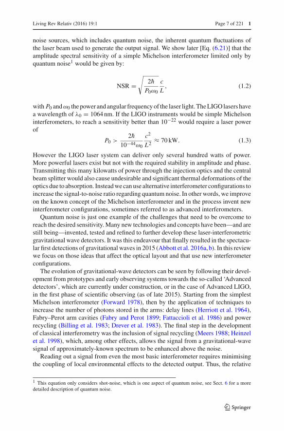
noise sources, which includes quantum noise, the inherent quantum fluctuations ofthe laser beam used to generate the output signal. We show later [Eq. (6.21)] that theamplitude spectral sensitivity of a simple Michelson interferometer limited only byquantum noise1 would be given by:
NSR =√
2h
P0ω0
c
L, (1.2)
with P0 andω0 the power and angular frequency of the laser light. The LIGO lasers havea wavelength of λ0 = 1064 nm. If the LIGO instruments would be simple Michelsoninterferometers, to reach a sensitivity better than 10−22 would require a laser powerof
P0 >2h
10−44ω0
c2
L2 ≈ 70 kW. (1.3)
However the LIGO laser system can deliver only several hundred watts of power.More powerful lasers exist but not with the required stability in amplitude and phase.Transmitting this many kilowatts of power through the injection optics and the centralbeam splitter would also cause undesirable and significant thermal deformations of theoptics due to absorption. Instead we can use alternative interferometer configurations toincrease the signal-to-noise ratio regarding quantum noise. In other words, we improveon the known concept of the Michelson interferometer and in the process invent newinterferometer configurations, sometimes referred to as advanced interferometers.
Quantum noise is just one example of the challenges that need to be overcome toreach the desired sensitivity. Many new technologies and concepts have been—and arestill being—invented, tested and refined to further develop these laser-interferometricgravitational wave detectors. It was this endeavour that finally resulted in the spectacu-lar first detections of gravitational waves in 2015 (Abbott et al. 2016a, b). In this reviewwe focus on those ideas that affect the optical layout and that use new interferometerconfigurations.
The evolution of gravitational-wave detectors can be seen by following their devel-opment from prototypes and early observing systems towards the so-called ‘Advanceddetectors’, which are currently under construction, or in the case of Advanced LIGO,in the first phase of scientific observing (as of late 2015). Starting from the simplestMichelson interferometer (Forward 1978), then by the application of techniques toincrease the number of photons stored in the arms: delay lines (Herriott et al. 1964),Fabry–Perot arm cavities (Fabry and Perot 1899; Fattaccioli et al. 1986) and powerrecycling (Billing et al. 1983; Drever et al. 1983). The final step in the developmentof classical interferometry was the inclusion of signal recycling (Meers 1988; Heinzelet al. 1998), which, among other effects, allows the signal from a gravitational-wavesignal of approximately-known spectrum to be enhanced above the noise.
Reading out a signal from even the most basic interferometer requires minimisingthe coupling of local environmental effects to the detected output. Thus, the relative
1 This equation only considers shot-noise, which is one aspect of quantum noise, see Sect. 6 for a moredetailed description of quantum noise.
123

1 Page 8 of 221 Living Rev Relativ (2016) 19:1
positions of all the components must be stabilised. This is commonly achieved bysuspending the mirrors etc. as pendulums, often multi-stage pendulums in series,and then applying closed-loop control to maintain the desired operating condition.The careful engineering required to provide low-noise suspensions with the correctvibration isolation and low-noise actuation is described in many works, for example,Braccini et al. (1996), Plissi et al. (2000), Barriga et al. (2009) and Aston et al. (2012).
As the interferometer optics become more complicated the resonance conditionsbecome more narrowly defined, i.e., the allowed combinations of inter-componentpath lengths required to allow the photon number in the interferometer arms to reach amaximum. It is likewise necessary to maintain angular alignment of all components sothat beams required to interfere are correctly co-aligned. Typically the beams need tobe aligned within a small fraction, and sometimes a very small fraction, of the far-fielddiffraction angle: the requirement can be in the low nano-radian range for km-scaledetectors (Morrison et al. 1994; Freise et al. 2007). Therefore, for each optical compo-nent there is typically one longitudinal, i.e., along the direction of light propagation,plus two angular degrees of freedom: pitch and yaw about the longitudinal axis. Acomplex interferometer consists of up to around seven highly sensitive componentsand so there can be of order 20 degrees of freedom to be measured and controlled(Acernese 2006; Winkler et al. 2007).
Although the light fields are linear in their behaviour the coupling between theposition of a mirror and the complex amplitude of the detected light field typicallyshows strongly nonlinear dependence on mirror positions due to the sharp resonancefeatures exhibited by cavity systems. The fields do vary linearly, or at least theyvary smoothly close to the desired operating point. So, while well-understood linearcontrol theory suffices to design the control system needed to maintain the opticalconfiguration at its operating point, the act of bringing the system to that operatingcondition is often a separate and more challenging nonlinear problem. In the currentversion of this work we consider only the linear aspects of sensing and control.
Control systems require actuators, and those employed are typically electrical-force transducers that act on the suspended optical components, either directly or—toprovide enhanced noise rejection—at upper stages of multi-stage suspensions. Thetransducers are normally coil-magnet actuators, with the magnets on the moving part,or, less frequently, electrostatic actuators of varying design. The actuators are fre-quently regarded as part of the mirror suspension subsystem and are not discussed inthe current work.
To give order to our review we consider the main physics describing the operationof the basic optical components: mirrors, beam splitters, modulators, etc., required toconstruct interferometers. Although all of the relevant physics is generally well knownand not new, we take it as a starting point that permits the introduction of notationand conventions. It is also true that the interferometry employed for gravitational-wave detection has a different emphasis than other interferometer applications. As aconsequence, descriptions or examples of a number of crucial optical properties forgravitational wave detectors cannot be found in the literature.
The purpose of this review is especially to provide a coherent theoretical frameworkfor describing such effects. With the basics established, it can be seen that the interfer-
123

Living Rev Relativ (2016) 19:1 Page 9 of 221 1
ometer configurations that have been employed in gravitational-wave detection maybe built up and simulated in a relatively straightforward manner.
1.3 Plane-wave analysis
The main optical systems of interferometric gravitational-wave detectors are designedsuch that all system parameters are well known and stable over time. The stability isachieved through a mixture of passive isolation systems and active feedback control.In particular, the light sources are some of the most stable, low-noise continuous-wave laser systems so that electromagnetic fields can be assumed to be essentiallymonochromatic. Additional frequency components can be modelled as small modu-lations in amplitude or phase. The laser beams are well collimated, propagate along awell-defined optical axis and remain always very much smaller than the optical ele-ments they interact with. Therefore, these beams can be described as paraxial and thewell-known paraxial approximations can be applied.
It is useful to first derive a mathematical model based on monochromatic, scalar,plane waves. As it turns out, a more detailed model including the polarisation and theshape of the laser beam as well as multiple frequency components, can be derivedas an extension to the plane-wave model. A plane electromagnetic wave is typicallydescribed by its electric field component (Fig. 3):
Fig. 3 The electric field component of an electromagnetic wave
with E0 as the (constant) field amplitude in V/m, ep the unit vector in the direction ofpolarisation, such as, for example, ey for S -polarised light, ω the angular oscillationfrequency of the wave, and k = ekω/c the wave vector pointing in the directionof propagation. The absolute phase ϕ only becomes meaningful when the field issuperposed with other light fields.
In this document we will consider waves propagating along the optical axis givenby the z-axis, so that kr = kz. For the moment we will ignore the polarisation and usescalar waves, which can be written as
E(z, t) = E0 cos(ωt − kz + ϕ). (1.4)
Further, in this document we use complex notation, i.e.,
E = � {E ′} with E ′ = E ′
0 exp(i (ωt − kz)
). (1.5)
123
1 Page 10 of 221 Living Rev Relativ (2016) 19:1
This has the advantage that the scalar amplitude and the phase ϕ can be given by one,now complex, amplitude E ′
0 = E0 exp(i ϕ). We will use this notation with complexnumbers throughout. For clarity we will simply use the unprimed letters for the aux-iliary field. In particular, we will use the letter E and also a and b to denote complexelectric-field amplitudes. But remember that, for example, in E = E0 exp(−i kz) nei-ther E nor E0 are physical quantities. Only the real part of E exists and deserves thename field amplitude.
1.4 Frequency domain analysis
In most cases we are either interested in the fields at one particular location, forexample, on the surface of an optical element, or we want to know the fields at allplaces in the interferometer but at one particular point in time. The latter is usuallytrue for the steady state approach: assuming that the interferometer is in a steady state,all solutions must be independent of time so that we can perform all computations att = 0 without loss of generality. In that case, the scalar plane wave can be written as
E = E0 exp(−i kz). (1.6)
The frequency domain is of special interest as numerical models of gravitational-wavedetectors tend to be much faster to compute in the frequency domain than in the timedomain.
2 Optical components: coupling of field amplitudes
When an electromagnetic wave interacts with an optical system, all of its parameterscan be changed as a result. Typically optical components are designed such that, ideally,they only affect one of the parameters, i.e., either the amplitude or the polarisation orthe shape. Therefore, it is convenient to derive separate descriptions concerning eachparameter. This section introduces the coupling of the complex field amplitude at opti-cal components. Typically, the optical components are described in the simplest possi-ble way, as illustrated by the use of abstract schematics such as those shown in Fig. 4.
2.1 Mirrors and spaces: reflection, transmission and propagation
The core optical systems of current interferometric gravitational interferometers arecomposed of two building blocks: a) resonant optical cavities, such as Fabry–Perotresonators, and b) beam splitters, as in a Michelson interferometer. In other words, thelaser beam is either propagated through a vacuum system or interacts with a partially-reflecting optical surface.
The term optical surface generally refers to a boundary between two media withpossibly different indices of refraction n, for example, the boundary between air andglass or between two types of glass. A real fused silica mirror in an interferometerfeatures two surfaces, which interact with a reflected or transmitted laser beam. How-ever, in some cases, one of these surfaces has been treated with an anti-reflection (AR)coating to minimise the effect on the transmitted beam.
123

Living Rev Relativ (2016) 19:1 Page 11 of 221 1
optical axis
mirror
Ein
Erefl
Etrans
Ein2
optics
E1
E4
E3
E2
optics
E1
E4
E3
E2
E5 E8
E7 E6
Fig. 4 This set of figures introduces an abstract form of illustration, which will be used in this document.The top figure shows a typical example taken from the analysis of an optical system: an incident field Einis reflected and transmitted by a semi-transparent mirror; there might be the possibility of second incidentfield Ein2. The lower left figure shows the abstract form we choose to represent the same system. The lowerright figure depicts how this can be extended to include a beam splitter object, which connects two opticalaxes
The terms mirror and beam splitter are sometimes used to describe a (theoretical)optical surface in a model. We define real amplitude coefficients for reflection andtransmission r and t , with 0 ≤ r, t ≤ 1, so that the field amplitudes can be written as(Fig. 5)
E2 = rE3 + i tE1
E4 = rE1 + i tE3
optical axis
mirror(optical surface described by coefficients r and t)
E1
E4
E2
E3
Fig. 5 The coupling of field amplitudes at a mirror component
The π/2 phase shift upon transmission (here given by the factor i ) refers to a phaseconvention explained in Sect. 2.4.
The free propagation of a distance D through a medium with index of refraction ncan be described with the following set of equations (Fig. 6):
E2 = E1 exp(−i k nD)
E4 = E3 exp(−i k nD)
optical axis
space(propagation defined by coefficients D and n)
E1
E4
E2
E3
Fig. 6 Coupling of field amplitudes for free propagation
123

1 Page 12 of 221 Living Rev Relativ (2016) 19:1
Fig. 7 Simplified schematic of a two mirror cavity. The two mirrors are defined by the amplitude coefficientsfor reflection and transmission. Further, the resulting cavity is characterised by its length D. Light fieldamplitudes are shown and identified by a variable name, where necessary to permit their mutual couplingto be computed
In the following we use n = 1 for simplicity.Note that we use above relations to demonstrate various mathematical methods for
the analysis of optical systems. However, refined versions of the coupling equationsfor optical components, including those for spaces and mirrors, are also required, see,for example, Sect. 2.6.
2.2 The two-mirror resonator
The linear optical resonator, also called a cavity is formed by two partially-transparentmirrors, arranged in parallel as shown in Fig. 7. This simple setup makes a very goodexample with which to illustrate how a mathematical model of an interferometer canbe derived, using the equations introduced in Sect. 2.1. A more detailed descriptionof the two-mirror cavity is provided in Sect. 5.1.
The cavity is defined by a propagation length D (in vacuum), the amplitude reflec-tivities r1, r2 and the amplitude transmittances t1, t2. The amplitude at each point inthe cavity can be computed simply as the superposition of fields. The entire set ofequations can be written as
a1 = i t1a0 + r1a′3
a′1 = exp(−i kD) a1
a2 = i t2a′1
a3 = r2a′1
a′3 = exp(−i kD) a3
a4 = r1a0 + i t1a′3 (2.1)
The circulating field impinging on the first mirror (surface) a′3 can now be computed
as
a′3 = exp(−i kD) a3 = exp(−i kD) r2a
′1 = exp(−i 2kD) r2a1
= exp(−i 2kD) r2 (i t1a0 + r1a′3). (2.2)
123
Living Rev Relativ (2016) 19:1 Page 13 of 221 1
This then yields
a′3 = a0
i r2t1 exp(−i 2kD)
1 − r1r2 exp(−i 2kD). (2.3)
We can directly compute the reflected field to be
a4 = a0
(r1 − r2t2
1 exp(−i 2kD)
1 − r1r2 exp(−i 2kD)
)= a0
(r1 − r2(r2
1 + t21 ) exp(−i 2kD)
1 − r1r2 exp(−i 2kD)
),
(2.4)while the transmitted field becomes
a2 = a0−t1t2 exp(−i kD)
1 − r1r2 exp(−i 2kD). (2.5)
The properties of two mirror cavities will be discussed in more detail in Sect. 5.1.
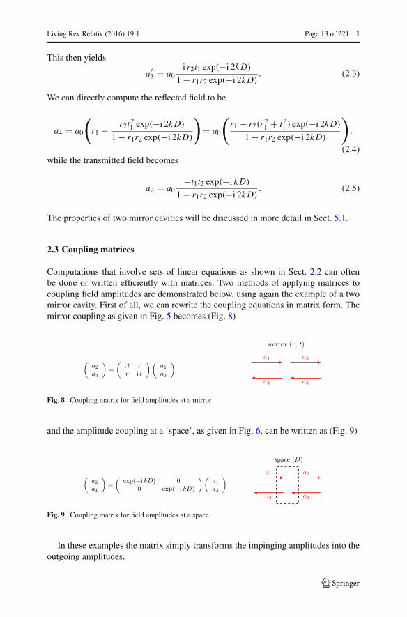
2.3 Coupling matrices
Computations that involve sets of linear equations as shown in Sect. 2.2 can oftenbe done or written efficiently with matrices. Two methods of applying matrices tocoupling field amplitudes are demonstrated below, using again the example of a twomirror cavity. First of all, we can rewrite the coupling equations in matrix form. Themirror coupling as given in Fig. 5 becomes (Fig. 8)
Fig. 8 Coupling matrix for field amplitudes at a mirror
and the amplitude coupling at a ‘space’, as given in Fig. 6, can be written as (Fig. 9)
Fig. 9 Coupling matrix for field amplitudes at a space
In these examples the matrix simply transforms the impinging amplitudes into theoutgoing amplitudes.
123

1 Page 14 of 221 Living Rev Relativ (2016) 19:1
Coupling matrices for numerical computations
The matrices introduced above are useful for storing and displaying the coupling coef-ficients for the light fields. However, if we want to compute the fields in an opticalsystem a different approach is required. An obvious application of linear couplingequations is to construct a large matrix representing extended optical system appro-priate with one equation for each field amplitude. The matrix represents a set of linearequations whose solution is a vector with all light fields in the optical system. Forexample, the set of linear equations for a mirror would be written as
⎛⎜⎜⎝
1 0 0 0−i t 1 −r 0
0 0 1 0−r 0 −i t 1
⎞⎟⎟⎠
⎛⎜⎜⎝a1a2a3a4
⎞⎟⎟⎠ =
⎛⎜⎜⎝a10a30
⎞⎟⎟⎠ = Msystem asol = ainput, (2.6)
where the input vector2 ainput has non-zero values for the impinging fields and asol isthe ‘solution’ vector, i.e., after solving the system of equations the amplitudes of theimpinging as well as those of the outgoing fields are stored in that vector.
As an example we apply this method to the two mirror cavity. The system matrixfor the optical setup shown in Fig. 7 becomes
⎛⎜⎜⎜⎜⎜⎜⎜⎜⎝
1 0 0 0 0 0 0−i t1 1 0 −r1 0 0 0−r1 0 1 −i t1 0 0 0
0 0 0 1 0 0 −e−i kD
0 −e−i kD 0 0 1 0 00 0 0 0 −i t2 1 00 0 0 0 −r2 0 1
⎞⎟⎟⎟⎟⎟⎟⎟⎟⎠
⎛⎜⎜⎜⎜⎜⎜⎜⎜⎝
a0a1a4a′
3a′
1a2a3
⎞⎟⎟⎟⎟⎟⎟⎟⎟⎠
=
⎛⎜⎜⎜⎜⎜⎜⎜⎜⎝
a0000000
⎞⎟⎟⎟⎟⎟⎟⎟⎟⎠
(2.7)
This is a sparse matrix. Sparse matrices are an important subclass of linear algebraproblems and many efficient numerical algorithms for solving sparse matrices arefreely available (see, for example, Davis 2006). The advantage of this method of con-structing a single matrix for an entire optical system is the direct access to all fieldamplitudes. It also stores each coupling coefficient in one or more dedicated matrix ele-ments, so that numerical values for each parameter can be read out or changed after thematrix has been constructed and, for example, stored in computer memory. The obvi-ous disadvantage is that the size of the matrix quickly grows with the number of opticalelements (and with the degrees of freedom of the system, see, for example, Sect. 9).
Coupling matrices for a compact system descriptions
The following method is probably most useful for analytic computations, or for opti-misation aspects of a numerical computation. The idea behind the scheme, which isused for computing the characteristics of dielectric coatings (Hecht 2002; Matuscheket al. 1997) and has been demonstrated for analysing gravitational wave detectors
2 In many implementations of numerical matrix solvers the input vector is also called the right-hand sidevector.
123
Living Rev Relativ (2016) 19:1 Page 15 of 221 1
(Mizuno and Yamaguchi 1999), is to rearrange equations as in Figs. 8 and 9 such thatthe overall matrix describing a series of components can be obtained by multiplicationof the component matrices. In order to achieve this, the coupling equations have to bere-ordered so that the input vector consists of two field amplitudes at one side of thecomponent. For the mirror, this gives a coupling matrix of
(a1a4
)= i
t
(−1 r−r r2 + t2
)(a2a3
). (2.8)
In the special case of the lossless mirror this matrix simplifies as we have r2 + t2 =R + T = 1. The space component would be described by the following matrix:
(a1a4
)=
(exp(i kD) 0
0 exp(−i kD)
)(a2a3
). (2.9)
With these matrices we can very easily compute a matrix for the cavity with twolossless mirrors as
Mcav = Mmirror1 × Mspace × Mmirror2 (2.10)
= −1
t1t2
(e+ − r1r2e− −r2e+ + r1e−
−r2e− + r1e+ e− − r1r2e+)
, (2.11)
with e+ = exp(i kD) and e− = exp(−i kD). The system of equation describing acavity shown in Eq. (2.1) can now be written more compactly as
(a0a4
)= −1
t1t2
(e+ − r1r2e− −r2e+ + r1e−
−r2e− + r1e+ e− − r1r2e+)(
a20
). (2.12)
This allows direct computation of the amplitude of the transmitted field resulting in
a2 = a0−t1t2 exp(−i kD)
1 − r1r2 exp(−i 2kD), (2.13)
which is the same as Eq. (2.5).The advantage of this matrix method is that it allows compact storage of any series
of mirrors and propagations, and potentially other optical elements, in a single 2 × 2matrix. The disadvantage inherent in this scheme is the lack of information about thefield amplitudes inside the group of optical elements.
2.4 Phase relation at a mirror or beam splitter
Throughout this article we use a slightly unintuitive definition for how the phase of alight field changes when in interacts with a mirror or beam splitter. In this section wemotivate this convention and show in detail that it is, for our purposes, mathematicalequivalent to other definitions.
123

1 Page 16 of 221 Living Rev Relativ (2016) 19:1
Fig. 10 This sketch shows a mirror or beam splitter component with dielectric coatings and the photographshows some typical commercially available examples (Newport Corporation 2008). Most mirrors and beamsplitters used in optical experiments are of this type: a substrate made from glass, quartz or fused silicais coated on both sides. The reflective coating defines the overall reflectivity of the component (anythingbetween R ≈ 1 and R ≈ 0, while the anti-reflective coating is used to reduce the reflection at the secondoptical surface as much as possible so that this surface does not influence the light. Please note that thedrawing is not to scale, the coatings are typically only a few microns thick on a several millimetre tocentimetre thick substrate
The magnitude and phase of reflection at a single optical surface can be derivedfrom Maxwell’s equations and the electromagnetic boundary conditions at the surface,and in particular the condition that the field amplitudes tangential to the optical surfacemust be continuous. The results are called Fresnel’s equations (Kenyon 2008). Thus,for a field impinging on an optical surface under normal incidence we can give thereflection coefficient as
r = n1 − n2
n1 + n2, (2.14)
with n1 and n2 the indices of refraction of the first and second medium, respectively.The transmission coefficient for a lossless surface can be computed as t2 = 1−r2. Wenote that the phase change upon reflection is either 0 or 180°, depending on whetherthe second medium is optically thinner or thicker than the first. It is not shown here butFresnel’s equations can also be used to show that the phase change for the transmittedlight at a lossless surface is zero. This contrasts with the definitions given in Sect. 2.1(see Fig. 5), where the phase shift upon any reflection is defined as zero and thetransmitted light experiences a phase shift of π/2. The following section explains themotivation for the latter definition having been adopted as the common notation forthe analysis of modern optical systems.
Composite optical surfaces
Modern mirrors and beam splitters that make use of dielectric coatings are complexoptical systems, see Fig. 10 whose reflectivity and transmission depend on the multipleinterference inside the coating layers and thus on microscopic parameters. The phasechange upon transmission or reflection depends on the details of the applied coatingand is typically not known. In any case, the knowledge of an absolute value of aphase change is typically not of interest in laser interferometers because the absolutepositions of the optical components are not known to sub-wavelength precision. Insteadthe relative phase between the incoming and outgoing beams is of importance. In thefollowing we demonstrate how constraints on these relative phases, i.e., the phase
123

Living Rev Relativ (2016) 19:1 Page 17 of 221 1
Fig. 11 The relation between the phase of the light field amplitudes at a beam splitter can be computedassuming a Michelson interferometer, with arbitrary arm length but perfectly-reflecting mirrors. The incom-ing field E0 is split into two fields E1 and E2 which are reflected at the end mirrors and return to the beamsplitter, as E3 and E4, to be recombined into two outgoing fields. These outgoing fields E5 and E6 aredepicted by two arrows to highlight that these are the sum of the transmitted and reflected components ofthe returning fields. We can derive constraints for the phase of E1 and E2 with respect to the input field E0from the conservation of energy: |E0|2 = |E5|2 + |E6|2
relation between the beams, can be derived from the fundamental principle of powerconservation. To do this we consider a Michelson interferometer, as shown in Fig. 11,with perfectly-reflecting mirrors. The beam splitter of the Michelson interferometer isthe object under test. We assume that the magnitude of the reflection r and transmissiont are known. The phase changes upon transmission and reflection are unknown. Dueto symmetry we can say that the phase change upon transmission ϕt should be thesame in both directions. However, the phase change on reflection might be differentfor either direction, thus, we write ϕr1 for the reflection at the front and ϕr2 for thereflection at the back of the beam splitter.
Then the electric fields can be computed as
E1 = r E0 ei ϕr1; E2 = t E0 ei ϕt . (2.15)
We do not know the length of the interferometer arms. Thus, we introduce two furtherunknown phases: Φ1 for the total phase accumulated by the field in the vertical armand Φ2 for the total phase accumulated in the horizontal arm. The fields impinging onthe beam splitter compute as
E3 = r E0 ei (ϕr1+Φ1); E4 = t E0 ei (ϕt+Φ2). (2.16)
The outgoing fields are computed as the sums of the reflected and transmitted com-ponents:
123
1 Page 18 of 221 Living Rev Relativ (2016) 19:1
E5 = E0
(R ei (2ϕr1+Φ1) + T ei (2ϕt+Φ2)
)E6 = E0 r t
(ei (ϕt+ϕr1+Φ1) + ei (ϕt+ϕr2+Φ2)
), (2.17)
with R = r2 and T = t2.It will be convenient to separate the phase factors into common and differential
ones. We can writeE5 = E0 ei α+
(R ei α− + T e−i α−
), (2.18)
with
α+ = ϕr1 + ϕt + 1
2(Φ1 + Φ2) ; α− = ϕr1 − ϕt + 1
2(Φ1 − Φ2) , (2.19)
and similarlyE6 = E0 r t e
i β+ 2 cos(β−), (2.20)
with
β+ = ϕt + 1
2(ϕr1 + ϕr2 + Φ1 + Φ2) ; β− = 1
2(ϕr1 − ϕr2 + Φ1 − Φ2) . (2.21)
For simplicity we now limit the discussion to a 50:50 beam splitter with r = t = 1/√
2,for which we can simplify the field expressions even further:
E5 = E0 ei α+ cos(α−); E6 = E0 ei β+ cos(β−). (2.22)
Conservation of energy requires that |E0|2 = |E5|2 + |E6|2, which in turn requires
cos2(α−) + cos2(β−) = 1, (2.23)
which is only true if
α− − β− = (2N + 1)π
2, (2.24)
with N as in integer (positive, negative or zero). This gives the following constrainton the phase factors
1
2(ϕr1 + ϕr2) − ϕt = (2N + 1)
π
2. (2.25)
One can show that exactly the same condition results in the case of arbitrary (lossless)reflectivity of the beam splitter (Rüdiger 1998).
123

Living Rev Relativ (2016) 19:1 Page 19 of 221 1
We can test whether two known examples fulfil this condition. If the beam-splittingsurface is the front of a glass plate we know that ϕt = 0, ϕr1 = π, ϕr2 = 0, whichconforms with Eq. (2.25). A second example is the two-mirror resonator, see Sect. 2.2.If we consider the cavity as an optical ‘black box’, it also splits any incoming beaminto a reflected and transmitted component, like a mirror or beam splitter. Furtherwe know that a symmetric resonator must give the same results for fields injectedfrom the left or from the right. Thus, the phase factors upon reflection must be equalϕr = ϕr1 = ϕr2. The reflection and transmission coefficients are given by Eqs. (2.4)and (2.5) as
rcav =(r1 − r2t2
1 exp(−i 2kD)
1 − r1r2 exp(−i 2kD)
), (2.26)
and
tcav = −t1t2 exp(−i kD)
1 − r1r2 exp(−i 2kD). (2.27)
We demonstrate a simple case by putting the cavity on resonance (kD = Nπ ). Thisyields
rcav =(r1 − r2t2
1
1 − r1r2
); tcav = i t1t2
1 − r1r2, (2.28)
with rcav being purely real and tcav imaginary and thus ϕt = π/2 and ϕr = 0 whichalso agrees with Eq. (2.25).
In most cases we neither know nor care about the exact phase factors. Instead wecan pick any set which fulfils Eq. (2.25). For this document we have chosen to usephase factors equal to those of the cavity, i.e., ϕt = π/2 and ϕr = 0, which is why wewrite the reflection and transmission at a mirror or beam splitter as
Erefl = r E0 and Etrans = i t E0. (2.29)
In this definition r and t are positive real numbers satisfying r2 + t2 = 1 for thelossless case. This definition is convenient due to its symmetry, for example, it allowsto specify mirrors and beamsplitters without defining a front and back face.
Please note that we only have the freedom to chose convenient phase factors whenwe do not know or do not care about the details of the coating, which performs thebeam splitting. If instead the details are important, for example, when computing theproperties of a thin coating layer, such as anti-reflex coatings, the proper phase factorsfor the respective interfaces must be computed and used. Similarly, for a simple glassplate this convention cannot be used.
2.5 Lengths and tunings: numerical accuracy of distances
The resonance condition inside an optical cavity and the operating point of an inter-ferometer depends on the optical path lengths modulo the laser wavelength, i.e., for
123

1 Page 20 of 221 Living Rev Relativ (2016) 19:1
Fig. 12 Illustration of an arm cavity of the Virgo gravitational-wave detector (Virgo 2015): the macroscopiclength L of the cavity is approximately 3 km, while the wavelength of the Nd:YAG laser is λ ≈ 1µm.The resonance condition is only affected by the microscopic position of the wave nodes with respect to themirror surfaces and not by the macroscopic length, i.e., displacement of one mirror by Δx = λ/2 re-createsexactly the same condition. However, other parameters of the cavity, such as the finesse, only depend onthe macroscopic length L and not on the microscopic tuning
light from an Nd:YAG laser length differences of less than 1 µm are of interest, notthe full magnitude of the distances between optics. On the other hand, several para-meters describing the general properties of an optical system, like the finesse or freespectral range of a cavity (see Sect. 5.1) depend on the macroscopic distance and donot change significantly when the distance is changed on the order of a wavelength.This illustrates that the distance between optical components might not be the bestparameter to use for the analysis of optical systems. Furthermore, it turns out thatin numerical algorithms the distance may suffer from rounding errors. Let us usethe Virgo (2015) arm cavities as an example to illustrate this. The cavity length isapproximately 3 km, the wavelength is on the order of 1 µm, the mirror positionsare actively controlled with a precision of 1 pm and the detector sensitivity can beas good as 10−18 m, measured on ∼10 ms timescales (i.e., many samples of the dataacquisition rate). The floating point accuracy of common, fast numerical algorithmsis typically not better than 10−15. If we were to store the distance between the cav-ity mirrors as such a floating point number, the accuracy would be limited to 3 pm,which does not even cover the accuracy of the control systems, let alone the sensitivity(Fig. 12).
A simple and elegant solution to this problem is to split a distance D betweentwo optical components into two parameters (Heinzel 1999): one is the macroscopic‘length’ L , defined as the multiple of a constant wavelength λ0 yielding the smallestdifference to D. The second parameter is the microscopic tuning T that is defined asthe remaining difference between L and D, i.e., D = L + T . Typically, λ0 can beunderstood as the wavelength of the laser in vacuum, however, if the laser frequencychanges during the experiment or multiple light fields with different frequenciesare used simultaneously, a default constant wavelength must be chosen arbitrarily.Please note that usually the term λ in any equation refers to the actual wavelengthat the respective location as λ = λ0/n with n the index of refraction at the localmedium.
We have seen in Sect. 2.1 that distances appear in the expressions for electromag-netic waves in connection with the wavenumber, for example,
E2 = E1 exp(−i kz). (2.30)
123

Living Rev Relativ (2016) 19:1 Page 21 of 221 1
Thus, the difference in phase between the field at z = z1 and z = z1 + D is given as
ϕ = −kD. (2.31)
We recall that k = 2π/λ = ω/c. We can define ω0 = 2π c/λ0 and k0 = ω0/c. Forany given wavelength λ we can write the corresponding frequency as a sum of thedefault frequency and a difference frequency ω = ω0 + Δω. Using these definitions,we can rewrite Eq. (2.31) with length and tuning as
− ϕ = kD = ω0L
c+ ΔωL
c+ ω0T
c+ ΔωT
c. (2.32)
The first term of the sum is always a multiple of 2π , which is equivalent to zero. Thelast term of the sum is the smallest, approximately of the order Δω ·10−14. For typicalvalues of L ≈ 1 m, T < 1 µm and Δω < 2π · 100 MHz we find that
ω0L
c= 0,
ΔωL
c� 2,
ω0T
c� 6,
ΔωT
c� 2 10−6, (2.33)
which shows that the last term can often be ignored.We can also write the tuning directly as a phase. We define as the dimensionless
tuningφ = ω0T/c. (2.34)
This yields
exp(
iω
cT
)= exp
(iω0
cT
ω
ω0
)= exp
(i
ω
ω0φ
). (2.35)
The tuning φ is given in radian with 2π referring to a microscopic distance of onewavelength3 λ0.
Finally, we can write the following expression for the phase difference between thelight field taken at the end points of a distance D:
ϕ = −kD = −(
ΔωL
c+ φ
ω
ω0
), (2.36)
3 Note that in other publications the tuning or equivalent microscopic displacements are sometimes definedvia an optical path-length difference. In that case, a tuning of 2π is used to refer to the change of the opticalpath length of one wavelength, which, for example, if the reflection at a mirror is described, corresponds toa change of the mirror’s position of λ0/2.
123

1 Page 22 of 221 Living Rev Relativ (2016) 19:1
or if we neglect the last term from Eq. (2.33) we can approximate (ω/ω0 ≈ 1) toobtain
ϕ ≈ −(
ΔωL
c+ φ
). (2.37)
This convention provides two parameters L and φ, that can describe distances witha markedly improved numerical accuracy. In addition, this definition often allowssimplification of the algebraic notation of interferometer signals. By convention weassociate a length L with the propagation through free space, whereas the tuningwill be treated as a parameter of the optical components. Effectively the tuning thenrepresents a microscopic displacement of the respective component. If, for example,a cavity is to be resonant to the laser light, the tunings of the mirrors have to be thesame whereas the length of the space in between can be arbitrary.
2.6 Revised coupling matrices for space and mirrors
Using the definitions for length and tunings we can rewrite the coupling equations formirrors and spaces introduced in Sect. 2.1 as follows. The mirror coupling becomes(Fig. 13)
Fig. 13 Revised coupling matrix for field amplitudes at a mirror
(compare this to Fig. 8), and the amplitude coupling for a ‘space’, formally written asin Fig. 9, is now written as (Fig. 14).
Fig. 14 Revised coupling matrix for field amplitudes at a space
2.7 FINESSE examples
2.7.1 Mirror reflectivity and transmittance
We use Finesse to plot the amplitudes of the light fields transmitted and reflected bya mirror (given by a single surface). Initially, the mirror has a power reflectance and
123

Living Rev Relativ (2016) 19:1 Page 23 of 221 1
Fig. 15 Finesse example: mirror reflectivity and transmittance
transmittance of R = T = 0.5 and is, thus, lossless. For the plot in Fig. 15 we tunethe transmittance from 0.5 to 0. Since we do not explicitly change the reflectivity,R remains at 0.5 and the mirror loss increases instead, which is shown by the tracelabelled ‘total’ corresponding to the sum of the reflected and transmitted light power.The plot also shows the phase convention of a 90° phase shift for the transmitted light.
Finesse input file for ‘Mirror reflectivity and transmittance’
laser l1 1 0 n1 % laser with P=1W at the default frequency
space s1 1 n1 n2 % space of 1m length
mirror m1 0.5 0.5 0 n2 n3 % mirror with T=R=0.5 at zero tuning
ad ad_t 0 n3 % an ‘amplitude’ detector for transmitted light
ad ad_r 0 n2 % an ‘amplitude’ detector for reflected light
set t ad_t abs
set r ad_r abs
func total = $r^2 + $t^2 % computing the sum of the reflected and
transmitted power
xaxis m1 t lin 0.5 0 100 % changing the transmittance of the mirror ‘m1’
yaxis abs:deg % plotting amplitude and phase of the results
2.7.2 Length and tunings
These Finessefiles demonstrate the conventions for lengths and microscopic positionsintroduced in Sect. 2.5. The top trace in Fig. 16 depicts the phase change of a beamreflected by a beam splitter as the function of the beam splitter tuning. By changingthe tuning from 0 to 180° the beam splitter is moved forward and shortens the pathlength by one wavelength, which by convention increases the light phase by 360°. On
123

1 Page 24 of 221 Living Rev Relativ (2016) 19:1
Fig. 16 Finesse example: Length and tunings
the other hand, if a length of a space is changed, the phase of the transmitted light isunchanged (for the default wavelength Δk = 0), as shown in the lower trace.Finesse input files for ‘Length and tunings’
File for top trace:
laser l1 1 0 n1 % laser with P=1W at the default
frequency
space s1 1 1 n1 n2 % space of 1m length
bs b1 1 0 0 0 n2 n3 dump dump % beam splitter as
‘turning mirror’, normal incidence
space s2 1 1 n3 n4 % another space of 1m length
ad ad1 0 n4 % amplitude detector
% 1) first trace: change microscopic position of
beamsplitter
xaxis b1 phi lin 0 180 100
yaxis deg % plotting the phase of the results
File for bottom trace:
laser l1 1 0 n1 % laser with P=1W at the default
frequency
space s1 1 1 n1 n2 % space of 1m length
bs b1 1 0 0 0 n2 n3 dump dump % beam splitter as
‘turning mirror’, normal incidence
space s2 1 1 n3 n4 % another space of 1m length
ad ad1 0 n4 % amplitude detector
% second trace: change length of space s1
xaxis s1 L lin 1 2 100
yaxis deg % plotting the phase of the results
123

Living Rev Relativ (2016) 19:1 Page 25 of 221 1
3 Light with multiple frequency components
So far we have considered the electromagnetic field to be monochromatic. This hasallowed us to compute light-field amplitudes in a quasi-static optical setup. In thissection, we introduce the frequency of the light as a new degree of freedom. In fact,we consider a field consisting of a finite and discrete number of frequency components.We write this as
E(t, z) =∑j
a j exp(i (ω j t − k j z)
), (3.1)
with complex amplitude factors a j , ω j as the angular frequency of the light fieldand k j = ω j/c. In many cases the analysis compares different fields at one specificlocation only, in which case we can set z = 0 and write
E(t) =∑j
a j exp(i ω j t
). (3.2)
In the following sections the concept of light modulation is introduced. As this inher-ently involves light fields with multiple frequency components, it makes use of thistype of field description. Again we start with the two-mirror cavity to illustrate howthe concept of modulation can be used to model the effect of mirror motion.
3.1 Modulation of light fields
Laser interferometers typically use three different types of light fields: the laser with afrequency of, for example, f ≈ 2.8 ·1014 Hz, radio frequency (RF) sidebands used forinterferometer control with frequencies (offset to the laser frequency) of f ≈ 1 · 106
to 150 · 106 Hz, and the signal sidebands at frequencies of 1–10 000 Hz.4 As thesemodulations usually have as their origin a change in optical path length, they are oftenphase modulations of the laser frequency, the RF sidebands are utilised for opticalreadout purposes, while the signal sidebands carry the signal to be measured (thegravitational-wave signal plus noise created in the interferometer).
Figure 17 shows a time domain representation of an electromagnetic wave of fre-quency ω0, whose amplitude or phase is modulated at a frequency Ω . One can easilysee some characteristics of these two types of modulation, for example, that ampli-tude modulation leaves the zero crossing of the wave unchanged whereas with phasemodulation the maximum and minimum amplitude of the wave remains the same. Inthe frequency domain in which a modulated field is expanded into several unmod-ulated field components, the interpretation of modulation becomes even easier: anysinusoidal modulation of amplitude or phase generates new field components, whichare shifted in frequency with respect to the initial field. Basically, light power is shiftedfrom one frequency component, the carrier, to several others, the sidebands. The rela-tive amplitudes and phases of these sidebands differ for different types of modulation
4 The signal sidebands are sometimes also called audio sidebands because of their frequency range.
123

1 Page 26 of 221 Living Rev Relativ (2016) 19:1
(a)
(b)
Fig. 17 Example traces for phase and amplitude modulation: the upper plot a shows a phase-modulatedsine wave and the lower plot b depicts an amplitude-modulated sine wave. Phase modulation is characterisedby the fact that it mostly affects the zero crossings of the sine wave. Amplitude modulation affects mostly themaximum amplitude of the wave. The equations show the modulation terms in red with m the modulationindex and Ω the modulation frequency
and different modulation strengths. This section demonstrates how to compute thesideband components for amplitude, phase and frequency modulation.
3.2 Phase modulation
Phase modulation can create a large number of sidebands. The number of sidebandswith noticeable power depends on the modulation strength (or depth) given by themodulation index m. Assuming an input field
Ein = E0 exp (i ω0 t), (3.3)
a sinusoidal phase modulation of the field can be described as
E = E0 exp(
i (ω0 t + m cos (Ω t))). (3.4)
This equation can be expanded using the identity (Gradshteyn and Ryzhik 1994)
exp(i z cos ϕ) =∞∑
k=−∞i k Jk(z) exp(i kϕ), (3.5)
with Bessel functions of the first kind Jk(m). We can write
E = E0 exp (i ω0 t)∞∑
k=−∞i k Jk(m) exp (i kΩ t). (3.6)
123
Living Rev Relativ (2016) 19:1 Page 27 of 221 1
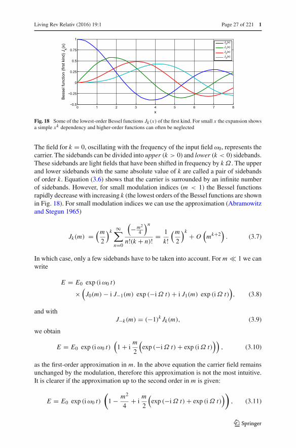
Fig. 18 Some of the lowest-order Bessel functions Jk (x) of the first kind. For small x the expansion showsa simple xk dependency and higher-order functions can often be neglected
The field for k = 0, oscillating with the frequency of the input field ω0, represents thecarrier. The sidebands can be divided into upper (k > 0) and lower (k < 0) sidebands.These sidebands are light fields that have been shifted in frequency by k Ω . The upperand lower sidebands with the same absolute value of k are called a pair of sidebandsof order k. Equation (3.6) shows that the carrier is surrounded by an infinite numberof sidebands. However, for small modulation indices (m < 1) the Bessel functionsrapidly decrease with increasing k (the lowest orders of the Bessel functions are shownin Fig. 18). For small modulation indices we can use the approximation (Abramowitzand Stegun 1965)
Jk(m) =(m
2
)k ∞∑n=0
(−m2
4
)nn!(k + n)! = 1
k!(m
2
)k + O(mk+2
). (3.7)
In which case, only a few sidebands have to be taken into account. For m 1 we canwrite
E = E0 exp (i ω0 t)
×(J0(m) − i J−1(m) exp (−i Ω t) + i J1(m) exp (i Ω t)
), (3.8)
and withJ−k(m) = (−1)k Jk(m), (3.9)
we obtain
E = E0 exp (i ω0 t)(
1 + im
2
(exp (−i Ω t) + exp (i Ω t)
)), (3.10)
as the first-order approximation in m. In the above equation the carrier field remainsunchanged by the modulation, therefore this approximation is not the most intuitive.It is clearer if the approximation up to the second order in m is given:
E = E0 exp (i ω0 t)
(1 − m2
4+ i
m
2
(exp (−i Ω t) + exp (i Ω t)
)), (3.11)
123

1 Page 28 of 221 Living Rev Relativ (2016) 19:1
which shows that power is transferred from the carrier to the sideband fields.Higher-order expansions in m can be performed simply by specifying the highest
order of Bessel function, which is to be used in the sum in Eq. (3.6), i.e.,
E = E0 exp (i ω0 t)order∑
k=−order
i k Jk(m) exp (i kΩ t). (3.12)
3.3 Frequency modulation
For small modulation, indices, phase modulation and frequency modulation can beunderstood as different descriptions of the same effect (Heinzel 1999). Following thesame spirit as above we would assume a modulated frequency to be given by
ω = ω0 + m′ cos (Ω t), (3.13)
and then we might be tempted to write
E = E0 exp(
i (ω0 + m′ cos (Ω t)) t), (3.14)
which would be wrong. The frequency of a wave is actually defined as ω/(2π) = f =dϕ/dt . Thus, to obtain the frequency given in Eq. (3.13), we need to have a phase of
ω0 t + m′
Ωsin (Ω t). (3.15)
For consistency with the notation for phase modulation, we define the modulationindex to be
m = m′
Ω= Δω
Ω, (3.16)
with Δω as the frequency swing—how far the frequency is shifted by the modulation—and Ω the modulation frequency—how fast the frequency is shifted. Thus, a sinusoidalfrequency modulation can be written as
E = E0 exp (i ϕ) = E0 exp
(i
(ω0 t + Δω
Ωcos (Ω t)
)), (3.17)
which is exactly the same expression as Eq. (3.4) for phase modulation. The practicaldifference is the typical size of the modulation index, with phase modulation having amodulation index of m < 10, while for frequency modulation, typical numbers mightbe m > 104. Thus, in the case of frequency modulation, the approximations for smallm are not valid. The series expansion using Bessel functions, as in Eq. (3.6), can stillbe performed; however, very many terms of the resulting sum need to be taken intoaccount.
123

Living Rev Relativ (2016) 19:1 Page 29 of 221 1
3.4 Amplitude modulation
In contrast to phase modulation, (sinusoidal) amplitude modulation always generatesexactly two sidebands. Furthermore, a natural maximum modulation index exists: themodulation index is defined to be one (m = 1) when the amplitude is modulatedbetween zero and the amplitude of the unmodulated field.
If the amplitude modulation is performed by an active element, for example bymodulating the current of a laser diode, the following equation can be used to describethe output field:
E = E0 exp (i ω0 t)(
1 + m cos (Ω t))
= E0 exp (i ω0 t)(
1 + m
2exp (i Ω t) + m
2exp (−i Ω t)
). (3.18)
However, passive amplitude modulators (like acousto-optic modulators or electro-optic modulators with polarisers) can only reduce the amplitude. In these cases, thefollowing equation is more useful:
E = E0 exp (i ω0 t)(
1 − m
2
(1 − cos (Ω t)
))= E0 exp (i ω0 t)
(1 − m
2+ m
4exp (i Ω t) + m
4exp (−i Ω t)
). (3.19)
3.5 Sidebands as phasors in a rotating frame
A common method of visualising the behaviour of sideband fields in interferometersis to use phase diagrams in which each field amplitude is represented by an arrow inthe complex plane.
We can think of the electric field amplitude E0 exp(i ω0t) as a vector in the complexplane, rotating around the origin with angular velocity ω0. To illustrate or to helpvisualise the addition of several light fields it can be useful to look at this problemusing a rotating reference frame, defined as follows. A complex number shall bedefined as z = x + i y so that the real part is plotted along the x-axis, while the y-axisis used for the imaginary part. We want to construct a new coordinate system (x ′, y′)in which the field vector is at a constant position. This can be achieved by defining
x = x ′ cos ω0t − y′ sin ω0t
y = x ′ sin ω0t + y′ cos ω0t, (3.20)
or
x ′ = x cos (−ω0t) − y sin (−ω0t)
y′ = x sin (−ω0t) + y cos (−ω0t) . (3.21)
123

1 Page 30 of 221 Living Rev Relativ (2016) 19:1
Fig. 19 Electric field vector E0 exp(i ω0t) depicted in the complex plane and in a rotating frame (x ′, y′)rotating at ω0 so that the field vector appears stationary
Figure 19 illustrates how the transition into the rotating frame makes the field vectorto appear stationary. The angle of the field vector in a rotating frame depicts the phaseoffset of the field. Therefore these vectors are also called phasors and the illustrationsusing phasors are called phasor diagrams. Two more complex examples of how phasordiagrams can be employed is shown in Fig. 20 (Chelkowski 2007).
Phasor diagrams can be especially useful to see how frequency coupling of light fieldamplitudes can change the type of modulation, for example, to turn phase modulationinto amplitude modulation. An extensive introduction to this type of phasor diagramcan be found in Malec (2006).
3.6 Phase modulation through a moving mirror
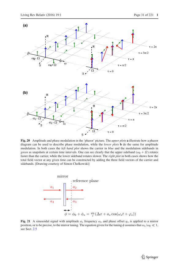
Several optical components can modulate transmitted or reflected light fields. In thissection we discuss in detail the example of phase modulation by a moving mirror.Mirror motion does not change the transmitted light; however, the phase of the reflectedlight will be changed as shown in Eq. (13).
We assume sinusoidal change of the mirror’s tuning as shown in Fig. 21. Theposition modulation is given as xm = as cos(ωst + ϕs), and thus the reflected field atthe mirror becomes (assuming a4 = 0)
a3 = r a1 exp(−i 2φ0) exp (i 2kxm) ≈ ra1 exp(−i 2φ0) exp(
i 2k0as cos(ωst + ϕs)),
(3.22)
setting m = 2k0as. This can be expressed as
a3 = ra1 exp(−i 2φ0)(
1 + im
2exp
(−i (ωst + ϕs)
)+ i
m
2exp
(i (ωst + ϕs)
))= ra1 exp(−i 2φ0)
(1 + m
2exp
(−i (ωst + ϕs − π/2)
)+ m
2exp
(i (ωst + ϕs + π/2)
)). (3.23)
123
Living Rev Relativ (2016) 19:1 Page 31 of 221 1
(a)
(b)
Fig. 20 Amplitude and phase modulation in the ‘phasor’ picture. The upper plots a illustrate how a phasordiagram can be used to describe phase modulation, while the lower plots b do the same for amplitudemodulation. In both cases the left hand plot shows the carrier in blue and the modulation sidebands ingreen as snapshots at certain time intervals. One can see clearly that the upper sideband (ω0 + Ω) rotatesfaster than the carrier, while the lower sideband rotates slower. The right plot in both cases shows how thetotal field vector at any given time can be constructed by adding the three field vectors of the carrier andsidebands. [Drawing courtesy of Simon Chelkowski]
Fig. 21 A sinusoidal signal with amplitude as frequency ωs and phase offset ϕs is applied to a mirrorposition, or to be precise, to the mirror tuning. The equation given for the tuning φ assumes that ωs/ω0 1,see Sect. 2.5
123

1 Page 32 of 221 Living Rev Relativ (2016) 19:1
3.7 Coupling matrices for beams with multiple frequency components
The coupling between electromagnetic fields at optical components introduced inSect. 2 referred only to the amplitude and phase of a simplified monochromatic field,ignoring all the other parameters of the electric field of the beam given in Eq. (3). How-ever, this mathematical concept can be extended to include other parameters providedthat we can find a way to describe the total electric field as a sum of components,each of which is characterised by a discrete value of the related parameters. In thecase of the frequency of the light field, this means we have to describe the field asa sum of monochromatic components. In the previous sections we have shown howthis could be done in the special case of an initial monochromatic field that is subjectto modulation: if the modulation index is small enough we can limit the number offrequency components that we need to consider. In many cases it is actually sufficientto describe a modulation only by the interaction of the carrier at ω0 (the unmodulatedfield) and two sidebands with a frequency offset of ±ωm to the carrier. A beam givenby the sum of three such components can be described by a complex vector:
a =⎛⎝ a(ω0)
a(ω0 − ωm)
a(ω0 + ωm)
⎞⎠ =
⎛⎝aω0aω1aω2
⎞⎠ (3.24)
with ω0 = ω0, ω0 − ωm = ω1 and ω0 + ωm = ω2. In the case of a phase modulatorthat applies a modulation of small modulation index m to an incoming light field a1,we can describe the coupling of the frequency component as follows:
a2,ω0 = J0(m)a1,ω0 + J1(m)a1,ω1 + J−1(m)a1,ω2a2,ω1 = J0(m)a1,ω1 + J−1(m)a1,ω0a2,ω2 = J0(m)a1,ω2 + J1(m)a1,ω0,
(3.25)
which can be written in matrix form:
a2 =⎛⎝ J0(m) J1(m) J−1(m)
J−1(m) J0(m) 0J1(m) 0 J0(m)
⎞⎠ a1. (3.26)
And similarly, we can write the complete coupling matrix for the modulator compo-nent, for example, as
⎛⎜⎜⎜⎜⎜⎜⎝
a2,w0a2,w1a2,w2a4,w0a4,w1a4,w2
⎞⎟⎟⎟⎟⎟⎟⎠
⎛⎜⎜⎜⎜⎜⎜⎝
J0(m) J1(m) J−1(m) 0 0 0J−1(m) J0(m) 0 0 0 0J1(m) 0 J0(m) 0 0 0
0 0 0 J0(m) J1(m) J−1(m)
0 0 0 J−1(m) J0(m) 00 0 0 J1(m) 0 J0(m)
⎞⎟⎟⎟⎟⎟⎟⎠
⎛⎜⎜⎜⎜⎜⎜⎝
a1,w0a1,w1a1,w2a3,w0a3,w1a3,w2
⎞⎟⎟⎟⎟⎟⎟⎠
(3.27)
123
Living Rev Relativ (2016) 19:1 Page 33 of 221 1
Fig. 22 Finesse example: modulation index
3.8 FINESSE examples
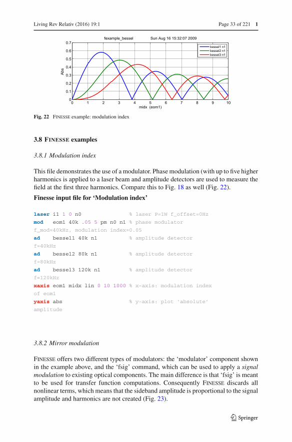
3.8.1 Modulation index
This file demonstrates the use of a modulator. Phase modulation (with up to five higherharmonics is applied to a laser beam and amplitude detectors are used to measure thefield at the first three harmonics. Compare this to Fig. 18 as well (Fig. 22).
Finesse input file for ‘Modulation index’
laser i1 1 0 n0 % laser P=1W f_offset=0Hz
mod eom1 40k .05 5 pm n0 n1 % phase modulator
f_mod=40kHz, modulation index=0.05
ad bessel1 40k n1 % amplitude detector
f=40kHz
ad bessel2 80k n1 % amplitude detector
f=80kHz
ad bessel3 120k n1 % amplitude detector
f=120kHz
xaxis eom1 midx lin 0 10 1000 % x-axis: modulation index
of eom1
yaxis abs % y-axis: plot ‘absolute’
amplitude
3.8.2 Mirror modulation
Finesse offers two different types of modulators: the ‘modulator’ component shownin the example above, and the ‘fsig’ command, which can be used to apply a signalmodulation to existing optical components. The main difference is that ‘fsig’ is meantto be used for transfer function computations. Consequently Finesse discards allnonlinear terms, which means that the sideband amplitude is proportional to the signalamplitude and harmonics are not created (Fig. 23).
123

1 Page 34 of 221 Living Rev Relativ (2016) 19:1
2
Fig. 23 Finesse example: mirror modulation
Finesse input file for ‘Mirror modulation’
laser i1 1 0 n1 % laser P=1W f_offset=0Hz
space s1 1 1 n1 n2 % space of 1m length
bs b1 1 0 0 0 n2 n3 dump dump % beam splitter as
‘turning mirror’, normal incidence
space s2 1 1 n3 n4 % another space of 1m
length
fsig sig1 b1 40k 1 0 % signal modulation
applied to beam splitter b1
ad upper 40k n4 % amplitude detector
f=40kHz
ad lower -40k n4 % amplitude detector
f=-40kHz
ad harmonic 80k n4 % amplitude detector
f=80kHz
xaxis sig1 amp lin 1 10 100 % x-axis: amplitude of
signal modulation
yaxis abs % y-axis: plot ‘absolute’
amplitude
4 Optical readout
In previous sections we have dealt with the amplitude of light fields directly andalso used the amplitude detector in the Finesse examples. This is the advantage ofa mathematical analysis versus experimental tests, in which only light intensity orlight power can be measured directly. This section gives the mathematical details formodelling photo detectors.
The intensity of a field impinging on a photo detector is given as the magnitude ofthe Poynting vector, with the Poynting vector given as (Yariv 1989)
123

Living Rev Relativ (2016) 19:1 Page 35 of 221 1
S = E × H = 1
μ0E × B. (4.1)
Inserting the electric and magnetic components of a plane wave, we obtain
|S| = 1
μ0cE2 = cε0E
20 cos2(ωt) = cε0
2E2
0 (1 + cos(2ωt)) , (4.2)
with ε0 the electric permeability of vacuum and c the speed of light.The response of a photo detector is given by the total flux of effective radiation5
during the response time of the detector. For example, in a photodiode a photon willrelease a charge in the n-p junction. The response time is given by the time it takesfor the charge to travel through the detector (and further time may be taken up in theelectronic processing of the signal). The size of the photodiode and the applied biasvoltage determine the travel time of the charges with typical values of approximately10 ns. Thus, frequency components faster than perhaps 100 MHz are not resolved bya standard photodiode. For example, a laser beam with a wavelength of λ = 1064 nmhas a frequency of f = c/λ ≈ 282 1012 Hz = 282 THz. Thus, the 2ω component ismuch too fast for the photo detector; instead, it returns the average power
|S| = cε0
2E2
0 . (4.3)
In complex notation we can write
|S| = cε0
2EE∗. (4.4)
However, for more intuitive results the light fields can be given in converted units, sothat the light power can be computed as the square of the light field amplitudes. Unlessotherwise noted, throughout this work the unit of light field amplitudes is
√watt. Thus,
the notation used in this document to describe the computation of the light power ofa laser beam is
P = EE∗. (4.5)
4.1 Detection of optical beats
What is usually called an optical beat or simply a beat is the sinusoidal behaviourof the intensity of two overlapping and coherent fields. For example, if we superpose
5 The term effective refers to that amount of incident light, which is converted into photo-electrons that arethen usefully extracted from the junction (i.e., do not recombine within the device). This fraction is usuallyreferred to as quantum efficiency η of the photodiode.
123

1 Page 36 of 221 Living Rev Relativ (2016) 19:1
Fig. 24 A beam with two frequency components hits the photo diode. Shown in this plot are the fieldamplitude, the corresponding intensity and the electrical output of the photodiode
two fields of slightly different frequency, we obtain
E = E0 cos(ω1t) + E0 cos(ω2t)
P = E2 = E20
(cos2(ω1t) + cos2(ω2t) + 2 cos(ω1t) cos(ω2t)
)= E2
0
(cos2(ω1t) + cos2(ω2t) + cos(ω+t) + cos(ω−t)
), (4.6)
with ω+ = ω1 + ω2 and ω− = ω1 − ω2. In this equation the frequency ω− can bevery small and can then be detected with the photodiode as illustrated in Fig. 24.
Pdiode = E20 (1 + cos(ω−t)) (4.7)
Using the same example photodiode as before: in order to be able to detect an opticalbeat ω− would need to be smaller than 100 MHz. If we take two, sightly detunedNd:YAG lasers with f = 282 THz, this means that the relative detuning of theselasers must be smaller than 10−7.
In general, for a field with several frequency components, the photodiode signalcan be written as
|E |2 = E · E∗ =N∑i=0
N∑j=0
aia∗j e
i (ωi−ω j ) t . (4.8)
For example, if the photodiode signal is filtered with a low-pass filter, such that onlythe DC part remains, we can compute the resulting signal by looking for all compo-nents without frequency dependence. The frequency dependence vanishes when thefrequency becomes zero, i.e., in all parts of Eq. (4.8) with ωi = ω j . The output is areal number, calculated like this:
x =∑i
∑j
ai a∗j with {i, j | i, j ∈ {0, . . . , N } ∧ ωi = ω j }. (4.9)
123

Living Rev Relativ (2016) 19:1 Page 37 of 221 1
4.2 Signal demodulation
A typical application of light modulation, is its use in a modulation-demodulationscheme, which applies an electronic demodulation to a photodiode signal. A ‘demod-ulation’ of a photodiode signal at a user-defined frequency ωx , performed by anelectronic mixer and a low-pass filter, produces a signal, which is proportional tothe amplitude of the photo current at DC and at the frequency ω0 ± ωx . Interestingly,by using two mixers with different phase offsets one can also reconstruct the phase ofthe signal, or to be precise the phase difference of the light at ω0 ± ωx with respectto the carrier light. This feature can be very powerful for generating interferometercontrol signals.
Mathematically, the demodulation process can be described by a multiplication ofthe output with a cosine: cos(ωx + ϕx ), where ϕx is the demodulation phase. Thiscosine is also called the ‘local oscillator’. The signal is
S0 = |E |2 = E · E∗ =N∑i=0
N∑j=0
aia∗j e
i (ωi−ω j ) t . (4.10)
Multiplied with the local oscillator it becomes
S1 = S0 · cos(ωx t + ϕx ) = S01
2
(ei (ωx t+ϕx ) + e−i (ωx t+ϕx )
)
= 1
2
N∑i=0
N∑j=0
aia∗j e
i (ωi−ω j ) t ·(ei (ωx t+ϕx ) + e−i (ωx t+ϕx )
). (4.11)
With Ai j = aia∗j and ei ωi j t = ei (ωi−ω j ) t we can write
S1 = 1
2
⎛⎝ N∑
i=0
Aii +N∑i=0
N∑j=i+1
(Ai j ei ωi j t+A∗
i j e−i ωi j t )
⎞⎠·
(ei (ωx t+ϕx ) + e−i (ωx t+ϕx )
).
(4.12)When looking for the DC components of S1 we get the following (Freise 2003):
S1,DC =∑i j
1
2(Ai j e
−i ϕx + A∗i j e
i ϕx ) with {i, j | i, j ∈ {0, . . . , N } ∧ ωi j = ωx }
=∑i j
�{Ai j e
−i ϕx}
. (4.13)
This would be the output of a mixer and a subsequent low-pass filter. The results forϕx = 0 and ϕx = π/2 are called in-phase and in-quadrature, respectively (or also
123

1 Page 38 of 221 Living Rev Relativ (2016) 19:1
first and second quadrature). They are given by
S1,DC,phase =∑i j
� {Ai j
},
S1,DC,quad =∑i j
{Ai j
}. (4.14)
If only one mixer is used, the output is always real and is determined by the demod-ulation phase. However, with two mixers generating the in-phase and in-quadraturesignals, it is possible to construct a complex number representing the signal amplitudeand phase:
z =∑i j
ai a∗j with {i, j | i, j ∈ {0, . . . , N } ∧ ωi j = ωx }. (4.15)
Often several sequential demodulations are applied in order to measure very specificphase information. For example, a double demodulation can be described as twosequential multiplications of the signal with two local oscillators and taking the DCcomponent of the result. First looking at the whole signal, we can write:
S2 = S0 · cos(ωx t + ϕx ) cos(ωyt + ϕy). (4.16)
This can be written as
S2 = S01
2(cos(ωyt + ωx t + ϕy + ϕx ) + cos(ωyt − ωx t + ϕy − ϕx ))
= S01
2(cos(ω+t + ϕ+) + cos(ω−t + ϕ−)), (4.17)
and thus reduced to two single demodulations. Since we now only care for the DC com-ponent we can use the expression from above [Eq. (4.15)]. These two demodulationsgive two complex numbers:
z1 =∑i j
Ai j with {i, j | i, j ∈ {0, . . . , N } ∧ ωi − ω j = ω+},
z2 =∑i j
Akl with {k, l | k, l ∈ {0, . . . , N } ∧ ωk − ωl = ω−}. (4.18)
The demodulation phases are applied as follows to get a real output (two sequentialmixers)
x = �{(z1 e−i ϕx + z2 ei ϕx ) e−i ϕy
}. (4.19)
In a typical setup, a user-defined demodulation phase for the first frequency (here ϕx )is given. If two mixers are used for the second demodulation, we can reconstruct thecomplex number
z = z1 e−i ϕx + z2 ei ϕx . (4.20)
123

Living Rev Relativ (2016) 19:1 Page 39 of 221 1
Fig. 25 Finesse example: optical beat
More demodulations can also be reduced to single demodulations as above.
4.3 FINESSE examples
4.3.1 Optical beat
In this example two laser beams are superimposed at a 50:50 beam splitter. The beamshave a slightly different frequency: the second beam has a 10 kHz offset with respectto the first (and to the default laser frequency). The plot illustrates the output of fourdifferent detectors in one of the beam splitter output ports, while the phase of thesecond beam is tuned from 0° to 180°. The photodiode ‘pd1’ shows the total powerremaining constant at a value of 1. The amplitude detectors ‘ad1’ and ‘ad10k’ detectthe laser light at 0 Hz (default frequency) and 10 kHz respectively. Both show aconstant absolute of
√1/2 and the detector ‘ad10k’ tracks the tuning of the phase
of the second laser beam. Finally, the detector ‘pd10k’ resembles a photodiode withdemodulation at 10 kHz. In fact, this represents a photodiode and two mixers used toreconstruct a complex number as shown in Eq. (4.15). One can see that the phase ofthe resulting electronic signal also directly follows the phase difference between thetwo laser beams (Fig. 25).
Finesse input file for ‘Optical beat’
const freq 10k % creating a constant for the
frequency offset
laser l1 1 0 n1 % laser with P=1W at the default
frequency
space s1 1n 1 n1 n2 % space of 1nm length
laser l2 1 $freq n3 % a second laser with f=10kHz
frequency offset
space s2 1n 1 n3 n4 % another space of 1nm length
123

1 Page 40 of 221 Living Rev Relativ (2016) 19:1
bs b1 0.5 0.5 0 0 n2 n5 dump n4 % 50:50 beam
splitter
space s3 1n 1 n5 n6 % another space of 1nm length
ad ad0 0 n6 % amplitude detector at f=0Hz
ad ad10k $freq n6 % amplitude detector at f=10kHz
pd pd1 n6 % simple photo detector
pd1 pd10k $freq n6 % photo detector with demodulation
at 10kHz
xaxis l2 phi lin 0 180 100 % changing the phase of the
l2-beam
yaxis abs:deg % plotting amplitude and phase
5 Basic interferometers
The large interferometric gravitational-wave detectors currently in operation are basedon two fundamental interferometer topologies: theFabry–Perot interferometer and theMichelson interferometer. The main instrument is very similar to the original inter-ferometer concept used in the famous experiment by Michelson and Morley (1887).The main difference is that modern instruments use laser light to illuminate the inter-ferometer to achieve much higher accuracy. Already an early prototype in 1971 hasthus achieved a sensitivity a million times better than Michelson’s original instru-ment (Moss et al. 1971). In addition, the Michelson interferometer used in currentgravitational-wave detectors has been enhanced by resonant cavities, which in turnhave been derived from the original idea for a spectroscopy standard published byFabry and Perot (1899). The following section will describe the fundamental proper-ties of the Fabry–Perot interferometer and the Michelson interferometer. A thoroughunderstanding of these basic instruments is essential for the study of the high-precisioninterferometers used for gravitational-wave detection.
5.1 The two-mirror cavity: a Fabry–Perot interferometer
We have computed the field amplitudes in a linear two-mirror cavity, also called aFabry–Perot interferometer, in Sect. 2.2. In order to understand the features of thisoptical instrument it is interesting to have a closer look at the power circulating inthe cavity. A typical optical layout is shown in Fig. 26; two parallel mirrors formthe Fabry–Perot cavity. A laser beam is injected through the first mirror (at normalincidence).
The behaviour of the (ideal) cavity is determined by the length of the cavity L , thewavelength of the laser λ and the reflectivity and transmittance of the mirrors. Usingthe mathematical description introduced in Sect. 2.2 and assuming an input power of|a0|2 = 1, we obtain the following equation for the circulating power:
123

Living Rev Relativ (2016) 19:1 Page 41 of 221 1
Fig. 26 Typical optical layout of a two-mirror cavity, also called a Fabry–Perot interferometer. Two mirrorsform the Fabry–Perot interferometer, a laser beam is injected through one of the mirrors and the reflectedand transmitted light can be detected by photo detectors
Fig. 27 Power enhancement in a two-mirror cavity as a function of the laser-light frequency. The peaksmarks the resonances of the cavity, i.e., modes of operation in which the injected light is resonantly enhanced.The frequency distance between two peaks is called free-spectral range (FSR)
P1 = |a1|2 = T1
1 + R1R2 − 2r1r2 cos (2kL), (5.1)
with k = 2π/λ, P , T = t2 and R = r2, as defined in Sect. 1.3. Similarly we couldcompute the transmission of the optical system as the input–output ratio of the fieldamplitudes. For example, with a0 the field injected into the cavity and a2 the fieldtransmitted by the cavity,
a2
a0= −t1t2 exp(−i kL)
1 − r1r2 exp(−i 2kL)(5.2)
is the frequency-dependent transfer function of the cavity in transmission (the fre-quency dependence is hidden inside the k = 2π f/c).
Figure 27 shows a plot of the circulating light power P1 over the laser frequency.The maximum power is reached when the cosine function in the denominator becomes
123
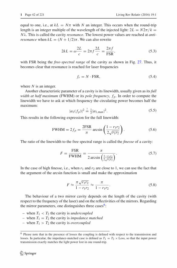
1 Page 42 of 221 Living Rev Relativ (2016) 19:1
equal to one, i.e., at kL = Nπ with N an integer. This occurs when the round-triplength is an integer multiple of the wavelength of the injected light: 2L = N2π/k =Nλ. This is called the cavity resonance. The lowest power values are reached at anti-resonance when kL = (N + 1/2)π . We can also rewrite
2kL = ω2L
c= 2π f
2L
c= 2π f
FSR, (5.3)
with FSR being the free-spectral range of the cavity as shown in Fig. 27. Thus, itbecomes clear that resonance is reached for laser frequencies
fr = N · FSR, (5.4)
where N is an integer.Another characteristic parameter of a cavity is its linewidth, usually given as its full
width at half maximum (FWHM) or its pole frequency, f p. In order to compute thelinewidth we have to ask at which frequency the circulating power becomes half themaximum:
|a1( f p)|2 != 12 |a1,max|2. (5.5)
This results in the following expression for the full linewidth:
FWHM = 2 f p = 2FSR
πarcsin
(1 − r1r2
2√r1r2
). (5.6)
The ratio of the linewidth to the free spectral range is called the finesse of a cavity:
F = FSR
FWHM= π
2 arcsin(
1−r1r22√r1r2
) . (5.7)
In the case of high finesse, i.e., when r1 and r2 are close to 1, we can use the fact thatthe argument of the arcsin function is small and make the approximation
F ≈ π√r1r2
1 − r1r2≈ π
1 − r1r2. (5.8)
The behaviour of a two mirror cavity depends on the length of the cavity (withrespect to the frequency of the laser) and on the reflectivities of the mirrors. Regardingthe mirror parameters, one distinguishes three cases6:
– when T1 < T2 the cavity is undercoupled– when T1 = T2 the cavity is impedance matched– when T1 > T2 the cavity is overcoupled
6 Please note that in the presence of losses the coupling is defined with respect to the transmission andlosses. In particular, the impedance-matched case is defined as T1 = T2 × Loss, so that the input powertransmission exactly matches the light power lost in one round-trip.
123
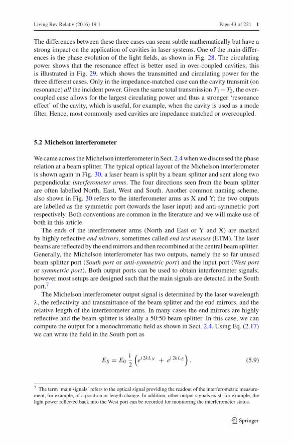
Living Rev Relativ (2016) 19:1 Page 43 of 221 1
The differences between these three cases can seem subtle mathematically but have astrong impact on the application of cavities in laser systems. One of the main differ-ences is the phase evolution of the light fields, as shown in Fig. 28. The circulatingpower shows that the resonance effect is better used in over-coupled cavities; thisis illustrated in Fig. 29, which shows the transmitted and circulating power for thethree different cases. Only in the impedance-matched case can the cavity transmit (onresonance) all the incident power. Given the same total transmission T1 +T2, the over-coupled case allows for the largest circulating power and thus a stronger ‘resonanceeffect’ of the cavity, which is useful, for example, when the cavity is used as a modefilter. Hence, most commonly used cavities are impedance matched or overcoupled.
5.2 Michelson interferometer
We came across the Michelson interferometer in Sect. 2.4 when we discussed the phaserelation at a beam splitter. The typical optical layout of the Michelson interferometeris shown again in Fig. 30, a laser beam is split by a beam splitter and sent along twoperpendicular interferometer arms. The four directions seen from the beam splitterare often labelled North, East, West and South. Another common naming scheme,also shown in Fig. 30 refers to the interferometer arms as X and Y; the two outputsare labelled as the symmetric port (towards the laser input) and anti-symmetric portrespectively. Both conventions are common in the literature and we will make use ofboth in this article.
The ends of the interferometer arms (North and East or Y and X) are markedby highly reflective end mirrors, sometimes called end test masses (ETM), The laserbeams are reflected by the end mirrors and then recombined at the central beam splitter.Generally, the Michelson interferometer has two outputs, namely the so far unusedbeam splitter port (South port or anti-symmetric port) and the input port (West portor symmetric port). Both output ports can be used to obtain interferometer signals;however most setups are designed such that the main signals are detected in the Southport.7
The Michelson interferometer output signal is determined by the laser wavelengthλ, the reflectivity and transmittance of the beam splitter and the end mirrors, and therelative length of the interferometer arms. In many cases the end mirrors are highlyreflective and the beam splitter is ideally a 50:50 beam splitter. In this case, we cancompute the output for a monochromatic field as shown in Sect. 2.4. Using Eq. (2.17)we can write the field in the South port as
ES = E0i
2
(ei 2kLN + ei 2kLE
). (5.9)
7 The term ‘main signals’ refers to the optical signal providing the readout of the interferometric measure-ment, for example, of a position or length change. In addition, other output signals exist: for example, thelight power reflected back into the West port can be recorded for monitoring the interferometer status.
123
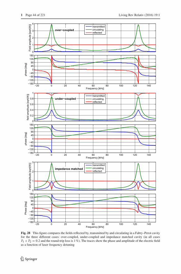
1 Page 44 of 221 Living Rev Relativ (2016) 19:1
Fig. 28 This figure compares the fields reflected by, transmitted by and circulating in a Fabry–Perot cavityfor the three different cases: over-coupled, under-coupled and impedance matched cavity (in all casesT1 + T2 = 0.2 and the round-trip loss is 1 %). The traces show the phase and amplitude of the electric fieldas a function of laser frequency detuning
123
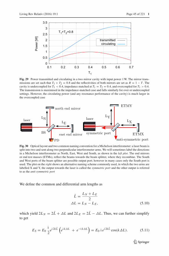
Living Rev Relativ (2016) 19:1 Page 45 of 221 1
Fig. 29 Power transmitted and circulating in a two mirror cavity with input power 1 W. The mirror trans-missions are set such that T1 + T2 = 0.8 and the reflectivities of both mirrors are set as R = 1 − T . Thecavity is undercoupled for T1 < 0.4, impedance matched at T1 = T2 = 0.4, and overcoupled for T1 > 0.4.The transmission is maximised in the impedance-matched case and falls similarly for over or undercoupledsettings. However, the circulating power (and any resonance performance of the cavity) is much larger inthe overcoupled case
Fig. 30 Optical layout and two common naming convention for a Michelson interferometer: a laser beam issplit into two and sent along two perpendicular interferometer arms. We will sometimes label the directionsin a Michelson interferometer as North, East, West and South, as shown in the left plot. The end mirrorsor end test masses (ETMs), reflect the beams towards the beam splitter, where they recombine. The Southand West ports of the beam splitter are possible output port; however in many cases only the South port isused. The plot on the right shows an alternative naming scheme commonly used, in which the two arms arelabelled X and Y, the output towards the laser is called the symmetric port and the other output is referredto as the anti-symmetric port
We define the common and differential arm lengths as
L = LN + LE
2ΔL = LN − LE , (5.10)
which yield 2LN = 2L + ΔL and 2LE = 2L − ΔL . Thus, we can further simplifyto get
ES = E0i
2ei 2k L
(ei kΔL + e−i kΔL
)= E0 i ei 2k L cos(kΔL). (5.11)
123

1 Page 46 of 221 Living Rev Relativ (2016) 19:1
Fig. 31 Power in the South port of a symmetric Michelson interferometer as a function of the arm lengthdifference ΔL . When the interferometer is set to ΔL/λ = 0.25 the input light is not transmitted into theSouth port: this condition is called the dark fringe
The photo detector then produces a signal proportional to
S = ESE∗S = P0 cos2(kΔL) = P0 cos2(2πΔL/λ). (5.12)
This signal is depicted in Fig. 31; it shows that the power in the South port changesbetween zero and the input power with a period of ΔL/λ = 0.5. The tuning atwhich the output power drops to zero is called the dark fringe. Current interferometricgravitational-wave detectors operate their Michelson interferometer at or near the darkfringe.
The above seems to indicate that the macroscopic arm-length difference plays norole in the Michelson output signal. However, this is only correct for a monochromaticlaser beam with infinite coherence length. In real interferometers care must be takenthat the arm-length difference is well below the coherence length of the light source.In gravitational-wave detectors the macroscopic arm-length difference is an importantdesign feature; it is kept very small in order to reduce coupling of laser noise intothe output but needs to retain a finite size to allow the transfer of phase modulationsidebands from the input to the output port; this is illustrated in the Finesse examplebelow and will be covered in detail in Sect. 8.11.
5.3 Michelson interferometer and the sideband picture
In the context of gravitational wave detection the Michelson interferometer is used formeasuring a very small differential change in the length of one arm versus the other.The very small amplitude of gravitational waves, or the equivalent small differentialchange of the arm lengths, requires additional optical techniques to increase the sen-sitivity of the interferometer. In this section we briefly introduce the interferometerconfigurations and review their effect on the detector sensitivity.
The Michelson interferometer can achieve its best sensitivity when operated in aquasi stationary mode, i.e., when the positions of mirrors and beamsplitters are care-fully controlled so that the key parameters, for example the light power inside theinterferometer and at the output ports, are nearly constant. We call such an interferom-eter state, described by a unique set of the key parameters, an operating point of theinterferometer (see Sect. 8 for a discussion of the control systems involved to reach
123

Living Rev Relativ (2016) 19:1 Page 47 of 221 1
Fig. 32 A Michelson interferometer shown with three types of light field: the ‘carrier’, representing theundistorted laser input field, ‘laser phase noise sidebands’, which enter the interferometer with the carrier,and ‘signal sidebands’, which are phase modulation sidebands caused by differential arm length motion.All three fields leave the interferometer through both output ports (here only the detector in the South portis shown). The graph shows the amplitude of the three light fields in the South port as a function of theMichelson tuning (differential arm length change). At 0◦ the Michelson is on a bright fringe and at 90◦ ona dark fringe
and maintain an operating point). For an interferometer in a steady state it is possibleto describe and analyse the behaviour using a steady state model, describing the lightfield coupling in the frequency domain and making use of the previously introducedconcept of sidebands, see Sect. 3.1.
Consider a Michelson interferometer which is to be used to measure a differentialarm length change. As an example for a signal to noise comparison we consider thephase noise of the injected laser light. For this example the noise can be representedby a sinusoidal modulation with a small amplitude at a single frequency, say 100 Hz.Therefore we can describe the phase noise of the laser by a pair of sidebands superim-posed on the main carrier light field entering the Michelson interferometer. Equally thechange of an interferometer arm represents a phase modulation of the light reflectedback from the end mirrors and the generated optical signal can be represented by apair of phase modulation sidebands, see Sect. 5.5.
In order to get an estimation of the signal to noise ratio we can trace the individualsidebands through the interferometer and compute their amplitude in the output port.Figure 32 shows the setup of a basic Michelson interferometer, indicating the insertionof the noise and signal sidebands. It also provides a plot of the sideband amplitudein the South output port as a function of the differential arm length of the Michelson
123

1 Page 48 of 221 Living Rev Relativ (2016) 19:1
interferometer. We can see that a tuning of 90◦ corresponds to the dark fringe, the stateof the interferometer in which the injected light (the carrier and laser noise) is reflectedback towards the laser and is not transmitted into the South port. The plot reveals twoadvantages of the dark fringe as an operating point: first of all the transmission ofthe signal sidebands to the photo detector is maximised while the laser phase noise isminimised. More generally at the dark fringe, all common mode effects, such as lasernoise, or common length changes of the arms, produce a minimal optical signal at theoutput port, whereas differential effects in the arms are maximised. Furthermore at thedark fringe the least amount of carrier light is transmitted to the photo detector. Thisis an advantage because it is technically often easier to make an accurate light powermeasurement when the total detected power is low.
It should be noted that with the interferometer on the dark fringe, only the signalsidebands would leave the interferometer. Typically these alone cannot create a strongsignal during detection. In the case of gravitational wave detection these sidebands aremany orders of magnitude smaller than the amplitude of the carrier. We require a beatbetween the signal sidebands and another field, a so-called local oscillator, to generatea strong electronic signal proportional to the amplitude of the signal sidebands. Thelocal oscillator can be created in different ways, the most common are:
– Apply an RF modulation to the laser beam, either before injecting it into theinterferometer or inside the interferometer. A small macroscopic length asymmetrybetween the two arms (Schnupp asymmetry, see Sect. 8.13) allows a significantamount of the RF sidebands to reach the South port when the interferometer isoperating on the dark fringe for the carrier. The RF sideband fields can be used asa local oscillator.
– Set the Michelson such that it is close to, but not exactly on, the dark fringe.The carrier leaking into the South port can thus be used as a local oscillator. Thisscheme preserves the advantages of the dark fringe but relies on very good powerstability of the carrier light.
– Superimpose an auxiliary beam onto the output before the photodetector. Forexample, a pick-off beam from the main laser can be used for this. The maindisadvantage of this concept is that it requires a very stable auxiliary beam (inphase as well as position) thus creating new control problems.
5.4 Michelson interferometer signal readout with DC offset, or RF modulation
As discussed in Sect. 4.1, one method for providing a local oscillator is to use a smallmicroscopic DC offset to tune the Michelson interferometer slightly away from thedark fringe. This allows a small amount of carrier to leak through to the output portto beat with the signal sidebands. The differential arm length difference required is
ΔL = π
2k0+ δoff , (5.13)
where k0 = ω0/c is the wavenumber of the carrier field and the DC offset is δoff 1.The field at the output port of a Michelson (as shown in Fig. 11) for a single carrier
123
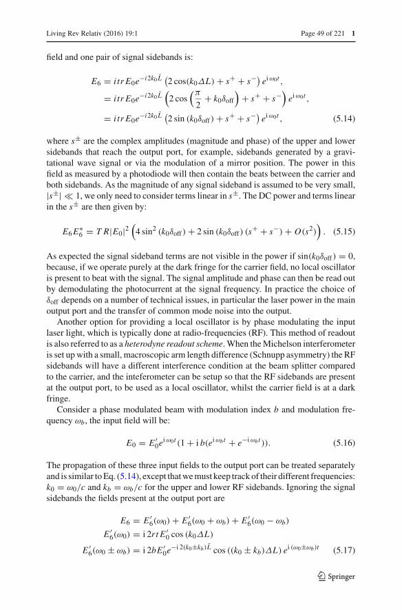
Living Rev Relativ (2016) 19:1 Page 49 of 221 1
field and one pair of signal sidebands is:
E6 = i tr E0e−i2k0 L
(2 cos(k0ΔL) + s+ + s−)
ei ω0t ,
= i tr E0e−i2k0 L
(2 cos
(π
2+ k0δoff
)+ s+ + s−)
ei ω0t ,
= i tr E0e−i2k0 L
(2 sin (k0δoff) + s+ + s−)
ei ω0t , (5.14)
where s± are the complex amplitudes (magnitude and phase) of the upper and lowersidebands that reach the output port, for example, sidebands generated by a gravi-tational wave signal or via the modulation of a mirror position. The power in thisfield as measured by a photodiode will then contain the beats between the carrier andboth sidebands. As the magnitude of any signal sideband is assumed to be very small,|s±| 1, we only need to consider terms linear in s±. The DC power and terms linearin the s± are then given by:
E6E∗6 = T R|E0|2
(4 sin2 (k0δoff) + 2 sin (k0δoff) (s+ + s−) + O(s2)
). (5.15)
As expected the signal sideband terms are not visible in the power if sin(k0δoff) = 0,because, if we operate purely at the dark fringe for the carrier field, no local oscillatoris present to beat with the signal. The signal amplitude and phase can then be read outby demodulating the photocurrent at the signal frequency. In practice the choice ofδoff depends on a number of technical issues, in particular the laser power in the mainoutput port and the transfer of common mode noise into the output.
Another option for providing a local oscillator is by phase modulating the inputlaser light, which is typically done at radio-frequencies (RF). This method of readoutis also referred to as a heterodyne readout scheme. When the Michelson interferometeris set up with a small, macroscopic arm length difference (Schnupp asymmetry) the RFsidebands will have a different interference condition at the beam splitter comparedto the carrier, and the inteferometer can be setup so that the RF sidebands are presentat the output port, to be used as a local oscillator, whilst the carrier field is at a darkfringe.
Consider a phase modulated beam with modulation index b and modulation fre-quency ωb, the input field will be:
E0 = E ′0e
i ω0t (1 + i b(ei ωbt + e−i ωbt )). (5.16)
The propagation of these three input fields to the output port can be treated separatelyand is similar to Eq. (5.14), except that we must keep track of their different frequencies:k0 = ω0/c and kb = ωb/c for the upper and lower RF sidebands. Ignoring the signalsidebands the fields present at the output port are
E6 = E ′6(ω0) + E ′
6(ω0 + ωb) + E ′6(ω0 − ωb)
E ′6(ω0) = i 2r t E ′
0 cos (k0ΔL)
E ′6(ω0 ± ωb) = i 2bE ′
0e−i 2(k0±kb)L cos ((k0 ± kb)ΔL) ei (ω0±ωb)t (5.17)
123
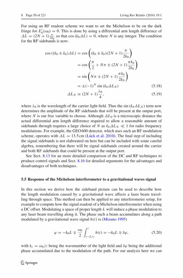
1 Page 50 of 221 Living Rev Relativ (2016) 19:1
For using an RF readout scheme we want to set the Michelson to be on the darkfringe for E ′
6(ω0) = 0. This is done by using a differential arm length difference ofΔL = (2N + 1) π
2k0so that cos (k0ΔL) = 0, where N is any integer. The condition
for the RF sidebands is now:
cos ((k0 ± kb)ΔL) = cos
((k0 ± kb)(2N + 1)
π
2k0
)
= cos
(π
2+ Nπ ± (2N + 1)
πkb2k0
)
= sin
(Nπ ± (2N + 1)
πkb2k0
)
= ±(−1)N sin (kbΔLN ) (5.18)
ΔLN ≡ (2N + 1)λ0
4, (5.19)
where λ0 is the wavelength of the carrier light field. Thus the sin (kbΔLN ) term nowdetermines the amplitude of the RF sidebands that will be present at the output port,where N is our free variable to choose. Although ΔL0 is a microscopic distance theactual differential arm length difference required to allow a reasonable amount ofsidebands through requires a large choice of N as kbΔLN 1 for radio frequencymodulations. For example, the GEO 600 detector, which uses such an RF modulationscheme, operates with ΔL = 13.5 cm (Lück et al. 2010). The final step of includingthe signal sidebands is not elaborated on here but can be included with some carefulalgebra, remembering that there will be signal sidebands created around the carrierand both RF sidebands that could be present at the output port.
See Sect. 8.13 for an more detailed comparison of the DC and RF techniques toproduce control signals and Sect. 8.16 for detailed arguments for the advantages anddisadvantages of both techniques.
5.5 Response of the Michelson interferometer to a gravitational waves signal
In this section we derive how the sideband picture can be used to describe howthe length modulation caused by a gravitational wave affects a laser beam travel-ling through space. This method can then be applied to any interferometer setup, forexample to compute how the signal readout of a Michelson interferometer when usinga DC offset. Modulating a space of proper length L will induce a phase modulation toany laser beam travelling along it. The phase such a beam accumulates along a pathmodulated by a gravitational wave signal h(t) is (Mizuno 1995)
ϕ = −k0L ∓ ω0
2
∫ t
t−L/ch(t) = −k0L ∓ δϕ, (5.20)
with kc = ω0/c being the wavenumber of the light field and δϕ being the additionalphase accumulated due to the modulation of the path. For our analysis here we can
123

Living Rev Relativ (2016) 19:1 Page 51 of 221 1
assume the gravitational wave signal is a simple sinusoidal function
h(t) = h0 cos(ωgwt + ϕgw
), (5.21)
where ωgw and ϕgw are the frequency and phase of the gravitational wave. The phaseaccumulated from propagating along the space is then8
δϕ = ω0h0
ωgwcos
(ωgwt + ϕgw − ωgw
L
2c
)sin
(ωgw
L
2c
). (5.22)
Thus an oscillating, time dependent phase is present in the light fields travelling alongthe space. Section 3.2 describes how such a modulation generates sideband fields; therespective modulation index and phase are
m = −ω0h0
ωgwsin
(kgwL
2
), (5.23)
ϕ = −kgwL
2+ ϕgw, (5.24)
with kgw = ωgw/c being the wavenumber for the gravitational wave signal sidebands.Using Eq. (3.10) the unscaled amplitude and phase of the upper, α+
gw, and lower, α−gw,
sidebands generated by a gravitational wave are then
Agw = −w0h0
2ωgwsin
(kgwL
2
), (5.25)
Φ±gw = π
2− L
(k0 ± kgw
2
)± ϕgw, (5.26)
α±gw = Agwe
iΦ±gwe±iωgw t . (5.27)
Note that α±gw must be scaled by the carrier field that is propagating into the space for
the complete sideband amplitude.To compute how a Michelson responds to a gravitational wave we must first consider
the modulation of the carrier field travelling in both directions along the arms. Boththe carrier and the created signal sideband fields propagate along each arm, as shownin Fig. 33, and are reflected by a mirror with amplitude reflectivity retm . The relevantcarrier fields are
a3 = a2 exp (−i k0L), (5.28)
a2 = retma1, (5.29)
a1 = a0 exp (−i k0L). (5.30)
8 Derivations of the accumulated phase can be found in many works, a simple example is presented inBond (2014).
123
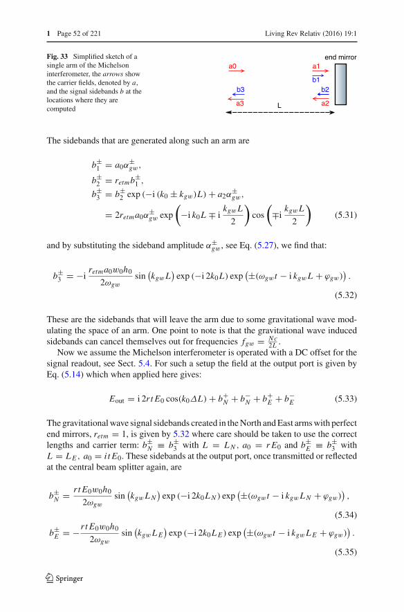
1 Page 52 of 221 Living Rev Relativ (2016) 19:1
Fig. 33 Simplified sketch of asingle arm of the Michelsoninterferometer, the arrows showthe carrier fields, denoted by a,and the signal sidebands b at thelocations where they arecomputed
The sidebands that are generated along such an arm are
b±1 = a0α
±gw,
b±2 = retmb
±1 ,
b±3 = b±
2 exp (−i (k0 ± kgw)L) + a2α±gw,
= 2retma0α±gw exp
(−i k0L ∓ i
kgwL
2
)cos
(∓i
kgwL
2
)(5.31)
and by substituting the sideband amplitude α±gw, see Eq. (5.27), we find that:
b±3 = −i
retma0w0h0
2ωgwsin
(kgwL
)exp (−i 2k0L) exp
(±(ωgwt − i kgwL + ϕgw)).
(5.32)
These are the sidebands that will leave the arm due to some gravitational wave mod-ulating the space of an arm. One point to note is that the gravitational wave inducedsidebands can cancel themselves out for frequencies fgw = Nc
2L .Now we assume the Michelson interferometer is operated with a DC offset for the
signal readout, see Sect. 5.4. For such a setup the field at the output port is given byEq. (5.14) which when applied here gives:
Eout = i 2r t E0 cos(k0ΔL) + b+N + b−
N + b+E + b−
E (5.33)
The gravitational wave signal sidebands created in the North and East arms with perfectend mirrors, retm = 1, is given by 5.32 where care should be taken to use the correctlengths and carrier term: b±
N ≡ b±3 with L = LN , a0 = r E0 and b±
E ≡ b±3 with
L = LE , a0 = i t E0. These sidebands at the output port, once transmitted or reflectedat the central beam splitter again, are
b±N = r t E0w0h0
2ωgwsin
(kgwLN
)exp (−i 2k0LN ) exp
(±(ωgwt − i kgwLN + ϕgw)),
(5.34)
b±E = −r t E0w0h0
2ωgwsin
(kgwLE
)exp (−i 2k0LE ) exp
(±(ωgwt − i kgwLE + ϕgw)).
(5.35)
123

Living Rev Relativ (2016) 19:1 Page 53 of 221 1
Note that an extra minus sign is included for the East-arm sidebands because thegravitational wave modulate the North and East arms differentially. Next we willwrite the arm lengths in terms of a macroscopic differential ΔL , and common modeL , lengths: LN = L+ΔL/2 and LE = L−ΔL/2. Along with this we also assume thatthe central beam splitter has a 50:50 splitting ration r = t = 1/
√2, that the common
mode length is an integer number of wavelengths for the carrier light exp(i k0 L) = 1,that L � ΔL , and that the gravitational wave’s wavelength is much larger than ΔL , sokgw(L + ΔL/2) ≈ kgw L . Taking these assumptions into account the sideband termsbecome
b±N = E0w0h0
4ωgwsin
(kgw L
)exp (−i k0ΔL) exp
(±(ωgwt − i kgw L + ϕgw)),
(5.36)
b±E = − E0w0h0
4ωgwsin
(kgw L
)exp (i k0ΔL) exp
(±(ωgwt − i kgw L + ϕgw)).
(5.37)
Finally the sum of the sidebands at the output is
b+N +b−
N +b+E +b−
E = i E0w0h0
ωgwsin
(kgw L
)sin (k0ΔL) cos
(ωgwt − kgw L+ϕgw
).
(5.38)
Now that we know the signal sideband fields at the output port, we can combine themwith the carrier field that is also present:
Eout = i E0 cos(k0ΔL) + b+N + b−
N + b+E + b−
E
= i E0
[cos(k0ΔL)+ w0h0
ωgwsin
(kgw L
)sin (k0ΔL) cos
(ωgwt − kgw L+ϕgw
)].
(5.39)
A photodiode placed at the output of the Michelson will then measure the power inthis beam from which we want to extract the gravitational wave amplitude, h0 andphase, ϕgw. The power in the beam contains multiple beat frequencies between all thecarrier and signal sidebands, with the terms oscillating at the frequency ωgw, are thoselinearly proportional to h0:
Pgw = |E0|2 w0h0
ωgwsin
(kgw L
)sin (2k0ΔL) cos
(ωgwt − kgw L + ϕgw
). (5.40)
As we are using DC readout, the differential arm length is chosen to operate slightlyaway from the dark fringe of the carrier field ΔL = π
2k0+δoff as discussed in Sect. 5.4.
The choice of DC offset is typically δoff λ0, the wavelength of the carrier light. So
123
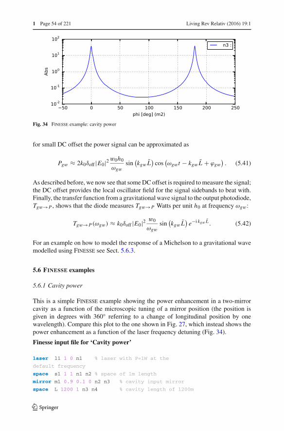
1 Page 54 of 221 Living Rev Relativ (2016) 19:1
Fig. 34 Finesse example: cavity power
for small DC offset the power signal can be approximated as
Pgw ≈ 2k0δoff |E0|2 w0h0
ωgwsin
(kgw L
)cos
(ωgwt − kgw L + ϕgw
). (5.41)
As described before, we now see that some DC offset is required to measure the signal;the DC offset provides the local oscillator field for the signal sidebands to beat with.Finally, the transfer function from a gravitational wave signal to the output photodiode,Tgw→P , shows that the diode measures Tgw→P Watts per unit h0 at frequency ωgw:
Tgw→P (ωgw) ≈ k0δoff |E0|2 w0
ωgwsin
(kgw L
)e−i kgw L . (5.42)
For an example on how to model the response of a Michelson to a gravitational wavemodelled using Finesse see Sect. 5.6.3.
5.6 FINESSE examples
5.6.1 Cavity power
This is a simple Finesse example showing the power enhancement in a two-mirrorcavity as a function of the microscopic tuning of a mirror position (the position isgiven in degrees with 360◦ referring to a change of longitudinal position by onewavelength). Compare this plot to the one shown in Fig. 27, which instead shows thepower enhancement as a function of the laser frequency detuning (Fig. 34).
Finesse input file for ‘Cavity power’
laser l1 1 0 n1 % laser with P=1W at the
default frequency
space s1 1 1 n1 n2 % space of 1m length
mirror m1 0.9 0.1 0 n2 n3 % cavity input mirror
space L 1200 1 n3 n4 % cavity length of 1200m
123
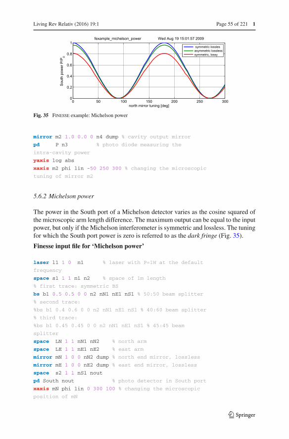
Living Rev Relativ (2016) 19:1 Page 55 of 221 1
Fig. 35 Finesse example: Michelson power
mirror m2 1.0 0.0 0 n4 dump % cavity output mirror
pd P n3 % photo diode measuring the
intra-cavity power
yaxis log abs
xaxis m2 phi lin -50 250 300 % changing the microscopic
tuning of mirror m2
5.6.2 Michelson power
The power in the South port of a Michelson detector varies as the cosine squared ofthe microscopic arm length difference. The maximum output can be equal to the inputpower, but only if the Michelson interferometer is symmetric and lossless. The tuningfor which the South port power is zero is referred to as the dark fringe (Fig. 35).
Finesse input file for ‘Michelson power’
laser l1 1 0 n1 % laser with P=1W at the default
frequency
space s1 1 1 n1 n2 % space of 1m length
% first trace: symmetric BS
bs b1 0.5 0.5 0 0 n2 nN1 nE1 nS1 % 50:50 beam splitter
% second trace:
%bs b1 0.4 0.6 0 0 n2 nN1 nE1 nS1 % 40:60 beam splitter
% third trace:
%bs b1 0.45 0.45 0 0 n2 nN1 nE1 nS1 % 45:45 beam
splitter
space LN 1 1 nN1 nN2 % north arm
space LE 1 1 nE1 nE2 % east arm
mirror mN 1 0 0 nN2 dump % north end mirror, lossless
mirror mE 1 0 0 nE2 dump % east end mirror, lossless
space s2 1 1 nS1 nout
pd South nout % photo detector in South port
xaxis mN phi lin 0 300 100 % changing the microscopic
position of mN
123

1 Page 56 of 221 Living Rev Relativ (2016) 19:1
Fig. 36 Finesse example: Michelson sideband output from a gravitational wave
5.6.3 Michelson gravitational wave response
This is a simple Finesse example showing how the arm spaces can be modulatedto produce the effect a gravitational wave would have on it. It outputs the amplitudeand phase of the upper sideband that reaches the output port. The dips in amplitudeoccur when the travel time of the photons along the interferometer arms equals onegravitational wave period and hence the signal accumulated in the first and second halfof the travel time cancel each other (the plot above does not have enough resolutionto show that the dips indicate zero signal, the non-zero amplitudes are an artefact ofthe numerical plotting routine). In this example the frequencies of the dips are givenas f = N c/1200 m = N 250 kHz, with N a positive integer (Fig. 36).
Finesse input file for ‘Michelson gravitational wave response’laser l1 1 0 nin
space s0 1 nin n1
bs BS 0.5 0.5 0 45 n1 ny1 nx1 nout
s syarm 600 ny1 ny2
m1 ETMy 100e-6 0 0 ny2 ny3
s sxarm 600 nx1 nx2
m1 ETMx 100e-6 0 90 nx2 nx3
# Apply a signal each arm with 180 phase difference
between them
fsig sig1 syarm 1 180
fsig sig1 sxarm 1 0
# output the upper sideband
ad upper 0 nout
xaxis sig1 f log 1k 1M 4000
# sets the ad detector frequency to the upper sideband
freq.
put upper f $x1
yaxis log abs:deg
123
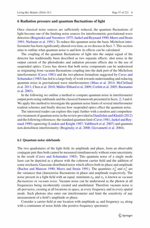
Living Rev Relativ (2016) 19:1 Page 57 of 221 1
6 Radiation pressure and quantum fluctuations of light
Once classical noise sources are sufficiently reduced, the quantum fluctuations oflight become one of the limiting noise sources for interferometric gravitational-wavedetectors (Braginskii and Vorontsov 1975; Jaekel and Reynaud 1990; Meers and Strain1991; Niebauer et al. 1991). To reduce this quantum noise the basic Michelson inter-ferometer has been significantly altered over time, as we discuss in Sect. 7. This sectionaims to outline what quantum noise is and how its effects can be calculated.
The coupling of the quantum fluctuations of light into the output signal of thedetector has traditionally been described as two separate effects: shot noise in theoutput current of the photodiodes and radiation pressure effects due to the use ofsuspended optics. Caves has shown that both noise components can be understoodas originating from vacuum fluctuations coupling into the dark port of the Michelsoninterferometer (Caves 1981) and the two-photon formalism suggested by Caves andSchumaker (1985) has led to a large body of work towards understanding and reducingquantum noise in gravitational wave interferometers (Miao et al. 2014; McClellandet al. 2011; Chen et al. 2010; Müller-Ebhard et al. 2009; Corbitt et al. 2005; Buonannoet al. 2003).
In the following we outline a method to compute quantum noise in interferometeroutput ports using sidebands and the classical framework presented in Sects. 2, 3 and 4.We apply this method to investigate the quantum noise limits of several interferometerreadout schemes and finally discuss how suspended optics effect the quantum noise.
The interested reader can explore this topic further with a modern and comprehen-sive treatment of quantum noise in the review provided in Danilishin and Khalili (2012)and the following references: the standard quantum limit (Caves 1981; Jaekel and Rey-naud 1990) squeezing (Loudon and Knight 1987; Vahlbruch et al. 2007) and quantumnon-demolition interferometry (Braginsky et al. 2000; Giovannetti et al. 2004).
6.1 Quantum noise sidebands
The two quadratures of the light field, its amplitude and phase, form an observableconjugate pair thus both cannot be measured simultaneously without some uncertaintyin the result (Caves and Schumaker 1985). This quantum noise of a single modelaser can be depicted as a phasor with the coherent carrier field and the addition ofsome stochastic Gaussian-distributed noise which affects both its phase and amplitude(Bachor and Manson 1990; Meers and Strain 1991). The quantities σ 2
φ and σ 2a are
the variances that characterise fluctuations in phase and amplitude respectively. Thenoise present in a light field with an equal, minimum σφ and σa is known as vacuumfluctuations or vacuum noise. Vacuum noise can be understood as the photon at allfrequencies being incoherently created and annihilated. Therefore vacuum noise isall-pervasive, existing at all locations in space, at every frequency and in every spatialmode. Such photons also enter our interferometer and limit the sensitivity of anymeasurement of a field’s amplitude or phase.
Consider a carrier field at one location with amplitude a0 and frequency ω0 alongwith a continuum of noise fields (the positive frequency spectrum):
123
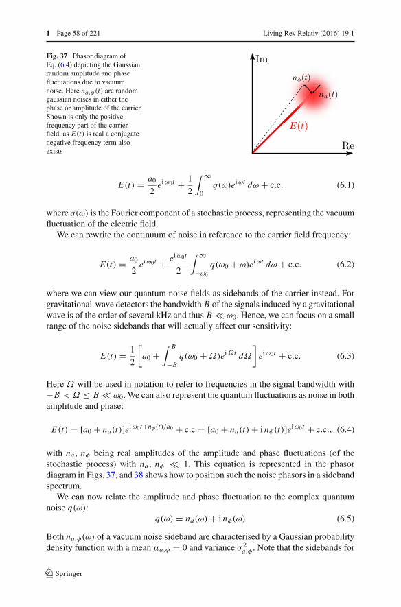
1 Page 58 of 221 Living Rev Relativ (2016) 19:1
Fig. 37 Phasor diagram ofEq. (6.4) depicting the Gaussianrandom amplitude and phasefluctuations due to vacuumnoise. Here na,φ(t) are randomgaussian noises in either thephase or amplitude of the carrier.Shown is only the positivefrequency part of the carrierfield, as E(t) is real a conjugatenegative frequency term alsoexists
E(t) = a0
2ei ω0t + 1
2
∫ ∞
0q(ω)ei ωt dω + c.c. (6.1)
where q(ω) is the Fourier component of a stochastic process, representing the vacuumfluctuation of the electric field.
We can rewrite the continuum of noise in reference to the carrier field frequency:
E(t) = a0
2ei ω0t + ei ω0t
2
∫ ∞
−ω0
q(ω0 + ω)ei ωt dω + c.c. (6.2)
where we can view our quantum noise fields as sidebands of the carrier instead. Forgravitational-wave detectors the bandwidth B of the signals induced by a gravitationalwave is of the order of several kHz and thus B ω0. Hence, we can focus on a smallrange of the noise sidebands that will actually affect our sensitivity:
E(t) = 1
2
[a0 +
∫ B
−Bq(ω0 + Ω)ei Ωt dΩ
]ei ω0t + c.c. (6.3)
Here Ω will be used in notation to refer to frequencies in the signal bandwidth with−B < Ω ≤ B ω0. We can also represent the quantum fluctuations as noise in bothamplitude and phase:
E(t) = [a0 + na(t)]ei ω0t+nφ(t)/a0 + c.c = [a0 + na(t) + i nφ(t)]ei ω0t + c.c., (6.4)
with na , nφ being real amplitudes of the amplitude and phase fluctuations (of thestochastic process) with na , nφ 1. This equation is represented in the phasordiagram in Figs. 37, and 38 shows how to position such the noise phasors in a sidebandspectrum.
We can now relate the amplitude and phase fluctuation to the complex quantumnoise q(ω):
q(ω) = na(ω) + i nφ(ω) (6.5)
Both na,φ(ω) of a vacuum noise sideband are characterised by a Gaussian probabilitydensity function with a mean μa,φ = 0 and variance σ 2
a,φ . Note that the sidebands for
123

Living Rev Relativ (2016) 19:1 Page 59 of 221 1
Fig. 38 This diagram depicts a carrier field as shown in Fig. 37 but expanded to show the vacuum noisesideband phasors that contribute towards the noise. The amplitude and phase of each sideband is a stochasticGaussian noise so that its real and imaginary parts are described by some probability distribution depictedby the blue faded region, the dashed circle represents the standard deviation of such fluctuations. The signalbandwidth B can be imagined as containing an infinite number of such vacuum noise sidebands, eachoscillating with a random phase and amplitude. Pictured are two upper and lower sidebands selected fromthis continuum of vacuum noise. The negative frequency phasors are not shown, they would be the mirroredconjugate versions of the positive phasors
the quantum noise are not representing a coherent and deterministic signal. This semi-classical approach is sufficient to motivate the design choices in laser interferometersfor gravitational wave detection. A rigorous approach would require to use operatorsinstead of sidebands. This approach is beyond the scope of this article, and insteadfully covered in the review article by Danilishin and Khalili (2012).
The variances na,φ(ω) are limited by the minimum uncertainty in the relation
σφσa ≥ hω
2, (6.6)
which gives for an integration time of one second, σ 2φ = σ 2
a = hω/2. As the phaseand amplitude of q(ω) is random we can only compute its expected value or ensemblevalue at a particular frequency:
〈q(ω)〉 = 〈μa〉 + i 〈μφ〉 = 0, (6.7)
which is zero as the mean of the noise is zero, hence on average no sidebands areactually observed. We can also consider the covariance between any two sidebands atfrequency ω and ω′. As q(ω) is a complex value there are multiple ways the covari-ance can be taken when considering the conjugates of either sideband, for example〈q(ω)q∗(−ω′)〉, 〈q∗(ω)q(−ω′)〉, etc.. However as the fluctuations in amplitude andphase at different frequencies are independent, the covariance between any two vac-uum noise sidebands is:
123

1 Page 60 of 221 Living Rev Relativ (2016) 19:1
〈q(ω)q∗(ω′)〉 = hω
2δ(ω − ω′), (6.8)
〈q(ω)q(ω′)〉 = 0, (6.9)
The delta function in the covariance signifies there is no correlation between differentfrequencies. The auto-covariance is then 〈q(ω)q∗(ω)〉 ∝ δ(ω − ω) = ∞, which mayseem odd at a first glance. However, this can be better understood in the time domainpicture, as we are measuring our signal over an idealistic infinite time span and as ournoise is Markovian (and therefore also ergodic), the time average of the power of asignal will be infinitely large.
Noise power spectral densities
Noise, i.e., a random signal, can be quantified using a power spectral density (PSD)which is a measure of the power in a signal per frequency. The definition of a single-sided PSD of some frequency domain value x(ω) is:
Sxx (ω)δ(ω − ω′) = 2〈x(ω)x∗(ω′)〉, (6.10)
with units [x]2/Hz. The cross-spectral-density between two values x(ω) and y(ω) issimilarly:
Sxy(ω)δ(ω − ω′) = 2〈x(ω)y∗(ω′)〉. (6.11)
The eventual physical noise we wish to compute is the noise in the demodulatedphotocurrent of the photodiode measuring the interferometer output signal, here wewill consider only photodiodes with 100 % quantum efficiency.9 The photocurrent Iis proportional to the detected light power I (t)∼P(t) and the PSD of the noise in thephotocurrent is:
SI (ω)δ(ω − ω′) = 2〈I (ω)I ∗(ω′)〉 (6.12)
The DC and ω ± Ω terms of the power on a photodiode for a single carrier withquantum noise sidebands is:
P(t) = E(t)E∗(t) = |a0|2 + a∗0
∫ B
−Bq(ω0 + Ω)ei Ωt dΩ
+ a0
∫ B
−Bq∗(ω0 + Ω)e−i Ωt dΩ + O(q2), (6.13)
terms of the order q2 are assumed to be a negligibly small contribution. The positivehalf of the photocurrent spectrum for 0 < Ω ≤ B is given by its Fourier transform:
I (Ω) ≡ F[I (t)] = a∗0q(ω0 + Ω) + a0q
∗(ω0 − Ω). (6.14)
9 It is proportional to a factor χ , the photodiodes quantum efficiency, which states how many Amps perWatt of incident power is output by the photodiode. We will assume here the efficiency is perfect, χ = 1,for simplicity.
123
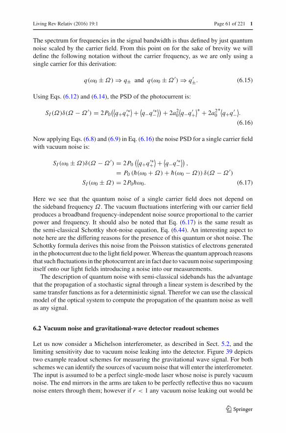
Living Rev Relativ (2016) 19:1 Page 61 of 221 1
The spectrum for frequencies in the signal bandwidth is thus defined by just quantumnoise scaled by the carrier field. From this point on for the sake of brevity we willdefine the following notation without the carrier frequency, as we are only using asingle carrier for this derivation:
q(ω0 ± Ω) ⇒ q± and q(ω0 ± Ω ′) ⇒ q ′±. (6.15)
Using Eqs. (6.12) and (6.14), the PSD of the photocurrent is:
SI (Ω)δ(Ω − Ω ′) = 2P0(⟨q+q ′∗+
⟩ + ⟨q−q ′∗−
⟩) + 2a20
⟨q−q ′+
⟩∗ + 2a20∗⟨q+q ′−
⟩.
(6.16)
Now applying Eqs. (6.8) and (6.9) in Eq. (6.16) the noise PSD for a single carrier fieldwith vacuum noise is:
SI (ω0 ± Ω)δ(Ω − Ω ′) = 2P0(⟨q+q ′∗+
⟩ + ⟨q−q ′∗−
⟩),
= P0 (h(ω0 + Ω) + h(ω0 − Ω)) δ(Ω − Ω ′)SI (ω0 ± Ω) = 2P0hω0. (6.17)
Here we see that the quantum noise of a single carrier field does not depend onthe sideband frequency Ω . The vacuum fluctuations interfering with our carrier fieldproduces a broadband frequency-independent noise source proportional to the carrierpower and frequency. It should also be noted that Eq. (6.17) is the same result asthe semi-classical Schottky shot-noise equation, Eq. (6.44). An interesting aspect tonote here are the differing reasons for the presence of this quantum or shot noise. TheSchottky formula derives this noise from the Poisson statistics of electrons generatedin the photocurrent due to the light field power. Whereas the quantum approach reasonsthat such fluctuations in the photocurrent are in fact due to vacuum noise superimposingitself onto our light fields introducing a noise into our measurements.
The description of quantum noise with semi-classical sidebands has the advantagethat the propagation of a stochastic signal through a linear system is described by thesame transfer functions as for a deterministic signal. Therefor we can use the classicalmodel of the optical system to compute the propagation of the quantum noise as wellas any signal.
6.2 Vacuum noise and gravitational-wave detector readout schemes
Let us now consider a Michelson interferometer, as described in Sect. 5.2, and thelimiting sensitivity due to vacuum noise leaking into the detector. Figure 39 depictstwo example readout schemes for measuring the gravitational wave signal. For bothschemes we can identify the sources of vacuum noise that will enter the interferometer.The input is assumed to be a perfect single-mode laser whose noise is purely vacuumnoise. The end mirrors in the arms are taken to be perfectly reflective thus no vacuumnoise enters through them; however if r < 1 any vacuum noise leaking out would be
123
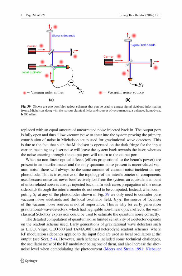
1 Page 62 of 221 Living Rev Relativ (2016) 19:1
(a) (b)
Fig. 39 Shown are two possible readout schemes that can be used to extract signal sideband informationfrom a Michelson along with the various classical fields and sources of vacuum noise, a balanced homodyne,b DC offset
replaced with an equal amount of uncorrected noise injected back in. The output portis fully open and thus allow vacuum noise to enter into the system proving the primarycontribution of noise in Michelson setup used for gravitational-wave detectors. Thisis due to the fact that such the Michelson is operated on the dark fringe for the inputcarrier, meaning any laser noise will leave the system back towards the laser, whereasthe noise entering through the output port will return to the output port.
When no non-linear optical effects (effects proportional to the beam’s power) arepresent in an interferometer and the only quantum noise present is uncorrelated vac-uum noise, there will always be the same amount of vacuum noise incident on anyphotodiode. This is irrespective of the topology of the interferometer or componentsused because noise can never be effectively lost from the system; an equivalent amountof uncorrelated noise is always injected back in. In such cases propagation of the noisesidebands through the interferometer do not need to be computed. Instead, when com-puting SI at any of the photodiodes shown in Fig. 39 we only need to consider purevacuum noise sidebands and the local oscillator field, ELO ; the source of locationof the vacuum noise sources is not of importance. This is why for early generationgravitational-wave detectors, which had negligible non-linear optical effects, the semi-classical Schottky expression could be used to estimate the quantum noise correctly.
The detailed computation of quantum noise limited sensitivity of a detector dependson the readout scheme used. Early generations of gravitational wave detectors suchas LIGO, Virgo, GEO 600 and TAMA300 used heterodyne readout schemes, whereRF modulation sidebands applied to the input field are used as local oscillators at theoutput (see Sect. 5.4). However, such schemes included some technical challenges,the oscillator noise of the RF modulator being one of them, and also increase the shot-noise level when demodulating the photocurrent (Meers and Strain 1991; Niebauer
123

Living Rev Relativ (2016) 19:1 Page 63 of 221 1
et al. 1991; Rakhmanov 2001; Buonanno et al. 2003). Thus the next generation ofdetectors opted for a DC readout scheme (Fricke et al. 2012; Hild et al. 2009), seeSect. 8.16. Both schemes depicted in Fig. 39 use a form of DC readout, which we willanalyse in more detail in the following sections. We do not cover the computation ofquantum noise with RF modulation readout schemes, the interested reader should seeHarms et al. (2007), Rakhmanov (2001) and Buonanno et al. (2003).
Noise-to-signal ratio for DC offset
A DC offset in the main Michelson interferometer (see Sect. 5.4) provides a localoscillator by making the interferometer operate slightly away from the dark fringe forthe carrier, and hence allowing some to leak through to the output port along withany signal sideband fields. The sources of vacuum noise that will contribute to thequantum noise are shown in Fig. 39b; however, as stated previously the total amountof noise present at the photodiode will be just pure vacuum noise as it is assumed thatthere are no non-linear optical effects. The local oscillator field at the output is givenby Eq. (5.11) and along with the vacuum noise sidebands the output field is:
Eout =[i E0e
−i2k L sin(k0δoff) + q+ei Ωt + q−e−i Ωt]ei ω0t . (6.18)
where we have used the dark fringe offset as stated in Eq. (5.13). The quantum noisePSD when using a DC offset is now essentially the same scenario as when derivingEq. (6.17), where a single carrier and noise sidebands were considered; except thatthe carrier power now depends on δoff :
SP,DC = 〈|Pout(Ω)|2〉 = 2P0 sin2 (k0δoff) hω0 ≈ 2P0(k0δoff)2hω0, (6.19)
where P0 is the power of the laser injected into the Michelson and k0δoff 1.To compute the noise-to-signal (NSR) ratio, which is used to describe the sensitivity
of our Michelson, the transfer function from a signal we want to measure to thephotodiode output is required. Here we will use the gravitational wave signal transferfunction from Eq. (5.42) which describes the Watts of power per unit of strain, h, atthe output detector
∣∣Tgw→P (ωgw)∣∣ ≈ k0δoff P0
w0
ωgwsin
(ωgw L
c
)W/h. (6.20)
We note that Tgw→P refers to the amplitude of the differential length modulation thatthe arms experience. Thus the NSR should be computed with the amplitude spectraldensity given as ASD = √
PSD:
NSR =√SP,DC
Tgw→P=
√2h
P0ω0
ωgw
sin(ωgw L/c)
h√Hz
, (6.21)
and example plot of such a sensitivity is shown in Fig. 40. The displacement sensitivitydoes not depend on the DC offset and can be improved, for example, by increasing
123

1 Page 64 of 221 Living Rev Relativ (2016) 19:1
Fig. 40 Shot-noise limited sensitivity of a Michelson, see Eq. (6.21), with L = 1000 m, R = T = 0.5 andP0 = 1 W
Fig. 41 The signal and noise fields in the homodyne detector as used in the balanced homodyne readoutscheme
the laser power. Eventually, building a more powerful laser is not possible withoutsacrificing stability in power and frequency. Instead we can also use a Fabry–Perotcavity (power recycling) to increase the effective power inside the interferometer, seeSect. 7.
Noise-to-signal ratio for balanced homodyne
Balanced homodyne readout involves the use of an external local oscillator whoseoptical frequency is the same as the main carrier light in the interferometer. The mainMichelson interferometer is operated on the dark fringe for the carrier so no carrier lightis present at the output port. This local oscillator is mixed with the signal sidebandsusing a beam splitter, such a setup is depicted in Fig. 39a and in more detail for thereadout in Fig. 41. As the signal sidebands are now split into two optical paths werequire two photodiodes to measure the signal, otherwise half the signal will be lostinstantly. The balanced aspect of this readout scheme refers to the fact that the twophotocurrents Ia and Ib are combined in such a way that the noise from either the localoscillator port or the signal port can be completely removed from the measurement.
No current generation gravitational-wave detector uses this form of homodynereadout for extracting gravitational wave signals. This has been due to the additionaltechnical challenges which are not present when using DC readout. It is however usedextensively for quantum noise measurements when non-vacuum states are injected into
123
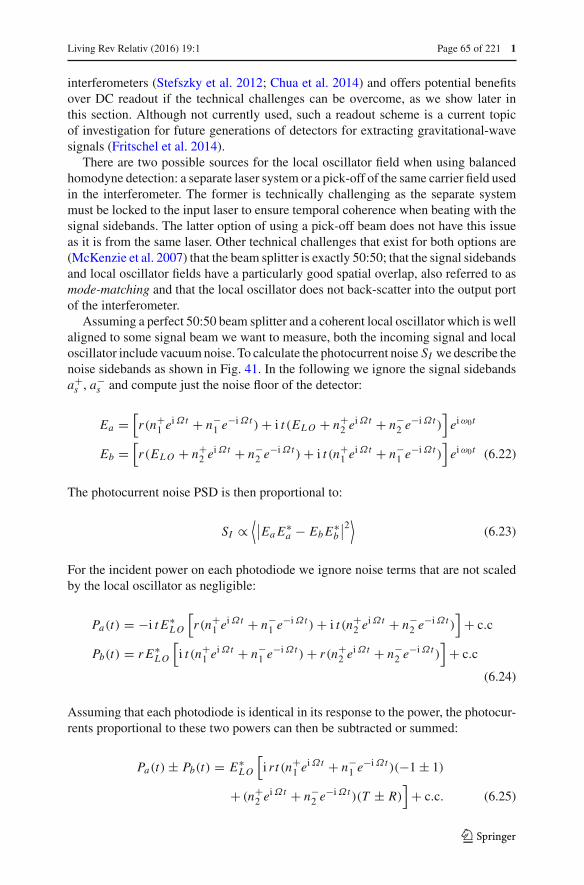
Living Rev Relativ (2016) 19:1 Page 65 of 221 1
interferometers (Stefszky et al. 2012; Chua et al. 2014) and offers potential benefitsover DC readout if the technical challenges can be overcome, as we show later inthis section. Although not currently used, such a readout scheme is a current topicof investigation for future generations of detectors for extracting gravitational-wavesignals (Fritschel et al. 2014).
There are two possible sources for the local oscillator field when using balancedhomodyne detection: a separate laser system or a pick-off of the same carrier field usedin the interferometer. The former is technically challenging as the separate systemmust be locked to the input laser to ensure temporal coherence when beating with thesignal sidebands. The latter option of using a pick-off beam does not have this issueas it is from the same laser. Other technical challenges that exist for both options are(McKenzie et al. 2007) that the beam splitter is exactly 50:50; that the signal sidebandsand local oscillator fields have a particularly good spatial overlap, also referred to asmode-matching and that the local oscillator does not back-scatter into the output portof the interferometer.
Assuming a perfect 50:50 beam splitter and a coherent local oscillator which is wellaligned to some signal beam we want to measure, both the incoming signal and localoscillator include vacuum noise. To calculate the photocurrent noise SI we describe thenoise sidebands as shown in Fig. 41. In the following we ignore the signal sidebandsa+s , a−
s and compute just the noise floor of the detector:
Ea =[r(n+
1 ei Ωt + n−
1 e−i Ωt ) + i t (ELO + n+
2 ei Ωt + n−
2 e−i Ωt )
]ei ω0t
Eb =[r(ELO + n+
2 ei Ωt + n−
2 e−i Ωt ) + i t (n+
1 ei Ωt + n−
1 e−i Ωt )
]ei ω0t (6.22)
The photocurrent noise PSD is then proportional to:
SI ∝⟨∣∣EaE
∗a − EbE
∗b
∣∣2⟩
(6.23)
For the incident power on each photodiode we ignore noise terms that are not scaledby the local oscillator as negligible:
Pa(t) = −i t E∗LO
[r(n+
1 ei Ωt + n−
1 e−i Ωt ) + i t (n+
2 ei Ωt + n−
2 e−i Ωt )
]+ c.c
Pb(t) = r E∗LO
[i t (n+
1 ei Ωt + n−
1 e−i Ωt ) + r(n+
2 ei Ωt + n−
2 e−i Ωt )
]+ c.c
(6.24)
Assuming that each photodiode is identical in its response to the power, the photocur-rents proportional to these two powers can then be subtracted or summed:
Pa(t) ± Pb(t) = E∗LO
[i r t (n+
1 ei Ωt + n−
1 e−i Ωt )(−1 ± 1)
+ (n+2 e
i Ωt + n−2 e
−i Ωt )(T ± R)]
+ c.c. (6.25)
123

1 Page 66 of 221 Living Rev Relativ (2016) 19:1
This shows that either the noise from the local oscillator, n±2 , or that coming along with
the signal, n±1 , can be removed. Typically the local oscillator noise will be larger than
that accompanying the signal thus we can compute Pa − Pb to remove it. It can alsobe seen here if the beam splitter is not 50:50, R �= T , the local oscillator noise cannotbe fully removed. Finally the subtracted photocurrent for the sideband frequency Ω
is:
Pa−b(Ω) ≡ F[Pa(t) − Pb(t)](Ω) = −i E∗LO(n+
1 + n−1
∗), (6.26)
where r = t = 1/√
2. For pure vacuum noise, n±1 ⇒ q±, the resulting photocurrent
noise PSD for this is that given by Eq. (6.17):
SI = 〈|Pa−b(Ω)|2〉 = 2PLO(〈q+q∗+〉 + 〈q−q∗−〉) ,
= 2PLOhω0 (6.27)
Therefore if correctly balanced the quantum noise is no greater than what is present fora DC offset readout. If the local oscillator power PLO is identical to the carrier powerin the DC offset scheme, then the sensitivity for the balanced homodyne detection isthe same as that for the DC offset detection, stated in Eq. (6.21), because the transferfunction from signal to the two photodiodes is essentially the same. One aspect whereit differs however is the phase of the local oscillator relative to the signal sidebandswhich is now a free parameter, which is known as the homodyne angle or the readoutphase. When using a DC offset readout scheme the readout phase is essentially fixed.Having the ability to vary this readout phase provides an extra degree of freedom foroptimising the quantum noise-to-signal ratio for gravitational wave signals. This isan assumed feature in some quantum non-demolition schemes (Braginsky et al. 1980;Braginsky and Khalili 1996) which introduce new methods for reducing the quantumnoise (Purdue and Chen 2002; Kimble et al. 2002; Khalili and Levin 1996; Chen 2003;Chen et al. 2010).
6.3 Quantum noise with non-linear optical effects or squeezed states
Up to this point we have only considered pure vacuum noise and linear optical effects,both of which are valid approximations for previous generations of gravitational wavedetectors. As the effective laser power in the interferometer is increased to reduceshot noise, the radiation pressure exerted on suspended optics by the circulating laserbeams will increase another noise significantly, the radiation pressure noise. As thesuspended mirrors are free to move under the influence of radiation pressure, anyfluctuation in the laser’s power will couple back into itself as phase modulation. Thisis a non-linear process as the amplitude of the motion is proportional to the power inthe beam, which leads to the upper and lower sidebands becoming correlated with oneanother. As explained in Sect. 6.4, such noise is prominent at low frequencies.
Then there is also the possibility of squeezing the vacuum noise, whereby still satis-fying the relationship 6.6, the uncertainty in either the phase or amplitude is increasedwhilst being and decreased in the other. This squeezed noise can be represented by
123
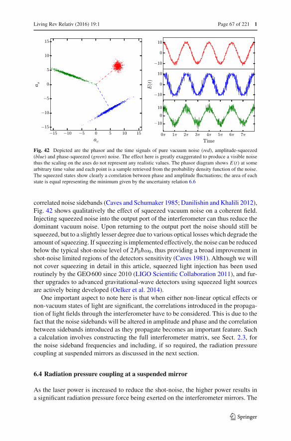
Living Rev Relativ (2016) 19:1 Page 67 of 221 1
Fig. 42 Depicted are the phasor and the time signals of pure vacuum noise (red), amplitude-squeezed(blue) and phase-squeezed (green) noise. The effect here is greatly exaggerated to produce a visible noisethus the scaling on the axes do not represent any realistic values. The phasor diagram shows E(t) at somearbitrary time value and each point is a sample retrieved from the probability density function of the noise.The squeezed states show clearly a correlation between phase and amplitude fluctuations; the area of eachstate is equal representing the minimum given by the uncertainty relation 6.6
correlated noise sidebands (Caves and Schumaker 1985; Danilishin and Khalili 2012),Fig. 42 shows qualitatively the effect of squeezed vacuum noise on a coherent field.Injecting squeezed noise into the output port of the interferometer can thus reduce thedominant vacuum noise. Upon returning to the output port the noise should still besqueezed, but to a slightly lesser degree due to various optical losses which degrade theamount of squeezing. If squeezing is implemented effectively, the noise can be reducedbelow the typical shot-noise level of 2P0hω0, thus providing a broad improvement inshot-noise limited regions of the detectors sensitivity (Caves 1981). Although we willnot cover squeezing in detail in this article, squeezed light injection has been usedroutinely by the GEO 600 since 2010 (LIGO Scientific Collaboration 2011), and fur-ther upgrades to advanced gravitational-wave detectors using squeezed light sourcesare actively being developed (Oelker et al. 2014).
One important aspect to note here is that when either non-linear optical effects ornon-vacuum states of light are significant, the correlations introduced in the propaga-tion of light fields through the interferometer have to be considered. This is due to thefact that the noise sidebands will be altered in amplitude and phase and the correlationbetween sidebands introduced as they propagate becomes an important feature. Sucha calculation involves constructing the full interferometer matrix, see Sect. 2.3, forthe noise sideband frequencies and including, if so required, the radiation pressurecoupling at suspended mirrors as discussed in the next section.
6.4 Radiation pressure coupling at a suspended mirror
As the laser power is increased to reduce the shot-noise, the higher power results ina significant radiation pressure force being exerted on the interferometer mirrors. The
123

1 Page 68 of 221 Living Rev Relativ (2016) 19:1
frequency spectrum of the force exerted on a perfectly reflectivity mirror by a singlebeam with power P(Ω) is given by (Meystre et al. 1985)
Frp(Ω) = 2P(Ω)
c. (6.28)
In order to attenuate seismic vibrations and produce free-masses as probes for gravi-tational waves, the mirrors in gravitational-wave detectors are suspended via a seriesof active and passive suspension systems. At frequencies well above the resonancesof the suspension systems the mirrors can be considered to be free (or quasi-free).Any fluctuation in the light power induces a motion in the suspended mirrors. Thisprocess converts power fluctuations into phase fluctuations, and this coupling can leadto optomechanical effects such as optical springs, which couple the motion of multiplesuspended optics together (Sheard et al. 2004; Aspelmeyer et al. 2014).
The induced longitudinal motion of a suspended mirror due to N f separate forcesbeing applied to it is:
δz(Ω) = H(Ω)
N f∑n=0
Fn(Ω), (6.29)
where H(Ω) is the mechanical susceptibility or mechanical transfer function from aforce applied to motion parallel to the mirrors surface normal. Similar relationshipsare possible for rotational motions considering torques applied to the mirror.
Mechanical transfer functions
The transfer function H(Ω) is determined by the specific setup of the suspensionsystems. The various resonances and features of the system can be represented withan expansion into poles and zeros:
H(Ω) =∏Nz
k=1(Zk − Ω2)
M∏Np
j=1(P j − Ω2)
P j = Ω2p, j − i Ωp, jΩ
Qp, j, Zk = Ω2
z,k − i Ωz,kΩ
Qz,k(6.30)
where M is the mass of the mirror in kg, {Ωp/z,i }Np/zi=1 is a set of frequencies for each
pole and zero and {Qp/z,i }Np/zi=1 the respective quality factors. When the frequencies
of interest (signal frequencies) are much higher than any pole or zero frequency,Ω � Ωp/z , we can assume a free mass, Nz = 0 and one pole of infinite Q at 0 Hz:
H(Ω) = − 1
MΩ2 . (6.31)
Approximations for radiation pressure
With the mirror position change being proportional to the laser power, δz ∝ P ,the problem is non-linear in terms of the complex field amplitudes. Solving such a
123
Living Rev Relativ (2016) 19:1 Page 69 of 221 1
problem in a complex interferometer setup is challenging and not possible using themethods outlined in Sect. 2, as the frequency domain model is assuming a linearsystem. However, for gravitational-wave detectors we can make some assumptionsabout the system:
– the motion of any optic is small, |δz| λ, when the interferometer is controlledand well-behaved, and we can linearise equations in δz,
– any high-frequency fluctuations in the beam are negligible due to H(Ω) ∝ 1/Ω2
and we ignore the effects of RF sidebands on the optics,– any low-frequency fluctuations are very small, such that the magnitude of any
sidebands is much less than the magnitude of its carrier field, which allows us toidentify a well defined carrier field in our calculations.
These are all valid assumptions for gravitational-wave detectors once they are operat-ing in a steady state and have well controlled optics. For a single carrier with amplitudeE0 and frequency ω0 and noise sidebands at frequency Ω , the incident field on a sus-pended mirror is:
Ei = (E0 + q+ei Ωt + q−e−i Ωt )ei ω0t + c.c. (6.32)
As with the approximations listed above we can assume |q±| |E0| and ω0 � Ω .The fluctuation in the beam power is then given by:
P(Ω) = q+E∗0 + q∗−E0 (6.33)
where we only consider sideband-carrier product terms and those with a frequencyΩ . Substituting the fluctuating power 6.33 into the radiation pressure force 6.28 tocompute the displacement 6.29 the motion of the mirror can be found. The amplitudeof the motion at frequency Ω induced via radiation pressure for a perfectly reflective,free-mass mirror is
δz = − 2
McΩ2
(q+E∗
0 + q∗−E0). (6.34)
Such a moving mirror, as discussed in Sect. 3.2, creates phase modulation sidebandsaround any carrier that is reflected from it. The reflected field, using Eq. (3.10), is:
Er = Ei
(1 + i k0
2
(δz+e−i Ωt + δz−ei Ωt
))ei ω0t , (6.35)
where to keep notation simpler, δz+ ≡ δz(+Ω) and δz− ≡ δz(−Ω)∗.Take the simple example of vacuum noise and a single carrier, with amplitude E0,
incident on a free mass mirror of mass M and calculate the noise after being reflected.The amplitude of the reflected upper and lower noise sidebands, qr,±, using Eqs. (6.29)and (6.35), are:
qr,± = v± + i E0k0δz±
2,
= v± − i E0k0v±E∗
0 + v∗∓E0
McΩ2 . (6.36)
123
1 Page 70 of 221 Living Rev Relativ (2016) 19:1
where v± are the incident pure vacuum noise sidebands. (6.36) shows that the reflectedupper and lower noise sidebands are now a mix of the incident upper and lowersidebands, i.e., after reflection they are correlated. There is additional phase noisepresent, and it scales as ∝ |E0|/Ω2. Thus, this noise is relevant at low frequenciesand when the beam power to mass ratio is significant.
The noise PSD for the reflected beam is computed using Eq. (6.16). This requirescomputing the various covariance and auto-covariances of the reflected noise side-bands 6.36 and their beating with the carrier field:
〈qr,±q ′r,∓〉 = − hω0E2
0
MΩ2c
(k0 + |E0|2k2
0
MΩ2c
)(6.37)
〈qr,±q ′∗r,±〉 = h(ω0 ± Ω)
2+ hω0|E0|4k2
0
M2c2Ω4 . (6.38)
To simplify the above we will also assume the carrier has zero phase, E∗0 = E0 and
that E0 = √P0. The power noise PSD using Eq. (6.16) is then
SI (Ω) = 2P0(⟨qr,+q ′∗
r,+⟩ + ⟨
qr,−q ′∗r,−
⟩) + 2P0⟨qr,−q ′
r,+⟩∗ + 2P∗
0
⟨qr,+q ′
r,−⟩
= 2hω0P0. (6.39)
Thus the noise is still just a flat shot noise limit, as expected. However, this only showsthe amplitude noise in the beam, not any phase noise. To compute the phase quadraturethe local oscillator must have an additional π/2 phase relative to the sidebands. Exper-imentally this could be achieved using the balanaced homodyne readout as mentionedin previous sections. Here we can simply add an additional phase to the carrier to thebeam after reflection, i.e., compute the PSD of a power fluctuation
P(Ω) = q+E∗0e
−i φ + q∗−E0ei φ (6.40)
where φ is our additional homodyne phase. Computing the PSD of this with φ = π/2to compute the phase fluctuations we see:
Sφ(Ω) = 2P0hω0 + 8h P30 ω0k2
0
M2c2Ω4 . (6.41)
This shows a flat shot noise fluctuation plus additional phase noise due to the vacuumnoise perturbing the mirror. In the limit of an infinitely heavy mirror we can see thisradiation pressure noise is removed and we are left with the vacuum noise fluctuationsin phase. It is these phase fluctuations that are converted from phase to amplitude noiseat the Michelson dark port that then lead to quantum noise limited sensitivity of thedetector at the output photodiode.
123
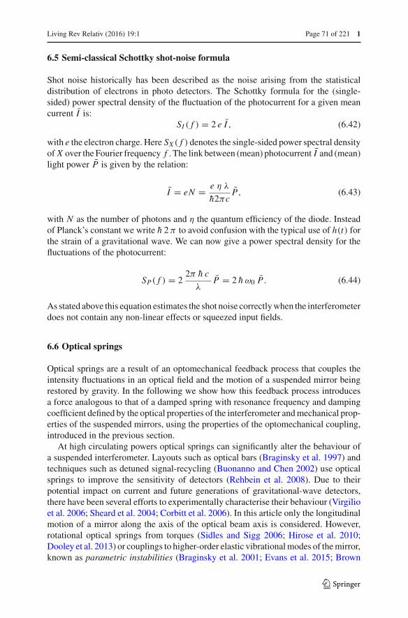
Living Rev Relativ (2016) 19:1 Page 71 of 221 1
6.5 Semi-classical Schottky shot-noise formula
Shot noise historically has been described as the noise arising from the statisticaldistribution of electrons in photo detectors. The Schottky formula for the (single-sided) power spectral density of the fluctuation of the photocurrent for a given meancurrent I is:
SI ( f ) = 2 e I , (6.42)
with e the electron charge. Here SX ( f ) denotes the single-sided power spectral densityof X over the Fourier frequency f . The link between (mean) photocurrent I and (mean)light power P is given by the relation:
I = eN = e η λ
h2πcP, (6.43)
with N as the number of photons and η the quantum efficiency of the diode. Insteadof Planck’s constant we write h 2 π to avoid confusion with the typical use of h(t) forthe strain of a gravitational wave. We can now give a power spectral density for thefluctuations of the photocurrent:
SP ( f ) = 22π h c
λP = 2 h ω0 P. (6.44)
As stated above this equation estimates the shot noise correctly when the interferometerdoes not contain any non-linear effects or squeezed input fields.
6.6 Optical springs
Optical springs are a result of an optomechanical feedback process that couples theintensity fluctuations in an optical field and the motion of a suspended mirror beingrestored by gravity. In the following we show how this feedback process introducesa force analogous to that of a damped spring with resonance frequency and dampingcoefficient defined by the optical properties of the interferometer and mechanical prop-erties of the suspended mirrors, using the properties of the optomechanical coupling,introduced in the previous section.
At high circulating powers optical springs can significantly alter the behaviour ofa suspended interferometer. Layouts such as optical bars (Braginsky et al. 1997) andtechniques such as detuned signal-recycling (Buonanno and Chen 2002) use opticalsprings to improve the sensitivity of detectors (Rehbein et al. 2008). Due to theirpotential impact on current and future generations of gravitational-wave detectors,there have been several efforts to experimentally characterise their behaviour (Virgilioet al. 2006; Sheard et al. 2004; Corbitt et al. 2006). In this article only the longitudinalmotion of a mirror along the axis of the optical beam axis is considered. However,rotational optical springs from torques (Sidles and Sigg 2006; Hirose et al. 2010;Dooley et al. 2013) or couplings to higher-order elastic vibrational modes of the mirror,known as parametric instabilities (Braginsky et al. 2001; Evans et al. 2015; Brown
123
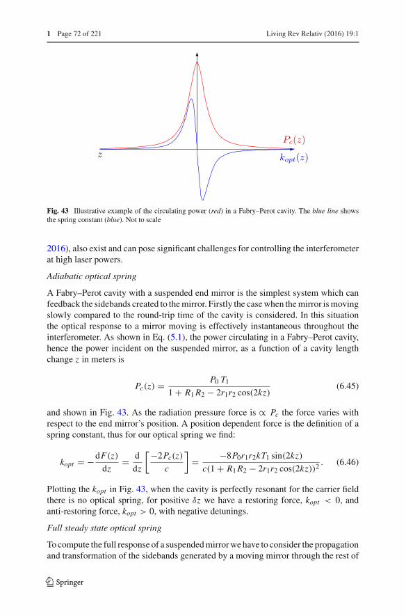
1 Page 72 of 221 Living Rev Relativ (2016) 19:1
Fig. 43 Illustrative example of the circulating power (red) in a Fabry–Perot cavity. The blue line showsthe spring constant (blue). Not to scale
2016), also exist and can pose significant challenges for controlling the interferometerat high laser powers.
Adiabatic optical spring
A Fabry–Perot cavity with a suspended end mirror is the simplest system which canfeedback the sidebands created to the mirror. Firstly the case when the mirror is movingslowly compared to the round-trip time of the cavity is considered. In this situationthe optical response to a mirror moving is effectively instantaneous throughout theinterferometer. As shown in Eq. (5.1), the power circulating in a Fabry–Perot cavity,hence the power incident on the suspended mirror, as a function of a cavity lengthchange z in meters is
Pc(z) = P0 T1
1 + R1R2 − 2r1r2 cos(2kz)(6.45)
and shown in Fig. 43. As the radiation pressure force is ∝ Pc the force varies withrespect to the end mirror’s position. A position dependent force is the definition of aspring constant, thus for our optical spring we find:
kopt = −dF(z)
dz= d
dz
[−2Pc(z)
c
]= −8P0r1r2kT1 sin(2kz)
c(1 + R1R2 − 2r1r2 cos(2kz))2 . (6.46)
Plotting the kopt in Fig. 43, when the cavity is perfectly resonant for the carrier fieldthere is no optical spring, for positive δz we have a restoring force, kopt < 0, andanti-restoring force, kopt > 0, with negative detunings.
Full steady state optical spring
To compute the full response of a suspended mirror we have to consider the propagationand transformation of the sidebands generated by a moving mirror through the rest of
123

Living Rev Relativ (2016) 19:1 Page 73 of 221 1
Fig. 44 A generic view of a closed-loop optomechanical transfer function for a suspended mirror withmechanical susceptibility H(Ω). Due to some motion δz(Ω) of a mirror the light is scattered from thecarrier. The IFO plant describes the optical transfer function of the sidebands propagating through theinterferometer and back to the mirror in question. The the interference of these then creates some radiationpressure force which is fed back into the mirror. Here ac is the carrier field at the mirror in question
the interferometer and finally back to the mirror in question. This process of scatteringand feedback is represented by the block diagram in Fig. 44. A sinusoidal force F(Ω) isacting on a mirror with mechanical susceptibility H(Ω); the motion δz(Ω) combinedwith the incident carrier field ac scatters light into the upper, a+
s , and lower, a−s ,
sidebands leaving the mirror. The IFO plant, G(±Ω) ≡ G±, is the optical transferfunctions for either the upper or lower sidebands leaving the mirror to those returningto it. Lastly the incident upper and lower sidebands, a′±
s = G±a±s , are combined again
with the carrier field to compute the radiation pressure force Frp(Ω) along with anexternal excitation ΔF(Ω) to feedback into the mirror.
To illustrate this in more detail a single carrier with a pair of sidebands describingsome amplitude modulation at a frequency Ω will be considered. This optical field isincident on a free mass mirror with a high reflectivity, R = r2 ≈ 1. The incident field,a
′±s , and reflected, a±
s , fields using the small phase modulation approximation 3.10are:
a′±s = G±a±
s , (6.47)
a±s = (a′±
s + i k δz±ac) (6.48)
Solving for the incident field using both 6.47 and 6.48 we find:
a′±s = i kG± δz±ac
1 − G± . (6.49)
To compute the total force acting on the mirror we must consider the intensity fluc-tuations of all incident and reflected beams, as the total momentum of the beams andthe suspended mirror must be conserved (Meystre et al. 1985). In this case there areonly beams on one side of the mirror, the intensity fluctuations of the reflected beamsare nearly the same as those of the incident beam as the mirror imprints only phasemodulation and R ≈ 1. The total force the mirror experiences is then:
Frp(Ω) ≈ 4
c
[a
′+s a∗
c + a′−∗s ac
]. (6.50)
123
1 Page 74 of 221 Living Rev Relativ (2016) 19:1
Now, considering the incoming beams 6.49, the force is:
Frp(Ω) ≈ 4i kPcc
[G+ − G−∗
1 − G+ − G−∗ + G+G−∗
]δz(Ω) ≡ κ(Ω) δz(Ω). (6.51)
This shows that the radiation pressure force is linearly dependent on δz for an arbitraryinterferometer layout described by G±. The complex valued scaling factor, κ(Ω),represents how the dynamic response of the suspended mirror is altered. Those termsindependent of Ω define the stiffness of the optical spring. Terms ∝ Ω describe anydamping, copt being the optical damping coefficient:
κ(Ω) = kopt + i Ωcopt(Ω) + O(Ω2). (6.52)
Higher order terms can also be significant, depending on the optical feedback, andcan alter the inertial behaviour by introducing terms ∝ Ω2. Such manipulation ofthe optomechanical coupling here can be exploited to improve the sensitivity ofgravitational-wave detectors (Ma et al. 2014).
The above analysis is applicable in the case of a single optical field. If there aremultiple optical fields of comparable amplitude, the sum of the multiple radiationpressure forces must be considered to compute the overall value of κ . The result(6.51) is also only applicable for optical fields with dominating radiation pressure onone single side of a near perfectly reflective mirror. The analytical calculation of othercases, such as, suspended beam splitters, multiple suspended optics, or multiple carrierfrequencies with higher order spatial modes, can become very complicated. Tools suchas Finesse take all these effects into account to ease studying such systems.
Optical spring in a cavity
The simplest case of an optical spring we can consider is that of an two-mirror opticalcavity with a single suspended mirror. The optical spring constant for this setup can bedetermined using Eq. (6.51). Here G± are the optical transfer functions for the upperand lower sidebands through one round-trip of the cavity after being created at thesuspended mirror. For this example we will take the input mirror to be fixed and theend mirror to be a suspended free mass. We determine G± by starting from where thesidebands are created at the suspended mirror, whose reflectivity is ≈1. These thenpropagate along the cavity length L twice with a reflection from the fixed input mirror,with reflectivity r1, before returning to the end mirror. In total the propagation is
G± = r1e∓i 2 Ω
c Lei 2φ. (6.53)
Here φ is some detuning of the input mirror position. Substituting this into (6.51) wefind:
G+ − G−∗
1 − G+ − G−∗ + G+G−∗ = i 2r1e−i 2 Ωc L sin(2φ)
1 + R1e−i 4 Ωc L − 2r1e−i 2 Ω
c L cos(2φ)(6.54)
123

Living Rev Relativ (2016) 19:1 Page 75 of 221 1
Fig. 45 Analytical versus numerical (Finesse) comparison of an optical spring. This is for a fixed inputfield and suspended (free-mass) end mirror. A force is applied to the end mirror and shown is the force-to-displacement of the end mirror transfer function. Inset plot shows zoomed region around the peak whichshows a good agreement with the peak shape and position
and:
κ(Ω) = −8kPcr1 sin(2φ)
c
e−i 2 Ωc L
1 + R1e−i 4 Ωc L − 2r1e−i 2 Ω
c L cos(2φ). (6.55)
When the cavity is on resonance, φ = 0, we see no optical spring, as expected.Likewise, in the DC limit Ω → 0, we find an agreement with (6.45). Shown in Fig. 45is and example of a force-to-displacement transfer function for the suspended endmirror when a force is applied.
6.7 Finesse examples
6.7.1 Optical spring
A simple example for an optical spring in a two mirror cavity with suspended mirrors.The cavity is slightly detuned which is required for creating the spring. The outputis the motion of a mirror while it is excited with a force of constant amplitude. Theresonance feature shown in Fig. 46 is the result of the optomechanical coupling of themirror with the cavity field.
Finesse input file for ‘optical spring’l l1 1 0 n1
m ITM 0.99 0.01 0 n1 n2
s s1 1 n2 n3
m ETM 1 0 -0.048 n3 n4
% Set the mass of the ETM in kg
attr ETM mass 1
% Here we are applying a force to the end mirror
123

1 Page 76 of 221 Living Rev Relativ (2016) 19:1
Fig. 46 Finesse example: Fabry–Perot cavity with an optical spring. The two traces show the amplitudeand phase of the mechanical response of one cavity mirror to an exciting force. The resonance feature closeto 10 Hz is the result of the optomechanical coupling of the mirror with the cavity field
Fig. 47 Finesse example: Homodyne detector with a squeezed light input. The blue trace shows thequantum noise in units of h f with a range of 0.2–20, compared to a quantum noise of 2h f for an unsqueezedsource. The green trace instead has the units ‘dB’ and shows an effective squeezing level, inferred from thedetected quantum noise
fsig aforce ETM Fz 1 0 1
% A detector for force-to-motion transfer function
xd ETMz ETM z
% scanning the frequency of the force
xaxis aforce f log 1 100 100000
yaxis log abs:deg
6.7.2 Homodyne detector and squeezed light
A laser and a squeezed light source are mixed with a beam splitter and then detectedwith a homodyne detector. The nominal quantum noise of an un-squeezed light fieldin the units of the blue trace are 2h f . The squeezing level of the squeezed light sourceis 10 dB, which means that the noise in one quadrature is 10 times lower than thiswhereas the other quadrature should be 10 times higher. With the phase of the localoscillator the homodyne detector can be tuned to measure the different quadratures.
123

Living Rev Relativ (2016) 19:1 Page 77 of 221 1
The green trace shows a computation of an effective squeezing level from the detectedquantum noise using the Schottky equation (Fig. 47).
Finesse input file for ‘homodyne detector and squeezed light’l LO 1 0 n1
sq sqz 0 10 0 n4
bs bs1 0.5 0.5 0 0 n1 n2 n3 n4
% homodyne detector attached to the two bs outputs
qhd quantum_noise 180 n2 n3
% what noise frequency (Omega) do we plot
fsig noise 1
% Output noise in units of hbar*f
scale PSD_hf quantum_noise
% varying the LO phase
xaxis LO phase lin 0 360 180
% compute the squeezing level
set QN_re quantum_noise re
func dB = 10 * log10(($QN_re + 1E-20)/2)
6.7.3 Quantum-noise limited interferometer sensitivity
This example shows the quantum-noise limited sensitivity of an advanced detectors.See “Appendix B” for the optical layout of the detector and Sect. 8.12 for more detailsabout the interferometer operation. The model is loosely based on the Advanced LIGOdesign file and thus we expect to see the peak sensitivity around 100 Hz at a sensitivityof about 10−23/
√Hz. We can see the both the ‘qnoised’ and ‘qshot’ detectors agree
at high frequencies, where the sensitivity is purely limited by shot noise. At lowfrequencies the two traces differ because only ‘qnoised’ takes into account the radiationpressure effects (Fig. 48).
The Finesse input file for this example is more complex than for other examplesbecause it contains a more complex interferometer setup and uses relatively advancedconcepts such as setting mechanical transfer function. See “Appendix A” for moreinformation on Finesse and where to find the documentation, such as the syntaxreference, required to follow this example.
Finesse input file for ‘quantum-limited interferometer sensitivity’l l1 $Pin 0 nin
s s1 0 nin nprc1
# Power recycling mirror
m1 prm $prmT 37.5u 90 nprc1 nprc2
s prc $lprc nprc2 nbsin
# Central beamsplitter
bs bs1 .5 .5 0 45 nbsin n0y n0x nbsout
# X-arm
s ichx $lmichx n0x n1x
m1 itmx $itmT 37.5u 90 n1x n2x
123

1 Page 78 of 221 Living Rev Relativ (2016) 19:1
s armx $Larm n2x n3x
m1 etmx 5u 37.5u 89.999875 n3x n4x
attr itmx mass $Mtm zmech sus1
attr etmx mass $Mtm zmech sus1
# Y-arm
s ichy $lmichy n0y n1y
m1 itmy $itmT 37.5u $michy_phi n1y n2y
s army $Larm n2y n3y
m1 etmy 5u 37.5u 0.000125 n3y n4y
attr itmy mass $Mtm zmech sus1
attr etmy mass $Mtm zmech sus1
# Signal recycling mirror
s src $lsrc nbsout nsrc1
m1 srm $srmT 37.5u $srm_phi nsrc1 nsrc2
# Force-to-position transfer function for longitudinal
# motions of test masses
tf sus1 1 0 p $mech_freq $mech_Q
const mech_freq 1
const mech_Q 1M # Guess for suspension Q factor
# offsets for DC readout: 100mW = michy_phi 0.07 OR
darm_phi .00025
const michy_phi 0
const darm_phi .00025
const Larm 3995
const itmT 0.014
const srmT 0.2
const prmT 0.03
const Pin 125
const Mtm 40
const srm_phi -90
const lmichx 4.5
const lmichy 4.45
const lprc 53
const lsrc 50.525
# A squeezed source could be injected into the dark port
sq sq1 0 0 90 nsrc2
# Differentially modulate the arm lengths
fsig darm armx 1 0
fsig darm2 army 1 180
# Output the full quantum noise limited sensitivity
qnoisedS NSR_with_RP 1 $fs nsrc2
# Output just the shot noise limited sensitivity
qshotS NSR_without_RP 1 $fs nsrc2
# We could also display the quantum noise and the signal
# separately by uncommenting these two lines.
# qnoised noise $fs nsrc2
123
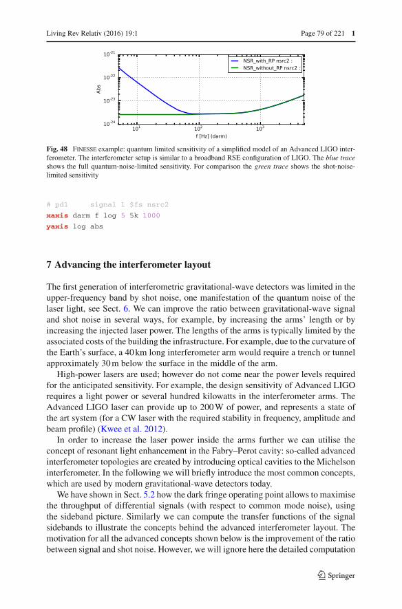
Living Rev Relativ (2016) 19:1 Page 79 of 221 1
Fig. 48 Finesse example: quantum limited sensitivity of a simplified model of an Advanced LIGO inter-ferometer. The interferometer setup is similar to a broadband RSE configuration of LIGO. The blue traceshows the full quantum-noise-limited sensitivity. For comparison the green trace shows the shot-noise-limited sensitivity
# pd1 signal 1 $fs nsrc2
xaxis darm f log 5 5k 1000
yaxis log abs
7 Advancing the interferometer layout
The first generation of interferometric gravitational-wave detectors was limited in theupper-frequency band by shot noise, one manifestation of the quantum noise of thelaser light, see Sect. 6. We can improve the ratio between gravitational-wave signaland shot noise in several ways, for example, by increasing the arms’ length or byincreasing the injected laser power. The lengths of the arms is typically limited by theassociated costs of the building the infrastructure. For example, due to the curvature ofthe Earth’s surface, a 40 km long interferometer arm would require a trench or tunnelapproximately 30 m below the surface in the middle of the arm.
High-power lasers are used; however do not come near the power levels requiredfor the anticipated sensitivity. For example, the design sensitivity of Advanced LIGOrequires a light power or several hundred kilowatts in the interferometer arms. TheAdvanced LIGO laser can provide up to 200 W of power, and represents a state ofthe art system (for a CW laser with the required stability in frequency, amplitude andbeam profile) (Kwee et al. 2012).
In order to increase the laser power inside the arms further we can utilise theconcept of resonant light enhancement in the Fabry–Perot cavity: so-called advancedinterferometer topologies are created by introducing optical cavities to the Michelsoninterferometer. In the following we will briefly introduce the most common concepts,which are used by modern gravitational-wave detectors today.
We have shown in Sect. 5.2 how the dark fringe operating point allows to maximisethe throughput of differential signals (with respect to common mode noise), usingthe sideband picture. Similarly we can compute the transfer functions of the signalsidebands to illustrate the concepts behind the advanced interferometer layout. Themotivation for all the advanced concepts shown below is the improvement of the ratiobetween signal and shot noise. However, we will ignore here the detailed computation
123

1 Page 80 of 221 Living Rev Relativ (2016) 19:1
Fig. 49 Optical layout of a Michelson interferometer with arm power recycling
of the shot noise and quantum noise discussed in Sect. 6. Instead we will compute onlythe transfer functions of the signal to the photo detector using the sideband picture. Wewill ignore radiation pressure noise and shot-noise contributions from any light fieldbut the local oscillator. Thus the amplitude of the signal sidebands in the detectionport give a good figure of merit for the shot-noise limited sensitivity of the detector.
7.1 Michelson interferometers with power recycling
The Michelson interferometer, when held on the dark fringe and ignoring internallosses, reflects all the incoming light back into the laser port; seen from the laser itacts like a highly reflective mirror. It was soon realised we can utilise this fact toincrease the light power inside the interferometer: an additional mirror inter the inputport, the so-called power-recycling mirror (PRM), will generate an optical cavitywith the Michelson interferometer acting as a second ‘mirror’. This scheme whichis now called power recycling was first proposed in 1983 independently by Billinget al. (1983) and Drever et al. (1983). The newly formed cavity is often called power-recycling cavity. The optical layout of a power-recycled Michelson interferometer isshown in Fig. 49. Figure 50 shows the amplitude of signal sidebands for different levelsof power recycling, as a function of the frequency of the signal. We will compare thisto similar plots for other techniques described below.
As we have discussed in Sect. 5.1, the power circulating inside a cavity can be muchhigher than the injected light power. The power enhancement is given by the finesse ofthe cavity which is given by the optical losses in the interferometer and the reflectivityof the power-recycling mirror. When the losses inside the Michelson interferometerare negligible the cavity formed by the Michelson and the power-recycling mirroris over-coupled and the power enhancement in the interferometer arms, also calledpower-recycling gain computes as
GPR = 4
TPRM≈ 2F
π(7.1)
with F the finesse of the power-recycling cavity.When the optical losses can not be ignored the maximum power-recycling gain
can be reached by impedance matching, i.e., setting the transmission of the power-
123

Living Rev Relativ (2016) 19:1 Page 81 of 221 1
Fig. 50 This graph shows the signal sideband amplitude for a differential arm length change, as detectedin the anti-symmetric output port, as a function of the frequency of the signal. The solid red trace at anamplitude of 1 refers to the case without power recycling. The other two traces show the increased amplitudefor different reflectivity’s of the power-recoiling mirror. Compare this plot also with Figs. 52 and 54
recycling mirror equal to the round trip losses of the power-recycling cavity and thegain becomes
GPR = 1
TPRM≈ F
π(7.2)
The power in the signal sidebands is proportional to the carrier power and thusscales with the power-recycling gain as well. The amplitudes plotted in Fig. 50 thusshow values of
√4/0.1 ≈ 6.32 and
√4/0.01 = 20.
Power-recycling has further advantages: the cavity effect can be used to reducebeam jitter and to filter laser frequency noise. The disadvantage is that another mirrorposition needs to be carefully maintained by a feedback control system. In addition,the increase in circulating power also increases the laser power within the substrate ofthe beam splitter which can cause thermal distortions leading to higher-optical losses.In practise this often limits the achievable power-recycling gain.
7.2 Michelson interferometers with arm cavities
Another way to employ cavities to enhance the light power circulating in the interfer-ometer arms is to place optical cavities into these arms, as so-called arm cavities,as shown in Fig. 51. This optical configuration sometimes referred to as Fabry–Perot–Michelson interferometer. Similar to power-recycling the finesse of the cavitydetermines the enhancement of the light power.
The arm cavities have another effect on the detector sensitivity: they affect not onlythe power of the circulating carrier field, but also that sidebands generated by a lengthchange. This results in a further increase of the sensitivity for signals with a frequencywithin the linewidth of the arm cavities but to a decrease in sensitivity regarding signalswith frequencies that fall outside the linewidth of the cavities. This can be shownagain very clearly with the sideband amplitudes detected at the interferometer outputas shown in Fig. 52. We can compare this results to the power-recycling case (Fig. 50):when the reflectivity of the PRM and ITMs is set to R = 0.99, the expected gain for
123
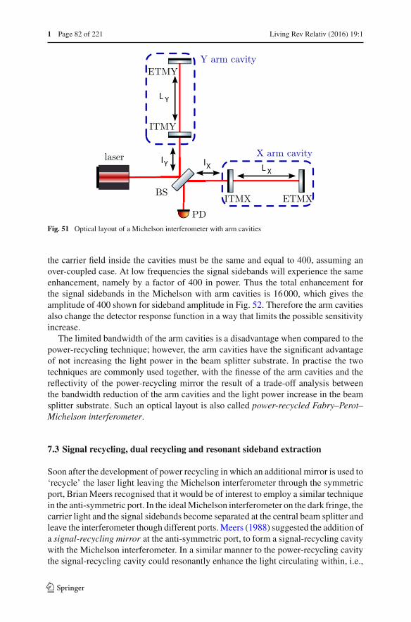
1 Page 82 of 221 Living Rev Relativ (2016) 19:1
Fig. 51 Optical layout of a Michelson interferometer with arm cavities
the carrier field inside the cavities must be the same and equal to 400, assuming anover-coupled case. At low frequencies the signal sidebands will experience the sameenhancement, namely by a factor of 400 in power. Thus the total enhancement forthe signal sidebands in the Michelson with arm cavities is 16 000, which gives theamplitude of 400 shown for sideband amplitude in Fig. 52. Therefore the arm cavitiesalso change the detector response function in a way that limits the possible sensitivityincrease.
The limited bandwidth of the arm cavities is a disadvantage when compared to thepower-recycling technique; however, the arm cavities have the significant advantageof not increasing the light power in the beam splitter substrate. In practise the twotechniques are commonly used together, with the finesse of the arm cavities and thereflectivity of the power-recycling mirror the result of a trade-off analysis betweenthe bandwidth reduction of the arm cavities and the light power increase in the beamsplitter substrate. Such an optical layout is also called power-recycled Fabry–Perot–Michelson interferometer.
7.3 Signal recycling, dual recycling and resonant sideband extraction
Soon after the development of power recycling in which an additional mirror is used to‘recycle’ the laser light leaving the Michelson interferometer through the symmetricport, Brian Meers recognised that it would be of interest to employ a similar techniquein the anti-symmetric port. In the ideal Michelson interferometer on the dark fringe, thecarrier light and the signal sidebands become separated at the central beam splitter andleave the interferometer though different ports. Meers (1988) suggested the addition ofa signal-recycling mirror at the anti-symmetric port, to form a signal-recycling cavitywith the Michelson interferometer. In a similar manner to the power-recycling cavitythe signal-recycling cavity could resonantly enhance the light circulating within, i.e.,
123

Living Rev Relativ (2016) 19:1 Page 83 of 221 1
Fig. 52 This graph shows the signal sideband amplitude for a Fabry–Perot–Michelson interferometer. Thesignal is a differential arm length change detected in the anti-symmetric output port, as a function of thefrequency of the signal. The solid red trace at an amplitude of 1 refers to the case without arm cavities.The other two traces show the increased amplitude for different reflectivities of the cavities’ input mirrors.Compare this also with Figs. 50 and 54
Fig. 53 Optical layout of aMichelson interferometer withsignal recycling
the signal sidebands. The optical layout of a signal-recycled Michelson interferometeris shown in Fig. 53.
It is somewhat counterintuitive that placing a highly-reflective mirror in front ofthe photo detector would increase the power detected on the same photo detector. Thisis because the signal sidebands are created within the interferometer, and thus withinthe signal recycling cavity, by a parametric effect, in which light is transferred from amuch larger reservoir, the carrier field. Gerhard Heinzel provides, in Appendix D ofhis thesis (Heinzel 1999), a clear and compact mathematical overview of a two-mirrorcavity including this effect.
When both recycling techniques are used together, power recycling for enhancingthe carrier power and signal recycling for increasing the signal interaction time, thecombination of the two methods is called dual recycling. It was actually the conceptof dual recycling which Meers (1988) proposed, and this was demonstrated first as atable-top experiment by the Glasgow group in 1991 (Strain and Meers 1991).
The combination of arm cavities and a signal-recycling mirror is sometimes alsocalled resonant sideband extraction (Mizuno et al. 1993). The difference betweensignal-recycling and resonant sideband extraction is that in the latter case the arm
123

1 Page 84 of 221 Living Rev Relativ (2016) 19:1
Fig. 54 This graph shows the signal sideband amplitude for a Michelson interferometer with differentsignal-recycling configurations. For all 4 traces the reflectivity of the signal-recycling mirror was set toR = 0.9, the interferometer arm length is 4 km. The red trace shows the tuned case in which the signal-recycling cavity is resonant for the carrier light and thus maximises signals around DC. The other red tracesshow different detunings, microscopic offsets to the longitudinal positions of the signal-recalling mirror.The maximum amplitude and bandwidth of the trace is the same in all four cases, just the frequency of thepeak sensitivity is shifted by the detuning. Compare this the plots for arm cavities in Fig. 52 and powerrecycling, Fig. 50
cavities have a very high finesse and the signal-recycling mirror is tuned to or near theanti-resonant operating point, thus effectively increasing the bandwidth of the detectorfor the signal sidebands. An analysis of the different techniques can be found in thethesis of Mizuno (1995). It is interesting to note that for all variants of the signalrecycling the total integrated gain remains constant. For example, the areas undercurves for the different detunings shown in Fig. 54 are constant.10 This means thatsignal-recycling is used to shape the response function of the detector with respect tothe signal-to-shot-noise ratio.
The main interferometer of an Advanced LIGO detector is based on a Michelsoninterferometer with arm cavities plus power and signal recycling. This configurationis most commonly called dual-recycled Fabry–Perot–Michelson interferometer eventhough the signal recycling mirror is here used in the resonant sideband extractionmode, see Fig. 130 for a schematic of this layout.
7.4 Sagnac interferometer
Another interferometer type which has a similar-looking optical layout to the Michel-son interferometer is the Sagnac interferometer, see Fig. 55. Originally proposed bySagnac (1913a, b) it became of interested to the gravitational-wave community as apossible alternative to the Michelson interferometer: in 1995 successful experimentaltests of a zero-area Sagnac demonstrated a different mode of operation, in which itbecomes insensitive to rotation but sensitive to mirror motion (Sun et al. 1996). Furtherinvestigations into the performance and technical limitations of a Sagnac interferomet-ric gravitational-wave detector have been undertaken (Mizuno et al. 1997; Petrovichev
10 The tuned case is slightly special, because the integrated area is half compared to the others, becausethe plot shows only the positive half of the total linewidth seen by signal sidebands.
123
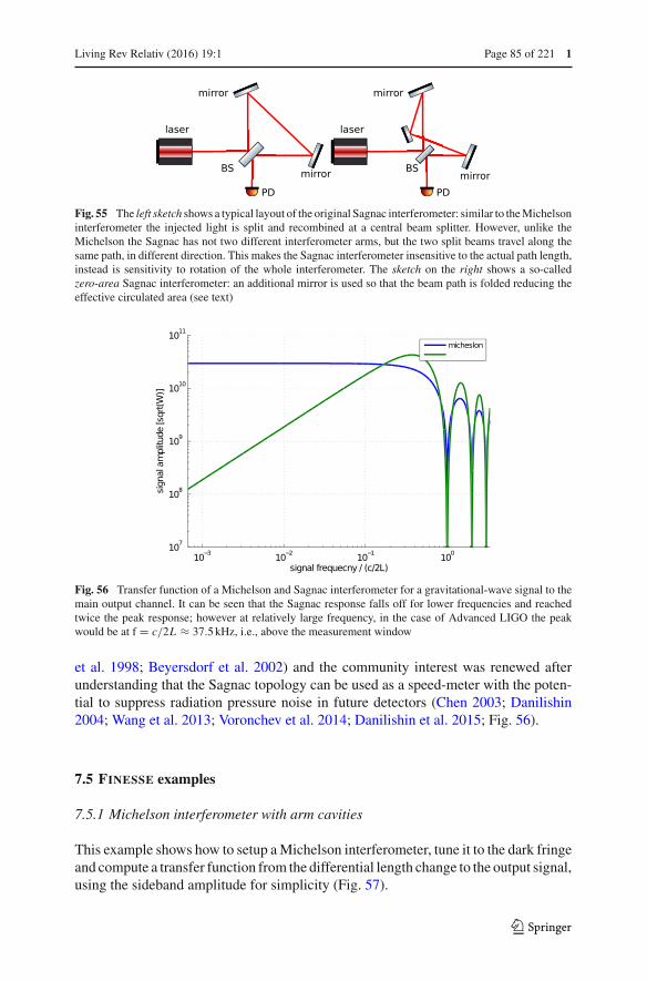
Living Rev Relativ (2016) 19:1 Page 85 of 221 1
Fig. 55 The left sketch shows a typical layout of the original Sagnac interferometer: similar to the Michelsoninterferometer the injected light is split and recombined at a central beam splitter. However, unlike theMichelson the Sagnac has not two different interferometer arms, but the two split beams travel along thesame path, in different direction. This makes the Sagnac interferometer insensitive to the actual path length,instead is sensitivity to rotation of the whole interferometer. The sketch on the right shows a so-calledzero-area Sagnac interferometer: an additional mirror is used so that the beam path is folded reducing theeffective circulated area (see text)
Fig. 56 Transfer function of a Michelson and Sagnac interferometer for a gravitational-wave signal to themain output channel. It can be seen that the Sagnac response falls off for lower frequencies and reachedtwice the peak response; however at relatively large frequency, in the case of Advanced LIGO the peakwould be at f = c/2L ≈ 37.5 kHz, i.e., above the measurement window
et al. 1998; Beyersdorf et al. 2002) and the community interest was renewed afterunderstanding that the Sagnac topology can be used as a speed-meter with the poten-tial to suppress radiation pressure noise in future detectors (Chen 2003; Danilishin2004; Wang et al. 2013; Voronchev et al. 2014; Danilishin et al. 2015; Fig. 56).
7.5 FINESSE examples
7.5.1 Michelson interferometer with arm cavities
This example shows how to setup a Michelson interferometer, tune it to the dark fringeand compute a transfer function from the differential length change to the output signal,using the sideband amplitude for simplicity (Fig. 57).
123
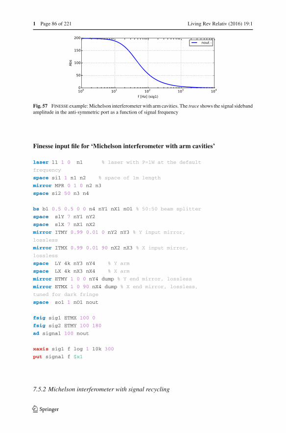
1 Page 86 of 221 Living Rev Relativ (2016) 19:1
Fig. 57 Finesse example: Michelson interferometer with arm cavities. The trace shows the signal sidebandamplitude in the anti-symmetric port as a function of signal frequency
Finesse input file for ‘Michelson interferometer with arm cavities’
laser l1 1 0 n1 % laser with P=1W at the default
frequency
space si1 1 n1 n2 % space of 1m length
mirror MPR 0 1 0 n2 n3
space si2 50 n3 n4
bs b1 0.5 0.5 0 0 n4 nY1 nX1 nO1 % 50:50 beam splitter
space slY 7 nY1 nY2
space slX 7 nX1 nX2
mirror ITMY 0.99 0.01 0 nY2 nY3 % Y input mirror,
lossless
mirror ITMX 0.99 0.01 90 nX2 nX3 % X input mirror,
lossless
space LY 4k nY3 nY4 % Y arm
space LX 4k nX3 nX4 % X arm
mirror ETMY 1 0 0 nY4 dump % Y end mirror, lossless
mirror ETMX 1 0 90 nX4 dump % X end mirror, lossless,
tuned for dark fringe
space so1 1 nO1 nout
fsig sig1 ETMX 100 0
fsig sig2 ETMY 100 180
ad signal 100 nout
xaxis sig1 f log 1 10k 300
put signal f $x1
7.5.2 Michelson interferometer with signal recycling
123
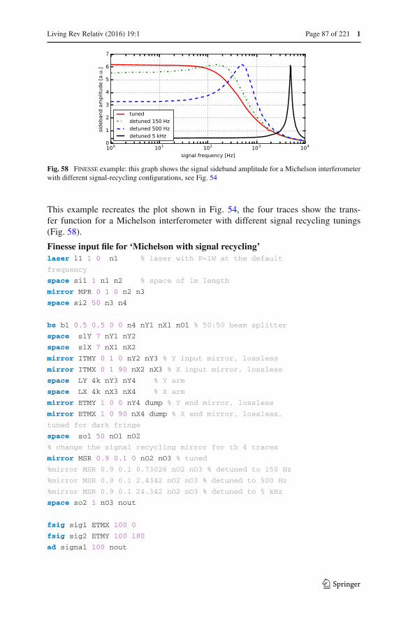
Living Rev Relativ (2016) 19:1 Page 87 of 221 1
Fig. 58 Finesse example: this graph shows the signal sideband amplitude for a Michelson interferometerwith different signal-recycling configurations, see Fig. 54
This example recreates the plot shown in Fig. 54, the four traces show the trans-fer function for a Michelson interferometer with different signal recycling tunings(Fig. 58).
Finesse input file for ‘Michelson with signal recycling’laser l1 1 0 n1 % laser with P=1W at the default
frequency
space si1 1 n1 n2 % space of 1m length
mirror MPR 0 1 0 n2 n3
space si2 50 n3 n4
bs b1 0.5 0.5 0 0 n4 nY1 nX1 nO1 % 50:50 beam splitter
space slY 7 nY1 nY2
space slX 7 nX1 nX2
mirror ITMY 0 1 0 nY2 nY3 % Y input mirror, lossless
mirror ITMX 0 1 90 nX2 nX3 % X input mirror, lossless
space LY 4k nY3 nY4 % Y arm
space LX 4k nX3 nX4 % X arm
mirror ETMY 1 0 0 nY4 dump % Y end mirror, lossless
mirror ETMX 1 0 90 nX4 dump % X end mirror, lossless,
tuned for dark fringe
space so1 50 nO1 nO2
% change the signal recycling mirror for th 4 traces
mirror MSR 0.9 0.1 0 nO2 nO3 % tuned
%mirror MSR 0.9 0.1 0.73026 nO2 nO3 % detuned to 150 Hz
%mirror MSR 0.9 0.1 2.4342 nO2 nO3 % detuned to 500 Hz
%mirror MSR 0.9 0.1 24.342 nO2 nO3 % detuned to 5 kHz
space so2 1 nO3 nout
fsig sig1 ETMX 100 0
fsig sig2 ETMY 100 180
ad signal 100 nout
123
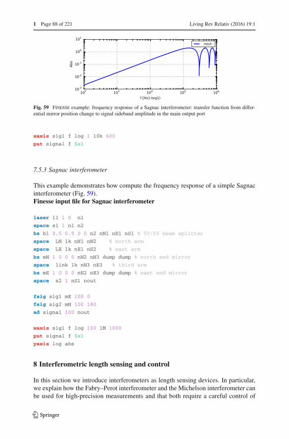
1 Page 88 of 221 Living Rev Relativ (2016) 19:1
Fig. 59 Finesse example: frequency response of a Sagnac interferometer: transfer function from differ-ential mirror position change to signal sideband amplitude in the main output port
xaxis sig1 f log 1 10k 600
put signal f $x1
7.5.3 Sagnac interferometer
This example demonstrates how compute the frequency response of a simple Sagnacinterferometer (Fig. 59).Finesse input file for Sagnac interferometer
laser l1 1 0 n1
space s1 1 n1 n2
bs b1 0.5 0.5 0 0 n2 nN1 nE1 nS1 % 50:50 beam splitter
space LN 1k nN1 nN2 % north arm
space LE 1k nE1 nE2 % east arm
bs mN 1 0 0 0 nN2 nN3 dump dump % north end mirror
space link 1k nN3 nE3 % third arm
bs mE 1 0 0 0 nE2 nE3 dump dump % east end mirror
space s2 1 nS1 nout
fsig sig1 mE 100 0
fsig sig2 mN 100 180
ad signal 100 nout
xaxis sig1 f log 100 1M 1000
put signal f $x1
yaxis log abs
8 Interferometric length sensing and control
In this section we introduce interferometers as length sensing devices. In particular,we explain how the Fabry–Perot interferometer and the Michelson interferometer canbe used for high-precision measurements and that both require a careful control of
123
Living Rev Relativ (2016) 19:1 Page 89 of 221 1
the base length (which is to be measured) in order to yield their large sensitivity. Inaddition, we briefly introduce the general concepts of error signals, transfer functionsand relevant elements of control theory, which are used to describe most essentialfeatures of length sensing and control.
In addition to sensing and controlling the distances between the components of aninterferometer, alignment sensing and control is required for correct operation. Whilewe do not deal with this aspect in detail, all of the ideas we develop for length sensingand control can be applied. The essential differences are that split photo-detectors arerequired to sense the relative angles of optical wavefronts, and control is be means ofactuators that are able to adjust the angles of optical components. For an introduction tothe essential ideas see Sect. 9.2 for an introduction to the relevant theory and Morrisonet al. (1994), for details of a practical implementation.
8.1 An overview of the control problem
A complete interferometer can have a large number of control loops for the variousmirrors and beam splitters, their suspension systems and many other components,such as the laser, active vibration-isolation systems etc. For practical purposes theseare usually divided into two broad classes that are often considered separately inthe design process. These divisions reflect a degree of independence of the variouscategories of control and simplify the design process by allowing the problem to besplit into a number of more easily tractable design elements.
The set of control loops that obtain signals from the detection of interference con-ditions or other properties of the light within the interferometer, and act on the majoroptical components of the interferometer to control those properties, is usually calledglobal control. As an example, a description of the global control system of Virgocan be found in Arnaud et al. (2005). On the other hand, loops that sense propertiesassociated with a single component, and act on that component are called local loops.A good example of local control is the system employed to damp the rigid-body modesof a mirror suspension, for an example from Advanced LIGO see Aston et al. (2012).By ‘cooling’ or quieting the motion of individual mirrors, the task faced by the globalcontrol system can be simplified. Further division of global interferometer control isfrequently made between systems that control longitudinal degrees of freedom, i.e.,relative positions of the mirrors and beam splitters along the direction of propagationof the light, and angular (alignment) control systems that are designed to stabilise thepointing of components.
Due to the presence of strong nonlinearity throughout much of the phase-spacevolume, there has been no attempt thus far to solve the multi-dimensional controlproblem as a whole. At least up to the present, the problem has been divided intoseveral smaller parts, with methods developed to deal with the particular details ofeach facet of the system, and each stage of operation from completely uncontrolled toheld at the operating point—a condition that is called ‘locked’.
This leads to yet another division: it is normal to separate the start-up phase i.e.,the process called acquisition of lock from the stable running condition (‘in lock’).This split is motivated, at least in part, by the consideration that signal sizes can
123

1 Page 90 of 221 Living Rev Relativ (2016) 19:1
differ greatly between the two stages. During acquisition electronic signals tend to belarge—corresponding to adjusting mirror positions by of order wavelengths, or more.By contrast, in operation the signals representing residual motion in the sensitivefrequency band may be 12 or more orders of magnitude smaller than the wavelengthof the light, to deliver the required measurement sensitivity.11
The jump in signal size between these two states is often dealt with by switching gainlevels or even substituting large parts of the control system: starting with large-rangebut noisy methods for acquisition and switching to low-noise, but small-range controlsfor operation. A good example of a more substantial transition is the arm length sta-bilization (ALS) scheme in Advanced LIGO, which employs additional lasers, mirrorcoatings and interferometric methods to provide wavelength-range sensing during theacquisition phase (Evans et al. 2009). When the long cavities (see “Appendix B”) arelocked, the control systems are switched over to the high-sensitivity, low-noise signalsderived from the main interferometer systems.
During acquisition of lock, the instantaneous operating point frequently lies in anon-linear region of the control space. Several methods have been developed to copewith this problem.
The simplest approach, employed in the early interferometer prototypes, was to waitfor a random co-incidence of suitable values to occur then to catch the system quicklyenough to hold it in the desired state. As the complexity of the interferometer topologiesincreased, and with that the number of degrees of freedom, the probability of the desiredstate occurring in a conveniently short time became rare. This led to the developmentof more sophisticated techniques for the first long-baseline interferometers.
As a first step it was realised that digital logic, implemented directly in electronicsor as software, could be employed to identify when one or more degrees of freedomhappened to fall close to the desired operating point, and to activate the relevant controlloop. This prevents false signals, frequently present in regions of phase space close tothe desired operating point, being fed back to the actuators and perturbing the system.In Pound–Drever–Hall locking, for example, when the phase modulation sidebandspass through resonance in the cavity, the error signal has the opposite sign from thatproduced by a carrier resonance. The acquisition process can be improved by enablingthe control system only when the circulating power within the cavity has exceededthe maximum possible power that a sideband can produce. By this means the controlsystem is only activated close to the desired operating point, improving the chancesof a successful lock.
A second way to improve matters is to linearise the behaviour, and so to increasethe capture range: i.e., the volume of phase space within which the various controlsignals are valid. This improvement can be accomplished by normalising the relevanterror signal according to some estimate of its slope, as measured by another signalsuch as the circulating optical power. As an example, the linear range in the Pound–Drever–Hall signal for locking a cavity may be extended by normalising with respect
11 The typical light wavelength is ∼10−6 m while all ground-based interferometers built or planned havetarget displacement noise spectral densities below ∼10−19 m/
√Hz in a frequency band of order 100 Hz
wide.
123
Living Rev Relativ (2016) 19:1 Page 91 of 221 1
to the power within the cavity, as measured by probing the light transmitted by thecavity.
Another approach, is to arrange for the first locking to be in a region of phase spacethat is relatively smooth, compared to the region in phase space surrounding the finaloperating point. This was an enabling technique for GEO 600 when it was first operatedin dual-recycled mode. It was found that by locking with signal recycling detuned bya few kHz, an initial lock was possible. The tuning was then stepped towards the targetvalue, in steps chosen to be small enough to avoid perturbing the lock. By this meansit was possible to reach a location in phase space which would essentially never haveoccurred by chance (Grote 2003).
After lock has been achieved by one or more of the above means, the control task isgenerally managed by linear control systems that may be analysed using standard lin-ear time invariant (LTI) control theory. Two generic approaches have been employedwith success. In one approach there is a set of separate single-input single output(SISO) controllers, one for each degree of freedom. The alternative is to deal withseveral degrees of freedom in a single multi-input multi-output (MIMO) controller.Recently, since the advent of computer-based, digital control systems, the MIMOapproach has become much more practical than it would be if implemented in ana-logue electronics. An important difference between the SISO and MIMO approachesconcerns how cross-coupling between the degrees of freedoms can dealt with.
Cross-coupling is commonly seen in both sensing and actuation, and considerableeffort is needed to develop control systems that operate correctly in the presence ofundesired mixing of signals. The main approaches to solving these problems withMIMO controllers is described in Sect. 8.7. Otherwise we discuss SISO controllers toprovide illustrative examples of control in idealised interferometers where there is nomixing of degrees of freedom at the point of sensing or actuation.
We introduce standard terminology from control theory. In each control loop a pointof reference is taken, called the error point at which we measure how the gain of theloop acts to suppress deviations from the desired operating point. Since a loop has noend, the selection of this point is somewhat arbitrary, but it is usually convenient totake the output from a photo-detector or its associated demodulator.
Likewise, we choose an actuation or feedback point at the interface between thecontrol electronics and the interferometer—again the precise division is somewhatarbitrary, but the electronic signal input to an actuator is frequently employed as thepoint of reference.
With these points defined, the part of the loop from error-point to feedback-point iscalled the controller or just the feedback, and the rest of the loop from feedback pointto the error point, in the causal direction, is called the plant.
Before a loop is activated, the signal that would be measured at the error point iscalled the error signal. In interferometry this is usually derived as an output from theoptical system and its photo-detectors, as explained in Sect. 8.5.
123

1 Page 92 of 221 Living Rev Relativ (2016) 19:1
8.2 Linear time-invariant control theory: introductory concepts
A full description of linear time-invariant (LTI) theory is beyond the scope of this arti-cle, therefore we restrict our description to a short summary of the essential concepts,with some relevant examples presented in the following sections.
In LTI models the superposition principle applies, frequencies do not mix and itis possible to represent any physical time-domain signals in the frequency domainthrough their Fourier transforms. The time-invariance means that the response of asystem to an input does not depend on the time at which that input is applied. Thisimplies that the differential equations describing the system are linear and homoge-neous with coefficients that are constant in time. In this case it is common to solvethese equations by employing methods based on the Laplace transform. The responseof the system is represented by its transfer function which is the Laplace transform ofits impulse response—i.e., the output produced in the time domain when the input isa Dirac-delta function. We look at transfer functions in mode detail in Sect. 8.5.
For LTI systems the eigenfunctions or basis functions of the solution are the complexexponentials. Consider an input of the form
SI = Aest , (8.1)
where A is a complex factor, s the Laplace transform variable and t is time, to aparticular system. If the output is
SO = Best , (8.2)
with different complex factor B, the system is described in full by the transfer function
T = SOSI
= Best
Aest= B
A, (8.3)
which is not a function of time.By implication, if the input to the system is a sinusoid (a single Fourier component)
the output is also a sinusoid with, generally, different amplitude and phase as describedby the transfer function. If the system consists of a series of optical, electronic andmechanical stages or sub-systems, the overall transfer function is the product of theindividual transfer functions. If there is feedback, then loop-algebra can be applied,and this represents summation of the signal from one point in a loop into an earlierpoint (feedback), or in the case of feed-forward to a later point. This is also a linearoperation, and so the system with feedback or feed-forward retains its LTI property.The most complicated case that need be considered is when there are two or morenested feedback loops (or equivalently two or more actuators that adjust one degreeof freedom (Shapiro et al. 2015)), in this case there are loop-algebraic techniques thatallow the system to be reduced to a single equivalent loop, such that nested loops ofany practical topology may be considered step by step.
In modelling LTI systems it is common to pick a representation from one ofa mathematically-equivalent set of options. The alternatives are described in, e.g.,
123

Living Rev Relativ (2016) 19:1 Page 93 of 221 1
Franklin et al. (1998). To give some examples, individual loops or blocks with oneinput and one output (called SISO—single input, single output systems), are com-monly represented by their transfer functions.
For LTI systems, the transfer functions can be written as rational polynomialsin the complex frequency variable s. The polynomials on both the numerator anddenominator of the transfer function can be factorised. This leads to an equivalentmathematical representation of the transfer function as a list of zeros (zeros of thenumerator) and poles (zeros of the denominator). In addition an overall gain factor,independent of frequency, is usually required. The poles and zeros may be repre-sented by their coordinates in the complex (s)-plane, or more phenomenologically bytheir resonant frequencies and damping factors. This leads to the so-called (z, p, k)-notation, where z represents one or more zeros, p the poles, and k represents an overallfrequency-independent gain factor.
For MIMO systems arrays of transfer functions can be employed to describe allpossible input–output relations, but it is more common to use the state-space represen-tation. Here a single set of matrices encapsulates the behaviour of the entire system.A description of this important method is beyond the scope, but full detail is given inFranklin et al. (1998).
In briefest summary, the state-space method involves writing the set of N secondorder differential equations representing the internal dynamics of a system which hasN degrees of freedom. These are reduced to 2N first-order equations by introducingthe time derivatives, i.e., generalised velocities, of the displacement-like coordinates.The solution of the resulting set of equations is then usually carried out numerically,using matrix methods.
8.3 Digital signal processing for control
In the past two decades digital control systems have been introduced into the control ofinterferometers, in modern instruments the majority of control systems contain digitalprocessing elements, although the interfaces with the interferometer remain analoguein almost all cases. The essential principles remain the same as in the continuous-time systems, and a common approach to the design of digital control systems startsby designing and simulating a continuous-time analogue model. When this modeloperates as required in simulation, the result is transformed to the discrete-time math-ematics of digital control. The resulting filters are then implemented in a combinationof software and hardware. In discrete-time models only a finite set of frequencies exist,limited at high frequencies by the Nyquist frequency, i.e., half of the sampling rate inthe digital system.
Digital models also have finite amplitude resolution, with the practical resolutionlimits occurring at the analogue-digital and digital-analogue interfaces (ADC, DACrespectively), rather than in the digital signal processing. These limitations are gen-erally handled by whitening the signal at the input and de-whitening at the output.For example, input signals with predominant low-frequency content may be high-passfiltered to render their spectral content relatively uniform, i.e., white, before samplingto make best use of the available resolution. The converse process can be applied at the
123

1 Page 94 of 221 Living Rev Relativ (2016) 19:1
Fig. 60 Bode plots to compare a digital representations with a first-order analogue transfer function and itsinverse. The analogue system has a single real pole at 0.1 Hz and single real zero at 10 Hz. When the transferfunction is inverted the pole becomes a zero, and the zero a pole. The bilinear transform is employed toproduce the digital equivalents, with a sampling frequency of 100 Hz. The highest frequency that can berepresented in this case is 50 Hz and it can be seen that the digital response becomes a poor approximationto the analogue one at frequencies approaching this limit. Note that, in a practical digital system, therewould be a finite time delay and corresponding phase-lag, not included here, and that further delays maybe present from anti-aliasing and anti-imaging filters—see text
output, with sufficient low-pass filtering applied to ensure that white noise resultingfrom the output conversion (DAC) is suppressed within the gravitational wave band.
In the description of digital controllers, the discrete mathematics of the z-planereplaces the continuous nature of the s-plane (Franklin et al. 1998). Transformingfrom one space to the other is something of an art, mainly due to the consequences offinite precision in the associated calculations. A bilinear transformation is commonlyemployed. To avoid problems of numerical accuracy in the associated calculations,complicated systems are broken down in to a series of second-order sections. Thesesubsystems have up to two poles and two zeros, i.e., the transfer functions have nohigher order than quadratic numerator and denominator. Such subsystems can betransformed more reliably.
The finite time-steps in digital processing limit the filter transfer functions thatmay be produced at frequencies approaching the Nyquist limit—see Figs. 60 and 61.Note however that with modern computers the sampling rate is often limited by theanalogue interfaces rather than the speed of processing. Where this is true the datastream can be up-sampled (interpolated) to a higher sampling rate for filtering, and thendown-sampled (decimated) to the original sampling rate before conversion back to theanalogue domain. This process can be used to improve the high-frequency responseof digital filters.
One further consequence of discrete time is that there is a finite delay associatedwith the analogue to digital, signal processing and digital to analogue steps. Thismust be considered in the development of feedback loops based on digital controls.
123
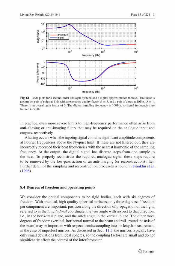
Living Rev Relativ (2016) 19:1 Page 95 of 221 1
Fig. 61 Bode plots for a second-order analogue system, and a digital approximation thereto. Here there isa complex pair of poles at 1 Hz with a resonance quality factor Q = 3, and a pair of zeros at 10 Hz, Q = 1.There is an overall gain factor of 3. The digital sampling frequency is 100 Hz, so signal frequencies arelimited to 50 Hz
In practice, even more severe limits to high-frequency performance often arise fromanti-aliasing or anti-imaging filters that may be required on the analogue input andoutputs, respectively.
Aliasing occurs when the ingoing signal contains significant amplitude componentsat Fourier frequencies above the Nyquist limit. If these are not filtered out, they areincorrectly recorded their beat frequencies with the nearest harmonic of the samplingfrequency. At the output, the digital signal has discrete steps from one sample tothe next. To properly reconstruct the required analogue signal these steps requireto be removed by the low-pass action of an anti-imaging (or reconstruction) filter.Further detail of the sampling and reconstruction processes is found in Franklin et al.(1998).
8.4 Degrees of freedom and operating points
We consider the optical components to be rigid bodies, each with six degrees offreedom. With practical, high-quality spherical surfaces, only three degrees of freedomper component are important: position along the direction of propagation of the light,referred to as the longitudinal coordinate, the yaw angle with respect to that direction,i.e., in the horizontal plane, and the pitch angle in the vertical plane. The other threedegrees of freedom (vertical, horizontal normal to the beam and roll around the axis ofthe beam) may be important with respect to noise coupling into the length measurementin the case of imperfect mirrors. As discussed in Sect. 11.5, the mirrors typically haveonly small deviations from ideal spheres, so the coupling factors are small and do notsignificantly affect the control of the interferometer.
123
1 Page 96 of 221 Living Rev Relativ (2016) 19:1
In the interferometer as a whole, one component, for example, a mirror or beamsplitter, may be chosen as the origin for the coordinate system. This allows one posi-tion and a pair of angles to be pre-defined. The positions and angles of the othercomponents may then be described with respect to this origin. Note, however, thatthe longitudinal degrees of freedom are measured with an optical ‘ruler’ that is basedon the wavelength of the light, and so the wavelength should be counted as one lon-gitudinal degree of freedom in the system as a whole (in the sense that the light hasthe same frequency everywhere which is usually true to a good approximation in theultra-stable environment of a gravitational-wave detector). Similarly the direction ofthe light beam entering the interferometer defines two angles.
To take an example, a simple cavity that is to be held on resonance with in-goinglight has two meaningful longitudinal degrees of freedom. For a cavity in isolationit would be usual to consider the position of one mirror relative to the other and thefrequency, or wavelength, of the light as the important parameters. Mathematicallythere are other equivalent choices, but in the control and operation of interferometersthe point is to find a convenient set of control variables.
Similarly, a simple Michelson interferometer has three components and three lon-gitudinal degrees of freedom. Again it would be usual to consider one componentas a reference. If the beam splitter is fixed, the three degrees of freedom are the twoarm-lengths and the optical wavelength, or frequency.
If a pair of cavities were to be placed, one each, into the arms of the simple Michel-son, the single degree of freedom of each mirror is replaced with the two of the cavity,for a total of five: once again, the same as the number of components. Fixing the beamsplitter, these are the laser wavelength, the two distances from the beam splitter to thenear mirrors of the cavities and the two lengths of the cavities.
An example of the degrees of freedom relevant to longitudinal control of a morecomplex system is shown in Sect. 8.12.
The choice between employing absolute or relative coordinates for the positions(and angles) of interferometer components is reflected in differences of approach in theavailable modelling software. In a Finesse model of a two-mirror cavity, for example,the longitudinal positions of the two mirrors are specified, and adjusting either of themchanges the resonant condition of the cavity (see, for example, Sect. 5.6.1). Likewise,adjusting the position of the input mirror changes the phase of both the light in thecavity, and the light reflected from the cavity. See Sect. 2.1 for a discussion of thispoint.
An operating interferometer requires various interference conditions to be main-tained, e.g., cavities should be kept on resonance, the dark-fringe condition in aMichelson interferometer must be met, and so forth. For each degree of freedomthis implies that there is an optimum value for best sensitivity or an operating pointin the multi-dimensional space representing the degrees of freedom. This point is notusually unique: for example, signals repeat modulo one round-trip wavelength, seebelow.
As most or all degrees of freedom are subject to movement or drift, they must becontrolled, generally by designing and implementing a separate control loop for eachone. These loops must be designed to hold the value of the degree of freedom close
123
Living Rev Relativ (2016) 19:1 Page 97 of 221 1
to such an operating point, where ‘close’ is determined by tolerance bounds that mustbe determined by calculation.
In most cases it is possible to evaluate a tolerance interval around the operatingpoint. The limits usually arise in the consideration of the coupling of some kind ofnoise into the sensitive measurement (frequency noise, power noise, beam directionnoise, etc.). For example, in the case of the dark fringe, sensitivity to laser powernoise is at a minimum at the perfectly dark condition, and the tolerable increase in thiscoupling may be used to set bounds on deviations from the operating point.
Bounds may also be set by considering the required linearity of signals. Non-linearity can lead to beating, which mixes noise into the measurement band. Forexample if there is a narrow spectral feature or ‘line’, such as a calibration line thatmay be applied to monitor instrumental sensitivity, or a suspension violin mode12 in themeasurement band, beating this with low frequency motion of suspended componentswill produce sidebands on either side of the narrow feature, and these may be of higheramplitude than the noise background at the frequencies of interest near the line. Non-linear operation may also cause problems for control systems, as its presence impliesthat the gain of control loops will depend on the magnitude of deviations from thenominal operating point. In the following (Sect. 8.5) it will be seen that the normalprocess of sensing the length of a cavity is reasonably linear only within a very narrowrange, in comparison to the wavelength of light, around the operating point, at least fora cavity of high finesse—a range of distance of order λ/F (see Sect. 5.1), or smaller.
In designing a control system for an interferometer, one can in principle considerthe space of possible values of all the degrees of freedom in an interferometer, butit is more usual to work with a sub-space, e.g., only the longitudinal degrees. Inthe angular case there is usually a unique operating point per degree of freedomcorresponding to one optimal alignment, but in the longitudinal case operating pointsare repeated as the relevant round-trip phase change steps in multiples of 2π , i.e.,one wavelength change in round-trip optical path distance. In this case it is usual toconsider the (hyper-)volume containing one repeat in each dimension: for km-longinterferometers there is very little difference between adjacent volumes. In a typicalinterferometer designed for gravitational wave detection, the number of degrees offreedom in combination with requirements on noise coupling and linearity mean thatonly a vanishingly small volume within the phase space corresponds to the acceptableregion around the desired operating point. This suggests one of the important questionsin operating a gravitational wave detector: how to bring every degree of freedom tothe desired operating point.
The diminutive scale of the useful volume in phase space can be illustrated bymeans of a simplified example. Here we consider the case of two degrees of freedomin a power recycled Michelson interferometer. Even fixing the location of the beamsplitter, there are three degrees of freedom (i.e., common arm length, differential arm
12 To minimise thermal noise in suspensions, low-loss materials and techniques are employed to avoiddissipation. The resonant modes of these suspensions are seen in the frequency domain as narrow spectralfeatures, or lines. The violin modes are transverse oscillations of the stretched suspension fibres that supportthe mirrors, which vibrate much like a violin string. The frequencies of these modes typically lie between300 and 800 Hz, and they are often conspicuous in the spectra of signals from gravitational-wave detectors.
123

1 Page 98 of 221 Living Rev Relativ (2016) 19:1
Fig. 62 Simplified example illustrating the restricted phase space volume in which interferometer controlsignals are expected to achieve significant magnitudes. In the left panel we show the modulus of the lightamplitude emerging at the detection/output port of a power recycled Michelson interferometer as a functionof both the length difference between the arms (in the plot, the two end mirrors have their tuning phaseshifted by the amount shown, but in opposition) and the tuning of the power recycling (the mirror has itstuning phase shifted by the amount shown). The normalised amplitude is shown on a linear scale from zeroto one. These two degrees of freedom are swept over two cycles from the nominal operating point at (0,0).The other possible longitudinal degrees of freedom, namely the common mode arm length and the opticalfrequency are kept constant. The size of a signal designed to sense the differential degree of freedom, andallow the interferometer to be locked at the operating point, would have significant magnitude only in theregion of the features like the one near (0,0) where there is a significant gradient in the horizontal directionin the plot. In this example, the power recycling mirror has a transmission of 1 %, and other componentshave no loss. In a practical detector there would be several other degrees of freedom. Typically there wouldalso be cavities of higher finesse, leading to even narrower features. The right panel shows a magnified viewof one of the ‘islands’ of useful signal, the operating point is a small region at coordinates (0,0) where thelight power is low
length and longitudinal position of the power recycling mirror. However, we chooseto produce a contour plot showing signal sizes as a function of just two degrees offreedom, Fig. 62. Here we vary the difference in the lengths of the two arms whilekeeping the average (or common mode) arm length fixed, and also to vary the positionof the power recycling mirror. In a practical interferometer there would be severalother degrees of freedom associated with, for example, arm cavities, signal recyclingand control of the common-mode arm length (or laser frequency), and in most casesthe cavities would be of higher finesse producing even narrower features—see, forexample, the parameters for Advanced LIGO in “Appendix B”.
123

Living Rev Relativ (2016) 19:1 Page 99 of 221 1
The complexity of sensing and control becomes apparent when one considers that,in the common case of the freely-suspended optical components in a ground-basedinterferometric gravitational wave detector, the initial condition, at the point of ‘switch-ing on’ the controls can be any random point within the space, with—in addition—awide range of initial velocities associated with each degree of freedom: up to perhapsof order one wavelength per second, in a typical ground-based instrument. How thisis dealt with is summarised in Sect. 8.1.
8.5 Error signals and transfer functions
In general, we will call an error signal any measured signal suitable for stabilising acertain experimental parameter p with a servo loop. The aim is to maintain the variablep at a user-defined value, the operating point, p0. Therefore, the error signal must be afunction of the parameter p. In most cases it is preferable to have a bipolar signal witha zero crossing at the operating point. The slope of the error signal at the operatingpoint is a measure of the ‘gain’ of the sensor, which in the case of interferometers isa combination of optics and electronics.
Transfer functions describe the propagation of a periodic signal through a plant andare usually given as plots of amplitude and phase over frequency, e.g., as Bode plots(see the following section). By definition a transfer function describes only the linearcoupling of signals inside a system. This means a transfer function is independentof the actual signal size. For small signals or small deviations, most systems can belinearised and correctly described by transfer functions.
Experimentally, network analysers are commonly used to measure a transfer func-tion: one connects a periodic signal (the source) to an actuator of the plant (which isto be analysed) and to an input of the analyser. A signal from a sensor that monitors acertain parameter of the plant is connected to the second analyser input. By mixing thesource with the sensor signal the analyser can determine the amplitude and phase ofthe input signal with respect to the source (amplitude equals one and the phase equalszero when both signals are identical).
Mathematically, transfer functions can be modelled similarly: applying a sinusoidalsignal sin(ωs t) to the interferometer, e.g., as a position modulation of a cavity mirror,will create phase modulation sidebands with a frequency offset of ±ωs to the carrierlight. If such light is detected in the right way by a photodiode, it will include a signalat the frequency component ωs , which can be extracted, for example, by means ofdemodulation (see Sect. 4.2).
Transfer functions are of particular interest in relation to error signals. Typically atransfer function of the error signal is required for the design of the respective electronicservo. A ‘transfer function of the error signal’ usually refers to a very specific setup:the system is held at its operating point, such that, on average, p = p0. A signal isapplied to the system in the form of a very small sinusoidal disturbance of p. Thetransfer function is then constructed by computing for each signal frequency the ratioof the error signal and the injected signal. Figure 63 shows an example of an errorsignal and its corresponding transfer function. The operating point shall be at
xd = 0 and xEP(xd = 0) = 0. (8.4)
123
1 Page 100 of 221 Living Rev Relativ (2016) 19:1
The optical transfer function Topt,xd with respect to this error signal is defined by
xEP( f ) = Topt,xdTdet xd( f ), (8.5)
with Tdet as the transfer function of the sensor. In the following, Tdet is assumed to beunity. At the zero crossing the slope of the error signal represents the magnitude ofthe transfer function for low frequencies:
∣∣∣∣dxEP
dxd
∣∣∣∣ ∣∣xd=0= |Topt,xd | ∣∣ f→0
(8.6)
The quantity above will be called the error-signal slope in the following text. It isproportional to the optical gain |Topt,xd |, which describes the amplification of thegravitational-wave signal by the optical instrument.
8.6 Bode plots: traditional control theory for SISO loops
An essential feature of a control system is stability, i.e., for a finite input the outputshould always be bounded. This is equivalent to requiring all of the transfer func-tion poles to correspond to decaying exponentials, so their real parts must be strictlynegative.
Prior to the routine application of computers, a number of tools (plots) were devel-oped to facilitate control system design. Although the root-locus, Nyquist and Bodeplots continue to be applied, computer models remove the practical (calculational)advantages of one over another. All of these methods present essentially equivalentinformation, and the choice of one over another is a matter of convenience or familiar-ity. Since Bode plots provide a complete description of minimum-phase, single-inputsingle-output (SISO) LTI control loops we choose to describe that approach as anexample.
Throughout this section, the system is described in continuous time, i.e., as ananalogue model. When the technique is applied to digital control systems discrete-time models are needed as discussed in Sect. 8.3.
A Bode plot of a system shows its transfer function in the form of log-magnitudeand linear-phase graphs against a logarithmic frequency axis—conventionally invertically-stacked plots with matching, aligned frequency axes, see Fig. 64 for a sim-ple example. In the context of the design of complete negative feedback loops, it iscommon, though not universal, to add π to the phase to represent the overall negativesign—this convention is assumed here. The standard procedure starts with consid-eration of the open-loop Bode plot. In this, the loop is broken (in the model) at aconvenient point, and the transfer function from there back to just before the break iscalculated and plotted. Remember that the total transfer function is computed as theproduct of individual transfer functions of parts of the loop that are connected in series.Particular attention is paid to the regions close to points where the transfer functionmagnitude crosses unity (i.e., zero on the log scale), called the unity gain point(s), andwhere the phase crosses −π in absolute terms, not modulo 2π . The transfer function
123
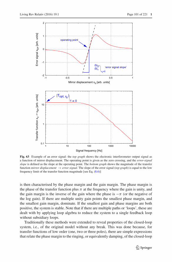
Living Rev Relativ (2016) 19:1 Page 101 of 221 1
Fig. 63 Example of an error signal: the top graph shows the electronic interferometer output signal asa function of mirror displacement. The operating point is given as the zero crossing, and the error-signalslope is defined as the slope at the operating point. The bottom graph shows the magnitude of the transferfunction mirror displacement → error signal. The slope of the error signal (top graph) is equal to the lowfrequency limit of the transfer function magnitude [see Eq. (8.6)]
is then characterised by the phase margin and the gain margin. The phase margin isthe phase of the transfer function plus π at the frequency where the gain is unity, andthe gain margin is the inverse of the gain where the phase is −π (or the negative ofthe log gain). If there are multiple unity gain points the smallest phase margin, andthe smallest gain margin, dominate. If the smallest gain and phase margins are bothpositive, the system is stable. Note that if there are multiple paths or ‘loops’, these aredealt with by applying loop algebra to reduce the system to a single feedback loopwithout subsidiary loops.
Traditionally these methods were extended to reveal properties of the closed-loopsystem, i.e., of the original model without any break. This was done because, fortransfer functions of low order (one, two or three poles), there are simple expressionsthat relate the phase margin to the ringing, or equivalently damping, of the closed-loop
123
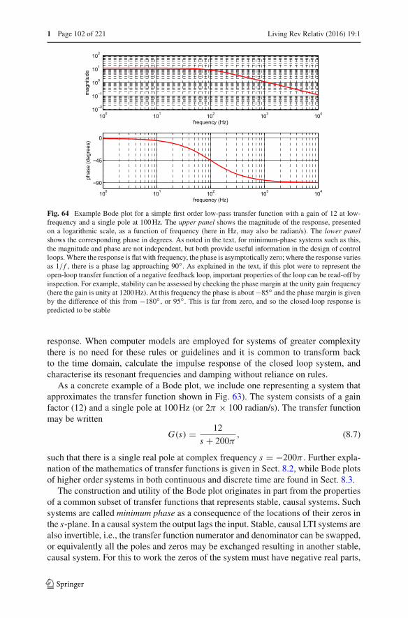
1 Page 102 of 221 Living Rev Relativ (2016) 19:1
Fig. 64 Example Bode plot for a simple first order low-pass transfer function with a gain of 12 at low-frequency and a single pole at 100 Hz. The upper panel shows the magnitude of the response, presentedon a logarithmic scale, as a function of frequency (here in Hz, may also be radian/s). The lower panelshows the corresponding phase in degrees. As noted in the text, for minimum-phase systems such as this,the magnitude and phase are not independent, but both provide useful information in the design of controlloops. Where the response is flat with frequency, the phase is asymptotically zero; where the response variesas 1/ f , there is a phase lag approaching 90◦. As explained in the text, if this plot were to represent theopen-loop transfer function of a negative feedback loop, important properties of the loop can be read-off byinspection. For example, stability can be assessed by checking the phase margin at the unity gain frequency(here the gain is unity at 1200 Hz). At this frequency the phase is about −85◦ and the phase margin is givenby the difference of this from −180◦, or 95◦. This is far from zero, and so the closed-loop response ispredicted to be stable
response. When computer models are employed for systems of greater complexitythere is no need for these rules or guidelines and it is common to transform backto the time domain, calculate the impulse response of the closed loop system, andcharacterise its resonant frequencies and damping without reliance on rules.
As a concrete example of a Bode plot, we include one representing a system thatapproximates the transfer function shown in Fig. 63). The system consists of a gainfactor (12) and a single pole at 100 Hz (or 2π × 100 radian/s). The transfer functionmay be written
G(s) = 12
s + 200π, (8.7)
such that there is a single real pole at complex frequency s = −200π . Further expla-nation of the mathematics of transfer functions is given in Sect. 8.2, while Bode plotsof higher order systems in both continuous and discrete time are found in Sect. 8.3.
The construction and utility of the Bode plot originates in part from the propertiesof a common subset of transfer functions that represents stable, causal systems. Suchsystems are called minimum phase as a consequence of the locations of their zeros inthe s-plane. In a causal system the output lags the input. Stable, causal LTI systems arealso invertible, i.e., the transfer function numerator and denominator can be swapped,or equivalently all the poles and zeros may be exchanged resulting in another stable,causal system. For this to work the zeros of the system must have negative real parts,
123

Living Rev Relativ (2016) 19:1 Page 103 of 221 1
so that when they become poles in the inverse system they are damped. It can be shownthat in such a system there is a strict relationship between the phase and the slope ofthe log-magnitude, as shown on a Bode plot—one is a Hilbert transform of the other.In practice this is equivalent to writing that the when the magnitude graph has a slopeof f −n , where f is the frequency, the phase approaches −nπ/2. This method allowsthe loop to be designed to meet various goals that are usually expressed in terms ofgain (or attenuation) that must be achieved in one or more range of frequencies, withstability checked by reading off the phase and gain margins.
In interferometry the optical transfer function is usually a significant aspect ofcontrol loops. Such transfer functions may be measured or found by calculation (e.g.,with Finesse). The corresponding transfer functions can be found by applying thetechniques described in Sect. 8.5.
8.7 Separating mixtures of the degrees of freedom: control matrices
In practice, each error signal intended to represent a particular degree of freedom of theoptical arrangement also contains some information about other degrees of freedom.To give a simple example of the mixing that may occur, any motion that leads to achange in the circulating light power in a cavity is likely to couple, at some level, toevery signal that depends on the intra-cavity light, unless the signal is precisely zero.
In most cases such mixing is undesirable as it is easier to design control systemsto deal with one degree of freedom in isolation. In the worst case, if the mixing, orcross-coupling is strong, it can lead to the formation of unintended feedback paths. Ifthe transfer function of such loops has a magnitude exceeding unity, there is a chancethat the loop may be unstable. A common cause of such instability is a resonance in theunintended or ‘parasitic’ loop. At such a resonance high gain is typically accompaniedby a phase lag of −π which will tend to be unstable unless some compensation isincluded, e.g., in the form of a notch filter to cancel the resonance.
Unwanted mixing of signals can also occur at the point of actuation. For example,a mirror may be common to two degrees of freedom of an interferometer. In an inter-ferometer with arm cavities, the cavity mirrors closest to the beam splitter behave inthis way. Moving such a mirror must then affect at least two length degrees of free-dom. This can be seen in Fig. 51 where motion of either of the two mirrors labelledITMX and ITMY affects the phase of the light in the respective arm cavity and alsothe interference condition of the Michelson interferometer. In contrast, the end mirrors(ETMX, ETMY) each affect only one longitudinal degree of freedom.
A further possible source of mixing between degrees of freedom arises at the pointof actuation. Feedback to control a mirror is often carried out in practice using an arrayof actuators, such as coil-magnet pairs, that push on the mirror at various points on itssurface. For example, it is common to employ a square-array of four magnets attachedto the rear surface of the mirror, as these allow longitudinal, pitch and yaw adjustment.If they are mounted close to the perimeter of the rear surface they may be out of theway of a transmitted light beam. With such an arrangement, each individual actuatorcauses changes to a mixture of angular and longitudinal degrees of freedom. If theactuators are not of precisely uniform strength and alignment, this leads to unintended
123
1 Page 104 of 221 Living Rev Relativ (2016) 19:1
components in the resultant force produced by the array. An actuation matrix, withfrequency-dependent elements where necessary, can be employed to orthogonalise theresponse of the system to commands from the controller, at least to some degree ofprecision.
The elements of actuation and sensing matrices are typically determined as a resultof simulation and measurement. Modelling may yield a set of starting values thatsuffice to allow the interferometer to operate. When operational residual mixing isnormally determined by carrying out all possible transfer function measurements. Themeasurements allow coupling matrices to be determined, and inverting the couplingmatrix provides the appropriate matrix necessary to remove unwanted mixing. Thisprocess is somewhat involved and benefits from automation.
8.8 Modern control methods in gravitational-wave detectors
During the past few decades new methods of designing sophisticated controllers basedon digital signal processing have emerged. A major benefit of the resulting ‘digitalcontrols’ is that the response of a control filter can be adjusted by changing filtercoefficients, this can even be achieved while the controller is operating, if that isrequired.
Digital control facilitates the application of so-called modern control methods inwhich optimisation methods are employed. As an indication of the possible advantagesthat may arise from this, we briefly mention two approaches to modern control ofapplication in interferometry. For a relevant description of these see, e.g., Franklinet al. (1998).
In the first approach, we consider the generation of an optimal filter with fixedcoefficients (gain, poles and zeros). In such a case, the plant to be controlled is charac-terised by some means, and the results are used in the design of an optimal filter. Forexample, if it can be assumed that a measurement produces an estimate of the systemcontaminated by noise, and a model of the system with the correct number of degreesof freedom exists, a Wiener filter may be formed as a result of least-squares fitting themodel to the data. If the result is to be inverted to provide a compensating filter in acontrol system, then the fit must be constrained produce a causal filter (with all polesand zeros having negative real parts, in an analogue model). The are standard methodsby which this may be accomplished.
The next step up in sophistication is to find a controller that remains optimal even ifthe underlying plant changes (or if its parameters cannot be measured accurately beforethe controller is put into operation). Such an adaptive controller, employs a Kalmanfilter—also called a Linear Quadratic Estimator. This is implemented as an algorithmthat operates on a series of measurements taken over time. These measurements areassumed to be contaminated with noise. The algorithm operates recursively to producean optimal estimate of the state of the physical system. During this process a model ofthe system, i.e., a representation of the equations of motion, with relevant coefficientsavailable to be adjusted, is iteratively updated. The model is assumed to have errorseither as a result of poor starting estimates or due to drifting of parameters over time. Aweighting function, also called a cost function, is applied to the measured data to allow
123

Living Rev Relativ (2016) 19:1 Page 105 of 221 1
less noisy or otherwise more important aspects of the data to have a stronger influenceon the outcome. At each iteration the model is employed to predict the current state,this is then compared with the actual state and the results of the comparison are usedto refine and update the model. When this method is made to operate, the model of theunderlying system converges to an optimal solution for the given weighting function.
8.9 Fabry–Perot length sensing
In Fig. 27 we have plotted the circulating power in a Fabry–Perot cavity as a functionof the laser frequency. The steep features in this plot indicate that such a cavity can beused to measure changes in the laser frequency. From the equation for the circulatingpower [see Eq. (5.1)],
P1/P0 = T1
1 + R1R2 − 2r1r2 cos (2kL)= T1
d, (8.8)
we can see that the actual frequency dependence is given by the cos(2kL) term. Writingthis term as
cos(2kL) = cos
(2π
L f
c
), (8.9)
we can highlight the fact that the cavity is in fact a reference for the laser frequency inrelation to the cavity length. If we know the cavity length very well, a cavity shouldbe a good instrument to measure the frequency of a laser beam. However, if we knowthe laser frequency very accurately, we can use an optical cavity to measure a length.In the following we will detail the optical setup and behaviour of a cavity used fora length measurement. The same reasoning applies for frequency measurements. Ifwe make use of the resonant power enhancement of the cavity to measure the cavitylength, we can derive the sensitivity of the cavity from the differentiation of Eq. (5.1),which gives the slope of the trace shown in Fig. 27,
d P1/P0
d L= −4T1r1r2k sin(2kL)
d2 , (8.10)
with d as defined in Eq. (8.8). This is plotted in Fig. 65 together with the cavity poweras a function of the cavity tuning. From Fig. 65 we can deduce a few key features ofthe cavity:
– The cavity must be held as near as possible to the resonance for maximum sensi-tivity. This is the reason that active servo control systems play an important rolein modern laser interferometers.
– If we want to use the power directly as an error signal for the length, we cannot usethe cavity directly on resonance because there the optical gain is zero. A suitableerror signal (i.e., a bipolar signal) can be constructed by adding an offset to thelight power signal. A control system utilising this method is often called DC-lockor offset-lock. However, we show below that more elegant alternative methods forgenerating error signals exist.
123

1 Page 106 of 221 Living Rev Relativ (2016) 19:1
Fig. 65 The top plot shows the cavity power as a function of the cavity tuning. A tuning of 360° refers to achange in the cavity length by one laser wavelength. The bottom plot shows the differentiation of the uppertrace. This illustrates that near resonance the cavity power changes very rapidly when the cavity lengthchanges. However, for most tunings the cavity seems not sensitive at all
Fig. 66 Typical setup for using the Pound–Drever–Hall scheme for length sensing and with a two-mirrorcavity: the laser beam is phase modulated with an electro-optical modulator (EOM). The modulationfrequency is often in the radio frequency range. The photodiode signal in reflection is then electricallydemodulated at the same frequency
– The differentiation of the cavity power looks like a perfect error signal for hold-ing the cavity on resonance. A signal proportional to such differentiation can beachieved with a modulation-demodulation technique.
8.10 The Pound–Drever–Hall length sensing scheme
This scheme for stabilising the frequency of a light field to the length of a cavity, orvice versa, is based on much older techniques for performing very similar actions withmicrowaves and microwave resonators (Pound 1946). Drever and Hall have adaptedsuch techniques for use in the optical regime (Drever 1983) and today what is nowcalled the Pound–Drever–Hall technique can be found in a great number of differenttypes of optical setups. An example layout of this scheme is shown in Fig. 66, inthis case for generating a length (or frequency) signal of a two-mirror cavity. Thelaser is passed through an electro-optical modulator, which applies a periodic phase
123

Living Rev Relativ (2016) 19:1 Page 107 of 221 1
modulation at a fixed frequency. In many cases the modulation frequency is chosensuch that it resides in the radio frequency band for which low-cost, low-noise electroniccomponents are available. The phase modulated light is then injected into the cavity.However, from the frequency domain analysis introduced in Sect. 5, we know that inmost cases not all the light can be injected into the cavity. Let’s consider the exampleof an over-coupled cavity with the reflectivity of the end mirror R2 < 1. Such a cavitywould have a frequency response as shown in the top traces of Fig. 28 (recall that theorigin of the frequency axis refers to an arbitrarily chosen default frequency, which forthis figure has been selected to be a resonance frequency of the cavity). If the cavityis held on resonance for the unmodulated carrier field, this field enters the cavity, getsresonantly enhanced and a substantial fraction is transmitted. If the frequency offset ofthe modulation sidebands is chosen such that it does not coincide with (or is near to) aninteger multiple of the cavity’s free spectral range, the modulation sidebands are mostlyreflected by the cavity and will not be influenced as much by the resonance conditionof the cavity as the carrier. The photodiode measuring the reflected light will see theoptical beat between the carrier field and the modulation sidebands. This includes acomponent at the modulation frequency which is a measure of the phase differencebetween the carrier field and the sidebands (given the setup as described above). Anyslight change of the cavity length would introduce a proportional change in the phaseof the carrier field and no change in the sideband fields. Thus the photodiode signalcan be used to measure the length changes of the cavity. One of the advantages of thismethod is the fact that the so-generated signal is bipolar with a zero crossing and steepslope exactly at the cavity’s resonance, see Fig. 67.
8.11 Michelson length sensing
Similarly to the two-mirror cavity, we can start to understand the length-sensing capa-bilities of the Michelson interferometer by looking at the output light power as afunction of a mirror movement, as shown in Fig. 31. The power changes as sinesquared with the maximum slope at the point when the output power (in what we callthe South port) is half the input power. The slope of the output power, which is theoptical gain of the instrument for detecting a differential arm-length change ΔL witha photo detector in the South port can be written as
dS
dΔL= 2π P0
λsin
(4π
λΔL
)(8.11)
and is shown in Fig. 68. The most notable difference of the optical gain of the Michelsoninterferometer with respect to the Fabry–Perot interferometer (see Fig. 65) is the wider,more smooth distribution of the gain. This is due to the fact that the cavity example isbased on a high-finesse cavity in which the optical resonance effect is dominant. In abasic Michelson interferometer such resonance enhancement is not present.
However, the main difference is that the measurement is made differentially bycomparing two lengths. This allows one to separate a larger number of possible noisecontributions, for example noise in the laser light source, such as amplitude or fre-
123

1 Page 108 of 221 Living Rev Relativ (2016) 19:1
Fig. 67 This figure shows an example of a Pound–Drever–Hall (PDH) signal of a two-mirror cavity. Theplots refer to a setup in which the cavity mirrors are stationary and the frequency of the input laser is tunedlinearly. The upper trace shows the light power circulating in the cavity. The three peaks correspond to thefrequency tunings for which the carrier (main central peak) or the modulation sidebands (smaller side peaks)are resonant in the cavity. The lower trace shows the PDH signal for the same frequency tuning. Coincidentwith the peaks in the upper trace are bipolar structures in the lower trace. Each of the bipolar structureswould be suitable as a length-sensing signal. In most cases the central structure is used, as experimentallyit can be easily identified because its slope has a different sign compared to the sideband structures
Fig. 68 Power and slope of a Michelson interferometer. The upper plot shows the output power of aMichelson interferometer as detected in the South port (as already shown in Fig. 31). The lower plot showsthe optical gain of the instrument as given by the slope of the upper plot
123
Living Rev Relativ (2016) 19:1 Page 109 of 221 1
quency noise. This is why the main instrument for gravitational-wave measurementsis a Michelson interferometer. However, the resonant enhancement of light power canbe added to the Michelson, for example, by using Fabry–Perot cavities within theMichelson as introduced in Sect. 7.2. This construction of new topologies by combin-ing Michelson and Fabry–Perot interferometers has culminated in the dual-recycledFabry–Perot–Michelson configuration that is the subject of the following section.
The Michelson interferometer has two longitudinal degrees of freedom (settingaside the optical wavelength as a third degree of freedom). These can be representedby the positions (along the optical axes) of the end mirrors. However, it is more efficientto use proper linear combinations of these and describe the Michelson interferometerlength or position information by the common and differential arm length, as intro-duced in Eq. (5.10):
L = LN+LE2
ΔL = LN − LE .
The Michelson interferometer is intrinsically insensitive to the common arm length L .
8.12 Advanced LIGO: an example of a complex interferometer
In this section we present a simplified overview of the dual-recycled Fabry–Perot–Michelson interferometer (DRFPMI) topology, as exemplified by the Advanced LIGOdetectors (Harry and the LIGO Scientific Collaboration 2010). At this level of detail,the description applies equally to Advanced Virgo (Acernese 2015).
Our description builds on the ideas presented in Sect. 7. The DRFPMI configura-tion is built around a Michelson interferometer, with 4 cavities added to modify thebehaviour of the system. As shown in Fig. 69, there are two Fabry–Perot arm cavitiesthat extend the light path in the arms of the interferometer to enhance the signal dueto gravitational waves. The Michelson is operated at, or very close to, a dark fringeso that, apart from losses, most of the light is reflected back in the direction towardslaser and injection optics, hence this input port is also called the ‘bright’ port of theinterferometer. A partially transmitting power-recycling mirror, placed at the brightport and adjusted to resonate the light, allows the power circulating within the inter-ferometer to build up (ideally by a factor of 1/loss), reducing the requirement for inputlight power.
The final cavity is formed by placing a partially transmitting mirror between theoutput or ‘dark’ port of the Michelson and the detection optics (consisting of a photo-detector, and perhaps some other components). This mirror recycles light that carriessignal information to the photo-detector, and is called the signal recycling mirror—seeSect. 7.3 for an introduction to this aspect of the interferometer configuration.
The idea of a bright fringe or port and dark fringe or port can be extended to formone of the central concepts in the control of complex interferometers. In the conditiondescribed, with the input or power recycling port maintained in the bright state, and theoutput or signal recycling port held in the dark state, there is a separation of light-fieldcomponents to one or other port according to their relative state in the interferometerarms. Here ‘component’ means light at a single frequency, i.e., a carrier or a sideband,
123

1 Page 110 of 221 Living Rev Relativ (2016) 19:1
Fig. 69 Schematic illustration of the dual-recycled Fabry–Perot–Michelson configuration showing themain optical components (i.e., 6 mirrors and the beam splitter), components of the light field in differentregions of the interferometer, photo-detectors and one possible representation of the degrees of freedom.The system is controlled by signals obtained from three photo-detectors: REFL, short for reflected port, andPOP, short for pick-off-port detect aspects of the light reflected by the Michelson, while the transmitted lightis detected at the anti-symmetric port (AS). The degrees of freedom are indicated by the various lengths ‘L’and ‘l’ with subscripts described in the text of the current section. Note that the lengths marked with capital‘L’s involve the long arms of the interferometer, while the others involve the short distances from the beamsplitter to the nearby components. Further detail of the sensing and control is discussed in “Appendix B”
and in a single optical mode (for a discussion of spatial modes, see Sect. 9). Suchlight-field components, which have spatial and temporal coherence, can interfere. Ifthey have the same phase in the two arms they interfere constructively at the brightport. If they have the opposite phase in the two arms they interfere constructively atthe dark port. Note that this arises because of the choice of interference of the carrierlight to create the bright and dark ports.
In the same way that the carrier light which has a common phase in the two armsappears at the bright port, any perturbation of the interferometer that is common to thetwo arms generates higher order modes and/or sidebands that have the same phase inthe two arms and thus causes an effect on the optical field at the bright port. Examplesof this would be in-phase arm-length changes, or the addition of the same amountof optical loss in the two arms. On the other hand, perturbations that are exactlyout-of-phase between the two arms have an effect on the light field at the dark port.An example would be that gravitational waves produce differential phase modulation
123

Living Rev Relativ (2016) 19:1 Page 111 of 221 1
sidebands that have opposite phase in the two arms, and these interfere constructivelyat the output port.
The distinction between effects that are either in-phase or have opposing phasesis frequently important in the control of interferometers. As noted in the previoussection for the case of the simple Michelson, it has become standard to consider thetwo physical degrees of freedom associated with the arms of an interferometer inlogical-combination as the common mode and the differential mode. For the samereasons, the bright port is also called the symmetric port and the dark port is calledthe anti-symmetric port.
The advantage of the choice of common and differential modes may be seen inconsideration of control loops to deal with laser-frequency fluctuations and to keepthe interferometer locked at the dark fringe, to give but two examples. In a nearly-symmetrical interferometer a fluctuation of the frequency of the in-going light will leadto a primarily common-mode effect, and it makes sense to stabilise the laser frequencywith respect to the common mode of the two arms. Similarly the gravitational wavesignal may be read-out as part of the error signal of a control loop for the dark fringe.Such a loop should act on the differential mode, rather than on the length of one armcavity, or the other.
Referring to Fig. 69, the physical optical path-lengths shown on the diagram maybe related to the logical degrees of freedom applied in interferometer control in thefollowing way. The solution presented here is not unique, but is intended as an exampleof one way to approach the problem. We deal with the degrees of freedom in turn, takethe beam splitter as a point of reference for the small ‘l’ lengths (as suggested on thefigure) and assume the laser frequency is fixed. This leaves 5 degrees of freedom tobe controlled:
– CARM Common-mode arm length, CARM = Lx + Ly . This corresponds to theaverage length of the arm cavities and is adjusted to keep both arm-cavities onresonance.
– DARM Differential arm length, DARM = Lx − Ly . This corresponds to thedifference in length of the two arm cavities and is used to maximise the constructiveinterference, at the output port, of sidebands resulting from differential arm-lengthchanges (this degree of freedom is therefore the source of the gravitational wavechannel).
– MICH Michelson arm length difference, MICH = lx − ly . MICH correspondsto the difference in length of the short arms of the Michelson, between the ITMsand the beam splitter, and determines the state of interference at the output port.In Advanced LIGO, the Michelson is operated close to the dark fringe.
– PRCL Power recycling cavity length, PRCL = L p + lx+ly2 . The power recycling
cavity is operated on resonance to maximise the power coupled into the centralinterferometer.
– SRCL Signal recycling cavity length, SRCL = Ls+ lx+ly2 . This corresponds to the
resonance condition of the signal recycling cavity. The operating point of SRCLdepends on the mode of operation of the interferometer. It can be tuned for aparticular frequency of gravitational wave or for broadband operation.
123

1 Page 112 of 221 Living Rev Relativ (2016) 19:1
Fig. 70 This length sensingscheme is often referred to asfrontal or Schnupp modulation:an EOM is used to phasemodulate the laser beam beforeentering the Michelsoninterferometer. The signal of thephotodiode in the South port isthen demodulated at the samefrequency used for themodulation
As a reminder, we restate that in a gravitational-wave detector, we are concernedwith microscopic variations of path lengths that may be up to several km.
In the following sections we discuss, in general terms, how the error signals canbe extracted from the optical system, combined and processed to provide signalsrepresenting the degrees of freedom to be controlled, and how the resulting signalscan be fed-back to force the optical system into the desired condition.
8.13 The Schnupp modulation scheme
In this and the following Sects. 8.14, 8.15 and 8.16, we introduce techniques forreading out signals from interferometers. These approaches complement and extendthe Pound–Drever–Hall method for readout from Fabry–Perot cavities presented inSect. 8.10.
Similar to the Fabry–Perot cavity, the Michelson interferometer is also often usedto set an operating point where the optical gain of a direct light power detection iszero. This operating point, given by ΔL/λ = (2N + 1) · 0.25 with N a non-negativeinteger, is called dark fringe. This operating point has several advantages, the mostimportant being the low (ideally zero) light power on the diode. Highly efficient andlow-noise photodiodes usually use a small detector area and thus are typically not ableto detect large power levels. By using the dark fringe operating point, the Michelsoninterferometer can be used as a null instrument or null measurement, which generallyis a good method to reduce systematic errors (Saulson 1994).
One approach to make use of the advantages of the dark fringe operating point isto use an operating point very close to the dark fringe at which the optical gain is notyet zero. In such a scenario a careful trade-off calculation can be done by computingthe signal-to-noise with noises that must be suppressed, such as the laser amplitudenoise. This type of operation is usually referred to as DC control or offset control andis very similar to the similarly-named mechanism used with Fabry–Perot cavities.
Another option is to employ phase modulated light, similar to the Pound–Drever–Hall scheme described in Sect. 8.10. The optical layout of such a scheme is depictedin Fig. 70: an electro-optical modulator is used to apply a phase modulation at afixed frequency, usually in the RF range, to the monochromatic laser light beforeit enters the interferometer. The photodiode signal from the interferometer output
123
Living Rev Relativ (2016) 19:1 Page 113 of 221 1
is then demodulated at the same frequency. This scheme allows one to operate theinterferometer precisely on the dark fringe. The method originally proposed by LiseSchnupp is also sometimes referred to as frontal modulation.
The optical gain of a Michelson interferometer with Schnupp modulation is shownin Fig. 75 in Sect. 8.17.
8.14 Extending the Pound–Drever–Hall technique to more complicated opticalsystems
To recap Sect. 8.10, in the Pound–Drever–Hall (PDH) or RF-reflection locking tech-nique sinusoidal radio-frequency phase modulation is applied to the light to producephase modulation sidebands. With phase modulation, higher order sidebands areimposed on the light, though the beats due to these are generally not employed inthe normal implementation of the Pound–Drever–Hall technique. The light is thenincident on the cavity that is to be controlled. The signal is obtained by detecting thereflected light on a photo-detector which has a square-law response to the light ampli-tude, and analysing the resulting beats. The important beats are between the carrierand the first order RF sidebands. The electronic signal from the photodiode is filteredto pass the beats in a frequency range around the modulation frequency, and multipliedor ‘mixed’ with an electronic signal at the modulation frequency: an electronic localoscillator. The output from the mixer is then low-pass filtered to remove oscillationsat harmonics of the modulation frequency. The useful signal is in one quadrature ofthe output from the photo-detector at the modulation frequency. The phase of the localoscillator is chosen to select the required quadrature.
During the 1980s and 1990s, the question arose of how to obtain control signals forsystems of coupled cavities and systems with combination of cavities in a Michelsoninterferometer. A good example is the power-recycled Fabry–Perot–Michelson inter-ferometer configuration as employed in initial LIGO and Virgo. In such a system, onepossibility is to add pick-offs (low-reflectivity beam splitters) to remove some of thelight reflected from each arm cavity for detection. This approach introduces a conflictbetween efficient power recycling that requires low loss, and the generation of a low-noise control signal, which argues for more highly reflecting beam splitters. It is ofinterest to identify other approaches that do not require additional detection ports. Withthis restriction, the problem becomes one of sensing all internal degrees of freedom byanalysing light fields reflected from or transmitted by the entire interferometer. Thishas been accomplished for the dual-recycled Michelson topology of GEO 600 (Grote2003), for the dual-recycled Fabry–Perot–Michelson configuration, e.g., AdvancedLIGO—see “Appendix B” for a short description of the sensing scheme.
The scope of this section permits discussion only of design principles. It is worthnoting, however, some practical matters that constrain the acceptable solutions. Forexample, the choice of modulation frequencies is usually restricted. One limit is thespeed of photo-detectors, and in particular quadrant photo-detectors, for alignmentsensing. This restriction makes the use of modulation frequencies above of order100 MHz highly challenging. Another limitation results from the presence of mode-cleaning cavities in the path from the laser to the interferometer. Due to practical
123
1 Page 114 of 221 Living Rev Relativ (2016) 19:1
difficulties in the design of in-vacuum modulators, modulation is usually appliedprior to the light passing the mode-cleaner. In this case the only available modulationfrequencies are whole-multiples of the free-spectral-range of the mode-cleaner. Notehowever that in-vacuum modulation is possible, and has been applied in GEO 600allowing a relatively free choice of modulation frequency which is important for themethod of locking the dual recycled system (Grote 2003).
The essence of the Pound–Drever–Hall method is that the light field is divided,according to frequency, into a component that suffers a phase change in response tovariation of the target degree of freedom for measurement, and a component that doesnot. Therefore, a starting point in the discovery of alternatives is to create circumstancesin which different light components, distinguished by frequency, resonate in differentlocations. Secondly, to produce a useful error signal, the output from the detectionprocess should contain a dominant linear component in terms of its magnitude as afunction of the target degree of freedom. Although it is desirable that the signal crosseszero at the operating point, it may be necessary and acceptable to subtract a (hopefullysteady) offset to obtain the required result. These aspects are dealt with in turn.
First we consider how zero-crossing signals may be obtained from beats. Thedesired zero-crossing linear slope is achieved most directly if the components of thelight are in quadrature, as is the case in Pound–Drever–Hall sensing: see Sects. 3.2and 8.10. This ensures that the measurement depends on the relative phase of the opti-cal field components, rather than their amplitudes. As an example of an alternative,quadrature is also achieved in the case of beating amplitude modulation sidebandsagainst phase modulation sidebands.
In cases like this, where beats are obtained between various sidebands, rather thanby beating with the carrier, the demodulated signal may either be obtained directlyby mixing the electronic signal with a local oscillator at the beat frequency, or byemploying double demodulation. A description of this process is shown in Sect. 4.2.
The condition for quadrature requires pairs of sidebands to be symmetrical so thatthey represent either pure phase modulation or pure amplitude modulation. In eitherof these cases, their resultant sum maintains a constant phase over time. If there is animbalance of the amplitude of the lower and upper sidebands, the phase of the resultantmust oscillate. This is equivalent to saying that the sidebands represent a mixture ofamplitude and phase modulation, or equivalently, that there is an unbalanced single-sideband component. Extraction of useful error signals is still possible, but it is to beexpected that there will be an offset in the demodulated signal, rather than a zero-crossing at the desired resonance condition.
Such sideband imbalance arises naturally in interferometers with detuned signalrecycling, see Sect. 7.3. In these interferometers, the resonance of the signal recyclingcavity is not centered on the carrier and so the response to upper and lower modulationsidebands can be expected to be asymmetrical. The beats produced on detection of theunbalanced sidebands may still produce a useful linear component, corresponding tothe part of the amplitude that is in the appropriate quadrature.
As an example of obtaining signals from beats between sidebands, we cite the impor-tant method called third-harmonic demodulation, introduced and explained in detailin Arai et al. (2000). In brief summary, this technique exploits the natural presence ofhigher harmonics in phase modulation for moderate to large modulation indices, e.g.,
123
Living Rev Relativ (2016) 19:1 Page 115 of 221 1
0.8 rad in the cited work. As noted above, such harmonics are passed by a mode-cleanerthat is resonant at the first harmonic, and depending on the design of the interferome-ter, at least some can be expected to be resonant in the power recycling cavity (the oddmembers of the series in the scheme described by Arai et al. (2000). By combiningthis method of demodulation with the introduction of asymmetry in the geometry ofthe interferometer, as described in the following section, it is possible to construct asensing system that provides well separated readout of the various degrees of freedom.In the cited scheme, neither the first or third order sidebands are strongly affected bythe phase of the arm cavities (when the carrier is on resonance), and the method allowsrelatively independent control of the other degrees of freedom.
The third harmonic demodulation approach has been extended, with results provenin a series of investigations on prototype interferometers, including a 4 m interfer-ometer with resonant sideband enhancement (Kawazoe et al. 2006), and experimentson the CalTech 40 m apparatus (Miyakawa et al. 2006) as part of the developmentof control systems for Advanced LIGO, in which third-harmonic demodulation isemployed—see “Appendix B”.
Next we return to the question of how sideband fields may be separated by break-ing the symmetry of the interferometer. To reduce noise couplings, interferometersare usually designed and built to be as symmetrical as possible. For instance, an inter-ferometer with perfectly matched arms is insensitive to the frequency of the light. Inthe design process it is usually assumed that the long arms of the interferometer mustbe kept as symmetrical as can be arranged in practice, but that controlled amounts ofasymmetry can be introduced in the paths from the beam splitter to the arm cavitiesor recycling mirrors as appropriate to facilitate the design of sensing schemes.
The methods discussed in this section stem from the Schnupp modulation techniquedescribed in Sect. 8.13. In the unmodified Michelson interferometer, shown in Fig. 70,the asymmetry required to maximise the strength of the sidebands at the output, withmodulation frequencies in the usual range (typically 10–100 MHz) is one quarter ofthe RF wavelength. The addition of power-recycling lowers the required asymmetrybecause in this case optimum transfer of sideband power occurs when the asymmetryleads to an out-coupling of equal strength to the transmission of the power recyclingmirror. This is in direct analogy with the transmission of light through an equal-mirrorFabry–Perot cavity.
An example of this ‘classical’ application of Schnupp modulation is found inGEO 600. Here the approximately 1200 m (optical path) arms are adjusted to differ inlength by about 10 cm, and this provides efficient transfer of ≈15 MHz sidebands tothe output port. The approach is described in Grote (2003).
The idea of Schnupp modulation influenced the development of Advanced LIGOsee, for example, Strain et al. (2003). It had been decided that phase modulation wouldbe applied prior to the in-vacuum mode-cleaner, thus constraining the modulationsidebands to fall in a harmonic series. A detailed description of these methods isbeyond the scope of this review, but some important features are described below.
The objective is always to cause distinct modulation sidebands to resonate indifferent physical regions within the interferometer. In a dual-recycling Fabry–Perot–Michelson configuration, it is necessary to control the (inner) Michelson, the powerrecycling cavity and the signal recycling cavity. Controlling the arm cavities may be
123
1 Page 116 of 221 Living Rev Relativ (2016) 19:1
achieved by beating the carrier with suitable sidebands, the hard part of the problemis to remove the influence of arm cavities on signals for the other degrees of freedom.For control of the signal recycling cavity, for example, at least one sideband must bedirected towards the signal recycling mirror. This can be accomplished by choosing adifference in the lengths of the two arms of the Michelson to arrange that one sidebandis on a bright fringe, and therefore strongly directed towards the signal recycling mir-ror. For further detail of this aspect of interferometer sensing, see Strain et al. (2003)and “Appendix B”.
One last design ingredient is that, in a ‘closed’ configuration like the dual-recyclingFabry–Perot–Michelson, light travelling back from one of the arms ‘sees’ another(effective) Michelson interferometer formed by the beam splitter and the two recyclingmirrors. A variation of the Schnupp technique can also be applied in that case, byadjusting the optical paths from the beam splitter to the recycling mirrors to be unequal.This provides further control over sideband resonance conditions in the various partsof the interferometer.
It can be appreciated that the design problem rapidly becomes too complex for a fulldescription in this review, but all of the main principles are included, and numericalcalculation allows these principles to be developed into a complete sensing scheme.
8.15 Complementary techniques: internal modulation, external modulation anddithering
For completeness we review a range of methods that have been applied in interferome-try for gravitational wave detection. The ideas follow on from the basic RF heterodynemethods introduced in Sect. 5.4. The first RF-modulation based signal readout schemefor a Michelson interferometer involved generating the RF sidebands in phase modu-lators placed into the arms of the interferometer, as shown in Fig. 71.
Although this technique, called internal modulation was shown to be successful ininterferometry up to the late 1980s (Shoemaker et al. 1988), it has not been possible todevise an implementation that operates with the low noise levels required for moderndetectors. A related concept, dithering of interferometer mirrors to phase modulatethe light within the interferometer, is described below. See also Sect. 3.8.2.
In the technique of external modulation (Man et al. 1990), a phase modulatedfield is derived from the common mode light within the interferometer as shown inFig. 72. Light picked-off from a convenient location, usually close to the beam splitteror even at its imperfectly anti-reflection coated rear surface, is phase modulated andrecombined with the main output field, by means of a second beam splitter. This Mach–Zehnder interferometer geometry is distinguished from general heterodyne methodsin that, when power recycling is present, the modulated field is obtained from withinthe power recycling cavity, where the light field may be more stable than the ingoinglight, due to the passive filtering provided by the power recycling cavity. Externalmodulation adds significant complexity to the output optics of an interferometer, andis disfavoured in advanced interferometers where the application of squeezed light isconsidered.
123

Living Rev Relativ (2016) 19:1 Page 117 of 221 1
Fig. 71 Michelson interferometer with internal modulation. Phase modulators are placed in the arms ofthe interferometer and driven sinusoidally in opposing phase at a radio-frequency. The strength of themodulation is chosen such that the light field at the output of the interferometer, at the dark fringe isstrongly dominated by the modulation sidebands. Since the sidebands are applied differentially, they appearpredominantly at the anti-symmetric port when the interferometer output is at the dark fringe for the carrierlight. If, as shown here, the light passes the modulators in both directions, the position of the modulatorsand the frequency chosen must be taken into account to avoid unwanted cancellation or enhancement ofthe effect
Fig. 72 Michelson interferometer with external modulation. In this version of external modulation, asample of the in-going light is picked off, phase modulated and recombined with the light emerging fromthe anti-symmetric port in a Mach–Zehnder arrangement. In an interferometer with power recycling, thelight to be modulated may be extracted from within the power-recycling cavity, where the filtering actionof the cavity may render it more stable. As with internal modulation, the sidebands should dominate thedetected light. In that case to improve efficiency and minimise the amount of light that is extracted fromthe power recycling cavity, detectors may be placed at both ports of the Mach–Zehnder interferometer, andthe resulting signals subtracted prior to demodulation. In the case of external modulation, the path-lengthsinvolved are normally small compared to the RF wavelength
Another approach to the generation of suitable signals is dithering, this is, effec-tively, the application of phase modulation sidebands by modulating parameters of thesystem, usually the positions or angles of mirrors, rather than modulating the ingo-ing light. In principle, dithering could be applied at distinct frequencies to as manycomponents of the system as there are degrees of freedom requiring to be controlled.
123

1 Page 118 of 221 Living Rev Relativ (2016) 19:1
There are practical limitations that restrict the application of dithering, and it isnormally applied to lock auxiliary degrees of freedom where the signal to noise require-ments are less severe. The limitations arise because dithering is commonly applied bymechanical means, resulting in restricted actuation force (to avoid either causing dam-age or adding noise due from powerful actuators). This imposes a limit to the productof imposed displacement and (dither-) frequency-squared, resulting in typical ditherfrequencies that do not exceed a few kHz. Dithering is, therefore, typically employedto monitor and control slowly varying aspects of the interferometer. A relatively recentapplication of dithering is in locking an output mode-cleaner for use with DC readout.This is discussed in the following section and in Ward et al. (2008).
8.16 Circumstances in which offset locking is favoured over modulationbasedtechniques
As mentioned in Sects. 5.4 and 8.13, the idea of offset-locking of Michelson interfer-ometers to produce a zero-crossing error signal for the differential displacement arisesnaturally. There are, however, disadvantages associated with this method of readout,and it has only become favoured over heterodyne methods due to particular circum-stances that associated with recently developed interferometer designs, as explainedbelow.
In a simple Michelson interferometer, the steepest gradient in the length to intensitytransfer function occurs half-way-up the fringe. However, operating in this conditionhas two disadvantages: half of the light is directed back towards the laser and sensitivityto laser power fluctuations is maximised. The latter problem can be ameliorated bysymmetrising the readout through the addition a photo-detector for the reflected light.On subtracting the signals from the detectors at the two ports of the interferometer,the displacement signals add while laser power fluctuations cancel, to the extent thatbalance is achieved. In this case, however, all the light is detected and there is nopossibility to take advantage of low-loss optics by adding power recycling.
A further problem when a simple Michelson is offset-locked is that the opticallocal oscillator for the measurement is a relatively noisy component of the light field.Indeed this last concern led to the choice of radio frequency modulation in the Pound–Drever–Hall and other techniques described above. In those techniques modulationfrequencies are chosen to fall at Fourier frequencies where technical laser noise is lessthan shot noise in the detected light power. This is typically true above about 10 MHzfor detection of the tens of mW of light from the argon-ion or Nd:YAG lasers typicallyemployed.
During the design of Enhanced and Advanced LIGO, Advanced Virgo and GEO-HF, three motivations emerged to prompt reconsideration of offset-locking methods.As noted in Sect. 3.1 it had been shown that modulation generally worsens shot-noiselimited performance, and these arguments were extended to show that it is impracticalto benefit from squeezed light in modulation based readout (Buonanno et al. 2003).Secondly, it was realised that, for the interferometer to achieve the planned sensitivity,the light within the power recycling cavity in a system such as Advanced LIGO, mustbe more stable than the best available RF oscillators, at Fourier frequencies of interest,
123
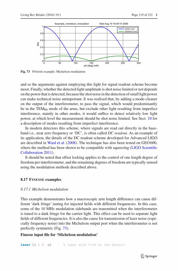
Living Rev Relativ (2016) 19:1 Page 119 of 221 1
Fig. 73 Finesse example: Michelson modulation
and so the arguments against employing this light for signal readout scheme becomemoot. Finally, whether the detected light amplitude is shot noise limited or not dependson the power that is detected, because the shot noise in the detection of small light powercan make technical noise unimportant. It was realised that, by adding a mode-cleaneron the output of the interferometer, to pass the signal, which would predominantlybe in the TEM00 mode of the arms, but exclude other light resulting from imperfectinterference, mainly in other modes, it would suffice to detect relatively low lightpower, at which level the measurement should be shot noise limited. See Sect. 10 fora description of modes resulting from imperfect interference.
In modern detectors this scheme, where signals are read out directly in the base-band i.e., near zero frequency or ‘DC’, is often called DC readout. As an example ofits application, the details of the DC readout scheme developed for Advanced LIGOare described in Ward et al. (2008). The technique has also been tested on GEO 600,where the method has been shown to be compatible with squeezing (LIGO ScientificCollaboration 2011).
It should be noted that offset locking applies to the control of one length degree offreedom per interferometer, and the remaining degrees of freedom are typically sensedusing the modulation methods described above.
8.17 FINESSE examples
8.17.1 Michelson modulation
This example demonstrates how a macroscopic arm length difference can cause dif-ferent ‘dark fringe’ tuning for injected fields with different frequencies. In this case,some of the 10 MHz modulation sidebands are transmitted when the interferometeris tuned to a dark fringe for the carrier light. This effect can be used to separate lightfields of different frequencies. It is also the cause for transmission of laser noise (espe-cially frequency noise) into the Michelson output port when the interferometer is notperfectly symmetric (Fig. 73).
Finesse input file for ‘Michelson modulation’
laser l1 1 0 n1 % laser with P=1W at the default
123
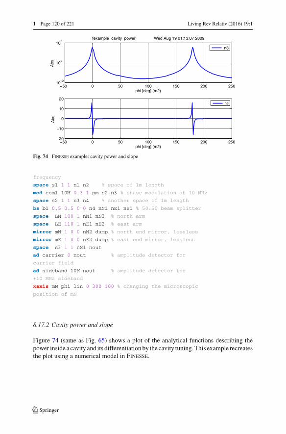
1 Page 120 of 221 Living Rev Relativ (2016) 19:1
Fig. 74 Finesse example: cavity power and slope
frequency
space s1 1 1 n1 n2 % space of 1m length
mod eom1 10M 0.3 1 pm n2 n3 % phase modulation at 10 MHz
space s2 1 1 n3 n4 % another space of 1m length
bs b1 0.5 0.5 0 0 n4 nN1 nE1 nS1 % 50:50 beam splitter
space LN 100 1 nN1 nN2 % north arm
space LE 110 1 nE1 nE2 % east arm
mirror mN 1 0 0 nN2 dump % north end mirror, lossless
mirror mE 1 0 0 nE2 dump % east end mirror, lossless
space s3 1 1 nS1 nout
ad carrier 0 nout % amplitude detector for
carrier field
ad sideband 10M nout % amplitude detector for
+10 MHz sideband
xaxis mN phi lin 0 300 100 % changing the microscopic
position of mN
8.17.2 Cavity power and slope
Figure 74 (same as Fig. 65) shows a plot of the analytical functions describing thepower inside a cavity and its differentiation by the cavity tuning. This example recreatesthe plot using a numerical model in Finesse.
123
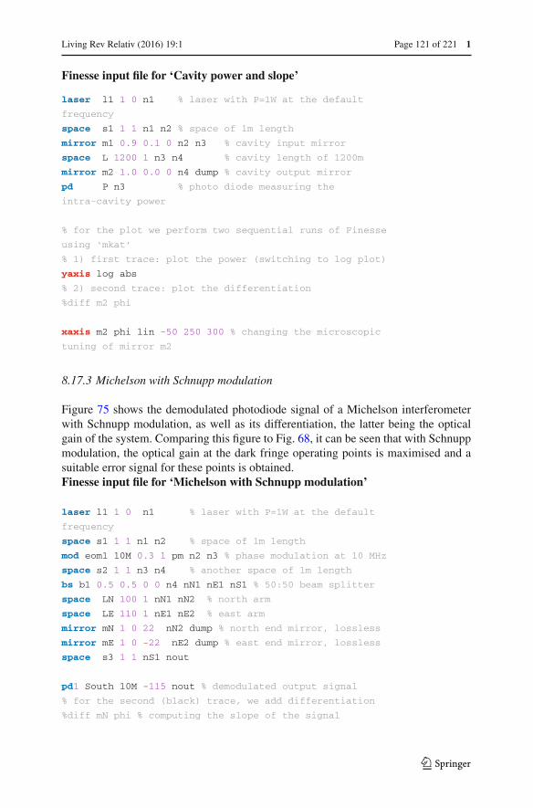
Living Rev Relativ (2016) 19:1 Page 121 of 221 1
Finesse input file for ‘Cavity power and slope’
laser l1 1 0 n1 % laser with P=1W at the default
frequency
space s1 1 1 n1 n2 % space of 1m length
mirror m1 0.9 0.1 0 n2 n3 % cavity input mirror
space L 1200 1 n3 n4 % cavity length of 1200m
mirror m2 1.0 0.0 0 n4 dump % cavity output mirror
pd P n3 % photo diode measuring the
intra-cavity power
% for the plot we perform two sequential runs of Finesse
using ‘mkat’
% 1) first trace: plot the power (switching to log plot)
yaxis log abs
% 2) second trace: plot the differentiation
%diff m2 phi
xaxis m2 phi lin -50 250 300 % changing the microscopic
tuning of mirror m2
8.17.3 Michelson with Schnupp modulation
Figure 75 shows the demodulated photodiode signal of a Michelson interferometerwith Schnupp modulation, as well as its differentiation, the latter being the opticalgain of the system. Comparing this figure to Fig. 68, it can be seen that with Schnuppmodulation, the optical gain at the dark fringe operating points is maximised and asuitable error signal for these points is obtained.Finesse input file for ‘Michelson with Schnupp modulation’
laser l1 1 0 n1 % laser with P=1W at the default
frequency
space s1 1 1 n1 n2 % space of 1m length
mod eom1 10M 0.3 1 pm n2 n3 % phase modulation at 10 MHz
space s2 1 1 n3 n4 % another space of 1m length
bs b1 0.5 0.5 0 0 n4 nN1 nE1 nS1 % 50:50 beam splitter
space LN 100 1 nN1 nN2 % north arm
space LE 110 1 nE1 nE2 % east arm
mirror mN 1 0 22 nN2 dump % north end mirror, lossless
mirror mE 1 0 -22 nE2 dump % east end mirror, lossless
space s3 1 1 nS1 nout
pd1 South 10M -115 nout % demodulated output signal
% for the second (black) trace, we add differentiation
%diff mN phi % computing the slope of the signal
123
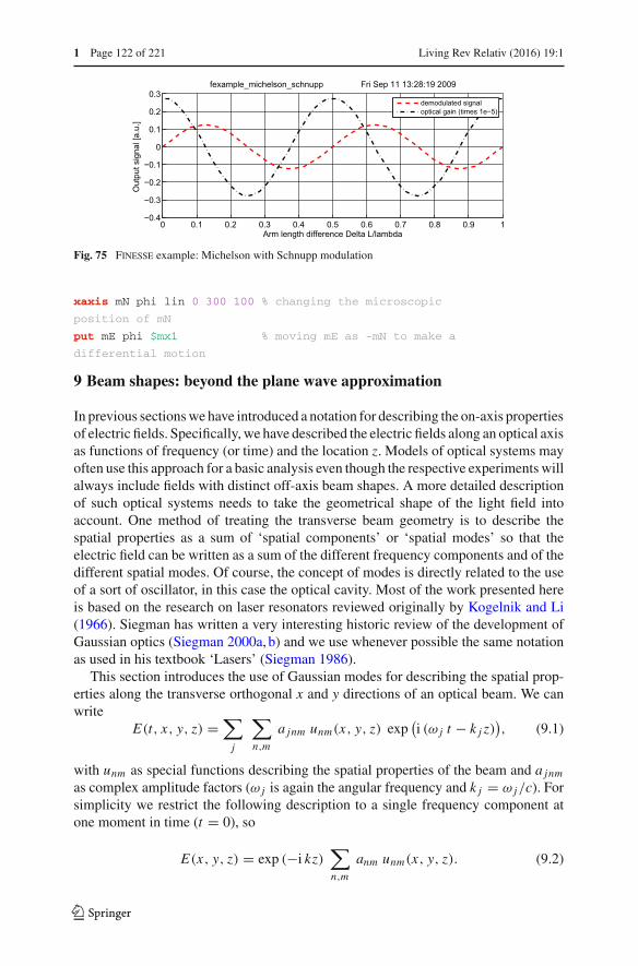
1 Page 122 of 221 Living Rev Relativ (2016) 19:1
Fig. 75 Finesse example: Michelson with Schnupp modulation
xaxis mN phi lin 0 300 100 % changing the microscopic
position of mN
put mE phi $mx1 % moving mE as -mN to make a
differential motion
9 Beam shapes: beyond the plane wave approximation
In previous sections we have introduced a notation for describing the on-axis propertiesof electric fields. Specifically, we have described the electric fields along an optical axisas functions of frequency (or time) and the location z. Models of optical systems mayoften use this approach for a basic analysis even though the respective experiments willalways include fields with distinct off-axis beam shapes. A more detailed descriptionof such optical systems needs to take the geometrical shape of the light field intoaccount. One method of treating the transverse beam geometry is to describe thespatial properties as a sum of ‘spatial components’ or ‘spatial modes’ so that theelectric field can be written as a sum of the different frequency components and of thedifferent spatial modes. Of course, the concept of modes is directly related to the useof a sort of oscillator, in this case the optical cavity. Most of the work presented hereis based on the research on laser resonators reviewed originally by Kogelnik and Li(1966). Siegman has written a very interesting historic review of the development ofGaussian optics (Siegman 2000a, b) and we use whenever possible the same notationas used in his textbook ‘Lasers’ (Siegman 1986).
This section introduces the use of Gaussian modes for describing the spatial prop-erties along the transverse orthogonal x and y directions of an optical beam. We canwrite
E(t, x, y, z) =∑j
∑n,m
a jnm unm(x, y, z) exp(i (ω j t − k j z)
), (9.1)
with unm as special functions describing the spatial properties of the beam and a jnm
as complex amplitude factors (ω j is again the angular frequency and k j = ω j/c). Forsimplicity we restrict the following description to a single frequency component atone moment in time (t = 0), so
E(x, y, z) = exp (−i kz)∑n,m
anm unm(x, y, z). (9.2)
123

Living Rev Relativ (2016) 19:1 Page 123 of 221 1
In general, different types of spatial modesunm can be used in this context. Of particularinterest are the Gaussian modes, which will be used throughout this document. Manylasers emit light that closely resembles a Gaussian beam: the light mainly propagatesalong one axis, is well collimated around that axis and the cross section of the intensityperpendicular to the optical axis shows a Gaussian distribution. The following sectionsprovide the basic mathematical framework for using Gaussian modes for analysingoptical systems.
9.1 A typical laser beam: the fundamental Gaussian mode
The beam produced from a real laser is not a plane wave, but has some intensity distri-bution. This is typically a roughly circular beam with a peak brightness near the centre.The intensity pattern of a beam generated by an ideal laser based on a stable opticalcavity with spherical mirrors would resemble a Gaussian beam. Figure 76 shows theintensity and amplitude distribution of a typical Gaussian beam, often characterisedby the beam spot size, w, the radius within which ∼86 % ( 1
e2 ) of the light power iscontained. As the beam propagates the beam spot size changes slowly, which producesa narrow beam of light with a small diffraction angle.
The use of cavities in interferometry provides the basis for the mathematical descrip-tion of laser beam shapes as Gaussian modes. A well designed cavity is a perfect opticalresonator for a particular Gaussian mode. As discussed above, the intensity distrib-ution can be characterised by the beam spot size, which determines the width of thebeam. In the case of Gaussian modes the wavefront, or phase, of the light field iscurved and can be expressed with a radius of curvature, RC . As the beam propagatesthe curvature of the wavefront changes. To achieve perfect resonance in an opticalcavity the curvature of the wavefront must match the curvature of the mirrors at theirpositions on the optical axis. The Gaussian beam whose curvatures match the mirrorsof a cavity is known as the cavity eigenmode, see Fig. 77.
9.2 Describing beam distortions with higher-order modes
In an ideal interferometer the laser beam would be a perfect Gaussian beam, withwavefronts exactly matched to the shape of the mirrors. However, in a real interfer-ometer mismatches between the beam and mirror curvatures, misalignments from theoptical axis and deviations of the mirror surfaces from a perfect sphere all contributeto distort the beam from the ideal Gaussian beam.
Small distortions of the fundamental beam can be described by the addition ofhigher-order modes. Higher-order modes have the same basic properties of the fun-damental Gaussian beam, with two exceptions: higher-order modes have differentintensity patterns from the simple spot of the fundamental mode and modes of differ-ent order pick up an extra phase upon propagation (the Gouy phase, see Sect. 9.10).
One simple example is a misaligned beam, whose centre has been shifted fromthe optical axis. This can be described by the addition of an order ‘1’ Hermite–Gaussmode, HG10 (Sect. 9.7), as illustrated in the left panel of Fig. 78. Such a distortion is afirst order effect and, as long as the misalignment is small, can be described with just
123

1 Page 124 of 221 Living Rev Relativ (2016) 19:1
Fig. 76 A typical laser beam intensity pattern (left) and the intensity and amplitude distributions of anormalised Gaussian beam (right). A Gaussian beam is characterised by its spot size, w, the radius at whichthe intensity falls to 1
e2 (∼14 %) of the peak intensity
Fig. 77 Simple depiction of acavity eigenmode. The positionand curvature of the mirrorsdetermine the cavity eigenmode,which is defined by the beamwaist size and position relativeto the mirrors
this one additional mode. In a similar way the second order effect such as a mismatchin beam size can be described by the addition of a single order ‘2’ mode, in this casethe Laguerre–Gauss mode LG10 (Sect. 9.11). A mismatch in beam size is illustratedin the right panel of Fig. 78.
The following sections describe details of Gaussian modes and how any paraxiallaser beam with distortions can be described by a sum of Gaussian modes.
9.3 The paraxial approximation
All electromagnetic waves are solutions to the general wave equation (Helmholtzequation), which in vacuum can be given as:
ΔE − 1
c2 E = 0. (9.3)
Mathematically, Gaussian modes represent solutions to the paraxial approximation ofthis equation. Laser light fields are a special class of electromagnetic waves. A laserbeam will have a characteristic size w describing the ‘width’ (the dimension of thefield transverse to the main propagation axis), and a characteristic length l definingsome local length along the propagation over which the beam characteristics do not
123
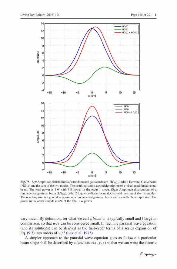
Living Rev Relativ (2016) 19:1 Page 125 of 221 1
Fig. 78 Left Amplitude distributions of a fundamental gaussian beam (HG00), order 1 Hermite–Gauss beam(HG10) and the sum of the two modes. The resulting sum is a good description of a misaligned fundamentalbeam. The total power is 1 W with 4 % power in the order 1 mode. Right Amplitude distributions of afundamental gaussian beam (LG00), order 2 Laguerre–Gauss beam (LG10) and the sum of the two modes.The resulting sum is a good description of a fundamental gaussian beam with a smaller beam spot size. Thepower in the order 2 mode is 4 % of the total 1 W power
vary much. By definition, for what we call a beam w is typically small and l large incomparison, so that w/ l can be considered small. In fact, the paraxial wave equation(and its solutions) can be derived as the first-order terms of a series expansion ofEq. (9.3) into orders of w/ l (Lax et al. 1975).
A simpler approach to the paraxial-wave equation goes as follows: a particularbeam shape shall be described by a function u(x, y, z) so that we can write the electric
123
1 Page 126 of 221 Living Rev Relativ (2016) 19:1
field asE(x, y, z) = u(x, y, z) exp (−i kz). (9.4)
Substituting this into the standard wave equation yields a differential equation for u:
(∂2x + ∂2
y + ∂2z
)u(x, y, z) − 2i k∂zu(x, y, z) = 0. (9.5)
Now we put the fact that u(x, y, z) should be slowly varying with z in mathematicalterms. The variation of u(x, y, z) with z should be small compared to its variation withx or y. Also the second partial derivative in z should be small. This can be expressedas ∣∣∣∂2
z u(x, y, z)∣∣∣ |2k∂zu(x, y, z)| ,
∣∣∣∂2x u(x, y, z)
∣∣∣ , ∣∣∣∂2y u(x, y, z)
∣∣∣ . (9.6)
With this approximation, Eq. (9.5) can be simplified to the paraxial wave equation,
(∂2x + ∂2
y
)u(x, y, z) − 2i k∂zu(x, y, z) = 0. (9.7)
Any field u that solves this equation represents a paraxial beam shape when used inthe form given in Eq. (9.4).
9.4 Transverse electromagnetic modes
In general, any solution u(x, y, z) of the paraxial wave equation, Eq. (9.7), can beemployed to represent the transverse properties of a scalar electric field representing abeam-like electro-magnetic wave. Especially useful in this respect are special familiesor sets of functions that are solutions of the paraxial wave equation. When such a setof functions is complete and countable, it is called a set of transverse electromagneticmodes (TEM). For instance, the set of Hermite–Gauss modes are exact solutions ofthe paraxial wave equation. These modes are represented by an infinite, countable andcomplete set of functions. The term complete means they can be understood as a basesystem of the function space defined by all solutions of the paraxial wave equation. Inother words, we can describe any solution of the paraxial wave equation u′ by a linearsuperposition of Hermite–Gauss modes:
u′(x, y, z) =∑n,m
a jnm unm(x, y, z), (9.8)
which in turn allows us to describe any laser beam using a sum of these modes:
E(t, x, y, z) =∑j
∑n,m
a jnm unm(x, y, z) exp(i (ω j t − k j z)
). (9.9)
123

Living Rev Relativ (2016) 19:1 Page 127 of 221 1
The Hermite–Gauss modes as given in this document (see Sect. 9.7) are orthonormalso that∫∫
dx dy unmu∗n′m′ = δnn′δmm′ =
{1 if n = n′ and m = m′0 otherwise
}. (9.10)
This means that, in the function space defined by the paraxial wave equation, theHermite–Gauss functions can be understood as a complete set of unit-length basisvectors. This fact can be utilised for the computation of coupling factors, as shown inSect. 11.3. Furthermore, the power of a beam, as given by Eq. (9.2), being detectedon a single-element photodetector (provided that the area of the detector is large withrespect to the beam) can be computed as
EE∗ =∑n,m
anma∗nm, (9.11)
or for a beam with several frequency components [compare with Eq. (4.9)] as
EE∗ =∑n,m
∑i
∑j
ainma∗jnm with {i, j | i, j ∈ {0, . . . , N } ∧ ωi = ω j }. (9.12)
9.5 Properties of Gaussian beams
The basic or ‘lowest-order’ Hermite–Gauss mode is equivalent to what is usuallycalled a Gaussian beam and is given by
u(x, y, z) =√
2
π
1
w(z)exp (i Ψ (z)) exp
(−i k
x2 + y2
2RC (z)− x2 + y2
w2(z)
). (9.13)
The parameters of this equation are explained in detail below. The shape of a Gaussianbeam is quite simple: the beam has a circular cross section, and the radial intensityprofile of a beam with total power P is given by
I (r) = 2P
πw2(z)exp
(−2r2/w2
), (9.14)
with w the spot size, defined as the radius at which the intensity is 1/e2 times themaximum intensity I (0). This is a Gaussian distribution, see Fig. 79, hence the nameGaussian beam.
Figure 80 shows a different cross section through a Gaussian beam: it plots thebeam size as a function of the position on the optical axis. Such a beam profile (for abeam with a given wavelength λ) can be completely determined by two parameters:the size of the minimum spot size w0 (called the beam waist) and the position z0 ofthe beam waist along the z-axis.
To characterise a Gaussian beam, some useful parameters can be derived from w0and z0. A Gaussian beam can be divided into two different sections along the z-axis: a
123

1 Page 128 of 221 Living Rev Relativ (2016) 19:1
Fig. 79 One dimensional cross-section of a Gaussian beam. The width of the beam is given by the radiusw at which the intensity is 1/e2 of the maximum intensity
Fig. 80 Gaussian beam profile along z: this cross section along the x–z-plane illustrates how the beam sizew(z) of the Gaussian beam changes along the optical axis. The position of minimum beam size w0 is calledbeam waist. See text for a description of the parameters �, zR and Rc
near field—a region around the beam waist, and a far field—far away from the waist.The length of the near-field region is approximately given by the Rayleigh range zR.The Rayleigh range and the spot size are related by
zR = πw20
λ. (9.15)
With the Rayleigh range and the location of the beam waist, we can usefully write
123

Living Rev Relativ (2016) 19:1 Page 129 of 221 1
w(z) = w0
√1 +
(z − z0
zR
)2
. (9.16)
This equation gives the size of the beam along the z-axis. In the far-field regime(z � zR, z0), it can be approximated by a linear equation, when
w(z) ≈ w0z
zR= zλ
πw0. (9.17)
The angle � between the z-axis and w(z) in the far field is called the diffractionangle13 and is defined by
� = arctan
(w0
zR
)= arctan
(λ
πw0
)≈ w0
zR. (9.18)
Another useful parameter is the radius of curvature of the wavefront at a givenpoint z. The radius of curvature describes the curvature of the ‘phase front’ of theelectromagnetic wave—a surface across the beam with equal phase—intersecting theoptical axis at the position z. We obtain the radius of curvature as a function of z:
RC (z) = z − z0 + z2R
z − z0. (9.19)
We also find:
RC ≈ ∞, z − z0 zR (beam waist)
RC ≈ z, z � zR, z0 (far field)
RC = 2zR, z − z0 = zR (maximum curvature).
(9.20)
9.6 Astigmatic beams: the tangential and sagittal plane
If the interferometer is confined to a plane (here the x–z plane), it is convenient to useprojections of the three-dimensional description into two planes (Rigrod 1965): thetangential plane, defined as the x–z plane and the sagittal plane as given by y and z.
The beam parameters can then be split into two respective parameters: z0,s , w0,s forthe sagittal plane and z0,t and w0,t for the tangential plane so that the Hermite–Gaussmodes can be written as
unm(x, y) = un(x, z0,t , w0,t ) um(y, z0,s, w0,s). (9.21)
Beams with different beam waist parameters for the sagittal and tangential plane areastigmatic.
13 Also known as the far-field angle or the divergence of the beam.
123
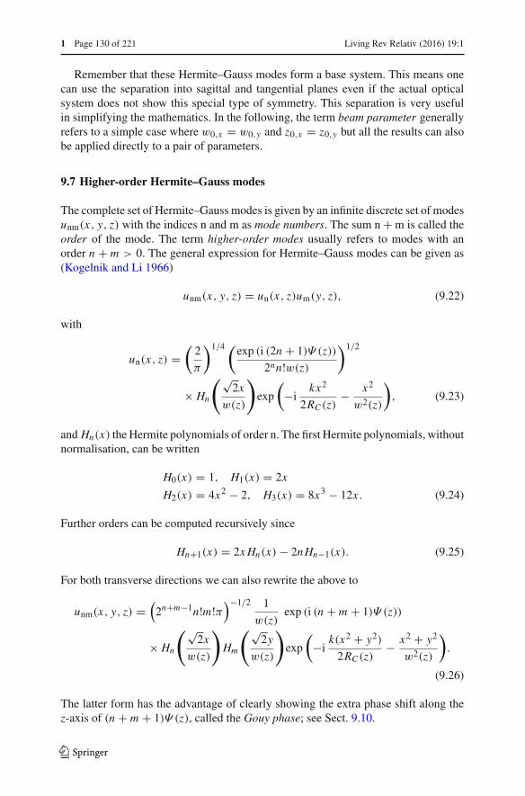
1 Page 130 of 221 Living Rev Relativ (2016) 19:1
Remember that these Hermite–Gauss modes form a base system. This means onecan use the separation into sagittal and tangential planes even if the actual opticalsystem does not show this special type of symmetry. This separation is very usefulin simplifying the mathematics. In the following, the term beam parameter generallyrefers to a simple case where w0,x = w0,y and z0,x = z0,y but all the results can alsobe applied directly to a pair of parameters.
9.7 Higher-order Hermite–Gauss modes
The complete set of Hermite–Gauss modes is given by an infinite discrete set of modesunm(x, y, z) with the indices n and m as mode numbers. The sum n + m is called theorder of the mode. The term higher-order modes usually refers to modes with anorder n + m > 0. The general expression for Hermite–Gauss modes can be given as(Kogelnik and Li 1966)
unm(x, y, z) = un(x, z)um(y, z), (9.22)
with
un(x, z) =(
2
π
)1/4 (exp (i (2n + 1)Ψ (z))
2nn!w(z)
)1/2
× Hn
(√2x
w(z)
)exp
(−i
kx2
2RC (z)− x2
w2(z)
), (9.23)
and Hn(x) the Hermite polynomials of order n. The first Hermite polynomials, withoutnormalisation, can be written
H0(x) = 1, H1(x) = 2x
H2(x) = 4x2 − 2, H3(x) = 8x3 − 12x . (9.24)
Further orders can be computed recursively since
Hn+1(x) = 2xHn(x) − 2nHn−1(x). (9.25)
For both transverse directions we can also rewrite the above to
unm(x, y, z) =(
2n+m−1n!m!π)−1/2 1
w(z)exp (i (n + m + 1)Ψ (z))
× Hn
(√2x
w(z)
)Hm
(√2y
w(z)
)exp
(−i
k(x2 + y2)
2RC (z)− x2 + y2
w2(z)
).
(9.26)
The latter form has the advantage of clearly showing the extra phase shift along thez-axis of (n + m + 1)Ψ (z), called the Gouy phase; see Sect. 9.10.
123

Living Rev Relativ (2016) 19:1 Page 131 of 221 1
9.8 The Gaussian beam parameter
For a more compact description of the interaction of Gaussian modes with opticalcomponents we will make use of the Gaussian beam parameter q (Kogelnik 1965).The beam parameter is a complex quantity defined as
1
q(z)= 1
RC (z)− i
λ
πw2(z). (9.27)
It can also be written as
q(z) = i zR + z − z0 = q0 + z − z0 and q0 = i zR. (9.28)
Using this parameter, Eq. (9.13) can be rewritten as
u(x, y, z) =√
2
π
q0
w0q(z)exp
(−i k
x2 + y2
2q(z)
). (9.29)
Other parameters, like the beam size and radius of curvature, can also be written interms of the beam parameter q:
w2(z) = λ
π
|q|2 {q} , (9.30)
w20 = {q} λ
π, (9.31)
zR = {q} (9.32)
and
RC (z) = |q|2� {q} . (9.33)
The Hermite–Gauss modes can also be written using the Gaussian beam parameteras14
unm(x, y, z) = un(x, z)um(y, z) with
un(x, z) =(
2
π
)1/4 (1
2nn!w0
)1/2 (q0
q(z)
)1/2 (q0 q∗(z)q∗
0 q(z)
)n/2
×Hn
(√2x
w(z)
)exp
(−i
kx2
2q(z)
). (9.34)
14 Please note that this formula from Siegman (1986) is very compact. Since the parameter q is a complexnumber, the expression contains at least two complex square roots. The complex square root requires adifferent algebra than the standard square root for real numbers. Especially the third and fourth factors can
not be simplified in any obvious way:(
q0q(z)
)1/2(q0q
∗(z)q∗
0 q(z)
)n/2�=
(qn+1
0 q∗n (z)
qn+1(z)q∗0n
)1/2
!
123
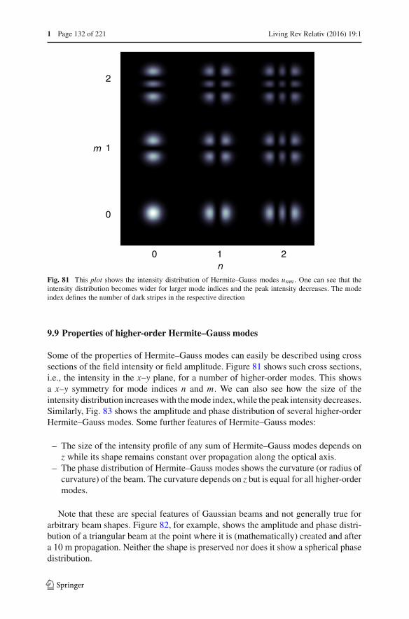
1 Page 132 of 221 Living Rev Relativ (2016) 19:1
Fig. 81 This plot shows the intensity distribution of Hermite–Gauss modes unm . One can see that theintensity distribution becomes wider for larger mode indices and the peak intensity decreases. The modeindex defines the number of dark stripes in the respective direction
9.9 Properties of higher-order Hermite–Gauss modes
Some of the properties of Hermite–Gauss modes can easily be described using crosssections of the field intensity or field amplitude. Figure 81 shows such cross sections,i.e., the intensity in the x–y plane, for a number of higher-order modes. This showsa x–y symmetry for mode indices n and m. We can also see how the size of theintensity distribution increases with the mode index, while the peak intensity decreases.Similarly, Fig. 83 shows the amplitude and phase distribution of several higher-orderHermite–Gauss modes. Some further features of Hermite–Gauss modes:
– The size of the intensity profile of any sum of Hermite–Gauss modes depends onz while its shape remains constant over propagation along the optical axis.
– The phase distribution of Hermite–Gauss modes shows the curvature (or radius ofcurvature) of the beam. The curvature depends on z but is equal for all higher-ordermodes.
Note that these are special features of Gaussian beams and not generally true forarbitrary beam shapes. Figure 82, for example, shows the amplitude and phase distri-bution of a triangular beam at the point where it is (mathematically) created and aftera 10 m propagation. Neither the shape is preserved nor does it show a spherical phasedistribution.
123
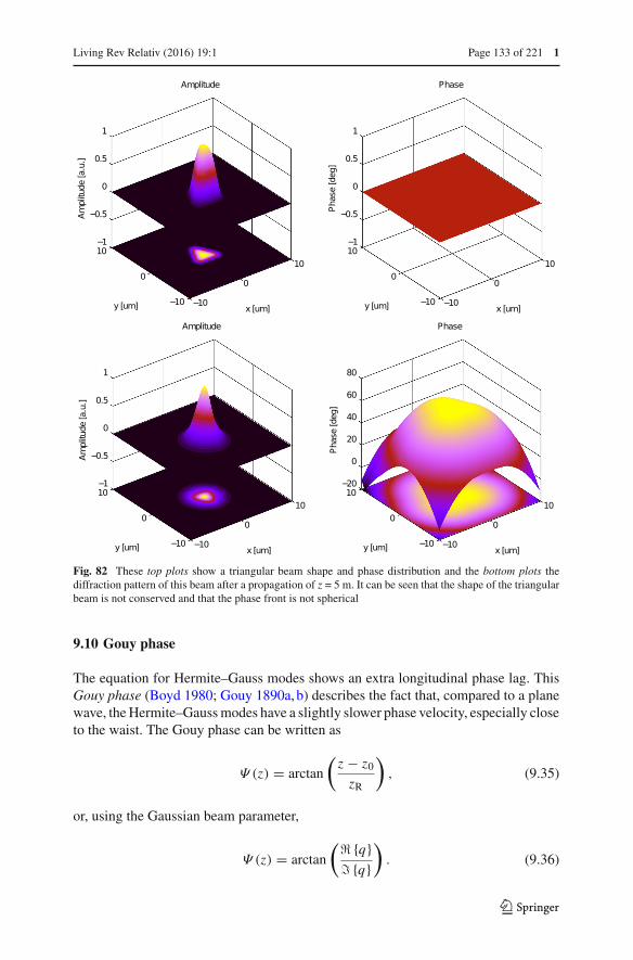
Living Rev Relativ (2016) 19:1 Page 133 of 221 1
Fig. 82 These top plots show a triangular beam shape and phase distribution and the bottom plots thediffraction pattern of this beam after a propagation of z = 5 m. It can be seen that the shape of the triangularbeam is not conserved and that the phase front is not spherical
9.10 Gouy phase
The equation for Hermite–Gauss modes shows an extra longitudinal phase lag. ThisGouy phase (Boyd 1980; Gouy 1890a, b) describes the fact that, compared to a planewave, the Hermite–Gauss modes have a slightly slower phase velocity, especially closeto the waist. The Gouy phase can be written as
Ψ (z) = arctan
(z − z0
zR
), (9.35)
or, using the Gaussian beam parameter,
Ψ (z) = arctan
(� {q} {q}
). (9.36)
123

1 Page 134 of 221 Living Rev Relativ (2016) 19:1
Compared to a plane wave, the phase lag ϕ of a Hermite–Gauss mode is
ϕ = (n + m + 1)Ψ (z). (9.37)
With an astigmatic beam, i.e., different beam parameters in the tangential and sagittalplanes, this becomes
ϕ =(n + 1
2
)Ψt (z) +
(m + 1
2
)Ψs(z), (9.38)
with
Ψt (z) = arctan
(� {qt } {qt }
), (9.39)
as the Gouy phase in the tangential plane (and Ψs is similarly defined in the sagittalplane).
9.11 Laguerre–Gauss modes
Laguerre–Gauss modes are another complete set of functions, which solve the paraxialwave equation. They are defined in cylindrical coordinates and can have advan-tages over Hermite–Gauss modes in the presence of cylindrical symmetry. Morerecently, Laguerre–Gauss modes are being investigated in a different context: using apure higher-order Laguerre–Gauss mode instead of the fundamental Gaussian beamcan significantly reduce the impact of mirror thermal noise on the sensitivity ofgravitational-wave detectors (Vinet 2009; Chelkowski et al. 2009). Laguerre–Gaussmodes are commonly given as (Siegman 1986)
u p,l(r, φ, z) = 1
w(z)
√2p!
π(|l| + p)! exp(i (2p + |l| + 1)Ψ (z))
×( √
2r
w(z)
)|l|L |l|p
(2r2
w(z)2
)exp
(−i k
r2
2q(z)+ i lφ
), (9.40)
with r, φ and z as the cylindrical coordinates around the optical axis. The letter p isthe radial mode index, l the azimuthal mode index15 and L |l|
p (x) are the associatedLaguerre polynomials:
L |l|p (x) = 1
p!p∑
j=0
p!j !
( |l| + pp − j
)(−x) j . (9.41)
All other parameters (w(z), q(z), . . .) are defined as above for the Hermite–Gaussmodes.
15 Siegman (1986) states that the indices must obey the following relations: 0 ≤ |l| ≤ p. However, that isnot the case.
123
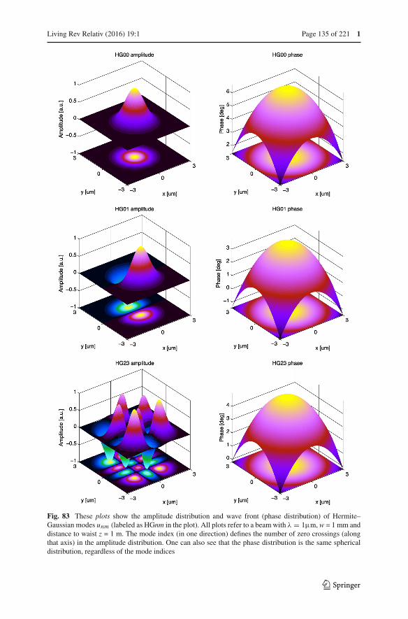
Living Rev Relativ (2016) 19:1 Page 135 of 221 1
Fig. 83 These plots show the amplitude distribution and wave front (phase distribution) of Hermite–Gaussian modes unm (labeled as HGnm in the plot). All plots refer to a beam with λ = 1µm, w = 1 mm anddistance to waist z = 1 m. The mode index (in one direction) defines the number of zero crossings (alongthat axis) in the amplitude distribution. One can also see that the phase distribution is the same sphericaldistribution, regardless of the mode indices
123
1 Page 136 of 221 Living Rev Relativ (2016) 19:1
The dependence of the Laguerre modes on φ as given in Eq. (9.40) results in aspiralling phase front, while the intensity pattern will always show unbroken concentricrings; see Fig. 84. These modes are also called helical Laguerre–Gauss modes becauseof the their special phase structure.
The reader might be more familiar with a slightly different type of Laguerre modes(compare Figs. 85 and 86) that features dark radial lines as well as dark concentricrings. Mathematically, these can be described simply by replacing the phase factorexp(i lφ) in Eq. (9.40) by a sine or cosine function. For example, an alternative set ofLaguerre–Gauss modes is given by Vinet and the Virgo Collaboration (2001)
ualtp,l(r, φ, z) = 2
w(z)
√p!
(1 + δ0lπ(|l| + p)! exp(i (2p + |l| + 1)Ψ (z))
×( √
2r
w(z)
)|l|L |l|p
(2r2
w(z)2
)exp
(−i k
r2
2q(z)
)cos(lφ). (9.42)
This type of mode has a spherical phase front, just as the Hermite–Gauss modes. Wewill refer to this set as sinusoidal Laguerre–Gauss modes throughout this document.
For the purposes of simulation it can be sometimes useful to decompose Laguerre–Gauss modes into Hermite–Gauss modes. The mathematical conversion for helicalmodes is given as (Beijersbergen et al. 1993; Abramochkin and Volostnikov 1991)
uLGp,l (x, y, z) =N∑
k=0
(−1)p(∓i )kb(|l| + p, p, k)uHGN−k,k(x, y, z), (9.43)
where ∓ is negative for positive l and positive for negative l and with real coefficients
b(n,m, k) =√
(N − k)!k!2Nn!m!
1
k! (∂t )k[(1 − t)n(1 + t)m]t=0, (9.44)
if N = 2p + |l|. The coefficients b(n,m, k) can be computed numerically by usingJacobi polynomials. Jacobi polynomials can be written in various forms:
Pα,βn (x) = (−1)n
2nn! (1 − x)−α(1 + x)−β(∂x )n(1 − x)α+n(1 + x)β+n, (9.45)
or
Pα,βn (x) = 1
2n
n∑j=0
(n + α
j
)(n + β
n − j
)(x − 1)n− j (x + 1) j , (9.46)
which leads to
b(n,m, k) =√
(N − k)!k!2Nn!m! (−2)k Pn−k,m−k
k (0). (9.47)
123

Living Rev Relativ (2016) 19:1 Page 137 of 221 1
Fig. 84 These plots show the amplitude distribution and wave front (phase distribution) of helical Laguerre–Gauss modes u pl . All plots refer to a beam with λ = 1µm, w = 1 mm and distance to waist z = 1 m
123

1 Page 138 of 221 Living Rev Relativ (2016) 19:1
Fig. 85 Intensity profiles for helical Laguerre–Gauss modes u pl . The u00 mode is identical to the Hermite–Gauss mode of order 0. Higher-order modes show a widening of the intensity and decreasing peak intensity.The number of concentric dark rings is given by the radial mode index p
Fig. 86 Intensity profiles for sinusoidal Laguerre–Gauss modes ualtpl . The u p0 modes are identical to the
helical modes. However, for azimuthal mode indices l > 0 the pattern shows l dark radial lines in additionto the p dark concentric rings
9.12 Tracing a Gaussian beam through an optical system
Whenever Gauss modes are used to analyse an optical system, the Gaussian beamparameters (or equivalent waist sizes and locations) must be defined for each locationat which field amplitudes are to be computed (or at which coupling equations areto be defined). In our experience the quality of a computation or simulation and the
123

Living Rev Relativ (2016) 19:1 Page 139 of 221 1
correctness of the results depend critically on the choice of these beam parameters.One might argue that the choice of a basis should not alter the result. This is correct,but there is a practical limitation: the number of modes having non-negligible powermight become very large if the beam parameters are not optimised, so that in practicea good set of beam parameters is usually required.
In general, the Gaussian beam parameter of a mode is changed at every opticalsurface in a well-defined way (see Sect. 9.13). Thus, a possible method of findingreasonable beam parameters for every location in the interferometer is to first set onlysome specific beam parameters at selected locations and then to derive the remainingbeam parameters from these initial ones: usually it is sensible to assume that the beamat the laser source can be properly described by the (hopefully known) beam parameterof the laser’s output mode. In addition, in most stable cavities the light fields shouldbe described by using the respective cavity eigenmodes. Then, the remaining beamparameters can be computed by tracing the beam through the optical system. ‘Trace’in this context means that a beam starting at a location with an already-known beamparameter is propagated mathematically through the optical system. At every opticalelement along the path the beam parameter is transformed according to the ABCDmatrix of the element (see below).
9.13 ABCD matrices
The transformation of the beam parameter can be performed by the ABCD matrix-formalism (Kogelnik 1965; Siegman 1986). When a beam passes an optical elementor freely propagates though space, the initial beam parameter q1 is transformed intoq2. This transformation can be described by four real coefficients as follows:
q2
n2= A q1
n1+ B
C q1n1
+ D, (9.48)
with the coefficient matrix
M =(A BC D
), (9.49)
n1 being the index of refraction at the beam segment defined by q1, and n2 the indexof refraction at the beam segment described by q2. ABCD matrices for some commonoptical components are given below, for the sagittal and tangential plane.
Transmission through a mirror
A mirror in this context is a single, partly-reflecting surface with an angle of incidenceof 90°. The transmission is described by (Fig. 87)
Fig. 87 ABCD matrix for the transmission through a surface at normal incidence
123

1 Page 140 of 221 Living Rev Relativ (2016) 19:1
with RC being the radius of curvature of the spherical surface. The sign of the radiusis defined such that RC is negative if the centre of the sphere is located in the directionof propagation. The curvature shown above (in Fig. 87), for example, is described by apositive radius. The matrix for the transmission in the opposite direction of propagationis identical.
Reflection at a mirror
The matrix for reflection is given by (Fig. 88)
Fig. 88 ABCD matrix for the reflection at a surface at normal incidence
The reflection at the back surface can be described by the same type of matrix bysetting C = 2n2/RC.
Transmission through a beam splitter
A beam splitter is understood as a single surface with an arbitrary angle of incidence α1.The matrices for transmission and reflection are different for the sagittal and tangentialplanes (Ms and Mt) (Fig. 89):
Fig. 89 ABCD matrix for the transmission through a surface with an arbitrary angle of incidence
with α2 given by Snell’s law:
n1 sin (α1) = n2 sin (α2), (9.50)
and Δn by
Δn = n2 cos (α2) − n1 cos (α1)
cos (α1) cos (α2). (9.51)
If the direction of propagation is reversed, the matrix for the sagittal plane is identicaland the matrix for the tangential plane can be obtained by changing the coefficients Aand D as follows:
A −→ 1/A,
D −→ 1/D. (9.52)
123

Living Rev Relativ (2016) 19:1 Page 141 of 221 1
Reflection at a beam splitter
The reflection at the front surface of a beam splitter is given by (Fig. 90):
Fig. 90 ABCD matrix for the reflection at a surface with an arbitrary angle of incidence
To describe a reflection at the back surface the matrices have to be changed asfollows:
RC −→ −RC,
n1 −→ n2,
α1 −→ −α2. (9.53)
Transmission through a thin lens
A thin lens transforms the beam parameter as follows (Fig. 91):
Fig. 91 ABCD matrix for a thin lens
where f is the focal length. The matrix for the opposite direction of propagation isidentical. Here it is assumed that the thin lens is surrounded by ‘spaces’ with index ofrefraction n = 1.
Transmission through a free space
As mentioned above, the beam in free space can be described by one base parameterq0. In some cases it is convenient to use a matrix similar to that used for the othercomponents to describe the z-dependency of q(z) = q0 + z. On propagation through afree space of the length L and index of refraction n, the beam parameter is transformedas follows (Fig. 92).
Fig. 92 ABCD matrix for free propagation (a ‘space’ component)
The matrix for the opposite direction of propagation is identical.
123
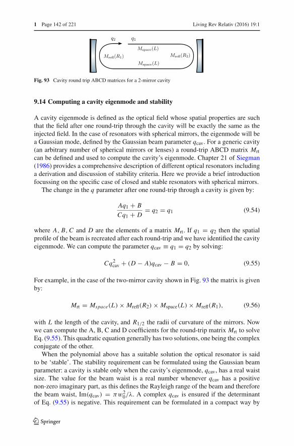
1 Page 142 of 221 Living Rev Relativ (2016) 19:1
Fig. 93 Cavity round trip ABCD matrices for a 2-mirror cavity
9.14 Computing a cavity eigenmode and stability
A cavity eigenmode is defined as the optical field whose spatial properties are suchthat the field after one round-trip through the cavity will be exactly the same as theinjected field. In the case of resonators with spherical mirrors, the eigenmode will bea Gaussian mode, defined by the Gaussian beam parameter qcav. For a generic cavity(an arbitrary number of spherical mirrors or lenses) a round-trip ABCD matrix Mrtcan be defined and used to compute the cavity’s eigenmode. Chapter 21 of Siegman(1986) provides a comprehensive description of different optical resonators includinga derivation and discussion of stability criteria. Here we provide a brief introductionfocussing on the specific case of closed and stable resonators with spherical mirrors.
The change in the q parameter after one round-trip through a cavity is given by:
Aq1 + B
Cq1 + D= q2 = q1 (9.54)
where A, B,C and D are the elements of a matrix Mrt . If q1 = q2 then the spatialprofile of the beam is recreated after each round-trip and we have identified the cavityeigenmode. We can compute the parameter qcav ≡ q1 = q2 by solving:
Cq2cav + (D − A)qcav − B = 0, (9.55)
For example, in the case of the two-mirror cavity shown in Fig. 93 the matrix is givenby:
Mrt = Mspace(L) × Mrefl(R2) × Mspace(L) × Mrefl(R1), (9.56)
with L the length of the cavity, and R1/2 the radii of curvature of the mirrors. Nowwe can compute the A, B, C and D coefficients for the round-trip matrix Mrt to solveEq. (9.55). This quadratic equation generally has two solutions, one being the complexconjugate of the other.
When the polynomial above has a suitable solution the optical resonator is saidto be ‘stable’. The stability requirement can be formulated using the Gaussian beamparameter: a cavity is stable only when the cavity’s eigenmode, qcav, has a real waistsize. The value for the beam waist is a real number whenever qcav has a positivenon-zero imaginary part, as this defines the Rayleigh range of the beam and thereforethe beam waist, Im(qcav) = πw2
0/λ. A complex qcav is ensured if the determinantof Eq. (9.55) is negative. This requirement can be formulated in a compact way by
123

Living Rev Relativ (2016) 19:1 Page 143 of 221 1
defining the parameter m as:
m ≡ A + D
2, (9.57)
where A and B are the coefficients of the round-trip matrix Mrt . The stability criterionthen simply becomes:
m2 < 1. (9.58)
The stability of simple cavities are often described using g-factors. These factorsare simply rescaled versions of the more generic m value:
g ≡ m + 1
2= A + D + 2
4, (9.59)
For the cavity to be stable the g-factor must fulfil the requirement:
0 ≤ g ≤ 1 (9.60)
The closer g is to the 0 or 1, the smaller the tolerances are for any change in thegeometry before the cavity becomes unstable.
For a simple two-mirror cavity of length L and mirror radii of curvature R1,2, itsg-factor is
g1 = 1 − L
R1, (9.61)
g2 = 1 − L
R2, (9.62)
g = g1g2. (9.63)
where g1,2 are the individual g-factors of the cavity mirrors and g is the g-factor ofthe entire cavity.
9.15 Round-trip Gouy phase and higher-order-mode separation
As discussed in Sect. 9.10, as a higher order optical mode propagates it accumulatesan additional phase, the Gouy phase, proportional to its mode order. To determinehow such a mode resonantes within an optical cavity the accumulated Gouy phaseon one round-trip through the cavity must be included. The round-trip Gouy phasewill determine which order of optical modes are resonant within a cavity. As theresonance condition of a mode is dependent on its order, this allows an optical setupto select particular orders of optical modes from an incident field. This behaviour isthe basis of mode-cleaner cavities; such as those used for the input and output lightof gravitational-wave detectors.
To compute the round-trip Gouy phase the evolution of the beam shape through thecavity must first be computed. This involves computing the round-trip ABCD matrix,MRT, as outlined in Sect. 9.14. With this matrix the round-trip Gouy phase is computed
123
1 Page 144 of 221 Living Rev Relativ (2016) 19:1
using its elements (Arai 2013):
ψRT = 2arccos
(sign(B)
√A + D + 2
4
), (9.64)
ψRT(g) = 2arccos(sign(B)
√g). (9.65)
As can be seen, the round-trip Gouy phase is linked to the cavity’s g-factor, (9.59).As the cavity approaches instability, g → 0 or 1, the phase accumulated by a modeTEMnm is then (n + m)ψRT(0) = (n + m)π/2 or (n + m)ψRT(1) = 0. In the latercase all higher order optical modes—regardless of their mode order—are resonant inthe cavity at the same time. In the former case either the odd or even mode orders areresonant at once.
The effect of the round-trip Gouy phase is often referred to as the higher ordermode separation frequency. This states how far the resonance of the next optical orderis in frequency:
δ f = ψRT
2πFSR. (9.66)
For example, the Advanced LIGO arm cavities have δ f ≈ 5 kHz.
9.16 Coupling of higher-order-modes
Now that we are able to compute the eigenmode of a particular cavity, what happens ifa beam with a slightly different eigenmode is injected into it? The aim of this sectionis to outline the problem. In reality producing a perfect Gaussian laser which matchesexactly the eigenmode of a cavity is essentially impossible, there will always be aminor difference. However we are still able to inject lasers into a cavity and producea resonance. This is because as long as the eigenmode of the incoming laser is nearlythe same, the majority of the laser light will ‘fit’ into the cavity and resonate, the restwill be reflected from it.
Let us consider a cavity with eigenmode q2 and an incident Gaussian beam witheigenmode q1. The incident beam has all of its power in the fundamental 00 mode. Fora cavity with perfectly spherical mirrors there are two possible ‘misconfigurations’that can take place:
– If the optical axes of the beam and the cavity do not overlap perfectly, the setup iscalled misaligned,
– If the beam size or shape at cavity input does not match the beam shape and sizeof the (resonant) fundamental eigenmode (q1(zcav) �= q2(zcav)), the beam is thennot mode-matched to the second cavity, i.e., there is a mode mismatch.
The coupling of a mode refers to how a spatial mode in one basis is represented inanother; e.g., which sum of modes in the cavity basis q2 produces the HG00 mode in theq1 basis. Hermite–Gauss modes are coupled whenever a beam is not matched or alignedto a cavity or beam segment. This coupling is sometimes referred to as scattering intohigher-order modes because in most cases the laser beam is a considered as a pure
123

Living Rev Relativ (2016) 19:1 Page 145 of 221 1
HG00 mode and any mode coupling would transfer power from the fundamental intohigher-order modes. However, in general every mode with non-zero power will transferenergy into other modes whenever mismatch or misalignment occur, and this effectalso includes the transfer from higher orders into a low order.
To compute the amount of coupling the beam must be projected into the basesystem of the cavity or beam segment it is being injected into. This is always possible,provided that the paraxial approximation holds, because each set of Hermite–Gaussmodes, defined by the beam parameter at a position z, forms a complete set. Such achange of the basis system results in a different distribution of light power in the newHermite–Gauss modes and can be expressed by coupling coefficients that yield thechange in the light amplitude and phase with respect to mode number.
Let us assume that a beam described by the beam parameter q1 is injected into asegment described by the parameter q2. Let the optical axis of the beam be misaligned:the coordinate system of the beam is given by (x, y, z) and the beam travels along thez-axis. The beam segment is parallel to the z′-axis and the coordinate system (x ′, y′, z′)is given by rotating the (x, y, z) system around the y-axis by the misalignment angleγ . The amplitude of a particular mode TEMnm in the beam segment is then definedas:
unm(x, y; q2) exp(
i (ωt − kz))
=∑n′,m′
kn,m,n′,m′un′m′(x, y; q1) exp(
i (ωt − kz′)),
(9.67)where un′m′(x, y; q1) are the Hermite–Gauss modes used to describe the injectedbeam, unm(x, y; q2) are the ‘new’ modes that are used to describe the light in the beamsegment and kn,m,n′,m′ is the coupling coefficient from each TEMn′m′ into TEMnm.Note that including the plane wave phase propagation within the definition of couplingcoefficients is important because it results in coupling coefficients that are independentof the position on the optical axis for which the coupling coefficients are computed.
Using the fact that the Hermite–Gauss modes unm are orthonormal, we can computethe coupling coefficients by the overlap integral (Bayer-Helms 1984):
kn,m,n′,m′ = exp(
i 2kz′ sin2(γ
2
)) ∫∫dx ′ dy′ un′m′ exp
(i kx ′ sin γ
)u∗nm . (9.68)
Since the Hermite–Gauss modes can be separated with respect to x and y, the couplingcoefficients can also be split into knmn′m′ = knn′kmm′ . These equations are very usefulin the paraxial approximation as the coupling coefficients decrease with large modenumbers. In order to be described as paraxial, the angle γ must not be larger than thediffraction angle. In addition, to obtain correct results with a finite number of modesthe beam parameters q1 and q2 must not differ too much.
The integral 9.68 can be computed directly using numerical integration methods.However, this can potentially be computationally very expensive depending on howdifficult the integrand is to evaluate and complex it. The following part of this sectionis based on the work of Bayer-Helms (1984) and provides an analytic solution to theintegral. Another description of coupling coefficients and their derivation can be foundin the work of Vinet and the Virgo Collaboration (2001). In Bayer-Helms (1984) the
123

1 Page 146 of 221 Living Rev Relativ (2016) 19:1
above integral is partly solved and the coupling coefficients are given by multiple sumsas functions of γ and the mode mismatch parameter K , which is defined by
K = 1
2(K0 + i K2), (9.69)
where K0 = (zR − z′R)/z′R and K2 = ((z − z0) − (z′ − z′0))/z′R . This can also bewritten using q = i zR + z − z0, as
K = i (q − q ′)∗
2 {q ′} . (9.70)
The coupling coefficients for misalignment and mismatch (but no lateral displace-ment) can then be written as
knn′ = (−1)n′E (x)(n!n′!)1/2(1 + K0)
n/2+1/4(1 + K ∗)−(n+n′+1)/2 {Sg − Su
},
(9.71)where
Sg =[n/2]∑μ=0
[n′/2]∑μ′=0
(−1)μ Xn−2μXn′−2μ′(n−2μ)!(n′−2μ′)!
min(μ,μ′)∑σ=0
(−1)σ Fμ−σ Fμ′−σ
(2σ)!(μ−σ)!(μ′−σ)! ,
Su =[(n−1)/2]∑
μ=0
[(n′−1)/2]∑μ′=0
(−1)μ Xn−2μ−1Xn′−2μ′−1
(n−2μ−1)!(n′−2μ′−1)!min(μ,μ′)∑
σ=0
(−1)σ Fμ−σ Fμ′−σ
(2σ+1)!(μ−σ)!(μ′−σ)! .
(9.72)
The corresponding formula for kmm′ can be obtained by replacing the following para-meters: n → m, n′ → m′, X, X → 0 and E (x) → 1 (see below). The notation [n/2]means [m
2
]=
{m/2 if m is even,(m − 1)/2 if m is odd.
(9.73)
The other abbreviations used in the above definition are
X = (i z′R − z′) sin (γ )/(√
1 + K ∗w0),
X = (i zR + z′) sin (γ )/(√
1 + K ∗w0),
F = K/(2(1 + K0)),
F = K ∗/2,
E (x) = exp(− X X
2
).
(9.74)
In general, the Gaussian beam parameter might be different for the sagittal andtangential planes and a misalignment can be given for both possible axes (around they-axis and around the x-axis), in this case the coupling coefficients are given by
knmm′n′ = knn′kmm′ , (9.75)
123
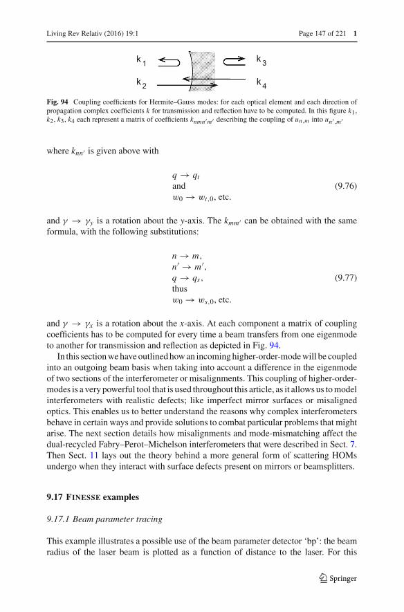
Living Rev Relativ (2016) 19:1 Page 147 of 221 1
Fig. 94 Coupling coefficients for Hermite–Gauss modes: for each optical element and each direction ofpropagation complex coefficients k for transmission and reflection have to be computed. In this figure k1,k2, k3, k4 each represent a matrix of coefficients knmn′m′ describing the coupling of un,m into un′,m′
where knn′ is given above with
q → qtandw0 → wt,0, etc.
(9.76)
and γ → γy is a rotation about the y-axis. The kmm′ can be obtained with the sameformula, with the following substitutions:
n → m,
n′ → m′,q → qs,thusw0 → ws,0, etc.
(9.77)
and γ → γx is a rotation about the x-axis. At each component a matrix of couplingcoefficients has to be computed for every time a beam transfers from one eigenmodeto another for transmission and reflection as depicted in Fig. 94.
In this section we have outlined how an incoming higher-order-mode will be coupledinto an outgoing beam basis when taking into account a difference in the eigenmodeof two sections of the interferometer or misalignments. This coupling of higher-order-modes is a very powerful tool that is used throughout this article, as it allows us to modelinterferometers with realistic defects; like imperfect mirror surfaces or misalignedoptics. This enables us to better understand the reasons why complex interferometersbehave in certain ways and provide solutions to combat particular problems that mightarise. The next section details how misalignments and mode-mismatching affect thedual-recycled Fabry–Perot–Michelson interferometers that were described in Sect. 7.Then Sect. 11 lays out the theory behind a more general form of scattering HOMsundergo when they interact with surface defects present on mirrors or beamsplitters.
9.17 FINESSE examples
9.17.1 Beam parameter tracing
This example illustrates a possible use of the beam parameter detector ‘bp’: the beamradius of the laser beam is plotted as a function of distance to the laser. For this
123

1 Page 148 of 221 Living Rev Relativ (2016) 19:1
Fig. 95 Finesse example: beam parameter tracing
Fig. 96 Finesse example: telescope and Gouy phase. The blue trace shows the Gouy phase accumulatedin the telescope, the green trace the beam spot size at the end of the telescope. The change on the x-axisrepresents a position tuning of the lens ‘L2’
simulation, the interferometer matrix does not need to be solved. ‘bp’ merely returnsthe results from the beam tracing algorithm of Finesse (Fig. 95).
Finesse input file for ‘Beam parameter tracing’
laser i1 1 0 n1 % laser with P=1W
gauss g1 i1 n1 1m -2 % a dummy beam parameter
maxtem 0 % we need only the u_00 mode
s s1 1 n1 n2 % a space of 1m length
bp width x w n2 % detecting the beam width (horizontal)
xaxis s1 L lin 0.1 8 200 % tuning the length of s1
9.17.2 Telescope and Gouy phase
This example shows the fine tuning of a telescope. The optical setup is similar tothe optical layout on the Virgo North-end detection bench, resembling the telescopefor the beam transmitted by the end mirror of one arm. The telescope consists of foursequential lenses with the purpose of reducing the beam size and provide a user defined
123

Living Rev Relativ (2016) 19:1 Page 149 of 221 1
Gouy phase for a split photo detector which is used for the alignment sensing system(Fig. 96).
Finesse input file for ‘Telescope and Gouy phase’l i1 6 0 0 nin
gauss g1 i1 nin 0.014852735 -2.2462888k
# multi-lens telescope, similar to the Virgo north end
detection
s sN2 1.77 nin nL1
lens L1 1.02 nL1 nL2
s sN3 .8996 nL2 nL3
lens L2 -.2 nL3 nL4
s sN4 .2146 nL4 nL5
lens L3 -.1 nL5 nL6
s sN5 .608 nL6 nL12
lens L4a -.1 nL12 nL13
s sN8 .759 nL13 nQ71
# Plot Gouy phase from through the entire telescope
gouy gn1 x sN2 sN3 sN4 sN5
# Plot beam size at end of telescope
bp w1 x w nQ71
# Tuning the position of lens L2 by changing the
lengths of
# the spaces in front and behind the lens.
xaxis* sN3 L lin -1m 1m 400
func sN4L = 1.1142 - $x1
noplot sN4L
put sN4 L $sN4L
9.17.3 LG33 mode
Finesse uses the Hermite–Gauss modes as a base system for describing the spatialproperties of laser beams. However, Laguerre–Gauss modes can be created using thecoefficients given in Eq. (9.43). This example demonstrates this and the use of a ‘beam’detector to plot amplitude and phase of a beam cross section (Fig. 97).
Finesse input file for ‘LG33 mode’
laser i1 1 0 n1 % laser with P=1W
gauss g1 i1 n1 1m 0 % a dummy beam parameter
maxtem 9 % we need modes up to n+m=9
tem i1 0 0 0 0 % HG coefficients to create LG33 mode
tem i1 9 0 0.164063 0
tem i1 8 1 0.164063 -90
tem i1 7 2 0 0
tem i1 6 3 0.125 -90
123

1 Page 150 of 221 Living Rev Relativ (2016) 19:1
Fig. 97 Finesse example: LG33 mode. The ring structure in the phase plot is due to phase jumps, whichcould be removed by applying a phase ‘unwrap’
tem i1 5 4 0.046875 180
tem i1 4 5 0.046875 -90
tem i1 3 6 0.125 180
tem i1 2 7 0 0
tem i1 1 8 0.164063 180
tem i1 0 9 0.164063 90
s s1 1 n1 n2 % space of 1m length
beam ccd 0 n2 % beam detector for carrier light
xaxis ccd x lin -5 5 200 % tune x position of beam
detector
x2axis ccd y lin -5 5 200 % tune y position of beam
detector
yaxis abs:deg % plot amplitude and phase
multi
10 Imperfect interferometers
Imperfections in a Michelson interferometer can refer to any of the differences betweena real interferometer and the perfect design. These include, but are not limited to: devi-ations of the optical properties of the mirrors from the design; the limits of longitudinaland alignment control of the mirrors; additional noise sources not included in our mod-els (i.e., electronic noise); and effects which distort the shape of the beam. To estimatethe impact of such imperfections on the Michelson’s performance is complicatedand requires substantial modelling. The greatest impact on the sensitivity arises fromasymmetries between the two arms. For accurate differential measurements, such asthose made in gravitational wave interferometers, the mirrors are very carefully man-ufactured to make the arms as similar as possible. Differences between the two arms,for example, imbalances in the finesse of the two arm cavities, will couple extra light
123
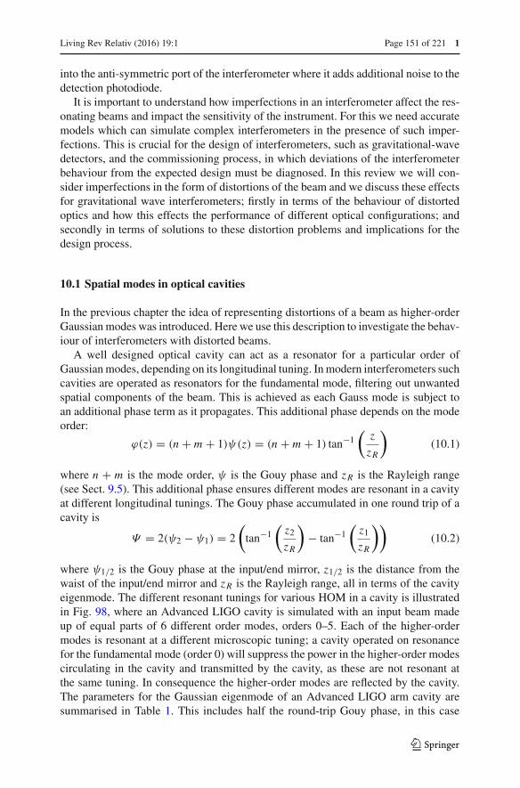
Living Rev Relativ (2016) 19:1 Page 151 of 221 1
into the anti-symmetric port of the interferometer where it adds additional noise to thedetection photodiode.
It is important to understand how imperfections in an interferometer affect the res-onating beams and impact the sensitivity of the instrument. For this we need accuratemodels which can simulate complex interferometers in the presence of such imper-fections. This is crucial for the design of interferometers, such as gravitational-wavedetectors, and the commissioning process, in which deviations of the interferometerbehaviour from the expected design must be diagnosed. In this review we will con-sider imperfections in the form of distortions of the beam and we discuss these effectsfor gravitational wave interferometers; firstly in terms of the behaviour of distortedoptics and how this effects the performance of different optical configurations; andsecondly in terms of solutions to these distortion problems and implications for thedesign process.
10.1 Spatial modes in optical cavities
In the previous chapter the idea of representing distortions of a beam as higher-orderGaussian modes was introduced. Here we use this description to investigate the behav-iour of interferometers with distorted beams.
A well designed optical cavity can act as a resonator for a particular order ofGaussian modes, depending on its longitudinal tuning. In modern interferometers suchcavities are operated as resonators for the fundamental mode, filtering out unwantedspatial components of the beam. This is achieved as each Gauss mode is subject toan additional phase term as it propagates. This additional phase depends on the modeorder:
ϕ(z) = (n + m + 1)ψ(z) = (n + m + 1) tan−1(
z
zR
)(10.1)
where n + m is the mode order, ψ is the Gouy phase and zR is the Rayleigh range(see Sect. 9.5). This additional phase ensures different modes are resonant in a cavityat different longitudinal tunings. The Gouy phase accumulated in one round trip of acavity is
Ψ = 2(ψ2 − ψ1) = 2
(tan−1
(z2
zR
)− tan−1
(z1
zR
))(10.2)
where ψ1/2 is the Gouy phase at the input/end mirror, z1/2 is the distance from thewaist of the input/end mirror and zR is the Rayleigh range, all in terms of the cavityeigenmode. The different resonant tunings for various HOM in a cavity is illustratedin Fig. 98, where an Advanced LIGO cavity is simulated with an input beam madeup of equal parts of 6 different order modes, orders 0–5. Each of the higher-ordermodes is resonant at a different microscopic tuning; a cavity operated on resonancefor the fundamental mode (order 0) will suppress the power in the higher-order modescirculating in the cavity and transmitted by the cavity, as these are not resonant atthe same tuning. In consequence the higher-order modes are reflected by the cavity.The parameters for the Gaussian eigenmode of an Advanced LIGO arm cavity aresummarised in Table 1. This includes half the round-trip Gouy phase, in this case
123
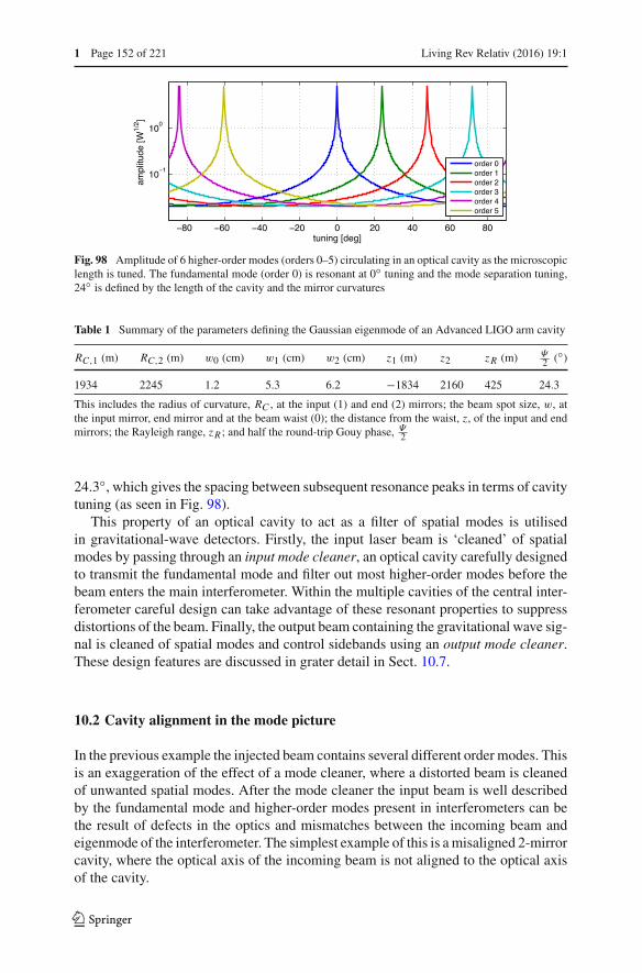
1 Page 152 of 221 Living Rev Relativ (2016) 19:1
Fig. 98 Amplitude of 6 higher-order modes (orders 0–5) circulating in an optical cavity as the microscopiclength is tuned. The fundamental mode (order 0) is resonant at 0◦ tuning and the mode separation tuning,24◦ is defined by the length of the cavity and the mirror curvatures
Table 1 Summary of the parameters defining the Gaussian eigenmode of an Advanced LIGO arm cavity
RC,1 (m) RC,2 (m) w0 (cm) w1 (cm) w2 (cm) z1 (m) z2 zR (m) Ψ2 (◦)
1934 2245 1.2 5.3 6.2 −1834 2160 425 24.3
This includes the radius of curvature, RC , at the input (1) and end (2) mirrors; the beam spot size, w, atthe input mirror, end mirror and at the beam waist (0); the distance from the waist, z, of the input and endmirrors; the Rayleigh range, zR ; and half the round-trip Gouy phase, Ψ
2
24.3◦, which gives the spacing between subsequent resonance peaks in terms of cavitytuning (as seen in Fig. 98).
This property of an optical cavity to act as a filter of spatial modes is utilisedin gravitational-wave detectors. Firstly, the input laser beam is ‘cleaned’ of spatialmodes by passing through an input mode cleaner, an optical cavity carefully designedto transmit the fundamental mode and filter out most higher-order modes before thebeam enters the main interferometer. Within the multiple cavities of the central inter-ferometer careful design can take advantage of these resonant properties to suppressdistortions of the beam. Finally, the output beam containing the gravitational wave sig-nal is cleaned of spatial modes and control sidebands using an output mode cleaner.These design features are discussed in grater detail in Sect. 10.7.
10.2 Cavity alignment in the mode picture
In the previous example the injected beam contains several different order modes. Thisis an exaggeration of the effect of a mode cleaner, where a distorted beam is cleanedof unwanted spatial modes. After the mode cleaner the input beam is well describedby the fundamental mode and higher-order modes present in interferometers can bethe result of defects in the optics and mismatches between the incoming beam andeigenmode of the interferometer. The simplest example of this is a misaligned 2-mirrorcavity, where the optical axis of the incoming beam is not aligned to the optical axisof the cavity.
123
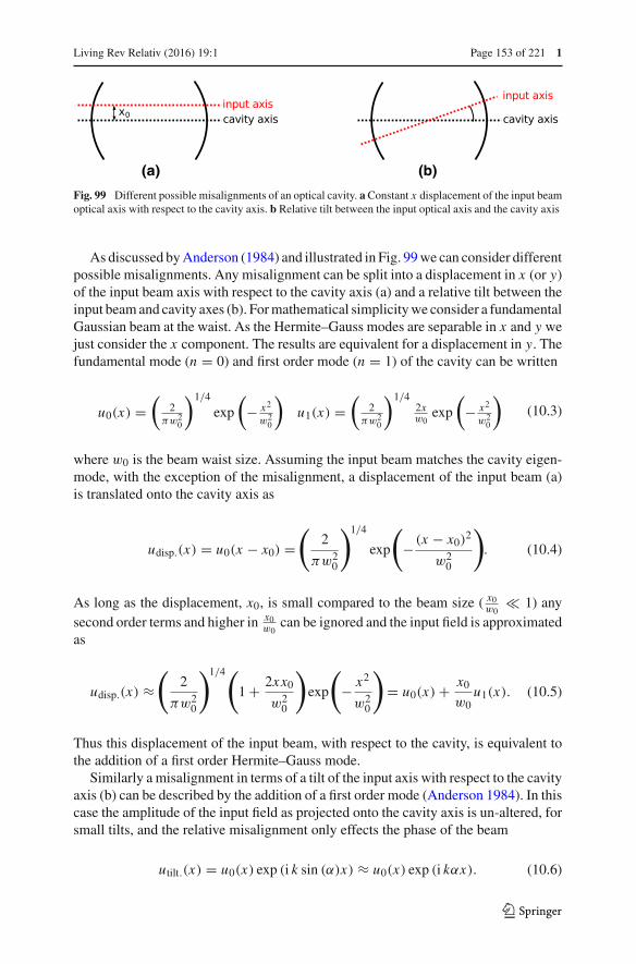
Living Rev Relativ (2016) 19:1 Page 153 of 221 1
(a) (b)
Fig. 99 Different possible misalignments of an optical cavity. a Constant x displacement of the input beamoptical axis with respect to the cavity axis. b Relative tilt between the input optical axis and the cavity axis
As discussed by Anderson (1984) and illustrated in Fig. 99 we can consider differentpossible misalignments. Any misalignment can be split into a displacement in x (or y)of the input beam axis with respect to the cavity axis (a) and a relative tilt between theinput beam and cavity axes (b). For mathematical simplicity we consider a fundamentalGaussian beam at the waist. As the Hermite–Gauss modes are separable in x and y wejust consider the x component. The results are equivalent for a displacement in y. Thefundamental mode (n = 0) and first order mode (n = 1) of the cavity can be written
u0(x) =(
2πw2
0
)1/4
exp
(− x2
w20
)u1(x) =
(2
πw20
)1/42xw0
exp
(− x2
w20
)(10.3)
where w0 is the beam waist size. Assuming the input beam matches the cavity eigen-mode, with the exception of the misalignment, a displacement of the input beam (a)is translated onto the cavity axis as
udisp.(x) = u0(x − x0) =(
2
πw20
)1/4
exp
(− (x − x0)
2
w20
). (10.4)
As long as the displacement, x0, is small compared to the beam size ( x0w0
1) anysecond order terms and higher in x0
w0can be ignored and the input field is approximated
as
udisp.(x) ≈(
2
πw20
)1/4 (1 + 2xx0
w20
)exp
(− x2
w20
)= u0(x) + x0
w0u1(x). (10.5)
Thus this displacement of the input beam, with respect to the cavity, is equivalent tothe addition of a first order Hermite–Gauss mode.
Similarly a misalignment in terms of a tilt of the input axis with respect to the cavityaxis (b) can be described by the addition of a first order mode (Anderson 1984). In thiscase the amplitude of the input field as projected onto the cavity axis is un-altered, forsmall tilts, and the relative misalignment only effects the phase of the beam
utilt.(x) = u0(x) exp (i k sin (α)x) ≈ u0(x) exp (i kαx). (10.6)
123

1 Page 154 of 221 Living Rev Relativ (2016) 19:1
For a small misalignment the higher-order terms of the exponential are ignored:
utilt.(x) ≈ u0(x) (1 + i kαx) = u0(x) + ikαw0
2u1(x). (10.7)
The relative tilt of the input beam is expressed with the addition of an order 1 mode,90◦ out of phase with the fundamental mode. This 90◦ phase factor is a useful featurewhich can be used to separate the order 1 modes caused by a displacement of theoptical axis and those caused by a tilt of the optical axis. A combination of these twotypes of misalignment can describe any misaligned cavity (providing the misalignmentis small).
The consequence of a misalignment of an optical cavity is the creation of first ordermodes. If we chose to describe the problem using the Gaussian beam parameters andaxis of the incoming beam as our basis, then the incoming beam is a pure fundamentalbeam and the first order modes are created when the light enters (and leaves) the cavity.Alternatively we can use the cavity eigenmode and cavity axis as our basis. In thiscase the higher-order modes are already present in the incoming beam. Either of theseapproaches is valid for such a simple distortion.
In more realistic cases the circulating field in a cavity is not completely described bya fundamental Gaussian beam, due to deviations of real mirrors from an ideal sphere.This can be modelled using the closest Gaussian eigenmode (from now on referred toas the eigenmode of the cavity) superimposed with higher-order modes. One can saythat the higher-order modes are created when the fundamental mode interacts with thedistorted mirrors.
To describe the input–output relations of a cavity for higher-order modes it isimportant to know at which location they have been created, in other words wherethey enter the cavity. For higher-order modes present in the input beam (not createdinside the cavity) the amplitude of these modes in the circulating field is given by:
acirc.n,m = i r2t1 exp (−i 2kL + i (1 + n + m)Ψ )
1 − r1r2 exp (−i 2kL + i (1 + n + m)Ψ )ainn,m, (10.8)
where ainn,m is the amplitude of the HOM in the incoming field. The equation is very
similar to that for a plane wave [Eq. (2.3)] with the addition of the Gouy phase pickedup for different modes. On the usual operating point of resonance for the fundamentalmode this simplifies to:
acirc.n,m = i r2t1 exp (i (n + m)Ψ )
1 − r1r2 exp (i (n + m)Ψ )ainn,m . (10.9)
A well designed cavity will have (n+m)Ψ �= N2π up to a high mode order to preventother modes resonating. In the case where we consider higher-order modes createdat individual mirrors, the equations are different. If the modes are created at the endmirror, with no higher-order modes present in the input beam, the circulating field isapproximated as:
123

Living Rev Relativ (2016) 19:1 Page 155 of 221 1
Fig. 100 Circulating power in an Advanced LIGO cavity with a 0.3µrad misalignment applied to the endmirror. The cavity is tuned and the circulating beam is detected for each peak in intra-cavity power. Mostof the power remains in the fundamental mode, resonant at ∼0◦, with some coupling into HG10, resonantat ∼24◦, and HG20, resonant at ∼50◦
acirc.n,m ≈ i r2t1 exp
(i (n + m)Ψ
2
)(1 − r1r2)(1 − r1r2 exp (i (n + m)Ψ ))
k0,0,n,m ain0,0, (10.10)
where k0,0,n,m is a coupling coefficient describing the phase and amplitude of the modeHGnm created at the end mirror, due to an incident HG00 mode. The approximationhere assumes the coupling is small and so does not include the loss of power from theHG00 mode and coupling from the HGnm mode back into HG00. This approximationis valid for small distortions, but including distortions on all the optics will quicklybecome very complicated analytically, and it is for such problems that simulation toolssuch as Finesse are valuable.
In Fig. 100 the effects of misalignment on intra-cavity power is illustrated. In thisexample an Advanced LIGO cavity has been modelled with a misaligned end mirror.The circulating power exhibits several peaks, corresponding to the resonances of thedifferent higher-order modes created due to the misalignment. Most of the powerremains in the fundamental mode (peak at ∼0◦). The misalignment of the cavity hasinduced higher-order modes, mostly the first order HG10 mode, whose resonance isobserved at ∼24◦. In this case the extent of the misalignment also results in the creationof the order 2 mode HG20, resonant at ∼50◦. During operation, where the cavity is onresonance for the HG00 mode, the relative power in higher-order modes is suppressed.There will still be some higher-order modes in the beam at this tuning, which degradethe purity of the beam transmitted and reflected from the cavity.
10.3 Mode mismatch
Another common defect of optical cavities with respect to an input laser beam isknown as mode mismatch (Mueller et al. 2000). Whilst (a small) misalignment is afirst order effect described by first order modes, a (small) mode mismatch is a secondorder effect, where the wavefront curvature or beam size of the incoming beam does
123
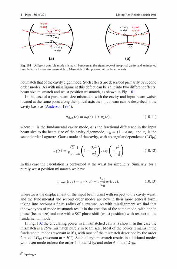
1 Page 156 of 221 Living Rev Relativ (2016) 19:1
(a) (b)
Fig. 101 Different possible mode mismatch between an the eigenmode of an optical cavity and an injectedlaser beam. a Beam size mismatch. b Mismatch of the position of the beam waists
not match that of the cavity eigenmode. Such effects are described primarily by secondorder modes. As with misalignment this defect can be split into two different effects:beam size mismatch and waist position mismatch, as shown in Fig. 101.
In the case of a pure beam size mismatch, with the cavity and input beam waistslocated at the same point along the optical axis the input beam can be described in thecavity basis as (Anderson 1984):
usize.(r) = u0(r) + ε u2(r), (10.11)
where u0 is the fundamental cavity mode, ε is the fractional difference in the inputbeam size to the beam size of the cavity eigenmode, w′
0 = (1 + ε)w0, and u2 is thesecond order Laguerre–Gauss mode of the cavity, with no angular dependence (LG10)
u2(r) =√
2
π
1
w0
(1 − 2r2
w20
). exp
(− r2
w20
)(10.12)
In this case the calculation is performed at the waist for simplicity. Similarly, for apurely waist position mismatch we have
uposit.(r, z) = u0(r, z) + ikz0
w20
u2(r, z), (10.13)
where z0 is the displacement of the input beam waist with respect to the cavity waist,and the fundamental and second order modes are now in their more general form,taking into account a finite radius of curvature. As with misalignment we find thatthe two types of mode mismatch result in the creation of the same mode, with one inphase (beam size) and one with a 90◦ phase shift (waist position) with respect to thefundamental mode.
In Fig. 102 the circulating power in a mismatched cavity is shown. In this case themismatch is a 25 % mismatch purely in beam size. Most of the power remains in thefundamental mode (resonant at 0◦), with most of the mismatch described by the order2 mode LG10 (resonant at ∼50◦). Such a large mismatch results in additional modeswith even mode orders: the order 4 mode LG20 and order 6 mode LG30.
123
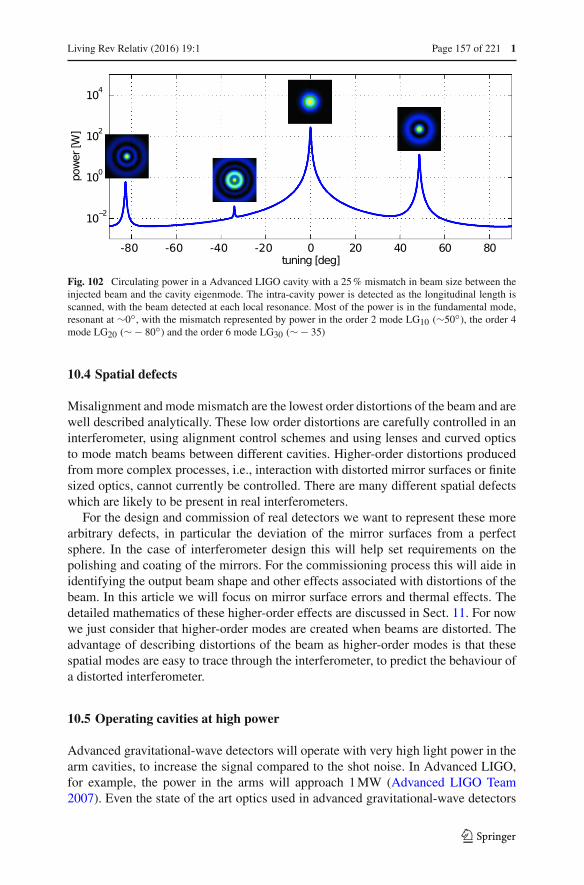
Living Rev Relativ (2016) 19:1 Page 157 of 221 1
Fig. 102 Circulating power in a Advanced LIGO cavity with a 25 % mismatch in beam size between theinjected beam and the cavity eigenmode. The intra-cavity power is detected as the longitudinal length isscanned, with the beam detected at each local resonance. Most of the power is in the fundamental mode,resonant at ∼0◦, with the mismatch represented by power in the order 2 mode LG10 (∼50◦), the order 4mode LG20 (∼ − 80◦) and the order 6 mode LG30 (∼ − 35)
10.4 Spatial defects
Misalignment and mode mismatch are the lowest order distortions of the beam and arewell described analytically. These low order distortions are carefully controlled in aninterferometer, using alignment control schemes and using lenses and curved opticsto mode match beams between different cavities. Higher-order distortions producedfrom more complex processes, i.e., interaction with distorted mirror surfaces or finitesized optics, cannot currently be controlled. There are many different spatial defectswhich are likely to be present in real interferometers.
For the design and commission of real detectors we want to represent these morearbitrary defects, in particular the deviation of the mirror surfaces from a perfectsphere. In the case of interferometer design this will help set requirements on thepolishing and coating of the mirrors. For the commissioning process this will aide inidentifying the output beam shape and other effects associated with distortions of thebeam. In this article we will focus on mirror surface errors and thermal effects. Thedetailed mathematics of these higher-order effects are discussed in Sect. 11. For nowwe just consider that higher-order modes are created when beams are distorted. Theadvantage of describing distortions of the beam as higher-order modes is that thesespatial modes are easy to trace through the interferometer, to predict the behaviour ofa distorted interferometer.
10.5 Operating cavities at high power
Advanced gravitational-wave detectors will operate with very high light power in thearm cavities, to increase the signal compared to the shot noise. In Advanced LIGO,for example, the power in the arms will approach 1 MW (Advanced LIGO Team2007). Even the state of the art optics used in advanced gravitational-wave detectors
123

1 Page 158 of 221 Living Rev Relativ (2016) 19:1
will absorb a proportion of the incident power. The mirrors produced for AdvancedLIGO have requirements of <0.5 parts-per-million (ppm) power absorption. With theexpected power in the arms this means ∼0.5 W will be absorbed in the mirror coatingsand substrates. During operation this absorption of power will lead to a temperaturegradient evolving in the optics, starting from a cold state defined by the temperatureof the environment and gradually developing a temperature field across the optic, witha hot point at the centre where the beam is most intense. Finally the temperature fieldof the mirrors will reach a steady state, where the optic is in thermal equilibrium. Thedevelopment of such temperature gradients in the mirrors will result in two types ofmirror aberration:
1. A thermal lens forms within the mirror due to the temperature dependent natureof the index of refraction of the substrate material (fused silica). This distortioncan be described mostly as a spherical lens, with some higher-order components(Hello and Vinet 1990; Vinet and the Virgo Collaboration 2001).
2. The mirror expands thermally, with the expansion greatest where the mirror ishottest, giving a non-uniform expansion over the mirror surface and effectivelydistorting the surface from the cold case. This thermal distortion is primarily achange in the radius of curvature of the mirror (Vinet and the Virgo Collaboration2001; Hello and Vinet 1990).
Both these effects will impact the shape of the beam in the arms, the thermal lens in theinput mirror distorting the beam injected into the cavities and the surface distortionsof the cavity mirrors changing the shape of the beam resonating in the arms. Theseeffects will be primarily second order effects, impacting the mode matching of thebeam into the arm cavities and the resonating eigenmode. Crucially these effects arenot constant: the temperature fields and thermal aberrations will evolve from the coldstate to thermal equilibrium, where this equilibrium state, or hot state, is dependent onthe interferometer input power. For example, Advanced LIGO is expected to operatewithin a range of input powers up to ∼100 W.16 The transitory nature of these thermalaberrations will be one of the key challenges for advanced interferometers. Effectivelythe input mode and cavity eigenmodes are constantly developing and require additionalsystems to control the resonating mode of the interferometer. For a more detaileddescription of the evolution of these thermal effects please refer to the Living Reviewsarticle by Vinet (2009). Here we will attempt to quantify this problem and motivate theneed for thermal compensation systems to correct the lensing and change in curvaturesof the mirrors at high power.
Firstly, we consider a single arm cavity of the second generation gravitational-wave detector Advanced LIGO (Arain et al. 2012). The two mirrors which make upthis cavity, the input test mass (ITM) and end test mass (ETM) are separated by ∼4 km.The radii of curvature and optical parameters are given in Table 2. These numbers referto the curvature of the mirrors in the cold state, before heating of the mirror from thelaser beam. During operation the mirrors will heat up as they absorb power from thelaser beam, creating a thermal lens in the ITM and distorting the reflective surfaces of
16 Here we refer to the input power as the power injected into the central Michelson interferometer, afterthe input mode cleaner and other input optics.
123

Living Rev Relativ (2016) 19:1 Page 159 of 221 1
Table 2 The design geometric and optical parameters of an Advanced LIGO arm cavity
RC (m) Transmittance Loss (ppm)
ITM 1934 1.4 % 37.5ETM 2245 5 ppm 37.5
The radius of curvature (RC ), proportion of power transmitted and proportion of power lost for the inputtest mass (ITM) and end test mass (ETM) are given. ppm refer to parts-per-million (Arain et al. 2012)
Table 3 The expected thermal aberration of the test masses in an Advanced LIGO arm cavity, as calculatedusing the Hello–Vinet method (Vinet and the Virgo Collaboration 2001; Hello and Vinet 1990), for 3 statesof operation corresponding to different input powers
fITM (km) δRC,ITM (km) δRC,ETM (km)
Cold case (0 W) ∞ ∞ ∞Low power (12.5 W) 50 1100 1600High power (125 W) 5 110 160
The aberrations are well described by second order effects: a spherical lens in the ITM characterised by focallength fITM and distortions of the reflective surfaces of the mirrors characterised by a change in curvatureδRC,ITM/δRC,ETM. In these cases of relatively low power absorption the distortions scale linearly withpower
both mirrors. Advanced LIGO is expected to operate within a range of input powers.Here we will refer to the cold case (0 W input power), low power (12.5 W inputpower) and high power (125 W input power). This gives a maximum of 800 kW inthe arm cavities at high power. The thermal lensing and distortions for each case aresummarised in Table 3, calculated using the Hello–Vinet method (Vinet and the VirgoCollaboration 2001; Hello and Vinet 1990).
The thermal lens is the dominant aberration and will have a large impact on thebeam injected into the cavity. However, it will not impact the eigenmode of the cavity,this is determined purely by the curvature of the highly reflective mirror surfaces.
Consider an individual arm cavity with an incoming laser mode matched to thecold optics (the design curvatures). The size of the beam corresponding to this coldeigenmode is plotted in blue in Fig. 103 along the length of the cavity. Next we considerthe hot eigenmode of the cavity, in this case corresponding to the curvatures of thecavity during high power operation (125 W). This is plotted in red. The mirrors are lesscurved and the eigenmode differs slightly from the cold case, with a slightly smallerbeam size at the input and end mirror and a larger waist. The mismatch between the twoeigenmodes is relatively small. The incoming beam, however, is strongly mismatchedbetween the possible cavity eigenmodes (shown plotted in orange). During high poweroperation the injected beam will experience a strong 5 km lens in the ITM, focussingthe beam and shifting the waist closer to the ITM, resulting in a larger beam at theETM.
In reality the hot eigenmode and input beam will develop over time as the mirrorsheat up and the aberrations evolve. This takes us from the cold case, where the incomingbeam is well matched to the cavity, to the hot case where there is a strong modemismatch. This will have a strong impact on the power injected into the cavity. During
123
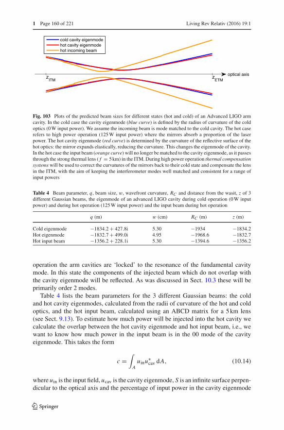
1 Page 160 of 221 Living Rev Relativ (2016) 19:1
Fig. 103 Plots of the predicted beam sizes for different states (hot and cold) of an Advanced LIGO armcavity. In the cold case the cavity eigenmode (blue curve) is defined by the radius of curvature of the coldoptics (0 W input power). We assume the incoming beam is mode matched to the cold cavity. The hot caserefers to high power operation (125 W input power) where the mirrors absorb a proportion of the laserpower. The hot cavity eigenmode (red curve) is determined by the curvature of the reflective surface of thehot optics: the mirror expands elastically, reducing the curvature. This changes the eigenmode of the cavity.In the hot case the input beam (orange curve) will no longer be matched to the cavity eigenmode, as it passesthrough the strong thermal lens ( f = 5 km) in the ITM. During high power operation thermal compensationsystems will be used to correct the curvatures of the mirrors back to their cold state and compensate the lensin the ITM, with the aim of keeping the interferometer modes well matched and consistent for a range ofinput powers
Table 4 Beam parameter, q, beam size, w, wavefront curvature, RC and distance from the wasit, z of 3different Gaussian beams, the eigenmode of an advanced LIGO cavity during cold operation (0 W inputpower) and during hot operation (125 W input power) and the input beam during hot operation
q (m) w (cm) RC (m) z (m)
Cold eigenmode −1834.2 + 427.8i 5.30 −1934 −1834.2Hot eigenmode −1832.7 + 499.0i 4.95 −1968.6 −1832.7Hot input beam −1356.2 + 228.1i 5.30 −1394.6 −1356.2
operation the arm cavities are ‘locked’ to the resonance of the fundamental cavitymode. In this state the components of the injected beam which do not overlap withthe cavity eigenmode will be reflected. As was discussed in Sect. 10.3 these will beprimarily order 2 modes.
Table 4 lists the beam parameters for the 3 different Gaussian beams: the coldand hot cavity eigenmodes, calculated from the radii of curvature of the hot and coldoptics, and the hot input beam, calculated using an ABCD matrix for a 5 km lens(see Sect. 9.13). To estimate how much power will be injected into the hot cavity wecalculate the overlap between the hot cavity eigenmode and hot input beam, i.e., wewant to know how much power in the input beam is in the 00 mode of the cavityeigenmode. This takes the form
c =∫Auinu
∗cav dA, (10.14)
where uin is the input field, ucav is the cavity eigenmode, S is an infinite surface perpen-dicular to the optical axis and the percentage of input power in the cavity eigenmode
123

Living Rev Relativ (2016) 19:1 Page 161 of 221 1
Fig. 104 The simulated circulating power in an Advanced LIGO arm cavity versus input laser power intothe power recycled interferometer with linear arm cavities. Three cases are simulated: no thermal effects,where the response is linear; including the change in curvature of the mirror surfaces due to thermal effects;and including both the change in curvature of the mirrors and the thermal lens induced in the input mirrordue to power absorbed in the mirrors. The addition of the thermal lens has the greatest impact, reducing thepower coupled into the arm cavities
is given by |c|2. In this case both beams are cylindrically symmetric fundamentalGaussian beams (not astigmatic) and the overlap can be calculated as
c = 2
π
1
winwcavexp (i Ψin − i Ψcav)
∫ 2π
0
∫ ∞
0exp
(− i kr2
2
(1
qin− 1
q∗cav
))r dφ dr.
(10.15)Integrating with respect to φ and changing variables to R = r2 we have
c = 2
winwcavexp (i Ψin − i Ψcav)
∫ ∞
0exp
(− i kR
2
(1
qin− 1
q∗cav
))dR. (10.16)
As �{
i k2
(1qin
− 1q∗
cav
)}> 0 the solution of this equation can be written as (Gradshteyn
and Ryzhik 1994)
c = − 4i
winwcavkexp (i Ψin − i Ψcav)
11qin
− 1q∗
cav
. (10.17)
Using this formula we calculate the overlap between the hot cavity eigenmode and hotinput beam as |c|2 = 52.5 %. Such a large mismatch between the incoming beam andcavity would therefore result in around half the circulating power expected from a planewave model or with a perfectly mode-matched beam. This is illustrated in Fig. 104,which shows the power circulating in a single arm cavity as the input power is increasedfrom 0 to 125 W, taking into account the 50:50 beam splitter and assuming a powerrecycling gain of 45 (in reality this will also be impacted by thermal effects). Whenno thermal effects are included the increase in circulating power is linear. Includingthe thermally induced reduction in curvature of the mirror surfaces, with the input
123

1 Page 162 of 221 Living Rev Relativ (2016) 19:1
beam remaining mode matched to the cold cavity, causes a small mismatch, which,at high powers can be noted in a reduction in the gain of the cavity. The largesteffect of the internal heating is in the creation of the thermal lens in the ITM, whichinduces a large mismatch between the beam injected into the cavity and the cavityeigenmode. This is reflected in a large reduction in the circulating power at high inputpowers, around the 50 % reduction predicted by the overlap between the hot inputbeam and cavity eigenmode. In this simple model we assume a linear scaling of thethermal distortions and lenses with input power. As these aberrations are determinedby the circulating power, which no longer scales linearly with input power, this is aslight over estimation of the power loss. In reality this process is more complicated:as the mirrors heat and their aberrations evolve the circulating power will decrease,but this will then reduce the thermal lensing and distortions. The expected stablecavity will therefore be slightly different to the cases shown here. However, theseplots illustrate the magnitude of the problem: such extreme mode mismatches areunacceptably high. We require some method to compensate these effects, especiallythe thermal lensing. Such compensation will need to be adaptive, to be applicablefor a range of input powers and for the transition from cold to hot, controlling themode resonating in the interferometer as the power is increased and the mirrors reachthermal equilibrium. In reality the thermal aberrations will differ slightly from ourmodels and more importantly the aberrations in each arm will differ from each other,due to differences in absorption for the individual mirrors. The thermal compensationsystems need to act on individual mirrors, incorporating sensors which monitor thecurrent state of the thermal aberrations in each arm and then feed back to systemswhich can correct the curvature of the mirror surfaces and the lenses in the ITMs.These compensation systems are discussed in more detail in Sect. 10.7 and in thecomprehensive review article by Vinet (2009).
10.6 The Michelson: differential imperfections
Previously we motivated operating a Michelson interferometer on the dark fringe inorder to maximise the differential gravitational wave signal and minimise the noiseat the dark port (see Sect. 5.3). The differential degrees of freedom, the Michelson(MICH) and differential arm length (DARM), are carefully controlled to maintain theinterferometer on the dark fringe, as discussed in Sect. 8.12. A well defined dark fringerelies on the fact that the two arms are very similar and essentially the carrier and anycommon mode effects cancel at the dark port. Simply we can express the field reflectedback towards the laser at the symmetric port as
Esym. = 1√2
(Ex + Ey
), (10.18)
where Ex and Ey refer to the fields coming from the individual arms. The field in theasymmetric port, or output port is
Easym. = 1√2
(Ex − Ey
). (10.19)
123
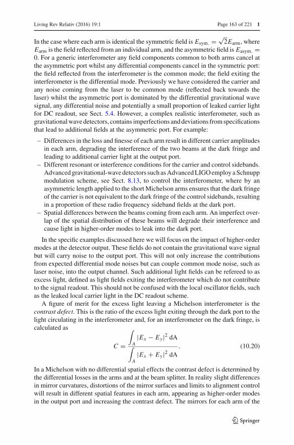
Living Rev Relativ (2016) 19:1 Page 163 of 221 1
In the case where each arm is identical the symmetric field is Esym. = √2Earm, where
Earm is the field reflected from an individual arm, and the asymmetric field is Easym. =0. For a generic interferometer any field components common to both arms cancel atthe asymmetric port whilst any differential components cancel in the symmetric port:the field reflected from the interferometer is the common mode; the field exiting theinterferometer is the differential mode. Previously we have considered the carrier andany noise coming from the laser to be common mode (reflected back towards thelaser) whilst the asymmetric port is dominated by the differential gravitational wavesignal, any differential noise and potentially a small proportion of leaked carrier lightfor DC readout, see Sect. 5.4. However, a complex realistic interferometer, such asgravitational wave detectors, contains imperfections and deviations from specificationsthat lead to additional fields at the asymmetric port. For example:
– Differences in the loss and finesse of each arm result in different carrier amplitudesin each arm, degrading the interference of the two beams at the dark fringe andleading to additional carrier light at the output port.
– Different resonant or interference conditions for the carrier and control sidebands.Advanced gravitational-wave detectors such as Advanced LIGO employ a Schnuppmodulation scheme, see Sect. 8.13, to control the interferometer, where by anasymmetric length applied to the short Michelson arms ensures that the dark fringeof the carrier is not equivalent to the dark fringe of the control sidebands, resultingin a proportion of these radio frequency sideband fields at the dark port.
– Spatial differences between the beams coming from each arm. An imperfect over-lap of the spatial distribution of these beams will degrade their interference andcause light in higher-order modes to leak into the dark port.
In the specific examples discussed here we will focus on the impact of higher-ordermodes at the detector output. These fields do not contain the gravitational wave signalbut will carry noise to the output port. This will not only increase the contributionsfrom expected differential mode noises but can couple common mode noise, such aslaser noise, into the output channel. Such additional light fields can be refereed to asexcess light, defined as light fields exiting the interferometer which do not contributeto the signal readout. This should not be confused with the local oscillator fields, suchas the leaked local carrier light in the DC readout scheme.
A figure of merit for the excess light leaving a Michelson interferometer is thecontrast defect. This is the ratio of the excess light exiting through the dark port to thelight circulating in the interferometer and, for an interferometer on the dark fringe, iscalculated as
C =
∫A
|Ex − Ey |2 dA∫A
|Ex + Ey |2 dA. (10.20)
In a Michelson with no differential spatial effects the contrast defect is determined bythe differential losses in the arms and at the beam splitter. In reality slight differencesin mirror curvatures, distortions of the mirror surfaces and limits to alignment controlwill result in different spatial features in each arm, appearing as higher-order modesin the output port and increasing the contrast defect. The mirrors for each arm of the
123

1 Page 164 of 221 Living Rev Relativ (2016) 19:1
detector are manufactured to be very similar in terms of their optical properties, whichwill determine differential arm losses; and their geometric and thermal properties,which will determine the higher-order mode content in each arm. In Advanced LIGOthe contrast defect should be lower than a few hundred ppm (∼2 × 10⁻⁴W/W) (Aasi2015). In addition the higher-order modes can be suppressed using an output modecleaner.
An example of the impact of higher order modes on contrast defect in a dual recycledMichelson have been observed at GEO 600, the German–British gravitational-wavedetector in Hannover (Danzmann et al. 1994; Abbott 2004). Unlike other gravitational-wave detectors GEO 600 does not include arm cavities, but instead has folded arms toincrease the effective arm length of the Michelson. As described in Lück et al. (2004),during the operation of GEO 600 it was discovered that a difference in the radii ofcurvature of the folding mirrors in the x and y arms (687 m in the x arm, 666 m inthe y arm) was causing a significant difference in the wavefront curvatures of thebeams returning from each arm. This mismatch between the two beams resulted in asignificant amount of power at the interferometer dark fringe: the degrade in overlapbetween the two beams reduced the effective destructive interference and consequentlythe output beam on the dark fringe was dominated by the order 2 mode typical ofa mode mismatch, LG10. The resulting loss of power into the anti symmetric portincreased the effective loss in the power recycling cavity, limiting the power build up to∼200 W/W, a significant reduction from the 300 W/W predicted for this configuration.The mismatch of the two arms also had a negative impact on the longitudinal errorsignal of the Michelson, reducing the magnitude of the error signal and increasing thesusceptibility to misalignments.
To reduce this mismatch and recover the power recycling gain the curvature of oneof the folding mirrors required correcting, to match that of the other arm. In this case thethermal properties of the mirrors were exploited, namely the dependence of the radiusof curvature of the mirrors to a temperature gradient, as was discussed in Sect. 10.5.In advanced detectors the temperature gradient which develops from high poweredbeams incident on the mirrors is an unwanted effect which results in the distortions ofthe mirror surfaces (primarily a change in curvature) and thermal lensing. In GEO 600this thermal behaviour was manipulated to alter the curvature of the folding mirror inthe East arm (x arm) using a ring heater placed behind the mirror substrate to producean appropriate temperature gradient in the East mirror (Lück et al. 2004). The extentof the change in mirror curvature is dependent on the ring heater power, which can begradually altered to find the power which corresponds to the optimum curvature (i.e.,∼666 m to match the North mirror).
In Fig. 105 the interference pattern at the dark fringe is shown for different ringheater powers. For relatively low powers (30 W) the two arms are still not well matchedand the dark port is dominated by the typical bullseye shape of the mismatch mode,LG10. As the ring heater power is increased from 30 to 66 W the mode matchingbetween the two arms increases and the power at the dark fringe is reduced, improvingthe contrast defect by an order of magnitude. Increasing the ring heater power to 71 Wfurther optimised the dark fringe, in terms of minimum power at the dark port. At thispoint the limitations of this curvature compensation are observed: the compensation isapplied as a spherical curvature correction and does not take into account differences
123

Living Rev Relativ (2016) 19:1 Page 165 of 221 1
Fig. 105 Interference pattern at the dark port of GEO 600, for different thermal compensation of the Eastarm folding mirrors, indicated by the different ring heater powers. The brightness of the beam images in thebottom row are slightly enhanced for better visibility. Image reproduced with permission from Lück et al.(2004), copyright by IOP
in curvature in the horizontal and vertical directions, i.e. astigmatism of the mirrors orbeam splitter. For ring heater powers of 66–74 W the output mode is still dominated byorder two modes but in this case these are the Hermite–Gauss modes consistent withastigmatic mismatches. At 66 W the mismatch between the two arms is compensatedin the vertical direction whereas optimum compensation in the horizontal directionrequires a ring heater power of 74 W.
To fully diagnose and understand the nature of this problem these measurementswere compared with Finesse simulations of GEO 600. In Fig. 106 the power circu-lating in the power recycling cavity is plotted against the power at the dark fringe,showing both simulation and experimental results. Two different experimental resultsare shown. The first result has the optimum curvature compensation applied with thepowers measured as the interferometer passes through the dark fringe (solid red trace).The second result is the case where the interferometer is locked to the dark fringe andthe curvature compensation is varied (black markers). The experimental and simula-tion results are sufficiently similar to suggest that our understanding of this problemis correct and that the low intra cavity power/high contrast defect is dominated by adifferential mode mismatch. The slight differences between the experimental resultsand the simulation observed at high intra cavity power can be explained by the limitsof the model: no astigmatic or higher-order spatial effects were included in this modeland hence the model represents a more simplified system than reality. The experimentand simulation are well matched for low intra-cavity power where the effects of thespherical mode mismatch dominate.
This experience at GEO 600 illustrates the need to have well matched arms. Thiscan be in terms of mode matching, as shown here, or in terms of mirror surfacedistortions and other defects. While low-order aberrations such as misalignment and
123

1 Page 166 of 221 Living Rev Relativ (2016) 19:1
Fig. 106 Comparison of measurements and simulations of the circulating power and dark fringe power inGEO 600. The measured fringe (red trace) and simulation (dashed blue trace) refer to the measured andsimulated powers for GEO 600 as the interferometer is moved through the dark fringe with the optimalcurvature compensation applied to the East folding mirror (that which best matches the two arms). Thecurvature compensation (black markers) refers to measurements made whilst the interferometer is lockedto the dark fringe and the curvature compensation of the East mirror is varied. Image reproduced withpermission from Lück et al. (2004), copyright by IOP
mode mismatch can be corrected during operation by means of additional controlsystems, higher-order effects are typically not actively controlled. It is crucial that theimpact of higher-order modes is considered during the design of an interferometer toavoid a large buildup of unwanted modes in the detector.
10.7 Advanced LIGO: implications for design and commissioning
The correct modelling of the impact of beam distortions in interferometers is crucial,not only to our understanding of the physics of real interferometers, but becauseit will have implications for real experiments, in particular during the design andcommissioning of detectors. There are many defects in an interferometer which willeffect the shape of the resonating beams. In complex advanced interferometers, suchas Advanced LIGO, additional systems help control the shape of the beam, mitigatingsome higher-order mode effects. The main sources of higher-order modes are:
– Misalignment Any tilt or lateral shift between the beam axis and a cavity axis,or between the axes of the multiple interdependent cavities in advanced inter-ferometers, will produce higher-order modes, for small misalignments these aredominated by first-order modes. In modern gravitational-wave detectors theseeffects are carefully controlled using alignment systems to maintain consistent
123

Living Rev Relativ (2016) 19:1 Page 167 of 221 1
optical axes within the interferometer and avoid a large amount of power in firstorder modes on the detection photodiode.
– Mismatch Second-order modes arise from a mismatch in beam size or wavefrontcurvature between the cavity eigenmode and incoming beam, or the multiplecavity eigenmodes in complex interferometers. In gravitational wave detectorsmismatches are the result of second-order mirror aberrations from the manufac-turing process or environmental processes such as thermal lensing. In Advancedinterferometers thermal compensation systems will be in place to correct the cur-vature of the arm cavity mirrors, to compensate any thermal lensing and to avoidlarge mode mismatches.
– Surface distortions Higher-order distortions of the beam are generally the resultof higher-order mirror distortions on the highly reflective mirror surfaces. Thesedefects can arise during the manufacturing process (so-called mirror figure error)or through environmental processes like the thermal distortion of the mirror sur-faces. Whilst first and second order distortions of the beam can be corrected it ismore difficult to actively correct modes of a higher order. A crucial part of thedesign process is to determine the tolerances and requirements for the polishingand coating of the interferometer mirrors, to ensure a low higher-order modescontent. This is discussed in more detail in Sect. 11.
– Apertures Higher-order modes are also generated when the circulating beamsencounter the effective aperture caused by the finite size of optical components.The ‘clipping’ of the beam results in a sharp cut-off, equivalent to the addition ofhigh order modes. The design of a well behaved optical setup will ensure the size ofthe optics, compared to the beam, is sufficiently large such that these higher-ordereffects are small and we can simple consider the effect of the aperture as a smallpower loss.
In this section we consider the impact higher-order mode effects have on the finaldesign of an advanced interferometer. The impact of beam distortions are carefullyconsidered during the design process and here we review the choices motivated bybeam shape and size for the particular case of Advanced LIGO.
The input mode cleaner
Gravitational-wave detectors use an optical cavity, called the input mode cleaner(IMC), between the laser and the main interferometer. The purpose of the IMC is toproduce a very pure fundamental TEM00 Gaussian beam for the detector input, filteringout higher-order spatial modes. It is also used as part of the laser frequency stabilisationsystem, producing a very stable carrier frequency. This is motivated by the desire toavoid injecting light fields into the interferometer which may couple additional noiseto the output photodiode. The interferometer is tuned to the operating point of onespecific mode, the carrier TEM00 mode. Any other fields will propagate differentlythrough the interferometer, for example, most higher-order modes do not enter thearm cavities and therefore carry different phase information than the TEM00 mode.
Another requirement of the IMC is to maximise transmission of the fundamentalcarrier mode, whilst also transmitting the radio frequency control sidebands applied tothe beam. For the case of Advanced LIGO the corresponding modulation frequenciesare 9 and 45 MHz. The requirement of high transmission for the carrier and certain
123
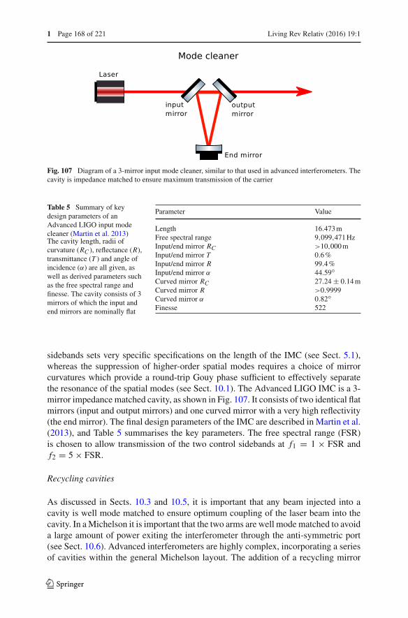
1 Page 168 of 221 Living Rev Relativ (2016) 19:1
Fig. 107 Diagram of a 3-mirror input mode cleaner, similar to that used in advanced interferometers. Thecavity is impedance matched to ensure maximum transmission of the carrier
Table 5 Summary of keydesign parameters of anAdvanced LIGO input modecleaner (Martin et al. 2013)The cavity length, radii ofcurvature (RC ), reflectance (R),transmittance (T ) and angle ofincidence (α) are all given, aswell as derived parameters suchas the free spectral range andfinesse. The cavity consists of 3mirrors of which the input andend mirrors are nominally flat
Parameter Value
Length 16.473 mFree spectral range 9,099,471 HzInput/end mirror RC >10,000 mInput/end mirror T 0.6 %Input/end mirror R 99.4 %Input/end mirror α 44.59◦Curved mirror RC 27.24 ± 0.14 mCurved mirror R >0.9999Curved mirror α 0.82◦Finesse 522
sidebands sets very specific specifications on the length of the IMC (see Sect. 5.1),whereas the suppression of higher-order spatial modes requires a choice of mirrorcurvatures which provide a round-trip Gouy phase sufficient to effectively separatethe resonance of the spatial modes (see Sect. 10.1). The Advanced LIGO IMC is a 3-mirror impedance matched cavity, as shown in Fig. 107. It consists of two identical flatmirrors (input and output mirrors) and one curved mirror with a very high reflectivity(the end mirror). The final design parameters of the IMC are described in Martin et al.(2013), and Table 5 summarises the key parameters. The free spectral range (FSR)is chosen to allow transmission of the two control sidebands at f1 = 1 × FSR andf2 = 5 × FSR.
Recycling cavities
As discussed in Sects. 10.3 and 10.5, it is important that any beam injected into acavity is well mode matched to ensure optimum coupling of the laser beam into thecavity. In a Michelson it is important that the two arms are well mode matched to avoida large amount of power exiting the interferometer through the anti-symmetric port(see Sect. 10.6). Advanced interferometers are highly complex, incorporating a seriesof cavities within the general Michelson layout. The addition of a recycling mirror
123

Living Rev Relativ (2016) 19:1 Page 169 of 221 1
Fig. 108 Two examples of a coupled cavity formed between a recycling mirror (RM) and an AdvancedLIGO arm cavity, made of the input and end test masses (ITM and ETM). The diagram on the left hasa single recycling mirror forming a cavity with the ITM. This is illustrative of the setup of Initial LIGO(Adhikari et al. 2006). The diagram on the right illustrates a folded recycling cavity, where two additionalmirrors in the recycling cavity reshape the beam between the recycling mirror and ITM. This is the setupused in Advanced LIGO (Arain and Mueller 2008). Illustrations are not to scale and in the case of LIGOthe distances between the recycling optics is much smaller (of the order 10 m) than the distance betweenthe test masses (4 km)
at the symmetric port (power recycling) and anti-symmetric port (signal recycling)form recycling cavities between these mirrors and the rest of the interferometer. Theparameters of these cavities must be carefully chosen to ensure a good mode matchbetween the eigenmodes of the recycling cavities and the arm cavities. The followingdiscussion of the design of the recycling cavities refers to the most common designbased on arguments presented in Arain and Mueller (2008). Note that the AdvancedVirgo project has chosen a different design approach (Acernese 2015).
For the design stage we first assume perfect matching of the arm cavities. Wecan then consider each recycling cavity acting with the arms as a simple coupledcavity. Two examples of a possible coupled cavity setup are shown in Fig. 108. Theeigenmode of the arm cavities is selected to produce large beams at the ITM (5.3 cm)and ETM (6.2 cm) to reduce thermal noise, with slightly smaller beams at the ITMas the thermal noise is lower here (fewer coating layers) and to prevent scatteringinto the recycling cavities. The curvatures are also carefully selected for a specificGouy phase to avoid higher-order modes easily ringing up in the arms: RC = 1934 m(ITM) and RC = 2245 m (ETM). The beam parameter of the arms is therefore a fixedparameter, and the properties of the recycling cavities should be chosen to mode matchthe recycling cavity to the arms.
The simplest design for the recycling cavities uses a single mirror coupled withthe arm cavities, as shown in the left diagram of Fig. 108, where the curvature of therecycling mirror is matched to the wavefront curvature of the arm cavity eigenmode.This was the layout chosen for power recycling in Initial LIGO. In this layout theeigenmode of the arm and recycling cavity can be matched. However, there is anotherconsideration for the design of the recycling cavities: the separation of higher-ordermode resonances. This is determined by the Gouy phase accumulated in the recyclingcavity (between RM and ITM). In Fig. 109, the Gouy phase of the eigenmode forthe Advanced LIGO arms is shown at different positions along the optical axis. TheITM and ETM are both far from the waist but the difference in Gouy phase (155.7◦,equivalent to −24.3◦) is far outside the linewidth of the cavity. With a single recyclingmirror the only possible positions do not allow for a large change in Gouy phase, as theITM is already in the far field. In reality there are additional limitations on the positionof the recycling mirror, such as the physical location of the vacuum chambers.
123
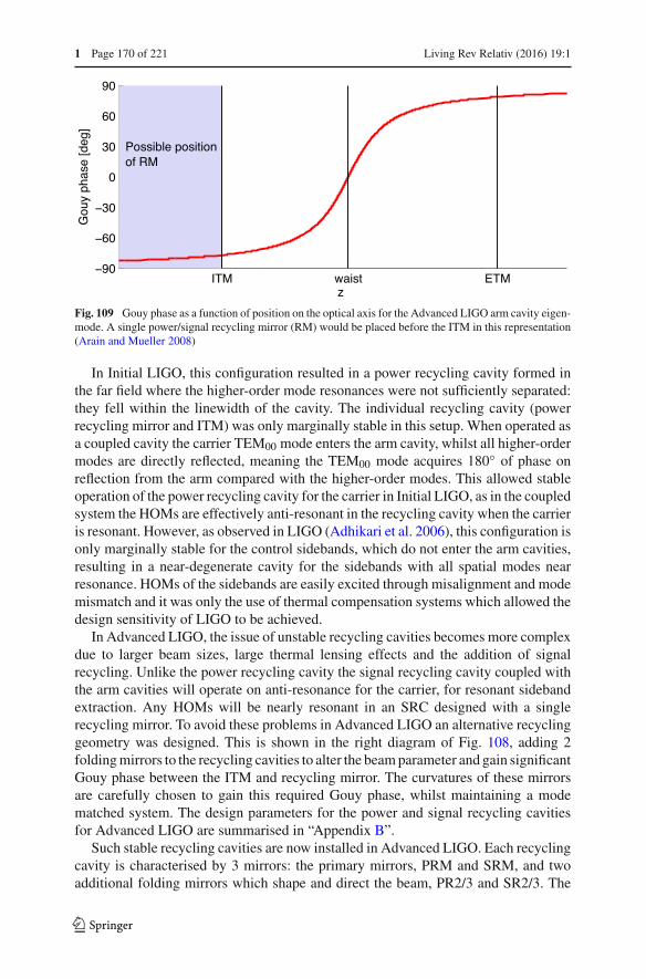
1 Page 170 of 221 Living Rev Relativ (2016) 19:1
Fig. 109 Gouy phase as a function of position on the optical axis for the Advanced LIGO arm cavity eigen-mode. A single power/signal recycling mirror (RM) would be placed before the ITM in this representation(Arain and Mueller 2008)
In Initial LIGO, this configuration resulted in a power recycling cavity formed inthe far field where the higher-order mode resonances were not sufficiently separated:they fell within the linewidth of the cavity. The individual recycling cavity (powerrecycling mirror and ITM) was only marginally stable in this setup. When operated asa coupled cavity the carrier TEM00 mode enters the arm cavity, whilst all higher-ordermodes are directly reflected, meaning the TEM00 mode acquires 180◦ of phase onreflection from the arm compared with the higher-order modes. This allowed stableoperation of the power recycling cavity for the carrier in Initial LIGO, as in the coupledsystem the HOMs are effectively anti-resonant in the recycling cavity when the carrieris resonant. However, as observed in LIGO (Adhikari et al. 2006), this configuration isonly marginally stable for the control sidebands, which do not enter the arm cavities,resulting in a near-degenerate cavity for the sidebands with all spatial modes nearresonance. HOMs of the sidebands are easily excited through misalignment and modemismatch and it was only the use of thermal compensation systems which allowed thedesign sensitivity of LIGO to be achieved.
In Advanced LIGO, the issue of unstable recycling cavities becomes more complexdue to larger beam sizes, large thermal lensing effects and the addition of signalrecycling. Unlike the power recycling cavity the signal recycling cavity coupled withthe arm cavities will operate on anti-resonance for the carrier, for resonant sidebandextraction. Any HOMs will be nearly resonant in an SRC designed with a singlerecycling mirror. To avoid these problems in Advanced LIGO an alternative recyclinggeometry was designed. This is shown in the right diagram of Fig. 108, adding 2folding mirrors to the recycling cavities to alter the beam parameter and gain significantGouy phase between the ITM and recycling mirror. The curvatures of these mirrorsare carefully chosen to gain this required Gouy phase, whilst maintaining a modematched system. The design parameters for the power and signal recycling cavitiesfor Advanced LIGO are summarised in “Appendix B”.
Such stable recycling cavities are now installed in Advanced LIGO. Each recyclingcavity is characterised by 3 mirrors: the primary mirrors, PRM and SRM, and twoadditional folding mirrors which shape and direct the beam, PR2/3 and SR2/3. The
123
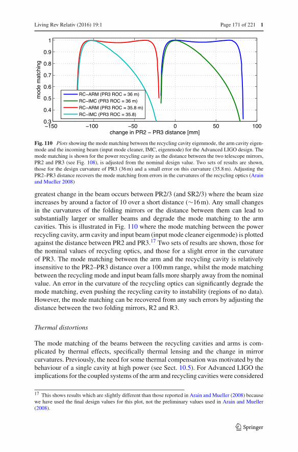
Living Rev Relativ (2016) 19:1 Page 171 of 221 1
Fig. 110 Plots showing the mode matching between the recycling cavity eigenmode, the arm cavity eigen-mode and the incoming beam (input mode cleaner, IMC, eigenmode) for the Advanced LIGO design. Themode matching is shown for the power recycling cavity as the distance between the two telescope mirrors,PR2 and PR3 (see Fig. 108), is adjusted from the nominal design value. Two sets of results are shown,those for the design curvature of PR3 (36 m) and a small error on this curvature (35.8 m). Adjusting thePR2–PR3 distance recovers the mode matching from errors in the curvatures of the recycling optics (Arainand Mueller 2008)
greatest change in the beam occurs between PR2/3 (and SR2/3) where the beam sizeincreases by around a factor of 10 over a short distance (∼16 m). Any small changesin the curvatures of the folding mirrors or the distance between them can lead tosubstantially larger or smaller beams and degrade the mode matching to the armcavities. This is illustrated in Fig. 110 where the mode matching between the powerrecycling cavity, arm cavity and input beam (input mode cleaner eigenmode) is plottedagainst the distance between PR2 and PR3.17 Two sets of results are shown, those forthe nominal values of recycling optics, and those for a slight error in the curvatureof PR3. The mode matching between the arm and the recycling cavity is relativelyinsensitive to the PR2–PR3 distance over a 100 mm range, whilst the mode matchingbetween the recycling mode and input beam falls more sharply away from the nominalvalue. An error in the curvature of the recycling optics can significantly degrade themode matching, even pushing the recycling cavity to instability (regions of no data).However, the mode matching can be recovered from any such errors by adjusting thedistance between the two folding mirrors, R2 and R3.
Thermal distortions
The mode matching of the beams between the recycling cavities and arms is com-plicated by thermal effects, specifically thermal lensing and the change in mirrorcurvatures. Previously, the need for some thermal compensation was motivated by thebehaviour of a single cavity at high power (see Sect. 10.5). For Advanced LIGO theimplications for the coupled systems of the arm and recycling cavities were considered
17 This shows results which are slightly different than those reported in Arain and Mueller (2008) becausewe have used the final design values for this plot, not the preliminary values used in Arain and Mueller(2008).
123

1 Page 172 of 221 Living Rev Relativ (2016) 19:1
Fig. 111 Plots showing mode matching at different input powers between the recycling cavities and thearms (RC-ARM) and recycling cavities and the input mode cleaner (RC-IMC) for the Advanced LIGOdesign. The mode overlap is calculated considering the thermal lens formed in the input test masses frompredicted absorptions in the ITMs. Two different designs are considered, one optimised for mode matchingat an input power of 0 W (cold optics) and one optimised for 18 W, the final Advanced LIGO design
during the design phase (Arain et al. 2012). In Fig. 111, the mode matching betweenthe recycling and arm cavities, and the recycling cavities and the input mode is shown,as the interferometer input power is increased. As the thermal lens in the ITM is byfar the dominant effect (10.5) this is the only thermal aberration included, modelledas a simple spherical lens. The first two traces in Fig. 111 (0 W design) show the modematching for the original design of the recycling cavities, where the parameters werechosen to match the cold optics of the arm cavities. A second design (18 W design)is also shown. In this case the mode matching between the recycling cavities, thearm cavities and the input mode was optimised for the expected thermal lensing of34.5 km18 at 18 W input power. The advantages of this design is that it gives a largerrange of input power at which the interferometer is well mode matched, without theneed for thermal compensation systems.
The plots shown in Fig. 111 show that the mode matching between the recyclingcavities and arm cavities is relatively independent of the expected thermal lensing.Whilst the eigenmode of the arm cavity is fixed, the recycling cavity eigenmodeis affected by the thermal lens. The recycling eigenmode curvature is fixed at thereflective ITM surface, and the beam size at this point only varies a small amount,maintaining the mode matching between the arm and recycling cavity. However, theeffect of the lens on the mode parameters is exaggerated during the large divergencebetween the recycling mirrors R2 and R3 (see Fig. 108) and this has a large impacton the beam size at the recycling mirror, and hence the mode matching between theinput beam and recycling cavity is significantly degraded. As we saw previously for asingle cavity, during high power operation the power coupled into the interferometerwill be significantly reduced.
18 34.5 km is the focal length when modelled as an individual lens in a vacuum, the approach in thisdocument. Sometimes quoted is 50 km corresponding to the lens when modelled inside the fused silicasubstrate of the ITM.
123

Living Rev Relativ (2016) 19:1 Page 173 of 221 1
In Advanced LIGO thermal compensation systems (TCS) will be employed at highpower, not only to ensure a large power buildup within the interferometer but to balancethe lensing and eigenmodes of the two arms to prevent a high contrast defect (Willems2009). The first is a ring-heater positioned near the anti-reflective surface of each testmass (Arain et al. 2012). These are used to heat the outer edge of the mirror to producea curvature in the opposite direction to that from heating by the beam. The ring heateralso corrects some of the thermal lens in the ITM substrate. An additional system isrequired to complete the correction of the thermal lens. This involves a compensationplate, placed in front of the ITMs, made of the same material (fused silica). A heatingpattern is projected onto this plate via a CO2 laser. This pattern is designed to heatthe compensation plate in such a way as to correct any thermal lensing in the ITM(Brooks et al. 2012).
The output mode cleaner
Even with state of the art optics, alignment systems to correct any misalignments andthermal compensation systems to correct for differential mismatches some light at theMichelson anti-symmetric port will be in higher-order modes. There will also be somepower in the control sidebands exiting the interferometer, as the dark fringe for thecarrier is not the dark fringe for the sidebands due to the applied Schnupp asymmetry(see Sect. 8.13 and “Advanced LIGO configuration” section in “Appendix B”). Theonly fields which should be present on the detection photodiode are the gravitationalwave signal sidebands and the local oscillator field, in the case of Advanced LIGO thisis the leaked carrier light for DC readout (see Sect. 6.2). If the power in the higher-order modes and control sidebands is sufficiently low they can be effectively strippedfrom the beam using an output mode cleaner (OMC), an optical cavity between theMichelson interferometer and the main photodiode.
The parameters of the output mode cleaner are carefully chosen to maximise thetransmission of the gravitational wave signal and local oscillator field, whilst suffi-ciently filtering out the unwanted spatial modes and control sidebands. The OMCdesign for Advanced LIGO is a Fabry–Perot cavity in a 4-mirror bow tie configuration(Arai et al. 2013), consisting of two flat mirrors (the input and output mirrors) and twocurved mirrors (high reflectors). To maximise the transmission of the desired fields thecavity is impedance matched between the input mirror and output mirror. Ignoring anylosses, the power in an individual field transmitted by an impedance matched cavity is
Ptrans. = T 2
1 + R2 − 2R cos (kLrt − Ψ (n + m + 1))P0, (10.21)
where T and R are the transmittance and reflectance properties of the input and outputcoupler, P0 is the power in the incoming field, k is the wavenumber of the field, Lrt
is the round-trip length of the cavity, Ψ is the round-trip Gouy phase and n and mare the higher-order mode indices of the field. In a lossless cavity all the power in afield is transmitted on resonance. For an Advanced LIGO OMC with realistic lossesthe transmission of the carrier TEM00 mode and signal sidebands is expected to be∼98 %. On anti-resonance the transmitted power can be approximated as
min(Ptrans.) = T 2
1 + R2 + 2RP0 ≈ T 2
4P0, (10.22)
123

1 Page 174 of 221 Living Rev Relativ (2016) 19:1
Table 6 Summary of keydesign parameters for theAdvanced LIGO output modecleaner (Arai et al. 2013)
The length, mirror radii ofcurvature (RC ) andtransmittance (T ) are given, aswell as derived parameters thefree spectral range and finesse
Parameter Value
Length 1.132 mFree spectral range 264.8 MHzInput/output mirror RC ∞High reflectors RC 2.5 mInput/output mirror T 8300 ppmHigh reflectors T 50 ppmFinesse 390Angle of incidence 4◦
as in the case of a high finesse cavity, R ≈ 1. In order to avoid transmitting the unwantedfields the length and curvatures of the cavity mirrors are very carefully chosen. Thelength of the cavity must not be resonant for the 9 MHz and 45 MHz control sidebands.The curvatures of the mirrors are chosen to ensure sufficient Gouy phase to avoidthe resonance of any higher-order modes entering the cavity. This requires carefulmodelling and a knowledge of which higher-order modes are expected to exit the maininterferometer. In Arai and Korth (2015) the HOM content is modelled using a powerlaw derived from the spectrum of higher-order modes observed in Enhanced LIGO.This predicts the total power in each order of modes exiting the interferometer as
PHOM = 1.8 × 10−3 × 10− N4.8 , (10.23)
where N is the mode order and N ≤ 2 (1st order modes are reduced via alignmentcontrol). Using this power law different mirror curvatures and lengths were modelledto find the optimum design for minimum transmission of the expected undesired fields.This design is presented in Arai et al. (2013) and the key parameters are summarisedin Table 6. With a finesse of ∼400 and an expected round-trip loss of 140 ppm thetransmission of undesirable fields is expected to be 10−5 W/W, relative to the powerinjected into the interferometer. This is equivalent to ∼1 mW at high power, comparedto ∼100 mW of reference carrier light for DC readout.
10.8 Commissioning
Commissioning describes the process of tuning and improving a gravitational-wavedetector after its subsystems have been installed and before the full system is opera-tional. This process typically takes several years because the interferometer couplesall the subsystems in a unique and complex way, which cannot be tested in advance.This is particularly important for advanced detectors which employ many cutting edgetechnologies which, although having been tested in the laboratory and at prototypefacilities, have never been implemented together in interferometers of this scale. Theefficiency of the commissioning process is crucial to achieving the expected sensitivityand providing an instrument for scientific data taking in a timely manner.
Through the commissioning process we observe effects never seen before, theinterferometer will be operated in a new regime, namely a full scale, high power, dualrecycled interferometer with arm cavities. In this extremely sensitive configuration pre-viously negligible effects could have a strong impact on interferometer performance.For example, parametric instabilities, where higher-order mode and radiation pressure
123
Living Rev Relativ (2016) 19:1 Page 175 of 221 1
effects couple together with the potential of ringing up high order sidebands, will likelybe a factor in this high powered regime (Braginsky et al. 2001; Evans et al. 2010; Graset al. 2010). Subsystems of the interferometer also use cutting edge techniques whichhave yet to be tested within the full framework of our advanced detectors.
During commissioning the interferometers are assembled in increments, buildingtowards the full dual recycled configuration. As the optics are installed many mea-surements are taken to test the behaviour of various subsystems and finally to test theresponse and noise budgets of the full interferometer. During this process it is cru-cial that we have accurate models of the interferometers. These must include possibledefects and higher-order mode effects, typically going beyond the more simplifiedmodels used in the design phase. For example, in Advanced LIGO measurements ofthe surfaces of the mirrors were taken prior to installation. This surface data can beused in simulations to model the expected distortion of the beams within the real inter-ferometers. During the commissioning process these models are used to check againstexperimental measurements. In the case where a measurement is not as expected mod-els are used to investigate the possible causes, adding in more realistic measurementsand tuning parameters to recreate the observed behaviour. From such models we canthen suggest solutions in the case of underperformance.
The interested reader is directed to the following documents, which give details onspecific modelling tasks to support the commissioning of Advanced LIGO, particularlythose which are concerned with higher-order mode effects19:
– Comparisons of alignment signals calculated for Fabry–Perot cavities using threemethods: Finesse, an analytic calculation and the FFT propagation simulationOSCAR (Ballmer et al. 2014).
– Comparisons of the control signals and sideband build up in Advanced LIGO, asmodelled in Finesse and Optickle (Bond et al. 2014a; Bond 2014).
– Investigation into the effect of mode-mismatch in the control signals of theAdvanced LIGO interferometer (Bond et al. 2014b).
– A dedicated commissioning investigation into power loss at the central beam split-ter in Advanced LIGO using Finesse (Bond et al. 2013).
– Finesse simulations of the alignment control signal of the Advanced LIGO inputmode cleaner (Kokeyama et al. 2013).
10.9 Finesse examples
10.9.1 Higher-order mode resonances
This example illustrates the different resonance conditions of the higher-order modesin an optical cavity. In the simulation an input beam made up of 6 different order modesis generated using the ‘tem’ commands. This beam is injected into an Advanced LIGOstyle cavity and the cavity length is tuned. Using amplitude detectors, ‘ad’, the differentorder modes are individually detected (Fig. 112).
19 Many more such documents exist for Advanced LIGO and other gravitational wave detectors. Thisselection is based on our familiarity with the described work.
123
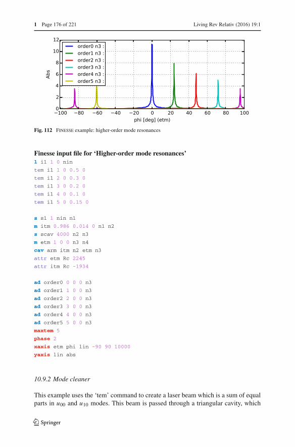
1 Page 176 of 221 Living Rev Relativ (2016) 19:1
Fig. 112 Finesse example: higher-order mode resonances
Finesse input file for ‘Higher-order mode resonances’l i1 1 0 nin
tem i1 1 0 0.5 0
tem i1 2 0 0.3 0
tem i1 3 0 0.2 0
tem i1 4 0 0.1 0
tem i1 5 0 0.15 0
s s1 1 nin n1
m itm 0.986 0.014 0 n1 n2
s scav 4000 n2 n3
m etm 1 0 0 n3 n4
cav arm itm n2 etm n3
attr etm Rc 2245
attr itm Rc -1934
ad order0 0 0 0 n3
ad order1 1 0 0 n3
ad order2 2 0 0 n3
ad order3 3 0 0 n3
ad order4 4 0 0 n3
ad order5 5 0 0 n3
maxtem 5
phase 2
xaxis etm phi lin -90 90 10000
yaxis lin abs
10.9.2 Mode cleaner
This example uses the ‘tem’ command to create a laser beam which is a sum of equalparts in u00 and u10 modes. This beam is passed through a triangular cavity, which
123

Living Rev Relativ (2016) 19:1 Page 177 of 221 1
Fig. 113 Finesse example: mode cleaner
acts as a mode cleaner. Being resonant for the u00, the cavity transmits this mode andreflects the u10 mode as can be seen in the resulting plots (Fig. 113).
Finesse input file for ‘Mode cleaner’
laser i1 1 0 n1 % laser with P=1W
maxtem 1 % need Hermite-Gauss modes
up to n+m=1
tem i1 0 0 1 0 % laser beam is a mix of
u_00 and u_10
tem i1 1 0 1 0
s s1 1 n1 n2 % a space of 1m length
% triangular mode cleaner cavity
bs bs1 .9 .1 0 0 n2 nrefl n3 n4 % input mirror
s sc1 2 n3 n5 % distance between b1 and bs2
bs bs2 .9 .1 0 0 ntrans dump n5 n6 % output mirror
s sc2 49 n4 n7 % distance between b1 and bs3
s sc3 49 n6 n8 % distance between b2 and bs3
bs bs3 1 0 0 0 n7 n8 dump dump % end mirror
attr bs3 Rc 150 % Rc=150m for bs3
cav cav1 bs1 n3 bs1 n4 % computing cavity parameters
run1: beam ccd ntrans % beam shape in transmission
run2: beam ccd nrefl % beam shape in reflection
xaxis ccd x lin -3 3 200 % tuning x,y axes of beam detector
x2axis ccd y lin -3 3 200
yaxis abs % plotting the absolute intensity
10.9.3 Misaligned cavity
In this example a misaligned cavity is scanned and the circulating power is detected.Additional spikes in the cavity scan indicate the higher-order modes (order one andtwo are visible) created by the misalignment (Fig. 114).
123
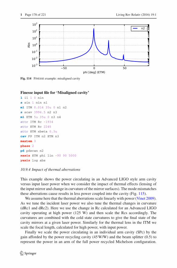
1 Page 178 of 221 Living Rev Relativ (2016) 19:1
Fig. 114 Finesse example: misaligned cavity
Finesse input file for ‘Misaligned cavity’l i1 1 0 nin
s sin 1 nin n1
m1 ITM 0.014 35u 0 n1 n2
s scav 3994.5 n2 n3
m1 ETM 5u 35u 0 n3 n4
attr ITM Rc -1934
attr ETM Rc 2245
attr ETM xbeta 0.3u
cav FP ITM n2 ETM n3
maxtem 3
phase 2
pd pdscan n2
xaxis ETM phi lin -90 90 5000
yaxis log abs
10.9.4 Impact of thermal aberrations
This example shows the power circulating in an Advanced LIGO style arm cavityversus input laser power when we consider the impact of thermal effects (lensing ofthe input mirror and change in curvature of the mirror surfaces). The mode mismatchesthese aberrations cause results in less power coupled into the cavity (Fig. 115).
We assume here that the thermal aberrations scale linearly with power (Vinet 2009).As we tune the incident laser power we also tune the thermal changes in curvature(dRc1 and dRc2). Here we use the change in Rc calculated for an Advanced LIGOcavity operating at high power (125 W) and then scale the Rcs accordingly. Thecurvatures are combined with the cold state curvatures to give the final state of thecavity mirrors at a given laser power. Similarly for the thermal lens in the ITM wescale the focal length, calculated for high power, with input power.
Finally we scale the power circulating in an individual arm cavity ($Pc) by thegain afforded by the power recycling cavity (45 W/W) and the beam splitter (0.5) torepresent the power in an arm of the full power recycled Michelson configuration.
123

Living Rev Relativ (2016) 19:1 Page 179 of 221 1
Fig. 115 Finesse example: thermal cavity
We also plot the theoretical linear circulating power, when thermal effects are notconsidered. Here the 280.7 W is the circulating power in a cavity simulated with nothermal or higher order mode defects.
Finesse input file for ‘Thermal cavity’l i1 1 0 nin
gauss g1 i1 nin 12m -1.83522k
s sin 1 nin na
lens TL inf na nb
s sTL 0 nb n1
m1 ITM 0.014 35u 0 n1 n2
s scav 3994.5 n2 n3
m1 ETM 5u 35u 0 n3 n4
cav arm ITM n2 ETM n3
maxtem 6
attr ITM Rc -1934
attr ETM Rc 2245
pd Pcirc n2
noplot Pcirc
set Pc Pcirc abs
func hot_power = $Pc * $x1 * 45/2
func cold_power = $x1 * 280.7 * 45/2
phase 3
variable Pin 0
xaxis Pin phi lin 0 125 500
func dRc1 = 0 - 1/(1/55000*$x1/125 + 1E-20)
noplot dRc1
func Rc1 = 0 - 1/(1/1934+1/$dRc1)
noplot Rc1
func dRc2 = 0 - 1/(1/80000*$x1/125 + 1E-20)
noplot dRc2
func Rc2 = 1/(1/2245+1/$dRc2)
noplot Rc2
123

1 Page 180 of 221 Living Rev Relativ (2016) 19:1
func foc = 6700*125/($x1+ 1E-20)
noplot foc
put TL f $foc
put ITM Ry $Rc1
put ITM Rx $Rc1
put ETM Ry $Rc2
put ETM Rx $Rc2
yaxis lin abs
11 Scattering into higher-order modes
Spatial variations in the optics that compose a laser interferometer, such as distortionsof the mirror surfaces, will change the shape of the circulating beams. Methods forquantifying such optical imperfections and their effects are required during the designof an interferometer and for modelling efforts to characterise the instrument duringoperation. In particularly, this is crucial during the design phase in order to produce,for example, polishing requirements for the mirror surfaces. At first glance it is notobvious how such optical defects should be characterised and we will show that thenature of the problem determines which approach to use.
Previously we introduced the idea that these distortions can be described as higher-order Gaussian modes and considered the impact of such modes on the interferometerperformance. In this section we consider the mechanisms and mathematics of thisscattering into higher-order modes, with particular emphasis on this process for mirrorsurface distortions. We will explore how different types of surface distortions impactthe beam shape and quantify which mirror shapes produce which higher order modes.Throughout this section we use measured data from the Advanced LIGO mirrors,kindly provided by GariLynn Billingsley of the LIGO Laboratory (Billingsley 2015).
11.1 Light scattering in interferometers
The term ‘scattering’ in interferometers can refer to several different processes. Mostcommonly it refers to imperfections of high spatial frequency that scatter light at largeangles away from the optical axis, effectively scattering light out of the path of thebeam. This is a different problem to scattering into higher order modes, which occurswhen the light is scattered back into the path of the beam (i.e., small angle scattering).Light scattered at large angles has the potential to be re-scattered back into the path ofthe beam by interactions with, for example, the walls of the beam tube. This will couplenew noises into the interferometer, from the beam tubes into the circulating light field.Low angle scattering into higher order modes can introduce noise in other ways, aswas discussed in Sect. 10. The effects of scattered light and mitigation solutions arean ongoing research topic in the gravitational wave community (Vinet et al. 1997;Yamamoto 2007; Accadia 2010; Vander-Hyde et al. 2015).
The different scattering processes require different methods for efficient, accuratemodelling. Whereas low-angle scattering can be modelled using a paraxial approach,either via a description of higher-order modes or using a Fourier propagation model,
123

Living Rev Relativ (2016) 19:1 Page 181 of 221 1
high-angle scattering is outside the paraxial approximation and can require computa-tionally heavy numerical algorithms for accurate results.
In this review we focus on low angle scattering which manifests itself as changesin the beam shape. Of course low and high angle scattering are not two separatephenomena, and we see the paraxial method fail at scattering angles greater than∼20◦. This region between high and low-angle scattering can be difficult to model,falling between the two regimes. In addition, the finite size of the mirrors in realinterferometers prevents the buildup of very high-order modes as these are wider thanthe mirrors and experience significant larger losses. In this way the finite size of thecavity mirrors can set a limit for high angle scattering.
The two regimes of scattering correspond to some extent to two commonly usedcategories for describing spatial surface defects:
1. Flatness, describing the overall shape of a mirror and its large scale, low spatialfrequency features. These defects impact the shape of the beam within the path,as can be described with higher spatial modes.
2. Roughness, the high spatial frequency distortions of the mirror which scatter lightout of the path of the beam.
11.2 Mirror surface defects
Realistic mirrors differ from their ideal form in that their optical and geometric prop-erties are not uniform over the optic. A possible categorisation of mirror imperfectionsin interferometers are:
– misalignment and curvature mismatch, i.e., a mismatch between the position, ori-entation and shape of the optics with respect to the laser beam
– non-uniform mirror phase effects, distorted surfaces and substrates will changethe phase distribution of a reflected or transmitted beam
– non-uniform amplitude effects: dirty or distorted optics can cause non-uniformabsorption and reflection
– apertures created by the finite size of the optics.
The mirrors can be characterised in detail before installation, see for example thepresentation (Billingsley and Zhang 2012). Figure 116 shows plots detailing somemeasured properties from an Advanced LIGO mirror (Billingsley 2015). Thesemirrormaps (see Sect. 11.5) can be used in simulations of detectors for a more accurate com-parison with experimental results or for the purposes of producing design requirementsfor the mirrors. In the following we discuss the effects of mirror surface distortions,as these are expected to be the dominant source of spatial beam distortions. Similarmethods can be used to model non-uniform absorption or reflection properties.
11.3 Coupling between higher-order modes
Any paraxial beam can be expressed as a sum of Hermite or Laguerre–Gauss modes.An expansion, in terms of Hermite–Gauss modes, of the arbitrary field u(x, y, z), canbe written as (Siegman 1986):
123
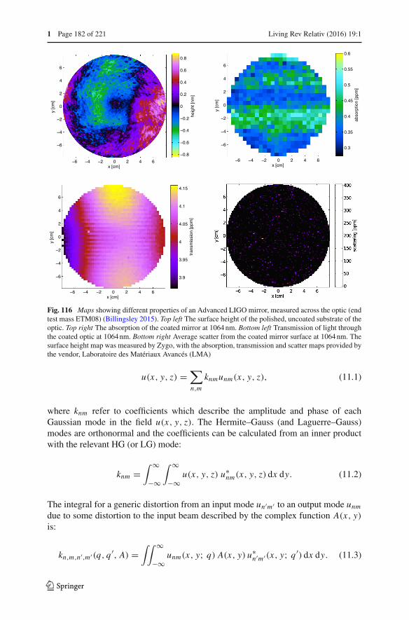
1 Page 182 of 221 Living Rev Relativ (2016) 19:1
Fig. 116 Maps showing different properties of an Advanced LIGO mirror, measured across the optic (endtest mass ETM08) (Billingsley 2015). Top left The surface height of the polished, uncoated substrate of theoptic. Top right The absorption of the coated mirror at 1064 nm. Bottom left Transmission of light throughthe coated optic at 1064 nm. Bottom right Average scatter from the coated mirror surface at 1064 nm. Thesurface height map was measured by Zygo, with the absorption, transmission and scatter maps provided bythe vendor, Laboratoire des Matériaux Avancés (LMA)
u(x, y, z) =∑n,m
knmunm(x, y, z), (11.1)
where knm refer to coefficients which describe the amplitude and phase of eachGaussian mode in the field u(x, y, z). The Hermite–Gauss (and Laguerre–Gauss)modes are orthonormal and the coefficients can be calculated from an inner productwith the relevant HG (or LG) mode:
knm =∫ ∞
−∞
∫ ∞
−∞u(x, y, z) u∗
nm(x, y, z) dx dy. (11.2)
The integral for a generic distortion from an input mode un′m′ to an output mode unmdue to some distortion to the input beam described by the complex function A(x, y)is:
kn,m,n′,m′(q, q ′, A) =∫∫ ∞
−∞unm(x, y; q) A(x, y) u∗
n′m′(x, y; q ′) dx dy. (11.3)
123

Living Rev Relativ (2016) 19:1 Page 183 of 221 1
In the special case when A(x, y) is exclusively misalignment
A(x, y) ⇒ A(x, y, γx , γy) = ei 2kz′(sin2(γx/2)+sin2(γy/2))ei k, (11.4)
the integral can be simplified to the Bayer-Helms coupling equation (9.68) as describedin Sect. 9.16. In general, however, the integral cannot be solved analytically. To modelrealistic mirror surfaces and how they couple higher-order-modes, numerical metrol-ogy data is used directly in the coupling coefficient integral. In the generic case A(x, y)represents a complex valued function that interpolates the measured data. For example,for the coupling in reflection from a mirror surface we have
krefl.nm,n′m′ =
∫ ∞
−∞
∫ ∞
−∞unm(x, y, z) exp (2i kn1z(x, y))u
∗n′m′(x, y, z) dx dy, (11.5)
where z(x, y) describes the distorted surface height and n1 is the index of refractionfor the incident and reflected fields. Similarly, for transmission through a distortedsurface we have
ktrans.nm,n′m′ =
∫ ∞
−∞
∫ ∞
−∞unm(x, y, z) exp (i k(n2 − n1)z(x, y))u
∗n′m′(x, y, z) dx dy,
(11.6)where n1 is the index of refraction for the incident beam and n2 is the index for thetransmitted beam. This process of distorting the beam is refereed to as coupling intoother modes, as the action of reflection from a distorted surface creates modes otherthan those contained in the incoming beam.
In interferometer simulations such as Finesse that use modes to describe the beamshape, a maximum order of the modes included Omax must be defined for each model.The coupling between all modes with an order less than the maximum order of modesis calculated in reflection and transmission of a distorted optic. This is represented asa coupling coefficient matrix, as described in Sect. 9.16, which computes the trans-formation of the incident light field as it interacts with the distorted optic. Thesecoupling matrices are inserted into the matrix describing the interferometer behaviour,as described in Sect. 2.3, giving the higher-order mode content at any position withinthe simulated setup. For well behaved optics, such as those installed in gravitational-wave detectors, we can accurately model realistic distortions of the beam with a finitenumber of modes, as long as we chose a good Gaussian basis (eigenmode) to work in.The further from the ideal eigenmode the more modes you will require to convergeto the correct result. It has been our experience that the best eigenmode is most oftenthat of the optical cavity, as given by the mirror curvatures and positions.
11.4 Simulation methods
Optical simulation tools inherently involve approximations in order to provide mean-ingful results within practical computation times. The most common approximationwhen modelling laser interferometers for gravitational-wave detectors is assuming aparaxial beam, allowing the use of a small angle approximation. There are two distinctsimulation methods based on the paraxial approximation:
123

1 Page 184 of 221 Living Rev Relativ (2016) 19:1
Fig. 117 Mirror map describing the measured surface height of an Advanced LIGO end test mass, beforecoating. The curvature, tilt and average offset of the surface are removed from the data, to clearly show thehigher-order distortions of the mirror surface
1. Modal decomposition with light fields expressed as linear combinations ofGaussian modes (solutions to the paraxial wave equation).
2. Fast Fourier Transform (FFT) methods where the light fields are represented asfinite numerical grids which are propagated through an optical system in the Fourierdomain.
The most important aspects of performing simulations with modal models are: (1) touse the correct Gaussian basis for the higher-order mode expansion; and (2) to useenough higher-order modes to recreate distortions of the wavefront. A good choice ofGaussian basis means a small number of modes should be sufficient to reproduce thedistortions we expect in gravitational wave interferometers. In this review we makeextensive use of the modal simulation Finesse, see “Appendix A”. Other modellingtools for laser interferometers are based on, or are using, Gaussian modes (Evans 2004;Vajente 2013). The FFT method formed the beginning of optical modelling in thegravitational-wave community and has been used extensively since (Vinet et al. 1992;Bochner and Hefetz 2003; Day et al. 2014; Jerome 2008). Both methods contain furtherapproximation, in the addition to assuming paraxial behaviour. In the case of modalmodels this arises from the finite number of modes. In FFT codes the finite grid sizeand resolution restricts the accuracy. A balance between accuracy and efficiency oftendetermines the number of modes and grid dimensions used in these simulations. Somepowerful tools have been developed which can use modal and FFT based methodsinternally (Caron et al. 1999; Yamamoto et al. 2015).
11.5 Mirror surface maps
In order to analyse the effects of mirror surface distortions we require numericaldescriptions of actual mirrors. In this section we discuss several methods for rep-
123
Living Rev Relativ (2016) 19:1 Page 185 of 221 1
resenting mirror surface data, with some methods more suited to use in numericalsimulations, whilst others allow an analytic analysis.
A powerful way to implement mirror surface distortions in modal models is byusing a numerical grid representing the surface height of the real mirrors, known asmirror maps. This is how mirror surface effects are implemented in the interferometersimulation Finesse (Freise 2015; Freise et al. 2004). The surface data is given as afunction over the x–y surface of the optic and can either be measured data from areal mirror or data generated from mathematical functions, for example, describingthe expected thermal distortion of a mirror. Mirror map data can be produced forsurface height, reflectivity, transmissivity or absorption over the surface of the optic.Unless otherwise noted we use the generic term mirror map referring to surface height.Figure 117 shows an example of a mirror map depicting the surface of an end test massproduced for Advanced LIGO (shown here with any curvature, tilt and offset removed)to illustrate the kinds of distortions of the mirrors we can expect. Note the nanometerscale of the graph, which is typical for mirrors in such high-precision interferometers.We can also see that the central region of the mirror exhibits less surface heightvariation. Again this is expected, as the requirements on the polishing of the mirrorare much more stringent in the centre of the optic where the beam is most intense.
Essentially mirror maps characterise the surfaces by their deviation from a perfectsphere. The terms for any piston, tilt and curvature are then expressed by individ-ual numbers (amplitude, angle and radius of curvature respectively). This raises theproblem of how to optimally define these low-order features for a distorted surface.For example, measureing the curvature of a real mirror is done by fitting a sphericalfunction to the measured surface data, minimising the difference between our refer-ence function, the spherical surface Zsphere, and our data, the mirror map Zmap. Thisis represented by minimising the function
f =∫ 2π
0
∫ R
0[Zmap − Zsphere]2 r dr dθ, (11.7)
where R is the radius over which we are measuring. For a typical distorted surface theresult can vary greatly with R. We could chose R to be the radius of the mirror, takinga measure of the curvature over the whole surface. However, if we consider the part ofthe mirror over which the Gaussian beams interact we can measure the curvature thebeam ‘sees’ more effectively. Therefore, it makes sense to weight our fitting routineusing a Gaussian function:
f =∫ 2π
0
∫ R
0W (r, θ)[Zmap − Zsphere]2 r dr dθ, (11.8)
where W (r, θ) is the weighting function, in most cases given by the intensity distribu-tion of the fundamental Gaussian beam and R is the radius of the mirror. The plots inFig. 118 show different estimates for the curvature of a mirror surface measured overdifferent regions and using a weighted fitting function. There is a significant differ-ence in curvature depending on the area or weighting used and we must take care touse the correct measurement for accurate models. It is especially important for modal
123

1 Page 186 of 221 Living Rev Relativ (2016) 19:1
Fig. 118 Estimates of mirror curvature over different radii and with different weightings for a distortedmirror surface. Three different estimates for the curvature of the surface are shown, (1) the spherical termover the whole 30 cm; (2) the spherical term over the central 16 cm region; and (3) the Gaussian weightedcurvature of the surface, using a weighting beam size of w = 6.2 cm
simulations that the correct curvature is measured, as this will determine the cavityeigenmodes, and the basis of our calculations. In most cases working in the cavityeigenmodes ensures efficient simulations: accurate results using the least higher ordermodes. The offset and tilt can be measured using similar methods, specifying the areaor weighting with which to measure the defect.
11.6 Spectrum of surface distortions
It is desirable to have an analytic description of a mirror surface, not just numericdata, for example, to categorise specific types of distortion. A commonly used methodfor describing surfaces is to use a spectrum over spatial frequencies or wavelengths.The distortion of a surface along the x-axis at a specific spatial frequency, F , can bewritten as:
Z(x) = A cos (2πFx + φ), (11.9)
where A is the amplitude of the distortion and φ is the initial phase of the distortion.For a purely cosine distortion φ = 0 and for purely sine φ = π
2 . A generic distortioncan be described by a sum of sines and cosines at different frequencies, Fn :
Z(x) =∑n
An cos(2πFn + φn). (11.10)
The coefficients and phases can be extracted from a discrete Fourier transform of mea-sured surface data z(x), calculated using a Fast Fourier Transform (FFT) algorithm:
Z(k) =N−1∑n=0
z(n) exp
(− i 2π(k − 1)(n − 1)
N
), (11.11)
where N is the number of elements in z, and n and k are integer indices related to thespatial coordinate x and k and spatial frequency F respectively. This method can be
123

Living Rev Relativ (2016) 19:1 Page 187 of 221 1
Fig. 119 Amplitude spectral density of the different spatial frequencies present in the Advanced LIGOmirror map ETM08, calculated using a 2D FFT and computing a radial average. The offset, tilt and commoncurvature terms have been removed prior to this analysis
adapted to a 2 dimensional surface, for example, by averaging a 2D Fourier transforminto a single 1D amplitude spectrum, similar to the root mean squared (rms) for eachspatial frequency. In Fig. 119 this analysis is shown for an Advanced LIGO mirror.From such an analysis we can identify what spatial frequencies are present or dominantin the mirror surfaces distortions.
Low spatial frequency distortions correspond to the overall mirror shape, higherspatial frequencies refer to the roughness of the mirror. The amplitude of the lowerspatial frequencies is significantly higher, as expected. Higher spatial frequencies occurnaturally with smaller amplitudes but are also required to be very small in gravitationalwave mirrors to reduce wide angle scattering out of the beam path.
11.7 Surface description with Zernike polynomials
A convenient model for describing the overall shape and low spatial frequency distor-tion of a mirror surface are Zernike polynomials. Zernike polynomials are a completeset of functions which are orthogonal over the unit disc and defined by radial index,n, and azimuthal index, m, with m ≤ n. For any index m we have
Z+mn (ρ, φ) = cos(mφ)Rm
n (ρ) the even polynomial
Z−mn (ρ, φ) = sin(mφ)Rm
n (ρ) the odd polynomial(11.12)
with ρ the normalised radius, φ the azimuthal angle and Rmn (ρ) the radial function
Rmn (ρ) =
⎧⎨⎩
∑ 12 (n−m)
h=0(−1)h(n−h)!
h!(
12 (n+m)−h
)!(
12 (n−m)−h
)!ρ
n−2h for even n − m
0 for odd n − m(11.13)
This gives n+1 non-zero Zernike polynomials for each value of n (for m = 0 the oddpolynomial is zero). Some common optical features are described by the low orderZernike polynomials, as shown in Fig. 120. The simplest polynomials represent effects
123

1 Page 188 of 221 Living Rev Relativ (2016) 19:1
Fig. 120 Plots of all the non-zero Zernike polynomials from n = 0 to n = 3. They go from oddpolynomials with m = −n on the far left to even polynomials with m = n on the far right, in steps of 2.The colour scale represents negative surface heights with greens and blues, zero with black and positivesurface heights with reds and purples
we are familiar with: offset (longitudinal tuning), tilt (misalignment) and curvature(mode mismatch). The higher n polynomials represent higher spatial frequencies.
Odd and even Zernike polynomials describe the same shape for given n and m,with a rotation of 90◦
m with respect to each other. A combination of the odd and evenpolynomials result in the same shape rotated by a given angle with an amplitude:
amn =√
(a−mn )2 + (a+m
n )2. (11.14)
Any surface defined over a disc can be described as a sum of Zernike polynomials, inthe same way any beam shape can be described as a sum of Gaussian modes, makingthese function suitable for the purposes of describing mirror surface distortions. Mirrorsurface data, Zmap, can be expressed as
Zmap =∑n,m
amn Zmn , (11.15)
where amn is the amplitude of the relevant Zernike polynomial in the surface. In theapproach taken here this amplitude has the same units as the map data. We can analysethe surface data contained in mirror maps by decomposing the surface into Zernikepolynomials, calculating the Zernike coefficients using an inner product and exploitingthe orthogonal nature of the polynomials
∫AZmap
(Nmn
)2Zmn dA = amn
(Nmn
)2∫AZmn Zm
n dA = amn . (11.16)
123

Living Rev Relativ (2016) 19:1 Page 189 of 221 1
Fig. 121 Representations of an Advanced LIGO mirror surface. Left Original surface map over 30 cmregion, with offset, tilt and curvature (Z0
2) removed. Center Map recreated from Zernike polynomials withn ≤ 20, representing the overall shape of the mirror. Right Residual surface after the Zernike map isremoved, showing the higher spatial frequencies
Fig. 122 Spectra of spatial frequencies in different ETM08 maps. The spectrum for the original map isshown, as well as those for maps created from Zernike polynomials up to a given order. As more polynomialsare added to the model the spectra tend to the original result
Here Nmn is a normalisation factor which gives
∫A(Nm
n Zmn )(Nm
n Zmn )dA = 1 and has
the form
Nmn =
√2(n + 1)
(1 + δm,0)π. (11.17)
Using numerical integration routines real surface data can be represented as a sumof Zernike polynomials. This is illustrated in Fig. 121, where an Advanced LIGOmirror map is recreated using low order Zernike polynomials (n ≤ 20). The overallshape of the Zernike surface looks very similar to the original map, but lacks thehigh spatial frequencies. These are shown in the residual map which also illustratesthe high polishing requirements for the central 16 cm region. Although high spatialfrequencies can be represented by Zernike polynomials it is often convenient formirror surface analysis to consider only the low order Zernike polynomials, with therest of the mirror description contained in spectra of spatial frequencies. In Fig. 122the spectrum of an Advanced LIGO mirror map is shown, as well as the spectra forZernike maps recreated using polynomials up to a given order, illustrating how loworder polynomials correspond to low spatial frequencies. Including more polynomialsin our model tends towards the original map.
123

1 Page 190 of 221 Living Rev Relativ (2016) 19:1
11.8 Mode coupling due to mirror surfaces defects
In Sect. 11.3 the method for calculating coupling coefficients numerically, for a genericsurface distortion, was discussed. For design of new laser interferometers we wanttools to predict which types of distortions will couple light into which higher-orderGaussian modes. Such a tool would allows us to compute specific requirements forthe distortions in optics for future detectors. For example, in Bond et al. (2011) theproposal of a new input laser mode, LG33, is analysed in terms of the performanceof such a high-order mode with the current mirrors. This involves an analysis of themirror shapes which will couple between LG33 and other modes of the same order, asthese modes have the potential to seriously degrade the performance. In such a case ananalytic approach to coupling, where the distortions are described by functions suchas the Zernike polynomials, is highly desirable.
Scattering into HOMs
Firstly we consider coupling from specific spatial frequencies within a mirror surface.Such an approach was also considered by Winkler et al. (1994), for an incident HG00mode. Here we expand on this work to present an analytic approach to scattering oflight in the modal picture from an arbitrary incident mode.
In this case the mirror surface is described using spatial frequencies and consideringthe x and y spatial components separately. For example, for the x distortion we have
Z(x) = h0 cos
(2π
�x + φ
), (11.18)
where h0 is the amplitude of the distortion and � is the spatial wavelength. Forsymmetric distortions (around x = 0) φ = 0, for anti-symmetric φ = π
2 . The couplingfrom a particular spatial wavelength is calculated using the Hermite–Gauss modes,separating the x and y components. As previously discussed, the coupling betweenHermite–Gauss modes can be separated into the x and y components (see Eq. 9.75)
knmn′m′ = knn′kmm′ . (11.19)
For the coupling from mode n to n′ we have
kn,n′ =∫ +∞
−∞Un exp (2i kZ)U∗
n′ dx . (11.20)
where Un is the x component of a Hermite–Gauss mode in the incident beam and Un′is the x component of a mode in the reflected beam. The product of the two modes is
UnU∗n′ = 1
w
√2
π
exp (i (n − n′)Ψ )√2n+n′n!n′! Hn
(√2x
w
)Hn′
(√2x
w
)exp
(−2x2
w2
).
(11.21)
123

Living Rev Relativ (2016) 19:1 Page 191 of 221 1
Assuming the distortion of the surface is small compared to the laser wavelength, avalid assumption when considering the mirrors of gravitational-wave detectors, weuse the approximation
exp (2i kZ) ≈ 1 + 2i kZ . (11.22)
The coupling equation can be furthered simplified due to the orthogonal nature of theHermite–Gauss modes.
kn,n′ =∫ ∞
−∞UnU
∗n′ dx + 2i k
∫ ∞
−∞ZUnU
∗n′ dx
= δn,n′ + 2i k∫ ∞
−∞ZUnU
∗n′ dx,
(11.23)
where δn,n′ is the Kronecker delta, equal to 1 forn = n′ and 0 otherwise. This representsthe coupling back into the incident mode. Expanding the equation and implementinga change of variable we have
kn,n′ = δn,n′ + C∫ ∞
−∞Hn(v)Hn′(v) exp (−v2) cos
(√2πw
�v + φ
)dv
= δn,n′ + C cos (φ)
∫ ∞
−∞Hn(v)Hn′(v) exp (−v2) cos
(√2πw
�v
)dv
−C sin (φ)
∫ ∞
−∞Hn(v)Hn′(v) exp (−v2) sin
(√2πw
�v
)dv, (11.24)
whereC = 2i kh0√
π
exp (i (n−n′)Ψ )√2n+n′n!n′!
and v =√
2xw
. (11.25)
These two integrals can be solved using the identities (Gradshteyn and Ryzhik 1994)
∫ ∞
0e−x2
sin (bx)Hp(x)Hp+2m+1(x) dx = 2p−1(−1)m√
π p!b2m+1
exp
(−b2
4
)L2m+1p
(b2
2
)∫ ∞
0e−x2
cos (bx)Hp(x)Hp+2m(x) dx = 2p−1(−1)m√
π p!b2m
exp
(−b2
4
)L2mp
(b2
2
). (11.26)
for b > 0, where L(x) refer to the Laguerre polynomials. In our case b =√
2πw�
.The first integral refers to coupling from asymmetric distortions (sine terms) wheren − n′ is odd and the second refers to coupling from symmetric distortions (cosineterms) where n − n′ is even. The solutions to these equations look very similar to theamplitude of the Laguerre–Gauss modes:
123
1 Page 192 of 221 Living Rev Relativ (2016) 19:1
|Up,l | = 1
W
√2p!
π(|l| + p)! exp
(− r2
W 2
)(√2r
W
)|l| ∣∣∣∣L |l|p
(2r2
W 2
)∣∣∣∣ . (11.27)
Note that r and W are not the radial coordinate and beam spot size as in the definitionof an LG mode, but related to the ratio of the beam size to the spatial wavelength, w
�.
For a complete solution with the correct phase the sign of the Laguerre-polynomialshould be included, as this disappears when taking the amplitude of the LG mode.Using these identities we have
kn,n′ = δn,n′ + C2pπW
√p!(|l| + p)!
2(√
2)|l|sign(L |l|p (π2r2)
) ∣∣Up,l∣∣
[cos (φ) cos(|l|π
2
) − sin (φ) sin(|l|π
2
)]= δn,n′ +C2pπW
√p!(|l|+ p)!
2(√
2)|l|sign(L |l|p (π2r2)
) ∣∣Up,l∣∣ cos
(φ + |l|π
2
),
(11.28)where
p = min (n, n′) l = n − n′ rW = π√
2w�
. (11.29)
The factors sin (|l|π2 ) and cos (|l|π
2 ) come from the combination of factors (−1)|l|/2
and (−1)(|l|−1)/2 with the fact that the integral including the sine term is 0 for evenn − n′ and the integral including the cosine term is 0 for odd n − n′. For simplicity
we set W =√
2π
, which gives r = w�
, the ratio of the beam spot size to the wavelengthof the spatial distortion. Finally substituting in the values for C and using p + |l| =max (n, n′) and n + n′ = 2p + |l| the equation becomes
k1n,n′ = δn,n′ + sign
(L |l|p (π2r2)
) 2i k h0√π
exp (ilΨ )|Up,l(W =√
2π
)| cos(φ + |l|π
2
),
(11.30)The coupling between Hermite–Gauss modes of different orders is well expressed bythis first order approximation, where the coupling is described with Laguerre–Gaussmodes of order n + n′. This is illustrated in Fig. 123 where the first order analyticalcoupling is compared with the numerical solution of the coupling integral for k2,6 overa range of spatial frequencies.
For coupling back into the same order (n = n′) we require up to second order,derived using the same method as described above. We have
kn,n′ ≈k1n,n′ −k2h2
0δn,n′ −sign(L |l|p (4π2r2)
) k2h20√
π|Up,l(W = 1√
2π)| cos
(2φ + |l|π
2
),
(11.31)where the second order corrections are also described by Laguerre–Gauss modes oforder n + n′ but with a beam spot parameter half the size of the that of the first ordercoupling.
Figure 124 illustrates the scattering into a range of higher order modes for differentspatial frequency mirror distortions. Two examples are given, an incident mode withn = 0 and an incident mode with n = 3. For low frequency spatial distortions
123

Living Rev Relativ (2016) 19:1 Page 193 of 221 1
Fig. 123 Comparison of the first order coupling approximation (analytical) with the numerical solution ofthe coupling between the x components of the Hermite–Gauss modes, U2 and U6
Fig. 124 The scattering into higher order modes across a range of spatial distortions (frequencies) for anincident U0 mode (left) and an incident U3 mode (right)
the coupling occurs mostly into low orders. For higher spatial frequencies, wherethe wavelength of the spatial distortion is smaller than the beam spot size, couplingoccurs into a vast number of higher order modes. In practice the amplitude of spatialdistortions is not constant across the spectrum of spatial wavelengths, as is illustratedhere (h0 = 1 nm), but decreases with spatial frequency. In realistic simulations and inexperiments the low order modes dominate, so much so that we can model gravitationalwave interferometers well with a finite number of modes.
Typically individual kn.n′ (where n �= n′) are of the order 10−3 for 1 nm distortions.For coupling back into the same mode kn,n ≈ 1 for small distortions. We wouldtherefore expect coupling from HGn,m to HGn,m′ or HGn′,m would be significantlylarger than coupling where both indices change, as these are of the order 10−3 ratherthan 10−6.
The analytical coupling approximation described here is discussed in detail in Bond(2014). This provides a quick analytical tool to predict the modes produced on inter-action with distorted mirrors and can be used to provide mirror surface requirementsand during the commissioning stage to predict the modal content of the resonatinglaser beams.
123

1 Page 194 of 221 Living Rev Relativ (2016) 19:1
Zernike coupling
Common analysis using spatial frequencies involves taking a statistical approach:performing numerous simulations using randomly generated realisations of mirrorsurfaces to determine the higher order mode behaviour for a mirror conforming toa particular spectrum of spatial frequencies. Such an approach for an LG33 modeinvestigation is detailed in Hong et al. (2011). Here we present an analytic approachwhich aims to identify the exact shapes which couple between different modes.
An analysis of mirror surface distortions in terms of Zernike polynomials is com-plementary to the approach of describing the shape of the beam in terms of Gaussianmodes. Both methods deal with the overall shape of the beam/mirror by expressingthem as sums of orthonormal functions. Now we have an analytic representation ofmirror surface distortions we can try and formulate a relation between particular mir-ror shapes and their impact on the beam. The coupling on reflection from a mirrordescribed by an individual Zernike polynomial, Zm
n , is
kn,mp,l,p′,l ′ =
∫AUp,l exp
(2i kZm
n
)U∗
p′,l ′dA, (11.32)
where Up,l is a mode in the incident beam and Up′,l ′ is a mode in the reflectedbeam. The Laguerre–Gauss modes are most suited for this analysis as they, like theZernike polynomials, are naturally described in cylindrical coordinates. Assuming thedistortions are small enough that the beam parameter remains unchanged, the productof the two LG fields is
Up,lU∗p′,l ′ = 1
w2
2
π
√p!p′!
(|l| + p)!(|l ′| + p′)! exp(i(2p + |l| − 2p′ − |l ′|)Ψ
)
×(√
2r
w
)|l|+|l ′|L |l|p
(2r2
w2
)L |l ′|p′
(2r2
w2
)exp
(−2r2
w2
)exp
(i φ
(l − l ′
)).
(11.33)To simplify the integral we can simplify the expansion of exp (2i kZ). Assuming 2kZis small we can use the approximation
exp (2i kZ) ≈ 1 + 2i kZ . (11.34)
This is a valid approximation for advanced gravitational wave interferometers, wherethe scale of distortions is not expected to exceed the order of 1 nm. Z = 10 nm anda wavelength of 1064 nm gives 2kZ ≈ 0.1. Making this approximation the couplingcoefficients are simplified
kn,mp,l,p′,l ′ =
∫AUp,lU
∗p′,l ′(1 + 2i kZm
n ) dA
= δp,p′δl,l ′ +∫ 2π
0
∫ R
0Up,lU
∗p′,l ′(2i kZm
n ) r dr dφ,
(11.35)
123

Living Rev Relativ (2016) 19:1 Page 195 of 221 1
where δp,p′δl,l ′ refers to coupling back into the same mode. The integral to calculateis over the surface with r → ∞, as Laguerre–Gauss modes are orthogonal over thisrange. But since the integrand is proportional to the Zernike polynomial, S becomesthe Zernike surface as Zm
n ( rR > 1) = 0, with R the Zernike radius.
Both Zernike polynomials and Laguerre–Gauss modes can be separated into thereangular and radial parts. The angular integrand is
exp (i φ(l − l ′)) ×{
cos (mφ) for even Zmn
sin (mφ) for odd Zmn
(11.36)
Considering the even Zernike polynomial the angular integrant becomes
Iφ =∫ 2π
0ei φ(l−l ′) e
imφ + e−imφ
2dφ =
[ei φ(l−l ′+m)
2i (l − l ′ + m)+ ei φ(l−l ′−m)
2i (l − l ′ − m)
]2π
0
.
(11.37)As ei 0 = ei N×2π = 1, for integer N , the integral is equal to 0. The only combinationof Zernike polynomials and Laguerre–Gauss modes to give a non-zero result occurswhen one of the exponentials disappears before the integration takes place. This occursfor l− l ′ +m = 0 or l− l ′ −m = 0. These same conditions also give the only non-zeroresults for the odd Zernike polynomials. This forms a coupling condition between theazimuthal indices of the shape of the mirror, the Zernike polynomial (m), and the LGmodes such a mirror couples between (l/l ′). This is summarised as
m = |l − l ′|. (11.38)
Unless this condition is satisfied the coupling between modes l and l’ is 0, to firstorder. This condition allows quick identification of the modes which are created fromcertain mirror shapes. It also agrees with previous work on misalignment and mode-mismatch. For example, the Zernike polynomial Z1
1 corresponds to misalignment andcouples from the fundamental mode into LG0,±1, the order 1 Laguerre–Gauss modes.Similarly the curvature polynomial, Z0
2, couples from LG0,0 to the order 2 mode LG0,1.Using this condition we can integrate with respect to φ:
Iφ =
⎧⎪⎪⎨⎪⎪⎩
0 m �= |l − l ′|π for even Zm
n±i π for odd Zm
n2π m = |l − l ′| = 0
(11.39)
The next step is to solve the radial integration. Making the variable substitutionx = 2r2
w2 the coefficient becomes
123

1 Page 196 of 221 Living Rev Relativ (2016) 19:1
kn,mp,l,p′,l ′ = δp,p′δl,l ′ + i k
Iφπ
√p!p′!
(|l| + p)!(|l ′| + p′)! exp (iΔoΨ )
×∫ X
0x
|l|+|l′|2 L |l|
p (x)L |l ′|p′ (x) exp (−x)Zm
n
(√x
2w
)dx, (11.40)
with X = 2R2
w2 and Δo = 2p + |l| − 2p′ − |l ′|, the difference in order between theincident and reflected modes. The integrand is in the form of f (x)g(x), where f (x) isa polynomial of x whose order depends on the mode and Zernike indices, and g(x) =exp(−x). This integration is solved using the incomplete gamma function, γ (n, x) =∫ x
0 tn−1e−t dt (Gradshteyn and Ryzhik 1994), which for integer n = 1, 2, . . . is
γ (n, x) = (n − 1)
Substituting in this solution to the integral we have the final solution to this couplingapproximation as
kn,mp,l,p′,l ′ = δp,p′δl,l ′ + Am
n i kIφπ
√p!p′!(p + |l|)!(p′ + |l ′|)!
×p∑
i=0
p′∑j=0
12 (n−m)∑h=0
(−1)i+ j+h
(p − i)!(p′ − j)!(|l| + i)!(|l ′| + j)!i ! j !1
X12 (n−2h)
× (n − h)!( 12 (n + m) − h
)! ( 12 (n − m) − h
)!h!× γ (i + j − h + 1
2(|l| + |l ′| + n) + 1, X). (11.42)
It is worth noting that the first order direct coupling described here is proportional tothe amplitude of the Zernike polynomial, Am
n .As with the Winkler scattering approximation detailed above we require up to
second order in the exponential expansion to accurately calculate the coupling backinto the incident mode. We have:
kn,mp,l,p′,l ′ =
∫Au p,l exp (2i kZm
n )u∗p′,l ′ dA
≈ δp,p′δl,l ′ + kn,m,1p,l,p′,l ′ + kn,m,2
p,l,p′,l ′ , (11.43)
where kn,m,1p,l,p′,l ′ is the first order coupling as given by Eq. (11.42) and kn,m,2
p,l,p′,l ′ is thesecond order coupling, given by:
kn,m,2p,l,p′,l ′ =
∫Au p,l u
∗p′,l ′(−2k2(Zm
n )2) dA. (11.44)
123
Living Rev Relativ (2016) 19:1 Page 197 of 221 1
As with the first order coupling we can split the integration into the radial and angularparts. The angular integration is:
Iφ ={∫ 2π
0 cos2 (mφ) exp (i φ(l − l ′)) dφ for even Zmn∫ 2π
0 sin2 (mφ) exp (i φ(l − l ′)) dφ for odd Zmn
(11.45)
Taking the even Zernike polynomial we have:
∫ 2π
0
1
4
(eimφ + e−imφ
)2ei φ(l−l ′) dφ
=∫ 2π
0
1
4
[ei φ(l−l ′+2m) + ei φ(l−l ′−2m) + 2ei φ(l−l ′)
]dφ. (11.46)
As with the angular integration for the first order coupling, a non-zero value is onlyachieved when the exponentials disappear before the integration. We therefore haveconditions for non-zero second order coupling:
2m = |l − l ′|or
l = l ′.(11.47)
Integrating with respect to φ we have:
Iφ =
⎧⎪⎪⎪⎪⎨⎪⎪⎪⎪⎩
0 2m �= |l − l ′|, l �= l ′π2 2m = |l − l ′|, even Zm
n−π
2 2m = |l − l ′|, odd Zmn
π l = l ′, m �= 02π l = l ′, m = 0.
(11.48)
For the radial integration we make the variable substitution x = 2r2
w2 which gives:
kn,m,2p,l,p′,l ′ = − 2k2 1
w2
2Iφπ
√p!p′!
(|l| + p)!(|l ′| + p′)! exp (i Δo ψ)
×∫ X
0x
|l|+|l′|2 L |l|
p (x)L |l ′|p′ (x) exp (−x)
[Rmn
(√x
2
w
R
)]2 √x
2w dx,
(11.49)where Δo is the difference in order between the incident and coupled mode andX = 2R2
w2 is the limit of the exponential. As with the first order coupling we use the
lower incomplete gamma function, γ (a, x) = ∫ x0 ta−1e−tdt to get the final solution:
123

1 Page 198 of 221 Living Rev Relativ (2016) 19:1
Fig. 125 Plots illustrating relationship between power scattered into higher order modes by a curvaturemismatched mirror and the relative beam size. Left Power scattered out of an incident 00 mode. RightPower scattered from LG33 into 2 other order 9 modes, LG41 and LG25. For both plots both the analyticalcoupling approximation and numerical results are shown
kn,m,2p,l,p′,l ′ = − Iφ
πk2A2
√p!p′!(p + |l|)!(p′ + |l ′|)! exp (i Δo ψ)
×p∑
i=0
p′∑j=0
12 (n−m)∑h=0
12 (n−m)∑g=0
(−1)i+ j+h+g(n − h)!(n − g)!Xh+g−n
(p − i)!(p′ − j)!(|l| + i)!(|l ′| + j)!i ! j !h!g!
× γ (i + j + n − h − g + 12 (|l| + |l ′|) + 1, X)
( 12 (n + m) − h)!( 1
2 (n + m) − g)!( 12 (n − m) − h)!( 1
2 (n − m) − g)! .(11.50)
Using this derivation of the second order term, combined with our previous derivationof the first order coupling, the amplitude/power coupled back into the incident modecan be calculated. In the left panel of Fig. 125 the power scattered out of an LG00 modeincident on an mode-mismatched mirror is plotted against the relative beam size. Thelarger the beam size the more of the distortion the beam ‘see’ and hence the more poweris scattered into higher order modes. In the right panel shows the power coupled froman LG33 mode incident on an astigmatic mirror into 2 other order 9 modes, LG41 andLG25. In both cases the analytic coupling approximation and numerical results agree.
This coupling approximation has proved particularly useful as it allows for quickidentification of the sources of coupled modes. For example, this approximation wasused in the case of an investigation into the compatibility of the LG33 mode withthe current advanced detector mirrors (Bond et al. 2011). The main cause of worseperformance, compared to the fundamental mode, is coupling into modes of the sameorder (in the case of LG33 order 9). This approximation means we can quickly identifywhich mirror distortions will couple between LG33 and other order 9 modes, and hencewhich mirror shapes need stricter requirements to produce LG33 compatible mirrors.Table 7 summarise the shapes which couple (to first order) into each order 9 mode fromLG33. Only shapes with specific azimuthal structures cause coupling between specificmodes, and here we see only even azimuthal indices (m) will cause problems for theLG33 mode. Using this approximation mirror requirements were derived to produce
123

Living Rev Relativ (2016) 19:1 Page 199 of 221 1
Table 7 Azimuthal index (m) of the Zernike shapes required to cause first order coupling from an incidentLG33 mode into each of the other order 9 modes
mode (p, l) 4, 1 2, 5 4, −1 1, 7 3, −3 0, 9 2, −5 1, −7 0, −9
m 2 2 4 4 6 6 8 10 12
an equivalent performance between an injected LG33 laser mode and a fundamentalmode (Bond et al. 2011).
11.9 Efficient coupling matrix computations with multiple distortions
Evaluating coupling coefficients numerically is a computationally expensive task if ananalytic solution is not known for a particular distortion to the beam shape. Analyticsolutions such as those from Bayer-Helms (1984) for mode-mismatches and misalign-ments (see Sect. 9.16) provide a fast way to compute the matrices for such effects.However, if a surface defect or some other distortion is also applied to a mirror thiscan require full numerical integration which is very slow, especially if the simulationvaries the mode-mismatch or alignments. Different distortions can mathematically beseparated into multiple coupling coefficient matrices, allowing a fast method to solveone which varies often, like mode-mismatch, and a slow numerical integration whichoften need only be performed once.
Consider two general distortions to the beam A and B, these could be tilts, apertures,surface defects, etc.
kMN =∫∫ ∞
−∞UN (x, y, q1)A(x, y)B(x, y)U∗
M (x, y, q2) dx dy. (11.51)
What we want to be able to do is separate the effects as the coupling caused by thedistortion A might be analytically solveable and variable and whereas B may takealong time to recompute and is constant, therefore we only want to compute it once.This is the typical scenario when considering simulating varying mode-mismatchesand static surface distortions or apertures on a mirror for example.
Such a coupling coefficient computation can be represented as vectors ina Hermite–Gaussian polynomial basis—for convenience we write for shorthand|UN (x, y, q1)〉 → |N , q1〉.
kMN = 〈N , q1|A(x, y)B(x, y)|M, q2〉, (11.52)
|N , q〉 =
⎡⎢⎢⎢⎢⎢⎢⎣
0...
U∗N (x, y, q)
...
0
⎤⎥⎥⎥⎥⎥⎥⎦
, 〈N , q| = [0 . . . UN (x, y, q) . . . 0
], (11.53)
123
1 Page 200 of 221 Living Rev Relativ (2016) 19:1
〈N , q1|M, q2〉 =∫∫ ∞
−∞UN (x, y, q1)U
∗M (x, y, q2) dx dy (11.54)
IMN =∞∑M
∞∑N
|N , q〉〈M, q|
=∞∑
N ,M=N
(∫∫ ∞
−∞UN (x, y, q)U∗
N (x, y, q) dx dy
)= 1. (11.55)
We then define two new vectors and the inner product between them
kMN = 〈vN |vM 〉 (11.56)
|vM , q2〉=
⎡⎢⎢⎢⎢⎢⎢⎣
0...
U∗M (x, y, q2)B(x, y)
...
0
⎤⎥⎥⎥⎥⎥⎥⎦
, 〈vN , q1|=[0 . . . A(x, y)U∗
N (x, y, q1) . . . 0],
(11.57)
We then insert the identity matrix, formed by a complete orthonormal basis set ofmodes,
kMN = 〈vN , q1| I |vM , q2〉 (11.58)
= 〈vNq1|( ∞∑
L
|L , ql〉〈L , ql |)
|vM , q2〉 (11.59)
=∞∑L
〈vN , q1|L , ql〉〈L , ql |vM , q2〉 (11.60)
=∞∑L
〈N , q1|A(x, y)|L , ql〉〈L , ql |B(x, y)|M, q2〉 (11.61)
From this we can see that we now have two separate inner products and a sum overthe infinite number of Hermite basis functions. In practice this is limited to a certainnumber of modes of interest. The last line is identical to a matrix multiplication whereeach inner product represents the element of a matrix,
kMN =∑L
〈N |A(x, y)|L〉〈L|B(x, y)|M〉 (11.62)
=∑L
AN L BLM = ( A B)MN , (11.63)
where each matrix is now coupling coefficients for each distortion.
123
Living Rev Relativ (2016) 19:1 Page 201 of 221 1
The expansion beam parameter ql can in theory be set to any value; however thecomputational requirements can be reduced if it is chosen sensibly. Remember thata mode-mismatch is present if q1 �= q2, so if ql is chosen to be either q1 or q2 themode-mismatch is present in only one of the matrices. This is beneficial as couplingcoefficient matrices are Hermitian if there is no mode-mismatch. Thus only one halfof the matrix elements need to be computed—when solving via numerical integrationthis can save a great deal of time. There is also the issue of matrix commutation,A(x, y) and B(x, y) are interchangeable in the derivation thus it appears [ A, B] = 0,which is a surprising result seeing as the functions can be any arbitrary values. Inpractice it is found that commutation errors are only present if the functions are notdescribed using enough higher-order-modes. If significant amount of information islost in modes that are not considered, commutation errors are likely to occur.
11.10 Clipping by finite apertures
Another spatial effect present in real interferometers is the finite size of the optics.Often in simulations with Gaussian modes or plane waves there is some intrinsicassumption that the optics are infinite. In reality the size of the optics is carefullychosen, optimising between large optics to contain the power of the incident beamsand smaller optics to reduce the impact of thermal noise.
A finite aperture in the path of a laser beam will produce higher-order modes.However, in the case of well designed interferometers, such as gravitational wavedetectors, the effect can often be modelled as just a loss of power in the fundamentalmode, so called clipping loss. In such interferometers the size of the optics are chosensuch that they are large enough, compared to the beam size, that very little power islost over the edges. For an LG mode this loss is given by:
lcli p = 1 −∫A
|u p,l |2 dA. (11.64)
The integral represents the normalised power reflected by a mirror with a finite aperture.For a large mirror the loss is effectively 0. The loss for LG modes is derived as:
lcli p = 1 − p!(p + |l|)!p∑
m=0
p∑n=0
(−1)n+m
(p − n)!(p − m)!
× 1
(|l| + n)!(|l| + m)!n!m!γ (|l| + n + m + 1, X),
(11.65)
where X = 2R2
w2 and γ is the lower incomplete gamma function. Generally a clipping
loss of the order 1 ppm (10−6) is desirable.Generic analytic coupling coefficients describing clipping at a circular aperture is
available in Vinet and the Virgo Collaboration (2001).
123

1 Page 202 of 221 Living Rev Relativ (2016) 19:1
Fig. 126 Scan of a cavity injected with an LG33 mode. The results for a cavity with perfectly sphericalmirrors show a single resonance for the order 9 mode. For an astigmatic cavity the high order resonances aresplit into the resonances of the astigmatic Hermite–Gauss modes, the eigenmodes of the cavity. Couplinginto orders 7 and 11 caused by the astigmatism also display this frequency splitting
11.11 Cavity modes of many shapes
A realistic cavity has a resonate mode which deviates slightly from that of a pureGaussian eigenmode: i.e., it is a perfect resonator for a slightly distorted Gaussianbeam, as described by the distorted cavity mirrors. As an example we consider thecase of an astigmatic cavity and the Laguerre–Gauss modes. An astigmatic cavity hasdiffering curvatures along the x and y axes. The Laguerre–Gauss modes, with theircylindrically symmetric properties, are not eigenmodes of such a system. In cases witha large astigmatism frequency splitting can be observed, where an injected Laguerre–Gauss mode is broken down into the eigenmodes of the cavity. For an astigmatic cavitythese eigenmodes are astigmatic Hermite–Gauss modes, which can be separated in xand y
un,m(x, y, z) = un(x, z, RC,x )um(y, z, RC,y), (11.66)
with different curvature associated with the x and y. The frequency splitting phenom-enon has its cause in the difference in Gouy phase accumulated in x and y for thedifferent modes. The total Gouy phase is:
ϕn,m = (n + 12 )ψx (z) + (m + 1
2 )ψy(z). (11.67)
This results in slightly different resonance frequencies for different Hermite–Gaussmodes of the same order. Consider for instance the Laguerre–Gauss mode LG33, anorder 9 mode. As described in Sect. 9.11, this mode can be described as a sum of order9 Hermite–Gauss modes. In the case where this mode is injected into an astigmaticcavity, instead of a single clean resonance peak at the order 9 resonance, we see aspread of resonances corresponding to the different Hermite–Gauss modes. This isillustrated in Figs. 126 and 127 where the individual higher-order resonances are splitacross the resonances of the astigmatic Hermite–Gauss modes: the eigenmodes ofsuch a cavity.
123
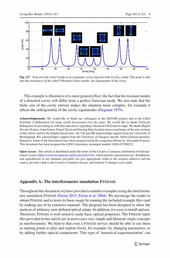
Living Rev Relativ (2016) 19:1 Page 203 of 221 1
Fig. 127 Scan over the order 9 peak in an astigmatic cavity injected with an LG33 mode. The peak is splitinto the resonances of the order 9 Hermite–Gauss modes, the eigenmodes of the cavity
This example is illustrative of a more general effect: the fact that the resonant modesof a distorted cavity will differ from a perfect Gaussian mode. We also note that thefinite size of the cavity mirrors makes the situation more complex, for example itaffects the orthogonality of the cavity eigenmodes (Siegman 1979).
Acknowledgements We would like to thank our colleagues in the GEO 600 project and in the LIGOScientific Collaboration for many useful discussions over the years. We would like to thank GariLynnBillingsley for providing us with data and advice regarding Advanced LIGO mirror maps. We thank MiguelDovale Álvarez, Anna Green, Daniel Töyrä and Haixing Miao for their time to read many of the new sectionsin this article and for the helpful discussions. AF, CB and DB acknowledge support from the University ofBirmingham. KS acknowledges support from the University of Glasgow and the Albert Einstein Institute,Hannover. Some of the illustrations have been prepared using the component library by Alexander Franzen.This document has been assigned the LIGO Laboratory document number LIGO-P1500233.
Open Access This article is distributed under the terms of the Creative Commons Attribution 4.0 Interna-tional License (http://creativecommons.org/licenses/by/4.0/), which permits unrestricted use, distribution,and reproduction in any medium, provided you give appropriate credit to the original author(s) and thesource, provide a link to the Creative Commons license, and indicate if changes were made.
Appendix A: The interferometer simulation FINESSE
Throughout this document we have provided a number examples using the interferom-eter simulation Finesse (Freise 2015; Freise et al. 2004). We encourage the reader toobtain Finesse and to learn its basic usage by running the included example files (andby making use of its extensive manual). The program has been designed to allow theanalysis of arbitrary, user-defined optical setups. In addition, it is easy to install and use.Therefore, Finesse is well suited to study basic optical properties. The Finesse inputfiles provided in this article are in most cases very simple and illustrate single conceptsin interferometry. We believe that even a Finesse novice should be able to use themas starting points to play and explore freely, for example, by changing parameters, orby adding further optical components. This type of ‘numerical experimentation’ can
123

1 Page 204 of 221 Living Rev Relativ (2016) 19:1
provide insights similar to real experiments, supplementing the understanding througha mathematical analysis with experience and intuition.
Free software
Finesse is a free software package developed and maintained by some of us (AFand DB): we provide free downloads of binaries for Linux, Windows and Macintoshcomputers online at: http://www.gwoptics.org/finesse/. The code is available underthe GPLv2 license and does not require any commercial software (such as Matlab) tocompile and run.
Development
Finesse is a numerical simulation written in the C language; it is actively developedto fix bugs as they are found and to add new features required to simulate new inter-ferometric systems. The recent updates allow modelling of suspended optics that areeffected by radiation pressure of the laser light as well as quantum effects such assqueezing and vacuum noise. We are further developing Pykat (Brown and Freise2015), a Python based toolbox to extend the use of Finesse, in particular for automat-ing tasks and data post-processing.
Gravitational-wave research
The Finesse development started in 1997 to support the design and commissioningof the gravitational-wave detector GEO 600 and Finesse has remained the standardsimulation software of that project. Since then Finesse has been developed continu-ously to meet the new challenges of the interferometric gravitational-wave detectorsworldwide such as LIGO, Virgo and KAGRA.20 Finesse provides a fast and versatiletool that is optimised for the type of low-noise, steady state laser interferometry usedby gravitational-wave detectors.
Appendix B: Advanced LIGO optical layout
In this review, the specific example of Advanced LIGO has been used to illustrate theoperation of an advanced gravitational wave detector. In this section, the layout andparameters of Advanced LIGO are presented, with a brief description of the motivationfor some of the key parameters.
Advanced LIGO configuration
Figure 128 shows the configuration of the central interferometer of Advanced LIGO,a dual recycled Michelson interferometer with Fabry–Perot arm cavities. The interfer-ometer is characterised by the parameters and performance of the different subsystemsof the interferometer: the arm cavities, power recycling cavity, signal recycling cavityand the Michelson.
Table 8 summarises the design optical parameters of the key components ofAdvanced LIGO: the input and end test masses (ITM and ETM) and the power and
20 A list of scientific papers and reports citing Finesse is provided in Freise (2015).
123
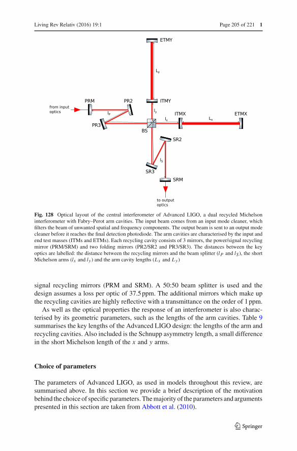
Living Rev Relativ (2016) 19:1 Page 205 of 221 1
Fig. 128 Optical layout of the central interferometer of Advanced LIGO, a dual recycled Michelsoninterferometer with Fabry–Perot arm cavities. The input beam comes from an input mode cleaner, whichfilters the beam of unwanted spatial and frequency components. The output beam is sent to an output modecleaner before it reaches the final detection photodiode. The arm cavities are characterised by the input andend test masses (ITMs and ETMs). Each recycling cavity consists of 3 mirrors, the power/signal recyclingmirror (PRM/SRM) and two folding mirrors (PR2/SR2 and PR3/SR3). The distances between the keyoptics are labelled: the distance between the recycling mirrors and the beam splitter (lP and lS ), the shortMichelson arms (lx and ly ) and the arm cavity lengths (Lx and Ly )
signal recycling mirrors (PRM and SRM). A 50:50 beam splitter is used and thedesign assumes a loss per optic of 37.5 ppm. The additional mirrors which make upthe recycling cavities are highly reflective with a transmittance on the order of 1 ppm.
As well as the optical properties the response of an interferometer is also charac-terised by its geometric parameters, such as the lengths of the arm cavities. Table 9summarises the key lengths of the Advanced LIGO design: the lengths of the arm andrecycling cavities. Also included is the Schnupp asymmetry length, a small differencein the short Michelson length of the x and y arms.
Choice of parameters
The parameters of Advanced LIGO, as used in models throughout this review, aresummarised above. In this section we provide a brief description of the motivationbehind the choice of specific parameters. The majority of the parameters and argumentspresented in this section are taken from Abbott et al. (2010).
123
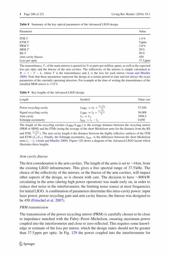
1 Page 206 of 221 Living Rev Relativ (2016) 19:1
Table 8 Summary of the key optical parameters of the Advanced LIGO design
Parameter Value
ITM T 1.4 %ETM T 5 ppmPRM T 3.0 %SRM T 20 %BS T 50 %Arm cavity finesse 450Loss per optic 37.5 ppm
The transmittance, T , of the main mirrors is quoted (in % or parts-per-million, ppm), as well as the expectedloss per optic and the finesse of the arm cavities. The reflectivity of the mirrors is simple calculated asR = 1 − T − L , where T is the transmittance and L is the loss for each mirror (Arain and Mueller2009). Note that these parameters represent the design at a certain period in time and not always the exactparameters of the currently operating detectors. For example at the time of writing the transmittance of theinstalled SRM mirror is ≈35 %
Table 9 Key lengths of the Advanced LIGO design
Length Symbol Value (m)
Power recycling cavity LPRC = lP + lx+ly2 57.656
Signal recycling cavity LSRC = lS + lx+ly2 56.008
Arm cavity Lx = Ly 3994.5Schnupp asymmetry lSch. = lx − ly 0.050
The length of the recycling cavities (LPRC/LSRC) is the average distance between the recycling mirror(PRM or SRM) and the ITMs (using the average of the short Michelson arms for the distance from the BS
and ITM,lx+ly
2 ). The arm cavity length is the distance between the highly reflective surfaces of the ITMand ETM (Lx /Ly ). Finally, the Schnupp asymmetry, lSch., is the difference between the short Michelsonarms lx − ly (Arain and Mueller 2009). Figure 128 shows a diagram of the Advanced LIGO layout whichillustrates these lengths
Arm cavity finesse
The first consideration is the arm cavities. The length of the arms is set to ∼4 km, fromthe existing LIGO infrastructure. This gives a free spectral range of 37.5 kHz. Thechoice of the reflectivity of the mirrors, or the finesse of the arm cavities, will impactother aspects of the design, so is chosen with care. The decision to have ∼800 kWcirculating in the arms (during high power operation) was made early on, in order toreduce shot noise in the interferometer, the limiting noise source at most frequenciesfor initial LIGO. A combination of parameters determine this intra-cavity power: inputlaser power, power recycling gain and arm cavity finesse; the finesse was designed tobe 450 (Fritschel et al. 2007).
PRM transmission
The transmission of the power recycling mirror (PRM) is carefully chosen to be closeto impedance matched with the Fabry–Perot–Michelson, ensuring maximum powercoupled into the interferometer and close to zero reflected. This requires some knowl-edge or estimate of the loss per mirror, which the design states should not be greaterthan 37.5 ppm per optic. In Fig. 129 the power coupled into the interferometer for
123
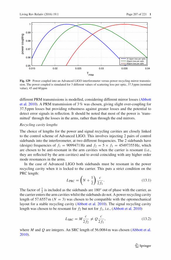
Living Rev Relativ (2016) 19:1 Page 207 of 221 1
0.015 0.02 0.025 0.03 0.035 0.040.95
0.96
0.97
0.98
0.99
1
TPRM
pow
er c
oupl
ing
37.5ppm loss per optic45ppm loss per optic60ppm loss per optic
Fig. 129 Power coupled into an Advanced LIGO interferometer versus power recycling mirror transmis-sion. The power coupled is simulated for 3 different values of scattering loss per optic, 37.5 ppm (nominalvalue), 45 and 60 ppm
different PRM transmissions is modelled, considering different mirror losses (Abbottet al. 2010). A PRM transmission of 3 % was chosen, giving slight over-coupling for37.5 ppm losses but providing robustness against greater losses and the potential todetect error signals in reflection. It should be noted that most of the power is ‘trans-mitted’ through the losses in the arms, rather than through the end mirrors.
Recycling cavity lengths
The choice of lengths for the power and signal recycling cavities are closely linkedto the control scheme of Advanced LIGO. This involves injecting 2 pairs of controlsidebands into the interferometer, at two different frequencies. The 2 sidebands have(design) frequencies of f1 = 9099471 Hz and f2 = 5 × f1 = 45497355 Hz, whichare chosen to be anti-resonant in the arm cavities when the carrier is resonant (i.e.,they are reflected by the arm cavities) and to avoid coinciding with any higher ordermode resonances in the arms.
In the case of Advanced LIGO both sidebands must be resonant in the powerrecycling cavity when it is locked to the carrier. This puts a strict condition on thePRC length:
LPRC =(N + 1
2
)c
2 f1. (13.1)
The factor of 12 is included as the sidebands are 180◦ out of phase with the carrier, as
the carrier enters the arm cavities whilst the sidebands do not. A power recycling cavitylength of 57.6557 m (N = 3) was chosen to be compatible with the optomechanicallayout for a stable recycling cavity (Abbott et al. 2010). The signal recycling cavitylength was chosen to be resonant for f2 but not for f1, i.e., (Abbott et al. 2010)
LSRC = Mc
2 f2�= Q
c
2 f1, (13.2)
where M and Q are integers. An SRC length of 56.0084 m was chosen (Abbott et al.2010).
123

1 Page 208 of 221 Living Rev Relativ (2016) 19:1
For control of Advanced LIGO one of the sidebands should exit the Michelson intothe signal recycling cavity and eventually the output port. However, in a Michelsonwhere the short arms between the beam splitter and ITMs (lx /ly) are the same lengththe dark fringe for the carrier will also be the dark fringe for the sidebands. In orderfor one of the sidebands ( f2) to leak into the signal recycling cavity we need someasymmetry between the two arms, the so-calledSchnuppasymmetry, lSch = lx−ly �= 0(Hild et al. 2009). In the case of Advanced LIGO a Schnupp asymmetry of 5 cm was acompromise between maximising the coupling of f2 into the signal recycling cavity fortwo different cases: broadband signal recycling and slightly detuned signal recycling(optimised for neutron star–neutron star in-spiral (NS–NS) signals).
Mode-matching
The curvatures of the highly reflective mirror surfaces and distances between individualmirrors determine the size and shape of the resonating beams. The individual cavitiesin the detector need to be well mode matched to maximise the power build up andavoid high contrast defects.
The eigenmode of the arm cavities is selected to produce large beams at the ITM(5.3 cm) and ETM (6.2 cm) to reduce thermal noise, with slightly smaller beams at theITM due to lower thermal noise (fewer coating layers) and to prevent scattering intothe recycling cavities. The curvatures are also carefully selected for a specific Gouyphase to avoid higher order modes easily ringing up in the arms: RC = 1934 m (ITM)and RC = 2245 m (ETM).
In initial LIGO the power recycling cavity was marginally unstable, enhancingthe power in higher order modes in the control sidebands and causing problems forcontrol (Gretarsson et al. 2007). To avoid this in Advanced LIGO the interferometerwas designed with stable recycling cavities: folded cavities which do not share the armcavity eigenmode (Arain and Mueller 2008), see Sect. 10.7. These cavities consist of3 mirrors, the primary recycling mirrors (PRM/SRM) and two additional mirrors toshape and direct the beam (PR2/SR2 and PR3/SR3). The curvatures and positions ofthe mirrors are chosen to ensure good mode matching into the arm cavities and toachieve a good spacing between higher order resonances (see Sect. 10.7).
The mode matching of the beams between the recycling cavities and arms is com-plicated by thermal effects, specifically thermal lensing and the change in mirrorcurvatures. Although this will be corrected by thermal compensation systems (Willems2009) it was decided to match the recycling cavities to the arms in the presence of50 km lenses in the ITMs, as expected for an input power of ∼12.5 W with coatingabsorptions of 0.5 ppm (Arain and Mueller 2009). This will potentially mitigate theuse of TCS at low power. In the end the cavities were designed for a 50 km lens insidethe substrate (effective 34.5 km lens) corresponding to 18 W input power.
Degrees of freedom
In Fig. 130 a simplified diagram of the Advanced LIGO dual recycled configurationis shown, with the lengths which require control labelled. The microscopic degrees offreedom associated with these lengths are:
– CARM Common-mode arm motion, CARM = Lx + Ly . This tunes the averagelength of the arm cavities and is used to keep the arms on resonance.
123

Living Rev Relativ (2016) 19:1 Page 209 of 221 1
Fig. 130 Simplified layout of the dual recycled Fabry–Perot–Michelson of Advanced LIGO, illustratingthe fields inside the interferometer. All main mirrors are shown: power and signal recycling mirrors (PRMand SRM); input test masses (ITMX and ITMY); end test masses (ETMX and ETMY); and the central beamsplitter. Also shown are the locations of various photodiodes: REFL (reflected port), POP (power recyclingpick off port) and AS (anti-symmetric port). The paths of the different light fields in the interferometerare shown. The carrier resonates inside the arm cavities and power recycling cavity, with the Fabry–Perot–Michelson tuned close to the carrier dark fringe. A small amount of carrier light leaks into the anti-symmetricport due to a small DC offset. The RF sidebands used for control resonate in the power recycling cavitybut are reflected from the arms. The Michelson is not at the dark fringe for the control sidebands and theyappear in the signal recycling cavity and at the Michelson output. The signal sidebands generated by agravitational wave originate in the arm cavities and then exit the Michelson through the anti-symmetric port
– PRCL Power recycling cavity length, PRCL = l p + lx+ly2 . The power recycling
cavity is operated on resonance to maximise the power coupled into the centralinterferometer.
– MICH Michelson arm length, MICH = lx − ly . MICH controls the short arms ofthe Michelson (between the ITMs and beam splitter) and determines the fringe atthe output port. Generally the Michelson is operated on the dark fringe.
– DARM Differential arm motion, DARM = Lx − Ly . This controls the differencein length of the two arm cavities and is used to get the best interference betweenthe two arms at the dark port.
– SRCL Signal recycling cavity length, SRCL = ls + lx+ly2 . Used to control the
operation of the signal recycling cavity. The operating point of SRCL dependson the mode of operation of the interferometer. It can be tuned for a particularfrequency of gravitational wave or for broadband operation.
123

1 Page 210 of 221 Living Rev Relativ (2016) 19:1
References
Aasi J et al (2015) Advanced LIGO. Class Quantum Gravity 32(7):074001Abbott B et al (2004) Detector description and performance for the first coincidence observations between
LIGO and GEO. Nucl Instrum Methods Phys Res Sect A Accel Spectrom Detect Assoc Equip 517:154–179. doi:10.1016/j.nima.2003.11.124
Abbott BP, Abbott R, Abbott TD, Abernathy MR, Acernese F, Ackley K, Adams C, Adams T, AddessoP, Adhikari RX et al (2016a) GW151226: observation of gravitational waves from a 22-solar-massbinary black hole coalescence. Phys Rev Lett 116:241103. doi:10.1103/PhysRevLett.116.241103.arXiv:1606.04855
Abbott BP, Abbott R, Abbott TD, Abernathy MR, Acernese F, Ackley K, Adams C, Adams T, Addesso P,Adhikari RX et al (2016b) Observation of gravitational waves from a binary black hole merger. PhysRev Lett 116:061102. doi:10.1103/PhysRevLett.116.061102
Abbott R, Adhikari R, Ballmer S, Barsotti L, Evans M, Fritschel P, Frolov V, Mueller G, Slagmolen B,Waldman S (2010) Advanced LIGO length sensing and control final design. LIGO document, LIGO,Pasadena. https://dcc.ligo.org/LIGO-T1000298/public
Abramochkin E, Volostnikov V (1991) Beam transformations and nontransformed beams. Opt Commun83:123–135. doi:10.1016/0030-4018(91)90534-K
Abramowitz M, Stegun IA (eds) (1965) Handbook of mathematical functions with formulas, graphs, andmathematical tables, corr edn. Dover, New York
Accadia T et al (2010) Noise from scattered light in Virgo’s second science run data. Class Quantum Gravity27(19):194011. doi:10.1088/0264-9381/27/19/194011
Acernese F et al (2006) The Virgo automatic alignment system. Class Quantum Gravity 23:S91–S101.doi:10.1088/0264-9381/23/8/S13
Acernese F et al (2015) Advanced Virgo: a second-generation interferometric gravitational wave detector.Class Quantum Gravity 32:024001
Adhikari R, Fritschel P, Waldman SJ (2006) Enhanced LIGO. LIGO Document LIGO-T060156, Pasadena.https://dcc.ligo.org/LIGO-T060156/public
Advanced LIGO Team (2007) Advanced LIGO reference design. Tech. Rep. LIGO-M060056-08, Pasadena.http://www.ligo.caltech.edu/docs/M/M060056-08/M060056-08.pdf
Anderson DZ (1984) Alignment of resonant optical cavities. Appl Opt 23:2944–2949. doi:10.1364/AO.23.002944
Arai K (2013) On the accumulated round-trip Gouy phase shift for a general optical cavity. Tech. Rep.T1300189, LIGO DCC, Pasadena. https://dcc.ligo.org/LIGO-T1300189/public
Arai K, Korth W (2015) aLIGO OMC optical design status. LIGO Document LIGO-G1201111, Pasadena.https://dcc.ligo.org/LIGO-G1201111/public
Arai K, Ando M, Moriwaki S, Kawabe K, Tsubono K (2000) New signal extraction scheme with harmonicdemodulation for power-recycled Fabry–Perot–Michelson interferometers. Phys Lett A 273:15–24.doi:10.1016/S0375-9601(00)00467-9
Arai K, Barnum S, Fritschel P, Lewis J, Waldman S (2013) Output mode cleaner design. LIGO DocumentLIGO-T1000276, Pasadena. https://dcc.ligo.org/LIGO-T1000276/public
Arain MA, Mueller G (2008) Design of the Advanced LIGO recycling cavities. Opt Express 16:10018–10032
Arain MA, Mueller G (2009) Optical layout and parameters for the Advanced LIGO cavities. Tech. rep.,Advanced LIGO, Pasadena, lIGO-T0900043-04
Arain MA, Mueller C, Mueller G (2012) Optical layout and parameters for the Advanced LIGO Cavities.Tech. Rep. LIGO-T0900043, Pasadena. https://dcc.ligo.org/LIGO-T0900043/public
Arnaud N, Arnault C, Barsuglia M, Bizouard MA, Brisson V, Cavalier F, Chiche R, Davier M, Eder C,Hello P, Heusse P, Kreckelbergh S, Mansoux B (2005) The global control of the Virgo experiment.Nucl Instrum Methods A 550:467–489. doi:10.1016/j.nima.2005.03.173
Aso Y, Michimura Y, Somiya K, Ando M, Miyakawa O, Sekiguchi T, Tatsumi D, Yamamoto H (2013)Interferometer design of the KAGRA gravitational wave detector. Phys Rev D 88:043007. doi:10.1103/PhysRevD.88.043007
Aspelmeyer M, Kippenberg TJ, Marquardt F (2014) Cavity optomechanics. Rev Mod Phys 86:1391–1452.doi:10.1103/RevModPhys.86.1391
Aston SM, Barton MA, Bell AS, Beveridge N, Bland B, Brummitt AJ, Cagnoli G, Cantley CA, Carbone L,Cumming AV, Cunningham L, Cutler RM, Greenhalgh RJS, Hammond GD, Haughian K, Hayler TM,
123
Living Rev Relativ (2016) 19:1 Page 211 of 221 1
Heptonstall A, Heefner J, Hoyland D, Hough J, Jones R, Kissel JS, Kumar R, Lockerbie NA, LodhiaD, Martin IW, Murray PG, O’Dell J, Plissi MV, Reid S, Romie J, Robertson NA, Rowan S, Shapiro B,Speake CC, Strain KA, Tokmakov KV, Torrie C, van Veggel AA, Vecchio A, Wilmut I (2012) Updateon quadruple suspension design for Advanced LIGO. Class Quantum Gravity 29(23):235004. doi:10.1088/0264-9381/29/23/235004
Bachor HA, Manson PJ (1990) Practical implications of quantum noise. J Mod Opt 37:1727–1740. doi:10.1080/09500349014551951
Ballmer S, Degallaix J, Freise A, Fulda P (2014) Comparing Finesse simulations, analytical solutions andOSCAR simulations of Fabry–Perot alignment signals. arXiv:1401.5727
Barriga P, Dumas JC, Woolley AA, Zhao C, Blair DG (2009) Compact vibration isolation and suspensionfor Australian International Gravitational Observatory: Performance in a 72 m Fabry-Perot cavity. RevSci Instrum 80:114501. doi:10.1063/1.3250841
Bayer-Helms F (1984) Coupling coefficients of an incident wave and the modes of spherical optical resonatorin the case of mismatching and misalignment. Appl Opt 23:1369–1380. doi:10.1364/AO.23.001369
Beijersbergen MW, Allen L, van der Veen HELO, Woerdman JP (1993) Astigmatic laser modeconverters and transfer of orbital angular momentum. Opt Commun 96:123–132. doi:10.1016/0030-4018(93)90535-D
Beyersdorf PT, Byer RL, Fejer MM (2002) Results from the Stanford 10 m Sagnac interferometer. ClassQuantum Gravity 19:1585–1589. doi:10.1088/0264-9381/19/7/348
Billing H, Maischberger K, Rüdiger A, Schilling R, Schnupp L, Winkler W (1983) The Munich gravitationalwave detector using laser interferometry. In: Meystre P, Scully M (eds) Quantum optics, experimentalgravity, and measurement theory, NATO ASI Series B, vol 94. Plenum Press, New York, pp 525–566
Billingsley G (2015) LIGO core optics reference page. Tech. rep., Pasadena. https://galaxy.ligo.caltech.edu/optics/
Billingsley G, Zhang L (2012) All about optics. Tech. rep., LIGO Laboratory, LIGO Scientific Collaboration,Pasadena. https://dcc.ligo.org/LIGO-G1200565/public
Bochner B, Hefetz Y (2003) Grid-based simulation program for gravitational wave interferometers withrealistically imperfect optics. Phys Rev D 68:082001. doi:10.1103/PhysRevD.68.082001
Bond C (2014) How to stay in shape: overcoming beam and mirror distortions in advanced gravitationalwave interferometers. PhD Thesis, University of Birmingham, Birmingham. http://etheses.bham.ac.uk/5223/2/Bond14PhD.pdf
Bond C, Fulda P, Carbone L, Kokeyama K, Freise A (2011) Higher order Laguerre–Gauss mode degeneracyin realistic, high finesse cavities. Phys Rev D 84:102002. doi:10.1103/PhysRevD.84.102002
Bond C, Fulda P, Brown D, Freise A (2013) Investigation of beam clipping in the Power Recycling Cavityof Advanced LIGO using FINESSE. Tech. Rep. LIGO-T1300954, Pasadena. https://dcc.ligo.org/LIGO-T1300954/public
Bond C, Fulda P, Brown D, Freise A (2014a) Comparing simulations of the Advanced LIGO Dual-RecycledMichelson. Tech. Rep. LIGO-T1400270, Pasadena. https://dcc.ligo.org/LIGO-T1400270/public
Bond C, Fulda P, Brown D, Freise A (2014b) Simulations of effects of LLO mode-mismatches on PRFPMIerror signals. Tech. Rep. LIGO-T1400182, Pasadena. https://dcc.ligo.org/LIGO-T1400182/public
Boyd R (1980) Intuitive explanation of the phase anomaly of focused light beams. J Opt Soc Am 70(7):877–880. doi:10.1364/JOSA.70.000877
Braccini S, Bradaschia C, Del Fabbro R, Di Virgilio A, Ferrante I, Fidecaro F, Flaminio R, Gennai A, GiassiA, Giazotto A, Gorini G, Losurdo G, Palla F, Pasqualetti A, Passuello D, Poggiani R, Torelli G, ZhangZ (1996) Seismic vibrations mechanical filters for the gravitational waves detector VIRGO. Rev SciInstrum 67:2899–2902. doi:10.1063/1.1147069
Braginskii VB, Vorontsov II (1975) Quantum-mechanical limitations in macroscopic experiments and mod-ern experimental technique. Sov Phys Usp 114:41–53. doi:10.1070/PU1975v017n05ABEH004362
Braginsky VB, Khalili FY (1996) Quantum nondemolition measurements: the route from toys to tools. RevMod Phys 68:1–11. doi:10.1103/RevModPhys.68.1
Braginsky VB, Vorontsov YI, Thorne KS (1980) Quantum nondemolition measurements. Science 209:547–557. doi:10.1126/science.209.4456.547
Braginsky VB, Gorodetsky ML, Khalili FY (1997) Optical bars in gravitational wave antennas. Phys LettA 232(5):340–348. doi:10.1016/S0375-9601(97)00413-1
Braginsky VB, Gorodetsky ML, Khalili FY, Thorne KS (2000) Energetic quantum limit in large-scaleinterferometers. In: Meshkov S (ed) Gravitational waves: third Edoardo Amaldi conference, AIP
123

1 Page 212 of 221 Living Rev Relativ (2016) 19:1
conference proceedings, vol 523. American Institute of Physics, Melville, pp 180–190. doi:10.1063/1.1291855. arXiv:gr-qc/9907057
Braginsky VB, Strigin SE, Vyatchanin SP (2001) Parametric oscillatory instability in Fabry–Perot interfer-ometer. Phys Lett A 287:331–338. doi:10.1016/S0375-9601(01)00510-2. arXiv:gr-qc/0107079
Brooks A, Cole A, Heptonstall A, Jacobson M, Lynch A, O’Connor S, Shao Z, Vorvick C (2012) ThermalCompensation Systems (TCS): CO2 Laser Projection System (CO2P): Final Design Document. LIGODocument T1100570, Pasadena, CA
Brown D, Freise A (2015) PyKat: Python interface and tools for Finesse. http://www.gwoptics.org/pykat/Brown DD (2016) Interactions of light and mirrors: advanced techniques for modelling future gravitational
wave detectors. PhD Thesis, University of Birmingham, Birmingham. http://etheses.bham.ac.uk/6500/Buonanno A, Chen Y (2002) Signal recycled laser-interferometer gravitational-wave detectors as optical
springs. Phys Rev D 65(4):042001. doi:10.1103/PhysRevD.65.042001. arXiv:gr-qc/0107021Buonanno A, Chen Y, Mavalvala N (2003) Quantum noise in laser-interferometer gravitational-wave detec-
tors with a heterodyne readout scheme. Phys Rev D 67:122005. doi:10.1103/PhysRevD.67.122005.arXiv:gr-qc/0302041
Caron B, Derome L, Flaminio R, Grave X, Marion F et al (1999) SIESTA, a time domain, generalpurpose simulation program for the VIRGO experiment. Astropart Phys 10:369–386. doi:10.1016/S0927-6505(98)00059-0
Caves C (1981) Quantum-mechanical noise in an interferometer. Phys Rev D 23:1693–1708. doi:10.1103/PhysRevD.23.1693
Caves CM, Schumaker BL (1985) New formalism for two-photon quantum optics. I. Quadrature phasesand squeezed states. II. Mathematical foundation and compact notation. Phys Rev A 31:3068–3111.doi:10.1103/PhysRevA.31.3068
Chelkowski S (2007) Squeezed light and laser interferometric gravitational wave detectors. PhD Thesis,Universität Hannover, Hannover. http://edok01.tib.uni-hannover.de/edoks/e01dh07/537859527.pdf
Chelkowski S, Hild S, Freise A (2009) Prospects of higher-order Laguerre–Gauss modes in future gravita-tional wave detectors. Phys Rev D 79:122002. doi:10.1103/PhysRevD.79.122002. arXiv:0901.4931
Chen Y (2003) Sagnac interferometer as a speed-meter-type, quantum-nondemolition gravitational-wavedetector. Phys Rev D 67:122004. doi:10.1103/PhysRevD.67.122004. arXiv:gr-qc/0208051
Chen Y, Danilishin SL, Khalili FY, Müller-Ebhardt H (2010) QND measurements for future gravitational-wave detectors. Gen Relativ Gravit 43:671–694. doi:10.1007/s10714-010-1060-y
Chua SSY, Slagmolen BJJ, Shaddock DA, McClelland DE (2014) Quantum squeezed light in gravitational-wave detectors. Class Quantum Gravity 31:183001
Corbitt T, Chen Y, Mavalvala N (2005) Mathematical framework for simulation of quantum fields in complexinterferometers using the two-photon formalism. Phys Rev A 72:013818. doi:10.1103/PhysRevA.72.013818
Corbitt T, Ottaway D, Innerhofer E, Pelc J, Mavalvala N (2006) Measurement of radiation-pressure-inducedoptomechanical dynamics in a suspended Fabry-Perot cavity. Phys Rev A 74(2):021802. doi:10.1103/PhysRevA.74.021802
Danilishin SL (2004) Sensitivity limitations in optical speed meter topology of gravitational-wave antennas.Phys Rev D 69:102003
Danilishin SL, Khalili FY (2012) Quantum measurement theory in gravitational-wave detectors. LivingRev Relativ 15:lrr-2012-5. doi:10.12942/lrr-2012-5. http://www.livingreviews.org/lrr-2012-5
Danilishin SL, Gräf C, Leavey SS, Hennig J, Houston EA, Pascucci D, Steinlechner S, Wright J, Hild S(2015) Quantum noise of non-ideal Sagnac speed meter interferometer with asymmetries. New J Phys17:043031
Danzmann K, Lück H, Rüdiger A, Schilling R, Schrempel M, Winkler W, Hough J, Newton G, RobertsonN, Ward H, Campbell A, Logan J, Robertson D, Strain K, Bennett J, Kose V, Kühne M, Schutz B,Nicholson D, Shuttleworth J, Welling H, Aufmuth P, Rinkleff R, Tünnermann A, Willke B (1994)GEO600: proposal for a 600 m laser-interferometric gravitational wave antenna, MPQ, vol 190. MPQGarching, Max Planck Institute of Quantum Optics, Garching
Davis TA (2006) Direct methods for sparse linear systems, fundamentals of algorithms, vol 2. SIAM,Philadelphia. http://www.cise.ufl.edu/research/sparse/CSparse/
Day RA, Vajente G, du Mezeray MP (2014) Accelerated convergence method for fast Fourier transformsimulation of coupled cavities. J Opt Soc Am A 31(3):652–660. doi:10.1364/JOSAA.31.000652
di Virgilio A, Barsotti L, Braccini S, Bradaschia C, Cella G, Corda C, Dattilo V, Ferrante I, Fidecaro F, FioriI, Frasconi F, Gennai A, Giazotto A, La Penna P, Losurdo G, Majorana E, Mantovani M, Pasqualetti
123

Living Rev Relativ (2016) 19:1 Page 213 of 221 1
A, Passuello D, Piergiovanni F, Porzio A, Puppo P, Rapagnani P, Ricci F, Solimeno S, Vajente G,Vetrano F (2006) Experimental evidence for an optical spring. Phys Rev A 74(1):013813. doi:10.1103/PhysRevA.74.013813
Dooley KL, Barsotti L, Adhikari RX, Evans M, Fricke TT, Fritschel P, Frolov V, Kawabe K, Smith-LefebvreN (2013) Angular control of optical cavities in a radiation-pressure-dominated regime: the EnhancedLIGO case. J Opt Soc Am A 30(12):2618–2626. doi:10.1364/JOSAA.30.002618
Drever RWP et al (1983) Gravitational wave detectors using laserinterferometers and optical cavities.Proceedings of the NATO ASI quantum optics and experimental general relativity, Bad Windsheim(1981) in quantum optics, experimental gravity and measurement theory. Plenum Press, New York,pp 503–524
Drever RWP, Hough J, Munley AJ, Lee SA, Spero RE, Whitcomb SE, Ward H, Ford GM, Hereld M,Robertson NA, Kerr I, Pugh JR, Newton GP, Meers BJ, Brooks ED III, Gürsel Y (1983) Gravitationalwave detectors using laser interferometers and optical cavities: ideas, principles and prospects. In:Meystre P, Scully MO (eds) Quantum optics, experimental gravity, and measurement theory, NATOASI Series B, vol 94. Plenum Press, New York, pp 503–514
Evans M (2004) Optickle simulation software. Tech. rep., Pasadena. https://github.com/Optickle/OptickleEvans M, Fritschel P, McClelland D, Miller J, Mullavey A, Shaddock D, Slagmolen B, Waldman S et al
(2009) Advanced LIGO arm length stabilisation system design. Tech. Rep. LIGO-T0900144-05,Pasadena. https://dcc.ligo.org/T0900144/public
Evans M, Barsotti L, Fritschel P (2010) A general approach to optomechanical parametric instabilities.Phys Lett A 374:665–671. doi:10.1016/j.physleta.2009.11.023
Evans M, Gras S, Fritschel P, Miller J, Barsotti L, Martynov D, Brooks A, Coyne D, Abbott R, AdhikariRX, Arai K, Bork R, Kells B, Rollins J, Smith-Lefebvre N, Vajente G, Yamamoto H, Adams C, AstonS, Betzweiser J, Frolov V, Mullavey A, Pele A, Romie J, Thomas M, Thorne K, Dwyer S, Izumi K,Kawabe K, Sigg D, Derosa R, Effler A, Kokeyama K, Ballmer S, Massinger TJ, Staley A, HeinzeM, Mueller C, Grote H, Ward R, King E, Blair D, Ju L, Zhao C (2015) Observation of parametricinstability in Advanced LIGO. Phys Rev Lett 114:161102. doi:10.1103/PhysRevLett.114.161102
Fabry C, Perot A (1899) Théorie et applications d’une nouvelle méthode de spectroscopie interférentielle.Ann Chim Phys 16:115–144
Fattaccioli D, Boulharts A, Brillet A, Man CN (1986) Sensitivity of multipass and Fabry–Perot delay linesto small misalignments. J Opt (Paris) 17:115–127. doi:10.1088/0150-536X/17/3/001
Forward RL (1978) Wideband laser-interferometer gravitational-radiation experiment. Phys Rev D 17:379–390. doi:10.1103/PhysRevD.17.379
Franklin G, Powell J, Workman M (1998) Digital control of dynamic systems, 3rd edn. Addison-Wesley,Boston
Freise A (2003) The next generation of interferometry: multi-frequency optical modelling, control conceptsand implementation. PhD Thesis, Universität Hannover, Hannover. http://edok01.tib.uni-hannover.de/edoks/e01dh03/361006918.pdf
Freise A (2015) FINESSE: an interferometer simulation. http://www.gwoptics.org/finesseFreise A, Heinzel G, Lück H, Schilling R, Willke B, Danzmann K (2004) Frequency-domain interferometer
simulation with higher-order spatial modes. Class Quantum Gravity 21:S1067–S1074. doi:10.1088/0264-9381/21/5/102. arXiv:gr-qc/0309012
Freise A, Bunkowski A, Schnabel R (2007) Phase and alignment noise in grating interferometers. New JPhys 9:433. doi:10.1088/1367-2630/9/12/433. arXiv:0711.0291
Fricke TT, Smith-Lefebvre ND, Abbott R, Adhikari R, Dooley KL, Evans M, Fritschel P, Frolov VV, KawabeK, Kissel JS, Slagmolen BJJ, Waldman SJ (2012) DC readout experiment in Enhanced LIGO. ClassQuantum Gravity 29:065005. doi:10.1088/0264-9381/29/6/065005
Fritschel P (2003) Second generation instruments for the Laser Interferometer Gravitational Wave Obser-vatory (LIGO). In: Cruise M, Saulson P (eds) Gravitational-wave detection, Proceedings of SPIE, vol4856. SPIE, Bellingham, pp 282–291. doi:10.1117/12.459090. arXiv:gr-qc/0308090
Fritschel P, Adhikari R, Ballmer S, Evans M (2007) Arm cavity Finesse for Advanced LIGO. LIGO Docu-ment T070303, Pasadena, CA
Fritschel P, Evans M, Frolov V (2014) Balanced homodyne readout for quantum limited gravitational wavedetectors. Opt Express 22:4224–4234. doi:10.1364/OE.22.004224
Giovannetti V, Lloyd S, Maccone L (2004) Quantum-enhanced measurements: beating the standard quantumlimit. Science 306:1330–1336. doi:10.1126/science.1104149. arXiv:quant-ph/0412078
Gouy LG (1890a) Sur la propagation anomale des ondes. C R Acad Sci 111:33
123
1 Page 214 of 221 Living Rev Relativ (2016) 19:1
Gouy LG (1890b) Sur une propriété nouvelle des ondes lumineuses. C R Acad Sci 110:1251Gradshteyn I, Ryzhik I (1994) Tables of integrals, series, and products, 5th edn. Academic Press, San DiegoGras S, Zhao C, Blair DG, Ju L (2010) Parametric instabilities in advanced gravitational wave detectors.
Class Quantum Gravity 27:205019Gretarsson AM, D’Ambrosio E, Frolov V, O’Reilly B, Fritschel PK (2007) Effects of mode degeneracy in
the LIGO Livingston Observatory recycling cavity. J Opt Soc Am B 24:2821. doi:10.1364/JOSAB.24.002821. arXiv:0708.3470
Grote H (2003) Making it work: second generation interferometry in GEO600! PhD Thesis, UniversitätHannover, Hannover. http://edok01.tib.uni-hannover.de/edoks/e01dh03/373626789.pdf
Harms J, Cochrane P, Freise A (2007) Quantum-noise power spectrum of fields with discrete classicalcomponents. Phys Rev A 76:023803. doi:10.1103/PhysRevA.76.023803. arXiv:quant-ph/0703119
Harry GM, the LIGO Scientific Collaboration, (2010) Advanced LIGO: the next generation of gravitationalwave detectors. Class Quantum Gravity 27:084006. doi:10.1088/0264-9381/27/8/084006
Hecht E (2002) Optics, 4th edn. Addison-Wesley, ReadingHeinzel G (1999) Advanced optical techniques for laser-interferometric gravitational-wave detectors. PhD
Thesis, Universität Hannover, Hannover. http://edok01.tib.uni-hannover.de/edoks/e002/265099560.pdf
Heinzel G, Strain K, Mizuno J, Skeldon K, Willke B, Winkler W, Schilling R, Rüdiger A, Danzmann K(1998) Experimental demonstration of a suspended dual recycling interferometer for gravitationalwave detection. Phys Rev Lett 81:5493–5496. doi:10.1103/PhysRevLett.81.5493
Hello P, Vinet JY (1990) Analytical models of thermal aberrations in massive mirrors heated by high powerlaser beams. J Phys Fr 51:1267–1282
Herriott D, Kogelnik H, Kompfner R (1964) Off-axis paths in spherical mirror interferometers. Appl Opt3:523–526. doi:10.1364/AO.3.000523
Hild S, Grote H, Degallaix J, Chelkowski S, Danzmann K, Freise A, Hewitson M, Hough J, Luck H, PrijateljM, Strain KA, Smith JR, Willke B (2009) DC-readout of a signal-recycled gravitational wave detector.Class Quantum Gravity 26:055012
Hirose E, Kawabe K, Sigg D, Adhikari R, Saulson PR (2010) Angular instability due to radiation pressurein the LIGO gravitational-wave detector. Appl Opt 49(18):3474–3484
Hong T, Miller J, Yamamoto H, Chen Y, Adhikari R (2011) Effects of mirror aberrations on Laguerre–Gaussian beams in interferometric gravitational-wave detectors. Phys Rev D 84:102001. doi:10.1103/PhysRevD.84.102001
Jaekel M, Reynaud S (1990) Quantum limits in interferometric measurements. Europhys Lett 13:301–306.doi:10.1209/0295-5075/13/4/003. arXiv:quant-ph/0101104
Jerome D (2008) OSCAR: a Matlab based FFT code. Tech. rep. http://www.mathworks.com/matlabcentral/fileexchange/20607-oscar
Kawazoe F, Kokeyama K, Sato S, Miyakawa O, Somiya K, Fukushima M, Arai N, Kawamura S, SugamotoA (2006) The experimental plan of the 4 m resonant sideband extraction prototype for the LCGT. JPhys Conf Ser 32:380–385. doi:10.1088/1742-6596/32/1/058
Kenyon IR (2008) The light fantastic: a modern introduction to classical and quantum optics. OxfordUniversity Press, Oxford
Khalili FY, Levin Y (1996) Speed meter as a quantum nondemolition measuring device for force. Phys RevD 54:4735–4737. doi:10.1103/PhysRevD.54.4735. arXiv:gr-qc/9603046
Kimble HJ, Levin Y, Matsko AB, Thorne KS, Vyatchanin SP (2002) Conversion of conventionalgravitational-wave interferometers into quantum nondemolition interferometers by modifying theirinput and/or output optics. Phys Rev D 65:022002
Kogelnik H (1965) On the propagation of Gaussian beams of light through lenslike media including thosewith a loss or gain variation. Appl Opt 4(12):1562–1569. doi:10.1364/AO.4.001562
Kogelnik H, Li T (1966) Laser beams and resonators. Proc IEEE 54:1312–1329. doi:10.1109/PROC.1966.5119
Kokeyama K, Arai K, Fulda P, Doravari S, Carbone L, Brown D, Bond C, Freise A (2013) Finesse simulationfor the alignment control signal of the a LIGO input mode cleaner. LIGO Document LIGO-T1300074,Pasadena. https://dcc.ligo.org/LIGO-T1300074/public
Kwee P, Bogan C, Danzmann K, Frede M, Kim H, King P, Pöld J, Puncken O, Savage RL, Seifert F,Wessels P, Winkelmann L, Willke B (2012) Stabilized high-power laser system for the gravitationalwave detector advanced LIGO. Opt Express 20:10617–10634. doi:10.1364/OE.20.010617
123

Living Rev Relativ (2016) 19:1 Page 215 of 221 1
Lax M, Louisell W, McKnight W (1975) From Maxwell to paraxial wave optics. Phys Rev A 11:1365–1370.doi:10.1103/PhysRevA.11.1365
LIGO Scientific Collaboration (2011) A gravitational wave observatory operating beyond the quantumshot-noise limit. Nat Phys 7:962–965. doi:10.1038/nphys2083
Loudon R, Knight P (1987) Squeezed light. J Mod Opt 34:709–759. doi:10.1080/09500348714550721Lück H, Freise A, Goßler S, Hild S, Kawabe K, Danzmann K (2004) Thermal correction of the radii of
curvature of mirrors for GEO 600. Class Quantum Gravity 21:S985–S989Lück H, Affeldt C, Degallaix J, Freise A, Grote H, Hewitson M, Hild S, Leong J, Prijatelj M, Strain KA,
Willke B, Wittel H, Danzmann K (2010) The upgrade of GEO 600. J Phys Conf Ser 228:012012.doi:10.1088/1742-6596/228/1/012012,0339. arXiv:1004.0339
Ma Y, Danilishin SL, Zhao C, Miao H, Korth WZ, Chen Y, Ward RL, Blair DG (2014) Narrowing thefilter-cavity bandwidth in gravitational-wave detectors via optomechanical interaction. Phys Rev Lett113:151102. doi:10.1103/PhysRevLett.113.151102
Malec M (2006) Commissioning of advanced, dual-recycled gravitational-wave detectors: simulations ofcomplex optical systems guided by the phasor picture. PhD Thesis, Universität Hannover, Hannover.http://edok01.tib.uni-hannover.de/edoks/e01dh06/510301622.pdf
Man CN, Shoemaker D, Pham TuM, Dewey D (1990) External modulation technique for sensitive inter-ferometric detection of displacements. Phys Lett A 148:8–16. doi:10.1016/0375-9601(90)90565-6
Martin R, Mueller G, Tanner D, Williams L, Gleason J, Feldbaum D, Mueller C, Heintze M (2013) AdvancedLIGO input optics final design document. LIGO Document LIGO-T0900386, Pasadena. https://dcc.ligo.org/LIGO-T0900386/public
Matuschek N, Kartner FX, Keller U (1997) Exact coupled-mode theories for multilayer interference coatingswith arbitrary strong index modulations. IEEE J Quantum Electron 33:295–302. doi:10.1109/3.555995
McClelland DE, Mavalvala N, Chen Y, Schnabel R (2011) Advanced interferometry, quantum optics andoptomechanics in gravitational wave detectors. Laser Photonics Rev 5:677–696. doi:10.1002/lpor.201000034
McKenzie K, Gray MB, Lam PK, McClelland DE (2007) Technical limitations to homodyne detection ataudio frequencies. Appl Opt 46:3389–3395. doi:10.1364/AO.46.003389
Meers BJ (1988) Recycling in laser-interferometric gravitational-wave detectors. Phys Rev D 38:2317–2326. doi:10.1103/PhysRevD.38.2317
Meers BJ, Strain KA (1991) Modulation, signal, and quantum noise in interferometers. Phys Rev A 44:4693–4703. doi:10.1103/PhysRevA.44.4693
Meystre P, McCullen JD, Vignes E, Wright EM (1985) Theory of radiation-pressure-driven interferometers.J Opt Soc Am B 2:1830–1840. doi:10.1364/JOSAB.2.001830
Miao H, Yang H, Adhikari RX, Chen Y (2014) Quantum limits of interferometer topologies for gravitationalradiation detection. Class Quantum Gravity 31:165010. doi:10.1088/0264-9381/31/16/165010
Michelson AA, Morley EW (1887) On the relative motion of the Earth and the Luminiferous Ether. Am JSci 34:333–345. doi:10.2475/ajs.s3-34.203.333. http://www.aip.org/history/gap/PDF/michelson.pdf
Miyakawa O, Ward R, Adhikari R, Evans M, Abbott B, Bork R, Busby D, Heefner J, Ivanov A, SmithM, Taylor R, Vass S, Weinstein A, Varvella M, Kawamura S, Kawazoe F, Sakata S, Mow-Lowry C(2006) Measurement of optical response of a detuned resonant sideband extraction gravitational wavedetector. Phys Rev D 74:022001. doi:10.1103/PhysRevD.74.022001. arXiv:gr-qc/0604078
Mizuno J (1995) Comparison of optical configurations for laser-interferoemtric gravitational-wave detec-tors. PhD Thesis, Universität Hannover, Hanover
Mizuno J, Yamaguchi I (1999) Method for analyzing multiple-mirror coupled optical systems. J Opt SocAm A 16:1730–1739. doi:10.1364/JOSAA.16.001730
Mizuno J, Strain KA, Nelson PG, Chen JM, Schilling R, Rüdiger A, Winkler W, Danzmann K (1993)Resonant sideband extraction: a new configuration for interferometric gravitational wave detectors.Phys Lett A 175:273–276. doi:10.1016/0375-9601(93)90620-F
Mizuno J, Rüdiger A, Schilling R, Winkler W, Danzmann K (1997) Frequency response of Michelson- andSagnac-based interferometers. Opt Commun 138:383–393. doi:10.1016/S0030-4018(97)00056-4
Morrison E, Meers B, Robertson D, Ward H (1994) Automatic alignment of optical interferometers. ApplOpt 33:5041–5049. doi:10.1364/AO.33.005041
Moss GE, Miller LR, Forward RL (1971) Photon-noise-limited laser transducer for gravitational antenna.Appl Opt 10(11):2495–2498. doi:10.1364/AO.10.002495
123
1 Page 216 of 221 Living Rev Relativ (2016) 19:1
Mueller G, Shu Q, Adhikari R, Tanner DB, Reitze D, Sigg D, Mavalvala N, Camp J (2000) Determinationand optimization of mode matching into optical cavities by heterodyne detection. Opt Lett 25:266–268.doi:10.1364/OL.25.000266
Müller-Ebhard H, Rehbein H, Hild S, Freise A, Chen Y, Schnabe R, Danzmann K, Lück H (2009) Review ofquantum non-demolition schemes for the Einstein Telescope. ET note ET-010-09. https://tds.ego-gw.it/itf/tds/
Newport Corporation (2008) Newport catalogue. Newport Corporation, Irvine. http://www.newport.com/Niebauer TM, Schilling R, Danzmann K, Rüdiger A, Winkler W (1991) Nonstationary shot noise and its
effect on the sensitivity of interferometers. Phys Rev A 43:5022–5029. doi:10.1103/PhysRevA.43.5022
Oelker E, Barsotti L, Dwyer S, Sigg D, Mavalvala N (2014) Squeezed light for advanced gravitational wavedetectors and beyond. Opt Express 22:21106–21121. doi:10.1364/OE.22.021106
Petrovichev B, Gray M, McClelland D (1998) Simulating the performance of Michelson- and Sagnac-basedlaser interferometric gravitational wave detectors in the presence of mirror tilt and curvature errors.Gen Relativ Gravit 30:1055–1074. doi:10.1023/A:1026600721872
Pitkin M, Reid S, Rowan S, Hough J (2011) Gravitational wave detection by interferometry (groundand space). Living Rev Relativ 14:lrr-2011-5. doi:10.12942/lrr-2011-5. http://www.livingreviews.org/lrr-2011-5
Plissi MV, Torrie CI, Husman ME, Robertson NA, Strain KA, Ward H, Lück H, Hough J (2000) GEO 600triple pendulum suspension system: seismic isolation and control. Rev Sci Instrum 71:2539–2545.doi:10.1063/1.1150645
Pound RV (1946) Electronic frequency stabilization of microwave oscillators. Rev Sci Instrum 17:490–505.doi:10.1063/1.1770414
Purdue P, Chen Y (2002) Practical speed meter designs for quantum nondemolition gravitational-waveinterferometers. Phys Rev D 66(12):122004 arXiv:gr-qc/0208049
Rakhmanov M (2001) Demodulation of intensity and shot noise in the optical heterodyne detection of laserinterferometers for gravitational waves. Appl Opt 40:6596–6605. doi:10.1364/AO.40.006596
Rehbein H, Müller-Ebhardt H, Somiya K, Danilishin SL, Schnabel R, Danzmann K, Chen Y (2008) Doubleoptical spring enhancement for gravitational-wave detectors. Phys Rev D 78(6):062003. doi:10.1103/PhysRevD.78.062003. arXiv:0805.3096
Rigrod W (1965) The optical ring resonator. Bell Syst Tech J 44:907–916. doi:10.1002/j.1538-7305.1965.tb04163.x
Rüdiger A (1998) Phase relationship at a symmetric beamsplitter. UnpublishedSagnac G (1913a) L’éther lumineux démontré par l’effet du vent relatif d’éther dans un interféromètre en
rotation uniforme. C R Acad Sci 157:708–710Sagnac G (1913b) Sur la preuve de la réalité de l’éther lumineux par l’expérience de l’interférographe
tournant. C R Acad Sci 157:1410–1413Saulson P (1994) Fundamentals of interferometric gravitational wave detectors. World Scientific, SingaporeShapiro BN, Adhikari R, Driggers J, Kissel J, Lantz B, Rollins J, Youcef-Toumi K (2015) Noise and control
decoupling of Advanced LIGO suspensions. Class Quantum Gravity 32(1):015004Sheard BS, Gray MB, Mow-Lowry CM, McClelland DE, Whitcomb SE (2004) Observation and charac-
terization of an optical spring. Phys Rev A 69:051801. doi:10.1103/PhysRevA.69.051801Shoemaker D, Schilling R, Schnupp L, Winkler W, Maischberger K, Rüdiger A (1988) Noise behavior of
the Garching 30-meter prototype gravitational-wave detector. Phys Rev D 38:423–432. doi:10.1103/PhysRevD.38.423
Sidles JA, Sigg D (2006) Optical torques in suspended Fabry–Perot interferometers. Phys Lett A 354:167–172. doi:10.1016/j.physleta.2006.01.051
Siegman A (1979) Orthogonality properties of optical resonator eigenmodes. Opt Commun 31(3):369–373.doi:10.1016/0030-4018(79)90217-7
Siegman A (1986) Lasers. University Science Books, Sausalito, CA, see also errata list at http://www.gwoptics.org/research/lasers_book_errata.pdf
Siegman A (2000a) Laser beams and resonators: beyond the 1960s. IEEE J Select Topics Quantum Electron6:1389–1399. doi:10.1109/2944.902193. http://www.stanford.edu/siegman/beams_and_resonators/beams_and_resonators_2.pdf
Siegman A (2000b) Laser beams and resonators: the 1960s. IEEE J Select Topics Quantum Electron6:1380–1388. doi:10.1109/2944.902192. http://www.stanford.edu/siegman/beams_and_resonators/beams_and_resonators_1.pdf
123

Living Rev Relativ (2016) 19:1 Page 217 of 221 1
Stefszky MS, Mow-Lowry CM, Chua SSY, Shaddock DA, Buchler BC, Vahlbruch H, Khalaidovski A,Schnabel R, Lam PK, McClelland DE (2012) Balanced homodyne detection of optical quantum statesat audio-band frequencies and below. Class Quantum Gravity 29:145015
Strain KA, Meers BJ (1991) Experimental demonstration of dual recycling for interferometric gravitational-wave detectors. Phys Rev Lett 66:1391–1394. doi:10.1103/PhysRevLett.66.1391
Strain KA, Müller G, Delker T, Reitze DH, Tanner DB, Mason JE, Willems PA, Shaddock DA, Gray MB,Mow-Lowry C, McClelland DE (2003) Sensing and control in dual-recycling laser interferometergravitational-wave detectors. Appl Opt 42:1244–1256. doi:10.1364/AO.42.001244
Sun KX, Fejer MM, Gustafson E, Byer RL (1996) Sagnac interferometer for gravitational-wave detection.Phys Rev Lett 76(17):3053–3056. doi:10.1103/PhysRevLett.76.3053
Vahlbruch H, Chelkowski S, Danzmann K, Schnabel R (2007) Quantum engineering of squeezed states forquantum communication and metrology. New J Phys 9(10):371. doi:10.1088/1367-2630/9/10/371.arXiv:0707.2845
Vajente G (2013) Fast modal simulation of paraxial optical systems: the MIST open source toolbox. ClassQuantum Gravity 30:075014. doi:10.1088/0264-9381/30/7/075014
Vander-Hyde D, Amra C, Lequime M, Magaña Sandoval F, Smith JR, Zerrad M (2015) Optical scatter ofquantum noise filter cavity optics. Class Quantum Gravity 32(13):135019. doi:10.1088/0264-9381/32/13/135019
Vinet JY (2009) On special optical modes and thermal issues in advanced gravitational wave interferometricdetectors. Living Rev Relativ 12:lrr-2009-5. doi:10.12942/lrr-2009-5. http://www.livingreviews.org/lrr-2009-5
Vinet JY, the Virgo Collaboration (2001) The Virgo physics book, vol. II: optics and related topics. Virgo,Cascina. http://www.virgo-gw.eu/vpb/
Vinet JY, Hello P, Man CN, Brillet A (1992) A high accuracy method for the simulation of non-ideal opticalcavities. J Phys I Fr 2:1287–1303. doi:10.1051/jp1:1992211
Vinet JY, Brisson V, Braccini S, Ferrante I, Pinard L, Bondu F, Tournie E (1997) Scattered light noise ingravitational wave interferometric detectors: a statistical approach. Phys Rev D 56:10. doi:10.1103/PhysRevD.56.6085
Virgo (2015) Virgo. https://www.virgo-gw.eu/Voronchev NV, Danilishin SL, Khalili FY (2014) A Sagnac interferometer as a gravitational-wave third-
generation detector. Moscow Univ Phys Bull 69:519–528. doi:10.3103/S0027134914060198Wang M, Bond C, Brown D, Brückner F, Carbone L, Palmer R, Freise A (2013) Realistic polarizing Sagnac
topology with DC readout for the Einstein Telescope. Phys Rev D 87:096008. doi:10.1103/PhysRevD.87.096008
Ward RL, Adhikari R, Abbott B, Abbott R, Barron D, Bork R, Fricke T, Frolov V, Heefner J, IvanovA, Miyakawa O, McKenzie K, Slagmolen B, Smith M, Taylor R, Vass S, Waldman S, Weinstein A(2008) DC readout experiment at the Caltech 40 m prototype interferometer. Class Quantum Gravity25(11):114030
Willems P (2009) Thermal compensation in the LIGO gravitational-wave interferometers. In: Frontiersin Optics 2009/Laser Science XXV/Fall 2009, OSA, OSA Optics & Photonics Technical Digest, pAOThA5. doi:10.1364/AOPT.2009.AOThA5
Winkler W, Schilling R, Mizuno J, Rüdiger A, Danzmann K, Strain KA (1994) Light scattering describedin the mode picture. Appl Opt 33:7547–7550. doi:10.1364/AO.33.007547
Winkler W, Danzmann K, Grote H, Hewitson M, Hild S, Hough J, Lück H, Malec M, Freise A, MossaviK, Rowan S, Rüdiger A, Schilling R, Smith J, Strain K, Ward H, Willke B (2007) The GEO 600 coreoptics. Opt Commun 280:492–499. doi:10.1016/j.optcom.2007.07.062
Yamamoto H (2007) LIGO I mirror scattering loss by non smooth surface structure. Tech. rep., LIGO Labora-tory, LIGO Scientific Collaboration, Pasadena. http://labcit.ligo.caltech.edu/~hiro/docs/T070170-00.pdf
Yamamoto H et al (2015) LIGO End to End simulation software. Tech. rep., Pasadena. http://www.ligo.caltech.edu/~e2e/
Yariv A (1989) Quantum electronics, 3rd edn. Wiley, New York
123
Copyright © 2022 FDOKUMEN