arX

iv:g

r-qc

/050

7081

v3 2

6 Ju

l 200

5LIGO-P040050-06-Z

Upper limits from the LIGO and TAMA detectors on the rate of gravitational-wave bursts

B. Abbott,28 R. Abbott,31 R. Adhikari,28 A. Ageev,36, 47 J. Agresti,28 B. Allen,61 J. Allen,29 R. Amin,32 S. B. Anderson,28

W. G. Anderson,49 M. Araya,28 H. Armandula,28 M. Ashley,48 F. Asiri,28, a P. Aufmuth,53 C. Aulbert,1 S. Babak,7

R. Balasubramanian,7 S. Ballmer,29 B. C. Barish,28 C. Barker,30 D. Barker,30 M. Barnes,28, b B. Barr,57 M. A. Barton,28

K. Bayer,29 R. Beausoleil,46, c K. Belczynski,40 R. Bennett,57, d S. J. Berukoff,1, e J. Betzwieser,29 B. Bhawal,28 I. A. Bilenko,36

G. Billingsley,28 E. Black,28 K. Blackburn,28 L. Blackburn,29 B. Bland,30 B. Bochner,29, f L. Bogue,31 R. Bork,28 S. Bose,64

P. R. Brady,61 V. B. Braginsky,36 J. E. Brau,59 D. A. Brown,28 A. Bullington,46 A. Bunkowski,2, 53 A. Buonanno,6, g

R. Burgess,29 D. Busby,28 W. E. Butler,60 R. L. Byer,46 L. Cadonati,29 G. Cagnoli,57 J. B. Camp,37 J. Cannizzo,37 K. Cannon,61

C. A. Cantley,57 L. Cardenas,28 K. Carter,31 M. M. Casey,57 J. Castiglione,56 A. Chandler,28 J. Chapsky,28, b P. Charlton,28, h

S. Chatterji,28 S. Chelkowski,2, 53 Y. Chen,1 V. Chickarmane,32, i D. Chin,58 N. Christensen,8 D. Churches,7 T. Cokelaer,7

C. Colacino,55 R. Coldwell,56 M. Coles,31, j D. Cook,30 T. Corbitt,29 D. Coyne,28 J. D. E. Creighton,61 T. D. Creighton,28

D. R. M. Crooks,57 P. Csatorday,29 B. J. Cusack,3 C. Cutler,1 J. Dalrymple,47 E. D’Ambrosio,28 K. Danzmann,53,2 G. Davies,7

E. Daw,32, k D. DeBra,46 T. Delker,56, l V. Dergachev,58 S. Desai,48 R. DeSalvo,28 S. Dhurandhar,27 A. Di Credico,47 M. Diaz,49

H. Ding,28 R. W. P. Drever,4 R. J. Dupuis,28 J. A. Edlund,28, b P. Ehrens,28 E. J. Elliffe,57 T. Etzel,28 M. Evans,28 T. Evans,31

S. Fairhurst,61 C. Fallnich,53 D. Farnham,28 M. M. Fejer,46 T. Findley,45 M. Fine,28 L. S. Finn,48 K. Y. Franzen,56 A. Freise,2, m

R. Frey,59 P. Fritschel,29 V. V. Frolov,31 M. Fyffe,31 K. S. Ganezer,5 J. Garofoli,30 J. A. Giaime,32 A. Gillespie,28, n

K. Goda,29 L. Goggin,28 G. Gonzalez,32 S. Goßler,53 P. Grandclement,40, o A. Grant,57 C. Gray,30 A. M. Gretarsson,31, p

D. Grimmett,28 H. Grote,2 S. Grunewald,1 M. Guenther,30 E. Gustafson,46, q R. Gustafson,58 W. O. Hamilton,32

M. Hammond,31 J. Hanson,31 C. Hardham,46 J. Harms,35 G. Harry,29 A. Hartunian,28 J. Heefner,28 Y. Hefetz,29 G. Heinzel,2

I. S. Heng,53 M. Hennessy,46 N. Hepler,48 A. Heptonstall,57 M. Heurs,53 M. Hewitson,2 S. Hild,2 N. Hindman,30 P. Hoang,28

J. Hough,57 M. Hrynevych,28, r W. Hua,46 M. Ito,59 Y. Itoh,1 A. Ivanov,28 O. Jennrich,57, s B. Johnson,30 W. W. Johnson,32

W. R. Johnston,49 D. I. Jones,48 G. Jones,7 L. Jones,28 D. Jungwirth,28, t V. Kalogera,40 E. Katsavounidis,29 K. Kawabe,30

W. Kells,28 J. Kern,31, u A. Khan,31 S. Killbourn,57 C. J. Killow,57 C. Kim,40 C. King,28 P. King,28 S. Klimenko,56

S. Koranda,61 K. Kotter,53 J. Kovalik,31, b D. Kozak,28 B. Krishnan,1 M. Landry,30 J. Langdale,31 B. Lantz,46 R. Lawrence,29

A. Lazzarini,28 M. Lei,28 I. Leonor,59 K. Libbrecht,28 A. Libson,8 P. Lindquist,28 S. Liu,28 J. Logan,28, v M. Lormand,31

M. Lubinski,30 H. Luck,53,2 M. Luna,54 T. T. Lyons,28, v B. Machenschalk,1 M. MacInnis,29 M. Mageswaran,28 K. Mailand,28

W. Majid,28, b M. Malec,2, 53 V. Mandic,28 F. Mann,28 A. Marin,29, w S. Marka,9 E. Maros,28 J. Mason,28, x K. Mason,29

O. Matherny,30 L. Matone,9 N. Mavalvala,29 R. McCarthy,30 D. E. McClelland,3 M. McHugh,34 J. W. C. McNabb,48

A. Melissinos,60 G. Mendell,30 R. A. Mercer,55 S. Meshkov,28 E. Messaritaki,61 C. Messenger,55 E. Mikhailov,29 S. Mitra,27

V. P. Mitrofanov,36 G. Mitselmakher,56 R. Mittleman,29 O. Miyakawa,28 S. Mohanty,49 G. Moreno,30 K. Mossavi,2

G. Mueller,56 S. Mukherjee,49 P. Murray,57 E. Myers,62 J. Myers,30 S. Nagano,2 T. Nash,28 R. Nayak,27 G. Newton,57

F. Nocera,28 J. S. Noel,64 P. Nutzman,40 T. Olson,44 B. O’Reilly,31 D. J. Ottaway,29 A. Ottewill,61, y D. Ouimette,28, t

H. Overmier,31 B. J. Owen,48 Y. Pan,6 M. A. Papa,1 V. Parameshwaraiah,30 A. Parameswaran,2 C. Parameswariah,31

M. Pedraza,28 S. Penn,24 M. Pitkin,57 M. Plissi,57 R. Prix,1 V. Quetschke,56 F. Raab,30 H. Radkins,30 R. Rahkola,59

M. Rakhmanov,56 S. R. Rao,28 K. Rawlins,29 S. Ray-Majumder,61 V. Re,55 D. Redding,28, b M. W. Regehr,28, b T. Regimbau,7

S. Reid,57 K. T. Reilly,28 K. Reithmaier,28 D. H. Reitze,56 S. Richman,29, z R. Riesen,31 K. Riles,58 B. Rivera,30 A. Rizzi,31, aa

D. I. Robertson,57 N. A. Robertson,46,57 C. Robinson,7 L. Robison,28 S. Roddy,31 A. Rodriguez,32 J. Rollins,9 J. D. Romano,7

J. Romie,28 H. Rong,56, n D. Rose,28 E. Rotthoff,48 S. Rowan,57 A. Rudiger,2 L. Ruet,29 P. Russell,28 K. Ryan,30 I. Salzman,28

V. Sandberg,30 G. H. Sanders,28, bb V. Sannibale,28 P. Sarin,29 B. Sathyaprakash,7 P. R. Saulson,47 R. Savage,30 A. Sazonov,56

R. Schilling,2 K. Schlaufman,48 V. Schmidt,28, cc R. Schnabel,35 R. Schofield,59 B. F. Schutz,1, 7 P. Schwinberg,30 S. M. Scott,3

S. E. Seader,64 A. C. Searle,3 B. Sears,28 S. Seel,28 F. Seifert,35 D. Sellers,31 A. S. Sengupta,27 C. A. Shapiro,48, dd

P. Shawhan,28 D. H. Shoemaker,29 Q. Z. Shu,56, eeA. Sibley,31 X. Siemens,61 L. Sievers,28, b D. Sigg,30 A. M. Sintes,1, 54

J. R. Smith,2 M. Smith,29 M. R. Smith,28 P. H. Sneddon,57 R. Spero,28, b O. Spjeld,31 G. Stapfer,31 D. Steussy,8 K. A. Strain,57

D. Strom,59 A. Stuver,48 T. Summerscales,48 M. C. Sumner,28 M. Sung,32 P. J. Sutton,28 J. Sylvestre,28, ff D. B. Tanner,56

H. Tariq,28 I. Taylor,7 R. Taylor,57 R. Taylor,28 K. A. Thorne,48 K. S. Thorne,6 M. Tibbits,48 S. Tilav,28, gg M. Tinto,4, b

K. V. Tokmakov,36 C. Torres,49 C. Torrie,28 G. Traylor,31 W. Tyler,28 D. Ugolini,52 C. Ungarelli,55 M. Vallisneri,6, hh

M. van Putten,29 S. Vass,28 A. Vecchio,55 J. Veitch,57 C. Vorvick,30 S. P. Vyachanin,36 L. Wallace,28 H. Walther,35

H. Ward,57 R. Ward,28 B. Ware,28, b K. Watts,31 D. Webber,28 A. Weidner,35, 2 U. Weiland,53 A. Weinstein,28 R. Weiss,29

H. Welling,53 L. Wen,1 S. Wen,32 K. Wette,3 J. T. Whelan,34 S. E. Whitcomb,28 B. F. Whiting,56 S. Wiley,5 C. Wilkinson,30

P. A. Willems,28 P. R. Williams,1, ii R. Williams,4 B. Willke,53, 2 A. Wilson,28 B. J. Winjum,48, e W. Winkler,2 S. Wise,56

A. G. Wiseman,61 G. Woan,57 D. Woods,61 R. Wooley,31 J. Worden,30 W. Wu,56 I. Yakushin,31 H. Yamamoto,28 S. Yoshida,45

K. D. Zaleski,48 M. Zanolin,29 I. Zawischa,53, jj L. Zhang,28 R. Zhu,1 N. Zotov,33 M. Zucker,31 and J. Zweizig28

2

(The LIGO Scientific Collaboration, http://www.ligo.org)

T. Akutsu,11 M. Ando,14 K. Arai,38 A. Araya,15 H. Asada,18 Y. Aso,14 P. Beyersdorf,38 Y. Fujiki,17 M.-K. Fujimoto,38

R. Fujita,21 M. Fukushima,38 T. Futamase,22 Y. Hamuro,17 T. Haruyama,23 K. Hayama,38 H. Iguchi,51 Y. Iida,14 K. Ioka,21

H. Ishizuka,25 N. Kamikubota,23 N. Kanda,20 T. Kaneyama,17 Y. Karasawa,22 K. Kasahara,25 T. Kasai,18 M. Katsuki,20

S. Kawamura,38 M. Kawamura,17 F. Kawazoe,41 Y. Kojima,12 K. Kokeyama,41 K. Kondo,25 Y. Kozai,38 H. Kudo,16

K. Kuroda,25 T. Kuwabara,17 N. Matsuda,50 N. Mio,10 K. Miura,13 S. Miyama,38 S. Miyoki,25 H. Mizusawa,17

S. Moriwaki,10 M. Musha,26 Y. Nagayama,20 K. Nakagawa,26 T. Nakamura,16 H. Nakano,20 K. Nakao,20 Y. Nishi,14

K. Numata,14 Y. Ogawa,23 M. Ohashi,25 N. Ohishi,38 A. Okutomi,25 K. Oohara,17 S. Otsuka,14 Y. Saito,23 S. Sakata,41

M. Sasaki,21 N. Sato,23 S. Sato,38 Y. Sato,26 K. Sato,42 A. Sekido,63 N. Seto,21 M. Shibata,19 H. Shinkai,43

T. Shintomi,23 K. Soida,14 K. Somiya,10 T. Suzuki,23 H. Tagoshi,21 H. Takahashi,17 R. Takahashi,38 A. Takamori,14

S. Takemoto,16 K. Takeno,10 T. Tanaka,65 K. Taniguchi,19 T. Tanji,10 D. Tatsumi,38 S. Telada,39 M. Tokunari,25

T. Tomaru,23 K. Tsubono,14 N. Tsuda,42 Y. Tsunesada,38 T. Uchiyama,25 K. Ueda,26 A. Ueda,38 K. Waseda,38

A. Yamamoto,23 K. Yamamoto,25 T. Yamazaki,38 Y. Yanagi,41 J. Yokoyama,21 T. Yoshida,22 and Z.-H. Zhu38

(The TAMA Collaboration)1Albert-Einstein-Institut, Max-Planck-Institut fur Gravitationsphysik, D-14476 Golm, Germany

2Albert-Einstein-Institut, Max-Planck-Institut fur Gravitationsphysik, D-30167 Hannover, Germany3Australian National University, Canberra, 0200, Australia

4California Institute of Technology, Pasadena, CA 91125, USA5California State University Dominguez Hills, Carson, CA 90747, USA

6Caltech-CaRT, Pasadena, CA 91125, USA7Cardiff University, Cardiff, CF2 3YB, United Kingdom

8Carleton College, Northfield, MN 55057, USA9Columbia University, New York, NY 10027, USA

10Department of Advanced Materials Science, The University of Tokyo, Kashiwa, Chiba 277-8561, Japan11Department of Astronomy, The University of Tokyo, Bunkyo-ku, Tokyo 113-0033, Japan

12Department of Physics, Hiroshima University, Higashi-Hiroshima, Hiroshima 739-8526, Japan13Department of Physics, Miyagi University of Education, Aoba Aramaki, Sendai 980-0845, Japan

14Department of Physics, The University of Tokyo, Bunkyo-ku,Tokyo 113-0033, Japan15Earthquake Research Institute, The University of Tokyo, Bunkyo-ku, Tokyo 113-0033, Japan

16Faculty of Science, Kyoto University, Sakyo-ku, Kyoto 606-8502, Japan17Faculty of Science, Niigata University, Niigata, Niigata 950-2102, Japan

18Faculty of Science and Technology, Hirosaki University, Hirosaki, Aomori 036-8561, Japan19Graduate School of Arts and Sciences, The University of Tokyo, Meguro-ku, Tokyo 153-8902, Japan

20Graduate School of Science, Osaka City University, Sumiyoshi-ku, Osaka 558-8585, Japan21Graduate School of Science, Osaka University, Toyonaka, Osaka 560-0043, Japan22Graduate School of Science, Tohoku University, Sendai, Miyagi 980-8578, Japan

23High Energy Accelerator Research Organization, Tsukuba, Ibaraki 305-0801, Japan24Hobart and William Smith Colleges, Geneva, NY 14456, USA

25Institute for Cosmic Ray Research, The University of Tokyo,Kashiwa, Chiba 277-8582, Japan26Institute for Laser Science, University of Electro-Communications, Chofugaoka, Chofu, Tokyo 182-8585, Japan

27Inter-University Centre for Astronomy and Astrophysics, Pune - 411007, India28LIGO - California Institute of Technology, Pasadena, CA 91125, USA

29LIGO - Massachusetts Institute of Technology, Cambridge, MA 02139, USA30LIGO Hanford Observatory, Richland, WA 99352, USA

31LIGO Livingston Observatory, Livingston, LA 70754, USA32Louisiana State University, Baton Rouge, LA 70803, USA

33Louisiana Tech University, Ruston, LA 71272, USA34Loyola University, New Orleans, LA 70118, USA

35Max Planck Institut fur Quantenoptik, D-85748, Garching,Germany36Moscow State University, Moscow, 119992, Russia

37NASA/Goddard Space Flight Center, Greenbelt, MD 20771, USA38National Astronomical Observatory of Japan, Tokyo 181-8588, Japan

39National Institute of Advanced Industrial Science and Technology, Tsukuba, Ibaraki 305-8563, Japan40Northwestern University, Evanston, IL 60208, USA

41Ochanomizu University, Bunkyo-ku, Tokyo 112-8610, Japan42Precision Engineering Division, Faculty of Engineering, Tokai University, Hiratsuka, Kanagawa 259-1292, Japan

43RIKEN, Wako, Saitaka 351-0198, Japan44Salish Kootenai College, Pablo, MT 59855, USA

45Southeastern Louisiana University, Hammond, LA 70402, USA46Stanford University, Stanford, CA 94305, USA

3

47Syracuse University, Syracuse, NY 13244, USA48The Pennsylvania State University, University Park, PA 16802, USA

49The University of Texas at Brownsville and Texas Southmost College, Brownsville, TX 78520, USA50Tokyo Denki University, Chiyoda-ku, Tokyo 101-8457, Japan

51Tokyo Institute of Technology, Meguro-ku, Tokyo 152-8551,Japan52Trinity University, San Antonio, TX 78212, USA

53Universitat Hannover, D-30167 Hannover, Germany54Universitat de les Illes Balears, E-07122 Palma de Mallorca, Spain55University of Birmingham, Birmingham, B15 2TT, United Kingdom

56University of Florida, Gainesville, FL 32611, USA57University of Glasgow, Glasgow, G12 8QQ, United Kingdom

58University of Michigan, Ann Arbor, MI 48109, USA59University of Oregon, Eugene, OR 97403, USA

60University of Rochester, Rochester, NY 14627, USA61University of Wisconsin-Milwaukee, Milwaukee, WI 53201, USA

62Vassar College, Poughkeepsie, NY 1260463Waseda University, Shinjyuku-ku, Tokyo 169-8555, Japan64Washington State University, Pullman, WA 99164, USA

65Yukawa Institute for Theoretical Physics, Kyoto University, Sakyo-ku, Kyoto 606-8502, Japan(Dated: February 5, 2008)

We report on the first joint search for gravitational waves bythe TAMA and LIGO collaborations. We lookedfor millisecond-duration unmodelled gravitational-wavebursts in 473 hr of coincident data collected duringearly 2003. No candidate signals were found. We set an upper limit of 0.12 events per day on the rate ofdetectable gravitational-wave bursts, at 90% confidence level. From simulations, we estimate that our detectornetwork was sensitive to bursts with root-sum-square strain amplitude above approximately1-3×10−19 Hz−1/2

in the frequency band 700-2000 Hz. We describe the details ofthis collaborative search, with particular emphasison its advantages and disadvantages compared to searches byLIGO and TAMA separately using the same data.Benefits include a lower background and longer observation time, at some cost in sensitivity and bandwidth. Wealso demonstrate techniques for performing coincidence searches with a heterogeneous network of detectorswith different noise spectra and orientations. These techniques include using coordinated signal injections toestimate the network sensitivity, and tuning the analysis to maximize the sensitivity and the livetime, subject toconstraints on the background.

PACS numbers: 04.80.Nn, 07.05.Kf, 95.30.Sf, 95.85.Sz

aCurrently at Stanford Linear Accelerator CenterbCurrently at Jet Propulsion LaboratorycPermanent Address: HP LaboratoriesdCurrently at Rutherford Appleton LaboratoryeCurrently at University of California, Los AngelesfCurrently at Hofstra UniversitygPermanent Address: GReCO, Institut d’Astrophysique de Paris (CNRS)hCurrently at Charles Sturt University, AustraliaiCurrently at Keck Graduate InstitutejCurrently at National Science FoundationkCurrently at University of SheffieldlCurrently at Ball Aerospace CorporationmCurrently at European Gravitational ObservatorynCurrently at Intel Corp.oCurrently at University of Tours, FrancepCurrently at Embry-Riddle Aeronautical UniversityqCurrently at Lightconnect Inc.rCurrently at W.M. Keck ObservatorysCurrently at ESA Science and Technology CentertCurrently at Raytheon CorporationuCurrently at New Mexico Institute of Mining and Technology /MagdalenaRidge Observatory InterferometervCurrently at Mission Research CorporationwCurrently at Harvard UniversityxCurrently at Lockheed-Martin CorporationyPermanent Address: University College DublinzCurrently at Research Electro-Optics Inc.aaCurrently at Institute of Advanced Physics, Baton Rouge, LA

I. INTRODUCTION

At present several large-scale interferometric gravitational-wave detectors are operating or are being commissioned:GEO [1], LIGO [2], TAMA [3], and Virgo [4]. In addition,numerous resonant-mass detectors have been operating for anumber of years [5, 6, 7]. Cooperative analyses by these ob-servatories could be valuable for making confident detectionsof gravitational waves and for extracting maximal informa-tion from them. This is particularly true for gravitational-wave bursts (GWBs) from systems such as core-collapse su-pernovae [8, 9, 10, 11], black-hole mergers [12, 13], andgamma-ray bursters [14], for which we have limited theoret-ical knowledge of the source and the resulting gravitational

bbCurrently at Thirty Meter Telescope Project at CaltechccCurrently at European Commission, DG Research, Brussels, BelgiumddCurrently at University of ChicagoeeCurrently at LightBit Corporationff Permanent Address: IBM Canada Ltd.ggCurrently at University of DelawarehhPermanent Address: Jet Propulsion Laboratoryii Currently at Shanghai Astronomical Observatoryjj Currently at Laser Zentrum Hannover

4

waveform to guide us. Advantages of coincident observationsinclude a decreased background from random detector noisefluctuations, an increase in the total observation time duringwhich some minimum number of detectors are operating, andthe possibility of locating a source on the sky and extractingpolarization information (when detectors at three or more sitesobserve a signal) [15]. Independent observations using differ-ent detector hardware and software also decrease the possibil-ity of error or bias.

There are also disadvantages to joint searches. Most no-tably, in a straightforward coincidence analysis the sensitivityof a network is limited by the least sensitive detector. In ad-dition, differences in alignment mean that different detectorswill be sensitive to different combinations of the two polariza-tion components of a gravitational wave. This complicates at-tempts to compare the signal amplitude or waveform as mea-sured by different detectors. Finally, differences in hardware,software, and algorithms make collaborative analyses techni-cally challenging.

In this article we present the first observational results froma joint search for gravitational waves by the LIGO and TAMAcollaborations. We perform a coincidence analysis target-ing generic millisecond-duration GWBs, requiring candidateGWBs to be detected by all operating LIGO and TAMA in-terferometers. This effort is complementary to searches forGWBs performed independently by LIGO [16] and TAMA[17] using the same data that we analyze here. Our goal isto highlight the strengths and weaknesses of our joint searchrelative to these single-collaboration searches, and to demon-strate techniques for performing coincidence searches with aheterogeneous network of detectors with different noise spec-tra and orientations. This search could form a prototype formore comprehensive collaborative analyses in the future.

In Section II we review the performance of the LIGO andTAMA detectors during the joint observations used for thissearch. We describe the analysis procedure in Section III, andthe tuning of the analysis in Section IV. The results of thesearch are presented in Section V. We conclude with somebrief comments in Section VI.

II. LIGO-TAMA NETWORK AND DATA SETS

The LIGO network consists of a 4 km interferometer “L1”near Livingston, Louisiana and 4 km “H1” and 2 km “H2” in-terferometers which share a common vacuum system on theHanford site in Washington. The TAMA group operates a 300m interferometer “T1” near Tokyo. These instruments attemptto detect gravitational waves by monitoring the interference ofthe laser light from each of two perpendicular arms. Minutedifferential changes in the arm lengths produced by a pass-ing gravitational wave alter this interference pattern. Basicinformation on the position and orientation of the LIGO andTAMA detectors can be found in [18, 19]. Detailed descrip-tions of their operation can be found in [2, 16, 17, 20].

In a search for gravitational-wave bursts, the key character-istics of a detector are the orientation, the noise spectrumandits variability, and the observation time.

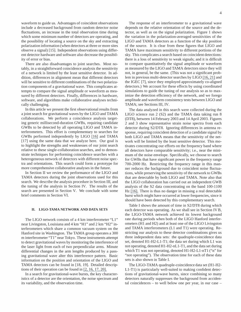
The response of an interferometer to a gravitational wavedepends on the relative orientation of the source and the de-tector, as well as on the signal polarization. Figure 1 showsthe variation in the polarization-averaged sensitivitiesof theLIGO and TAMA detectors as a function of the sky positionof the source. It is clear from these figures that LIGO andTAMA have maximum sensitivity to different portions of thesky. This complicates a search based on coincident detections:there is a loss of sensitivity to weak signals; and it is difficultto compare quantitatively the signal amplitude or waveformas measured by the LIGO and TAMA detectors since they willnot, in general, be the same. (This was not a significant prob-lem in previous multi-detector searches by LIGO [16, 21] andthe IGEC [7], since they employed approximately co-aligneddetectors.) We account for these effects by using coordinatedsimulations to guide the tuning of our analysis so as to max-imize the detection efficiency of the network, and we foregoamplitude and waveform consistency tests between LIGO andTAMA; see Sections III, IV.

The data analyzed in this search were collected during theLIGO science run 2 (S2) and the TAMA data taking run 8(DT8), between 14 February 2003 and 14 April 2003. Figures2 and 3 show representative strain noise spectra from eachdetector during S2/DT8. Ignoring differences in antenna re-sponse, requiring coincident detection of a candidate signal byboth LIGO and TAMA means that the sensitivity of the net-work will be limited by the least sensitive detector. This mo-tivates concentrating our efforts on the frequency band whereall detectors have comparable sensitivity; i.e., near the mini-mum of the noise envelope. Specifically, we choose to searchfor GWBs that have significant power in the frequency range700-2000 Hz. Restricting the frequency range in this man-ner reduces the background due to coincident noise fluctua-tions, while preserving the sensitivity of the network to GWBsthat are detectable by both LIGO and TAMA. Note also thatthe LIGO collaboration has carried out an independent GWBanalysis of the S2 data concentrating on the band 100-1100Hz [16]. There is thus no danger in missing a real detectableburst which might have occurred at lower frequencies, sinceitshould have been detected by this complementary search.

Table I shows the amount of time in S2/DT8 during whicheach detector was operating. As we shall see in Section IV B,the LIGO-TAMA network achieved its lowest backgroundrate during periods when both of the LIGO Hanford interfer-ometers (H1 and H2) and at least one of the LIGO Livingstonand TAMA interferometers (L1 and T1) were operating. Re-stricting our analysis to these detector combinations gives usthree independent data sets: the quadruple-coincidence dataset, denoted H1-H2-L1-T1; the data set during which L1 wasnot operating, denoted H1-H2-nL1-T1, and the data set duringwhich T1 was not operating, denoted H1-H2-L1-nT1 (“n” for“not operating”). The observation time for each of these datasets is also shown in Table I.

The LIGO-TAMA quadruple-coincidence data set (H1-H2-L1-T1) is particularly well-suited to making confident detec-tions of gravitational-wave bursts, since combining so manydetectors naturally suppresses the background from acciden-tal coincidences – to well below one per year, in our case –

5

Degrees East Longitude

Deg

rees

Nor

th L

atitu

de0.9

0.8

0.7

0.6

0.5 0.50.9

0.8

0.7

0.6

0.50.5

0.10.4

0.30.2

0.1

0.20.3

0.4

0.10.4

0.30.2

0.1

0.20.30.4

−180 −120 −60 0 60 120 180−90−60

−30

0

30

6090

Degrees East Longitude

Deg

rees

Nor

th L

atitu

de

0.9

0.8

0.7

0.6

0.5 0.5

0.9

0.8

0.7

0.6

0.5 0.5

0.1 0.2 0.3 0.4

0.1

0.20.30.4

0.1 0.2 0.3 0.4

0.1

0.20.30.4

−180 −120 −60 0 60 120 180−90−60

−30

0

30

6090

Degrees East Longitude

Deg

rees

Nor

th L

atitu

de

0.9

0.8

0.7

0.6

0.5 0.5

0.9

0.8

0.7

0.6

0.5 0.5

0.10.2 0.3 0.4

0.1 0.2 0.3 0.4

0.10.20.30.4

0.1 0.2 0.30.4

0.4

−180 −120 −60 0 60 120 180−90−60

−30

0

30

6090

FIG. 1: Polarization-averaged antenna amplitude responses(

F 2+ + F 2

×

)1/2∈ [0, 1], in Earth-based coordinates. [See equation (4.3) and [19]

for definitions of these functions and of Earth-based coordinates.] The top plot is for the LIGO Hanford detectors (H1, H2). The middle plot isfor LIGO Livingston (L1). The bottom plot is for TAMA (T1). High contour values indicate sky directions of high sensitivity. The directionsof maximum (null) sensitivity for each detector are indicated by the * (.) symbols. The directions of LIGO’s maximum sensitivity lie close toareas of TAMA’s worst sensitivity and vice versa.

while maintaining high detection sensitivity. Meanwhile,thetriple-coincidence data sets (H1-H2-nL1-T1 and H1-H2-L1-nT1) contribute the bulk of our observation time. In particular,the high T1 duty cycle (82%) allows us to use the large amountof H1-H2 data in H1-H2-nL1-T1 coincidence that would oth-erwise be discarded because of the poor L1 duty cycle (33%).

The LIGO-TAMA detector network therefore has more thantwice as much useful data as the LIGO detectors alone. Thisincrease in observation time allows a proportional decrease inthe limit on the GWB rate which we are able to set with thecombined detector network (for negligible background), andincreases the probability of seeing a rare strong gravitational-

6

102

103

10−22

10−21

10−20

10−19

10−18

Frequency (Hz)

Str

ain

Noi

se (

Hz

−1/2

)T1H1H2L1

FIG. 2: S2-averaged amplitude noise spectra for the LIGO detectors,and a representative DT8 spectrum for the TAMA detector. We fo-cus on GWBs which have significant energy in the frequency range700-2000 Hz (indicated by the vertical dashed lines), whereeach in-terferometer has approximately the same noise level.

103

10−21

10−20

10−19

Frequency (Hz)

Str

ain

Noi

se (

Hz

−1/2

)

T1H1H2L1

FIG. 3: The same amplitude noise spectra as in Figure 2, focusing onthe frequency range 700-2000 Hz. The peaks at multiples of 400/3Hz in the TAMA spectrum are due to a coupling between the radio-frequency modulation signal and the laser source; these frequenciesare removed by the data conditioning discussed in Section III A 2.

wave event. Furthermore, while the LIGO-TAMA networkuses only half of the TAMA data, we shall see that the sup-pression of the background by coincidence allows it to placestronger upper limits on weak GWBs than can TAMA alone.

The LIGO and TAMA detectors had not yet reached theirdesign sensitivities by the time of the S2/DT8 run; neverthe-less, the quantity of coincident data available – nearly 600hours – provided an excellent opportunity to develop and testjoint searches between our collaborations. In addition, thesensitivity of these instruments in their common frequencyband was competitive with resonant-mass detectors (see for

detector observation fraction of total

combination time (hr) observation time

H1 1040 74%

H2 821 58%

L1 536 38%

T1 1158 82%

H1-H2-L1-T1 256 18%

H1-H2-nL1-T1 320 23%

H1-H2-L1-nT1 62 4%

network totals 638 45%

TABLE I: Observation times and duty cycles of the LIGO andTAMA detectors individually, and in various combinations,duringS2/DT8. The symbol nL1 (nT1) indicates times when L1 (T1) wasnot operating. The network data sets are disjoint (non-overlapping).

example [22]), but with a much broader bandwidth. Finally,there is always the possibility of a fortunate astrophysicalevent giving rise to a detectable signal.

III. ANALYSIS METHOD

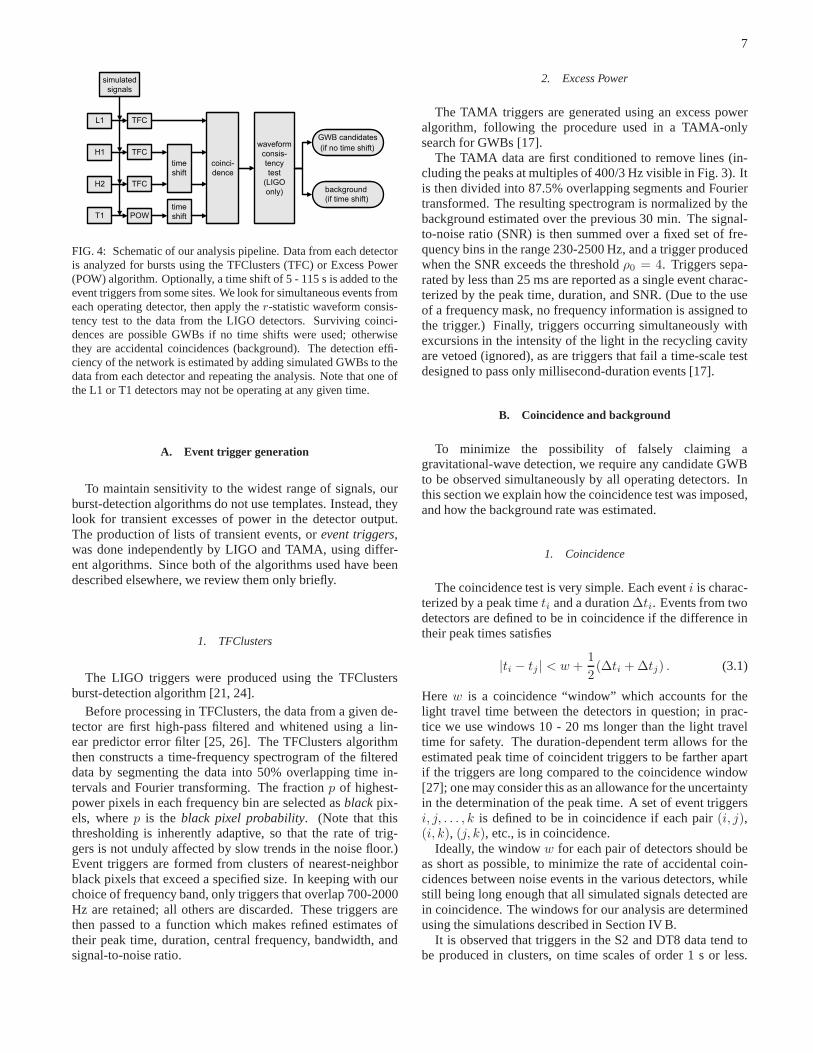
Our analysis methodology is similar, though not identi-cal, to that used in the LIGO S1 and S2 un-triggered GWBsearches [16, 21]. The essential steps are illustrated in Fig-ure 4. These are:

1. Search the data from each detector separately for burstevents.

2. Look for simultaneous (“coincident”) events in all op-erating detectors.

3. Perform a waveform consistency test on the data fromthe LIGO interferometers around the time of each coin-cidence.

4. Estimate the background rate from coincident detec-tor noise fluctuations by repeating the coincidence andwaveform consistency tests after artificially shifting intime the events from different sites.

5. Compare the number of coincidences without timeshifts to that expected from the background to set anupper limit on the rate of detectable bursts. (A signifi-cant excess of events indicates a possible detection.)

6. Estimate the network sensitivity to true GWBs (i.e., thefalse dismissal probability) by adding simulated signalsto the detector data and repeating the analysis.

In the following subsections we describe these steps in moredetail. In addition, the various thresholds used for event gener-ation, coincidence, etc., are tuned to maximize the sensitivityof the analysis; this tuning is described in Section IV B.

The LIGO software used in this analysis is available pub-licly [23].

7

T1

simulated

signals

coinci-

dence

waveform

consis-

tency

test

(LIGO

only) b a c k g r o u n d

(if time shift)

GWB candidates

(if no time shift)

H2

L1

H1

time

shift

time

shift

TFC

TFC

TFC

POW

FIG. 4: Schematic of our analysis pipeline. Data from each detectoris analyzed for bursts using the TFClusters (TFC) or Excess Power(POW) algorithm. Optionally, a time shift of 5 - 115 s is addedto theevent triggers from some sites. We look for simultaneous events fromeach operating detector, then apply ther-statistic waveform consis-tency test to the data from the LIGO detectors. Surviving coinci-dences are possible GWBs if no time shifts were used; otherwisethey are accidental coincidences (background). The detection effi-ciency of the network is estimated by adding simulated GWBs to thedata from each detector and repeating the analysis. Note that one ofthe L1 or T1 detectors may not be operating at any given time.

A. Event trigger generation

To maintain sensitivity to the widest range of signals, ourburst-detection algorithms do not use templates. Instead,theylook for transient excesses of power in the detector output.The production of lists of transient events, orevent triggers,was done independently by LIGO and TAMA, using differ-ent algorithms. Since both of the algorithms used have beendescribed elsewhere, we review them only briefly.

1. TFClusters

The LIGO triggers were produced using the TFClustersburst-detection algorithm [21, 24].

Before processing in TFClusters, the data from a given de-tector are first high-pass filtered and whitened using a lin-ear predictor error filter [25, 26]. The TFClusters algorithmthen constructs a time-frequency spectrogram of the filtereddata by segmenting the data into 50% overlapping time in-tervals and Fourier transforming. The fractionp of highest-power pixels in each frequency bin are selected asblackpix-els, wherep is the black pixel probability. (Note that thisthresholding is inherently adaptive, so that the rate of trig-gers is not unduly affected by slow trends in the noise floor.)Event triggers are formed from clusters of nearest-neighborblack pixels that exceed a specified size. In keeping with ourchoice of frequency band, only triggers that overlap 700-2000Hz are retained; all others are discarded. These triggers arethen passed to a function which makes refined estimates oftheir peak time, duration, central frequency, bandwidth, andsignal-to-noise ratio.

2. Excess Power

The TAMA triggers are generated using an excess poweralgorithm, following the procedure used in a TAMA-onlysearch for GWBs [17].

The TAMA data are first conditioned to remove lines (in-cluding the peaks at multiples of 400/3 Hz visible in Fig. 3).Itis then divided into 87.5% overlapping segments and Fouriertransformed. The resulting spectrogram is normalized by thebackground estimated over the previous 30 min. The signal-to-noise ratio (SNR) is then summed over a fixed set of fre-quency bins in the range 230-2500 Hz, and a trigger producedwhen the SNR exceeds the thresholdρ0 = 4. Triggers sepa-rated by less than 25 ms are reported as a single event charac-terized by the peak time, duration, and SNR. (Due to the useof a frequency mask, no frequency information is assigned tothe trigger.) Finally, triggers occurring simultaneouslywithexcursions in the intensity of the light in the recycling cavityare vetoed (ignored), as are triggers that fail a time-scaletestdesigned to pass only millisecond-duration events [17].

B. Coincidence and background

To minimize the possibility of falsely claiming agravitational-wave detection, we require any candidate GWBto be observed simultaneously by all operating detectors. Inthis section we explain how the coincidence test was imposed,and how the background rate was estimated.

1. Coincidence

The coincidence test is very simple. Each eventi is charac-terized by a peak timeti and a duration∆ti. Events from twodetectors are defined to be in coincidence if the difference intheir peak times satisfies

|ti − tj | < w +1

2(∆ti + ∆tj) . (3.1)

Here w is a coincidence “window” which accounts for thelight travel time between the detectors in question; in prac-tice we use windows 10 - 20 ms longer than the light traveltime for safety. The duration-dependent term allows for theestimated peak time of coincident triggers to be farther apartif the triggers are long compared to the coincidence window[27]; one may consider this as an allowance for the uncertaintyin the determination of the peak time. A set of event triggersi, j, . . . , k is defined to be in coincidence if each pair(i, j),(i, k), (j, k), etc., is in coincidence.

Ideally, the windoww for each pair of detectors should beas short as possible, to minimize the rate of accidental coin-cidences between noise events in the various detectors, whilestill being long enough that all simulated signals detectedarein coincidence. The windows for our analysis are determinedusing the simulations described in Section IV B.

It is observed that triggers in the S2 and DT8 data tend tobe produced in clusters, on time scales of order 1 s or less.

8

0 20 40 60 80 100 120

10−4

10−2

10−2

10−3

10−5

0 20 10040 60 80 1201

1.1

1.2

1.3

1.4

0 20 40 60 80 100 12010

−1

100

0 20 40 60 80 100 120

10−4

10−3

10−2

10−5

T1L1

H1 H2

FIG. 5: Autocorrelogram of trigger peak times from each detector.These are histograms of the difference in peak time between eachpair of triggers from a given detector, binned in 0.2 s intervals. Thehorizontal axis is the time difference (units of s); the vertical axis isthe number of trigger pairs per bin divided by the observation timeand the bin width (units of s−2). With this normalization, the meanvalue is the square of the trigger rate. An autocorrelogram value sig-nificantly above the mean indicates a correlation in the timeof eventtriggers. Each detector shows some excess above Poisson rates atdelays of up to a few seconds. The sharp dip in the T1 curve nearzero time is due to the clustering of the T1 triggers. The smaller rel-ative fluctuations in the L1 and T1 curves are due to the much highertrigger rates from these detectors, which results in more triggers perbin.

We therefore count groups of coincident triggers that are sep-arated in time by less than 200 ms as a single GWB candidatewhen estimating the GWB rate.

Note that no attempt is made to compare the amplitude orSNR of events between detectors. Such comparisons are dif-ficult due to the differences in alignment of the detectors (ex-cept for the H1-H2 pair); see Figure 1. We do, however, im-pose a test on the consistency of the waveform shape as mea-sured by the various LIGO detectors; see Section III C.

2. Background

Even in the absence of real gravitational-wave signals, oneexpects some coincidences between random noise-generatedevents. We estimate this background rate by repeating the co-incidence procedure after adding artificial relative time shiftsof ±5, 10, . . . , 115 s to the triggers from the LIGO Hanfordand/or TAMA sites, as indicated in Figure 4. (We do not shiftthe triggers from H1 and H2 relative to each other, in casethere are true correlated noise coincidences caused by localenvironmental effects.) These shifts are much longer than thelight travel time between the sites, so that any resulting co-incidence cannot be from an actual gravitational wave. Theyare also longer than detector noise auto-correlation times(seeFigure 5), and shorter than time scales on which trigger ratesvary, so that each provides an independent estimate of the ac-cidental coincidence rate.

The H1-H2-nL1-T1 and H1-H2-L1-nT1 data sets eachcome from 2 sites, so that we have 46 nonzero relativetime shifts in{−115,−110, . . . , 115} s. Hence, the small-

est nonzero background rate that can be measured for thesedata sets is approximately(46T )−1, whereT is the observa-tion time [28]. The H1-H2-L1-T1 network has 3 sites, for atotal of 472 − 1 = 2208 independent time shifts. We use allof these time shifts, so the smallest nonzero background ratethat we can measure for the quadruple-coincidence data set isapproximately(2208T )−1.

C. Waveform consistency test

The event generation and coincidence procedures outlinedabove are designed to detect simultaneous excesses of powerin each detector, without regard to the waveform of the event.To test if the waveforms as measured in each detector are con-sistent with one another (as one would expect for a GWB), weapply a test based on the linear correlation coefficient betweendata streams, ther-statistic [29]. We will see in Section IV Bthat ther-statistic test is very effective at eliminating acciden-tal coincidences, with very little probability of rejecting a truegravitational-wave signal. (See also [16] for demonstrationsof ther-statistic with other simulated GWB waveforms.)

The r-statistic test consists of computing the cross-correlation of the time-series data from pairs of detectorsaround the time of a coincidence. A GWB will increase themagnitude of the cross-correlation above that expected fromnoise alone. The measured cross-correlations are comparedto those expected from Gaussian noise using a Kolmogorov-Smirnov test with 95% confidence level. If not consistent,then the logarithmic significance (negative log of the probabil-ity) of each cross-correlation is computed and averaged overdetector pairs. We refer to the resulting quantity asΓ. If themaximum averaged significance exceeds a thresholdΓ0, thenthe coincidence is accepted as a candidate GWB; otherwise itis discarded. The thresholdΓ0 is chosen sufficiently high toreduce the background by the desired amount without reject-ing too many real GWB signals. For more details on the test,see [29].

Ther-statistic test was developed for use in LIGO searches,and it is based on the premise that a real gravitational-wavesignal will have similar form in different detectors. It is notclear that it can be applied safely to detectors with very dif-ferent orientations (such as LIGO and TAMA), which see dif-ferent combinations of the two polarizations of a gravitationalwave. Since this matter is still under study, we use ther-statistic test to compare data between the LIGO detectors only(i.e., H1-H2, H2-L1, and L1-H1, but not including T1).

D. Statistical analysis

Our scientific goal of this search is to detect GWBs, or inthe absence of detectable signals, to set an upper limit on theirmean rate, and to estimate the minimum signal amplitude towhich our network is sensitive.

The coincidence procedure described in Section III B pro-duces two sets of coincident events. The set with no artificialtime shift is produced by background noise and possibly also

9

by gravitational-wave bursts. The time-shifted set containsonly events produced by noise, and hence characterizes thebackground.

Given the number of candidate GWBs and the estimateof the number of accidental coincidences expected from thebackground, we use the Feldman-Cousins technique [30] tocompute the 90% confidence level upper limit or confidenceinterval on the rate of detectable gravitational-wave bursts. Inpractice, since we are not prepared to claim a detection basedonly on such a statistical analysis, we choose in advance to useonly the upper value of the Feldman-Cousins confidence inter-val. We report this upper valueR90% as an upper limit on theGWB rate, regardless of whether the Feldman-Cousins confi-dence interval is consistent with a rate of zero. Because of thismodification our upper limit procedure has a confidence levelgreater than 90%; i.e., our upper limits are conservative.

The rate upper limitR90% from the Feldman-Cousins pro-cedure applies to GWBs for which our network has perfectdetection efficiency. For a population of GWB sources forwhich our detection efficiency isǫ(h), whereh is the GWBamplitude and0 ≤ ǫ(h) ≤ 1, the corresponding rate upperlimit R90%(h) is

R90%(h) ≤ R90%

ǫ(h). (3.2)

This defines a region of rate-versus-strength space which isexcluded at 90% confidence by our analysis. The exact do-main depends on the signal type through our efficiencyǫ(h).We will construct such exclusion regions for one hypotheticalpopulation of GWB sources.

IV. SIMULATIONS AND TUNING

There are a number of parameters in the analysis pipeline ofFigure 4 that can be manipulated to adjust the sensitivity andbackground rate of our network. The most important are thethresholds for trigger generation (the TFClusters black pixelprobabilityp and the Excess Power SNR thresholdρ0), ther-statistic thresholdΓ0, and the coincidence windowsw for eachdetector pair. Our strategy is to tune these parameters to max-imize the sensitivity of the network to millisecond-durationsignals while maintaining a background of less than 0.1 sur-viving coincidences expected over the entire S2/DT8 data set.

A. Simulations

The LIGO-TAMA network consists of widely separated de-tectors with dissimilar noise spectra and antenna responses.To estimate the sensitivity of this heterogeneous network weadd (or “inject”) simulated gravitational-wave signals into thedata streams from each detector, and re-analyze the data inexactly the same manner as is done in the actual gravitational-wave search; this is indicated in Figure 4 by the “simulatedsignals” box. These injections are done coherently; i.e., theycorrespond to a GWB incident from a specific direction on the

sky. The simulated signals include the effects of the antennaresponse of the detectors, and the appropriate time delays dueto the physical separation of the detectors.

These simulations require that we specify a target popula-tion, including the waveform and the distribution of sourcesover the sky. We select a family of simple waveforms thathave millisecond durations and that span the frequency rangeof interest, 700-2000 Hz. Specifically, we use linearly polar-ized Gaussian-modulated sinusoids:

h+(t) = hrss

(

π

2f20

)

−1/4

sin [2πf0(t − t0)] e−

(t−t0)2

τ2 , (4.1)

h×(t) = 0 .

(Other waveforms, along with these, have been considered in[16, 17, 21].) Heret0 is the peak time of the signal envelope.The central frequencyf0 of each injection is picked randomlyfrom the values 700, 849, 1053, 1304, 1615, 2000 Hz, whichspan our analysis band in logarithmic steps. The efficiency ofdetection of these signals thus gives us a measure of the net-work sensitivity averaged over our band. We set the envelopewidth asτ = 2/f0, which gives durations of approximately 1-3ms. The corresponding quality factor isQ ≡

√2πf0τ = 8.9

and the bandwidth is∆f = f0/Q ≃ 0.1f0, so these arenarrow-band signals.

The quantityhrss in equation (4.1) is the root-sum-squareamplitude of the plus polarization:

[∫

∞

−∞

dt h2+(t)

]1/2

= hrss (4.2)

We findhrss to be a convenient measure of the signal strength.While it is a detector-independent amplitude,hrsshas the sameunits as the strain noise amplitude spectrum of the detectors,which allows for a direct comparison of the signal amplituderelative to the detector noise. All amplitudes quoted in thisreport arehrss amplitudes.

Lacking any strong theoretical bias for probable sky posi-tions of sources of short-duration bursts, we distribute the sim-ulated signals isotropically over the sky. We select the polar-ization angle randomly with uniform distribution over[0, π].

A total of approximately 16800 of these signals were in-jected into the S2/DT8 data. For each signal, the actual wave-form h(t) as it would be seen by a given detector was com-puted,

h(t) = F+h+(t) + F×h×(t) = F+h+(t) , (4.3)

andh(t) was added to the detector data. HereF+, F× are theusual antenna response factors, which are functions of the skydirection and polarization of the signal relative to the detector(see for example [19]). The signals in the different detectorswere also delayed relative to one another according to the skyposition of the source.

These simulated signals were shared between LIGO andTAMA by writing the signalsh(t) in frame files [31, 32], in-cluding the appropriate detector response and calibrationef-fects. These signal data were added to the data streams fromthe individual detectors before passing through TFClusters or

10

Excess Power. In addition to providing estimates of the net-work detection efficiency, the ability of these two independentsearch codes to recover the injected signals is an importanttestof the validity of the pipeline.

An injected signal is considered detected if there is a coin-cident event from the network within 200 ms of the injectiontime. The network efficiencyǫ(hrss) is simply the fraction ofevents of amplitudehrss which are detected by the network.We find that good empirical fits to the measured efficienciescan be found in the form

ǫ(hrss) =1

1 +

(

hrss

h50%rss

)α[1+β tanh(hrss/h50%rss )]

, (4.4)

whereh50%rss > 0, α < 0, and−1 < β ≤ 0. Hereh50%

rss isthe amplitude at which the efficiency is 0.5,α parameterizesthe width of the transition region, andβ parameterizes theasymmetry of the efficiency curve abouthrss = h50%

rss . Whenpresenting efficiencies we will use fits of this type.

As we shall see, the efficiency transitions from zero (forweak signals) to unity (for strong signals), over about an or-der of magnitude in signal amplitude. It proves convenientto characterize the network sensitivity by the single num-ber h50%

rss at which the efficiency is 0.5. This amplitude is afunction of the trigger-generation thresholds; it and the back-ground rate are the two performance measures that we use toguide the tuning of our analysis.

B. Tuning procedure

As stated earlier, our tuning strategy is to maximize the de-tection efficiency of the network while maintaining a back-ground rate of less than approximately 0.1 events over the en-tire data set. For simplicity, we chose a single tuning for theproduction and analysis of all event triggers from all data sets.This strategy is implemented as follows:

1. For TFClusters, the efficiency for detecting the sine-Gaussian signals and the background rate are mea-sured for each detector for a large number of parame-ter choices. For each black-pixel probabilityp (whichdetermines the background rate) the other ETG param-eters are set to obtain the lowesth50%

rss value [33]. TheTAMA Excess Power algorithm is tuned independentlyfor short-duration signals as described in [17]. The re-sulting performance of each detector is shown in Fig-ure 6.

2. The coincidence windoww for each detector pair inequation (3.1) is fixed by performing coincidence on thetriggers from the simulated signals. We find that select-ing windows only slightly larger (by∼ 1ms) than thelight travel time between the various detector pairs (seeTable II) ensures that all of the injections detected by allinterferometers produce coincident triggers. For sim-plicity, we use a single window ofw = 20 ms for coin-cidence between any LIGO detectors [34] and a single

detector pair separation (km) separation (ms)

LHO-LLO 3002 10.0

LLO-TAMA 9683 32.3

TAMA-LHO 7473 24.9

TABLE II: Separation of the LIGO and TAMA interferometers, us-ing data from [19].

window of w = 43 ms for coincidence between anyLIGO detector and TAMA. These choices correspondto using the longest possible time delay plus a∼10 mssafety margin.

3. To obtain the best network sensitivity versus back-ground rate, we select the single-detector ETG thresh-olds (p, ρ0) to matchh50%

rss as closely as possible be-tween the detectors. (This is similar in spirit to theIGEC tuning [7], although not the same, as we arenot able to easily compare the amplitude of individualevents from our misaligned broadband detectors.) Inpractice, the TAMA detector has slightly poorer sen-sitivity than the LIGO detectors. We therefore set theTAMA threshold as low as we consider feasible,ρ0 =4; this sets the sensitivity of the network as a whole.We then choose the LIGO single-detector thresholds forsimilar efficiency.

4. The final threshold is that for ther-statistic, denotedβ. In practice we find that ther-statistic has negligibleeffect on the network efficiency forβ < 5. We setβ =3, which proved sufficient to eliminate all time-lagged(accidental) coincidences while rejecting less than 1%of the injected signals.

Figure 6 shows the resultingh50%rss and background rate for

each of the three coincidence combinations. Table III showstrigger rates and livetimes for each coincidence combination.

We note from Figure 6 that the network background ratesare 5-9 orders of magnitude smaller than the rates of theindividual detectors. Roughly speaking, adding a detectorwith event rateRi and coincidence windoww to the networkchanges the network background rate by a factor of approx-imately2Riw. From the single-detector rates of Figure 6 orTable III we estimate that H1 and H2 each reduce the back-ground rate by∼ 103, L1 by∼ 50, and T1 by∼ 10. This iswhy we require both H1 and H2 to be operating: they suppressstrongly the background for our network.

We have confirmed that the background rate estimated fromtime shifts is consistent with that expected from Poisson statis-tics. Assuming Poisson statistics, the expected backgroundrateR for a set ofN detectors with ratesRi is approximately

R ≈ 1

w

N∏

i=1

2Riw (4.5)

where we assume a single coincidence windoww for sim-plicity. Using this formula and the single-detector rates from

11

10−10

10−8

10−6

10−4

10−2

100

10−20

10−19

10−18

Background Rate (s −1)

Am

plitu

de fo

r 50

% E

ffici

ency

(H

z−1

/2)

H1H2L1T1H1−H2−L1−T1H1−H2−nL1−T1H1−H2−L1−nT1

FIG. 6: Amplitudeh50%rss for 50% detection efficiency versus back-

ground rate for each of the individual detectors, and for thethreecoincidence combinations. The circles on the single-detector curvesindicate the tuning selected for trigger generation. The circle, square,and triangle denote the resulting amplitude at 50% efficiency and anupper limit on the background rate for the H1-H2-L1-T1, H1-H2-nL1-T1, and H1-H2-L1-nT1 networks after ther-statistic with thesetuning choices. (We can only compute upper limits on the back-ground rates for coincidence because no time-shifted coincidencessurvive the waveform consistency test.) The efficiency is averagedover all of the sine-Gaussian signals in our analysis band.

Table III, one predicts background rates before the r-statisticconsistent with those determined from time delays. Thisagreement gives increased confidence in our background esti-mation.

It is also worth noting that the 50% efficiency pointh50%rss

is a very shallow function of the background rate for multipledetectors. Hence, there is little value in lowering the triggerthresholds to attempt to detect weaker signals. For example,allowing the triple-coincidence background rate of TFClusters(the rate for the H1-H2-L1-nT1 data) to increase by 3 ordersof magnitude lowersh50%

rss by less than a factor of 2. For fourdetectors,h50%

rss varies even more slowly with the backgroundrate. This is why we tune for≪1 background event over theobservation time; there is almost no loss of efficiency in doingso.

To avoid bias from tuning our pipeline using the same datafrom which we derive our upper limits, the tuning was donewithout examining the full zero-time-shift coincidence triggersets. Instead, preliminary tuning was done using a 10% sub-set of the data, referred to as theplayground, which was notused for setting upper limits. Final tuning choices were madeby examining the time-shifted coincidences and the simula-tions over the full data set. As it happens, the only parameteradjusted in this final tuning was ther-statistic thresholdΓ0;we required the full observation time to have enough back-ground coincidences to allow reasonably accurate estimatesof the background suppression by ther-statistic test.

Figure 7 shows the efficiency of the LIGO-TAMA networkas a function of signal amplitude for each of the three data sets,

10−20

10−19

10−18

10−17

0

0.2

0.4

0.6

0.8

1

Signal Amplitude (Hz −1/2)

Effi

cien

cy

H1−H2−L1−T1H1−H2−nL1−T1H1−H2−L1−nT1Combined

FIG. 7: Detection efficiency over the various data sets individually,and combined, using the final tuning. The combined efficiencycurveis the average of the curves for the three data sets, weightedby theirobservation times. These efficiencies are averaged over allof thesine-Gaussian signals in our analysis band. There is a statistical un-certainty at each point in these curves of approximately 1-3% due tothe finite number of simulations performed.

and also the average efficiency weighted by the observationtime of each data set. By design, the efficiencies are verysimilar, withh50%

rss values in the range1-2 × 10−19 Hz−1/2.Figure 8 shows how the combined efficiency varies across

our frequency band; the weak dependence on the central fre-quency of the injected signal is a consequence of the flatnessof the envelope of the detector noise spectra shown in Fig-ure 3. This is corroborated by the efficiency for the H1-H2-L1-nT1 data set (without TAMA), shown in Figure 9. Theimprovement in the low-frequency sensitivity for this datasetindicates that TAMA limits the network sensitivity at low fre-quencies, as expected from the noise spectra.

C. Systematic and statistical uncertainties

The only significant systematic uncertainty in our analy-sis is in the overall multiplicative scale of the calibration (thecoupling of strain to the output of the individual detectors).The “1-σ” uncertainties were estimated as∼9% for L1 and∼4% for each of H1, H2, and T1 [35]. Simple Monte-Carlomodeling indicates that, with 90% confidence, theh50%

rss valuefor any given network combination will not be more than 4%larger than the estimated value due to these uncertainties.Weallow for this uncertainty in our rate-versus-strength plots byshifting our limit curves to largerhrss by 4%.

The main statistical uncertainty in our results is in the ef-ficiency at any given signal amplitude, due to the finite num-ber of simulations performed. This can be quantified throughthe uncertainty in the parameters found for the efficiency fits(4.4), and is typically less than 5%. We account for this byshifting our rate-versus-strength upper limit curves upward at

12

10−20

10−19

10−18

10−17

0

0.2

0.4

0.6

0.8

1

Signal Amplitude (Hz −1/2)

Effi

cien

cy

700 Hz849 Hz1053 Hz1304 Hz1615 Hz2000 Hz

FIG. 8: Detection efficiency for the combined data set, by centralfrequencyf0 of the sine-Gaussian signal in equation (4.1). There is astatistical uncertainty at each point in these curves of approximately2-4% due to the finite number of simulations performed.

10−20

10−19

10−18

10−17

0

0.2

0.4

0.6

0.8

1

Signal Amplitude (Hz −1/2)

Effi

cien

cy

700 Hz849 Hz1053 Hz1304 Hz1615 Hz2000 Hz

FIG. 9: Detection efficiency for the H1-H2-L1-nT1 data set (i.e.,with only the LIGO detectors operating), by central frequency f0 ofthe sine-Gaussian signal in equation (4.1). There is a statistical un-certainty at each point in these curves of approximately 2-6% dueto the finite number of simulations performed. The improved effi-ciency for lower-frequency signals indicates that sensitivity at thesefrequencies is limited by the TAMA detector. This behavior is con-sistent with the noise spectra shown in Figure 3.

each amplitude by 1.28 times the estimated statistical uncer-tainty in the corresponding efficiency. (The factor 1.28 givesa 90% limit, assuming Gaussian statistics.)

V. ANALYSIS RESULTS

After making the final tuning choices, we performed thecoincidence analysis without time shifts for all three data

sets. No event triggers survived the coincidence andr-statistictests, so we have no candidate gravitational-wave signals.

Table III shows for each data set the rate of triggers, thenumber of coincident events before and after ther-statistictest, and the total amount of data analyzed after removing theplayground and accounting for the dead time of the TAMA ve-toes. Also shown are the number of accidental coincidencesand the effective observation time from the time-shift exper-iments, which provide our estimate of the background rates.Finally, the upper limits on the rate of detectable gravitational-wave bursts are shown.

As discussed in Section III D, our upper limits are obtainedusing the Feldman-Cousins procedure [30]. This algorithmcompares the observed number of events to that expected fromthe background. As a rule, for a fixed number of observedevents, the upper limit is stronger (lower) for higher back-grounds. Since our backgrounds are too low to be measuredaccurately (there are no surviving time-shifted coincidencesafter ther-statistic), we conservatively assume zero back-ground in calculating our upper limits. Since there are alsono surviving coincidences without time shifts, the rate limitsfrom the Feldman-Cousins procedure take on the simple form

Ri90% =

2.44

Ti(5.1)

whereTi is the observation time for a particular network com-bination (see Table IV of [30] withb = 0, n = 0). This givesthe limits shown in Table III. Additionally, since all threedatasets have essentially zero background, we can treat them col-lectively as a single experiment by summing their observationtimes and the number of detected events (which happens to bezero):

Rcombined90% =

2.44∑

i Ti(5.2)

The resulting upper limit of 0.12 detectable events per day at90% confidence is the primary scientific result of this analysis.

By dividing the rate upper limits by the efficiency for agiven population of GWB sources, as in equation (3.2), weobtain upper limits on the GWB rate as a function of the burstamplitude. Averaging over the network combinations gives

Rcombined90% (hrss) =

2.44∑

i ǫi(hrss)Ti(5.3)

For example, for our tuning population of isotropically dis-tributed sources of sine-Gaussian GWBs, and averaging overall f0 (i.e., using the efficiencies in Figure 7), one obtains therate-versus-strength upper limits shown in Figure 10. GWBrates and amplitudes above a given curve are excluded by thatdata set with at least 90% confidence.

A. Comparison to other searches

The LIGO-TAMA search for GWBs is one of several suchsearches reported recently. Table IV shows the observation

13

Data Set H1-H2-L1-T1 H1-H2-nL1-T1 H1-H2-L1-nT1 Combined

RH1 (s−1) 0.0157 0.0151 0.0137

RH2 (s−1) 0.0164 0.0183 0.0150

RL1 (s−1) 0.399 - 0.377

RT1 (s−1) 1.03 1.04 -

N 0/0 1/0 0/0 1/0

T (hr) 165.3 257.0 51.2 473.5

Nbck 31/0 57/0 0/0

Tbck (hr) 3.422×105 1.139×104 2.243×103

〈N〉 0.015/<0.0005 1.3/<0.03 <0.03/<0.03 <1.4/<0.05

R90% (day−1) 0.35 0.23 1.1 0.12

TABLE III: Results of the LIGO-TAMA analysis for each data set separately, and combined.RH1, etc., are the measured single-detectortrigger rates.N is the total number of coincidences before/after ther-statistic waveform consistency test.T is the total observation timeanalyzed, after removal of the playground and veto dead times. Nbck andTbck are the corresponding summed numbers from the time-shiftexperiments.〈N〉 is the expected number of accidental coincidences during the observation time. (ForNbck = 0, we estimate〈N〉 < T/Tbck.)R90% is the resulting upper limit on the rate of detectable gravitational-wave events, at 90% confidence.

10−20

10−19

10−18

10−17

10−1

100

101

Signal Amplitude (Hz −1/2)

90%

Rat

e U

pper

Lim

it (d

ay−1

)

H1−H2−L1−T1H1−H2−nL1−T1H1−H2−L1−nT1Combined

FIG. 10: Rate-versus-strength upper limits from each LIGO-TAMAdata set, and combined, for the isotropic distribution of sources ofsine-Gaussian GWBs described in Section IV A. The region aboveany curve is excluded by that experiment with at least 90% confi-dence. These curves include the allowances for uncertainties in thecalibration and in the efficiencies discussed in Section IV C.

time, rate upper limit, and approximate frequency band forLIGO-TAMA, the LIGO-only S2 search [16], the TAMA-only DT9 search [17], and the IGEC search [7]. Our limitof 0.12 events per day is the strongest limit yet placed ongravitational-wave bursts by broadband detectors. Even so, itis still approximately a factor of 30 larger than the IGEC limit,which was derived from approximately two years of data froma network of 5 resonant-mass detectors. Note however that thebroadband nature of the LIGO and TAMA detectors meansthat they are sensitive to a wider class of signals than resonant-mass detectors; the IGEC search is only sensitive to GWBswith significant power at the resonant frequencies of all of theoperating detectors.

Network T (day) R90% (day−1) band (Hz)

LIGO-TAMA S2/DT8 19.7 0.12 700-2000

LIGO-only S2 10.0 0.26 100-1100

TAMA-only DT9 8.1 0.49 230-2500

IGEC 707.9 0.0041 694-930

TABLE IV: Observation times, rate upper limits, and frequencybands for LIGO-TAMA and other recent burst searches [7, 16, 17].The stated frequency range for the IGEC search is the range oftheresonant frequencies of the detectors used. The IGEC upper limit ap-plies only to signals with significant power at the resonant frequen-cies of all of the operating detectors.

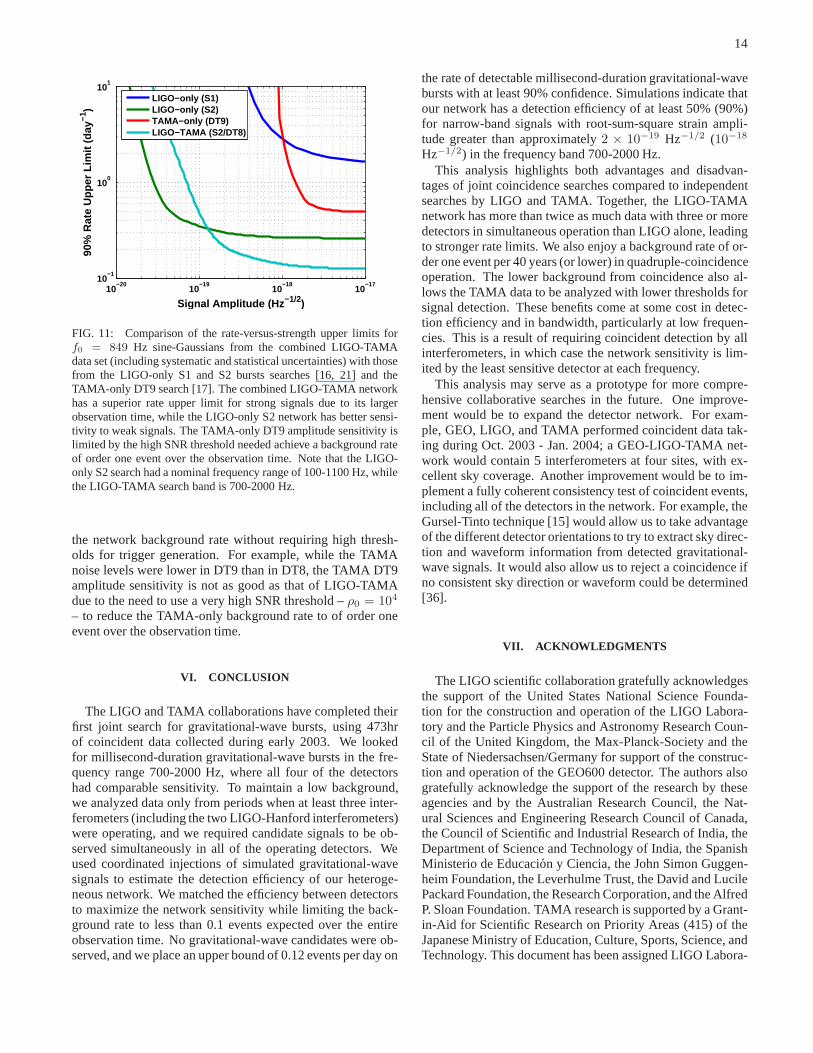
Since our sine-Gaussian test waveforms are narrow-bandsignals, we cannot compare directly our sensitivity to thatof the IGEC network. More concrete comparisons can bemade between the performance of the LIGO-TAMA networkand LIGO and TAMA individually, by considering the rate-versus-strength upper limit forf0 = 849 Hz sine-Gaussians.Figure 11 shows the upper limits for this waveform from theLIGO-only S1 and S2 searches [16, 21], the TAMA DT9search [17], and the present analysis. Compared to LIGOalone, the much longer observation time afforded by joiningthe LIGO and TAMA detectors allows the LIGO-TAMA net-work to set stronger rate upper limits for amplitudes at whichboth LIGO and TAMA are sensitive. The joint network alsoenjoys a lower background rate from accidental coincidences,particularly for the quadruple-coincidence network: of order1/40 yr−1 for quadruple coincidence, versus of order 2 yr−1

for the LIGO-only S2 analysis. However, the band of goodsensitivity for LIGO-TAMA does not extend to low frequen-cies, due to the poorer TAMA noise level there. The LIGO-only analysis also has better sensitivity to weak signals, espe-cially near the lower edge of our frequency band. Comparedto TAMA alone, the LIGO-TAMA network has better sensi-tivity to weak signals because coincidence with LIGO lowers

14

10−20

10−19

10−18

10−17

10−1

100

101

Signal Amplitude (Hz −1/2)

90%

Rat

e U

pper

Lim

it (d

ay−1

)LIGO−only (S1)LIGO−only (S2)TAMA−only (DT9)LIGO−TAMA (S2/DT8)

FIG. 11: Comparison of the rate-versus-strength upper limits forf0 = 849 Hz sine-Gaussians from the combined LIGO-TAMAdata set (including systematic and statistical uncertainties) with thosefrom the LIGO-only S1 and S2 bursts searches [16, 21] and theTAMA-only DT9 search [17]. The combined LIGO-TAMA networkhas a superior rate upper limit for strong signals due to its largerobservation time, while the LIGO-only S2 network has bettersensi-tivity to weak signals. The TAMA-only DT9 amplitude sensitivity islimited by the high SNR threshold needed achieve a background rateof order one event over the observation time. Note that the LIGO-only S2 search had a nominal frequency range of 100-1100 Hz, whilethe LIGO-TAMA search band is 700-2000 Hz.

the network background rate without requiring high thresh-olds for trigger generation. For example, while the TAMAnoise levels were lower in DT9 than in DT8, the TAMA DT9amplitude sensitivity is not as good as that of LIGO-TAMAdue to the need to use a very high SNR threshold –ρ0 = 104

– to reduce the TAMA-only background rate to of order oneevent over the observation time.

VI. CONCLUSION

The LIGO and TAMA collaborations have completed theirfirst joint search for gravitational-wave bursts, using 473hrof coincident data collected during early 2003. We lookedfor millisecond-duration gravitational-wave bursts in the fre-quency range 700-2000 Hz, where all four of the detectorshad comparable sensitivity. To maintain a low background,we analyzed data only from periods when at least three inter-ferometers (including the two LIGO-Hanford interferometers)were operating, and we required candidate signals to be ob-served simultaneously in all of the operating detectors. Weused coordinated injections of simulated gravitational-wavesignals to estimate the detection efficiency of our heteroge-neous network. We matched the efficiency between detectorsto maximize the network sensitivity while limiting the back-ground rate to less than 0.1 events expected over the entireobservation time. No gravitational-wave candidates were ob-served, and we place an upper bound of 0.12 events per day on

the rate of detectable millisecond-duration gravitational-wavebursts with at least 90% confidence. Simulations indicate thatour network has a detection efficiency of at least 50% (90%)for narrow-band signals with root-sum-square strain ampli-tude greater than approximately2 × 10−19 Hz−1/2 (10−18

Hz−1/2) in the frequency band 700-2000 Hz.This analysis highlights both advantages and disadvan-

tages of joint coincidence searches compared to independentsearches by LIGO and TAMA. Together, the LIGO-TAMAnetwork has more than twice as much data with three or moredetectors in simultaneous operation than LIGO alone, leadingto stronger rate limits. We also enjoy a background rate of or-der one event per 40 years (or lower) in quadruple-coincidenceoperation. The lower background from coincidence also al-lows the TAMA data to be analyzed with lower thresholds forsignal detection. These benefits come at some cost in detec-tion efficiency and in bandwidth, particularly at low frequen-cies. This is a result of requiring coincident detection by allinterferometers, in which case the network sensitivity is lim-ited by the least sensitive detector at each frequency.

This analysis may serve as a prototype for more compre-hensive collaborative searches in the future. One improve-ment would be to expand the detector network. For exam-ple, GEO, LIGO, and TAMA performed coincident data tak-ing during Oct. 2003 - Jan. 2004; a GEO-LIGO-TAMA net-work would contain 5 interferometers at four sites, with ex-cellent sky coverage. Another improvement would be to im-plement a fully coherent consistency test of coincident events,including all of the detectors in the network. For example, theGursel-Tinto technique [15] would allow us to take advantageof the different detector orientations to try to extract skydirec-tion and waveform information from detected gravitational-wave signals. It would also allow us to reject a coincidence ifno consistent sky direction or waveform could be determined[36].

VII. ACKNOWLEDGMENTS

The LIGO scientific collaboration gratefully acknowledgesthe support of the United States National Science Founda-tion for the construction and operation of the LIGO Labora-tory and the Particle Physics and Astronomy Research Coun-cil of the United Kingdom, the Max-Planck-Society and theState of Niedersachsen/Germany for support of the construc-tion and operation of the GEO600 detector. The authors alsogratefully acknowledge the support of the research by theseagencies and by the Australian Research Council, the Nat-ural Sciences and Engineering Research Council of Canada,the Council of Scientific and Industrial Research of India, theDepartment of Science and Technology of India, the SpanishMinisterio de Educacion y Ciencia, the John Simon Guggen-heim Foundation, the Leverhulme Trust, the David and LucilePackard Foundation, the Research Corporation, and the AlfredP. Sloan Foundation. TAMA research is supported by a Grant-in-Aid for Scientific Research on Priority Areas (415) of theJapanese Ministry of Education, Culture, Sports, Science,andTechnology. This document has been assigned LIGO Labora-

15

tory document number LIGO-P040050-06-Z.

[1] B. Willke et al., Class. Quant. Grav.21 S417 (2004).[2] D. Sigg, Class. Quant. Grav.21 S409 (2004).[3] R. Takahashi, Class. Quant. Grav.21 S403 (2004).[4] F. Acerneseet al., Class. Quant. Grav.21 S385 (2004).[5] E. Amaldi et al., Astron. Astrophys.216 325 (1989).[6] Z. A. Allen et al., Phys. Rev. Lett.85 5046 (2000).[7] P. Astoneet al., Phys. Rev. D68 022001 (2003).[8] T. Zwerger and E. Muller, Astron. Astrophys.320 209 (1997).[9] H. Dimmelmeier, J. Font, and E. Muller, Astron. Astro-

phys.388 917 (2002).[10] H. Dimmelmeier, J. Font, and E. Muller, Astron. Astro-

phys.393 523 (2002).[11] C. Ott, A. Burrows, E. Livne, and R. Walder, Astrophys. J. 600

834 (2004).[12] E. E. Flanagan and S. A. Hughes, Phys. Rev. D57 4535 (1998).[13] E. E. Flanagan and S. A. Hughes, Phys. Rev. D57 4566 (1998).[14] P. Meszaros, Ann. Rev. Astron. Astrophys.40 137 (2002).[15] Y. Gursel and M. Tinto, Phys. Rev. D40 3884 (1989).[16] B. Abbott et al., Upper limits on gravitational-wave bursts in

LIGO’s second science run, arXiv:gr-gc/0505029 (2005).[17] M. Ando et al., Phys. Rev. D71 082002 (2005).[18] W. Althouseet al., Rev. Sci. Instrum.72 3086 (2001).[19] W. G. Anderson, P. R. Brady, J. D. E. Creighton, and

E. E. Flanagan, Phys. Rev. D63 042003 (2001).[20] B. Abbottet al., Nucl. Instrum. Meth. A517 154 (2004).[21] B. Abbottet al., Phys. Rev. D69 102001 (2004).[22] V. Fafone, Class. Quant. Grav.21 S377 (2004).[23] The LIGO software used in this analysis is available

in the LIGO Scientific Collaboration’s CVS archives athttp://www.lsc-group.phys.uwm.edu/cgi-bin/cvs/viewcvs.cgi/?cvsroot=lscsoft. TFClus-ters is in LAL and LALWRAPPER, while the r-statisticand all other driver and post-processing codes are in theMATAPPS subsection. The version tag isrStat-1-2tagfor the r-statistic and s2ligotama 20050525 a forthe other driver and post-processing codes. The TF-Clusters version is that for LDAS version 1.1.0; seehttp://www.ldas-sw.ligo.caltech.edu/cgi-bin/index.cgi.

[24] J. Sylvestre, Phys. Rev. D66 102004 (2002).

[25] S. Chatterji, L. Blackburn, G. Martin, and E. Katsavounidis,Class. Quant. Grav.21 S1809 (2004).

[26] The prefiltering for TFClusters was done in two stages. First, asixth order modified butterworth high pass filter with a cutofffrequency of 100 Hz was applied. Then a detector-dependentFIR linear predictor error filter was applied. The LPEF filtershave approximately unity rms output, a training time of 4 sec-onds (from the middle of the lock segment being analyzed), andorder of 1024.

[27] In practice we find that the typical trigger durations are∼1 msfor LIGO and∼5-8 ms for TAMA. These are much less thanthe light travel times, so that the dominant contribution tothebackground comes from the window termw.

[28] The smallest nonzero measurable rate is slightly higher than(46T )−1 because triggers within 115 s of the edge of a datasegment are dropped in some time shifts. The same holds forthe 3-site time shifts.

[29] L. Cadonati, Class. Quant. Grav.21 S1695 (2004).[30] G. J. Feldman and R. D. Cousins, Phys. Rev. D57 3873 (1998).[31] LIGO Data and Computing Group and Virgo Data Acquisition

Group, LIGO Technical Document LIGO-T970130-F, 2002.[32] S. Klimenko, M. Rakhmanov, and I. Yakushin, LIGO Technical

Document LIGO-T040042-00, 2004.[33] In the notation of [24], the parameters used for TFClusters in

this analysis are a segment length of 300 s,α = 1, σ = 2,~δ = 0 (no generalized clusters),p = 10−4 (H1, H2),p = 10−3

(L1), time resolutionT = 1/128 s, fmin = 700 Hz,fmax =2000 Hz. In contrast to [24], the black-pixel threshold is set bysimply ranking the pixel powers, rather than by using a Rice fit.

[34] We could have imposed a tighter coincidence window betweenH1 and H2, since they are co-located, and further reduced thebackground rate. This is not necessary, however, since the falserate is already too small to be measured accurately; see Ta-ble III.

[35] G. Gonzalez, M. Landry, B. O’Reilly, and H. Radkins, LIGOTechnical Document LIGO-T040060-01, 2004.

[36] L. Wen and B. Schutz,Coherent data analysis strategies using anetwork of gravitational wave detectors, in preparation (2005).