LIGO-P080021-01-Z

The Einstein@Home search for periodic gravitational waves in LIGO S4 data

B. Abbott,16 R. Abbott,16 R. Adhikari,16 P. Ajith,2 B. Allen,2, 55 G. Allen,32 R. Amin,20 D. P. Anderson,41

S. B. Anderson,16 W. G. Anderson,55 M. A. Arain,42 M. Araya,16 H. Armandula,16 P. Armor,55 Y. Aso,10

S. Aston,40 P. Aufmuth,15 C. Aulbert,2 S. Babak,1 S. Ballmer,16 H. Bantilan,8 B. C. Barish,16 C. Barker,18

D. Barker,18 B. Barr,43 P. Barriga,54 M. A. Barton,43 M. Bastarrika,43 K. Bayer,17 J. Betzwieser,16

P. T. Beyersdorf,28 I. A. Bilenko,23 G. Billingsley,16 R. Biswas,55 E. Black,16 K. Blackburn,16 L. Blackburn,17

D. Blair,54 B. Bland,18 T. P. Bodiya,17 L. Bogue,19 R. Bork,16 V. Boschi,16 S. Bose,56 P. R. Brady,55

V. B. Braginsky,23 J. E. Brau,48 M. Brinkmann,2 A. Brooks,16 D. A. Brown,33 G. Brunet,17 A. Bullington,32

A. Buonanno,44 O. Burmeister,2 R. L. Byer,32 L. Cadonati,45 G. Cagnoli,43 J. B. Camp,24 J. Cannizzo,24

K. Cannon,16 J. Cao,17 L. Cardenas,16 T. Casebolt,32 G. Castaldi,51 C. Cepeda,16 E. Chalkley,43 P. Charlton,9

S. Chatterji,16 S. Chelkowski,40 Y. Chen,6, 1 N. Christensen,8 D. Clark,32 J. Clark,43 T. Cokelaer,7 R. Conte,50

D. Cook,18 T. Corbitt,17 D. Coyne,16 J. D. E. Creighton,55 A. Cumming,43 L. Cunningham,43 R. M. Cutler,40

J. Dalrymple,33 K. Danzmann,15, 2 G. Davies,7 D. DeBra,32 J. Degallaix,1 M. Degree,32 V. Dergachev,46

S. Desai,34 R. DeSalvo,16 S. Dhurandhar,14 M. Dıaz,36 J. Dickson,4 A. Dietz,7 F. Donovan,17 K. L. Dooley,42

E. E. Doomes,31 R. W. P. Drever,5 I. Duke,17 J.-C. Dumas,54 R. J. Dupuis,16 J. G. Dwyer,10 C. Echols,16

A. Effler,18 P. Ehrens,16 G. Ely,8 E. Espinoza,16 T. Etzel,16 T. Evans,19 S. Fairhurst,7 Y. Fan,54 D. Fazi,16

H. Fehrmann,2 M. M. Fejer,32 L. S. Finn,34 K. Flasch,55 N. Fotopoulos,55 A. Freise,40 R. Frey,48 T. Fricke,16, 49

P. Fritschel,17 V. V. Frolov,19 M. Fyffe,19 J. Garofoli,18 I. Gholami,1 J. A. Giaime,19, 20 S. Giampanis,49

K. D. Giardina,19 K. Goda,17 E. Goetz,46 L. Goggin,16 G. Gonzalez,20 S. Gossler,2 R. Gouaty,20 A. Grant,43

S. Gras,54 C. Gray,18 M. Gray,4 R. J. S. Greenhalgh,27 A. M. Gretarsson,11 F. Grimaldi,17 R. Grosso,36

H. Grote,2 S. Grunewald,1 M. Guenther,18 E. K. Gustafson,16 R. Gustafson,46 B. Hage,15 J. M. Hallam,40

D. Hammer,55 C. Hanna,20 J. Hanson,19 J. Harms,2 G. Harry,17 E. Harstad,48 K. Hayama,36 T. Hayler,27

J. Heefner,16 I. S. Heng,43 M. Hennessy,32 A. Heptonstall,43 M. Hewitson,2 S. Hild,40 E. Hirose,33 D. Hoak,19

D. Hosken,39 J. Hough,43 S. H. Huttner,43 D. Ingram,18 M. Ito,48 A. Ivanov,16 B. Johnson,18 W. W. Johnson,20

D. I. Jones,52 G. Jones,7 R. Jones,43 L. Ju,54 P. Kalmus,10 V. Kalogera,26 S. Kamat,10 J. Kanner,44 D. Kasprzyk,40

E. Katsavounidis,17 K. Kawabe,18 S. Kawamura,25 F. Kawazoe,25 W. Kells,16 D. G. Keppel,16 F. Ya. Khalili,23

R. Khan,10 E. Khazanov,13 C. Kim,26 P. King,16 J. S. Kissel,20 S. Klimenko,42 K. Kokeyama,25 V. Kondrashov,16

R. K. Kopparapu,34 D. Kozak,16 I. Kozhevatov,13 B. Krishnan,1 P. Kwee,15 P. K. Lam,4 M. Landry,18

M. M. Lang,34 B. Lantz,32 A. Lazzarini,16 M. Lei,16 N. Leindecker,32 V. Leonhardt,25 I. Leonor,48 K. Libbrecht,16

H. Lin,42 P. Lindquist,16 N. A. Lockerbie,53 D. Lodhia,40 M. Lormand,19 P. Lu,32 M. Lubinski,18 A. Lucianetti,42

H. Luck,15, 2 B. Machenschalk,2 M. MacInnis,17 M. Mageswaran,16 K. Mailand,16 V. Mandic,47 S. Marka,10

Z. Marka,10 A. Markosyan,32 J. Markowitz,17 E. Maros,16 I. Martin,43 R. M. Martin,42 J. N. Marx,16 K. Mason,17

F. Matichard,20 L. Matone,10 R. Matzner,35 N. Mavalvala,17 R. McCarthy,18 D. E. McClelland,4 S. C. McGuire,31

M. McHugh,22 G. McIntyre,16 G. McIvor,35 D. McKechan,7 K. McKenzie,4 T. Meier,15 A. Melissinos,49

G. Mendell,18 R. A. Mercer,42 S. Meshkov,16 C. J. Messenger,2 D. Meyers,16 J. Miller,43, 16 J. Minelli,34 S. Mitra,14

V. P. Mitrofanov,23 G. Mitselmakher,42 R. Mittleman,17 O. Miyakawa,16 B. Moe,55 S. Mohanty,36 G. Moreno,18

K. Mossavi,2 C. MowLowry,4 G. Mueller,42 S. Mukherjee,36 H. Mukhopadhyay,14 H. Muller-Ebhardt,2 J. Munch,39

P. Murray,43 E. Myers,18 J. Myers,18 T. Nash,16 J. Nelson,43 G. Newton,43 A. Nishizawa,25 K. Numata,24

J. O’Dell,27 G. Ogin,16 B. O’Reilly,19 R. O’Shaughnessy,34 D. J. Ottaway,17 R. S. Ottens,42 H. Overmier,19

B. J. Owen,34 Y. Pan,44 C. Pankow,42 M. A. Papa,1, 55 V. Parameshwaraiah,18 P. Patel,16 M. Pedraza,16

S. Penn,12 A. Perreca,40 T. Petrie,34 I. M. Pinto,51 M. Pitkin,43 H. J. Pletsch,2 M. V. Plissi,43 F. Postiglione,50

M. Principe,51 R. Prix,2 V. Quetschke,42 F. Raab,18 D. S. Rabeling,4 H. Radkins,18 N. Rainer,2 M. Rakhmanov,30

M. Ramsunder,34 H. Rehbein,2 S. Reid,43 D. H. Reitze,42 R. Riesen,19 K. Riles,46 B. Rivera,18 N. A. Robertson,16, 43

C. Robinson,7 E. L. Robinson,40 S. Roddy,19 A. Rodriguez,20 A. M. Rogan,56 J. Rollins,10 J. D. Romano,36

J. Romie,19 R. Route,32 S. Rowan,43 A. Rudiger,2 L. Ruet,17 P. Russell,16 K. Ryan,18 S. Sakata,25 M. Samidi,16

L. Sancho de la Jordana,38 V. Sandberg,18 V. Sannibale,16 S. Saraf,29 P. Sarin,17 B. S. Sathyaprakash,7

S. Sato,25 P. R. Saulson,33 R. Savage,18 P. Savov,6 S. W. Schediwy,54 R. Schilling,2 R. Schnabel,2 R. Schofield,48

B. F. Schutz,1, 7 P. Schwinberg,18 S. M. Scott,4 A. C. Searle,4 B. Sears,16 F. Seifert,2 D. Sellers,19 A. S. Sengupta,16

P. Shawhan,44 D. H. Shoemaker,17 A. Sibley,19 X. Siemens,55 D. Sigg,18 S. Sinha,32 A. M. Sintes,38, 1

B. J. J. Slagmolen,4 J. Slutsky,20 J. R. Smith,33 M. R. Smith,16 N. D. Smith,17 K. Somiya,2, 1 B. Sorazu,43

L. C. Stein,17 A. Stochino,16 R. Stone,36 K. A. Strain,43 D. M. Strom,48 A. Stuver,19 T. Z. Summerscales,3

K.-X. Sun,32 M. Sung,20 P. J. Sutton,7 H. Takahashi,1 D. B. Tanner,42 R. Taylor,16 R. Taylor,43 J. Thacker,19

K. A. Thorne,34 K. S. Thorne,6 A. Thuring,15 K. V. Tokmakov,43 C. Torres,19 C. Torrie,43 G. Traylor,19 M. Trias,38

arX

iv:0

804.

1747

v1 [

gr-q

c] 1

0 A

pr 2

008

W. Tyler,16 D. Ugolini,37 J. Ulmen,32 K. Urbanek,32 H. Vahlbruch,15 C. Van Den Broeck,7 M. van der Sluys,26

S. Vass,16 R. Vaulin,55 A. Vecchio,40 J. Veitch,40 P. Veitch,39 S. Vigeland,8 A. Villar,16 C. Vorvick,18

S. P. Vyachanin,23 S. J. Waldman,16 L. Wallace,16 H. Ward,43 R. Ward,16 M. Weinert,2 A. Weinstein,16 R. Weiss,17

S. Wen,20 K. Wette,4 J. T. Whelan,1 D. M. Whitbeck,34 S. E. Whitcomb,16 B. F. Whiting,42 C. Wilkinson,18

P. A. Willems,16 H. R. Williams,34 L. Williams,42 B. Willke,15, 2 I. Wilmut,27 W. Winkler,2 C. C. Wipf,17

A. G. Wiseman,55 G. Woan,43 R. Wooley,19 J. Worden,18 W. Wu,42 I. Yakushin,19 H. Yamamoto,16 Z. Yan,54

S. Yoshida,30 M. Zanolin,11 J. Zhang,46 L. Zhang,16 C. Zhao,54 N. Zotov,21 M. Zucker,17 and J. Zweizig16

(The LIGO Scientific Collaboration, http://www.ligo.org)1Albert-Einstein-Institut, Max-Planck-Institut fur Gravitationsphysik, D-14476 Golm, Germany

2Albert-Einstein-Institut, Max-Planck-Institut fur Gravitationsphysik, D-30167 Hannover, Germany3Andrews University, Berrien Springs, MI 49104 USA

4Australian National University, Canberra, 0200, Australia5California Institute of Technology, Pasadena, CA 91125, USA

6Caltech-CaRT, Pasadena, CA 91125, USA7Cardiff University, Cardiff, CF24 3AA, United Kingdom

8Carleton College, Northfield, MN 55057, USA9Charles Sturt University, Wagga Wagga, NSW 2678, Australia

10Columbia University, New York, NY 10027, USA11Embry-Riddle Aeronautical University, Prescott, AZ 86301 USA12Hobart and William Smith Colleges, Geneva, NY 14456, USA13Institute of Applied Physics, Nizhny Novgorod, 603950, Russia

14Inter-University Centre for Astronomy and Astrophysics, Pune - 411007, India15Leibniz Universitat Hannover, D-30167 Hannover, Germany

16LIGO - California Institute of Technology, Pasadena, CA 91125, USA17LIGO - Massachusetts Institute of Technology, Cambridge, MA 02139, USA

18LIGO Hanford Observatory, Richland, WA 99352, USA19LIGO Livingston Observatory, Livingston, LA 70754, USA20Louisiana State University, Baton Rouge, LA 70803, USA

21Louisiana Tech University, Ruston, LA 71272, USA22Loyola University, New Orleans, LA 70118, USA23Moscow State University, Moscow, 119992, Russia

24NASA/Goddard Space Flight Center, Greenbelt, MD 20771, USA25National Astronomical Observatory of Japan, Tokyo 181-8588, Japan

26Northwestern University, Evanston, IL 60208, USA27Rutherford Appleton Laboratory, Chilton, Didcot, Oxon OX11 0QX United Kingdom

28San Jose State University, San Jose, CA 95192, USA29Sonoma State University, Rohnert Park, CA 94928, USA

30Southeastern Louisiana University, Hammond, LA 70402, USA31Southern University and A&M College, Baton Rouge, LA 70813, USA

32Stanford University, Stanford, CA 94305, USA33Syracuse University, Syracuse, NY 13244, USA

34The Pennsylvania State University, University Park, PA 16802, USA35The University of Texas at Austin, Austin, TX 78712, USA

36The University of Texas at Brownsville and Texas Southmost College, Brownsville, TX 78520, USA37Trinity University, San Antonio, TX 78212, USA

38Universitat de les Illes Balears, E-07122 Palma de Mallorca, Spain39University of Adelaide, Adelaide, SA 5005, Australia

40University of Birmingham, Birmingham, B15 2TT, United Kingdom41University of California at Berkeley, Berkeley, CA 94720 USA

42University of Florida, Gainesville, FL 32611, USA43University of Glasgow, Glasgow, G12 8QQ, United Kingdom

44University of Maryland, College Park, MD 20742 USA45University of Massachusetts, Amherst, MA 01003 USA46University of Michigan, Ann Arbor, MI 48109, USA

47University of Minnesota, Minneapolis, MN 55455, USA48University of Oregon, Eugene, OR 97403, USA

49University of Rochester, Rochester, NY 14627, USA50University of Salerno, 84084 Fisciano (Salerno), Italy

51University of Sannio at Benevento, I-82100 Benevento, Italy52University of Southampton, Southampton, SO17 1BJ, United Kingdom

53University of Strathclyde, Glasgow, G1 1XQ, United Kingdom54University of Western Australia, Crawley, WA 6009, Australia

2

55University of Wisconsin-Milwaukee, Milwaukee, WI 53201, USA56Washington State University, Pullman, WA 99164, USA

(Dated: April 10, 2008)

A search for periodic gravitational waves, from sources such as isolated rapidly-spinning neutronstars, was carried out using 510 hours of data from the fourth LIGO science run (S4). The searchwas for quasi-monochromatic waves in the frequency range from 50 Hz to 1500 Hz, with a linearfrequency drift f (measured at the solar system barycenter) in the range −f/τ < f < 0.1 f/τ ,where the minimum spin-down age τ was 1000 years for signals below 300 Hz and 10 000 years above300 Hz. The main computational work of the search was distributed over approximately 100 000computers volunteered by the general public. This large computing power allowed the use of arelatively long coherent integration time of 30 hours, despite the large parameter space searched.No statistically significant signals were found. The sensitivity of the search is estimated, along withthe fraction of parameter space that was vetoed because of contamination by instrumental artifacts.In the 100 Hz to 200 Hz band, more than 90% of sources with dimensionless gravitational wave strainamplitude greater than 10−23 would have been detected.

PACS numbers: 04.80.Nn, 95.55.Ym, 97.60.Gb, 07.05.Kf

I. INTRODUCTION

Gravitational waves are a fundamental prediction ofEinstein’s General Theory of Relativity [1, 2]. But thesewaves are very weak, so although there is compelling in-direct evidence for their existence [3], direct detection hasso far not been possible.

In the past decade, advances in lasers, optics and con-trol systems have enabled construction of a new gener-ation of gravitational-wave detectors [4] that offer thefirst realistic promise of a direct detection. The LaserInterferometer Gravitational-wave Observatory (LIGO)[5, 6] is currently the most sensitive of these instruments.LIGO consists of three kilometer-scale instruments. Twoare located in a common vacuum envelope in Hanford,Washington, USA and the other is located in Livingston,Louisiana, USA.

This paper reports on the results of the Ein-stein@Home search for “continuous wave” sources in thedata from the fourth LIGO science run (S4). The con-figuration of the LIGO detectors during the S4 run isdescribed in a separate instrumental paper [7].

A. Continuous wave (CW) sources and detectionmethods

“Continuous waves” (CW) are quasi-monochromaticgravitational-wave signals whose duration is longer thanthe observation time. They have a well-defined frequencyon short time-scales, which can vary slowly over longertimes. These types of waves are expected, for example,from spinning neutron stars with non-axisymmetric de-formations. If the system is isolated, then it loses angularmomentum to the radiation. The spinning slows down,and the gravitational-wave frequency decreases. Gravi-tational acceleration towards a large nearby mass distri-bution can also produce such a frequency drift (of eithersign). Many possible emission mechanisms could leadthe to the emission of such waves by spinning neutron

stars [8, 9, 10, 11, 12, 13, 14, 15, 16].If there were no acceleration between the LIGO de-

tectors and the GW sources, then it would be possibleto search for CW signals from unknown sources usingonly “standard” computing resources, such as a high-end workstation or a small computing cluster. In thiscase the analysis technique would be simple: computethe Fast Fourier Transform (FFT) [17, 18] of the originaltime-series data, and search along the frequency axis forpeaks in the power spectrum. Time-domain resamplingor similar techniques could be used to compensate for theeffects of a linear-in-time frequency drift.

However, this simple analysis is not possible becauseof the terrestrial location of the LIGO detectors: sig-nals that are purely sinusoidal at the source are Doppler-modulated by the Earth’s motion and thus are no longersinusoidal at the detector. The Earth’s rotation aboutits axis modulates the signal frequency at the detectorby approximately one part in 106, with a period of onesidereal day. In addition, the Earth’s orbit about theSun modulates the signal frequency at the detector byapproximately one part in 104, with a period of one year.These two modulations, whose exact form depends uponthe precise sky location of the source, greatly complicatethe data analysis when searching for unknown sources.The search becomes even more complicated if the CW-emitter is part of a binary star system, since the orbitalmotion of the binary system introduces additional mod-ulations into the waveform.

The “brute force” approach to the data analysis prob-lem would employ matched filtering, convolving all avail-able data with a family of template waveforms corre-sponding to all possible putative sources. The resultingsearch statistic is called the F-statistic and was first de-scribed in a seminal paper of Jaranowski, Krolak, andSchutz [19]. But even for isolated neutron stars (i.e.which are not in binary systems) the parameter spaceof possible sources is four-dimensional, with two param-eters required to describe the source sky position usingstandard astronomical equatorial coordinates α (right as-

3

cension) and δ (declination), and additional coordinates(f, f) denoting the intrinsic frequency and frequencydrift. To achieve the maximum possible sensitivity, thetemplate waveforms must match the source waveformsto within a fraction of a cycle over the entire observationtime (with current detectors this is months or years). Soone must choose a very closely spaced grid of templates inthis four-dimensional parameter space, and the computa-tional cost exceeds all available computing resources onthe planet [20]. Thus the direct approach is not possiblein practice.

More efficient and sensitive methods for this type ofsearch have been studied for more than a decade and areunder development [21, 22, 23, 24, 25]. In this paper, thefrequency-domain method described in [26, 27] is used tocalculate the F-statistic. In order to maximize the possi-ble integration time, and hence achieve a more sensitivecoherent search, the computation was distributed amongapproximately 105 computers belonging to ∼ 5×104 vol-unteers in ∼ 200 countries. This distributed computationproject, called Einstein@Home [28], follows the modelof a number of other well-known volunteer distributedcomputing projects such as SETI@home [29] and Fold-ing@home [30].

Other methods have also been employed for the CWsearch of the S4 data [31, 32] and searches for other signaltypes (burst, inspiral, stochastic background) have alsobeen carried out [33, 34, 35, 36, 37, 38] with this dataset. The results of these searches are all upper bounds,with no detections reported.

B. Outline of this paper

The outline of this paper is as follows. Sections IIand III describe the overall construction of the search,including the data set preparation, regions of parame-ter space searched, and the choices of thresholds andsensitivities. Section IV describes the post-processingpipeline. The level of sensitivity of the search is esti-mated in Section V. Section VI describes the vetoing ofinstrumental line artifacts and the fraction of parame-ter space that was therefore excluded. Section VII de-scribes the end-to-end validation of the search and thepost-processing pipeline, which was done by injectingsimulated CW signals into the detector hardware. Sec-tion VIII describes the final results of the search, followedby a short conclusion.

II. DATA SELECTION AND PREPARATION

The data for the S4 run was collected between Febru-ary 22, 2005 and March 23, 2005. The data analyzedconsisted of 300 hours of data from the LIGO Hanford4-km (H1) detector and 210 hours of data from the LIGOLivingston 4-km (L1) detector.

FIG. 1: Strain amplitude spectral densitiespSh(f) of the

S4 data from the LIGO detectors H1 (top) and L1 (bottom).The gray curves are medians of the entire uncleaned LIGO S4science-mode data set with a frequency resolution of 0.125 Hz.The black curves show the cleaned S4 data used in this anal-ysis with a frequency resolution of 0.5 Hz. The top (bottom)plot is the mean of the 10 H1 (7 L1) 30-hour data segmentsused in this Einstein@Home analysis.

The search method used here (explained in detail inSection III) consists of computing a coherent F-statisticover data segments of 30 hours each, and combining theseresults via an incoherent coincidence scheme. However,the 30-hour segments have time-gaps, and the number oftemplates needed for the coherent F-statistic step growsrapidly as the gaps get longer. For this reason, the startand end times of the data segments were selected basedon the criteria that the gaps totaled no more than tenhours: each data segment contains 30 hours of science-mode data and lies within a total time span of less than40 hours. Here and in the following the term “segment” isalways used to refer to one of these time stretches of data,each of which contains exactly Tobs = 30 h of data. Thetotal time spanned by the data in segment j is writtenTspan,j ; 30 h < Tspan,j < 40 h.

The data segments consist of uninterrupted blocks of1800 s of contiguous science-mode data. This is for tech-nical reasons: the F-statistic code uses Short FourierTransforms (SFTs) over TSFT = 1800 s as input data,(this data format is described in [39]). To produce theseSFTs, the data is first calibrated in the time domain us-ing the method described in [40, 41]. Then the data iswindowed in 1800 s intervals using a Tukey window with

4

j Detector tj [s] tendj [s] Tspan,j [s]

1 H1 794461805 794583354 121549

2 H1 794718394 794840728 122334

3 H1 795149016 795285470 136454

4 H1 793555944 793685616 129672

5 H1 795493128 795626713 133585

6 H1 793936862 794078332 141470

7 H1 794885406 795015166 129760

8 H1 794244737 794378322 133585

9 H1 794585154 794714794 129640

10 H1 793766877 793910817 143940

11 L1 795553209 795678679 125470

12 L1 795115986 795246307 130321

13 L1 795408715 795545555 136840

14 L1 794625269 794762685 137416

15 L1 794053883 794197272 143389

16 L1 794206397 794328337 121940

17 L1 794875424 795016053 140629

TABLE I: Segments of S4 data used in this search, in orderof decreasing sensitivity at 141.3 Hz for H1 and at 135.3 Hzfor L1. The columns are the data segment index j, the GPSstart time tj , the GPS end time tend

j , and the time spanned

Tspan,j = tendj − tj .

a characteristic turn-on/turn-off time of 500 ms, followedby an FFT.

Applying the above constraints to the S4 data setyielded a total of Nseg = 17 data segments (10 from H1, 7from L1), labeled by j = 1, · · · , 17. The GPS start timeof segment j is denoted tj , and these values are listed inTable I.

The maximum Doppler modulation (from the Earth’smotion about the Sun) is about one part in 104. Over thelength of S4, and in the parameter range considered, thefrequency changes due to intrinsic spin-down are smallerstill. This means that the CW signals searched for herealways stays within a narrow frequency band, drifting nomore than about ±0.15 Hz from some fiducial frequency.For this reason the input data, spanning the frequencyrange of 50 Hz to 1500 Hz, is partitioned in the frequencydomain into 5800 “slices” of 0.5 Hz plus wings of 0.175 Hzon either side. The size of one such input data slice is7 368 000 bytes for H1 (containing 600 SFTs from 10 seg-ments) and 5 157 600 bytes for L1 (containing 420 SFTsfrom 7 segments).

The detector data contains dozens of narrow-bandspectral lines whose origin is instrumental, for examplethe harmonics of the 60 Hz mains frequency, and vio-lin modes of the mirror suspensions in the range from342 Hz - 350 Hz (H1) and 335 Hz - 355 Hz (L1). To sim-plify later analysis, line features that are known to beinstrumental artifacts are removed (“cleaned”) from thedata by replacing the frequency-domain data bins withcomputer-generated random Gaussian values. The fre-

H1

fLine[Hz] N ∆fLine[Hz]

1.0 1450 0.0006

60.0 1 3.0

60.0 24 1.0

87.4 1 0.1

109.9 1 0.2

122.1 1 0.3

193.94 1 0.02

242.1 1 0.3

279.24 1 0.2

279.9 1 0.3

329.55 1 0.15

329.77 1 0.07

335.8 1 1.0

346.0 1 4.0

392.365 1 0.01

392.835 1 0.01

393.1 1 0.0

393.365 1 0.01

393.835 1 0.01

546.05 1 0.05

564.05 1 0.05

566.1 1 0.1

568.1 1 0.1

646.38 1 0.02

648.835 1 0.035

688.5 1 2.0

694.75 1 1.25

973.3 1 0.0

1030.55 1 0.1

1032.18 1 0.04

1032.58 1 0.1

1033.855 1 0.05

1034.6 1 0.4

1042.5 1 1.5

1142.83 1 0.11

1143.57 1 0.2

1144.033 1 0.2

1144.3 1 0.0

1144.567 1 0.2

1145.033 1 0.2

1145.766 1 0.11

1374.44 1 0.1

1377.14 1 0.1

1389.06 1 0.06

1389.82 1 0.07

1391.5 1 0.5

L1

fLine[Hz] N ∆fLine[Hz]

1.0 1450 0.0006

36.8725 39 0.8

54.7 1 0.0

60.0 25 1.0

108.12 1 0.28

115.5 1 0.1

131.9 1 0.3

137.65 1 0.15

138.2 1 0.1

141.75 1 0.05

143.0 1 0.2

154.0 1 0.2

162.35 1 0.15

168.1 1 0.3

189.0 1 0.05

190.683 1 0.05

191.9 1 0.3

197.65 1 0.15

280.9 1 0.7

329.3 1 0.2

345.0 1 10.0

396.7 1 0.0

648.35 1 0.15

686.5 1 1.0

688.83 1 0.5

693.7 1 0.7

777.9 1 0.05

927.7 1 0.0

1000.00 1 0.05

1029.5 1 0.25

1031 1 0.5

1033.6 1 0.2

1041 1 1.0

1151.5 1 0.0

1372.925 1 0.075

1374.7 1 0.1

1375.2 1 0.1

1380 1 2.0

1387.4 1 0.05

1388.5 1 0.5

TABLE II: Instrumental lines removed from the input data.The three columns show the frequency of the fundamentalharmonic fLine, the number of harmonics N , and the band-width ∆fLine removed on either side of the central frequency(total bandwidth removed per harmonic is 2∆fLine). In to-tal 77.92 Hz of H1 data and 144.29 Hz of L1 data have beenexcluded ab initio. If ∆fLine = 0 then the line-cleaning algo-rithm replaces a single Fourier bin with the average of bins oneither side. The spacing between Fourier bins is 1/1800 Hz.

5

quencies of these lines are shown in Table II. The clean-ing algorithm uses a moving-in-frequency median of thepower in individual frequency bins to determine the in-strumental noise floor. To prevent bias at the boundariesof the cleaned regions, the mean of the random values toreplace the line features interpolates linearly between thenoise floor at either side of the line feature. The mediannoise strain amplitude spectra of the final cleaned H1 andL1 data sets are shown in Figure 1.

III. DATA PROCESSING

Figure 2 is a schematic flow-diagram of the Ein-stein@Home data processing which is described in thissection and in the following section on post-processing.It shows what parts of the analysis were done by projectparticipants, what parts were done on project servers,and the relationships between these.

A. BOINC workunit distribution and validation

The computational work of the search is partitionedinto 6 731 410 workunits (separate computing tasks) andprocessed using the Berkeley Open Infrastructure forNetwork Computing (BOINC) [42, 43, 44]. Because thework is done on computers that are not owned or con-trolled by our scientific collaboration or institutions, anyindividual result could be wrong. Error sources includedefective hardware (such as over-clocked memory), defec-tive software (erroneous system libraries), and malicioususers (faking correct results). To identify and eliminatesuch errors, BOINC was configured so that each worku-nit is done independently by computers owned by at leastthree different volunteers.

The most common types of errors (lack of disk space,corrupted or missing input files, inconsistent internalstate, etc.) are detected during program execution. If anerror is detected during run-time, the program reportsto the Einstein@Home server that the workunit was un-successful, and BOINC generates another instance of theworkunit, to be sent to another volunteer’s computer.This behavior is repeated as necessary until three suc-cessful results have been obtained.

The three successful results obtained for each workunitare then compared by an automatic validator, which re-jects results that do not agree closely. The validation pro-cess is more complicated than simple byte-by-byte com-parison of output files, because Einstein@Home supportsmultiple computing platforms (Windows, GNU/Linux,Mac OS X on Intel and PPC, FreeBSD, and Solaris) anddifferences in CPU hardware, compiler instruction order-ing, and floating-point libraries mean that correct andvalid result files may exhibit small numerical differences.The automatic validation takes place in two steps.

The output files have a fixed five-column format andcontain 13 000 candidate events, with one line per candi-

FIG. 2: Schematic overview of the Einstein@Home data-processing and subsequent post-processing.

date event, as described in Section III C. The first vali-dation step checks that the file syntax is correct and thateach value is within the allowed range for that column.This detects most file corruption.

Then the validator does comparison of all possible pairsof result files. For a given pair of result files, the valida-tor checks that corresponding candidate events lie on the

6

same template grid-point and have F-statistic values thatagree to within 1%. Since each file contains the 13 000events with the largest values of the F-statistic, numer-ical fluctuations in determining the value of F can leadto slightly different lists being returned on different plat-forms. Hence the validator tolerates unpaired candidateevents if they lie within 1% of the smallest value on thelist.

A workunit is validated once it has three results thatagree with one another to within these tolerances. Ifthe three results do not pass this validation step, theEinstein@Home server generates more instances of thisworkunit until three valid results have been obtained.For the search described in this paper, a “post-mortem”analysis of the computation shows that the probability ofa successful but invalid result is small (0.36%), and theerrors which make a successful result invalid are typicallyunique and irreproducible. Hence we estimate that it ishighly improbable that even a single incorrect result hasbeen marked as “valid” by the automatic validator.

B. Workunit design

The different workunits cover (search) different partsof parameter space. A key design goal of these workunitsis that they should have roughly equal computational runtimes, of the order of ∼ 8 hours, and that the computa-tional effort to carry out the entire search should lastabout 0.5–1 years. Another key design goal is that eachworkunit uses only a small re-usable subset of the totaldata set. These allow Einstein@Home volunteers to douseful computations on the one-day timescale, and mini-mizes the download burden on their internet connectionsand on the Einstein@Home data servers.

Each workunit uses only one segment of data over anarrow frequency-range, but covers the whole sky and thefull range of frequency-derivatives f at that frequency.Therefore, the entire search is divided into computationalunits over different data segments and frequency-bands.In the following it will be useful to label the workunitsby three indices (j, k, `), where j = 1, · · · , 17 denotes thedata segment, k = 1, · · · , 2900 labels the 0.5 Hz band cov-ered by the input data file, and ` = 1, · · · ,M(j, k) enu-merates individual workunits associated with data seg-ment j and frequency band k. Note that each workunituses a frequency band that is smaller than the 0.5 Hzcovered by the input data files, i.e. M(j, k) ≥ 1.

1. Search grid in parameter space

The parameter space is gridded in such a way thatno point has a “squared-distance” from its nearest gridpoint that exceeds a certain “maximal mismatch”. Thedistance is defined by a metric on parameter space, firstintroduced in [21, 22]. The squared distance is the frac-tional loss of squared signal-to-noise ratio (SNR2) due

to waveform mismatch between the putative signal andthe template. The search grid was constructed basedon the projected metric on the subspace orthogonal tothe frequency direction ∂f with f = 0.. For any givenworkunit, the parameter-space grid is a Cartesian prod-uct of uniformly-spaced steps df in frequency, uniformly-spaced steps df in frequency derivative, and a two-dimensional sky-grid, which has non-uniform spacingsdetermined by the projected metric. For frequencies inthe range [50, 290) Hz, the maximal mismatch was chosenas m = 0.2 (corresponding to a maximal loss in SNR2 of20%), while in the range [300, 1500) Hz, the maximal mis-match was m = 0.5. Due to a bug in the script generatingthe sky-grids, the range [290, 300) Hz, was covered by fre-quency and spin-down steps corresponding to m = 0.2,whereas the sky-grids were constructed for m = 0.5. Thedistribution of actual mismatches in this frequency rangewill therefore be somewhat in between those of the low-frequency and high-frequency workunits.

It can be shown [45] that these relatively large mis-matches give near-optimal sensitivity for a coherentsearch at fixed CPU power. Choosing finer grid spac-ings (i.e. a smaller mismatch) would require searchingmore grid-points, thus reducing the maximal possible co-herent integration time. A coarser search grid would al-low longer integrations but at a larger average loss inSNR. Because of these two competing tendencies, thesensitivity as a function of mismatch m has a maximumin the range m ∼ 0.25–0.7, depending on the choice offalse-dismissal rate from the grid mismatch. Full detailsof the parameter-space grid and workunit constructionare given in [45]; a short summary follows.

2. Search grid in frequency and frequency-derivative

The step-size in frequency was determined using themetric-based expression

dfj =2√

3mπ Tspan,j

, (1)

so the frequency-spacing depends on Tspan,j of thedata segment j. For the low-frequency workunits(f < 300 Hz), this results in frequency steps in the rangedfj ∈ [3.43, 4.06]µHz, while for high-frequency workunitsdfj ∈ [5.42, 6.41]µHz.

The range of frequency-derivatives f searched is de-fined in terms of the “spin-down age” τ ≡ −f/f , namelyτ ≥ 1000 years for low-frequency and τ ≥ 10 000 years forhigh-frequency workunits. Younger neutron stars thanthe limited range of the search probably would have lefta highly visible (Sedov phase) supernova remnant or apulsar wind nebula, and thus our search for unknownneutron stars targeted older objects, which also resultedin less computational cost. The search also covers asmall “spin-up” range, so the actual ranges searched aref ∈ [−f/τ, 0.1f/τ ]. In f the grid points are spaced ac-

7

FIG. 3: Four different sky-grids in Hammer-Aitoff [46] projec-tion. The top row is for frequency f = 60 Hz and the bottomrow is for f = 310 Hz. The left column shows data segmentj = 1 (from H1) with a spanned time of Tspan,1 = 33.8 h,while the right column shows data segment j = 15 (from L1)with a spanned time of Tspan,15 = 39.8 h. The grid pointsare spaced more closely for a longer spanned time, and for ahigher frequency.

cording to

dfj =12√

5mπ T 2

span,j

, (2)

resulting in resolutions dfj ∈ [1.84, 2.59] × 10−10 Hz/sfor low-frequency workunits, and dfj ∈ [2.92, 4.09] ×10−10 Hz/s for high-frequency workunits, depending onthe duration Tspan,j of different segments j.

3. Search grid in the sky parameters

The resolution of the search grid in the sky-directionsdepends both on the start-time tj and duration Tspan,j ofthe segment, as well as on the frequency. The number ofgrid points on the sky scales as ∝ f2, and approximatelyas ∝ T 2.4

span,j for the range of Tspan,j ∼ 30 − −40 h usedin this search. Contrary to the simple uniform spacingsin f and f , the sky-grids are computed beforehand andshipped together with the workunits. In order to sim-plify the construction of workunits and limit the amountof different input-files to be sent, the sky-grids are fixedover a frequency range of 10 Hz, but differ for each datasegment j. The sky-grids are computed at the higher endof each 10 Hz band, so they are slightly “over-covering”the sky instead of being too coarse. The search coversa frequency range of 1450 Hz, and so there are 145 dif-ferent sky-grids for each segment. To illustrate this, fourof these sky-grids are shown in Figure 3 correspondingto two different data segments at two distinct frequencybands.

To ensure that each workunit takes a similar amountof CPU time, the total number of template grid points of

each workunit is chosen to be approximately constant forall workunits. However, in practice, this number can varyby up to a factor of 2 due to discretization effects. Thenumber of points in the sky-grids grows with frequency asf2 and the number of points in the spin-down grid growslinearly with f . Thus, to keep the number of templates(and therefore the CPU time) approximately constant,the frequency range covered by each workunit decreasesas f−3. Hence for fixed j, M(j, k) is roughly proportionalto k3.

C. The output of a workunit

The result from completing one workunit on an Ein-stein@Home host computer is a ZIP-compressed ASCIItext file containing the 13 000 candidate events with thelargest values of the F-statistic found over the parameter-space grid points analyzed by that workunit. Each lineof the output file contains five columns: frequency (Hz),right ascension angle (radians), declination angle (ra-dians), spin-down-rate (Hz/s) and 2F (dimensionless).The frequency is the frequency at the Solar SystemBarycenter (SSB) at the instant of the first data pointin the corresponding data segment.

The number 13 000 was decided in advance, when theworkunits were first launched on the Einstein@Homeproject, which was about one year before the post-processing pipeline was developed. The network band-width required to retain more than 13 000 candidatesper workunit, and the storage space required to pre-serve them, would have exceeded the capacity of theEinstein@Home server and its internet connection. Forfrequency-band and data segment combinations withsmall numbers of workunits, for example the j = 1 dataset from 301.0 Hz to 301.5 Hz, almost all of the 13 000candidate events are later used in the post-processingpipeline. However (as can be seen later in Figure 4) formost frequency-bands the post-processing pipeline onlyneeded and used a fraction of the events that were re-turned.

Returning the “loudest” 13 000 candidate events effec-tively corresponds to a floating threshold on the value ofthe F-statistic. This avoids large lists of candidate eventsbeing produced in regions of parameter space containingnon-Gaussian noise, such as instrumental artifacts thatwere not removed a priori from the input data.

IV. POST-PROCESSING

As shown previously in Figure 2, after result files arereturned to the Einstein@Home servers by project par-ticipants, further post-processing is carried out on thoseservers and on dedicated computing clusters. The goalof this post-processing pipeline is to identify consistentcandidate events that appear in many of the 17 differentdata segments.

8

In this paper, a consistent (coincident) set of “candi-date events” is called a “candidate”. Candidate eventsfrom different data segments are considered coincidentif they cluster closely together in the four-dimensionalparameter space. A clustering method using a grid of“coincidence cells” will reliably detect strong CW sig-nals, which would produce candidate events with closely-matched parameters.

The post-processing pipeline operates in 0.5 Hz-widefrequency-bands, and can be summarized in three steps.In step one, the coincident false alarm probability is fixed.In step two, the frequency values of candidate events areshifted to the same fiducial time. In step three, a gridof cells is constructed in the four-dimensional parameterspace, and each candidate event is assigned to a particu-lar cell. In the following the details involved in each stepare described.

A. Preparation and selection of candidate events

In the first step the individual result files are preparedfor the later analysis by uncompressing them and keepingonly a subset of the candidate events: from the (j, k, `)’thworkunit only the E(j, k, `) candidate events with thelargest values of 2F are retained.

The number of these candidate events is chosen a priorito obtain a pre-determined fixed false alarm probability.The false alarms should be approximately uniformly dis-tributed among the workunits, since each workunit exam-ines a similar number of independent grid points in pa-rameter space. The number of candidate events is chosenso that in a 0.5 Hz-wide frequency-band the probabilitythat one or more coincidence cells after doing the clus-tering (in step three) has Cmax = 7 or more coincidencesis PF = 0.001. Thus, in the analysis of 2900 such fre-quency bands, in random noise one would expect to findonly about three candidates with seven or more coinci-dences. (As explained later in Section IV F 1, this overallprobability for the entire search is somewhat increasedbecause the coincidence cell grids are also shifted by halftheir width in 16 possible combinations).

In terms of the notation introduced in the previoussection, the number of candidate events kept from the(j, k, `)’th workunit takes the form

E(j, k, `) =Eseg(k)M(j, k)

, (3)

where Eseg(k) is shown in Figure 4. Because the indi-vidual workunits are constructed to use approximatelythe same amount of CPU time, each workunit examinesapproximately the same number of templates in param-eter space, so the same number of candidate events areretained from all workunits which have the same inputdata file and data segment. This implies that the numberof candidate events that are kept per data segment j and

FIG. 4: The circles show the number of candidate eventsEseg(k) retained per data segment and per 0.5 Hz frequencyband in the post-processing in each 10 Hz band. Thedashed curve represents the number of candidate events whichare returned from volunteering hosts participating in Ein-stein@Home. The strange location of the point at 290 Hzis explained in Sec. III B 1.

per frequency band is independent of the data segment j:

M(j,k)∑`=1

E(j, k, `) = Eseg(k) . (4)

Since the sky-grids are fixed in 10 Hz intervals, Eseg(k)takes the same value for all values of k in the range of20p+ 1, · · · , 20(p+ 1) where p labels the sky-grids by aninteger in the range p ∈ 0, · · · , 144.

It is illustrative to look at a specific case. For exam-ple consider the 0.5 Hz band covering [301.0, 301.5) Hz,this band is labeled by k = 503. As is shown in Fig-ure 4, in this band the post-processing pipeline retainsEseg(k = 503) = 24 960 candidate events from each of the17 different 30-hour data segments. The 30-hour datasegment from H1 with the shortest time span (j = 1) hasapproximately 4.3 × 108 templates divided among justM(j = 1, k = 503) = 2 workunits, so 12 480 candidateevents are retained from each of these workunits. The 30-hour data segment from L1 with the longest time span(j = 15) has approximately 1.7 × 109 templates dividedamong M(j = 15, k = 503) = 7 workunits, so 3 565 can-didate events are retained from each of these workunits.In the later stage of the post-processing, this ensures thateach of the different data segments contributes equally tothe probability of generating false alarms in the coinci-dence step.

9

B. Number of cells in the post-processingcoincidence grid

It is important to calculate the number of coincidencecells in the coincidence grid. Together with the desiredfalse alarm probability, this determines the number ofcandidate events to retain in the post-processing pipeline.

The number of coincidence cells Ncell(k) contained ineach 0.5 Hz frequency band k (while doing the clusteringin step three) is determined by the sizes of the cells. Thisis given by

Ncell(k) =(

0.5 Hz∆f

)(1.1 fτ∆f

)∫ π/2

−π/2

dδ

∆δ(δ)

∫ 2π

0

dα

∆α(δ),

(5)where ∆f denotes the coincidence cell width in frequency,∆f denotes the width in spin-down, and ∆α(δ) and∆δ(δ) denote the coincidence cell widths in right ascen-sion and declination (both of which vary with declinationδ). The choice of the coincidence cell sizes will be ex-plained in detail later when step three will be described.

C. False alarm rate and the number of candidateevents retained

The number of candidate events that must be retainedis determined by the number of cells in the coincidencegrid Ncell(k) and by the desired probability of false alarmPF for false coincidence of candidate events from Cmax

or more data segments in each 0.5 Hz band. To re-late these quantities, consider the case of random in-strumental noise, in which the candidate events are dis-tributed uniformly about the coincidence grid. Concen-trate on a single 0.5 Hz band k, and consider the firstof the Nseg = 17 data segments. A total of Eseg(k)candidate events must be distributed uniformly amongNcell(k) coincidence cells. Each candidate event falls ina random coincidence cell, independent of the locationsof the previous candidate events. The probability thatthe first candidate event falls in the first coincidence cellis 1/Ncell(k), and hence the probability that the first co-incidence cell remains empty is 1− 1/Ncell(k). If the re-maining Eseg(k) − 1 candidate events fall independentlyand at random into the coincidence cells, then this gen-erates a binomial distribution, and the probability thatthe first coincidence cell contains no candidate events is

pk(0) =(

1− 1Ncell(k)

)Eseg(k)

. (6)

Since the first coincidence cell is equivalent to any other,the probability that the candidate events from the firstdata segment populate any given coincidence cell withone or more candidate events is thus given by

ε(k) = 1− pk(0) = 1−(

1− 1Ncell(k)

)Eseg(k)

. (7)

In random noise, the candidate events produced by eachdifferent data segment are independent, so that the coin-cidence cells that are “marked” by one or more candidateevents are also described by a (different) binomial distri-bution. Without loss of generality, again consider thefirst coincidence cell. The probability that it containscandidate events from n distinct data segments is thengiven by (

Nseg

n

)[ε(k)

]n[1− ε(k)]Nseg−n

, (8)

where(ab

)= a!

b!(a−b)! is the binomial coefficient. Thus theprobability per coincidence cell of finding Cmax or morecoincidences is given by

PF

Ncell(k)=

Nseg∑n=Cmax

(Nseg

n

)[ε(k)]n[1− ε(k)]Nseg−n . (9)

For the desired PF = 0.1% = 10−3 per 0.5 Hz band k,this equation is solved numerically to find Eseg(k). Theresults for Eseg(k) are shown in Figure 4.

D. Choice of false alarm probability and detectionthreshold

The goal of this work is to make a confident detec-tion, not to set upper limits with the broadest possiblecoverage band. This is reflected in the choice of the ex-pected false alarm probability and the choice of a detectionthreshold.

The detection threshold of 12 events was chosen be-cause, as described in Section VII, the hardware injec-tions are only “turned on” for 12 of the 17 data seg-ments. The detection threshold ensures that these simu-lated signals are properly detected by the post-processingpipeline.

The choice of false alarm probability (PF = 0.1% =10−3 per 0.5 Hz band to have coincidences in Cmax = 7or more data segments) is a pragmatic choice, which leadsto an extremely small false alarm rate at the detectionthreshold. For actual data, the probability of finding7 or more coincidences in a given 0.5 Hz band can besomewhat larger than the target value of 0.1% becausethe candidate events are not uniformly distributed overthe grid of coincidence cells and because (as described inSection IV F 1) 16 sets of coincidence cells are used foreach 0.5 Hz band.

In random noise, the probability of reaching the detec-tion threshold of 12 coincidences depends on the numberof cells in the coincidence grid, which is a function offrequency. Some representative numbers are given in Ta-ble III; they vary from about 10−15 to 10−13 dependingupon the 0.5 Hz band. The false alarm probabilities de-crease very rapidly with increasing coincidence number.For example the probability of finding 14 or more co-incidences in random noise varies from about 10−18 to10−21.

10

fk[Hz] k Ncell(k) PF(C ≥ 7) PF(C ≥ 12) PF(C ≥ 14)

50.0 1 734 500 10−3 1.5× 10−13 3.0× 10−18

290.0 481 35 198 800 10−3 8.7× 10−15 5.7× 10−20

301.0 503 2 161 284 10−3 6.7× 10−14 9.9× 10−19

1499.5 2900 233 345 981 10−3 2.2× 10−15 8.4× 10−21

TABLE III: False alarm probabilities PF in four different0.5 Hz frequency bands labeled by the integer k. The fre-quency at the lower boundary of the 0.5 Hz band k is denotedby fk. The number of coincidence cells in the k’th half-Hz fre-quency band is denoted by Ncell(k). The probability of find-ing 7 or more coincidences (C ≥ 7) in randomly-distributednoise is fixed to be 0.1%. The probability of finding 12 ormore coincidences (the detection threshold, C ≥ 12) in ran-dom noise varies over two orders of magnitude, from about10−15 to 10−13. The probability of finding 14 or more coinci-dences (C ≥ 14) in random noise varies from about 10−18 to10−21.

Once might ask why we chose to specify a uniformfalse alarm probability, across all frequencies, of 0.1% forCmax = 7, rather than directly specify a much lower falsealarm probability at the detection threshold C = 12. Thiswas because we wanted the most significant coincidentevents due to noise alone to have C values a few less thanour detection threshold, and we wanted these candidatesto be uniformly distributed over frequency bands. Anydetected signals could then be compared against fairlyuniform fields of noise candidates in adjacent frequencybands. If a uniform false alarm probability had beenspecified at the C = 12 level, then the expected noisecandidates with C ∼ 7 would not have been uniformlydistributed over frequency, due to the differing numbersof coincidence cells in each frequency band.

The choice of detection threshold and false alarm prob-ability sacrifice a small amount of sensitivity comparedwith a higher values, but ensures that high numbers ofcoincidences are extremely improbable in random noise.A strong signal (say a factor of 1.5 above the upper curvein Figure 9) would be expected to produce 15 or more co-incidences in this detection pipeline. With the thresholdsthat we have adopted, this would stand out very strongly:the probability of having even one such an event appearin coincidence in random noise is about 10−22 per 0.5 Hzband.

E. Shifting candidate event frequencies to a fixedfiducial time

In the second step of the post-processing, the frequencyvalue of each retained candidate event is shifted to thesame fiducial time: the GPS start time of the earliest(j = 4) data segment, tfiducial = t4 = 793 555 944 s. Thisshifting is needed because a CW source with non-zerospin-down would produce candidate events with differentapparent frequency values in each data segment. This

FIG. 5: Additional “wings” at the boundaries of each 0.5 Hzfrequency band must be included in the coincidence analy-sis stage of the post-processing. This is because spin-downcan carry a source below this half-Hz band, and spin-up cancarry it above the band. To illustrate this, the frequencyband k = 498 (covering [299, 299.5) Hz) is (partly) shown bythe dark-gray shaded area. The dashed sloped lines show theboundaries of the small additional regions (light gray) in fre-quency space whose candidate events must also be consideredin the post-processing. Because the allowed spin-up range isten times smaller than the allowed spin-down range, the up-per boundary has a slope ten times smaller than the lowerboundary.

step would shift these candidate events back to the samefrequency value:

f(tfiducial) = f(tj) + [tfiducial − tj ] f , (10)

where f and f(tj) are the spin-down-rate and frequencyof a candidate event reported by the search code in theresult file, and tj is the timestamp of the first datumin the data segment. At the end of the second step, allcandidate events for the 0.5 Hz band are merged into onefile.

These candidate events are collected from a frequencyinterval that is slightly wider than 0.5 Hz. To see whythis is necessary, consider a potential source whose fre-quency in the first data segment (j = 4) is at the lower(or upper) boundary of the 0.5 Hz interval. If the sourcehas the minimum (or maximum) allowed value of f , thenin the later data segments it moves into, or is recordedin, the previous (or next) 0.5 Hz band. This effect ismost apparent for the last j = 11 data segment, as illus-trated in Figure 5. So in collecting the candidate eventsfor analysis of a given 0.5 Hz band, the frequency rangeis enlarged slightly for events coming from later and laterdata segments, as shown in Figure 5.

11

F. Search for coincident candidate events

The third step and final stage of the post-processingis to search for parameter-space coincidence among thecandidate events. If a CW source is present that is strongenough to be confidently detected, then it would producelarge F-statistic values (i.e. candidate events) in manyor all of the 17 data segments. In addition, the values ofthe frequency at the fiducial time f(tfiducial), sky position(given by right ascension α and declination δ), and spin-down f for these candidate events would agree amongall data segments (within some coincidence “window” or“cell”).

1. Coincidence search algorithm

To find coincidences, a grid of cells is constructed infour-dimensional parameter space, as described previ-ously. This analysis uses rectangular cells in the coor-dinates (f, f , α cos δ, δ). The dimensions of the cells areadapted to the parameter space search. Each candidateevent is assigned to a particular cell. In cases where twoor more candidate events from the same data segment jfall into the same cell, only the candidate event havingthe largest value of 2F is retained in the cell. Then thenumber of candidate events per cell coming from distinctdata segments is counted, to identify cells with more co-incidences than would be expected by random chance.

The search for coincident cells containing large num-bers of candidate events is done with an efficient codethat uses linked-list data structures, N logN sort algo-rithms, and logN bisection search algorithms. To ensurethat candidate events located on opposite sides of a cellborder are not missed, the entire cell coincidence grid isshifted by half a cell width in all possible 24 = 16 combi-nations of the four parameter-space dimensions. Hence16 different coincidence cell grids are used in the analysis.

The cells in the coincidence grid are constructed tobe as small as possible to reduce the probability of co-incidences due to false alarms. However, since each ofthe 17 different data segments uses a different parame-ter space grid, the coincidence cells must be chosen tobe large enough that the candidate events from a CWsource (which would appear at slightly different points inparameter space in each of the 17 data segments) wouldstill lie in the same coincidence cell.

2. Frequency and spin-down coincidence windows

In frequency, the spacing of the parameter-space gridis largest for the data segment with the smallest valueof Tspan,j , which is the first data segment j = 1. Atfirst, this would appear to be the correct size ∆f forthe coincidence cell in the frequency direction. Howeversince the frequency of a candidate event must be shiftedto a fixed fiducial time according to its spin-down value,

and since that spin-down value can not be more accuratethan the f spacing, the size of the coincidence cell mustbe somewhat larger to accommodate the effects of thisdiscretization error in f . The coincidence window in thefrequency direction is thus determined by

∆f = maxj

(dfj + ∆t dfj

), (11)

where the maximization over j selects the data segmentwith the smallest Tspan,j (which is j = 1) and

∆t = |maxj

tj −minj

tj | = t11 − t4 = 1 997 256 s (12)

is the total time span between the latest and earliest datasegments. For safety, e.g. against noise fluctuations thatcould shift a candidate peak, ∆f has been increased bya further 40% below 300 Hz, so that the width of thecoincidence cell in frequency is ∆f = 0.77 × 10−3 Hz,and by 30% above 300 Hz, so that ∆f = 1.08× 10−3 Hz.

For the spin-down parameter, the size of the coinci-dence cell is given by the largest dfj spacing in the pa-rameter space grid, which is also determined by the small-est value of Tspan,j . For safety this is also increased by40% below 300 Hz giving ∆f = 3.7× 10−10 Hz s−1, andby 30% above 300 Hz giving ∆f = 5.18× 10−10 Hz s−1.

3. Coincidence windows in apparent sky position

Determining the optimal size for the coincidence cellsin the sky coordinate directions is more difficult. Each ofthe 17 different data segments uses a different sky-grid, asillustrated in Figure 3. Ideally the size of the coincidencecells in these sky directions must be just large enough toenclose one parameter space grid point from each of the17 different sky-grids. A practical solution to determinethe coincidence cells, which is close to optimal, makes useof an observation concerning the parameter-space metricthat first appears in [25].

To understand the properties of the parameter-spacemetric, first consider the relative orders-of-magnitude ofthe different frequency modulation effects. The frac-tional Doppler shift due to the Earth’s annual orbitalmotion about the Sun has magnitude |vorbital|/c = 10−4

and the fractional Doppler shift due to the detector’sdaily motion about the Earth rotation axis has magni-tude |vrotational|/c = 10−6. For the Tspan ≈ 40 h periodof a single coherent integration, one can approximate themotion of the Earth’s center of mass as motion with con-stant acceleration (along a parabolic trajectory) ratherthan as circular motion. The neglected term in the frac-tional Doppler shift has magnitude |vorbital|T 2

span/2c ≈|vorbital||ω|2T 2

span/2c ≈ 4 × 10−8, where |ω| = 2π/yearis the magnitude of the Earth’s orbital angular velocityabout the sun. This term is a factor of 25 smaller than|vrotational|/c and hence can be neglected. With this ap-proximation, the orbital motion of the Earth is simplyresponsible for an apparent shift in the frequency f and

12

FIG. 6: Example sky-grid and its projection onto the equa-torial plane. This sky-grid corresponds to the data segmentj = 7 used in the frequency range from 60 Hz to 70 Hz. Thetop plot shows a Hammer-Aitoff projection of the sky-grid.The middle plots show the projection of the sky-grid pointsin the northern hemisphere (left column) and in the southernhemisphere (right column) onto the equatorial plane. Thebottom plots show histograms of cos(δ) and the dashed linerepresents a linear fit to the distribution showing its unifor-mity.

spin-down rate f of a source: the effects of the Earth’scenter of mass motion are degenerate with a shift in fre-quency and spin-down. So the Earth’s orbital motioncauses a signal only to shift to a different template in fand f ; the Earth’s rotation has a period of one siderealday and can not be modeled by a shift in f or f . Notethat terms are neglected only in determining where toplace search grid points in parameter space (because theneglected terms have an insignificant effect on where thegrid points are placed). The actual filtering of the datauses “exact” barycentering routines (total timing errorsbelow 3µs).

The search grid in parameter space is a Cartesian prod-uct of a frequency grid, a spin-down grid, and a two-dimensional sky grid. Since the search maximizes the de-tection statistic over frequency and spin-down, the met-ric used to place grid points on the sky [45] may be ob-tained by minimizing the four-dimensional metric overfrequency and spin-down and projecting it into the skydirections. As shown in the previous paragraph, this two-dimensional projected sky metric is well-approximated byassuming that the Earth is spinning about its axis buthas its center of mass at rest. If the coherent integrationperiod is an integer number of days, then by symmetrythe two-dimensional metric on the sky is invariant underrotation about Earth’s axis (∂α is a Killing vector). Thisis still an approximate symmetry for the search describedhere, since the coherent integration period and Tspan arelonger than the rotation period (one day).

One can easily find coordinates in which this approxi-mate sky metric (the four-dimensional metric, minimizedover frequency and spin-down and projected onto the skydirections) is proportional to diag(1, 1). These new sky-coordinates are obtained by perpendicular projection of apoint on the two-sphere (celestial sphere) vertically downinto the unit radius disk that lies in the equatorial plane.If n denotes a unit vector pointing from the SSB to thesource the new coordinates are the components of n inthe equatorial plane: nx = cos δ cosα, ny = cos δ sinα.Points which are equally spaced in these coordinates cor-respond to equal spacing in Doppler shift, since sourceDoppler shift due to the Earth’s rotation is just pro-portional to the component of the source direction vec-tor in the equatorial plane. It then follows from rota-tional invariance that (with these approximations) theprojected sky metric in these coordinates is proportionalto diag(1, 1) [47]. The effect may be immediately seenin Figure 6: the grid of “equally-spaced” points forms a(roughly) uniform square grid on the unit radius disk inthe equatorial plane. Computing the Jacobian of the co-ordinate transformation shows that in the original coor-dinates (α, δ) the coordinate-space density of grid pointsshould be proportional to | cos δ sin δ| = | sin(2δ)|.

This simple behavior of the projected sky metric guidesthe construction of the coincidence-windows in the skydirections. Define polar coordinates (r, α) on the unitradius disk in the equatorial plane by r = cos δ. The co-ordinate boundaries of uniformly distributed coincidencecells containing a single parameter-grid point are thengiven by r dα = dr = const. When written in terms ofthe original coordinates this becomes

cos(δ) dα = | sin(δ)| dδ = const. (13)

This is not directly useful, because it is singular as δ → 0,but suggests a coincidence window size which varies withdeclination according to the model

∆α(δ) = ∆α(0)/ cos(δ) (14)

∆δ(δ) =

∆δ(0) if |δ| < δc,

∆α(0)/| sin(|δ| − κ∆α(0))| if |δ| ≥ δc.

13

To ensure continuity at δ = δc, the transition point δc isdefined by the condition ∆α(0)/| sin(|δc| − κ∆α(0))| =∆δ(0). κ is a tuning parameter of order unity, describedbelow. An example of this coincidence window model isshown in Figure 7.

For each of the 145 different 10 Hz bands, the win-dow size is determined by the three constants ∆α(0),∆δ(0) and κ. For each sky-grid p these values are di-rectly determined from the sky-grids used in the searchas follows. For each 10 Hz frequency band the maximumdistances between adjacent declination points to eitherside are calculated for each of the 17 sky-grids as a func-tion of declination δ. In this way, 17 different overlayingcurves ∆j(δ) (one per data segment) are obtained. Theseare indicated by the circles in Figure 7 for a representa-tive 510 Hz−520 Hz frequency band as illustration. Thenthe parameter ∆δ(0) is obtained by considering the max-imum separation to either side between all neighboringdeclination grid points and between the 17 different sky-grids, increased by a 10% safety factor as

∆δ(0) = 1.1 maxj,δ∆j(δ) . (15)

The largest separations near the poles (1.4 < |δ| ≤ π/2)are then found and increased by a safety factor of 20%to determine the parameter ∆α(0) via

∆α(0) = 1.2 maxj,δ∆j(|δ| > 1.4) . (16)

Finally, the parameter κ was chosen by visually examin-ing diagrams similar to Figure 7 for all 145 of the 10 Hzbands. A κ value of 1.5 was found to be sufficient inmost cases, while some bands required somewhat higheror lower values. For each triple of sky-coincidence param-eters, tests were then performed to check that each sky-cell contained at least one sky-point from each data seg-ment. In Figure 7 the complete declination coincidencewindow model given by Equation (14) is represented bythe solid black curve.

The three parameters for all sky-grids as a function offrequency are shown in Figure 8. As stated above, thesky-grids are constant for 10 Hz-wide steps in frequency,and so these parameters vary with the same step-size.

G. Output of the coincidence search andsignificance of a candidate

The output of the post-processing pipeline is a listof the most coincident candidates. In each frequencyband of coincidence-window width ∆f , the coincidencecell containing the largest number of candidate events isfound. Thus for each frequency band the pipeline findsthe most coincident candidate maximized over the skyand over the spin-down parameter-range. The pipelineoutputs the average frequency of the coincidence cell,the average sky position and spin-down of the candidateevents, the number of candidate events in the coincidencecell, and the significance of the candidate.

FIG. 7: The sky coincidence-window model for the frequencyband from 510 − 520 Hz. The horizontal axis shows the dec-lination δ in radians. On the vertical axis, the circles labeled∆j(δ) correspond to the the maximum distance in radians toneighboring δ-points on either side. The solid curve shows thedeclination coincidence-window model ∆δ(δ) with the param-eters ∆δ(0) = 0.2489, ∆α(0) = 0.0433, and κ = 1.5 used inthis frequency band. It lies just above the largest declinationseparations shown. The stars denote the borders of the dec-lination coincidence cell-grid and the diamonds represent theborders of the shifted declination coincidence cell-grid.

FIG. 8: The parameters ∆α(0), ∆δ(0) and κ of the skycoincidence-window model as a function of the 10 Hz fre-quency band.

The “significance” of a candidate was first introducedin [27]. A candidate, consisting of the candidate events1, . . . , Q, has significance

S(1, . . . , Q) =Q∑q=1

(Fq − ln(1 + Fq)) , (17)

14

where Q ≤ 17 is the number of candidate events in thesame coincidence cell. To understand the meaning ofthe significance, consider the case of pure Gaussian noisewith no signal present. In this case the values of 2F havea central χ2 distribution with four degrees of freedom.The corresponding probability density function p0 of 2Fis given by

p0(2F) =F2e−F . (18)

The false alarm probability P0 that 2F exceeds a certainthreshold 2F0 when there is no signal present has theform

P0(2F0) = (1 + F0) e−F0 . (19)

The joint false alarm probability of candidate events1, . . . , Q can be written as

∏Qq=1 P0(2Fq). Therefore, in

this analysis candidates are ranked according to

1−Q∏q=1

P0(2Fq) = 1− e−S , (20)

where S =∑Qq=1− lnP0(2Fq) is exactly the significance

defined in Equation (17). Thus ranking candidates by Sis equivalent to ranking them by false alarm probability:candidates with large positive significance would not beexpected to occur in Gaussian random noise. As will bedescribed later in Section VIII the significance is usedto rank equally coincident candidates within the samenarrow frequency-band. In such cases the candidate withthe largest significance is considered.

The post-processing pipeline has been validated by in-ternal testing, and also using simulated CW signals cre-ated via so-called “software injections” [48]. In addition,Section VII presents realistic end-to-end testing of theanalysis pipeline using “hardware injections”, where sim-ulated isolated-pulsar signals are physically added intothe interferometer control systems to produce instru-mental signals that are indistinguishable from those thatwould be produced by physical sources of gravitationalwaves.

V. ESTIMATED SENSITIVITY

The sensitivity of the search is estimated using Monte-Carlo methods for a population of simulated sources. Thegoal is to find the strain amplitude h0 at which 10%,50%, or 90% of sources uniformly populated over thesky and in their “nuisance parameters” (described below)would be detected. As previously discussed, the falsealarm probability (of getting 7 or more coincidences in a0.5 Hz frequency-band) is of order 10−3. In this analysis,“detectable” means “produces coincident events in 12 ormore distinct data segments”. The false alarm probabil-ity for obtaining 12 or more coincidences in a 0.5 Hz band

is of order 10−14, making it extremely unlikely for can-didate events from random noise to show up consistentlyin 12 or more segments of data. This is therefore an esti-mate of the signal strength required for high-confidencedetection. The pipeline developed for this purpose oper-ates in 0.5 Hz frequency bands and consists of testing alarge number of distinct simulated sources (trials) to seeif they are detectable. A “trial” denotes a single simu-lated source which is probed for detection.

A. Iteration method

For every trial, source parameters are randomly cho-sen independent of the previous trial, except for the in-trinsic amplitude h0. For the first trial h0 is set to astarting value 30

√Sh/30 hours. The rule for varying h0

depends upon the last Nlast trials, where N10%last = 100,

N50%last = 20, and N90%

last = 100. In the past Nlast trials, ifmore than 10%, 50%, or 90% of simulated sources havebeen detected then h0 is decreased by 0.25 h0/ntrial forthe following trial, where ntrial is an integer in the range0 ≤ ntrial ≤ 1000 that is incremented with each addi-tional trial. On the other hand, if less than 10%, 50%,90% of simulated sources have been detected then h0 isincreased by 0.25 h0/ntrial for the next trial. This processis followed until h0 has converged to a stationary rangeafter 1000 trials. Then the median of h0 is found usingthe h0-values starting from that trial, where the desireddetection level has been reached the first time during theNlast trials. The following describes the pipeline for asingle trial.

B. Population of simulated sources

For each trial, a random source frequency is chosenfrom a uniform distribution in a given 0.5 Hz frequencyband and a frequency-derivative is drawn from a uniformdistribution in the range covered by the Einstein@Homesearch. A sky position is chosen from a uniform distri-bution on the celestial sphere, and random values arechosen for the pulsar “nuisance parameters”. These arethe inclination parameter cos(ι), initial phase Φ0, andpolarization angle ψ as defined in [19], and are all drawnfrom the appropriate uniform distributions.

C. Determination of 2F values for a singlesimulated source

The noise floors of the different SFTs are estimated atthe source’s frequency intervals using a running medianwith a window of ±25 frequency bins. Figure 1 showedthe average of these for the data segments used from eachinstrument.

Then for each set of parameters the detection statis-tic 2F is estimated using a semi-analytic method. From

15

the estimated noise floor at the simulated source’s fre-quency and given the other source parameters, the expec-tation value of the F-statistic is calculated analyticallyas given in [19]. A random number is then drawn from anon-central χ2 distribution with four degrees of freedomand with the corresponding mean value.

These random numbers, drawn from the appropriatedistribution of 2F values, would be sufficient to deter-mine the sensitivity of the search, if the template gridin parameter space were very closely spaced, so that thetemplate bank always contained at least one waveformthat was a very close match to the putative signal. How-ever the grid in parameter space used in this search isquite “coarse”, corresponding to a mismatch of 20% be-low 290 Hz and 50% above 300 Hz, so that the 2F valuethat would be returned by the search might be signifi-cantly lower than the value drawn from the distributionabove. To account for this effect, the sensitivity predic-tion considers the mismatch between the parameters ofthe simulated signals (determined by a random numbergenerator) and the template grid points of the search(fixed as described earlier). For each simulated source,the search grid point that is nearest in the sense of themetric is located. Then, using the parameter-space met-ric, the mismatch between the simulated signal and theclosest search template is computed. This gives the frac-tional amount by which the 2F value is reduced.

From this ensemble of 2F values, one can determinethe number of coincidences that would be produced byeach simulated source. As previously described, the post-processing sets an effective lower threshold on the F-statistic of the retained candidate events. For each sim-ulated source, these thresholds are determined by exam-ining the exact workunits that would have contained thecorresponding signal. Then the number of data segmentsfor which the estimated 2F values are above threshold iscounted. If the 2F values are above threshold in 12 ormore of the 17 data segments, the simulated source islabeled as “detected”, else it is labeled as “undetected”.

D. Search sensitivity, estimated errors, andcomparison with the expected sensitivity

Shown in Figure 9 are the resulting search sensitiv-ity curves as functions of frequency. Each data point onthe plot denotes the results of 1000 independent trials.These show the values of h0 as defined in [19] such that10%, 50%, and 90% of simulated sources produce 12 ormore coincidences in the post-processing pipeline. Thedominant sources of error in this sensitivity curve areuncertainties in the magnitudes of the LIGO detectorresponse functions (calibration errors). Details of thesefrequency-dependent uncertainties may be found in ref-erence [41]. The uncertainties are typically of order 5%(L1) and 8% (H1) in the frequency band from 50-1500Hz, and are always less than 10%. Systematic errors,which arise because of the finite number of Monte-Carlo

trials and similar effects, are less than ±2%. These canbe added in quadrature to the uncertainties given in [41]to obtain frequency-dependent error bounds in the sen-sitivity curve. The resulting error in this sensitivity plotis below 10% at all frequencies.

The behavior of the curves shown in Figure 9 essen-tially reflect the instrument noise given in Figure 1. Onemay fit the curves obtained in Figure 9 to the strain noisepower spectral density Sh(f) and then describe the threesensitivity curves in Figure 9 by

hD0 (f) ≈ RD

√Sh(f)

30 hours, (21)

where the pre-factors RD for different detection proba-bilities levels D = 90%, 50%, and 10% are well fit below300 Hz by R90% = 31.8, R50% = 20.1, and R10% = 12.6,above 300 Hz by R90% = 33.2, R50% = 21.0, and R10% =12.9.

Some other published CW searches were done at 95%detection confidence. For comparison in the next section,the sensitivity of this search at that confidence is R95% =36.2 below 300 Hz and R95% = 37.9 above 300 Hz. Theiteration method previously described used N95%

last = 200.

E. Comparison with sensitivity of other search andupper limit methods

The methods used here would be expected to yieldvery high confidence if a strong signal were present. It isinteresting to compare the sensitivity of this detectionmethod with the sensitivity of CW upper limits suchas that of reference [27]. The sensitivity of the high-confidence detection method used here is well-describedby Equation 21. The same equation describes the re-sults of the S2 F-statistic loudest-event upper limit anal-ysis [27], but in that work the 95% detection confidencecurve has a pre-factor R95% = 29.5. It is useful to under-stand the source of this apparent difference in sensitivity(a factor of 37.9/29.5 = 1.28). There are three maincontributors to this difference.

The most significant difference between the two anal-yses is the spacing of the search grid templates. Inthis search, the templates are significantly farther apart(worst-case 50% loss of signal-to-noise ratio, or expected2F) than in [27], where the worst-case mismatch wasnegligible. This effect of employing different mismatcheshas been studied by running the sensitivity estimationpipeline using simulated sources only at the template gridpoints, and reduces R95% in Equation (21) by a factor of1.17.

Another difference between the two analyses is the de-tection criteria. In this work, detection requires a signalto produce 12 or more coincidences between the 17 dif-ferent data segments. This corresponds to a false alarmprobability (in Gaussian noise) of order 10−14 per 0.5 Hzfrequency-band. This is different from [27], where sim-ulated signals are compared against the loudest candi-

16

FIG. 9: Estimated sensitivity of the Einstein@Home searchfor isolated CW sources in the LIGO S4 data set. The set ofthree curves shows the source strain amplitudes h0 at which10% (bottom), 50% (middle) and 90% (top) of simulatedsources would be confidently detected by the Einstein@Homepipeline (appearing in coincidence in 12 or more of the 17 datasegments). The centers of the circles labeled P0 to P9 givethe strain amplitudes of the S4 hardware injections as listed inTable IV. Based on this curve, one would expect that the sim-ulated signals P3, P4 and P8 could be confidently detected,and that P0, P1 and P5 would not be detected.

date found (largest 2F). An equivalent detection crite-rion for this work would be to compare the simulatedsignals against the loudest candidates (per 0.5 Hz band).These typically had 7 or 8 coincidences, correspondingto a Gaussian noise false alarm probability of order 10−3

and 10−5, respectively. To estimate the effect on the sen-sitivity, the sensitivity estimation pipeline was rerun, butnow requiring the signal to exceed the 2F-thresholds inonly 7 of the 17 data segments. This reduced R95% inEquation (21) by an additional factor of 1.14.

The least important difference between the two anal-yses is the effective threshold on the F-statistic. As ex-plained in Sections IV A and IV C, only a subset of can-didate events with the largest values of 2F are retainedin the post-processing, fixing the false alarm probability.The smallest 2F-value on this list is typically around 28or slightly higher. In [27] a fixed threshold of 2F = 20has been used. Then, events with a combined significancebelow S = 64.4 [see Equation (17)] were also dropped.While it is difficult to compare these two criteria, theyseem to be fairly close.

Taken together, the differences in grid spacing and de-tection thresholds are responsible for, and explain, thesensitivity difference in the two analyses (a factor of1.17× 1.14 = 1.33 ≈ 1.28).

VI. VETOING OF INSTRUMENTAL LINEARTIFACTS

When the instrument data was prepared and cleaned,narrow-band instrumental line features of known originwere removed, as previously described in Section II. How-ever, the data also contained stationary instrumental linefeatures that were not understood, or were poorly under-stood. These features were not removed from the inputdata for the search. As a consequence, the output fromthe post-processing pipeline contains instrumental arti-facts that in some respects mimic CW signals. But theseartifacts tend to cluster in certain regions of parameterspace, and in many cases they can be automatically iden-tified and vetoed. In previous incoherent searches for CWsources in LIGO data [32] the S-veto method has beenemployed, which excludes the regions of parameter spacewhere there is little or no frequency modulation fromthe Earth’s motion, leading to a relatively stationary de-tected frequency. This cannot directly be applied to acoherent matched-filtering search using the F-statistic.Thus the method used here will be similar, but arisesfrom a conceptually different approach that is appropri-ate for an F-statistic search.

A. Parameter space locations of instrumental lines

For a coherent observation of 30 hours the parameter-space regions where instrumental lines tend to appear aredetermined by the global-correlation hypersurfaces [49] inparameter space. The global-correlation hypersurface onwhich stationary instrumental lines preferably producecandidate events is shown in [49] to be described by

f +(ω × vav) · n

cf(tfiducial) = 0 , (22)

where c denotes the speed of light, n is a unit vectorpointing to the source’s sky-location in the SSB frameand relates to the equatorial coordinates α and δ byn = (cos δ cosα, cos δ sinα, sin δ), ω is the angular ve-locity vector of the Earth as it orbits around the Sun(|ω| ≈ 2π/year) and vav is the average velocity of theEarth (|vav| ≈ 9.9 × 10−5 c). This equation can also beunderstood on simple physical grounds. The l.h.s. ofEquation (22) is the rate of change of detector outputfrequency, for a source whose SSB frequency and spin-down are f and f . An instrumental line, which has fixeddetector frequency, mimics such a source when the l.h.s.vanishes.

The potential CW sources whose locations in parame-ter space are consistent with Equation (22) will not pro-duce a modulation pattern that would distinguish themfrom an instrumental line. As the resolution in parame-ter space is finite, the post-processing analysis eliminates(vetoes) candidates that satisfy the condition∣∣∣∣ f +

(ω × vav) · nc

f(tfiducial)∣∣∣∣ < ε , (23)

17

FIG. 10: The average fraction of sky excluded by the vetomethod as a function of frequency, uniformly averaged overthe searched spin-down range.

where the parameter ε > 0 accounts for a certain toler-ance needed due to the parameter-space gridding. Thistolerance-parameter can be understood as

ε =∆f∆T

Ncell , (24)

where ∆f denotes width in frequency (corresponding tothe coincidence-cell width in the post-processing) up towhich candidate events can be resolved during the char-acteristic length of time ∆T , and Ncell represents the sizeof the vetoed or rejected region, measured in coincidencecells . In this analysis ∆T = 2 122 735 s (≈ 24 days) isthe total time interval spanned by the data

∆T = |maxj

tendj −min

jtj | = tend

11 − t4 . (25)

For potential sources that satisfy (23), the modulationdue to the Earth’s motion does not make the signal ap-pear in more than Ncell coincidence cells during ∆T .

B. Fraction of parameter space excluded by theveto

One can visualize and calculate the volume of the re-gion in four-dimensional parameter space that is excludedby this veto. For a given source sky position, Equa-tion (23) is linear in f and f . Thus, for fixed sky positionn, the veto condition (23) defines two parallel lines in the(f, f)-plane. Candidate events that lie in the region be-tween the lines are discarded (vetoed). Candidates thatlie outside this region are retained (not vetoed). The lo-cations of these two lines in the (f, f) plane depend uponthe sky position. The fractional volume excluded by the

veto depends upon whether or not (as the source po-sition varies over the sky) the excluded region betweenthe lines lies inside or outside of the boundaries of thesearch, or intersects it. In this work, for the search re-gion −f/τ < f < 0.1 f/τ described in the Abstract,the excluded region lies entirely within the parameterspace above 300 Hz, but crosses the boundaries below300 Hz. This is because a wider range of spin-down agesis searched below 300 Hz.

The fractional volume of the region in parameter spaceexcluded by the veto may be easily calculated. The de-tails of the calculation are in Appendix A. The resultingfraction of sky excluded by the veto (uniformly averagedover spin-down) as a function of frequency is shown inFigure 10. In this search, the fraction of the sky ex-cluded for frequencies f ∈ [300, 1500) Hz has been fixedat the constant fraction 30%. In this search, the frac-tion of the sky excluded for frequencies f ∈ [50, 300) Hzhas been chosen to depend upon the values of f and f ,where the uniform average of the excluded sky fractionover the spin-down range considered in this analysis is36% at 50 Hz and 6% just below 300 Hz. Finally, Fig-ure 15 shows a conclusion diagram illustrating which ofthe candidates have been vetoed in this search.

VII. HARDWARE-INJECTED SIGNALS

A good way to test and validate search algorithms andcode is to add simulated signals into the detector’s datastream. This can either be done while the experimentis in progress (real-time injections) or after the data hasbeen collected (software injections). If it is done whilethe experiment is in progress, the simulated signals caneither be added into the hardware (into feedback anderror-point control signals) or after data acquisition.

At the time that the S4 run was carried out, ten sim-ulated CW signals were injected at the hardware level:using magnetic coil actuators, the interferometer mirrorswere physically made to move as if a gravitational wavewas present.

A. Parameters of hardware injections

Table IV shows the parameters of the hardware injec-tions that were carried out at the LIGO detectors duringthe S4 run, mimicking gravitational-wave signals fromten different isolated pulsars with different frequencies,sky locations, and frequency derivatives. The ten ar-tificial pulsars are denoted Pulsar0 to Pulsar9. At thetime of the injections, lack of complete knowledge of theinstrument’s response function (calibration) meant thatthe actual hardware injections did not actually have theintended strain amplitudes as given in the Table. The ef-fective strain amplitudes may be computed from correc-tion factors provided in reference [32]. These factors are1.12 for all simulated pulsars in the H1 detector. In the

18

FIG. 11: Einstein@Home results showing the 10 hardware-injected pulsar signals labeled P0 to P9. Here, a narrow band ofwidth 2× 10−4 f to either side of each injection’s frequency f is considered. The color-bar in each plot indicates the number ofcoincidences. As shown in the color-scale, only candidates having 7 or more coincidences appear. For each hardware injectiona group of three different sub-plots are given representing different projections of the parameter space. The left sub plot is aHammer-Aitoff projection of the entire sky. The middle sub-plot shows declination δ versus frequency f . The right sub-plotshows spin-down f versus frequency f , where the region between the two horizontal magenta dashed lines refers to searchedrange of spin-downs. The center of a magenta circle represents the location of the injection. P4 and P8 appear at the wrong skyposition because their intrinsic spin-downs lie outside the searched range. Table VI shows a comparison with the expectationsfor these simulated signals.

L1 detector, the correction factor is 1.11 for all simulatedpulsars, except for Pulsar1 (1.15) and Pulsar9 (1.18).

B. Duty cycle of hardware injections

During S4 the hardware injections were not active allof the time. Table V shows the fractional overlap betweenthe times when the hardware injections were active andthe times of the S4 Einstein@home data segments. Ascan be seen from the table, the hardware injections wereonly turned on during twelve of the data segments ana-lyzed in this paper, and for two of those twelve data datasegments, the injections were only turned on for about20% of the data taking time. In the remaining ten datasegments, the hardware injections were turned on for al-

most the entire segment. This needs to be taken intoaccount when analyzing the Einstein@Home search re-sults for these injections. Because of this, the maximumpossible number of coincidences expected from these sim-ulated signals is 12, even though 17 data segments aresearched.

C. Results from the hardware injections

For each hardware-injected pulsar signal Table VI com-pares a prediction for the outcome of the Einstein@Homesearch to the actual results found through the Ein-stein@Home analysis pipeline. The predicted valuesgiven in Table VI are obtained by feeding the sensitivity-estimation pipeline, which was described in Section V,

19

Name f(tref) [Hz] f [Hz s−1] α [rad] δ [rad] ψ [rad] Φ0 [rad] cos ι [rad] h0

Pulsar0 265.57693318 −4.15× 10−12 1.248817 −0.981180 0.770087 2.66 0.794905 4.93× 10−25

Pulsar1 849.07086108 −3.00× 10−10 0.652646 −0.514042 0.356036 1.28 0.463799 4.24× 10−24

Pulsar2 575.16356732 −1.37× 10−13 3.756929 0.060109 −0.221788 4.03 −0.928575 8.04× 10−24

Pulsar3 108.85715940 −1.46× 10−17 3.113189 −0.583579 0.444280 5.53 −0.080666 3.26× 10−23

Pulsar4 1402.11049084 −2.54× 10−08 4.886707 −0.217584 −0.647939 4.83 0.277321 4.56× 10−22

Pulsar5 52.80832436 −4.03× 10−18 5.281831 −1.463269 −0.363953 2.23 0.462937 9.70× 10−24

Pulsar6 148.44006451 −6.73× 10−09 6.261385 −1.141840 0.470985 0.97 −0.153727 2.77× 10−24

Pulsar7 1220.93315655 −1.12× 10−09 3.899513 −0.356931 0.512323 5.25 0.756814 1.32× 10−23

Pulsar8 193.94977254 −8.65× 10−09 6.132905 −0.583263 0.170471 5.89 0.073904 3.18× 10−23

Pulsar9 763.8473216499 −1.45× 10−17 3.471208 1.321033 −0.008560 1.01 −0.619187 8.13× 10−24

TABLE IV: Parameters for hardware-injected CW signals during the S4 run, labeled Pulsar0 to Pulsar9. The parametersare defined at the GPS reference time tref = 793130413 s in the Solar System Barycenter. These are the frequency f(tref), the

spin-down f , the sky position right ascension α and declination δ, the polarization angle ψ, the initial phase Φ0, the inclinationparameter cos ι, and the dimensionless strain amplitude h0. Because the calibration was only accurately determined afterS4 was finished, the H1 strain amplitudes should be multiplied by the correction factor 1.12. The L1 amplitudes should bemultiplied by 1.15 for Pulsar1, 1.18 for Pulsar9, and 1.11 for the others.

j Detector Overlapping Fractional

Duration [s] Overlap

1 H1 107201 99.3 %

2 H1 107554 99.6 %

3 H1 107272 99.3 %

4 H1 0 0

5 H1 99799 92.4 %

6 H1 0 0

7 H1 101991 94.4 %

8 H1 21268 19.7 %

9 H1 100773 93.3 %

10 H1 0 0

11 L1 23164 21.5 %

12 L1 106760 98.9 %

13 L1 107294 99.4 %

14 L1 102711 95.1 %

15 L1 0 0

16 L1 0 0

17 L1 98696 91.4 %

TABLE V: The time overlap between the Einstein@Homedata segments and the hardware injections. The hardwareinjections were only turned on about 2/3 of the time. Thecolumns are data segment index j, detector, the duration ofthe overlap, and the fractional overlap (obtained by dividingthe third column by 30 hours = 108 000 s).

with the parameters of the simulated pulsars and onlyconsidering data segments where the hardware injectionswere active.

As shown in Table VI and consistent with Figure 9, thehardware-injected signals Pulsar0, Pulsar1, Pulsar5 andPulsar6 are too weak to be confidently detected by thesearch. In contrast, Pulsar2, Pulsar3, Pulsar4 and Pul-

Name Predicted Measured Predicted Measured

C C S SPulsar2 12 13 263.1 249.3

Pulsar3 12 12 3160.9 2397.5

Pulsar4 12 12 35108.2 1749.6

Pulsar7 6 7 93.2 100.0

Pulsar8 12 13 3692.6 2263.6

Pulsar9 7 7 131.2 98.9

TABLE VI: The estimated (predicted) and obtained (mea-sured) results for the hardware-injected pulsar signals. Foreach simulated signal the predicted number of coincidences Cand a predicted value for the significance S is given, as well asthe measured number of coincidences and measured value forthe significance from the Einstein@Home search. The mea-sured values are obtained by maximizing over a narrow bandof 2 × 10−4 f on either side of the injection frequency, thewhole sky and the entire spin-down range. As explained inthe text, Pulsar4 and Pulsar8 are not expected to have thecorrect significance. Pulsar0, Pulsar1, Pulsar5 and Pulsar6are not listed. They are so weak that they produce less than7 coincidences, consistent with random noise containing nosignal.

sar8 are clearly detected. The parameters of Pulsar7 andPulsar9 are such that in both cases the search pipelinefound 7 coincidences, but this is consistent with the levelof coincidences that would result from Gaussian noisewith no signal present, and so these are not confidentlydetected.

Figure 11 presents the results of the search for all hard-ware injections. Small subspaces of the search parame-ter space around the hardware injections are shown, aswell as the locations of the artificial signal parameters.The subspaces considered in Figure 11 and also for the(measured) results presented in Table VI are constrained

20

FIG. 12: Numbers of coincidences greater than 7 (top) andthe significance (bottom) of all candidates found in the Ein-stein@Home post-processing, shown as functions of frequency.The light-gray shaded rectangular regions highlight the S4hardware injections, listed in Table IV. The data points col-ored in dark-gray show the candidates resulting from thehardware-injected CW signals.

to a band of 2 × 10−4 f to either side of the injectedfrequency. This choice of frequency-bandwidth is moti-vated by the global parameter-space correlations [49, 50]and represents the approximate maximum extension infrequency-direction of a global-correlation hypersurfacegenerated by a single signal.

Moreover, the global correlations also explain the sig-nificant sky position offset between the a priori location ofthe simulated source and the location where the searchlocated the source with respect to the detected signalsPulsar4 and Pulsar8. This arises because for Pulsar4 andPulsar8, the spin-down range that is searched (region be-tween dashed lines in the far right column) is too smallto include the actual spin-down value used in creatingthe simulated signals. Due to the global parameter-spacecorrelations the offset between the actual and detectedspin-down value gives rise to the offset in the sky posi-tion. The observed structure of large-coincident eventsin the sky is consistent with a (sky-projected) global-correlation hypersurface first found analytically in [49].This is also why Pulsar4 shows a considerable discrep-ancy between the significance that would have been ex-pected if the search-grid had also covered the a prioriparameters, and the significance that was actually ob-served in the search, as shown in Table VI.

VIII. RESULTS

This section presents the results of the Einstein@HomeS4 CW search. Figures 12 and 13 give a summary of all

FIG. 13: All candidates obtained from the post-processingthat have more than 7 coincidences, shown in Hammer-Aitoffprojections of the sky. The color-bar indicates the numberof coincidences of a particular candidate (cell). The upperplot includes the S4 hardware-injected pulsars. In the lowerplot, bands of 2×10−4 f width to either side of the hardwareinjections’ frequencies f have been removed.

post-processing results, from 50 to 1500 Hz. In Figure 12the coincidences and significance of all candidates thathave 7 or more coincidences are shown as functions offrequency. Figure 13 presents the same information asgiven in Figure 12, but projected on the sky, and showingall cells that have more than 7 candidate events.

In Figure 13 the number of coincidences is maximizedover the entire sky and full spin-down range. The colorindicates the numbers of coincidences, where the samecolor-scale has been used in each plot. The maximumpossible number of coincidences ranges from a minimumof 0 to a maximum of 17 (the number of data segmentsanalyzed). The meaning of 0 coincidences is that thereis no candidate event found, 1 coincidence means a sin-gle candidate events is found (which is always coincidentwith itself).

Four illustrative examples of different types of typi-cal post-processing results in particular 10 Hz bands areshown in Appendix B by Figures 16, 18, 17, and 19.

Table VII shows all candidates (cells) which have 10

21

fcand [Hz] fstart [Hz] ∆fcand [Hz] δcand [rad] αcand [rad] fcand [Hz s−1] Ccand CH1cand CL1

cand Scand Information

193.9276 193.9263 0.040112 −0.583514 4.723595 −5.6001× 10−09 13 7 6 2263.6 Pulsar 8

575.1681 575.1562 0.030612 0.285505 3.834511 −5.0913× 10−10 13 7 6 249.3 Pulsar 2

1128.1147 1128.0336 0.220321 −1.395918 0.744273 −3.4249× 10−09 13 10 3 219.3 H1 MC 2/3

108.8549 108.8522 0.008158 −0.705729 3.361465 −4.4362× 10−11 12 9 3 2397.5 Pulsar 3

329.6107 329.5507 0.066447 1.027320 1.336051 −5.7799× 10−10 12 10 2 3127.1 Demod

545.9973 545.9929 0.10958 −0.293877 4.849960 −1.5782× 10−09 12 10 2 893.3 H1 MC 2/3

566.0868 566.0490 0.105853 −1.367663 0.665233 −1.626× 10−09 12 10 2 2340.8 H1 MC 2/3

568.0886 567.9893 0.165769 −1.323532 0.726729 −1.7149× 10−09 12 10 2 4137.7 H1 MC 2/3

648.8288 648.6930 0.206223 −1.232868 1.005733 −1.0298× 10−09 12 10 2 1870.8 H1 MC 1

1143.9976 1143.9182 0.232221 −1.491264 1.314456 −7.7434× 10−10 12 10 2 1028.8 H1 Cal

1144.5198 1144.4533 0.228407 −1.535248 4.497733 −2.5257× 10−11 12 10 2 989.8 H1 Cal

1289.6769 1289.5081 0.242915 1.461093 0.266878 −2.0949× 10−09 12 10 2 493.7 H1 MC 1

1402.2838 1402.2677 0.063117 1.025583 2.502838 −3.8482× 10−09 12 6 6 1749.6 Pulsar 4

329.7593 329.7396 0.066078 −1.536179 4.887048 −5.5375× 10−10 11 10 1 3038.3 Demod

335.7735 335.7100 0.065415 0.469606 0.955884 −1.0646× 10−09 11 10 1 298.5 EM Interference

545.9232 545.8662 0.063608 −1.060735 1.078303 −8.032× 10−10 11 10 1 196.8 H1 MC 2/3

564.1219 564.0096 0.113783 0.386877 1.111355 −1.6868× 10−09 11 10 0 1069.3 H1 MC 2/3

646.3758 646.3206 0.127884 −1.281366 0.897933 −1.8931× 10−09 11 10 1 3202.7 H1 MC 1

1092.1387 1091.9671 0.217482 −0.523866 1.302500 −6.4347× 10−11 11 10 1 196.7 H1 MC 2/3

1136.2217 1136.1460 0.168345 −1.216945 0.935876 −3.4811× 10−09 11 10 1 165.6 H1 MC 2/3

1142.8210 1142.7200 0.23173 −1.310037 1.114563 −3.5022× 10−09 11 10 1 250.7 H1 Cal

1145.8318 1145.6515 0.231067 1.330065 0.976422 −2.0297× 10−10 11 10 1 256.4 H1 Cal

1376.7370 1376.4697 0.271536 0.201677 1.282354 −2.3875× 10−09 11 9 2 165.0 TM violin

1388.6402 1388.4070 0.279967 1.176082 0.850794 −2.8907× 10−09 11 10 1 200.0 TM violin

56.9966 56.9966 −0.935903 0.150238 −1.5029× 10−09 10 8 2 136.7 EM Interference

329.4918 329.4784 0.021358 −1.307440 4.692056 −5.2405× 10−10 10 10 0 1137.8 Demod

392.8322 392.8322 −1.210088 1.268596 −1.069× 10−09 10 9 1 150.9 H1Cal

393.4060 393.4057 0.000342 0.632053 1.270922 −1.1043× 10−09 10 9 1 154.7 H1Cal

646.7224 646.7224 0.002174 −1.446520 0.825633 −1.8813× 10−09 10 3 7 2774.4 L1 MC 1

648.4132 648.4132 0.024291 1.319729 1.033730 −1.8479× 10−09 10 3 7 5067.5 L1 MC 1

658.6353 658.6353 0.000055 −0.470832 4.762475 −1.6992× 10−09 10 3 7 261.4 EX +15v

777.9202 777.8377 0.117087 1.511859 4.010213 −5.6101× 10−10 10 3 7 1951.7 EM Interference

1296.4962 1296.4962 −0.993190 4.557370 −1.0022× 10−09 10 3 7 247.1 L1 MC 1

TABLE VII: The post-processing candidates that have 10 or more coincidences. The frequency fcand corresponds to the mostcoincident candidate in the band. The lowest frequency of a candidate in the band is labeled by fstart. The difference fromthe highest frequency is given by ∆fcand. The parameters δcand, αcand, fcand, Ccand = CH1

cand + CL1cand and Scand are for the most

significant most coincident candidate within the frequency band, where CH1cand and CL1

cand denote the number of coincidencescontributing to Ccand from detector H1 and L1, respectively. The column “Information” lists information about the source.The following are understood sources of narrow-band line noise in the instrument: “Demod” are the electronics boards thatdemodulate the signal at the antisymmetric port of the interferometer, “H1 (or L1) MC 1” is a violin mode resonance of thefirst mode cleaner mirror, “H1 MC 2/3” are violin mode resonances of the second and third mode cleaner mirrors,“TM violin”are harmonics of the test mass violin modes, “EX +15v” is a fifteen volt power supply at the end station of the X arm, “EMInterference” is electromagnetic interference, “H1 Cal” are side-bands of calibration lines at 393.1 Hz and 1144.3 Hz.

or more coincidences. In cases where a set of candidatesis clustered together at slightly different frequencies, Ta-ble VII lists the bandwidth in frequency covered by thesecandidates and shows the parameters of the most co-incident candidate. If candidates within these narrowfrequency-bands have the same number of coincidences,then the candidate with the largest significance is shown.

Table VIII shows the same information after the veto

method described in Section VI has been applied, forcandidates with 9 or more coincidences. There are nocandidates that exceed the predefined detection thresh-old of appearing in 12 or more data segments. (Note thatthis would be a threshold for initiating a more extensiveinvestigation of the candidate event, not a threshold forannouncing a discovery!)

Figure 14 shows all candidates from the post-

22

fcand [Hz] fstart [Hz] ∆fcand [Hz] δcand [rad] αcand [rad] fcand [Hz s−1] Ccand CH1cand CL1

cand Scand Information

193.9276 193.9261 0.040646 −0.583514 4.723595 −5.6001× 10−09 13 7 6 2263.6 Pulsar 8

575.1681 575.1562 0.039394 0.285505 3.834511 −5.0913× 10−10 13 7 6 249.3 Pulsar 2

108.8549 108.8518 0.008506 −0.705729 3.361465 −4.4362× 10−11 12 9 3 2397.5 Pulsar 3

1402.2838 1402.2488 0.08678 1.025583 2.502838 −3.8482× 10−09 12 6 6 1749.6 Pulsar 4

545.9987 545.9568 0.141563 −0.398855 5.013332 −4.6693× 10−10 11 10 1 794.1 H1 MC 2/3

56.9966 56.9963 0.000933 −0.935903 0.150238 −1.5029× 10−09 10 8 2 136.7 EM Interference

329.4849 329.4833 0.005843 −0.344739 5.171401 −5.6694× 10−10 10 10 0 1024.0 EM Interference

329.6040 329.6040 −0.439100 1.006331 −5.2546× 10−10 10 9 1 2625.6 EM Interference

329.7434 329.7413 0.032463 −0.338712 5.025108 −5.6923× 10−10 10 9 1 2490.4 EM Interference

567.9984 567.9984 0.051768 −0.353846 5.116972 −1.5532× 10−09 10 9 1 409.3 EM Interference

69.6964 69.6964 −1.223613 4.232687 −5.4823× 10−10 9 9 0 130.3 EM Interference

317.4207 317.4207 1.389330 2.663214 −8.0338× 10−10 9 3 6 157.8 EM Interference

329.5615 329.5615 −1.027976 3.822726 −6.3014× 10−10 9 7 2 2176.0 Demod

335.7541 335.7141 0.056927 1.395059 3.271989 −6.362× 10−10 9 9 0 259.3 EM Interference

795.4783 795.4783 0.245291 3.211417 −1.4374× 10−09 9 7 2 110.7 EM Interference

1092.1564 1092.1564 −0.252089 1.099873 −2.1099× 10−11 9 8 1 147.1 H1 MC 2/3

1117.3032 1117.3032 −0.207300 4.051169 −3.3192× 10−09 9 4 5 116.1 Unknown

1145.6678 1145.6678 −0.247554 5.067301 −3.1679× 10−09 9 6 3 168.7 H1 Cal

TABLE VIII: Post-processing candidates that have 9 or more coincidences and that are not excluded by the veto. The frequencyfcand corresponds to the most coincident candidate in the band. The lowest frequency of a candidate in the band is labeled byfstart. The difference from the highest frequency is given by ∆fcand. The parameters δcand, αcand, fcand, Ccand = CH1

cand + CL1cand

and Scand are for the most significant most coincident candidate within the frequency band, where CH1cand and CL1

cand denotethe number of coincidences contributing to Ccand from detectors H1 and L1, respectively. The column “Information” listsinformation about the source. The following are understood sources of narrow-band line noise in the instrument: “Demod” arethe electronics boards which demodulate the signal at the antisymmetric port of the interferometer, “H1 MC 2/3” are violinmode resonances of the second and third mode cleaner mirrors,“EM Interference” is electromagnetic interference, “H1 Cal”are side-bands of a 1144.3 Hz calibration line. For the single candidate labeled “Unknown” in the last column no instrumentalsource could be confidently identified, however the 9 coincidences are far below the confident-detection threshold.

processing results that have not been discriminated bythe veto introduced in Section VI. Figure 15 illustratesthe fraction of candidates that has been excluded by theveto. Removing fractional bands of 2×10−4 f around thefrequencies f of the S4 hardware injections, the veto dis-criminates 99.5% of all candidates that have more than7 coincidences.

IX. CONCLUSION

These are the first published results from the Ein-stein@Home project, which was launched in February2005. While no credible CW sources were found in thissearch of LIGO S4 data, the results clearly establish thatthis type of distributed computing project can carry outa credible and sensitive search for such signals.

In retrospect, it probably would have been a good ideato employ identical grids on the four-dimensional param-eter space for all 17 data segments. This would haverequired more CPU time on the part of participants, butwould have greatly simplified and sped up the develop-ment of the post-processing pipeline and would also havegreatly simplified the interpretation of the results.

A similar search (also with a 30-hour time baseline)

has already been completed using 660 hours of data fromthe beginning of the S5 science run. The post-processingof that data set is currently underway, using methodsidentical to those employed here.

Future Einstein@Home searches overcome some of thesensitivity limitations discussed at the end of Section Vby doing the incoherent step (called “post-processing” inthis paper) on the host machines. This allows the useof the optimal threshold of 2F ∼ 5, so those searchesare expected to be the most sensitive blind CW searchesthat will be possible using LIGO data. Results from thosesearches should become available within the next one totwo years, and are expected to offer more than one orderof magnitude improvement in strain sensitivity comparedwith the work presented here.

In the longer term, further increases in sensitivity willprobably result mostly from improvements in the detec-tors rather than from improvements in the data anal-ysis methods. In 2009 LIGO is expected to begin itsS6 run with an “enhanced” detector configuration thatshould improve on S5 sensitivity by at least a factor oftwo. By 2014, an advanced LIGO detector configurationshould give at least another factor of five improvement.By combining these data sets with those from LIGO’sinternational partner projects Virgo and GEO, there is

23

FIG. 14: Candidates not eliminated by the veto. Thisshows Hammer-Aitoff sky projections of all candidates ob-tained from post-processing that had more than 7 coinci-dences and that passed the veto. The upper plot includesthe S4 hardware injections. The lower plot removes bandsof 2× 10−4 f width to either side of the hardware injections’frequencies f . In comparison to Figure 13, after excluding thehardware injections, the veto rejects 99.5% of all candidates.

real hope that the first direct CW detection can be madeusing methods like the ones described here.

X. ACKNOWLEDGMENTS

The authors thank the tens of thousands of volunteerswho have supported the Einstein@Home project by do-nating their computer time and expertise for this anal-ysis. Without their contributions, this work would nothave been possible.

The authors gratefully acknowledge the support of theUnited States National Science Foundation for the con-struction and operation of the LIGO Laboratory and theParticle Physics and Astronomy Research Council of theUnited Kingdom, the Max-Planck-Society and the Stateof Niedersachsen/Germany for support of the construc-tion and operation of the GEO600 detector. The authorsalso gratefully acknowledge the support of the research by

FIG. 15: Conclusion diagram of candidates discriminatedby the veto method. All candidate cells obtained from post-processing that have more than 7 coincidences are shown,where the color-bar indicates the number of coincidences of aparticular cell. The vertical axis represents the veto quantityon the left-hand side of (23), as a function of frequency. Can-didates located below the magenta line are eliminated by theveto. The four accumulations of highly coincident cells abovethe magenta line are the hardware injected pulsars, which arenot eliminated by the veto.

these agencies and by the Australian Research Council,the Natural Sciences and Engineering Research Coun-cil of Canada, the Council of Scientific and IndustrialResearch of India, the Department of Science and Tech-nology of India, the Spanish Ministerio de Educacion yCiencia, The National Aeronautics and Space Adminis-tration, the John Simon Guggenheim Foundation, theAlexander von Humboldt Foundation, the LeverhulmeTrust, the David and Lucile Packard Foundation, the Re-search Corporation, and the Alfred P. Sloan Foundation.

This document has been assigned LIGO Laboratorydocument number LIGO-P080021-01-Z.

APPENDIX A: FRACTION OF PARAMETERSPACE EXCLUDED BY THE VETO METHOD

The fractional volume of the region in parameter spaceexcluded by the veto method presented in [49] and used inSection VI may be easily calculated. Since the time ∆Tis small compared to one year, one may use the followingapproximation

(ω × vav) · n ≈ |ω||vav| cos θ , (A1)

where θ ∈ [0, π] is the angle between the SSB-to-Earthvector and the source sky position n. The veto condi-tion (23) may then be rewritten as

|f + γf cos θ| < ε , (A2)

24

where γ is defined as γ = |ω||vav|/c. For fixed values off and f the situation is depicted in Table IX. Dependingupon the values of (±ε− f)/γf , a part of the sky mightbe excluded by the veto. As shown in the Table, thereare six possible cases, determined by the values of

cos θ− =ε− fγf

and (A3)

cos θ+ =−ε− fγf

. (A4)

For example in the case (labeled case 4 in Table IX) whereboth cos θ− and cos θ+ lie in the range [−1, 1] then theexcluded region of the sky is an annulus defined by 0 ≤θ− < θ < θ+ ≤ π, and the excluded solid angle is

Ωexcluded =∫ 2π

0

dφ

∫ θ+

θ−

dθ sin θ (A5)

= 2π(cos θ− − cos θ+) . (A6)

The fraction of sky excluded in this case is then

Ωexcluded

4π= (cos θ− − cos θ+)/2 (A7)

=ε

γf(A8)

= εc

|ω| |vav|1f. (A9)

In the other cases listed in Table IX the excluded regionof the sky might be a cap about θ = 0 or about θ = π orthe null set, or the entire sky.

In this search, the fraction of the sky excluded for fre-quencies f ∈ [300, 1500) Hz has been fixed at the con-stant fraction Ωexcluded/4π = 30%. This is equivalent tochoosing ε to be a linear function of frequency

ε = 0.3|ω||vav|

cf . (A10)

In this search, the fraction of the sky excluded for fre-quencies f ∈ [50, 300) Hz has been chosen to depend uponthe value of f . The instruments allow (e.g. comparewith Figure 15) the use of a frequency-independent valueε = 5.4 × 10−10 Hz/s which corresponds to Ncell = 1.5.Within the region of parameter space which is searched(−f/τ < f < 0.1 f/τ for τ = 1000 years) cases 4, 5, or6 from Table IX occur depending of the spin-down valuef . If

f > ε− |ω||vav|fc

, (A11)

then case 4 of Table IX applies, and the fraction of skyexcluded is given by

Ωexcluded

4π= ε

c

|ω| |vav|1f. (A12)

This fraction ranges from 52% at 50 Hz to 8.7% at 300 Hz.If f is in the interval

f ∈[−ε− |ω||vav|f

c, ε− |ω||vav|f

c

], (A13)

then case 5 of Table IX applies, and the fraction of skyexcluded is given by

Ωexcluded

4π=

12

(1 +

ε+ f

f |ω||vav|/c

). (A14)

Finally, if

f < −ε− |ω||vav|fc

, (A15)

then case 6 applies and none of the sky is excludedby the veto: Ωexcluded = 0. Below 300 Hz, one cancompute a uniform average of the excluded sky fractionover the spin-down range considered in this analysis. Asshown in Figure 10 this gives an excluded sky fractionof 36% at 50 Hz and 6% just below 300 Hz.

APPENDIX B: ILLUSTRATIVE EXAMPLES OFTYPICAL POST-PROCESSING RESULTS

In the following, illustrative examples of different typesof typical post-processing results in four individual 10 Hzbands are shown in Figures 16, 18, 17, and 19. Fig-ure 16 shows a 10 Hz frequency band containing pureGaussian noise. Figure 18 shows the frequency band ofthe hardware-injected signal Pulsar2. Figure 17 shows a“quiet” 10 Hz band of real instrument data without any“noisy” lines. In contrast to this, Figure 19 shows a noisyband which is polluted by instrumental noise artifacts.

As described in Section VIII, each of these plots showsthe number of coincidences maximized over the entiresky and full spin-down range. The color indicates thenumbers of coincidences, where the same color-scale hasbeen used in each figure.

[1] A. Einstein, Uber Gravitationswellen. Sitzungsberichteder Preussischen Akademie der Wissenschaften zu Berlin,154 - 167 (1918).

[2] A. Einstein, Naherungsweise Integration der Feldgle-ichungen der Gravitation. Sitzungsberichte der Preussis-chen Akademie der Wissenschaften zu Berlin, 688 - 696

25

Range of Range of Excluded sky fraction

Case cos θ+ = −ε−fγf

cos θ− = ε−fγf

Ωexcluded/4π

1 (−∞,−1) (−∞,−1) 0

2 (−∞,−1) [−1, 1] (cos θ− + 1)/2 = (1 + ε−fγf

)/2

3 (−∞,−1) (1,∞) 1

4 [−1, 1] [−1, 1] (cos θ− − cos θ+)/2 = ε/γf

5 [−1, 1] (1,∞) (1− cos θ+)/2 = (1 + ε+fγf

)/2

6 (1,∞) (1,∞) 0

TABLE IX: For given values of frequency f and spin-down f , this shows the fractional volume of the sky excluded by theveto (23). There are six possible cases, depending upon the values of cos θ− and cos θ+. (There are six rather than nine cases

because cos θ+ is never greater than cos θ−.) For the ranges of f and f considered in this work, case 4 applies above 300 Hz.

Between 50 Hz and 300 Hz, because of the wider range of f considered, the three cases 4, 5 and 6 are found. Values of cos θoutside the range [−1, 1] correspond to imaginary (unphysical) values of θ. In such cases the upper and/or lower limits ofintegration are replaced by θ = π or θ = 0 respectively, as can be seen from the final column of this table.

(1916).[3] J. M. Weisberg and J. H. Taylor, Relativistic Binary Pul-

sar B1913+16: Thirty Years of Observations and Anal-ysis, in Binary Radio Pulsars, ASP Conference Series,Vol. 328, Proceedings of the conference held 11-17 Jan-uary, 2004, Aspen, Colorado, USA. Edited by F.A. Rasioand I.H. Stairs. San Francisco: Astronomical Society ofthe Pacific, 2005., p.25

[4] J. Hough and S. Rowan, Laser interferometry for the de-tection of gravitational waves, Journal of Optics A: Pureand Applied Optics, Volume 7, Issue 6, pp. S257-S264(2005)

[5] A. Abramovici et al., Science 256, 325 (1992).[6] B. Barish and R. Weiss, Phys. Today 52, 44 (1999).[7] D. Sigg (for the LSC), Class. Quant. Grav. 23, S51-6

(2006).[8] L. Bildsten, Astrophys. J. 501, L89 (1998).[9] G. Ushomirsky, C. Cutler, and L. Bildsten, Mon. Not. R.

Astron. Soc. 319, 902 (2000).[10] C. Cutler, Phys. Rev. D 66, 084025 (2002).[11] A. Melatos and D. J. B. Payne, Astrophys. J. 623, 1044

(2005).[12] B. J. Owen, Phys. Rev. Lett. 95, 211101 (2005).[13] B. J. Owen, L. Lindblom, C. Cutler, B. F. Schutz, A. Vec-

chio, and N. Andersson, Phys. Rev. D 58, 084020 (1998).[14] N. Andersson, K. D. Kokkotas, and N. Stergioulas, As-

trophys. J. 516, 307 (1999).[15] D. I. Jones and N. Andersson, Mon. Not. R. Astron. Soc.

331, 203 (2002).[16] C. Van Den Broeck, Class. Quantum Grav. 22, 1825

(2005).[17] J. W. Cooley and J. W. Tukey, An Algorithm for the

Machine Calculation of Complex Fourier Series, Math.Comput. 19: 297301 (1965).

[18] N. Brenner and C. Rader, A New Principle for FastFourier Transformation, IEEE Acoustics, Speech andSignal Processing 24, 264-266 (1976).

[19] P. Jaranowski, A. Krolak, and B. F. Schutz, Phys. Rev.D 58, 063001 (1998) .

[20] P. Jaranowski and A. Krolak, Phys. Rev. D 61 062001(2000).

[21] R. Balasubramanian, B.S. Sathyaprakash, and S.V. Dhu-randhar, Phys. Rev. D 53, 3033 (1996).

[22] B. J. Owen, Phys. Rev. D 53, 6749 (1996).[23] T. A. Apostolatos, Phys. Rev. D 52, 605 (1995).[24] P. Brady, T. Creighton, C. Cutler and B.F. Schutz, Phys.

Rev. D 57, 2101 (1998).[25] P. Brady, T. Creighton, Phys. Rev. D 61, 082001 (2000).[26] B. Abbott et al. (The LIGO Scientific Collaboration),

Phys. Rev. D 69, 082004 (2004).[27] B. Abbott et al. (The LIGO Scientific Collaboration),

Phys. Rev. D 76, 082001 (2007).[28] The distributed computing project Einstein@Home can

be found at http://einstein.phys.uwm.edu/.[29] D. P. Anderson, J. Cobb, E. Korpela, M. Lebofsky and

D. Werthimer, SETI@home: An experiment in public-resource computing, Commun. ACM 45, 56–61 (2002) .

[30] S. M. Larson, C. D. Snow, M. R. Shirts, and V. S. Pande,“Folding@Home and Genome@Home: Using distributedcomputing to tackle previously intractable problems incomputational biology”, in Computational Genomics,Richard Grant, editor, Horizon Press, (2002).

[31] B. Abbott et al. (The LIGO Scientific Collaboration),M. Kramer, and A. G. Lyne, Phys. Rev. D 76, 042001(2007).

[32] B. Abbott et al. (The LIGO Scientific Collaboration),Phys. Rev. D 77, 022001 (2008).

[33] B. Abbott et al. (The LIGO Scientific Collaboration),Class. Quant. Grav. 24, 5343 (2007).

[34] B. Abbott et al. (The LIGO Scientific Collaboration), toappear in Phys. Rev. D, preprint arXiv:0709.0766 (2007).

[35] B. Abbott et al. (The LIGO Scientific Collaboration), toappear in Phys. Rev. D, preprint arXiv:0704.3368 (2007).

[36] B. Abbott et al. (The LIGO Scientific Collaboration),Astrophys. J. 659, 918 (2007).

[37] B. Abbott et al. (The LIGO Scientific Collaboration),Phys. Rev. D 76, 082003 (2007).

[38] B. Abbott et al. (The LIGO Scientific Collaboration),Phys. Rev. D 76, 022001 (2007).

[39] G. Mendell, Short-Time Fourier Transform Specification,LIGO Technical Document T020043-00-W (2002).

[40] X. Siemens et al, Class. Quant. Grav. 21, S1723-S1736(2004).

[41] A. Dietz et al., Calibration of the LIGO Detectors for S4,LIGO Technical Document T050262 (2005).

[42] The Einstein@Home project is built upon the BOINC

26

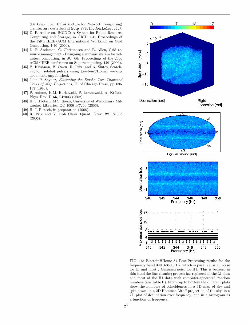
(Berkeley Open Infrastructure for Network Computing)architecture described at http://boinc.berkeley.edu/.

[43] D. P. Anderson, BOINC: A System for Public-ResourceComputing and Storage, in GRID ’04: Proceedings ofthe Fifth IEEE/ACM International Workshop on GridComputing, 4-10 (2004).

[44] D. P. Anderson, C. Christensen and B. Allen, Grid re-source management - Designing a runtime system for vol-unteer computing, in SC ’06: Proceedings of the 2006ACM/IEEE conference on Supercomputing, 126 (2006).

[45] B. Krishnan, B. Owen, R. Prix, and A. Sintes, Search-ing for isolated pulsars using Einstein@Home, workingdocument, unpublished.

[46] John P. Snyder, Flattening the Earth: Two ThousandYears of Map Projections, U. of Chicago Press, pp.130-133 (1993).

[47] P. Astone, K.M. Borkowski, P. Jaranowski, A. Krolak,Phys. Rev. D 65, 042003 (2002).

[48] H. J. Pletsch, M.S. thesis, University of Wisconsin - Mil-waukee Libraries, QC 1000 .P7266 (2006).

[49] H. J. Pletsch, in preparation (2008).[50] R. Prix and Y. Itoh Class. Quant. Grav. 22, S1003

(2005).

FIG. 16: Einstein@Home S4 Post-Processing results for thefrequency band 340.0-350.0 Hz, which is pure Gaussian noisefor L1 and mostly Gaussian noise for H1. This is because inthis band the line-cleaning process has replaced all the L1 dataand most of the H1 data with computer-generated randomnumbers (see Table II). From top to bottom the different plotsshow the numbers of coincidences in a 3D map of sky andspin-down, in a 2D Hammer-Aitoff projection of the sky, in a2D plot of declination over frequency, and in a histogram asa function of frequency.

27

FIG. 17: Einstein@Home S4 Post-Processing results for a“quiet” frequency band of real instrumental data from 110.0-120.0 Hz. From top to bottom the different plots show thenumbers of coincidences in a 3D map of sky and spin-down,in a 2D Hammer-Aitoff projection of the sky, in a 2D plot ofdeclination over frequency, and in a histogram as a functionof frequency.

FIG. 18: Einstein@Home S4 Post-Processing results for thefrequency band 570.0-580.0 Hz including a hardware injectedCW signal (Pulsar2). From top to bottom the different plotsshow the numbers of coincidences in a 3D map of sky andspin-down, in a 2D Hammer-Aitoff projection of the sky, in a2D plot of declination over frequency, and in a histogram asa function of frequency.

28

FIG. 19: Einstein@Home S4 Post-Processing results for a“noisy” frequency band of data polluted by instrumental noiseartifacts from 640.0-650.0 Hz. These spectral features are res-onance modes of the mode cleaner optics suspensions. Fromtop to bottom the different plots show the numbers of coinci-dences in a 3D map of sky and spin-down, in a 2D Hammer-Aitoff projection of the sky, in a 2D plot of declination overfrequency, and in a histogram as a function of frequency.

29