Output value-based initialization for radial basis function neural networks

Neural Processing Letters (2007) 25:209–225DOI 10.1007/s11063-007-9039-8

Output value-based initialization for radial basis functionneural networks

Alberto Guillén · Ignacio Rojas · Jesús González · Héctor Pomares ·L. J. Herrera · O. Valenzuela · F. Rojas

Received: 11 November 2005 / Accepted: 29 March 2007 / Published online: 12 May 2007© Springer Science+Business Media B.V. 2007

Abstract The use of Radial Basis Function Neural Networks (RBFNNs) to solve functionalapproximation problems has been addressed many times in the literature. When designing anRBFNN to approximate a function, the first step consists of the initialization of the centers ofthe RBFs. This initialization task is very important because the rest of the steps are based onthe positions of the centers. Many clustering techniques have been applied for this purposeachieving good results although they were constrained to the clustering problem. The nextstep of the design of an RBFNN, which is also very important, is the initialization of theradii for each RBF. There are few heuristics that are used for this problem and none of themuse the information provided by the output of the function, but only the centers or the inputvectors positions are considered. In this paper, a new algorithm to initialize the centers andthe radii of an RBFNN is proposed. This algorithm uses the perspective of activation gradesfor each neuron, placing the centers according to the output of the target function. The radiiare initialized using the center’s positions and their activation grades so the calculation of theradii also uses the information provided by the output of the target function. As the experi-ments show, the performance of the new algorithm outperforms other algorithms previouslyused for this problem.

Keywords RBF · Neural networks · RBFNN · Initialization · Function approximation ·Radii · Centers

1 Introduction

Formally, the functional approximation problem can be formulated as, given a set of obser-vations {(�xk; yk); k = 1, . . . , n} with yk = F(�xk) ∈ IR and �xk ∈ IRd , it is desired to obtain a

A. Guillén (B) · I. Rojas · J. González · H. Pomares · L. J. Herrera · O. Valenzuela · F. RojasDepartment of Computer Architecture and Computer Technology, University of Granada,C/ Periodista Daniel Saucedo s/n, Granada 18071, Spaine-mail: [email protected]

123

210 A. Guillén et al.

function F so yk � F(�xk). Once this function is learned, it will be possible to generate newoutputs from input data that were not specified in the original data set.

For the functional approximation problem, Artificial Neural Networks (ANNs) have thecapacity of estimating a model from empirical data. Therefore, they can act as interpolatorsso they return an output for any input, even if this input was not in the training data.

ANNs are computational systems inspired by the structure, processing method, and learn-ing ability of a biological brain. In the artificial system, a neuron corresponds to a processingunit which, given an input, it uses a function to compute an output. These systems are largelyused in many areas of science and engineering applications involving classification, optimi-zation and function approximation [12].

Within the ANNs, it exists a variety of types depending on the activation function or thenumber of layers. One of them is the RBFNN that was introduced by Broomhead and Lowe[7]. These RBFNNs have the capability of approximating any given function [8,26,30], there-fore they have been successfully applied to many problems related with nonlinear regressionand function approximation [22,35,36]. The main characteristic of this kind of ANN is thatit has a two-layer, fully connected network in which each neuron implements a gaussianfunction as follows:

φ(�x; �ci , ri ) = exp

(−||�ci − �x ||2

r2i

), i = 1, . . . , m (1)

where �x is an input vector, �ci is the center and ri is the radius of the i-th RBF. Gauss-ian functions are very appropriate for function approximation because they are continuous,differentiable, provide a softer output, and improve the interpolation capabilities [5,33].

The output layer implements a weighted sum of all the outputs from the hidden layer:

F (�x; C, R,�) =m∑

i=1

φ(�x; �c i , ri ) · �i (2)

where �i are the output weights, which show the contribution of a hidden layer to the cor-responding output unit and can be obtained optimally by solving a linear equation system.After the initialization of the centers and the radii, once all the previous elements have beencalculated, a local search algorithm can be applied to make a fine tuning of the model. Othermethodologies to train RBFNNs have been presented in Karayiannis [20] and Randolph-Gipsand Karayiannis [32], where reformulated and cosine RBFs are presented. The methodol-ogy is based on a gradient descent that does not use any initialization technique. GeneticAlgorithms have been also applied to design RBFNNs to approximate functions [17].

This paper presents the Output Value-Based Initializer (OVI) algorithm, which calculatesthe initial values for the centers and radii of an RBFNN according to the output values of thetarget function. To accomplish this task, the Output Value-Based Initializer (OVI) algorithmcalculates a hypothetic activation value for each center in order to place it and, once thecenters are placed, the radii are calculated using this activation value.

The remaining of this paper, in order to make it self-contained, is organized as follows:Sect. 2 describes the details of the centers and radii initialization problem, Sect. 3 describesthe OVI algorithm, Sect. 4 shows the experimental results and in Sect. 5 conclusions aredrawn.

123

Output value-based initialization for radial basis function 211

2 Statement of the problem

The design of an RBFNN to approximate a given function requires a sequence of steps. Thefirst one is the initialization of the RBF centers. This initialization task has been traditionallysolved using clustering algorithms [1,2,37]. For example in Karayiannis and Mi [21] and inZhu et al. [39] the initial model to design the RBFNN is created using clustering. Traditionalclustering algorithms have been used to initialize centers [4,11,28], but they were designedto solve classification problems. In these kind of problems, the input data have to be assignedto a pre-defined set of labels. This does not fit well enough when working with functionapproximation since a continuous interval of real numbers is defined to be the output of theinput data.

Related to the previous point, when classifying, if a label is not assigned correctly, theerror could be greatly increased. In the functional approximation problem is not like that, ifthe generated output value is near the real output, the error may not increase too much.

The initialization of the centers of an RBFNN, designed to approximate a given function,is not a trivial task and it should be done using the information provided by the output of thetarget function, otherwise, the centers could be placed in areas where the target function iseasy to model, making them useless.

The target function can have an output with a high variability in some areas and withother areas where the variability is not that high. Because of this, if many centers are placedin the areas where the function is not too variable, the ANN will not have enough neuronsto approximate the variable zones. Classical clustering techniques ignore the output of thefunction, just considering the input data vectors, but there are some other clustering tech-niques that use the information provided by the target function output. These algorithms areknown as input–output clustering algorithms and some of them have been applied to theinitialization of the RBF centers for function approximation problem [16,29,34].

In this framework, the need of using specific algorithms designed to initialize the centersinstead of using traditional clustering algorithms is obvious. Several algorithms have beendesigned specifically for this task, but they all were inspired in previous clustering algorithms[19,18,23,29]. This motivated the design of the algorithm proposed in this paper. This newalgorithm uses the information provided by the output of the function to be approximatedso it concentrates the centers through the areas with a high variability, placing less centerswhere the function is not too variable.

The design of an RBFNN also requires the initialization of the radii for each RBF. Usuallythis step has been performed using heuristics as the K-Nearest Neighbor (KNN) algorithm[24] or the Closest Input Vector (CIV) algorithm [21]. These heuristics ignore the outputof the function when initializing the radii, they only use the center positions or the inputvector positions. The new proposed algorithm makes an initialization using the center posi-tions and the activation grade of each input vector depending on its output, this allows thealgorithm to improve the results in comparison with the classical heuristic employed for thistask.

3 OVI: an output value-based initializer

This section contains the description of the new algorithm that initializes both the centers andthe radii of an RBFNN to approximate a function. First, the general scheme and the severalcomponents of the algorithm are briefly presented, then, in the following subsections, theseelements are described in detail.

123


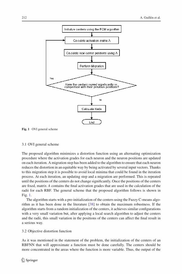
Fig. 1 OVI general scheme

3.1 OVI general scheme

The proposed algorithm minimizes a distortion function using an alternating optimizationprocedure where the activation grades for each neuron and the neuron positions are updatedon each iteration. A migration step has been added to the algorithm to ensure that each neuronreduces the distortion in an equitable way by being activated by several input vectors. Thanksto this migration step it is possible to avoid local minima that could be found in the iterationprocess. At each iteration, an updating step and a migration are performed. This is repeateduntil the positions of the centers do not change significantly. Once the positions of the centersare fixed, matrix A contains the final activation grades that are used in the calculation of theradii for each RBF. The general scheme that the proposed algorithm follows is shown inFig. 1.

The algorithm starts with a pre-initialization of the centers using the Fuzzy C-means algo-rithm as it has been done in the literature [38] to obtain the maximum robustness. If thealgorithm starts from a random initialization of the centers, it achieves similar configurationswith a very small variation but, after applying a local search algorithm to adjust the centersand the radii, this small variation in the positions of the centers can affect the final result ina serious way.

3.2 Objective distortion function

As it was mentioned in the statement of the problem, the initialization of the centers of anRBFNN that will approximate a function must be done carefully. The centers should bemore concentrated in the areas where the function is more variable. Thus, the output of the

123


function to be approximated must be considered as important information when initializingthe centers.

Since the centers have to be placed in the input vectors space, it is necessary to includein the algorithm an element that allows it to keep a reference between the output and theinput space. The objective is to keep a balance between the coordinates in the input spaceand the output it generates. If the two elements described, the output of the function and itscoordinates in the input space, are considered, it is possible to define a distortion function:

δ =n∑

k=1

m∑i=1

D2ikal

ik |Y pk | (3)

where Dik represents the Euclidean distance from a center ci to an input vector �xk, aik is theactivation value that determines how important the input vector �xk is for the center �ci , l is aparameter to control the degree of overlapping between the neurons, Yk is the preprocessedoutput of the input vector �xk , and p allows the influence of the output when initializing thecenters to increase or decrease.

This distortion function combines the information provided by a coordinate in the inputvector space and its corresponding output in such a way that, if a neuron is near an inputvector and the output of the input vector is high, the activation value of that neuron respectthat input vector will be high.

The original output of the function is preprocessed before starting the algorithm. The ideais to think of the output space as a flat surface (Y (�xk) = 0), where some of the values ofthis surface have been modified by an n-dimensional element, obtaining yk . From this, wecan assume that the most common value of the target function is constant and equal 0. Thepreprocessing of the output is performed by making the most frequent output value equal 0.This can be easily performed by subtracting the fuzzy mode to each one of the output valuesyk . Once this situation is achieved, all the most common values that have an output around0 will not affect the distortion significantly.

Let A = [aik], be the activation matrix, this matrix is restricted by the following condi-tions:

–∑m

i=1 aik = 1, ∀k = 1...n

– 0 <∑n

k=1 aik < n, ∀i = 1...m.

If aik is high, it means that the neuron (center i) is significantly activated by the inputvector �xk . The first restriction forces every input vector to activate at least one neuron, 1being the maximum grade of activation. The second restriction forces each neuron to shareevery input vector with the others, so all neurons will have an activation value even thoughthis can be very small. Thanks to this restriction, it is easier to maintain an overlap betweenthe RBFs allowing the ANN to make a softer interpolation of the target function.

The objective is to minimize the distortion function so the neurons are only activated whenit is necessary. The minimum of the distortion function will be reached when the distancefrom a center to an input vector with a high output value is the smallest. If this occurs, thevalue for aik will be the highest for this center, but very small for the other centers. Analternating optimization procedure is used to minimize the distortion function. Let C = [�ci ]be the matrix containing the coordinates of all the centers. On each iteration, the algorithmcalculates the matrix A from the matrix C supposing that C is the matrix where a minimumfor the distortion function is obtained. Once a new A is calculated it is possible to recalculate

123


the matrix C using the previous A. This iterative process ends when any of the two matricesdo not change significantly.

The equations to calculate these matrices at each iteration are:

aik =⎛⎝ m∑

j=1

(Dik

D jk

) 2l−1

⎞⎠

−1

(4)

�ci =∑n

k=1 alik �xk |Y p

k |∑nk=1 al

ik |Y pk | (5)

where Dik is the Euclidean distance between �xk and �ci , Yk is the preprocessed output ofthe target function, and l is the parameter to control the degree of overlapping between theneurons.

These equations are obtained by applying Lagrange multipliers and calculating the deriv-ative of the objective function, therefore, convergence is guaranteed (see Appendix).

3.3 Migration step

The iteration of the steps presented above makes a gradient descent to reach a minimum ofthe distortion function defined in Eq. 3. It uses an iterative process that can get stuck in alocal minima, specially when working with noncontinuous data sets. This problem can beeasily solved introducing a migration step as it was done in Pantanè and Russo [28].

The migration step aims to find the optimal vector quantization where each center makesequal contribution to the total distortion [15]. The migration algorithm iterates many times,moving centers on each iteration, until each center contributes equally to the distortion func-tion defined to be minimized. The distortion never increases so the convergence is not alteredby the migration step.

The migration step provides more robustness to the algorithm since it helps to find thesame configuration independently of the starting point of the centers.

Each center is assigned an individual distortion value that is defined as:

disti =n∑

k=1

D2ikal

ik |Y pk | (6)

so the sum of all the distortions for each center is equal to the global distortion function thatit is being minimized. Using this distortion measure, it is possible to assign an utility for eachcenter. A center is useful if it increases the global distortion in comparison with the others.The utility of a center is defined as:

uti = distidist

(7)

where dist is the mean distortion of the centers.After calculating the utility, there will be useful centers, with utility >1, and centers with

utility ≤1 that are not useful. In order to make sure that each center contributes equally to thetotal distortion, a center with a low utility will be moved near a center with utility greater than1. After the movement of the center, this modification will be accepted if the total distortionhas been decreased, otherwise, the moved center will be marked as processed and another

123


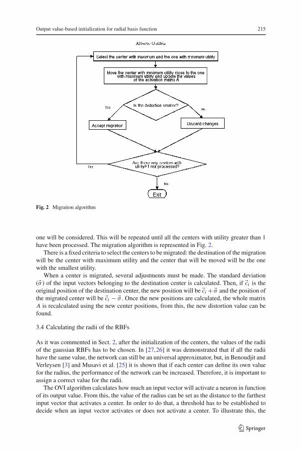
Fig. 2 Migration algorithm

one will be considered. This will be repeated until all the centers with utility greater than 1have been processed. The migration algorithm is represented in Fig. 2.

There is a fixed criteria to select the centers to be migrated: the destination of the migrationwill be the center with maximum utility and the center that will be moved will be the onewith the smallest utility.

When a center is migrated, several adjustments must be made. The standard deviation(�σ ) of the input vectors belonging to the destination center is calculated. Then, if �ci is theoriginal position of the destination center, the new position will be �ci + �σ and the position ofthe migrated center will be �ci − �σ . Once the new positions are calculated, the whole matrixA is recalculated using the new center positions, from this, the new distortion value can befound.

3.4 Calculating the radii of the RBFs

As it was commented in Sect. 2, after the initialization of the centers, the values of the radiiof the gaussian RBFs has to be chosen. In [27,26] it was demonstrated that if all the radiihave the same value, the network can still be an universal approximator, but, in Benoudjit andVerleysen [3] and Musavi et al. [25] it is shown that if each center can define its own valuefor the radius, the performance of the network can be increased. Therefore, it is important toassign a correct value for the radii.

The OVI algorithm calculates how much an input vector will activate a neuron in functionof its output value. From this, the value of the radius can be set as the distance to the farthestinput vector that activates a center. In order to do that, a threshold has to be established todecide when an input vector activates or does not activate a center. To illustrate this, the

123


0 1 2 3 4 5 6 7 8 9 100.6

0.4

0.2

0

0.2

0.4

0.6

0.8

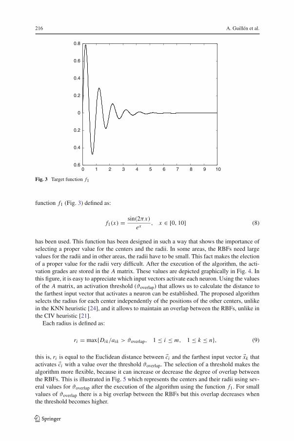
Fig. 3 Target function f1

function f1 (Fig. 3) defined as:

f1(x) = sin(2πx)

ex, x ∈ [0, 10] (8)

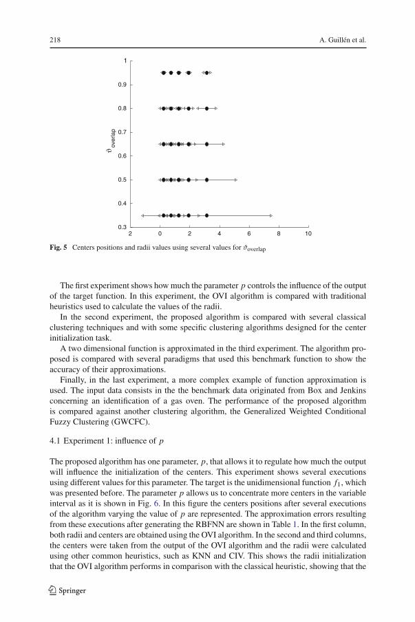
has been used. This function has been designed in such a way that shows the importance ofselecting a proper value for the centers and the radii. In some areas, the RBFs need largevalues for the radii and in other areas, the radii have to be small. This fact makes the electionof a proper value for the radii very difficult. After the execution of the algorithm, the acti-vation grades are stored in the A matrix. These values are depicted graphically in Fig. 4. Inthis figure, it is easy to appreciate which input vectors activate each neuron. Using the valuesof the A matrix, an activation threshold (ϑoverlap) that allows us to calculate the distance tothe farthest input vector that activates a neuron can be established. The proposed algorithmselects the radius for each center independently of the positions of the other centers, unlikein the KNN heuristic [24], and it allows to maintain an overlap between the RBFs, unlike inthe CIV heuristic [21].

Each radius is defined as:

ri = max{Dik/aik > ϑoverlap, 1 ≤ i ≤ m, 1 ≤ k ≤ n}, (9)

this is, ri is equal to the Euclidean distance between �ci and the farthest input vector �xk thatactivates �ci with a value over the threshold ϑoverlap. The selection of a threshold makes thealgorithm more flexible, because it can increase or decrease the degree of overlap betweenthe RBFs. This is illustrated in Fig. 5 which represents the centers and their radii using sev-eral values for ϑoverlap after the execution of the algorithm using the function f1. For smallvalues of ϑoverlap there is a big overlap between the RBFs but this overlap decreases whenthe threshold becomes higher.

123


0 1 2 3 4 5 6 7 8 9 100

0.1

0.2

0.3

0.4

0.5

0.6

0.7

0.8

0.9

1

0 1 2 3 4 5 6 7 8 9 100

0.1

0.2

0.3

0.4

0.5

0.6

0.7

0.8

0.9

1

center 1 center 2

0 1 2 3 4 5 6 7 8 9 100

0.1

0.2

0.3

0.4

0.5

0.6

0.7

0.8

0.9

1

0 1 2 3 4 5 6 7 8 9 100

0.1

0.2

0.3

0.4

0.5

0.6

0.7

0.8

0.9

1

center 3 center 4

0 1 2 3 4 5 6 7 8 9 100

0.1

0.2

0.3

0.4

0.5

0.6

0.7

0.8

0.9

1

0 1 2 3 4 5 6 7 8 9 100.5

0

0.5

1

center 5 All the centers

Fig. 4 Activation grades for five centers after the execution of the algorithm using f1

4 Experiments

In this section the behavior of the algorithm in function of several parameters is analyzed andit is compared with other algorithms that have been used to initialize the centers of RBFNNsor the complete RBFNN.

123


2 0 2 4 6 8 100.3

0.4

0.5

0.6

0.7

0.8

0.9

1

ϑov

erla

p

Fig. 5 Centers positions and radii values using several values for ϑoverlap

The first experiment shows how much the parameter p controls the influence of the outputof the target function. In this experiment, the OVI algorithm is compared with traditionalheuristics used to calculate the values of the radii.

In the second experiment, the proposed algorithm is compared with several classicalclustering techniques and with some specific clustering algorithms designed for the centerinitialization task.

A two dimensional function is approximated in the third experiment. The algorithm pro-posed is compared with several paradigms that used this benchmark function to show theaccuracy of their approximations.

Finally, in the last experiment, a more complex example of function approximation isused. The input data consists in the the benchmark data originated from Box and Jenkinsconcerning an identification of a gas oven. The performance of the proposed algorithmis compared against another clustering algorithm, the Generalized Weighted ConditionalFuzzy Clustering (GWCFC).

4.1 Experiment 1: influence of p

The proposed algorithm has one parameter, p, that allows it to regulate how much the outputwill influence the initialization of the centers. This experiment shows several executionsusing different values for this parameter. The target is the unidimensional function f1, whichwas presented before. The parameter p allows us to concentrate more centers in the variableinterval as it is shown in Fig. 6. In this figure the centers positions after several executionsof the algorithm varying the value of p are represented. The approximation errors resultingfrom these executions after generating the RBFNN are shown in Table 1. In the first column,both radii and centers are obtained using the OVI algorithm. In the second and third columns,the centers were taken from the output of the OVI algorithm and the radii were calculatedusing other common heuristics, such as KNN and CIV. This shows the radii initializationthat the OVI algorithm performs in comparison with the classical heuristic, showing that the

123


0 1 2 3 4 5 6 7 8 9 100.6

0.4

0.2

0

0.2

0.4

0.6

0.8

0 1 2 3 4 5 6 7 8 9 100.6

0.4

0.2

0

0.2

0.4

0.6

0.8

p = 1 p = 1.5

0 1 2 3 4 5 6 7 8 9 100.6

0.4

0.2

0

0.2

0.4

0.6

0.8

0 1 2 3 4 5 6 7 8 9 100.6

0.4

0.2

0

0.2

0.4

0.6

0.8

p = 2.5 p = 4.5

Fig. 6 Centers placement using several values of p

Table 1 Average and standard deviation of the approximation error (NRMSE) for function f1 using severalvalues of p and several heuristics for the radii initialization

p OVI OVI-KNN OVI-CIV

1 0.044 (0.000) 0.167 (0.021) 0.107 (0.017)

1.5 0.041 (0.000) 0.131 (0.001) 0.153 (0.000)

2.5 0.105 (0.000) 0.151 (0.000) 0.151 (0.000)

4.5 0.102 (0.000) 0.155 (0.000) 0.231 (0.000)

proposed algorithm significantly outperforms the other two heuristics independently of thevalue of the parameter p.

Another remarkable characteristic is the robustness of the results obtained using the pro-posed algorithm, that allows to obtain the same configuration from different initializations,providing very similar approximation errors on several executions for the same parameters.

As it is shown in Fig. 6, the bigger the value of p is, the closer the centers are placed in theinterval where the variability of the function is higher. The results show that, for small valuesof p, the approximations are good but when p is highly augmented, the error increases. Thisis because all the centers are concentrated in the interval where the function is more variable

123


0.5

0

0.5

0.5

0

0.50

1

2

3

4

5

6

7

8

9

Fig. 7 Target function f5

and no centers are placed in the other areas therefore, these areas cannot be modeled. Anadvisable value of p could be 1.5, this value has been used for all the following experimentsallowing the algorithm to obtain appropriate results. The election of the value of p makesthe algorithm more flexible if there is a chance of a human expert determining its value.

4.2 Experiment 2: 1D function

This experiment compares the proposed algorithm with the traditional clustering algorithmsthat have been used to initialize the centers and with the two input–output algorithms CFAand FCFA. The target function f1, previously introduced, is the one that was used to compareCFA and FCFA with other clustering techniques.

Table 2 shows the approximation errors after generating the RBFNN using the KNNalgorithm with K = 1 for all the algorithms except for the OVI algorithm. In the results, theapproximation errors of the OVI algorithm are smaller than the error obtained using the otheralgorithms. It is very important to remark on the robustness of the algorithm, that startingfrom a random point, it is able to reach the same configuration, as it is the most robust of allthe other compared algorithms.

4.3 Experiment 3: 2D function

This experiment consists in the approximation of the two dimensional function f5 (Fig. 7)that was originally proposed in Cherkassky and Lari-Najafi, [9] and is defined as:

f5(x1, x2) = 42.659(0.1 + x1(0.05 + x41 − 10x2

1 x22 + 5x4

2 )) x1, x2 ∈ [−0.5, 0.5] (10)

This function has been used as a benchmark in several papers. In Cherkassky et al. [10]the approximation was done using multilayer perceptrons (MLP) and in Pomares [31] itwas used an algorithm for identification of rule-based fuzzy systems. The target functionwas also approximated in Friedman [13] using the Projection Pursuit (PP), and a Mul-

123


Table 2 Average and standard deviation of the approximation error (NRMSE) for function f1 using severalnumbers of neurons (m)

m HCM FCM ELBG CFA FCFA OVI

6 0.759 (0.263) 0.783 (0.317) 0.152 (0.122) 0.090 (0.008) 0.103 (0.060) 0.041 (0.031)

7 0.344 (0.281) 0.248 (0.115) 0.111 (0.072) 0.081 (0.016) 0.069 (0.017) 0.029 (0.012)

8 0.227 (0.368) 0.150 (0.162) 0.093 (0.064) 0.053 (0.028) 0.048 (0.031) 0.014 (0.001)

9 0.252 (0.386) 0.300 (0.160) 0.073 (0.057) 0.056 (0.027) 0.027 (0.024) 0.010 (0.001)

10 0.087 (0.100) 0.285 (0.334) 0.064 (0.039) 0.047 (0.015) 0.011 (0.015) 0.007 (0.003)

–0.5

0

0.5

–0.5

0

0.5–5

–4

–3

–2

–1

0

1

2

3

4

Fig. 8 Training set for function f5

tivariate Adaptive Regression Splines (MARS) algorithm was used in Friedman [14]. Amulti-objective GA was used in González et al. [17] to design RBFNNs to approximate thisfunction.

All the algorithms have been compared used a training set of 400 inputs generatedrandomly from a grid of 20 × 20 (Fig. 8). The approximations have been tested with adata set of 961 input vectors generated randomly over a grid of 31 × 31.

The results are shown in Table 3, where all the previous algorithms described in the para-graphs above are compared with the proposed algorithm. The OVI algorithm improves theresults significantly providing smaller approximation errors. Another aspect of note is therobustness of the proposed algorithm, that finds the same configuration independently of thestarting positions of the centers as it occurred in the previous experiments.

4.4 Experiment 4: time series prediction

In this experiment, the benchmark data originated from Box and Jenkins [6], concerningan identification of a gas oven is used. To obtain the data, air and methane were deliveredinto a gas oven to obtain a mixture of gases containing CO2. There were originally 296data points y(t), u(t), from t = 1 to t = 296. The value y(t) is the output CO2 con-

123


Table 3 Mean approximationerror and standard deviationwhen approximating f5 usingseveral numbers of neurons orfuzzy rules (m)

Algorithm m Test NRMSE

MLP 15 0.308

PP – 0.504

CTM – 0.131

MARS – 0.190

Cherkassky et al. [10] 40 0.038

Gonzalez [17] 13 0.023 (0.001)

14 0.021 (0.005)

15 0.017 (0.005)

16 0.016 (0.009)

17 0.015 (8.5E-5)

Proposed algorithm 13 0.004 (0.002)

14 0.002 (0.001)

15 0.002 (0.001)

16 0.002 (0.001)

17 0.001 (0.000)

Table 4 Approximation errors(RMSE) for the Box-Jenkins dataset using the FCM, GWCM andthe OVI algorithms

Algorithm RMSE

GWFCM 0.187

FCM 0.204

OVI 0.1749

centration and u(t) is the input gas flow rate. The objective is to predict y(t) based on{y(t −1), y(t −2), y(t −3), y(t −4), u(t −1), u(t −2), u(t −3), u(t −4), u(t −5), u(t −6)}.

This reduces the number of effective data points to 290 and set the dimension of theproblem to 10.

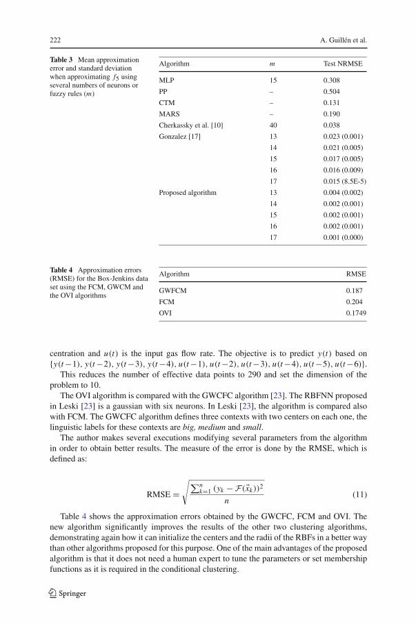
The OVI algorithm is compared with the GWCFC algorithm [23]. The RBFNN proposedin Leski [23] is a gaussian with six neurons. In Leski [23], the algorithm is compared alsowith FCM. The GWCFC algorithm defines three contexts with two centers on each one, thelinguistic labels for these contexts are big, medium and small.

The author makes several executions modifying several parameters from the algorithmin order to obtain better results. The measure of the error is done by the RMSE, which isdefined as:

RMSE =√∑n

k=1 (yk − F(�xk))2

n(11)

Table 4 shows the approximation errors obtained by the GWCFC, FCM and OVI. Thenew algorithm significantly improves the results of the other two clustering algorithms,demonstrating again how it can initialize the centers and the radii of the RBFs in a better waythan other algorithms proposed for this purpose. One of the main advantages of the proposedalgorithm is that it does not need a human expert to tune the parameters or set membershipfunctions as it is required in the conditional clustering.

123


0 50 100 150 200 250 30044

46

48

50

52

54

56

58

60

62

Time

Out

put

OriginalPredicted by OVI

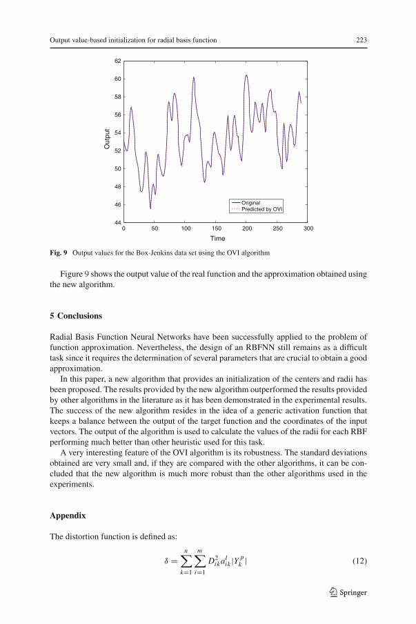
Fig. 9 Output values for the Box-Jenkins data set using the OVI algorithm

Figure 9 shows the output value of the real function and the approximation obtained usingthe new algorithm.

5 Conclusions

Radial Basis Function Neural Networks have been successfully applied to the problem offunction approximation. Nevertheless, the design of an RBFNN still remains as a difficulttask since it requires the determination of several parameters that are crucial to obtain a goodapproximation.

In this paper, a new algorithm that provides an initialization of the centers and radii hasbeen proposed. The results provided by the new algorithm outperformed the results providedby other algorithms in the literature as it has been demonstrated in the experimental results.The success of the new algorithm resides in the idea of a generic activation function thatkeeps a balance between the output of the target function and the coordinates of the inputvectors. The output of the algorithm is used to calculate the values of the radii for each RBFperforming much better than other heuristic used for this task.

A very interesting feature of the OVI algorithm is its robustness. The standard deviationsobtained are very small and, if they are compared with the other algorithms, it can be con-cluded that the new algorithm is much more robust than the other algorithms used in theexperiments.

Appendix

The distortion function is defined as:

δ =n∑

k=1

m∑i=1

D2ikal

ik |Y pk | (12)

123


If the values of the matrix C are fixed, the values for matrix A can be calculated by Eq. 4.To obtain the equation to update centers, fixed a matrix A and making the derivative equal

zero we have that:

∂δ

∂ci=

n∑k=1

m∑i=1

alik(2�xk − 2�ci )|Y p

k | = 0, (13)

from where it is easy to obtain Eq. 5.

Acknowledgements This work has been partially supported by the Spanish CICYT Project TIN2004-01419.

References

1. Baraldi A, Blonda P (1999a) A survey of fuzzy clustering algorithms for pattern recognition – Part I.IEEE Trans Syst Man Cybern 29(6): 786–801

2. Baraldi A, Blonda P (1999b) A survey of fuzzy clustering algorithms for pattern recognition – Part II.IEEE Trans Syst Man Cybern 29(6): 786–801

3. Benoudjit N, Verleysen M (2003) On the kernel widths in radial basis function networks. Neural ProcessLett 18(2): 139–154

4. Bezdek JC (1981) Pattern recognition with fuzzy objective function algorithms. Plenum, New York5. Bors AG (2001) Introduction of the Radial Basis Function (RBF) networks. OnLine Symp Electron Eng

1: 1–76. Box GEP, Jenkins GM (1976) Time series analysis, forecasting and control. Holden Day, San Francisco

CA7. Broomhead DS, Lowe D (1988) Multivariate functional interpolation and adaptive networks. Complex

Syst 2: 321–3558. Chen T, Chen H (1995) Approximation capability to functions of several variables, nonlinear function-

als, and operators by radial basis function networks. IEEE Trans Neural Networks 6(4): 904–9109. Cherkassky V, Lari-Najafi H (1991) Constrained topological mapping for nonparametric regression

analysis. Neural Networks 4(1): 27–4010. Cherkassky V, Gehring D, Mulier F (1996) Comparison of adaptative methods for function estimation

from samples. IEEE Trans Neural Networks 7: 969–98411. Duda RO, Hart PE (1973) Pattern classification and scene analysis. Wiley, New York12. Elanayar S, Shin YC (1994) Radial basis function neural networks for approximation and estimation of

nonlinear stochastic dynamic systems. IEEE Trans Neural Networks 5: 594–60313. Friedman J (1981) Projection pursuit regression. J Am Statist Assoc 76: 817–82314. Friedman JH (1991) Multivariate adaptive regression splines (with discussion). Ann Stat 19: 1–14115. Gersho A (1979) Asymptotically optimal block quantization. IEEE Trans Inform Theory 25(4): 373–

38016. González J, Rojas I, Pomares H, Ortega J, Prieto A (2002) A new clustering technique for function

aproximation. IEEE Trans Neural Networks 13(1): 132–14217. González J, Rojas I, Ortega J, Pomares H, Fernández F, Díaz A (2003) Multiobjective evolutionary

optimization of the size, shape, and position parameters of radial basis function networks for functionapproximation. IEEE Trans Neural Networks 14(6): 1478–1495

18. Guillén A, Rojas I, González J, Pomares H, Herrera L, Valenzuela O, Prieto A (2005a) Improving clus-tering technique for functional approximation problem using fuzzy logic: ICFA algorithm. Lecture NotesComp Sci 3512: 272–280

19. Guillén A, Rojas I, González J, Pomares H, Herrera L J (2005b) RBF centers initialization using fuzzyclustering technique for function approximation problems. Fuzzy Econ Rev 10(2): 27–44

20. Karayiannis NB (1999) Reformulated radial basis neural networks trained by gradient descent. IEEETrans Neural Networks 10(3):657–671

21. Karayiannis NB, Mi GW (1997) Growing radial basis neural networks: merging supervised and unsu-pervised learning with network growth techniques. IEEE Trans Neural Networks 8: 1492–1506

22. Karayiannis NB, Balasubramanian M, Malki HA (2003) Evaluation of cosine radial basis function neuralnetworks on electric power load forecasting. In: Proceedings of the International Joint Conference onNeural Networks, vol 3, pp 2100–2105

123


23. Leski JM (2003) Generalized weighted conditional fuzzy clustering. IEEE Trans Fuzzy Syst 11(6):709–715

24. Moody J, Darken C (1989) Fast learning in networks of locally-tunned processing units. Neural Comput1(2): 281–294

25. Musavi MT, Ahmed W, Chan K, Faris K, Hummels D (1992) On the training of radial basis functionsclassifiers. Neural Networks 5(4): 595–603

26. Park J, Sandberg JW (1991) Universal approximation using radial basis functions network. Neural Com-put 3: 246–257

27. Park J, Sandberg I (1993) Approximation and radial basis function networks. Neural Comput 5: 305–31628. Patanè G, Russo M (2001) The enhanced-LBG algorithm. Neural Networks 14(9): 1219–123729. Pedrycz W (1998) Conditional fuzzy clustering in the design of radial basis function neural networks.

IEEE Trans Neural Networks 9(4): 601–61230. Poggio T, Girosi F (1990) Networks for approximation and learning. In: Proceedings of the IEEE, vol

78, pp 1481–149731. Pomares H (2000) Nueva metodología para el dise no automático de sistemas difusos. PhD dissertation,

University of Granada, Spain32. Randolph-Gips M M, Karayiannis N B (2003) Cosine radial basis function neural networks. In: Pro-

ceedings of the International Joint Conference on Neural Networks, vol 3, pp 96–10133. Rojas I, Anguita M, Prieto A, Valenzuela O (1998) Analysis of the operators involved in the definition

of the implication functions and in the fuzzy inference proccess. Int J Approx Reason 19: 367–38934. Runkler TA, Bezdek JC (1999) Alternating cluster estimation: a new tool for clustering and function

approximation. IEEE Trans Fuzzy Syst 7(4): 377–39335. Schilling RJ, Carroll JJ, Al-Ajlouni AF (2001) Approximation of nonlinear systems with radial basis

function neural networks. IEEE Trans Neural Networks 12(1): 1–1536. Sigitani T, Iiguni Y, Maeda H (1999) Image interpolation for progressive transmission by using radial

basis function networks. IEEE Trans Neural Networks 10(2): 381–38937. Uykan Z, Gzelis C, Celebei ME, Koivo HN (2000) Analysis of input–output clustering for determining

centers of RBFN. IEEE Trans Neural Networks 11(4): 851–85838. Zhang J, Leung Y (2004) Improved possibilistic C–means clustering algorithms. IEEE Trans Fuzzy Syst

12: 209–21739. Zhu Q, Cai Y, Liu L (1999) A global learning algorithm for a RBF network. Neural Networks 12:

527–540

123

Output value-based initialization for radial basis function neural networks

Documents

Transcript of Output value-based initialization for radial basis function neural networks