Local-Scale Urban Meteorological Parameterization Scheme (LUMPS): LongwaveRadiation Parameterization and Seasonality-Related Developments

THOMAS LORIDAN AND C. S. B. GRIMMOND

Department of Geography, King’s College London, London, United Kingdom

BRIAN D. OFFERLE

FluxSense, Goteborg, Sweden

DUICK T. YOUNG AND THOMAS E. L. SMITH

Department of Geography, King’s College London, London, United Kingdom

LEENA JARVI

Department of Geography, King’s College London, London, United Kingdom, and Department of Physics,

University of Helsinki, Helsinki, Finland

FREDRIK LINDBERG*

Department of Geography, King’s College London, London, United Kingdom

(Manuscript received 14 January 2010, in final form 21 August 2010)

ABSTRACT

Recent developments to the Local-scale Urban Meteorological Parameterization Scheme (LUMPS),

a simple model able to simulate the urban energy balance, are presented. The major development is the

coupling of LUMPS to the Net All-Wave Radiation Parameterization (NARP). Other enhancements include

that the model now accounts for the changing availability of water at the surface, seasonal variations of active

vegetation, and the anthropogenic heat flux, while maintaining the need for only commonly available mete-

orological observations and basic surface characteristics. The incoming component of the longwave radiation

(LY) in NARP is improved through a simple relation derived using cloud cover observations from a ceilometer

collected in central London, England. The new LY formulation is evaluated with two independent multiyear

datasets (qodz, Poland, and Baltimore, Maryland) and compared with alternatives that include the original

NARP and a simpler one using the National Climatic Data Center cloud observation database as input. The

performance for the surface energy balance fluxes is assessed using a 2-yr dataset (qodz). Results have an

overall RMSE , 34 W m22 for all surface energy balance fluxes over the 2-yr period when using LY as forcing,

and RMSE , 43 W m22 for all seasons in 2002 with all other options implemented to model LY.

1. Introduction

The characterization of surface–atmosphere energy

exchange is at the core of most meteorological

applications, ranging from weather forecasting to pol-

lutant dispersion and boundary layer height modeling. As

shown by Grimmond et al. (2010a,b) in their model

comparison project, no optimum compromise can yet be

identified between the complexity of the parameteriza-

tion schemes involved (both in terms of computational

cost and amount of required input information) and

their performance in simulating the main components of

the surface energy balance in urban areas (SEB; Oke

1987). The Local-scale Urban Meteorological Parame-

terization Scheme (LUMPS) of Grimmond and Oke

(2002) is by design one of the simplest models available.

* Current affiliation: Dept. of Earth Sciences, Gothenburg

University, Goteborg, Sweden.

Corresponding author address: Thomas Loridan, Environmental

Monitoring and Modelling Group, Dept. of Geography, King’s

College London, London WC2R 2LS, United Kingdom.

E-mail: thomas.loridan@gmail.com

JANUARY 2011 L O R I D A N E T A L . 185

DOI: 10.1175/2010JAMC2474.1

� 2011 American Meteorological Society

The parameterization of storage heat (DQS) belongs to

the category of empirical models as defined by Masson

(2006), as it uses observed relations between net all-

wave radiation (Q*) and surface components, which are

combined based on their fractions present [Objective

Hysteresis Model (OHM), Grimmond et al. (1991);

Grimmond and Oke (1999)]. The turbulent fluxes of

sensible heat (QH) and latent heat (QE) are subsequently

partitioned from the available energy (Q* 2 DQS) using a

version of the Holtslag and van Ulden (1983) combination-

type model with coefficients determined for urban areas

(Grimmond and Oke 2002). This type of approach to-

ward modeling QH is commonly used to characterize the

state of the planetary boundary layer (friction velocity,

mixing height, Obukhov length) in many of the meteo-

rological preprocessors developed by the dispersion

modeling community [e.g., Complex Terrain Dispersion

Model (CTDM) plus algorithms for unstable situations

(CTDMPLUS; Perry 1992), or Atmospheric Dispersion

Modeling System (AERMOD) Meteorological Prepro-

cessor (AERMET; Cimorelli et al. 2005)].

The original urban SEB directly modeled by

LUMPS is

Q* 5 QH

1 QE

1 DQS. (1)

The anthropogenic heat flux (QF) was initially consid-

ered to be implicitly contained within the coefficients

because observations were used to derive their estimates

(Grimmond and Oke 2002). However, it was stressed

that the sites used in the derivation did not include large

QF fluxes relative to the radiative forcing, so consequently

they were not explicitly included (Grimmond and Oke

2002). Microscale advection processes are included within

the parameterization implicitly. The net advection of heat

and moisture (DQA) from larger-scale patchiness (such as

between neighborhoods) is not included in the model, as

with other urban land surface schemes (Grimmond et al.

2010a,b) a mesoscale model is needed to resolve this (in

which LUMPS would be embedded if ‘‘online’’). The

original LUMPS is able to simulate the SEBs of urban

areas if provided with observations of Q* and common

meteorological variables (air temperature, pressure, hu-

midity, and precipitation) at the local or neighborhood

scales (102–104 m) along with basic surface cover infor-

mation (fraction of surface area occupied by vegetation,

buildings, or impervious materials).

The most restrictive of these requirements is the need

for Q* at the local scale. To eliminate this dependency,

the Net All-wave Radiation Parameterization (NARP) of

Offerle et al. (2003) is incorporated. Instead of Q*, in-

coming shortwave radiation (KY), near-surface air tem-

perature (Ta), vapor pressure (ea), and relative humidity

(RH) are required, along with bulk surface albedo and

emissivity estimates (a0 and «0, respectively). The com-

bined LUMPS–NARP system (hereafter referred to as

LUMPS) is easily employed for most urban meteorolog-

ical applications, and can be considered for implemen-

tation in numerical weather prediction (NWP) models

(e.g., Taha 1999) where its use of simple input information

and its low computational cost would fit the main re-

quirements (Loridan et al. 2010). The good performance

of NARP is critical as Q* is the key driver for the other

submodels. However, when NARP is evaluated, a night-

time bias is noticeable from some of the scatterplots

(when Q* , 0 W m22) with a clear discontinuity in the

modeled values. In the absence of incoming solar radia-

tion, this bias directly relates to longwave radiation and, in

particular, the incoming component (LY).

In this paper an alternative method for LY is de-

veloped with cloud data from a site in central London

based on measured relative humidity and air tempera-

ture. Performance is evaluated at two independent sites

(qodz, Poland, and Baltimore, Maryland). Other new

features in LUMPS allow for changing water availability

at the surface, changing vegetation phenology, and an-

thropogenic heat. The whole LUMPS system is evalu-

ated using an independent dataset (qodz).

2. Modeling incoming longwave radiation

a. The original NARP model

In NARP (Offerle et al. 2003), LY is considered to be

emitted by a single-layer atmosphere with radiative pro-

perties satisfying the Stefan–Boltzmann law:

LY 5 «sky

sT4sky, (2)

where s is the Stefan’s constant (W m22 K24) and Tsky is

the bulk atmospheric temperature, approximated by mea-

sured Ta (K). The sky emissivity «sky is based on Prata’s

(1996) clear-sky «clear, which is corrected to account for the

radiative impacts of clouds:

«clear

5 1� (1 1 w)e�ffiffiffiffiffiffiffiffiffiffiffiffi1.213wp

; w 5 46.5(ea/T

a)

«sky

5 «clear

1 (1� «clear

)F2CLD, (3)

where w is the precipitable water content (g cm22) and

FCLD represents the portion of the sky covered by clouds

(0 , FCLD , 1). In NARP, FCLD is estimated from the

ratio of measured KY and the theoretical clear-sky value

at the location (Kclear). This is obtained from (Crawford

and Duchon 1999)

FCLD

(KY, Kclear

) 5 1� KY

Kclear

; Kclear

5 IEX

cos(Z)t,

(4)

186 J O U R N A L O F A P P L I E D M E T E O R O L O G Y A N D C L I M A T O L O G Y VOLUME 50

where IEX is the extraterrestrial (or ‘‘top’’ of the atmo-

sphere) insolation, Z is the solar zenith angle, and t

is the atmospheric transmissivity parameterized from

measured surface pressure, temperature, and relative

humidity to represent the combined effects of Rayleigh

scattering, absorption by permanent gases and water

vapor, and absorption–scattering by aerosols.

Such a representation of cloud coverage is not appli-

cable at low sun elevation angles (Offerle et al. 2003;

Lindberg et al. 2008) and is obviously not applicable at

night. As a consequence, the original NARP only com-

putes FCLD for Z , 808, and keeps a constant value from

sunset to sunrise. The use of Smith’s (1966) empirical re-

lation in the computation of the atmospheric transmissivity

t in (4) (Crawford and Duchon 1999) is a limitation on the

application of NARP as it involves latitude-dependent

coefficients only available for the Northern Hemisphere

that are not time sensitive.

b. Cloud and radiation data from central London

Here, FCLD is parameterized using cloud height and

cover data from a Vaisala CL31 ceilometer (Vaisala Oyj

2006), situated at King’s College London (51.5118N,

0.1168W). The instrument consists of a low-powered,

eye-safe, single-wavelength (910 6 10 nm at 258C) laser

that samples the volume of air directly above the in-

strument, returning the height-normalized optical vol-

ume backscatter intensity of the atmosphere using the

lidar principle (Emeis et al. 2004). The CL31 uses a high

laser pulse repetition frequency of 10 kHz to cancel

noise (Eresmaa et al. 2006). Cloud information and a

backscatter profile are generated every 15 s from sam-

ples taken every 67 ms for 50 ms to give a vertical profile

resolution of 10 m up to an altitude of 7.7 km. An inbuilt

cloud detection algorithm provides cloud-base level in-

formation for up to three heights (dependent on signal

extinction due to cloud thickness). By postprocessing

the cloud-height data, it is possible to compute the cloud

cover (FCLD) using data from before and after each

particular measurement. Each profile (every 15 s) was

classified as being either cloudy (Cb 5 1) or clear (Cb 5

0). To best represent the cloud cover influence on LY,

a 900-s time window (450 s before and after each mea-

surement) was used to calculate the mean cloud cover

for each particular measurement:

FCLD

(t) 51

2tw

�tw

t5�tw

Cb(t)

24

35, (5)

where FCLD is cloud cover fraction at measurement time

t and tw is the time window expressed as a number of

measurements; in the current analysis tw 5 30.

In addition, a Kipp and Zonen CNR1 radiometer and

a Vaisala WXT510 weather transmitter (temperature,

humidity, pressure) were mounted on a tower (site name

KSK) located 48.1 m above sea level. The 500-m-radius

circle around the tower has a mean building height of

20.7 6 7.8 m and plan area fractions of building 5 33.9%,

impervious 5 34.4%, and water 5 26% (with the remaining

fraction composed of grass, shrubs, and nonconiferous

trees).

c. A new parameterization of cloud impact on LY

A requirement for inclusion within LUMPS is that

the meteorological inputs are easily procurable, which is a

central issue for most meteorological preprocessors (e.g.,

in dispersion modeling). Based on both common data

availability and physical considerations, a set of possible

predictors is initially identified. It includes the air tem-

perature (K), relative humidity (%), vapor pressure, and

vapor pressure deficit (hPa), as well as the precipitable

water content (g cm22), the specific humidity (kg kg21),

and the cooling rate of the air (K s21). An improved for-

ward stepwise selection process [least angle regression;

Bradley et al. (2004)] is used to identify the predictors that

demonstrate the largest correlation with the processed

FCLD data (section 2a), to sort the quantities best able to

explain cloud coverage for the period 1 July 2008–30 June

2009 in London. Least angle regression does not require

the predictors to be independent of each other. The first

predictor selected from such analysis is relative humidity

(RH), followed by air temperature (Ta), suggesting that

the formulation for FCLD should be primarily based on

RH and could potentially gain from using Ta as a com-

plementary source of information.

A locally weighted polynomial regression procedure

[locally weighted scatterplot smoothing (lowess); Cleveland

1981)] was applied to the hourly averaged FCLD and RH

measurements (Fig. 1) to identify the dominant trend.

With nonlinear regression, the lowess curve is approxi-

mated by

FCLD

(RH) 5 AeB3RH; A 5 0.185, B 5 0.017. (6)

Repeating this for each temperature range, the influence

of Ta on A and B can be studied. To represent the

evolution of the nonlinear regression curve, B is allowed

to evolve as a function of Ta while A is kept at 0.185. The

following relation is fitted through the B coefficient

values to allow for the Ta dependency:

B(Ta) 5 0.015 1 1.9 3 10�4T

a. (7)

Physically, this translates the idea that for a given RH

the water vapor concentration of the air is higher at

JANUARY 2011 L O R I D A N E T A L . 187

warm temperatures than it would be for cooler ones

(i.e., the Clausius–Clapeyron principle) making long-

wave absorption–emission more likely. To avoid sys-

tematic biases at very low humidity levels (e.g., FCLD 6¼0 if RH 5 0), the parameterization is forced through the

origin. The resulting temperature-dependent family of

functions is plotted in Fig. 1 and is defined as

FCLD

(RH, Ta) 5 0.185[e(0.01511.9310�4T

a)3RH � 1]. (8)

Finally, as in Crawford and Duchon (1999), FCLD is not

squared [cf. with Eq. (3)], yielding this parameterization

for LY:

LY(ea, T

a, RH) 5 «

clear(e

a, T

a) 1 [1� «

clear(e

a, T

a)]

�3 F

CLD(RH, T

a)�

3 sT4a. (9)

Having removed the latitude-dependent calculation of

Kclear, and with ea, Ta, and RH as the only inputs, this

empirical LY model offers the advantage of an easy

implementation within LUMPS and is applicable to any

hour of the day.

Additionally, the use of observed FCLD rather than

modeled FCLD is considered. This requires more input

but the added accuracy should greatly improve LY. If

such data are not available directly at the desired loca-

tion, they can be obtained from the fraction of sky

coverage typically observed at the nearest airport and

archived by the National Climatic Data Center (NCDC

2009). Coverage in 10ths is used for FCLD in

LY(ea, T

a, NCDC) 5 «

clear(e

a, T

a)

�1 [1� «

clear(e

a, T

a)]

3 FCLD

(NCDC)�

3 sT4a. (10)

d. Evaluation of the new incoming longwaveradiation model

The LY model in Eq. (9) is evaluated using data from

two independent sites (Grimmond et al. 2002; Offerle

et al. 2006): Cub Hill in Baltimore (39.418N, 76.528W)

and Lipowa in qodz (51.758N, 19.468E). In addition, the

original version that uses KY and Kclear [Eqs. (3) and

(4)], and the simplified one requiring observed FCLD

FIG. 1. Hourly cloud fraction value as a function of the RH in air temperature classes for 1 Jul

2008–30 Jun 2009 in London. See text for explanation of the lines.

188 J O U R N A L O F A P P L I E D M E T E O R O L O G Y A N D C L I M A T O L O G Y VOLUME 50

data [Eq. (10)], are applied to permit direct performance

comparison. Apart from the different synoptic condi-

tions and geographical locations characterizing them,

the two sites are selected because of their multiyear

datasets and, hence, wide seasonal conditions. Radiation

components (KY, K[, LY, and L[) were obtained using

a Kipp and Zonen CNR1, Ta, RH (Campbell Scientific

500, Baltimore and Rotronic MP100H, qodz), and sta-

tion pressure (Vaisala PTB101B, Baltimore; PTA427,

qodz). The measurement periods used are 24 May 2001–

31 December 2006 for Baltimore and November 2000–

31 December 2002 for qodz. In qodz, observations of

turbulent and storage heat fluxes are used to evaluate

the ability of LUMPS to simulate the urban SEB (see

section 3).

With the exception of FCLD, the required inputs are

available from measurements at the same location as

LY. The observed FCLD were obtained from NCDC for

Baltimore–Washington International Airport and qodz’s

Wladyslaw Reymont Airport. Time periods with data gaps

in either Ta, RH, or FCLD(NCDC) are excluded from the

analysis (17.2% of the periods excluded for BA01–BA06

and 17.4% for LO01 and LO02).

To evaluate the performance of the four approaches,

the root-mean-square errors (RMSE) and mean bias er-

ror (MBE) are used with scatter- and box plots (Fig. 2).

The fourth alternative obtains FCLD by Eq. (4) when Z #

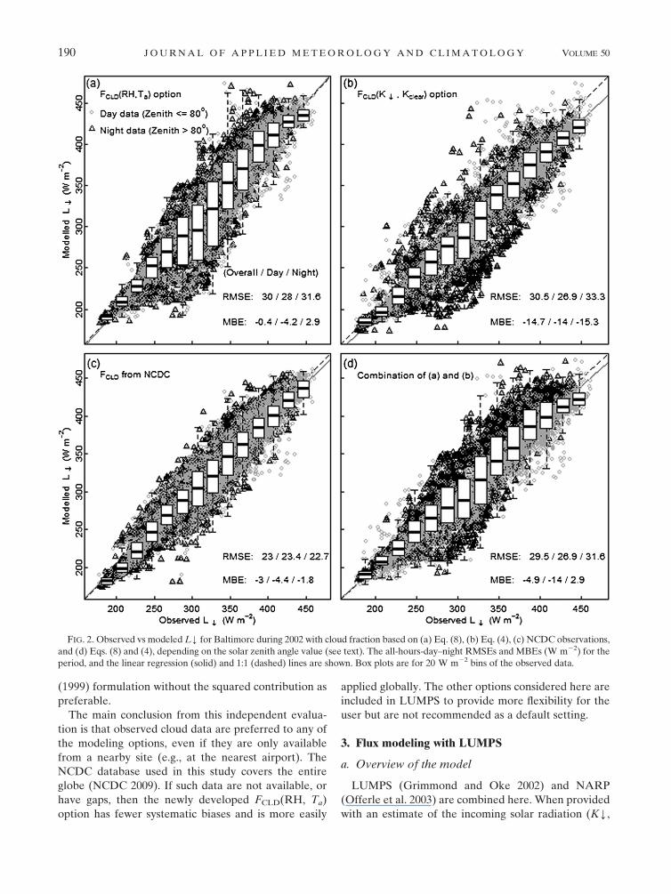
808; otherwise, Eq. (8) is used (Fig. 2d). For the first

complete year at Baltimore (2002, hereinafter BA02)

there are similar overall RMSE results (;30 W m22) for

approaches that model FCLD (Figs. 2a, 2b, and 2d). The

original FCLD (KY, Kclear) performs best during the day-

time (1.1 W m22 smaller RMSE; day Z # 808) and the new

FCLD (RH, Ta) best at night (1.7 W m22 smaller RMSE;

night Z . 808). However, linear regression shows a notice-

able negative bias relative to the 1:1 line with the FCLD (KY,

Kclear) (Fig. 2b), suggesting a significant tendency to un-

derestimate LY. This is confirmed by the overall, day and

night negative MBEs (215, 14, and 215 W m22) and the

box-plot medians. For the new FCLD(RH, Ta), all of the

MBE are improved (20.4, 24.2, and 2.9 W m22) and

the linear regression (close to the 1:1 line) confirms very

few biases. The interquartile range (IQR) for the ob-

served values of LY in the range 280–350 W m22 is

larger but with fewer outliers. The combined method

slightly outperforms the other two in terms of RMSE

(#1 W m22 smaller) but both its negative overall MBE

value (24.9 W m22) and the linear regression line con-

firm it has inherited the tendency to underestimate LYfrom the original daytime formulation. As expected, use

of NCDC FCLD data yields the best performance with the

lowest RMSE ($6.5 W m22 smaller), no significant

biases identified, and the smallest IQRs (Fig. 2c).

A similar pattern is found for the other Baltimore data-

sets (BA01 and BA03) and qodz (LO01 and LO02) with

systematically lower biases from the new FCLD(RH, Ta)

(improvements in jMBEj of 3.9 in BA01, 16.9 in BA03,

and 8.5 W m22 in both LO01 and LO02) and comparable

overall RMSEs (within 62 W m22 overall RMSE differ-

ence for BA01–BA03 and LO01 and LO02; see Fig. 3).

Only BA06 shows a larger bias (7.3 W m22 larger overall

jMBEj, and a switch to positive) and significantly poorer

RMSE (5.7 W m22 larger overall RMSE) from the new

model. The best improvement is obtained for the BA04

and BA05 datasets when the RMSEs are consistently

lower [5.7 (4.1) W m22 reduction in overall RMSE for

BA04 (BA05)]. In most cases, the added value of a pa-

rameterization that is applicable 24 h day21 is clearly no-

ticeable from the nighttime RMSE. The 4th alternative,

the combination of two FCLD models, is not shown as it can

be inferred from the other RMSE statistics. In all situa-

tions, using observed rather than modeled FCLD [Eq. (10)]

provides the best performance (overall 5–7 W m22 RMSE

smaller than the second-best option).

To investigate the impacts of seasonality, the Baltimore

and qodz 2002 datasets are split into December–February

(DJF), March–May (MAM), June–August (JJA), and

September–November (SON) (Fig. 4). The FCLD(KY,

Kclear) has a systematic negative MBE in LY for all sea-

sons (223.4 # MBE # 26.7 W m22), whereas using

FCLD(RH, Ta) there is a switch from negative to positive

MBEs (217.5 # MBE # 14.7 W m22) when moving

toward the summer (JJA). This is linked to the temper-

ature formulation (7) selected to modulate the FCLD(RH)

relation (Fig. 1); although designed to account for the

temperature influence on RH, the range of Ta values used

for the model development with observation from the

London site (23.58C # Ta # 28.78C) is not as wide as the

one occurring during BA02 (214.58C # Ta # 33.68C) and

L002 (217.58C # Ta # 30.88C). Unexpectedly low (high)

biases might therefore occur at very cold (warm) tem-

peratures. For the RMSE, no clear evolution is identified

but the poorer overall performance of the FCLD(RH, Ta)

model during the SON period for both sites and during

DJF for qodz are noted.

Mean diurnal plots by season, for the two sites (Fig. 5),

confirm the switch in bias from an underestimation

of LY in winter to its overestimation in summer from

FCLD(RH, Ta). Most importantly the plots highlight the

discontinuities inherent in a FCLD based on KY: a poor

nighttime approximation and strong discontinuities at

low sun elevation angles. A systematic daytime under-

estimation is also clearly noticeable. This is linked to

the squared FCLD term in Eq. (3), which directly reduces

the contribution of cloud coverage to the modeled LY.

This supports use of the original Crawford and Duchon

JANUARY 2011 L O R I D A N E T A L . 189

(1999) formulation without the squared contribution as

preferable.

The main conclusion from this independent evalua-

tion is that observed cloud data are preferred to any of

the modeling options, even if they are only available

from a nearby site (e.g., at the nearest airport). The

NCDC database used in this study covers the entire

globe (NCDC 2009). If such data are not available, or

have gaps, then the newly developed FCLD(RH, Ta)

option has fewer systematic biases and is more easily

applied globally. The other options considered here are

included in LUMPS to provide more flexibility for the

user but are not recommended as a default setting.

3. Flux modeling with LUMPS

a. Overview of the model

LUMPS (Grimmond and Oke 2002) and NARP

(Offerle et al. 2003) are combined here. When provided

with an estimate of the incoming solar radiation (KY,

FIG. 2. Observed vs modeled LY for Baltimore during 2002 with cloud fraction based on (a) Eq. (8), (b) Eq. (4), (c) NCDC observations,

and (d) Eqs. (8) and (4), depending on the solar zenith angle value (see text). The all-hours-day–night RMSEs and MBEs (W m22) for the

period, and the linear regression (solid) and 1:1 (dashed) lines are shown. Box plots are for 20 W m22 bins of the observed data.

190 J O U R N A L O F A P P L I E D M E T E O R O L O G Y A N D C L I M A T O L O G Y VOLUME 50

observed), incoming longwave radiation (LY, observed

or modeled), near-surface air temperature (Ta, observed)

and bulk radiative properties of the surface (a0, «0, esti-

mated from observations or field survey), NARP is able to

compute the net all-wave radiation flux Q*, which controls

the magnitude of the modeled SEB Eq. (1):

Q* 5 KY(1� a0) 1 «

0(LY� sT4

a)� 0.08KY(1� a0).

(11)

The final term on the right-hand side of Eq. (11) is in-

cluded to correct for the differences between the radi-

ative temperature of the surfaces and the near-surface

temperature Ta by which they are approximated here

[Holtslag and van Ulden (1983); van Ulden and Holtslag

(1985); see discussion of Eq. (16) in Offerle et al. (2003)].

Five options are implemented in LUMPS for LY:

1) provided by the user from either observations or the

output of an NWP model at a similar scale; local ob-

servations are preferred as they are the most accurate;

2) modeled from Eq. (10) using observations of cloud

fraction (e.g., NCDC);

3) modeled using Eq. (9), without any further input

requirement;

4) modeled as in Offerle et al. (2003); and

5) modeled by combining options 3 and 4 (i.e., as in Fig. 2d).

FIG. 3. The RMSE (analyzed for all-daytime–nighttime hours) and MBE (all hours only) when

modeling LY for Baltimore (2002–06, BA01–BA06) and qodz (2001–02, LO01 and LO02) using options

(a),(b), and (c) given in Fig. 2.

FIG. 4. As in Fig. 3, but for DJF, MAM, JJA, and SON 2002.

JANUARY 2011 L O R I D A N E T A L . 191

Options 3–5 have equivalent input requirements but op-

tion 3 is more widely applicable (section 2; not restricted

to the Northern Hemisphere, applicable 24 h day21).

The second submodel in LUMPS, the OHM of

Grimmond et al. (1991) for storage heat (DQS), is a func-

tion of Q* and its first-order derivative [Grimmond and

Oke’s (2002) Eq. (2)]. The user specifies n surface types,

which characterize the fraction area cover ( fi) and the

appropriate coefficients [see Table 1 in Grimmond and

Oke (2002) and Table 4 in Meyn and Oke (2009)]. As it

requires Q*, DQS will suffer from any bias in LY.

The available energy (Q* 2 DQS) and land cover

characteristics control the turbulent fluxes of heat and

moisture following a modified combination approach

[de Bruin and Holtslag (1982); Grimmond and Oke

(2002), their Eqs. (3) and (4)]. The partitioning co-

efficients (a, b) are calculated based on the vegetation

fractions (Grimmond and Oke 2002, see their Table 5).

An increase of a (representing additional moisture)

would directly enhance QE while limiting QH. Any

error in LY will cascade through from Q* to DQS and

the turbulent fluxes QH and QE.

The new developments to LUMPS allow runs through

the seasons and synoptic weather conditions. First, a sur-

face water balance is implemented as a simple bucket

model. Precipitation accumulates in a reservoir of pre-

defined capacity (e.g., rescap 5 10 mm). Drainage com-

mences when accumulated water exceeds a user-defined

threshold (e.g., rain cover 5 0.01 mm). When the surface

is wet, potential evaporation occurs. When the air tem-

perature is greater than 08C, the bucket is drained at

a specified rate (e.g., resdrain 5 0.25 mm h21) and latent

heat flux from the preceding hour is also removed from

the bucket.

Second, the fraction of area that has active vegetation is

allowed to vary based on vegetation phenology (V), which

is parameterized from a combination of growth and decay

functions as shown in Eq. (12). For the Northern

Hemisphere the two functions are multiplied (summed

for the Southern Hemisphere):

V(d

i,Northern hemisphere)

51

1 1 10ks(d

s�d

i)

31

1 1 10kf(d

i�d

f)

V(di ,Southern hemisphere)

51

1 1 10ks(d

s�d

i)

11

1 1 10kf(d

i�d

f)

ds5

sstart

1 sstop

2; d

f5

fstart

1 fstop

2; k

s5

log1� V

0

V0

� �

ds� s

start

; kf5

log1� V

0

V0

� �

fstop� d

f

, (12)

FIG. 5. Diurnal mean observed and modeled LY for the same seasons as in Fig. 4. See text or Fig. 2 for details on model options.

192 J O U R N A L O F A P P L I E D M E T E O R O L O G Y A N D C L I M A T O L O G Y VOLUME 50

where the days of year (DOYs) indicate the start of leaf-

on, sstart, or leaf-off, fstart; ds (df) is the median point of

the spring (fall) period; sstop ( fstop) is the end of the

spring (fall) period; and di is the current DOY. Co-

efficients ks and kf characterize the slopes of the growth

and decay curves, respectively. The transition window

coefficient width (V0 5 0.03) allows for a 3% fraction of

the growth (decay) to occur outside the specified window.

Third, anthropogenic heat flux is included. There are

a wide range of techniques for simulating QF (Kikegawa

et al. 2003; Sailor and Lu 2004; Offerle et al. 2005) but

our preference is for minimal input requirements. Fol-

lowing Pigeon et al. (2007), a parameterization based on

the air temperature is implemented:

QF

(Ta

, Tc) 5 Q

F ,min1 Q

F,slope(T

c� T

a) and

QF

(Ta

$ Tc) 5 Q

F ,min, (13)

where QF,min is the minimum anthropogenic heat, QF,slope

is the slope, and Tc is the critical temperature. The co-

efficients in Eq. (13) will vary depending on climatic and

cultural habits. One set of coefficients will account for

diurnal variations in temperature but not behavioral

differences (e.g., day of week, working hours). Alterna-

tively, QF values from a different source can be read in

(e.g., Flanner 2009; Allen et al. 2010); QF is added to Q*

before calculating DQS and does not influence the out-

going longwave radiation and hence Q*.

The model surface characteristics can be either static

(fixed) or dynamic (changing each time step). The dy-

namic approach allows a more correct comparison with

the observations as the flux footprint for each time pe-

riod is used as a filter (Grimmond and Oke 1991).

b. Model evaluation

The ‘‘base run’’ of LUMPS (section 3a) omits QF and

uses static surface characteristics. Simulations are for

the Lipowa site in qodz (Q*, QH, QE, DQS) and Cub Hill

in Baltimore (Q* only) for the range of LY options.

Measurements of the 3D wind velocities and virtual

temperature using a sonic anemometer (Applied Tech-

nologies, model K type), and water vapor fluctuations

from a krypton hygrometer (Campbell Scientific Inc.,

model KH2O) at 37 m above the ground were used to

calculate the turbulent sensible and latent heat fluxes

(Offerle 2003; Offerle et al. 2006). The mean building

height (ZH 5 10.6 m) in qodz [see Table 3 in Offerle

et al. (2006)] ensures that sensors are located above the

2ZH transition height (e.g., Kastner-Klein and Rotach

2004) and should therefore be representative of the local

scale. The storage heat flux is estimated by using the

element surface temperature method (ESTM; Offerle

et al. 2005) based on measurements of wall, road (infrared

thermometers), roof, and air (fast-response thermocou-

ples) temperatures for a 6-month period in 2002 (July–

December). Linear regression is used with the surface

temperatures from the radiation components, air tem-

perature, and solar zenith angle to obtain a complete

temperature and DQS dataset for the 2 yr [Eq. (4); Offerle

et al. (2005)].

The model is forced with hourly values of air temper-

ature (Ta), atmospheric pressure (Pa), relative humidity

(RH), incoming solar radiation (KY), and precipitation

rate. Hourly observations of LY are provided for option 1

and cloud fraction from NCDC for option 2. Input

parameter values used for the qodz runs are given in

Table 1. Data gaps in the input variables (i.e., Ta, RH,

FCLD(NCDC), or LY) were filled to allow LUMPS to

run continuously but these periods are excluded from

the evaluation.

The choice of an appropriate model is dependent on

the application. Consideration needs to be given to the

variables to which a model must have small tolerance of

error (or greatest capability). Baklanov et al. (2009)

discuss five applications: air quality exposure studies,

urban climate studies and development of strategies to

mitigate the intensity of heat islands, emergency re-

sponse pathways for toxic gas releases, forecasting air

quality and weather, and urban planning. These require

different fluxes and variables (e.g., wind speed, wind di-

rection, temperature, humidity, pollutant concentration,

turbulent fluxes) to be correct and/or have different levels

of tolerance at different times of the day. For example,

meteorological preprocessors for air quality and disper-

sion have the estimation of QH as a major goal, for their

ultimate use in estimating Obukhov length and turbulent

motions. For that use, a 10 or 20 W m22 error in QF at

night may have major unwanted consequences, such as

shifting the stability from stable to unstable or vice versa.

However, for estimating the surface heat fluxes with an

NWP model, the QH accuracy at night may not be so

important. Here, we do not assess the performance for

a particular application. Thus, there is no desired or re-

quired accuracy beyond the ideal of zero model error.

1) NET ALL-WAVE RADIATION

Simulations of Q* with LY options 1–4 for the LO02

and BA03 datasets are plotted (Fig. 6) and statistics for

all eight datasets are computed (Table 2). Option 5 is not

shown. As expected, the use of observed LY yields the

best performance in all cases, with the overall RMSE

from 3.7 to 13.4 W m22 better than the second-best

option. Option 2 is arguably second best, with lower

RMSEs in most cases and good agreement between the

linear regression and 1:1 lines (e.g., Fig. 6b1); however,

this option tends to overestimate Q* (MBE . 10 W m22).

JANUARY 2011 L O R I D A N E T A L . 193

The levels of statistical performance for options 3 and 4

are poorer, with a tendency toward an underestimation

of Q* for option 4 (214 # MBE # 3 W m22 with

a mean of 25.4 W m22 over the eight datasets; negative

intercept for six out of eight datasets) and over-

estimation for option 3 (3 # MBE # 14 W m22 with

a mean of 7.4 W m22). The nighttime bias from option

4, with a clear discontinuity for low Q* values, is best

seen from Fig. 6d2 (also Fig. 6d1). Option 3 does not have

such a discontinuity, although the scattering of points is

higher than for option 1 for low Q* values (Fig. 6c).

2) IMPACTS ON ALL SURFACE ENERGY BALANCE

FLUXES

All fluxes modeled in LUMPS are explicitly linked to

Q*. The overall errors for QH and DQS are 30 # RMSE #

43 W m22, for all options and seasons, and for QE they

are 22 # RMSE # 33 W m22. The ability to model the

diurnal cycle varies with season. The daytime maximum

value of the mean measured QH flux, for instance, varies

between 65 in winter and .200 W m22 in spring, but the

RMSE only vary from 33 to 40 W m22 for the four op-

tions (Fig. 7). Although LUMPS is simple, it is able to

reproduce the main aspects of the surface–atmosphere

energy exchange in urban areas, including both its diurnal

and seasonal variabilities. Note that for all fluxes except

Q*, the levels of RMSE performance for the four LYoptions are within 64 W m22.

For Q*, LY option 2 consistently leads to the highest

daytime maximum for all seasons and is the only option

to overestimate the observed maximum value in most

cases whereas option 4 tends to underestimate such

daytime maxima for all periods except DJF (Fig. 7a).

Nighttime levels of performance vary considerably from

one season to the other. Option 4 underestimates Q* in

the hours preceding sunrise in most cases (e.g., Fig. 7a)

but appears to be reasonable in the early hours of the

night. Option 3 has a tendency to overestimate the ob-

served nighttime Q* values and closely follows option 2.

Option 1 is closest to the observations in most cases. In

terms of RMSE, option 1 is by far the most accurate

choice (6 # RMSE # 11 W m22) while the other three

options are more comparable. In terms of MBE, options

1–3 exhibit positive biases for all seasons, with the

highest value to be found for option 2 in MAM (MBE 5

20 W m22), while option 4 has negative biases from

September to February.

The direct link between Q* and DQS through OHM

is apparent from the relative levels of performance of

the four options (Figs. 7e–h), where those with higher

(lower) Q* values also generate higher (lower) storage

(see overall MBE statistics). The discrepancies are at-

tributed to OHM not accounting for all the processes

involved in the determination of DQS. The influence of

seasonality on the performance is clear (Fig. 7), with

a noticeable underestimation during winter (220 #

MBE # 216 W m22) and an overestimation in summer

(19 # MBE # 24 W m22). Patterns of anthropogenic

energy usage, the frequency of rain episodes (with water

runoff absorbing heat from the surface and transporting

it out of the system), the decrease in storage efficiency at

high wind speeds, or the variability in turbulent heat

exchange when the prevailing wind direction changes

(hence leading to different fetch characteristics) are

TABLE 1. LUMPS model parameters assigned for the qodz runs (2001–2002). Note that QF was initially not included in the base run.

Model input parameters Values assigned for qodz runs

Bulk albedo (a0), emissivity («0) a0 5 0.08, «0 5 0.92

Lat, lon Lat 5 51.758N, lon 5 19.468E

No. of surface types in OHM n 5 3

Fraction cover of each surface type fbuild 5 0.3 buildings, fimp 5 0.4 impervious, fveg 5 0.3 vegetated

OHM coefficients Vegetation, mixed forest (McCaughey 1985); roof, bitumen spread

over flat industrial membrane (Meyn and Oke 2009); impervious,

mean of all five concrete and asphalt sources [see Table 4 in

Grimmond and Oke (1999)]

Reservoir capacity (rescap), drainage

rate (resdrain), threshold for complete

surface coverage (rain cover)

rescap 5 10 mm, resdrain 5 0.25 mm h21, rain cover 5 0.01 mm

Vegetation phenology (12) sstart 5 69; sstop 5 144; fstart 5 281; fstop 5 324; V0 5 0.03

aint, aslope, bint, and bslope a 5 aint

1 aslope

3 fveg

3 V(di)

b 5 bint 1 bslope 3 f veg 3 V(di)

aslope

( fveg

. 0:9) 5 0:8; aslope

( fveg

# 0:9) 5 0:686

aint 5 0:2; bint 5 3 W m�2; bslope 5 17 W m�2

Anthropogenic heat for run 2 [Eq. (13)] QF,min 5 15 W m22, QF,slope 5 2.7 W m22 8C21, Tc 5 78C

194 J O U R N A L O F A P P L I E D M E T E O R O L O G Y A N D C L I M A T O L O G Y VOLUME 50

among the possible reasons for such a seasonal switch in

the model biases.

For all options, the modeled daytime QH overestimates

the observed values for all seasons except MAM (Fig. 7j),

where the maximum daytime magnitude of the flux is in

good agreement with the measurements; whereas, QE is

underpredicted in all cases except MAM (Fig. 7n). This

apparent trade-off between the two fluxes suggests that

LUMPS would benefit from a more accurate partitioning

of the available energy between the two turbulent pro-

cesses. In particular, the correct characterization of the a

and b coefficients as a function of the site-specific surface

characteristics is of critical importance (see Table 1). The

analysis of nighttime QH and QE modeled values reveals

a systematic bias from LUMPS, with a significant un-

derestimation for all seasons but JJA; such a pattern,

combined with the fact that the biggest bias is to be

observed for the DJF period, hints at the importance of

(nighttime) anthropogenic heating in qodz (Klysik and

Fortuniak 1999; Offerle et al. 2005, 2006), which is not in

the base run. Finally, in the case of MAM (Figs. 7b, 7f, 7j,

and 7n), LUMPS correctly simulates the daytime mag-

nitude of the peak Q*, DQS, and QH fluxes but over-

estimates the daytime QE; thus, not all of the available

energy (Q* 2 DQS) should be used (provided) by tur-

bulent processes and some loss (gain) should occur via

other sinks (sources) instead. The net advection of heat

and moisture into/out of the area (DQA) can alter the

turbulent exchanges, while QF at night can complement

QH and QE to provide the energy needed to close the

balance (this is very likely the case in Figs. 7i and 7m).

Rigorously, and following the notation from Offerle

FIG. 6. Observed vs modeled net all-wave radiation Q* for the LY options: (a) 1, (b) 2, (c) 3 and (d) 4 for (top) LO02 and (bottom) BA03.

The overall RMSE and MBE statistics, the linear regression (solid), and the 1:1 (dashed) lines are shown.

TABLE 2. RMSE and MBE for modeling Q* using LY options 1–4 for all hourly data for qodz and Baltimore (see text). Here, N is the

number of hours analyzed for each dataset.

Site

RMSE (W m22) MBE (W m22) Slope (–)/intercept (W m22)

N 1 2 3 4 1 2 3 4 1 2 3 4

LO01 3309 8.8 22.2 28.5 23.0 5.4 12.9 9.8 23.4 0.986/6.2 1.002/12.8 0.980/11.0 0.971/21.7

LO02 4582 8.7 22.7 26.3 21.6 6.2 14.8 11.5 0.4 0.994/6.6 1.005/14.5 0.982/12.6 0.971/2.3

BA01 1852 14.2 29.5 29.2 26.8 9.4 18.6 13.7 21.8 0.968/10.4 0.976/19.4 0.951/15.2 0.955/20.4

BA02 5285 16.9 29.5 28.4 28.0 7.2 16.9 5.7 2.7 0.947/11.0 0.955/20.2 0.938/10.3 0.937/7.3

BA03 4954 25.1 28.8 31.7 34.4 7.7 10.1 2.9 213.7 0.906/14.9 0.920/16.3 0.894/11.1 0.930/28.4

BA04 6508 22.1 27.4 28.0 29.4 12.2 13.2 5.7 29.7 0.939/17.8 0.948/17.9 0.937/11.5 0.930/23.3

BA05 5985 15.0 26.8 29.5 29.6 7.4 13.0 4.3 29.6 0.957/11.2 0.954/17.0 0.934/10.2 0.930/23.5

BA06 6719 16.9 26.6 29.0 28.7 23.5 16.1 8.1 28.3 0.950/1.6 0.946/21.5 0.931/15.1 0.928/21.0

JANUARY 2011 L O R I D A N E T A L . 195

et al. (2005), the energy available for turbulent processes

should therefore be expressed as

QH

1 QE

5 Q* 1 QF� DQ

S� DQ

A� S, (14)

where S represents all sources and sinks of energy

present at the scale of study, but not represented by the

other terms, such as rainwater channeling heat out of the

system or photosynthetic heat (Offerle et al. 2006). Such

a detailed representation of these processes is however

not the aim of a model like LUMPS, since it would re-

quire an increase in both the complexity of the param-

eterization involved and the amount of inputs required.

This study can also be seen as a sensitivity analysis of

LUMPS to LY and consequently to Q*. Clearly, LY is

important in the surface energy balance and critical to

Q*, as well as being a key driver for DQS, QH, and QE.

However, the RMSE differences between the four LY

FIG. 7. Diurnal mean observed and modeled (a)–(d) Q*, (e)–(h) DQS, (i)–(l) QH, and (m)–(p) QE fluxes for LO02 by season for (left) DJF,

(left center) MAM, (right center) JJA, and (right) SON. See text for details on the modeling options. RMSE and MBE statistics are given.

196 J O U R N A L O F A P P L I E D M E T E O R O L O G Y A N D C L I M A T O L O G Y VOLUME 50

options (,4 W m22) account for less than 10% of the

overall RMSEs for DQS, QH, and QE, which suggests

that some other important processes are missing in

LUMPS. These are needed to account for other types of

energy transfers and limit the coupling between Q* and

the rest of the fluxes.

3) ANALYSIS OF MODEL ERROR

To assess the importance of such unrepresented pro-

cesses, an analysis of the model error dependency on

a set of meteorological variables is performed. Plots of

the error between the modeled (using LY as forcing, i.e.,

option 1 as advised in section 3a) and observed values of

Q*, DQS, QH, and QE for the 2-yr period as a function of

air temperature, number of hours after a rain episode,

wind direction, and wind speed (Fig. 8) provide insights

into the importance of missing processes, including po-

tential trends between the model error and variables.

Assuming that QF is closely correlated to the air tem-

perature, the model error evolution as a function of Ta

should therefore reflect the importance of the QF con-

tribution to the SEB. Similarly, fetch characteristics are

determined by wind direction while heat loss due to

rainwater should decrease with time after a rain episode.

LUMPS does not account for a decrease in the efficiency

of the heat storage from urban surfaces at higher wind

speeds, which should be reflected in the modeled SEB if

turbulent transport is important.

The influence of rain episodes on the flux error is the

least pronounced (Figs. 8e–h), although an underesti-

mation of latent heat fluxes immediately after pre-

cipitation events (lowess curve and IQR for the first 12 h

after rain below the 0 error line; see Fig. 8h) suggests that

the surface may dry too rapidly and requires a lower

dryness threshold, while the positive slope in the evo-

lution of the error in DQS (Fig. 8f) indicates that the

channeling of heat by rainwater might impact energy

storage. Under weak winds, OHM underestimates the

storage capacity (lowess and median for winds below

1 m s21 below the 0-error line) whereas it starts to

overestimate it when wind speed values exceed 4 m s21

(Fig. 8n). These results are in agreement with Meyn and

Oke (2009), who suggest that the a1 coefficient for built

surfaces (Table 1) should decrease exponentially as a func-

tion of wind speed. The errors in the turbulent fluxes evolve

in the opposite direction (i.e., toward an underestimation

for strong winds). Caution should be used when interpret-

ing the limited data for winds above 8 m s21.

For all fluxes, the error is most sensitive to air tem-

perature and wind direction (trends identified by the

lowess curves and box-plot medians are more pro-

nounced than for the other two variables). Figure 9,

which separates daytime (KY . 0) and nighttime (KY 5 0)

errors, provides a more complete picture of the error

dependency. Of particular interest is the underpredic-

tion of QH for low nocturnal temperatures [between 20

and 50 W m22 underprediction for Ta , 08C, as indi-

cated by the solid lowess curve (Fig. 9g) or the median of

the box plots], as it supports the hypothesis that an-

thropogenic heating plays an important role, particu-

larly in the nocturnal energy balance. Without an

explicit representation of QF, LUMPS assumes that all

of the (Q* 2 DQS) nighttime energy deficit is to be

compensated by turbulent heat exchange and conse-

quently simulates large negative QH (and QE) fluxes

when these should be close to zero (see Fig. 7i) with the

additional input of heat from QF. This clear under-

prediction of LUMPS is reduced when temperatures

increase (;10 W m22 underprediction), with a thresh-

old around 78C (vertical line in Figs. 9a–h). During the

day, the trend is less pronounced, but still noticeable and

leads to the overprediction of QH for positive temper-

atures, hence confirming the day time maximum over-

estimations identified from Fig. 7. The evolution of the

error in the modeled DQS and Q* (Figs. 9a, 9b, 9e, and

9f) also exhibits a marked change in slope around this

same threshold temperature of 78C. For high tempera-

tures, and especially at night, LUMPS overestimates Q*

(by up to 10 W m22; Figs. 9a and 9e) and DQS (by up to

40 W m22; Figs. 9b and 9f). The biggest errors in modeling

DQS are found at temperatures above 208C, confirming

some limitations of OHM in the summer (Fig. 7g).

The analysis of error dependency by wind direction is

only possible with respect to the tower location. The

surface cover fractions around the site (see Fig. 2 in

Offerle et al. 2006) have a clear contrast between the

more vegetated section west of the tower [wind direction

from 1508 to 3308; Offerle et al. (2006)] and the rest of

the area (more urbanized). The lowess trend for QH

clearly depicts a strong influence of the fetch charac-

teristics on the magnitude and sign of the error [up to

30 W m22 overestimation from the lowess when the

wind is from the south during the daytime, with a median

of ;50 W m22 for wind directions in the range 2208–

2408 (Fig. 9k) and down to a 30 W m22 underestimation

from the lowess when the wind is from the north at night

(Fig. 9o)]. For QE, the lowess follows the 0-error line and

the spread of points is considerably smaller (see IQR;

Figs. 9l and 9p) and less impacted by wind direction. A

tendency toward underestimation when the wind comes

from the north is noted, with the lowess going below the

0-error line and the IQR increasing. In the base run,

fixed surface characteristics were used, so some of the

errors can be attributed to the variability in the observed

values. During the day, LUMPS overpredicts if the

JANUARY 2011 L O R I D A N E T A L . 197

footprint extends to more vegetated surfaces; for QE,

the tendency is toward an underprediction when the

fluxes are from the urbanized sector, which disappears

when they are from the vegetated one. As observed

from Fig. 7, the nighttime turbulent activity modeled

by LUMPS appears to be systematically larger than

suggested by the measurements (larger negative QH

values). When the fetch is from the more urbanized

sector, the observed QH fluxes are likely to be small

(near-neutral condition), therefore leading to negative

errors (see Fig. 9o for wind directions between 08 and

1208), while for a more vegetated source area (e.g., south-

southwest of the tower) the nighttime negative fluxes are

closer to the actual observed values and the error becomes

smaller. These conclusions extend to the evolution of the

error in the estimation of DQS (Figs. 9j and 9n) given the

FIG. 8. Error between modeled (using LY option 1) and observed values of Q*, DQS, QH, and QE for the entire 2-yr period as a function

of (a)–(d) air temperature, (e)–(h) number of hours after a rain episode, (i)–(l) wind direction, and (m)–(p) wind speed. Zero-error

(horizontal, dashed) and lowess (solid) lines are shown. Box plots are for bins of 28C temperature for (a)–(d), 12 h after rain for (e)–(h), 208

wind direction for (i)–(l), and 1 m s21 wind speed for (m)–(p). RMSE and MBE statistics over the 2 yr are indicated in (a)–(d).

198 J O U R N A L O F A P P L I E D M E T E O R O L O G Y A N D C L I M A T O L O G Y VOLUME 50

direct link between DQS and the turbulent fluxes in

LUMPS. During the day, the overestimation of QH (Fig.

9k) is matched by an underestimation of DQS (Fig. 9j) and

vice versa. At night, DQS is overestimated when the wind

comes from the more urbanized sector and the lowess trend

is close to the 0-error line when it is from the south, which is

an inverse correlation with the trend in the error for QH.

Note that Q* is not particularly sensitive to wind direction

(as shown by the lowess curve position and the small IQR;

Figs. 9i and 9m) but the lowess and medians show a con-

stant LUMPS overprediction of around 5 W m22.

These results suggest that an important process cur-

rently missing in LUMPS is the representation of QF. It

also suggests that for model evaluation purposes the

FIG. 9. Error [(a)–(d),(i)–(l) daytime and (e)–(h),(m)–(p) nighttime] between modeled (using LY option 1) and observed values of Q*, DQS,

QH, and QE for the 2-yr period as a function of (top and top middle) air temperature and (bottom and bottom middle) wind direction. Lowess

lines for base run (solid) and run 2 (QF, changing surface characteristics) (dashed). Box plots (white—wider for the base run; gray—narrower

run 2 are for bins of 28C temperature for (a)–(h) and 208 wind direction for (i)–(p). RMSE and MBE statistics are indicated in (a)–(h) for base

run (left) and run 2 (right). For Q*, both runs are the same. See text for definition of the vertical threshold (dashed) lines.

JANUARY 2011 L O R I D A N E T A L . 199

characterization of the flux footprint is important for

assigning parameter values.

4) ANTHROPOGENIC HEAT AND DYNAMIC

SURFACE FOOTPRINT

The approach taken to include QF is described in Eq.

(13). The parameter values were assigned for qodz

(Table 1) as QF,min 5 15 W m22 [see typical July values

reported in Klysik (1996) for the city of qodz] and the

slope QF,slope matches the 2.7 W m22 8C21 identified by

Offerle et al. (2005) during October–March 2001–02. The

value of the critical temperature (Tc) is assumed to be 78C

from the error evolution plots (Figs. 9c and 9g).

Following Grimmond and Oke (1991, 2002), a dy-

namic flux footprint for the hourly surface characteris-

tics is computed by Offerle et al. (2006) using Schmid’s

(1994) Flux Source Area Model (FSAM) with a 5 km 3

5 km GIS grid (spatial resolution 5 100 m) centered

on the measurement tower. The database of buildings

( fbuild), vegetated ( fveg), and impervious ( fimp) surface

covers allows us to calculate the a1i, a2i, and a3i co-

efficients for DQS, as well as a and b in the turbulent

heat fluxes, at each time step (see Table 1). This offers

a better characterization of the fetch variability and al-

lows for better accountability of daily–seasonal changes

in the stability and wind patterns in the observations.

The performance from run 2 of LUMPS is indicated by

a second set of lowess (dashed) curves and (gray nar-

rower) box plots in Fig. 9. RMSE and MBE statistics for

the two simulations are presented in Figs. 9a–h (base run/

run 2). The impacts of the additional QF are clearly no-

ticeable in Fig. 9g, where the nighttime negative bias in

QH for low temperatures is removed (the dashed lowess

curve and medians follow the zero-error line) and the

corresponding MBE is reduced by .10 W m22; that is,

the (Q* 2 DQS) energy deficit is compensated by QF

input rather than a negative QH. The impacts on night-

time QE are limited (Fig. 9h) but the MBE was reduced

by 2.3 W m22; DQS is overestimated at low temperatures

(Fig. 9f) and now is more obviously related to the over-

predicted Q* (Fig. 9e). Given the larger magnitude of the

fluxes during the day, the impacts of QF are less obvious

(Figs. 9b–d). A systematic overestimation of QH values

regardless of temperature occurs and suggests that the

daytime performance has declined with QF inclusion.

This is confirmed by the statistics (;12 W m22 increase

in daytime MBE). The pattern in DQS error leads to

better agreement with Q* than was previously found (i.e.,

an overestimation of Q* should trigger an overestimation

of DQS). As the Q* results are not impacted by the two

modifications, the statistics are identical.

The errors with wind direction (Figs. 9i–p), when the

dynamical footprint surface fractions are used, produce

small differences. When the wind originates from the

vegetated sector, the lowess curves and medians of the

QE error (Figs. 9l and 9p) are now slightly closer to zero.

Similarly, the difference in daytime DQS between the

two runs (Fig. 9j) is more pronounced when the foot-

print is from the more urbanized sector (08–1508), in-

dicating DQS from the vegetated sector has been reduced.

The systematic overestimation of the daytime QH values

is clearly noticeable (Fig. 9c), while nighttime perfor-

mance shows some significant improvement (Fig. 9o).

The benchmarking procedure of E. Blyth and M. Pryor

(2010, personal communication) was applied to check for

statistically significant changes in the mean modeled QH,

QE, and DQS values between the base run and run 2 using

a two-sided t test with a Welsh correction to assume non

equal variance (Adler 2010). Results indicate that sig-

nificant improvements in the model performance are

found for QH and QE during the nighttime as well as DQS

during the day. The modeling of QE for run 2 does not

provide any significant difference from the base run

during the daytime, while daytime QH and nighttime DQS

significantly degrades for run 2.

Thus, we conclude that the addition of QF, in its current

form, helps remove the systematic biases in nighttime

turbulent fluxes of QH, but generates a daytime systematic

overestimation. The evolution of DQS also results in more

coherence with Q* biases when QF is included. Any im-

provement in modeling Q* should be reflected in DQS,

when the modeled energy balance accounts for a QF

contribution. The use of variable measurement footprint

characteristics did not provide as much improvement as

expected but did result in slightly better performance from

the more vegetated sector (lower DQS and QH, and higher

QE). The limited overall improvement from these simple

modifications demonstrates the difficulty in representing

such processes with a restricted level of complexity. It also

highlights the strength of the flux formulations in LUMPS’

ability to simulate the overall magnitude of the surface

energy balance in urban areas (overall RMSE , 34 W m22

for all fluxes over the 2 yr of data fromqodz; Fig. 8) from an

extremely limited amount of input information. Further

efforts to better represent surface variability and anthro-

pogenic heat without any radical change in the level of

modeling complexity involved are however still needed.

4. Conclusions

The simple model LUMPS now incorporates the NARP

radiation model, changing availability of water at the sur-

face, vegetation phenology, and a simple anthropogenic

heat flux model. These new developments have been ac-

complished while maintaining the need for limited forcing

data and surface information.

200 J O U R N A L O F A P P L I E D M E T E O R O L O G Y A N D C L I M A T O L O G Y VOLUME 50

Several alternatives to modeling incoming longwave

radiation from commonly available data are considered.

A simple formulation based on relative humidity, air

temperature, and vapor pressure is developed with

cloud fraction data from a site in central London be-

fore being tested at two independent sites (qodz, Poland,

and Baltimore, Maryland). The performance of this sim-

ple parameterization is compared with the method of

Offerle et al. (2003), based on observed incoming solar

radiation and an estimate of its clear-sky value. A third

alternative uses observed cloud data from the National

Climatic Data Center. Although the performances of the

two approaches in modeling the cloud fraction are very

similar, it can be argued that the new formulation exhibits

less bias at night and has the advantage of a wider appli-

cability. In all cases the use of the observed cloud fraction

information leads to an increased level of performance in

the modeling of LY.

In the second part of the study, the impacts of the LYapproach are evaluated as part of an assessment of

LUMPS’s ability to simulate the surface energy balance

fluxes. Results highlight the good overall performance

of the scheme [overall RMSE , 34 W m22 for all fluxes

over the 2 yr of data from qodz when using LY as the

forcing (Fig. 8) and RMSE , 43 W m22 for all seasons

and all LY options in 2002 (Fig. 7)]. Analysis of the error

evolution as a function of air temperature and wind di-

rection suggests that an explicit representation of an-

thropogenic heat and a better characterization of the

flux footprint in LUMPS are useful.

Acknowledgments. Thanks are given to all those who

were involved in the Baltimore, qodz, and London field

campaigns, especially John Hom (USDA FS), Krzysztof

Fortuniak (UL), Alastair Reynolds (KCL), and Steve

Scott (IU). Thanks are also given to Eleanor Blyth (CEH)

and Matt Pryor (Met Office) for discussions about JULES

benchmarking. Financial support for this project for the

fieldwork and the analyses was provided to SG by the U.S.

National Science Foundation (ATM-0710631, BCS-

0221105, BCS-0095284), EU (FP7-ENV-2007-1 211345)

BRIDGE, Met Office, USDA Forest Service (CA-

11242343-082, 04-CA-11242343-124, 05-CA-11242343-11),

and King’s College London. The LUMPS model is available

online (http://geography.kcl.ac.uk/micromet/index.htm).

REFERENCES

Adler, J., 2010: R in a Nutshell. O’Reilly Media, 611 pp.

Allen, L., F. Lindberg, and C. S. B. Grimmond, 2010: Global to city

scale urban anthropogenic heat flux: Model and variability.

Int. J. Climatol., in press, doi:10.1002/joc.2210.

Baklanov, A., J. Ching, C. S. B. Grimmond, and A. Martilli, 2009:

Model urbanization strategies: Summaries, recommendations

and requirements. Urbanization of Meteorological and Air

Quality Models, A. Baklanov et al., Eds., Springer-Verlag,

151–162.

Bradley, E., T. Hastie, I. Johnstone, and R. Tibshirani, 2004:

Least angle regression. Ann. Stat., 32, 407–499, doi:10.1214/

009053604000000067.

Cimorelli, A. J., and Coauthors, 2005: AERMOD: A dispersion

model for industrial source applications. Part I: General model

formulation and boundary layer characterization. J. Appl.

Meteor., 44, 682–693.

Cleveland, W. S., 1981: LOWESS: A program for smoothing

scatterplots by robust locally weighted regression. Amer. Stat.,

35, 54.

Crawford, T. M., and C. E. Duchon, 1999: An improved parame-

terization for estimating effective atmospheric emissivity for

use in calculating daytime downwelling longwave radiation.

J. Appl. Meteor., 38, 474–480.

de Bruin, H. A. R., and A. A. M. Holtslag, 1982: A simple pa-

rameterization of surface fluxes of sensible and latent heat

during daytime compared with the Penman–Monteith con-

cept. J. Appl. Meteor., 21, 1610–1621.

Emeis, S., C. Munkel, S. Vogt, W. J. Muller, and K. Schafer, 2004:

Atmospheric boundary-layer structure from simultaneous

SODAR, RASS, and ceilometers measurements. Atmos. En-

viron., 34, 273–286.

Eresmaa, N., A. Karppinen, S. M. Joffre, J. Rasanen, and H. Talvitie,

2006: Mixing height determination by ceilometer. Atmos. Chem.

Phys., 6, 1485–1493.

Flanner, M. G., 2009: Integrating anthropogenic heat flux with global

climate models. Geophys. Res. Lett., 36, L02801, doi:10.1029/

2008GL036465.

Grimmond, C. S. B., and T. R. Oke, 1991: An evaporation–

interception model for urban areas. Water Resour. Res., 27,

1739–1755.

——, and ——, 1999: Heat storage in urban areas: Observations

and evaluation of a simple model. J. Appl. Meteor., 38,

922–940.

——, and ——, 2002: Turbulent heat fluxes in urban areas: Ob-

servations and a Local-Scale Urban Meteorological Parame-

terization Scheme (LUMPS). J. Appl. Meteor., 41, 792–810.

——, H. A. Cleugh, and T. R. Oke, 1991: An objective urban heat

storage model and its comparison with other schemes. Atmos.

Environ., 25B, 311–326.

——, B. D. Offerle, J. Hom, and D. Golub, 2002: Observation of

local-scale heat, water, momentum and CO2 fluxes at Cub

Hill, Baltimore. Preprints, Fourth Urban Environment Symp.,

Norfolk, VA, Amer. Meteor. Soc., 10.6. [Available online at

http://ams.confex.com/ams/pdfpapers/37022.pdf.]

——, and Coauthors, 2010a: Initial results from phase 2 of the In-

ternational Urban Energy Balance Comparison. Int. J. Climatol.,

in press, doi:10.1002/joc.2227.

——, and Coauthors, 2010b: The International Urban Energy

Balance Models Comparison Project: First results from phase

1. J. Appl. Meteor. Climatol., 49, 1268–1292.

Holtslag, A. A. M., and A. P. van Ulden, 1983: A simple scheme for

daytime estimates of the surface fluxes from routine weather

data. J. Climate Appl. Meteor., 22, 517–529.

Kastner-Klein, P., and M. W. Rotach, 2004: Mean flow and tur-

bulence characteristics in an urban roughness sublayer.

Bound.-Layer Meteor., 111, 55–84.

Kikegawa, Y., Y. Genshi, H. Yoshikado, and H. Kondo, 2003:

Development of a numerical simulation system toward com-

prehensive assessments of urban warming countermeasures

JANUARY 2011 L O R I D A N E T A L . 201

including their impacts upon the urban buildings’ energy de-

mands. Appl. Energy, 76, 449–466.

Klysik, K., 1996: Spatial and seasonal distribution of anthropogenic

heat emissions in qodz, Poland. Atmos. Environ., 30, 3397–3404.

——, and K. Fortuniak, 1999: Temporal and spatial characteristics

of the urban heat island of qodz, Poland. Atmos. Environ., 33,

3885–3895.

Lindberg, F., B. Holmer, and S. Thorsson, 2008: SOLWEIG

1.0—Modelling spatial variations of 3D radiant fluxes and

mean radiant temperature in complex urban settings. Int.

J. Biometeor., 52, 697–713.

Loridan, T., and Coauthors, 2010: Trade-offs and responsiveness of

the single-layer urban canopy parameterization in WRF: An

offline evaluation using the MOSCEM optimization algorithm

and field observations. Quart. J. Roy. Meteor. Soc., 136, 997–

1019, doi:10.1002/qj.614.

Masson, V., 2006: Urban surface modelling and the meso-scale

impact of cities. Theor. Appl. Climatol., 84, 35–45.

McCaughey, H., 1985: Energy balance storage terms in a mature

mixed forest at Petawawa Ontario—A case study. Bound.-

Layer Meteor., 31, 89–101.

Meyn, S. K., and T. R. Oke, 2009: Heat fuxes through roofs and

their relevance to estimates of urban heat storage. Energy

Build., 41, 745–752.

NCDC, cited 2009: National Climatic Data Center. [Available

online at http://www.ncdc.noaa.gov/oa/ncdc.html.]

Offerle, B., 2003: The energy balance of an urban area: Examining

temporal and spatial variability through measurements, remote

sensing and modelling. Ph.D. thesis, Indiana University, 218 pp.

——, C. S. B. Grimmond, and T. R. Oke, 2003: Parameterization of

net all-wave radiation for urban areas. J. Appl. Meteor., 42,

1157–1173.

——, ——, and K. Fortuniak, 2005: Heat storage and anthropo-

genic heat flux in relation to the energy balance of a central

European city center. Int. J. Climatol., 25, 1405–1419, doi:10.1002/

joc.1198.

——, ——, ——, K. Klysik, and T. R. Oke, 2006: Temporal vari-

ations in heat fluxes over a central European city centre.

Theor. Appl. Climatol., 84, 103–116.

Oke, T. R., 1987: Boundary Layer Climates. Routledge, 435 pp.

Perry, S. G., 1992: CTDMPLUS: A dispersion model for sources in

complex topography. Part I: Technical formulations. J. Appl.

Meteor., 31, 633–645.

Pigeon, G., D. Legain, P. Durand, and V. Masson, 2007: Anthropo-

genic heat releases in an old European agglomeration (Toulouse,

France). Int. J. Climatol., 27, 1969–1981.

Prata, A. J., 1996: A new long-wave formula for estimating

downward clear-sky radiation at the surface. Quart. J. Roy.

Meteor. Soc., 122, 1127–1151.

Sailor, D. J., and L. Lu, 2004: A top-down methodology for de-

veloping diurnal and seasonal anthropogenic heating profiles

for urban areas. Atmos. Environ., 38, 2737–2748.

Schmid, H. P., 1994: Source areas for scalars and scalar fluxes.

Bound.-Layer Meteor., 67, 293–318.

Smith, W. L., 1966: Note on the relationship between total precipitable

water and surface dewpoint. J. Appl. Meteor., 5, 726–727.

Taha, H., 1999: Modifying a mesoscale meteorological model to

better incorporate urban heat storage: A bulk-parameterization

approach. J. Appl. Meteor., 38, 466–473.

Vaisala Oyj, 2006: Vaisala Ceilometer CL31 user’s guide. Vaisala

Oyj, Helsinki, Finland, 134 pp.

van Ulden, A. P., and A. A. M. Holtslag, 1985: Estimation of at-

mospheric boundary layer parameters for diffusion applica-

tions. J. Climate Appl. Meteor., 24, 1196–1207.

202 J O U R N A L O F A P P L I E D M E T E O R O L O G Y A N D C L I M A T O L O G Y VOLUME 50