Parameterization of vocal tract area functions by empirical orthogonal modes
38
0095—4470/98/030207#24 $30.00/0 ( 1998 Academic Press Journal of Phonetics (1998) 26, 223—260 Article ID: jp980076 Parameterization of vocal tract area functions by empirical orthogonal modes Brad H. Story National Center for Voice and Speech, WJ Gould Research Center, Denver Center for the Performing Arts, 1245 Champa St, Denver CO 80204, USA Ingo R. Titze National Center for Voice and Speech, WJ Gould Research Center, Denver Center for the Performing Arts, Denver USA and Dept. Speech Pathology and Audiology, University of Iowa, USA Received 8 September 1997, revised 30 March 1998, accepted 22 April 1998 A set of ten vowel area functions, based on MRI measurements, has been parameterized by an ‘‘empirical orthogonal mode decomposition’’ which accurately represents each area function as the sum of the mean area function and proportional amounts of a series of orthogonal basis functions. The mean area function was found to possess a formant structure similar to that of a uniform tube (i.e., nearly equally spaced formants) suggesting that empirical orthogonal modes are perturbations on the mean ( & neutral) vowel shape much like past vocal tract analyses have considered perturbations on a uniform tube. The acoustic characteristics of the two most significant empirical orthogonal modes were examined, showing that both modes tend to increase the first formant as the modal amplitude coefficients are both increased from negative to positive values. However, the second formant was found to decrease in frequency for increasing values of the first modal coefficient and to increase for increasing values of the second mode coefficient. Next, a mapping between F1-F2 formant pairs and vocal tract area functions is proposed which is largely one-to-one but was initially limited by a constant vocal tract length. A possible method to include variable vocal tract length and higher ordered orthogonal modes in the mapping is given. The mode-to-formant mapping suggested the possibility of an inverse mapping to determine physiologically realistic area functions from a speech waveform and a simple example is presented. Finally, empirical orthogonal modes for a collection of ten vowels and eight consonants were derived and showed many similarities to those for the vowel-only case. ( 1998 Academic Press 1. Introduction Models of the vocal tract have long been used to transform articulatory parameters, such as the positions of the tongue, lips and velum, to an area function; i.e., the cross-sectional area of the vocal tract as a function of the distance from the glottis. These models have typically been defined with reference to the midsagittal plane, which is a convenient refer- ence because of the large body of x-ray films of speech production that are available for
Transcript of Parameterization of vocal tract area functions by empirical orthogonal modes

Journal of Phonetics (1998) 26, 223—260Article ID: jp980076
Parameterization of vocal tract area functionsby empirical orthogonal modes
Brad H. StoryNational Center for Voice and Speech, WJ Gould Research Center, Denver Center for thePerforming Arts, 1245 Champa St, Denver CO 80204, USA
Ingo R. TitzeNational Center for Voice and Speech, WJ Gould Research Center, Denver Center for thePerforming Arts, Denver USA and Dept. Speech Pathology and Audiology, University of Iowa, USA
Received 8 September 1997, revised 30 March 1998, accepted 22 April 1998
A set of ten vowel area functions, based on MRI measurements, has beenparameterized by an ‘‘empirical orthogonal mode decomposition’’ whichaccurately represents each area function as the sum of the mean areafunction and proportional amounts of a series of orthogonal basisfunctions. The mean area function was found to possess a formantstructure similar to that of a uniform tube (i.e., nearly equally spacedformants) suggesting that empirical orthogonal modes are perturbationson the mean (&neutral) vowel shape much like past vocal tract analyseshave considered perturbations on a uniform tube. The acousticcharacteristics of the two most significant empirical orthogonal modeswere examined, showing that both modes tend to increase the firstformant as the modal amplitude coefficients are both increased fromnegative to positive values. However, the second formant was found todecrease in frequency for increasing values of the first modal coefficientand to increase for increasing values of the second mode coefficient. Next,a mapping between F1-F2 formant pairs and vocal tract area functions isproposed which is largely one-to-one but was initially limited bya constant vocal tract length. A possible method to include variable vocaltract length and higher ordered orthogonal modes in the mapping isgiven. The mode-to-formant mapping suggested the possibility of aninverse mapping to determine physiologically realistic area functionsfrom a speech waveform and a simple example is presented. Finally,empirical orthogonal modes for a collection of ten vowels and eightconsonants were derived and showed many similarities to those for thevowel-only case. ( 1998 Academic Press
1. Introduction
Models of the vocal tract have long been used to transform articulatory parameters, suchas the positions of the tongue, lips and velum, to an area function; i.e., the cross-sectionalarea of the vocal tract as a function of the distance from the glottis. These models havetypically been defined with reference to the midsagittal plane, which is a convenient refer-ence because of the large body of x-ray films of speech production that are available for
0095—4470/98/030207#24 $30.00/0 ( 1998 Academic Press
224 B. H. Story and I. R. ¹itze
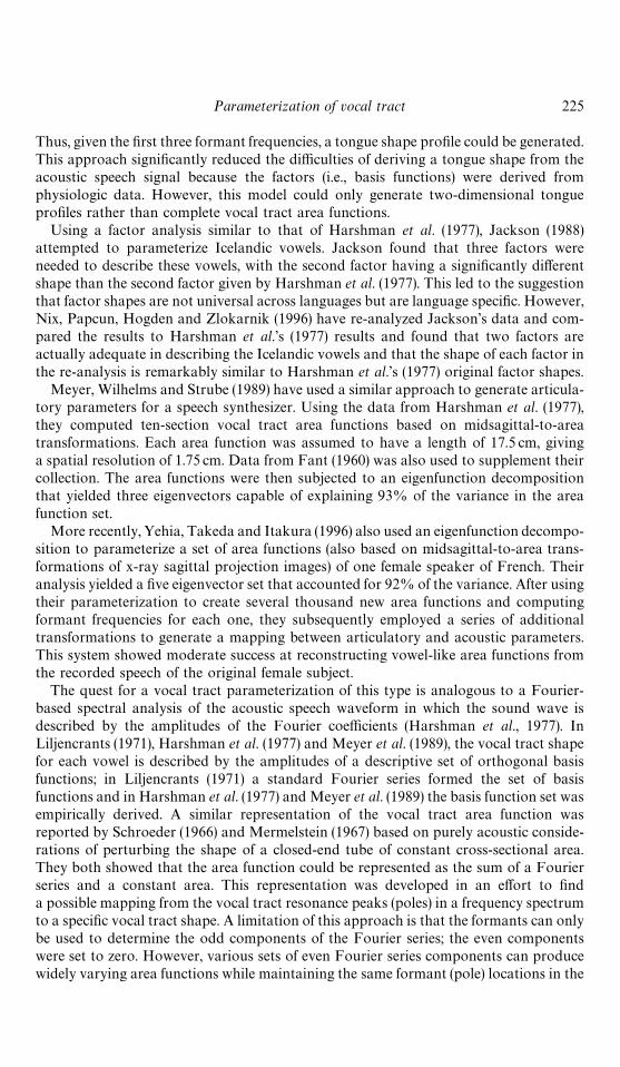
analysis (e.g., Munhall, Vatikiotis-Bateson & Tohkura, 1994), and also the physiologicalcorrelation between model parameters and human articulatory structures. Such para-metric models provide a simple, compressed representation of the state of the vocaltract at a given point in time. Articulatory parameters typically are of lower dimensionthan a full area function representation, but they are dependent on an accurate trans-formation from midsagittal distance to cross-sectional area. Examples of such midsagit-tally based models can be found in Lindblom and Sundberg (1971), Mermelstein (1973),Coker (1976), and Browman and Goldstein (1990).
Other highly compact articulatory models are those of Stevens and House (1955) andFant (1960), both of which represented the vocal tract with only three parameters: theplace and cross-sectional area of the main vocal tract constriction and a ratio of lipprotrusion to lip open area. With these parameters, the entire area function from justabove the glottis to the lip can be constructed by empirically-based rules.
Models such as these all depend heavily on the intuition and experience of theresearcher to decide which features of the vocal tract shape are most significant and howto provide a numerical description of those features. This approach has producedvaluable tools for synthesizing speech and for explaining many phenomena in bothspeech production and perception. However, it would be useful to have a more objectiveparameterization of the vocal tract shape. An example of such an approach is found inLiljencrants (1971), where he sought to explain the midsagittal profile of the tongue for 10vowel shapes with a Fourier series representation. He made three key observationsregarding his collection of tongue profiles: (1) the mean displacement of the tongue froma neutral position did not significantly change across vowels, implying a conservation ofmass of the tongue body; (2) the fine structure of each profile was much smaller than thatof the overall shape variation; and (3) many of the tongue profiles showed a strongresemblance to a sinusoid. These particular features suggested that the shape of thetongue for each vowel could be described by proportional amounts of a standard set oforthogonal basis functions: in this case, a Fourier series. Liljencrants found that thetongue shape could be reconstructed with small error using only a DC term and the firstsignificant Fourier component. This representation produced about a 9 to 1 compressionof the original data.
A similar study was performed by Harshman, Ladefoged and Goldstein (1977) wheremidsagittal tongue profiles for 10 English vowels were analyzed. However, instead ofusing an a priori set of the basis functions (i.e., Fourier series), a specialized 3-way factoranalysis was developed to decompose the tongue shapes into a set of empirical factorsthat characterized the displacement of the tongue during production of the 10 vowels.Their analysis revealed two underlying displacement patterns, various proportions ofwhich could be used to reconstruct the original tongue shapes. Much like the Fourierdescription proposed by Liljencrants (1971), the two displacement patterns uncovered bythe factor analysis allow the tongue profile of all the vowel shapes to be represented bya set of basic features (or patterns) and a set of amplitude (weighting) coefficients thatdefine each individual vowel.
The primary difference between the two studies is that the basis functions areempirically derived by the analysis in Harshman et al. (1977) rather then chosen a priorias in Liljencrants (1977). Lagefoged, Harshman, Goldstein and Rice (1978) used a mul-tiple regression analysis to generate a model in which the weighting coefficients of thederived tongue shape factors from Harshman et al. (1977) were represented as a functionof the formants (F1, F2 and F3) measured from acoustic recordings of their subjects.
Parameterization of vocal tract 225
Thus, given the first three formant frequencies, a tongue shape profile could be generated.This approach significantly reduced the difficulties of deriving a tongue shape from theacoustic speech signal because the factors (i.e., basis functions) were derived fromphysiologic data. However, this model could only generate two-dimensional tongueprofiles rather than complete vocal tract area functions.
Using a factor analysis similar to that of Harshman et al. (1977), Jackson (1988)attempted to parameterize Icelandic vowels. Jackson found that three factors wereneeded to describe these vowels, with the second factor having a significantly differentshape than the second factor given by Harshman et al. (1977). This led to the suggestionthat factor shapes are not universal across languages but are language specific. However,Nix, Papcun, Hogden and Zlokarnik (1996) have re-analyzed Jackson’s data and com-pared the results to Harshman et al.’s (1977) results and found that two factors areactually adequate in describing the Icelandic vowels and that the shape of each factor inthe re-analysis is remarkably similar to Harshman et al.’s (1977) original factor shapes.
Meyer, Wilhelms and Strube (1989) have used a similar approach to generate articula-tory parameters for a speech synthesizer. Using the data from Harshman et al. (1977),they computed ten-section vocal tract area functions based on midsagittal-to-areatransformations. Each area function was assumed to have a length of 17.5 cm, givinga spatial resolution of 1.75 cm. Data from Fant (1960) was also used to supplement theircollection. The area functions were then subjected to an eigenfunction decompositionthat yielded three eigenvectors capable of explaining 93% of the variance in the areafunction set.
More recently, Yehia, Takeda and Itakura (1996) also used an eigenfunction decompo-sition to parameterize a set of area functions (also based on midsagittal-to-area trans-formations of x-ray sagittal projection images) of one female speaker of French. Theiranalysis yielded a five eigenvector set that accounted for 92% of the variance. After usingtheir parameterization to create several thousand new area functions and computingformant frequencies for each one, they subsequently employed a series of additionaltransformations to generate a mapping between articulatory and acoustic parameters.This system showed moderate success at reconstructing vowel-like area functions fromthe recorded speech of the original female subject.
The quest for a vocal tract parameterization of this type is analogous to a Fourier-based spectral analysis of the acoustic speech waveform in which the sound wave isdescribed by the amplitudes of the Fourier coefficients (Harshman et al., 1977). InLiljencrants (1971), Harshman et al. (1977) and Meyer et al. (1989), the vocal tract shapefor each vowel is described by the amplitudes of a descriptive set of orthogonal basisfunctions; in Liljencrants (1971) a standard Fourier series formed the set of basisfunctions and in Harshman et al. (1977) and Meyer et al. (1989) the basis function set wasempirically derived. A similar representation of the vocal tract area function wasreported by Schroeder (1966) and Mermelstein (1967) based on purely acoustic conside-rations of perturbing the shape of a closed-end tube of constant cross-sectional area.They both showed that the area function could be represented as the sum of a Fourierseries and a constant area. This representation was developed in an effort to finda possible mapping from the vocal tract resonance peaks (poles) in a frequency spectrumto a specific vocal tract shape. A limitation of this approach is that the formants can onlybe used to determine the odd components of the Fourier series; the even componentswere set to zero. However, various sets of even Fourier series components can producewidely varying area functions while maintaining the same formant (pole) locations in the
226 B. H. Story and I. R. ¹itze
frequency spectrum. This is the classic many-to-one mapping problem. The problem ofunknown even Fourier components is equivalent to not knowing the location of thezeroes for a given vocal tract configuration. This lack of information about the zeroes isalso the primary cause of difficulties in extracting vocal tract area functions based onLPC analysis.
Unfortunately, all of the studies cited above have suffered from the incomplete natureof area functions derived from sagittal x-ray projection images. Magnetic resonanceimaging (MRI), which is both safe for the subject and allows for three-dimensionalimaging, is now becoming an attractive alternative to x-ray techniques for studying thespatial detail of the vocal tract. Recently, Story, Titze and Hoffman (1996) have reporteda set of MRI-based area functions corresponding to 10 vowels, 2 liquids, 3 plosives, and3 nasals for one adult male speaker. The area functions were obtained from directmeasurements of 3-D vocal tract reconstructions. It is the purpose of this paper to firstdevelop a speaker-specific parameterization of a subset of those vocal tract shapes (tenvowels: i, >, 2, æ, ö, ", &, υ, o, u) using a technique that decomposes them into empiricalorthogonal modes, similar to the method described by Meyer et al. (1989). This para-meterization is then used to explore possible connections between mode shape, articula-tion, and acoustic characteristics. Finally, the method is extended to all 18 area functionsgiven in Story et al. (1996) and results are compared with the vowel only case. It isrecognized that the use of data from a single subject does not allow for any statisticallysignificant statements to be made about a general population of speakers. However, it isof interest to understand the general phonetic characteristics as well as those qualitieswhich make a speaker unique. Thus, a method which decomposes a set of vocal tractshapes for one speaker at a time retains the detail that is unique to that person. Thispaper is intended to lay out a method that can be used for additional sets of vocal tractshapes that will hopefully be acquired from many more subjects in the future.
2. Empirical orthogonal mode decomposition
Statistical techniques that utilize a linear orthogonal transformation to extract a low-dimensional set of prominent features from a high-dimensional input set have been usedin many fields, and as a result go by several different names. Principal componentsanalysis, Karhunen-Loeve transform, empirical orthogonal functions, or singular valuedecomposition are a few of the names used to identify the method. In this paper, the term‘‘empirical orthogonal modes’’ will be used since it implies that basis functions arederived purely from empirical data and the term ‘‘mode’’ is used to emphasize a similarityto a modal decomposition of a dynamical system into natural modes. Occasionally, theterms ‘‘orthogonal modes’’ or simply ‘‘modes’’ will be used; these should be assumed tomean the same as ‘‘empirical orthogonal modes’’.
Decomposition of a data set into orthogonal modes transforms a high dimensionalinput into a low-dimensional output consisting of significant, uncorrelated featureswhere a small number of the features account for most of the variance in the original dataset. The particular method used in this study to extract modes is given in general terms inHerzel et al. (1995) and specifically applied to vocal fold vibratory patterns in Berry et al.(1994). The formulation of the method will now be given in terms that are specific to theanalysis of the area function set in Story et al. (1996). The notation will be similar to thatused by Herzel et al. (1995) except that the temporal dimension will be replaced by
Parameterization of vocal tract 227
a phoneme dimension (the term ‘phoneme’ is used here only to conveniently denotea collection of both vowel and consonant area functions).
In this paper, the term ‘‘area vector’’ will refer to the collection of vocal tract cross-sectional area values represented in an ordered vector. This contrasts with the ‘‘areafunction’’, which is defined here as the combination of the area vector and a correspond-ing length vector which indicates each area element’s distance from the glottis. Areafunctions will typically be shown in figures (that is, area vectors plotted against lengthvectors) but the area vectors are used in the analysis.
Each area function in Story et al. (1996) was reported as a set of cross-sectional areaswith a constant length interval of 0.396 cm; the space between data points was assumedto be represented by a cylindrical tube section. The number of sections comprising eacharea function was chosen to most closely represent the measured length of the vocal tractduring production of a given vowel or consonant. However, to extract empirical ortho-gonal functions, all of the area functions must be represented as vectors of equal length.Hence, each area function was fitted with a cubic spline and resampled to be 44 sectionslong. In order to maintain the original vocal tract lengths, the length intervals betweencross-sectional areas have now been made phoneme dependent. The resulting areavectors and length intervals (d
l) for the ten vowels are given in Table I; the length of any
given area function is now 44dl.
To perform the decomposition of the area vectors into empirical orthogonal modes,assume that any area vector in the set can be represented by a mean and a variable part,
A(x, p)"A0(x)#a (x, p) (1)
where A (x, p) is the area vector for a given phoneme p, A0(x) is the mean area vector
across the data set, and a (x, p) is the variation that is superimposed on A0(x) to produce
a specific area vector. The x denotes the index vector [1, 2,2 , 44], where 1 represents thefirst section above the glottis and section 44 is at the lips. The phoneme-dimension isdenoted by p and for the vowel only case, which will be the main focus of this paper, p"[1, 2,2, 10], representing the vowels ordered as [i, >, 2, æ, ö, ", &, υ, o, u] (see Table I). Ifconsonants are added to the analysis, p would be increased accordingly; e.g., for all 18 ofthe vowels and consonants given in Story et al. (1996), p"[1, 2,2 , 18]. The mean areavector A
0(x) is computed by
A0(x)"
1
M
M+
p/1
A(x, p) (M"number of phonemes). (2)
The superimposed variations are computed by subtracting the mean area vector from allthe area vectors in the input data set,
a (x, p)"A(x, p)!A0(x). (3)
The elements of a real, symmetric, covariance matrix R of the a (x, p)’s can now becomputed as
Rij"
1
M!1
M+p/1
a (xi, p)a(x
j, p) (i, j"1, 2, 2 , N) (4)
where M is again the number of area vectors in the input set and N is the numberof elements in each area vector (N"44). A matrix of N-element normalized eigen-vectors / and an N-element vector of eigenvalues j can now be computed from
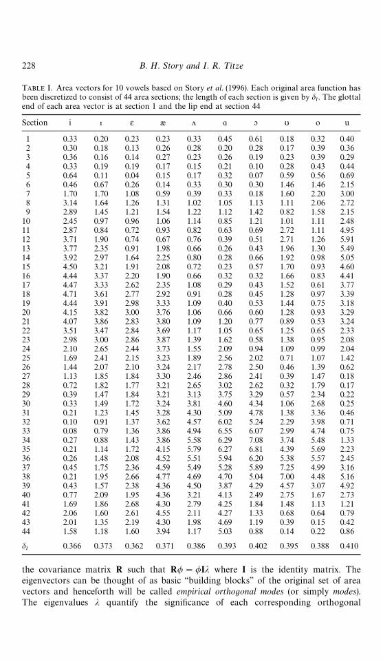
TABLE I. Area vectors for 10 vowels based on Story et al. (1996). Each original area function hasbeen discretized to consist of 44 area sections; the length of each section is given by d
l. The glottal
end of each area vector is at section 1 and the lip end at section 44
Section i > 2 æ ö " & υ o u
1 0.33 0.20 0.23 0.23 0.33 0.45 0.61 0.18 0.32 0.402 0.30 0.18 0.13 0.26 0.28 0.20 0.28 0.17 0.39 0.363 0.36 0.16 0.14 0.27 0.23 0.26 0.19 0.23 0.39 0.294 0.33 0.19 0.19 0.17 0.15 0.21 0.10 0.28 0.43 0.445 0.64 0.11 0.04 0.15 0.17 0.32 0.07 0.59 0.56 0.696 0.46 0.67 0.26 0.14 0.33 0.30 0.30 1.46 1.46 2.157 1.70 1.70 1.08 0.59 0.39 0.33 0.18 1.60 2.20 3.008 3.14 1.64 1.26 1.31 1.02 1.05 1.13 1.11 2.06 2.729 2.89 1.45 1.21 1.54 1.22 1.12 1.42 0.82 1.58 2.15
10 2.45 0.97 0.96 1.06 1.14 0.85 1.21 1.01 1.11 2.4811 2.87 0.84 0.72 0.93 0.82 0.63 0.69 2.72 1.11 4.9512 3.71 1.90 0.74 0.67 0.76 0.39 0.51 2.71 1.26 5.9113 3.77 2.35 0.91 1.98 0.66 0.26 0.43 1.96 1.30 5.4914 3.92 2.97 1.64 2.25 0.80 0.28 0.66 1.92 0.98 5.0515 4.50 3.21 1.91 2.08 0.72 0.23 0.57 1.70 0.93 4.6016 4.44 3.37 2.20 1.90 0.66 0.32 0.32 1.66 0.83 4.4117 4.47 3.33 2.62 2.35 1.08 0.29 0.43 1.52 0.61 3.7718 4.71 3.61 2.77 2.92 0.91 0.28 0.45 1.28 0.97 3.3919 4.44 3.91 2.98 3.33 1.09 0.40 0.53 1.44 0.75 3.1820 4.15 3.82 3.00 3.76 1.06 0.66 0.60 1.28 0.93 3.2921 4.07 3.86 2.83 3.80 1.09 1.20 0.77 0.89 0.53 3.2422 3.51 3.47 2.84 3.69 1.17 1.05 0.65 1.25 0.65 2.3323 2.98 3.00 2.86 3.87 1.39 1.62 0.58 1.38 0.95 2.0824 2.10 2.65 2.44 3.73 1.55 2.09 0.94 1.09 0.99 2.0425 1.69 2.41 2.15 3.23 1.89 2.56 2.02 0.71 1.07 1.4226 1.44 2.07 2.10 3.24 2.17 2.78 2.50 0.46 1.39 0.6227 1.13 1.85 1.84 3.30 2.46 2.86 2.41 0.39 1.47 0.1828 0.72 1.82 1.77 3.21 2.65 3.02 2.62 0.32 1.79 0.1729 0.39 1.47 1.84 3.21 3.13 3.75 3.29 0.57 2.34 0.2230 0.33 1.49 1.72 3.24 3.81 4.60 4.34 1.06 2.68 0.2531 0.21 1.23 1.45 3.28 4.30 5.09 4.78 1.38 3.36 0.4632 0.10 0.91 1.37 3.62 4.57 6.02 5.24 2.29 3.98 0.7133 0.08 0.79 1.36 3.86 4.94 6.55 6.07 2.99 4.74 0.7534 0.27 0.88 1.43 3.86 5.58 6.29 7.08 3.74 5.48 1.3335 0.21 1.14 1.72 4.15 5.79 6.27 6.81 4.39 5.69 2.2336 0.26 1.48 2.08 4.52 5.51 5.94 6.20 5.38 5.57 2.4537 0.45 1.75 2.36 4.59 5.49 5.28 5.89 7.25 4.99 3.1638 0.21 1.95 2.66 4.77 4.69 4.70 5.04 7.00 4.48 5.1639 0.43 1.57 2.38 4.36 4.50 3.87 4.29 4.57 3.07 4.9240 0.77 2.09 1.95 4.36 3.21 4.13 2.49 2.75 1.67 2.7341 1.69 1.86 2.68 4.30 2.79 4.25 1.84 1.48 1.13 1.2142 2.06 1.60 2.61 4.55 2.11 4.27 1.33 0.68 0.64 0.7943 2.01 1.35 2.19 4.30 1.98 4.69 1.19 0.39 0.15 0.4244 1.58 1.18 1.60 3.94 1.17 5.03 0.88 0.14 0.22 0.86
dl
0.366 0.373 0.362 0.371 0.386 0.393 0.402 0.395 0.388 0.410
228 B. H. Story and I. R. ¹itze
the covariance matrix R such that R/"/Ij where I is the identity matrix. Theeigenvectors can be thought of as basic ‘‘building blocks’’ of the original set of areavectors and henceforth will be called empirical orthogonal modes (or simply modes).The eigenvalues j quantify the significance of each corresponding orthogonal

Parameterization of vocal tract 229
mode by indicating how much of the total variance it accounts for in the input dataset (i.e., the set of original area vectors); in particular, each individual eigenvalueji
divided by the sum of all the eigenvalues will yield the percentage of varianceaccounted for by its corresponding mode /
i(x).
A result of the decomposition of area vectors as stated above is that the resultingorthogonal modes are ordered from least significant to most significant; i.e., the 44thmode accounts for the largest amount of variance. However, it is intuitively moredesirable for the most significant mode to be ordered such that it is ‘‘first’’ and the secondmost significant mode to be ordered ‘‘second’’, etc. Thus, the eigenvector (modal) matrix/ has been reordered to accommodate this desire and the remainder of the analysisshown below reflects this reordering.
Defining Ci(p) as the amplitude coefficient of the i5) mode corresponding to the p5) area
function, the superimposed variation characterizing each area vector can be computed by
a (x, p)"M+i/1
Ci(p)/
i(x). (5)
The amplitude coefficients are obtained by projecting the original data set onto the set ofmodes (normalized eigenvectors, / (x)),
Ci(p)"
N+j/1
a (xj, p)/
i(x
j) (i"1, 2, 2, N). (6)
Once the coefficients have been computed, area vectors can be reconstructed by combin-ing Equations 5 and 1 to get
A(x, p)"A0(x)#
N+i/1
Ci(p)/
i(x) (N"44). (7)
The corresponding length vector, required to reconstruct the area function, is generated by
¸ (x)"x ) dl(p). (8)
Equation 7 will ‘‘perfectly’’ reconstruct all of the original area vectors because all of thederived modes are used (i.e., N"44). However, if just a few of the low-ordered modesaccount for nearly all of the variance, the reconstruction of the area vectors can beperformed by summing over less than N modes with a loss of only a small amount of theoriginal fidelity. This provides a compression of the original area functions from N cross-sectional areas to much less than N modal amplitude coefficients. Thus, N in Equation7 may be replaced with an N@ where N@;N, assuming that N@ modes account for asufficient amount of the variance.
Experimentation with area vectors reconstructed with a small number of modes (e.g.,N@"4) showed them to be closely matched to the originals (the next section will discussthis further). However, due to the incomplete nature of the reconstruction (i.e., use of onlyfour modes), areas in the highly constricted regions of the vocal tract often dippedslightly below zero, which is obviously unrealistic. Just as sharp temporal features in anacoustic waveform are composed of many harmonics, sharp spatial features in an areafunction, such as a tight constriction, must be represented by many modes.
To avert this problem, a square root pre-processing operation was applied to eachoriginal area vector prior to performing the modal decomposition laid out in Equations1—7. This effectively converts each area into the radius of a circular cross-section, except
230 B. H. Story and I. R. ¹itze
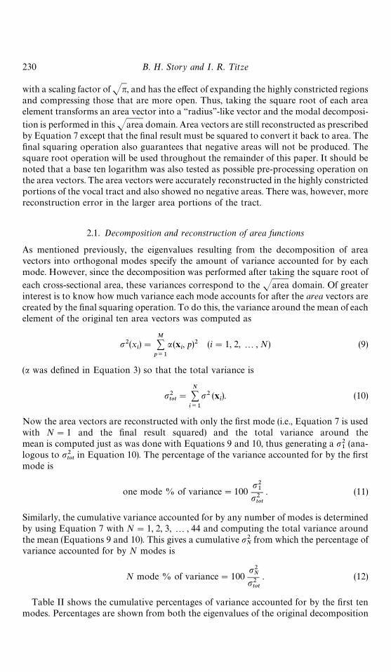
with a scaling factor of Jn, and has the effect of expanding the highly constricted regionsand compressing those that are more open. Thus, taking the square root of each areaelement transforms an area vector into a ‘‘radius’’-like vector and the modal decomposi-
tion is performed in this Jarea domain. Area vectors are still reconstructed as prescribedby Equation 7 except that the final result must be squared to convert it back to area. Thefinal squaring operation also guarantees that negative areas will not be produced. Thesquare root operation will be used throughout the remainder of this paper. It should benoted that a base ten logarithm was also tested as possible pre-processing operation onthe area vectors. The area vectors were accurately reconstructed in the highly constrictedportions of the vocal tract and also showed no negative areas. There was, however, morereconstruction error in the larger area portions of the tract.
2.1. Decomposition and reconstruction of area functions
As mentioned previously, the eigenvalues resulting from the decomposition of areavectors into orthogonal modes specify the amount of variance accounted for by eachmode. However, since the decomposition was performed after taking the square root of
each cross-sectional area, these variances correspond to the Jarea domain. Of greaterinterest is to know how much variance each mode accounts for after the area vectors arecreated by the final squaring operation. To do this, the variance around the mean of eachelement of the original ten area vectors was computed as
p2(xi)"
M+
p/1
a (xi, p)2 (i"1, 2, 2, N) (9)
(a was defined in Equation 3) so that the total variance is
p2tot"
N+i/1
p2 (xi). (10)
Now the area vectors are reconstructed with only the first mode (i.e., Equation 7 is usedwith N"1 and the final result squared) and the total variance around themean is computed just as was done with Equations 9 and 10, thus generating a p2
1(ana-
logous to p2tot
in Equation 10). The percentage of the variance accounted for by the firstmode is
one mode % of variance"100p21
p2tot
. (11)
Similarly, the cumulative variance accounted for by any number of modes is determinedby using Equation 7 with N"1, 2, 3, 2 , 44 and computing the total variance aroundthe mean (Equations 9 and 10). This gives a cumulative p2
Nfrom which the percentage of
variance accounted for by N modes is
N mode % of variance"100p2N
p2tot
. (12)
Table II shows the cumulative percentages of variance accounted for by the first tenmodes. Percentages are shown from both the eigenvalues of the original decomposition
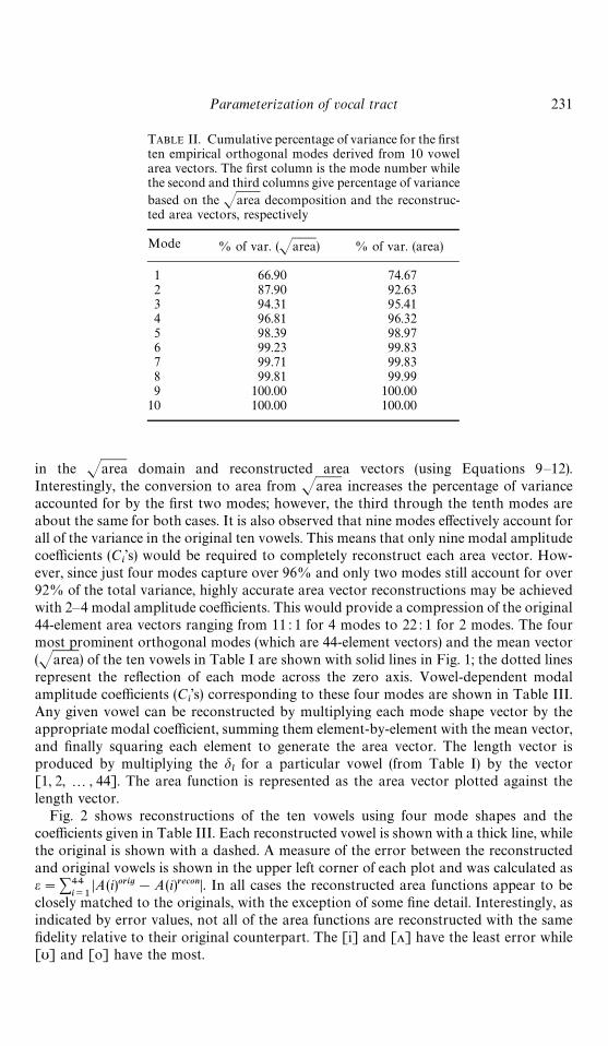
TABLE II. Cumulative percentage of variance for the firstten empirical orthogonal modes derived from 10 vowelarea vectors. The first column is the mode number whilethe second and third columns give percentage of variancebased on the Jarea decomposition and the reconstruc-ted area vectors, respectively
Mode % of var. (Jarea) % of var. (area)
1 66.90 74.672 87.90 92.633 94.31 95.414 96.81 96.325 98.39 98.976 99.23 99.837 99.71 99.838 99.81 99.999 100.00 100.00
10 100.00 100.00
Parameterization of vocal tract 231
in the Jarea domain and reconstructed area vectors (using Equations 9—12).Interestingly, the conversion to area from Jarea increases the percentage of varianceaccounted for by the first two modes; however, the third through the tenth modes areabout the same for both cases. It is also observed that nine modes effectively account forall of the variance in the original ten vowels. This means that only nine modal amplitudecoefficients (C
i’s) would be required to completely reconstruct each area vector. How-
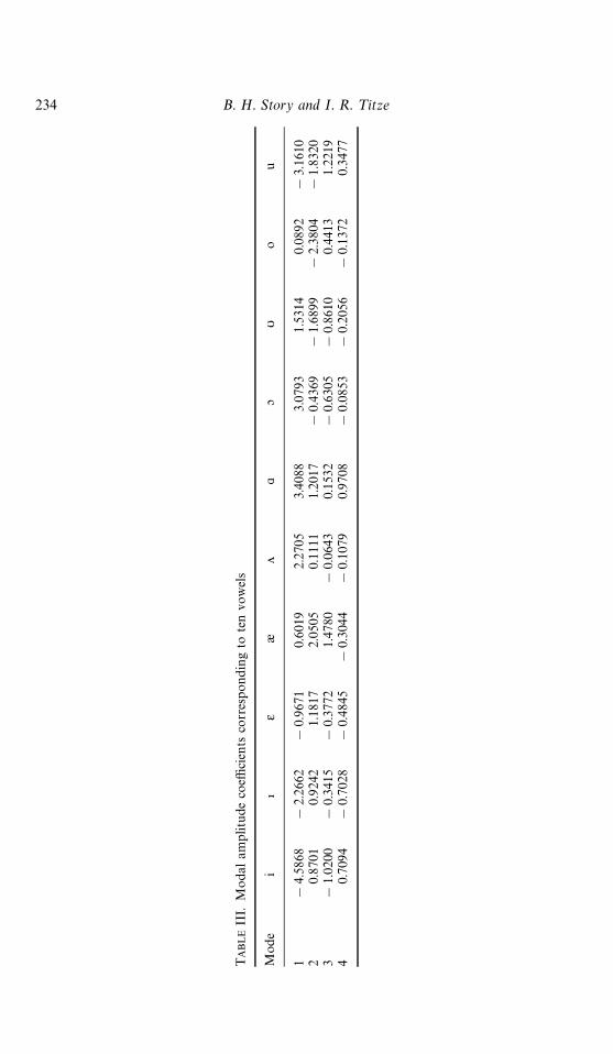
ever, since just four modes capture over 96% and only two modes still account for over92% of the total variance, highly accurate area vector reconstructions may be achievedwith 2—4 modal amplitude coefficients. This would provide a compression of the original44-element area vectors ranging from 11 : 1 for 4 modes to 22 : 1 for 2 modes. The fourmost prominent orthogonal modes (which are 44-element vectors) and the mean vector(Jarea) of the ten vowels in Table I are shown with solid lines in Fig. 1; the dotted linesrepresent the reflection of each mode across the zero axis. Vowel-dependent modalamplitude coefficients (C
i’s) corresponding to these four modes are shown in Table III.
Any given vowel can be reconstructed by multiplying each mode shape vector by theappropriate modal coefficient, summing them element-by-element with the mean vector,and finally squaring each element to generate the area vector. The length vector isproduced by multiplying the d
lfor a particular vowel (from Table I) by the vector
[1, 2, 2, 44]. The area function is represented as the area vector plotted against thelength vector.
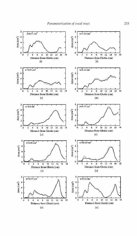
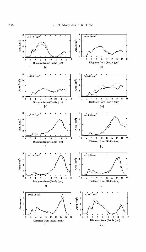
Fig. 2 shows reconstructions of the ten vowels using four mode shapes and thecoefficients given in Table III. Each reconstructed vowel is shown with a thick line, whilethe original is shown with a dashed. A measure of the error between the reconstructedand original vowels is shown in the upper left corner of each plot and was calculated ase"+44
i/1DA(i)orig!A(i)reconD. In all cases the reconstructed area functions appear to be
closely matched to the originals, with the exception of some fine detail. Interestingly, asindicated by error values, not all of the area functions are reconstructed with the samefidelity relative to their original counterpart. The [i] and [ö] have the least error while[υ] and [o] have the most.
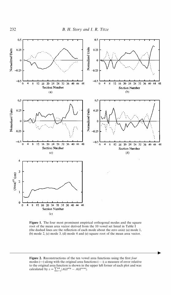
Figure 1. The four most prominent empirical orthogonal modes and the squareroot of the mean area vector derived from the 10 vowel set listed in Table I(the dashed lines are the reflection of each mode about the zero axis): (a) mode 1,(b) mode 2, (c) mode 3, (d) mode 4 and (e) square root of the mean area vector.
cFigure 2. Reconstructions of the ten vowel area functions using the first fourmodes (—) along with the original area functions (- - -); a measure of error relativeto the original area function is shown in the upper left forner of each plot and wascalculated by e"+44
i/1DA(i)orig!A(i)recon D.
232 B. H. Story and I. R. ¹itze
Parameterization of vocal tract 233
TA
BLE
III.
Moda
lam
plit
ude
coeffi
cien
tsco
rres
pon
din
gto
ten
vow
els
Mod
ei
>2
æö
"&
υo
u
1!
4.58
68!
2.26
62!
0.96
710.
6019
2.27
053.
4088
3.07
931.
5314
0.08
92!
3.16
102
0.87
010.
9242
1.18
172.
0505
0.11
111.
2017
!0.
4369
!1.
6899
!2.
3804
!1.
8320
3!
1.02
00!
0.34
15!
0.37
721.
4780
!0.
0643
0.15
32!
0.63
05!
0.86
100.
4413
1.22
194
0.70
94!
0.70
28!
0.48
45!
0.30
44!
0.10
790.
9708
!0.
0853
!0.
2056
!0.
1372
0.34
77
234 B. H. Story and I. R. ¹itze

Parameterization of vocal tract 235
Vowel reconstructions using only two mode shapes are shown in Fig. 3. As expected,the reconstructed area functions are not matched as closely to the originals as with fourmodes but they still reasonably approximate the original vowels. The error for [>, 2, ö, o]has increased only slightly over the previous case, while more significant error increasesare observed for the other vowels.
2.2. Articulatory interpretation of mode shapes
While the previous section discussed the modal decomposition simply as a methodof parameterizing and compressing the area functions, it is also of interest to investi-gate a possible articulatory interpretation of the empirical orthogonal modes. Sincethe modal decomposition extracts the most prominent features or patterns from theinput data set, it is likely that the most prominent modes contain significant articulatoryinformation.
The first mode shape in Fig. 1 accounts for nearly 75% of the total variance in the areavector set (see Table II), which makes it, by far, the most prominent mode. It hasa back-to-front asymmetry that, for a negative amplitude coefficient, would largelyreplicate the forward and upward movement of the tongue and some upward jawmovement (recall that the area vectors are the sum of the mean area vector and the modeshapes; thus, a negatively valued portion of a mode shape reduces the cross-sectionalarea). Equivalently, a positive modal amplitude coefficient would signify a backward anddownward tongue movement and a dropping of the jaw. Thus, it is not surprising thatthe coefficients for ["] and [i] (the most extreme front and back vowels) given in TableIII have the largest positive and negative values, respectively, for the first mode in the set.However, because each mode encompasses the entire length of the vocal tract, thestructure of the tongue and jaw cannot account for the complete shape of the first mode.For example, the shape of the region between 0 and 5 cm (from the glottis) is due to thelower pharyngeal structure such as the epilaryngeal tube and epiglottis.
The second mode (Fig. 1b), which accounts for 18% of the total variance, crosses thezero axis several times and allows for tract variations in areas where the first mode hasdiminished amplitude, as would be expected for orthogonal modes. Because it can affecta large region in the middle of the vocal tract, this mode may capture the up-downmotion and possible arching of the tongue. Note that the coefficients for the second modein Table III have large negative values for the vowels [υ, o, u], all of which have amid-tract constriction. The [æ] has a large positive coefficient for the secondmode combined with a low-valued first mode coefficient to create a expansion that isfarther back than for ["]. Additionally, the region of the second mode between 0and 5 cm defines the shaping of the epilarynx and the lower pharynx with moredetail than mode 1. At the lip end of the vocal tract, mode 2 can exert much moreinfluence than can mode 1, indicating that it may also contain shaping of the vocal tractcorresponding to lip rounding and spreading. Again, note that the large negativecoefficient values of mode 2 for the vowels [o, υ, u], also generate lip rounding as well asa mid-tract constriction.
Any region in which the amplitude of the mode shape is near zero represents a portionof the vocal tract that changes very little across vowels. With regard to modes 1 and 2,such a region exists from about 0—1.5 cm above the glottis. Both modes have amplitudesclose to zero indicating that the epilaryngeal section does not change much across thevowels. This can also be seen in Figs. 2 and 3 where all ten vowels are plotted.
236 B. H. Story and I. R. ¹itze
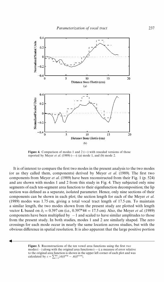
Figure 4. Comparison of modes 1 and 2 (—) with rescaled versions of thosereported by Meyer et al. (1989) (- - -): (a) mode 1, and (b) mode 2.
Parameterization of vocal tract 237
It is of interest to compare the first two modes in the present analysis to the two modes(or as they called them, components) derived by Meyer et al. (1989). The first twocomponents from Meyer et al. (1989) have been reconstructed from their Fig. 1 (p. 524)and are shown with modes 1 and 2 from this study in Fig. 4. They subjected only ninesegments of each ten-segment area function to their eigenfunction decomposition; the lipsection was defined as a separate, isolated parameter. Hence, only nine sections of theircomponents can be shown in each plot; the section length for each of the Meyer et al.(1989) modes was 1.75 cm, giving a total vocal tract length of 17.5 cm. To maintaina similar length, the two modes shown from the present study are plotted with lengthvector L based on d
l"0.397 cm (i.e., 0.397*44"17.5 cm). Also, the Meyer et al. (1989)
components have been multiplied by !1 and scaled to have similar amplitudes to thosefrom the present study. In both studies, modes 1 and 2 are similarly shaped. The zerocrossings for each mode occur in nearly the same location across studies, but with theobvious difference in spatial resolution. It is also apparent that the large positive portion
bFigure 3. Reconstructions of the ten vowel area functions using the first twomodes (—) along with the original area functions (- - -); a measure of error relativeto the original area function is shown in the upper left corner of each plot and wascalculated by e"+44
i/1DA(i)orig!A(i)recon D.
238 B. H. Story and I. R. ¹itze
at the lip end of mode 2 (approximately 16 cm to 17.5 cm) from this study is due to lipmotion, since the Meyer et al. (1989) components did not include the lips.
The third and fourth modes correspond mainly to higher spatial frequency detail orthe fine structure of the area vector shape, which makes it difficult to speculate on thepossible articulatory connection to these modes. Their respective coefficients in Table IIIindicate their diminished significance for reconstructing the vowel shapes.
3. Acoustic considerations
In this section, the acoustic characteristics of the mean area function will be firstexamined. Then the effect of adding increasing amplitudes of the mode shapes to themean area function will be studied in terms of formant perturbations.
3.1. Significance of the mean area function
It has often been the case that theoretical analyses of the vocal tract formant structurebegin by considering a uniform tube, closed at the glottis and open at the mouth, withformants spaced according to
Fn"
(2n!1)c
4¸(n"1, 2, 3, 2)
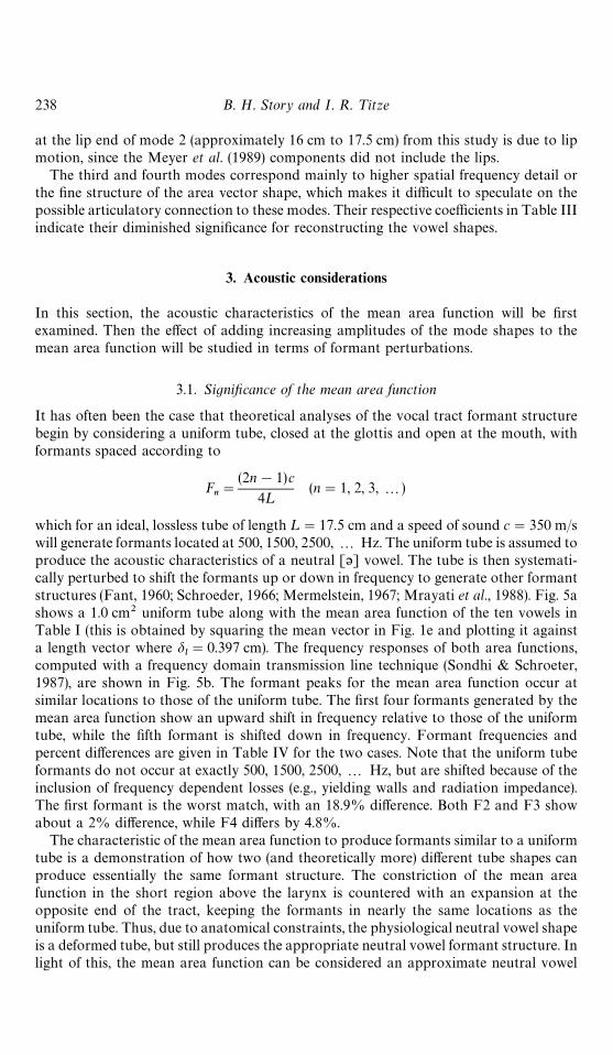
which for an ideal, lossless tube of length ¸"17.5 cm and a speed of sound c"350 m/swill generate formants located at 500, 1500, 2500, 2 Hz. The uniform tube is assumed toproduce the acoustic characteristics of a neutral [ə] vowel. The tube is then systemati-cally perturbed to shift the formants up or down in frequency to generate other formantstructures (Fant, 1960; Schroeder, 1966; Mermelstein, 1967; Mrayati et al., 1988). Fig. 5ashows a 1.0 cm2 uniform tube along with the mean area function of the ten vowels inTable I (this is obtained by squaring the mean vector in Fig. 1e and plotting it againsta length vector where d
l"0.397 cm). The frequency responses of both area functions,
computed with a frequency domain transmission line technique (Sondhi & Schroeter,1987), are shown in Fig. 5b. The formant peaks for the mean area function occur atsimilar locations to those of the uniform tube. The first four formants generated by themean area function show an upward shift in frequency relative to those of the uniformtube, while the fifth formant is shifted down in frequency. Formant frequencies andpercent differences are given in Table IV for the two cases. Note that the uniform tubeformants do not occur at exactly 500, 1500, 2500, 2 Hz, but are shifted because of theinclusion of frequency dependent losses (e.g., yielding walls and radiation impedance).The first formant is the worst match, with an 18.9% difference. Both F2 and F3 showabout a 2% difference, while F4 differs by 4.8%.
The characteristic of the mean area function to produce formants similar to a uniformtube is a demonstration of how two (and theoretically more) different tube shapes canproduce essentially the same formant structure. The constriction of the mean areafunction in the short region above the larynx is countered with an expansion at theopposite end of the tract, keeping the formants in nearly the same locations as theuniform tube. Thus, due to anatomical constraints, the physiological neutral vowel shapeis a deformed tube, but still produces the appropriate neutral vowel formant structure. Inlight of this, the mean area function can be considered an approximate neutral vowel
Figure 5. Comparison of the mean area function with a uniform tube; the vocaltract length was 17.5 cm for both cases: (a) mean area function (—) and 1 cm2uniform tube (- - -), and (b) frequency response of the mean area function (—) and1 cm2 uniform tube (- - -).
TABLE IV. First four formant frequencies of a 1 cm2 uniformtube and the mean area function based on 10 vowels; both hada length of 17.5 cm. Percent differences between the two sets offormant frequencies are also shown
Tract shape F1 F2 F3 F4
uniform tube 528 1482 2456 3436mean area 628 1510 2506 3606function% diff 18.9 2.0 2.0 4.9
Parameterization of vocal tract 239
configuration and other vowels are produced by imposing perturbations on it. Theseperturbations were quantified (for one speaker) in Section 2.1 with the decomposition ofthe area vector set into orthogonal modes.
A comparison of the Fourier series representation of the area function suggested bySchroeder (1966) and the modal representation presented in this paper show an interest-ing similarity. Following Schroeder (1966), the area function can be represented by
A (x)"A0#A
0
M+
m/1
pmcosA
(2m!1)nx
l B , (13)
240 B. H. Story and I. R. ¹itze
in which pm
is the coefficient determining the magnitude of the mth odd Fouriercomponent, M is the number of formants, and l is the vocal tract length. In this equation,the area function A (x) is the sum of the uniform tube cross-sectional area A
0and the
scaled (by A0) sum of the odd Fourier cosine series (a standard set of orthogonal basis
functions) over the number of formants extracted from a speech waveform spectrum;A
0is a scalar value, since the area along the length of the tube was constant. Inclusion of
even cosine terms in Equation 13 will not significantly effect the locations of the formantsbut will greatly alter the resulting area function. Thus, in theory, an infinite number ofarea function shapes could generate the same formant structure. By comparison, theempirical orthogonal mode representation given by Equation 7 (recall A(x, p)"A
0(x)#
+Ni/1
Ci(p) /
i(x)), also generates an area function by the sum of a constant and the sum of
a set of scaled basis functions. The difference is that the constant, A0(x), is a spatially
varying area vector and the basis functions are the empirically-based orthogonal modes.In summary, Equation 13 (from Schroeder) is based on the theoretically-derived
acoustical possibilities of deforming a uniform tube, whereas Equation 7 is based on theempirically-derived physiological possibilities of deforming the neutral vocal tract shape.When reconstructing the original ten vowels, Equations 7 and 8 are automaticallyconstrained to generate physiologically realistic area functions. While it is not possible tosay whether area functions generated by arbitrary combinations of modal coefficients(i.e., not corresponding to any of the ten original vowels) would be part of a speaker’sphysiologic repertoire, it is likely that the use of empirical orthogonal modes would givemore realistic area functions than a mathematical basis function set (e.g., Fourier series),especially if the coefficients C
iare not extended beyond the maximum and minimum
values obtained for the original ten vowels. It is noted, however, that the epilaryngealregion of the vocal tract (1.5—2 cm above the glottis) is definitely constrained by thesubject’s physiology, since the amplitude of all the mode shapes in this region is nearzero (see Fig. 1). This ensures that this region will have small cross-sectional areas(similar to those of the mean area vector in this region) regardless of the modal coefficientvalues.
3.2. Acoustic effects of the mode shapes
In the previous section, the mean area function was shown to have a formant spectrumsimilar to that of a uniform tube. In this section we will examine the displacement of themean vowel formant locations due to the superposition of varying amplitudes of modes1 and 2 upon the mean area function.
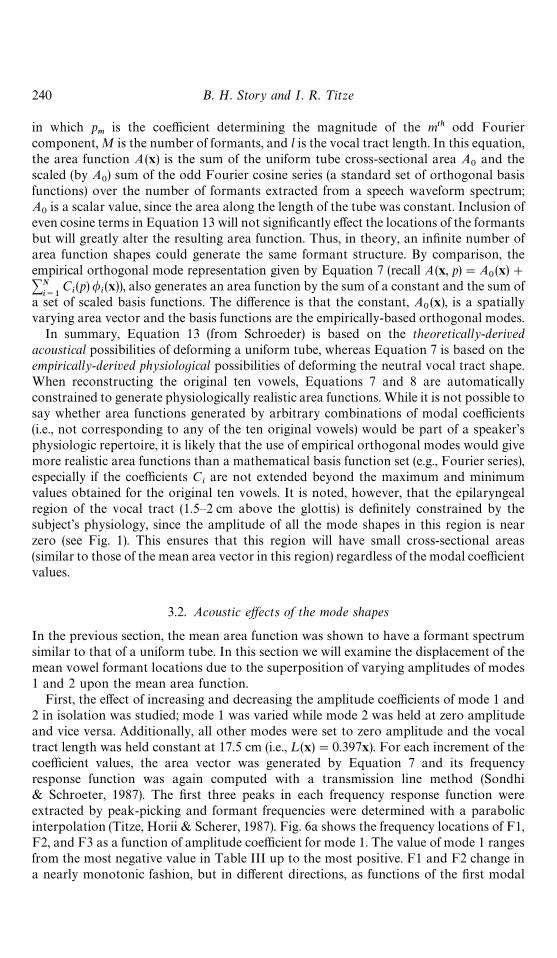
First, the effect of increasing and decreasing the amplitude coefficients of mode 1 and2 in isolation was studied; mode 1 was varied while mode 2 was held at zero amplitudeand vice versa. Additionally, all other modes were set to zero amplitude and the vocaltract length was held constant at 17.5 cm (i.e., ¸ (x)"0.397x). For each increment of thecoefficient values, the area vector was generated by Equation 7 and its frequencyresponse function was again computed with a transmission line method (Sondhi& Schroeter, 1987). The first three peaks in each frequency response function wereextracted by peak-picking and formant frequencies were determined with a parabolicinterpolation (Titze, Horii & Scherer, 1987). Fig. 6a shows the frequency locations of F1,F2, and F3 as a function of amplitude coefficient for mode 1. The value of mode 1 rangesfrom the most negative value in Table III up to the most positive. F1 and F2 change ina nearly monotonic fashion, but in different directions, as functions of the first modal
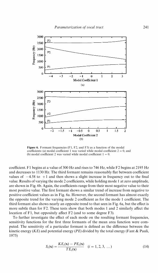
Figure 6. Formant frequencies (F1, F2, and F3) as a function of the modalcoefficients: (a) modal coefficient 1 was varied while modal coefficient 2"0, and(b) modal coefficient 2 was varied while modal coefficient 1"0.
Parameterization of vocal tract 241
coefficient. F1 begins at a value of 300 Hz and rises to 746 Hz, while F2 begins at 2195 Hzand decreases to 1130 Hz. The third formant remains reasonably flat between coefficientvalues of !4.58 to #1 and then shows a slight increase in frequency out to the finalvalue. Results of varying the mode 2 coefficients, while holding mode 1 at zero amplitude,are shown in Fig. 6b. Again, the coefficients range from their most negative value to theirmost positive value. The first formant shows a similar trend of increase from negative topositive coefficient values as in Fig. 6a. However, the second formant has almost exactlythe opposite trend for the varying mode 2 coefficient as for the mode 1 coefficient. Thethird formant also shows nearly an opposite trend to that seen in Fig. 6a, but the effect ismore subtle than for F2. These tests show that both modes 1 and 2 similarly affect thelocation of F1, but oppositely affect F2 (and to some degree F3).
To further investigate the effect of each mode on the resulting formant frequencies,sensitivity functions for the first three formants of the mean area function were com-puted. The sensitivity of a particular formant is defined as the difference between thekinetic energy (KE) and potential energy (PE) divided by the total energy (Fant & Pauli,1975)
Si(x)"
KEi(x)!PE
i(x)
¹E (x)(i"1, 2, 3, 2) (14)
i

242 B. H. Story and I. R. ¹itze
where x is the index vector [1, 2, 2 , 44] and i is the formant number. The sensitivityfunction can then be used to compute the change in a particular formant frequency (F
i)
due to perturbation of the area function (DA) with the relation,
DFi
Fi
"
N+n/1
Si(x)
DA (x)
A(x). (15)
This equation says that, if the sensitivity function is positive valued and the areaperturbation is also positive (area is increased), the change in formant frequency will beupward (positive). If the area change is negative (area decreased), the formant frequencywill decrease. When the sensitivity function is negative, the opposite effect occurs forpositive or negative area perturbations.
The sensitivity function for the first formant is shown superimposed onto the first twomode shapes in Fig. 7a. From 0 cm to 11 cm, the sensitivity function is negatively valued,meaning that expanding this portion of the mean area function would move F1 down-ward in frequency. Conversely, from 11 cm to the lips, an expansion in the mean areafunction will raise F1. In the same two portions of the vocal tract (i.e., 0 to 11 cm and11 cm to the lips), mode 1 maintains nearly the same polarity as the F1 sensitivityfunction. This means that a positive valued modal amplitude coefficient for mode 1 willdecrease the cross-sectional area where the sensitivity is negative, and increase it wherethe sensitivity is positive, thus raising F1. Recall that ["], which typically has a high F1around 700 Hz, also has a large positive coefficient for mode 1 (see Table III) and [i] hasa large negative mode 1 coefficient to generate its characteristically low F1 of about300 Hz. The second mode maintains the same polarity as the F1 sensitivity function from0 cm to about 6.5 cm (except for a small positive value at 3.5 cm) and then has oppositepolarity out to 10 cm. From 10 cm to the end of the vocal tract, mode 2’s polarity withrespect to the F1 sensitivity function oscillates. The net effect on F1 due to a positivelyvalued mode 2 coefficient would be a raising of F1 but with less effectiveness than mode1. This trend can be seen in Fig. 6b where F1 rises with increasing values of the secondmodal coefficient.
The F2 sensitivity function is given in Fig. 7b along with the shapes of the first andsecond modes. Except for the region from 0 cm to 5 cm, mode 1 has mostly oppositepolarity to the sensitivity function, while mode 2 is primarily of the same polarity. Thus,positive valued coefficients for mode 1 tend to lower F2, while positive coefficients formode 2 will raise F2; the same trend was observed in Figs. 6a and b.
To condense these observations, the normalized correlation (at zero lag) of each modewith each sensitivity function was computed and results are shown graphically in Fig. 8.Mode 1 has a positive correlation of 0.53 with the F1 sensitivity function and a negativecorrelation of !0.56 with the sensitivity function for F2. The F3 sensitivity was alsocomputed but found to be nearly uncorrelated with either modes 1 or 2. Mode 2 ispositively correlated to F1 sensitivity with a value of 0.36, and also to F2 sensitivity, witha value of 0.65. The largest correlation value for both modes occurred for F2, eventhough they have opposite signs. Thus, with nearly equal valued modal amplitudecoefficients, mode 1 and 2 can have almost the same effect on F2, but in oppositedirections.
Up to this point we have ignored the effect of vocal tract length, which has been heldconstant at 17.5 cm throughout this section. Repeating the above tests with a shortenedor lengthened vocal tract produces similar relationships between formant patterns and
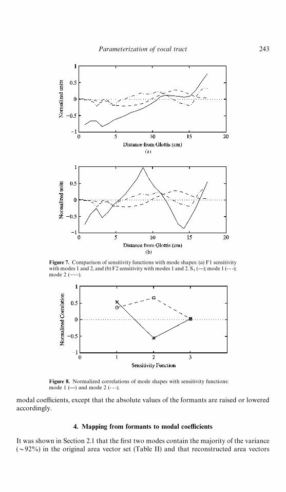
Figure 7. Comparison of sensitivity functions with mode shapes: (a) F1 sensitivitywith modes 1 and 2, and (b) F2 sensitivity with modes 1 and 2. S
1(—); mode 1 (- - -);
mode 2 ()-)-)-).
Figure 8. Normalized correlations of mode shapes with sensitivity functions:mode 1 (—) and mode 2 (- - -).
Parameterization of vocal tract 243
modal coefficients, except that the absolute values of the formants are raised or loweredaccordingly.
4. Mapping from formants to modal coefficients
It was shown in Section 2.1 that the first two modes contain the majority of the variance(&92%) in the original area vector set (Table II) and that reconstructed area vectors
244 B. H. Story and I. R. ¹itze
based on only the first two modes generate reasonable approximations to the originalvowels (Fig. 3). Additionally, the previous section has indicated a strong correlationbetween these first two modes and the first two formant frequencies. The results suggestthat the mode/formant relationship could be exploited to create a mapping betweenmodal coefficients and formant frequencies. Toward this goal, a two-dimensional grid ofmode 1 and 2 amplitude coefficients was generated by choosing the same maximum andminimum bounding values for each mode as for Fig. 6, and pairing 48 incremental valuesbetween them while all other modal amplitude coefficients are set to zero. This is shownmathematically by
Dc1"
Cmax1
!Cmin1
M!1(16a)
Dc2"
Cmax2
!Cmin2
M!1(16b)
c1(i)"Cmin
1#iDc
1i"1, 2, M!1 (17a)
c2(i)"Cmin
2#jDc
2j"1, 2 , M!1 (17b)
where Dc1
and Dc2
are the coefficient increments, Cmax1
, Cmin1
, Cmax2
, and Cmin2
, are themaxima and minima of the mode 1 and mode 2 coefficients derived for the original tenvowels, and M"50. The index i represents the increment of the mode 1 coefficient, whilej is the increment of the mode 2 coefficient. Vocal tract length is again held constant, butat the mean length of the original vowels which is 16.90 cm (d
i"0.384 cm). The result is
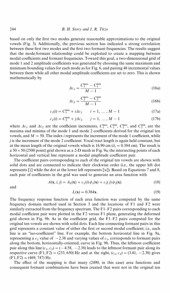
a 50]50 (2500 point) grid shown as a 2-D mesh in Fig. 9a; the intersecting points of eachhorizontal and vertical line represent a modal amplitude coefficient pair.
The coefficient pairs corresponding to each of the original ten vowels are shown withsolid dots and are connected to indicate their clockwise order (i.e., the upper left dotrepresents [i] while the dot at the lower left represents [u]). Based on Equations 7 and 8,each pair of coefficients in the grid was used to generate an area function with
A(x, i, j)"A0(x)#c
1(i)/
1(x)#c
2( j)/
2(x). (18)
and¸ (x)"0.384x. (19)
The frequency response function of each area function was computed by the samefrequency domain method used in Section 3 and the locations of F1 and F2 weresimilarly extracted from the frequency spectrum. The F1—F2 pairs corresponding to eachmodal coefficient pair were plotted in the F2 versus F1 plane, generating the deformedgrid shown in Fig. 9b. As in the coefficient grid, the F1—F2 pairs computed for theoriginal ten vowels are shown with solid dots. Each line connecting formant pairs in thisgrid represents a constant value of either the first or second modal coefficient; i.e., eachline is an ‘‘iso-coefficient’’ line. For example, the bottom horizontal line in Fig. 9a,representing a c
2value of !2.38 and varying values of c
1, corresponds to formant pairs
along the bottom, horizontally-oriented, curve in Fig. 9b. Thus, the leftmost coefficientpair along this line (c
1, c
2)"(!4.58, !2.38) leads to the leftmost formant pair along its
respective curve (F1, F2)"(233, 650) Hz and at the right, (c1, c
2)"(3.41,!2.38) gives
(F1,F2)"(469, 747) Hz.The effect of the mapping is that many (2490, in this case) area functions and
consequent formant combinations have been created that were not in the original ten

Figure 9. Mapping of mode 1 and mode 2 coefficient pairs to F1—F2 pairs, wherethe dots represent the coefficients and formant frequencies of the original tenvowels: (a) modal coefficient grid (b) corresponding F1—F2 grid and (c) modifiedcoefficient grid when those coefficients generating the saturated portion of theF1—F2 grid are removed.
Parameterization of vocal tract 245
vowel set. In a visual, qualitative sense, the F1—F2 plane is created by deforming themodal coefficient grid such that the upper right-hand corner is pulled down and to theright, which stretches the upper portion of the grid, and at the same time a compressionpushes the lower right-hand corner upward and to the left. The upper boundary of thegrid shows a saturation in the form of an apparent folding of the F1—F2 pairs, so thatseveral pairs of coefficients corresponding to the boundary would produce nearly thesame formant locations for F1 and F2. This saturation region corresponds to largepositive c
2coefficients and is most prevalent when c
1is close to its most negative or most
positive values. Fig. 9c shows a reformatted coefficient grid where the coefficient pairs inthe saturation region have been removed, suggesting that the formant saturation couldbe eliminated by plotting only those formant pairs which have a correspondence in thisreformatted grid.
With the exception of the saturation region, the F1—F2 grid represents a one-to-onemapping between F1 and F2 formant frequencies and modal coefficients (or equivalently

246 B. H. Story and I. R. ¹itze
an area function created by the coefficients). This suggests that an utterance consisting ofconnected vowels could be analyzed to extract F1 and F2 as functions of time, and thencould be mapped back to the modal coefficient grid, and consequently to area functions.Hence, a time-dependent series of physiologically realistic area functions could beobtained from the acoustic speech waveform. However, a limitation of such a mappingwould be the constant vocal tract length that was used to generate the area functions andconsequent formant grid. In fact, this nontrivial problem is typically encountered withmost inverse mappings of speech-to-area function. As examples, Schroeder (1966),Mermelstein (1967), Wakita (1972) all specified a constant vocal tract length prior toperforming their respective inverse mapping schemes. As Mermelstein (1967) notes,‘‘tracts of different length can be distorted to yield the same formant frequencies. Hence,differences in the length of speakers’ tracts do not necessarily manifest themselves insystematic formant differences’’, suggesting that the actual vocal tract length would bevery difficult, if not impossible, to obtain. However, Atal, Chang, Mathews and Tukey(1978) attempted to include vocal tract length in an inverse mapping as a recoverableparameter. They first generated a forward mapping from incremented articulatory modelparameters such as place of maximum constriction, area of the maximum constrictionand mouth opening, lip protrusion, and total vocal tract length to formant frequenciesfor F1, F2, and F3. The inverse mapping was then realized by correspondences betweenthe formants and the articulatory parameters. They found, however, that three formantfrequencies were unable to resolve a set of articulatory parameters uniquely.
To include vocal tract length in the present mapping approach, the dlin Equation 8
could be incrementally swept through its full range (see Table I) similar to c1
and c2; this
would also be similar to the Atal et al. (1978) approach. If as many values of dlwere
combined with all of the previous values of c1
and c2, the number of coefficient ‘‘triples’’
would increase to 125000 (503). This could be reduced somewhat by using coarserincrements of d
lthan the other coefficients but still presents a more complicated mapping
than that presented previously. In addition, it would almost certainly generate a non-uniqueness between formants and modal/length coefficients. Such nonuniqueness maybe an advantage with a more sophisticated system of matching formants to coefficients,but at this time we prefer to maintain the simplicity of the initial approach, that is tocontrol only the mode 1 and 2 coefficients. An alternative method to include vocal tractlength is to modify the mapping shown in Fig. 9 so that d
lvaries as a function of c
1and
c2; define this as d
lvar. Thus, the mapping is generated just as it was before, except that
dlvar
is calculated for every coefficient pair based on their values. The dlvar
’s are calculatedas a weighted sum of the original ten d
l(p)’s, where the weights are based on the squared
distances between a given pair of coefficients c1(i), c
2( j) and the coefficients derived for
the original ten vowels C1(p), C
2(p) . This is accomplished by first computing the
reciprocal of the squared distances
dp(i, j)"M[C
1(p)!c
1(i, j)]2#[C
2(p)!c
2(i, j)]2#eN~1 (p"1, 2, 3210) (20)
where e"1]10~16 and is included to ensure that dp(i, j) does not become infinite under
the condition c1(i)"C
1(p) and c
2( j)"C
2(p). Next define the weights w
p(i, j) to be the
dp(i, j)’s normalized to their sum across the ten vowels
wp(i, j)"
dp(i, j)
+10p/1
dp(i, j)
(p"1, 2, 3210) (21)
Parameterization of vocal tract 247
so that each weight has a value between 0 and 1 and the sum of the weights +10p/1
wp(i, j) is
equal to 1. Now dlvar
(i, j) can be calculated as
dlvar
(i, j)"10+
p/1
wp(i, j) d
l(p) (22)
where the dl(p)’s are derived from the original vowel area functions and were given in
Table I. Thus, an area vector is generated as before with Equation 18 but the lengthvector is now given by
¸(x)"dlvar
(i, j)x (23)
For cases when c1(i) and c
2( j) are equivalent to one of the original vowels (i.e.,
c1(i)"C
1(p) and c
2( j)"C
2(p)), the weight corresponding to that vowel would be 1 while
all others would be 0, thus equating dlvar
(i, j) to dl(p).
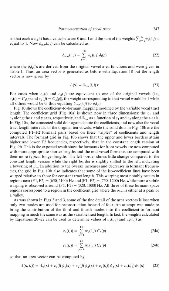
Fig. 10 shows the coefficient-to-formant mapping modified by the variable vocal tractlength. The coefficient grid (Fig. 10a) is shown now in three dimensions: the c
1and
c2along the x and y axes, respectively, and d
lvaras a function of c
1and c
2along the z-axis.
In Fig. 10a, the connected solid dots again denote the coefficients, and now also the vocaltract length intervals, of the original ten vowels, while the solid dots in Fig. 10b are thecomputed F1—F2 formant pairs based on these ‘‘triples’’ of coefficients and lengthintervals. The formant grid in Fig. 10b shows that the upper and lower borders attainhigher and lower F2 frequencies, respectively, than in the constant length version ofFig. 9b. This is the expected result since the formants for front vowels are now computedwith more appropriate shorter lengths and the mid-vowel formants are computed withtheir more typical longer lengths. The left border shows little change compared to theconstant length version while the right border is slightly shifted to the left, indicatinga lowering of F1. In addition to the overall increases and decreases in formant frequen-cies, the grid in Fig. 10b also indicates that some of the iso-coefficient lines have beenwarped relative to those for constant tract length. This warping most notably occurs inregions near (F1, F2)"(650, 2100) Hz and (F1, F2)"(750, 1200) Hz, while more a subtlewarping is observed around (F1, F2)"(320, 1000) Hz. All three of these formant spaceregions correspond to a region in the coefficient grid where the d
lvaris either at a peak or
a valley.As was shown in Figs 2 and 3, some of the fine detail of the area vectors is lost when
only two modes are used for reconstruction instead of four. An attempt was made tobring the contribution of the third and fourth modes into the coefficient-to-formantmapping in much the same was as the variable tract length. In fact, the weights calculatedby Equations 20—22 can be used to determine values of c
3(i, j) and c
4(i, j) as
c3(i, j)"
10+p/1
wp(i, j) C
3(p) (24a)
c4(i, j)"
10+p/1
wp(i, j) C
4(p) (24b)
so that an area vector can be computed by
A(x, i, j)"A0(x)#c
1(i)/
1(x)#c
2( j)/
2(x)#c
3(i, j) /
3(x)#c
4(i, j)/
4(x) (25)
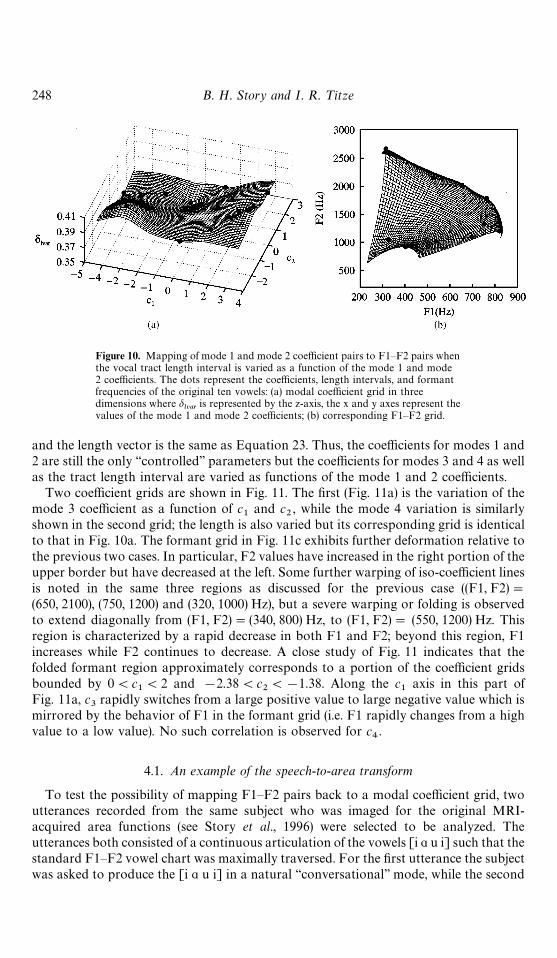
Figure 10. Mapping of mode 1 and mode 2 coefficient pairs to F1—F2 pairs whenthe vocal tract length interval is varied as a function of the mode 1 and mode2 coefficients. The dots represent the coefficients, length intervals, and formantfrequencies of the original ten vowels: (a) modal coefficient grid in threedimensions where d
lvaris represented by the z-axis, the x and y axes represent the
values of the mode 1 and mode 2 coefficients; (b) corresponding F1—F2 grid.
248 B. H. Story and I. R. ¹itze
and the length vector is the same as Equation 23. Thus, the coefficients for modes 1 and2 are still the only ‘‘controlled’’ parameters but the coefficients for modes 3 and 4 as wellas the tract length interval are varied as functions of the mode 1 and 2 coefficients.
Two coefficient grids are shown in Fig. 11. The first (Fig. 11a) is the variation of themode 3 coefficient as a function of c
1and c
2, while the mode 4 variation is similarly
shown in the second grid; the length is also varied but its corresponding grid is identicalto that in Fig. 10a. The formant grid in Fig. 11c exhibits further deformation relative tothe previous two cases. In particular, F2 values have increased in the right portion of theupper border but have decreased at the left. Some further warping of iso-coefficient linesis noted in the same three regions as discussed for the previous case ((F1, F2)"(650, 2100), (750, 1200) and (320, 1000) Hz), but a severe warping or folding is observedto extend diagonally from (F1, F2)"(340, 800) Hz, to (F1, F2)" (550, 1200) Hz. Thisregion is characterized by a rapid decrease in both F1 and F2; beyond this region, F1increases while F2 continues to decrease. A close study of Fig. 11 indicates that thefolded formant region approximately corresponds to a portion of the coefficient gridsbounded by 0(c
1(2 and !2.38(c
2(!1.38. Along the c
1axis in this part of
Fig. 11a, c3
rapidly switches from a large positive value to large negative value which ismirrored by the behavior of F1 in the formant grid (i.e. F1 rapidly changes from a highvalue to a low value). No such correlation is observed for c
4.
4.1. An example of the speech-to-area transform
To test the possibility of mapping F1—F2 pairs back to a modal coefficient grid, twoutterances recorded from the same subject who was imaged for the original MRI-acquired area functions (see Story et al., 1996) were selected to be analyzed. Theutterances both consisted of a continuous articulation of the vowels [i " u i] such that thestandard F1—F2 vowel chart was maximally traversed. For the first utterance the subjectwas asked to produce the [i " u i] in a natural ‘‘conversational’’ mode, while the second
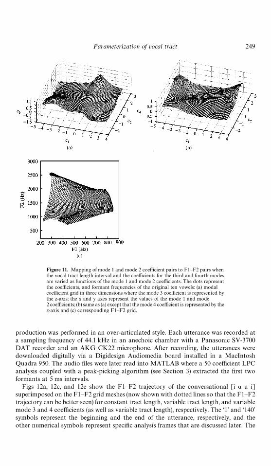
Figure 11. Mapping of mode 1 and mode 2 coefficient pairs to F1—F2 pairs whenthe vocal tract length interval and the coefficients for the third and fourth modesare varied as functions of the mode 1 and mode 2 coefficients. The dots representthe coefficients, and formant frequencies of the original ten vowels: (a) modalcoefficient grid in three dimensions where the mode 3 coefficient is represented bythe z-axis; the x and y axes represent the values of the mode 1 and mode2 coefficients; (b) same as (a) except that the mode 4 coefficient is represented by thez-axis and (c) corresponding F1—F2 grid.
Parameterization of vocal tract 249
production was performed in an over-articulated style. Each utterance was recorded ata sampling frequency of 44.1 kHz in an anechoic chamber with a Panasonic SV-3700DAT recorder and an AKG CK22 microphone. After recording, the utterances weredownloaded digitally via a Digidesign Audiomedia board installed in a MacIntoshQuadra 950. The audio files were later read into MATLAB where a 50 coefficient LPCanalysis coupled with a peak-picking algorithm (see Section 3) extracted the first twoformants at 5 ms intervals.
Figs 12a, 12c, and 12e show the F1—F2 trajectory of the conversational [i " u i]superimposed on the F1—F2 grid meshes (now shown with dotted lines so that the F1—F2trajectory can be better seen) for constant tract length, variable tract length, and variablemode 3 and 4 coefficients (as well as variable tract length), respectively. The ‘1’ and ‘140’symbols represent the beginning and the end of the utterance, respectively, and theother numerical symbols represent specific analysis frames that are discussed later. The
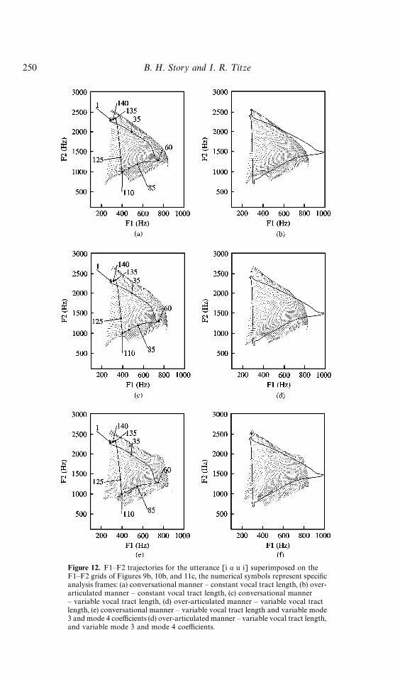
Figure 12. F1—F2 trajectories for the utterance [i " u i] superimposed on theF1—F2 grids of Figures 9b, 10b, and 11c, the numerical symbols represent specificanalysis frames: (a) conversational manner — constant vocal tract length, (b) over-articulated manner — constant vocal tract length, (c) conversational manner— variable vocal tract length, (d) over-articulated manner — variable vocal tractlength, (e) conversational manner — variable vocal tract length and variable mode3 and mode 4 coefficients (d) over-articulated manner — variable vocal tract length,and variable mode 3 and mode 4 coefficients.
250 B. H. Story and I. R. ¹itze
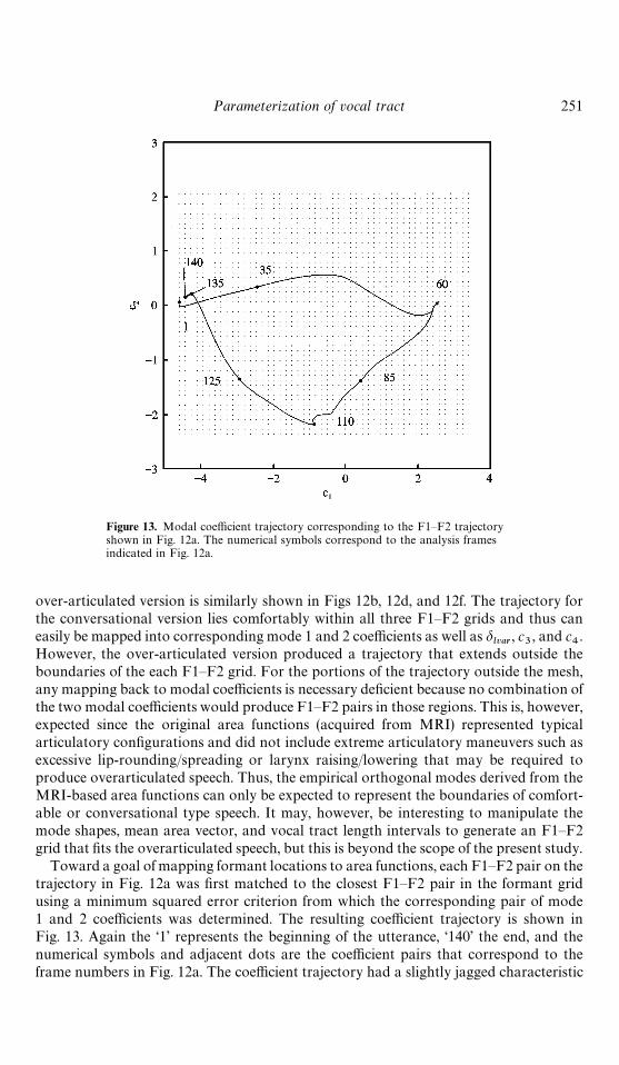
Figure 13. Modal coefficient trajectory corresponding to the F1—F2 trajectoryshown in Fig. 12a. The numerical symbols correspond to the analysis framesindicated in Fig. 12a.
Parameterization of vocal tract 251
over-articulated version is similarly shown in Figs 12b, 12d, and 12f. The trajectory forthe conversational version lies comfortably within all three F1—F2 grids and thus caneasily be mapped into corresponding mode 1 and 2 coefficients as well as d
lvar, c
3, and c
4.
However, the over-articulated version produced a trajectory that extends outside theboundaries of the each F1—F2 grid. For the portions of the trajectory outside the mesh,any mapping back to modal coefficients is necessary deficient because no combination ofthe two modal coefficients would produce F1—F2 pairs in those regions. This is, however,expected since the original area functions (acquired from MRI) represented typicalarticulatory configurations and did not include extreme articulatory maneuvers such asexcessive lip-rounding/spreading or larynx raising/lowering that may be required toproduce overarticulated speech. Thus, the empirical orthogonal modes derived from theMRI-based area functions can only be expected to represent the boundaries of comfort-able or conversational type speech. It may, however, be interesting to manipulate themode shapes, mean area vector, and vocal tract length intervals to generate an F1—F2grid that fits the overarticulated speech, but this is beyond the scope of the present study.
Toward a goal of mapping formant locations to area functions, each F1—F2 pair on thetrajectory in Fig. 12a was first matched to the closest F1—F2 pair in the formant gridusing a minimum squared error criterion from which the corresponding pair of mode1 and 2 coefficients was determined. The resulting coefficient trajectory is shown inFig. 13. Again the ‘1’ represents the beginning of the utterance, ‘140’ the end, and thenumerical symbols and adjacent dots are the coefficient pairs that correspond to theframe numbers in Fig. 12a. The coefficient trajectory had a slightly jagged characteristic
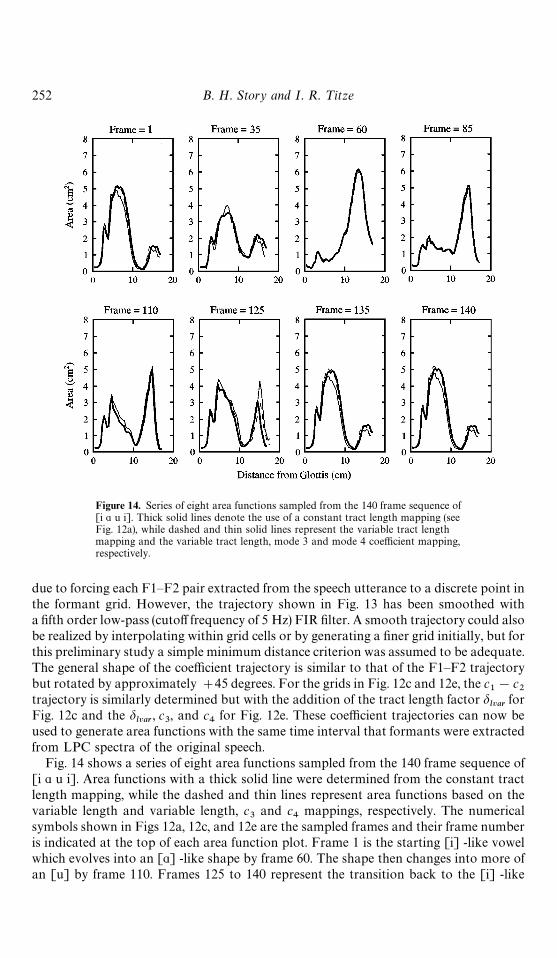
Figure 14. Series of eight area functions sampled from the 140 frame sequence of[i " u i]. Thick solid lines denote the use of a constant tract length mapping (seeFig. 12a), while dashed and thin solid lines represent the variable tract lengthmapping and the variable tract length, mode 3 and mode 4 coefficient mapping,respectively.
252 B. H. Story and I. R. ¹itze
due to forcing each F1—F2 pair extracted from the speech utterance to a discrete point inthe formant grid. However, the trajectory shown in Fig. 13 has been smoothed witha fifth order low-pass (cutoff frequency of 5 Hz) FIR filter. A smooth trajectory could alsobe realized by interpolating within grid cells or by generating a finer grid initially, but forthis preliminary study a simple minimum distance criterion was assumed to be adequate.The general shape of the coefficient trajectory is similar to that of the F1—F2 trajectorybut rotated by approximately #45 degrees. For the grids in Fig. 12c and 12e, the c
1!c
2trajectory is similarly determined but with the addition of the tract length factor d
lvarfor
Fig. 12c and the dlvar
, c3, and c
4for Fig. 12e. These coefficient trajectories can now be
used to generate area functions with the same time interval that formants were extractedfrom LPC spectra of the original speech.
Fig. 14 shows a series of eight area functions sampled from the 140 frame sequence of[i " u i]. Area functions with a thick solid line were determined from the constant tractlength mapping, while the dashed and thin lines represent area functions based on thevariable length and variable length, c
3and c
4mappings, respectively. The numerical
symbols shown in Figs 12a, 12c, and 12e are the sampled frames and their frame numberis indicated at the top of each area function plot. Frame 1 is the starting [i] -like vowelwhich evolves into an ["] -like shape by frame 60. The shape then changes into more ofan [u] by frame 110. Frames 125 to 140 represent the transition back to the [i] -like
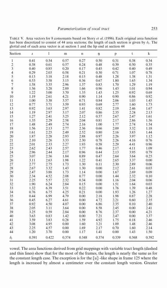
TABLE V. Area vectors for 8 consonants based on Story et al. (1996). Each original area functionhas been discretized to consist of 44 area sections; the length of each section is given by d
l. The
glottal end of each area vector is at section 1 and the lip end at section 44
Section O l m n ŋ p t k
1 0.41 0.54 0.57 0.27 0.50 0.31 0.38 0.342 0.38 0.61 0.57 0.24 0.48 0.39 0.50 0.353 0.40 0.85 0.20 0.17 0.45 0.42 0.40 0.494 0.29 2.03 0.58 0.21 0.30 0.71 1.07 0.785 0.13 3.18 2.18 0.15 0.48 1.28 1.38 1.316 0.53 3.58 3.15 0.36 0.67 1.80 1.65 1.347 1.58 3.35 2.96 1.37 0.83 1.70 1.29 1.198 1.56 3.28 2.89 1.66 0.96 1.43 1.01 0.949 1.22 3.00 3.70 1.35 1.43 1.25 0.92 0.69
10 1.19 2.61 4.21 0.90 1.14 0.90 0.86 0.9211 1.00 3.38 3.57 0.71 0.84 2.06 1.03 1.4512 0.77 3.71 3.59 0.93 0.69 2.77 1.60 1.7313 0.92 3.63 2.97 1.41 0.82 2.19 2.46 1.6714 1.19 2.97 3.17 2.07 0.86 2.35 2.24 2.1315 1.27 2.41 3.25 2.12 0.57 2.67 2.47 1.6116 1.35 2.29 2.58 2.04 0.81 2.17 2.86 1.5617 1.48 2.49 2.74 2.16 1.00 1.77 2.74 1.5418 1.56 2.13 2.77 2.36 0.66 2.09 3.32 1.1819 1.61 2.25 2.49 2.52 0.80 2.16 3.83 1.4420 1.87 2.28 2.93 2.88 0.97 2.26 3.97 1.1221 2.10 2.26 3.33 2.30 0.78 2.26 4.16 0.7622 2.01 2.33 2.27 1.93 0.58 2.29 4.41 0.9623 2.62 2.43 2.57 1.77 0.46 2.17 4.11 1.0924 2.96 2.44 2.17 0.96 0.44 2.13 3.95 0.7925 3.07 2.56 1.84 0.89 0.47 2.64 3.64 0.2526 3.11 2.63 1.98 1.22 0.41 2.65 3.37 0.0027 2.77 2.75 1.73 1.30 0.11 2.30 2.89 0.0628 2.67 3.32 1.43 1.30 0.00 2.12 2.61 0.0329 2.47 3.88 1.73 1.14 0.00 1.67 2.69 0.0930 2.34 4.52 2.08 0.77 0.00 1.44 2.32 0.1031 2.25 5.57 2.32 0.34 0.00 1.16 2.04 0.0632 1.90 6.24 2.84 0.15 0.00 1.51 1.64 0.0333 1.32 6.39 3.51 0.22 0.00 1.76 1.39 0.4834 0.76 6.75 4.25 0.21 0.00 1.93 1.26 1.2735 0.44 6.99 4.79 0.00 2.18 1.98 0.87 2.2836 0.45 6.27 4.61 0.00 4.72 2.21 0.60 2.3537 0.92 4.50 4.07 0.00 6.86 2.35 0.10 2.4038 2.05 3.11 3.64 0.00 8.58 2.45 0.00 2.4139 3.25 0.59 2.84 0.00 8.76 2.37 0.00 4.2140 3.63 0.83 1.42 0.00 7.21 2.47 0.00 3.3741 3.59 3.83 0.28 1.59 4.92 1.75 0.18 2.4642 3.08 4.95 0.00 1.60 3.21 1.09 1.48 2.4643 2.25 4.57 0.00 1.69 2.17 0.70 1.60 2.1444 1.20 3.70 0.00 1.17 1.41 0.00 1.43 1.50
dl
0.391 0.422 0.374 0.348 0.374 0.339 0.368 0.392
Parameterization of vocal tract 253
vowel. The area functions derived from grid mappings with variable tract length (dashedand thin lines) show that for the most of the frames, the length is nearly the same as forthe constant length case. The exception is for the [u] -like shape in frame 125 where thelength is increased by almost a centimeter over the constant length version. Greater
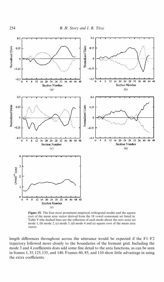
Figure 15. The four most prominent empirical orthogonal modes and the squareroot of the mean area vector derived from the 18 vowel—consonant set listed inTable V (the dashed lines are the reflection of each mode about the zero axis): (a)mode 1, (b) mode 2, (c) mode 3, (d) mode 4 and (e) square root of the mean areavector.
254 B. H. Story and I. R. ¹itze
length differences throughout across the utterance would be expected if the F1—F2trajectory followed more closely to the boundaries of the formant grid. Including themode 3 and 4 coefficients does add some fine detail to the area functions, as can be seenin frames 1, 35, 125, 135, and 140. Frames 60, 85, and 110 show little advantage in usingthe extra coefficients.
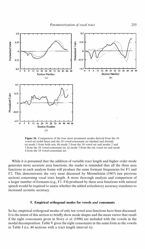
Figure 16. Comparison of the four most prominent modes derived from the 10vowel set (solid lines) and the 18 vowel-consonant set (dashed and dotted):(a) mode 1 from both sets, (b) mode 2 from the 10 vowel set and modes 2 and3 from the 18 vowel-consonant set, (c) mode 3 from the ten vowel set and mode4 from the 18 vowel-consonant set.
Parameterization of vocal tract 255
While it is presumed that the addition of variable tract length and higher order modegenerates more accurate area functions, the reader is reminded that all the three areafunctions in each analysis frame will produce the same formant frequencies for F1 andF2. This demonstrates the very issue discussed by Mermelstein (1967) (see previoussection) concerning vocal tract length. A more thorough analysis and comparison ofa larger number of formants (e.g., F1—F4) produced by these area functions with naturalspeech would be required to assess whether the added articulatory accuracy translates toincreased acoustic accuracy.
5. Empirical orthogonal modes for vowels and consonants
So far, empirical orthogonal modes of only ten vowel area functions have been discussed.It is the intent of this section to briefly show mode shapes and the mean vector that resultif the eight consonants given in Story et al. (1996) are included with the vowels in themodal decomposition. Table V gives the eight consonants in the same form as the vowelsin Table I (i.e, 44 sections with a tract length interval d ).
l
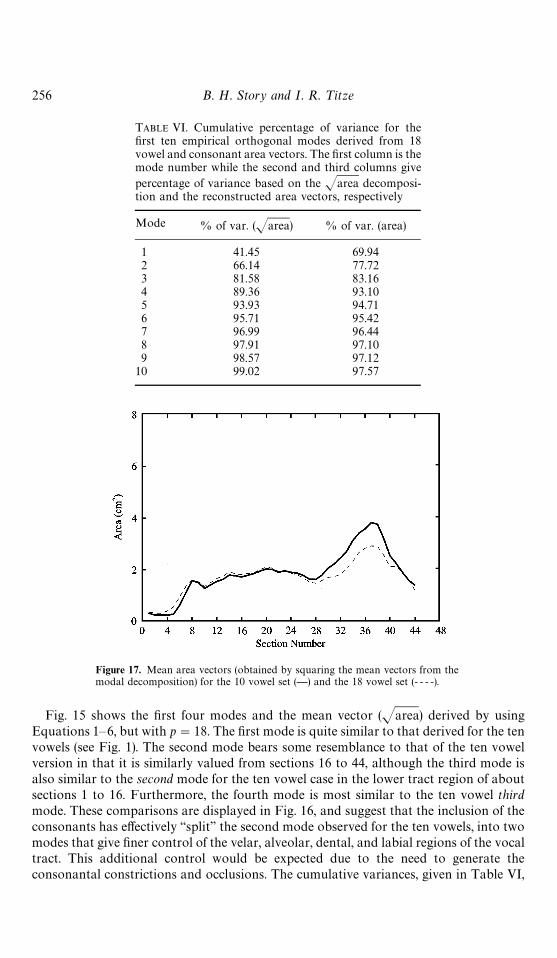
TABLE VI. Cumulative percentage of variance for thefirst ten empirical orthogonal modes derived from 18vowel and consonant area vectors. The first column is themode number while the second and third columns givepercentage of variance based on the Jarea decomposi-tion and the reconstructed area vectors, respectively
Mode % of var. (Jarea) % of var. (area)
1 41.45 69.942 66.14 77.723 81.58 83.164 89.36 93.105 93.93 94.716 95.71 95.427 96.99 96.448 97.91 97.109 98.57 97.12
10 99.02 97.57
Figure 17. Mean area vectors (obtained by squaring the mean vectors from themodal decomposition) for the 10 vowel set (—) and the 18 vowel set (- - - -).
256 B. H. Story and I. R. ¹itze
Fig. 15 shows the first four modes and the mean vector (Jarea) derived by usingEquations 1—6, but with p"18. The first mode is quite similar to that derived for the tenvowels (see Fig. 1). The second mode bears some resemblance to that of the ten vowelversion in that it is similarly valued from sections 16 to 44, although the third mode isalso similar to the second mode for the ten vowel case in the lower tract region of aboutsections 1 to 16. Furthermore, the fourth mode is most similar to the ten vowel thirdmode. These comparisons are displayed in Fig. 16, and suggest that the inclusion of theconsonants has effectively ‘‘split’’ the second mode observed for the ten vowels, into twomodes that give finer control of the velar, alveolar, dental, and labial regions of the vocaltract. This additional control would be expected due to the need to generate theconsonantal constrictions and occlusions. The cumulative variances, given in Table VI,
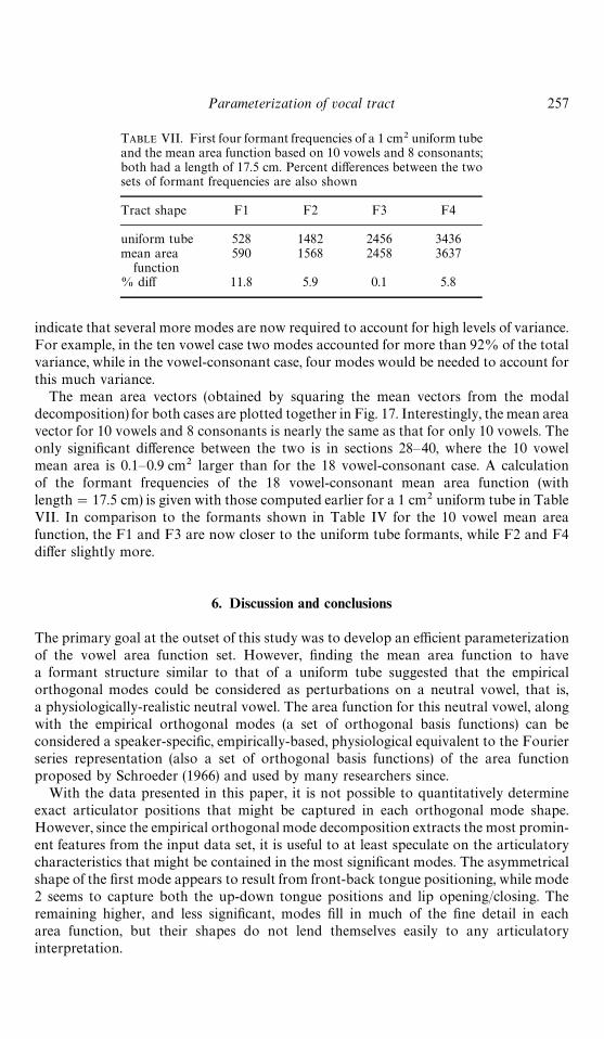
TABLE VII. First four formant frequencies of a 1 cm2 uniform tubeand the mean area function based on 10 vowels and 8 consonants;both had a length of 17.5 cm. Percent differences between the twosets of formant frequencies are also shown
Tract shape F1 F2 F3 F4
uniform tube 528 1482 2456 3436mean area 590 1568 2458 3637
function% diff 11.8 5.9 0.1 5.8
Parameterization of vocal tract 257
indicate that several more modes are now required to account for high levels of variance.For example, in the ten vowel case two modes accounted for more than 92% of the totalvariance, while in the vowel-consonant case, four modes would be needed to account forthis much variance.
The mean area vectors (obtained by squaring the mean vectors from the modaldecomposition) for both cases are plotted together in Fig. 17. Interestingly, the mean areavector for 10 vowels and 8 consonants is nearly the same as that for only 10 vowels. Theonly significant difference between the two is in sections 28—40, where the 10 vowelmean area is 0.1—0.9 cm2 larger than for the 18 vowel-consonant case. A calculationof the formant frequencies of the 18 vowel-consonant mean area function (withlength"17.5 cm) is given with those computed earlier for a 1 cm2 uniform tube in TableVII. In comparison to the formants shown in Table IV for the 10 vowel mean areafunction, the F1 and F3 are now closer to the uniform tube formants, while F2 and F4differ slightly more.
6. Discussion and conclusions
The primary goal at the outset of this study was to develop an efficient parameterizationof the vowel area function set. However, finding the mean area function to havea formant structure similar to that of a uniform tube suggested that the empiricalorthogonal modes could be considered as perturbations on a neutral vowel, that is,a physiologically-realistic neutral vowel. The area function for this neutral vowel, alongwith the empirical orthogonal modes (a set of orthogonal basis functions) can beconsidered a speaker-specific, empirically-based, physiological equivalent to the Fourierseries representation (also a set of orthogonal basis functions) of the area functionproposed by Schroeder (1966) and used by many researchers since.
With the data presented in this paper, it is not possible to quantitatively determineexact articulator positions that might be captured in each orthogonal mode shape.However, since the empirical orthogonal mode decomposition extracts the most promin-ent features from the input data set, it is useful to at least speculate on the articulatorycharacteristics that might be contained in the most significant modes. The asymmetricalshape of the first mode appears to result from front-back tongue positioning, while mode2 seems to capture both the up-down tongue positions and lip opening/closing. Theremaining higher, and less significant, modes fill in much of the fine detail in eacharea function, but their shapes do not lend themselves easily to any articulatoryinterpretation.
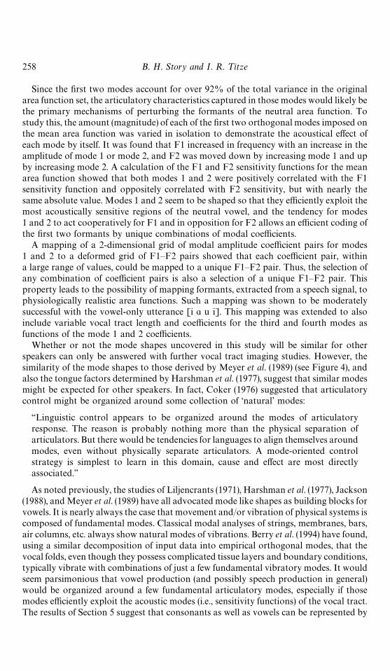
258 B. H. Story and I. R. ¹itze
Since the first two modes account for over 92% of the total variance in the originalarea function set, the articulatory characteristics captured in those modes would likely bethe primary mechanisms of perturbing the formants of the neutral area function. Tostudy this, the amount (magnitude) of each of the first two orthogonal modes imposed onthe mean area function was varied in isolation to demonstrate the acoustical effect ofeach mode by itself. It was found that F1 increased in frequency with an increase in theamplitude of mode 1 or mode 2, and F2 was moved down by increasing mode 1 and upby increasing mode 2. A calculation of the F1 and F2 sensitivity functions for the meanarea function showed that both modes 1 and 2 were positively correlated with the F1sensitivity function and oppositely correlated with F2 sensitivity, but with nearly thesame absolute value. Modes 1 and 2 seem to be shaped so that they efficiently exploit themost acoustically sensitive regions of the neutral vowel, and the tendency for modes1 and 2 to act cooperatively for F1 and in opposition for F2 allows an efficient coding ofthe first two formants by unique combinations of modal coefficients.
A mapping of a 2-dimensional grid of modal amplitude coefficient pairs for modes1 and 2 to a deformed grid of F1—F2 pairs showed that each coefficient pair, withina large range of values, could be mapped to a unique F1—F2 pair. Thus, the selection ofany combination of coefficient pairs is also a selection of a unique F1—F2 pair. Thisproperty leads to the possibility of mapping formants, extracted from a speech signal, tophysiologically realistic area functions. Such a mapping was shown to be moderatelysuccessful with the vowel-only utterance [i " u i]. This mapping was extended to alsoinclude variable vocal tract length and coefficients for the third and fourth modes asfunctions of the mode 1 and 2 coefficients.
Whether or not the mode shapes uncovered in this study will be similar for otherspeakers can only be answered with further vocal tract imaging studies. However, thesimilarity of the mode shapes to those derived by Meyer et al. (1989) (see Figure 4), andalso the tongue factors determined by Harshman et al. (1977), suggest that similar modesmight be expected for other speakers. In fact, Coker (1976) suggested that articulatorycontrol might be organized around some collection of ‘natural’ modes:
‘‘Linguistic control appears to be organized around the modes of articulatoryresponse. The reason is probably nothing more than the physical separation ofarticulators. But there would be tendencies for languages to align themselves aroundmodes, even without physically separate articulators. A mode-oriented controlstrategy is simplest to learn in this domain, cause and effect are most directlyassociated.’’
As noted previously, the studies of Liljencrants (1971), Harshman et al. (1977), Jackson(1988), and Meyer et al. (1989) have all advocated mode like shapes as building blocks forvowels. It is nearly always the case that movement and/or vibration of physical systems iscomposed of fundamental modes. Classical modal analyses of strings, membranes, bars,air columns, etc. always show natural modes of vibrations. Berry et al. (1994) have found,using a similar decomposition of input data into empirical orthogonal modes, that thevocal folds, even though they possess complicated tissue layers and boundary conditions,typically vibrate with combinations of just a few fundamental vibratory modes. It wouldseem parsimonious that vowel production (and possibly speech production in general)would be organized around a few fundamental articulatory modes, especially if thosemodes efficiently exploit the acoustic modes (i.e., sensitivity functions) of the vocal tract.The results of Section 5 suggest that consonants as well as vowels can be represented by
Parameterization of vocal tract 259
a small set of modes; however, more modes are necessary to adequately describe thecombined vowel-consonant set.
For some purpose, such as simulating connected speech segments, a vocal tractparameterization that utilizes mode shapes is an attractive alternative to controllingindividual articulator positions. Since the typical articulatory specifiers such as tonguetip, tongue body, lip position, etc. are efficiently ‘‘packaged’’ by the mode shapes,extensive knowledge of how the articulators are coordinated is not needed. As anexample, a simple model for simulation of speech production could be depicted asa time-dependent voice source specified by the desired fundamental frequency (F
0) and
amplitude (A0) (glottal flow pulse-shaping parameters such as skewing and open quo-
tients could also be specified to control the voice quality). The time-dependent articula-tion could be governed by the choice of two coefficient values (c
1and c
2) which scale the
orthogonal modes. Also, based on the mapping between coefficients and formantlocations, the selection of a given pair of coefficient values is equivalent to a selection ofa unique pair of F1 and F2. Thus, formant values could also be used as controlparameters. As stated, this simple modeling approach may not yield high quality speechsimulation, but could serve as a starting point for further development.
Future work needs to focus on the limitations of this study. In particular, thecoefficient-to-formant mapping should be extended to include higher formants, whichmay be essential for differentiating certain speech sounds (e.g., [1] and [O]) and enhanc-ing the general quality of any speech synthesis produced with the area functions.The effect of nasalization and consonantal constriction on the formant grid also needsto be explored in order to go beyond the realm of idealized vowel-like speech. Further-more, the methods used for including variable tract length and higher ordered modesshould be compared to other possible approaches, such as generating more extensivemulti-dimensional coefficient/length grids similar to those proposed by Atal et al. (1978).It will also be of interest to apply the modal decomposition to area function sets for otherspeakers to see if their mode shapes are essentially the same as those shown here. Itwould appear that the modes capture the global qualities necessary to generate phoneti-cally appropriate vowel sounds, but they likely also contain subtle variations thatcomprise an ‘‘acoustic signature’’ for a particular person.
This work was supported by Grant R01 DC02532 from the National Institute on Deafness andother Communication Disorders. The author would like to thank Dr. David Berry for fruitfuldiscussions on empirical orthogonal mode decomposition. Three reviewers are also acknowledgedfor their helpful suggestions on improving the original manuscript.
References
Atal, B. S., Chang, J. J., Mathews, M. V. & Tukey, J. W. (1978) Inversion of articulatory-to-acoustictransformation in the vocal tract by a computer sorting-sorting technique, Journal of Acoustical Society ofAmerica, 63 (5), 1535—1555.
Berry, D. A., Herzel, H., Titze, I. R. & Krischer, K. (1994) Interpretation of biomechanical simulations ofnormal and chaotic vocal fold oscillations with empirical eigenfunctions, Journal of Acoustical Society ofAmerica, 95 (6), 3595—3604.
Browman, C. & Goldstein, L. (1990) Gestural specification using dynamically-defined articulatory structures,Haskins ¸ab. Stat. Rep. on Speech Res., SR-103/104, 95—110.
Coker, C. H. (1976) A model of articulatory dynamics and control, Proceedings of IEEE, 64(4), 452—460.Fant, G. (1960) ¹he Acoustic ¹heory of Speech Production. The Hague: Mouton.
260 B. H. Story and I. R. ¹itze
Fant, G. & Pauli, S. (1975) Spatial characteristics of vocal tract resonance modes; In Fant, Proc. Speech Comm.Sem. 74., Stockholm, Sweden, Aug 1—3, 121—132.
Harshman, R., Ladefoged, P. & Goldstein, L. (1977) Factor analysis of tongue shapes, Journal of AcousticalSociety of America, 62 (3), 693—707.
Herzel, H., Krischer, K., Berry, D. A. & Titze, I. R. (1995) Analysis of spatio-temporal patterns by means ofempirical orthogonal functions, In Spatio-¹emporal Patterns in Nonequilibrium Complex Systems (P. E.Cladis and P. Palffy-Muhoray, editors), pp. 505—518. Reading, MA: Addison-Wesley.
Jackson, M. T. T. (1988) Analysis of tongue positions: Language-specific and cross-lignuistic models, Journal ofAcoustical Society of America, 84(1), 124—143.
Ladefoged, P., Harshman, R., Goldstein, L. & Rice, L. (1978) Generating vocal tract shapes from formantfrequencies, Journal of Acoustical Society of America, 64(4), 1027—1035.
Liljencrants, J. (1985) Speech Synthesis with a Reflection-Type Line Analog, DS Dissertation, Dept. of SpeechComm. and Music Acous., Royal Inst. of Tech., Stockholm, Sweden.
Liljencrants, J. (1971) Fourier series description of the tongue profile, S¹¸-QPSR, 4, 10—18.Lindblom, B. & Sundberg, J. (1971) Acoustical consequences of lip, tongue, jaw and larynx movement, Journal
of Acoustical Society of America, 4 (2), 1166—1179.Mermelstein, P. (1973) Articulatory model for the study of speech production, Journal of Acoustical Society of
America, 53 (4), 1070—1082.Mermelstein, P. (1967) Determination of the vocal-tract shape from measured formant frequencies, Journal of
Acoustical Society of America, 41(5), 1283—1294.Meyer, P., Wilhelms, R. & Strube, H. W. (1989) A quasiarticulatory speech synthesizer for German language
running in real time, Journal of Acoustical Society of America, 86 (2), 523—539.Mrayati, M., Carre, R. & Guerin, B. (1988) Distinctive regions and modes: A new theory of speech production,
Speech Comm., 7, 257—286.Munhall, K. G., Vatikiotis-Bateson, E. & Tohkura, Y. (1994) X-ray film database for speech research, ATR
Technical Report, Human Information Processing Research Laboratories.Nix, D. A., Papcun, G., Hogden, J. & Zlokarnik, I. (1996) Two cross-linguistic factors underlying tongue shapes
for vowels, Journal of Acoustical Society of America, 99(6), 3707—3717.Schroeder, M. R. (1966) Determination of the geometry of the human vocal tract by acoustic measurements,
Journal of Acoustical Society of America, 41(4), 1002—1010.Sondhi, M. M. & Schroeter, J. (1987) A hybrid time-frequency domain articulatory speech synthesizer, IEEE
¹ransactions ASSP, ASSP-35(7), 955—967.Stevens, K. N. & House, A. S. (1995) Development of a quantitative description of vowel articulation, Journal of
Acoustical Society of America, 27(3), 484—493.Story, B. H., Titze, I. R. & Hoffman, E. A. (1996) Vocal tract area functions from magnetic resonance imaging,
Journal of Acoustical Society of America, 100(1), 537—554.Story, B. H. (1995) Speech Simulation with an Enhanced Wave-Reflection Model of the Vocal Tract, Ph. D.
Dissertation, University of Iowa.Titze, I. R., Horii, Y. & Scherer, R. C. (1987) Some technical considerations in voice perturbation measure-
ments. Journal of Speech and Hearing Research, 30, 252—260.Wakita, H. (1972) Estimation of the vocal tract shape by optimal inverse filtering and acoustic/articulatory
conversion methods, SCRL Monograph No. 9, Speech Communications Research Laboratory, Inc., SantaBarbara, CA.
Yehia, H. C., Takeda, K. & Itakura, F. (1996) An acoustically oriented vocal-tract model, IEICE ¹rans. Inf& Syst., E79-D(8), 1198—1208.