Automatic parameterization of human retina image
226
Poznan University of Technology Faculty of Automatic Control, Robotics, and Electrical Engineering Institute of Automatic Control and Robotics Division of Electronic Systems and Signal Processing Automatic parameterization of human retina image Agnieszka Stankiewicz Ph.D. dissertation Supervisor: Prof. dr hab. eng. Adam Dąbrowski Auxiliary Supervisor: Dr eng.Tomasz Marciniak Poznań 2022
-
Upload
khangminh22 -
Category
Documents
-
view
0 -
download
0
Transcript of Automatic parameterization of human retina image

Poznan University of Technology
Faculty of Automatic Control, Robotics, and Electrical Engineering
Institute of Automatic Control and Robotics
Division of Electronic Systems and Signal Processing
Automatic parameterization of human retina image
Agnieszka Stankiewicz
Ph.D. dissertation
Supervisor:
Prof. dr hab. eng. Adam Dąbrowski
Auxiliary Supervisor:
Dr eng.Tomasz Marciniak
Poznań 2022


First, I would like to thank my supervisor
prof. dr hab. eng. Adam Dąbrowski,
for his guidance and invaluable advice
throughout this thesis work.
I would like to thank my auxiliary supervisor
dr eng. Tomasz Marciniak,
for his continuous support, insightful comments,
patience, and inspiring cooperation with clinicians.
I would also like to express my deepest gratitude to my
husband and daughters,
for their understanding,
constant encouragement,
and contribution that they are.


A. Stankiewicz v
Abstract
This thesis presents the results of studies concerning the automatic investigation of optical
coherence tomography (OCT) retina images. The disorders at the border of the human eye retina and
vitreous (called vitreoretinal interface – VRI) can cause severe retinal damage and carry a high risk of
vision loss. Their early detection and accurate assessment are beneficial for successful therapy.
Current approaches for evaluating the VRI pathologies are based only on descriptive methods
(subjective analysis without quantitative measurement). The author of this dissertation introduces
innovative solutions for quantitative assessment of the preretinal space and VRI based on automatic
OCT image analysis.
The primary measured characteristic indicative of pathological changes is the thickness
of particular retina layers. For that reason, precise segmentation of OCT retinal image is the key
element for parameterization of the retina and preretinal space. While manual segmentation
of volumetric data is very time-consuming, current automatic methods are insufficient to investigate
the changes in the vitreoretinal interface.
The author investigated individual steps of the retina image segmentation process and designed
procedures for improving the automatic analysis of low quality data acquired with OCT. The research
included selecting appropriate methods for speckle noise reduction and identifying low-quality image
parts that hinder the overall segmentation process. In addition, the proposed improvements were
evaluated for graph theory-based segmentation of retinal layers for subjects with VRI disorders.
The main research conducted by the author concerned the development of novel methods
for segmentation and parameterization of VRI pathology, namely the vitreomacular traction (VMT).
The proposed method uses fully convolutional neural networks. The tested architectures based on the
encoder-decoder design are UNet, LFUNet, ReLayNet, AttUNet, and DRUNet. The proposed system
allows for achieving preretinal space segmentation accuracy of up to 96 %.
The presented research was conducted as a part of the CAVRI (Computer Analysis of VitreoRetinal
Interface) Project. This project is based on interdisciplinary cooperation between the Division
of Electronic Systems and Signal Processing, Poznan University of Technology, with ophthalmology
specialists from the Department of Ophthalmology, Heliodor Swiecicki University Hospital, Poznan
University of Medical Sciences. The proposed solutions were tested on a specially prepared database
of OCT images. In addition, the author of this thesis prepared a custom software called OCTAnnotate
to provide the ophthalmology experts with specialized tools to evaluate the vitreoretinal interface.
The methods proposed in this thesis were also implemented in this open-source software.
The obtained segmentations were the basis for automated parameterization of pathologic retina
structure. The devised parameters valuable for clinicians are the volume of the preretinal space, the
area of attachment of the vitreous to the retina surface, the contour of the fovea, and the parameters
of the fovea pit shape. The developed techniques allowed for the generation of profiles of VMT
disorder in the form of data or images understandable to clinicians. The results of experiments show
that the designed algorithms provide valuable information for quantitative analysis of the VMT
pathology stage and its progress in a long-term observation.


A. Stankiewicz vii
Streszczenie
W pracy przedstawiono badania dotyczące automatycznej analizy obrazów optycznej tomografii
koherencyjnej (ang. optical coherence tomography — OCT) siatkówki oka ludzkiego. Choroby
na granicy siatkówki i ciała szklistego (zwanego interfejsem szklistkowo-siatkówkowym, ang.
vitreoretinal interface — VRI) mogą być przyczyną ciężkich uszkodzeń siatkówki i niosą ze sobą wysokie
ryzyko utraty wzroku. Ich wczesne rozpoznanie i dokładna ocena są niezbędne dla skutecznej terapii.
Aktualne metody oceny patologii VRI bazują na metodach opisowych (subiektywnej analizie bez
pomiarów ilościowych). Autorka tej rozprawy zaproponowała innowacyjne rozwiązania ilościowej
oceny przestrzeni przedsiatkówkowej oraz stanu VRI oparte na automatycznej analizie obrazów OCT.
Podstawową mierzoną cechą wskazującą na zmiany patologiczne jest grubość poszczególnych
warstw siatkówki. Z tego powodu segmentacja obrazu siatkówki OCT jest kluczowym elementem
parametryzacji siatkówki i przestrzeni przedsiatkówkowej. Podczas gdy ręczna segmentacja danych
wolumetrycznych jest bardzo czasochłonna, dotychczasowe metody automatyczne
są niewystarczające do badania zmian w interfejsie szklistkowo-siatkówkowym.
Autorka pracy badała poszczególne etapy procesu segmentacji obrazu siatkówki i opracowała
procedury usprawnienia automatycznej analizy obrazów OCT niskiej jakości. Badania obejmują wybór
odpowiednich metod redukcji szumu speklowego oraz identyfikację fragmentów obrazu które
utrudniają proces segmentacji. Zaproponowane ulepszenia oceniono poprzez analizę skuteczności
segmentacji warstw siatkówki opartej na teorii grafów dla pacjentów ze schorzeniami VRI.
Głównym tematem przeprowadzonych przez autorkę badań było opracowanie innowacyjnych
metod segmentacji i parametryzacji patologii VRI: trakcji szklistkowo-plamkowej (ang. vitreomacular
traction — VMT). Zaproponowana metoda wykorzystuje w pełni splotowe sieci neuronowe.
Przetestowane architektury oparte na topologii w układzie enkoder-dekoder to: UNet, LFUNet,
ReLayNet, AttUNet oraz DRUNet. Zaproponowany system pozwala na uzyskanie dokładności
segmentacji przestrzeni przedsiatkówkowej do 96 %.
Zaprezentowane badania zostały wykonane w ramach projektu CAVRI (ang. Computer Analysis
of VitreoRetinal Interface). Projekt ten bazuje na interdyscyplinarnej współpracy specjalistów Zakładu
Układów Elektronicznych i Przetwarzania Sygnałów, Politechniki Poznańskiej ze specjalistami Kliniki
Chorób Oczu, Katedry Chorób Oczu i Optometrii, Szpitala Klinicznego im. Heliodora Święcickiego,
Uniwersytetu Medycznego im. Karola Marcinkowskiego w Poznaniu. Zaproponowane rozwiązania
zostały przetestowane na specjalnie przygotowanej bazie obrazów OCT. Opracowane metody
ewaluacji VRI zostały zaimplementowane w autorskim oprogramowaniu OCTAnnotate udostępnionym
na licencji open-source.
Uzyskane segmentacje były podstawą do automatycznej parametryzacji patologicznej struktury
siatkówki. Opracowane parametry cenne dla klinicystów to objętość przestrzeni przedsiatkówkowej,
obszar styku ciała szklistego i powierzchni siatkówki, obrys dołka plamki żółtej, oraz parametry kształtu
dołka plamki żółtej. Opracowane techniki pozwoliły na wygenerowanie zrozumiałych przez lekarzy
profili wolumetrycznych zmian VMT. Wyniki eksperymentów wskazują, że zaprojektowane algorytmy
dostarczają cennych informacji do ilościowej analizy stanu patologii VMT i jej zmian w długookresowej
obserwacji.


A. Stankiewicz ix
List of Abbreviations
2
2D: two-dimensional .............................................. 2
3
3D: three-dimensional ............................................ 3
A
ACC: Accuracy ....................................................... 48
AD: anisotropic diffusion filtering......................... 69
AD3D: three-dimensional anisotropic diffusion ... 71
AMD: age-related macular degeneration ............... 4
A-scan: axial scan .................................................. 20
AVG: averaging filtering ........................................ 68
B
BM3D: block-matching and 3D filtering ............... 31
BM4D: block-matching and 4D filtering ............... 31
B-scan: cross-section complied of parallel A-
scans ................................................................ 20
C
CAVRI: Computer Analysis of VitreoRetinal
Interface (Project) .............................................. 7
CF: central fovea ................................................... 18
CNN: convolutional neural network ..................... 30
CRT: Central Retina Thickness ............................ 131
D
DA: Data augmentation ........................................ 60
DC: Dice coefficient .............................................. 48
DME: Diabetic Macular Edema ............................... 3
E
ELM: external limiting membrane ........................ 12
ERM: epiretinal membrane .................................... 5
ETDRS: Early Treatment Diabetic Retinopathy
Study ................................................................ 18
F
FCN: fully-convolutional network ......................... 30
FPC: fovea pit contour ........................................ 132
FTMH: full-thickness macular hole ....................... 16
G
GCL: ganglion cell layer ........................................ 12
GMM: Gaussian mixture models .......................... 43
GTDP: graph theory and dynamic programming .. 42
I
IFT: inverse Fourier transformation ..................... 19
ILM: inner limiting membrane .............................. 12
IM: inner macula .................................................. 18
INL: inner nuclear layer .......................................... 3
IPL: inner plexiform layer ..................................... 12
IQR: interquartile range........................................ 85
IS: inner segment of photoreceptors ................... 12
IS/OS: inner-outer photoreceptor junction .......... 46
M
MAE: Mean Absolute Error .................................. 47
MCT: Motion correction technology ...................... 6
MH: Macular Hole .................................................. 4
mTCI: maximum tissue contrast index ................. 35
MWT: multiframe wavelet thresholding .............. 71
O
OCT: Optical Coherence Tomography .................... 2
OCTA: optical coherence tomography
angiography ....................................................... 5
OM: outer macula ................................................ 18
ONH: optic nerve head ........................................... 5
ONL: outer nuclear layer ...................................... 12
OPL: outer plexiform layer ................................... 12
OS: outer segment of photoreceptors ................. 12
P
PCV: posterior cortical vitreous ............................ 12
PVD: posterior vitreous detachment .................... 13
Q
QI: quality index ................................................... 35

List of Abbreviations
x A. Stankiewicz
R
RDM: Relative Distance Map .............................. 114
ReLU: rectified linear unit ..................................... 56
RMSE: Root Mean Squared Error .......................... 47
RNFL: retinal nerve fiber layer ................................ 3
ROI: region of interest .......................................... 52
RPE: retinal pigment epithelium ........................... 12
S
SD: standard deviation.......................................... 47
SD-OCT: spectral-domain optical coherence
tomography ....................................................... 3
SNR: signal-to-noise ration ................................... 31
SoftMax: normalized exponential function .......... 56
T
TD-OCT: time-domain optical coherence
tomography ..................................................... 18
TRT: Total Retinal Thickness ................................... 3
V
VM: Virtual Map ................................................. 152
VMA: vitreomacular adhesion .............................. 14
VMT: vitreomacular traction .................................. 5
VRI: vitreoretinal interface ..................................... 5
W
WCCE: Weighted Categorical Cross-Entropy Loss 98
WDice: Weighted Dice Loss .................................. 98
WST: wavelet soft thresholding ............................ 69

A. Stankiewicz xi
Contents
Abstract .......................................................................................................................... v
Streszczenie ................................................................................................................. vii
List of Abbreviations ..................................................................................................... ix
1 Introduction .............................................................................................................. 1
1.1 Imaging of human retina ................................................................................... 1
1.2 Parameterization of the retina image ............................................................... 3
1.3 Automated retinal image analysis ..................................................................... 4
1.4 Aims, scope, and scientific thesis ...................................................................... 6
1.5 Organization of the thesis .................................................................................. 8
2 Automated retina image processing ...................................................................... 11
2.1 Retina and preretinal structure in OCT images ............................................... 11
2.1.1 Human retina structure ............................................................................ 11
2.1.2 The vitreoretinal interface (VRI) ............................................................... 12
2.1.3 Vitreomacular traction (VMT) .................................................................. 14
2.2 OCT imaging technique .................................................................................... 18
2.2.1 Hardware aspects of OCT technology ...................................................... 18
2.2.2 Noise in OCT images ................................................................................. 24
2.2.3 Analysis of OCT image quality .................................................................. 33
2.2.4 Image acquisition protocols ..................................................................... 36
2.3 Current methods of retina layers segmentation from OCT images ................ 39
2.3.1 Overview of OCT image segmentation methods ..................................... 39
2.3.2 Graph-based retina segmentation ........................................................... 48
2.3.4 Neural networks in use of retina layers segmentation ............................ 53
2.3.5 U-Net architecture .................................................................................... 55
3 Graph-based segmentation of the retina ............................................................... 61
3.1 CAVRI database ................................................................................................ 61
3.1.1 Availability of OCT data ............................................................................ 61
CONTENTS
xii A. Stankiewicz
3.1.2 CAVRI dataset statistics ............................................................................ 62
3.1.3 Quality of OCT data .................................................................................. 65
3.2 Proposed methods for enhancement of OCT image segmentation ................ 66
3.2.1 Influence of OCT image quality on image analysis ................................... 66
3.2.2 Selection of noise reduction method ....................................................... 68
3.2.3 Adaptive selection of the region of interest............................................. 78
3.2.4 Influence of layer tracking on segmentation accuracy ............................ 84
4 Segmentation of preretinal space with neural networks ....................................... 91
4.1 Employment of UNet-based neural networks for PCV detection ................... 91
4.1.1 Selection of network architecture ............................................................ 91
4.1.2 Training and evaluation setup .................................................................. 96
4.2 Influence of training parameters on PCV segmentation accuracy .................. 97
4.2.1 Loss function ............................................................................................. 98
4.2.2 Data augmentation ................................................................................. 104
4.3 Improving correctness of layers topology ..................................................... 112
4.3.1 Problem formulation .............................................................................. 112
4.3.2 Enhancing Preretinal Space segmentation with Relative Distance Map 114
4.3.3 Increasing segmentation accuracy with a non-typical kernel size ......... 121
5 Application of the proposed solutions ................................................................. 131
5.1 Fovea Parameterization ................................................................................. 131
5.1.1 Current fovea evaluation ........................................................................ 131
5.1.2 Proposed automatic fovea pit parameterization ................................... 132
5.1.3 Example of automatic fovea parameterization in the long term VMA/VMT
observation ........................................................................................................... 144
5.2 Preretinal space parameterization ................................................................ 148
5.2.1 Current manual evaluation of preretinal space ..................................... 148
5.2.2 Proposed Virtual Map for evaluation of the preretinal space ............... 152
5.2.3 Advantage of volumetric preretinal space parameterization in the long
term VMA/VMT observation ................................................................................ 160
6 Conclusions ........................................................................................................... 167

CONTENTS
A. Stankiewicz xiii
Bibliography .................................................................................................................. 173
List of Figures ................................................................................................................ 189
List of Tables ................................................................................................................. 193
A1. Information on interdisciplinary research cooperation .................................... 195
A2. OCTAnnotate software ...................................................................................... 199
A2.1 General information ................................................................................... 199
A2.2 "OCT cross-sections" tab ............................................................................ 201
A2.3 “Retina analysis” tab .................................................................................. 203
A2.4 "Preretinal space" tab ................................................................................ 207
A2.5 “Error analysis” tab .................................................................................... 210


1
Chapter
1 Introduction
1.1 Imaging of human retina
The retina is a specialized light-sensitive tissue responsible for receiving visual signals from the
outside world and transmitting them further to the brain. The retina is placed at the back
of the eye between the translucent vitreous body and the choroid. It has a layered structure
of tissue interlaced with a blood vessels network, from which the inner parts of the retina
receive their nourishment [1]. The retinal blood vessels pass into the eye through the optic
nerve head with the nerve fibers. The placement of the retina in the structure of the eye
is illustrated in Figure 1.1.
Figure 1.1 Eye structure (copied with permission from Encyclopeadia Bretannica, Inc.)
The development of tools for imaging the human retina has undergone a dramatic
evolution during the last few years [2]. In vivo visualization methods of retinal tissue started
with the invention of the ophthalmoscope in 1851 [3]. It allows for evaluation and early
diagnosis of the eye interior, which is crucial for selecting appropriate treatment and
preserving vision.
Detailed analysis of morphological structures of the retina was further revolutionized with
the introduction of noninvasive imaging modalities, such as fundus photography [4]. Fundus
photography had its origin in 1910 when the construction of the first fundus camera enabled

1 Introduction
2 A. Stankiewicz
the capturing of the retina image [5]. Since that day, this type of retina documentation has
become a standard imaging technique. However, because of its safety and low cost, it is still
used on a day to day practice.
An extension of this method was the invention of fluorescein angiography in 1961. In this
method, the image is captured using narrow-band filters to emphasize a fluorescent dye
injected into the bloodstream [6]. In the 1990s, the indocyanine green dye was introduced,
which glows in the infrared section of the spectrum. This approach came into use with the
development of digital cameras sensitive to infrared light. It allows for highlighting the
structure of the choroid and not only vessels of the inner retina.
The advantages of fundus images are their high resolution and good quality. Such
photographs present a wide area of the retinal vessel network in great detail [7]. They depict
blood flow patterns and hemorrhaging or obstructions in the vascular network. An example
of fundus images is presented in Figure 1.2.
(a) fundus photography
(b) fundus angiography
Figure 1.2 Examples of fundus images (images from Heliodor Świecicki Uniwersity Hospital in Poznan)
Some pathological changes cannot be adequately visualized and evaluated with fundus-
like modalities because they only provide a two-dimensional (2D) en face view of the back
of the eye.
Additionally to these methods, there is a range of other, more advanced technologies for
evaluating the retina structures and changes. They include ultrasound, optical coherence
tomography (OCT), and laser-based blood flowmeters [2]. Thanks to these methods,
a tomographic image of the eye can be made. Moreover, it gives the possibility to observe and
diagnose the eye and the circulatory system within. Especially the introduction of the OCT
imaging technique has been a milestone in understanding and managing retinal diseases.
First introduced in 1991, optical coherence tomography is a fast, safe, and non-invasive
method of examining soft tissue up to 3 mm in depth. It is based on spectral interferometry
of near-infrared light reflected from semi-transparent objects [8]. The rapid development
of this imaging technology vastly contributed to its application in many clinical specialties.
For example, OCT has a high potential for use in ophthalmology [9], mainly due to the
demonstrated applicability in micron-resolution, cross-sectional visualization of the eye's
1 Introduction
A. Stankiewicz 3
anterior and posterior parts. In contrast to previous fundus representations, OCT presents
a three-dimensional (3D) image of the tissue, thus visualizing all of the retinal structures
in depth.
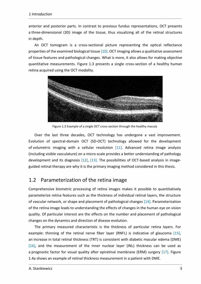
An OCT tomogram is a cross-sectional picture representing the optical reflectance
properties of the examined biological tissue [10]. OCT imaging allows a qualitative assessment
of tissue features and pathological changes. What is more, it also allows for making objective
quantitative measurements. Figure 1.3 presents a single cross-section of a healthy human
retina acquired using the OCT modality.
Figure 1.3 Example of a single OCT cross-section through the healthy macula
Over the last three decades, OCT technology has undergone a vast improvement.
Evolution of spectral-domain OCT (SD-OCT) technology allowed for the development
of volumetric imaging with a cellular resolution [11]. Advanced retina image analysis
(including visible vasculature) on a micro-scale provides a better understanding of pathology
development and its diagnosis [12], [13]. The possibilities of OCT-based analysis in image-
guided retinal therapy are why it is the primary imaging method considered in this thesis.
1.2 Parameterization of the retina image
Comprehensive biometric processing of retina images makes it possible to quantitatively
parameterize retina features such as the thickness of individual retinal layers, the structure
of vascular network, or shape and placement of pathological changes [14]. Parameterization
of the retina image leads to understanding the effects of changes in the human eye on vision
quality. Of particular interest are the effects on the number and placement of pathological
changes on the dynamics and direction of disease evolution.
The primary measured characteristic is the thickness of particular retina layers. For
example: thinning of the retinal nerve fiber layer (RNFL) is indicative of glaucoma [15],
an increase in total retinal thickness (TRT) is consistent with diabetic macular edema (DME)
[16], and the measurement of the inner nuclear layer (INL) thickness can be used as
a prognostic factor for visual quality after epiretinal membrane (ERM) surgery [17]. Figure
1.4a shows an example of retinal thickness measurement in a patient with DME.
1 Introduction
4 A. Stankiewicz
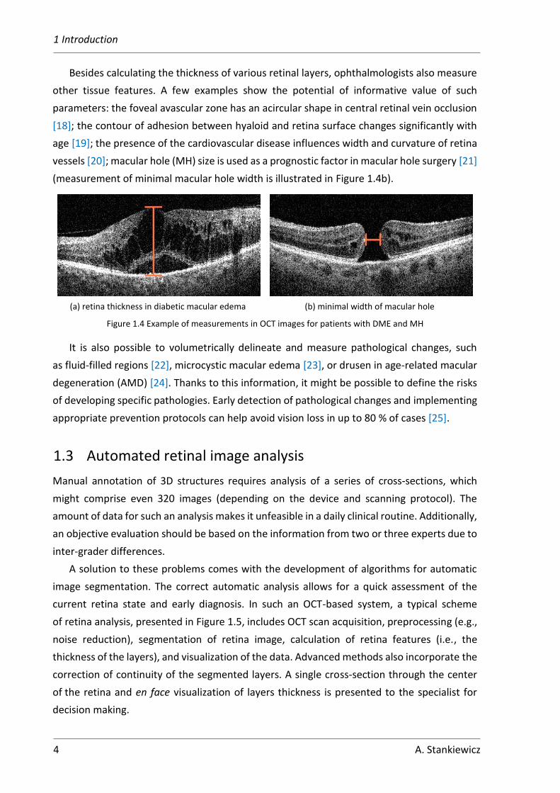
Besides calculating the thickness of various retinal layers, ophthalmologists also measure
other tissue features. A few examples show the potential of informative value of such
parameters: the foveal avascular zone has an acircular shape in central retinal vein occlusion
[18]; the contour of adhesion between hyaloid and retina surface changes significantly with
age [19]; the presence of the cardiovascular disease influences width and curvature of retina
vessels [20]; macular hole (MH) size is used as a prognostic factor in macular hole surgery [21]
(measurement of minimal macular hole width is illustrated in Figure 1.4b).
(a) retina thickness in diabetic macular edema
(b) minimal width of macular hole
Figure 1.4 Example of measurements in OCT images for patients with DME and MH
It is also possible to volumetrically delineate and measure pathological changes, such
as fluid-filled regions [22], microcystic macular edema [23], or drusen in age-related macular
degeneration (AMD) [24]. Thanks to this information, it might be possible to define the risks
of developing specific pathologies. Early detection of pathological changes and implementing
appropriate prevention protocols can help avoid vision loss in up to 80 % of cases [25].
1.3 Automated retinal image analysis
Manual annotation of 3D structures requires analysis of a series of cross-sections, which
might comprise even 320 images (depending on the device and scanning protocol). The
amount of data for such an analysis makes it unfeasible in a daily clinical routine. Additionally,
an objective evaluation should be based on the information from two or three experts due to
inter-grader differences.
A solution to these problems comes with the development of algorithms for automatic
image segmentation. The correct automatic analysis allows for a quick assessment of the
current retina state and early diagnosis. In such an OCT-based system, a typical scheme
of retina analysis, presented in Figure 1.5, includes OCT scan acquisition, preprocessing (e.g.,
noise reduction), segmentation of retina image, calculation of retina features (i.e., the
thickness of the layers), and visualization of the data. Advanced methods also incorporate the
correction of continuity of the segmented layers. A single cross-section through the center
of the retina and en face visualization of layers thickness is presented to the specialist for
decision making.

1 Introduction
A. Stankiewicz 5
Figure 1.5 Scheme of a typical retina image analysis procedure
Several algorithms for retina image segmentation are currently available in commercial
applications [26–28]. Unfortunately, their use is limited to:
• segmentation of retinal layers
• segmentation of the optic nerve head (ONH)
• cornea segmentation.
Furthermore, algorithms for OCT retina image analysis incorporated into commercial
devices are limited to thickness measurement of TRT or selected retina layers (like RNFL
or ganglion cell complex (GCC)) [26–28]. The automatic analysis may also include retina
volume or ONH area and volume. Additional scanning protocols designed for vessel
inspection (namely optical coherence tomography angiography — OCTA) are equipped with
tools for calculating vessel density in a selected area and delineating a non-flow area (a semi-
automatic method). Measurement of other retina features such as corneal thickness and
angle, length of vitreous attachment, the width of retinal vessels is typically performed
manually by the experts and often in an external application.
Automatic assessment of the retina is mainly focused on detecting pathologies the most
commonly associated with lower visual acuity or loss of vision. These problems are glaucoma
(by measuring the thickness of RNFL around ONH), AMD (by analyzing outer retina segments),
and DME (by calculating TRT) [25].
Apart from those disorders, ever more present pathological changes associated with the
aging eye are the problems with the vitreoretinal interface (VRI). The VRI describes the
connection between the vitreous (filling the eye) and the retina's surface. As the eye ages,
vitreous degeneration may lead to the development of pathologies at the VRI. These are
mainly: epiretinal membrane (ERM) and vitreomacular traction (VMT). Epidemiology studies
of VRI pathologies show even 3.4 % of prevalence for ERM and 1.6 % for VMT in patients over
63 years old, and these numbers increase with age [29]. Examples of OCT cross-sections
through the macula in the presence of VMT and ERM are illustrated in Figure 1.6.
In 2013, a panel of specialists developed an OCT-based anatomic classification system
for diseases of the vitreomacular interface [30]. However, the lack of specific guidelines
for this class of pathologies is why, until now, no standardized evaluation method has been
developed. Currently, available OCT devices do not include automatic analysis of VRI or even
segmentation of the posterior surface of the vitreous.
Preprocessing
(e.g. noise reduction) Retina image segmentation
Visualization
Correction of layers continuity
OCT scan acquisition
Calculation of retina features

1 Introduction
6 A. Stankiewicz
Figure 1.6 Example of OCT images with vitreoretinal pathologies
A quantitative analysis of ERM and VMT development is not possible without appropriate
tools available to the clinicians. Therefore, the application of automatic image analysis for this
purpose is expected to be of immense help during clinical research and practice.
Unfortunately, due to the specificity of VRI reflective properties, the existing layers
segmentation methods are not applicable in a straightforward fashion.
Automatic retina image analysis is not immune to problems [31]. The most common
causes of erroneous image segmentation are connected with the acquisition problems, such
as low image quality (e.g., high noise level, low resolution) and acquisition errors
(e.g., reflections of the tissue, low signal quality). Nonetheless, issues resulting from the
characteristics of the object itself are also of importance, and these are involuntary eye
movements, the presence of pathological changes, shadows caused by vessels or anterior eye
disorders, as well as non-uniform tissue reflectivity.
Moreover, even with the modern devices able to take single tissue depth measurement
with the time of 1
70000 of a second, the acquisition of a volumetric scan lasts approximately
1 second1. For patients with diseased eyes, this is a long time. Furthermore, involuntary eye
movements frequently cause a discontinuity in the scan data. This situation is most common
in patients with fixation problems caused by central vision loss or lower central visual acuity.
Motion correction technology (MCT) algorithms can counteract this phenomenon, but they
usually prolong scan acquisition even further. Additionally, colossal data size (around several
dozens to several hundred MB for a single 3D OCT scan) increases the processing time.
The above-mentioned disadvantages make a quantitative evaluation of retina features
during examination difficult and hinder clinical research.
1.4 Aims, scope, and scientific thesis
This thesis presents algorithms for automatic analysis of OCT retina images to accurately and
automatically asses VRI conditions.
1 Detailed information about imaging speed and scanning protocols of OCT devices is provided in Section 2.2
(a) vitreomacular traction
(b) epiretinal membrane

1 Introduction
A. Stankiewicz 7
The main objective of the thesis can be divided into three parts:
• improvement of retina segmentation for low quality OCT data (cognitive
investigation)
• development of preretinal space segmentation methods (cognitive investigation)
• automatic extraction of biometrical features for VMT pathology assessment (clinical
application).
Following detailed tasks will help to achieve the selected goals:
I. selection of case targeted image denoising methods for improved retina
segmentation accuracy
II. improvement of stability of the graph-based image segmentation system for low
quality OCT images
III. formulation of methods for segmentation of the preretinal space from a 3D OCT scan
IV. selection of parameters for quantitative analysis of VRI for a clinical application.
A database of OCT retinal images has been created to check the effectiveness of the
algorithms experimentally. This database consists of three-dimensional cross-sections of the
macula imagined using the Avanti RTvue OCT device [27]. The cohort includes 23 healthy
volunteers (25 eyes) and 23 patients (25 eyes) with the aforementioned specific disease
of VMT, giving 46 subjects (50 eyes) in total. A set of 3D OCT scans was acquired with
a specially prepared scanning protocol. In addition, the experts performed manual
segmentation of the retinal layers to provide reference data for image segmentation accuracy
analysis. The detailed information on the gathered data is provided in Section 3.1.
The presented research was conducted in cooperation with ophthalmology specialists
from the Department of Ophthalmology at Heliodor Swiecicki University Hospital, Poznan
University of Medical Sciences, as a part of the CAVRI (Computer Analysis of VitreoRetinal
Interface) Project. The medical ethics committee of Poznan University of Medical Sciences
approved the project under resolution number 422/14, dated May 8, 2014. Unless stated
otherwise, all OCT images presented in this thesis were obtained as part of the CAVRI project.
Scientific thesis
Based on the previously mentioned objectives, the following scientific thesis can be
formed: accurate segmentation and parameterization of pathological changes associated
with the vitreoretinal interface and visualized with 3D OCT images can be done with:
• appropriate selection of image quality enhancement methods for graph-based retina
layers segmentation
• precise preretinal space segmentation algorithms
• automatic parameterization techniques of vitreoretinal interface structures.

1 Introduction
8 A. Stankiewicz
Consequently, the proposed techniques allow developing tools for ophthalmologists
to assess VRI pathology's evolution quantitatively. The results of this work will help
understand the investigated diseases' processes.
1.5 Organization of the thesis
This thesis is divided into three parts and, altogether, six chapters. The first part (Chapters 1
and 2) presents the fundamentals of retina image processing and gives an overview of the
investigated vitreoretinal interface pathologies. The second part, Chapters 3 and 4, provides
a detailed description of the innovative author’s solutions for retina and preretinal space
segmentation based on volumetric OCT images with present VRI pathology. In the last part,
Chapters 5 and 6, the present potential applications of derived methods in clinical diagnostics
with the proposed parameterization approaches and conclude the author’s achievements.
Part I — introduction and fundamentals
Chapter 2, “Automated retinal image processing,” provides additional background
information on retina image processing. It starts with an overview of the retina structure and
explains processes occurring at the vitreoretinal interface. Next, the development of VRI
pathologies (with a focus on VMT) and their characteristics are presented. This chapter also
includes an overview of optical coherence tomography technology, its characteristics, quality
assessment methods, and image acquisition protocols. Furthermore, typical retina image
analysis methods are described for retina layers segmentation from OCT images.
Part II — proposed image analysis algorithms (improvements and new approaches)
This part, consisting of Chapters 3 and 4, includes the proposed OCT image segmentation
methods and their evaluation. The formulated scientific thesis is proven with a large number
of experiments described in this part of the dissertation.
Chapter 3, “Graph-based segmentation of retina,” focuses on improving the stability of the
image segmentation system and selecting case targeted image denoising methods to achieve
the first of the stated main objectives: improved retina segmentation accuracy.
A detailed description of the database used during the experiments is provided in Section
3.1. The verification of the proposed methods described in subsequent chapters included
a comparison of automatic segmentation results with the reference data.
Section 3.2 describes research towards I. of the detailed tasks. It shows the influence
of image quality on layers segmentation accuracy. First, the influence of OCT image quality
on the graph-based segmentation algorithm for retina layers is presented. The following
image denoising methods were examined: averaging filtering [32], anisotropic diffusion [33],
1 Introduction
A. Stankiewicz 9
wavelet soft thresholding [34], block-matching and 3D filtering (BM3D) [35]. Here, their
application for separate 2D B-scans as well as 3D OCT data was tested. Finally, the effect
of noise suppression methods is evaluated based on image segmentation for healthy and
pathological retinas.
Section 3.2 also presents studies on overcoming image acquisition problems as the II.
detailed task of the thesis. Primary concerns are focused on insufficient exposure at the
peripheral regions of a 3D OCT scan. In this section, the author proposed identifying low signal
areas and excluding them from the tissue segmentation step. Several approaches for selecting
an area for exclusion are described. They are based on fixed-length and adaptive estimation
of the signal strength. Additionally, layers tracking based on three-dimensional information
of previously obtained layers segmentation was proposed here.
Chapter 4, “Segmentation of preretinal space with neural networks,” describes the proposed
algorithms for segmentation of the vitreoretinal interface structures to achieve the second
of the stated main objectives: the development of preretinal space segmentation methods.
This goal is achieved by completing the III. of the detailed tasks, namely segmentation of the
preretinal space.
Section 4.1 begins with describing an application of a fully convolutional neural network
to obtain pixel-wise semantic segmentation of preretinal space in an OCT image. The author
describes five selected UNet-based [36] network architectures (baseline UNet, LFUNet,
Attention UNet, ReLayNet, and DRUNet) and presents the network training setup.
In Section 4.2, two types of loss functions for network training are presented, namely
Cross-Entropy Loss and Dice Loss (and their weighted combinations). This section contains
the description of experiments conducted to determine: the most promising loss function and
the baseline comparison of the performance of the five network topologies in the designed
task. Additionally, 4 data augmentation techniques are presented, their implementation
for the OCT images and their influence on preretinal space segmentation efficiency.
Section 4.3 presents a problem of incorrect topological order of segmented classes
common in pixel-wise semantic segmentation tasks. Two solutions are proposed. The first
incorporates adding a Relative Distance Map to the input image as a second channel.
The author tested two types of maps (maps utilizing prior segmentations and maps not
requiring double network training). The second approach proposed by the author aims
to enlarge the network’s field of view by using a bigger convolution kernel. Furthermore, the
author proposed and tested a second method to overcome topology incorrectness problems.
The evaluated solution incorporates a non-typical horizontal or vertical convolutional kernels.

1 Introduction
10 A. Stankiewicz
Part III — clinical application and concluding remarks
Chapter 5, “Application of the proposed solutions,” describes research to complete the third
of the main thesis objectives: automatic extraction of biometrical features for VMT pathology
assessment. It provides an analysis of parameterization techniques for the vitreoretinal
interface. The IV. detailed task of this research — a selection of parameters for quantitative
description of the vitreoretinal interface — is this Chapter's main subject.
Section 5.1 includes statistics of automatic retina parameterization studies. First,
the author presented automated extraction of fovea pit features that requires precise
segmentation methods described in Chapter 4. Additionally, the author described a set
of new parameters to ascertain the state of the fovea pit and its contour, as well as their
reproducibility for a long-term VMA/VMT observation.
Furthermore, the author proposes an automatic investigation of selected biomarkers that
describe the connection between the vitreous and the retina, namely the preretinal volume
and adhesion area. The surfaces of ILM and PCV segmented with methods described
in Chapter 5 are presented in a manner easily understandable to the clinicians, i.e., in the
form of virtual profile maps. Section 5.2 presents the proposed method for calculating VRI
connection profiles and examples of its implementation for VMT pathology evaluation.
The results described in these Sections confirm the possibility of accurately detecting the
presence of VMT pathology and its current stage, based on the proposed volumetric retinal
parameters.
Chapter 6, “Conclusions,” summarizes the obtained results. It was concluded that the
performance of image segmentation algorithms could be improved by selecting a proper
denoising algorithm that accurately suppresses OCT speckle noise. The performed
experiments show that tissue continuity characteristics and low quality data parts also impact
retina segmentation accuracy.
The last chapter also summarizes the advantages of the developed algorithms for the
segmentation of preretinal space. The performed experiments confirmed new algorithms'
ability to introduce valuable information about the vitreoretinal interface. Furthermore, the
proposed volumetric parameters describing the fovea and preretinal space show a potential
to support diagnostic procedures and aid in clinical investigations of long-term VRI changes.
Appendix A1 lists works published by the CAVRI groups in the conducted research.
Appendix A2, “OCTAnnotate software,” includes additional information about open-source
software developed during the research. This computer program was developed especially
for clinicians from Department of Ophthalmology at Heliodor Swiecicki University Hospital,
Poznan University of Medical Sciences. It implements the solutions for evaluating the
vitreoretinal interface proposed in this thesis.

11
Chapter
2 Automated retina image processing
2.1 Retina and preretinal structure in OCT images
Research presented in this dissertation focuses on the posterior segment of the human eye
and mainly the retina structure in the fovea area. This section presents retina morphological
structures relevant for further image processing and VRI features parameterization.
2.1.1 Human retina structure
The retina is a light-sensitive layer of tissue in the innermost part of the eye. Thanks to the
eye's optics and translucent properties of the vitreous, the photons of light come through the
cornea, lens, and vitreous, forming a focused two-dimensional image of the visible world. They
strike the retina cells initiating a cascade of electrical impulses further transmitted by the
nerves [1]. Retina’s function is analogous to the film or image sensor in a camera.
Histological analysis of the retina reveals a layered structure of densely packed neural cells
(ganglion cells, bipolar cells, and light-sensitive photoreceptors) and a layer of pigmented
epithelial cells [37]. Although there are only these four main tissue layers, thanks to the OCT
imaging technique, it is possible to visualize ten layers of the structured cell parts (Figure 2.1).
Figure 2.1 Layers and sections of the healthy human retina visualized with the OCT
Vitreous body
Posterior Cortical Vitreous
Preretinal space
Inner Limiting Membrane
Nerve Fiber Layer
Ganglion Cell Layer
Inner Plexiform Layer
Inner Nuclear Layer
Outer Plexiform Layer
Outer Nuclear Layer
External Limiting Membrane
Inner Photoreceptor Segment
Outer Photoreceptor Segment
Inner Segment Ellipsoid Zone
Retinal Pigment Epithelium
Fovea
Parafovea
Perifovea
Midperipheral retina Macula
1.8 mm 0.5 mm
1.5 mm

2 Automated retina image processing
12 A. Stankiewicz
The retina layers distinguishable with the OCT are as follows:
• Inner Limiting Membrane (ILM), separating the retina from the vitreous
• Nerve Fiber Layer (NFL), containing axons of ganglion cells
• Ganglion Cell Layer (GCL), containing nuclei of ganglion cells
• Inner Plexiform Layer (IPL), enclosing synaptic connections between ganglion and
bipolar cells
• Inner Nuclear Layer (INL), consisting of nuclei of bipolar cells, as well as laterally
arranged amacrine and horizontal cells that provide an inhibitory function to the
surrounding neurons (horizontal cells are connected to photoreceptors, and amacrine
cells support bipolar cells)
• Outer Plexiform Layer (OPL), enclosing synaptic connections between bipolar and
photoreceptor cells
• Outer Nuclear Layer (ONL), containing nuclei of photoreceptors
• External Limiting Membrane (ELM), separating the light-sensitive part of the
photoreceptors from the rest of the neural tract
• Inner Segment of Photoreceptors (IS)
• Outer Segment of Photoreceptors (OS)
• Retinal Pigment Epithelium (RPE), consisting of densely packed pigmented epithelial
cells that interconnect with photoreceptors.
The light-sensitive rods and cones are situated under the inner neural cells through which
the light has to pass first. The inner layers of neurons are absent only in the central region
of the retina, called the fovea. Anatomic definition of the fovea describes it as a 1.8 mm
diameter area with the highest concentration of the photoreceptor cells (190 000 cones /
1 mm2), ensuring the highest acuity of the central field of vision [38]. The region around the
fovea with a diameter of 2.8 mm is defined as parafovea. The region around the parafovea
until the macula's edge (5.8 mm in diameter) is called perifovea. The lack of inner layers in the
fovea is visible as depression, as shown in Figure 2.1.
2.1.2 The vitreoretinal interface (VRI)
The vitreoretinal interface is defined as the connection between the vitreous (filling the
eye) and the retina (at the back of the eye). The vitreous body is an optically clear semisolid
gel structure consisting of approximately 98 % water and 2 % structural macromolecules [39].
The vitreous body, enclosed with the posterior cortical vitreous (PCV), a cortex composed

2 Automated retina image processing
A. Stankiewicz 13
of a dense collagen matrix, helps keep the retina pressed against the underlying choroid.
The PCV is estimated to be 100-110 µm thick [40] and has hyperreflective properties when
illuminated with infrared light. The places of the strongest adhesion between the PCV and the
retina's surface are at the fovea, the optic nerve head, and major retinal vessels. The strength
of this connection defines the subsequent evolution of the vitreoretinal interface.
As the eye ages, the vitreous gel liquefies and collapses. This process coincides with the
weakening of the vitreoretinal adhesion and progressively leads to posterior vitreous
detachment (PVD). The PVD development (which starts in young adulthood and advances over
the decades) was classified into four stages listed in Table 2.1 [41]. A schematic illustration
of each stage is presented in Figure 2.2.
Table 2.1 Classification of PVD stages
Stage Definition Vitreous attachment characteristics
0 absence of PVD vitreous fully attached to the retina
1 focal perifoveal PVD vitreous detached in 1–3 perifoveal quadrants
2 perifoveal PVD vitreous attached to the fovea, the optic nerve head,
and the mid-peripheral retina, otherwise detached
3 macular PVD vitreous attached to optic nerve head and mid-
peripheral retina
4 complete PVD vitreous fully detached from the retina
(a) Stage 0
(b) Stage 1
(c) Stage 2
(d) Stage 3
(e) Stage 4
Figure 2.2 Illustration of PVD stages (areas with light blue color depict the vitreous; dark orange represents the retina and optic nerve head,
light orange illustrates the outer eye tissues) [41]
The detachment usually starts at the place of the weakest adhesion in one of the four
peripheral quadrants (nasal, superior, temporal, or inferior). Then progressively follows into
the other quadrants until the attachment involves only the fovea, ONH, and mid-peripheral

2 Automated retina image processing
14 A. Stankiewicz
retina. In the next step, the PCV elevates from the macula. Complete PVD can be diagnosed
when the vitreous has no connection with the posterior or mid-peripheral part of the retina.
An incomplete PVD with normal foveal morphologic features and partial attachment
of vitreous to the macula is called vitreomacular adhesion (VMA).
Posterior vitreous detachment is in itself natural, harmless, and asymptomatic. Proper
PVD development has no visible impact on the retina tissue or visual acuity. Therefore, most
patients do not notice its occurrence. However, complete detachment is common in around
10 % of individuals at the age of 50, 40 % of subjects between 60 and 70 years old, and almost
all subjects at the age of 80 [42]. Furthermore, the prevalence of PVD is significantly more
common in women than in men of comparable age [43]. Additionally, it has been found that
PVD develops at an earlier age in myopic eyes than in emmetropic or hyperopic eyes [44].
2.1.3 Vitreomacular traction (VMT)
A situation may occur during PVD when the vitreous collapses, but the collagen fibers
at the edge of the PCV hold the vitreous firmly to the retina. In such a case, without the
weakening of the VRI, the process of PVD can become pathological [39].
The course of anomalous PVD development depends on the adhesion pattern, vitreous gel
liquefaction regions, and possible lamellar splits in the PCV (called „vitreoschisis”). Although
the biochemical mechanisms behind this process are not yet fully understood, the scientists
derived a group of pathologies with their origin in anomalous changes in the VRI [45]. The
most common are the epiretinal membrane, vitreomacular traction, macular hole,
vitreopapillary traction, and peripheral retinal tears. The possible paths of VRI pathologies
development are illustrated in Figure 2.3.
Figure 2.3 Vitreoretinal pathologies associated with anomalous PVD (orange marked groups are the focus of this thesis) (based on [46])
Anomalous PVD
Retina Tears
Retinal Detachment
Vitreopapillary Traction
Vitreous Hemorrhage
Vitreomacular Traction
Epiretinal Membrane
Macular Pucker
Macular Hole
intact PCV (full-thickness)
posterior separation
peripheral traction
peripheral separation
axial traction
macular
adhesion
optic disc
adhesion
lamellar split in PCV
(vitreoschisis)
foveal
detachment
inward
contraction
outward
contraction

2 Automated retina image processing
A. Stankiewicz 15
The author of this thesis has focused on developing automatic segmentation algorithms
for one of the most common disorders of the VRI, namely vitreomacular traction. Detailed
characteristics and classification of those pathologies are provided in the following sections.
The vitreomacular traction syndrome is caused by focal adhesion of the PCV to the ILM
at the fovea with peripheral PVD separation and intact (full-thickness) PCV. It is characterized
by an elevation of the retinal surface by traction forces and a distortion of the intraretinal
structure. Figure 2.4 illustrates an example of an optical coherence tomography B-scan
of VMT.
Figure 2.4 Example of an OCT B-scan through the macula from a patient with VMT
The VMT syndrome may occur as an isolated condition or be associated with a wide range
of macular disorders, including macular pucker, macular hole, macular detachment, cystoid
macular edema, diabetic macular edema, and age-related macular degeneration [47].
The vitreomacular traction causes gradual, progressive vision loss. It can manifest with
metamorphopsia (straight lines appear wavy), visual acuity deterioration, impairment
of central vision, and blurred vision.
The epidemiology statistics for VMT show a relatively low prevalence of 0.6 % (14 / 4490
eyes) when analyzed on a group of subjects of age over 45 [48]. This value increases
significantly with age, from 1 % in a group of 63-74 years old to 5.6 % in patients over 85 years
old [29]. However, another 4-year prospective study shows VMT development in 36 % (69 /
185 eyes) of cases with primary persistent VMA [49]. The VMT is equally frequent in men and
women, and its bilateral evolution is evident in about 17 % of subjects. Various studies show
the possibility of spontaneous VMT resolution in up to 23 % of subjects [47].
If VMT is left untreated, the probability of developing severe retina damage (frequently
a formation of a macular hole) increases with time. Thus a surgical intervention is required.
The current treatment of choice for the VMT is pars plana vitrectomy. A positive outcome
for this procedure is observable in up to 75 % of cases [50]. Although this surgery is usually
PCV
ILM
Points of traction

2 Automated retina image processing
16 A. Stankiewicz
effective in improving visual function and relieving symptoms, it is costly and risky.
Furthermore, subsequent development of the epiretinal membrane after this surgery has
been reported [51].
Classification of VRI pathologies
There is currently no consensus on the classification protocols for VRI disorders. However,
in 2013 the first proposition for the classification and staging of VRI diseases was made
by Duker et al. [30]. It included: VMA, VMT, macular hole, lamellar hole, and macular schisis.
They were defined based on the analysis of anatomic criteria present in at least 1 OCT B-scan.
Table 2.2 includes definitions and classification parameters of these conditions.
Table 2.2 Classification of VRI pathologies by Duker et al. [30]
Class VMA VMT FTMH
Definition
• perifoveal vitreous
cortex detachment
from the retinal
Surface
• attachment of the
vitreous cortex within
a 3-mm radius of the
fovea
• no detectable change
in foveal contour
or underlying retinal
tissue
• perifoveal vitreous cortex
detachment from the retinal
surface
• attachment of the vitreous
cortex within a 3-mm radius
of the fovea
• distortion of the foveal
surface associated with
attachment
• intraretinal structural
changes, and/or elevation
of the fovea above the RPE
• no full-thickness interruption
of all retinal layers
• full-thickness foveal lesion
interrupting all macular
layers from the ILM to the
RPE
Subclassification
by size • focal (≤ 1500 µm)
• broad (> 1500 µm)
• small (≤ 250 µm)
• medium
((250 𝜇𝑚, 400 𝜇𝑚⟩)
• large (> 400 µm)
by other
conditions
• isolated
• concurrent
• VMT present
• VMT absent
by cause • primary
• secondary
Furthermore, VMT may be hard to distinguish from focal VMA in case of only subtle
distortion of the fovea contour [46]. Such a slight elevation of the fovea margins may
be difficult to detect, especially during a simplified OCT examination. Therefore,
in contradiction to the presented diameter-based classification, ophthalmologists also
consider a shape-based VMT analysis protocol [52]. The classification based on adhesion
morphology can be divided into two types, illustrated in Figure 2.5:

2 Automated retina image processing
A. Stankiewicz 17
• V-shaped pattern — persistent vitreous adhesion to the fovea with perifoveal
detachment
• J-shaped pattern — incomplete PVD with persistent nasal attachment and temporal
detachment.
(a) V-shaped VMT
(b) J-shaped VMT
Figure 2.5 The pattern of vitreomacular adhesion in the VMT syndrome captured with OCT [52]
The latest research regarding VMT analysis proposes the parameterization of VRI
characteristics for focal VMT based on several morphological features composing an acronym
“WISPERR” [53]. Table 2.3 lists the features that have been considered significant for the
classification of VMT severity. Nevertheless, it should be noted that such analysis is made
manually and based solely on a central cross-section through the retina.
Table 2.3 Classification of morphological features for focal VMT (WISPERR) [53]
Feature Values
width of attachment measurement of the longest vitreomacular adhesion through the fovea [µm]
vitreoretinal interface
(0) none
(1) thickened ILM without ERM
(2) ERM
(3) ERM within the central 1–mm or contiguous with VMT
foveal shape
(0) normal
(1) abnormal profile (e.g., elevation, asymmetry)
(2) eversion
RPE abnormalities
in central 1–mm
(0) not present
(1) present
central retinal thickness measurement [µm]
inner retina changes within
the central 3–mm
(0) none
(1) cysts or cleavage
outer retina changes within
the central 3–mm
(0) none
(1) focal abnormalities without subretinal fluid
(2) subretinal fluid with OS–RPE separation
(3) defect in OS (size [µm])
(4) FTMH, the minimum horizontal diameter of the MH [µm]

2 Automated retina image processing
18 A. Stankiewicz
The standard retina evaluation involves the retina thickness measurement within
individual sectors of an ETDRS grid [54]. The ETDRS grid (illustrated in Figure 2.6) is comprised
of 3 concentric circles centered at the fovea that divides the macula into 3 zones: the central
fovea (CF) (less than 1 mm in diameter), the inner macula (IM) (1 – 3 mm), and the outer
macula (OM) (3 – 6 mm). Each ring is divided into quadrants: temporal, inferior, nasal, and
superior. The position of temporal and nasal parts depends on the scanned eye. It is used with
OCT scans for spatial reference in clinical practice and literature, hence its utilization in this
thesis.
Figure 2.6 ETDRS grid [55]
2.2 OCT imaging technique
2.2.1 Hardware aspects of OCT technology
The optical coherence tomography technique utilizes low-coherence light in the near-
infrared wavelengths (0.75 – 1.4 µm) to obtain high-resolution measurements of light echoes
reflected from the semi-transparent materials [11].
Early OCT devices performed interference analysis of the light reflected from the reference
mirror and the scanned object. The axial movement of the reference mirror results in different
flight time delays for the reference light beam. Similarly, the light reflected from the examined
object has a time delay corresponding to its depth. The image intensity values are determined
by the envelope of the interferogram [8]. This method is called a time-domain OCT (TD-OCT).
The speed of depth scans, called A-scans, is limited by the speed of the reference mirror
(up to thousands of A-scans per second), resulting in low resolution of the gathered data.
Thus, making a three-dimensional evaluation of objects prone to even subtle movements not
feasible [56].
However, measuring the interference spectrum allows for simultaneous detection of light
echoes back-scattered from all sample depths. This approach utilizing the Fourier transform
of the interference signal is called Fourier-domain OCT (FD-OCT). Here, the light spectrum

2 Automated retina image processing
A. Stankiewicz 19
S(ω) has a broad spectral bandwidth (hundreds of nanometers). The frequency of oscillatory
signal modulating the light source spectrum encodes the information of the location
of reflective points along the sampling beam. The intensity output of the interferometer may
be expressed in the Fourier domain as [57]:
𝑆𝑡𝑜𝑡𝑎𝑙(𝜔) = 𝑆(𝜔) [𝑎𝑟 +∑𝑎𝑛𝑛
+ 2 ∑ √𝑎𝑛𝑎𝑚 cos(𝜏𝑛𝑚𝜔)
𝑚≠𝑛
+ 2∑√𝑎𝑟𝑎𝑛 cos(𝜏𝑛𝜔)
𝑛
] (2.1)
where ar describes light attenuation in the reference arm, coefficients an characterize the
attenuation of light back-reflected from an n-th layer of the measured sample, and values τn
are the delays of waves returning from layers within the examined object. An inverse Fourier
transformation (IFT) provides a reconstruction of the axial structure of the sample:
𝐼(𝜏) = IFT{𝑆(𝜔)},
𝐼(𝜏) = (𝑎𝑟 +∑𝑎𝑛𝑛
)Γ(𝜏) + ∑ √𝑎𝑛𝑎𝑚(Γ(𝜏)⨂𝛿(𝜏 ± 𝜏𝑛𝑚)
𝑚≠𝑛
+∑√𝑎𝑟𝑎𝑛(Γ(𝜏)⨂𝛿(𝜏 ± 𝜏𝑛))
𝑛
.
(2.2)
where Γ(τ) represents the auto-correlation (coherence) function between the light reflected
from the reference mirror and the measured object, and δ(τ) stands for the impulse response.
Although Fercher et al. first introduced this concept in 1995 [58], it was only in 2003 that
three independent research groups demonstrated a powerful sensitivity and speed advantage
of FD-OCT over TD-OCT [59–61]. FD-OCT imaging enables data acquisition up to ∼100 faster
compared to TD-OCT systems. Furthermore, since imaging sensitivity is linearly dependent
on acquisition time, increasing the speed also improves the sensitivity of the device [62]. The
increased interest in OCT research led to the development of two types of FD-OCT analysis:
• Spectral-domain OCT (SD-OCT) – It employs a broad-bandwidth light source,
a spectrometer, and a high-speed line scan camera (CMOS or CCD linear sensor)
to calculate the interference spectrum [63–66]. A diffraction grating is used
to decompose the obtained interferogram spectrally. Then, the depth of each scatter
signal is determined with the Fourier transform of the spectral correlogram intensities.
• Swept-source OCT (SS-OCT), or time encoded frequency domain OCT – It uses
a modulated narrow-bandwidth light source and a photosensor, which measures the
correlogram for each center wavelength as a function of time [67], [68]. The acquired
interferogram is subjected to a Fourier transform to obtain the final depth scan.
Other approaches use adaptive optics [69] and better light sources [70] to achieve
ultrahigh resolution of the OCT system.
The research presented in this dissertation utilizes processing of signals (scans in the form
of images) gathered using SD-OCT technique. A general scheme of the SD-OCT approach,
as introduced by Kałużny et al. [9], is illustrated in Figure 2.7.

2 Automated retina image processing
20 A. Stankiewicz
Figure 2.7 Diagram of the SD-OCT method
The detection procedure is as follows: a broad-bandwidth light source is split into two
beams, one of which is directed onto the sample tissue, and the second is reflected from
a fixed-position reference mirror; both back-reflected beams have a time delay related to the
length of the light’s path (in the case of the sample beam it is determined by the depth of the
measured internal structures); the spectral modulation of the two beams interference
is measured with a spectrometer; Fourier transformation of the interference signal results
in an axial scan (called A-scan) measurement. Multiple parallel A-scans yield a cross-section
of the examined object (called a B-scan).
The safety requirements (regarding the amount of light that the retina can be illuminated
with) limit the acceptable scanning time to 1–3 seconds per volume. A higher imaging speed
allows for increasing the number of A-scans acquired within the fixed time. Increasing the
number of parallel tomograms obtained in a sequence makes it possible to yield a higher
resolution of the three-dimensional data. Such a boost in OCT image resolution enhances the
comprehension of the internal structures of the measured object. Ultrahigh imaging speed
is also beneficial for reducing motion artifacts and the patient’s comfort.
The transverse (fast-scanning) resolution of an OCT B-scan also depends on the central
wavelength and the quality of the galvanic scanning mirrors and is typically 10–40 µm [4]. The
longitudinal resolution depends on the central wavelength and width of the radiation source
spectrum and is currently 3–8 µm in commercially available scanners. The non-fast scanning
lateral resolution results, on the other hand, from the scanning protocol (limited only by the
acquisition time). In modern OCT devices, with an acquisition speed of 70 000 A-scans per
second [27], performing a 3D scan (e.g., 141 B-scans with a resolution of 640×385 points each)
takes around 0.8 seconds. Fast measurement assures no artifacts caused by movements of the
Reference mirror
Broadband light source Fiber coupler
Analyzed
object
Diffraction grating
Spectrometer
Scanning
mirror
Digital signal processing module
Interferogram A-scan
Fourier Transform

2 Automated retina image processing
A. Stankiewicz 21
eyeball. The newest devices also employ motion correction technology (MCT) to minimize this
problem [71].
Applications of OCT technology
The near-infrared light employed by the OCT technique proves to be optimal for examining
biological objects [72]. Thanks to OCT, it is possible to acquire images that accurately depict
the actual structure and functions of the tissue. The invention of the Fourier domain OCT has
further influenced medicine.
Although OCT technology was initially developed for transparent tissues [73], its fast and
non-invasive characteristics promote it as a promising imaging technique for transparent and
non-transparent, soft and hard objects. Additionally, the absorption and scattering properties
of the eye tissues make its use in ophthalmology especially appealing. For instance,
Wojtkowski et al. were the first to demonstrate its high enough sensitivity in retinal imaging
[65]. Visualizing the internal retinal features in detail allows for the early identification
of disease characteristic biomarkers and evaluating their evolution in response to therapy.
Lately, more and more FD-OCT devices are being developed by various commercial
organizations for use in ophthalmology and other clinical fields. For example, OCT technology
enables in vivo examination of the skin [74] (including volumetric fingerprint analysis [75]),
respiratory tract [76], gastrointestinal tract [77], nervous systems [78], and many others.
Optical coherence tomography is also of interest in industrial applications, such
as nondestructive testing, artwork examination [79], material thickness measurements [80],
surface roughness characterization [81], and pharmacology [82]. Additionally, feedback-based
OCT systems apply to the control of manufacturing processes, and fiber-based architectures
allow for easier access to hard-to-reach spaces [83].
Interpretation of OCT images
The imagined tissue's reflectivity, absorption, and scattering properties influence the OCT
signal. A tissue with a high scattering coefficient and a property of scattering the light
in a perfectly backward direction results in strong reflection. A similar situation occurs at the
boundary between materials of different refractive ratios [8]. Hence, making a map of the
sample’s reflectivity in the form of an OCT image.
The signal strength is represented as the intensity value in the OCT image. High intensity
(white color) corresponds to relatively high reflectivity, mainly caused by collagen fiber
bundles, cell walls, and nuclei. Low intensity (black color) corresponds to relatively low
reflectivity, like air or clear fluids. The gray-scaled values illustrate the reflectivity of various
tissues. Furthermore, intrinsic differences in optical tissue properties determine OCT image
contrast. Also, the image intensity decreases exponentially with depth due to light
attenuation in the sample. More so by the blood vessels than by other tissues [2].

2 Automated retina image processing
22 A. Stankiewicz
Although the exact correlation between the histology of the tissue and its OCT image
is still under investigation, the current understanding of OCT properties allows interpreting
imagined tissues, as shown in Figure 2.1. High reflectivity layers include nerve fiber layer,
plexiform layers, a junction between inner and outer photoreceptor segments, and retinal
pigment epithelium. Low reflectivity layers represent nuclear layers and photoreceptor
segments.
OCT characteristics impeding image processing
As was mentioned in Section 1.4, data acquisition is only the first step in the whole
processing pipeline leading to the medical diagnosis. Nevertheless, the quality of the OCT scan
is a crucial factor to consider since the diagnostic measurements are performed directly from
the acquired image. It influences both manual analysis and computer-aided segmentation
systems. For example, retina layers segmentation algorithms fail if the image is blurred
or corrupted by noise. However, these are not the only two causes of an erroneous automatic
retina investigation. It might be argued that such reasons can be divided into technology-
based and biology-based, as illustrated in Figure 2.8.
Figure 2.8 Classification of phenomena impeding OCT image segmentation
The main reasons for the low performance of retina image analysis algorithms resulting
from the applied technology are:
• speckle noise
Due to the coherent imaging technique, the OCT images have characteristic granular
patterns called speckles. These patterns, having an irregular form, may obscure the
subtle features of the examined tissue. Most of the literature considers speckle
as an unwanted noise that degrades the image quality, affecting subsequent processing.

2 Automated retina image processing
A. Stankiewicz 23
However, the speckle results from multiple scattering of light within the examined
object [84]; hence, it carries additional informative value.
Schmitt [85] states that the noise that corrupts OCT images is non-Gaussian,
multiplicative, and neighborhood correlated. Thus it cannot be easily suppressed
by standard software denoising methods. Nevertheless, plenty of methods have been
developed to reduce its influence. Since OCT noise characteristics and their suppression
methods are extensive, they will be described further in Section 2.2.2.
• resolution
The resolution of OCT images is considered low compared to other retina imaging
modalities (especially color fundus photography). For example, a single OCT cross-
section through the macula center, acquired with the Avanti RTvue device in a line scan
mode, has a resolution of 1020×960 pixels. Such an image corresponds to 2×12 mm
of the tissue. Bearing in mind retina physiology, this means that pixels in the
photoreceptor area of a single A-scan represent about 6.25 cone cells. Although such
resolution is not challenging for the retina layers segmentation algorithms, a single
cross-section provides very limited information and is usually utilized for initial
screening or documentation. The acquisition modalities having the primary role in the
treatment planning consist of multiple cross-sections, which in turn enforces lower
transverse resolution (ranging from 55 to 134 pixels per millimeter), and even lower
longitudinal resolution. The lower the resolution, the retina layers boundaries become
blurry and imprecise, thus harder to detect accurately.
• optical issues
This group includes reflections, obstructions, media opacities, underexposure, defocus,
depolarization, and improper centering [86]. Although image analysis algorithms can
overcome some of the acquisition-based difficulties during preprocessing (as shown
in Section 4.1), such errors hider these efforts. Fortunately, some of these sub-optimal
imaging conditions can be detected prior to the image segmentation step, and
if necessary, the device software will advise additional acquisition steps.
• device-dependence
As Ehnes et al. [87] explained, some segmentation algorithms are device-dependent and
limited to analyzing inner and outer retinal boundaries. Furthermore, the number
of segmented layers varies between methods and is specific to individual OCT devices
(see Section 2.3).
The second category of the phenomena impeding automatic OCT image analysis methods
comprises issues pertaining to the biology of the examined object. The following aspects
should be considered when evaluating the image of the retina:

2 Automated retina image processing
24 A. Stankiewicz
• uneven tissue reflectivity
In the OCT image, tissues have uneven reflectivity and grainy texture related to the
speckle component. Furthermore, the intensity of a homogeneous area decreases with
depth deterministically. This intrinsic characteristic of OCT imaging contradicts the
general assumption of segmentation algorithms that the intensity variation
of homogeneous regions is only due to the noise [2], [88].
The adjacent retinal layers have low image contrast due to only slight differences in the
examined tissue at a small depth scale of imaging [89]. Such a problem leads
to difficulties in distinguishing anatomical structures of the retina (for example, the
border between GCL and IPL layers).
• shadows caused by blood
Hypo-reflectivity of the hemoglobin, while allowing for the vessels' detection, is also
an issue for the image analysis. Shadows caused by the vessels obscure the tissue
underneath, and the structural information is partly lost. Darker areas within the retina
layers interfere with edge detection and other methods. However, some works
(e.g., [90]) address automatic vessel detection for more accurate segmentation results.
• motion artifacts
Unexpected movement of the patient’s eye or blinking is also relevant. Movement
during the examination causes data loss and improper image segmentation. Although
the latest OCT devices include additional features like scanning laser ophthalmoscopy
or eye-tracking [91], such solutions are not yet widely available.
• presence of diseases and pathology
A good quality OCT scan is harder to achieve on diseased eyes. Thus most of the
available methods and algorithms for automated retinal segmentation are insufficient
[22], [92]. Moreover, in severe pathologies, like age-related macular degeneration
(AMD), vitreomacular traction (VMT), or pigment epithelial detachment (PED),
automated algorithms fail in most cases due to the heavily abnormal data.
Automated OCT image segmentation systems require proper pre-processing steps
to overcome said obstructions. The experiments presented in the following chapters will
demonstrate the influence of some of the described problems.
2.2.2 Noise in OCT images
As was stated in Mayer et al. [93], automated segmentation fails on more than half of the
low quality images. Noise is one of the primary reasons for degrading the quality of an OCT
image.

2 Automated retina image processing
A. Stankiewicz 25
Origins of noise in OCT
The research on the OCT images noise [94] shows that it is not an entirely random noise
as it contains some specific information. It is influenced by the subject’s motion and optical
properties of the system, such as the size and temporal coherence of the light source, the
beam’s phase deviation, and the detector’s aperture [85]. It is possible to distinguish the
following origins of OCT noise:
1. shot noise – related to the discrete nature of the photocurrent generated by the
photodetector [57]; additive in nature; can be adequately described by the Additive
White Gaussian Noise process [95]; is substantially lower in SD-OCT due to the parallel
registration of the spectral signal [9].
2. relative intensity noise (RIN) – light intensity fluctuations generated by the radiation
source used in the OCT system; increases along with the optical power; can be reduced
by the balanced detection and cascaded superluminescent diodes [57], [96].
3. read noise – generated in the receiving circuit of the OCT system; its influence increases
along with the scanning depth when the level of the useful signal decreases; can
be reduced using higher-power radiation sources, low-noise radiation detectors, and
low-noise amplifiers [97].
4. coherent noise – generated by reflections within the measuring instrument [57];
extending the exposure time increases the influence of coherent noise over the shot
noise; by subtracting the signal registered without the object present in the sampling
arm, it is possible to remove the coherent noise not correlated with the object;
coherence noise connected to the measured sample might be reduced among others
by adjusting the optical path difference between the reference mirror and the surface
of the examined object [65].
5. speckle noise – an inherent characteristic of images acquired with any imaging
technique based on the detection of coherent waves [98]; the speckle noise is a result
of interference of multiply-scattered radiation; carries both the structural component
of the imaged object as well as the noise component; can be suppressed by multiple
acquisitions and averaging.
A specific feature of OCT imaging is the very high dynamics of the recorded signals. These
dynamics are related to the attenuation of the signal, along with the depth of imaging. Image
parts corresponding to the strong signal are degraded mainly through speckles. While
for parts of the image where the signal level is weak, the fundamental cause of image
degradation is the noise generated in the receiving circuit of the OCT system.

2 Automated retina image processing
26 A. Stankiewicz
Reducing these OCT noise origins may be attempted with various hardware and software
techniques (including unique detectors, additional measurements, and acquisitions).
Improvement of methods for suppressing noise types 1-4 requires access to the hardware and
raw data recorded by the device. Such access is not feasible in clinical studies without the
manufacturer's cooperation. Thus, noise types 1-4 will not be subjected to the discussion
in this thesis. The variety of software approaches for OCT noise reduction is focused on the
fifth noise source, as discussed in the following sections.
Characteristics of speckle
Speckle is a fundamental property of signals acquired by narrow-band detection systems.
Multiple back-scattering of the radiation inside and outside of the sampled object and random
delays of the forward-propagating and returning beam influence the spatial coherence of the
returning wave. The scattered beam forms local places of constructive and destructive
interference, thus causing the appearance of speckles [85]. The speckle noise reduces image
contrast and hinders the detection of boundaries of the examined structures, as shown
in Figure 2.9.
(a) B-scan with expert’s manual segmentation
(b) B-scan with automatic segmentation of retinal
layers (places with erroneous segmentation are indicated by arrows)
Figure 2.9 Example of OCT retina cross-section (B-scan) with segmentation errors [99]
As Wojtkowski [62] discussed, the grainy structure of the image changes with the
longitudinal and lateral resolution of the scan. The lower the longitudinal resolution, the
vertical size of the speckle decreases. The broader the diameter of the beam illuminating the
cornea (higher lateral fast-scanning resolution), the smaller the width of the speckle.
By achieving the smaller speckle size, it is possible to identify the image irregularities
associated with the tissue instead of the measuring system.
Additionally, the speckles can be categorized into signal-degrading and signal-carrying
speckles. The first group corresponds to the auto-correlation signals resulting from multiple
scattering in the studied medium. The signal-carrying speckles are associated with the cross-
correlation signals (the interference of single scattering radiation with the radiation coming

2 Automated retina image processing
A. Stankiewicz 27
from the reference arm). Thus, not every speckle in the image is characterized as undesirable.
The parameters of these speckles may depend on the studied object.
Speckle models
Speckle noise in OCT images can be approximated as a multiplicative noise with the
mathematical model as in (2.3) [94]:
𝐼(𝑥, 𝑦) = 𝐼(𝑥, 𝑦)𝑁𝑚(𝑥, 𝑦) + 𝑁𝑎(𝑥, 𝑦) (2.3)
where 𝑥 and 𝑦 are the indexes of the 2D image, 𝐼 represents the noise-free OCT image, 𝐼 is
the noisy observation of 𝐼, 𝑁𝑚 and 𝑁𝑎 are the multiplicative and additive noise, respectively.
Since the additive noise component is significantly smaller than the multiplicative component,
the 𝑁𝑎 element in Equation (2.3) can be omitted [100].
Nevertheless, the high dynamic range of the recorded data cannot be accurately displayed
on a monitor. Therefore, the OCT signal is log-compressed to fit the display range. Such
operation changes the speckle characteristics from multiplicative to the additive form of the
envelope signal [85], [101].
The generally adopted statistical behavior of the speckle noise evolved during the last
years, from decaying exponential distribution [85], through Gaussian distribution [101],
to Rayleigh distribution [94], [102]. However, recent studies show that a Gamma distribution
is also suitable for modeling speckles in ultrasound and OCT images [103–105]. As reported
by Anoop et al. [103], the Gamma distribution of the shape 𝜌 and scale 𝛽 is described as (2.4):
𝑓(𝑥; 𝜌, 𝛽) =xρ−1e
−𝑥𝛽
𝛽𝜌𝛤(𝜌)for 𝑥 > 0, and 𝜌, 𝛽 > 0 (2.4)
where 𝑥 denotes the location for each statistically independent observation, and 𝛤(𝜌) is the
Gamma function defined as (2.5):
𝛤(𝜌) = ∫ 𝑥𝜌−1e−𝑥 𝑑𝑥∞
0
(2.5)
Speckle denoising methods
Reduction of noise in the OCT images is necessary for proper tissue analysis. However,
it is not possible to automatically assess the level of OCT noise. The techniques for OCT image
denoising can be categorized into two groups [84], [98]: 1) hardware-based and 2) digital
image post-processing techniques, as illustrates Figure 2.10.
The first group is the methods executed during the acquisition time. They require
recording multiple uncorrelated frames (the so-called multi-frame methods) of a single target
sampled using different parameters (i.e., at different times, frequencies, directions). Next, the
acquired data are averaged to form a composite image.

2 Automated retina image processing
28 A. Stankiewicz
Figure 2.10 Classification of OCT image denoising methods
The following compounding techniques can be found in the literature: spatial
compounding [106], [107], angular compounding [108], [109], polarization compounding
[110], and frequency compounding [102].
Their advantage is improving the dynamic range of OCT A-scans [111] and reducing the
occurrence of the auto-correlation components. Noise minimization and tissue structure
enhancements improve with the number of images used for the averaging [112], [113].
However, the compounding techniques require hardware modifications that can
be expensive and difficult to implement in different OCT imaging systems. Additionally,
performing multiple subsequent acquisitions extends the acquisition time considerably. That,
in turn, can cause artifacts associated with involuntary eye movements, trouble with
maintaining vision focus and blinking. The standard number of frames used in the multi-frame
techniques is 32, and when using the MCT, even 80 [27]. While for a single OCT cross-section,
this setting is acceptable, applying it to a 3D OCT image would increase the acquisition time
up to 62 seconds (for 100×800 A-scans gathered with the speed of 70 000 A-scans per second)
[114], [115]. It is unfeasible to achieve a valid scan from such prolonged recording.
Therefore, it is crucial to investigate digital image processing methods to facilitate OCT
noise reduction. Such an image denoising algorithm should increase the signal-to-noise ratio
while preserving the image information (such as contrast, textures, and edges) and minimizing
artifacts [116]. Furthermore, the filtration parameters should consider speckle size
characteristics resulting from resolution, a decrease in signal-to-noise ratio along with the
scanning depth, and the directionality of the structures (in order to avoid blurring thin lines).

2 Automated retina image processing
A. Stankiewicz 29
The literature review describes numerous image processing techniques applied to OCT
image despeckling. The following description presents some of them, categorized according
to the image processing classification scheme in Figure 2.10:
1. Spatial analysis:
a. Classic image filtering techniques, such as:
i. averaging filtering [32] – In this method, a square filter with odd numbers of rows
and columns (e.g., 3×3) is used. However, rectangular filters, such as 3×19, can
also be found in the application for OCT images [90].
ii. median filtering [32], [117] - Its advantage in preprocessing OCT examinations
is to preserve the edges and tissue features and reduce the influence of the
speckle noise.
iii. adaptive Wiener filter [118], [119] – This filter computes local statistics (mean and
variance) with nearest-neighbor constraints for each pixel. The goal is to obtain
a linear estimate of a noise-free image to minimize the mean squared error
between the original and estimated images.
b. Advanced traditional methods:
i. rotating kernel transformation [120] - This locally adaptive technique is based on
the sequential application of directional masks and selecting the maximum output.
It emphasizes thin edges in the image while suppressing a noisy background.
ii. I-divergence regularization [121] – This method minimizes the I-divergence
measure for regularization and generates a synthesized complex amplitude image
that extrapolates additional detail of the known data. It can despeckle the data
while retaining the detail of the original image.
iii. local Bayesian estimation [122] - This method uses the recorded data projection
into the logarithmic space. Next, the conditional posterior sampling approach
is used to find a general Bayesian least-squares estimate of the noise-free data.
c. The partial differential equation (PDE)-based filtering:
i. regular nonlinear diffusion [123] – It is an efficient speckle noise reduction
method since it preserves the edges of the imagined tissue.
ii. interval type-II fuzzy anisotropic diffusion filtering [33] – In addition to the regular
anisotropic diffusion, it considers the uncertainty in the calculated diffusion
coefficient. This method optimizes the trade-off between signal-to-noise ratio and
edge blurring.
iii. complex diffusion filters [124], [125], indicating better feature preservation
(for photoreceptor segments and retinal vessels) [126].
iv. total generalized variation decomposition (TGVD) [100], [127] – It minimizes
an energy function that takes into account first- and second-order derivatives

2 Automated retina image processing
30 A. Stankiewicz
of the image, the divergence function, and the penalty parameter. Its advantage
is the ability to preserve the objects’ edges without generating the staircase effect.
d. Machine learning
i. conditional generative adversarial network (cGAN) [128] – This deep learning
model has good generalization ability. Thanks to the edge loss function added
to the final objective, the model is sensitive to edge-related details. The overall
denoising performance surpasses other traditional and deep learning methods.
ii. convolutional neural network (CNN) [129], [130] – The multi-input fully-
convolutional network (FCN) architecture allows the exploitation of high degrees
of correlation and complementary information among neighboring OCT images
through pixel by pixel fusion of multiple FCNs.
iii. learnable despeckling framework (LDF) [131] – LDF uses the autoencoder NN
to decide which speckle reduction algorithm is the most effective on a given
image. The result is based on a figure of merit (FOM) – a single image quality metric
learned with this method.
2. Filtering in transform domains
a. Parametric methods
i. wavelet thresholding [132] (among others, spatially adaptive filtering [34] and
dual-tree complex wavelet transformation [133]) – In the wavelet thresholding
method, the noise is evenly distributed between wavelet coefficients. On the
other hand, most of the informative content is concentrated among the
coefficients with high magnitude. By selecting a proper threshold value,
it is possible to reduce the noise while maintaining the characteristic features
of the image [134].
ii. curvelets transform [135] – This method applies similarly to the wavelet
transform. Thanks to the robust directional features of curvelets, it is possible
to efficiently represent edges and other structures along curves in the 3D image.
iii. contourlet transform [136], [137] – It is another extension of the wavelet
transform exploiting multi-directional information. It improves the signal-to-noise
ratio, preserves the edges, and gives an advantage for capturing object contours.
iv. ripplet transform [138] – It generalizes the curvelet transform with additional
parameters to improve capturing the singularities along the curves.
b. Data adaptive methods:
i. multiscale sparsity-based tomographic denoising (MSBTD) [139] – A method that
uses sparse representation technique (to approximate an image by a weighted
average of basic elements from a learned dictionary of base functions).
Its advantage also came from a non-uniform scanning pattern (fraction of B-scans

2 Automated retina image processing
A. Stankiewicz 31
are captured slowly with higher than nominal SNR). The sparse representation
dictionary for high-SNR images is obtained using compressive sensing principles
and applied to denoising the neighboring low-SNR B-scans.
ii. independent component analysis (ICA) [140] – this statistical technique
for revealing hidden factors from a generative model of the observed multivariate
data can be beneficial when fewer B-scan images are available.
The literature review also reveals mixed methods that incorporate several of the above-
described approaches. Examples of these are:
• bilateral filtering [104] – This approach nonlinearly combines range filter (with values
decreasing with the decay in dissimilarity) and domain filter (with weights inversely
proportional to the distance between pixels). It removes noise while preserving edges
in the image.
• collaborative shock filtering [141] – The method combines the image blocks' similarity
measure with shock filtering to smooth the areas of the same intensities and sharpen
the edges between them.
• cluster-based speckle reduction framework (CSRF) [142] – This technique performs
clustering pixels into regions with similar optical properties and applies the despeckling
filter on each cluster individually. Its advantage is preserving the edges and enabling
more straightforward image analysis methods.
• block-matching and 3D/4D filtering (BM3D, BM4D) [35], [143] – This algorithm
is based on an enhanced sparse representation in a transform domain. The sparsity
enhancement is achieved by grouping 2D (or 3D) similar image fragments into 3D
(or 4D) blocks. Then, every group undergoes a transformation and collaborative
filtering with the Wiener filter. The BM3D algorithm adequately preserves the edges
between the inner tissue structures but tends to excessively smooth the inner areas.
However, the BM4D algorithm gives promising results for the application in medical
images.
• combination of spatial filters with wavelet transform [144] – This method utilizes
a multi-frame approach and takes advantage of the information from neighboring
frames to minimize the effect of blurring and emphasize the details in the image.
Not all presented approaches were derived using OCT images of the human retina. Most
of them were tested on the images of other subjects (e.g., animals) or nonmedical and
synthetic images. Furthermore, the number of analyzed images and their dimensions also
differ. Table 2.4 summarizes the variety of analyzed images.

2 Automated retina image processing
32 A. Stankiewicz
Table 2.4 Types of images used for testing image denoising methods
Subject Subject type Number of images Image size [px] References
Synthetic and non-medical images
Lena 1 image 256×256 [121]
Lena, Office, Planes Cameraman, Rice 5 images n/d [132]
Cameraman, Barbara, Mona Lisa, mechanical tools, squares
4 images and 1 synthetic n/d [125]
various black and white geometrical shapes
1 synthetic image n/d [124], [126]
horizontal and multi-directional structures
2 synthetic images n/d [136]
a simulated 2D phantom image 1 synthetic image 256×256 [104], [138]
a simulated synthetic OCT retina cross-section
1 synthetic image n/d [100]
OCT of animal tissue
tadpole single B-scan 1000×600 [121]
rabbit single B-scan n/d [32]
rat (UHROCT database) one 2D and one 3D scan n/d [122]
rat prostate nerves 3 B-scans n/d [133]
pig retina 455 frames (13 B-scans, each recorded at 35 eye positions)
768×496 [113], [132]
pig retina see Mayer 1024×512 [104]
swine retina 20 B-scans
bovine retina 64 compounded B-scans 1000×512 [118]
OCT of human tissues (other than the retina)
human fingertip single 3D scan 512×512×10 [35]
skin 256 B-scans 1000×580 [144]
skin single B-scan 1000×512 [33]
coronary arteries one coronary B-scan n/d [120]
temporal bone single B-scan 700×1024 [34]
heart tube 2 B-scans n/d [136]
skin 1360 B-scans n/d [119]
OCT of human retina (healthy)
healthy retina
13 eyes: 1 macular 3D scan each 200×200×1024 [124]
50 B-scans n/d [112]
single B-scan 1000×512 [33]
single B-scans image with artificially added various Gaussian noise levels (5 %, 15 %, 25 %), single B-scan image without artificial noise
1024×512 [126]
single 3D scan 256×512×64 [135]
single B-scan 512×256 [137]
10 3D scans 40×280×1000 [139]
30 eyes: 100 B-scans each 500×1030 [100]

2 Automated retina image processing
A. Stankiewicz 33
Subject Subject type Number of images Image size [px] References
OCT of human retina (pathologic)
15 various retina pathologies 30 eyes: single B-scan each 500×750 [145]
3 eyes with choroidal neovascularization, 2 with cystoid macular edema, 9 with diabetic retinopathy, and 5 with age-related macular degeneration
Total of 19 macular 3D scans 200×200×1024 [124]
AMD 7 3D scans 40×280×1000 [139]
images from Optos 3 single B-scans n/d [136]
Other modalities ultrasound of the prostate and spleen 50 images n/d [138]
magnetic resonance of the brain single 3D scan 256×256×128 [143]
n/d – not disclosed
2.2.3 Analysis of OCT image quality
Poor quality OCT scans increase the likelihood of improper segmentation of retinal layers,
thus an erroneous measurement of their thickness, leading to incorrect assessment of retina
structure and misdiagnosis. For example, in TD-OCT analysis, poor quality scans with low signal
strength lead to underestimating RNFL thickness [146], [147]. Figure 2.11 shows B-scans
obtained with the use of the Copernicus HR device. The acquisition consists of 100 B-scans –
each with a resolution of 800×1010 pixels. The manufacturer software determined the scan
quality as average (QI equal to 4.52 on a scale of 0 to 10). Nevertheless, it is clear that even
in a good quality image, the segmentation can be hindered by the lesions present in the retina
(Figure 2.11c) or underexposed peripheral regions (Figure 2.11d).
(a) fundus reconstruction (en face view)
(b) B-scan no. 53 with expert’s annotations,
QI = 5.29
(c) B-scan no. 53 with automatic annotations
(d) B-scan no. 8 with automatic annotations,
QI = 2.01 Figure 2.11 Sample 3D OCT examination – 100×800×1010 data points; places with erroneous segmentation are indicated with arrows [148]
Good quality OCT scans are necessary for proper interpretation of the data. Modern SD-
OCT devices provide an automated assessment of the quality of the acquired scan in real-time.
This feedback to the operator improves the likelihood of obtaining a good quality scan.
Nevertheless, one should remember that in some cases (e.g., cataracts), even the
reexamination will not improve the image quality.

2 Automated retina image processing
34 A. Stankiewicz
Measures of image quality analysis
Each OCT device manufacturer develops its own scan quality measure. However, such
metrics calculated by the device software usually have different scales, and their formula
is not often provided to the public. For the same reason, the image quality indexes are not
necessarily comparable across instruments [146].
Currently, there are several metrics utilized to evaluate OCT scan quality. The OCT data
quality assessment has two components: signal quality and analysis quality. Generally, the
quality of the acquired signal influences the quality of post-processing and the performance
of the image analysis. Thus, it is desirable to control the image quality at acquisition time [149].
The manufacturers are working on establishing a parameter that can evaluate image quality
in a manner similar to an OCT expert to obtain accurate and reliable clinical measurements.
The first OCT devices calculated the signal-to-noise ratio (SNR) as a sole parameter for the
objective evaluation of the acquired image quality. The SNR assessment indicates the strength
of the acquired signal based on the single strongest A-scan within a given image.
Unfortunately, it discriminates the distribution of this signal strength throughout the image
[149]. Furthermore, calculation of the SNR value requires the hardware parameters and
preprocessed signal data that are proprietary and not available to OCT users [62], [97].
Fortunately, the quality of the post-processing denoising algorithms can be assessed,
without accessing raw signal data, with the use of:
• signal-to-mean square error (S/MSE) ratio [150] – a measure suitable for quantitative
evaluation, computed based on the original and denoised data and defined as in (2.6):
𝑆
𝑀𝑆𝐸= 10 log10 [
∑ 𝐼𝑖2𝑁
𝑖=1
∑ (𝐼�� − 𝐼𝑖)2𝑁
𝑖=1
] (2.6)
where 𝑁 is the image size, 𝐼 is the denoised image, and 𝐼 is the original image.
• correlation parameter X – proposed by Wang et al. [151] to evaluate the performance
of edge preservation or sharpness:
𝑋 =∑ (∆𝐼𝑖 − ∆𝐼��) × (∆𝐼𝑖 − ∆𝐼
𝑖)
𝑁𝑖=1
√∑ (∆𝐼𝑖 − ∆𝐼��) × (∆𝐼𝑖 − ∆𝐼��)𝑁𝑖=1 × ∑ (∆𝐼𝑖
𝑁𝑖=1 − ∆𝐼 𝑖) × (∆𝐼𝑖 − ∆𝐼
𝑖)
(2.7)
where 𝛥𝐼 and 𝛥𝐼 are the high-pass filtered versions of 𝐼 and 𝐼 respectively, obtained via
a 3×3 standard pixel approximation of the Laplacian operator. The ��𝐼 and 𝛥𝐼 are the
mean values of 𝐼 and 𝐼 , respectively. If the correlation measure 𝜒 is close to unity,
it indicates an optimal effect of edge preservation.
• mean structure similarity index (MSSIM) [151] – can be used to compare the
luminance, contrast, and structure of two images with the formula (2.8):

2 Automated retina image processing
A. Stankiewicz 35
𝑀𝑆𝑆𝐼𝑀(𝑋, 𝑌) =1
𝑁∑𝑆𝑆𝐼𝑀(𝑋𝑖, 𝑌𝑖)
𝑁
𝑖=1
(2.8)
𝑆𝑆𝐼𝑀(𝑋, 𝑌) = (2𝜇𝑥𝜇𝑦 + 𝐶1) × (2𝜎𝑥𝑦 + 𝐶2)
(𝜇𝑥2 + 𝜇𝑦2 + 𝐶1) × (𝜎𝑥2 + 𝜎𝑦2 + 𝐶2) (2.9)
where 𝑋 and 𝑌 are the original and the denoised images, respectively, 𝜇𝑖 is the mean
intensity, 𝜎𝑖 is the standard deviation, and the constant 𝐶𝑖 is used to ensure stability.
• contrast to noise ratio (CNR) – is defined for specific regions of interest in the image
[126]. It gives an objective measure of useful contrast (defined as the difference
of means) between a background noise (reference) and an imagined feature (target).
The CNR is described by (2.10):
𝐶𝑁𝑅 = 10 log (𝜇𝑡 − 𝜇𝑟
√𝜎𝑡2 + 𝜎𝑟2
) (2.10)
where 𝜇 and 𝜎 are the pixel mean and standard deviation of an area of the image, while
𝑟 and 𝑡 denote the reference and target image, respectively.
• signal strength (SS) – is an image quality parameter introduced in the Stratus OCT
software [149]. SS parameter combines SNR and the uniformity of the signal within
a scan [152]. The SS scale ranges from 1 to 10, with 1 representing poor image quality
and 10 representing excellent quality. The Copernicus HR device utilizes a similar
parameter (named QI). A good quality scan is required for this device to have at least
6 points, and a low-quality image is up to 4 points [114]. Therefore, it is advised
to analyze scans having average quality (between 4 and 6 points) with caution.
• quality index (QI) – is a measure introduced by Stein et al. [149] that utilizes the image
histogram and is expressed as (2.11):
𝑄𝐼 = 𝑃𝑠 − 𝑃𝑙𝑃𝑙
𝑁𝑚𝑠𝑁𝑛𝑚
100 (2.11)
where 𝑃𝑙, 𝑃𝑛, and 𝑃𝑠 are the pixel intensity values corresponding to 1 % (lowest
percentile), 75 % (noise) and 99 % (saturation) of all recorded intensities; if 𝑃𝑚 is defined
as a mathematical mean of 𝑃𝑠 and 𝑃𝑛, then the 𝑁𝑚𝑠 denotes the number of pixels with
the intensities from 𝑃𝑚 to 𝑃𝑠, and 𝑁𝑛𝑚 denotes the number of pixels with the intensities
from 𝑃𝑛 to 𝑃𝑚. The higher the value of QI, the better the OCT image quality. The QI value
is computed from an entire OCT volume consisting of multiple B-scans.
• maximum tissue contrast index (mTCI) – a metric proposed by Huang et al. [153].
It is based on the intensity histogram decomposition model (2.12):
𝑚𝑇𝐶𝐼 = 𝑁3 − 𝑁1𝑁2 − 𝑁1
(2.12)

2 Automated retina image processing
36 A. Stankiewicz
where 𝑁1 denotes the voxel intensity value of the highest peak in the histogram, 𝑁2 is
the separation point (99 % of the accumulative density of the background voxels)
between the vitreous having low reflectance and the foreground corresponding
to various retinal tissues having higher reflectance, and 𝑁3 denotes the saturation point
(99.9 % of all voxels). Higher mTCI values represent a better quality image.
• segmentability index (SI) – is a quality measure derived by Lee et al. [147] for better
segmentation of the RNFL borders. The SI parameter ranges from 0 to 1, with larger SI
values corresponding to a more reliable segmentation. The calculation SI is based
on a random forest regressor utilizing 12 statistical features (means and standard
deviations), of which 6 describe OCT voxel intensities, dark-to-bright and bright-to-dark
edge costs. 4 features describe gradient costs alongside the RNFL borders. The last two
features correspond to the outer boundary of RPE.
The measures based on the image histogram (e.g., the QI, mTCI, and similar quality
metrics) correspond to the subjective evaluation of an expert [147]. Thus, they may help
identify OCT scans leading to correct intraretinal layer segmentations.
2.2.4 Image acquisition protocols
A single acquisition in SD-OCT (i.e., the analyzing beam directed at one point of the object)
produces one vertical line of the tomogram, called an A-scan. This line represents reflective
properties of the sample in depth along the analyzing beam, as illustrated in Figure 2.12a).
The axial resolution of the scan is inversely proportional to the width of the bandwidth.
Modern OCT devices allow measuring tissue structure up to 3 mm in depth.
A 2D tomographic image, called B-scan, requires a single sweep of the scanning beam over
the object's surface. The width of a singular B-scan examination ranges from 6 to 12 mm. The
scan depth equals 3 mm since the B-scan comprises a series of A-scans. An example of such
a 2D linear slice through the macula center is presented in Figure 2.12b. The intensity of the
grayscale image representing the data encodes the measured values. It is also possible
to obtain a B-scan image by moving the scanning beam over a circular trajectory. This
procedure is used to analyze the thickness of retinal layers around the optic nerve head.
A volumetric scan of the object is composed of a collection of 2D images obtained
in a parallel fashion, as illustrated in Figure 2.12c. It represents a 3D structure with a surface
of up to 9 by 12 mm. The scan dimensions depend on the device and selected scanning
protocol.
Every manufacturer offers various scanning protocols for both the macular region and
ONH (e.g., single 2D slice, two perpendicular 2D slices forming a cross, radially formed set
of 2D slices, multiple parallel 2D slices forming a 3D scan, a single circular cross-section around
the optic nerve, and their various combinations).

2 Automated retina image processing
A. Stankiewicz 37
(a) A-scan
(b) B-scan
(c) 3D scan
Figure 2.12 OCT scanning dimensions
This section includes a description of the protocols most commonly utilized in macular
research and acquisition patterns used to create the CAVRI database. The protocols are
described using the Avanti RTvue device, manufactured by Optovue [27].
2D ”Line” scan
This type of scan consists of a single horizontal line scan. It is a basic high-speed protocol
that allows for a preliminary analysis of the object's structure. In the Avanti RTvue device, the
2D slice is acquired multiple times (120 by default), and the obtained frames are subjected
to averaging as a speckle elimination technique. The available range of the measurement
length is 2-12 mm. This parameter is set to 12 mm by default and can be adjusted by the user
as needed. The depth of the scan is 3 mm. Such a B-scan has 1020×960 pixels in resolution.
An example of a high-quality image obtained with this protocol illustrates Figure 2.13.
(a) scanned area of the eye (b) B-scan image (c) en face view with marked
scanning trajectory (orange line)
Figure 2.13 "Line" scanning protocol

2 Automated retina image processing
38 A. Stankiewicz
A " Cross Line " is another high-speed protocol that allows for a preliminary eye condition
analysis is called a ”Cross Line.” It consists of 2 scan lines (as described above) arranged
orthogonally: one horizontal and one vertical. Each 2D slice is acquired multiple times (60 by
default), and the obtained frames are averaged (separately for horizontal and vertical lines).
As can be expected, both single and cross lines provide very limited information about
tissue volume. However, thanks to short acquisition time and good quality (thanks to the
averaging of multiple samples), they are frequently utilized for initial screening
or documentation.
“3D Retina” scan
This type of scan, illustrated in Figure 2.14, allows for imaging objects in 3D. This scanning
protocol consists of a fixed number of parallel lines (for example, 141) distributed at fixed
intervals. The scanned region spans the width determined by the user and encompassing the
central macula.
(a) scanned area (b) set of B-scan images (c) en face view with marked scanning trajectories (orange)
Figure 2.14 "3D Retina" scanning protocol
The data dimensions of this scan are non-equal for the fast-scanning and non-fast-
scanning directions. Unfortunately, a dense measurement grid prevents the use of averaging
methods (through time constraints), making this scan of lesser quality. The default settings
for this type of scan for various manufacturers are described in Table 2.5.
Obtaining a 3D OCT image requires compromising the scan resolution and the acquisition
time. However, some commercially available scanners can currently acquire close-to isotropic
3D volumes (meaning that the size of each voxel is the same in all three dimensions). Based
on the data in Table 2.5, we see that typically the OCT devices aim to achieve as high lateral
resolution as possible or isometricity in the x-y plane. Nevertheless, the axial resolution (in the
z plane) is usually much higher.
Since every device manufacturer defines its own scanning protocol, comparing scans
acquired with two different devices requires rescaling the data to achieve identical voxel sizes.
The goal of achieving isotropic imaging gives an advantage for quantifying the morphological
properties of the retina. In effect, fewer assumptions need to be made about the structures
between the measured points.

2 Automated retina image processing
A. Stankiewicz 39
Table 2.5 Characteristics of 3D scan acquisition with various OCT devices1
Device Volume
dimensions
[mm]
Number of
data points Voxel size
[um]
Acquisition speed
[A-scans/s]
Acquisition time [s]
Copernicus HR Optopol Technology [114]
8×8×2 100×800×1080 80×10×1.85 27 000 2.96
REVO NX
Optopol Technology [154] 7×7×2.2 128×1024×944 54.7×6.8×2.3 110 000 1.19
Avanti RTvue XR Optovue [27]
7×7×2 141×385×640 49.6×18.2×3.1 70 000 0.78
DRI OCT Triton Topcon [28]
7×7×2.5 256×512×992 27.3×13.7×2.6 100 000 1.31
Cirrus HD-OCT Carl Zeiss Meditec [155], [156]
6×6×2 200×200×1024 30×30×1.95 27 000 1.48
Spectralis HRA+OCT, Heidelberg Engineering [157]
6×6×1.8 193×512×512 31×11.7×3.5 40 000 2.47
ENVISU C class 2300, Bioptigen [158]
10×5×3.4 100×500×1030 100×10×3.3 32 000 1.56
2.3 Current methods of retina layers segmentation from OCT
images
2.3.1 Overview of OCT image segmentation methods
The availability of OCT imaging opens up many paths to a better understanding of retinal
structures. However, to objectively (numerically) assess changes in these structures,
it is necessary to employ image segmentation, particularly retinal layers segmentation. As was
mentioned in Chapter 1, the retinal layer thickness is an essential indicator of disease status.
The correct retina layers borders must be first localized and extracted from the image
to determine tissue thickness. Such automatic detection is a challenging step in any medical
image analysis system [159], [160]. Hence, various image processing techniques have been
developed over the last decades [2], [88]. The following pages present their categorization,
along with the discussion on their strong and weak points.
According to the literature [4], the first reported methods for automatic segmentation
of TD-OCT scans were based on 2D image analysis or individual analysis of each image column.
With this in mind, Kafieh et al. [88] divided OCT layers segmentation techniques into five
1 Data obtained from the literature and based on files gathered from the manufacturers at the 48th congress
of Polish ophthalmologists (2014).

2 Automated retina image processing
40 A. Stankiewicz
groups with the increasing complexity of data investigation: 1) applicable to A-scans,
2) intensity-based, 3) active contours, 4) pattern recognition and artificial intelligence, and
5) graph-based analysis. It is worth noticing that most of the methods developed before 2010
relied heavily on model-based approaches, in contrast to recent data-driven methods.
Based on the recent literature review [161], [162], the methods for retina layers
segmentation from OCT can be grouped into categories as illustrated in Figure 2.15 and
roughly characterized as follows:
Figure 2.15 Division of OCT layer segmentation techniques
I. Intensity-based methods, among others: thresholding, peak finding, gradient analysis,
and edge detection. These methods are based on either 1) intensity values of individual
pixels to find the most prominent layers or on 2) the gradients and variations between
them to extract the edge information. They are usually used to determine the most
significant retina layers.
These were the early approaches to retina layers segmentation, primarily developed
for TD-OCT images and a 1D application. A significant drawback of algorithms applicable
to A-scans is that they lack the contribution from surrounding 3D data. They were
subsequently extended to dual or multiple thresholding and the 2D analysis of gradients
or edges [163]. Table 2.6 summarizes the types of OCT data used to evaluate these
methods. Further works include SD-OCT data and 3D approaches [164], [165].
Although such methods can be easily implemented, they are inaccurate, do not perform
well on thin layers, are frequently case-dependent, and are prone to errors caused
by noise and pathologies. More advanced methods can later correct these disadvantages.
However, simple peak finding or edge detection can still be a primary step in detecting
potential regions of interest or nodes for graphs.
3D 2D 1D
OCT layers segmentation techniques
Intensity-based
Active contours
Artificial Intelligence
Graph search
Mixed

2 Automated retina image processing
A. Stankiewicz 41
Table 2.6 Division of referenced intensity-based retina layers segmentation methods
Method 1D 2D
TD-OCT SD-OCT TD-OCT SD-OCT
Thresholding [73] [166], [167]
Peak-finding [15], [89], [163],
[168–170], [171–174] [175]
Edge-based [163], [176] [177], [178] [177], [179], [180]
II. Active contour modeling methods based on an energy-minimizing spline for the energy
functional consisting of smoothness constraint of the spline, and image feature-based
constraints computed from the image gradient [84]. This method for retinal layer
segmentation in a 2D image utilizes the initially detected boundaries from thresholding
computation and gradient image. This approach aims to segment a B-scan into disjoint
sub-regions representing retinal layers.
Such a method is well suited for the segmentation of fluid-filled regions, as Fernández et al.
[22] proposed in their manually initialized deformable models. The significant drawbacks
of applying active contour modeling to SD-OCT data are computational demands and low
precision due to noise and pathologies. However, their performance surpasses intensity-
based B-scan approaches [88], [162].
The majority of the solutions proposed in the literature on the subject of applying active
contour modeling to retina layers segmentation focus on 2D SD-OCT data: [15], [93], [178],
[181–187]. However, some 3D approaches also can be found [188].
III. Graph search techniques [87], [90], [189–191]
The methods that (for many years) were the most efficient in determining retinal layers
from OCT images were based on graph search techniques, such as max-flow-min-cut
or shortest path algorithms. In general, image pixels are treated as nodes of a graph,
for which an optimal solution must be found based on the previously set constraints.
These methods can incorporate 2D and 3D image data and use various constraints and
graph edge weight optimization to improve the segmentation accuracy. A detailed
description of graph theory and dynamic programming framework (GTDP) utilized
by researchers for retinal layer segmentation can be found in Section 2.3.2.
Graph-based approaches have high accuracy in determining retinal layer boundaries.
Especially so if additional smoothness constraints have been added (i.e., limiting the
distance between neighboring surface points or maintaining predefined distance between
parallel layers) or regional information utilized. Additionally, no previous dataset training
is necessary to apply this solution. However, they have high computational costs, primarily
if used directly on a 3D set, and might be inefficient if OCT scan quality is too low or retina
pathology too severe.

2 Automated retina image processing
42 A. Stankiewicz
IV. Artificial intelligence, including pattern recognition, machine learning, and unsupervised
clustering methods [167], [192].
Many reported methods propose using various machine learning and pattern recognition
techniques, both supervised and unsupervised. Several examples below describe how they
can be applied to retina layers segmentation. In addition, they may be applied directly
to the image intensity values, gradient, combination of image features, or other textural
information. In contrast to previously introduced methods, these approaches mainly
incorporate 3D data.
a. Supervised learning
i. Support Vector Machines (SVM) [193], [194] – Here, a semi-automatic method
for detecting the boundaries of the retinal layers is proposed. It uses a multi-
resolution hierarchical representation vector machine from SD-OCT images
for which incorporated features include intensity value, gradient, spatial location,
mean and variance of the neighbors, and manually drawn regions. The final
segmentation is obtained after pixel classification.
ii. Active Appearance Model (AAM) [195] - Kajic et al. proposed a statistical model
trained on a set of manually segmented images using the shape and texture
information of the images. The advantage of such supervised learning is the
tolerance to noisy or missing data.
iii. Random Forest (RF) [196] – In this study, after image normalization and spatial
transformation, a set of features is fed into the Random Forest classifier previously
trained with labeled ground truth data. The final segmentation results given by the
classifier are the boundary probabilities at every pixel.
iv. Neural Networks
This broad group of algorithms to learn characteristic features of a given data was
relatively recently employed in retina layers segmentation [161]. The principle
of this approach utilizes a network of interconnected nodes, which process the
input image data according to a given signal function and weights that are adjusted
during the learning process. Beneficial for such a method is the ability to segment
input images with high precision provided that a sufficiently big dataset with
reference annotations is available for the training. However, improvements
in performance achieved, especially for pathological cases, gives an advantage
over state-of-the-art graph-based methods. A more detailed characterization
of deep learning for retina layers segmentation includes Section 2.3.3.
The cost of using neural networks for image segmentation is time consumption
(training network parameters can take from hours to even days) and high
resources requirements (the bigger the neural net, the more operational memory
is needed). In addition, fine-tuning the network topography (i.e., number of layers,

2 Automated retina image processing
A. Stankiewicz 43
number of nodes, method of weights calculation) can be painstaking. Another
disadvantage is the need to perform the entire training step again if any changes
in the dataset or preprocessing stage are done.
b. Unsupervised learning
i. Fuzzy C-means clustering [197] – in Mayer et al. [197], for each peak in the image,
a feature vector is constructed that was subsequently clustered with fuzzy
C-means clustering to define boundaries. Median and Gaussian filters were then
used in post-processing for error reduction.
ii. Gaussian Mixture Models (GMM) [192] – intelligent tracking kernel extracts
boundaries by moving and matching its double faces with locally clustered images
generated by GMM clustering.
iii. Markov Gibbs Random Field (MGRF) [198] – Sleman et al. demonstrated that
an MGRF including intensity, shape, and spatial information of retina layers could
be used to segment the selected area of the retinal fovea, which integrated
an adaptive patient-specific retinal atlas.
Machine learning solutions devised for retina layers segmentation are not limited to those
mentioned above and can be applied to 2D as well as 3D data. Although not always as good
as graph-based methods, these methods have good accuracy. Especially unsupervised
clustering results in less accuracy due to noise, pathologies, and devices from where OCT
is obtained. An additional disadvantage for many algorithms may be the high time
consumption necessary to train the model.
V. Mixed methods – They hierarchically apply multiple approaches to take advantage of their
potential and minimize time consumption or sensitivity to OCT-specific challenges.
Kafieh et al. [199] have shown that a K-means cluster can be applied on a diffusion map
created using Eigen-values and functions decomposition from SD-OCT image intensities.
Such combination of diffusion maps with K-means clustering as an intermediate step
reduces the search space to improve accuracy and layer detection by the graph search
method. Moreover, this method relying on regional image texture exhibits robustness
in case of low contrast between neighboring boundaries.
Nevertheless, most recent solutions combine machine learning methods with classic
or graph-based approaches. One of the approaches proposes using Random Forest to train
the classifier that determines the cost function of the graph-search step [200]. Hu et al.
described another concept in which image context information obtained with
a Convolutional Neural Network is further supplied to a three-neighbor directed graph
[201]. A similar approach for ONH was published by Zang et al. [202]. Dodo et al. presented
a method for six retina layers segmentation using Fuzzy Histogram Hiperbolization, Fuzzy
C-Means clustering, and continuous Max-flow optimization [203]. Lu et al. [204] proposed

2 Automated retina image processing
44 A. Stankiewicz
a novel approach for multiclass retinal fluid segmentation, incorporating graph cuts, a Fully
Convolutional Network, Random Forest, and a Level Set method.
Table 2.7 presents the types of images utilized to test some of the described layer
segmentation methods. The use of synthetic images or OCT scans of animal tissue is common
for these algorithms. Although most use a healthy human retina, the most recent approaches
focus on more challenging pathologic eye images. Still, the number of analyzed images
is relatively small, and their dimensions differ.
Table 2.7 Types of images used for testing the retina layer segmentation methods
Subject Subject type Number of images Image size [px] References
OCT of animal tissue
healthy and diseased rodent retina n/d 1024×500 [183]
Mice 200 B-scans n/d [191]
Mice 10 eyes, single 3D ONH scan 1024×400×400 [200]
canine 10 eyes, single 3D ONH scan 768×496×19
OCT of human retina (healthy)
18 eyes, single B-scan 4mm n/d [163]
single 3D scan 1024×320×138 [164]
19 eyes, single B-scan 43 eyes, 3× 3D scan
1024×480 480×512×128
[165]
72 eyes, 6 radial B-scans 1024×512 [168]
23 eyes, 6 radial B-scans n/d [89]
10 eyes, 6 radial B-scans 1024×512 [170]
70 eyes, 24 radial B-scans n/d [172]
65 eyes, 16 B-scans 640×933 [173]
15 eyes, 6 radial B-scans TD-OCT 1024×512 [177]
10 eyes, 1 raster scan (set of horizontal and vertical B-scan images), SD-OCT
640×669 640×401
[177]
10 eyes, single 3D scan 1024×512×128 [180]
14 eyes, single B-scan 16 eyes, single B-scan
450×600 496×1537
[182]
204 eyes, single circular ONH B-scan 768×496 [93]
30 eyes, 150 B-scans 512×496 [188]
4 B-scans 1200×700 [192]
2 eyes, 3D scan 512×496×193 [194]
466 B-scans (from 17 eyes) 1024×512 [195]
14 eyes, single 3D scan 1024×496×49 [196]
5 eyes, single circular ONH B-scan 768×496 [197]
35 eyes, single 3D scan n/d [198]
10 eyes, 10 B-scans 1000×100, 500×200
[90]
91 B-scans n/d [87]
13 eyes, single 3D scan 1024×200×200 [190]
78 eyes, single 3D ONH scan 640×304×304 [202]
225 B-scans 992×512 [203]

2 Automated retina image processing
A. Stankiewicz 45
Subject Subject type Number of images Image size [px] References
OCT of human retina (pathologic)
ERM 16 eyes, single B-scan 4mm n/d [163]
AMD single 3D scan 1024×320×138 [164]
choroidal vasculopathy
AMD 15 eyes, single 3D scan 1024×512×128 [180]
20 eyes, single 3D scan 512×496×49 [188]
glaucoma 19 eyes, single B-scan 1024×480 [165]
drusen, glaucoma 2 eyes, single 3D scan 480×512×128
glaucoma
6 radial B-scans, 3 circular ONH scans n/d [15]
24 eyes, 6 radial B-scans n/d [89]
130 eyes, 16 B-scans 640×933 [173]
single 3D scan 512×496×193 [194]
7 eyes, single circular ONH B-scan 768×496 [197]
10 eyes, single 3D scan 1024×200×200 [199]
10 eyes, single 3D ONH scan 1024×200×200 [200]
104 eyes, single 3D ONH scan 640×304×304 [202]
retinis pigmentosa 95 B-scans (30 patients) 1537×496 [185]
multiple sclerosis 21 eyes, single 3D scan 1024×496×49 [196]
choroidal neovascularization, intra- and sub-retinal fluid, pigment epithelial detachment
26 eyes, 78 3D scan in total 1024×200×200 [190]
diabetic retinopathy 10 eyes, 50 B-scans in total 768×496 [201]
n/d – not disclosed
Retina layers segmentation implemented in commercial OCT devices
Segmentation approaches published in the literature vary between the applied methods
and the number of detected retina boundaries. Interestingly, in the last decade, scientists
have proven possibilities of segmenting up to 12 retina borders with various image processing
techniques, e.g., 9 layers with GMM-based pixel classification [192], 9 layers with geodesic
distance approach [205], 9 layers with deep learning combined with graph search [206],
10 layers with support vector machines combined with graph theory [191], 11 layers with
graph theory [87], 12 layers with a hybrid model combining intensity, spatial and shape
information [207].
The number of retinal layer boundaries segmented by the commercial applications varies
between the devices. Although the specific algorithms implemented in commercial devices
are not publicly available, based on the analysis of the segmentation of the subsequent cross-
sections, it can be derived that they use 2D analysis independently on each B-scan. Table 2.8
presents the detailed analysis and comparison of the available analytics.

2 Automated retina image processing
46 A. Stankiewicz
Table 2.8 Number of layers segmentable with commercial OCT applications
Device Manufacturer Segmentable borders Thickness maps
Copernicus HR [114]
Optopol Technology
5: ILM, RNFL/GCL, IS/OS, OS/RPE, RPE/Choroid
Full Retina, RNFL IS/OS-RPE, RPE
REVO NX
[154] Optopol Technology
6: ILM, RNFL/GCL, IPL/INL, IS/OS, OS/RPE, RPE/Choroid
Full Retina, RNFL, RNFL+GCL+IPL, GCL+IPL, RPE, Inner Retina, Outer Retina
Avanti RTvue XR [27]
Optovue 5: ILM, RNFL/GCL, IPL/INL IS/OS, RPE/Choroid
Full Retina, RNFL, GCC
DRI OCT Triton [28]
Topcon 7: ILM, RNFL/GCL, IPL/INL, IS/OS, OS/RPE, RPE/Choroid, Choroid/Sclera
Full Retina, RNFL, GCL+IPL, RNFL+GCL+IPL, Choroid
Cirrus HD-OCT [155], [156]
Carl Zeiss Meditec
6: ILM, RNFL/GCL, IPL/INL, IS/OS, OS/RPE, RPE/Choroid
Full Retina, RNFL, GCL+IPL, RPE
Spectralis HRA+OCT [157]
Heidelberg Engineering
10: ILM, RNFL/GCL, ELM, GCL/IPL, IPL/INL, INL/OPL, IS/OS, OS/RPE, RPE/Choroid, Bruch's Membrane
Full Retina, RNFL, GCC
OCTExplorer software [208]
Iowa Institute for Biomedical Imaging
11: ILM, RNFL/GCL, GCL/IPL, IPL/INL, INL/OPL, OPL/ELM, ELM/IS, IS/OS, Inner Boundary OS, OS/RPE, RPE/Choroid
Full Retina, and between any neighboring layers
Determining segmentation accuracy
Although a majority of novel approaches have increasingly good accuracy in detecting
retinal layers, heavily abnormal data samples in severe pathologies can still cause
segmentation errors. Despite the multitude of methods devised in this field, accurate retinal
layer segmentation still has much room for improvement when dealing with pathological
eyes, as was illustrated in Figure 2.9. All the while, noise and low image quality pose
a challenge for proper retina segmentation, as discussed in Section 2.2.
The practical method of determining segmentation accuracy is to obtain manual
segmentations of the investigated images that can be later compared with the developed
algorithm. Unfortunately, such manual delineation of retina layers on each OCT cross-section
is a very time-consuming task. Some works reported 10-15 minutes necessary to annotate
6 lines on a single OCT B-scan [188], [196]. The medical experts preparing grand truth data
for this study informed of up to 30 minutes necessary for a precise segmentation of images
with severe VRI disorders.
Poor signal-to-noise ratio, image artifacts, and uncertainty of retina borders in the
presence of pathology make obtaining gold standard (reference) data even more challenging.
Such issues also lead to inter-observer variability [24].
A numerical comparison of automatic and manual segmentation is necessary to evaluate
the performance of a devised method. The primary metric for algorithm precision analysis
is calculating absolute or signed error (frequently in μm rather than in pixels) evaluated for all

2 Automated retina image processing
A. Stankiewicz 47
A-scans using the mean and standard deviation or other metrics [201]. Equations (2.13) and
(2.14) describe the calculation of Mean Absolute Error (MAE) with Standard Deviation (SD).
Equation (2.15) defines Root Mean Squared Error (RMSE) for a single retina border on one
OCT B-scan as will be used in this work:
𝑀𝐴𝐸 =1
𝑛∑|𝐴(𝑥) − 𝑀(𝑥)|
𝑛
𝑥=1
(2.13)
𝑆𝐷 = √∑ [(𝐴(𝑥) − 𝑀(𝑥)) − 𝑀𝐴𝐸]
2𝑛𝑥=1
𝑛
(2.14)
𝑅𝑀𝑆𝐸 = √1
𝑛∑(𝐴(𝑥) − 𝑀(𝑥))
2𝑛
𝑥=1
(2.15)
where 𝐴(𝑥) and 𝑀(𝑥) denote the vertical positions of the segmented boundary at the 𝑥-th
A-scan of the automatic and manual annotation, respectively, and 𝑛 is the number of A-scans
in the given cross-section.
The standard statistical measure for the task of classifying pixels to a given layer is the Dice
coefficient (DC) [203], [209] as given by Equation (2.16).
𝐷𝐶 = 2 |𝐺𝑇 ∩ 𝑆𝐸𝐺|
|𝐺𝑇| + |𝑆𝐸𝐺| (2.16)
where 𝐺𝑇 are the pixels manually annotated for a given retina layer (not the border), 𝑆𝐸𝐺
is the set of pixels labeled by the segmentation methods. In the Boolean data using the
definition of true positive (TP), false positive (FP), and false negative (FN), this formula (also
known as F1-score) can be defined as:
𝐷𝐶 = 𝐹1 = 2𝑇𝑃
2𝑇𝑃 + 𝐹𝑃 + 𝐹𝑁 (2.17)
When also utilizing the value of true negative (TN), we can calculate the accuracy metric
(ACC) formulated with the Equation (2.18):
𝐴𝐶𝐶 =𝑇𝑃 + 𝑇𝑁
𝑇𝑃 + 𝐹𝑃 + 𝑇𝑁 + 𝐹𝑁 (2.18)
Some papers also described the study on the repeatability of segmentation or retina
thickness measurement based on OCT data [210], [211]. This way of verifying if the resulting
segmentation line will be the same (for another scan of the same eye performed within
minutes) is a valuable tool for confirming given algorithm stability. Nevertheless, this is not
a common practice and requires a specific acquisition protocol or access to the specially
prepared dataset.

2 Automated retina image processing
48 A. Stankiewicz
2.3.2 Graph-based retina segmentation
This section describes the general approach of the graph-theoretic framework with
dynamic programming [212] for retina layers segmentation as was proposed by Chiu et al.
[90]. This algorithm is the basis for the method investigated in this dissertation.
The general methodology stems from treating each pixel in the investigated B-scan image
as nodes of a graph. The weights of the graph's edges are assigned based on a priori
information about the layer boundaries. The general scheme of the algorithm for a single OCT
B-scan is shown in Figure 2.16.
Figure 2.16 General scheme of the retina layer segmentation in the OCT B-scan [90], [148]
Primarily the input image is subjected to gradient analysis, from which an adjacency
matrix with the graph weights is calculated. Next, the start and endpoints of the graph are
selected, and the shortest path between them is found utilizing Dijkstra’s algorithm [212].
The obtained path represents the segmented retina layer border. A detailed description
of the algorithm is presented in the subsections below.
Preprocessing
The beginning step for this algorithm is basic denoising with a Gaussian filter. Although,
as presented in Section 2.2.2, many methods for OCT image denoising are available and still
undergoing research. In Chapter 3, an influence of the image denoising method on retina layer
segmentation will be shown, with a particular focus on the selection of a method best suited
for enhancing the accuracy of segmentation of vitreoretinal interface pathologies. Figure 2.17
illustrates (a) an original image and (b) its denoised version filtered with a Gaussian mask,
as was proposed in [90].
Inherent to the method, the minimum-weighted path crossing the image from the starting
point to the end node of the graph tends to be the shortest geometric path (since a path
Input image
Vertical gradient analysis
Compute graph weights
Find shortest path
Preprocessing (denoising,
image flattening)
Adjacency matrix
Initialize start and end of the graph

2 Automated retina image processing
A. Stankiewicz 49
passing a fewer number of edges accumulates a lower total sum of weights). Thus, irregular
or strongly curved image edges (as observed in Figure 2.17a) are discouraged. As a result,
an advantage is given to smoother lines even with relatively lower gradient values.
The solution utilized to overcome this problem is image transformation designed
to shorten the desired path. Such transformation, straightening the natural retina curvature
(visible in an OCT image), is commonly referred to as image flattening.
(a) original image
(b) image after denoising
(c) flattened image
Figure 2.17 Preprocessing steps illustrated on an OCT cross-section
This procedure is performed based on a preliminary estimate of the RPE layer, which
is considered the most hyper-reflective in the OCT image. Therefore, finding the pixel with the
greatest intensity in each column is possible. A second-order polynomial is fitted to the
obtained points after locating and removing any outliers of over 50 pixels in the vertical
direction. Next, each column is shifted up or down to obtain a flat RPE line through the whole
image width. Parts of an image that were not within the original field of view can
be extrapolated from the mirror image or filled with the value of 0. Figure 2.17c illustrates
a result of such image transformation.
Graph representation and weights calculation
Considering an image I of the size 𝑀 ×𝑁 pixels as a graph G, all the pixels are treated
as nodes 𝑣 ∈ 𝑉 of the undirected graph connected by the edges 𝑒 ∈ 𝐸 . For each edge,
a nonnegative weight (cost) 𝑤(𝑒) is assigned. After selecting the beginning and end nodes
of the graph, it is possible to find a path between them by selecting a set of graph edges.
Finding the path through the graph is performed by determining the route that has the lowest
overall sum of weights. Such path segments (cuts) an image into separate regions and
represents a border of the selected layer of the retina in the investigated OCT B-scan.
A crucial step in this algorithm is an appropriate assignment of edge weights. Although
functions of distances between the pixels or differences between intensity values are
commonly used in determining weight values [213], a feature describing the transition

2 Automated retina image processing
50 A. Stankiewicz
between two regions of different brightness can be utilized for an OCT image. For example,
low weights can be assigned to the graph edges corresponding to the high values of the
vertical image gradient and contrariwise for the rest of the image. This is established on the
assumption that the searched line has distinguishing features with respect to the surrounding
area. Here we can take advantage of the fact that the neighboring retina layers have different
reflectivity, resulting in intensity difference between pixels in the vertical direction. Equation
(2.19) defines the calculation of edge weight 𝑤(𝑣𝑎, 𝑣𝑏) between nodes 𝑣𝑎 and 𝑣𝑏 using
vertical gradient values:
𝑤(𝑣𝑎 , 𝑣𝑏) = 2 − (𝜕𝑓(𝑣𝑎)
𝜕𝑦+𝜕𝑓(𝑣𝑏)
𝜕𝑦) + 𝑤𝑚𝑖𝑛 (2.19)
where 𝜕𝑓/𝜕𝑦 represents vertical intensity gradients for the nodes 𝑣𝑎 and 𝑣𝑏 normalized
to the range of ⟨0,1⟩, and 𝑤𝑚𝑖𝑛 denotes the minimal edge weight (set at a low positive value
equal to 10−5 ) that is necessary to ensure system stability – i.e., finding a path even
if a B-scan contains information holes. From Equation (2.19), node pairs with large vertical
gradients generate low weight values. By calculating separate edge maps for dark-to-light and
light-to-dark intensity transitions, it is possible to account for alternating intensity levels
of subsequent retina layers (as was discussed in Section 2.2.1).
Figure 2.18 presents an example of gradient images utilized for the generation
of adjacency matrixes for (a) NFL/GCL, IPL/INL, OPL/ONL, RPE/Choroid layer boundaries, and
(b) ILM, INL/OPL, ELM, IS/OS, OS/RPE layer boundaries. As can be seen, different structures
are emphasized in each image.
(a) light-to-dark gradient
(b) dark-to-light gradient
Figure 2.18 Example of gradient images used to calculate weights for image borders
Since the desired path should cut the image smoothly through the neighboring pixels, each
node is linked with only its eight nearest neighbors (e.g., 8-connected pixels), and all remaining
graph nodes are disconnected. Such an approach excludes the need to incorporate geometric
distance weights. The calculated weights for dark-to-light and light-to-dark image gradients
are stored in separate sparse adjacency matrixes 𝐴 ∈ ℝ𝑀𝑁×𝑀𝑁 containing edge weights

2 Automated retina image processing
A. Stankiewicz 51
for every node pair permutation. For an undirected graph, 𝐴 is symmetric, thus allowing
to ignore half of the matrix (upper or lower triangle).
Automatic initialization of start and endpoint of the path
To make the algorithm work autonomously and eliminate the need to calculate the
shortest path between every possible pair of nodes in the graph, the start and end points
of the path are selected arbitrarily.
Assuming that the searched layer stretches over the entire width of the analyzed image
and knowing that Dijkstra’s algorithm promotes paths with the lowest overall weight, this
initialization procedure adds a column of nodes on both sides of the graph. Those columns are
assigned with minimal weights 𝑤𝑚𝑖𝑛 to their edges, ensuring their connectivity and allowing
for minimal resistance of the cut. Next, the start and end nodes of the graph are predefined
in the newly added columns (for example, in the top left and bottom right corners) since their
position will not affect the path moving across the image. Finally, the added columns can
be deleted after segmentation, leaving the original image with the obtained cut.
Finding the minimum-weighted path
The minimum weighted path is searched after assigning weights to the appropriate edges
and selecting graph endpoints. For this purpose, techniques such as Dijkstra’s algorithm [212]
(or other optimization algorithms for graph theory, e.g., the max-flow-min-cut technique
[214]) can be utilized. The selection of a suitable method may depend on the data.
Figure 2.19 illustrates an example of a B-scan image with an orange dashed line denoting
the segmentation cut made using this automatic method.
Figure 2.19 An example of the OCT image segmentation result [148]
Feedback and search region limitation
Since several parallel retina layers within proximity to each other have similar
characteristic features (brightness or gradient transition), it is preferable to restrict the search

2 Automated retina image processing
52 A. Stankiewicz
area of the graph for each layer. Limiting graph space is done utilizing a priori knowledge about
the retina structure shown in the image. For example, both OPL/ONL and IPL/INL borders
represent the transition of higher intensity values of pixels over the border to the ones under
it. Therefore, after segmenting the OPL/ONL boundary, it is possible to limit the region
of interest (ROI) to the area between ILM and OPL layers while searching for IPL/INL boundary.
In practice, it means excluding from the graph the edges that are outside of the desired ROI.
Introducing the region of interest into the search region also limits the number of possible
paths, shortening the computational time.
Considering parallel layers of alternating brightness, the segmentation is performed
recursively for each retina layer separately, taking into account the information about the
previously segmented layers. The order of segmentation is based on prominence as the
following:
1. the boundaries with darker regions over the hyper-reflective layers:
a. ILM – top retina border in the image
b. IS/OS – the most prominent border under ILM
c. OS/RPE – the boundary directly under IS/OS
d. INL/OPL – the boundary between ILM and IS/OS
2. the borders with more prominent layers over the less distinct ones:
a. NFL/GCL – the most distinct border directly under ILM
b. IPL/INL – the boundary between NFL/GCL and INL/OPL
c. OPL/ONL – border between IPL/INL and IS/OS).
Figure 2.20 illustrates a region of interest created from previously segmented INL/OPL
and IS/OS boundaries, overlaid on an image in which OPL/ONL border is searched.
(a) OCT cross-section with previously
segmented INL/OPL and IS/OS borders
(b) OCT image with overlaid region
of interest for OPL/ONL search
Figure 2.20 Example of an image with the overlaid region of interest for segmenting an intermediate layer

2 Automated retina image processing
A. Stankiewicz 53
2.3.4 Neural networks in use of retina layers segmentation
Deep learning methods are recently (since 2017) a popular area of research for retina
layers segmentation [161]. Recent literature shows the employment of various neural
network architectures for retina layers segmentation. Most of them are developed and
tested on both normal and heavily abnormal data. This task can be approached in two
different ways.
1) The first is the pixel classification problem, where the neural network tries to predict
the probability of each pixel in an OCT image belonging to a class defined as a region
between specific layers borders. The most commonly used architecture for this task
is called a U-Net. It was developed only in 2015 specifically for the segmentation
of biomedical images. It is an FCN with a U-shaped topography (which will
be described further in this Section). Other proposed frameworks are built either
based on this network or with a combination of other topologies and approaches (like
residual or dilating blocks).
2) In the second approach, the network provides a probability map of a pixel belonging
to a boundary between specified layers. Those methods require additional post-
processing steps to extract the final boundary position from such a probability map.
In the majority of the literature, this step is performed with a graph-cut algorithm.
Various topographies of CNN are utilized for this task.
Table 2.9 lists a summary of the current approaches.
Table 2.9 Summary of neural network frameworks for retina layers segmentation
Approach Network name (topography) Dataset Number of layers Ref.
Pixel-wise
semantic
segmentation
ReLayNet (based on U-Net
[36] and DeconvNet [215])
Duke SD-OCT public DME dataset [216]:
10 patients
• 10 volumes, 11 B-scans each
(512×740 px) = 110 images
7 layers and fluid
segmentation
[217]
U-Net for pixel classification
and graph search for
boundary detection
24 patients (6 with ERM, 6 with DME, 12
healthy)
• 24 volumes (31 B-scans each)
= 744 images
4 layers:
RNFL, GCL+IPL,
INL, OPL
[218]
Uncertainty U-Net
(introduced Dropout after
convolution block)
50 patients (16 with DME, 24 with RVO,
10 with AMD and CNV)
• 50 volumes, 49 B-scans each
(512×496 px) = 2450 images
Photoreceptor
layer and its
disruptions
[219]
U-Net 3D Isfahan public dataset [220],
13 healthy subjects
• 13 volumes, 10 B-scans each
= 130 images
7 layers [221]
DenseNet (FCN) [222] University of Miami dataset [223]: 10
patients with mild non-proliferative
diabetic retinopathy
• 10 volumes, 5 B-scans each
(768×496 px) = 50 images
5 borders:
ILM, RNFL/GCL,
IPL/INL, OPL/ONL,
RPE/Choroid
[224]
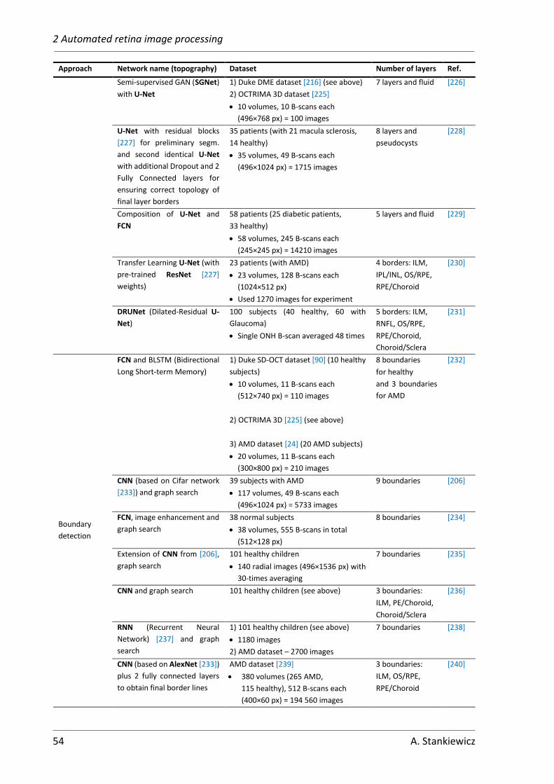
2 Automated retina image processing
54 A. Stankiewicz
Approach Network name (topography) Dataset Number of layers Ref.
Semi-supervised GAN (SGNet)
with U-Net
1) Duke DME dataset [216] (see above)
2) OCTRIMA 3D dataset [225]
• 10 volumes, 10 B-scans each
(496×768 px) = 100 images
7 layers and fluid [226]
U-Net with residual blocks
[227] for preliminary segm.
and second identical U-Net
with additional Dropout and 2
Fully Connected layers for
ensuring correct topology of
final layer borders
35 patients (with 21 macula sclerosis,
14 healthy)
• 35 volumes, 49 B-scans each
(496×1024 px) = 1715 images
8 layers and
pseudocysts
[228]
Composition of U-Net and
FCN
58 patients (25 diabetic patients,
33 healthy)
• 58 volumes, 245 B-scans each
(245×245 px) = 14210 images
5 layers and fluid [229]
Transfer Learning U-Net (with
pre-trained ResNet [227]
weights)
23 patients (with AMD)
• 23 volumes, 128 B-scans each
(1024×512 px)
• Used 1270 images for experiment
4 borders: ILM,
IPL/INL, OS/RPE,
RPE/Choroid
[230]
DRUNet (Dilated-Residual U-
Net)
100 subjects (40 healthy, 60 with
Glaucoma)
• Single ONH B-scan averaged 48 times
5 borders: ILM,
RNFL, OS/RPE,
RPE/Choroid,
Choroid/Sclera
[231]
Boundary
detection
FCN and BLSTM (Bidirectional
Long Short-term Memory)
1) Duke SD-OCT dataset [90] (10 healthy
subjects)
• 10 volumes, 11 B-scans each
(512×740 px) = 110 images
2) OCTRIMA 3D [225] (see above)
3) AMD dataset [24] (20 AMD subjects)
• 20 volumes, 11 B-scans each
(300×800 px) = 210 images
8 boundaries
for healthy
and 3 boundaries
for AMD
[232]
CNN (based on Cifar network
[233]) and graph search
39 subjects with AMD
• 117 volumes, 49 B-scans each
(496×1024 px) = 5733 images
9 boundaries [206]
FCN, image enhancement and
graph search
38 normal subjects
• 38 volumes, 555 B-scans in total
(512×128 px)
8 boundaries [234]
Extension of CNN from [206],
graph search
101 healthy children
• 140 radial images (496×1536 px) with
30-times averaging
7 boundaries [235]
CNN and graph search 101 healthy children (see above) 3 boundaries:
ILM, PE/Choroid,
Choroid/Sclera
[236]
RNN (Recurrent Neural
Network) [237] and graph
search
1) 101 healthy children (see above)
• 1180 images
2) AMD dataset – 2700 images
7 boundaries [238]
CNN (based on AlexNet [233])
plus 2 fully connected layers
to obtain final border lines
AMD dataset [239]
• 380 volumes (265 AMD,
115 healthy), 512 B-scans each
(400×60 px) = 194 560 images
3 boundaries:
ILM, OS/RPE,
RPE/Choroid
[240]

2 Automated retina image processing
A. Stankiewicz 55
Approach Network name (topography) Dataset Number of layers Ref.
Pixel
classification
and boundary
detection
2 cascaded modified U-Nets
for both pixel classification
and boundary detection with
topology assurance
1) 35 patients (with 21 macula sclerosis,
14 healthy) (same as [228])
9 boundaries
and pseudocysts
[228]
U-Net with residual blocks
with 2 fully connected outputs
(pixel classification and
surface position detection for
improved topology)
1) 35 patients (with 21 macula sclerosis,
14 healthy) (same as [228])
2) Duke DME dataset [216]
9 boundaries
and fluid
[241]
2.3.5 U-Net architecture
This subsection describes a basic U-Net architecture [36] employed for retina layers
segmentation in an OCT image. This topology, upon which various solutions are built, is also
the basis of the proposed solution described in this dissertation.
The U-Net is a version of a fully convolutional network [242], as each block consists
of a repeated application of convolutions. Two main parts of the network can be
distinguished: a contracting path (frequently described as an encoder) and an expansive path
(called the decoder). In each level of the contracting part, the input matrix is subjected two
times to a padded convolution (denoted as Conv 3×3) with a 3×3 kernel mask [243]. Each
convolution is followed by the rectified linear unit (ReLU) activation function [244]. This
is followed by a downsampling operation of 2×2 max pooling with stride 2 (MaxPool 2×2).
These blocks comprise a single level of the encoder, repeated four times. The number
of feature channels is doubled at each level while the spatial information is reduced.
In the decoder part of the network, the feature matrix is subjected to 2×2 convolution
(denoted as UpConv 2×2), with which the data is upsampled in the spatial dimension while
at the same the number of feature channels is reduced by half. Such matrix is next
concatenated with corresponding features from the encoder path, followed by applying two
3×3 convolutions and ReLU functions similarly to the first part of the network. At the final
level, a 1×1 convolution is applied to the resulting feature matrix to map them into the desired
number of classes.
Finally, an activation function is applied to the output to obtain the probability of each
pixel belonging to a given class. Typically, for binary classification, it is a sigmoid function
(defined with Equation (2.20)), or for multiclass classification, a SoftMax function (described
with Equation (2.21)).
Sigmoid( 𝐼(𝑥, 𝑦) ) =1
1 + e−𝐼(𝑥,𝑦) (2.20)
Softmax( 𝐼(𝑥, 𝑦) ) =e𝐼(𝑥,𝑦)
∑e𝐼(𝑥,𝑦) (2.21)

2 Automated retina image processing
56 A. Stankiewicz
It is essential to select the input image size divisible completely by 2 to the power of the
number of pooling operations in the encoder part. Similarly, the number of initial features
in the original U-Net is 64. Other possibilities, such as 32 or 128, are also applicable, though
this parameter affects the performance and accuracy of the network.
Figure 2.21 illustrates an application of the U-Net to an OCT B-scan with 64 initial features,
4 encoding/decoding levels, and 8 output classes corresponding to 1: region over the retina,
2-7: 6 retina layers (7 borders), 8: region below the retina.
Figure 2.21 U-Net architecture (example for input OCT image of resolution 512×512 px with a single channel (gray-scale) and 8-channel one-hot encoded output for 8 separate segmented image regions). Each blue box
represents a multi-channel feature map (the number of channels is denoted on top of the box). The input size at each level is denoted on the left-hand side of the boxes. White boxes denote feature maps copied from the
encoder to the decoder part of the network. Legend in the lower-left corner describes operations indicated with colored arrows
Preprocessing
To reduce variability in OCT data, most of the methods apply basic image preprocessing
such as image normalization (i.e., rescaling to the range of ⟨0,1⟩ ) or standardization
(otherwise known as z-score) with the following Equation:
𝑧(𝑥, 𝑦) =𝐼(𝑥, 𝑦) − 𝜇
𝜎 (2.22)
where 𝑥 and 𝑦 are the indexes of pixels within the image 𝐼, 𝜇 is the mean of all pixels, and
𝜎 denotes the standard deviation of pixels intensity values.
Although some of the reported applications of neural networks for OCT retina layers
segmentation utilize image flattening with respect to the Bruch’s membrane (with the same
procedure as described in Section 2.3.2), it is not as common as with graph-based approach.
Moreover, none of them apply any image denoising algorithm or other methods of enhancing
image quality. What must be remembered is that applying any kind of preprocessing step, one
must always perform it for training, validation, and testing to ensure that the network
operates on the same principles.

2 Automated retina image processing
A. Stankiewicz 57
Training
Since neural networks are a type of supervised machine learning, obtaining image
segmentations is divided into training and testing phases. During the training, an image
is processed by the network, and the resulting output is compared with the reference. From
this comparison, a loss value is calculated (various types of loss functions utilized for retina
layers segmentation will be discussed later). This value is utilized to update the weights of the
network layers before processing the next image. The training goal is to minimize the loss
value by repeatedly processing all images through the network. The number of repetitions
(called epochs) can be chosen arbitrarily or be dependent on the learning process.
Conversely, it is considered good practice to divide the images in the cohort into three
parts: training, validation, and testing subsets. These subsets should be exclusive, and each
should have a similar distribution of all parameters (such as image size, intensity values, spatial
parameters such as retina orientation, number of subjects from each pathology class). While
the images in the training dataset are used to learn the network parameters, the images in the
validation dataset may be processed by the network after each training epoch to determine
the improvement (or not) of the learning process. Although the loss calculated during the
validation step is not utilized to update the network parameters, it can be used to tune the
general experiment's parameters (such as the total number of epochs).
The final learned parameters of the network (the weights of the convolution kernels) are
used in the testing stage to obtain a segmentation of the images on the data not yet previously
“seen” by the network. Finally, the results of this step are compared between competing
segmentation methods.
Apart from training a neural network separately in each experiment, it is also possible
to utilize a network previously trained on a different dataset. Such procedure is called transfer
learning [245]. The principle involves training a network that can segment other objects in the
image (e.g., chair or cat) to segment the desired objects (such as retina fluids). Although
it may shorten the training process, this strategy is not common in the area of retina layers
segmentation [238].
Loss function
The previously mentioned loss can also be described as an error between the output of the
network and the reference data. Numerous loss functions that can be used for medical image
segmentation tasks have been identified in the literature [246]. They can be either
distribution-based, region-based, boundary-based, or compounded [247]. Frequently, each
author of a specific segmentation task implements their version of this crucial algorithm
component. The most commonly used loss functions for retina layers segmentation are:

2 Automated retina image processing
58 A. Stankiewicz
• Cross-Entropy Loss [248] (also called logistic loss, log loss, or negative log-likelihood)
is a distribution-based criterion. It is defined as a measure of the difference between
two probability distributions for a given random variable or set of events. Its use
in both general target classification and pixel-classification segmentation provides
good results. A Binary Cross-Entropy Loss is used in a simplified task, where only two
classes are defined (the segmented object and background). It is defined as:
𝐿𝐶𝐸(𝑦, ��) = −1
𝑁∑[𝑦𝑖 log(��𝑖) + (1 − 𝑦𝑖) log(1 − ��𝑖)]
𝑁
𝑖=1
(2.23)
where 𝑦𝑖 is the ground truth (taking a value of 0 or 1) of the 𝑖-th element in the set
of 𝑁 elements, and ��𝑖 is the corresponding predicted value (in image segmentation:
the probability of a pixel 𝑖 belonging to the segmented object).
In the task of multi-class segmentation, where each retina layer is defined as a separate
class, this loss function is applied to each class separately, and the final loss value
(called Categorical Cross-Entropy) is summed across all classes with the following
Equation:
𝐿𝐶𝐸(𝑦, ��) = −∑(1
𝑁𝑐∑[𝑦𝑖 log(��𝑖)]𝑖∈𝑐
)
𝑐∈𝐶
(2.24)
where 𝐶 is the number of classes and 𝑁𝑐 is the number of elements in class 𝑐 ∈ 𝐶.
• Dice Loss [249] is another type of loss function widely utilized for image segmentation.
Its advantage is the independence from class imbalance (a situation in which one class
has substantially more (or less) elements than other classes from the set). This
situation is frequent in OCT retina images, as retina layers span significantly fewer
pixels than the vitreous or the region below the retina. Dice Loss is a region-based
criterion aiming to maximize the overlap of regions between the ground truth and
predicted segmentation. It can be expressed as:
𝐿𝐷𝑖𝑐𝑒(𝑦, ��) = 1 −∑(2∑ 𝑦𝑖��𝑖𝑖∈𝑐 + 휀
∑ 𝑦𝑖𝑖∈𝑐 + ∑ ��𝑖𝑖∈𝑐 + 휀)
𝑐∈𝐶
(2.25)
where 휀 ∈ ⟨0.1, 1⟩ is a value added for numerical stability to avoid division by 0.
Although many more loss functions can be found in the literature [246], they are mostly
variations of the two most commonly utilized described above. In most recent works
regarding retina layers segmentation, these two functions are combined (summed with
arbitrarily chosen weights) and referred to as Dice-Cross-Entropy Loss (or Combo Loss).
Additionally, it is also possible to provide weights for each class to be segmented both
for 𝐿𝐷𝑖𝑐𝑒 and 𝐿𝐶𝐸 functions. Such weights can further help with class imbalance as they can
be derived from the number of elements belonging to each class.

2 Automated retina image processing
A. Stankiewicz 59
Data augmentation (DA)
As part of a data-driven field of artificial intelligence, deep neural networks are highly
dependent on the data itself. Furthermore, the greater complexity of the network requires
more training examples. More training examples with greater variability allow to obtain
a better model [250]. Unfortunately, the number of training examples of OCT retina images
is scarce. As shown in Section 3.1.1, even if many OCT images can be acquired, it is also
necessary to provide reference data for those examples. Creating manual segmentations
requires expertise, and it is very time-consuming for multiple 3D OCT images. In such
a situation creating artificial examples through data augmentation is a solution.
Data augmentation is a method of creating multiple data instances similar to those already
existing in the dataset but with varying characteristics. The newly generated examples
represent a more comprehensive set of possible variations of the data, thus allowing the
model to generalize better [243] (for example, better learn which pixels belong to the given
retina layers regardless of an image of a left or right eye, retina angle, size of the image
or presence of noise).
Employing data augmentation allows to improve the robustness of the model, especially
if the available dataset has very few training samples. Although in image processing, a variety
of image augmentation techniques are possible (such as flipping, cropping, rotation,
translation, noise injection, change of contrast, color space transformations, and others)
[251], not all of them are applicable to OCT retina images. For example, a vertical flip would
invert the topology of retina layers, which is unacceptable in layers segmentation. Therefore,
the image augmentation techniques most frequently used in the literature are horizontal flip,
random rotation, cropping, and scaling (in the case of training on data from various
manufacturers).


61
Chapter
3 Graph-based segmentation of the
retina
This Chapter describes the proposed improvements of algorithms for segmentation of retina
layers from low quality OCT images. It starts in Section 3.1 with the description of OCT image
data gathered to validate the proposed algorithms.
Section 3.2 introduces the necessary enhancements of low quality OCT data. For this
purpose, an analysis of the denoising method able to enhance features specific
to vitreomacular traction is described. Furthermore, the author introduces segmentation
enhancement with an adaptive selection of the region of interest for analyzed OCT volume.
Additionally, the author proposes layers tracking to boost algorithm performance
by incorporating information on previously segmented layers.
3.1 CAVRI database
3.1.1 Availability of OCT data
Since the introduction of OCT technology in ophthalmology, investigating eye diseases
with this modality has become the interest of various research centers worldwide. The need
to obtain numerous images along with reference data of manual annotations became an issue
for those who wished to conduct experiments in this field. Unfortunately, any data suitable
for analysis belonged either to the manufacturers of the OCT devices (such data was used
to create a reference eye atlas for a given device) or hospitals utilizing said devices, thus not
publicly available. Furthermore, the authors of published algorithms usually perform the test
on their private datasets. This makes it hard to rank developed algorithms against each other.
It should be noted that until 2018 not many OCT image databases were publicly available
for research purposes. However, since then, a few datasets of OCT images of normal eyes and
those affected with the most common retinal diseases have been published. These can
be divided into two types:
• datasets aimed at pathology classification – contain only single cross-sections
through the fovea and a label of the disease
• databases aimed at developing retina segmentation algorithms for various
pathologies – contain volumetric or raster OCT data with corresponding manual
layer segmentations.

3 Graph-based segmentation of retina
62 A. Stankiewicz
Table 3.1 summarizes the statistical information of currently available public human OCT
datasets for both pathology classification and retina layers segmentation. Nevertheless, none
of the listed OCT datasets include a specific eye disease named VMT investigated in this work.
Furthermore, in most, the number of cross-sections or volumes is scarce. Also, not all contain
reference layers segmentations for a whole OCT volume or more than 3 layers. As can be seen,
the number of manually labeled OCT volumes in most of the datasets does not exceed 25
subjects.
Table 3.1 Summary of publicly available OCT databases
Database Diseased Number of
subjects Annotations
Volume
/ single image Device References
AROI nAMD1 25
for 1136 B-scans:
fluids and
4 layer boundaries
volume
128 B-scans: 1024×512 px
3200 images in total
Zeiss Cirrus
HD OCT 4000 [252]
OCTID
Normal
AMD
CSR2
DR3
MH
206
55
102
107
102
only for 25 Normal:
7 layer boundaries
single central B-scan
1024×512 px
resized to 750×500 px
572 images in total
Zeiss Cirrus
HD OCT [253]
DUKE Farsiu Normal
AMD
115
269
only for central 5mm:
3 layer boundaries
volume
100 B-scans: 512×1000 px
38400 images in total
Heidelberg
Spectralis
SD-OCT
[239]
Miami Dataset DR 10 5 layer boundaries
volume
50 B-scans: 768×496 px
50 images in total
Heidelberg
Spectralis
SD-OCT
[223]
OCTRIMA3D Normal 10 8 layer boundaries
volume
10 B-scans: 610×496 px
100 images in total
Heidelberg
Spectralis
SD-OCT
[225]
DUKE Chiu 2011
AMD 25 3 layer boundaries
volume
11 B-scans: 512×1000 px
275 images in total
Bioptigen
SD-OCT [24]
DUKE Chiu 2015
DME 10 8 layer boundaries
volume
61 B-scans: 496×768 px
610 images in total
Heidelberg
Spectralis
SD-OCT
[216]
DUKE
Srinivansan
Normal
AMD
DME
15
15
15
no
volume
from 37 to 97 B-scans
512×492 px
3231 images in total
Heidelberg
Spectralis
SD-OCT
[254]
Labeled OCT
Images for
Classification
Normal
AMD
DME
CNV4
26 315
8 616
11 348
37 205
no
single central B-scan
512×496 px
83 484 images in total
Heidelberg
Spectralis OCT [255]
1 nAMD – neovascular age-related macular degeneration
2 CSR – central serous retinopathy
3 DR – diabetic retinopathy
4 CNV – choroidal neovascularization
3.1.2 CAVRI dataset statistics
A database of eye images with VMT pathology has been created to check the effectiveness
of the proposed retina segmentation algorithms experimentally. This database consists
of three-dimensional cross-sections of the macula (3D Retina scanning protocol) imagined
using the Avanti RTvue OCT device [27]. The cohort includes 66 healthy volunteers (78 eyes)

3 Graph-based segmentation of retina
A. Stankiewicz 63
and 46 subjects (52 eyes) with VMT, giving 102 subjects (130 eyes) in total. All of the patients
signed an agreement form to participate in the study.
For each eye qualified by the specialist for the study following OCT scans were performed
after pharmacological pupil dilation:
• one Line scan
• one Cross scan
• four 3D Retina scans.
For volumetric parameterization of the retina, only the three-dimensional scans were
considered for further analysis. The examined volume (7×7×2 mm3 of the macula)
is represented by 141×385×640 data points (i.e., 141 B-scans with 385×640 resolution). This
means that a B-scan of the size 385×640 px, as in Figure 3.1a, represents the area of 7×2 mm,
as illustrated in Figure 3.1b.
(a) OCT image of size 640×385 px
(b) OCT image (a) resized to show spatial area it represents
Figure 3.1 Data vs. spatial representation of OCT image
OCT volumes with severe motion artifacts or underexposure (caused, e.g., by cornea
occluding) were excluded from the image analysis. Next, three ophthalmologists from the
Department of Ophthalmology, Heliodor Swiecicki University Hospital, Poznan University
of Medical Sciences, manually segmented the remaining portion of the acquired scans.
Annotations included 7 retina borders (namely: ILM, RNFL/GCL, IPL/INL, INL/OPL, OPL/ONL,
IS/OS, RPE/Choroid) and the posterior cortical vitreous (PCV). The manual annotations were
obtained with a proprietary software called OCTAnnotate developed by the author of this
thesis. A detailed explanation of the software capabilities is included in Appendix A2. This
reference data was further used for evaluating investigated algorithms.
The PCV line in OCT images has a vertical thickness of 3-10 px, which may cause
disagreements between experts. Thus, from the obtained data, the author selected a subset
of 50 subjects with less than 3 px of maximum difference of manual segmentation between
the experts. One 3D OCT image from each of these 50 subjects was utilized to evaluate the

3 Graph-based segmentation of retina
64 A. Stankiewicz
correctness of segmentation algorithms in Chapters 3 and 4. These 50 unique volumetric scans
are referred to in this thesis as the CAVRI-A1 subset.
Furthermore, the selected patients were monitored for changes in the vitreoretinal
interface for 4 years. The frequency of visits stemmed from 4 to 12 months and depended
on the arrangements with the leading physician. For long-term observation, at least 4 scans
were considered necessary. The patient was excluded from the further study if full PVD
occurred or the condition impeded the patient’s ability to see, thus qualified for a surgical
procedure. Unfortunately, at least 4 scans could not have been obtained for all 50 subjects
who qualified for the study. The final group for a long-term observation includes 12 cases with
VMA and 14 cases with VMT (26 cases in total) and is called CAVRI-A2. This subset was utilized
for the parameterization experiments in Chapter 5. The number of scans with annotations
used in this study lists Table 3.2.
Table 3.2 Statistical analysis of CAVRI database – number of eyes, 3D scans, and single cross-sections for a given pathology
VRI status Isolated
cases
Cases with
coexisting
pathology
Total
cases
Cases with single
examination
Long-term
observation
Unique
examples
Total
examinations
No. of 3D scans / No. of B-scans
VMA 19 6 25 13 / 1 833 12×4 / 6 768 25 / 3 525 61 / 8 601
VMT 20 5 25 11 / 1 551 14×4 / 7 896 25 / 3 525 67 / 9 447
Total 39 11 50 24 / 3 384 26×4 / 14 664 50 / 7 050 128 / 18 048
Subset: CAVRI-A2 CAVRI-A1
The subjects’ ages ranged from 48 to 80 years (mean age was 62.2 and standard deviation
7.8 years) for VMA and from 57 to 79 years (mean: 67.8, standard deviation: 5.7) for VMT. The
gathered data confirms the notion of a higher prevalence of VMT in women than in men, as 18
of 25 VMT patients and 13 out of 25 VMA subjects were women. The scans were acquired
for 19 right and 31 left eyes.
Of 25 VMT patients, the majority had a V-shaped pattern, and only two could be classified
as J-shaped, making this type of classification invalid for the gathered cohort. In addition, the
coexisting pathology present in 11 of the cases was either AMD or subretinal effusion. Those
pathologies are located in the outer retina and are not connected with the vitreoretinal
interface. Thus their presence would not impede the automated analysis of the VRI structure.
The main metric of comparison between subjects is the preretinal space volume,
calculated from the reference segmentation of PCV and ILM lines. For VMA, the average
preretinal space volume is 3.17 (± 1.96) mm3, while for VMT, it is 12.19 (± 6.09) mm3.
The Wilcoxon test yielded a p-value close to zero (3.6∙10−10), confirming that this comparison
is statistically significant. Figure 3.2 presents a box plot of the preretinal space volumes
for these groups. As can be seen, their distributions are significantly different.

3 Graph-based segmentation of retina
A. Stankiewicz 65
Figure 3.2 Box plot of preretinal space volume distributions for VMA and VMT subjects in the CAVRI dataset
3.1.3 Quality of OCT data
To numerically assess the quality of the obtained OCT data, values of two metrics were
calculated for each 3D OCT scan, namely the QI (Quality Index) parameter and the mTCI
(maximum Tissue Contrast Index).
The mean value (and standard deviation) of the mTCI for VMA subjects is 5.49 (± 2.28),
while for the VMT patients, it is 4.4 (± 1.77). Figure 3.3 presents the histogram bar plot of the
distribution of the mTCI values for the scans in the CAVRI database. The mTCI index indicates
that the majority of the scans have a low quality (lower index value).
Figure 3.3 Histogram of mTCI values for scans in the CAVRI database
The second parameter calculated for the images is the QI, and its mean (and standard
deviation) values are 40.03 (± 8.17) and 38 (± 7.98) for VMA and VMT subsets, respectively.
Figure 3.4 illustrates the histogram of QI values distribution for the CAVRI database images.
This parameter indicates a more normal distribution of the quality of the gathered images.
The mTCI and QI indexes are based on the histogram calculation, thus corresponding to the
0
5
10
15
20
25
30
1 2 3 4 5 6 7 8 9 10 11 12 13 14 15
Nu
mb
er o
f 3
D s
can
s
mTCI value
VMA VMT

3 Graph-based segmentation of retina
66 A. Stankiewicz
subjective evaluation of an expert. The difference in their distribution might result from the
division of pixel intensities that each algorithm considers as belonging to the foreground
or background (noise).
Figure 3.4 Histogram of QI values for scans in the CAVRI database
3.2 Proposed methods for enhancement of OCT image
segmentation
3.2.1 Influence of OCT image quality on image analysis
Image quality is an important factor in proper structure segmentation, as was described
in Section 2.2. Further, Section 3.1 included a detailed qualitative analysis of OCT data
available for this research. As can be inferred, insufficient signal levels for many samples
in the dataset impede segmentation accuracy.
The author conducted an experiment to determine the baseline retina layers
segmentation accuracy of the OCT images in the CAVRI dataset. The test utilized the state-of-
the-art segmentation method based on graph theory as described in Section 2.3.2, performed
for each B-scan separately. The algorithm based on Caserel software [256] was implemented
in Matlab/Simulink environment [257] and adjusted for the images in the CAVRI database.
The test utilized only retina layers segmentation without detecting pathology or elements
of the vitreoretinal interface. The analysis included both normal and diseased tissue images
(the CAVRI-A1 subset). Segmentation accuracy was measured numerically with the indicators
of mean absolute error (MAE), and root mean squared error (RMSE) (see Section 2.3.1
for details). The results are presented in Table 3.3 and illustrated in Figure 3.5. The best results
are for the outer borders of IS/OS and RPE/Choroid, which can be attributed to their higher
than neighboring tissue reflectivity. Lower values are observed for intraretinal borders where
pixel intensities for tissue layers are similar.
0
1
2
3
4
5
6
7
20 22 24 26 28 30 32 34 36 38 40 42 44 46 48 50 52 54 56 58 60
Nu
mb
er o
f 3
D s
can
s
QI value
VMA VMT

3 Graph-based segmentation of retina
A. Stankiewicz 67
Table 3.3 Results of preliminary OCT layers segmentation for low quality image
Retina border MAE [px] SD [px] RMSE [px]
All borders 4.57 7.27 14.01
ILM 2.84 8.48 15.90
NFL/GCL 6.65 11.71 19.23
IPL/INL 6.13 11.09 15.78
INL/OPL 7.61 10.86 15.87
OPL/ONL 5.32 9.64 13.32
IS/OS 1.95 4.69 6.85
RPE/Choroid 1.51 3.48 5.18
Figure 3.5 Illustration of erroneous retina layers segmentation for 2 examples of low quality B-scans
The results shown in Figure 3.5 and Table 3.3 underline the importance of addressing the
problem of low OCT image quality before attempting retina layers segmentation.
To improve the segmentation accuracy and eliminate the occurrence of errors,
as illustrated in Figure 3.5, the author of this thesis proposed addressing the problem
of insufficient quality of the OCT data. Three enhancements have been introduced (two during
preprocessing stage and one for improving the shortest path search step):
• selection of speckle suppression method (Section 3.2.2)
• elimination of underexposed image areas (Section 3.2.3)
• tracking searched layers through the OCT volume (Section 3.2.4).

3 Graph-based segmentation of retina
68 A. Stankiewicz
The proposed improvements are described in detail in the following subsections. Their
place in the general graph-search algorithm signifies orange blocks in Figure 3.6.
Figure 3.6 Scheme of retina layers segmentation with layers tracking and limiting search region
3.2.2 Selection of noise reduction method
In Section 2.2.2, the specificity of speckle noise in OCT images is characterized, as well as
the typical methods of reducing this noise. To analyze their influence on the vitreoretinal
interface segmentation accuracy four most promising methods from the groups presented
in Figure 2.10 were selected, which are:
• classical methods: averaging filtering
• partial differential equation-based: anisotropic diffusion
• parametric method: wavelet thresholding
• mixed methods: block-matching and collaborative filtering.
The goal of the comparison was to analyze:
• the achieved segmentation accuracy (as the main metric of comparison) and
• the time consumption (to assess clinical applicability).
The examined methods and their tested parameters are described in detail in the following
subsections.
2D methods
Averaging filtering
The first evaluated image denoising method is the basic averaging filtering (further
referred to as AVG). It is based on performing a two-dimensional convolution
of an investigated image with a previously defined filter. The filter mask is usually defined
as a square matrix with an odd number of rows and columns (e.g., 3×3), although rectangular
Input image
Vertical gradient analysis
Compute graph
weights
Find shortest
path
Preprocessing (denoising,
image flattening)
Adjacency matrix
Initialize start and end of the
graph
Limit search region
Information of the previously found paths

3 Graph-based segmentation of retina
A. Stankiewicz 69
filters, such as 3×19, can also be found in the literature [90]. Here, four filter sizes were tested:
3×3, 5×5, 7×7, and 9×9.
It should be mentioned that the averaging approach is the main noise suppression method
used for the line scanning protocol that utilizes multiple acquisitions in a single eye position.
Anisotropic diffusion filtering
Anisotropic diffusion (AD) is an efficient noise reduction method. For an input image 𝐼 this
method, proposed by Perona and Malik [123], defines the denoised image as:
𝐼 = 𝑐(𝑥, 𝑦)∆𝐼 (3.1)
where Δ represents the Laplace operator, and 𝑐(𝑥, 𝑦) describes the diffusion coefficient
dependent on the position (𝑥, 𝑦) in the image space, according to the function:
𝑐(𝑥, 𝑦) = e|∇𝐼|2
2𝜅2 (3.2)
where ∇ defines gradient, 𝜅 is the denoising parameter, being a positive real value that
is related to the noise level and the expected edge preservation in the image.
The image gradient calculated with the Prewitt operator is used for edge detection since
it is considered robust to noise [33]. The lower value of the diffusion coefficient allows
to avoid blurring of the edges, while the bigger value allows for the smoothing of areas
between the edges. Choosing an optimal 𝜅 parameter value leads to preserving the lines and
structures in the image (important for interpretation). This technique is useful for reducing
the speckle noise in OCT images.
Wavelet thresholding
The wavelet thresholding (WT) method provides good results in denoising OCT images.
This is mainly due to the fact that the noise is evenly distributed between wavelet coefficients,
while the majority of the informative content is concentrated among the coefficients with
high magnitude. By selecting a proper threshold value (which might be a difficult task), we can
reduce the noise, maintaining characteristic features of the image [134].
In this algorithm, a single B-scan 𝐼𝑖 (𝑖 denoting the index of the cross-section within the 3D
scan), represented in the logarithmic scale, is decomposed with the wavelet transform of the
maximum decomposition level 𝐿 . A result of this transformation are approximation
coefficients 𝐴𝑖𝐿 and detail coefficients 𝑊𝑖,𝐷
𝐿 , where 𝐷 describes the direction (horizontal
or vertical) of image filtering. During the experiments, a wavelet soft thresholding (WST)
method was used with the Haar wavelet [258].
The denoising operations consist of reducing the detail coefficients for a position 𝑥 in the
image based on the weight 𝐺𝑖,𝐷𝐿 :
��𝑖,𝐷𝐿 (𝑥) = 𝐺𝑖,𝐷
𝐿 (𝑥) ∙ 𝑊𝑖,𝐷𝐿 (𝑥) (3.3)

3 Graph-based segmentation of retina
70 A. Stankiewicz
where each weight 𝐺𝑖,𝐷𝐿 is calculated for a manually selected threshold 𝜏 according to the
following Equation:
𝐺𝑖,𝐷𝐿 (𝑥) = {
𝑊𝑖,𝐷𝐿 (𝑥) − sgn(𝑊𝑖,𝐷
𝐿 (𝑥))𝜏
𝑊𝑖,𝐷𝐿 (𝑥)
for |𝑊𝑖,𝐷𝐿 (𝑥)| > 𝜏
0 otherwise
(3.4)
The last step of this algorithm requires performing the inverse wavelet transform. Figure
3.7a presents a general scheme of the described algorithm.
(a) single image wavelet thresholding (b) multiframe wavelet thresholding
Figure 3.7 Scheme of B-scan image denoising algorithm
BM3D
The block-matching and 3D filtering algorithm [259] consists of two cascades: a hard-
thresholding and a Wiener filtering, both of which incorporate:
1) grouping: similar 2D image fragments are grouped together and stacked in a 3D data
array. A fragment is grouped if its dissimilarity measure with a reference fragment
falls below a specified threshold.
2) collaborative filtering: performed on every fragments group separately by applying
a 3D linear transform, shrinking the transform coefficients (by hard-thresholding
or Wiener filtering), and inverting the linear transform to reproduce all fragments.
3) aggregation: the transformation of the blocks back to the 2D image. The final estimate
of all overlapping image fragments is aggregated using a weighted average.
The approach of grouping similar pixels within an OCT image (regardless of their position)
gives this method the potential for removing speckles and smoothing retina tissues.

3 Graph-based segmentation of retina
A. Stankiewicz 71
3D methods
3D Anisotropic diffusion
The three-dimensional anisotropic diffusion (AD3D) filtering is an extension of the above-
described method, which was performed for each B-scan separately. On the other hand,
the 3D approach is performed on a whole volume simultaneously, taking into account voxel
size in each scan direction.
Multiframe wavelet thresholding
The multiframe wavelet thresholding (MWT) [113] method is an extension of the WST,
but instead of operating on a single image, it uses a set of frames 𝐼𝑖, 𝑖 ∈ ⟨1, 𝑁⟩, where 𝑁
defines the number of the processed B-scans. This approach assumes no correlation between
noise in subsequent image frames.
Similarly, as with the 2D version, the calculation of the significance weight 𝐺sig,𝑖,𝐷𝐿 (𝑥)
for the detail coefficients allows for estimation of the local noise. It is computed as follows:
𝐺sig,𝑖,𝐷𝐿 (𝑥) = {
1 for |𝑊𝑖,𝐷𝐿 (𝑥)| ≥ 𝑘𝜎𝑆,𝑖,𝐷
𝐿 (𝑥)
𝜃𝑖 (𝑊1,𝐷𝐿 (𝑥),… ,𝑊𝑁,𝐷
𝐿 (𝑥)) otherwise (3.5)
𝜎𝑆,𝑖,𝐷𝐿 2
(𝑥) =1
𝑁 − 1∑ (𝑊𝑖,𝐷
𝐿 (𝑥) − 𝑊𝑗,𝐷𝐿 (𝑥))
2𝑁
𝑗=1,𝑗≠𝑖
(3.6)
where 𝜎𝑆,𝑖,𝐷 defines the mean squared distance between the detail coefficients in individual
images, parameter 𝑘 describes the noise reduction level, and 𝜃𝑖 is the normalized parameter
calculated as in (3.7):
𝜃𝑖(𝑤1, … , 𝑤𝑁) =1
𝑁 − 1∑ |1 −
𝑤𝑖𝑤𝑗|
𝑁
𝑗=1,𝑗≠𝑖
(3.7)
The extension from the 2D WST version incorporates obtaining new detail and
approximation coefficients for all images and averaging them before performing the inverse
transform. A general scheme of this approach is illustrated in Figure 3.7b for an example of 3
frames. Although this algorithm was developed for a set of frames of a single exposed tissue
area, the author tested the use of 3 subsequent frames in the 3D OCT set as input images
for this method. This approach is based on the fact the distance between the subsequent
B-scans in the 3D examination (for the utilized 3D Retina protocol) is about 50 µm. Thus, only
a little change in the tissue structure is observed in the neighboring cross-sections.

3 Graph-based segmentation of retina
72 A. Stankiewicz
BM4D
Similarly, as with the AD3D algorithm, the block-matching technique can be used
in a volumetric manner. Here, the grouping is performed for all pixels within the analyzed 3D
scan. Such methodology can further improve the structural cohesion of pixel intensities
in an image.
Comparison of denoising algorithms
As was mentioned earlier, the retina layers segmentation procedure is a key step
in defining the morphological structure of the retina during the diagnosis. However, it was
also shown that noise in OCT images is causing errors in the segmentation of the retina layers.
For that reason, the author of this thesis tested the effectiveness of the denoising methods
based on the image segmentation accuracy. The segmentation algorithm selected for this
study (reported by Chiu et al. [90]) was described in Section 2.3.2. Additionally, for OCT
images, a reference image (an ideal image without noise) does not exist. Thus, it is difficult
to calculate the accuracy of denoising algorithms directly.
Each image was denoised with each of the earlier described methods. For every method
(except block-matching), various parameter values presented in Table 3.4 were tested.
Examples of B-scans obtained after applying each investigated denoising method are
illustrated in Figure 3.8.
Table 3.4 Values of parameters chosen for tested denoising methods
Method AVG AD (2D/3D) WST MWT
Parameter Mask size 𝜿 τ 𝒌
Value 1 3×3 1 1 0.1
Value 2 5×5 5 10 1
Value 3 7×7 10 30 10
Value 4 9×9 20 100 100
The original single cross-section (Figure 3.8a) has a visibly high noise content (a grainy
structure). Comparison with image Figure 3.8b clearly shows that the method of basic
averaging (most commonly used for OCT image analysis) blurs the image while the noise is still
present. The anisotropic diffusion filtering in 2D and 3D forms (Figure 3.8c and 3.8e) shows
the unification and smoothing of tissues, although some additional white and black spots are
visible.

3 Graph-based segmentation of retina
A. Stankiewicz 73
(a) original B-scan image
(b) average filtering (3×3 mask)
(c) anisotropic diffusion (𝜅 = 20)
(d) wavelet soft thresholding (τ = 10)
(e) 3D anisotropic diffusion (𝜅 = 20)
(f) multiframe wavelet thresholding (𝑘 = 10)
(g) BM3D
(h) BM4D
Figure 3.8 Example of original B-scan and illustration of tested noise reduction methods

3 Graph-based segmentation of retina
74 A. Stankiewicz
The wavelet thresholding method (Figure 3.8d and Figure 3.8f) also blurs the image,
although the regions of individual tissues are smoothed. Additionally, bigger threshold values
for the 2D approach cause rectangular-shaped artifacts to appear in the image. On the other
hand, the 3D method provides a good quality image with low noise content and visible tissue
separation. The block-matching algorithm (Figure 3.8g and Figure 3.8h) produces smooth
tissue regions while enhancing the edges and position of the blood vessels. A side effect of this
approach is wavy artifacts within the tissue areas that may impede image interpretation.
It can also be noticed that the 2D methods reduce the visibility of the PCV line present
in the upper left part of the image. WMF and BM4D methods best reveal this line, thanks
to which it is possible to maintain the most informative content about the pathology
distribution.
After noise suppression, each 3D scan was subjected to automatic image segmentation
based on the graph theory. Verification of effectiveness of the implemented methods was
based on the calculation of the MAE (SD) and RMSE (with formulas described in Section 2.3)
between the automatic and manual segmentations of 7 retina layers borders: ILM, NFL/GCL,
IPL/INL, INL/OPL, OPL/ONL, IS/OS, and RPE/Choroid. Due to divergence in annotating layer
borders by experts and computers, the difference between them lower than 3 pixels was
considered negligible (i.e., error equal to zero). All algorithms were implemented in the
Matlab/Simulink environment [257].
Figure 3.9 presents the segmentation results after each investigated denoising method.
As can be seen, the graph-based approach produces irregular segmentation lines due to high
dependence on the local image gradient. The 3D methods render better segmentations than
the 2D ones, and the wavelet-based method is better than the AD. Method BM4D (Figure
3.9h) provides the best accuracy for segmenting pathological tissue, although still some
inadequacies can be found in places where the segmentation lines are joined (center of the
image).
The influence of tested parameter values for each method is illustrated in box plots of the
MAE [px] in Figure 3.10. It is visible that smaller filter masks for the averaging filtering provide
better results (Figure 3.10a) since bigger masks tend to blur tissue edges. The BM approach
in both the 2D and 3D forms (Figure 3.10b) also improves the segmentation accuracy. It can
also be inferred that lower values of 𝜅 parameter in the AD method (Figure 3.10c) and
threshold τ for the WST method (Figure 3.10d) guarantee better performance. On the other
hand, the change of the 𝜅 value in the AD3D approach does not have improvement effect
(Figure 3.10e). Similarly results show that the 𝑘 parameter in MWT does not influence retina
layers segmentation accuracy (Figure 3.10f). Additionally, the segmentation error distribution
shown in Figure 3.10g confirms that the 3D approaches give better accuracy than their
2D versions.

3 Graph-based segmentation of retina
A. Stankiewicz 75
(a) reference segmentation
(b) average filtering (3×3 mask)
(c) anisotropic diffusion (κ = 20)
(d) wavelet soft thresholding (τ = 10)
(e) 3D anisotropic diffusion (κ = 20)
(f) multiframe wavelet thresholding (𝑘 = 10)
(g) BM3D
(h) BM4D
Figure 3.9 Illustration of reference layers segmentation and automatic segmentation results after noise reduction with analyzed methods. Data is presented in a 200×200 pixels section (image is squeezed vertically
for visualization) cropped from the center of the image in Figure 3.8.

3 Graph-based segmentation of retina
76 A. Stankiewicz
(a) averaging filtering
(b) block-matching
(c) anisotropic diffusion
(d) wavelet soft thresholding
(e) 3D anisotropic diffusion
(f) multiframe wavelet thresholding
(g) best of (a), (c) – (f), BM3D, BM4D
Figure 3.10 Box plots of MAE [px] (for all patients) of automatic retina layers segmentation after preprocessing with filtering methods (the number next to the abbreviation in the legends denotes tested parameter value)

3 Graph-based segmentation of retina
A. Stankiewicz 77
Table 3.5 and Table 3.6 contain MAE and RMSE results obtained for the best parameter
values for each denoising method. The best values for each segmented layer are denoted
in bold. It is worth mentioning that IS/OS and RPE/Choroid borders achieve better
segmentation accuracy than other layers, regardless of the denoising method. The
quantitative results indicate better segmentation performance using the 3D methods than the
2D ones, and all denoising methods positively influence the segmentation (compared to the
baseline data). Furthermore, the AD methods provide lower average error values than the
WST and MWT approaches. The best effect on segmentation has the block-matching
algorithm in the 3D version (BM4D), although the 2D variant outperforms it for IS/OS border.
Table 3.5 MAE (SD) values for automatic segmentation of selected retina layers [px]
Method None AVG
(3×3 px)
AD
(𝜿 = 𝟏)
WST
(𝝉 = 𝟏)
BM3D AD3D
(𝜿 = 𝟏)
MWT
(𝝉 = 𝟏𝟎)
BM4D
All layers 4.57 (7.27) 4.37 (7.15) 4.45 (7.11) 4.65 (7.72) 4.18 (6.93) 4.53 (7.21) 4.88 (7.33) 3.62 (6.07)
ILM 2.84 (8.48) 2.86 (8.66) 2.80 (8.42) 3.00 (9.54) 2.53 (7.60) 2.83 (8.47) 3.07 (7.80) 2.42 (7.16)
NFL/GCL 6.65 (11.71) 6.64 (11.70) 6.46 (11.45) 6.78 (12.52) 6.17 (11.43) 6.57 (11.53) 7.17 (11.77) 5.67 (10.71)
IPL/INL 6.13 (11.09) 5.72 (10.79) 5.94 (10.81) 6.23 (11.61) 5.52 (10.78) 6.05 (10.97) 6.39 (11.30) 4.40 (9.20)
INL/OPL 7.61 (10.86) 7.08 (10.49) 7.39 (10.56) 7.70 (11.28) 7.10 (10.54) 7.53 (10.76) 7.83 (11.27) 6.01 (8.67)
OPL/ONL 5.32 (9.64) 4.89 (9.29) 5.15 (9.42) 5.42 (10.00) 4.68 (9.34) 5.25 (9.60) 5.64 (9.98) 3.70 (7.80)
IS/OS 1.95 (4.69) 2.08 (4.82) 1.91 (4.63) 1.97 (4.78) 1.90 (4.54) 1.95 (4.72) 2.49 (4.92) 1.91 (4.46)
RPE/Choroid 1.51 (3.48) 1.33 (3.13) 1.46 (3.43) 1.48 (3.44) 1.39 (3.37) 1.50 (3.50) 1.59 (3.27) 1.22 (3.14)
Table 3.6 RMSE values for automatic segmentation of selected retina layers [px]
Method None AVG
(3×3 px)
AD
(𝜿 = 𝟏)
WST
(𝝉 = 𝟏)
BM3D AD3D
(𝜿 = 𝟏)
MWT
(𝝉 = 𝟏𝟎)
BM4D
All layers 14.01 13.96 13.87 14.65 13.13 13.82 16.03 12.03
ILM 15.90 16.08 15.80 17.06 13.15 15.65 17.19 12.58
NFL/GCL 19.23 19.25 19.02 20.01 18.32 18.85 21.73 17.74
IPL/INL 15.78 15.63 15.56 16.43 15.07 15.53 18.55 13.25
INL/OPL 15.87 15.61 15.67 16.44 15.32 15.69 18.58 13.12
OPL/ONL 13.32 13.23 13.22 13.99 12.84 13.24 15.91 11.05
IS/OS 6.85 7.01 6.82 6.90 6.50 6.82 8.00 6.53
RPE/Choroid 5.18 4.72 5.16 5.12 5.41 5.20 5.02 5.18
The analysis of the image quality improvement based on the QI value distribution
is illustrated in Figure 3.11. As can be noticed, each method influences the image quality,
enhancing or decreasing the tissue contrast. The QI value can be improved with the AD, WST,
and AD3D methods, while the general distribution shifts to lower values for AVG, BM3D,
WMF, and BM4D approaches.

3 Graph-based segmentation of retina
78 A. Stankiewicz
Figure 3.11 Box plot of QI values distribution for tested images after denoising with selected methods
Time consumption of tested denoising methods
Although the accuracy obtained with the noise suppression method is an important factor,
the time consumption of this step should also be taken into account. Table 3.7 summarizes
the average time performance of each evaluated denoising approach for a single B-scan and
a 3D volume. The test was performed in the Matlab/Simulink environment on a PC with a 64-
bit Windows operating system, 8 BG of RAM, and an Intel Core i7-3770 CPU (3.40 GHz)
processor. For the algorithms that utilize a single 2D cross-section, the time is summed up for
all B-scans in a 3D Retina volume.
Table 3.7 Average time consumption of tested denoising methods [s]
Method AVG
(3×3 px)
AD
(𝜿 = 𝟏)
WST
(𝝉 = 𝟏)
BM3D AD3D
(𝜿 = 𝟏)
WMF
(𝒌 = 𝟏𝟎)
BM4D
1 B-scan 0.25 0.39 0.21 2.94 1.56 1.46 13.23
3D volume
(141 B-scans) 34.64 55.35 30.00 415.10 219.54 206.41 1865.55
The measured time for 2D approaches is substantially lower than for the 3D methods, with
the smallest value for WST. Within 3D methods, the WMF is the quickest. It should also
be noted that the computational time of the block-matching algorithm is much longer than
other methods (6.9 minutes for the 2D version and 31.1 minutes for the 3D version using
Matlab/Simulink implementation), which is unacceptable for a clinical solution.
3.2.3 Adaptive selection of the region of interest
As was shown in Section 3.2.1 in Figure 3.5, low quality B-scan images frequently have
underexposed tissue regions (i.e., with very low signal) in the peripheral areas of the scan.
As a result, the retinal layers are in those regions almost entirely invisible. Such a situation
conflicts with the graph-search method assumption of the continuity of the layers within the

3 Graph-based segmentation of retina
A. Stankiewicz 79
whole image width. The author of this thesis considers it the main cause of errors during
automatic image segmentation.
An appropriate solution to this situation can be removing low signal parts of the B-scan
image along the image sides to overcome the discussed obstacle. Furthermore, this cropping
procedure can be performed in a fixed or an adaptive manner, depending on the OCT signal
strength. The author of this thesis tested these two propositions.
Figure 3.12 presents the idea of identification of low quality parts of an image. The dashed
line represents examples of cut lines: red line – initial image without cutting, orange line –
image cut with constant width, green line – image cut with adaptively computed width.
Figure 3.12 Two methods of removing low-level signal areas illustrated on (left) the B-scan image and (right) the reconstructed fundus image [148]
For the adaptive solution, the image column at which a single B-scan image (of size 𝑀 rows
by 𝑁 columns) should be cropped is defined by finding the first from the side column 𝑖 ,
in which the maximum value of the brightness (𝑋) is higher than the predefined threshold
𝑡ℎ ∈ ⟨0, 255⟩, as it is described by Equation (3.8):
𝑖: max𝑗∈⟨1,𝑀⟩
(𝑋𝑖𝑗) < 𝑡ℎ 𝑖 ∈ ⟨1, 𝑁⟩ (3.8)
Additionally, due to high variations in the maximum brightness value of each column,
the computed cut width may not be similar for the neighboring cross-sections (as ideally
presented in the right image in Figure 3.12). This causes a non-smooth cut region when
analyzing the fundus overview. To overcome this, the preliminarily cut borders determined
with Equation (3.8) are subjected to a morphological operation with a disc structuring element
of the size 5×5 px defined in the Matlab/Simulink environment as the strel operator [257].
adaptive algorithm
constant crop width
without
cropping
adaptive algorithm
B-scan cross-section

3 Graph-based segmentation of retina
80 A. Stankiewicz
Comparison of standard segmentation method and adaptive improvement technique
The experiments aimed at determining the influence of the proposed method of removing
low quality parts of the scan were performed by calculating the segmentation accuracy as the
main metric of comparison. As before, seven retina layers are segmented, and the MAE (SD)
and RMSE of their automatic and manual values are calculated.
From the 50 patients in the CAVRI-A1 dataset, scans of 26 subjects (12 VMA and 14 VMT)
had underexposed peripheral regions. Baseline results for those selected patients presents
Table 3.8. Quantitative data are divided into subjects with only VMA condition and those with
VMT pathology. As can be noticed, the MAE is similar in both groups, with slightly better
values for the VMT subjects.
Table 3.8 Baseline results of retina layers segmentation without removing low strength signal
Retina border VMA VMT
MAE [px] SD [px] RMSE [px] MAE [px] SD [px] RMSE [px]
All borders 4.75 9.65 13.41 4.45 6.60 9.96
ILM 3.61 12.72 13.48 2.44 7.04 7.57
NFL/GCL 6.22 15.31 16.69 5.04 10.30 11.53
IPL/INL 6.69 14.38 16.03 6.31 10.17 12.02
INL/OPL 8.24 13.67 16.25 7.93 10.07 12.92
OPL/ONL 5.53 12.06 13.39 5.95 9.46 11.22
IS/OS 1.84 5.08 5.47 2.02 4.58 5.08
RPE/Choroid 1.13 2.83 3.09 1.44 3.65 3.99
On the selected group of low quality OCT data, the two proposed solutions were tested,
namely image cropping with constant width and with adaptively computed width. For each
method, a set of experiments were performed:
• cropping with constant width of 5 %, 10 %, and 15 % of the B-scan width
• cropping with adaptive width based on the intensity threshold 𝑡ℎ of: 60, 100, and 140.
Box plots of the obtained MAE results are illustrated in Figure 3.13 and Figure 3.14 for VMA
and VMT groups, respectively.
As expected, better performance of the layers segmentation algorithm can be achieved
by removing low signal strength data from the analysis. The median values in box plots
in Figure 3.13 and Figure 3.14 indicate that the more of the peripheral region is removed with
a constant parameter, the lower error values are obtained. This is true for both patients'
subsets. For the constant width method, the lowest errors are obtained for removing 15 %
of the image width. Their mean and median values are 4.09 px and 3.29 px for the VMA subset
and 4.10 px and 3.80 for the VMT group, respectively.

3 Graph-based segmentation of retina
A. Stankiewicz 81
Figure 3.13 Box plot of MAE [px] values of retina layers segmentation for VMA group.
Figure 3.14 Box plot of MAE [px] values of retina layers segmentation for VMT group
The improvement with the adaptive method is slightly lower for the VMA group regardless
of the utilized threshold value and allows to obtain the best result with 𝑡 = 140. The mean
and median values are 4.68 px and 3.67 px, respectively. On the other hand, the accuracy gain
is better with the adaptive approach when segmenting images with VMT pathology. It allows
to obtain mean and median error of 3.84 px and 3.51 px, respectively.
The calculated MAE, SD, and RMSE values for results of cropping 15 % image width
are listed in Table 3.9. Table 3.10 presents the results of cropping images based on the
intensity threshold value of 𝑡 = 140.
From the comparison of the results from Table 3.9 and Table 3.10, as well as the initial
results reported in Table 3.8, it can be observed that the proposed adaptive approach gives
the best results for both VMA and VMT groups. Some improvement can also be observed
by removing 15 % of image width, but only for the VMA subset. Close analysis indicates lower
error values for all layers regardless of the utilized method. This is further confirmed with
images in Figure 3.15 presenting correct retina layers segmentations achieved with
the proposed method for the same cross-sections as in Figure 3.5. As can be noticed
by limiting the search region of the graph-based method, it is possible to reduce the influence
of underexposed tissue areas.

3 Graph-based segmentation of retina
82 A. Stankiewicz
Table 3.9 Results of layers segmentation after B-scan cropping of constant 15 % width
Retina border VMA VMT
MAE [px] SD [px] RMSE [px] MAE [px] SD [px] RMSE [px]
All borders 4.09 8.63 11.81 4.10 8.01 10.99
ILM 3.28 11.52 12.12 2.64 9.73 10.13
NFL/GCL 5.19 13.47 14.43 4.52 12.20 12.99
IPL/INL 5.61 12.77 13.91 5.60 11.41 12.64
INL/OPL 7.27 12.42 14.34 7.26 11.17 13.14
OPL/ONL 4.63 10.62 11.53 5.34 10.49 11.68
IS/OS 1.48 4.57 4.82 1.81 4.75 5.11
RPE/Choroid 1.14 2.86 3.07 1.56 3.75 4.08
Table 3.10 Results of layers segmentation after adaptive cropping of B-scan width (with threshold 𝑡 = 140)
Retina border VMA VMT
MAE [px] SD [px] RMSE [px] MAE [px] SD [px] RMSE [px]
All borders 4.68 9.20 12.76 3.84 5.23 8.26
ILM 3.87 11.70 12.54 2.11 5.03 5.56
NFL/GCL 6.10 14.03 15.44 4.32 8.45 9.49
IPL/INL 6.48 13.56 15.18 5.38 8.37 9.90
INL/OPL 8.04 13.04 15.60 7.03 8.41 10.90
OPL/ONL 5.35 11.74 13.01 5.00 7.94 9.32
IS/OS 1.82 5.15 5.53 1.69 3.63 4.05
RPE/Choroid 1.11 2.67 2.91 1.34 3.14 3.46
Figure 3.15 Example of correct retinal layers segmentation for cross-sections from Figure 3.5
after adaptive cropping of the region of interest

3 Graph-based segmentation of retina
A. Stankiewicz 83
The obtained layer borders allow for generating a virtual profile map of the distances
between selected layers. The ophthalmology specialists use such analysis to evaluate retinal
thickness in various regions around the fovea, e.g., with a circular ETDRS grid [54] (circles with
diameters of 1, 3, and 6 mm around the fovea center). Figure 3.16 illustrates a virtual map
of the distance between ILM and IS/OS borders for the reference (a) and automatic (b, c, d)
annotations.
(a) manual
(b) without cutting areas of low signal levels
(c) cropping the B-scan image with the selected
constant width
(d) the adaptive technique of removing the low
quality area
Figure 3.16 Retina thickness map calculated from the segmented layers
3 Graph-based segmentation of retina
84 A. Stankiewicz
A close investigation of the obtained profiles indicates that excluding low quality parts
from the graph search visually improves the algorithm's accuracy. Figure 3.16b demonstrates
a map calculated with the baseline approach without an image cut. It contains artifacts
in segmentation between the 60th and 70th cross-sections in the form of a red line. Similarly,
erroneous segmentation was detected around 126th B-scan image (indicated with a blue line).
Elimination of the selected parts with the constant width method (Figure 3.16c) allowed
to improve segmentation near the lower outer sector but introduced other erroneous results
in central cross-sections. Figure 3.16d presents an application of the adaptive technique that
removed erroneous segmentations from the peripheral regions and also in the central B-scan.
3.2.4 Influence of layer tracking on segmentation accuracy
Low OCT data quality hiders also segmentation within a 3D scan, for example, in place
of shadows caused by blood or low contrast between tissue layers. In such a situation, local
changes in intensity gradient lead to erroneous segmentation, even if the segmentation was
correct in a neighboring cross-section with similar quality.
To eliminate the occurrence of such cases, the author proposed a solution extending
the previously described graph-based algorithm to track the positions of the previously found
two of the most prominent layers (namely ILM and IS/OS borders) in the neighboring images.
This idea is based on the assumption that retinal layers are, by definition, continuous in the
plane of a single image and between the cross-sections.
The proposed solution incorporates limiting the search region of the graph for a given layer
based on its placement in the neighboring cross-sections. The defined region of interest (ROI)
includes the area encompassing a given line within a vertically limited zone in the B-scan.
The pixels' weights outside of the ROI are removed from the graph's adjacency matrix. This
zone's maximum possible vertical width was determined empirically as 20 pixels on each
vertical side of the previously found line. This allows for the removal of invalid boundaries
prior to the graph cut. An example of the obtained ROI for the ILM line is shown in Figure 3.17.
The conducted experiment was aimed at testing a combination of previously proposed
solution (i.e., limiting graph search to high-quality OCT signal described in Section 3.2.3) with
two variants of the proposed method for the two most prominent lines in the OCT image:
• tracking of only ILM surface
• tracking of ILM and IS/OS borders.
Furthermore, for tracking both of the lines, three starting points have been tested:
• starting from the 3D scan edge (denoted as [E])
• starting from 1/3rd of the 3D scan vertical plane (i.e., 47th of 141 cross-sections, denoted as [M])
• starting from the center of the 3D scan (denoted as [C]).

3 Graph-based segmentation of retina
A. Stankiewicz 85
(a) ILM segmentation
(b) ROI around found ILM
Figure 3.17 Example of OCT B-scan (a) with the detected ILM line marked with a red line and (b) with the narrow region of interest (ROI) visible as a non-gray-overlayed area along the found ILM line
The results of the conducted experiments are presented in the following figures. Figure
3.18 presents box plots of MAE values for VMA and VMT subsets for automatic retina layers
segmentation without removing low quality signal areas at the scan edges. It can be noticed
that the interquartile range (IQR) of the distributions for both subsets diminishes slightly with
tracking both ILM and IS/OS borders: from 1.76 px to 1.20 px for the VMA subset (Figure
3.18a) and from 2.44 to 2.12 px for VMT (Figure 3.18b).
When tracking only the ILM layer, such a situation does not occur. Moreover, when the
starting cross-section of image analysis is at the edge of the scan (denoted as [E]),
the interquartile value for VMA increases. This can be explained by error propagation for the
low quality peripheral region. Nevertheless, we do not observe significant changes in the
median value across the variants. The biggest gain of 0.06 px for the VMA subset is detected
when tracking both layers and starting from 1/3rd of the scan – the obtained median of MAE
is 3.62 px. For the VMT subset, the gain in median value is even lower (namely 0.03 px) when
tracking only the ILM layer regardless of the analysis starting point, resulting in a median
of MAE equal to 3.84 px.
Figure 3.19 illustrates results for VMA and VMT subjects while removing 15 % of the image
width. As can be observed, layer tracking for the VMA subset allows to achieve narrower MAE
distribution with the same median value of 3.26 px, regardless of the tracking starting point.
On the other hand, for VMT subjects tracking only ILM leads to greater MAE values, with the
broadest error distribution when starting from the center of the 3D scan. The best result
for VMT with a median of 3.43 px was obtained for tracking both layer borders and starting
from the central cross-section.

3 Graph-based segmentation of retina
86 A. Stankiewicz
(a) VMA subset
(b) VMT subset
Figure 3.18 Box plots of MAE [px] of automatic retina layers segmentation for various layers tracking approaches without removing low quality signal at the scan edges
(a) VMA subset
(b) VMT subset
Figure 3.19 Box plots of MAE [px] of automatic retina layers segmentation for various layers tracking approaches with cutting 15 % of image width
The box plots for adaptive width cut for VMA and VMT subset are presented in Figure 3.20.
Similarly, as in Figure 3.19, results for the VMA subset show that additional layer tracking
provides better segmentation with narrower MAE distribution (the interquartile value
changed from 4.37 to 3.22 px), but here an improvement in the median is also observed.
The greatest gain in the median value is observed for tracking both ILM and IS/OS borders and
starting from 1/3rd of the scan vertical width: from 4.00 to 3.30 px. For the VMT subset,
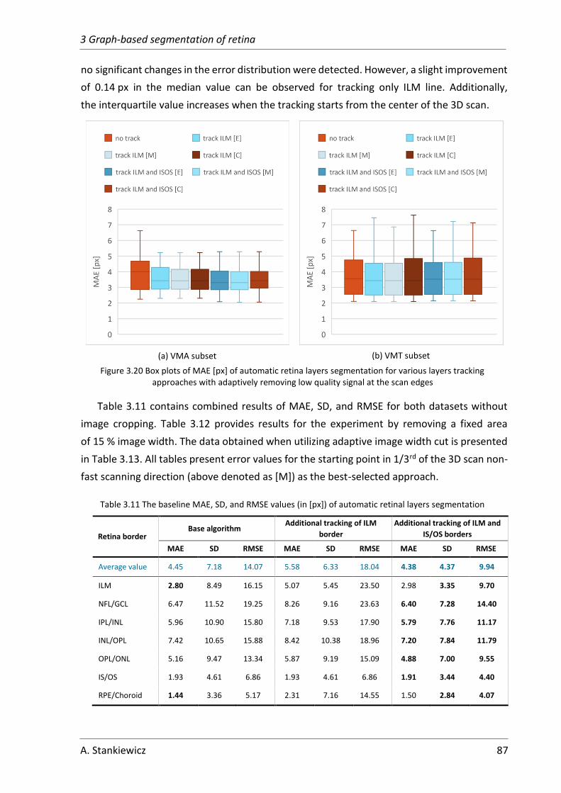
3 Graph-based segmentation of retina
A. Stankiewicz 87
no significant changes in the error distribution were detected. However, a slight improvement
of 0.14 px in the median value can be observed for tracking only ILM line. Additionally,
the interquartile value increases when the tracking starts from the center of the 3D scan.
(a) VMA subset
(b) VMT subset
Figure 3.20 Box plots of MAE [px] of automatic retina layers segmentation for various layers tracking approaches with adaptively removing low quality signal at the scan edges
Table 3.11 contains combined results of MAE, SD, and RMSE for both datasets without
image cropping. Table 3.12 provides results for the experiment by removing a fixed area
of 15 % image width. The data obtained when utilizing adaptive image width cut is presented
in Table 3.13. All tables present error values for the starting point in 1/3rd of the 3D scan non-
fast scanning direction (above denoted as [M]) as the best-selected approach.
Table 3.11 The baseline MAE, SD, and RMSE values (in [px]) of automatic retinal layers segmentation
Retina border Base algorithm
Additional tracking of ILM
border
Additional tracking of ILM and
IS/OS borders
MAE SD RMSE MAE SD RMSE MAE SD RMSE
Average value 4.45 7.18 14.07 5.58 6.33 18.04 4.38 4.37 9.94
ILM 2.80 8.49 16.15 5.07 5.45 23.50 2.98 3.35 9.70
NFL/GCL 6.47 11.52 19.25 8.26 9.16 23.63 6.40 7.28 14.40
IPL/INL 5.96 10.90 15.80 7.18 9.53 17.90 5.79 7.76 11.17
INL/OPL 7.42 10.65 15.88 8.42 10.38 18.96 7.20 7.84 11.79
OPL/ONL 5.16 9.47 13.34 5.87 9.19 15.09 4.88 7.00 9.55
IS/OS 1.93 4.61 6.86 1.93 4.61 6.86 1.91 3.44 4.40
RPE/Choroid 1.44 3.36 5.17 2.31 7.16 14.55 1.50 2.84 4.07
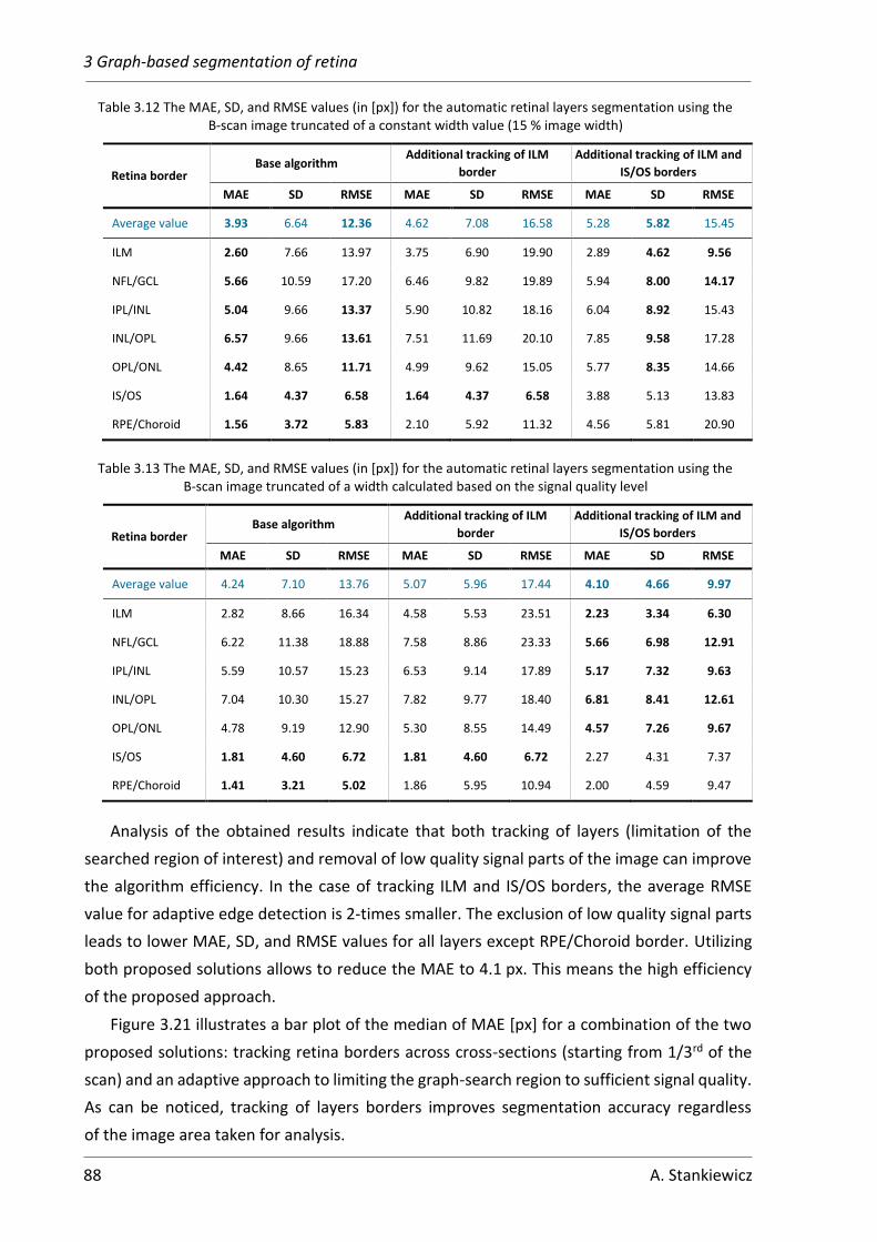
3 Graph-based segmentation of retina
88 A. Stankiewicz
Table 3.12 The MAE, SD, and RMSE values (in [px]) for the automatic retinal layers segmentation using the B-scan image truncated of a constant width value (15 % image width)
Retina border Base algorithm
Additional tracking of ILM
border
Additional tracking of ILM and
IS/OS borders
MAE SD RMSE MAE SD RMSE MAE SD RMSE
Average value 3.93 6.64 12.36 4.62 7.08 16.58 5.28 5.82 15.45
ILM 2.60 7.66 13.97 3.75 6.90 19.90 2.89 4.62 9.56
NFL/GCL 5.66 10.59 17.20 6.46 9.82 19.89 5.94 8.00 14.17
IPL/INL 5.04 9.66 13.37 5.90 10.82 18.16 6.04 8.92 15.43
INL/OPL 6.57 9.66 13.61 7.51 11.69 20.10 7.85 9.58 17.28
OPL/ONL 4.42 8.65 11.71 4.99 9.62 15.05 5.77 8.35 14.66
IS/OS 1.64 4.37 6.58 1.64 4.37 6.58 3.88 5.13 13.83
RPE/Choroid 1.56 3.72 5.83 2.10 5.92 11.32 4.56 5.81 20.90
Table 3.13 The MAE, SD, and RMSE values (in [px]) for the automatic retinal layers segmentation using the B-scan image truncated of a width calculated based on the signal quality level
Retina border Base algorithm
Additional tracking of ILM
border
Additional tracking of ILM and
IS/OS borders
MAE SD RMSE MAE SD RMSE MAE SD RMSE
Average value 4.24 7.10 13.76 5.07 5.96 17.44 4.10 4.66 9.97
ILM 2.82 8.66 16.34 4.58 5.53 23.51 2.23 3.34 6.30
NFL/GCL 6.22 11.38 18.88 7.58 8.86 23.33 5.66 6.98 12.91
IPL/INL 5.59 10.57 15.23 6.53 9.14 17.89 5.17 7.32 9.63
INL/OPL 7.04 10.30 15.27 7.82 9.77 18.40 6.81 8.41 12.61
OPL/ONL 4.78 9.19 12.90 5.30 8.55 14.49 4.57 7.26 9.67
IS/OS 1.81 4.60 6.72 1.81 4.60 6.72 2.27 4.31 7.37
RPE/Choroid 1.41 3.21 5.02 1.86 5.95 10.94 2.00 4.59 9.47
Analysis of the obtained results indicate that both tracking of layers (limitation of the
searched region of interest) and removal of low quality signal parts of the image can improve
the algorithm efficiency. In the case of tracking ILM and IS/OS borders, the average RMSE
value for adaptive edge detection is 2-times smaller. The exclusion of low quality signal parts
leads to lower MAE, SD, and RMSE values for all layers except RPE/Choroid border. Utilizing
both proposed solutions allows to reduce the MAE to 4.1 px. This means the high efficiency
of the proposed approach.
Figure 3.21 illustrates a bar plot of the median of MAE [px] for a combination of the two
proposed solutions: tracking retina borders across cross-sections (starting from 1/3rd of the
scan) and an adaptive approach to limiting the graph-search region to sufficient signal quality.
As can be noticed, tracking of layers borders improves segmentation accuracy regardless
of the image area taken for analysis.

3 Graph-based segmentation of retina
A. Stankiewicz 89
Figure 3.21 Bar plot of an average error for each variant of the automatic segmentation methods
Summary of the proposed methods for enhancement of retina layers segmentation from
OCT images
The experiments presented in this Chapter discussed the influence of OCT data quality
on the accuracy of retina layers segmentation with a graph-based method. To summarize,
the conducted experiments show that retina layers segmentation accuracy is affected by the
speckle noise and can be improved with propped selection of noise suppression in OCT image.
A comparison of results for the two investigated subsets (VMA and VMT) leads to the
following conclusions:
1) Noise reduction:
a. the best segmentation accuracy can be obtained with OCT noise suppression
with block-matching and collaborative filtering (BM4D); nevertheless,
this method requires the longest computational time and cannot be applied
directly in a clinical application
b. the WST method is a balanced solution to compromise the required time with
segmentation accuracy and image quality.
2) Removing low quality signal:
a. the conducted experiment confirm that low signal strength areas of the OCT
B-scans impede proper segmentation of retina layers.
b. the suggested solution of limiting graph search region to visible area of retina
tissue improves segmentation accuracy: the gain in MAE value is 14 % for both
VMA and VMT subsets.
c. despite higher computational requirements, the adaptive method allows
for better results than the easier method of removing parts of the image with
a constant width.
3.1
3.2
3.3
3.4
3.5
3.6
3.7
3.8
3.9
no track track ILM [M] track ILM and ISOS [M]
Med
ian
of
MA
E [p
x]
no cut cut 15% adaptive cut

3 Graph-based segmentation of retina
90 A. Stankiewicz
d. the distribution of the segmentation error for the VMA subset is better when
using adaptive width cut regardless of the tracking method, while for the VMT
subset both edge cutting methods improve segmentation (although
the combination of tracking both layers and using fixed image width cut
provided the best results)
3) Layers tracking:
a. tracking of ILM layers allows to lower the MAE values in the majority of the
cases, while tracking of both ILM and IS/OS borders provides better results than
only tracking ILM layer
b. setting the starting point for tracking at the edge of the scan (i.e., first cross-
section) is susceptible to error propagation stemming from low signal strength
in the peripheral area and diminishes the accuracy of the overall segmentation
c. for the VMA subset, the best results are obtained when the starting point
for tracking is set in the center of the scan, where the signal strength and layers
contrast is high, and no discontinuities of the layers in healthy tissue are
present
d. for the VMT subset, the best results are obtained for tracking from 1/3rd of the
scan (where the probability of tissue irregularities is low and the signal level
is sufficiently high); setting the starting point in the center of the scan
introduces error propagation due to irregularities and discontinuities of the
tissue.
The conducted experiments prove that the accurate analysis of low quality OCT images
is possible even when OCT signal quality is too low, and underexposure or the presence
of lesions requires adjustment of the graph-based algorithm. Furthermore, the proposed
adaptive solution improves the segmentation accuracy, which is the first and crucial step
for further calculations in medical diagnosis.

91
Chapter 4
4 Segmentation of preretinal space
with neural networks
In this Chapter, an algorithm for segmentation of preretinal space is presented. For this
purpose, the author utilized a convolutional neural network in a task of pixel-wise semantic
segmentation. Section 4.1 describes the proposed solution, an adaptation of five network
architectures for OCT data, and the training setup. Section 4.2 evaluates the selected network
architectures. A set of experiments presents the influence of two types of loss function and
four data augmentation techniques on the overall segmentation scores.
Section 4.3 discusses the problem of the incorrect topology of segmented classes that
results from similar intensities of the pixels in vitreous and preretinal space areas of the OCT
image. The author presents two solutions of incorporating either a Relative Distance Map
or a non-typical convolution kernel. Extensive experiments contained in this Section evaluate
their effect on improving topological correctness.
4.1 Employment of UNet-based neural networks for PCV
detection
4.1.1 Selection of network architecture
For the segmentation of the PCV line using a deep learning approach, the author utilized
a fully convolutional neural network based on the U-Net topology. The literature review
indicated five convolutional network architectures that gave promising results. They include
UNet, Attention UNet, ReLayNet, LFUNet, and DRUNet. These five networks were adapted
to the task of preretinal space segmentation. The processing pipeline of the proposed system
to obtain a segmentation of VRI structures from a single OCT image is presented in Figure 4.1.
The proposed framework learns correct preretinal space segmentation by separately
processing a cohort of 2D OCT cross-sections. The predicted probability maps produced by the
neural network are compared with the ground truth, and the resulting error (loss) is used
to update the network weights. The final binary segmentation maps are used to calculate
borders between the segmented image regions, namely the PCV, ILM, and RPE lines. During
the test phase, error metrics of Dice Coefficient (DC), Mean Absolute Error (MAE), and
Topology Incorrectness Index (TII) are computed.

4 Segmentation of preretinal space with neural networks
92 A. Stankiewicz
Figure 4.1 General scheme of the processing pipeline
Below is a short description of each tested architecture and its characteristics. Each
network was adapted for the preretinal space segmentation problem by defining the number
of output channels of multi-class classification as 4 separate retina structures aimed
to identify: vitreous, preretinal space, retina, and region below the retina. The input for each
network is a single channel (gray-scale) OCT image with 640×384 px resolution. Figures
located under the descriptions illustrate the architecture of each network model. Each blue
box represents a multi-channel feature map (the number of channels is denoted on top of the
box). The input size at each level is denoted on the left-hand side of the boxes. White boxes
denote feature maps copied from the encoder to the decoder part of the network. Legend
in the lower-left corner describes operations indicated with colored arrows. The most
promising topologies are:
• Baseline UNet – is an architecture proposed by [36] that obtains good accuracy in the
semantic segmentation of biomedical images. The detailed construction of the UNet
architecture was described in Section 2.3.4. The advantage of UNet is a skip
connection: i.e., the feature maps at the end of each encoder level are concatenated
to the upsampled decoder maps before being processed by the convolution blocks.
Such operation allows for preserving relevant information from the input features.
The final probability maps are obtained by applying a softmax activation function after
a final 1×1 px convolution operation in the decoder block that transforms the last
feature matrix into a segmentation mask for each class. Figure 4.2 presents a scheme
of this architecture (with 32 initial features).
Ground
truth
DC
Neural Network
Weights update
Input image
MAE
Loss
Predictions Segmentation lines
PCV
ILM
RPE
PCV ILM
RPE
Set of 3D scans
𝐼
𝐼
TII

4 Segmentation of preretinal space with neural networks
A. Stankiewicz 93
Figure 4.2 U-Net architecture employed for the preretinal space segmentation problem
• Attention UNet – An extension of the UNet architecture is the Attention UNet
proposed by [260]. It introduces attention gates to highlight any significant features
passed through the skip connection. Its advantage is maintaining a simple design while
decreasing model sensitivity to the background regions. The general design of this
network is similar to the baseline UNet, with five double 3×3 px convolution blocks
in the encoder and decoder paths. The attention module is applied to each encoding
result before concatenating to the decoder blocks. This grid-based gating mechanism
aims to minimize the influence of irrelevant or noisy features. The PyTorch
implementation of the Attention UNet network utilized in this experiment was
obtained from [261]. Figure 4.3 illustrates the adaptation of this network (with 32
initial features) to the task of preretinal space segmentation.
Figure 4.3 Attention Gates U-Net architecture employed for the preretinal space segmentation problem

4 Segmentation of preretinal space with neural networks
94 A. Stankiewicz
• ReLayNet [217] was the first CNN employed for the retina layer segmentation task.
It is based on UNet, but with fewer convolution layers in each encoder and decoder
block, a non-expanding number of features, and only 3 pooling/unpooling operations.
An addition to such simplified architecture is the Batch Normalization procedure
performed after each convolution and before the ReLU activation function.
The ReLayNet also differs from the baseline UNet with the kernel size used for each
convolution, which is 7×3 px instead of 3×3 px. As was reported in [217], this ensures
that the receptive field at the lowest level in the network covers the entire retina
depth. Figure 4.4 illustrates the adjustment of this network for the preretinal space
segmentation.
Figure 4.4 ReLayNet architecture employed for the preretinal space segmentation problem
• The LFUNet network architecture is a combination of UNet [36] and FCN [262] with
additional dilated convolutions [263]. In this network, the encoder part incorporates
the baseline UNet encoder (4 blocks of two convolution layers with kernel size 3×3 and
a 2×2 px max pooling layer with stride 2). The decoder part consists of two parallel
paths: the baseline UNet decoder and an adaptation of FCN. The FCN path performs
the addition of up-sampled feature blocks from the last encoder block with original
encoder blocks of the matching size. The upsampling in both paths is performed with
the 2×2 px up-convolution layer after each convolution block. The additional strength
of this network introduces the last part, which is a concatenation of final feature maps
obtained from both decoder paths. They are subsequently dilated with three separate
kernels, and the resulting matrices are again concatenated before final convolution.
The output probability map for each pixel belonging to one of 𝐶 classes was obtained
with the Softmax function. ReLu (Rectified Linear Unit) was used for all activation
functions in the hidden layers. Adaptation of this architecture (with 32 initial features)
to the preretinal space segmentation task is presented in Figure 4.5.

4 Segmentation of preretinal space with neural networks
A. Stankiewicz 95
Figure 4.5 LFUNet architecture employed for the preretinal space segmentation problem
• The DRUNET architecture [231] also comprises an encoder and decoder parts with
skip-connections. As with the ReLayNet, the pooling operations here are reduced to 3.
Incorporating residual blocks [227] in both parts is what gives this topology the
advantage. The contribution of the residual block is the addition of a residual feature
map (from the first map in each of the lower levels) after a 1×1 convolution layer.
Additionally, all blocks were constructed using dilated convolution layers, which allows
for a bigger field of view for this architecture. The dilation rate doubles from 1 to 4
in the encoder path. The features are transferred from the encoder to the decoder
sections with a residual block with a dilation rate of 8. In the decoder part, two residual
blocks with dilation rates of 4 and 2 are used. A standard block (without residual
connection) with a dilation rate of 1 is used at the last decoder level. A 1×1 convolution
layer with the number of filters equal to the segmented classes and a softmax
activation function produces the final probability outputs. In contrast to previous
networks, 16 initial features are sufficient here, and their number does not increase
with each level (similar to the ReLayNet). Figure 4.6 presents the adjustment of this
topology to the preretinal space segmentation task.
Based on the literature review, these five network architectures were selected as the most
promising for the preretinal space segmentation from the OCT images. Each of the topologies
has its strengths and individual characteristics likely to contribute to this task. A comparison
of their performance is described in the following Sections.
Although some networks (e.g., ReLayNet) were originally trained on image patches, this
approach cannot be applied to the considered task. Due to the PCV line not being sufficiently
visible throughout the scan or partially connected to the ILM line, using narrow patches could
mislead the network. In the proposed experiment, the input to each network is an entire

4 Segmentation of preretinal space with neural networks
96 A. Stankiewicz
B-scan with the resolution of 640×384 px (illustrated in the above Figures) to encourage
smoother layer surfaces across the image.
Figure 4.6 DRUNet architecture employed for the preretinal space segmentation problem
4.1.2 Training and evaluation setup
This Section describes the setup and parameters of the system for all segmentation
experiments conducted with DNN described above. The evaluation metrics used for
comparison are the Dice Coefficient and Mean Absolute Error described in Section 2.3.1.
Additionally, in the course of experiments, a new metric of Topology Incorrectness Index (TII)
(described in Section 4.3) was established to determine the topology correctness of the
segmented anatomical regions.
The goal of the segmentation task is to predict 4 separate areas in the image, further
described as a set of classes 𝐶 = {0: Vitreous, 1: Preretinal Space, 2: Retina, 3: Space
under Retina}. The task in a multi-class classification is to obtain the class-wise probabilities
of each pixel in the image. Then, after a SoftMax function, each pixel is assigned to the class
with the highest probability.
All neural networks described in this paper were implemented using Python 3.7 with
PyTorch 1.8.1 [264] and NVIDIA CUDA 11.2 libraries [265]. The experiments were conducted
on a 64-bit Ubuntu operating system with an Intel Core i7-7700K 4.20GHz computing
processor and 32 GB RAM. In addition, the NVIDIA GeForce GTX 1080 Ti GPU card with 11 GB
memory was used during training and evaluation.
The CAVRI dataset of 7050 images was randomly split into training, validation, and testing
subsets with the ratio of 80 %, 10 %, and 10 %, respectively. Each image, before processing,

4 Segmentation of preretinal space with neural networks
A. Stankiewicz 97
was subjected to a standard 𝑧 − score normalization [266]. The network weights were
learned with the images from the training set. At the end of each training epoch model's
accuracy and validation loss were calculated using the validation set. After a finished training,
the obtained network model was evaluated using the test set, which contains images
previously unseen by the network.
The PyTorch Lightning 1.3.5 library was used for experiments to implement training,
validation, and testing procedures. During training, the network weights were optimized using
an Adam optimizer [267] and the following parameters: learning rate 𝑙𝑟 = 5 ∙ 10−6, 𝛽1 =
0.9, 𝛽2 = 0.999. The batch size was set to one, due to the random cropping procedure used
for data augmentation (see Section 4.3), which produces images of various sizes. Every
network was trained for at least 50 epochs, and the training was stopped if the validation loss
did not decay for the last five epochs. Models were evaluated on the best checkpoint
determined with the lowest validation loss value. Although the original UNet, LFUNet, and
Attention UNet architectures have 64 channels in the first layer, these networks were
implemented with 32 initial feature vectors due to memory constraints. However, based
on the initial experiments, this change does not significantly impact model accuracy. Similarly,
no significant difference in performance for the DRUNet topology was observed when using
32 or 16 initial features; thus, the smaller number was selected.
During training, the progress of the learning process is ascertained at the end of every
epoch by calculating:
• accuracy (ACC) according to Equation (2.18),
• and loss value with one of the methods described in Section 4.2.1.
These two metrics are obtained for both the training and validation sets. The final model
evaluation was performed using the test set, and the metrics of:
• Dice Coefficient (DC) – computed for each of the segmented classes separately
(i.e., Vitreous, Preretinal Space, Retina, and Region below Retina) with Equation (2.16),
• Mean Absolute Error (MAE) with Standard Deviation (SD) – calculated using Equation
(2.13) for three lines (i.e., PCV, ILM, and RPE) separating the segmented regions.
4.2 Influence of training parameters on PCV segmentation
accuracy
A comprehensive set of experiments designed to measure the performance of various
deep neural networks employed to segment preretinal space from OCT images was
performed. This section presents the evaluation of the influence of loss function, data
augmentation, and network architecture on the model accuracy.

4 Segmentation of preretinal space with neural networks
98 A. Stankiewicz
4.2.1 Loss function
The specificity of retina layers segmentation in OCT images requires a comprehensive
evaluation of the experiment setup. This includes analysis of the parameters such as loss
function and its weights. Thus, the accuracy of segmentation with the most commonly used
loss functions is compared in this Section.
The author of the thesis tested the segmentation accuracy of the prediction 𝐼 for a ground
truth image 𝐼 using Weighted Categorical Cross-Entropy Loss (WCCE) 𝐿𝑊𝐶𝐶𝐸(𝐼, 𝐼) , and
Weighted Dice Loss (WDice) 𝐿𝑊𝐷𝑖𝑐𝑒(𝐼, 𝐼) which are extensions of loss functions described in
Section 2.3.4, as well as their weighted sum defined as a Combined Loss function 𝐿𝑡𝑜𝑡𝑎𝑙(𝐼, 𝐼).
The adaptation of WCCE Loss to the problem of preretinal space segmentation with
separate weights for each segmented region describes Equation (4.1):
𝐿𝑊𝐶𝐶𝐸(𝐼, 𝐼) = − ∑[1𝑛𝑐∑𝜔𝑐(𝑥, 𝑦) · 𝐼𝑐(𝑥, 𝑦) · log (𝐼𝑐(𝑥, 𝑦))𝑥,𝑦
]
𝑐∈𝐶
(4.1)
where 𝐼𝑐(𝑥, 𝑦) is a binary ground truth mask for class 𝑐 ∈ 𝐶 = {0, 1, 2, 3} (defined in Section
4.1.2) taking value 0 or 1 at each location (𝑥, 𝑦) , for 𝑥 ∈ 𝑋 = {1, . . . , 𝑤} and 𝑦 ∈ 𝑌 =
{1, . . . , ℎ}, where 𝑤 and ℎ denote the width and height of the image respectively; 𝐼𝑐(𝑥, 𝑦)
is the prediction probability of the pixel with indices 𝑥 and 𝑦 belonging to class 𝑐; 𝑛𝑐 is the
number of elements in a given class 𝑐; and 𝜔𝑐(𝑥, 𝑦) is an additional weight given to each pixel
based on its class and position within it.
In detail, the PCV line is frequently on the level of speckle noise, and because of OCT
characteristics, the region edges can be blurred. Hence, to boost the network’s sensitivity
to class boundaries, the pixels at the edges are given additional weight 𝑞1 . Additionally,
the pixels belonging to classes of interest (namely preretinal space and retina) are given
an additional weight 𝑞2 to adjust for their lower area in the image (as opposed to the
background). Equation (4.2) describes the overall pixel weight calculation:
𝜔𝑐(𝑥, 𝑦) = 1 + 𝑞1 ∙ 𝑓(|∇𝑦𝐼𝑐(𝑥, 𝑦)| > 0) + 𝑞2 ∙ 𝑓(𝐼𝑐(𝑥, 𝑦)|𝑐=1,2) (4.2)
where 𝑓(∗) is an indicator function taking the value of 1 if the (∗) is true, and else 0. The ∇𝑦
operator represents the vertical gradient. The weights 𝑞1 = 10 and 𝑞2 = 5 are chosen
experimentally. The utilized loss function is implemented as proposed in the referenced and
compared methods [217], [229] to sustain consistency between each network architecture.
Figure 4.7 illustrates a visualization of the weights calculated for an example of an OCT
image and its ground truth data. Colors in the ground truth represent the assignment of each
pixel to a given class (black – Vitreous, dark gray – Preretinal Space, light gray – Retina, and
white – Region below Retina). For the 4 selected classes, the weighing scheme associates the
value of 1 to the background regions (both the Vitreous and the Region below the Retina) and

4 Segmentation of preretinal space with neural networks
A. Stankiewicz 99
5 for the classes of interests (i.e., Preretinal Space and Retina). The borders between classes
have a weight of 10. The colors in the weight map denote the weight value for a given pixel.
The plot on the right visualizes a cross-section of the weight map through the middle (192nd
column for an image of 640×384 px resolution).
Original Image Ground truth 𝐼 Weights map 𝜔
Central cross-section
of the weights map
𝜔(: ,192)
Figure 4.7 Visualization of the pixel-wise weight components for the cross-entropy loss.
The second loss function is computed based on a Dice coefficient (2.16). The Dice
Coefficient utilized to measure the overlap of regions belonging to a given class 𝑐 describes
the adapted Equation (4.3):
𝐷𝑖𝑐𝑒𝑐 =2|𝐼𝑐 ∩ 𝐼𝑐|
|𝐼𝑐| + |𝐼𝑐| (4.3)
where |∗| denotes a sum of pixels in the corresponding mask of ground-truth 𝐼𝑐 and
prediction 𝐼𝑐 for a class 𝑐.
Consequently, the Dice loss 𝐿𝐷𝑖𝑐𝑒 takes into account the Dice Coefficient for all of the
classes. It is expressed as follows:
𝐿𝐷𝑖𝑐𝑒(𝐼, 𝐼) = 1 −∑ 𝜆𝑐𝐷𝑖𝑐𝑒𝑐(𝐼𝑐, 𝐼𝑐)𝑐∈𝐶
(4.4)
where 𝜆𝑐 is a weight assigned to each class to compensate for their imbalance within the set.
Numeric analysis of all of the pixels in the dataset belonging to each class shows that the
preretinal space is the most underrepresented class, while the background (vitreous region
and the region below the retina) spans the largest area in each volume. The weights 𝜆𝑐
presented in Table 4.1 are calculated for each class using the following formula:
𝜆𝑐 =
1𝑛𝑐
∑1𝑛𝑐𝑐
(4.5)

4 Segmentation of preretinal space with neural networks
100 A. Stankiewicz
where 𝑛𝑐 is the number of pixels belonging to class 𝑐 for all 𝑐 ∈ 𝐶. All weights sum up to 1,
giving a Dice loss equal to 0 for all classes with a maximum Dice Coefficient, according
to Equation (4.4).
Table 4.1 Loss weights 𝜆𝑐 for each segmented class
Class 0: Vitreous 1: Preretinal Space 2: Retina 3: Region below Retina
Loss weight 0.1 0.5 0.29 0.11
The overall loss function 𝐿𝑡𝑜𝑡𝑎𝑙(𝐼, 𝐼) , being a weighted sum of the above-described
formulas, is calculated as follows:
𝐿𝑡𝑜𝑡𝑎𝑙(𝐼, 𝐼) = 𝛼𝐿𝐶𝐸(𝐼, 𝐼) + 𝛽𝐿𝐷𝑖𝑐𝑒(𝐼, 𝐼) (4.6)
where 𝛼 ∈ ⟨0,1⟩ and 𝛽 ∈ ⟨0,1⟩ are the weights assigned to each loss component.
The parameters for pixel-wise weight in Equation (4.2) are 𝑞1 = 10 and 𝑞2 = 5.
Segmentation results – comparison of various loss functions
This subsection presents a quantitative comparison of preretinal space segmentation with
a UNet architecture using various combinations of the above-described loss functions. Next,
the performance of five DNN networks described in Section 4.1 was tested with the most
promising loss function.
To evaluate which loss function would be the best for the defined task, the author of the
thesis trained a basic UNet network using various loss functions according to Equation (4.6):
• Weighted Categorical Cross-Entropy Loss (i.e., 𝛼 = 1, 𝛽 = 0) only,
• Weighted Dice Loss (i.e., 𝛼 = 0, 𝛽 = 1) only,
• Combined Loss with equal weights for CCE and Dice Loss (i.e., 𝛼 = 1, 𝛽 = 1),
• Combined Loss favoring CCE Loss (i.e., 𝛼 = 1, 𝛽 = 0.5),
• Combined Loss favoring Dice Loss (i.e., 𝛼 = 0.5, 𝛽 = 1).
Figure 4.8 presents the accuracy and loss values used to evaluate the training process.
As can be seen in the plots, the accuracy in both the training (Figure 4.8a) and the validation
(Figure 4.8c) phases increases rapidly from 0 in the initial epochs. It saturates at 0.995 for the
40th epoch for both training and validation. The growth rate is similar for all losses, although
the accuracy using only Dice Loss and only CE Loss increases more slowly than the others.
The quickest accuracy growth is obtained with Combined Loss with weights 𝛼 = 0.5, 𝛽 = 1,
although at the end of the training best validation accuracy is obtained with Combined Loss
with weights 𝛼 = 1, 𝛽 = 0.5 (0.997).

4 Segmentation of preretinal space with neural networks
A. Stankiewicz 101
(a) training accuracy
(b) training loss
(c) validation accuracy
(d) validation loss
Figure 4.8 Plots of accuracy and loss for training and validation subsets comparing various tested loss functions
The loss values (Figure 4.8b and Figure 4.8d) represent the loss calculated with each
described method. As the combined loss is a sum of both CE and Dice loss, its value is greater
than each of them separately, and the final values cannot be compared directly. Nevertheless,
all loss values decrease in each epoch (i.e., the network learns valuable information), and after
50 epochs reach the value of 0.04 for the Dice Loss and 0.085 for the CE Loss.
Table 4.2 contains the test results obtained for this experiment. They indicate that the
best accuracy can be obtained with the Combined Loss with the weights of 𝛼 = 1 (for WCCE
Loss) and 𝛽 = 0.5 (for WDice Loss). Only the MAE value for the PCV line gave a better result
with a Combined Loss favoring the Dice component. The lowest accuracy values for the
Preretinal Space (both Dice Coefficient and the PCV MAE) were obtained using WCCE Loss
only. Other image regions received the lowest scores when utilizing only Weighted Dice Loss.
Therefore, both methods can be considered beneficial for maintaining good accuracy of both
Retina and Preretinal Space regions segmentation. Based on the above, the Combined Loss
with weight values of 𝛼 = 1 and 𝛽 = 0.5 were chosen for all further experiments.
It should also be noted that the Dice Coefficients of Vitreous, Retina, and Region below
Retina are close to or above 0.99 regardless of the loss function used. The significant influence
can be observed only for the Preretinal Space scores and PCV line, for which the best loss
combination gives an improvement of 3.7 %.
0.9
0.92
0.94
0.96
0.98
1
0 5 10 15 20 25 30 35 40 45 50
Acc
ura
cy
Epoch
WCCE WDice Cb (equal)
Cb (+WCCE) Cb (+Wdice)
0
0.5
1
1.5
0 5 10 15 20 25 30 35 40 45 50
Loss
Epochs
WCCE WDice Cb (equal)
Cb (+WCCE) Cb (+Wdice)
0.920.930.940.950.960.970.980.99
1
0 5 10 15 20 25 30 35 40 45 50
Acc
ura
cy
Epochs
WCCE WDice Cb (equal)
Cb (+WCCE) Cb (+Wdice)
0
0.2
0.4
0.6
0.8
0 5 10 15 20 25 30 35 40 45 50
Loss
Epochs
WCCE WDice Cb (equal)
Cb (+WCCE) Cb (+Wdice)

4 Segmentation of preretinal space with neural networks
102 A. Stankiewicz
Table 4.2 Dice Coefficient and Mean Absolute Error results of 4-class segmentation with UNet using various loss functions and weights
Loss
Dice Coefficient MAE [px]
Vitreous Preretinal
space Retina
Region
b. Retina PCV ILM RPE
Weighted Cross Entropy 0.9921 0.9089 0.9927 0.9976 10.40 0.57 0.78
Weighted Dice 0.9895 0.9431 0.9913 0.9956 2.67 0.66 1.04
Weighted Combined Loss (α=1, β=1) 0.9928 0.9386 0.9919 0.9968 2.73 0.60 0.91
Weighted Combined Loss (α=0.5, β=1) 0.9924 0.9403 0.9921 0.9967 2.52 0.61 0.85
Weighted Combined Loss (α=1, β=0.5) 0.9942 0.9458 0.9929 0.9976 2.83 0.56 0.75
Segmentation results – comparison of various network architectures
The next experiment was designed to compare the performance of the five selected neural
network architectures. All five topologies are trained with the same parameters (e.g., learning
rate, loss function, number of epochs). Figure 4.9 illustrates the learning process of the five
networks.
(a) training accuracy
(b) training loss
(c) validation accuracy
(d) validation loss
Figure 4.9 Plots of accuracy and loss for training and validation subsets showing performance of various network architectures with the same parameters
The training accuracy (Figure 4.9a) and loss (Figure 4.9b) are computed at the end of each
epoch on the training set. As can be noticed the models gain accuracy of over 0.99 at the end
of the training. The lowest value of 0.994 obtains ReLayNet, and the Attention UNet reaches
0.94
0.95
0.96
0.97
0.98
0.99
1
0 5 10 15 20 25 30 35 40 45 50
Acc
ura
cy
Epochs
UNet LFUNet AttUNet
ReLayNet DRUNet
0
0.2
0.4
0.6
0.8
1
0 5 10 15 20 25 30 35 40 45 50
Loss
Epochs
UNet LFUNet AttUNet
ReLayNet DRUNet
0.9
0.92
0.94
0.96
0.98
1
0 5 10 15 20 25 30 35 40 45 50
Acc
ura
cy
Epochs
UNet LFUNet AttUNet
ReLayNet DRUNet
0
0.2
0.4
0.6
0.8
1
0 5 10 15 20 25 30 35 40 45 50
Loss
Epochs
UNet LFUNet AttUNet
ReLayNet DRUNet

4 Segmentation of preretinal space with neural networks
A. Stankiewicz 103
the best accuracy of close to 1. Similarly, the training loss drops to 0.12 for all networks except
the Attention UNet, which achieved a training loss of 0.03.
On the other hand, when analyzing the validation plots of accuracy (Figure 4.9c) and loss
(Figure 4.9d), it is apparent that both Attention UNet and ReLayNet have not learned
to generalize. After reaching a loss value of around 0.25 and 0.4, respectively, their loss
increases and appears to have a random component. Furthermore, the rest of the models did
not show the signs of overfitting – their loss steadily decreased and retained lower values.
These models obtained much lower validation loss at the end of the training: 0.11 for UNet,
0.12 for LFUNet, and 0.18 for DRUNet.
Table 4.3 presents baseline results of DC and MAE scores obtained utilizing various
network architectures and the best Loss function determined in the previous experiment.
In addition, Table 4.3 includes the results of a graph-based approach employed for this task
as an extension of the method described in Chapter 3. Here, the graph search was conducted
to directly find three segmentation layers (i.e., PCV, ILM, and RPE), for which the MAE results
were performed in a straightforward fashion using Equation (2.13). As the obtained lines
separate regions searched with semantic pixel-wise segmentation, these regions were used
to calculate the corresponding Dice Coefficients. The graph-search algorithm was
implemented in the Matlab/Simulink environment [257] on a 64-bit PC with Windows 10
operating system, Intel Core i7-3770 3.40 GHz processor, and 8 GB RAM.
Table 4.3 The baseline Dice Coefficient and Mean Absolute Error (with Standard Deviation) results of 4 class pixel segmentation with various neural network models
Model
Dice Coefficient MAE (SD) [px]
Vitreous Preretinal
space Retina
Region
b. Retina PCV ILM RPE
Graph-search 0.9842 0.8217 0.9385 0.9888 7.29 (13.7) 5.10 (12.1) 5.20 (15.5)
UNet 0.9942 0.9458 0.9929 0.9976 2.83 (6.05) 0.56 (0.14) 0.75 (0.35)
LFUNet 0.9928 0.9337 0.9922 0.9972 3.11 (5.72) 0.60 (0.18) 0.84 (0.46)
Attention UNet 0.9822 0.8679 0.9918 0.9953 5.40 (10.04) 0.63 (0.77) 0.87 (1.11)
ReLayNet 0.9529 0.7827 0.9906 0.9814 25.66 (26.34) 0.84 (1.30) 1.45 (1.77)
DRUNet 0.9923 0.9184 0.9891 0.9972 4.23 (10.20) 0.80 (1.19) 1.13 (0.93)
The Dice Coefficient and MAE (SD) metrics show that all neural networks perform better
than the graph-based method. It should be noted that when utilizing graph search, the MAE
value is over 5 px for both retina borders, while for all CNNs, this value varies between 0.5 and
1.5 px. From the CNNs, the UNet has the best performance in all segmented areas and
borders, with 94.58 % Preretinal Space classification correctness and MAE for PCV line
of 2.8 px. Furthermore, the ReLayNet gives the worst results (78.27 % DC for the Preretinal
Space and MAE of 25.66 px for PCV), which may be explained by a relatively lower number
of features compared to other architectures.

4 Segmentation of preretinal space with neural networks
104 A. Stankiewicz
In general, the preretinal space boundary of PCV and the image classes it separates (i.e.,
Vitreous and Preretinal Space) have worse accuracy than the clearly defined ILM and RPE
borders and the two image regions they define. This confirms the difficulty of determining
preretinal space boundary due to similar pixel intensities of this region to the vitreous part.
4.2.2 Data augmentation
This Section describes data augmentation (DA) techniques utilized in this research
to improve the model's ability to generalize and increase the overall segmentation accuracy.
Thanks to this, the number of the image examples in the training subset expanded artificially
with each technique while maintaining the data characteristics that may occur naturally.
The following 2D transformations from those introduced in Section 2.3.5 were used:
• Horizontal Flip – allows obtaining a mirrored image which coincides with having a scan
of the other eye (left for right and right for left), preserving the morphology of retinal
structures (such as vessels and layers topology).
• Rotation – slight variations in retina orientation are natural when acquiring an OCT scan.
Thus, training the model with randomly rotated examples allows it to anticipate various
retina orientation angles. To determine the range of feasible rotations, the author
performed a statistical analysis of the retina orientation distribution within the CAVRI
dataset (see Figure 4.10). The obtained results indicate similar distribution for all subsets
(within ±25°). Therefore, an angle span of ±20° was selected for a random rotation.
Figure 4.10 Circular distributions of retina orientations in each subset of the CAVRI dataset [268]
• Vertical Translation – automatic acquisition protocol in an OCT device aims to focus
the device's optics on the retina and place it in the center of the scan. Therefore,
a statistical analysis of the retina position within the image was performed to determine
the retina vertical position distribution. For that purpose, the center of mass in each
image was estimated. The obtained positions were plotted within the image dimensions
range, as illustrated in Figure 4.11. As can be seen, each subset maintains a similar
distribution, confirming the appropriate dissemination of samples between the subsets.
Based on the gathered information, the range of vertical translation of the image was
set to ±10 % of the image height, equal to ±64 px.

4 Segmentation of preretinal space with neural networks
A. Stankiewicz 105
Figure 4.11 Distribution of center of mass of images. Blue dots represent the calculated position of the center of mass for each OCTcross-section. The Red ’+’ sign denotes the mean center of mass, and the red ellipsis encapsulates the 2.5 standard deviations of the data. The data is presented on the plane with resolutions
equal to the OCT cross-sections [268]
• Random Crop – performing an augmentation technique of random cropping allows
to improve the robustness of the network regardless of image size or the ratio of fovea
width to the image width. In the following experiments, a crop with randomly selected
values for both width and height was employed (within the range of 80 – 100 % of the
original values).
Utilization of such data augmentation techniques allowed to increase the number
of training examples, as shown in Table 4.4.
Table 4.4 Number of images used for the training and evaluation [268]
CAVRI Dataset Training Validation Testing
Baseline images 5608 721 721
After removing 3 % of anomalies [268] 5434 701 703
After removing 3 % of anomalies and adding DA 27170 701 703
Figure 4.12 illustrates the application of the selected data augmentation techniques
on examples of OCT images from the CAVRI database.

4 Segmentation of preretinal space with neural networks
106 A. Stankiewicz
Original Image Horizontal flip Random rotation Random translation Random crop
Figure 4.12 Example B-scans and their transformations with selected data augmentation techniques
Segmentation results – effect of various data augmentation techniques
The following experiment was set up to test the influence of data augmentation
on training the neural network model. Utilizing only basic UNet architecture, the author
tested expanding the training subset with:
• each data augmentation technique separately (4 tests, 10 868 training examples),
• two techniques (6 test combinations, 16 302 training examples),
• three techniques (4 test combinations, 21 736 training examples),
• all techniques (27 170 training examples).

4 Segmentation of preretinal space with neural networks
A. Stankiewicz 107
Table 4.5 presents the results of DC, and MAE (with SD) obtained on the test subset.
The values are grouped according to the number of images used for the training (i.e., the
number of data augmentation techniques used).
Table 4.5 Dice Coefficient and Mean Absolute Error (with Standard Deviation) results of 4 class segmentation with baseline UNet using various data augmentation techniques (best values in a given category are in bold)
Model
Dice Coefficient MAE (SD) [px]
Vitreous Preretinal
space Retina
Region
b. Retina PCV ILM RPE
No augmentation 0.9954 0.9486 0.9931 0.9978 2.19 (4.55) 0.54 (0.17) 0.73 (0.36)
Flip 0.9958 0.9471 0.9929 0.9978 2.72 (6.17) 0.59 (0.49) 0.77 (0.50)
Rotation 0.9964 0.9560 0.9939 0.9982 1.69 (3.69) 0.50 (0.13) 0.64 (0.26)
Translation 0.9961 0.9524 0.9937 0.9981 2.24 (5.44) 0.51 (0.13) 0.65 (0.28)
Crop 0.9957 0.9483 0.9937 0.9980 3.32 (6.89) 0.57 (0.71) 0.67 (0.61)
Flip + Rotation 0.9963 0.9541 0.9938 0.9982 2.53 (7.03) 0.52 (0.30) 0.65 (0.34)
Flip + Translation 0.9965 0.9555 0.9940 0.9982 2.31 (5.21) 0.50 (0.13) 0.62 (0.28)
Flip + Crop 0.9966 0.9578 0.9941 0.9983 1.48 (2.93) 0.51 (0.38) 0.62 (0.40)
Rotation + Translation 0.9965 0.9567 0.9940 0.9982 1.83 (3.83) 0.49 (0.12) 0.62 (0.26)
Rotation + Crop 0.9964 0.9558 0.9940 0.9982 1.91 (4.49) 0.50 (0.22) 0.62 (0.30)
Translation + Crop 0.9964 0.9576 0.9940 0.9982 1.73 (4.19) 0.52 (0.71) 0.64 (0.65)
Flip + Rot. + Trans. 0.9967 0.9573 0.9942 0.9982 1.99 (5.18) 0.50 (0.23) 0.61 (0.31)
Flip + Rot. + Crop 0.9968 0.9575 0.9941 0.9983 1.62 (3.32) 0.50 (0.19) 0.61 (0.28)
Flip + Trans. + Crop 0.9967 0.9569 0.9943 0.9982 1.98 (4.87) 0.49 (0.32) 0.58 (0.32)
Rot. + Trans. + Crop 0.9964 0.9584 0.9942 0.9983 1.68 (4.07) 0.49 (0.22) 0.60 (0.32)
Flip + Rot. + Trans. + Crop 0.9968 0.9591 0.9944 0.9984 1.33 (2.88) 0.50 (0.28) 0.57 (0.29)
Although it might be expected that utilizing any data augmentation technique improves
model performance, as can be seen in Table 4.5, only in the case of adding Rotation of the
input image that supposition holds true (all DC values were increased by up to 0.74 % and
MAE values were decreased by up to 0.5 px). This supports the observation that angle setting
for each patient is an individual parameter that can change even between examinations.
Moreover, the Cropping of the image lowered the segmentation accuracy of the preretinal
space (DC dropped by 0.03 %, and MAE value for PCV increased by 1.13 px), and the Flipping
of the image degraded all metrics except the Dice Coefficient of the background regions.
When implementing two data augmentation techniques, thus tripling the number
of training examples, a combination of Flipping and Cropping provided the best results for all
metrics (improvement of 0.92 % DC for Preretinal Space and 0.71 px MAE for PCV).
An exception is the MAE value for ILM and RPE lines (here, a combination of Rotation and
Translation improved the MAE value to 0.49 px).
By combining three data augmentation techniques, the results are of similar
improvement. Their differences are up to 0.15 % of DC and 0.37 px of MAE value. Thus,

4 Segmentation of preretinal space with neural networks
108 A. Stankiewicz
no best approach was ascertained here. Nevertheless, combining all 4 methods provided the
best results and improved the classification of Preretinal Space to 95.91 % and lowered
the MAE value for the PCV line to 1.33 px (and to 0.5 px for ILM and 0.57 px for RPE lines).
No significant improvement for other classes was observed, as they are all above 99.44 %
correctly segmented.
Segmentation results – effect of data augmentation for various CNNs
Following the results of the above experiment, the author tested the influence of applying
all data augmentation methods (i.e., horizontal flip, random rotation, random translation,
and random cropping) on the performance of the selected five neural network architectures.
Figure 4.13 presents training and validation metrics obtained during this analysis.
(a) training accuracy
(b) training loss
(c) validation accuracy
(d) validation loss
Figure 4.13 Plots of accuracy and loss for training and validation subsets showing training performance of various network architectures when utilizing all data augmentation techniques
Plots presented in Figure 4.13a show that the training accuracy reaches 98 % after only 2
epochs when without data augmentation, at least 7 epochs were needed (see Figure 4.9a).
Although training loss in Figure 4.13b obtains a value similar to before (Figure 4.9b), and the
Attention UNet being the best architecture (with training loss of 0.05), here LFUNet and
baseline UNet have a lower value (0.075), while training loss of ReLayNet and DRUNet
saturate at the level of 0.1.
0.97
0.975
0.98
0.985
0.99
0.995
1
0 5 10 15 20 25 30 35 40 45 50
Acc
ura
cy
Epochs
UNet LFUNet AttUNet
ReLayNet DRUNet
0
0.1
0.2
0.3
0.4
0 5 10 15 20 25 30 35 40 45 50
Loss
Epochs
UNet LFUNet AttUNet
ReLayNet DRUNet
0.97
0.98
0.99
1
0 5 10 15 20 25 30 35 40 45 50
Acc
ura
cy
Epochs
UNet LFUNet AttUNet
ReLayNet DRUNet
0
0.2
0.4
0.6
0.8
1
0 5 10 15 20 25 30 35 40 45 50
Loss
Epochs
UNet LFUNet AttUNet
ReLayNet DRUNet

4 Segmentation of preretinal space with neural networks
A. Stankiewicz 109
Plots in Figure 4.13c show that for validation accuracy, the saturation level of values close
to 1 (only ReLayNet and Attention UNet has a lower value of 0.98 and 0.993, respectively) are
achieved for earlier epochs. The validation loss (Figure 4.13d) has greater values than the
training loss, as can be expected. Similarly, as for previous measures, the final values at the
50th epoch are lower (0.09 for LFUNet and 0.16 for DRUNet) when compared to the
experiment without utilized data augmentation (0.12 and 0.21 for LFUNet and DRUNet,
respectively, in Figure 4.9d). Here also, an overtraining of ReLayNet and Attention UNet can
be observed.
By comparing plots from Figure 4.13 and Figure 4.9, a conclusion can be made that
by adding data augmentation, it is possible to train the network using a smaller number
of epochs with lower validation loss.
Table 4.6 shows the effect of applying models trained with data augmentation on the
testing set. Since the graph-based approach is not a machine learning method (data
augmentation is not applicable here), it was excluded from the comparison.
Table 4.6 Dice Coefficient and Mean Absolute Error (with Standard Deviation) results of 4 class pixel segmentation with various neural networks using 4 data augmentation techniques
Model
Dice Coefficient MAE (SD) [px]
Vitreous Preretinal
space Retina
Region
b. Retina PCV ILM RPE
UNet 0.9968 0.9591 0.9944 0.9984 1.33 (2.88) 0.50 (0.28) 0.57 (0.29)
LFUNet 0.9973 0.9590 0.9942 0.9985 1.50 (3.53) 0.50 (0.12) 0.57 (0.24)
Attention UNet 0.9850 0.8802 0.9926 0.9956 4.02 (6.54) 0.60 (0.26) 0.80 (0.73)
ReLayNet 0.9603 0.8015 0.9918 0.9859 12.63 (13.84) 0.71 (0.59) 0.96 (0.88)
DRUNet 0.9951 0.9370 0.9916 0.9978 2.35 (3.76) 0.62 (0.23) 1.09 (1.58)
As can be expected, adding more varying images helps train the network. This strategy
boosts the segmentation outcome in all of the methods. The MAE value of the PCV line is two
times smaller compared to the data in Table 4.3 (for all methods). Slight improvement in MAE
value for ILM and RPE lines can be observed (of 0.1 px and 0.2 px, respectively). The Dice
Coefficient for the Preretinal Space class has improved from 1.5 % for the UNet, and up to
2.5 % for LFUNet architecture (compared to Table 4.3). The Dice Coefficients for other classes
remained at a similar level of over 99.44 – 99.85 %. The ReLayNet and Attention UNet obtain
poor results of both DC (80.15 % and 88.02 % for Preretinal Space, respectively) and MAE
(12.69 px and 4.02 px for PCV).
Figure 4.14 illustrates the improvement in DC distribution for the Preretinal Space class
after utilizing the data augmentation technique. From the box plots can be deduced that not
only the average value has increased (presented in Table 4.6), but the overall performance
was also improved. This conclusion is based on a visibly narrower interquartile range (IQR)

4 Segmentation of preretinal space with neural networks
110 A. Stankiewicz
and a higher minimum score for all tested network architectures. The biggest improvement
is observed for the LFUNet (increase in minimum value by 7.6 % and 2.8 % in IQR).
(a) without data augmentation
(b) with data augmentation
Figure 4.14 Box plots for Dice Coefficient of Preretinal Space for various neural network architectures
Figure 4.15 presents examples of the obtained segmentation masks. Examples shown
in Figure 4.15 include a set of representative cases of VMT and VMA and illustrate a qualitative
comparison of the obtained results. It includes 2 VMA cases (rows 1 and 2), 2 VMT cases with
perifoveal vitreous detachment (examples 3 and 4), and 1 VMA case of slight detachment over
a wide area (last row).
Standard UNet architecture and LFUNet provide the best probability maps, although UNet
has slightly better performance in segmenting preretinal space, retinal area, and PCV border.
In the presented images, it is visible that poor evaluation scores from Table 4.6 for ReLayNet
and Attention UNet are the effect of the network's difficulty in discerning the areas with
similar intensities (namely: Vitreous, Preretinal Space, and Region below the Retina).
As an effect, patches of those classes appear in incorrect places in the prediction masks. Such
occurrences are less common with UNet and LFUNet; nevertheless, those architectures are
not immune to them, and further improvements are necessary.
The UNet and LFUNet correctly learn the preretinal and retinal borders (regardless of the
PCV intensity in the image). Their results are a significant improvement over the graph-based
method. For both VMT and VMA cases, these networks perform very well visually.
Furthermore, the placement of preretinal space in the image or the area it spans does not
affect their accuracy.

4 Segmentation of preretinal space with neural networks
A. Stankiewicz 111
OCT Image Ground truth Graph search UNet Attention
UNet LFUNet ReLayNet DRUNet
Figure 4.15 Example B-scans with corresponding reference mask and segmentation results for analyzed neural networks and a graph-based method. Each shade in the segmentation mask represents a separate class.
The neural network learns smoother region borders than the graph-search (dependent
on image intensity gradient). Since it is not affected by local intensity variations -- it can
robustly generalize the preretinal space structure. Moreover, the graph-based approach has
difficulty correctly detecting the PCV border where it connects with the ILM line. This
is a disadvantage compared to the neural network methods that do not present such
hindering.
In cases when the preretinal space takes a narrow area of the image (e.g., last row in Figure
4.15), a slight thickening of preretinal space in the prediction mask (e.g., region border 1 px
higher) would significantly affect the DC value (e.g., decreasing it by half). Such a result may

4 Segmentation of preretinal space with neural networks
112 A. Stankiewicz
lead to the assumption that the designed network is not performing well. Thus, the MAE value
(relatively small in such a case) should also be considered.
When comparing the performance of various network architectures, not only their
accuracy should be taken into account, but also their computational complexity and time
needed for evaluation. Table 4.7 presents the training and prediction time for the tested
networks and the number of their trainable parameters.
Table 4.7 Comparison of complexity and average time consumption of the evaluated DNN models
Model
No. of
parameters
[×106]
Training time
without DA
(50 epochs) [h]
Training time
with DA
(50 epochs) [h]
Prediction time
(3D scan of 141 B-scans) [s]
excluded
image loading
included
image loading
UNet 7.8 4.17 18.33 0.26 6.33
LFUNet 8.1 9.58 29.58 0.32 6.98
Attention UNet 9.4 7.92 34.38 0.47 6.97
ReLayNet 28.3 6.67 27.92 0.19 6.52
DRUNet 0.88 2.92 12.50 0.29 5.46
From the data presented in Table 4.6 and Table 4.7, it can be noticed that both ReLayNet
and Attention UNet, despite having a greater number of network features, do not obtain
correct segmentations. UNet and LFUNet, having around 8 million parameters, obtain similar
accuracy results, with UNet being slightly better (0.17 px lower MAE for PCV line).
Interestingly, the DRUNet architecture, despite having a significantly lower number
of parameters (9 times less than UNet and LFUNet), obtains only a 2.2 % lower DC for
classification of Preretinal Space and 1 px higher MAE of PCV. Furthermore, DRUNet produces
good quality maps with only some imperfections near borders and singular pixel patches
of the incorrect class (see Figure 4.15).
Thanks to incorporating specialized equipment like the NVIDIA GeForce GTX 1080 Ti
GPGPU card for fast image processing, the total prediction time for a 3D OCT scan (including
loading scan to memory) is from about 5.6 s for DRUNet, up to almost 7 s for LFUNet. This
is an acceptable time consumption for a clinical application.
4.3 Improving correctness of layers topology
4.3.1 Problem formulation
The disadvantage of pixel classification is the difficulty of the network to capture high-level
information about the problem, such as the fact that the retina layers have strict topological
order, and no pixel from the upper retinal layer can be classified as part of the layers located
below and vice versa. Figure 4.16 illustrates such topologically incorrect classification.

4 Segmentation of preretinal space with neural networks
A. Stankiewicz 113
Image Ground truth Segmentation result
Exam
ple
1
Exam
ple
2
Figure 4.16 Two examples of topologically incorrect segmentation of OCT retina image using baseline UNet architecture. Each color in the ground truth and segmentation map represent a different class (from the
darkest: Vitreous, Preretinal Space, Retina, Region below Retina).
This problem is prevalent for the tasks where pixels from different classes have similar
spatial characteristics (e.g., intensity, gradient). Although the most recent approaches are
focused on ensuring the correct topology of retina layers during segmentation [269], [270],
they tend to increase the system's complexity.
To analyze the prevalence of this problem within the CAVRI dataset, the author introduced
Topology Incorrectness Index (TII). This metric indicates the percentage of tested images with
incorrect layers topology in the vertical direction. It is computed based on a vertical gradient
of the predicted segmentation mask. The author tested the segmentation masks obtained
with the best models from the previous experiment (with data augmentation, see Section
4.2.2). The results are presented in Table 4.8.

4 Segmentation of preretinal space with neural networks
114 A. Stankiewicz
Table 4.8 Topology incorrectness index (TII) of OCT segmentation using data augmentation
Model DC for
Preretinal Space
MAE (SD)
for PCV TII [%]
No. of
parameters
UNet 0.9591 1.33 (2.88) 15.08 7.8 M
LFUNet 0.9590 1.50 (3.53) 11.52 8.1 M
DRUNet 0.9370 2.35 (3.76) 30.30 3.4 M
Attention UNet 0.8802 4.02 (6.54) 44.95 9.4 M
ReLayNet 0.8015 12.63 (13.84) 88.34 28.3 M
As can be deduced from the information gathered in Table 4.8, both UNet and LFUNet
provide segmentation maps with 95.9 % correctness (Dice Coefficient) and low border error
value (1.3 – 1.5 px of MAE for PCV). Nevertheless, even up to 15 % of OCT cross-sections
contain incorrect order of classes. These erroneous patches can be small and near the
segmented borders, which has a relatively low impact on the classification metrics.
Nevertheless, other network architectures suffer significantly from this problem, with
ReLayNet being the worst (88 % of images with erroneous topology).
The author of this thesis addressed the issue of incorrect class topology in OCT image
segmentation by introducing a Relative Distance Map tailored to preretinal space
characteristics as guidance information for the system. The proposed solution is described
in detail in Section 4.3.2, with a comparison to the state-of-the-art method. Furthermore, the
author also proposed and evaluated an alternative improvement method incorporating
various sizes of the convolution kernel of the DNN. This is discussed further in Section 4.3.3.
4.3.2 Enhancing Preretinal Space segmentation with Relative Distance Map
It is important to notice that the problem of preserving correct retina layers topology
during segmentation is even more challenging for the preretinal space since it has almost the
same intensity range as the vitreous. Thus, it could be beneficial to provide additional
information to the neural network that incorporates weight for each image pixel regarding its
position within the image. Such weight map, called Relative Distance Map (RDM), can
be added to the neural network as a second channel of the input image. The discussed
solution is based on an approach presented by Lu et al. [204]. This method utilizes prior
information of retina borders obtained from an initial segmentation with a CNN.
The author of this thesis proposed a modified version of this approach tailored to the
problem of segmenting the preretinal space. Here, the weight map utilizes prior segmentation
of both the retina borders and the preretinal space border. In addition, the author also tested
if a map calculated without prior segmentation (which would not require two cascaded
networks and is computationally less expensive) could also facilitate this task. Figure 4.17
presents a general scheme describing the idea of utilizing an RDM.

4 Segmentation of preretinal space with neural networks
A. Stankiewicz 115
Figure 4.17 Proposed improvement of the preretinal space segmentation system with DNN [268]
Relative Distance Map based on prior segmentation
In the original solution [204] (referred to in this thesis as 2NetR – second net Retina) weight
in the map 𝑀(𝑥, 𝑦) for each pixel with indexes 𝑥 and 𝑦 is calculated with Equation (4.7):
𝑀(𝑥, 𝑦) =𝑦 − 𝐼𝐿𝑀(𝑥)
𝑅𝑃𝐸(𝑥) − 𝐼𝐿𝑀(𝑥) (4.7)
where 𝐼𝐿𝑀(𝑥) and 𝑅𝑃𝐸(𝑥) represent the vertical index value of ILM and RPE lines in an 𝑥
column of the image, respectively. As a result, the RDM takes:
• a negative value for pixels above the retina: 𝑀(𝑥, 𝑦) ∈ (−∞, 0),
• value in the range between 0 and 1 for pixels within the retina region: 𝑀(𝑥, 𝑦) ∈ ⟨0, 1⟩,
• a value greater than 1 for pixels below the retina: 𝑀(𝑥, 𝑦) ∈ (1,∞).
Given similar pixel intensities of the Vitreous and Preretinal Space classes, such weight
assignment may not be sufficient to distinguish between them. To increase the significance
of preretinal space, the author proposed to utilize a distance map (further called 2NetPR –
second net PreRetinal space) that would take the following values:
• for vitreous region: 𝑀(𝑥, 𝑦) ∈ (−∞, 0),
• for preretinal space: 𝑀(𝑥, 𝑦) ∈ ⟨0, 0.5),
• for retina: 𝑀(𝑥, 𝑦) ∈ ⟨0.5, 1⟩,
• for the region below the retina: 𝑀(𝑥, 𝑦) ∈ (1,∞).
This can be defined for each pixel with the Equation:

4 Segmentation of preretinal space with neural networks
116 A. Stankiewicz
𝑀(𝑥, 𝑦) =
{
𝑦 − 𝑃𝐶𝑉(𝑥)
𝑅𝑃𝐸(𝑥) − 𝑃𝐶𝑉(𝑥) if 𝑦 < 𝑃𝐶𝑉(𝑥) or 𝑦 > 𝑅𝑃𝐸(𝑥),
1
2
𝑦 − 𝑃𝐶𝑉(𝑥)
𝐼𝐿𝑀(𝑥) − 𝑃𝐶𝑉(𝑥) if 𝑦 ∈ ⟨𝑃𝐶𝑉(𝑥), 𝐼𝐿𝑀(𝑥)⟩,
1
2
𝑦 − 𝐼𝐿𝑀(𝑥)
𝑅𝑃𝐸(𝑥) − 𝐼𝐿𝑀(𝑥) if 𝑦 ∈ ⟨𝐼𝐿𝑀(𝑥), 𝑅𝑃𝐸(𝑥)⟩.
(4.8)
with 𝑃𝐶𝑉(𝑥) representing the 𝑦 coordinate of the PCV line in 𝑥 image column.
Nevertheless, such a map requires prior knowledge of the retina borders in a given cross-
section. This information can be obtained via the graph-theory approach [204] or by
performing the segmentation twice – incorporating two neural networks [229]. Furthermore,
this method is subjected to error propagation, which may occur if the initial segmentation
algorithm provides incorrect ILM and RPE borders.
Relative Distance Map without prior segmentation
To minimize the need for multiple segmentation runs, the author also investigated
an approach that does not require any a priori knowledge about the retina position within the
analyzed image. Two following solutions are evaluated:
• Basic Map with Orientation (further called BasicOrient) – Firstly, a map of linearly
spaced values in the range of ⟨0,1⟩ is taken into consideration. This test aims to check
if such a simple map will provide the network with sufficient information about the
layers' hierarchy. Additionally, the values are arranged according to the retina
orientation to account for its rotation within the image. The retina orientation
is determined by applying a Gaussian filter on the image (with σ = 3), obtaining vertical
and horizontal image edges using Sobel edge detection, calculating pixel-wise arctan
of the acquired borders, and estimating its mean value.
• Cumulative Sum Map (further called CumSum) – The second method is based
on calculating a cumulative sum of intensity image values for each column of the
image. This approach stems from the assumption that pixels in the vitreous and
preretinal space region have very low-intensity values compared to the retinal region.
Additionally, the pixels below the retina have average (or low) intensity, hence
providing lower variations in the cumulative sum.
Figure 4.18 illustrates prepared distance maps for an example of an input B-scan, using
four methods described above. The color of the upper row images represents values in the
range given for each distance map. The images below illustrate the same map but in grayscale.
Here, the colors represent the value range of B-scan image intensity (i.e., black: values below
0, the shade of gray: values in the range of ⟨0,1⟩, white: values bigger than 1).
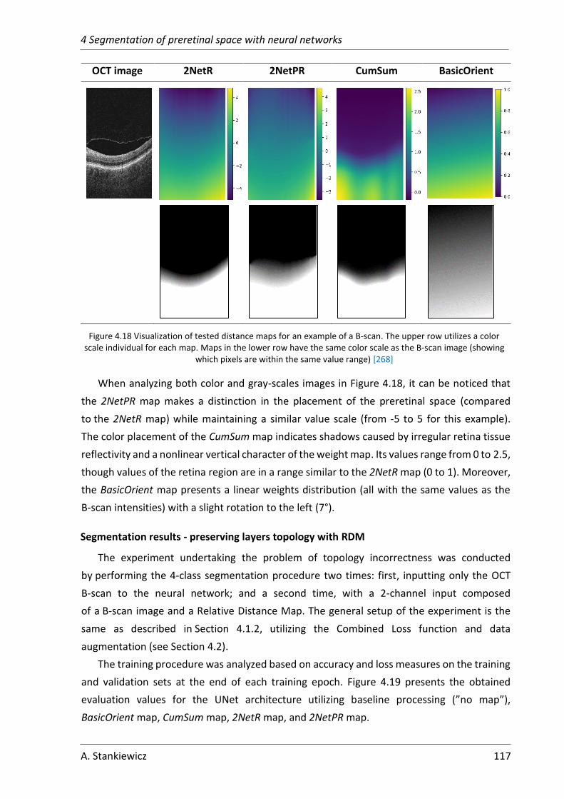
4 Segmentation of preretinal space with neural networks
A. Stankiewicz 117
OCT image 2NetR 2NetPR CumSum BasicOrient
Figure 4.18 Visualization of tested distance maps for an example of a B-scan. The upper row utilizes a color scale individual for each map. Maps in the lower row have the same color scale as the B-scan image (showing
which pixels are within the same value range) [268]
When analyzing both color and gray-scales images in Figure 4.18, it can be noticed that
the 2NetPR map makes a distinction in the placement of the preretinal space (compared
to the 2NetR map) while maintaining a similar value scale (from -5 to 5 for this example).
The color placement of the CumSum map indicates shadows caused by irregular retina tissue
reflectivity and a nonlinear vertical character of the weight map. Its values range from 0 to 2.5,
though values of the retina region are in a range similar to the 2NetR map (0 to 1). Moreover,
the BasicOrient map presents a linear weights distribution (all with the same values as the
B-scan intensities) with a slight rotation to the left (7°).
Segmentation results - preserving layers topology with RDM
The experiment undertaking the problem of topology incorrectness was conducted
by performing the 4-class segmentation procedure two times: first, inputting only the OCT
B-scan to the neural network; and a second time, with a 2-channel input composed
of a B-scan image and a Relative Distance Map. The general setup of the experiment is the
same as described in Section 4.1.2, utilizing the Combined Loss function and data
augmentation (see Section 4.2).
The training procedure was analyzed based on accuracy and loss measures on the training
and validation sets at the end of each training epoch. Figure 4.19 presents the obtained
evaluation values for the UNet architecture utilizing baseline processing (”no map”),
BasicOrient map, CumSum map, 2NetR map, and 2NetPR map.

4 Segmentation of preretinal space with neural networks
118 A. Stankiewicz
(a) training accuracy
(b) training loss
(c) validation accuracy
(d) validation loss
Figure 4.19 Accuracy and loss plots for training and validation datasets.
From the plots presented in Figure 4.19, no significant difference in the training can
be observed. For the training accuracy (Figure 4.19a), the BasicOrient map obtains lower
values (0.992 instead of an average of 0.993 after 50 epochs). Validation accuracy (Figure
4.19c) is similar for all maps, with the highest value of 0.9983 reached after the first 10 epochs
using the 2NetPR map and baseline approach, achieving a slightly lower final accuracy
(0.9978).
Figure 4.19b illustrating the training loss, indicates that the 2NetPR map allows the
network to reach the lowest loss value faster (after barely 10 epochs) without overfitting –
its validation loss (Figure 4.19d) does not increase over the next training epochs.
Nevertheless, all other methods obtain lower validation loss (from 0.083 to 0.088) except for
the 2NetPR, which stops at 0.108.
Table 4.9 includes the results of the evaluation on the test subset. It contains Dice
Coefficient values for five tested network architectures with each of the proposed maps and
the baseline investigation. The best results obtained for each neural network architecture are
marked in bold.
0.984
0.986
0.988
0.99
0.992
0.994
0 5 10 15 20 25 30 35 40 45 50
Acc
ura
cy
Epochs
no map BasicOrient CumSum
2NetR 2NetPR
0
0.05
0.1
0.15
0.2
0.25
0 5 10 15 20 25 30 35 40 45 50
Loss
Epochs
no map BasicOrient CumSum
2NetR 2NetPR
0.99
0.992
0.994
0.996
0.998
1
0 5 10 15 20 25 30 35 40 45 50
Acc
ura
cy
Epochs
no map BasicOrient CumSum
2NetR 2NetPR
0
0.05
0.1
0.15
0.2
0.25
0.3
0 5 10 15 20 25 30 35 40 45 50
Loss
Epochs
no map BasicOrient CumSum
2NetR 2NetPR

4 Segmentation of preretinal space with neural networks
A. Stankiewicz 119
Table 4.9 Dice Coefficient of 4 class pixel segmentation with various relative distance maps
Model Distance
Map
Dice Coefficient
Vitreous Preretinal space Retina Region b. Retina
UNet
--- 0.9968 0.9591 0.9944 0.9984
BasicOrient 0.9976 0.9606 0.9944 0.9987
CumSum 0.9977 0.9609 0.9945 0.9987
2NetR 0.9976 0.9601 0.9943 0.9986
2NetPR 0.9975 0.9588 0.9943 0.9987
LFUNet
--- 0.9973 0.9590 0.9942 0.9985
BasicOrient 0.9975 0.9583 0.9942 0.9987
CumSum 0.9977 0.9605 0.9944 0.9987
2NetR 0.9974 0.9581 0.9944 0.9987
2NetPR 0.9973 0.9571 0.9943 0.9987
DRUNet
--- 0.9951 0.9370 0.9916 0.9978
BasicOrient 0.9870 0.8935 0.9889 0.9914
CumSum 0.9932 0.9153 0.9909 0.9975
2NetR 0.9928 0.9195 0.9915 0.9979
2NetPR 0.9960 0.9513 0.9909 0.9975
Attention UNet
--- 0.9850 0.8802 0.9926 0.9956
BasicOrient 0.9824 0.8551 0.9880 0.9962
CumSum 0.9886 0.9025 0.9926 0.9981
2NetR 0.9860 0.8675 0.9920 0.9980
2NetPR 0.9963 0.9508 0.9926 0.9981
ReLayNet
--- 0.9603 0.8015 0.9918 0.9859
BasicOrient 0.9614 0.7528 0.9771 0.9930
CumSum 0.9730 0.7937 0.9906 0.9976
2NetR 0.9651 0.7594 0.9905 0.9974
2NetPR 0.9968 0.9544 0.9927 0.9981
The results in Table 4.9 show that for all of the neural network architectures adding
an RDM improves segmentation for the Vitreous, Preretinal Space, and Region below the
Retina classes (only for the Retina class, no improvement was observed since both retina
borders are distinctly visible). The greatest gain is noted for the Preretinal Space class: 7.06 %
and 15.29 % for the Attention UNet and ReLayNet, respectively, but only 0.18 %, 0.15 %, and
1.43 % for the UNet, LFUNet, and DRUNet respectively. It should be noticed that with the
neural networks with better initial segmentation scores (UNet and LFUNet), only slight
improvement can be observed, and it is with the CumSum map. For the networks with lower
original Dice Coefficient values of Preretinal Space (Attention UNet, ReLayNet, and DRUNet),
the 2NetPR map provides better results.
Table 4.10 presents MAE results and the TII for these experiments to indicate how each
discussed method influences the network's ability to discern similar classes.

4 Segmentation of preretinal space with neural networks
120 A. Stankiewicz
Table 4.10 Mean Absolute Error (with Standard Deviation) and Topology Incorrectness Index results of 4 class pixel segmentation with various distance maps
Model Distance Map MAE (SD) [px] TII
[%] PCV ILM RPE
UNet
--- 1.33 (2.88) 0.50 (0.28) 0.57 (0.29) 15.1
BasicOrient 1.42 (3.33) 0.47 (0.12) 0.56 (0.26) 4.8
CumSum 1.25 (2.52) 0.47 (0.12) 0.55 (0.25) 6.8
2NetR 1.48 (2.94) 0.48 (0.27) 0.59 (0.38) 9.4
2NetPR 1.20 (2.49) 0.50 (0.33) 0.57 (0.50) 3.7
LFUNet
--- 1.50 (3.53) 0.50 (0.12) 0.57 (0.24) 11.5
BasicOrient 1.58 (3.32) 0.49 (0.12) 0.58 (0.26) 8.8
CumSum 1.22 (2.54) 0.47 (0.12) 0.56 (0.25) 4.8
2NetR 1.64 (3.97) 0.48 (0.22) 0.56 (0.40) 6.3
2NetPR 1.26 (2.57) 0.51 (0.33) 0.56 (0.40) 5.0
DRUNet
--- 2.35 (3.76) 0.62 (0.23) 1.09 (1.58) 36.0
BasicOrient 6.77 (8.15) 1.46 (0.48) 1.88 (1.02) 54.9
CumSum 3.86 (6.72) 0.65 (0.31) 1.04 (0.87) 49.4
2NetR 3.50 (6.48) 0.76 (2.97) 0.98 (2.84) 40.0
2NetPR 1.97 (6.81) 0.80 (5.20) 1.05 (3.84) 18.4
Attention UNet
--- 4.02 (6.54) 0.60 (0.26) 0.80 (0.73) 50.5
BasicOrient 7.31 (13.36) 0.87 (2.01) 2.05 (5.40) 52.9
CumSum 4.50 (11.96) 0.59 (0.21) 0.79 (0.53) 38.7
2NetR 4.74 (11.54) 0.72 (1.86) 0.98 (1.87) 44.1
2NetPR 2.04 (4.18) 0.65 (2.07) 0.86 (2.25) 12.8
ReLayNet
--- 12.63 (13.84) 0.71 (0.59) 0.96 (0.88) 88.3
BasicOrient 20.00 (23.96) 0.59 (2.26) 0.79 (5.54) 92.0
CumSum 15.06 (19.13) 0.79 (0.89) 1.00 (0.72) 79.5
2NetR 18.55 (19.63) 0.70 (0.65) 1.11 (0.82) 88.1
2NetPR 1.42 (2.64) 0.58 (0.72) 0.81 (0.88) 10.8
When analyzing the results from Table 4.10, it can be noticed that all maps have improved
the topology for CNNs that previously performed relatively better with respect to vertical
layers order (i.e., UNet and LFUNet). Here, the best TII improvement is from 15.1 % to 3.7 %
for UNet with 2NetPR and from 11.5 % to 4.8 % for LFUNet with CumSum. At the same time,
the best performance for these networks for MAE values gave the CumSum map – 0.47 px for
ILM and 0.55 px for RPE (the only exception is the MAE for PCV line that has the lowest value
of 1.2 px when utilizing 2NetPR map).
For the other networks (DRUNet, Attention UNet, and ReLayNet), the simple BasicOrient
map increases the topology error (TII increased to 54.9 %, 52.9 %, and 92 % for these
networks, respectively) and the MAE (2.9 times for DRUNet, 1.8 times for Attention UNet, and
1.6 times for ReLayNet). Nevertheless, the 2NetPR gives the best topology improvement and
reduces the incorrectness of class order to 18.4 %, 12.8 %, and 10.8 % for these architectures,
respectively. The lowest MAE value for PCV is also obtained using the 2NetPR map (1.97 px
for DRUNet, 2.04 px for Attention UNet, and 1.42 px for ReLayNet, which are values close

4 Segmentation of preretinal space with neural networks
A. Stankiewicz 121
to those obtained by UNet and LFUNet). No significant improvement can be observed for the
MAE of ILM and RPE lines, and the error values are similar (ranging from 0.58 px to 1 px).
From the above comparison, the proposed maps significantly improve layers' topology
(from 2 to 8 times). Two of the proposed relative distance maps (CumSum and 2NetPR)
perform better than the original 2NetR map. Furthermore, the CumSum map is less
computationally expensive and does not require any prior segmentation. Nevertheless,
a simple linear map (BasicOrient) does not preserve correct layers topology and, in most
cases, hiders network's ability to segment OCT images properly. On the other hand, for UNet
and LFUNet, this map lowered the number of images with incorrect topology (to 4.8 % and
8.8 %, respectively).
4.3.3 Increasing segmentation accuracy with a non-typical kernel size
As was stated before, the pixel intensity values of the Preretinal Space class are similar
to those of the Vitreous class. Therefore, classification of a given pixel may be done based
on limited information about the pixel’s surroundings. Furthermore, the shape and area of the
preretinal space vary from B-scan to B-scan.
Another way of increasing the network’s robustness to the spatial hierarchy of the classes
is by increasing its field of view. This can be achieved with is using a bigger convolution kernel.
Although AlexNet [233] used a big 11×11 px kernel which increases object classification, after
the introduction of the VGG network [271], large kernels were replaced with multiple small
3×3 filters. Since then, the majority of works on CNN (including those described in the
literature review in Section 2) use only standard square kernels of the size 3×3. On the other
hand, the ReLayNet [217] authors incorporated a vertical convolutional kernel of 7×3 px
to be consistent with input OCT image dimensions. They also explained that the network with
such kernel size could capture the entire retina at the lowest encoder level.
Nevertheless, for the retina layers segmentation task this approach has not been
sufficiently discussed or analyzed. Furthermore, in standard image processing, the shape and
values of an applied filter are designed to reflect the shape of features to detect [272].
For example, there are different filters for vertical, horizontal, and diagonal edge detection
tasks. In the neural network solution, when the orientation and shape of the objects to be
classified are unknown, a square convolution kernel gives an advantage.
A close analysis of OCT images allowed the author of this thesis to notice that:
• image dimensions are non-equal with different ratios for fast-scanning and non-
fast-scanning directions; typically, as was indicated in [217], kernel shape in CNN
should reflect the input image shape (e.g., a CNN with a square input image has
a square-shaped kernel), and therefore a network with rectangular input data
could benefit from a rectangular convolution filter

4 Segmentation of preretinal space with neural networks
122 A. Stankiewicz
• the searched objects within the image (retina borders and layers) are arranged
horizontally (only a small difference in intensity can be detected from left to right
side of the image, mainly due to rotation or spherical tissue structure), and pixel
intensities vary significantly in the vertical direction in a narrow part of the image
(retina layers)
• the PCV line has various arrangements within a 3D OCT scan, it is frequently
underexposed (what generates line discontinuities), and its placement,
orientation, and attachment points are hard to foresee.
The above observations allowed the author of this thesis to hypothesize that the image
processing performed with a convolution kernel tailored to the data distribution in the image
would be beneficial for retina segmentation. Furthermore, it can also be advantageous
to utilize a bigger convolutional kernel to detect spatial intensity changes. Therefore,
in contrast to common CNN approaches, the author investigated utilizing a non-typical
convolutional kernel, both of a bigger size and rectangular shape. In the proposed
experiments, the influence of the following kernel sizes is analyzed:
• square kernels: 3×3, 5×5, and 7×7 px
• vertical kernels: 5×3, 7×3, and 9×3 px
• horizontal kernels: 3×5, 3×7, and 3×9 px.
Figure 4.20 illustrates different fields of view spanned with standard (3×3 px), vertical
(7×3 px), and horizontal (3×7 px) kernels.
(a) square kernel
(b) vertical kernel
(c) horizontal kernel
Figure 4.20 Illustration of retina region in OCT image covered with each analyzed kernel type
Segmentation results – applying a non-typical convolution kernel
The author of the thesis proposed conducting the following experiment: to perform OCT
image segmentation with the previously discussed neural network architectures (i.e., UNet,
LFUNet, DRUNet, and ReLayNet), utilizing various kernel sizes. The tested kernel size
is consistent for all network layers (in all of the encoder and decoder blocks, and the last 1×1
convolution filter remains unchanged). The experiment setup is the same as described in
Section 4.1.2 with 4 data augmentation techniques and a Combined Loss function.
Figure 4.21 presents training and validation loss values used to evaluate the training
process of a UNet with various convolution kernels. The plotted training loss curves (Figure
4.21a, c, and e) show that the bigger the kernel, the lower the training loss, and therefore the

4 Segmentation of preretinal space with neural networks
A. Stankiewicz 123
model better fits the training data. Nevertheless, no significant gain can be observed
for kernels bigger than 5×5, 3×5, and 5×3 px (with the lowest value of 0.05 for both horizontal
and vertical kernels and 0.04 for 7×7 kernel).
As can be deduced from the validation loss (Figure 4.21b, d, and f), a network with a bigger
kernel reaches a lower loss value in fewer epochs (15 for square kernels and 20 for both
horizontal and vertical convolution kernels). The final loss value for bigger kernels is lower
than for a standard 3×3 kernel (0.093 for 3×3 kernel, 0.07 for 7×7 kernel). Additionally,
the validation loss of a rectangular kernel is similar to that of 7×7 (0.07 for 9×3 and 0.075
for 3×9). Nevertheless, no significant gain for kernels over 3×7 and 7×3 px is detected.
(a) training loss / square kernel
(b) validation loss / square kernel
(c) training loss / vertical kernel
(d) validation loss / vertical kernel
(e) training loss / horizontal kernel
(f) validation loss / horizontal kernel
Figure 4.21 Plots of training and validation loss for segmentation with UNet and various convolutional kernel types and sizes.
0
0.05
0.1
0.15
0.2
0.25
0.3
0 5 10 15 20 25 30 35 40 45 50
Loss
Epochs
3×3 5×5 7×7
0
0.05
0.1
0.15
0.2
0.25
0 5 10 15 20 25 30 35 40 45 50
Loss
Epochs
3×3 5×5 7×7
0
0.05
0.1
0.15
0.2
0.25
0.3
0 5 10 15 20 25 30 35 40 45 50
Loss
Epochs
3×3 5×3 7×3 9×3
0
0.05
0.1
0.15
0.2
0 5 10 15 20 25 30 35 40 45 50
Loss
Epochs
3×3 5×3 7×3 9×3
0
0.05
0.1
0.15
0.2
0.25
0.3
0 5 10 15 20 25 30 35 40 45 50
Loss
Epochs
3×3 3×5 3×7 3×9
0
0.05
0.1
0.15
0.2
0 5 10 15 20 25 30 35 40 45 50
Loss
Epochs
3×3 3×5 3×7 3×9

4 Segmentation of preretinal space with neural networks
124 A. Stankiewicz
Table 4.11 to Table 4.14 present the effect of convolutional kernel size on the performance
of preretinal space segmentation on the test set. Understandably, the average DC increases
for all segmented regions as the kernel size increases (gain for the Preretinal Space with 7×7
kernel is 0.44 % for UNet, 0.48 % for LFUNet, 1.1 % for DRUNet, and 20.04 % for ReLayNet).
The same observation can be made for the MAE for all searched borders, but the greatest
improvement is observed for the PCV line (MAE lower by 0.43 px for UNet, 0.62 px for LFUNet,
0.84 px for DRUNet, and 111.3 px for ReLayNet).
When it comes to the TII improvement, the presented data indicate that for all of the
network architectures, the standard 3×3 kernel does not provide the best results (TII
decreases by 9.4 % for UNet, 8.25 % for LFUNet, 8.39 % for DRUNet, and 3.7 % for ReLayNet
even with the 5×3 kernel). The greatest improvement in topology correctness can be observed
with a vertical 9×3 kernel for UNet and LFUNet (TII decreased by 12.75 % and 10.38 %,
respectively). The networks with initially worse topology index benefit the most from a square
7×7 kernel (TII improvement by 16.22 % and 15.93 % for DRUNet and ReLayNet, respectively).
Table 4.11 DC, MAE, and TII results of OCT segmentation with various kernel sizes for UNet model
Kernel size
[px]
DC MAE (SD) [px] TII
[%] Vitreous Preretinal
space Retina
Region
b. Retina PCV ILM RPE
3×3 0.9968 0.9591 0.9944 0.9984 1.33 (2.88) 0.50 (0.28) 0.57 (0.29) 15.08
5×5 0.9980 0.9615 0.9945 0.9988 1.08 (2.16) 0.47 (0.12) 0.54 (0.24) 4.55
7×7 0.9981 0.9635 0.9948 0.9988 0.92 (0.97) 0.45 (0.12) 0.52 (0.23) 4.55
5×3 0.9978 0.9615 0.9944 0.9987 1.17 (2.44) 0.48 (0.17) 0.58 (0.26) 5.69
7×3 0.9981 0.9628 0.9946 0.9988 0.95 (0.94) 0.47 (0.12) 0.54 (0.25) 2.84
9×3 0.9981 0.9626 0.9947 0.9988 0.93 (0.74) 0.47 (0.12) 0.52 (0.25) 2.42
3×5 0.9977 0.9620 0.9945 0.9987 1.22 (2.86) 0.47 (0.12) 0.55 (0.25) 9.67
3×7 0.9980 0.9631 0.9946 0.9987 0.98 (1.83) 0.46 (0.12) 0.55 (0.25) 6.83
3×9 0.9981 0.9640 0.9946 0.9987 0.90 (1.04) 0.46 (0.12) 0.54 (0.24) 5.12
Table 4.12 DC, MAE, and TII results of OCT segmentation with various kernel sizes for LFUNet model
Kernel size
[px]
DC MAE (SD) [px] TII
[%] Vitreous Preretinal
space Retina
Region
b. Retina PCV ILM RPE
3×3 0.9973 0.9590 0.9942 0.9985 1.50 (3.53) 0.50 (0.12) 0.57 (0.24) 11.52
5×5 0.9981 0.9630 0.9947 0.9988 0.91 (0.81) 0.47 (0.12) 0.53 (0.24) 2.84
7×7 0.9982 0.9638 0.9947 0.9988 0.88 (0.72) 0.46 (0.13) 0.52 (0.23) 2.99
5×3 0.9980 0.9613 0.9944 0.9987 1.17 (2.78) 0.48 (0.12) 0.55 (0.24) 3.27
7×3 0.9981 0.9632 0.9947 0.9988 0.90 (0.80) 0.46 (0.12) 0.52 (0.23) 3.13
9×3 0.9981 0.9631 0.9946 0.9987 0.89 (0.63) 0.47 (0.13) 0.54 (0.25) 1.14
3×5 0.9978 0.9622 0.9946 0.9987 1.10 (2.57) 0.47 (0.13) 0.54 (0.24) 7.25
3×7 0.9980 0.9631 0.9947 0.9988 0.94 (1.48) 0.47 (0.12) 0.52 (0.23) 4.55
3×9 0.9980 0.9626 0.9946 0.9987 0.99 (1.65) 0.47 (0.12) 0.54 (0.24) 4.41

4 Segmentation of preretinal space with neural networks
A. Stankiewicz 125
Table 4.13 DC, MAE, and TII results of OCT segmentation with various kernel sizes for DRUNet model
Kernel
size [px]
DC MAE (SD) [px] TII
[%] Vitreous Preretinal
space Retina
Region
b. Retina PCV ILM RPE
3×3 0.9951 0.9370 0.9916 0.9978 2.35 (3.76) 0.62 (0.23) 1.09 (1.58) 35.99
5×5 0.9961 0.9428 0.9922 0.9979 1.82 (3.07) 0.58 (0.17) 0.86 (0.59) 25.03
7×7 0.9967 0.9480 0.9928 0.9982 1.51 (1.35) 0.57 (0.19) 0.77 (0.64) 19.77
5×3 0.9952 0.9389 0.9921 0.9980 2.14 (3.50) 0.61 (0.29) 0.86 (0.51) 27.60
7×3 0.9950 0.9288 0.9917 0.9978 2.50 (4.57) 0.61 (0.22) 0.90 (0.50) 35.42
9×3 0.9934 0.9179 0.9917 0.9978 3.51 (7.04) 0.61 (0.21) 0.92 (0.54) 43.81
3×5 0.9945 0.9382 0.9914 0.9978 2.50 (5.83) 0.62 (0.23) 0.94 (0.78) 33.29
3×7 0.9917 0.9121 0.9886 0.9971 5.54 (6.02) 0.93 (0.31) 1.21 (1.82) 59.32
3×9 0.9943 0.9346 0.9907 0.9977 2.40 (3.95) 0.69 (0.68) 1.11 (1.81) 33.00
Table 4.14 DC, MAE, and TII results of OCT segmentation with various kernel sizes for ReLayNet model
Kernel size
[px]
DC MAE (SD) [px] TII
[%] Vitreous Preretinal
space Retina
Region
b. Retina PCV ILM RPE
3×3 0.8686 0.6384 0.9782 0.9451 121.24 (78.46) 1.94 (4.06) 5.15 (5.84) 100.00
5×5 0.9447 0.8047 0.9909 0.9769 21.74 (38.21) 0.72 (0.75) 1.44 (1.85) 93.31
7×7 0.9688 0.8388 0.9920 0.9885 9.94 (13.53) 0.64 (0.47) 0.93 (0.92) 84.07
5×3 0.9393 0.7900 0.9906 0.9721 14.69 (14.13) 0.95 (2.09) 1.57 (1.90) 96.30
7×3 0.9603 0.8015 0.9918 0.9859 12.63 (13.84) 0.71 (0.59) 0.96 (0.88) 88.34
9×3 0.9676 0.8068 0.9904 0.9893 11.17 (12.91) 0.68 (0.34) 1.09 (0.68) 85.78
3×5 0.9156 0.7543 0.9831 0.9557 22.64 (24.98) 1.06 (1.57) 2.22 (3.01) 98.86
3×7 0.9167 0.7481 0.9851 0.9590 41.36 (54.81) 1.01 (1.17) 4.80 (6.57) 98.29
3×9 0.9192 0.7758 0.9871 0.9570 29.09 (37.86) 0.82 (2.12) 1.83 (3.30) 97.44
A noticeable improvement in segmentation accuracy can be observed mainly for
Preretinal Space class and PCV line. Interestingly the results for UNet and LFUNet obtained
with both horizontal kernel of the size 3×9 px and vertical kernel of 9×3 px are comparable
to those obtained with a 7×7 square kernel (the biggest difference in MAE is 0.02 px for UNet
and 0.11 px for LFUNet).
For the Retina class, the gain in Dice Coefficient is limited to 0.04 % for UNet, 0.05 % for
LFUNet, 0.12 % for DRUNet, and 1.38 % for ReLayNet. Furthermore, the MAE improvement
of retina borders (i.e., ILM and RPE lines) does not exceed 0.05 px for UNet and LFUNet,
0.32 px for DRUNet, and 4.22 px for ReLayNet, which is obtained with a 7×7 square kernel.
Figure 4.22 to Figure 4.25 present results of Preretinal Space Dice Coefficients for the
evaluated neural network architectures. Here, square, vertical, and horizontal kernels are
ordered by the area spanned by the kernel and depicted with consistent colors for each kernel
type.

4 Segmentation of preretinal space with neural networks
126 A. Stankiewicz
Figure 4.22 Dice Coefficients of Preretinal Space class segmentation for UNet with various kernel sizes
When analyzing bar plots of Preretinal Space DC values for UNet (Figure 4.22), it can be
noticed that all rectangular kernels (regardless of their orientation) give better results than
the 3×3 and 5×5 square kernels. Additionally, a horizontal 3×9 kernel outperforms the 7×7
kernel by 0.15 %. Interestingly, all horizontal kernels give better results (by 0.05 %, 0.03 %,
and 0.14 % for 3×5, 3×7, and 3×9 kernels respectively) than their vertical counterparts.
Figure 4.23 Dice Coefficients of Preretinal Space class segmentation for LFUNet with various kernel sizes
For LFUNet (Figure 4.23) the worst result (95.9 %) is obtained with the standard 3×3
kernel, and the best with 7×7 kernel (96.38 %). Furthermore, kernels of the size 3×7, 7×3, and
9×3 px perform similarly (gain of 0.01 %, 0.02 %, and 0.01 %, respectively) to a square kernel
of 5×5 px (which spans a greater area). With smaller kernels (i.e., 5×3 and 3×5 px) higher DC
value is obtained with a horizontal kernel (gain of 0.09 %), while for bigger kernels (i.e., 9×3
and 3×9 px) the result is better with a vertical kernel (gain by 0.05 %).
DRUNet results in Figure 4.24 show that all square kernels are better than any rectangular
kernel. The best Dice Coefficient of 94.8 % was obtained with a 7×7 mask. Although
improvement over the 3×3 kernel is only 1.1 %. Furthermore, horizontal kernels give a higher
DC value (e.g., 1.5 % gain for 3×9 kernel) than their vertical counterparts (except for kernels
3×5 and 5×3, with equivalent results of 93.8 %). Nevertheless, incorporating kernel 9×3
decreased the Dice Coefficient by 2.1 % compared to the 5×3 kernel.
0.958
0.959
0.96
0.961
0.962
0.963
0.964
0.965
3×3 5×3 3×5 7×3 3×7 5×5 9×3 3×9 7×7
Dic
e C
oef
fici
ent
UNet
square kernel
vertical kernel
horizontal kernel
0.958
0.959
0.96
0.961
0.962
0.963
0.964
0.965
3×3 5×3 3×5 7×3 3×7 5×5 9×3 3×9 7×7
Dic
e C
oef
fici
ent
LFUNet
square kernel
vertical kernel
horizontal kernel

4 Segmentation of preretinal space with neural networks
A. Stankiewicz 127
Figure 4.24 Dice Coefficients of Preretinal Space class segmentation for DRUNet with various kernel sizes
Figure 4.25 Dice Coefficients of Preretinal Space class segmentation for ReLayNet with various kernel sizes
For the ReLayNet (Figure 4.25), a square kernel of 7×7 px produces the best result with
a DC value of 83.9 %. Here the gain of 20.1 % over the standard 3×3 kernel is significant.
Furthermore, the results for the vertical kernel give better segmentation scores than their
horizontal counterparts (an improvement from 3.1 % for the 9×3 kernel to 5.3 % for the 7×3
kernel). These results confirm the validity of selecting the 7×3 kernel by the authors of this
architecture, although the gathered data show a possibility for further improvement.
To objectively select a convolution kernel for OCT data segmentation, its computational
cost and prediction time should also be considered. Table 4.15 presents the number
of parameters learned by each network and the prediction time (excluding the time of loading
the image into the memory / and including that time).
Data presented in Table 4.15 confirms that prediction time increases with the size of the
network, with the longest prediction for a square kernel of 7×7 px (from 5.9 s for DRUNet
up to 13.3 s for LFUNet). The difference between the prediction time between the smallest
and the largest convolution kernel is 4 s for UNet, 6.3 s for LFUNet, 0.9 s for DRUNet, and 1.9 s
for ReLayNet. It can also be observed that performing computations with a horizontal kernel
is slightly faster (a difference of 0.05 s on average) than with a vertical kernel of the same size.
0.9
0.91
0.92
0.93
0.94
0.95
0.96
3×3 5×3 3×5 7×3 3×7 5×5 9×3 3×9 7×7
Dic
e C
oef
fici
ent
DRUNet
square kernel
vertical kernel
horizontal kernel
0.6
0.65
0.7
0.75
0.8
0.85
3×3 5×3 3×5 7×3 3×7 5×5 9×3 3×9 7×7
Dic
e C
oef
fici
ent
ReLayNet
square kernel
vertical kernel
horizontal kernel

4 Segmentation of preretinal space with neural networks
128 A. Stankiewicz
Table 4.15 Prediction time1 for the evaluated neural networks
Kernel
size
UNet LFUNet DRUNet ReLayNet
No. of
parameters
[×106]
Prediction
time [s]
No. of
parameters
[×106]
Prediction
time [s]
No. of
parameters
[×106]
Prediction
time [s]
No. of
parameters
[×106]
Prediction
time [s]
3×3 7.8 0.257 / 6.33 8.1 0.324 / 6.98 0.88 0.248 / 5.46 13.7 0.148 / 5.85
5×5 20.3 0.336 / 8.01 20.7 0.406 / 9.64 2.1 0.261 / 5.91 33.2 0.170 / 6.69
7×7 39.1 0.337 /10.31 39.6 0.407 /13.34 4.0 0.273 / 6.39 62.4 0.185 / 7.72
5×3 12.5 0.338 / 7.10 12.8 0.409 / 8.15 1.3 0.265 / 5.58 21.0 0.187 / 6.36
7×3 17.2 0.339 / 7.63 17.5 0.410 / 9.02 1.8 0.268 / 5.72 28.3 0.189 / 6.52
9×3 21.9 0.344 / 8.27 22.3 0.411 /10.02 2.3 0.259 / 5.84 35.6 0.189 / 6.77
3×5 12.5 0.333 / 7.07 12.8 0.407 / 8.11 1.3 0.250 / 5.63 21.0 0.185 / 6.27
3×7 17.2 0.338 / 7.60 15.5 0.408 / 9.00 1.8 0.259 / 5.80 28.3 0.186 / 6.49
3×9 21.9 0.339 / 8.20 22.3 0.410 / 9.90 2.3 0.257 / 5.95 35.6 0.187 / 6.79
The experiments described in this Section show that by applying an appropriate
convolution kernel, it is possible to boost the segmentation accuracy of the neural network.
Nevertheless, the size and orientation of such masks should be adapted to the specificity
of the network architecture. For example, the DRUNet, which incorporates convolutions with
dilatation, benefits from a square kernel, while both UNet and LFUNet perform the best with
horizontal kernels.
Although a bigger convolutional kernel increases the computational cost of the system,
the author poses that such adjustment (even utilizing a non-uniform filter) improves the
accuracy of pixel-wise segmentation. Furthermore, it can be noticed that by utilizing
a horizontal convolution kernel, it is possible to learn network weights that better fit the
horizontal arrangement of the searched retina layers. Furthermore, a bigger convolution
kernel helps to overcome the problem of PCV border discontinuity within the OCT image,
making the network robust to these kinds of problems.
Summary of preretinal space segmentation with neural networks
The experiments presented in this Chapter discussed the specific character of the
preretinal space segmentation problem based on the OCT data. A detailed analysis of the
obtained results with the use of various neural network architectures leads to the following
conclusions:
1) a Combined Loss function favoring distribution-based over the region-based criterion
provides the best segmentation results for the 4-class classification of OCT images
in the gathered cohort
2) application of any data augmentation technique improves the segmentation accuracy
for the examined data, and the best results are obtained when all discussed techniques
are applied (horizontal flip, random rotation, random translation, random cropping),
1 The hardware utilized for the test is the same as for the training (see Section 4.1.2).

4 Segmentation of preretinal space with neural networks
A. Stankiewicz 129
thus significantly expanding the training subset and improving models ability
to generalize
3) from the five evaluated neural network architectures, the baseline UNet and
its extended version of LFUNet provide the best segmentation accuracy (both with and
without utilizing data augmentation)
a. the Attention UNet and ReLayNet do not obtain sufficient results for the
preretinal space task
b. the DRUNet architecture produces results slightly worse than UNet, with
a much lower number of parameters to train
4) for all of the tested network architectures occurs a problem with incorrect class
topology within the OCT image (most noticeable for the ReLayNet and Attention UNet
models, less so for the other networks)
5) the method of adding a Relative Distance Map as a second channel to the network’s
input image to improve the topology correctness resulted in a significant improvement
in segmented classes order
a. the proposed 2NetPR map tailored to the preretinal space properties provides
the best results here
b. for UNet and LFUnet, better pixel classification scores also are obtained with
the CumSum map
6) accuracy of the pixel-wise semantic image segmentation can be improved by selecting
an appropriate convolution kernel
a. choosing the biggest kernel of 7×7 px is not necessary, as the results show that
non-typical kernels of 3×9 and 9×3 provide similar classification accuracy with
lower computational requirements
b. experiments confirm that vertical kernels give the best improvement in terms
of topology correctness.
The conducted experiments prove that the proposed application of neural networks
to preretinal space segmentation from OCT images gives good results. Furthermore,
it is a robust solution even with underexposed or pathological tissue. It is not susceptible
to tissue discontinuity, as is the case with the graph-based approach. The proposed method
provides accurate preretinal space segmentation, the first and crucial step for the quantitative
evaluation of VRI changes during medical diagnosis.

130

131
Chapter
5 Application of the proposed solutions
In order to accurately assess the pathology evolution and select an appropriate treatment
course, it is crucial to obtain objective measurements of the analyzed tissue. Thus,
the quantitative tools for diagnosis and disease monitoring are essential in clinical practice.
Precise segmentation algorithms of retina layers and the preretinal area analyzed in this thesis
are crucial elements in diagnostic assessment.
The methods derived in Chapter 3 for improving retina layers segmentation were further
used in the clinical application of automated fovea parameterization described in Section 5.1.
In addition, the novel preretinal space segmentation technique introduced in Chapter 4 was
subjected to an automated VMA and VMT analysis investigated in Section 5.2.
5.1 Fovea Parameterization
5.1.1 Current fovea evaluation
Thanks to utilizing OCT imaging technology and measurement tools available in the OCT
software, it is possible to manually quantify the current retina condition and its changes [273].
As described in Section 1.2, a primary feature used to detect and assess vision-related diseases
is the retina thickness, particularly Central Retina Thickness (CRT) [16]. Figure 5.1 illustrates
the CRT measurement performed manually on the OCT image.
Figure 5.1 Example of current fovea evaluation by manual measurement of central retina thickness (CRT)
To evaluate the state of the retina and the possibility of developing a macular hole,
it is also possible to measure foveal diameter, foveal depth, fovea angle, and curvature [274],
[275]. Other measurements for quantitative analysis are also the area of the fovea pit and the
area of the inner retina within the central cross-section [276]. Nevertheless, all of these
CRT 187 µm

5 Application of the proposed solutions
132 A. Stankiewicz
parameters are obtained only manually, and no reports have been found that evaluated these
parameters in terms of suitability for VMA and VMT assessment. Typically, the retina thickness
remains the primary comparable parameter along with the retina volume measurement
within individual sectors of an ETDRS grid [54].
5.1.2 Proposed automatic fovea pit parameterization
When analyzing the volumetric characteristics of the fovea pit with present VMA or VMT
conditions, the fovea contour and shape can be considered interesting parameters. Figure 5.2
presents a visualization of the 3D OCT macula scan with the annotated ideal fovea contour.
Figure 5.2 3D visualization of OCT macula scan with annotated ideal fovea contour [277]
To measure the characteristics of the fovea shape in the presence of VRI changes,
the author of the thesis introduced the fovea pit contour (FPC) parameterization [277].
Its calculation is performed automatically based on a single 3D OCT scan and can be used
to quantify and evaluate the macula changes that occur with time. It aims to aid clinical
differentiation between normal and pathologic macular conditions. Figure 5.3 presents
a general scheme for calculating the fovea pit contour profile based on a 3D OCT scan
centered at the macula.
The first step of the algorithm is the acquisition of volumetric OCT data. Next,
preprocessing procedures are performed. Here are employed the adaptive techniques
proposed in Chapter 3, i.e., wavelet-based (WST) noise reduction and adaptive selection
of image area useful for further analysis.
The next step is the segmentation of the OCT image to detect the inner limiting membrane
(ILM) and retinal pigment epithelium (RPE) boundaries of the retina. This procedure
is performed with the graph-based algorithm utilizing layer tracking described in Section 3.2.4.
Ideal fovea contour

5 Application of the proposed solutions
A. Stankiewicz 133
Figure 5.3 The general scheme of an algorithm for automatic calculation of fovea contour profile
Next, from the segmented lines, a retina thickness virtual map 𝑉𝑀𝑅 is calculated
as a difference between the ILM and RPE surfaces. Equation (5.1) is used here:
𝑉𝑀𝑅(𝑥, 𝑦) = 𝑤𝑧(𝐼𝐿𝑀(𝑥, 𝑦) − 𝑅𝑃𝐸(𝑥, 𝑦)) (5.1)
where 𝑥 ∈ ⟨0, 384⟩ denotes the horizontal index of the OCT cube (i.e., the B-scan column),
𝑦 ∈ ⟨0, 140⟩ sands for the index of the cross-section, 𝑤𝑧 represents the axial resolution of the
scan, 𝐼𝐿𝑀 and 𝑅𝑃𝐸 are matrixes of the segmented ILM and RPE surfaces, and 𝑉𝑀𝑅 is the

5 Application of the proposed solutions
134 A. Stankiewicz
matrix of the retina virtual map values. This results in distance matrixes of the size 141×385
for one 3D OCT scan (the dimensions stem from the scan resolution).
The last step of the algorithm is a calculation of individual fovea pit parameters, including:
• coordinates of macula center (𝑥𝑐, 𝑦𝑐 ) – this is a reference point for further
calculations. It is determined as the highest elevation of the IS/OS junction layer
based on the flattened (with respect to the RPE layer) retina borders. For a healthy
eye, this coordinate also corresponds to the lowest depression of the retina surface
(i.e., ILM layer). Figure 5.4 illustrates the found macula center annotated with
a vertical orange line on a B-scan of a VMA subject.
Figure 5.4 Example of central B-scan with annotated macula center (orange vertical line)
• fovea pit contour (FPC) [277] – defined as a ridge around the fovea center
o The search for FPC is performed individually in each of 360 equally spaced
angles 𝛼 ∈ {0, 1, … , 359}. The algorithm determines the 𝐹𝑃𝐶(𝛼) as a position
of maximum retina thickness value along the line from the fovea center
(𝑥𝑐, 𝑦𝑐) constructed at the 𝛼 angle. The search is performed within the inner
macula (IM), i.e., between the circles specified around the fovea center with
radiuses 𝑟1 = 0.5 mm and 𝑟2 = 1.8 mm, respectively. Figure 5.5a illustrates
the search region on a retina thickness virtual map.
o The identified 360 points form a curve describing the fovea pit contour.
The curve coordinates are subjected to mean filtering with a window of 5
elements to minimize irregularities. Figure 5.5b illustrates the computed FPC
curve overlaid on the color retina thickness map with the ETDRS grid. Figure
5.5c illustrates an example of the retina thickness plot (blue line) of a B-scan
from Figure 5.4. The fovea center (𝑥𝑐 , 𝑦𝑐) and two contour points of 𝐹𝑃𝐶(0)
and 𝐹𝑃𝐶(180) are annotated with red dots. The black arrows indicate
the measured distance from the fovea center to the contour points.
The vertical orange lines illustrate the limits of the search region.
o It should be noted that the FPC can be defined only for a macula with
a depression in the central area. Limiting the search region by excluding
the central fovea (i.e., defining the inner circle of 𝑟1 = 0.5 mm) allowed
to perform FPC search also for mild VMT cases (i.e., with deformed fovea pit,

5 Application of the proposed solutions
A. Stankiewicz 135
but still present ridge around the fovea distortion). Nevertheless, the FPC
cannot be obtained for patients with advanced VMT stage, where the disease
progression resulted in fovea eversion.
• central retina thickness (CRT) – this value is determined directly from the 𝑉𝑀𝑅
at the coordinates of the macula center (see Figure 5.6):
𝐶𝑅𝑇 = 𝑉𝑀𝑅(𝑥𝑐, 𝑦𝑐) (5.2)
• central fovea pit depth 𝐹𝑃𝐷𝐶 – the distance between the mean value of retina
thickness along the FPC curve and retina surface at the fovea center coordinates
(see Figure 5.6):
𝐹𝑃𝐷𝐶 =∑ 𝑉𝑀𝑅(𝐹𝑃𝐶(𝛼)𝛼 )
360− 𝑉𝑀𝑅(𝑥𝑐, 𝑦𝑐) (5.3)
(a) retina thickness map with annotated circles (of r1 and r2 radiuses) bounding the search region; the FPC(α) point is searched along the line drawn from
the fovea center at the α angle
(b) retina thickness map with overlaid ETDRS grid and obtained fovea pit contour
(c) retina thickness profile through the central B-scan with annotated fovea center (middle red dot), fovea contour points (left and right red dots), limits of the search region (vertical orange lines), distance from the
fovea center to the contour border (black arrows)
Figure 5.5 Illustration of FPC search method for a VMA case
Fovea pit contour
α r1
r2
FPC(0) FPC(180)

5 Application of the proposed solutions
136 A. Stankiewicz
Figure 5.6 Illustration of automatically measured fovea pit parameters for a VMA example
• maximal fovea pit depth 𝐹𝑃𝐷𝑀 – the distance between the mean value of the
retina thickness along the FPC curve and the lowest retina surface point enclosed
by the FPC curve:
𝐹𝑃𝐷𝑀 =∑ 𝑉𝑀𝑅(𝐹𝑃𝐶(𝛼)𝛼 )
360− min∀𝑥,𝑦⊂𝐹𝑃𝐶
𝑉𝑀𝑅(𝑥, 𝑦) (5.4)
• central fovea diameter 𝐹𝐶𝐷 – the distance in the 𝑥 direction between the opposite
fovea contour points within the central B-scan (see Figure 5.6):
𝐹𝐶𝐷 = 𝑤𝑥|𝑥𝐹𝑃𝐶(0) − 𝑥𝐹𝑃𝐶(180)| (5.5)
where 𝑥𝐹𝑃𝐶(𝛼) denotes the 𝑥 coordinate of the FPC point at the 𝛼 angle, and 𝑣𝑥 is
the lateral scan resolution.
• central fovea pit area 𝐹𝐶𝐴 – area enclosed by the line 𝐿𝐷 connecting the central
fovea diameter points (𝐹𝑃𝐶(0) and 𝐹𝑃𝐶(180)) and the retina surface within the
central B-scan (see a shaded area in Figure 5.6); it is computed as:
𝐹𝐶𝐴 = 𝑤𝑥𝑤𝑧 ∑ (𝐿𝐷(𝑥) − 𝑉𝑀𝑅(𝑥, 𝑦𝑐))
𝑥𝐹𝑃𝐶(180)
𝑥=𝑥𝐹𝑃𝐶(0)
(5.6)
where 𝐿𝐷(𝑥) denotes a value of the line connecting the 𝐹𝐶𝐷 endpoints. It can be
obtained with the equation:
𝐿𝐷(𝑥) =(𝑥 − 𝑥𝐹𝑃𝐶(0))|𝑉𝑀𝑅(𝑥𝐹𝑃𝐶(180), 𝑦𝑐) − 𝑉𝑀𝑅(𝑥𝐹𝑃𝐶(0), 𝑦𝑐)|
|𝑥𝐹𝑃𝐶(180) − 𝑥𝐹𝑃𝐶(0)|+ 𝑉𝑀𝑅(𝑥𝐹𝑃𝐶(0), 𝑦𝑐) (5.7)
• fovea shape coefficient 𝑐𝐹𝑆 – the correlation of the fovea shape within the central
B-scan to a function 𝐹𝐺 (see a gray curve fitted to the fovea contour points in Figure
5.6) obtained by parameterization of a Gaussian function with available fovea
features. The 𝐹𝐺 function and 𝑐𝐹𝑆 parameter are computed as follows:
FCA
FFCD CRT
FPDC
FCD
FG
LD

5 Application of the proposed solutions
A. Stankiewicz 137
𝐹𝐺(𝑥) = 𝐶𝑅𝑇 + 𝐹𝑃𝐷𝐶 − 𝐹𝑃𝐷𝑀 e− (𝑥−𝜇)2
2𝜎2 (5.8)
𝑐𝐹𝑆 =𝑛∑ (𝐹𝐺(𝑥)𝑉𝑀𝑅(𝑥, 𝑦𝑐))𝑥 − ∑ 𝐹𝐺(𝑥)𝑥 ∑ 𝑉𝑀𝑅(𝑥, 𝑦𝑐)𝑥
√𝑛∑ 𝐹𝐺2(𝑥)𝑥 − (∑ 𝐹𝐺(𝑥)𝑥 )2√𝑛∑ 𝑉𝑀𝑅
2(𝑥, 𝑦𝑐)𝑥 − (∑ 𝑉𝑀𝑅(𝑥, 𝑦𝑐)𝑥 )2 (5.9)
where the expected value 𝜇 = 𝑥𝑐 is the position of the fovea pit center along the
B-scan width, and the variance 𝜎 =𝐹𝐶𝐷
2√2ln2∗𝑏 is determined by the fovea pit
diameter 𝐹𝐶𝐷 divided by the coefficient 𝑏 = 2.5 and the ratio of 2√2ln2 between
the FWHM (i.e., full width at half maximum) value and 𝜎. The 𝑏 value was obtained
experimentally based on the ratio between the 𝐹𝐶𝐷 and the width of the fovea pit
at half of its depth. Value 𝑛 is the number of 𝑥 points within 𝐹𝐶𝐷.
The 𝑐𝐹𝑆 can take values in the range of ⟨−1,1⟩ Where 1 represents the highest
similarity of the fovea shape to the parameterized Gaussian function, and the value
of -1 indicates the lowest correlation of these curves.
• fovea pit area 𝐹𝑃𝐶𝐴 – the area enclosed by the FPC curve in the lateral direction,
defined as a sum of areas of triangles created by two neighboring contour points
and scan center:
𝐹𝑃𝐶𝐴 = 𝑤𝑥𝑤𝑦∑√𝑠(𝛼)(𝑠(𝛼) − 𝑟𝐹𝑃𝐶(𝛼))(𝑠(𝛼) − 𝑟𝐹𝑃𝐶(𝛼+1))(𝑠(𝛼) − 𝑑(𝛼))
𝛼
(5.10)
𝑠(𝛼) =1
2(𝑟𝐹𝑃𝐶(𝛼) + 𝑟𝐹𝑃𝐶(𝛼+1) + 𝑑(𝛼)) (5.11)
𝑑(𝛼) = √(𝑥𝐹𝑃𝐶(𝛼) − 𝑥𝐹𝑃𝐶(𝛼+1))2+ (𝑦𝐹𝑃𝐶(𝛼) − 𝑦𝐹𝑃𝐶(𝛼+1))
2 (5.12)
where 𝑠(𝛼) is the perimeter of a single triangle created between points 𝐹𝑃𝐶(𝛼),
𝐹𝑃𝐶(𝛼 + 1) , and (𝑥𝑐, 𝑦𝑐) , 𝑑(𝛼) is the distance between points 𝐹𝑃𝐶(𝛼) and
𝐹𝑃𝐶(𝛼 + 1), 𝑦𝐹𝑃𝐶(𝛼) denotes the 𝑦 coordinate of the FPC point at the 𝛼 angle, 𝑤𝑦
is the lateral non-fast scanning data resolution.
• fovea pit volume 𝐹𝑃𝑉 – the volume of the fovea pit enclosed by the retina surface
and the surface connecting the FPC points,
𝐹𝑃𝐶𝑉 = 𝑤𝑥𝑤𝑦𝑤𝑧∑ℱ(𝑟𝑐(𝑥, 𝑦) < 𝑟𝐹𝑃𝐶(𝛽))(𝐿𝑇(𝑥, 𝑦, 𝛽) − 𝑉𝑀𝑅(𝑥, 𝑦))
𝑥,𝑦
(5.13)
𝛽 =180 arctan
𝑦 − 𝑦𝑐𝑥 − 𝑥𝑐
𝜋 (5.14)

5 Application of the proposed solutions
138 A. Stankiewicz
𝐿𝑇(𝑥, 𝑦, 𝛽) =(𝑦 − 𝑦𝐹𝑃𝐶(𝛽)) (𝑉𝑀𝑅(𝑥𝐹𝑃𝐶(𝛽+180), 𝑦𝐹𝑃𝐶(𝛽+180)) − 𝑉𝑀𝑅(𝑥𝐹𝑃𝐶(𝛽), 𝑦𝐹𝑃𝐶(𝛽)))
𝑦𝐹𝑃𝐶(𝛽+180) − 𝑦𝐹𝑃𝐶(𝛽)
+ 𝑉𝑀𝑅(𝑥𝐹𝑃𝐶(𝛽), 𝑦𝐹𝑃𝐶(𝛽))
(5.15)
where ℱ(∙) is a function taking a value of 1 if the expression in the parenthesis
is true and 0 otherwise, 𝑟𝑐(𝑥, 𝑦) is the radius to the point (𝑥, 𝑦) from the central
fovea point (𝑥𝑐, 𝑦𝑐), 𝑟𝐹𝑃𝐶(𝛽) is the radius of the FPC point at the angle of 𝛽 defined
as the angle between the (𝑥, 𝑦) point and the fovea center point (𝑥𝑐, 𝑦𝑐) ,
𝐿𝑇(𝑥, 𝑦, 𝛽) is the line connecting 𝐹𝑃𝐶(𝛽) and 𝐹𝑃𝐶(𝛽 + 180) points, 𝑦𝐹𝑃𝐶(𝛽)
represents the 𝑦 coordinate of the 𝐹𝑃𝐶(𝛽) point.
• perimeter 𝐹𝑃𝐶𝑃 of the FPC curve calculated as a sum of distances between all
subsequent FPC points:
𝐹𝑃𝐶𝑃 =∑√(𝑤𝑥(𝑥𝐹𝑃𝐶(𝛼) − 𝑥𝐹𝑃𝐶(𝛼−1)))2+ (𝑤𝑦(𝑦𝐹𝑃𝐶(𝛼) − 𝑦𝐹𝑃𝐶(𝛼−1)))
2
𝛼
(5.16)
• circularity 𝐹𝑃𝐶𝐶 of the FPC curve computed as follows
𝐹𝑃𝐶𝐶 = 4𝜋𝐹𝑃𝐶𝐴
𝐹𝑃𝐶𝑃2 (5.17)
• maximal and minimal Feret diameters [µm] of the FPC shape.
The parameters listed above are automatically calculated by the OCTAnnotate software
designed by the author of this thesis. The software is described in detail in Appendix A2.
Figure 5.7 illustrates the graphical interface of the OCT cross-sections tab in this software.
It is used to evaluate the segmented layers' correctness visually and, if necessary, make
manual corrections. In this tab, the image on the left presents the central B-scan, and the
cross-section on the right is a composition of a perpendicular, non-fast scanning cross-section.
The blue and green lines in the reconstructed fundus image in the lower right corner illustrate
the position of the presented cross-sections from the en face view. Each segmented retinal
layer and the vitreous border are denoted with a color line on the OCT B-scan. The colors
associated with each layer are denoted in the upper right section of the tab.
Figure 5.8 presents the Retina analysis tab in the OCTAnnotate software. The color map
in the upper left corner presents the retina thickness virtual map (VM) with overlaid ETDRS
grid and automatically computed fovea pit contour. On the right of the VM are listed all of the
automatically computed retina statistics described in this section. Plots on the far right
illustrate retina thickness in the currently investigated B-scan (upper) and central B-scan
(middle) with annotated scan center and contour points (red dots). The plot in the lower right
corner presents a retina thickness profile along the FPC curve. The ETDRS grids in the lower
left part of the tab present total retina and inner retina volumetric analysis in individual ETRDS
sectors.
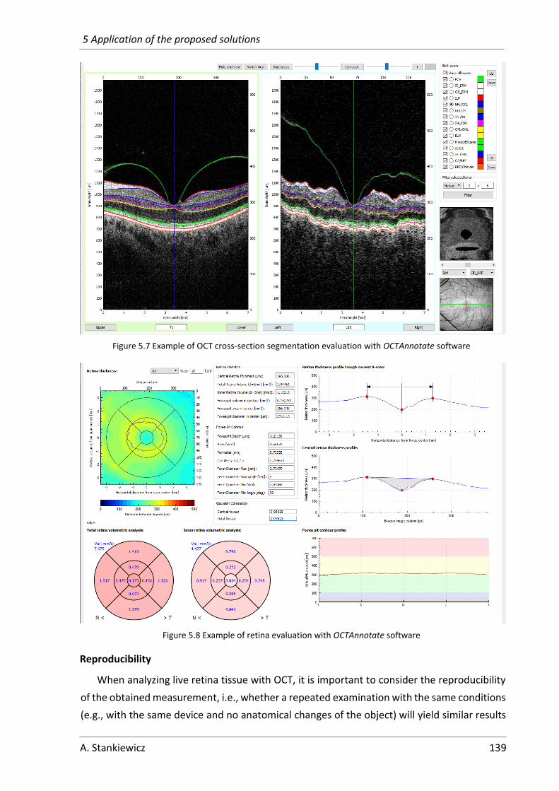
5 Application of the proposed solutions
A. Stankiewicz 139
Figure 5.7 Example of OCT cross-section segmentation evaluation with OCTAnnotate software
Figure 5.8 Example of retina evaluation with OCTAnnotate software
Reproducibility
When analyzing live retina tissue with OCT, it is important to consider the reproducibility
of the obtained measurement, i.e., whether a repeated examination with the same conditions
(e.g., with the same device and no anatomical changes of the object) will yield similar results

5 Application of the proposed solutions
140 A. Stankiewicz
[278–280]. The measurement of a live retina tissue may be influenced by many factors such
as light exposition, light wavelength, ocular magnification, or OCT device model [275]. Despite
the automation of the acquisition process (e.g., automatic selection of focus and scanning
area), two subsequent three-dimensional OCT scans typically do not have the exact same
orientation or position.
Figure 5.9 shows 4 OCT cross-sections through the fovea center acquired from one eye
during 5 minutes. As can be seen, each scan varies in the orientation and position of the retina
tissue and image contrast and brightness.
Figure 5.9 OCT cross-sections through the fovea from 4 subsequent examinations of one eye [277]
Due to the challenges mentioned above, the author of this thesis investigated the
reproducibility of the fovea pit contour calculation and its variation resulting from the OCT
acquisition [277]. The experiment was conducted for a set of 4 scans acquired from a healthy
eye in 5 minutes. Each scan was analyzed according to the algorithm presented in Figure 5.3
to determine the fovea contour curve.
Figure 5.10 FPC retina thickness profile calculated for 4 examinations of a single eye, with average and
standard deviation values computed for all angles [277]

5 Application of the proposed solutions
A. Stankiewicz 141
Figure 5.10 presents the obtained average and standard deviation values of the FPC retina
thickness profile computed for 360 angles. As can be seen, the data distribution for the retina
thickness around the FPC profile has a high correlation. The average standard deviation for all
the angles is 1.63 µm. These results lead to the conclusion that changes in the scan orientation
do not have a significant impact on the determination of the FPC parameters for healthy eyes.
Retina shape parameterization using FPC characteristics
To investigate the validity of the proposed parameters in clinical application, the author
performed a statistical analysis of the scans in the CAVRI dataset. That includes 25 VMA
subjects, 4 VMT subjects without fovea deformation – denoted as VMT0, and 13 VMT subjects
with slight fovea deformations that are not classified as eversion – denoted as VMT1. Subjects
with severe VMT were excluded from the analysis due to no visible ridge around the fovea.
Figure 5.11 presents box plots of the automatically obtained typical fovea pit parameters
for the scans in the CAVRI dataset.
(a) central retina thickness
(b) fovea pit depth
(c) foveal area within the central B-scan
(d) foveal diameter within the central B-scan
Figure 5.11 Statistics of typical fovea parameters for the CAVRI dataset
As can be expected, the CRT value (illustrated in Figure 5.11a) statistically increases with
progressing VMT. Here, the mean CRT value is 194.88 µm for VMA subjects, 206.87 µm

5 Application of the proposed solutions
142 A. Stankiewicz
for VMT0, and 230.66 µm for the VMT1 subset. The increase in CRT is related to the decrease
in fovea pit depth, as shown in Figure 5.11b. The mean 𝐹𝑃𝐷𝐶 values are 130.71 µm, 105.86
µm, and 82.69 µm for VMA, VMT0, and VMT1 respectively. Nevertheless, it should be noted,
that the mean difference between 𝐹𝑃𝐷𝐶 values for the investigated subjects is greater than
the differences in CRT.
Similarly, the central foveal area 𝐹𝐶𝐴 results in Figure 5.11c present lower values with
progressing fovea changes, although their distribution is similar. The mean and standard
deviation values of 𝐹𝐶𝐴 are 130.06 (± 39.79) µm2, 111.94 (± 49.35) µm2, and 98.22 (± 43.78)
µm2 for the VMA, VMT0, and VMT1, respectively. On the other hand, when analyzing central
fovea diameter 𝐹𝐶𝐷 values in Figure 5.11d, their distributions present no significant difference
between subsets. The mean 𝐹𝐶𝐷 values are 2361.77 (± 290.44) µm, 2310.55 (± 406.63) µm,
and 2463.74 (± 280.92) µm for VMA, VMT0, and VMT1 subsets, respectively. These results
lead to the conclusion that the changes in the fovea pit shape have no significant influence
on the shape of the parafoveal region (i.e., within the inner macula ETDRS ring).
The newly introduced fovea shape coefficient 𝑐𝐹𝑆 , reflects the fovea pit deformations
resulting from progressing VMT. This can be deduced by analyzing the results presented
in Figure 5.12a. Here, the mean and standard deviation values are 0.987 ± 0.007 for VMA
group, 0.974 ± 0.012 for VMT0, and 0.821 ± 0.289 for VMT1. These results show that the fovea
shape changes with the development of VMT (the more advanced VMT, the lower 𝑐𝐹𝑆 value).
The presented box plot shows that VMA can be distinguished from VMT with this parameter,
although differentiation between the beginning stages of VMT might benefit from
combination with other parameters.
(e) fovea shape coefficient
(f) fovea pit volume
Figure 5.12 Statistics of proposed fovea parameters for the CAVRI dataset
Figure 5.12b presents the automatically computed volume of the fovea pit 𝐹𝑃𝑉. Here, the
mean and standard deviation values are 0.118 ± 0.042 mm3 for VMA, 0.103 ± 0.040 mm3
for VMT0, and 0.098 ± 0.036 mm3 for VMT1. Although the box plot shows a wide distribution
of the volume data for all subsets with a common range between 0.089 and 0.127 mm3,

5 Application of the proposed solutions
A. Stankiewicz 143
the mean values and box plot whiskers confirm a tendency of more advanced VMT cases
having lower values of fovea pit volume.
Figure 5.13 illustrates the fovea contour statistics in the form of box plots. The main
analyzed characteristics are FPC area, perimeter, circularity, and maximal Feret diameter.
Figure 5.13a with FPC area measurements shows that the mean value of FPC area 𝐹𝑃𝐶𝐴
is similar for all subsets (i.e., 3.85, 3.99, and 3.95 mm2 for VMA, VMT0, and VMT1 groups,
respectively). It is also noticeable that the range of the obtained values is relatively wide
(e.g., 2.69 mm2 for VMA, 1.97 mm2 for VMT0, and 1.98 mm2 for VMT1), although the
distribution of VMT is narrower than that of VMA.
(a) FPC area
(b) FPC perimeter
(c) FPC circularity
(d) maximal Feret diameter of the FPC
Figure 5.13 Statistics of selected fovea pit contour (FPC) parameters for the CAVRI dataset
The calculated FPC perimeter 𝐹𝑃𝐶𝑃 values are presented in Figure 5.13b. Here, the mean
and SD values are 8.402 ± 0.953 mm for VMA, 8.915 ± 0.992 mm for VMT0, and 8.974
± 0.775 mm for VMT1. Although the mean values are similar, they slightly increase with the
development of VMT, which may be associated with increased irregularity and distortion
of the fovea pit center.

5 Application of the proposed solutions
144 A. Stankiewicz
The mean values of FPC circularity 𝐹𝑃𝐶𝐶 of 0.685 ± 0.073 for VMA, 0.628 ± 0.049 for VMT0
and 0.625 ± 0.118 for VMT1 also support that assumption. These measurements are
presented in Figure 5.13c. Interestingly, the subjects of both VMA and VMT had nonregular
FPC, which can be deduced from the wide distribution of the FPC circularity parameter.
Nevertheless, the VMT, in general, tends to have smaller values of the FPC circularity.
The maximal FPC diameter 𝐹𝑃𝐶𝐷 values presented in Figure 5.13d indicate that fovea
distortion and change in shape lead to increased maximal FPC diameter (e.g., from 2.48 mm,
to 2.58 mm, and 2.64 mm mean values for VMA, VMT0, and VMT1 subset, respectively). Also,
both minimum and maximum values of the box plots increase for each investigated group.
5.1.3 Example of automatic fovea parameterization in the long term
VMA/VMT observation
The volumetric fovea parameterization presented in Section 5.1.2 can be used for a long-
term evaluation. This will be demonstrated by observing changes in the fovea pit parameters
for the case of VMT. A 69-year-old patient (at the time of enrollment) with VMT in the left eye
was examined 4 times in the observation period of 3 years. Table 5.1 presents the current
typical evaluation of fovea shape with the CRT and retina volume measurement in individual
ETDRS grid sectors (i.e., central fovea (CF), central fovea with inner macula (CF+IM), and total
retina).
Analysis of B-scans in Table 5.1 shows that by the time of the first examination, the patient
suffered from a mild VMT. Based on the B-scan image (for the initial exam), the fovea pit
is slightly distorted, and the IS/OS layer in the central fovea is elevated. From the gathered
measurements, both the CRT values and retina volume in all investigated areas (i.e., CF,
CF+IM, and total ETDRS grid) steadily increased over time.
The change is small between the first and second examination (only a 3.1 µm increase
in CRT and 0.002 mm3 in CF volume). After another 7 months (until the third visit), the
measurable change is more significant, i.e., 15.53 µm in CRT and 0.008 mm3 in CF volume.
After 3 years of observation, the VMT progressed to fovea eversion, visible in the last cross-
section. Since the previous examination, CRT and CF volume increased by 77.62 µm and
0.043 mm3, respectively. These values show, in general, the progress of VMT with time.
Next, the author also gathered with automatic parameterization the fovea characteristics
typically measured manually and the proposed FPC and shape values proposed in Section
5.1.2. The results obtained for the above-analyzed subject are presented in Table 5.2.
Data gathered in Table 5.2 shows that the diameter of the fovea pit in the central cross-
section slightly increases from examination to examination (from 2534.35 µm at the beginning
to 2697.69 µm final measurement). At the same time, its area and depth decreased (area
decreased by 73.12 mm2, which is 47 %, and central depth decreased by 92.61 µm, i.e., 83 %).

5 Application of the proposed solutions
A. Stankiewicz 145
Table 5.1 Example of typical fovea evaluation for subsequent control exams of one patient: central B-scan images, with central retina thickness (CRT) and volume in ETDRS grid
Exam no. /
Time elapsed Central B-scan
Retina volume quantified
in ETDRS grid sectors
Typical automatic retina
parameterization 1
/ -
--
CRT:
CF retina volume:
CF+IM retina volume:
Total retina volume:
195.61 µm
0.177 mm3
2.044 mm3
7.698 mm3
2 /
2 m
on
ths
CRT:
CF retina volume:
CF+IM retina volume:
Total retina volume:
198.71 µm
0.179 mm3
2.056 mm3
7.687 mm3
3 /
9 m
on
ths
CRT:
CF retina volume:
CF+IM retina volume:
Total retina volume:
214.24 µm
0.187 mm3
2.091 mm3
7.877 mm3
4 /
3 y
ears
CRT:
CF retina volume:
CF+IM retina volume:
Total retina volume:
291.86 µm
0.220 mm3
2.131 mm3
7.876 mm3
Furthermore, fovea pit depth in the exact fovea center and the introduced measurement
of maximal fovea pit depth decrease with the progression of VMT. However, its changes are
not as big and are noticeable only for the last examination (i.e., 19.53 µm of central depth and
62.04 µm for maximal depth) when the fovea underwent eversion. Similarly, with time, the
automatically measured fovea pit volume has decreased, from 0.153 mm3 in the beginning
to 0.141 mm3 after 2 months and to 0.095 mm3 by the last examination.
The fovea shape coefficient results indicate that even if the measured diameter, area,
or depth in the central B-scan does not indicate the progression of VMT, this is reflected in the
parameterized fovea shape. This value decreased from 0.984 in the 1st examination to 0.979
in the 2nd, 0.957 in the 3rd, and finally to 0.259 when the fovea shape was distinctly distorted.

5 Application of the proposed solutions
146 A. Stankiewicz
Table 5.2 Automatically obtained fovea pit parameters with OCTAnnotate software for an example of VMT
Parameter
Exam 1
/ ---
Exam 2
/ 2 months
Exam 3
/ 9 months
Exam 4
/ 3 years
Typ
ical
ly
mea
sure
d
man
ual
ly central fovea pit diameter [µm] 2534.35 2570.31 2679.92 2697.69
central fovea pit area [mm2] 156.04 145.63 144.72 82.92
central fovea pit depth [µm] 112.14 112.06 100.16 19.53
No
vel
maximal fovea pit depth [µm] 114.53 112.12 100.24 62.04
fovea pit volume [mm3] 0.153 0.141 0.141 0.095
fovea shape coefficient [-] 0.984 0.979 0.957 0.259
Fove
a P
it C
on
tou
r
FPC area [mm2] 4.569 4.465 4.846 4.599
FPC perimeter [mm] 8.734 8.601 8.818 8.688
FPC circularity [-] 0.753 0.759 0.783 0.766
FPC maximal Feret diameter [µm] 2.735 2.733 2.759 2.734
FPC minimal Feret diameter [µm] 2.031 2.061 2.031 1.951
The fovea pit contour parameters obtained for the investigated subject give inconclusive
results. The measured FPC area varied from 4.465 mm2 to 4.846 mm2 in the observation
period. The FPC perimeter also varied with no apparent tendency from 8.601 mm
to 8.818 mm. These two parameters are directly linked to the FPC circularity (in the range
of 0.753 to 0.783), which did not show significant changes.
Table 5.3 illustrates the retina thickness virtual maps with annotated FPC and central fovea
profiles (with annotated fovea center, contour points, central area, and fitted shape function)
for the investigated examinations.
Investigating virtual color maps with fovea pit contour in Table 5.3 and its parameters
listed in Table 5.2, it is noticeable that the general shape of the fovea contour is similar in all
of the scans. The color maps also indicate that the retina thickness did not change between
the first and third examinations. The change after 3 years involved only the central fovea
(the color of the virtual map changed in the CF ring of the ETDRS from green to yellow).
The plots of the central retina profile and fitted to them Gaussian-based curve show
progressing changes of the VMT. Between the 1st, 2nd, and 3rd examination, the thickness
profile shows increased elevation of the retina surface in the fovea region (peaks in the central
fovea depression indicate edges of the vitreous contact area that elevate the fovea). As can
be noticed, the proposed parameterized shape curve indicates a correct fit to the annotated
red points. The last examination shows an even more distorted fovea center with a shape
disjoined from the gray curve, confirmed by the calculated correlation values in Table 5.2.

5 Application of the proposed solutions
A. Stankiewicz 147
Table 5.3 Example of proposed fovea evaluation for subsequent control exams of one patient: central B-scan, retina thickness virtual map, ETDRS grid with retina volumes in individual sectors, central retina profile plot
Exam no.
/ Time
elapsed
Retina thickness virtual map Plot of central retina profile 1
/ -
--
2 /
2 m
on
ths
3 /
6 m
on
ths
4 /
3 y
ears

5 Application of the proposed solutions
148 A. Stankiewicz
5.2 Preretinal space parameterization
5.2.1 Current manual evaluation of preretinal space
Currently, the medical community lacks the understanding of which retinal biomarkers
lead to spontaneous resolution or pathological development of VMT. Such assessment
is needed for providing a prognosis based on OCT images. Most clinicians rely on visual
inspection of a 2D or 3D scan and a descriptive evaluation of the current VMT stage. Figure
5.14a presents an example of a central OCT cross-section from a 3D scan of a patient with
VMT in the right eye. Figure 5.14b illustrates the 3D OCT data of this scan presented in the
form of a cloud of points, allowing only a visual assessment of changes in VRI (without
quantitative analysis).
(a) central B-scan
(b) 3D visualization as a cloud of points
Figure 5.14 Example of VMT evaluation with Copernicus HR OCT device
CAVRI dataset classification by Duker
Standard methods of evaluation and classification of VMA and VMT rely on analyzing
a single horizontal spectral domain OCT scan, as proposed by Duker et al. [30]. The single
parameter used to determine the state of VMT is the width of vitreous to retina adhesion
(at the fovea). An example of such evaluation is illustrated in Figure 5.15.
Figure 5.15 Example of a B-scan image used for descriptive assessment with annotated measurement of vitreoretinal adhesion width.
Elevated fovea PCV

5 Application of the proposed solutions
A. Stankiewicz 149
This simplified assessment technique defines the analyzed case as either broad or focal
adhesion. The statistical analysis of subjects within the CAVRI dataset with this parameter
is presented in Table 5.4 and Figure 5.16. The only information deduced from this assessment
is that focal adhesion is more prevalent in VMT cases, and broad adhesion is more common
in VMA. Furthermore, this analysis is made manually since no OCT device provides automatic
tools to measure the vitreous adhesion area.
Table 5.4 Statistics of CAVRI dataset based on evaluation proposed by Duker et al. [30]
Classification VMA VMT
focal (≤ 1500 µm) 2 19
broad (> 1500 µm) 23 6
Figure 5.16 Histogram of CAVRI cases according to Duker classification (a vertical gray line shows the division between focal and broad classes)
CAVRI dataset classification with WISPERR
The WISPERR classification [53] of VMT changes was presented in Section 2.1.3. Although
proposed in 2016, this evaluation protocol was cited 21 times1, only concerning the outcome
after macular hole surgery. Furthermore, none of the citing papers described statistical
analysis of their cohort using this parametric assessment.
For the proprietary CAVRI dataset, these parameters were determined manually
to observe the trend of parameters distribution in the study group. The data is presented
in Table 5.5 and Figure 5.17.
1 https://scholar.google.com/scholar?cites=12120084529609086048, accessed on 24/02/2022
0
2
4
6
8
10
12
14
Nu
mb
er o
f ca
ses
Vitreous attatchment width [µm]
VMT focal VMT broad VMA focal VMA broad
15
00
µm
th
resh
old
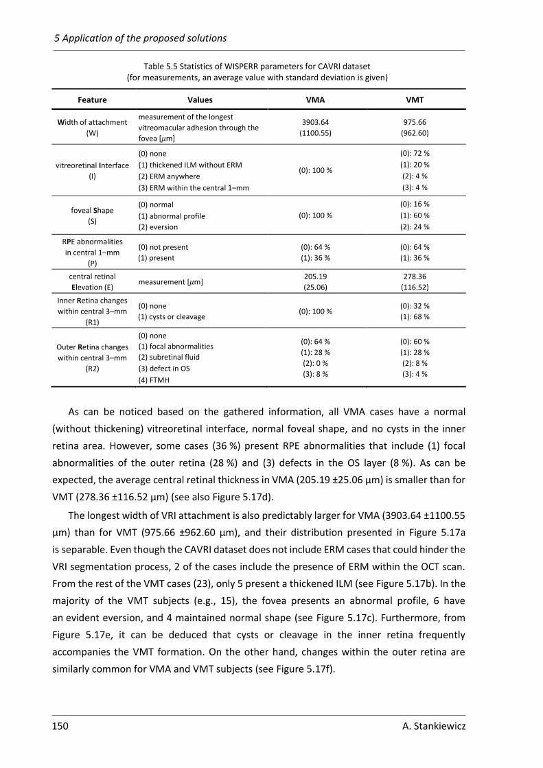
5 Application of the proposed solutions
150 A. Stankiewicz
Table 5.5 Statistics of WISPERR parameters for CAVRI dataset (for measurements, an average value with standard deviation is given)
Feature Values VMA VMT
Width of attachment
(W)
measurement of the longest
vitreomacular adhesion through the
fovea [µm]
3903.64
(1100.55)
975.66
(962.60)
vitreoretinal Interface
(I)
(0) none
(1) thickened ILM without ERM
(2) ERM anywhere
(3) ERM within the central 1–mm
(0): 100 %
(0): 72 %
(1): 20 %
(2): 4 %
(3): 4 %
foveal Shape
(S)
(0) normal
(1) abnormal profile
(2) eversion
(0): 100 %
(0): 16 %
(1): 60 %
(2): 24 %
RPE abnormalities
in central 1–mm
(P)
(0) not present
(1) present
(0): 64 %
(1): 36 %
(0): 64 %
(1): 36 %
central retinal
Elevation (E) measurement [µm]
205.19
(25.06)
278.36
(116.52)
Inner Retina changes
within central 3–mm
(R1)
(0) none
(1) cysts or cleavage (0): 100 %
(0): 32 %
(1): 68 %
Outer Retina changes
within central 3–mm
(R2)
(0) none
(1) focal abnormalities
(2) subretinal fluid
(3) defect in OS
(4) FTMH
(0): 64 %
(1): 28 %
(2): 0 %
(3): 8 %
(0): 60 %
(1): 28 %
(2): 8 %
(3): 4 %
As can be noticed based on the gathered information, all VMA cases have a normal
(without thickening) vitreoretinal interface, normal foveal shape, and no cysts in the inner
retina area. However, some cases (36 %) present RPE abnormalities that include (1) focal
abnormalities of the outer retina (28 %) and (3) defects in the OS layer (8 %). As can be
expected, the average central retinal thickness in VMA (205.19 ±25.06 μm) is smaller than for
VMT (278.36 ±116.52 μm) (see also Figure 5.17d).
The longest width of VRI attachment is also predictably larger for VMA (3903.64 ±1100.55
μm) than for VMT (975.66 ±962.60 μm), and their distribution presented in Figure 5.17a
is separable. Even though the CAVRI dataset does not include ERM cases that could hinder the
VRI segmentation process, 2 of the cases include the presence of ERM within the OCT scan.
From the rest of the VMT cases (23), only 5 present a thickened ILM (see Figure 5.17b). In the
majority of the VMT subjects (e.g., 15), the fovea presents an abnormal profile, 6 have
an evident eversion, and 4 maintained normal shape (see Figure 5.17c). Furthermore, from
Figure 5.17e, it can be deduced that cysts or cleavage in the inner retina frequently
accompanies the VMT formation. On the other hand, changes within the outer retina are
similarly common for VMA and VMT subjects (see Figure 5.17f).

5 Application of the proposed solutions
A. Stankiewicz 151
(a) W feature
(b) I feature
(c) S feature
(d) E feature
(e) R1 feature
(f) R2 feature
Figure 5.17 Statistical charts of WISPERR features for the CAVRI dataset
0
5
10
15
20
25
30
0 1 2 3
Nu
mb
er o
f ca
ses
Classification grade for Interface feature
VMA VMT
0
5
10
15
20
25
30
0 1 2
Nu
mb
er o
f ca
ses
Classification grade for Shape feature
VMA VMT
0
5
10
15
20
25
30
0 1
Nu
mb
er o
f ca
ses
Classification grade for Inner Retinafeature
VMA VMT
0
2
4
6
8
10
12
14
16
18
0 1 2 3
Nu
mb
er o
f ca
ses
Classification grade for Outer Retinafeature
VMA VMT

5 Application of the proposed solutions
152 A. Stankiewicz
Although this parameterization gives more information than the classification by Duker
et al. [30], it is still ambiguous. For example, they do not indicate the location of changes in the
vitreoretinal interface (e.g., in the superior, inferior, left, or right part of the macula). Thus far,
it is unknown how these parameters should be used to assess the VMT stage, predict its
progression, or propose a treatment course. Furthermore, all parameters need to be obtained
manually, as none are implemented in any commercial or research software.
5.2.2 Proposed Virtual Map for evaluation of the preretinal space
A more sophisticated approach for preretinal space assessment involves 3D imaging of the
whole PCV and retinal complex. One of the solutions proposed by the author is visualization
using the so-called Virtual Maps (VM) of the distance between the segmented structures.
It allows the quantification of the preretinal space volume.
The proposed solution utilizes 3D OCT cross-sections to generate a Virtual Map of the
preretinal space profile. The acquired series of 3D OCT volumetric data was subjected
to automatic segmentation of retina and preretinal space borders presented in Chapter 4.
The proposed algorithm for preparing a quantitative Virtual Map for the VMA and VMT
assessment illustrated in Figure 5.18 consists of the following steps:
1. Acquisition of a 3D OCT scan.
2. Image preprocessing (noise suppression and image cropping for graph-based
method, or normalization for DNN-based method).
3. PCV, ILM, and RPE lines segmentation in every B-scan in a 3D set (with either graph
search or DNN).
4. VRI structures parameterization:
a. Preretinal space
i. calculation of distance between the PCV and ILM line
ii. generation of a Virtual Map of the preretinal space profile
iii. calculation of preretinal space volume in each ETDRS sector
b. Vitreous to retina adhesion area
i. calculation of the adhesion area between PCV and ILM lines
ii. generation of a quantitative map of the adhesion area.
For each acquired OCT B-scan, the developed system calculates vertical distances (depths)
between the vitreous and the surface of the retina (i.e., between the ILM and PCV lines) with
the following Equation:
𝑉𝑀𝑃𝑅(𝑥, 𝑦) = 𝑃𝐶𝑉(𝑥, 𝑦) − 𝐼𝐿𝑀(𝑥, 𝑦) (5.18)
where 𝑥 ∈ ⟨0, 384⟩ denotes the horizontal index of the OCT cube (i.e., the B-scan column),
𝑦 ∈ ⟨0, 140⟩ sands for the index of the cross-section, 𝑉𝑀𝑃𝑅 is the matrix of the preretinal
space virtual map values, and 𝑃𝐶𝑉 and 𝐼𝐿𝑀 are matrixes of the segmented PCV and ILM

5 Application of the proposed solutions
A. Stankiewicz 153
surfaces, respectively. This results in distance matrixes are the size of 141×385 for each 3D
OCT scan (the dimensions of the matrix depend on the scan resolution).
Figure 5.18 General methodology for volumetric parameterization of the preretinal space
Preprocessing(noise suppression and cropping of the low quality peripheral regions)
Genera on of quan ta ve map presen ng distance profile of VMA VMT
OCT examina on
Acquisi on of a 3D OCT scan
Segmenta on of the PCV and ILM on a single B scan
Calcula on of the distance between thesegmented borders
Calcula on of prere nal space volumes for each ETDRS sector
Calcula on of the adhesionarea between thesegmented borders
Calcula on of adhesionarea for each ETDRS sector
egionAverage ( )
A mm
0.64 (0.23)
4.35 (2.00)
7.45 (4.36)
otal 12.44 (6.22)
Genera on of quan ta ve map presen ng adhesion areaof VMA VMT

5 Application of the proposed solutions
154 A. Stankiewicz
Next, the obtained VM matrix is visualized as a color depth map, as illustrates Figure 5.19.
Here, the VM is overlaid on a reconstructed fundus image (to reference the placement
of retinal vessels). Figure 5.19 presents examples of segmented central B-scans and their
corresponding preretinal space Virtual Maps for VMA and VMT subjects from a CAVRI dataset.
(a) central B-scan with layers segmentations for VMA example
(b) central B-scan with layers segmentation
for VMT example
(c) virtual map for VMA example
(d) virtual map for VMT example
Figure 5.19 Examples of preretinal space virtual profile map
The width and height of the VM image are described in [mm] with respect to the fovea
center, and the color of the VM at each point illustrates the depth of the preretinal space
in [µm]. This provides a clinician with valuable information on the stage of posterior vitreous
detachment in the examined region.
When interpreting VM for VMA example in Figure 5.19c, it can be noticed that the vitreous
has separated from the retina surface in the right (nasal) area with a distance of around
200 μm1 (pink color of VM), and upper-right (superior-nasal) area with a distance of about
1 201 μm in 314th column of 67th B-scan for this example according to the data in the OCTAnnotate software.

5 Application of the proposed solutions
A. Stankiewicz 155
300 μm (pink orange color of VM). Slight elevation (about 50 μm denoted with dark purple
color) can also be observed in the lower (inferior) region. The rest of the scan shows the
vitreous attached to the retina (the black semi-transparent color). It should be noted that such
detailed analysis is not possible based solely on the central B-scan (as illustrated in Figure
5.19a), which gives information only for the nasal and temporal quadrants. A similar
observation can be made about the VMT case presented in Figure 5.19b and d.
As shown in Section 3.2.3, the ETDRS grid may be superimposed on a Virtual Map for
spatial reference (as is visible in Figure 5.19c and d). The quantitative assessment of the
preretinal space and adhesion area is performed for each ETDRS quadrant separately and
in rings. The developed algorithms are designed to assess quantitatively:
• preretinal space volume for all 9 ETDRS sectors
• vitreous to retina adhesion area for 3 ETDRS rings.
The calculations and visualization methods developed during this research were
implemented in the OCTAnnotate software designed by the author of this thesis (see
Appendix A2).
Figure 5.20 illustrates the Preretinal Space tab of the graphical user interface
in OCTAnnotate software. In the left part of the tab, the Duker and WISPERR classification
parameters are placed. Next, to the right of these parameters is a reconstructed fundus image
with overlaid ETDRS grid and vitreous to retina contact areas overlaid in yellow. Below this
map are displayed the numerical values of the contact area in ETDRS rings. The color map
in the center of the tab, with overlaid ETDRS grid, represents the vertical differences between
the previously segmented PCV and ILM surfaces. The color bar below the map illustrates the
values assigned to each map color. The circular graph on the right illustrates the numerical
values of the preretinal space in specific sectors of the ETDRS grid. The values visible in each
sector denote the preretinal space volume in a given sector. The background color
representing this value (the greater volume, the darker color) allows a quick and intuitive
assessment.
Figure 5.20 Example of preretinal space evaluation with the OCTAnnotate software

5 Application of the proposed solutions
156 A. Stankiewicz
Analysis of measurement error
Figure 5.21 illustrates calculating the volume between ILM and PCV surfaces. From the
B-scan resolution and the number of B-scans stems the volume 𝑉𝑣𝑜𝑥𝑒𝑙 of a single voxel:
𝑉𝑣𝑜𝑥𝑒𝑙 = 𝑤𝑥 × 𝑤𝑦 × 𝑤𝑧 (5.19)
where, 𝑤𝑥 is the lateral fast-scanning data resolution (18,18 µm), 𝑤𝑦 is the distance between
neighboring B-scans (49,6 µm), and 𝑤𝑧 is the axial resolution (3,1 µm)1. This gives a single
voxel the volume of 2795.36 μm3 (i.e., 0.000002795 mm3).
Based on these values, it is possible to calculate the error of preretinal space volume
quantification. For example, when the PCV line is segmented with an MAE of 1 px, the volume
of preretinal space will differ by 1×141×385 px, which is 0.1517 mm3 within the whole OCT
scan, and by 0.088 mm3 within the ETDRS grid. For a healthy retina with an average thickness
of 200 μm, this equals 1.55 % of 9.8 mm3 retina volume within a 7×7×2 mm OCT scan. This
error margin is clinically acceptable considering the examined area and voxel size.
Figure 5.21 Illustration of voxel measurement
Preretinal volume parameterization using ETDRS grid
For the gathered OCT scans in the CAVRI dataset, the conducted research also involved
statistical analysis of the quantified preretinal space volume within each sector of the ETDRS
grid. For that purpose, the obtained segmentation was processed as was described above and
in Figure 5.18. The calculations were made in the OCTAnnotate software (see Appendix A2).
The author calculated preretinal space volume and generated virtual maps representing
the distance between the PCV and retina surface for each patient in the VMA and VMT groups
within the CAVRI dataset. The obtained results allowed the clinicians to quantitatively assess
the differences in each ETDRS sector between these two groups of subjects. Figure 5.22
presents the box plots of the calculated volumes for the central fovea and 4 inner macula
sectors. Figure 5.23 presents corresponding preretinal space volumes for the outer macula,
while Figure 5.24 illustrates the sum of inner and outer sectors in each quadrant of the ETDRS.
1 wx, wy, and wz values for 3D Retina scan are obtained with Avanti RTvue OCT device (Optovue Inc.)

5 Application of the proposed solutions
A. Stankiewicz 157
Figure 5.22 Box plot of preretinal space volume for CAVRI dataset within fovea and inner ETDRS ring
Figure 5.23 Box plot of preretinal space volume for CAVRI dataset within fovea and outer ETDRS ring
Figure 5.24 Box plot of preretinal space volume for CAVRI dataset within fovea and four ETDRS sectors
The gathered results indicate that the preretinal space volume in the inner macula region
is similar in all directions. The biggest difference is observed for the VMT subset between the

5 Application of the proposed solutions
158 A. Stankiewicz
nasal inner IQR of 0.247 mm3 and the inferior inner IQR of 0.414 mm3. The most significant
difference in the average preretinal space volume is detected between the temporal inner
(0.293 mm3) and superior inner (0.336 mm3) sectors. For the VMA subset, the calculated
preretinal space volumes are significantly smaller, with the biggest average value being
0.035 mm3 for the superior inner sector and the smallest average value of 0.0098 mm3 for the
inferior inner sector.
The preretinal space of the fovea is understandably significantly smaller due to the
spanning range of a smaller diameter and frequently having attached vitreous to the retina
surface. The average value of the preretinal space in the central fovea for VMA
is 0.00184 mm3, while for the VMT is 0.079 mm3.
The data presented in Figure 5.23 indicates greater vitreous separation from the retina
surface for VMT subjects in the superior outer quadrant (average value of 1.654 mm3) than
in the inferior, nasal and temporal outer quadrants (average value of 1.376 mm3, 1.316 mm3,
and 1.326 mm3, respectively). Furthermore, the smallest IQR value is observed for the nasal
outer sector (0.823 mm3) and the biggest for superior and inferior outer sectors (1.448 mm3
and 1.459 mm3, respectively). Although the outer ETDRS ring spans a 3.38 times greater area
than the inner ring, the preretinal space volumes in these rings differ on average 4.54 times
for VMT and 16.22 times for VMA.
For VMA subjects, the distribution of preretinal space volume is similar for the outer and
inner ETDRS rings. The biggest average value in the outer ring is obtained for the superior
sector (0.533 mm3) and the smallest for the inferior sector (0.224 mm3). The nasal and
temporal sectors have a similar average preretinal space volume (0.347 mm3 and 0.313 mm3,
respectively) but differ in the IQR (0.38 mm3 and 0.32 mm3, respectively).
Due to the fact that the preretinal space volume values are significantly greater in the
outer ring than in the inner ring and the fovea, the data presented in Figure 5.24 maintain
a similar distribution to the values described for the outer ETDRS ring. It should also be noted
that the average preretinal space volume for the VMT subjects is 4.83 and 4.36 times greater
than for VMA in the temporal and nasal quadrants, respectively, and 3.50 and 7.20 times
greater in the superior and inferior quadrants, respectively.
Parameterization of vitreous to retina adhesion area
The vitreous to retina adhesion area corresponds to the PCV-ILM distance equal to 0 µm.
To account for retinal layers segmentation error and annotation uncertainty, the author set
a margin of 10 µm when determining the VRI adhesion area. Figure 5.25 illustrates the
adhesion area overlaid on the reconstructed fundus image for examples of VMA and VMT
presented in Figure 5.19.

5 Application of the proposed solutions
A. Stankiewicz 159
(a) VMA example
(b) VMT example
Figure 5.25 Visualization of the adhesion area (in red) overlaid on the reconstructed fundus image
When analyzing the adhesion map for the VMA example in Figure 5.19a, it can be noticed
that the vitreous is fully connected in the Central Fovea region (i.e., 0.785 mm2), spans 58 %
of Inner Macula (i.e., 4.086 mm2), and 14 % of Outer Macula (i.e., 3.969 mm2). Furthermore,
compared to the preretinal space volume map, the contact area map shows in more detail
that the vitreous is separated in the superior and nasal inner macula and superior, nasal, and
inferior outer sectors. Irregularities also noticeable in such maps stem from border annotation
uncertainties concerning axial resolution (1 px represents 3.1 μm).
Table 5.6 includes the average adhesion values for each ETDRS ring for VMA and VMT
subjects from the CAVRI dataset and a VMA/VMT ratio for these areas. For VMA subjects, the
adhesion area stems almost the whole Central Fovea (94.6 %) on average, while in VMT,
it is about 32.6 % of the CF region. For the Inner Macula ring difference between these values
is even greater: 10.1 % for VMT and 77.2 % for VMA. When investigating the Outer Macula
ring, the adhesion area spans a significantly smaller area than the area of the whole OM (6.2 %
for VMT and 23.2 % for VMA). This confirms that OM (and the area beyond it) is the first region
of vitreous separation. Furthermore, the calculated adhesion areas are 4.79 times greater for
VMA than for VMT subjects. The greatest difference is observed for the inner macula region,
for which the VMA/VMT adhesion ratio is 7.66. Figure 5.26 illustrates box plots for these
subsets.
From data in Table 5.6 and Figure 5.26, it is also noticeable that the range of adhesion area
values for CF in VMA is very small (standard deviation of 0.096 mm2). This can be explained
by the fovea being one of the last regions separating from the vitreous. Thus, the adhesion
spans almost all of the CF until it separates.

5 Application of the proposed solutions
160 A. Stankiewicz
Table 5.6 Average adhesion area values for VMA and VMT in individual rings of ETDRS grid
Region Total area
[mm2]
Average (SD) adhesion area [mm2] VMA / VMT
adhesion ratio VMT VMA
Central Fovea 0.785 0.256 (0.222) 0.743 (0.096) 2.90
Inner Macula 6.284 0.633 (1.089) 4.849 (1.635) 7.66
Outer Macula 21.205 1.306 (2.694) 4.912 (3.514) 3.76
Total 28.274 2.195 (3.626) 10.504 (4.680) 4.79
Figure 5.26 Box plot of vitreoretinal contact area for CAVRI dataset in 3 ETDRS rings
The proposed method allows to perform precise determination of the adhesion area.
It is much more accurate than a simple approximation with an ellipse proposed by [47]. Since
the strength of the attachment between the posterior surface of the hyaloid and the retina
is considered an important factor in VMA and VMT pathology, the developed quantitative
evaluation methods are valuable tools for their assessment.
5.2.3 Advantage of volumetric preretinal space parameterization in the long
term VMA/VMT observation
The volumetric analyses presented earlier are an effective tool for long-term evaluation.
This will be demonstrated by observing changes in the preretinal space for the case of VMT.
A 66-year-old patient (at the time of enrollment) with VMT in both eyes was examined 6 times
in the observation period of 1.5 years. After 3 months, the VMT in the right eye was
disconnected, while the left eye remained under observation.
Table 5.7 presents an evaluation with the current manual parameterization methods
by Duker and WISPERR. The obtained measurements show how limited the classification
by Duker is, where attachment width during the first three months differs by only 255.20 μm,
and the classification remains unchanged.

5 Application of the proposed solutions
A. Stankiewicz 161
Table 5.7 Example of typical VMT evaluation with current classification methods for subsequent control exams of one patient: central B-scan images, classification by Duker, and WISPERR parameterization
Exam no. /
Time elapsed Central B-scan Duker classification
WISPERR
parameterization 1
/ -
--
Adhesion width:
Classification:
3627.60 µm
Broad
W:
I:
S:
P:
E:
R1:
R2:
3627.60 µm
(1)
(1)
(0)
208.03 µm
(1)
(0)
2 /
1 m
on
th
Adhesion width:
Classification:
3427.08 µm
Broad
W:
I:
S:
P:
E:
R1:
R2:
3500.00 µm
(1)
(1)
(0)
217.34 µm
(1)
(0)
3 /
3 m
on
ths
Adhesion width:
Classification:
3372.40 µm
Broad
W:
I:
S:
P:
E:
R1:
R2:
3226.56 µm
(1)
(1)
(0)
245.28 µm
(1)
(0)
4 /
6 m
on
ths
Adhesion width:
Classification:
273.44 µm
Focal
W:
I:
S:
P:
E:
R1:
R2:
401.04 µm
(1)
(2)
(1)
291.86 µm
(1)
(1)
5 /
1 y
ear
Adhesion width:
Classification:
255.21 µm
Focal
W:
I:
S:
P:
E:
R1:
R2:
255.21 µm
(1)
(1)
(1)
254.60 µm
(1)
(1)
6 /
1.5
yea
r
Adhesion width:
Classification:
---
---
W:
I:
S:
P:
E:
R1:
R2:
---
(1)
(1)
(1)
167.66 µm
(1)
(1)

5 Application of the proposed solutions
162 A. Stankiewicz
Between the 3rd and 4th examination, the vitreous detaches in the temporal region (see
right side of the B-scan), the attachment width decreases to 273.44 μm and changes the
classification to focal. The final examination shows a total vitreous detachment, for which
most measurements cannot be obtained.
Data gathered in Table 5.7 shows that the WISPERR parameterization allows for a more
detailed analysis of the current VMT stage and development prognosis. The W parameter
is similar to the Duker adhesion width measurement and, for the 1st examination, has the
same value of 3627.60 μm. In the given example, the W parameter decreases during the first
three months, but to 3226.56 μm instead of 3372.40 μm. These differences result from the
cross-section used for the measurement. In the following examinations, the W parameter also
decreases significantly. However, the 4th observation shows that the broadest adhesion
(401.04 μm) is almost twice as long as the Duker measurement (273.44 μm), thus not in the
central B-scan. Between the 4th and 5th examination, the attachment becomes more focal.
Its maximal width diminished further to 255.21 μm, changing the shape of the fovea and
allowing a smaller retina elevation (E parameter decreases from 291.86 μm to 254.50 μm).
With WISPERR parameterization, valuable information give the parameters W and E. For
the evaluated patient, when the width attachment (W parameter) was decreasing, the E value
increased from 208.03 μm in the beginning to 245.28 μm in the 3rd examination indicating
a strong pull of the detaching vitreous. The E value increased further to 291.86 μm in the 4th
examination, when the attachment became focal. Then, the elevation width decreased
to 254.60 μm along with the decrease in maximal width (W), which suggests a weakening
of the VRI adhesion and an upcoming vitreous separation. After vitreous detachment, the
fovea shape returns to a natural depression with a central retina thickness of 167.66 μm.
The I parameter is constant for all examinations and shows a thickened ILM structure.
The S parameter for the first three examinations indicates an abnormal fovea shape (1) and
changes to eversion (2) when the adhesion becomes focal, returning to the abnormal profile
right after the vitreous detachment. The parameter P directly corresponds to parameter R2,
which describes the RPE structure. The first three examinations show a normal RPE (0), while
after the change in the attachment (broad to focal), dehiscence in the RPE layer is visible (1),
which stays even after the vitreous detachment. Finally, parameter R1 indicates that cysts
have formed in the inner retina. Although this parameter is directly linked to the shape of the
fovea (fovea eversion in most cases causes retinal cysts), the cysts were present even for the
abnormal fovea profile (R1 value of (1)) and stayed after vitreous detachment.
Although such analysis gives valuable information about the changes of the VMT,
the proposed volumetric evaluation shows preretinal space volume changes over time
in individual ETDRS sectors. Table 5.8 illustrates the evaluation of the same OCT scans with
virtual color maps of the preretinal space, ETDRS volume grids, and adhesion area maps with
measured contact area in each ETDRS ring.

5 Application of the proposed solutions
A. Stankiewicz 163
Table 5.8 Example of proposed VMT evaluation for subsequent control exams of one patient: virtual color maps, ETDRS grids with preretinal volumes in individual sectors, adhesion area maps, and parameters
Exam no. / Time
elapsed
Preretinal space virtual map
Preretinal space volume quantified in ETDRS grid sectors
Vitreous to retina adhesion area
1 /
---
CF: 0.222 mm3
IM: 3.891 mm3
OM: 12.807 mm3
2 /
1 m
on
th
CF: 0.359 mm3
IM: 3.838 mm3
OM: 12.077 mm3
3 /
3 m
on
ths
CF: 0.247 mm3
IM: 2.456 mm3
OM: 8.520 mm3
4 /
6 m
on
ths
CF: 0.091 mm3
IM: 0.0 mm3
OM: 0.0 mm3

5 Application of the proposed solutions
164 A. Stankiewicz
Exam no. / Time
elapsed
Preretinal space virtual map
Preretinal space volume quantified in ETDRS grid sectors
Vitreous to retina adhesion area
5 /
1 y
ear
CF: 0.050 mm3
IM: 0.0 mm3
OM: 0.0 mm3
6 /
1.5
yea
r
CF: 0.0 mm3
IM: 0.0 mm3
OM: 0.0 mm3
Data presented in ETDRS volume grids in Table 5.8 include the volume of total preretinal
space in the EDTRS range at the beginning of the study as 1.711 mm3, followed by 1.804 mm3
in the next test, 3.142 mm3 in the third, 5.633 mm3 in the fourth, 5.974 mm3 in the fifth, and
7.823 mm3 in the sixth test. The vitreous adhesion in the ETDRS area in the first examination
was 16.92 mm2, and in subsequent studies, it was 16.27 mm2, 11.22 mm2, 0.09 mm2,
0.05 mm2, respectively, and in the sixth study, it was zero.
The detailed analysis of the virtual maps and ETDRS volume grids clearly shows that the
vitreous was first separated in the outer nasal area (with a preretinal space volume
of 1.016 mm3). The detachment progressed to the outer superior region to reach 1.654 mm3
after 3 months. Maps for the 4th examination (after 6 months) illustrate that the vitreous
is detached in whole inner and outer macula rings (with a volume of 4.634 mm3 in the outer
and 0.93 mm3 in the inner ETDRS ring), and the attachment spans only the central fovea.
The contact area map shows that the central fovea region is constantly attached throughout
the evaluation and detaches as last. Interestingly the changes in VRI associated with
weakening of the vitreous adhesion between the 4th and 5th examination are visible as a slight
increase of preretinal volume in all ETDRS sectors.
The measured preretinal space volume changes are also visualized in Figure 5.27 for four
ETDRS quadrants in total. The data indicate that although the greatest separation was in the

5 Application of the proposed solutions
A. Stankiewicz 165
nasal area (1.148 mm3) initially, its change up to the 5th examination was only by 0.016 mm3.
The largest progress can be observed in the superior quadrant, which changed from initial
0.48 mm3 to 1.85 mm3 in the 3rd examination and finally to 2.51 mm3. The preretinal space
volume in the superior quadrant also remained the greatest throughout every observation
period. Furthermore, the measured volume increased in the temporal and inferior quadrants
only after vitreous separation in the outer ETDRS ring.
Figure 5.27 Bar plot of preretinal space volume in the central fovea and four ETDRS quadrants
Summary of application of the proposed solutions
The author presented novel volumetric parameterization methods for evaluating retina
and preretinal space characteristics with present VMA and VMT. The proposed automatic
parameterization methods were applied in a clinical setting and analyzed in terms of validity.
The statistical analysis of subjects from the CAVRI dataset indicates the following key results:
1) concerning fovea parameterization:
a. the standard evaluation parameters of CRT, fovea pit depth 𝐹𝑃𝐷 , central fovea
area 𝐹𝐶𝐴 and central fovea diameter 𝐹𝐶𝐷 , can be determined in an automatic
procedure; their distributions show the difference for the investigated VMT cases
b. fovea shape coefficient 𝑐𝐹𝑆, introduced by the author, shows a correlation of the
measured retina thickness profile to a statistically normal fovea shape, and has
a potential to be used as a parameter for VMT stage classification; the
automatically obtained fovea pit volume and maximal fovea pit depth provide
further details about the changes in the fovea pit region
c. the proposed fovea pit contour and its characteristics (area, perimeter, circularity,
and maximal diameter) have acceptable reproducibility and indicate slight
differences between the VMA and VMT development
0
0.5
1
1.5
2
2.5
3
Exam 1 Exam 2 Exam 3 Exam 4 Exam 5 Exam 6
Pre
reti
nal
sp
ace
volu
me
[mm
3 ]
Fovea Temporal Superior Nasal Inferior

5 Application of the proposed solutions
166 A. Stankiewicz
d. introduced automatic fovea pit parameterization can be used to illustrate changes
in the fovea that occur in the long term VMA/VMT observation
2) concerning preretinal space parameterization:
a. both Duker and WISPERR-based classification of the VRI (limited to the central OCT
cross-section) do not fully reveal the possible changes that occur in VRI
b. using the presented algorithms, it is possible to create detailed VRI virtual maps
that accurately reflect the profile of the vitreous body adherence to the retina and
allow to assess the preretinal space volume in individual ETDRS sectors quickly
c. developed parameterization methods of the preretinal space volume and VRI
contact area allows to quantitatively and accurately distinguish VMA and VMT
d. in a long-term VMA/VMT observation, the proposed quantitative parameterization
of preretinal space volume and contact area provides more detail about the
progression of the vitreous separation than Duker or WISPERR classifications
(especially in the superior and inferior macula regions).
The obtained results prove the validity of the proposed parameterization of the fovea and
preretinal space for accurate assessment of the VMA/VMT condition. The developed methods
for automatic segmentation and parameterization of preretinal space and retina allow
to measure differences between VMA and AMT and track their changes in time. The author
believes that the proposed parametric evaluation can provide valuable information to further
the understanding of VMA and VMT progression. The obtained parameterized data has the
potential to be used for diagnostics and clinical decision-making, as well as in research.

167
Chapter
6 Conclusions
Biometric analysis of the retina morphological structures is crucial for diagnosing patients with
ophthalmic diseases. Implementation of non-invasive diagnostic methods, such as optical
coherence tomography (OCT), in modern visualization systems, allows for the investigation
of the retina at the cellular scale. Modern OCT devices allow for detailed visualization of the
vitreous and retinal area with the acquisition speed of up to 100 000 A-scans/second and axial
scan resolution of 3 µm. Although a volumetric 3D scan provides more information about
retina changes in the whole macular region, its acquisition time takes even 1 s. Also, its quality
is much lower than multiply acquired and averaged single B-scan examination through the
macula center. For this reason, advanced signal processing algorithms are necessary
to improve the obtained 3D image quality and reliability of its investigation.
The amount of data acquired using the OCT modality makes a detailed manual assessment
of the examined tissue impractical in the clinical routine. The introduction of automatic
segmentation of the retinal structures from medical images allows the analysis of the retina
tissue quantitatively. The software solutions implemented in modern OCT devices are
increasingly advanced. Nevertheless, some pathological changes, e.g., those in the border
of the vitreous and the retina (i.e., vitreoretinal interface), still lack effective methods
for segmentation, parameterization, and pathology stage assessment. Because the VRI
abnormalities (e.g., vitreomacular adhesion and traction – VMA/VMT) have been classified
by a team of ophthalmologists relatively recently, i.e., in 2013, there are no automated
methods for determining the profile of VMT in relation to the surface of the retina.
The research objective in this thesis was to extract biometrical features mainly
for VMA/VMT assessment using automatic procedures based on volumetric OCT data.
The main achievements of this work can be summarized in the following remarks:
1. Manufacturers of OCT devices constantly try to overcome the low quality of the
acquired images. In order to improve the segmentation accuracy for the gathered
CAVRI OCT images with specific conditions of VMT, the author tested several state-of-
the-art noise reduction methods. The goal was to obtain the correct segmentation
of the retina layers with a graph-based approach and enhance the vitreoretinal
interface characteristics – mainly the low signal level of the vitreous border. However,
graph-based segmentation using image gradient analysis is susceptible to noise and
local signal level variations.

6 Conclusions
168 A. Stankiewicz
a. The author tested the following noise reduction methods: averaging filtering,
median filtering, anisotropic diffusion, wavelet soft thresholding, block-matching
and collaborative filtering (BM3D), 3D anisotropic diffusion, multiframe wavelet
soft thresholding, and 3D block-matching and collaborative filtering (BM4D). The
literature-based methods were adopted to the specificities of 3D OCT data, and
a wide range of filter parameters were tested.
The conducted experiments demonstrate that among 2D noise reduction methods
(i.e., those applied to each OCT B-scan separately), the BM3D allows obtaining the
best layers segmentation accuracy with an average MAE of 4.18 px for all layers.
Furthermore, from the group of 3D methods (i.e., considering neighboring
B-scans), the BM4D method also provides the best segmentation accuracy with
an average MAE of 3.62 px. Nevertheless, it should be noted that this method
is also the most computationally expensive, where filtering of 3D volume takes
415.10 s and 18655.55 s for BM3D and BM4D, respectively.
b. The author noticed that low signal strength parts of the B-scan hinder the process
of finding the shortest path of the graph-based algorithm for retina layers
segmentation. Thus, the author proposed a method of removing low quality parts
of the OCT image to improve the stability of the graph search method.
The tested methods involved two approaches: removing the constant width of the
peripheral section of the B-scan from further investigation or performing
an adaptive cropping technique based on a selected threshold. Both approaches
were tested with multiple threshold values.
The obtained results show that for the VMA cases, the best result is obtained with
cropping of a constant 15 % of B-scan width, which improves the segmentation
accuracy for this group from 4.75 px of MAE to 4.09 px. On the other hand, for the
VMT subset, the best outcome gives the adaptive cropping of B-scan width with
the threshold of 𝑡=140, and improvement of MAE value from 4.45 px to 3.84 px.
c. Furthermore, the author proposed tracking specific retina layers borders (i.e., ILM
and IS/OS) when processing subsequent OCT cross-sections. This procedure allows
further improvement of the segmentation correctness.
The general idea stems from the fact that the retina tissue is continuous between
neighboring cross-sections; thus, it is possible to limit the search region for the
graph-based method to the desired B-scan area. Additionally, the author tested
the influence of the tracking procedure’s starting point (i.e., from the edge of the
scan, from 1/3rd of the scan, or the center of the scan) on the overall segmentation
correctness and eventual error propagation.
Based on the obtained results, it can be concluded that the best results can
be obtained when both hyperreflective retina borders (i.e., ILM and IS/OS) are

6 Conclusions
A. Stankiewicz 169
tracked throughout the 3D OCT scan starting from the 1/3rd of the volume.
The average MAE value for all cases with this approach is 4.10 px. Additionally,
as illustrated in Section 3.2.3, the proposed solution allowed removing inter-
section irregularities of the segmented retina borders.
2. The current solution implemented in research or commercial OCT software does not
allow for segmentation of the vitreous border (i.e., PCV) and preretinal space area
or precise quantitative observation of its changes in VMA and VMT cases. Therefore,
the author aimed to obtain correct PCV line segmentation using modern OCT image
analysis based on neural networks.
a. For automated preretinal space segmentation, the author selected the most
promising convolutional neural networks and implemented them in 4-class pixel-
wise semantic segmentation for PCV extraction from OCT images. Among the
selected architectures were: baseline UNet, LFUNet, Attention UNet, DRUNet, and
ReLayNet.
i. First, two cost functions (e.g., Categorical Cross-Entropy Loss and Weighted
Dice Loss) and three of their combinations with various weights were tested.
The best results with a Preretinal Space Dice Coefficient of 0.9458 were
obtained utilizing a Combined Loss function with a weight of 1 for Weighted
Categorical Cross-Entropy Loss and 0.5 for Weighted Dice Loss.
ii. Using the selected loss function, the author tested the performance of the
above-listed network architectures. Here, the best results for the Preretinal
Space were obtained with the baseline UNet with the MAE of 2.83 px, 0.56 px,
and 0.75 px for PCV, ILM, and RPE borders, respectively. It should be noted that
the deep learning approach provides better results for preretinal space
segmentation than the graph-search method, for which the obtained Dice
Coefficient was only 0.8217 and MAE was 7.29 px, 5.10 px, and 5.20 px for PCV,
ILM, and RPE lines, respectively.
iii. Additionally, the author analyzed the influence of 4 data augmentation
techniques (horizontal flip, random rotation, random translation, and random
cropping) on the improvement of preretinal space segmentation.
The conducted experiments show that the preretinal space segmentation can
be improved with additional data augmentation from 0.9486 to 0.9591 for the
Preretinal Space Dice Coefficient with baseline UNet.
b. The author also discussed the problem of the incorrect order of segmented retina
borders and proposed a solution for reducing the number of topologically incorrect
segmentations. Two approaches were tested: incorporating additional topology
information in the form of a Relative Distance Map (RDM) and utilizing a nontypical
convolution kernel.
6 Conclusions
170 A. Stankiewicz
i. Two RDMs utilizing prior segmentation of the retina borders (referred
to as 2NetR and 2NetPR) were proposed, and additional two RDMs that do not
require prior information of the retina borders (named BasicOrient, and
CumSum). Results presented in Section 4.3.2 show that the 2NetPR map
proposed by the author reduces the percentage of topology errors from 15.1 %
to 3.7 % for UNet and even from 88.3 % to 10.8 % for ReLayNet. For LFUNet,
the best results were obtained with the CumSum method, for which the
topology incorrectness decreased from 11.5 % to 4.8 %.
ii. To increase the robustness of the network to a spatial hierarchy of the classes,
the author proposed increasing the network’s field of view with a bigger
convolution kernel. Three types of kernels were tested: typical square (3×3,
5×5, and 7×7), vertical (5×3, 7×3, and 9×3), and horizontal (3×5, 3×7, and 3×9).
The greatest improvement in topology was observed for vertical 9×3 kernel
for UNet and LFUNet (incorrectness decreased to 2.42 % and 1.14 %,
respectively). For the UNet, the best Preretinal Space Dice Coefficient of 0.9640
and MAE for PCV of 0.90 px were obtained with horizontal kernel 3×9. Similar
results for Preretinal Space Dice Coefficient of 0.9638 and PCV MAE of 0.88 px
for LFUNet were obtained with kernel 7×7. It can be noticed that a solution
utilizing a non-standard convolution kernel gives better results than additional
RDM while omitting the problem of error propagation.
3. Precise retina and vitreous borders segmentation in an OCT scan is key to the correct
assessment of retina and preretinal space. Thanks to correct OCT image segmentation,
the parameters of the morphological structures can be obtained automatically.
Currently, no research or commercial OCT software provides an automated
measurement of VRI features and structures. The research conducted by the author
aimed at developing automatic parameterization of VRI for quantitative VMA/VMT
assessment.
a. In Section 5.1, the author proposed and evaluated novel fovea parameterization
techniques for VMA and VMT investigation. A set of key fovea anatomical features
(based on a central B-scan) has been implemented in an automatic procedure.
Additionally, the author introduced new parameters of the fovea shape
coefficient, fovea pit contour, and volume (based on a 3D OCT scan). The statistical
analysis of the fovea parameters within VMA/VMT subsets and long-term VMT
observation indicates the proposed parameters' validity and usefulness in tracking
VRI changes.
b. Utilizing this thesis's preretinal space segmentation method, the author performed
automated parameterization of the preretinal space volume and vitreous to retina
adhesion area within each ETRDS grid sector. The author shows that observation

6 Conclusions
A. Stankiewicz 171
of the preretinal space volume is a unique and informative way to monitor changes
in the vitreoretinal interface. The discussion in Section 5.2 presents the advantage
of incorporating, proposed by the author, volumetric 3D analysis of VRI profiles
in the form of virtual maps. Furthermore, by performing a structural investigation
of VMA/VMT using the designed 3D data analysis (instead of a single B-scan),
the author presents tools to quantitatively and objectively track disease
progression in long-term observation.
In summarizing, the results of experiments presented by the author prove the scientific
thesis stated in Section 1.4. Thus, in the author’s opinion, the scientific aim of this Ph.D.
dissertation has been accomplished.
The innovative way of observing changes in the VRI area was developed thanks to the
cooperation of an interdisciplinary research team consisting of employees of the Department
of Ophthalmology, Heliodor Swiecicki University Hospital, Poznan University of Medical
Sciences, and employees of the Division of Electronic Systems and Signal Processing, Institute
of Automatic Control and Robotics, Poznań University of Technology. The cooperation
resulted in multiple publications in scientific journals, conference presentations, and the
submission of a patent application (see Appendix 1).
Open-source software prepared during conducted research and published
on http://dsp.org.pl/badania/4/ and the https://github.com/krzyk87 pages can help other
scientists in the study of VRI pathologies and improvement of medical image analysis
procedures. Furthermore, the gathered unique OCT dataset can be helpful to research groups
worldwide investigating ophthalmic pathologies. The OCTAnnotate software (see Appendix 2)
was used for long-term follow-up of patients in the doctoral research of Elżbieta Marciniak,
M.D., and in research related to master's and bachelor's theses in the Department
of Ophthalmology at Poznan University of Medical Sciences.
Furthermore, the research presented within this thesis was supported by the National
Science Centre with the following research grants:
• Preludium 8: “Maximizing informative content of low quality OCT scans for modern
computer-aided diagnostic procedures (Project CADOCT),” project no. 2014/15/N/
ST6/00710, 2015 – 2017.
• Etiuda 7: “Automatic parameterization of human retina image,” project no.
2019/32/T/ST6/00500, 2019 – 2021.
Concluding, the proposed solutions for precise segmentation and parameterization of the
retina and preretinal space can be applied in a clinical setting to aid during the diagnostic
procedures. The developed algorithms contribute to the scientific development of medical
imaging technologies and boost advanced diagnostic software solutions. The designed
software provides ophthalmologists with new tools to study VRI and conduct a quantitative

6 Conclusions
172 A. Stankiewicz
assessment of VMT pathology. Additionally, they present the data in a format intelligible
for clinicians, such as virtual maps of epiretinal pathologies.
Furthermore, the proposed precise segmentation and quantitative evaluation are suitable
for classification protocols. They can be used to automatically classify the retina and preretinal
space state in various VMA/VMT cases and other conditions. The introduced parameterization
has the potential to aid in the automatic detection of morphological changes, monitoring the
progression of the disorder, early pathology detection, or classification of the pathology
advancement. The presented research can significantly impact the clinicians’ approach
to patients with VRI pathologies. It has potentially valuable input for selecting case-
appropriate treatment therapy or planning a surgical strategy.

173
Bibliography
[1] H. Davson, Human Eye. Encyclopedia Brittanica, 2016. [2] D. C. DeBuc, “A Review of Algorithms for Segmentation of Retinal Image Data Using Optical
Coherence Tomography,” in Image Segmentation, P.-G. Ho, Ed. InTech, 2011, pp. 16–54. [3] H. von Helmholtz, “In World Encyclopedia. Oxford University Press.” 2005. [4] M. D. Abràmoff, M. K. Garvin, and M. Sonka, “Retinal imaging and image analysis,” Biomedical
Engineering, IEEE Reviews in, vol. 3, pp. 169–208, 2010. [5] A. Gullstrand, “Neue methoden der reflexlose ophthalmoskopie,” Berichte Deutche
Ophthalmologische Gesellschaft, vol. 36, 1910. [6] H. R. Novotny and D. L. Alvis, “A method of photographing fluorescence in circulating blood in
the human retina,” Circulation, vol. 24, pp. 82–86, 1961. [7] M. M. Fraz, P. Remagnino, A. Hoppe, and others, “Blood vessel segmentation methodologies in
retinal images – A survey,” Comput. Methods Programs Biomed., vol. 108, pp. 407–433, 2012. [8] D. Huang, E. A. Swanson, and al. et, “Optical coherence tomography,” Science, vol. 254, pp.
1178–1181, 1991. [9] J. J. Kaluzny, A. Szkulmowska, T. Bajraszewski, M. Szkulmowski, B. J. Kaluzny, I. Gorczynska, P.
Targowski, and M. Wojtkowski, “Retinal imaging by spectral optical coherence tomography,” European Journal of Ophthalmology, vol. 17, no. 2, pp. 238–245, 2007.
[10] M. R. Hee, J. A. Izatt, E. A. Swanson, D. Huang, J. S. Schuman, C. A. Puliafito, and J. G. Fujimoto, “Optical coherence tomography for micron-resolution ophthalmic imaging,” IEEE Eng. Med. Biol., vol. 14, pp. 67–76, 1995.
[11] W. Drexler and J. G. Fujimoto, Eds., Optical Coherence Tomography, Technology, and Applications. Springer-Verlag Berlin Heidelberg, 2008.
[12] M. Inoue, J. J. Jung, C. Balaratnasingam, K. K. Dansingani, E. Dhrami-Gavazi, M. Suzuki, T. E. de Carlo, A. Shahlaee, M. A. Klufas, A. E. Maftouhi, J. S. Duker, A. C. Ho, M. Q.-E. Maftouhi, D. Sarraf, and K. B. Freund, “A Comparison Between Optical Coherence Tomography Angiography and Fluorescein Angiography for the Imaging of Type 1 Neovascularization,” Investigative Ophthalmology & Visual Science, vol. 57, no. 9, pp. 314–323, 2016.
[13] B. Sikorski, D. Bukowska, D. Ruminski, I. Gorczynska, M. Szkulmowski, K. Krawiec, G. Malukiewicz, and M. Wojtkowski, “Visualization of 3D retinal microcapillary network using OCT,” Acta Ophthalmologica, vol. 91, no. s252, 2013.
[14] M. Sonka and M. D. Abràmoff, “Quantitative analysis of retinal OCT,” Medical Image Analysis, vol. 33, pp. 165–169, 2016.
[15] O. Tan, G. Li, A. T.-H. Lu, R. Varma, D. Huang, and A. I. for Glaucoma Study Group, “Mapping of Macular Substructures with Optical Coherence Tomography for Glaucoma Diagnosis,” Ophthalmology, vol. 115, no. 6, pp. 949–956, 2008.
[16] C.-S. Yang, C.-Y. Cheng, F.-L. Lee, W.-M. Hsu, and J.-H. Liu, “Quantitative assessment of retinal thickness in diabetic patients with and without clinically significant macular edema using optical coherence tomography,” Acta Ophthalmologica Scandinavica, vol. 79, pp. 266–270, 2001.
[17] F. Okamoto, Y. Sugiura, Y. Okamoto, T. Hiraoka, and T. Oshika, “Inner Nuclear Layer Thickness as a Prognostic Factor for Metamorphopsia after Epiretinal Membrane Surgery,” Retina, vol. 35, pp. 2107–2114, 2015.
[18] M. C. de Salles, A. Kvanta, U. Amren, and D. Epstein, “Optical Coherence Tomography Angiography in Central Retinal Vein Occlusion: Correlation Between the Foveal Avascular Zone and Visual Acuity,” Investigative Ophthalmology & Visual Science, vol. 57, no. 9, pp. 242–246, 2016.
[19] A. C. Palacio, A. Gupta, B. L. W. Nesmith, P. R. Jadav, Y. Schaal, and S. Schaal, “Vitreomacular adhesion evolution with age in healthy human eyes,” Retina, vol. 37, no. 1, pp. 118–123, 2017.

Bibliography
174 A. Stankiewicz
[20] L.-J. Li, M. K. Ikram, and T. Y. Wong, “Retinal vascular imaging in early life: insights into processes and risk of cardiovascular disease,” The Journal of Physiology, vol. 594, no. 8, pp. 2175–2203, 2016.
[21] S. Ullrich, C. Haritoglou, C. Gass, M. Schaumberger, M. W. Ulbig, and A. Kampik, “Macular hole size as a prognostic factor in macular hole surgery,” Br J Ophthalmol, vol. 86, no. 4, 2002.
[22] D. C. Fernandez, “Delineating fluid-filled region boundaries in optical coherence tomography images of the retina,” IEEE Transactions on Medical Imaging, vol. 24, no. 8, pp. 929–945, 2005.
[23] B. J. Antony, A. Lang, E. K. Swingle, O. Al-Louzi, A. Carass, S. Solomon, P. A. Calabresi, S. Saidha, and J. L. Prince, “Simultaneous Segmentation of Retinal Surfaces and Microcystic Macular Edema in SDOCT Volumes,” Proceedings of SPIE–the International Society for Optical Engineering, p. 9784, 2016.
[24] S. J. Chiu, J. A. Izatt, R. V. O’Connell, K. P. Winter, C. A. Toth, and S. Farsiu, “Validated automatic segmentation of AMD pathology including drusen and geographic atrophy in SD-OCT images,” Investigative Ophthalmology & Visual Science, vol. 53, no. 1, pp. 53–61, 2012.
[25] O. Partyka and M. J. Wysocki, “Epidemiology of eye diseases and infrastructure of ophthalmology in Poland,” Przegląd Epidemiologiczny, vol. 69, no. 4, pp. 773–777, 905–908, 2015.
[26] Carl Zeiss Meditec Inc., Cirrus HD-OCT: How to read the Cirrus reports. 2012. [27] Optovue Inc., RTVue XR 100 Avanti System. User manual. Software Version 2016.0.0. 2016. [28] T. Corporation, DRI OCT Triton series. Swept Source Optical Coherence Tomography. 2015. [29] S. M. Meuer, C. E. Myers, B. E. Klein, M. K. Swift, Y. Huang, S. Gangaputra, J. W. Pak, R. P. Danis,
and R. Klein, “The epidemiology of vitreoretinal interface abnormalities as detected by spectral-domain optical coherence tomography: the beaver dam eye study,” Ophthalmology, vol. 122, no. 4, pp. 787–795, 2015.
[30] J. S. Duker, P. K. Kaiser, S. Binder, M. D. de Smet, A. Gaudric, E. Reichel, S. R. Sadda, J. Sebag, R. F. Spaide, and P. Stalmans, “The International Vitreomacular Traction Study Group classification of vitreomacular adhesion, traction, and macular hole,” Ophthalmology, vol. 120, no. 12, pp. 2611–2619, 2013.
[31] Y. Song, B. R. Lee, Y. W. Shin, and Y. J. Lee, “Overcoming Segmentation Errors in Measurements of Macular Thickness Made by Spectral-Domain Optical Coherence Tomography,” Retina, vol. 32, no. 3, pp. 569–580, 2012.
[32] J. Rogowska and M. E. Brezinski, “Image processing techniques for noise removal, enhancement and segmentation of cartilage OCT images,” Physics in Medicine and Biology, vol. 47, no. 4, pp. 641–655, 2002.
[33] P. Puvanathasan and K. Bizheva, “Interval type-II fuzzy anisotropic diffusion algorithm for speckle noise reduction in optical coherence tomography images,” Optics Express, vol. 17, no. 2, pp. 733–746, 2009.
[34] Z. Hongwei, L. Baowang, and F. Juan, “Adaptive wavelet transformation for speckle reduction in optical coherence tomography images,” in IEEE International Conference on Signal Processing, Communications, and Computing (ICSPCC), pp. 1–5, 2011.
[35] L. Wang, Z. Meng, X. S. Yao, T. Liu, Y. Su, and M. Qin, “Adaptive Speckle Reduction in OCT Volume Data Based on Block-Matching and 3-D Filtering,” IEEE Phot. Technol. Lett., vol. 24, no. 20, pp. 1802–1804, 2012.
[36] O. Ronneberger, P. Fischer, and T. Brox, “U-Net: Convolutional Networks for Biomedical Image Segmentation.” 2015.
[37] W. J. Krause, Krause’s Essential Human Histology for Medical Students. Boca Raton: Universal Publishers, 2005.
[38] H. Gross, F. Blechinger, and B. Achtner, “Human Eye,” in Handbook of Optical Systems: Volume 4. Survey of Optical Instruments, John Wiley & Sons, Ltd, 2008, pp. 1–87.
[39] J. Sebag, “Vitreous: the resplendent enigma,” Br J Ophthalmol, vol. 93, no. 8, pp. 989–991, 2009. [40] J. Sebag, “Anatomy and pathology of the vitreo-retinal interface,” Eye, vol. 6, pp. 541–552, 1992.

Bibliography
A. Stankiewicz 175
[41] E. Uchino, A. Uemura, and N. Ohba, “Initial stages of posterior vitreous detachment in healthy eyes of older persons evaluated by optical coherence tomography,” Arch Ophthalmol, vol. 119, pp. 1475–9, 2001.
[42] H. Itakura, S. Kishi, D. Li, and others, “Evolution of vitreomacular detachment in healthy subjects,” JAMA Ophthalmol, vol. 131, no. 10, pp. 1348–1352, 2013.
[43] B. Lindner, “Acute posterior vitreous detachment and its retinal complications,” Acta Ophthalmol, vol. 87 (suppl), pp. 1–108, 1966.
[44] M. W. Johnson, “Perifoveal vitreous detachment and its macular complications,” Trans Am Ophthalmol Soc, vol. 103, pp. 537–67, 2005.
[45] J. Sebag, M. Niemeyer, and M. J. Koss, “III.B. Anomalous Posterior Vitreous Detachment and Vitreoschisis,” in Vitreous: in Health and Disease, J. Sebag, Ed. New York, NY: Springer New York, 2014, pp. 241–263.
[46] P. Stalmans, J. S. Duker, P. K. Kaiser, J. S. Heier, P. U. Dugel, A. Gandorfer, J. Sebag, and J. A. Haller, “OCT-based interpretation of the vitreomacular interface and indications for pharmacologic vitreolysis,” Retina, vol. 33, no. 10, pp. 2003–2011, 2013.
[47] M. Codenotti, L. Iuliano, G. Fogliato, G. Querques, and F. Bandello, “A novel spectral-domain optical coherence tomography model to estimate changes in vitreomacular traction syndrome,” Graefe’s Archive for Clinical and Experimental Ophthalmology, vol. 252, no. 11, pp. 1729–1735, 2014.
[48] M. A. Zapata, M. S. Figueroa, E. E. Gonzalez, C. Huguet, J. Giralt, R. G. Pinazo, and E. Abecia, “Prevalence of Vitreoretinal Interface Abnormalities on Spectral-Domain OCT in Healthy Participants over 45 Years of Age,” Ophthalmology Retina, vol. 1, no. 3, pp. 249–254, 2017.
[49] G. P. Theodossiadis, I. P. Chatziralli, T. N. Sergentanis, I. Datseris, and P. G. Theodossiadis, “Evolution of vitreomacular adhesion to acute vitreofoveal separation with special emphasis on a traction-induced foveal pathology. A prospective study of spectral-domain optical coherence tomography,” Graefes Arch Clin Exp Ophthalmol, vol. 253, pp. 1425–1435, 2015.
[50] H. R. McDonald, R. N. Johnson, and H. Schatz, “Surgical results in the vitreomacular traction syndrome,” Ophthalmology, vol. 101, no. 8, pp. 1397–1402, 1994.
[51] K. H. Sonoda, T. Sakamoto, H. Enaida, M. Miyazaki, Y. Noda, T. Nakamura, A. Ueno, M. Yokoyama, T. Kubota, and T. Ishibashi, “Residual vitreous cortex after surgical posterior vitreous separation visualized by intravitreous triamcinolone acetonide,” Ophthalmology, vol. 111, no. 2, pp. 226–230, 2004.
[52] J. Bottos, J. Elizalde, E. B. Rodrigues, M. Farah, and M. Maia, “Classifications of vitreomacular traction syndrome: diameter vs. morphology,” Eye, vol. 28, pp. 1107–1112, 2014.
[53] D. H. Steel, L. Downey, K. Greiner, H. Heimann, T. L. Jackson, Z. Koshy, D. A. Laidlaw, L. Wickham, and Y. Yang, “The design and validation of an optical coherence tomography-based classification system for focal vitreomacular traction,” Eye, vol. 30, no. 2, pp. 314–24, 2016.
[54] H. A. Leder and M. J. Elman, “Early Treatment Diabetic Retinopathy Study (ETDRS),” in Encyclopedia of Ophthalmology, U. Schmidt-Erfurth and T. Kohnen, Eds. Berlin, Heidelberg: Springer Berlin Heidelberg, 2018, pp. 676–679.
[55] M. Röhlig, R. K. Prakasam, J. Stüwe, C. Schmidt, O. Stachs, and H. Schumann, “Enhanced Grid-Based Visual Analysis of Retinal Layer Thickness with Optical Coherence Tomography,” Information, vol. 10, no. 9, p. 266, 2019.
[56] A. F. Fercher, C. K. Hitzenberger, W. Drexler, G. Kamp, and H. Sattmann, “In vivo optical coherence tomography,” Americal Journal of Ophthalmology, vol. 116, pp. 113–114, 1993.
[57] M. Wojtkowski, “High-speed optical coherence tomography: basics and applications,” Appl. Opt., vol. 49, no. 16, pp. D30–D61, 2010.
[58] A. F. Fercher, C. K. Hitzenberger, G. Kamp, and S. Y. El-Zaiat, “Measurement of intraocular distances by backscattering spectral interferometry,” Optics Communications, vol. 117, no. 1–2, 1995.

Bibliography
176 A. Stankiewicz
[59] J. F. de Boer, B. Cense, B. H. Park, M. C. Pierce, G. J. Tearney, and B. E. Bouma, “Improved signal-to-noise ratio in spectral-domain compared with time-domain optical coherence tomography,” Optics Letters, vol. 28, no. 21, pp. 2067–2069, 2003.
[60] M. A. Choma, M. V. Sarunic, C. Yang, and J. A. Izatt, “Sensitivity advantage of swept source and Fourier domain optical coherence tomography,” Optics Express, vol. 11, no. 18, pp. 2183–2189, 2003.
[61] R. Leitgeb, C. K. Hitzenberger, and A. F. Fercher, “Performance of fourier domain vs. time domain optical coherence tomography,” Optics Express, vol. 11, no. 8, pp. 889–894, 2003.
[62] M. Wojtkowski, Obrazowanie za pomocą tomografii optycznej OCT z detekcją fourierowską. Wyd. Uniwersytetu Mikołaja Kopernika, 2009.
[63] B. Cense, N. Nassif, T. C. Chen, M. C. Pierce, S. Yun, B. H. Park, B. Bouma, G. Tearney, and J. F. de Boer, “Ultrahigh-resolution high-speed retinal imaging using spectral-domain optical coherence tomography,” Opt. Express, vol. 12, no. 11, pp. 2435–2447, 2004.
[64] N. Nassif, B. Cense, B. H. Park, S. H. Yun, T. C. Chen, B. E. Bouma, G. J. Tearney, and J. F. de Boer, “In vivo human retinal imaging by ultrahigh-speed spectral domain optical coherence tomography,” Opt. Lett., vol. 29, no. 5, pp. 480–482, 2004.
[65] M. Wojtkowski, R. Leitgeb, A. Kowalczyk, T. Bajraszewski, and A. F. Fercher, “In vivo human retinal imaging by Fourier domain optical coherence tomography,” J. Biomed. Opt., vol. 7, no. 3, pp. 457–463, 2002.
[66] M. Wojtkowski, V. J. Srinivasan, T. H. Ko, J. G. Fujimoto, A. Kowalczyk, and J. S. Duker, “Ultrahigh-resolution, high-speed, Fourier domain optical coherence tomography and methods for dispersion compensation,” Opt. Express, vol. 12, no. 11, pp. 2404–2422, 2004.
[67] S. R. Chinn, E. A. Swanson, and J. G. Fujimoto, “Optical coherence tomography using a frequency-tunable optical source,” Optics Letters, vol. 22, no. 5, pp. 340–342, 1997.
[68] S. H. Yun, G. J. Tearney, B. E. Bouma, B. H. Park, and J. F. de Boer, “High-speed spectral-domain optical coherence tomography at 1.3 μm wavelength,” Optics Express, vol. 11, no. 26, pp. 3598–3604, 2003.
[69] B. Hermann, E. J. Fernandez, A. Unterhuber, H. Sattmann, A. F. Fercher, W. Drexler, P. M. Prieto, and P. Artal, “Adaptive-optics ultra high-resolution optical coherence tomography,” Optics Letters, vol. 29, no. 18, pp. 2142–2144, 2004.
[70] W. Drexler, U. Morgner, R. K. Ghanta, F. X. Kartner, J. S. Schuman, and J. G. Fujimoto, “Ultrahigh-resolution ophthalmic optical coherence tomography,” Nature Medicine, vol. 7, no. 4, pp. 502–507, 2001.
[71] M. F. Kraus, B. Potsaid, M. A. Mayer, R. Bock, B. Baumann, J. J. Liu, J. Hornegger, and J. G. Fujimoto, “Motion correction in optical coherence tomography volumes on a per A-scan basis using orthogonal scan patterns,” Biomedical Optics Express, vol. 3, no. 6, pp. 1182–1199, Jun. 2012.
[72] M. H. Niemz, Laser-Tissue interactions. Springer-Verlag, Berlin Heidelberg, 1996. [73] M. R. Hee, J. A. Izatt, E. A. Swanson, D. Huang, J. S. Schuman, C. P. Lin, C. A. Puliafito, and J. G.
Fujimoto, “Optical coherence tomography of the human retina,” Arch Ophthalmol, vol. 113, no. 3, pp. 325–332, 1995.
[74] J. Welzel, “Optical coherence tomography in dermatology: a review,” Skin Res Technol, vol. 7, no. 1, pp. 1–9, 2001.
[75] E. Auksorius and A. Boccara, “Fingerprint imaging from the inside of a finger with full-field optical coherence tomography,” Biomedical Optics Express, vol. 6, no. 11, 2015.
[76] R. A. McLaughlin, P. B. Noble, and D. D. Sampson, “Optical Coherence Tomography in Respiratory Science and Medicine: From Airways to Alveoli,” Physiology, vol. 29, no. 5, pp. 369–380, 2014.
[77] T. S. Kirtane and M. S. Wagh, “Endoscopic Optical Coherence Tomography (OCT): Advances in Gastrointestinal Imaging,” Gastroenterology Research and Practice, vol. 2014, no. 376367, 2014.

Bibliography
A. Stankiewicz 177
[78] D. A. Boas, H. Wang, E. Konukoglu, B. Fischl, S. Sakadzic, and C. V. Magnain, “Imaging human brain cyto- and myelo-architecture with quantitative OCT,” in Proc. SPIE 10051, Neural Imaging and Sensing, p. 100510C, 2017.
[79] P. Targowski, M. Iwanicka, B. J. Rouba, and C. Frosinini, “OCT for Examination of Artwork,” in Optical Coherence Tomography: Technology and Applications, W. Drexler and J. G. Fujimoto, Eds. Springer International Publishing, 2015, pp. 2473–2495.
[80] W. J. Walecki and F. Szondy, “Integrated quantum efficiency, reflectance, topography and stress metrology for solar cell manufacturing,” in Proc. SPIE 7064, Interferometry XIV: Applications, p. 70640A, 2008.
[81] G. Guss, I. Bass, R. Hackel, and S. G. Demos, “High-resolution 3-D imaging of surface damage sites in fused silica with Optical Coherence Tomography,” in Proc. SPIE 6720, Laser-Induced Damage in Optical Materials, p. 67201F, 2007.
[82] Y. Dong, H. Lin, V. Abolghasemi, L. Gan, J. A. Zeitler, and Y.-C. Shen, “Investigating Intra-Tablet Coating Uniformity With Spectral-Domain Optical Coherence Tomography,” Journal of Pharmaceutical Sciences, vol. 106, no. 2, pp. 546–553, 2017.
[83] M. Dufour, G. Lamouche, B. Gauthier, C. Padioleau, and J.-P. Monchalin, “Inspection of hard-to-reach industrial parts using small- diameter probes,” in SPIE Newsroom, 2006.
[84] A. Baghaie, Z. Yu, and R. M. D’souza, “State-of-the-Art in Retinal Optical Coherence Tomography Image Analysis,” Quantitative Imaging in Medicine and Surgery, vol. 5, no. 4, pp. 603–617, 2015.
[85] J. M. Schmitt, S. H. Xiang, and K. M. Yung, “Speckle in Optical Coherence Tomography,” Journal of Biomedical Optics, vol. 4, no. 1, pp. 95–105, 1999.
[86] G. M. Somfai, H. M. Salinas, C. A. Puliafito, and D. C. Fernandez, “Evaluation of potential image acquisition pitfalls during optical coherence tomography and their influence on retinal image segmentation,” Journal of Biomedical Optics, vol. 12, no. 4, 2007.
[87] A. Ehnes, Y. Wenner, C. Friedburg, M. N. Preising, W. Bowl, W. Sekundo, E. M. zu Bexten, K. Stieger, and B. Lorenz, “Optical Coherence Tomography (OCT) Device Independent Intraretinal Layer Segmentation,” Translational Vision Science and Technology, vol. 3, no. 1, 2014.
[88] R. Kafieh, H. Rabbani, and S. Kermani, “A review of algorithms for segmentation of optical coherence tomography from retina,” J Med Signals Sens, vol. 3, no. 1, pp. 45–60, 2013.
[89] H. Ishikawa, D. M. Stein, G. Wollstein, S. Beaton, J. G. Fujimoto, and J. S. Schuman, “Macular segmentation with optical coherence tomography,” Investigative Ophthalmology & Visual Science, vol. 46, no. 6, pp. 2012–2017, 2005.
[90] S. J. Chiu, X. T. Li, P. Nicholas, C. A. Toth, J. A. Izatt, and S. Farsiu, “Automatic segmentation of seven retinal layers in SDOCT images congruent with expert manual segmentation,” Optics Express, vol. 18, no. 18, pp. 19413–19428, 2010.
[91] A. Baghaie, Z. Yu, and R. M. D’Souza, “Involuntary eye motion correction in retinal optical coherence tomography: Hardware or software solution?,” Medical Image Analysis, vol. 37, pp. 129–145, 2017.
[92] K. Vermeer, J. van der Schoot, J. de Boer, and H. Lemij, “Automated Retinal and NFL Segmentation in OCT Volume Scans by Pixel Classification,” in ARVO 2010 Annual Meeting - Association for Research in Vision and Ophthalmology, 2010.
[93] M. A. Mayer, J. Hornegger, C. Y. Mardin, and R. P. Tornow, “Retinal Nerve Fiber Layer Segmentation on FD-OCT Scans of Normal Subjects and Glaucoma Patients,” Biomedical Optics Express, vol. 1, no. 5, pp. 1358–1383, 2010.
[94] B. Karamata, K. Hassler, M. Laubscher, and T. Lasser, “Speckle statistics in optical coherence tomography,” J. Opt. Soc. Am. A., vol. 22, no. 4, pp. 593–596, 2005.
[95] M. Gargesha, M. W. Jenkins, A. M. Rollins, and D. L. Wilson, “Denoising and 4D visualization of OCT images,” Optics Express, vol. 16, pp. 12313–12333, 2008.
[96] S. Shin, U. Sharma, H. Tu, W. Jung, and S. A. Boppart, “Characterization and Analysis of Relative Intensity Noise in Broadband Optical Sources for Optical Coherence Tomography,” IEEE Photonics Technology Letters, vol. 22, no. 14, pp. 1057–1059, 2010.

Bibliography
178 A. Stankiewicz
[97] J. F. de Boer, R. Leitgeb, and M. Wojtkowski, “Twenty-five years of optical coherence tomography: the paradigm shift in sensitivity and speed provided by Fourier domain OCT,” Biomedical Optics Express, vol. 8, no. 7, pp. 3248–3280, 2017.
[98] Q. Chen, L. de Sisternes, T. Leng, and D. L. Rubin, “Application of Improved Homogeneity Similarity-Based Denoising in Optical Coherence Tomography Retinal Images,” J Digit Imaging, vol. 28, pp. 346–361, 2015.
[99] A. Stankiewicz, T. Marciniak, A. Dąbrowski, M. Stopa, P. Rakowicz, and E. Marciniak, “Denoising methods for improving automatic segmentation in OCT images of human eye,” Bulletin of the Polish Academy of Sciences, Technical Sciences, vol. 65, no. 1, pp. 71–78, 2017.
[100] J. Duan, W. Lu, C. Tench, I. Gottlob, F. Proudlock, N. N. Samani, and L. Bai, “Denoising optical coherence tomography using second order total generalized variation decomposition,” Biomedical Signal Processing and Control, vol. 24, pp. 120–127, 2016.
[101] M. Bashkansky and J. Reintjes, “Statistics and reduction of speckle in optical coherence tomography,” Opt Lett, vol. 25, pp. 545–547, 2000.
[102] M. Pircher, E. Götzinger, R. A. Leitgeb, A. F. Fercher, and C. K. Hitzenberger, “Speckle reduction in optical coherence tomography by frequency compounding,” Journal of Biomedical Optics, vol. 8, no. 3, pp. 565–570, 2003.
[103] B. N. Anoop, G.N. Girish, P. V. Sudeep, and J. Rajan, “Advanced Classification Techniques for Healthcare Analysis,” C. Chakraborty, Ed. IGI Global, 2019, pp. 286–310.
[104] P. V. Sudeep, S. I. Niwas, P. Palanisamy, J. Rajan, Y. Xiaojun, X. Wang, Y. Luo, and L. Liu, “Enhancement and bias removal of optical coherence tomography images: An iterative approach with adaptive bilateral filtering,” Computers in Biology and Medicine, vol. 71, pp. 97–107, 2016.
[105] G. Vegas-Sánchez-Ferrero, D. Martín-Martínez, S. Aja-Fernández, and C. Palencia, “On the influence of interpolation on probabilistic models for ultrasonic images,” in 2010 IEEE International Symposium on Biomedical Imaging: From Nano to Macro, pp. 292–295, 2010.
[106] M. R. Avanaki, R. Cernat, P. J. Tadrous, and T. Tatla, “Spatial Compounding Algorithm for Speckle Reduction of Dynamic Focus OCT Images,” Photonics Technology Letters, vol. 25, pp. 1439–42, 2013.
[107] M. Hughes, M. Spring, and A. Podoleanu, “Speckle noise reduction in optical coherence tomography of paint layers,” Appl Opt, vol. 49, pp. 99–107, 2010.
[108] N. Iftimia, B. E. Bouma, and G. J. Tearney, “Speckle reduction in optical coherence tomography by path length encoded angular compounding,” J Biomed Opt, vol. 8, pp. 260–263, 2003.
[109] J. M. Schmitt, “Array detection for speckle reduction in optical coherence microscopy,” Phys Med Biol, vol. 42, pp. 1427–39, 1997.
[110] M. Kobayashi, H. Hanafusa, K. Takada, and J. Noda, “Polarization-independent interferometric optical-time-domain reflectometer,” J Lightwave Technol, vol. 9, pp. 623–628, 1991.
[111] M. Szkulmowski and M. Wojtkowski, “Averaging techniques for OCT imaging,” Optics Express, vol. 21, no. 8, pp. 9757–9773, 2013.
[112] A. Baghaie, R. M. D’souza, and Z. Yu, “Sparse and low rank decomposition based batch image alignment for speckle reduction of retinal OCT images,” in IEEE 12th International Symposium on Biomedical Imaging (ISBI), 2015.
[113] M. A. Mayer, A. Borsdorf, M. Wagner, J. Hornegger, C. Y. Mardin, and R. P. Tornow, “Wavelet denoising of multiframe optical coherence tomography data,” Biomedical Optics Express, vol. 3, no. 3, pp. 572–589, 2012.
[114] Optopol Technology, SOCT Copernicus HR. User Manual Software Version 4.3.0. 2011. [115] Optovue Inc., RTVue XR 100 Avanti Edition. User manual. 2014. [116] Q. Chen, Q. S. Sun, and D. S. Xia, “Homogeneity similarity based image denoising,” Pattern
Recogn, vol. 43, pp. 4089–4100, 2010. [117] R. Bernstein, “Adaptive nonlinear filters for simultaneous removal of different kinds of noise in
images,” IEEE Trans Circ Syst, vol. 34, pp. 1275–1291, 1987.

Bibliography
A. Stankiewicz 179
[118] A. Ozcan, A. Bilenca, A. E. Desjardins, B. E. Bouma, and G. J. Tearney, “Speckle reduction in optical coherence tomography images using digital filtering,” J. Opt. Soc. Am. A, vol. 24, no. 7, pp. 1901–1910, 2007.
[119] E. Rashedi, S. Adabi, D. Mehregan, S. Conforto, and X. Chen, “An Adaptive Cluster-based Filtering Framework for Speckle Reduction of OCT Skin Images.” 2018.
[120] J. Rogowska and M. E. Brezinski, “Evalutation of the adaptive speckle suppression filter for coronary optical coherence tomography imaging,” IEEE Trans Med Imaging, vol. 19, pp. 1261–1266, 2000.
[121] D. L. Marks, T. S. Ralston, and S. A. Boppart, “Speckle reduction by I-divergence regularization in optical coherence tomography,” J. Opt. Soc. Am. A, vol. 22, no. 11, pp. 2366–2371, 2005.
[122] A. Wong, A. Mishra, K. Bizheva, and D. A. Clausi, “General Bayesian estimation for speckle noise reduction in optical coherence tomography retinal imagery,” Optics Express, vol. 18, no. 8, pp. 8338–8352, 2010.
[123] P. Perona and J. Malik, “Scale-space and edge detection using anisotropic diffusion,” IEEE Trans. Pattern Anal. and Mach. Intell., vol. 12, pp. 629–639, 1990.
[124] R. Bernardes, C. Maduro, P. Serranho, A. Araújo, S. Barbeiro, and J. Cunha-Vaz, “Improved adaptive complex diffusion despeckling filter,” Optics Express, vol. 18, no. 23, pp. 24048–24059, 2010.
[125] G. Gilboa, N. Sochen, and Y. Y. Zeevi, “Image enhancement and denoising by complex diffusion processes,” IEEE Trans Pattern Anal Mach Intell, vol. 26, pp. 1020–1036, 2004.
[126] H. M. Salinas and D. C. Fernandez, “Comparison of PDE-based nonlinear diffusion approaches for image enhancement and denoising in optical coherence tomography,” IEEE Trans Med Imaging, vol. 26, pp. 761–771, 2007.
[127] R. Hongwei, Q. Lei, and Z. Xinjun, “Speckle reduction and cartoon-texture decomposition of ophthalmic optical coherence tomography images by variational image decomposition,” Optik, vol. 127, no. 19, pp. 7809–7821, 2016.
[128] Y. Ma, X. Chen, W. Zhu, X. Cheng, D. Xiang, and F. Shi, “Speckle noise reduction in optical coherence tomography images based on edge-sensitive cGAN,” Biomed. Opt. Express, vol. 9, no. 11, pp. 5129–5146, Nov. 2018.
[129] A. Abbasi, A. Monadjemi, L. Fang, H. Rabbani, and Y. Zhang, “Three-dimensional optical coherence tomography image denoising through multi-input fully-convolutional networks,” Computers in Biology and Medicine, vol. 108, pp. 1–8, 2019.
[130] N. Gour and P. Khanna, “Speckle denoising in optical coherence tomography images using residual deep convolutional neural network,” Multimedia Tools and Applications, vol. 79, pp. 15679–15695, 2019.
[131] S. Adabi, E. Rashedi, A. Clayton, H. Mohebbi-Kalkhoran, X. Chen, S. Conforto, and M. N. Avanaki, “Learnable despeckling framework for optical coherence tomography images,” Journal of Biomedical Optics, vol. 23, no. 1, pp. 1–12, 2018.
[132] W. Habib, A. M. Siddiqui, and I. Touqir, “Wavelet based despeckling of multiframe optical coherence tomography data using similarity measure and anisotropic diffusion filtering,” in IEEE International Conference on Bioinformatics and Biomedicine (BIBM), pp. 330–333, 2013.
[133] S. Chitchian, M. A. Fiddy, and N. M. Fried, “Denoising during optical coherence tomography of the prostate nerves via wavelet shrinkage using dual-tree complex wavelet transform,” J. Biomedical Optics, vol. 14, no. 1, pp. 14–31, 2009.
[134] S. Mallat, A Wavelet Tour of Signals Processing, 3rd ed. Academic Press, 2009. [135] Z. Jian, L. Yu, B. Rao, B. J. Tromberg, and Z. Chen, “Three-dimensional speckle suppression in
optical coherence tomography based on the curvelet transform,” Optics Express, vol. 18, no. 2, pp. 1024–1032, 2010.
[136] Q. Guo, F. Dong, S. Sun, B. Lei, and B. Z. Gao, “Image denoising algorithm based on contourlet transform for optical coherence tomography heart tube image,” IET Image Processing, vol. 7, no. 5, pp. 442–450, 2013.

Bibliography
180 A. Stankiewicz
[137] J. Xu, H. Ou, E. Y. Lam, P. C. Chui, and K. K. Wong, “Speckle reduction of retinal optical coherence tomography based on contourlet shrinkage,” Opt Lett, vol. 38, pp. 2900–3, 2013.
[138] D. Gupta, R. S. Anand, and B. Tyagi, “Ripplet domain non-linear filtering for speckle reduction in ultrasound medical images,” Biomedical Signal Processing and Control, vol. 10, pp. 79–91, 2014.
[139] L. Fang, S. Li, Q. Nie, J. A. Izatt, C. A. Toth, and S. Farsiu, “Sparsity based denoising of spectral domain optical coherence tomography images,” Biomed Opt Express, vol. 3, pp. 927–942, 2012.
[140] A. Baghaie, R. M. D’Souza, and Z. Yu, “Application of Independent Component Analysis techniques in speckle noise reduction of retinal OCT images,” Optik, vol. 127, no. 15, pp. 5783–5791, 2016.
[141] G. Liu, Z. Wang, G. Mu, and P. Li, “Efficient OCT Image Enhancement Based on Collaborative Shock Filtering,” Journal of Healthcare Engineering, vol. 2018, pp. 2040–2295, 2018.
[142] M. H. Eybposh, Z. Turani, D. Mehregan, and M. Nasiriavanaki, “Cluster-based filtering framework for speckle reduction in OCT images,” Biomed Opt Express, vol. 9, no. 12, pp. 6359–6373, Dec. 2018.
[143] M. Maggioni, V. Katkovnik, K. Egiazarian, and A. Foi, “A Nonlocal Transform-Domain Filter for Volumetric Data Denoising and Reconstruction,” IEEE Trans. Image Process., vol. 22, no. 1, pp. 119–133, 2013.
[144] J. J. Gómez-Valverde, J. E. Ortuño, P. Guerra, B. Hermann, B. Zabihian, J. L. Rubio-Guivernau, A. Santos, W. Drexler, and M. J. Ledesma-Carbayo, “Evaluation of speckle reduction with denoising filtering in optical coherence tomography for dermatology,” in IEEE 12th International Symposium on Biomedical Imaging (ISBI), 2015.
[145] K. S. Abbirame, N. Padmasini, R. Umamaheshwari, and S. M. Yacin, “Speckle noise reduction in spectral domain optical coherence tomography retinal images using fuzzification method,” in Int. Conf. on Green Computing Communication and Electrical Engineering (ICGCCEE), pp. 1–6, 2014.
[146] M. Balasubramanian, C. Bowd, G. Vizzeri, R. N. Weinreb, and L. M. Zangwill, “Effect of image quality on tissue thickness measurements obtained with spectral-domain optical coherence tomography,” Opt Express, vol. 17, no. 5, pp. 4019–4036, Mar. 2009.
[147] K. Lee, G. H. S. Buitendijk, H. Bogunovic, H. Springelkamp, A. Hofman, A. Wahle, M. Sonka, J. R. Vingerling, C. C. W. Klaver, and M. D. Abràmoff, “Automated Segmentability Index for Layer Segmentation of Macular SD-OCT Images,” Translational Vision Science & Technology, vol. 5, no. 2, pp. 14–14, 2016.
[148] A. Stankiewicz, T. Marciniak, A. Dąbrowski, M. Stopa, P. Rakowicz, and E. Marciniak, “Improving Segmentation of 3D Retina Layers Based on Graph Theory Approach For Low Quality OCT Images,” Metrology and Measurement Systems, vol. 23, no. 2, pp. 269–280, 2016.
[149] D. M. Stein, H. Ishikawa, R. Hariprasad, G. Wollstein, R. J. Noecker, J. G. Fujimoto, and J. S. Schuman, “A new quality assessment parameter for optical coherence tomography,” British Journal of Ophthalmology, vol. 90, no. 2, pp. 186–190, 2006.
[150] L. Gagnon and A. Jouan, “Speckle filtering of SAR images: a comparative study between complex-wavelet-based and standard filters,” in Proc. SPIE 3169, Wavelet Applications in Signal and Image Processing V, vol. 3169, pp. 80–91, 1997.
[151] Z. Wang, A. C. Bovik, H. R. Sheikh, and E. P. Simoncelli, “Image Quality Assessment: From Error Visibility to Structural Similarity,” IEEE Transactions on Image Processing, vol. 13, no. 4, pp. 600–612, 2004.
[152] M. M. Ha, J. M. Kim, H. J. Kim, K. H. Park, M. Kim, and C. Y. Choi, “Low Limit for Effective Signal Strength in the Stratus OCT in Imperative Low Signal Strength Cases,” Korean J Ophthalmol, vol. 26, no. 3, pp. 182–188, 2012.
[153] Y. Huang, S. Gangaputra, K. E. Lee, A. R. Narkar, R. Klein, B. E. K. Klein, S. M. Meuer, and R. P. Danis, “Signal Quality Assessment of Retinal Optical Coherence Tomography Images,” Investigative Ophthalmology & Visual Science, vol. 53, no. 4, pp. 2133–2141, 2012.
[154] Optopol Technology, “REVO NX. User Manual Software Version 7.2.” 2017. [155] Carl Zeiss Meditec Inc., “Cirrus HD-OCT 5000: Advancing Smart OCT.” 2015.

Bibliography
A. Stankiewicz 181
[156] Carl Zeiss Meditec Inc., “Cirrus HD-OCT 4000: Certainty in seconds. Certainty for years.” 2011. [157] Heidelberg Engineering GmbH, “Spectralis HRA + OCT User manual software version 5.7.” 2013. [158] Leica, “ENVISU C2300 OCT.” 2019. [159] F. G. Zöllner, M. Kociski, L. Hansen, A.-K. Golla, A. Š. Trbali, A. Lundervold, A. Materka, and P.
Rogelj, “Kidney Segmentation in Renal Magnetic Resonance Imaging - Current Status and Prospects,” IEEE access, vol. 9, pp. 71577–71605, 2021.
[160] M. Strzelecki and A. Materka, Tekstura obrazów biomedycznych: Metody analizy komputerowej. Wydawnictwo Naukowe PWN, 2017.
[161] S. De Zanet, C. Ciller, S. Apostolopoulos, S. Wolf, and R. Sznitman, “Computational Retinal Image Analysis, Tools, Applications and Perspectives,” Academic Press, 2019, pp. 121–133.
[162] A. Hussain, “Automatic Optical Coherence Tomography Imaging Analysis for Retinal Disease Screening,” The University of Melbourne, 2017.
[163] M. A. Baroni, P. B. Fortunato, and A. La Torre, “Towards Quantitative Analysis Of Retinal Features In Optical Coherence Tomography,” Medical Engineering & Physics, vol. 29, pp. 432–441, 2007.
[164] T. Fabritius, S. Makita, M. Miura, R. Myllylä, and Y. Yasuno, “Automated segmentation of the macula by optical coherence tomography,” Optics Express, vol. 17, no. 18, pp. 15659–15669, 2009.
[165] Q. Yang, C. A. Reisman, Z. Wang, Y. Fukuma, M. Hangai, N. Yoshimura, A. Tomidokoro, M. Araie, A. S. Raza, D. C. Hood, and K. Chan, “Automated layer segmentation of macular OCT images using dual-scale gradient information,” Opt. Express, vol. 18, no. 20, pp. 21293–21307, Sep. 2010.
[166] E. Götzinger, M. Pircher, W. Geitzenauer, C. Ahlers, B. Baumann, S. Michels, U. Schmidt-Erfurth, and C. K. Hitzenberger, “Retinal pigment epithelium segmentation by polarization sensitive optical coherence tomography,” Optics Express, vol. 16, no. 21, pp. 16410–16422, 2008.
[167] M. Szkulmowski, M. Wojtkowski, B. Sikorski, T. Bajraszewski, V. J. Srinivasan, A. Szkulmowska, J. J. Kałużny, J. G. Fujimoto, and A. Kowalczyk, “Analysis of posterior retinal layers in spectral optical coherence tomography images of the normal retina and retinal pathologies,” Journal of Biomedical Optics, vol. 12, no. 4, 2007.
[168] D. C. Fernández, H. M. Salinas, and C. A. Puliafito, “Automated detection of retinal layer structures on optical coherence tomography images,” Opt. Expr., vol. 13, no. 25, pp. 10200–10216, 2005.
[169] H. Ishikawa, S. Piette, J. M. Liebmann, and R. Ritch, “Detecting the inner and outer borders of the retinal nerve fiber layer using optical coherence tomography,” Graefe’s Arch Clin Exp Ophthalmol, vol. 240, 2002.
[170] M. Shahidi, Z. Wang, and R. Zelkha, “Quantitative Thickness Measurement of Retinal Layers Imaged by Optical Coherence Tomography,” American Journal of Ophthalmology, vol. 139, no. 6, pp. 1056–1061, 2005.
[171] C. Ahlers, C. Simader, W. Geitzenauer, G. Stock, P. Stetson, S. Dastmalchi, and U. Schmidt-Erfurth, “Automatic segmentation in three-dimensional analysis of fibrovascular pigment epithelial detachment using high-definition optical coherence tomography,” British Journal of Ophthalmology, vol. 92, no. 2, pp. 197–203, 2008.
[172] V. J. Srinivasan, B. K. Monson, M. Wojtkowski, R. A. Bilonick, I. Gorczynska, R. Chen, J. S. Duker, J. S. Schuman, and J. G. Fujimoto, “Characterization of Outer Retinal Morphology with High-Speed, Ultrahigh-Resolution Optical Coherence Tomography,” Investigative ophthalmology & visual science, vol. 49, no. 4, 2008.
[173] O. Tan, V. Chopra, A. T.-H. Lu, J. S. Schuman, H. Ishikawa, R. Varma, and D. Huang, “Detection of Macular Ganglion Cell Loss in Glaucoma by FourierDomain Optical Coherence Tomography,” Ophthalmology, vol. 116, no. 12, pp. 2305–2314, 2009.
[174] A. Tumlinson, B. Hermann, B. Hofer, B. Považay, T. Margrain, A. Binns, and W. Drexler, “Techniques for extraction of depth-resolved in vivo human retinal intrinsic optical signals with optical coherence tomography,” Japanese journal of ophthalmology, vol. 53, pp. 315–26, 2009.

Bibliography
182 A. Stankiewicz
[175] Y. Huang, A. V. Cideciyan, G. I. Papastergiou, E. Banin, S. L. Semple-Rowland, A. H. Milam, and S. G. Jacobso, “Relation of Optical Coherence Tomography to Microanatomy in Normal and rd Chickens,” Investigative Ophthalmology & Visual Science, vol. 39, no. 12, pp. 2405–2416, 1998.
[176] D. Koozekanani, K. Boyer, and C. Roberts, “Retinal Thickness Measurements From Optical Coherence Tomography Using a Markov Boundary Model,” IEEE Transactions on Medical Imaging, vol. 20, no. 9, pp. 900–916, 2001.
[177] A. M. Bagci, M. SHAHIDI, R. ANSARI, M. BLAIR, N. P. BLAIR, and R. ZELKHA, “Thickness Profiles of Retinal Layers by OpticalCoherence Tomography Image Segmentation,” American Journal of Ophthalmology, vol. 146, no. 5, pp. 679–687, 2008.
[178] R. Koprowski and Z. Wrobel, “Layers recognition in tomographic eye image based on random contour analysis. Computer recognition systems 3.,” Adv Intell Soft Comput, vol. 57, pp. 471–478, 2009.
[179] R. Koprowski and Z. Wrobel, “Identification of layers in a tomographic image of an eye based on the canny edge detection,” Inf Technol Biomed Adv Intell Soft Comput, vol. 47, pp. 232–239, 2008.
[180] S. Niu, Q. Chen, L. de Sisternes, D. L. Rubin, W. Zhang, and Q. Liu, “Automated retinal layers segmentation in SD-OCT images using dual-gradient and spatial correlation smoothness constraint,” Computers in Biology and Medicine, vol. 54, pp. 116–128, 2014.
[181] S. Farsiu, S. J. Chiu, J. A. Izatt, and C. A. T. M.D., “Fast detection and segmentation of drusen in retinal optical coherence tomography images,” in Ophthalmic Technologies XVIII, vol. 6844, pp. 48–59, 2008.
[182] I. Ghorbel, F. Rossant, I. Bloch, S. Tick, and M. Paques, “Automated segmentation of macular layers in OCT images and quantitative evaluation of performances,” Pattern Recognition, vol. 44, no. 8, pp. 1590–1603, 2011.
[183] A. Mishra, A. Wong, K. Bizheva, and D. A. Clausi, “Intra-retinal layer segmentation in optical coherence tomography images,” Optics Express, vol. 17, no. 26, pp. 23719–23728, 2009.
[184] M. Mujat, R. C. Chan, B. Cense, B. H. Park, C. Joo, T. Akkin, T. C. Chen, and J. F. de Boer, “Retinal nerve fiber layer thickness map determined from optical coherence tomography images,” Optics Express, vol. 13, no. 23, pp. 9480–9491, 2005.
[185] F. Rossant, I. Bloch, I. Ghorbel, and M. Paques, “Parallel Double Snakes. Application to the segmentation of retinal layers in 2D-OCT for pathological subjects,” Pattern Recognition, vol. 48, no. 12, pp. 3857–3870, 2015.
[186] C. A. Toth, S. Farsiu, S. J. Chiu, A. A. Khanifar, and J. A. Izatt, “Automatic Drusen Segmentation and Characterization in Spectral Domain Optical Coherence Tomography (SDOCT) Images of AMD Eyes,” Invest. Ophthalmol. Vis. Sci., vol. 49, p. 5394, 2008.
[187] A. Yazdanpanah, G. Hamarneh, B. Smith, and M. Sarunic, “Intra-retinal Layer Segmentation in Optical Coherence Tomography Using an Active Contour Approach,” in Proc. of the 12th International Conference on Medical Image Computing and Computer-Assisted Intervention: Part II, no. 5762, pp. 649–656, 2009.
[188] P. A. Dufour, L. Ceklic, H. Abdillahi, S. Schroder, S. D. Dzanet, U. Wolf-Schnurrbusch, and J. Kowal, “Graph-Based Multi-Surface Segmentation of OCT Data Using Trained Hard and Soft Constraints,” IEEE Transactions on Medical Imaging, vol. 32, no. 3, pp. 531–543, 2013.
[189] M. K. Garvin, M. D. Abràmoff, R. Kardon, S. R. Russell, X. Wu, and M. Sonka, “Intraretinal Layer Segmentation of Macular Optical Coherence Tomography Images Using Optimal 3-D Graph Search,” IEEE Transactions on Medical Imaging, vol. 27, no. 10, pp. 1495–1505, 2008.
[190] G. Quellec, K. Lee, M. Dolejsi, M. K. Garvin, M. D. Abràmoff, and M. Sonka, “Three-dimensional analysis of retinal layer texture: identification of fluid-filled regions in SD-OCT of the macula,” IEEE Transactions on Medical Imaging, vol. 29, no. 6, pp. 1321–1330, 2010.
[191] P. P. Srinivasan, S. J. Heflin, J. A. Izatt, V. Y. Arshavsky, and S. Farsiu, “Automatic segmentation of up to ten layer boundaries in SD-OCT images of the mouse retina with and without missing layers due to pathology,” Biomedical Optics Express, vol. 5, no. 2, pp. 348–365, 2014.
Bibliography
A. Stankiewicz 183
[192] Y.-M. Cha and J.-H. Han, “High-Accuracy Retinal Layer Segmentation for Optical Coherence Tomography Using Tracking Kernels Based on the Gaussian Mixture Model,” IEEE Journal of Selected Topics in Quantum Electronics, vol. 20, no. 2, 2014.
[193] A. R. Fuller, R. J. Zawadzki, S. Choi, D. F. Wiley, J. S. Werner, and B. Hamann, “Segmentation of Three-dimensional Retinal Image Data,” IEEE Trans Vis Comput Graph, vol. 13, no. 6, pp. 1719–1726, 2007.
[194] K. A. Vermeer, J. van der Schoot, H. G. Lemij, and J. F. de Boer, “Automated segmentation by pixel classification of retinal layers in ophthalmic OCT images,” Biomed Opt Express, vol. 2, no. 6, pp. 1743–1756, 2011.
[195] V. Kajić, B. Považay, B. Hermann, B. Hofer, D. Marshall, P. L. Rosin, and W. Drexler, “Robust segmentation of intraretinal layers in the normal human fovea using a novel statistical model based on texture and shape analysis,” Optics Express, vol. 18, no. 14, pp. 14730–14744, 2010.
[196] A. Lang, A. Carass, M. Hauser, E. S. Sotirchos, P. A. Calabresi, H. S. Ying, and J. L. Prince, “Retinal layer segmentation of macular OCT images using boundary classification.,” Biomedical optics express, vol. 4, no. 7, pp. 1133–1152, 2013.
[197] M. A. Mayer, R. P. Tornow, J. Hornegger, and F. E. Kruse, “Fuzzy C-means clustering for retinal layer segmentation on high resolution oct images,” in Analysis of Biomedical Signals and Images, pp. 160–166, 2008.
[198] A. A. Sleman, A. Soliman, M. Ghazal, H. Sandhu, S. Schaal, A. Elmaghraby, and A. El-Baz, “Retinal Layers OCT Scans 3-D Segmentation,” in 2019 IEEE International Conference on Imaging Systems and Techniques (IST), pp. 1–6, 2019.
[199] R. Kafieh, H. Rabbani, M. D. Abramoff, and M. Sonka, “Intra-retinal layer segmentation of 3D optical coherence tomography using coarse grained diffusion map,” Med Image Anal., vol. 17, no. 8, pp. 907–928, 2013.
[200] B. J. Antony, M. D. Abramoff, M. M. Harper, W. Jeong, E. H. Sohn, Y. H. Kwon, R. Kardon, and M. K. Garvin, “A combined machine-learning and graph-based framework for the segmentation of retinal surfaces in SD-OCT volumes,” Biomedical Optics Express, vol. 4, pp. 2712–2728, 2013.
[201] K. Hu, B. Shen, Y. Zhang, C. Cao, F. Xiao, and X. Gao, “Automatic segmentation of retinal layer boundaries in OCT images using multiscale convolutional neural network and graph search,” Neurocomputing, vol. 365, pp. 302–313, 2019.
[202] P. Zang, J. Wang, T. T. Hormel, L. Liu, D. Huang, and Y. Jia, “Automated segmentation of peripapillary retinal boundaries in OCT combining a convolutional neural network and a multi-weights graph search,” Biomed. Opt. Express, vol. 10, no. 8, pp. 4340–4352, Aug. 2019.
[203] B. I. Dodo, Y. Li, D. Kaba, and X. Liu, “Retinal Layer Segmentation in Optical Coherence Tomography Images,” IEEE Access, vol. 7, pp. 152388–152398, 2019.
[204] D. Lu, M. Heisler, S. Lee, G. W. Ding, E. Navajas, M. V. Sarunic, and M. F. Beg, “Deep-learning based multiclass retinal fluid segmentation and detection in optical coherence tomography images using a fully convolutional neural network,” Medical Image Analysis, vol. 54, pp. 100–110, 2019.
[205] J. Duan, C. Tench, I. Gottlob, F. Proudlock, and L. Bai, “Automated Segmentation of Retinal Layers from Optical Coherent Tomography Images Using Geodesic Distance,” Pattern Recognition, vol. 72, no. C, pp. 158–175, Dec. 2017.
[206] L. Fang, D. Cunefare, C. Wang, R. H. Guymer, S. Li, and S. Farsiu, “Automatic segmentation of nine retinal layer boundaries in OCT images of non-exudative AMD patients using deep learning and graph search,” Biomed. Opt. Express, vol. 8, no. 5, pp. 2732–2744, May 2017.
[207] A. A. Sleman, A. Eltanboly, A. Soliman, M. Ghazal, H. Sandhu, S. Schaal, R. Keynton, A. Elmaghraby, and A. El-Baz, “An Innovative 3D Adaptive Patient-Related Atlas for Automatic Segmentation of Retina Layers from OCT Images,” in 2018 25th IEEE International Conference on Image Processing (ICIP), pp. 729–733, 2018.
[208] Iowa Institute for Biomedical Imaging and Retinal Image Analysis Lab, “The Iowa Reference Algorithms.” .

Bibliography
184 A. Stankiewicz
[209] H. Zhang, J. Yang, K. Zhou, Z. Chai, J. Cheng, S. Gao, and J. Liu, “BioNet: Infusing Biomarker Prior into Global-to-Local Network for Choroid Segmentation in Optical Coherence Tomography Images.” 2019.
[210] I. Ctori and B. Huntjens, “Repeatability of Foveal Measurements Using Spectralis Optical Coherence Tomography Segmentation Software,” Plos One, vol. 10, no. 6, pp. 1–14, 2015.
[211] D. Hanumunthadu, T. Ilginis, M. Restori, M. Sagoo, A. Tufail, K. S. Balaggan, and P. J. Patel, “Spectral-domain Optical Coherence Tomography Retinal and Choroidal Thickness Metric Repeatability in Age-related Macular Degeneration,” Americal Journal of Ophthalmology, vol. 166, pp. 154–161, 2016.
[212] E. W. Dijkstra, “A note on two problems in connexion with graphs,” Numerische Mathematik, vol. 1, no. 1, pp. 269–271, 1959.
[213] J. Shi and J. Malik, “Normalized Cuts and Image Segmentation,” IEEE Trans. Pattern Anal. Mach. Intell., vol. 22, no. 8, pp. 888–905, 2000.
[214] M. Niemeijer, M. K. Garvin, B. van Ginneken, M. Sonka, and M. D. Abramoff, “Vessel segmentation in 3D spectral OCT scans of the retina,” in Proc. SPIE Medical Imaging 2008: Image Processing, vol. 6914, pp. 69141R1–69141R8, 2008.
[215] H. Noh, S. Hong, and B. Han, “Learning Deconvolution Network for Semantic Segmentation,” CoRR, vol. abs/1505.04366, 2015.
[216] S. J. Chiu, M. J. Allingham, P. S. Mettu, S. W. Cousins, J. A. Izatt, and S. Farsiu, “Kernel regression based segmentation of optical coherence tomography images with diabetic macular edema,” Biomed Opt Express, vol. 6, no. 4, pp. 1172–1194, 2015.
[217] A. G. Roy, S. Conjeti, S. P. K. Karri, D. Sheet, A. Katouzian, C. Wachinger, and N. Navab, “ReLayNet: retinal layer and fluid segmentation of macular optical coherence tomography using fully convolutional networks,” Biomed. Opt. Express, vol. 8, no. 8, pp. 3627–3642, Aug. 2017.
[218] A. Ben-Cohen, D. Mark, I. Kovler, D. Zur, A. Barak, M. Iglicki, and R. Soferman, “Retinal layers segmentation using Fully Convolutional Network in OCT images,” 2017.
[219] J. Orlando, P. Seeböck, H. Bogunović, S. Riedl, C. Grechenig, S. Waldstein, B. Gerendas, and U. Schmidt-Erfurth, “U2-Net: A Bayesian U-Net Model With Epistemic Uncertainty Feedback For Photoreceptor Layer Segmentation In Pathological OCT Scans,” in 2019 IEEE 16th International Symposium on Biomedical Imaging (ISBI), pp. 1441–1445, 2019.
[220] M. Kashefpur, R. Kafieh, S. Jorjandi, H. Golmohammadi, Z. Khodabande, M. Abbasi, N. Teifuri, A. A. Fakharzadeh, M. Kashefpoor, and H. Rabbani, “Isfahan MISP Dataset,” J Med Signals Sens, vol. 7, no. 1, pp. 43–48, 2017.
[221] F. Kiaee, H. Fahimi, R. Kafieh, A. Brandt, and H. Rabbani, “Three Dimensional Fully Convolutional Networks for Segmentation of Optical Coherence Tomography Images in Neurodegenerative Disease.” 2018.
[222] G. Huang, Z. Liu, L. van der Maaten, and K. Q. Weinberger, “Densely Connected Convolutional Networks,” in Proceedings of the IEEE Conference on Computer Vision and Pattern Recognition (CVPR), 2017.
[223] J. Tian, B. Varga, E. Tatrai, P. Fanni, G. M. Somfai, W. E. Smiddy, and D. C. Debuc, “Performance evaluation of automated segmentation software on optical coherence tomography volume data,” Journal of Biophotonics, vol. 9, no. 5, pp. 478–489, 2016.
[224] M. Pekala, N. Joshi, T. Y. Alvin Liu, N. M. Bressler, D. Cabrera DeBuc, and P. Burlina, “Deep learning based retinal OCT segmentation,” Computers in Biology and Medicine, vol. 114, p. 103445, 2019.
[225] J. Tian, B. Varga, G. M. Somfai, W.-H. Lee, W. E. Smiddy, and D. C. DeBuc, “Real-Time Automatic Segmentation of Optical Coherence Tomography Volume Data of the Macular Region,” PLOS ONE, vol. 10, p. e0133908, 2015.
[226] X. Liu, J. Cao, T. Fu, Z. Pan, W. Hu, K. Zhang, and J. Liu, “Semi-Supervised Automatic Segmentation of Layer and Fluid Region in Retinal Optical Coherence Tomography Images Using Adversarial Learning,” IEEE Access, vol. 7, pp. 3046–3061, 2019.

Bibliography
A. Stankiewicz 185
[227] K. He, X. Zhang, S. Ren, and J. Sun, “Deep Residual Learning for Image Recognition,” in 2016 IEEE Conference on Computer Vision and Pattern Recognition (CVPR), pp. 770–778, 2016.
[228] Y. He, A. Carass, Y. Liu, B. M. Jedynak, S. D. Solomon, S. Saidha, P. A. Calabresi, and J. L. Prince, “Deep learning based topology guaranteed surface and MME segmentation of multiple sclerosis subjects from retinal OCT,” Biomed. Opt. Express, vol. 10, no. 10, pp. 5042–5058, Oct. 2019.
[229] D. Ma, D. Lu, M. Heisler, S. Dabiri, S. Lee, G. W. Ding, M. V. Sarunic, and M. F. Beg, “Cascade Dual-branch Deep Neural Networks for Retinal Layer and fluid Segmentation of Optical Coherence Tomography Incorporating Relative Positional Map,” in Proceedings of the Third Conference on Medical Imaging with Deep Learning, vol. 121, pp. 493–502, 2020.
[230] I. Z. Matovinovic, S. Loncaric, J. Lo, M. Heisler, and M. Sarunic, “Transfer Learning with U-Net type model for Automatic Segmentation of Three Retinal Layers In Optical Coherence Tomography Images,” in 2019 11th International Symposium on Image and Signal Processing and Analysis (ISPA), pp. 49–53, 2019.
[231] S. K. Devalla, P. K R, B. Sreedhar, S. Perera, J. M. Mari, K. Chin, T. Tun, N. Strouthidis, T. Aung, A. Thiery, and M. Girard, “DRUNET: A Dilated-Residual U-Net Deep Learning Network to Digitally Stain Optic Nerve Head Tissues in Optical Coherence Tomography Images,” Biomedical Optics Express, vol. 9, no. 7, pp. 3244–3265, 2018.
[232] K. Gopinath, S. B. Rangrej, and J. Sivaswamy, “A Deep Learning Framework for Segmentation of Retinal Layers from OCT Images,” in 2017 4th IAPR Asian Conference on Pattern Recognition (ACPR), pp. 888–893, 2017.
[233] A. Krizhevsky, I. Sutskever, and G. E. Hinton, “Imagenet classification with deep convolutional neural networks,” in Proceedings of the Advances in Neural Information Processing Systems, pp. 1097–1105, 2012.
[234] Y. Liu, G. Ren, G. Yang, X. Xi, X. Chen, and Y. Yin, “Fully convolutional network and graph-based method for co-segmentation of retinal layer on macular OCT images,” in Proceedings of 24th International Conference on Pattern Recognition (ICPR 2018), pp. 3081–3085, 2018.
[235] J. Hamwood, D. Alonso-Caneiro, S. A. Read, S. J. Vincent, and M. J. Collins, “Effect of patch size and network architecture on a convolutional neural network approach for automatic segmentation of OCT retinal layers,” Biomed. Opt. Express, vol. 9, no. 7, pp. 3049–3066, Jul. 2018.
[236] D. Alonso-Caneiro, S. A. Read, J. Hamwood, S. J. Vincent, and M. J. Collins, “Use of convolutional neural networks for the automatic segmentation of total retinal and choroidal thickness in OCT images,” in 1st Conference on Medical Imaging with Deep Learning (MIDL 2018), 2018.
[237] F. Visin, K. Kastner, K. Cho, M. Matteucci, A. C. Courville, and Y. Bengio, “ReNet: A Recurrent Neural Network Based Alternative to Convolutional Networks,” CoRR, vol. abs/1505.00393, 2015.
[238] J. Kugelman, D. Alonso-Caneiro, S. A. Read, S. J. Vincent, and M. J. Collins, “Automatic segmentation of OCT retinal boundaries using recurrent neural networks and graph search,” Biomed. Opt. Express, vol. 9, no. 11, pp. 5759–5777, Nov. 2018.
[239] S. Farsiu, S. Chiu, R. V. O’Connell, F. A. Folgar, E. Yuan, J. A. Izatt, and C. A. Toth, “Quantitative Classification of Eyes with and without Intermediate Age-related Macular Degeneration Using Optical Coherence Tomography,” Ophthalmology, vol. 121, no. 1, pp. 162–172, 2014.
[240] A. Shah, L. Zhou, M. D. Abrámoff, and X. Wu, “Multiple surface segmentation using convolution neural nets: application to retinal layer segmentation in OCT images,” Biomed. Opt. Express, vol. 9, no. 9, pp. 4509–4526, Sep. 2018.
[241] Y. He, A. Carass, Y. Liu, B. M. Jedynak, S. D. Solomon, S. Saidha, P. A. Calabresi, and J. L. Prince, “Fully Convolutional Boundary Regression for Retina OCT Segmentation,” in Medical Image Computing and Computer Assisted Intervention – MICCAI 2019, pp. 120–128, 2019.
[242] Y. LeCun and others, “Generalization and network design strategies,” Connectionism in perspective, vol. 19, pp. 143–155, 1989.
[243] I. Goodfellow, Y. Bengio, and A. Courville, Deep learning. MIT press, 2016.
Bibliography
186 A. Stankiewicz
[244] X. Glorot, A. Bordes, and Y. Bengio, “Deep sparse rectifier neural networks,” in Proceedings of the fourteenth international conference on artificial intelligence and statistics, pp. 315–323, 2011.
[245] T. G. Karimpanal and R. Bouffanais, “Self-organizing maps for storage and transfer of knowledge in reinforcement learning,” Adaptive Behavior, vol. 27, no. 2, pp. 111–126, 2019.
[246] J. Ma, J. Chen, M. Ng, R. Huang, Y. Li, C. Li, X. Yang, and A. L. Martel, “Loss odyssey in medical image segmentation,” Medical Image Analysis, vol. 71, p. 102035, 2021.
[247] S. Jadon, “A survey of loss functions for semantic segmentation,” in 2020 IEEE Conference on Computational Intelligence in Bioinformatics and Computational Biology (CIBCB), pp. 1–7, 2020.
[248] M. Yi-de, L. Qing, and Q. Zhi-bai, “Automated image segmentation using improved PCNN model based on cross-entropy,” in Proceedings of 2004 International Symposium on Intelligent Multimedia, Video and Speech Processing, 2004., pp. 743–746, 2004.
[249] C. H. Sudre, W. Li, T. Vercauteren, S. Ourselin, and M. Jorge Cardoso, “Generalised Dice Overlap as a Deep Learning Loss Function for Highly Unbalanced Segmentations,” in Deep Learning in Medical Image Analysis and Multimodal Learning for Clinical Decision Support, pp. 240–248, 2017.
[250] R. S. (Great Britain), Machine Learning: The Power and Promise of Computers that Learn by Example. Royal Society: London, 2017.
[251] C. Shorten and T. M. Khoshgoftaar, “A survey on Image Data Augmentation for Deep Learning,” Journal of Big Data, vol. 6, no. 60, pp. 1–48, 2019.
[252] Image Processing Group and University of Zagreb, “Annotated Retinal OCT Images database.” 2021.
[253] P. Gholami, P. Roy, M. K. Parthasarathy, and V. Lakshminarayanan, “OCTID: Optical coherence tomography image database,” Computers & Electrical Engineering, vol. 81, p. 106532, 2020.
[254] P. P. Srinivasan, L. A. Kim, P. S. Mettu, S. W. Cousins, G. M. Comer, J. A. Izatt, and S. Farsiu, “Fully automated detection of diabetic macular edema and dry age-related macular degeneration from optical coherence tomography images,” Biomed. Opt. Express, vol. 5, no. 10, pp. 3568–3577, Oct. 2014.
[255] D. Kermany, K. Zhang, and M. Goldbaum, “Labeled Optical Coherence Tomography (OCT) and Chest X-Ray Images for Classification.” 2018.
[256] P.-Y. Teng, “Caserel - An Open Source Software for Computer-aided Segmentation of Retinal Layers in Optical Coherence Tomography Images.” 2013.
[257] Mathworks and Inc., Matlab R2014b. User’s Guide. 2014. [258] G. Nason and B. Silverman, “The stationary wavelet transform and some statistical
applications,” Lecture Notes in Statistics, vol. 103, pp. 281–299, 1995. [259] K. Dabov, A. Foi, V. Katkovnik, and K. Egiazarian, “Image Denoising by Sparse 3-D Transform-
Domain Collaborative Filtering,” IEEE Transactions on Image Processing, vol. 16, no. 8, pp. 2080–2095, 2007.
[260] J. Schlemper, O. Oktay, M. Schaap, M. Heinrich, B. Kainz, B. Glocker, and D. Rueckert, “Attention gated networks: Learning to leverage salient regions in medical images,” Medical Image Analysis, vol. 53, pp. 197–207, 2019.
[261] J. Lee, “Pytorch Implementation of U-Net, R2U-Net, Attention U-Net, Attention R2U-Net.” . [262] E. Shelhamer, J. Long, and T. Darrell, “Fully Convolutional Networks for Semantic
Segmentation,” IEEE Transactions on Pattern Analysis and Machine Intelligence, vol. 39, no. 4, pp. 640–651, 2017.
[263] F. Yu and V. Koltun, “Multi-Scale Context Aggregation by Dilated Convolutions,” CoRR, vol. abs/1511.07122, 2016.
[264] A. Paszke, S. Gross, F. Massa, A. Lerer, J. Bradbury, G. Chanan, T. Killeen, Z. Lin, N. Gimelshein, L. Antiga, A. Desmaison, A. Kopf, E. Yang, Z. DeVito, M. Raison, A. Tejani, S. Chilamkurthy, B. Steiner, L. Fang, J. Bai, and S. Chintala, “PyTorch: An Imperative Style, High-Performance Deep Learning Library,” in Advances in Neural Information Processing Systems 32, H. Wallach, H.

Bibliography
A. Stankiewicz 187
Larochelle, A. Beygelzimer, F. dtextquotesingle Alché-Buc, E. Fox, and R. Garnett, Eds. Curran Associates, Inc., 2019, pp. 8024–8035.
[265] NVIDIA, P. Vingelmann, and F. H. P. Fitzek, “CUDA, release: 11.2.” 2020. [266] E. Kreyszig, Advanced Engineering Mathematics, Fourth ed. Wiley, 1979. [267] D. P. Kingma and J. Ba, “Adam: A Method for Stochastic Optimization,” in 3rd International
Conference on Learning Representations, ICLR 2015, San Diego, CA, USA, May 7-9, 2015, Conference Track Proceedings, 2015.
[268] A. Stankiewicz, T. Marciniak, A. Dabrowski, M. Stopa, E. Marciniak, and B. Obara, “Segmentation of Preretinal Space in Optical Coherence Tomography Images Using Deep Neural Networks,” Sensors, vol. 21, no. 22, 2021.
[269] Y. He, A. Carass, Y. Yun, C. Zhao, B. M. Jedynak, S. D. Solomon, S. Saidha, P. A. Calabresi, and J. L. Prince, “Towards Topological Correct Segmentation of Macular OCT from Cascaded FCNs,” in Fetal, Infant and Ophthalmic Medical Image Analysis, pp. 202–209, 2017.
[270] X. Liu, J. Cao, S. Wang, Y. Zhang, and M. Wang, “Confidence-Guided Topology-Preserving Layer Segmentation for Optical Coherence Tomography Images With Focus-Column Module,” IEEE Transactions on Instrumentation and Measurement, vol. 70, pp. 1–12, 2021.
[271] K. Simonyan and A. Zisserman, “Very Deep Convolutional Networks for Large-Scale Image Recognition.” 2015.
[272] R. Tadeusiewicz and P. Korohoda, Komputerowa analiza i przetwarzanie obrazów. Wydawnictwo Fundacji Postkepu Telekomunikacji, 1997.
[273] D. Weinberger, R. Axer-Siegel, D. Landau, and Y. Yassur, “Retinal thickness variation in the diabetic patient measured by the retinal thickness analyser,” British Journal of Ophthalmology, vol. 82, no. 9, pp. 1003–1006, 1998.
[274] A. S. C. Silva, J. Figueira, S. Simao, N. Gomes, C. Neves, A. Meireles, N. Ferreira, and R. Bernardes, “Unveiling preclinical idiopathic macular hole formation using support vector machines,” in 2014 IEEE-EMBS International Conference on Biomedical and Health Informatics (BHI), pp. 585–588, 2014.
[275] M. K. Parthasarathy and M. Bhende, “Effect of ocular magnification on macular measurements made using spectral domain optical coherence tomography,” Indian Journal of Ophthalmology, vol. 63, no. 5, p. 427, 2015.
[276] S. Tick, F. Rossant, I. Ghorbel, A. Gaudric, J.-A. Sahel, P. Chaumet-Riffaud, and M. Paques, “Foveal shape and structure in a normal population,” Investigative ophthalmology & visual science, vol. 52, no. 8, pp. 5105–5110, 2011.
[277] A. Stankiewicz, T. Marciniak, A. Dabrowski, M. Stopa, P. Rakowicz, and E. Marciniak, “Influence of OCT Acquisition on Fovea Shape Analysis in the Parameterization Applications,” in 2018 Baltic URSI Symposium (URSI), pp. 217–220, 2018.
[278] A. Giani, M. Cigada, N. Choudhry, A. P. Deiro, M. Oldani, M. Pellegrini, A. Invernizzi, P. Duca, J. W. Miller, and G. Staurenghi, “Reproducibility of retinal thickness measurements on normal and pathologic eyes by different optical coherence tomography instruments,” American journal of ophthalmology, vol. 150, no. 6, pp. 815–824, 2010.
[279] S. B. Bressler, A. R. Edwards, C. M. Andreoli, P. A. Edwards, A. R. Glassman, G. J. Jaffe, M. Melia, J. K. Sun, D. R. C. R. Network, W. Committee, and others, “Reproducibility of Optovue RTVue optical coherence tomography retinal thickness measurements and conversion to equivalent Zeiss Stratus metrics in diabetic macular edema,” Translational vision science & technology, vol. 4, no. 1, pp. 5–5, 2015.
[280] G. J. M. Tangelder, R. G. L. Van der Heijde, B. C. P. Polak, and P. J. Ringens, “Precision and Reliability of Retinal Thickness Measurements in Foveal and Extrafoveal Areas of Healthy and Diabetic Eyes,” Invest Ophthalmol Vis Sci, vol. 49, no. 6, pp. 2627–2634, Jun. 2008.
[281] Qt Documentation. Qt Company, 2021. [282] E. Eichhammer, “QCustomPlot.” 2021. [283] R. D. Hipp, “SQLite.” 2020.


189
List of Figures
FIGURE 1.1 EYE STRUCTURE (COPIED WITH PERMISSION FROM ENCYCLOPEADIA BRETANNICA, INC.) ............................................. 1
FIGURE 1.2 EXAMPLES OF FUNDUS IMAGES (IMAGES FROM HELIODOR ŚWIECICKI UNIWERSITY HOSPITAL IN POZNAN)..................... 2
FIGURE 1.3 EXAMPLE OF A SINGLE OCT CROSS-SECTION THROUGH THE HEALTHY MACULA ......................................................... 3
FIGURE 1.4 EXAMPLE OF MEASUREMENTS IN OCT IMAGES FOR PATIENTS WITH DME AND MH .................................................. 4
FIGURE 1.5 SCHEME OF A TYPICAL RETINA IMAGE ANALYSIS PROCEDURE.................................................................................. 5
FIGURE 1.6 EXAMPLE OF OCT IMAGES WITH VITREORETINAL PATHOLOGIES ............................................................................. 6
FIGURE 2.1 LAYERS AND SECTIONS OF THE HEALTHY HUMAN RETINA VISUALIZED WITH THE OCT ................................................ 11
FIGURE 2.2 ILLUSTRATION OF PVD STAGES (AREAS WITH LIGHT BLUE COLOR DEPICT THE VITREOUS; DARK ORANGE REPRESENTS THE
RETINA AND OPTIC NERVE HEAD, LIGHT ORANGE ILLUSTRATES THE OUTER EYE TISSUES) [41] ............................................ 13
FIGURE 2.3 VITREORETINAL PATHOLOGIES ASSOCIATED WITH ANOMALOUS PVD (ORANGE MARKED GROUPS ARE THE FOCUS OF THIS
THESIS) (BASED ON [46]).................................................................................................................................... 14
FIGURE 2.4 EXAMPLE OF AN OCT B-SCAN THROUGH THE MACULA FROM A PATIENT WITH VMT ............................................... 15
FIGURE 2.5 THE PATTERN OF VITREOMACULAR ADHESION IN THE VMT SYNDROME CAPTURED WITH OCT [52]............................ 17
FIGURE 2.6 ETDRS GRID [55] ...................................................................................................................................... 18
FIGURE 2.7 DIAGRAM OF THE SD-OCT METHOD ............................................................................................................. 20
FIGURE 2.8 CLASSIFICATION OF PHENOMENA IMPEDING OCT IMAGE SEGMENTATION ............................................................. 22
FIGURE 2.9 EXAMPLE OF OCT RETINA CROSS-SECTION (B-SCAN) WITH SEGMENTATION ERRORS [99] ......................................... 26
FIGURE 2.10 CLASSIFICATION OF OCT IMAGE DENOISING METHODS .................................................................................... 28
FIGURE 2.11 SAMPLE 3D OCT EXAMINATION – 100×800×1010 DATA POINTS; PLACES WITH ERRONEOUS SEGMENTATION ARE
INDICATED WITH ARROWS [148] .......................................................................................................................... 33
FIGURE 2.12 OCT SCANNING DIMENSIONS ..................................................................................................................... 37
FIGURE 2.13 "LINE" SCANNING PROTOCOL...................................................................................................................... 37
FIGURE 2.14 "3D RETINA" SCANNING PROTOCOL ............................................................................................................ 38
FIGURE 2.15 DIVISION OF OCT LAYER SEGMENTATION TECHNIQUES .................................................................................... 40
FIGURE 2.16 GENERAL SCHEME OF THE RETINA LAYER SEGMENTATION IN THE OCT B-SCAN [90], [148] .................................... 48
FIGURE 2.17 PREPROCESSING STEPS ILLUSTRATED ON AN OCT CROSS-SECTION ...................................................................... 49
FIGURE 2.18 EXAMPLE OF GRADIENT IMAGES USED TO CALCULATE WEIGHTS FOR IMAGE BORDERS ............................................. 50
FIGURE 2.19 AN EXAMPLE OF THE OCT IMAGE SEGMENTATION RESULT [148] ...................................................................... 51
FIGURE 2.20 EXAMPLE OF AN IMAGE WITH THE OVERLAID REGION OF INTEREST FOR SEGMENTING AN INTERMEDIATE LAYER ........... 52
FIGURE 2.21 U-NET ARCHITECTURE (EXAMPLE FOR INPUT OCT IMAGE OF RESOLUTION 512×512 PX WITH A SINGLE CHANNEL (GRAY-
SCALE) AND 8-CHANNEL ONE-HOT ENCODED OUTPUT FOR 8 SEPARATE SEGMENTED IMAGE REGIONS). EACH BLUE BOX
REPRESENTS A MULTI-CHANNEL FEATURE MAP (THE NUMBER OF CHANNELS IS DENOTED ON TOP OF THE BOX). THE INPUT SIZE
AT EACH LEVEL IS DENOTED ON THE LEFT-HAND SIDE OF THE BOXES. WHITE BOXES DENOTE FEATURE MAPS COPIED FROM THE
ENCODER TO THE DECODER PART OF THE NETWORK. LEGEND IN THE LOWER-LEFT CORNER DESCRIBES OPERATIONS INDICATED
WITH COLORED ARROWS..................................................................................................................................... 56
FIGURE 3.1 DATA VS. SPATIAL REPRESENTATION OF OCT IMAGE ......................................................................................... 63
FIGURE 3.2 BOX PLOT OF PRERETINAL SPACE VOLUME DISTRIBUTIONS FOR VMA AND VMT SUBJECTS IN THE CAVRI DATASET ....... 65
FIGURE 3.3 HISTOGRAM OF MTCI VALUES FOR SCANS IN THE CAVRI DATABASE ..................................................................... 65
FIGURE 3.4 HISTOGRAM OF QI VALUES FOR SCANS IN THE CAVRI DATABASE ......................................................................... 66
FIGURE 3.5 ILLUSTRATION OF ERRONEOUS RETINA LAYERS SEGMENTATION FOR 2 EXAMPLES OF LOW QUALITY B-SCANS ................. 67
FIGURE 3.6 SCHEME OF RETINA LAYERS SEGMENTATION WITH LAYERS TRACKING AND LIMITING SEARCH REGION ........................... 68
FIGURE 3.7 SCHEME OF B-SCAN IMAGE DENOISING ALGORITHM .......................................................................................... 70

List of Figures
190 A. Stankiewicz
FIGURE 3.8 EXAMPLE OF ORIGINAL B-SCAN AND ILLUSTRATION OF TESTED NOISE REDUCTION METHODS ...................................... 73
FIGURE 3.9 ILLUSTRATION OF REFERENCE LAYERS SEGMENTATION AND AUTOMATIC SEGMENTATION RESULTS AFTER NOISE REDUCTION
WITH ANALYZED METHODS. DATA IS PRESENTED IN A 200×200 PIXELS SECTION (IMAGE IS SQUEEZED VERTICALLY FOR
VISUALIZATION) CROPPED FROM THE CENTER OF THE IMAGE IN FIGURE 3.8. ................................................................. 75
FIGURE 3.10 BOX PLOTS OF MAE [PX] (FOR ALL PATIENTS) OF AUTOMATIC RETINA LAYERS SEGMENTATION AFTER PREPROCESSING
WITH FILTERING METHODS (THE NUMBER NEXT TO THE ABBREVIATION IN THE LEGENDS DENOTES TESTED PARAMETER VALUE) 76
FIGURE 3.11 BOX PLOT OF QI VALUES DISTRIBUTION FOR TESTED IMAGES AFTER DENOISING WITH SELECTED METHODS .................. 78
FIGURE 3.12 TWO METHODS OF REMOVING LOW-LEVEL SIGNAL AREAS ILLUSTRATED ON (LEFT) THE B-SCAN IMAGE AND (RIGHT) THE
RECONSTRUCTED FUNDUS IMAGE [148] ................................................................................................................ 79
FIGURE 3.13 BOX PLOT OF MAE [PX] VALUES OF RETINA LAYERS SEGMENTATION FOR VMA GROUP. ......................................... 81
FIGURE 3.14 BOX PLOT OF MAE [PX] VALUES OF RETINA LAYERS SEGMENTATION FOR VMT GROUP .......................................... 81
FIGURE 3.15 EXAMPLE OF CORRECT RETINAL LAYERS SEGMENTATION FOR CROSS-SECTIONS FROM FIGURE 3.5 AFTER ADAPTIVE
CROPPING OF THE REGION OF INTEREST .................................................................................................................. 82
FIGURE 3.16 RETINA THICKNESS MAP CALCULATED FROM THE SEGMENTED LAYERS .................................................................. 83
FIGURE 3.17 EXAMPLE OF OCT B-SCAN (A) WITH THE DETECTED ILM LINE MARKED WITH A RED LINE AND (B) WITH THE NARROW
REGION OF INTEREST (ROI) VISIBLE AS A NON-GRAY-OVERLAYED AREA ALONG THE FOUND ILM LINE ................................. 85
FIGURE 3.18 BOX PLOTS OF MAE [PX] OF AUTOMATIC RETINA LAYERS SEGMENTATION FOR VARIOUS LAYERS TRACKING APPROACHES
WITHOUT REMOVING LOW QUALITY SIGNAL AT THE SCAN EDGES ................................................................................. 86
FIGURE 3.19 BOX PLOTS OF MAE [PX] OF AUTOMATIC RETINA LAYERS SEGMENTATION FOR VARIOUS LAYERS TRACKING APPROACHES
WITH CUTTING 15 % OF IMAGE WIDTH .................................................................................................................. 86
FIGURE 3.20 BOX PLOTS OF MAE [PX] OF AUTOMATIC RETINA LAYERS SEGMENTATION FOR VARIOUS LAYERS TRACKING APPROACHES
WITH ADAPTIVELY REMOVING LOW QUALITY SIGNAL AT THE SCAN EDGES ...................................................................... 87
FIGURE 3.21 BAR PLOT OF AN AVERAGE ERROR FOR EACH VARIANT OF THE AUTOMATIC SEGMENTATION METHODS ....................... 89
FIGURE 4.1 GENERAL SCHEME OF THE PROCESSING PIPELINE ............................................................................................... 92
FIGURE 4.2 U-NET ARCHITECTURE EMPLOYED FOR THE PRERETINAL SPACE SEGMENTATION PROBLEM ......................................... 93
FIGURE 4.3 ATTENTION GATES U-NET ARCHITECTURE EMPLOYED FOR THE PRERETINAL SPACE SEGMENTATION PROBLEM ............... 93
FIGURE 4.4 RELAYNET ARCHITECTURE EMPLOYED FOR THE PRERETINAL SPACE SEGMENTATION PROBLEM .................................... 94
FIGURE 4.5 LFUNET ARCHITECTURE EMPLOYED FOR THE PRERETINAL SPACE SEGMENTATION PROBLEM ....................................... 95
FIGURE 4.6 DRUNET ARCHITECTURE EMPLOYED FOR THE PRERETINAL SPACE SEGMENTATION PROBLEM ...................................... 96
FIGURE 4.7 VISUALIZATION OF THE PIXEL-WISE WEIGHT COMPONENTS FOR THE CROSS-ENTROPY LOSS. ....................................... 99
FIGURE 4.8 PLOTS OF ACCURACY AND LOSS FOR TRAINING AND VALIDATION SUBSETS COMPARING VARIOUS TESTED LOSS
FUNCTIONS .................................................................................................................................................... 101
FIGURE 4.9 PLOTS OF ACCURACY AND LOSS FOR TRAINING AND VALIDATION SUBSETS SHOWING PERFORMANCE OF VARIOUS NETWORK
ARCHITECTURES WITH THE SAME PARAMETERS ...................................................................................................... 102
FIGURE 4.10 CIRCULAR DISTRIBUTIONS OF RETINA ORIENTATIONS IN EACH SUBSET OF THE CAVRI DATASET [268] ...................... 104
FIGURE 4.11 DISTRIBUTION OF CENTER OF MASS OF IMAGES. BLUE DOTS REPRESENT THE CALCULATED POSITION OF THE CENTER OF
MASS FOR EACH OCTCROSS-SECTION. THE RED ’+’ SIGN DENOTES THE MEAN CENTER OF MASS, AND THE RED ELLIPSIS
ENCAPSULATES THE 2.5 STANDARD DEVIATIONS OF THE DATA. THE DATA IS PRESENTED ON THE PLANE WITH RESOLUTIONS
EQUAL TO THE OCT CROSS-SECTIONS [268] ......................................................................................................... 105
FIGURE 4.12 EXAMPLE B-SCANS AND THEIR TRANSFORMATIONS WITH SELECTED DATA AUGMENTATION TECHNIQUES .................. 106
FIGURE 4.13 PLOTS OF ACCURACY AND LOSS FOR TRAINING AND VALIDATION SUBSETS SHOWING TRAINING PERFORMANCE
OF VARIOUS NETWORK ARCHITECTURES WHEN UTILIZING ALL DATA AUGMENTATION TECHNIQUES ................................... 108
FIGURE 4.14 BOX PLOTS FOR DICE COEFFICIENT OF PRERETINAL SPACE FOR VARIOUS NEURAL NETWORK ARCHITECTURES ............. 110
FIGURE 4.15 EXAMPLE B-SCANS WITH CORRESPONDING REFERENCE MASK AND SEGMENTATION RESULTS FOR ANALYZED NEURAL
NETWORKS AND A GRAPH-BASED METHOD. EACH SHADE IN THE SEGMENTATION MASK REPRESENTS A SEPARATE CLASS. ...... 111

List of Figures
A. Stankiewicz 191
FIGURE 4.16 TWO EXAMPLES OF TOPOLOGICALLY INCORRECT SEGMENTATION OF OCT RETINA IMAGE USING BASELINE UNET
ARCHITECTURE. EACH COLOR IN THE GROUND TRUTH AND SEGMENTATION MAP REPRESENT A DIFFERENT CLASS (FROM THE
DARKEST: VITREOUS, PRERETINAL SPACE, RETINA, REGION BELOW RETINA). .............................................................. 113
FIGURE 4.17 PROPOSED IMPROVEMENT OF THE PRERETINAL SPACE SEGMENTATION SYSTEM WITH DNN [268] ......................... 115
FIGURE 4.18 VISUALIZATION OF TESTED DISTANCE MAPS FOR AN EXAMPLE OF A B-SCAN. THE UPPER ROW UTILIZES A COLOR SCALE
INDIVIDUAL FOR EACH MAP. MAPS IN THE LOWER ROW HAVE THE SAME COLOR SCALE AS THE B-SCAN IMAGE (SHOWING WHICH
PIXELS ARE WITHIN THE SAME VALUE RANGE) [268] ............................................................................................... 117
FIGURE 4.19 ACCURACY AND LOSS PLOTS FOR TRAINING AND VALIDATION DATASETS. ............................................................ 118
FIGURE 4.20 ILLUSTRATION OF RETINA REGION IN OCT IMAGE COVERED WITH EACH ANALYZED KERNEL TYPE ............................. 122
FIGURE 4.21 PLOTS OF TRAINING AND VALIDATION LOSS FOR SEGMENTATION WITH UNET AND VARIOUS CONVOLUTIONAL KERNEL
TYPES AND SIZES. ............................................................................................................................................ 123
FIGURE 4.22 DICE COEFFICIENTS OF PRERETINAL SPACE CLASS SEGMENTATION FOR UNET WITH VARIOUS KERNEL SIZES .............. 126
FIGURE 4.23 DICE COEFFICIENTS OF PRERETINAL SPACE CLASS SEGMENTATION FOR LFUNET WITH VARIOUS KERNEL SIZES ........... 126
FIGURE 4.24 DICE COEFFICIENTS OF PRERETINAL SPACE CLASS SEGMENTATION FOR DRUNET WITH VARIOUS KERNEL SIZES .......... 127
FIGURE 4.25 DICE COEFFICIENTS OF PRERETINAL SPACE CLASS SEGMENTATION FOR RELAYNET WITH VARIOUS KERNEL SIZES ........ 127
FIGURE 5.1 EXAMPLE OF CURRENT FOVEA EVALUATION BY MANUAL MEASUREMENT OF CENTRAL RETINA THICKNESS (CRT) .......... 131
FIGURE 5.2 3D VISUALIZATION OF OCT MACULA SCAN WITH ANNOTATED IDEAL FOVEA CONTOUR [277] .................................. 132
FIGURE 5.3 THE GENERAL SCHEME OF AN ALGORITHM FOR AUTOMATIC CALCULATION OF FOVEA CONTOUR PROFILE .................... 133
FIGURE 5.4 EXAMPLE OF CENTRAL B-SCAN WITH ANNOTATED MACULA CENTER (ORANGE VERTICAL LINE) .................................. 134
FIGURE 5.5 ILLUSTRATION OF FPC SEARCH METHOD FOR A VMA CASE ............................................................................... 135
FIGURE 5.6 ILLUSTRATION OF AUTOMATICALLY MEASURED FOVEA PIT PARAMETERS FOR A VMA EXAMPLE ................................ 136
FIGURE 5.7 EXAMPLE OF OCT CROSS-SECTION SEGMENTATION EVALUATION WITH OCTANNOTATE SOFTWARE.......................... 139
FIGURE 5.8 EXAMPLE OF RETINA EVALUATION WITH OCTANNOTATE SOFTWARE .................................................................. 139
FIGURE 5.9 OCT CROSS-SECTIONS THROUGH THE FOVEA FROM 4 SUBSEQUENT EXAMINATIONS OF ONE EYE [277] ..................... 140
FIGURE 5.10 FPC RETINA THICKNESS PROFILE CALCULATED FOR 4 EXAMINATIONS OF A SINGLE EYE, WITH AVERAGE AND STANDARD
DEVIATION VALUES COMPUTED FOR ALL ANGLES [277] ........................................................................................... 140
FIGURE 5.11 STATISTICS OF TYPICAL FOVEA PARAMETERS FOR THE CAVRI DATASET .............................................................. 141
FIGURE 5.12 STATISTICS OF PROPOSED FOVEA PARAMETERS FOR THE CAVRI DATASET .......................................................... 142
FIGURE 5.13 STATISTICS OF SELECTED FOVEA PIT CONTOUR (FPC) PARAMETERS FOR THE CAVRI DATASET ................................ 143
FIGURE 5.14 EXAMPLE OF VMT EVALUATION WITH COPERNICUS HR OCT DEVICE ............................................................... 148
FIGURE 5.15 EXAMPLE OF A B-SCAN IMAGE USED FOR DESCRIPTIVE ASSESSMENT WITH ANNOTATED MEASUREMENT OF
VITREORETINAL ADHESION WIDTH. ...................................................................................................................... 148
FIGURE 5.16 HISTOGRAM OF CAVRI CASES ACCORDING TO DUKER CLASSIFICATION (A VERTICAL GRAY LINE SHOWS THE DIVISION
BETWEEN FOCAL AND BROAD CLASSES) ................................................................................................................ 149
FIGURE 5.17 STATISTICAL CHARTS OF WISPERR FEATURES FOR THE CAVRI DATASET ........................................................... 151
FIGURE 5.18 GENERAL METHODOLOGY FOR VOLUMETRIC PARAMETERIZATION OF THE PRERETINAL SPACE ................................. 153
FIGURE 5.19 EXAMPLES OF PRERETINAL SPACE VIRTUAL PROFILE MAP ................................................................................. 154
FIGURE 5.20 EXAMPLE OF PRERETINAL SPACE EVALUATION WITH THE OCTANNOTATE SOFTWARE ........................................... 155
FIGURE 5.21 ILLUSTRATION OF VOXEL MEASUREMENT ..................................................................................................... 156
FIGURE 5.22 BOX PLOT OF PRERETINAL SPACE VOLUME FOR CAVRI DATASET WITHIN FOVEA AND INNER ETDRS RING ................ 157
FIGURE 5.23 BOX PLOT OF PRERETINAL SPACE VOLUME FOR CAVRI DATASET WITHIN FOVEA AND OUTER ETDRS RING ............... 157
FIGURE 5.24 BOX PLOT OF PRERETINAL SPACE VOLUME FOR CAVRI DATASET WITHIN FOVEA AND FOUR ETDRS SECTORS ........... 157
FIGURE 5.25 VISUALIZATION OF THE ADHESION AREA (IN RED) OVERLAID ON THE RECONSTRUCTED FUNDUS IMAGE ..................... 159
FIGURE 5.26 BOX PLOT OF VITREORETINAL CONTACT AREA FOR CAVRI DATASET IN 3 ETDRS RINGS ........................................ 160
FIGURE 5.27 BAR PLOT OF PRERETINAL SPACE VOLUME IN THE CENTRAL FOVEA AND FOUR ETDRS QUADRANTS ......................... 165

List of Figures
192 A. Stankiewicz
FIGURE A1.1 COOPERATION BETWEEN THE DEPARTMENT OF OPHTHALMOLOGY AND THE DIVISION OF SIGNAL PROCESSING AND
ELECTRONIC SYSTEMS ...................................................................................................................................... 195
FIGURE A2.1 VIEW OF THE PATIENTS TAB IN THE OCTANNOTATE SOFTWARE....................................................................... 200
FIGURE A2.2 VIEW OF THE "OCT CROSS-SECTIONS" TAB IN THE OCTANNOTATE SOFTWARE .................................................. 201
FIGURE A2.3 VIEW OF THE "RETINA ANALYSIS" TAB IN THE OCTANNOTATE SOFTWARE ......................................................... 203
FIGURE A2.4 ILLUSTRATION OF A RETINA THICKNESS VIRTUAL MAP SECTION OF THE “RETINA ANALYSIS” TAB .............................. 204
FIGURE A2.5 ILLUSTRATION OF PART OF "RETINA ANALYSIS" TAB WITH RETINA STATISTICS VALUES ........................................... 205
FIGURE A2.6 ILLUSTRATION OF RETINA THICKNESS PROFILE FOR THE CURRENTLY INVESTIGATED B-SCAN .................................... 205
FIGURE A2.7 ILLUSTRATION OF RETINA THICKNESS PROFILE FOR THE CENTRAL B-SCAN ........................................................... 206
FIGURE A2.8 ILLUSTRATION OF THE RETINA THICKNESS PROFILE ALONG THE FOVEA PIT CONTOUR CURVE .................................... 206
FIGURE A2.9 ILLUSTRATION OF ETDRS GRIDS WITH VOLUME INFORMATION FOR TOTAL AND INNER RETINA ............................... 207
FIGURE A2.10 VIEW OF THE "PRERETINAL SPACE" TAB IN THE OCTANNOTATE SOFTWARE ..................................................... 207
FIGURE A2.11 ILLUSTRATION OF A PRERETINAL SPACE VIRTUAL MAP ................................................................................... 208
FIGURE A2.12 ILLUSTRATION OF PRERETINAL SPACE ETDRS VOLUME GRID ......................................................................... 209
FIGURE A2.13 ILLUSTRATION OF CONTACT AREA MAP WITH MEASUREMENTS ....................................................................... 209
FIGURE A2.14 ILLUSTRATION OF AUTOMATICALLY COMPUTED VRI CLASSIFICATION PARAMETERS IN THE "PRERETINAL SPACE" TAB 210
FIGURE A2.15 VIEW OF THE "ERROR ANALYSIS" TAB IN THE OCTANNOTATE SOFTWARE ........................................................ 210
FIGURE A2.16 ILLUSTRATION OF RETINA THICKNESS VIRTUAL MAP COMPUTED FROM AUTOMATIC LAYERS SEGMENTATION OVERLAID
ON A RECONSTRUCTED FUNDUS IMAGE ................................................................................................................ 211
FIGURE A2.17 ILLUSTRATION OF (LEFT) A LIST OF LAYERS TO DISPLAY ON AN OCT B-SCAN AND (RIGHT) ERROR MEASUREMENTS
BETWEEN AUTOMATIC AND REFERENCE RETINA LAYERS SEGMENTATIONS .................................................................... 212

193
List of Tables
TABLE 2.1 CLASSIFICATION OF PVD STAGES .................................................................................................................... 13
TABLE 2.2 CLASSIFICATION OF VRI PATHOLOGIES BY DUKER ET AL. [30] ............................................................................... 16
TABLE 2.3 CLASSIFICATION OF MORPHOLOGICAL FEATURES FOR FOCAL VMT (WISPERR) [53] ................................................ 17
TABLE 2.4 TYPES OF IMAGES USED FOR TESTING IMAGE DENOISING METHODS ........................................................................ 32
TABLE 2.5 CHARACTERISTICS OF 3D SCAN ACQUISITION WITH VARIOUS OCT DEVICES .............................................................. 39
TABLE 2.6 DIVISION OF REFERENCED INTENSITY-BASED RETINA LAYERS SEGMENTATION METHODS .............................................. 41
TABLE 2.7 TYPES OF IMAGES USED FOR TESTING THE RETINA LAYER SEGMENTATION METHODS .................................................. 44
TABLE 2.8 NUMBER OF LAYERS SEGMENTABLE WITH COMMERCIAL OCT APPLICATIONS ........................................................... 46
TABLE 2.9 SUMMARY OF NEURAL NETWORK FRAMEWORKS FOR RETINA LAYERS SEGMENTATION ................................................ 53
TABLE 3.1 SUMMARY OF PUBLICLY AVAILABLE OCT DATABASES .......................................................................................... 62
TABLE 3.2 STATISTICAL ANALYSIS OF CAVRI DATABASE – NUMBER OF EYES, 3D SCANS, AND SINGLE CROSS-SECTIONS FOR A GIVEN
PATHOLOGY ..................................................................................................................................................... 64
TABLE 3.3 RESULTS OF PRELIMINARY OCT LAYERS SEGMENTATION FOR LOW QUALITY IMAGE .................................................... 67
TABLE 3.4 VALUES OF PARAMETERS CHOSEN FOR TESTED DENOISING METHODS ..................................................................... 72
TABLE 3.5 MAE (SD) VALUES FOR AUTOMATIC SEGMENTATION OF SELECTED RETINA LAYERS [PX] ............................................. 77
TABLE 3.6 RMSE VALUES FOR AUTOMATIC SEGMENTATION OF SELECTED RETINA LAYERS [PX] ................................................... 77
TABLE 3.7 AVERAGE TIME CONSUMPTION OF TESTED DENOISING METHODS [S] ...................................................................... 78
TABLE 3.8 BASELINE RESULTS OF RETINA LAYERS SEGMENTATION WITHOUT REMOVING LOW STRENGTH SIGNAL ............................ 80
TABLE 3.9 RESULTS OF LAYERS SEGMENTATION AFTER B-SCAN CROPPING OF CONSTANT 15 % WIDTH ........................................ 82
TABLE 3.10 RESULTS OF LAYERS SEGMENTATION AFTER ADAPTIVE CROPPING OF B-SCAN WIDTH (WITH THRESHOLD 𝑡 = 140) ..... 82
TABLE 3.11 THE BASELINE MAE, SD, AND RMSE VALUES (IN [PX]) OF AUTOMATIC RETINAL LAYERS SEGMENTATION .................... 87
TABLE 3.12 THE MAE, SD, AND RMSE VALUES (IN [PX]) FOR THE AUTOMATIC RETINAL LAYERS SEGMENTATION USING THE B-SCAN
IMAGE TRUNCATED OF A CONSTANT WIDTH VALUE (15 % IMAGE WIDTH) .................................................................... 88
TABLE 3.13 THE MAE, SD, AND RMSE VALUES (IN [PX]) FOR THE AUTOMATIC RETINAL LAYERS SEGMENTATION USING THE B-SCAN
IMAGE TRUNCATED OF A WIDTH CALCULATED BASED ON THE SIGNAL QUALITY LEVEL ....................................................... 88
TABLE 4.1 LOSS WEIGHTS 𝜆𝑐 FOR EACH SEGMENTED CLASS .............................................................................................. 100
TABLE 4.2 DICE COEFFICIENT AND MEAN ABSOLUTE ERROR RESULTS OF 4-CLASS SEGMENTATION WITH UNET USING VARIOUS LOSS
FUNCTIONS AND WEIGHTS ................................................................................................................................. 102
TABLE 4.3 THE BASELINE DICE COEFFICIENT AND MEAN ABSOLUTE ERROR (WITH STANDARD DEVIATION) RESULTS OF 4 CLASS PIXEL
SEGMENTATION WITH VARIOUS NEURAL NETWORK MODELS .................................................................................... 103
TABLE 4.4 NUMBER OF IMAGES USED FOR THE TRAINING AND EVALUATION [268] ................................................................ 105
TABLE 4.5 DICE COEFFICIENT AND MEAN ABSOLUTE ERROR (WITH STANDARD DEVIATION) RESULTS OF 4 CLASS SEGMENTATION WITH
BASELINE UNET USING VARIOUS DATA AUGMENTATION TECHNIQUES (BEST VALUES IN A GIVEN CATEGORY ARE IN BOLD) ..... 107
TABLE 4.6 DICE COEFFICIENT AND MEAN ABSOLUTE ERROR (WITH STANDARD DEVIATION) RESULTS OF 4 CLASS PIXEL SEGMENTATION
WITH VARIOUS NEURAL NETWORKS USING 4 DATA AUGMENTATION TECHNIQUES ......................................................... 109
TABLE 4.7 COMPARISON OF COMPLEXITY AND AVERAGE TIME CONSUMPTION OF THE EVALUATED DNN MODELS ........................ 112
TABLE 4.8 TOPOLOGY INCORRECTNESS INDEX (TII) OF OCT SEGMENTATION USING DATA AUGMENTATION ................................ 114
TABLE 4.9 DICE COEFFICIENT OF 4 CLASS PIXEL SEGMENTATION WITH VARIOUS RELATIVE DISTANCE MAPS ................................. 119
TABLE 4.10 MEAN ABSOLUTE ERROR (WITH STANDARD DEVIATION) AND TOPOLOGY INCORRECTNESS INDEX RESULTS OF 4 CLASS
PIXEL SEGMENTATION WITH VARIOUS DISTANCE MAPS ............................................................................................ 120
TABLE 4.11 DC, MAE, AND TII RESULTS OF OCT SEGMENTATION WITH VARIOUS KERNEL SIZES FOR UNET MODEL ..................... 124
TABLE 4.12 DC, MAE, AND TII RESULTS OF OCT SEGMENTATION WITH VARIOUS KERNEL SIZES FOR LFUNET MODEL ................. 124
List of Tables
194 A. Stankiewicz
TABLE 4.13 DC, MAE, AND TII RESULTS OF OCT SEGMENTATION WITH VARIOUS KERNEL SIZES FOR DRUNET MODEL ................ 125
TABLE 4.14 DC, MAE, AND TII RESULTS OF OCT SEGMENTATION WITH VARIOUS KERNEL SIZES FOR RELAYNET MODEL ............... 125
TABLE 4.15 PREDICTION TIME FOR THE EVALUATED NEURAL NETWORKS .............................................................................. 128
TABLE 5.1 EXAMPLE OF TYPICAL FOVEA EVALUATION FOR SUBSEQUENT CONTROL EXAMS OF ONE PATIENT: CENTRAL B-SCAN IMAGES,
WITH CENTRAL RETINA THICKNESS (CRT) AND VOLUME IN ETDRS GRID ..................................................................... 145
TABLE 5.2 AUTOMATICALLY OBTAINED FOVEA PIT PARAMETERS WITH OCTANNOTATE SOFTWARE FOR AN EXAMPLE OF VMT ....... 146
TABLE 5.3 EXAMPLE OF PROPOSED FOVEA EVALUATION FOR SUBSEQUENT CONTROL EXAMS OF ONE PATIENT: CENTRAL B-SCAN,
RETINA THICKNESS VIRTUAL MAP, ETDRS GRID WITH RETINA VOLUMES IN INDIVIDUAL SECTORS, CENTRAL RETINA PROFILE
PLOT ............................................................................................................................................................. 147
TABLE 5.4 STATISTICS OF CAVRI DATASET BASED ON EVALUATION PROPOSED BY DUKER ET AL. [30] ........................................ 149
TABLE 5.5 STATISTICS OF WISPERR PARAMETERS FOR CAVRI DATASET (FOR MEASUREMENTS, AN AVERAGE VALUE WITH STANDARD
DEVIATION IS GIVEN) ........................................................................................................................................ 150
TABLE 5.6 AVERAGE ADHESION AREA VALUES FOR VMA AND VMT IN INDIVIDUAL RINGS OF ETDRS GRID ................................ 160
TABLE 5.7 EXAMPLE OF TYPICAL VMT EVALUATION WITH CURRENT CLASSIFICATION METHODS FOR SUBSEQUENT CONTROL EXAMS OF
ONE PATIENT: CENTRAL B-SCAN IMAGES, CLASSIFICATION BY DUKER, AND WISPERR PARAMETERIZATION ....................... 161
TABLE 5.8 EXAMPLE OF PROPOSED VMT EVALUATION FOR SUBSEQUENT CONTROL EXAMS OF ONE PATIENT: VIRTUAL COLOR MAPS,
ETDRS GRIDS WITH PRERETINAL VOLUMES IN INDIVIDUAL SECTORS, ADHESION AREA MAPS, AND PARAMETERS ................. 163

195
Appendix
A1. Information on interdisciplinary
research cooperation
The doctoral dissertation was prepared with interdisciplinary cooperation between the
University Medical and the Poznań University of Technology. Figure A1.1 shows the
cooperation schematically between teams of ophthalmology specialists from the University's
Eye Diseases Clinic Medical in Poznań and engineers from the Division of Electronic Systems
and Signal Processing, Institute of Automatic Control and Robotics, Poznań University of
Technology.
Figure A1.1 Cooperation between the Department of Ophthalmology and the Division of Signal Processing and
Electronic Systems
The following scientific publications were produced as a result of the cooperation:
1. A. Stankiewicz, T. Marciniak, A. Dąbrowski, M. Stopa, E. Marciniak, B. Obara,
“Segmentation of Preretinal Space in Optical Coherence Tomography Images Using
Deep Neural Networks,” Sensors (Special Issue: Biometric Technologies Based on
Optical Coherence Tomography (OCT)), vol. 21, no. 22, 7521, DOI:
10.3390/s21227521.
2. T. Marciniak, A. Stankiewicz, A. Dąbrowski, M. Stopa, P. Rakowicz, E. Marciniak,
“Measurement of retina vessels by segmentation of images reconstructed from
optical coherence tomography data,” Metrology and Measurement Systems, Vol. 26,
No. 3, pp. 449–461 2019.
3. A. Stankiewicz, T. Marciniak, A. Dąbrowski, M. Stopa, P. Rakowicz, E. Marciniak,
“Denoising methods for improving automatic segmentation in OCT images of the
human eye,” Bulletin of the Polish Academy of Sciences, Technical Sciences, vol. 65,
no. 1, pp. 71-78, DOI: 10.1515/bpasts-2017-0009, 2017.

A1 Information on interdisciplinary research cooperation
196 A. Stankiewicz
4. M. Stopa, E. Marciniak, P. Rakowicz, A. Stankiewicz, T. Marciniak, A. Dabrowski,
“Imaging and Measurement of the Preretinal Space in Vitreomacular Adhesion and
Vitreomacular Traction by a New Spectral Domain Optical Coherence Tomography
Analysis,” Retina, vol. 37, no. 10, pp. 1839–1846, DOI:
10.1097/IAE.0000000000001439, 2017. 128
5. A. Stankiewicz, T. Marciniak, A. Dąbrowski, M. Stopa, P. Rakowicz, E. Marciniak,
“Improving Segmentation of 3D Retina Layers Based on Graph Theory Approach for
Low Quality OCT Images”, Metrology and Measurement Systems, vol. 23, no. 2, pp.
269-280, 2016.
The results of joint research were also presented at scientific conferences:
1. E. Marciniak, H. Dudziak, A. Stankiewicz, T. Marciniak, M. Stopa, „Kontur
zagłębienia dołka w oczach po zabiegu odwarstwienia siatkówki”, L Zjazd Okulistów
Polskich, Warszawa, 2019.
2. M. Stopa, E. Marciniak, P. Rakowicz, A. Stankiewicz, T. Marciniak, A. Dąbrowski,
“Foveal pit contour in healthy human eyes - A new parameter that enhances our
current evaluation of the fovea,” 17th EURETINA Congress, Barcelona, 2017.
3. A. Stankiewicz, T. Marciniak, A. Dąbrowski, M. Stopa, P. Rakowicz, E. Marciniak,
“Novel Full-Automatic Approach for Segmentation of Epiretinal Membrane from 3D
OCT Images”, 21st International IEEE Conference on Signal Processing Algorithms,
Architectures, Arrangements and Applications (SPA 2017), Poznań, Poland, pp. 100-
105, 2017
4. A. Stankiewicz, T. Marciniak, A. Dąbrowski, M. Stopa, E. Marciniak, “Volumetric
Segmentation of Human Eye Blood Vessels Based on OCT Images”, 25th European
Signal Processing Conference, (EUSIPCO 2017), Kos, Greece, pp. 36-40, 2017.
5. M. Stopa, E. Marciniak, P. Rakowicz, A. Stankiewicz, T. Marciniak, A. Dąbrowski,
“Kontur zagłębienia dołka w zdrowych oczach – nowy parametr do oceny bieguna
tylnego, XLVIII Zjazd Okulistów Polskich, Kraków, 2017.
6. A. Stankiewicz, T. Marciniak, A. Dąbrowski, M. Stopa, P. Rakowicz, E. Marciniak,
„Segmentacja i parametryzacja struktury naczyń krwionośnych siatkówki oka
ludzkiego za pomocą OCT”, XVI Krajowa Konferencja Elektroniki, Darłówko
Wschodnie, pp. 442-449, 2017.
7. A. Konieczka, A. Stankiewicz, J. Balcerek, „Odszumianie obrazów OCT z
wykorzystaniem detekcji krawędzi i uśredniania”, XVI Krajowa Konferencja
Elektroniki, Darłówko Wschodnie, pp. 392-397, 2017.
8. A. Stankiewicz, T. Marciniak, A. Dąbrowski, M. Stopa, P. Rakowicz, E. Marciniak,
“Automatic Modeling and Classification of Vitreomacular Traction Pathology Stages,”

A1 Information on interdisciplinary research cooperation
A. Stankiewicz 197
6th International Conference on Image Processing Theory, Tools and Applications
(IPTA 2016), Oulu, Finland, pp. 1-6, 2016.
9. M. Stopa, E. Marciniak, P. Rakowicz, A. Stankiewicz, T. Marciniak, A. Dabrowski,
“Imaging and measurement of the preretinal space in vitreomacular adhesion and
vitreomacular traction by a new SD-OCT scan analysis,” 16th EURETINA Congress,
Copenhagen, 2016.
10. A. Stankiewicz, T. Marciniak, A. Dąbrowski, M. Stopa, E. Marciniak, A. Michalski,
“Matching 3D OCT Retina Images into Super-Resolution Dataset for Detailed 3D
Segmentation”, 20th International IEEE Conference on Signal Processing Algorithms,
Architectures, Arrangements and Applications (SPA 2016), Poznań, Poland, pp. 130-
137, 2016.
11. M. Stopa, E. Marciniak, P. Rakowicz, A. Stankiewicz, T. Marciniak, A. Dąbrowski,
“Obrazowanie i pomiary przestrzeni przedsiatkówkowej w przyleganiu szklistkowo-
plamkowym i w trakcji szklistkowo-plamkowej za pomocą nowej analizy skanów SD-
OCT”, XLVII Zjazd Okulistów Polskich, Wrocław 2016.
12. A. Stankiewicz, T. Marciniak, A. Dąbrowski, M. Stopa, P. Rakowicz, E. Marciniak,
„Metody poprawy dokładności automatycznej segmentacji obrazów w interfejsach
biometrycznych OCT”, XV Krajowa Konferencja Elektroniki, Darłówko Wschodnie, pp.
345-353, 2016.
13. A. Stankiewicz, “Automatic Identification of Pathologies in Vitreoretinal Interface,”
IFIP Doctoral Seminar on Software-Intensive Systems Engineering, Poznań, Poland,
2015.
14. M. Stopa, E. Marciniak, P. Rakowicz, A. Stankiewicz, T. Marciniak, A. Dąbrowski, “SD-
OCT virtual maps of the posterior vitreous cortex: A precise tool to study the
vitreomacular traction”, 15th EURETINA Congress, Nice, 2015.
15. M. Stopa, E. Marciniak, P. Rakowicz, A. Stankiewicz, T. Marciniak, A. Dąbrowski,
„Wirtualne mapy błony granicznej tylnej ciała szklistego - precyzyjne narzędzie do
badania interfejsu szklistkowo-plamkowego”, XLVI Zjazd Okulistów Polskich, Poznań,
2015.
16. A. Stankiewicz, T. Marciniak, A. Dąbrowski, M. Stopa, P. Rakowicz, E. Marciniak,
„Analiza obrazów OCT niskiej jakości”, XIV Krajowa Konferencja Elektroniki, Darłówko
Wschodnie, pp. 558-565, 2015.
17. A. Stankiewicz, T. Marciniak, A. Dąbrowski, M. Stopa, E. Marciniak, “A New OCT-
based Method to Generate Virtual Maps of Vitreomacular Interface Pathologies,”
18th International IEEE Conference on Signal Processing Algorithms, Architectures,
Arrangements and Applications (SPA 2014), Poznań, Poland, pp. 83-88, 2014.

A1 Information on interdisciplinary research cooperation
198 A. Stankiewicz
18. E. Marciniak, T. Marciniak, M. Stopa, A. Dąbrowski, A. Stankiewicz, „Zaawansowana
analiza trakcji witreoretinalnej z zastosowaniem spektralnej optycznej tomografii
koherentnej”, XLV Zjazd Okulistów Polskich, Łódź, 2014.
The team also prepared a patent application for an invention entitled: “Measurement
device and method for measuring and generating a topographic map of the preretinal space,”
filed on July 1, 2020. The filed application can be found under the following link:
https://ewyszukiwarka.pue.uprp.gov.pl/search/pwp-details/P.434532. The invention was
published on February 21, 2022, in the Bulletin of the Polish Patent Office, which can be found
under the link: https://api-ewyszukiwarka.pue.uprp.gov.pl/api/collection/36c662110a0ab32
a116e14c6923bb5fd#search=434532.

199
Appendix
A2. OCTAnnotate software
A2.1 General information
The OCTAnnotate is a software developed for clinical investigation of macular pathologies
from 3D OCT scans, focusing on the vitreoretinal interface (VRI) presented in this dissertation.
The author of this thesis prepared the graphical user interface and implemented algorithmic
tools based on the cooperation with clinicians and medical students from the Department of
Ophthalmology, Poznań University of Medical Scientists.
This software allows for:
• maintaining a database of OCT scans (including filtering and searching through
the gathered list of patients, visits, and scans)
• quick preview of OCT scans in the database (with reconstructed fundus image
and central OCT cross-sections)
• opening 3D OCT scans from various manufacturers (directly from the list of scans
in the database or as external files)
• visualization of OCT cross-sections
• image processing for enhancement of the investigated features (e.g., change of
contrast and brightness, filtering)
• manual determination of the boundaries of the retinal structures (adding new
segmentations and editing existing ones)
• loading automated retina layers segmentations (from Matlab and Python files)
• calculating and displaying retina thickness profile and fovea parameters
• calculating and displaying vitreoretinal interface parameters
• performing error calculations between automatic and manual retina layers
segmentations.
Currently, it is possible to visualize and perform parametrization of retina structures
based on 3D OCT scans of the human retina obtained using the following protocols:
• Centralna 3D with Copernicus HR (from Optopol Technology, Poland)
• Retina 3D with Revo NX (from Optopol Technology, Poland)
• 3D Retina with Avanti RTvue (from Optovue Inc., USA).

A2 OCTAnnotate software
200 A. Stankiewicz
It is possible also to incorporate analysis of Retina Map scans from the Avanti RTvue
device and the 3D scans from Topcon Triton, Zeiss Cirrus HD OCT, and Heidelberg Spectralis
SD-OCT devices.
Figure A2.1 illustrates the graphical user interface of the software with visible:
• database of patients
• selected patient visits and scans
• filtering and searching interface
• preview of the selected scan (reconstructed fundus and central horizontal and
vertical cross-sections).
Figure A2.1 View of the Patients tab in the OCTAnnotate software
The prepared software is an autonomous program, i.e., no additional software is required
to run it. It was created for computers with the Windows operating system and tested on
Windows 7 and 10. This application was prepared in the C++ programming language with Qt
[281] and QCustomPlot [282] libraries.
The database interface utilizes the SQLite libraries [283] to store and filter the records
with internal SQL commands (it is not required for the user to know the SQL syntax). It is
possible to use several databases of patients and switch between them if necessary. The

A2 OCTAnnotate software
A. Stankiewicz 201
database stores information such as the patient’s name, age, gender, list of eye disorders
(assigned manually by the user), or user’s notes regarding the given subject.
The user can select a subject from the list of patients to list his/her visits and scans. After
selecting a 3D scan from the list of scans in the lower window, the program displays a quick
scan preview in the right part of the window. Double-clicking the scan name with the left
mouse button loads the entire scan into the memory for a detailed investigation.
Furthermore, any 3D stack of images (.bmp or .tiff files) in a single folder can be loaded for
investigation. In such a case, the software requires additional information on voxel size.
A2.2 "OCT cross-sections" tab
Figure A2.2 illustrates the graphical interface of the OCT cross-sections tab in this
software. It is used to visually inspect particular OCT cross-sections, evaluate the segmented
layers' correctness, and, if necessary, make manual corrections.
Figure A2.2 View of the "OCT cross-sections" tab in the OCTAnnotate software
In this tab:
• the image on the left presents the currently investigated B-scan (denoted with a green
line in the reconstructed fundus image in the lower right corner of the window)

A2 OCTAnnotate software
202 A. Stankiewicz
• the image on the right is a perpendicular, non-fast scanning cross-section composed
of stacking selected image columns of all horizontal B-scans (placement of this cross-
section in the 3D data is visualized with a vertical blue line in the reconstructed fundus
image)
• each segmented retinal layer is denoted with a color line in the OCT B-scan image (the
colors associated with each layer are denoted in the upper right part of the tab)
• buttons and sliders in the upper part of the tab provide basic image processing such
as zooming in or out of the image, automatic and manual adjustment of brightness or
contrast, and switching between a horizontal and vertical display of the images.
The following retina structure borders are possible to annotate by the user:
1. PCV (posterior cortical vitreous)
2. ERM (epiretinal membrane) – inner and outer boundary
3. ILM (inner limiting membrane)
4. NFL/GCL (nerve fiber layer / ganglion cell layer)
5. GCL/IPL (inner plexiform layer)
6. IPL/INL (inner nuclear layer)
7. INL/OPL (outer plexiform layer)
8. OPL/ONL (outer nuclear layer)
9. ELM (external limiting membrane)
10. Myoid / Ellipsoid Zone
11. IS/OS (inner / outer segments of photoreceptors)
12. IB OPR (inner boundary of outer photoreceptor segment)
13. OS/RPE (retinal pigment epithelium)
14. RPE/Choroid.
If there is a file with previous annotations for the selected OCT scan, these annotations
will be drawn in the B-scan image on the scan loading. The user can determine which lines
will be displayed by selecting checkboxes next to the desired retina boundaries. Similarly, to
change the layer’s annotation, the user must select a radio button next to the given layer.
Making changes (or new annotations) is done by drawing on the B-scan image while holding
a left mouse button. A given segmentation line can have only one vertical position in each
image column. The segmentations are erased by moving the mouse while holding the right
mouse button.
By clicking on the reconstructed fundus image (in the lower right part of the window), the
user can select the B-scan and the perpendicular cross-section corresponding to the given
mouse position in the fundus image.

A2 OCTAnnotate software
A. Stankiewicz 203
The place in the fundus image marked with a red cross illustrates the current position of
the center of the macula. The default midpoint is equal to the scan execution center unless
otherwise specified. This point can also be changed manually by the user.
A2.3 “Retina analysis” tab
The “Retina analysis” tab provides the information for quantitative evaluation of the
retina thickness and volume, fovea profile, and parameters derived in this thesis. Figure A2.3
presents the Retina analysis tab in the OCTAnnotate software.
Figure A2.3 View of the "Retina analysis" tab in the OCTAnnotate software
The following data is displayed in this tab:
1. Retina thickness virtual map with overlaid ETDRS grid and automatically computed
fovea pit contour. The retina thickness within individual sectors of an ETDRS grid is the
primary comparable parameter for retina disease assessment. For this purpose, a virtual
map of the retina thickness is calculated as a difference between the annotated ILM and
RPE retina borders. Figure A2.4 illustrates an example of this data visualization
technique.
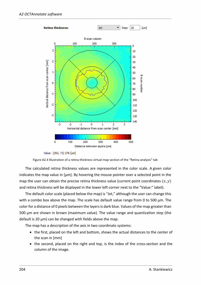
A2 OCTAnnotate software
204 A. Stankiewicz
Figure A2.4 Illustration of a retina thickness virtual map section of the “Retina analysis” tab
The calculated retina thickness values are represented in the color scale. A given color
indicates the map value in [μm]. By hovering the mouse pointer over a selected point in the
map the user can obtain the precise retina thickness value (current point coordinates (𝑥, 𝑦)
and retina thickness will be displayed in the lower left corner next to the “Value:” label).
The default color scale (placed below the map) is “Jet,” although the user can change this
with a combo box above the map. The scale has default value range from 0 to 500 μm. The
color for a distance of 0 pixels between the layers is dark blue. Values of the map greater than
500 μm are shown in brown (maximum value). The value range and quantization step (the
default is 20 μm) can be changed with fields above the map.
The map has a description of the axis in two coordinate systems:
• the first, placed on the left and bottom, shows the actual distances to the center of
the scan in [mm]
• the second, placed on the right and top, is the index of the cross-section and the
column of the image.

A2 OCTAnnotate software
A. Stankiewicz 205
2. Retina statistics derived for this thesis,
including:
• central retina thickness
• total and inner retina volume
within central 3 mm diameter
• fovea pit volume, area, and depth
• central fovea diameter and area (in
the central B-scan)
• fovea pit contour statistics:
perimeter, circularity, maximal and
minimal Feret diameters
• fovea shape correlation to a
Gaussian function (for central
cross-section and volumetric
segmentation)
Figure A2.5 presents these parameters
automatically calculated and displayed for
the user. The detailed information on the
procedures utilized for calculations of these
values.
Figure A2.5 Illustration of part of "Retina analysis"
tab with retina statistics values
3. Retina thickness profile for the currently investigated B-scan (Figure A2.6) and central
B-scan (Figure A2.7)
Figure A2.6 Illustration of retina thickness profile for the currently investigated B-scan
On these plots the following features are annotated:
• scan center and contour points (red dots)
• central fovea pit area (gray region in Figure A2.7)
• 3D Gaussian function estimation (gray line fitted to the fovea pit shape).

A2 OCTAnnotate software
206 A. Stankiewicz
Figure A2.7 Illustration of retina thickness profile for the central B-scan
4. Retina thickness profile along the fovea pit contour curve. This plot illustrated in Figure
A2.8 shows a circular profile of the fovea thickness contour starting from the temporal
direction (T), through the superior (S), nasal (N), inferior (I), and back to the temporal.
Figure A2.8 Illustration of the retina thickness profile along the fovea pit contour curve
5. Volumes within individual ETDRS grid sectors (see Figure A2.9):
• full-thickness retina (left grid)
• inner layers retina (right grid).
The ETDRS grid is a circular graph with the numerical values of the tissue volumes
in specific sectors of the retina. The values visible in each sector denote the retina volume
in a given sector. The background color allows a quick and intuitive assessment (the greater
volume, the darker color).
An additional feature of the software is the possibility to export the automatically
measured retina parameters for further statistical analysis. In addition, the obtained virtual
maps and ETDRS volumetric grids can be used for publishing and case reporting.

A2 OCTAnnotate software
A. Stankiewicz 207
Figure A2.9 Illustration of ETDRS grids with volume information for total and inner retina
A2.4 "Preretinal space" tab
The "Preretinal space" tab provides detailed information about the vitreoretinal interface
parameters derived in this thesis. Figure A2.10 illustrates the “Preretinal Space” tab of the
graphical user interface in the OCTAnnotate software.
Figure A2.10 View of the "Preretinal space" tab in the OCTAnnotate software

A2 OCTAnnotate software
208 A. Stankiewicz
The main features presented here are:
1. Virtual map of the preretinal space – the color map in the center of the tab with overlaid
ETDRS grid. It represents the vertical differences between the segmented PCV and ILM
surfaces. The color bar below the map illustrates the values assigned to each map color.
Figure A2.11 Illustration of a preretinal space virtual map
Similarly, as with the virtual retina map, the preretinal space profile can be adjusted for
color scale and scale quantization steps with the controls above the image. If necessary the
maximal value of the color scale (default of 700 µm) can also be changed by the user.
Furthermore, in this tab, it is also possible to illustrate the thickness of any individual layer
of the retina (the distance between any two segmented borders). The choice between which
layers to calculate and display the map is made by selecting the layer name from the lists on
the left side of the window (the user can select the top and bottom layer borders).
By checking the "Overlay on fundus image" box above the displayed thickness map, the
reconstructed fundus image will be shown in the image. The transparency of the virtual map
can be adjusted with a visible slider above the map.

A2 OCTAnnotate software
A. Stankiewicz 209
2. ETDRS grid map of preretinal space
volume.
This graph illustrates the same kind of
information as the grids in the “Retina
analysis” map, but for the preretinal
space. Values in each ETDRS field
(calculated based on the virtual map)
indicate volume in each sector. The
value outside of the grid in the upper left
corner is the sum of all fields.
The preretinal space volume grid
has a color background calculated based
on the percentage of the volume
occupied within each sector (the greater
volume, the darker the background
color).
Figure A2.12 Illustration of preretinal space
ETDRS volume grid
3. Contact area map overlaid on the
reconstructed fundus image.
Next to the virtual map is a
reconstructed fundus image with
overlaid ETDRS grid and a contact area
(in yellow) between the vitreous and the
retina.
Below this map are displayed the
numerical values of the contact area in
three ETDRS rings (CF – central fovea, IM
– inner macula, OM – outer macula).
Values on the right of each field provide
percentages of the contact area with
respect to each ring area.
Due to segmentation uncertainties
between the experts, a threshold
parameter (with default value of 10 µm)
was introduced, i.e., the vertical
difference between PCV and ILM less
then a given threshold is treated as 0.
Figure A2.13 Illustration of contact area map with
measurements

A2 OCTAnnotate software
210 A. Stankiewicz
4. Automatic VRI classification with
Duker and WISPERR parameters.
Based on the reference segmentations
the program automatically computes
the vitreoretinal interface parameters
for Duker and WISPERR classification.
The displayed values are obtained
based on the reference segmentations.
Width measurements are calculated
from the contact map values. The VRI is
based on the relative pixel intensity
around the ILM border. The fovea shape
is derived from the fovea pit to Gaussian
correlation estimation.
Figure A2.14 Illustration of automatically computed VRI classification parameters in the "Preretinal space" tab
A2.5 “Error analysis” tab
The last tab illustrated in Figure A2.15 provides error analysis between the automatic and
reference segmentations currently loaded into the software memory.
Figure A2.15 View of the "Error analysis" tab in the OCTAnnotate software

A2 OCTAnnotate software
A. Stankiewicz 211
Data in this tab allows the user to visually compare the reference and automatic
segmentation lines on each OCT cross-section individually. Additionally the software provides
visualization of the virtual map for a selected retina layer (see example for total retina
thickness map in Figure A2.16).
Figure A2.16 Illustration of retina thickness virtual map computed from automatic layers segmentation overlaid on a reconstructed fundus image
Similarly to the preretinal space virtual map this visualization can be overlaid on
a reconstructed fundus image (with various transparency settings), and adjusted for color
scale, value range, and scale quantization step.
For the loaded reference and automatic segmentations the program calculates vertical
difference between each layer annotations. The default error measurements include:
• mean squared error (MSE) and its standard deviation (SD) for all segmented layers
(in [px])
• MSE and SD for a layer selected by the user (in [px] and [µm])
• percentage of erroneous segmentations for the selected layer
• MSE and SD for the virtual map (in [px] and [µm]).
Figure A2.17 presents these statistics in the software window.

A2 OCTAnnotate software
212 A. Stankiewicz
Figure A2.17 Illustration of (left) a list of layers to display on an OCT B-scan and (right) error measurements between automatic and reference retina layers segmentations