Frozen soil parameterization in a distributed biosphere hydrological model

Hydrol. Earth Syst. Sci., 14, 557–571, 2010www.hydrol-earth-syst-sci.net/14/557/2010/© Author(s) 2010. This work is distributed underthe Creative Commons Attribution 3.0 License.

Hydrology andEarth System

Sciences

Frozen soil parameterization in a distributed biosphere hydrologicalmodel

L. Wang1, T. Koike1, K. Yang2, R. Jin3, and H. Li3

1Dept. of Civil Engineering, the University of Tokyo, Tokyo, Japan2Lab. of Tibetan Environment Changes and Land Surface Processes, Institute of Tibetan Plateau Research, Chinese Academyof Sciences, Beijing, China3Cold and Arid Regions Environmental and Engineering Research Institute, Chinese Academy of Sciences, Lanzhou, China

Received: 26 October 2009 – Published in Hydrol. Earth Syst. Sci. Discuss.: 9 November 2009Revised: 8 March 2010 – Accepted: 17 March 2010 – Published: 23 March 2010

Abstract. In this study, a frozen soil parameterization hasbeen modified and incorporated into a distributed biospherehydrological model (WEB-DHM). The WEB-DHM with thefrozen scheme was then rigorously evaluated in a small coldarea, the Binngou watershed, against the in-situ observationsfrom the WATER (Watershed Allied Telemetry ExperimentalResearch). First, by using the original WEB-DHM withoutthe frozen scheme, the land surface parameters and two vanGenuchten parameters were optimized using the observedsurface radiation fluxes and the soil moistures at upper layers(5, 10 and 20 cm depths) at the DY station in July. Second,by using the WEB-DHM with the frozen scheme, two frozensoil parameters were calibrated using the observed soil tem-perature at 5 cm depth at the DY station from 21 November2007 to 20 April 2008; while the other soil hydraulic param-eters were optimized by the calibration of the discharges atthe basin outlet in July and August that covers the annuallargest flood peak in 2008. With these calibrated parameters,the WEB-DHM with the frozen scheme was then used for ayearlong validation from 21 November 2007 to 20 November2008. Results showed that the WEB-DHM with the frozenscheme has given much better performance than the WEB-DHM without the frozen scheme, in the simulations of soilmoisture profile at the cold regions catchment and the dis-charges at the basin outlet in the yearlong simulation.

Correspondence to:L. Wang([email protected])

1 Introduction

Frozen soil (comprising permafrost and seasonally-frozensoil) process is critically important in the land surface hy-drology of cold regions, since the freeze-thaw cycle signif-icantly modulates the soil hydraulic and thermal character-istics that directly affect the water and energy cycles in thesoil-vegetation-atmosphere transfer (SVAT) system.

At present, the improved modeling of the frozen soil pro-cess in a land surface scheme has been recognized an indis-pensable task for more reliable estimates of soil moisture andtemperature profiles, particularly in the winter of NorthernHemisphere. The Project for Intercomparison of Land sur-face Parameterization Schemes phase 2(d) (PILPS 2(d)) hasshown that the models with a frozen soil parameterizationgenerally simulated realistic soil temperature during winterthan those without a frozen scheme (Luo et al., 2003). Up tonow, many studies have made efforts on improving the frozensoil parameterization in land surface modeling (e.g., Bonanet al., 1996; Slater et al., 1998; Koren et al., 1999; Smirnovaet al., 2000; Li and Koike, 2003; Poutou et al., 2004; Woo etal., 2004; Niu and Yang, 2006; Zhang et al., 2007; Nicolskyet al., 2007; Luo et al., 2009).

By contrast, the frozen soil process is often inadequatelyrepresented or even neglected in most distributed hydrolog-ical models for basin-scale simulations, with only very fewexceptions (e.g., Cherkauer and Lettenmaier; 1999; Zhanget al., 2000; Stocker-Mittaz et al., 2002; Tian et al., 2006;Mou et al., 2008; Ye et al., 2009). In fact, the represen-tations of the frozen soil process can be indispensable indistributed hydrological modeling for the understanding ofthe water and energy cycles in some Northern-Hemisphere

Published by Copernicus Publications on behalf of the European Geosciences Union.

http://creativecommons.org/licenses/by/3.0/

558 L. Wang et al.: Frozen soil parameterization in a distributed biosphere hydrological model

Datum

Inter flow Groundwater table

Impervious Surface

Hillslope Unit

l

River

Precipitation

Soil surface

CO2 H

Rlw

λET

Surface flow

Rsw

Grid size in the model

DEM grid size

(c) (d)

(a) (b)

2

1

3 5

4

7

6

9

8

Outlet

Flow Intervals Subbasin

Groundwater flow

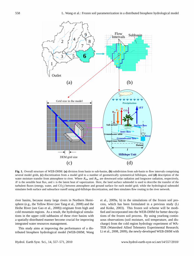
Fig. 1. Overall structure of WEB-DHM:(a) division from basin to sub-basins,(b) subdivision from sub-basin to flow intervals comprisingseveral model grids,(c) discretization from a model grid to a number of geometrically symmetrical hillslopes, and(d) description of thewater moisture transfer from atmosphere to river. WhereRsw andRlw are downward solar radiation and longwave radiation, respectively,H is the sensible heat flux, andλ is the latent heat of vaporization. Here, the land surface submodel is used to describe the transfer of theturbulent fluxes (energy, water, and CO2) between atmosphere and ground surface for each model grid; while the hydrological submodelsimulates both surface and subsurface runoff using grid-hillslope discretization, and then simulates flow routing in the river network.

river basins, because many large rivers in Northern Hemi-sphere (e.g., the Yellow River (see Tang et al., 2008) and theHeihe River (see Gao et al., 2008)) originate from high andcold mountain regions. As a result, the hydrological simula-tions in the upper cold subbasins of these river basins witha spatially-distributed manner become crucial for improvingintegrated water resources management.

This study aims at improving the performance of a dis-tributed biosphere hydrological model (WEB-DHM; Wang

et al., 2009a, b) in the simulations of the frozen soil pro-cess, which has been formulated in a previous study (Liand Koike, 2003). This frozen soil scheme will be modi-fied and incorporated into the WEB-DHM for better descrip-tions of the frozen soil process. By using yearlong contin-uous observations (soil moisture, soil temperature, and dis-charge) from the cold region hydrology experiment of WA-TER (Watershed Allied Telemetry Experimental Research;Li et al., 2008, 2009), the newly-developed WEB-DHM with

Hydrol. Earth Syst. Sci., 14, 557–571, 2010 www.hydrol-earth-syst-sci.net/14/557/2010/

L. Wang et al.: Frozen soil parameterization in a distributed biosphere hydrological model 559

the revised frozen scheme has been rigorously evaluated ina small cold river basin (Binggou) at the upper area of theHeihe River.

2 Model description

The WEB-DHM (Water and Energy Budget-based Dis-tributed Hydrological Model) was a distributed biosphere hy-drological model, which can give consistent descriptions ofwater, energy and CO2 fluxes at a basin scale (see Fig. 1).It can efficiently simulate hydrological processes of large-scale river basins while incorporating subgrid topography(see Wang et al., 2009a).

In the study, a new version of the WEB-DHM has been de-veloped by modifying and incorporating a frozen soil param-eterization (Li and Koike, 2003). First, the original WEB-DHM is briefly reviewed in Sect. 2.1. Details about the hy-drological submodel were discussed in Wang et al. (2009a);while the formulations of the land surface submodel can befound in Sellers et al. (1996a). Second, the frozen soil pa-rameterization in WEB-DHM is presented in detail.

2.1 Review of the original WEB-DHM

2.1.1 General model structure

As illustrated in Fig. 1, the general model structure can bedescribed as follows:

1. A digital elevation model (DEM) is used to define thetarget basin, which is then divided into sub-basins (seeFig. 1a). Within a given sub-basin, a number of flowintervals are specified to represent time lags and the ac-cumulating processes in the river network. Each flowinterval includes several model grids (see Fig. 1b).

2. For each model grid with one combination of land usetype and soil type, the land surface submodel inde-pendently calculates turbulent fluxes between the atmo-sphere and land surface (see Fig. 1b and d). The verti-cal distributions of water for all the model grids, suchas ground interception storage and soil moisture profile,can be obtained through this biophysical process.

3. Each model grid is subdivided into a number of geo-metrically symmetrical hillslopes (see Fig. 1c). A hills-lope with unit length is called a basic hydrological unit(BHU) of the WEB-DHM. For each BHU, the hydro-logical submodel is used to simulate lateral water redis-tributions and calculate runoff comprised of overland,lateral subsurface and groundwater flows (see Fig. 1cand d). Overland flow is described by Manning’s equa-tion, and lateral subsurface flow and groundwater dis-charge are simulated using Darcy’s law (Wang et al.,2009a). The runoff for a model grid is the total responseof all BHUs within it.

4. For simplicity, the streams located in one flow intervalare combined into a single virtual channel. All the flowintervals are linked by the river network generated fromthe DEM. All runoff from the model grids in the givenflow interval is accumulated into the virtual channel andled to the outlet of the river basin. The flow routing ofthe entire river network in the basin is modeled usingthe kinematic wave approach.

2.1.2 Soil model

Two different soil subdivision schemes are used in describingland surface processes and hydrological processes.

In the calculation of land surface processes, the three-layersoil structure for the unsaturated zone is the same as that inSiB2. The depth of the first layer (D1) is defined as 5 cm,while the root depth (D1 +D2) could be defined accordingto vegetation type by SiB2 default. The thickness of the deepsoil zone (D3) changes with fluctuation of the water tableand is equal to the depth of the groundwater level minus thethickness of the upper two layers.

In the simulation of soil water flow, a multiple-sublayersoil structure is employed to describe the unsaturated zone.In the model, the non-uniform vertical distribution is rep-resented using an assumption of exponentially decreasinghydraulic conductivity with increasing soil depth given bykz = ksurface·exp(−f · z) (Beven, 1982; Cabral et al., 1992;Robinson and Sivapalan, 1996), whereksurfaceandkz are hy-draulic conductivities at the soil surface and depthz, andf is a decay factor. The surface layer with a depthD1 iskept as the first layer. The root zone and deep soil zone areuniformly subdivided into several sublayers. As shown inFig. 2, the multiple-sublayer structure is employed to calcu-late vertical interlayer flows and lateral runoff. The verticalinterlayer flows in the unsaturated zone are described using aone-dimensional Richards equation (see Wang et al., 2009a).

In this soil model, the van Genuchten equation (vanGenuchten, 1980) is used as the soil hydraulic function.

2.2 Frozen soil parameterization

2.2.1 Soil hydraulic properties

Total volumetric water content of thej -th soil layer (θj ;m3 m−3) is defined as

θj = θliq,j +θice,jρice

ρliq. (1)

Where,θliq,j andθice,j are the liquid water content and theice content (m3 m−3) of thej -th soil layer;ρice andρliq arethe density (kg m−3) of ice and liquid water, respectively.

For thej -th soil layer, the unfrozen water content (θliq,j )

is assumed as a simple power function of soil temperature(Tsoil,j ) (see Nakano et al., 1982; Romanovsky and Os-terkamp, 2000; Li and Koike, 2003)

θliq,j = a(Tf −Tsoil,j )b, (2)

www.hydrol-earth-syst-sci.net/14/557/2010/ Hydrol. Earth Syst. Sci., 14, 557–571, 2010


D3

D2

D1

Ds

Dg

qsfc

qg Aquifer Model

qsub

Impervious Boundary

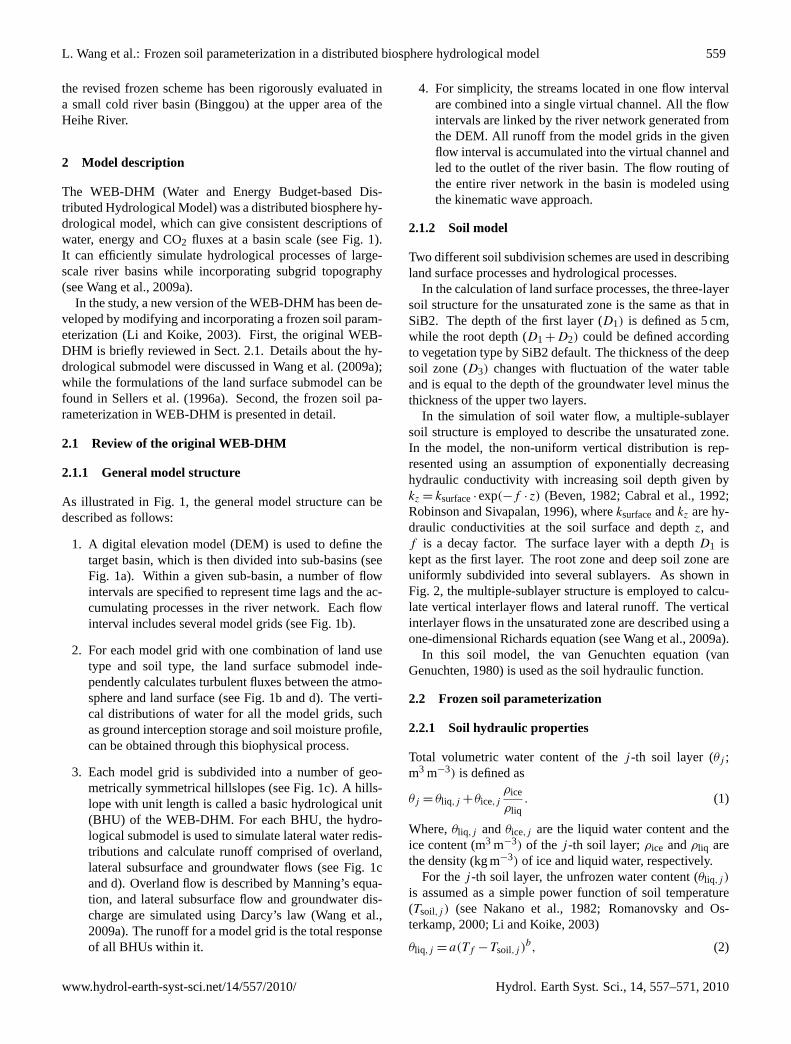
Fig. 2. Soil model of the WEB-DHM. Two different soil subdivi-sion schemes are used for describing land surface and hydrologicalprocesses, respectively. The three-layer soil structure used in SiB2is retained to represent the unsaturated zone in the calculations ofland surface processes. The unsaturated zone is divided into multi-ple sublayers when simulating water flows within it and water ex-changes with groundwater aquifer.

where,a andb are two empirical coefficients associated withsoil type. Then the changing rate of liquid soil moisture (orice) to soil temperature can be derived as

∂θliq,j

∂Tsoil,j= −

ρice

ρliq

∂θice,j

∂Tsoil,j= (−ab)

(Tf −Tsoil,j

)b−1. (3)

The soil hydraulic conductivityKj and soil matric potentialψj at thej -th soil layer in the unsaturated zone are describedusing a modified version of the van Genuchten’s equation(van Genuchten, 1980):

Kj = fice,jKsat,j

(θliq,j −θr

θs−θr

)1/2

[1−

(1−

(θliq,j −θr

θs−θr

)−1/m)m]2

, (4)

ψj =1

α

( θliq,j −θr(θs−θice,j

)−θr

)−1/m

−1

1/n

. (5)

Where,θs is porosity andθr is residual water content;α, nare empirical parameters in van Genuchten’s equation withm= 1−1

/n; the hydraulic conductivity reduction factor for

thej -th soil layer (fice,j ) is defined as a function of soil tem-perature at that layer

fice,j = exp(−10·

(Tf −Tsoil,j

))and 0.05≤ fice,j ≤ 1; (6)

andKsat,j is the saturated hydraulic conductivity at depthz(defined as the location of the center of thej -th soil layer),which is measured downward in a direction normal to the soilsurface (m). Ksat,j is represented using the assumption of anexponential increase in hydraulic conductivity with increas-ing soil depth (that is the decay factorf <0).

Similar toKj , the groundwater hydraulic conductivityKGis also formulated considering the frozen soil effect

KG = fice,GKG0. (7)

Where, the reduction factorfice,G (= exp(−10·

(Tf −TB

))and 0.05≤ fice,G ≤ 1) is expressed as a function of the tem-perature of the bottom soil layer (TB); KG0 is the ground-water hydraulic conductivity without considering frozen soil(m s−1).

2.2.2 Soil thermal properties

For the soil temperatures at the ground surface and the deepsoil, the force-restore model (Deardorff, 1977) of the heatbalance in the soil surface is kept, but the effective heat ca-pacities of the soil surface and the snow-free soil are modi-fied to represent the latent heat of fusion or the change of soilthermal conductivity

Cg∂Tg

∂t=Rng−Hg−λEg−

2πCd

τd

(Tg−Td

)−ξgs, (8)

Cd∂Td

∂t=

1

2(365π)1/2(Rng−Hg−λEg), (9)

where,Cg andCd are the effective heat capacity (J m−2 K−1)

for the soil surface and the snow-free soil;Tg and Td arethe temperatures for the soil surface and the deep soil, re-spectively (K);Rng is the absorbed net radiation by soil sur-face (W m−2); Hg is the sensible heat flux from soil surface(W m−2); Eg is the bare soil evaporation rate (kg m−2 s−1);λ is the latent heat of vaporization (J kg−1); τd is daylength(s); ξgs is the energy transfer due to phase changes in snowon ground (W m−2).

The soil thermal conductivity (Hs,new; W m−1 K−1) is cal-culated following Li and Cheng (1995)

Hs=

[1.5·(1−θs)+1.3θ1

0.75+0.65θs−0.4θ1

]0.4186, (10)

Hs,new=

{Hs+

(Hs,max−Hs

)·θice,1·

(ρice

/ρliq

)/(θ1−θliq,min

)Tg≤Tf

Hs Tg>Tf.

(11)



Where,Hs is soil thermal conductivity without consideringfrozen soil;Hs,max is the maximum heat conductivity afterfreezing;θliq,min is the minimum liquid water content afterfreezing. In the study,θliq,min = 0.05; whileHs,max = 2.5considering the existence of gravels in the soil.

The new equations ofCd andCg are described as follows

Cd = 0.5

(Hs,newCsoil ·86 400

π

)1/2. (12)

Cg=

ds

(Csoil+ρliqLf

∂θliq,1∂Tg

)+min

[0.05,

(Mgw+Mgs

)]Cw Tg<Tf−0.01

dsCsoil+min[0.05,

(Mgw+Mgs

)]Cw Tf−0.01≤Tg≤Tf

Cd+min[0.05,

(Mgw+Mgs

)]Cw Tg>Tf

,

(13)

where ds is the effective depth (m) that feels the di-urnal change of temperature (Stull, 1988);Csoil isthe volumetric heat capacity of soil (J m−3 K−1) andCsoil =

(0.5·(1−θs)+θliq,1+0.175·θice,1

)·4.186×106; the

ρliqLf(∂θliq,1

/∂Tg

)represents the apparent heat capacity

of soil freezing in the surface soil layer, and∂θliq,1/∂Tg =

(−ab)(Tf −Tg

)b−1; Mgw is the soil interception of liquidwater store (m);Cw is the volumetric heat capacity of water(J m−3 K−1). It should be mentioned that when the soil sur-face temperature is just below the freezing point, the phasechanging rate∂θliq,1

/∂Tg reaches its maximum value, mak-

ing the effective heat capacity a very large value and there-fore hampering the heat transfer. In order to solve this prob-lem,Cg = dsCsoil+min

[0.05,

(Mgw+Mgs

)]Cw is set for the

transition zone fromTf −0.01 toTf in this study.The depth of seasonal frost penetration is determined by

the soil temperature profile, which is solved with Stefan so-lution (Yershov, 1990). The Stefan solution assumes a linearsoil temperature profile in the frozen soil column, and forsimplicity the soil temperature at 5 cm (Tsoil,D1) is assumedas

Tsoil,D1 = ηTg+(1−η)Td. (14)

Where,η is an empirical factor andη= 0.5 is used in thisstudy.

The frost and thaw depths (ζf and ζt) is simulated fol-lowing Li and Cheng (1995), and can be expressed in equa-tions of the approximation Stefan solution (The Institute ofGeocryology, 1974; Li and Koike, 2003) as follows.

ζf =

√√√√√2κfτht∑i=1

(Tf −Tsoil,D1

)Lfρlθ

, (15)

ζt =

√√√√√2κtτht∑i=1

(Tsoil,D1 −Tf

)Lfρiθ

, (16)

where,κf , andκt are the thermal conductivity of freezingand thawing soils (W m−1 K−1), respectively;τh is the timelength (s) andτh = 3600 s in the study.

After determining the position of freezing front, the sub-layer soil temperature in the root zone and deep soil are esti-mated by a simple function of frost depth.

If z≤ ζf , the soil temperature at a given depthz is

Tsoil,z = Tf +(Tsoil,D1 −Tf

)(1−

z

ζf

); (17)

If z> ζf , the soil temperature at a given depthz is

Tsoil,z = Tf +(Td−Tf)

(z−ζf

Ds−ζf

), (18)

whereDs is the top soil depth (see Fig. 2).

3 Datasets for the study area

The cold region hydrology experiment is one of key exper-iments within the Watershed Allied Telemetry Experimen-tal Research (WATER; Li et al., 2008, 2009). The Binggouwatershed (Fig. 3), located at 100◦12′–100◦18′ E and 38◦1′–38◦4′ N, is one of the three foci experimental areas wherecold region hydrology experiments were carried out withinthe framework of the WATER.

The Binggou watershed, located in the upper reaches ofthe Heihe River Basin (Fig. 3), is a high mountain drainagesystem with an area of 30.48 km2. The elevation is fromabout 3440 to 4400 m (Fig. 3). The watershed has the ob-vious vertical-zonality natural landscape (Yang et al., 1992).In the altitude from 3440 to 4000 m, there is mainly alpinemeadow; while in the altitude from 3440 to 3700 m, theshrubs and the fish-scale shape sod coexist. In the regionabove 4000 m, there is mainly the non-vegetation’s alpinedesert, and the exposed decency rock debris quite grows hav-ing high water-permeability. The longterm mean annual tem-perature is about−5.8◦C in the mean altitude (3900 m) ofthe watershed (Yang et al., 1992). In the watershed, the per-mafrost distributes at the region higher than 4000 m, withthe air temperature lower than 0◦C in 9 months (Septem-ber to next May); while the discontinuous permafrost domi-nates the region lower than 4000 m, with the air temperaturelower than 0◦C in 7 months (October to next April) (Yang etal., 1993). The longterm mean annual precipitation is about686 mm, with about 74% rainfall and 26% snowfall (Zhangand Yang, 1991). The snowfall prevails from October toApril; the rainfall concentrates on July and August; whilesleet occurs in May, June and September (Yang et al., 1992).The mean depth of the seasonable snowpack is about 0.5 m,with a maximum of 0.8–1.0 m (Yang et al., 1993).

The datasets of the Binggou Watershed, as used in WEB-DHM, are as described below.

DEM and land use were provided by the WATER project(Li et al., 2008, 2009). The model simulation adopted a grid



102°0'0"E

102°0'0"E

100°0'0"E

100°0'0"E

98°0'0"E

98°0'0"E

44°0

'0"N

42°0

'0"N

42°0

'0"N

40°0

'0"N

40°0

'0"N

38°0

'0"N

38°0

'0"N

−0 150 30075 Km

Heihe River Basin

0 3,3001,650 m

/ Dadongshu-Yakou (DY)Station

BinggouStream gauge

River

DEM4400 m 3440 m

Legend

Fig. 3. The Binggou watershed.

size of 250 m, and the subgrid topography was described bya 50 m resolution DEM. The land uses have been reclassi-fied to 3 SiB2 categories (Agriculture/C3 grassland, Dwarftrees and shrubs, and broadleaf shrubs with bare soil). Inthe Dadongshu-Yakou (DY) station (with the elevation of4146.8 m; see Fig. 3), surface meteorological variables, aswell as soil moisture and soil temperature profiles were mea-sured (with soil moisture and temperature sensors) contin-uously at the 10-min interval from 21 November 2007 to20 November 2008. The precipitation, relative humidity, airtemperature, and wind speed, as well as air pressure, down-ward longwave and shortwave radiation, obtained from thestation were summated into the hourly time series and takenas the forcing data for the whole watershed because the basinis small and distributed data is not available. The surfaceair temperature inputs were modified with a lapse rate of6.5 K km−1, considering the elevation differences betweenthe model grids and the DY station. However, the altitudi-nal effect on relative humidity was assumed negligible. Atthe basin outlet, the Binggou stream gauge was newly builtin 2008 and discharge data has been obtained from 17 Jan-uary to 20 November 2008 for model evaluation, with thefrequency of several times a day. The method of dischargemeasurements is briefly described as follows. First, a rect-angle cross section was built using concrete at the selectedpoint. Second, the water depth (which was used to derivethe area of the cross section) and the flow velocity at thecross section were measured by the local staff several times

a day (not hourly). Third, the flow velocity and the area ofthe cross-section were used to calculate the discharge at thecross-section.

The dynamic vegetation parameters are Leaf Area Index(LAI) and the Fraction of Photosynthetically Active Radia-tion (FPAR) absorbed by the green vegetation canopy, andcan be obtained from satellite data. Global LAI and FPARMOD15 BU 1 km data sets (Myneni et al., 1997) were usedin this study. These are 8-daily composites of MOD15A2products and were obtained using the Warehouse InventorySearch Tool (WIST) of NASA.

All simulations were carried out with 250 m spatial reso-lution and hourly time step.

4 Model evaluations at the Binggou watershed

For the Binggou watershed, the hydrological processes arenot only controlled by the hydro-meteorological conditionsof the land surface, but also by the underlying frozen soil.The spring snowmelt occupies about 30% of the annualrunoff; while the residual comes from rainfall and groundwa-ter (Zhang and Yang, 1991). In the lower area of the water-shed, soil starts thawing around April and stops by August;while in the upper regions, soil starts thawing around lateMay. In the watershed, the thickness of the active frozen soillayer is about 1.0–1.5 m in the lower regions, and is greaterthan 3.0 m in the upper mountain regions (Yang et al., 1993).



In the early spring (April to May), with the increase of airtemperature, snowmelt occurs from the lower regions to themountain areas. However, during this period (April to May),the air temperature exceeds 0◦C only at noon, but drops tobelow 0◦C at night. Consequently, much of the snowmeltwater freezes again at night before its departure from snow-pack. Therefore, the snowmelt runoff in the early spring issmall (around 15% of annual runoff; Zhang and Yang, 1991).From May to June (late spring), the air temperature increasesto above 0◦C stably, and the snowmelt runoff becomes verylarge (greater than 25% of annual runoff; Zhang and Yang,1991). This is also attributed to the little permeability ofthe underlying seasonal frozen soil layers which have thawedonly in upper soil layers (Kane and Stein, 1983). In summer,snow and seasonal frozen soil layers disappear, and thus rain-fall becomes the major source for river discharges. But thepermanent frozen soil layers still exist, which prohibit thewater infiltration to deeper layers. Heavy rainfall events insummer will usually result in severe flash floods in this wa-tershed, along with landslides and debris flows (Yang et al.,1993).

4.1 Model calibration

The vegetation static parameters including morphological,optical and physiological properties were initially definedfollowing Sellers et al. (1996b). In the summer 2008, byusing the WEB-DHM without the frozen scheme, the landsurface parameters were optimized using the observed radi-ation fluxes at the DY station in July; and then the two vanGenuchten parameters (α andn) were optimally obtained bythe calibration of the July soil moistures at upper layers (5, 10and 20 cm depths) at the DY station. In the cold season from21 November 2007 to 20 April 2008, by using the WEB-DHM with the frozen scheme, the parameters (a andb) usedin the frozen soil scheme were optimized through matchingthe simulated and observed soil temperatures at 5 cm depth(Tsoil,D1). Third, by using the WEB-DHM with the frozenscheme, the other soil hydraulic parameters were optimallyobtained by the calibration of the discharges at the basin out-let in July and August that covers the annual largest floodpeak in 2008.

4.1.1 Parameters optimized through the WEB-DHMwithout the frozen scheme

First, the land surface parameters were optimized using theobserved surface radiation fluxes at the DY station in July.For the DY station, land is covered by the SiB2 biome 9(“Agriculture/C3 grassland”). The canopy cover fraction,the height of canopy top, and the height of canopy bot-tom, as well as the root depth (Dr), the top soil depth (Ds),and the ground roughness length (zs) have been designed as0.2, 0.05 m, 0.005 m, 0.25 m, 1.25 m, and 0.001 m accord-ing to the field obervations in Li et al. (2009). The soil re-

flectance to visible radiation for the SiB2 biome 9 was op-timized as 0.15 using observed upward shortwave radiationin July 2008; while the surface emissivity has been kept as1.0 following Seller et al. (1996b). Other time-invariant veg-etation parameters were set following Sellers et al. (1996b).Soil hydraulic properties have been kept equal to values de-rived from FAO (2003) during the calibration of land surfaceparameters.

Second, the two van Genuchten parameters (α andn)wereoptimized by using the measured soil moistures at upper lay-ers at the DY station. The porosity and the residual soil mois-ture were set as 0.585 and 0.017 according to the yearlongsoil moisture measurements from 21 November 2007 to 20November 2008 in the DY station. The van Genuchten pa-rametersα andn regulate the soil hydraulic function whichcontrols the soil water transport. They were optimized as0.1 and 2.1, respectively, by comparing the simulated andobserved soil moistures at the upper soil layers (5, 10, and20 cm) in July 2008 at the DY station; while keeping the orig-inal values ofKsurfaceobtained from FAO (2003).

4.1.2 Parameters optimized through the WEB-DHMwith the frozen scheme

First, at the DY station, the frozen soil parameters (a andb)are optimized through matching the simulated and observedTsoil,D1 in the cold season (from 21 November 2007 to 20April 2008); whileds is set as 0.6 m, according to the mea-sured winter soil temperature profiles at the DY station (Li etal., 2009).

Second, at the basin-scale, the other soil hydraulic param-eters were further optimized to obtain good reproduction ofthe flood event that occurred at the Binggou stream gaugeduring the summer (July and August) of 2008. These pa-rameters include the saturated hydraulic conductivity for soilsurfaceKsurface, the soil anisotropy ratioanik, the groundwa-ter hydraulic conductivity (without considering frozen soil)KG0, and the hydraulic conductivity decay factorf . Theoptimization was done using a trial and error method bymatching the simulated and observed flood peaks and tails.It should be mentioned that the assumption of an exponentialincrease in hydraulic conductivity with increasing soil depthis used in the WEB-DHM with the frozen scheme (f <0).

The basin-averaged values of the land surface and soil hy-draulic parameters, as well as the frozen soil parameters usedin the Binggou watershed are listed in Table 1.

4.1.3 Calibration results

The bias error (BIAS) and root mean squared error (RMSE)are used as evaluation criterion for the simulated results,where BIAS and RMSE are defined as

BIAS =

∑N

i=1(xsi−xoi)

/N, (19)



Table 1. Basin-averaged values of the parameters used in the Binggou watershed.

Symbol Parameters Unit Value Source

Land surface parameters

z2 Height of canopy top m 0.05 Li et al. (2009)z1 Height of canopy bottom m 0.005 Li et al. (2009)V Canopy cover fraction 0.3 Li et al. (2009)αs,V Soil reflectance to visible radiation 0.12 Optimizationzs Ground roughness length m 0.001 Li et al. (2009)Dr Root depth (D1+D2) m 0.25 Li et al. (2009)Ds Top soil depth (D1+D2+D3) m 1.25 Li et al. (2009)

Soil hydraulic parameters

θs Porosity 0.585 Li et al. (2009)θr Residual soil water content 0.017 Li et al. (2009)Ksurface Saturated hydraulic conductivity for soil surface mm/h 4.4 Optimizationf Hydraulic conductivity decay factor −1.84 Optimizationα van Genuchten parameter 0.1 Optimizationn van Genuchten parameter 2.1 Optimizationanik Hydraulic conductivity anisotropy ratio 22.4 OptimizationKG0 Groundwater hydraulic conductivity without considering frozen soil mm/h 1.0 Optimization

Frozen soil parameters

ds Effective depth that feels the diurnal change of temperature m 0.6 Li et al. (2009)a empirical coefficient 0.0616 Optimizationb empirical coefficient −0.5133 Optimization

0

200

400

600

800

1000

1200

1400

2008.7.1 2008.7.11 2008.7.21 2008.7.31

Dow

nwar

d Sh

ortw

ave

Rad

iati

on

Rsd_obs

0

50

100

150

200

250

300

2008.7.1 2008.7.11 2008.7.21 2008.7.31Upw

ard

Shor

twav

e R

adia

tion

Rsu_obs Rsu_simBIAS = -3.8 W/m2 RMSE = 32.6 W/m2

Fig. 4. Simulated and observed hourly upward shortwave radiation(unit: W m−2) at the DY station in July 2008, by using the WEB-DHM without the frozen scheme.

RMSE=

√∑N

i=1(xsi−xoi)2

/N, (20)

wherexoi is the observation,xsi is the simulation, andN isthe total number of time series for comparison.

Figure 4 shows the simulated and observed hourly upwardsolar radiation from 1 to 31 July 2008 at DY station withthe BIAS and the RMSE, by using the WEB-DHM without

the frozen scheme. The observed soil moisture and tempera-ture profiles were used to initialize the model at the first hourof 1 July 2008; while the initial water table depth was as-sumed as same as the initial depth of the unsaturated zone(Ds=1.25 m). After the calibration of the soil reflectance tovisible radiation, the diurnal cycles of the upward solar ra-diation are well represented by the calibrated WEB-DHMwithout the frozen scheme. The BIAS and RMSE for thesimulated upward shortwave radiation at the DY station are−3.8 W m−2 and 32.6 W m−2, respectively. It should bementioned that the measurements of upward longwave radi-ation in the station were found erroneous for all periods, andwas not used for model evaluation in the study.

Figure 5 illustrates the hourly evolutions of precipitationand the simulated and observed hourly volumetric liquid soilmoisture at 5, 10, 20, 40, 80, and 120 cm in July 2008 atthe DY station, by using the WEB-DHM without the frozenscheme. Reasonable responses of soil moisture at the upperlayers (5, 10, and 20 cm) to the rainfall events are reproducedwith high accuracies (Fig. 5b–d). The BIAS for the simu-lated soil moistures at 5, 10, and 20 cm are−0.003, 0.011,and−0.012; while their RMSE values are 0.031, 0.029 and0.030, respectively. The soil moisture at 120 cm is also ac-curately simulated by the WEB-DHM without the frozenscheme (see Fig. 5g), since the soil at this depth was stillin frozen in July at the station. The RMSE values for the



0.0

2.0

4.0

6.0

8.0

2008.7.1 2008.7.11 2008.7.21 2008.7.31

Pre

cipi

tati

on (

mm

/hou

r) (a)

0

0.1

0.2

0.3

0.4

0.5

2008.7.1 2008.7.11 2008.7.21 2008.7.31

Soil

moi

stur

e

Obs_5cm Sim (0~5cm)(b)

BIAS = -0.003 RMSE = 0.031

0

0.1

0.2

0.3

0.4

0.5

2008.7.1 2008.7.11 2008.7.21 2008.7.31

Soil

moi

stur

e

Obs_10cm Sim (5~15cm)(c)

BIAS = 0.011 RMSE = 0.029

0

0.1

0.2

0.3

0.4

0.5

2008.7.1 2008.7.11 2008.7.21 2008.7.31

Soil

moi

stur

e

Obs_20cm Sim (15~25cm)(d)

BIAS = -0.012 RMSE = 0.030

0

0.1

0.2

0.3

0.4

0.5

2008.7.1 2008.7.11 2008.7.21 2008.7.31

Soil

moi

stur

e

Obs_40cm Sim (35~45cm)(e)

BIAS = -0.045 RMSE = 0.052

0

0.1

0.2

0.3

0.4

0.5

2008.7.1 2008.7.11 2008.7.21 2008.7.31

Soil

moi

stur

e

Obs_80cm Sim (75~85cm)(f)

BIAS = -0.108 RMSE = 0.154

0

0.1

0.2

0.3

0.4

0.5

2008.7.1 2008.7.11 2008.7.21 2008.7.31

Soil

moi

stur

e

Obs_120cm Sim (115~125cm)(g)

BIAS = -0.001 RMSE = 0.001

Fig. 5. Hourly precipitation(a), and the simulated and observedhourly volumetric liquid soil moisture at 5, 10, 20, 40, 80, and120 cm(b–g) at the DY station in July 2008, by using the WEB-DHM without the frozen scheme.

240

250

260

270

280

290

2007.11.21 2007.12.21 2008.1.20 2008.2.19 2008.3.20 2008.4.19

Soil

tem

pera

ture

(K

) Obs_5cm Sim_5cm

BIAS = 0.84 K RMSE = 1.68 K

(a)

0

5

10

15

20

2008.7.1 2008.7.16 2008.7.31 2008.8.15 2008.8.30

Dis

char

ge (

m3 /s

)

0

5

10

15

20

25

30

Prec

ipita

tion

(mm

/hou

r)

Precipitation

Qobs

Qsim

(b)

Fig. 6. The hourly simulated and observed soil temperature at 5 cmin the DY station from 21 December 2007 to 20 April 2008(a), andthe calibrated hydrograph at the Binggou gauge in July and August2008(b), by using the WEB-DHM with the frozen scheme.

simulated soil moisture at 40 and 80 cm (particularly 80 cm)are relatively large, which can be attributed to the thawingactivity. It reveals that even in the summer simulations at theDY station, a frozen soil scheme is essential.

Figure 6a gives the hourly simulated and observed soiltemperature at 5 cm in the DY station from 21 December2007 to 20 April 2008, by using the WEB-DHM with thefrozen scheme. After the calibration of frozen soil parame-ters (a andb), the soil temperature at 5 cm in the cold seasonsis well reproduced, with the BIAS and RMSE values equalto 0.84 K and 1.68 K, respectively.

Figure 6b plots the calibrated hourly hydrograph from Julyto August 2008 at the Binggou gauge, by using the WEB-DHM with the frozen scheme. Here, the WEB-DHM withthe frozen scheme was initialized from a previous simulationstarting from 21 November 2007. It is shown that after cal-ibration, in general the model reproduces both the peak andbase flows well. The difference of timing and magnitudes be-tween the observed and simulated peak flows is possibly at-tributed to the sparse density of the meteorological sites usedin the study (only the DY station). It should be mentionedthat the discharges at the Binggou gauge were measured dis-continuously and irregularly, and thereby the evaluation cri-terions (e.g., the Nash-Sutcliffe model efficiency coefficient(Nash and Sutcliffe, 1970) and the bias error are not esti-mated.



0

0.2

0.4

0.6

0.8

1

1.2

1.4

2008.5.1 2008.5.31 2008.6.30 2008.7.30 2008.8.29

Tha

w d

epth

(m

)

Obs Sim

BIAS = -0.15 m RMSE = 0.20 m

Fig. 7. Hourly observed (interpolated from the observations of soiltemperature profile) and simulated thaw depth at the DY station,from 1 May to 31 August 2008, by using the WEB-DHM with thefrozen scheme.

250

270

290

310

2007.11.21 2008.2.29 2008.6.8 2008.9.16

Soil

tem

pera

ture

(K

) T5cm_obs T5cm_sim(a) BIAS = -0.20 K; RMSE = 2.56 K

250

270

290

310

2007.11.21 2008.2.29 2008.6.8 2008.9.16

Soil

tem

pera

ture

(K

) Td_obs Td_sim(b) BIAS = -0.50 K; RMSE = 1.47 K

Fig. 8. Hourly observed and simulated temperature at 5 cmT5cm (a)and temperature of deep soilTd (b) at the DY station, from 21November 2007 to 20 November 2008 by using the WEB-DHMwith the frozen scheme.

4.2 Model validation

The calibrated WEB-DHM with the frozen scheme was thenused for a yearlong simulation from 21 November 2007 to20 November 2008, to check its performance.

4.2.1 Thaw depth at the DY station from 1 May to31 August 2008

Figure 7 displays the hourly observed (interpolated from theobservations of soil temperature profile) and simulated thawdepth at the DY station, from 1 May to 31 August 2008, byusing the WEB-DHM with the frozen scheme. It is shownthat in general the model estimates the thaw depth with anacceptable accuracy, with the BIAS and RMSE values equalto −0.15 m and 0.20 m, respectively.

0

0.2

0.4

0.6

0.8

1

1.2

2007.11.21 2008.2.19 2008.5.19 2008.8.17 2008.11.15

Date

Snow

dep

th (m

)

snowd_obs

snowd_sim

(a) WEB-DHM without frozen scheme

0

0.2

0.4

0.6

0.8

1

1.2

2007.11.21 2008.2.19 2008.5.19 2008.8.17 2008.11.15

Date

Snow

dep

th (m

)

snowd_obs

snowd_sim

(b) WEB-DHM with frozen scheme

Fig. 9. Hourly snow depth at the DY station from 21 November2007 to 20 November 2008, simulated by the WEB-DHM withoutand with the frozen scheme. Here, the snow depth is assumed asfive times of the snow-water equivalent, and the large fluctuationsof the observed snow depth at the station were caused by strongwind blowing.

4.2.2 Soil temperature at the DY station from21 November 2007 to 20 November 2008

Figure 8a gives the hourly observed and simulatedTsoil,D1

from 21 November 2007 to 20 November 2008 at the DY sta-tion, by using the WEB-DHM with the frozen scheme. Fig-ure 8b plots the hourly simulatedTd by the WEB-DHM withthe frozen scheme, comparing to the average of soil temper-atures at 20, 40, and 80 cm. In general, the WEB-DHM withthe frozen scheme well reproduces the yearlongTsoil,D1 andTd, with the BIAS of−0.20 K and−0.50 K, and the RMSEof 2.56 K and 1.47 K forTsoil,D1 andTd, respectively.

4.2.3 Snow depth at the DY station from 21 November2007 to 20 November 2008

Figure 9 compares the hourly snow depth at the DY stationfrom 21 November 2007 to 20 November 2008, simulated bythe WEB-DHM without and with the frozen scheme. Here,the snow depth is assumed as five times of the snow-waterequivalent, and the large fluctuations of the observed snowdepth at the station were caused by the strong wind blowing.It is obvious that the WEB-DHM with the frozen schemepredicts the snow depth much better than the WEB-DHMwithout the frozen scheme.

4.2.4 Soil moisture at the DY station from 21 November2007 to 20 November 2008

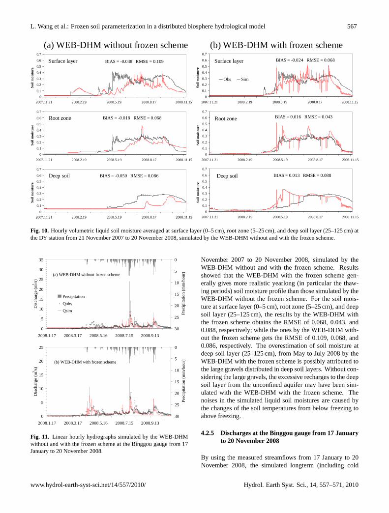
Figure 10 draws the hourly volumetric liquid soil moistureaveraged at surface layer (0–5 cm), root zone (5–25 cm),and deep soil layer (25–125 cm) at the DY station from 21



(a) WEB-DHM without frozen scheme (b) WEB-DHM with frozen scheme

0

0.1

0.2

0.3

0.4

0.5

0.6

0.7

2007.11.21 2008.2.19 2008.5.19 2008.8.17 2008.11.15

Soil

moi

stur

e

Surface layer BIAS = -0.048 RMSE = 0.109

0

0.1

0.2

0.3

0.4

0.5

0.6

0.7

2007.11.21 2008.2.19 2008.5.19 2008.8.17 2008.11.15

Soil

moi

stur

e

Obs Sim

Surface layer BIAS = -0.024 RMSE = 0.068

0

0.1

0.2

0.3

0.4

0.5

0.6

0.7

2007.11.21 2008.2.19 2008.5.19 2008.8.17 2008.11.15

Soil

moi

stur

e

Root zone BIAS = -0.018 RMSE = 0.068

0

0.1

0.2

0.3

0.4

0.5

0.6

0.7

2007.11.21 2008.2.19 2008.5.19 2008.8.17 2008.11.15

Soil

moi

stur

e

Root zone BIAS = 0.016 RMSE = 0.043

0

0.1

0.2

0.3

0.4

0.5

0.6

0.7

2007.11.21 2008.2.19 2008.5.19 2008.8.17 2008.11.15

Soil

moi

stur

e

Deep soil BIAS = -0.050 RMSE = 0.086

0

0.1

0.2

0.3

0.4

0.5

0.6

0.7

2007.11.21 2008.2.19 2008.5.19 2008.8.17 2008.11.15

Soil

moi

stur

e

Deep soil BIAS = 0.013 RMSE = 0.088

Fig. 10. Hourly volumetric liquid soil moisture averaged at surface layer (0–5 cm), root zone (5–25 cm), and deep soil layer (25–125 cm) atthe DY station from 21 November 2007 to 20 November 2008, simulated by the WEB-DHM without and with the frozen scheme.

0

5

10

15

20

25

30

35

2008.1.17 2008.3.17 2008.5.16 2008.7.15 2008.9.13

Dis

char

ge (

m3 /s

)

0

5

10

15

20

25

30

Prec

ipita

tion

(mm

/hou

r)

Precipitation

Qobs

Qsim

(a) WEB-DHM without frozen scheme

0

5

10

15

20

25

2008.1.17 2008.3.17 2008.5.16 2008.7.15 2008.9.13

Dis

char

ge (

m3 /s

)

0

5

10

15

20

25

30

Prec

ipita

tion

(mm

/hou

r)(b) WEB-DHM with frozen scheme

Fig. 11. Linear hourly hydrographs simulated by the WEB-DHMwithout and with the frozen scheme at the Binggou gauge from 17January to 20 November 2008.

November 2007 to 20 November 2008, simulated by theWEB-DHM without and with the frozen scheme. Resultsshowed that the WEB-DHM with the frozen scheme gen-erally gives more realistic yearlong (in particular the thaw-ing periods) soil moisture profile than those simulated by theWEB-DHM without the frozen scheme. For the soil mois-ture at surface layer (0–5 cm), root zone (5–25 cm), and deepsoil layer (25–125 cm), the results by the WEB-DHM withthe frozen scheme obtains the RMSE of 0.068, 0.043, and0.088, respectively; while the ones by the WEB-DHM with-out the frozen scheme gets the RMSE of 0.109, 0.068, and0.086, respectively. The overestimation of soil moisture atdeep soil layer (25–125 cm), from May to July 2008 by theWEB-DHM with the frozen scheme is possibly attributed tothe large gravels distributed in deep soil layers. Without con-sidering the large gravels, the excessive recharges to the deepsoil layer from the unconfined aquifer may have been sim-ulated with the WEB-DHM with the frozen scheme. Thenoises in the simulated liquid soil moistures are caused bythe changes of the soil temperatures from below freezing toabove freezing.

4.2.5 Discharges at the Binggou gauge from 17 Januaryto 20 November 2008

By using the measured streamflows from 17 January to 20November 2008, the simulated longterm (including cold



0.001

0.01

0.1

1

10

100

1000

2008.1.17 2008.3.17 2008.5.16 2008.7.15 2008.9.13

Dis

char

ge (

m3 /s

)

0

5

10

15

20

25

30

Prec

ipita

tion

(mm

/hou

r)

(a) WEB-DHM with frozen scheme, but with constant K G

0.001

0.01

0.1

1

10

100

1000

2008.1.17 2008.3.17 2008.5.16 2008.7.15 2008.9.13

Dis

char

ge (

m3 /s

)

0

5

10

15

20

25

30

Prec

ipita

tion

(mm

/hou

r)

(b) WEB-DHM with frozen scheme

Fig. 12. Logarithmic hourly hydrographs simulated by using theWEB-DHM with the frozen scheme, neglecting(a) and consider-ing (b) the frozen soil effect on the groundwater hydraulic conduc-tivity at the Binggou gauge from 17 January to 20 November 2008.

seasons) hourly discharges at Binggou gauge are further eval-uated.

Figure 11 displays the hourly hydrographs simulated bythe WEB-DHM without and with the frozen scheme at theBinggou gauge from 17 January to 20 November 2008. Re-sults show that the streamflows simulated by the WEB-DHMwith the frozen scheme agree fairly well with the obser-vations; while those calculated by the WEB-DHM withoutthe frozen scheme have large difference from the observa-tions, with the overestimation of baseflows (January–April),the underestimation of snowmelt flows (April–May), and theoverestimation of peak flows (July–August). The improvedsimulation results by the WEB-DHM with the frozen schemecan be attributed to the following reasons:

1. The consideration of reduction factor of the ground-water hydraulic conductivity (fice,G) largely improvesthe model’s performance from January to April (alsosee Fig. 12). Figure 12b demonstrates the logarithmichourly hydrographs simulated by using the WEB-DHMwith the frozen scheme at the Binggou gauge from 17January to 20 November 2008, which further confirmsthe good performance of the new system in simulatingbase flows. Without the treatments of the frozen soil ef-fect on the groundwater hydraulic conductivity, exces-sive baseflows have been obtained from January to April2008 (see Fig. 12a).

2. In the spring season (April–May), more snowmeltrunoff calculated by the WEB-DHM with the frozenscheme is due to the treatments of the hydraulic conduc-tivity reduction for each soil layer (fice,j ) as a functionof soil temperature, which has resulted in less infiltra-tion during the snow melting.

3. The poorer flood peaks obtained by the WEB-DHMwithout the frozen scheme, are possibly caused by theoverestimation of the soil hydraulic conductivities at thedeep soil layer and the unconfined aquifer during thethawing process.

5 Concluding remarks

In this study, the distributed biosphere hydrological modelWEB-DHM was improved by incorporating a frozen soil pa-rameterization. The WEB-DHM with the frozen scheme wasthen applied to the Binggou watershed for evaluation usingthe in-situ observations from WATER.

After calibrating land surface parameters, soil hydraulicparameters, and frozen soil parameters, the WEB-DHM withthe frozen scheme was then used for a yearlong validationfrom 21 November 2007 to 20 November 2008, to check themodel’s applicability in the continuous simulation. Resultsshow that the WEB-DHM with the frozen scheme has givenmuch better performance than the WEB-DHM without thefrozen scheme, in the simulations of soil moisture profile atthe DY station and the discharges (base and peak flows aswell as snowmelt runoff) at the basin outlet in the yearlongsimulation.

In the literatures regarding to the frozen soil parameteriza-tion in land surface modeling, there are mainly three ways tosimulate the ice content or the unfrozen water content withinthe soil. These methods estimate the ice content dependingon the heat available (e.g., Slater et al., 1998; Takata andKimoto, 2000; Dai et al., 2003), or using the freezing pointdepression equation (e.g., Koren et al., 1999; Smirnova etal., 2000; Niu and Yang, 2006; Zhang et al., 2007), or re-lying on empirical equations (Pauwels and Wood, 1999; Liand Koike, 2003). The empirical equations-based frozen soilparameterization by Li and Koike (2003) is used in the study,to improve the original WEB-DHM for simulating frozensoil dynamics, largely due to its simple structure and lowcomputation costs. Furthermore, the study by Li and Koike(2003) has shown the good compatibility between the empir-ical frozen soil parameterization and SiB2; while the origi-nal WEB-DHM uses a hydrologically-improved SiB2 (Wanget al., 2009c) as its land surface submodel. Although themethod in the study estimates the ice content based on em-pirical equations, the calibrated WEB-DHM with the frozenscheme has demonstrated acceptable accuracies in simulat-ing point-scale frozen soil dynamics and basin-scale inte-grated streamflows. Meanwhile, the frozen scheme usingempirical equations also results in difficulty in achieving an



optimal set of the frozen soil parametersa andb, as the newmodel (the WEB-DHM with the frozen scheme) is very sen-sitive to the two parameters (particularlyb) in simulating thesoil temperature and moisture profiles.

Different from Li and Koike (2003) that formulated frozensoil process in a 1-D land surface model (SiB2), this studyhas modified and incorporated the frozen soil scheme intoa distributed biosphere hydrological model (WEB-DHM).The newly-developed WEB-DHM with the frozen schemehas made it possible to simulate the basin-scale cold-regionland surface hydrological processes in a spatially-distributedmanner while considering the topographically-driven lateralflows. It can be used as a model operator in the catchment-scale land surface hydrological data assimilation system incold regions, to improve modelling of soil moisture and thesurface energy budget as well as streamflows.

Appendix A

Nomenclature

Symbol Definition

Cd effective heat capacity for the snow-free soil(J m−2 K−1)

Cg effective heat capacity for the soil surface(J m−2 K−1)

Csoil volumetric heat capacity of soil (J m−3 K−1)

Cw volumetric heat capacity of water(J m−3 K−1)

ds effective depth that feels the diurnal changeof temperature (m)

Eg bare soil evaporation rate (kg m−2 s−1)

f hydraulic conductivity decay factorfice,G reduction factor for the groundwater hy-

draulic conductivityfice,j hydraulic conductivity reduction factor for

thej -th soil layerHg sensible heat flux from soil surface (W m−2)

Hs soil thermal conductivity without consideringfrozen soil

Hs,new soil thermal conductivity considering frozensoil

KG groundwater hydraulic conductivity (m s−1)

KG0 constant groundwater hydraulic conductivitywithout considering frozen soil effect (m s−1)

Kj soil hydraulic conductivity at thej -th soillayer (m s−1)

Ksat,j saturated hydraulic conductivity for thej -thsoil layer (m s−1)

Ksurface saturated conductivity at the soil surface(m s−1)

Lf latent heat of fusion (J kg−1)

Mgw soil interception of liquid store (m)Mgs snow-ice stored on the ground (m)n empirical parameter in van Genuchten’s

equationRng absorbed net radiation by soil surface

(W m−2)

TB temperature of the bottom soil layer (K)Td temperature of the deep soil (K)Tf freezing point of water (K)Tg soil surface temperature (K)Tsoil,D1 soil temperature at 5 cm (K)Tsoil,j soil temperature at thej -th soil layer (K)Tsoil,z soil temperature at a given depthz (K)

Greek letters

α empirical parameters in van Genuchten’sequation

ζf frost depth (m)ζt thaw depth (m)θice,j ice content of thej -th soil layer (m3 m−3)

θj total volumetric water content of thej -th soillayer (m3 m−3)

θliq,j liquid water content of thej -th soil layer(m3 m−3)

θr residual soil water content (m3 m−3)

θs porosity (m3 m−3)

λ latent heat of vaporization (J kg−1)

ξgs energy transfer due to phase changes in snowon ground (W m−2)

ρice density of ice (kg m−3)

ρliq density of liquid water (kg m−3)

ψj soil matric potential at thej -th soil layer

Acknowledgements.This study was funded by grants from JapanAerospace Exploration Agency. Parts of this work were alsosupported by grants from the Ministry of Education, Culture,Sports, Science and Technology of Japan. The data used in thepaper are provided by the Chinese Academy of Sciences ActionPlan for West Development Program (grant number: KZCX2-XB2-09) and Chinese State Key Basic Research Project (grantnumber: 2007CB714400). The fifth author (H. Li) was supportedby National Natural Science Foundation of China (grant number:40671040).

Edited by: W. Wagner

References

Beven, K. J.: On subsurface storm flow: an analysis of responsetimes, Hydrol. Sci. J., 4, 505–519, 1982.

Bonan, G.: A land surface model (LSM version 1.0) for ecological,hydrological, and atmospheric studies: technical description anduser’s guide, NCAR Technical Note 417, NCAR, Boulder Co.,USA, 1996.



Cabral, M. C., Garrote, L., Bras, R. L., and Entekhabi, D.: A kine-matic model of infiltration and runoff generation in layered andsloped soils, Adv. Water Resour., 15, 311–324, 1992.

Cherkauer, K. A. and Lettenmaier, D. P.: Hydrologic effects onfrozen soils in the upper Mississippi River basin, J. Geophys.Res., 104(D16), 19599–19610, 1999.

Dai, Y., Zeng, X., Dickinson, R. E., et al.: The Common LandModel, B. Am. Meteorol. Soc., 84, 1013–1023, 2003.

Deardorff, J. W.: Efficient prediction of ground surface temperatureand moisture, with inclusion of a layer of vegetation, J. Geophys.Res., 83, 1889–1903, 1977.

FAO: Digital soil map of the world and derived soil properties, Landand Water Digital Media Series Rev. 1, United Nations Food andAgriculture Organization, CD-ROM, 2003.

Gao, Y., Chen F., Barlage, M., et al.: Enhancement of land surfaceinformation and its impact on atmospheric modeling in the HeiheRiver Basin, northwest China, J. Geophys. Res., 113, D20S90,doi:10.1029/2008JD010359, 2008.

Kane, D. L. and Stein, J.: Water Movement Into Seasonally FrozenSoils, Water Resour. Res., 19(6), 1547–1557, 1983.

Koren, V., Schaake, J., Mitchell, K., Duan, Q., Chen, F., andBaker, J.: A parameterization of snowpack and frozen ground in-tended for NCEP weather and climate models, J. Geophys. Res.,104(D16), 19569–19585, 1999.

Li, S. and Cheng, G.: Problem of Heat and Moisture Transferin Freezing and Thawing Soils. Lanzhou Univ. Press, Lanzhou,China, 203 pp, 1995.

Li, X. and Koike, T.: Frozen soil parameterization in SiB2 and itsvalidation with GAME-Tibet observations, Cold Reg. Sci. Tech-nol., 36, 165–182, 2003.

Li, X., Ma, M. G., Wang, J., Liu, Q., Che, T., Hu, Z. Y., Xiao, Q.,Liu, Q. H., Su, P. X., Chu, R. Z., Jin, R., Wang, W. Z., and Ran, Y.H.: Simultaneous remote sensing and ground-based experimentin the Heihe River Basin: Scientific objectives and experimentdesign, Adv. Earth Sci., 23, 897–914, 2008.

Li, X., Li, X. W., Li, Z. Y., Ma, M. G., Wang, J., Xiao, Q., Liu, Q.,Che, T., Chen, E. X., Yan, G. J., Hu, Z. Y., Zhang, L. X., Chu, R.Z., Su, P. X., Liu, Q. H., Liu, S. M., Wang, J. D., Niu, Z., Chen,Y., Jin, R., Wang, W. Z., Ran, Y. H., Xin, X. Z., and Ren, H. Z.:Watershed Allied Telemetry Experimental Research, J. Geophys.Res., 114, D22103, doi:10.1029/2008JD011590, 2009.

Luo, L., Robock, A., Vinnikov, K. Y., et al.: Effects of frozen soilon soil temperature, spring infiltration, and runoff: results fromthe PILPS 2(d) experiments at Valdai, Russia, J. Hydrometeorol.,4, 334–351, 2003.

Luo, S., Lu, S., and Zhang, Y.: Development and validation of thefrozen soil parameterization scheme in Common Land Model,Cold Reg. Sci. Technol., 55, 130–140, 2009.

Myneni, R. B., Nemani, R. R., and Running, S. W.: Algorithm forthe estimation of global land cover, LAI and FPAR based onradiative transfer models, IEEE. T. Geosci. Remote, 35, 1380–1393, 1997.

Mou, L., Tian, F., Hu, H., and Sivapalan, M.: Extension of theRepresentative Elementary Watershed approach for cold regions:constitutive relationships and an application, Hydrol. Earth Syst.Sci., 12, 565–585, 2008,http://www.hydrol-earth-syst-sci.net/12/565/2008/.

Nakano, Y., Tice, A. R., and Oliphant, J. L.: Transport of water infrozen soil: I. Experiment determination of soil water diffusiv-

ity under isothermal condition, Adv. Water. Resour., 5, 221–226,1982.

Nash, J. E., and Sutcliffe, J. V.: River flow forecasting through con-ceptual models part I - A discussion of principles, J. Hydrol.,10(3), 282–290, 1970.

Nicolsky, D. J., Romanovsky, V. E., Alexeev, V. A., and Lawrence,D. M.: Improved modeling of permafrost dynamics in aGCM land-surface scheme, Geophys. Res. Lett., 34, L08501,doi:10.1029/2007GL029525, 2007.

Niu, G. and Yang, Z.: Effects of frozen soil on snowmelt runoffand soil water storage at a continental scale, J. Hydrometeorol.,7, 937–952, 2006.

Pauwels, V. R. N. and Wood, E. F.: A soil-vegetation-atmospheretransfer scheme for the modeling of water and energy balanceprocesses in high latitudes. 1. Model improvements, J. Geophys.Res., 104, 27811–27822, 1999.

Poutou, E., Krinner, G., Genthon, C., and de Noblet-Ducondre, N.:Role of soil freezing in future boreal climate change, Clim. Dy-nam., 23, 621–639, 2004.

Robinson, J. S. and Sivapalan, M.: Instantaneous response func-tions of overland flow and subsurface stormflow for catchmentmodels, Hydrol. Processes, 10, 845–862, 1996.

Romanovsky, V. E. and Osterkamp, T. E.: Effects of unfrozen wa-ter on heat and mass transport processes in the active layer andpermafrost, Permafrost Periglac. Process., 11, 219–239, 2000.

Sellers, P. J., Randall, D. A., Collatz, G. J., Berry, J. A., Field, C.B., Dazlich, D. A., Zhang, C., Collelo, G. D., and Bounoua,L.: A revised land surface parameterization (SiB2) for atmo-spheric GCMs, Part I: Model Formulation, J. Climate, 9, 676–705, 1996a.

Sellers, P. J., Los, S. O., Tucker, C. J., Justice, C. O., Dazlich, D.A., Collatz, G. J., and Randall, D. A.: A revised land surface pa-rameterization (SiB2) for atmospheric GCMs, Part II: The gener-ation of global fields of terrestrial biosphysical parameters fromsatellite data, J. Climate, 9, 706–737, 1996b.

Slater, A. G., Pitman, A. J., and Desborough, C. E.: Simulation offreeze-thaw cycles in a general circulation model land surfacescheme, J. Geophys. Res., 103(D10), 11303–11312, 1998.

Smirnova, T. G., Brown, J. M., Benjamin, S. G., and Kim, D:Parameterization of cold-season processes in the MAPS land-surface scheme, 105(D3), 4077–4086, 2000.

Stocker-Mittaz, C., Hoelzle, M., and Haeberli, W.: Permafrost dis-tribution modeling based on energy-balance data: a first step,Permafrost Periglacial Processes, 13, 271–282, 2002.

Stull, R. B.: An Introduction to Boundary Layer Meteorology,Kluwer Academic Publishers, The Netherlands, 1988.

Takata, K. and Kimoto, M.: A numerical study on the impact of soilfreezing on the continental-scale seasonal cycle, J. Meteor. Soc.Japan, 78, 199–221, 2000.

Tang, Q., Oki, T., Kanae, S., and Hu, H.: Hydrological cycleschange in the Yellow River Basin during the last half of the twen-tieth century, J. Climate, 21, 1790–1806, 2008.

Tian, F., Hu, H., Lei, Z., and Sivapalan, M.: Extension of theRepresentative Elementary Watershed approach for cold regionsvia explicit treatment of energy related processes, Hydrol. EarthSyst. Sci., 10, 619–644, 2006,http://www.hydrol-earth-syst-sci.net/10/619/2006/.

The Institute of Geocryology: Siberia Branch, Academy of SovietUnion, General Geocryology, translated by: Guo, D., Liu, T.,


http://www.hydrol-earth-syst-sci.net/12/565/2008/

http://www.hydrol-earth-syst-sci.net/10/619/2006/


and Zhang, W., 1988. Sciences Press of China, Beijing, 318 pp.,1974.

van Genuchten, M. T.: A closed form equation for predicting thehydraulic conductivity of unsaturated soils, Soil Sci. Soc. Am.J., 44, 892–898, 1980.

Wang, L., Koike, T., Yang, K., Jackson, T., Bindlish, R., andYang, D.: Development of a distributed biosphere hydrologi-cal model and its evaluation with the Southern Great Plains Ex-periments (SGP97 and SGP99), J. Geophys. Res., 114, D08107,doi:10.1029/2008JD010800, 2009a.

Wang, L., Koike, T., Yang, K., and Yeh, P. J. F.: Assessment of adistributed biosphere hydrological model against streamflow andMODIS land surface temperature in the upper Tone River Basin,J. Hydrol., 377, 21–34, 2009b.

Wang, L., Koike, T., Yang, D., and Yang, K.: Improving the hydrol-ogy of the Simple Biosphere Model 2 and its evaluation withinthe framework of a distributed hydrological model, Hydrol. Sci.J., 54(6), 989–1006, 2009c.

Woo, M., Arain, M. A., Mollinga, M., and Yi, S.: A two-directional freeze and thaw algorithm for hydrologic andland surface modelling, Geophys. Res. Lett., 31, L12501,doi:10.1029/2004GL019475, 2004.

Yang, Z., Yang, Z., and Zhang, X.: Runoff and its generation modelof cold region in Binggou Basin of Qilian Mountain, Memoirsof Lanzhou Institute of Glaciology and geocryology, ChineseAcademy of Sciences, 7, 91–99, 1992 (in Chinese).

Yang, Z., Yang, Z., Liang, F., and Wang, Q.: Permafrost hydrolog-ical processes in Binggou Basin of Qilian Mountains, J. Glaciol.Geocryol., 15(2), 235–241, 1993 (in Chinese).

Ye, B. S., Yang, D. Q., Zhang, Z. L., and Kane, D.: Vari-ation of hydrological regime with permafrost coverage overLena Basin in Siberia, J. Geophys. Res., 114, D07102,doi:10.1029/2008JD010537, 2009.

Yershov, E. D.: General geocryology, Cambridge University press,1990.

Zhang, X., Sun, S., and Xue, Y.: Development and testing of afrozen soil parameterization for cold region studies, J. Hydrom-eteorol., 8, 690–701, doi:10.1175/JHM605.1, 2007.

Zhang, Z., Kane, D. L., and Hinzman, L. D.: Development and ap-plication of a spatially-distributed Arctic hydrological and ther-mal process model (ARHYTHM), Hydrol. Processes, 14, 1017–1044, 2000.

Zhang, X. and Yang, Z.: The primary analysis of water balance in inBinggou Basin of Qilian Mountains, J. Glaciol. Geocryol., 13(1),35–42, 1991 (in Chinese).


Frozen soil parameterization in a distributed biosphere hydrological model

Documents

Transcript of Frozen soil parameterization in a distributed biosphere hydrological model