ECOSYSTEM SERVICES IN A BIOSPHERE RESERVE ...

ECOSYSTEM SERVICES IN A BIOSPHERE RESERVE CONTEXT:

IDENTIFICATION, MAPPING AND VALUATION

BASANE CLAIRE NTSHANE

A THESIS SUBMITTED IN FULFILMENT OF THE REQUIREMENTS OF A PhD

INSCIENCE

DEPARTMENT OF ENVIRONMENTAL SCIENCE

FACULTY OF SCIENCE

RHODES UNIVERSITY

OCTOBER 2016

ABSTRACT

Despite their contribution to human well-being, ecosystem services (ES) are being destroyed

by anthropogenic activities, taken for granted and often compromised during land use

decision making. The question that often arises is, what value do ES have compared to other

undertakings that are economically robust, such as mining? The vision of the Millenium

Ecosystem Assessment (MA) was a world in which natural assets (including ES) are

appreciated and integrated into decision-making. The biodiversity strategy of the Convention

on Biological Diversity (CBD) also concerns the integration of natural assets into decision

making. Responding to challenges facing ES and their mainstreaming into decision-making

has been constrained by lack of data and requires new tools and approaches.

Integrating natural assets into decision-making is very important for South Africa (SA),

where ES have been a crucial part of human systems for decades, and also because of the

country’s commitment to the implementation of the CBD's biodiversity strategy. With the

aim of incorporating ES into decision-making in an integrated way, this study was conducted

in two biosphere reserves (BRs), Vhembe and Waterberg, in Limpopo Province, SA. The

aims of the study were the identification, mapping and valuation of ES following an

integrated approach. In order to achieve these aims, the study attempted to address four key

objectives: (1) to assess and evaluate the status of mapping and valuation of ES in SA, (2) to

identify and quantify ES and their indicators, (3) to investigate and analyse the impact of land

use/cover (LU/LC) change to ES and (4) to conduct valuation of selected ES.

Two separate literature reviews were undertaken to assess and evaluate the status of mapping

and valuation of ES in SA, thus addressing study objective 1. Both reviews detected a

significant research gap with regard to mapping and valuation of supporting services in SA.

To identify ES and indicators provided by the two BRs and to assess the impact of LU/LC

change and its effect on ES, a participatory scenario planning process was conducted under

three different scenarios, namely ecological development, social development and economic

development. It became clear that LU issues were diverse in nature and affected ES in a

number of ways and that there were always trade-offs in the choice of LU. For example,

yields of ES were best in the ecological development scenario and were affected negatively,

together with agricultural commodity production, in the social development and economic

development scenarios. A mapping exercise was undertaken to illustrate the spatial

distribution of ES supply and demand, involving five ES and 15 indicators using existing

i

datasets and the Integrated Valuation of Ecosystem Services and Trade-offs (InVEST)

mapping tool, again addressing objective 2 of the study.

Carbon storage and habitat quality were assessed, modelled and quantified and their values

provided in biophysical terms using InVEST modelling tools, thus addressing objective 4 of

the study. High quantities of carbon storage and high habitat quality were recorded in natural

areas and low quantities were recorded in managed systems (cultivated, urban and plantation

areas). InVEST was again applied to conduct an economic valuation of two provisioning ES,

timber and firewood, by determining their net present values, attempting to address objective

4 of the study. Results revealed that, at 12% discount rate, the net present value (NPV) for

timber production accounted for R23 317/ha in VBR and R57 304/ha in WBR. However, at

lower discount rates (4 and 7%), the NPVs for timber were negative in VBR and positive in

WBR. With regard to firewood production, the NPVs were negative against all three discount

rates in both study areas.

I conclude by proposing a four-step integrated approach that can aid the successful

incorporation of ES into decision-making: (1) maintain a balance between the social,

economic and ecological aspects when making decisions on ES, (2) strive for an evidence-

based approach to decision-making (use quantities and values), (3) apply integrated

approaches (methods and techniques) to quantification and valuation, and (4) communicate

all steps along the way. The results of this study will serve as a baseline for integration of ES

into decision-making in SA.

Key words: ecosystem services; valuation; InVEST; biosphere reserve; spatially explicit;

mapping; social; economic; ecological; ecosystem services indicators.

ii

DECLARATION

I, Ntshane Basane Claire hereby declare that all the work contained in this document is my

own original work, has not been submitted previously in any educational institution for the

purpose of obtaining any qualification. All the quoted work and referred literature has been

acknowledged accordingly with full references. This thesis is submitted in fulfilment of a

PhD in Environmental Science in the Faculty of Science at Rhodes University, South Africa.

Signature:

Date: October 2016

iii

TABLE OF CONTENTS

ABSTRACT................................................................................................................................. i-ii

DECLARATION...........................................................................................................................iii

TABLE OF CONTENTS............................................................................................................iv-x

LIST OF TABLES.........................................................................................................................xi

LIST OF FIGURES............................................................................................................... xii-xiii

LIST OF ABBREVIATIONS................................................................................................xiv-xvi

ACKNOWLEDGEMENTS........................................................................................................xvii

DEDICATION...........................................................................................................................xviii

CHAPTER 1: BACKGROUND AND CONTEXTUAL SETTING..........................................11.1 NTRODUCTION................................................................................................................... 1-2

1.2 RESEARCH RATIONALE...................................................................................................2-5

1.3 REESEARCH AIMS, OBJECTIVES AND KEY QUESTIONS........................................ 5-6

1.4 GENERAL MATERIALS AND METHODS......................................................................... 6

1.4.1 MODELLING, MAPPING AND VALUATION APPROACH........................................... 6

1.4.1.1 Mapping of ecosystem services.......................................................................................... 6

1.4.1.1.1 What is mapping?.........................................................................................................6-7

1.4.1.1.2 Mapping approaches........................................................................................................ 7

1.4.1.2 Valuation of ecosystem services....................................................................................... 7

1.4.1.2.1 Values and valuation.....................................................................................................7-8

1.4.1.2.2 Traditional valuation approaches.................................................................................. 8-9

1.4.1.2.2.1 Ecological valuation approach...................................................................................... 9

1.4.1.2.2.2 Socio-cultural valuation approach...........................................................................9-10

1.4.1.2.2.3 Economic valuation approach................................................................................ 10-11

1.4.1.2.3 Limitations of the traditional valuation approaches......................................................11

1.4.1.2.4 Integrated valuation approach........................................................................................ 12

1.4.1.3 Valuation and mapping approach adopted by this study........................................... 12-15

1.4.2 STUDY AREAS.................................................................................................................15

1.4.2.1 Study area selection..................................................................................................... 15-16

1.4.2.2 Vhembe Biosphere Reserve.............................................................................................. 16

1.4.2.2.1 Biophysical location.................................................................................................. 16-17

1.4.2.2.2 Climate............................................................................................................................17

iv

171.4.2.2.3 Geology and soils

1.4.2.2.4 Vegetation...................................................................................................................... 18

1.4.2.3 Waterberg Biosphere Reserve.......................................................................................... 19

1.4.2.3.1 Biophysical location....................................................................................................... 19

1.4.2.3.2 Climate............................................................................................................................19

1.4.2.3.3 Geology and soils...................................................................................................... 19-20

1.4.2.3.4 Vegetation...................................................................................................................... 20

1.5 STRUCTURE OF THE THESIS............................................................................................ 21

1.6 REFERENCES..................................................................................................................22-28

1.7. APPENDICES....................................................................................................................... 29

1.7.1 Appendix 1A: Valuation approaches and techniques used for differrent ecosystem

services and their values..........................................................................................................29-33

CHAPTER 2: VALUATION OF ECOSYSTEM SERVICES IN PROTECTED AREAS:A CASE STUDY FROM SOUTH AFRICA............................................................................. 34Abstract ........................................................................................................................................ 34

2.1 INTRODUCTION.................................................................................................................. 35

2.1.1 What are protected areas?...............................................................................................35-36

2.1.2 Benefits provided by protected areas................................................................................... 36

2.1.3 Threats to protected areas.................................................................................................... 37

2.1.4 Why do we need to value protected areas?.........................................................................38

2.1.5 Different ways to value ecosystem services provided by protected areas?...................38-40

2.1.6 Overview of valuation of ecosystem services in protected areas...................................40-41

2.2 MATERIALS AND METHODS.......................................................................................41-42

2.3 RESULTS..........................................................................................................................42-50

2.3.1 Objectives for valuation..................................................................................................42-432.3.2 Geographic area coverage.................................................................................................... 432.3.3 Protected areas categories covered...................................................................................... 432.3.4 Ecosystem services covered............................................................................................43-442.3.5 Valuation methods applied.................................................................................................. 442.3.6 Reference source type.......................................................................................................... 442.4 DISCUSSION......................................................................................................................... 51

2.4.1 Objectives for valuation....................................................................................................... 512.4.2 Geographic area coverage.................................................................................................... 512.4.3 Protected areas categories covered...................................................................................... 522.4.4 Ecosystem services covered2.4.5 Methods of valuation used ..

v

52-54 .... 54

2.4.6 Reference source type........................................................................................................ 542.5 CONCLUSIONS................................................................................................................ 54-55

2.6 REFERENCES.................................................................................................................. 56-62

CHAPTER 3: LANDUSE CHANGE SCENARIOS FOR TWO BIOSPHERE RESERVES IN SOUTH AFRICA............................................................................................ 63Abstract ........................................................................................................................................ 63

3.1 INTRODUCTION.............................................................................................................64-66

3.2 MATERIALS AND METHODS............................................................................................ 66

3.2.1 STUDY AREAS.............................................................................................................66-67

3.2.2 SCENARIO PLANNING PROCESS.................................................................................. 68

3.2.2.1 Definition of the purpose of the scenarios........................................................................ 683.2.2.2 The system's structure and major driver of change.....................................................68-713.2.2.3 Generation of the scenarios..........................................................................................71-723.2.2.4 Implications of the scenarios and use by decision makers..........................................72-733.3 RESULTS............................................................................................................................. 74

3.3.1 Ecological development scenario...................................................................................74-753.3.2 Economic development scenario....................................................................................75-763.3.3 Social development scenario...........................................................................................76-783.4 DISCUSSION......................................................................................................................... 78

3.4.1 Ecological development scenario...................................................................................78-793.4.2 Economic development scenario.................................................................................... 80-813.4.3 Social development scenario...........................................................................................81-823.5 CONCLUSIONS..................................................................................................................... 82

3.6 REFERENCES.................................................................................................................. 83-90

3.7 APPENDICES........................................................................................................................ 91

3.7.1 Appendix 3A: Sample questionnaire..............................................................................91-92

CHAPTER 4: ECOSYSTEM SERVICES AND THEIR INDICATORS: IDENTIFICATION AND MAPPING....................................................................................... 93Abstract ........................................................................................................................................ 93

4.1 INTRODUCTION.................................................................................................................94

4.1.1 What are ecosystem services............................................................................................... 944.1.1.1 Ecosystem services as benefits....................................................................................94-954.1.1.2 Ecosystem services as processes....................................................................................... 954.1.1.3 Ecosystem services as functions..................................................................................95-964.1.2 Classification of ecosystem services...............................................................................96-984.1.3 Mapping of ecosystem services......................................................................................98-994.2 MATERIALS AND METHODS..........................................................................................99

4.2.1 Study area.................................................................................................................... 99-100

vi

4.2.2 Sources of data............................................................................................................ 100-1024.2.3 Overview of ES mapping in South Africa..........................................................................1034.2.4 Mapping of ecosystem services and its indicators..............................................................1034.2.4.1 Provisioning services...................................................................................................... 1034.2.4.1.1 Indicators for provisioning services...................................................................... 103-1044.2.4.1.2 Provisioning ecosytem services................................................................................... 1044.2.4.2 Regulating services........................................................................................................1044.2.4.2.1 Indicators of regulating services........................................................................... 104-1054.2.4.2.2 Regulating ecosystem services.................................................................................... 1054.2.4.3 Supporting services.................................................................................................. 105-1064.2.4.4 Cultural services....................................................................................................... 106-1074.3 RESULTS............................................................................................................................107

4.3.1 OVERVIEW OF ES MAPPING IN SA............................................................................ 107

4.3.1.1 Regulating services..........................................................................................................107

4.3.1.2 Provisioning services............................................................................................... 107-108

4.3.1.3 Cultural services.............................................................................................................. 108

4.3.1.4 Supporting services..........................................................................................................108

4.3.2 ECOSYSTEM SERVICES IN A BR CONTEXT........................................................... 109


4.3.2.2 Cultural services....................................................................................................... 115-117

4.3.2.3 Regulating services.................................................................................................. 118-124

4.3.2.4 Supporting services.................................................................................................. 124-125

4.4 DISCUSSION...................................................................................................................125

4.4.1 OVERVIEW OF ECOSYSTEM SERVICES MAPPING IN SA......................................125

4.4.1.1 Provisioning services...................................................................................................... 125

4.4.1.2 Regulating services..........................................................................................................125

4.4.1.3 Cultural services.............................................................................................................. 126

4.4.1.4 Supporting services..........................................................................................................126

4.4.2 ECOSYSTEM SERVICES IN A BR CONTEXT........................................................... 126


4.4.2.2 Regulating services.................................................................................................. 129-130

4.4.2.3 Cultural services....................................................................................................... 130-131

4.4.2.4 Supporting services.................................................................................................. 131-132

4.5 CONCLUSIONS....................................................................................................................132

4.6 REFERENCES.............................................................................................................. 133-142

4.7 APPENDICES...................................................................................................................... 143

vii

4.7.1 Appendix 4A: Selected ecosystem services classification frameworks..................... 143-146

4.7.2 Appendix 4B: Literature reviewed.............................................................................. 147-150

4.7.3 Appendix 4C: Spatial representation of indicators of ecosystem services in Waterberg

and Vhembe Biosphere Reserves........................................................................................ 151-165

CHAPTER 5: HABITAT ASSESSMENT FOR ECOSYSTEM SERVICES IN SOUTHAFRICA......................................................................................................................................166

Abstract........................................................................................................................................166

5.1 INTRODUCTION......................................................................................................... 166-169

5.2.1 Study area.................................................................................................................... 169-170

5.2.2 InVEST biodiversity model............................................................................................... 170

5.2.3 Running the InVEST model........................................................................................ 170-171

5.3 RESULTS............................................................................................................................171

5.3.1 Habitat quality............................................................................................................. 171-1725.3.2 Habitat loss and degradation....................................................................................... 172-1755.3.3 Degradadtion of vegetation in the study area............................................................. 175-1765.4 DISCUSSION................................................................................................................ 176-177

5.4.1 Habitat quality............................................................................................................. 177-1785.4.2 Habitat loss and degradation....................................................................................... 178-1805.5 CONCLUSIONS....................................................................................................................180

5.6 REFERENCES.............................................................................................................. 181-187

5.7 APPENDICES...................................................................................................................... 188

5.7.1 Appendix 5A: InVEST Habitat quality model data requirements.............................. 188-190

5.7.2 Appendix 5B: Published article: Chapter 5 ................................................................ 191-203

CHAPTER 6: ABOVE-GROUND CARBON STORAGE ASSESSEMENT IN SOUTH AFRICA..................................................................................................................................... 204Abstract ...................................................................................................................................... 204

6.1 INTRODUCTION.........................................................................................................205-206

6.2 MATERIALS AND METHODS.......................................................................................... 206

6.2.1 Study areas .................................................................................................................206-2086.2.2 Estimation of carbon storage in landcover/vegetation types............................................. 2086.2.3 Quantification and mapping of carbon stocks................................................................... 2096.2.4 Correlation between carbon storage, vegetation and land cover................................209-2106.2.5 Running the InVEST carbon storage model...................................................................... 2106.3 RESULTS........................................................................................................................... 210

6.3.1 Carbon stored in land cover types............................................................................. 210-213

viii

6.3.2 Carbon stored in vegetation types.............................................................................213-2166.4 DISCUSSION....................................................................................................................... 216

6.4.1 Carbon storage and land cover types..........................................................................216-2186.4.2 Carbon storage and vegetation types..........................................................................218-2206.5 CONCLUSIONS................................................................................................................... 220

6.6 REFERENCES..............................................................................................................221-225

CHAPTER 7: ECONOMIC VALUATION OF PROVISIONING SERVICES IN A BIOSPHERE RESERVE......................................................................................................... 226Abstract....................................................................................................................................... 2267.1 INTRODUCTION.........................................................................................................226-229

7.2 MATERIALS AND METHODS.......................................................................................... 229

7.2.1 Study area....................................................................................................................229-2307.2.2 Valuation approach used in the study.........................................................................230-2327.2.3 Information sourcing...................................................................................................232-2337.2.4 Data collected..................................................................................................................... 2337.2.4.1 State of timber production in the study area............................................................233-2347.2.4.2 State of firewood production in the study area...............................................................2357.2.5 Calculation of the required input data.........................................................................235-2397.2.6 Process followed to run the InVEST timber model .........................................................2397.2.7 Interpretation of the InVEST model results................................................................239-2407.3 RESULTS............................................................................................................................ 240

7.3.1 Economic value of timber production in the study areas............................................240-2417.3.2 Economic value of firewood production in the study areas............................................... 2417.4 DISCUSSION....................................................................................................................... 241

7.4.1 Economic value of timber production in the study area.............................................242-2437.4.2 Economic value of firewood production in the study area.........................................243-2447.5 CONCLUSIONS................................................................................................................... 244

7.6 REFERENCES..............................................................................................................245-248

CHAPTER 8: SYNTHESIS AND CONCLUSIONS............................................................. 2498.1 INTRODUCTION................................................................................................................ 2498.2 SYNTHESIS OF MAJOR FINDINGS..........................................................................249-2558.3 CONCLUDING REMARKS.........................................................................................255-2568.4 REFERENCES..............................................................................................................257-258

ix

LIST OF TABLES

Table 1.1 Chapters covered by the study...................................................................................... 21

Table 2.1 Overview of valuation of ES generated in protected areas in SA ...........................45-50

Table 3.1 Main stakeholders who participated on the study......................................................... 69

Table 3.2 Stakeholders’ views on trends in land use changes and their associated drivers......... 70

Table 3.3 Stakeholders’ views on trends in the supply of ecosystem services and their major

drivers .......................................................................................................................................... 71

Table 4.1 Datasets used................................................................................................................102

Table 5.1 Threat data used to run InVEST ...............................................................................188

Table 5.2 Sensitivity of different habitat types to threats .........................................................190

Table 6.1 Input data used to calculate carbon storage/ha in different land cover types............209

Table 6.2 Percentage representation of carbon stored in different land covers types

in the study areas......................................................................................................................... 211

Table 7.1 InVEST timber/firewood production model data requirements..........................231-232

Table 7.2 VBR and WBR's inputs for timber production ......................................................... 234

Table 7.3 VBR and WBR's input for firewood production....................................................... 235

Table 7.4 Calculation of plantantion proportion of harvest....................................................... 236

Table 7.5 Calculation of plantation harvesting costs................................................................... 237

Table 7.6 Calculation of plantation maintenance costs............................................................... 237

Table 7.7 Calculation of WACC..........................................................................................238-239

Table 7.8 The economic values of timber production in VBR and WBR at different discount

rates......................................................................................................................................240-241

Table 7.9 The economic values of firewood production in the study areas .............................241

x

LIST OF FIGURES

Figure 1.1 Linkages between ecosystem services and human well-being.....................................5

Figure 1.2 A schematic illustration of the key questions and objectives addressed in the core

six chapters of this study................................................................................................................. 6

Figure 1.3 InVEST Toolbox..........................................................................................................13

Figure 1.4 Study area locations: map of South Africa showing the provincial and biosphere

reserve boundaries........................................................................................................................ 16

Figure 1.5 Vhembe Biosphere Reserve vegetation map................................................................18

Figure 1.6 Waterberg Biosphere Reserve vegetation map...........................................................20

Figure 3.1 Map of Limpopo Province of South Africa, showing the five district municipalities

(Waterberg, Vhembe, Greater Sekhukhune, Capricorn and Mopani) and the location of the

Waterberg Biosphere Reserve (WBR) and Vhembe Biosphere Reserve (VBR) study areas, as

well as sizes of each biosphere's three zones (core, buffer and transition)................................ 67

Figure 3.2 Scenario planning development framework outlining activities undertaken in each

stage of the scenario development process.................................................................................. 73

Figure 3.3 An illustration of the ecological development scenario, showing interactions

between conservation (current and future conservation area extension) and agriculture

(current) in the VBR and WBR study areas.................................................................................75

Figure 3.4 An illustration of the economic development scenario, showing interactions

between proposed mining developments, conservation (current and future conservation area

extension) and agriculture (current) in the VBR and WBR study areas......................................76

Figure 3.5 An illustration of the social development scenario, showing interactions between

land restitution, conservation (current and future conservation area extension) and agriculture

(current) in the VBR and WBR study areas.................................................................................78

Figure. 4.1 Number of ecosystem services mapped in SA and number of indicators used to

map them....................................................................................................................................108

Figure 4.2 Illustration of water provisioning service in WBR indicating areas with high and

low water yield............................................................................................................................ 112

Figure 4.3 Illustration of water provisioning service in VBR indicating areas with high and

low water yield............................................................................................................................ 113

Figure 4.4 Grazing potential in terms of LSU per hectare in W BR.......................................... 114

Figure 4.5 Grazing potential in terms of LSU per hectare in VBR........................................... 115

xi

Figure 4.6 An illustration of erosion prevention service through soil retention in Waterberg

Biosphere Reserve (illustration of high and low soil retention areas.......................................119

Figure 4.7 An illustration of erosion prevention service through soil retention in Vhembe

Biosphere Reserve (illustration of high and low soil retention areas) .....................................120

Figure 4.8 An illustration of climate regulating service indicating high, medium and low

carbon sequestration areas in Waterberg Biosphere Reserve....................................................121

Figure 4.9 An illustration of climate regulating service indicating high, medium and low

carbon sequestration areas in Vhembe Biosphere Reserve........................................................122

Figure 4.10 An illustration of nutrients (nitrogen and phosphorus) export in the Waterberg

Biosphere Reserve study area indicating low and high export values.......................................123

Figure 4.11 An illustration of nutrients (nitrogen and phosphorus) retention (kg/ha) in the

Vhembe Biosphere Reserve study area indicating low and high nutrient retention values.......124

Figure 5.1. Habitat quality in the Vhembe Biosphere Reserve and the northern parts of

Kruger National Park study areas .............................................................................................172

Figure 5.2 Habitat changes in the Vhembe Biosphere Reserve and the northern parts of

Kruger National Park study areas .............................................................................................173

Figure 5.3. The extent of habitat loss in the Vhembe Biosphere Reserve and the northern

parts of Kruger National Park study areas ..................................................................................174

Figure 5.4. The extent of transformed habitats and natural habitats in the Vhembe Biosphere

Reserve and the northern parts of Kruger National Park study areas .......................................175

Figure. 5.5. The extent of degradation of vegetation types in the Vhembe Biosphere Reserve

and the northern parts of Kruger National Park study areas .....................................................176

Figure 6.1 An illustration of TAG C (MgC) storage range in different land cover types

(cultivated areas, degraded areas, plantations and natural forest) in the Waterberg study area,

including the WBR...................................................................................................................... 212

Figure 6.2 An illustration of TAG C (MgC) storage range in different land cover types

(cultivated areas, degraded areas, plantations and natural areas) in the Vhembe study area,

including the VBR...................................................................................................................... 213

Figure 6.3 An illustration of the TAG C (MgC) stored in different vegetation types in

Vhembe study area, ranked low, medium or high in terms of the amount of C stored area......215

Figure 6.4 An illustration of the TAG C (MgC) storage range in different vegetation types in

the Waterberg study area (vegetation types are represented by biomes), ranked low, medium

or high in terms of the amount of C stored................................................................................216

xii

Figure 8.1 Conceptual framework highlighting where the study is contributing new

knowledge to the existing theories.............................................................................

LIST OF ABBREVIATIONS

1. ARC Agricultural Resource Council

2. ARIES Artificial intelligence for Ecosystem Services

3. BR Biosphere reserve

4. CA Conservation area

5. CBD Convention on Biological Diversity

6. CICES Common International Classification of Ecosystem Services

7. COP Conference of the Parties

8. CSIR Council for Scientific and Industrial Research

9. CM Choice Modelling

10. CV Contingent Valuation

11. DAFF Department of Agriculture, Forestry & Fisheries

12. DEA Department of Environmental Affairs

13. DEAT Department of Environmental Affairs and Tourism

14. DEFRA Department for Environment Food & Rural Affairs

15. DME Department of Minerals & Energy

16. DWAF Department of water Affairs

17. EDS Ecosystem disservice

18. Eftec Economics for the Environmental Consultants

19. ES Ecosystem services

20. ESA Ecological Society of America

21. ESRI Environmental Systems Research Institute

22. EPWP Extended Public Works Programme

23. FAO Food and Agriculture Organization

24. GDP Gross Domestic Product

25. GOI Government of India

26. GHG Greenhouse effect

27. GUMBO Global Unified Metamodel of the Biosphere

28. HP Hedonic Pricing

xiii

254

29. ICMM International Council on Mining & Metals

30. InVEST Integrated Valuation of Ecosystem Services & Trade-offs

31. IPBES Intergovernmental Platform on Biodiversity & Ecosystem

Services

32. IPCC Intergovernmental Panel on Climate Change

33. IUCN International Union for the Conservation of Nature

34. KLF Komatiland Forests

35. KNP Kruger National Park

36. LC Land cover

37. LDA Limpopo Department of Agriculture

38. LGDS Limpopo Growth & Development Strategy

39. LM Local municipality

40. LSU Large Stock Unit

41. LU Land use

42. MA Millennium Ecosystem Assessment

43. MAB Man and Biosphere

44. MAI Mean Annual Increment

45. MIMES Multiscale Integrated Models of Ecosystem services

46. MNPMP Marakele National Park Management Plan

47. NBSAP National Biodiversity Strategy and Action Plan

48. NEMA National Environmental Management Act

49. NEM:PAA National Environmental Management: Protected Areas Act

50. NFA National Forest Act

51. NLC National Land Cover

52. NPF National Park Forum

53. NPAES National Protected Area Expansion Strategy

54. NSBA National Spatial Biodiversity Assessment

55. NWRS National Water Resource Strategy

56. OPAL Offset Portfolio Analyzer and Locator

57. PA Protected area

58. PAK Protected areas in Kenya

59. PAWC Plant Available Water Content

60. PGRC Provincial Government Responsible for Conservation

61. PLOS Private Land Owners

xiv

62. RIOS

63. SA

64. SANBI

65. SANParks

66. SAMABNC

67. SoIVES

68. StatsSA

69. TAU

70. TC

71. TEEB

72. TEV

73. TNPV

74. UNEP

75. UNFCCC

76. UNESCO

77. VBR

78. VDMIDP

79. WACC

80. WBR

81. WDMIDP

82. WMB

83. WTTC

Resource Investment Optimization System

South Africa

South African National Biodiversity Institute

South African National Parks

South African Man and Biosphere National Committee

Social Values for Ecosystem Services

Statistics South Africa

Transvaal Agricultural Union

Travel Cost

The Economics of Ecosystems and Biodiversity

Total Economic Value

Total Net Present Value

United Nations Environment Programme

United Nations Framework Convention on Climate Change

United Nations Educational, Scientific and Cultural

Organization

Vhembe Biosphere Reserve

Vhembe District Municipality Integrated Development Plan

Weighted Average Cost of Capital

Waterberg Biosphere Reserve

Waterberg District Municipality Integrated Development Plan

Waterberg Meander Brochure

World Travel and Tourism Council

xv

ACKNOWLEDGEMENTS

First and foremost, I would like to thank God, the Almighty, who made all things possible,

for His continuous protection, blessings and mercy. Secondly, I would like to thank all my

family members for all the support, patience and encouragement throughout this journey,

especially my aunt Hellinah, my sisters, Tinyiko and Gladness, for always being my pillars of

strength and support. I would never have been able to achieve this project without the support

and encouragement of many friends, too numerous to name here, who were a source of

support on different levels.

My deepest appreciation to my supervisor, Professor J. Gambiza (Rhodes University). His

immense knowledge helped me throughout the duration of the research and writing of this

thesis. I could not have chosen a better advisor and mentor for my Ph.D. study. I am deeply

grateful for the valuable contributions made by Dr L. Dziba (Council for Scientific and

Industrial Research) to this study. I am greatly indebted to Mr C. Mashava and Ms N. Tantsi

who assisted with the surveys. I also thank Mrs B. Bradley, T, Khoza and F.H Mugwabana

for assisting with the review of the manuscripts.

My sincere gratitude goes to South African National Parks, for offering me the study

opportunity and financial support to allow me to complete the project, also for the

contributions and participation of colleagues on various levels of this study. I would also like

to acknowledge the contributions made by the following people Messrs M. Powell, C.

Wademann and K. Mangwale, for their stimulating discussions, advice and constructive

comments. Dr. P. OFarell and Mr M. Engelbrecht are thanked for assisting with some of the

models used in this study.

Informal and formal discussions, as well as interviews with the following people, also

contributed immensely to the study: Dr R. Barber, Mr J. van Rooy, Dr W. Schack, Mr B.

Penzhorn, Dr P. Benson, Mr K. Maud, Mr A. Venter, Mr M. Nephawe, Mr P. van Rensburg,

Mr J. Fourie, Mr S. McCartney, Mr E. Nemavhola, Mr P. van Staden, Mr J. Miller, Mr S.

Khoza, Mr R. Wadley, Mr B. Mostert, Mr J. Linden, Mr L. Mabila, Dr C. Cardjorlolo, Mr T

Ross, J Erwee, Mr. D. Liebenberg, Ms K. Abrams and others not mentioned here who have

contributed in one way or another.

xvi

DEDICATION

This work is dedicated to the Almighty, never forsaking God, who never abandoned me, but

was always by my side throughout this journey and as always carried out His promise: ‘I will

never leave you, nor forsake you’-Hebrews 13:5.

To my beloved mother, Mphephu Sarah Ntshane (late) for your love and belief in me and

being a source o f inspiration on my academic journey.

To my uncle, Risimati Highlord Mashava (late), for laying a good academic foundation for

everyone in the family, it made such a difference.

To my husband Fhatuwani Mugwabana and our children for your unconditional love,

patience, encouragement and support throughout this journey.

xvii

CHAPTER 1

CONCEPTUAL AND CONTEXTUAL SETTINGS

1.1 NTRODUCTION

An ecosystem is defined as “a dynamic complex of plant, animal and micro-organism

communities and their non-living environment interacting as a functional unit at any given

scale" (Convention on Biological Diversity (CBD) 1992). Ecosystems produce a wide range

of goods and services that are crucial for human well-being, collectively called ecosystem

services (ES) (Millennium Ecosystem Assessment (MA) 2005; Nelson et al. 2009). The term

ES was first recorded during the 1960s (King 1966; Helliwell 1969). Since these early

records, considerable efforts have been put into the definition of the concept of ES (Daily

1997; Binning et al. 2002; Brown et al. 2007; TEEB 2010). It is obvious from these

definitions that the term ES means different things to different people, although there is

strong connectedness of these definitions in terms of what they stand for. In the definitions of

Daily (1997), Binning et al. (2002) and Brown et al. (2007), the concepts of ES, goods and

services were separated. However, other researchers put these two concepts together (MA

2005; Costanza et al. 1997). So far, the most popular definition is that of the MA (2005),

where ES are defined as the “benefits that people obtain from the ecosystems”. Another

definition is that of de Groot et al. (2010) describing ES as a “subset of biophysical structures

and processes that provide services.”

Just like the definitions of ES, many methods of classification of goods and services have

been proposed (Costanza et al. 1997; Daily 1997; Bastian and Schreiber 1999; Wilson and

Hoehn 2006; Brown et al. 2007; Mertz et al. 2007; Costanza 2008; de Groot et al. 2010;

CICES 2011), with numerous differences in the way ES were grouped and named (TEEB

2010; CICES 2011; Hermann et al. 2011). These differences could be brought about by the

complexity of the way in which ecosystems produce ES (Costanza 2008; TEEB 2010; CICES

2011; Hermann et al. 2011). Appendix 1A provides details of five selected ES

frameworks/typologies.

1

While much research and debate on the term ES have taken place (Boyd and Banzhaf 2007;

Wallace 2007; Costanza 2008; Fisher and Turner 2008; Haines-Young and Potschin 2009;

TEEB 2010), it should be noted that ecosystems provide not only benefits, but also

disservices to human well-being (O’Farrell et al. 2007; Zhang et al. 2007; Dunn 2010; TEEB

2010; Escobedo et al. 2011; von Dohren and Haase 2014). In simple terms, ecosystem

disservices (EDS) are the opposite of ES in that they have a negative impact on human well

being, whereas an ES is beneficial (MA 2005). One of the earliest definitions of EDS is that

of Lyytimaki and Sipila (2009), who refer to EDS as “functions of an ecosystem that are

perceived as negative for human well-being.” Some examples of EDS include biophysical

hazards (diseases, allergenic and poisonous organisms) and geophysical hazards (floods,

heatwaves and storms) (Lyytimaki and Sipila 2009; von Dohren and Haase 2014). In an

attempt to understand the concept of EDS better, it is imperative to understand the context in

which it is used. In the review done by von Dohren and Haase (2015), it was found that EDS

were mostly associated with agricultural and urban environments. In their association with

agriculture, EDS mainly result from negative activities pertaining to land use, such as the

incorrect use of fertilizers and pesticides, biodiversity loss, soil and water pollution, or

introduction of invasive species (O’Farrell et al. 2007; Power 2010; Escobedo et al. 2011;

Firbank et al 2013; von Dohren and Haase 2015). In the urban setting, EDS are associated

with disease-causing vectors, air and water pollution, infrastructure malfunctioning and

spread of allergies (Lyytimaki et al. 2008; Arnold 2012; Dobbs et al. 2011; Escobedo et al.

2011; von Dohren and Haase 2015), among others.

1.2 RESEARCH RATIONALE

The MA (2005) formally put human beings in the central context of ES, reflecting that natural

ecosystems provide humans with services that are indispensable to their well-being, although

prior to this assessment other authors, e.g. Daily (1997), also recognised the linkage between

ES and human well-being. Despite their contribution to human well-being, natural assets

(including ES), are being destroyed by anthropogenic activities. What can be deduced from

the contextual settings of the EDS concept above, is that it is linked to what the MA (2005)

listed as some of the causes of the degradation of ES, of which agriculturally related activities

are at the top of the list (MA 2005; Power 2010). At the rate that ES are suffering

degradation, EDS will have equally negative impacts on human well-being. Although some

are inflicted naturally, most EDS are human-induced (MA 2005) and linked to human

2

population growth, among others (Tilman et al. 2002; Norris 2008). Figure: 1.1 illustrates the

conceptual framework of ES (MA 2005), showing the linkages between ES and human well

being and the associated drivers of change, which are either natural or anthropogenic.

Other concerns are related to the fact that ES are grossly undervalued by society (Daily et al.

2009), not mainly because of lack of awareness of their link to human well-being, but because

for ages, human society has undermined the services that are available for free, not formally

traded in markets (MA 2005, Daily et al. 2009). Other challenges are that natural assets are

poorly understood and rarely monitored (Heal 2000a; MA 2005, Maler et al. 2008; Daily et

al., 2009), and often compromised during land use decisions in favour of undertakings that

are economically robust. Southern Africa is not an exception from the concerns raised above.

According to the regional assessments regarding the links between ES and poverty alleviation

conducted by Shackleton et al. (2008), ES such as fresh water provisioning, fodder provision,

soil fertility, biodiversity, wild products (wild foods and medicinal resources), and cultural

and spiritual value, among others, are being threatened and subjected to degradation by

factors such as climate change, land transformation and poverty, among others (Shackleton et

al. 2008). The degradation of ES in Southern Africa and elsewhere in the world is borne

disproportionately by the poor (MA 2005; Shackleton et al. 2008).

Given the challenges faced by natural assets and the fact that both ES degradation and EDS

could have long-term negative effects on human well-being, strategies were put in place to

minimize further degradation of ES. Among these strategies are the establishment of

protected areas (PAs) and socio-ecological systems such as biosphere reserves (BRs). BRs are

defined as ecosystems of terrestrial and coastal nature, combining conservation and

sustainable use of natural resources and concerned with the promotion of harmony between

human beings and nature (UNESCO 2010).

In South Africa (SA), the BR concept was introduced in 1990 (Pool-Stanvliet 2013), when

UNESCO’s Man and Biosphere (MAB) programme was identified as an appropriate

approach to a holistic conservation strategy to address the transformation and destruction of

natural habitats in the fynbos biome (Burgers et al. 1990; Pool-Stanvliet 2013). However, SA

was officially introduced to the MAB programme by the signing of an agreement with

UNESCO in 1995. Implementation of bio-regional planning following the sustainable

development approach of BRs in the Western Cape Province led to the designation of

Kogelberg as the first BR in SA in 1998. Bioregional planning was a management system that

3

formed the basis for spatial planning (Pool-Stanvliet 2013). Currently, there are six BRs in SA

(Kogelberg, Cape West Coast, Waterberg, Kruger to Canyons, Cape Winelands and Vhembe)

across three provinces (Western Cape, Limpopo and Mpumalanga).

Given their concern with the society, ecology and the economy, both the concepts of ES and

socio-ecological systems such as BRs' principles are rooted in the promotion of sustainable

development for human well-being (MA 2005; UNESCO 2010). According to the Bruntland

report (Bruntland and WCED 1987), sustainable development is the development that meets

the needs of the current generation without compromising the needs of the future generation.

Given the complex nature of human-environment systems (Wiek et al. 2012), there is a need

for research into sustainability. This study therefore falls under sustainability science, which

is a discipline that is concerned with the needs of society and the sustainability of the life

support system (Wiek et al. 2012).

The vision of the MA (2005) was that “ES are recognized and incorporated into decision

making” (Daily et al. 2009). Similarly, the Convention on Biological Diversity (CBD 2010),

of which approximately 200 countries, including SA, are signatories, requires that natural

capital be incorporated into national accounting. Without this integration, natural assets are

ignored and suffer immense degradation (MA 2005; Daily et al. 2009). However, the

integration of ES into decision-making is mainly constrained by lack of data (Petter et al.

2013). In an attempt to address this challenge, this study aimed to identify, map and value ES

in two BRs in Limpopo Province of SA.

According to Daily et al. (2009), five elements have to be addressed in order to integrate ES

successfully into decision-making: (1) focus on other services beyond provisioning services,

(2) an understanding of the interlinked production of services, (3) an understanding of the

decision-making process of individual stakeholders, (4) integration of research into

institutional design and policy implementation, and (5) introduction of evidence-based policy

in performance evaluation and improvement over time. Furthermore, according to the MA

(2005), in order to improve the effectiveness of decision-making in these contexts and the

outcomes of decisions for human well-being, the decision-making process has to satisfy

certain aspects, which include: (1) use of the best available information, including the

quantities and values of ES, (2) transparency and stakeholder engagement, (3) recognising

that not all ES values can be quantified, (4) assessment of trade-offs across different ES and

(5) ensuring accountability by providing for regular monitoring and evaluation.

4

Provisioning ( food; water) Regulating (climate ; disease regulation)

Cultural (recreational; spiritual) Supporting (primary production; soil formation)

Human well-being Drivers of change

^ a ! — i

Poverty reduction Freedom & choice

Good social relations Health

Security

Economic Socio-political Demographic

Science & technology Culture & religious

Land use/cover change Climate change

Species introduction/removal

Figure 1.1 Ecosystem services conceptual framework (Source: MA 2005).

1.3 RESEARCH AIMS, OBJECTIVES AND KEY QUESTIONS

The aims of the study were the identification, mapping and valuation of ES. In order to

achieve these aims, the study attempted to answer the following key questions: (1) What are

different ES and their indicators provided by the study areas? (2) What are the impacts of land

use/land cover (LU/LC) change on ES in the study areas? (3) What are the quantities of

selected ES in the study areas? (4) What are the values of selected ES in the study areas? In

order to answer the research questions mentioned above, the following objectives have been

addressed: (1) to assess and evaluate the status of mapping and valuation of ES in SA, (2) to

identify and quantify ES and their indicators in the study areas, (3) to investigate and analyse

the impact of LU/LC change to ES in the study areas, and (4) to conduct valuation of selected

ES in the study areas.

5

STUDY AIMS

Identification, mapping and valuation of ES

f t

1. To assess and evaluate the status of mapping and valuation of ES in SA.

f t

\A—NC Objectives )l\| -^— i/ l

f t

2. To investigate and analyse the impact of LU/LC in the study areas

What are the different ES provided by the study areas?

What are the quantities of selected ES in the study areas?

Key questions

What are the values of selected ES in the study areas?

f t

3. To identify and quantify ES and their indicators

f t

/>——N\ Objectives y\l .... v \

4. To conduct valuation of selected ES in the study areas.

IkCONCLUSION

Integrated approach to successfully incorporate ES into decision-making

Figure 1.2 A schematic illustration of the key questions and objectives addressed in the core six chapters of this study.

1.4 GENERAL MATERIALS AND METHODS

1.4.1 MODELLING, MAPPING AND VALUATION APPROACH

1.4.1.1 Mapping of ecosystem services

1.4.1.1.1 What is mapping?

Given the importance of integrating ES into decisions (MA 2005; Nelson et al. 2009), the

tools to aid this integration are crucial. Among the key tools to integrate ES in decision

making is mapping (Crossman et al. 2013; Martmez-Harms and Balvanera 2015). Mapping is

a very useful method for spatially illustrating and quantifying ecosystem services in terms of

6

supply and demand (Crossman et al. 2013). Mapping can also be used to estimate quantities

biophysically, estimate benefits and trade-offs and establish trends (Daily et al. 2009; Deng et

al. 2011; Tallis et al. 2011). Mapping is furthermore a very useful tool that can be used to

support decision-making at various levels (Crossman et al. 2013; Martinez-Harms and

Balvanera 2015).

1.4.1.1.2 Mapping approaches

There are different approaches to mapping ES, leading to inconsistency in quantifying and

mapping them (Eppink et al. 2012; Crossman et al. 2013; Martinez--Harms and Balvanera

2015). However, a blueprint has recently been developed that will serve as a standardised

approach (Crossman et al. 2013). Egoh et al. (2012) classify the methods used to map ES into

three groups, which include the use of proxies and indicators, collection of primary data and

the use of models with indicators as variables.

Just like the mapping approaches, a number of tools have also been developed to map ES.

Among these is the Integrated Valuation of Ecosystem Services (InVEST) (Tallis et al. 2011).

InVEST is an open access popular mapping tool and has been applied widely, including in

this study (Nelson et al. 2009; Bai et al. 2011; Swetnam et al. 2011). Other popular mapping

tools applicable to ES are the Artificial Intelligence for Ecosystem Services (ARIES), which

is a web-based ES mapping tool (Villa et al. 2009); the Social Values for Ecosystem Services

(SoIVES), which is a global information system (GIS) mapping tool that focuses mainly on

social values such as recreation and aesthetic quality (Sherrouse et al. 2011) and the Global

Unified Metamodel of the Biosphere (GUMBO), which applies a simulation model to model

the interactions of human capital, built and social, with natural capital (Andrade et al. 2010;

Crossman et al. 2013).

1.4.1.1 Valuation of ecosystem services

1.4.1.2.1 Values and valuation

Various values that human societies derive from nature (ecosystems/ES) are divided into use

and non-use values (MA 2005, Haines-Young and Potschin 2009; TEEB 2010). Use values

are associated with the utility that people derive from ES either directly (extractive) or

indirectly (non-extractive) (MA 2005, Haines-Young and Potschin 2005; TEEB 2010). Use

value approaches are divided into three types: (1) direct use, which results from direct use of

7

ES either in a consumptive format, e.g. wild fruit or timber, or a non-consumptive format, i.e.

recreation; (2) indirect use, which implies those values derived from services performing

regulating functions, i.e. climate regulation, flood control and prevention; and (3) option

values, which are related to the importance that people attach to the sustainability of ES for

the fulfilment of individual benefits, e.g. conserving ecosystems for future generations (MA

2005, Haines-Young and Potschin 2009; TEEB 2010) (see Appendix 1A).

Non-use values refer to values linked to things that people do not consume or use directly and

are mainly based on ethical, socio-cultural, religious and philosophical considerations (MA,

2005). Non-use and existence values were formally introduced by Krutilla (1967) and are

divided into three types: (1) bequest value, which is the value individuals attach to the future

sustainability of ES benefits, i.e. conserving nature for the benefit of the next generations; (2)

altruist value, which is the value individuals attach to the fact that some of the members of

the current generation have access to benefits provided by species and ecosystems; and (3)

existence value, which is related to the fulfilment that people derive from the continued

existence of species and ecosystems.

Since ES affect human welfare (MA 2005; TEEB 2010), the value of their impact should be

measured. Like the term ES, the term value inspires debate (TEEB 2010; Farber et al. 2002;

MA 2005). According to Gomez-Baggethun et al. (2014), valuation is associated with value,

importance or worth placement of an object and may be defined as “the act of assessing,

appraising or measuring value, as value attribution, or as framing valuation.” To illustrate the

value chain discourse better, Haines-Young and Potschin (2009) have pointed out the

importance of distinguishing benefits from values, as benefits may be constant, but values

could be influenced by time.

1.4.1.2.2 Traditional valuation approaches

The existence of different definitions of ES and approaches to its classification (MA 2005;

Brown et al. 2007; Boyd and Banzhaf 2006) resulted in various approaches and techniques

(MA 2005; TEEB 2010; Haines-Young and Potschin 2010) that can be used to estimate both

use and non-use values. It should be noted though that while ES definitions and typologies

lack consistency and standards (MA 2005; Wallace 2007; Costanza 2008; Hermann et al.

2011), ES valuation approaches and techniques seem to be standardised (MA 2005; Haines-

Young and Potschin 2010; TEEB 2010). Valuation of ES approaches can be divided into

8

ecological, socio-cultural and economic ones (MA 2005; de Groot et al. 2002; Daily et al.

2009; Haines-Young and Potschin 2010; TEEB 2010; Gomez-Baggethun et al. 2014).

Appendix 1A presents different ES typologies and the valuation methodologies that can be

applied to different ES. It provides details of different valuation approaches (ecological,

economic and socio-cultural), methods (direct market, indirect market - stated preference and

revealed preference) as well as related techniques: travel cost (TC), hedonic pricing (HP);

replacement cost, avoided cost, etc.). It also clarifies the concept of nature's values (use and

non-use), types of use values (direct/indirect use; consumptive use, e.g. food crops; non

consumptive use, e.g. recreation).

1.4.1.2.21 Ecological valuation approach

Ecological values, sometimes referred to as biophysical, encompass parameters such as the

complexity, diversity and rarity of an ecosystem (de Groot et al. 2002; Gomez-Baggethun et

al. 2014). Ecological values, e.g. the value of fires in nutrient recycling and tree species in

controlling erosion (Hermann et al. 2011), are related to functions and ecological processes

of the ecosystems (de Groot et al. 2002; Daily et al. 2009; Gomez-Baggethun et al. 2014), or

of what the MA (2005) refers to as supporting ES or biodiversity (Gomez-Baggethun et al.

2014). The ecological valuation approach examines the importance in terms of quantities and

qualities of attributes and characteristics related to nature (MA 2005; Gomez-Baggethun et al.

2014) and its values are mainly expressed in biophysical terms (Daily et al. 2009, Gomez-

Baggethun et al. 2014). Given the fact that ecosystem processes and functions are

interconnected, biophysical measurements are therefore necessary to determine how ES are

generated (Haines-Young and Potschin 2009).

1.41.2.2.2 Socio-cultural valuation approach

Socio-cultural values, e.g. perceptions, ethics and equity, are linked to information functions

(de Groot et al. 2002; Scholte et al. 2015). According to Gomez-Baggethun et al. (2014)

socio-cultural values are also related to material, moral, spiritual, aesthetic and therapeutic

values that people attach to the environment. The MA (2005) refers to socio-cultural values as

non-material benefits people obtain from ecosystems of historical, aesthetic, cultural,

spiritual, recreational and educational nature. According to Costanza et al. (1997), cultural

values are associated with the aesthetic, artistic, educational, spiritual and/or scientific

characteristics of ecosystems. The presence of the key words spiritual, aesthetic and

9

moral/ethical in the definitions above suggests their importance and weight in association

with cultural values. It can also be deduced from these definitions that values forming part of

the socio-cultural category are rooted in the mind/perceptions of an individual. Cultural ES

are therefore closely related to social science (Daily et al. 2009; Chan et al. 2012; Milcu et al.

2013). Social reasons play an important role in the identification of important environmental

functions that contribute to human well-being, physical and mental health, education, cultural

identity, spiritual and heritage values (English Nature 1994; de Groot et al. 2002). Natural

systems also form an important source of indispensable non-material benefits necessary for

the sustainability of human well-being (Norton 1987; de Groot et al. 2002).

L4.1.2.2.3 Economic valuation approach

Economic valuation is an approach that seeks to determine the value of ES in financial terms

(MA 2005; Haines-Young and Potschin 2010; TEEB 2010). Economic valuation, mainly the

total economic value approach, is applied to value both use (direct and indirect) and non-use

values. In this approach, values are derived from the direct market transactions, or indirectly

from parallel markets associated with the goods to be valued, or values from hypothetical

markets (TEEB 2010). Direct market valuation approaches are divided into (1) market price-

based ones, used to obtain value (reflected in the market price) of most of the provisioning

services that are sold in markets, e.g. agricultural crops; (2) cost-based approaches, which are

based on estimating the costs associated with recreating the needed benefit/ES, e.g.

restoration/mitigation cost of climate change; and (3) production function based approaches

that estimate the contribution of a given ES to the delivery of another, e.g. the contribution of

soil fertility to the production of a raw materials such as fodder and timber.

Indirect market approaches are used when surrogate markets do not exist (de Groot et al

2002; MA 2005; TEEB 2010). These are divided into stated and revealed preference

approaches. Revealed preference approaches are based on observing individual choices

related to the ES. This approach is divided into the Travel Cost (TC) method, which is mainly

used to derive recreational value, and the Hedonic Pricing (HP) method, which is based on

the implicit demand for an environmental attribute of marketed commodities, such as the

proximity of a house to a nice landscape (de Groot et al 2002; MA 2005; TEEB 2010).

In stated preference approaches, individuals state their choices by means of a

survey/questionnaire (de Groot et al. 2002; MA 2005; TEEB 2010). This approach is divided

10

into the contingent valuation method, which uses questionnaires to ask people how much they

are prepared to pay for the provisioning of a service, choice modelling, in which people are

faced with two or more alternatives of a services to be valued with different attributes

(including money to be paid for the service) and group valuation, which can be used to

capture values that may escape individual-based surveys, i.e. non-human values or value

pluralism (Spash 2008; TEEB 2010).

1.4.1.2.3 Limitations of the traditional valuation approaches

Although there seems to be consistency in the traditional valuation approaches (MA 2005;

TEEB 2010, Haines-Young and Potschin 2010), there are limitations (MA 2005; Daily et al.

2009) as well. In cases where they were applied, it was noted that a great deal of attention

was paid to capturing the value of direct use values and less attention was paid to non-

use/indirect values (Chan et al. 2012; Gomez-Baggethun et al. 2014). Although traditional

valuation approaches have the capacity to estimate values successfully, they have also been

found to be more focused on capturing the value of a single service, concentrating mainly on

the economic values of those services that are tradable on formal market platforms (MA

2005; Daily et al. 2009; TEEB 2010). The capability of capturing the value of multiple

services simultaneously or in an integrated way, which is crucial in the quest to integrate ES

in decision-making (MA 2005; Daily et al. 2009), is questionable for most of these

approaches (MA 2005; Daily et al. 2009; Gomez-Baggethun et al. 2014). For example, in

attempting to estimate the value of ES provided by a protected area, Travel Cost Method

(TCM) will be used to determine the value of recreation, the willingness to pay method will

be used to estimate the value of biodiversity separately and HP will be used to estimate the

value of direct use values, e.g. timber, thatch.

Evidence also seems to suggest neglect of the determination of non-economic values (socio

cultural and ecological) (MA 2005; Daily et al. 2009; Gomez-Baggethun et al. 2014; Scholte

et al. 2015), while compelling evidence exists that a great deal of attention was paid to

capturing the economic value (MA 2005; Hein et al. 2006; Daily et al. 2009; Haines-Young

and Potschin 2009; TEEB 2010; Hermann et al. 2011; Gomez-Baggethun et al. 2014). Cases

where socio-cultural values were measured in economic terms involved recreational and

sometimes educational benefits (Chan and Ruckelshaus 2010; Milcu et al. 2013). However,

most of the ES in this category are difficult to measure (TEEB 2010; Milcu et al. 2013) and

methods are lacking to capture some of the services falling in this category (Benayas et al.

11

2009; Hermann et al. 2011; Milcu et al. 2013). As with most of the non-use ES, measuring

services in biophysical terms are challenging (MA 2005; Daily et al. 2009; Haines-Young and

Potschin 2009, TEEB 2010).

1.4.1.2.4 Integrated valuation approach

There are various integrated approaches that can be used in the field of valuation of ES,

among others the GUMBO, Multiscale Integrated Models of ES (MIMES), InVEST,

Resource Investment Optimization System (RIOS) and Offset Portfolio Analyzer and Locator

(OPAL) (Daily et al. 2009; Andrade et al. 2010; Tallis et al. 201l; Mandle 2014; Vogl et al.

2015). GUMBO is a software suite that models the dynamic and complex links between

social, economic and biophysical systems of ES and their contribution to human well-being

on a global scale (Andrade et al. 2010). MIMES uses a number of computational models to

integrate the understanding of functions and ES and their interactions with human well-being

in different spatial scales (Andrade et al. 2010). RIOS is a software-based modelling tool

developed with the aim of improving returns from conservation investments, in different

environmental, social and legal contexts. RIOS combines biophysical, social, and economic

data to provide a standard approach to activities related to watershed management in different

situations globally. With this approach, users are able to select suitable areas for protection

and restoration of watersheds in order to maximize the ecological return on investment (Vogl

et al. 2014). OPAL is a stand-alone software tool that enables users to estimate the effect of

activities related to developments, ecosystems of terrestrial nature and the services they

render, and then select mitigation measures to deal efficiently with impacts. It can also track

how the environmental impact of development and mitigation activities affect people.

1.4.1.3 Valuation and mapping approach adopted by this study

The study applied the InVEST approach. InVEST is an approach that was developed by the

Natural Capital Project in partnership with Stanford University, aiming at aligning economic

forces with conservation by incorporating natural capital while making decisions such as

those on land use (Daily et al. 2009). The InVEST is a system for quantifying values of

ecosystem services across landscapes. It consists of a suite of different modelling, valuation

and mapping tools (Tallis et al. 2011). Among these are carbon storage and sequestration,

timber production and habitat quality models. InVEST models use data on LU/LC to

12

determine economic, biophysical and social values of ES provided by the landscape, Figure

1.3 shows the InVEST toolbox.

The InVEST emanated from the need to take into consideration all aspects of the environment

(ecological, social and economic) during valuation (MA 2005), in order to integrate natural

assets successfully into decision-making (MA 2005, Daily et al. 2009), an idea first put

forward by the MA (2005). InVEST is a software tool that consists of a modelling suite

designed to quantify and value multiple services simultaneously. The main purpose of

InVEST is to align economic forces with conservation (Daily et al. 2009), making it more

relevant to the main aim of expressing the values of ES holistically.

Another advantage that makes InVEST more advanced than some of the valuation approaches

(Andrade et al. 2010) is that it includes decision makers in an interactive and participatory

process (Daily et al. 2009, Tallis et al 2011) during its first stages, which is crucial in

improving the reliability of a valuation method (Haines-Young and Potschin 2009). The

InVEST makes integrating natural capital into decision-making possible by informing

managers and other decision makers about the impact of different management options of

resource management choices involving the economy, human well-being and the environment

in an integrated way (Daily et al. 2009). Outputs of InVEST are displayed according to

stakeholder preference, spatially, graphically and/or in balance sheets. The values can be

expressed in biophysical (e.g. tons of carbon), economic (e.g. dollars), or cultural (e.g. visitor-

days) terms (Nelson et al. 2009; Daily et al. 2009).

Figure 1.3 InVEST Toolbox (Source: Daily et al. 2009)

13

The first research question is covered by chapter 2, which looked at the status of valuation in

SA, focusing on PAs, including BRs. Through various search engines, a desktop review of 28

studies that conducted valuation of ES in SA's PAs was done. The review followed the

approach of Le Maitre et al. (2007) of reading abstracts and selecting studies that conducted

valuation of ES, although in this case the focus was on PAs, covering the following aspects:

objectives of the study, geographic coverage focusing on major biomes (Mucina and

Rutherford 2009); protected areas categories covered (IUCN 2004), ES covered, following

the MA (2005) classification (MA 2005) and valuation approach/method applied.

The second and third research questions are addressed by chapter 4: Ecosystem services and

its indicators: identification and mapping. Different ES indicators that occur in the study areas

were investigated through stakeholder engagement. This was followed by a desktop review of

studies that mapped ES and indicators used to map them in SA. The last stage covered in this

chapter was mapping; 15 indicators and five ES were mapped using existing datasets and

InVEST methodology. The maps were produced in standard GIS Environmental Systems

Research Institute (ESRI) format. The fourth research question is covered by chapter 3 and is

addressed by the first phase of the InVEST methodology, which involves a participatory

decision-making process with stakeholders to identify and evaluate critical management

decisions and to develop scenarios and projects indicating how provisioning of services might

change in response to those decisions. The study followed a four-step process for creating

scenarios, as presented in the work of Wollenberg et al. (2000). The steps are: (1) definition of

the purpose of the scenarios; (2) information about a system’s structure and major drivers of

change; (3) generation of the scenarios and (4) implications of the scenarios.

Research questions 5 and 6 are covered by chapters 5-7, involving the modelling,

quantification and valuation of ES, thus attempting to address the second phase of the

InVEST approach. These are outlined as follows: Chapter 5 involves modelling and

assessment of the condition of habitats combining threat data and LU/LC, to determine

habitat quality and the extent of degradation. The InVEST model involved here is

biodiversity: habitat quality and rarity model. Chapter 6 involves the assessment of carbon

storage in the study areas, using the InVEST carbon storage and sequestration model. The

InVEST carbon storage and sequestration model assesses and estimates carbon stocks in the

landscape, using LU/LC data and carbon stored in the four pools, above ground, below

ground, dead organic matter and soil. Chapter 7 involves modelling two provisioning ES,

timber and firewood, in the study area following the InVEST timber modelling approach. The

14

InVEST timber production model estimates the production value of natural forests and

forestry plantations. The timber model analyses the production of timber in natural and

planted forests and outputs the net present values over some user-defined time interval.

1.4.2 STUDY AREAS

1.4.2.1 Study area selection

SA is divided into nine provinces, among which is Limpopo Province. Limpopo Province is

located in the far northern part of the country, bordering Zimbabwe in the north, Mozambique

in the east and Botswana in the west. Limpopo Province is divided into five district

municipalities: Mopani, Capricorn, Sekhukhune, Waterberg and Vhembe.

The selection focus was biome-based, in this case the savannah, and within the same

provincial borders. Other factors behind the rationale for the study area selection include that

both have BRs and diverse LU, experience variable rainfall patterns and are situated within

the savannah biome. The study areas are located within the Waterberg and Vhembe BRs. The

selection of these two BRs was meant to allow for comparison to a certain extent, in view of

their differences, although they also share similarities. Figure 1.4 shows the location of the

study area.

15

SA _P rovinces| Eastern C ape

Free State

Gauteng

Kw azulu Natal

District_municipahtyJ Capricorn

| Greater Sekhukhune

~ | Mopani

V hem be

W aterberg S t u d y _ a r e a s

M pum alanga

Northern C a pe

Lim popo W B R

V B RNorth W est W estern C a pe

200 ISO 3 2 0

Figure 1.4 Study area locations: map of SA showing the provincial and biosphere reserve

boundaries.

1.4.2.2 Vhembe Biosphere Reserve

1.4.2.2.1 Biophysical location

The Vhembe Biosphere Reserve (VBR) became SA’s sixth BR in June 2009. The VBR is

located in the northern tip of Limpopo Province. It is situated in Vhembe district municipality

and covers five local municipality areas: Blouberg, Makhado, Thulamela, Musina and

Mutale. The central point lies at 22, 794241° S and 30, 002458°E (Dombo et al. 2006). The

VBR covers an area of 3 070 000 ha, consisting of three components following the UNESCO

BR structure: the core (460 000 ha), buffer (357 500 ha) and transition zone (225 260 ha). It

includes the northern part of the Kruger National Park (KNP), the Makuleke Wetlands

Ramsar Site, the Soutpansberg and Blouberg biodiversity hotspots, as well as the

16

http://www.golimpopo.com/region_Vhembe_5.html

Mapungubwe Cultural Landscape and World Heritage Site and the Makgabeng Plateau

(Dombo et al. 2006. A significant part of the VBR falls within two international important

transfrontier conservation areas (TFCAs) with Botswana, Zimbabwe and Mozambique.

TFCAs are large areas straddling two or more countries covering large-scale natural systems

and encompassing one or more protected areas (de Villiers 1999). It is drained by five

tributaries of the Limpopo River system (Dombo et al. 2006).

1.4.2.2.2 Climate

The Limpopo region has low rainfall, which generally falls in summer and varies between

200 mm in the hot dry areas to 1 500 mm in the high-rainfall areas. The greater part of the

catchment receives less than 500 mm of rainfall per year, with the hot dry areas, located

mostly in the main Limpopo River Valley itself, receiving about 200-400 mm per annum

(FAO 2004).


With regard to the geological composition of the basin, the Limpopo mobile belt and the

Bushveld Igneous Complex separate the Kalahari and the Zimbabwe cratons. The cratons

consist of igneous and metamorphic rocks, at the base of the continental crust (FAO 2004).

The Kalahari craton is mostly covered with sedimentary rocks. The genesis of the Basement

Complex falls within the Archaean period. Granite and gneiss are the dominant rock types of

the Basement Complex on the highveld and escarpment of SA, with quartzite, granodiorites

and various slightly to moderately metamorphosed sedimentary rock types occurring

subordinately (FAO 2004). The southern part of the Limpopo River Basin within the highveld

is characterised by the occurrence of Karoo sediments (Vryheid Formation), including

sandstones, clay stones, shales and coal deposits (FAO 2004).

Soils in VBR are weak and shallow, on hard or weathering rocks. The Soutpansberg and

Blouberg regions are dominated by rock with limited soil, shallow soil or weathering rock

with clay soil and soil with a high base status in places. The dominant soil forms are

Glenrosa, Plinthic catena, Primacutanic and/or Pedocutanic and Red-yellow apedal, following

MacVicar et al.’s (1977) soil classification system.

17

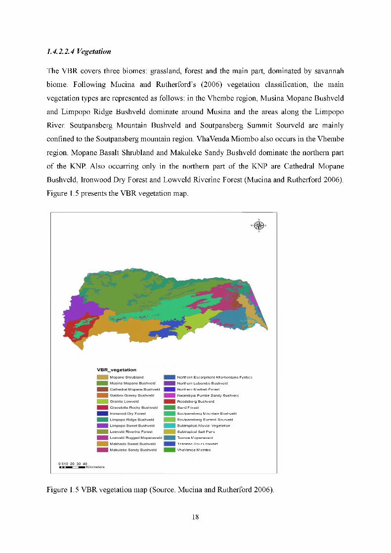
1.4.2.2.4 Vegetation

The VBR covers three biomes: grassland, forest and the main part, dominated by savannah

biome. Following Mucina and Rutherford’s (2006) vegetation classification, the main

vegetation types are represented as follows: in the Vhembe region, Musina Mopane Bushveld

and Limpopo Ridge Bushveld dominate around Musina and the areas along the Limpopo

River. Soutpansberg Mountain Bushveld and Soutpansberg Summit Sourveld are mainly

confined to the Soutpansberg mountain region. VhaVenda Miombo also occurs in the Vhembe

region. Mopane Basalt Shrubland and Makuleke Sandy Bushveld dominate the northern part

of the KNP. Also occurring only in the northern part of the KNP are Cathedral Mopane

Bushveld, Ironwood Dry Forest and Lowveld Riverine Forest (Mucina and Rutherford 2006).

Figure 1.5 presents the VBR vegetation map.

Northern Escarpment Afromontane Fynbos

Northern Lebombo Bushveld

Northern Mistbelt Forest

Nwambyia-Pumbe Sandy Bushveld

Roodeberg Bushveld

Sand Forest

Soutpansberg Mountain Bushveld

Soutpansberg Summit Sourveld

Subtropical Alluvial Vegetation

Subtropical Salt Pans

Tsende Mopaneveld

Tzaneen Sour Lowveld

VhaVenda Miombo

Figure 1.5 VBR vegetation map (Source: Mucina and Rutherford 2006).

18

1.4.2.3 Waterberg Biosphere Reserve

1.4.2.3.1 Biophysical location

The Waterberg Biosphere Reserve (WBR) was the first savannah BR in SA and was

proclaimed in 2001. It is situated in the Waterberg district of Limpopo Province, located

within latitudes 23°10-24°40’S and longitudes 27°30’-28°40’E (WBR 2012). It covers an

area of 654 033 ha and includes Marakele National Park, Mokolo Dam Nature Reserve,

Wonderkop Nature Reserve and Masebe Nature Reserve as core areas (WBR 2012). The

WBR is very significant in the conservation of the important cycads plant species

E n cep h a la r to s eugene m araisii, endemic in Waterberg Mountains, and the Cape vulture (Gyps

coprotheres) colony, one of the largest breeding colonies in the world, situated in the Marakele

National Park (MNPMP 2014). It is drained by four major tributaries of the Limpopo River,

namely the Lephalala, Mokolo, Matlabas and the Mokgalakwena (De Klerk 2003; WBR

2012).

1.4.2.3.2 Climate

The climate is temperate, semi-arid in the south to arid in the extreme north. Rainfall is

seasonal, with most rainfall occurring during the summer months. The winters are very dry

(WBR, 2012). Annual rainfall varies from 500 to 750 mm. The mean annual temperature is

17.6°C (Mucina and Rutherford 2006), with the warmest month having an average of 25°C

and the coldest month's average being 10°C (WBR 2012).


The main geological mass of the Waterberg consists of sedimentary rock, bound by

escarpments on the north, east and south (WBR 2012). Its central portion forms the Palala

Plateau. These sediments are entirely detrital and include sandstones, mudstones, shales,

conglomerates and lenses of grits (WBR 2012). Conglomerates and occasionally breccias

mark the lower levels of the Waterberg series. The formation consists of dominantly quartzite

sandstones, but also conglomerates, flagstones and shale (WBR 2012).

Soils are leached and sandy, mostly of a diastrophic nature. Because of the hilly and

mountainous nature of the terrain, a large portion of the soil is very shallow and rocky (WBR,

2012). The dominant soil forms are Mishap and Glenrosa (in rocky areas) and Clovelly and

Avalon in flat areas, according to MacVicar et al.’s (1977) soil classification system.

19

http://www.theta.org.za/

1.4.2.3.4 Vegetation

The WBR is classified as a savannah biome. The vegetation classification of Mucina and

Rutherford (2006) characterises the WBR by seven different vegetation types. Central Sandy

Bushveld and Waterberg Mountain Bushveld dominate the areas around the Waterberg

Mountains. Western Sandy Bushveld occurs mainly in the low-lying areas. Also occurring

within the WBR are Limpopo Sweet Bushveld, Makhado Sweet Bushveld, Roodeberg

Bushveld and Waterberg-Magalies Summit Sourveld. Figure 1.6 presents the WBR vegetation

map.

Springbokvlakte Thornveld

Subtropical Alluvial Vegetation

Subtropical Freshwater Wetlands

Subtropical Salt Pans

Waterberg Mountain Bushveld

Waterberg-Magaliesberg Summit Sourveld

Western Sandy Bushveld

Figure 1.6 WBR vegetation map (Source: Mucina and Rutherford 2006).

20

1.5 STRUCTURE OF THE THESIS

In addition to this introductory chapter (Chapter 1), and synthesis (Chapter 8), the thesis is

arranged into six chapters (Chapters 2-7), each addressing a key objective as outlined below

(Table 1.1). The six core chapters have been formatted following the requirements of the

target journal for publication, chapter 3 have already been submitted for publication and

chapter 5 have been published.

Table 1.1 Chapters covered by the study.

Chapter Title

1 Conceptual and contextual settings

2 Valuation of ecosystem services in protected areas: a review from SA

3 Land use change scenarios for two biosphere reserves in SA

4 Ecosystem services and their indicators: identification and mapping

5 Habitat condition assessment for ecosystem services

6 Above-ground carbon storage assessment in SA

7 Economic valuation of provision ecosystem services in a biosphere reserve context

8 Synthesis and conclusions

21

1.6 REFERENCES

Andrade, D.C., Romeiro, A.R., Boumans, R., Sobrinho, R.P. and TOsto S.G. 2010. New

methodological perspectives on the valuation of ecosystem services: Toward a

dynamic-integrated valuation approach. International Society for Ecological

Economics Conference: Advancing Sustainability in Time of Crisis, Oldengurg and

Bremen, Germany.

Arnold, E. 2012. Pollution - load zones of allergic tree pollen in Boston (master’s

dissertation).

Bai, Y., Zhuang, C., Ouyang, Z., Zheng, H. and Jiang, B. 2011. Spatial characteristics

between biodiversity and ecosystem services in a human-dominated watershed.

Ecological Complexity, 8:177-183.

Bastian, O. and Schreiber, K. F. (eds). 1999. Analyse und okologische Bewertung der

Landschaft, Heidelberg; Berlin (Spektrum), 2nd edn.

Binning, C., Cork, S., Parry, R. and Shelton, D. 2001. Natural assets: An inventory of

ecosystem goods and services in the Goulburn Broken Catchment. CSIRO Sustainable

Ecosystems, Canberra.

www.ecosvstemservicesproiect.org/html/publications/index.htm

Boyd, J. and Banzhaf, S. 2006. What are ecosystem services? The need for standardized

environmental accounting units. Energy and Natural Resources Division, Resources

for the Future, 1616 P St., NW Washington, DC 20036 202-328-5013, United States.

Brown, T.C., Bergstrom, J.C. and Loomis, J.B. 2007. Defining, valuing, and providing

ecosystem goods and services. Natural Resources Journal, 47(2): 329-376.

Brundtland, G.H. and World Commission on Environment and Development. Our Common

Future: Report of the World Commission on Environment and Development. Oxford

University, 1987.

Burgers, C.J., Fairall, N. and Andrag, R.H. Raamwerk vir ’n holistiese

bewaringstrategie in die fynbosbioom: Die biosfeerreservaatkonsep? (Framework for

a holistic conservation strategy in the Fynbos Biome: The biosphere reserve concept?)

Cape Town: Cape Provincial Administration; 1990 (unpublished document).

Chan, K.M.A. and Ruckelshaus, M. 2010. Characterizing changes in marine

ecosystem services. Biological Reports, 2:4.

Chan, K., Guerry, A., Balvanera, P., Klain, S., Satterfield, T., Basurto, X., Bostrom, A.,

22

http://www.ecosvstemservicesproiect.org/html/publications/index.htm

Chuenpagdee, R. Gould, R., Halpern, B.S., Hannahs, N., Levine, J., Norton, B.,

Ruckelshaus, M., Russell, R., Tam, J. and Woodside, U. 2012. Where are cultural and

social in ecosystem services? A framework for constructive engagement, BioScience,

62(8):744-756.

CBD (Convention on Biological Biodiversity). 1992. United Nations Conference on

Environment and Development: The Rio Earth Summit. Rio de Janeiro, Brazil.

CBD (Convention on Biological Diversity). 2010. Conference of the Parties’ Decision

X/2: Strategic Plan for Biodiversity 2011-2020 and the Aichi Targets. A ten year

framework for action by all countries and stakeholders to save and enhance benefits

for people. The tenth meeting of the Conference of the Parties, Nagoya, Aichi

Prefecture, Japan.

CICES (Common International Classification of Ecosystem Services). 2011. European

Environment Agency paper prepared for discussion at the expert meeting on

ecosystem accounts organised by the UNSD, the EEA and the World Bank, London,

December 2011. Prepared by: Roy Haines-Young and Marion Potschin, Centre for

Environmental Management, University of Nottingham, UK

Costanza, R. 2008. Ecosystem services: Multiple classification systems are needed: Letter to

the editor. Biological Conservation, 141: 350-352.

Costanza, R., d’Arge, R., de Groot, R., Farber, S., Grasso, M., Hannon, B., Limburg, K.,

Naeem, S., O’Neill, R.V., Paruelo, J., Raskin, R.G., Sutton, P. and van den Belt, M.

1997. The value of the world’s ecosystem services and natural capital. Nature, 387:

253-260.

Crossman, N.D., Benjamin, B., Nedkov, S., Willemen, L., Petz, K., Palomo, I., Drakou, E.G.,

Martin-Lopez, B., McPhearson, T., Boyanova, K., Alkemade, R., Egoh, B., Dunbar,

M.B., Maes, J. 2013. A blueprint for mapping and modelling ecosystem services.

Ecosystem Services, 4: 4-14.

Daily, G.C. (Ed). 1997. Nature’s services: Societal dependence on natural ecosystems.

Washington DC: Island Press.

Daily, G., Polasky, S., Goldstein, J., Kareiva, P.M., Mooney, H.A., Pejchar, L., Ricketts,

T.H., Salzman, J. and Shallenberger, R. 2009. Ecosystem services in decision-making:

Time to deliver. Frontiers in Ecology and the Environment, 7(1): 21-28.

de Groot, R.S., Wilson, M.A. and Boumans, R.M.J. 2002. A typology for the classification,

description and valuation of ecosystem functions, goods and services. Ecological

Economics, 41:393-408.

23

de Groot, R.S., Alkemade, R., Braat, L., Hein, L. and Willemen, L. 2010. Challenges in

integrating the concept of ecosystem services and values in landscape planning,

management and decision making. Ecological Complexity, 7(3):260-272.

De Klerk, A. 2003. A land use model for the Waterberg Biosphere Reserve. Master’s degree

dissertation, University of Pretoria

Deng, X.Y., Chen, X.F., Chuvieco, E., Warner, T. and Wilson, J.P. 2007. Multi-scale

linkages between topographic attributes and vegetation indices in a mountainous

landscape. Remote Sensing Environment, 111(1): 122-134.

de Villiers, B. 1999. Peace Parks. The way ahead, Pretoria: HSRC.

Dobbs, C., Escobedo, F. and Zipperer, W. 2011. A framework for developing urban

forest ecosystem services and goods indicators. Landscape Urban

Planning, 99: 196-206.

Dombo, L., Crafford, J., Fouche, P., Gaigher, I., Hahn, N., Linden, J. and Rosmarin, J., 2006.

The Proposed Vhembe Biosphere Reserve Application to UNESCO. Limpopo

Province Department of Economic Development, Environment and Tourism,

Republic of South Africa.

Dunn, R.R. 2010. Global mapping of ecosystem disservices: The unspoken reality that nature

sometimes kills us. Biotropica, 42(5): 555-557.

Egoh, B., Drakou, E.G., Dunbar, M.B., Maes, J. and Willemen, L. 2012. Indicators

for Mapping Ecosystem Services: A Review Publications Office of the European

Union, Luxemburg.

English Nature, 1994. Sustainability in practice, Issue 1, Planning for Environmental

Sustainability, English Nature, Peterborough, UK. In: Mac Donald, D.V., Hanley, N.,

Moffatt, I., 1999. Applying the concept of natural capital criticality to regional

resource management. Ecological Economics 29: 73-87.

Escobedo, F. J., Kroeger, T. and Wagner, J. E. 2011. Urban forests and pollution mitigation:

Analyzing ecosystem services and disservices. Environmental Pollution, 159:2078

2087.

Eppink, F.V., Werntze, A., Mas, S., Popp, A. and Seppelt, R., 2012. Land management and

ecosystem services: how collaborative research programmes can support better

policies. Ecological Perspectives for Science and Society, 21: 55-63.

FAO (Food and Agriculture Organization of the United Nations). 2004. Drought impact

24

mitigation and prevention in the Limpopo River Basin, A situation analysis. Land and

Water Discussion Paper 4. Prepared by the FAO Sub-regional Office for Southern and

East Africa, Harare.

Farber S.C., Costanza R. and Wilson M.A. 2002. Economic and ecological concepts for

valuing ecosystem services. Ecological Economics, 41: 375-392.

Firbank, L.G., Elliott, J., Drake, B., Cao, Y. and Gooday, R. 2013. Evidence of sustainable

intensification among British farms. Agriculture, Ecosystems and Environment, 173:

58-65.

Fisher, B. and Turner, K. 2008. Ecosystem services: Classification for valuation. Biological

Conservation, 141: 1167-1169.

Gomez-Baggethun, E., Martin-Lopez, B., Barton, D., Braat, L., Saarikoski, H.,

Kelemen, M., Garcia-Llorente, E., van den Bergh, J., Arias, P., Berry, P., Potschin, L.

M., Keene, H., Dunford, R., Schroter-Schlaack, C.and P. Harrison. 2014. EU FP7

OpenNESS Project Deliverable 4.1. State-of-the-art Report on Integrated Valuation of

Ecosystem Services. European Commission FP7.

Haines-Young, R.H. and Potschin, M.B. 2009. Methodologies for defining and assessing

ecosystem services. Final Report, JNCC, Project Code C08-0170-0062, 69 pp.

Haines-Young, R.H. and Potschin, M.B. 2010. The links between biodiversity,

ecosystem services and human well-being. - Ecosystem Ecology: A new synthesis.

Heal, G. 2000a. Nature and the marketplace: Capturing the value of ecosystem services.

Washington, DC: Island Press.

Hein, L., van Koppen, K., de Groot, R.S. and van Ierland, E.C. 2006. Spatial scales,

stakeholders and the valuation of ecosystem services. Ecological Economics, 57(2):

209-228.

Helliwell, D.R. 1969. Valuation of wildlife resources. Regional Studies, 3:41-49.

Hermann, A., Schleifer, S. and Wrbka, T. 2011. The concept of ecosystem services regarding

landscape research: A review. Living Reviews in Landscape Research, 5:1-37.

IUCN (International Union for the Conservation of Nature). 2004. Protected areas

categories. ISSN: 0960-211X. Switzerland, Nature Bureau, UK. PARKS, 14:1.

King, R.T. 1966. Wildlife and man. NY Conservationist, 20(6), 8-11.

Krutilla, J.V. 1967. Conservation reconsidered. The American Economic Review, 57(4):777-

786.

Le Maitre, D.C., O’Farrell, P. and Reyers, B. 2007. Ecosystem services in South Africa: A

25

research theme that can engage environmental, economic and social scientists in the

development of sustainability science? South African Journal o f Science, 101.

Lyytimaki, J. and M. Sipila. 2009. Hopping on one leg - the challenge of ecosystem

disservices for urban green management. Urban Forestry & Urban Greening, 8(4):

309-315.

MacVicar, C.N., de Villiers, J.M., Loxton, R.F., Verster, E., Lambrechts, J.J.N.,

Merrywheather, F.R., le Roux, J., van Rooyen, T.H. and Harmse, H.J. von M. 1977.

Soil classification - A binomial system for South Africa, pp 150. Department of

Agricultural Technical Services, Soil and Irrigation Research Institute, Pretoria.

Maler, K. G., Aniyar, S. and Jansson A. 2009. Accounting for ecosystems. Environmental &

Resource Economics, 42(1): 39-51.

Mandle, L. 2014. OPAL: Offset Portfolio Analyzer and Locator version 1.0. A tool for

integrating biodiversity and ecosystem services into impact assessment and offset

portfolio design: User’s guide.

MNPMP (Marakele National Park Management Plan). 2014. Marakele National Park

Management Plan for the period 2014-2024. Prepared by Novellie, P. and Spies A.

Martinez-Harms, M.J. and Balvanera, P. 2015. Methods for mapping ecosystem service

supply: A review. International Journal o f Biodiversity Science, Ecosystem Services

& Management, 8 (1-2): 17-25.

Mertz, O., Ravnborg, H.M., Lovei, G., Nielsen, I. and Konijendijk, C.C. 2007. Ecosystem

services and biodiversity in developing countries. Biodiversity and Conservation,

16(10): 2729-2737.

MA (Millennium Ecosystem Assessment). 2005. Ecosystems and human well-being:

Synthesis, World Resource Institute. Washington, DC: Island Press.

Milcu, A.I., Hanspach, J., Abson, D. and Fisher, J. 2013. Cultural ecosystem services: A

literature review and prospects for future research. Ecology and Society, 18(3): 44.

Mucina, L. and Rutherford, M.C. (eds.) 2006. The vegetation of South Africa, Lesotho and

Swaziland. Strelitzia 19. South African National Botanical Institute, Pretoria.

Nelson, E., Mendoza, G., Regetz, J., Polasky, S., Tallis, H., Richard Cameron, D., Chan

K.M., Daily, G.C., Goldstein, J., Kareiva, P.M., Lonsdorf, E., Naidoo, R., Ricketts,

T.H. and Shaw, M.R. 2009. Modelling multiple ecosystem services, biodiversity

conservation, commodity production, and trade-offs at landscape scales. The

Ecological Society of America: Frontiers in Ecological Environment, 7(1): 4-11.

Norris, K. 2008. Agriculture and biodiversity conservation: Opportunity knocks.

26

Conservation Letters, 1:2-11.

Norton, B.G. 1987. Why preserve natural variety? Princeton, New Jersey: Princeton

University Press.

O’Farrell, P.J., Donaldson J.S., and Hoffman, M.T. 2007. The influence of ecosystem goods

and services on livestock management practices on the Bokkeveld plateau, South

Africa. Agriculture, Ecosystems & Environment, 122(3):312-324.

Pool-Stanvliet, R. 2013. UNESCO's Man and the Biosphere Programme in South

Africa. South African Journal o f Science, 109(9):10.

Power, A.G. 2010. Ecosystem services and agriculture: Tradeoffs and synergies.

Philosophical Transactions o f the Royal Society, 365:2959-2971.

Schackleton, C., Schackleton, S., Gambiza, J., Nel, E., Rowntree, K. and Urquhart, P. 2008.

Links between Ecosystem Services and Poverty Alleviation: Situation analysis for

arid and semi-arid lands in Southern Africa. Ecosystem Services and Poverty

Reduction Research Programme: DFID, NERC, ESRC.

Sherrouse, B.C., Clement, J.M. and Semmens, D.J. 2011. A GIS application for assessing,

mapping, and quantifying the social values of ecosystem services. Applied

Geography, 31:748-760.

Scholte, S.K., van Teeffelen, A.J.A. and Verburg, P.H. 2005. Integrating socio-cultural

perspectives into ecosystem service valuation: A review of concepts and methods.

Ecological Economics, 114: 67-78.

Spash, C. 2008. Deliberative monetary valuation and the evidence for a new value theory.

Land Economics, 83(3): 469-488.

Swetnam, R.D., Fisher, B., Mbilinyi, B.P., Munishi, P.K.T., Willcock, S., Ricketts, T.,

Mwakalila, S., Balmford, A., Burgess, N.D., Marshall, A.R. and Lewis, S.L. 2011.

Mapping socio-economic scenarios of land cover change: A GIS method to enable

ecosystem service modelling. Journal o f Environmental Management, 92: 563-574.

Tallis, H.T., Ricketts, T., Guerry, A.D., Nelson, E., Ennaanay, D., Wolny, S., Olwero, N.,

Vigerstol, K., Pennington, D., Mendoza, G., Aukema, J., Foster, J., Forrest, J.,

Cameron, D., Lonsdorf, E., Kennedy, C., Verutes, G., Kim, C.K., Guannel, G.,

Papenfus, M., Toft, J., Marsik, M. and Bernhardt, J. 2011. InVEST 2.0 beta User’s

Guide. The Natural Capital Project, Stanford.

TEEB (The Economics of Ecosystems & Biodiversity). 2010. Mainstreaming the Economics

of Nature: A synthesis of the approach, conclusions and recommendations of TEEB.

ISBN 978-3-9813410-3-4. Malta: Progress Press.

27

Tilman, D., Cassman, K.G, Matson, P.A., Naylor, R. and Polasky, S. 2002. Agricultural

sustainability and intensive production practices. Nature, 418: 671-677.

UNESCO. 2010. Lessons from Biosphere Reserves in the Asia-Pacific Region, and Way

Forward. A regional review of biosphere reserves in Asia and the Pacific to achieve

sustainable development, UNESCO Office, Jakarta. Regional Science Bureau for Asia

& the Pacific.

Villa, F., Ceroni, M., Bagstad, K., Johnson, G. and Kriviv, S. 2009. ARIES (Artificial

Intelligence for Ecosystem Services): A new tool for ecosystem services assessment,

planning, and valuation. In: Proceedings of the 11th International BioECON

Conference on Economic Instruments to Enhance the Conservation and Sustainable

Use of Biodiversity, Venice, Italy.

von Dohren, P. and Haase, D. 2015. Ecosystem disservices research: A review of the state of

the art with a focus on cities. Ecological Indicators, 52: 490-497.

Vogl, A., Tallis, H., Douglass, J., Sharp, R., Wolny, S., Veiga, F., Benitez, S., Leon, J.,

Game, E., Petry, P., Guimeraes, J. and Lozano, J.S. 2015. Resource Investment

Optimization System Introduction & Theoretical Documentation. Natural Capital.

Project, Stanford University in partnership with The Nature Conservancy and Fauna

& Flora International. http://data.naturalcapitalproiect.org/rios.

Wallace, K.J. 2007. Classification of ecosystem services: Problems and solutions. Biological

Conservation, 139:235-246.

WBR (Waterberg Biosphere Reserve). 2012. Ten Year Periodic Review 2001-2011.

http://www.docstoc.com/myoffice/recommendations?docId=161286419&download.

Wiek A, Ness B., Brand F.S., Schweizer-Ries P., and Farioli F. 2012. From complex

systems analysis to transformational change: A comparative appraisal of sustainability

science projects. Sustainability Science, 7 (Suppl).

Wilson, M.A. and Hoehn, J.P. 2006. Valuing environmental goods and services using benefit

transfer: The state-of-the art and science. Ecological Economics, 60(2):335-342.

Wollenberg, E., D. Edmunds, and L. Buck. 2000. Anticipating change: Scenarios as a tool for

adaptive forest management, a guide. Center for International Forestry Research.

Bogor.

Zhang, W., Ricketts, T.H., Kremen, C., Carney, K. and S. M. Swinton. 2007. Ecosystem

Services and dis-services to agriculture. Ecological Economics, 64:253-260.

28

http://data.naturalcapitalproject.org/rios

http://www.docstoc.com/myoffice/recommendations?docId=161286419&download

1.7 APPENDICES

1.7.1 Appendix 1A: Valuation approaches and techniques used for different ES according to their values (source: adapted from de Groot et al. 2002; MA

2005; Farber et al. 2006; TEEB 2010).

ECOSYSTEM SERVICES TYPES OF VALUES VALUATION APPROACH VALUATION

TECHNIQUE

MA (2005) typology USE VALUES - Utility that people

derive from ecosystems directly or

indirectly, including option value

Major categories of valuation approaches are

divided into economic and non-economic (mainly

ecological and socio-cultural)

Valuation techniques for

different approaches

i.Direct market - market

price-based, factor income,

replacement, avoided,

mitigation and restoration

cost methods

2.Stated preference -

contingent valuation, choice

modelling, group valuation

3.Revealed preference - travel

cost, hedonic pricing

NON-USE - linked to things that people

do not consume or use directly; they are

divided into bequest, altruist and

existence values

Provisioning Direct use values Economic category Valuation techniques symbols

29

Includes all

extractive/consumptive

products that are obtained from

ecosystems.

D irectly used by human beings

(consumptive or non-consum ptive)

Valuation approaches applicable to this category

determine the value o f ES in m onetary terms - they

are divided into direct and indirect m arket

approaches. Indirect m arket approach is divided

into revealed and stated preference valuation

approaches

M P - M arket price

F I - Factor income

A C - Avoided cost

R C - Replacem ent cost

TC - Travel cost

H P - H edonic pricing

PF - Production function

Food - food products derived

from plants, animals and

microbes (i.e. crops, wild foods,

spices, meat)

Direct use Direct market (market price-based) FI

Fibre - wood, cotton, wool, silk Direct use Direct market (market price-based) FI

Fuel- wood, dung and other

sources of energy


Biochemicals - natural

medicines and pharmaceuticals


Ornamental resources - animals

and plant products (skin, shells,

flowers)


Fresh water supply - from

various resources (dams, lakes,

rivers)

Direct use Direct market (cost-based) AC, RC

Grazing material - fodder Direct use Direct market (market price-based) MP

Regulating Indirect use - ES indirectly used by

human beings

Direct market and indirect market (revealed

preference) valuation approaches

Direct market valuation

techniques

30

Option value

Benefits obtained fro m the

regulation o f ecosystem

processes

1. M arketprice-based (FI)

2. Cost-based valuation

techniques - AC, R C

Climate regulation - of

temperature and precipitation

and/or greenhouse emission or

sequestration

Indirect use Direct market (cost-based) AC

Erosion regulation - soil

retention and prevention of

landslides by vegetative cover

Indirect use Direct market (cost-based) AC, RC

Disease regulation - control of

human pathogens (e.g cholera)

and disease vectors (e.g

mosquitoes)

Indirect use Direct market (cost-based, market-price) RC, FI

Water regulation - timing and

magnitude of aquifer recharge,

runoff and flooding

Indirect use Direct market (cost-based, market-price) AC, FI

Water purification and waste

treatment - the filtering out,

detoxification and

decomposition of organic waste

in water bodies through soil

processes

Indirect use Direct market (cost-based) RC

31

Disturbance/natural hazard

regulation-reduction of the

damage caused by hurricanes

and large waves by the presence

of coastal ecosystems such as

mangroves and coral reefs

Indirect use Direct market (cost-based) AC, RC

Cultural services Direct use, non-use, option values Socio-cultural category -focus on non-material

benefits people obtain from this category Indirect market valuation

techniques

N on-m aterial benefits people

obtain fro m the ecosystems.

R evealed preference approach - based on

observation o f individual choices in existing

markets

Sta ted preference approach - use surveys to

simulate m arket and dem and fo r E S

R evealed preference (TC,

HP)

Sta ted preference (CV, CM,

GV)

Recreational - ecotourism,

outdoor sports and recreational

experiences

Direct use - non-consumptive

Revealed preference valuation approaches

TC, HP

Cultural diversity - including

use of nature as motif in books,

films, painting, folklore,

national symbols, architecture,

advertising,

Direct use - non-consumptive Stated preference valuation approach CV

Spiritual and historical - use of

nature for religious or heritage

value or natural merit.

Direct use - non-consumptive Stated preference valuation approach CV

32

http://en.wikipedia.org/wiki/Ecotourism



Educational - use of natural

systems for school excursions

and scientific discovery

Direct use - non-consumptive Direct market MP

Aesthetic information Direct use - non-consumptive Revealed preference valuation approach HP

Supporting services Use values - indirectly Ecological/biophysical category Direct market valuation

techniques

Those services that are

necessary fo r the production o f

all other ecosystem services

Valuation approaches relevant fo r this category

examine the ecological importance o f attributes,

qualities and quantities characterising na ture 's

condition and function ing

1. Cost-based (AC, RC)

2.

Production-based (PF)

Nutrient cycling Indirect use Direct market (cost-based) RC

Pollination Indirect use Direct market (cost-based) RC, AC

Primary production Indirect use Direct market (production function-based) PF

Photosynthesis Indirect use Direct market (production function-based) PF

Soil formation Indirect use Direct market (cost-based) AC

33

http://en.wikipedia.org/wiki/Scientific_discovery



CHAPTER 2

VALUATION OF ECOSYSTEM SERVICES IN PROTECTED AREAS: A REVIEW

FROM SOUTH AFRICA

This chapter intended for submission to the Journal: E co sys tem S erv ices as Ntshane B.C. and

Gambiza J. Valuation of ecosystem services in protected areas: A review from South Africa.

Abstract

Despite the fact that protected areas (PAs) provide a variety of ecosystem services (ES), their

value is often not reflected in decision-making. Challenges exist in advocating the case of

these systems amidst the drive for economic development, where biodiversity conservation is

often compromised in favour of other land uses that are economically robust, such as mining.

The Convention on Biological Diversity, of which approximately 200 countries, including

South Africa (SA), are signatories, requires that natural assets be incorporated into national

accounting. It is against this backdrop that valuation of ES provided by PAs becomes crucial.

We reviewed 25 studies that conducted valuation of ES generated by PAs in SA, with the aim

of understanding the status on valuation and to identify the research gaps in this regard. In

order to achieve the main aim, the study attempted to answer the following questions: (1)

What were the objectives of the study? (2) Which geographic areas were covered? (3) Which

IUCN PAs categories were covered? (4) Which ES were covered? and (5) Which valuation

approach/method was applied? The results of the study indicate that valuation focussed on

6% of around 500 PAs that exist in SA, covering three of the IUCN PA categories across

seven vegetation biomes, mainly to determine the economic value. Of these studies, 76%

focused on cultural ES, 28% on provisioning and 4% on supporting ES, and 4% on regulating

ES. The review highlighted research gaps in terms of geographic area coverage, as well as

supporting and regulating services. This study thus proposes an integrated valuation of all ES

provided by PAs, in order to provide evidence to mobilise support for their existence and to

mainstream them into national accounting.

Key words: ecosystem services, valuation, protected areas, economic value, Convention on

Biological Diversity.

34

2.1 INTRODUCTION

Conservation communities are striving to balance the need for mainstreaming natural assets

for economic development and the conservation of biodiversity (Bajracharya and Dahal 2008;

TEEB 2010; Le Maitre et al. 2007). Until recently, many protected areas (PAs) were mainly

established for biodiversity conservation, with more emphasis on the hands-off approach

(Bajracharya and Dahal 2008; Pullin et al. 2011). However, the establishment of the

Convention on Biological Diversity (CBD 2010) prompted the development of approaches

that promote sustainable utilization of natural resources. These developments shifted

perceptions that PAs represent institutions that promote people's displacement, inaccessibility

and non-utilization of the natural resources (Colchester 2001; McLaughlin 2011) to a more

inclusive triple bottom line approach that reflects social, economic and ecological dimensions

(CBD 2010) to address tangible and intangible benefits for human well-being. Despite the

fact that protected areas (PAs) provide a variety of ecosystem services (ES), their value is

often not reflected in decision-making. Challenges exist in advocating the case of these

systems amidst the drive for economic development, where biodiversity conservation is often

compromised in favour of other land uses. Furthermore, the CBD, of which approximately

200 countries, including South Africa (SA), are signatories, requires that natural assets be

incorporated into national accounting.

2.1.1 What are protected areas?

PAs are the backbone of biodiversity conservation (Stolton et al. 2010; IUCN 2004) and are

defined as “areas of land and/or sea especially dedicated to the protection and maintenance of

biological diversity, and of natural and associated cultural resources, and managed through

legal or other effective means (IUCN 2004). The International Union for the Conservation of

Nature (IUCN) further adopted a six-category PA system (IUCN 2004), which includes strict

nature reserves (IUCN Category Ia), wilderness areas (IUCN Category Ib), national parks

(IUCN Category II), natural monuments or features (IUCN Category III), habitat/species

management areas (IUCN Category IV), protected landscapes/seascapes (IUCN Category V)

and protected areas with sustainable use of natural resources (IUCN Category VI), (IUCN

2004).

Given all the challenges facing natural assets, the IUCN PAs alone are not enough to

conserve biodiversity (NSBA 2004). Other strategies also meant to achieve biodiversity

35

conservation aims are the conservation stewardship programs and biosphere reserves (BRs),

(NSBA 2004; UNESCO 2010). BRs are terrestrial and coastal ecosystems aimed at

reconciling conservation efforts to achieve biological diversity with sustainable utilization

(UNESCO 2010) For the purpose of this analysis, PAs will include all the IUCN categories

and UNESCO's BRs. The importance of PAs is confirmed by the ongoing commitment to

putting land aside for conservation purposes (NPAES 2008; Pullin et al. 2011) emanating

from the CBD's Aichi target 11 (CBD 2010). In SA, PAs, totalling around 500 (DEAT 2003)

represent 6.5% of the terrestrial surface area across 10 major biomes and 0.4% of the marine

areas (NPAES 2008) In line with the CBD's Aichi target, PAs in SA therefore still need to be

expanded to an additional 8.8% of the terrestrial surface area to include most of the

threatened and rare vegetation types, and approximately 40% of the marine area by 2020

(NPAES 2008) to ensure the sustainability of the country's biodiversity and ecological

processes.

2.1.2 Benefits provided by protected areas

PAs provide benefits, called ES, which are important for human well-being (MA 2005;

Stolton et al. 2010). Since their inception, many definitions and methods of classification have

been proposed (de Groot et al. 2002; MA 2005; TEEB 2010). The MA (2005) defines ES as

benefits that people derive from ecosystems, and arrange them into four primary categories:

provisioning, regulation, supporting and cultural categories.

In view of their intact nature, mainly underpinned by their primary function of biodiversity

conservation (IUCN 2004; Stolton et al. 2010), most PAs are capable of providing ES. The

term PA implies that most of the ES produced are protected from several threats, because of

various laws and regulations that govern them (NEMPAA 2003; CBD 2010), thus making

them suitable and sustainable in supplying a variety of ES (Stolton et al. 2010). On top of

their well-known functions of protecting biodiversity and providing ES that contribute to

human well-being (MA 2005), PAs are known for contributing positively to countries’

economies through ecotourism, among others (Bajracharya and Dahal 2008; Stolton et al.

2010).

36

2.1.3 Threats to protected areas

The importance of PAs in protecting biodiversity and providing ES cannot be emphasized

enough, amidst severe degradation caused by among others climate change, alien species

invasion, agricultural activities, habitat destruction and unsustainable resource extraction (MA

2005). Some of these induced pressures could have been exacerbated by the fact that most

PAs historically imposed restrictions on both access and utilization of resources (Pullin et al.

2011) coupled with forced removals to make way for PAs’ establishment (Colchester 2001;

McLaughlin et al. 2011). Since natural resources are the backbone of many countries'

economies (Bajracharya and Dahal 2008; Stolton et al. 2010), growing pressures on resource

utilization will not only have an impact on biodiversity resilience (MA 2005) but will also

reduce PAs' capacity to render social and economic contributions (Bajracharya and Dahal

2008; Stolton et al. 2010).

In SA, some historical pressures related to PAs’ establishment are being addressed through

various stakeholder engagement programs and benefit-sharing arrangements (Pelser et al.

2011), informed by regulations that advocate the inclusion of communities in the

management of PAs and sharing of benefits derived from these PAs (CBD 2010; NEM:PAA,

2003). However, the existence of these regulations is not enough to guarantee the PA system

the attention it deserves; challenges still exist in respect of attempts to advocate the

importance of these systems (Strydom and King 2009; Lopoukhine et al. 2012) for economic

growth (Bajracharya and Dahal 2008; Stolton et al. 2010). Concerns are brewing in areas

where conservation is compromised in favour of economic robust land uses, such as mining

(Turner 2012). Although some of these activities are likely to give the necessary boost to the

economy, mining-related activities are regarded as unsustainable in view of their limited life

span (Tilton 2009) when compared to PAs, which can be sustained indefinitely if threats

could be held at bay. For example, SA's popular Kruger National Park was established in

1902 (SANParks 2010) and is still highly sustainable.

The challenges faced by PAs, on the other hand, could be aggravated by the fact that there is

little evidence of the contribution of PAs to either the country's economy or human well

being (Pullin et al. 2011; Lopoukhine et al. 2012). Evidently, because of lack of information

that reflects the value of ecosystems and the ES they provide (MA 2005; Daily et al. 2009)

natural systems are often ignored during decision-making (Daily et al. 2009) and hence suffer

immense degradation (MA 2005; Daily et al. 2009; TEEB 2010).

37

2.1.4 Why do we need to value ecosystem services provided by protected areas?

It is well known that ES provided by PAs are often difficult to quantify (Stolton et al. 2010)

and many of the generated ES are not involved in market transactions (Daily et al. 2009;

TEEB 2010), thus making it difficult to include them in decision-making (MA 2005; Daily et

al. 2009). In the absence of information and associated evidence to support their contributions

to the national economy (Lopoukhine et al. 2012) natural assets, including PAs, are often

compromised, making way for other land uses that are known to be economically robust

(Strydom and King 2009; TEEB 2010; Turner 2012). Valuation is useful in providing strong

arguments against mining (TEEB 2010).

PAs as strategies meant to conserve biodiversity are managed under the prescripts of the CBD

(CBD 2010). The CBD prescribed 20 deliverables called Aichi targets. All nations are

required to incorporate these targets into their national plans and report progress with their

delivery every two years through CBD's Conference of the Parties meetings (CBD 2010).

The CBD's Aichi targets 1 and 2 require biodiversity to be integrated into development and

planning processes and incorporated into national accounting and decision-making (CBD

2010) to encourage their appreciation, recognize their worth and minimize their destruction

(MA 2005; Daily et al. 2009). Valuation is crucial for illustrating the importance of

biodiversity (Stolton et al. 2010), thus making it possible for PAs to be integrated into

decision-making (Daily et al. 2009; TEEB 2010; Stolton et al. 2010), and can also assist in

justifying PAs' policies (TEEB 2010). Valuation not only affords natural assets an

opportunity to be aligned with the CBD's Aichi targets; it is also an important mechanism

that assists them to reflect their social, ecological and economic value, required for decision

making (MA 2005; Daily et al. 2009). The term valuation is referred to as a process of

expressing value related to a specific action or object, in order to achieve a certain goal

(Farber et al. 2002). Valuation of ES is not a recent phenomenon, but has been conducted for

more than six decades (Hotelling 1949).

2.1.5 Different ways to value ecosystem services provided by protected areas

According to Farber et al. (2002) valuation is the process of expressing a value for a

particular action or object. Many approaches and techniques can be applied to estimate both

use and non-use values (de Groot et al. 2002; Farber et al. 2002; TEEB 2010). These are

divided into economic, non-economic and integrated valuation approaches (de Groot et al.

2002; Farber et al. 2002; Daily et al. 2009; TEEB, 2010). Non-economic valuation

38

approaches include most of the socio-cultural and ecological valuation approaches (de Groot

et al. 2002; Farber et al. 2002; TEEB 2010). Ecological valuation approaches are determined

both by the integrity of the regulation and habitat functions of the ecosystem and by

ecosystem parameters such as complexity, diversity and rarity (de Groot et al. 2002; Farber et

al. 2002; TEEB 2010). Socio-cultural value mainly relates to information functions (de Groot

et al. 2002).

Economic valuation approaches attempt to determine the value of goods and services in

monetary terms (de Groot et al. 2002; Farber et al. 2002; Daily et al. 2009; TEEB 2010) and

are divided into the following valuation approaches: direct market, indirect market,

contingent and group valuation (de Groot et al. 2002; Farber et al. 2002; TEEB 2010).

Direct market approaches are used to determine the values of those ES that can be involved in

market transactions, such as timber and crops (de Groot et al. 2002; Farber et al. 2002; TEEB

2010). Indirect market valuation approaches are used when there are no explicit markets (de

Groot et al. 2002; TEEB 2010). These include the (1) avoided cost, e.g. flood control service

by wetlands (avoids property damage), (2) replacement cost, e.g. replacing natural waste

treatment with human-made systems, (3) factor income, e.g. enhancing water quality to

increase fish cash, thus increasing the income of fishermen, (4) hedonic pricing based on the

demand for an environmental attribute related to the marketed ES (de Groot et al. 2002;

Farber et al. 2002; TEEB 2010), and (5) the travel cost (TC) method, which was originally

proposed in the 1940s (Hotelling 1949) and is mainly used to determine the value associated

with benefits that require traveling, e.g recreation (de Groot et al. 2002; Farber et al. 2002;

TEEB 2010).

Contingent valuation approaches are used to estimate value by eliciting individuals’

preferences/choices by means of a survey/questionnaire, e.g. asking respondents how much

they are willing to pay for the provisioning of an ES (de Groot et al. 2002; Farber et al. 2002;

TEEB 2010). Contingent valuation came on the scene during the 1960s (Knetsch and Davis

1966). The last valuation approach is group valuation, which combines stated preference

techniques with elements of deliberative political and social processes (de Groot et al. 2002;

Farber et al. 2002; TEEB 2010).

The integrated valuation approaches are very recent (Daily et al. 2009; Andrade et al. 2010)

and take into consideration all aspects of ecosystems: social, economic and ecological (Daily

et al. 2009). Among the well-known integrated valuation approaches are: Integrated

39

Valuation of Ecosystem Services and Trade-offs (InVEST), Multiscale Integrated Models of

ES (MIMES) and Global Unified Metamodel of the Biosphere (GUMBO) (Daily et al. 2009;

Andrade et al. 2010) What these approaches have in common is the ability to value multiple

services simultaneously and at different scales, rightfully placing them among crucial tools

that can be used in processes to incorporate natural assets in decision-making (MA 2005;

Daily et al. 2009).

2.1.6 Overview of valuation of ecosystem services in protected areas

Numerous studies have been undertaken in various countries regarding valuation of ES

generated by PAs since a few decades ago (Hadker et al. 1997; Hotelling 1949; Ulph and

Reynolds 1981). In Africa, valuation of ES was introduced more than two decades ago

(Moran 1994; Turpie et al. 2010). In SA, valuation of ES has been recorded since about two

decades ago (Razafindralambo 1998).

Despite progress made in understanding the value of ES provided by PAs (Bajracharya and

Dahal 2008; Stolton et al. 2010), almost no study reports an analysis of the status of valuation

of ES generated by these systems in SA. On the related subject of valuation, only one study

gave an idea of the status of valuation of ES in SA, by reviewing 40 studies that had assessed

values of ES found in different habitats (DEA 2012) while another reviewed 17 studies that

looked at ES generally, not specifically valuation (Le Maitre et al. 2007). Despite the fact that

both reviews included most of the major habitats, fewer than 50 studies that assessed ES were

recorded. Since ES generated by PAs were not given special focus, but formed part of these

general analyses, this highlights a major research gap related to understanding benefits

provided by PAs. Understanding of ES generated by PAs in SA is crucial in mainstreaming

biodiversity and ES into national accounting and as a mechanism for achieving the ministerial

deliverable agreement sub-output 4.4 of Outcome 10: Environment Delivery Agreement

(DEA 2012).

We addressed this research gap by reviewing studies that conducted valuation of ES

generated by SA's PAs and BRs. Our study attempted to answer the following questions: (1)

What were the objectives of valuation? (2) Which geographic areas were covered? (3) Which

IUCN PAs categories were covered? (4) Which ES were covered? (5) Which valuation

approach/method was applied? This review will serve as a basis for valuation of ES in SA.

40

2.2 MATERIALS AND METHODS

We reviewed literature on the valuation of ES in SA. The review covered studies that were

conducted from 1990s until 2014. Data was collected during the years 2012-2014. The review

covered the use of carefully designed search strings (key words); a specific search followed

these key words: valuation of ES in PAs/conservation areas (CAs), valuation of PAs/CAs,

economic valuation of ES; economic valuation of PAs/CAs, ecological valuation of PAs/CAs.

The search strategy included searching of multiple databases, such as Science Direct, Scopus,

Web of Knowledge, Google, Google Scholar and Sabinet.

To avoid publication bias, the review included some grey literature as well. The criteria to

identify differences and similarities of ES in terms of how they were described, classified and

valued were adopted from Haines-Young and Potschin (2009). The scope of the search was

Africa, then Southern Africa and further narrowed down to SA. Because of a vast body of

literature on ES valuation, this study mainly focused on PAs. Search results yielded 46 studies

that conducted valuation of ES in SA, covering different study areas that included marine

environments and some of the major biomes (Cooper and Jayiya 2001; Le Maitre et al. 2009;

De Lange et al. 2011). Results were screened using predetermined inclusion criteria by

screening titles and abstracts and where necessary full text. Of the 46 studies found through

the search, 25 conducted valuation of ES generated by PAs in SA.

The last step followed in this review was the analysis and synthesis of the results. Relevant

studies were arranged according to five aspects: (1) objectives for valuation, (2) geographic

area covered, focused on major biomes, following Mucina and Rutherford’s classification

(Mucina and Rutherford 2006) and whether a PA was situated in a marine or terrestrial area,

(3) PA categories covered, focusing on the IUCN list of PA categories (IUCN 2004), (4) ES

covered, following the MA's classification of ES, (MA 2005) and division of ES into

provisioning (including consumptive and extractive products from plants and animals for

food, fibre, fuel, biochemicals, ornamental resources, and grazing material; regulating

(including climate regulation, disease regulation, water and natural disaster regulations);

cultural (consisting of non-material benefits people obtain from ecosystems, such as

recreational and educational activities, cultural heritage and diversity, as well as spiritual and

historical aspects), as well as the supporting category, which consisted of services that are

necessary for the production of other ES (such as nutrient cycling, primary production,

41

pollination and soil formation), (5) valuation method/approach applied (including different

approaches such as ecological, economic and social (socio-cultural) and different techniques

falling under them) (de Groot et al. 2002; Farber et al. 2002; TEEB 2010), and (6) the type of

source document, e.g peer-reviewed article, discussion document, report, dissertation/thesis.

Although the main focus of the entire study of which this paper forms part was BRs, there

were only six BRs in SA at the time the study was conducted, which were not enough to

provide for a comprehensive valuation analysis. A decision was then taken rather to

undertake an exclusive review of PAs, as they represent the highly protected zonation

component (core areas) within a BR structure and are often compromised when important

land-use decisions are made and more economically robust decisions are favoured (Turner

2012). There is also a perception that for PAs to get the attention they deserve, they have to

undergo a valuation process, in order to reflect their social, ecological and economic values

(Stolton et al. 2010), thus providing the necessary evidence to support land-use decisions

affecting them financially and politically, while generally raising awareness of these systems’

role in conservation of the natural and cultural heritage. This review will thus provide

baseline information for assessing the status of valuation of ES in PAs in SA.

2.3 RESULTS

Of the 46 studies found through the search, 25 conducted valuation of ES generated by PAs in

SA. A summary of the studies is presented in Table 2.1, with more details covered in the

sections below.

2.3.1 Objectives of valuation

The main objective of the 25 studies was the determination of the values of selected ES.

Although 14 of the studies had the word ‘economic’ in their titles/objectives, it was found

that seven of them integrated more than one objective; in total there were 31 objectives. The

main focus of 21 of these objectives was the determination of economic values; of these eight

determined socio-economic values. Five determined the values of selected ES generally

without specifying whether these were economic or otherwise, two determined visitors'

willingness to pay for an ES, two estimated biodiversity values, two assessed costs and

benefits, one determined the non-consumptive value of ES and one assessed whether clearing

42

of alien species would add value to ES. More details regarding studies’ objectives are

presented in Table 2.1.

2.3.2 Geographic area covered

The studies involved seven of the nine major vegetation biomes that occur in SA, namely

savanna, forest, fynbos, Indian Ocean Coastal Belt, grassland; Succulent-Karoo and Nama-

Karoo. The studies were conducted in both the terrestrial and marine environment. The

terrestrial environment involved 13 PAs, Kruger, Namaqua, Karoo, Pilanesberg, Tankwa,

Agulhas (national parks), and the following nature reserves: Hluhluwe-Umfolozi, Umgeni,

Hester Malan Flower Reserve, Goedgap, Anysberg and Oorlogskloof nature reserve), as well

as a transfrontier conservation area (Kgalagadi). In the marine environment, five national

parks (Garden route, Wilderness, West-Coast, Table Mountain, Kogelberg and Tsitsikamma

National Park) were involved.

2.3.3 Protected areas categories covered

Twenty-one of the valuation studies involved 13 PAs of national importance, falling under

IUCN Category II and represented by the following national parks: Kruger, Karoo,

Pilanesberg, Tankwa, Tsitsikamma, Namaqua, Agulhas, Wilderness, Garden Route, Karoo,

West Coast, Table Mountain and a transfrontier conservation area (Kgalagadi). There were 10

PAs of regional importance, represented as follows: eight fell under IUCN Category Ia (strict

nature reserves) represented by DeHoop, Umgeni, Anysberg, Hluhluwe-Umfolozi, Hester

Malan Flower Reserve, Goedgap and Oorlogskloof nature reserve, one fell under IUCN

Category Ib (wilderness areas), represented by Cederberg Wilderness Area, and one was a BR

(Kogelberg).

2.3.4 Ecosystem services covered

In terms of the ES covered, all four categories of ES following the chosen classification were

considered as follows: (1) under provisioning, three studies looked at fish and two focused on

honey, three studies focused on water, two focused on fuelwood, one study looked at timber,

one study was on grazing, and two studies focused on medicinal plants); (2) under regulating

one study focused on both carbon sequestration and restoration; (3) under cultural, the most

popular ES was recreational/tourism with 19 studies, followed by education and existence

values with four studies each, and the last one was aesthetic with one study; and (4) under

43

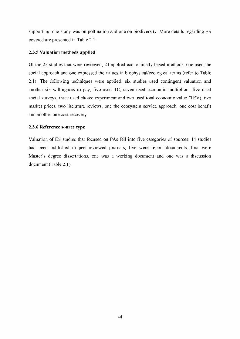
supporting, one study was on pollination and one on biodiversity. More details regarding ES

covered are presented in Table 2.1.

2.3.5 Valuation methods applied

Of the 25 studies that were reviewed, 23 applied economically based methods, one used the

social approach and one expressed the values in biophysical/ecological terms (refer to Table

2.1). The following techniques were applied: six studies used contingent valuation and

another six willingness to pay, five used TC, seven used economic multipliers, five used

social surveys, three used choice experiment and two used total economic value (TEV), two

market prices, two literature reviews, one the ecosystem service approach, one cost benefit

and another one cost recovery.

2.3.6 Reference source type

Valuation of ES studies that focused on PAs fell into five categories of sources: 14 studies

had been published in peer-reviewed journals, five were report documents, four were

Master's degree dissertations, one was a working document and one was a discussion

document (Table 2.1).

44

Table 2.1 Overview of valuation of ES generated from protected areas in SA

Reference Source type Study area Study objective ES involved Valuation method Value estimated

1. Blignaut and

Moolman 2006

Working paper -Kruger National

Park (KNP)

- Savanna biome

-To quantify the potential

of restored natural capital

to alleviate

poverty and conserve

nature

- Recreational

- Timber

- Fuel wood

- Medicinal plants

- Honey

- Willingness to

pay- TEV

Yes

2. Dikgang and

Muchapondwa 2012

Journal article - Kgalagadi

Transfrontier Park

(KTP)

-Savanna biome

-To investigate the

values communities

assign to biodiversity

conservation

in the Kgalagadi area

-Biodiversity -Contingent

-Choice

experiment

-Willingness to

pay

Yes

3. Dikgang and

Muchapondwa 2013

Discussion paper -KTP

- Savanna biome

-To value ES in the KTP -Provisioning

services

(hunting, grazing,

fuel wood, medicinal

plants)

-Choice

experiment

Yes

4. Dikgang and

Muchapondwa 2014

Journal article -KTP

-Savanna biome

-To value selected

attributes of nature-based

tourism, and to assess

their potential to

contribute to Khomani

SAN community

-Recreational -Choice

experiment

method

-Willingness to

pay

Yes

45

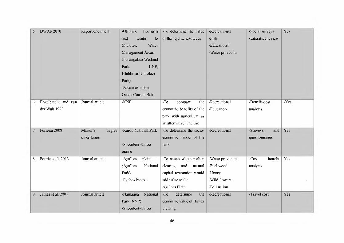
5. DWAF 2010 Report document -Olifants, Inkomati

and Usutu to

Mhlatuze Water

Management Areas

(Ismangaliso Wetland

Park, KNP,

Hluhluwe-Umfolozi

Park)

-Savanna/Indian

Ocean Coastal Belt

-To determine the value

of the aquatic resources

-Recreational

-Fish

-Educational

-Water provision

-Social surveys

-Literature review

Yes

6. Engelbrecht and van

der Walt 1993

Journal article -KNP -To compare the

economic benefits of the

park with agriculture as

an alternative land use

-Recreational

-Education

-Benefit-cost

analysis

-Yes

7. Ferreira 2008 Master's degree

dissertation

-Karoo National Park

-Succulent-Karoo

biome

-To determine the socio

economic impact of the

park

-Recreational -Surveys and

questionnaires

Yes

8. Fourie et al. 2013 Journal article -Agulhas plain -

(Agulhas National

Park)

-Fynbos biome

-To assess whether alien

clearing and natural

capital restoration would

add value to the

Agulhas Plain

-Water provision

-Fuel wood

-Honey

-Wild flowers

-Pollination

-Cost benefit

analysis

Yes

9. James et al. 2007 Journal article -Namaqua National

Park (NNP)

-Succulent-Karoo

-To determine the

economic value of flower

viewing

-Recreational -Travel cost Yes

46

10. Le Maitre et al. 2009 Report document -Succulent-Karoo -To develop a spatially -Water -Social Yes

biome explicit overview of the -Grazing assessment

ecosystem services of the -Recreational -Proportional

-PAs involved: Succulent-Karoo -Natural products weighting

Anysberg, Ecosystem Programme -Restoration approach

Tankwa, Goedgap, domain -Carbon -Ecosystem

Hester Malan Flower -To identify the sequestration service-based

Reserve, relationships between approach

Oorlogskloof, NNP different kinds of -Household

beneficiaries income approach

and the ES they depend -Market price

on. method

11. Motlhake 2006 Master's degree -Pilanesberg National -To determine the socio- -Recreational -Semi-structured Yes

dissertation Park (PNP) economic impact of interviews

nature-based tourism on

-Savanna biome surrounding communities

12. Mouton 2009 Master's degree -Wilderness National -To determine the socio- -Recreational -Economic Yes

dissertation Park (WNP) economic benefits of the multiplier analysis

-Marine park

-To determine the length

-Fynbos and forest of residency as an

biome influential factor in the

social impact of tourism

13. Nikodinoska et al. Journal article -PNP -To determine visitors’ -Recreational -Contingent Yes

2014 willingness to pay to -Willingness to

-Savanna biome control the invasion of O. pay

47

stricta

14. Oberholzer et al. 2010 Journal article -Tsitsikamma

National Park

-Marine

-Fynbos and forest

biome

-To determine

the economic value of

the park

-To assess communities’

perceptions of the park

and how they benefit

from it

-Recreational -Economic

multiplier analysis

Yes

15. Razafindralambo

1998

Master's degree

dissertation

-Umgeni Nature

Reserve

-Grassland/forest

biome

- To determine visitors’

willingness to pay for

environmental change

-To assess the value of

the reserve through

implicit prices of

travelling costs to the site

-Recreational -Travel cost

-Contingent

Yes

16. Saayman and

Saayman 2006

Journal article -KNP

-Savanna biome

-To determine the

economic contribution of

visitor spending


multiplier

Yes

17. Saayman et al. 2009 Journal article -Karoo National Park

-Nama-Karoo biome

-To determine

the socio-economic

impact on the local

economy

-To determine the impact

of tourism business

development in the

-Recreational

-Education

-Existence value

-Input-output

model

-Economic

multiplier

-Sample

matrix inversion

Yes

48

Karoo district,

18. Saayman et al. 2009 Journal article -WNP

-Fynbos/forest biome


economic impact of the

park

-Existence value -Economic

multiplier

Yes

19. Saayman 2014 Journal article -Table Mountain

National Park

(TMNP)

-Fynbos biome

-Marine

-To determine the non

consumptive value of

five marine species


demographic and

behavioral

variables that influence

willingness to pay to see

these species.

-Non-consumptive

value

-Willingness to

pay-Regression

analysis

Yes

20. Sims-Castley et al.

2005

Journal article -Indalo Private

Protected Areas

Association (Eastern

Cape)

-Grassland, Fynbos

Savanna, Thicket

Forest,Nama-Karoo


economic significance of

game reserves


multipliers

-Yes

21. Standish et al. 2004 Report document -TMNP

-Fynbos biome

-Marine

-To assess the economic

impact of the park

-Recreational

-Aesthetic

-Educational

-Contingent

-Willingness to

pay-Travel cost

Yes

22. Turpie and Joubert

2001

Journal article -KNP Rivers

-Savanna biome

-To estimate the

economic impact of

-Recreational -Travel cost

-Contingent

Yes

49

water quality on tourism -Conjoint

23. Turpie 2003 Journal article -West Coast National

Park, De

Hoop Nature Reserve

and the Cederberg

Wilderness

Area)

-Marine

- Fynbos biome

-To estimate biodiversity

existence value

-Existence value -Contingent Yes

24. Turpie et al. 2006 Report document -Garden Route MPAs

-Fynbos, forest

-To estimate the costs

and benefits associated

with the MPAs and how

these costs and benefits

might change under

different scenarios

-Recreational

-Fish

-Opportunity cost

-Option and

existence

-TEV

-Travel cost

-Contingent

Yes

25. Turpie et al. 2009 Report document -Kogelberg Coast BR

-MPAs

-To determine the value

of the Kogelberg Coast

BR

-Recreational

-Fish

-Literature review Yes

50

2.4 DISCUSSION

2.4.1 Objectives for valuation of ecosystem services

The common objective in the 25 studies was determination of the economic value of ES. This

is not surprising, as mainly those ES that are tradable in markets are seen as a reflection of

natural systems’ value to human well-being (MA 2005; Daily et al. 2009). The fact that only

two studies focused on the determination of non-economic values is a major research gap,

since integrating ES successfully into decision-making requires all values to be taken into

account, including those that are not reflected in economic terms (MA 2005; Daily et al.

2009; TEEB 2010).

2.4.2 Geographic area covered

Although most of the major biomes were considered, two biomes, namely Albany thicket and

desert, were omitted, despite the fact that two of the well-known national parks (Addo and

Richtersveld) are situated in these biomes. The omission of desert in valuation was also found

elsewhere (DEA 2012; de Groot et al. 2012). The fact that these biomes received no attention

at all is a serious issue of concern, given their association with some of the ES (DEA 2012;

SANParks 2010). Although biomes such as grassland and forest were included in valuation,

they were not given adequate consideration, since valuation only focused on a small portion

that formed part of other biomes. Fewer studies on grasslands and forests were also a finding

in the study conducted by DEA (2012) and this could be attributed to the fact that only 1% of

both biomes are conserved in national PAs (SANParks 2010). In sharp contrast, forest was

among the most frequently studied biomes (Costanza et al. 2014). Aggravating the grassland

situation is the fact that only 2% is under conservation overall in SA, making it the least

conserved biome (NPAES 2008).

The situation in the forest biome is slightly different; although it currently represents the best

conserved biome in SA at 13%, (NPAES 2008), only 1% is represented in national PAs

(SANParks 2010). Fynbos and savanna biomes, however, received more attention than the

other biomes, followed by the Succulent-Karoo and Nama-Karoo biomes respectively. More

studies on valuation, approximately 40%, were recorded on the savanna biome. This could be

attributed to the fact that this biome is well protected in two of the larger and well-known

national parks in SA (Kruger and the Kgalagadi) (NPAES 2008; SANParks 2010), on which

most of the studies concentrated. A high concentration of valuation studies on the fynbos

51

biome was also a finding elsewhere (Le Maitre et al. 2007; DEA 2012). These findings are

not surprising, since fynbos ranks third in terms of biome representation under conservation

in SA (NPAES 2008; SANParks 2010). Although marine areas also received reasonable

attention, overall more studies conducting valuation of ES were done on the terrestrial

component. This was also found to be the case in the analysis done by DEA (2012), which

covered most of the habitat types in SA. This finding is to be expected, since the

establishment of marine PAs in SA still lags far behind the set targets (NPAES 2008).

2.4.3 Protected areas categories covered

There are approximately 500 PAs in SA, which include private (private nature reserves and

game ranches) and state land (national parks, provincial nature reserves, world heritage sites),

etc. (DEAT 2003), but only 26 (approximately 6%) have been involved in valuation.

Although this is a good attempt, there is a need for more valuation studies to focus on

biodiversity and ES conserved in PAs, to ensure that they are reflected in national accounting

in line with the CBD's objectives and to assist in their integration in decision-making (MA

2005; Daily et al. 2009; CBD, 2010). More focus on national parks was expected, as they are

of national importance. However, the focus of the 21 studies was mainly on 12 of the existing

21 national PAs (SANParks, 2010). It is therefore highly recommended for the remaining

nine PAs to be exposed to valuation studies as well, as valuation for biodiversity could be

used to provide arguments against conflicting land use, such as mining (TEEB 2010).

2.4.4 Ecosystem services covered

Although a number of ES underwent valuation, special preference was shown for use-values,

while little attention was paid to non-use values; this was also a finding elsewhere (Daily et

al. 2009; TEEB 2010). Despite the shortcomings mentioned above, the review revealed that

almost all ES categories (MA 2005) represented in SA's PAs underwent a valuation process.

For cultural ES to have topped the ranking in the valuation studies are good news, since

strong emphasis has only been placed on this category recently (MA 2005). More valuation

studies on recreation and tourism than any other ES under the cultural ES category correlates

with other findings (de Groot et al. 2012; Milcu et al. 2013). Provisioning ES came second,

with at least seven studies undertaking valuation of these ES, involving commodities such as

water, grazing, honey, fuel wood, timber, medicinal plants and fish. This finding is in close

correlation with the results of de Groot et al. (2012), where the provisioning category had the

52

second most studied ES. Although provisioning came second in terms of valuation studies

under review, more studies were expected, as this category encompasses valuable direct,

tangible benefits to people (MA 2005). Fewer valuation studies conducted on water was also

a finding elsewhere (DEA 2012). This, however, was in contrast with the results of de Groot

et al. and Brander et al. (2013), who identified water as the most frequently studied service.

Water is a valuable and scarce resource in SA (DEA 2012), thus more studies on it were

expected, since more solutions and strategies, such as payment for ES (Bajracharya and Dahal

2008), could assist water conservation in SA.

Two studies focused on valuation of supporting services, involving pollination and

biodiversity. Less attention paid to this context is in close correlation with other workers’

findings (DEA 2012; de Groot et al. 2012). This is not entirely surprising, as it reflects the

difficulties associated with capturing the value of these types of services (MA 2005; TEEB

2010), since they are not commonly traded in formal markets (MA 2005; Daily et al. 2009).

The regulating category of ES was studied less; only one study was found through the search.

ES involved in valuation in this category were carbon sequestration and restoration. Other

regulating ES, such as air quality and carbon storage, received no attention. Fewer valuation

studies on regulating services were also found by Costanza et al. (2006) in a study involving

New Jersey's natural capital. However, this category of ES was the second most studied in

another study (de Groot et al. 2012). Despite the recent assignment of economic value to this

type of ES, the occurrence of fewer studies on these ES could be attributed to the fact that

they remain invisible in society's daily accounts (TEEB 2010). Fewer studies on regulating

ES indicate a serious shortcoming, since the issue of carbon storage and sequestration is

prominent in SA, given its association with climate change (MA 2005; DEA 2010). It is also

concerning that PAs are not taking the lead in the valuation of regulating ES, since these are

vital for climate change adaptation to sustain ecological processes (NPAES 2008; Stolton et

al. 2010).

Another value that received some attention was existence value. At least four studies that

were reviewed conducted valuation of the existence value of PAs and/or biodiversity (Turpie

2003; Saayman et al. 2009a; 2009b; Dikgang and Muchapondwa 2012). Attention paid to this

matter indicates that societies are conscious of the value attached to PAs in terms of their

continued existence for the benefit of present and future generations (Bajracharya and Dahal

2008; Stolton et al. 2010).

53

2.4.5 Methods of valuation used

Generally, over-emphasis on the use of the individual TEV methodologies was noticed.

Although TEV methods have the ability to assess some non-use benefits, they concentrate

mainly on the economic values of single services. This kind of assessment was also done

elsewhere (TEEB 2010). Furthermore, economic valuation was found to be the most

commonly used approach elsewhere (de Groot et al. 2012). In view of the need to include ES

in decision-making, including ES provided by PAs, an integrated approach is recommended

as one of the best strategies (Daily et al. 2009) to achieve this need. Although a wide range of

techniques was applied by studies in this review, there is a major shortcoming in the use of

approaches that are incapable of valuing ES holistically, especially in biophysical and socio

cultural terms (Daily et al. 2009; TEEB 2010). The inclusion of both direct use and indirect

use values is crucial in illustrating the relationship between human well-being and ES (TEEB

2010).

2.4.6 Reference source type

Notwithstanding the effort put into the studies under review and regardless of their different

purposes, more work still needs to be done. In terms of the published articles, the 14 studies

reviewed did not cover all the services and the important habitats of PAs in SA, and this is a

serious shortcoming. The number of published articles indicates that ES is still a new concept

and not yet fully developed in SA. Given the importance of incorporating natural assets into

national accounting (CBD 2010), and the challenges associated with land use decision

making for economic growth (Lopoukhine et al. 2012), more studies are needed on the values

provided by PAs to inform land use decision-making.

2.5 CONCLUSIONS

SA has shown progress in attempting to value ES, but more work still needs to be done. Some

of the research gaps highlighted by this study include (1) inadequate geographic coverage,

since two of the major biomes have been omitted, (2) inadequate information on regulating

services, (3) no information on supporting services, (4) overlooking spiritual and amenity

services in the cultural category, and (5) inadequate representation of different goods and

services under the provisioning category. In terms of valuation methods, it has been noted

that despite better representation of various methodologies by the studies, less emphasis was

54

put on the integrated category, which is crucial in realizing the MA's (2005) vision of

integrating ES in decision-making.

Furthermore, the review identified lack of valuable estimates of the overall value of ES

generated in PAs. Until the total value of PAs can be reflected in an integrated way, thus

reflecting their importance and contribution to the country's economy, challenges will

continue to exist in justifying their existence in the current economic growth-orientated

period. The shortcomings highlighted above reflect gaps in alignment with the CBD's Aichi

targets and its sustainable development principles, which are mandatory for all signatory

countries, thus calling for more research to bridge this gap. Since PAs are national assets and

valuation of ES requires considerable investment in time and money, this calls for national

allocation of funds and sponsorships to support valuation of ES in PAs.

55

2.6 REFERENCES

Andrade, D.C., Romeiro, A.R., Boumans, R., Sobrinho, R.P. and TOsto, S.G. 2010. New

methodological perspectives on the valuation of ecosystem services: Toward a

dynamic-integrated valuation approach. International Society for Ecological

Economics Conference: Advancing Sustainability in Time of Crisis, Oldengurg and

Bremen, Germany.

Bajracharya, S.B. and Dahal, N. 2008. Shifting paradigms in protected area management.

NTNC, Kathmandu. ISBN: 978-9917-2-016234-1.

http://www.ntnc.org.np/sites/default/files/publicaations/Book Final Verson.pdf.

Benayas, J.M.R., Newton, A.C., Diaz, A. and Bullock, J.M. 2009. Enhancement of

biodiversity and ecosystem services by ecological restoration: A meta-analysis,

S c ien ce , 325(5944): 1121-1124.

Blignaut, J. and Moolman, C. 2006. Quantifying the potential of restored natural capital to

alleviate poverty and help conserve nature: A case study from South Africa.

Department of Economics Working Paper Series, Working Paper: 2006; 07,

University of Pretoria, South Africa.

Brander, L., Brouwer, R., and Wagtendonk, A. 2013. Economic valuation of regulating

services provided by wetlands in agricultural landscapes: Meta-analysis. E co lo g ic a l

E ng ineering , 56: 89-96.

Colchester, M. 2001. Salvaging nature: Indigenous peoples, protected areas and

biodiversity conservation, World Rainforest Movement and Forest Peoples Programme.

Montevideo, Uruguay and Moreton-in-the-Marsh, UK.

CBD (Convention on Biological Diversity). 2010. Conference of the Parties’ Decision

X/2: Strategic Plan for Biodiversity 2011-2020 and the Aichi Targets. A ten year

framework for action by all countries and stakeholders to save and enhance benefits for

people. The tenth meeting of the Conference of the Parties, Nagoya, Aichi Prefecture,

Japan. https://www.cbd.int/doc/strategic-plan/2011-2020/Aichi-Targets.

Costanza, R., Wilson, M., Troy, A., Voinov, A., Liu, S. and D’Agostino, S. 2006. The Value

of New Jersey’s Ecosystem Services and Natural Capital. Portland State University

PDXScholar, 7-1-2006. Institute for Sustainable Solutions Publications and Presentations

Institute for Sustainable Solutions. http://pdxscholar.library.pdx.edu/iss pub.

Costanza,R., de Groot,R., Sutton, P., van der Ploeg,V., Anderson, S.J., Kubiszewski, I.,

56

http://www.ntnc.org.np/sites/default/files/publicaations/Book_Final_Verson.pdf

https://www.cbd.int/doc/strategic-plan/2011-2020/Aichi-Targets.

http://pdxscholar.library.pdx.edu/iss_pub

Farber, S. and Turner, R.K. 2014. Change In the global value of ecosystem services.

G lo b a l E n v iro n m en t C hange, 26, 152-158.

Cooper, J., Jayiya, T., Van Niekerk, L., De Wit, M., Leaner, J. and Moshe, D. 2001. An

assessment of the economic values of different uses of estuaries in South Africa. CSIR

Report No. ENVS-C 2001-119. CSIR, Stellenbosch, South Africa.


T.H., Salzman, J. and Shallenberger, R. 2009. Ecosystem services in decision-making:

Time to deliver. F ro n tie rs in E c o lo g y a n d the E nviro n m en t, 7(1): 21-28.

Daniel, T.C., Muhar, A., Arnberger, A., Aznar, O., Boyd, J., Chan, K., Costanza, R.,

Elmqvist, T., Flint C., Gobster, P., Gret-Regamey, A. Lave, R., Muhar, S., Penker, M.,

Ribe, R.G., Schauppenlehner, T., Sikor, T., Soloviy, I., Spierenburg, M., Taczanowska,

K., Tam J. and von der Dunk, A. 2012. Contributions of cultural services to the

ecosystem services agenda. P ro cee d in g s o f the N a tio n a l A c a d e m y o f Sciences,

109:8812-8819.

DEA (Department of Environmental Affairs), 2012. State of play: baseline valuation

report on biodiversity and ecosystem services; South Africa.

http://www.teebweb.org/wp-content/uploads/2011/02/STATE-OF-PLAY-SA.

DEAT (Department of Environmental Affairs and Tourism). 2003. Republic of South

Africa's thematic report on protected areas or areas where special measures need to be

taken to conserve biological diversity. https://www.cbd.int/doc/world/za/za-nr-pa-pdf.

de Groot., R.S., Wilson, M.A. and Boumans, R.M.J. 2002. A typology for the classification,

description and valuation of ecosystem functions, goods and services. E co log ica l.

E conom ics, 41:191-408.

de Groot, R., Brander, L., van der Ploeg, S., Costanza, R., Bernard, F., Braat., Christie, M.,

Crossman, N., Ghermandi, A., Hein, L., Hussain, S., Kumar, P., McVittie, A., Portela,

R., Rodriguez, L.C., Brinkm, P. and van Beukering, P. 2012. Global estimates of the

value of ecosystems and their services in monetary units. E co sys tem S ervices, 1: 50-61

De Lange, W.J., Veldtman, R. and Allsopp, M.H. 2011. Valuation of pollinator forage

services provided by Eucalyptus cladocalyx. J o u rn a l o f E n v iro n m en ta l M a n a g em en t,

125C:12-18.

Dikgang, J. and Muchapondwa, E. 2012. The valuation of biodiversity conservation by the

South African Khomani San “bushmen” community. E co lo g ic a l E co n o m ics, 84:7-14.

Dikgang, J. and Muchapondwa, E. 2013. The economic valuation of dryland ecosystem

57

http://www.teebweb.org/wp-content/uploads/2011/02/STATE-OF-PLAY-

https://www.cbd.int/doc/world/za/za-nr-pa-pdf

services in the South African Kgalagadi by the local communities. EfD 13-15,

December 2013, Washington DC, United States of America.

Dikgang, J. and Muchapondwa, E. 2014. The economic valuation of nature-based tourism

in the South African Kgalagadi area and implications for the Khomani San ‘bushmen’

community. J o u rn a l o f E n v iro n m en ta l E co n o m ic s a n d P o licy , 1(1): 106-122.

DWAF (Department of Water Affairs). 2010. The nature, distribution and value of

aquatic ecosystem services of the Olifants, Inkomati and Usutu to Mhlatuze Water

Management Areas. Contract Report by Anchor Environmental Consultants for

Department: Water Affairs pp. 162. http://www.anchorenvironmental.co.za.

Engelbrecht, W.G. and van der Walt, P.T. 1993. Notes on the economic uses of the Kruger

National Park. K oedoe, 16(2):111-119.

Farber, S.C., Costanza, R. and Wilson, M.A. 2002. Economic and ecological concepts for

valuing ecosystem services. Special Issue: The Dynamics and Value of Ecosystem

Services: Integrating Economic and Ecological Perspectives. E c o lo g ic a l E conom ics,

41: 175-192

Ferreira, M. 2008. The socio-economic impact of tourism in the Karoo National Park.

Dissertation submitted in partial fulfilment of the requirements of the degree Master of

Commercii in Tourism at the Potchefstroom Campus of North West University, South

Africa. http://dspace.nwu.ac.za/bitstream/handle/10194/1707/ferreiramadelien?

Fourie, H., Dewit, M.P. and Van der Merwe, A. 2013. The role and value of water in natural

capital restoration on the Agulhas plain. Department of Agriculture and Stellenbosch

University, Western Cape, South Africa.

Hadker, N., Sharma, S., David, A. and Muraleedharan, T.R. 1997. Willingness-to-pay for

Borivli National Protected area: Evidence from contingent valuation. E co lo g ic a l

E co n o m ics, 21:105-122.

Haines-Young, R.H. and Potschin, M.B. 2009. Methodologies for defining and assessing


Hotelling, H. 1949. An economic study of the monetary valuation of recreation in the

national parks, Washington DC: US. Department of the Interior, National Park Service

and Recreational Planning Division.

IUCN (International Union for the Conservation of Nature). 2004. Protected areas

categories. ISSN: 0960-211X. Switzerland, Nature Bureau, UK. PARKS 14:1.

James, I., Hoffman, T., Munro, A. and Smart, R. 2007. The economic value of flower tourism

58

http://www.anchorenvironmental.co.za/

http://dspace.nwu.ac.za/bitstream/handle/10194/1707/ferreiramadelien?

at the Namaqua National Park, South Africa. S o u th A fr ic a n J o u rn a l o f E co n o m ic a n d

M a n a g em en t S c ien ces , 10: 2007 (4).

Knetsch, J.L. and Davis, R.K.1966. Comparisons of method for recreation evaluation. In

A.V. Kneese and S.C. Smith, (eds.), Water Research. Baltimore. R eso u rces f o r the

F uture , 125-142.

Le Maitre, D.C., O’Farrell, P. and Reyers, B.2007. Ecosystem services in South Africa: A

research theme that can engage environmental, economic and social scientists in the

development of sustainability science? S o u th A fr ica n J o u rn a l o f S c ien ce , 101.

Le Maitre, D., O’Farrell, P., Milton, S., Atkinson, D., De Lange, W., Egoh, B.,

Reyers, B., Colvin, C., Maherry, A. and Blignaut, J. 2009. Assessment and evaluation

of ecosystem services in the Succulent Karoo biome. Report prepared for the

Succulent Karoo Ecosystem Programme (SKEP). Council for Scientific and Industrial

Research (CSIR). Coordinated by South African National Biodiversity Institute, with

the support of the Critical Ecosystem Partnership, Programme, for the Succulent

Karoo Ecosystem Programme. South Africa.

Lopoukhine, N., Crawhall, N., Dudley, P., Figgis, C., Karibuhoye, D., Laffoley, J., Londono,

M., MacKinnon, K. and Sandwith, T. 2012. Protected areas: Providing natural

solutions to 21st century challenges », S.A.P.I.EN.S. http://sapiens.revues.org/1254.

McLaughlin, C.M. 2011. People living in protected areas: A comparative study of the

social impacts of conservation in Latin America's MamirAu sustainable development

reserve and Ria Celestun Biosphere Reserve. Paper submitted in partial fulfilment of

the requirements for the Degree of Master of Arts in International Affairs and Natural

Resources and Sustainable Development, American University United Nations.

MA (Millennium Ecosystem Assessment). 2005. Ecosystems and human well

being: Synthesis, World Resource Institute. Island Press, Washington DC.

Milcu, A.I., Hanspach, J., Abson, D. and Fischer, J. 2013. Cultural ecosystem services:

A literature review and prospects for future research. E c o lo g y a n d Society, 18, 3:44.

Moran, D. (1994). Contingent valuation and biodiversity: Measuring the user surplus of

Kenyan protected areas. B io d ive rs ity C o nserva tion , 1(8): 661-684.

Moran, D. 1994. Contingent valuation and biodiversity: Measuring the user surplus of

Kenyan protected areas. B io d ivers ity C onserva tion , 1(8): 661-684.

Motlhake, S.G. 2006. The socio-economic impacts of nature-based tourism: The case

study of Bakgatla ba-ga Kgafela in the Pilanesberg National Park.

http://hdl.handle.net/10519/254.

59

http://sapiens.revues.org/1254

http://hdl.handle.net/10539/254

Mouton, M.E. 2009. Socio-economic impact of an urban park: The case of

Wilderness National Park. Dissertation submitted for the degree Magister Artium in

Tourism at the North West University. Potchefstroom, South Africa.

http://dspace.nwu.ac.za/bitstream/handle/10194/5096/mouton.

Mucina, L. and Rutherford, M.C., (eds). 2006. The vegetation of South Africa, Lesotho and

Swaziland. Strelitzia 19: South African National Botanical Institute, Pretoria, South

Africa. M ila n C h y try F o lia G eobotanica , 41(4): 461-461.

NEMPAA (National Environmental Management: Protected Areas Act). Act no. 57 of 2003:

Biodiversity policy and strategy for South Africa: Strategy on buffer zones for

national parks (2011). For general information (Gazette No. 15020 - Notice 106).

Nikodinoska, N., Foxcroft, L.C., Rouget, M., Paletto, A. and Notaro, S. 2014.

Tourists’ perceptions and willingness to pay for the control of Opuntia stricta invasion

in protected areas: A case study from South Africa, 1-8. K oedoe, 56(1).

Nieto-Romero, M., Oteros-Rozas, E., Gonzalez. J.A. and Martin-Lopez, B. 2014. Exploring

the knowledge landscape of ecosystem services assessments in Mediterranean

agroecosystems: Insights for future research. E n v iro n m en ta l S c ien ce & P olicy , 37:

121-133.

NPAES (National Protected Area Expansion Strategy for South Africa).2008.

Priorities for expanding the protected area network for the ecological sustainability

and climate change adaptation. Government of South Africa. Pretoria.

NSBA (National Spatial Biodiversity Assessment). 2004. Available from the South

African National Biodiversity Institute . http://www.sanbi.org/biodiversity/nsba.

Oberholzer, S., Saayman, M., Saayman, A. and Slabbert, E. 2010. The socio-economic

impact of Africa’s oldest marine park. K oedoe, 52(1): Art. #879.

Pelser, A., Redelinghuys, N. and Velelo, N. 2011. People, Parks and Poverty: Integrated

Conservation and Development Initiatives in the Free State Province of South Africa,

Biological Diversity and Sustainable Resources Use, PhD. Oscar Grillo (Ed.), ISBN:

978-951-107-706-2. http://www.intechopen.com/books/biological-diversity-and-

sustainable-resources-use/people-parks-andpoverty-.

Pullin, A.S., Bangpan, M., Dalrymple, S., Dickson, K., Haddaway, N.R., Healey, J.R.,

Hauari, H., Hockley, N., Jones, J.P.G., Dalling, J.W., Barkan, P., Bellingham, P.J.,

Healey, J.R. and Tanner. 2011. Human well-being impacts of terrestrial protected

areas. Environmental Evidence, 2:19.

Razafindralambo, R. 1998. Economic valuation of protected areas: The Umgeni

60

http://dspace.nwu.ac.za/bitstream/handle/10394/5096/mouton

http://www.mendeley.com/c/6662691141/p/21608981/nikodinoska-2014-tourists-perceptions-and-willingness-to-pay-for-the-control-of-iopuntia-strictai-invasion-in-protected-areas-a-case-study-from-south-africa/

http://www.mendeley.com/c/6662691141/p/21608981/nikodinoska-2014-tourists-perceptions-and-willingness-to-pay-for-the-control-of-iopuntia-strictai-invasion-in-protected-areas-a-case-study-from-south-africa/

http://www.sanbi.org/biodiversity/nsba

http://www.intechopen.com/books/biological-diversity-and-sustainable-resources-use/people-parks-andpoverty-

http://www.intechopen.com/books/biological-diversity-and-sustainable-resources-use/people-parks-andpoverty-

Valley Nature Reserve case study. Master’s degree dissertation, School of

Environment and Development, University of Natal, Pietermaritzburg.

Saayman, M. and Saayman, A. 2006. Estimating the economic contribution of visitor

spending in the Kruger National Park to the regional economy. J o u rn a l o f Susta in a b le

Tourism , 14(1): 67-88.

Saayman, M., Saayman, A. and Ferreira, M. 2009a. The socio-economic impact of the

Karoo National Park. K oedoe, 51(1): Art. #158.

Saayman, M., Van der Merwe, P., Saayman, A. and Mouton, M.E. 2009b. The socio

economic impact of an urban park: The case of Wilderness National Park. J o u rn a l o f

P o licy R esea rch in Tourism , L e isu re a n d E ven ts. 1£1): 247-264.

Saayman, M. 2014. The non-consumptive value of selected marine species at Table

Mountain National Park: An exploratory study, tourism research in economic environs

and society, North-West University. S o u th A fr ica n J o u rn a l o f E co n o m ic a n d

M a n a g em en t Sciences, 17(2): 184-191.

SANParks (South African National Parks). 2010. Biodiversity, Science and

SANParks: Biodiversity conservation in times of change. SANParks Scientific

Services, Lorreta Steyn Graphic Design Studio. Republic of South Africa.

Sims-Castley, R., Kerley, G.I.H., Geach, B. and Langholz, J. 2005. Socio-economic

significance of ecotourism-based private game reserves in South Africa’s Eastern

Cape Province. P A R K S , 15:6-18.

Standish, B., Boting, A., Van Zyl, H., Leiman, T. and Turpie, J. 2004. The economic

contribution of Table Mountain National Park. South African National Parks. The

Graduate School of Business, University of Cape Town, South Africa.

http://www.sanparks.org/docs/parks table mountain.

Stolton, S., Mansourian, S. and Dundley, N. 2010. Valuing protected areas. World Bank's

Global Environment Facility Coordination Team, World Bank GEF Operations.

Strydom, H.A. and King, N.D. 2009. Environmental management in South Africa:

Challenges to justify the existence of protected areas. Second Edition, Juta Law.

TEEB (The Economics of Ecosystems & Biodiversity). 2010. The Economics of

Ecosystems and Biodiversity Ecological and Economic Foundations. Edited by

Pushpam Kumar. Earthscan, London and Washington.

Tilton, J.E. 2009. Is mineral depletion a threat to sustainable mining? Paper

presented at the International Conference on Sustainable Mining: Santiago de

Compostela, Spain, Version 90509.

61

http://www.tandfonline.com/loi/rprt20?open=1%23vol_1

http://www.sanparks.org/docs/parks_table_mountain

Turner, S.D, 2012. World heritage sites and the extractive industries.

http://www.icmm.com.document/1787.

Turpie, J. and Joubert, A. 2001. Estimating potential impacts of a change in river quality

on the tourism value of Kruger National Park: An application of travel cost,

contingent, and conjoint valuation methods. W aterSA, 27(1):187-198.

Turpie, J. 2003. The existence value of biodiversity in South Africa: How interest,

experience, knowledge, income and perceived level of threat influence local

willingness to pay. E c o lo g ic a l E conom ics, 46:199-216.

Turpie, J., Clark, B. and Hutchings, K. 2006. The economic value of marine protected

areas along the Garden Route coast, South Africa, and implications of changes in size

and management. A report prepared for WWF - SA by Anchor Environmental

Consultants & Percy FitzPatrick Institute, University of Cape Town, South Africa.

Turpie, J.K., Clark, B.M., Hutchings, K., Orr, K.K. and de Wet, J. 2009. Ecology, Value and

Management of the Kogelberg Coast Prepared for: WWF-CAPE Marine Programme.

Anchor Environmental Consultants. http://www.anchorenvironmental.co.za.

Turpie, J., Barnes, J., Lange, G. and Martin, R. 2010. Economic values of Namibia

Protected Area System. A case study for increased investment. A study commissioned

by Ministry of Environmental and Tourism: Directorate of Parks and wildlife

Management, Republic of Namibia.

Ulph, A. and Reynolds, I. 1981. An Economic Evaluation of National Parks. Center for

Resource and Environmental Studies, Australian National University, Canberra.

UNESCO (United Nations Educational, Scientific and Cultural Organization). 2010.

Lessons from biosphere reserves in the Asia-Pacific region, and way forward. A

regional review of biosphere reserves in Asia and the Pacific to achieve sustainable

development, UNESCO Office, Jakarta. Regional Science Bureau for Asia and the

Pacific.

62

http://www.icmm.com.document/3787

http://www.anchorenvironmental.co.za

CHAPTER 3

LAND USE CHANGE SCENARIOS FOR TWO BIOSPHERE RESERVES IN SOUTHAFRICA

This chapter has been intended for submission to the journal of N a tu re C o n serva tio n as:

Ntshane, B.C. and J. Gambiza.

ABSTRACT

Conflicting visions on conservation and development goals are a common challenge facing

land use planners in and around protected areas. The biosphere reserve concept is designed to

include local stakeholders’ interests in decision-making to achieve sustainable development

goals. This study applied a participatory scenario planning process in Vhembe Biosphere

Reserve (VBR) and Waterberg Biosphere Reserve (WBR) in South Africa, to assess the

effects of changes in land use on biodiversity conservation and ecosystem services (ES). We

looked at three different development scenarios, namely ecological, social and economic.

Drivers of land use change were diverse and affected biodiversity and ES in a number of

ways. There were always trade-offs in the choice of land use. Under the ecological

development scenario, land use change impacted on biodiversity and ES positively as a result

of the expansion of conservation areas (CAs) by 40% in WBR and 30% in VBR whereas

agricultural ES decreased by 2% in WBR and <1% in VBR. Under the economic

development scenario at least 20% of the land could be lost to mining in both biosphere

reserves leading to loss of biodiversity and ES. In the social development scenario,

biodiversity and ES in 20% of the conservation area and 3% of agricultural land could be

affected negatively in WBR as a consequence of the land restitution program. In sharp

contrast, negative impacts to biodiversity and ES in 25% of the CAs and ES in 30% of

agricultural land could result from the land restitution program in VBR. Yields of ES in the

ecological development scenario were likely to be much higher than in both the social and

economic development scenarios. The main driving force in all three scenarios was economic

growth.

Key words: biosphere reserve; ecosystem services; land reform; land use; protected area;

scenario planning; sustainable development.

63

3.1 INTRODUCTION

Biodiversity loss is a major ecological crisis globally and has accelerated massively in

response to human actions (Rockstrom et al. 2009). The causes of biodiversity loss include

transformation of land use to agriculture and invasion of alien vegetation leading to habitat

loss and degradation (Hooke et al. 2012; Dar et al. 2015). Habitat loss is regarded as the

greatest threat to biodiversity and may lead to species extinction (MA 2005). Habitat

degradation causes a decline in ES (MA 2005). ES are benefits that people derive from

ecosystems. The Millenium Ecosystem Assessment (MA), (2005) organizes ES into four

categories: provisioning (e.g., food, water, raw materials, medicinal plants), regulating

(climate regulating, natural disaster regulating, disease regulating), cultural (recreation,

spiritual value, cultural heritage, aesthetic quality) and supporting (primary production, soil

formation). Besides the MA's (2005) ES typology, a number of ES classification systems has

been developed and the research on ES is ongoing (Haines-Young and Potschin 2013; TEEB

2010).

Establishment of conservation areas (CAs) is one of the strategies for combating the loss of

biodiversity and ES. To achieve this, the International Union for the Conservation of Nature

(IUCN) established a system of protected areas (PAs) (Dudley 2008). In view of the

magnitude of biodiversity loss and the rate at which it is progressing, PAs alone are

inadequate for the conservation of biodiversity (Kuntonen van't Riet 2007). Some of the

factors that hamper PAs’ effectiveness are conflicting economic development and

conservation visions that result in degradation of land and the rapid transformation of land

use around PAs (Naughton-Treves et al. 2005; Palomo et al. 2011). There is therefore a need

to look at complementary strategies such as biosphere reserves (BRs) for conserving

biodiversity.

BRs are social-ecological systems established to reconcile conservation, economic and social

development goals while improving the relationship between man and the environment

(UNESCO 2010). The concept of BRs was formally established in UNESCO’s Man and

Biosphere program (MAB) in 1973. Each BR consists of three zones, namely the core, buffer

and transition zones. The core consists of protected sites to conserve biological diversity,

represented mainly by formally registered PAs. The buffer zone surrounds the core area and

is used for activities compatible with sound ecological practices. Finally, the transition zone

64

contains a variety of developmental activities, which includes agriculture, settlements and

other uses (UNESCO 2010).

Despite their potential benefits, BRs are facing major challenges. There is a discrepancy

between the goals of a BR and the legislation on conservation and sustainable development

which hampers the successful implementation of the BR concept (UNESCO 2010). Although

the MAB program sought to reconcile conservation with development, with the aim of

achieving sustainable development, the achievement of this aim is often crippled by the

perception that humans are harmful to the environment (Bosak 2008). This kind of

incoherence often leads to top down approaches which ignore local knowledge (Bosak 2008).

Harmonization of the relationship between humans and nature may help to promote the BR's

aim of sustainable development. However, striking a balance to achieve development and

conservation land use goals in socio-ecological systems has proven to be a challenge (Palomo

et al. 2011) and it is uncertain how changes in land use will affect biodiversity conservation

and the provisioning of ES. Scenario planning has been applied to address some of these

challenges (Palomo et al. 2011; Schwenker and Wulf 2013).

Scenario planning was developed during the twentieth century (Borjeson et al. 2006; Kishita

et al. 2016). Scenarios are used to describe a plausible or anticipated future state or trajectory

(Rawluk and Godber 211; Schwenker and Wulf 2013; Beach and Clark 2015; Kishita et al.

2016). Scenarios are multi-purpose and powerful approaches for decision-making (Borjeson

et al. 2006; Beach and Clark 2015). They are used to address complexity and uncertainty

(Priess and Hauck 2014) and to analyse drivers of change (Wollenberg et al. 2000). They can

be used to facilitate stakeholders’ understanding, communication and networking of ideas

regarding different issues and to provide guidance in the policy arena (Wulf et al. 2010;

Oteros-Rozas et al. 2015).

There are many methods and approaches to scenario planning (Wollenberg et al. 2000; Priess

and Hauck 2014; Kishita et al. 2016). Scenarios may be grouped according to purpose or

methodological approach (Dettinger et al. 2012; Oteros-Rozas et al. 2015). Scenario planning

methods could be expert-led, exploratory, anticipatory or participatory and involve different

forms of stakeholders' inputs (Rawluk and Godber 2011; Palomo et al. 2011; Dettinger et al.

2012; Oteros-Rozas et al. 2015; Kishita et al. 2016). Scenario analysis may also be qualitative

or quantitative.

65

http://link.springer.com/search?facet-creator=%22Burkhard+Schwenker%22

http://link.springer.com/search?facet-creator=%22Burkhard+Schwenker%22

Scenario planning has been applied widely in social-ecological systems for land use planning

and to explore potential future developments and the impacts of climate and land use changes

on biodiversity and ES (Palomo et al. 2011; Beach and Clark 2015; Carpenter et al. 2015,

Catano et al. 2015; Oteros-Rozas et al. 2015). Scenarios are applicable at different

geographical scales, and have been very useful for global initiatives such as the millennium

ecosystem assessment and the intergovernmental platform on biodiversity and ES. Our study

applied a participatory planning approach as described in Wollenberg et al. (2000) to develop

three future scenarios. Our objective was to evaluate the effects of land use changes in

response to different drivers of change and management strategies on biodiversity

conservation and ES.


3.2.1 STUDY AREAS

Waterberg Biosphere Reserve (WBR) is the first savannah BR in SA and was proclaimed in

2001. It is situated in the Waterberg district of Limpopo Province. It covers an area of 654

033 ha and includes a national park and six declared nature reserves (WBR 2012). The extent

of the core zone is 121 249 ha, consisting of government-owned land. The buffer zone

consists of 146 157 ha of privately owned land. Agricultural land use has changed over the

last 30 years from crop and cattle farming to game farming (De Klerk 2003; WBR 2012).

Mining occurs within the WBR, but on a small scale, mainly on the periphery of the transition

zone of the BR (De Klerk 2003; WBR 2012).

Vhembe Biosphere Reserve (VBR) became SA’s sixth BR in June 2009. It includes two

national parks, several nature reserves, the Soutpansberg and Blouberg biodiversity hotspots,

as well as the Makgabeng Plateau (Dombo et al. 20006). It covers an area of 3 070 000 ha,

including its 460 000 ha core area, a 357 500 ha buffer zone and a 225 260 ha transition zone.

Current land uses include crop and cattle farming (Dombo et al. 2006). Game farming and the

hunting industry have expanded rapidly over the past two decades (Dombo et al. 2006).

Mining also takes place at several sites around the VBR area (Dombo et al. 2006). Fig. 3.1

shows the location of the study areas.

66

Limpopo Province

Vhembe

MopaniCapricorn

Waterberg

WBR Greater Sekhukhune

SOUTH AFRICA

LIMPOPO PROVINCE

Land use/cover Zonation sizes (ha)Degraded areas WBRCultivated areas Core zone 121 249Forest plantationsBuffer zone 146 157

Transition zone 386 627MinesVBRNatural vegetationCore zone 460 000Urban areasBuffer zone 357 500WetlandsTransition zone 225 260120

Kilometers

Figure 3.1 Map of Limpopo Province of South Africa, showing the five district municipalities (Waterberg, Vhembe, Greater Sekhukhune, Capricorn and Mopani) and the location of the Waterberg Biosphere Reserve (WBR) and Vhembe Biosphere Reserve (VBR) study areas, as well as sizes of each biosphere's three zones (core, buffer and transition).

67

3.2.2 SCENARIO PLANNING PROCESS

This study applied a four-stage scenario-based approach as described in Wollenberg et al.

(2000). The four stages applied for scenario analysis were: (1) definition of the purpose of the

scenarios; (2) information about a system’s structure and major drivers of change; (3)

generation of the scenarios and (4) implications of the scenarios.

3.2.2.1 Definition of the purpose of the scenarios

The purpose of the scenarios was to identify and assess land use decision options and their

assumed impacts on biodiversity and ES in response to different drivers of change and

uncertainties which include among others government policies, climate change and economic

development needs in line with the BRs’ visions.

3.2.2.2 The system’s structure and major drivers of change

Both BRs had established stakeholders’ engagement platforms through park forums and BRs

stakeholders meetings. We decided to refer to both platforms as issues that were often

discussed on both sides were similar especially those regarding land use. The BRs’

stakeholders’ lists were compiled from landowners’ registers, nature conservancies as well as

the membership of national park forums (NPF) falling within the borders of the BRs and kept

by the secretariat in the BR committee. The VBR had over 100 registered stakeholders and

the WBR had 80 stakeholders. The percentages of representation were calculated based on 80

stakeholders for the WBR and 100 stakeholders for the VBR. The first stakeholder

engagement process considered for the purpose of this analysis was held in 2010 in WBR and

2011 in VBR. During these meetings, stakeholders raised and deliberated different land use

issues, drivers of change as well future plans in line with the desired BRs’ visions. Fourteen

stakeholders attended the meeting held in 2010 and 10 attended the meeting held in 2011.

The second process involved face-to-face interviews of stakeholders. Sixteen stakeholders

were interviewed. Of the stakeholders who were interviewed, 10 were from the WBR,

representing 13% of the BR's stakeholders and six stakeholders, representing 6% were from

the VBR’s stakeholders (Table 1). Face-to-face interviews were followed by a questionnaire

survey sent by email to key stakeholders. Eight stakeholders responded to the questionnaires.

68

Of these respondents, five were from the WBR (representing 6% of the stakeholders) and

three stakeholders (representing 3%) were from the VBR. A follow-up telephonic interview

was conducted, in an attempt to reach stakeholders who had not responded to the

questionnaires nor taken part in the one-on-one interviews. Seventeen of them responded.

Nine (11,25% of stakeholders) represented the WBR and eight (representing 8% of

stakeholders) were from the VBR. In the end a total of 47 stakeholders participated in the

interviews and surveys in both BRs (Table 3.1).

Table 3.1 Main stakeholders who participated in the study

Stakeholder group Meeting

participation

Face-to face

interview

Questionnaire

survey

Telephonic

interview

VBR WBR VBR WBR VBR WBR VBR WBR

National park forums 2 4 2 1 2

Department of Environmental Affairs 1 1 4

Nature conservancies 2 1 1 1 1 3

Agricultural Union 1 2

Biosphere reserve private landowners 5 8 4 1 1 2 4

Local municipalities 3 2 2

Independent ecologists 1 1 2

Biosphere reserves 2 1 1

National parks 2 6 1 2 1 1

Mining companies x3 (focus area: iron ore in 1 2

WBR and coal in VBR)

Total 10 28 6 10 3 5 14 9

69

Data collected through all stakeholders’ engagement processes were organized into drivers of

change and uncertainties as in Rawluk and Godber (2011). For the purpose of this analysis,

uncertainties included land use and policy environment as it was not certain how they will

develop in future in response to different drivers of change. Stakeholders identified 12 drivers

of change and six different kinds of land uses. Government policies that were identified as

having a potential of contributing to land use tenure include the National Protected Areas

Strategy, land reform program and economic development policies. Stakeholders were not

familiar with the concept of ES, unpacking of this concept enhanced their understanding. At

the end, four provisioning services, three regulating services and one cultural service were

identified. We also requested stakeholders’ inputs on trends on land use (Table 3.2).

Table 3.2 Stakeholders’ views on trends in land use changes and their associated drivers.

Both land use changes and drivers are listed in decreasing order of importance.

Past Current Future Drivers of change

Cattle farming Conservation Conservation Economic growth

Crop farming Game farming Ecotourism Government policies

Game farming Crop farming Game farming Climate change

Conservation Cattle farming Crop farming Institutional arrangements

Tourism Tourism Mining Technology

Mining Mining Cattle farming Population growth

Information received from stakeholders regarding ES are presented on Table 3.3.

Past trends were back casted for a period of 30 years from 2010. The current period was taken

as 2009-2010.

70

Table 3.3 Stakeholders’ views on trends in the supply of ecosystem services and their major

drivers. For a given ecosystem services, drivers are listed in decreasing order of importance.

Ecosystem service Past Current Future Driver of change

Agricultural crops (food provisioning)

Dominant Decreased Decreased Climate change Land restitution Institutional arrangement

Ecotourism (cultural services)

Not popular Increased Dominant Economic growth Climate change Land use change

Wild plant products Abundant Decreased Decreased Land use change Unsustainable utilization Population growth Climate change

Livestock products Abundant Decreased Declined Land use change Climate change

Water provisioning Abundant Scarce Scarce Population growth Climate change PollutionUnsustainable utilization

Air regulation Well- functioning Reduced Declined Industrialization (pollution) Climate change Deforestation

Regulation by wetlands Well-functioning Reduced Declined Agriculture Urbanization Climate change Industrialization

Regulation by forests Well-functioning Reduced Declined Agriculture Urbanization Climate change Industrialization Economic development

3.2.2.3 Generation of the scenarios

According to Wollenberg et al. (2000), scenarios can be based on the comparison of desirable

and undesirable situations. Uncertainty data were further coded into three contrasting themes

of a BRs sustainable development, namely ecological, economic and social. Based on these

themes, we generated three scenarios: ecological development, economic development and

social development within a time frame of 30 years from 2010 (Fig. 3.2).

71

The ecological development scenario was driven by the SA government's Protected Areas

Expansion Strategy (NPAES) of 2008, and focused mainly on conservation area expansion.

This strategy aimed at addressing the shortfall to conserve biodiversity and ecological

processes effectively through the current PAs (NPAES 2008). The NPAES (2008) seeks to

increase PAs by 8.8% (10.8 million ha), adding to the current conserved areas of 7.9 millon

ha to reach the targeted 12% by 2030. The expansion target set for Limpopo Province is

5.5%, representing 687 000 ha, to be achieved in 2030.

The economic development scenario involved mainly mining developments, driven by

economic needs. This scenario was mainly driven by government's job creation and

economic growth objectives. South Africa’s Economic Policy and Growth Strategy (Manuel

2007), recognized mining as one of the sectors with potential to boost the economy. The

Minerals and Mining Policy White Paper for South Africa (1998) also identified mineral

beneficiation as one of the priority growth nodes for job creation to achieve a target of 5

million jobs by 2020.

The social development scenario was mainly driven by the SA Government's land reform

program. This program is embedded in the SA's Land Affairs White Paper of 1997's land

policy aiming at redistributing at least 30% of agricultural land to poor and previously

disadvantaged people by 2014. The program consists of three sub-programs: (1) land tenure,

strengthens the security of tenure of farm dwellers living on commercial farms, (2) land

redistribution, which focuses on giving previously disadvantaged people the opportunity to

own land through settlement and acquisition grants and (3) land restitution, which aims to

return land or compensate victims unfairly dispossessed of their land after SA’s 1913 Land

Act.

3.2.2.4 Implications of the scenarios and use by decision-makers

The final step outlined by Wollenberg et al. (2000) involves analyzing the implications of the

scenarios to decision-making. In WBR, the generated preliminary scenarios were presented

orally and in maps in a meeting held in 2012, attended by 14 stakeholders (Table 3.1). Maps

were produced using GIS ArcMap program (ESRI 2013). Lack of opportunity to hold a

meeting in VBR led to telephonic discussion of the scenarios in 2013 with six stakeholders

(Table 3.1). Based on the information that was received from both BRs, generally, the

72

economic development scenario was influencing land owners to enter into stewardship

programme as a way to counteract on mining. Tourism opportunities presented by the

ecological development scenario motivated decision making into partnership with large CAs

for various tourism activities in both BRs. The social development scenario was crucial in

assisting stakeholders to rethink their approaches to land restitution and find ways to make it

work in both BRs.

•Presentation of final scenarios to stakeholders (Oral and maps)

•Stakeholders engagement (meetings and interviews: face to face, telephonic, emails)

r \j

•Uncertainity data coding (ecological, social and economic themes)

Step 4: Implication of scenarios to

decision makers

Step 1: Defining the purpose of the

Step 3: Generation of scenarios

Step 2: Information about system's

structure and drivers of change

•Scenarios: Social development, economic development and ecological develoment

Stakeholders data (drivers of change and uncertainity themes)

Figure. 3.2 Scenario planning development framework outlining activities undertaken in each stage of the scenario development process.

73

3.3 RESULTS

3.3.1 Ecological development scenario

The outcome of this scenario showed that 90% of the 38 stakeholders who were interviewed

indicated that CAs have the potential to expand in future, because of the current shift of land

use in favor of ecotourism, with 10% seeing it as a solution to prevent mining development,

since it is prohibited within PAs, according to the National Environmental Management Act

(NEM:PAA 2003). For this reason, most of the private landowners practicing conservation

are in the process of entering a stewardship program or contractual agreements as a way of

saving their lands from the mining invasion, thus increasing the core area’s size.

As a result of the planned CAs expansion, the core zone of the WBR will grow by 40% from

its current size of 104 179 ha. Contributing to the growth is the inclusion of the CAs currently

in the buffer zone, which are in the process of acquiring PA status. The core, Marakele

National Park (MRNP), will contribute to this growth by 100 000 ha following its expansion

strategy. In VBR, the expansion plan includes the integration of 33 000 ha of fragmented land

of Mapungubwe National Park, the inclusion of a private nature reserve of 36 000 ha and the

privately owned land centrally located in the core area, as well as the biodiversity hotspot of

the Soutpansberg Mountains (Fig. 3.3). The planned expansion will add over 150 000 ha

(30%) to the existing core area, thus contributing positively to the conservation of

biodiversity and ES. In WBR, approximately 2 000 ha (2%) of agricultural land could be lost

due to conservation area expansion, while in VBR, less than 500 ha (<1%) of agricultural area

could be lost as a result of this development. Fig. 3.3 also presents the state of agriculture and

CAs under the ecological development scenario.

74

Figure 3.3 An illustration of the ecological development scenario, showing interactions between conservation (current and future conservation area extension) and agriculture (current) in the VBR and WBR study areas.

3.3.2 Economic development scenario

According to 80% of the 38 stakeholders interviewed, mining development is seen as the

potential future land use after conservation. This conclusion took into consideration the

recorded mining prospecting rights granted by the relevant authority in the study areas. In

VBR, the core, buffer and transition zones are expected to be affected by coal mining; over

600 000 ha (20%) could be lost in this regard. In WBR, the core area (MRNP) and

surrounding areas are under threat of mining development, amounting to 25 528 ha, of which

11 784 ha will be inside the park. Reduction in core areas might impact negatively on the

conservation of biodiversity and ES. Meanwhile, more prospecting applications affecting

more than 40 properties, over 100 000 ha, were received in this BR during 2010 to 2012,

75

bringing the total area under threat of mining developments to about 140 000 ha (20%). Fig.

3.4 shows changes in land use under the economic development scenario.

Waterberg biosphere reserve (W B R )

Figure 3.4 An illustration of the economic development scenario, showing interactions

between proposed mining developments, conservation (current and future conservation area

extension) and agriculture (current) in the VBR and WBR study areas.

3.3.3 Social development scenario

The outcome of this scenario indicated that 20% of the 38 stakeholders interviewed identified

land restitution as the major driver of land use change in future, compared to the other two

processes of land reform. At least 60% of the stakeholders identified it as a threat to

agricultural ES and 30% saw it as an economic driver through ecotourism, while 10% saw it

76

as threatening biodiversity conservation. In WBR, claims for at least 102 168 ha of land under

restitution have been gazetted and claims for 39 625 ha are expected to be gazetted in future

and settled within the next 30 years. This will bring about an increase from the current settled

claims of approximately 17 544 ha, from the five major claims lodged with the land claims

commissioner. The total loss of CAs (core and buffer) to land claims in this context is at least

45 146 ha (20%) and at least 6 045 ha (3%) of agricultural land is involved with assumed

negative impacts on biodiversity and ES.

In VBR, about 114 976 ha are expected to be claimed and the claims are expected to be

resolved within the next 30 years, adding to the current settled (12 671 ha) and gazetted (817

776 ha) sections totaling an area of 830 447 ha. About 113 814 ha (25%) of the 830 447 ha

will have a negative impact on biodiversity conservation, while 62 267 ha (30%) will affect

agricultural ES negatively with highly productive areas being lost. Land restitution might

negatively affect biodiversity conservation and the provisioning of agricultural ES. The

mining sector will also be affected negatively by at least 2 828 ha being lost as a result of land

restitution. Figure 3.5 shows land use change under the social development scenario.

77

Waterberg biosphere reserve (W B R )

Figure 3.5 An illustration of the social development scenario, showing interactions between

land restitution, conservation (current and future conservation area extension) and agriculture

(current) in the VBR and WBR study areas.

3.4 DISCUSSION

3.4.1 Ecological development scenario

The core and buffer zones of both BRs will grow as a result of conservation area expansion.

The consequence of the growth of core and buffer zones is the expansion of PA systems thus

contributing to biodiversity conservation. Animal species with large home ranges such as

elephants will thrive well under this scenario. Conservation area expansion will also

contribute to the diversity in plant species, resulting in diversity of animal species.

Consequent to the expansion, the production of ES is likely to be higher, with substantial

78

opportunities for recreational activities, biodiversity conservation, an increased carbon pool,

and improved water quality (Nelson et. al. 2009; Power 2010). Nature-based tourism is an

important source of income around the world (Koberl et al. 2016) and contributes

approximately 10% to SA's GDP (WTCC 2013). The region is therefore likely to experience

economic growth and employment opportunities in response to increased tourism. As more

PAs are added, more sustainable use of ES is expected. Since PAs are controlled legally, it is

assumed that legal protection of habitats will mitigate the impact of threats to biodiversity and

ES (Tallis et al. 2011).

As a trade-off, the consequences of increased tourism among others is reduced water quality

and quantity, thus impacting negatively on water dependent biodiversity and ES (Ying 2015;

Sonya 2015; Sanyanunthana and Benabdelhafid 2016) as more natural areas create

opportunities for bringing more tourists into the area, resulting in a high demand for water

resources and energy. Tourism has also been found to adversely affect biodiversity through

wildlife mortality (Pickering et al. 2003), mainly due to road kills as a result of speeding and

driving at night (N tshane, B .C . P e rso n a l observ.). Increased tourism has also been associated

with a decline in composition and abundance of native species (Tolvanen and Kangas 2016).

Tourism has been found to contribute negatively to biodiversity through the spread of alien

species (Tolvanen and Kangas 2016) as the development of tourism roads creates corridors

for the dispersal of alien vegetation. For example, Dar et al. (2015) found that most alien

species were thriving well along the roadsides.

Information presented by stakeholders suggested that at least 3% of agricultural areas could

be lost as a result of conservation area expansion (Fig. 3.3). Agriculture alone accounts for

70-85% of global water use (Foley et al. 2005; Power 2010). Replacement of agricultural

areas by conservation would mean an improvement in water quality and quantity with

positive impact on biodiversity conservation as reported by Nelson et al. (2009). Agricultural

practices also affect biodiversity through emissions of pollutants into water resources and

reduced water quantity through irrigation, withdrawals and diversion (Foley et al. 2005). As a

trade-off, a change in land use from agriculture to nature conservation will reduce the

production of agricultural ES such as food crops, fibre, forage, fuel and soil carbon among

others (Power 2010).

79

http://www.sciencedirect.com/science/article/pii/S0048969715003745

3.4.2 Economic development scenario

The results presented by this scenario assume that more mining development will take place

in future, especially in the buffer and transition zones of the BRs. Generally, the implications

of this scenario include densification and expansion of mining in the BR (Fig. 3.4). The main

problem associated with mining is the likelihood of biodiversity loss in the core areas. The

most obvious contributor to biodiversity loss in this context is the clearing of vegetation

(Alvarez-Berrios and Aide 2015) resulting in habitat loss ultimately leading to species

extinction (Scholes and Biggs 2004). Another consequence of the clearing of vegetation could

be a decrease in the provisioning of ES such as raw materials, medicinal plants, the carbon

pool and regulation services for natural disasters such as floods and hurricanes (MA 2005).

Mining has also been associated with pollution that has negative impacts on biodiversity and

water provisioning service (Besser et al. 2009). Another consequence of mining development

in the study areas is loss of agricultural land (Fig. 3.3). The loss of agricultural areas could be

associated with competition for resources such as water and land (Ashton et al. 2001) and

pollution of crops (Scholes and Biggs 2004). The consequence of loss in agricultural land is a

reduction in agricultural ES (Power 2010). On a positive note, reduced agricultural areas due

to mining could improve water regulation services; reduce habitat loss, sedimentation,

biodiversity loss and greenhouse gas emissions among others (Power 2010).

IUCN (2011) found that mining is currently affecting at least 25% of PAs in Africa. This,

together with more prospecting rights granted by the authorities of the Department of Mining

and Energy (DME), is increasing fears that mining could overtake conservation within the

BRs with increasing negative impacts on biodiversity and ES. Another concern is “gaps in

legislation” related to mining in many countries (Kuntonen-van’t Riet 2007). None of the PAs

in the study area is regulated by legislation containing clauses to allow mining operations.

Although registered PAs are also protected by legislation, developing countries often seek to

exploit mineral resources as a way of providing much-needed revenue (Alvarez-Berrios and

Aide 2015; IUCN 2011). The intergovernmental Forum on Mining, Minerals, Metals and

Sustainable Development also recognizes the effect of mining on the environment (IGF

2010), hence the biodiversity offset program is meant to compensate for the impact of

biodiversity loss (ICMM 2005). This program has failed to date (Kuntonen van't Riet 2007),

indicating that it might be time for the DME to employ other sustainable mining development

strategies. On a positive note, drawing from the contributions made by mining in SA during

80

2010, which is 9% of total GDP (R230 billion) and 514 760 jobs, therefore, more mining

development means economic growth in the region and more employment opportunities.

Mining in SA was managed by DME and conservation by the Department of Environmental

Affairs (DEA). Concern about conflict between these two departments through their

legislation was raised in a report by Kuntonen-van't Riet (2007). This report indicates that

since the DME currently “authorize[s] mining from an environmental perspective”, conflict

of interest is inevitable, since the DME is supposed to promote mining. To date the process of

mining has involved application for a prospecting license from the DME; some applications

have been granted without an ecological impact assessment and even granted in no-mining

areas, i.e. PAs (N tshane, B .C . P e r so n a l observ). This makes the application of NEMA (2008)

regulations difficult and conflict between the two departments has emerged. According to

NEMA (2008) prescripts, the DEA must authorize mining activities. Despite the recently

gazetted Biodiversity Policy and Strategy on Buffer Zones for National Parks (2012) of the

National Environmental Management: Protected Areas Act (NEM:PAA 2003), which aims to

protect PAs by regulating mining developments in areas located 10 km from PAs, and NEMA

(2008) prohibiting mining in PAs, mining prospecting rights are still granted within the buffer

and core zones of these BRs. There are currently more than 20 prospecting license

applications affecting the core and buffer zones in these BRs.

3.4.3 Social development scenario

The outcome of this scenario indicated that more than 20% of agricultural areas could be

negatively affected by restitution (Fig. 3.5). Negative impacts on agricultural areas affect the

provisioning of ES such as food crops, forage, fibre, fuel and genetic resources as well as the

delivery of regulating services such as ground cover, soil carbon and water regulation (Power

2010). In SA, production of land under the redistribution program declined by 44% (de

Villiers 2008) and the program has fallen short in reaching the set targets in terms of the

hectares of land planned for redistribution (Greenberg 2010). On the other hand, some studies

suggest that most of the restituted land under agricultural areas did not yield the expected

results (Moabelo 2007). A decline in agricultural production associated with land restitution

has also been reported (Holt-Jensen and Raagmaa 2010; Mafa et al. 2015). The decline in the

productivity of land under land reform programs is associated with inadequate post-settlement

financial support and skills enhancement (Manenzhe 2007; Moabelo 2007). Perhaps

81

exploring opportunities for achieving this program’s set targets through the expansion of CAs

(NPAES 2008) could fast-track the achievement of the set target.

In the economic and ecological development scenarios, land restitution was found to have

minimal impact in terms of land use. Literature suggests that co-management in PAs subject

to land restitution, as promoted by this MOA, coupled with the alignment with NEM: PAA

(2003) is proving to be a good management strategy (de Koning 2010; Weidemann 2011).

This strategy, though, poses challenges: there are often conflicts between the management

authority and the claimants regarding access to resources (Kepe et al. 2005). This mainly

happens when ecotourism as a highly regarded option for land use does not yield the expected

economic benefits for the claimants (Kepe et al. 2005).

3.5 CONCLUSIONS

Biodiversity and ES were threatened under the economic and social development scenarios in

both BRs. The portion of the biodiversity conservation area that could be lost under these

scenarios was 200 000 ha in VBR and 100 000 ha in WBR. Our results suggested that

economic needs were an important driver of land use change in the three scenarios. Our

results further showed potential synergies between the ecological development and social

development scenarios and potential conflicts between the economic development and

ecological as well as social development scenarios.

These results could be used to inform land use planning such as CAs expansion and land

reform agenda. Given the importance of both conservation and economic development, BRs

should aim at creating a balance between these to promote co-existence and sustainable

development. Agriculture as a food production sector needs government support. The focus

must be on striking a balance between agriculture and mining development, as both

contribute positively to GDP and are more likely to occur in the same BR zone and may

therefore compete for resources. For land reform to succeed in agricultural areas,

beneficiaries of the land reform program need the necessary support from government.

82

3.6 REFERENCES

Alvarez-Berrios, N. L., and T. M. Aide. 2015. Global demand for gold is another threat for

tropical forests. E n v iro n m en ta l R esea rch L e tte rs 10:1.

Ashton, P. J., D. Love, H. Mahachi, and P. H. G. M. Dirks. 2001. An Overview of the Impact

of Mining and Mineral Processing Operations on Water Resources and Water Quality

in the Zambezi, Limpopo and Olifants Catchments in Southern Africa. Breaking new

ground: mining, minerals and sustainable development. The report of the MMSD

Project. London: Earthscan. [Online] URL:

http://www.iied.org/mmsd/mmsd pdfs/indonesia hr baseline

Beach, D.M., and D.A. Clark. 2015. Scenario planning during rapid ecological change:

lessons and perspectives from workshops with southwest Yukon wildlife managers.

E co lo g y a n d S o c ie ty 20(1):61.

Besser, J. M., W. G. Brumbaugh, A. L. Allert, C. J. Schmitt, and C. G. Ingersoll. 2009.

Ecological impacts of lead mining on Ozark streams: Toxicity of sediment and pore

water. E co to x ic o lo g y a n d E n v iro n m en ta l S a fe ty 72:516-526.

Borjeson, L., M. Hojer, K. Dreborg, T. Ekvall, and G. Finnveden. 2006. Scenario types and

techniques: towards a user's guide. F u tu re s 38:723-739.

Bosak, K. 2008. Nature, conflict and biodiversity conservation in the Nanda Devi Biosphere

Reserve. C o n serva tio n a n d S o c ie ty 6:211-224.

Carpenter, S.R., E.M. Bennett, and G.D. Peterson. 2006. Editorial: Special Feature on

Scenarios for Ecosystem Services. E co lo g y a n d S o c ie ty 11(2):32.

Catano, C.P., S.S. Roman'ach, J.M. Beerens, L.G. Pearlstine, L.A. Brandt, K.M. Hart, F. J.

Mazzotti, and J.C. Trexler. 2015. Using scenario planning to evaluate the impacts of

climate change on wildlife populations and communities in the Florida Everglades.

E n v iro n m en ta l M a n a g e m e n t 55:807-823.

Dar, P. A., Z. A. Reshi, and M. A. Shah. 2015. Roads act as corridors for the spread of alien

plant species in the mountainous regions: A case study of Kashmir Valley, India.

T ro p ica l E c o lo g y 56:49-56.

De Klerk, A. 2003. A land use model for the Waterberg Biosphere Reserve. Master's Degree

Thesis, University of Pretoria. [Online] URL:

http://upetd.up.ac.za/thesis/available/etd-09022003-ble/etd-09022003-

113240/unrestricted

83

http://www.iied.org/mmsd/mmsd_pdfs/indonesia_hr_baseline

http://upetd.up.ac.za/thesis/available/etd-09022003-ble/etd-09022003-113240/unrestricted


de Koning, M.A.I. 2010. Returning Manyeleti Game Reserves to its rightful owners: Land

restitution in protected areas in Mpumalanga, South Africa. Based on PhD Thesis

Analysis of a model designed for land restitution in protected areas in South Africa.

University of South Africa, South Africa. [Online] URL:

http://www.fao.org/docrep/013/i1758e/i1758e10.pdf.

Dettinger, M. D., F. Martin Ralph, M. Hughes, T. Das, P. Neiman, D. Cox, G. Estes, D.

Reynolds, R. Hartman, D. Cayan, and L. Jones. 2012. Design and quantification of an

extreme winter storm scenario for emergency preparedness and planning exercises in

California. N a tu ra l H a za rd s 60(3):1085.

de Villiers, B. 2008. Land Reform: A Commentary. Johannesburg: Konrad Adenauer

Stiftung. 2008. Series: Policy paper. [Online] URL:

http://www.worldcat.org/title/land-reform-a-commentary/oclc/302391759

Dombo, L., J. Crafford, P. Fouche, I. Gaigher, N. Hahn, J. Linden, and J. Rosmarin. 2006.




Dudley, N. 2008. Guidelines for applying protected area management categories. Gland,

Switzerland: IUCN. x + 86pp. With Stolton, S., P. Shadie and N. Dudley. 2013. IUCN

WCPA Best practice guidance on recognizing protected areas and assigning

management categories and governance types, Best Practice Protected Area

Guidelines Series No. 21, Gland, Switzerland: IUCN. ISBN: 978-2-8317-1636-7.

[Online] URL:

http://cmsdata.iucn.org/../guidelines for applying protected area management

ESRI (Environmental Systems Research Institute). 2013. ArcGIS for Desktop Advanced

Student Edition, Version 10.2.

Foley, J. A., R. Defries, G. P. Asner, C. Barford, G. Bonan, S. R. Carpenter, F. S. Chapin, M.

T. Coe, G. C. Daily, H. K. Gibbs, J. H. Helkowski, T. Holloway, E. A. Howard, C. J.

Kucharik, C. Monfreda, J. A. Patz, I. C. Prentice, N. Ramankutty, and P. K. Snyder.

2005. Global consequences of land use. S cien ce 309:570-574.

Greenberg, S. 2010. Status report on land and agricultural policy in South Africa. Research

Report PLAAS. Institute for poverty, land and agrarian studies. [Online] URL:

http://www.plass.org.za/plass-publication/rr-40

84

http://www.fao.org/docrep/013/i1758e/i1758e10.pdf

http://www.worldcat.org/title/land-reform-a-commentary/oclc/302391759

http://cmsdata.iucn.org/guidelines_for_applying_protected_area_management

http://www.plass.org.za/plass-publication/rr-40

Haines-Young, R., and M. Potschin. 2013. Common International Classification of

Ecosystem Services (CICES). Consultation on version 4, August-December 2012

EEA Framework Contract No. EEA/EIA/09/003. Centre for Environmental

Management, University of Nottingham, UK.

Holt-Jensen, A., and G. Raagmaa. 2010. Restitution of agricultural land in Estonia:

Consequences for landscape development and production. N o rsk G eo g ra fisk

T id sskrift 64:129-141.

Hooke, R., J. Martin-Duque, and J. Pedraza. 2012. Land transformation by humans: A

review. GSA Today 22(12): 1-10. [Online] URL:

http://blog.nature.org/science/2013/08/21/forests-arising-global- climate-

superpower/#sthash.PW37VK7q.dpuf

IUCN (International Union for the Conservation of Nature). 2011. The West African

protected areas newsletter 45. Ouagadougou: Programme Aires Protegees en Afrique

de l'Ouest. [Online] URL:

http://www.papaco.org/publication/lettreAPAO-45-0911%20ENG.pdf

ICMM (International Council on Mining and Metals). 2005. Biodiversity Offsets - A Briefing

Paper for the Mining Industry. 2005. International Council on Mining and Metals. 19

Stratford place, London W1C 1BQ, United Kingdom. [Online] URL:

http://www.iucn.org/themes/business/Biodiversitv%20Qffsets/Svnthesis%20paper%2

0Letterhead.pdf

Kepe, T., R. Wynberg, and W. Ellis. 2005. Land reform and biodiversity conservation in

South Africa: Complementary or in conflict? Programme for Land and Agrarian

Studies, University of the Western Cape, South Africa Graduate School of

Environmental Studies, University of Strathclyde, Scotland. In te rn a tio n a l J o u rn a l o f

B io d ivers ity S c ien ce a n d M a n a g e m e n t 1:3-16.

Kishita, Y., K. Hara, M. Uwasu, and Y. Umeda. 2016. Research needs and challenges faced

in supporting scenario design in sustainability science: a literature review.

S u sta in a b ility S c ience 11:331-347.

Koberl, J., F. Prettenthaler, and D. N. Bird. 2016. Modelling climate change impacts on

tourism demand: A comparative study from Sardinia (Italy) and Cap Bon (Tunisia).

Special Issue on Climate Change, Water and Security in the Mediterranean. S cience

o f The T o ta l E n v iro n m en t 543:1039-1053.

85

http://blog.nature.org/science/2013/08/21/forests-a

http://www.papaco.org/publication/lettreAPAO-45-0911%20ENG.pdf

http://www.iucn.org/themes/business/Biodiversity%20Offsets/Synthesis%20paper%252%090Letterhead.pdf

http://www.iucn.org/themes/business/Biodiversity%20Offsets/Synthesis%20paper%252%090Letterhead.pdf

Kuntonen-van't Riet, J. 2007. Strategic review of the status of biodiversity management in

the South African mining industry. Report prepared for South African Mining and

Biodiversity Forum, the Chamber of Mines of South Africa and the World

Conservation Union (IUCN) South African Office. [Online] URL:

http://www.livediverse.eu/wp-content/uploads/2009/.../M9.2-South-Africa.pdf

Mafa, O., E.S. Gudhlanga, N. Manyeruke, E.H.M. Matarive, and J. Mpofu. 2015. Gender,

politics and land use in Zimbabwe 1980-2012. Council for the Development of Social

Science Research in Africa (CODESRIA). CP 18524, Dakar, Senegal.

Manenzhe, T. J. 2007. Post-settlement challenges for land reform beneficiaries: Three case

studies from Limpopo Province. Master's Degree Thesis, Land and Agragrian Studies

University of Western Cape. [Online] URL:

http://etd.uwc.ac.za/xmlui/handle/11394/2350

Manuel, T. A. 2007. Ministry: Finance Republic of South Africa. Economic Policy and South

Africa's Growth Strategy. GIBS-HSF 'New Growth Paths'. [Online] URL:

http://www.treasury.gov.za/comm media/speeches/2007/2007031901.pdf


Synthesis, World Resource Institute. Washington, DC: Island Press. [Online] URL:

http://www.unep.org/maweb/documents/document.356.aspx.pdf

Moabelo, K. E. 2007. The land claims process in Limpopo Province: A case study of the

Makotopong Community, South Africa. Master's thesis. Department of Agricultural

Economics, Extension and Rural Development, University of Pretoria. [Online] URL:

http://upetd.up.ac.za/thesis/available/etd-02092009-111424/.../dissertation.pdf

Naughton-Treves, L., M. Buck-Holland, and K. Brandon. 2005. The role of protected areas in

conserving biodiversity and sustaining local livelihoods. A n n u a l R ev iew o f

E n v iro n m en t a n d R eso u rces 30:219-252.

NEMA (National Environmental Management Amendment Act) 62. 2008. South African

Legislation and Environmental Acts, Department of Environmental Affairs and

Tourism, Republic of South Africa: Vol. 523 Cape Town 9 January 2009, No. 31789.

[Online] URL: http://cer.org.za/wp-content/uploads/2010/03/NEM-Amendment-Act

62-of-2008.pdf

NEM:PAA (National Environmental Management: Protected Areas Act) 57/2003.

Biodiversity policy and strategy for South Africa: Strategy on buffer zones for

national parks: For general information (Gazette No. 35020 - Notice 106).

86

http://www.livediverse.eu/wp-content/uploads/2009/.../M9.2-South-Africa.pdf

http://etd.uwc.ac.za/xmlui/handle/11394/2350

http://www.treasury.gov.za/comm_media/speeches/2007/2007031901.pdf

http://www.unep.org/maweb/documents/document.356.aspx.pdf

http://upetd.up.ac.za/thesis/available/etd-02092009-111424/.../dissertation.pdf

http://cer.org.za/wp-content/uploads/2010/03/NEM-Amendment-Act%0962-of-2008.pdf

http://cer.org.za/wp-content/uploads/2010/03/NEM-Amendment-Act%0962-of-2008.pdf

[Online] URL: http://cer.org.za/wp-content/uploads/2010/05/57-OF-2003-

NATIONAL-ENVIRONMENTAL-MANAGEMENT-PROTECTED-AREAS-

ACT 2

NPAES (National Protected Area Expansion Strategy for South Africa). 2008. Priorities for

expanding the protected area network for the ecological sustainability and climate

change adaptation. Government of South Africa. Pretoria, ISBN 978-1919976-55-6.

[Online] URL:

https://www.environment.gov.za/sites/default/files/docs/nationalprotected areasexpan

sion strategy.pdf

Nelson, E., G. Mendoza, J. Regetz, S. Polasky, H. Tallis, D. Richard Cameron, K.M. Chan,

G.C. Daily, J. Goldstein, P.M. Kareiva, E. Lonsdorf, R. Naidoo, T.H. Ricketts, and M.

R. Shaw. 2009. Modelling multiple ecosystem services, biodiversity conservation,

commodity production, and trade-offs at landscape scales. F ro n tie rs in E co lo g y a n d

the E n v iro n m en t 7:4-11.

Oteros-Rozas, E., B. Martin-Lopez, T. Daw, E. L. Bohensky, J. Butler, R. Hill, J. Marin-

Ortega, A. Quinlan, F. Ravera, I. Ruiz-Mallen, M. Thyresson, J. Mistry, I. Palomo, G.

D. Peterson, T. Plieninger, K. A. Waylen, D. Beach, I. C. Bohnet, M. Hamann, J.

Hanspach, K. Hubacek, S. Lavorel, and S. Vilardy. 2015. Participatory scenario

planning in place-based social-ecological research: insights and experiences from 23

case studies. E co lo g y a n d S o c ie ty 20(4):32.

Palomo, I., B. Martin-Lopez, C. Lopez-Santiago, and C. Montes. 2011.

Participatory scenario planning for protected areas management under the ecosystem

services framework: The donana social-ecological system in south-western Spain.

E co lo g y a n d S o c ie ty 16(1):23.

Pickering, C. M., J. Harrington, and G. Worboys. 2003. Environmental impacts of tourism on

the Australian Alps protected areas. In te rn a tio n a l M o u n ta in S o c ie ty , M o u n ta in

R esea rch a n d D eve lo p m en t 23:247-254.

Power, A. G. 2010. Ecosystem services and agriculture: Tradeoffs and synergies.

P h ilo so p h ica l T ransactions o f the R o y a l S o c ie ty 365:2959-2971.

Priess, J. A., and J. Hauck. Integrative Scenario Development. 2014. E co lo g y a n d S o c ie ty

19(1):12.

87

http://cer.org.za/wp-content/uploads/2010/05/57-OF-2003-NATIONAL-ENVIRONMENTAL-MANAGEMENT-PROTECTED-AREAS-ACT_2



https://www.environment.gov.za/sites/default/files/docs/nationalprotected_areasexpan%09sion_strategy.pdf

https://www.environment.gov.za/sites/default/files/docs/nationalprotected_areasexpan%09sion_strategy.pdf

Rawluk, A., and A, Godber. 2011. Widening the scope of scenario planning in small

communities: a case study use of an alternative method. E c o lo g y a n d S o c ie ty

16(1):11.

Rockstrom, J., W. Steffen, K. Noone, A. Persson, F. S. Chapin III, E. Lambin, T. M.

Lenton, M. Scheffer, C. Folke, H. Schellnhuber, B. Nykvist, C. A. de Wit, T. Hughes,

S. van der Leeuw, H. Rodhe, S. Sorlin, P. K. Snyder, R. Costanza, U. Svedin, M.

Falkenmark, L. Karlberg, R. W. Corell, V. J. Fabry, J. Hansen, B. Walker, D.

Liverman, K. Richardson, P. Crutzen, and J. Foley. 2009. Planetary boundaries:

Exploring the safe operating space for humanity. E co lo g y a n d S o c ie ty 14(2):32.

Sanyanunthana, K.I., and A. Benabdelhafid. 2016. The Value Added Tourism Logistics

Industry of Thailand. J o u rn a l o f Tourism a n d H o sp ita lity 4:187.

Scholes, R. J., and R. Biggs. 2004. The Southern African Millennium Assessment ... Chapter

10 - Synthesis: Ecosystem Services in Southern Africa. Council for Scientific and

Industrial Research, Pretoria, South Africa. [Online] URL:

http://www.millenniumassessment.org/documents sga/SAfMA Regional Report -

final.pdf

Schwenker, B., and T. Wulf. 2013. Scenario-based Strategic Planning Developing Strategies

in an Uncertain World. Roland Berger School of Strategy and Economics. ISBN: 978

3-658- 02874-9 (Print) 978-3-658-02875-6 (Online).

Sonya, G. 2015. Sustainable tourism in Canada's North. A case study of Frontiers North

Adventures [online]. In: Wilson, E (Ed); Witsel, M (Editor). CAUTHE 2015: Rising

Tides and Sea Changes: Adaptation and Innovation in Tourism and Hospitality. Gold

Coast, QLD: School of Business and Tourism, Southern Cross University, 2015: 144

154. Availability. [Online] URL:

http://search.informit.com.au/documentSummary;dn=208618876622538;res=IELBUS

Tallis, H. T., T. Ricketts, A. D. Guerry, E. Nelson, D. Ennaanay, S. Wolny, N. Olwero, K.

Vigerstol, D. Pennington, G. Mendoza, J. Aukema, J. Foster, J. Forrest, D. Cameron,

E. Lonsdorf, C. Kennedy, G. Verutes, C. K. Kim, G. Guannel, M. Papenfus, J. Toft,

M. Marsik, and J. Bernhardt. 2011. InVEST 2.0 Beta user's guide. The Natural

Capital Project, Stanford. [Online] URL:

http://data.naturalcapitalproiect.org/natcap/NatCap%20Publications/InVEST 2.0beta

UsersGuide.pdf

88

http://www.millenniumassessment.org/documents_sga/SAfMA_Regional_Report_-%09final.pdf

http://www.millenniumassessment.org/documents_sga/SAfMA_Regional_Report_-%09final.pdf

http://search.informit.com.au/documentSummary;dn=208618876622538;res=IELBUS

http://data.naturalcapitalproject.org/natcap/NatCap%20Publications/InVEST_2.0beta_%09UsersG%09uide.pdf

http://data.naturalcapitalproject.org/natcap/NatCap%20Publications/InVEST_2.0beta_%09UsersG%09uide.pdf

TEEB (The Economics of Ecosystems & Biodiversity). 2010. Mainstreaming the Economics

of Nature: A synthesis of the approach, conclusions and recommendations of TEEB.

ISBN 978-3-9813410-3-4. Malta: Progress Press.

The Intergovernmental Forum on Mining, Minerals, Metals and Sustainable Development

(IGF). 2010. A Mining Policy Framework: Mining and Sustainable Development.

[Online] URL:

http://www.globaldialogue.info/Mining%20Policy%20Framework%20final.pdf

Tolvanen, A., and K. Kangas. 2016. Tourism, biodiversity and protected areas - Review from

northern Fennoscandia. J o u rn a l o f E n v iro n m en ta l M a n a g em en t 169:58-66.

UNESCO (United Nations Educational, Scientific and Cultural Organization). 2010. Lessons

from biosphere reserves in the Asia-Pacific region, and way forward. A regional

review of biosphere reserves in Asia and the Pacific to achieve sustainable

development, Ecological Sciences for Sustainable Development. Regional Science

Bureau for Asia and the Pacific. UNESCO Office, Jakarta. [Online] URL:

http://unesdoc.unesco.org/images/0018/001883/188345e.pdf

WBR (Waterberg Biosphere Reserve). 2012. Ten Year Periodic Review 2001-2011. [Online]

URL: http://www.docstoc.com/myoffice/recommendations?docId=161286419

Weidemann, M. 2011. Land restitution, community rights and conservation: A success story.

Consultancy Africa, Intelligence's Optimistic Africa Unit. [Online] URL:

http://www.polity.org.za/article/land-restitution-community-rights-and-conservation-

a-success-story-2011 -09-13

White Paper on South African Land Policy. 1997. Department of Land Affairs: Pretoria,

South Africa. [Online] URL: http://www.ruraldevelopment.gov

White Paper: A Minerals and Mining Policy for South Africa. 1998. Department of Minerals

and Energy. Pretoria, Republic of South Africa. [Online] URL:

http://www.gov.za/sites/www.gov.za/files/white paper mining minerals policy 2pdf

Wollenberg, E., D. Edmunds, and L. Buck. 2000. Using scenarios to make decisions about

the future: anticipatory learning for adaptive co-management of community forests.

L a n d sca p e a n d U rban P la n n in g 47:65-77.

WTTC (World Travel and Tourism Council). 2013. Benchmarking Travel & Tourism in

South Africa: how does Travel & Tourism compare to other sectors? Summary of

Findings. [Online] URL:

http://www.wttc.org//media/files/reports/benchmark%20reports/country%20results/

south%20africa%20benchmarking%202013.pdf

89

http://www.globaldialogue.info/Mining%20Policy%20Framework%20final.pdf

http://unesdoc.unesco.org/images/0018/001883/188345e.pdf

http://www.docstoc.com/myoffice/recommendations?docId=161286419

http://www.polity.org.za/article/land-restitution-community-rights-and-conservation-%09a-success-story-2011-09-13

http://www.polity.org.za/article/land-restitution-community-rights-and-conservation-%09a-success-story-2011-09-13

http://www.ruraldevelopment.gov/

http://www.gov.za/sites/www.gov.za/files/white_paper_mining_minerals_policy_2pdf

http://www.wttc.org/media/files/reports/benchmark%20reports/country%20results/%09south%20africa%20benchmarking%202013.pdf

http://www.wttc.org/media/files/reports/benchmark%20reports/country%20results/%09south%20africa%20benchmarking%202013.pdf

Wulf, T., P. Meissner, and S. Stubner. 2010. A scenario-based approach to strategic planning

- Integrating planning and process perspective of strategy. Center for Scenario

Planning-Roland Berger Research Unit. Leipzig Graduate School of Management.

[Online1URL:http://www.scenarioplanning.eu/fileadmin/user upload/ imported/filea

min/user upload/Tool Description Scenario Matrix.pdf

Ying, A. N. 2015. Tourism development and ecological environment protection. J o u rn a l o f

L a n d sca p e R esea rch 7:43-44.

90

http://www.scenarioplanning.eu/fileadmin/user_upload/_imported/filea%09min/user_upload/Tool_Description_Scenario_Matrix.pdf

http://www.scenarioplanning.eu/fileadmin/user_upload/_imported/filea%09min/user_upload/Tool_Description_Scenario_Matrix.pdf

3.7 APPENDICES

3.7.1 Appendix 3A Sample questionnaire

Name: Organisation:Issues 1-Highest 2. High 3. Low 4.Lowest

1. Current land use

2. Land use 10 years ago

3. Dominant land use 30 years from now

4. What are the major drivers of land use change?

5. What kind of land use is desirable?

6. How can stakeholders influence sustainable land use?

7. Impacts of landrestitution/ claims on current and future land use

8. Impacts of mining developments on current and future land use

9. Impacts of conservation

91

on the current and future land use

10. Impacts of agriculture on current and future land use

11. What are ecosystem services?

12. How can land use affect ecosystem services?

92

CHAPTER 4

ECOSYSTEM SERVICES AND THEIR INDICATORS: IDENTIFICATION AND

MAPPING

This chapter is intended for submission to the journal E co sys tem S erv ices as:

Ntshane, B.C. and Gambiza, J. Ecosystem services and its indicators: identification and

mapping

Abstract

Ecosystem services (ES) have evolved as an important concept in natural resource

management. The Millennium Ecosystem Assessment (MA) combined broad global expertise

on the subject of ES, contextualising its linkages with human well-being, something that had

been lacking in most studies. The vision of MA is a world in which natural assets are

incorporated into decision-making. Spatial representation of the distribution of ES is critical

for integrating ES into important decision-making such as land use planning. However,

mapping the distribution of ES in a landscape can be constrained by lack of data. The overall

aims of this study were: (1) to identify research gaps regarding mapping of ES in SA, and (2)

to provide baseline data that will inform the inclusion of ES in land use planning, as well as

raising awareness of the concept of ES in SA. The following objectives were addressed in

order to achieve the study aims above: (1) reviewed studies that mapped ES in South Africa

(SA), using a desktop study, (2) gave an overview of indicators of ES through the stakeholder

engagement process, (3) gave a spatial ArcMap GIS representation of 15 indicators of ES

(seven provisioning, two regulating, three cultural and three supporting), and two ES (one for

provisioning and one for regulating) using existing datasets, and lastly (4) mapped three ES

represented by nutrient retention, water yield and soil retention using Integrated Valuation of

Ecosystem Services (InVEST) tools. InVEST is a modelling tool used to map, value and

model ES using a global information system interface. The results of the review reveal that

regulating ES were studied the most with supporting ES being studied the least.

Key words: Biosphere reserve; ecosystem service using; degradation; unsustainable; well

being; utilisation; land use; spatial

93

4.1 INTRODUCTION

4.1.1 W hat are ecosystem services?

The concept of ecosystem services (ES) has gained importance in natural resource

management and a great deal of research has been conducted on it (Costanza et al. 1997;

Daily 1997; Binning 2001; de Groot et al. 2002; Kremen 2005; MA 2005; Brown et al 2007;

Petter et al. 2013). Many definitions and classification structures concerning ES have been

developed. In the work of Daily (1997), Binning et al. (2002) and Brown et al. (2007),

definitions of ES distinguished between ecosystem goods and services, whereas the

Millennium Ecosystem Assessment (MA 2005) and Costanza et al. (1997) grouped them

together. For the purpose of this analysis, ES are defined as benefits people derive from

ecosystems (MA 2005).

The difference in the definitions referred to above clearly depicts the ongoing debate about

the core meaning of ES to people (Boyd and Banzhaf 2007; Wallace 2008; Costanza 2008;

TEEB 2010). While it is important to realize that no single definition can be ‘one size fits all’,

especially for complex systems such as ES, what is needed is a standard definition that will

capture the complexity of ES generation and how these services translate to benefits that

support human well-being (TEEB 2010), what Haines-Young and Potschin (2009) referred to

as “definitional rigour”. Notwithstanding the proposals by Haines and Young (2009) and

TEEB (2010) highlighted above, this study adopted the MA's (2005) definition, which refers

to ES as benefits that are derived from ecosystems for human well-being. On top of the fact

that it is clear and concise, the MA's (2005) definition depicts the important relationship that

exists between the human being (as the beneficiary) and the ecosystem (the provider of

benefits). More definitions of ES are discussed in detail in the sections that follow.

4.1.1.1 Ecosystem services as benefits

Some ES studies differentiate services from benefits (Boyd and Banzhaf 2007; Fisher and

Turner 2008), while others consider them to be the same (Costanza et al. 1997; Daily et al.

1997; MA 2005; Wallace 2007; Costanza 2008). According to Costanza et al. (1997), ES are

the “benefits human populations derive, directly or indirectly, from ecosystem functions”. Turner (2008) and Fisher et al. (2009), in Haines-Young and Potschin (2009), further argued

94

that what the MA (2005) refers to as cultural ES are not services, but benefits contributed by

ecosystems. However, these are very confusing arguments, since the MA's (2005) typology

consists of categories (provisioning, regulating, supporting and cultural) of ES (food, climate

regulation, recreational, soil formation, etc.), and cultural ES are referred to as benefits of

immaterial nature that people derive from ecosystems (MA 2005). For the purpose of this

study, the MA's (2005) definition, which refers to ES as benefits that humans obtain from

ecosystems, supporting their survival and quality of life directly and indirectly (McAlpine and

Wotton 2009; Harrington et al. 2010), will be adopted.

4.1.1.2 Ecosystem services as processes

It is also very important to distinguish ecological and ecosystem processes from functions and

benefits, in the sense that for ecosystems to render a service, such as provisioning of clean

drinking water, they have to depend on ecological processes, such as primary production or

nutrient cycling (TEEB 2010). Ecosystem processes’ definition is well articulated in Brown

(2006), in which they are referred to as the “cycles and interactions among those abiotic and

biotic components that produce ecosystem goods and services”. Brown et al. (2006) further

outline the connection that exists between ES and ecosystem processes; ES are defined as the

specific results of those processes that directly either sustain or enhance human life.

However, other definitions (Daily et al. 1997; ESA 2000; de Groot et al. 2002) confuse ES

with processes, conditions or capacity, which can be seen as a means to produce an end result.

For example, Daily (1997) defines ES as the “conditions and processes through which natural

ecosystems and the species that make them up sustain and fulfil human life.” The Ecological

Society of America (ESA) (2000) defines ES as “processes by which the environment

produces resources that one often takes for granted”, such as clean water, timber and habitat

for fisheries and pollination of native and agricultural plants (ESA 2000). de Groot et al.

(2002) define ES as “the capacity of natural processes and components to provide goods and

services that satisfy human needs, directly or indirectly.”

95

4.1.1.3 Ecosystem services as functions

Just like other definitions of ES discussed above, there is disagreement about the term

ecosystem functions. Some see it as a synonym for processes (Wallace 2007). Another

definition related to this is that of Jax (2005), who refers to functions as both processes and

capabilities of an ecosystem to produce ES. Ecosystem functions are also referred to as the

habitat, biological or system properties or processes of an ecosystem (Costanza et. al. 1997).

TEEB (2010) refers to functions as a representation of the potential of an ecosystem to deliver

services. Kremen (2005) defines ES as the set of ecosystem functions that is useful to

humans. There seems to be a distinction between the processes and functions of an

ecosystem, and hence for the purpose of this analysis, de Groot’s definition, which refers to

functions as “the capacity of natural processes and components to provide goods and services

that satisfy human needs, directly or indirectly” (de Groot 1992; de Groot et al. 2002), will be

adopted.

4.1.2 Classification of ecosystem services

Just like the definitions of ES, many methods of classification of goods and services have

been proposed (Constanza et al. 1997; Daily 1997; Bastian and Schreiber 1999; MA 2005;

Wilson and Hoehn 2006; Brown et al. 2007; Mertz et al. 2007; Costanza 2008; de Groot et al.

2010; CICES 2011), with numerous differences in the way ES are grouped and named (TEEB

2010; CICES 2011; Hermann et al. 2011). Appendix 4A presents details of five selected ES

classification frameworks. These differences could be brought about by the complexity of the

way in which ecosystems produce ES (Costanza 2008; TEEB 2010; CICES 2011; Hermann et

al. 2011). This section highlights some of them.

Wilson and Hoehn (2006) and Mertz et al. (2007) divide ES into two main categories: (i) the

provision of direct market goods or services such as timber, pulp and carbon; and (ii) the

provision of non-market goods or services, which include biodiversity and habitats for plant

and animal life. Daily et al. (1997) and Brown et al. (2007) distinguish between goods and

services. Bastian and Schreiber (1999) and the recent common international classification of

ecosystem services (CICES 2011) classify ES into three main categories. The CICES

categories are provisioning, regulating and cultural and exclude what the MA (2005) refers to

as supporting categories. This could be associated with the fact that supporting services are

96

not seen as ES that provide benefits to people directly/indirectly, but underpin the production

of other services (MA 2005). Bastian and Schreiber (1999) took a different approach,

following the three dimensions of sustainability and classifying productive/provisioning

services into economic, regulatory services into ecological and the cultural category of ES

into social services (Bastian et al. 2012). Daily (1997), de Groot et al. (2010) and the MA

(2005) group ES into four primary categories; however, some differences were noted.

Following these typologies, de Groot's category of regulating services includes some of the

ES forming part of the supporting category in the MA's typology, such as pollination and soil

formation. Daily's (1997) typology drops the supporting services category and introduces a

different category called preservation of options, which caters for the so-called maintenance

function. Moreover, in the work of Daily (1997), cultural services are called life-fulfilling

functions and regulating series are called regeneration processes.

Costanza (2008) groups ES into five categories according to their spatial characteristics,

while de Groot et al.’s (2002) category of regulation functions mixes what the MA (2005)

separated into regulating and supporting services. DEFRA (2005) groups ES into six

categories, mainly based on both their ecological and economic functions: purification and

detoxification, cycling processes, regulation and stabilisation, habitat provision, regeneration,

production and a life-fulfilling role. These classification methods have two categories in

common: production/provisioning and regulating services. Stabilising and habitat functions

seem to be related to the supporting services, following the MA's (2005) approach, while the

information function is more or less the same as the cultural services of the MA (2005).

Recognition of different functions and processes of ecosystems and the contribution of each

of these functions/processes to human life are also clear from the classification methods

above. Although de Groot et al’s (2010) typology also classified ES into four main categories,

and three of them (provisioning, cultural and regulating) are similar to those of the MA

(2005), the fourth one, called habitat services, only caters for what the MA (2005) calls

supporting services to a small extent.

Despite the fact that the MA (2005) forms the focal point of many studies (Haines-Young and

Potschin 2009; TEEB 2010; Hermann et al. 2011), including this one, its typology has been

widely criticized for mixing ES with functions and ES with benefits, among others (Boyd and

Banzhaf 2007; Wallace 2007, 2008; Fisher and Turner 2008; Costanza 2008; Fisher et al.

2009; Haines-Young and Potschin 2009). What also clearly supports these criticisms from one

97

of the latest ES typologies (CICES 2011) and those of Wallace (2007) and Costanza (2008), is

the dropping of the supporting role of ecosystems. Some refer to it as the means or the

intermediate good (Boyd and Banzhaf 2007; Maler et al. 2009; Hermann et al. 2011). What

this development could mean is that while the roles of its components are known, this

category does not necessarily need to be part of the actual classification of the final ES

produced. Contrasting views on whether services have to be utilized by people (MA 2005) or

not (Costanza 2008; Turner et al. 2008) also emerge from these typologies. Although it is

quite clear that research on ES classification will keep evolving to address different contexts,

it is important to note that it might be difficult to devises a typology that will fit all purposes.

For the purpose of this analysis, the researcher used the MA’s typology (2005), as it

represents a simple and clear functional way of classifying ES, and moreover reflects better

on the social, ecological and economic interactions. Appendix 4A presents selected ES

typologies forming part of this review.

The MA (2005) combined broad global expertise in the subject of ES, and classified ES into

four categories: supporting (nutrient cycling, soil formation and primary production);

provisioning (food, fresh water, wood, fibre and fuel); regulating (climate regulation, flood

regulation, disease regulation and water purification), and cultural (aesthetic, spiritual,

educational and recreational). The MA approach places the human being in the central

context, and has been applied widely ever since its formulation (Beaumont et al. 2006;

Balvanera et al. 2006; Haines-Young and Potschin 2009; Nelson et al. 2009; Hermann et al.

2011). The integration of ES into decision-making has been highlighted as one of the key

issues to address in the field of ES (MA 2005; Daily et al. 2009). International collaborations,

such as the International Platform on Biodiversity and Ecosystem Services (IPBES),

recognize the need for integrating values in the science of ecosystem services (Gomez-

Baggethun et al. 2014). IPBES was established with the aim of strengthening the interfaces

between science and policy for biodiversity and ecosystem services for human well-being, the

conservation and sustainable use of biodiversity, as well as sustainable development (Diaz et

al. 2015).

4.1.3 Mapping of ecosystem services

Spatial representation on the distribution of ES is critical for integrating ES into important

decision-making (Petter et al. 2013), such as land use (LU) planning. However, mapping the

distribution of ES in a landscape can be constrained by lack of data (Petter et al. 2013). There

98

is a common understanding that LU decision-making with regard to supply and demand

pertaining to ES could be best illustrated spatially (Crossman et al. 2013; Martinez-Harms

and Balvanera 2015). The importance of integrating ES into LU planning has also been

highlighted by other researchers (Chan et al. 2006; Egoh et al. 2008; Goldstein et al. 2012;

Bateman et al. 2013; Sumarga and Hein 2013).

Mapping of ES has grown tremendously since the past decade (Costanza et al. 1997) and

various studies have been undertaken on mapping of ES ever since at different scales for

different purposes, which include the spatial illustration of supply and demand of ES

(Raudsepp-Hearne et al. 2010; Schulp et al. 2012; Burkhard et al. 2012; Kroll et al. 2012.

Other reasons for mapping ES were to assess spatial congruence and trade-offs, as well as to

quantify biophysical values (Egoh et al. 2009; Nelson et al. 2009; Willemen et al. 2008; Deng

et. al. 2011). A number of studies have mapped ES in South Africa (SA) (Rouget et al. 2004;

Mills et al. 2005; Egoh et al. 2008); however, focus on the collection of spatial data on ES is

limited. Moreover, more primary data are needed to map the demand and supply of the actual

ES (Maes et al. 2012).

In this study we gave an overview of spatial representation of ES and indicators used to map

ES in SA. Particularly, we: (1) reviewed studies that mapped ES in SA, (2) gave an overview

of indicators of ES through a stakeholder engagement process, (3) gave a spatial

representation of 15 indicators of ES (seven provisioning, two regulating, three cultural and

three supporting), two ES (one for provisioning and one for regulating) using existing

datasets, and lastly, (4) mapped three ES, two in the regulating category represented by

nutrient retention and soil retention and one in the provisioning category represented by water

yield using Integrated Valuation of Ecosystem Services (InVEST) tools. The overall aims of

this study were: (1) to identify research gaps regarding mapping of ES in SA, and (2) to

provide baseline data that will inform the inclusion of ES in LU planning, as well as raising

awareness of the concept of ES in SA.


4.2.1 Study area

Limpopo Province is located in the far northern part of SA and it is divided into five district

municipalities: Vhembe, Mopani, Capricorn, Sekhukhune and Waterberg. The study was

undertaken in Vhembe and Waterberg Biosphere Reserves (BRs), which represent two of the

99

three BRs in Limpopo Province. BRs are internationally recognised under the United Nations

Educational, Scientific and Cultural Organisation’s (UNESCO) Man and the Biosphere

(MAB) programme; they represent terrestrial and coastal ecosystems promoting solutions to

reconcile the conservation of biodiversity with sustainable use of natural resources (UNESCO

2010). BRs are therefore special entities for both people and the environment and are living

examples of how human beings and nature can co-exist while respecting each other's needs

(GOI 2007). The core zone consists of strictly protected areas, the buffer contains those areas

where limited human activity is permitted and the transition represents areas where greater

human activity is allowed (UNESCO 2010). The BR concept is being fast-tracked where

holistic sustainable solutions that balance environmental conservation needs are sought

(UNESCO 2010). However, in BRs, systems where ES have also been recognised as an

integral part, ES remain a less researched subject, thus making it difficult to integrate them

into decision-making, hence this study.

The Vhembe Biosphere Reserve (VBR) is located on the northern tip of Limpopo Province,

bordering Zimbabwe in the north, Mozambique in the east and Botswana in the west, and is

situated within the Limpopo River Basin, in the Vhembe district of Limpopo Province. The

climate is arid to semi-arid with summer rainfall (Dombo et al. 2006), with the hot dry areas,

located mostly in the main Limpopo River Valley itself, receiving about 200-400 mm of rain

per annum (Mustafa 2007). The Waterberg Biosphere Reserve (WBR) is the second BR in

SA, proclaimed in 2001, and covers an area of 1 727 614 ha (WBR 2012). It is situated in the

Waterberg district of Limpopo Province. The climate is semi-arid in the south to arid in the

extreme north. Rainfall is seasonal; most rainfall occurs during the summer months and the

winters are very dry (WBR 2012). Annual rainfall varies from 500 to 750 mm. The mean

annual temperature is 17.6°C (Mucina and Rutherford 2006).

4.2.2 Sources of data

The first stage of information-gathering regarding ES involved stakeholder engagement. This

was done with the purpose of examining indicators of ES in a BR context in terms of the type,

usage and extent thereof. Fifty key stakeholders were selected from the existing BR forums,

representing different constituencies from a total of around 180 members for both WBR and

VBR. It should be noted that more than 50% of stakeholders represented in both BRs were

individual private landowners; hence it was not necessary to include all of them in the survey.

Of the targeted 50 key stakeholders, only 38 participated during the surveys; the

100

representation was as follows: four represented Limpopo Provincial Government responsible

for conservation, four represented National Parks, four represented the Nature Conservancy

of Waterberg, two represented Soutpansberg Conservancy, two represented the Transvaal

Agricultural Union, ten represented private landowners, four represented the national parks

forums, four represented local municipalities, two represented BRs and two were independent

ecologists.

The second stage of information gathering was through a questionnaire sent by email to a

wide range of stakeholders on the stakeholders’ lists of both BRs, but only eight stakeholders

responded to the questionnaires. These were one ecologist, three private landowners and two

representatives of park forums, one representative of a BR and one representative of a nature

conservancy. Follow-up was done by telephone in an attempt to involve some of the key

stakeholders who had neither responded to the questionnaires nor taken part in face-to-face

interviews. Fourteen stakeholders took part in the telephonic interviews out of the 22 whose

contact numbers were available on the register and did not form part of the 50 that were

targeted for the survey. The representation was as follows: four represented the provincial

government responsible for conservation, three represented nature conservancies, two

represented the Transvaal Agricultural Union, two represented local municipalities, one

represented a BR and two represented private landowners. Twenty-two stakeholders who

listed their phone numbers on the register were phoned. Four of them were not available for

the interview because of other commitments, two of the phones were not working and two

people were not willing to participate in the interviews. Fourteen of them responded.

The last stage of information-gathering involved a literature review. A literature review was

conducted during the period 2012 to 2014. We searched electronic databases of Google

Scholar, Google, Scopus and Science direct, whose titles included a combination of the key

words “ecosystem services” and “mapping”, as well as “ecosystem services” and “indicators”

and identified 120 papers that mapped and discussed ES and their indicators. Out of these, we

selected those that mainly concentrated on SA. The aim was to build on the existing reviews

of Egoh et al. (2012), Martinez-Harmse and Balvanera (2012), as well as Crossman et al.

(2013), but on a regional level. In the end around10 papers that specifically focused on

mapping ES and their indicators in SA formed part of this analysis. (Appendix 4B contains

information on the papers that were reviewed). We also investigated spatial datasets on local

101

and national scales that were available and could be useful to map and quantify ES in SA.

(Table 4.1 contains information on datasets used.)

Table 4.1 Datasets used

Dataset Ecosystem services involved

Source

1. South Africa- National Land Cover 2009

Cultivated fields, water bodies, plantations

South African National Biodiversity Institute 2009

2. Cultivated fields

Cultivated fields Agricultural Research Council

3. Agricultural commodities

Cultivated and horticultural crops

Limpopo Department of Agriculture 2012

4. Forestry plantations

Timber provisioning Department of Water Affairs and Forestry 2008

5. Wetlands Regulating Department of Water Affairs and Forestry

6. Soils Supporting Agricultural Research Council

7. Vegetation Supporting and regulating

Vegetation of Lesotho, Namibia, South Africa, DVD -

Mucina and Rutherford 2006

8. Catchments Water provisioning Department of Water Affairs and Forestry

9. Dams: Water provisioning Department of Water Affairs and Forestry

10. National Protected Areas

Cultural ES National Biodiversity Assessment 2011

Land capability

11. National Spatial Biodiversity Assessment (NSBA 2004)

Carbon sequestration SANBI-BGIS

102

4.2.3. Overview of ecosystem services mapping in SA

In the 10 papers identified through electronic databases, two issues were specifically

investigated: the type of ES mapped and indicators used to map these services. ES were

arranged following the MA’s classification (2005).

4.2.4 Mapping of ecosystem services and their indicators

While a considerable number of ES were mapped according to the literature reviewed, data

were not easily accessible. For this reason, some of the ES were not included in this review,

but only their indicators. However, where data were available, some of the services and

indicators were included even if they did not form part of the review in order to fill the gap

where data were lacking. In the end a total of 40 maps (20 on each BR), represented by five

ES and 15 indicators of ES were produced for the purpose of this study, 17 of which used

existing datasets and three used InVEST tools; these were two regulating services (nutrient

retention and soil retention), as well as one water provisioning service represented by water

yield.

4.2.4.1 Provisioning services

In this category, nine maps were produced. Seven maps representing indicators of

provisioning services were represented as follows: three represented food provision, one

fodder (grazing), one raw material and two water provisioning. Two ES mapped were water

yield and grazing potential.

4 .2 .4 .1 .1 In d ica to rs o f p ro v is io n in g serv ices

Indicators of food provisioning were represented by land cover as the secondary indicator to

map food crops, as well as areas with high potential for crop production. The third indicator

of food provisioning service was represented by game farms. Game farms were mapped from

the existing NSBA (2004) protected areas (PAs) layer, which is a combination of various

datasets, from the Department of Environmental Affairs, national and provincial conservation

organisations. Game farms fall under Type 3 PAs in the NBSA (2004) PA layer.

Indicators of water provisioning were represented by water catchment areas and surface water

supply and combined data on dams, rivers and lakes from two datasets, DWAF (2008) and

103

National Spatial Biodiversity Assessment (NSBA 2004). Indicators of fodder production were

represented by LC data in hectares representing lucerne, planted pasture and natural grazing.

Horticultural and agricultural datasets from the Limpopo Department of Agriculture (2012)

were used to map fodder production indicators. Indicators of raw materials production were

represented by national LC (SANBI 2009) representing area coverage in hectares of timber

plantation, as well as areas with afforestation potential, using the NSBA (2004) dataset.

4 .2 .4 .1 .2 P ro v is io n in g ecosystem serv ices

Two provisioning ES, represented by grazing potential and water yield service, were included

in this study. Grazing potential was mapped from the national grazing potential dataset,

developed by the Council for Scientific and Industrial Research in 1998 on behalf of the

Agriculture Research Council (ARC). From this dataset, grazing potential was calculated

from the duration of the growing season, the geology, the slope, the degree of woody plant

cover and the condition of the vegetation. The method to map water yield was based on the

InVEST runoff water yield, which is one of the components of the nutrient retention model.

This service determines how much water is available for human use after infiltration,

evaporation and plant water uptake processes have been completed. Inputs considered for the

mapping of this service include a digital elevation model (Jarvis et al. 2008), rainfall (Lynch

2004), evapotranspiration (Schulze and Horan 2007), soil depth to root-restricting layer

(Schulze and Horan 2007), plant available water fraction (Schulze and Horan 2007), national

land cover (Van den Berg et al. 2008) and the evapotranspiration co-efficient for each of the

LC classes.

4.2.4.2 Regulating services

We focused on three regulating services: carbon sequestration, water purification (nutrient

retention) and erosion prevention (soil retention). The following indicators of ES were also

mapped: erosion prevention indicator represented by vegetation cover, as well as indicator of

regulation of extreme events represented by wetlands.

4 .2 .4 .2 .1 In d ica to rs o f reg u la tin g serv ices

Wetlands were mapped using a point data layer obtained from Cowan (1995) and a vector

geospatial wetland layer extracted from the NSBA (2004) dataset. The final wetland layer

104

followed Cowan’s (1995) classification system. An erosion prevention indicator was

represented by a vegetation map in each BR. Maps were produced using the existing dataset

of Mucina and Rutherford (2006) indicating vegetation classification.

4 .2 .4 .2 .2 R e g u la tin g eco system serv ices

A carbon sequestration map was produced from the existing NSBA layer (2004). The authors

firstly classified vegetation following Mucina and Rutherford’s (2006) vegetation

classification. Vegetation types were classified into three categories according to their ability

to sequester carbon: low to none (e.g. desert), medium (e.g. grassland), and high (e.g. thicket,

forest) (NSBA 2004).

A water purification (nutrient retention) service was mapped using the InVEST water

purification nutrient retention model. This model estimates the quantity and value of

pollutants (nitrogen and phosphorus) retained for water purification from a landscape. Input

data that were used to map nutrient retention in the study were: Digital Elevation Model, soil

depth, precipitation, plant available water content, plant available water content fraction,

average annual potential evapotranspiration, LU/land cover (LC), watersheds and model

coefficients data (a table of LU/LC classes, water purification valuation data, water

purification threshold data and annual nutrient load threshold information for each of the

points of interest).

Erosion prevention (soil retention service) was mapped using the InVEST soil retention

model. This model calculates the average annual soil loss from a land surface as well as the

ability of the land surface to retain and capture sediment. The potential soil loss was

calculated based on geomorphological, LU and climatic conditions. It used the Universal Soil

Loss Equation (Wischmeier and Smith 1978) to estimate average soil loss in tons per hectare

on an annual basis. Inputs used include national LC (Van den Berg, et al. 2008), as well as

LC and management factors associated with each LU class, rainfall erosivity (Le Roux et al.

2008) and soil erodibility layer (Schulze and Horan 2007).

4.2.4.3 Supporting services

In this category, the actual ES were not included because of data constraints; only indicators

were considered and three were mapped. We used biogeographical nodes as indicators of

105

areas/features to support ecological processes. Vegetation types were used to identify

biogeographical nodes as those areas where four or more vegetation types co-exist within

500 m. The biogeographical nodes were mapped using the National Spatial Biodiversity

Assessment (2004) dataset. The second indicator mapped was critical biodiversity priority

areas, using the National Biodiversity Spatial Assessment layer (SANBI 2004). The following

were used to identify terrestrial biodiversity priority areas: data on species of special concern,

vegetation types and ecological processes. Species of special concern were endemic and

threatened plants, birds, frogs, mammals, scarabs and scorpions. Vegetation types were the

vegetation types of Mucina and Rutherford (2006).

Soil characteristics were included as the third supporting services indicator. The map was

produced using the ARC dataset. The ARC soil dataset combined Van der Watt and Van

Rooyen’s classification system and that of MacVicar et al. (1977). The soils were classified

into soil forms. The soil forms were determined according to diagnostic horizons in a soil

profile according to the classification system, and given different names, such as. Clovelly,

Hutton, Arcadia, Avalon, etc.

4.2.4.4 Cultural services

In this category as well, only indicators were mapped. One indicator for aesthetic services and

two for recreational issues and ecotourism were considered. As most PAs render both

aesthetic and ecotourism services, the researcher chose to use the existing PAs as indicators

of recreational and ecotourism and the national PA expansion focus areas (NPAEAs) as

indicators of aesthetic service. The NPAEAs were recognized as those intact and

unfragmented areas that represented high biodiversity and ecological persistence. These

NPAEAs were identified through a systematic process of biodiversity planning in 2008 and

formed part of the National Protected Area Expansion Strategy.

The existing PA layer was based on the NSBA's PA layer (NSBA 2004), which combined

data sets from provincial and national PA agencies, such as South African National Parks, the

Department of Environmental Affairs and provincial conservation organisations and

classified PAs into three types: 1, 2 and 3. Type 1 PAs included national parks, provincial

nature reserves, local authority nature reserves and forest nature reserves. Type 2 and type 3

PAs included private nature reserves, heritage sites and nature conservancies, among others.

106

The second indicator of recreational and tourism mapping was important bird areas/routes

(IBA). This indicator was mapped using the NSBA layer (2004). IBA areas are based on

certain criteria based on the species that occur in the geographic area. Bird species included

were those of global or regional conservation concern; species with a restricted range/biome

and congregatory bird species with regard to concentrations in terms of numbers.

4.3 RESULTS

4.3.1 OVERVIEW OF ECOSYSTEM SERVICES MAPPING IN SA

The results of the review indicated that around 10 studies mapped ES in SA (Appendix 4B).

All four categories of ES following the MA's classification (2005) were represented; Figure

4.1 displays ES that were mapped in SA.


At least 12 different indicators were used to map the above-mentioned services as follows: (1)

climate regulation: vegetation map, above ground biomass, soil carbon, nutrient flux, carbon

storage and sequestration, (2) regulation of water flows: ground water, (3) erosion prevention:

LC, soil characteristics, vegetation map and precipitation, (4) maintenance of soil fertility:

soil productivity, soil characteristics, and (5) water purification: soil characteristics,

precipitation, LC, watersheds.

Regulating services were given more attention in terms of mapping compared to other types

of ES in the reviewed studies. Five ES were mapped in this category. These were climate

regulation, regulation of water flows, erosion prevention, maintenance of soil fertility and

water purification.


Ten different indicators were used to map provisioning services as follows: (1) food

provisioning: the following indicators were mostly considered for mapping this type of

service: crop yield, numbers of livestock, LC, grain production, and fodder production, (2)

water provisioning: runoff, precipitation and ground water were used mainly as proxies for

water availability, and (3) raw materials: indicators for provisioning of raw material included

fuel wood and wood production.

107

Provisioning services were the second mapped services after regulating services based on the

reviewed studies. Three ES were considered for mapping by these studies: food provisioning,

water provisioning and raw material.


Based on the reviewed studies, the following six indicators were used to map recreational and

ecotourism services: viewsheds, potential viewing, flower viewing. Aesthetic enjoyment

service indicators were mainly represented by protected areas, spiritual, aesthetic and

recreational services. From the reviewed studies, two cultural services were mapped

representing recreational issues and ecotourism, as well as aesthetic enjoyment.


Indicators for the soil accumulation service included soil characteristics and leaf litter, and

those for maintenance of soil fertility included soil characteristics and soil productivity. In

total, four indicators were used to map two ES in this category.

Supporting services received the least attention in terms of mapping compared to the other

three categories of ES mentioned above, possibly because of lack of sufficient data. Only two

services were mapped, namely maintenance of soil fertility and soil accumulation.

Figure. 4.1 Number of ecosystem services (ES) mapped in SA and number of indicators used

to map them.

108

4.3.2 ECOSYSTEM SERVICES IN A BIOSPHERE RESERVE CONTEXT

Through a stakeholder engagement process, a wide range of ES indicators that could be used

to quantify/map ES in both BRs, representing all four categories of the MA (2005), was

identified. From the existing national datasets we were able to give a spatial representation of

the distribution of some of these indicators and respective services provided by the two BRs.

This information is presented as Figures 4C.1-4C.30 in Appendix 4C.


In terms of the first food provisioning indicator represented by land capability, medium land

capability was dominating in VBR, with low and high capabilities less pronounced. In WBR

high land capability was dominating, with low and medium land capability ranges less

represented. With regard to the second food-provisioning indicator (represented by

agricultural crops) information received from stakeholders indicated that a variety of

horticultural and agricultural food crops existed in the two BRs. In VBR, land was primarily

used for agriculture, producing mainly maize and subtropical fruits. At least 13 145 ha were

reserved for maize production. M a n g ife ra In d ic a (mango) was an important subtropical fruit

covering 4 122 ha, yielding over 100 000 tons per year. M u s a a cu m in a ta (banana) production

covered 2 158 ha. Citrus was also an important crop, covering 5 364 ha and yielding over

180 000 tons per year. P e rse a a m erica n a (avocado) production covered 4 406 ha and yielded

around 40 000 tons per season. Other crops included M a c a d a m ia in teg r ifo lia (macadamia

nuts) (5 677 ha), P sid iu m g u a ja v a (guava) (652 ha), T riticum aestivu m (wheat) (830 ha) and

different types of vegetables, covering more than 5 000 ha (Figure 4C.2).

In WBR, cultivation of different crops covers 178 963 ha in total. Food-related crops

included Z ea m a ys (maize) (7440 ha), P h a seo lu s vu lg a ris (dry beans) (280 ha), wheat (1610

ha), Arachis hypogaea (ground nuts) (490 ha), Macadamia integrifolia (53 ha) and fruit, i.e.

Vitis vinifera (grapes), citrus species (808 ha), P ru n u s p e r s ic a (peaches) (115 ha), P ersea

A m erica n a (35 ha), M u s a a cu m in a ta (16 ha) and Mangifera Indica (32 ha), as well as

different vegetables, i.e. So la n u m tuberosum (potatoes), B ra ssica o le ra cea (cabbage), Ju g la n s

c in erea (butternuts) and other seasonal garden crops covering around 10 000 ha (Figure

4C.1). Dairy products and meat, i.e. pork, beef and poultry, were also produced from

livestock farming.

109

Food provisioning occurred through game/livestock and/or fish farming. Both BRs had

tourism establishments comprising mainly game farms in both the core and the buffer zones,

which practise hunting either in the form of trophy hunting or for meat that some of them

supply to butcheries and abattoirs. Fishing did occur on a small scale for subsistence

purposes; otherwise, no large successful commercial fisheries were known to exist within

these BRs. In WBR food provisioning was derived from 474 825 ha of game farms, 21 635 ha

used for mixed farming of livestock and game, as well as 79 704 ha used for livestock. In

VBR, livestock covered 9 362 ha and included 77 516 C a p ra a eg a g ru s h ircu s (goats), 17 477

Ovis aries (sheep), 21 818 Sus domesticus (pigs) and 180 678 B o s ta u ru s (cattle). Poultry was

also kept on 204 poultry farms producing approximately 52 000 broilers annually. There were

18 fish projects in the VBR, operating on a small scale (VDMIDP 2012).

Regarding water provisioning indicators, both the VBR and WBR were part of the Limpopo

River catchment area. The Matlabas, Sunday, Mamba and Sand Rivers originated from the

Waterberg Mountains. There were four large rivers: Lephalala, Mokolo, Matlabas and

Mokgalakwena. These rivers were fed by a number of smaller rivers and streams such as the

Melkrivier, the Blokland Spruit, the Taaibos Spruit and the Platbos Spruit; all these

contributed to freshwater resources in the WBR (Figure 4C.7). The VBR's Limpopo River

catchment area had seven rivers serving as sub-catchments, namely the Nwanedzi, Sand,

Ndzhelele, Mokgalakwena, Shingwedzi, Letaba and Levhuvu. The Ndzhelele, Nwanedzi and

Luvuvhu Rivers were perennial and the rest were seasonal. There were also freshwater lakes

and swamps (Lake Fundudzi, Zwavhavili and Mphaphuli marshes), which contributed to the

provisioning of fresh water in the VBR (Figure 4C.8).

As a fodder provisioning indicator, different kinds of grass species were available in the VBR

for various purposes, including grazing and as a feeding supplement for livestock and game.

The production of grazing in VBR was as follows: Lucerne covered 823 ha, of which 477 ha

was planted in winter and 346 ha in summer. This commodity was mainly produced to make

profit. Planted pastures comprised 35 876 ha, which was also meant to make profit, of which

12 730 ha were produced in winter and 23 106 ha in summer (Figure 4C.12). By way of

comparison, natural grass vegetation covered a larger area (14 510 ha) in the VBR compared

to lucerne and planted pastures and was mainly used as open grazing for domestic livestock,

with some of the landowners sometimes packaging it for sale during seasons of drought, as it

can thrive naturally and survives under dry conditions. In WBR both lucerne and planted

pastures were mainly produced for business purposes, while natural grazing was generally not110

linked to the market; however, some of the landowners indicated that they used it from time

to time to make a profit as well. Planted pastures covered 16 673 ha (7 095 ha - winter, 9 578

ha - summer) and 64 760 ha were covered by natural grazing. With regard to lucerne, 1 245

ha were covered, of which 828 ha was winter production and 417 ha was summer production

(Figure 4C.11).

Indicators of raw material provisioning in the study area were represented by timber

production and areas with potential for afforestation. The indicator for timber production in

the study area was represented by LC of areas covered by timber plantation and potential

afforestation areas in hectares. More than 200 timber plantations were recorded in VBR, most

of which were commercial; the biggest encountered covered more than 10 000 ha. In WBR,

timber plantations were only available in small patches and were mainly used for domestic

household purposes, covering at least 760 ha. There was no evidence of commercial timber

operations in this BR. With regard to afforestation potential in the study areas, both BRs were

dominated by areas with low afforestation potential. Areas with high potential for

afforestation occurred only in VBR, but on a very small scale. These areas were concentrated

in the already forested areas. In WBR there was limited potential for afforestation on a

moderate scale.

Regarding a water yield provisioning ecosystem service, consumption in WBR ranges

between 0-498 mm per annum, whereas in VBR water yield ranges between 0-1388 mm per

annum, as presented by Figures 4.2 and 4.3. The water yield results of this study correspond

with those of the NSBA (2004) and are also aligned with important catchment areas.

111

Figure 4.2 Illustration of water provisioning service in WBR indicating areas

with high and low water yield.

112

Figure 4.3 Illustration of water provisioning service in VBR indicating areas with high and

low water yield.

With regard to grazing provisioning, the results presented by Figures 4.4 and 4.5 indicate that

each BR could support 1 to 22 large stock units (LSU) in terms of grazing potential. In WBR

grazing potential ranging between 2 and 6 LSU was more pronounced. The highest LSU

potential of 18-22 LSU was recorded in the Nyl River Floodplain. In VBR the grazing

potential range of 1-2 LSU was dominant. Most areas in both BRs fell within the 0-1 LSU

range in terms of grazing potential.

113

Figure 4.4 Grazing potential in terms of LSU/ha in WBR.

114

Figure 4.5 Grazing potential in terms of LSU/ha in VBR.


In this category, no data were available to give a spatial representation of the actual

ecosystem services. Because of this, only indicators were included in this analysis, namely

aesthetic enjoyment, recreational issues and ecotourism, cultural heritage and diversity, as

well as educational resources indicators.

In WBR, recreation and tourism were represented by seven conservation areas in private

ownership, along with most of the areas forming part of the Waterberg conservancy. The

main activities in these zones were hunting safaris and nature-based tourism. Nature-based

tourism activities included elephant-back safaris, horse riding, guided safari drives and bush

walks, fishing, hunting and hiking, as well as mountain and quad biking. There were also

115

around 200 different overnight tourism facilities, with an occupancy rate ranging between

40% and 60%, accommodating up to 500 000 tourists per annum.

In VBR, recreational benefits were provided by more than10 conservation areas in private

ownership. There were also over 140 known tourism establishments offering different kinds

of tourism products, ranging from overnight facilities, guided trails, game viewing, eco

routes, hiking and fishing to bird watching. There were approximately 10 eco routes that

guided tourists to different tourism facilities in the VBR. Among them were the Greater

Mapungubwe Heritage Route, Land of the Legend Route, Mapungubwe-Kruger Route and

Footsteps of the Ancestors Route.

Another indicator of cultural services considered for mapping was important birding routes.

In VBR, Ivory Route and Soutpansberg Route together had approximately 40 bird-watching

sites and 540 different bird species. Other important birding recognised routes were known as

KNP, Blouberg and Mapungubwe. In WBR there were two birding routes, known as the Nyl

River Floodplain and Waterberg System birding routes. The Waterberg system was the main

one, covering around 50% of the WBR.

With regard to aesthetic enjoyment in both BRs, there was rich landscape diversity with

outstanding cultural and biological features that offer high-quality aesthetic enjoyment. In

WBR, aesthetic enjoyment was specifically rendered by a national park (Marakele) and six

state nature reserves (including Masebe, Nylsvlei; D’nyala, Wonderkop, Mokolo Dam and

Moepel). In VBR, the indicator for aesthetic enjoyment was represented by a national park

(Mapungubwe) and formally proclaimed state PAs (Blouberg, Happy Rest, Langjan, Musina,

Nwanedzi, and Makuya, among others).

There was growing appreciation of the value of cultural heritage and indigenous knowledge

generally in the two BRs, which contributed to growth in socio-economic benefits. The areas

have a long history of human occupation and have been inhabited by a succession of people

over hundreds of thousands of years, with its history spanning more than a million years.

There were also a considerable number of sites rich in human history with evidence of graves,

rock art and other significant sites related to various eras of early human history.

In the VBR, the Mapungubwe cultural landscape is a world heritage site, which houses

remains of the early humans who occupied that area. In one of the hills in the park there are

important grave sites, which are believed to be those of members of royal families of the first

116

kingdom that ruled in the area. The site attracts many visitors from all over the world. There

are also descendants of the four clans claiming to be related to ancestors buried on

Mapungubwe Hill, who visit the area from time to time to appease their ancestors. In

addition, there are various centres that support indigenous knowledge systems, e.g. Leseba

and Mokgalakwena Craft Art Centre. Individual carvers, crafters and potters work in the area.

Approximately 1000 rock art sites have been recorded in VBR.

In the WBR, a few significant memorial sites have been selected and form part of the tourism

route. Makapans Valley contains the cave of hearths fossil site bearing evidence of early

human (ho m in id ) life in the Waterberg. St John's Church is regarded as a living testament of

the early settlers and a spiritual haven for their descendants. A memorial commemorates a

skirmish between the Boers and the British forces during the Anglo Boer war, and 24 Rivers

is a commemorative cemetery where 544 women and children who died in the concentration

camps at Nylstroom were buried. The David Livingstone Memorial is a national heritage site

marking the spot where David Livingstone rested during a journey he undertook with his wife

from his mission station in Botswana in 1847. The Eugene Marais site is where this famous

poet and writer spent many years studying termites.

Education programmes as an indicator of educational resources was important in both BRs to

the extent that they have been extended to conservation areas in the form of environmental

education. In WBR, there are two educational centres in Marakele National Park and the

Lapalala Wilderness Area. The following nature reserves offer ongoing research programmes,

especially for post-graduate studies: Masebe, Welgevonden and Nylsvlei Nature Reserves. In

VBR, there are four permanent research stations that undertake research projects ranging

from ecological and agricultural to socio-economic studies. These are Lajuma Research

Centre, Mara Research Centre, the Herbarium Soutpansbergensis and the University of

Venda. There are also various establishments that have environmental education support

facilities, i.e. Mapungubwe and Kruger National Park (KNP) Education and Interpretation

Centres and Schoemansdal Environmental Centre, which accommodates school children.

Various provincial and private reserves offer ongoing research programmes for both

undergraduate and post-graduate studies.

117

4.3.2.3 R egulating services

At least three regulating ES were included in this study. These were carbon sequestration,

nutrient retention and sediment retention. Indicators of regulating services were also included,

namely natural vegetation as well as wetlands.

As an indicator of a regulating service by natural vegetation, both BRs played a role in

climate regulation and mitigation of natural disasters. This was evident from the amount of

natural forest coverage, which accounted for around 2000 000 ha in VBR and around 1000

000 ha in WBR, giving an indication of good carbon storage. In VBR, natural forested areas,

responsible for regulating natural disasters, accounted for over 2 000 000 ha, representing at

least 26 vegetation types, following the classification of Mucina and Rutherford (2006). In

WBR, natural vegetation covered over 1 000 000 ha, representing 13 vegetation types

(Mucina and Rutherford 2006). In both BRs, these areas were mainly dominated by

conservation areas and a host of other intact ecosystems.

In the VBR, wetlands regulation services were performed by various wetlands representing

at least four South African wetland classes. The Limpopo and Luvuvhu riverine areas consist

of floodplains in their lower reaches. Other wetlands in the vicinity are marshes and swamps

(Zwavhavili and Mphaphuli); four peat-fens are located in Mutale, Mapungubwe and the

farms Ontmoet and Bergplaats. Springs and oases are represented by Madimuhulu Spring,

Sulphur Springs, Tshipise and Mphemphu Aventura Resorts and Evangeline hot spring

floodplains. Lake Fundudzi, which is the biggest freshwater lake in SA, is also located in this

BR. All these form part of regulating ES. The Waterberg is best described as a large wetland,

since it is a major catchment area for the Limpopo Basin. The Marakele National Park and

surrounding areas contain several important wetland areas, which act as sponges from the

Waterberg complex, feeding the BR and including some important sites, such as the Nylsvlei

floodplain, a registered Ramsar Site, which is the largest inland floodplain in SA.

The amount of soil retention ecosystem service was 551 769/tons/ha in WBR and 782

801/tons/a in VBR (see Figures 4.6 and 4.7). In VBR, soil retention was more pronounced

around water catchment areas and very low around areas surrounded by PAs.

118

Figure. 4.6 An illustration of erosion prevention service through soil

retention in WBR (illustration of high and low soil retention areas)

119

Figure. 4.7 An illustration of erosion prevention service through soil retention

in VBR (illustration of high and low soil retention areas)

Climate regulation by carbon sequestration potential in the study areas is represented by

Figures 4.8 and 4.9, illustrating areas represented as low, medium and high. In WBR, high

carbon sequestration potential was recorded in areas around the Nyl River Floodplain, and

low carbon storage potential was recorded around the indigenous forest area in Marakele

National Park and some of the bushland-dominated areas. The larger part of the BR was

dominated by medium carbon sequestration potential. In VBR, the high carbon sequestration

range was more pronounced along the indigenous forest belt, with the major part of the BR

dominated by medium carbon sequestration potential.

120

Figure 4.8 An illustration of climate regulating service indicating high, medium

and low carbon sequestration areas in WBR.

121

Figure 4.9 An illustration of climate regulating service indicating high, medium

and low carbon sequestration areas in VBR.

With regard to the water purification service nutrient retention, more nitrogen (2 349-37 462

kg/ha) was retained than phosphorus (983-11 255 kg/ha) in WBR (Figure 4.10). In VBR,

nitrogen retention ranged between 5 398 and 93 723 kg/ha, whereas phosphorus retention

ranged between 2 823 and 27 989 kg/ha (Figure 5.11). With regard to nutrient export, up to

81476 kg/ha of nitrogen and 15273 kg/ha of phosphorus were exported per year in VBR. In

WBR, the highest records of nutrients exported per year were as follows: 40426 kg/ha for

nitrogen and phosphorus 8312 kg/ha.

122

W BR Nutrients retentionW BR boundary P h o s p h o ru s

N itro g e n V a lu e

va ueLow (0 - 2 349) High (983 - 11 255)

_ \ High (2 349 - 37 462)K ilo m e te rs

Figure 4.10 An illustration of nutrients (nitrogen and phosphorus) export in the WBR

study area indicating low and high export values.

123

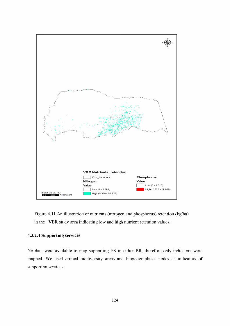
Figure 4.11 An illustration of nutrients (nitrogen and phosphorus) retention (kg/ha)

in the VBR study area indicating low and high nutrient retention values.


No data were available to map supporting ES in either BR, therefore only indicators were

mapped. We used critical biodiversity areas and biogeographical nodes as indicators of

supporting services.

124

With regard to indicators of biodiversity, both BRs showed abundance in terms of critical

biodiversity areas that have the potential to support a range of species. These areas were

mainly located in intact ecosystems and included existing PAs and identified PA expansion

priority areas. These areas were more pronounced in WBR than the VBR.

With regard to the second indicator of supporting services (ecological processes support),

results indicated that low ecological support areas represented by biogeographical nodes were

dominant in both BRs. Apart from this, VBR also contained medium ecological support areas

and WBR contained four isolated patches of high ecological support areas.

4.4 DISCUSSION

4.4.1 OVERVIEW OF ECOSYSTEM SERVICES MAPPING IN SA


This category of ES ranked second out of the four MA (2005) categories, in terms of

mapping. This finding was the same in other studies (Egoh et al. 2008; Martinez-Harms and

Balvanera 2015; Crossman et al. 2013). Despite the fact that it came second with regard to

mapping in the current review, this type of service was expected to have exceeded the current

levels in terms of studies undertaken, as it forms the basis of human well-being because of its

direct contribution to basic human needs, such as health and nutrition (MA 2005). Owing to

the direct link of provisioning services with human well-being, spatial representation of their

distribution could aid decision-making regarding their supply and demand (MA 2005;

Crossman et al. 2013).


The finding of regulating services as the most mapped ES compared to the other three

(supporting, cultural and provisioning) concurs with that of Egoh et al. (2012); Crossman et

al. (2013), as well as Martinez-Harms and Balvanera (2015). Since ES mapping is regarded as

an important tool for decision-making (Martinez-Harms and Balvanera 2015), high

consideration for regulating services, especially carbon storage and sequestration, could be

125

attributed to its association with climate change mitigation and adaption decision-making

(IPCC 2007).


This type of service was ranked third in this study with regard to ES mapping studies

undertaken. This finding was the same in previous reviews (Egoh et al. 2008; Crossman et al.

2012; Martinez-Harms and Balvanera 2015). However, it was not expected that services in

this category would receive less attention, since they are directly linked to human well-being,

as they represent important aspects related to culture, aspirations, diversity and values (MA

2005). We expected recreational and tourism ES to have received more attention, as they

represent the fastest growing industries in the world that contribute to countries’ economies,

including the economy of SA (Dilys and Urquhart 2001; Van der Merwe and Saayman 2003;

WTTC 2012; VDMIDP 2013). However, less attention being paid to this type of services was

not very surprising, since it is only recently that it has been receiving attention at all (MA

2005; TEEB 2010).


Supporting services were found to have been mapped least often by the studies reviewed.

This finding was expected, as this type of service was associated with major data gaps that

also made it difficult to quantify (TEEB 2010, Egoh et al. 2012). Another contributing factor

was that it contained fewer services, e.g. two under TEEB's classification (2010) (TEEB

2010; Egoh et al. 2012), and the services included were mainly soil-related (MA 2005; Egoh

et al. 2012). Despite these challenges, soil characteristics were used by most of the studies

forming part of this review as proxies to map mainly regulating services.

4.4.2 ECOSYSTEM SERVICES IN A BR CONTEXT


With regard to food provisioning service indicators, results suggest that the VBR had more

agricultural areas than the WBR, thus producing more food crops, despite the fact that on

district level, Waterberg had more land (4 360 262 ha) under agriculture than Vhembe

(2 076 390 ha), (LDA 2012). More agricultural areas in VBR could be attributed to the fact

126

that the VBR was larger than the WBR in size and included the whole Vhembe district

municipality area (Dombo et al. 2006). Moreover, large agricultural areas in VBR could have

been influenced by the presence of a human population of over 1 million (StatsSA 2001;

Dombo et al. 2006), whereas human settlement in WBR consisted of only 30 rural

settlements, with fewer than 100 000 inhabitants (WBR 2012). The differences in climate

might also have contributed to the difference in crops produced. In VBR, agricultural areas

were furthermore aligned with important catchment areas, although that was not the case in

WBR.

In terms of the water provisioning indicator, water catchments, the results indicated that there

were more water catchments in VBR than in WBR. This finding could be associated with the

fact that the VBR was situated within the Limpopo River catchment, which served as the

main catchment for streams flowing downstream northwards, including those from the WBR

(Dombo et al. 2006; WBR 2012). Otherwise the WBR was known to be better water-

resourced than the VBR mainly because of its association with the Waterberg Mountains and

semi-arid climate (WBR 2012). Water yield as well seems to be correlating with catchment

areas, and followed the same pattern as in strategically water-resourced areas of NSBA

(2004).

However, despite the findings above, it should be noted that water is a very scarce resource in

SA (NWRS 2004), where more than 80% of rivers’ ecosystems are threatened and

endangered (NSBA 2004). Moreover, the quality and quantity of most rivers globally are

affected by various anthropogenic activities (Townsend 1997; Parker 2000; Hancock 2002;

Govorushko 2005; Tafangenyasha and Dzinomwa 2005). Among these activities, agriculture

accounts for the highest water usage, followed by mining (NWRS 2004). With water

functioning as both a provisioning service and a supporting service, the consequence of water

shortage is detrimental to the provisioning of other ES. The MA (2005) also identified water

supply as one of the 15 ES that were in a poor condition because of unsustainable use,

therefore the sustainability of this ES for future use will be determined by the efforts put into

its conservation by the present generation.

In respect of raw material provisioning indicators, results indicate that there was higher

potential for afforestation, mainly for species consuming less water, in WBR than the VBR.

This involved mainly areas located in the buffer zones. The finding of high afforestation

127

potential in WBR, compared to the VBR, could be attributed to the fact that these areas had a

mild climate with average rainfall of 500-700 mm per annum (WBR 2012), whereas VBR

was situated in a very dry area with a hot climate, receiving 200-400 mm of rainfall per

annum (Dombo et al. 2006; Mustafa 2007). Contrary to this finding, the VBR currently has

plantations yielding high timber production for commercial purposes; meanwhile no timber

plantations are known to exist in WBR for commercial purposes. However, the current high-

production timber plantations in VBR were mainly concentrated in areas that have been

identified as having high potential for afforestation (NBSA 2004). On the other hand, existing

plantation areas were aligned with high water yield areas.

There is no dispute that forests are an important source of raw materials, including timber and

fibre (MA 2005), which are both essential in construction and agricultural industries around

the world. However, the forest ecosystem is one of the systems in a degraded state (MA

2005), to the extent that natural intact forests cover only 0.4% of land surface in SA (DAFF

2011). Continued unsustainable utilisation may therefore lead to severe degradation that

might have a negative impact on the provisioning of fibre and timber. Although forestry

plantations have the potential to fulfil some functions provided by natural forests, i.e.

provisioning of fibre and timber, they consume too much water (Duncan 1993; Fahey 1994).

Despite this shortcoming, in SA forestry plantations are an important commodity, contributing

at least 2% to the country's GDP, of which Limpopo contributes 0.5% (DAFF 2013).

The provisioning of grazing is regarded as an important service required to maintain the

health of livestock (LDA 2012), which in turn contributes to nutrition for human well-being

in both BRs. The indicators for grazing, which were illustrated by lucerne, natural grazing

and planted pastures, were found to be scattered in areas that had low to medium land

capability. However, a high concentration of these crops was aligned with a high land

capability range. This observation suggests that farmers were influenced by climate for their

fodder production, as they seemed to be concentrating on high rainfall areas and fertile soils

to produce their crops, which is a common-sense approach expected to be applied in this

situation.

In terms of grazing capacity, we found both BRs to have the potential of supporting up to 22

ha/LSU. A minor correlation was found between grazing potential and land capability in

VBR, e.g. areas around the KNP in VBR; although they were dominated by a

128

grazing capacity of between 2 and 6 ha/LSU, they fell in the low-medium land capability

range. The rest of the PAs could support only up to two LSU. The same observation was

made for WBR, where most of the PAs seemed to fall in the 0-2 ha/LSU range. In essence

PAs could support fewer LSU, with the exception of the KNP. This finding was not

surprising, as most of the PAs were conserving game species with different dietary

requirements, not merely based on grazing, as some were browsers.


High soil retention areas were found within the same range as areas with high soil

accumulation potential in the study conducted by Egoh et al.(2008). The finding of high soil

retention in areas prone to high soil accumulation concurs with that of Egoh et al. (2008).

Since soil retention is a function of slope (Mukhlisin et al. 2011), high soil retention areas

were concentrated in flat areas, as expected. Meanwhile, areas around the Soutpansberg

complex in VBR were found to be prone to soil erosion, which was expected, since they were

situated at a high altitude (Dombo et al. 2006).

High carbon sequestration potential areas were associated with some of the PAs in the study

areas, including the northern tip of KNP. In the case of the WBR, some of the areas around

Marakele National Park were associated with low carbon sequestration. The finding of high

carbon sequestration in PAs could be attributed to the fact that these areas were aligned with

high carbon storage (Egoh et al. 2008). High carbon storage areas were therefore expected to

have high sequestration potential. The finding of low carbon sequestration potential around

the indigenous forest belt was expected, as the remaining indigenous forests in SA are highly

protected (NFA 1998). The finding of a medium carbon sequestration range in both BRs was

aligned with the medium carbon storage range, as the areas were also situated within the

savanna biome, which has been found to contain medium carbon storage, according to Egoh

et al. (2008).

A high water purification service in the study areas was associated with high catchment areas.

Other workers also found higher nutrient fluxes in areas with more rainfall and freshwater

discharge (Howarth et al. 2006a). In this case, the finding of high nitrogen export could be

associated with the fact that most of the highly productive agricultural areas were found in

high concentration in the water catchment areas (NSBA 2004). High nutrient retention was

also closely aligned with transformed areas, specifically those carrying out agricultural129

activities, as they rely on the administration of excessive nutrients/fertilizers to enhance the

productivity of their crops and pastures (Zaimes and Schulz 2002; Ator and Denver 2015).

Nutrient export is determined by the amount of fertilizers/nutrients applied. Phosphorus

exports were lower than nitrogen; moreover, more nitrogen is retained than phosphorus.

The finding of less phosphorus being exported has been attributed to the fact that this nutrient

has been found to be generally less mobile (Zaimes and Schulz 2002) and mainly exported

through surface water (Ator and Denver 2015), which could be limited by rainfall. On the

other hand, we expected less phosphorus to be retained, as it remains on the soil surface and

is thus easily washed away by surface water (Lourenzi et al. 2014; Ator and Denver 2015).

High retention of nitrogen could be attributed to the fact that this nutrient is mainly absorbed

into the soil through ground water and ground water transport is generally slow (Lourenzi et

al 2014; Ator and Denver 2015). The main factor contributing to more nutrient export is the

administration of more nutrients, and more nitrogen has been found to be administered than

phosphorus (Lourenzi et al. 2014; Ator and Denver 2015). Another factor contributing to

more nitrogen export is a more permeable ground water table that easily allows nutrients to

pass through (Lourenzi et al. 2014).

Since most of the regulating services form part of the 15 ES that the MA (2005) has found to

be degraded, mainly through anthropogenic activities (Coetzee 1995; Kling et al. 2003; MA

2005) these BRs cannot be exempted from this in view of various human activities taking

place in the transition zone. Evidence of mining prospecting applications granted even in the

buffer and core zones (Department of Minerals and Energy register), and mining being

identified as one of the economic growth catalysts (VDMIDP 2012; WDMIDP 2013) suggest

the likelihood of more mining activities taking place in the foreseeable future. Mining

activities are associated with various impacts on aquatic ecosystems (Klemow 2000),

affecting these habitats (Butler 2006; Besser et al. 2009) and water quality (Phillips 2001;

Besser et al. 2009). Since BRs do not have formal legal protection, it might be difficult to

counter these activities. It is therefore important to note that the sustainability of wetlands and

associated ecosystems providing regulating ES lies in the hands of the surrounding human

communities, and degradation of such areas will affect the delivery of important ES.

130

4.4.2.3 C ultural services

The finding of more bird areas as indicators of cultural services in WBR than in the VBR

could be attributed to the prevailing naturalness in this BR, especially its less developed state.

Although most of these important bird areas have already been incorporated in some of the

PAs, some have been left out. However, it was comforting to realise that most of these areas

were recognised as part of critical biodiversity areas.

Results suggested great potential for economic growth and employment through cultural ES,

i.e. recreation, in the study area. Tourism contributes an average of over two million rands

annually in Vhembe (VDMIDP 2012). Although no information was available on the

contribution of tourism to the Waterberg region, it was clear that this type of LU contributed

positively to the rest of the Limpopo Province, where it was acknowledged as a catalyst for

economic growth and job creation (LGDS 2005; VDMIDP 2012; WDMIDP 2013) and also as

a driver of LU change (De Klerk 2003; LDA 2011). The situation in the WBR and VBR in

terms of tourism development was also influenced by the fact that the recreational and

tourism industries were among the fastest growing industries in the world (Dilys and

Urquhart 2001; Van der Merwe and Saayman 2003; WTTC 2012), serving as an important

source of income and employment. (Dilys and Urquhart 2001; McMichael et al. 2003; MA

2005). SA was no exception.


Although critical biodiversity areas were well represented in both BRs, they were found not

to be aligned with the national PAs expansion strategy, and very small portions fell within the

existing PAs in both BRs. It was clear that the current PAs expansion strategy for SA (2008)

was not informed by the critical biodiversity areas, despite the fact that this information was

already available (since 2004). We were expecting critical biodiversity areas to inform the

PAs expansion strategy.

Although it seemed that there were abundant supporting services and most were found to be

reasonably intact in both BRs, evidence suggested that in the sphere of supporting ES, various

human activities, such as mining, agriculture and tourism (FAO 1998; MA 2005), were

affecting these kinds of services negatively. Although the impact of supporting ES directly or

indirectly can only be proven after a long time (MA 2005; UNEP 2009), there is no doubt that

131

their degradation is likely to affect the direct delivery of basic ES, i.e. food and water

necessary for human well-being. In both BRs mining is more likely to affect mountain

ecosystems in the near future, when considering current trends and prospects that there are

sought-after minerals in the Waterberg and Soutpansberg complex, as evidenced by

prospecting applications. The impact of mining on these mountains could affect ES such as

water resources, since mountains are instrumental in hydrological cycles (Beniston et al.

1997; MA 2005) and most rivers and wetlands in the BRs originate from the mountain slopes.

Indicators contributing to soil formation will also be affected, since soil originates from the

weathering process of geological formations (AgriInfo 2011) such as mountains.

4.5 CONCLUSIONS

This study has identified and provided a spatial representation of some of the ES services

mapped in SA to date and indicators used to map them on a local scale represented by VBR

and WBR. Information provided by this study will thus assist in bridging the gap of lack of

baseline information regarding ES in a BR context. Although data collated in this analysis

will assist in raising awareness about BRs and ES in general, more work needs to be done to

make societies aware of the value of ES to human well-being. Insufficient data on the case

study areas highlight research gaps that need to be addressed if the concept of ES is to be

successfully adopted and integrated in decision-making on LU planning. Information

provided by this study will serve as baseline data for future ES related studies, including

mapping and valuation in SA and BRs elsewhere.

Since some of the indicators in SA were found to be threatened and endangered, including

wetlands and rivers (NSBA 2004), government-funded programmes such as Working for

Water, responsible for the removal of alien species along some of the major rivers, and

Working for Wetlands, focusing on wetland rehabilitation, should be encouraged in order to

improve the functioning of these ES in both BRs. Government intervention is also needed to

inform legal means that will protect the status of BRs in SA. Perhaps the inclusion of the BR

concept as one of the International Union for the Conservation of Nature’s formal PA

categories could assist globally, in ensuring the sustainability and protection of BRs from

anthropogenically driven degradation. Ways and means should also be found to encourage

research studies, which could be collated in a BR database, raising further awareness of the

BR concept.

132

4.6 REFERENCES

AgriInfo. 2011. Introduction to soil science: Weathering of rocks and minerals. My

Agriculture Information Bank. http://www.agriinfo.in.

Ator, S.W. and Denver, J.M. 2015. Understanding nutrients in the Chesapeake Bay

Watershed and implications for management and restoration-the eastern shore. A

summary of U.S. geological survey circular 1406, USGS Science for Changing

World.

Balvanera, P., Pfisterer, A.B., Buchmann, N., He, J., Nakashizuka, T., Raffaelli, D. and

Schimid, B. 2006. Quantifying the evidence for biodiversity effects on ecosystem

functioning and services. E co lo g y L etters, 9(10):1146-1156.

Bastian, O. and Schreiber, K. F. (eds). 1999. Analyse und okologische Bewertung der

Landschaft, Heidelberg; Berlin (Spektrum), 2nd edn.

Bateman, I.J., Harwood, A.R., Mace, G.M., Watson, R.T., Abson, D.J., Andrews, B., Binner,

A., Crowe A., Day, B.H., Dugdale, S., Fezzi, C., Foden, J., Hadley, D., Haines-

Young, R., Hulme, M., Kontoleon, A., Lovett, A.A., Munday, P., Pascual, U.,

Paterson, J., Perino, G., Sen, A., Siriwardena, G., van Soest, D. and Termansen, M.

2013. Bringing ecosystem services into economic decision-making: Land use in the

United Kingdom. Science, 341.

Beaumont, N.J., Austen, M.C., Atkins, J.P., Burdon, D., Degraer, S., Dentinho, T.P., Derous,

S., Holm, P., Horton, T., van Ierland, E., Marboe, A.H., Starkey, D.J., Townsend, M.

and Zarzycki, T. 2006. Identification, definition and quantification of goods and

services provided by marine biodiversity: Implications for the ecosystem approach.

M a rin e P o llu tio n B u lle tin , 54: 253-265.

Beniston, M., Diaz, H.F.and Bradley R.S., 1997. Climatic change at high elevations sites:

An overview. C lim a tic C hange, 36: 233-251.

Besser, J.M., W.G. Brumbaugh, A. L. Allert, C.J. Schmitt and C.G. Ingersoll.

2009. Ecological impacts of lead mining on Ozark streams: Toxicity of sediment and

pore water. E co to x ic o lo g y a n d E n v iro n m en ta l Sa fe ty , 72(2): 516-526.

Binning, C., S. Cork, Parry, R. and Shelton, D. 2001. Natural assets: An inventory of

ecosystem goods and services in the Goulburn Broken Catchment. CSIRO Sustainable

Ecosystems, Canberra. www.ecosvstemservicesproiect.org/html/publications.

Boyd, J. and Banzhaf, S. 2006. What are ecosystem services? The need for standardized

133

http://www.agriinfo.in/

http://www.ecosystemservicesproject.org/html/publications/index.htm

environmental accounting units. Energy and Natural Resources Division, R eso u rces

f o r the F u tu re , 1616 P St., NW Washington, DC 20036 202-328-5013, United States.

Brown, T.C., Bergstrom, J.C. and Loomis, J.B. 2007. Defining, valuing, and providing

ecosystem goods and services. N a tu ra l R eso u rces Jo u rn a l, 47: 229-376.

Burkhard, B., Kroll, F., Nedkov, S. and Muller, F. 2012b. Mapping ecosystem service supply,

demand and budgets. E c o lo g ic a l In d ica tors, 21:17-29.

Butler, R. 2006. Environmental impact of mining in the rainforest. Mining in Peru.

Mongabay.com.

Chan, K.M.A., Shaw, M.R., Cameron, D.R., Underwood, E.C. and Daily, G.C. 2006.

Conservation planning for ecosystem services. P L O S B io lo g y , 0040379.

CICES (Common International Classification of Ecosystem Services). 2011. European

Environment Agency paper prepared for discussion at the expert meeting on

ecosystem accounts organised by the UNSD, the EEA and the World Bank, London,

December 2011. Contract No: No. EEA/BSS/07/007, November 2011 Prepared by:

Roy Haines-Young and Marion Potschin, Centre for Environmental Management,

University of Nottingham, UK.

Coetzee, M.A. 1995. Water pollution in South Africa: Its impact on wetland biota. In: G.I.

Cowen (Ed), Wetlands of South Africa. Department of Environmental Affairs and

Tourism, Pretoria, South Africa.

Costanza, R., d’Arge, R., de Groot, R., Farber, S., Grasso, M., Hannon, B., Limburg, K.,

Naeem, S., O’Neill, R.V., Paruelo, J., Raskin, R.G., Sutton, P., and van den Belt, M.

1997. The value of the world’s ecosystem services and natural capital. N ature , 387:

253-260.

Costanza, R. 2008. Ecosystem services: Multiple classification systems are needed:

Letter to the editor. B io lo g ic a l C onserva tion , 141: 350-352.

Cowan, G.I. 1995. Wetlands of South Africa. Department of Environmental Affairs and

Tourism. Pretoria, Republic of South Africa.

Crossman, N.D., Benjamin, B., Nedkov, S., Willemen, L., Petz, K., Palomo, I., rakou, E.G.,

Martin-Lopez, B., McPhearson, T., Boyanova, K., Alkemade, R., Egoh, B., Dunbar,

M.B. and Maes, J. A blueprint for mapping and modelling ecosystem services. 2013.

E co sys tem Services, 4:4-14.

DAFF (Department of Agriculture, Forestry and Fisheries). 2011. State of forests report

2007-2009, Republic of South Africa. Printed by Directorate Communication, ISBN

978-1-86871-326-4. http://www2.dwaf.gov.za.134

http://www2.dwaf.gov.za/

DAFF (Department of Agriculture, Forestry and Fisheries). 2013. Pocket Guide to South

Africa 2012/13. http://www.gcis.gov.za/2012/03%20Agriculture.pdf.

Daily, G.C. 1997. Nature’s services: Societal dependence on natural ecosystems. Island Press,

Washington, DC.

Daily, G., Polasky, S. Goldstein, J., Kareiva, P.M., Mooney, H.A., Pejchar, L., Ricketts, T.H.,

Salzman, J, and Shallenberger R. 2009. Ecosystem services in decision-making: Time

to deliver. F ro n tie rs in E co lo g y a n d the E nviro n m en t, 7(1): 21-28.

DEFRA (Department for Environment Food and Rural Affairs). 2005. The economic, social

and ecological value of ecosystem services: Literature review, final report. Prepared

by Economics for the Environmental Consultants (eftec).

http://www.gov.uk/evidence/economics/foodfarm/reports.

de Groot, R.S. 1992. Functions of nature: Evaluation of nature in environmental planning,

management and decision making. Groningen: Wolters-Noordhoff.

de Groot, R.S., Wilson, M.A. and Boumans, R.M.J. 2002. A typology for the classification,

description and valuation of ecosystem functions, goods and services. E co lo g ic a l

E conom ics, 41: 393-408.

de Groot, R.S., Alkemade, R., Braat, L., Hein, L. and Willemen, L. 2010. Challenges in

integrating the concept of ecosystem services and values in landscape planning,

management and decision making. E c o lo g ic a l C om plexity , 7(3):260-272.

De Klerk, A. 2003. A land use model for the Waterberg Biosphere Reserve. Dissertation,

University of Pretoria. http://upetd.up.ac.za/thesis/available/etd-09022003-ble/etd-

09022003-113240/unrestricted

Diaz, S., Demissew, S., Carabias, J., Joly, C., Lonsdale, M., Ash, N., Larigauderie, A.,

Adhikari, J. R., Arico, S., Baldi, A., Bartuska, A., et al. 2015. The IPBES Conceptual

Framework - connecting nature and people. C u rren t O p in io n in E n v iro n m en ta l

Susta in a b ility , 14:1-16.

Dilys, R. and Urquhart, P. 2001. Pro-poor tourism: Harnessing the world's largest industry

for the world's poor world summit on sustainable development. International Institute

for Environment and Development in Collaboration with the Regional and

International Network Group (RING). Supported by Swedish International

Development Cooperation Agency.

Dombo, L., Crafford, J., Fouche, P., Gaigher, I., Hahn, N., Linden, J. and Rosmarin, J. 2006.

135

http://www.gcis.gov.za/2012/03%20Agriculture.pdf

http://www.gov.uk/evidence/economics/foodfarm/reports






Duncan, M.J. 1993. Does planting pines reduce groundwater recharge? New Zealand

Hydrological Society, Nelson Symposium. Abstracts with programme.

Egoh, B., Reyers, B., Rouget, M., Richardson, D.M., Le Maitre, D.C. and van Jaarsveld, A.S.

2008. Mapping ecosystem services for planning and management. A g ricu ltu re ,

E co sys tem s & E nviro n m en t, 127(1 -2) :135-140.

Egoh, B., Drakou, E.G., Dunbar, M.B., Maes, J. and Willemen, L. 2012. Indicators

for Mapping Ecosystem Services: A Review Publications Office of the European

Union, Luxembourg.

ESA (Ecological Society of America). 2000. Ecosystem services: A primer. E co lo g ica l

S o c ie ty o f A m erica .

Fahey, B. 1994. The effect of plantation forestry on water yield in New Zealand. NZIF

Conference, Nelson. Land Care Research. http://www.nzif.org

FAO (Food and Agriculture Organization of the United Nations). 1998. Moving mountains:

Mountains globally important ecosystems. The Mountain Regions Programme at the

Environmental Change Unit, University of Oxford, UK. Produced by Forestry

Department, UNASYLVA. http://www.fao.org/docrep/w9300e/w9300.htm

Fisher, B. and Turner, K. 2008. Ecosystem services: Classification for valuation. B io lo g ic a l

C onserva tion , 141: 1167-1169.

Fisher, B., Turner, R. K. and Morling, P. 2009. Defining and classifying ecosystem services

for decision making. E c o lo g ic a l E conom ics, 68(3):643-653.

Goldstein, J.H., Caldarone, G., Duarte, T.K., Ennaanay, D., Hannahs, N., Mendoza, G.,

Polasky, S., Wolny, S. and Daily, G.C. 2012. Integrating ecosystem services trade

offs into land use. P N A S , 109:197565-7570. National Academy of Science.

GOI (Government of India). 2007. Protection, development, maintenance and research in

biosphere reserves in India. Guidelines and Proformae. Ministry of Environment and

Forests, CGO Complex, Lodi Road, New Delhi -110003. Website:

http://www.enfovfor.nic.in

Gomez-Baggethun, E., Martin-Lopez, B., Barton, D., Braat, L., Saarikoski, H., Kelemen, M.,

Garcia-Llorente, E., van den Bergh, J., Arias, P., Berry, P., Potschin, L. M., Keene,

H., Dunford, R., Schroter-Schlaack, C.and P. Harrison. 2014. EU FP7 OpenNESS

136

http://www.nzif.org/

http://www.fao.org/docrep/w9300e/w9300.htm

http://www.enfovfor.nic.in/

Project Deliverable 4.1. S ta te -o f-th e -a rt R e p o r t o n In te g ra te d V alua tion o f E co sys tem

Services. European Commission FP7.

Govorushko, S.M. 2005. Effect of human activities on rivers: International congress on River

Basin Management. Director of EAA Centre, Pacific Geographical Institute,

Vladivostok. Natural Resources of China.

http://www2.dsi.gov.tr/English/congress2007/chapter 2Z37.pdf.

Haines-Young, R.H. and Potschin M.B. 2009. Methodologies for defining and assessing


Hancock, P.J. 2002. Human impacts on the stream-ground water exchange zone. University

of New England, Armidale, Australia. E co sys tem M a n a g em en t, 29(6):763-781.

Harrington, R., Anton, C., Dawson, T.P., de Bello, F., Feld, C.K., Haslett, J.R., Kluvankova-

Oravska, T., Kontogianni, A., Lavorel, S., Luck, G.W., Rounsevell, M.D.A.,

Samways, M.J., Settele, J., Skourtos, M., Spangenberg, J.H., Vandewalle, M., Zobel,

M. and Harrison, P.A. 2010, Ecosystem services and biodiversity conservation:

concepts and a glossary. B io d ive rs ity a n d C o nserva tion , 19(10):2773-2790.

Hermann, A., Schleifer, S. and Wrbka, T. 2011. The concept of ecosystem services regarding

landscape research: A review. L iv in g R ev iew s in L a n d sca p e R esearch , 5:1-37.

Howarth, R.W., Boyer, E.W., Marino, R., Swaney, D., Jaworski, N. and Goodale, C., 2006a.

The influence of climate on average nitrogen export from large watersheds in

the northeastern United States. B io g eo ch em is try 79, 163-186.

IPCC (Intergovernmental Panel on Climate Change). 2007. Climate Change 2007: The

Scientific Basis. Contribution of Working Group I to the Fourth Assessment Report of

the Intergovernmental Panel on Climate Change, edited by S. Solomon et al.,

Cambridge Univ. Press, New York.

Jarvis, A., Reuter, H.I., Nelson, A. and Guevara, E. 2008. Hole-filled SRTM for the

globe version 4. http://srtm.csi.cgiar.org.

Jax, K. 2005. Function and functioning in ecology: What does it mean? O ikos, 111(3): 641

648.

Klemow, K.M. 2000. Environmental effects of mining in the Anthracite region: Problems and

possible solutions. Presented to the US House of Representatives Committee on

Resources Oversight Hearing on the Abandoned Mine Reclamation Needs of the

Pennsylvania Anthracite Fields. Wilkes University, Wilkes-Barre, PA18766.

Scranton, Pennsylvania.

Kling, G., Hayhoe, K., Johnson, L., Magnuson, J., Polasky, S., Robinson, S., Shuter, B.,137

http://www2.dsi.gov.tr/English/congress2007/chapter_2/37.pdf

http://srtm.csi.cgiar.org/

Wander, M., Wuebbles, D. and Zak, D. 2003. Confronting climate change in the Great

Lakes region. A Report of the Ecological Society of America and the Union of

Concerned Scientists, Washington, DC.

Kremen, C. and Ostfeld, R.S. 2005. A call to ecologists: Measuring, analyzing, and

managing ecosystem services. F ro n tie rs in E c o lo g y a n d the E n vironm en t, 3: 540-548.

Kroll, F., Muller, F., Haase, D. and Fohrer, N. 2012. Rural-urban gradient analysis of

ecosystem services supply and demand dynamics. L a n d use P o licy , 29:521-535.

LDA (Limpopo Department of Agriculture). 2012. The Mapping of Agricultural Commodity

Production in the Limpopo Province, Final Report. Directorate Spatial Information

Services. Limpopo Provincial Government of South Africa, Polokwane.

[email protected].

Le Roux, J.J., Morgenthal, T.L., Malherbe, J., Summer, P.D. and Pretorius, D.J. 2008.

Water erosion prediction at a national scale for South Africa. W aterSA , 34(3):305-

314.

LGDS (Limpopo Growth and Development Strategy). 2005. Limpopo Economic

Development, Environment and Tourism.

Lourenzi, C.R., Ceretta, C.A., Cerini, J.B., Ferreira, P.A.A., Lorensini, F., Girotto, E.,

Tiecher, T.L., Schapanski, D.E. and Brunetto, G. 2014. Available content, surface

runoff and leaching of phosphorus forms in a typic hapludalf treated with organic and

mineral nutrient sources. R e v is ta B r a s ile ir a D e C ien cia D o So lo , 38(2): 544-556.

Lynch, S.D. 2004. Development of raster database of annual, monthly and daily

rainfall for Southern Africa. Report to the Water Research Commission. WRC report

no. 1156/1/04.


Synthesis. World Resource Institute. Island Press, Washington, DC.

McAlpine, K.G. and Wotton, D.M. 2009. Conservation and the delivery of ecosystem

services: A literature review. S cien ce f o r con serva tio n , 295.

Maes, J., Egoh, B., Willemen, L., Liquete, C., Vihervaara, P., Schagner, J.P., Grizzetti, B.,

Drakou, E.G., La Notte, A., Zulian, G., Bouraoui, F., Paracchini, M.L., Braat, L., and

Bidoglio, G. 2012. Mapping ecosystem services for policy support and decision

making in the European Union. E co sys tem Services, 1: 31-39.


138

mailto:[email protected]

Merrywheather, F.R., le Roux, J., van Rooyen, T.H., and Von M. Harmse, H.J. 1977.

Soil classification: A binomial system for South Africa. S c ien tific B u lle tin No. 390,

Department of Agriculture Technical Services, Republic of South Africa, Pretoria.

Maler, K. G., Aniyar, S. and Jansson A. 2009. Accounting for ecosystems. E n v iro n m en ta l &

R eso u rce E conom ics, 42(1): 39-51.

Martinez-Harms, M.J. and Balvanera, P. 2015. Methods for mapping ecosystem service

supply: A review. In te rn a tio n a l J o u rn a l o f B io d ivers ity Science, E co sys tem S erv ices

& M a n a g em en t, 8(1-2): 17-25.

McMichael, A.J., Butler, C.D. and Folke, C. 2003. New visions for addressing sustainability,

S c ien ce , 302(5652):1919-1920.

Mertz, O., Ravnborg, H.M., Lovei, G., Nielsen, I. and Konijendijk, C.C. 2007. Ecosystem

services and biodiversity in developing countries. B io d ivers ity a n d C onserva tion ,

16(10): 2729-2737.

Mills, A.J., Cowling, R.M., Fey, M.V., Kerley, G.I.H., Donaldson, J.S., Lechmere-

Oertel, R.R., Sigwele, A.M., Skowno, A.L. and Rundel, P. 2005. Effects of goat

pastoralism on ecosystem carbon storage in semiarid thicket, Eastern Cape South

Africa. A u stra lia n E co lo g y , 30: 797-804.


Swaziland. S tre litz ia , 19. South African National Botanical Institute, Pretoria.

Mukhlisin, M., Baidillah, M.R., Taha, M.R. and El-Shafie, A. 2011. Effect of

soil water retention model on slope stability analysis.

In te rn a tio n a l J o u rn a l o f the P h y s ic a l Sciences, 6(19): 4629-4635,

Mustafa, M. 2007. Validation of satellite based rainfall estimation over the Limpopo Basin. A

thesis submitted in partial fulfilment of the requirements for the degree of Master of

Science in Agricultural Meteorology. Faculty of Science, University of Zimbabwe.

NFA (National Forest Act). National Forest Act. No. 84. Of 1998. Gazette No. 19408,

Notice No. 1388. Republic of South Africa, Pretoria.

NSBA (National Spatial Biodiversity Assessment). 2004. Republic of South Africa,

South Africa National Biodiversity Institute, Planning Unit. BGIS.

NWRS (National Water Resource Strategy). 2004. South Africa's water situation and

strategies to balance supply and demand. First edition. Chapter 2.

Nelson, E., Mendoza, G., Regetz, J., Polasky, S., Tallis, H., Richard Cameron D., Chan,

K.M., Daily, G.C., Goldstein, J., Kareiva, P.M., Lonsdorf, E., Naidoo, R., Ricketts,

T.H. and Shaw, M.R. 2009. Modelling multiple ecosystem services, biodiversity139

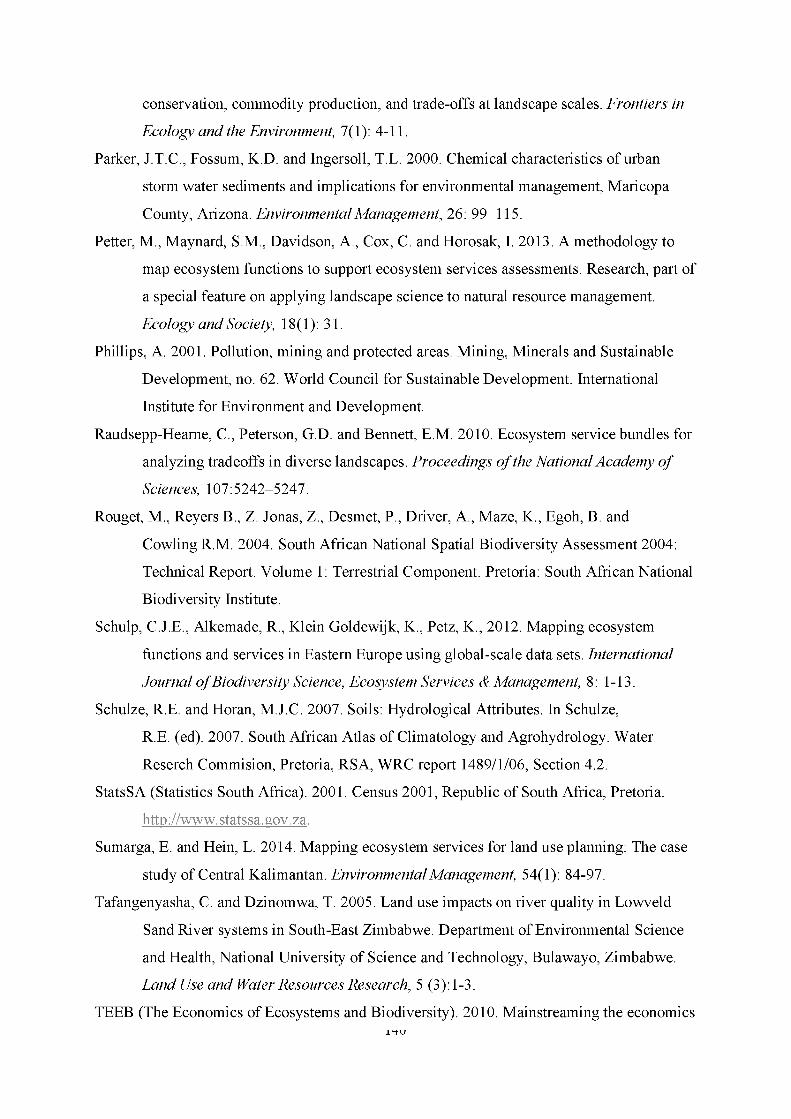
conservation, commodity production, and trade-offs at landscape scales. F ro n tie rs in

E co lo g y a n d the E nvironm en t, 7(1): 4-11.

Parker, J.T.C., Fossum, K.D. and Ingersoll, T.L. 2000. Chemical characteristics of urban

storm water sediments and implications for environmental management, Maricopa

County, Arizona. E n v iro n m en ta l M a n a g em en t, 26: 99-115.

Petter, M., Maynard, S.M., Davidson, A., Cox, C. and Horosak, I. 2013. A methodology to

map ecosystem functions to support ecosystem services assessments. Research, part of

a special feature on applying landscape science to natural resource management.

E co lo g y a n d Society, 18(1): 31.

Phillips, A. 2001. Pollution, mining and protected areas. Mining, Minerals and Sustainable

Development, no. 62. World Council for Sustainable Development. International

Institute for Environment and Development.

Raudsepp-Hearne, C., Peterson, G.D. and Bennett, E.M. 2010. Ecosystem service bundles for

analyzing tradeoffs in diverse landscapes. P ro cee d in g s o f the N a tio n a l A ca d e m y o f

Sciences, 107:5242-5247.

Rouget, M., Reyers B., Z. Jonas, Z., Desmet, P., Driver, A., Maze, K., Egoh, B. and

Cowling R.M. 2004. South African National Spatial Biodiversity Assessment 2004:

Technical Report. Volume 1: Terrestrial Component. Pretoria: South African National

Biodiversity Institute.

Schulp, C.J.E., Alkemade, R., Klein Goldewijk, K., Petz, K., 2012. Mapping ecosystem

functions and services in Eastern Europe using global-scale data sets. In te rn a tio n a l

J o u rn a l o f B io d ivers ity Science, E co sys tem S erv ices & M a n a g em en t, 8: 1-13.

Schulze, R.E. and Horan, M.J.C. 2007. Soils: Hydrological Attributes. In Schulze,

R.E. (ed). 2007. South African Atlas of Climatology and Agrohydrology. Water

Reserch Commision, Pretoria, RSA, WRC report 1489/1/06, Section 4.2.

StatsSA (Statistics South Africa). 2001. Census 2001, Republic of South Africa, Pretoria.

http://www.statssa.gov.za.

Sumarga, E. and Hein, L. 2014. Mapping ecosystem services for land use planning: The case

study of Central Kalimantan. E n v iro n m en ta l M a n a g em en t, 54(1): 84-97.

Tafangenyasha, C. and Dzinomwa, T. 2005. Land use impacts on river quality in Lowveld

Sand River systems in South-East Zimbabwe. Department of Environmental Science

and Health, National University of Science and Technology, Bulawayo, Zimbabwe.

L a n d Use a n d W ater R eso u rces R esea rch , 5 (3):1-3.

TEEB (The Economics of Ecosystems and Biodiversity). 2010. Mainstreaming the economics140

http://www.statssa.gov.za/

of nature. A synthesis of the approach, conclusions and recommendations of TEEB.

United Nations Environment Programme. Progress Press, Malta.

Townsend, C.R., Arbuckle C.J., Crowl, T.A. and Scarsbrook, M.R. 1997. The relationship

between land use and physicochemistry, food resources and macro invertebrate

communities in tributaries of the Taieri River, New Zealand: A hierarchically scaled

approach. F resh w a te r B io logy, 37:177-191.

Turner, R.K., Georgiou, S. and Fisher, B. 2008. Valuing ecosystem services: The case of

multi-functional wetlands. London: Earthscan.

UNESCO (United Nations Educational, Scientific and Cultural Organization). 2010. Lessons

from biosphere reserves in the Asia-Pacific region, and way forward. A regional

review of biosphere reserves in Asia and the Pacific to achieve sustainable

development, UNESCO Office, Jakarta. Regional Science Bureau for Asia and the

Pacific.

UNEP (United Nations Environment Programme). 2009. Ecosystem Management

Programme. A new approach to sustainability. UNON Publishing Services Section,

Nairobi, ISO 14001: 2004 manufacturer.

Van den Berg, E.C., Plarre, C., Van den Berg, H.M. and Thompson, M.W. 2008. The

South African National Land Cover 2000. Agricultural Research Council (ARC). And

Council for Scientific and Industrial Research (CSIR), Pretoria, Report no.

GW/A/208/86.

Van der Merwe, P. and Saayman, M. 2003. Determining the economic value of game farm

tourism. K oedoe, 46(2):103-112.

VDMIDP (Vhembe District Municipality Integrated Development Plan). 2012. IDP for

2011/12 financial year. http://www.mfma.treasury.gov.za

Wallace, K.J. 2007. Classification of ecosystem services: Problems and solutions. B io lo g ic a l

C onserva tion , 139:235-246.

Wallace, K.J. 2008. Ecosystem services: Multiple classifications or confusion? B io lo g ic a l

C onserva tion , 141:353-354.

WBR (Waterberg Biosphere Reserve). 2012. 10 Year Periodic Review. United Nations

Educational, Scientific and Cultural Organization: Man and Biosphere (MAB)

Programme.

WDMIDP (Waterberg District Municipality Integrated Development Plan). 2013. IDP for

2012/13 financial year. http://www.waterberg.gov.za.

Wilson, M.A. and Hoehn, J.P. 2006. Valuing environmental goods and services using benefit141

http://www.mfma.treasury.gov.za/

http://www.waterberg.gov.za/

transfer: The state-of-the art and science. E c o lo g ic a l E co n o m ics , 60(2):335-342.

Wischmeier, W.H. and Smith, D. 1978. Predicted rainfall erosion losses: a guide to

conservation planning. USDA-ARS Agriculture Handbook, Washington D.C.

WMB (Waterberg Meander Brochure). 2009. Volume 1. http://www.waterbergmeander.co.za

WTTC (World Travel and Tourism Council). 2012. Travel and Tourism Economic Impact

2012. The Authority on World Travel and Tourism. http://www.wttc.org.

strategies to balance supply and demand. First edition. Chapter 2.

Zaimes, G.N. and Schultz, R.C. 2002. Phosphorus in agricultural watersheds: A literature

review. Department of Forestry, Iowa State University, Ames, Iowa.

http://www.buffer.forestry.iastate.edu/Assets/Phosphorus review.pdf

142

http://www.waterbergmeander.co.za/

http://www.wttc.org/

http://www.buffer.forestry.iastate.edu/Assets/Phosphorus_review.pdf

4.7 APPENDICES

4.7.1 Appendix 4A: Selected ES typologies/classification frameworks.

Daily (1997) MA (2005) Bastian and Schreiber (1999) de Groot et al. (2010) CICES (2011)

Production of goods Provisioning services Economic services Provisioning services Provisioning

Food Food Renewable resources (herbal and

animal) biomass/non-renewable

resources (mineral raw materials

and fossil fuel)

Food Nutrition -

Plants and animals (terrestrial, marine and

freshwater

Fresh water supply Available renewable resource:

water

Water Potable water

Pharmaceuticals Biochemicals - natural

medicines and

pharmaceuticals

Biochemical products and

medicinal resources

Materials

Medicinal resources

Genetic resources Genetic resources Genetic materials Genetic resources,

Ornamental resources -

animals and plant products

(skin, shells, flowers)

Ornamental species and/or

resources

Skins, shells, bones

Energy (biomass fuel) Fibre - wood, cotton,

wool, silk, timber

Fuel, fibre and other raw

materials

Timber

143

Biomass fuel Energy

Wood, energy crops, dung, fat, oils

Industrial products - - - -

Regeneration processes Regulation services Ecological services Regulation services Regulation and maintenance

Partial stabilization of climate Climate regulation - of

temperature and

precipitation and/or

greenhouse emission or

sequestration

Regulation of materials and

energy cycles

Climate regulation Physical environment regulation

Moderation of weather

extremes

Air quality regulation Atmospheric regulation (climate, carbon

sequestration)

Water purification and waste

treatment - the filtering out,

detoxification and

decomposition of organic

waste in water bodies through

soil processes

Water purification and

waste treatment - the

filtering out,

detoxification and

decomposition of organic

waste in water bodies

through soil processes

Waste treatment Water quality regulation (purification and

oxygenation), water cooling

Soil formation and regeneration Paedogenesis and soil quality regulation

(maintenance of soil fertility)

Control of pests and species Disease regulation -

control of human

pathogens (e.g cholera)

and disease vectors (e.g

mosquitoes)

Regulation and regeneration of

population and biocoenose

Biological regulation

Regulation of biotic environment

Pest and disease control

144

Stabilising processes

Translocation processes (seed

dispersal)

Pollination Pollination Life cycle maintenance and habitat

protection (pollination and seed dispersal)

Cycling and filtration

processes

- - Gene pool protection (nursery)

Erosion regulation Erosion protection Flow regulation

Mass flow regulation (erosion and

avalanche protection)

Coastal and river channel

stability

Storm protection Natural hazard mitigation Airflow regulation (windbreak, shelter belts)

Regulation of hydrological

cycle

Water regulation Water regulation Water flow regulation

Life-fulfilling functions Cultural services Social services Cultural and amenity Cultural

Recreation and ecotourism Recreational function Recreation and tourism Intellectual and experiential

Recreation and community activities

(charismatic or iconic wildlife or habitats)

Scientific discovery Educational values and

knowledge systems

Information function (science and

education)

Education and science Information and knowledge

(scientific, educational, prey for hunting or

collection)

Cultural, intellectual and

spiritual inspiration

Cultural heritage and

diversity

Psychological function (aesthetic,

ethic) Cultural heritage and identity

Symbolic

Heritage (cultural landscapes, landscape)

145




Spiritual and religious

values, inspiration

Spiritual and religious

inspiration

Spiritual (wilderness, naturalness, sacred

places or species)

Aesthetic beauty Aesthetic values Aesthetic

Aesthetic

Serenity Sense of place - Sense of place, tranquillity

Existence value

Preservation of options Supporting services

Habitat or supporting services

Maintenance of the ecological

components and systems

needed for future supply

Nutrient cycling - Nursery habitat

Pollination Gene pool protection

- Primary production -

Photosynthesis

- -

- Soil formation -

146

4.7.2 A ppendix 4B: L iterature reviewed

Extent of the study Ecosystem services

involved

Primary indicator Secondary Indicators Source

Local Food provision Fodder provision Livestock O'Farrell 2011

Local Food provision Fodder provision Livestock Reyers 2009

Local Food provision Fodder provision Vegetation map Egoh 2010

Local Food provision Grain production Crop yield van Jaarsveld 2005

National Water provision Fodder provision Livestock Wilgen 2008

Local Water provision Water supply Surface water O'Farrell 2011

Local Water provision Water supply Ground water O'Farrell 2011

Local Water provision Water supply Surface water Egoh 2011

National Water provision Water supply Surface water Egoh 2009

147

Local Water provision Water supply Surface/ground water van Jaarsveld 2005

National Water provision Water supply Surface water Wilgen 2008

National Water provision Water supply Surface water Egoh et al. 2008

Local Raw materials Fuel wood Wood production van Jaarsveld 2005

Local Raw materials Raw material Raw material Chisholm 2010

National Climate regulation Carbon storage Vegetation map Egoh et al. 2008

National Climate regulation Carbon storage Vegetation map Egoh 2009

Local Climate regulation Carbon storage Above ground

biomass

Reyers 2009

Local Climate regulation Carbon storage Above ground

biomass

Vegetation map

Egoh 2010

Local Climate regulation Carbon storage Soil carbon Egoh 2011

Local Climate regulation Carbon sequestration Above ground Egoh 2011

148

biomass

Local Climate regulation Carbon sequestration Nutrient flux Chisholm 2010

National Regulation of water

flows

Water regulation Ground water Egoh 2008


flows


Local Regulation of water

flows

Water regulation Flow regulation

Water regulation

Reyers 2009

Local Regulation of water

flows

Water recharge Ground water

Water characteristics

Egoh 2010


flows


National Erosion prevention Soil retention Vegetation map Egoh 2008

National Erosion prevention Soil retention Vegetation map Egoh 2009

Local Erosion prevention Soil retention Vegetation map Egoh 2011

Local Erosion prevention Soil erosion Precipitation Reyers 2009

149

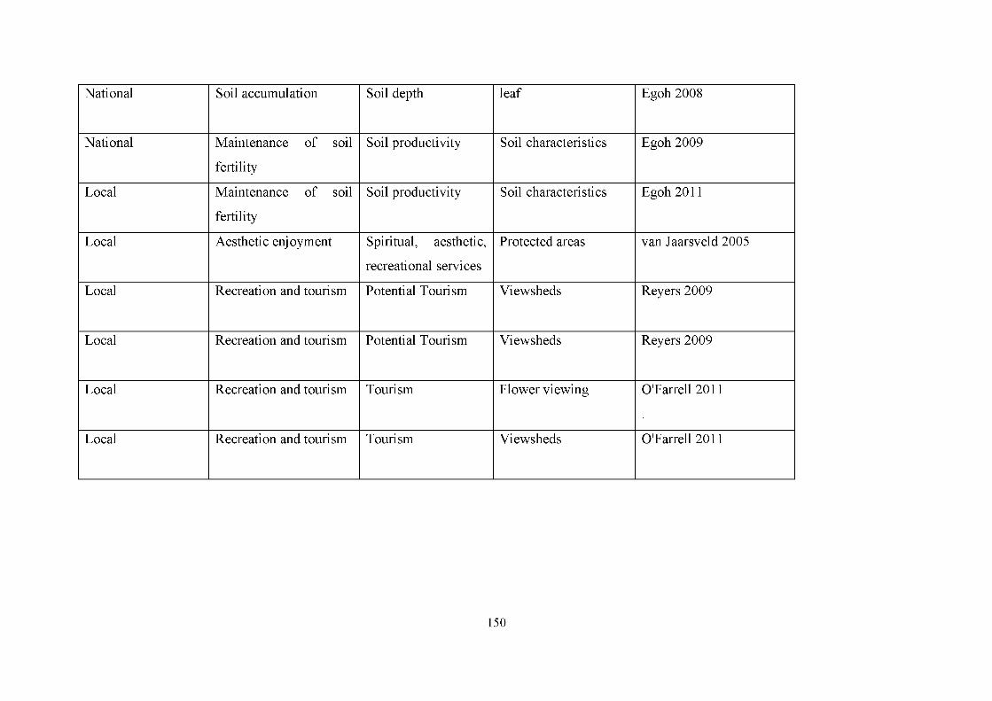
National Soil accumulation Soil depth leaf Egoh 2008

National Maintenance of soil

fertility

Soil productivity Soil characteristics Egoh 2009

Local Maintenance of soil

fertility

Soil productivity Soil characteristics Egoh 2011

Local Aesthetic enjoyment Spiritual, aesthetic,

recreational services

Protected areas van Jaarsveld 2005

Local Recreation and tourism Potential Tourism Viewsheds Reyers 2009

Local Recreation and tourism Potential Tourism Viewsheds Reyers 2009

Local Recreation and tourism Tourism Flower viewing O'Farrell 2011

Local Recreation and tourism Tourism Viewsheds O'Farrell 2011

150

4.7.3 Appendix 4C: Spatial representation of indicators of ecosystem services in Waterberg and Vhembe Biosphere Reserves

Figure 4C. 1 An illustration of an indicator of food provisioningservice in WBR, represented by horticultural and agricultural crops.

Figure 4C.2 An illustration of an indicator of food provisioningservice in VBR, represented by horticultural and agricultural crops.

151

Figure 4C.3 An illustration of an indicator of food provisioningservice in WBR, represented by land capability to produceagricultural crops.

Figure 4C.4 An illustration of an indicator of food provisioningservice in VBR, represented by land capability to produceagricultural crops.

152

Figure 4C.5 An illustration of food provisioning indicator in WBR, represented by game farms.

Figure 4C.6 An illustration of food provisioning indicator in VBR, represented by game farms.

153

Figure 4C.7 An illustration of an indicator for water provisioningservice in WBR, represented by surface water supply by rivers and dams

Figure 4C.8 An illustration of an indicator for water provisioningservice in VBR, represented by surface water supply by rivers and dams

154

VBR_lmportant_catchment areasM A R & % o f w a t e r _ p r o v i d e d

135-220 (W ater>50% )

220 420 (W ater>30% )

420-2707 (W ater>10% )0 10 20

__ ̂ VBR_bour»dary

Figure 4C. 10 An illustration of an indicator of water provisioning service in VBR, represented by important catchment areas. (calculated using mean annual runoff MAR).

WBR Important catchment areasM A R & % o f w a t e r p r o v id e d

135-220 (W ater>50% )

W BR _boundaryk i mater*

Figure 4C.9 An illustration for an indicator of water provisioning service in WBR, represented by important catchment areas. (calculated using mean annual runoff MAR)

155

service in WBR represented by hectares of land covered by grazing crops (natural grazing, lucerne and planted pastures)

service in VBR represented by hectares of land covered bygrazing crops (natural grazing, lucerne and planted pastures)

156

WBR_Timber_plantations_ J WBR_boundary

Existing plantationsAftorestation_polentiai

v e r y lo w

MediumK I ' M r ' . - .

VBR_7lmber_plantations| V B R _ b o u n d a ry

E xi st xi g_ pla nt ati on sA ff or est at w n _ potential

very low

0 510 20 30 40KRomeiei • h m

Figure 4C. 13 An illustration of an indicator of raw material provisioning service in WBR, represented by land covered by timber plantations and potential afforestation areas.

157

Figure 4C. 14 An illustration of an indicator of raw materialprovisioning service in VBR, represented by land coveredby timber plantations and potential afforestation areas.

F of o s I

ForestBush land

i Kilometers

Wbr forest woods

F< rest ana w oo dland

I W B R _boundary12 5 2 5

V B R F o r e s t s & W o o d l a n d s

Forest and Woodland

__| VBR_boundary< qmotf

Figure 4C.15 An illustration of an indicator of regulating service in WBR, represented by vegetation cover.

Figure 4C.16 An illustration of an indicator of regulating service services in VBR represented by vegetation cover.

158

Figure 4C.17 An illustration of an indicator of regulating servicein WBR, represented by areas covered by wetlands.

Figure 4C.18 An illustration of an indicator of regulatingservice in VBR, represented by areas covered by wetlands.

159

N

VBR biodiveristy support areaslm p o r t a n c e _ s c o r e

0 (Low)

Ki ometers

Figure 4C.19 An illustration of biodiversity support indicatorin WBR, represented by biogeographic areas (ecological support areas)

Figure 4C.20 An illustration of biodiversity support indicatorin VBR, represented by biogeographic areas (ecological support areas)

160

Figure 4C.21 An illustration of an indicator of supporting service in WBR represented by critical biodiversity areas.

Figure 4C.22 An illustration of an indicator of supportingservice in VBR represented by critical biodiversity areas.

161

Figure 4C.23 An illustration of a supporting service indicator in WBR represented by soil characteristics (forms).

Figure 4C.24 An illustration of a supporting service indicator,in VBR, represented by soil characteristics (forms).

162

Figure 4C.25 An illustration of an indicator of culturalService (recreational and ecotourism) in WBR, represented.by important bird areas.

Figure 4C.26 An illustration of an indicator of cultural services(recreational and ecotourism) in VBR, representedby important bird areas.

163

Figure 4C.27 An illustration of an indicator of culturalservice (recreational and ecotourism) in WBR, represented byby protected areas.

Figure 4C.28 An illustration of an indicator of culturalservice (recreational and ecotourism) in VBR, representedby protected areas.

164

Figure 4C.29 An illustration of an indicator of cultural service in WBR(aesthetic quality), represented by protected expansion focus areas.

Figure 4C.30 An illustration of an indicator of cultural service in VBR(aesthetic quality), represented by protected expansion focus areas.

165

CHAPTER 5

HABITAT CONDITION ASSESSMENT FOR ECOSYSTEM SERVICES

This chapter has been published on In te rn a tio n a l J o u rn a l o f B io d ivers ity Science, E co sys tem

S erv ices & M a n a g em en t as: Ntshane B.C and Gambiza, J. Habitat condition assessment for

ecosystem services.

Abstract

Biodiversity is the foundation of life-support systems on earth and underpins the delivery of

ecosystem services (ES) important for human well-being. The loss of biodiversity worldwide,

however, remains one of the most daunting challenges. Among the major causes of biodiversity

loss is habitat loss due to transformation of land to agricultural, mining and urban areas. We applied

the Integrated Valuation of Ecosystem Services and Trade-offs (InVEST) modelling tool to assess

the condition of habitats as a service that provides living spaces for plants and animals, and as a

supporting service for the delivery of other ES in a biosphere reserve in South Africa. Results

indicated that 72% of the surveyed habitats were of high quality to provide the necessary services.

However, some of the habitats were found to be affected by threats as follows: low (0-20%) to

moderate (20-32%) habitat loss was recorded in habitats adjacent to mining and plantation areas,

and high (32-56%) to severe (56-95%) habitat loss was recorded in habitats in close proximity to

urban and cultivated areas. At least 56% of the vegetation types found in the study area were

threatened by transformation to agriculture, mining and urban areas. We strongly recommend that

existing biodiversity policies and legislation should be enforced to avoid habitat loss and

degradation.

Key words: b iod iversity; ecosystem serv ices; h a b ita t loss; h a b ita t qua lity; va lua tion ; h u m a n w e ll

being.

5.1 INTRODUCTION

The protection of biodiversity is an international obligation, with approximately 200 nations

committing to it (CBD 1992). The term biodiversity originates from the concept of biological

diversity, which was coined during the 20th century (Dasmann 1968; Soule and Wilcox 1980) and

has been in use for almost three decades (Wilson 1988; Bibby et al. 1992; Eldredge 1992; Harper

and Hawksworth 1994; Gaston 1996). The Convention on Biological Diversity (CBD 1992) defines

166

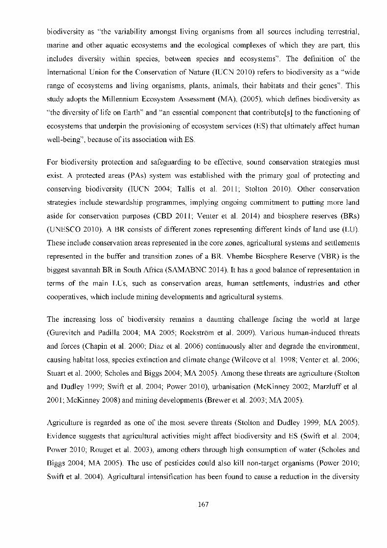
biodiversity as “the variability amongst living organisms from all sources including terrestrial,

marine and other aquatic ecosystems and the ecological complexes of which they are part, this

includes diversity within species, between species and ecosystems”. The definition of the

International Union for the Conservation of Nature (IUCN 2010) refers to biodiversity as a “wide

range of ecosystems and living organisms, plants, animals, their habitats and their genes”. This

study adopts the Millennium Ecosystem Assessment (MA), (2005), which defines biodiversity as

“the diversity of life on Earth” and “an essential component that contribute[s] to the functioning of

ecosystems that underpin the provisioning of ecosystem services (ES) that ultimately affect human

well-being”, because of its association with ES.

For biodiversity protection and safeguarding to be effective, sound conservation strategies must

exist. A protected areas (PAs) system was established with the primary goal of protecting and

conserving biodiversity (IUCN 2004; Tallis et al. 2011; Stolton 2010). Other conservation

strategies include stewardship programmes, implying ongoing commitment to putting more land

aside for conservation purposes (CBD 2011; Venter et al. 2014) and biosphere reserves (BRs)

(UNESCO 2010). A BR consists of different zones representing different kinds of land use (LU).

These include conservation areas represented in the core zones, agricultural systems and settlements

represented in the buffer and transition zones of a BR. Vhembe Biosphere Reserve (VBR) is the

biggest savannah BR in South Africa (SAMABNC 2014). It has a good balance of representation in

terms of the main LUs, such as conservation areas, human settlements, industries and other

cooperatives, which include mining developments and agricultural systems.

The increasing loss of biodiversity remains a daunting challenge facing the world at large

(Gurevitch and Padilla 2004; MA 2005; Rockstrom et al. 2009). Various human-induced threats

and forces (Chapin et al. 2000; Diaz et al. 2006) continuously alter and degrade the environment,

causing habitat loss, species extinction and climate change (Wilcove et al. 1998; Venter et. al. 2006;

Stuart et al. 2000; Scholes and Biggs 2004; MA 2005). Among these threats are agriculture (Stolton

and Dudley 1999; Swift et al. 2004; Power 2010), urbanisation (McKinney 2002; Marzluff et al.

2001; McKinney 2008) and mining developments (Brewer et al. 2003; MA 2005).

Agriculture is regarded as one of the most severe threats (Stolton and Dudley 1999; MA 2005).

Evidence suggests that agricultural activities might affect biodiversity and ES (Swift et al. 2004;

Power 2010; Rouget et al. 2003), among others through high consumption of water (Scholes and

Biggs 2004; MA 2005). The use of pesticides could also kill non-target organisms (Power 2010;

Swift et al. 2004). Agricultural intensification has been found to cause a reduction in the diversity

167

of organisms responsible for nutrient cycling, as well as ground water pollution (Swift et al. 2004;

Scholes and Biggs 2004).

Urbanisation refers to an increase in the number and extent of population and cities (Uttara et al.

2012). Concerns about the impact of urbanisation on biodiversity have been raised by a number of

researchers (Marzluff et al. 2001; McKinney 2002; McKinney 2008; Uttara et al. 2012).

Urbanisation has been found to have an impact on biodiversity and ES in a number of ways,

including indigenous species’ extinction and habitat loss (Marzluff et al. 2001; McKinney 2002;

McKinney 2008; Uttara et al. 2012), as well as indigenous vegetation removal (Uttara et al. 2012).

While industrial developments, such as mining, are seen as a quick solution to economic

development (Turner 2012), these kinds of LU come with a cost to the natural environment (IUCN

2011a; 2011b). Mining has been associated with habitat destruction due to removal of vegetation

(Ashton et al. 2001; Phillips 2001), high water consumption (DWAF 2004; MA 2005) and high

consumption of natural resources (Brewer et al. 2003; MA 2005). Mining activities have been

found to degrade and alter both terrestrial and aquatic habitats, causing the decline of indigenous

species (Ashton et al. 2001; Phillips 2001). Many world heritage sites and PAs around the world

were found to be affected negatively by various activities related to mining (Turner 2012). A study

undertaken by the IUCN (2011a; 2011b) found that at least 25% of PAs were threatened by mining

in West Africa. In another study (Osti et al. 2011), 27% of World Heritage sites in Sub-Saharan

Africa were found to have oil and gas concessions. This situation presents a challenge in terms of

dealing with a threat whose solution is beyond the employment of conservation strategies, i.e. PAs.

Perhaps what the above-mentioned forms of LU have in common is the effect on habitats (MA

2005; McKinney 2008; Power 2010; Uttara et al. 2012). Some of the examples of how LU has

affected habitat quality include various types of pollution and vegetation removal associated with

agriculture, urban development and mining activities (Czech et al. 2000; Ashton et al. 2001; Rouget

et al. 2003; Power 2010; Uttara et al. 2012). A habitat can be defined as an area’s condition and

resources that contribute to the reproduction and continuous existence of species (Hall et al. 1997;

Tallis et al. 2011). The state of biodiversity in an area can be determined through the condition of

its habitat; the importance of a habitat, on the other hand, depends on its quality. Habitat quality is

defined as the environment's ability and capacity to provide adequate support and conditions to

enable the persistent survival of species (Tallis et al. 2011).

A habitat’s role regarding ecosystem services is two-fold. The first role is that of being a service

itself, by for example providing refuge for wildlife. The second role is that of being a supporting

service that underpins the delivery of other services, such as provisioning (e.g. food and water),

168

cultural (e.g. recreation, aesthetic quality) and regulating (climate regulation, flood regulation)

services (MA 2005). Ecosystem services are defined as benefits that people derive from ecosystems

(MA 2005). It is important to note that LU choices result in trade-offs between/among services, e.g.

the advancement of agriculture as a LU instead of conservation in a specific area will have an

impact on biodiversity and water resources because of chemicals used to intensify agricultural

productivity (Foley et al. 2005).

If managers are to reach their biodiversity conservation goals, they should conduct biodiversity

condition/threat assessments (Margoluis and Salafsky 2001; Tallis et al. 2011). Modelling and

biodiversity assessment, which include the impact of LU on habitat quality in a given area, assist in

(1) understanding the patterns of distribution and richness of biodiversity in the landscape, (2)

comparison of spatial patterns of biodiversity and ES, (3) identification of synergies and trade-offs

in different scales and scenarios and (4) development of strategies for biodiversity conservation

(Tallis et al. 2011.) Information on habitat quality allows one to make informed decisions about

different conservation strategies, i.e. conservation area expansion, introduction and removal of

species and identification of the habitats that provide high ES, as well as the type of ES provided by

different habitats. Several studies (Nelson et al. 2009; Polasky et al. 2011; Kovacs et al. 2013;

Bhagabati et al. 2014) undertook threat assessment and modelling to determine the impact of

threats on a suite of biodiversity features and ES, on different scales and densities.

This study applied the Integrated Valuation of Ecosystem Services and Trade-offs (InVEST)

biodiversity habitat quality model described in Tallis et al. (2011) to assess the condition of habitat

as an ES and that of providing a supporting service for the delivery of other ES The model

combined information on land use (LU)/land cover (LC) and threats to determine the degradation

and extent thereof, on different habitat types in a biosphere reserve (BR). We selected InVEST

because: (1) it can provide estimates of the level and value of ES that are provided by a given area,

and (2) its models are spatially explicit, with a flexible spatial resolution, thereby enabling users to

address questions at different scales.


5.2.1 Study area

A BR consists of different zones representing different kinds of land use. These include

conservation areas represented in the core zones, agricultural systems and settlements represented

in the buffer and transition zones of a BR. Vhembe Biosphere Reserve (VBR) is the biggest

savannah BR in South Africa (SAMABNC 2014). It has a good balance of representation in terms169

of the main land uses such as conservation areas, human settlements, industries and other

cooperatives, which included mining developments and agricultural systems. Despite its size of

3 070 000 ha, this study purposefully extended the VBR study area to cover the whole of the

northern section of one of the two major core areas, the Kruger National Park and the whole

western section up to the end of the existing BR boundary. This extension enabled us to obtain

additional information on the status of biodiversity within the VBR and its most important buffer

areas.

There are diverse land uses in the study area (Dombo et al. 2006). Conservation is one of the

dominant forms of land use with about 1 000 000 ha of land under formal protection, including

state-owned land (two national parks and provincial reserves) (Dombo et al. 2006). Agricultural

systems are also well represented in the Vhembe region. Human settlements are fairly well

developed and the human population size is about 1 500 000 (Stats SA 2012). There is also good

diversity of vegetation types in the study area, with more than 30 types represented (Mucina and

Rutherford 2006).

5.2.2 InVEST biodiversity model

InVEST is a modeling suite that uses land use/ land cover patterns to estimate values and levels of

biodiversity found in a landscape (Tallis et al. 2011). The InVEST biodiversity model 2.2.0 as

described by Tallis et al. (2011) uses information about threats to biodiversity together with LU/LC

to produce habitat quality and degradation maps, which provide information about the quality and

degradation of different types of habitat in an area over time. The LU/LC map for the VBR was

derived from a 2009 LU/LC map for South Africa (SANBI 2009) which was the most recent one at

the time of our study. We selected the InVEST habitat quality modelling tool because it allows for a

rapid assessment of the impacts of different threats and land uses on biodiversity and ES (Tallis et

al. 2011; Guerry et al. 2012). More details regarding the InVEST biodiversity quality model are

contained in Appendix 5A.

5.2.3 Running the InVEST biodiversity model

The following process was followed in this study to run the InVEST biodiversity model, as

described in Tallis et al. (2011):

Step 1- Creation of workspace

For each InVEST model, including biodiversity and conservation, a separate workspace was

created on the computer hard drive. This was followed by the creation of a folder under the

workspace where all output files were stored.170

Step 2 - Running the model

After completion of step one, an ArcMap document was opened followed by adding an InVEST

toolbox located on the hard drive. This was followed by double-clicking on the biodiversity

InVEST toolbox which created an interface where all required values were authorised.

Step 3 - Progress dialogue

The completion of step two brought about a dialogue on the interface, which indicated the model

running progress. After the model had been run successfully, it produced either an output or an

intermediate folder which contained degradation and quality maps with values. The results were

viewed on the ArcMap through an add data button (ESRI 2013). The maps attribute tables

contained degradation and habitat quality values.

5.3 RESULTS

Among the seven land cover types represented in the study area, two were regarded as natural

habitats (water bodies and natural areas), and five as transformed habitats (cultivation, mining,

plantation, degraded and urban built-up). Three of these (cultivation, mining and urbanisation) were

found to have impacts on natural habitats.

5.3.1 Habitat quality

The distribution of habitats with high quality service in relation to those with low quality service in

the landscape is shown in Figure 5.1. About 72% of the habitats were of a high quality and were

associated with natural areas. The remaining habitats were of a low quality (28%) and were found

in areas under different land uses that excluded conservation.

171

Figure 5.1. Habitat quality in the Vhembe Biosphere Reserve and the northern parts of Kruger

National Park study areas.

5.3.2 Habitat loss and degradation

The results of habitat service loss are shown in Figures 2, 3 and 4 and habitat service degradation is

presented in Figure 5. Figure 2 indicates that 35% of the habitat services were lost. In sharp

contrast, 65% of the habitat services were intact. We further quantified the extent of habitat service

loss across the landscape as follows: low habitat loss from 0-20%, moderate habitat loss

represented by 20-32%, high habitat loss represented by 32-56% and 56-95% representing severe

habitat loss (Figure 5.3).

Areas affected by habitat services loss are shown in Figure 5.4. Natural areas and water bodies in

formal PAs and privately owned natural areas surrounding PAs had low habitat service loss.

Moderate habitat service loss was recorded in areas surrounding cultivation, urbanisation, mining

172

and plantations. Areas adjacent to mining, urban development and cultivation had high habitat

service loss and severe habitat service loss was mainly recorded in areas in close proximity to

Figure 5.2 Habitat changes in the Vhembe Biosphere Reserve and the northern parts of Kruger

National Park study areas.

We further quantified the extent of habitat loss across the landscape as follows: low habitat loss

from 0-20%, moderate habitat loss represented by 20-32%, high habitat loss represented by 32-56%

and 56-95% representing severe habitat loss (Figure 5.3).

173

Figure 5.3. The extent of habitat loss in the Vhembe Biosphere Reserve and the northern parts of

Kruger National Park study areas.

Habitat types affected by habitat loss are shown in Figure 5.4. Natural areas and water bodies in

formal PAs and privately owned natural areas surrounding PAs had low habitat loss. Moderate

habitat loss was recorded in areas surrounding cultivation, urbanisation, mining and plantations.

Areas adjacent to mining, urban development and cultivation had high habitat loss and severe

habitat loss was mainly recorded in areas in close proximity to cultivated areas.

174

Figure 5.4. The extent of transformed habitats and natural habitats in the Vhembe Biosphere

Reserve and the northern parts of Kruger National Park study areas.

5.3.3 Degradation of vegetation in the study area

The degradation of vegetation types in the study area is illustrated in Figure 5.5. At least 19 of the

34 vegetation types (i.e., 56%) were degraded1

1 The affected vegetation types were Granite Lowveld Bushveld, Gravellote Rocky Bushveld, Makhado Sweet Bushveld, Roodeberg Bushveld, Tzaneen Sour Lowveld, Polokwane Plateau Bushveld, Lowveld Rugged Mopane Veld, Tsende Mopane Veld, Mmabolo Mountain Bushveld, Northern Mistbelt Forest, Woodbush Granite Grassland, Soutpansberg Mountain Bushveld, Musina Mopane Bushveld, Soutpansberg Summit Sourveld, Strydpoort Summit Sourveld, Subtropical Alluvial Vegetation, Limpopo Ridge Bushveld, Limpopo Sweet Bushveld and Makuleke Sandy Bushveld. Of these, Makhado Sweet Bushveld was found to 1be most degraded. Moderate degradation was recorded in Roodeberg Bushveld, Polokwane Plateau Bushveld, Mmabolo Mountain Bushveld, Northern Mistbelt Forest, Soutpansberg Mountain Bushveld, Tzaneen Sour Lowveld, 'Musina Mopane Bushveld, Woodbush Granite Grassland and Gravellote Rocky Bushveld. Low degradation was recorded in the following vegetation types; Granite Lowveld Bushveld, Lowveld Rugged Mopane Veld, Tsende Mopane Veld, Soutpansberg Mountain Bushveld, Strydpoort Summit Sourveld, Subtropical Alluvial Vegetation, Limpopo Ridge Bushveld, Limpopo Sweet Bushveld and Makuleke Sandy Bushveld. Despite the fact that some of the vegetation types are well protected, such as Musina Mopane Bushveld and Limpopo Ridge Bushveld, they are still affected by degradation.

175

Figure. 5.5. The extent of degradation of vegetation types in the Vhembe Biosphere Reserve and

the northern parts of Kruger National Park study areas.

5.4. DISCUSSION

Our results as discussed above demonstrated that the InVEST habitat quality model is useful for the

following reasons: First, it has the ability to characterize the sensitivity of habitats types to various

threats. Second, it takes into account the different impacts of threats on habitats. Third, it allows

estimation of the relative impacts of one threat over another. Guerry et al. (2012) highlighted other

advantages of the InVEST, tool which included its applicability to marine systems to evaluate

different effects of management practices on the delivery of ES. InVEST, however, has some

drawbacks and therefore should be applied with caution, as it does not provide detailed species

176

occurence data. It also provides some difficulties for modelling changes in the occurrence of

multiple species, their persistence, or vulnerability under future conditions. The following sections

contain more discussions on the specific results as per the set objectives.

5.4.1 Habitat quality

Most habitats (72%) were in good condition. A habitat in a good state has the capacity to deliver a

service of providing suitable living conditions for plants and animal species, and as a supporting

service which underpins the delivery of other services such as provisioning, cultural and regulating

services (MA 2005). Furthermore, a habitat is considered to be in good quality due to the high

quality resources that maximise species survival such as food and nesting sites among other things

(Morrison et al. 2006; Johnson 2007). Habitat quality is also influenced by the proximity of sources

of degradation (Tallis et al. 2011). High quality habitats are associated with intact ecosystems with

minimal human influence (Tallis et al. 2011). An area dominated by high-quality habitats

represents high biodiversity (Johnson 2007). We attributed the dominance of high quality habitats

in PAs to their regulation (NEMPAA 2003), the presence of deterrents and law-enforcement, which

in privately owned conservation areas were moderately provided (N tshane B .C , p e r s o n a l

o b serva tio n ). Other researchers have also shown that legal protection of habitats mitigates the

impacts of threats on biodiversity (Stolton and Dundley 1999; Tallis et al. 2011).

The presence of high quality habitats within conservation areas suggested that these areas had the

potential to support the delivery of a suite of ES such as cultural (recreation), provisioning

(medicinal plants and timber), and regulating services (Dombo et al. 2006; Stolton et al. 2010;

WBR 2012). Although the habitats were generally found to be of good quality, they could still be

vulnerable to degradation, since human pressure/threats are likely to intensify in future. This

normally happens with growing demands on ES due to growing human populations (MA 2005).

The adverse impacts of agriculture, mining and urban developments on natural ecosystems are thus

expected to continue especially in developing countries where poverty and population growth are

high (Tilman et al. 2002; MA 2005).

About 28% of the habitats were of a low quality due to anthropogenic threats. These habitats were

in close proximity to mining, plantations, cultivated areas and urban settlements. Low quality

habitat was attributed to habitat destruction due to removal of vegetation which is usually carried

out during implementation of different land use activities (Ashton et al. 2001; McKinney 2008;

Koh and Gardner 2010). Conversion of natural systems to agriculture was found to reduce some ES

(Rouget et al. 2003; Power 2010). However, low quality habitats in areas designated for agricultural

177

activities were found to be doing well in delivering food-provisioning services such as crops and

livestock (Dombo et al. 2006; LDA 2012; WBR 2012). Nevertheless, these low quality habitats are

poor in terms of biodiversity value (Rouget et al. 2003; Tallis et al. 2011). Low habitat quality has

been associated with degraded areas (Lindenmayer 2008; Koh and Gardner 2010). Low habitat

quality has furthermore been associated with low biodiversity in general (Bender et al. 2003; Fahrig

2003; Tischendorf et al. 2003), since a habitat in a poor state has limited ability to provide suitable

conditions for species and to support the provision of other services needed to support human well

being (MA 2005).

5.4.2 Habitat loss and degradation

About 35% of the habitats were lost. This resulted in loss of services associated with the provision

of suitable living conditions for wildlife and with supporting the delivery of other ES. Cultivation

was the greatest cause of habitat loss, followed by urbanisation and plantations, with mining

causing the lowest impact. Other researchers have also recorded the contribution of different land

uses such as agriculture (Rouget et al. 2003; Venter et al. 2006; McKinney 2008; Polasky et al.

2011), mining (Ashton et al. 2001; Phillips 2001) and urbanisation (Rouget et al. 2003; Venter et al.

2006; McKinney 2008; Uttara et al. 2012) to habitat loss. For example, Rouget et al. (2003) found

that 30% of sub-tropical thicket had been transformed due to conversion of land to agriculture

leading to significant loss of biodiversity in this global biodiversity hotspot.

Areas with low habitat loss fell within the core areas (represented by PAs) of the BR (Dombo et al.

2006; WBR 2012). Low habitat loss in areas represented by PAs means insignificant loss of habitat

services such as living spaces for wildlife and gene pool protection, thus protecting species from

decline. Low habitat loss in PAs provides an opportunity for the delivery of recreational, raw

materials and a host of regulating services, among others (Stolton et al. 2010). Low habitat loss in

natural areas was not surprising since PAs are expected to be effective tools for conserving and

protecting biodiversity (IUCN 2004; Stolton 2010; Tallis et al. 2011). Moreover, core areas are

strictly protected by legislation and activities in these areas are highly regulated (NEMPAA 2003).

Areas that suffered significant habitat loss were surrounded by human dominated landscapes such

as urbanization, agriculture and mining. These landscapes fall within the transition zone of the BR

which caters for different land use systems (Dombo et al. 2006; WBR 2012). It is important to note

that, urbanization, mining and agriculture are spatially disparate land use systems as permitted by

the current land use zone management (Dombo et al. 2006; WBR 2012) and are not necessarily

degraded areas. However, these land uses are regarded as major threats which lead to habitat

178

service loss and ultimately to biodiversity and other ES loss (Ashton et al. 2001; MA 2005; Uttara

et al. 2012; Chaplin-Kramer et al. 2015).

The finding of high habitat loss in areas surrounded by urban areas confirms the conclusions of

other workers who found urbanisation to be the second highest driver of habitat loss (Czech et al.

2000; Venter et al. 2006; McKinney 2008; Uttara et al. 2012). Severe habitat loss in areas adjacent

to cultivated areas confirms the findings of other studies (Stolton and Dudley 1999; MA 2005;

Venter et al. 2006; Power 2010). Agriculture has been found to be the greatest cause of habitat loss

in many landscapes (Rouget et al. 2003; Chaplin-Kramer et al. 2015). Habitat service loss is

regarded as the main cause of extinction of species (Foley et al. 2005; MA 2005; Lindenmayer et al.

2008; Rockstrom et al. 2009). Mining has been found to have a negative impact on biodiversity

(Ashton et al. 2001; Brewer et al. 2003; MA 2005). South Africa is not exempted from this

phenomenon (DWAF 2004; Munnik et al. 2010; van der Burg 2012). Legislation has been put in

place to address the negative impacts of mining activities on biodiversity (DEA et al. 2013),

although more resources need to be channelled towards implementation of the policies (DEA et al.

2013).

The finding that Makhado Sweet Bushveld was the most degraded vegetation type of the 19

vegetation types found in the study areas (Figure 5), is not surprising, as this vegetation type has

been found to be hardly protected (Mucina and Rutherford 2006). Similarly, vegetation types found

to have been moderately affected by habitat loss were also at great risk, as they were poorly

protected or unprotected (Mucina and Rutherford 2006). The degradation of vegetation under

protection might be a result of threats such as pollution, edge effects and habitat fragmentation

which are not prevented by the presence of physical/legal or other types of protection (Tallis et al.

2011). Degradation of vegetation has a negative impact on the delivery of ES (MA 2005; Tallis et

al. 2011).

Our study could be compared to that of La Notte (2012) with regard to the use of environmental

indicators such as habitat sensitivity to threats and the impact of human pressure on habitats, as

well as the application of the mapping approach. However, thorough comparison of La Notte

(2012) and our findings was difficult due to the following differences. First, La Notte (2012) used

the BT technique to value the services, we used InVEST. Second, it valued services in monetary

terms, in our study services were valued in biophysical terms. Lastly, our study assessed and

mapped habitats for ecosystem services in response to human pressure such as urbanisation,

mining, and cultivation, La Notte's (2012) study valued and mapped habitat services using three

different indicators (ecological value, ecological sensitivity and human pressure).

179

Our results demonstrated that the InVEST habitat quality model is useful because of the following

reasons. First, it has the ability to characterize the sensitivity of habitats types to various threats.

Second, it takes into account the different impacts of threats on habitats. And third, it allows

estimation of the relative impacts of one threat over another. Guerry et al. (2012) highlighted other

advantages of the InVEST tool which included its applicability to marine systems to evaluate

different effects of management practices on the delivery of ES. InVEST, however, has some

drawbacks and therefore should be applied with caution as it does not provide detailed species

occurrence data. It also provides some difficulties for modeling changes in the occurrence of

multiple species, their persistence, or vulnerability under future conditions.

5.5. CONCLUSIONS

We demonstrated the contribution of anthropogenic threats to habitat loss. Habitat loss often

followed a pattern with more degradation found in human-dominated systems, than in natural

systems such as conservation areas. Although PAs systems are still crucial for preserving and

protecting biodiversity, they are vulnerable to threats. Human-induced impacts resulted in loss of

habitat service and degradation that negatively affected the delivery of other ES. There were trade

offs between human-induced land uses and biodiversity conservation.

Land uses such as urbanisation, agriculture and mining should find ways to accommodate

biodiversity conservation. Strategies should be put in place to inform management of vegetation

types that are threatened by degradation. Habitat condition assessment is highly recommended to

serve as a basis for assessing delivery of ES and for informing land use planning.

180

5.6 REFERENCES

Ashton, P.J., Love, D., Mahachi, H. and Dirks, P.H.G.M. 2001. An Overview of the

Impact of Mining and Mineral Processing Operations on Water Resources and Water

Quality in the Zambezi, Limpopo and Olifants Catchments in Southern Africa Breaking

new ground: Mining, minerals and sustainable development. The report of the MMSD

Project. London: Earthscan, 2002. http://www.iied.org/mmsd/mmsd pdfs.

Bender, D.J., Tischendorf, L. and Fahrig, L. 2003. Evaluation of patch isolation metrics for

predicting animal movement in binary landscapes. L andscape. E co lo g y , 18:17-39.

Bhagabati, N.K., Rickets, T., Sulistyawan, T.B.S., Conte, M., Ennaanay, D., Hadian, O.,

Mckenzie, E., Olwero, N., Rosenthal, A., Tallis, H. and Wolny, S. 2014. Ecosystem services

reinforce Sumatran tiger conservation in land use plans. B io lo g ic a l C onserva tion , 169:147

156.

Bibby, C.J., Collar, N.J., Crosby, M.J., Heath, M.F., Imboden, C., Johnson, T.H., Long, A.J.,

Stattersfield, A.J. and Thirgood S.J. 1992. Putting biodiversity on the map: Priority areas for

global conservation. International Council for Bird Preservation. Trends in Ecology and

Evolution. 8:1-37.

Brewer, D., Dennis, D., Fry, G., Milton, D., Dambacher, J., van der Velde, T., Manson, F.,

Heales, D., Koutsoukos, A. and Skewes T. et al. 2003. Assessment of Mine Impacts on

Lihir Island Fish Communities with an Estimation of the Potential Fisheries Resources.

Brisbane: Commonwealth Scientific and Industrial Research Organisation.

Chapin III, F.S., Zaveleta, E.S., Eviner, V.T., Naylor, R.L., Vitousek, P.M., Lavorel, S., Reynolds,

H.L., Hooper, D.U., Sala O.E. and Hobbie S.E. et al. 2000. Consequences of changing

biotic diversity. N a tu re , 405: 234-242.

Chaplin-Kramer, R., Sharp, R.P., Mandle, L., Sim, S., Johnson, J., Isabela Butnar, I.,

Canalsb, L.M., Eichelbergera, B.A., van Ramlerd, I., Muellerb, C., et al. 2015. Spatial

patterns of agricultural expansion determine impacts on biodiversity and carbon storage.

PNAS 112:24.

CBD (Convention on Biological Diversity). 1992. Nairobi Final Act of the Conference for

the Adoption of the Agreed Text of the Convention on Biological Diversity, Section IX.

United Nations Environmental Programme, Nairobi, Kenya.

https://www.cbd.int/doc/handbook/cbd-hb-09-en.pdf.

CBD (Convention on Biological Diversity). 2011. Conference of the Parties Decision X/2:

Strategic Plan for Biodiversity 2011-2020. http://www.cbd.int/decision/cop/7id.

181

http://www.iied.org/mmsd/mmsd_pdfs

https://www.cbd.int/doc/handbook/cbd-hb-09-en.pdf

http://www.cbd.int/decision/cop/?id

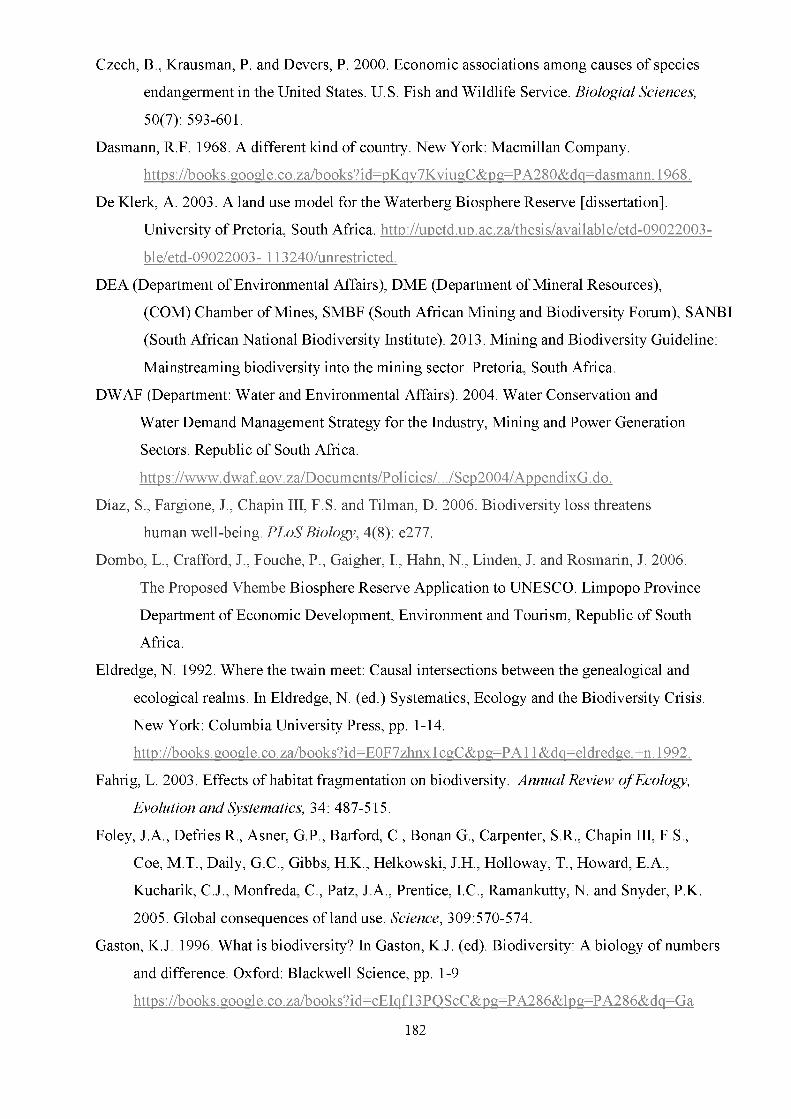
Czech, B., Krausman, P. and Devers, P. 2000. Economic associations among causes of species

endangerment in the United States. U.S. Fish and Wildlife Service. B io lo g ia l Sciences,

50(7): 593-601.

Dasmann, R.F. 1968. A different kind of country. New York: Macmillan Company.

https://books.google.co.za/books?id=pKqy7KviugC&pg=PA280&dq=dasmann,1968.

De Klerk, A. 2003. A land use model for the Waterberg Biosphere Reserve [dissertation].

University of Pretoria, South Africa. http://upetd.up.ac.za/thesis/available/etd-09022003-

ble/etd-09022003- 113240/unrestricted.

DEA (Department of Environmental Affairs), DME (Department of Mineral Resources),

(COM) Chamber of Mines, SMBF (South African Mining and Biodiversity Forum), SANBI

(South African National Biodiversity Institute). 2013. Mining and Biodiversity Guideline:

Mainstreaming biodiversity into the mining sector. Pretoria, South Africa.

DWAF (Department: Water and Environmental Affairs). 2004. Water Conservation and

Water Demand Management Strategy for the Industry, Mining and Power Generation

Sectors. Republic of South Africa.

https://www.dwaf.gov.za/Documents/Policies/.../Sep2004/AppendixG.do.

Diaz, S., Fargione, J., Chapin III, F.S. and Tilman, D. 2006. Biodiversity loss threatens

human well-being. P L o S B io lo g y , 4(8): e277.


The Proposed Vhembe Biosphere Reserve Application to UNESCO. Limpopo Province

Department of Economic Development, Environment and Tourism, Republic of South

Africa.

Eldredge, N. 1992. Where the twain meet: Causal intersections between the genealogical and

ecological realms. In Eldredge, N. (ed.) Systematics, Ecology and the Biodiversity Crisis.

New York: Columbia University Press, pp. 1-14.

http://books.google.co.za/books?id=E0F7zhnx1cgC&pg=PA11&dq=eldredge,+n.1992.

Fahrig, L. 2003. Effects of habitat fragmentation on biodiversity. A n n u a l R ev iew o f E cology,

E vo lu tio n a n d System atics, 34: 487-515.

Foley, J.A., Defries R., Asner, G.P., Barford, C., Bonan G., Carpenter, S.R., Chapin III, F.S.,

Coe, M.T., Daily, G.C., Gibbs, H.K., Helkowski, J.H., Holloway, T., Howard, E.A.,

Kucharik, C.J., Monfreda, C., Patz, J.A., Prentice, I.C., Ramankutty, N. and Snyder, P.K.

2005. Global consequences of land use. Science , 309:570-574.

Gaston, K.J. 1996. What is biodiversity? In Gaston, K.J. (ed). Biodiversity: A biology of numbers

and difference. Oxford: Blackwell Science, pp. 1-9

https://books.google.co.za/books?id=cEIqf13PQScC&pg=PA286&lpg=PA286&dq=Ga

182

https://books.google.co.za/books?id=pKqy7KviugC&pg=PA280&dq=dasmann,1968

http://upetd.up.ac.za/thesis/available/etd-09022003-ble/etd-09022003-%20113240/unrestricted

http://upetd.up.ac.za/thesis/available/etd-09022003-ble/etd-09022003-%20113240/unrestricted

https://www.dwaf.gov.za/Documents/Policies/.../Sep2004/AppendixG.do

http://books.google.co.za/books?id=E0F7zhnx1cgC&pg=PA11&dq=eldredge,+n.1992

https://books.google.co.za/books?id=cEIqf13PQScC&pg=PA286&lpg=PA286&dq=Gaston,+K.J.,+1996.%20

Guerry, D.A., Ruckelshaus, M.H., Arkema, K.K., Bernhardt, J.R., Guannel, G., Kim, C., Marsik,

M., Papenfus, M., Toft, J.E., Verutes. G. et al. 2012. Modelling benefits from nature using

ecosystem services to inform coastal and marine spatial planning. Int. J. Biodivers. Sci.

Ecosyst. Serv. Manage. 8(1-2):107-121.

Gurevitch, J, Padilla, DK. 2004. Are invasive species a major cause of extinctions? Trends in

E co lo g y a n d E vo lu tio n , 19: 470-474.

Hall, L.S., Krausman, P.R. and Morrison M.L. 1997. The habitat concept and a plea for standard

terminology. Wildlife Society Bulletin, 25:173-182.

Harper, J.L. and Hawksworth, D.L. 1994. Biodiversity: Measurement and estimation preface.

P h ilo so p h ica l T ransactions o f the R o y a l S o c ie ty o f L o n d o n B, 345: 5-12.

IUCN (International Union for the Conservation of Nature). 2004. Protected Areas

Programme. Vol 14, no 3. Protected Areas Categories. The International Journal for Protected

Area Managers. ISSN: 0960-233X. Switzerland, Nature Bureau, UK:

http://cmsdata.iucn.org/downloads/14 3lowres.pdf.

IUCN (International Union for the Conservation of Nature). 2010. About Biodiversity:

International year of biodiversity. http://iucn.org/iyb/about. Accessed in 2013.

IUCN (International Union for the Conservation of Nature). 2011a. Evolution du secteur

minier en Afrique de l’Ouest. Quel impact sur le secteur de la conservation? Ouagadougou:

UICN Programme Afrique Centrale et Occidentale: Etudes du PAPACO 10.

http://www.papaco.org/publication/mining%20study%20complete.pdf.

IUCN (International Union for the Conservation of Nature). 2011b. The West African

Protected Areas Newsletter 45. Ouagadougou: Programme Aires Protegees en Afrique de

l’Ouest. http://www.papaco.org/publication/lettreAPAO-45-0911%20ENG.pdf.

Johnson, M.D. 2007. Measuring habitat quality: A review. The Condor 109:489-504.

Koh, L.P. and Gardner, T.A. 2010. Conservation in human-modified landscapes, Chapter 13. In

Sodhi, N.S. and Erlich, P.R. (eds.) 2010: Conservation Biology for All. Oxford University

Press. http//ukcatalogue.oup.com/product/9780199554249.do.

Kovacs, K., Polasky, S., Nelson, E., Keeler, B.L., Pennington, D., Plantinga, A.J., and

Taff, S.J. 2013. Evaluating the return in ecosystem services from investment in public land

acquisitions. P L o S O NE, 8(6): e62202.

Kurdoglu, O. and £ok9aliskan, B.A. 2011. Assessing the effectiveness of protected area

management in the Turkish Caucasus. Faculty of Forestry, Karadeniz Technical University,

61080 Trabzon, Turkey. African Journal of Biotechnology. 10(75): 17208-17222.

183

http://cmsdata.iucn.org/downloads/14_3lowres.pdf

http://iucn.org/iyb/about

http://www.papaco.org/publication/mining%20study%20complete.pdf

http://www.papaco.org/publication/lettreAPAO-

La Notte, A. 2012. Mapping and valuing habitat services: two applications at a local scale.

International Journal of Biodiversity Science, Ecosystem Services and Management 8 (1-2):

80-90.

LDA (Limpopo Department of Agriculture). 2012. The mapping of agricultural commodity

production in the Limpopo Province, final report. Directorate Spatial Information Services.

Limpopo Provincial Government of South Africa, Polokwane.

[email protected].

Lindenmayer, D., Hobbs, R., Montague-Drake, R., Alexandra, J., Bennett, A., Burgman, M., Cae,

P., Calhoun, A., Cramer, V. and Cullen, P. 2008. A checklist for ecological management of

landscapes for conservation. E co lo g y L e tters, 11:78-91.

MacArthur, R. and Wilson, E.O. 1967. The theory of island biogeography. Princeton, NJ: Princeton

University Press.

Margoluis, R and Salafsky, N. 2001. Is our project succeeding? A guide to threat reduction

assessment for conservation. Biodiversity Support Program, Washington D.C.

http://www.rmportal.net/librarv/content/tools/biodiversitv-support.../download.

Marzluff, J.M., McGowan, K.J., Donnelly, R. and Knight, R.L. 2001. Causes and consequences of

expanding American crow populations. In Marzluff J.M., Bowman R. and Donnelly R.

(eds.) Avian Ecology and Conservation in an Urbanizing World. Norwell, M.A.: Kluwer

Academic, 333:365.

McKinney, M.L. 2002. Urbanization, biodiversity, and conservation. B io lo g ic a l Science, 52: 883

890.

McKinney, M.L. 2008. Effects of urbanization on species richness diversity: A review of plants and

animals. U rban E co system , 11: 161-176.

MA (Millennium Ecosystem Assessment). 2005. Ecosystems and human well-being: Synthesis,

World Resource Institute. Washington, DC: Island Press.

Morrison, M.L, Marcot B.G. and Mannan, R.W 2006. Wildlife-habitat relationships: concepts andrdapplications. 3 ed. Island Press, Washington, DC.

Mucina, L., and Rutherford, M.C. eds.) 2006. The vegetation of South Africa, Lesotho and

Swaziland. S tre litz ia 19: South African National Botanical Institute, Pretoria, South Africa.

Folia G eobotanica , 43(4): 461-463.

Munnik, V., Hochmann, G., Hlabane, M. and Law, S. 2010. The Social and Environmental

Consequences of Coal Mining in South Africa: A case study. A joint initiative of

environmental monitoring group, Cape Town, South Africa and Both Ends, Amsterdam,

The Netherlands.


184

mailto:[email protected]

http://www.rmportal.net/library/content/tools/biodiversity-support.../download

K.M., Daily, G.C., Goldstein, J., Kareiva, P.M., Lonsdorf, E., Naidoo, R., Ricketts, T.H. and

Shaw, M.R. 2009. Modelling multiple ecosystem services, biodiversity conservation,

commodity production, and trade-offs at landscape scales. The Ecological Society of

America: F ro n tie rs in E c o lo g ic a l E n vironm en t, 7(1): 4-11.

NEM:PAA (National Environmental Management: Protected Areas Act). 2003. Act no. 57:

Biodiversity policy and strategy for South Africa: Strategy on buffer zones for national

parks: For general information (Gazette No. 35020 - Notice 106). http://cer.org.za/wp-

content/uploads/2010/05/57-OF-2003 -NATIONAL-ENVIRONMENTAL-

MANAGEMENT-PROTECTED-AREAS-ACT 2.

Osti, M., Coad, L., Fisher, J.B., Bomhard, B. and Hutton, J.M. 2011. Oil and gas development in

the world heritage and wider protected area network in sub-Saharan Africa. B io d ivers ity

C onserva tion , 20: 1863-1877.

Phillips, A. 2001. Pollution, mining and protected areas. Mining, minerals and sustainable

development, no. 62. World Council for Sustainable Development. International Institute

for Environment and Development. http://pubs.iied.org/pdfs/G00554.pdf.

Polasky, S., Nelson, E., Pennington, D.N. and Johnson, K. 2011. The impact of land-use

change on ecosystem services, biodiversity and returns to landowners: A case study in the

state of Minnesota. E n v iro n m en ta l a n d R eso u rce E conom ics, 48: 219-242.

Power, A.G. 2010. Ecosystem services and agriculture: Trade-offs and synergies.

P h ilo so p h ica l T ransactions o f the R o y a l S o c ie ty B, 365: 2959-2971.

Rockstrom, J., Steffen, W., Noone, K., Persson, A., Chapin III, F. S., Lambin, E., Lenton, T.

M., Scheffer, M., Folke, C., Schellnhuber, H., Nykvist, B., de Wit, C. A. Hughes, T. van der

Leeuw, S., Rodhe, H., Sorlin, S., Snyder, P. K., Costanza, R. Svedin, U., Falkenmark, M.

Karlberg, L. Corell, R. W., Fabry, V. J., Hansen, J., Walker, B., Liverman, D., Richardson,

K., Crutzen, P. and Foley, J. 2009. Planetary boundaries: Exploring the safe operating space

for humanity. E co lo g y a n d So cie ty , 14:2-32.

Rouget, M., Richardson, D.M., Cowling, R.M., Lloyd, J.W. and Lombard, A.T. 2003. Current

patterns of habitat transformation and future threats to biodiversity in terrestrial ecosystems

of the Cape floristic region, South Africa. B io lo g ic a l C onserva tion , 112: 63-85.

SAMABNC (South African Man and Biosphere National Committee). 2014. National report on the

implementation of Madrid Action Plan. 26th Session UNESCO Man and Biosphere

Programme ICC International Coordinating Council, Sweden, 10-13 June 2014.

SANBI (South African National Biodiversity Institute). 2009. National Land Cover 2009, Pretoria,


Scholes, R.J., and Biggs, R. (eds.) 2004. Ecosystem services in Southern Africa: A

185

http://cer.org.za/wp-content/uploads/2010/05/57-OF-2003_-NATIONAL-ENVIRONMENTAL-MANAGEMENT-PROTECTED-AREAS-ACT_2



http://pubs.iied.org/pdfs/G00554.pdf

regional assessment. The Regional-Scale Component of the Southern African Millennium

Ecosystem. Council for Scientific and Industrial Research.

Soule, M.E., Wilcox, B.A., and Bruce, A. (eds.) 1980. Conservation biology: An evolutionary-

ecological perspective, Massachusetts: Sinauer.

StatsSA (Statistics South Africa). 2012. Census 2011 Statistical release-P0301.4. Republic of South

Africa, Pretoria. http://www.statssa.gov.za. Accessed in 2013.

Stolton, S., and Dundley, N. 1999. A preliminary survey of management status and threats in

forest protected areas. P A R K S 9, 27-33. Protected Areas Programme. IUCN, Gland,

Switzerland.

Stolton, S. 2010. Arguments for protected areas: Linking environment and well-being. In Stolton

S., and Dudley N., (eds.) London: Earthscan. ISBN: 978-1-84407-881-3. p. 273.

Stolton, S., Mansourian, S. and Dundley, N. 2010. Valuing protected areas. World Bank's

Global Environment Facility Coordination Team, World Bank GEF Operations.

Stuart, L., Raven, P., and Raven, P. 2000. Biodiversity: Extinction by numbers.

N ature , 403: 843-845.

Swift, M.J., Izac A.M.N. and van Noordwijk, M. 2004. Biodiversity and ecosystem services in

agricultural landscapes - Are we asking the right questions? A g ricu ltu re , E co sys te m s &

E n vironm en t, 104: 113-134.


Vigerstol, K., Pennington, D., Mendoza, G., Aukema, J., Foster, J., Forrest, J., Cameron,

D., Lonsdorf, E., Kennedy, C., Verutes, G., Kim, C.K., Guannel, G., Papenfus, M., Toft,

J., Marsik, M. and Bernhardt, J. 2011. InVEST 2.0 beta User’s Guide. The Natural Capital

Project, Stanford.

Tilman, D., Cassman, K.G., Matson, P.A., Naylor, R. and Polasky, S. 2002. Agricultural

sustainability and intensive production practices. N a tu re , 418: 671-677.

Tischendorf, L., Bender, D.J. and Fahrig, L. 2003. Evaluation of patch isolation

metrics in mosaic landscapes for specialist vs generalist dispersers. L a n d sca p e E co logy, 18:

41-50.

Turner, S.D. 2012. World heritage sites and the extractive industries.

http://www.icmm.com.document/3787.

UNESCO (United Nations Educational, Scientific and Cultural Organization). 2010. Lessonsfrom biosphere reserves in the Asia-Pacific region, and way forward. A regional review of biosphere reserves in Asia and the Pacific to achieve sustainable development, Ecological Sciences for Sustainable Development. Regional Science Bureau for Asia and the Pacific. UNESCO Office, Jakarta. http://www.unesco.org/new/en/... sciences/... sciences/.../asia-and- the-pacific.

Uttara, S., Bhuvandas, N. and Aggarwal, V. 2012. Impacts of urbanization on environment.

186


http://www.icmm.com.document/3787

http://www.unesco.org/new/en/..._sciences/..._sciences/.../asia-and-the-pacific

http://www.unesco.org/new/en/..._sciences/..._sciences/.../asia-and-the-pacific

In te rn a tio n a l J o u rn a l o f R esea rch in E n g in e e r in g a n d A p p lie d Sciences, 2:1637-1645.

van der Burg, G. 2012. The impact of coal mining on agriculture - a pilot study. Bureau for

Food and Agricultural Policy, South Africa.

http://bfap.co.za/documents/presentations/2012/Impact%20of%20Mining.

Venter, O., Brodeur N.N., Nemiroff L., Belland B., Dolinsek I.J., and Grant J.W.A. 2006. Threats

to endangered species in Canada. B io lo g ic a l Sciences, 56: 903-910.

Venter, O., Fuller R.A., Segan, D.B., Carwardine J., Brooks T., Butchart, S.H.M., Di Marco M.,

Iwamura T., Joseph L. and O'Grady D., Possingham, H.P., Rondinini, C., Smith, R.J.,

Venter, M., and Watson, J.E.M. 2014. Targeting global protected area expansion for

imperiled biodiversity. P L oS . B io lo g y , 12(6): e1001891.

WBR (Waterberg Biosphere Reserve (WBR). 2012. Ten Year Periodic Review 2001-2011.

http://www.docstoc.com/mvoffice/recommendations?docId=161286419&download.

Wilcove D.S., Rothstein D., Dubow J., Phillips A., and Losos E. 1998. Quantifying threats to

imperiled species in the United States. Assessing the relative importance of habitat

destruction, alien species, pollution, over exploitation and disease. B io lo g ic a l Sciences, 48:

607-615.

Wilson, E.O. and Peter F.M. (eds.) 1988. Biodiversity. Washington D.C.: National Academy of

Sciences/Smithsonian Institution, ISBN: 0-309-56736-X, 538 pages, 6 x 9.

http://www.nap.edu/catalog/989.html. Accessed in 2014.

187

http://bfap.co.za/documents/presentations/2012/Impact%20of%20Mining

http://www.docstoc.com/mvoffice/recommendations?docId=161286419&download

http://www.nap.edu/catalog/989.html.%20Accessed%20in%202014

5.7 APPENDICES

5.7.1: Appendix 5A: InVEST habitat quality model data requirements

5.7.1.1 Data needed to run the model

Human-modified land use/land cover (LU/LC) types such as urbanisation, cultivation and mining that cause habitat fragmentation or an edge effect (McKinney 2002; Tallis et al. 2011) were identified as threats. Table 1 presents data required to run the model. The model also uses data on habitat threat density and its effects on habitat quality; here the model considered human-modified LU/LC types that cause habitat fragmentation, edge effect, and degradation in neighbouring habitats as threats, e.g. the conversion of a habitat LU/LC to non-habitat LU/LC reduces the size

Threat Maximum distance Weight DecayCultivation 0.2 0.7 0Mines 30 1 0Urban 60 1 0Threat - the name of the specific threat.Maximum distance - the maximum distance over which each threat affected habitat quality (measured in kilometres).Weight - the impact of each threat on habitat quality, relative to other threats. Weights ranged from 1 at the highest, to 0 at the lowest.Decay - indicated whether the impact of the threat decreased linearly or exponentially across space. The value could be either 0 or 1. A value of 1 indicated a linear decline in impact,while 0 indicated an exponential decline.___________________________________________and continuity of neighbouring habitat patches. Each threat source was mapped on a raster grid, with a grid cell value indicating the presence (1) or absence (0) of a threat (i.e. crop field, etc.). Table 5.1 presents threat data used to run InVEST.

Table 5.1. Threat data used to run InVEST

5.7.1.2 The impact of threat on habitat condition

According to Tallis et al. (2011), there are four factors that determine the impact of a threat on habitat condition. The first is the relative impact of each threat. Some threats may be more damaging to a habitat, and a relative impact score quantifies this. A degradation source’s weight indicates the relative destructiveness of a degradation source to all habitats. The weight can take on any value from 0 to 1; e.g., if an urban area has a threat weight of 1 and the threat weight of roads is set to equal 0.5, then the urban area causes twice the disturbance, all else being equal, to all habitat types (Tallis et al. 2011).

The distance between the habitat and the source of the threat and between the source and the impact of the threat across space is the second mitigating factor (Tallis et al. 2011). Tallis et al. (2011) further highlight that the impact of a threat on a habitat decreases as the distance from the source of

188

degradation increases; grid cells that are in close proximity to threats will experience more impacts. The impact of a threat source on a habitat in the grid cell will partly depend on how quickly it decreases, or decays, over space. The user can choose either a linear or an exponential distance- decay function to describe how a threat decays over space (Tallis et al. 2011). In this study, an exponential decay function was applied.

The level of legal/institutional/social or physical protection from disturbance in each cell is the third factor that may mitigate the impacts of threats on habitats; if the grid cell is in a formal PA it will be represented by the value 0, but if it is completely accessible it will be assigned a value of 1. It is assumed that the more protection there is for a system acting as a barrier to degradation, the less it will be affected by nearby threats, regardless of the type (Tallis et al. 2011). According to Tallis et al. (2011), the relative sensitivity of each habitat type to each threat to the landscape is the last mitigating factor; when generating the total degradation in a cell with habitat, values closer to 1 indicates greater sensitivity. The model uses [0,1] to indicate the sensitivity of LU/LC (habitat type) to a threat; values closer to 1 indicate greater sensitivity. Tallis et al. (2011), further indicate that the more sensitive a habitat type is to a threat, the more degraded the habitat type will be by that threat.

The study applied general principles of landscape ecology and conservation biology to determine the sensitivity of a particular habitat type to degradation, following Forman (1995); Lindenmayer et al. (2008) and Tallis et al. (2011). Sensitivity weights were determined as in Tallis et al. (2011). Table 5.2 presents data showing sensitivity of the habitats to threats. Following other studies (MacArthur and Wilson 1967; Tallis et al. 2011), we considered biodiversity generally and it was assumed that human-modified landscapes (transformed habitats) surrounding natural habitats were unsuitable for species use (MacArthur and Wilson 1967; Tallis et al. 2011). In this case 0 was assigned to managed LU/LC types (transformed habitats) and 1 to unmanaged types (natural habitats). As in Tallis et al. (2011), the inputs used for the model are applicable to biodiversity in general, not specifically to a certain guild or species.

5.7.1.3 Habitat quality and degradation scores

A landscape habitat quality score was generated by summing all the grid cell scores on habitat quality, as in Tallis et al. (2011). The relationship between habitat quality and degradation scores is not linear, but depends on a half saturation function (k parameter) (Tallis et al., 2011). Again following Tallis et al. (2011), a half saturation function was used to translate the degradation score of a grid cell into a habitat quality, biodiversity model interface set k = 30. Habitat quality will decrease when a grid cell's degradation score increases (Tallis et al. 2011).

189

Table 5.2. Sensitivity of different habitat types to threats

ROWID LU/LCCODE

NAME HABITAT L_cultivation L_urban L mines

0 1 Natural 1 0.5 0.8 11 5 Water bodies 1 0.8 0.5 0.8

2 2 Cultivation 0 0 0 03 3 Degraded 0 0 0 04 4 Urban built-

up0 0 0 0

5 6 Plantations 0 0 0 06 7 Mines 0 0 0 0

190

5.7.2: Appendix 5B: Published article, C hapter 5

INTERNATIONAL JOURNAL OF BIODIVERSITY SCIENCE, ECOSYSTEM SERVIdS & MANAGEMENT, 2016V O L 12, NO. 4r 242-254httpj7dx.<k>u>rgp 10.1000/21513732J016.1217935

Habitat assessment for ecosystem services in South AfricaBasarte Claire Ntshane* and James Gambiza0

‘ Conservation Services Division, South African National Parks, Pretoria, South Africa;Department of Environmental Science, Rhodes University, Grahamstcwvn. South Africa

ABSTRACTBiodiversity is the foundation of life-support systems on earth and underpins the delivery of ecosystem services (ES) important for human well-being. The loss of biodiversity worldwide, however, remains one o f the most daunting challenges. Among the major causes of biodiversity loss is habitat loss due to transformation o f land to agricultural, mining and urban areas. We applied the Integrated Valuation of Ecosystem Services and Trade-offs (InVEST) biodiversity modelling tool to assess the condition of habitats to support the delivery of ES in a biosphere reserve (BR) in South Africa. Results Indicated that 72% of the surveyed habitats were o f high quality to provide the necessary services. However, some of the habitats were found to be affected by threats as follows: low (0-20% ) to moderate (20-32%) habitat loss was recorded in habitats adjacent to mining and plantation areas, and high (32-56%) to severe (56-95%) habitat loss was recorded in habitats in dose proximity to urban and cultivated areas. At least 56% of the vegetation types found in the study area were threatened by transformation to agriculture, mining and uiban areas. We strongly recommend that existing biodiversity policies and legislation should be enforced to avoid habitat loss and degradation.

ARTICLE HSTORYReceived 3 December 2015 Accepted 13 July 2016

EDITED BYRudolf de G root

KEYWORDSBiodiversity ecosystem services habitat InVFST; valuator

1. In traductionThe protection of biodiversity is an international obligation, with approximately 200 nations commit ting to it (CBD 1992). The term biodiversity originates from the concept of biological diversity, which was coined during the twentieth century (Dasmann 1968; Soule et al. 1980) and has been in use for almost three decades (Wilson & Peter 1988; Bibby et al. 1992; Eldredge 1992; Harper & Hawksworth 1994; Gaston 1996). There are several definitions of biodiversity (CBD 1992; MA 2005; IUCN 2010). Our study adopted the Millennium Ecosystem Assessment’s (MA) (2005) definition which is 'the diversity of life on Earth’ and ’an essential component that contribute [s] to the functioning of ecosystems that underpin the provisioning of ecosystem services (ES) that ultimately affect human well-being'. We adopted the MA definition because of its association with the supply of ES.

Sound conservation strategies are needed to effectively protect biodiversity. A protected areas (PAs) system was established with the primary goal of protecting and conserving biodiversity (IUCN 2004; Stolton 2010; Tallis et al. 2011). Despite the presence of conservation strategies such as PAs, biosphere reserves (BRs), stewardship programmes (NPEAS 2008; Stolton 2010; UNESCO 2010; Kurdoglu & Qok^allskan 2011) and the ongoing commitment of putting more land aside for conservation purposes

CONTACT Bas-ane Claire Ntshane Q daire.Ntshanegrsanparks.org O 2016 in Id find UK Limited, lading a Taylor & Franca Group

(CBD 2011; Venter et al. 2014), the increasing loss of biodiversity remains a daunting challenge facing the world at large (Gurevitch & Padilla 2004; MA 2005; Rockstrom et al 2009). Various human induced threats and forces (Chapin III et al. 2000; Diaz et al. 2006) continually alter and degrade the environment, causing habitat loss, species extinction and climate change (Wilcove et al. 1998; Stuart et al. 2000; Scholes & Biggs 2004; MA 2005; Venter et al. 2006). Among these threats are agriculture (Stolton 8c Dudley 1999; Rouget et al. 2003; Swift et al. 2004; Power 2010), urbanisation (Marzluff et al. 200h McKinney 2002, 2008) and mining developments (Brewer et al. 2003; MA 2005).

Agriculture is regarded as one of the most severe threats (Stolton 8c Dundley 1999; Rouget et al. 2003; MA 2005). Evidence suggests that agricultural activ ities might negatively affect biodiversity and ES (Swift et al. 2004; Power 2010), among others through high consumption of water (Scholes 8c Biggs 2004; MA 2005). The use of pesticides could also kill non-target organisms (Swift et al 2004; Power 2010). Other obvious adverse effects of agricultural intensification on biodiversity are the eutro phication of water systems through use of inorganic fertilizers; reduction in the diversity of organisms responsible for nutrient cycling as well as ground water pollution (Scholes 8c Biggs 2004; Swift et al. 2004; Bukolaet al. 2015).

191

I INTERNATIONAL JOURNAL OF SlODlYEfttfTY 4GE MCE, ECOSYSTEM SERVICES* MANAGEMENT @

Urbanination refers to an increase in the num ber o f cities and size o f populations (U ttara et al. 3012). A num ber of researchers have raised concerns about the impact o f urbanisation on biodiversity (Marzluff et al. 2001; McKinney 2002, 2008;, Uttara et al. 2012). Urbanisation has been found to adversely affect biodiversity7 and ES through indigenous species' extinction and habitat loss (Marzluff e t al. 2001; McKinney 2002, 2008) as well as the removal o f indigenous vegetation (U ttara et al. 2012).

Although industrial developments such as mining are seen as a quick solution to economic growth (Turner 2012), these kinds o f land use (LU) come with a cost to the natural environm ent (IUCN 201 la, 201 lb). Mining may result in habitat destruction due to removal o f vegetation (Ashton et al. 2001; Phillips 2001) and high consum ption o f water and other natural resources (Brewer et al. 2003; DWAF 2004; MA 2005). Mining activities have been found to degrade and alter both terrestrial and aquatic habi tats, causing a decline in the abundance o f indigenous species (Ashton et al. 2001; Phillips 2001). Many- w orld heritage sites and PAs around the world have been negatively7 affected by various activities related to mining (Turner 2012). IUCN (2011a, 20lib ) found that mining threatened at least 25% of PAs in W est Africa. Osti et al. (2011) found that 27% of W orld Heritage sites in Sub Saharan Africa were threatened with oil and gas mining. This situation presents a major challenge in dealing with a threat whose solution is beyond the em ploym ent o f conser vation strategies such as PAs

Perhaps what the above m entioned forms o f LU have in com m on is the effect on habitats (MA 2005; McKinney 2008; Power 2010; Uttara et al. 2012). Examples o f LU effects on habitat quality7 include various types o f pollution and vegetation removal associated with agriculture; urban developments and mining activities (Ashton et al. 2001; Czech et al. 2000; Rouget et al. 2003; Power 2010; Uttara et al. 2012). A habitat can be defined as an area's condition and re sou rce s that contribute to the reproduction and the continuous existence o f species (Hall et al. 1997; Tallis et al. 2011). The stale o f biodiversity7 in an area can be determ ined by the condition of its habitat whereas the im portance o f a habitat depends on its quality7. Habitat quality7 is defined as the environ ment s ability7 and capacity7 to provide adequate sup port and conditions to enable the persistence of species (Tallis et al. 2011).

A habitat's role regarding ES is two fold. The first role is that o f being a service itself by, for example, providing refiige for wildlife. The second role is that o f being a supporting service that underpins the delivery o f other services such as provisioning (e.g., food and water), cultural (e.g., recreation, aesthetic

quality7) and regulating (e.g. , climate regulation, flood regulation) sen7ices, according to MA's (2005) frame work. Due to the fact that the most updated classifi cations o f ES (TEEB 2010; CICES 2011) exclude the supporting sem ce category, this study adopted the MA (2005) framework because it classifies habitat as a supporting sen7ice. The MA (2005) fiirther defines ES as the bene fits that people derive from ecosystems. However, in the most recent classifications o f ES (TEEB 2010; CICES 2011), ES are defined as contri butions o f ecosystems to hum an well being. W hat is im portant to note from these definitions is that hum ans derive som ething from ecosystems for their well being. It is w orth mentioning that LU choices result in trade offs between and am ong services. For example, the conversion o f land from consen7ation to agriculture may have a negative impact on biodiver sity7 and water resources because o f the clearing of land and pollution from chemicals used to intensily agricultural production (Rouget et al. 2003; Foley et al. 2005).

If managers are to reach their biodiversity conser vation goals, they should conduct biodiversity7 condi tion/threat assessments (Margoluis & Salafsky 2001; T allis et al. 2011). Modelling and biodiversity7 assess ment, which include assessing the impacts o f LU on habitat quality7 in a given area, assist in ( l ) under standing the patterns o f distribution and richness of biodiversity7 in the landscape, (2) comparison o f p a tial patterns o f biodiversity7 an d ES, (3) identification o f synergies and trade offs across different scales and scenarios an d (4) development o f strategies for biodiversity7 con sen7 at ion (T allisetai. 2011.) Information on habitat quality allows one to make informed deci sions about different conservation strategies (Rouget et al. 2003) such as con sen7 at ion area expansion, introduction and removal of species and identifies tion o f habitats that provide high ES, as well as types o f ES provided by different habitats. Modelling is a use fill tool for assessing the impacts of threats on a suite o f biodiversity7 features and ES (Nelson et al. 2009; Polasky et al. 2011; Kovacs et al. 2013; Bhagabati e t al. 2014).

This study applied the Integrated Valuation of Ecosystem Services and Trade ofls (InVEST) biodkver shy7 habitat quality model described in Tallis et al. (2011) to assess the condition of habitat as an ES and that o f providing a supporting sem ce for the delivery o f other ES. The model combined information on LU/ land cover (LQ and threats to determine the degrada tion and extent thereof, on different habitat types in a BR. We selected InVEST because: (1) it can provide estimates o f the level and value o f ES that are provided by a given area and (2) its models are spatially explicit, with a flexible spatial resolution, thereby enabling users to address questions at different scales.

244 @ ft. C NTSHANE AND J.GAMBIZA

2. Materials and methods

2.1. Study area

A BR consists of different zones representing different kinds of LU. These indude con sedation areas repre sented in the core zones, agricultural systems and settlements represented in the buffer and transition zones of a BR. Vhembe Biosphere Reserve (VBR) is the biggest savannah BR in South Africa (SAMABMC 2014). It has a good balance of representation in terms of the main LUs such as conservation areas, human settlements, industries and other cooperatives, which included mining developments and agricultural sys terns Despite its size of 3070,000 ha, this study pur po sefully extended the VBR study area to cover the whole of the northern section of one of the two major core areas, the Kruger National Park and the whole western section up to the end of the existing BR boundary. This extension enabled us to obtain addi tional information on the status of biodiversity7 within the VBR and its most important buffer areas.

There are diverse LUs in the study area (Dombo et al. 2006). Conservation is one of the dominant forms of LU with about 1,000,000 ha of land under formal protection, including state owned land (two national parks and provincial reserves) (Dombo et al. 2006). Agricultural systems are also well represented in the Vhembe region. Human settlements are fairly well developed and the human population size is about 1,500,000 (Stats SA 2012). There is also good diversity7 of vegetation types in the study area, with more than 30 types represented (Mucina & Rutherford 2006).

2.2. invest biodiversity model

InVEST is a modelling suite that uses LU/LC patterns to estimate values and levels of biodiversity7 found in a landscape (Tallis et al. 2011). The InVEST biodiversity model 2.2.0 as described by7 Tallis et al. (2011) uses information about threats (Table 1) to biodiversity7 together with LU/LC and information on the sensitivity7 of habitat types to threats (Table 2) to produce habitat quality7 and degradation maps, which provide intbrma tion about the quality7 and degradation of different types of habitat in an area over time. The LU/LC map for the VBR was derived from a 2009 LU/LC map for South Africa (SANBI 2009) which was the most recent

T a b le 1 . Th neat da ta used t o ru n InVEST.

Threat Maximum distance W eight DecayCultivation GJ 0.7 0Mines 30 11 0Urban 60 1 0

Theat - the name of the specific threa tMaamum distance - the maximum distance over which ^ c h threat

affected habitat quality I measured in kilom etres!Weight - the impact o f each threat on habitat quality, relative to other

threats. Weights ranged from 1 at the highest, to 0, at the low est Decay - indicated whether the impact o f the threat decreased lin a rty or

exponent ial ly acrossspace. The value could be either 0 or 1. A value of 1 indicated a linear dec line in impact, while 0 indicated an exponential decline.

one at the time of our study. We selected the InVEST habitat quality7 modelling tool because it allows for a rapid assessment of the impacts of different threats and LUs on biodiversity7 and ES (Tallis et al. 2011; Guerry et al. 2012). More details regarding the InVEST biodi versity quality model are contained in Annexure A.

2.3. Running the InVEST biodiversity model

The following process was followed in this study to run the InVEST biodiversity7 model, as described in Tallis et al. (2011):

Step 1 - Creation of workspaceFor each InVEST model, including biodiversity7

and conservation, a separate workspace was created on the computer hard drive. This was followed by the creation of a folder under the workspace where all output files were stored.

Step 2 - Running the modelAfter completion of step 1, an ArcMap document

was opened followed by adding an InVEST toolbox located on the hard drive This was followed by double-clicking on the biodiversity7 InVEST toolbox which created an interface where all required values were authorised.

Step 3 Progress dialogueThe completion of step 2 brought about a dialogue

on the interface, which indicated the model running progress. After the model had been run snccessliiily, it produced either an output or an intermediate folder which contained degradation and quality7 maps with values The results were viewed on the ArcMap through an add data button (ESRI 2013). The maps attribute tables contained degradation and habitat quality values.

T a b le 1. 5 e n s itiv ity o f d if fe r e n t h a b ita t ty p e s t o th re a ts .

ROW® LU/LC CODE NAME HABITAT IL cultivation L urban L mines

0 1 Natural 1 G.5 GJ 111 5 W ater bodies t OJJ 0.5 as2 2 Cultivation 0 G 0 03 3 Degraded 0 G 0 04 4 Urban built-up 0 0 a oS 6 Plantations 0 0 a 06 7 Mines 0 G 0 0

193

INTERNATIONAL JOURNAL OF BlODR/ERSfTY SQENCE, ECOSYSTEM SERVICES & MANAGEMENT ♦ :

3. Results 3.7. Habitat quality

The distribution of habitats with high quality senAmong the seven LC types represented in the studyarea, two were regarded as natural habitats (water in relation to those with low-quality sem ce inbodies and natural areas) and five as transformed landscape is shown in Figure 1. About 72% of

habitats were of a high quality and were associahabitats (cultivation, mining, plantation, degradedand urban built up). Three of these (cultivation with natural areas. The remaining habitats were c

low quality (28%) and were found in areas unmining and urbanisation) were found to have impactson natural habitats. different LUs that excluded conservation.

&

**•

«

. v 'X

$w

Habitat quality

| Low (28%)

- i i

Figure 1. H ab itat quality in th e Vhem be Biosphere Reserve and th e northern parts of Kruger National Park study areas.

194

and 56-95% representing severe habitat loss (Figure 3).

Areas affected by habitat services loss are shown in Figure 4. Natural areas and water bodies in formal PAs and privately owned natural areas surrounding PAs had low habitat service loss. Moderate habitat service loss was recorded in areas surrounding cultivation, urbanisation, mining and plantations. Areas adjacent to mining, urban development and cultivation had high habitat service loss and severe habitat service loss was mainly recorded in areas in close proximity to cultivated areas.

246 @ B. C. NT SHANE AND J. GAMBIZA

c n H C = a H i K ilo m e ters 0 10 20 40 60 60

Figure 2. H ab itat changes in th e V hem be Biosphere Reserve and th e northern parts o f Kruger National Park study areas.

Habitat loss and degradation

The results of habitat service loss are shown in Figures 2-4 and habitat service degradation is presented in Figure 5. Figure 2 indicates that 35% of the habitat services were lost. In sharp contrast. 65% of the habitat services were intact.

We further quantified the extent of habitat service loss across the landscape as follows: low habitat loss from 0% to 20%, moderate habitat loss represented by 20 32%, high habitat loss represented by 32 -56%

195

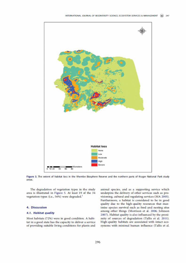
INTERNATIONAL JOURNAL O f BIODfVERSfTY SCIENCE, ECOSYSTEM SERVICES & MANAGEMENT @ 247

wm •

t S

' J

< 3tr

Habitat lossNona- . V.

M b Im • na

save aKi n m e t o r s

0 10 20

Figure 3. The extent of habitat loss in the Vhem be Biosphere Reserve and the northern parts of Kruger National Park studya i s a s

The degradation of vegetation types in the study animal species, and as a supporting service whicharea is illustrated in Figure 5. At least 19 of the 34 underpins the deliverv of other services such as provegetation types (i.e., 56%) were degraded.1 visioning, cultural and regulating services (MA 2005).

Furthermore, a habitat is considered to be in goodquailty due to the high quality resources that max

4. Discussion imise species survival such as food and nesting sitesamong other things (Morrison et al. 2006; Johnson4.1. Habitat quality 2007). Habitat quality is also influenced by the proxi

Most habitats (72%) were in good condition. A habi mity of sources of degradation (Tallis et al. 2011).High quality habitats are associated with intact ecotat in a good state has the capacity to deliver a service

of providing suitable living conditions for plants and svstems with minimal human influence (Tallis et al.

196

246 @ &. C NT SHANE AND J. GAMBIZA

Figure 4. The extent o f transformed habitats and natural habitats in the Vhem be Biosphere Reserve and the northern parts of Kruger National Park study areas.

2011). An area dominated by high quality habitats represents high biodiversity (Johnson 2007). We attributed the dominance of high quality habitats in PAs to their regulation (NE.MPAA 2003). the pre sence of deterrents and law enforcement, which in privately owned conservation areas were moderately provided (Personal observation''). Other researchers have also shown that legal protection of habitats mitigates the impacts of threats on biodiversity (Stolton & Dundley 1999; Tallis et aL 2011).

The presence of high quality habitats within con servation areas suggested that these areas had the potential to support the delivery of a suite of ES such as cultural (recreation), provisioning (medicinal plants and timber) and regulating services (Dombo et al. 2006; Stolton et al. 2010; WBR 2012). Although the habitats were generally found to be of good qual ity, they could still be vulnerable to degradation, since human pressure/threats are likely to intensify in future. This normally happens with growing demands

197

INTERNATIONAL JOURNAL OF BIODIVERSITY SCIENCE. ECOSYSTEM SERVICES & MANAGEMENT @ 249

Figure 5. The ex ten t of degradation of vegetation types in the Vhem be Biosphere Reserve and th e northern parts o f Kruger National Park study areas.

on ES due to growing human populations (Clay et al. 1994; \1A 2005). The adverse impacts of agriculture, mining and urban developments on natural ecosystems are thus expected to continue especially in developing countries where poverty and population growth are high (Tilman et al. 2002; MA 2005; NPC 2011 ) .

About 28% of the habitats were of a low quality due to anthropogenic threats. These habitats were in close proximity to mining, plantations, cultreated areas and urban settlements. Low quality habitat was attributed to habitat destruction due to removal of vegetation which is usually carried out during

implementation of different LU activities (Ashton et al. 2001; McKinney 2008; Koh & Gardner 2010). Conversion of natural systems to agriculture was found to reduce some ES (Rouget et al. 2003; Power 2010). However, low quality habitats in areas desig nated for agricultural activities were found to be doing well in delivering food provisioning services such as crops and livestock (Dombo et al. 2006; LDA 2012; WBR 2012). Nevertheless, these low qual ity habitats are poor in terms of biodiversity value (Rouget et al. 2003; Tallis et al. 2011). Low habitat quality has been associated with degraded areas (Lindenmayer et aL 2008; Koh & Gardner 2010).

198

Low habitat quality has furthermore been associated with low biodiversity' in general (Bender et al. 3003; Fahrig 3003; Tischendorf et al. 3003), since a habitat in a poor state has limited ability to provide suitable conditions for species and to support the provision of other services needed to support human well being (MA 3005).

150 @ B. t NTSHANE AND J. GAMBlZA

4.2. Habitat loss and degradation

About 35% of the habitats were lost. This resulted in loss of services associated with the provision of sui table living conditions for wildlife and with support ing the delivery of other ES. Cultivation was the greatest cause of habitat loss, followed by urbanisa tion and plantations, with mining causing the lowest impact. Other researchers have also recorded the contribution of different LUs such as agriculture (Rouget et al. 3003; Venter et al. 2006; McKinney- 2008; Ft>Lasky et al. 3011), m ining (Ashton et al. 3001; Phillips 3001) and urbanisation (Rouget et al. 3003; Venter et al. 2006; McKinney 2008; Uttara et al. 2012) to habitat loss. For example; Rouget et al. (2003) found that 30% of subtropical thicket had been transformed due to conversion of land to agri culture leading to significant loss of biodiversity7 in this global biodiversity7 hotspot.

Areas with low habitat loss fell within the core areas (represented by PAs) of the BR (Dombo et al. 2006; WBR 2012). Low habitat loss in areas repre sented by PAs means insignificant loss of habitat services such as living spaces for wildlife and gene pool protection, thus protecting species from decline. Low habitat loss in PAs provides an opportunity7 for the delivery of recreational, raw materials and a host o f regulating services, among others (Stolton et al. 2010). Low habitat loss in natural areas was not surprising since PAs are expected to be effective tools for conserving and protecting biodiversity7 (IUCN 3004; Stolton 2010; Tallis et al. 2011). Moreover, core areas are strictly protected by legisla tion and activities in these areas are highly regulated (NEMPAA 3003).

Areas that suffered significant habitat loss were surrounded by human dom inated landscapes such as urbanisation, agriculture and mining. These land scapes fall within the transition zone of the BR which caters for different LU systems (Dombo et al. 2006; WBR 2012). It is important m note that, urbanisa tion, mining and agriculture are spatially disparate LQ systems as permitted by the current LU zone management (Dombo et al. 2006; WBR 2012) and are not necessarily degraded areas. Flowever, these LUs are regarded as major threats which lead to habitat service loss and ultimately to biodiversity7

and other ES loss (Ashton et al. 2001; MA 2005; Uttara et al. 2012; Chaplin Kramer et al. 2015).

The finding of high habitat loss in areas sur rounded by urban areas confirms the conclusions of other workers who found urbanisation to be the second highest driver o f habitat loss (Czech et al. 2000; Venter et al. 2006; McKinney 2008; Uttara et al. 2012). Severe habitat loss in areas adjacent to cultivated areas confirms the findings of other studies (Stolton & Dundley 1599; MA 2005; Venter et al. 2006; Power 2010). Agriculture has been found to be the greatest cause of habitat loss in many land scapes (Rouget et al_ 2003; Chaplin Kramer et aL 2015). Habitat service loss is regarded as the main cause of extinction of species (Foley et al. 2005; MA 2005; Lindenmayer et al. 2008; Rockstrdm et al. 2009). Mining has been found to have a negative impact on biodiversity7 (Ashton et al. 2001; Brewer et al. 2003; MA 2005). South Africa is not exempted from this phenomenon (DWAF 2004; M unn iket al. 2010; van der Burg 2012). Legislation has been put in place to address the negative impacts of mining activ ities on biodiversity7 (DEA et al. 2013), although more resources need to be channelled towards implementa tion of the policies (DEA e ta l . 2013).

The finding that Makhado Sweet Bushveld was the most degraded vegetation type of the 19 vegetation types found in the study areas (Figure 5), is not surprising, as this vegetation ty7pe has been found to be hardly protected (Mucina & Rutherford 2006). Similarly, vegetation types found to have been mod erately affected by habitat loss were also at great risk, as they were poorly protected or unprotected (Mucina & Rutherford 2006). The degradation of vegetation under protection might be a result of threats such as pollution, edge effects and habitat fragmentation which are not prevented by the pre sence o f physical/legal or other types of protection (Tallis et al. 2011). Degradation of vegetation has a negative impact on the delivery of ES (MA 2005; Tallis et al. 2011).

O ur study could be compared with that of La Notte (2012) with regard to the use o f environmental indicators such as habitat sensitivity7 to threats and the impact of human pressure on habitats, as well as the application of the mapping approach. However, thorough comparison of La Notte (2012) and our findings was difficult due to the following differences. First, La Notte (2012) used the Benefit Transfer (BT) technique to value the services, we used InVEST. Second, it valued services in monetary7 terms; in our study services were valued in biophysical terms. Lastly, our study assessed and mapped habitats for ES in response to hum an pressure such as urbanisa tion, mining and cultivation. La Notte "s (2012) study valued and mapped habitat services using three

199

INTERNATIONAL JOURNAL OF BlODfYEKITY SCIENCE. ECOSYSTEM SERVICES &■ MANAGEMENT (* ) 251

different indicators (ecological value, ecological sen sitivkty and human pressure).

Our results demonstrated that the InVEST habitat ■quality model is use till because of the following rea sons. First, it has the ability7 to characterise the sensi tivity of habitats types to various threats. Second, it takes into account the different impacts of threats on habitats. And third, it allows estimation of the relative impacts of one threat over another. Guerry et al. (3012) highlighted other advantages of the InVEST tool which included its applicability to marine syv terns to evaluate different effects of management practices on the delivery of ES. InVEST. however, has some drawbacks and therefore should be applied with caution as it does not provide detailed species occurrence data. It also provides some difficulties for modelling changes in the occurrence of multiple spe ties, their persistence or vulnerability under future conditions.

5. ConclusionsWe demonstrated the contribution of anthropogenic threats to habitat loss. Habitat loss often followed a pattern with more degradation found in human dominated systems than in natural systems such as conservation areas. Although PAs systems are still crucial for preserving and protecting biodiversity, they are vulnerable to threats. Human induced impacts resulted in loss of habitat service and degra dation that negatively affected the delivery of other ES. There were trade offs between human induced LUs and biodiversity7 conservation.

LUs such as urbanisation, agriculture and mining should find ways to accommodate biodiversity7 con servation. Strategies should be put in place to inform management of vegetation types that are threatened by degradation. Habitat condition assessment is highly recommended to serve as a basis for assessing delivery of ES and for informing LU planning.

Note

I. T ilt affected Vegetation types Were Granite Lowveld Bushveld, Gravellote Rocky Bushveld, Atakliado Sweet Bushveld, Roodeberg Bushveld, Tzaneen Sour Lowveld, Polokwane Plateau Bushveld, Lowveld Rugged Alopane Veld, Tsende Alb pane Veld, Atrnabolo Mountain Bushveld, Northern Mistbelt Forest, Woodbush Granite Grassland, Soutpansberg Mu on Li in Bushveld, Musina Mopane Bushveld, Soutpansberg Summit Sourveld, Strydpoort Summit Sourveld, Subtropical Alluvial Vegetation, LimpOpO Ridge Bushveld, Lim pO pO Sweet Bushveld and Makuleke Sandy Bushveld. Of these, Atakliado Sweet Bushveld Was found to he most degraded. Moderate degradation was recorded in Roodeberg

Bushveld, Polokwane Plateau Bushveld, Mmabolo \to un tain Bushveld, Northern Mistbelt Forest Soutpansberg Mountain Bushveld, Tzaneen Sour Lowveld, Musina Mopane Bushveld, Woodbush Granite Grassland and Gravellote Rocky Bushveld. Low degradation Was recorded in the following vegetation. types; Granite Lowveld Bushveld, Lowveld Rugged Mopane Veld, Tsende Mopane Veld, Soutpansberg Mountain Bushveld, Strydpoort Summit Sourveld, Subtropical Alluvial Vegetation, Limpopo Ridge Bushveld, LimpOpO Sweet Bushveld and Makuleke Sandy Bushveld. Despite the fact tliat some of the Vegetation types are well protected Such as Musina Mopane Bushveld and Limpopo Ridge Bushveld, they are Still affected by degradation

Disclosure statement

No potential conflict of interest was reported by the authors.

References

Ashton PI, Love D, Mahachi H, Dirks PHGM. 2001. An overview of the impact of mining and mineral processing operations On water resources and Water quality in. the Zambezi, Limpopo and Olifrints catchments in Southern Africa breaking new ground: mining, minerals and Sustainable development The report of the MM5D Project. London Earthscan, 2002. (cited 2013], Available from: http:ffww w. iied orgfmmsd fmmsd_pdfs

Bender DJ, Tischendorf L, Falirig L. 2003. Evaluation o f patch isolation metrics for predicting animal movement in binary landscapes. Landscape EcO. IS: I 7-39

Btiagabati NK, Rickets T, Sulistyawan TB5, Conte Al, F,nnaanay D, I Indian O, Atckenzie r„ Olwero N, Rosen dial A, Tallis H. Wolny S. 20M. Ecosystem services reinforce Sumatran tigjtr conservation in land use plans. Biol Conserv. 169:147-156.

Bibby CJ, Collar NJ, Crosby Mf, Heatb AtF, Irnboden C, Johnson TH, Long AJ, Stattersfield A], Thirgpod SJ. 1992. Putting biodiversity On the map: priority areas for global conservation International council for bird preservation. Trends Ecol EvoluL 8:1-37.

Brewer D, Dennis D, Fry G, Atdton D, Dambaclter J, Van der Velde T, Alan son F, Heales D, Kuutsoukos A, Skewes T, et al. 2003. Assessment o f mine impacts on Liliir Island Fish communities with an estimation o f the potential fisheries resources. Brisbane: Commonwealth Scientific and Industrial Research Or^inisation.

Bukula D, Zaid Al, Olalekan FI, Faldo A. 2013. Consequences of anthropogenic activities On fish and the aqua he environment. Poult Fish Wddl 5ci. 3:2.

CBD (Convention on Biological Diversity). 1992. Nairobi final act o( Lhe conference for Lhe adoption of the agreed tev tof the convention on biological diversity. SectionIX United Nations Environmental Programme; Nairobi, Kenya, cited 2013. Available from: httpsi/fwwW.cbd.intf docfha nd bookfebd -h b-09-en .pdf

CBD (Convention on Biological Diversity). 2011. Conference o f the Parties Decision X/2 Strategic Plan for Biodiversity 2011-2020. [cited 2014]. Available from: lit tp: ffWW w. cLhI in tfdecl slo rtfeopf? id

Chapin III FS, Zaveleta ES, Eviner VT, Naylor RL, Vltousek PAL Lavorel 5, Reynolds HL. Hooper DU, Sala Or,

200

http://wwW.cbd.intf

Hobbie ST, et al. 201"!C. Consequences of changi[g biotic diversity. Nature. 405:234-242.

Chaplin-Kramer R, Sharp RP, Mandie L, Sim 5, Johnson J, Isabela Butnar I, Canals b LM, ELclkelbergera BA, Van Rarnlerd I, MuelLerb C, f t iJ. 2015. Spatial pattern* o f jgriLiiitural expansion determine impacts On bhkdiver- slty and Carhon Storage. PnaS. I 12:7402-7407.

CICES (.Common International Classification of Ecosystem Services). 2011. European environment agency: paper prepared for discussion at the expert meeting On ecosystem accounts organised by Lhe UNSD, the EE A and tike World Bank, London, December 20M. Prepared by: Roy Haines-Young and Marion Potschin, Centre for Environmental Management; UK: University o f Nottingham.

Clay DC. Guido M, Wallace 5 IW4. Population and. land degradation: environmental and natural resources policy arid training project, Madison, WL Departments o f Agricultural Economics arrd Sociology, Geography, and Resource Development MidiLgan State University. USA, ISSN 1072-9496. [cited 2014]. Available from: htlp://pdf. u said, go F/pdf_docs/PNABW661. PDP

Ctech B, Kraus man P, DeverS P. 2000. Economic associations among Causes of Species endangerment in the United States. U.5. fish and wildlife service. Bird ScL. 50593-601.

Dasmann RP 1968. A Different Kind of Country [Internet]. New York (NY): Macmillan Company, [cited 2014], Available from: https / / books googje co .2a/books? id =p_ Kqy7Kv iugCfltpg- PA2 SO&dq -das man n ,+ rf ,+ 1968,

DEA (Department o f Environmental Aftiklrs), DME (Department o f Mineral Resources),(COM) Cliamber of Mines, 5MJ1E (South African Mining and Biodiversity Forum), SANBI (South African National Biodiversity Institute). 2013. Mining and biodiversity guideline: mainstreaming biodiversity into tike mining sector. Pretoria: T ypo Colour Specialists cc.

Dial S, FargiOne J, Chapin ]]] PS Tdman D. 2006. Biodiversity loss threatens human well-being PLoS Biol. 4:e277.

Dombo L, Crafford J, Fouche P. Gaiglker I. Hahn N, Linden J, Rosmarirt J. 2006. Tike proposed Vhembe biosphere reserve application to UNESCO. Limpopo province department of economic development Republic o f South Africa: Environment and Tourism.

DWAF (Department: Water and Environmental Affairs). 2004. Water conservation and Water demand management Strategy for the industry, mining and power generation sectors. Republic of South Africa, cited 2013. Available from: https://wvrw.dwsf.g0v.2a/D 0cuments/ Policies/. . ./Sep2004/AppcndixG.do

Eld red gr N. 1992. W Ike re tike twain m eet causal intersections between the genealogical and ecological realms. Trr Eldredge, editor. Systematics, ecology and tike bhkdiver- sity crisis. New York (NY): Columbia University Press; p. 1 — 14. [cited 2014], Available from: https//books.goo gle.co.2a /books? id - E0F7 2hn Jt I cgCfitpg- PA I I Stdg- eld redge, + rt.,+ 1992

E5R1 (Environmental Systems Research Institute!. 2013. ArcGIS for Desktop. Advanced Student Edition, Version 10.2. Redlands (CA): ESRI.

Falirig L 2003. Effects o f Itabitat fragmentation On biodiversity. A m u Rev Ecol Evol Syst. 34:487-515.

Foley JA, De fries R, Asner GP, Barford C, Bonan G, Carpenter SR, Chapin 111 PS, Coe MT, Daily GC, Gibbs HK, e t al. 2005. Global con sequences o f land use. Science. 309570-574.

152 @ B. C NTSHAUE AND J. GAMBlZA

Gaston KJ. 1996. What is biodiversity? In: Gaston KJ, editors. Biikdiversity: a biology o f numbers and difference. Oxford: Blackwell Science; p. 1-9. [cited 2013], Available from h ttps//bo oks. go ogltco ja/bookj?H *eE [qfl2 PQScCSp g« PA286EtLpg-PA28fi&dq=GaStOn,t K.J.. + 1996

Guerry DA, RuckelslkauS MH, Arkema KK, Bernhardt ]R. Guannel G, Kim C, Marsik M, Papenfus M, Toft JE VeruteS G, et al. 2012 Modelling benefits from nature using ecosystem services to inform coastal and marine spatial planning Int ] Biodivers ScL Ecosyst Serv Manage. 8:107-121.

Gurevitch J, Padilla DK. 2004. Are invasive pecies a major cause of extinctions? Trends Ecol Evol. 19:470-474.

Hall LS, Kraus m an PR, Morrison ML 1997. Tire h a b ita t C O nC eptand a p le a for Standard te rm in o lo g y . Wild! Soc Bull. 25:173-182.

Harper JL, Hawksworth DL. 1994. Biikdiversity: measurement and estimation preface. PhdoS Trans R Soc Lond B. 345:5-12.

IUCN (International Union for the Conservation of Nat urel. 2004. Protected Areas Programme. Vol 14, no 3. Protected Areas Categories. Tike It; ter national Journal for Protected Area Managers. ISSN: 0960-233X1. Swi tier land, Nature Bureau, UK. [cited 2013], Available from ht tp//cm sda ta. iucn.org/downkkads/l4_3lowreS.pdf

IUCN (International Union for the Conservation o fNature). 2010. About Biodiversity:!nternational year o f biikdiversity. [cited 2013], Available from: h ttp //Leen. O rg /Lyb /abou t

IUCN (International Union for the Conservation o fNature). 2011a. Evolution du Secteur minier en Afrique de 1'OueSL Quel impact Sur le Secteur de la conservation? Ouagadougou: UICN Ptogramme Afrique Centrale et Occidentaie: Etudes du PAPACO 10. [cited 2013], Available from: http://w w w .papaco.org/publication/ mLningfe20study9fc20complete.pdf

IUCN (International Union for the Conservation o fNature). 2011b. Tike West African Protected AreasNewsletter 45. Ouagadougou: PrOgamme Aires Protegees en Afrique de I'OueSt. [cited 2013], Available f to m : h ttp : //WW wpapaCO.org/pu bl Lea tion /lettre APAO- 45-0911 %20ENG.pdf

Johnson MD. 2007. Measuring habitat quality: a review. Tike Condor. 109489-504.

Koh LP, Gardner T A. 2010. Conservation in hum an-m od- Uied landscapes, Chapter 13. In: Sikdlki NS, Erlich PR, editors. Conservation biology for all. Oxford University Press, [cited 2014], Available from http://ukcatalogue. Ou p.com /prikduct /97B0199554249.do

Kovacs K, Polasky 5, Nelson E, Keeler BL, Pennington D. Plantinga AJ. 2013. Evaluatug the return in ecosystem services from investment in public land acquisitions. PLoS One. 8:e62202

KurdogluO, Qok^aliskan BA. 2011. Assessing the effectiveness o f protected area management in tike turkish Caucasus. Faculty of forestry, karadenil technical university, 61080 TrabiOn, Turkey. Afri ] Biotechnol. 10:1720817222.

La Notte A. 2012. Mapping and valuing IkabLtat services: two applications at a local scale. Int ] BiikdiverS 5ci Ecosyst Serv Manage. 8:80-92

LDA (Limpopo Department o f Agriculture). 2012 Tike mapping of agricultural commodity production in the Limpopo Province, final report. Directorate Spatial Information Services. Limpopo Provincial Government of South Africa, Polokwane. Available from: gisreques t (Sagrie.lLmpOpO.gov. ia

201

https://wvrw.dwsf.g0v.2a/D0cuments/

http://www.papaco.org/publication/

http://ukcatalogue

INTERNATIONAL JOUKUALQF BIODIVERSITY SOEMCE, ECOSYSTEM SERVICES^ MANAGEMENT @ 155

Lindenmayer D, Hobbs R, Montague-Drake R, Alexandra ], Bennett A, Burgman M, Cae R, Calhoun A, Cramer V, Cullen F. 2008. A olieckiist for ecological managementof Landscapes for conservation. Ecol Lett. 11:73-91.

MA (Millennium Ecosystem Assessment). 2005-. Ecosystems acid human well-being: synthesis, world resource institute. Washington, DC’: Island Press.

MargoluiS R, Salatsky N 2001. Is Our project Succeeding? A guide to tlimat reduction assessment for conservation. Biodiversity Support Program, Washington D.C. (cited 2014], Available from: http:Zfwww.rmpOrtaL.nctfLibrary/ con ten tf tools /biodiversity-support.. ./download

Mar duff JM, McGowan KJ, Donnelly R Knight RL 2001. Causes and consequences of expanding American Crow populations. In: Marzluff JM, Bowman R, Donnelly R editors. Avian ecology and conservation in an urbanizing WOrLcL Nor well (MA): K Lower Academic; p. 333-365.

McKinney ML 2002. Urbanization, biodiversity, and conservation. Biol ScL 52:383-390.

McKinney ML 2008. Effects of urbanization Ort Species richness diversity a review of plants and animals. Urban Ecosyst. 11:161—176.

Morrison ML, Marco t EG, Mann an RW. 2006. Wildlife- habitat relationships: concepts and applications. 3rd ed. Washington, DC: Islarid Press.

Mucina L, Rutherford MC, editors. 2006. Tlie vegetation o f South Africa, Lesotho and Swaziland. Strelitzia 19: South African national botanical institute. Pretoria South Africa Folia Geobot. 43:461 -463.

Munnik V, Hochmann G, HLabane M, Law S. 2010. Tlie social and environmental consequences o f coal mining in South Africa: a case study. A joint initiative of environmental monitoring group, Cape Town, South Africa and Both Ends. Amsterdam.

Nelson E, Mendoza G, Regetz J, Polasky S, Tallis H, Ricliard Cameron D. Chan KM, Daily GC, Goldstein J. Kareiva PM, et al. 2009. Modelling multiple ecosystem services, biodiversity conservation, commodity production, and trade-offs at landscape Scales. Front Ecol Environ. 7:4-11.

NEAtFAA (National Environmental Management: Protected Areas Act). 2003. Act no. 57: Bitidivcrsitypolicy and strategy for South Africa: Strategy On buffer zones for national parks: Tor general information (Gaartte No. 35020 - Notice 106). Available from: http://cCT.org.za/wp-eontcnL/uploads/20IO/ O5f57-Or-2003-N.ATION.AL-ENVIRONMENT.AL- M ANAGEMENT-PROTECTTED-AR EA5-ACT_2

NPAES (National Protected Area Expansion Strategy for South Africa). 2008. Priorities for expanding the protected area network for tlie ecological Sustainability and dim ate change adaptation. Government of Soutli Africa. Pretoria, ISBN 978-1919976^55-6. Available from: h tip S: / / WW w.en Vi rO nmen t.gOv.Za/sites/defa ult/fdes /does/ rtationalp rOtected_areaScxpan sion_S trategy.pd f

NPC (National Planning Commission). 2011. National Development Plan-Vision for 2030 (November 2011). Republic of South Africa 15 BN:978-0-621^10475-2, RP270/20II. Available from: http:f/www.govza/issues/ nat ional-develop me nt-p Ian -2030.

Osti M. Coad L. Fisher JB, Bomliard B. Hutton JM. 2011. Oil and gas development in the world Heritage and wider protected area network in Sub-Saharan Africa. Biodivers Conserv. 20:1S63-I S77.

P LiilLipS A 2 DO ]. Pollution, m ini ng and protected area S. Min Lrxg, minerals and Sustainable development, no 62. World Conned for Sustainable Development International

Institute for Environment and Development. |dted 2013], Available from: ht^j://pubsiiedorg/pd(s/G005S4pdf

Polasky 5, Nelson E, PermingLO] DN, Johnson K. 20] ]. Tlie impact of land-use charge on ecosystem services, biodiversity and returns to landowners: a Case Study in the State of Minnesota. Environ Resour Econ 43:219-242.

Power AG. 2010. Ecosystem services and agriculture: tradeoffs and synergies. Plid Trans R Soc. 3652959-2971.

RockstrOm J, Steffen W, NoOne K, PerSSOn A, Chapin ]]] PS, Lam bin E, LentOn TM, Scheffer M, FoLke C, Sclie llnh ube r H, et al. 2009. Planetary boundaries: exploring the Safe Operating Space for humanity. Ecol Soc. 142-32. cited 2013. Available from: http:f/www. ecology andsociety .Org/vol 14/i ss2/a rt32 /

Rouget M, Ricliardson DM, Cowling RM, LLoyd JW, Lorn bard AT. 2003. Cur re nt pat te rrt S O f liab iLat Lra ns for - m at inn and future tli reals to biodiversity in terrestrial ecosystems of the Cape floristic region, South Africa. Biol Conserv. 11263-35.

5.AM.ABNC (Soutli African Man and Biosphere National Committee). 2014. National report On the implementation of Mad rid act ion plan. 26th SeS Sion LTNE5C O Ma n and Biosphere Programme ICC International Coordinating Council; Sweden; 2014 Jun 10- 13L Pretoria Department of Environmental Affiirs.

SANBI (Sou tli African National Biodiversity InSLiLue).2009. NaLlOnal land cover 2009. Pretoria: Republic o f South Africa.

Scholes RJ, Biggs R editors. 2004. Ecosystem services in Southern Africa a regional assessment. Tlie regional- scale component of the Southern African mi 11 enni uni ecosystem. Pretoria Council for Scientific arid Industrial Research.

Soule ME, Wilcox BA, Bruce A, editors. 1930. Conservation biology: an evolutionary-ecological perspective. Massachusetts: Sirtauer.

Stats SA (Statistics South Africa). 2012 Census 2011 Statistical release-P0301.4. Available frortc http//wWW. statssagovza.

Stolton S. 20] ft. Arguments for protected areas: Llnkirg environ mart and well-being. Stolton S, Dudley N, editors. London: Earth scan; p. 273. ISBN: 973-1-34407-S31-3.

S toltOn 5, Dundley N. 1999. A preliminary Sur vey of tm nage- ment statu sand threats in fores t pro tected area s. PARKS 9, 27-33. Gland: Protected Areas Programme. IUCN.

SLoltOn S, ManSOurian S, Dundley N. 2010. Valuing protected areas. Washington (DC): World Bank’s Global Environment Facility Coordination Team, World Bank GEF Ope ratio ns.

Stuart L, Raven P, Raven P. 2000. Biodiversity extinction by numbers. Nature. 403:34 3-345.

Swiff MJ, Izac AMN, van Noordwijk M. 2004. Biodiversity and ecosystem services in agricultural landscapes - Are we asking the right questions? Agric. Ecosyst Environ 104:113-134.

Tallis HT, Ricketts T, Guerry AD, Nelson E, Ennaanay D, Wolny 5, Olwero N, Vigorstol K. Pennington D. Mendoza G, et al. 201 I. InVEST 20 beta User's Guide. Stanford: Tlie Natural Capital Project, Stanford, (cited 2011], Available from: httpwwWnatura[capitaIprojecL Org/p ubs /In VE5T_2. Dbcta_U serS_Cu Ltlc .pdf.

TEEB (The Economics of Ecosystems and Biodiversity)2010. Chapter I: Integrating the ecological and economic d imen sio ns in biodiversity and ecosystem services Valuation. Available from: http://wwW.teebweb.org/wp- COntent/upload/20l3/0l4/D0-Cliapter- I .

202

http://www.rmpOrtaL.nctfLibrary/

http://cCT.org.za/wp-eontcnL/uploads/20IO/

http://www.govza/issues/

http://wwW.teebweb.org/wp-COntent/upload/20l3/0l4/D0-Cliapter-

http://wwW.teebweb.org/wp-COntent/upload/20l3/0l4/D0-Cliapter-

Tliman D, Cass mail KG, Ma tson P A, Nayio r R, Pola sky S. 2nn2. Agricultural Sustainability and intensive production practices. Nature. *113:671-677.

T i s c h e n d o r f L B e n d e r D J . F a l i r i g L . 2003. E v a l n a t i o n o f p a t c h i s o l a t i o n m e t r i c s in m o s a i d a n d s c a p e s t o r s p e c i a l i s t

VS g e n e r a l i s t d i s p e r s e r s . L a n d s c a p e E c o . I B:41 —50.Turner $D 2012. World heritage sites and the extractive

industries. Available from: littpS://cmsdataiuCnOrg/dowrt load s/ whs_and_extractive_indu stries_20_j un_ 12 .pdf

LtNESCO (United Nations Educational, Scientific and Cultural Organization). 2010. Lessons from biosphere reserves in tlie Asia-Pacific region, and way forward. A regional review of biosphere reserves in Asia and the Pacific to achieve Sustainable development, Ecological Sciences for Sustainable Development. Regional Science Bureau for Asia and the Pacific: UNESCO Office, Jakarta. Available from: http:ffwWw.unesco.org/rtewf en/_ —sciences/., .sciences/.. 7asia-and-the-paeific_

L Tt t a r a S, B I il iv a n d a S N , A g g a rV v a l V . 2012. I m p a c t s o f u r b a n i z a t i o n o n t h e e n v i r o n m e n t I n t J R e s E n g A p p l

SCL 2: 1637- 1645.van der Burg G 2012. Tlie impact of coal mining on

agr icultu re-a pilot Study. Bureau tor Food and Agricultural Policy, South Africa. [cited 2013],

251 © B. C NTSHAhE AND J. GAMBIA

Available from: htip://bfap.co.zafdocumentsfpresenta Lion s/201 2 flmpact %20of%20Mi ning

Venter O, Brodeur NN, Nemiroff L, Belland B, Dolinsek IJ, Grant JWA. 2006. TlireatS to Cndargered Species in Canada. Biol Sci. 56:003-910.

Venter O, Fuller FLA, began DB, CarWafdine J, Brooks T, Butchart SHM, Di Marco M, Iwamura T, Joseph L, O’Grady DO. et al. 2014. Targttirtg global protected area expansion for imperiled biodiversity. PLoS Biol. I2:e 1001891.

WBR (Waterberg Biosphere Reserve). 2012 Ten year periodic review 2001-2011. feited 2012], Available front http:/f www.docstoc.com/myofficefrecom mendations? docld-16 12 36419&down load

Wilcove DS, Roths te in D, Dubow J, Pliillips A, Losos E 1998. Quantifying threats to imperiled species in the United States. Assessing tlie relative importance of liabi- tat destruction, alien species, pollution, over exploitation and disease. Biol ScL 48607-615.

Wilson EG, Peter FM, editors. 1988. Biodiversity. Washington D.C.: National Academy of Sciences/ Smithsonian Institution. ISBN: 0-309-56736-X, 538pages, 6 x 9 . feited 2014], Available from: htlp:ffwww. nap.ed u/ca ta logf989. htm l

203

http://wWw.unesco.org/rtewf

http://www.docstoc.com/myofficefrecom

CHAPTER 6

ABOVE-GROUND CARBON STORAGE ASSESSMENT IN A SOCIO- ECOLOGICAL

SYSTEM: A CASE STUDY FROM SOUTH AFRICA

This chapter is intended for submission to the journal E co sys tem S erv ices as Ntshane B.C andGambiza J.

Abstract

The Millenium Ecosystem Assessment (2005) found that at least 15 ecosystem services were in a

poor state; among those were regulating services, which included climate regulating services (i.e.

carbon storage and sequestration). One of the major consequences of the degradation of climate

regulating services is climate instability. Since climate instability is of global concern, successfully

stabilizing it requires global cooperation. In response to this need, countries came together and

established the United Nations Framework Convention to Combat Climate Change and the Kyoto

protocol. To comply with these commitments successfully, information on among others carbon

stocks is required. I applied the Integrated Valuation of Ecosystem Services and Trade-offs

(InVEST) to quantify and map carbon stored in an above-ground pool in four land cover types

(natural forest, cultivated areas, plantations and degraded areas) in two socio-ecological systems in

South Africa. I recorded some variations in terms of carbon storage per land cover type in the two

study sites under analysis, Vhembe and Waterberg socio-ecological systems. In Waterberg socio

ecological system, the total above ground (TAG) carbon storage was as follows: natural forest

contained 70%, cultivated areas 25%, degraded areas 4% and the lowest stocks (1%) were found in

plantation areas. On the other hand, the Vhembe socio-ecological system had TAG carbon storage

of 64% in natural forest, 30% in plantations, 5% in degraded areas and 1% in cultivated areas. In

terms of carbon storage in vegetation, the savanna biome had the highest storage, followed by

grassland, forest and azonal vegetation respectively. The results further suggested that there is no

correlation between vegetation types in terms of its protection status and carbon storage. This study

recommends wide-ranging assessments of this nature in SA to inform climate change decision

making.

Key words: Climate change; Millenium Ecosystem Assessment; Convention on Climate Change;

ecosystem services; Kyoto protocol; InVEST

204

6.1 INTRODUCTION

The Millenium Ecosystem Services Assessment (MA) (2005) found that at least 15 ecosystem

services (ES) were in a poor state, among them regulating services. Following the MA's (2005)

classification of ES, regulating services include regulation for natural disasters and climate

regulation (by carbon (C) storage and sequestration). In Southern Africa, on top of regulating

services, provisioning services such as water, wild products (food and medicinal resources) and

fodder, as well as some of the cultural ES, among others, are being subjected to degradation

(Schackleton et al. 2008).

Ecosystems regulate the earth's climate by adding and removing greenhouse gases (GHG) from the

atmosphere (Tallis et al. 2011). Ecosystems collectively store more C than the atmosphere (Lal

2004). By storing the terrestrial carbon, ecosystems keep carbon dioxide (CO2) out of the

atmosphere where it would contribute to climate change (Tallis et al. 2011). A significant amount

of C is stored in living organisms and their dead, undecomposed or partially decomposed remains

in soil, on the sea floor or in sedimentary rock. Global atmospheric concentrations of GHG, CO2,

methane (CH4) and nitrous oxide (N2O) have increased dramatically as a result of human activities

(MA 2005; DEAT 2004; IPCC 2007). The increase in CO2 is mainly due to the use of fossil fuel,

while the increase in N2O is attributed to land use change due to agriculture (IPCC 2007). Tropical

deforestation currently accounts for approximately one fifth of the net increase in atmospheric CO2

(IPCC 2007). The emissions of GHG are predicted to grow in future despite practices of sustainable

development (IPCC 2007).

Clearing of forests contribute to C emissions (IPCC 2007). Increasing concentrations of C

emissions in the atmosphere contribute to climate change, which affects human well-being through

adverse impacts on the availability of fresh water, food production and the distribution and seasonal

transmission of vector-borne infectious diseases (MA 2005; IPCC 2007). Climate change is

therefore regarded as a threat to sustainable development that could undermine poverty alleviation

efforts, with implications for ES (MA 2005). If nothing is done to address the current levels of

GHG emissions, climate change could become the greatest environmental problem to hit the 21st

century, with some of its impacts highly likely to be irreversible (MA 2005; IPCC 2007).

In response to the challenges posed by climate change, countries came together and established the

United Nations Framework to Combat Climate Change (UNFCCC) in 1992 and the Kyoto Protocol

in 1997. In response to these global obligations, countries are required to develop climate change

response policies that will inform mitigation and adaptation strategies, including C emission

205

reduction, activities regarding C sequestration, C accounting and land use planning (Archard et al.

2004; Naidoo et al. 2008; Law et al. 2015; DEA 2015).

South Africa (SA) is a significant emitter of GHG, ranking among the world's top 15 energy

intensive countries (DEAT 2004). As a signatory country, SA has to comply with the requirements

of the UNFCCC and the Kyoto protocol. To implement its climate change response policy

successfully, SA has to understand the impact and magnitude of climate change (DEA 2015). In

order to inform the required understanding, information on C stored in the ecosystems is required as

a baseline and to inform climate change mitigation strategies (DEA 2015). Carbon is stored in four

fundamental pools: soil and dead organic matter, below ground and above ground (IPCC 2007;

Tallis et al. 2011). Forests, including tree plantations, are major sinks of atmospheric C (IPCC

2007).

Several studies that have been undertaken to estimate and map C stocks in SA focused mainly on

soil and vegetation in general (Rouget et al. 2004; Mills et al. 2005; Egoh et al. 2008). This study

aimed at assessing C stored in an above-ground pool in SA. The main objectives were (1) to

estimate the amount of C stored in land cover and vegetation types (2) to map C stored in land

cover and vegetation types; and (3) to assess the relationship between C storage and vegetation

type. Understanding C dynamics in different land cover types was also crucial to inform

management decisions and climate change mitigation assessment (Birdsey et al. 2006; IPCC 2007;

DEA 2015).


6.2.1 Study areas

The study areas were located in Limpopo, one of the nine provinces in SA. Limpopo covers five

district municipalities: Capricorn, Vhembe, Waterberg, Sekhukhune and Mopane. The criteria for

study area selection were as follows: (1) it had to be a district municipality; and (2) it had to contain

a biosphere reserve (BR). On the basis of these criteria, within Limpopo Province, two district

municipalities, Waterberg and Vhembe, met the requirements. Waterberg is the largest (49 504

km ) of the five district municipalities in the province and hosts Waterberg Biosphere Reserve

(WBR). Vhembe covers 21 349 km and hosts Vhembe Biosphere Reserve (VBR). To make

comparisons feasible, the Vhembe area was extended to cover parts of Capricorn and Mopani

district municipalities. For the purpose of this analysis, the Waterberg area will be known as the

Waterberg socio-ecological system (WSES) and also as Waterberg study area and the Vhembe

206

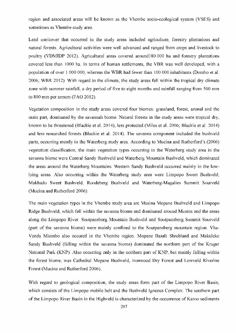
region and associated areas will be known as the Vhembe socio-ecological system (VSES) and

sometimes as Vhembe study area.

Land use/cover that occurred in the study areas included agriculture, forestry plantations and

natural forests. Agricultural activities were well advanced and ranged from crops and livestock to

poultry (VDMIDP 2012). Agricultural areas covered around180 000 ha and forestry plantations

covered less than 1000 ha. In terms of human settlements, the VBR was well developed, with a

population of over 1 000 000, whereas the WBR had fewer than 100 000 inhabitants (Dombo et al.

2006; WBR 2012). With regard to the climate, the study areas fell within the tropical dry climate

zone with summer rainfall, a dry period of five to eight months and rainfall ranging from 500 mm

to 800 mm per annum (FAO 2012).

Vegetation composition in the study areas covered four biomes: grassland, forest, azonal and the

main part, dominated by the savannah biome. Natural forests in the study areas were tropical dry,

known to be threatened (Blackie et al. 2014), less protected (Miles et al. 2006; Blackie et al. 2014)

and less researched forests (Blackie et al. 2014). The savanna component included the bushveld

parts, occurring mostly in the Waterberg study area. According to Mucina and Rutherford’s (2006)

vegetation classification, the main vegetation types occurring in the Waterberg study area in the

savanna biome were Central Sandy Bushveld and Waterberg Mountain Bushveld, which dominated

the areas around the Waterberg Mountains. Western Sandy Bushveld occurred mainly in the low-

lying areas. Also occurring within the Waterberg study area were Limpopo Sweet Bushveld,

Makhado Sweet Bushveld, Roodeberg Bushveld and Waterberg-Magalies Summit Sourveld

(Mucina and Rutherford 2006).

The main vegetation types in the Vhembe study area are Musina Mopane Bushveld and Limpopo

Ridge Bushveld, which fell within the savanna biome and dominated around Musina and the areas

along the Limpopo River. Soutpansberg Mountain Bushveld and Soutpansberg Summit Sourveld

(part of the savanna biome) were mainly confined to the Soutpansberg mountain region. Vha

Venda Miombo also occured in the Vhembe region. Mopane Basalt Shrubland and Makuleke

Sandy Bushveld (falling within the savanna biome) dominated the northern part of the Kruger

National Park (KNP). Also occurring only in the northern part of KNP, but mainly falling within

the forest biome, was Cathedral Mopane Bushveld, Ironwood Dry Forest and Lowveld Riverine

Forest (Mucina and Rutherford 2006).

With regard to geological composition, the study areas form part of the Limpopo River Basin,

which consists of the Limpopo mobile belt and the Bushveld Igneous Complex. The southern part

of the Limpopo River Basin in the Highveld is characterized by the occurrence of Karoo sediments207

(Vryheid Formation), including sandstones, clay stones, shales and coal deposits (FAO 2004). The

geological formation in the Waterberg study area consisted of dominantly quartzite sandstones, but

also conglomerates, flagstones and shale (WBR 2012).With regard to soil composition, in the far

northern parts of the Vhembe area soils are weak and shallow, on hard or weathering rocks. The

Soutpansberg and Blouberg regions are dominated by rock with limited soil, shallow soil or

weathering rock with clay soil and soil with a high base status in places. The dominant soils forms

are Glenrosa, Plinthic catena, Primacutanic and/or Pedocutanic and Red-yellow apedal, following

MacVicar et al.’s (1977) soil classification system. In the western portion of the study area soils are

leached and sandy, mostly of a diastrophic nature. Because of the hilly and mountainous nature of

the terrain, a large portion of the soil is very shallow and rocky (WBR 2012). The dominant soil

forms are Mishap and Glenrosa (in rocky areas) and Clovelly and Avalon in flat areas, according to

MacVicar et al.’s (1977) soil classification system.

6.2.2 Estimation of carbon storage in land cover/vegetation types

I estimated C stored in the above-ground pool in four land cover types (natural forest, plantations,

cultivated areas and degraded areas). I also estimated C stored in different vegetation types in the

natural forest land cover following the vegetation classification of Mucina and Rutherford (2006).

Like Rouget et al. (2004), I ranked Mucina and Rutherford's vegetation biomes (forest, savanna,

grassland and azonal) as very low, low, medium or high, depending on the amount of C stored.

High C storage areas were identified as C hotspots. Like Aaron and Gibbs (2008) and Petrescu et

al. (2012), I used the Intergovernmental Panel on Climate Change’s (IPCC) Tier-1 default values

for above-ground biomass (IPCC 2006) specific to the location of the study sites in terms of

continent (in this case Africa) and ecoregion (in this case tropical dry forest), to calculate the above

ground C storage per hectare (ha) in metric tons (Mg) as presented in Table 6.1. Since the IPCC

data were reported in dry biomass, total living vegetation biomass was converted to C value using

the default C conversion factor of 0.5 (Tallis et al. 2011). Table 6.1 presents the input data used to

calculate C storage/ha in different land cover types in the study area.

208

Table 6.1 Input data used to calculate carbon storage/ha in different land cover types (Adapted from

IPCC 2006).

Vegetation type Above-ground

biomass/ha in

metric tons (Mg)

Biomass-to-carbon

conversion factor

Carbon (C) value in

metric tons/ha (Mg/ha)

Natural forest 130 0.5 65Plantations 60 0.5 30Cultivation 10 0.5 5Degraded areas 2 0.5 1

6.2.3 Quantification and mapping of carbon stocks

I applied the Integrated Valuation of Ecosystem Services and Trade-offs (InVEST) C storage and

sequestration modelling suite as described in Tallis et al. (2011) to map and quantify the total above

ground (TAG) C stored in each of the four selected land cover types. I used C values (MgC/ha) in

Table 6.1 together with the South African National Land Cover map (2009), developed by the

South African Biodiversity Institute (SANBI 2009) as input data to run InVEST InVEST consists

of spatially explicit tools that map and value ES in an integrated way. The InVEST C storage and

sequestration model uses data on land cover and C stored in one or more of the four fundamental C

pools (above-ground biomass, below-ground biomass, soil and dead organic matter) to estimate the

amount of C currently stored in a landscape or the amount of C sequestrated over time. For the

purpose of this study, the C biomass was assessed in one pool, above ground. Above-ground

biomass constitutes the largest C pool (Buyinza et al. 2014; Liu et al. 2014) in terrestrial

ecosystems. The determination of above-ground biomass is very useful in assessing changes in

vegetation structure (Buyinza et al. 2014).

6.2.4 Correlation between carbon storage and land cover/vegetation types assessment

The vegetation classification system of Mucina and Rutherford (2006) was used to classify

vegetation into biomes and different types (savanna, forests; grassland, azonal, etc). Vegetation was

further divided into four categories according to its status: critically endangered, endangered,

vulnerable or protected. The hypothesis of the study was that protected vegetation types will have

more C stocks than less protected, threatened and vulnerable vegetation types. Similarly, natural

land cover types (such as natural forests), will have more C stored than transformed land cover

types (cultivated/plantation areas and degraded areas) The amount of C stored in different land

209

cover/vegetation types was determined by overlaying C storage maps on vegetation maps using

ArcGIS spatial analyst tools (ESRI 2013).

6.2.5 Running the InVEST carbon storage model

Following Tallis et al. (2011), an InVEST toolbox was first added to the existing Arc map toolbox.

The C storage model was selected and an interface was opened. In this interface all required data to

run the model were uploaded and authorized. Once all the required inputs had been entered and

authorized, the model’s running progress log was displayed until the model had been completed

successfully. Final results were contained in the output folder of the model, displayed as to t_ C _ cu r

(total current C stored). This was the sum of all C stored in the C pools included, in this case above

ground. An intermediate folder contained data of each C pool independently; in this case it was

displayed as C _ a b o ve_ cu r (current C stored in the above-ground pool).

6.3 RESULTS

6.3.1 Carbon storage and land cover types

Results, as presented in Table 6.2, indicated that the Waterberg study area contained a higher

amount of total above ground (TAG) C stored in its hotspot areas (33 200 MgC, representing 70%),

compared to the Vhembe study area, where a TAG amount of 26 000 MgC (representing 64%) was

stored. The land cover type storing more C in both study areas was natural forest. In the Waterberg

study area, C was stored in different land cover types as follows: the highest amount of C (33 200

MgC, representing 70%) was contained in natural areas, followed by cultivated areas with 12 000

MgC (representing 25%) and degraded areas with 2000 MgC (representing 4%). The lowest

amount of C, amounting to 400 MgC (representing 1%), was stored in forestry plantations. Carbon

storage in the Vhembe socio-ecological system was represented as follows: natural areas contained

the highest amount of C stored (26 000 MgC, representing 64%), followed by plantations with

12 000 MgC (representing 30%) and degraded areas with 2000 MgC, representing 5% (Table 6.2).

The lowest amount of 400 MgC (representing 1%) was found in cultivated areas. Figures 6.1 and

6.2 show C storage ranges in different land cover types in the study areas ranked as very low, low,

medium and high. Table 6.2 presents the percentage representation of C stored in different land

cover types in the study areas.

210

Table 6.2 Percentage representation of carbon stored in different land cover types in the study areas.

Study areas Land cover

type

Carbon (C)

stocks/ha in

metric tons

(Mg)

Total above-ground

(TAG) C stocks in M g

TAG C (%)

Waterberg Natural forest 65 33 200 70

Cultivated areas 5 12 000 25

Degraded areas 1 2 000 4

Plantations 30

Vhembe

Natural forest 65 26 000 64

Plantations 30 12 000 30

Cultivated areas 5 400 1

Degraded areas 1 2 000 5

211

Plantations - 400 MgC (Very low -1% )

WSES_Carbon (MgC) storagejand cover

WSES_boundary

| | W BRboundary

MgC value (Range)

□ Natural forests - 33 000 MgC (High - 70%)

Cultivated areas - 12 000 MgC (Medium - 25%)

□ Degraded areas - 2 000 MgC ( Low - 4%)

Figure 6.1 An illustration of the TAG C (MgC) storage range in different land cover types

(cultivated areas, degraded areas, plantations and natural forest) in the Waterberg socio-ecological

system (WSES), including the WBR.

212

"•4,

■J -.V

VSES_Carbon (MgC) storage_land cover

VSES_Boundary

□ VBR_Boundary

MgC value (Range)

Cultivated areas 400 MgC (Very low -1% )

Degraded 2 000 MgC (Low - 5%)

Plantations 12 000 MgC (Medium - 30%)

Natural forests 26 000 MgC (High - 64%)0 12.5 25 100

Kilometers

Figure 6.2 An illustration of TAG C (MgC) storage range in different land cover types (cultivated

areas, degraded areas, plantations and natural areas) in the Vhembe socio-ecological system

(VSES), including the VBR.

6.3.2 Carbon storage and vegetation types

In general, the savanna vegetation biome was found to contain the highest amount of C,

representing 70% in the Waterberg study area and 64% in the Vhembe study area. The vegetation

types falling within the savanna biome (Dwaalboom Thornveld, Madikwe Dolomite Bushveld,

Western Sandy Bushveld, Roodeberg Bushveld) were found to be dominating in the medium to

high C storage range (12 000-33 200 MgC) in the Waterberg study area. However, vegetation types

such as Strydpoort Summit Sourveld and Mamabolo Mountain Bushveld, also in the savanna

biome, were recorded in the low to medium C storage range (400-12 000 MgC). Some of the

213

vegetation types (Makhado Sweet Bushveld (savanna), Limpopo Sweet Bushveld (savanna),

Subtropical Alluvial Vegetation (azonal), Waterberg Mountain Bushveld (savanna), Poung

Dolomite Mountain Bushveld, Central Sandy Bushveld (savanna) and Polokwane Plateau

Bushveld) were represented in all three C storage ranks: low, medium and high C storage ranking

areas. Azonal vegetation types were recorded in the medium C storage range, representing only

10% of C storage. Grassland was recorded in the medium-high C storage range, covering at least

20% of C storage in the study area.

In the Vhembe study area, savanna biome vegetation types were found to be dominating in all C

storage ranks, representing 64% of C storage. In terms of C storage per vegetation type, included in

the lowest ranking (0-2000 MgC) were Mopane Shrubveld (savanna), Soutpansberg Mountain

Bushveld (savanna) and Makuleke Sandy Bushveld (savanna); medium-ranked C areas (2 000

12 000 MgC) included Makhado Sweet Bushveld (savanna), Granite Lowveld Bushveld (savanna),

Lowveld Rugged Mopane Veld (savanna), Tsende Mopane Veld (savanna) and Tzaneen Sourveld

(savanna) and among vegetation with the highest C stored (12 000-26 000 MgC) were Musina

Mopane Bushveld (savanna), Polokwane Plateau and Woodbush Granite Grassland. Figures 6.3 and

6.4 illustrate C storage in different vegetation types in the study areas. Forest and azonal vegetation

biomes were found to be dominating in the high C storage range. Grassland vegetation types in this

study area were recorded in the medium-high C storage range as well.

214

VSES_Carbon (M gC) storage_vegetation

Carbon storage_range VSES Boundaryvegetation biome

Azonal Vegetation400 MgC -Very low (1%)ForestsDegraded 2 000 MgC - Low (5%)Grassland12 000 MgC -Medium (30%)

□ Savanna26 000 MgC - High (64%)

0 12 .5 25 1 0 0Ki ometers

Figure 6.3 An illustration of the TAG C (MgC) storage in different vegetation types in Vhembe socio-ecological system (VSES), ranked low, medium or high in terms of the amount of C stored.

215

Figure 6.4 An illustration of the TAG C (MgC) storage range in different vegetation types in the

Waterberg socio-ecological system (WSES) study area (vegetation types are represented by

biomes), ranked low, medium or high in terms of the amount of C stored.

6.4 DISCUSSION

6.4.1 Carbon storage in land cover types

Results indicated that both study areas had high C stocks in natural forest land cover. The finding of

high C stocks in natural forests is consistent with other studies (Buyinza et al. 2014; Lucey et al.

2014; Mugagga et al. 2015). Natural forests are associated with high C stocks, as they are less

transformed (FAO 2012; Golden Agri-Resource and SMART 2012). High C stocks found in natural

forests in the study area could also be associated with the fact that these areas were dominated by

protected areas, which are known for their intact nature and have also been found to contain high C

stocks (Campbell et al. 2008; IUCN 2010; Fongnzossie et al. 2014). Results also indicated that the

Waterberg study area had more C storage hotspots than the Vhembe study area. This could be216

attributed to the fact that this area was associated with the WBR, which was less developed, with a

population of fewer than 100 000 (WBR 2012), and the dominant land uses were game farming and

ecotourism, which are associated with conservation (WBR 2012). As expected, the situation in the

Vhembe study area was slightly different, as it was highly developed in terms of land use, which

included cultivation and livestock farming, as well as well-established human settlements with a

population of around 1 500 000 (Dombo et al. 2006; StatsSA 2012). Human populations are known

to exert pressure on natural vegetation in the quest to establish settlements and agricultural land

(Mugagga et al. 2015).

In terms of other land cover types, other than natural forests, I found some variations. Forest

plantations were found to contain more C stocks in the Vhembe study area than cultivated land.

This finding was consistent with the study's hypothesis, which indicated that natural areas will

contain more C stocks than transformed areas. The finding of plantation land cover with more C

stocks in the Vhembe study area than in cultivated lands was consistent with those of other

researchers (Mugagga et al. 2015; Rahman et al. 2015). The finding of more C stocks in plantations

than in cultivated areas is attributed to the higher number of trees, compared to few scattered trees

usually associated with agricultural/cultivated plots (Mugagga et al. 2015). Consistent with these

observations, plantation areas are the second most extensive form of land cover, with more areas

covered in hectares in the Vhembe study area (SANBI 2009). However, the finding of less C

storage in cultivated areas was not surprising, as this type of land use has been associated with

vegetation and habitat destruction (Ashton et al. 2001; McKinney 2008; Koh and Gardner 2010). A

decline in C stocks has been associated with a decline in vegetation density (Dewi et al. 2009;

Solichin et al. 2011; Golden Agri-Resources and SMART 2012). Agricultural areas have also

generally been associated with lower C stocks (IPCC 2006; Lucey et al. 2014), and their activities

have been associated with a reduction in certain ES (Power 2010; Rouget et al. 2003). Clearing of

forests for agricultural purposes results in stored C in vegetation being released into the atmosphere

(Gibbs et al. 2007; IPCC 2007; Buyinza et al. 2014).

A slightly different observation was made in the Waterberg study area, where cultivated areas were

found to contain more C stocks than forest plantations. This observation was expected and

attributed to the high intensity of agricultural land use in these study areas. Also attributed to lower

C stocks is persistent clearing/logging, as it reduces stored C (IPCC 2007; Tallis et al. 2011). In this

case it also so happened that in the Waterberg study area, the few remain of forest plantations were

scattered and cut every second or third year through the Expanded Public Works Programme, thus

releasing more C into the atmosphere. I also support the observations made by Mugagga et al.

(2015), that the only time when agriculture could have more C stocks than forest plantations, as in217

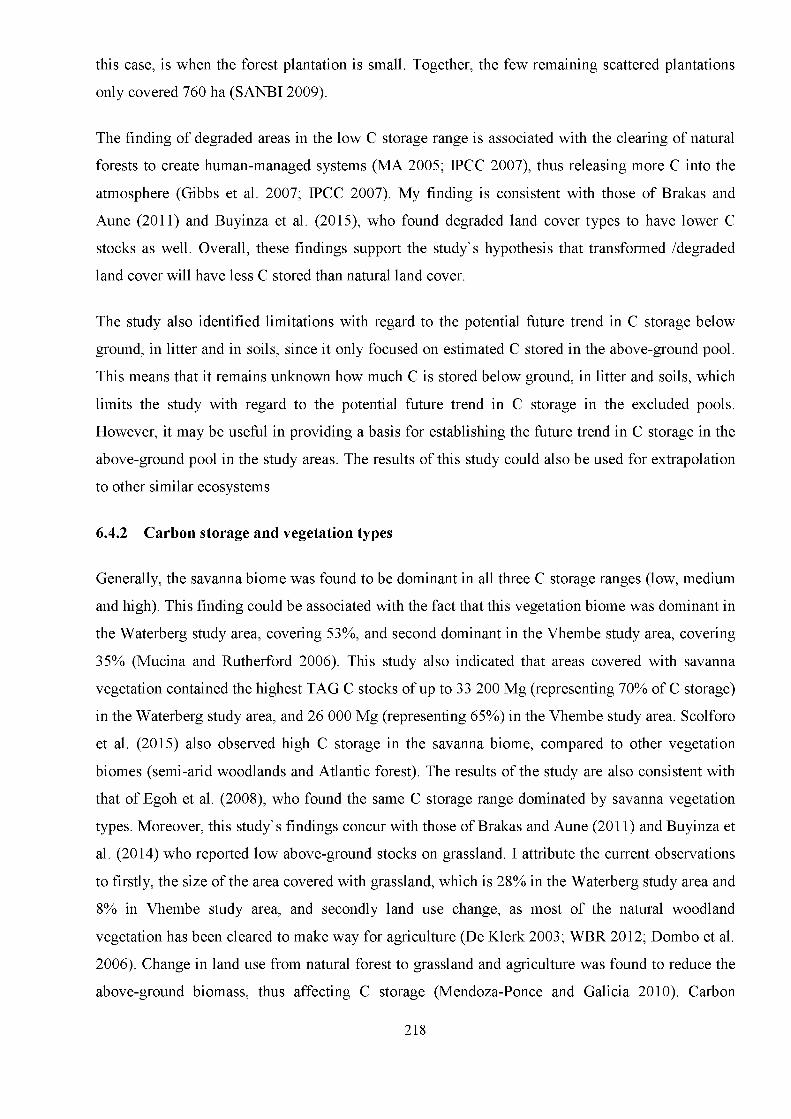
this case, is when the forest plantation is small. Together, the few remaining scattered plantations

only covered 760 ha (SANBI 2009).

The finding of degraded areas in the low C storage range is associated with the clearing of natural

forests to create human-managed systems (MA 2005; IPCC 2007), thus releasing more C into the

atmosphere (Gibbs et al. 2007; IPCC 2007). My finding is consistent with those of Brakas and

Aune (2011) and Buyinza et al. (2015), who found degraded land cover types to have lower C

stocks as well. Overall, these findings support the study's hypothesis that transformed /degraded

land cover will have less C stored than natural land cover.

The study also identified limitations with regard to the potential future trend in C storage below

ground, in litter and in soils, since it only focused on estimated C stored in the above-ground pool.

This means that it remains unknown how much C is stored below ground, in litter and soils, which

limits the study with regard to the potential future trend in C storage in the excluded pools.

However, it may be useful in providing a basis for establishing the future trend in C storage in the

above-ground pool in the study areas. The results of this study could also be used for extrapolation

to other similar ecosystems

6.4.2 Carbon storage and vegetation types

Generally, the savanna biome was found to be dominant in all three C storage ranges (low, medium

and high). This finding could be associated with the fact that this vegetation biome was dominant in

the Waterberg study area, covering 53%, and second dominant in the Vhembe study area, covering

35% (Mucina and Rutherford 2006). This study also indicated that areas covered with savanna

vegetation contained the highest TAG C stocks of up to 33 200 Mg (representing 70% of C storage)

in the Waterberg study area, and 26 000 Mg (representing 65%) in the Vhembe study area. Scolforo

et al. (2015) also observed high C storage in the savanna biome, compared to other vegetation

biomes (semi-arid woodlands and Atlantic forest). The results of the study are also consistent with

that of Egoh et al. (2008), who found the same C storage range dominated by savanna vegetation

types. Moreover, this study's findings concur with those of Brakas and Aune (2011) and Buyinza et

al. (2014) who reported low above-ground stocks on grassland. I attribute the current observations

to firstly, the size of the area covered with grassland, which is 28% in the Waterberg study area and

8% in Vhembe study area, and secondly land use change, as most of the natural woodland

vegetation has been cleared to make way for agriculture (De Klerk 2003; WBR 2012; Dombo et al.

2006). Change in land use from natural forest to grassland and agriculture was found to reduce the

above-ground biomass, thus affecting C storage (Mendoza-Ponce and Galicia 2010). Carbon

218

storage in the azonal vegetation biome covered around 12% in the Waterberg study area and 22% in

the Vhembe study area, mainly in the medium to high C storage range. However, I lacked detailed

previous data to compare my findings.

The forest vegetation biome was found to have the least C storage of around 7% in Waterberg study

area. The finding of less C storage in the forest vegetation biome of the Waterberg study area is in

contradiction with that of Rouget et al. (2004) and Buyinza et al. (2014), who found high C stocks

in forest vegetation. I attribute the finding of low C storage in the forest biome mainly to the size of

the area covered, which was less than 10% in the Waterberg study area. However, a significant

difference was found in the Vhembe study area, where the forest vegetation biome stored more than

50% of C. High C storage in the forest biome compared to other biomes was also found elsewhere

(Rouget et al 2004; Brakas and Aune 2011). I attribute the current finding of high C storage in the

Vhembe study area to the size covered by the forest biome, which was more than half of the study

area under analysis.

With regard to individual vegetation types, I found significant variation. The low to medium C

storage recorded in Strydpoort Summit Sourveld and Mamabolo Mountain Bushveld vegetation

types could be attributed to the fact that they were found to be poorly to moderately protected

(Mucina and Rutherford 2006). Similarly, the finding of Limpopo Sweet Bushveld, Makhado

Sweet Bushveld, Waterberg Mountain Bushveld, Central Sandy Bushveld, Polokwane Plateau

Bushveld and Poung Dolomite Mountain Bushveld vegetation types with low C storage in the study

area was not surprising, as they were poorly protected (Mucina and Rutherford 2006). The finding

of Dwaalboom Thornveld, Roodeberg Bushveld and Western Sandy Bushveld vegetation types in

the medium to high C storage range, despite being poorly protected, could be attributed to the fact

that they were found to be less threatened (Mucina and Rutherford 2006). Subtropical alluvial

vegetation being represented in the medium to high C storage rank could be associated with the fact

that this vegetation type was found to be well protected and less threatened (Mucina and Rutherford

2006.

The finding of Musina Mopane Bushveld with high C storage in the Vhembe study area indicated

that this vegetation type had good C storage potential, despite the fact that it was found to be poorly

conserved (Mucina and Rutherford 2006). However, the finding of high C stored in Musina

Mopane Bushveld and Polokwane Plateau and Woodbush Granite Grassland vegetation types in the

Vhembe study area was not expected, as they were found to be poorly protected or not protected at

all (Mucina and Rutherford 2006). The same is true for the finding of low C stored in Mopane

Shrubveld and Makuleke Sandy Bushveld in the same study area, as both these vegetation types219

were well protected (Mucina and Rutherford 2006). However, the finding of low C stored in

Soutpansberg Mountain Bushveld, again in the Vhembe study area, was expected, as this vegetation

type was found to be poorly protected (Mucina and Rutherford 2006). The study findings above

suggest that there is no correlation between C storage and vegetation types, as hypothesised.

6.5 CONCLUSIONS

The study managed to (1) quantify C stored in land cover and vegetation types in the study areas;

(2) map the spatial distribution of C storage in the study area; (3) demonstrate that the type of land

use has an effect on C storage in the ecosystems; and (4) indicate that there is no correlation

between C storage in vegetation types and their protection/conservation status; vegetation types that

fell within protected areas did not contain high C stocks as expected and vice versa. Given the

importance of social-ecological systems such as BRs in the delivery of vital ES such as C storage,

and the fact that natural forest cover is continuously being degraded through various human-

induced activities, it is highly recommended that (1) a wide range of assessments like this one be

conducted so that they will form the basis for decision-making on land use planning and climate

change mitigation and (2) strategies that focus on the preservation of whatever C is currently stored

are developed, to decrease further degradation.

Although some strides have been made in raising awareness about the impact of climate change,

more still needs to be done to deal with the persistent problems caused by this phenomenon. It is for

this reason that countries, including SA, are required to put more effort into their climate change

focus strategies in order to meet their international obligations. With so much C stored in this area,

it is clear that SA could be contributing more from the remaining ecoregions; all that is required is

to prevent the acceleration of anthropocentric climate change through the implementation of

sustainable climate change mitigation and adaptation strategies.

220

6.6 REFERENCES

Aaron, R. and Gibbs, H.K. 2008. New IPCC Tier-1 Global Biomass Carbon Map

for the Year 2000. Available online from the Carbon Dioxide Information Analysis Center.

O a k Ridge National Laboratory, Oak Ridge, Tennessee. http://cdiac.ornl.gov.

Archard, F., Eva, H.D., Mayaux, P., Stibig, H.J. and Belward, A. 2004. Improved estimates

of net carbon emissions from land cover change in the tropics for the 1990s. Global

B io g eo ch em ica l C ycles, 18: GB2008.

Ashton, P.J., Love, D., Mahachi, H. and Dirks, P.H.G.M. 2001. An overview of the impact of

mining and mineral processing operations on water resources and water quality in the

Zambezi, Limpopo and Olifants catchments in Southern Africa. Breaking new ground:

Mining, minerals and sustainable development. The report of the MMSD Project. London:

Earthscan, 2002. http://www.iied.org/mmsd/mmsd pdfs.

Birdsey, R., Pregitzer, K. and Lucier, A. 2006. Forest carbon management in the United

States: 1600-2100. JE Q , 35:1461-1469.

Blackie, R., Baldauf, C., Gautier, D., Gumbo, D., Kassa, H., Parthasarathy, N., Paumgarten,

F., Sola, P., Pulla, S., Waeber, P. and Sunderland, T. 2014. Tropical dry forests: The state of

global knowledge and recommendations for future research. Discussion Paper. Bogor,

Indonesia: CIFOR.

Brakas, S.G. and Aune, J.B. 2011. Biomass and Carbon Accumulation in Land Use Systems

of Claveria, the Philippines. In: Kumar B.M., Nair P.K.R. Carbon Sequestration Potential of

Agroforestry Systems: Opportunities and Challenges, Advances in Agroforestry 8.

Buyinza, J., Tumwebaze, S.B., Namaalwa, J. and Byakagaba, P. 2014. Above-ground

biomass and carbon stocks of different land cover types in Mt. Elgon, Eastern Uganda.

In te rn a tio n a l J o u rn a l o f R esea rch on L a n d -u se S usta inab ility , 1: 51-61.

Campbell, A., Miles, L., Lysenko, I., Hughes, A. and Gibbs, H. 2008. Carbon storage in

protected areas: Technical report. UNEP World Conservation Monitoring Centre.

DEAT (Department of Environmental Affairs and Tourism). 2004. A National Climate

Change Response Strategy for South Africa. Pretoria, Republic of South Africa.

DEA (Department: Environmental Affairs). 2015. South African National Terrestrial

Carbon Sinks Assessment. Pretoria, Republic of South Africa.

De Klerk, A. 2003. A land use model for the Waterberg Biosphere Reserve. Dissertation,

University of Pretoria. http://upetd.up.ac.za/thesis/available/etd-09022003-ble/etd-

09022003-113240/unrestricted.

Dewi, S., Khasanah, N., Rahayu, S., Ekadinata, A. and van Noordwijk, M. 2009. Carbon

221

http://cdiac.ornl.gov/

http://www.iied.org/mmsd/mmsd_pdfs

http://upetd.up.ac.za/thesis/available/etd-09022003-ble/etd-

footprint of Indonesian palm oil production: A pilot study. World Agroforestry Centre-

ICRAF SEA, Regional Office.


The proposed Vhembe Biosphere Reserve application to UNESCO. Limpopo Province

Department of Economic Development, Environment and Tourism, Republic of South

Africa.

Egoh, B., Reyers, B., Rouget, M., Richardson, D.M., Le Maitre, D.C. and Van Jaarsveld,

A.S. 2008. Mapping ecosystem services for planning and management. A gricu ltu re ,

E co sys te m s a n d E n v iro n m en t, 127(1-2): 135-140.

ESRI (Environmental Systems Research Institute). 2013. ArcGIS for Desktop. Advanced

Student Edition, Version 10.2. Redlands (CA): ESRI.


mitigation and prevention in the Limpopo River Basin, a situation analysis. Land and Water

Discussion Paper 4. Prepared by the FAO Sub-regional Office for Southern and East Africa,

Harare.

FAO (Food and Agriculture Organization of the United Nations). 2012. The state of food and

agriculture. Food and Agriculture Organization of the United Nations. Viale delle Terme di

Caracalla, Rome, Italy.

Fongnzossie, E.F., Sonwa, D.J, Kemeuze, V., Auzel, P. and Nkongmeneck, B. 2014. Above

ground carbon assessment in the Kom-Mengame forest conservation complex, South

Cameroon: Exploring the potential of managing forests for biodiversity and carbon. N a tu ra l

R eso u rces F orum , 38: 220-232.

Gibbs, H.K., Brown, S., Niles, J.O. and Foley, J.A. 2007. Monitoring and estimating tropical

forest carbon stocks: Making REDD a reality. E n v iro n m en ta l R esea rch L etters, 2: 045023.

Golden Agri-Resources., SMART and The Forest Trust and Greenpeace. 2012. High carbon

stock forest study report

http://www.goldenagri.com.sg/pdfs/misc/High Carbon Stock Forest Study Report

IUCN (International Union for the Conservation of Nature). 2010. About biodiversity:

International year of biodiversity. http://iucn.org/iyb/about. Accessed in 2013.

IPCC (Intergovernmental Panel on Climate Change). 2006. IPCC Guidelines for National

Greenhouse Gas Inventories, Prepared by the National Greenhouse Gas Inventories

Programme, edited by Eggleston H.S., Buendia L., Miwa K., Ngara T. and Tanabe K.

Published: IGES, Japan.

IPCC (Intergovernmental Panel on Climate Change). 2007. Climate Change 2007: The

222

http://www.goldenagri.com.sg/pdfs/misc/High_Carbon_Stock_Forest_Study_Report

http://iucn.org/iyb/about

Scientific Basis. Contribution of Working Group I to the Fourth Assessment Report of the

Intergovernmental Panel on Climate Change, edited by Solomon et al., Cambridge Univ.

Press, New York.

Koh, L.P. and Gardner, T.A. 2010. Conservation in human-modified landscapes, Chapter 13:

In Sodhi and Erlich 2010: Conservation Biology for All. Oxford University Press.

http//ukcatalogue.oup.com/product/9780199554249.do. Accessed in 2014.

Kyoto Protocol to the United Nations Framework Convention on Climate Change. 1998.

Adopted in Kyoto Japan 1997. http://unfccc.int/resource/docs/convkp/kpeng.pdf.

Lal, R. 2004. Soil carbon sequestration impacts on global climate change and food

security. Science, 304:1623-1627.

Law, E.A., Bryan, B.A., Torabi, N., Bekessy, S.A, McAlpine, C.A. and Wilson, K.A. 2015.

Measurement matters in managing landscape carbon. E co sys tem Services, 13:6-15.

Liu, X., Ekoungoulou, R., Loumeto, J.J., Ifo, S.A., Bocko, Y.E. and Koula, F.E. 2014.

Evaluation of carbon stocks in above- and below ground biomass in Central Africa:

Case study of Lesio-louna tropical rainforest of Congo. B io g eo sc ien ces D iscuss, 11: 10703

10735.

Lucey, J., Hill, J., van der Meer, P., Wageningen, A., Reynolds, G. and Agus, F. 2014.

Change in carbon stocks arising from land-use conversion to oil palm plantations. A

science-for-policy paper for the Oil Palm Research-Policy Partnership Network. Indonesian

Agency for Agricultural Research and Development University of York, UK. The project

was funded by the British Foreign and Commonwealth Office.

MA (Millennium Ecosystem Assessment). 2005. Ecosystems and Human Well-being:

Synthesis, World Resource Institute. Island Press, Washington, DC.


Merrywheather, F.R., le Roux, J., van Rooyen, T.H., Harmse, H.J. and von, M. 1977. Soil

Classification - A Binomial System for South Africa. Department of Agricultural Technical

Services, Soil and Irrigation Research Institute, Pretoria, Republic of South Africa, pp 150.

McKinney, M.L. 2008. Effects of urbanization on species richness diversity: A review of

plants and animals. U rban E cosystem , 11, 161-176.

Mendoza-Ponce, A. and Galicia, L. 2010. Aboveground and belowground biomass and

carbon pools in highland temperate forest landscape in Central Mexico. F o res try

83(5):497-506

Miles, L., Newton, A., DeFries, R., Ravilious, C., May, I., Blyth, S., Kapos, V. and

Gordon, J. 2006. A global overview of the conservation status of tropical dry forests.

J o u rn a l o f B io g eo g ra p h y , 33(3):491-505.

223

http://unfccc.int/resource/docs/convkp/kpeng.pdf

Mills, A.J., Cowling, R.M., Fey, M.V., Kerley, G.I.H., Donaldson, J.S., Lechmere-Oertel,

R.R., Sigwele, A.M., Skowno, A.L. and Rundel, P. 2005. Effects of goat pastoralism on

ecosystem carbon storage in semiarid thicket, Eastern Cape South Africa. A u stra lia n

E c o lo g y , 30,797-804.


Swaziland. Strelitzia 19: South African National Botanical Institute, Pretoria, South Africa.

M ila n C h y try F o lia G eobotan ica , 43(4): 461-463.

Mugagga, F., Nagasha, B., Barasa, B. and Buyinza, M. 2015. The effect of land use on

carbon stocks and implications for climate variability on the slopes of Mount Elgon, Eastern

Uganda. In te rn a tio n a l J o u rn a l o f R e g io n a l D eve lo p m en t, 2:1.

Naidoo, R., Balmford, A., Costanza, R., Fisher, D., Green R.E., Lehner, B., Malcolm, T.R.

and Ricketts, T.H. 2008. Global mapping of ecosystem services and conservation priorities.

P ro ceed in g s o f the N a tio n a l A ca d e m y o f Sciences, 105: 9495-9500.

Petrescu, A.M.R., Abad-Vi ~nas, R., Janssens-Maenhout, G., Blujdea, V.N.B. and Grassi, G.

2012. Global estimates of carbon stock changes in living forest biomass: EDGARv4.3 -

Time series from 1990 to 2010. B io g eo sc ien ces, 9:3437-3447.

Power, A.G. 2010. Ecosystem services and agriculture: Trade-offs and synergies.

P h ilo so p h ica l T ran sa ctio n s o f the R o y a l Society, 365:2959-2971.

Rahman, M., Kabir, E., Jahir Uddin Akon, A.S.M. and Ando, K. 2015. High carbon stocks

in roadside plantations under participatory management in Bangladesh. G lo b a l E co lo g y a n d

C onserva tion , 3: 412-423.

Rouget, M., Richardson, D.M., Cowling, R.M., Lloyd, J.W. and Lombard, A.T. 2003.

Current patterns of habitat transformation and future threats to biodiversity in terrestrial

ecosystems of the Cape floristic region, South Africa. B io lo g ic a l C onserva tion , 112: 63-85.

Rouget, M., Reyers, B., Jonas, Z., Desmet, P., Driver, A., Maze, K., Egoh, B. and Cowling,

R.M. 2004. South African National Spatial Biodiversity Assessment: Technical Report.

Volume 1: Terrestrial Component. South African National Biodiversity.

SANBI (South African National Biodiversity Institute). 2009. National Land Cover

2009, South Africa. Pretoria, Republic of South Africa.

Schackleton, C., Schackleton, S., Gambiza, J., Nel, E., Rowntree, K. and Urquhart, P. 2008.

Links between Ecosystem Services and Poverty Alleviation: Situation analysis for arid and

semi-arid lands in Southern Africa. Ecosystem Services and Poverty Reduction Research

Programme: DFID, NERC, ESRC.

Scolforo, H.F., Scolforo, J.R.S., Mello, C.R., Mello, J.M., Filho, A.C.F. and Silva,

224

http://www.ncbi.nlm.nih.gov/pubmed/?term=Scolforo%20HF%5Bauth%5D

http://www.ncbi.nlm.nih.gov/pubmed/?term=Scolforo%20JR%5Bauth%5D

http://www.ncbi.nlm.nih.gov/pubmed/?term=Mello%20CR%5Bauth%5D

http://www.ncbi.nlm.nih.gov/pubmed/?term=Mello%20JM%5Bauth%5D

http://www.ncbi.nlm.nih.gov/pubmed/?term=Ferraz%20Filho%20AC%5Bauth%5D

L.C.R. (ed). 2015. Spatial distribution of aboveground carbon stock of the arboreal vegetation in Brazilian biomes of savanna, Atlantic forest and semi-arid woodland. PLoS

One, 10(6): e0128781.StatsSA (Statistics South Africa). 2012. Census 2011 Statistical Release-P0301.4.

http://www.statssa.gov.za. Accessed in 2013.Solichin, M., Lingenfelder, M. and Steinmann, K.H. 2011. Tier 3 Biomass Assessment for

Baseline Emission in Merang Peat Swamp Forest. Workshop on tropical wetland

ecosystems of Indonesia: Science needs to address climate change adaptation and

mitigation. Denpasar, Bali, Indonesia.Tallis, H.T., Ricketts, T., Guerry, A.D., Nelson, E., Ennaanay, D., Wolny, S., Olwero, N.,

Vigerstol, K., Pennington, D., Mendoza, G., Aukema, J., Foster, J., Forrest, J., Cameron,

D., Lonsdorf, E., Kennedy, C., Verutes, G., Kim, C.K., Guannel, G., Papenfus, M., Toft,J., Marsik, M. and Bernhardt, J. 2011. InVEST 2.0 beta User’s Guide. The Natural Capital Project, Stanford.

UNFCCC (United Nations Framework Convention on Climate Change). 1992. United

Nations Conference on Environment and Development; Rio de Janeiro, Brazil. FCCC/INFORMAL/84GE.05-62220 (E) 200705. https:/ /unfccc .int/resource/docs/convkp/conveng.p df.

VDMIDP. 2012. Vhembe District Municipality Integrated Development Plan

2011/12 financial year. http://www.mfma.treasury.gov.za.WBR (Waterberg Biosphere Reserve). 2012. Ten Year Periodic Review 2001-2011.

http://www.docstoc.com/myoffice/recommendations?docId=161286419&download. Accessed in 2012.

225


https://unfccc.int/resource/docs/convkp/conveng.pdf

http://www.mfma.treasury.gov.za

http://www.docstoc.com/myoffice/recommendations?docId=161286419&download

CHAPTER 7

ECONOMIC VALUATION OF PROVISIONING SERVICES IN TWO BIOSPHERE

RESERVES IN SOUTH AFRICA

This chapter is intended for submission to the journal E c o lo g ic a l E co n o m ic s as:

Ntshane, B.C. and Gambiza, J.

Abstract

The importance of biosphere reserves (BRs) cannot be underrated as an important source of

ecosystem services (ES) that contribute to human well-being. Among these ES are timber and

firewood. Firewood remains a primary source of energy for heating and cooking for many

households around the world, including South Africa, and timber is an important source of fuel and

infrastructural material. The production of planted forests forms a major part of the South African

economy, therefore determining their economic contribution is very important. I applied the

Integrated Valuation of Ecosystem Services and Trade-offs tool, to determine the net present value

(NPV) of two provisioning ES (timber and firewood) in a BR context, focusing on planted forests.

Taking into consideration various input factors, at a 12% discount rate, the NPV for timber

production accounted for R23 317/ha in VBR and R57 304/ha in Waterberg biosphere reserve

(WBR). However, at lower discount rates (4 and 7%), the NPVs for timber were negative in

Vhembe biosphere reserve (VBR) and positive in WBR. With regard to firewood production, the

NPVs were negative against all three discount rates in both study areas. The results suggest that

profit generation in terms of firewood production in both study areas is unsustainable; however,

there is good investment potential in timber production in the VBR study area.

Key words: Ecosystem services; economic valuation; total net present value, biosphere reserve,

forest plantations, provisioning.

7.1 INTRODUCTION

Biosphere reserves (BRs) are socio-ecological systems that consist of multiple subsystems of

natural and man-made origins (Ostrom 2009; Palomo et al. 2011), such as forest ecosystems of both

plantation and indigenous nature. Forest ecosystems cover over 4 billion hectares (ha) globally

(FAO 2010), comprising around 95% of the indigenous component and around 5% of plantations

and representing 31% of the world’s surface area (FAO 2010). Of this, 17%, representing 650

226

million ha, can be found in Africa (FAO 2004). In the South African context, forest covers over 40

million ha, of which the indigenous component makes up 0.4% of the land surface area (DAFF

2011a), covering 492 700 ha, while plantations cover approximately 1.4% of the surface area,

representing 1.3 million ha of the country’s total land surface area (Grundy and Wynberg 2001;

DAFF 2011a).

Forest is an important land cover component globally and its enormous contributions to human

wellbeing cannot be overstated. The importance of forests is pronounced as the source of various

ecosystem services (ES) that contribute to human wellbeing ecologically, socially and economically

(Eftec 2010; DAFF 2011a; FAO 2012; Aggrawal et al. 2013). Some of the important contributions

made by forests include performing various regulating functions such as mitigating natural disasters

and phenomena, e.g. floods and climate change. Forests are also responsible for the production of

consumptive products such as browsing material for livestock and game (Aggrawal et al. 2013;

FAO 2012), fuel wood and raw material such as timber.

Firewood remains an important contributor to satisfying energy requirements throughout the world

(FAO 2010). Firewood satisfies at least 27% of total primary energy requirements in Africa (FAO

2014) and about 90% of South African rural households use firewood for various purposes,

including heating and cooking (Shackleton et al. 2007; Chirwa et al. 2010). About 8 billion of the

world's population depend on forests for their shelter requirements (FAO 2014). In South Africa

(SA), households’ collection of timber seems to be on a small scale; more focus is placed on retail

and exports (DAFF 2011b). Notwithstanding the need for firewood and timber to meet various

households requirements throughout the world (FAO 2014), meeting these demands comes with

some trade-offs. On top of other anthropogenic pressures exerted on natural forest ecosystems, i.e.

desertification, habitat loss and degradation, as well as land use decisions that tend to be made in

economic terms (Seidl et al. 2007; Daily et al. 2009, Kovacs et al. 2013), the demand for timber and

firewood contributes to a further decline in the natural forest cover and climate change (MA 2005;

IPCC 2007). In fact, natural forest cover has declined tremendously and it is now ranked among the

most threatened land covers in the world (MA 2005).

Given the magnitude and dynamics of anthropogenic challenges to natural forest ecosystems,

societies are forced to employ various strategies to address them. In SA, the much-needed solution

to supplement the social, ecological and economic value chain of the declining natural forest cover

could be found through forest plantations. This includes mitigating the risks posed by the climate

change phenomenon and meeting the demand for timber and firewood, among others. In the

2010/11 financial year, about 233 069 tons of firewood were produced from planted forests in SA,

227

of which 26 292 tons were harvested in Limpopo Province. Planted forests also yielded 4 611 723

m3 for sawlogs, poles and droppers, as well as 1 09 1 094 tons of mining timber and pulpwood

(DAFF 2011b). Given the fact that planted forests cover less than 2% of SA (DAFF 2011a), more

forest plantations can be added to the system through the afforestation process, thus providing the

much sought-after mitigation to climate change and shrinking forest cover (FAO 2010; DAFF

2011a). However, species suitable for afforestation must be selected with care, as exotic species

(P inus a n d E u ca lyp tu s spp) are known to consume more water compared to indigenous species

such as B erch e m ia zeyh er i, C e ltis A fr ic a n a and P ta ero xy lo n obliquum , among others (Gush et al.

2011).

Knowledge of the economic value provided by forest ecosystems is beneficial when making tough

land use decisions concerning these systems, while assisting in stimulating appreciation of the ES

they provide (Seidl et al. 2007; Nelson et al. 2009; Kovacs et al. 2013). Some of the well-known

valuation strategies include taking into consideration the economic, social and ecological

contributions made by ecosystems (TEEB 2010; Haines-Young and Potschin 2009; Tallis et al.

2011; Gomez-Baggethun et al. 2014).

Economic valuation approaches attempt to determine the value of goods and services in monetary

terms (Haines-Young and Potschin 2009; TEEB 2010; Gomez-Baggethun et al. 2014). Economic

valuation approaches are divided into three types: the direct market, revealed preference and stated

preference approaches (Haines-Young and Potschin 2009; TEEB 2010; Gomez-Baggethun et al.

2014). Direct market approaches are used to determine the values of those ES that can be involved

in market transactions. These approaches are further divided into three main approaches: the market

price, cost-based and production function approach. The market price-based approach is applicable

to those ES that are often sold in markets (Haines-Young and Potschin 2009; TEEB 2010; Gomez-

Baggethun et al. 2014), including most of the provisioning ES, e.g. timber and crops. The cost-

based approach is related to the cost estimated for the replacement of ES artificially and is further

divided into replacement and mitigation/restoration cost methods (Haines-Young and Potschin;

Eftec 2010); the restoration cost method refers to costs estimated for the restoration of lost/damaged

ES. The production-function approach is further divided into two types: production-function and

factor income approaches, which are used to estimate how much a particular ES contributes to the

delivery of another ES that is traded in the existing market, e.g. how soil fertility improves timber

production and therefore the income of the landowner (Eftec 2010).

The economic value of forests can be measured through the financial contribution of the harvested

products to the regional economy (Wu et al. 2007; Eftec 2010; Kovacs et al. 2013). Various studies

228

have conducted valuation of ES provided by forest ecosystems (Wu et al. 2007; Nelson et al. 2009;

Eftec 2010; Kovacs et al. 2013), but the focus on the determination of the net present value (NPV)

is limited. In SA, determining the economic contribution of planted forests is very important, as

they play a crucial role by contributing to the economy, contributing around 1.2% to GDP,

amounting to an estimated R12 billion and providing 170 000 jobs. We conducted an economic

valuation of two important ES provided by planted forests, timber and firewood, in a BR context

using the Integrated Valuation of Ecosystem Services (InVEST) modelling and valuation tools. In

order to achieve the main aims of the study, the following objectives had to be addressed: (1) to

determine the NPV of timber and firewood production in the study areas, and (2) to quantify the

volume of timber and firewood biomass produced in the study areas.


7.2.1 Study area

The study areas were located in Limpopo Province of SA in the Vhembe and Waterberg district

municipalities. Both study areas were situated in socio-ecological systems called BRs, which

through their zonation structure allowed different ecosystems of both natural and unnatural origin

to co-exist (UNESCO 2010). UNESCO's Man and Biosphere Program BR concept in South Africa

made its mark with the establishment of the first BR in 1998: Kogelberg, situated in the Western

Cape Province. Currently there are six BRs in South Africa, three of which are situated in Limpopo

Province: Vhembe, Waterberg and Kruger to Canyon. The focus of the study was Vhembe (VBR)

and Waterberg (WBR).

In the VBR and WBR, diverse land use took place in both natural and unnatural ecosystems. Most

of the indigenous forest areas left were found in protected areas (PAs), including the famous

gallery forest of the Mapungubwe National Park in VBR and Apiesrivierspoort forest in Marakele

National Park in the WBR. Most indigenous forests found outside this type of protection are under

threat of degradation (PAK 2008). One of the well-known indigenous forest areas outside PAs is

Thathe-Vonde, which is part of the Komatiland Forests (KLF) in the VBR. The indigenous forest

components mentioned here exist for conservation purposes only; no commercial harvesting takes

place. If harvesting occurs at all, it is carried out illegally for subsistence purposes. This study

excluded the analysis of indigenous forests' production of timber and firewood on purpose, as the

production of these commodities in this context does not form part of their management objectives

and neither timber nor firewood production for commercial purposes takes place within the

indigenous component. In WBR, since there was no known commercial plantation in existence,

229

and planted forests as land use have been converted to other land uses, the study focuses on the

remaining isolated pockets of plantations.

7.2.2 Valuation approach used in this study

I used the InVEST approach (Tallis et al. 2011) to determine the economic value of timber and

firewood production in the study areas. InVEST is a spatially explicit modelling tool that consists

of a suite of models that map and value ecosystem goods and services provided by nature (Daily et

al. 2009; Tallis et al. 2011). Among these modelling suites is a timber production model.

The InVEST timber production model estimates the production value of natural forests and

forestry plantations. This model analyses the amount and volume of legally harvested timber from

natural forests and managed plantations based on the harvest level and cycle. The model’s output

maps the NPV of forest harvests over some user-defined time interval. If the timber parcel map is

associated with the current land use/land cover (LU/LC) map the model calculates, for each timber

parcel, the NPV of harvests that occurred between the current year and some user-defined date.

The total net present value (TNPV) includes the revenue that will be generated from selling all

timber/firewood harvested from the current year to the number of years that the plantation will be

valued (T) after the current year, less harvest and management costs incurred during this period.

Finally, all monetary values are discounted back to the current year’s present value, assuming that

harvest practices and prices are static over the time interval. The valuation model estimates the

economic value of timber based on the market price, harvest and management costs and a discount

rate and calculates its economic value. Since firewood production in this analysis is an output of

timber plantations, the InVEST timber model applied here will be applied to firewood production

as well as the firewood production from timber plantations under analysis.

Data tools needed to run the model successfully include a GIS vector dataset, projected in meters,

with a unique identifier that indicates the different timber parcels on the landscape (Tallis et al.

2011). The model also requires a separate data table about the timber/firewood parcels on the

landscape that can be joined to the polygon dataset in #1. Columns contain an attribute for each

parcel. Table 7.1 presents InVEST timber production data requirements (Tallis et al. 2011).

230

Table 7.1 InVEST timber/firewood production model data requirements

Attribute Description Calculation methodology

Timber_parcel Demarcated timber compartment per age class Timber parcels were numbered 1 to 8 in

VBR and 1 in WBR

Parcel_ID Same as timber/firewood parcel ID in #1. IDs

must match the parcel IDs used in the polygon

map.

Determined by the model

Parcel_area The area of the timber/firewood parcel in

hectares

Extracted from the plantation map's

attribute table

Percentage of harvest The proportion of the timber/firewood parcel

area that is harvested each harvest period;

units are integer percentage.

Parcel area/rotation period, obtained from

the plantation management

Harvesting_mass The mass of wood harvested per hectare in

each harvest period (in metric tons (Mg) for

Eucalyptus spp. and cubic meters for pinus

species.

Obtained from the plantation management

Frequency of harvest The frequency of harvest periods, in years, for

each parcel

Harvesting takes place every year, =1

Price (R) The marketplace value of the wood harvested

from the parcel

Obtained from the plantation management

Maintenance_cost (R) The annualized cost ha_1 of maintaining the

timber/firewood parcel

Harvesting_cost (R) The cost incurred per ha when harvesting.

T The number of years from (current year

(yr_cur) or future year (yr_fut) that parcel

harvests will be valued. If the parcel is in an

even age rotation managed plantation, T can

be any number, although a large T is not

recommended. If the harvest is expected to be

an immediate one-time clear cut T = 1.

The parcels were rotation managed, 30 years

for Pinus spp . and 12 years for Eucalyptus

spp.

Immediate_harvest This attribute answers whether a harvest

occurs immediately - whether a harvest

occurs in yr_cur, or whether the user is

evaluating a forest parcel associated with a

future LU/LC scenario occurring in yr_fut.

Answer yes (entered as YES or Y) or no

(entered as NO or N) to whether a harvest

should be calculated for yr_cur or yr_fut. If

yes, then the NPV of harvest in the parcel

includes a harvest in yr_cur.

NPV includes harvest in yr_cur (yes applied

for all timber parcels)

231

Biomass

Expansion

Factor

(BCEF)

An expansion factor that translates the mass

of harvested wood into volume of harvested

wood. The expansion factor is measured in

Mg of dry wood per m3 of wood. The

expansion factor is a function of stand type

and stand age (this factor is known as the

biomass expansion factor in the literature). If

data on this expansion factor are not available,

one can use the BCEFR row in table 4.5 of

IPCC (2006). Otherwise, this expansion factor

can be set equal to 1 for each parcel.

Set equal to 1 for each parcel as

recommended by the model.

Market Discount Rate This is optional and only required for Chosen discount rate was 12% calculated

valuation. This number is not supplied in a based on weighted average cost of capital

table, but instead is input directly through a (WACC) using South African rates (prime,

tool interface. The tool’s default value is 7% government bond, tax, interest rate and

per year, and the other one is 3%. The rate CPIX among others), as well as the

will, however, differ and depend on the recommended rates of 4% and 7% for

country and landscape being evaluated. environmental projects

7.2.3 Information sourcing

The first stage of data collection to meet the requirements of the model, as indicated in Table 7.1,

was through stakeholder engagement. This process was conducted by interviewing stakeholders

who owned forest plantations between period 2012 and 2013, with the aim of understanding the

extent, value and benefits of the forest ecosystems found in the study areas. In VBR, 22

stakeholders who were managing forest plantations over 200 ha and willing to participate in the

survey were interviewed. The total population of stakeholders with forest plantations according to

the information received from the Department of Agriculture, Forestry and Fisheries was around

200. At least eight stakeholders in VBR were accessible for face-to-face interviews and 14 were

interviewed telephonically. The selection targeted mainly those that were in the forestry business,

managed at least 200 ha of forestry plantation and were accessible for the interviews. In WBR, 10

stakeholders, situated in the proximity of the available forest plantation patches, were contacted to

establish an understanding regarding the use of these plantations. Four stakeholders were

interviewed face to face and six were interviewed telephonically. The reason for the lower number

of stakeholders involved in the WBR compared to the VBR was mainly that only a few plantation

patches were left, generally in isolated places, and most were outside stakeholders' properties.

The WBR and VBR forestry plantation datasets used were extracted from the SA National Land

Cover dataset (SANBI 2009). Supplementary information pertaining to timber parcels, such as size232

in hectares (ha), harvesting mass, percentage of harvest, frequency of harvest and selling price

(market value) of harvested wood was acquired through engagement with the landowners.

Additional information pertaining to maintenance and harvesting costs was obtained from Forestry

Valuations (2012). Information pertaining to firewood production in VBR was extracted from the

report by Venter (2009) and in WBR it was obtained from the EPWP project manager who was

involved with the cutting/clearing of the plantations, as well as some of the stakeholders who were

harvesting firewood from time to time in some of the plantations.

7.2.4 Data collected

7.2.4.1 State of timber production in the study areas

The VBR study area had more than 200 timber plantations, most of which were very small. The

study focus was KLF. The KLF plantation was selected, as it is the biggest forest plantation in the

VBR and operates commercially. For the purpose of this study, only commercial timber plantation

production in five parcels was analyzed. Of the five, one was managed for E u ca lyp tu s spp. only;

the other four produced a mixture of P in u s spp. and E u ca lyp tu s spp. P in u s spp . are managed for

up to 30 years, while E u ca lyp tu s spp. are harvested every 12 years in all the timber parcels. The

five main timber plantations were further divided into eight parcels, separating the two dominating

species of E u ca lyp tu s spp. and P in u s spp. The first timber parcel covered 5 766 ha, comprising

5 245 ha of P in u s spp. and 521 ha of E u ca lyp tu s spp. The second timber parcel covered 222 ha

and was dominated by E u ca lyp tu s spp. The third timber parcel covered 613 ha and was managed

for both P in u s spp. (425 ha) and E u ca lyp tu s spp. (188 ha).The fourth timber parcel covered

776.75 ha, with 325 ha covered by E u ca lyp tu s spp. and 441 ha covered by P in u s spp. The last

timber parcel covered 4 017 ha and was dominated by E u ca lyp tu s spp.

Harvesting involved at least a third of the timber parcels, (3% fo r P in u s spp. and 8% for

E u ca lyp tu s sp p .) once per annum. Given the fact that the plantation under analysis was operating

commercially, it was easy to obtain the market value of the harvested timber, and the information

received reveals that P in u s spp. was sold at R450/Mg and E u ca lyp tu s spp. at R400/Mg. It was also

revealed through engagement with the plantation management that the volume of harvested wood

amounted to 380 Mg/ha for P in u s spp. and 200 Mg/ha for E u ca lyp tu s spp. We could not obtain a

breakdown of the harvesting and maintenance cost from the plantation management, therefore the

information on this was obtained from the free access Forestry Valuations (2012) website.

In WBR, no timber plantations were available that were managed for commercial purposes. Only

small patches of abandoned plantations were left. The remaining patches consisted only of233

E u ca lyp tu s spp. species; there was no P in u s spp. The total forest plantation patches covered an area

of 760 ha, comprising various small isolated patches. Because timber production in WBR occurred

on a small scale, mainly for domestic purposes, the whole plantation left in WBR was treated as a

single parcel covering 760 ha, of which 10% was harvested every year, mainly for domestic use,

but for the purpose of this study we used 8% as the proportion of harvest to be consistent with the

value applied in the VBR study area.

No maintenance cost was incurred to keep up production, since this production mainly involved a

collection of abandoned old plantations, most of which the landowners wanted to see eradicated, to

the extent of commissioning Government's Extended Public Works Program (EPWP) to deal with

it. However, costs were incurred during harvesting, since this was carried out using various

machines such as chainsaws, which needed consumables to operate. The focus was therefore on the

EPWP operations. It cost the EPWP around R350 per person per day (according to the information

provided by the EPWP project manager), taking into consideration wages, transport, machinery and

consumables, to carry out an operation, with a team of 10 people taking a day to clear 1 ha.

However, for the sake of consistency, we decided to apply the same values applied in VBR for

harvesting cost. Table 7.2 contains input data sourced for the purpose of the analysis of WBR and

VBR timber production.

Table 7.2 VBR and WBR's inputs to timber production

VBR's inputs to timber production

Parcel

ID

Parcel

area

(ha)

% o f

harvest

Freq harv

(in years)

Harvest

Mass

(Mg/ha)

Market value

(in rands) o f

harvested

wood (Mg)

Maint

_cost

(R/ha)

Harv_cost

(R/ha)

Years

parcel

will be

valued

(T)

Immed harv

(Yes/No)

Biomass

expansion

factor

(BCEF)

1 5245 3 1 380 450 2460 2849 30 Yes 12 521 8 1 200 400 2950 3167 12 Yes 13 222 8 1 200 400 2950 3167 12 Yes 14 425 3 1 380 450 2460 2849 30 Yes 15 188 8 1 200 400 2950 3167 12 Yes 16 325 8 1 200 400 2950 3167 12 Yes 17 441 3 1 380 450 2460 2849 30 Yes 18 4017 8 1 200 400 2950 3167 12 Yes 1

WBR's inputs to timber production

1 760 8 1 200 400 0 3167 60 Yes 1

234

7.2.4.2 State o f firewood production in the study areas

The production of firewood in VBR happened during timber processing, where timber products that

did not meet the requirements of a standard market product were regarded as waste and used as

firewood. This happened in two of the five timber plantations under analysis in the VBR. Although

two timber plantations were involved, only the one close to the communities was used in this

analysis. The output generated through this process amounted to an average of 20 tons per ha

(Venter 2009) and was collected by the local communities who later resold it in their villages.

Firewood cost around R80 a ton (Forestry Valuations 2012).

The production of firewood in WBR was slightly different from that in the VBR. It occurred on

isolated patches of timber left after land use change. Although the plantation patches together

amounted to more than 760 ha, this analysis only involves 10% of the one that formed part of the

EPWP alien clearing program along the main core area, as indicated for timber production in this

BR as well. Again for the sake of consistency, an 8% proportion of the harvest was used. The

following outputs were also the same as those used for timber production in the WBR: percentage

(proportion) of harvest, frequency of harvest and harvesting mass. No maintenance costs were

associated with firewood production in WBR. Harvesting costs amounted to R3 000/ha; however,

as we did for timber production, for the sake of consistency, we applied the Forestry Valuations

(2012) value for harvesting costs, which amounted to R3167/ha. Firewood cost around R10 for 8 kg

bag. We used the minimum price of R80/ton for firewood to be consistent with the other study area.

Table 7.3 contains input data sourced for the purpose of the analysis of firewood production in the

WBR and VBR study areas.

Table 7.3 WBR and VBR's input to firewood production

Inputs to firewood production

Parcel

ID

Parcel

area

(ha)

% o f

harvest

Freq harv

(in years)

H arvest

M ass

(Mg/ha)

M arket

value (in

rands) o f

harvested

w ood (Mg)

M ain t

_cost

(ha)

H arv_cost

(ha)

Years

parcel

w ill

be

valued

(T)

Im m ed harv

(Yes/No)

Biomass

expansion

fa c to r

(BCEF)

VBR 4017 8 1 20 80 0 3167 12 Yes 1

Firewood

WBR 760 8 1 20 80 0 3167 60 Yes 1

Firewood

235

7.2.5 C alculation o f the required input data

The formulae used to calculate the required input were taken from Forestry Valuations (2012). The

percentage of harvest is calculated through the following formula: Parcel area (A)/rotation period

(C) and then the value is converted into a percentage of B, as displayed in Table 7.4.

Table 7.4 Calculation of plantation proportion of harvest

A B C DParcel _ID Parcel_area Rotation period/num ber o f Percentage o f harvest

years tha t parcel w ill valued (T)

be

1 5 245 30 5245/30=175175 is equal 8.34% of the parcel area (B).

2 521 12 521/12 =43 (8.25%)

3 222 12 222/12 =19 (8.56%)

4 425 30 425/30 =14 (8.30%)

5 188 12 188/12 =16 (8.51%)

6 325 12 325/12 =27 (8.30%)

7 441 30 441/30 =15 (3.40%)

8 4017 12 4017/12 =335 (8.33%)

The formula for calculating harvesting cost was as follows: R/ton x MAI x T

(B x C x D), (see Table 7.5). MAI means mean annual increment and R stands for rand.

236

Table 7.5 Calculation of plantation harvesting costs

A B C D E F

Parcel area (ha) Rand per ton (R/ton) R/ton/ha/T Rotation Total HarvestingStandard forest cost (MAI) period harvesting cost/haequals 90 for Pinus (T) costsspp. and 190 for (ha) (E/12)Eucalyptus spp.

5 245 90 12.66 30 34 182 2849

521 190 16.67 12 38 000 3167

222 190 16.67 12 38 000 3167

425 90 12.66 30 34 182 2849

188 190 16.67 12 38 000 3167

325 190 16.67 12 38 000 3167

441 90 12.66 30 34 182 2849

4 017 190 16.67 12 38 000 3167

Maintenance cost is calculated as follows: Total rand per ha (R/ha (E) x parcel area (A). Rand per

hectare is the sum of annualized R/ha (B), fire protection R/ha (B) and overheads R/ha (D), all of

which are standard forest costs from Forestry Valuations (2012) (refer to Table 7.6).

Table 7.6 Calculation of plantation maintenance costs

A B C D E FParcel area Annualized Fire protection Overheads R/ha Total Total costs

(ha) R/ha R/ha R/ha (maintenance)

(Standard (Standard fo rest =Sum =(E x A)

(Standard fo rest

cost)

fo res t cost) cost) (B:D)

5 245 485 750 1200 2 435 12 770 650521 967 750 1200 2 917 1 519 992222 967 750 1200 2 917 646 333425 485 750 1200 2 435 1 034 437188 967 750 1200 2 917 548 333325 967 750 1200 2 917 948 792441 485 750 1200 2 435 1 074 2734 017 967 750 1200 2 435 11 716 367

237

NPV is a common and useful cash flow measure for short-term investments (Cubbage et al. 2013).

There is a wide range of methods that can be used to calculate the discount rate; among these is the

Weighted Average Cost of Capital. The Weighted Average Cost of Capital (WACC) is a blend of

the cost of equity and the cost of debt (Forestry Valuations 2012); see table 8.9. In this study, NPV

was calculated using discount rates of 4%, 7% and 12%. The discount rate of 7% is the InVEST

default value recommended for environmental projects (Tallis et al. 2011) and 4% is the

recommended discount rate for timber valuation in SA (Forestry Valuations 2012). A discount rate

of 12% was the nearest value to 11.80 % calculated based on WACC (see table 7.7.), and discount

rates above 10% are recommended for developing countries (Khatun 2010). The NPV has been

used as indicator for assessing economic returns for plantations (Keca et al. 2012; Wang et al.

2014).

Table 7.7 Calculation of WACC

Calculation of WACC

WACC = Kd x d% + Ke x e%

Where:

Kd After tax rate of return on debt capital d% Debt capital as % debt + equity

Ke Rate of return on equity e% Ordinary share capital as % of

debt + equity

Cost of Equity

E xpected return on equity = R f + p x M arket R isk Prem ium + Sm all Share Prem ium + Specific Com pany R isk Factor

Rf 8.33% Government bond as a t 30 Septem ber 2014 (South Africa)

P 1.00 Beta, the correlation between the company and the market, < 1 worst, 1 = same, >

1 better

Market Risk

Premium

6.0% Long term

Small Share

Premium

4.0% Subjective, debatable

Company Risk

Factor

2.0% Subjective, debatable

Cost of equity 20.33%

Cost of debt

Prime rate 9.25% South A frica prim e rate as a t 30 Septem ber 2014

Company 1.00% Premium

Interest rate 10.25%

238

Tax rate 28.0%

Cost of debt 7.4%

WACC Conversion from nominal to real rate

Debt: eauity ratio Real rate WACC = (1 + nominal WACC)/(1 +

Inflation rate) -1

d% 40% Long-term CPIX 3.0%

e% 60% Real WACC = 11.80%

WACC = 15.2%

7.2.6 Process followed to run the InVEST timber model

The following is the process followed in this study to run the InVEST timber production model, as

described by Tallis et al. (2011):

Step 1- Creation of workspace

First the InVEST timber files were unzipped to the computer’s C drive, followed by the creation of

a workspace on the computer hard drive and a folder under the workspace where all output files

were saved.

Step 2 - Running the model

After all the processes of Step one had been completed, an arc map document was opened, and then

an InVEST toolbox (located in the C-drive) was added. Double-clicking on the timber InVEST

toolbox brought about an interface, which required the filling in of values on all required prompts,

followed by authorization.

Step 3 - Progress dialogue

Upon completion of all processes required under Step 2, a progress dialogue indicated the script

running progress (including whether the model had run successfully or failed to run). Upon

successful completion of the model, new folders (containing results) appeared in the workspace,

called intermediate and output, containing several raster grids.

7.2.7 Interpretation of the InVEST model results

The results were found in intermediate and output folders, as indicated in Step 3 of the process of

running the model above. These folders contained timber/firewood shp. files, among others. In the

timber/firewood shp. file attribute table, there were three columns. The first column gave each

timber/firewood parcel’s TNPV. This was the TNPV of timber production in terms of the user-

defined currency. The TNPV included the revenue that would be generated from selling all

timber/firewood harvested from yr_cur to T years after the current year less harvest and

management costs incurred during this period. Finally, all monetary values were discounted back to239

the current year’s present value. Negative values indicate that costs (management and harvest) are

greater than income (price times harvest levels). The second column was the TBiomass column,

which gave the total biomass (in Mg) of harvested timber parcel. Biomass harvested from each

parcel was measured in metric tonne per hectare. The third column was the TVolume column,

which gave the total volume (m ) of harvested wood removed from each timber parcel (Tallis et al.

2011).

7.3. RESULTS

7.3.1 Economic value of timber production in the study areas

The results for timber production in VBR are summarized as follows: at 4% discount rate, the NPV

was -R3216/ha for P in u s spp. and -R3403 for E u ca lyp tu s spp., at 7% discount rate, TNPV was -

R2645 for P in u s spp. and -R3107 for E u ca lyp tu s spp. and at 12% discount rate the NPV for P in u s

spp. was R23 317/ha and for E u ca lyp tu s spp. it was R22 177/ha. Biomass production was R342/ha

for P in u s spp. and R192/ha for E u ca lyp tu s spp.

The results for timber production in WBR are summarized as follows: at 4% discount rate, the NPV

for timber production in WBR was R144 621/ha, at 7% discount rate, NPV was R92 334/ha, and at

12% discount rate the NPV was 57 304/ha and for biomass production it was R1200/ha. The NPV

values for timber production in VBR at 12% discount rate (D/R) and for WBR at 12%, 7% and 4%

discount rates are displayed in Table 7.8 below.

Table 7.8 The economic values of timber production in VBR and WBR at different discount rates (D/R)

Parcel ID Parcel_ha TNPV in rands NPV/ha TBiomass Biomass D/Rin rands /ha

Economic value timber production in VBR at 12% D/R

1 5245 12 229 766 23 317 1 793 790 342

2 521 11 554 387 22 177 100 032 192

3 222 4 923 366 22 177 42 624 192

4 425 9 909 779 23 317 145 350 342 12%

5 188 4 169 337 22 177 36 096 192

6 325 7 207 630 22 177 62 400 192

7 441 10 282 799 23 317 150 822 342

8 4017 89 086 318 22 177 771 264 192

Economic value timber production in WBR at 12, 7 and 4% D/R

240

1 435 515 92 57 304 12%

760 701 741 12 92 334 729 600 960 7%

109 911 798 144 621 4%

7.3.2 Economic value of firewood production in the study areas

The NPVs of firewood production in the VBR study area were as follows: At 4% discount rate, it

was -R1 223/ha, at 7% discount rate -R1 065/ha and at 12% discount rate -R869/ha. There was no

change with regard to biomass production; regardless of the change in discount rate, it was 192/ha

at all three discount rates.

In WBR study area, the production of firewood with regard to NPVs was as follows: -R2 949/ha at

4% discount rate, - R1 883/ha at 7% discount rate and -R1 168/ha at 12% discount rate. As in the

VBR study area, the volume of the biomass produced did not change with the change in discount

rate; it was R960/ha for all three discount rates (4%, 7% and 12%). The NPV and biomass volume

for WBR and VBR firewood production are displayed in Table 7.9 below.

Table 7.9 The economic values of firewood production in VBR and WBR study areas

Economic value firewood production in VBR and WBR

Parcel_ID Parcel_ha Discount rate TNPV NPV/ha in in TBiomass Biomass/hain rands rands (Mg)

12% -34 936 25 -869

VBR 7% -42 796 87 -1 065 771 264 192

Firewood 4 017 4% -49 150 94 -1 223

WBR 760 12% -88 823 0 -1 168/ha

Firewood 7% -14 311 93 -1 883/ha 729 600 960

4% -22 416 38 -2 949/ha

241

7.4 D ISC U SSIO N

7.4.1 Economic value of timber production in the study areas

Our results indicate consistency with regard to biomass production, as the values remain the same

for all timber parcels in both study areas, regardless of the difference in discount rate. As expected,

there seems to be a correlation between the size of the timber parcel and the total biomass produced

in metric tons: the bigger the timber parcel, the more the volume of biomass produced in tons. The

same observation was made by Finn et al. (2011). However, regardless of the difference in total

biomass, biomass/ha was the same for all E u ca lyp tu s spp. timber parcels (192/ha) and all P in u s spp.

timber parcels (342/ha).

A slightly different observation was made on timber performance with regard to the NPV. In VBR,

all timber parcels generated negative NPV on discount rates of 4% and 7%. Negative NPV

associated with the use of a 7% discount rate was also observed elsewhere (Hill 2004). However,

our results contradict those of Salek and Sloup (2012), who obtained positive values of NPV

regardless of the use of a 4% or 5% discount rate in a study conducted in Vietnam. We associate

this contradiction with prices and maintenance costs, which are obviously different from country to

country. Negative NPVs are mainly associated with high maintenance and harvesting costs and low

profits (Finn et al 2011; Tallis et al. 2011). However, discount rates of 4% and 7% were expected to

contribute to positive NPVs, as rates between 3% and 7% are highly recommended for discounting

environmental projects (Tallis et al. 2011).

At 12% discount rate, timber plantations in VBR produced positive NPV. Positive NPVs were also

observed for WBR timber production against all three discount rates (4%, 7% and 12%). Other

researchers also found positive NPV for plantations at 12% discount rate (Lopez et al. 2009;

Khatun 2010; Sumarga et al. 2015). Positive NPV in VBR is associated with higher profits and low

management costs. Although the difference in currency seemed to have made a slight difference,

there is some correlation in these results and those of Lopez et al. (2009), where the maximum NPV

was $2 238/ha at 12% discount rate. This value is in the same range as the NPVs obtained in the

VBR study area, namely R22 177/ha for E u ca lyp tu s spp. production and R23 317/ha for P in u s spp .,

given the exchange rate of the US dollar against the SA rand, which was around R11 at the time the

study was conducted. However, our observation of positive NPV against 12% discount rate

contradicts the findings of Keca et al. (2012), where the NPV for timber production was negative

against 12% discount rate.

242

The positive NPVs produced here suggest that the income could be higher than the costs (Tallis et

al. 2011). However, the WBR timber production was expected to yield no profit in the current

study, since timber parcels are not used for commercial purposes, but mainly for household needs

on an ad hoc and private case basis and whatever isolated patches are still available, the landowners

want to see eradicated (N tshane B .C , P e r so n a l o bserva tion ), as they are seen as part of invasive

alien vegetation that consumes a lot of water (DAFF 2011b). Another factor that contributed to the

difference between the VBR and WBR NPVs is the difference in management costs, which was

higher in the VBR, as it included both harvesting and maintenance costs; for the WBR it was only

harvesting costs that were incurred, as there was no need to maintain plantations that were being

chopped down as they were no longer wanted.

7.4.2 Economic value of firewood production in the study areas

The NPV of firewood production in WBR was -R2 949/ha at 4% discount rate, -R1 883/ha at 7%

discount rate and R-1 168/ha at 12% discount rate. These values reflect that firewood production

was not yielding any profit in this BR. Negative NPVs against all three discount rates indicated

here mean that management costs were more than the income. This could be attributed to the fact

that the income supposed to be generated/ha was low if compared to costs incurred for harvesting.

Taking into consideration the market value of firewood, which was R80/ton, from the 20 tons

generated/ha the total income amounted to R1 600, while the harvesting cost was R3 167/ha. Lack

of profit in this regard could also be attributed to the fact that profit generation is not a primary

objective for firewood production in this BR; production is aimed at getting rid of the abundant

timber parcels.

Firewood production in VBR reflects NPV of -R1 223/ha at 4% discount rate, -R1 065/ha at 7%

discount rate and -R869/ha at 12% discount rate. Again, negative values, according to Tallis et al.

(2011), indicate that the management costs are higher than the profit generated. The results reflect

negative NPV regardless of the discount rate used. As in WBR, we attribute this to the higher

management cost applied (to cover harvesting). Under normal circumstances, if the plantation was

meant for firewood production, at the current market value and associated costs involved, which are

supposed to include maintenance costs on top of the harvesting costs, the plantation would make

double the loss. It should be noted that maintenance costs were excluded here to avoid double

counting; since the primary objective of the parcel involved is timber and firewood production is a

secondary objective.

Data generated on the valuation of timber and firewood production in the study areas will be

valuable in providing baseline information in terms of cost implications and profits associated with

243

undertaking new afforestation programs and sustainable forest management. Data produced through

valuation is very valuable, as it provides mean values per ha, needed to advocate the importance of

both natural and unnatural ecosystems, especially those that rely heavily on other ES as inputs to

produce their outputs. In the absence of information and associated evidence, it may happen that

some ecosystems are compromised, making way for others that are known to be high economic

injectors.

7.5 CONCLUSIONS

Our results suggest unsustainable production in plantations whose primary objective is firewood

production with the purpose of making profit. However, there is some kind of sustainability in

firewood production as a secondary objective, as profit will be made with the realization of the

primary objective, e.g. timber production, as in the case of VBR. This also provides opportunities

to meet firewood needs without compromising biodiversity in the natural forest ecosystems. Our

results indicate that there is potential for good investment in timber production in the VBR study

area, given the good profits observed in terms of the NPV at 12% discount rate.

Given the importance of forest ecosystems in the delivery of vital ES, contributing to the national

economy and the fact that natural forest cover is continuously being degraded through various

human-induced activities, it is crucial for afforestation programs to be considered. More skills and

advancement of the knowledge system are also needed to understand how to best optimize timber

yield, while employing the most acceptable, efficient and water-saving methods to establish forest

plantations.

There is a good opportunity to conduct successful afforestation programs by focusing on

indigenous forest species that use water efficiently, such as B erch e m ia zeyh er i, C eltis A fr ica n a and

P ta ero xy lo n obliquum , among others, in new plantations, since they consume less water compared

to forest plantations of E u ca lyp tu s spp. and P in u s spp. Embarking on afforestation programs that

focus on indigenous species will not only pay off in terms of financial profits, but will also be

appreciated as a positive step towards addressing the global crisis of degrading and shrinking forest

cover, while on the other hand increasing the storage of carbon in ecosystems, which is required to

stabilize and regulate natural phenomena and prevent disasters such as climate change and floods.

244

7.6 R E FER EN C ES

Aggrawal, A., Cashore, B., Hardin, R., Shepherd, G., Benson, C. and Miller, D. 2013.

Economic contributions of forests. Background Paper 1, United Nations Forum on Forests,

10th Session, Istanbul, Turkey. http://www.un.org/esa/forests/pdf/session documents/unff10.

Chirwa, P.W., Ham,C., Maphiri, S. and Balmer, M. 2010. Bioenergy use and food

preparation practices of two communities in the Eastern Cape Province of South Africa.

J o u rn a l o f E n erg y in S o u th ern A fr ica , 21:4.

Cubbage, F., Donagh, P.M., Balmelli, G., Olmos, V.M., Bussoni, A., Rubilar, R., De

La Torre, R., Lord, R., Huang, J., Hoeflich, V.A., Murara, M., Kanieski, B., Hall, P., Yao,

R., Adams, P., Kotze, H., Monges, E., Perez, C.H., Wikle, J., Abt, R., Gonzalez, R. and

Carrero, O. 2013. Global timber investments and trends, 2005-2011. N ew Z e a la n d J o u rn a l

o f F o res try Science, 44(1):S7.


T.H., Salzman, J. and Shallenberger, R. 2009. Ecosystem services in decision-making: Time

to deliver. F ro n tie rs in E co lo g y a n d the E n vironm en t, 7(1): 21-28.

DAFF (Department of Agriculture, Forestry and Fisheries). 2011a. State of forests report

2007-2009, Republic of South Africa. Printed by Directorate Communication, ISBN 978-1

86871-326-4. http://www2.dwaf.gov.za.

DAFF (Department of Agriculture, Forestry and Fisheries). 2011b. Department of

Agriculture, Forestry and Fisheries: Forestry and Natural Resources Management Branch

Report on Commercial Timber Resources and Primary Roundwood Processing in South

Africa. Compiled on behalf of the Directorate: Forestry Regulation and Oversight by

Forestry Economics Services CC.

Eftec (Economics for the Environmental Consultants). 2010. Initial assessment of the costs

and benefits of the national forest - Eftec, July 2010. A report commissioned by Defra, with

support from the National Forest Company. http://www.nationalforest.org


mitigation and prevention in the Limpopo River Basin, a situation analysis. Land and Water

Discussion Paper 4. Prepared by the FAO Sub-regional Office for Southern and East Africa,

Harare.

FAO (Food and Agriculture Organization). 2010. Global forest resources assessment

2010: Main report. FAO Forestry Paper.

163: Main report. Food and Agriculture Organization of the United Nations, Rome.

FAO (Food and Agriculture Organization of the United Nations). 2012. The state of food and

245

http://www.un.org/esa/forests/pdf/session_documents/unff10

http://www2.dwaf.gov.za/

http://www.nationalforest.org/

agriculture. Food and Agriculture Organization of the United Nations. Viale delle Terme di

Caracalla, Rome, Italy.

FAO (Food and Agriulture Organization of the United Nations). 2014. State of the World's

Forests: Enhancing the socioeconomic benefits from forests, chapter 3: The multibenefits

provided by forests.

Finn, S., Keiffer, S., Koroncai, B. and Koroncai. B. 2011. Assessment of InVEST 2.1 Beta:

Ecosystem Services Valuation Software.

http://climateadaptation.tumblr.com/post/4499822904/ecosystem-services.

Forestry Valuations. 2012. http://www.forestrvvaluations.com/dcfoverview.html

Gomez-Baggethun, E., Martin-Lopez, B., Barton, D., Braat, L., Saarikoski, H., Kelemen, M.,

Garcia-Llorente, E., van den Bergh, J., Arias, P., Berry, L., Potschin, M., Keene, H.,

Dunford, R., Schroter-Schlaack, C. and Harrison, P. 2014. State-of-the-art Report on

Integrated Valuation of Ecosystem Services. European Commission FP7, 2014. EU FP7

OpenNESS Project Deliverable 4.1.

Grundy, I. and Wynberg, R. 2001. Integration of biodiversity into national forest planning

Programmes: The case study of South Africa. Centre for International Forest Research.

Bogor, Indonesia.

Gush, M.B., Dye, P.J., Geldenhuys, C.J. and Bulcock, H.H., 2011. Volumes and

efficiencies of water-use within selected indigenous and introduced tree species in South

Africa: Current results and potential applications. In: Proceedings of the 5th Natural Forests

and Woodlands Symposium, Richards Bay, 11-14 April.

http://www.forestry.co.za/uploads/File/Research/2013.

Haines-Young, R.H. and Potschin M.B. 2009. Methodologies for defining and assessing


Hill, C.M. 2004. Economic benefits and costs of tree planting for salinity control. A

contributed paper presented at the 48th Annual Conference of the Australian Agricultural

and Resource Economics Society Melbourne, Victoria 11-13 Feb. 2004.

IPCC (Intergovernmental Panel on Climate Change. 2007. Contribution of working

group III to the fourth assessment report of the Intergovernmental Panel on Climate Change.

Cambridge, UK: Cambridge University Press.

Keca, L., Keca, N. and Pantic, D. 2012. Net present value and internal rate of return as

indicators for assessment of cost-efficiency of poplar plantations: A Serbian case study.

In te rn a tio n a l F o res try R eview , 14:2.

Khatun, K. 2010. Competing ecosystem services: An assessment of carbon and timber in the

tropical forests of Central America. B C 3 W orking P a p e r Series, 2010-14.

246

http://climateadaptation.tumblr.com/post/4499822904/ecosystem-services

http://www.forestrvvaluations.com/dcfoverview.html

http://www.forestry.co.za/uploads/File/Research/2013

Kovacs, K., Polasky, S., Nelson, E., Keeler, B.L., Pennington, D., Plantinga, A.J., and

Taff, S.J. 2013. Evaluating the return in ecosystem services from investment in public land

acquisitions. P L o S O NE, 8(6): e62202. \

Lopez, J., De La Torre, R. and Cubbage, F. 2009. Effect of land prices, transportation costs,

and site productivity on timber investment returns for pine plantations in Colombia. N ew

F orests , DOI 10.1007/s11056-009-9173-4.


synthesis, World Resource Institute. Washington: DC Island Press.

Nelson, E., Mendoza, G., Regetz, J., Polasky, S., Tallis, H., Richard Cameron, D., Chan,


Shaw, M. R. 2009. Modelling multiple ecosystem services, biodiversity conservation,

commodity production, and trade-offs at landscape scales. F ro n tie rs in E c o lo g ic a l

E n vironm en t, 7(1):4-11.

Ostrom, E. 2009. A general framework for analyzing sustainability of

social-ecological systems. Science, 325: 419.

PAK (Protected Areas in Kenya) 2008. The case of Mount Elgon in north-west Kenya. A

review of Kenya's CBD Programme of Work on Protected Areas. Indigenous Information

Network, FPP Series on Forest Peoples and Protected Areas.

http://www.forestpeoples.org/sites/fpp/files/publication/2010/08/kenyareview.

Palomo, I., Martin-Lopez, B., Lopez-Santiago, C. and Montes, C. 2011. Participatory

scenario planning for protected areas management under the ecosystem services framework:

The donana social-ecological system in south-western Spain. E co lo g y a n d Society, 16(1):

23.

Salek, L. and Sloup, R. 2012. Economic evaluation of proposed pure and mixed stands

in Central Vietnam highlands. J o u rn a l o f A g ricu ltu re a n d R u r a l D eve lo p m en t in the Tropics

a n d Sub trop ics, 113(1):21-29.

SANBI (South African National Biodiversity Institute). 2009. National Land Cover

2009, South Africa. Pretoria, Republic of South Africa.

Seidl, R., Rammer, W., Dietmar Jager, D., Currie ,W.S., Manfred, J. and Lexer, M.J. 2007.

Assessing trade-offs between carbon sequestration and timber production within a

framework of multi-purpose forestry in Austria. F o re s t E co lo g y a n d M a n a g em en t, 248: 64

79.

Shackleton, C.M., Buiten, E., Annecke, W., Banks, D.A., Bester, J., Everson, T., Fabricius,

C., Ham, C., Kees, M., Modise, M., Phago, M., Prasad, G., Smit, W., Twine, W.,

Underwood, M., Von Maltitz, G. and Wenzel, P. 2007. Exploring the options for fuelwood

247

http://www.forestpeoples.org/sites/fpp/files/publication/2010/08/kenyareview

policies to support poverty alleviation policies: Evolving policy dimensions in South Africa.

F orests , T rees & L ive lih o o d s, 17:269-292.

Sumarga, H.E., Edens, B. and Suwarno, A. 2015. Mapping monetary values of ecosystem

services in support of developing ecosystem accounts. E co sys tem Services, 12:71-83.

TEEB (The Economics of Ecosystems and Biodiversity). 2010. The economics of

ecosystems and biodiversity: Mainstreaming the economics of nature, a synthesis of the

approach, conclusions and recommendations of TEEB. P Sukhdev (ed) [S.I]: TEEB, 36 p

ill, ISBN 9783981341034, London UK: Earthscan.


Vigerstol, K., Pennington, D., Mendoza, G., Aukema, J., Foster, J., Forrest, J., Cameron, D.,

Lonsdorf, E., Kennedy, C., Verutes, G., Kim, C.K., Guannel, G., Papenfus, M., Toft, J.,

Marsik, M. and Bernhardt, J. 2011. InVEST 2.0 beta User’s Guide. The Natural Capital

Project, Stanford.

UNESCO (United Nations Educational, Scientific and Cultural Organization). 2010.

Lessons from biosphere reserves in the Asia-Pacific region, and way forward. A regional

review of biosphere reserves in Asia and the Pacific to achieve sustainable development,

UNESCO Office, Jakarta. Regional Science Bureau for Asia and the Pacific.

Venter, S. 2009. Situation analysis of firewood production in the Entabeni plantation. A

report prepared for the Komatiland Forest Management.

Wang, Y., Bai, G., Shao, G. and Cao, Y. 2014. An analysis of potential investment returns

and their determinants of poplar plantations in state-owned forest enterprises of China. N ew

F orests , 45:251-264

Wu, S., Hou, Y. and Yuan, G. 2007. Valuation of forest ecosystem goods and services and

forest natural capital of the Beijing municipality, China. Forests in the service of the people.

U nasylva, 234(235): 61, 2010.

248

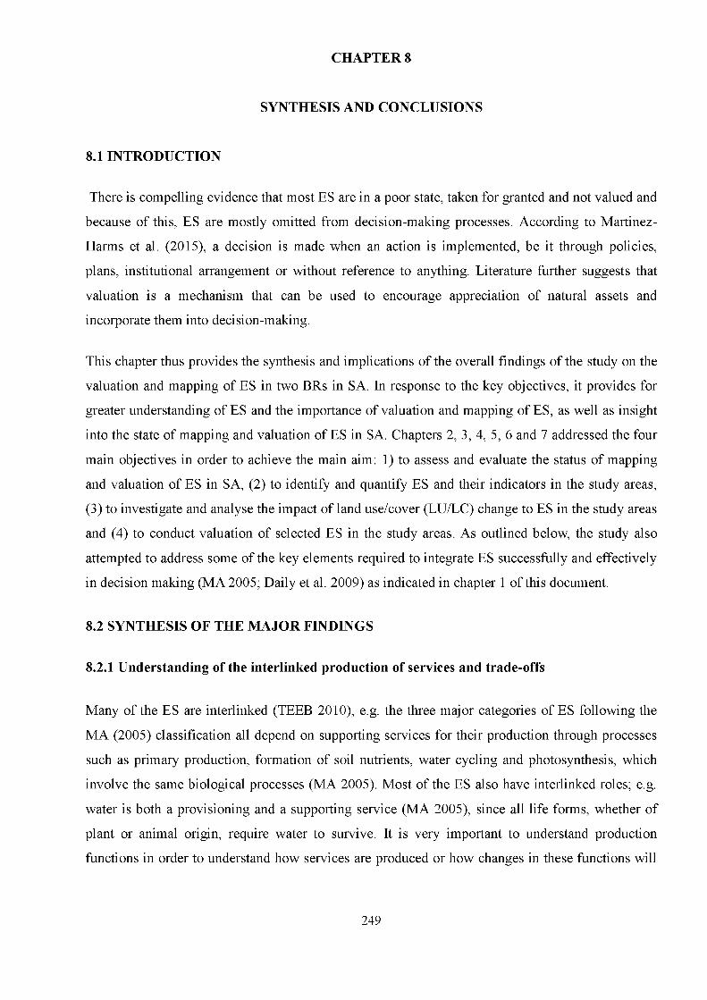
CHAPTER 8

SYNTHESIS AND CONCLUSIONS

8.1 INTRODUCTION

There is compelling evidence that most ES are in a poor state, taken for granted and not valued and

because of this, ES are mostly omitted from decision-making processes. According to Martinez-

Harms et al. (2015), a decision is made when an action is implemented, be it through policies,

plans, institutional arrangement or without reference to anything. Literature further suggests that

valuation is a mechanism that can be used to encourage appreciation of natural assets and

incorporate them into decision-making.

This chapter thus provides the synthesis and implications of the overall findings of the study on the

valuation and mapping of ES in two BRs in SA. In response to the key objectives, it provides for

greater understanding of ES and the importance of valuation and mapping of ES, as well as insight

into the state of mapping and valuation of ES in SA. Chapters 2, 3, 4, 5, 6 and 7 addressed the four

main objectives in order to achieve the main aim: 1) to assess and evaluate the status of mapping

and valuation of ES in SA, (2) to identify and quantify ES and their indicators in the study areas,

(3) to investigate and analyse the impact of land use/cover (LU/LC) change to ES in the study areas

and (4) to conduct valuation of selected ES in the study areas. As outlined below, the study also

attempted to address some of the key elements required to integrate ES successfully and effectively

in decision making (MA 2005; Daily et al. 2009) as indicated in chapter 1 of this document.

8.2 SYNTHESIS OF THE MAJOR FINDINGS

8.2.1 Understanding of the interlinked production of services and trade-offs

Many of the ES are interlinked (TEEB 2010), e.g. the three major categories of ES following the

MA (2005) classification all depend on supporting services for their production through processes

such as primary production, formation of soil nutrients, water cycling and photosynthesis, which

involve the same biological processes (MA 2005). Most of the ES also have interlinked roles; e.g.

water is both a provisioning and a supporting service (MA 2005), since all life forms, whether of

plant or animal origin, require water to survive. It is very important to understand production

functions in order to understand how services are produced or how changes in these functions will

249

affect ES produced (TEEB 2010), as well as the role of biodiversity in delivering

supporting/production services (MA 2005; TEEB 2010).

It is also very important to understand interconnectivity, as it might increase the likelihood of

double counting of ES (MA 2005; TEEB 2010). Also important to note is that these interlinkages

do not always result in synergies; there are trade-offs as well (Nelson et al. 2009). The study

managed to demonstrate this understanding in chapter 3, through LU change scenarios, as well as in

chapter 4 where ES that occur in the study area were identified and mapped. In chapter 5 the

researcher demonstrated how ES may affect one another, as a result of interdependence, e.g. when

provisioning ES such as agricultural activities are intensified, they might have an impact on water

(agricultural activities are associated with high consumption of water) or primary production

(because of vegetation clearing).

8.2.2 Stakeholders engagement in decision making process

Stakeholders engagement process forms one of the central issues of this study, which includes

understanding of the decision making process of individual stakeholders and transparency as

demonstrated in chapters 3, 4 and 7. A famous slogan of Latin origin, “Nothing about Us without

Us”, supports the idea that decisions should be effected in consultation with the affected

individuals, not without them (Charlton 2000). Generally, stakeholder engagement is regarded as

one of the most crucial elements of decision-making (MA 2005, Daily et al. 2009; Young et al.

2013). While it is important to include stakeholders in decision-making, they must also be given an

opportunity and platform to be personally involved in various decision-making processes. The

essence of this study was to promote the integration of ES into decision-making through different

stakeholder engagement processes, valuation and mapping. Chapter 3 dealt with stakeholder

engagement through scenario planning, chapter 4 dealt with mapping and identification of ES

(through stakeholder engagement), and chapter 7 dealt with the valuation of two provisioning ES

(timber and firewood).

8.2.3 Focus on other ES beyond provisioning services and understanding that not

all ES are valued

Literature evidence suggests that provisioning ES have long been given some kind of recognition,

including valuation (Portman 2013; Martinez-Harms et al. 2015). The understanding of other ES,

such as regulating and cultural ES, had started to emerge and had advanced significantly by the

time the MA (2005) was done. Although understanding of these types of services generally is

starting to develop, there is still a gap in the value domain, which is aggravated by the difficulties250

associated with capturing values of these types of services, as most of them are not traded in

markets, which contributes to their degradation and undervaluing, as well as society’s failure to

appreciate their worth.

In this study, attempts have been made to focus on other services beyond provisioning in order to

reflect their worth. This was done by (1) reviewing valuation and mapping of ES studies in chapter

2 and 4, (2) understanding the type of ES and their indicators that occur in the study areas, covered

by chapter 4, (3) giving special attention to supporting ES such as biodiversity, covered by chapter

5, which mainly focuses on habitat condition assessment, and (4) focusing on regulating services by

assessing and quantifying carbon storage in the study area, covered by chapter 6.

It is well known that the aim of conservation has been to safeguard biodiversity, which underpins

most of the supporting ES. Biodiversity conservation strategies, though, have to a certain extent

been associated with a hands-off and human exclusive approach (McLaughlin 2011; Pullin et al.

2011), which has been met with mixed feelings and resentment, to the detriment of conservation

efforts (Beltran 2000; Ayivor et al. 2013). Perhaps the emphasis was rather on benefit for future

generations (focused on the existence value), and promoting the uses of other ES (i.e. cultural and

regulating) than on provisioning. The new buzzword, “ecosystem services”, which is linked with

benefits to human well-being, is proving to be acceptable as a better alternative to the traditional

biodiversity concept, providing an opportunity to assist the achievement of biodiversity

conservation goals (MA 2005, TEEB 2010). More strategies and mechanisms are still needed

though, to fully unleash the potential of ES to enhance biodiversity conservation goals.

This study further demonstrated an understanding that not all ES are valued in chapter 5, where

biodiversity conservation, whose values can mainly be expressed in biophysical, terms (Daily et al.

2009), was modelled.

8.2.4 Use of the best available information

In the rapidly changing context of decision-making pertaining to natural assets, the challenge lies in

making effective use of information and relevant tools to keep abreast with these changes. Relevant

tools that can aid the successful integration of ES to decision making include

quantification/mapping and valuation. The relevancy of the study with this element is outlined in

chapters 4 where mapping of ES was conducted as well as chapters 5 and 7 that dealt with valuation

of ES.

251

8.2.5 Integration of research into institutional design and policy implementation

Although the importance of integrating the science of ES into decision-making, such as policy

making, has been strongly emphasised and reinforced through international obligations, among

others the Intergovernmental Platform of Biodiversity and Ecosystem Services and the Convention

on Biological Diversity, it remains a challenge. To integrate science and policy successfully is

problematic (Godfrey et al. 2010), therefore various procedures and institutional arrangements have

to be made available to achieve this (Heinrich 2007; Godfrey et al. 2010). Being faced with ES in

the decision-making integration gap and science-policy interface gap indicates a dire need for

robust strategies to achieve the much needed integration of research into institutional design and

policy implementation.

One of the fundamental issues regarding ES assessment is an understanding of the socio-ecological

context (Martinez-Harms et al. 2015). In this study, ES assessment was conducted mainly in a BR.

Because they are socio-ecological systems, meant to promote sustainable development, while

conserving biological diversity and promoting sustainable resource use, BRs have to conform to

relevant institutional requirement designs and policies. BRs' main principles of sustainable

development thus make it easy to apply the CBD's three main objectives: (1) the conservation of

biological diversity, (2) the sustainable use of its genetic resources and (3) the fair and equitable

sharing of benefits. Mechanisms such as valuation can be used to generate information that can

assist in designs and policy implementation in socio-ecological institutions such as BRs. Valuation

has been applied in chapter 5, 6 and 7, the results of which provide valuable information that can

contribute to institutional designs and policy implementation related to socio-ecological systems,

BRs in this case.

8.2.6 Evidence based, performance monitoring, evaluation and accountability

According to Heinrich (2007), the aim of both performance management and evidence-based policy

is to improve effectiveness by basing decision-making on scientific evidence. However, in order to

achieve this, there must be an understanding of how to distinguish evidence from non-evidence,

how to communicate such evidence, and how to judge quality and reliability. Lastly, there must

also be a balance between information processes for decision-making and accountability (Heinrich

2007).

Accountability, monitoring and evaluation, are also very important aspects in influencing decision

making, such as whether to improve or discontinue the intervention, strategy or policy (UNICEF

252

2003). The main purpose of evaluation is to determine the significance of a policy, strategy or

intervention (UNICEF 2003). In order for the evaluation process to be objective, among others it

needs to reconcile the perspectives of different stakeholders (UNICEF 2003). An evaluation report,

on the other hand, should include findings and evidence, conclusions, recommendations and lessons

learnt (UNICEF 2003).

Chapters 5, 6 and 7 dealt mainly with valuation of selected ES in the BRs, with chapters 5 and 6

focusing on the biophysical component and chapter 7 focusing on the economic component. In

chapter 5 modelling results of the habitat condition assessment provided valuation evidence

required to make informed decisions on issues such as carrying capacity, introduction and removal

of game, threats to biodiversity and ways to deal with these. Chapter 6 dealt with the assessment of

carbon storage and quantification of its values, thus providing information required to deal with the

climate change phenomenon. Chapter 7 addresses the integration of ES into the national and

regional economy, as the main activities focus on the contribution that ES make to the economy

both directly through timber sales and indirectly through making provision for an alternative cost-

effective energy source (fuel wood), thus contributing to poverty alleviation. This information

presents an opportunity to integrate ES into decision-making, as it provides the basis for informed

decisions to improve governance and effectiveness related to biodiversity conservation and

economic development.

8.2.7 Contribution of the study to the field of ES

All eight chapters attempted to highlight the importance of integrating ES in decision-making for

conservation and LU planning through the application of different tools, i.e. value mapping,

modelling and quantification. The study also highlights new insights into the existing theories on

ES, which in this case are socio-ecological systems and sustainability science. Figure 8.1 provides

for the adjusted conceptual framework (MA 2005), denoting areas where the current study is

providing new knowledge on the existing theories of ES, in this case socio-ecological systems and

sustainability science, as indicated in chapter 1.

253

Provisioning (food; water)

Regulating (climate ; disease regulation)

Cultural (recreational; spiritual)

Supporting (primary production; soil formation)

Human well-being

I Poverty reduction Freedom & choice

Good social relations Health Security

Drivers of change

Distribution and Quantities Valuation and

Appraisals

Economic Socio-political Demographic

Science & technonlogy Culture & religion

Land use/cover change Climate change

Speciesintrodction/removal Decision=making

Management strategies & poliicies

4 Societal relevance

Figure 8.1 Conceptual framework (adapted from MA 2005) highlighting areas (red, green and

purple) where the study is contributing new knowledge to the existing theories.

In conclusion, a four-step integrated approach that can aid the successful incorporation of ES into

decision-making is proposed: (1) maintain a balance between the social, economic and ecological

aspects when making decisions on ES, (2) strive for an evidence-based approach to decision

making (use quantities and values), (3) apply integrated approaches (methods and techniques) to

quantification and valuation, and (4) communicate all steps along the way.

254

8.3 FUTURE RESEARCH QUESTIONS

This study identified a few areas that need research in the field of ES valuation to continue where

this study left off. The following questions are relevant in this regard.

• To what extent do PAs contribute to the national economy and poverty alleviation?

• What is the economic value of PAs compared to other land use, such as mining and

agriculture?

• What is the value (ecological, social, and economic) of ES generated by PAs?

• What is the value (ecological, social, and economic) of ES generated by BRs?

• What are the quantities of ES generated by PAs?

• What are the quantities of ES generated by BRs?

8.4 CONCLUDING REMARKS

It has become clear that in order to maintain a balance between biodiversity conservation and the

mainstreaming of economic benefits, responding to challenges facing socio-ecological systems

such as BRs now requires new approaches and tools. The management of PAs, including BRs,

needs to realise the important role various tools, such as valuation and mapping of ES, can play in

building a body of evidence to advocate the case of these natural assets in economic-orientated

periods. Decision-makers must take a holistic approach (considering economic, social and

ecological aspects) and take into account the associated trade-offs when making LU decisions

regarding natural systems. To keep up with the changing context for managing PAs and socio

ecological systems, there must be a paradigm shift in management approaches and attitudes.

There is growing appreciation of the concept of ES among policy makers and governments as a

means to unlock new opportunities for economic development, to safeguard natural assets and to

influence decision-making through its valuation. There is a strong need for countries to prioritise

valuation of ES in PAs, as they represent auditable systems in achieving the CBD's objectives of

integrating ES into national accounting and economies. Moreover, countries should embrace the

BR model, as it represents a holistic approach that integrates the social, ecological and economic

aspects to attain sustainable development goals. To date, ES has been a whirlwind subject of

science, which strives to address current challenges and trends, including the science-policy

interface, to inform decision-making. In order to bridge the gap between science and policy, there

255

must be an interface and monitoring mechanism to ensure that policies are informed by evidence,

while policies on the other hand strive to support decision-making.

Amidst increased understatement of the fact that valuation is a means of incorporating natural

assets into decision-making, practitioners must be competent enough to apply this approach to

satisfy this need, and it must be ensured that approaches in this regard integrate social, ecological

and economic needs/requirements to ensure sustainability. In order to enhance the contribution of

valuation to decision-making, it is important to understand different areas where its application can

be more meaningful and valuable. Understanding and selecting appropriate methods that can be

employed in this regard are crucial requirements. To make valuation work in decision-making,

careful consideration is also necessary during analysis and interpretation processes to ensure that it

is applied in a simplistic and practical manner. Although valuation has broken new ground and the

stage has been set for it to be turned into a useful tool for decision-making, it must be noted that it

is only a means to an end, not the end itself.

256

8.5 REFERENCES

Ayivor, J.S., Gordon, C. and Ntiamoa-Baidu, Y. 2013. Protected area management and

livelihood conflicts in Ghana. P a rks: The In te rn a tio n a l J o u rn a l o f P ro te c te d A re a s a n d

C onserva tion , 19:1.

Beltran, J. (ed.). 2000. Indigenous and Traditional Peoples and Protected Areas:

Principles, Guidelines and Case Studies. IUCN, Gland, Switzerland and Cambridge, UK

and WWF International, Gland, Switzerland. xi +133pp. [Pre-publication].

CBD (Convention on Biological Diversity). 2010. Strategic Plan for Biodiversity 2011-2020

and the Aichi Targets. A ten year framework for action by all countries and stakeholders to

save and enhance benefits for people. The tenth meeting of the Conference of the Parties,

held from 18 to 29 October 2010, in Nagoya, Aichi Prefecture, Japan.

https://www.cbd.int/doc/strategic-plan/2011-2020/Aichi-Targets.

Charlton, J.I. 2000. Nothing about Us without Us: Disability Oppression and

Empowernment. University of California Press. https://books.google.co.za/books.


T.H., Salzman, J. and Shallenberger, R. 2009. Ecosystem services in decision-making: Time

to deliver. F ro n tie rs in E co lo g y a n d the E n vironm en t, 7(1): 21-28.

Godfrey, L., Funke, N. and Mbizvo, C. 2010. Bridging the science-policy interface: A new

era for South African research and the role of knowledge brokering. S o u th A fr ica n Jo u rn a l

o f Sc ience , 106:5-6.

Heinrich, C.J. 2007. Evidence-based policy and performance management: Challenges and

prospects in two parallel movements. The A m er ica n R ev iew o f P u b lic A dm in istra tio n ,

37(3):255-277.

Martinez-Harms, M.J., Bryan, B.A., Balvanera, P., Law, E.A., Rhodes, J.R., Possingham,

H.P. and Wilson, K.A. 2015. Making decisions for managing ecosystem services. B io lo g ic a l

C onserva tion , 184: 229-238.


Synthesis. World Resource Institute: Washington, DC; Island Press.

McLaughlin, C.M. 2011. People living in protected areas: A comparative study of the

social impacts of conservation in Latin America's MamirAu sustainable development

reserve and Ria Celestun Biosphere Reserve. Paper Submitted in Partial Fulfilment of the

Requirements for the Degree of Master of Arts in International Affairs and Natural

Resources and Sustainable Development, American University United Nations.

https://www.american.edu/sis/gep/upload/08 2011 McLaughlin SRP.pdf.

257

https://www.cbd.int/doc/strategic-plan/2011-2020/Aichi-Targets

https://books.google.co.za/books

https://www.american.edu/sis/gep/upload/08_2011_McLaughlin_SRP.pdf



Shaw, M.R. 2009. Modelling multiple ecosystem services, biodiversity conservation,

commodity production, and trade-offs at landscape scales. The Ecological Society of

America. Frontiers in Ecological Environment, 7(1): 4-11.

TEEB (The economics of ecosystems and biodiversity). 2010. Mainstreaming the economics

of nature: A synthesis of the approach, conclusions and recommendations of TEEB.

Portman, M. 2013. Ecosystem services in practice: Challenges to real world implementation

of ecosystem services across multiple landscapes: A critical review. Applied Geography,

45(2013): 185e192.

Pullin, A.S., Bangpan, M., Dalrymple, S., Dickson, K., Haddaway, N.R., Healey, J.R.,

Hauari, H., Hockley, N., Jones, J.P.G., Dalling, J.W., Barkan, P., Bellingham, P.J., Healey,

J.R. and Tanner. 2011. Human well-being impacts of terrestrial protected areas.

Environmental Evidence, 2:19.

UNICEF, 2003. Programme, policy and procedures manual: Programme operations,

UNICEF, New York, Revised May 2003, pp. 109-120.

Young, J.C., Jordan, A., Searle, K.R., Butler, A., Chapman, D.S., Simmons, P. and

Watt, A.D. 2013. Does stakeholder involvement really benefit biodiversity conservation?

Biological Conservation, 158: 359-370.

258

ECOSYSTEM SERVICES IN A BIOSPHERE RESERVE ...

Documents

Transcript of ECOSYSTEM SERVICES IN A BIOSPHERE RESERVE ...