UNSTRUCTURED MESH PARAMETERIZATION FOR A SMALL WIND TURBINE SIMULATION
12
UNSTRUCTURED MESH PARAMETERIZATION FOR A SMALL WIND TURBINE SIMULATION Angelo Bezerra Modolo Campus do Pici – Bloco 714 – CEP 60455-760 – Fortaleza - CE [email protected] Marco Antonio Bezerra Diniz Campus do Pici – Bloco 714 – CEP 60455-760 – Fortaleza - CE [email protected] Mauricio Soares de Almeida Campus do Pici – Bloco 714 – CEP 60455-760 – Fortaleza - CE [email protected] Paulo Alexandre Costa Rocha Campus do Pici – Bloco 714 – CEP 60455-760 – Fortaleza - CE [email protected] Helio Henrique Barbosa Rocha Campus do Pici – Bloco 714 – CEP 60455-760 – Fortaleza - CE [email protected] Abstract. Computational studies of wind turbines have been growing considerably in recent years. This is due to the fact that the reduction of analysis time, costs in the development of wind turbines and the high reliability of the results. Then, a survey of mesh convergence was conducted, consisting of a mesh with a static external domain and a rotating internal domain for the simulation of a 5 m diameter wind turbine. The turbine studied is a model with three blades, designed with the help of software SDPA 1.0 - Development System for Wind Turbine Blades - developed in the Laboratory of Aerodynamics and Fluid Mechanics. The SDPA computes chord and the twist angle for optimum blade sections according to the theory of BEM. The blade is optimized for a specific speed value λ = 7. with NACA 63215 profile. The meshes were generated by software ANSYS ICEM CFD to different values of downstream distance, upstream distance, static domain diameter, maximal size of elements over the blades, minimal size of elements over the blades, maximal size of external domain and maximal size of internal domain. Simulations were performed by software ANSYS CFX using RANS k-ω SST turbulence model. Solution independence to mesh has been achieved and the resulting mesh has been used to plot the power curve of the wind turbine. The values of power coefficient were calculated with reasonable precision and the obtained mesh has been considered adequate to the proposed study. At the end of the study, we compare the results obtained with the BEM available and it could be verified that simulation represented very well problem proposed. Keywords: parameterization, mesh, wind turbine, convergence. 1. INTRODUCTION The wind energy has become an appreciable source of energy for many countries. Its recognition as a source of energy used in a commercial scale is due to the necessity to use alternative sources of energy that are renewable, clean and commercially viable (Martins et al., 2008; Khan and Iqbal, 2005; Da Silva et al., 2005; Lund and Mathiesen, 2009; Ozerdem et al., 2006). The wind power generation has taken an important role in the energy matrix of various countries. The worldwide capacity reached 32 GW in the early 2000s. Brazil presented, in 2010, a installed wind capacity of 931 MW, a small number in front of other countries with similar potential. However, this figure also indicates the growth potential of the Brazilian wind market, a fact confirmed by the growth rate of the same year, which reached 35%. Ceará has a prominent role in this scenario, since it has more than 104 MW of installed capacity (Silva, 2003). In this context, tools to improve some aspect of the design and operation of wind turbines are very useful. The computational fluid dynamics (CFD) has shown a robust, accessible and little cost to predict the behavior of wind turbines in various situations (Baxevanou et al., 2008; Li et al., 2012; Lanzafame and Messina, 2013; Kishore et al.,2013; Hu et al.,2006). The adjustable parameters in a CFD mesh are numerous and careful study of their values can lead to a better compromise between computational effort and outcome uncertainty. In addition, one can choose between different possible configurations for the fluid domains used, which allows a large number of approaches being studied.
-
Upload
independent -
Category
Documents
-
view
1 -
download
0
Transcript of UNSTRUCTURED MESH PARAMETERIZATION FOR A SMALL WIND TURBINE SIMULATION
UNSTRUCTURED MESH PARAMETERIZATION FOR A SMALL WIND
TURBINE SIMULATION
Angelo Bezerra Modolo Campus do Pici – Bloco 714 – CEP 60455-760 – Fortaleza - CE
Marco Antonio Bezerra Diniz Campus do Pici – Bloco 714 – CEP 60455-760 – Fortaleza - CE
Mauricio Soares de Almeida Campus do Pici – Bloco 714 – CEP 60455-760 – Fortaleza - CE
Paulo Alexandre Costa Rocha Campus do Pici – Bloco 714 – CEP 60455-760 – Fortaleza - CE
Helio Henrique Barbosa Rocha Campus do Pici – Bloco 714 – CEP 60455-760 – Fortaleza - CE
Abstract. Computational studies of wind turbines have been growing considerably in recent years. This is due to the
fact that the reduction of analysis time, costs in the development of wind turbines and the high reliability of the results.
Then, a survey of mesh convergence was conducted, consisting of a mesh with a static external domain and a rotating
internal domain for the simulation of a 5 m diameter wind turbine. The turbine studied is a model with three blades,
designed with the help of software SDPA 1.0 - Development System for Wind Turbine Blades - developed in the
Laboratory of Aerodynamics and Fluid Mechanics. The SDPA computes chord and the twist angle for optimum blade
sections according to the theory of BEM. The blade is optimized for a specific speed value λ = 7. with NACA 63215
profile. The meshes were generated by software ANSYS ICEM CFD to different values of downstream distance,
upstream distance, static domain diameter, maximal size of elements over the blades, minimal size of elements over the
blades, maximal size of external domain and maximal size of internal domain. Simulations were performed by software
ANSYS CFX using RANS k-ω SST turbulence model. Solution independence to mesh has been achieved and the
resulting mesh has been used to plot the power curve of the wind turbine. The values of power coefficient were
calculated with reasonable precision and the obtained mesh has been considered adequate to the proposed study. At
the end of the study, we compare the results obtained with the BEM available and it could be verified that simulation
represented very well problem proposed.
Keywords: parameterization, mesh, wind turbine, convergence.
1. INTRODUCTION
The wind energy has become an appreciable source of energy for many countries. Its recognition as a source of
energy used in a commercial scale is due to the necessity to use alternative sources of energy that are renewable, clean
and commercially viable (Martins et al., 2008; Khan and Iqbal, 2005; Da Silva et al., 2005; Lund and Mathiesen, 2009;
Ozerdem et al., 2006). The wind power generation has taken an important role in the energy matrix of various countries.
The worldwide capacity reached 32 GW in the early 2000s. Brazil presented, in 2010, a installed wind capacity of 931
MW, a small number in front of other countries with similar potential. However, this figure also indicates the growth
potential of the Brazilian wind market, a fact confirmed by the growth rate of the same year, which reached 35%. Ceará
has a prominent role in this scenario, since it has more than 104 MW of installed capacity (Silva, 2003).
In this context, tools to improve some aspect of the design and operation of wind turbines are very useful. The
computational fluid dynamics (CFD) has shown a robust, accessible and little cost to predict the behavior of wind
turbines in various situations (Baxevanou et al., 2008; Li et al., 2012; Lanzafame and Messina, 2013; Kishore et
al.,2013; Hu et al.,2006). The adjustable parameters in a CFD mesh are numerous and careful study of their values can
lead to a better compromise between computational effort and outcome uncertainty. In addition, one can choose
between different possible configurations for the fluid domains used, which allows a large number of approaches being
studied.

Given the importance of this tool for the sector and its straightforward application, this paper aimed to study the
influence of some of the most important parameters of a grid with two domains for the simulation of a wind turbine.
It is expected in this study to develop a tetrahedral mesh with a static domain and a rotating domain to simulate a
small wind turbine and study the influence of the values assigned to its parameters on the outcome of simulations by
finite volume method.
More specifically, this work proposes to:
Study the influence of the geometrical characteristics of the mesh on the simulation;
Obtain values for these parameters that make the simulation independent of the mesh;
Get a mesh that meets a good compromise between computational effort and uncertainty of simulation
results.
2. MATERIALS AND METHODS
This paper was carried out with the aid of a computer with the CFD solver ANSYS CFX 12.1 and mesh generation
software ANSYS ICEM CFD. Seven parameters were evaluated for a 5m diameter turbine: downstream distance,
upstream distance, diameter of the static domain, maximum size of an element on the blade, minimum size of an
element on the blade, maximum size of an element in the static field and maximum size of an element in the rotation
domain.
Each parameter was studied for seven distinct values, which means 49 simulations. It was determined for each
parameter the value that makes the solution independent of the mesh, known as the convergence value mesh. This value
was used in the simulation of the following parameters.
At the end of the parameterization, a grid was obtained that minimally interferes the simulation result without,
however, resulting too much computational effort. This mesh was used to plot the power curve of the turbine.
The turbine studied is a three bladed model, designed with the aid of software SDPA 1.0 - Sistema de
Desenvolvimento de Pás de Aerogeradores - developed in the Laboratory of Aerodynamics and Fluid Mechanics
(Modolo and Rocha, 2009). The SDPA computes the chord and twist angle for optimum blade sections according to the
theory of BEM (Burton et al., 2001). The blade is optimized to a value of tip speed ratio .
The rotor diameter is 5 m, and it uses the NACA 63215 profile. The turbine is designed so that at each point of the
profile blades are in optimum attack angle, i.e., the angle at which the profile has the highest ratio between the values of
lift and drag. Under these conditions, the profile has the following characteristics:
Optimal angle of attack: ; Lift coeficiente ;
Drag coefficient: ;
Lift/drag ratio: .
The choice of a three bladed model is because it provides good compromise between the maximum value and the
operating range width of the turbine, as illustrated by Figure 1.
Figure 1 - Effect of the number of blades on the power curve of the turbine. (Burton, et al., 2001).
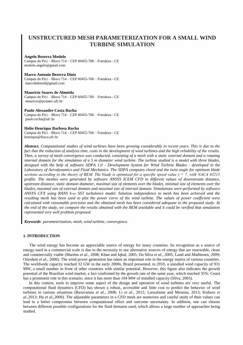
The methodology leads to two curves that completely describe the geometry of the turbine. The first curve defines
the value of the chord represented by , for each point of the blade, while the second defines the angle . All lengths are
dimensionless dividing by . The graphics with the design aspects are presented in Figure 2.
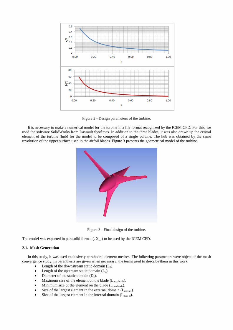
Figure 2 - Design parameters of the turbine.
It is necessary to make a numerical model for the turbine in a file format recognized by the ICEM CFD. For this, we
used the software SolidWorks from Dassault Systèmes. In addition to the three blades, it was also drawn up the central
element of the turbine (hub) for the model to be composed of a single volume. The hub was obtained by the same
revolution of the upper surface used in the airfoil blades. Figure 3 presents the geometrical model of the turbine.
Figure 3 - Final design of the turbine.
The model was exported in parasolid format (. X_t) to be used by the ICEM CFD.
2.1. Mesh Generation
In this study, it was used exclusively tetrahedral element meshes. The following parameters were object of the mesh
convergence study. In parenthesis are given when necessary, the terms used to describe them in this work.
Length of the downstream static domain (Ld).
Length of the upstream static domain (Lu).
Diameter of the static domain (Ds).
Maximum size of the element on the blade (Lmax blade).
Minimum size of the element on the blade (Lmin blade).
Size of the largest element in the external domain (Lmax ex).
Size of the largest element in the internal domain (Lmax in).
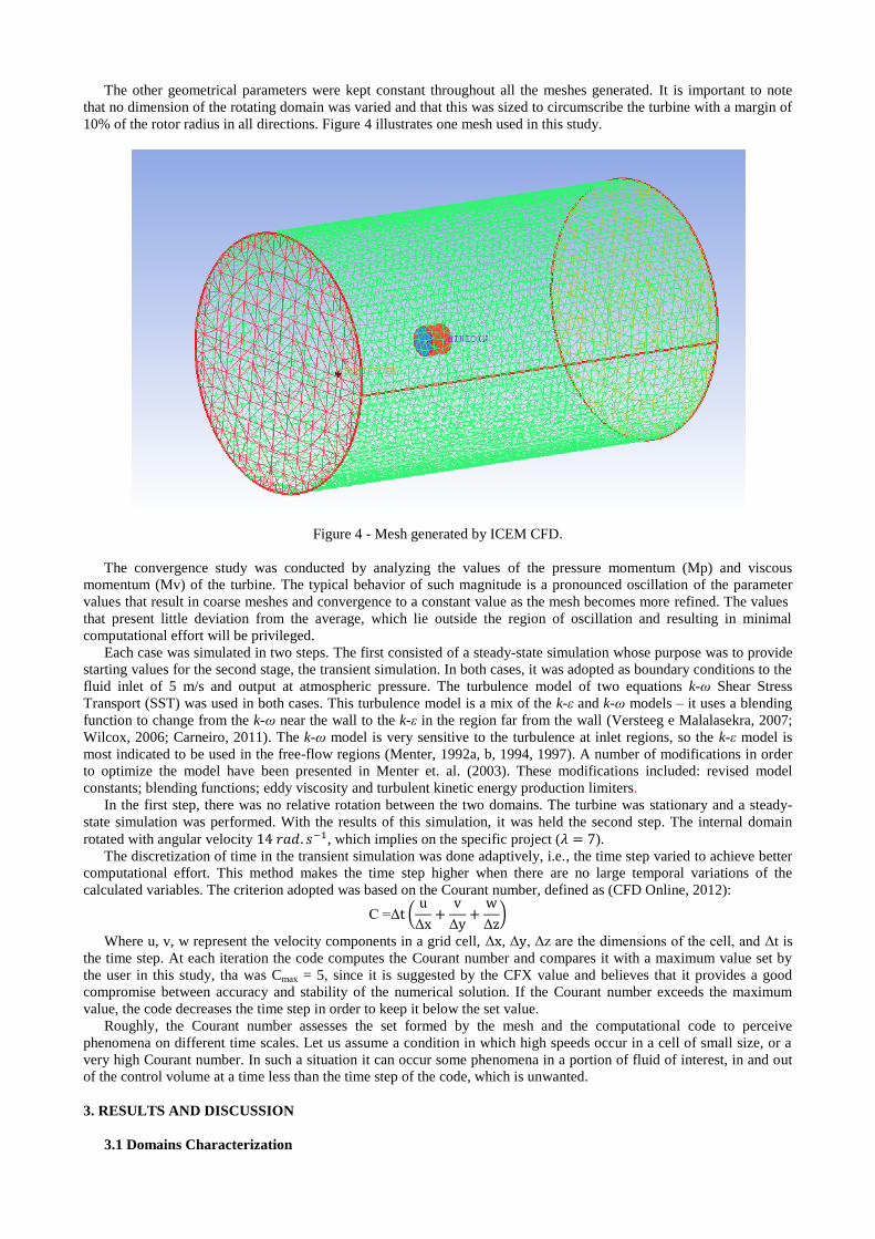
The other geometrical parameters were kept constant throughout all the meshes generated. It is important to note
that no dimension of the rotating domain was varied and that this was sized to circumscribe the turbine with a margin of
10% of the rotor radius in all directions. Figure 4 illustrates one mesh used in this study.
Figure 4 - Mesh generated by ICEM CFD.
The convergence study was conducted by analyzing the values of the pressure momentum (Mp) and viscous
momentum (Mv) of the turbine. The typical behavior of such magnitude is a pronounced oscillation of the parameter
values that result in coarse meshes and convergence to a constant value as the mesh becomes more refined. The values
that present little deviation from the average, which lie outside the region of oscillation and resulting in minimal
computational effort will be privileged.
Each case was simulated in two steps. The first consisted of a steady-state simulation whose purpose was to provide
starting values for the second stage, the transient simulation. In both cases, it was adopted as boundary conditions to the
fluid inlet of 5 m/s and output at atmospheric pressure. The turbulence model of two equations k-ω Shear Stress
Transport (SST) was used in both cases. This turbulence model is a mix of the k-ε and k-ω models – it uses a blending
function to change from the k-ω near the wall to the k-ε in the region far from the wall (Versteeg e Malalasekra, 2007;
Wilcox, 2006; Carneiro, 2011). The k-ω model is very sensitive to the turbulence at inlet regions, so the k-ε model is
most indicated to be used in the free-flow regions (Menter, 1992a, b, 1994, 1997). A number of modifications in order
to optimize the model have been presented in Menter et. al. (2003). These modifications included: revised model
constants; blending functions; eddy viscosity and turbulent kinetic energy production limiters.
In the first step, there was no relative rotation between the two domains. The turbine was stationary and a steady-
state simulation was performed. With the results of this simulation, it was held the second step. The internal domain
rotated with angular velocity , which implies on the specific project ( ).
The discretization of time in the transient simulation was done adaptively, i.e., the time step varied to achieve better
computational effort. This method makes the time step higher when there are no large temporal variations of the
calculated variables. The criterion adopted was based on the Courant number, defined as (CFD Online, 2012):
Where u, v, w represent the velocity components in a grid cell, , , z are the dimensions of the cell, and t is
the time step. At each iteration the code computes the Courant number and compares it with a maximum value set by
the user in this study, tha was Cmax = 5, since it is suggested by the CFX value and believes that it provides a good
compromise between accuracy and stability of the numerical solution. If the Courant number exceeds the maximum
value, the code decreases the time step in order to keep it below the set value.
Roughly, the Courant number assesses the set formed by the mesh and the computational code to perceive
phenomena on different time scales. Let us assume a condition in which high speeds occur in a cell of small size, or a
very high Courant number. In such a situation it can occur some phenomena in a portion of fluid of interest, in and out
of the control volume at a time less than the time step of the code, which is unwanted.
3. RESULTS AND DISCUSSION
3.1 Domains Characterization
The length of the static domain was measured downstream of the system origin at the center of the rotor, the face of
the cylinder downstream of the turbine. This distance is of great importance to the independence of the result with
respect to the mesh, since it is in this portion of the domain that the wake is generated by the turbine and therefore much
of the phenomena relevant to the characterization of the problem is present.
As previously noted, the turbine draws energy flow in the form of pressure, and this quantity is gradually recovered
as the wake is re-energized by surrounding free stream. By adopting a too short downstream distance, the wake will not
be sufficiently covered by the domain and the phenomena that occur in this space will not be taken into account in the
simulation. On the other hand, the adoption of a length that is too long implies in counterproductive computational
effort, since the calculations are performed for a portion of the flow that has reached equilibrium with the free stream.
According to Burton et al. (2001), the influence on the flow of the turbine downstream and upstream is practically
nonexistent for distances greater than ten times the diameter of the turbine. Due to the nature of the problem, it is
expected that a similar value is obtained in this study and therefore 10D was used as the center of the interval studied
for this parameter. The values used, based on the diameter of the turbine were:
2,5D
5D
7,5D
10D
15D
20D
25D
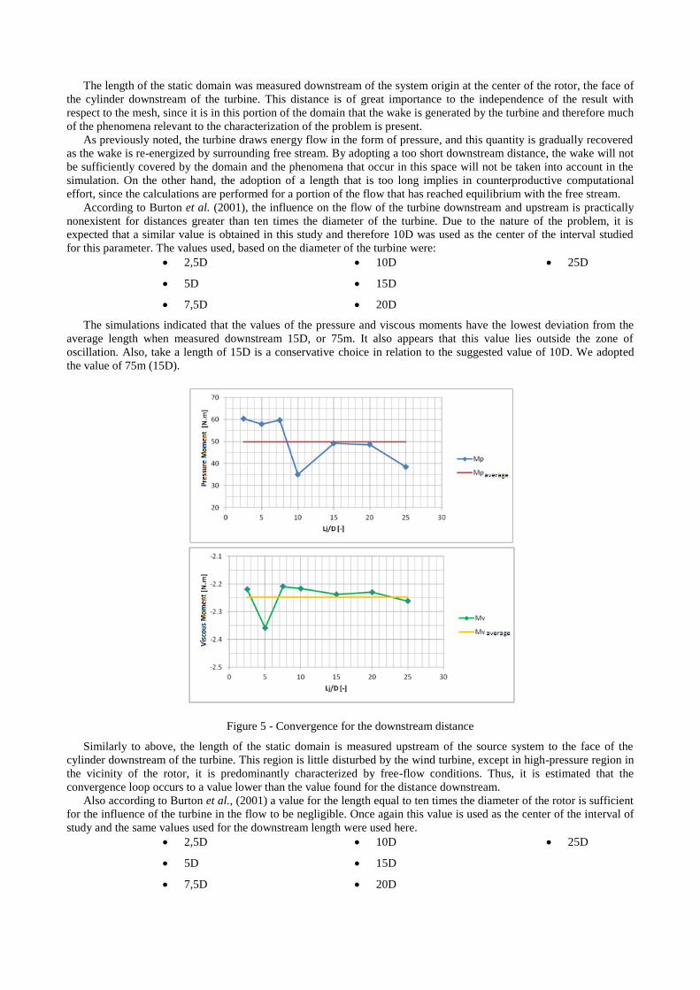
The simulations indicated that the values of the pressure and viscous moments have the lowest deviation from the
average length when measured downstream 15D, or 75m. It also appears that this value lies outside the zone of
oscillation. Also, take a length of 15D is a conservative choice in relation to the suggested value of 10D. We adopted
the value of 75m (15D).
Figure 5 - Convergence for the downstream distance
Similarly to above, the length of the static domain is measured upstream of the source system to the face of the
cylinder downstream of the turbine. This region is little disturbed by the wind turbine, except in high-pressure region in
the vicinity of the rotor, it is predominantly characterized by free-flow conditions. Thus, it is estimated that the
convergence loop occurs to a value lower than the value found for the distance downstream.
Also according to Burton et al., (2001) a value for the length equal to ten times the diameter of the rotor is sufficient
for the influence of the turbine in the flow to be negligible. Once again this value is used as the center of the interval of
study and the same values used for the downstream length were used here.
2,5D
5D
7,5D
10D
15D
20D
25D
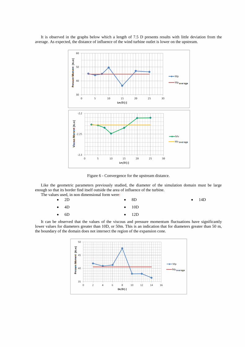
It is observed in the graphs below which a length of 7.5 D presents results with little deviation from the
average. As expected, the distance of influence of the wind turbine outlet is lower on the upstream.
Figure 6 - Convergence for the upstream distance.
Like the geometric parameters previously studied, the diameter of the simulation domain must be large
enough so that its border find itself outside the area of influence of the turbine.
The values used, in non dimensional form were:
2D
4D
6D
8D
10D
12D
14D
It can be observed that the values of the viscous and pressure momentum fluctuations have significantly
lower values for diameters greater than 10D, or 50m. This is an indication that for diameters greater than 50 m,
the boundary of the domain does not intersect the region of the expansion cone.

Figure 7 - Convergence for the external diameter.
3.2 Mesh Characterization
By limiting the maximum size of the elements adjacent to the turbine we proceed a further refinement of the
mesh over this region and hence smaller errors compared to the real solution of the problem. The surface of the
turbine is a critical region where further refinement is required due to the complex geometry and the large spatial
variation of flow properties in its neighborhood.
As the center of the interval parameter it was adopted the minor chord of the blades, which corresponds to the
shortest length present in the studied geometry. The minor chord measures 0.1240 m. The studied interval was
defined from fractions of that reference length, as follows:
5/8
6/8
7/8
8/8
10/8
14/8
16/8
Figure 8 - Convergence of the maximum size of the elements over the blade.
Since the behavior of the pressure momentum in relation to the parameter studied was markedly
periodic, it is not possible to conclude which value should be adopted. Remained so the initial value.
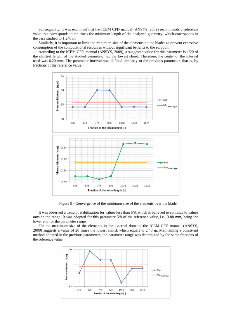
Subsequently, it was examined that the ICEM CFD manual (ANSYS, 2009) recommends a reference
value that corresponds to ten times the minimum length of the analyzed geometry, which corresponds in
the case studied to 1,240 m.
Similarly, it is important to limit the minimum size of the elements on the blades to prevent excessive
consumption of the computational resources without significant benefits to the solution.
According to the ICEM CFD manual (ANSYS, 2009), a suggested value for this parameter is 1/20 of
the shortest length of the studied geometry, i.e., the lowest chord. Therefore, the center of the interval
used was 6.20 mm. The parameter interval was defined similarly to the previous parameter, that is, by
fractions of the reference value.
Figure 9 - Convergence of the minimum size of the elements over the blade.
It was observed a trend of stabilization for values less than 6/8, which is believed to continue to values
outside the range. It was adopted for this parameter 5/8 of the reference value, i.e., 3.88 mm, being the
lower end for the parameter range.
For the maximum size of the elements in the external domain, the ICEM CFD manual (ANSYS,
2009) suggests a value of 20 times the lowest chord, which equals to 2.48 m. Maintaining a consistent
method adopted in the previous parameters, the parameter range was determined by the same fractions of
the reference value.
.

Figure 10 - Convergence for the maximum size of the elements in the external domain.
It was adopted the central value of the parameter range because it presents the lowest deviation from
the average for both momentums.
The methodology used to determine the maximum size of the elements for the internal domain is
identical to that adopted for the previous parameter.
Figure 11 - Convergence of the maximum size of the elements for the internal domain.
It was adopted the value of 6/8 because it presents the lowest deviation from the average for both
momentums. Table 1 illustrates the values in meters for each parameter evaluated in addition to the
adopted convergence value:
Table 1: Summary of the values applied in the parameterization
Parameter Values [m] Lj [m] 12.5 25 37.5 50 75 100 125 Lm [m] 12.5 25 37.5 50 75 100 125 De [m] 10 20 30 40 50 60 70 Lmax pá [mm] 77,5 93,0 108 124 155 217 248 Lmin pá [mm] 3,88 4,65 5.43 6,20 7,75 10,85 12,40 Lmax ex [m] 1,55 1,86 2,17 2,48 3,10 4,34 4,96 Lmax in [m] 1,55 1,86 2,17 2,48 3,10 4,34 ----

3.3 Power Coefficient
After the parameter adjustment procedure, the obtained mesh was used to evaluate the power
extracted from the turbine for different values of the tip speed ratio. It was expected that the power peak
would occur at λ 7, the value to which the turbine is designed to provide optimum efficiency. It was
remained the free stream velocity constant and equal to 5 m/s, while the angular velocity of the turbine
was varied. For the power extracted it was multiplied the resulting momentum, i.e., the sum of the viscous
and pressure momentums, by the angular velocity. The results obtained by CFX simulation are shown in
Figure 17 and compared with the results calculated iteratively by the Blade Element – Momentum theory
(BEM).
Figure 12 - Power curve of the wind turbine.
The curve exhibits a behavior consistent with the expectation. The model of project adopted
disregards friction losses and results in a turbine with theoretical yield equal to the Betz limit. Peak power
occurred on the designed tip speed ratio and approached significantly the Betz limit, which is consistent
with the simplification of the project template. If the viscous momentum is overlooked, it is obtained a Cp
0.5658 for λ 7, which is 4.5% lower than the Betz limit ( p 0.5926).
4. CONCLUSION
Seven different parameters were adopted to study the convergence of a mesh with two domains for the
simulation of a small wind turbine. The work resulted in a mesh that produces an independent solution.
After the convergence study, it was determined the power curve of the turbine under study. When
comparing the power curve obtained by simulation with the values expected for the turbine under study, it
was observed that the parameterization was successful and that the obtained mesh is appropriate for the
case studied.
In this paper, a number of difficulties were encountered and it is believed that the results obtained in
this study can be significantly improved, once it is observed the best practices in relation to these
problems.
Due to time constraints associated with this work, the simulation parameters were truncated after a
week, before the convergence of the numerical solution was achieved. To avoid errors, all simulations for
a parameter have been truncated at identical time steps. It is suggested longer simulations, preferably until
they reach numerical convergence, because they have lower residual error and expected to lead to better
results.
Furthermore, discretization of time in the transient simulation was performed adaptively to the
Courant number. A possible improvement would be to limit the Courant number towards lower values,
thus obtaining smaller time steps, which can lead to more accurate results with respect to time. Other
approaches are possible to the time discretization and deserve to be considered as options.
6. ACKNOWLEDGEMENTS
This research was jointly supported by the Coordenação de Aperfeiçoamento de Pessoal de Nível
Superior (CAPES) and the Conselho Nacional de Desenvolvimento Científico e Tecnológico (CNPq).
The support received is gratefully acknowledged.
7. BIBLIOGRAPHY
A.NSYS C.FX, Release 1.2.1. GNU LESSER GENERAL PUBLIC LICENSE (LGPL) Introduction to
the C.FX Tutorials.
Baxevanou, C.A.; Chaviaropoulos, P.K.; Voutsinas, S.G.; Vlachos, N.S., 2008. Evaluation study of a
Navier– Stokes CFD aeroelastic model of wind turbine airfoils in classical flutter. Journal of Wind
Engineering and Industrial Aerodynamics, Vol. 96, p. 1425– 1443.
Burton, T.; Sharpe, D.; Jenkins, N. And Bossanyi, E. Wind Energy Handbook. John Wiley and Sons,
West Sussex, England. 2001.
Carneiro, F. O. M., 2011. Levantamento de curvas de eficiência de aerogeradores de 3m de diâmetro
utilizando modelos de turbulência RANS de uma e duas equações comparação experimental.
Master´s thesis, Universidade Federal do Ceará – UFC.
CFD online [acesso em 3/9/2012], Disponível em: http://www.cfd-online.com.
Da Silva, E.P.; Marin Neto, A.J.; Ferreira, P.F.P.; Camargo, J.C.; Apolina´rio, F.R.; Pinto, C.S., 2005.
Analysis of hydrogen production from combined photovoltaics, wind energy and secondary
hydroelectricity supply in Brazil. Solar Energy, Vol. 78, p. 670–677.
Hu, D.; Hua, O.; Du, Z., 2006. A study on stall-delay for horizontal axis wind turbine. Renewable Energy,
Vol. 31, p. 821–836.
Khan, M.J.; Iqbal, M.T., 2005. Pre-feasibility study of stand-alone hybrid energy systems for applications
in Newfoundland. Renewable Energy, Vol. 30, p. 835–854.
Kishore, R. A.; Coudron, T.; Priya, S., 2013. Small-scale wind energy portable turbine (SWEPT). Journal
of Wind Engineering and Industrial Aerodynamics, Vol. 116. p. 21–31.
Lanzafame, R.; Messina, M., 2013. Advanced brake state model and aerodynamic post-stall model for
horizontal axis wind turbines. Renewable Energy, Vol. 50, p. 415-420.
Li, Y.; Paik, K.; Xing, T.; Carrica, P. M., 2012. Dynamic overset CFD simulations of wind turbine
aerodynamics. Renewable Energy, Vol. 37, p. 285-298.
Lund, H.; Mathiesen, B.V., 2009. Energy system analysis of 100% renewable energy systems—The case
of Denmark in years 2030 and 2050. Energy, Vol. 34, p. 524– 531.
Martins, F. R.; Guarnieri, R. A.; Pereira, E.B., 2008. O aproveitamento da energia eólica. Revista
Brasileira de Ensino de Física, v. 30, n. 1, p. 1304.
Menter, F. R., 1992a. Performance of Popular Turbulence Models for Attached and Separated Adverse
Pressure Gradient Flow, AIAA J., Vol. 30, pp. 2066–2072.
Menter, F. R., 1992b. Improved Two-equation k–ω Turbulence Models for Aerodynamic Flows, NASA
Technical Memorandum TM-103975, NASA Ames, CA.
Menter, F., 1994. Two-equation Eddy-viscosity Turbulence Model for Engineering Applications, AIAA J.,
Vol. 32, pp. 1598–1605.
Menter, F., 1997. Eddy-viscosity Transport Equations and their Relation to the k–ε Model, Trans. ASME,
J. Fluids Eng., Vol. 119, pp. 876–884.
Menter, F. R., Kuntz, M. and Langtry, R., 2003. Ten Years of Industrial Experience with the SST
Turbulence Model, Proceedings of the Fourth International Symposium on Turbulence, Heat and Mass
Transfer, Begell House, Redding, CT.

Modolo, A. B. , Rocha, P. A. C. , 2009. SDPA 1.0 - Ferramenta Auxiliar de Projeto de Pás de Turbinas
Eólicas de Eixo Horizontal.
Ozerdem, B.; Ozer, S.; Tosun, M., 2006. Feasibility study of wind farms: A case study for Izmir, Turkey.
Journal of Wind Engineering and Industrial Aerodynamics, Vol. 94, p. 725–743.
Silva, G.R., 2003. Características de Vento da Região Nordeste – Análise, Modelagem e Aplicações para
Projetos de Centrais Eólicas, Dissertação (mestrado) – Universidade Federal de Pernambuco, Curso de
Pós-Graduação em Engenharia Mecânica. Recife.
Versteeg, H.; Malalasekra, W. An introduction to Computational Fluid Dynamics: The Finite Volume
Method. 2nd
edition, 2007.
Wilcox, D.C., Turbulence Modeling for CFD. 3rd
edition, 2006.
8. RESPONSIBILITY NOTICE
The authors are the only responsible for the printed material included in this paper.