Seasonality and nutrient-uptake capacity of Sargassum spp. in ...
218
Department of Environment and Agriculture School of Science Seasonality and nutrient-uptake capacity of Sargassum spp. in Western Australia Tin Hoang Cong This thesis is presented for the Degree of Doctor of Philosophy of Curtin University May 2016
-
Upload
khangminh22 -
Category
Documents
-
view
0 -
download
0
Transcript of Seasonality and nutrient-uptake capacity of Sargassum spp. in ...

Department of Environment and Agriculture
School of Science
Seasonality and nutrient-uptake capacity of Sargassum spp.
in Western Australia
Tin Hoang Cong
This thesis is presented for the Degree of
Doctor of Philosophy
of
Curtin University
May 2016

ii
DECLARATION
To the best of my knowledge and belief this thesis contains no material previously
published by any other person except where due acknowledgment has been made.
This thesis contains no material which has been accepted for the award of any other
degree or diploma in any university.
Signature:……………………
Date: …………………………

iii
ACKNOWLEDGEMENTS
Many people and organizations have helped me during this Ph.D. program. I would
first like to express my deep gratitude to all of them.
I would like to acknowledge the Department of Foreign Affairs, Australian
Government for sponsoring me by the Australian Awards to undertake a Ph.D. study
at the Department of Environment and Aquatic Science, Curtin University, Perth,
Western Australia. I also thank the International Sponsored Students Unit liaison
officers Julie Craig, Kristen Soon, Chris Kerin, and Hoa Pham, as without their
valuable assistance my research would have been very difficult.
I wish to express my warm and sincere thanks to both of my supervisors, Professor
Dr. Ravi Fotedar and Dr. Michael O’Leary, for their fantastic guidance, support and
encouragement that they have provided throughout my Ph.D. studies. They have
worked tirelessly to guide, correct, and advise me to keep all my objectives on track.
I am indebted to Iain Parnum and Malcom Perry of the Centre for Marine Science
and Technology (CMST), and Rodrigo Garcia, Peter Fearns, and Mark Broomhall of
the Remote Sensing and Satellite Research Group, Department of Imaging and
Applied Physics, Curtin University for their significant support during the field study
trips and in remote-sensing techniques. I would also like to thank staff of the Western
Australia Herbarium, Rottnest Island Authority, Department of Wildlife and Parks
(previously known as Department of Environment and Conservation) for their kind
assistance in access to their database, the study sites, and sampling permits.
Many thanks to Anthony Cole, Simon Longbottom, and Rowan Kleindienst for their
dedicated assistance during both field and laboratory studies. I would like to thanks
Thang Le for his assistance in line drawing several illustration figures. Special thanks
to my best friend and great diving buddy, Anthony Cole, for spending time
participating in most of the sampling trips, English correction, and time enjoying
beers.
I would also like to thank my delightful mentors around the global ocean including
Dr. Michael Lomas (Bigelow Laboratory for Ocean Sciences, USA), Dr. Varis Ransi
(National Oceanic and Atmospheric Administration–NOAA (USA), Prof. Joji
Ishizaka (Nagoya University, Japan), Prof. Matsumura Satsuki (National Research

iv
Institute of Far Seas Fisheries, Japan), Dr. Sophie Seeyave (The Partnership for
Observation of the Global Oceans–POGO), Dr. Shovonlal Roy (The University of
Reading, UK), A/Prof. Dr. Pham T. N. Lan, MSc. Mai V. Pho, Dr. Luong Q. Doc,
Dr. Nguyen Q. Tuan, Dr. Duong B. Hieu (Hue University of Science, Vietnam), Mr.
Tong P. Hoang Son (Institution of Oceanography, Vietnam) for their on–going
support and invaluable advice. In particular, I would like to acknowledge A/Prof. Dr.
Ton T. Phap for his valuable instruction during my early scientific career as I am
sure I wouldn’t be where I am now if I hadn’t listened to him. Furthermore, I cannot
forget many of my colleagues and friends for their encouragement in my early
academic life. Some of them can be named, such as Mrs. Phan T. Hang, Lilian
Kruge, Nguyen T. T. Hieu, Dr. Trinh D. Mau, Dr. Bui B. Dang, but there are many
who are not listed here.
I would also like to thank all my fellow postgraduate students and colleagues in
Curtin University including Ong M. Quy, Dinh Q. Huy, Mai V. Ha, Pham D. Hung,
Bui T. Ha, Le T. Ky, Ardiansyah Ali, Ilham Alimin, Irfan Ambas, Suleman,
Himawan Achmad, Muhammad A. B. Siddik, and Nguyen V. Binh at Curtin Aquatic
Research Laboratory for their happiness and support during the years spent there.
Beyond all, my deepest thanks go to my family for their support, encouragement, and
interest in my work. Especially, I thank my wife, Nguyen T. Bich Ngoc, who
patiently supported me when I was nearly exhausted. She dedicated her time, energy
and love to looking after our daughter, Hoang B. Chau, and the family, so that I
could fully concentrate on my studies and career at each step. Thanks to my parents,
my parents in-law, all my brothers and sisters for their dreams, hopes, emotional
support, and prayers. I would like to state from the bottom of my heart that I could
not have finished my Ph.D. program without the support of those mentioned above.

v
PREAMBLE
The thesis consists of nine chapters. Chapter 1 presents a comprehensive literature
review on satellite remote-sensing of marine habitats mapping and the importance of
Sargassum spp., taxonomy, distribution, reproduction, phenology effects of
environment factors and nutrient-uptake capacity, all under the influence of the
seasonality of Western Australia (WA).
Chapter 2 introduces and provides an overview of the thesis with detail of the site
selection criteria and the description of the study sites. This chapter also presents
justification for the study and states the research questions, followed by the aims and
objectives of the study.
Chapter 3 to 8 address the main objectives of the thesis. These chapters have been
either presented at national or international conferences, seminars or independently
submitted to peer-review scholarly journals for publication. The full list of attended
conferences, seminars, and published journals is provided on pages xxvii‒xxix.
Chapter 3 presents the spectral response of marine submerged aquatic vegetation
(SAV) habitat along the WA coast. This chapter provides a comprehensive study on
spectral reflectance profiles of SAV species and is an important pre-requisite study to
meet the objectives in Chapters 4 and 5. Chapter 4 identifies and maps the marine
SAV in the shallow coastal water using WorldView-2 (WV-2) satellite data. This
chapter also presents methods and interprets the results when using WV-2 on
classification and building SAV distribution maps including Sargassum spp. Chapter
5 presents the remoted-sensing mapping of Sargassum sp. distribution around
Rottnest Island, WA using high spatial resolution WV-2 satellite data.
Chapter 6 describes the life cycle and ecology of Sargassum species in WA by
presenting the primary data on distribution, growth rate, and reproduction of the
species. This chapter documents the life cycle of Sargassum spinuligerum along the
WA coast based on field observations and laboratory works. This base line
knowledge of the biology and ecology of the local species gives vital information on
the seasonality of Sargassum that is described in Chapter 7.

vi
Chapter 7 illustrates the seasonal variations in water quality as a driver of seasonal
changes in Sargassum at the study site. Based on the findings of the seasonality study
in chapter 7, a laboratory experiment was conducted which is described in chapter 8.
The chapter 8 explores the effects of nutrient and initial biomass on the growth rate
and nutrient-uptake of S. spinuligerum thus providing essential information on the
aquaculture potential of Sargassum.
The thesis is completed with a general discussion of key findings and conclusions in
Chapter 9. This chapter also summarizes all of the main results of this study, and
discusses the findings in a broader context. The chapter ends with several
recommendations for potential studies on the topic.

vii
ABSTRACT
Sargassum is one of the most diverse genera of the marine macroalgae, is distributed
worldwide, and is mainly dominant in tropical and sub-tropical shallow waters. The
Sargassum spp. play a major role in forming the SAV (submerged aquatic
vegeteation) habitats with high productivity and biomass to maintain healthy coastal
ecosystems. To date, there have been a limited number of studies on seasonal
variation on Sargassum communities and no studies on the ecological characteristics
of growth, reproduction, and the life cycle of Sargassum spp. undertaken along the
subtropical zone of the WA coast. Moreover, there have been no studies using multi-
spectral satellite remote-sensing to map Sargassum, canopy macroalgae, seagrasses,
and its associated habitats along the WA coast. Recently, Sargassum species have
also been proposed as potential candidates for marine culture in the large scale
macroalgae farms. However, there are limited reported studies on the cultivation
conditions and ecology of Sargassum spp.
The main aim of the present study was to investigate the influence of seasonality of
water qualities, canopy cover, thallus length, and distribution of Sargassum beds
around Point Peron and Rottnest Island, WA. The study presented primary data on
growth rate and, reproduction, and documented the life cycle of Sargassum
spinuligerum based on field surveys and laboratory works. The spectral reflectance
optical data of macroalgae (red, green, and brown), seagrasses, and sediment
characteristics in coastal waters were measured in order to support the selection of
suitable satellite sensors for different benthos. The feasibility of the WV-2 satellite
data for identifying and evaluating classification methods has been validated for
mapping the diversity of SAV in coastal habitats. Therefore, assessing the
distribution of Sargassum beds using high-spatial resolution WV-2 satellite images
from this study could be considered the first such approach.
The data on canopy cover, thallus length, biomass, reproduction, and distribution
patterns of Sargassum spp. were collected every three months during the period from
2012 to 2014 from four different reef zones along monitored transects. In air spectral
reflectance profiles of Sargassum spp. and other SAV species were acquired using
the FieldSpec®
4 Hi-Res portable spectroradiometer. High spatial resolution satellite
images WV-2 with 2-m spatial resolution was employed to estimate the spatial

viii
distribution pattern of Sargassum and SAV using different classifiers. A series of
experiments were also conducted to test the effects of different initial biomass and
nutrient loads on the growth rate and nutrient-uptake capacity of Sargassum spp.
The Sargassum beds in Point Peron indicated significant seasonal changes in canopy
cover and thallus length. However, there were no significant differences between the
reef zones. The results also showed that the Sargassum spp. coverage and mean
thallus length are significantly influenced by the concentrations of PO43-
. Sargassum
spp. in the WA coast have several distinct growth phases, varied growth rates,
seasonal reproduction and an annual life cycle. The growth rate of Sargassum was
highest in the cooler months, and canopy cover and biomass were also highest
toward the end of the growing period in spring to summer.
The eight-band high-resolution multi-spectral WV-2 satellite imagery has great
potential for mapping and monitoring Sargassum spp. beds as well as other
associated coastal marine habitats. Both Mahalanobis distance (MDiP), supervised
minimum distance (MiD) classification methods showed greater classification
accuracy than the spectral angle mapper (SAM) classifier. S. spinuligerum could be
cultivated under the outdoor conditions with the optimum initial stocking biomass at
15.35 ± 1.05 g per 113-L of seawater enriched with Aquasol®, which contributed to a
relatively higher SGR than other tested commercial fertilizers.
The research contributed to a better understanding of the seasonal abundance of
Sargassum spp. in WA waters which in turn will assist in the farming of Sargassum
spp. These data provide the necessary information for coastal marine management
and conservation as well as sustainable utilization of this renewable marine resource.
The methods can also be extended and applied in a bio-monitoring program for
Sargassum beds along the Australian coast and in other similar regions.

ix
TABLE OF CONTENTS
DECLARATION ii
ACKNOWLEDGEMENTS iii
PREAMBLE v
ABSTRACT vii
TABLE OF CONTENTS ix
LIST OF FIGURES xvii
LIST OF TABLE xxiii
LIST OF ABBREVIATIONS xxv
LIST OF PUBLICATIONS xxvii
Chapter 1. LITERATURE REVIEW 30
1.1. TAXONOMY OF SARGASSUM ................................................................... 30
1.2. MORPHOLOGY ............................................................................................ 31
1.3. IMPORTANCE OF SARGASSUM SPP. ........................................................ 33
1.4. SPECIES DISTRIBUTION ........................................................................... 36
1.4.1. Spatial distribution and diversity ...................................................... 37
1.4.2. Temporal distribution of Sargassum ................................................ 41
1.5. REPRODUCTION IN SARGASSUM ............................................................ 43
1.6. LIFE CYCLE AND PRODUCTIVITY OF SARGASSUM SPECIES ........... 45
1.7. EFFECTS OF ENVIRONMENT PARAMETERS ON SARGASSUM ......... 47
1.7.1. Nutrient requirements ....................................................................... 47
1.7.2. Temperature ...................................................................................... 48
1.7.3. Irradiance .......................................................................................... 49
1.7.4. Salinity .............................................................................................. 49
1.7.5. Water motion/ current ...................................................................... 49

x
1.7.6. Rainfall and sediment ....................................................................... 50
1.7.7. CO2 and pH ...................................................................................... 51
1.8. SARGASSUM IN AQUACULTURE/MARICULTURE ............................... 52
1.9. COASTAL HABITATS AND SARGASSUM BEDS MAPPING ................. 54
1.9.1. Satellite imagery remote-sensing on coastal habitat mapping ......... 54
1.9.2. Mapping Sargassum and other associated habitats .......................... 56
1.9.3. Methods on the identification and mapping of marine benthic
habitats ............................................................................................. 59
1.9.4. The limitation of mapping benthic habitat methods ......................... 62
1.10. SARGASSUM AND GLOBALLY CHANGING ENVIRONMENTS .......... 62
Chapter 2. INTRODUCTION 65
2.1. RATIONALE OF THE STUDY .................................................................... 65
2.2. AIM OF THE STUDY ................................................................................... 67
2.3. OBJECTIVES ................................................................................................ 67
2.4. SIGNIFICANCES .......................................................................................... 68
2.5. STUDY SITE DESCRIPTION ...................................................................... 68
2.5.1. Marine environments of Western Australia ..................................... 68
2.5.2. Marine environments around Point Peron, Shoalwater Islands Marine
Park ................................................................................................... 70
2.5.3. Marine environments around Rottnest Island .................................. 71
Chapter 3. SPECTRAL RESPONSE OF MARINE SUBMERGED
AQUATIC VEGETATION 73
3.1. INTRODUCTION .......................................................................................... 73
3.2. DATA AND METHODS ............................................................................... 75
3.2.1. Study area and sample collection ..................................................... 75
3.2.2. Spectral data collection .................................................................... 75
3.2.3. Data analysis ..................................................................................... 77

xi
3.3. RESULTS AND DISCUSSION .................................................................... 77
3.3.1. The spectral characteristics of SAV ................................................. 77
3.3.2. Factors affecting the SAV spectral characteristics ........................... 79
Chapter 4. IDENTIFICATION AND MAPPING OF MARINE
SUBMERGED AQUATIC VEGETATION IN SHALLOW
COASTAL WATERS WITH WORLDVIEW-2 SATELLITE DATA
82
4.1. INTRODUCTION .......................................................................................... 82
4.2. METHODS ..................................................................................................... 83
4.2.1. Study area ......................................................................................... 83
4.2.2. Field surveys and vegetation classes ................................................ 84
4.2.3. Spectral reflectance measurement and processing ........................... 85
4.2.4. WorldView-2 image acquistion ........................................................ 85
4.2.5. Remote-sensing image processing ................................................... 85
4.2.6. Accuracy assessment ........................................................................ 86
4.3. RESULTS ....................................................................................................... 86
4.3.1. Marine submerged aquatic vegetation distribution substrates.......... 86
4.3.2. Spectral reflectance characteristics................................................... 86
4.3.3. Mapping the distribution of marine submerged aquatic vegetation . 87
4.3.4. Accuracy assessment ........................................................................ 88
4.4. DISCUSSION ................................................................................................ 89

xii
Chapter 5. REMOTE-SENSED MAPPING OF SARGASSUM SPP.
DISTRIBUTION AROUND ROTTNEST ISLAND, WESTERN
AUSTRALIA USING HIGH SPATIAL RESOLUTION
WORLDVIEW-2 SATELLITE DATA 93
5.1. INTRODUCTION .......................................................................................... 93
5.2. METHODS ..................................................................................................... 95
5.2.1. Study area ......................................................................................... 96
5.2.2. Ground truth of Sargassum beds ...................................................... 96
5.2.3. Satellite data acquisition ................................................................... 96
5.2.4. WorldView-2 image pre-processing methods .................................. 98
5.2.5. Image classification and data analysis ............................................ 102
5.2.6. Accuracy assessment ...................................................................... 102
5.3. RESULTS ..................................................................................................... 104
5.3.1. Sargassum spp. percentage cover and thallus length from field-
survey data ..................................................................................... 104
5.3.2. Separating Sargassum spp. and other macroalgae groups ............. 105
5.3.3. Spatial distribution of Sargassum spp. from satellite remote-sensing
data ................................................................................................. 108
5.3.4. Accuracy assessment ...................................................................... 109
5.4. DISCUSSION .............................................................................................. 111
Chapter 6. THE SPATIAL DISTRIBUTION, LIFE CYCLE AND
SEASONAL GROWTH RATE OF SARGASSUM SPINULIGERUM
IN THE WESTERN AUSTRALIAN COAST 115
6.1. INTRODUCTION ........................................................................................ 115
6.2. MATERIALS AND METHODS ................................................................. 116
6.2.1. Site description ............................................................................... 116
6.2.2. Spatial distribution of Sargassum and other submerged aquatic
vegetation ....................................................................................... 117

xiii
6.2.3. Reproductive phenology studies .................................................... 117
6.2.4. The specific growth rate of Sargassum .......................................... 118
6.2.5. Data analysis ................................................................................... 118
6.3. RESULTS ..................................................................................................... 118
6.3.1. Spatial distribution of Sargassum around Rottnest Island ............. 118
6.3.2. Life cycle studies of Sargassum spinuligerum in the WA coast .... 120
6.3.3. Seasonality of S. spinuligerum growth rate in Point Peron ............ 123
6.4. DISCUSSION .............................................................................................. 124
Chapter 7. SEASON CHANGES IN WATER QUALITY AND
SARGASSUM BIOMASS IN WESTERN AUSTRALIA 129
7.1. INTRODUCTION ........................................................................................ 129
7.2. MATERIALS AND METHODS ................................................................. 131
7.2.1. Study sites ....................................................................................... 131
7.2.2. Field sampling methods .................................................................. 132
7.2.3. Meteorological data and environmental parameters....................... 133
7.2.4. Satellite remote-sensing data and processing ................................. 134
7.2.5. Data analysis ................................................................................... 135
7.3. RESULTS ..................................................................................................... 135
7.3.1. Temporal variation in environmental conditions ........................... 135
7.3.2. Seasonal pattern of Sargassum canopy cover ................................ 138
7.3.3. The mean length of Sargassum thalli ............................................. 139
7.3.4. The distribution of Sargassum beds and associated marine habitats
........................................................................................................ 140
7.3.5. Multivariate analysis ...................................................................... 141
7.4. DISCUSSION .............................................................................................. 143
7.4.1. Seasonal growth trends in Sargassum beds .................................... 143
7.4.2. Comparison in the seasonality of Sargassum biomass between Point
Peron and other localities ............................................................... 145

xiv
7.4.3. Distribution of Sargassum spp. from both in situ and space
observations ................................................................................... 148
Chapter 8. EFFECT OF NUTRIENT MEDIA AND INITIAL
BIOMASS ON GROWTH RATE AND NUTRIENT-UPTAKE OF
SARGASSUM SPINULIGERUM (SARGASSACEAE,
PHAEOPHYTA) 150
8.1. INTRODUCTION ........................................................................................ 150
8.2. MATERIALS AND METHODS ................................................................. 151
8.2.1. Plant collection and preparation ..................................................... 151
8.2.2. Experiment protocol and enriched cultivation media ..................... 152
8.2.3. Data collection and analysis ........................................................... 153
8.2.4. Statistical analysis .......................................................................... 154
8.3. RESULTS ..................................................................................................... 154
8.3.1. Water quality parameters ................................................................ 154
8.3.2. The effect of cultured nutrient media on the SGRs ........................ 155
8.3.3. The effect of ISB on the SGR ........................................................ 156
8.3.4. The effect of different nutrient supplies on NUR ........................... 158
8.4. DISCUSSION .............................................................................................. 158
Chapter 9. GENERAL DISCUSSION, CONCLUSIONS AND
RECOMMENDATIONS 163
9.1. INTRODUCTION ........................................................................................ 163
9.2. MARINE HABITATS MAPPING BY SATELLITE REMOTE-SENSING
IMAGERIES ................................................................................................ 164
9.2.1. Spectral reflectance library ............................................................. 165
9.2.2. Mapping submerged aquatic vegetation habitats ........................... 166
9.2.3. Mapping Sargassum sp. ................................................................. 167
9.2.4. Comparison between different classifiers in mapping marine habitats
........................................................................................................ 168

xv
9.3. SEASONALITY OF SARGASSUM BIOMASS .......................................... 169
9.3.1. Seasonality as a driver of Sargassum biomass changes ................. 169
9.3.2. Life cycles of Sargassum spp. and climate zones .......................... 170
9.3.3. Increasing water temperature and Sargassum abundance .............. 171
9.3.4. Factors impacting the Sargassum biomass ..................................... 172
9.3.5. Seasonal changes in water quality and Sargassum biomass .......... 177
9.3.6. Nutrient and Sargassum biomass ................................................... 178
9.4. PROJECT ASSUMPTIONS AND LIMITATIONS .................................... 179
9.5. CONCLUSIONS .......................................................................................... 180
9.6. RECOMMENDATIONS FOR THE FURTHER RESEARCH ................... 181
REFERENCES 183
APPENDICES 211
Appendix 1. A scheme used for habitat classification based on ground truth data. ...... 211
Appendix 2. An illustration of 12 dominance species have been recognized along the
selected sites in WA. .................................................................................... 212
Appendix 3. Copies of re-print articles that have been published or are in press at the
time of submission this dissertation. ............................................................ 213


xvii
LIST OF FIGURES
Figure 1.1 The synthetic morphological of Sargassum spp. (The line drawing from
the collected fresh samples by author). ................................................... 32
Figure 1.2 The variability of Sargassum morphology characters a) receptacles, b)
vesicles, and c) blades (leaf-like). ........................................................... 33
Figure 1.3 A typical coastal marine ecosystem, where macroalgae (e.g. Sargassum
spp.) plays as primary producer after phytoplankton. Macroalgae are
significant contributors to carbon flux in the coastal ocean. In the oceans’
carbon cycle, macroalgae are responsible for the transfer of carbon
dioxide from the atmosphere to the deep ocean (©
The author). .............. 34
Figure 1.4 Dried Sargassum sp. is sold in a local market at Phu Quoc Island,
Vietnam as (a) herbal plants and (b) processed as sweet soup. Photos
taken on January 18, 2013 (©
The author). ............................................... 35
Figure 1.5 The distribution of tropical and sub-tropical Sargassum species (yellow
area). The total number of species in each region was compared with the
total number of the world wide Sargassum species. CA: Central America,
C: Caribbean, SA: South America, A: Africa, RS: Red Sea, IO: Indian
Ocean, SWA: South West Asia, SEA: South East Asia, O: Oceania, PI:
Pacific Islands. Data was adopted from Thabard (2012) and (Yoshida,
1989) and the base map was derived from Ocean Data View. ............... 38
Figure 1.6 The development and releasing of Oogonial in Sargassum heterophyllum.
Adopted from Critchley et al. (1991). ..................................................... 45
Figure 1.7 The global aquaculture production (a) and the global capture production
(b) of Phaeophyceae macroalgal, according to FAO Fishery Statistic
(FAO, 2012) ............................................................................................ 52
Figure 1.8 The concept diagram presents the spatial and temporal resolution of
available satellite remote-sensing imagery for various earth science
applications (Adopted from Hedley et al., 2016). ................................... 57
Figure 2.1 Map showing the selected study locations along the Western Australian
coast, Australia. The dash lines symbolize marine protected areas’
boundaries. .............................................................................................. 69
Figure 2.2 Study area, with sampling sites shown by arrows. Point Peron is located
approximately 50 kilometers south of Perth City, WA. .......................... 70
Figure 2.3 The map of study area, Rottnest Island 32 00 115 30 E , off the A
coast about 19 kilometres west of Fremantle. One of the largest A Class
Reserves in the Indian Ocean. ................................................................. 71
Figure 2.4 Several survey activities were carried out at the study sites (a) sampling water
quality and spectral reflectance, (b) monitoring and measuring Sargassum
by SCUBA technique at Point Peron, (c) free-diving and monitoring the
Sargassum beds at the intertidal areas, and (d) illustrating a typical subtidal

xviii
Sargassum bed as feeding grounds for marine species around Rottnest
Island........................................................................................................ 72
Figure 3.1 Location of the study area, Point Peron in indicated in the red box and is
part of the Shoalwater Islands Marine Park, Rockingham, WA. ............ 75
Figure 3.2 (a) Sample collection at Point Peron, the Shoalwater Islands Marine Park,
Rockingham, WA, (b) Classification the collected samples into
differences SAV groups, (c) A white spectral on plate was used as the
reference and optimization, and (d) The FieldSpec® 4 Hi-Res portable
spectroradiometer for reflectance collection. .......................................... 76
Figure 3.3 The selected mean in situ reflectance signature of marine SAV group of
(a) red algae (b) green algae, (c) brown algae, and (d) seagrass at visible
wavelengths 400−680 nm n = 20). ...................................................... 78
Figure 3.4 PCA component 1 and 2 scatter plot labelled by marine SAV group. Five
groups of SAV are indicated by different circles (i) red algae in red
circles, (ii) benthic substrate in black circles, (iii) brown algae in violet
circles, (iv) green algae in green circles. ................................................. 79
Figure 4.1 The conceptual diagram used to classify marine SAV habitats in clear
shallow coastal waters. ............................................................................ 84
Figure 4.2 The in air spectral signatures of the main inter- and subtidal SAV species
and substrates in WA. Note: Sal = Sargassum longifolium, Sas = S.
spinuligerum, Ecr = Ecklonia radiata, Cos = Colpomenia sinuosa, Asa =
Asparagopsis armata, Hyr = Hypnea ramentacea, Bas = Ballia sp., Amp
= Amphiroa anceps, Eua = Euptilota articulata, Bac = Ballia
callitrichia, Mes = Metagoniolithon stelliferum, Ula = Ulva australis,
Ens = Entermorpha sp., Cod = Codium duthieae, Cag = Caulerpa
germinata, Caf = C. flexis, Brv = Bryopsis vestita, Ama = Amphibolis
antartica, Pos = Posidonia sp., Sed = Sediment, Ser = Sediment/Rubble,
Lir = Limestone rocks with red coralline algae covering........................ 87
Figure 4.3 Comparison of classification results from three different classifier
methods, MDiP, MiD, and SAM, at Rottnest Island study sites. ............ 88
Figure 4.4 Comparison of classification results of three different classifier methods,
MDiP, MiD, and SAM, at Point Peron study sites. ................................. 90
Figure 5.1 Map of the study area, Rottnest Island (32o00'S−115
o30'E), off the WA
coast about 19 kilometers west of Fremantle. One of the largest A Class
Reserve in the Indian Ocean.................................................................... 95
Figure 5.2 The composite image of WV-2 of Rottnest Island, WA, captured at 02:49
h (GMT) on October 28, 2013. One-hundred-m field survey transects
with ground truth locations red points ● around Rottnest Island. ........ 97
Figure 5.3 Diagram presenting the methodology used to map macroalgae distribution
and the associated benthic habitats at Point Peron using high-spatial
resolution satellite imagery and field survey data. Sites: LZ = Lagoon
zone, BR = Back reef, RC = Reef crest, and FR = Fore reef zone. ......... 98

xix
Figure 5.4 The ground truth survey images that taken from the study sites. (a) Sand
substrate, (b) Limestone substrate, (c) Sargassum spp. habitat, (d) Red
algae, (e) Seagrass (Amphibolis australis), (f) Algae turf habitat. ........ 102
Figure 5.5 The percentage coverage of Sargassum spp. observed from different sites
during spring season 2013. Thomson = Thomson Bay, Parker = Porpoise
Bay, Green = Green Island, Rocky = Rocky Bay, Parakeet = Parakeet
Bay, Salmon = Salmon Bay, Rollan = Strickland Bay, Armstrong = Little
Armstrong Bay. Each column shows the mean and standard error of five
observed quadrats (0.5 × 0.5 m). ........................................................... 105
Figure 5.6 Spectral profiles of the majority of benthic components extracted from
WV-2 imagery. (a) Limestone substrate; (b) Sand substrate; (c) Algae
turf (Coralline algae, red algae, green algae, and brown algae); (d)
Seagrass; (e) Sargassum spp.; (f) Ecklonia sp. vs. Sargassum spp. ...... 107
Figure 5.7 The result of spectral math of three bands red-edge, red-edge, and yellow
bands showed the visibly observed distribution of Sargassum spp. beds
with yellow pixels and red color for submerged reefs around the study
sites. ....................................................................................................... 108
Figure 5.8 Validation accuracy for each habitat type from different classifiers.
Producer accuracy results (a) and User accuracy (b). Minimum distance
(MiL), Mahalanobis (MaH), the K-means (KM), and parallelepiped
(PaR) classifiers..................................................................................... 109
Figure 6.1 A typical spatial distribution and percentage coverage of Sargassum spp.
and other coastal marine submerged vegetation along the transects (a) in
the Parker Point (32o 01.493S – 115
o 31.719E); (b) the Green Island area
(Rottnest Island) (32o 1’0.55”S – 115
o 29’55E ; c Parakeet Bay 31
o
59.417S – 115o 30.400E) in spring (Oct. 2013) in Rottnest Island, WA.
............................................................................................................... 120
Figure 6.2 Schematic representation of the life cycle of S. spinuligerum sexual
reproduction in relation to seasonal changes. (a) Reproductive thallus; (b)
Receptacles; (c) Sperm cells; (d) Egg cells; (e) Oogonial/Zygotes develop
on conceptacle; (f) Germling released and attached onto substrates to
develop young thalli; (g) Fully growth thalli. Five stages including i)
dormancy; ii) the new growth season/regeneration/recruitment; iii)
increasing biomass; iv) maturity and reproductive; and v) die
back/senescent. ...................................................................................... 121
Figure 6.3 Schematic representation of the life cycle of S. spinuligerum vegetative
reproduction in relation to seasonal changes. (a) Reproductive thalli; (b)
Remaining holdfasts; (c) Recruitment new thalli from the remaining
holdfasts; (d) Fully grown thalli. Five stages including i) dormancy; ii)
the new growth season/regeneration/ recruitment; iii) Maximum standing
crop/increasing biomass; iv) maturity and reproductive; and v) die back
senescence. ............................................................................................ 122

xx
Figure 6.4 Inter-annual changes in (a) mean canopy cover (solid line), (b) fresh
biomass weight (dotted line) and canopy coverage (light solid line), and
(c) specific growth rate (cm per day) with the standard deviations
(vertical bars) of the main thallus at different reef areas in Point Peron.
............................................................................................................... 124
Figure 7.1 Study area, with sampling sites shown by arrows. Point Peron is located
approximately 50 kilometers south of Perth City, WA. ........................ 131
Figure 7.2 The diagram of one transect which including four reef zones: Lagoon
zone (LZ), Back reef (BR), Reef crest (RC) and Fore reef (FR) zone.
Adapted with modification from Rützler and Macintyre (1982) .......... 132
Figure 7.3 Seasonal changes in (a) air temperature (maximum and minimum value)
and sea surface temperature, (b) PAR and rainfall, (c) Chl-a and CDOM
index, (d) Sea level pressure and euphotic depth, (e) Sargassum canopy
cover and fresh biomass at the study sites. Sargassum fresh biomass was
not available for the sampling trips in September, December 2012 and
February 2013. The air temperature and rainfall data were obtained from
the Garden Island weather station, Bureau of Meteorology, Australian
Government. The euphotic depth, CDOM, PAR, SST, Sea level pressure,
and Chl-a in the study area (32°12'–32°17' S, 115°38'–115°42' E) were
extracted from the Giovanni online data system, developed by NASA.
............................................................................................................... 136
Figure 7.4 Seasonality of (a) percentage canopy cover, (b) mean thallus length, and
(c) fresh biomass of Sargassum observed in four different areas during
spring 2012 to 2014. Each column for (a) and (b) present the mean and
standard error, and (c) the fresh Sargassum biomass samples. Three
replicated quadrats (0.5 × 0.5 m) (n = 3) and four replicates (n = 4) were
measured for CC and MTL, respectively. ............................................. 139
Figure 7.5 Map of the benthic habitat from satellite image classifications showing the
canopy macroalgae beds (Sargassum species), their distribution and
associated sublittoral habitats (seagrass, sand, and muddy sand) around
Point Peron in summer (February 7, 2013). .......................................... 141
Figure 7.6. Principal Component Analysis biplot showing the relationship between
Sargassum sampling time, CC, MTL, fresh biomass, and the physico-
chemical parameters: FB represents fresh biomass (g 0.25 m2); Cond.
represents conductivity (mS m-1
); CC represents canopy coverage (%);
MTL represents mean thallus length (cm); NW represents a northward
wind (m s-1
); MaxAT represents maximum air temperature (oC); SE
represents solar exposure (MJ m-2
); CDOM represents colored dissolved
organic matter; i-SST represents in situ sea surface temperatures; MinAT
represents minimum air temperature (oC); ED represents euphotic depth
(m); SSTs represents satellite-derived sea surface temperatures (oC); Sal
represents salinity (psu); DO represents dissolved oxygen (mg L-1
); SLP
represents sea level pressure (hPa). ....................................................... 142

xxi
Figure 7.7 Diagram showing the seasonal variation in Sargassum biomass in
different climate zones across Australia and other geographical areas. (a)
Point Peron, WA with a Mediterranean climate; (b) Magnetic Island,
Australia with a humid continental climate; (c) Pock Dickson, Malaysia
with a tropical rainforest climate; and (d) Cape Peñas, Spain with and
oceanic climate. The phase of increasing biomass includes recruitment
and growth up stages. The stabilization biomass phase includes the late
growth and reproduction stages. The reduction phase consists of
senescence and regeneration periods. The outer ring and second ring
represent SST and solar exposure, respectively. The light color represents
months with a low temperature and the darker color represents those with
a high temperature. ................................................................................ 145
Figure 8.1 The diagram shows the four replicated Sargassum biomass in cultivation
media (a) in the designed 113-L experiment tanks at outdoor conditions
at the field trial area of CARL (b). The total of 16 tanks were randomly
employed for three difference nutrient concentration treatments and
control condition (seawater). Every nutrient and control treatment had
four replicates. The initial biomass is shown at (c) the beginning of the
experiment and (d) after seven weeks. .................................................. 152
Figure 8.2 Specific growth rate (SGR), apical growth rate from main (Main) and
lateral branches (Lateral) between treatments (mean ± S.E.) in outdoor
cultivation conditions. (a) SGR after three and seven weeks of cultivation
(% g per day); (b) main thallus growth rate (% per day); and (c) lateral
thallus growth rate (% per day). ............................................................ 156
Figure 8.3 Specific growth rate (SGR), apical growth rate from main and lateral
thallus between ISB treatments (mean ± S.E.) in outdoor cultivation
conditions. ISB1 equivalent with an averaged value of 15.35 g; ISB2
equivalent with an averaged value of 18.77 g; ISB3 equivalent with an
averaged value of 28.07 g; and ISB4 equivalent with an averaged value of
40.91 g. (a) SGR after three and seven weeks of cultivation (% g per
day); (b) main thallus growth rate (% per day); and (c) lateral thallus
growth rate (% per day). ........................................................................ 157
Figure 8.4 Change in NO3- and PO4
3- uptake rates under different nutrient media of S.
spinuligerum at different treatments and over the different cultivation
times. Values are means ± S.E. (n = 4). ................................................ 160
Figure 9.1 The processing procedure for marine habitat mapping by using DII
method from WV-2 imagery. (A) False-color WV-2 after geometric and
atmospheric corrections with combination of 237 bands; (B) Imagery
after reflectance correction and ToA reflectance; (C) Vegetation have
been performed with 687 and 768 bands (D) Bared sand substrate. ..... 168
Figure 9.2 Results of PCA presents eigenvalues (grey bars) and cumulative
variability (markers line). ...................................................................... 172

xxii
Figure 9.3 Conceptual framework of the interaction effect of seasonality, weather
variables, water qualities and distributing geographic (reef zones) on
canopy cover, thallus length and distribution of Sargassum community
for Point Peron, WA coast. ................................................................... 177

xxiii
LIST OF TABLE
Table 1.1 Ethanol production from the major land crops and macroalgal* ............... 36
Table 1.2 The overview of macroalgae species cultured in tropical waters
(McLachlan et al., 1993; Vu et al., 2003) ............................................... 53
Table 1.3 Studies that have used the WV-2 and other high spatial resolution satellite
imagery to map coastal ecosystem/habitat vegetation since October 2010.
................................................................................................................. 58
Table 1.4 Introduced macroalgae species in the coastal areas of Western Australia
(Wells et al., 2009). ................................................................................. 64
Table 3.1 The check list of collected submerged aquatic vegetation species from
Point Peron, the Shoalwater Islands Marine Park ................................... 77
Table 5.1 Characteristics of WV-2 multispectral eight band and panchromatic images
acquired at Rottnest Island, WA. ............................................................ 99
Table 5.2 Spectral information, spatial resolution, gain-offset and band-averaged
solar spectral irradiance of the WV-2 in Rottnest Island acquired on 28
October 2013. ........................................................................................ 100
Table 5.3 Earth-Sun Distance in Astronomical Units .............................................. 101
Table 5.4 A scheme used for habitat classification based on ground truth data. ..... 103
Table 5.5 Confusion matrix for WV-2 classification of Rottnest Island Reserve using
four classifiers. The accuracy assessment was based on selected main
habitats from WV-2 images. ................................................................. 110
Table 5.6 Confusion matrix of the overall accuracy of the classification maps
obtained from the WV-2 image. ............................................................ 112
Table 6.1 The value of canopy cover, fresh biomass, mean thallus length and specific
growth rate of Sargassum at difference seasons at Point Peron, WA. .. 123
Table 7.1 Seasonality of physico-chemical parameters (mean ± S.E.) observed at
Point Peron, WA. SSTs = Sea surface temperatures, DO = Dissolved
oxygen. .................................................................................................. 137
Table 7.2 Seasonality of the mean nutrient concentrations in collected seawater
during the study period at Point Peron, WA. All data represent the means
from four replicates (± S.E.). ................................................................. 138
Table 7.3 Multiple comparisons of canopy coverage (%) and thallus length (cm)
between the sites (n = 46) ...................................................................... 140
Table 7.4 Correlation matrix between different physiochemical parameters at the
study sites. The level of significance is P < 0.05. ................................. 143
Table 8.1 Overall means of water parameters of different cultivated media during seven
cultivation weeks. ................................................................................... 155

xxiv
Table 8.2 Mean (± S.E.) uptake rate of NO3- and PO4
3- of S. spinuligerum in different
nutrient media for seven cultivation weeks (n = 4). .............................. 158
Table 8.3 Specific growth rate of S. spinuligerum under different combinations of
initial stocking biomasses and nutrient supplies (mean ± S.E.). Negative
growth rate presents mortality. .............................................................. 159
Table 9.1 The habitat characteristics of monitored transects in the selected sites of
WA coastal waters. ................................................................................ 167
Table 9.2 Comparison of MDiP, MiD, and SAM classification accuracy at Rottnest
Island and Point Peron image ................................................................ 169
Table 9.3. Eigenvectors values of the principal components*. ................................ 173
Table 9.4 The seasonal variation in Sargassum species and their correlation with the
environmental parameters reported in tropical and subtropical waters. .... 175

xxv
LIST OF ABBREVIATIONS
Acronym Description and typical units
AHC Agglomerative hierarchical clustering
ALOS The Advanced Land Observing Satellite
ANOVA Analysis of variance
APHA American Public Health Association
AVNIR-2 The Advanced Visible and Near Infrared Radiometer Type-2
BoM Bureau of Meteorology, Australian Government
BR Back reef
CARL Curtin Aquatic Research Laboratory
CC Canopy cover (%)
CDOM Colored dissolved organic matter
CHRIS-PROBA Compact High Resolution Imaging Spectrometer-Project for On-
Board Autonomy
DO Dissolved oxygen (mg L-1
)
DPW Department of Parks and Wildlife, Government of Western
Australia formerly named the Department of Environment and
Conservation (DEC)
ED Euphotic depth (m)
EEZ Exclusive economic zone
ENVI Environment for visualizing image
FB Fresh biomass (g 0.25 m-2
)
FR Fore reef zone
GHG Greenhouse gases
GPS Global Positioning System
HAI Hyperspectral airborne imagery
HICO The Hyperspectral Imager for the Coastal Ocean
IOPs The inherent optical properties
IPCC The Intergovernmental Panel on Climate Change
ISB Initial stocking biomass
KM K-means
LZ Lagoon zone
MaxAT Maximum air temperature (oC)
MDiP Mahalanobis distance
MiD Supervised minimum distance

xxvi
MiL Minimum likelihood method
MinAT Minimum air temperature (oC)
MODIS Moderate Resolution Imaging Spectroradiometer
MHSR Multispectral high-spatial resolution
MTL Mean thallus length (cm)
NASA The National Aeronautics and Space Administration
NIR Near-infrared
NW Northward wind (m s-1
)
PAR Photosynthetically active radiation (Einstein m-2
d-1
)
PCA Principle Component Analysis
RC Reef crest
SAM Spectral angle mapper
SAV Submerged aquatic vegetation
SE Solar exposure (MJ m-2
)
SLP Sea level pressure (hPa)
SPOT-4 Satellite Pour l'Observation de la Terre-4
SRSI Satellite remote-sensing imagery
SSTs Sea surface temperatures (oC)
WA Western Australia
WV-2 World View-2

xxvii
LIST OF PUBLICATIONS
Articles
The following Ph.D. outcomes that have been published or are in the review process
at the time of submission this dissertation:
1. Hoang C. Tin, Mick O’Leary, Ravi Fotedar, Rodrigo Garcia, 2015. Spectral
response of marine submerged aquatic vegetation: A case study in Western
Australia coast. IEEE/MTS OCEAN’S 15 Proceedings, Washington, DC, USA.
pp. 1 5. [Chapter 3]
2. Hoang C. Tin, Garcia, R., O’Leary, M., and Fotedar, R., 2016. Identification and
mapping of marine submerged aquatic vegetation in shallow coastal waters with
WorldView-2 satellite data. Journal of Coastal Research. SI 75 2 , 1287−1291.
doi:10.2112/SI75-258. 1. [Chapter 4]
3. Hoang C. Tin, Michael J. O’Leary, Ravi Fotedar, in press Remote-sensed
mapping of Sargassum spp. distribution around Rottnest Island, Western
Australia using high spatial resolution WorldView-2 satellite data. Journal of
Coastal Research. doi:10.2112/jcoastres-d-15-00077.1. [Chapter 5]
4. Hoang C. Tin, Anthony J. Cole, Fotedar Ravi, O’ Leary J. Michael, Lomas
Michael, Roy Shovonlol, (in press) Season changes in water quality and
Sargassum biomass in Southwest Australia, Marine Ecology Progress Series.
551, 63−79. doi:10.3354/meps11735. [Chapter 7]
5. Hoang C. Tin, Cole J. Anthony, Fotedar Ravi, O’ Leary J. Michael, Effects of
nutrient media and initial biomass on growth rate and nutrient-uptake of
Sargassum spinuligerum (Sargassaceae, Phaeophyta). Springer Plus [Under
revision - Chapter 8]
6. Hoang C. Tin, Ravi Fotedar, Anthony J. Cole, Michael J. O’ Leary, Chapter 6.
The spatial distribution, life cycle and seasonal growth rate of Sargassum
spinuligerum in the Western Australian coast. Journal of Experimental Marine
Biology and Ecology [Under preparation - Chapter 6]

xxviii
Abstracts
The following scientific conferences and seminars that I have been presented results
with either oral or poster presentations from Ph.D. project outcomes:
1. Hoang C. Tin, Ravi K. Fotedar, Michael J. O’Leary, 2016. Identification and
mapping of marine submerged aquatic vegetation in shallow coastal waters with
WorldView-2 satellite data. The 14th
International Coastal Symposium, Sydney,
NSW, Australia [Oral Presentation].
2. Hoang C. Tin, Anthony J. Cole, Ravi Fotedar, Mick O’Leary, 2015. Seasonality
and distributions of macroalgae Sargassum beds at Point Peron, Shoalwater
Islands Marine Park, Western Australia. Journal of Royal Society of Western
Australia. 98: 97−98 [Extended Abstract].
3. Hoang C. Tin, Rodrigo Garcia, Michael J. O’Leary, Ravi Fotedar, 2015. Spectral
response of marine submerged aquatic vegetation: a case study in Western
Australia coast. IEEE/MTS OCEAN’S 15 Conference, Washington, DC, USA
[Oral Presentation].
4. Hoang C. Tin, Ravi K. Fotedar, Michael J. O’Leary, 2015. The ecology of
Sargassum spp. in Southwest Australia: seasonality, abundance, and habitat
mapping. NOAA Science Seminar Series, NOAA Headquarter, Washington, DC,
USA [Oral Presentation].
5. Tin C. Hoang, Michael J. O’Leary, Ravi Fotedar, 2015. Mapping of the Brown
macroalgae beds around Rottnest Island using 2-meter resolution WorldView-2
satellite data. Oceans and Society: the Blue Planet Symposium, Cairns, QL,
Australia [Poster].
6. Tin C. Hoang and Mick O’Leary, 2014. Seasonality and distributions of
macroalgae Sargassum beds at Point Peron, Shoalwater Islands Marine Park,
Western Australia. The Royal Society of Western Australia - Centenary
Postgraduate Symposium, The University of Western Australia, Perth, WA,
Australia [Oral presentation].

xxix
7. Rodrigo Garcia, John Hedley, Tin C. Hoang, Peter Fearns, 2014. Optimal choice
of spectral classes for higher precision benthic classification, Ocean Optics XXII,
Portland, Maine, USA [Poster].
8. Tin C. Hoang, Ravi Fotedar, Mick O’Leary, 2012. Seasonality and nutrient-
uptake capacity of Sargassum spp. in Western Australia. Tropical Research
Network Conference, Cairns, QL, Australia [Oral presentation].

Chapter 2. Introduction
30
Chapter 1. LITERATURE REVIEW
1.1. TAXONOMY OF SARGASSUM
Sargassum genus is known as marine brown macroalgae. Its name is derived from the
word sargazo, meaning gulfweed or macroalgae, which was used by Portuguese
navigators when it was first found in tropical Atlantic waters in the 15th
century
(Thabard, 2012). Sargassum, described over 190 years ago (Agardh, 1820 '1821'),
belongs to the Sargassaceae family, the order Fucales, one of 16 orders of Phaeophyta
(Brown algae), and the class Phaeophyceae (Luning, 1990). Since then, according to
Algae Base, there have been 878 Sargassum species identified, but only 340 species
have been taxonomically accepted (Guiry and Guiry, 2014).
The Sargassum genus has been identified around the globe (Guiry and Guiry, 2014).
Agardh was a well-known scientist who conducted numerous studies on Sargassum
taxonomy (Figure 1.1). In 1820, Agardh had established a classification system for the
Sargassum genus and described 62 species. He divided the genus into seven groups
and arranged them into the Fucoideae order.
The classification of Sargassum genera and number of accepted taxonomically:
Doman: -Eukaryota (27519 species)
Kingdom: -Chromista (11066 spe.)
Sub-kingdom: -Chromobiota (10927 spe.)
Phyllum: -Heterokontophyta (3101 spe.)
Division: -Phaeophyta – brown algae
Class: -Phaeophyceae (1760 spe.)
Order: -Fucales (521 spe.)
Family: -Sargassaceae (480 spe.)
Genus: -Sargassum (340 spe.)
In 1824, Agardh increased the number of Sargassum to 67 identified species. Based
on morphogenic relations between stem and blade, Agardh divided the Sargassum

Chapter 2. Introduction
31
genus classification system into five subgenera including Phyllotricha, Schizophycus,
Bactrophycus, Arthrophycus, and Eusargassum (~ Sargassum) (Agardh, 1820 '1821').
In 1983, Yoshida divided the Sargassum genus into two subgenera including
Arthrophycus and Bactrophycus, and the three remain genera. However, the
classification method was not followed by the International Botanical code and
created confusion in classifying this genus into species level (Phillips, 1994b). In
addition, the classification at species level also found difficulty to separating the
Arthrophycus and Bactrophycus subgenera (Yoshida, 1989).
The overview of classification works and the number of species that have been
taxonomically accepted in a number of countries and territories in the East, West
Asian, Pacific and Oceania regions will be discussed.
1.2. MORPHOLOGY
Sargassum is one of the genera that has the most complex morphology of the
Phaeophyta division. They have two main life forms, pelagic and submerged. In the
submerged group, Sargassum have a rather extensive holdfast that is securely attached
onto substrates and the main branch (thallus) carries leaf-like structures, and vesicles
that assist the thalli staying upward in the water column (Figure 1.1). The average
length of the main branches and leaves are different from species to species and with
different geographic distributions. In the pelagic group, Sargassum is a floating and
drifting type based on currents and the waves (Butler and Stoner, 1984; Hanson, 1977;
Hu et al., 2015).

Chapter 2. Introduction
32
Figure 1.1 The synthetic morphological of Sargassum spp. (The line drawing from the
collected fresh samples by author).
The morphology of Sargassum varies from species to species. The traditional
Sargassum taxonomy is based on the morphology of holdfast, stem (stipe/blade),
branches, leaves, vesicles, and receptacles (reproductive structure) (Figure 1.2)
(Yoshida, 1985; 1989). Of these, air blades or vesicles play an important role in
keeping the thalli upright in the water column. Moreover, the vegetation structure of
Sargassum is polymorphic. For instance, Kilar and Hanisak (1988) have found 47
different morphology structures of S. polyceratium species in the Sargassum
community in Florida, USA (Kilar and Hanisak, 1988).

Chapter 2. Introduction
33
Even at the species level, there is a great variation in vegetation morphology
throughout the life cycle of Sargassum. There are three main factors that change their
morphology: i) the effects of environment such as wave, depth and tidal flat; ii) the
changing morphological structure throughout their life cycle; and iii) the different
geographical distribution (Yoshida, 1989). Another study on receptacle morphology
of Sargassum spp. at Reunion Rocks, South Africa, showed that there are three types
of receptacles that have been found in S. elegans and S. incisifolium in the wild. These
are i) terete, ii) three-cornered, and iii) twisted receptacles (Gillespie and Critchley,
1997).
Figure 1.2 The variability of Sargassum morphology characters a) receptacles, b) vesicles,
and c) blades (leaf-like).
In summary, Sargassum is a polymorphic species, but the majority of Sargassum
taxonomy studies have employed morphological methods. In the recent years,
therefore, the phylogenetic and molecular classification techniques have been
introduced to retrieve and revise the results of traditional morphology methods
(Kantachumpoo et al., 2015; Mattio et al., 2015a, b).
1.3. IMPORTANCE OF SARGASSUM SPP.
Sargassum, like many other macroalgal species, has a significant contribution to both
marine ecosystems and human needs. In coastal areas and surrounding off-shore
islands, well-developed Sargassum beds play vital ecological roles as a food resource

Chapter 2. Introduction
34
and nursery areas for numerous organisms and for fish breeding. They also provide
feeding grounds for several types of sea birds and sea lions that live on and around
these islands (Tyler, 2010). Sargassum also contribute to CO2 absorption from the
atmosphere and distribute it to the deep layers of the ocean (Figure 1.3) (Aresta et al.,
2005a, b; Feely et al., 2001; Gao and McKinley, 1994; Ito et al., 2009; Muraoka,
2004; Sahoo et al., 2012; Tang et al., 2011).
Figure 1.3 A typical coastal marine ecosystem, where macroalgae (e.g. Sargassum spp.)
plays as primary producer after phytoplankton. Macroalgae are significant contributors to
carbon flux in the coastal ocean. In the oceans’ carbon cycle, macroalgae are responsible for
the transfer of carbon dioxide from the atmosphere to the deep ocean (©The author).
Macroalgae are rich in nutrients for human needs (Gellenbeck and Chapman, 1983),
as medicines (Chengkui et al., 1984; Kumar et al., 2011) and fertilizers (Hong et al.,
2007), and can be used as living renewable resources in the form of bio-fuels (Aresta
et al., 2005a; Borines et al., 2011; Langlois et al., 2012; Sahoo et al., 2012). Of those,
Sargassum have been used for medicinal purposes for several thousand years. The
Chinese literature has recorded that they used macroalgae for herbal uses and
decoction as drugs about two thousand years ago (Figure 1.4). According to ancient
Chinese literature, several macroalgal species such as Sargassum fusiforme,

Chapter 2. Introduction
35
Laminaria japonica, Porphyra spp. and Ulva spp. have been used in herbal medicine
for over 20 centuries (Chengkui et al., 1984).
Figure 1.4 Dried Sargassum sp. is sold in a local market at Phu Quoc Island, Vietnam as (a)
herbal plants and (b) processed as sweet soup. Photos taken on January 18, 2013 (©The
author).
At the present, 95% of the world’s bio-fuel products originates from edible oils. The
input materials for this industry are primarily based on the seasonality of crops and
land-based agriculture area. Therefore, microalgae and macroalgae have great
potential to partly replace the land-based agriculture products and provide sustainable
bio-fuel and bio-materials (Bharathiraja et al., 2015). Macroalgae biomass is a product
that synthesizes atmospheric CO2 via the photosynthesis processes. This product is
known as a clean, non-toxic, and biodegradable energy and does not affect the
greenhouse gases (GHG); also, it is a renewable source (Aresta et al., 2005b). The
bioenergy farms also do not affect the traditional agriculture land and fresh water
bodies (Aitken et al., 2014; Alvarado-Morales et al., 2013; Aresta et al., 2005a;
Fargione et al., 2008; Kerrison et al., 2015; Nassar et al., 2011; Romijn, 2011).
Therefore, the research and development into bioenergy projects from macroalgae has
received more attention and investment (Kerrison et al., 2015). Table 1.1 presents the
ethanol production from the major land crops and macroalgae. Consequently, bio-oil
has recently been widely produced and used in Europe, the United States, and Asia
(Aresta et al., 2005b).

Chapter 2. Introduction
36
Table 1.1 Ethanol production from the major land crops and macroalgal*
Raw
material
Moisture in raw
material (%)
Carbohydrates etc.
(%) **
Ethanol production per 1
ton of raw material
Kg/ton L/ton
Corn 14.5 70.6 360.8 462.6
Barley 14.0 76.2 389.5 499.3
Wheat 10.0 75.2 384.4 492.8
Rice 15.5 73.8 377.2 483.6
Sweet potato 66.1 31.5 161.0 206.4
Potato 79.8 17.6 90.0 115.3
Sugarcane 60.0 15.0 76.7 98.3
Macroalgae
(S. horneri) 90.0 5.8 29.6 38.0
*. Based on Aizawa et al. (2007)
**. Macroalgae contains different component subject to fermentation (alginates, etc.)
than that of land crops (starches, glucose).
1.4. SPECIES DISTRIBUTION
The distribution of marine benthic communities are controlled by substrate
availability, depths, and light intensity of the study area, and salinity of marine
provinces (Nord, 1996). In addition, previous studies have shown that the growth,
development, and distribution of Sargassum beds are strongly influenced by physico-
chemical water parameters (Mattio et al., 2008; Payri, 1987; Ragaza and Hurtado,
1999), as they play an important role in influencing nutrient-uptake through
photosynthesis (Nishihara and Terada, 2010). The seasonal variations in physico-
chemical parameters of seawater strongly influence changes in Sargassum canopy
structure which in turn affects the density of the local populations (Ang and De
Wreede, 1992; Arenas and Fernández, 2000; Ateweberhan et al., 2009; Rivera and
Scrosati, 2006).
Sargassum is usually found along the sheltered shores where they form abundant
meadows on common substrates such as limestone rocks, dead coral, and rubble
(Arenas et al., 2002). A study on the distribution of S. muticum found that the hard
benthos are the favored substrates for this species for growth and development (Staehr
and Wernberg, 2009). Meanwhile, other studies showed that the distribution of S.

Chapter 2. Introduction
37
muticum had a strong relationship with rock substrates where the diameter of rocks are
larger than 10 cm, but those areas structured with little stones, gravels and sand are
unsuitable for the growth of Sargassum (Arenas et al., 1995; Norton, 1977; Uchida et
al., 1991). In general, Sargassum species are usually found in sheltered and hard
substrates in the coastal areas to settle and develop (Arenas et al., 2002; Staehr and
Wernberg, 2009).
1.4.1. Spatial distribution and diversity
The Sargassum genus is distributed worldwide, and is especially dominant in tropical
and shallow sub-tropical waters (Hanisak and Samuel, 1987; Mattio et al., 2008;
Mattio and Payri, 2011; Yoshida, 1985). About half of Sargassum species are found
(> 360 species) in tropical and subtropical regions. Sargassum are mostly attached to
rocks but also have floating forms such as pelagic species such as S. fluitans and S.
natans in the Sargasso Sea, the Gulf Stream (Hanisak and Samuel, 1987; Hwang et
al., 2007a; Komatsu et al., 2003; Yatsuya, 2007).
The majority of Sargassum species are distributed in the northern and southern Pacific
Ocean at the biodiversity hotspots including the Indian Ocean, Southeast Asia (SEA)
and Australia. Shimabukuro et al. (2008) estimated that there are approximately 140
tropical and subtropical Sargassum species in the eastern Asian countries such as
Japan, China and the Philippines (Shimabukuro et al., 2008).
S. muticum originated from Southeast Asia and the Japan Sea (Arenas et al., 1995;
Kerrison and Le, 2016; Tsukidate, 1984; Uchida et al., 1991; Wright and Heyman,
2008), but this species is also known as a non-native or invasive species in the West
Atlantic Ocean including United States, Mexico (Aguilar-Rosas and Machado, 1990),
Irish West Coast, Ireland (Baer and Stengel, 2010; Kraan, 2009), Danish (Thomsen et
al., 2006), and European coasts (Rueness, 1989). This species is considered one of the
greatest threats to marine biodiversity and valuable natural resources of the global
oceans (Kraan, 2009; Lawrence, 1984; Rueness, 1989).

Chapter 2. Introduction
38
Figure 1.5 The distribution of tropical and sub-tropical Sargassum species (yellow area). The
total number of species in each region was compared with the total number of the world
wide Sargassum species. CA: Central America, C: Caribbean, SA: South America, A:
Africa, RS: Red Sea, IO: Indian Ocean, SWA: South West Asia, SEA: South East Asia, O:
Oceania, PI: Pacific Islands. Data was adopted from Thabard (2012) and (Yoshida, 1989)
and the base map was derived from Ocean Data View.
The distribution area and percentage of Sargassum species composition that have been
identified at different geographical areas is given in Figure 1.5. Of these, the number
of species in SEA is the highest all over the world, followed by Southwest Asia and
Australia (Oceanic). The lowest number of species was found in Central America
(CA) (1%).
In Japan, Murase et al. (2000) reported that S. macrocarpum is extensively distributed
from Aomori Prefecture to Kyushu in the Sea of Japan and from Chiba Prefecture to
Kyushu in the Pacific Ocean. In Korea, S. fulvellum has a wide spatial distribution that
ranges from the southern to the eastern coast of Korea (Hwang et al., 2007a). In the
Pacific Ocean, Mattio et al. (2008) revealed that there were significant differences in
the spatial distribution of similar species in the same tidal flat areas.
In Japan, one of the earliest and most comprehensive Sargassum studies was
described by Yoshida (1985). The author reported that there were around 50

Chapter 2. Introduction
39
Sargassum species found in the Japan Sea (Yoshida, 1985; 1989). Of these, there were
19 Sargassum species and their relative genera (Hizikia, Coccophora, and
Myagropsis) which are dominant and formed large pelagic macroalgal beds around
the Japan Sea and Pacific Ocean (Yoshida, 1985). In addition, a study by
Shimabukuro et al. (2008) reported that there are 60 Sargassum species distributed
around the Japan Sea, most of which are of subtropical origin (Shimabukuro et al.,
2008).
In India, according to a recent study on species composition of macroalgae in the Goa
coastal area, 145 macroalgae species have been found belonging to 64 species of red
algae, 41 species of green algae, and 40 species of brown algae. Of these, 12
Sargassum species have been identified at the study area (Pereira and Almeida, 2014).
In Korea, according to Lee and Kang (2007), 28 Sargassum species have been
identified in Korea. Of these, S. fulvellum is one of the most abundant in the Korean
Sea and has been widely used for salad and soups (Hwang et al., 2007a; Sohn, 1993).
The effect of environment parameters on S. horneri has also been studied (Choi et al.,
2009).
In Vietnam, the latest review of macroalgae studies has been published; in total 827
macroalgae species have been reported belonging to red macroalgae (412 species),
green macroalgae (180 species), brown macroalgae (147 species), and cyanobacteria
(88 species). The review also showed that Vietnam and the Philippines have a similar
number of identified Sargassum species and subspecies (~70), but this was higher
than other neighbouring countries such as Taiwan, Thailand, and Malaysia (Nguyen et
al., 2013). In particular, 14 Sargassum species have been found in the coastal areas of
Quang Ngai province, Central Vietnam (Le et al., 2015). Of these, S. mcclurei, S.
polycystum, S. ilicifolium, S. oligocystum, S. siliquosum, S. berberifolium, S. herklotsii
and S. heslowianum are the most abundant species in the region and can produce an
annual biomass of approximately 1,680 tons per year.
In the Philippines, eight Sargassum species have been found at Balibago, Calatangan,
Batangas, Philippines. Of these, S. siliquosum and S. paniculatum are the most
abundant species at the reef-flat edge (Ang, 1986). In 1992, Trono reported 28 taxa
belonging to the Sargassum genus in the Philippines waters (Trono, 1992). Of these,

Chapter 2. Introduction
40
there were 13 taxa that have not been identified to the species level and could be
considered new species for science. S. crassifolium, S. feldmannii, S. gracillimum, S.
kushimotense, and S. turbinarioides species have been identified for the first time in
the Philippines’ flora (Trono, 1992). Noteworthy, a recent review of Philippines’
macroalgae diversity showed that 73 Sargassum species were described in the period
from 1980−1999 (Ganzon-Fortes, 2012).
In Malaysia, according to Wong and Pang (2004), 32 Sargassum species have been
identified and only one subgenus of Sargassum has been found in Malaysian waters
(May-Lin, 2011; Wong and Phang, 2004). Of these, S. polycystum, S. binderi, and S.
siliquosum have been identified as the most abundant species in the Teluk Kemang
area (May-Lin and Ching-Lee, 2013).
In Thailand, Sargassum taxonomy studies by Noiraksar and Ajisaka (2009) reported
ten species along the Gulf of Thailand. Of these, S. polycystum was widely distributed
at all of the sampled sites. S. cinereum, S. longifructum and S. swartzii were found for
the first time in the Thai macroalgae community (Noiraksar and Ajisaka, 2009). A
recently published study on Sargassum taxonomy employed the Nuclear Ribisomal
Spacer 2 (ITS2) sequences and morphological data for reclassification of the
Sargassum genus in Thailand (Kantachumpoo et al., 2015). The results showed that
eight popular Sargassum species have been identified. However, there were only six
distinct clades obtained when the ITS2 method was applied. Therefore, it is required
to have further/in-depth evaluations on phylogenetic relationships and species
boundaries of Sargassum species from Thailand using morphological and other DNA
markers (Kantachumpoo et al., 2015).
In New Caledonia, eight macroalgal species belonging to Sargassaceae have been
found. Of these, 6 species belonging to Sargassum genus and two species of
Hormophysa and Cystoseira genus (Mattio et al., 2008).
In brief, to date, the largest numbers of Sargassum species have been identified in the
Philippines (73) and Vietnamese (72) waters belonging to the Southeast Asian Sea,
followed by Japan (60 species), Australia (43), Korea (28), Malaysia (21), India (12),
Thailand (10), and New Caledonia (8).

Chapter 2. Introduction
41
There are about 46 Sargassum species along the WA coast (DEC, 2011), whereas
eight Sargassum species were recorded at Rottnest Island (Kendrick, 1993). The
majority of them have been studied to determine their taxonomic affiliation, including
the molecular basis of identification (e.g. Dixon and Huisman, 2010; Goldberg and
Huisman, 2004; Kendrick, 1993; Kendrick and Walker, 1994), and physiology (De
Clerck et al., 2008; Huisman et al., 2009; Kumar et al., 2011; Muñoz and Fotedar,
2010; Staehr and Wernberg, 2009). However, there are a limited number of studies on
the impacts of seasonality on Sargassum along the subtropical/temperate coastal zone
of WA (Kendrick, 1993; Kendrick and Walker, 1994).
For instance, S. howeanum has the highest biomass in autumn and the lowest biomass
in the summer. However, this was in contrast to a nearby region where the greatest
biomass was found in the summer and lowest in the autumn.
On the shallow subtidal and intertidal reefs around the WA coast, Sargassum spp.
form a dominant brown macroalgal group that shows strong seasonal variation
(Kendrick and Walker, 1991). The highest biomass and density of reproductive thalli
are recorded in spring (September to November) (Kendrick, 1993; Kendrick and
Walker, 1994). According to Kendrick (1993), S. spinuligerum in the subtidal zone
has an increased density of vegetative thalli from autumn (March to May) to winter
(June to August). S. spinuligerum reproduces in spring (September to November) and
summer (December to February), when it reaches the greatest biomass. To date, there
has been little research on the distribution of Sargassum around Australian waters in
general and WA coastal waters in particular.
1.4.2. Temporal distribution of Sargassum
The growth of macroalgae varies among seasons and life cycle stages. Seasonal
patterns in growth of Gracilaria foliifera, Ulva species (Rosenberg and Ramus, 1982),
Laminaria longicruris (Gagné et al., 1982), Callophyllis variegata (Ávila et al.,
2014), and Sargassum from New Caledonia, South Pacific (Mattio et al., 2008) and
from Florida, USA have been studied. The growth of macroalgae is dependent on the
bioavailability of nutrients, irradiance, and photosynthetic quantum yield (Hwang et
al., 2007b), water temperature, salinity (Hanisak and Samuel, 1987) and wave
exposures (Andrew and Viejo, 1998; Engelen et al., 2005). In addition, different

Chapter 2. Introduction
42
Sargassum species are temperature, depth and cultivation stage dependent for growth
(Hwang et al., 2004). The variation of Sargassum biomass is based on seasonal
changes and regional climate in different regions. For instance, in Malaysia, the
seasonal variation of two Sargassum biomass of S. baccularia and S. binderi has been
observed and the variation of reproduction is also examined (Wong and Phang, 2004).
In Japan, the annual variation of five common Sargassum species: Myagropsis
myagroides, S. paten, S. macrocarpum, S. siliquastram, and S. piluliferum was studied
in Yoro, western Wakasa Bay, Japan sea (Yatsuya et al., 2005). Another study by
Haraguchi (2008) revealed that S. horneri usually develops slowly in the summer
when the temperature warms up and increase their growth rate in autumn as the
temperature decreases (Haraguchi and Sekida, 2008). This study showed that a
decrease in sea temperatures in the winter promoted the growth of Sargassum
germlings of the subtropical species. Meanwhile, in temperate species, the
development has a broader temperature and it has also been shown that several
Sargassum species develop easily in the high temperature of the summer (~25oC)
(Haraguchi et al., 2005; Haraguchi and Sekida, 2008).
In another study of Sargassum communities in Hiroshima coast, Japan Sea, it was
revealed that the majority of Sargassum species are well developed in the autumn
when the water temperature is decreasing. The Sargassum community began to
mature in May and June when the sea temperature rose to around 18°C (Tsukidate,
1992).
An ecological study of S. thunbergii was completed early in the Gulf of Maizuru,
Japan and showed that holdfast and stem remains after the main branch (primary
laterals) had decayed (Umezaki, 1974). In the winter, Sargassum thalli are relatively
short and grow slowly. In the summer, the water temperature is increasing, and
Sargassum thalli show rapid growth in both length and productivity. The optimum
temperature for Sargassum to achieve the highest length ranges from 27 o
C to 29oC.
Yoshida (1985) reported that the floating Sargassum around the Japanese coast
reached its peak biomass in May and can obtain up to 1.6 tons per km-2
or 5.6 tons per
square nautical mil (Yoshida, 1985). However, to date, the seasonality of Sargassum
from WA has not yet been fully documented.

Chapter 2. Introduction
43
1.5. REPRODUCTION IN SARGASSUM
Several Sargassum species can have both sexual and vegetative reproduction (Singh et
al., 2010). In vegetative reproduction, some thalli fragments detach from the mother
thalli and then grow as new plants. The vegetative reproduction is relatively common
in pelagic Sargassum species such as S. natans, S. muticum and S. hystrix (Trainor,
1978).
In sexual reproduction, fertilization occurs between male and female gametes into a
new generation. The receptacles have abundant male and female reproductive
structures. Male reproductive structures are called antheridia while female
reproductive structure are called oogonia. Male and female conceptacles can be placed
on the same plants or different plants, which are called monoecious or androgynous
(dioecious), respectively.
In general, most Sargassum species reproduce annually. S. thunbergia in China has a
peak biomass in the spring until early summer (Zhang, et al., 2009). However, the
reproduction is dependent on the environment conditions; several Sargassum species
can have two reproduction times per year such as S. thunbergia in Chiba and Nagasaki
(Akira and Masafumi, 1999).
Gabriela and Rafael (2011) studied the vegetation morphology and reproduction of S.
lapazeanum in the south-western Gulf of California, Mexico and showed this species
to be dioic, as female and male conceptacles are located on the same receptacle.
However, male and female conceptacles have a different maturation time. This study
also reported that the presence of cauline structures could be in response to the
development of the main thallus as well as in response to reproduce new generations
(Gabriela and Rafael, 2011). The cauline structure was also described in previous
studies for S. horridum and other species in Japan (Noro et al., 1994; Yoshida et al.,
1999).
Yoshida et al. (1999) studied the development of embryos in cauline leaves of S.
macrocarpum (Fucales, Phaeophyta) under laboratory conditions. The authors
revealed that it was not clear whether adventive embryos were produced in wild
conditions, and what their role in the establishment of wild populations of S.
macrocarpum is. The vegetative propagation from remaining holdfasts plays an

Chapter 2. Introduction
44
important role for S. thunbergia and Hizikia fusiformis (Sargassaceae) species in the
wild population (Yoshida et al., 1999).
Recently, Yan and Zhang (2014) conducted studies on the development of zygote
embryos and on the development of S. vachellianum germlings in the East China Sea.
The results showed that temperature has a significant effect on germling development
during the first 20 days of cultivation. The optimum temperature to cultivate this
species is 21oC and 40 µmol photon m
-2 s
-1 of irradiance (Yan and Zhang, 2014).
Male gametangia release a large amount of sperms, while most female conceptacles
produce from four to six oogonia with a diameter of 40 × 32 µm, which increases to
157 × 105 µm when they are young and released, respectively (Critchley et al., 1991)
(Figure 1.6). However, Trainor (1987) reported that only Ascophyllum genus released
four oogonium, the remaining genera produced two (e.g. Pelvetia) or one egg (e.g.
Sargassum) (Trainor, 1978).
In S. heterophyllum, gametes are released in the winter with semi-lunar cycles. The
release of gametes occur during the winter prevent the germling stages from hot
temperatures in the summer ~30−33oC) (Critchley et al., 1991). In addition, the
release of gametes is also dependent on several environment factors such as tide/lunal
phase, day length, temperature, and hormones (Critchley et al., 1991). Likewise,
Yoshikawa et al. (2014) stated that the development of receptacles at S. horneri were
affected by the irradiance and day length.
The studies of Sargassum communities in the Japan Sea showed that while most of the
thalli are detached from the substrates after maturation, only a few species detach
before maturation (Yatsuya, 2007). An evaluation study on the floating Sargassum in
the Japan Sea also revealed that fragments can float for less than two weeks in nature.
Only a few species can survive prolonged floating of over eight weeks (Yatsuya,
2007).

Chapter 2. Introduction
45
Figure 1.6 The development and releasing of Oogonial in Sargassum heterophyllum.
Adopted from Critchley et al. (1991).
In general, Sargassum usually has an annual life cycle. However, their life cycles is
affected by the local environment, climate, and local geographic conditions so that
several species have life cycles with biannual reproduction.
1.6. LIFE CYCLE AND PRODUCTIVITY OF SARGASSUM SPECIES
The growth and mortality rate of Sargassum species varies among seasons and life
cycle stages and is dependent on the bioavailability of nutrients, salinity, irradiance,
water depth, pH, photosynthetic quantum yield, water temperature, and salinity
(Hanisak and Samuel, 1987; Hwang et al., 2004; 2007a; Liu et al., 2007; Pustizzi et
al., 2004; Schaffelke and Klumpp, 1998).
Sargassum has either an annual or fairly long life-time of 3−4 years. A typical life
cycle of Sargassum species includes growth phase, reproduction, maturation, and die-
off (decay) (Ang, 2007). Sargassum’s life cycle includes diploid and haplobiotic
phases (Critchley et al., 1991). The receptacles’ structure holds conceptacles. In S.
heterophyllum both male and female conceptacles can be found on the same
receptacle. Of these, oogonial conceptacles are the most predominant (Critchley et al.,
1991).

Chapter 2. Introduction
46
Sexual reproduction is marked by the production of eggs on the oogonial conceptacles
and antheridia developed from the male conceptacles. The fertilization occurs in the
water column and become a diploid spore. Then, the spores develop inside the
sporangia to produce gametes (De Wreede, 1976). There are several studies that have
succeeded in documenting the sexual and vegetative reproduction of several
Sargassum species at different geographical areas, such as the trade-off between
sexual and vegetative reproduction of S. thunbergia along the Shandong Peninsula
coast, China (Chu et al., 2011), reproductive phenology of S. muticum at Friday
Harbor, Washington USA (Aguilar-Rosas and Machado, 1990; Baer and Stengel,
2010; Lawrence, 1984; Norton, 1977), S. muticum at Kurosima, Japan (Tsukidate,
1984), S. horneri at Maizuru Bay and Obama Bay, Japan (Choi et al., 2009; Pang et
al., 2009; Uchida, 1993; Umezaki, 1984), S. yezoense at the coastal area of Oshika
Peninsula, Japan (Yukio et al., 2002), S. vachellianum at Zhejiang province, China
(Yan and Zhang, 2014), and S. polyceratium in the coastal area of Venezuela (Engelen
et al., 2005). In Malaysia, the reproduction of S. baccularia and S. binderi was studied
by Wong & Phang (2004).
Productivity of Sargassum is species dependent. A study of brown macroalgae
productivity in the Sargassaceae family was conducted by Yatsuya et al. (2005),
where they were monitored over a period of 13 months at the west of Wakasa bay,
Japan Sea. The annual net production of five macroalgae species was estimated to be
approximately 2407, 2132, 1471, 1458, and 1197 g dry wt m-2
for S. patens, S.
macrocarpum, S. piluliferum, S. siliquastrum, and Myagropsis myagroides,
respectively (Yatsuya et al., 2005).
Baer and Stengel (2010) have carried out comparative studies on the production,
development, and reproduction of an invasive S. muticum, in different levels of wave
exposure in the Irish Sea. The results showed that the development of receptacles have
a significant difference between wave exposure conditions. A study on ecology and
the life cycle of a green macroalgae species, Nitella sp., was carried out at Capel
wetlands, WA (Annan and John, 2012). This study analyzed the morphological,
ecological and life cycle as well as classification of the Nitella sp. The results showed
charophyte species commence their life cycle in the autumn when the water
temperature starts to fill up the ponds and continue their reproduction phases until the

Chapter 2. Introduction
47
winter. To avoid the increasing temperature, reproduction always takes place in the
spring and mature oospores are produced before the approach of summer when the
water levels of the ponds are lowest until the ponds dry up (Annan and John, 2012).
1.7. EFFECTS OF ENVIRONMENT PARAMETERS ON SARGASSUM
The growth and development of Sargassum species depends directly on important
environmental parameters such as nutrient concentrations, temperature, light, salinity,
rainfall, pH, and wave action (Liu et al., 2007; Newsted, 2004; Pustizzi et al., 2004;
Singh and Singh, 2015).
1.7.1. Nutrient requirements
Similar to other terrestrial plants, macroalgae require inorganic carbon, light, water
and essential trace elements for photosynthesis and hence for growth and
development. There are 21 elements required for the metabolism of plants; more than
half of these are present in the macroalgae (Lobban and Harrison, 1994). Besides
macro-nutrients, macroalgae also require several essential mineral ions and vitamins
for growth. During cultivation, three vitamin groups namely, vitamin B12
(cyanocobalamin), thiamine and biotin are usually added to the culture environment
(Lobban and Harrison, 1994).
In the marine environment, nitrogen is one of the common factors that frequently
affects the growth of macroalgae (Lobban and Harrison, 1994). Following nitrogen,
phosphorus is the second element that affects the growth and development of
macroalgae. However, the nutrient requirements are different for each macroalgae
species. Nitrogen concentration in sea water could be a limiting element for a
macroalgal species, while phosphorus can be limiting for other species. A study on
Enteromorpha intestinalis showed that the addition of nitrogen in sea water increases
its growth rate, while the decrease of salinity decreases the growth-rate (Kamer and
Fong, 2001).
Nitrate, ammonia and urea are used as nitrogen sources to support macroalgae growth,
where ammonium is the basic nitrogen unit that macroalgae need to synthesize amino
acids. Macroalgae requires and uses an amount of nitrogen that is approximately 55 to
111 times higher than terrestrial plants, aiming to meet the demands of increasing

Chapter 2. Introduction
48
biomass quickly (Eustance et al., 2013). Rosenberg and Probyn (1984) studied the
absorption of nutrients and the growth rate of several brown macroalgae species
including Fucus distichus subsp. edentates and Chordaria flagelliformis (Rosenberg et
al., 1984).
Zhang et al. (2009) observed the seasonal variation of kelp community at Goupi
Island, China, and showed that nitrogen is one of the main factors affecting the growth
and development of S. horneri and also controls nitrate changes in the aquatic
ecosystems (Zhang et al., 2009).
1.7.2. Temperature
Temperature is considered the main factor for the growth and maturation of
Sargassum, with the majority based on the water depth levels of Sargassum beds
(Plouguerné et al., 2006). According to Haraguchi et al. (2005) S. horneri, S.
hemiphyllum, and S. micracathum can grow in the maximum critical temperature of
27oC. Meanwhile, S. piluliferum, S. fulvellum, and Myagropsis myagroides can grow
in the maximum temperature 30oC and this increases to 31
oC for S. patens, S.
macrocarpum, and S. thumbergii species (Haraguchi et al., 2005).
Several studies on variation of the macroalgae community in the east of the
Cantabrian Sea in relation to the increasing sea surface temperature revealed that there
was a strong variation of macroalgae community structure at the study area in the
period from 1991 to 2008. The changes include: i) the benthos community increased
in coralline algal; ii) a change in the distribution characteristic of canopy macroalgae;
iii) the disappearance of kelps (Ecklonia sp.); iv) the increase of warm/tropical water
species; v) the introduction of invasive species; and vi) a higher biodiversity index
(Díez et al., 2012).
A study on the effect of temperature on seasonality of Sargassum in Japan showed
that sub-tropical Sargassum grow well at temperatures in the range of 16–21oC. This
temperature range also coincides with seawater temperature in the winter in the
southern Japan Sea (Nagai et al., 2011). Choi et al. (2009) studied the effects of
temperature, irradiance, and day length on the growth pattern in the period from
germling to mature S. horneri in Korea. The results showed that the germling and
blade stages of S. horneri have optimum temperature ranges of 10–25°C, irradiances

Chapter 2. Introduction
49
(20–80 μmol photons m−2
s−1
), and day lengths (8–24 h). Of these, the optimal
conditions to get the highest relative growth rates (RGR) for germlings was found to
be 21% day−1
(25°C, 20 μmol photons m−2
s−1
) and 13% day−1
(8 h day length). The
authors also stated that RGR was similar to the RGR of the wild Sargassum
community (Choi et al., 2009).
In laboratory conditions, Hamza et al. (2015) studied the effect of temperature and
substrates on the growth of S. echinocarpum spores in Abu Dhabi coast. The results
showed that germlings acquired the greatest length at 35oC and limited their growth at
temperatures below 25oC. In addition, the rate of germling development was the
highest with paper filter substrate (P = 0.02) compared to other substrates including
clear base and cotton base (Hamza et al., 2015).
1.7.3. Irradiance
Zou and Gao (2005) reported the effect of irradiance and temperature on
photosynthesis of Hizikia fusiforme (Sargassaceae) leaves and receptacle structures.
The results showed leaves and receptacles are independent of temperature and reach
the greatest value of 200 µmol photons m−2
s−1
at 30oC (Zou and Gao, 2005).
1.7.4. Salinity
Similar to light and temperature, salinity is also one of the most important
environmental factors that affects the growth and development of Sargassum (Chu et
al., 2012; Henning, 2004; Hwang et al., 2006; Qingman et al., 2014; Wong, 1996; Yu
et al., 2012). Coastal marine macroalgae communities are usually impacted by the
variation of salinity as a result of rainfall and runoff from the inland area (Chu et al.,
2012). Thus, most research into the effects of salinity on Sargassum growth revealed
that this is a genus that can grow in a wide range of salinities and has a broad
tolerance. For instance, S. duplicatum is a euryhaline species and can grow well in
salinity from 15 to 35 psu. Of these, the greatest growth rate was found at 34 psu
(Hales and Fletcher, 1989).
1.7.5. Water motion/ current
Wave action is one of the physical limiting factors for the growth and distribution of
marine macroalgae, including Sargassum in the intertidal zone (Andrew and Viejo,

Chapter 2. Introduction
50
1998; Engelen et al., 2005; Wichachucherd et al., 2010). A study on the effect of
wave exposure and intraspecific density on the survival and growth rate of S. muticum
in northern Spain revealed that young thalli grow faster in areas that are affected by
the waves. However, at the end of the growth phase, the length of macroalgae is
similar to those without wave exposure, because the top of the main primary thalli
were broken down by waves (Andrew and Viejo, 1998). The results of this study show
that waves affect the distribution and development of juvenile stages in the Sargassum
life cycle in the inter-tidal zone.
Another study on S. muticum in the Irish west coast showed that the growth rate and
development of receptacle were significantly different between different two wave
expose conditions. There were significant differences in the growth rate and
development of receptacles at different wave-exposed studied sites. At the sheltered
site, just 10% of plants were found to be fertile, while 100% plant fertility was found
at the exposed sites and the tidal pools (Baer and Stengel, 2010).
1.7.6. Rainfall and sediment
Rainfall is another physical factor that plays an important role in controlling
production biomass of Sargassum species (Wong and Phang, 2004). Wong and Phang
(2004) studied biomass variation of two Sargassum species at Cape Richado,
Malaysia and showed that rainfall is a key factor affecting Sargassum biomass.
Hamedd and Ahmed (1999) showed that the highest Sargassum biomass season
usually occurs in the pre-monsoon period coinciding with high rainfall (Hameed and
Ahmed, 1999). In particular, when an El Niño occurs, on average every 3−7 years,
this will cause heavy flooding in the central and eastern Pacific and cause drought in
the western Pacific regions.
Sediment is one of limitation factors for Sargassum growth and development. A
recent study showed that sediment effected the early stages of the S. horneri life cycle
in the subtidal reefs (Bi et al., 2016). The experimental results on effect of sediment
coverage on attachment and development of germlings revealed that attachment rate
of zygotes reached 81.5% of the control group, while medium dusting sediment (~0.5
mm thickness) only had 3.6% and 0% for heavy dusting sediment (~0.7 mm

Chapter 2. Introduction
51
thickness). For the germlings, only 1.0% survived and there was 100% mortality when
covered by medium sediment and high coverage, respectively (Bi et al., 2016).
1.7.7. CO2 and pH
An increase in CO2 concentration leads to an increased in CO2 concentration in the
atmosphere. Ocean absorption of CO2 contributes to reduce the effect of atmospheric
warming due to greenhouse gas triggers (Doney et al., 2009). However, the absorption
in turn contributes to decreased pH levels of the ocean, which leads to ocean
acidification. Atmospheric CO2 has increased from approximately 280 to 395 ppm and
has caused the pH of the ocean surface to drop by 0.1 pH units since the Industrial
Revolution (Raven et al., 2005). According to the Intergovernmental Panel on Climate
Change (IPCC) scenario projections, in 2014, atmospheric CO2 was 760 ppm and will
rise above 1000 ppm by 2100. This increase will cause the pH of the surface of the
ocean water to reduce from 0.3 to 0.4 pH units (Caldeira and Wickett, 2003, 2005;
Raven et al., 2005). The coupling of global temperatures rising to 2ºC and ocean
acidification increasing higher than Pre-Industrial levels can lead to coral ecosystems
becoming increasingly dominated by macroalgae, loss of biodiversity of marine
ecosystems and less of an appeal for the tourism industry (Aronson et al., 2002;
Wernberg, Russell, Moore, et al., 2011).
In WA waters, acidification of the sea surface water has increased by about 30% since
1950 (Doney et al., 2009). Projections show that the pH level of sea surface water will
be greatly reduced by 2050 (Orr et al., 2005; Raven et al., 2005). The decrease in pH
levels of ocean water affects the growth of corals and calcifying organisms because it
reduces the number of available carbonate ions needed to build up their skeleton/shells
(Doney et al., 2009). In contrast, the increase in CO2 levels in seawater leads to an
increase in the photosynthesis rate of macroalgae/aquatic plants due to more CO2
diffusing from the external environment into the plant cells. However, there are long-
term effects of the increase in CO2 concentration on the growth rate of algae, because
it affects the availability of nutrients. When using CO2 for photosynthesis, plants need
more nutrition to grow (Giordano et al., 2005; Porzio et al., 2011; Xu Zhiguang et al.,
2010). Relatively few studies have been conducted to understand the impact of
decreasing ocean pH levels on either marine ecosystems or macroalgae of the WA
region (Doney et al., 2009). Therefore, it is clear that more studies are required to

Chapter 2. Introduction
52
provide a better understanding on the biological and ecological response of species to
climate change in order to determine their vulnerability (Morgan et al., 2008).
1.8. SARGASSUM IN AQUACULTURE/MARICULTURE
Macroalgae have been cultivated and utilized since the 1970s (e.g. CMFRI, 1979;
Gellenbeck and Chapman, 1983). They have been cultivated all over the world, in
tropical and temperate areas, particularly in tropical areas such as the Indian Ocean
and the tropical Pacific Ocean (Table 1.2). Among the three macroalgae groups, red
and brown macroalgae are most commonly cultivated (Gellenbeck and Chapman,
1983). Generally, there are two kinds of macroalgae cultivations. Macroalgae are
cultivated either in shore-based facilities such as tanks and ponds or in open ocean
systems (Gellenbeck and Chapman, 1983). These cultivation techniques can also be
integrated; for example, initial growth phase in coastal waters can be followed by
transfer to shore-based facilities. This approach can be further integrated with prawn
and fish farming with macroalgae. The macroalgae can produce a high concentration
of dissolved nutrients in the monoculture ponds (Mai et al., 2008). The study by Mai
et al. (2008, 2010) has shown that integrating Sargassum sp. into Western King Prawn
culture is beneficial for prawn farming. Sargassum can assist in maintaining optimum
water quality and thus reduce the environmental impacts of aquaculture activities (Mai
et al., 2008).
Figure 1.7 The global aquaculture production (a) and the global capture production
(b) of Phaeophyceae macroalgal, according to FAO Fishery Statistic (FAO, 2012)
Sargassum species are cultivable species as they have a high growth rate, long life
cycle, and the reproduction spores can be released in the first year of culture (Kraan,
2009; May-Lin and Ching-Lee, 2013). Therefore, both submerged and floating

Chapter 2. Introduction
53
Sargassum have been considering as “energy farms or biomass farms” that have full
potential for biomass development for green/clean energy and alginate industries since
the 1960s (Hanisak and Samuel, 1987; Menzel and Ryther, 1961).
Table 1.2 The overview of macroalgae species cultured in tropical waters (McLachlan et al.,
1993; Vu et al., 2003)
Region Country Species Purpose Remarks
Pacific Ocean Fiji islands Eucheuma cottonii
E. spinosum
Kappaphycus sp.
Maldives
islands
Eucheuma sp. Industrial
production
Kiribati Eucheuma sp. Mariculture Fanning Atoll
Eucheuma striatum Introduced Marakei
Lagoon
Tuvalu Eucheuma sp. Funafuti
lagoon
The
Philippines
Eucheuma sp.
Kappaphycus
alvareziivar.
tambalang
Economic Visayas
Malaysia Gracilaria sp.
Hawaii (US) Kappaphycus
alvarezii
K. striatum Imported species
E. denticulatum
Japan E. striatum
E. alvarezii
Caulerpa lentillifera Green algae
China Eucheuma sp. Carrageenan
Taiwan Eucheuma sp. Mariculture
Vietnam Gracilaria asiatica Integrated culture,
water treatment
G. heteroclada
G. tenuistipitata Cultivation
K. alvarezii Introduced for
cultivation
Australia G. eduli Townsville
Indian Ocean India G. edulis
Tanzania Eucheuma sp.
Madagascar Eucheuma sp.
Mediterranean
Sea
Caulerpa taxifolia Introduced
Caribbean Sea St. Lucia Gracilaria sp.

Chapter 2. Introduction
54
A pilot study of Tsukidate (1992) on the establishment of Sargassum beds with
artificial reefs at the Japan Sea, showed that Sargassum beds were maintain well in the
first two years with mono- or multi-species community structure. However,
Sargassum beds were starting decay and replaced with other invasive species in the
third year. Therefore, the supplementation of seeding is necessary to maintain the
healthier and longer Sargassum beds after two years (Tsukidate, 1992).
A study on breeding of S. vachellianum on artificial reefs was carried out in Gouqi
Island, China (Chai et al., 2014). The field trail result showed that the average length
of young seedlings reached 31.85 ± 0.62 mm and 41.31 ± 1.39 mm at slow current site
and rush current site, respectively. After a one year trial, the S. vachellianum reached
the average length of 15.51 ± 3.42 cm. However, this research did not present the
survival and mortality rates after a certain time (Chai et al., 2014).
1.9. COASTAL HABITATS AND SARGASSUM BEDS MAPPING
1.9.1. Satellite imagery remote-sensing on coastal habitat mapping
Satellite remote-sensing imagery (SRSI) has been used as a powerful tool to estimate
the biomass of terrestrial and marine plants on large areas in order to limit the field
study costs, which can be time-consuming, and can even destroy the study areas in
several restricted regions (Andréfouët et al., 2004). In recent years, satellite remote-
sensing studies have been successfully applied to map coastal marine ecosystems
(Andréfouët and Robinson, 2003; Andréfouët et al., 2004; Benfield et al., 2007; Casal
et al., 2011a, b; Fearns et al., 2011; Maheswari, 2013; Mumby et al., 2004; Vahtmäe
and Kutser, 2007; Vahtmäe et al., 2012). Most of these techniques have focused on
seagrass meadows (Ha et al., 2012; Hoang et al., 2011; Komatsu et al., 2003) and
coral reefs (Mumby et al., 1998; 2004; Scopélitis et al., 2009; 2010). Several initial
studies have validated a methodology for mapping Laminariales (Kept forest) in
turbid waters by using Satellite Pour l'Observation de la Terre-4 (SPOT-4) satellite
images (Casal et al., 2011a).
The very first scheme for mapping macroalgae was mentioned in the 1970s by Norton
from the Department of Botany, University of Glasgow, Scotland (Norton, 1970;
1971). He used his scheme to map the macroalgae distribution around the British coast
as the first knowledge on geographical distribution of marine algae in the British Isles.

Chapter 2. Introduction
55
To date, there are three universal sampling methods: direct observations, indirect
observations, and integrated methods; these are widely used by coastal scientists for
mapping marine SAV.
In the direct observation method, marine habitat mapping is usually implemented
using ground surveys by side-scan sonar, hydro-acoustic and direct visual
observations using either scuba or free-diving techniques. These techniques have been
used in numerous studies to map the distribution of macroalgae and seagrasses (e.g.
Fearns et al., 2011; Komatsu et al., 2002; Tecchiato et al., 2011). However, all of
these techniques are extremely time-consuming, expensive and often unfeasible for
large areas.
In the indirect methods, a range of earth observation satellite imageries such as
IKONOS, SPOT, Landsat, the Compact High Resolution Imaging Spectrometer
Project for On-Board Autonomy (CHRIS-PROBA), and Medium Resolution Imaging
Spectrometer (MERIS) can be used for mapping spatial and temporal distribution of
marine habitats (e.g. Andréfouët et al., 2004; Casal et al., 2011a, b; Gower et al.,
2006; Hoang et al., 2011). For example, Gower et al. (2006) combined the MERIS
and Moderate Resolution Imaging Spectroradiometer (MODIS) to interpret extensive
lines of floating Sargassum in the Gulf of Mexico. The satellite observation results
showed that Sargassum biomass was higher than previously estimated. Fearns et al.
(2011) reported for the first time the application of airborne hyperspectral, HyMap,
remote-sensing model for coastal habitat mapping in WA’s waters. Thus, these
indirect methods have been used as the most cost-effective method in order to collect
data quickly on a large scale. However, the ground truth data from the field trips are
also required to improve the accuracy and validate the interpretation results. Satellite
remote-sensing imagery requires fewer field surveys, and with the cost of imagery
decreasing with concurrent improvements in spatial and temporal resolution, there has
been a rapid increase in the use of SRSI for various marine-mapping applications.
Thus, recent studies have shown the advantages of several integrated methods in
mapping and detecting the most abundant of macroalgae along the coast. The clearest
and most direct method for marine habitat mapping is integrated visual observations
ground-truth data using either scuba or snorkeling techniques which provides an
essential input to the remote-sensing interpretations (Komatsu et al., 2002). For

Chapter 2. Introduction
56
instance, a methodology for mapping Laminariales (Kelp) in turbid waters of the Seno
de Corcubión (Northwest Spain), using SPOT-4 satellite images was developed,
which showed that the mapping of Sargassum beds could be improved through the
application of higher spectral images, increasing spatial and radiometric resolution as
well as by performing new field calibrations simultaneously to the acquisition of
images (Casal et al., 2011a). Lower resolution Landsat (30 m) and higher resolution
QuickBird (2.4 m) satellite images have been used to estimate the spatial distribution
of 11 Sargassum beds in South West Lagoon, New Caledonia (Mattio et al., 2008). Le
et al. (2009) applied remote-sensing techniques to detect the distribution of Sargassum
meadows in coastal waters of Khanh Hoa province, Vietnam. The Depth Invariance
Index (DII) algorithm was mainly employed to detect Sargassum meadows. This was
also the first distribution map of Sargassum meadows in coastal waters of Khanh Hoa
province, Vietnam, to have been established. In 2010, by using satellite and field
images, Liu and co-workers also demonstrated that green-algal tide re-occurred in
June 2009 from the Jiangsu coast (Liu et al., 2009; 2010). Another study by John et al.
(2011) reported on the inter- and intra-annual patterns of Ulva prolifera green tides in
Yellow Sea during 2007-2009 periods. The authors concluded that Ulva prolifera
waste from Porphyra aquaculture rafts caused the blooms during these periods (John
et al., 2011). Another study by Zavalas et al. (2014) on macroalgae community
classification shows that the application of bathymetric Light Detection and Ranging
(LiDAR) yielded high accuracy rates of classification of mixed brown algae and
sediment substrata, which were 74% and 93%, respectively (Zavalas et al., 2014).
1.9.2. Mapping Sargassum and other associated habitats
Satellite remote-sensing imagery has been successfully applied for mapping marine
habitats in shallow coastal waters, especially in clear water with good light
penetration, where it is easy to carry out field observations (Green et al., 2000). A
range of different satellite imagery has been used for mapping the spatial and temporal
distribution of macroalgae and their associated habitats, including MERIS (Gower et
al., 2005), SPOT-2/4 (Casal et al., 2011a), Landsat (Vahtmäe and Kutser, 2007),
IKONOS (Andréfouët et al., 2004; Sagawa et al., 2008; 2012; Stumpf et al., 2003),
CHRIS-PROBA (Casal et al., 2011b), The Advanced Land Observing Satellite

Chapter 2. Introduction
57
(ALOS) The Advanced Visible and Near Infrared Radiometer Type-2 (AVNIR-2)
(Hoang et al., 2009; Phauk et al., 2012; Sagawa et al., 2012) (Figure 1.8).
The recent launch of the commercial WV-2 satellite has further increased the spatial
and spectral resolution of SRSI, with images having a 0.5-m spatial resolution for the
single panchromatic band (450–800 nm) and a 2-m resolution for the eight
multispectral bands. In addition to the four standard colors: blue, green, red and near-
infrared 1 (NIR-1), WV-2 includes four new colors i.e., coastal band (400–500 nm),
yellow band (585–625 nm), red edge (705–745 nm) and NIR2 (860–1,040 nm), which
are particularly useful for coastal ecosystem studies (DigitalGlobe, 2013; Updike and
Comp, 2010). Thus, to date, WV-2 satellite images provide the highest available
spatial and spectral resolutions (eight spectral sensors ranging from 400 1040 nm)
(DigitalGlobe, 2013; Lee et al., 2011).
Figure 1.8 The concept diagram presents the spatial and temporal resolution of available
satellite remote-sensing imagery for various earth science applications (Adopted from
Hedley et al., 2016).
However, there have been no studies using these high-resolution satellite images for
the detailed mapping of SAV and Sargassum beds in coastal waters. In addition, a

Chapter 2. Introduction
58
direct visual approach integrated with high spatial resolution remote-sensing
observations could be a robust approach to minimize the costs while increasing the
accuracy of detection and distribution patterns of Sargassum shallow coastal waters.
Table 1.3 Studies that have used the WV-2 and other high spatial resolution satellite imagery
to map coastal ecosystem/habitat vegetation since October 2010.
Location Depth
(m)
Satellite
imagery
Employed
techniques/methods
Identified
habitats
Overall
habitat map
accuracy
Cited
Offshore
island of
Singapore
0–0.8 WV-2
(eight
bands)
Unsupervised
classification and
contextual editing.
Seagrass
meadow,
mangroves and
coral reefs.
n.a. (1)
Singapore
coastal
waters
0.1–
20
WV-2
(eight
bands)
Computed
reflectance spectra of
SAV.
SAV,
seagrasses.
Possible to
detect SAV in
low-turbidity
water (up to 25
NTU).
(2)
Recife de
Fora, Brazil
n.a. WV-2
including
"Coastal
Blue" band
A back-and-forth
shifting by selecting
RGB triplets
generates polygons;
Inverse Distance
Weighted model.
Coral reef system,
seagrass &
macroalgae,
coralline algae,
coral & octocoral,
zooanthidean.
A map of coral
reef and
benthic habitat
at the scale of
1:5,000.
(3)
Gulf of
Mannar,
India
n.a. WV-2
including
"Coastal
Blue" band
Atmospheric
correction, Radiance
conversion, ToA
reflectance.
Water, seagrass,
island, coral reef
n.a. (4)
Almería
coast
(Southern
Spain)
n.a. GeoEye-1
and WV-2
Sensor models and
geometric quality
assessment tests
Assessing
geometric
accuracy
n.a. (5)
The Wax
Lake delta,
USA
n.a. WV-2,
IKONOS,
OrbView-3
MLC and SVM
classifiers.
Fresh water
marsh species
75% for MLC
from WV-2
imageries
(6)
Dukuduku,
South Africa
n.a. WV-2 (eight
bands)
The object-based and
pixel-based
classification
Subtropical
coastal forest.
86.9%
(k = 0.82)
(7)
Darwin,
Australia
n.a. WV-2 and
aerial
photographs
The object-based
image analysis and
SVM classifiers
Mangrove
Species
Classification
89%
(k = 0.86)
(8)
Abbreviations: n.a.: not available, ToA: Top-of-atmosphere, MLC: Maximum likelihood
classification, SVM: Support vector machine. Literature cited: (1) Chen et al., 2011; (2) Soo-Chin and
Chew-Wai, 2012; (3) Seoane et al., 2012; (4) Maheswari, 2013; (5) Aguilar et al., 2013; (6) Carle et
al., 2014; (7) Malahlela et al., 2014; (8) Heenkenda et al., 2014.
The WV-2 satellite has been effectively used to map seagrass, and macroalgae since
2010 (Aguilar et al., 2013; Cerdeira-Estrada et al., 2012; Chen et al., 2011;
Heenkenda et al., 2014; Maheswari, 2013; Midwood and Chow-Fraser, 2010; Seoane
et al., 2012; Soo Chin and Chew Wai, 2012). However, no systematic study into the
utility of WV-2 imagery for the remote-sensing of macroalgae has been performed,

Chapter 2. Introduction
59
particularly of Sargassum spp. No studies have used multispectral satellite remote-
sensing to map marine habitats in general or to map canopy macroalgae along the WA
Southwest coast. Therefore, assessing the distribution of Sargassum beds using high
spatial resolution satellite images WV-2 from this study could be considered the first
such approach.
Noiraksar et al. (2014) has shown the potential of using the objective-based
classification methods to interpret the distribution of macroalgal canopy and
Sargassum spp. by ALOS AVNIR-2 satellite images (Noiraksar et al., 2014). Within
four years from the date of successful operation (October 2010) there has been a
number of research studies using the WV-2 images data in assessing coastal
ecosystems. So far, we have found that the number of published applications of
remote-sensing image by WV-2 data in coastal ecosystems studies is still minimal.
For instance, the WV-2 imageries were used to map seagrass, mangroves, and coastal
reef ecosystems in Singapore (Chen et al., 2011). In Brazil, Seoane et al. (2012) used
WV-2 and Quickbird images to map benthic habitats such as coral reefs, macroalgae,
and coralline algae ecosystems (Seoane et al., 2012). Another study in the Gulf of
Mannar, India, used WV-2 satellite data and GIS to evaluate the water quality
parameters, seagrass and coral reef in marine protected areas (Maheswari, 2013).
Therefore, assessing the distribution of Sargassum beds by using high spatial
resolution satellite images WV-2 from this study could be also considered the first
approach. This approach allows a sufficiently accurate classification of results that
showed the advantages of its satellite image source and practicality.
1.9.3. Methods on the identification and mapping of marine benthic habitats
1.9.3.1 Reflectance response library of marine submerged aquatic vegetation
Satellite remote-sensing imagery is one of the main techniques in mapping the
distribution and coverage of macroalgae based on the difference of optical signatures
and spectral reflectance profiles (Kutser et al., 2006). Spectral reflectance profiles that
allow the differences between benthic substrates to be determined are usually narrow.
Therefore, the hyperspectral instruments are encouraged in mapping the distribution
of benthic habitats (Kutser et al., 2006). The different between benthic habitats and

Chapter 2. Introduction
60
substrate types at different water depths were calculated by subtracting the reflectance
of a substrate type with another substrate at the same depth (Kutser et al., 2006).
In order to provide the input data for SRSI classification, it is necessary to collect and
analyze the spectral reflectance profiles of various macroalgae species and their
associated substrates. For instance, to classify and identify invasive macroalgae
species including Caulerpa racemose var. cylindracea and C. taxifolia in the Adriatic
Sea, Kisevic et al. (2011) collected and analyzed the spectral reflectance profiles of
these species to initially separate the invasive species with other native species in the
same genus (e.g. Caulerpa cf. laetevirens) (Kisevic et al., 2011).
According to Kutser et al. (2006) the reflectance profiles of optically dark bottom
macroalgae such as brown and red macroalgae are related to their depth in the water
column when using the multispectral sensors. Landsat 7 ETM+ and IKONOS imagery
are not suitable to determine these differences. Both brown and red macroalgae could
be identified from the water column if the depth is more than 1 m. Landsat 7 ETM+
and IKONOS cannot be used for mapping the Fucus meadows in the coastal area of
Estonia, as these images cannot detect Fucus sp. in the deep waters. While the
Advanced Land Imager (ALI) can be detected the differences of benthic habitats at the
depth up to 1.5 m (using band 2), MERIS can identify Furcellaria at a depth of around
4 m. Moreover, sand and Furcellaria can be separated by MERIS sensors at a water
depth of up to 6 m. Therefore, the majority of Furcellaria lumbricalis can be mapped
with MERIS data as the mentioned conditions (Kutser et al., 2006). According to
Andréfouet et al. (2004), the integrated results of ground truth and IKONOS 4-m
resolution imagery gave the overall accuracy up to 70%.
1.9.3.2 Maximum Chlorophyll Index techniques
The Maximum Chlorophyll Index (MCI) method has been used as a helpful tool to
detect algal bloom. MCI employs spectral band 709 nm of MERIS data. The MERIS
can be analyzed and the real-time data used at the global scale for an early warning
system of algae bloom (Gower et al., 2005).
The MCI methods of MERIS imagery was also used to detect the massive pelagic
Sargassum at the Gulf of Mexico in July, in which the highest biomass was found at
the north-west of the Gulf (Gower et al., 2006). It is also considered the first scientific

Chapter 2. Introduction
61
report on the application of satellite remote-sensing detect Sargassum which opens up
a novel theme in the study of distribution, spatial and temporal variation of
Sargassum.
The integration between satellite remote-sensing and the ground truth that is usually
collected by the research vessels provide an advantageous data for Sargassum studies,
but still encounter some limitations on spatial resolution, cloud cover, and sunlight
glints (Grower and King, 2008). However, knowledge of the annual life cycle of
Sargassum is not sufficient to meet the requirements of recent studies. For instance,
the original locations of Sargassum in the Gulf of Mexico and Sargasso Sea are not
clear.
1.9.3.3 Supervised and Unsupervised Classification methods
Interpreting the acquired data and classifying land cover features are the main
objectives of satellite remote-sensing studies. There are two major classification
approaches: supervised and unsupervised classification methods (Xie et al., 2008).
Of these, supervised classification methods are essential tools for extracting
information from SRSI (Richards, 2013). The classification processes are based on a
training dataset which is related to each class of interest. Maximum likelihood,
Mahalanobis, Minimum distance, Parallelepiped classification, and Spectral angle
mapper are commonly used to classify vegetation and land use land cover
applications (Movia et al., 2015; Richards, 2013). As such, the supervised
classification methods usually go through two processes including training and
classification. The accuracy of supervised classification is mostly dependent on the
quantity and quality of the training dataset (Lang et al., 2008; McCaffrey and
Franklin, 1993; Xie et al., 2008). For instance, a study on mapping kelp forests in
turbid waters by SPOT-4 satellite imagery showed that the interpreter, analysis, and
supervised classification methods were given an accuracy over 70% for each method
(Casal et al., 2011a).
By contrast, unsupervised classification methods are based on a clustering algorithm
to classify satellite remote sensing data, without the support of a training dataset in
the study areas (Richards, 2013). The unsupervised classification is mainly based on
the spectral values of land cover features. The similar spectral values are classified
Chapter 2. Introduction
62
into the same group of the SRSI (Lang et al., 2008; Lillesand et al., 2004). In
unsupervised classification groups, there are numerous classification algorithms that
have been widely used in vegetation classification such as K-means and Isodata
Clustering (Richards, 2013). For instance, Movia et al. (2015) employed three
unsupervised classification methods to classify very high resolution (VHR) aerial
images to provide information in agricultural and urban features. This study used K-
means, Self-organizing map and Maximum likelihood techniques to interpret five
cover classes of the study area (Movia et al., 2015).
1.9.4. The limitation of mapping benthic habitat methods
The high density of phytoplankton and particulate organic matter could limit the
detection and mapping of macroalgal habitats in the water column, especially during a
phytoplankton bloom. Kutser et al. (2006) showed that chlorophyll concentration
ranged from 1−4 mg m-3
from winter to summer at the Bantic Sea. However, the
chlorophyll concentration increased up to 30−100 mg m-3
in the spring (Kutser et al.,
2006).
In addition, the distribution of macroalgal communities are significantly controlled by
substrate availability, water depths, salinity, and photoperiod of the coastal oceans
(Nord, 1996). In the Bantic Sea, green macroalgae are usually found in hard substrates
and the shallowest of the subtidal areas (Nord, 1996). Green macroalgae present a
high diversity of species, polymorphic including ephemeral filamentous to perennial
species with large thalli (Kutser et al., 2006). However, according to Martin and Torn
(2004), the brown macroalgae Fucus vesiculosus develops in belts at the depth of
about 6 m (Georg and Kaire, 2004).
1.10. SARGASSUM AND GLOBALLY CHANGING ENVIRONMENTS
Through photosynthesis, phytoplankton, macroalgae and shellfish can directly and
indirectly absorb a significant volume of CO2 in the coastal oceans (Tang et al., 2011).
Marine phytoplankton and macroalgae contribute approximately 71% of carbon
storage in oceanic sediments during their life cycles, where macroalgae contribute at
least 50% of the world’s carbon fixation (Chung et al., 2011). Therefore, macroalgae
play a significant role in carbon sequestration in oceans and in coastal waters (Chung
et al., 2011).
Chapter 2. Introduction
63
Climate change, especially the increase in sea surface temperature (SST) and ocean
acidification, is causing long-term effects to coral reefs and marine ecosystems’ health
around the world oceans. Sargassum macroalgae also play vital roles in climate
change responses such as carbon fixation and sequestration of coastal ecosystems (Xu
Zhiguang et al., 2010). They absorb CO2 from the atmosphere and distribute it in the
deep layers of the ocean as one important part of the ocean carbon sink (Aresta et al.,
2005a; CMFRI, 1979; Gellenbeck and Chapman, 1983; Hong et al., 2007).
In WA, the annual average overnight minimum temperature has been increasing by
about 1.1oC and SST has been increasing by around 0.84
oC since 1910 (Bidwell and
McLachlan, 1985; Cresswell and Golding, 1980; IOCI, 2009; Pearce and Feng, 2007).
Warming around the whole of the WA state is occurring in the winter and spring
(BoM-Australia, 2013). This increasing SST may affect the Leeuwin Current that has
a major influence on marine environments and ecosystems along the southwest WA
coast (Morgan et al., 2008). A number of coral species in coastal WA have moved
south with cooler waters by about 100−200 km due to their reaction to the warming of
ocean water in the coastal region of WA (Greenstein and Pandolfi, 2008)
Temperature is a common factor that has a major effect on an aquatic organisms’
health (Petton et al., 2013). The coupling of increased global temperatures rising to
2ºC and ocean acidification going higher than the Pre-Industrial Revolution can lead
to coral ecosystems becoming increasingly dominated by macroalgae, loss of
biodiversity of coral reef ecosystems and the attractiveness for the tourism industry
(Aronson et al., 2002). Western Australia is one of the 25 biodiversity hotspots of the
world and holds up to five of Australia’s 15 biodiversity hotspots (Morgan et al.,
2008). However, relatively few studies have been conducted to better understand the
impact of increasing SST and ocean acidification on either marine ecosystems or
macroalgae of the WA region (Doney et al., 2009).
As a consequence of increasing SST, new macroalgae species have appeared or have
been introduced by scientists and cultivators (Boudouresque and Verlaque, 2010;
Philippart et al., 2011; Wells et al., 2009). For example, 106 non-native macroalgae
species have been introduced into the Mediterranean waters (Boudouresque and
Verlaque, 2010) and five introduced macroalgae species were discovered in A’s
coastal waters (Wells et al., 2009) (Table 1.4). Therefore, it is clear that more studies

Chapter 2. Introduction
64
are required to provide a better understanding of the biological and ecological
response of species to climate change in order to determine their vulnerability
(Morgan et al., 2008).
Table 1.4 Introduced macroalgae species in the coastal areas of Western Australia (Wells et
al., 2009).
No. Common
name Scientific name Classification Remarks
1 Dead man’s
fingers,
oyster thief
Codium fragile ssp.
fragile
Green algae
(Chlorophyta)
Introduced via hull
fouling, vessels and
their equipment
2 Forked
grateloup’s
weed
Grateloupia
imbricata
Red algae
(Rhodophyta)
Originally from Japan,
introduced via hull
fouling
3 False codium Pseudocodium
devriesii
Green algae
(Chlorophyta)
Original described
from South Africa,
introduced via hull
fouling
4 Elachista orbicularis Ochrophyta
5 Stictyosiphon
soriferus
Ochrophyta

Chapter 2. Introduction
65
Chapter 2. INTRODUCTION
2.1. RATIONALE OF THE STUDY
Sargassum belongs to the marine SAV groups and is one of the most important
genera of aquatic ecosystems in providing food, shelter, habitats for reproduction and
a feeding ground for aquatic animals. Similarly to seagrasses and coral reefs,
Sargassum also plays an important role in forming coastal marine ecosystems as
primary producers and ecosystem engineers (Harley et al., 2012; Tyler, 2010). As
ecosystem engineers, the canopy of Sargassum species contributes to form a benthic
ecosystem where coastal marine aquatic species can find refuge and reproduce
(Mattio et al., 2013; Tanaka and Leite, 2003). Like other coastal ecosystems,
Sargassum beds have high biodiversity, but they are under growing pressures from
human activities in terms of water quality, and natural pressure from seasonal
variation, as well as the changing climate (Andrew and Viejo, 1998; Ang, 2007;
Ateweberhan et al., 2009; Cortés et al., 2014; Engelen et al., 2005; Espinoza and
Rodriguez, 1987; Wernberg et al., 2011; Zhang et al., 2009). It is predicted that by
the middle of the 21st century, commercial fish and marine stocks will collapse
beyond the recovery point if the human impacts are not mitigated effectively (Worm
et al., 2006).
Understanding the biology and ecology of Sargassum species is one of the important
tasks that needs to be addressed on both regional and global scales, and is of
worldwide concern. For example, Sargassum biomass has been steadily declining in
both biomass and coverage area in Asia (Zhang et al., 2009) and there is limited
information on the ecology and distribution of Sargassum populations in the Asia
Pacific region (Cortés et al., 2014; Mattio et al., 2008; McLachlan et al., 1993;
Phillips, 1994a). Furthermore, there has been an increase in the distribution area of
invasive S. muticum in European waters (Cacabelos et al., 2013; Hales and Fletcher,
1989; Norton, 1977; Rueness, 1989; Thomsen et al., 2006) and a massive bloom of
pelagic Sargassum in North Atlantic (Maria et al., 2012), Caribbean Sea (Camacho
and Hernandez-Carmona, 2012; Camacho et al., 2015; Gower et al., 2006), and in
the Sargasso Sea due to effect of environmental stressors (Gower et al., 2006; Hu et
al., 2015).
Chapter 2. Introduction
66
In addition, knowledge of the spatial and temporal distribution characteristics of
Sargassum beds in coastal waters is essential information in understanding the past
and current status of spatial distribution which can be compared with changes in the
future. However, our knowledge of the current distribution, geographical locations,
and ecological functioning of Sargassum and other SAV is still poor due to the
limitations of expensive traditional survey methods (Brown et al., 2011). Moreover,
it is estimated that only 5 10% of the seafloor area has been mapped with the same
resolution as in terrestrial studies (Wright and Heyman, 2008). Therefore, the
effective management and sustainable exploitation of Sargassum resources in coastal
waters is faced with several limitations.
To the best of our knowledge, to date, there are only three publications on Sargassum
mapping using satellite remote-sensing (Andréfouët et al., 2004; Mattio et al., 2008;
Noiraksar et al., 2012). Of these, there were two studies that applied SPOT imagery
(Andréfouët et al., 2004; Mattio et al., 2008) and a study with ALOS AVNIR-2
imagery (Noiraksar et al., 2014) with the spatial resolution of 5 m and 10 m,
respectively. The previous studies merely reported the distribution and location of
Sargassum beds rather than assessing adjacent SAV habitats and their classification
accuracy was limited.
The coastal areas of WA have received little scientific attention on the ecology and
biology characteristics of macroalgae in general and Sargassum in particular. Several
publications of Sargassum studies were carried out in WA waters including on
taxonomy (Dixon and Huisman, 2010; Goldberg and Huisman, 2004) and
recruitment in structuring beds (Kendrick and Walker, 1994). As such, there are no
published data on: 1) the evaluation of seasonal changes in biomass, and growth rate
of Sargassum in WA waters; 2) the use of high spatial and spectral resolution to
assess the spatial distribution characteristic of Sargassum and other associated
habitats in the coastal shallow waters; 3) the ecology and life cycle of most
Sargassum species, which has not yet been documented; and 4) the baseline
information on the requirements of initial Sargassum biomass for successful
cultivation.
Therefore, studies on distribution, reproduction and life cycle of the most abundant
Sargassum species in WA waters would provide baseline information for

Chapter 2. Introduction
67
management. The present study approaches the interdisciplinary methods including
satellite remote-sensing techniques, ecological studies, and aquatic plant cultivation
that aim to fully understand the knowledge gaps 1 4 . The aim of this study is to
comprehensively understand the biology, ecology, life cycle, distribution, and
seasonal changes of Sargassum and determine how this impacts the broader spatial
distribution of Sargassum beds using in situ observations and satellite remote-
sensing methods.
2.2. AIM OF THE STUDY
The main aim of the research was to study the seasonal abundance and distribution of
Sargassum spp. and their associated habitats around Point Peron and Rottnest Island
in WA, and nutrient-uptake capacities of the native species of Sargassum
spinuligerum.
2.3. OBJECTIVES
This aim of the research was achieved by meeting the following objectives:
1. To identify and select sampling sites to study the abundance, productivity and
distribution of Sargassum spp. based on the secondary data and field surveys.
2. To contribute as the primary spectral reflectance profile library for a
comprehensive data on SAV species and their associated substrates.
3. To validate the feasibility of the WV-2 satellite data for identifying and
mapping SAV in coastal habitats.
4. To evaluate the supervised and unsupervised classification methods for
classifying SAV and other associated benthic habitats.
5. To identify and map the distribution of Sargassum and other associated
benthic habitats in shallow coastal waters with WV-2 satellite data.
6. To document the reproduction and life stages of Sargassum spinuligerum in
the WA coast.

Chapter 2. Introduction
68
7. To determine the seasonal variation in water quality and biomass changes of
Sargassum spp. around Point Peron, WA.
8. To estimate the growth rates and productivity of the most abundant
Sargassum species in WA waters.
9. To investigate the effect of different commercially available fertilizers and
different quantities of initial stocking biomass on the growth rate and nutrient
uptake of S. spinuligerum in outdoor cultivation conditions.
2.4. SIGNIFICANCES
The outcomes of this research project aim to contribute to improving knowledge of
the Sargassum community along the WA coast by
1. Providing an understanding of the seasonal abundance and variety of the
Sargassum community around Point Peron and Rottnest Island, WA.
2. Providing understanding of the effects of environmental parameters on the
abundance and biomass of Sargassum species.
3. Contributing to the collection of data on the growth and productivity of
Sargassum both under outdoor and laboratory conditions.
4. Documenting the life cycle of Sargassum spinuligerum in WA waters.
5. Assessing the distribution of Sargassum beds and other coastal marine SAV
ecosystems using remote-sensing studies.
6. Providing an estimate of the nutrient-uptake capacity of Sargassum species in
outdoor cultivation conditions.
2.5. OVERVIEW OF THE STUDY SITES
2.5.1. Marine environments of Western Australia
Western Australia is the largest state in Australia and has the longest coastal line,
with more than 13,500 km, excluding islands (Searle and Woods, 1986; Wells et al.,
2009). WA is surrounded by the Indian Ocean to the west and the Great Australian

Chapter 2. Introduction
69
Bight to the southeast of the state. WA has unique geology topography and
geological history has formed an area that has high biodiversity and unique marine
organisms. Environment and natural resources in WA are recognized as the
distinctive habitats of several corals, mangroves, rocky shores, sandy beaches, salt
marshes, macroalgal, and seagrass species (Fox and Beckley, 2005). The WA waters
have also been identified as the home of several marine habitats and wildlife on the
world such as whale sharks, humpback whales, and several threatened sea turtles
species.
Figure 2.1 Map showing the selected study locations along the Western Australian
coast, Australia. The dash lines symbolize marine protected areas’ boundaries.
The poleward Leeuwin Current is a unique current in the WA waters. The current
moves in a southerly direction and related to increasing SST. The Leeuwin Current
brings low salinity and warm tropical water along the continental shelf break of WA.
Several previous studies have shown that the Leeuwin Current is stronger in the
austral winter as the current has a major thermosteric effect and brings warm water
from the Pacific to Indian Oceans (Feng et al., 2003; Schwartz, 2005).
There are all three tidal environments along the coast of WA including micro-tidal
(less than 2 m), meso-tidal range 2−4 m , and macro-tidal (range greater than 4 m).
Of these, the tides belongs of the coastal line of Perth, WA, is in a micro-tidal

Chapter 2. Introduction
70
environment (< 2 m). Point Peron belongings to Cockburn Sound, Southwest
Australia where there is a low-energy, diurnal, and micro-tidal environment with a
maximum of 0.6 m in the spring tide (Masselink and Pattiaratchi, 2001; Travers,
2007).
Rottnest Island and Point Peron, Rockingham are recognized as biodiversity hotspots
of the WA coast and have been selected as pilot study sites for the region. Ten and
four survey transects have been carried out at Rottnest Island and Point Peron,
respectively (Figure 2.1). Both study sites are dominated with canopy forming
macroalgae (i.e. Sargassum sp., Ecklonia sp.), seagrass (i.e. Amphibolis sp., Posidonia
sp.), and other associated SAV species such as Ballia sp., Metagoniolithon sp.,
Asparogopsis sp., Gracilaria sp., and Ulva sp.
2.5.2. Marine environments around Point Peron, Shoalwater Islands Marine Park
Point Peron, a small cape west of Rockingham City, is located 50 kilometers south of
Perth, WA (Figure 2.2). The study site was selected to be Point Peron, WA, which is
a small peninsula located within the Shoalwater Islands Marine Park, an area of
approximately 67 km2, west of Rockingham city. The point is approximately 930 m
long and 1,450 m wide and is surrounded by a chain of limestone reefs and islands,
including Garden Island to the north. As part of the Shoalwater Islands Marine Park,
Point Peron has a high diversity of marine fauna and flora and is one of the fifteen
biodiversity hotspots in Australia (DEC, 2011).
Figure 2.2 Study area, with sampling sites shown by arrows. Point Peron is located
approximately 50 kilometers south of Perth City, WA.

Chapter 2. Introduction
71
2.5.3. Marine environments around Rottnest Island
Rottnest Island is one of the largest A Class Reserves in WA. The island is 11
kilometers long and 4.5 kilometers at the widest part, with a total area of about 1,900
hectares (Figure 2.3). Rottnest Island is ecologically unique because it is located
exactly at the boundary between tropical and temperate zones, with both temperate
and tropical species co-inhabiting the marine environment (Rottnest, 2014). This is a
unique habitat for a range of flora and fauna such as nine seagrass species, around 10
thousand quokkas, 16 species of butterflies and 360 species of fish, some of which
cannot be found in WA coastal waters. In addition, coral communities on the south
coast of Rottnest Island, Parker Point, are the most southerly tropical coral in the
world (Rottnest, 2014).
Figure 2.3 The map of study area, Rottnest Island 32 00 115 30 E , off the A coast
about 19 kilometres west of Fremantle. One of the largest A Class Reserves in the Indian
Ocean.
Rottnest Island is one of the first places to be discovered and named in WA. The
name of Rottnest originated from “Rat’s nest” by a Dutch maritime officer when he
found many quokkas on the island (Rigby and Ward, 1969). Tropical marine species
are sustained by the Leeuwin Current, which transport warm tropical waters south
along the WA coastline. This allows the island to host one of the southernmost coral
reefs in Australia and in the world. The island’s biodiversity is internationally
acknowledged as having a high conservation value, consisting of mollusks,
seagrasses, macroalgae, coral, and fish species with both tropical and temperate
affinities (Rottnest, 2014).

Chapter 2. Introduction
72
In the earliest days (1830s), the island was used as a prison for Aboriginal men from
WA regions. Then, the island was a key military base and a holiday place for WA
governors. In the early 1900s, the Island was employed as a tourist destination when
ferries carried tourists from the mainland to Rottnest Island on Sundays. With the
Island’s Mediterranean climate, scenic natural environment, biodiversity and
turquoise waters, with 63 sheltered beaches and 20 bays, Rottnest Island has become
one of the most well-known islands for holiday makers and marine conservation in
the WA region and across Australia (Phillip, 1988).
Figure 2.4 Several survey activities were carried out at the study sites (a) sampling water
quality and spectral reflectance, (b) monitoring and measuring Sargassum by SCUBA
technique at Point Peron, (c) free-diving and monitoring the Sargassum beds at the
intertidal areas, and (d) illustrating a typical subtidal Sargassum bed as feeding grounds
for marine species around Rottnest Island.
The marine environment of Rottnest Island is mainly affected by the Leeuwin
Current. The Leeuwin Current moves southward along the continental shelf and then
turns to the east. The regular monitoring program at Rottnest Island shows that the
current causes a decrease of salinity, and SST remains around 22oC in the autumn-
winter period (Cresswell and Golding, 1980). Thus, all of these unique features make
Rottnest Island an ideal place to study the ecological and spatial distribution of
macroalgae in general, and Sargassum spp. in particular (Figure 2.4).

Chapter 3. Spectral response of marine submerged aquatic vegetation
73
Chapter 3. SPECTRAL RESPONSE OF MARINE SUBMERGED
AQUATIC VEGETATION
Paper published in the MTS/IEEE Proceedings of OCEAN’S 15 Washington DC, USA, 1 5.
(Appendix 3)
3.1. INTRODUCTION
Marine SAV is an important component of the coastal intertidal and subtidal
ecosystems due to their ecological and conservational values (Michael et al., 2004;
Zavalas et al., 2014). In coastal and estuarine areas, SAV is well-defined as a
combination of seagrasses, oligo-haline grass, benthic macroalgae, and floating
macroalgae that covers from 10 to 100% substrates. In this study, we focused on the
two main abundant SAV groups of seagrasses and benthic macroalgae, which play an
important role in coastal marine ecosystems in WA. There are three basic groups of
reef macroalgae that consist of turf algae, crustose calcareous algae, and fleshy
macroalgae. Of those, turf algae and macroalgae are the main sources of carbon
fixation and provide primary productivity for reef organisms (Berner, 1990). Based
on the characteristics of pigment composition we have divided the benthic
macroalgae groups into three sub-groups consisting of red, green, and brown
macroalgae.
However, the evaluation of large scale SAV distribution, seasonal fluctuations, and
the effect of environmental factors is quite demanding due to the limited study areas
and the combination of interdisciplinary knowledge (Nieder et al., 2004). Therefore,
remote-sensing has been used as a useful tool for SAV monitoring in both freshwater
and saltwater environments (Visser et al., 2013). A number of techniques have been
widely adopted for the classification of marine habitats using in situ substrate
reflectance (Nurdin et al., 2012; O’Neill et al., 2011). There are two common
techniques of remote-sensing now includes access to specific study objectives and
spectral reflectance. i) Understand the characteristics of spectral reflectance of SAV
objects to distinguish them; ii) Based on the ground truth data to extract the spectral
reflectance from remote-sensing data. The spectral reflectance of SAV has an
important role in the analysis and interpretation of habitat classification. However,
Chapter 3. Spectral response of marine submerged aquatic vegetation
74
the collection of SAV specimens and their spectral reflectance, with measurements
of the optical properties of water in the field are time and labor-intensive and may
also be affected by weather conditions (e.g. Gómez, 2014; Hochberg et al., 2003;
Visser et al., 2013). Therefore, the establishment of a spectral reflectance library of
SAV spectral is necessary to assess the distribution of coastal marine SAV in larger
scale remotely sensing.
There have been a number of studies analysing many spectral reflectance
characteristics of marine benthos objects. However, these studies have focused on the
spectral reflectance of the sea surface (Chen et al., 2014; Gómez, 2014; Lubac and
Loisel, 2007; Vandermeulen et al., 2015), planktonic algae such as pelagic
Sargassum (Dierssen et al., 2015; Hu et al., 2015; Suwandana et al., 2012),
analysing the spectral reflectance of coral reef benthos such as live and dead corals
(Hedley and Mumby, 2002; Hochberg and Atkinson, 2003; Mumby et al., 2004;
Nurdin et al., 2012), fresh water SAV (O’Neill et al., 2011; Visser et al., 2013; Zou
et al., 2013), seagrasses (Barillé et al., 2010; Shuchman et al., 2013; Suwandana et
al., 2012; Yuan and Zhang, 2008; Zou et al., 2013), and terrestrial mangroves
(Ajithkumar et al., 2008; Fitoka and Keramitsoglou, 2008; Peng et al., 2013;
Thackrah et al., 2004). At present, there are a few studies that document the spectral
reflectance of the coastal substrate components including seagrass, macroalgae, and
their substrates (sandy, coral, and limestone rocks) (Hochberg and Atkinson, 2003;
Peñuelas et al., 1993). Therefore, the major objective of the present study aimed to
gather optical data of macroalgae (red, green, and brown), seagrasses, and sediment
characteristics in coastal waters in order to support the selection of spectral bands
and bandwidths for different environmental conditions such as clear water and high
turbidity water bodies and to choose suitable satellite sensors for different benthos.
This study may contribute as the primary spectral reflectance profile library for
marine macroalgae with a comprehensive data on SAV species components and their
associated substrates to provide input foundation information for remote-sensing
studies that assess the distribution and seasonal variation of coastal marine SAV
ecosystems.

Chapter 3. Spectral response of marine submerged aquatic vegetation
75
Figure 3.1 Location of the study area, Point Peron in indicated in the red box and is part of
the Shoalwater Islands Marine Park, Rockingham, WA.
3.2. DATA AND METHODS
3.2.1. Study area and sample collection
Twenty-two (22) submerged coastal aquatic plant species that included red, green,
brown macroalgae, and seagrasses (Table 3.1) were collected from Point Peron, WA
32.2715 °S−115.6865 °E to measure their in situ spectral reflectance (Figure 3.1).
Point Peron belongs to the Shoalwater Islands Marine Park, Rockingham, WA
(Figure 3.2 a-b) and is one of the fifteen biodiversity hotspots in Australia.
SAV samples were collected by free-diving at intertidal and subtidal areas of Point
Peron at the depth range from 0.5 to 2.0 m. The collected samples were stored in
chilled containers and transferred to Curtin Aquatic Research Laboratory (CARL)
within two hours. The fresh SAV samples were overnight stocked in bulk tanks with
the filtered seawater and aeration. The spectral reflectance of the SAV samples was
measured the following day under clear sky conditions.
3.2.2. Spectral data collection
The spectral reflectance of SAV has an important role in the analysis and
interpretation of habitat classification. However, the collection of SAV specimens
and their spectral reflectance, with measurements of the optical properties of water in
the field are time and labor-intensive and may also be affected by weather conditions

Chapter 3. Spectral response of marine submerged aquatic vegetation
76
(e.g. Gómez, 2014; Hochberg et al., 2003; Visser et al., 2013). Therefore, the
establishment of a spectral reflectance library of SAV spectral is necessary to assess
the distribution of coastal marine SAV in larger scale remote-sensing.
Figure 3.2 (a) Sample collection at Point Peron, the Shoalwater Islands Marine Park,
Rockingham, WA, (b) Classification the collected samples into differences SAV groups, (c)
A white spectral on plate was used as the reference and optimization, and (d) The FieldSpec®
4 Hi-Res portable spectroradiometer for reflectance collection.
In air spectral reflectance profiles were acquired at wavelengths between 350 to
2151 nm at 1 nm resolution. The FieldSpec®
4 Hi-Res foreoptic via the pistol grip
was clamped to a retort stand 30 cm directly above the test sample at a small angle
off nadir. At this distance the 25º field of view of the foreoptic completely captured
the area occupying the benthic sample. The reflectance measurements were carried
out by the FieldSpec® 4 Hi-Res portable spectroradiometer on a cloudless day
between 10:00 am and 2:00 pm local hours. A white spectral on plate was used as the
reference and optimization was done first before recording the reflectance of each
sample. The spectral reflectance profiles were measured at the outdoor experiment
facility of the Physics Department, Curtin University, Australia (Figure 3.2 c-d).

Chapter 3. Spectral response of marine submerged aquatic vegetation
77
3.2.3. Data analysis
The spectral data were transferred into the statistic package to analysis. Correlation
and spectral clustering were employed to evaluate the differences between SAV
groups. One-way analysis of variance (ANOVA) was used to determine any
significant different SAV pair at each wavelength band. Principle Component
Analysis (PCA) technique was done with IBM® SPSS
® 20 (IBM Corporation,
Chicago, USA) factor analysis.
Table 3.1 The check list of collected submerged aquatic vegetation species from Point Peron,
the Shoalwater Islands Marine Park
SAV groups Species Acronym
Brown macroalgae
Sargassum longifolium
Sargassum spinuligerum
Ecklonia radiata
Colpomenia sinuosa
Sal
Sas
Ecr
Cos
Red macroalgae
Asparagopsis armata
Hypnea ramentacea
Ballia sp.
Amphiroa anceps
Euptilota articulata
Ballia callitrichia
Metagoniolithon stelliferum
Asa
Hyr
Bas
Amp
Eua
Bac
Mes
Green macroalgae
Ulva australis
Entermorpha sp.
Codium duthieae
Caulerpa germinata
Caulerpa flexis
Bryopsis vestita
Ula
Ens
Cod
Cag
Caf
Brv
Seagrass Amphibolis antartica
Posidonia sp.
Ama
Pos
Sand/sediment
Sediment
Sediment/Rubble
Limestone rocks with red coralline
algae covering
Sed
Ser
Lir
3.3. RESULTS AND DISCUSSION
3.3.1. The spectral characteristics of SAV
The comparison of the measured spectral reflectance value of SAV groups and their
associated substrate revealed the significant spectral reflectance and absorption
regions. There are significant differences in reflectance spectra characterizing red,

Chapter 3. Spectral response of marine submerged aquatic vegetation
78
green, brown macroalgae, and seagrass (Figure 3.3). The red macroalgae contained
reflectance peaks in the red spectral regions (580 nm) and strong absorption features
in blue and green spectral regions (Figure 3.3a).
The green macroalgae had common absorption features with peaks at blue spectral
regions (450 nm) and maximizes spectral reflectance in the green spectral regions
(550 nm). Of those, Ulva australis and Bryopsis vestita have spectral reflectance
value of 0.06 and 0.09, respectively, and greater than the four remaining species in
the group with the spectral reflectance peaks value of 0.04 (Figure 3.3b).
Figure 3.3 The selected mean in situ reflectance signature of marine SAV group of (a) red
algae b green algae, c brown algae, and d seagrass at visible wavelengths 400−680 nm
(n = 20).
The brown macroalgae had strong spectral absorption peaks in the blue and green
spectral regions 400−550 nm . The spectral reflectance peaks were observed
between 600 and 650 nm. In particular, Colpomenia sinuosa has the highest spectral
reflectance with value of following Ecklonia radiata the spectral reflectance peak

Chapter 3. Spectral response of marine submerged aquatic vegetation
79
valued at Meanwhile, the lower peak reflectance values of two Sargassum species’
spectral absorption and reflectance reaches 0.03 (Figure 3.3c).
There was a significant difference in spectral profiles between Posidonia sp. and
Amphibolis antartica. Posidonia sp. had maximum spectral absorption in blue and
green spectral regions 450−550 nm and maximum reflectance in the red spectral
region 600−650 nm . hile, Amphibolis antartica had spectral absorption in blue
spectral regions 400−500 nm) and spectral reflectance peak in green spectral region
(550 nm) (Figure 3.3d).
Figure 3.4 PCA component 1 and 2 scatter plot labelled by marine SAV group. Five groups
of SAV are indicated by different circles (i) red algae in red circles, (ii) benthic substrate in
black circles, (iii) brown algae in violet circles, (iv) green algae in green circles.
3.3.2. Factors affecting the SAV spectral characteristics
The score plot (Figure 3.4) represents the first two eigenvectors from the PCA that
cumulatively explained 92.3% of the spectral variance. In this figure red macroalgae
are predominantly constrained on the lower left hand area of the plot. The first two
components of the PCA analysis have high effectiveness in separating the data

Chapter 3. Spectral response of marine submerged aquatic vegetation
80
between macroalgal groups. The classification revealed that there are undoubtedly
distinctions between SAV groups based on their spectral characteristic and pigment
composition (Peñuelas et al., 1993). There were only a few species of seagrasses and
red macroalgae, Asparagopsis armata misclassified. For example, the Posidonia sp.
was classified as near green macroalgae, while Amphibolis antartica had spectral
characteristics similar to the red macroalgae. In addition, the red macroalgae,
Asparagopsis armata was hierarchical near the brown macroalgae group (Figure
3.4).
The primary analysis showed that the SAV groups can be accurately classified from
remote-sensing data based on their spectral reflectance profiles (Kisevic et al., 2011).
PCA results showed the significant differences between SAV groups as well as their
associated bottom substrates. The separation of different macroalgae species within
the same group is feasible and proven accurate through the t-test. However, the
problem with this analysis is based on the hyperspectral measurements at 1 nm.
While, multispectral satellite sensors such as WV-2 and Landsat are only few
wavebands which will not capture those reflection peaks. The other issue is that there
is an impeding water column between the benthos and the sensor. Since the 1970s, it
has been known that the water column, especially the depth, greatly reduce the
capability of remote-sensing to distinguish between benthic classes at depth (Call et
al., 2003).
The collection of SAV samples for establishes the spectral reflectance library should
be considered to the seasonality of SAV species. The difference in the spectral
profiles of two seagrasses species in this study is a typical example. There were only
two seagrass species in this group, but each species had the different absorption
characteristic and spectral reflectance. Amphibolis antartica had spectral
characteristics similar to the green macroalgae, while Posidonia sp. had similar
spectral characteristics to red macroalgae. This can be explained by biological
characteristics of SAV in sample collection time. Notably, at the time of sampling,
Posidonia sp. species was the end of the growing season (Larkum and West, 1990;
West and Larkum, 1979) and the sample of Posidonia sp. samples were collected just
the above-ground, which could be the remain of plant senescence part. Therefore,

Chapter 3. Spectral response of marine submerged aquatic vegetation
81
there were modified pigment compositions of Posidonia sp. itself in different
phenology phases of SAV.
The challenge arises when there is a water column which modulates the spectral
reflectance of the benthos and where different substrates start to look the same,
thereby significantly reducing the capability of remote-sensing. The other issue is
that the majority of benthic habitat classifications are done with high spatial
resolution satellites that only have a handful of spectral bands in the visible domain,
such as WV-2, IKONOS, QuickBird, and Landsat 7, 8. The lower spectral resolution
has often led to a lower ability to differentiate between the classes. Hence, combined
with the effects of variable water column and we have a very difficult problem to
solve.

Chapter 4. Identification and mapping of marine submerged aquatic vegetation
82
Chapter 4. IDENTIFICATION AND MAPPING OF MARINE
SUBMERGED AQUATIC VEGETATION IN SHALLOW
COASTAL WATERS WITH WORLDVIEW-2 SATELLITE
DATA
Paper published in the Journal of Coastal Research, SI75: 1287−1291.
doi: 10.2112/SI75-258.1. (Appendix 3)
4.1. INTRODUCTION
Marine SAV is one of the most important constituents of aquatic ecosystems as a
place to provide food, shelter, reproduction and a feeding ground for aquatic animals
(Harwell and Sharfstein, 2009; Yuan and Zhang, 2008). SAV habitat is a place to
absorb wave energy, nutrients, produce oxygen, and increases the clarity of coastal
water. SAV including the submerged macroalgae belong to three different groups,
brown macroalgae (phylum Ochrophyta), red macroalgae (phylum Rhodophyta), and
green macroalgae (phylum Chlorophyta) and seagrass which growth on sandy, dead
coral, and limestone substrates in the shallow waters (Modjeski, 2008).
Therefore, identifying and mapping SAV groups in shallow coastal waters is a vital
task and objective for management and conservation of biodiversity and coastal
natural resources (Gibbons et al., 2006). However, because of difficulties with the
large scale of coastal areas and the limitation of field survey data the understanding
of these ecosystems’ distribution is still limited. ith the large geographical scale of
the marine coastal area mapping requires effort and it is time consuming to survey
and collect field information (Carle et al., 2014).
High spatial resolution satellite remote-sensing is an effective tool for monitoring,
evaluating and mapping biodiversity and natural resources in coastal areas (Gibbons
et al., 2006; Green et al., 1996). There are numerous studies that have used high-
resolution satellite images for identifying and mapping coastal habitats such as coral
reefs (Benfield et al., 2007), seagrass meadows (Guimarães et al., 2011), mangroves
(Heenkenda et al., 2014; Ozdemir and Karnieli, 2011), macroalgae (Garcia et al.,
2015; Hoang et al., 2015a), and freshwater/ salt marsh (Carle et al., 2014). However,

Chapter 4. Identification and mapping of marine submerged aquatic vegetation
83
these studies mostly utilized sensors with fewer than four spectral bands in the
visible domain, which limited the detailed classification of vegetation (Feilhauer et
al., 2013). To overcome the limitations, in October 2010, a WV-2 satellite was
successfully launched into orbit and began to acquire high spatial resolution images,
0.5-m for panchromatic and 2-m for multispectral images, and high spectral
resolution (eight bands) including four additional spectral bands with additional near-
infrared, coastal-blue, yellow, and red-edge bands (Updike and Comp, 2010).
Evaluation and validation of the feasibility of the new spectral bands of WV-2
satellite data on identifying and mapping SAV in coastal habitats are a necessity.
This work not only contributes to scientific research but also provides useful
information for managers, conservationists, and coastal planners, and is particularly
relevant for marine conservation parks’ authorities. The main objectives of the
present study were: 1) validating the feasibility of the WV-2 satellite data for
identifying and mapping SAV in coastal habitats; 2) evaluating three machine
learning algorithms/classification methods, Mahalanobis distance (MDiP),
supervised minimum distance (MiD), and spectral angle mapper (SAM), for mapping
the diversity of SAV.
4.2. METHODS
In this section, we present a description of the study area, spectral reflectance
measurements, WV-2 images acquired, processing methods, and the accuracy
assessment used in this study.
4.2.1. Study area
Rottnest Island and Point Peron, Rockingham are recognized as biodiversity hotspots
of the WA coast and have been selected as pilot study sites for the region. The tidal
range of the WA coast is relatively low (± 1 m). Rottnest Island is located off the
WA coast approximately 19 kilometers from the port of Fremantle, while Point
Peron is a large limestone region at Shoalwater Islands Marine Park on the
Rockingham coast (Figure 2.1). The study sites are dominated by canopy forming
macroalgae such as Sargassum sp., Ecklonia sp., seagrasses (Amphibolis sp.,
Posidonia sp.), and other associated SAV species such as Ballia sp., Metagoniolithon
sp., Asparogopsis sp., Gracilaria sp., and Ulva sp.

Chapter 4. Identification and mapping of marine submerged aquatic vegetation
84
4.2.2. Field surveys and vegetation classes
The purpose of mapping mainly focuses on the abundance of habitats. Consequently,
broad-scale field surveys were conducted as much as possible. We used a
combination of both SCUBA and free-diving methods to collect ground truth data of
the dominant habitat types. Ten and three survey transects were carried out at
Rottnest Island and Point Peron, respectively (Figure 2.1). Along the transects, SAV
samples, in the depth range between 0.2 and 3.5 m, were collected and underwater
photographs taken.
Figure 4.1 The conceptual diagram used to classify marine SAV habitats in clear shallow
coastal waters.
The classification of benthic habitats at the two study sites was based on a hierarchal
classification scheme that included four levels and five classes (Figure 4.1).
Classification at level 1 was based on the pixel reflectance value that best separated
vegetated and non-vegetated benthos. The non-vegetated level 1 substrates were
subdivided into sandy and limestone substrates by means of reflectance
characteristics. Likewise the vegetated level 1 substrates were classed as either
macroalgae and seagrass by means of spectral reflectance and the ground truth data
from the field surveys. Level 3 classification, including five different habitat classes,
largely depended on the characteristics of spectral reflectance to divide them into two
groups of canopy algae and algae turf. The group of seagrass, sand, and limestone
was also similar to level 2.

Chapter 4. Identification and mapping of marine submerged aquatic vegetation
85
4.2.3. Spectral reflectance measurement and processing
Twenty-two SAV samples that included macroalgae, seagrass, sand and limestone
substrates were collected at Point Peron (32.2715 oS−115.6865
oE), WA on August
22, 2014. The SAV samples were preserved in cold containers and transported to the
CARL within four hours of collection. The samples were then identified to species
level and their spectral reflectance was measured by an ASD FieldSpec®
4 Hi-Res
portable spectroradiometer (1-nm resolution, 350−2500 nm coverage . All samples
were placed on a non-reflective black tray and measured from nadir position (~10o).
Twenty replicates were measured for each sample.
4.2.4. WorldView-2 image acquistion
Recently, WV-2 satellite images were one of the highest spatial resolutions with 0.5-
m and 2-m for panchromatic and multispectral bands, respectively. Moreover, WV-2
satellite images also have a great number of spectral bands (eight multispectral
bands) and especially the strengthening of unique bands including coastal band (396–
458 nm), yellow (584–632), red-edge (699–749), NIR2 (856–1043) that have not found
in the previous remote-sensing satellite data (Updike and Comp, 2010).
Two WV-2 scenes covering the Rottnest Island and Point Peron, Rockingham
regions were acquired for study areas in the WA coastal waters. The selected WV-2
were captured on February 7 and October 28, 2013 for Point Peron, Rockingham and
Rottnest Island, respectively. The captured time of the satellite corresponds to
Australian mid-spring and late summer, coinciding with the most dominant SAV
habitat development, particularly the canopy macroalgae such as Sargassum sp. and
Ecklonia sp. (Hoang et al., 2015b; Kendrick and Walker, 1994).
4.2.5. Remote-sensing image processing
The WV-2 digital numbers were first converted to top of atmosphere surface
reflectance values with the procedure given by Updike and Comp (2010). The Fast
Line-of-sight Atmospheric Analysis of Spectral Hypercubes (FLAASH) algorithm
was then used for atmospheric correction. Then, the variable depth model derived by
Lyzenga (1981) was employed for water-column corrections of the WV-2 imagery
(Lyzenga, 1981). High-resolution panchromatic data (0.5-m) were fused with the

Chapter 4. Identification and mapping of marine submerged aquatic vegetation
86
lower resolution multispectral bands (2-m) to create a colorized high-resolution
dataset.
4.2.6. Accuracy assessment
Overall classification accuracy was calculated by dividing the total number of
calculated pixels by the total error pixel in the classification process; overall
classification accuracy was measured in units of percent. Index error (error matrices)
was used to calculate the user's and producer's accuracy. In particular, the error
matrix user’s accuracy was used to determine the accuracy of the object’s
classification and Cohen’s kappa Ҡ) index of n parameter estimation.
4.3. RESULTS
In this section, we describe the marine SAV types, spectral reflectance
characteristics, mapping SAV distribution, and results of accuracy assessment.
4.3.1. Marine submerged aquatic vegetation distribution substrates
According to field surveys, the distribution area of SAV at selected sites in WA coast
is mainly distributed on the limestone substrates within depths ranging from 0.2 to
3.5 m. The major substrates are sandy and limestone rock.
4.3.2. Spectral reflectance characteristics
The results of the PCA analysis measuring the surface spectral reflectance of 19 SAV
groups and three substrate types showed that all SAV groups in shallow coastal
waters (<3 m) can be divided into four main groups: brown macroalgae, red
macroalgae, green macroalgae, and benthic substrate groups. The seagrass group has
two dominant species, Posidonia sp. and Amphibolis sp. The results from in air
spectral measurements showed that the sand and limestone substrates were
completely different from the reflectance spectra of the other SAV species (Fearns et
al., 2011). The peak spectral reflectance values of brown macroalgae species were
usually at 550 nm. Brown and red macroalgae usually have longer wavelengths and
could have more than one maximum point (580 and 650 nm) (Figure 4.2).
Regression between in situ and WV-2 satellite-derived spectral reflectance, based on
the classification results PCA and we found that all species of SAV and substrates

Chapter 4. Identification and mapping of marine submerged aquatic vegetation
87
can be classified into four main groups. Therefore, in the present study, four major
substrate habitats including seagrass, mixed SAV, turf algae, canopy algae, and two
main benthos substrate types including bare limestone and sand were selected for
habitat mapping.
Figure 4.2 The in air spectral signatures of the main inter- and subtidal SAV species and
substrates in WA. Note: Sal = Sargassum longifolium, Sas = S. spinuligerum, Ecr =
Ecklonia radiata, Cos = Colpomenia sinuosa, Asa = Asparagopsis armata, Hyr = Hypnea
ramentacea, Bas = Ballia sp., Amp = Amphiroa anceps, Eua = Euptilota articulata, Bac =
Ballia callitrichia, Mes = Metagoniolithon stelliferum, Ula = Ulva australis, Ens =
Entermorpha sp., Cod = Codium duthieae, Cag = Caulerpa germinata, Caf = C. flexis, Brv
= Bryopsis vestita, Ama = Amphibolis antartica, Pos = Posidonia sp., Sed = Sediment, Ser =
Sediment/Rubble, Lir = Limestone rocks with red coralline algae covering.
4.3.3. Mapping the distribution of marine submerged aquatic vegetation
The results of the MDiP, MiD and SAM classification methods revealed that the
distribution area differed with each method (Figure 4.3 Figure 4.4). The MDiP
classifier showed that the mixed SAV was in deep waters. Seagrasses were identified
as the dominant habitat and were usually distributed in the shallow waters where a
sandy bottom is the most dominant. With the MiD classifier, seagrass was also
identified as the highest distributed habitat that included the deep water areas.

Chapter 4. Identification and mapping of marine submerged aquatic vegetation
88
Canopy algae, algae turf, and sand were also interpreted similarly to the results of the
MDiP method. Likewise, the SAM classifier expressed the sketchy interpretation
results and unclear pattern of some seagrass, mixed SAV, and sand. Canopy algae
and algae turf were not presented clearly either. At Point Peron, fresh biomass of
Sargassum at the inter-tidal zone reached 5651.7 ± 754.5, 5218.9 ± 192.6, 1136.6 ±
526.4, and 3472.2 ± 434.2 gram per square meter (g m-2
) for spring, summer, fall,
and winter, respectively.
4.3.4. Accuracy assessment
In Rottnest Island, the confusion matrix showed that the highest overall accuracy was
achieved with the MiD classification method (90.93%), followed by the MDiP
classification method (90.66%). The lowest overall accuracy was found in the SAM
classification method with a value of 49.93%. In particular, the MiD classification
methods had user’s accuracy ranging from 86.9% for mixed SAV to 100% for the
bare limestone class. In the MiD classification methods, all identified classes had a
user’s accuracy greater than 70%.
Figure 4.3 Comparison of classification results from three different classifier methods,
MDiP, MiD, and SAM, at Rottnest Island study sites.
Producer’s accuracy ranged from 43.8% for the canopy algae class and 100% for
both seagrass and sand classes. Five out of six classes had a producer's accuracy
greater than 70%, excluding the canopy algae class with 43.8%. User's accuracy of
the MDiP classifier gave only the seagrass class less than 70% (66.6%), while the

Chapter 4. Identification and mapping of marine submerged aquatic vegetation
89
remaining classes were greater than 70%. Producer's accuracy of canopy algae was
45.7%, while the remaining classes had values greater than 70%. The user's accuracy
of SAM had an accuracy value greater than 70%. Two out of the six classification
classes had producer's accuracy of less than 70%, including canopy algae and sand.
At Point Peron, the overall accuracy of the MiD classifier also reached the highest
value of 97.13% (coefficient Ҡ = 0.94). The MDiP classifier with general accuracy
value reached 94.16% (Ҡ = 0.88), and the lowest value SAM classifier a value of
88.43% (coefficient Ҡ = 0.74). In the classification results of the MiD classifier, only
the producer's accuracy of the bare limestone class was 68.58%, none of the classes
had classification results less than 70% in terms of both user's and producer's
accuracy. Similarly to the MDiP classifier, only the user's accuracy of the canopy algae
class was valued at 66.7%; the remaining classes in terms of both user’s and
producer’s accuracy were greater than 70%. The SAM classifier gave two out of six
classes user’s accuracy values lower than 70% including canopy algae and sand. The
remaining results for both user’s and producer’s accuracy were above 70%.
4.4. DISCUSSION
Rehabilitation and development of SAV habitats is currently one of the priority
activities in ecosystem conservation, including freshwater ecosystems (Harwell and
Sharfstein, 2009; Herrera-Silveira and Morales-Ojeda, 2009; Yuan and Zhang,
2008). However, assessing the growth and mapping the current state of distribution of
SAV on a large scale is very time-consuming and labour-intensive not only because of
geographical issues but also because of seasonal and weather variations (Yuan and
Zhang, 2008). The results of this study can be compared with those of the recent
studies that used high-resolution satellite imagery for mapping of shallow coastal
vegetation. Fearns et al. (2011) used the Hyperspectral Imager for the Coastal Ocean
(HICO) in mapping marine vegetation that showed the optical model could classify 80%
of the image pixels. Of those, approximately 50% of pixels were distinguished as
seagrass and sand, and 90% were classified as macroalgae (Fearns et al., 2011).
Regarding the optimum depth for classification SRSI, this present study showed a
similar trend to that of Reshitnyk and colleagues (2014) as results suggested that WV-2
imagery can provide the finest interpretation of eelgrass, and brown and green
macroalgae habitats at depths above < 3.0 m.

Chapter 4. Identification and mapping of marine submerged aquatic vegetation
90
Figure 4.4 Comparison of classification results of three different classifier methods, MDiP,
MiD, and SAM, at Point Peron study sites.
The overall accuracy of the classification outcomes in the present study is higher
than that of the study by Kumar and colleagues (2015) when using support vector
machine (SVM), artificial neural network (ANN), and SAM classification methods
for classifying crop and non-crop canopy in India. The highest overall accuracy
found in SVM and ANN algorithms was 93.45% and 92.32%, respectively.
Likewise, the SAM method has low accuracy among the classification methods
(74.99%) (Kumar et al., 2015). In this study, MDiP and MiD methods demonstrated
potential for identifying and mapping SAV with WV-2 multispectral high-spatial
resolution (MHSR) satellite imagery. This was validated by the highest overall
accuracy (greater than 90%) for both study sites in WA. The MDiP method showed
that mixed SAV was in deep waters rather than shallow coastal waters.
This study supports the feasibility of previous studies suggesting that MHSR satellite
data (e.g. QuickBird, WV-2) would be suitable for mapping benthic macroalgae
cover in regions of very high heterogeneity (Vahtmäe and Kutser, 2007). In addition,
the MHSR imagery data combined with field surveys in coastal shallows are a
perfect fit. However, hyperspectral airborne imagery (HAI) is an advantageous
imagery source which have the abundantly information to assess coastal marine

Chapter 4. Identification and mapping of marine submerged aquatic vegetation
91
habitats due to its hyperspectral characteristic bands, regardless data acquire price.
Hyperspectral airborne imagery is still very expensive compared with MHSR as it is
collected by separate regions for each study purpose (Yuan and Zhang, 2008).
The similarity of reflectance spectra of seagrass species to those of other macroalgae
groups is owed to their biological characteristics. A study of seagrass distribution by
remote-sensing in Bourgneuf Bay (France) for Zostera marina and Z. noltii species
showed reflectance spectra distinct from micro and macroalgae, particularly in the
wavelength used NIR band (Barillé et al., 2010). Our results for in air measurement
and reflectance spectra of 22 SAV species showed that two seagrass species,
Posidonia sp. and Amphibolis sp., had reflectance spectra characterized by green and
red macroalgae groups, respectively. As either they can have many different
emphytes algae on the leaves’ surface or they were on older stages in the life cycle
when the leaves’ pigments was changing. A similar pattern was found by Yuan and
Zhang (2008), who found that the spectral reflectance ratios of submerged aquatic
species decreased with the aging SAV species (Yuan and Zhang, 2008). This can be
explained by the aging vegetation, decaying, and appearing of emphytes organisms
on their leaves, branches, and thallus’ surface. Therefore, spectral reflectance not
only reflects the host species but is also affected by many other fouling organisms.
In conclusion, this work demonstrates a case study using high-spatial resolution
satellite images in evaluating SAV identification and distribution in shallow coastal
waters. The major advantages of increasing the number of spectral bands and spatial
resolution are better detection ability and SAV distribution map with clear water
column as WA coastal waters. The results revealed that both MDiP and MiD
classification methods showed better evidence for the greater accuracy of SAV
classification results than the SAM classification method. Classification results also
showed a full representation of the distribution of SAV groups in shallow coastal
areas.


Chapter 5. Remote-sensed mapping of Sargassum spp. distribution
93
Chapter 5. REMOTE-SENSED MAPPING OF SARGASSUM SPP.
DISTRIBUTION AROUND ROTTNEST ISLAND, WESTERN
AUSTRALIA USING HIGH SPATIAL RESOLUTION
WORLDVIEW-2 SATELLITE DATA
Paper published in the Journal of Coastal Research. doi: 10.2112/jcoastres-d-15-00077.1 (in
press) (Appendix 3)
5.1. INTRODUCTION
The marine brown algae Sargassum spp. is an ecologically important genus, which
has a worldwide distribution, and is especially dominant in tropical and shallow sub-
tropical waters (Hanisak and Samuel, 1987; Mattio et al., 2008; Mattio and Payri,
2011). As a living renewable resource, Sargassum spp. also has economic value,
including potential use in medicines, fertilizer, bio-fuel/energy resources, and a
carbon offset, whereby it has the ability to both fix and sequester CO2 from the
atmosphere and distribute it among the different layers of the ocean (Aresta,
Dibenedetto, Carone, et al., 2005; Gellenbeck and Chapman, 1983; Hong et al.,
2007). As such, there is an increasing need to map the density and spatial distribution
of Sargassum spp. beds, to quantify better the total biomass of this valuable resource.
Marine habitat mapping is usually undertaken using ground surveys and direct visual
observations, side-scan sonar, and free-diving. All of these techniques are extremely
time-consuming, expensive and are often unfeasible for large areas (Fearns et al.,
2011; Komatsu et al., 2002; Tecchiato et al., 2011). A more cost-effective method
that is often employed is satellite remote-sensing imagery (SRSI). Satellite remote-
sensing imagery requires fewer field surveys, and with the cost of imagery
decreasing with concurrent improvements in spatial and temporal resolution, there
has been a rapid increase in the use of SRSI for various marine-mapping
applications.
Satellite remote-sensing imagery has been successfully applied for mapping marine
habitats in shallow coastal waters, especially in clear water with good light
penetration, where it is easy to carry out field observations (Green et al., 2000). A
range of different satellite imagery has been used for mapping the spatial and

Chapter 5. Remote-sensed mapping of Sargassum spp. distribution
94
temporal distribution of macroalgae and their associated habitats, including MERIS
(Gower et al., 2005), IKONOS (Andréfouët et al., 2004; Sagawa, Mikami, et al.,
2012; Sagawa et al., 2008; Stumpf et al., 2003), SPOT-2/4 (Carle et al., 2014; Le et
al., 2009), Landsat (Vahtmäe and Kutser, 2007), CHRIS-PROBA (Casal et al.,
2011b), and ALOS AVNIR-2 (Hoang et al., 2009; Phauk et al., 2012; Sagawa et al.,
2012).
The recent launch of the commercial WV-2 satellite has further increased the spatial
and spectral resolution of SRSI, with images having a 0.5-m spatial resolution for the
single panchromatic band (450–800 nm) and a 2-m resolution for the eight
multispectral bands. In addition to the four standard colors: blue, green, red and
near infrared 1, WV-2 includes four new colors, i.e. coastal band (400–500 nm),
yellow band (585–625 nm , red edge (705–745 nm) and near infrared 2 NIR2:
860–1,040 nm), which are particularly useful for coastal ecosystem studies
(DigitalGlobe, 2013; Updike and Comp, 2010).
The WV-2 satellite has been effectively used to map SAV, seagrass, and macroalgae,
since 2010 (Cerdeira-Estrada et al., 2012; Chen et al., 2011; Maheswari, 2013;
Midwood and Chow-Fraser, 2010; Seoane et al., 2012; Soo Chin and Chew Wai,
2012). However, no systematic study into the utility of WV-2 imagery for the
remote-sensing of macroalgae has been performed, particularly of Sargassum spp.
Fearns et al. (2011) reported the application of a hyperspectral remote-sensing model
for coastal substrate mapping around Rottnest Island and along the WA coast, using
the airborne hyperspectral sensor data, HyMap, which was collected along shallow
areas of the WA coast during April 2004. Harvey (2009) also used hyperspectral
remote-sensing in the study of Rottnest Island’s substrate habitats. No studies have
used multispectral satellite remote-sensing to map marine habitats in general or to
map canopy macroalgae along the WA southwest coast. Therefore, assessing the
distribution of Sargassum beds using high spatial resolution satellite images WV-2
from this study could be considered the first such approach.
On the shallow subtidal and intertidal reefs around the WA coast, Sargassum spp.
form a dominant brown macroalgae group that shows strong seasonal variation
(Kendrick and Walker, 1991). The highest biomass and density of reproductive thalli
is recorded in spring (September to November) (Kendrick, 1993; Kendrick and

Chapter 5. Remote-sensed mapping of Sargassum spp. distribution
95
Walker, 1994). According to Kendrick (1993), S. spinuligerum in the subtidal has an
increased density of vegetative thalli from autumn (March to May) to winter (June to
August). S. spinuligerum reproduces in spring (September to November) and
summer (December to February), when it reaches the greatest biomass. In this study,
we have obtained high-resolution satellite imagery in spring (October 2013) that
aimed to capture the highest biomass and density of Sargassum spp. surrounding
Rottnest Island.
The main objective of this chapter was to test the utility and ability of WV-2 imagery
in the mapping, monitoring, and classification of Sargassum beds and associated
habitats around Rottnest Island. This was achieved through the combination of
ground truth validation and the methodological development of image processing
techniques. The present study is expected to contribute to a better understanding of
the distribution of Sargassum spp. beds and their potential impact on broader
ecosystem functions.
Figure 5.1 Map of the study area, Rottnest Island (32o00'S−115
o30'E), off the WA coast
about 19 kilometers west of Fremantle. One of the largest A Class Reserve in the Indian
Ocean.
5.2. METHODS
This study integrates field observations and high spatial resolution WV-2 imagery
processing techniques to provide an assessment of coastal marine Sargassum beds
around Rottnest Island, WA. Field observation methods included free-diving,
monitoring transects, quantify quadrats, and underwater photography techniques. The
satellite remote-sensing processing techniques are described below.

Chapter 5. Remote-sensed mapping of Sargassum spp. distribution
96
5.2.1. Study area
Rottnest Island is 11 km long and 4.5 km at the widest part, with a total area of about
1900 hectares (Figure 5.1) see Section 2.5.3 marine environments around
Rottnest Island for more details of sampling area.
5.2.2. Ground truth of Sargassum beds
Ground truth validation of SRSI was carried out using photoquadrat snorkel surveys.
A total of 98 random ground truth points (GTPs) were collected along ten 100 m
long transects. Field data were collected over a 2-day trip on September 21 22, 2013,
with two trips after classification or validation being carried out on November 24,
2013 and on February 14, 2015.
Each transect was surveyed for species composition, percentage cover, and thallus
height of Sargassum spp. (Figure 5.2). Transects were designed to cover the major
bays, points, reefs, and sanctuaries around the island (sand, coral, and rocky
habitats), as well as to cover a range of water depths. Along each transect line, five
0.5 × 0.5 m quadrats were randomly placed within a 10- to 20-m distance between
each quadrat, at a bottom depth ranging between 0.5 to 3.5 m. Within each quadrat,
the percentage cover of all macroalgae groups including Sargassum spp. were
measured, as well as the length of five randomly selected Sargassum thalli for mean
thallus length (MTL), which was measured from the base to the tip of the selected
branches. The percentage cover was calculated based on the percentage cover of
macroalgae in a quadrat. The quadrat was divided into 25 small square boxes, with
each box representing 4% of the cover. For instance, if Sargassum covered 10 small
boxes within a quadrat, it was indicated with a 40% cover. The mean value of canopy
cover for each transect represent data from random quadrats. Numerous fresh
Sargassum spp. were collected at these selected study sites and were then stored in
plastic bags and transported to CARL.
5.2.3. Satellite data acquisition
Currently, WV-2 satellite imagery is one of the highest spatial resolution commercial
imagery in the world. The WV-2 satellite was launched into orbit in mid-October
2009 and was fully operational on January 6, 2010 (DigitalGlobe, 2013). The WV-2

Chapter 5. Remote-sensed mapping of Sargassum spp. distribution
97
imagery used in this study was obtained at 02:38:58 Greenwich mean time (GMT) on
October 28, 2013. The WV-2 image was collected during the season that that has
shown historically high Sargassum spp. biomass cover in the region (Kendrick,
1993; Kendrick and Walker, 1994). The selection of WV-2 images was based on two
key factors: (1) captured time that coincided with high Sargassum spp. distribution
periods (late spring/early summer), and (2) the highest-quality images during cloud-
free coverage.
Figure 5.2 The composite image of WV-2 of Rottnest Island, WA, captured at 02:49 h
(GMT) on October 28, 2013. One-hundred-m field survey transects with ground truth
locations (red points ●) around Rottnest Island.
The WV-2 image data are composed of eight bands, six of which are visible and the
other two are near-infrared bands with a 2-m spatial resolution (Table 5.1). Notably,
the WV-2 satellite carries a sensor with spectral bands of the coastal band (400–450
nm), which is capable of penetrating into the shallow water column (DigitalGlobe,
2013; Seoane et al., 2012; Updike and Comp, 2010). The WV-2 image was
georeferenced in the Universal Transverse Mercator (UTM) World Geodetic System
1984 (WGS84), zone 50 south (50S), which used a cubic convolution method for
resampling.

Chapter 5. Remote-sensed mapping of Sargassum spp. distribution
98
5.2.4. WorldView-2 image pre-processing methods
A flow chart of the analysis processes of mapping macroalgae, other macroalgae
groups and their associated benthic habitats using high-resolution WV-2 imagery is
shown in Figure 5.3.
Figure 5.3 Diagram presenting the methodology used to map macroalgae distribution
and the associated benthic habitats at Point Peron using high-spatial resolution
satellite imagery and field survey data. Sites: LZ = Lagoon zone, BR = Back reef,
RC = Reef crest, and FR = Fore reef zone.

Chapter 5. Remote-sensed mapping of Sargassum spp. distribution
99
5.2.4.1 Geometric correction
The raw WV-2 satellite images were registered in UTM-50S and converted to
geographical longitude and latitude WGS84. The satellite images were delivered as a
level LV3D product to ensure that they were sensor corrected, radiometrically
corrected, and orthorectified (DigitalGlobe, 2013; Eckert, 2012; Liang et al., 2012).
5.2.4.2 Converting WorldView-2 data to reflectance
Two steps are involved in the conversion of WV-2 data to reflectance values. The
first step involves converting the digital number (DN) in the range from 0 to 255 into
radiance values, and the second step converts the radiance in watts per square meter
per steradian per micron (W m-2
sr-1
µm-1
) into reflectance values. This process
requires relevant input information, such as the distance between the sun and the
earth (in astronomical units), the day of the year (Julian date), and solar zenith angle.
Table 5.1 Characteristics of WV-2 multispectral eight band and panchromatic images
acquired at Rottnest Island, WA.
Imagery parameters Multispectral
Acquired dates October 28, 2013
Acquired times/ local time 02:49:25 GMT/10:49:25 Australia/Perth
Top left coordinate 352350.00mE,462504.00mN
Rows/Columns 3974/6826
Path one swathe, 91 km2
Nadir/Off-Nadir Nadir/20° off-nadir
Projection/Datum SUTM50/WGS84
Processing level Ortho-Ready Standard Level 2A
Resampling method Cubic convolution
Data storage format Geo TIFF
Mean Sun elevation/ Azimuth 65.0o/ 45.6
o
Cloud Cover 0%
Band and spatial resolution 2.00 × 2.00 m
5.2.4.3 Digital number to radiance
To convert DN values to radiance values, the gain and offset method was used with
these values from the metadata file (Table 5.2) (Chavez, 1996). The formula to
convert DN to radiance using gain and bias values is:
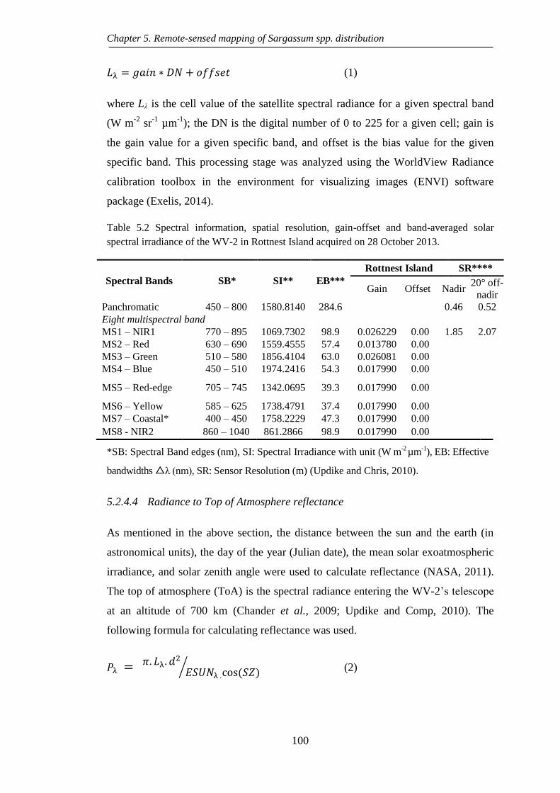
Chapter 5. Remote-sensed mapping of Sargassum spp. distribution
100
(1)
where Lλ is the cell value of the satellite spectral radiance for a given spectral band
(W m-2
sr-1
µm-1
); the DN is the digital number of 0 to 225 for a given cell; gain is
the gain value for a given specific band, and offset is the bias value for the given
specific band. This processing stage was analyzed using the WorldView Radiance
calibration toolbox in the environment for visualizing images (ENVI) software
package (Exelis, 2014).
Table 5.2 Spectral information, spatial resolution, gain-offset and band-averaged solar
spectral irradiance of the WV-2 in Rottnest Island acquired on 28 October 2013.
Spectral Bands SB* SI** EB***
Rottnest Island SR****
Gain Offset Nadir 20° off-
nadir
Panchromatic 450 – 800 1580.8140 284.6 0.46 0.52
Eight multispectral band
MS1 – NIR1 770 – 895 1069.7302 98.9 0.026229 0.00 1.85 2.07
MS2 – Red 630 – 690 1559.4555 57.4 0.013780 0.00
MS3 – Green 510 – 580 1856.4104 63.0 0.026081 0.00
MS4 – Blue 450 – 510 1974.2416 54.3 0.017990 0.00
MS5 – Red-edge 705 – 745 1342.0695 39.3 0.017990 0.00
MS6 – Yellow 585 – 625 1738.4791 37.4 0.017990 0.00
MS7 – Coastal* 400 – 450 1758.2229 47.3 0.017990 0.00
MS8 - NIR2 860 – 1040 861.2866 98.9 0.017990 0.00
*SB: Spectral Band edges (nm), SI: Spectral Irradiance with unit (W m-2
µm-1), EB: Effective
bandwidths △λ nm , SR: Sensor Resolution (m) (Updike and Chris, 2010).
5.2.4.4 Radiance to Top of Atmosphere reflectance
As mentioned in the above section, the distance between the sun and the earth (in
astronomical units), the day of the year (Julian date), the mean solar exoatmospheric
irradiance, and solar zenith angle were used to calculate reflectance (NASA, 2011).
The top of atmosphere (ToA) is the spectral radiance entering the WV-2’s telescope
at an altitude of 700 km (Chander et al., 2009; Updike and Comp, 2010). The
following formula for calculating reflectance was used.
⁄ (2)

Chapter 5. Remote-sensed mapping of Sargassum spp. distribution
101
where ρλ = the unit-less planetary reflectance; Lλ = the spectral radiance for a given
spectral band (from equation 1); d is the earth–sun distance in astronmoical units
(Table 5.3); ESUNλ is the mean solar exoatmospheric irradiance for the given
spectral band, and SZ is the solar zenith angle (extracted from metadata files). The
step of converting the radiance to ToA can be processed by calibrated radiance at the
data specific utilities in spectral toolbox in the ENVI 4.7 software (Exelis, 2014).
Table 5.3 Earth-Sun Distance in Astronomical Units
Julian
Day Distance
Julian
Day Distance
Julian
Day Distance
Julian
Day Distance
Julian
Day Distance
1 .9832 74 .9945 152 1.0140 227 1.0128 305 .9925
15 .9836 91 .9993 166 1.0158 242 1.0092 319 .9892
32 .9853 106 1.0033 182 1.0167 258 1.0057 335 .9860
46 .9878 121 1.0076 196 1.0165 274 1.0011 349 .9843
60 .9909 135 1.0109 213 1.0149 288 .9972 365 .9833
5.2.4.5 Atmospheric correction
The WV-2 satellite spectral data were atmospherically corrected, using the dark
substrate method, to reduce haze and other influences of atmospheric and solar
illumination. The major principle of the dark substrate method is to calculate the
mean value of deep water pixels (Gordon and McCluney, 1975; Liang et al., 2012;
Stumpf et al., 2003). The atmospheric correction was carried out using the dark
substrate tool box in ENVI software (Exelis, 2014).
5.2.4.6 Water column corrections
This study made use of the variable depth model derived by Lyzenga (1981) for
water-column corrections and is one of the most popular methods when using
satellite remote-sensing images for the mapping the marine coastal ecosystems. The
depth invariant index (DII) was calculated as follows:
(3)
where Li is the measured radiance of a given band i; Lj is the measured radiance of
given band j, and ki/kj is the ratio of the attenuation coefficient that is derived from
the slope of the log-transformed plot at numerous different depths.

Chapter 5. Remote-sensed mapping of Sargassum spp. distribution
102
5.2.4.7 Masking
To eliminate the spectral variability that is affected by terrestrial and deep water
areas, the vector layer of these areas was masked to the satellite images.
Figure 5.4 The ground truth survey images that taken from the study sites. (a) Sand substrate,
(b) Limestone substrate, (c) Sargassum spp. habitat, (d) Red algae, (e) Seagrass (Amphibolis
australis), (f) Algae turf habitat.
5.2.5. Image classification and data analysis
Field survey data on macroalgae distribution and abundance were processed using
the ENVI 4.7 Integrated Development Language remote-sensing software. Four
classifiers the minimum distance (MiL), Mahalobis (MaH), K-means (KM), and
Parallelepiped (PaR) classifiers were chosen for this study, because they are the
most commonly used classifiers in marine coastal habitat mapping studies to date
(Andréfouët et al., 2004; Belgiu et al., 2014; Benfield et al., 2007; Carle et al., 2014;
Ghosh and Joshi, 2014; Muslim et al., 2012). The coastal habitat around Rottnest
Island can be categorized into six classes: rocky substrate, sandy, canopy macroalgae
(Sargassum spp. and Ecklonia spp.), red macroalgae, seagrass, and mixed vegetation.
The whole analysis process is presented in a diagram in Figure 5.4 and the scheme
for habitat classification is supplied in Table 5.4.
5.2.6. Accuracy assessment
Error matrices and Cohen’s kappa Ҡ) were used to assess the accuracy of the
classification results. These are helpful models to understand the accuracy of the
classification scheme. The Ҡ coefficient can be employed to assess the agreement

Chapter 5. Remote-sensed mapping of Sargassum spp. distribution
103
between classification results and reality (Congalton, 1991). Cohen’s kappa is
calculated as follows:
∑ ∑
∑
(4)
The producer and user accuracy were also calculated for each classification result
(Congalton and Green, 2009). The producer and user accuracy are one of the most
popular indices to evaluate classification outcomes. The producer accuracy is an
index that measures the possibility that the classifier fitted the image pixel in class A
similar to the ground truth in class A. The producer accuracy index is also related to
the errors of omission (exclusion) (Congalton, 1991; Congalton and Green, 2009).
From the user perspective, the user accuracy is an index to measure the possibility
that the classifier labeled the image pixel in class A. The overall accuracy and the Ҡ
coefficient for the four classification techniques was also evaluated.
Table 5.4 A scheme used for habitat classification based on ground truth data.
Class 1 Class 2 Description Ground truth
image
Unveg
etat
ed
Sandy substrate Fine sand with bared substrates Fig. 5.4a
Limestone
substrate
Either bared substrates or some
coralline on its surface. Fig. 5.4b
Veg
etat
ed
Canopy
macroalgae
(Sargassum spp.
& Ecklonia spp.)
Most abundant Sargassum spp.,
commonly found in tidal and
sub-littoral zone and mostly
attached to the limestone rock.
Fig. 5.4c
Red macroalgae
Red algae (Gracilaria sp.) and
coralline algae often found in
limestone rock, sand, and mud.
Fig. 5.4d
Seagrass
Amphibolis sp. often found on
sandy substrates in the sub-
littoral zone. Also found on
gravel and firm, clay banks.
Fig. 5.4e
Algae turf The community of green, red,
and brown algae Fig. 5.4f

Chapter 5. Remote-sensed mapping of Sargassum spp. distribution
104
5.3. RESULTS
This study is the first of its kind to use WV-2 high-resolution multispectral satellite
imagery to map Sargassum spp. distribution. Eight Sargassum spp. have been
identified in intertidal and subtidal beds around Rottnest Island. Among these
Sargassum spp., S. spinuligerum, S. distichum, and S. podacanthum are most
abundant (Kendrick, 1993). However, because of the similarities in morphological
structure, including thallus color and length, holdfast shapes, stipe, and primary
branches (Kendrick, 1993; Mattio et al., 2008), individual Sargasum species could
not be distinguished or separated spectrally. Therefore, Sargassum spp. distribution
was defined at the genus level.
5.3.1. Sargassum spp. percentage cover and thallus length from field-survey
data
5.3.1.1 Percentage cover of Sargassum spp. and other macroalgae groups
In the period between September and November 2013, the spatial distribution of
Sargassum spp. showed statistically significant differences (P = 0.008) in percentage
cover between monitored transect lines around Rottnest Island. The highest
percentage cover of Sargassum spp. was found on the inshore reefs at depths of 0.5
to 3.5 m in the areas around Salmon Bay, Rocky Bay, and Armstrong Bay, with
values of 61.6 ± 11.5, 53.3 ± 13.1, and 48.3 ± 14.3%, respectively. The percentage
cover in Parakeet Bay and Green Island area was 45.9 ± 24.0 and 18.9 ± 10.5%,
respectively. The lowest percentage cover of Sargassum spp. was found in the Parker
Point area (15 ± 5.7%) and Thomson Bay had a cover of 4.3 ± 0.0% (Figure 5.5).
For other macroalgae groups, Ecklonia sp. in particular, statistically significant
differences (P = 0.041) were observed between monitored transect lines. The greatest
percentage cover was found in Green Island, Thomson Bay, Parker Point, and Rocky
Bay, with values of 77.8 ± 10.2, 59.3 ± 0.0, 51.3 ± 13.4 and 42.8 ± 13.2%,
respectively. The lowest percentage cover of other macroalgae groups were found in
the Parakeet Bay, Armstrong Bay, and Salmon Bay, with values of 40.9 ± 24.0, 36.7
± 9.4 and 17.9 ± 6.4%, respectively.

Chapter 5. Remote-sensed mapping of Sargassum spp. distribution
105
Figure 5.5 The percentage coverage of Sargassum spp. observed from different sites during
spring season 2013. Thomson = Thomson Bay, Parker = Porpoise Bay, Green = Green
Island, Rocky = Rocky Bay, Parakeet = Parakeet Bay, Salmon = Salmon Bay, Rollan =
Strickland Bay, Armstrong = Little Armstrong Bay. Each column shows the mean and
standard error of five observed quadrats (0.5 × 0.5 m).
5.3.1.2 Thallus length
There were no statistically significant differences (P = 0.069) between the monitored
transects in terms of mean thallus length (MTL). The MTL of Sargassum spp., was
highest along the monitored transect in Salmon Bay (45.5 ± 4.5 cm). Armstrong Bay,
Parker Point, and Rocky Beach had MTL values of 4.9 ± 40.3, 36.1 ± 6.54, and 29.8
± 4.9 cm, respectively. The lowest MTL of 25.8 ± 0.6 cm was found in Green Island.
5.3.2. Separating Sargassum spp. and other macroalgae groups
Spectral profile analysis of the major substrate types and biological communities
around Rottnest Island showed that there was a significant difference between
limestone and sand substrates, and Sargassum spp., Ecklonia sp., algae turf, and
seagrass communities (Figure 5.6). It is the characteristically different spectral
profiles between the major substrate types and biological communities that enable
the Sargassum spp. distribution to be mapped.
Comparing the spectral profiles of bare sand and limestone rock, sand has a higher
and increasing reflectance intensity across the 400- to 750-nm spectrum than does

Chapter 5. Remote-sensed mapping of Sargassum spp. distribution
106
limestone rock, for which the reflectance decreases after 650 nm and has peak at 500,
550, and 650 nm. In addition, it is rare to encounter bare limestone rock, and the
reflectance value is probably influenced by encrusting and turf algae. The substrate
reflectance components are significantly different when compared with the spectral
reflectance of biological communities, such as Sargassum spp., Ecklonia sp., algal
turf, and seagrass (Figure 5.6a, b).
Sargassum spp. and Ecklonia sp. have a similar bimodal spectral reflectance pattern,
with a first weak-intensity peak at 600 nm and the lowest value at 650 nm, with the
change of reflection direction. The major difference between the two species is the
overall intensity; Ecklonia sp. exhibit higher peak values of 0.05 at the 600-nm
wavelength, whereas Sargassum spp. have the highest spectral reflectance value of
0.02 at 600 nm which has a lower peak value than for Ecklonia sp. (Figure 6e, f).
Algae turf communities can include coralline algae, red algae, green algae, and
brown folios algae. The spectral reflectance values of the algae turf communities on
Rottnest Island are often dictated by the coralline algae, which have a high cover
abundance and irradiance value peaking between 550 and 600 nm (Figure 6c).
The three main seagrass species distributed around Rottnest Island are Posidonia sp.,
Amphibolis sp., and Halophila sp., among which Posidonia sp., and Amphibolis sp.
have the most abundant distributions. Because of the similarity of spectral profiles in
the present study, we classified all three seagrass species into one group. These
species have highest reflectance irradiance values between 500 and 550 nm (Figure
5.6d).

Chapter 5. Remote-sensed mapping of Sargassum spp. distribution
107
Figure 5.6 Spectral profiles of the majority of benthic components extracted from WV-2
imagery. (a) Limestone substrate; (b) Sand substrate; (c) Algae turf (Coralline algae, red
algae, green algae, and brown algae); (d) Seagrass; (e) Sargassum spp.; (f) Ecklonia sp. vs.
Sargassum spp.

Chapter 5. Remote-sensed mapping of Sargassum spp. distribution
108
Figure 5.7 The result of spectral math of three bands red-edge, red-edge, and yellow bands
showed the visibly observed distribution of Sargassum spp. beds with yellow pixels and red
color for submerged reefs around the study sites.
5.3.3. Spatial distribution of Sargassum spp. from satellite remote-sensing data
The combined results of the three-band match with red-edge, red-edge, and yellow
bands showed that the macroalgae beds with a majority of Sargassum spp. were
detected by yellow and orange patterns. The following environmental and biological
factors helped to detect the Sargassum spp. bed boundaries: (1) the beds are found in
clear waters and in shallow intertidal and subtidal zones (0.5–10 m); (2) Sargassum
spp. and other brown macroalgae (Ecklonia spp., Cystoseira spp.) show a preference
for rocky substrates, i.e. not sandy, which cannot be confused with seagrass on a
sandy substrate; and (3) Sargassum spp. have different spectral characteristics

Chapter 5. Remote-sensed mapping of Sargassum spp. distribution
109
compared to other macroalgae groups that are highly distinct in the high-resolution
WV-2 imagery (2-m) (Figure 5.7).
Figure 5.8 Validation accuracy for each habitat type from different classifiers. Producer
accuracy results (a) and User accuracy (b). Minimum distance (MiL), Mahalanobis (MaH),
the K-means (KM), and parallelepiped (PaR) classifiers.
Satellite remote-sensing WV-2 data showed the highest densities of Sargassum spp.
around Rottnest Island along the shallow subtidal zone on limestone substrates. The
area around Green Island contained patches of high Sargassum spp. coverage, but the
distribution of Sargassum spp. in this area was not even and was instead
concentrated mainly around fringing reefs (Figure 5.7). In Little Armstrong Bay and
Stark Bay areas, the distribution of macroalgae was also high and was concentrated
in large meadows on the right side and the outside of the fringing reefs. The area had
red color patterns, which supposedly symbolize submerged coral reef platforms.
5.3.4. Accuracy assessment
The accuracy assessment method was employed to test four classifiers: the Minimum
distance, Mahalanobis, K-means, and parallelepiped (PaR) methods. The minimum
distance method produced the greatest classification accuracy results for the seawater

Chapter 5. Remote-sensed mapping of Sargassum spp. distribution
110
class followed by accuracy rates for Sargassum spp., sand, and coral reef of 99.8,
97.8, 81.8, and 75.5%, respectively. The highest accuracy rates obtained by the
Mahalanobis classification method were found in the seawater class (99.6%),
followed by Sargassum spp. (98.1%), sand (80.3%), and coral reef (78.1%). The
classification results produced by the parallelepiped classification method were
95.7% for the seawater class, 99.1% for sand, 96.1% for Sargassum spp., and 7.5%
for coral reef. Of the four classification methods, the K-means method produced the
lowest accuracy rates for seawater (45.6%), Sargassum spp. (34.5%), and coral reef
(0%), but yielded the highest accuracy rate for sand (100; Table 5.5).
Table 5.5 Confusion matrix for WV-2 classification of Rottnest Island Reserve using four
classifiers. The accuracy assessment was based on selected main habitats from WV-2
images.
Classes Classifiers Test areas/ ground truth (Percentage)
Seawater Sand Sargassum Coral reef Total
Unclassified MiL 0 0 0 0 0
MaH 0 0 0 0 0
KM 0 0 0 0 0
PaR 4.3 0.9 2.9 3.3 3.9
Seawater MiL 99.8 0 0.2 0.1 70.6
MaH 99.6 0 0.1 0.3 70.4
KM 45.6 0 0.5 0.1 32.3
PaR 95.7 0 0 0.1 67.6
Sand MiL 0 81.8 0 21.2 2.0
MaH 0 80.4 0 18.5 1.9
KM 0.3 100 65.2 99.7 20.9
PaR 0 99.1 0.2 85.7 4.1
Sargassum MiL 0 0 97.8 3.2 24.4
MaH 0 0 98.1 3.2 24.5
KM 2.8 0 34.4 0.3 10.5
PaR 0 0 96.1 3.5 24.0
Coral reef MiL 0.2 18.2 2.1 75.5 3.0
MaH 0.4 19.7 1.8 78.1 3.2
KM 51.4 0 0 0 36.3
PaR 0 0.1 0.8 7.5 0.4
Total MiL 100 100 100 100 100
MaH 100 100 100 100 100
KM 100 100 100 100 100
PaR 100 100 100 100 100
Minimum distance (MiL), Mahalanobis (MaH), the K-means (KM) and parallelepiped (PaR)

Chapter 5. Remote-sensed mapping of Sargassum spp. distribution
111
5.4. DISCUSSION
To date, no studies on the use of WV-2 images for mapping Sargassum spp.,
particularly along the Australian coast, have been performed. This study showed a
high level of accuracy in classifying Sargassum spp. using WV-2 imagery,
highlighting the utility of SRSI in mapping shallow marine environments. The
integrated study of high-resolution satellite data provides useful and valuable
information for natural resource managers to respond to questions of seasonal change
in Sargassum spp. biomass and the typical substrate utilised by Sargassum spp.
(Andréfouët et al., 2004).
However, benthic habitat mapping using the object-based and supervised
classification technique is still subject to a number of limitations, i.e. the method
requires the gathering of ground-truth data. Field data collection is relatively time
consuming and expensive (Komatsu et al., 2002; Muslim et al., 2012; Vahtmäe and
Kutser, 2013). In addition, field data do not always correlate with satellite image
data, because of discrepancies in spatial resolution, time lag between photos and
surveys, field survey techniques, and effects due to the environmental conditions of
data collection (Kutser et al., 2006). In terms of ground truth, this study found that a
minimum of 10 transects with five survey quadrats per transect, for a total survey
area of approximately 20 km2, is required for a high-accuracy assessment. Moreover,
this study recommends a survey quadrat size of 0.5 × 0.5 m, which is the standard
method for general benthic habitat mapping studies (e.g. Duarte and Kirkman, 2001;
Japar et al., 2001; McKenzie et al., 2001; Short and Duarte, 2001). We believe that
this approach returns better accuracy assessments than numerous previous studies
that merely employ the manta tow technique for the photography of the benthic
substrate (<0.25 m2 per site) (Noiraksar et al., 2014).
In addition, this study highlights the importance of understanding seasonal variations
in Sargassum spp. biomass and distribution before acquiring WV-2 image data.
Spring was chosen for this study, because it is when the biomass and cover of
Sargassum spp. peak in Rottnest Island. Thus, it is important to understand the
seasonality of Sargassum spp., so that WV-2 imagery captures the period of highest
biomass and facilitates the mapping of Sargassum spp. There is additional value in

Chapter 5. Remote-sensed mapping of Sargassum spp. distribution
112
investigating the utility of WV-2 image data to track and understand the seasonal
variations in Sargassum spp. biomass and distribution.
One limitation of this study is that it has yet to assess the comparable classification
results of the VW-2 pan-sharpened and broad-spectral bands. Likewise, a potential
error that might be encountered in the study of coastal ecosystems is the variation in
the inherent optical properties (IOPs) of the water column. For example, coastal
waters are often affected by runoff, upwelling, and water mixing, which can lead to
high concentrations of phytoplankton, inorganic particles, and colored dissolved organic
matter (CDOM). A change in the IOPs affects both the shape and magnitude of the
reflectance spectra (Vahtmäe and Kutser, 2013). Therefore, further work is required to
evaluate the differences in classification results between pan-sharpened and broad-
spectral bands and other very high-resolution remote-sensing data (e.g., hyperspectral
images and aerial photography) and to assess the potential effect of changing the IOP
conditions.
Table 5.6 Confusion matrix of the overall accuracy of the classification maps obtained from
the WV-2 image.
Overall accuracy (%) Kappa coefficient
Minimum distance 98.32 0.96
Mahalanobis 98.30 0.96
K-means 42.50 0.22
Parallelepiped 93.50 0.86
The producer and user accuracies were employed and compared among the four
classification techniques of this study (Figure 5.8). The advantages of the coastal
(400–450 nm) and yellow (585–625 nm) bands were illustrated by the high
classification accuracy of these types of habitats (Table 5.6). These are the unique
bands that are only found in WV-2 images. With these bands, WV-2 images can
penetrate through the clear water column and gather appropriate information about
bottom habitats in the shallow waters. A similar study by Su et al. (2008) showed
that in the water sector, green light (500–600 nm) can reach a maximum depth of 15
m, red light (600–700 nm) can penetrate to 5 m and infrared light (700–800 nm) to
0.5 m (Green et al., 2000; Su et al., 2008). The overall classification accuracies
achieved in the present study are higher than those found by Noiraksar et al. (2014),

Chapter 5. Remote-sensed mapping of Sargassum spp. distribution
113
who mapped Sargassum beds in Chon Buri province, Thailand, using ALOS
AVNIR-2 images. They used minimum distance and supervised maximum likelihood
classification methods, which resulted in overall accuracy rates of 67% and 69%,
respectively. However, a study by Carle et al. (2014), which mapped the distribution
of freshwater marsh species using WV-2 imagery, showed that maximum likelihood
classifiers delivered the highest overall classification accuracy (75%). They also
found that the coastal blue and red-edge bands played a major role in enhancing
vegetation mapping.
Comparing the classification results of this study with those of the previous studies on
the Sargassum group and other coastal habitats showed that our study results have a
higher classification accurate ratio (Carle et al., 2014; Heenkenda et al., 2014; Malahlela
et al., 2014). This can be explained by two factors. First, as discussed earlier, this study
was evaluated source imaging at high spatial resolution (2-m) and spectral resolution
(eight bands). In particular, the coastal band is capable of deeply penetrating and
gathering appropriate information from marine habitats. Second, our study area (Rottnest
Island, which is situated 20 km offshore) has clear ocean waters with a relatively low
influence of coastal sediments and nutrients. Consequently, the clearness of the water
column is high because of low concentrations of phytoplankton, inorganic particles, and
CDOM in the water. According to Vahtmäe and Kutser (2013), in clear ocean waters,
optical remote-sensing can be limiting at a depth of 30 m. However, the spectrum of
information that is most useful to separate the substrate components is achieved at a
depth of 5 to 6 m. Likewise, another study in an open-sea area showed that benthic
plants cannot be identified at a bottom depth below about 5 m (Vahtmäe et al., 2012). In
this study, therefore, the detection range of Sargassum spp. lies within the depth range
from 0.5 to 3.5 m and is wholly useful spectral information. In addition, the findings of
this study agree with those of Vahtmae and Kutser (2013), who showed that the
classification outcomes from the object-based methods provide higher-quality benthic
habitat maps than did the spectral library method (Vahtmäe and Kutser, 2013).
In summary, this study has increased understanding of the spatial distribution of
Sargassum beds around coastal area of Rottnest Island, WA, using field survey and
remote-sensing techniques. Based on the results, we conclude that eight-band high-
resolution multispectral WV-2 satellite imagery has a great potential for mapping and

Chapter 5. Remote-sensed mapping of Sargassum spp. distribution
114
monitoring Sargassum beds, as well as other associated coastal marine habitats. The
results are relevant for coastal marine health monitoring and economic planning
purposes on the WA coast using high-resolution satellite imagery with a large-scale
coverage. However, further study to detect the biomass of Sargassum beds, using
WV-2 in combination with in situ observation data, is required.

Chapter 6. The spatial distribution, life cycle and seasonal growth rate
115
Chapter 6. THE SPATIAL DISTRIBUTION, LIFE CYCLE AND
SEASONAL GROWTH RATE OF SARGASSUM
SPINULIGERUM IN THE WESTERN AUSTRALIAN COAST
6.1. INTRODUCTION
The majority of Sargassum species are distributed in the northern and southern Pacific
Ocean at the biodiversity hotspots including the Indian Ocean, Southeast Asia and
Australia. Shimabukuro et al. (2008) had estimated that there are approximately 140
tropical and subtropical Sargassum species in the eastern Asian countries such as
Japan, China and the Philippines (Shimabukuro et al., 2008). On the shallow subtidal
and intertidal reefs around the WA coast, Sargassum spp. form a dominant brown
macroalgae group that shows strong seasonal variation (Kendrick and Walker, 1991).
S. spinuligerum is widely distributed globally and is one of the most important brown
macroalgae species in tropical and temperate regions (Kendrick, 1993; Kendrick and
Walker, 1991; Mattio et al., 2008). This species constitutes a canopy of habitats with
high productivity and contributes to maintaining a healthy coastal ecosystem.
The growth and mortality rate of S. spinuligerum varies between seasons and life
cycle stages and is dependent on the irradiance, water depth, salinity, pH,
photosynthetic quantum yield, water temperature, and bioavailability of nutrients
(Hanisak and Samuel, 1987; Hwang et al., 2004; 2007a; Liu et al., 2007; Pustizzi et
al., 2004; Schaffelke and Klumpp, 1998). The highest biomass and density of
reproductive thalli is recorded in the spring (September to November) (Kendrick,
1993; Kendrick and Walker, 1994). According to Kendrick (1993), S. spinuligerum in
the subtidal zone has an increased density of vegetative thalli from the autumn (March
to May) to the winter (June to August). S. spinuligerum reproduces in spring
(September to November) and summer (December to February), when it reaches the
highest biomass.
So far, no studies have ever documented the ecological characteristics such as growth,
reproduction, and life cycle of S. spinuligerum, in particular around the WA coast.
The previous studies in Australia on the Sargassum species were only confined to
taxonomy and distribution (Dixon and Huisman, 2010; Fulton et al., 2014; Goldberg

Chapter 6. The spatial distribution, life cycle and seasonal growth rate
116
and Huisman, 2004; Kendrick, 1993; Kendrick and Walker, 1994; Vuki and Price,
1994) and the sexual and vegetative reproduction of various Sargassum species
inhabiting different geographical areas, for example S. thunbergia at the Shandong
Peninsula coast, China (Chu et al., 2011), S. muticum at Friday Harbor, Washington,
USA (Aguilar-Rosas and Machado, 1990; Baer and Stengel, 2010; Lawrence, 1984;
Norton, 1977), S. muticum at Kurosima, Japan (Tsukidate, 1984), S. horneri at
Maizuru Bay and Obama Bay, Japan (Choi et al., 2009; Pang et al., 2009; Uchida,
1993; Umezaki, 1984), S. yezoense at the coastal area of Oshika Peninsula, Japan
(Yukio et al., 2002), and S. vachellianum at Zhejiang province, China (Yan and
Zhang, 2014), S. polyceratium at the coastal area of Venezuela (Engelen, Breeman, et
al., 2005).
In recent years, due to over-harvesting of natural stocks, pollution, and changing
climate, a decline in Sargassum biomass and distribution have been reported (Díez et
al., 2012; Yu et al., 2013). From 2012–2014, due to a number of extreme weather
conditions such as the hottest and prolonged heat in the summer of 2014 and the
lowest temperature in the winter of 2015 along the WA coast, the distribution and
abundance of S. spinuligerum was affected (Fulton et al., 2014; Singh and Singh,
2015). Therefore, the aim of this study was to document the spatial distribution, life
cycle, and growth rate of S. spinuligerum based on the field study data.
6.2. MATERIALS AND METHODS
6.2.1. Site description
The study was carried out at two study areas off the WA coast, Point Peron and
Rottnest Island. Point Peron belongs to Shoalwater Marine Park and is located off
Rockingham City area, whereas, Rottnest Island is located about 18 km from the Perth
city area (Figure 2.1). These two areas belong to the Southwest Australian eco-region
which is one of 34 biodiversity hotspots globally based on the Conservation
International report on the unique and highly threatened flora. In addition, the eco-
region of south WA is one of the five Mediterranean eco-region biomes with an
extremely high biodiversity but also is also under stress due to the anthropogenic
causes (Morgan et al., 2008).

Chapter 6. The spatial distribution, life cycle and seasonal growth rate
117
6.2.2. Spatial distribution of Sargassum and other submerged aquatic
vegetation
Spatial distribution of Sargassum spp. and other SAV were carried out at intertidal
zones around Rottnest Island with water depth from 0.3 to 2.5 m. The distribution
characteristics and canopy coverage (CC) were documented and surveyed at nine
transects during three sampling trips. Canopy coverage percentage was monitored
using a standard quadrat (0.5 × 0.5 m). The standard quadrat was divided into 25 small
cells with each cell corresponding to 4% of the total quadrat. Along the monitored
transects, a series of underwater videos was also recorded and stored to study and
illustrate the spatial distribution.
6.2.3. Reproductive phenology studies
The study on the growth and reproduction phenology of S. spinuligerum was carried
out at Point Peron from September 2012 to December 2014. The mean thallus length
(MTL), CC, and the fresh biomass (FB) were measured at four permanent transect
lines with a sampling frequency of once in every three months. The location of
transect lines were recorded by hand-held GPS device (Garmin eTrex® 10).
The MTL was measured from the holdfast to the highest tip of the thallus. Five thalli
were measured and then averaged out for the mean value with a standard error (S.E.).
Canopy coverage was measured using the same presented methods in section 6.2.2 for
Rottnest Island. The fresh biomass was quantified by randomly placing the quadrats
along the defined transects. All Sargassum species were collected from inside the
quadrats, dried and then weighed using a digital scale. The fresh biomass was counted
for all Sargassum species regardless of how many species were collected in the
quadrat. An amount of selected fresh Sargassum samples within monitored quadrats
was collected in labeled polyethylene bags, stored in a cool-box and then transported
to the CARL, Curtin University within three hours after sampling.
The samples at the CARL were washed with filtered seawater to remove any
epiphytes and fouling organisms, and then stocked in the large composite holding tank
(113-L) with constant aeration for further laboratory studies. During all field sampling
trips, the presence of reproductive thalli and receptacles on the identified S.
spinuligerum were observed and recorded at each sampling time and then examined by

Chapter 6. The spatial distribution, life cycle and seasonal growth rate
118
SMZ1500 stereoscopic zoom microscopy (Nikon, Japan) in the CARL. The
reproductive morphology specimens such as main thalli, receptacles, and young thalli
were photographed and line drawn for each stage of the life cycle. The samples were
morphologically identified by comparing with the previous studies (Garton, 1997;
Noro et al., 1994; Phillips, 1994b).
6.2.4. The specific growth rate of Sargassum
The length of the main thallus was measured at every sampling trip at Point Peron
during the study period. Main thallus growth rate (cm d-1
) was measured to determine
the apical growth rate using equation (1) (Hanisak and Samuel, 1987; Mai et al.,
2010).
Specific Growth Rate (SGR) = Change in height/ Change in time
where SGR is specific growth rate of the main thallus (cm d-1
), change in height is the
mean thallus length of Sargassum between two sampling trips, and change in time is a
period of time between two sampling trips. Unit of time is per days.
6.2.5. Data analysis
Field monitoring data were analyzed and processed by a statistical software IBM®
SPSS®
Statistics version 20 (New York, USA) and Microsoft Excel 2010. One way of
analysis of variance (ANOVA) was employed and principally used to test any
significant differences among surveyed seasons. Once a significant difference between
treatments was observed, the Fisher's least significant difference (LSD) test was used
for multiple mean comparisons. The statistical significance level was set at P < 0.05.
6.3. RESULTS
6.3.1. Spatial distribution of Sargassum around Rottnest Island
Field observations showed that there are three dominant Sargassum species, S.
spinurigerum, S. swartzii, and S. confusum, in both of the surveyed study sites. S.
spinurigerum had the widest distribution. In Point Peron, S. spinurigerum is usually
found in shallow waters in the intertidal zone and up to 2-m in depth, while S.
swartzii, and S. confusum are dominant in deeper areas over 2 m deep.

Chapter 6. The spatial distribution, life cycle and seasonal growth rate
119
In Rottnest Island, the spatial distribution of Sargassum spp. in the monitored
transects was divided into three main areas: Sargassum, seagrasses, and mixed
seaweed zones (Figure 6.1). In Parker Point, the first Sargassum area was found
approximately 80 m from the shore with a maximum depth of around 2.0 m (Figure
6.1a). Sargassum dominated with canopy coverage of approximately 90%, Gracilaria
sp. covers about 5%, and the rest was covered by other macroalgae. Limestone is the
dominant substrate in this area. At the end of the monitored transect line (~150 m),
seagrasses are predominate (90%) with sand and rubble at depths of approximately 2.5
m. The red macroalgae group (i.e. Gracillaria sp.) and other algae groups accounted
for about 5% with scattering distribution. At the furthest area from the transect, at a
distance of 150 to 220 m from the shore, Sargassum dominated with a canopy
coverage around 95%; the red macroalgae and seagrass groups accounted for 2% and
3%, respectively.
In the Green Island transect (Rottnest Island) (Figure 6.1b), the distribution pattern of
marine submerged vegetation was divided into four main areas including in-shore
Sargassum, seagrasses, off-shore Sargassum, and mixed areas. The first Sargassum
area was found from the shore to 50 m further with a dominant limestone substrate.
The maximum depth was found up to 1.8 m, and the Sargassum canopy coverage was
reached 90%, red macroalgae and seagrasses occupied around 10%. The second area
from the shore was dominated by seagrasses (90%), and the rest was Gracillaria spp.
and other macroalgae. In this transect, the distribution pattern of marine submerged
vegetation was also divided into four main zones: in-shore Sargassum, seagrass, off-
shore Sargassum, and mixed macroalgae zones; in order from the shore to the further
area, the abundant canopy coverage was over 90% for each group.
Overall, the survey results of the monitored transects showed that Sargassum was
largely distributed on limestone and rubble substrates with depths ranging from 0.2 to
3.5 m. Sargassum can be found right from the shore or in the furthest areas of the
transect. Likewise, seagrass was usually distributed in sandy bottoms with an average
depth of 2.0 m. The red macroalgae and other macroalgae groups often had a scattered
distribution on the limestone reef or were associated with seagrass and Sargassum
spp.

Chapter 6. The spatial distribution, life cycle and seasonal growth rate
120
Figure 6.1 A typical spatial distribution and percentage coverage of Sargassum spp. and
other coastal marine submerged vegetation along the transects (a) in the Parker Point (32o
01.493S – 115o 31.719E); (b) the Green Island area (Rottnest Island) (32
o 1’0.55”S – 115
o
29’55E ; c Parakeet Bay 31o 59.417S – 115
o 30.400E) in spring (Oct. 2013) in Rottnest
Island, WA.
6.3.2. Life cycle studies of Sargassum spinuligerum in the WA coast
S. spinuligerum (Sargassaceae, Fucales) have a single life cycle/ history phase. The
life cycle of S. spinuligerum in the subtidal zone of WA coast can be divided into five
stages including i) dormancy; ii) the new growth season/regeneration/recruitment; iii)

Chapter 6. The spatial distribution, life cycle and seasonal growth rate
121
increasing biomass; iv) maturity and reproductive; and v) die back/senescent phase
(Figure 6.2).
Figure 6.2 Schematic representation of the life cycle of S. spinuligerum sexual
reproduction in relation to seasonal changes. (a) Reproductive thallus; (b)
Receptacles; (c) Sperm cells; (d) Egg cells; (e) Oogonial/Zygotes develop on
conceptacle; (f) Germling released and attached onto substrates to develop young
thalli; (g) Fully growth thalli. Five stages including i) dormancy; ii) the new growth
season/regeneration/recruitment; iii) increasing biomass; iv) maturity and
reproductive; and v) die back/senescent.
i) Dormancy phase: This phase usually commences from the end of summer to early
autumn (February March). Dormancy is found after conceptacles reduce
division/meiosis inside male and female conceptacles to produce spermatozoids and
oospores. Spermatozoids are motile and oospores are non-motile. The fertilized eggs
develop into young gametophytes that freely travel in the water bodies and then settle
on the substrate surfaces. In the vegetative productive form, the dormancy phase is
found from the broken thallus, from the remaining holdfasts on the substrates.

Chapter 6. The spatial distribution, life cycle and seasonal growth rate
122
ii) The new growth season phase/recruitment: This phase often commences from early
autumn to early winter (March June). The young gametophyte starts growing and the
holdfasts begin the recruitment of a new thallus from their old holdfasts.
iii) Maximum standing crop/increasing biomass phase: In WA, this phase starts from
early winter and continues to the middle of spring June September . The thallus
steadily increases in biomass in early spring (August September).
iv) The maturity and reproductive phase: This phase runs from the middle of spring to
early summer September December . Sargassum reach their maximum biomass and
begin the second reproduction phase by developing receptacles. Sargassum biomass
stabilizes for several months before shifting to the next phase.
Figure 6.3 Schematic representation of the life cycle of S. spinuligerum vegetative
reproduction in relation to seasonal changes. (a) Reproductive thalli; (b) Remaining
holdfasts; (c) Recruitment new thalli from the remaining holdfasts; (d) Fully grown
thalli. Five stages including i) dormancy; ii) the new growth season/regeneration/
recruitment; iii) Maximum standing crop/increasing biomass; iv) maturity and
reproductive; and v) die back senescence.

Chapter 6. The spatial distribution, life cycle and seasonal growth rate
123
v) The die back phase: This phase commences from the beginning until the end of
summer December January). Mature Sargassum die off leaving only some remaining
holdfasts.
Sexual reproduction is found in most Sargassum species in the coastal intertidal
zones, while vegetative reproduction is also found in the majority of Sargassum
species within the coastal subtidal zones (Figure 6.3). During vegetative reproduction,
while the majority of the Sargassum thalli dies, the holdfasts often remains (v). This
holdfasts remains dominant during the warmer months (i), and then begins to grow in
the new growth phase (ii), finally forming a new thallus in the colder months. The
thallus increases in biomass (iii), and then reproduces before senescence in the
summer (iv).
Table 6.1 The value of canopy cover, fresh biomass, mean thallus length and specific growth
rate of Sargassum at difference seasons at Point Peron, WA.
Season Canopy cover
(%)
Fresh biomass
(g wt m-2
) MTL (cm) SGR (cm d
-1)
Spring 78.83 ± 3.92a 1412.9 ± 177.36
a 36.55 ± 6.41
a 0.98 ± 0.41
a
Summer 70.03 ± 3.55a 963.2 ± 199.14
b 34.46 ± 3.59
a -0.79 ± 0.49
b
Autumn 30.69 ± 5.13b 284.14 ± 76.96
c 15.76 ± 2.12
b -0.74 ± 0.47
b
Winter 54.73 ± 8.64c 868.06 ± 103.44
b 16.18 ± 1.23
b 0.38 ± 0.32
ab
F 15.127 8.275 5.901 3.085
P < 0.001 < 0.001 0.002 0.04
6.3.3. Seasonality of S. spinuligerum growth rate in Point Peron
There were significant differences (P < 0.005) in CC, FB, MTL and SGR between
seasons as determined by one-way ANOVA with F(3, 45) = 15.127, F(3, 33) = 8.275,
F(3, 45) = 5.901, and F(3, 37) = 3.085, respectively (Table 6.1). The lowest values of
CC, FB, and SGR were found in May and June. The highest value of CC and FB were
found in December (2012, 2014), while the SGR reached the highest value in July
(2013), December (2013) and September (2014). The lowest SGR occurred in
February 2013 and January 2014 (Figure 6.4). Overall, the highest CC and FB
occurred in the spring coinciding with increasing sun light and temperature.
Meanwhile, the highest SGR was found in winter Jun July) and spring (September).

Chapter 6. The spatial distribution, life cycle and seasonal growth rate
124
Figure 6.4 Inter-annual changes in (a) mean canopy cover (solid line), (b) fresh
biomass weight (dotted line) and canopy coverage (light solid line), and (c) specific
growth rate (cm per day) with the standard deviations (vertical bars) of the main
thallus at different reef areas in Point Peron.
6.4. DISCUSSION
This present study could be considered one of the first on the spatial distribution, life
cycle, and growth rate of S. spinuligerum along the WA coast. The study has
documented the main growth and development stages of S. spinuligerum in
association with inter-season variations in water quality. The previous study on the
growth and development of an invasive Sargassum species (S. muticum) showed that
there was a strong relationship between the length and width of germlings, and the

Chapter 6. The spatial distribution, life cycle and seasonal growth rate
125
number of produced rhizoids during the first development stages (Norton, 1977). A
study on the reproduction of S. muticum at La Jolla, California (USA) showed that a
higher ratio of thalli carrying fertilized receptacles was usually found from late
December to March, and also coincided with SST values from 13.1−15.0oC
(Lawrence, 1984).
Sargassum is one of the genera of brown macroalgae that is difficult in taxonomic
classification due to the large variation of morphology in its life cycle (Kantachumpoo
et al., 2015). There are various receptacles and morphological structures of Sargassum
species during their various life cycles, as well as surrounding environmental
conditions such as waves, currents, and the availability of nutrients. For instance,
thalli develop more branches in strong wave conditions than in quiet waters (Gillespie
and Critchley, 1997). A study on S. lapazeanum species in the south-western Gulf of
California showed that this species is dioic; there are male and female conceptacles on
the same receptacle but with different maturation times (Gabriela and Rafael, 2011).
S. spinuligerum have both male conceptacles (antheridia) and female conceptacles
(monoecious) on the same thallus as similar to S. filipendula (Redmond et al., 2014;
Scrosati, 2002).
The reproduction morphology of Sargassum is called receptacles and is usually found
either at the secondary or tertiary of the main thalli. The surface of the receptacles
usually have many little pouches called conceptacles which carry gametangia
(Gillespie and Critchley, 1997). According to morphology, receptacles are classified
into three different types including terate (S. elegans), three-cornered (S.
heterophyllum/S. incisifolium), and twisted (Sargassum sp.). Of those species, the
three-cornered type have the largest number of conceptacles per area of unit. The
terate receptacles have an average number of conceptacles per area unit (Gillespie and
Critchley, 1997). In some rare cases, it was found that the process of sexual
reproduction can disappear particularly in those species with the floating life cycle
(free-floating forms) in seas such as the Sargasso Sea. Here, the process of vegetative
reproduction occurs by developing new crops from the thallus segments (Maria et al.,
2012). Furthermore, in vegetative reproduction, the Sargassum species in coastal areas
often regenerated by the development of new thalli from old holdfasts from the
previous year that remained on the substrate (Figure 6.3). Some previous studies have

Chapter 6. The spatial distribution, life cycle and seasonal growth rate
126
shown that the growth rate of thallus regeneration from holdfasts is often greater than
sexual reproduction where development occurs from a zygote (Kendrick, 1993;
Kendrick and Walker, 1994).
In WA coastal area, S. spinuligerum is an abundant species that forms dense
populations with the canopy coverage area of over 80% at the study sites. Therefore,
the morphology of this species makes it quite easy identify in the field. In this study,
the classification of species in the Sargassum genus was mainly based on the
traditional morphological taxonomy that relies on the thalli, vesicles, leaves, and
receptacles characteristics. This classification method generally produces accurate
results for common species with distinct morphological characteristics. However,
genetic analysis is needed to assess the Sargassum species that have morphological
similarities in WA waters. A study on the systematics of Sargassum in Thailand
showed that based on Nuclear Ribisomal Internal Transcribed Spacer 2 (ITS2) data
gives the relationship between species with the phylogenetic tree constructed from
genetic analysis data found in coastal regions in Thailand (Kantachumpoo et al.,
2015).
A pilot study of the growing S. naozhoue nse species in the Leizhou canal,
Guangdong, China showed that this species can be grown from seeds after six months
cultivation in tanks to achieve a size of up to 5 cm in length. Then, the cultivating
plants were moved into the sea conditions for a further 95 cultivation days. The
biomass obtained after cultivation periods reached 1750 kg wet wt. km-1
per rope. In
addition, this study also found that this species has high heat resistance and the ability
to survive in water temperatures up to 33.7°C (Xie et al., 2013). However, another
study on S. muticum at Baja California Peninsula in Mexico showed that the highest
number of the reproduction structures was present in the late spring and early summer
May July .
The lowest number of reproduction structures was usually found at the end of winter
(March) in the Southern Hemisphere (Aguilar-Rosas and Machado, 1990). According
to the biomass results, the length and density of the main thallus of S. yezoense in
Oshika Peninsula, its life cycle and the development of this species was divided into
three main phases; i) germination phase: the biomass and thallus length with the
smallest size (< 10 cm), usually taking place in the period from August to November;

Chapter 6. The spatial distribution, life cycle and seasonal growth rate
127
ii) the development stage: the biomass increases by increasing of the main thallus,
usually takes place in the period from November to December; and iii) maturation
phase takes place in the period from June to August, when the thalli are reaching their
maximum length (Yukio et al., 2002). In our study, the germination phase occurred
from early autumn to winter, the development stage from winter to spring and the
maturation phase from spring to early summer. The new growth season
phase/recruitment phase coincides with short light day (~11h) and low temperature
months (~18oC) (Dawes, 1987). The maximum standing crop/biomass phase has been
found to have a strong relationship between increasing biomass and an availability of
nutrients in the water bodies.
In conclusion, Sargassum communities in WA have several distinct growth phases,
varied growth rates, seasonal reproduction and an annual life cycle. There are three
main species of Sargassum found in coastal WA (S. spinuligerum, S. swartzii, S.
confusum), of which S. spinuligerum has the greatest distribution and is usually found
in the intertidal zone, at a depth of up to 2 m. The growth rate under matural
conditions is highest in the cooler months, and canopy cover and biomass were
highest toward the end of the growing period in spring to summer. In the survey areas,
Sargassum was widely distributed on limestone and rubble substrates, with a high
canopy coverage in these areas. S. spinuligerum have a single annual life cycle
beginning with the dormancy phase. Afterwards, the young thalli undergo the
recruitment phase when growth begins from zygotes and remaining holdfasts for
sexual and vegetative reproductive respectively, then the maximum biomass phase,
the maturity and reproductive phase, and finally the die back or senescence phase.
This study provides novel and up-to-date information on the morphology, growth,
reproduction and life cycle of S. spinuligerum of WA coastal waters.


Chapter 7. Season changes in water quality and Sargassum biomass
129
Chapter 7. SEASON CHANGES IN WATER QUALITY AND
SARGASSUM BIOMASS IN WESTERN AUSTRALIA
Paper publised in the Marine Ecology Progress Series. 551, 63−79. doi:10.3354/meps11735
(Appendix 3)
7.1. INTRODUCTION
Sargassum spp. are brown macroalgae with a global distribution, and are especially
dominant in shallow tropical and sub-tropical waters (Hanisak and Samuel, 1987;
Mattio et al., 2008; Mattio and Payri, 2011). Sargassum spp. are commonly attached
to rocks, but can also have floating life forms. In coastal areas and surrounding
offshore islands they form dominant communities playing vital ecological roles for
marine ecosystems by providing feeding grounds for sea birds and sea lions and
providing essential nursery habitats for invertebrates, larval and juvenile fish
surrounding these islands (Tyler, 2010; Wells and Rooker, 2004). Sargassum spp.
also represents a living renewable resource that is used in medicines, and for the
production of fertilisers, alginate, and bio-fuels (Arenas and Fernández, 2000;
Chengkui et al., 1984; Hong et al., 2007; Rivera and Scrosati, 2006).
Approximately 46 Sargassum species are found along the WA coast (Herbarium,
2013) and the majority of these have been studied to determine their taxonomic
affiliation, including the molecular basis of identification (Dixon and Huisman,
2010; Dixon et al., 2012; Goldberg and Huisman, 2004; Kendrick, 1993; Kendrick
and Walker, 1994; Rothman et al., 2015), and physiology (De Clerck et al., 2008;
Huisman et al., 2009; Kumar et al., 2011; Muñoz and Fotedar, 2011; Staehr and
Wernberg, 2009). However, few studies have been performed on the impact of
seasonality on Sargassum along the subtropical and temperate coastal zone of WA
(Kendrick, 1993; Kendrick and Walker, 1994). Previous studies have shown that the
growth, development and distribution of Sargassum beds are strongly influenced by
physiochemical water parameters (Mattio et al., 2008; Payri, 1987; Ragaza and
Hurtado, 1999), which play an important role in influencing nutrient-uptake via
photosynthesis (Nishihara and Terada, 2010). Seasonal variations in the
physiochemical parameters of seawater strongly influence changes in Sargassum

Chapter 7. Season changes in water quality and Sargassum biomass
130
canopy structure, which in turn, affect the density of the local populations (Ang and
De Wreede, 1992; Arenas and Fernández, 2000; Ateweberhan et al., 2009; Rivera
and Scrosati, 2006).
In recent years, satellite remote-sensing studies have successfully been applied to
benthic marine habitat mapping, and more specifically, have been used to estimate
macroalgae biomass in the coastal waters (Andréfouët and Robinson, 2003; Benfield
et al., 2007; Casal et al., 2011a; Fearns et al., 2011; Kutser et al., 2006; Maheswari,
2013; Vahtmäe and Kutser, 2007). However, the most clear and direct method for
marine habitat mapping is visual observations, also termed ground truth data, using
either SCUBA or snorkelling, which provides an essential input to remote-sensing
observations (Komatsu et al., 2002). A methodology for mapping Laminariales
(Kelp) in turbid waters of the Seno de Corcubión (Northwest Spain), using SPOT-4
satellite images was developed, which showed that the mapping of Sargassum beds
could be improved through the application of higher spectral images, increasing the
spatial and radiometric resolution and performing new field calibrations
simultaneously with the acquisition of images (Casal et al., 2011a). Lower resolution
Landsat (30 m) and higher resolution QuickBird (2.4 m) satellite images have been
used to estimate the spatial distribution of 11 Sargassum beds in South West Lagoon,
New Caledonia (Mattio et al., 2008). Nevertheless, only a few studies have been
carried out to assess of the spatial distribution of Sargassum and their temporal
biomass variations in marine coastal areas using high-resolution satellite remote-
sensing data (Hoang 2015; Noiraksar et al., 2014).
The WV-2 satellite images provide one of the highest available spatial and spectral
resolutions (eight spectral sensors ranging from 400–1040 nm) (DigitalGlobe, 2013;
Lee et al., 2011). However, no detailed mapping studies of Sargassum have been
performed using high-resolution satellite images, such as WV-2. In addition, a direct
visual approach that is integrated into high spatial resolution remote-sensing
observations could represent a robust approach to minimize costs and increase the
accuracy of detection and distribution patterns of Sargassum shallow coastal waters.
The aim of this study was to investigate the effects of seasonal changes in water
quality on canopy cover, mean thallus length and the Sargassum biomass at a
fringing limestone reef in Point Peron, WA. We have used in situ observations and

Chapter 7. Season changes in water quality and Sargassum biomass
131
remote-sensing methods to study the seasonal variation in physico-chemical water
parameters with changes in mean thallus length (MTL), canopy cover (CC), and
fresh biomass (FB) of the Sargassum community and determined how these changes
impact the broader spatial distribution of Sargassum.
Figure 7.1 Study area, with sampling sites shown by arrows. Point Peron is located
approximately 50 kilometers south of Perth City, WA.
7.2. MATERIALS AND METHODS
7.2.1. Study sites
The demonstration site was selected to be Point Peron, WA, which is a small
peninsula located within the Shoalwater Islands Marine Park, an area of
approximately 67 km2, west of Rockingham city, 50 kilometers south of Perth City,
WA (Figure 7.1). The point is approximately 930 m wide and 1450 m long and is
surrounded by a chain of limestone reefs and islands, including Garden Island to the
north. As part of the Shoalwater Islands Marine Park, Point Peron has a high
diversity of marine fauna and flora (DEC, 2011).
The study area includes a chain of limestone reefs approximately 450 m offshore
(32°14'–32°17'S and 115°39'–115°42'E). The coastal area of Point Peron was divided
into four zones: the Lagoon zone (LZ), Back reef (BR), Reef crest (RC), and Fore
reef (FR) zone with the distance approximately 100 m between each zone (Rützler
and Macintyre, 1982) (Figure 7.2). The field studies were carried out from
September 2012 to December 2014 during four well-defined seasons; summer

Chapter 7. Season changes in water quality and Sargassum biomass
132
(December to February), autumn (March to May), winter (July to August), and
spring (September to November) (BoM-Australia, 2013).
Figure 7.2 The diagram of one transect which including four reef zones: Lagoon
zone (LZ), Back reef (BR), Reef crest (RC) and Fore reef (FR) zone. Adapted with
modification from Rützler and Macintyre (1982)
7.2.2. Field sampling methods
7.2.2.1 Sampling frequency
The total duration of the trial was two and half years wherein summer and spring
were represented three times and winter and autumn were represented twice. At least
one sampling trip was carried out per season, however, we could sample twice during
summer and spring seasons which were then averaged out. During every trip, four
400 m long transects were sampled. The average depth along each transect ranged
from 0.3 to 2.5 m. For water quality analysis, one sample was collected from every
transect. For canopy cover, fresh biomass, and mean thallus length of Sargassum
spp., every transect was further monitored from four reef zones by deploying random
quadrats (0.5 × 0.5 m), one for each reef zone. The distance between the quadrats
ranged from 20 to 80 m. The above protocol provided four samples for water quality
analysis and 16 (4 transects × 4 quadrats) samples for Sargassum measurements per
season.

Chapter 7. Season changes in water quality and Sargassum biomass
133
7.2.2.2 Sampling description
The transects were selected based-on the actual study site’s topography and covering
a range of different habitats. Using SCUBA survey techniques, we monitored and
sampled Sargassum spp. along four predefined transects extending from the coastline
to offshore. From each transect the seawater samples were collected in a 1-L
polyethylene bottle. The Sargassum spp. within each quadrat was collected, stored in
labelled polyethylene bags and brought to the CARL, Curtin University, WA. The
locations of the sampling quadrats were recorded by a hand-held GPS (Garmin
eTrex® 10). The collected Sargassum samples were retained in fibreglass tanks with
seawater under natural sunlight. The samples were provided with constant aeration
till further measurements. Fresh specimens were photographed immediately after
arrival at the CARL. The holdfasts, blades, vesicles, and receptacles were also
examined and photographed. Sargassum specimens were identified based-on
taxonomic references (Garton, 1997; Guiry and Guiry, 2014; Huisman and Walker,
1990; Noro et al., 1994; Phillips, 1994a). A morphological study of Sargassum
samples was under taken on dried specimens. Herbarium specimens were stored at
the CARL. Underwater video and photographs were captured along the monitored
transects from five sampling trips in June and September in 2013, and January,
March, and July in 2014. These data were used for ground truth and classifying the
marine habitats.
7.2.3. Meteorological data and environmental parameters
Meteorological data, including the maximum (MaxAT, oC), mean, and minimum
(MinAT, oC) air temperature and monthly rainfall for each season, were acquired
from the nearest Bureau of Meteorology weather station, at Garden Island
(32°14'24"S–115°40'48"E), 2 km north of Point Peron (BoM-Australia, 2013).
Euphotic depth (ED) (m), sea level pressure (SLP) (hPa), colored dissolved organic
matter (CDOM) index, photosynthetically active radiation (PAR), sea surface
temperatures (SSTs), and chlorophyll-a concentration (Chl-a) (mg m-3
) in the study
area (32°12'–32°17'S, 115°38'–115°42'E) were extracted from MODIS satellite data.
The northward wind (NW) (m s-1
) was extracted from the Modern Era Retrospective-
analysis for Research and Applications (MERRA) flat form in the Giovanni system,

Chapter 7. Season changes in water quality and Sargassum biomass
134
developed and maintained by the National Aeronautics and Space Administration
(NASA) (Acker and Leptoukh, 2007).
In situ sea water temperature (i-SST), conductivity, and pH were measured in each
season using a portable waterproof oC/mV/pH meter (CyberScan pH 300, Eutech
Instruments, Singapore). Salinity was measured using a hand-held refractometer
(Atago® RHS-10ATC, Japan) in practical salinity units, and dissolved oxygen (DO)
was determined with a digital DO meter (YSI®
55, Perth Scientific, Australia). Four
seawater samples were collected during each sampling season for the analysis of
nutrients; nitrate (NO3-), nitrite (NO2
-), ammonium (NH4
+), and phosphate (PO4
3-).
All samples were stored in 250-mL bottles and kept in a cold container
(approximately 10oC) in the dark. Samples were transferred to the CARL for analysis
within 48 h following collection and followed the methods described in Standard
Methods for the Examination of Water and Wastewater (APHA 1998). Nitrate and
nitrite were measured using a Hach DR/890 Colorimeter (Hach, Loveland, CO,
USA) with the cadmium reduction method (Method 8171) and diazotization method
(Method 8507), respectively (APHA 1998). Phosphate concentration was analysed
by Ascorbic acid method (Standard Method 4500-PE) and ammonium was
determined by using Aquanal™
test kits (Sigma-Aldrich®, Germany).
7.2.4. Satellite remote-sensing data and processing
WV-2 satellite images at a 2-m spatial resolution were acquired on February 7, 2013
(austral summer), which was a period of high biomass and areal extent of Sargassum
beds. Satellite remote-sensing WV-2 images were adjusted to pseudo-color
composite images prior to the classification process, to enhance the image contrast to
detect the Sargassum beds.
The acquired WV-2 images from DigitalGlobe® were registered into
Georeferenced−the global geodetic system 1984 for latitude and longitude. The
ground truth data were acquired and confirmed using in situ field checks from five
survey trips in 2013 and 2014. The ENVI environment for visualizing images was
used to mask out the land area that was not used for classification at the study area
(Exelis, 2014). Methods of K-means unsupervised classification and maximum
livelihood supervised classification were employed for image classification as these

Chapter 7. Season changes in water quality and Sargassum biomass
135
are the most commonly used classifier in reef studies (Benfield et al., 2007; Hoang et
al., 2015b). A toolbox in ENVI was employed for the classification and to count the
number of pixels of the WV-2 satellite image that was used to detect the distribution
of Sargassum beds. After classification, the data were converted from raster to vector
format and were edited in geographical information systems software packages. The
complete diagrammatic processing imagery is presented in Figure 5.3.
7.2.5. Data analysis
Seaweed distribution and abundance data were processed using statistical software,
IBM®
SPSS Statistics 20 and Microsoft®
Excel 2010. One-way ANOVA and general
linear models were employed to test for significant differences between seasons in
seawater quality. A two-way ANOVA was carried out to test the effects of seasons
and distribution sites on the Sargassum CC and MTL. The multiple comparison, least
significant difference LSD’s post hoc test, was also implemented to test for the
statistical significance among treatments. The statistical significance level was set at
0.05. Principle component analysis (PCA) was employed to evaluate the interaction
between the physical, chemical and biological parameters and their effect on
Sargassum spp. Results from the PCA were acquired based on the correlation matrix
of the mean values of water quality parameters against sampling times. Principle
component analysis was prepared by using the latest XLSTAT 2015.1.01 (Addinsoft™
,
France) package for Microsoft® Excel. All the results were presented as means ± S.E.
(standard error), unless otherwise stated.
7.3. RESULTS
7.3.1. Temporal variation in environmental conditions
The analysis of air temperature over the three study years (2012–2014) indicates that the
monthly mean temperature was highest in the summer months (December–February).
Temperatures then decreased in autumn (March–May) and were lowest in winter (June–
August) and finally increased in spring (September–November). In the summer months,
the maximum monthly mean temperature reached 28.2 ± 0.6oC and in autumn, it reached
24.1 ± 0.9oC. In winter and spring, the maximum monthly mean temperatures were 18.5
± 0.2 and 21.7 ± 1.3oC, respectively. In 2012, the mean air temperature reached a
maximum in January (30.5oC) and was lowest in July (9.9
oC) (Figure 7.3a).
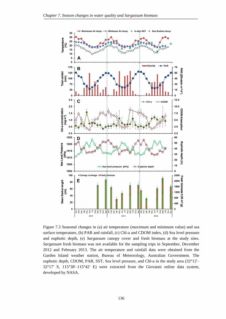
Chapter 7. Season changes in water quality and Sargassum biomass
136
Figure 7.3 Seasonal changes in (a) air temperature (maximum and minimum value) and sea
surface temperature, (b) PAR and rainfall, (c) Chl-a and CDOM index, (d) Sea level pressure
and euphotic depth, (e) Sargassum canopy cover and fresh biomass at the study sites.
Sargassum fresh biomass was not available for the sampling trips in September, December
2012 and February 2013. The air temperature and rainfall data were obtained from the
Garden Island weather station, Bureau of Meteorology, Australian Government. The
euphotic depth, CDOM, PAR, SST, Sea level pressure, and Chl-a in the study area (32°12'–
32°17' S, 115°38'–115°42' E) were extracted from the Giovanni online data system,
developed by NASA.

Chapter 7. Season changes in water quality and Sargassum biomass
137
Sea surface temperatures also showed a seasonal pattern, with values ranging from
12.9 to 24.1oC. There were significant (ANOVA, F(9, 37) = 551.23, P < 0.001)
differences in SSTs between the seasons, except for between winter and spring.
Rainfall and PAR usually showed an inverse pattern and both showed a strong
seasonal variation. The PAR reached the highest value in the summer at 58.5 ± 1.5
Einstein m-2
d-1
(a maximum in December 2013 of 63.2 Einstein m-2
d-1
) (Figure
7.3b). Although the monthly rainfall was only 2.6mm, mean summer rainfall was
11.9 ± 6.4mm. In contrast, the PAR was the lowest in the winter months at 22.8 ± 3.6
Einstein m-2
d-1
(17.5 Einstein m-2
d-1
in June 2013) and the highest mean rainfall of
95.5 ± 11.9mm was reached in winter (the maximum value of 151.6 mm was in
September 2013 (Figure 7.3b).
Table 7.1 Seasonality of physico-chemical parameters (mean ± S.E.) observed at Point
Peron, WA. SSTs = Sea surface temperatures, DO = Dissolved oxygen.
Year Month Season Salinity (psu) pH Cond. (ECs) SSTs (oC) DO (mg L
-1)
2012 Sep Spr. 36.5 ± 0.29 8.1 ± 0.08ab
-65.9 ± 2.89a 17.6 ± 0.2
d 7.53 ± 0.28
c
Dec Sum. 35.8 ± 0.31 8.1 ± 0.05ab
-98.8 ± 0.28d 22.1 ± 0.1
f 6.07 ± 0.08
b
2013 Apr Aut. 35.5 ± 0.20 8.1 ± 0.06ab
-92.5 ± 6.13c 22.8 ± 0.3
h 6.08 ± 0.02
b
Jun Win. 35.5 ± 0.29 8.0 ± 0.06b -87.8 ± 0.25
bc 16.3 ± 0.3
b 8.27 ± 0.13
d
Sep Spr. 35.8 ± 0.25 8.1 ± 0.11ab
-88.0 ± 0.00bc
17.0 ± 0.0c 7.75 ± 0.25
c
Dec Sum. 35.7 ± 0.14 8.0 ± 0.02b -82.1 ± 2.79
b 24.1 ± 0.0
z 5.92 ± 0.40
b
2014 Mar Aut. 35.8 ± 0.18 7.8 ± 0.14c -83.8 ± 2.95
b 22.6 ± 0.1
gh 5.99 ± 0.05
b
Jul Win. 35.5 ± 0.29 8.2 ± 0.01ab
-87.0 ± 0.58bc
12.9 ± 0.2a 5.39 ± 0.01
a
Sep Spr. 35.4 ± 0.24 8.2 ± 0.01ab
-69.7 ± 0.28a 19.7 ± 0.1
e 5.84 ± 0.03
ab
Dec Sum. 35.8 ± 0.17 8.2 ± 0.02a -68.3 ± 0.50
a 22.2 ± 0.1
fg 7.33 ± 0.11
cd
F 1.43 3.32 17.01 551.23 30.05
P 0.224 0.007 < 0.05 < 0.05 < 0.05
The mean in the same column with different superscript letter are significantly different at the 0.05
level.
Seawater salinity in the study area ranged from 35.4 to 36.5 among the seasons, but
the differences were not significant (ANOVA, F(9, 37) = 1.43, P = 0.224). The
electrical conductivity of seawater in the study area also differed significantly
between the sampled seasons (ANOVA, F(9, 37) = 17.01, P < 0.001), with
conductivity values ranging from -98.87 to -65.87 ECs. Dissolved oxygen (ANOVA,
F(9, 37) = 30.05, P < 0.001) and pH (ANOVA, F(9, 37) = 3.32, P = 0.007) were
significantly different between the seasons and ranged from 5.39 to 8.27 mg L-1
, and
7.82–8.21, respectively (Table 7.1).

Chapter 7. Season changes in water quality and Sargassum biomass
138
Significant differences were observed in all nutrient levels among seasons during the
study period at Point Peron as determined by one-way ANOVA where NO2-
(ANOVA, F(3, 36) = 12.05, P < 0.05), NO3- (ANOVA, F(3, 36) = 13.38, P < 0.05),
NH4+
(ANOVA, F(3, 32) = 5454, P < 0.05), PO43-
(ANOVA, F(3, 36) = 7.38, P =
0.001). In particular, the concentration of nitrite was relatively low, ranging from
2.2–17.4 µg L-1
during the study period. The nitrate concentration reached its highest
value in spring 2014 (0.48 ± 0.06 mg L-1
) and lowest value in summer 2013 (0.02 ±
0.001 mg L-1
). The concentration of ammonium during the study period ranged from
0.6–2.0 mg L-1
and that of phosphate ranged from 0.08–0.72 mg L-1
and reached the
highest value in spring 2014 and lowest value in summer 2013. In general, the
nutrient concentrations were lowest in autumn and highest in spring throughout the
study period (Table 7.2 Seasonality of the mean nutrient concentrations in collected
seawater during the study period at Point Peron, WA. All data represent the means
from four replicates (± S.E.).
Table 7.2 Seasonality of the mean nutrient concentrations in collected seawater during the
study period at Point Peron, WA. All data represent the means from four replicates (± S.E.).
Year Month Season NO2- (µg L
-1) NO3
-(mg L
-1) PO4
3-(mg L
-1) NH4
+(mg L
-1)
2012 Sep Spr. 6.33 ± 1.86b 0.33 ± 0.08
cd 0.45 ± 0.08
c 1.97 ± 0.12
de
Dec Sum. 13.25 ± 2.07c 0.05 ± 0.02
a 0.14 ± 0.02
a 1.70 ± 0.13
cd
2013 Apr Aut. 2.00 ± 0.41a 0.02 ± 0.00
a 0.24 ± 0.03
b 0.73 ± 0.09
a
Jun Win. 4.50 ± 0.65ab
0.02 ± 0.00a 0.14 ± 0.02
a 1.55 ± 0.06
c
Sep Spr. 3.50 ± 0.65ab
0.17 ± 0.00bc
0.20 ± 0.01ab
2.00 ± 0.06e
Dec Sum. 10.50 ± 1.56c 0.09 ± 0.01
ab 0.26 ± 0.03
b 1.11 ± 0.04
b
2014 Mar Aut. 2.75 ± 0.48a 0.02 ± 0.01
a 0.19 ± 0.02
ab 0.55 ± 0.10
a
Jul Win. 3.00 ± 0.58ab
0.02 ± 0.00a 0.22 ± 0.06
ab 1.53 ± 0.09
c
Sep Spr. 3.33 ± 0.33ab
0.42 ± 0.04d 0.72 ± 0.05
d 2.03 ± 0.09
e
Dec Sum. 5.00 ± 0.67ab
0.28 ± 0.09c 0.17 ± 0.03
ab
F 12.05 13.38 7.38 54.54
P < 0.05 < 0.05 0.001 < 0.05
The data is presented as the mean ± S.E. of four replicates per sampling period. The different
superscript letters are significantly different means of environment parameters in the same column.
The mean difference is significant at the 0.05 level.
7.3.2. Seasonal pattern of Sargassum canopy cover
The mean values of Sargassum CC in the selected quadrats at the four sites were
higher during the warmer months (spring and summer) than in the cooler months
(autumn and winter). The mean value of Sargassum CC for the whole area was
highest (91.7 ± 2.6%) in spring 2014 and was lowest (29.7 ± 10.1%) in autumn 2013

Chapter 7. Season changes in water quality and Sargassum biomass
139
at all sites. Thus, a two-way ANOVA revealed that both seasons and reef sites did
affect the Sargassum CC which differed significantly between sampling seasons
(ANOVA, F(9, 26) = 9.88, P < 0.001) and reef sites (ANOVA, F(3, 26) = 5.86, P =
0.03) from spring 2012 to summer 2014 (Figure 7.4a).
Figure 7.4 Seasonality of (a) percentage canopy cover, (b) mean thallus length, and (c) fresh
biomass of Sargassum observed in four different areas during spring 2012 to 2014. Each
column for (a) and (b) present the mean and standard error, and (c) the fresh Sargassum
biomass samples. Three replicated quadrats (0.5 × 0.5 m) (n = 3) and four replicates (n = 4)
were measured for CC and MTL, respectively.
7.3.3. The mean length of Sargassum thalli
The mean length of the seasonally harvested Sargassum thalli from randomized
quadrats at each site is shown in Figure 5. The longest thalli were found in months
with higher temperatures (summer 2013 and spring to summer 2014). The MTL for
all sampling sites was highest in spring 2014 (53.5 ± 9.6 cm). In a similar pattern of

Chapter 7. Season changes in water quality and Sargassum biomass
140
coverage, the MTL was also lowest in the cold months, when the mean length ranged
from 11.5 ± 1.5 cm and 13.6 ± 0.7 cm for autumn 2013 and 2014 winter, respectively
(Figure 7.4b).
In terms of spatial distribution, the BR sites had the longest Sargassum thalli during
all seasons (31.3 ± 4.7cm). The height of Sargassum thalli in the FR averaged 28.4 ±
6.9cm in all seasons. The shortest thalli were present in the LZ (25.9 ± 4.3cm). The
two-way ANOVA revealed that reef sites did not affect the Sargassum MTL
(ANOVA, F(3, 26) = 0.59, P = 0.628), but the seasonal changes did have an effect
(ANOVA, F(9, 26) = 10.868, P < 0.001) from spring 2012 to summer 2014.
7.3.4. The distribution of Sargassum beds and associated marine habitats
The Sargassum CC was widely distributed around Point Peron. The highest coverage
of Sargassum was recorded at the FR, followed by the RC, BR and LZ sites, with
values of 75.9 ± 6.5%, 63 ± 6.7%, 61.4 ± 6.7%, and 51.9 ± 6.4%, respectively (Table
7.3). However, no differences (P > 0.05) were found between sampling sites. The
surveyed data showed that three dominant Sargassum species were present in the
study area; S. spinuligerum, S. swartzii, and S. confusum. In addition, S. longifolium
was less abundant in the FR zone than the other species.
Table 7.3 Multiple comparisons of canopy coverage (%) and thallus length (cm) between the
sites (n = 46)
Sites Canopy coverage (%) Thalli length (cm)
Mean ± S.E Mean ± S.E
Lagoon zone 51.9 6.4 25.9 4.3
Back reef 61.4 6.7 31.3 4.7
Reef crest 63.5 6.7 28.5 4.9
Fore reef zone 75.9 6.5 28.4 6.9
The classification of the benthic habitat was confirmed using WV-2 satellite images.
Sargassum was mainly distributed on the coral reefs and submerged limestone
substrates from Gull Rock to Bird Island, White Rock and further west from Point
Peron, extending to the area further south of the Shoalwater Islands Marine Park.
Field studies showed that the bottom depth of the Sargassum distribution area was
relatively shallow (between 1.5 and 10 m). A sandy bottom and hard coral substrates
were frequently found around Sargassum beds, and the boundaries between

Chapter 7. Season changes in water quality and Sargassum biomass
141
Sargassum and seagrass beds were detected with a high spatial resolution (2-m). Five
bottom types were identified, including macroalgae (Sargassum sp. and Ecklonia sp.)
canopy, seagrass, sand, muddy sand, and bare substrate, which were classified by the
K-means unsupervised classification method (Figure 7.5).
Figure 7.5 Map of the benthic habitat from satellite image classifications showing the canopy
macroalgae beds (Sargassum species), their distribution and associated sublittoral habitats
(seagrass, sand, and muddy sand) around Point Peron in summer (February 7, 2013).
7.3.5. Multivariate analysis
The principle component analysis (PCA) to establish multi-dimensional relationships
among the studied parameters showed that there were four first principle components
that accounted for 88.6% of the total variation. The first principle component
accounted for over 43.3% of the total variation between sampling seasons and
consisted of the physiochemical parameters PAR, SSTs, SE, ED, MinAT, MaxAT,
CDOM, salinity, and NW. The second principle component accounted for 28.3% of
the variation and included nutrient parameters such as MLT, CC, NO3-, PO4
3-, FB,
conductivity, NH4+, and Chl-a. The third principle component explained 9.7% of the
total variation, and included DO, NH4+, rainfall, NO2
-, PAR, and CC. The fourth
principle component explained 7.4% of the total variation, and consisted of salinity,

Chapter 7. Season changes in water quality and Sargassum biomass
142
rainfall, and conductivity parameters; 6.6% of the total variation was explained by
the fifth principle component and 4.8% of the variation of the sampling seasons by
the sixth component.
Figure 7.6. Principal Component Analysis biplot showing the relationship between
Sargassum sampling time, CC, MTL, fresh biomass, and the physico-chemical parameters:
FB represents fresh biomass (g 0.25 m2); Cond. represents conductivity (mS m
-1); CC
represents canopy coverage (%); MTL represents mean thallus length (cm); NW represents a
northward wind (m s-1
); MaxAT represents maximum air temperature (oC); SE represents
solar exposure (MJ m-2
); CDOM represents colored dissolved organic matter; i-SST
represents in situ sea surface temperatures; MinAT represents minimum air temperature (oC);
ED represents euphotic depth (m); SSTs represents satellite-derived sea surface temperatures
(oC); Sal represents salinity (psu); DO represents dissolved oxygen (mg L
-1); SLP represents
sea level pressure (hPa).
The bi-plot chart of the first and second components explained 71.6% of the total
variation in the environmental parameters during the sampling time. The results
showed that nutrient composition (NO3-, PO4
3-, NH4
+) and Sargassum community
structure (CC, FB, and MTL) were encountered at the spring sampling times. The
PAR, salinity, and SSTs were key parameters during the summer. The Sargassum
population structure was typically explained by rainfall, SLP, and pH parameters
during the winter months (Figure 7.6).

Chapter 7. Season changes in water quality and Sargassum biomass
143
7.4. DISCUSSION
7.4.1. Seasonal growth trends in Sargassum beds
This study investigated the ecology and seasonal growth trends in the brown algae,
Sargassum spp. at Point Peron, WA for the first time. Sargassum biomass increased
during the winter and early spring, and stabilized during late spring and early
summer, before decreasing during the late summer and early autumn. This pattern of
(i) increase; (ii) stabilization; and (iii) reduction in biomass is linked to the five main
stages of the Sargassum life cycle, including: recruitment and growth (increase in
biomass), senescence and reproduction (stabilization of the biomass), and
regeneration (reduction in biomass) (Gillespie and Critchley, 1999). Here, we
investigated which of the key environmental parameters, including SSTs, nutrients
availability, and irradiance are responsible for regulating the timing of the Sargassum
life cycle events (Figure 7.7a).
Table 7.4 Correlation matrix between different physiochemical parameters at the study sites.
The level of significance is P < 0.05.
Variables CC MTL FB PAR Rain SST Chl pH DO NO2- NO3
- PO43- NH4
+
CC 1
MTL 0.82 1
FB 0.83 0.76 1
PAR 0.21 0.39 -0.10 1
Rain 0.31 -0.18 0.42 -0.65 1
SST -0.23 0.08 -0.43 0.70 -0.72 1
Chl-a 0.55 0.34 0.53 -0.57 0.53 -0.49 1
Sal -0.18 -0.16 -0.35 0.54 -0.38 0.65 -0.38
pH -0.11 -0.02 0.40 -0.72 0.41 -0.37 0.33 1
DO -0.33 -0.43 -0.55 -0.11 -0.04 -0.27 -0.16 -0.43 1
NO2- 0.05 0.21 -0.31 0.90 -0.73 0.58 -0.53 -0.87 0.15 1
NO3- 0.80 0.82 0.70 0.02 0.16 -0.10 0.66 0.13 -0.21 -0.17 1
PO43-
0.73 0.90 0.69 0.11 -0.07 0.05 0.57 0.18 -0.37 -0.07 0.95 1
NH4+ 0.74 0.35 0.65 -0.34 0.75 -0.69 0.70 0.10 0.12 -0.42 0.66 0.43 1
7.4.1.1 Increase in biomass
This study showed that Sargassum biomass began to increase in early winter from
new recruits and remaining holdfasts, increased throughout winter and accelerates
during spring. The highest nutrient concentrations, including NO3-, PO4
3-, NH4
+ were

Chapter 7. Season changes in water quality and Sargassum biomass
144
measured during winter and early spring, which coincided with the increase in
biomass and the highest growth rates. Considering that these high nutrient values
occurred in the winter and spring, which is a high rainfall season for southwest WA
rain water run-off from the land probably played a vital role in the accelerated
growth phase of Sargassum spp. Notably, this phase of high growth was negatively
correlated with SSTs, i.e. the fastest growth rates occurred during the period with the
lowest SSTs and irradiance (r = -0.43) (Table 7.4) and only a weak correlation was
observed between PAR and Sargassum spp., and this trend was also observed in
other studies (Fulton et al., 2014; Sangil et al., 2015).
7.4.1.2 Stabilization of biomass
Following the growth phase, Sargassum biomass stabilized, with little or no observed
change in MTL or CC between early spring (September) to mid-summer (January).
This period is characterized by higher SSTs, longer day lengths, and relatively high
nutrient concentrations and primary productivity. Higher concentrations of
ammonium were found at Point Peron during the late spring and were strongly
correlated with the increase in CC and fresh biomass (r = 0.74 and 0.65,
respectively).
7.4.1.3 Reduction in biomass
Following the reproductive stage, there was a reduction in Sargassum biomass
beginning in late summer (February) through the end of autumn (April to May). Die-
off occurred towards the end of summer, when some holdfasts remained and
regenerated into new thalli in autumn and winter (Arenas et al., 1995; Hoang et al.,
2015a). The decomposition of Sargassum thalli might lead to an increase in nitrite
concentrations in the summer and autumn months.
In general, the timing of the Sargassum life cycle is geared so that full plant maturity
is reached by late spring or early summer for the plant to take advantage of the
highest levels of sunlight to redirect energy towards sexual reproduction. Towards
the end of spring, the growth rates of Sargassum spp. begin to slow and cease as they
enter the reproductive stage (Kendrick and Walker, 1994). The reproductive activity
of Sargassum spp. occurs mainly in mid-summer via the release of ova and sperm
into the water column (Gillespie and Critchley, 1999).

Chapter 7. Season changes in water quality and Sargassum biomass
145
Figure 7.7 Diagram showing the seasonal variation in Sargassum biomass in different
climate zones across Australia and other geographical areas. (a) Point Peron, WA with a
Mediterranean climate; (b) Magnetic Island, Australia with a humid continental climate; (c)
Pock Dickson, Malaysia with a tropical rainforest climate; and (d) Cape Peñas, Spain with
and oceanic climate. The phase of increasing biomass includes recruitment and growth up
stages. The stabilization biomass phase includes the late growth and reproduction stages. The
reduction phase consists of senescence and regeneration periods. The outer ring and second
ring represent SST and solar exposure, respectively. The light color represents months with a
low temperature and the darker color represents those with a high temperature.
7.4.2. Comparison in the seasonality of Sargassum biomass between Point
Peron and other localities
To further understand how environmental parameters such as nutrients, SSTs, and
irradiance drive the Sargassum spp. growth cycle, we compared the seasonal results
from Point Peron to other geographic regional studies in Australia and overseas.

Chapter 7. Season changes in water quality and Sargassum biomass
146
7.4.2.1 Point Peron and Magnetic Island in Australia’s Great Barrier Reef region
(Fig. 7b)
Magnetic Island is located 8 km off the North Queensland coast at about 22˚S
experiences a tropical savanna-type climate, with a distinct wet summer and dry
winter (opposite to the WA). The increase in Sargassum biomass on Magnetic Island
occurs at the beginning of spring to mid-summer, stabilization occurs between mid-
summer and mid-autumn, and reduction occurs between mid-autumn and the start of
spring (Vuki and Price, 1994). The increasing biomass on Magnetic Island occurs
during cooler SSTs towards the end of the dry season, and increasing irradiance,
stabilization and growth of reproductive organs occurs during the period of highest
irradiance and SSTs. In contrast to Point Peron, reproduction on Magnetic Island
occurs several months later, with the reduction in biomass occurring during the high
SSTs, whereas on Point Peron it occurs during the lowest SSTs and irradiance levels.
Sargassum beds in Magnetic Island, Australia do not reach their highest MTL until
autumn (Vuki and Price, 1994). However, a similar relationship between CC and
mean thallus length was observed at both study sites. A positive correlation was
found between CC and MTL in Magnetic Island (r = 0.73), and a strong correlation
was also present in the Point Peron study (r = 0.82). When the MTL was high, the
Sargassum spp. in the selected quadrats also had a greater density, in turn resulting in
a high biomass.
The difference in the Sargassum growth cycle can be explained by high rainfall
during the summer (December to February, 624.9 ± 275.3 mm), which coincides
with high nutrient concentrations from run-off, which provide optimum conditions
for Sargassum growth (Vuki and Price, 1994). The later growing stage of Sargassum
beds in Magnetic Island might be caused by the irregular, high rainfall and lower
radiation in summer than in spring and winter, due to the higher cloud cover at this
time, or a difference in Sargassum species composition.
7.4.2.2 Point Peron and Pock Dickson, Malaysia with a tropical forest climate
(Fig. 7c)
Tropical regions near the equator experience high SSTs and high rainfall throughout
the whole year, with little difference between the wet and dry season. Several

Chapter 7. Season changes in water quality and Sargassum biomass
147
seasonality studies have been performed on Sargassum in tropical regions, such as
Pock Dickson in Malaysia, the northern part of the Philippines, and New Caledonia.
Due to the effect of two strong monsoons, the Sargassum beds reveal two periods of
increasing biomass rates (January to February and June to July) and decreasing
biomass rates (April and September) (May-Lin and Ching-Lee, 2013). Thus, the
growth cycle depends on seasonal changes in the monsoon, the species of Sargassum
and the existing nutrient availability (Schaffelke and Klumpp, 1998). The highest
biomass can occur in the wet season for some species (e.g. S. binderior) or the dry
season for others (e.g. S. siliquosum). In these tropical areas, the seasonality of
Sargassum beds can be more dependent on changes in SSTs and rainfall (i.e. tropical
monsoons).
A study in New Caledonia in the Indo-Pacific region showed that Sargassum spp.
have a high MTL in the summer months due to higher rainfall at this time, which
causes an increased nutrient concentration and growth (Mattio et al., 2008).
However, in the Philippines, Sargassum biomass is highest in the dry season, which
possibly coincides with high SSTs (Ang, 1986). Thus, equatorial climates can also
experience a range of seasonal effects on Sargassum spp., although this might be less
pronounced than in more temperate climates such as that at Point Peron.
7.4.2.3 Point Peron and studies in the Northern Hemisphere (Fig. 7d)
Cape Peñas (Asturias, Spain) is located at latitude 43.4oN and has a similar
Mediterranean climate to Point Peron, and experiences warm dry summers and cool
wet winters. The summer season occurs from June to September, with a mean daily
high air temperature above 20°C. The increase in Sargassum biomass on Cape Peñas
occurs from mid-autumn to late-winter, stabilization with peak biomass occurs
between the end of winter and the end of spring, and reduction occurs between early
summer and mid-autumn. Growth increases during the winter until spring, when
higher SSTs increase photosynthesis and productivity and provide optimum growth
conditions, followed by senescence from early summer to mid-autumn (Arenas and
Fernández, 2000). Seasonal changes in temperature are also thought to drive the
growth of Sargassum spp. at La Palma, and in the Canary Islands, Spain. The
biomass of S. flavifolium reaches its maximum in spring to summer and is similar to
that of Sargassum spp. in this study, coinciding with an increase in the SST and day

Chapter 7. Season changes in water quality and Sargassum biomass
148
length (irradiance) (Sangil et al., 2015). The growth and development of Sargassum
in the study sites in Spain and WA share a similar seasonal pattern, which can be
explained by similar climate zones. However, they occur at different times of the
year due to the reverse timing of seasons in the Northern and Southern hemispheres.
7.4.3. Distribution of Sargassum spp. from both in situ and space observations
The distribution of Sargassum beds was restricted mainly to shallow water habitats, similar
to the results of others (Hanisak and Samuel, 1987a; Mattio et al., 2008; Mattio and Payri,
2011). Because the holdfasts grow on limestone rock substrates, the beds were widely
distributed throughout these habitats, but not on sandy substrates, where seagrass was
dominant. A similar study in New Caledonia found that Sargassum was dominant on
rubble substrate and rocky bottoms, ranging from to 12 m deep (Mattio et al., 2008). In
this study, biomass increased as depth increased along the transects, and showed some
variation in reef zones from the LZ to the FR. This represents a trend, suggesting that the
biomass of Sargassum beds increases at greater depths, until light becomes a limiting
factor (Ang, 1986; Rützler and Macintyre, 1982; Vuki and Price, 1994).
The highest MTL of Sargassum in all seasons is related to its distribution area and
was found in the BR zone, which is protected by the RC zone further offshore, where
the waves and currents are broken down and their kinetic energy reduces before they
approach the shoreline. The lowest MTL value was found in the LZ. The length of thalli
in the LZ reflects the shallow depth here, as well as the high heat absorption from the
sun, which causes higher SSTs than at other study sites. At Point Peron, the mean MTL
of Sargassum species is similar to that found for S. ilicifolium and S. subrepandum in the
southern Red Sea, which was 38.71 cm and 32.65 cm, respectively (Ateweberhan et al.,
2009). The MTL here is also similar to that from a phenology study of Sargassum
species in Tung Ping Chau Marine Park, Hong Kong (48.2 ± 29.9 cm) (Ang, 2007).
However, the MTL of Sargassum in Point Peron is shorter than that found in previous
studies in Rottnest Island, WA (10–95 cm) (Kendrick, 1993), in the middle reef flat of
Magnetic Island, North-Eastern Australia (Vuki and Price, 1994) and in other studies in
Malaysia (May-Lin and Ching-Lee, 2013; Wong and Phang, 2004).
The present study was initially applied using WV-2 satellite remote-sensing data to
determine the spatial distribution of Sargassum and associated marine benthic

Chapter 7. Season changes in water quality and Sargassum biomass
149
habitats in the study area. This study can be considered as an original approach for
the region when using more advantageous satellite remote-sensing data, with higher
spatial and spectral resolution, than the previous studies in Thailand with ALOS
AVNIR-2 images (10 m spatial resolution) (Noiraksar et al., 2014), New Caledonia
with Landsat images (30 m) and QuickBird (2.4 m) (Mattio et al., 2008).
Thus, the further studies could apply the recent archived results for identifying and
mapping Sargassum beds for the WA region (Garcia et al., 2015; Hoang et al.,
2015b, c). The results of spatial distribution characteristics of Sargassum beds play
an important role in providing information on regional natural resource management
and a better understanding of the distribution characteristics, areas, and seasonality of
Sargassum, in terms of the highest biomass.
However, a limitation does exist in this study due to the inadequate WV-2 satellite
remote-sensing data sources in evaluating the brown canopy macroalgal distribution.
The current satellite remote-sensing image only reflects the distribution of brown
canopy macroalgal (Sargassum sp. and Ecklonia sp.) in the peak biomass season,
spring. However, if there were more than one satellite remote-sensing images during
another season available at the study region that would markedly illustrate the
seasonal variation in the distribution area.
In summary, this study provides primary and novel information on Sargassum spp. at
Point Peron using a combination of in situ and satellite remote-sensing observations.
The results show that the Sargassum beds demonstrated a seasonal variation pattern
in CC and MTL, which was significantly influenced by the nutrient concentration
(PO43-
, NO3-, NH4
+), Chl-a, and rainfall (P < 0.05). This seasonal variation pattern is
similar to that found in areas with a temperate or Mediterranean climate, such as
Rottnest Island, Australia and Cape Peñas, Spain (Arenas and Fernández, 2000;
Kendrick and Walker, 1994). The highest peaks in Sargassum biomass generally
occurred between late spring and early summer. This seasonal pattern was also found
in Sargassum CC and MTL. The seasonal variation in Sargassum biomass, CC and
MTL at Point Peron was closely associated with seasonal changes in the PAR and
nutrient concentration. These results provide essential information for coastal marine
management and conservation, as well as for the sustainable utilisation of this
renewable marine resource.

Chapter 8. Effect of nutrient media and initial biomass on growth rate
150
Chapter 8. EFFECT OF NUTRIENT MEDIA AND INITIAL
BIOMASS ON GROWTH RATE AND NUTRIENT-UPTAKE
OF SARGASSUM SPINULIGERUM (SARGASSACEAE,
PHAEOPHYTA)
Paper has been submitted to the Springer Plus – An Open Access journal (Under revision)
8.1. INTRODUCTION
The genera Sargassum belongs to the family Sargassaceae (Phaeophyta), and is one
of the most diverse genera in the family, with over 336 species (Guiry and Guiry,
2014). Sargassum is distributed globally in both temperate and warm waters, and is
most abundant in subtidal areas of the Indo-west Pacific and Australia (Tseng et al.,
1985). In WA, there are 46 Sargassum species (Huisman and Walker, 1990). The
Sargassum species are a great source of polysaccharides and phenolic compounds
(Keusgen and Glombitza, 1995, 1997) for cosmetics, pharmaceutical, and biofuel
extraction industries (Gao and Hua, 1997; Gellenbeck and Chapman, 1983; Hanisak
and Samuel, 1987; Murase et al., 2000; Pang et al., 2009).
Temperature, light intensity, nutrient availability, salinity, and initial stocking
biomass (ISB) are the most important environmental factors to ensure a high growth
rate of culturing macroalgal species (Mendes et al., 2012; Michael and Ami, 1991).
The nutrient-uptake capacity is one of the vital parameters to accelerate macroalgae
growth and increase the productivity of Sargassum spp. Several studies have shown
that the nutrients, particularly nitrogenized forms, are essential for algae growth
(Nelson et al., 2001; Yang et al., 2005; 2006). The macroalgae can use the nutrients
in the water to increase its photosynthetic ability and then convert them into
productivity (Bezerra and Marinho-Soriano, 2010; Marinho-Soriano et al., 2009).
For instance, the red algae Gracilaria tikvahiae, can uptake ammonium-nitrogen
relatively fast, and can increase the nitrogen content in the tissue within eight hours
or less (Ryther et al., 1981). After a four-week culture, the nutrient uptake capacity
of G. birdiae for PO43-
, NH4+, and NO3
- decreases by 93.5%, 34%, and 100%,
respectively (Marinho-Soriano et al., 2009). Determining the nutrient-uptake and
photosynthesis of green algae, Ulva prolifera, under different conditions revealed

Chapter 8. Effect of nutrient media and initial biomass on growth rate
151
that there was a limit to nitrate-uptake, but an increase in phosphorus. The N/P or
NO3-/NH4
+ ratio affects the uptake rate, and at the N/P of and 7.5, U. prolifera
achieves the highest N P uptake rates (Guimaraens, 1999). However, there are a
limited number of studies on the optimum ISB required, nutrient-uptake, and
optimum cultivation environment of S. spinuligerum under laboratory conditions
(Hanisak and Samuel, 1987).
Global production of macroalgae occurs mainly in marine and brackish waters (FAO,
2012; Muñoz et al., 2011). The volume of farmed macroalgae production has
increased from 3.8 million tons in 1990 to 19 million tons in 2010 and 26.1 million
tons in 2013. However, only 4.5% of the total macroalgae production in 2010 came
from cultivation; the remaining production was harvested from the wild (FAO,
2012). According to the Food and Agriculture Organization (FAO) of the United
Nations’ 2014 , there are a few dominant macroalgae species that constitute 98.9%
of the world production such as Laminaria japonica, Eucheuma sp., Gracilaria sp.,
Porphyra sp., and Undaria pinnatifida. China, which produces the largest amount of
cultivated macroalgae, manufactured 13.5 million tons in 2013 (FAO, 2014).
Sargassum still remains a small percentage of total macroalgae production and is
considerably lower than its potential production and market demand.
To date, the Sargassum species has been proposed as a potential candidate for marine
culture in large scale macroalgae farms (Gao and Hua, 1997; Pang et al., 2009).
However, there are a limited number of studies on the cultivation conditions and
ecology of S. spinuligerum (Hanisak and Samuel, 1987). The objectives of this study
were to investigate the effect of different commercially available fertilizers and
different quantities of ISB on the growth rate and nutrient-uptake of S. spinuligerum
in outdoor cultivation conditions.
8.2. MATERIALS AND METHODS
8.2.1. Plant collection and preparation
S. spinuligerum was collected from Point Peron, Shoalwater Islands Marine Park,
WA (32o16.32'S−115
o41.25'E) on September 2013. Specimens were collected using
free-diving techniques. All holdfasts of macroalgae were collected, immediately

Chapter 8. Effect of nutrient media and initial biomass on growth rate
152
transferred into sampling buckets with fresh seawater and then relocated to the
CARL, Curtin University within three hours of collection.
In the CARL, the samples were well rinsed with filtered seawater to remove all
epiphytes such as diatoms, red macroalgae (Gracilarria sp.), detritus and any
decapods or snails attached to the receptacles (Hanson, 1977; Muñoz and Fotedar,
2010). The samples were then stored in the stocking tanks for acclimation with
similar salinity to that of seawater (~36 psu) for two days. Four ISBs were used for
culture as four different treatments from ISB1 to ISB4 with mean values of 15.35 ±
1.05 g, 18.77 ± 1.04 g, 28.07 ± 1.37 g, and 40.91 ± 2.25 g (n = 48, F = 51.56, P <
0.05), respectively. The selected ISBs were based on the previous trials.
Figure 8.1 The diagram shows the four replicated Sargassum biomass in cultivation
media (a) in the designed 113-L experiment tanks at outdoor conditions at the field
trial area of CARL (b). The total of 16 tanks were randomly employed for three
difference nutrient concentration treatments and control condition (seawater). Every
nutrient and control treatment had four replicates. The initial biomass is shown at (c)
the beginning of the experiment and (d) after seven weeks.
8.2.2. Experiment protocol and enriched cultivation media
Cultivation nutrient media: The seawater was collected from Hillary Harbor, WA
(31°49'35S−115°44.16'E) and then transferred to the CARL by truck. Seawater was
filtered through a 5 µm filter to eliminate phytoplankton and organic suspended
materials. Sixteen 113-L round plastic tanks (40 × 60∅ cm) were used as containers

Chapter 8. Effect of nutrient media and initial biomass on growth rate
153
with aeration. The cultured nutrient media was randomly enriched at the experiment
tanks with an amount of 1325 mL of three dissolved commercial available fertilizers
Hortico®
(Yates, Australia), Seasol® (Miracle-Gro, USA), and Aquasol
® (Yates,
Australia). The initial nutrient concentration of cultured media was based on
established requirements for other Gracilaria cliftonii species (Kumar et al., 2011)
(Figure 8.1).
Experimental procedure: The experiment was conducted in the CARL in Perth,
Australia, from September 21 to November 6, 2013. These cultured tanks were
maintained at outdoor field trial area conditions with an average temperature of 22oC,
salinity at 36 psu, and natural sunlight with a 12 h light and dark cycle
(sunrise/sunset−6:20 am/6:05 pm) (Hanisak and Samuel, 1987).
8.2.3. Data collection and analysis
Environmental parameters: Water temperature (WT), salinity, dissolved oxygen
(DO), conductivity, and pH were measured weekly. WT was automatically
monitored and recorded every hour using a submerged HOBO Pendant®
Temperature Data Logger 64K (OneTemp, Australia) for seven weeks. Salinity was
maintained between 35 and 36psu, and regularly checked by a hand held
refractometer (Atago® RHS-10ATC, Japan). DO was measured with a DO meter
(YSI®55, Perth Scientific, Australia). Conductivity and pH were determined with a
digital pH meter (Cyber scan, pH 300, Eutech Instrument, Singapore).
Nutrient concentration: Nutrients in the cultivation media were analyzed fortnightly.
Ammonia (NH4+), nitrate (NO3
-), nitrite (NO2
-), and phosphate (PO4
3-) were
determined using AQUANAL™
test kits (Sigma-Aldrich®, Germany) - plus
ammonium (NH4+) 0.2–8.0 mg L
-1, nitrate (NO3
-) 1–50 mg L
-1 and phosphate (PO4
3-)
0.02–0.4 mg L-1
, respectively.
Specific growth-rate (SGR): The fresh weight, length, and number of lateral branches
were measured at the commencement, the middle (three weeks) and the end of the
experiment (after seven weeks). Then, samples were dried at 95oC for 48 hours in an
oven to obtain dry weights. From the initial time, the SGR (%) was calculated using
the following equation (1) (Hanisak and Samuel, 1987; Mai et al., 2010):

Chapter 8. Effect of nutrient media and initial biomass on growth rate
154
SGR = 100 ln t/ o t-1 1
where SGR is specific growth rate % g d-1 , o is ISB fresh weight, and t is the
final weight of macroalgae after the experiment day .
Main and lateral thalli growth rates % d-1 were measured to determine apical
growth rate using the following equation 2 :
AGR = ((Ln(Lf) – Ln(Li))/t x 100 (2)
where AGR is apical growth rate of main and lateral thalli (% d-1
), Lf is final length
of the thalli, Li is initial length of the thalli, and t is cultivation time in days.
Nutrient-uptake rate: Nutrient-uptake rate (NUR) was calculated using the following
equation 3 (Fan et al., 2014; Ryther et al., 1981):
NUR = (C0 – Ct)V/DW/t (3)
where NUR is the nutrient-uptake rate of Sargassum (mg nutrient g-1
DW h-1
); C0
and Ct are the nutrient concentration at the beginning and at time (t) of the
experiment (mg L-1
); respectively; t is time between two measures (days); V is the
water volume (L); and DW is the Sargassum dry weight (gram).
8.2.4. Statistical analysis
The data were statistically analyzed using IBM®
SPSS® Statistics 22 for Windows
(IBM Corporation, Chicago, USA) and Microsoft Excel 2013. A one-way ANOVA
was employed to test the significance of the variance between treatments. The
multiple comparisons, least significant difference (LSD) post hoc test, was also
implemented to test for statistical significance among treatments. The statistical
significance level was set at 0.05, and the results were presented as means ± standard
error (S.E.) unless otherwise stated.
8.3. RESULTS
8.3.1. Water quality parameters
The water quality was fairly constant during the experimental period. The averaged
DO, WT, and pH were 6.13 ± 0.12, 21.5 ± 0.3 oC, and 8.28 ± 0.04, respectively.

Chapter 8. Effect of nutrient media and initial biomass on growth rate
155
Conductivity and salinity were -93.5 ± 1.87 ECs and 36.2 ± 0.8 psu, respectively.
There were significant differences during the experimental period in terms of DO (df
= 107, F = 5.08, P = 0.002), pH (df = 108, F = 22.67, P < 0.05) and conductivity (df
= 107, F = 16.15, P < 0.05). However, there were no significant differences in
temperature and salinity during the experiment period (Table 8.1).
Table 8.1 Overall means of water parameters of different cultivated media during seven
cultivation weeks.
Parameters Enriched nutrient treatments/ Cultured media
P-value SW N1 N2 N3
DO (mg L-1
) 6.13 ± 0.12a 6.34 ± 0.11
a 6.83 ± 0.13
b 6.46 ± 0.14
a 0.002
WT (oC) 21.5 ± 0.3 21.6 ± 0.3 22.1 ± 0.3 21.2 ± 0.3 0.194
pH 8.28 ± 0.035 8.25 ± 0.03 8.69 ± 0.04a 8.41 ± 0.05
b < 0.005
Cond. (ECs) -93.54 ± 1.87cb
-89.23 ± 3.38c -114.10 ± 2.38
a -100.11 ± 2.85
bc < 0.005
Salinity (psu) 36.2 ± 0.8 36.8 ± 0.9 35.5 ± 0.9 36.6 ± 0.9 0.697
WT represents water temperature (oC); Cond. represents conductivity (ECs); values represent mean ±
S.E. of three replicates per treatment. Alphabetical superscript letters in the same row show
significant differences at α = 0.05 using the LSD test.
8.3.2. The effect of cultured nutrient media on the SGRs
The SGR of S. spinuligerum was influenced by cultured nutrient media. S.
spinuligerum had the highest growth rate in all cultured nutrient media during the
first three weeks of the experiment. Of those, the SGR of Hortico® treatment reached
the highest percentage value 1.61 ± 0.38% g per day. Meanwhile, the main thallus
reached the highest value in the Aquasol® treatment with the value of 0.82 ± 0.16%
per day. There were significant (P < 0.05) differences between the cultured nutrient
media treatments regarding main thallus growth. However, there was no statistical
difference in the SGR and lateral thallus of S. spinuligerum during the cultivated
period.
At the end of the experimental period (after seven weeks), there were significant
differences in the growth rate of S. spinuligerum main thallus (df = 58, F = 5.41, P =
0.002). However, there was no difference between the cultured nutrient media
treatments in the SGR and lateral thallus. The average growth rate of their highest
SGR in the Aquasol® reached 1.31 ± 0.31% g per day and the lowest value in
Hortico® treatment reached 0.54 ± 0.09% g per day (Figure 8.2a). The main and
lateral thalli reached the highest value in the Aquasol® treatment with a value of 0.59
± 0.11 and 1.46 ± 0.39% g per day, respectively (Figure 8.2b, c).

Chapter 8. Effect of nutrient media and initial biomass on growth rate
156
8.3.3. The effect of ISB on the SGR
There was a significant difference (P < 0.05) between ISB treatments on the SGR of S.
spinuligerum, and the SGR reached the highest value in the ISB4 treatment: 1.70 ± 0.26
(% g per day) after three weeks of cultivation (Figure 8.3a). Meanwhile, the main and
lateral thalli reached the highest values in the IBS1 treatment: 0.75 ± 0.16 and 2.37 ±
0.84 (% per day), respectively (Figure 8.3b, c). However, there was no significant
difference (P > 0.05) between ISB treatments on main and lateral thalli growth rates.
Figure 8.2 Specific growth rate (SGR), apical growth rate from main (Main) and lateral
branches (Lateral) between treatments (mean ± S.E.) in outdoor cultivation conditions. (a)
SGR after three and seven weeks of cultivation (% g per day); (b) main thallus growth rate
(% per day); and (c) lateral thallus growth rate (% per day).

Chapter 8. Effect of nutrient media and initial biomass on growth rate
157
After seven weeks of culture, the SGR and main thallus were significantly different
(P < 0.05) among the ISB treatments. The entire SGR, main, and lateral thallus
reached the highest value in the ISB1 treatment with 1.54 ± 0.19, 0.49 ± 0.11, and
1.19 ± 0.30% g per day (Figure 8.3).
Figure 8.3 Specific growth rate (SGR), apical growth rate from main and lateral thallus
between ISB treatments (mean ± S.E.) in outdoor cultivation conditions. ISB1 equivalent
with an averaged value of 15.35 g; ISB2 equivalent with an averaged value of 18.77 g; ISB3
equivalent with an averaged value of 28.07 g; and ISB4 equivalent with an averaged value of
40.91 g. (a) SGR after three and seven weeks of cultivation (% g per day); (b) main thallus
growth rate (% per day); and (c) lateral thallus growth rate (% per day).

Chapter 8. Effect of nutrient media and initial biomass on growth rate
158
8.3.4. The effect of different nutrient supplies on NUR
During the first two weeks of the experiment, there was a significant difference (P <
0.05) in nitrate concentration between the cultured nutrient media treatments.
Meanwhile, there were no statistical differences in phosphate, nitrite and ammonia
between treatments (P > 0.05).
There were significant differences (P < 0.05) in NO3- uptake-rates between the
cultured nutrient media treatments over the cultivation period. For PO43-
, there were
significant differences between the cultured nutrient media treatments after the first,
second and fourth weeks (P < 0.05), and there was no significant difference in PO43-
uptake-rate after seven weeks of cultivation (Figure 8.4, Table 8.2).
Table 8.2 Mean (± S.E.) uptake rate of NO3- and PO4
3- of S. spinuligerum in different
nutrient media for seven cultivation weeks (n = 4).
Media
NO3- PO4
3-
2 weeks
4
weeks
6
weeks
7
weeks
2
weeks
4
weeks
6
weeks
7
weeks
Hortico
4.6 ±
0.89
4.1 ±
0.92
3.1 ±
0.52a
2.8 ±
0.42a
3.9 ±
1.04
2.3 ±
0.43a
1.3 ±
0.28
0.4 ±
0.26
Seasol
4.1 ±
0.61
2.6 ±
0.19
2.0 ±
0.14b
1.8 ±
0.10b
3.7 ±
1.06
2.0 ±
0.51a
1.3 ±
0.32
0.5 ±
0.32
Aquasol
3.4 ±
1.33
2.5 ±
0.46
2.1 ±
0.38ab
1.8 ±
0.29b
2.1 ±
0.25
1.3 ±
0.10b
0.8 ±
0.06
0.1 ±
0.09
Seawater
-1.6 ±
0.88a
-0.9 ±
0.33a
0.3 ±
0.05
-0.1 ±
0.08
1.2 ±
0.44a
0.9 ±
0.20ab
0.7 ±
0.15
0.1 ±
0.09
Means in the same column with different superscript letters signify significant differences at P < 0.05.
8.4. DISCUSSION
The results of the present study indicate that S. spinuligerum could be grown in
outdoor conditions with WT ranging from 17.3 to 25.3oC (averaged 21.5 ± 0.3
oC),
salinity at 36.2 ± 0.8 psu, pH ranging from 8.25 to 8.69, with the optimum ISB at
15.35 ± 1.05 g per 113-L. Regardless of the cultured nutrient media treatments, the
ISB1 (~ 15 g) had the highest value for S. spinuligerum growth. The Aquasol®
resulted in the highest values of SGR, main, and lateral thalli after seven weeks of
cultivation. This combination had the same pattern/results at combination number
nine when we combined ISB1 and Aquasol® (Table 8.3). There was a significant
difference (P < 0.05) between ISB treatments on the SGR of S. spinuligerum, and
SGR was highest in the ISB4 treatment with 1.70 ± 0.26 (% g per day) after three

Chapter 8. Effect of nutrient media and initial biomass on growth rate
159
weeks of cultivation. The highest SGR in all of the study experiments was 2.54 ±
0.28 (% g per day), which is similar to results found in a study on S. baccularia in
the central Great Barrier Reef, Australia, where the maximum value reached 2.71 ±
20.76 (% per day) under a continuous nutrient supply (Schaffelke and Klumpp,
1998). Our results were also similar to the SGR of S. horneri, with values of 2.7 ±
0.75 (% per day, in length) and 3.28 ± 1.03 (% per day, in fresh weight) after being
cultivated for 25 days in an enriched nutrient media of 10 mg KNO3 + 1mg KH2PO4
(Pang et al., 2009).
Table 8.3 Specific growth rate of S. spinuligerum under different combinations of initial
stocking biomasses and nutrient supplies (mean ± S.E.). Negative growth rate presents
mortality.
Combination
number Nutrients Biomass (g) SGR Main Lateral
1 Hortico 15 0.88 ± 0.09 0.35 ± 0.15 1.20 ± 0.77
2 Hortico 20 0.42 ± 0.08 0.26 ± 0.09 0.45 ± 0.32
3 Hortico 30 0.53 ± 0.24 0.17 ± 0.04 0.28 ± 0.11
4 Hortico 40 0.46 ± 0.18 0.25 ± 0.09 1.00 ± 0.74
5 Seasol 15 1.63 ± 0.27 0.29 ± 0.08 0.70 ± 0.07
6 Seasol 20 0.87 ± 0.09 0.26 ± 0.13 0.87 ± 0.13
7 Seasol 30 0.68 ± 0.25 0.22 ± 0.09 0.82 ± 0.09
8 Seasol 40 1.46 ± 0.31 0.30 ± 0.16 1.26 ± 0.16
9 Aquasol 15 2.54 ± 0.28 1.08 ± 0.22 1.25 ± 0.42
10 Aquasol 20 1.76 ± 0.27 0.29 ± 0.09 2.51 ± 0.80
11 Aquasol 30 1.28 ± 0.35 0.33 ± 0.06 0.71 ± 0.96
12 Aquasol 40 -0.35 ± 0.43 0.68 ± 0.14 1.35 ± 0.94
13 Seawater 15 1.12 ± 0.25 0.26 ± 0.10 1.62 ± 0.92
14 Seawater 20 -1.34 ± 0.48 -0.28 ± 0.00 -1.97 ± 0.00
15 Seawater 30 1.31 ± 0.32 0.20 ± 0.13 0.20 ± 0.38
16 Seawater 40 1.65 ± 0.19 0.41 ± 0.06 0.87 ± 0.53
Conversely, our SGR results were lower than another previous study on integrated
macroalgae (Sargassum) - prawn culture system (ISP) (Mai et al., 2008). The ISP
results showed that after 30 days of cultivation, Sargassum sp. grew rapidly in a
monoculture media and integrated with prawn as 5.70 ± 0.82 and 0.74 ± 3.16 (% g
per day), respectively (Mai et al., 2010). Meanwhile, our SGR results on S.
spinuligerum were much higher than other published studies on various Sargassum
species in Florida, US: S. cymosum (0.094 ± 0.011% per day), S. filipendula (0.107 ±
0.003% per day), S. fluitans (0.109 ± 0.003% per day), S. natans (0.073 ± 0.005%
per day), S. polyceratium (0.078 ± 0.015% per day), and S. pteropleuron (0.112 ±

Chapter 8. Effect of nutrient media and initial biomass on growth rate
160
0.008% per day) (Hanisak and Samuel, 1987). One possible explanation for the
difference in SGR from the previous studies might relate to different cultural
conditions and nutrient media (Guimaraens, 1999; Pickering et al., 1993).
Figure 8.4 Change in NO3- and PO4
3- uptake rates under different nutrient media of S.
spinuligerum at different treatments and over the different cultivation times. Values are
means ± S.E. (n = 4).
To assess the nutrient-uptake ability of S. spinuligerum, in this study, we reserved the
cultivation media from the initial cultivation until the end of the experiment. During
the experiment period, we only removed and adjusted salinity by adding fresh water
into the tanks. It is believed that different species not only have different growth rates
and nutrient requirements but also depend on the cultivation media exchange scheme
of the experiment (Pedersen and Borum, 1996). In a study on S. baccularia from the
Great Barrier Reef in a continuous flow culture system, the growth rate reached the
highest values with supplied nutrient concentrations at 208 mg L-1
and 29.4 mg L-1
for N-NH4/L and P-PO4, respectively. However, the growth rate of this species
decreased when the nutrient concentration increased (Schaffelke and Klumpp, 1998).

Chapter 8. Effect of nutrient media and initial biomass on growth rate
161
N and P concentrations in S. baccularia tissue increased when nutrient
concentrations increased, but the tissue N and P concentration became saturated
when N and P reached around 2.5% and 0.22% (dry weight), respectively.
However, the nutrient concentration of this study was lower than a study on S.
horneri using 10 mg of KNO3 L-1
and 1 mg of KH2PO4 L-1
. The cultivation media
was renewed once every two days (Pang et al., 2009). While previous studies have
been conducted on the nutrient requirements of macroalgal, such as Lamina
saccharina (Hsiao, 1972), Enteromorpha intestinalis (Kamer and Fong, 2001), and S.
baccularia (Schaffelke and Klumpp, 1998) the cultivation media was changed either
weekly or once every two weeks.
This study indicated that the main thallus reached the highest value in the Aquasol®
treatment at 0.82 ± 0.16% per day. The different cultivation media significantly
influenced the growth rate of S. spinuligerum during the first three weeks of the
experiment. There was a statistical difference between cultivation media treatments
on main thallus growth (P < 0.05). Our experimental results showed that the P uptake
rate steadily decreased over cultivation time, and the concentration of PO43-
in the
cultivate media was reduced to 38.9% and 59.6% after the fourth and sixth weeks,
respectively. After the sixth cultivation week, PO43-
and NH4+ concentrations began
to increase in all the experiments due to the mortality of Sargassum thalli. Then, they
released into the cultivation media a quantity of PO43-
and NH4+ that created an
advantageous environment for the opportunistic fast-growing algae; Ulva sp. (Fan et
al., 2014), Porphyra sp. (Hafting, 1999; Israel et al., 1999; Liu et al., 2010; Varela-
A'lvarez et al., 2007), Chaetomorpha linum (Xu and Lin, 2008), and Enteromorpha
intestinalis (Kamer and Fong, 2001) grew in the tanks as well as attached to the
Sargassum thallus. In the experiments with lower growth rates or thalli mortality, the
growth of Porphyra sp. algae was higher than in the other experiments. In
comparison with the fast-growing macroalgae species, Ulva sp., Porphyra sp., and
Enteromorpha sp. have N demand per biomass that is 30 times higher than in the
slow-growing Sargassum species. The reason is that the growth rate of the fast-
growing species is ten times faster and their N requirements are three times higher
than in the slow-growing species (Pedersen and Borum, 1996).

Chapter 8. Effect of nutrient media and initial biomass on growth rate
162
In summary, the different cultivation media significantly influenced growth rates of
S. spinuligerum in both the SGR and NUR. The laboratory experiment on growth
rate revealed that S. spinuligerum is significantly affected by stocking biomass in
culture conditions where a lower initial biomass can yield better growth rates. The
study indicated that S. spinuligerum could be cultivated for biomass in outdoor
conditions with the optimum ISB at 15.35 ± 1.05 g per 113-L, enriched with
Aquasol®, which contributed to a relatively higher SGR than other tested commercial
fertilizers. The use of Aquasol®
is recommended as a supplying nutrient to enhance
the highest SGR of Sargassum cultivation. Further studies could investigate the
growth ability in coastal environments where the effects of river flow could cause
eutrophication. Additional research may be required on the physiological response of
S. spinuligerum when cultivated under changing key environmental parameters such
as increasing seawater temperature and ocean acidification.

Chapter 9. General discussion, conclusions and recommendations
163
Chapter 9. GENERAL DISCUSSION, CONCLUSIONS AND
RECOMMENDATIONS
9.1. INTRODUCTION
The Sargassum genus is considered one of the key groups of SAV that has high
ecological and economic value in the coastal zone of tropical and subtropical regions
(Chopin and Sawhney, 2009; Noro et al., 1994; Trono, 1992). The present study was
focused on investigating the temporal and spatial distributions, abundance and
diversity of the Sargassum genus due to seasonal changes around Point Peron and
Rottnest Island, WA.
The results demonstrated that Sargassum have strong seasonal variation and are
significantly influenced by the environmental parameters in the WA waters. The
spatial distribution of SAV is a combination of environmental parameters and the
composition of substrate, such as bathymetry, substrate morphology and structure,
benthic biota, and water currents (Baker and Harris, 2012; Harris, 2012a). Therefore,
the distribution maps for SAV are typically used in integrated coastal zone
management programs by the local government authorities and for scientific surveys
in coastal monitoring programs (Harris, 2012b). Accurate data on the distribution of
SAV in general and Sargassum spp. habitats in particular, are important for marine
managers to establish sustainable management plans of the coastal marine
ecosystems (Baker and Harris, 2012).
This chapter provides an overview and discusses the research findings that were
presented from chapters 3 to 8. The end of the chapter provides conclusions and
summary of recommendations for the future research. In the first three research
objectives of this project, we attempted to collect and construct a spectral reflectance
library for the majority of SAV species including Sargassum in WA waters,
providing vital inputs for the satellite remote-sensing studies (Objective 2),
identification and mapping the SAV habitats (Objective 3), and evaluating the
distribution of Sargassum along the WA coastal waters (Objective 4).

Chapter 9. General discussion, conclusions and recommendations
164
The present study is considered a novel approach in marine benthic ecology as the
study has applied the high-spatial and spectral resolution to access the distribution of
Sargassum and SAV habitats in shallow coastal waters (Objective 4 and 5) (Hoang et
al., 2015b; Hoang et al., 2016). In addition, this study documents the reproduction,
growth rate and life stages of S. spinuligerum in the WA coast (Objective 6 and 7).
Noteworthy, this is the first study which also provides an understanding of the effects
of environmental parameters on the abundant of Sargassum biomass in WA waters
(Objective 8) (Hoang, O’Leary, and Fotedar, 2015). The present study has
contributed background data on the growth and productivity of Sargassum spp. both
under outdoor and laboratory conditions (Objective 9).
9.2. MARINE HABITATS MAPPING BY SATELLITE REMOTE-SENSING
IMAGERIES
The structure of benthic communities is determined by the group of organisms and
their associated benthos (Hochberg and Atkinson, 2003). Quantifying the structure of
benthic communities is a first step towards understanding the ecological functions of
coral reefs, seagrass, and macroalgal communities (Kinsey, 1985). The SAV habitats
may be constituted by mono-species or multi-species which range from a few
centimeters up to a hundred meters (Buddemeier and Smith, 1999). Similarly to coral
reefs, the different benthic substrates play a vital role in distribution and development
of SAV species including macroalgae and seagrasses. In addition, the SAV
community structure is always in state of temporal variation (Buddemeier and Smith,
1999) and spatial heterogeneity (Hochberg and Atkinson, 2003). Instead of spatial
variation, SAV communities such as seagrasses and macroalgae also have strong
fluctuation over their life cycle from a few months to several years (Hoang et al.,
2015a, b).
Therefore, identifying and accessing the temporal and spatial variations of SAV
habitats are very important in understanding the SAV community structure in the
coastal waters. However, the assessment of SAV community structure is relatively
difficult when using conventional/ecological methods such as diving surveys, in situ
quadrats, underwater photos, and transects (Miller and Müller, 1999). Moreover,
these ecological methods are highly labor-intensive and time-consuming. On the
other hand, the satellite remote-sensing is one of the most powerful and cost-

Chapter 9. General discussion, conclusions and recommendations
165
effective techniques to collect the spatial and temporal data of the SAV ecosystems
in both regional and global scale (Hochberg and Atkinson, 2003; Mumby et al.,
1999). In the present study, high-resolution satellite remote-sensing imageries (i.e.
WV-2) were coupled with the SAV spectral reflectance library, in situ quadrats, and
transects to identify, classify, and access the spatial distribution of SAV communities
in the selected areas along the WA coast.
9.2.1. Spectral reflectance library
The spectral reflectance patterns of SAV species are controlled by their pigment
contents. SAV species in the coastal shallow waters can be classified into five major
groups such as green, red, and brown macroalgae, seagrasses, and substrates (e.g.
corals, sand, limestones, and rubble) and the difference between benthos substrates at
different depths can be measured by subtracting the contrast of a typical substrate
with another benthos at the same depth (Kutser et al., 2006).
Recently, there have been numerous studies on the spectral reflectance of coastal
marine species in general (e.g. Harvey, 2009; Harvey et al., 2007) and of coral
groups in particular (e.g. Hedley et al., 2016; Miyazaki and Harashima, 1993;
Russell et al., 2016), but relatively a few studies are available on detailed
measurements and on establishing a spectral reflectance library of SAV species
(Garcia et al., 2015). Therefore, the present study can be considered a contribution to
bridge the data gap as well as to establish a comprehensive spectral reflectance
library of SAV species, including Sargassum species.
The spectral shape of absorption of SAV relates to backscattering, absorption, and
fluorescence of different species (Russell et al., 2016). The study on coral spectral
reflectance has shown that spectrum absorption is carried out by pigments both in
photosynthetic symbionts and in host tissues (Russell et al., 2016). The results of the
22 measured and analyzed spectral reflectance profiles of the major SAV species in
the coastal waters showed that there was a statistical difference between the collected
SAV species.
Correlation and Principle Component Analysis (PCA) methods were employed to
evaluate the differences between SAV groups. The results have documented the
spectral features of SAV and their associated habitats in Shoalwater Islands Marine

Chapter 9. General discussion, conclusions and recommendations
166
Park, WA, and developed a spectral library to distinguish among seagrass species
and algae groups (green, red, and brown benthic macroalgal). The PCA results also
indicated that SAV species were clearly separated between green, red, and brown
macroalgal and associated substrates. The results of this study are similar to previous
studies on healthy and bleached Acropora corals (Holden and Ledrew, 1999).
However, there was no significant difference when comparing the reflectance
spectral between the similar coral genera that were collected from the different
distribution areas (Holden and Ledrew, 1999). The implications of this study will
contribute to better estimate and detect the distribution and seasonal variation of
SAV on a broader scale (Hoang et al., 2016).
9.2.2. Mapping submerged aquatic vegetation habitats
During the next 30 years, it is predicted that more than half of the world’s reef areas
could be lost (Wilkinson, 2000); followed by favorable environmental conditions, the
reefs will then become covered by macroalgae, and macroalgae species leading to an
algal phase (Hochberg and Atkinson, 2003). Therefore, understanding the current
status of reefs’ structure in general and macroalgae cover in particular are an
important area of study. The current spatial distribution of macroalgae on reefs can
provide a base line data for future studies.
There were several comprehensive reviews on the history and current status of
satellite remote-sensing in coral by Green et al. (1996; 2000) and Hedley et al.
(2016). They reported that the majority of remote-sensing coral studies were using
either Landsat or SPOT satellite images. However, their classification accuracy still
requires further improvement. On the other hand, airborne sensors with high spatial
and spectral resolutions provide more detailed information and have higher
classification accuracy (Mumby et al., 1998).
With regard to depth, the present study identified the distribution of SAV at depths
ranging from 0.2 to 3.5 m (Table 9.1). The distribution depths of the present study
are also similar to previous studies in ecology, and the distribution of Sargassum spp.
in WA (Kendrick, 1993), Malaysia (May-Lin and Ching-Lee, 2013), Hong Kong
(Leung et al., 2014), Mauritius and Réunion (Mattio et al., 2013).

Chapter 9. General discussion, conclusions and recommendations
167
Table 9.1 The habitat characteristics of monitored transects in the selected sites of WA
coastal waters.
Transect
characteristic LiS SaB GiB SB RoB SBa LaB PB MaJ ToB PP1 PP2 PP3
Length (km) 0.38 0.34 0.23 0.04 0.2 0.78 0.42 0.18 0.32 0.39
Wide (km) 0.27 0.26 0.37 0.09 0.41 0.97 0.54 0.44 0.33 0.91
Area (km2) 0.102 0.088 0.085 0.004 0.082 0.756 0.227 0.079 0.106 0.35
Habitat/Substrate
Sandy x - - - - x x x x x - x -
Life coral x - - - - - - - - - - - -
Dead coral x x x x x - - - - - x - x
Limestone x x x x x x x x - - - - -
Depth (m) 0.5-2 0.2-3 0.5-
2.5
0.5-
3,5
0.3-
2.5
0.2-
2.5
0.2-
3.0
0.2 -
2.5
3,0 1-3 2,5 2,0 2,5
Dominant
habitats
Seagrass x - - - x x x x x x - - -
Canopy algae - - x x - - - - - - x x x
Algae turf - - x x - - - - - - x x
Mixed MSAV x x x x x x x x x x x x x
Canopy cover
(%)
Seaweed cover
(%)
Surveys period 9-11 9-11 9-11 9-11 9-11 9-11 9-11 9-11 9-11 9-11 10 10 10
Little Salmon Bay = LiS., Salmon Bay = SaB, Green Island Bay = GiB, Strickland Bay = SB, Rocky Bay = RoB, Stark Bay = SBa,
Little Amstrong Bay = LaB, Paraket Bay = PB; Main Jetty = MaJ, Thomson Bay = ToB, PP1-3: Point Peron transects 1-3.
9.2.3. Mapping Sargassum sp.
Based on the classification results of SAV habitats in coupled with the spectral
reflectance profiles library of Sargassum, Ecklonia, and other canopy macroalgal
communities, a detailed classification Sargassum map has been established in the
area around Rottnest Island. To date, the present study is considered the third study
on mapping of submerged Sargassum habitats using satellite remote-sensing
(Andréfouët et al., 2004; Hu, 2011; Noiraksar et al., 2014) and an improvement over
the previous study in term of classification accuracy and interpreter mapping results.
The current study acquired higher spatial and spectral resolutions (i.e. WV-2) and a
relatively large number of ground truth data in both benthic habitats and
environmental parameters relative to previous studies (Hoang et al., 2015b).
The limitation of spatial and spectral resolutions of satellite sensors can lead to the
ambiguous and incorrect classification results of benthic habitats (Garcia et al.,
2015). To improve the classification accuracy, it is necessary to enhance the spatial
and spectral resolutions of satellite sensors as well as to increase the frequency of
ground truth data collection. During the current research (Oct. 2012), we acquired the

Chapter 9. General discussion, conclusions and recommendations
168
highest commercial satellite imagery data, WV-2, with high spatial and spectral
resolutions. Therefore, this is a significant contribution for the classification results
of Sargassum and other SAV groups with higher overall classification accuracy than
the previous studies that have mapped Sargassum and SAV by using other satellite
images (Noiraksar et al., 2014). The processing procedure for marine habitat
mapping from high spatial resolution WV-2 imagery is presented in Figure 9.1.
Figure 9.1 The processing procedure for marine habitat mapping by using DII method from
WV-2 imagery. (A) False-color WV-2 after geometric and atmospheric corrections with
combination of 237 bands; (B) Imagery after reflectance correction and ToA reflectance; (C)
Vegetation have been performed with 687 and 768 bands (D) Bared sand substrate.
9.2.4. Comparison between different classifiers in mapping marine habitats
In the present study, the results of three classification methods such as Mahalanobis
Distance (MDiP), Supervised Minimum Distance (MiD), and Support Angel
Machine (SAM) classifiers were evaluated (Table 9.2). These classification methods
are considered the most commonly and accurately used methods in the coastal
ecosystems’ classification (Andréfouët et al., 2004; Belgiu et al., 2014; Benfield et
al., 2007; Carle et al., 2014; Ghosh and Joshi, 2014; Hoang et al., 2015b; Muslim et
al., 2012). MDiP classification is a method for classifying the distance towards using
the statistics of each class. This method is similar to the Maximum Likelihood
method, but this method observes that all of the variables have equal value, so the
processing time is faster. Meanwhile, the MiD method uses the average vector of
each region of interest (ROI) and finds the Euclidean distance from each unknown

Chapter 9. General discussion, conclusions and recommendations
169
pixel to the average vector of each class. All pixels are classified to the closest ROI
class.
In addition, the WV-2 images were radiometrically calibrated according to the sensor
surface that was publicized by DigitalGlobe® (Updike and Comp, 2010). The study
areas are pure coastal waters and have an approximate distance from residential areas
as well as belonging to protected marine parks. Hence, water quality is relatively
high, so here we assume the influence of the irrherence optical properties (IOPs) of
the water column are lowest.
Table 9.2 Comparison of MDiP, MiD, and SAM classification accuracy at Rottnest Island
and Point Peron image
*MDiP = Mahalanobis Distance, MiD = Minimum Distance, SAM = Spectral Angle Mapper, UA = User's
accuracy, PA = Producer’s accuracy, OA = Overall accuracy, ROT = Rottnest Island, POP = Point Peron.
9.3. SEASONALITY OF SARGASSUM BIOMASS
9.3.1. Seasonality as a driver of Sargassum biomass changes
This is the second study on the seasonal variation of Sargassum in subtropical
region. The previous study was carried out at Rottnest Island, WA (Kendrick and
Walker, 1991) (Table 9.4) which merely observed the seasonal growth and
reproductive patterns of Sargassum under the field conditions and did not investigate
the relationship between Sargassum and environmental variables. SSTs have strong
effects on the Sargassum populations in tropical regions and could be one of main
driving factors for the growth and senescence of Sargassum (Ang, 1985, 1986;
Fulton et al., 2014). In the subtropical regions, however, SST is not the primary
factor in driving the seasonality of Sargassum, which instead is driven by the
Classifiers MDiP
MiD
SAM
Accuracy indices UA (%) PA (%)
UA (%) PA (%) UA (%) PA (%)
Class ROT POP ROT POP
ROT POP ROT POP
ROT POP ROT POP
Seagrass 66.62 77.18 98.23 99.13
83.81 84.65 100 100
80.89 98.94 87.73 92.68
Canopy algae 95.8 66.7 45.71 96.3
93.17 96.22 43.8 99.16
100 66.84 7.98 94.15
Sand 100 99.46 100 85.69
99.25 95.2 100 96.05
97 21.02 44.7 88.82
Algae turf 83.31 73.35 100 90.56
87.47 96.87 93.74 93.82
93.33 86.8 76.67 72.5
Mixed SAV 95.31 99.47 91.75 95.81
86.93 100 99.92 98.06
99.98 99.06 86.87 89.36
Bare limestone 100 100 76.13 73.64
100 77.1 77.48 68.58
100 92.81 72.35 80.21
OA (%) 90.66 94.16
90.93 97.13
49.93 88.43
Kappa 0.849 0.884 0.853 0.942 0.389 0.740

Chapter 9. General discussion, conclusions and recommendations
170
availability of nutrients in the water bodies. This finding was found by PCA and
correlation test results between Sargassum and multi-variable environmental
parameters. This is also similar with previous studies in the subtropical regions such
as by Kendrick and Walker (1994).
This study also shows that Sargassum MTL reached the highest value in the period
of decreasing SST (late autumn–winter). Similar growth patterns were also observed
at other Sargassum species in tropical and temperate regions such as Caribbean of
Colombia (Camacho and Hernandez-Carmona, 2012), and in the Red Sea
(Ateweberhan et al., 2009). In contrast, several previous studies in tropical regions of
Malaysia also reported that nutrients were a driving factor for Sargassum growth
(May-Lin and Ching-Lee, 2013; Wong and Phang, 2004). However, this study did
not take into account other environmental parameters including nutrients in the
context of multi-dimensional relationship. A study by Cortés et al. (2014) on the
tropical Sargassum populations in Costa Rica showed that thalli length had a
relationship with increasing SST. On the other hand, the minimum thalli length was
found in April which coincided with the end of upwelling. Conceivably, the
enrichment of nutrient source from upwelling enhanced the growth of Sargassum
(Cortés et al., 2014).
Meanwhile, in temperate and Mediterranean regions, the growth rate of Sargassum
had an inverse pattern where the highest growth rates occurred during the warmest
SST periods, such as in Spain (Arenas et al., 1995), Japan (Yoshida, 1985), and
France (Plouguerné et al., 2006).
9.3.2. Life cycles of Sargassum spp. and climate zones
On a regional scale, life cycle of Sargassum is affected by the seasonal variations in
the environmental parameters. In different geographical areas, the local climate
conditions control the seasonal changes of water quality. Therefore, the life cycle of
Sargassum could be strongly influenced by climatic conditions in its distribution
areas. The life cycle of Sargassum in Point Peron, WA has been investigated and
presented in the chapter 8 and compared with the life cycle of other Sargassum
species in different geographic areas, including wet tropical, subtropical, temperate,
and Mediterranean climates. The results showed that the growth and reproduction of

Chapter 9. General discussion, conclusions and recommendations
171
Sargassum in the subtropical climate (WA) has a similar pattern with Mediterranean
conditions (Spain) (Arenas and Fernández, 2000) but a reverse seasonality pattern as
they are distributed in two different hemispheres.
This is supported by the recruitment study on Sargassum in Rottnest Island by
Kendrick (Kendrick and Walker, 1994). The present study on life cycle and
reproduction of Sargassum in Point Peron is the second study in WA waters which
aims to provide and improve the understanding of ecology and reproductive biology
of Sargassum. However, in this research, the life cycle is limited to the field
observation data over a period of 2.5 years.
9.3.3. Increasing water temperature and Sargassum abundance
Sea surface temperature has been rapidly increasing over recent decades in both the
regional and global scales (Díez et al., 2012; Haraguchi and Sekida, 2008; Nagai et
al., 2011). According to the IPCC fourth assessment report (2007), the SST had
steadily increased by approximately 0.13oC per decade over the last 50 years.
However, SST was predicted to increase by 0.2oC per decade within the next two
decades. Several studies have found evidence that benthic organisms have shifted to
higher latitude regions in relation to warming climate (Díez et al., 2012).
Although Point Peron experiences a Mediterranean-style climate, Ningaloo, which is
located 1,000 km to the north of WA at a latitude of about 22.5oS, experiences a hot
and dry sub-tropical climate. Ningaloo reefs experience higher SST (32.2 ± 0.5oC
annually) and drier conditions all-year-round, and the heat potential is among the
highest on Earth. Comparable to at Point Peron, Sargassum biomass at Ningaloo is
the lowest in winter and increases throughout spring and summer, driven by
increases in SST and irradiance that increases Sargassum metabolism and
photosynthesis (Fulton et al., 2014). The increased biomass in Sargassum on
Ningaloo reef occurs early in spring (November) to mid-summer, stabilization occurs
between mid-summer and early autumn, and reduction occurs between mid-autumn
and the start of spring. The increasing biomass on the Ningaloo reefs occurs during
periods of increasing SST and irradiance. The biomass stabilization phase occurs
during months with a high water temperature (36.6 ± 2.0oC) and PAR. In Ningaloo,
the high variation in SSTs might account for the strong influence of temperature on

Chapter 9. General discussion, conclusions and recommendations
172
Sargassum biomass. It is unlikely that nutrient concentrations drive growth in
Ningaloo as significantly as in Point Peron, as nutrient run-off and upwelling are
limited in this area (Fulton et al., 2014). In addition, it is essential to take into
account the impacts of the recent heatwave records in the relationship between
growth and development of Sargassum populations in Australia (IOCI, 2009).
9.3.4. Factors impacting the Sargassum biomass
The present study showed that Sargassum canopy cover reaches the highest value in
cooler months (autumn to winter) than in warmer months (spring to summer). The
majority of Sargassum spp. generally become less common from late February to
April. Numerous holdfasts remain behind and develop into new thalli during the
following autumn and winter seasons. The disappearing of Sargassum spp. could be
related to the length of summer days, leading to increased water temperatures.
Figure 9.2 Results of PCA presents eigenvalues (grey bars) and cumulative variability
(markers line).
The seasonal variation in growth and reproduction of Sargassum are different from
the different populations and geographical areas. There are even differences in
phenology between species in the same area. A study on seasonal variation of the
Sargassum population in Hong Kong waters showed that two common species S.
hemiphyllum and S. siliquastrum have different spatial and vertical variations in the

Chapter 9. General discussion, conclusions and recommendations
173
water column. In particular, the growth and reproduction of S. hemiphyllum took
place two months earlier than S. siliquastrum (Leung et al., 2014). Therefore,
environmental parameters are used control the phenological growth and reproduction
of Sargassum species.
Table 9.3. Eigenvectors values of the principal components*.
F1 F2 F3 F4 F5 F6
CC -0.036 0.368 0.126 0.170 -0.049 -0.133
MTL 0.058 0.372 -0.108 0.008 -0.072 0.175
FB -0.116 0.326 -0.042 0.229 0.138 0.217
SLP -0.261 -0.066 -0.182 -0.065 -0.329 0.210
NW 0.144 0.239 0.312 -0.138 0.121 0.369
ED 0.293 -0.012 -0.099 0.083 -0.005 0.319
PAR 0.295 0.100 0.127 0.131 -0.045 0.000
Rainfall -0.255 0.037 0.191 0.189 0.277 -0.280
i-SST 0.295 0.042 -0.118 -0.196 0.104 0.086
MaxAT 0.217 0.171 -0.234 -0.310 -0.069 -0.208
MinAT 0.288 0.026 -0.146 -0.179 0.115 -0.210
SST 0.275 -0.037 -0.270 -0.012 0.053 -0.259
Chl-a -0.222 0.194 -0.155 -0.059 -0.236 -0.329
CDOM 0.205 0.057 0.218 0.076 0.527 -0.142
SE 0.294 0.104 0.119 0.133 -0.061 -0.008
Sal 0.179 -0.115 -0.135 0.495 -0.198 -0.266
pH -0.198 -0.003 -0.375 0.000 0.367 0.288
Cond -0.026 0.343 0.081 0.232 -0.262 0.127
DO -0.017 -0.137 0.428 -0.492 -0.191 -0.020
NO2- 0.270 0.023 0.188 0.077 -0.344 0.047
NO3- -0.045 0.358 -0.092 -0.234 0.037 -0.173
PO43-
-0.004 0.354 -0.234 -0.193 -0.021 -0.020
NH4+ -0.193 0.241 0.286 -0.049 0.067 -0.227
*The physico-chemical parameters including CC represents canopy coverage (%); MTL
represents mean thallus length (cm); FB represents fresh biomass (g 0.25m-2
); SLP
represents sea level pressure (hPa); NW represents a northward wind (m s-1
); ED represents
euphotic depth (m); i-SST represents in situ sea surface temperatures; MaxAT represents
maximum air temperature (oC); MinAT represents minimum air temperature (
oC); SST
represents satellite-derived sea surface temperatures (oC); CDOM represents colored
dissolved organic matter; SE represents solar exposure (MJ m-2
); Sal represents salinity;
Cond. represents conductivity (mS m-1
); DO represents dissolved oxygen (mg L-1
).
Principle component analysis presented the correlation matrix of Sargassum;
environmental parameters between seasons showed that four first components
accounted for 88.6 % of the total variation. The corresponding eigenvectors are
summarized in Table 9.3. The percentage cumulative variability and the actual
eigenvalue are shown in Figure 9.2.

Chapter 9. General discussion, conclusions and recommendations
174
Previous studies have shown that application of PCA and CA methods are very
useful in assessing water quality with a large dataset. Based-on the PCA and
correlation analysis results, this study demonstrated that the availability of nutrients
is an important resource as well as one of the main factors affecting the growth and
reproduction of Sargassum in WA waters. Numerous studies have applied the PCA
method to detect sources of pollution in the study areas. Principle component
analysis and CA were employed in evaluating of pollution in Manchar Lake,
Pakistan (Kazi et al., 2009). Sheela et al. (2012) used PCA and CA to assess the
main factors that affect the seasonal changes of water quality. Thirteen physico-
chemical parameters were collected at 33 sampling sites in different areas of Lake
Leusiedler See, Hungary to identify the primary process liable for the heterogeneity
in several areas of the lake using PCA and CA techniques (Magyar et al., 2013). In
addition, PCA and CA were also recognized as powerful tools in the assessment of
water quality in Lake Naivasha with three separate areas that have been clearly
classified (Ndungu et al., 2015).
In Asian–Pacific regions such as in the Philippines (Hurtado and Ragaza, 1999;
Ragaza and Hurtado, 1999), French Polynesia (Payri, 1987), Mauritius and Réunion,
Western Indian Ocean (Mattio et al., 2008), and in New Caledonia, South Pacific
(Mattio et al., 2013), the seasonal variation in biomass and growth of Sargassum has
been thoroughly studied. The research showed that a relative increase in biomass
occurred during the colder months. A study by Wong and Phang (2004) showed that
water temperature has a strong impact on the increase of biomass of S. baccularia in
Cape Rachado, Malaysia. The increase in biomass of S. binderi was significantly
correlated with an increase in sunshine, water temperature, and rainfall (Wong and
Phang, 2004).
Therefore, the present study provides an overview of the development of Sargassum
at different climate and geographical regions. In addition, the effects of seasonal
changes on Sargassum are presented (Figure 8.8, Chapter 8). Thus, it is necessary to
develop a procedure/set of standard to monitor and detect the water quality and health
of the coastal ecosystems’ using Sargassum as a biological indicator.

Chapter 9. General discussion and conclusions
175
Table 9.4 The seasonal variation in Sargassum species and their correlation with the environmental parameters reported in tropical and subtropical waters.
Study site Country Climate Species Max MTL Peak FB Max CC Nutrient SST PAR Rainfall Sub. Depth (m) Ref.
Point Peron Australia Csa Sargassum
spp.
Sp.-Su.
(9–12)
Sp.-Su.
(10–12)
Sp.-Su.
(10–1)
x Rb, CR 1.5–10 (1)
Rottnest Isl. Australia Csa S. spp. Sp.
(8–9)
Su.
(1–2)
Su.
(1–2)
- - - - S, Rb,
CR
- (2)
Ningaloo reef Australia Bwh S. spp. - Su.
(2)
- - CR 1–5 (3)
Magnetic Isl. Australia Dfb S. spp. Au.
(3–4)
Sp.
(01)
Sp.
(10)
- - - - CR. - (4)
Port Dickson Malaysia Af S. binderi Wet
(1–2)
- - x x x CR - (5)
S.
siliquosum
Dry
(6–7)
- - x x x CR -
The Northern Philippines Af S. spp. - - Dry
(10)
- - - - - (6)
Tung-Ping C. Hong Kong Cwa S. spp. Au.
(11–2)
- - - - - - - 10 (7)
New Caledonia N.
Caledonia
Af S. spp. Wet
(12–3)
- - - - - - CR,
Rb, S
20 (8)
Cape Peñas Spain Cfb S. muticum Wi.
(12–1)
Sp.-Su.
(4–6)
- - - - - Rb - (9)
La Palma Isl. Spain Bwh S.
flavifolium
Sp.-Su.
(5–7)
- - - - P, Rb,
S
6–18 (10)
Massawa Eritrea Bwh S. spp. Su.
(2–3)
- - - - - - CR - (11)
Gulf of Cali. Mexico Bwh S. spp. - Sp.
(4–5)
- - - - - CR - (12)
Note: Climate zones (according to Köppen-Geiger climate classification): Af = tropical rainforest climate, Bwh = Hot desert climate, Cfb = Oceanic climate,
Csa = Mediterranean climate, Cwa = Humid subtropical climate, Dfb = Humid continental climate. Sp. = spring (specific months), Su.= summer, Au.= autumn,
Wi.= winter for oceanic climate and Mediterranean and Wet= wet months, Dry= dry months for the tropical climate zones. (-) = data not available, () =
affected/ correlated factors (P < 0.05), (x) = no correlated factors. Sub. = substrate types: C = cobbles, S = sand-covered, R = rock, Rb = rubble, CR = coral reef. Ref.= References; (1) This study, (2) Kendrick and Walker, 1994, (3) Fulton et al., 2014, (4) Vuki and Price, 1994, (5) May-Lin and Ching-Lee, 2013, (6)
Ang, 1986, (7) Ang, 2007, (8) Mattio et al., 2008, (9) Arenas and Fernández, 2000, (10) Sangil et al., 2015, (11) Ateweberhan et al., 2009, (12) McCourt, 1984.


Chapter 9. General discussion and conclusions
177
9.3.5. Seasonal changes in water quality and Sargassum biomass
As already discussed in the previous sections, there are many different physical,
chemical and biological parameters that affect Sargassum populations (Figure 9.3).
This study showed that water quality had a strong effect on the growth and
reproduction of Sargassum (Hoang et al., 2015a). The results of the present study
revealed that instead of nutrient concentration of water bodies, rainfall has a
significant effect on the seasonal growth pattern of Sargassum beds in WA waters.
Figure 9.3 Conceptual framework of the interaction effect of seasonality, weather variables,
water qualities and distributing geographic (reef zones) on canopy cover, thallus length and
distribution of Sargassum community for Point Peron, WA coast.
The weather variables such as (a) air temperature, radiation and rainfall affect water
quality (b) the interaction of the Sargassum CC, MTL, FB, and distribution on water
quality and (c) vice versa; (d) the variation of Sargassum community structure at
difference geographical zones (reef zones); (e) the variation of water temperature,
radiation and rainfall at difference geographical zones–study sites; (f) weather
variables affecting Sargassum community structure as well as (g) the effects of
season’s conditions; i seasons are also drivers of water quality changes and h
Sargassum community structure. In this study, we assessed the effect of environment

Chapter 9. General discussion and conclusions
178
parameters on Sargassum canopy cover; the effect of SST on the Sargassum and the
relationship between nutrient concentration and Sargassum thallus length. However,
how Sargassum communities affect water quality (c) and differences in water
qualities at different geographical areas (d) have not yet been examined.
9.3.6. Nutrient and Sargassum biomass
Previous field trials and laboratory experiments have shown the important role of
nutrient availability on Sargassum growth and reproduction (Mai et al., 2010;
Matanjun et al., 2009; Schaffelke and Klumpp, 1998). The oligotrophic conditions in
tropical regions where coral is distributed limits Sargassum growth. There are
significant impacts of anthropogenic nutrients input on the growth and development
of macroalgae, including Sargassum in coastal areas. In this study with the analysis
of multi-parameters by PCA to find the interaction between various biological,
physical and chemical factors and Sargassum parameters. The analysis outcome
showed that the Sargassum CC, FB, and MTL were strongly affected by nutrient
concentration (NO3-, PO4
3-) in the study areas (Hoang et al., 2015a). The enriched
nutritional source in the water bodies can be added by various sources including the
increase in rainfall in the late autumn and early winter, then increasing the amount of
water runoff, and the mixing of coastal water.
In order to combine the field observation data and the analysis results from Chapter
8, we have conducted experiments on cultivating Sargassum with different
supplements of commercial nutrients under laboratory conditions, demonstrating that
there were significant differences in SGR between nutrient supplements compared
with the control treatment that cultivated with seawater only. These results were
similar to the findings of Schaffdke and Klumpp (1998b) when they cultivated S.
baccularia and observed the growth of germlings. The experiment revealed that
germling growth rate increased when supplied more nutrients. However, the nutrient
supplement can become a limiting factor in the growth and development of
Sargassum (Pedersen and Borum, 1996; Schaffelke and Klumpp, 1998).
The results also showed that the vegetative reproduction, S. spinuligerum in
laboratory conditions grow faster than in the natural conditions. This result is also
similar to the previous studies of Tsukidate (1984) which showed that the

Chapter 9. General discussion and conclusions
179
first/primary laterals grow faster than the secondary laterals, and that the secondary
laterals grow quicker than the third laterals. There was no significant difference in
reproductive rate between the secondary and the third laterals (Tsukidate, 1984).
When comparing the growth rate of vegetation reproduction (thallus segment) of the
present study with other studies which were grown from seed/spores collected from
the wild, it was shown that the growth rate of thallus segments are much higher than
plants grown from spores (Hwang et al., 2007b; Pang et al., 2009). The branch that
has also been cultivated in the sea has the same growth rate as the laboratory studies.
Results showed that culture usually has the highest growth rate in spring (Norton,
1977). The previous studies also found that most Sargassum species in tropical and
subtropical conditions begin to thrive in the fall when water temperatures begin to
decrease (Tsukidate, 1992).
At present, macroalgae and Sargassum in particular have been considered potential
candidates for raw materials development in the biofuel production industry to
combat climate change (Aitken et al., 2014; Alvarado-Morales et al., 2013; Borines
et al., 2011; Sahoo et al., 2012). Therefore, it is essential to understand growth
conditions, nutrients in the cultivation medium, and life cycle assessment of
Sargassum species as these are the key information for Sargassum culture on a large
scale (Aitken et al., 2014; Alvarado-Morales et al., 2013; Costa et al., 2015; Hwang
et al., 2006; Redmond et al., 2014).
9.4. PROJECT ASSUMPTIONS AND LIMITATIONS
Seasonal observation of herbivory rate data is one of the limitations of this study.
The intraspecific competition between species, and the effect of tidal regime on the
growth, reproduction and distribution of Sargassum are also the limitations of the
present study. Therefore, the concept of this study (Figure 9.3) has been not
completed yet with integration of all factors that are related to Sargassum
populations.
Before this research was carried out the Sargassum genus was clearly identified as a
priority species of this project, although other associated SAV groups and their
benthic habitats at the study areas are also vital components of the coastal shallow
habitats in the study area. However, a limitation of this project was that it was not

Chapter 9. General discussion and conclusions
180
conducted in deep taxonomy, especially the classification of Sargassum species
composition in the study area. In the present study, we have attempted to identify
several of the most common and abundant Sargassum species along the WA coast to
carry out the experiments under both field and laboratory conditions.
Another limitation is the satellite remote-sensing database, although the present study
only used the latest SRSI (2013) which had already secured high spatial and spectral
resolution imagery (Hoang et al., 2015b). However, due to a limitation in the
project’s budget, we could only map with the spatial distribution of Sargassum at
their highest value period. This could be a limitation of the present study but also
provide a new/potential research topic that needs to be investigated to expand
research in the near future. In addition, the detailed description of the classifiers and
introduce the classification algorithms are beyond the scope of this project.
9.5. CONCLUSIONS
The main conclusions of the study are summarized below:
1. The study has established a spectral reflectance library for SAV species and
associated substrates for coastal marine habitat mapping by hyper- and multi-
spectral remote-sensing data.
2. Eight-band high resolution multispectral WV-2 satellite imagery is an
excessive potential for mapping and monitoring Sargassum spp. and other
associated coastal marine habitats.
3. The MDiP and MiD classification methods provide evidence for the greater
accuracy of SAV classification results than the SAM classification method.
4. The spatial distribution of Sargassum is strongly dependant on benthos
morphology and geographical locations such as reef areas along the coastal
line.
5. The Sargassum spp. beds are influenced by seasonal variations in canopy
cover and mean thallus length which were significantly influenced by the
nutrient concentrations (PO43-
) and rainfall.

Chapter 9. General discussion and conclusions
181
6. Sargassum canopy cover reaches the highest value in the cooler months
(autumn to winter) than in the warmer months (spring to summer).
7. The majority of Sargassum spp. generally become less common from late
February to April.
8. Numerous holdfasts remain behind after summer and develop into new thalli
during the following autumn and winter seasons.
9. Nutrient concentrations in water bodies, influenced by rainfall have
significant effect on the seasonal growth pattern of Sargassum beds in WA
waters.
10. The annual life cycle of S. spinuligerum in WA shows distinct seasonal
growth rates, life cycle phases.
11. Different cultivation media and initial stocking biomass has a significant
influence on SGR and NUR. S. spinuligerum can be cultivated under outdoor
conditions with the optimum initial stocking biomass at 15.35 g per 113-L
with a relatively higher SGR.
12. The enriched seawater enriched by Aquasol® can increase the specific growth
rate of S. spinuligerum under outdoor cultivation conditions.
13. The spatial and temporal variation of Sargassum provides necessary
information for coastal marine management and conservation and sustainable
utilization of this marine resource.
9.6. RECOMMENDATIONS FOR THE FURTHER RESEARCH
The following recommendations for future research are suggested:
1. A long-term seasonal data of SAV spectral reflectance should be collected.
2. Develop the technology to quantify biomass of SAV and seaweed species
from satellite imagery.
3. Extend mapping methods to include other sites in Australia and coastal
regions.

Chapter 9. General discussion and conclusions
182
4. Study into the impact of decreasing pH on biomass, diversity and health of
Sargassum and other macroalgal species.
5. The influence of climate change variables on nutrient-uptake capacities of
Sargassum and other SAV species needs to be quantified.
6. Conduct further study on marine plant taxonomy to evaluate the biodiversity
of Sargassum and other SAV groups along the WA coast.
7. Detailed study on quantifying the male and female reproduction organs
during reproductive phase of Sargassum spp. should be conducted.
8. The survival rate of reproductive organs of Sargassum spp. should be
evaluated both under field and laboratory conditions during its life cycle.

References
183
REFERENCES
Acker, J.G., and Leptoukh, G. 2007. Online analysis enhances use of NASA earth
science data. 8: 14–17.
Agardh, C.A. 1820 '1821'. Species algarum rite cognitae, cum synonymis, differentiis
specificis et descriptionibus succinctis [Lund]: ex officina Berlingiana ed.:
Pars prima. 168 p.
Aguilar-Rosas, R., and Machado, G.A. 1990. Ecological aspects of Sargassum
muticum (Fucales, Phaeophyta) in Baja California, Mexico: reproductive
phenology and epiphytes. Hydrobiologia, 204–205: 185–190.
Aguilar, M.A., Saldaña, M.d.M., and Aguilar, F.J. 2013. Assessing geometric
accuracy of the orthorectification process from GeoEye-1 and WorldView-2
panchromatic images. International Journal of Applied Earth Observation
and Geoinformation, 21: 427–435.
Aitken, D., Bulboa, C., Godoy-Faundez, A., Turrion-Gomez, J.L., and Antizar-
Ladislao, B. 2014. Life cycle assessment of macroalgae cultivation and
processing for biofuel production. Journal of Cleaner Production, 75: 45–56.
Aizawa, M., Asaoka, K., Atsumi, M., and Sakou, T. 2007. Seaweed bioethanol
production in Japan - The Ocean sunrise project. OCEANS' 2007. 1–5.
Ajithkumar, T.T., Thangaradjou, T., and Kannan, L. 2008. Spectral reflectance
properties of mangrove species of the Muthupettai mangrove environment,
Tamil Nadu. Journal of Environmental Biology, 29: 785–788.
Akira, K., and Masafumi, I. 1999. On growth and maturation of Sargassum
thunbergii from southern part of Nagasaki Prefecture, Japan. Japanese
Journal of Phycology, 3: 179–186.
Alvarado-Morales, M., Boldrin, A., Karakashev, D.B., Holdt, S.L., Angelidaki, I.,
and Astrup, T. 2013. Life cycle assessment of biofuel production from brown
seaweed in Nordic conditions. Bioresource Technology, 129: 92–99.
Andréfouët, S., and Robinson, J.A. 2003. The use of Space Shuttle images to
improve cloud detection in mapping of tropical coral reef environments.
International Journal of Remote Sensing, 24: 143–149.
Andréfouët, S., Zubia, M., and Payri, C. 2004. Mapping and biomass estimation of
the invasive brown algae Turbinaria ornata (Turner) J. Agardh and
Sargassum mangarevense (Grunow) Setchell on heterogeneous Tahitian coral
reefs using 4–meter resolution IKONOS satellite data. Coral Reefs, 23: 26–
38.
Andrew, N., and Viejo, R. 1998. Effects of wave exposure and intraspecific density
on the growth and survivorship of Sargassum muticum (Sargassaceae:
Phaeophyta). European Journal of Phycology, 33: 251–258.
Ang, P.O.J. 1985. Studies on the recruitment of Sargassum spp. (Fucales:
Phaeophyta) in Balibago, Calatagan, Philippines. Journal of Experimental
Marine Biology and Ecology, 91: 293–301.
Ang, P.O.J. 1986. Analysis of the vegetation structure of a Sargassum community in
the Philippines. Marine Ecology Progress Series, 28: 9–19.

References
184
Ang, P.O.J. 2007. Phenology of Sargassum spp. in Tung Ping Chau Marine Park,
Hong Kong SAR, China. In A. Robert, B. Juliet, O. Edvar, & T. C. Alan
(eds.), Eighteenth International Seaweed Symposium Vol. 1: Springer
Netherlands. 403–410.
Ang, P.O.J., and De Wreede, R.E. 1992. Density-dependence in a population of
Fucus distichus. Marine Ecology Progress Series, 90: 169–181.
Annan, I., and John, J. 2012. Ecology and life cycle of a Nitella sp. from Capel
Wetlands, Western Australia. Journal of the Royal Society of Western
Australia, 95: 1–11.
Arenas, F., and Fernández, C. 2000. Size structure and dynamics in a population of
Sargassum muticum (Phaeophyceae). Journal of Phycology, 36: 1012–1020.
Arenas, F., Fernández, C., Rico, J.M., Fernández, E., and Haya, D. 1995. Growth and
reproductive strategies of Sargassum muticum (Yendo) Fensholt and
Cystoseira nodicaulis (Whit.) Roberts. Scientia Marina, 59: 1–8.
Arenas, F., Viejo, R.M., and Fernández, C. 2002. Density-dependent regulation in an
invasive seaweed: responses at plant and modular levels. Journal of Ecology,
90: 820–829.
Aresta, M., Dibenedetto, A., and Barberio, G. 2005. Utilization of macro-algae for
enhanced CO2 fixation and biofuels production: Development of a computing
software for an LCA study. Fuel Processing Technology, 86: 1679–1693.
Aresta, M., Dibenedetto, A., Carone, M., Colonna, T., and Fragale, C. 2005.
Production of biodiesel from macroalgae by supercritical CO2 extraction and
thermochemical liquefaction. Environmental Chemistry Letters, 3: 136–139.
Aronson, R., Precht, W., Toscano, M., and Koltes, K. 2002. The 1998 bleaching
event and its aftermath on a coral reef in Belize. Marine Biology, 141: 435–
447.
Ateweberhan, M., Bruggemann, J.H., and Breeman, A.M. 2009. Seasonal changes in
size structure of Sargassum and Turbinaria populations (Phaeophyceae) on
tropical reef flats in the Southern Red Sea. Journal of Phycology, 45: 69–80.
Ávila, M., Piel, M.I., and Alcapan, A. 2014. Indoor and outdoor culture of
Callophyllis variegata (Bory) Kützing (Gigartinales, Rhodophyta) in
southern Chile. Journal of Applied Phycology, 26: 769–774.
Baer, J., and Stengel, D.B. 2010. Variability in growth, development and
reproduction of the non-native seaweed Sargassum muticum (Phaeophyceae)
on the Irish west coast. Estuarine, Coastal and Shelf Science, 90: 185–194.
Baker, E.K., and Harris, P.T. 2012. 2 - Habitat mapping and marine management
Seafloor geomorphology as benthic habitat London: Elsevier. 23–38.
Barillé, L., Robin, M., Harin, N., Bargain, A., and Launeau, P. 2010. Increase in
seagrass distribution at Bourgneuf Bay (France) detected by spatial remote
sensing. Aquatic Botany, 92: 185–194.
Belgiu, M., Drǎguţ, L., and Strobl, J. 2014. Quantitative evaluation of variations in
rule-based classifications of land cover in urban neighbourhoods using
WorldView-2 imagery. ISPRS Journal of Photogrammetry and Remote
Sensing, 87: 205–215.

References
185
Benfield, S.L., Guzman, H.M., Mair, J.M., and Young, J.A.T. 2007. Mapping the
distribution of coral reefs and associated sublittoral habitats in Pacific
Panama: a comparison of optical satellite sensors and classification
methodologies. International Journal of Remote Sensing, 28: 5047–5070.
Berner, T. 1990. Coral-reef algae. In Z. Dubinsky (ed.), Ecosystems of the World 25:
Coral Reefs Amsterdam: Elsevier. 253–264.
Bezerra, A.F., and Marinho-Soriano, E. 2010. Cultivation of the red seaweed
Gracilaria birdiae (Gracilariales, Rhodophyta) in tropical waters of northeast
Brazil. Biomass and Bioenergy, 34: 1813–1817.
Bharathiraja, B., Chakravarthy, M., Ranjith, K.R., Yogendran, D., Yuvaraj, D.,
Jayamuthunagai, J., Praveen, K.R., and Palani, S. 2015. Aquatic biomass
(algae) as a future feed stock for bio-refineries: A review on cultivation,
processing and products. Renewable and Sustainable Energy Reviews, 47:
634–653.
Bi, Y., Feng, M., Jiang, R., Wu, Z., Zhang, S., and Wang, W. 2016. The effects of
sediment on Sargassum horneri in the early life stages on rocky subtidal
reefs. Aquatic Botany, 132: 17–23.
Bidwell, R.G.S., and McLachlan, J. 1985. Carbon nutrition of seaweeds:
Photosynthesis, photorespiration and respiration. Journal of Experimental
Marine Biology and Ecology, 86: 15–46.
BoM-Australia. 2013. Western Australia weather and warnings. Retrieved 15
January, 2015, from http://www.bom.gov.au.
Borines, M.G., McHenry, M.P., and de Leon, R.L. 2011. Integrated macroalgae
production for sustainable bioethanol, aquaculture and agriculture in Pacific
island nations. Biofuels, Bioproducts and Biorefining, 5: 599–608.
Boudouresque, C.F., and Verlaque, M. 2010. Is global warming involved in the
success of seaweed introductions in the Mediterranean Sea? In A. Israel, R.
Einav, & J. Seckbach (eds.), Seaweeds and their role in globally changing
environments London: Springer, 31–50.
Brown, C.J., Smith, S.J., Lawton, P., and Anderson, J.T. 2011. Benthic habitat
mapping: A review of progress towards improved understanding of the
spatial ecology of the seafloor using acoustic techniques. Estuarine, Coastal
and Shelf Science, 92: 502–520.
Buddemeier, R.W., and Smith, S.V. 1999. Coral adaptation and acclimatization: A
most ingenious paradox. American Zoologist, 39: 1–9.
Butler, J.N., and Stoner, A.W. 1984. Pelagic Sargassum: has its biomass changed in
the last 50 years? Deep Sea Research Part A. Oceanographic Research
Papers, 31: 1259–1264.
Cacabelos, E., Olabarria, C., Viejo, R.M., Rubal, M., Veiga, P., Incera, M., Gestoso,
I., Vaz-Pinto, F., Mejia, A., Engelen, A.H., and Arenas, F. 2013. Invasion of
Sargassum muticum in intertidal rockpools: Patterns along the Atlantic
Iberian Peninsula. Marine Environmental Research, 90: 18–26.
Caldeira, K., and Wickett, M.E. 2003. Oceanography: Anthropogenic carbon and
ocean pH. Nature, 425: 365–365.

References
186
Caldeira, K., and Wickett, M.E. 2005. Ocean model predictions of chemistry changes
from carbon dioxide emissions to the atmosphere and ocean. Journal of
Geophysical Research: Oceans, 110: C09S04.
Call, K.A., Hardy, J.T., and Wallin, D.O. 2003. Coral reef habitat discrimination
using multivariate spectral analysis and satellite remote sensing. International
Journal of Remote Sensing, 24: 2627–2639.
Camacho, O., and Hernandez-Carmona, G. 2012. Phenology and alginates of two
Sargassum species from the Caribbean coast of Colombia. Ciencias Marinas,
38: 381–392.
Camacho, O., Mattio, L., Draisma, S., Fredericq, S., and Diaz-Pulido, G. 2015.
Morphological and molecular assessment of Sargassum (Fucales,
Phaeophyceae) from Caribbean Colombia, including the proposal of
Sargassum giganteum sp. nov., Sargassum schnetteri comb. nov. and
Sargassum section Cladophyllum sect. nov. Systematics and Biodiversity, 13:
105–130.
Carle, M.V., Wang, L., and Sasser, C.E. 2014. Mapping freshwater marsh species
distributions using WorldView-2 high-resolution multispectral satellite
imagery. International Journal of Remote Sensing, 35: 4698–4716.
Casal, G., Sánchez-Carnero, N., Sánchez-Rodríguez, E., and Freire, J. 2011a.
Remote sensing with SPOT-4 for mapping kelp forests in turbid waters on the
south European Atlantic shelf. Estuarine, Coastal and Shelf Science, 91: 371–
378.
Casal, G., Kutser, T., Domínguez-Gómez, J.A., Sánchez-Carnero, N., and Freire, J.
2011b. Mapping benthic macroalgal communities in the coastal zone using
CHRIS-PROBA mode 2 images. Estuarine, Coastal and Shelf Science, 94:
281–290.
Cerdeira-Estrada, S., Heege, T., Kolb, M., Ohlendorf, S., Uribe, A., Muller, A.,
Garza, R., Ressl, R., Aguirre, R., Marino, I., Silva, R., and Martell, R. 2012.
Benthic habitat and bathymetry mapping of shallow waters in Puerto morelos
reefs using remote sensing with a physics based data processing. 2012 IEEE
International Geoscience and Remote Sensing Symposium (IGARSS). 4383–
4386.
Chai, Z., Huo, Y., He, Q., Huang, X., Jiang, X., and He, P. 2014. Studies on breeding
of Sargassum vachellianum on artificial reefs in Gouqi Island, China.
Aquaculture, 424–425: 189–193.
Chander, G., Markham, B.L., and Helder, D.L. 2009. Summary of current
radiometric calibration coefficients for Landsat MSS, TM, ETM+, and EO-1
ALI sensors. Remote Sensing of Environment, 113: 893–903.
Chavez, J.P.S. 1996. Image-based atmospheric corrections - Revisited and improved.
Photogrammetric Enginerring & Remote Sensing, 62: 1025–1036.
Chen, J., Yin, S., Xiao, R., Xu, Q., and Lin, C. 2014. Deriving remote sensing
reflectance from turbid Case II waters using green-shortwave infrared bands
based model. Advances in Space Research, 53: 1229–1238.
Chen, P., Liew, S.C., Lim, R., and Kwoh, L.K. 2011. Mapping coastal ecosystems of
an offshore landfill island using WorldView-2 high resolution satellite

References
187
imagery. The 34th
International symposium on remote sensing of
environment: The GEOSS Era: Towards operational environmental
monitoring, Sydney, Australia.
Chengkui, Z., Tseng, C.K., Junfu, Z., and Chang, C.F. 1984. Chinese seaweeds in
herbal medicine. Hydrobiologia, 116–117: 152–154.
Choi, H., Lee, K., Yoo, H., Kang, P., Kim, Y., and Nam, K. 2009. Physiological
differences in the growth of Sargassum horneri between the germling and
adult stages. In M. Borowitzka, A. Critchley, S. Kraan, A. Peters, K. Sjøtun,
& M. Notoya (eds.), The proceeding of 19th
International Seaweed
Symposium Vol. 2: Springer Netherlands. 279–285.
Chopin, T., and Sawhney, M. 2009. Seaweeds and their mariculture. In H. S. John,
K. T. Karl, & A. T. Steve (eds.), Encyclopedia of ocean sciences (Second
edition) Oxford: Academic Press. 317–326.
Chu, S., Zhang, Q., Liu, S., Zhang, S., Tang, Y., Lu, Z., and Yu, Y. 2011. Trade-off
between vegetative regeneration and sexual reproduction of Sargassum
thunbergii. Hydrobiologia, 678: 127–135.
Chu, S.H., Zhang, Q.S., Liu, S.K., Tang, Y.Z., Zhang, S.B., Lu, Z.C., and Yu, Y.Q.
2012. Tolerance of Sargassum thunbergii germlings to thermal, osmotic and
desiccation stress. Aquatic Botany, 96: 1–6.
Chung, I., Beardall, J., Mehta, S., Sahoo, D., and Stojkovic, S. 2011. Using marine
macroalgae for carbon sequestration: a critical appraisal. Journal of Applied
Phycology, 23: 877–886.
CMFRI. 1979. Lad to land Release of technology on seaweed culture. Lab to land
Series, Central Marine Fisheries Research Institute (CMFRI), Golden Jubilee:
1–6.
Congalton, R.G. 1991. A review of assessing the accuracy of classifications of
remotely sensed data. Remote Sensing of Environment, 37: 35–46.
Congalton, R.G., and Green, K. 2009. Assessing the accuracy of remotely sensed
date-principles and practices, Second edition. New York: CRC Press. 200 p.
Cortés, J., Samper-Villarreal, J., and Bernecker, A. 2014. Seasonal phenology of
Sargassum liebmannii J. Agardh (Fucales, Heterokontophyta) in an upwelling
area of the Eastern Tropical Pacific. Aquatic Botany, 119: 105–110.
Costa, J.C., Oliveira, J.V., Pereira, M.A., Alves, M.M., and Abreu, A.A. 2015.
Biohythane production from marine macroalgae Sargassum sp. coupling dark
fermentation and anaerobic digestion. Bioresource Technology, 190: 251–
256.
Cresswell, G.R., and Golding, T.J. 1980. Observations of a south-flowing current in
the southeastern Indian Ocean. Deep Sea Research Part A. Oceanographic
Research Papers, 27: 449–466.
Critchley, A.T., Peddemors, V.M., and Pienaar, R.N. 1991. Reproduction and
establishment of Sargassum heterophyllum (Turner) C.Ag. (Phaeophyceae,
Fucales). British Phycological Journal, 26: 303–314.

References
188
Dawes, C.J. 1987. Physiological ecology of two species of Sargassum (Fucales,
Phaeophyta) on the west coast of Florida. Bulletin of Marine Science, 40:
198–209.
De Clerck, O., Verbruggen, H., Huisman, J.M., Faye, E.J., Leliaert, F., Schils, T.,
and Coppejans, E. 2008. Systematics and biogeography of the genus
Pseudocodium (Bryopsidales, Chlorophyta), including the description of P.
natalense sp. nov. from South Africa. Phycologia, 47: 225–235.
De Wreede, R.E. 1976. The phenology of three species of Sargassum (Sargassaceae,
Phaeophyta) in Hawaii. Phycologia, 15: 175–183.
DEC. 2011. Shoalwater Islands Marine Park - Western Australia’s submerged
wonders. Department of Environment and Conservation, Swan Coastal
District Office. (2010615-0211-5K).
Dierssen, H.M., Chlus, A., and Russell, B. 2015. Hyperspectral discrimination of
floating mats of seagrass wrack and the macroalgae Sargassum in coastal
waters of Greater Florida Bay using airborne remote sensing. Remote Sensing
of Environment, 167: 247–258.
Díez, I., Muguerza, N., Santolaria, A., Ganzedo, U., and Gorostiaga, J.M. 2012.
Seaweed assemblage changes in the eastern Cantabrian Sea and their
potential relationship to climate change. Estuarine, Coastal and Shelf
Science, 99: 108–120.
DigitalGlobe. 2013. The benefits of the 8 spectral bands of WorldView-2. 12 p.
Dixon, R., and Huisman, J. 2010. Species boundaries within Sargassum (Fucales:
Phaeophyceae) of Western Australia ASPAB Conference 2010, Rottnest
Island, Western Australia. 21 p.
Dixon, R.R.M., Huisman, J.M., Buchanan, J., Gurgel, C.F.D., and Spencer, P. 2012.
A morphological and molecular study of Austral Sargassum (Fucales,
Phaeophyceae) supports the recognition of Phyllotricha at genus level, with
further additions to the genus Sargassopsis. Journal of Phycology, 48: 1119–
1129.
Doney, S.C., Fabry, V.J., Feely, R.A., and Kleypas, J.A. 2009. Ocean acidification:
the other CO2 problem. Annual Review of Marine Science, 1: 169–192.
Duarte, C.M., and Kirkman, H. 2001. Chapter 7 - Methods for the measurement of
seagrass abundance and depth distribution. In F. T. Short & C. A. S. G. Coles
(eds.), Global Seagrass Research Methods Amsterdam: Elsevier Science.
141–153.
Eckert, S. 2012. Improved forest biomass and carbon estimations using texture
measures from WorldView-2 satellite data. Remote Sensing, 4: 810–829.
Engelen, A., Breeman, A., Olsen, J., Stam, W., and Åberg, P. 2005. Life history
flexibility allows Sargassum polyceratium to persist in different
environments subjected to stochastic disturbance events. Coral Reefs, 24:
670–680.
Engelen, A.H., Åberg, P., Olsen, J.L., Stam, W.T., and Breeman, A.M. 2005. Effects
of wave exposure and depth on biomass, density and fertility of the fucoid
seaweed Sargassum polyceratium (Phaeophyta, Sargassaceae). European
Journal of Phycology, 40: 149–158.

References
189
Espinoza, J., and Rodriguez, H. 1987. Seasonal phenology and reciprocal
transplantation of Sargassum sinicola Setchell et Gardner in the southern
Gulf of California. Journal of Experimental Marine Biology and Ecology,
110: 183–195.
Eustance, E., Gardner, R.D., Moll, K.M., Menicucci, J., Gerlach, R., and Peyton,
B.M. 2013. Growth, nitrogen utilization and biodiesel potential for two
chlorophytes grown on ammonium, nitrate or urea. Journal of Applied
Phycology, 25: 1663–1677.
Exelis. 2014. ENVI products. Retrieved 28/02/2014, from http://www.exelisvis.com.
Fan, X., Xu, D., Wang, Y., Zhang, X., Cao, S., Mou, S., and Ye, N. 2014. The effect
of nutrient concentrations, nutrient ratios and temperature on photosynthesis
and nutrient uptake by Ulva prolifera: implications for the explosion in green
tides. Journal of Applied Phycology, 26: 537–544.
FAO. 2012. The state of world fisheries and aquaculture. Rome, Italia: FAO
Fisheries and Aquaculture Department. 230 p.
FAO. 2014. The state of world fisheries and aquaculture – Opportunities and
challenges. Rome, Italia: FAO Fisheries and Aquaculture Department. 243 p.
Fargione, J., Hill, J., Tilman, D., Polasky, S., and Hawthorne, P. 2008. Land clearing
and the biofuel carbon debt. Science, 319: 1235–1238.
Fearns, P.R.C., Klonowski, W., Babcock, R.C., England, P., and Phillips, J. 2011.
Shallow water substrate mapping using hyperspectral remote sensing.
Continental Shelf Research, 31: 1249–1259.
Feely, R.A., Sabine, C.L., Takahashi, T., and Wanninkhof, R. 2001. Uptake and
storage of carbon dioxide in the ocean: the glodal CO2 survey.
Oceanography, 14: 18–32.
Feilhauer, H., Thonfeld, F., Faude, U., He, K.S., Rocchini, D., and Schmidtlein, S.
2013. Assessing floristic composition with multispectral sensors–A
comparison based on monotemporal and multiseasonal field spectra.
International Journal of Applied Earth Observation and Geoinformation, 21:
218–229.
Feng, M., Meyers, G., Pearce, A., and Wijffels, S. 2003. Annual and interannual
variations of the Leeuwin Current at 32°S. Journal of Geophysical Research:
Oceans, 108: 3355.
Fitoka, E., and Keramitsoglou, I. (eds.). 2008. Inventory, assessment and monitoring
of Mediterranean wetlands: Mapping wetlands using earth observation
techniques: MedWet publication. 139 p.
Fox, N.J., and Beckley, L.E. 2005. Priority areas for conservation of Western
Australian coastal fishes: A comparison of hotspot, biogeographical and
complementarity approaches. Biological Conservation, 125: 399–410.
Fulton, C.J., Depczynski, M., Holmes, T.H., Noble, M.M., Radford, B., Wernberg,
T., and Wilson, S.K. 2014. Sea temperature shapes seasonal fluctuations in
seaweed biomass within the Ningaloo coral reef ecosystem. Limnology and
Oceanography, 59: 156–166.
References
190
Gabriela, A.-S., and Rafael, R.-R. 2011. Vegetative and reproductive anatomy of
Sargassum lapazeanum (Fucales: Sargassaseae) in the south-western Gulf of
California, Mexico. Algae, 26: 327–331.
Gagné, J.A., Mann, K.H., and Chapman, A.R.O. 1982. Seasonal patterns of growth
and storage in Laminaria longicruris in relation to differing patterns of
availability of nitrogen in the water. Marine Biology, 69: 91–101.
Ganzon-Fortes, E.T. 2012. A historical account of biodiversity studies on Philippine
seaweeds (1800–1999). Coastal Marine Science, 35: 182–201.
Gao, K., and Hua, W. 1997. In situ growth rates of Sargassum horneri (Fucales,
Phaeophyta). Phycological Research, 45: 55–57.
Gao, K., and McKinley, K. 1994. Use of macroalgae for marine biomass production
and CO2 remediation: a review. Journal of Applied Phycology, 6: 45–60.
Garcia, R.A., Hedley, J.D., Hoang, C.T., and Fearns, P.R.C.S. 2015. A method to
analyze the potential of optical remote sensing for benthic habitat mapping.
Remote Sensing, 7: 13157–13189.
Garton, J.T. 1997. Field guide and atlas of the seaweed resources of the Philippines.
Philippines: Makati City. 306 p.
Gellenbeck, K.W., and Chapman, D.J. 1983. Seaweed uses: the outlook for
mariculture. Endeavour, 7: 31–37.
Georg, M., and Kaire, T. 2004. Classification and description of phytobenthic
communities in the waters of the West-Estonian Archipelago Sea.
Hydrobiologia, 514: 151–162.
Ghosh, A., and Joshi, P.K. 2014. A comparison of selected classification algorithms
for mapping bamboo patches in lower Gangetic plains using very high
resolution WorldView-2 imagery. International Journal of Applied Earth
Observation and Geoinformation, 26: 298–311.
Gibbons, P., Zerger, A., Jones, S., and Ryan, P. 2006. Mapping vegetation condition
in the context of biodiversity conservation. Ecological Management &
Restoration, 7: S1–2.
Gillespie, R.D., and Critchley, A.T. 1997. Morphometric studies of Sargassum spp.
(Sargassaceae, Phaeophyta) from Reunion Rocks, KwaZulu-Natal, South
Africa. I. Receptacles. South African Journal of Botany, 63: 356–362.
Gillespie, R.D., and Critchley, A.T. 1999. Phenology of Sargassum spp.
(Sargassaceae, Phaeophyta) from Reunion Rocks, KwaZulu-Natal, South
Africa. In J. Kain, M. Brown, & M. Lahaye (eds.), The 16th
International
Seaweed Symposium Vol. 137: Springer Netherlands. 201–210.
Giordano, M., Beardall, J., and Raven, J.A. 2005. CO2 concentrating mechanisms in
algae: mechanisms, environmental modulation, and evolution. Annual Review
of Plant Biology, 56: 99–131.
Goldberg, N.A., and Huisman, J.M. 2004. Sargassum kendrickii (Fucales,
Phaeophyceae), a new species of subgenus Phyllotrichia from southern
Australia. Botanica Marina, 47: 424–430.
Gómez, R.A. 2014. Spectral reflectance analysis of the Caribbean Sea. Geofísica
Internacional, 53: 385–398.

References
191
Gordon, H.R., and McCluney, W.R. 1975. Estimation of the depth of sunlight
penetration in the sea for remote sensing. Applied optics, 14: 413 416.
Gower, J., and King, S. 2008. New results from a global survey using MERIS MCI.
The 2nd MERIS/(A)ATSR User Workshop, Rome, Italy.
Gower, J., Chuanmin, H., Borstad, G., and King, S. 2006. Ocean color satellites
show extensive lines of floating Sargassum in the Gulf of Mexico.
Geoscience and Remote Sensing, IEEE Transactions on, 44: 3619 3625.
Gower, J., King, S., Borstad, G., and Brown, L. 2005. Detection of intense plankton
blooms using the 709 nm band of the MERIS imaging spectrometer.
International Journal of Remote Sensing, 26: 2005 2012.
Green, E.P., Mumby, P.J., Edwards, A.J., and Clark, C.D. 1996. A review of remote
sensing for the assessment and management of tropical coastal resources.
Coastal Management, 24: 1 40.
Green, E.P., Mumby, P.J., Edwards, A.J., and Clark, C.D. 2000. Remote sensing
handbook for tropical coastal management. Paris, France: UNESCO. 316 p.
Greenstein, B.J., and Pandolfi, J.M. 2008. Escaping the heat: range shifts of reef
coral taxa in coastal Western Australia. Global Change Biology, 14: 513 528.
Guimaraens, M. 1999. The influence of environmental factors on the seasonal
dynamics of Ulva sp. and Sargassum sp. in the Cabo Frio upwelling region of
Brazil. (Ph.D.), University of Miami, Miami, Florida.
Guimarães, M.H.M.E., Cunha, A.H., Nzinga, R.L., and Marques, J.F. 2011. The
distribution of seagrass (Zostera noltii) in the Ria Formosa lagoon system and
the implications of clam farming on its conservation. Journal for Nature
Conservation, 20: 30 40.
Guiry, M.D., and Guiry, G.M. 2014. AlgaeBase. Retrieved 29/09/2014, from
National University of Ireland, Galway http://www.algaebase.org
Ha, N.T., Kunihiko, Y., and Tong, P.H.S. 2012. Seagrass mapping using ALOS
AVNIR-2 data in Lap An Lagoon, Thua Thien Hue, Viet Nam. Remote
Sensing of the Marine Environment II, Kyoto, Japan. S1-9.
Hafting, J.T. 1999. Effect of tissue nitrogen and phosphorus quota on growth of
Porphyra yezoensis blades in suspension cultures. Hydrobiologia, 398/399:
305 314.
Hales, J.M., and Fletcher, R.L. 1989. Studies on the recently introduced brown alga
Sargassum muticum (Yendo) Fensholt: The effect of temperuture, irradiance
and salinity on germling growth. Botanica Marina, 32: 167 176.
Hameed, S., and Ahmed, M. 1999. Seasonal variation in seaweed biomass from the
rocky shore of Pacha, near Karachi, Pakistan (Arabian Sea). Pakistan Journal
of Biological Sciences, 2: 1044 1052.
Hamza, W., Bogardus, R., Ahmadani, A., Al Meskari, R., and Al Hashmi, A. 2015.
Effects of temperature and substrate variations on vegetative growth of spores
of the brown alga Sargassum echinocarpum J. Agardh under laboratory
conditions. Journal of Applied Phycology: 1 7.
Hanisak, M.D., and Samuel, M. 1987. Growth rates in culture of several species of
Sargassum from Florida, USA. Hydrobiologia, 151 152: 399 404.

References
192
Hanson, R.B. 1977. Pelagic Sargassum community metabolism: Carbon and
nitrogen. Journal of Experimental Marine Biology and Ecology, 29: 107 118.
Haraguchi, H., Murase, N., Misukami, Y., Noda, M., Yoshida, G., and Terawaki, T.
2005. The optimal and maximum critical temperatures of nine species of
Sargassaceae in the coastal water of Yamaguchi Prefecture, Japan. Japanese
Journal of Phycology, 53: 7 13.
Haraguchi, H., and Sekida, S. 2008. Recent changes in the distribution of Sargassum
species in Kochi, Japan Kuroshio Science, 2: 41 46.
Harley, C.D.G., Anderson, K.M., Demes, K.W., Jorve, J.P., Kordas, R.L., Coyle,
T.A., and Graham, M.H. 2012. Effects of climate change on global seaweed
communities. Journal of Phycology, 48: 1064 1078.
Harris, P.T. 2012a. 3 Anthropogenic threats to benthic habitats. In P. T. Baker & E.
K. Harris (eds.), Seafloor geomorphology as benthic habitat Vol. A2,
London: Elsevier. 39 60 p.
Harris, P.T. 2012b. 6 Seafloor geomorphology - coast, shelf, and abyss. In P. T.
Baker & E. K. Harris (eds.), Seafloor geomorphology as benthic habitat Vol.
A2, London: Elsevier. 109 155 p.
Harvey, M. 2009. Development of techniques to classify marine benthic habitats
using hyperspectral imagery in oligotrophic, temperate waters. (Ph.D.
thesis), Murdoch University, Perth.
Harvey, M., Kobryn, H.T., Beckley, L.E., Heege, T., Hausknecht, P., and Pinnel, N.
2007. Mapping the shallow marine benthic habitats of Rottnest Island,
Western Australia. The 3rd
EARSeL workshop remote sensing of the coastal
zone, Bolzano, Italy. 1 11.
Harwell, M.C., and Sharfstein, B. 2009. Submerged aquatic vegetation and bulrush
in Lake Okeechobee as indicators of greater Everglades ecosystem
restoration. Ecological Indicators, 9: S46 55.
Hedley, J., Roelfsema, C., Chollett, I., Harborne, A., Heron, S., Weeks, S., Skirving,
W., Strong, A., Eakin, C., Christensen, T., Ticzon, V., Bejarano, S., and
Mumby, P. 2016. Remote sensing of coral reefs for monitoring and
management: A review. Remote Sensing, 8: 118.
Hedley, J.D., and Mumby, P.J. 2002. Biological and remote sensing perspectives of
pigmentation in coral reef organisms. Advances in Marine Biology, 43: 277–
317.
Heenkenda, M., Joyce, K., Maier, S., and Bartolo, R. 2014. Mangrove species
identification: Comparing WorldView-2 with aerial photographs. Remote
Sensing, 6: 6064.
Henning, S. 2004. Effects of reduced salinity on reproduction and germling
development in Sargassum muticum (Phaeophyceae, Fucales). European
Journal of Phycology, 39: 293–299.
Herbarium, W. 2013. Department of Parks and Wildlife. Retrieved on 15.February
2013 http://florabase.dpaw.wa.gov.au/help/copyright
Herrera-Silveira, J.A., and Morales-Ojeda, S.M. 2009. Evaluation of the health status
of a coastal ecosystem in southeast Mexico: Assessment of water quality,

References
193
phytoplankton and submerged aquatic vegetation. Marine Pollution Bulletin,
59: 72–86.
Hoang, C.T., Cole, J.A., O’Leary, J.M., and Fotedar, R. 2015a. Seasonality and
distributions of macro-algae Sargassum beds at Point Peron, Shoalwater
Islands Marine Park, Western Australia. Journal of Royal Society of Western
Australia, 98: 97–98.
Hoang, C.T., Garcia, R., O’Leary, J.M., and Fotedar, R. 2016. Identification and
mapping of marine submerged aquatic vegetation in the shallow coastal
waters using WorldView-2 satellite data. Journal of Coastal Research, IS75:
1287–1291.
Hoang, C.T., Nguyen, Q.T., and Tong, P.H.S. 2009. Ultilization of the Advanced
Land Observation Satellite (ALOS) imagery and Geographical Information
System (GIS) in evaluating plant cover in Huong Phong Commune, Huong
Tra district, Thua Thien Hue province. Application GIS in natural resources
and environment studies, Hue City, Vietnam. 192–199.
Hoang, C.T., O’Leary, J.M., and Fotedar, R. 2015b. Remote-sensed mapping of
Sargassum spp. distribution around Rottnest Island, Western Australia using
high spatial resolution WorldView-2 satellite data. Journal of Coastal
Research: doi: 10.2112/jcoastres-d-2115-00077.00071.
Hoang, C.T., O’Leary, J.M., Fotedar, R., and Garcia, R. 2015c. Spectral response of
marine submerged aquatic vegetation: A case study in Western Australia
coast. OCEANS'15 MTS/IEEE Washington DC, USA. 1–5.
Hoang, C.T., Ton, T.P., Nguyen Q.T., and Tong P.H.S. 2011. Application of remote
sensing and geographical information system (GIS) techniques in assessing
the existing situation of seagrass medows at coastal wetland in Huong Phong
commune, Huong Tra district, Thua Thien Hue province. Journal of Science,
65: 231–239.
Hochberg, E.J., and Atkinson, M.J. 2003. Capabilities of remote sensors to classify
coral, algae, and sand as pure and mixed spectra. Remote Sensing of
Environment, 85: 174–189.
Hochberg, E.J., Atkinson, M.J., and Andréfouët, S. 2003. Spectral reflectance of
coral reef bottom-types worldwide and implications for coral reef remote
sensing. Remote Sensing of Environment, 85: 159–173.
Holden, H., and Ledrew, E. 1999. Hyperspectral identification of coral reef features.
International Journal of Remote Sensing, 20: 2545–2563.
Hong, D., Hien, H., and Son, P. 2007. Seaweeds from Vietnam used for functional
food, medicine and biofertilizer. Journal of Applied Phycology, 19: 817–826.
Hsiao, S.I.-c. 1972 Nutritional requirements for gametogenesis in Laminaria
saccharina (L.) Lamouroux. (Ph.D.), Simon Fraser University.
Hu, C. 2011. Sargassum injury assessment plan: mapping using remote sensing M.
C. Trustees ed.: College of Marine Science, University of South Florida. 25p.
Hu, C., Feng, L., Hardy, R.F., and Hochberg, E.J. 2015. Spectral and spatial
requirements of remote measurements of pelagic Sargassum macroalgae.
Remote Sensing of Environment, 167: 229–246.

References
194
Huisman J. M., Phillips J. C., and Freshwater D. W. 2009. Rediscovery of Gelidiella
ramellosa (Katzing) Feldmann et Hamel (Gelidiales: Rhodophyta) from near
the type locality in Western Australia. Cryptogamie Algologie, 30: 3–16.
Huisman, J.M., and Walker, D.I. 1990. A catalogue of the marine plants of Rottnest
Island, Western Australia, with notes on their distribution and biogeography.
Kingia, 1: 349–459.
Hwang, E., Baek, J., and Park, C. 2007a. Assessment of optimal depth and photon
irradiance for cultivation of the brown alga, Sargassum fulvellum (Turner) C.
Agardh. Journal of Applied Phycology, 19: 787–793.
Hwang, E.K., Park, C.S., and Baek, J.M. 2007b. Artificial seed production and
cultivation of the edible brown alga, Sargassum fulvellum (Turner) C.
Agardh: Developing a new species for seaweed cultivation in Korea. In R.
Anderson, J. Brodie, E. Onsøyen, & A. Critchley (eds.), Eighteenth
International Seaweed Symposium Vol. 1: Springer Netherlands. 25–31
Hwang, E.K., Ha, D.S., Baek, J.M., Wee, M.Y., and Park, C.S. 2006. Effects of pH
and salinity on the cultivated brown alga Sargassum fulvellum and associated
animals. Algae, 21: 317–321.
Hwang, R.-L., Tsai, C.-C., and Lee, T.-M. 2004. Assessment of temperature and
nutrient limitation on seasonal dynamics among species of Sargassum from a
coral reef in Southern Taiwan. Journal of Phycology, 40: 463–473.
IOCI. 2009. How Western Australia's climate has changed. Perth: Indian Ocean
Climate Initiative - Western Australia. 2 p.
Israel, A., Katz, S., Dubinsky, Z., Merrill, J., and Friedlander, M. 1999.
Photosynthetic inorganic carbon utilization and growth of Porphyra linearis
(Rhodophyta). Journal of Applied Phycology, 11: 447–453.
Ito, Y., Nakano, Y., Matsushita, S., Mikami, N., Yokoyama, J., Kirihara, S., and
Notoya, M. 2009. Estimations of quantities of carbon storage by seaweed and
seagrass beds. Fisheries Engineering, 46: 135–146.
Japar, S.B., Bandeira, S.O., and Milchakova, N.A. 2001. Chapter 11 - Methods to
measure macroalgal biomass and abundance in seagrass meadows. In F. T.
Short & C. A. S. G. Coles (eds.), Global Seagrass Research Methods
Amsterdam: Elsevier Science. 223–235.
John, K.K., Dongyan, L., Fearns, P., and Garcia, R. 2011. Inter- and intra-annual
patterns of Ulva prolifera green tides in the Yellow Sea during 2007–2009,
their origin and relationship to the expansion of coastal seaweed aquaculture
in China. Marine Pollution Bulletin, 62: 1169–1182.
Kamer, K., and Fong, P. 2001. Nitrogen enrichment ameliorates the negative effects
of reduced salinity on the green macroalga Enteromorpha intestinalis. Marine
Ecology Progress Series, 218: 87–93.
Kantachumpoo, A., Uwai, S., Noiraksar, T., and Komatsu, T. 2015. Systematics of
marine brown alga Sargassum from Thailand: A preliminary study based on
morphological data and nuclear ribosomal internal transcribed spacer 2
(ITS2) sequences. Ocean Science Journal, 50: 251–262.
Kazi, T.G., Arain, M.B., Jamali, M.K., Jalbani, N., Afridi, H.I., Sarfraz, R.A., Baig,
J.A., and Shah, A.Q. 2009. Assessment of water quality of polluted lake using

References
195
multivariate statistical techniques: A case study. Ecotoxicology and
Environmental Safety, 72: 301–309.
Kendrick, G.A. 1993. Sargassum beds at Rottnest Island: species composition and
abundance. Proceedings of the 5th
international marine biological workshop -
The marine flora and fauna of Rottnest Island, Western Australia. 455–472.
Kendrick, G.A., and Walker, D.I. 1991. Dispersal distances for propagules of
Sargassum spinuligerum (Sargassaceae, Phaeophyta) measured directly by
vital staining and venturi suction sampling. Marine Ecology Progress Series,
79: 133–138.
Kendrick, G.A., and Walker, D.I. 1994. Role of recruitment in structuring beds of
Sargassum spp. (Phaeophyta) at Rottnest Island, Western Australia. Journal
of Phycology, 30: 200–208.
Kerrison, P.D., and Le, N.H. 2016. Environmental factors on egg liberation and
germling production of Sargassum muticum. Journal of Applied Phycology,
28: 481–489.
Kerrison, P.D., Stanley, M.S., Edwards, M.D., Black, K.D., and Hughes, A.D. 2015.
The cultivation of European kelp for bioenergy: Site and species selection.
Biomass and Bioenergy, 80: 229–242.
Keusgen, M., and Glombitza, K.-W. 1995. Phlorethols, fuhalols and their derivatives
from the brown alga Sargassum spinuligerum. Phytochemistry, 38: 975–985.
Keusgen, M., and Glombitza, K.-W. 1997. Pseudofuhalols from the brown alga
Sargassum spinuligerum. Phytochemistry, 46: 1403–1415.
Kilar, J.A., and Hanisak, M.D. 1988. Seasonal patterns of morphological variability
in Sargassum polyceratium (Phaeophyta). Journal of Phycology, 24: 467–
473.
Kinsey, D.W. 1985. Metabolism, calcification and carbon production: 1 systems
level studies. The Proceedings of the 5th
International Coral Reef Congress,
Tahiti. 505–526.
Kisevic, M., Smailbegovic, A., Gray, K.T., Andricevic, R., Craft, J.D., Petrov, V.,
Brajcic, D., and Dragicevic, I. 2011. Spectral reflectance profile of Caulerpa
racemosa var. cylindracea and Caulerpa taxifolia in the Adriatic Sea. The 3rd
workshop on hyperspectral image and signal processing: Evolution in remote
sensing (WHISPERS). 1–4.
Komatsu, T., Igararashi, C., Tatsukawa, K., Nakaoka, M., Hiraishi, T., and Taira, A.
2002. Mapping of seagrass and seaweed beds using hydro-acoustic methods.
Fisheries Science, 68: 580–583.
Komatsu, T., Igararashi, C., Tatsukawa, K., Sultana, S., Matsuoka, Y., and Harada,
S. 2003. Use of multi-beam sonar to map seagrass beds in Otsuchi Bay on the
Sanriku Coast of Japan. Aquatic Living Resources, 16: 223–230.
Kraan, S. 2009. Sargassum muticum (Yendo) Fensholt in Ireland: an invasive species
on the move. The proceedings of the 19th
International Seaweed Symposium,
Kobe, Japan. 375–382.

References
196
Kumar, M., Gupta, V., Kumari, P., Reddy, C.R.K., and Jha, B. 2011. Assessment of
nutrient composition and antioxidant potential of Caulerpaceae seaweeds.
Journal of Food Composition and Analysis, 24: 270–278.
Kumar, P., Gupta, D.K., Mishra, V.N., and Prasad, R. 2015. Comparison of support
vector machine, artificial neural network, and spectral angle mapper
algorithms for crop classification using LISS IV data. International Journal
of Remote Sensing, 36: 1604–1617.
Kumar, V., Fotedar, R., and Longbottom, S. 2011. Effect of nutrient media on the
growth, physicochemical and agar properties of Gracilaria cliftonii cultured
in ocean and inland saline water. Journal of Applied Aquaculture, 23: 317–
328.
Kutser, T., Vahtmäe, E., and Martin, G. 2006. Assessing suitability of multispectral
satellites for mapping benthic macroalgal cover in turbid coastal waters by
means of model simulations. Estuarine, Coastal and Shelf Science, 67: 521–
529.
Lang, R., Shao, G., Pijanowski, B.C., and Farnsworth, R.L. 2008. Optimizing
unsupervised classifications of remotely sensed imagery with a data-assisted
labeling approach. Computers & Geosciences, 34: 1877–1885.
Langlois, J., Sassi, J.-F., Jard, G., Steyer, J.-P., Delgenes, J.-P., and Hélias, A. 2012.
Life cycle assessment of biomethane from offshore-cultivated seaweed.
Biofuels, Bioproducts and Biorefining, 6: 387–404.
Larkum, A.W.D., and West, R.J. 1990. Long-term changes of seagrass meadows in
Botany Bay, Australia. Aquatic Botany, 37: 55–70.
Lawrence, E.D. 1984. Reproductive phenology of newly introduced populations of
the brown alga, Sargassum muticum (Yendo) Fensholt. Hydrobiologia, 116–
117: 403–407.
Le, N.H., Tong, P.H.S., and Vo, X.M. 2009. Application of remote sensing
techniques to detect the distribution of Sargassum meadows in coastal waters
of Khanh Hoa province. National conference proceding on marine biology
and sustainable development, Hanoi, Vietnam. 574–580.
Le, N.H., Vo, X.M., Hoang, C.T., Vo, T.T., and Tong, P.H.S. 2015. Assessment of
Sargassum communities in Quang Ngai coast using satellite remote sensing
and geographical information system (GIS) techniques. Science and
Technology Journal of Agriculture and Rural Development, 5: 58–66.
Lee, K.R., Kim, A.M., Olsen, R.C., and Kruse, F.A. 2011. Using WorldView-2 to
determine bottom-type and bathymetry. Ocean Sensing and Monitoring III,
Florida, USA. 80300D–80312.
Leung, Y.H., Yeung, C.W., and Ang, P.O.J. 2014. Assessing the potential for
recovery of a Sargassum siliquastrum community in Hong Kong. Journal of
Applied Phycology, 26: 1097–1106.
Liang, S., Li, X., and Wang, J. 2012. Advanced remote sensing: Terrestrial
information extraction and applications. Boston: Academic Press. 800 p.
Lillesand, T.M., Kiefer, R.W., and Chipman, J.W. 2004. Remote sensing and image
interpretation. Fifth edition. New York, USA: Wiley. 763 p.

References
197
Liu, D., Keesing, J.K., Dong, Z., Zhen, Y., Di, B., Shi, Y., Fearns, P., and Shi, P.
2010. Recurrence of the world’s largest green-tide in 2009 in Yellow Sea,
China: Porphyra yezoensis aquaculture rafts confirmed as nursery for
macroalgal blooms. Marine Pollution Bulletin, 60: 1423–1432.
Liu, D., Keesing, J.K., Xing, Q., and Shi, P. 2009. orld’s largest macroalgal bloom
caused by expansion of seaweed aquaculture in China. Marine Pollution
Bulletin, 58: 888–895.
Liu, W., Au, D.W.T., Anderson, D.M., Lam, P.K.S., and Wu, R.S.S. 2007. Effects of
nutrients, salinity, pH and light:dark cycle on the production of reactive
oxygen species in the alga Chattonella marina. Journal of Experimental
Marine Biology and Ecology, 346: 76–86.
Lobban, C.S., and Harrison, P.J. 1994. Seaweed ecology and physiology: Cambridge
University Press, United Kingdon. 366 p.
Lubac, B., and Loisel, H. 2007. Variability and classification of remote sensing
reflectance spectra in the eastern English Channel and southern North Sea.
Remote Sensing of Environment, 110: 45–58.
Luning, K. 1990. Seaweeds: their environment, biogeography, and ecophysiology.
USA: John Wiley & Sons. 527 p.
Lyzenga, D.R. 1981. Remote sensing of bottom reflectance and water attenuation
parameters in shallow water using aircraft and Landsat data. International
Journal of Remote Sensing, 2: 71–82.
Magyar, N., Hatvani, I.G., Székely, I.K., Herzig, A., Dinka, M., and Kovács, J. 2013.
Application of multivariate statistical methods in determining spatial changes
in water quality in the Austrian part of Neusiedler See. Ecological
Engineering, 55: 82–92.
Maheswari, R. 2013. Mapping the under water habitat related to their bathymetry
using Worldview-2 coastal, yellow, rededge, NIR-2 satellite imagery in Gulf
of Mannar to conserve the marine resource. International Journal of Marine
Science, 3: 91–97.
Mai, H., Fotedar, R., and Fewtrell, J. 2008. Removal of inorganic nitrogen by
integrating seaweed (Sargassum sp.) into Western King Prawn (Penaeus
latisulcatus, Kishinouye 1896) culture Conference on International Research
on Food Security, Natural Resource Management and Rural Development,
Hohenheim, Germany. 1–7.
Mai, H., Fotedar, R., and Fewtrell, J. 2010. Evaluation of Sargassum sp. as a
nutrient-sink in an integrated seaweed-prawn (ISP) culture system.
Aquaculture, 310: 91–98.
Malahlela, O., Cho, M.A., and Mutanga, O. 2014. Mapping canopy gaps in an
indigenous subtropical coastal forest using high-resolution WorldView-2
data. International Journal of Remote Sensing, 35: 6397–6417.
Maria, T.M.d., Patrícia, M.G., Maria, H.B.-N., and Eduardo, N.O. 2012. Verification
of Sargassum natans (Linnaeus) Gaillon (Heterokontophyta: Phaeophyceae)
from the Sargasso Sea off the coast of Brazil, western Atlantic Ocean. Check
List, 8: 638–641.

References
198
Marinho-Soriano, E., Nunes, S.O., Carneiro, M.A.A., and Pereira, D.C. 2009.
Nutrients' removal from aquaculture wastewater using the macroalgae
Gracilaria birdiae. Biomass and Bioenergy, 33: 327–331.
Masselink, G., and Pattiaratchi, C.B. 2001. Seasonal changes in beach morphology
along the sheltered coastline of Perth, Western Australia. Marine Geology,
172: 243–263.
Matanjun, P., Mohamed, S., Mustapha, N., and Muhammad, K. 2009. Nutrient
content of tropical edible seaweeds, Eucheuma cottonii, Caulerpa lentillifera
and Sargassum polycystum. Journal of Applied Phycology, 21: 75–80.
Mattio, L., Anderson, R.J., and Bolton, J.J. 2015. A revision of the genus Sargassum
(Fucales, Phaeophyceae) in South Africa. South African Journal of Botany,
98: 95–107.
Mattio, L., Bolton, J.J., and Anderson, R.J. 2015. Contribution to the revision of the
genus Sargassum (Fucales, Phaeophyceae) in Madagascar using
morphological and molecular data. Cryptogamie Algologie, 36: 143–169.
Mattio, L., Dirberg, G., Payri, C., and Andréfouët, S. 2008. Diversity, biomass and
distribution pattern of Sargassum beds in the South West lagoon of New
Caledonia (South Pacific). Journal of Applied Phycology, 20: 811–823.
Mattio, L., and Payri, C. 2011. 190 years of Sargassum taxonomy, facing the advent
of DNA phylogenies. The Botanical Review, 77: 31–70.
Mattio, L., Zubia, M., Loveday, B., Crochelet, E., Duong, N., Payri, C.E., Bhagooli,
R., and Bolton, J.J. 2013. Sargassum (Fucales, Phaeophyceae) in Mauritius
and Réunion, western Indian Ocean: taxonomic revision and biogeography
using hydrodynamic dispersal models. Phycologia, 52: 578–594.
May-Lin, B. 2011. Phenology of Sargassum species at Teluk Kemang, Port Dickson,
Malaysia. (Master of Science), University of Tunku Abdul Rahman.
May-Lin, B., and Ching-Lee, W. 2013. Seasonal growth rate of Sargassum species at
Teluk Kemang, Port Dickson, Malaysia. Journal of Applied Phycology, 25:
805–814.
McCaffrey, T.M., and Franklin, S.E. 1993. Automated training site selection for
large-area remote-sensing image analysis. Computers & Geosciences, 19:
1413–1428.
McKenzie, L.J., Finkbeiner, M.A., and Kirkman, H. 2001. Chapter 5 - Methods for
mapping seagrass distribution. In F. T. Short & C. A. S. G. Coles (eds.),
Global Seagrass Research Methods Amsterdam: Elsevier Science. 101–121.
McLachlan, J.L., Gao, G., and South, G.R. 1993. A selected bibliography on seaweed
aquaculture research and development in the tropical Pacific. Suva, Fiji: The
University of the South Pacific (UPS) library. 44 p.
Mendes, L., Vale, L.S., Martins, A., Yokoya, N., Marinho-Soriano, E., and
Colepicolo, P. 2012. Influence of temperature, light and nutrients on the
growth rates of the macroalga Gracilaria domingensis in synthetic seawater
using experimental design. Journal of Applied Phycology, 24: 1419–1426.
Menzel, D.W., and Ryther, J.H. 1961. Annual variations in primary production of the
Sargasso sea off Bermuda. Deep Sea Research (1953), 7: 282–288.

References
199
Michael, F., and Ami, B.-A. 1991. The effect of outdoor culture conditions on
growth and epiphytes of Gracilaria conferta. Aquatic Botany, 39: 315–333.
Michael, K.W., Batleson, R., Bergstrom, P., Carter, V., Gallegos, C., Hunley, W.,
Karrh, L., Koch, E., Landwehr, J., Moore, K., Murray, L., Naylor, M.,
Rybicki, N., Court, S.J., and Wilcox, D. 2004. Habitat requirements for
submerged aquatic vegetation in Chesapeake Bay: Water quality, light
regime, and physical-chemical factors. Estuaries, 27: 363–377.
Midwood, J.D., and Chow-Fraser, P. 2010. Mapping floating and emergent aquatic
vegetation in coastal wetlands of eastern Georgian Bay, Lake Huron, Canada.
Wetlands, 30: 1141–1152.
Miller, I., and Müller, R. 1999. Validity and reproducibility of benthic cover
estimates made during broad scale surveys of coral reefs by manta tow. Coral
Reefs, 18: 353–356.
Miyazaki, T., and Harashima, A. 1993. Measuring the spectral signatures of coral
reefs. International Geoscience and Remote Sensing Symposium - GARSS
'93. Better Understanding of Earth Environment. 693–695.
Modjeski, A.C. 2008. Submerged aquatic vegetation aerial hyperspectral imaging
and ground truthing survey: Use of aerial hyperspectral imaging in defining
habitat areas of Particular-Concern for Summer Flounder in a high-energy
estuarine environment. In J. W. Goodrich-Mahoney, L. P. Abrahamson, J. L.
Ballard, & S. M. Tikalsky (eds.), Environment concerns in rights-of-way
management 8th
International Symposium Amsterdam: Elsevier. 723–728.
Morgan, L., Molin, J.A., George, R., McKellar, R., and Conte, J. 2008. Climate
change, vulnerability and adaptation for South West Western Australia—
1970 to 2006. Bunbury, Western Australia: WA Department of Agriculture
and Food.132 p.
Movia, A., Beinat, A., and Crosilla, F. 2015. Comparison of unsupervised vegetation
classification methods from VHR images after shadows removal by
innovative algorithms. The International Archives of the Photogrammetry,
Remote Sensing and Spatial Information Sciences, XL-7/W3: 1269–1276.
Mumby, P.J., Clark, C.D., Green, E.P., and Edwards, A.J. 1998. Benefits of water
column correction and contextual editing for mapping coral reefs.
International Journal of Remote Sensing, 19: 203–210.
Mumby, P.J., Green, E.P., Edwards, A.J., and Clark, C.D. 1999. The cost-
effectiveness of remote sensing for tropical coastal resources assessment and
management. Journal of Environmental Management, 55: 157–166.
Mumby, P.J., Skirving, W., Strong, A.E., Hardy, J.T., LeDrew, E.F., Hochberg, E.J.,
Stumpf, R.P., and David, L.T. 2004. Remote sensing of coral reefs and their
physical environment. Marine Pollution Bulletin, 48: 219–228.
Muñoz, J., and Fotedar, R. 2010. Epiphytism of Gracilaria cliftonii (Withell, Millar
& Kraft) from Western Australia. Journal of Applied Phycology, 22: 371–
379.
Muñoz, J., and Fotedar, R. 2011. Seasonal variations of agar extracted from different
life stages of Gracilaria cliftonii (Gracilariales, Rhodophyta) from Western
Australia. African Journal of Marine Science, 33: 59–65.

References
200
Muñoz, J., Kumar, V., and Fotedar, R. 2011. Seaweed culture with special reference
to Latin America In R. Fotedar & B. Phillips (eds.), Recent advances and new
species in aquaculture Australia: Wiley-Blackwell. 252–276.
Muraoka, D. 2004. Seaweed resources as a source of carbon fixation. Bulletin of
Fisheries Research Agency Supplement 1: 59–63.
Murase, N.O., Kito, H.I., Mizukami, Y.U., and Maegawa, M.I. 2000. Productivity of
a Sargassum macrocarpum (Fucales, Phaeophyta) population in Fukawa Bay,
Sea of Japan. Fisheries Science, 66: 270–277.
Muslim, A.M., Komatsu, T., and Dianachia, D. 2012. Evaluation of classification
techniques for benthic habitat mapping. Remote sensing of the marine
environment II, Kyoto, Japan. W85251–85259.
Nagai, S., Yoshida, G., and Tarutani, K. 2011. Change in species composition and
distribution of algae in the coastal waters of Western Japan. In S. Casalegno
(ed.), Global warming impacts – case studies on the economy, human health,
and on urban and natural environments: InTech. 290 p.
Nassar, A.M., Harfuch, L., Bachion, L.C., and Moreira, M.R. 2011. Biofuels and
land-use changes: searching for the top model. Interface Focus, 1: 224–232.
Ndungu, J., Augustijn, D.C.M., Hulscher, S.J.M.H., Fulanda, B., Kitaka, N., and
Mathooko, J.M. 2015. A multivariate analysis of water quality in Lake
Naivasha, Kenya. Marine and Freshwater Research, 66: 177–186.
Nelson, S.G., Glenn, E.P., Conn, J., Moore, D., Walsh, T., and Akutagawa, M. 2001.
Cultivation of Gracilaria parvispora (Rhodophyta) in shrimp-farm effluent
ditches and floating cages in Hawaii: a two-phase polyculture system.
Aquaculture, 193: 239–248.
Newsted, J.L. 2004. Effect of light, temperature, and pH on the accumulation of
phenol by Selenastrum capricornutum, a green alga. Ecotoxicology and
Environmental Safety, 59: 237–243.
Nguyen, V.T., Le, N.H., Lin, S.-M., Steen, F., and De Clerck, O. 2013. Checklist of
the marine macroalgae of Vietnam. Botanica Marina, 56: 207–227.
Nieder, W.C., Barnaba, E., Findlay, S.E.G., Hoskins, S., Holochuck, N., and Blair,
E.A. 2004. Distribution and abundance of submerged aquatic vegetation and
Trapa natans in the Hudson river estuary. Journal of Coastal Research: 150–
161.
Nishihara, G.N., and Terada, R. 2010. Spatial variations in nutrient supply to the red
algae Eucheuma serra (J. Agardh) J. Agardh. Phycological Research, 58: 29–
34.
Noiraksar, T., and Ajisaka, T. 2009. Taxonomy and distribution of Sargassum
(Phaeophyceae) in the Gulf of Thailand. The proceeding of 19th
International
Seaweed Symposium. 513–527.
Noiraksar, T., Sawayama, S., Phauk, S., and Komatsu, T. 2014. Mapping Sargassum
beds off the coast of Chon Buri Province, Thailand, using ALOS AVNIR-2
satellite imagery. Botanica Marina, 57: 367–377.
Noiraksar, T., Komatsu T., Shuhei S., Sophany P., and Ken-ichi H. 2012. Mapping
Sargassum beds off, Chon Buri Province, Thailand, using ALOS AVNIR2

References
201
image. Proceeding of SPIE on Land Surface Remote Sensing. F-85241–
85210.
Nord, T. 1996. Mapping and monitoring of phytobenthic biodiversity in the Northern
Baltic Sea - background, methods and recommendations. Copenhagen:
Ekspressen Tryk og Kopicenter. 92 p.
Noro, T., Ajisaka, T., and Yoshida, T. 1994. Species of Sargassum subgenus
Sargassum (Fucales) with compressed primary branches. Vol. 4: California
Sea Grant College. 23–31 p.
Norton, T.A. 1970. Mapping seaweeds. Marine Pollution Bulletin, 1: 118.
Norton, T.A. 1971. Mapping the distribution of seaweeds around the British Isles.
Biological Conservation, 3: 143.
Norton, T.A. 1977. The growth and development of Sargassum muticum (Yendo)
Fensholt. Journal of Experimental Marine Biology and Ecology, 26: 41–53.
Nurdin, N., Komatsu, T., Yamano, H., Arafat, G., Rani, C., and Akbar, A.M. 2012.
Spectral response of the coral rubble, living corals, and dead corals: study
case on the Spermonde Archipelago, Indonesia. Remote Sensing of the
Marine Environment II, Kyoto, Japan. 85251A–85210.
O’Neill, J.D., Costa, M., and Sharma, T. 2011. Remote sensing of shallow coastal
benthic substrates: In situ spectra and mapping of eelgrass (Zostera marina)
in the Gulf Islands national park reserve of Canada. Remote Sensing, 3: 975.
Orr, J.C., Fabry, V.J., Aumont, O., Bopp, L., Doney, S.C., Feely, R.A.,
Gnanadesikan, A., Gruber, N., Ishida, A., Joos, F., Key, R.M., Lindsay, K.,
Maier-Reimer, E., Matear, R., Monfray, P., Mouchet, A., Najjar, R.G.,
Plattner, G.-K., Rodgers, K.B., Sabine, C.L., Sarmiento, J.L., Schlitzer, R.,
Slater, R.D., Totterdell, I.J., Weirig, M.-F., Yamanaka, Y., and Yool, A.
2005. Anthropogenic ocean acidification over the twenty-first century and its
impact on calcifying organisms. Nature, 437: 681–686.
Ozdemir, I., and Karnieli, A. 2011. Predicting forest structural parameters using the
image texture derived from WorldView-2 multispectral imagery in a dryland
forest, Israel. International Journal of Applied Earth Observation and
Geoinformation, 13: 701–710.
Pang, S., Liu, F., Shan, T., Gao, S., and Zhang, Z. 2009. Cultivation of the brown
alga Sargassum horneri: sexual reproduction and seedling production in tank
culture under reduced solar irradiance in ambient temperature. Journal of
Applied Phycology, 21: 413–422.
Payri, C.E. 1987. Zonation and seasonal variation of the commonest algae on
Tiahura reef (Moorea Island, French Polynesia). Botanica Marina, 30: 141–
149.
Pearce, A., and Feng, M. 2007. Observations of warming on the Western Australian
continental shelf. Marine and Freshwater Research, 58: 914–920.
Pedersen, M.F., and Borum, J. 1996. Nutrient control of algal growth in estuarine
waters. Nutrient limitation and the importance of nitrogen requirements and
nitrogen storage among phytoplankton and species of macroalgae. Marine
Ecology Progress Series, 142: 261–272.

References
202
Peng, D., Jiang, Z., Huete, A., Ponce-Campos, G., Nguyen, U., and Luvall, J. 2013.
Response of spectral reflectances and vegetation indices on varying juniper
cone densities. Remote Sensing, 5: 5330.
Peñuelas, J., Gamon, J.A., Griffin, K.L., and Field, C.B. 1993. Assessing community
type, plant biomass, pigment composition, and photosynthetic efficiency of
aquatic vegetation from spectral reflectance. Remote Sensing of Environment,
46: 110–118.
Pereira, N., and Almeida, M.R. 2014. A preliminary checklist of marine algae from
the Coast of Goa. Indian Journal of Geo-Marine Sciences, 43: 655–665.
Petton, B., Pernet, F., Robert, R., and Boudry, P. 2013. Temperature influence on
pathogen transmission and subsequent mortalities in juvenile Pacific oysters
Crassostrea gigas. Aquaculture Environment Interactions, 3: 257–273.
Phauk, S., Komatsu, T., Sawayama, S., and Noiraksar, T. 2012. Marine habitat
mapping: using ALOS AVNIR-2 satellite image for seagrass beds at Rabbit
(Koh Tonsay) Island, Cambodia. Remote Sensing of the Marine Environment
II, Kyoto, Japan. 85250V.
Philippart, C.J.M., Anadón, R., Danovaro, R., Dippner, J.W., Drinkwater, K.F.,
Hawkins, S.J., Oguz, T., O'Sullivan, G., and Reid, P.C. 2011. Impacts of
climate change on European marine ecosystems: Observations, expectations
and indicators. Journal of Experimental Marine Biology and Ecology, 400:
52–69.
Phillips, N. 1994a. Biogeography of Sargassum (Phaeophyta) in the Pacific basin
Vol. 5: California Sea Grant College. 107–144 p.
Phillips, N. 1994b. Biogeography of Sargassum (Phaeophyta) in the Pacific basin. In
I. A. Abbott & J. N. Norris (eds.), Taxonomy of economic seaweeds with
reference to some Pacific and Caribbean species USA: California Sea Grant
Program. 107–144 p.
Pickering, T.D., Sladden, V.H., Furneaux, R.H., Hemmingson, J.A., and Redfearn, P.
1993. Comparison of growth rate in culture, dry matter content, agar content
and agar quality of two New Zealand red seaweeds, Gracilaria chilensis Bird,
McLachlanet Oliveira and Gracilaria truncata Kraft. Journal of Applied
Phycology, 5: 85–91.
Plouguerné, E., Le Lann, K., Connan, S., Jechoux, G., Deslandes, E., and Stiger-
Pouvreau, V. 2006. Spatial and seasonal variation in density, reproductive
status, length and phenolic content of the invasive brown macroalga
Sargassum muticum (Yendo) Fensholt along the coast of Western Brittany
(France). Aquatic Botany, 85: 337–344.
Porzio, L., Buia, M.C., and Hall-Spencer, J.M. 2011. Effects of ocean acidification
on macroalgal communities. Journal of Experimental Marine Biology and
Ecology, 400: 278–287.
Pustizzi, F., MacIntyre, H., Warner, M.E., and Hutchins, D.A. 2004. Interaction of
nitrogen source and light intensity on the growth and photosynthesis of the
brown tide alga Aureococcus anophagefferens. Harmful Algae, 3: 343–360.

References
203
Qingman, C., Haiwen, W.P.L., and Yuan, C. 2014. Effect of salinity on the growth
and biochemical composition of Sargassum thunbergii and Gracilaria
verrucosa. Applied Mechanics & Materials: 577–580.
Ragaza, A.R., and Hurtado, A.Q. 1999. Sargassum studies in Currimao, Ilocos Norte,
Northern Philippines II. Seasonal variations in alginate yield and viscosity of
Sargassum carpophyllum J. Agardh, Sargassum ilicifolium (Turner) C.
Agardh and Sargassum siliquosum J. Agardh (Phaeophyta, Sargassaceae).
Botanica Marina, 42: 327–331.
Raven, J.F., Caldeira, K., Elderfield, H.F., Hoegh-Guldberg, O., Lis, P., Riebesel, U.,
Shepherd, J.F., Turle, C., Watson, A.F., Heap, R., Banes, R., and Quinn, R.
2005. Ocean acidification due to increasing atmospheric carbon dioxide.
The Clyvedon Press Ltd ed. Cardiff, UK: The Royal Society. 68 p.
Redmond, S., Kim, J.K., Yarish, C., Pietrak, M., and Bricknell, I. 2014. Culture of
Sargassum in Korea: techniques and potential for culture in the U.S. Orono,
ME: Maine Sea Grant College Program. 16 p.
Reshitnyk, L., Costa, M., Robinson, C., and Dearden, P. 2014. Evaluation of
WorldView-2 and acoustic remote sensing for mapping benthic habitats in
temperate coastal Pacific waters. Remote Sensing of Environment, 153: 7–23.
Richards, J.A. 2013. Remote Sensing Digital Image Analysis: An Introduction Fifth
Edition ed.: Springer Berlin Heidelberg. 494 p.
Rigby, P., and Ward, K. 1969. Rottnest Island Sketchbook. Perth, Western Australia:
National Library of Australia. 63 p.
Rivera, M., and Scrosati, R. 2006. Population dynamics of Sargassum lapazeanum
(Fucales, Phaeophyta) from the Gulf of California, Mexico. Phycologia, 45:
178–189.
Romijn, H.A. 2011. Land clearing and greenhouse gas emissions from Jatropha
biofuels on African Miombo Woodlands. Energy Policy, 39: 5751–5762.
Rosenberg, C., and Ramus, J. 1982. Ecological growth strategies in the seaweeds
Gracilaria foliifera (Rhodophyceae) and Ulva sp. (Chlorophyceae): Soluble
nitrogen and reserve carbohydrates. Marine Biology, 66: 251–259.
Rosenberg, G., Probyn, T.A., and Mann, K.H. 1984. Nutrient-uptake and growth
kinetics in brown seaweeds: Response to continuous and single additions of
ammonium. Journal of Experimental Marine Biology and Ecology, 80: 125–
146.
Rothman, M.D., Mattio, L., Wernberg, T., Anderson, R.J., Uwai, S., Mohring, M.B.,
and Bolton, J.J. 2015. A molecular investigation of the genus Ecklonia
(Phaeophyceae, Laminariales) with special focus on the Southern
Hemisphere. Journal of Phycology, 51: 236–246.
Rottnest, F.I. 2014. Rottnest Conservation Foundation - Conserving the Essence of
Rottnest. Retrieved 16-02-2014, from http://www.rottnestfoundation.org.au
Rueness, J. 1989. Sargassum muticum and other introduced Japanese macroalgae:
Biological pollution of European coasts. Marine Pollution Bulletin, 20: 173–
176.

References
204
Russell, B., Dierssen, H., LaJeunesse, T., Hoadley, K., Warner, M., Kemp, D., and
Bateman, T. 2016. Spectral reflectance of Palauan reef-building coral with
different symbionts in response to elevated temperature. Remote Sensing, 8:
164.
Rützler, K., and Macintyre, I.G. 1982. The habitat distribution and community
structure of the barrier reef complex at Carrie Bow Cay, Belize. In K. Rützler
& I. G. Macintyre (eds.), The Atlantic Barrier Reef Ecosystem at Carrie Bow
Cay, Belize, 1: Structure and Communities Vol. 12, Washington DC, USA:
Smithsonian Institution. 539 p.
Ryther, J.H., Corwin, N., DeBusk, T.A., and Williams, L.D. 1981. Nitrogen uptake
and storage by the red alga Gracilaria tikvahiae (McLachlan, 1979).
Aquaculture, 26: 107–115.
Sagawa, T., Mikami, A., Aoki, M.N., and Komatsu, T. 2012. Mapping seaweed
forests with IKONOS image based on bottom surface reflectance. Remote
Sensing of the Marine Environment II, Kyoto, Japan. Q1–7.
Sagawa, T., Mikami, A., Komatsu, T., Kosaka, N., Kosako, A., Miyazaki, S., and
Takahashi, M. 2008. Mapping seagrass beds using IKONOS satellite image
and side scan sonar measurements: a Japanese case study. International
Journal of Remote Sensing, 29: 281–291.
Sagawa, T., Watanabe, T., Watanuki, A., Koike, T., Kamimura, H., and Komatsu, T.
2012. Can ALOS-3/HISUI detect seaweed beds more precisely than
ALOS/AVNIR-2? Remote Sensing of the Marine Environment II, Kyoto,
Japan. Y1–9.
Sahoo, D., Elangbam, G., and Devi, S.S. 2012. Using algae for carbon dioxide
capture and bio-fuel production to combat climate change. Phykos, 42: 32-38.
Sangil, C., Sansón, M., and Afonso-Carrillo, J. 2015. Spatio-temporal variations and
recruitment of Sargassum flavifolium Kützing in sublittoral cobble bottoms:
relationships with environmental variables. Journal of Applied Phycology,
27: 455–467.
Schaffelke, B., and Klumpp, D.W. 1998. Nutrient-limited growth of the coral reef
macroalga Sargassum baccularia and experimental growth enhancement by
nutrient addition in continuous flow culture. Marine Ecology Progress Series,
164: 199–211.
Schwartz, M.L. 2005. Encyclopedia of Coastal Science. 1211 p.
Scopélitis, J., Andréfouët, S., Phinn, S., Arroyo, L., Dalleau, M., Cros, A., and
Chabanet, P. 2010. The next step in shallow coral reef monitoring:
Combining remote sensing and in situ approaches. Marine Pollution Bulletin,
60: 1956–1968.
Scopélitis, J., Andréfouët, S., Phinn, S., Chabanet, P., Naim, O., Tourrand, C., and
Done, T. 2009. Changes of coral communities over 35 years: Integrating in
situ and remote-sensing data on Saint-Leu Reef (la Réunion, Indian Ocean).
Estuarine, Coastal and Shelf Science, 84: 342–352.
Scrosati, R. 2002. An updated definition of genet applicable to clonal seaweeds,
bryophytes, and vascular plants. Basic and Applied Ecology, 3: 97–99.

References
205
Searle, D.J., and Woods, P.J. 1986. Detailed documentation of a Holocene sea-level
record in the perth region, southern Western Australia. Quaternary Research,
26: 299–308.
Seoane, J.C.S., Arantes, R.C.M., and Castro, C.B. 2012. Benthic habitat mapping at
Recife de Fora, Brazil: Imagery and GIS. The 12th
International Coral Reef
Symposium, Cairns, Australia.
Sheela, A.M., Letha, J., Joseph, S., Chacko, M., Sanal kumar, S.P., and Thomas, J.
2012. Water quality assessment of a tropical coastal lake system using
multivariate cluster, principal component and factor analysis. Lakes &
Reservoirs: Research & Management, 17: 143–159.
Shimabukuro, H., Terada, R., Noro, T., and Yoshida, T. 2008. Taxonomic study of
two Sargassum species (Fucales, Phaeophyceae) from the Ryukyu Islands,
southern Japan: Sargassum ryukyuense sp. nov. and Sargassum pinnatifidum
Harvey. Botanica Marina, 51: 26–33.
Short, F.T., and Duarte, C.M. 2001. Chapter 8 - Methods for the measurement of
seagrass growth and production. In F. T. Short, , C. A. Short, & R. G. Coles
(eds.), Global Seagrass Research Methods Amsterdam: Elsevier Science.
155–182.
Shuchman, R.A., Sayers, M.J., and Brooks, C.N. 2013. Mapping and monitoring the
extent of submerged aquatic vegetation in the Laurentian Great Lakes with
multi-scale satellite remote sensing. Journal of Great Lakes Research, 39:
78–89.
Singh, S.P., and Singh, P. 2015. Effect of temperature and light on the growth of
algae species: A review. Renewable and Sustainable Energy Reviews, 50:
431–444.
Singh, V., Pande, P.C., and Jain, D.K. 2010. A text book of botany 4th ed. New
Delhi, India: Rastogi Publications. 1116p.
Sohn, C.-H. 1993. Porphyra, Undaria and Hizikia cultivation in Korea. Korean
Journal of Phycology, 8: 207–216.
Soo Chin, L., and Chew Wai, C. 2012. Detecting submerged aquatic vegetation with
8-band WorldView-2 satellite images. 2012 IEEE International Geoscience
and Remote Sensing Symposium (IGARSS), Munich, Germany. 2560–2562.
Staehr, P.A., and Wernberg, T. 2009. Physiological responses of Ecklonia radiata
(Laminariales) to a latitudinal gradient in ocean temperature. Journal of
Phycology, 45: 91–99.
Stumpf, R.P., Holderied, K., and Sinclair, M. 2003. Determination of water depth
with high-resolution satellite imagery over variable bottom types. Limnology
and Oceanography, 48: 547–556.
Su, H., Liu, H., and Heyman, W.D. 2008. Automated derivation of bathymetric
information from multi-spectral satellite imagery using a non-linear inversion
model. Marine Geodesy, 31: 281–298.
Suwandana, E., Kawamura, K., Sakuno, Y., Evri, M., and Lesmana, A.H. 2012.
Hyperspectral reflectance response of seagrass (Enhalus acoroides) and
brown algae (Sargassum sp.) to nutrient enrichment at laboratory scale.
Journal of Coastal Research, 28: 956–963.

References
206
Tanaka, M.O., and Leite, F.P.P. 2003. Spatial scaling in the distribution of
macrofauna associated with Sargassum stenophyllum (Mertens) Martius:
analyses of faunal groups, gammarid life habits, and assemblage structure.
Journal of Experimental Marine Biology and Ecology, 293: 1–22.
Tang, Q., Zhang, J., and Fang, J. 2011. Shellfish and seaweed mariculture increase
atmospheric CO2 absorption by coastal ecosystems. Marine Ecology Progress
Series, 424: 97–104.
Tecchiato, S., Parnum, I., Collins, L., and Gavrilov, A. 2011. Using multi-beam
echosounder backscatter data to map sediments and seagrass. The 4th
International conference and exhibition on underwater acoustic
measurements: Technologies & Results, Kos, Greece. 1679–1685.
Thabard, M. 2012. Effects of macroalgae, with emphasis on Sargassum spp., on
coral reef recruitment processes in Martinique (French West Indies). (Ph.D.),
University of Portsmouth.
Thackrah, G., Rhind, P., Hurford, C., and Barnsley, M. 2004. Using earth
observation data from multiple sources to map rare habitats in a coastal
conservation area. Journal of Coastal Conservation, 10: 53–64.
Thomsen, M.S., Wernberg, T., Stæhr, P.A., and Pedersen, M.F. 2006. Spatio-
temporal distribution patterns of the invasive macroalga Sargassum muticum
within a Danish Sargassum-bed. Helgoland Marine Research, 60: 50–58.
Trainor, F.R. 1978. Introductory Phycology. USA: John Wiley & Sons, Inc. 525p.
Travers, A. 2007. Low-energy beach morphology with respect to physical setting: A
case study from Cockburn Sound, Southwestern Australia. Journal of Coastal
Research, 23: 429–444.
Trono, G.C.J. 1992. The genus Sargassum in the Philippines. In I. A. Abbott (ed.),
Taxonomy of economic seaweeds with reference to some Pacific and Western
Atlantic species Vol. 3: California Sea Grant College. 43–94.
Tseng, C.K., Yoshida, T., and Chiang, Y.M. 1985. East Asiatic species of Sargassum
subgenus Bactrophycus J.Agardh (Sargassaceae, Fucales), with keys to the
sections and species. In I. A. Abbott & J. N. Norris (eds.), Taxonomy of
economic seaweeds with reference to some Pacific and Caribbean species
USA: California Sea Grant Program. 1–14.
Tsukidate, J.-I. 1992. Ecology of Sargassum spp. and Sargassum forest formation.
The Eighteenth U.S.-Japan Meeting on Aquaculture, Port Ludlow,
Washington. 63–72.
Tsukidate, J. 1984. Studies on the regenerative ability of the brown algae,
Sargassumm muticum (Yendo) Fensholt and Sargassumm tortile C. Agardh.
Hydrobiologia, 116–117: 393–3971.
Tyler, R.M. 2010. Seaweed distribution and abuandance in the Inland Bays. Dover,
USA: Delaware Department of Natural Resources and Environmental
Control. 18 p.
Uchida, T. 1993. The life cycle of Sargassum horneri (Phaeophyta) in laboratory
culture. Journal of Phycology, 29: 231–235.

References
207
Uchida, T., Yoshikawa, K., Arai, A., and Arai, S. 1991. Life cycle and its control of
Sargassum muticum (Phaeophyta) in batch cultures. Nippon Suisan
Gakkaishi, 57: 2249–2253.
Umezaki, I. 1974. Ecological studies of Sargassum thunbergii (Mertens) O. Kuntze
in Maizuru Bay, Japan Sea. The botanical magazine - Shokubutsu-gaku-
zasshi, 87: 285–292.
Umezaki, I. 1984. How many eggs will be discharged from the plant of Sargassumm
horneri? Hydrobiologia, 116–117: 398–402.
Updike, T., and Comp, C. 2010. Radiometric use of WorldView-2 imagery
DigitalGlobe ed. Vol. 1.0. Longmont, USA: DigitalGlobe corporate. 17 p.
Vahtmäe, E., and Kutser, T. 2007. Mapping bottom type and water depth in shallow
coastal waters with satellite remote sensing. Journal of Coastal Research:
185–189.
Vahtmäe, E., and Kutser, T. 2013. Classifying the Baltic Sea shallow water habitats
using image-based and spectral library methods. Remote Sensing, 5: 2451-
2474.
Vahtmäe, E., Kutser, T., Kotta, J., Pärnoja, M., Möller, T., and Lennuk, L. 2012.
Mapping Baltic Sea shallow water environments with airborne remote
sensing. Oceanology, 52: 803–809.
Vandermeulen, R.A., Arnone, R., Ladner, S., and Martinolich, P. 2015. Enhanced
satellite remote sensing of coastal waters using spatially improved bio-optical
products from SNPP–VIIRS. Remote Sensing of Environment, 165: 53–63.
Varela-A'lvarez, E., Stengel, D.B., and Guiry, M.D. 2007. Seasonal growth and
phenotypic variation in Porphyra linearis (Rhodophyta) populations on the
West Coast of Ireland. Journal Phycology, 43: 90–100.
Visser, F., Wallis, C., and Sinnott, A.M. 2013. Optical remote sensing of submerged
aquatic vegetation: Opportunities for shallow clearwater streams.
Limnologica - Ecology and Management of Inland Waters, 43: 388–398.
Vu, V.T., Dao, M.S., Dao, T.H., Ha, D.T., Nguyen, C., Nguyen, C.T., Nguyen, H.D.,
Nguyen, H.P., Nguyen, T.X.T., Nguyen, V.C., Pham, T.N., and Pham, T.
2003. The checklist of marine and brackish aquacultural species in Vietnam:
DANIDA project - Fisheries Department. 104 p.
Vuki, V.C., and Price, I.R. 1994. Seasonal changes in the Sargassum populations on
a fringing coral reef, Magnetic Island, Great barrier reef region, Australia.
Aquatic Botany, 48: 153–166.
Wells, F.E., Mc Donald, J.I., and Huisman, J.M. 2009. Introduced marine species in
Western Australia. Perth: Department of Fisheries. 102 p.
Wells, R., and Rooker, J.R. 2004. Spatial and temporal patterns of habitat use by
fishes associated with Sargassum mats in the northwestern Gulf of Mexico.
Bulletin of Marine Science, 74: 81–99.
Wernberg, T., Russell, B.D., Moore, P.J., Ling, S.D., Smale, D.A., Campbell, A.,
Coleman, M.A., Steinberg, P.D., Kendrick, G.A., and Connell, S.D. 2011.
Impacts of climate change in a global hotspot for temperate marine

References
208
biodiversity and ocean warming. Journal of Experimental Marine Biology
and Ecology, 400: 7–16.
Wernberg, T., Russell, Bayden D., Thomsen, Mads S., Gurgel, C.Frederico D.,
Bradshaw, Corey J.A., Poloczanska, Elvira S., and Connell, Sean D. 2011.
Seaweed communities in retreat from ocean warming. Current Biology, 21:
1828–1832.
West, R.J., and Larkum, A.W.D. 1979. Leaf productivity of the seagrass, Posidonia
australis, in eastern Australian waters. Aquatic Botany, 7: 57–65.
Wichachucherd, B., Liddle, L.B., and Prathep, A. 2010. Population structure,
recruitment, and succession of the brown alga, Padina boryana Thivy
(Dictyotales, Heterokontophyta), at an exposed shore of Sirinart National
Park and a sheltered area of Tang Khen Bay, Phuket Province, Thailand.
Aquatic Botany, 92: 93–98.
Wilkinson, C. 2000. Status of coral reefs of the world: 2000. Townsville,
Queensland, Australia: Australian Institute of Marine Sci-ence. 363 p.
Wong, C.-L., and Phang, S.-M. 2004. Biomass production of two Sargassum species
at Cape Rachado, Malaysia. Hydrobiologia, 512: 79–88.
Wong, S.-L. 1996. Salinity, light intensity, temperature, and nitrate effects on the
growth of Sargassum duplicatum Bory (Phaeophyta) and Hypnea cervicornis
J. Agardh (Rhodophyta) in Taiwan ACTA Oceanographica Taiwanica, 3:
297–309.
Worm, B., Barbier, E.B., Beaumont, N., Duffy, J.E., Folke, C., Halpern, B.S.,
Jackson, J.B.C., Lotze, H.K., Micheli, F., Palumbi, S.R., Sala, E., Selkoe,
K.A., Stachowicz, J.J., and Watson, R. 2006. Impacts of biodiversity loss on
ocean ecosystem services. Science, 314: 787–790.
Wright, D.J., and Heyman, W.D. 2008. Introduction to the special issue: marine and
coastal GIS for geomorphology, habitat mapping, and marine reserves.
Marine Geodesy, 31: 223–230.
Xie, E., Liu, D., Jia, C., Chen, X., and Yang, B. 2013. Artificial seed production and
cultivation of the edible brown alga Sargassum naozhouense Tseng et Lu.
Journal of Applied Phycology, 25: 513–522.
Xie, Y., Sha, Z., and Yu, M. 2008. Remote sensing imagery in vegetation mapping: a
review. Journal of Plant Ecology, 1: 9–23.
Xu, Y., and Lin, J. 2008. Effect of temperature, salinity, and light intensity on the
growth of the green macroalga, Chaetomorpha linum. Journal of the World
Aquaculture Society, 39: 847–851.
Xu Zhiguang, Dinghui Zou, and Kunshan Gao. 2010. Effects of elevated CO2 and
phosphorus supply on growth, photosynthesis and nutrient-uptake in the
marine macroalga Gracilaria lemaneiformis (Rhodophyta). Botanica Marina,
53: 123–129.
Yan, X.-h., and Zhang, J. 2014. Embryology of zygote and development of germling
in Sargassum vachellianum Greville (Fucales, Phaeophyta). Journal of
Applied Phycology, 26: 577–585.

References
209
Yang, H., Zhou, Y., Mao, Y., Li, X., Liu, Y., and Zhang, F. 2005. Growth characters
and photosynthetic capacity of Gracilaria lemaneiformis as a biofilter in a
shellfish farming area in Sanggou Bay, China. Journal of Applied Phycology,
17: 199–206.
Yang, Y.-F., Fei, X.-G., Song, J.-M., Hu, H.-Y., Wang, G.-C., and Chung, I.K. 2006.
Growth of Gracilaria lemaneiformis under different cultivation conditions
and its effects on nutrient removal in Chinese coastal waters. Aquaculture,
254: 248–255.
Yatsuya, K. 2007. Floating period of Sargassacean thalli estimated by the change in
density. Journal of Applied Phycology, 20: 797–800.
Yatsuya, K., Nishigaki, T., Douke, A., and Wada, Y. 2005. Annual net production of
the five Sargassaceae species in Yoro, western Wakasa Bay, Sea of Japan.
Fisheries Science, 71: 1098–1106.
Yoshida, G., Uchida, T., Arai, S., and Terawaki, T. 1999. Development of adventive
embryos in cauline leaves of Sargassum macrocarpum (Fucales,
Phaeophyta). Phycological Research, 47: 61–64.
Yoshida, T. 1985. Western Pacific Asiatic species of Sargassum - subgenus
Sargassum with keys to the species. In I. A. Abbott & J. N. Norris (eds.),
Taxonomy of economic seaweeds with reference to some Pacific and
Caribbean species USA: California Sea Grant Program. 1–22.
Yoshida, T. 1989. Taxonomy of Sargassum. The Korean Journal of Phycology, 4:
107–110.
Yoshikawa, S., Kamiya, M., and Ohki, K. 2014. Photoperiodic regulation of
receptacle induction in Sargassum horneri (Phaeophyceae) using clonal
thalli. Phycological Research, 62: 206–213.
Yu, Y.Q., Zhang, Q.S., Tang, Y.Z., Zhang, S.B., Lu, Z.C., Chu, S.H., and Tang, X.X.
2012. Establishment of intertidal seaweed beds of Sargassum thunbergii
through habitat creation and germling seeding. Ecological Engineering, 44:
10–17.
Yu, Z., Hu, C., Sun, H., Li, H., and Peng, P. 2013. Pond culture of seaweed
Sargassum hemiphyllum in southern China. Chinese Journal of Oceanology
and Limnology, 31: 300–305.
Yuan, L., and Zhang, L.-Q. 2008. Mapping large-scale distribution of submerged
aquatic vegetation coverage using remote sensing. Ecological Informatics, 3:
245–251.
Yukio, A., Kaoru, N., and Kazuya, T. 2002. Annual life cycle and productivity of the
brown alga Sargassum yezoense off the coast of the Oshika Peninsula, Japan.
SUISANZOSHOKU, 50: 25–30.
Zavalas, R., Ierodiaconou, D., Ryan, D., Rattray, A., and Monk, J. 2014. Habitat
classification of temperate marine macroalgal communities using bathymetric
LiDAR. Remote Sensing, 6: 2154–2175.
Zhang, Q.S., Li, W., Liu, S., and Pan, J.H. 2009. Size-dependence of reproductive
allocation of Sargassum thunbergii (Sargassaceae, Phaeophyta) in Bohai Bay,
China. Aquatic Botany, 91: 194–198.

References
210
Zhang, S.Y., Wang, L., and Wang, W.D. 2009. Algal communities at Gouqi Island in
the Zhoushan archipelago, China. The proceedings of the 19th
International
Seaweed Symposium, Kobe, Japan. 403–411.
Zou, D., and Gao, K. 2005. Photosynthetic characteristics of the economic brown
seaweed Hizikia fusiforme (Sargassaceae, Phaeophyta), with special reference
to its “leaf” and receptacle. Journal of Applied Phycology, 17: 255–259.
Zou, W., Yuan, L., and Zhang, L. 2013. Analyzing the spectral response of
submerged aquatic vegetation in a eutrophic lake, Shanghai, China.
Ecological Engineering, 57: 65–71.
Every reasonable effort has been made to acknowledge the owners of copyright
material. I would be pleased to hear from any copyright owner who has been omitted
or incorrectly acknowledged.

Appendices
211
APPENDICES
APPENDIX 1. A scheme used for habitat classification based on ground truth data.
Class 1 Class 2 Description WV-2 image texture Ground truth photo
Un
-veg
etat
ed
Rocky
substrate
Either bared
substrates or some
coralline on its
surface.
Sandy
substrate
Fine sand with bared
substrates
Veg
etat
ed
Canopy
macroalgal
(Sargassum
& Ecklonia)
Most abundant of
Sargassum spp.,
commonly found in
subtidal zone and
mostly attached to
the rocky reef
substrates
Red
macroalgae
Red algae
(Gracilaria sp.)
Rock, sand, mud,
Sargassum and
seagrass beds
Seagrass Amphibolis sp. often
found on sandy
substrates in the sub-
littoral zone. Also
found on gravel and
firm, clay banks.
Mixed
Vegetation
The community of
seagrass, coralline
algae, Sargassum,
Red macroalgae

Appendices
212
APPENDIX 2. An illustration of 12 dominance species have been recognized
along the selected sites in WA.
a) Asparogopsis armata; b) Gracilaria flagelliformis; c) Amphiroa anceps; d) Caulerpa
flexilis; e) Ulva australis; f) Caulerpa obscura; g) Sargassum sp.; h) Ecklonia radiata; i)
Zonaria sp.; j) Dictyopteris muelleri; k) Possidonia sp.; l) Amphibolis antartica.
Scale bars: 5 cm.

Appendices
213
APPENDIX 3. Copies of re-print articles that have been published or are in
press at the time of submission this dissertation.

Appendices
214

Appendices
215
Appendices
216

Appendices
217

Appendices
218