Advances in Water Resources 63 (2014) 179–193

Contents lists available at ScienceDirect

Advances in Water Resources

journal homepage: www.elsevier .com/ locate/advwatres

An efficient numerical model for hydrodynamic parameterization in 2Dfractured dual-porosity media

0309-1708/$ - see front matter � 2013 Elsevier Ltd. All rights reserved.http://dx.doi.org/10.1016/j.advwatres.2013.11.008

⇑ Corresponding author. Tel.: +33 3 68 85 04 48.E-mail address: fahs@unistra.fr (M. Fahs).

Hassane Fahs a,b, Mohamed Hayek c, Marwan Fahs a,⇑, Anis Younes a

a LHyGes, Université de Strasbourg/EOST, CNRS, 1 Rue Blessig, 67000 Strasbourg, Franceb Lebanese International University, School of Arts and Sciences, 146404 Beirut, Lebanonc AF-Consult Switzerland Ltd, Täfernstrasse 26, CH-5405 Baden, Switzerland

a r t i c l e i n f o

Article history:Received 23 April 2013Received in revised form 21 November 2013Accepted 21 November 2013Available online 3 December 2013

Keywords:Dual-porosity mediaAdaptive multiscale parameterizationRefinement indicatorAdjoint-state method

a b s t r a c t

This paper presents a robust and efficient numerical model for the parameterization of the hydrodynamicin fractured porous media. The developed model is based upon the refinement indicators algorithm foradaptive multi-scale parameterization. For each level of refinement, the Levenberg–Marquardt methodis used to minimize the difference between the measured and predicted data that are obtained by solvingthe direct problem with the mixed finite element method. Sensitivities of state variables with respect tothe parameters are calculated by the sensitivity method. The adjoint-state method is used to calculate thelocal gradients of the objective function necessary for the computation of the refinement indicators.Validity and efficiency of the proposed model are demonstrated by means of several numerical experi-ments. The developed numerical model provides encouraging results, even for noisy data and/or witha reduced number of measured heads.

� 2013 Elsevier Ltd. All rights reserved.

1. Introduction

Fluids flow through fractured porous media is a processencountered in many areas of the geosciences ranging fromgroundwater hydrology to oil production. Several conceptual mod-els have been developed to describe the hydrodynamic of fracturedporous media [17,19,29,33,39,50,52,55]. An attractive one is thedual porosity model which is firstly introduced by Barenblattet al. [2] in order to quantify flow in fractured rock. Dual modelhas been commonly used to describe the preferential movementof water and solutes at the macroscopic scale, the variably-satu-rated fractured rock formations and structured soils, the leachingof pollutants into soils and groundwater, and the solute transportthrough clay soils [4,16,21–26,30–35,37,38,43,45–47]. The mainidea of the dual-porosity model is to consider at each point ofthe computational domain two porosities, one associated withthe matrix, and the other associated with the fractures system.For each point of space, the model attributes hydraulic propertiesand pressure heads for both the matrix and the fractures. It as-sumes a macroscopic Darcy flow over the reservoir for the frac-tured system and no flow within the matrix system.Mathematically, the model consists of two equations, the massconservation in the matrix and in the fractures. These equationsare coupled by means of an exchange linear term.

The dual-porosity model introduces different parameters suchas hydraulic conductivity, specific storage capacity, and the ex-change rate coefficient between the fractures and the matrix. Mostof these parameters cannot be measured directly due to prohibitivecosts and because the relevant scale of measurement might be un-known or incompatible with the addressed problem. Thereforethese parameters should be estimated by model calibration.

There are few studies concerning the estimation of the hydrau-lic parameters of the fractured porous media using the concept ofdual-porosity model [7,16,46]. All these studies consider problemsinvolving the well-defined geometrical distribution of the hetero-geneity in the computational domain. Hence, they are limited tohomogeneous domains or to cases where the identifiable geologicindicators and the hydraulic parameters are clearly correlated.

However, when the distribution of the heterogeneity is not pre-scribed, the problem becomes more complicated. This situationcan be encountered in the case where hydraulic parameters donot correlate well with lithology. In this case the parametersshould be calculated in each cell of the computational mesh. Thiscalculation requires measurement data in each mesh element,which is practically impossible due to the high cost of the experi-mental measurements. An alternative technique is the parameter-ization which consists in reducing the number of unknownparameters using different techniques such as the zonation, thepoint estimation, the heuristic interpolation function, the pilotpoints or the conditional simulation. A vast literature exists onthese subjects (e.g., review of [9]) and references therein. The

180 H. Fahs et al. / Advances in Water Resources 63 (2014) 179–193

parameterization by zonation [6,8,20,38,40,49,51] consists indefining sub-domains (zones) in which the parameters are as-sumed to be constant. By this way the number of parameters canbe significantly reduced but the shape and the number of thesezones should be a priori known [28]. Thus, the parameterizationrequires an algorithm (the so-called zonation algorithm) to deter-mine clearly the number of zones and their geometricaldistribution.

The aim of this work is to develop a robust and efficient numericalmodel for the parameterization of the hydrodynamic in 2D dual-porosity media. Advanced and appropriate techniques are used foreach computational task of the developed model.

The developed model is based on the adaptive multi-scale meth-od which consists in solving the problem through successiveapproximations by refining the parameters at the next refiner scaleall over the domain and stopping the process when the refinementno longer induces a significant decrease in the objective functionany more [3,12,27]. In this work we combine the adaptive multi-scale method with the refinement indicators as the zonation algo-rithm. Refinement indicators do not require significant additionalcalculations to define an adaptive progressing parameterizationbut require specific algorithms to define the shape of the zones.

The adaptive multi-scale method with refinement indicators hasbeen used for the parameterization of the hydrodynamic in 2D sat-urated porous media [3,12,27] and 1D unsaturated porous media[28]. It is extended here to treat 2D fractured porous media via thedual porosity model. To do so, special attention should be paid tosome supplementary points of difficulty such as the considerationof two state variables (the pressure head in the fractures and the ma-trix), the treatment of multidimensional parameters, the zonationalgorithm for an unstructured triangular mesh and the optimizationof the computational efforts.

For the optimization procedure, we use the Levenberg–Marqu-ardt algorithm [36,41]. This algorithm interpolates between theGauss–Newton algorithm and the method of gradient descent. Itconverges to the solution even if the initial values are very far fromthe final minimum. The Jacobian and the Hessian matrices (neededfor the Levenberg–Marquardt algorithm) are calculated using thesensitivity method [48]. For the calculation of the local gradientsof the objective function with respect to the mesh element param-eters (necessary for the calculation of the refinement indicators)we use the adjoint-state method [10,48]. This method is more con-venient for that calculation than the sensitivity method since it re-quires the resolution of only one supplementary system at eachtime step. The adjoint state method is modified here to take intoaccount the two state variables (pressure heads in the matrixand the fractures).

For the direct problem, we use the mixed finite element (MFE)method since it is locally conservative and produces accurate andconsistent velocity fields even for highly heterogeneous domains[54]. For the zonation we describe an appropriate algorithm fortreating the unstructured triangular mesh. The algorithm proceedsby using two different meshes for the spatial discretization and forthe refinement indicators. Efficiency and robustness of the devel-oped numerical model are evaluated by studying its capability toprovide proper parameterization even in critical cases, such as com-plex zone distribution, lack of data and/or measurement errors.

2. The direct problem

2.1. Mathematical model

At the Darcy scale, the partial differential equations describingthe flow in a dual-porosity medium are written as:

Sf@hf

@t¼ �r � qf þ aðhm � hf Þ þ ff ð1Þ

Sm@hm

@t¼ aðhf � hmÞ ð2Þ

where indexes f and m refer to the fracture and matrix continua,respectively, h ½L� is the hydraulic head, S ½L�1� the specific storagecapacity, a ½L�1T�1� the exchange rate coefficient between the frac-tures and the matrix, f ½M3T�1� a sink-source term per unit volumeand q is the macroscopic fluid flux density given by Darcy’s Law:

qf ¼ �Kf � rhf ; ð3Þ

where K ½LT�1� is the hydraulic conductivity (which is a tensor inmultidimensional flow). Eq. (2) assumes that flow in the matrix isnegligible (term in Km dropped out) and that pumping wells are lo-cated in the fractures continuum.

2.2. Discretization

The direct problem is solved using the MFE method. The meth-od proceeds by approximating simultaneously the hydraulic headh and the velocity q. It is locally conservative and leads to accurateand consistent evaluation of the velocity field even in highly heter-ogeneous domains [18,42]. The hybridization technique is oftenused with the MFE method to reduce the unknowns to the pressureat the edges or faces and to obtain a positive definite linear system[5,11]. To remove non-physical oscillations when the MFE methodis used with small time steps, we use the mass lumping formula-tion introduced in [53]. A detailed review of this method is givenby Younes et al. [54].

Note that both rectangular and triangular meshes can be usedfor the spatial discretization. However the MFE method is devel-oped here for unstructured triangular meshes since they are moresuitable for practical problems with complex geometry and localmesh refinement.

In the following, we recall the main steps of the lumped formu-lation of the MFE method for solving the flow equations in dual-porosity media.

Inside each mesh element E, the velocity is approximated withlinear basis functions as follows

qf ¼X3

j¼1

Q Ef ;jw

Ej ð4Þ

where QEf ;j is the flux (in the fracture media) across the edge j of the

element E and wEj is the Raviart–Thomas basis function given by

wEi ¼

12jEj

x� xE;i

z� zE;i

� �ð5Þ

where jEj is the area of element E and xE;i and zE;i are the coordinatesof the vertex i of E (opposed to the edge i).

With the MFE method, Darcy’s law (3) is treated separatelyfrom the mass conservation equation. The variational formulationof Darcy’s law is given by (see [1,53])Z

EðKE

f Þ�1

qf

h i:wE

i ¼ hEf � ThE

f ;i ð6Þ

where hEf and KE

f are respectively the fracture hydraulic head andthe fracture conductivity at the element E and ThE

f ;i is the averagefracture head on the edge i of E.

Substituting Eq. (4) into Eq. (6), leads to the following matrixform

X3

j¼1

BEijQ

Ef ;j ¼ hE

f � ThEf ;i ð7Þ

where the local matrix BEij ¼

RE wET

i ðKEf Þ�1

wEj can be expressed analyt-

ically for triangles. Superscript T indicates the transpositionoperator.

H. Fahs et al. / Advances in Water Resources 63 (2014) 179–193 181

The flux is expressed in terms of the head using the mass lump-ing. We firstly approximate the flux �Q E

f ;i across the edge i of the ele-ment E under steady state conditions and without sink/sourceterms by inverting Eq. (7) and using Eq. (1), we get�Q E

f ;i ¼X

j

NEijThE

f ;j ð8Þ

where NEij ¼ �

detðKEf Þ

jEj rTi K�1

f rj and ri is the edge vector face to the ver-

tex i of the element E.In the second step of the mass lumping procedure, the accumu-

lation, the sink/source and the exchange terms are distributed overthe edges to obtain the total flux. For the edge i of E, the total flux isgiven by

Q Ef ;i ¼ �Q E

f ;i �jEj3

SEf

dThEf ;i

dt� aEðThE

m;i � ThEf ;iÞ � f E

f

!ð9Þ

where SEf and f E

f are respectively the fracture storage coefficient andthe fracture sink-source term of the element E, aE is the exchangerate coefficient between the fracture and the matrix continua atthe element E and ThE

m;i is the average matrix head on the edge i of E.Using Eq. (8), the general expression of the flux can be written

as follows,

Q Ef ;i ¼

Xj

NEijThE

j �jEj3

SEf

dThEf ;i

dt� aEðThE

m;i � ThEf ;iÞ � f E

f

!: ð10Þ

Once the fluxes are obtained, they are used to write the continuitiesof flux between elements E and E’ sharing a common edge iðQE

f ;i þ QE0

f ;i ¼ 0Þ. Also continuities of the pressure headsðThE

f ;i ¼ ThE0

f ;i and ThEm;i ¼ ThE0

m;iÞ are used to reduce the number of un-knowns. This leads to the following equation:

jEjSEf

3þjE0jSE0

f

3

!dThE

f ; i

dt¼X

j

NEijThE

f ; j þX

j

NE0

ij ThE0

f ; j þjEjaE

3þ jE

0jaE0

3

� �

ðThEm;i � ThE

f ; iÞ þjEj3

f Ef þjE0j3

f E0

f ð11Þ

Now, the time derivative is discretized using an implicitscheme, which gives:

jEjSEf

3þjE0jSE0

f

3

!ThE;nþ1

f ;i

Dt�X

j

NEijThE;nþ1

f ;j �X

j

NE0

ij ThE0 ;nþ1f ;j

þ jEjaE

3þ jE

0jaE0

3

� �ThE;nþ1

m;i � ThE;nþ1f ;i

� �

¼jEjSE

f

3þjE0jSE0

f

3

!ThE;n

f ;i

Dtþ jEj

3f Ef þjE0j3

f E0f ð12Þ

where Dt is the time step size and index n refers to the time steplevel.

Using Eq. (2), we can write

ThE;nþ1m;i � ThE;nþ1

f ;i ¼ ThE;nm;i � ThE;nþ1

f ;i

� �e�aEþaE0

SEmþSE0

m

Dtð13Þ

By substituting (13) in (12), we get

13jEjSE

f þ jE0jSE0

f

Dt� ðjEjaE þ jE0jaE0 Þe

�aEþaE0

SEmþSE0

m

Dt" #

ThE;nþ1f ;i

�X

j

NEijThE;nþ1

f ;j �X

j

NE0

ij ThE0 ;nþ1f ;j

¼jEjSE

f

3þjE0jSE0

f

3

!ThE;n

f ;i

Dt� jEjaE

3þ jE

0jaE0

3

� �e�aEþaE0

SEmþSE0

m

DtThE;n

m;i

þ jEj3

f Ef þjE0j3

f E0f ð14Þ

Using Eqs. (13) and (14), the matrix form of the direct systemcan be written as follows

A � Thnþ1f ¼ Fn

f

I � Thnþ1m ¼ Fn

m

(ð15Þ

where A is the mass matrix of size Ne� Ne (Ne is the number ofedges of the computational mesh). I (of size Ne� Ne) is the identitymatrix, Thnþ1

f and Thnþ1m (of size Ne) are respectively the vectors rep-

resenting the hydraulic head in the fracture and the matrix at thetime step (n + 1) and Fn

f and Fnm (of size Ne) are the vectors of second

member.

3. The inverse problem

From a practical point of view, the resolution of system (15) re-quires four types of parameter Kf , Sf , Sm and a. However, parame-ters Sm and a appear as fraction in the system (14). Hence they arestrongly correlated and cannot be estimated simultaneously. Toavoid this problem, we assume that the storage coefficient Sm isknown and we search to estimate the other corresponding param-eters. In other words, we propose to estimate the triplet of param-eters fKf ; Sf ;ag for a given value of Sm.

3.1. Formulation of the inverse problem

In order to estimate the set of parameters fKf ; Sf ;ag, measure-ments of the state variables must be supplied. We assume thatthe observed hydraulic heads (in the matrix and in the fractures)are located at the element edges of the computational mesh. Formodeling purposes, the objective is to identify Kf , Sf and a froma limited number of observations scattered in the field. We usethe classical least square error function J as the objective function.For a given set of Np parameters p ¼ ðp1; p2; . . . ; pNpÞ

T, the objectivefunction measures the errors between predicted and observedheads in the fractures and the matrix,

JðpÞ ¼ 12

XNt�1

n¼0

XNe

i¼1

Xnþ1f ;i ðThnþ1

f ;i � Thnþ1;Of ;i Þ

2þXnþ1

m;i ðThnþ1m;i � Thnþ1;O

m;i Þ2h ið16Þ

where Nt is the total number of time steps, Thnþ1f ;i and Thnþ1

m;i arerespectively the predicted hydraulic head in the fracture and thematrix on the edge (i) of the computational mesh at the time step(n + 1), Thnþ1;O

f ;i and Thnþ1;Om;i are the corresponding measured values

and Xnþ1f ;i and Xnþ1

m;i are the weight given to the observations as-sumed to be equal to 1 if a measurement is taken at the edge (i)at the time step (n + 1) and 0 elsewhere.

3.2. Optimization of the objective function

The optimization procedure is performed using the Levenberg–Marquardt algorithm [36,41]. This algorithm is a modification ofthe Gauss–Newton method which navigates between the Gauss–Newton algorithm and the method of steepest descent [44].Combining the robustness of the latter with the computational effi-ciency of the Gauss–Newton method, the Levenberg–Marquardtalgorithm is a highly valued optimization tool for nonlinear prob-lems of least-squares fitting in many engineering fields. This algo-rithm proceeds to the solution iteratively starting from an initialset of parameters. It consists in adding a positive quantity g tothe Hessian diagonal. Hence, the iterative process is given by:

pnew ¼ pold � ðJfT �Xf � Jf þ JmT �Xm � Jmþ gIÞ�1� rJðpoldÞ ð17Þ

where, Xf and Xm are the weight matrices having Xnþ1f ;i and Xnþ1

m;i

(defined in the previous sections) as coefficients, rJ is the gradient

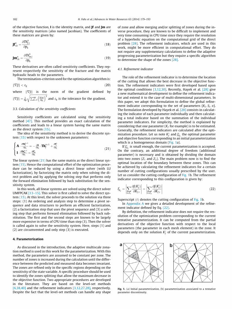
a b

Fig. 1. (a) Initial parameterization, (b) parameterization associated to a tentativeparameter discontinuity.

182 H. Fahs et al. / Advances in Water Resources 63 (2014) 179–193

of the objective function, I is the identity matrix, and Jf and Jm arethe sensitivity matrices (also named Jacobian). The coefficients ofthese matrices are given by:

Jfni;k ¼

@Thnf ;i

@pkð18Þ

Jmni;k ¼

@Thnm;i

@pkð19Þ

These derivatives are often called sensitivity coefficients. They rep-resent respectively the sensitivity of the fracture and the matrixhydraulic heads to the parameters.

The termination-criterion used for the optimization algorithm is:

krJk < eg ð20Þ

where krJk is the norm of the gradient defined by

krJk ¼ 1Np

ffiffiffiffiffiffiffiffiffiffiffiffiffiffiffiffiffiffiffiffiffiffiffiffiffiffiPnpk¼1

@JðpÞ@pk

� �2r

and eg is the tolerance for the gradient.

3.3. Calculation of the sensitivity coefficients

Sensitivity coefficients are calculated using the sensitivitymethod [47]. This method provides an exact calculation of thecoefficients and leads to a linear system having the same matrixas the direct system (15).

The idea of the sensitivity method is to derive the discrete sys-tem (15) with respect to the unknown parameters:

A � @Thnþ1f

@pk¼ � @A

@pk� Thnþ1

f þ @Fnf

@pk

I � @Thnþ1m

@pk¼ @Fn

m@pk

8><>: ð21Þ

The linear system (21) has the same matrix as the direct linear sys-tem (15). Hence the computational effort of the optimization proce-dure can be reduced by using a direct linear solver (with LUfactorization), by factorizing the matrix only when solving the di-rect problem and by applying the solving step that performs onlythe forward elimination followed by back substitution for the sen-sitivity system.

In this work, all linear systems are solved using the direct solverUMFPCAK [13–15]. This solver is first called to solve the direct sys-tem (15). At this level, the solver proceeds to the solution via threesteps: (1) An ordering and analysis step to determine a pivot se-quence and data structures to perform an efficient factorization,(2) a factorization step that uses the pivot sequence and (3) a solv-ing step that performs forward elimination followed by back sub-stitution. The first and the second steps are known to be largelymore expensive in terms of CPU time than step (3). Then the solveris called again to solve the sensitivity system. Here, steps (1) and(2) are circumvented and only step (3) is executed.

4. Parameterization

As discussed in the introduction, the adaptive multiscale zona-tion method is used in this work for the parameterization. With thismethod, the parameters are assumed to be constant per zone. Thenumber of zones is increased during the calculation until the differ-ence between the predicted and measured data becomes invariant.The zones are refined only in the specific regions depending on thesensitivity of the state variable. A specific procedure should be usedto identify the zones splitting that allow the maximum decrease inthe objective function. Two appropriate procedures are developedin the literature. They are based on the level-set methods[6,38,40] and the refinement indicators [3,12,27,28], respectively.Despite the fact that the level-set methods can handle any shape

of zone and allow merging and/or splitting of zones during the in-verse procedure, they are known to be difficult to implement andvery time consuming in CPU time since they require the resolutionof a hyperbolic equation on the computational grid of the directproblem [28]. The refinement indicators, which are used in thiswork, might be more efficient in computational effort. They donot require any supplementary calculations to define the adaptiveprogressing parameterization but they require a specific algorithmto determine the shape of the zones [28].

4.1. Refinement indicator

The role of the refinement indicator is to determine the locationof the cutting that allows the best decrease in the objective func-tion. The refinement indicators were first developed based uponthe optimal conditions [3,12,30]. Recently, Hayek et al. [28] givea new mathematical development to define the refinement indica-tor and extend it to the case of multi-dimensional parameters. Inthis paper, we adopt this formulation to define the global refine-ment indicator corresponding to the set of parameters {Kf ; Sf ;a}.The formulation developed by Hayek et al. [28] consists in calculat-ing the indicator of each parameter individually and then calculat-ing a total indicator based on the summation of the individualparameter indicators. For simplicity, the method is explained byconsidering that one parameter (Kf for example) is to be estimated.Generally, the refinement indicators are calculated after the opti-mization procedure. Let us note K�f and J�Kf

the optimal parameterand objective function corresponding to an initial parameterizationwhich is a homogeneous domain (Fig. 1a).

If J�Kfis small enough, the current parameterization is accepted.

On the contrary, an additional degree of freedom (additionalparameter) is necessary and is obtained by dividing the domaininto two zones (Z1 and Z2). The main problem now is to find theoptimal location of the boundary between these zones. This canbe achieved by calculating the refinement indicators for a certainnumber of cutting configurations usually prescribed by the user.Let us consider the cutting configuration of Fig. 1b. The refinementindicator corresponding to this configuration is given by:

I‘Kf¼Xi2Z1

@JðK�f Þ@Kf ;i

���������� ¼

Xi2Z2

@JðK�f Þ@Kf ;i

���������� ð22Þ

Superscript ð‘Þ denotes the cutting configuration of Fig. 1b.In Appendix A we gives a detailed development of the refine-

ment indicator defined by Eq. (22).By definition, the refinement indicator does not require the res-

olution of the optimization problem corresponding to the currenttentative parameterization. It can be computed from the partialderivatives of the objective function with respect to the localparameters (the parameter in each mesh element) in the zone. Itdepends only on the solution K�f of the current parameterization.

H. Fahs et al. / Advances in Water Resources 63 (2014) 179–193 183

In practice, and as defined in [28], a dimensionless refinement indi-cator is implemented in the numerical model. This dimensionlessrefinement indicator is defined as follows:

~I‘Kf¼

I‘Kf

max8‘ðI‘KfÞ

ð23Þ

where max8‘ðI‘KfÞ represents the largest value of the indicator in all

zone configurations. Similar to Kf we define the dimensionlessrefinement indicators ~I‘Sf

and ~I‘a corresponding to parameters Sf

and a, respectively. The zonation is assumed to be similar for thetriplet of parameters (Kf , Sf and a). Consequently, these parametersare discontinuous at the same locations of the domain. Therefore, itis coherent to use an overall refinement indicator in order to definethe interfaces between zones. The global refinement indicator cor-responding to the triplet of parameters fKf ; Sf ;ag is defined as thesummation of ~I‘Kf

, ~I‘Sfand ~I‘a:

~k‘ ¼ ~I‘Kfþ~I‘Sf

þ~I‘a ð24Þ

4.2. Refinement strategy

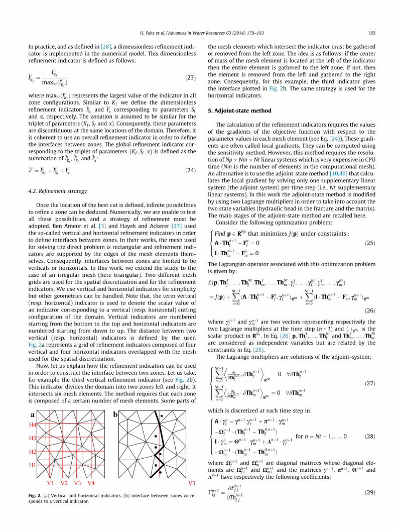
Once the location of the best cut is defined, infinite possibilitiesto refine a zone can be deduced. Numerically, we are unable to testall these possibilities, and a strategy of refinement must beadopted. Ben Ameur et al. [3] and Hayek and Ackerer [27] usedthe so-called vertical and horizontal refinement indicators in orderto define interfaces between zones. In their works, the mesh usedfor solving the direct problem is rectangular and refinement indi-cators are supported by the edges of the mesh elements them-selves. Consequently, interfaces between zones are limited to beverticals or horizontals. In this work, we extend the study to thecase of an irregular mesh (here triangular). Two different meshgrids are used for the spatial discretization and for the refinementindicators. We use vertical and horizontal indicators for simplicitybut other geometries can be handled. Note that, the term vertical(resp. horizontal) indicator is used to denote the scalar value ofan indicator corresponding to a vertical (resp. horizontal) cuttingconfiguration of the domain. Vertical indicators are numberedstarting from the bottom to the top and horizontal indicators arenumbered starting from down to up. The distance between twovertical (resp. horizontal) indicators is defined by the user.Fig. 2a represents a grid of refinement indicators composed of fourvertical and four horizontal indicators overlapped with the meshused for the spatial discretization.

Now, let us explain how the refinement indicators can be usedin order to construct the interface between two zones. Let us take,for example the third vertical refinement indicator (see Fig. 2b).This indicator divides the domain into two zones left and right. Itintersects six mesh elements. The method requires that each zoneis composed of a certain number of mesh elements. Some parts of

a b

V3

H1

V1 V2 V3 V4

H2

H3

H4

Fig. 2. (a) Vertical and horizontal indicators, (b) interface between zones corre-sponds to a vertical indicator.

the mesh elements which intersect the indicator must be gatheredor removed from the left zone. The idea is as follows: if the centerof mass of the mesh element is located at the left of the indicatorthen the entire element is gathered to the left zone. If not, thenthe element is removed from the left and gathered to the rightzone. Consequently, for this example, the third indicator givesthe interface plotted in Fig. 2b. The same strategy is used for thehorizontal indicators.

5. Adjoint-state method

The calculation of the refinement indicators requires the valuesof the gradients of the objective function with respect to theparameter values in each mesh element (see Eq. (24)). These gradi-ents are often called local gradients. They can be computed usingthe sensitivity method. However, this method requires the resolu-tion of Np� Nm� Nt linear systems which is very expensive in CPUtime (Nm is the number of elements in the computational mesh).An alternative is to use the adjoint-state method [10,49] that calcu-lates the local gradient by solving only one supplementary linearsystem (the adjoint system) per time step (i.e., Nt supplementarylinear systems). In this work the adjoint-state method is modifiedby using two Lagrange multipliers in order to take into account thetwo state variables (hydraulic head in the fracture and the matrix).The main stages of the adjoint-state method are recalled here.

Consider the following optimization problem:

Find p 2 RNp that minimizes JðpÞ under constraints :

A � Thnþ1f � Fn

f ¼ 0

I � Thnþ1m � Fn

m ¼ 0

8>><>>: ð25Þ

The Lagrangian operator associated with this optimization problemis given by:

Lðp;Th1f ; . . . ;ThNt

f ;Th1m; . . . ;ThNt

m ; c1f ; . . . ; cNt

f ; c1m; . . . ; cNt

m Þ

¼ JðpÞ þXNt�1

n¼0

hA � Thnþ1f � Fn

f ; cnþ1f iRNe þ

XNt�1

n¼0

hI � Thnþ1m � Fn

m; cnþ1m iRNe

ð26Þ

where cnþ1f and cnþ1

m are two vectors representing respectively thetwo Lagrange multipliers at the time step (n + 1) and h; iRNe is thescalar product in RNe . In Eq. (26) p, Th1

f ; . . . ;ThNtf and Th1

m; . . . ;ThNtm

are considered as independent variables but are related by theconstraints in Eq. (25).

The Lagrange multipliers are solutions of the adjoint-system:

XNt�1

n¼0

@L

@Thnþ1f

; dThnþ1f

� RNe¼ 0 8dThnþ1

f

XNt�1

n¼0

@L

@Thnþ1m� dThnþ1

m

D ERNe¼ 0 8dThnþ1

m

8>>>><>>>>:

ð27Þ

which is discretized at each time step in:

A � cnf ¼ cnþ1:cnþ1

f þ pnþ1 � cnþ1m

�Xnþ1f � ðThnþ1

f � ThO;nþ1f Þ

I � cnm ¼ Hnþ1 � cnþ1

m þ Knþ1 � cnþ1f

�Xnþ1m � ðThnþ1

m � ThO;nþ1m Þ

8>>>>><>>>>>:

for n ¼ Nt � 1; . . . ;0 ð28Þ

where Xnþ1f and Xnþ1

m are diagonal matrices whose diagonal ele-ments are Xnþ1

f ;i and Xnþ1m;i and the matrices cnþ1, pnþ1, Hnþ1 and

Knþ1 have respectively the following coefficients:

Cnþ1i;j ¼

@Fnþ1f ;i

@Thnþ1f ;j

ð29Þ

184 H. Fahs et al. / Advances in Water Resources 63 (2014) 179–193

Pnþ1i;j ¼

@Fnþ1m;i

@Thnþ1f ;j

ð30Þ

Hnþ1i;j ¼

@Fnþ1m;i

@Thnþ1m;j

ð31Þ

Z4

Z2

Z3

Z3

Z1

Z1

Z21Z1

Z3 Z4

Z22

Z2

Z4

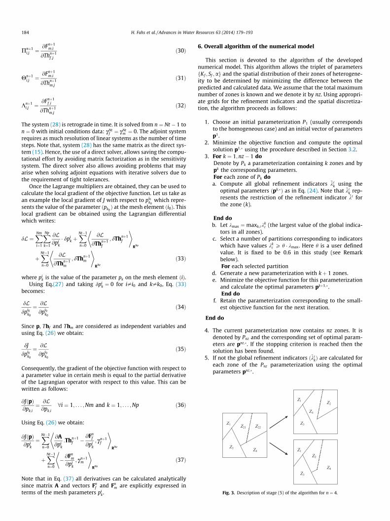
Fig. 3. Description of stage (5) of the algorithm for n ¼ 4.

Knþ1i;j ¼

@Fnþ1f ;i

@Thnþ1m;j

ð32Þ

The system (28) is retrograde in time. It is solved from n ¼ Nt � 1 ton ¼ 0 with initial conditions data: cNt

f ¼ cNtm ¼ 0. The adjoint system

requires as much resolution of linear systems as the number of timesteps. Note that, system (28) has the same matrix as the direct sys-tem (15). Hence, the use of a direct solver, allows saving the compu-tational effort by avoiding matrix factorization as in the sensitivitysystem. The direct solver also allows avoiding problems that mayarise when solving adjoint equations with iterative solvers due tothe requirement of tight tolerances.

Once the Lagrange multipliers are obtained, they can be used tocalculate the local gradient of the objective function. Let us take asan example the local gradient of J with respect to pi0

k0which repre-

sents the value of the parameter ðpk0Þ at the mesh element ði0Þ. This

local gradient can be obtained using the Lagrangian differentialwhich writes:

dL ¼XNm

i¼1

XNp

k¼1

@L@pi

k

� dpik þ

XNt�1

n¼0

@L@Thnþ1

f

; dThnþ1f

* +RNe

þXNt�1

n¼0

@L@Thnþ1

m

; dThnþ1m

* +RNe

ð33Þ

where pik is the value of the parameter pk on the mesh element ðiÞ.

Using Eq.(27) and taking dpik ¼ 0 for i–i0 and k–k0, Eq. (33)

becomes:

dLdpi0

k0

¼ @L@pi0

k0

ð34Þ

Since p, Thf and Thm are considered as independent variables andusing Eq. (26) we obtain:

dJ

dpi0k0

¼ @L@pi0

k0

ð35Þ

Consequently, the gradient of the objective function with respect toa parameter value in certain mesh is equal to the partial derivativeof the Lagrangian operator with respect to this value. This can bewritten as follows:

@JðpÞ@pk;i

¼ @L@pk;i

8i ¼ 1; . . . ;Nm and k ¼ 1; . . . ;Np ð36Þ

Using Eq. (26) we obtain:

@JðpÞ@pi

k

¼XNt�1

n¼0

@A@pi

k

:Thnþ1f �

@Fnf

@pik

; cnþ1f

* +RNe

þXNt�1

n¼0

� @Fnm

@pik

; cnþ1m

* +RNe

ð37Þ

Note that in Eq. (37) all derivatives can be calculated analyticallysince matrix A and vectors Fn

f and Fnm are explicitly expressed in

terms of the mesh parameters pik.

6. Overall algorithm of the numerical model

This section is devoted to the algorithm of the developednumerical model. This algorithm allows the triplet of parametersfKf ; Sf ;ag and the spatial distribution of their zones of heterogene-ity to be determined by minimizing the difference between thepredicted and calculated data. We assume that the total maximumnumber of zones is known and we denote it by nz. Using appropri-ate grids for the refinement indicators and the spatial discretiza-tion, the algorithm proceeds as follows:

1. Choose an initial parameterization P1 (usually correspondsto the homogeneous case) and an initial vector of parametersp1.

2. Minimize the objective function and compute the optimalsolution p1;� using the procedure described in Section 3.2.

3. For k ¼ 1;nz� 1 do

Denote by Pk a parameterization containing k zones and bypk the corresponding parameters.For each zone of Pk do a. Compute all global refinement indicators ~k‘k using the

optimal parameters ðpk;�Þ as in Eq. (24). Note that ~k‘k rep-resents the restriction of the refinement indicator ~k‘ forthe zone (k).

End dob. Let kmax ¼maxk;‘k

k‘ (the largest value of the global indica-

tors in all zones).c. Select a number of partitions corresponding to indicators

which have values kk‘ P h � kmax. Here h is a user defined

value. It is fixed to be 0.6 in this study (see Remarkbelow).

For each selected partition

d. Generate a new parameterization with kþ 1 zones.e. Minimize the objective function for this parameterization

and calculate the optimal parameters pkþ1;�.

End do

f. Retain the parameterization corresponding to the small-est objective function for the next iteration.

End do

4. The current parameterization now contains nz zones. It isdenoted by Pnz and the corresponding set of optimal param-eters are pnz;�. If the stopping criterion is reached then thesolution has been found.

5. If not the global refinement indicators ð~k‘kÞ are calculated foreach zone of the Pnz parameterization using the optimalparameters pnz;�.

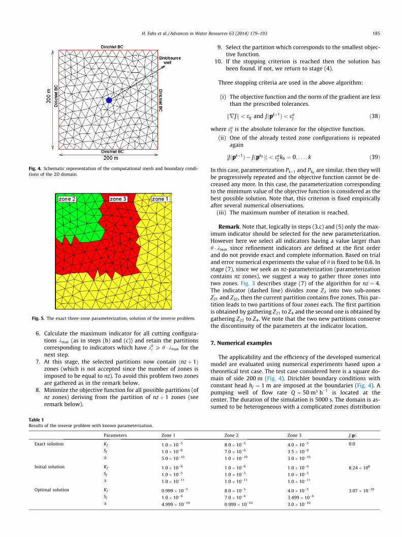
Fig. 4. Schematic representation of the computational mesh and boundary condi-tions of the 2D domain.

Fig. 5. The exact three-zone parameterization, solution of the inverse problem.

H. Fahs et al. / Advances in Water Resources 63 (2014) 179–193 185

6. Calculate the maximum indicator for all cutting configura-tions kmax (as in steps (b) and (c)) and retain the partitionscorresponding to indicators which have kk

‘ P h � kmax for thenext step.

7. At this stage, the selected partitions now contain ðnzþ 1Þzones (which is not accepted since the number of zones isimposed to be equal to nz). To avoid this problem two zonesare gathered as in the remark below.

8. Minimize the objective function for all possible partitions (ofnz zones) deriving from the partition of nzþ 1 zones (seeremark below).

Table 1Results of the inverse problem with known parameterization.

Parameters Zone 1

Exact solution Kf 1:0� 10�5

Sf 1:0� 10�6

a 5:0� 10�10

Initial solution Kf 1:0� 10�6

Sf 1:0� 10�5

a 1:0� 10�11

Optimal solution Kf 0:999� 10�5

Sf 1:0� 10�6

a 4:999� 10�10

9. Select the partition which corresponds to the smallest objec-tive function.

10. If the stopping criterion is reached then the solution hasbeen found. If not, we return to stage (4).

Three stopping criteria are used in the above algorithm:

(i) The objective function and the norm of the gradient are lessthan the prescribed tolerances.

Z

8

7

1

1

1

1

8

7

0

krJk < eg and Jðpkþ1Þ < eaJ ð38Þ

where eaJ is the absolute tolerance for the objective function.

(ii) One of the already tested zone configurations is repeatedagain

jJðpkþ1Þ � Jðpk0 Þj < eaJ k0 ¼ 0; . . . ; k ð39Þ

In this case, parameterization Pkþ1 and Pk0 are similar, then they willbe progressively repeated and the objective function cannot be de-creased any more. In this case, the parameterization correspondingto the minimum value of the objective function is considered as thebest possible solution. Note that, this criterion is fixed empiricallyafter several numerical observations.

(iii) The maximum number of iteration is reached.

Remark. Note that, logically in steps (3.c) and (5) only the max-imum indicator should be selected for the new parameterization.However here we select all indicators having a value larger thanh � kmax since refinement indicators are defined at the first orderand do not provide exact and complete information. Based on trialand error numerical experiments the value of h is fixed to be 0.6. Instage (7), since we seek an nz-parameterization (parameterizationcontains nz zones), we suggest a way to gather three zones intotwo zones. Fig. 3 describes stage (7) of the algorithm for nz ¼ 4.The indicator (dashed line) divides zone Z2 into two sub-zonesZ21 and Z22, then the current partition contains five zones. This par-tition leads to two partitions of four zones each. The first partitionis obtained by gathering Z21 to Z4 and the second one is obtained bygathering Z22 to Z4. We note that the two new partitions conservethe discontinuity of the parameters at the indicator location.

7. Numerical examples

The applicability and the efficiency of the developed numericalmodel are evaluated using numerical experiments based upon atheoretical test case. The test case considered here is a square do-main of side 200 m (Fig. 4). Dirichlet boundary conditions withconstant head hf ¼ 1 m are imposed at the boundaries (Fig. 4). Apumping well of flow rate Q ¼ 50 m3 h�1 is located at thecenter. The duration of the simulation is 5000 s. The domain is as-sumed to be heterogeneous with a complicated zones distribution

one 2 Zone 3 JðpÞ

:0� 10�5 4:0� 10�5 0:0

:0� 10�6 3:5� 10�6

:0� 10�10 3:0� 10�10

:0� 10�6 1:0� 10�6 8:24� 108

:0� 10�5 1:0� 10�5

:0� 10�11 1:0� 10�11

:0� 10�5 4:0� 10�5 3:07� 10�20

:0� 10�6 3:499� 10�6

:999� 10�10 3:0� 10�10

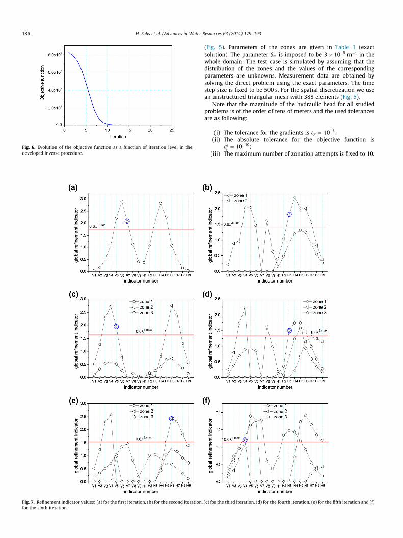
Fig. 6. Evolution of the objective function as a function of iteration level in thedeveloped inverse procedure.

Fig. 7. Refinement indicator values: (a) for the first iteration, (b) for the second iteration,for the sixth iteration.

186 H. Fahs et al. / Advances in Water Resources 63 (2014) 179–193

(Fig. 5). Parameters of the zones are given in Table 1 (exactsolution). The parameter Sm is imposed to be 3� 10�5 m�1 in thewhole domain. The test case is simulated by assuming that thedistribution of the zones and the values of the correspondingparameters are unknowns. Measurement data are obtained bysolving the direct problem using the exact parameters. The timestep size is fixed to be 500 s. For the spatial discretization we usean unstructured triangular mesh with 388 elements (Fig. 5).

Note that the magnitude of the hydraulic head for all studiedproblems is of the order of tens of meters and the used tolerancesare as following:

(i) The tolerance for the gradients is eg ¼ 10�3;(ii) The absolute tolerance for the objective function is

eaJ ¼ 10�10;

(iii) The maximum number of zonation attempts is fixed to 10.

(c) for the third iteration, (d) for the fourth iteration, (e) for the fifth iteration and (f)

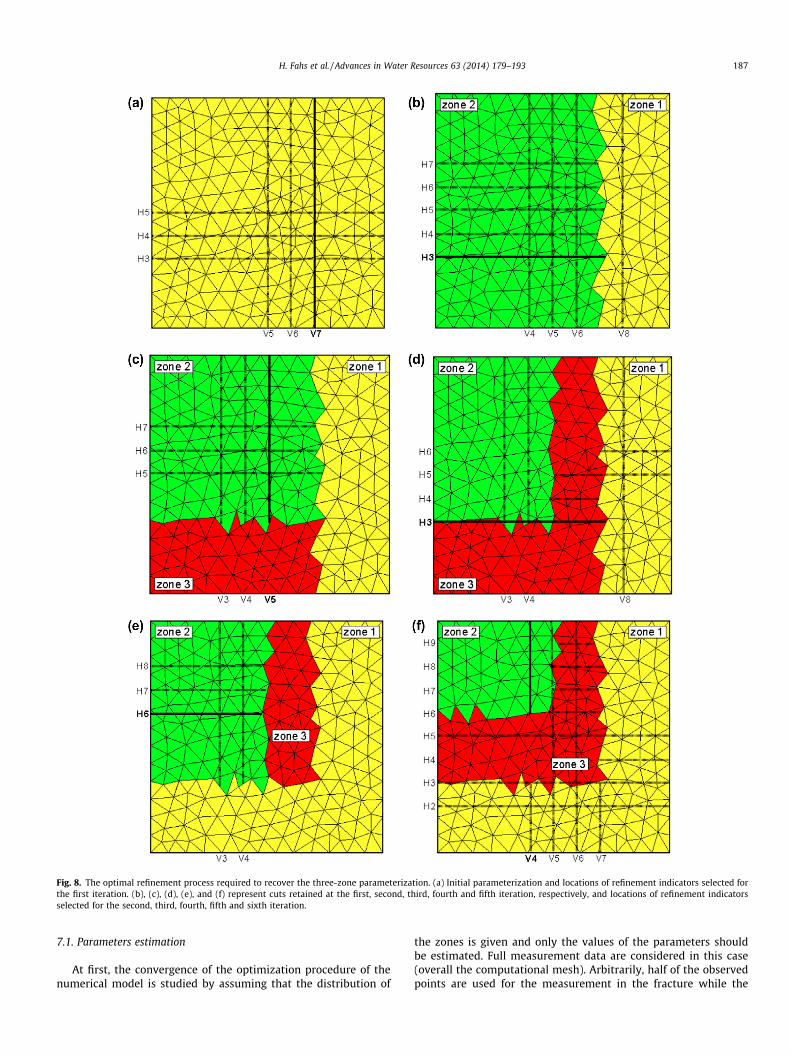
Fig. 8. The optimal refinement process required to recover the three-zone parameterization. (a) Initial parameterization and locations of refinement indicators selected forthe first iteration. (b), (c), (d), (e), and (f) represent cuts retained at the first, second, third, fourth and fifth iteration, respectively, and locations of refinement indicatorsselected for the second, third, fourth, fifth and sixth iteration.

H. Fahs et al. / Advances in Water Resources 63 (2014) 179–193 187

7.1. Parameters estimation

At first, the convergence of the optimization procedure of thenumerical model is studied by assuming that the distribution of

the zones is given and only the values of the parameters shouldbe estimated. Full measurement data are considered in this case(overall the computational mesh). Arbitrarily, half of the observedpoints are used for the measurement in the fracture while the

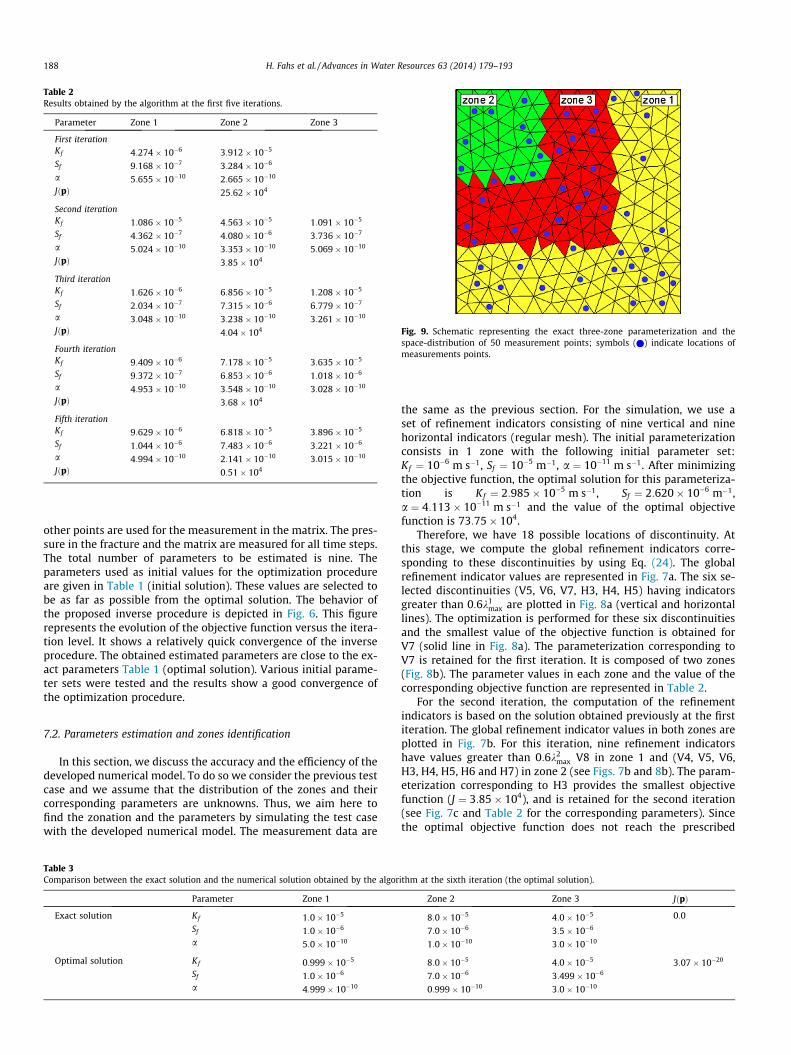
Table 2Results obtained by the algorithm at the first five iterations.

Parameter Zone 1 Zone 2 Zone 3

First iterationKf 4:274� 10�6 3:912� 10�5

Sf 9:168� 10�7 3:284� 10�6

a 5:655� 10�10 2:665� 10�10

JðpÞ 25:62� 104

Second iterationKf 1:086� 10�5 4:563� 10�5 1:091� 10�5

Sf 4:362� 10�7 4:080� 10�6 3:736� 10�7

a 5:024� 10�10 3:353� 10�10 5:069� 10�10

JðpÞ 3:85� 104

Third iterationKf 1:626� 10�6 6:856� 10�5 1:208� 10�5

Sf 2:034� 10�7 7:315� 10�6 6:779� 10�7

a 3:048� 10�10 3:238� 10�10 3:261� 10�10

JðpÞ 4:04� 104

Fourth iterationKf 9:409� 10�6 7:178� 10�5 3:635� 10�5

Sf 9:372� 10�7 6:853� 10�6 1:018� 10�6

a 4:953� 10�10 3:548� 10�10 3:028� 10�10

JðpÞ 3:68� 104

Fifth iterationKf 9:629� 10�6 6:818� 10�5 3:896� 10�5

Sf 1:044� 10�6 7:483� 10�6 3:221� 10�6

a 4:994� 10�10 2:141� 10�10 3:015� 10�10

JðpÞ 0:51� 104

Fig. 9. Schematic representing the exact three-zone parameterization and thespace-distribution of 50 measurement points; symbols ( ) indicate locations ofmeasurements points.

188 H. Fahs et al. / Advances in Water Resources 63 (2014) 179–193

other points are used for the measurement in the matrix. The pres-sure in the fracture and the matrix are measured for all time steps.The total number of parameters to be estimated is nine. Theparameters used as initial values for the optimization procedureare given in Table 1 (initial solution). These values are selected tobe as far as possible from the optimal solution. The behavior ofthe proposed inverse procedure is depicted in Fig. 6. This figurerepresents the evolution of the objective function versus the itera-tion level. It shows a relatively quick convergence of the inverseprocedure. The obtained estimated parameters are close to the ex-act parameters Table 1 (optimal solution). Various initial parame-ter sets were tested and the results show a good convergence ofthe optimization procedure.

7.2. Parameters estimation and zones identification

In this section, we discuss the accuracy and the efficiency of thedeveloped numerical model. To do so we consider the previous testcase and we assume that the distribution of the zones and theircorresponding parameters are unknowns. Thus, we aim here tofind the zonation and the parameters by simulating the test casewith the developed numerical model. The measurement data are

Table 3Comparison between the exact solution and the numerical solution obtained by the algor

Parameter Zone 1

Exact solution Kf 1:0� 10�5

Sf 1:0� 10�6

a 5:0� 10�10

Optimal solution Kf 0:999� 10�5

Sf 1:0� 10�6

a 4:999� 10�10

the same as the previous section. For the simulation, we use aset of refinement indicators consisting of nine vertical and ninehorizontal indicators (regular mesh). The initial parameterizationconsists in 1 zone with the following initial parameter set:Kf ¼ 10�6 m s�1, Sf ¼ 10�5 m�1, a ¼ 10�11 m s�1. After minimizingthe objective function, the optimal solution for this parameteriza-tion is Kf ¼ 2:985� 10�5 m s�1, Sf ¼ 2:620� 10�6 m�1,a ¼ 4:113� 10�11 m s�1 and the value of the optimal objectivefunction is 73:75� 104.

Therefore, we have 18 possible locations of discontinuity. Atthis stage, we compute the global refinement indicators corre-sponding to these discontinuities by using Eq. (24). The globalrefinement indicator values are represented in Fig. 7a. The six se-lected discontinuities (V5, V6, V7, H3, H4, H5) having indicatorsgreater than 0:6k1

max are plotted in Fig. 8a (vertical and horizontallines). The optimization is performed for these six discontinuitiesand the smallest value of the objective function is obtained forV7 (solid line in Fig. 8a). The parameterization corresponding toV7 is retained for the first iteration. It is composed of two zones(Fig. 8b). The parameter values in each zone and the value of thecorresponding objective function are represented in Table 2.

For the second iteration, the computation of the refinementindicators is based on the solution obtained previously at the firstiteration. The global refinement indicator values in both zones areplotted in Fig. 7b. For this iteration, nine refinement indicatorshave values greater than 0:6k2

max V8 in zone 1 and (V4, V5, V6,H3, H4, H5, H6 and H7) in zone 2 (see Figs. 7b and 8b). The param-eterization corresponding to H3 provides the smallest objectivefunction (J ¼ 3:85� 104), and is retained for the second iteration(see Fig. 7c and Table 2 for the corresponding parameters). Sincethe optimal objective function does not reach the prescribed

ithm at the sixth iteration (the optimal solution).

Zone 2 Zone 3 JðpÞ

8:0� 10�5 4:0� 10�5 0:0

7:0� 10�6 3:5� 10�6

1:0� 10�10 3:0� 10�10

8:0� 10�5 4:0� 10�5 3:07� 10�20

7:0� 10�6 3:499� 10�6

0:999� 10�10 3:0� 10�10

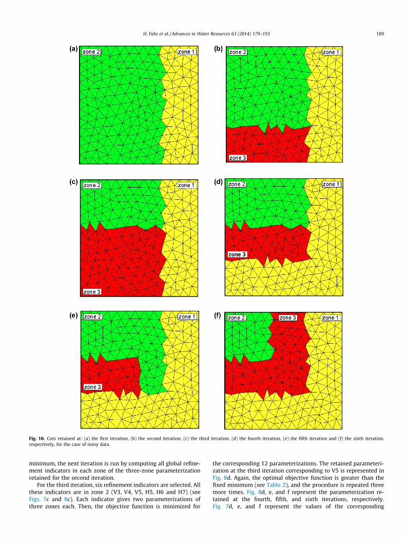
Fig. 10. Cuts retained at: (a) the first iteration, (b) the second iteration, (c) the third iteration, (d) the fourth iteration, (e) the fifth iteration and (f) the sixth iteration,respectively, for the case of noisy data.

H. Fahs et al. / Advances in Water Resources 63 (2014) 179–193 189

minimum, the next iteration is run by computing all global refine-ment indicators in each zone of the three-zone parameterizationretained for the second iteration.

For the third iteration, six refinement indicators are selected. Allthese indicators are in zone 2 (V3, V4, V5, H5, H6 and H7) (seeFigs. 7c and 8c). Each indicator gives two parameterizations ofthree zones each. Then, the objective function is minimized for

the corresponding 12 parameterizations. The retained parameteri-zation at the third iteration corresponding to V5 is represented inFig. 8d. Again, the optimal objective function is greater than thefixed minimum (see Table 2), and the procedure is repeated threemore times. Fig. 8d, e, and f represent the parameterization re-tained at the fourth, fifth, and sixth iterations, respectively.Fig. 7d, e, and f represent the values of the corresponding

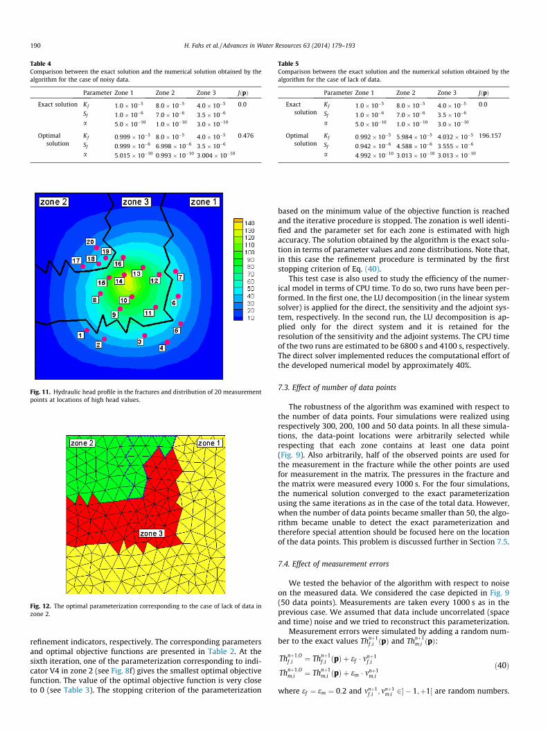
Table 4Comparison between the exact solution and the numerical solution obtained by thealgorithm for the case of noisy data.

Parameter Zone 1 Zone 2 Zone 3 JðpÞ

Exact solution Kf 1:0� 10�5 8:0� 10�5 4:0� 10�5 0:0

Sf 1:0� 10�6 7:0� 10�6 3:5� 10�6

a 5:0� 10�10 1:0� 10�10 3:0� 10�10

Optimalsolution

Kf 0:999� 10�5 8:0� 10�5 4:0� 10�5 0:476

Sf 0:999� 10�6 6:998� 10�6 3:5� 10�6

a 5:015� 10�10 0:993� 10�10 3:004� 10�10

Fig. 11. Hydraulic head profile in the fractures and distribution of 20 measurementpoints at locations of high head values.

Fig. 12. The optimal parameterization corresponding to the case of lack of data inzone 2.

Table 5Comparison between the exact solution and the numerical solution obtained by thealgorithm for the case of lack of data.

Parameter Zone 1 Zone 2 Zone 3 JðpÞ

Exactsolution

Kf 1:0� 10�5 8:0� 10�5 4:0� 10�5 0:0

Sf 1:0� 10�6 7:0� 10�6 3:5� 10�6

a 5:0� 10�10 1:0� 10�10 3:0� 10�10

Optimalsolution

Kf 0:992� 10�5 5:984� 10�5 4:032� 10�5 196:157

Sf 0:942� 10�6 4:588� 10�6 3:555� 10�6

a 4:992� 10�10 3:013� 10�10 3:013� 10�10

190 H. Fahs et al. / Advances in Water Resources 63 (2014) 179–193

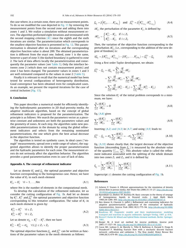
refinement indicators, respectively. The corresponding parametersand optimal objective functions are presented in Table 2. At thesixth iteration, one of the parameterization corresponding to indi-cator V4 in zone 2 (see Fig. 8f) gives the smallest optimal objectivefunction. The value of the optimal objective function is very closeto 0 (see Table 3). The stopping criterion of the parameterization

based on the minimum value of the objective function is reachedand the iterative procedure is stopped. The zonation is well identi-fied and the parameter set for each zone is estimated with highaccuracy. The solution obtained by the algorithm is the exact solu-tion in terms of parameter values and zone distributions. Note that,in this case the refinement procedure is terminated by the firststopping criterion of Eq. (40).

This test case is also used to study the efficiency of the numer-ical model in terms of CPU time. To do so, two runs have been per-formed. In the first one, the LU decomposition (in the linear systemsolver) is applied for the direct, the sensitivity and the adjoint sys-tem, respectively. In the second run, the LU decomposition is ap-plied only for the direct system and it is retained for theresolution of the sensitivity and the adjoint systems. The CPU timeof the two runs are estimated to be 6800 s and 4100 s, respectively.The direct solver implemented reduces the computational effort ofthe developed numerical model by approximately 40%.

7.3. Effect of number of data points

The robustness of the algorithm was examined with respect tothe number of data points. Four simulations were realized usingrespectively 300, 200, 100 and 50 data points. In all these simula-tions, the data-point locations were arbitrarily selected whilerespecting that each zone contains at least one data point(Fig. 9). Also arbitrarily, half of the observed points are used forthe measurement in the fracture while the other points are usedfor measurement in the matrix. The pressures in the fracture andthe matrix were measured every 1000 s. For the four simulations,the numerical solution converged to the exact parameterizationusing the same iterations as in the case of the total data. However,when the number of data points became smaller than 50, the algo-rithm became unable to detect the exact parameterization andtherefore special attention should be focused here on the locationof the data points. This problem is discussed further in Section 7.5.

7.4. Effect of measurement errors

We tested the behavior of the algorithm with respect to noiseon the measured data. We considered the case depicted in Fig. 9(50 data points). Measurements are taken every 1000 s as in theprevious case. We assumed that data include uncorrelated (spaceand time) noise and we tried to reconstruct this parameterization.

Measurement errors were simulated by adding a random num-ber to the exact values Thnþ1

f ;i ðpÞ and Thnþ1m;i ðpÞ:

Thnþ1;Of ;i ¼ Thnþ1

f ;i ðpÞ þ ef � mnþ1f ;i

Thnþ1;Om;i ¼ Thnþ1

m;i ðpÞ þ em � mnþ1m;i

ð40Þ

where ef ¼ em ¼ 0:2 and mnþ1f ;i ; mnþ1

m;i 2� � 1;þ1½ are random numbers.

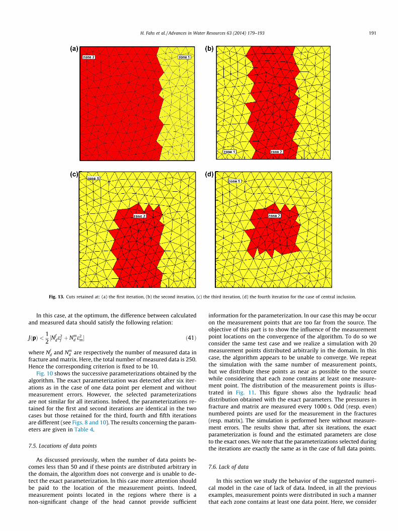
Fig. 13. Cuts retained at: (a) the first iteration, (b) the second iteration, (c) the third iteration, (d) the fourth iteration for the case of central inclusion.

H. Fahs et al. / Advances in Water Resources 63 (2014) 179–193 191

In this case, at the optimum, the difference between calculatedand measured data should satisfy the following relation:

JðpÞ < 12½Nf

de2f þ Nm

d e2m� ð41Þ

where Nfd and Nm

d are respectively the number of measured data infracture and matrix. Here, the total number of measured data is 250.Hence the corresponding criterion is fixed to be 10.

Fig. 10 shows the successive parameterizations obtained by thealgorithm. The exact parameterization was detected after six iter-ations as in the case of one data point per element and withoutmeasurement errors. However, the selected parameterizationsare not similar for all iterations. Indeed, the parameterizations re-tained for the first and second iterations are identical in the twocases but those retained for the third, fourth and fifth iterationsare different (see Figs. 8 and 10). The results concerning the param-eters are given in Table 4.

7.5. Locations of data points

As discussed previously, when the number of data points be-comes less than 50 and if these points are distributed arbitrary inthe domain, the algorithm does not converge and is unable to de-tect the exact parameterization. In this case more attention shouldbe paid to the location of the measurement points. Indeed,measurement points located in the regions where there is anon-significant change of the head cannot provide sufficient

information for the parameterization. In our case this may be occuron the measurement points that are too far from the source. Theobjective of this part is to show the influence of the measurementpoint locations on the convergence of the algorithm. To do so weconsider the same test case and we realize a simulation with 20measurement points distributed arbitrarily in the domain. In thiscase, the algorithm appears to be unable to converge. We repeatthe simulation with the same number of measurement points,but we distribute these points as near as possible to the sourcewhile considering that each zone contains at least one measure-ment point. The distribution of the measurement points is illus-trated in Fig. 11. This figure shows also the hydraulic headdistribution obtained with the exact parameters. The pressures infracture and matrix are measured every 1000 s. Odd (resp. even)numbered points are used for the measurement in the fractures(resp. matrix). The simulation is performed here without measure-ment errors. The results show that, after six iterations, the exactparameterization is found and the estimated parameters are closeto the exact ones. We note that the parameterizations selected duringthe iterations are exactly the same as in the case of full data points.

7.6. Lack of data

In this section we study the behavior of the suggested numeri-cal model in the case of lack of data. Indeed, in all the previousexamples, measurement points were distributed in such a mannerthat each zone contains at least one data point. Here, we consider

192 H. Fahs et al. / Advances in Water Resources 63 (2014) 179–193

the case where, in a certain zone, there are no measurement points.To do so we modified the case depicted in Fig. 11 by removing themeasurement points from the second zone and adding them intozones 1 and 3. We realize a simulation without measurement er-rors. The algorithm performed eight iterations and terminated withthe second stopping criterion (41) since the eighth and the sixthiterations are similar. The parameterization which corresponds tothe smallest objective function is presented in Fig. 12. This param-eterization is obtained after six iterations and the correspondingobjective function value is about 200. The obtained parameteriza-tion is different from the exact one. Indeed, zone 1 is the same,however a part of zone 3 (the dashed boundary) is gathered to zone2. The lack of data affects locally the parameterization and conse-quently the parameter values (see Table 5). Only the interface be-tween zone 2 (which does not contain measurement points) andzone 3 has been changed. The parameter values in zones 1 and 3are well estimated compared to the values in zone 2 (Table 5).

Finally it is relevant to recall that the numerical model has beentested for several configurations of heterogeneity distribution.Good convergence has been obtained even for complicated cases.As an example, we present the required iterations for the case ofcentral inclusion (Fig. 13).

8. Conclusion

This paper describes a numerical model for efficiently identify-ing the hydrodynamic parameters in 2D dual-porosity media. Anadaptive multiscale algorithm, based on the concept of globalrefinement indicators is proposed for the parameterization. Theprinciple is as follows: We search the parameters vector as a piece-wise constant and unknowns are both the parameters values andthe geometry of zones. At each step, the algorithm ranks new pos-sible parameterizations in the domain by using the global refine-ment indicators and selects from the remaining nominatedparameterizations, the one which gives the best actual decreasein the objective function.

The algorithm is tested on synthetic cases. In ideal cases (‘‘en-ough’’ measurements, spread over a wide range of values), the sug-gested algorithm allows to identify the proper parameterizationand the hydraulic parameters for each zone. The measurement er-rors do not seriously affect the algorithm behavior. The algorithmprovides a good parameterization even in case of lack of data.

Appendix A. The concept of refinement indicator

Let us denote K�f and J�Kfthe optimal parameter and objective

function corresponding to the homogeneous case. Hence, we havethe value of Kf in each mesh element

K�f ;i ¼ K�f 8i ¼ 1; . . . ;Nm ðA:1Þ

where Nm is the number of elements in the computational mesh.To develop the calculation of the refinement indicator, let us

consider the cutting configuration of Fig. 1b. And let us denoteby K1�

f , K2�f and J12�

Kfthe optimal parameters and objective function

corresponding to this tentative configuration. The value of Kf ineach mesh element is given by:

K1�f ;i ¼ K1�

f 8i 2 Z1

K2�f ;i ¼ K2�

f 8i 2 Z2

ðA:2Þ

Let us denote r�Kf¼ K1�

f � K2�f , then we have

K1�f ;i � K2�

f ;j ¼ r�Kf8ði; jÞ 2 Z1 � Z2 ðA:3Þ

The optimal objective functions J�Kfand J12�

Kfcan be written as func-

tions of the parameter values in the mesh elements as follows:

J�Kf¼ J K�f ;1; . . . ;K�f ;Nm

� �and J12�

Kf¼ J K1�

f ;ii2Z1; K2�

f ;ii2Z2

� �ðA:4Þ

dK�f ;i the perturbation of the parameter K�f ;i is defined by:

dK�f ;i ¼K1�

f ;i � K�f ;i if i 2 Z1

K2�f ;i � K�f ;i if i 2 Z2

(ðA:5Þ

Then, the variation of the objective function corresponding to theperturbation dK�f ;i (i.e., corresponding to the addition of the new de-gree of freedom) is:

dJ�Kf¼ JðK1�

f ;ii2Z1; K2�

f ;ii2Z2Þ � JðK�f ;1; . . . ;K�f ;Nm

Þ ¼ J12�Kf� J�Kf

ðA:6Þ

Using a first order Taylor development, we obtain:

J12�Kf� J�Kf

¼ dJ�Kf�XNm

i¼1

@J@Kf ;i

dK�f ;i

¼Xi2Z1

@J@Kf ;i

dK�f ;i þXi2Z2

@J@Kf ;i

dK�f ;i

�Xi2Z1

@J@Kf ;i

ðK1�f ;i � K�f ;iÞ þ

Xi2Z2

@J@Kf ;i

ðK2�f ;i � K�f ;iÞ ðA:7Þ

Since the solution K�f of the initial problem corresponds to a mini-mum, we have:

XNe

i¼1

@JðK�f Þ@Kf ;i

¼ 0 ðA:8Þ

Eq. (A.8) gives

Xi2Z1

@JðK�f Þ@Kf ;i

¼ �Xi2Z2

@JðK�f Þ@Kf ;i

ðA:9Þ

Inserting (A.2) and (A.3) in (A.7) and using (A.9) leads to:

J12�Kf� J�Kf

¼ r�Kf

Xi2Z1

@JðK�f Þ@Kf ;i

¼ �r�Kf

Xi2Z2

@JðK�f Þ@Kf ;i

ðA:10Þ

Eq. (A.10) shows clearly that, the largest decrease of the objectivefunction (descending from J�Kf

) is measured by the absolute valueof the quantity

Pi2Z1

@JðK�f Þ@Kf ;i

. This absolute value is called the refine-ment indicator associated with the splitting of the whole domaininto two zones Z1 and Z2, and it is defined by:

I‘Kf¼Xi2Z1

@J K�f� �@Kf ;i

������������ ¼

Xi2Z2

@JðK�f Þ@Kf ;i

���������� ðA:11Þ

Superscript ð‘Þ denotes the cutting configuration of Fig. 1b.

References

[1] Ackerer P, Younes A. Efficient approximations for the simulation of densitydriven flow in porous media. Adv Water Res 2006;31:15–27. http://dx.doi.org/10.1016/j.advwatres.2007.06.001.

[2] Barenblatt GI, Zheltov YP, Kochina IN. Basic concepts in the theory of seepageof homogeneous liquids in fissured rocks. J Appl Math Mech1960;24:1286–303. http://dx.doi.org/10.1016/0021-8928(60)90107-6.

[3] Ben Ameur H, Chavent G, Jaffré J. Refinement and coarsening indicators foradaptive parameterization: application of the estimation of hydraulictransmissivities. Inverse Prob 2002;18(3):775–94. http://dx.doi.org/10.1088/0266-5611/18/3/317.

[4] Boudreau BP. Diagenetic models and their implementation: modelingtransport and reactions in aquatic sediments. Springer-Verlag; 1997. p. 414.

[5] Brezzi F, Fortin M. Mixed and hybrid finite element methods. Berlin: Springer;1991.

[6] Burger M. A level set method for inverse problems. Inverse prob2001;17:1327–56. http://dx.doi.org/10.1088/0266-5611/17/5/307.

[7] Cacas MC, Ledoux E, de Marsily G, Tillie B, Barbreau A, Durand E, Feuga B,Peaudecerf P. Modeling fracture flow with a stochastic discrete fracturenetwork: calibration and validation 1. The flow model. Water Resour Res1990;26(3):479–89. http://dx.doi.org/10.1029/WR026i003p00479.

H. Fahs et al. / Advances in Water Resources 63 (2014) 179–193 193

[8] Carrera J, Neuman SP. Estimation of aquifer parameters under transient andsteady state conditions: 3. Application to synthetic and field data. WaterResour Res 1986;22(2):228–42. http://dx.doi.org/10.1029/WR022i002p00228.

[9] Carrera J, Alcolea A, Medina A, Hidalgo J, Slooten J. Inverse problem inhydrogeology. Hydrogeol J 2005;13:206–22. http://dx.doi.org/10.1007/s10040-004-0404-7.

[10] Chavent G. Identification of functional parameter in partial differentialequations. In: Goodson RE, Polis M, editors. Identification of parameters indistributed systems. New York: Am. Soc. Mech. Eng; 1974. p. 31–48.

[11] Chavent G, Roberts JE. A unified physical presentation of mixed, mixed hybridfinite elements and standard finite difference approximations for thedetermination of velocities in waterflow problems. Adv Water Res1991;14:329–48. http://dx.doi.org/10.1016/0309-1708(91)90020-O.

[12] Chavent G, Bissel R. Indicator for the refinement of parameterization. In:Tanaka M, Dulikravich GS, editors. Inverse problems in engineeringmechanics. Elsevier; 1998. p. 309–14.

[13] Davis TA. A column pre-ordering strategy for the unsymmetric-patternmultifrontal method. ACM Trans Math Softw 2004;30(2):165–95. http://dx.doi.org/10.1145/992200.992205.

[14] Davis TA. Algorithm 832: UMFPACK, an unsymmetric-pattern multifrontalmethod. ACM Trans Math Softw 2004;30(2):196–9. http://dx.doi.org/10.1145/992200.992206.

[15] Davis TA, Duff IS. A combined unifrontal/multifrontal method for unsymmetricsparse matrices. Technical Report, TR-97-016. Gainesville, FL: Computer andInformation Science and Engineering Department, University of Florida; 1999.

[16] Delay F, Kaczmaryk A, Ackerer P. Inversion of interference hydraulic pumpingtests in both homogeneous and fractal dual media. Adv Water Res2007;30:314–34. http://dx.doi.org/10.1016/j.advwatres.2006.06.008.

[17] Dershowitz WS, Einstein HH. Characterizing rock joint geometry with jointsystem models. Rock Mech Rock Eng 1988;1(1):21–51. http://dx.doi.org/10.1007/BF01019674.

[18] Durlofsky LJ. Accuracy of mixed and control volume finite elementapproximations to Darcy velocity and related quantities. Water Resour Res1994;30(4):965–73. http://dx.doi.org/10.1029/94WR00061.

[19] Dverstorp B, Andersson J. Application of the discrete fracture network conceptwith field data: possibilities of model calibration and validation. Water ResourRes 1989;25(3):540–50. http://dx.doi.org/10.1029/WR025i003p00540.

[20] Eppstein MJ, Dougherty DE. Simultaneous estimation of transmissivity valuesand zonation. Water Resour Res 1996;32(11):3321–36. http://dx.doi.org/10.1029/96WR02283.

[21] Gerke HH, van Genuchten MT. A dual-porosity model for simulating thepreferential movement of water and solutes in structured porous media.Water Resour Res 1993;29(2):305–19. http://dx.doi.org/10.1029/92WR02339.

[22] Gerke HH, van Genuchten MT. Evaluation of a first order water transfer termfor variably saturated dual-porosity flow models. Water Resour. Res.1993;29(4):1225–38. http://dx.doi.org/10.1029/92WR02467.

[23] Gerke HH, van Genuchten MT. Macroscopic representation of structuralgeometry of simulating water and solute movement in dual-porosity media.Adv Water Res 1996;19:343–57. http://dx.doi.org/10.1016/0309-1708(96)00012-7.

[24] Hantush MM, Mariño MA, Islam MR. Models for leaching of pesticides in soilsand groundwater. J Hydrol 2000;227:66–83. http://dx.doi.org/10.1016/S0022-1694(99)00166-3.

[25] Hantush MM, Govindaraju RS, Mariño MA, Zhang Z. Screening mode forvolatile pollutants in dual-porosity soils. J Hydrol 2002;260:58–74. http://dx.doi.org/10.1016/S0022-1694(01)00597-2.

[26] Hantush MM, Govindaraju RS. Theoretical development and analyticalsolutions for transport of volatile organic compounds in dual-porosity soils. JHydrol 2003;279:18–42. http://dx.doi.org/10.1016/S0022-1694(03)00157-4.

[27] Hayek M, Ackerer P. An adaptive subdivision algorithm for the identification ofthe diffusion coefficient in two-dimensional elliptic problems. J Math ModelAlgorithms 2007;6:529–45. http://dx.doi.org/10.1007/s10852-006-9046-1.

[28] Hayek M, Lehmann F, Ackerer P. Adaptive multi-scale parameterization forone-dimensional flow in unsaturated porous media. Adv Water Res2008;31:28–43. http://dx.doi.org/10.1016/j.advwatres.2007.06.009.

[29] Herbert AW, Lanyon GW. Discrete fracture network modelling of flow andtransport within a fracture zone at Stripa. In: Proceedings of the ISRM RegionalConference on Fractured and Jointed Rock Masses, Lake Tahoe, vol. 3. Berkeley,California: Lawrence Berkeley National Laboratory; 1992. p. 699–708.

[30] Jarvis NJ, Jansson PE, Dik PE. Modelling water and solute transport inmacroporous soil. 1. Model description and sensitivity analysis. J Soil Soc1991;42:59–70. http://dx.doi.org/10.1111/j.1365-2389.1991.tb00091.x.

[31] Jarvis NJ, Jansson PE, Dik PE. Modelling water and solute transport inmacroporous soil. 2. Chloride breakthrough under non-steady flow. J Soil Soc1991;42:71–81. http://dx.doi.org/10.1111/j.1365-2389.1991.tb00092.x.

[32] Kätterer TB, Schmied KC, Abbaspour KC, Schulin R. Single and dual-porositymodelling of multiple tracer transport through soil columns: effects of initialmoisture and mode of application. Eur J Soil Soc 2001;52(1):25–36. http://dx.doi.org/10.1046/j.1365-2389.2001.00355.x.

[33] Khaleel R. Scale dependence of continuum models for fractured basalts. WaterResour Res 1989;25(8):1847–55. http://dx.doi.org/10.1029/WR025i008p01847.

[34] Larsbo M, Jarvis N. Simulating solute transport in a structured field soil:uncertainty in parameter identification and predictions. J Environ Qual2005;34:621–34. http://dx.doi.org/10.2134/jeq2005.0621.

[35] Larsson MH, Jarvis NJ. Evaluation of a dual-porosity model to predict field scalesolute transport in a macroporous soil. J Hydrol 1999;215:153–71. http://dx.doi.org/10.1016/S0022-1694(98)00267-4.

[36] Levenberg K. A method for the solution of certain nonlinear problems in leastsquares. Quart Appl Math. 1944;2:164–8. MR0010666 (6,52a).

[37] Lichtner PC. Critique of dual continuum formulation of multi-componentreactive transport in fractured porous media. Geophys Monogr2000;122:281–98. http://dx.doi.org/10.1029/GM122p0281.

[38] Lien M, Berre I, Mannseth T. Combined adaptative and level-set parameterestimation. Multiscale Model Simul 2007;4(4):1349–72. http://dx.doi.org/10.1137/050623152.

[39] Long JCS, Remer JS, Wilson CR, Witherspoon PA. Porous media equivalents fornetworks of discontinuous fractures. Water Resour Res 1982;18(3):645–58.http://dx.doi.org/10.1029/WR018i003p00645.

[40] Lu Z, Robinson BA. Parameter identification using the level set method.Geophys Res Lett 2006;33:L06404. http://dx.doi.org/10.1029/2005GL025541.

[41] Marquardt DW. An algorithm for least squares estimation of non-linearparameters. J Soc Ind Appl Math 1963;11(431):441. http://dx.doi.org/10.1137/0111030.

[42] Mosé R, Siegel P, Ackerer P, Chavent G. Application of the mixed hybrid finiteelement approximation in a groundwater flow model: luxury or necessity?Water Resour Res 1994;30(11):3001–12. http://dx.doi.org/10.1029/94WR01786.

[43] Oda M. Permeability tensor for discontinuous rock masses. Geotechnique1985;35:483. http://dx.doi.org/10.1680/geot.1985.35.4.483.

[44] Press WH, Flannery BP, Teukolsky SA, Vetterling WT. Numerical recipes: theart of scientific computing. 2nd ed. Cambridge: Cambridge University Press;1992.

[45] Ray C, Ellsworth TR, Valocchi AJ, Boast CW. An improved dual-porosity modelfor chemical transport in macroporous soils. J Hydrol 1997;193:270–92.http://dx.doi.org/10.1016/S0022-1694(96)03141-1.

[46] Schwartz RC, Juo ASR, McInnes KJ. Estimating parameters for a dual-porositymodel to describe non-equilibrium, reactive transport in an fine-textured soil. JHydrol 2000;229:149–67. http://dx.doi.org/10.1016/S0022-1694(00)00164-5.

[47] Šimunek J, Jarvis NJ, van Genuchten MT, Gårdenäs A. Review and comparisonof models for describing non-equilibrium and preferential flow and transportin the vadose zone. J Hydrol 2003;272:14–35. http://dx.doi.org/10.1016/S0022-1694(02)00252-4.

[48] Sun NZ. Inverse problems in groundwater modelling. Dordrecht, TheNetherlands: Kluwer Academic; 1994. p. 337.

[49] Sun NZ, Yeh WG. Identification of parameter structure in groundwater inverseproblem. Water Resour Res 1985;21(6):869–83. http://dx.doi.org/10.1029/WR021i006p00869.

[50] Svensson U. A continuum representation of fracture networks. Part I: methodand basic test cases. J Hydrol 2001;250:170–86. http://dx.doi.org/10.1016/S0022-1694(01)00435-8.

[51] Tsai FTC, Sun NZ, Yeh WG. Global–local optimization for parameter structureidentification in three-dimensional groundwater modeling. Water Resour Res2003;39(2):1043. http://dx.doi.org/10.1029/2001WR001135.

[52] Wilson CR, Witherspoon PA, Long JCS, Galbraith RM, Dubois AO, MacphersonMJ. Large-scale hydraulic conductivity measurements in fractured granite. Int JRock Mech Min Sci Geomech Abstr 1983;20(6):71–83. http://dx.doi.org/10.1016/0148-9062(83)90596-X.

[53] Younes A, Ackerer P, Lehmann F. A new mass lumping scheme for the mixedhybrid finite element method. Int J Numer Methods Eng 2006;67:89–107.http://dx.doi.org/10.1002/nme.1628.

[54] Younes A, Ackerer P, Delay F. Mixed finite elements for solving 2-D diffusion-type equations. Rev Geophys 2010;48:RG1004. http://dx.doi.org/10.1029/2008RG000277.

[55] Zhang X, Sandersson DJ, Harkness RM, Last NC. Evaluation of the 2-Dpermeability tensor for fractured rock mass. Int J Rock Mech Min SciGeomech Abstr 1996;33(1):17–37. http://dx.doi.org/10.1016/0148-9062(95)00042-9.