Diffusion least-mean squares with adaptive combiners
16
IEEE TRANSACTIONS ON SIGNAL PROCESSING, VOL. 58, NO. 9, SEPTEMBER 2010 4795 Diffusion Least-Mean Squares With Adaptive Combiners: Formulation and Performance Analysis Noriyuki Takahashi, Member, IEEE, Isao Yamada, Senior Member, IEEE, and Ali H. Sayed, Fellow, IEEE Abstract—This paper presents an efficient adaptive combination strategy for the distributed estimation problem over diffusion net- works in order to improve robustness against the spatial variation of signal and noise statistics over the network. The concept of min- imum variance unbiased estimation is used to derive the proposed adaptive combiner in a systematic way. The mean, mean-square, and steady-state performance analyses of the diffusion least-mean squares (LMS) algorithms with adaptive combiners are included and the stability of convex combination rules is proved. Simulation results show i) that the diffusion LMS algorithm with the proposed adaptive combiners outperforms those with existing static com- biners and the incremental LMS algorithm, and ii) that the the- oretical analysis provides a good approximation of practical per- formance. Index Terms—Adaptive filter, adaptive networks, combination, diffusion, distributed algorithm, distributed estimation, energy conservation. I. INTRODUCTION D ISTRIBUTED or cooperative processing over net- works has been emerging as an efficient data processing technology for network applications, such as environment mon- itoring, disaster relief management, source localization, and other applications [2]–[7]. In contrast to classical centralized techniques, distributed processing utilizes local computations at each node and communications among neighboring nodes to solve problems over the entire network. This useful capability expands the scalability and flexibility of the network and leads to a wide range of applications. In this paper, we consider the problem of distributed estima- tion over adaptive networks as advanced in [8]–[14]. The objec- tive of this problem is to estimate adaptively certain parameters Manuscript received July 16, 2009; accepted May 11, 2010. Date of publica- tion June 01, 2010; date of current version August 11, 2010. The associate editor coordinating the review of this manuscript and approving it for publication was Dr. Daniel P. Palomar. This material was based on work supported in part by the National Science Foundation under awards ECS-0601266, ECS-0725441, and CCF-0942936. The work of the N. Takahashi was also supported in part by the Japan Society for the Promotion of Science (JSPS) while visiting the UCLA Adaptive Systems Laboratory. Some preliminary parts of this work appeared in Proceedings of the International Conference on Acoustics, Speech and Signal Processing (ICASSP), Taipei, Taiwan, April 2009 [1]. N. Takahashi is with the Global Edge Institute, Tokyo Institute of Technology, Tokyo, 152-8550, Japan (e-mail: [email protected]). I. Yamada is with the Department of Communications and Integrated Systems, Tokyo Institute of Technology, Tokyo 152-8550, Japan (e-mail: [email protected]). A. H. Sayed is with the Department of Electrical Engineering, University of California, Los Angeles, CA 90095 USA (e-mail: [email protected]). Color versions of one or more of the figures in this paper are available online at http://ieeexplore.ieee.org. Digital Object Identifier 10.1109/TSP.2010.2051429 of interest in a distributed manner. Specifically, each node of the network is allowed to cooperate with its neighbors in order to improve the accuracy of its local estimate. Such coopera- tion enables each node to leverage the spatial diversity obtained from the geographical distribution of the nodes as well as the temporal diversity. Evidently, the performance of the resulting adaptive network depends on the mode of cooperation, for ex- ample, incremental [9], diffusion [10], or probabilistic diffusion [11]. Although each mode possesses its own advantages, in this paper, we focus on the diffusion mode of cooperation because this mode is more robust to node and link failure [11]. In the diffusion mode of cooperation, the nodes exchange their estimates with neighbors and fuse the collected estimates via linear combinations [10]. Several combination rules, such as the Metropolis [15] and relative-degree [12] rules, have been proposed that are based solely on the network topology, i.e., the combination weights are calculated from the degree of each node, and hence do not reflect the node profile. Therefore, the performance of such rules may deteriorate if, for instance, the signal-to-noise ratio (SNR) at some nodes is appreciably lower than others; because the noisy estimates of such nodes diffuse into the entire network by cooperation among the nodes. There- fore, the design of combination weights plays a key role in the diffusion mode of cooperation. In [12] and [14], offline optimization of the combination weights was proposed based on the steady-state performance analysis. If the weights are optimized in advance, the per- formance of algorithms improves. However, such offline optimization requires the knowledge of network statistics, such as regressors and noise profile. Moreover, it might be difficult to solve the optimization problem in a distributed manner because the problem depends on information of the entire network. This difficulty can be overcome by resorting to online learning of the combination weights, say adaptive combiners. Initial investigations on adaptive combiners for diffusion algorithms were done in [8] based on the convex combination of two adaptive filters [16]. However, the structure of this adaptive combiner limits the degree of freedom of the weights; indeed, only one scalar coefficient is adaptive. In this paper, we take a more systematic and more general approach than [8] and formulate the problem of controlling the combination weights as a well defined minimum variance unbi- ased estimation problem. We then use the problem to propose an adaptive combination rule that learns its combination weights so that the effect of noisy estimates is reduced. The resulting com- biner is fully adaptive, i.e., in contrast to the offline optimization approach in [14], no knowledge of the network statistics is re- quired. We also analyze the performance of the proposed adap- 1053-587X/$26.00 © 2010 IEEE
-
Upload
independent -
Category
Documents
-
view
3 -
download
0
Transcript of Diffusion least-mean squares with adaptive combiners
IEEE TRANSACTIONS ON SIGNAL PROCESSING, VOL. 58, NO. 9, SEPTEMBER 2010 4795
Diffusion Least-Mean Squares With AdaptiveCombiners: Formulation and Performance Analysis
Noriyuki Takahashi, Member, IEEE, Isao Yamada, Senior Member, IEEE, and Ali H. Sayed, Fellow, IEEE
Abstract—This paper presents an efficient adaptive combinationstrategy for the distributed estimation problem over diffusion net-works in order to improve robustness against the spatial variationof signal and noise statistics over the network. The concept of min-imum variance unbiased estimation is used to derive the proposedadaptive combiner in a systematic way. The mean, mean-square,and steady-state performance analyses of the diffusion least-meansquares (LMS) algorithms with adaptive combiners are includedand the stability of convex combination rules is proved. Simulationresults show i) that the diffusion LMS algorithm with the proposedadaptive combiners outperforms those with existing static com-biners and the incremental LMS algorithm, and ii) that the the-oretical analysis provides a good approximation of practical per-formance.
Index Terms—Adaptive filter, adaptive networks, combination,diffusion, distributed algorithm, distributed estimation, energyconservation.
I. INTRODUCTION
D ISTRIBUTED or cooperative processing over net-works has been emerging as an efficient data processing
technology for network applications, such as environment mon-itoring, disaster relief management, source localization, andother applications [2]–[7]. In contrast to classical centralizedtechniques, distributed processing utilizes local computationsat each node and communications among neighboring nodes tosolve problems over the entire network. This useful capabilityexpands the scalability and flexibility of the network and leadsto a wide range of applications.
In this paper, we consider the problem of distributed estima-tion over adaptive networks as advanced in [8]–[14]. The objec-tive of this problem is to estimate adaptively certain parameters
Manuscript received July 16, 2009; accepted May 11, 2010. Date of publica-tion June 01, 2010; date of current version August 11, 2010. The associate editorcoordinating the review of this manuscript and approving it for publication wasDr. Daniel P. Palomar. This material was based on work supported in part bythe National Science Foundation under awards ECS-0601266, ECS-0725441,and CCF-0942936. The work of the N. Takahashi was also supported in part bythe Japan Society for the Promotion of Science (JSPS) while visiting the UCLAAdaptive Systems Laboratory. Some preliminary parts of this work appeared inProceedings of the International Conference on Acoustics, Speech and SignalProcessing (ICASSP), Taipei, Taiwan, April 2009 [1].
N. Takahashi is with the Global Edge Institute, Tokyo Institute of Technology,Tokyo, 152-8550, Japan (e-mail: [email protected]).
I. Yamada is with the Department of Communications and IntegratedSystems, Tokyo Institute of Technology, Tokyo 152-8550, Japan (e-mail:[email protected]).
A. H. Sayed is with the Department of Electrical Engineering, University ofCalifornia, Los Angeles, CA 90095 USA (e-mail: [email protected]).
Color versions of one or more of the figures in this paper are available onlineat http://ieeexplore.ieee.org.
Digital Object Identifier 10.1109/TSP.2010.2051429
of interest in a distributed manner. Specifically, each node ofthe network is allowed to cooperate with its neighbors in orderto improve the accuracy of its local estimate. Such coopera-tion enables each node to leverage the spatial diversity obtainedfrom the geographical distribution of the nodes as well as thetemporal diversity. Evidently, the performance of the resultingadaptive network depends on the mode of cooperation, for ex-ample, incremental [9], diffusion [10], or probabilistic diffusion[11]. Although each mode possesses its own advantages, in thispaper, we focus on the diffusion mode of cooperation becausethis mode is more robust to node and link failure [11].
In the diffusion mode of cooperation, the nodes exchangetheir estimates with neighbors and fuse the collected estimatesvia linear combinations [10]. Several combination rules, suchas the Metropolis [15] and relative-degree [12] rules, have beenproposed that are based solely on the network topology, i.e.,the combination weights are calculated from the degree of eachnode, and hence do not reflect the node profile. Therefore, theperformance of such rules may deteriorate if, for instance, thesignal-to-noise ratio (SNR) at some nodes is appreciably lowerthan others; because the noisy estimates of such nodes diffuseinto the entire network by cooperation among the nodes. There-fore, the design of combination weights plays a key role in thediffusion mode of cooperation.
In [12] and [14], offline optimization of the combinationweights was proposed based on the steady-state performanceanalysis. If the weights are optimized in advance, the per-formance of algorithms improves. However, such offlineoptimization requires the knowledge of network statistics, suchas regressors and noise profile. Moreover, it might be difficult tosolve the optimization problem in a distributed manner becausethe problem depends on information of the entire network.This difficulty can be overcome by resorting to online learningof the combination weights, say adaptive combiners. Initialinvestigations on adaptive combiners for diffusion algorithmswere done in [8] based on the convex combination of twoadaptive filters [16]. However, the structure of this adaptivecombiner limits the degree of freedom of the weights; indeed,only one scalar coefficient is adaptive.
In this paper, we take a more systematic and more generalapproach than [8] and formulate the problem of controlling thecombination weights as a well defined minimum variance unbi-ased estimation problem. We then use the problem to propose anadaptive combination rule that learns its combination weights sothat the effect of noisy estimates is reduced. The resulting com-biner is fully adaptive, i.e., in contrast to the offline optimizationapproach in [14], no knowledge of the network statistics is re-quired. We also analyze the performance of the proposed adap-
1053-587X/$26.00 © 2010 IEEE
4796 IEEE TRANSACTIONS ON SIGNAL PROCESSING, VOL. 58, NO. 9, SEPTEMBER 2010
tive combiner. In the mean-transient analysis, we show that sta-bility in the mean is improved via convex combinations, even ifthey are random and time-varying. This analysis is done underweaker assumptions than those given in our prior work [1]. Onthe other hand, in the mean-square performance analysis, we de-rive the learning behavior and the steady-state performance ofthe diffusion LMS algorithm with the proposed adaptive com-biners. We finally verify via simulations that the theoretical per-formance curves agree closely with experimental performancecurves.
The paper is organized as follows. In the end of this sec-tion, we summarize the notation we use throughout the paper. InSection II, a mathematical model for the distributed estimationproblem and two types of diffusion strategies are introduced.In Section III, an adaptive combination rule is established byformulating a minimum variance unbiased estimation problem.Sections IV and V analyze the performance of the diffusionLMS algorithm with the proposed adaptive combiners. Also,stability conditions and explicit performance expressions are de-rived. Section VI studies the proposed combiner and the resultsof the analysis in numerical simulations. We also verify thatthe theoretical performance analysis provides a good approxi-mation of experimental performance. Finally, we conclude thepaper in Section VII.
A. Notation
Let and denote the sets of real and complex numbers, re-spectively. We use boldface letters to denote random variablesand normal font for deterministic (non-random) quantities, e.g.,
and , respectively. Capital letters are used for matrices andsmall letters for vectors and scalars. All vectors are column vec-tors except for regression vectors, which are denoted bythroughout. The superscript represents the transpose of amatrix or a vector, while represents the Hermitian (conju-gate) transpose. The superscript is also used to representcomplex conjugation for scalars. The notation standsfor a vector obtained by stacking the specified vectors. Simi-larly, we use to denote the (block) diagonal matrixconsisting of the specified vectors or matrices. The trace of amatrix is denoted by and expectation is denoted by .We omit the brackets if there is no possibility of confusion.Other notation will be introduced as necessary.
II. CTA AND ATC DIFFUSION LMS ALGORITHMS
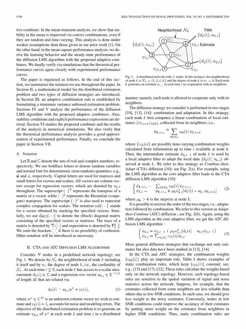
Consider nodes in a predefined network topology; seeFig. 1. We denote by the neighborhood of node including
itself and by the degree of node , i.e., the cardinality of. At each time , each node has access to a scalar mea-
surement and a regression row vectorof length that are related via
(1)
where is an unknown column vector we wish to esti-mate and accounts for noise and modeling errors. Theobjective of the distributed estimation problem is to generate anestimate of at each node and time in a distributed
Fig. 1. A distributed network with � nodes. In this instance, the neighborhoodof node � is � � ��� �� �� �� and the degree of node � is � � �. Each node� generates an estimate � at each time � in cooperation with its neighbors.
manner; namely, each node is allowed to cooperate only with itsneighbors.
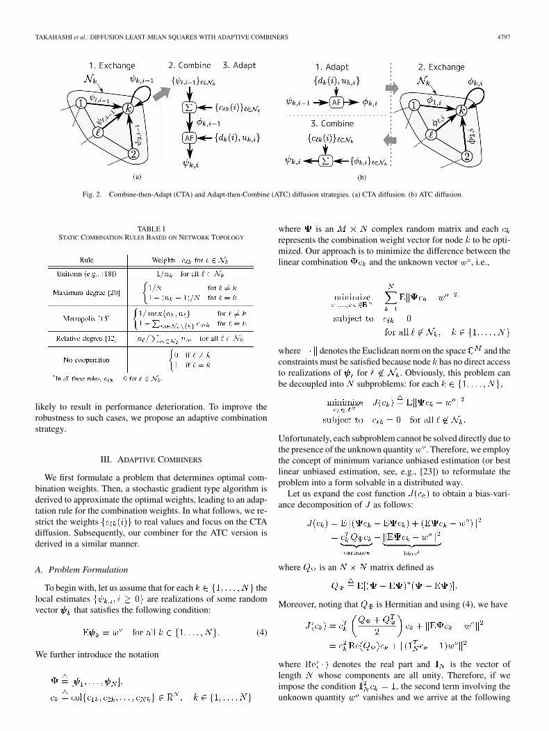
The diffusion strategy we consider is performed in two stages[10], [13], [14]: combination and adaptation. In this strategy,each node first computes a linear combination of local esti-mates collected from its neighbors, i.e.,
where are possibly time-varying combination weightscalculated from information up to time available at node .Then, the intermediate estimate of node is used bya local adaptive filter to adapt the local data ob-served at node . We refer to this strategy as Combine-then-Adapt (CTA) diffusion [10]; see Fig. 2(a). For example, usingthe LMS algorithm as the core adaptive filter leads to the CTAdiffusion LMS algorithm [10]:
(2)
where is the stepsize at node .It is possible to reverse the order of the two stages, i.e., adapta-
tion followed by combination. We refer to this version as Adapt-then-Combine (ATC) diffusion ; see Fig. 2(b). Again, using theLMS algorithm as the core adaptive filter, we get the ATC dif-fusion LMS algorithm :
(3)
More general diffusion strategies that exchange not only esti-mates but also data have been studied in [13], [14].
In the CTA and ATC strategies, the combination weightsplay an important role. Table I shows examples of
static combination rules, which keep constant; see,e.g., [15] and [17]–[22]. These rules calculate the weights basedonly on the network topology. However, such topology-basedrules are sensitive to the spatial variation of signal and noisestatistics across the network. Suppose, for example, that theestimates collected from some neighbors are less reliable thanothers due to low SNR conditions. In such case, we should giveless weight to the noisy estimates. Conversely, nodes in lowSNR conditions could improve the accuracy of their estimatesby putting more weight on the estimates from neighbors inhigher SNR conditions. Thus, static combination rules are
TAKAHASHI et al.: DIFFUSION LEAST-MEAN SQUARES WITH ADAPTIVE COMBINERS 4797
Fig. 2. Combine-then-Adapt (CTA) and Adapt-then-Combine (ATC) diffusion strategies. (a) CTA diffusion. (b) ATC diffusion.
TABLE ISTATIC COMBINATION RULES BASED ON NETWORK TOPOLOGY
likely to result in performance deterioration. To improve therobustness to such cases, we propose an adaptive combinationstrategy.
III. ADAPTIVE COMBINERS
We first formulate a problem that determines optimal com-bination weights. Then, a stochastic gradient type algorithm isderived to approximate the optimal weights, leading to an adap-tation rule for the combination weights. In what follows, we re-strict the weights to real values and focus on the CTAdiffusion. Subsequently, our combiner for the ATC version isderived in a similar manner.
A. Problem Formulation
To begin with, let us assume that for each thelocal estimates are realizations of some randomvector that satisfies the following condition:
(4)
We further introduce the notation
where is an complex random matrix and eachrepresents the combination weight vector for node to be opti-mized. Our approach is to minimize the difference between thelinear combination and the unknown vector , i.e.,
where denotes the Euclidean norm on the space and theconstraints must be satisfied because node has no direct accessto realizations of for . Obviously, this problem canbe decoupled into subproblems: for each ,
Unfortunately, each subproblem cannot be solved directly due tothe presence of the unknown quantity . Therefore, we employthe concept of minimum variance unbiased estimation (or bestlinear unbiased estimation, see, e.g., [23]) to reformulate theproblem into a form solvable in a distributed way.
Let us expand the cost function to obtain a bias-vari-ance decomposition of as follows:
where is an matrix defined as
Moreover, noting that is Hermitian and using (4), we have
where denotes the real part and is the vector oflength whose components are all unity. Therefore, if weimpose the condition , the second term involving theunknown quantity vanishes and we arrive at the following
4798 IEEE TRANSACTIONS ON SIGNAL PROCESSING, VOL. 58, NO. 9, SEPTEMBER 2010
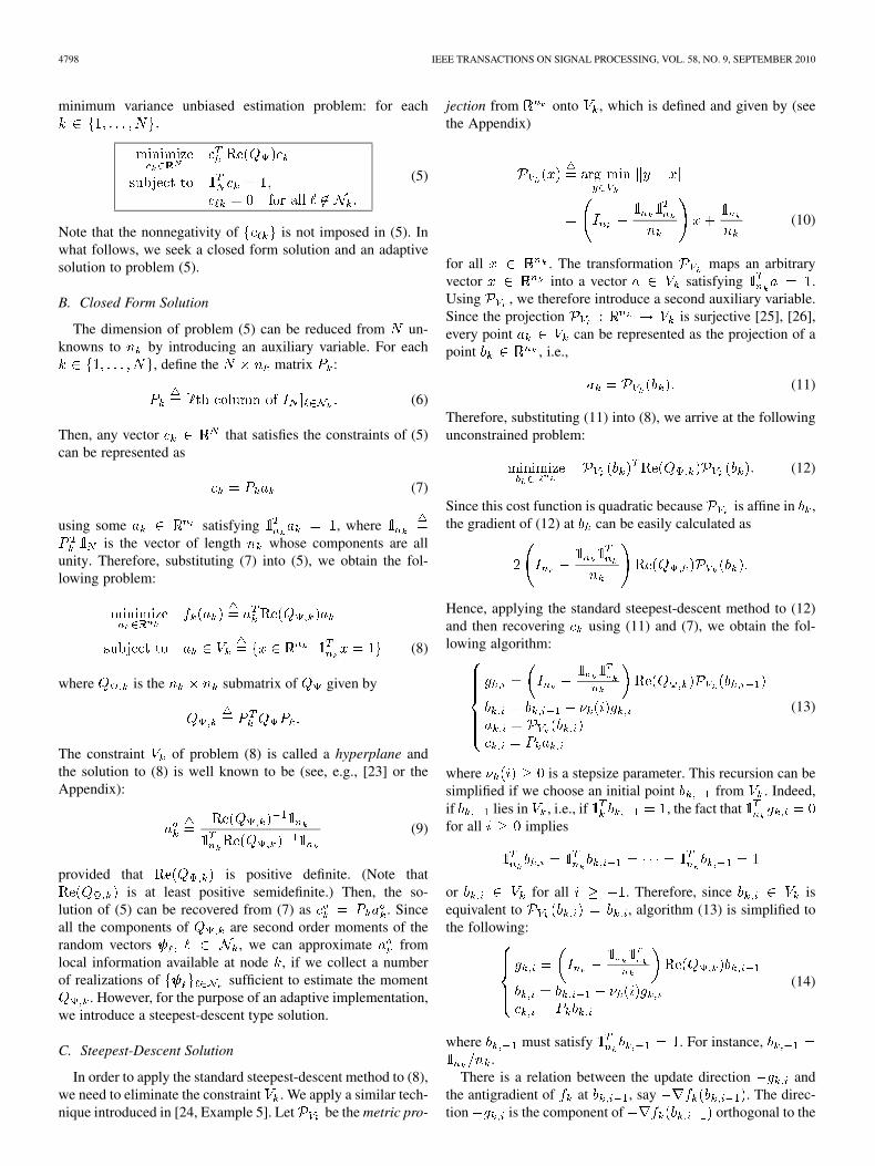
minimum variance unbiased estimation problem: for each
(5)
Note that the nonnegativity of is not imposed in (5). Inwhat follows, we seek a closed form solution and an adaptivesolution to problem (5).
B. Closed Form Solution
The dimension of problem (5) can be reduced from un-knowns to by introducing an auxiliary variable. For each
, define the matrix :
(6)
Then, any vector that satisfies the constraints of (5)can be represented as
(7)
using some satisfying , whereis the vector of length whose components are all
unity. Therefore, substituting (7) into (5), we obtain the fol-lowing problem:
(8)
where is the submatrix of given by
The constraint of problem (8) is called a hyperplane andthe solution to (8) is well known to be (see, e.g., [23] or theAppendix):
(9)
provided that is positive definite. (Note thatis at least positive semidefinite.) Then, the so-
lution of (5) can be recovered from (7) as . Sinceall the components of are second order moments of therandom vectors , we can approximate fromlocal information available at node , if we collect a numberof realizations of sufficient to estimate the moment
. However, for the purpose of an adaptive implementation,we introduce a steepest-descent type solution.
C. Steepest-Descent Solution
In order to apply the standard steepest-descent method to (8),we need to eliminate the constraint . We apply a similar tech-nique introduced in [24, Example 5]. Let be the metric pro-
jection from onto , which is defined and given by (seethe Appendix)
(10)
for all . The transformation maps an arbitraryvector into a vector satisfying .Using , we therefore introduce a second auxiliary variable.Since the projection is surjective [25], [26],every point can be represented as the projection of apoint , i.e.,
(11)
Therefore, substituting (11) into (8), we arrive at the followingunconstrained problem:
(12)
Since this cost function is quadratic because is affine in ,the gradient of (12) at can be easily calculated as
Hence, applying the standard steepest-descent method to (12)and then recovering using (11) and (7), we obtain the fol-lowing algorithm:
(13)
where is a stepsize parameter. This recursion can besimplified if we choose an initial point from . Indeed,if lies in , i.e., if , the fact thatfor all implies
or for all . Therefore, since isequivalent to , algorithm (13) is simplified tothe following:
(14)
where must satisfy . For instance,.
There is a relation between the update direction andthe antigradient of at , say . The direc-tion is the component of orthogonal to the
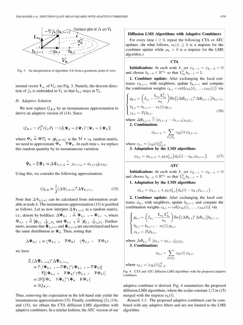
TAKAHASHI et al.: DIFFUSION LEAST-MEAN SQUARES WITH ADAPTIVE COMBINERS 4799
Fig. 3. An interpretation of algorithm (14) from a geometric point of view.
normal vector of ; see Fig. 3. Namely, the descent direc-tion of is embedded in so that stays in .
D. Adaptive Solution
We now replace by an instantaneous approximation toderive an adaptive version of (14). Since
where is the random matrix,we need to approximate . At each time , we replacethis random quantity by its instantaneous variation:
Using this, we consider the following approximation:
(15)
Note that can be calculated from information avail-able at node . The instantaneous approximation (15) is justifiedas follows. Let us now interpret as a random matrix,
i.e., denote by boldface: , where
and . Further-more, assume that and are uncorrelated and havethe same distribution as . Then, noting that
we have
Thus, removing the expectation in the left-hand side yields theinstantaneous approximation (15). Finally, combining (2), (14),and (15), we obtain the CTA diffusion LMS algorithm withadaptive combiners. In a similar fashion, the ATC version of our
Fig. 4. CTA and ATC diffusion LMS algorithms with the proposed adaptivecombiners.
adaptive combiner is derived. Fig. 4 summarizes the proposeddiffusion LMS algorithms, where the scalar constant in (15)merged with the stepsize .
Remark 3.1: The proposed adaptive combiners can be com-bined with any adaptive filters and are not limited to the LMSalgorithm.
4800 IEEE TRANSACTIONS ON SIGNAL PROCESSING, VOL. 58, NO. 9, SEPTEMBER 2010
E. Normalized Stepsize Rule
As we will see in the next section, the stability of the CTAdiffusion LMS algorithm is ensured in the mean sense if weuse convex combination weights for . Since algo-rithm (16) (see Fig. 4) guarantees , the weight vector
becomes convex combination if for all. A possible choice for that enforces
is the following:
(18)
where and are constants, denotes themaximum norm, and is the th component of . Itis easily verified from (18) and the second line of (14) that theweight vector enforces a convex combination for all ,provided that the initial vector is a convex combination.Hence, is ensured to be a convex combination aswell.
Remark 3.2: As used in [8], [16], another possible way to en-sure the nonnegativity of each weight is to introduce a param-eterization of the form , whereis any real number. Such a parameterization is useful to guar-antee convex combination of two estimates because any weights
of the form
become convex combination. However, if we consider convexcombination of more than two estimates, that parameterizationis not generally useful because it is as difficult to handle the con-straint . Moreover, the cost func-tion in (8) becomes nonlinear due to the introduction of
.
IV. MEAN TRANSIENT ANALYSIS
In this section, the mean transient analysis of the CTA dif-fusion LMS algorithm with any adaptive combiners, includingthe proposed combiner in Fig. 4, is presented. The goal of thissection is to find sufficient conditions under which every localestimate converges in the mean to the unknown parameter byextending the techniques of [10] to the challenging case wherethe combination weights are adaptive (i.e., time-variant) as op-posed to static. To begin with, let us introduce a mathematicaltool for the analysis.
A. Block Maximum Norm
Given a vector consistingof blocks , we define the blockmaximum norm on by
where denotes the standard Euclidean norm on asbefore. We also define the matrix norm induced from the blockmaximum norm. Namely, given an matrix , itsinduced norm is defined as
This kind of norms is useful for the analysis of diffusion typealgorithms; see for example [27] and [26]. The block maximumnorm inherits the unitary invariance of the Euclidean normunder block-wise transformation.
Lemma 4.1: Let be anblock unitary matrix with unitary blocks
. Then, the following hold:a) for all ;b) for all .
Proof: Property a) immediately follows from the fact thatfor every . On the other hand, property b)
immediately follows from a).
B. Mean Convergence Analysis
Let us now interpret the data as random variables. Recall thatrandom variables are denoted by boldface letters, e.g., . Toconstruct a data model in terms of global quantities, we intro-duce the following global quantities across the network:
. . .
Note that is the block diagonal matrix with diag-onal blocks . Then, data model (1) canbe written as
Here, we assume the following throughout our analysis:Assumption 4.2 (Data model):a) The regressors are i.i.d. in time and spatially inde-
pendent, with .b) The noise is i.i.d. zero-mean in time and spatially
independent, with . In addition, isindependent of the regressors .
Although the independence of regressors might be unrealisticin practice, such assumptions are employed frequently in theanalysis of adaptive algorithms and lead to a close agreementbetween theory and experiments; see, for example, [10], [28],and references therein.
We next derive the state space model of the CTA diffusionLMS algorithm with adaptive combiners. Let beany real random combination weights of node at time thatsatisfy for and . We
TAKAHASHI et al.: DIFFUSION LEAST-MEAN SQUARES WITH ADAPTIVE COMBINERS 4801
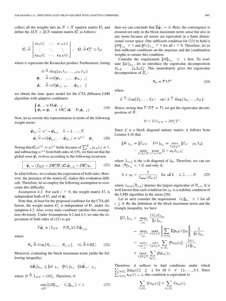
collect all the weights into an random matrix anddefine the random matrix as follows:
.... . .
...
where represents the Kronecker product. Furthermore, letting
we obtain the state space model for the CTA diffusion LMSalgorithm with adaptive combiners:
(19)
Now, let us rewrite this representation in terms of the followingweight errors:
(20)
Noting that holds because of ,and subtracting from both sides of (19), we find out that theglobal error evolves according to the following recursion:
(21)
In what follows, we evaluate the expectation of both sides. How-ever, the presence of the matrix makes this evaluation diffi-cult. Therefore, let us employ the following assumption to over-come this difficulty:
Assumption 4.3: For each , the weight matrix isindependent both of and of .
Note that, at least for the proposed combiner for the CTA dif-fusion, the weight matrix is independent of under As-sumption 4.2. Also, every static combiner satisfies this assump-tion obviously. Under Assumptions 4.2 and 4.3, we take the ex-pectation of both sides of (21) to get
where
(22)
Moreover, evaluating the block maximum norm yields the fol-lowing inequality:
where . Therefore, if
(23)
then we can conclude that . Here, the convergence isensured not only in the block maximum norm sense but also inany norm because all norms are equivalent in a finite dimen-sional vector space. One sufficient condition for (23) to hold is
and for all . Therefore, let usfind sufficient conditions on the stepsizes and the combinationweights to ensure this condition.
Consider the requirement first. To eval-uate , let us introduce the eigenvalue decomposition
. This immediately gives the eigenvaluedecomposition of :
(24)
where
Hence, noting that , we get the eigenvalue decom-position of :
Since is a block diagonal unitary matrix, it follows fromLemma 4.1b that
where is the th diagonal of . Therefore, we can seethat if, and only if,
(25)
where denotes the largest eigenvalue of . It iswell known that each condition for is a stability condition ofthe LMS algorithm in the mean [28].
Let us next consider the requirement for all. By the definition of the block maximum norm and the
triangle inequality, we have
Therefore, it suffices to find conditions under whichfor all . Since
, this condition is equivalent to
4802 IEEE TRANSACTIONS ON SIGNAL PROCESSING, VOL. 58, NO. 9, SEPTEMBER 2010
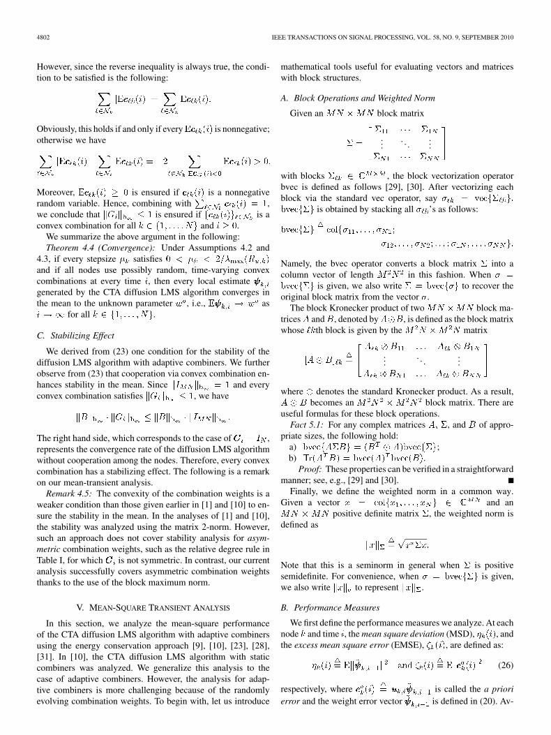
However, since the reverse inequality is always true, the condi-tion to be satisfied is the following:
Obviously, this holds if and only if every is nonnegative;otherwise we have
Moreover, is ensured if is a nonnegativerandom variable. Hence, combining with ,we conclude that is ensured if is aconvex combination for all and .
We summarize the above argument in the following:Theorem 4.4 (Convergence): Under Assumptions 4.2 and
4.3, if every stepsize satisfiesand if all nodes use possibly random, time-varying convexcombinations at every time , then every local estimategenerated by the CTA diffusion LMS algorithm converges inthe mean to the unknown parameter , i.e., as
for all .
C. Stabilizing Effect
We derived from (23) one condition for the stability of thediffusion LMS algorithm with adaptive combiners. We furtherobserve from (23) that cooperation via convex combination en-hances stability in the mean. Since and everyconvex combination satisfies , we have
The right hand side, which corresponds to the case of ,represents the convergence rate of the diffusion LMS algorithmwithout cooperation among the nodes. Therefore, every convexcombination has a stabilizing effect. The following is a remarkon our mean-transient analysis.
Remark 4.5: The convexity of the combination weights is aweaker condition than those given earlier in [1] and [10] to en-sure the stability in the mean. In the analyses of [1] and [10],the stability was analyzed using the matrix 2-norm. However,such an approach does not cover stability analysis for asym-metric combination weights, such as the relative degree rule inTable I, for which is not symmetric. In contrast, our currentanalysis successfully covers asymmetric combination weightsthanks to the use of the block maximum norm.
V. MEAN-SQUARE TRANSIENT ANALYSIS
In this section, we analyze the mean-square performanceof the CTA diffusion LMS algorithm with adaptive combinersusing the energy conservation approach [9], [10], [23], [28],[31]. In [10], the CTA diffusion LMS algorithm with staticcombiners was analyzed. We generalize this analysis to thecase of adaptive combiners. However, the analysis for adap-tive combiners is more challenging because of the randomlyevolving combination weights. To begin with, let us introduce
mathematical tools useful for evaluating vectors and matriceswith block structures.
A. Block Operations and Weighted Norm
Given an block matrix
.... . .
...
with blocks , the block vectorization operatorbvec is defined as follows [29], [30]. After vectorizing eachblock via the standard vec operator, say
is obtained by stacking all ’s as follows:
Namely, the bvec operator converts a block matrix into acolumn vector of length in this fashion. When
is given, we also write to recover theoriginal block matrix from the vector .
The block Kronecker product of two block ma-trices and , denoted by , is defined as the block matrixwhose th block is given by the matrix
.... . .
...
where denotes the standard Kronecker product. As a result,becomes an block matrix. There are
useful formulas for these block operations.Fact 5.1: For any complex matrices , and of appro-
priate sizes, the following hold:a) ;b) .
Proof: These properties can be verified in a straightforwardmanner; see, e.g., [29] and [30].
Finally, we define the weighted norm in a common way.Given a vector and an
positive definite matrix , the weighted norm isdefined as
Note that this is a seminorm in general when is positivesemidefinite. For convenience, when is given,we also write to represent .
B. Performance Measures
We first define the performance measures we analyze. At eachnode and time , the mean square deviation (MSD), , andthe excess mean square error (EMSE), , are defined as:
(26)
respectively, where is called the a priorierror and the weight error vector is defined in (20). Av-
TAKAHASHI et al.: DIFFUSION LEAST-MEAN SQUARES WITH ADAPTIVE COMBINERS 4803
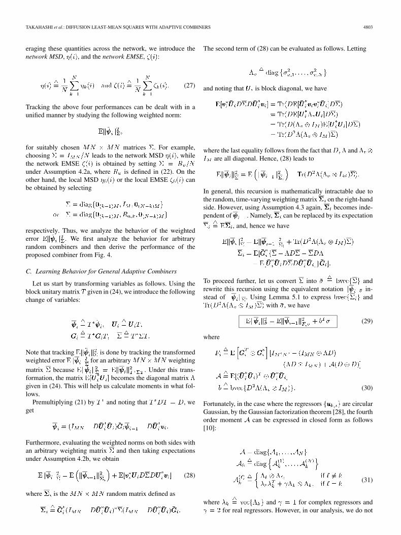
eraging these quantities across the network, we introduce thenetwork MSD, , and the network EMSE, :
(27)
Tracking the above four performances can be dealt with in aunified manner by studying the following weighted norm:
for suitably chosen matrices . For example,choosing leads to the network MSD , whilethe network EMSE is obtained by settingunder Assumption 4.2a, where is defined in (22). On theother hand, the local MSD or the local EMSE canbe obtained by selecting
respectively. Thus, we analyze the behavior of the weightederror . We first analyze the behavior for arbitraryrandom combiners and then derive the performance of theproposed combiner from Fig. 4.
C. Learning Behavior for General Adaptive Combiners
Let us start by transforming variables as follows. Using theblock unitary matrix given in (24), we introduce the followingchange of variables:
Note that tracking is done by tracking the transformedweighted error for an arbitrary weighting
matrix because . Under this trans-formation, the matrix becomes the diagonal matrixgiven in (24). This will help us calculate moments in what fol-lows.
Premultiplying (21) by and noting that , weget
Furthermore, evaluating the weighted norms on both sides withan arbitrary weighting matrix and then taking expectationsunder Assumption 4.2b, we obtain
(28)
where is the random matrix defined as
The second term of (28) can be evaluated as follows. Letting
and noting that is block diagonal, we have
where the last equality follows from the fact that andare all diagonal. Hence, (28) leads to
In general, this recursion is mathematically intractable due tothe random, time-varying weighting matrix on the right-handside. However, using Assumption 4.3 again, becomes inde-pendent of . Namely, can be replaced by its expectation
, and, hence we have
To proceed further, let us convert into andrewrite this recursion using the equivalent notation in-stead of . Using Lemma 5.1 to express and
with , we have
(29)
where
(30)
Fortunately, in the case where the regressors are circularGaussian, by the Gaussian factorization theorem [28], the fourthorder moment can be expressed in closed form as follows[10]:
(31)
where and for complex regressors andfor real regressors. However, in our analysis, we do not
4804 IEEE TRANSACTIONS ON SIGNAL PROCESSING, VOL. 58, NO. 9, SEPTEMBER 2010
assume that are circular Gaussian but just assume thatis known.
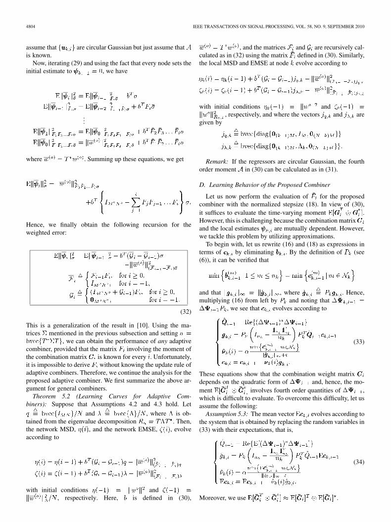
Now, iterating (29) and using the fact that every node sets theinitial estimate to , we have
...
where . Summing up these equations, we get
Hence, we finally obtain the following recursion for theweighted error:
,
(32)
This is a generalization of the result in [10]. Using the ma-trices mentioned in the previous subsection and setting
, we can obtain the performance of any adaptivecombiner, provided that the matrix involving the moment ofthe combination matrix is known for every . Unfortunately,it is impossible to derive without knowing the update rule ofadaptive combiners. Therefore, we continue the analysis for theproposed adaptive combiner. We first summarize the above ar-gument for general combiners.
Theorem 5.2 (Learning Curves for Adaptive Com-biners): Suppose that Assumptions 4.2 and 4.3 hold. Let
and , where is ob-tained from the eigenvalue decomposition . Then,the network MSD, , and the network EMSE, , evolveaccording to
with initial conditions and, respectively. Here, is defined in (30),
, and the matrices and are recursively cal-culated as in (32) using the matrix defined in (30). Similarly,the local MSD and EMSE at node evolve according to
with initial conditions and, respectively, and where the vectors and are
given by
Remark: If the regressors are circular Gaussian, the fourthorder moment in (30) can be calculated as in (31).
D. Learning Behavior of the Proposed Combiner
Let us now perform the evaluation of for the proposedcombiner with the normalized stepsize (18). In view of (30),it suffices to evaluate the time-varying moment .However, this is challenging because the combination matrixand the local estimates are mutually dependent. However,we tackle this problem by utilizing approximations.
To begin with, let us rewrite (16) and (18) as expressions interms of by eliminating . By the definition of (see(6)), it can be verified that
and that , where . Hence,multiplying (16) from left by and noting that
, we see that evolves according to
(33)
These equations show that the combination weight matrixdepends on the quadratic form of and, hence, the mo-ment involves fourth order quantities of ,which is difficult to evaluate. To overcome this difficulty, let usassume the following:
Assumption 5.3: The mean vector evolves according tothe system that is obtained by replacing the random variables in(33) with their expectations, that is,
(34)
Moreover, we use .
TAKAHASHI et al.: DIFFUSION LEAST-MEAN SQUARES WITH ADAPTIVE COMBINERS 4805
Although this assumption is unrealistic, is guaranteedto satisfy at least the constraints andfor . Since can be calculated by
(35)
the remaining task is to calculate the moment . To calculatethe th component of , which is given by
we employ the following assumption:Assumption 5.4: For each time , the a priori error
is spatially independent and independent of the re-gressor . Furthermore, we use the approximation
.The independence between and is a common as-
sumption in the analysis of adaptive filters [28], [31]. Now, byusing the approximation , it follows from (17)that
where the second equality follows from the data model. This gives, under Assumption 5.4,
that
Also, the spatial independence of the regressors yields
for . Therefore, can be approximated by
(36)
Combining this approximation and Theorem 5.2, we can trackthe mean-square performance of the CTA diffusion LMS withthe proposed combiners. The following is the summary of theperformance evaluation for the proposed combiner:
Theorem 5.5 (Learning Curves for the Proposed Combiner):Under Assumptions 4.2, 4.3, 5.3 and 5.4, the mean-squareperformance of the CTA diffusion LMS algorithm with theproposed combiner can be evaluated as follows. For each
, initialize as in Theorem 5.2 and set, where is the initial combination weight
vector. Then, repeat the following for every :1) calculate via (36);2) for each , update via (34);3) calculate via (35) to approximate in (30) by
4) use to update and in Theorem 5.2 and then updateevery local EMSE and the other performances.
E. Steady-State Mean-Square Performance
Let us now evaluate the steady-state MSD and EMSE, whichare defined as the limits of and , respectively. One pos-sible way is to calculate and iteratively according toTheorem 5.5 until they converge. However, this may take a longtime and does not clarify the relation between the parametersand the steady-state performance. Thus, we seek closed formexpressions for the steady-state performance.
Now, let us return to (29). In view of this, if the matrix canbe approximated by some constant matrix , then we wouldhave
Evaluating this equation at the limit, we get
or
Hence, replacing the free parameter by , weget
(37)
This provides the steady-state mean-square performance bychoosing as before. Therefore, let us find a good approxima-tion for .
Recall that the time-dependent factor of is . Weapproximate this by using defined in (36). In view of (36),if every local EMSE is sufficiently small, then by ignoring
we have a reasonable approximation. Namely, we assume that
for sufficiently large . Moreover, comparing (34) with the orig-inal algorithm (14) and the optimal solution (9), we assume that
converges to
(38)
Finally, letting
and approximating by , weobtain the following approximation:
(39)
The use of this approximation with (37) leads to the followingresult.
4806 IEEE TRANSACTIONS ON SIGNAL PROCESSING, VOL. 58, NO. 9, SEPTEMBER 2010
Theorem 5.7 (Steady-State Mean-Square Performance):Suppose that converges to defined in (38) and thematrix defined in (39) is such that is nonsingular.Then, the steady-state network MSD, , and the steady-statenetwork EMSE, , are approximately given as follows:
where and are defined as in Theorem 5.2. Similarly, thesteady-state MSD, , and the steady-state EMSE, , of node
are approximately given as follows:
where and are also defined as in Theorem 5.2.Remark 5.7: Although we focused on the analysis of CTA
diffusion, the analysis of ATC version can be done in a similarway. In [14], performance analysis of more general CTA andATC diffusion LMS algorithms equipped with static combinershas been done.
VI. SIMULATION RESULTS
In this section, we show the performance of the proposedadaptive combiner and compare our performance analysis withexperiments.
A. Performance Comparison
We consider two simulation scenarios, say Examples 1 and 2,over different network topologies. In both examples, we com-pare the CTA and ATC diffusion LMS algorithms with the fol-lowing combiners: i) the proposed adaptive combiner, ii) thestatic combiners shown in Table I, and iii) the adaptive com-biner based on convex combination of two adaptive filters (seefor details [8]). We also compare these diffusion algorithms withthe incremental LMS algorithm, which cycles estimates along apredefined cyclic path (see [9] for details).
In Example 1, we consider a network topology withnodes shown in Fig. 5. The unknown vector is set to
. Both the regressors and the noise are zero-mean Gaussian, i.i.d. in time and independent in space. Theirstatistics are shown in Fig. 5. The stepsize of the LMS algo-rithm used at each node is set to , except for the in-cremental LMS algorithm. For the incremental LMS algorithm,the stepsize is set to because the incrementalLMS algorithm uses the LMS-type iterations times for every
[9]. For the proposed combiner, is set to forevery and the normalized stepsize rule (18) with and
is used.Fig. 6(a) and (b) shows the learning behavior of each algo-
rithm in terms of the network MSD, which is defined in (27).The expectation is calculated by averaging 200 independent ex-periments. We observe that the proposed algorithm outperformsthe other algorithms at the steady-state, although the conver-gence speed is a little slower than the others. On the other hand,Fig. 6(c) and (d) shows the steady-state MSD at each node,which is obtained by averaging the last 100 samples after a suf-ficient number of iterations. From Fig. 6, we find out that theATC diffusion LMS algorithms outperform the CTA versions.
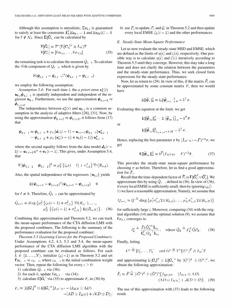
Fig. 5. Network settings for Example 1: topology with � � �� nodes and 35links (top), regressor statistics (bottom left) and noise variances (bottom right).In the incremental LMS algorithm, we used the following cyclic path: �� ��
�� �� �� �� ��� ��� ��� ��� ��� � � ��� ��
�.
Fig. 6. Performance results for Example 1. (a) and (b): Learning curves of net-work MSD. (c) and (d): Steady-state MSD. (a) CTA; (b) ATC; (c) CTA; and (d)ATC.
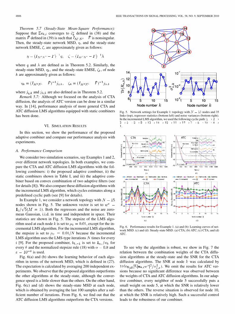
To see why the algorithm is robust, we show in Fig. 7 therelation between the combination weights of the CTA diffu-sion algorithms at the steady-state and the SNR for the CTAdiffusion algorithms. The SNR at node was calculated by
. We omit the results for ATC ver-sions because no significant difference was observed betweenthe weights of CTA and ATC diffusion algorithms. In our adap-tive combiner, every neighbor of node 5 successfully puts asmall weight on node 5, at which the SNR is relatively lowerthan the others. The reverse situation is observed for node 10,at which the SNR is relatively high. Such a successful controlleads to the robustness of our combiner.
TAKAHASHI et al.: DIFFUSION LEAST-MEAN SQUARES WITH ADAPTIVE COMBINERS 4807
Fig. 7. Combination weights � ��� and � ��� of the CTA diffusion algo-rithms at steady-state in Example 1. The result for the ATC versions is omittedbecause almost the same results were observed.
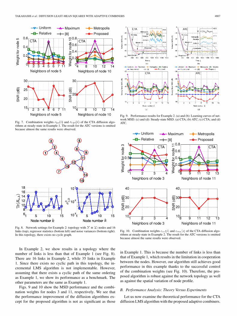
Fig. 8. Network settings for Example 2: topology with � � �� nodes and 16links (top), regressor statistics (bottom left) and noise variances (bottom right).In this topology, there exists no cycle graph.
In Example 2, we show results in a topology where thenumber of links is less than that of Example 1 (see Fig. 8).There are 16 links in Example 2, while 35 links in Example1. Since there exists no cyclic path in this topology, the in-cremental LMS algorithm is not implementable. However,assuming that there exists a cyclic path of the same orderingas Example 1, we show its performance as a benchmark. Theother parameters are the same as Example 1.
Figs. 9 and 10 show the MSD performance and the combi-nation weights for nodes 3 and 11, respectively. We see thatthe performance improvement of the diffusion algorithms ex-cept for the proposed algorithm is not as significant as those
Fig. 9. Performance results for Example 2. (a) and (b): Learning curves of net-work MSD. (c) and (d): Steady-state MSD. (a) CTA; (b) ATC; (c) CTA; and (d)ATC.
Fig. 10. Combination weights � ��� and � ��� of the CTA diffusion algo-rithms at steady-state in Example 2. The result for the ATC versions is omittedbecause almost the same results were observed.
in Example 1. This is because the number of links is less thanthat of Example 1, which results in the limitation in cooperationbetween the nodes. However, our algorithm still achieves goodperformance in this example thanks to the successful controlof the combination weights (see Fig. 10). Therefore, the pro-posed algorithm is robust against the network topology as wellas against the spatial variation of node profile.
B. Performance Analysis: Theory Versus Experiments
Let us now examine the theoretical performance for the CTAdiffusion LMS algorithm with the proposed adaptive combiners.
4808 IEEE TRANSACTIONS ON SIGNAL PROCESSING, VOL. 58, NO. 9, SEPTEMBER 2010
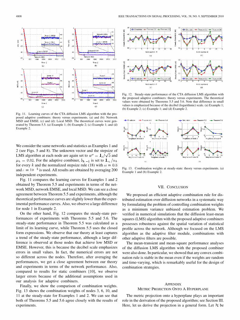
Fig. 11. Learning curves of the CTA diffusion LMS algorithm with the pro-posed adaptive combiners: theory versus experiments. (a) and (b): NetworkMSD and EMSE. (c) and (d): Local MSD. The theoretical curves were gen-erated by Theorem 5.5. (a) Example 1; (b) Example 2; (c) Example 1; and (d)Example 2.
We consider the same networks and statistics as Examples 1 and2 (see Figs. 5 and 8). The unknown vector and the stepsize ofLMS algorithm at each node are again set to and
. For the adaptive combiner, is set tofor every and the normalized stepsize rule (18) withand is used. All results are obtained by averaging 200independent experiments.
Fig. 11 compares the learning curves for Examples 1 and 2obtained by Theorem 5.5 and experiments in terms of the net-work MSD, network EMSE, and local MSD. We can see a closeagreement between Theorem 5.5 and experiments, although thetheoretical performance curves are slightly lower than the exper-imental performance curves. Also, we observe a large differencefor node 1 in Example 2.
On the other hand, Fig. 12 compares the steady-state per-formances of experiments with Theorems 5.5 and 5.6. Thesteady-state performance in Theorem 5.5 was calculated as alimit of its learning curve, while Theorem 5.5 uses the closedform expressions. We observe that our theory at least capturesa trend of the steady-state performance, although a large dif-ference is observed at those nodes that achieve low MSD orEMSE. However, this is because the decibel scale emphasizeserrors in small values. In fact, the numerical errors are notso different across the nodes. Therefore, after averaging theperformances, we get a close agreement between our theoryand experiments in terms of the network performance. Also,compared to results for static combiners [10], we observelarger errors because of the additional assumptions used inour analysis for adaptive combiners.
Finally, we show the comparison of combination weights.Fig. 13 shows the combination weights of nodes 3, 6, 10, and11 at the steady-state for Examples 1 and 2. We can see thatboth of Theorems 5.5 and 5.6 agree closely with the results ofexperiments.
Fig. 12. Steady-state performance of the CTA diffusion LMS algorithm withthe proposed adaptive combiners: theory versus experiments. The theoreticalvalues were obtained by Theorems 5.5 and 5.6. Note that difference in smallvalues is emphasized because of the decibel (logarithmic) scale. (a) Example 1;(b) Example 2; (c) Example 1; and (d) Example 2.
Fig. 13. Combination weights at steady-state: theory versus experiments. (a)Example 1 and (b) Example 2.
VII. CONCLUSION
We proposed an efficient adaptive combination rule for dis-tributed estimation over diffusion networks in a systematic wayby formulating the problem of controlling combination weightsas a minimum variance unbiased estimation problem. Weverified in numerical simulations that the diffusion least-meansquares (LMS) algorithm with the proposed adaptive combinerspossesses robustness against the spatial variation of statisticalprofile across the network. Although we focused on the LMSalgorithm as the adaptive filter module, combinations withother adaptive filters are possible.
The mean-transient and mean-square performance analysesof the diffusion LMS algorithm with the proposed combinerwere also done. In particular, we showed that any convex combi-nation rule is stable in the mean even if the weights are randomand time-varying, which is remarkably useful for the design ofcombination strategies.
APPENDIX
METRIC PROJECTION ONTO A HYPERPLANE
The metric projection onto a hyperplane plays an importantrole in the derivation of the proposed algorithm; see Section III.Here, let us derive the projection in a general form. Let be
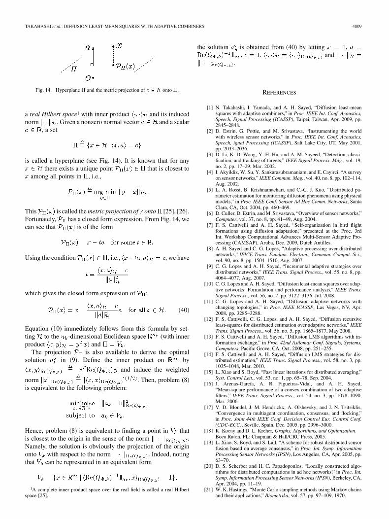
TAKAHASHI et al.: DIFFUSION LEAST-MEAN SQUARES WITH ADAPTIVE COMBINERS 4809
Fig. 14. Hyperplane � and the metric projection of � � � onto �.
a real Hilbert space1 with inner product and its inducednorm . Given a nonzero normal vector and a scalar
, a set
is called a hyperplane (see Fig. 14). It is known that for anythere exists a unique point that is closest to
among all points in , i.e.,
This is called the metric projection of onto [25], [26].Fortunately, has a closed form expression. From Fig. 14, wecan see that is of the form
Using the condition , i.e., , we have
which gives the closed form expression of :
(40)
Equation (10) immediately follows from this formula by set-ting to the -dimensional Euclidean space (with innerproduct ) and .
The projection is also available to derive the optimalsolution in (9). Define the inner product on by
and induce the weighted
norm . Then, problem (8)is equivalent to the following problem:
Hence, problem (8) is equivalent to finding a point in thatis closest to the origin in the sense of the norm .Namely, the solution is obviously the projection of the originonto with respect to the norm . Indeed, notingthat can be represented in an equivalent form
1A complete inner product space over the real field is called a real Hilbertspace [25].
the solution is obtained from (40) by lettingand
.
REFERENCES
[1] N. Takahashi, I. Yamada, and A. H. Sayed, “Diffusion least-meansquares with adaptive combiners,” in Proc. IEEE Int. Conf. Acoustics,Speech, Signal Processing (ICASSP), Taipei, Taiwan, Apr. 2009, pp.2845–2848.
[2] D. Estrin, G. Pottie, and M. Srivastava, “Instrumenting the worldwith wireless sensor networks,” in Proc. IEEE Int. Conf. Acoustics,Speech, ignal Processing (ICASSP), Salt Lake City, UT, May 2001,pp. 2033–2036.
[3] D. Li, K. D. Wong, Y. H. Hu, and A. M. Sayeed, “Detection, classi-fication, and tracking of targets,” IEEE Signal Process. Mag., vol. 19,no. 2, pp. 17–29, Mar. 2002.
[4] I. Akyildiz, W. Su, Y. Sankarasubramaniam, and E. Cayirci, “A surveyon sensor networks,” IEEE Commun. Mag., vol. 40, no. 8, pp. 102–114,Aug. 2002.
[5] L. A. Rossi, B. Krishnamachari, and C.-C. J. Kuo, “Distributed pa-rameter estimation for monitoring diffusion phenomena using physicalmodels,” in Proc. IEEE Conf. Sensor Ad Hoc Comm. Networks, SantaClara, CA, Oct. 2004, pp. 460–469.
[6] D. Culler, D. Estrin, and M. Srivastava, “Overview of sensor networks,”Computer, vol. 37, no. 8, pp. 41–49, Aug. 2004.
[7] F. S. Cattivelli and A. H. Sayed, “Self-organization in bird flightformations using diffusion adaptation,” presented at the Proc. 3rdInt. Workshop Computational Advances Multi-Sensor Adaptive Pro-cessing (CAMSAP), Aruba, Dec. 2009, Dutch Antilles.
[8] A. H. Sayed and C. G. Lopes, “Adaptive processing over distributednetworks,” IEICE Trans. Fundam. Electron., Commun. Comput. Sci.,vol. 90, no. 8, pp. 1504–1510, Aug. 2007.
[9] C. G. Lopes and A. H. Sayed, “Incremental adaptive strategies overdistributed networks,” IEEE Trans. Signal Process., vol. 55, no. 8, pp.4064–4077, Aug. 2007.
[10] C. G. Lopes and A. H. Sayed, “Diffusion least-mean squares over adap-tive networks: Formulation and performance analysis,” IEEE Trans.Signal Process., vol. 56, no. 7, pp. 3122–3136, Jul. 2008.
[11] C. G. Lopes and A. H. Sayed, “Diffusion adaptive networks withchanging topologies,” in Proc. IEEE ICASSP, Las Vegas, NV, Apr.2008, pp. 3285–3288.
[12] F. S. Cattivelli, C. G. Lopes, and A. H. Sayed, “Diffusion recursiveleast-squares for distributed estimation over adaptive networks,” IEEETrans. Signal Process., vol. 56, no. 5, pp. 1865–1877, May 2008.
[13] F. S. Cattivelli and A. H. Sayed, “Diffusion LMS algorithms with in-formation exchange,” in Proc. 42nd Asilomar Conf. Signals, Systems,Computers, Pacific Grove, CA, Oct. 2008, pp. 251–255.
[14] F. S. Cattivelli and A. H. Sayed, “Diffusion LMS strategies for dis-tributed estimation,” IEEE Trans. Signal Process., vol. 58, no. 3, pp.1035–1048, Mar. 2010.
[15] L. Xiao and S. Boyd, “Fast linear iterations for distributed averaging,”Syst. Control Lett., vol. 53, no. 1, pp. 65–78, Sep. 2004.
[16] J. Arenas-García, A. R. Figueiras-Vidal, and A. H. Sayed,“Mean-square performance of a convex combination of two adaptivefilters,” IEEE Trans. Signal Process., vol. 54, no. 3, pp. 1078–1090,Mar. 2006.
[17] V. D. Blondel, J. M. Hendrickx, A. Olshevsky, and J. N. Tsitsiklis,“Convergence in multiagent coordination, consensus, and flocking,”in Proc. Joint 44th IEEE Conf. Decision Control Eur. Control Conf.(CDC-ECC), Seville, Spain, Dec. 2005, pp. 2996–3000.
[18] K. Kocay and D. L. Kreher, Graphs, Algorithms, and Optimization.Boca Raton, FL: Chapman & Hall/CRC Press, 2005.
[19] L. Xiao, S. Boyd, and S. Lall, “A scheme for robust distributed sensorfusion based on average consensus,” in Proc. Int. Symp. InformationProcessing Sensor Networks (IPSN), Los Angeles, CA, Apr. 2005, pp.63–70.
[20] D. S. Scherber and H. C. Papadopoulos, “Locally constructed algo-rithms for distributed computations in ad hoc networks,” in Proc. Int.Symp. Information Processing Sensor Networks (IPSN), Berkeley, CA,Apr. 2004, pp. 11–19.
[21] W. K. Hastings, “Monte Carlo sampling methods using Markov chainsand their applications,” Biometrika, vol. 57, pp. 97–109, 1970.
4810 IEEE TRANSACTIONS ON SIGNAL PROCESSING, VOL. 58, NO. 9, SEPTEMBER 2010
[22] N. Metropolis, A. W. Rosenbluth, M. N. Rosenbluth, A. H. Teller, andE. Teller, “Equation of state calculations by fast computing machines,”J. Chem. Phys., vol. 21, no. 6, pp. 1087–1092, Jun. 1953.
[23] A. H. Sayed, Adaptive Filters. New York: Wiley, 2008.[24] I. Yamada and N. Ogura, “Adaptive projected subgradient method
for asymptotic minimization of sequence of nonnegative convexfunctions,” Numer. Funct. Anal. Optim., vol. 25, no. 7, pp. 593–617,Jan. 2004.
[25] D. G. Luenberger, Optimization by Vector Space Methods. NewYork: Wiley-Interscience, 1969.
[26] D. P. Bertsekas and J. N. Tsitsiklis, Parallel and Distributed Computa-tion: Numerical Methods, 1st ed. Singapore: Athena Scientific, Jan.1997.
[27] N. Takahashi and I. Yamada, “Parallel algorithms for variational in-equalities over the cartesian product of the intersections of the fixedpoint sets of nonexpansive mappings,” J. Approx. Theory, vol. 153, no.2, pp. 139–160, Aug. 2008.
[28] A. H. Sayed, Fundamentals of Adaptive Filtering. New York: Wiley-IEEE Press, 2003.
[29] D. S. Tracy and R. P. Singh, “A new matrix product and its applicationsin partitioned matrix differentiation,” Statistica Neerlandica, vol. 26,no. 4, pp. 143–157, 1972.
[30] R. H. Koning, H. Neudecker, and T. Wansbeek, “Block Kroneckerproducts and the Vecb operator,” Economics Dept., Institute of Eco-nomics Research, Univ. of Groningen, Groningen, The Netherlands,Tech. Rep. 351, 1990.
[31] T. Y. Al-Naffouri and A. H. Sayed, “Transient analysis of adaptivefilters with error nonlinearities,” IEEE Trans. Signal Process., vol. 51,no. 3, pp. 653–663, Mar. 2003.
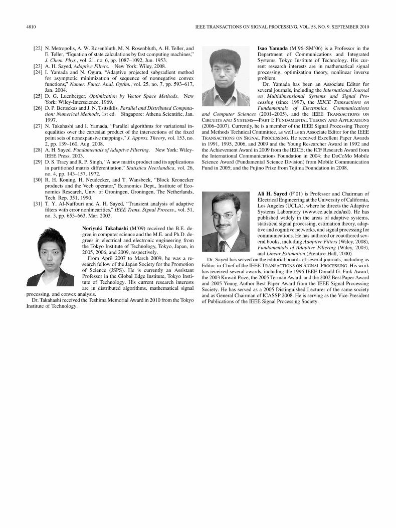
Noriyuki Takahashi (M’09) received the B.E. de-gree in computer science and the M.E. and Ph.D. de-grees in electrical and electronic engineering fromthe Tokyo Institute of Technology, Tokyo, Japan, in2005, 2006, and 2009, respectively.
From April 2007 to March 2009, he was a re-search fellow of the Japan Society for the Promotionof Science (JSPS). He is currently an AssistantProfessor in the Global Edge Institute, Tokyo Insti-tute of Technology. His current research interestsare in distributed algorithms, mathematical signal
processing, and convex analysis.Dr. Takahashi received the Teshima Memorial Award in 2010 from the Tokyo
Institute of Technology.
Isao Yamada (M’96–SM’06) is a Professor in theDepartment of Communications and IntegratedSystems, Tokyo Institute of Technology. His cur-rent research interests are in mathematical signalprocessing, optimization theory, nonlinear inverseproblem.
Dr. Yamada has been an Associate Editor forseveral journals, including the International Journalon Multidimensional Systems and Signal Pro-cessing (since 1997), the IEICE Transactions onFundamentals of Electronics, Communications
and Computer Sciences (2001–2005), and the IEEE TRANSACTIONS ON
CIRCUITS AND SYSTEMS—PART I: FUNDAMENTAL THEORY AND APPLICATIONS
(2006–2007). Currently, he is a member of the IEEE Signal Processing Theoryand Methods Technical Committee, as well as an Associate Editor for the IEEETRANSACTIONS ON SIGNAL PROCESSING. He received Excellent Paper Awardsin 1991, 1995, 2006, and 2009 and the Young Researcher Award in 1992 andthe Achievement Award in 2009 from the IEICE; the ICF Research Award fromthe International Communications Foundation in 2004; the DoCoMo MobileScience Award (Fundamental Science Division) from Mobile CommunicationFund in 2005; and the Fujino Prize from Tejima Foundation in 2008.
Ali H. Sayed (F’01) is Professor and Chairman ofElectrical Engineering at the University of California,Los Angeles (UCLA), where he directs the AdaptiveSystems Laboratory (www.ee.ucla.edu/asl). He haspublished widely in the areas of adaptive systems,statistical signal processing, estimation theory, adap-tive and cognitive networks, and signal processing forcommunications. He has authored or coauthored sev-eral books, including Adaptive Filters (Wiley, 2008),Fundamentals of Adaptive Filtering (Wiley, 2003),and Linear Estimation (Prentice-Hall, 2000).
Dr. Sayed has served on the editorial boards of several journals, including asEditor-in-Chief of the IEEE TRANSACTIONS ON SIGNAL PROCESSING. His workhas received several awards, including the 1996 IEEE Donald G. Fink Award,the 2003 Kuwait Prize, the 2005 Terman Award, and the 2002 Best Paper Awardand 2005 Young Author Best Paper Award from the IEEE Signal ProcessingSociety. He has served as a 2005 Distinguished Lecturer of the same societyand as General Chairman of ICASSP 2008. He is serving as the Vice-Presidentof Publications of the IEEE Signal Processing Society.