The PLS method -- partial least squares projections to latent ...
44
PLS in industrial RPD - for Prague 1 (44) Submitted version, June 2004 The PLS method -- partial least squares projections to latent structures -- and its applications in industrial RDP (research, development, and production). Svante Wold , Research Group for Chemometrics, Institute of Chemistry, Umeå University, S-901 87 Umeå, Sweden Lennart Eriksson Umetrics AB, POB 7960, SE-907 19 Umeå, Sweden Johan Trygg Research Group for Chemometrics, Institute of Chemistry, Umeå University, S-901 87 Umeå, Sweden Nouna Kettaneh Umetrics Inc., 17 Kiel Ave, Kinnelon, NJ 07405, USA Abstract The chemometrics version of PLS was developed around 25 years ago to cope with and utilize the rapidly increasing volumes of data produced in chemical laboratories. Since then, the first simple two-block PLS has been extended to deal with non-linear relationships, drift in processes (adaptive PLS), dynamics, and with the situation with very many variables (hierarchical models). Starting from a few examples of some very complicated problems confronting us in RDP today, PLS and its extensions and generalizations will be discussed. This discussion includes the scalability of methods to increasing size of problems and data, the handling of noise and non-linearities, interpretability of results, and relative simplicity of use.
-
Upload
khangminh22 -
Category
Documents
-
view
4 -
download
0
Transcript of The PLS method -- partial least squares projections to latent ...
PLS in industrial RPD - for Prague 1 (44)
Submitted version, June 2004
The PLS method -- partial least squares projections to latent structures -- and its applications in industrial RDP (research, development, and production). Svante Wold, Research Group for Chemometrics, Institute of Chemistry, Umeå University, S-901 87 Umeå, Sweden Lennart Eriksson Umetrics AB, POB 7960, SE-907 19 Umeå, Sweden Johan Trygg Research Group for Chemometrics, Institute of Chemistry, Umeå University, S-901 87 Umeå, Sweden Nouna Kettaneh Umetrics Inc., 17 Kiel Ave, Kinnelon, NJ 07405, USA Abstract
The chemometrics version of PLS was developed around 25 years ago to cope with and utilize the rapidly increasing volumes of data produced in chemical laboratories. Since then, the first simple two-block PLS has been extended to deal with non-linear relationships, drift in processes (adaptive PLS), dynamics, and with the situation with very many variables (hierarchical models).
Starting from a few examples of some very complicated problems confronting us in RDP today, PLS and its extensions and generalizations will be discussed. This discussion includes the scalability of methods to increasing size of problems and data, the handling of noise and non-linearities, interpretability of results, and relative simplicity of use.

PLS in industrial RPD - for Prague 2 (44)
1. INTRODUCTION 1.1. General considerations Regression by means of projections to latent structures (PLS) is today a widely used chemometric data analytical tool [1-8]. It applies to any regression problem in industrial research, development, and production (RDP), regardless of whether the data set is short/wide or long/lean, or contains linear or non-linear systematic structure, with or without missing data, and possibly are also ordered in two or more blocks across multiple model layers. PLS exists in many different shapes and implementations. The two-block predictive PLS version [1-8] is the most often used form in science and technology. Thise latter is a method for relating two data matrices, X and Y, by a linear multivariate model, but goes beyond traditional regression in that it models also the structure of X and Y. PLS derives its usefulness from its ability to analyze data with many, noisy, collinear, and even incomplete variables in both X and Y. PLS has the desirable property that the precision of the model parameters improves with the increasing number of relevant variables and observations. The regression problem, i.e., how to model one or several dependent variables, responses, Y, by means of a set of predictor variables, X, is one of the most common data-analytical problems in science and technology. Examples in RDP include relating Y = analyte concentration to X = spectral data measured on the chemical samples (Example 1), relating Y = toxicant exposure levels to X = gene expression profiles for rats for the different doses (Example 2), and relating Y = the quality and quantity of manufactured products to X = the conditions of the manufacturing process (Example 3). Traditionally, this modelling of Y by means of X is done using MLR, which works well as long as the X-variables are fairly few and fairly uncorrelated, i.e., X has full rank. With modern measuring instrumentation, including spectrometers, chromatographs, sensor batteries, and bio-analytical platforms, the X-variables tend to be many and also strongly correlated. We shall therefore not call them "independent", but instead "predictors", or just X-variables, because they usually are correlated, noisy, and also incomplete. In handling numerous and collinear X-variables, and response profiles (Y), PLS allows us to investigate more complex problems than before, and analyze available data in a more realistic way. However, some humility and caution is warranted; we are still far from a good understanding of the complications of chemical, biological, and technological systems. Also, quantitative multivariate analysis is still in its infancy, particularly in applications with many variables and few observations (objects, cases). This article reviews PLS as it has developed to become a standard tool in chemometrics and used in industrial RDP. The underlying model and its assumptions are discussed, and commonly used diagnostics are reviewed together with the interpretation of resulting parameters. Three examples are used as illustrations: First, a multivariate calibration data set, second a gene expression profile data set, and third a batch process data set. These data sets are decribed in Section 2. 1.2. Notation We shall employ the common notation where column vectors are denoted by bold lower case characters, e.g., v, and row vectors shown as transposed, e.g. v'. Bold upper

PLS in industrial RPD - for Prague 3 (44)
case characters denote matrices, e.g. X. * multiplication, e.g., A*B ' transpose, e.g., v', X’ a index of components (model dimensions); (a=1,2,...,A) A number of components in a PC or PLS model i index of objects (observations, cases); (i=1,2,...,N) N number of objects (cases, observations) k index of X-variables (k=1,2,...,K) m index of Y-variables (m=1,2,...,M) X matrix of predictor variables, size (N * K) Y matrix of response variables, size (N * M) bm regression coefficient vector of the m.th y. Size (K*1) B matrix of regression coefficients of all Y's. Size (K*M) ca PLS Y-weights of component a. C the (M * A) Y-weight matrix; ca are columns in this matrix. E the (N*K) matrix of X-residuals fm residuals of m.th y-variable; (N*1) vector F the (N*M) matrix of Y-residuals G the number of CV groups (g=1,2, ..,G). pa PLS X-loading vector of component a. P Loading matrix; pa are columns of P. R2 multiple correlation coefficient; amount Y "explained" in terms of SS. RX
2 amount X "explained" in terms of SS. Q2 cross-validated R2; amount Y "predicted". ta X-scores of component a. T score matrix (N*A), where the columns are ta ua Y-scores of component a. U score matrix (N*A), where the columns are ua wa PLS X-weights of component a. W the (K * A) X-weight matrix; wa are columns in this matrix. wa
* PLS weights transformed to be independent between components W* (K * A) matrix of transformed PLS weights; wa
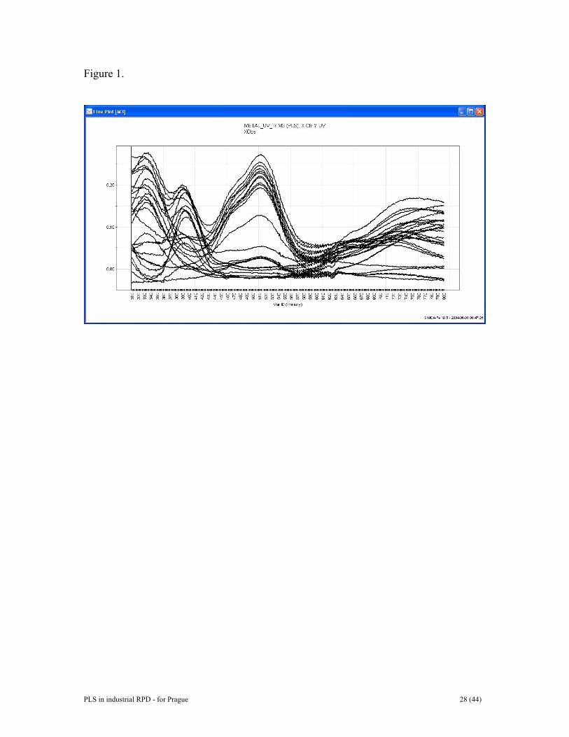
* are columns in W*. 2. EXAMPLE DATA SETS 2.1. Data set I: Multivariate calibration data Fiftytwo (52) mixtures with four different metal-ion complexes were analyzed with a Shimadzu 3101PC UV-VIS spectrophotometer in the wavelength region 310-800 nm, sampling at each wavelength [9]. The metal-ion complexes were mixed according to a design with the following ranges: FeCl3 [0-0.25 mM], CuSO4 [0-10 mM], CoCl2[0-50mM], Ni(NO3)2 [0-50 mM]. Note that the design matrix (i.e. concentration matrix Y) constructed here, does not have orthogonal columns. The UV-VIS data were split into a calibration and prediction set with 26 observations in each [9]. A line plot of the training set spectral data is given in Figure 1. Prior to modeling, the spectral data were column centrered and the concentration matrix
PLS in industrial RPD - for Prague 4 (44)
was column centered and scaled to unit variance (UV). For more details, please see reference 9. The objective of this investigation was to use the spectral matrix (X) to model the concentration data (matrix Y), and to explore if such a model would be predictive for the prediction setadditional new samples. 2.2 Data set II: Gene array data Gene array data are becoming increasingly common within the pharmaceutical and agrochemical industries. By studying which genes are either up or down-regulated it is hoped to be able to gain an insight into the genetic basis of disease. Gene chips are composed of short DNA strands bound to a substrate. The genetic sample under test is labelled with a fluorescent tag and placed in contact with the gene chip. Any genetic material with a complimentary sequence will bind to the DNA strand and be shown by fluorescence. From a data analysis point of view gene chip data are very similar to spectroscopic data. Firstly Tthe data often have a large amount of systematic variation and secondly the large numbers of genes across a grid are analogous to the large number of wavelengths in a spectrum. If gene grid data are plotted versus fluorescent intensity we get a ‘spectrum’ of gene expression. Some examples are seen in Figure 2. The data come from a toxicity study where the gene expression profiles for different doses of a toxin are investigated. The objective of this investigation was to be able to recognisze which genes are changing in response to a particular toxin so that these changes may be used to screen new drugs for toxicity in the future [10]. The gene grids used were composed of 1611 gene probes on a slide (or chip) and 4 different doses were given (Control, Low, Medium, High). Five animals were used per dose (some missing - 17 in total). Four grid repeats (W,X,Y,Z) were used per slide (also called spots) with 3 replicates (a,b,c) per animal. This gives 12 measurements in total per animal, i.e., 17 x 12 = 204, but two grid repeats were missing so the total number of observations is 196. It is informative to evaluate the raw data. Figure 2 shows a few examples and some of the observations look distinctly different. Observation C02bX is typical of the majority of observations. C02cY has a single signal which totally dominates the ‘gene spectrum’; possibly an extraneous object on the slide is causing this high point. Observations C04aY; M29bX; L21aX; L23aY are odd in a similar fashion, whereas all observations from Animal 28 have a very noisy appearance. 2.3 Data set III: Batch process data The third data set is a three-way data set from semi-conductor industry and deals with wafers from an etching tool. The N * J * K three-way data table (Figure 3) has the “directions” batches (N) * variables (J) * time (K). J = 19 variables were measured on N = 109 wafers during the 5 steps (phases) of the tool. The 19 variables were measured on-line every other second. Phases 2, 4, and 5 were steady state for some variables and dynamic for others, and phases 1 and 3 were transients.
Prior to the data analysis the entire phase 3 was deleted because of too few observations. Also, two batches were deleted for the same reason. Additionally, three variables, although chemically important, had no variation across the remaining four

PLS in industrial RPD - for Prague 5 (44)
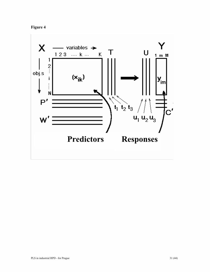
phases and were therefore excluded. As a final step, each phase of the tool was configured such that only active variables were used in each phase. Of the 109 wafers, 50 were tested as good and the rest as bad ones. Preliminary modelling activities (no results shown) identified 5 of these as outliers (tricky batches which temporarily go out of control). Seven arbitrarily selected good batches were also withdrawn for predictive purposes. Hence, out of the 50 good batches, 38 will be used for model training. The objective of this study was to train a model on the 38 selected good batches and verify that this model could distinguish between future good and bad batches. 3. PLS AND THE UNDERLYING SCIENTIFIC MODEL PLS is a way to estimate parameters in a scientific model, which basically is linear (see 4.4 for non-linear PLS models). This model, like any scientific model, consists of several parts, the philosophical, the conceptual, the technical, the numerical, the statistical, and so on. Our chemical thinking makes us formulate the influence of structural change on activity (and other properties) in terms of "effects" -- lipophilic, steric, polar, polarizability, hydrogen bonding, and possibly others. Similarly, the modelling of a chemical process is interpreted using "effects" of thermodynamics (equilibria, heat transfer, mass transfer, pressures, temperatures, and flows) and chemical kinetics (reaction rates). Although this formulation of the scientific model is not of immediate concern for the technicalities of PLS, it is of interest that PLS modelling is consistent with "effects" causing the changes in the investigated system. The concept of latent variables (section 4.1) may be seen as directly or indirectly corresponding to these effects. 3.1. The data – X and Y The PLS model is developed from a training set of N observations (objects, cases, compounds, process time points) with K X-variables denoted by xk (k=1,...,K), and M Y-variables ym (m=1,2,...,M). These training data form the two matrices X and Y (Figure 4) of dimensions (NxK) and (NxM), respectively. In example 1, N = 26, K = 391 401, and M = 4 in the training set. Later, predictions for new observations are made based on their X-data, i.e., digitized spectra. This gives predicted X-scores (t-values), X-residuals, their residual SD.s, and y-values (concentrations of the four ions) with confidence intervals. 3.2. Transformation, scaling and centering Before the analysis, the X- and Y-variables are often transformed to make their distributions be fairly symmetrical. Thus, variables with range of more than one magnitude of ten are often logarithmically transformed. If the value zero occurs in a variable, the fourth root transformation is a good alternative to the logarithm. Results of projection methods such as PLS depend on the scaling of the data. With an appropriate scaling, one can focus the model on more important Y-variables, and use experience to increase the weights of more informative X-variables. In the absence of knowledge about the relative importance of the variables, the standard multivariate approach is to (i) scale each variable to unit variance by dividing them by their SD.s, and
PLS in industrial RPD - for Prague 6 (44)
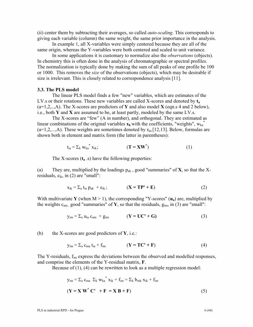
(ii) center them by subtracting their averages, so called auto-scaling. This corresponds to giving each variable (column) the same weight, the same prior importance in the analysis. In example 1, all X-variables were simply centered because they are all of the same origin, whereas the Y-variables were both centered and scaled to unit variance. In some applications it is customary to normalize also the observations (objects). In chemistry this is often done in the analysis of chromatographic or spectral profiles. The normalization is typically done by making the sum of all peaks of one profile be 100 or 1000. This removes the size of the observations (objects), which may be desirable if size is irrelevant. This is closely related to correspondence analysis [11]. 3.3. The PLS model The linear PLS model finds a few "new" variables, which are estimates of the LV.s or their rotations. These new variables are called X-scores and denoted by ta (a=1,2,..,A). The X-scores are predictors of Y and also model X (eqn.s 4 and 2 below), i.e., both Y and X are assumed to be, at least partly, modeled by the same LV.s. The X-scores are “few” (A in number), and orthogonal. They are estimated as linear combinations of the original variables xk with the coefficients, "weights", wka
* (a=1,2,...,A). These weights are sometimes denoted by rka [12,13]. Below, formulas are shown both in element and matrix form (the latter in parentheses): tia = Σk wka
* xik ; (T = XW*) (1) The X-scores (ta .s) have the following properties: (a) They are, multiplied by the loadings pak , good "summaries" of X, so that the X-residuals, eik, in (2) are "small": xik = Σa tia pak + eik ; (X = TP' + E) (2) With multivariate Y (when M > 1), the corresponding "Y-scores" (ua) are, multiplied by the weights cam , good "summaries" of Y, so that the residuals, gim, in (3) are "small": yim = Σa uia cam + gim (Y = UC' + G) (3) (b) the X-scores are good predictors of Y, i.e.: yim = Σa cma tia + fim (Y = TC' + F) (4) The Y-residuals, fim express the deviations between the observed and modelled responses, and comprise the elements of the Y-residual matrix, F. Because of (1), (4) can be rewritten to look as a multiple regression model: yim = Σa cma Σk wka
* xik + fim = Σk bmk xik + fim (Y = X W* C’ + F = X B + F) (5)
PLS in industrial RPD - for Prague 7 (44)
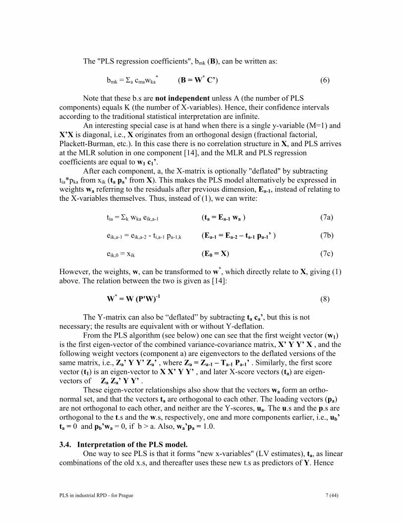
The "PLS regression coefficients", bmk (B), can be written as: bmk = Σa cmawka
* (B = W* C’) (6) Note that these b.s are not independent unless A (the number of PLS components) equals K (the number of X-variables). Hence, their confidence intervals according to the traditional statistical interpretation are infinite. An interesting special case is at hand when there is a single y-variable (M=1) and X’X is diagonal, i.e., X originates from an orthogonal design (fractional factorial, Plackett-Burman, etc.). In this case there is no correlation structure in X, and PLS arrives at the MLR solution in one component [14], and the MLR and PLS regression coefficients are equal to w1 c1’. After each component, a, the X-matrix is optionally "deflated" by subtracting tia*pka from xik (ta pa’ from X). This makes the PLS model alternatively be expressed in weights wa referring to the residuals after previous dimension, Ea-1, instead of relating to the X-variables themselves. Thus, instead of (1), we can write: tia = Σk wka eik,a-1 (ta = Ea-1 wa ) (7a) eik,a-1 = eik,a-2 - ti,a-1 pa-1,k (Ea-1 = Ea-2 – ta-1 pa-1’ ) (7b) eik,0 = xik (E0 = X) (7c) However, the weights, w, can be transformed to w*, which directly relate to X, giving (1) above. The relation between the two is given as [14]: W* = W (P'W)-1 (8) The Y-matrix can also be “deflated” by subtracting ta ca’, but this is not necessary; the results are equivalent with or without Y-deflation. From the PLS algorithm (see below) one can see that the first weight vector (w1) is the first eigen-vector of the combined variance-covariance matrix, X’ Y Y’ X , and the following weight vectors (component a) are eigenvectors to the deflated versions of the same matrix, i.e., Za’ Y Y’ Za’ , where Za = Za-1 – Ta-1 Pa-1’ . Similarly, the first score vector (t1) is an eigen-vector to X X’ Y Y’ , and later X-score vectors (ta) are eigen-vectors of Za Za’ Y Y’ . These eigen-vector relationships also show that the vectors wa form an ortho-normal set, and that the vectors ta are orthogonal to each other. The loading vectors (pa) are not orthogonal to each other, and neither are the Y-scores, ua. The u.s and the p.s are orthogonal to the t.s and the w.s, respectively, one and more components earlier, i.e., ub’ ta = 0 and pb’wa = 0, if b > a. Also, wa’pa = 1.0. 3.4. Interpretation of the PLS model. One way to see PLS is that it forms "new x-variables" (LV estimates), ta, as linear combinations of the old x.s, and thereafter uses these new t.s as predictors of Y. Hence
PLS in industrial RPD - for Prague 8 (44)
PLS is based on a linear model (see, however, section 4.4). Only as many new t.s are formed as are needed, as are predictively significant (section 3.8). All parameters, t, u, w (and w*), p, and c are determined by a PLS algorithm as described below. For the interpretation of the PLS model, the scores, t and u, contain the information about the objects and their similarities / dissimilarities with respect to the given problem and model. The weights wa or the closely similar wa
* (see below), and ca, give information about how the variables combine to form the quantitative relation between X and Y, thus providing an interpretation of the scores, ta and ua. Hence, these weights are essential for the understanding of which X-variables are important (numerically large wa-values), and which X-variables that provide the same information (similar profiles of wa-values). The PLS weights wa express both the “positive” correlations between X and Y, and the “compensation correlations” needed to predict Y from X clear from the secondary variation in X. The latter is everything varying in X that is not primarily related to Y. This makes wa difficult to interpret directly, especially in later components (a > 1). By using an orthogonal expansion of the X-parameters in O-PLS, one can get the part of wa that primarily relates to Y, thus making the PLS interpretation more clear [15]. The part of the data that are not explained by the model, the residuals, are of diagnostic interest. Large Y-residuals indicate that the model is poor, and a normal probability plot of the residuals of a single Y-variable are useful for identifying outliers in the relationship between T and Y, analogously to MLR. In PLS we also have residuals for X; the part not used in the modelling of Y. These X-residuals are useful for identifying outliers in the X-space, i.e., observations that do not fit the model. This, together with control charts of the X-scores, ta, is often used in multivariate statistical process control [16]. 3.4.1 Rotated coefficients and the interpretation of the PLS calibration model in terms of the pure spectra of the chemical constituents A common use of PLS is in indirect calibration in which the explicit objective is to predict the concentrations (Y matrix) from the digitized spectra (X matrix), in a set of N samples. PLS is able to handle many, incomplete, and correlated predictor variables in X in a simple and straightforward way. It linearly transforms the original columns of the X matrix into a new set of orthogonal column vectors, the scores T, whose inverse (TTT)-1 exists and is diagonal. As shown above (5), the PLS model can also be rearranged as a regression model, Y = XBPLS+FPLS where BPLS = W(PTW)-1CT (9) Using basic linear algebra it is possible to rewrite the PLS model so that it predicts X from Y instead of Y from X. This follows from equation 5 where,
(Y-FPLS) = XBPLS (10) Multiplying both sides with (BPLS
TBPLS)-1BPLST gives
(Y-FPLS)(BPLSTBPLS)-1BPLS
T = XBPLS(BPLS
TBPLS)-1BPLST (11)
PLS in industrial RPD - for Prague 9 (44)
then replacing XBPLS(BPLSTBPLS)-1BPLS
T = X - EPLS becomes (Y-FPLS)(BPLS
TBPLS)-1BPLST
= X - EPLS (12)
Define KPLS
T = (BPLSTBPLS)-1BPLS
T gives (Y-FPLS)KPLS
T = X - EPLS (13)
Replacing Yhat= Y-FPLS and swapping sides of some terms in the equation X = YhatKPLS
T + EPLS (14)
In Equation 14, the PLS model has now been reformulated to predict X instead of Y. It may not seem obvious why these steps were necessary. The transformation on the right hand side of Equation 11 is similar to the projection steps in a principal component analysis model where the BPLS matrix represents the loading matrix. The projection of X onto the BPLS loadings, XBPLS(BPLS
TBPLS)-1 , results in a score matrix whose outer product with the loadings BPLS
T equals the predicted Xhat, i.e. X - EPLS . In fact, Xhat equals X, if
the X matrix and the BPLS matrix span an identical column space. Replacing KPLST =
(BPLSTBPLS)-1BPLS
T as done in Equation 14, yields an equation for prediction of X, in the same form as the CLS method, see Equation 1. This corresponds to a transformation of the BPLS matrix into the pure constituent profile estimates, KPLS. If desired, it is also possible to replace the BPLS matrix (in Equation 9) with KPLS(KPLS
TKPLS)-1 for prediction of Y. Hence, Y = XKPLS (KPLS
TKPLS)-1 + FPLS (15)
Equation 9 and Equation 15 give identical predictions of Y. This shows that indirect calibration methods are able to estimate the pure constituent profiles in X similarly to direct calibration. Note however, that this does not mean that KPLS is identical to KCLS, but they are usually similar. It is, however, possible to discern situations when KCLS and KPLS estimates will differ substantially. 3.5 Geometric interpretation PLS is a projection method and thus has a simple geometric interpretation as a projection of the X-matrix (a swarm of N points in a K-dimensional space) down on an A-dimensional hyper-plane in such a way that the coordinates of the projection (ta, a=1,2,..,A) are good predictors of Y. This is indicated in Figure 5. The direction of the plane is expressed as slopes, pak, of each PLS direction of the plane (each component) with respect to each coordinate axis, xk. This slope is the cosine of the angle between the PLS direction and the coordinate axis. Thus, PLS develops an A-dimensional hyper-plane in X-space such that this plane well approximates X (the N points, row vectors of X), and at the same time, the positions of the projected data points on this plane, described by the scores tia, are related to the values of the responses, activities, Yim (see Figure 5). 3.6 Incomplete X and Y matrices (missing data). Projection methods such as PLS tolerate moderate amounts of missing data both in X and in Y. To have missing data in Y, it must be multivariate, i.e. have at least two columns. The larger the matrices X and Y are, the higher proportion of missing data is
PLS in industrial RPD - for Prague 10 (44)
tolerated. For small data sets with around 20 observations and 20 variables, around 10 to 20 % missing data can be handled, provided that they are not missing according to some systematic pattern. The NIPALS PLS algorithm automatically accounts for the missing values, in principle by iteratively substituting the missing values by predictions by the model. This corresponds to, for each component, giving the missing data values that have zero residuals and thus have no influence on the component parameters ta and pa. Other approaches based on the EM algorithm have been developed, and often work better than NIPALS for large percentages of missing data. [17,18]. One should remember, however, that with much missing data, any resulting parameters and predictions are highly uncertain. 3.7 One Y at a time, or all in a single model ? PLS has the ability to model and analyze several Y.s together, which has the advantage to give a simpler over-all picture than one separate model for each Y-variable. Hence, when the Y.s are correlated, they should be analyzed together. If the Y.s really measure different things, and thus are fairly independent, a single PLS model tends to have many components and be difficult to interpret. Then a separate modelling of the Y.s gives a set of simpler models with fewer dimensions, which are easier to interpret. Hence, one should start with a PCA of just the Y-matrix. This shows the practical rank of Y, i.e., the number of resulting components, APCA. If this is small compared to the number of Y-variables (M), the Y.s are correlated, and a single PLS model of all Y.s is warranted. If, however, the Y.s cluster in strong groups, which is seen in the PCA loading plots, separate PLS models should be developed for these groups. 3.8 The number of PLS components, A In any empirical modelling, it is essential to determine the correct complexity of the model. With numerous and correlated X-variables there is a substantial risk for "over-fitting", i.e., getting a well fitting model with little or no predictive power. Hence a strict test of the predictive significance of each PLS component is necessary, and then stopping when components start to be non-significant. Cross-validation (CV) is a practical and reliable way to test this predictive signifi-cance [1-8]. This has become the standard in PLS analysis, and incorporated in one form or another in all available PLS software. Good discussions of the subject were given by Wakeling and Morris [19], and Denham [20]. Basically, CV is performed by dividing the data in a number of groups, G, say, five to nine, and then developing a number of parallel models from reduced data with one of the groups deleted. We note that having G=N, i.e., the leave-one-out approach, is not recommendable [21]. After developing a model, differences between actual and predicted Y-values are calculated for the deleted data. The sum of squares of these differences is computed and collected from all the parallel models to form PRESS (predictive residual sum of squares), which estimates the predictive ability of the model. When CV is used in the sequential mode, CV is performed on one component after the other, but the peeling off (equation 7b, section 3.3) is made only once on the full data matrices, where after the resulting residual matrices E and F are divided into groups

PLS in industrial RPD - for Prague 11 (44)
for the CV of next component. The ratio PRESSa/SSa-1 is calculated after each component, and a component is judged significant if this ratio is smaller than around 0.9 for at least one of the y-variables. Slightly sharper bonds can be obtained from the results of Wakeling and Morris [19]. Here SSa-1 denotes the (fitted) residual sum of squares before the current component (index a). The calculations continue until a component is non-significant. Alternatively with “total CV”, one first divides the data into groups, and then calculates PRESS for each component up to, say 10 or 15 with separate “peeling” (7b, section 3.3) of the data matrices of each CV group. The model with number of components giving the lowest PRESS/(N-A-1) is then used. This "total" approach is computationally more taxing, but gives similar results. Both with the “sequential” and the "total" mode, a PRESS is calculated for the final model with the estimated number of significant components. This is often re-expressed as Q2 (the cross-validated R2) which is (1-PRESS/SS) where SS is the sum of squares of Y corrected for the mean. This can be compared with R2 = (1-RSS/SS), where RSS is the fitted residual sum of squares. In models with several Y.s, one obtains also Rm
2 and Qm2 for each Y-variable, ym.
These measures can, of course, be equivalently expressed as RSD's (residual SD's) and PRESD's (predictive residual SD's). The latter is often called SDEP, or SEP (standard error of prediction), or SECV (standard error of cross-validation). If one has some knowledge of the noise in the investigated system, for example ± 0.3 units for log(1/C) in QSAR.s, these predictive SD's should, of course, be similar in size to the noise. 3.9 Model validation Any model needs to be validated before it is used for "understanding" or for predicting new events such as the biological activity of new compounds or the yield and impurities at other process conditions. The best validation of a model is that it consis-tently precisely predicts the Y-values of observations with new X-values – a validation set. But an independent and representative validation set is rare. In the absence of a real validation set, two reasonable ways of model validation are given by cross-validation (CV, see section 3.8) which simulates how well the model predicts new data, and model re-estimation after data randomization which estimates the chance (probability) to get a good fit with random response data. 3.10 PLS algorithms The algorithms for calculating the PLS model are mainly of technical interest, we here just point out that there are several variants developed for different shapes of the data [2,22,23]. Most of these algorithms tolerate moderate amounts of missing data. Either the algorithm, like the original NIPALS algorithm below, works with the original data matrices, X and Y (scaled and centered). Alternatively, so called kernel algorithms work with the variance-covariance matrices, X’X, Y’Y, and X’Y, or association matrices, XX’ and YY’, which is advantageous when the number of observations (N) differs much from the number of variables (K and M). For extensions of PLS, the results of Höskuldsson regarding the possibilities to modify the NIPALS PLS algorithm are of great interest [3]. Höskuldsson shows that as
PLS in industrial RPD - for Prague 12 (44)
long as the steps (C) to (G) below are unchanged, modifications can be made of w in step (B). Central properties remain, such as orthogonality between model components, good summarizing properties of the X-scores, ta , and interpretability of the model parameters. This can been used to introduce smoothness in the PLS solution [24], to develop a PLS model where a majority of the PLS coefficients are zero [25], align w with à priori specified vectors (similar to “target rotation” of Kvalheim [26]), and more. The simple NIPALS algorithm of Wold et al. [2] is shown below. It starts with optionally transformed, scaled, and centered data, X and Y, and proceeds as follows (note that with a single y-variable, the algorithm is non-iterative): A. Get a starting vector of u , usually one of the Y columns. With a single y, u = y. B. The X-weights, w: w = X’ u / u’u (here w can now be modified) norm w to ||w|| = 1.0 C. Calculate X-scores, t t = X w D. The Y-weights, c: c = Y’ t / t’t E. Finally, an updated set of Y-scores, u: u = Y c / c’ c F. Convergence is tested on the change in t, i.e., ||told - tnew || / ||tnew|| < ε , where ε is “small”, e.g., 10-6 or 10-8. If convergence has NOT been reached, return to (B), otherwise continue with (G), and then (A). If there is only one y-variable, i.e., M=1, the procedure converges in a single iteration, and one proceeds directly with (G). G. Remove (deflate, peel off) the present component from X and Y, and use these deflated matrices as X and Y in the next component. Here the deflation of Y is optional; the results are equivalent whether Y is deflated or not. p = X’ t / (t’ t) X = X – t p’ Y = Y – t c’ H. Continue with next component (back to step A) until cross-validation (see above) indicates that there is no more significant information in X about Y.
PLS in industrial RPD - for Prague 13 (44)
Golub et al. recently has reviewed the attractive properties of matrix decompositions of the Wedderburn type [27]. The PLS NIPALS algorithm is such a Wedderburn decomposition, and hence is numerically and statistically stable. 3.11 Standard Errors and Confidence Intervals Numerous efforts have been made to theoretically derive confidence intervals of the PLS parameters, see e.g., [20, 28]. Most of these are, however, based on regression assumptions, seeing PLS as a biased regression model based on independent X-variables, i.e, a full rank X. Only recently, in the work of Burnham, MacGregor, et al. [12], have these matters been investigated with PLS as a latent variable regression model. A way to estimate standard errors and confidence intervals directly from the data is to use jack-knifing [29]. This was recommended by H.Wold in his original PLS work [1], and has recently been revived by Martens [30] and others. The idea is simple; the variation in the parameters of the various sub-models obtained during cross-validation is used to derive their standard deviations (called standard errors), followed by using the t-distribution to give confidence intervals. Since all PLS parameters (scores, loadings, etc.) are linear combinations of the original data (possibly deflated), these parameters are close to normally distributed, and hence jack-knifing works well. 4. ASSUMPTIONS UNDERLYING PLS AND SOME EXTENSIONS 4.1. Latent Variables. In PLS modelling we assume that the investigated system or process actually is influenced by just a few underlying variables, latent variables (LV.s). The number of these LV.s is usually not known, and one aim with the PLS analysis is to estimate this number. Also, the PLS X-scores, ta , are usually not direct estimates of the LV.s, but rather they span the same space as the LV.s. Thus, the latter (denoted by V) are related to the former (T) by a, usually unknown, rotation matrix, R, with the property R’R = 1 : V = T R’ or T = R V Both the X- and the Y-variables are assumed to be realizations of these underlying LV.s, and are hence not assumed to be independent. Interestingly, the LV assumptions closely correspond to the use of microscopic concepts such as molecules and reactions in chemistry and molecular biology, thus making PLS philosophically suitable for the modelling of chemical and biological data. This has been discussed by, among others, Wold [31,32], Kvalheim [33], and recently from a more fundamental perspective, by Burnham et al. [12,13]. In spectroscopy, it is clear that the spectrum of a sample is the sum of the spectra of the constituents multiplied by their concentrations in the sample. Identifying the latter with t (Lambert-Beers “law”), and the spectra with p, we get the latent variable model X = t1p1´ + t2p2´+ … = TP´ + noise. In many applications this interpretation with the data explained by a number of “factors” (components) makes sense.
PLS in industrial RPD - for Prague 14 (44)
As discussed below, we can also see the scores, T, as comprised of derivatives of an unknown function underlying the investigated system. The choice of the interpretation depends on the amount of knowledge about the system. The more knowledge we have, the more likely it is that we can assign a latent variable interpretation to the X-scores or their rotation. If the number of LV.s actually equals the number of X-variables, K, then the X-variables are independent, and PLS and MLR give identical results. Hence we can see PLS as a generalization of MLR, containing the latter as a special case in situations when the MLR solution exists, i.e., when the number of X- and Y-variables is fairly small in comparison to the number of observations, N. In most practical cases, except when X is generated according to an experimental design, however, the X-variables are not independent. We then call X rank deficient. Then PLS gives a "shrunk" solution which is statistically more robust than the MLR solution, and hence gives better predictions than MLR [34]. PLS gives a model of X in terms of a bilinear projection, plus residuals. Hence, PLS assumes that there may be parts of X that are unrelated to Y. These parts can include noise and/or regularities non-related to Y. Hence, unlike MLR, PLS tolerates noise in X. 4.2. Alternative derivation The second theoretical foundation of LV-models is one of Taylor expansions [35]. We assume the data X and Y to be generated by a multi-dimensional function F(u,v), where the vector variable u describes the change between observations (rows in X) and the vector variable v describes the change between variables (columns in X). Making a Taylor expansion of the function F in the u-direction, and discretizing for i = observation and k = variable, gives the LV-model. Again, the smaller the interval of u that is modelled, the fewer terms we need in the Taylor expansion, and the fewer components we need in the LV-model. Hence, we can interpret PCA and PLS as models of similarity. Data (variables) measured on a set of similar observations (samples, items, cases, …) can always be modelled (approximated) by a PC- or PLS model. And the more similar are the observations, the fewer components we need in the model. We hence have two different interpretations of the LV-model. Thus, real data well explained by these models can be interpreted as either being a linear combination of “factors” or according to the latter interpretation as being measurements made on a set of similar observations. Any mixture of these two interpretations is, of course, often applicable. 4.3. Homogeneity Any data analysis is based on an assumption of homogeneity. This means that the investigated system or process must be in a similar state throughout all the investigation, and the mechanism of influence of X on Y must be the same. Thus in turn, corresponds to having some limits on the variability and diversity of X and Y. Hence, it is essential that the analysis provides diagnostics about how well these assumptions indeed are fulfilled. Much of the recent progress in applied statistics has concerned diagnostics [36], and many of these diagnostics can be used also in PLS modelling as discussed below. PLS also provides additional diagnostics beyond those of
PLS in industrial RPD - for Prague 15 (44)
regression-like methods, particularly those based on the modelling of X (score and loading plots and X-residuals). 4.4. Non-linear PLS For non-linear situations, simple solutions have been published by Höskuldsson [4], and Berglund et al. [37]. Another approach based on transforming selected X-variables or X-scores to qualitative variables coded as sets of dummy variables, the so called GIFI approach [38,39], is described elsewhere [15]. 4.5 PLS-discriminant analysis (PLS-DA) The objective with discriminant analysis is to find a model that separates classes of observations on the basis of the values of their X-variables [1, 40, 41]. The model is developed from a training set of observations of known class belonging, and assumptions about the structure of the data. Typical applications in chemistry include the classification of samples according to their origin in space (e.g., a French or Italian wine) or time (i.e., dating), the classification of molecules according to properties (e.g., acid or base, beta receptor agonist or antagonist), or the classification of reactions according to mechanism (e.g., SN1 or SN2). Provided that each class is "tight" and occupies a small and separate volume in X-space, one can find a plane - a discriminant plane - in which the projected observations are well separated according to class. If the X-variables are few and independent (i.e., the regression assumptions are fulfilled), one can derive this discriminant plane by means of multiple regression with X and a "dummy matrix" Y that expresses the class belonging of the training set observations. This dummy Y matrix has G-1 columns (for G classes) with ones and zeros, such that the g.th column is one and the others zero for observations of class g when g < G-1. For class G all columns have the value of -1. With many and collinear X-variables it is natural to use PLS instead of regression for the model estimation. This gives PLS discriminant analysis, PLS-DA. With PLS-DA it is easier to use G instead of G-1 columns in the Y dummy matrix since the rank deficiency is automatically taken care of in PLS. Projecting new observations onto the discriminant plane gives predicted values of all the Y-columns, thus predicting the class of these observations. Since the modeled and predicted Y-values are linear combinations of the X-variables, these Y’s are close to normally distributed for observations of one homogeneous class. Hence simple statistics based on the normal distribution can be used to determine the class belonging of new observations. When some of the classes are not tight, often due to a lack of homogeneity and similarity in these non-tight classes, the discriminant analysis does not work. Then other approaches, such as, SIMCA (soft independent modelling of class analogy) have to be used, where a PC or PLS model is developed for each tight class, and new observations are classified according to their nearness in X-space to these class models. 4.6 Analysis of three-way data tables Data tables are not always two-way (observations x variables), but sometimes three-way, four-way etc. In analytical chemistry, for instance, array detectors are being

PLS in industrial RPD - for Prague 16 (44)
used in liquid chromatography, producing a whole spectrum at each chromatographic time-point, i.e., every 30 seconds or so. Each spectrum is a vector with, say, 256 elements, which gives a two-way table for each analyzed sample. Hence, a set of N samples gives a N x K x L three way table (sample x chromatogram x spectrum). If now additional properties have been measured on the samples, for instance scales of taste, flavour, or toxicity, there is also an N x M Y matrix. A three-way PLS analysis will model the relation between X and Y. The traditional approach has been to reduce the X-matrix to an ordinary two-way table by, for instance, using the spectral chromatograms to estimate the amounts of the interesting chemical constituents in each sample. Thereafter the two-way matrix is related to Y by PLS or some other pertinent method. Sometimes, however, the compression of X from three to two dimensions is difficult, and a direct three-way (or four-way, or ...) is preferable. Two PLS approaches are possible for this direct analysis. One is based on unfolding of the X-matrix to give an N x p two-way matrix (here p = K x L), which then is related to Y by ordinary PLS. This unfolding is accomplished by "slicing" X into L pieces of dimension N x K, or into M pieces of dimension N x L. These are then put sidewise next to each other, giving the "unfolded" two-way matrix. After the development of the PLS model, new observations can be unfolded to give a long vector with K x L elements. Inserting this into the PLS model gives predicted t-scores for the new observations, predicted y-values, DModX-values, etc., just like ordinary PLS. This unfolding of a multi-way matrix X to give a two-way matrix can be applied also to four-way, five-way, etc., matrices, and also, of course, to multi-way Y-matrices. Hence, the approach is perfectly general, although it perhaps looks somewhat inefficient in that correlations along several directions in the matrices are not explicitly used. Since, however, the results are exactly the same for all unfoldings that preserve the "object direction" as a "free" single way in the unfolded matrix, this inefficiency is just apparent and not real. For the interpretation of the model, the loading and weight vectors of each component (pa , and wa ) can be "folded back" to form loading and weight "sheets" (K x L), which can then be plotted, analyzed by PCA, etc. A second approach, which is difficult to extend to more than three ways, however, is to model X as a tri-linear expansion, where each component is the outer product of three vectors, say, t, p, and r. The scores corresponding to the object direction (t) are used as predictors of Y in the ordinary PLS sense. We realize that this gives a more constrained model with consequently poorer models except in the case when X is indeed very close to tri-linear. In order to analyze the wafer data set (Example III), the approach to batch analysis presented in [1, 42] is used. The basic premise of this approach it to analyze three-way batch data in two model layers. Typical configurations of batch-data are seen in Figures 3 and 6. On the lower (observation) level the three-way batch data are unfolded preserving the variable direction (Figure 6), and a PLS model is computed between the unfolded X-data and time or a suitable maturity variable. The X-score vectors of this PLS model consecutively capture linear, quadratic, cubic, …, dependencies between the measured process data and time or maturity. Subsequently, these score vectors are re-arranged (Figure 7) and used on the upper (batch) level where relationships among whole batches are investigated (Figure 7). The re-arrangement (cf
PLS in industrial RPD - for Prague 17 (44)
Figure 7) of the scores and other model statistics (DModX, predicted time) enables batch control charts [42] to be produced. The resulting control charts can be used to follow the trace of a developing batch, and extract warnings when it tends to depart from the typical trace of a normal, good batch. 4.7 Hierarchical PLS models In PLS, models with many variables, plots and lists of loadings, coefficients, VIP, etc., become messy, and results are difficult to interpret. There is then a strong temptation to reduce the number of variables to a smaller, more manageable number. This reduction of variables, however, often removes information, makes the interpretation misleading, and seriously increases the risk for spurious models. A better alternative is often to divide the variables into conceptually meaningful blocks, and then apply hierarchical multi-block PLS (or PC) models [1,43,44]. In QSAR the blocks may correspond to different regions of the modelled molecules and different types of variables (size descriptors, polarity descriptors, etc.), and in multivariate calibration the blocks may correspond to different spectral regions. In process modelling, the process usually has a number of different steps (e.g., raw material, reactor, precipitation step, etc.), and variables measured on these different steps constitute natural blocks. These may be further divided according to the type of variables, e.g., temperatures, flows, pressures, concentrations, etc. The idea with multivariate hierarchical modelling is very simple. Take one model dimension (component) of an existing projection method, say PLS (two-block), and substitute each variable by a score vector from a block of variables. We call these score vectors "super variables". On the "upper" level of the model, a simple relationship, a "super model", between rather few "super variables" is developed. In the lower layer of the model, the details of the blocks are modelled by block models as block-scores time block loadings. Conceptually this corresponds to seeing each block as an entity, and then developing PLS models between the "super-blocks". The lower level provides the "variables" (block scores) for these block relationships. This blocking leads to two model levels; the upper level where the relationships between blocks are modelled, and the lower level showing the details of each block. On each level, "standard" PLS or PC scores and loading plots, as well as residuals and their summaries such as DModX, are available for the model interpretation. This allows an interpretation focussed on pertinent blocks and their dominating variables. 5 RESULTS FOR DATA SET I The calibration set was used as foundation for the PLS calibration model (see Figure 1 for a plot of the raw data). According to cross-validation – with seven exclusion groups – five components were optimal. Plots of observed and estimated/predicted metal ion concentrations for the calibration and prediction sets are shown in Figure 8. As seen, the predictive power is good and matches the estimations for the training set. Apart from prediction of analyte concentrations in unknown samples, spectral profile estimation of pure components is of central importance in multivariate calibration applications. As outlined in reference [9], and discussed above in section 3.4.1, O-PLS neatly paves the way for such pure profile estimation, by means of accounting for the Y-orthogonal X-variation (“structured noise”) in a separate part of the model. Thus, O-PLS
PLS in industrial RPD - for Prague 18 (44)
was used to compute an alternative multivariate calibration model. It consisted of four Y-related compontents and one Y-orthogonal component of structured noise. This model has identical predictive power to the previous model. The observed and estimated pure spectra are plotted in Figure 9 (a and b). Data have been normalized for comparative purposes. The estimated pure spectra were derived from the rotated regression coefficients K=B(BTB)-1. They are in excellent agreement with the measured pure spectra. In conclusion, this study shows that the measured spectral data are relevant for quantitative assessment of metal ion concentrations in aqeous solution. One important aspect underpinning this study is the use of design of experiments (DOE) to compose representative and informative calibration and prediction sets of data [45,46]. DOE is critically important in multivariate calibration in order to raise the quality of predictions and model interpretability. The use of O-PLS further enhances model transparency by allowing pure spectral profiles to be estimated. Furthermore, as shown in reference 9, the merits of O-PLS become even more apparent in case not all constituents in X are parameterized in Y. And, the latter is valid regardless of whether DOE has been used to devise the Y-matrix, or not. 6 RESULTS FOR DATA SET II The gene grid data set was mean-centered and scaled to unit variance. In order to overview the data set we applied PCA. PCA with 2 components gives R2 = 0.41 and Q2 = 0.39, a weak model but useful for visualisation. Hotellings T2 shows the odd behaviour of observations from animal 28 (Figure 10). The DModX plot identifies the same outliers as those found ‘bye eye’ (Figure 11). Looking at the score plot the four treatment groups show some clustering but there is also a degree of overlap. The outlying samples spotted in Figure 11 were removed as were all the samples originating from the odd animal 28. Then, in order to observe the gene changes that occur when going from one group to another PLS-discriminant analysis (PLS-DA) was used. A practical way to conduct PLS-DA is to compare two classes at a time. Figure 12 shows a score plot from the PLS-DA between Control and High. The underlying model is very strong, R2Y =0.93 and Q2Y = 0.92 so there is no doubt the separation between control and high-dosed animals is real and well manifested. The plot shows complete separation of the two groups. PLS-DA may often give better separation than the passive SIMCA method for classification problems. In order to find out which genes are either up or down-regulated we constructed the contribution plot displayed in Figure 13. This plot is a group-contribution plot highlighting the difference between the average control sample and the average high-dosed sample. Sometimes such plots can be very “crowded” and it may be advisable to use zooming-in functionality to increase interpretability. The right-hand part of the plot shows a magnification of the variable region 930-950 and points to which variables have been upregulated for the animals exposed to the high dose of the toxin in question. In conclusion, this example shows that multivariate data analysis is suitable to analyze and visualize analytical bioinformatics data. Such assessments may provide an overview of the data and uncovers experimental variations and outliers. Contribution plotting may be used to see which genes have altered relative to another observation. PLS-DA can be used to determine the differences in gene expression between treatment

PLS in industrial RPD - for Prague 19 (44)
groups. The data may be scaled or transformed differently in order to optimise the separation between treatment groups or to focus on the number of genes that change. 7 RESULTS FOR DATA SET III In order to accomplish the observation level models the three-way data structure was unfolded as to a two-way array preserving the direction of the variables (cf Figures 6-9). Four PLS models, one for each phase (i.e., phases 1, 2, 4, and 5), were fitted between the measured variables and time for the 38 trainings set batches. These models were very efficient in modelling batch behavior and explained variances exceeded 50% all the time. The scores of the four observation level PLS models were used to create batch control charts. These control charts were used to make predictions for the prediction set batches. Figure 14 presents some prediction results for batches 73, 219, 233 and 302, using the phase 1 model and its associated t1-score and DModX-control charts. Additional control charts (t2-score, t3-score, etc.) are available but are not plotted. There are also additional control charts for the other three phases, but such results are not provided for reasons of brevity. Batch 73 is a bad batch and it is mostly outside the control limits in both control charts, and it ends up outside the model according to DModX. Batch 219 tested good, but is tricky according to t1 and is a borderline case according to DModX. It ends up good in the DModX graph. Batch 233 also tested good, but clearly has problems in the early stage of phase 1. Batch 302 is a good batch and was one of the seven randomly withdrawn batches preserved for predictions. It consistently behaves well throughout the entire duration of the batch. Contribution plotting may be used to interrogate the model and highlight which underlying variables are actually contributing to an observed process upset. As an example, Figure 15 uncovers that the variable TV_POS is much too high in the early stage of phase 1 of batch 233. To accomplish a model of the evolution of the whole batch, the score vectors of the four concatenated lower level PLS models were rearranged as depicted in Figure 7. PCA was then used to create the batch level model. Eighteen principal components were obtained, which accounted for 76% of the variance. The scores of the first two components together with DModX after 18 components are rendered in Figure 16 (a and b). The score plot shows the homogeneous distribution of the 38 reference batches. According to the DModX-statistic there are no more outlying batches. The batch model was applied to the 71 prediction batches, the results of which are plotted in Figure 16 (c and d). For comparative purposes the 38 reference batches are also charted. Many of the prediction set batches are found different from the reference batches. Contribution plotting can be used to uncover why and how a certain batch deviates from normality. Figure 17 relates to batch 73. Apparently, batch 73 is very different in phase 2. A closer inspection of the predicted DModX plot (Figure 16d) indicates that the seven good batches in the prediction set (batches 217, 224, 230, 234, 292, 302, 309) are closest to the model. Six of these are, in fact, inside the model tolerance volume. All problematic batches are outside Dcrit. Hence, the predictive power of the batch model is not mistaken.
PLS in industrial RPD - for Prague 20 (44)
In conclusion, thirty-eight reference batches were used to train a batch model to recognize “good” operating conditions. This model was able to categorize between good and problematic batches. The predictive power of the upper level PLS model was very good for the 71 test batches. Six out of seven good batches, deliberately left out from the modelling, were correctly predicted. Contribution plotting was used to understand why problematic batches deviated. 8 DISCUSSION Modern data acquisition techniques like cDNA arrays, 2D-electrophoresis-based proteomics, spectroscopy, chromatography, etc., yield a wealth of data about every sample. Resulting high-density high-volume data-sets can readily exceed thousands of observations and variables, well beyond the reach of intuitive comprehension. Figures 1 and 2 provide raw data plots, which are difficult to overview as such, and particularly when contemplating many such profiles of a series of experiments. For these and similar types of data-sets, data-driven analysis by means of multivariate projection methods greatly facilitates the understanding of complex data structures and thereby complements hypothesis-driven research. An attractive property of PCA, PLS, and their extensions, is that they apply to almost any type of data matrix, e.g., matrices with many variables (columns), many observations (rows), or both. The precision and reliability of the projection model parameters related to the observations (scores, DModX) improve with increasing number of relevant variables. This is readily understood by realizing that the “new variables”, the scores, are weighted averages of the X-variables. Any (weighted) average becomes more precise the more numerical values are used as its basis. Hence, multivariate projection methods work well with “short and wide” matrices, i.e., matrices with many more columns than rows. The data-sets treated here are predominantly short and wide (micro-array data & metabonomics example), but occasionally long and lean (hierarchical proteomics data set). The great advantage of PCA, PLS, and similar methods, is that they provide rapid, powerful views of the your data, compressed to two or three dimensions. Initial looks at score and loading plots may reveal groups in the data that were previously unknown or uncertain. In order to interpret the patterns of a score plot one may examine the corresponding loading plot. In PCA there is a direct score-loading correspondence, whereas the interpretation of a PLS model may be a bit more difficult if the X-matrix contains structured noise that is unrelated to Y. Further looks at how each variable contributes to the separation in each dimension gives insights into the relative importance of each variable. Moreover, DModX and other residual plots may uncover moderate outliers in data, i.e., samples where the signatures in their variables are different from the majority of observations. Serious outliers have a more profound impact on the model and they therefore show up as strong outliers in a score plot. The PCA score plot in Figure 10, for example, highlights the existence of one deviating animal, and the DModX plot in Figure 11 shows the existence of several moderate outliers. In this situation, contribution plotting is a helpful approach in order to delineate why and how this outlier is different.

PLS in industrial RPD - for Prague 21 (44)
Plotting of scores and residuals versus time, or some other external order of data collection (e.g., geographical coordinates) is also informative. Such plots may reveal (unwanted) trends in the data. The color-coding of samples by sex or other group of interest provides an indication of whether such issues affect grouping within your set. Coding by analytical number or sampling order may reveal analytical drift, which may be a serious problem with complex analytical and bioanalytical techniques. When samples of interest that “should” be grouped are not, PCA, PLS, etc., give warning to a problem in understanding, or previously hidden complexity within the data. One of the great assets of multivariate projection methods is the plethora of available model parameters and other diagnostic tools – and plots and lists thereof – which aid in getting fundamental insights into the data generation process even when there are substantial levels of missing data. These include:
• Discovering (often unexpected) groupings in the data. • Seeing discontinuous relationships in the data. • Seeing relationships between variables. • Identifying variables separating two or more classes. • Classifying unknown observations into known classes. • Building mathematical models of large datasets. • Compressing large datasets into smaller, more informative datasets
8.1 Reliability, flexibility, versatility and scalability of multivariate projection methods Many data mining and analytical techniques are available for processing and overviewing multivariate data. However, we believe that latent variable projection methods are particularly apt at handling the data analytical challenges arising from analytical and bio-analytical data. Projection based methods are designed to effectively handle the hugely multivariate nature of such data. In this paper, we have presented PLS and some extensions for the analysis of the three example data-sets. However, as discussed below, there exist other twists and aspects of these techniques, contributing to their general applicability and increasing popularity. An often overlooked question is how to design ones experiment in order to make sure that they contain a maximum amount of information. Design of experiments (DOE) generates a set of representative, informative and diverse experiments [45-47]. Since one objective is to be restrictive with experiments, a DOE-protocol is normally tailored towards the precise needs of the on-going investigation. This means that in a screening application many factors are studied in a design with few experiments, whereas in an optimization study few factors are investigated in detail using rather many experimental trials. With analytical, bioanalytical and simlar data, the number of samples (“experiments”) is often not such a serious issue as in expensive experimentation. Then other designs, such as onion designs are of relevance [48,49]. Irrespective of its origin and future use, any DOE-protocol will benefit from an analysis using multivariate projection methods, especially if the protocol has paved the way for extensive and multivariate measurements on its experimental trial. Thus, DOE [45-49] and its extension for design in molecular properties [1], is an expeditious route towards obtaining informative, reliable, and useful multivariate models.

PLS in industrial RPD - for Prague 22 (44)
Furthermore, there are many tools “surrounding” multivariate projection methods, jointly striving to improve their utility, flexibility, and versatility. Thus, there are many methods of pre-processing multivariate data, all trying to reshape the data to be better suited for the subsequent analysis. Common techniques for pre-processing of multivariate data include methods for scaling and centering, transformation, expansion, and signal correction and compression [1]. We here just mention that neglecting proper pre-processing may make the multivariate analysis fruitless. 9 CONCLUDING REMARKS Multivariate projection methods represent a useful and versatile technology to modeling, monitoring and prediction of the often complex problems and data structures encountered within data-rich disciplines in RDP. The results may be graphically displayed in many different ways and this all works because the methods capture the dominant, latent properties of the system under study. It is our belief that as multivariate chemometric methods evolve and develop, this will involve applications to data-rich RDP-disciplins. Hence, we look forward to an interesting future for “multivariate RDP data analysis” and the many new innovative ideas that will probably be seen in the near future. REFERENCES
1. Eriksson, L., Johansson, E., Kettaneh-Wold, N., and Wold, S., Multi- and Megavariate Data Analysis – Principles and Apllications, Umetrics, 2001.
2. Wold, S., Sjöström, M., and Eriksson, L., PLS regression: A basic tool of chemometrics, Chemometrics and Intelligent Laboratory Systems, 58, 109-130, 2001.
3. Wold,Soft modeling. The basic design and some extensions., In Vol.II of Jöreskog, K.- G. and Wold, H., Ed.s., Systems under indirect observation, Vol.s I and II., North- Holland, Amsterdam, 1982.
4. Wold, S., Ruhe, A., Wold, H., and Dunn III, W.J., The Collinearity Problem in Linear Regression. The Partial Least Squares Approach to Generalized Inverses, SIAM J. Sci. Stat. Comput. 5 (1984) 735-743.
5. Höskuldsson, A. PLS regression methods., J.Chemometr., 2 (1988) 211-228. 6. Höskuldsson, A. Prediction Methods in Science and Technology, Vol.1. Thor
Publishing, Copenhagen, 1996. ISBN 87-985941-0-9. 7. Wold, S., Johansson, E., and Cocchi, M. PLS -- Partial least squares projections
to latent structures. In H.Kubinyi (Ed.), 3D QSAR in Drug Design, Theory, Methods, and Applications. ESCOM Science Publishers, Leiden, 1993.
8. Tenenhaus, M. La Regression PLS: Theorie et Pratique. Technip, Paris, 1998. 9. Trygg, J., (2004), Prediction and spectral profile estimation in multivariate
calibration, Journal of Chemometrics, In press. 10. Atif U, Earll M, Eriksson L, Johansson E, Lord P, Margrett S (2002) Analysis of
gene expression datasets using partial least squares discriminant analysis and principal component analysis. In: Martyn Ford, David Livingstone, John Dearden and Han Van de Waterbeemd (Eds.), Euro QSAR 2002, Designing Drugs and Crop Protectants: processes, problems and solutions. Blackwell Publishing, ISBN 1-4051-2561-0, pp 369-373.
PLS in industrial RPD - for Prague 23 (44)
11. Jackson, J.E. A User's guide to principal components. Wiley, N.Y., 1991. 12. Burnham, A.J., MacGregor, J.F., and Viveris, R. Latent Variable Regression
Tools. Chemom.Intell.Lab.Syst., 48 (1999) 167-180. 13. Burnham, A., Viveros, R., and MacGregor, J. Frameworks for Latent Variable
Multivariate Regression. J.Chemometr. 10 (1996) 31-45. 14. Manne, R. Analysis of two partial least squares algorithms for multivariate
calibration. Chemom.Intell.Lab.Syst., 1 (1987) 187-197. 15. Wold, S., Trygg, J., Berglund, S., and Antti, H., Some recent developments in
PLS modellling, Chemometrics and Intelligent Laboratory Systems, 58, 131-150, 2001.
16. Nomikos, P., and MacGregor, J.F. Multivariate SPC Charts for Monitoring Batch Processes, Technometrics, 37 (1995) 41-59.
17. Nelson, P.R.C., Taylor, P.A., MacGregor, J.F., Missing Data Methods in PCA and PLS: Score Calculations with Incomplete Observation. Chemom.Intell.Lab.Syst., 35 (1996) 45-65.
18. Grung, B., and Manne, R., Missing Values in Principal Component Analysis. Chemom.Intell.Lab.Syst., 42 (1998) 125-139.
19. Wakeling, I.N., and Morris, J.J. A test of significance for partial least squares regression. J.Chemometr. 7 (1993) 291-304.
20. Denham, M.C., Prediction Intervals in Partial Least Squares, Journal of Chemometrics, 11, 39-52, 1997.
21. Shao, J. Linear Model Selection by Cross-validation. J.Amer.Stat.Assoc. 88 (1993) 486 - 494.
22. Lindgren, F., Geladi, P., and Wold, S. The kernel algorithm for PLS, I. Many observations and few variables. J.Chemometr. 7 (1993) 45-59.
23. Rännar, S., Geladi, P., Lindgren, F., and Wold, S. The kernel algorithm for PLS, II. Few observations and many variables. J.Chemometr. 8 (1994) 111-125.
24. Esbensen, K.H., and Wold, S. SIMCA, MACUP, SELPLS, GDAM, SPACE & UNFOLD: The ways towards regionalized principal components analysis and subconstrained N-way decomposition -- with geological illustrations. Proc.Nord.Symp. Appl. Statist. Stavanger 1983 (O.J.Christie, Ed.), 11-36. ISBN 82-90496-02-8.
25. Kettaneh-Wold, N., MacGregor, J. F., Dayal, B., and Wold, S. Multivariate design of process experiments (M-DOPE). Chemom.Intell.Lab.Syst., 23 (1994) 39-50.
26. Kvalheim, O.M., Christy, A.A., Telnaes, N., and Bjoerseth, A. Maturity determination of organic matter in coals using the methylphenantrene distribution. Geochim.Cosmochim.Acta 51 (1987) 1883-1888.
27. Chu, M.T., Funderlic, R.E., and Golub, G.H. A Rank-One Reduction Formula and its Applications to Matrix Factorizations. SIAM Review 37 (1995) 512-530.
28. Serneels, S., Lemberge, P., and Van Espen, P.J., Calculation of PLS prediction intervals using efficient recursive relations for the Jacobian matrix, Journal of Chemometrics, 18 (2004) 76-80.
29. Efron, B., and Gong, G. A leisurely look at the bootstrap, the jackknife, and cross-validation, Amer.Statist. 37 (1983) 36-48.
PLS in industrial RPD - for Prague 24 (44)
30. Martens, H., and Martens, M. Modified Jack-knife Estimation of Parameter Uncertainty in Bilinear Modeling (PLS). Food Quality and Preference 11 (2000) 5-16.
31. Wold, S., Albano, C., Dunn III, W.J., Edlund, U., Eliasson, B., Johansson, E., Norden,B., and Sjöström, M. The indirect observation of molecular chemical systems. Chapter 8 in K.-G.Jöreskog and H.Wold, Ed.s. Systems under indirect observation, Vol.s I and II. North-Holland, Amsterdam, 1982.
32. Wold, S., Sjöström, M., Eriksson, L. PLS in Chemistry. In: The Encyclopedia of Computational Chemistry. (Schleyer, P. v. R.; Allinger, N. L.; Clark, T.; Gasteiger, J.; Kollman, P. A.; Schaefer III, H. F.; Schreiner, P. R., Eds.), John Wiley & Sons, Chichester, 1999, pp 2006-2020.
33. Kvalheim, O.,The Latent Variable, an Editorial. Chemom.Intell.Lab.Syst., 14 (1992) 1-3.
34. Frank, I.E., and Friedman, J.H. A Statistical View of some Chemometrics Regression Tools. With discussion. Technometrics 35 (1993) 109-148.
35. Wold, S. A Theoretical Foundation of Extrathermodynamic Relationships (Linear Free Energy Relationships). Chem.Scr. 5 (1974) 97-106.
36. Belsley, D.A., Kuh, E., and Welsch, R.E. Regression diagnostics: Identifying influential data and sources of collinearity. Wiley, N.Y., 1980.
37. Berglund, A., and Wold, S. INLR, Implicit Non-Linear Latent Variable Regression. J.Chemom. 11 (1997) 141-156.
38. Wold, S., Berglund, A., Kettaneh, N., Bendwell, N., and Cameron, D.R, The GIFI Approach to Non-Linear PLS Modelling, J. Chemometr. (2001). Update needed
39. Eriksson, L., Johansson, E., Lindgren, F., Wold, S., GIFI-PLS: Modeling of Non-Linearities. and Discontinuities in QSAR. QSAR, 19 (2000) 345-355.
40. Sjöström, M., Wold, S., and Söderström, B. PLS Discriminant Plots. Proceedings of PARC in Practice, Amsterdam, June 19-21, 1985. Elsevier Science Publishers B.V., North-Holland, 1986.
41. Ståhle, L., and Wold, S. Partial Least Squares Analysis with Cross-Validation for the Two-Class Problem: A Monte Carlo Study, J. Chemometr. 1 (1987), 185-196.
42. Wold, S., Kettaneh, N., Fridén, H., and Holmberg, A., Modelling and Diagnostics of Batch Processes and Analogous Kinetic Experiments, Chemometrics and Intelligent Laboratory Systems, 44, 331-340, 1998.
43. Wold, S., Kettaneh. N., and Tjessem, K., Hierarchical Multiblock PLS and PC Models for Easier Model Interpretation and as an Alternative to Variable Selection, Journal of Chemometrics, 10, 463-482, 1996.
44. Eriksson, L., Johansson, E., Lindgren, F., Sjöström, M., and Wold, S., Megavariate Analysis of Hierarchical QSAR Data, Journal of Computer-Aided Molecular Design 16 (2002) 711-726.
45. Box, G.E.P., Hunter, W.G., and Hunter, J.S. Statistics for experimenters. Wiley, New York, 1978.
46. Kettaneh-Wold, N. Analysis of mixture data with partial least squares. Chemom.Intell.Lab.Syst., 14 (1992) 57-69.

PLS in industrial RPD - for Prague 25 (44)
47. Eriksson L, Johansson E, Kettaneh-Wold N, Wikström C, Wold S (2000) Design of experiments – Principles and Applications, Umetrics AB, 2000, ISBN 91-973730-0-1.
48. Olsson, I., Gottfries, J., and Wold, S., D-optimal Onion Design (DOOD) in Statistical Molecular Design, Chemometrics and Intelligent Laboratory Systems. Accepted for publication.
49. Eriksson L, Arnhold T, Beck B, Fox T, Johansson E, and Kriegl JM (2004), Onion design and its application to a pharmaceutical QSAR problem, Journal of Chemometrics, Accepted for publication.

PLS in industrial RPD - for Prague 26 (44)
Figure Legends Figure 1. Line plot of raw data of example I. Figure 2. Some typical gene-spectra of example II. See text for further details. Figure 3. Batch-data often involve three distinct blocks of data, i.e., initial conditions (the Z-matrix), evolution measurements (the X-matrix), and results and quality characteristics (the Y-matrix). These data tables can be analyzed independently with PCA or related to each other by PLS. Figure 4. Data of PLS can be arranged as two tables, matrices, X and Y. Note that the raw data may have been transformed (e.g., logarithmically), and usually have been centered and scaled before the analysis. Figure 5. Thhee geometric representation of PLS. The X-matrix can be represented as N points in the K dimensional space where each column of X (xk) defines one coordinate axis. The PLSR model defines an A-dimensional hyper-plane, which in turn, is defined by one line, one direction, per component. The direction coefficients of these lines are pak. The coordinates of each object, i, when its data (row i in X) are projected down on this plane are tia. These positions are related to the values of Y. Figure 6. The three-way data table is unfolded by preserving the direction of the variables. This gives a two-way matrix with N x J rows and K columns. Each row contains data points xijk from a single batch observation (batch i, time j, variable k). If regression is made against local batch time, the resulting PLS scores reflect linear (t1), quadratic (t2), and cubic (t3) relationships to local batch time. Figure 7. In the batch level modelling, all available data are used to obtain a model of whole batches. Note that each row corresponds to one batch. Initial conditions data are often pooled with process evolution data to form a new X-matrix, XB. This XB-matrix is regressed against the final results contained in the Y-matrix. When used for batch monitoring, the resulting PLS-model may be used to categorize evolving batches as good or bad. It is also possible to interpret which initial condition data and process evolution data exert the highest influence on the type and quality of resulting product. Figure 8. Plots of observed and estimated/predicted metal ion concentration for the calibration and prediction sets. Figure 9. Observed and estimated pure spectra for the metal ion example. (a, left) Pure spectral profiles. (b, right) O-PLS spectral profiles, KO-PLS . Figure 10. Scatter plot of two first score vectors. Samples from the deviating animal number 28 are encircled. Figure 11. DModX chart indicating some moderate outliers in the second data set.

PLS in industrial RPD - for Prague 27 (44)
Figure 12. PLS-DA score plot between “high” and “control” animals in data set II. The plot shows complete separation between the two classes. Controls (C) are more spread out than the high exposure (H), and also indicated to be clustered. Figure 13. Contribution plot between average control sample and average high sample. This plot shows which genes have been up- and down-regulated. The right-hand portion is a magnification of parts of the contribution plot. Figure 14. Predicted batch control charts for batches 73, 219, 233, and 302. Upper row shows t1-score charts and bottom row provides DModX control charts. Figure 15. A contribution plot suggesting that variable TV_POS is much too high in th early stage of phase 1 of batch 233. Figure 16. Plots from the whole batch model. (a, top left) Scores t1 and t2 of training set. (b, to right) DModX plot of training set. (c, bottom left) Same as a) but extended to cover prediction set batches. (d, bottom right) Same as a) but extended to cover prediction set batches. Figure 17. Contribution plot of prediction set batch number 73. Apparently, batch 73 is very different from a normal, good batch in pahase 2.
PLS in industrial RPD - for Prague 28 (44)
Figure 1.

PLS in industrial RPD - for Prague 29 (44)
Figure 2.
C02aW C02bX
C02cY M28aW

PLS in industrial RPD - for Prague 30 (44)
Figure 3
Variables
Batches
TimeOne batch
Variables
Initial conditions Evolution measurements Resultscharacteristics
Variables
Z X Y
PLS in industrial RPD - for Prague 31 (44)
Figure 4
Predictors Responses
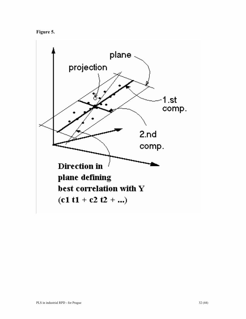
PLS in industrial RPD - for Prague 32 (44)
Figure 5.

PLS in industrial RPD - for Prague 33 (44)
B1
B2
X Y
Time
B3
…
Bn
Variables
Batches
Figure 6
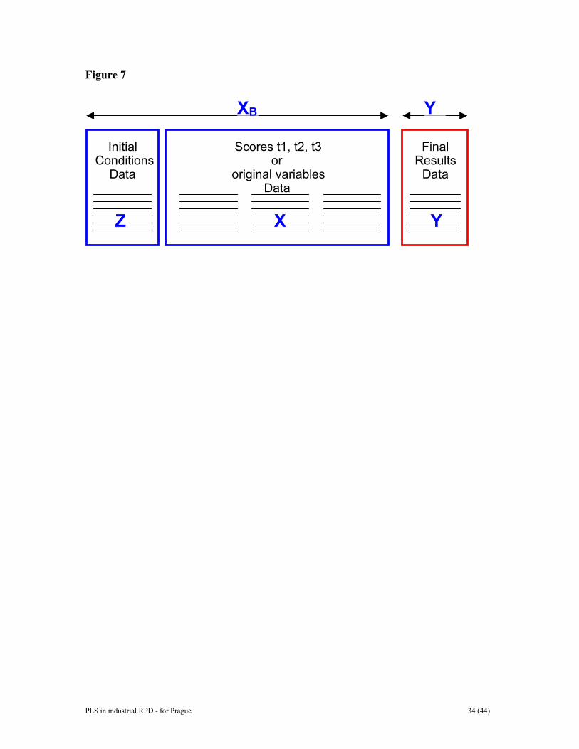
PLS in industrial RPD - for Prague 34 (44)
Figure 7
InitialConditions
Data
FinalResults
Data
Scores t1, t2, t3or
original variablesData
XB Y
Z X Y
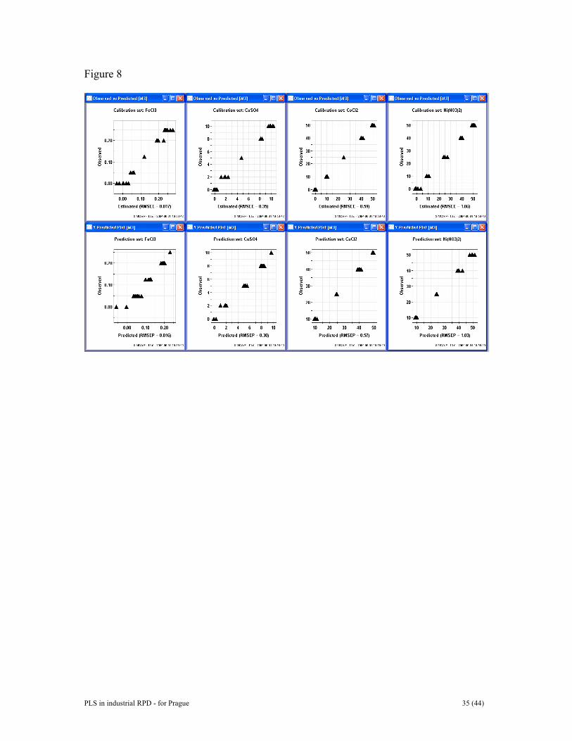
PLS in industrial RPD - for Prague 35 (44)
Figure 8

PLS in industrial RPD - for Prague 36 (44)
Figure 9
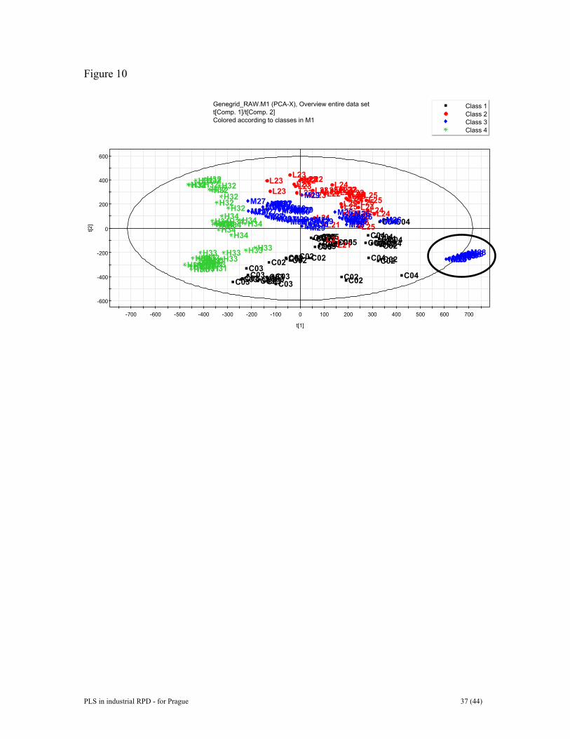
PLS in industrial RPD - for Prague 37 (44)
Figure 10
-600
-400
-200
0
200
400
600
-700 -600 -500 -400 -300 -200 -100 0 100 200 300 400 500 600 700
t[2]
t[1]
Genegrid_RAW.M1 (PCA-X), Overview entire data sett[Comp. 1]/t[Comp. 2]Colored according to classes in M1
Class 1Class 2Class 3Class 4
C02C02
C02C02C02C02C02C02C02C02
C02C02C03C03 C03C03 C03C03
C03C03C03C03 C03C03
C04C04
C04
C04
C04C04C04C04 C04C04C04C04C05C05C05C05C05C05C05C05C05C05C05C05
L21L21
L21L21
L22L22
L22L22
L22L22L22L22L23L23 L23L23 L23
L23L23
L23L23
L23
L23L23
L24L24
L24L24
L24L24
L24L24L25
L25L25
L25
L25L25
L25L25
L25L25L25
L25
M26M26M26M26M26M26
M26M26M26M26M26M26M27
M27M27
M27M27M27
M27M27M27M27
M27M27
M28M28M28M28M28M28M28M28M28M28M28M28
M29
M29
M29M29
M29M29
M29M29M30
M30M30
M30M30M30 M30M30M30M30
M30M30
H31H31
H31H31H31H31H31H31H31H31
H31H31
H32H32H32
H32H32
H32H32H32
H32H32
H32H32
H33H33
H33H33
H33H33H33H33
H33H33H33H33
H34
H34H34H34 H34H34H34H34H34H34H34H34
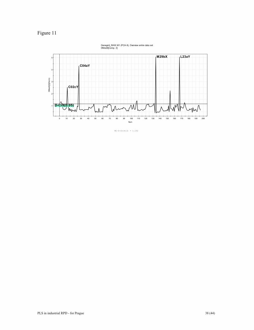
PLS in industrial RPD - for Prague 38 (44)
Figure 11
1
2
3
4
5
0 10 20 30 40 50 60 70 80 90 100 110 120 130 140 150 160 170 180 190 200
DM
odX[
2](N
orm
)
Num
Genegrid_RAW.M1 (PCA-X), Overview entire data setDModX[Comp. 2]
M1-D-Crit[2] = 1.152
C02cY
C04aY
M29bX L23aY
D-Crit(0.05)

PLS in industrial RPD - for Prague 39 (44)
Figure 12
-40
-30
-20
-10
0
10
20
30
40
-50 -40 -30 -20 -10 0 10 20 30 40
t[2]
t[1]
Genegrid_RAW.M9 (PLS-DA), PLS-DA controls & high UVt[Comp. 1]/t[Comp. 2]Colored according to classes in M9
Ellipse: Hotelling T2 (0.95)
Class 1Class 2
HHHHHHHHHHHH
HHHH
HHHHHHHH HHHH
HH
HH
HHH
HHHHH
HH
HH
HHHH
C CC CC C
C
CCCCCC
CCCCCC
CC
C
C CC CC CC C CCCC
CC CCCCCC
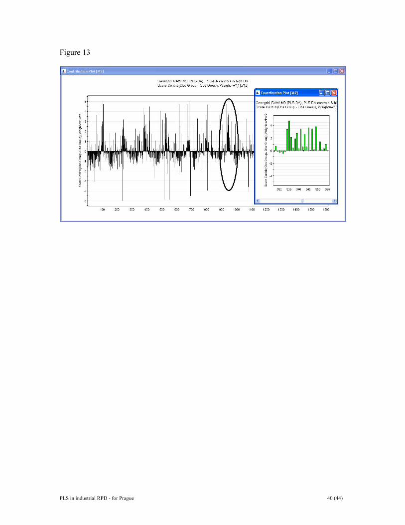
PLS in industrial RPD - for Prague 40 (44)
Figure 13

PLS in industrial RPD - for Prague 41 (44)
Figure 14
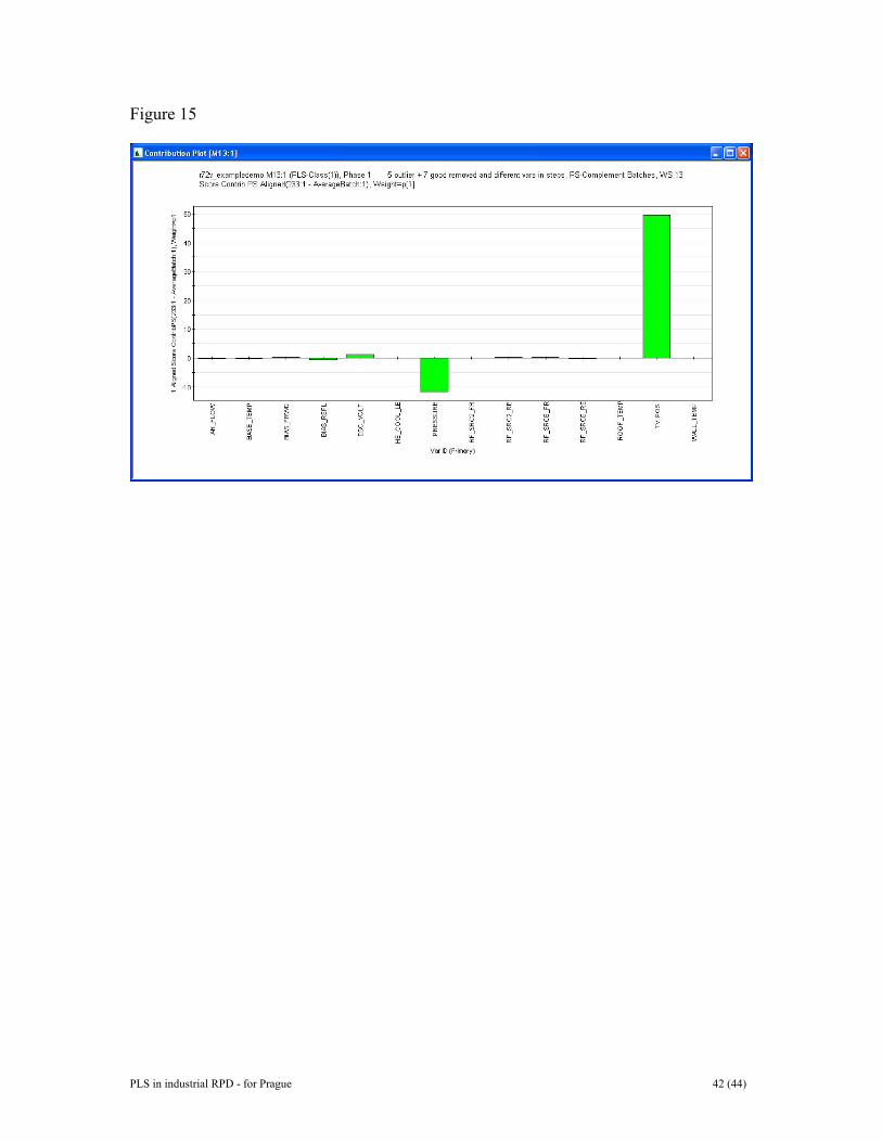
PLS in industrial RPD - for Prague 42 (44)
Figure 15
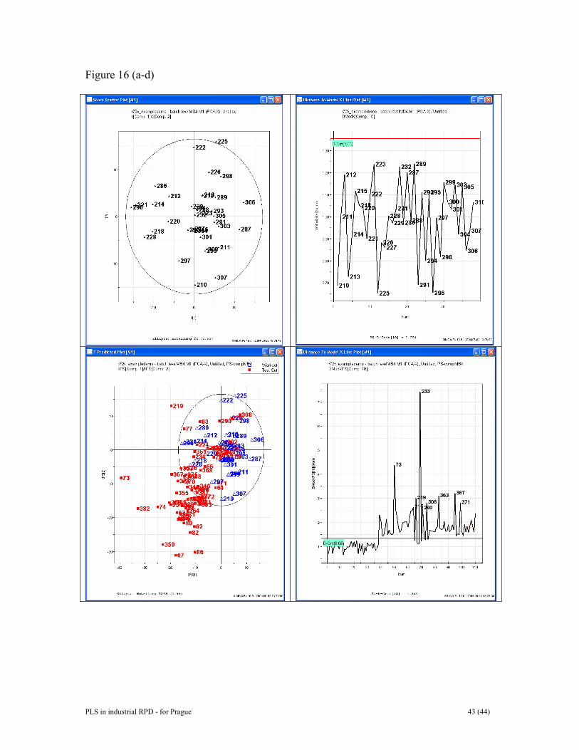
PLS in industrial RPD - for Prague 43 (44)
Figure 16 (a-d)
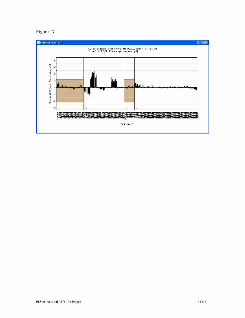
PLS in industrial RPD - for Prague 44 (44)
Figure 17