
Linear least squares - RELATE
118
Least Squares Data Fitting Existence, Uniqueness, and Conditioning Solving Linear Least Squares Problems Outline 1 Least Squares Data Fitting 2 Existence, Uniqueness, and Conditioning 3 Solving Linear Least Squares Problems Michael T. Heath Scientific Computing 2 / 61
-
Upload
khangminh22 -
Category
Documents
-
view
0 -
download
0
Transcript of Linear least squares - RELATE

Least Squares Data FittingExistence, Uniqueness, and Conditioning
Solving Linear Least Squares Problems
Outline
1 Least Squares Data Fitting
2 Existence, Uniqueness, and Conditioning
3 Solving Linear Least Squares Problems
Michael T. Heath Scientific Computing 2 / 61
Least Squares Data FittingExistence, Uniqueness, and Conditioning
Solving Linear Least Squares Problems
Least SquaresData Fitting
Method of Least Squares
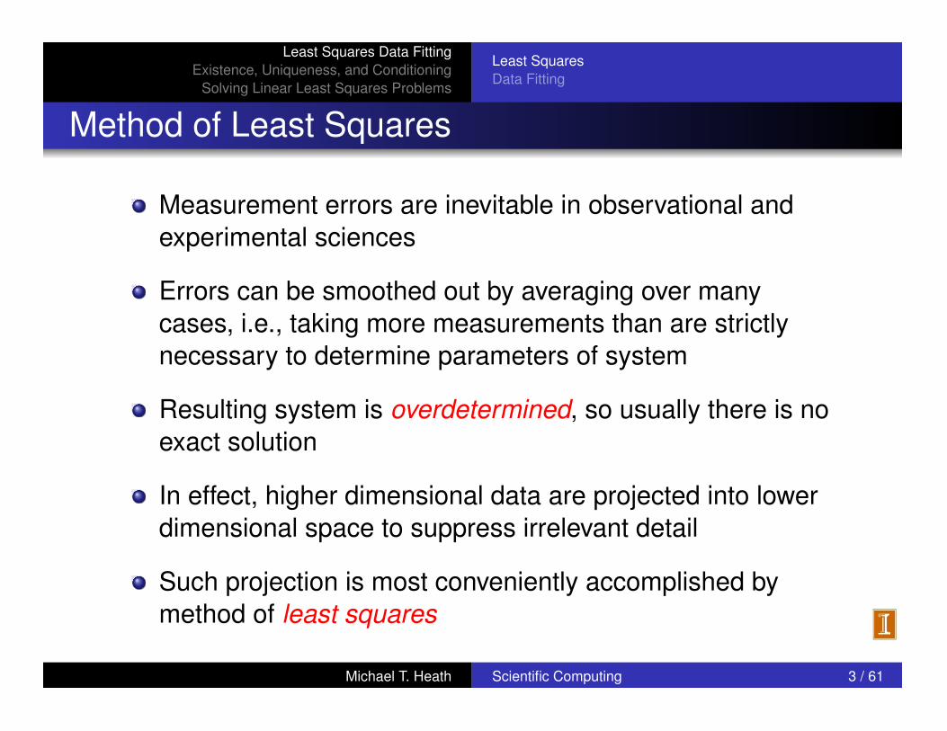
Measurement errors are inevitable in observational andexperimental sciences
Errors can be smoothed out by averaging over manycases, i.e., taking more measurements than are strictlynecessary to determine parameters of system
Resulting system is overdetermined, so usually there is noexact solution
In effect, higher dimensional data are projected into lowerdimensional space to suppress irrelevant detail
Such projection is most conveniently accomplished bymethod of least squares
Michael T. Heath Scientific Computing 3 / 61

Least Squares Data FittingExistence, Uniqueness, and Conditioning
Solving Linear Least Squares Problems
Least SquaresData Fitting
Linear Least Squares
For linear problems, we obtain overdetermined linearsystem Ax = b, with m⇥ n matrix A, m > n
System is better written Ax ⇠=
b, since equality is usuallynot exactly satisfiable when m > n
Least squares solution x minimizes squared Euclideannorm of residual vector r = b�Ax,
min
x
krk22
= min
x
kb�Axk22
Michael T. Heath Scientific Computing 4 / 61

Least Squares Idea
This system is overdetermined. There are more equations than unknowns.
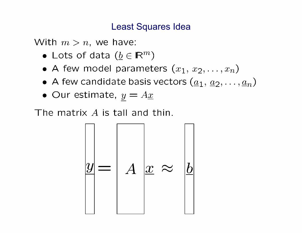
Least Squares Idea
❑ With m > n, we have: ❑ Lots of data ( b ) ❑ A few parameters (

Most Important Picture
❑ The vector y is the orthogonal projection of b onto span(A).
❑ The projection results in minimization of || r ||2 , which, as we shall see, is equivalent to having r := b – Ax ? span(A)
Least Squares Data FittingExistence, Uniqueness, and Conditioning
Solving Linear Least Squares Problems
Existence and UniquenessOrthogonalityConditioning
Orthogonality, continued
Geometric relationships among b, r, and span(A) areshown in diagram
Michael T. Heath Scientific Computing 13 / 61

1D Projection
• Consider the 1D subspace of lR2 spanned by a1:
↵a1 2 span{a1}.
• The projection of a point b 2 lR2 onto span{a1} is the point onthe line y = ↵a1 that is closest to b.
• To find the projection, we look for the value ↵ that minimizes||r|| = ||↵a1 � b|| in the 2-norm. (Other norms are also possible.)
a1
↵a1b
b� ↵a1
a1
y = ↵a1
b
r = b� ↵a1
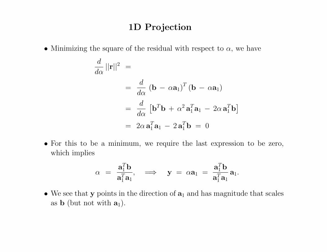
1D Projection
• Minimizing the square of the residual with respect to ↵, we have
d
d↵||r||2 =
=d
d↵(b � ↵a1)
T (b � ↵a1)
=d
d↵
⇥b
Tb + ↵2
a
T1 a1 � 2↵ a
T1 b
⇤
= 2↵ a
T1 a1 � 2 aT1 b = 0
• For this to be a minimum, we require the last expression to be zero,which implies
↵ =a
T1 b
a
T1 a1
, =) y = ↵a1 =a
T1 b
a
T1 a1
a1.
• We see that y points in the direction of a1 and has magnitude that scalesas b (but not with a1).

Projection in Higher Dimensions
• Here, we have basis coe�cients xi written as x = [x1 . . . xn]T .
• As before, we minimize the square of the norm of the residual
||r||2 = ||Ax� b||2
= (Ax � b)T (Ax � b)
= bTb � bTAx � (Ax)T b + xTATAx
= bTb + xTATAx � 2xTATb.
• As in the 1D case, we require stationarity with respect to all coe�cients
d
dxi||r||2 = 0
• The first term is constant.
• The second and third are more complex.

Projection in Higher Dimensions
• Define c = ATb and H = ATA such that
xTATb = xTc = x1c1 + x2c2 + . . . xncn.
xTATAx = xTHx =nX
j=1
nX
k=1
xkHkjxj
• Di↵erentiating with respect to xi,
d
dxi
�xTATb
�= ci =
�ATb
�i, and
d
dxi
�xTHx
�=
nX
j=1
Hijxj +nX
k=1
xk Hki
= 2nX
j=1
Hij xj = 2 (Hx)i .

Projection in Higher Dimensions
• From the preceding pages, the minimum is realized when
0 =d
dxi
�xTATAx � 2xTATb
�= 2
�ATAx � ATb
�i, i = 1, . . . , n
• Or, in matrix form:
x =�ATA
��1ATb.
• As in the 1D case, our projection is
y = Ax = A�ATA
��1ATb.
• y has units and length that scale with b, but it lies in the range of A.
• It is the projection of b onto R(A).

Important Example: Weighted Least Squares
• Standard inner-product:
(u, v)2 :=mX
i=1
ui vi = u
Tv,
||r||22 =mX
i=1
r
2i = r
Tr,
• Consider weighted inner-product:
(u, v)W :=mX
i=1
uiwi vi = u
TWv, where
W =
2
6664
w1
w2. . .
wm
3
7775, wi > 0.
||r||2w =mX
i=1
wir2i = r
TWr,

• If we want to minimize in a weighted norm:
Find x 2 lRnsuch that ||r||2W is minimized.
• Require
d
dxi
h(b � Ax)T W (b � Ax)
i
=d
dxi
⇥b
TWb + x
TA
TWAx � x
TA
TWb� b
TWAx
⇤
=d
dxi
⇥x
TA
TWAx � 2xT
A
TWb
⇤
= 0.
• Thus,x =
�A
TWA
��1A
TWb,
y = Ax = A
�A
TWA
��1A
TWb, ⇡ b.
• y is the weighted least-squares approximation to b.
• Works for any SPD W , not just (positive) diagonal ones.
• Can be used to solve linear systems.

Using Least Squares to Solve Linear Systems
• In particular, suppose Wb = z.
• Linear system — z is right-hand side, known.— b is unknown.
• Want to find weighted least-squares fit, y ⇡ b, minimizing||y � b ||2W with y 2 R(A).
• Answer:
y = A
�A
TWA
��1A
TWb
= A
�A
TWA
��1A
Tz
= Ax

Using Least Squares to Solve Linear Systems
• Suppose W is a sparse m⇥m matrix with (say) m > 106.
• Factor cost is likely very large (superlinear in m).
• If A = (a1 a2 · · · an), n ⌧ m, can form n vectors,
WA = (Wa1Wa2 · · · Wan),
and the Gram matrix, W̃ = A
TWA = [aTi Waj], and solve
W̃x = A
Tz =
0
BBB@
a
T1 z
a
T2 z...
a
Tnz
1
CCCA,
which requires solution of a small n⇥ n system, W̃ .
Using Least Squares to Solve Linear Systems
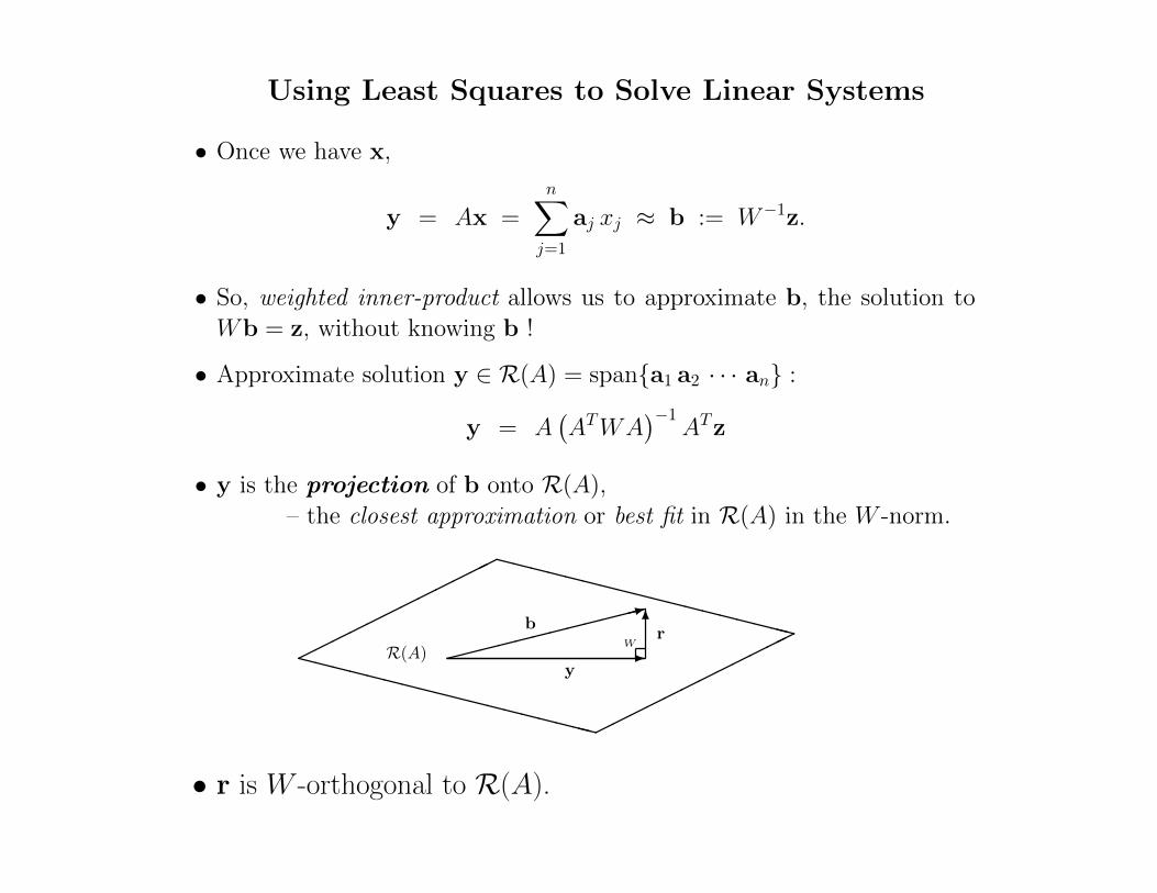
• Once we have x,
y = Ax =nX
j=1
aj xj ⇡ b := W
�1z.
• So, weighted inner-product allows us to approximate b, the solution toWb = z, without knowing b !
• Approximate solution y 2 R(A) = span{a1 a2 · · · an} :
y = A
�A
TWA
��1A
Tz
• y is the projection of b onto R(A),– the closest approximation or best fit in R(A) in the W -norm.
XXXXXXXXXXXXXXXXXX
������������XXXXXXXXXXXXXXXXXX
������������W⇠⇠⇠⇠⇠⇠⇠⇠⇠⇠⇠⇠:6
-R(A)r
y
b
• r is W -orthogonal to R(A).

Using Least Squares to Solve Linear Systems
• Very often can have accurate approximations with n ⌧ m.
• In particular, if :=cond(W ), and
R(A) = span{Wb, W
2b, · · · ,W k
b}= span{z, Wz, · · · ,W k�1
z},
then can have an accurate answer with k ⇡p.
• Can keep increasing R(A) with additional matrix-vector products.
• This method corresponds to conjugate gradient iteration applied to theSPD system Wb = z.

Back to Standard Least Squares
❑ Suppose we have observational data, { bi } at some independent times { ti } (red circles).
❑ The ti s do not need to be sorted and can in fact be repeated.
❑ We wish to fit a smooth model (blue curve) to the data so we can compactly describe (and perhaps integrate or differentiate) the functional relationship between b(t) and t.
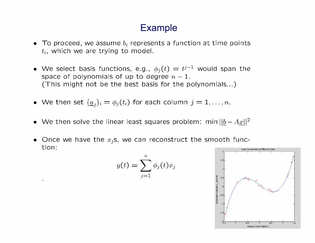
Example

Matlab Example % Linear Least Squares Demo degree=3; m=20; n=degree+1; t=3*(rand(m,1)-0.5); b = t.^3 - t; b=b+0.2*rand(m,1); %% Expect: x =~ [ 0 -1 0 1 ] plot(t,b,'ro'), pause %%% DEFINE a_ij = phi_j(t_i) A=zeros(m,n); for j=1:n; A(:,j) = t.^(j-1); end; A0=A; b0=b; % Save A & b. %%%% SOLVE LEAST SQUARES PROBLEM via Normal Equations &&&& x = (A'*A) \ A'*b plot(t,b0,'ro',t,A0*x,'bo',t,1*(b0-A0*x),'kx'), pause plot(t,A0*x,'bo'), pause %% CONSTRUCT SMOOTH APPROXIMATION tt=(0:100)'/100; tt=min(t) + (max(t)-min(t))*tt; S=zeros(101,n); for k=1:n; S(:,k) = tt.^(k-1); end; s=S*x; plot(t,b0,'ro',tt,s,'b-') title('Least Squares Model Fitting to Cubic') xlabel('Independent Variable, t') ylabel('Dependent Variable b_i and y(t)')

Python Least Squares Example
. . .
. . .

Note on the text examples
❑ Note, the text uses similar examples.
❑ The notation in the examples is a bit different from the rest of the derivation… so be sure to pay attention.

Least Squares Data FittingExistence, Uniqueness, and Conditioning
Solving Linear Least Squares Problems
Least SquaresData Fitting
Data Fitting
Given m data points (t
i
, y
i
), find n-vector x of parametersthat gives “best fit” to model function f(t,x),
min
x
mX
i=1
(y
i
� f(t
i
,x))2
Problem is linear if function f is linear in components of x,
f(t,x) = x
1
�
1
(t) + x
2
�
2
(t) + · · ·+ x
n
�
n
(t)
where functions �
j
depend only on t
Problem can be written in matrix form as Ax ⇠=
b, witha
ij
= �
j
(t
i
) and b
i
= y
i
Michael T. Heath Scientific Computing 5 / 61

Least Squares Data FittingExistence, Uniqueness, and Conditioning
Solving Linear Least Squares Problems
Least SquaresData Fitting
Data Fitting
Polynomial fitting
f(t,x) = x
1
+ x
2
t+ x
3
t
2
+ · · ·+ x
n
t
n�1
is linear, since polynomial linear in coefficients, thoughnonlinear in independent variable t
Fitting sum of exponentials
f(t,x) = x
1
e
x2t+ · · ·+ x
n�1
e
xnt
is example of nonlinear problem
For now, we will consider only linear least squaresproblems
Michael T. Heath Scientific Computing 6 / 61

Least Squares Data FittingExistence, Uniqueness, and Conditioning
Solving Linear Least Squares Problems
Least SquaresData Fitting
Example: Data Fitting
Fitting quadratic polynomial to five data points gives linearleast squares problem
Ax =
2
66664
1 t
1
t
2
1
1 t
2
t
2
2
1 t
3
t
2
3
1 t
4
t
2
4
1 t
5
t
2
5
3
77775
2
4x
1
x
2
x
3
3
5 ⇠=
2
66664
y
1
y
2
y
3
y
4
y
5
3
77775= b
Matrix whose columns (or rows) are successive powers ofindependent variable is called Vandermonde matrix
Michael T. Heath Scientific Computing 7 / 61

Least Squares Data FittingExistence, Uniqueness, and Conditioning
Solving Linear Least Squares Problems
Least SquaresData Fitting
Example, continued
For datat �1.0 �0.5 0.0 0.5 1.0
y 1.0 0.5 0.0 0.5 2.0
overdetermined 5⇥ 3 linear system is
Ax =
2
66664
1 �1.0 1.0
1 �0.5 0.25
1 0.0 0.0
1 0.5 0.25
1 1.0 1.0
3
77775
2
4x
1
x
2
x
3
3
5 ⇠=
2
66664
1.0
0.5
0.0
0.5
2.0
3
77775= b
Solution, which we will see later how to compute, is
x =
⇥0.086 0.40 1.4
⇤T
so approximating polynomial is
p(t) = 0.086 + 0.4t+ 1.4t
2
Michael T. Heath Scientific Computing 8 / 61

Least Squares Data FittingExistence, Uniqueness, and Conditioning
Solving Linear Least Squares Problems
Least SquaresData Fitting
Example, continued
Resulting curve and original data points are shown in graph
< interactive example >
Michael T. Heath Scientific Computing 9 / 61

Least Squares Data FittingExistence, Uniqueness, and Conditioning
Solving Linear Least Squares Problems
Existence and UniquenessOrthogonalityConditioning
Existence and Uniqueness
Linear least squares problem Ax ⇠=
b always has solution
Solution is unique if, and only if, columns of A are linearlyindependent, i.e., rank(A) = n, where A is m⇥ n
If rank(A) < n, then A is rank-deficient, and solution oflinear least squares problem is not unique
For now, we assume A has full column rank n
Michael T. Heath Scientific Computing 10 / 61

Least Squares Data FittingExistence, Uniqueness, and Conditioning
Solving Linear Least Squares Problems
Existence and UniquenessOrthogonalityConditioning
Normal Equations
To minimize squared Euclidean norm of residual vector
krk22
= rTr = (b�Ax)T (b�Ax)
= bTb� 2xTATb+ xTATAx
take derivative with respect to x and set it to 0,
2ATAx� 2ATb = 0
which reduces to n⇥ n linear system of normal equations
ATAx = ATb
Michael T. Heath Scientific Computing 11 / 61
Least Squares Data FittingExistence, Uniqueness, and Conditioning
Solving Linear Least Squares Problems
Existence and UniquenessOrthogonalityConditioning
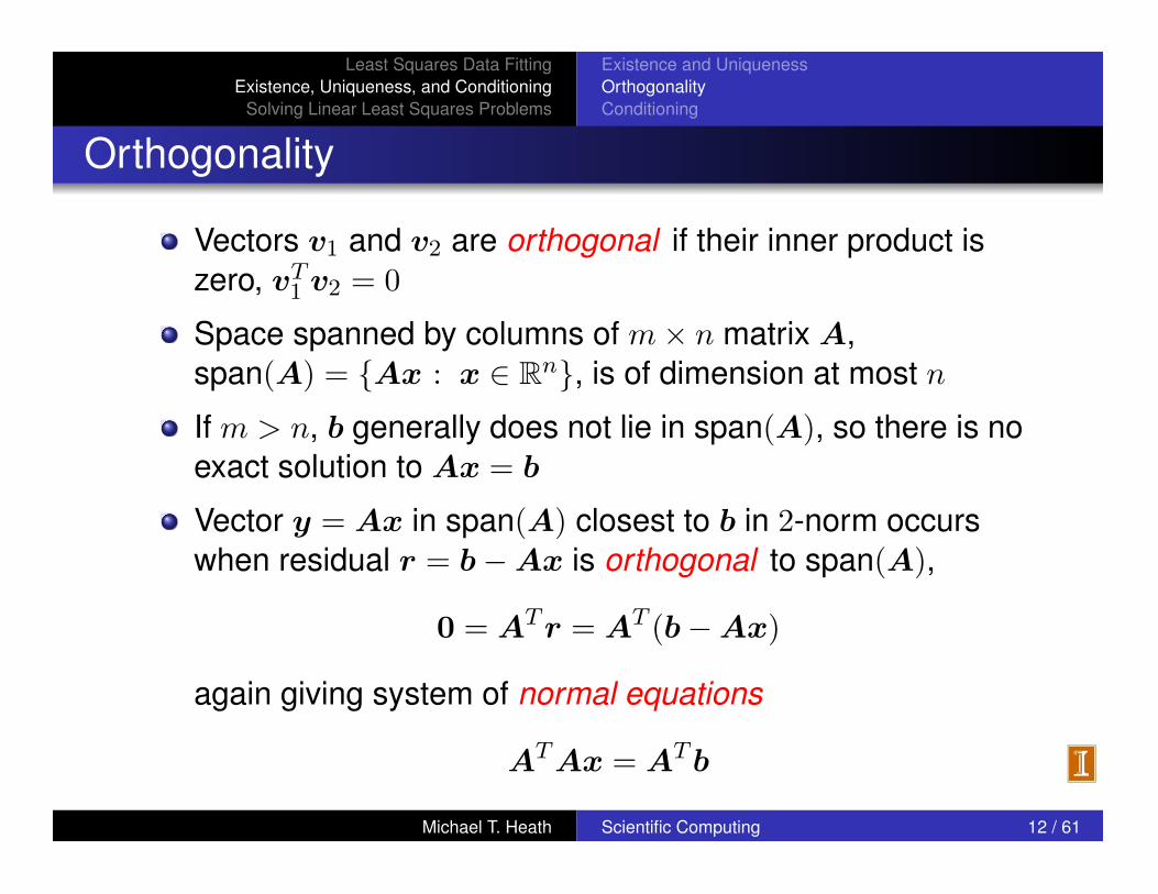
Orthogonality
Vectors v1
and v2
are orthogonal if their inner product iszero, vT
1
v2
= 0
Space spanned by columns of m⇥ n matrix A,span(A) = {Ax : x 2 Rn}, is of dimension at most n
If m > n, b generally does not lie in span(A), so there is noexact solution to Ax = b
Vector y = Ax in span(A) closest to b in 2-norm occurswhen residual r = b�Ax is orthogonal to span(A),
0 = ATr = AT
(b�Ax)
again giving system of normal equations
ATAx = ATb
Michael T. Heath Scientific Computing 12 / 61

Least Squares Data FittingExistence, Uniqueness, and Conditioning
Solving Linear Least Squares Problems
Existence and UniquenessOrthogonalityConditioning
Orthogonality, continued
Geometric relationships among b, r, and span(A) areshown in diagram
Michael T. Heath Scientific Computing 13 / 61

Least Squares Data FittingExistence, Uniqueness, and Conditioning
Solving Linear Least Squares Problems
Existence and UniquenessOrthogonalityConditioning
Orthogonal Projectors
Matrix P is orthogonal projector if it is idempotent(P 2
= P ) and symmetric (P T
= P )
Orthogonal projector onto orthogonal complementspan(P )
? is given by P? = I � P
For any vector v,
v = (P + (I � P )) v = Pv + P?v
For least squares problem Ax ⇠=
b, if rank(A) = n, then
P = A(ATA)
�1AT
is orthogonal projector onto span(A), and
b = Pb+ P?b = Ax+ (b�Ax) = y + r
Michael T. Heath Scientific Computing 14 / 61

Least Squares Data FittingExistence, Uniqueness, and Conditioning
Solving Linear Least Squares Problems
Existence and UniquenessOrthogonalityConditioning
Pseudoinverse and Condition Number
Nonsquare m⇥ n matrix A has no inverse in usual sense
If rank(A) = n, pseudoinverse is defined by
A+
= (ATA)
�1AT
and condition number by
cond(A) = kAk2
· kA+k2
By convention, cond(A) = 1 if rank(A) < n
Just as condition number of square matrix measurescloseness to singularity, condition number of rectangularmatrix measures closeness to rank deficiency
Least squares solution of Ax ⇠=
b is given by x = A+ b
Michael T. Heath Scientific Computing 15 / 61

Least Squares Data FittingExistence, Uniqueness, and Conditioning
Solving Linear Least Squares Problems
Existence and UniquenessOrthogonalityConditioning
Sensitivity and Conditioning
Sensitivity of least squares solution to Ax ⇠=
b depends onb as well as A
Define angle ✓ between b and y = Ax by
cos(✓) =
kyk2
kbk2
=
kAxk2
kbk2
Bound on perturbation �x in solution x due to perturbation�b in b is given by
k�xk2
kxk2
cond(A)
1
cos(✓)
k�bk2
kbk2
Michael T. Heath Scientific Computing 16 / 61

Least Squares Data FittingExistence, Uniqueness, and Conditioning
Solving Linear Least Squares Problems
Existence and UniquenessOrthogonalityConditioning
Sensitivity and Conditioning, contnued
Similarly, for perturbation E in matrix A,
k�xk2
kxk2
/�[cond(A)]
2
tan(✓) + cond(A)
� kEk2
kAk2
Condition number of least squares solution is aboutcond(A) if residual is small, but can be squared orarbitrarily worse for large residual
Michael T. Heath Scientific Computing 17 / 61

Least Squares Data FittingExistence, Uniqueness, and Conditioning
Solving Linear Least Squares Problems
Normal EquationsOrthogonal MethodsSVD
Normal Equations Method
If m⇥ n matrix A has rank n, then symmetric n⇥ n matrixATA is positive definite, so its Cholesky factorization
ATA = LLT
can be used to obtain solution x to system of normalequations
ATAx = ATb
which has same solution as linear least squares problemAx ⇠
=
b
Normal equations method involves transformations
rectangular �! square �! triangular
Michael T. Heath Scientific Computing 18 / 61

Spoiler: Normal Equations not Recommended
❑ So far, our examples have used normal equations approach, as do the next examples.
❑ After the introduction, most of this chapter is devoted to better methods in which columns of A are first orthogonalized.
❑ Orthogonalization methods of choice:
❑ Householder transformations (very stable) ❑ Givens rotations (stable, and often cheaper than Householder) ❑ Gram-Schmidt (better than normal eqns, but not great) ❑ Modified Gram-Schmidt (better than “classical” Gram-Schmidt)

Least Squares Data FittingExistence, Uniqueness, and Conditioning
Solving Linear Least Squares Problems
Normal EquationsOrthogonal MethodsSVD
Example: Normal Equations MethodFor polynomial data-fitting example given previously,normal equations method gives
ATA =
2
41 1 1 1 1
�1.0 �0.5 0.0 0.5 1.0
1.0 0.25 0.0 0.25 1.0
3
5
2
66664
1 �1.0 1.0
1 �0.5 0.25
1 0.0 0.0
1 0.5 0.25
1 1.0 1.0
3
77775
=
2
45.0 0.0 2.5
0.0 2.5 0.0
2.5 0.0 2.125
3
5,
ATb =
2
41 1 1 1 1
�1.0 �0.5 0.0 0.5 1.0
1.0 0.25 0.0 0.25 1.0
3
5
2
66664
1.0
0.5
0.0
0.5
2.0
3
77775=
2
44.0
1.0
3.25
3
5
Michael T. Heath Scientific Computing 19 / 61
Least Squares Data FittingExistence, Uniqueness, and Conditioning
Solving Linear Least Squares Problems
Normal EquationsOrthogonal MethodsSVD
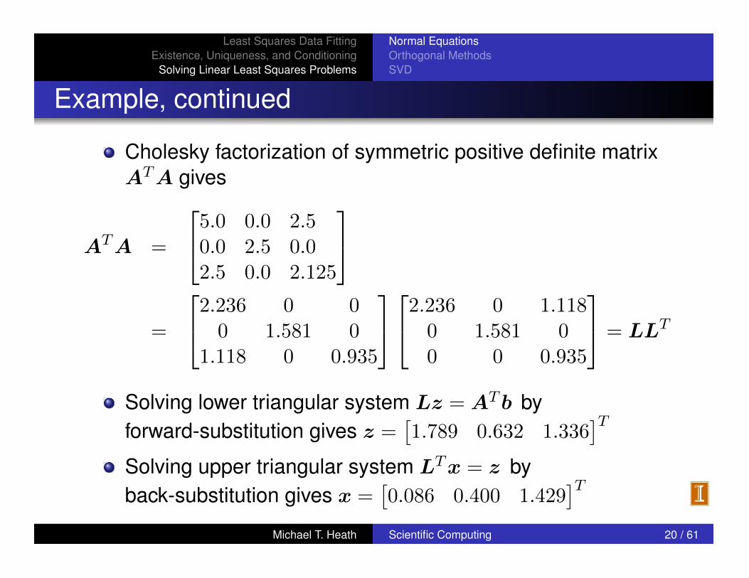
Example, continued
Cholesky factorization of symmetric positive definite matrixATA gives
ATA =
2
45.0 0.0 2.5
0.0 2.5 0.0
2.5 0.0 2.125
3
5
=
2
42.236 0 0
0 1.581 0
1.118 0 0.935
3
5
2
42.236 0 1.118
0 1.581 0
0 0 0.935
3
5= LLT
Solving lower triangular system Lz = ATb byforward-substitution gives z =
⇥1.789 0.632 1.336
⇤T
Solving upper triangular system LTx = z byback-substitution gives x =
⇥0.086 0.400 1.429
⇤T
Michael T. Heath Scientific Computing 20 / 61
Least Squares Data FittingExistence, Uniqueness, and Conditioning
Solving Linear Least Squares Problems
Normal EquationsOrthogonal MethodsSVD
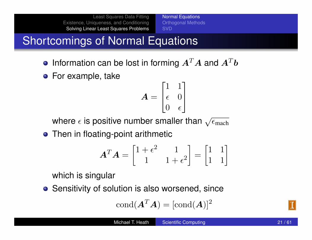
Shortcomings of Normal Equations
Information can be lost in forming ATA and ATb
For example, take
A =
2
41 1
✏ 0
0 ✏
3
5
where ✏ is positive number smaller than p✏mach
Then in floating-point arithmetic
ATA =
1 + ✏
2
1
1 1 + ✏
2
�=
1 1
1 1
�
which is singularSensitivity of solution is also worsened, since
cond(ATA) = [cond(A)]
2
Michael T. Heath Scientific Computing 21 / 61

❑ Avoid normal equations:
❑ ATA x = ATb
❑ Instead, orthogonalize columns of A
❑ Ax = QRx = b
❑ Columns of Q are orthonormal ❑ R is upper triangular

Projection, QR Factorization, Gram-Schmidt
• Recall our linear least squares problem:
y = Ax ⇡ b,
which is equivalent to minimization / orthogonal projection:
r := b � Ax ? R(A)
||r||2 = ||b � y||2 ||b � v||2 8v 2 R(A).
• This problem has solutions
x =
�ATA
��1AT b
y = A�ATA
��1AT b = P b,
where P := A�ATA
��1AT
is the orthogonal projector onto R(A).
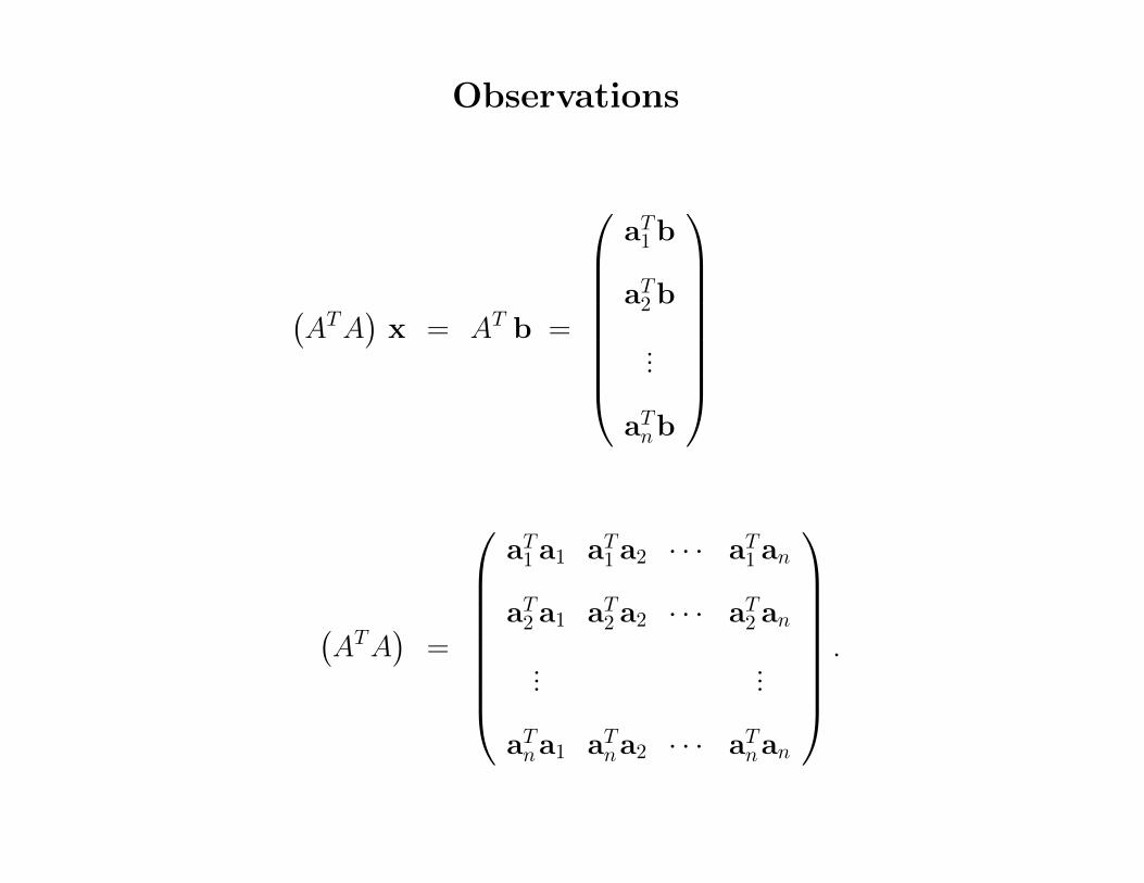
Observations
�ATA
�x = AT b =
0
BBBBBBB@
aT1 b
aT2 b
.
.
.
aTnb
1
CCCCCCCA
�ATA
�=
0
BBBBBBB@
aT1 a1 aT1 a2 · · · aT1 an
aT2 a1 aT2 a2 · · · aT2 an
.
.
.
.
.
.
aTna1 aTna2 · · · aTnan
1
CCCCCCCA
.
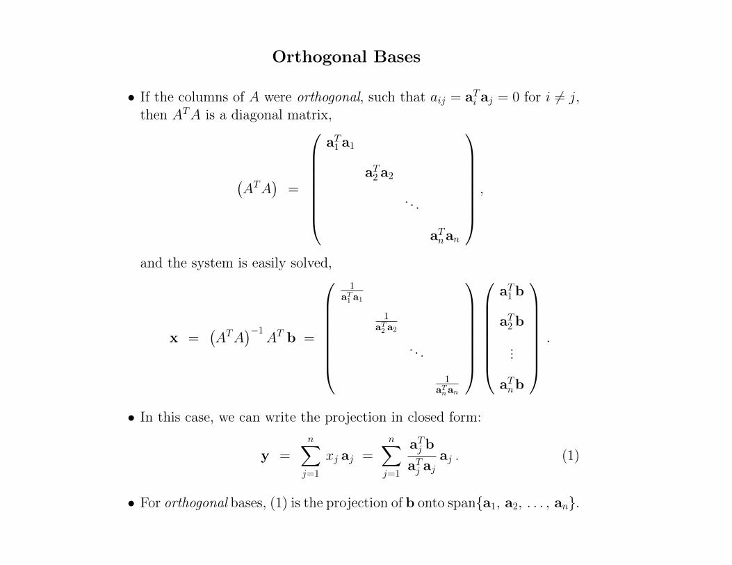
Orthogonal Bases
• If the columns of A were orthogonal, such that aij = aTi aj = 0 for i 6= j,
then ATA is a diagonal matrix,
�ATA
�=
0
BBBBBBB@
aT1 a1
aT2 a2
.
.
.
aTnan
1
CCCCCCCA
,
and the system is easily solved,
x =
�ATA
��1AT b =
0
BBBBBBB@
1aT1 a1
1aT2 a2
.
.
.
1aTnan
1
CCCCCCCA
0
BBBBBBB@
aT1 b
aT2 b
.
.
.
aTnb
1
CCCCCCCA
.
• In this case, we can write the projection in closed form:
y =
nX
j=1
xj aj =
nX
j=1
aTj b
aTj ajaj . (1)
• For orthogonal bases, (1) is the projection of b onto span{a1, a2, . . . , an}.

Orthonormal Bases
• If the columns are orthogonal and normalized such that ||aj|| = 1,
we then have aTj aj = 1, or more generally
aTi aj = �ij, with �ij :=
(1, i = j
0, i 6= jthe Kronecker delta,
• In this case, ATA = I and the orthogonal projection is given by
y = AAT b =
nX
j=1
aj�aTj b
�.
Example: Suppose our model fit is based on sine functions,
sampled uniformly on [0, ⇡]:
�j(t) = sin j ti , ti = ⇡ i/m, i = 1, . . . ,m.
In this case,
A = ( �1(ti) �2(ti) · · · �n(ti) ) ,
ATA =
n
2
I.

QR Factorization
• Generally, we don’t a priori have orthonormal bases.
• We can construct them, however. The process is referred to as QR
factorization.
• We seek factors Q and R such that QR = A with Q orthogonal (or,
unitary, in the complex case).
• There are two cases of interest:
Reduced QR
Q1
R= A
Full QR
Q
R
O= A
• Note that
A = Q
R
O
�=
⇥Q1 Q2
⇤ R
O
�= Q1R.
• The columns of Q1 form an orthonormal basis for R(A).
• The columns of Q2 form an orthonormal basis for R(A)?.

QR Factorization: Gram-Schmidt
• We’ll look at three approaches to QR:
– Gram-Schmidt Orthogonalization,
– Householder Transformations, and
– Givens Rotations
• We start with Gram-Schmidt - which is most intuitive.
• We are interested in generating orthogonal subspaces that match thenested column spaces of A,
span{ a1 } = span{q1 }
span{ a1, a2 } = span{q1, q2 }
span{ a1, a2, a3 } = span{q1, q2, q3 }
span{ a1, a2, . . . , an } = span{q1, q2, . . . , qn }

QR Factorization: Gram-Schmidt
• It’s clear that the conditions
span{ a1 } = span{q1 }
span{ a1, a2 } = span{q1, q2 }
span{ a1, a2, a3 } = span{q1, q2, q3 }
span{ a1, a2, . . . , an } = span{q1, q2, . . . , qn }
are equivalent to the equations
a1 = q1 r11
a2 = q1 r12 + q2 r22
a3 = q1 r13 + q2 r23 + q3 r33
... =... + · · ·
an = q1 r1n + q2 r2n + · · · + qn rnn
i.e., A = QR
(For now, we drop the distinction between Q and Q1, and focus only onthe reduced QR problem.)

Gram-Schmidt Orthogonalization
• The preceding relationship suggests the first algorithm.
Let Qj�1 := [q1 q2 . . .qj�1] , Pj�1 := Qj QTj�1, P?,j�1 := I � Pj�1.
for j = 2, . . . , n� 1
vj = aj � Pj�1 aj = (I � Pj�1) aj = P?,j�1 aj
qj =vj
||vj||=
P?,j�1aj||P?,j�1aj||
end
• This is Gram-Schmidt orthogonalization.
• Each new vector qj starts with aj and subtracts o↵ the projection ontoR(Qj�1), followed by normalization.

Classical Gram-Schmidt Orthogonalization
XXXXXXXXXXXXXXXXXXXX
��������������XXXXXXXXXXXXXXXXXXXX
��������������⌘
⌘⌘⌘
⌘⌘⌘
⌘⌘
⌘⌘⌘
⌘⌘36
-XXXXzq1
���✓
q2
R(Q2)
a3
r33q3
P2a3
P2a3 = Q2QT2 a3
= q1
qT1a3
qT1q1
+ q2
qT2a3
qT2q2
= q1qT1a3 + q
2qT2a3
In general, if Qk is an orthogonal matrix, then
Pk = QkQTk is an orthogonal projector onto R(Qk)
5

Gram-Schmidt Orthogonalization
• The preceding relationship suggests the first algorithm.
Let Qj�1 := [q1 q2 . . .qj�1] , Pj�1 := Qj QTj�1, P?,j�1 := I � Pj�1.
for j = 2, . . . , n� 1
vj = aj � Pj�1 aj = (I � Pj�1) aj = P?,j�1 aj
qj =vj
||vj||=
P?,j�1aj||P?,j�1aj||
end
• This is Gram-Schmidt orthogonalization.
• Each new vector qj starts with aj and subtracts o↵ the projection ontoR(Qj�1), followed by normalization.

Gram-Schmidt: Classical vs. Modified
• We take a closer look at the projection step, vj = aj � Pj�1 aj.
• The classical (unstable) GS projection is executed as
vj = aj
for k = 1, . . . , j � 1,
vj = vj � qk
�qTk aj
�
end
• The modified GS projection is executed as
vj = aj
for k = 1, . . . , j � 1,
vj = vj � qk
�qTkvj
�
end

Mathematical Di↵erence Between CGS and MGS
• Let P̃?,j, := I � qjqTj
• The CGS projection step amounts to
vj =⇣P̃?,j�1 P̃?,j�2 · · · P̃?,1
⌘aj
=⇣I � P̃1 � P̃2 � · · · � P̃j�1
⌘aj
= aj � P̃1aj � P̃2aj � · · · � P̃j�1aj
= aj �j�1X
k=1
P̃k aj.
• The MGS projection step is equivalent to
vj = P̃?,j�1
⇣P̃?,j�2
⇣· · ·
⇣P̃?,1 aj
⌘· · ·
⌘⌘
=⇣I � P̃j�1
⌘ ⇣I � P̃j�2
⌘· · ·
⇣I � P̃1
⌘aj
=j�1Y
k=1
⇣I � P̃k
⌘aj

Mathematical Di↵erence Between CGS and MGS
• Lack of associativity in floating point arithmetic drives the di↵erencebetween CGS and MGS.
• Conceptually, MGS projects the residual, rj := aj � Pj�1aj.
• As we shall see, neither GS nor MGS are as robust asHouseholder transformations.
• Both, however, can be cleaned up with a second-pass through theorthogonalization process. (Just set A = Q and repeat, once.)
MGS is an example of the idea that “small corrections are preferred to large ones: Better to update v by subtracting off the projection of v, rather than the projection of a.

Least Squares Data FittingExistence, Uniqueness, and Conditioning
Solving Linear Least Squares Problems
Normal EquationsOrthogonal MethodsSVD
Gram-Schmidt Orthogonalization
Given vectors a1
and a2
, we seek orthonormal vectors q1
and q2
having same span
This can be accomplished by subtracting from secondvector its projection onto first vector and normalizing bothresulting vectors, as shown in diagram
< interactive example >
Michael T. Heath Scientific Computing 44 / 61

Least Squares Data FittingExistence, Uniqueness, and Conditioning
Solving Linear Least Squares Problems
Normal EquationsOrthogonal MethodsSVD
Gram-Schmidt Orthogonalization
Process can be extended to any number of vectorsa1
, . . . ,ak
, orthogonalizing each successive vector againstall preceding ones, giving classical Gram-Schmidtprocedure
for k = 1 to n
qk
= ak
for j = 1 to k � 1
r
jk
= qTj
ak
qk
= qk
� r
jk
qj
end
r
kk
= kqk
k2
qk
= qk
/r
kk
end
Resulting qk
and r
jk
form reduced QR factorization of A
Michael T. Heath Scientific Computing 45 / 61
! Coefficient involves original ak

Least Squares Data FittingExistence, Uniqueness, and Conditioning
Solving Linear Least Squares Problems
Normal EquationsOrthogonal MethodsSVD
Modified Gram-Schmidt
Classical Gram-Schmidt procedure often suffers loss oforthogonality in finite-precision
Also, separate storage is required for A, Q, and R, sinceoriginal a
k
are needed in inner loop, so qk
cannot overwritecolumns of A
Both deficiencies are improved by modified Gram-Schmidtprocedure, with each vector orthogonalized in turn againstall subsequent vectors, so q
k
can overwrite ak
Michael T. Heath Scientific Computing 46 / 61

Least Squares Data FittingExistence, Uniqueness, and Conditioning
Solving Linear Least Squares Problems
Normal EquationsOrthogonal MethodsSVD
Modified Gram-Schmidt QR Factorization
Modified Gram-Schmidt algorithm
for k = 1 to n
r
kk
= kak
k2
qk
= ak
/r
kk
for j = k + 1 to n
r
kj
= qTk
aj
aj
= aj
� r
kj
qk
end
end
< interactive example >
Michael T. Heath Scientific Computing 47 / 61
Matlab Demo: house.m
! Coefficient involves modified aj

Classical & Modified GS: Notes

Classical & Modified GS: Notes

Householder Transformations: Notes
Least Squares Data FittingExistence, Uniqueness, and Conditioning
Solving Linear Least Squares Problems
Normal EquationsOrthogonal MethodsSVD
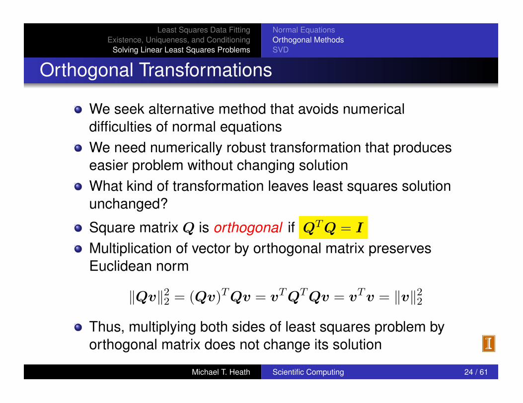
Orthogonal Transformations
We seek alternative method that avoids numericaldifficulties of normal equationsWe need numerically robust transformation that produceseasier problem without changing solutionWhat kind of transformation leaves least squares solutionunchanged?
Square matrix Q is orthogonal if QTQ = I
Multiplication of vector by orthogonal matrix preservesEuclidean norm
kQvk22
= (Qv)TQv = vTQTQv = vTv = kvk22
Thus, multiplying both sides of least squares problem byorthogonal matrix does not change its solution
Michael T. Heath Scientific Computing 24 / 61

Least Squares Data FittingExistence, Uniqueness, and Conditioning
Solving Linear Least Squares Problems
Normal EquationsOrthogonal MethodsSVD
Triangular Least Squares Problems
As with square linear systems, suitable target in simplifyingleast squares problems is triangular form
Upper triangular overdetermined (m > n) least squaresproblem has form
RO
�x ⇠=
b1
b2
�
where R is n⇥ n upper triangular and b is partitionedsimilarly
Residual iskrk2
2
= kb1
�Rxk22
+ kb2
k22
Michael T. Heath Scientific Computing 25 / 61

Least Squares Data FittingExistence, Uniqueness, and Conditioning
Solving Linear Least Squares Problems
Normal EquationsOrthogonal MethodsSVD
Triangular Least Squares Problems, continued
We have no control over second term, kb2
k22
, but first termbecomes zero if x satisfies n⇥ n triangular system
Rx = b1
which can be solved by back-substitution
Resulting x is least squares solution, and minimum sum ofsquares is
krk22
= kb2
k22
So our strategy is to transform general least squaresproblem to triangular form using orthogonal transformationso that least squares solution is preserved
Michael T. Heath Scientific Computing 26 / 61

Least Squares Data FittingExistence, Uniqueness, and Conditioning
Solving Linear Least Squares Problems
Normal EquationsOrthogonal MethodsSVD
QR FactorizationGiven m⇥ n matrix A, with m > n, we seek m⇥m
orthogonal matrix Q such that
A = Q
RO
�
where R is n⇥ n and upper triangularLinear least squares problem Ax ⇠
=
b is then transformedinto triangular least squares problem
QTAx =
RO
�x ⇠=
c1
c2
�= QTb
which has same solution, since
krk22
= kb�Axk22
= kb�Q
RO
�xk2
2
= kQTb�RO
�xk2
2
Michael T. Heath Scientific Computing 27 / 61

Least Squares Data FittingExistence, Uniqueness, and Conditioning
Solving Linear Least Squares Problems
Normal EquationsOrthogonal MethodsSVD
Orthogonal Bases
If we partition m⇥m orthogonal matrix Q = [Q1
Q2
],where Q
1
is m⇥ n, then
A = Q
RO
�= [Q
1
Q2
]
RO
�= Q
1
R
is called reduced QR factorization of A
Columns of Q1
are orthonormal basis for span(A), andcolumns of Q
2
are orthonormal basis for span(A)
?
Q1
QT
1
is orthogonal projector onto span(A)
Solution to least squares problem Ax ⇠=
b is given bysolution to square system
QT
1
Ax = Rx = c1
= QT
1
b
Michael T. Heath Scientific Computing 28 / 61

QR for Solving Least Squares
• Start with Ax ⇡ b
Q
RO
�x ⇡ b
QTQ
RO
�x =
RO
�x ⇡ QT
b = [Q1Q2] b =
c1
c2
�.
• Define the residual,
r := b � y = b � Ax
||r|| = ||b � Ax||
= ||QT(b � Ax) ||
=
����
����
✓c1
c2
◆�
✓Rx
O
◆����
����
=
����
����(c1 �Rx)
c2
����
����
||r||2 = ||c1 � Rx||2 + ||c2||2
• Norm of residual is minimized when Rx = c1 = QT1 b, and
takes on value ||r|| = ||c2||.

QR Factorization and Least Squares Review
• Recall: Ax ⇡ b.
A = QR or A = [Ql Qr]
RO
�,
with Q̃ := [Ql Qr] square.
• If Q̂ and Q̃ are m⇥m orthogonal matrices, then Q̂Q̃ is also orthogonal.
• Least squares problem: Find x such that
r := (QRx � b) ? range(A) ⌘ range(Q).
0 = QTr = QTQRx � QT
b
Rx = QTb
x = R�1QTb.
• Can solve least squares problem by finding QR = A.

• Projection,y = Ax
= QRx
= QQTb
= Q(QTQ)�1QTb
= projection onto R(Q).
• Compare with normal equation approach:
y = A(ATA)�1ATb
= projection onto R(A) ⌘ R(Q).
• Here, QQT and A(ATA)�1AT are both projectors.
• QQT is generally better conditioned than the normal eqution approach.

Least Squares Data FittingExistence, Uniqueness, and Conditioning
Solving Linear Least Squares Problems
Normal EquationsOrthogonal MethodsSVD
Computing QR Factorization
To compute QR factorization of m⇥ n matrix A, withm > n, we annihilate subdiagonal entries of successivecolumns of A, eventually reaching upper triangular form
Similar to LU factorization by Gaussian elimination, but useorthogonal transformations instead of elementaryelimination matrices
Possible methods includeHouseholder transformationsGivens rotationsGram-Schmidt orthogonalization
Michael T. Heath Scientific Computing 29 / 61

Method 2: Householder Transformations

Least Squares Data FittingExistence, Uniqueness, and Conditioning
Solving Linear Least Squares Problems
Normal EquationsOrthogonal MethodsSVD
Householder TransformationsHouseholder transformation has form
H = I � 2
vvT
vTv
for nonzero vector vH is orthogonal and symmetric: H = HT
= H�1
Given vector a, we want to choose v so that
Ha =
2
6664
↵
0
...0
3
7775= ↵
2
6664
1
0
...0
3
7775= ↵e
1
Substituting into formula for H, we can take
v = a� ↵e1
and ↵ = ±kak2
, with sign chosen to avoid cancellationMichael T. Heath Scientific Computing 30 / 61

Householder Reflection
v

Householder Derivation
Ha = a� 2
vTa
vTv
0
BBBBB@
v1
v2.
.
.
vm
1
CCCCCA=
0
BBBBB@
↵
0
.
.
.
0
1
CCCCCA
v = a� ↵e1 � Choose ↵ to avoid cancellation.
vTa = aTa� ↵a1, vTv = aTa� 2↵a1 + ↵2
Ha = a� 2
�aTa� ↵a1
�
aTa� 2↵a1 + ↵2(a� ↵e1)
= a� 2
||a||2 ± ||a||a12||a||2 ± 2||a||a1
(a� ↵e1)
= a� (a� ↵e1) = ↵e1.
Choose ↵ = �sign(a1)||a|| = �✓
a1|a1|
◆||a||.
Least Squares Data FittingExistence, Uniqueness, and Conditioning
Solving Linear Least Squares Problems
Normal EquationsOrthogonal MethodsSVD
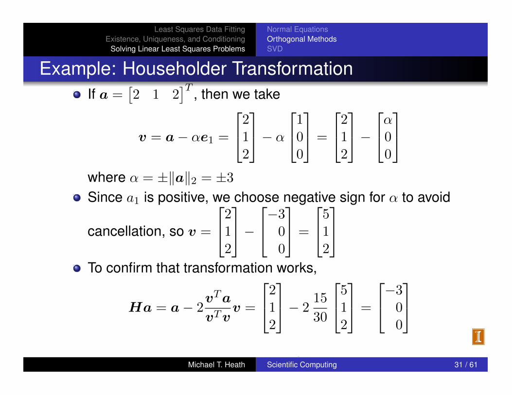
Example: Householder TransformationIf a =
⇥2 1 2
⇤T , then we take
v = a� ↵e1
=
2
42
1
2
3
5� ↵
2
41
0
0
3
5=
2
42
1
2
3
5�
2
4↵
0
0
3
5
where ↵ = ±kak2
= ±3
Since a
1
is positive, we choose negative sign for ↵ to avoid
cancellation, so v =
2
42
1
2
3
5�
2
4�3
0
0
3
5=
2
45
1
2
3
5
To confirm that transformation works,
Ha = a� 2
vTa
vTvv =
2
42
1
2
3
5� 2
15
30
2
45
1
2
3
5=
2
4�3
0
0
3
5
< interactive example >Michael T. Heath Scientific Computing 31 / 61

Least Squares Data FittingExistence, Uniqueness, and Conditioning
Solving Linear Least Squares Problems
Normal EquationsOrthogonal MethodsSVD
Householder QR Factorization
To compute QR factorization of A, use Householdertransformations to annihilate subdiagonal entries of eachsuccessive column
Each Householder transformation is applied to entirematrix, but does not affect prior columns, so zeros arepreserved
In applying Householder transformation H to arbitraryvector u,
Hu =
✓I � 2
vvT
vTv
◆u = u�
✓2
vTu
vTv
◆v
which is much cheaper than general matrix-vectormultiplication and requires only vector v, not full matrix H
Michael T. Heath Scientific Computing 32 / 61

Least Squares Data FittingExistence, Uniqueness, and Conditioning
Solving Linear Least Squares Problems
Normal EquationsOrthogonal MethodsSVD
Householder QR Factorization, continued
Process just described produces factorization
Hn
· · ·H1
A =
RO
�
where R is n⇥ n and upper triangular
If Q = H1
· · ·Hn
, then A = Q
RO
�
To preserve solution of linear least squares problem,right-hand side b is transformed by same sequence ofHouseholder transformations
Then solve triangular least squares problemRO
�x ⇠=
QTb
Michael T. Heath Scientific Computing 33 / 61

Least Squares Data FittingExistence, Uniqueness, and Conditioning
Solving Linear Least Squares Problems
Normal EquationsOrthogonal MethodsSVD
Householder QR Factorization, continued
For solving linear least squares problem, product Q ofHouseholder transformations need not be formed explicitly
R can be stored in upper triangle of array initiallycontaining A
Householder vectors v can be stored in (now zero) lowertriangular portion of A (almost)
Householder transformations most easily applied in thisform anyway
Michael T. Heath Scientific Computing 34 / 61

Least Squares Data FittingExistence, Uniqueness, and Conditioning
Solving Linear Least Squares Problems
Normal EquationsOrthogonal MethodsSVD
Example: Householder QR Factorization
For polynomial data-fitting example given previously, with
A =
2
66664
1 �1.0 1.0
1 �0.5 0.25
1 0.0 0.0
1 0.5 0.25
1 1.0 1.0
3
77775, b =
2
66664
1.0
0.5
0.0
0.5
2.0
3
77775
Householder vector v1
for annihilating subdiagonal entriesof first column of A is
v1
=
2
66664
1
1
1
1
1
3
77775�
2
66664
�2.236
0
0
0
0
3
77775=
2
66664
3.236
1
1
1
1
3
77775
Michael T. Heath Scientific Computing 35 / 61

Least Squares Data FittingExistence, Uniqueness, and Conditioning
Solving Linear Least Squares Problems
Normal EquationsOrthogonal MethodsSVD
Example, continued
Applying resulting Householder transformation H1
yieldstransformed matrix and right-hand side
H1
A =
2
66664
�2.236 0 �1.118
0 �0.191 �0.405
0 0.309 �0.655
0 0.809 �0.405
0 1.309 0.345
3
77775, H
1
b =
2
66664
�1.789
�0.362
�0.862
�0.362
1.138
3
77775
Householder vector v2
for annihilating subdiagonal entriesof second column of H
1
A is
v2
=
2
66664
0
�0.191
0.309
0.809
1.309
3
77775�
2
66664
0
1.581
0
0
0
3
77775=
2
66664
0
�1.772
0.309
0.809
1.309
3
77775
Michael T. Heath Scientific Computing 36 / 61

Least Squares Data FittingExistence, Uniqueness, and Conditioning
Solving Linear Least Squares Problems
Normal EquationsOrthogonal MethodsSVD
Example, continued
Applying resulting Householder transformation H2
yields
H2
H1
A =
2
66664
�2.236 0 �1.118
0 1.581 0
0 0 �0.725
0 0 �0.589
0 0 0.047
3
77775, H
2
H1
b =
2
66664
�1.789
0.632
�1.035
�0.816
0.404
3
77775
Householder vector v3
for annihilating subdiagonal entriesof third column of H
2
H1
A is
v3
=
2
66664
0
0
�0.725
�0.589
0.047
3
77775�
2
66664
0
0
0.935
0
0
3
77775=
2
66664
0
0
�1.660
�0.589
0.047
3
77775
Michael T. Heath Scientific Computing 37 / 61
Least Squares Data FittingExistence, Uniqueness, and Conditioning
Solving Linear Least Squares Problems
Normal EquationsOrthogonal MethodsSVD
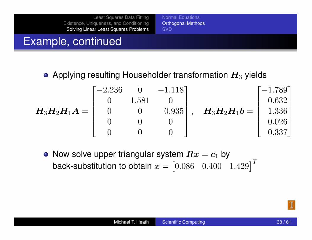
Example, continued
Applying resulting Householder transformation H3
yields
H3
H2
H1
A =
2
66664
�2.236 0 �1.118
0 1.581 0
0 0 0.935
0 0 0
0 0 0
3
77775, H
3
H2
H1
b =
2
66664
�1.789
0.632
1.336
0.026
0.337
3
77775
Now solve upper triangular system Rx = c1
byback-substitution to obtain x =
⇥0.086 0.400 1.429
⇤T
< interactive example >
Michael T. Heath Scientific Computing 38 / 61

kth Householder Transformation (Reflection)

Successive Householder Transformations
2
66664
x x x
x x xx x x
x x xx x x
3
77775H1
�!
2
66664
x x x0 x x0 x x0 x x0 x x
3
77775H2
�!
2
66664
x x x
x x0 x0 x0 x
3
77775H3
�!
2
66664
x x x
x xx00
3
77775
A H1A H2H1A H3H2H1A

Householder Transformations
H1A =
0
BB@
x x x
x x
x x
x x
1
CCA , H1 b �! b(1) =
0
BB@
x
x
x
x
1
CCA
H2H1A =
0
BB@
x x x
x x
xx
1
CCA , H2 b(1) �! b(2) =
0
BB@
x
x
xx
1
CCA
H3H2H1A =
0
BB@
x x x
x xx
1
CCA , H3 b(2) �! b(3) =
✓c1c2
◆.
Questions: How does H3H2H1 relate to Q or Q1??
What is Q in this case?

Method 3: Givens Rotations

Least Squares Data FittingExistence, Uniqueness, and Conditioning
Solving Linear Least Squares Problems
Normal EquationsOrthogonal MethodsSVD
Givens Rotations
Givens rotations introduce zeros one at a timeGiven vector
⇥a
1
a
2
⇤T , choose scalars c and s so that
c s
�s c
� a
1
a
2
�=
↵
0
�
with c
2
+ s
2
= 1, or equivalently, ↵ =
pa
2
1
+ a
2
2
Previous equation can be rewrittena
1
a
2
a
2
�a
1
� c
s
�=
↵
0
�
Gaussian elimination yields triangular systema
1
a
2
0 �a
1
� a
2
2
/a
1
� c
s
�=
↵
�↵a
2
/a
1
�
Michael T. Heath Scientific Computing 39 / 61
Least Squares Data FittingExistence, Uniqueness, and Conditioning
Solving Linear Least Squares Problems
Normal EquationsOrthogonal MethodsSVD
Givens Rotations, continued
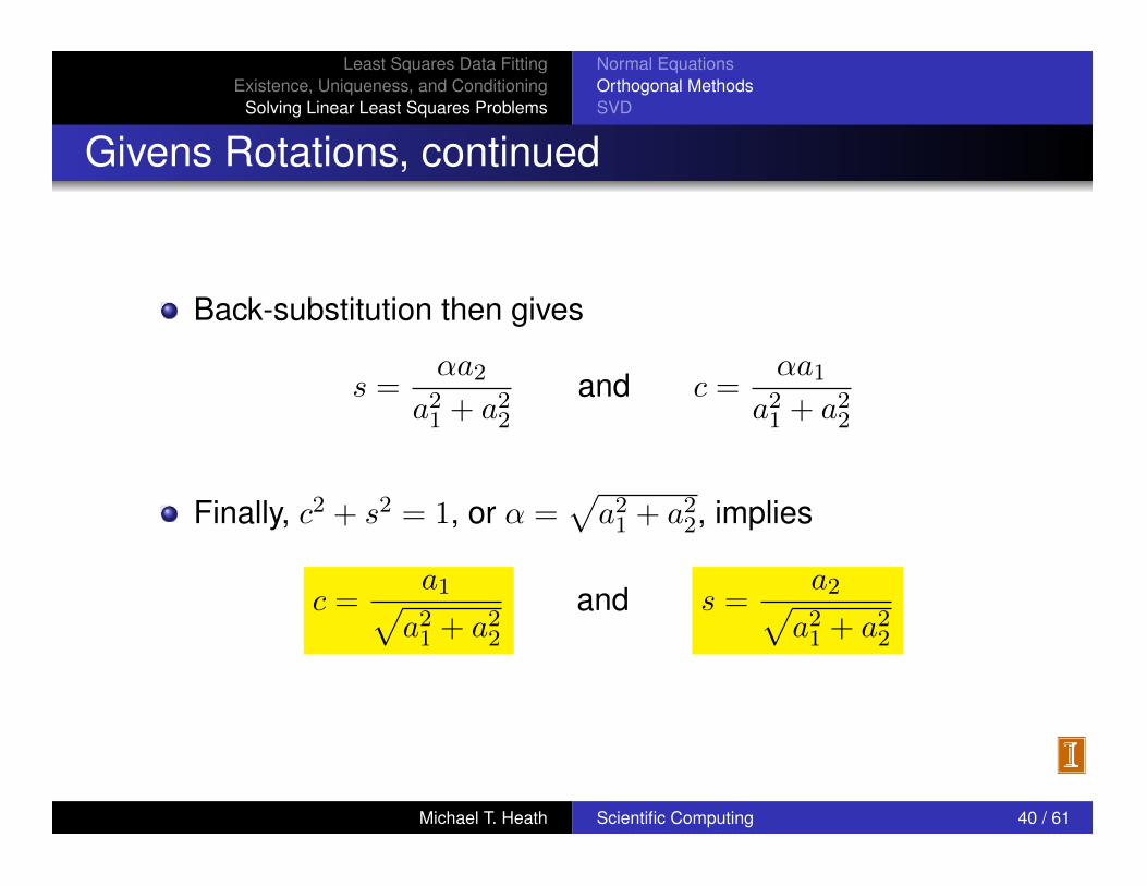
Back-substitution then gives
s =
↵a
2
a
2
1
+ a
2
2
and c =
↵a
1
a
2
1
+ a
2
2
Finally, c2 + s
2
= 1, or ↵ =
pa
2
1
+ a
2
2
, implies
c =
a
1pa
2
1
+ a
2
2
and s =
a
2pa
2
1
+ a
2
2
Michael T. Heath Scientific Computing 40 / 61

2 x 2 Rotation Matrices

Least Squares Data FittingExistence, Uniqueness, and Conditioning
Solving Linear Least Squares Problems
Normal EquationsOrthogonal MethodsSVD
Example: Givens Rotation
Let a =
⇥4 3
⇤T
To annihilate second entry we compute cosine and sine
c =
a
1pa
2
1
+ a
2
2
=
4
5
= 0.8 and s =
a
2pa
2
1
+ a
2
2
=
3
5
= 0.6
Rotation is then given by
G =
c s
�s c
�=
0.8 0.6
�0.6 0.8
�
To confirm that rotation works,
Ga =
0.8 0.6
�0.6 0.8
� 4
3
�=
5
0
�
Michael T. Heath Scientific Computing 41 / 61

Least Squares Data FittingExistence, Uniqueness, and Conditioning
Solving Linear Least Squares Problems
Normal EquationsOrthogonal MethodsSVD
Givens QR Factorization
More generally, to annihilate selected component of vectorin n dimensions, rotate target component with anothercomponent
2
66664
1 0 0 0 0
0 c 0 s 0
0 0 1 0 0
0 �s 0 c 0
0 0 0 0 1
3
77775
2
66664
a
1
a
2
a
3
a
4
a
5
3
77775=
2
66664
a
1
↵
a
3
0
a
5
3
77775
By systematically annihilating successive entries, we canreduce matrix to upper triangular form using sequence ofGivens rotations
Each rotation is orthogonal, so their product is orthogonal,producing QR factorization
Michael T. Heath Scientific Computing 42 / 61

Givens Rotations
Gk =
2
664
I
G
I
3
775
• If G is a 2 ⇥ 2 block, Gk Selectively acts on two adjacent rows.
• The full rows.

Least Squares Data FittingExistence, Uniqueness, and Conditioning
Solving Linear Least Squares Problems
Normal EquationsOrthogonal MethodsSVD
Givens QR Factorization
Straightforward implementation of Givens method requiresabout 50% more work than Householder method, and alsorequires more storage, since each rotation requires twonumbers, c and s, to define it
These disadvantages can be overcome, but requires morecomplicated implementation
Givens can be advantageous for computing QRfactorization when many entries of matrix are already zero,since those annihilations can then be skipped
< interactive example >
Michael T. Heath Scientific Computing 43 / 61

Givens QR
❑ A particularly attractive use of Givens QR is when A is upper Hessenberg – A is upper triangular with one additional nonzero diagonal below the main one: Aij = 0 if i > j+1
❑ In this case, we require Givens row operations applied only n times, instead of O(n2) times.
❑ Work for Givens is thus O(n2), vs. O(n3) for Householder.
❑ Upper Hessenberg matrices arise when computing eigenvalues.

Successive Givens Rotations
As with Householder transformations, we apply successive Givens rotations,G1, G2, etc.
G1A =
0
BB@
x x xx x x
x x x
x x
1
CCA , H1 b �! b(1) =
0
BB@
xx
x
x
1
CCA
G2G1A =
0
BB@
x x x
x x x
x x
x x
1
CCA , G2 b(1) �! b(2) =
0
BB@
x
x
x
x
1
CCA
G3G2G1A =
0
BB@
x x x
x x
x xx x
1
CCA , G3 b(2) �! b(3) =
0
BB@
x
x
xx
1
CCA
• How many Givens rotations (total) are required for the m ⇥ n
case?
• How does . . . G3G2G1 relate to Q or Q1?
• What is Q in this case?

Least Squares Data FittingExistence, Uniqueness, and Conditioning
Solving Linear Least Squares Problems
Normal EquationsOrthogonal MethodsSVD
Rank Deficiency
If rank(A) < n, then QR factorization still exists, but yieldssingular upper triangular factor R, and multiple vectors xgive minimum residual norm
Common practice selects minimum residual solution xhaving smallest norm
Can be computed by QR factorization with column pivotingor by singular value decomposition (SVD)
Rank of matrix is often not clear cut in practice, so relativetolerance is used to determine rank
Michael T. Heath Scientific Computing 48 / 61

Least Squares Data FittingExistence, Uniqueness, and Conditioning
Solving Linear Least Squares Problems
Normal EquationsOrthogonal MethodsSVD
Example: Near Rank Deficiency
Consider 3⇥ 2 matrix
A =
2
40.641 0.242
0.321 0.121
0.962 0.363
3
5
Computing QR factorization,
R =
1.1997 0.4527
0 0.0002
�
R is extremely close to singular (exactly singular to 3-digitaccuracy of problem statement)If R is used to solve linear least squares problem, result ishighly sensitive to perturbations in right-hand sideFor practical purposes, rank(A) = 1 rather than 2, becausecolumns are nearly linearly dependent
Michael T. Heath Scientific Computing 49 / 61

Least Squares Data FittingExistence, Uniqueness, and Conditioning
Solving Linear Least Squares Problems
Normal EquationsOrthogonal MethodsSVD
QR with Column Pivoting
Instead of processing columns in natural order, select forreduction at each stage column of remaining unreducedsubmatrix having maximum Euclidean norm
If rank(A) = k < n, then after k steps, norms of remainingunreduced columns will be zero (or “negligible” infinite-precision arithmetic) below row k
Yields orthogonal factorization of form
QTAP =
R SO O
�
where R is k ⇥ k, upper triangular, and nonsingular, andpermutation matrix P performs column interchanges
Michael T. Heath Scientific Computing 50 / 61
Least Squares Data FittingExistence, Uniqueness, and Conditioning
Solving Linear Least Squares Problems
Normal EquationsOrthogonal MethodsSVD
QR with Column Pivoting, continued
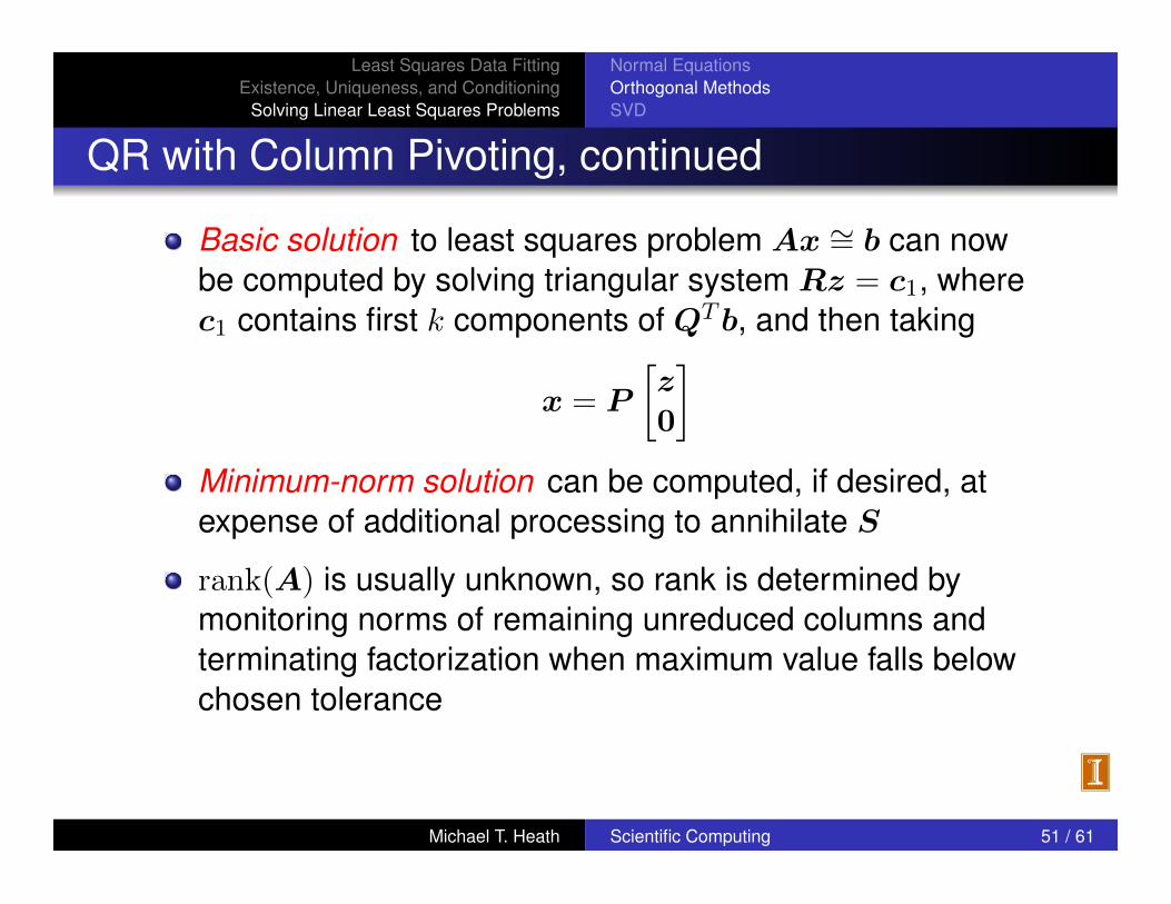
Basic solution to least squares problem Ax ⇠=
b can nowbe computed by solving triangular system Rz = c
1
, wherec1
contains first k components of QTb, and then taking
x = P
z0
�
Minimum-norm solution can be computed, if desired, atexpense of additional processing to annihilate S
rank(A) is usually unknown, so rank is determined bymonitoring norms of remaining unreduced columns andterminating factorization when maximum value falls belowchosen tolerance
< interactive example >
Michael T. Heath Scientific Computing 51 / 61
Classical GS:
q̃k= ak
forj = 1, . . . , k � 1,
rjk = qTjak
q̃k= q̃
k� q
jrjk
end
qk= q̃
k/||q̃
k||
Modified GS:
q̃k= ak
forj = 1, . . . , k � 1,
rjk = qTjq̃k
�q̃k= q̃
k� q
jrjk
end
qk= q̃
k/||q̃
k||
• Modifed GS computes the projection onto qjusing the remainder,
ak �Qj�1ak, rather than simply projecting ak onto qj.
• At each step, you are working with a smaller correction.
• Essentially the same e↵ect is realized by running classical GS twice, firston A, then on Q. On the second pass, the corrections are very small andhence less sensitive to round-o↵.
• Classical GS is attractive for parallel computing. Why?
1

Least Squares Data FittingExistence, Uniqueness, and Conditioning
Solving Linear Least Squares Problems
Normal EquationsOrthogonal MethodsSVD
Comparison of Methods
Forming normal equations matrix ATA requires aboutn
2
m/2 multiplications, and solving resulting symmetriclinear system requires about n3
/6 multiplications
Solving least squares problem using Householder QRfactorization requires about mn
2 � n
3
/3 multiplications
If m ⇡ n, both methods require about same amount ofwork
If m � n, Householder QR requires about twice as muchwork as normal equations
Cost of SVD is proportional to mn
2
+ n
3, withproportionality constant ranging from 4 to 10, depending onalgorithm used
Michael T. Heath Scientific Computing 59 / 61
Least Squares Data FittingExistence, Uniqueness, and Conditioning
Solving Linear Least Squares Problems
Normal EquationsOrthogonal MethodsSVD
Comparison of Methods, continued
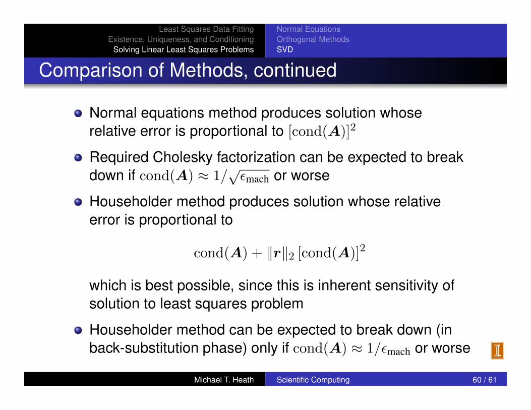
Normal equations method produces solution whoserelative error is proportional to [cond(A)]
2
Required Cholesky factorization can be expected to breakdown if cond(A) ⇡ 1/
p✏mach or worse
Householder method produces solution whose relativeerror is proportional to
cond(A) + krk2
[cond(A)]
2
which is best possible, since this is inherent sensitivity ofsolution to least squares problem
Householder method can be expected to break down (inback-substitution phase) only if cond(A) ⇡ 1/✏mach or worse
Michael T. Heath Scientific Computing 60 / 61

Least Squares Data FittingExistence, Uniqueness, and Conditioning
Solving Linear Least Squares Problems
Normal EquationsOrthogonal MethodsSVD
Comparison of Methods, continued
Householder is more accurate and more broadlyapplicable than normal equations
These advantages may not be worth additional cost,however, when problem is sufficiently well conditioned thatnormal equations provide sufficient accuracy
For rank-deficient or nearly rank-deficient problems,Householder with column pivoting can produce usefulsolution when normal equations method fails outright
SVD is even more robust and reliable than Householder,but substantially more expensive
Michael T. Heath Scientific Computing 61 / 61

Least Squares Data FittingExistence, Uniqueness, and Conditioning
Solving Linear Least Squares Problems
Normal EquationsOrthogonal MethodsSVD
Singular Value Decomposition
Singular value decomposition (SVD) of m⇥ n matrix A hasform
A = U⌃V T
where U is m⇥m orthogonal matrix, V is n⇥ n
orthogonal matrix, and ⌃ is m⇥ n diagonal matrix, with
�
ij
=
⇢0 for i 6= j
�
i
� 0 for i = j
Diagonal entries �
i
, called singular values of A, areusually ordered so that �
1
� �
2
� · · · � �
n
Columns ui
of U and vi
of V are called left and rightsingular vectors
Michael T. Heath Scientific Computing 52 / 61
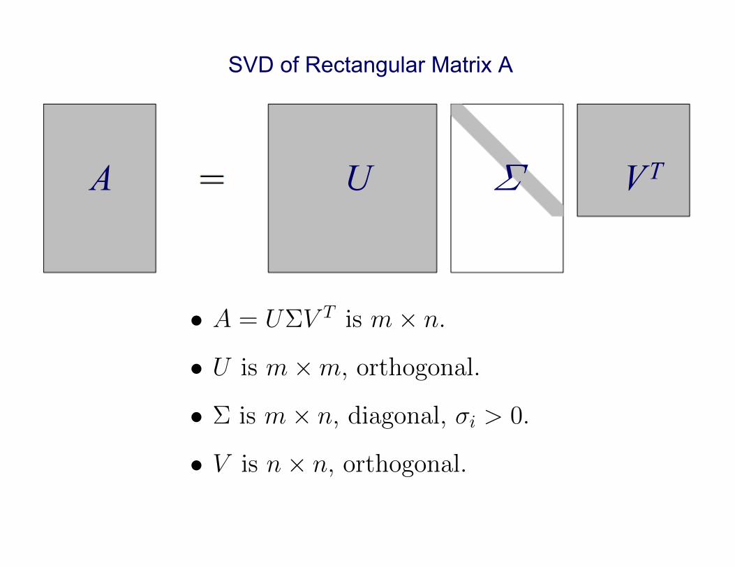
SVD of Rectangular Matrix A
• A = U⌃V Tis m⇥ n.
• U is m⇥m, orthogonal.
• ⌃ is m⇥ n, diagonal, �i > 0.
• V is n⇥ n, orthogonal.
1
A U § V T

Least Squares Data FittingExistence, Uniqueness, and Conditioning
Solving Linear Least Squares Problems
Normal EquationsOrthogonal MethodsSVD
Example: SVD
SVD of A =
2
664
1 2 3
4 5 6
7 8 9
10 11 12
3
775 is given by U⌃V T
=
2
664
.141 .825 �.420 �.351
.344 .426 .298 .782
.547 .0278 .664 �.509
.750 �.371 �.542 .0790
3
775
2
664
25.5 0 0
0 1.29 0
0 0 0
0 0 0
3
775
2
4.504 .574 .644
�.761 �.057 .646
.408 �.816 .408
3
5
< interactive example >
Michael T. Heath Scientific Computing 53 / 61
In square matrix case, U § VT closely related to eigenpair, X ¤ X-1

Least Squares Data FittingExistence, Uniqueness, and Conditioning
Solving Linear Least Squares Problems
Normal EquationsOrthogonal MethodsSVD
Applications of SVD
Minimum norm solution to Ax ⇠=
b is given by
x =
X
�i 6=0
uT
i
b
�
i
vi
For ill-conditioned or rank deficient problems, “small”singular values can be omitted from summation to stabilizesolution
Euclidean matrix norm : kAk2
= �
max
Euclidean condition number of matrix : cond(A) =
�
max
�
min
Rank of matrix : number of nonzero singular values
Michael T. Heath Scientific Computing 54 / 61

SVD for Linear Least Squares Problem: A = U⌃V T
Ax ⇡ b
U⌃V T ⇡ b
UTU⌃V T ⇡ UT b
⌃V T ⇡ UT b
R̃
O
�x =
✓c1c2
◆
x =nX
j=1
vj1
�j(c1)j =
nX
j=1
vj1
�juTj b
1
A = U⌃V T
Ax ⇡ b
U⌃V T ⇡ b
UTU⌃V T ⇡ UT b
⌃V T ⇡ UT b
R̃
O
�x =
✓c1c2
◆
x =nX
j=1
vj1
�j(c1)j =
nX
j=1
vj1
�juTj b
1
uuuu
A = U⌃V T
Ax ⇡ b
U⌃V T ⇡ b
UTU⌃V T ⇡ UT b
⌃V T ⇡ UT b
R̃O
�x ⇡
✓c1c2
◆
R̃x = c1
x =nX
j=1
vj1
�j(c1)j =
nX
j=1
vj1
�juTj b
1

SVD for Linear Least Squares Problem: A = U⌃V T
Ax ⇡ b
U⌃V T ⇡ b
UTU⌃V T ⇡ UT b
⌃V T ⇡ UT b
R̃
O
�x =
✓c1c2
◆
x =nX
j=1
vj1
�j(c1)j =
nX
j=1
vj1
�juTj b
1
• SVD can also handle the rank deficient case.
• If there are only k singular values �j > ✏ then
take only the first k contributions.
x =
kX
j=1
vj1
�ju
Tj b
1

Least Squares Data FittingExistence, Uniqueness, and Conditioning
Solving Linear Least Squares Problems
Normal EquationsOrthogonal MethodsSVD
Pseudoinverse
Define pseudoinverse of scalar � to be 1/� if � 6= 0, zerootherwiseDefine pseudoinverse of (possibly rectangular) diagonalmatrix by transposing and taking scalar pseudoinverse ofeach entryThen pseudoinverse of general real m⇥ n matrix A isgiven by
A+
= V ⌃+UT
Pseudoinverse always exists whether or not matrix issquare or has full rankIf A is square and nonsingular, then A+
= A�1
In all cases, minimum-norm solution to Ax ⇠=
b is given byx = A+ b
Michael T. Heath Scientific Computing 55 / 61

Least Squares Data FittingExistence, Uniqueness, and Conditioning
Solving Linear Least Squares Problems
Normal EquationsOrthogonal MethodsSVD
Orthogonal Bases
SVD of matrix, A = U⌃V T , provides orthogonal bases forsubspaces relevant to A
Columns of U corresponding to nonzero singular valuesform orthonormal basis for span(A)
Remaining columns of U form orthonormal basis fororthogonal complement span(A)
?
Columns of V corresponding to zero singular values formorthonormal basis for null space of A
Remaining columns of V form orthonormal basis fororthogonal complement of null space of A
Michael T. Heath Scientific Computing 56 / 61

Least Squares Data FittingExistence, Uniqueness, and Conditioning
Solving Linear Least Squares Problems
Normal EquationsOrthogonal MethodsSVD
Lower-Rank Matrix ApproximationAnother way to write SVD is
A = U⌃V T
= �
1
E1
+ �
2
E2
+ · · ·+ �
n
En
with Ei
= ui
vT
i
Ei
has rank 1 and can be stored using only m+ n storagelocationsProduct E
i
x can be computed using only m+ n
multiplicationsCondensed approximation to A is obtained by omittingfrom summation terms corresponding to small singularvaluesApproximation using k largest singular values is closestmatrix of rank k to AApproximation is useful in image processing, datacompression, information retrieval, cryptography, etc.
< interactive example >Michael T. Heath Scientific Computing 57 / 61
Low Rank Approximation to A = U⌃V T
Ax ⇡ b
U⌃V T ⇡ b
UTU⌃V T ⇡ UT b
⌃V T ⇡ UT b
R̃
O
�x =
✓c1c2
◆
x =nX
j=1
vj1
�j(c1)j =
nX
j=1
vj1
�juTj b
1
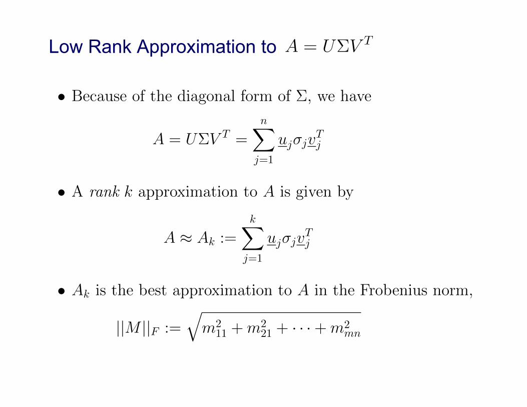
• Because of the diagonal form of ⌃, we have
A = U⌃V T=
nX
j=1
uj�jvTj
• A rank k approximation to A is given by
A ⇡ Ak :=
kX
j=1
uj�jvTj
• Ak is the best approximation to A in the Frobenius norm,
||M ||F :=
qm2
11 +m221 + · · ·+m2
mn
1

SVD for Image Compression
❑ If we view an image as an m x n matrix, we can use the SVD to generate a low-rank compressed version.
❑ Full image storage cost scales as O(mn)
❑ Compress image storage scales as O(km) + O(kn), with k < m or n.
• Because of the diagonal form of ⌃, we have
A = U⌃V T=
nX
j=1
uj�jvTj
• A rank k approximation to A is given by
A ⇡ Ak :=
kX
j=1
uj�jvTj
• Ak is the best approximation to A in the Frobenius norm,
||M ||F :=
qm2
11 +m221 + · · ·+m2
mn
1
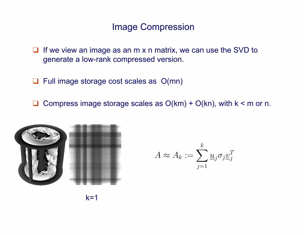
Image Compression
❑ If we view an image as an m x n matrix, we can use the SVD to generate a low-rank compressed version.
❑ Full image storage cost scales as O(mn)
❑ Compress image storage scales as O(km) + O(kn), with k < m or n.
k=1
• Because of the diagonal form of ⌃, we have
A = U⌃V T=
nX
j=1
uj�jvTj
• A rank k approximation to A is given by
A ⇡ Ak :=
kX
j=1
uj�jvTj
• Ak is the best approximation to A in the Frobenius norm,
||M ||F :=
qm2
11 +m221 + · · ·+m2
mn
1

Image Compression
❑ If we view an image as an m x n matrix, we can use the SVD to generate a low-rank compressed version.
❑ Full image storage cost scales as O(mn)
❑ Compress image storage scales as O(km) + O(kn), with k < m or n.
k=1 k=2 k=3 (m=536,n=432)
Note: we don’t store matrix – just vectors u1 and v1.

Matlab code
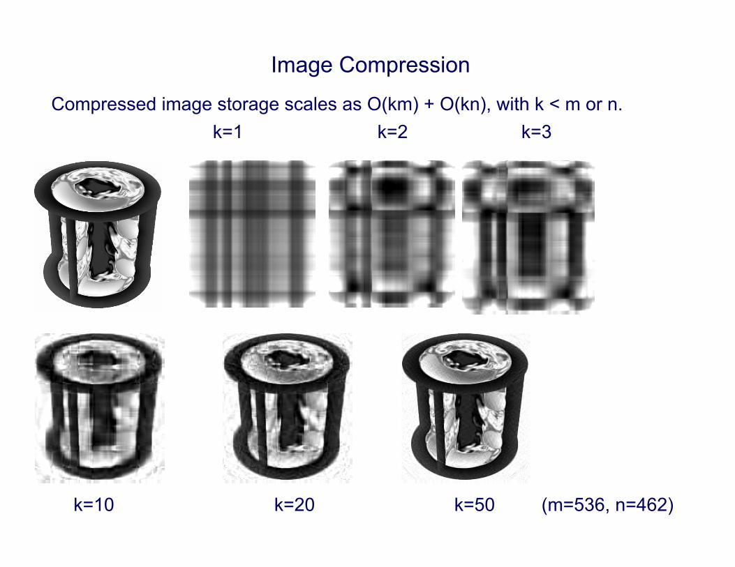
Image Compression
Compressed image storage scales as O(km) + O(kn), with k < m or n. k=1 k=2 k=3
k=10 k=20 k=50 (m=536, n=462)

Low-Rank Approximations to Solutions of Ax = b
❑ Other functions, aside from the inverse of the matrix, can also be approximated in this way, at relatively low cost, once the SVD is known.
If �1 �2 · · · �n,
x ⇡Pk
j=1 �+j vju
Tj b
1