Nonlinear dynamic partial least squares modeling of a full-scale

biological wastewater treatment plant

Dae Sung Lee a, Min Woo Lee a, Seung Han Woo b, Young-Ju Kim c, Jong Moon Park a,*a Advanced Environmental Biotechnology Research Center, Department of Chemical Engineering/

School of Environmental Science and Engineering, Pohang University of Science and Technology, San 31,

Hyoja-dong, Pohang, Gyeongbuk 790-784, Republic of Koreab Department of Chemical Engineering, Hanbat National University, San 16-1, Deokmyeong-dong, Yuseong-gu, Daejeon 305-719, Republic of Korea

c Department of Environmental Engineering, Kyungpook National University, Sankyuk-dong, Buk-gu, Daegu 702-701, Republic of Korea

Received 11 December 2005; received in revised form 2 May 2006; accepted 4 May 2006

www.elsevier.com/locate/procbio

Process Biochemistry 41 (2006) 2050–2057

Abstract

Partial least squares (PLS) has been extensively used in process monitoring and modeling to deal with many, noisy, and collinear variables.

However, the conventional linear PLS approach may be not effective due to the fundamental inability of linear regression techniques to account for

nonlinearity and dynamics in most chemical and biological processes. A hybrid approach, by combining a nonlinear PLS approach with a dynamic

modeling method, is potentially very efficient for obtaining more accurate prediction of nonlinear process dynamics. In this study, neural network

PLS (NNPLS) were combined with finite impulse response (FIR) and auto-regressive with exogenous (ARX) inputs to model a full-scale biological

wastewater treatment plant. It is shown that NNPLS with ARX inputs is capable of modeling the dynamics of the nonlinear wastewater treatment

plant and much improved prediction performance is achieved over the conventional linear PLS model.

# 2006 Elsevier Ltd. All rights reserved.

Keywords: Multivariate statistical process control; Neural network; Partial least squares (PLS); Dynamic system; Nonlinear system; Wastewater treatment plant

1. Introduction

Recent advances in computer technology and instrumenta-

tion techniques enable us to collect large amounts of data

from chemical and biological processes. With the increasing

data dimensionality, multivariate statistical process control

(MVSPC) has become very important and essential to extract

the useful information from the measurement data for

improving process performance and product quality. During

the last decade, it has been successfully applied for monitoring

and modeling of chemical/biological processes [1–5].

One of the most popular MVSPC techniques is partial least

squares (PLS). PLS is a linear multivariate process identifica-

tion method that projects the input-output data down into a

latent space, extracting a number of principal factors with an

orthogonal structure, while capturing most of the variance in

the original data [6,7]. Linear PLS derives its usefulness from

its ability to analyze data with strongly collinear, noisy and

* Corresponding author. Tel.: +82 54 279 2275; fax: +82 54 279 8659.

E-mail address: jmpark@postech.ac.kr (J.M. Park).

1359-5113/$ – see front matter # 2006 Elsevier Ltd. All rights reserved.

doi:10.1016/j.procbio.2006.05.006

numerous variables in both the predictor matrix X and

responses Y [8].

However, when applying the linear PLS to modeling real

processes, there have been some difficulties in its practical

applications since most real problems are inherently nonlinear

and dynamic [9–11]. A number of methods have been proposed

to integrate nonlinear features within the linear PLS framework

to produce a nonlinear PLS algorithm. A quadratic PLS

modeling method was proposed to fit the functional relation

between each pair of latent scores by quadratic regression [12].

Neural networks were also incorporated into linear PLS to

identify the relationship between the input and the output

scores, while retaining the outer mapping framework of linear

PLS algorithm [13,14]. In the neural network PLS (NNPLS),

because only small size network is trained at one time, the over-

parametrized problem of the direct neural network approach

such as multi-layer perceptron is circumvented even when the

training data are very sparse. In addition, NNPLS does not

require any kind of functional expansion compared to

functional-link neural networks [15].

The conventional PLS implicitly assumes that the mea-

surements are time independent and suited for modeling

D.S. Lee et al. / Process Biochemistry 41 (2006) 2050–2057 2051

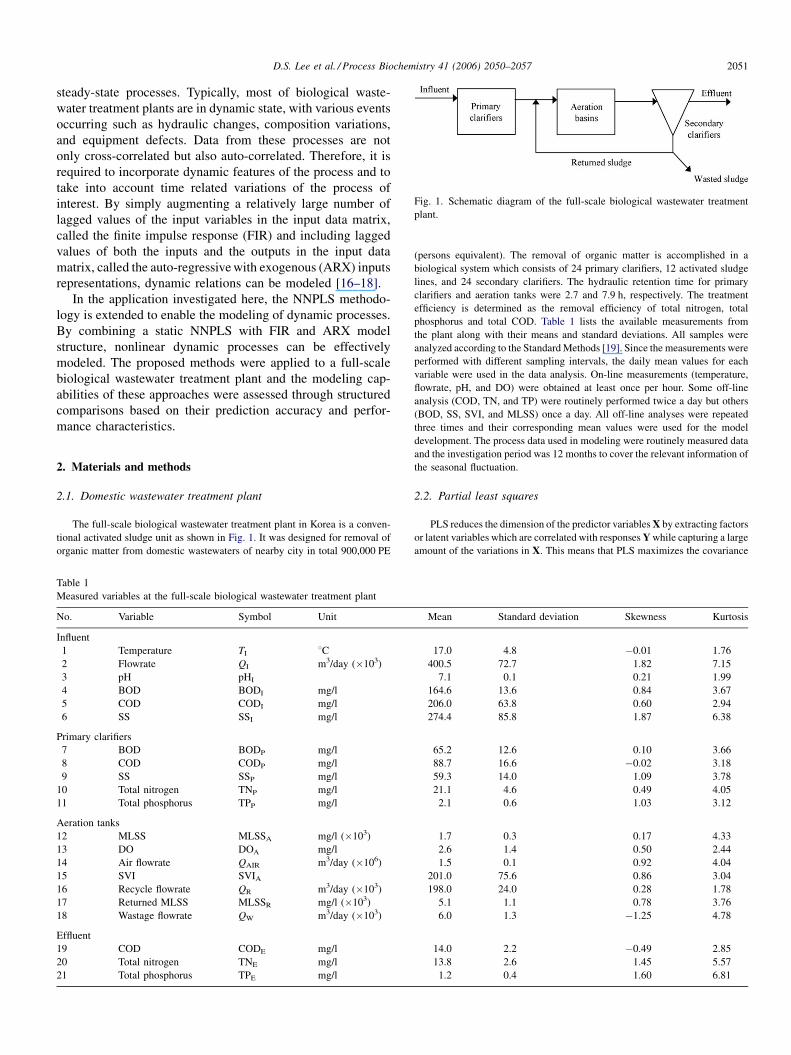
Fig. 1. Schematic diagram of the full-scale biological wastewater treatment

plant.

steady-state processes. Typically, most of biological waste-

water treatment plants are in dynamic state, with various events

occurring such as hydraulic changes, composition variations,

and equipment defects. Data from these processes are not

only cross-correlated but also auto-correlated. Therefore, it is

required to incorporate dynamic features of the process and to

take into account time related variations of the process of

interest. By simply augmenting a relatively large number of

lagged values of the input variables in the input data matrix,

called the finite impulse response (FIR) and including lagged

values of both the inputs and the outputs in the input data

matrix, called the auto-regressive with exogenous (ARX) inputs

representations, dynamic relations can be modeled [16–18].

In the application investigated here, the NNPLS methodo-

logy is extended to enable the modeling of dynamic processes.

By combining a static NNPLS with FIR and ARX model

structure, nonlinear dynamic processes can be effectively

modeled. The proposed methods were applied to a full-scale

biological wastewater treatment plant and the modeling cap-

abilities of these approaches were assessed through structured

comparisons based on their prediction accuracy and perfor-

mance characteristics.

2. Materials and methods

2.1. Domestic wastewater treatment plant

The full-scale biological wastewater treatment plant in Korea is a conven-

tional activated sludge unit as shown in Fig. 1. It was designed for removal of

organic matter from domestic wastewaters of nearby city in total 900,000 PE

Table 1

Measured variables at the full-scale biological wastewater treatment plant

No. Variable Symbol Unit

Influent

1 Temperature TI 8C2 Flowrate QI m3/day (�103)

3 pH pHI

4 BOD BODI mg/l

5 COD CODI mg/l

6 SS SSI mg/l

Primary clarifiers

7 BOD BODP mg/l

8 COD CODP mg/l

9 SS SSP mg/l

10 Total nitrogen TNP mg/l

11 Total phosphorus TPP mg/l

Aeration tanks

12 MLSS MLSSA mg/l (�103)

13 DO DOA mg/l

14 Air flowrate QAIR m3/day (�106)

15 SVI SVIA

16 Recycle flowrate QR m3/day (�103)

17 Returned MLSS MLSSR mg/l (�103)

18 Wastage flowrate QW m3/day (�103)

Effluent

19 COD CODE mg/l

20 Total nitrogen TNE mg/l

21 Total phosphorus TPE mg/l

(persons equivalent). The removal of organic matter is accomplished in a

biological system which consists of 24 primary clarifiers, 12 activated sludge

lines, and 24 secondary clarifiers. The hydraulic retention time for primary

clarifiers and aeration tanks were 2.7 and 7.9 h, respectively. The treatment

efficiency is determined as the removal efficiency of total nitrogen, total

phosphorus and total COD. Table 1 lists the available measurements from

the plant along with their means and standard deviations. All samples were

analyzed according to the Standard Methods [19]. Since the measurements were

performed with different sampling intervals, the daily mean values for each

variable were used in the data analysis. On-line measurements (temperature,

flowrate, pH, and DO) were obtained at least once per hour. Some off-line

analysis (COD, TN, and TP) were routinely performed twice a day but others

(BOD, SS, SVI, and MLSS) once a day. All off-line analyses were repeated

three times and their corresponding mean values were used for the model

development. The process data used in modeling were routinely measured data

and the investigation period was 12 months to cover the relevant information of

the seasonal fluctuation.

2.2. Partial least squares

PLS reduces the dimension of the predictor variables X by extracting factors

or latent variables which are correlated with responses Y while capturing a large

amount of the variations in X. This means that PLS maximizes the covariance

Mean Standard deviation Skewness Kurtosis

17.0 4.8 �0.01 1.76

400.5 72.7 1.82 7.15

7.1 0.1 0.21 1.99

164.6 13.6 0.84 3.67

206.0 63.8 0.60 2.94

274.4 85.8 1.87 6.38

65.2 12.6 0.10 3.66

88.7 16.6 �0.02 3.18

59.3 14.0 1.09 3.78

21.1 4.6 0.49 4.05

2.1 0.6 1.03 3.12

1.7 0.3 0.17 4.33

2.6 1.4 0.50 2.44

1.5 0.1 0.92 4.04

201.0 75.6 0.86 3.04

198.0 24.0 0.28 1.78

5.1 1.1 0.78 3.76

6.0 1.3 �1.25 4.78

14.0 2.2 �0.49 2.85

13.8 2.6 1.45 5.57

1.2 0.4 1.60 6.81

D.S. Lee et al. / Process Biochemistry 41 (2006) 2050–20572052

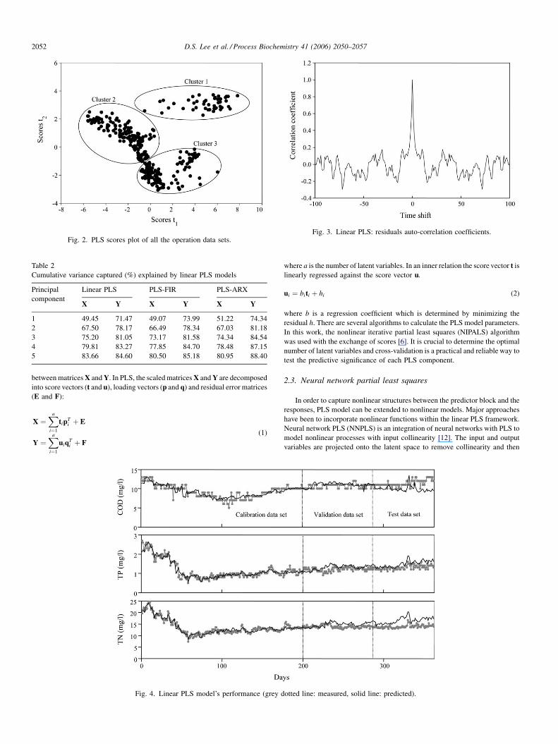
Fig. 2. PLS scores plot of all the operation data sets.Fig. 3. Linear PLS: residuals auto-correlation coefficients.

Table 2

Cumulative variance captured (%) explained by linear PLS models

Principal

component

Linear PLS PLS-FIR PLS-ARX

X Y X Y X Y

1 49.45 71.47 49.07 73.99 51.22 74.34

2 67.50 78.17 66.49 78.34 67.03 81.18

3 75.20 81.05 73.17 81.58 74.34 84.54

4 79.81 83.27 77.85 84.70 78.48 87.15

5 83.66 84.60 80.50 85.18 80.95 88.40

between matrices X and Y. In PLS, the scaled matrices X and Y are decomposed

into score vectors (t and u), loading vectors (p and q) and residual error matrices

(E and F):

X ¼Xa

i¼1

tipTi þ E

Y ¼Xa

i¼1

uiqTi þ F

(1)

Fig. 4. Linear PLS model’s performance (grey d

where a is the number of latent variables. In an inner relation the score vector t is

linearly regressed against the score vector u.

ui ¼ biti þ hi (2)

where b is a regression coefficient which is determined by minimizing the

residual h. There are several algorithms to calculate the PLS model parameters.

In this work, the nonlinear iterative partial least squares (NIPALS) algorithm

was used with the exchange of scores [6]. It is crucial to determine the optimal

number of latent variables and cross-validation is a practical and reliable way to

test the predictive significance of each PLS component.

2.3. Neural network partial least squares

In order to capture nonlinear structures between the predictor block and the

responses, PLS model can be extended to nonlinear models. Major approaches

have been to incorporate nonlinear functions within the linear PLS framework.

Neural network PLS (NNPLS) is an integration of neural networks with PLS to

model nonlinear processes with input collinearity [12]. The input and output

variables are projected onto the latent space to remove collinearity and then

otted line: measured, solid line: predicted).

D.S. Lee et al. / Process Biochemistry 41 (2006) 2050–2057 2053

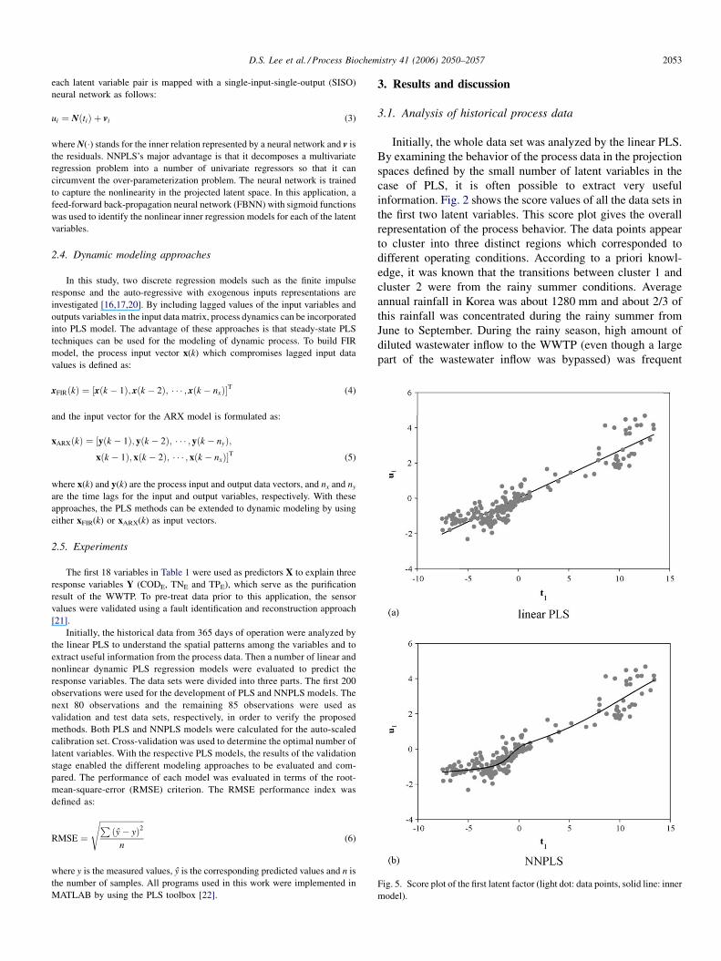
Fig. 5. Score plot of the first latent factor (light dot: data points, solid line: inner

model).

each latent variable pair is mapped with a single-input-single-output (SISO)

neural network as follows:

ui ¼ NðtiÞ þ vi (3)

where N(�) stands for the inner relation represented by a neural network and v is

the residuals. NNPLS’s major advantage is that it decomposes a multivariate

regression problem into a number of univariate regressors so that it can

circumvent the over-parameterization problem. The neural network is trained

to capture the nonlinearity in the projected latent space. In this application, a

feed-forward back-propagation neural network (FBNN) with sigmoid functions

was used to identify the nonlinear inner regression models for each of the latent

variables.

2.4. Dynamic modeling approaches

In this study, two discrete regression models such as the finite impulse

response and the auto-regressive with exogenous inputs representations are

investigated [16,17,20]. By including lagged values of the input variables and

outputs variables in the input data matrix, process dynamics can be incorporated

into PLS model. The advantage of these approaches is that steady-state PLS

techniques can be used for the modeling of dynamic process. To build FIR

model, the process input vector x(k) which compromises lagged input data

values is defined as:

xFIRðkÞ ¼ ½xðk � 1Þ; xðk � 2Þ; � � � ; xðk � nxÞ�T (4)

and the input vector for the ARX model is formulated as:

xARXðkÞ ¼ ½yðk � 1Þ; yðk � 2Þ; � � � ; yðk � nyÞ;xðk � 1Þ; xðk � 2Þ; � � � ; xðk � nxÞ�T (5)

where x(k) and y(k) are the process input and output data vectors, and nx and ny

are the time lags for the input and output variables, respectively. With these

approaches, the PLS methods can be extended to dynamic modeling by using

either xFIR(k) or xARX(k) as input vectors.

2.5. Experiments

The first 18 variables in Table 1 were used as predictors X to explain three

response variables Y (CODE, TNE and TPE), which serve as the purification

result of the WWTP. To pre-treat data prior to this application, the sensor

values were validated using a fault identification and reconstruction approach

[21].

Initially, the historical data from 365 days of operation were analyzed by

the linear PLS to understand the spatial patterns among the variables and to

extract useful information from the process data. Then a number of linear and

nonlinear dynamic PLS regression models were evaluated to predict the

response variables. The data sets were divided into three parts. The first 200

observations were used for the development of PLS and NNPLS models. The

next 80 observations and the remaining 85 observations were used as

validation and test data sets, respectively, in order to verify the proposed

methods. Both PLS and NNPLS models were calculated for the auto-scaled

calibration set. Cross-validation was used to determine the optimal number of

latent variables. With the respective PLS models, the results of the validation

stage enabled the different modeling approaches to be evaluated and com-

pared. The performance of each model was evaluated in terms of the root-

mean-square-error (RMSE) criterion. The RMSE performance index was

defined as:

RMSE ¼

ffiffiffiffiffiffiffiffiffiffiffiffiffiffiffiffiffiffiffiffiffiffiPðy� yÞ2

n

s(6)

where y is the measured values, y is the corresponding predicted values and n is

the number of samples. All programs used in this work were implemented in

MATLAB by using the PLS toolbox [22].

3. Results and discussion

3.1. Analysis of historical process data

Initially, the whole data set was analyzed by the linear PLS.

By examining the behavior of the process data in the projection

spaces defined by the small number of latent variables in the

case of PLS, it is often possible to extract very useful

information. Fig. 2 shows the score values of all the data sets in

the first two latent variables. This score plot gives the overall

representation of the process behavior. The data points appear

to cluster into three distinct regions which corresponded to

different operating conditions. According to a priori knowl-

edge, it was known that the transitions between cluster 1 and

cluster 2 were from the rainy summer conditions. Average

annual rainfall in Korea was about 1280 mm and about 2/3 of

this rainfall was concentrated during the rainy summer from

June to September. During the rainy season, high amount of

diluted wastewater inflow to the WWTP (even though a large

part of the wastewater inflow was bypassed) was frequent

D.S. Lee et al. / Process Biochemistry 41 (2006) 2050–20572054

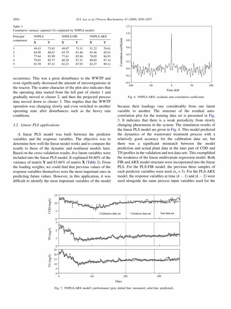
Fig. 6. NNPLS-ARX: residuals auto-correlation coefficients.

Table 3

Cumulative variance captured (%) explained by NNPLS models

Principal

component

NNPLS NNPLS-FIR NNPLS-ARX

X Y X Y X Y

1 49.43 73.83 49.07 73.31 51.22 76.61

2 64.99 80.67 63.79 81.46 65.46 82.61

3 77.64 83.99 77.61 85.94 78.05 84.93

4 79.03 85.77 60.20 87.31 80.85 87.14

5 83.39 87.21 82.23 87.93 82.27 89.11

occurrence. This was a great disturbance to the WWTP and

even significantly decreased the amount of microorganisms in

the reactor. The scatter character of the plot also indicates that

the operating data started from the left part of cluster 1 and

gradually moved to cluster 2, and then the projected process

data moved down to cluster 3. This implies that the WWTP

operation was changing slowly and even switched to another

operating state after disturbances such as the heavy rain

conditions.

3.2. Linear PLS applications

A linear PLS model was built between the predictor

variables and the response variables. The objective was to

determine how well the linear model works and to compare the

results to those of the dynamic and nonlinear models later.

Based on the cross-validation results, five latent variables were

included into the linear PLS model. It explained 84.60% of the

variance of matrix Y and 83.66% of matrix X (Table 2). From

the loading weights, we could find that previous values of the

response variables themselves were the most important ones in

predicting future values. However, in this application, it was

difficult to identify the most important variables of the model

Fig. 7. NNPLS-ARX model’s performance (grey

because their loadings vary considerably from one latent

variable to another. The structure of the residual auto-

correlation plot for the training data set is presented in Fig.

3. It indicates that there is a weak periodicity from slowly

changing phenomena in the system. The simulation results of

the linear PLS model are given in Fig. 4. This model predicted

the dynamics of the wastewater treatment process with a

relatively good accuracy for the calibration data set, but

there was a significant mismatch between the model

prediction and actual plant data in the later part of COD and

TN profiles in the validation and test data sets. This exemplified

the weakness of the linear multivariate regression model. Both

FIR and ARX model structure were incorporated into the linear

PLS. For the PLS-FIR model, the previous three samples of

each predictor variables were used (nx = 3). For the PLS-ARX

model, the response variables at time (k � 1) and (k � 2) were

used alongside the same process input variables used for the

dotted line: measured, solid line: predicted).

D.S. Lee et al. / Process Biochemistry 41 (2006) 2050–2057 2055

PLS-FIR model (ny = 2). The time lags were determined by

trial-and-error to minimize the RMSE of the validation data set.

One-step-ahead predictions were chosen to enable the PLS

models to be compared. The regression performance of the

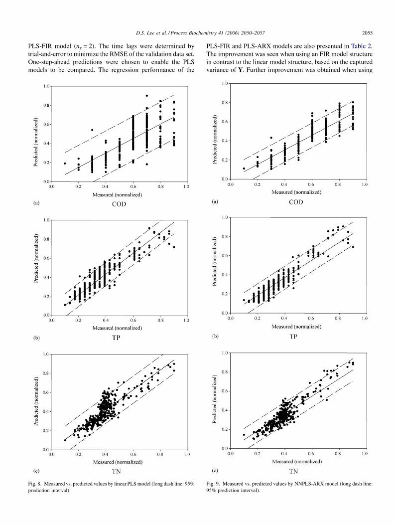
Fig. 8. Measured vs. predicted values by linear PLS model (long dash line: 95%

prediction interval).

PLS-FIR and PLS-ARX models are also presented in Table 2.

The improvement was seen when using an FIR model structure

in contrast to the linear model structure, based on the captured

variance of Y. Further improvement was obtained when using

Fig. 9. Measured vs. predicted values by NNPLS-ARX model (long dash line:

95% prediction interval).

D.S. Lee et al. / Process Biochemistry 41 (2006) 2050–20572056

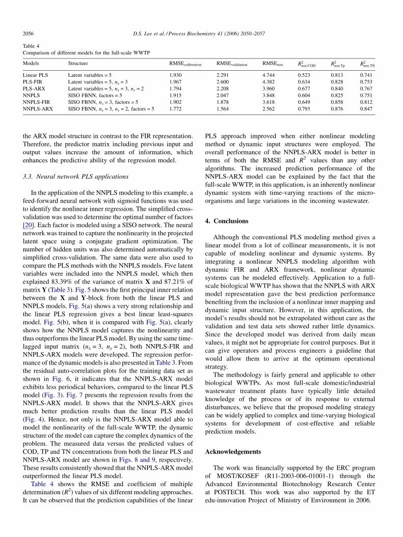
Table 4

Comparison of different models for the full-scale WWTP

Models Structure RMSEcalibration RMSEvalidation RMSEtest R2test;COD R2

test;Tp R2test;TN

Linear PLS Latent variables = 5 1.930 2.291 4.744 0.523 0.813 0.741

PLS-FIR Latent variables = 5, nx = 3 1.967 2.600 4.382 0.634 0.828 0.753

PLS-ARX Latent variables = 5, nx = 3, ny = 2 1.794 2.208 3.960 0.677 0.840 0.767

NNPLS SISO FBNN, factors = 5 1.915 2.047 3.848 0.604 0.825 0.751

NNPLS-FIR SISO FBNN, nx = 3, factors = 5 1.902 1.878 3.618 0.649 0.858 0.812

NNPLS-ARX SISO FBNN, nx = 3, ny = 2, factors = 5 1.772 1.564 2.562 0.793 0.876 0.847

the ARX model structure in contrast to the FIR representation.

Therefore, the predictor matrix including previous input and

output values increase the amount of information, which

enhances the predictive ability of the regression model.

3.3. Neural network PLS applications

In the application of the NNPLS modeling to this example, a

feed-forward neural network with sigmoid functions was used

to identify the nonlinear inner regression. The simplified cross-

validation was used to determine the optimal number of factors

[20]. Each factor is modeled using a SISO network. The neural

network was trained to capture the nonlinearity in the projected

latent space using a conjugate gradient optimization. The

number of hidden units was also determined automatically by

simplified cross-validation. The same data were also used to

compare the PLS methods with the NNPLS models. Five latent

variables were included into the NNPLS model, which then

explained 83.39% of the variance of matrix X and 87.21% of

matrix Y (Table 3). Fig. 5 shows the first principal inner relation

between the X and Y-block from both the linear PLS and

NNPLS models. Fig. 5(a) shows a very strong relationship and

the linear PLS regression gives a best linear least-squares

model. Fig. 5(b), when it is compared with Fig. 5(a), clearly

shows how the NNPLS model captures the nonlinearity and

thus outperforms the linear PLS model. By using the same time-

lagged input matrix (nx = 3, ny = 2), both NNPLS-FIR and

NNPLS-ARX models were developed. The regression perfor-

mance of the dynamic models is also presented in Table 3. From

the residual auto-correlation plots for the training data set as

shown in Fig. 6, it indicates that the NNPLS-ARX model

exhibits less periodical behaviors, compared to the linear PLS

model (Fig. 3). Fig. 7 presents the regression results from the

NNPLS-ARX model. It shows that the NNPLS-ARX gives

much better prediction results than the linear PLS model

(Fig. 4). Hence, not only is the NNPLS-ARX model able to

model the nonlinearity of the full-scale WWTP, the dynamic

structure of the model can capture the complex dynamics of the

problem. The measured data versus the predicted values of

COD, TP and TN concentrations from both the linear PLS and

NNPLS-ARX model are shown in Figs. 8 and 9, respectively.

These results consistently showed that the NNPLS-ARX model

outperformed the linear PLS model.

Table 4 shows the RMSE and coefficient of multiple

determination (R2) values of six different modeling approaches.

It can be observed that the prediction capabilities of the linear

PLS approach improved when either nonlinear modeling

method or dynamic input structures were employed. The

overall performance of the NNPLS-ARX model is better in

terms of both the RMSE and R2 values than any other

algorithms. The increased prediction performance of the

NNPLS-ARX model can be explained by the fact that the

full-scale WWTP, in this application, is an inherently nonlinear

dynamic system with time-varying reactions of the micro-

organisms and large variations in the incoming wastewater.

4. Conclusions

Although the conventional PLS modeling method gives a

linear model from a lot of collinear measurements, it is not

capable of modeling nonlinear and dynamic systems. By

integrating a nonlinear NNPLS modeling algorithm with

dynamic FIR and ARX framework, nonlinear dynamic

systems can be modeled effectively. Application to a full-

scale biological WWTP has shown that the NNPLS with ARX

model representation gave the best prediction performance

benefiting from the inclusion of a nonlinear inner mapping and

dynamic input structure. However, in this application, the

model’s results should not be extrapolated without care as the

validation and test data sets showed rather little dynamics.

Since the developed model was derived from daily mean

values, it might not be appropriate for control purposes. But it

can give operators and process engineers a guideline that

would allow them to arrive at the optimum operational

strategy.

The methodology is fairly general and applicable to other

biological WWTPs. As most full-scale domestic/industrial

wastewater treatment plants have typically little detailed

knowledge of the process or of its response to external

disturbances, we believe that the proposed modeling strategy

can be widely applied to complex and time-varying biological

systems for development of cost-effective and reliable

prediction models.

Acknowledgements

The work was financially supported by the ERC program

of MOST/KOSEF (R11-2003-006-01001-1) through the

Advanced Environmental Biotechnology Research Center

at POSTECH. This work was also supported by the ET

edu-innovation Project of Ministry of Environment in 2006.

D.S. Lee et al. / Process Biochemistry 41 (2006) 2050–2057 2057

Appendix A. Nomenclature

a number of latent variables

ARX a

uto-regressive with exogenous input

b r

egression coefficient

COD c

hemical oxygen demand (mg/l)

E e

rror matrix

F e

rror matrix

FBNN f

eed-forward back-propagation neural network

FIR fi

nite impulse response

h r

esiduals

MVSPC m

ultivariate statistical process control

n n

umber of samples

nx, ny t

ime lag for the input and output variables

NNPLS n

eural network partial least squares

p l

oading vector

PE p

ersons equivalent

PLS p

artial least squares

q l

oading vector

RMSE r

oot-mean-square-error

t s

core vector

TN t

otal nitrogen (mg/l)

TP t

otal phosphorus (mg/l)

u s

core vector

v r

esiduals

WWTP w

astewater treatment plant

x i

nput vector

X p

redictor matrix

y m

easured variable

y p

redicted value

Y r

esponse matrix

References

[1] Lee DS, Jeon CO, Park JM, Chang KS. Hybrid neural network modelling

of a full-scale industrial wastewater treatment process. Biotechnol Bioeng

2002;78:670–82.

[2] Lee DS, Park JM, Vanrolleghem PA. Adaptive multiscale principal

component analysis for on-line monitoring of a sequencing batch reactor.

J Biotechnol 2005;116:195–210.

[3] Lee DS, Vanrolleghem PA. Monitoring of a sequencing batch reactor using

adaptive multiblock pricipal component analysis. Biotechnol Bioeng

2003;82(4):489–97.

[4] MacGregor JF, Kourti T. Statistical process control of multivariate pro-

cesses. Control Eng Pract 1995;3:403–14.

[5] Wise BM, Gallagher NB. The process chemometrics approach to process

monitoring and fault detection. J Proc Control 1996;6:329–48.

[6] Geladi P, Kowalski BR. Partial least-squares regression: a tutorial. Anal

Chim Acta 1986;185:1–17.

[7] Wold S, Ruhe A, Wold H, Dunn WJ. The Collinearity problem in linear

regression. The partial least squares approach to generalized inverse.

SIAM J Sci Stat Comput 1984;3:735–43.

[8] Wold S, Sjostrom M, Eriksson L. PLS-regression: a basic tool of chemo-

metrics. Chemom Intell Lab Syst 2001;58:109–30.

[9] Baffi G, Martin EB, Morris AJ. Non-linear projection to latent structures

revisited (the neural network PLS algorithm). Comput Chem Eng

1999;23:1293–307.

[10] Wang X, Kruger U, Lennox B. Recursive partial least squares algorithms

for monitoring complex industrial processes. Cont Eng Practice

2003;11:613–32.

[11] Gallagher NB, Wise BM, Butler SW, White DD, Barna GG. Development

and benchmarking of multivariate statistical process control tools for a

semiconductor etch process: improving robustness through model updat-

ing. In: Proceedings of the ADCHEM 97. Banff, Canada; 1997. p. 78.

[12] Wold S, Kettaneh-Wold N, Skagerberg B. Nonlinear PLS modeling.

Chemom Intell Lab Syst 1989;7:53–65.

[13] Lee DS, Vanrolleghem PA, Park JM. Parallel hybrid modeling methods for

a full-scale cokes wastewater treatment plant. J Biotechnol 2005;115:317–

28.

[14] Qin SJ, McAvoy TJ. Non-linear PLS modelling using neural networks.

Comput Chem Eng 1992;16:379–91.

[15] Chen S, Billings SA. Neural network for nonlinear dynamic system

modeling and identification. Int J Cont 1992;56:319–46.

[16] Baffi G, Martin EB, Morris AJ. Non-linear dynamic projection to latent

structures modelling. Chemom Intell Lab Syst 2000;52:5–22.

[17] Qin SJ, McAvoy TJ. Nonlinear FIR modelling via a neural net PLS

approach. Comput Chem Eng 1996;20(2):147–59.

[18] Ricker NL. The use of biased least-squares estimators for parameters in

discrete-time pulse response models. Ind Eng Chem Res 1988;27:343–50.

[19] APHA. Standard methods for the examination of water and wastewater,

19th ed. Washington DC: American Public Health Association; 1995.

[20] Qin SJ. Partial least squares regression for recursive system identification.

In: Proceedings of the 32nd Conference on Decision and Control. San

Antonio, Texas; 1993. p. 2617.

[21] Dunia R, Oin SJ, Edgar TF, McAvoy TJ. Identification of faulty sensors

using principal component analysis. AIChE J 1996;42:2797–812.

[22] Wise BM, Gallagher NB. PLS toolbox version 2. 1 for use with

MATLABTM Washington DC: Eigenvector Research; 2000.