Journal of Computational and Applied Mathematics 156 (2003) 159–177www.elsevier.com/locate/cam

Solution of the least-squares problem for logistic functionD. Juki+c∗, R. Scitovski

Department of Mathematics, University J.J. Strossmayer, Gajev trg 6, HR-31000 Osijek, Croatia

Received 12 March 2002; received in revised form 10 August 2002

Abstract

Given the data (pi; ti; fi); i=1; : : : ; m; m¿ 3, we consider the best least-squares approximation of parametersfor the logistic function t �→ f(t; ; ; �) = =(1 + e−�t); ; �¿ 0; ∈R. We give necessary and su5cientconditions which guarantee the existence of such optimal parameters.c© 2003 Elsevier Science B.V. All rights reserved.

MSC: 65D10; 65C20; 62J02

Keywords: Nonlinear least squares; Logistic function; Existence problem

1. Introduction

The logistic growth model (see [16])

y′ = �y(1− y

); ; �¿ 0

was developed by the Belgian mathematician Pierre Verhulst [16]. Parameter � can be interpreted asthe maximum possible rate of population growth, while parameter is the upper limit of populationgrowth and it is called carrying capacity (see [12,13,16]). The solution of the Verhulst’s model isthe so-called logistic function

f(t; ; ; �) =

1 + e−�t ; ; �¿ 0; ∈R: (1)

The graph of this function is an “S”-shaped curve.The logistic model occurs frequently in various applied areas, such as biology (see [13]), agricul-

ture (see [7]), marketing (see [5]), economics (see [12]), etc. Some generalizations of the logistic

∗ Corresponding author. Fax: +385-31-224-801.E-mail addresses: jukicd@mathos.hr (D. Juki+c), scitowsk@etfos.hr (R. Scitovski).

0377-0427/03/$ - see front matter c© 2003 Elsevier Science B.V. All rights reserved.doi:10.1016/S0377-0427(02)00910-X

160 D. Juki+c, R. Scitovski / Journal of Computational and Applied Mathematics 156 (2003) 159–177

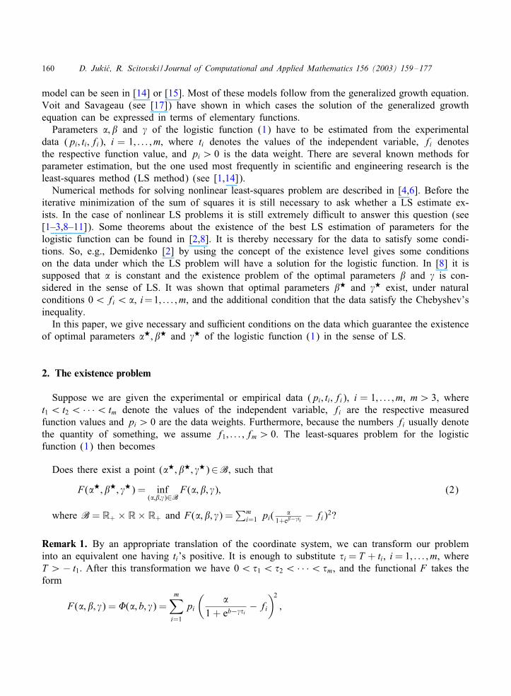
model can be seen in [14] or [15]. Most of these models follow from the generalized growth equation.Voit and Savageau (see [17]) have shown in which cases the solution of the generalized growthequation can be expressed in terms of elementary functions.Parameters ; and � of the logistic function (1) have to be estimated from the experimental

data (pi; ti; fi); i = 1; : : : ; m; where ti denotes the values of the independent variable, fi denotesthe respective function value, and pi ¿ 0 is the data weight. There are several known methods forparameter estimation, but the one used most frequently in scientiKc and engineering research is theleast-squares method (LS method) (see [1,14]).Numerical methods for solving nonlinear least-squares problem are described in [4,6]. Before the

iterative minimization of the sum of squares it is still necessary to ask whether a LS estimate ex-ists. In the case of nonlinear LS problems it is still extremely di5cult to answer this question (see[1–3,8–11]). Some theorems about the existence of the best LS estimation of parameters for thelogistic function can be found in [2,8]. It is thereby necessary for the data to satisfy some condi-tions. So, e.g., Demidenko [2] by using the concept of the existence level gives some conditionson the data under which the LS problem will have a solution for the logistic function. In [8] it issupposed that is constant and the existence problem of the optimal parameters and � is con-sidered in the sense of LS. It was shown that optimal parameters ? and �? exist, under naturalconditions 0¡fi ¡, i=1; : : : ; m, and the additional condition that the data satisfy the Chebyshev’sinequality.In this paper, we give necessary and su5cient conditions on the data which guarantee the existence

of optimal parameters ?; ? and �? of the logistic function (1) in the sense of LS.

2. The existence problem

Suppose we are given the experimental or empirical data (pi; ti; fi), i = 1; : : : ; m, m¿ 3, wheret1¡t2¡ · · ·¡tm denote the values of the independent variable, fi are the respective measuredfunction values and pi ¿ 0 are the data weights. Furthermore, because the numbers fi usually denotethe quantity of something, we assume f1; : : : ; fm ¿ 0. The least-squares problem for the logisticfunction (1) then becomes

Does there exist a point (?; ?; �?)∈B; such that

F(?; ?; �?) = inf(;;�)∈B

F(; ; �); (2)

where B= R+ × R× R+ and F(; ; �) =∑m

i=1 pi( 1+e−�ti

− fi)2?

Remark 1. By an appropriate translation of the coordinate system, we can transform our probleminto an equivalent one having ti’s positive. It is enough to substitute �i = T + ti, i= 1; : : : ; m, whereT ¿− t1: After this transformation we have 0¡�1¡�2¡ · · ·¡�m, and the functional F takes theform

F(; ; �) = �(; b; �) =m∑i=1

pi

(

1 + eb−��i− fi

)2;

D. Juki+c, R. Scitovski / Journal of Computational and Applied Mathematics 156 (2003) 159–177 161

where b= + �T . Functional � is of the same type as F; and since the map (; ; �) �→ (; b; �) isa bijection of B onto B; our problem is equivalent to the following one:Does there exist a point (?; b?; �?)∈B; such that �(?; b?; �?) = inf (;b; �)∈B �(; b; �)?

3. The optimal parameters existence theorem

In this section, we suppose that the given data (pi; ti; fi), i = 1; : : : ; m, m¿ 3, are such thatpi; fi ¿ 0, i = 1; : : : ; m, and t1¡t2¡ · · ·¡tm.The following lemma, which we are going to use in the proof of Theorem 1, shows that there

exist data such that problem (2) has no solution.

Lemma 1. Let (pi; ti; fi); i = 1; : : : ; m; m¿ 3; be the data. If the data are such that

(i) the points (ti; fi); i = 1; : : : ; m; all lie on some exponential curve y(t) = b ect , b¿ 0, c �= 0; or(ii) f16f2 = f3 = · · ·= fm= : A,

then problem (2) has no solution.

Proof.

(i) Since F(; ; �)¿ 0 for all (; ; �)∈B, and

lim→∞F(; ln − ln b; c) = lim

→∞

m∑i=1

pi

(

1 + e−ln b−cti− fi

)2

=m∑i=1

pi(becti − fi)2 = 0;

this means that inf (;; �)∈B F(; ; �) = 0. Furthermore, since the graph of any logistic functionof type (1) intersects the graph of exponential function y(t) = bect in at most three points, andm¿ 3, it follows that F(; ; �)¿ 0 for all (; ; �)∈B, and hence problem (2) has no solution.

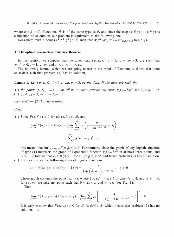
(ii) Let us consider the following class of logistic functions:

t �→ f(t;A; ��0 + ln(A=y0 − 1); �) = A

1 +(

Ay0

− 1)e−�(t−�0)

; �¿ 0

whose graph contains the point (�0; y0), where (�0; y0) = (t1; f1) in case f1¡A, and if f1 = A,for (�0; y0) we take any point such that 0¡y0¡A and �0¡t1 (see Fig. 1).Then

lim�→∞F(A; ��0 + ln(A=y0 − 1); �) = lim

�→∞

m∑i=1

pi

[A

1 + ( Ay0

− 1)e−�(ti−�0)− fi

]2= 0:

It is easy to show that F(; �; )¿ 0 for all (; ; �)∈B, which means that problem (2) has nosolution.

162 D. Juki+c, R. Scitovski / Journal of Computational and Applied Mathematics 156 (2003) 159–177

Fig. 1.

The following lemma will be used in the proof of Theorem 1—the main results of the paper.

Lemma 2. Let (pi; ti; fi), i=1; : : : ; m, m¿ 3, be the data, such that not all points (ti; fi), i=1; : : : ; m,lie on some exponential curve. Furthermore, let us suppose that point (b0; c0)∈R2+ is a solution ofthe weighted least-squares problem

inf(b;c)∈R2+

G(b; c) where G(b; c) =m∑i=1

pi(becti − fi)2:

Thenm∑i=1

pi(b0ec0ti − fi)ec0ti = 0 andm∑i=1

pi(b0ec0ti − fi)ec0ti ti = 0: (3)

Furthermore, there exists at least one i0 ∈{1; : : : ; m} such that b0ec0ti0 − fi0 ¿ 0.

Proof. The proof follows from equalities:

9G9b (b0; c0) = 2

m∑i=1

pi(b0ec0ti − fi)ec0ti = 0 and

9G9c (b0; c0) = 2b0

m∑i=1

pi(b0ec0ti − fi)ec0ti ti = 0: (4)

Theorem 1. Let the data (pi; ti; fi), i = 1; : : : ; m, m¿ 3, be given, such that t1¡t2¡ · · ·¡tm andfi ¿ 0, i = 1; : : : ; m. Then problem (2) has no solution if and only if the data have one of thefollowing two properties:

(i) the points (ti; fi); i = 1; : : : ; m; all lie on some exponential curve y(t) = bect , b¿ 0, c �= 0; or(ii) f16f2 = f3 = · · ·= fm.

Proof. If the points (ti; fi), i = 1; : : : ; m, possess either of the two mentioned properties, then byLemma 1 problem (2) has no solution.Let us show the converse. Suppose that points (ti; fi), i = 1; : : : ; m, have neither of the two

mentioned properties. We show that problem (2) has a solution. By Remark 1 we can assume that0¡t1¡t2¡ · · ·¡tm.

D. Juki+c, R. Scitovski / Journal of Computational and Applied Mathematics 156 (2003) 159–177 163

Since the functional F is nonnegative, there exists F? := inf (;; �)∈B F(; ; �). Let (n; n; �n) bea sequence in B, such that

F? = limn→∞F(n; n; �n) = lim

n→∞

m∑i=1

pi

(n

1 + en−�nti− fi

)2: (5)

We Krst show that the sequence (n; n; �n) is bounded by showing that the functional F cannotattain its inKmum F? in either of the following three ways:

(I) (n) is an unbounded and (2n + �2n) is a bounded sequence,(II) (n) is a bounded and (2n + �2n) is an unbounded sequence,(III) both (n) and (2n + �2n) are unbounded sequences.

Without loss of generality, whenever we have a bounded sequence, we are going to assume itis convergent—otherwise by the Bolzano–Weierstrass theorem, we take a convergent subsequence.Furthermore, whenever we have an unbounded sequence, by taking an appropriate subsequence ifnecessary, we may assume that it converges to ∞ or −∞. Thus, by taking appropriate subsequencesif necessary, the above three cases are:

I. (n → ∞) and (∃ r? ∈ [0;∞); 2n + �2n → r?),II. (∃ ? ∈ [0;∞); n → ?) and (2n + �2n → ∞),III. (n → ∞) and (2n + �2n → ∞).In each of these cases we are going to Knd a point in B, in which the functional F attains a

value which is smaller than limn→∞ F(n; n; �n), thus showing that neither of these three cases ispossible.(I) In the Krst case we would have that limn→∞ F(n; n; �n) =∞, which means that in this case

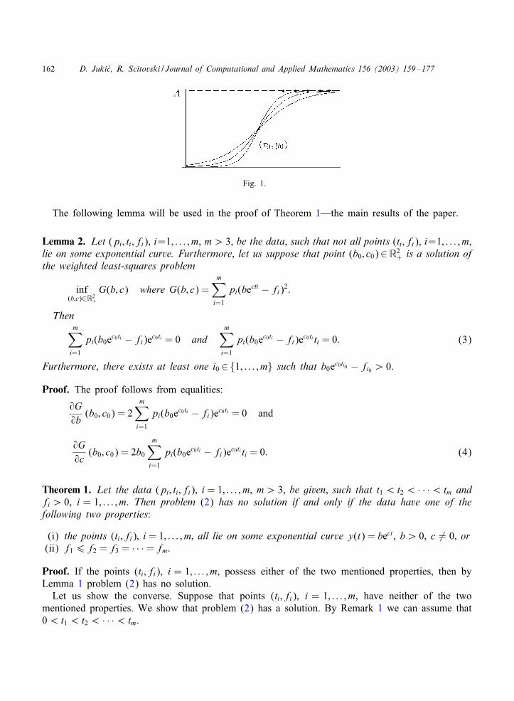
the functional F cannot attain its inKmum.Before we start considering cases (II) and (III), let us Krst deKne the vectors

ui := (1; ti); u0i :=1√1 + t2i

(1; ti); i = 1; : : : ; m:

Furthermore, let l be the arc of the unit sphere S1 := {r∈R2:‖r‖=1} from the point u01 to the pointu0m, and let l− := {r∈ S1:rsT6 0 for all s∈ l}. Note that l− is the arc of the unit sphere from thepoint v0m := 1=

√1 + t2m(−tm; 1) to the point v01 := 1=

√1 + t21(t1;−1) (see Fig. 2).

(II) Case n → ?¿ 0 and 2n + �2n → ∞. By using notations�n := (n;−�n); �0n :=

�n‖�n‖

; n∈N and �0 := limn→∞ �

0n

we can write

f(ti; n; n; �n) =n

1 + e�nuTi; i = 1; : : : ; m; n∈N:

Since ‖�n‖ → ∞, the value of limn→∞ �nuTi = limn→∞ ‖�n‖�0nuTi depends on the inner product�0uTi = limn→∞ �0nuTi i.e., on the position of the vector �0 on the sphere S1 (see Fig. 2). Let us

164 D. Juki+c, R. Scitovski / Journal of Computational and Applied Mathematics 156 (2003) 159–177

Fig. 2.

denote

I− :={i∈{1; : : : ; m}: lim

n→∞�n · uTi =−∞

};

I+ :={i∈{1; : : : ; m}: lim

n→∞�n · uTi =∞

};

I0 :={i∈{1; : : : ; m}: lim

n→∞�n · uTi ∈R

}:

Note that the sets I−; I+ and I0 are pairwise disjoint and that I0 is either an empty or a one-pointset I0 = {i0}. Note also that every ti, i∈ I+, is less than tj, j∈ I−.If I0 = {i0}, let us denote l0 := limn→∞ n=(1 + e‖�n‖�

0n·uTi0 ). Note that 0¡l0¡?, and that

tmaxI+ ¡ti0 ¡tminI− .Now the corresponding weighted sum of squares can be written in the form

limn→∞F(n; n; �n) = lim

n→∞∑

i∈I+∪I0∪I−pi

(n

1 + e‖�n‖�0n·uTi− fi

)2

=∑i∈I+

pif2i +∑i∈I0

pi(l0 − fi)2 +∑i∈I−

pi(? − fi)2: (6)

Only one of the following two cases can occur: (1) I− = ∅ or (2) I− �= ∅.(II.1) Consider the case I− = ∅. In this case I0 = ∅ and I+ = {1; : : : ; m}, or I0 = {m} and I+ =

{1; : : : ; m− 1}, so from (6) we obtain

limn→∞F(n; n; �n)¿

m−1∑i=1

pif2i := : F1:

Let us Knd a point in B, in which the functional F attains a value which is smaller than F1.For that purpose we choose any real number 0¿fm and consider the following class of logistic

D. Juki+c, R. Scitovski / Journal of Computational and Applied Mathematics 156 (2003) 159–177 165

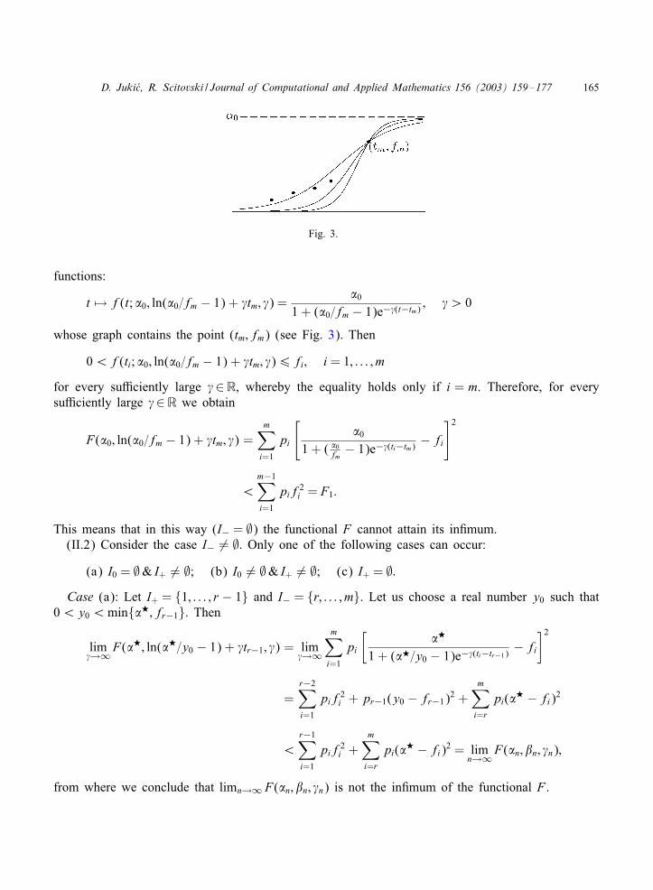
Fig. 3.

functions:

t �→ f(t; 0; ln(0=fm − 1) + �tm; �) =0

1 + (0=fm − 1)e−�(t−tm); �¿ 0

whose graph contains the point (tm; fm) (see Fig. 3). Then

0¡f(ti; 0; ln(0=fm − 1) + �tm; �)6fi; i = 1; : : : ; m

for every su5ciently large �∈R, whereby the equality holds only if i = m. Therefore, for everysu5ciently large �∈R we obtain

F(0; ln(0=fm − 1) + �tm; �) =m∑i=1

pi

[0

1 + ( 0fm − 1)e−�(ti−tm)− fi

]2

¡m−1∑i=1

pif2i = F1:

This means that in this way (I− = ∅) the functional F cannot attain its inKmum.(II.2) Consider the case I− �= ∅. Only one of the following cases can occur:

(a) I0 = ∅& I+ �= ∅; (b) I0 �= ∅& I+ �= ∅; (c) I+ = ∅:Case (a): Let I+ = {1; : : : ; r − 1} and I− = {r; : : : ; m}. Let us choose a real number y0 such that

0¡y0¡min{?; fr−1}. Then

lim�→∞F(?; ln(?=y0 − 1) + �tr−1; �) = lim

�→∞

m∑i=1

pi

[?

1 + (?=y0 − 1)e−�(ti−tr−1)− fi

]2

=r−2∑i=1

pif2i + pr−1(y0 − fr−1)2 +m∑i=r

pi(? − fi)2

¡r−1∑i=1

pif2i +m∑i=r

pi(? − fi)2 = limn→∞F(n; n; �n);

from where we conclude that limn→∞ F(n; n; �n) is not the inKmum of the functional F .

166 D. Juki+c, R. Scitovski / Journal of Computational and Applied Mathematics 156 (2003) 159–177

Table 1

? ¿ QfI−I0 = ∅ I0 = {i0}

�0 Any number ¡t1 ti0y0 Any number such that 0¡y0¡ QfI− l0 Any number such that QfI− ¡¡? Any number such that max{l0; QfI−}¡¡?

? ¡ QfI−I0 = ∅ I0 = {i0}

�0 Any number ¡t1 ti0 Any number such that ? ¡¡ QfI− Any number such that ? ¡¡ QfI−y0 Any number from (0; ) l0

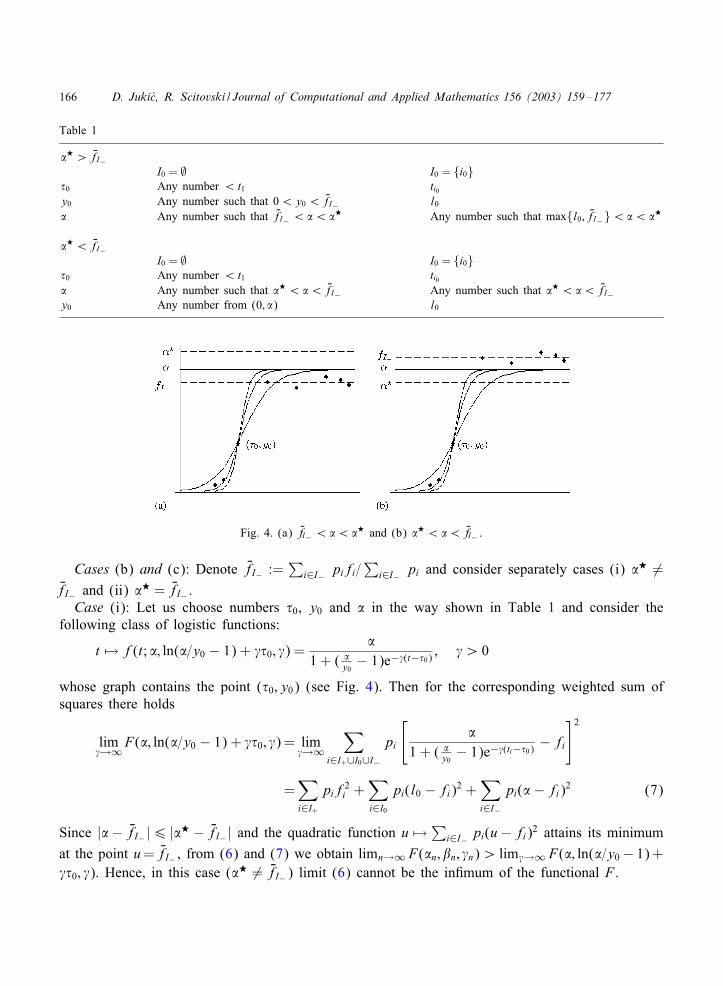
Fig. 4. (a) QfI− ¡¡? and (b) ? ¡¡ QfI− .

Cases (b) and (c): Denote QfI− :=∑

i∈I− pifi=∑

i∈I− pi and consider separately cases (i) ? �=QfI− and (ii) ? = QfI− .Case (i): Let us choose numbers �0, y0 and in the way shown in Table 1 and consider the

following class of logistic functions:

t �→ f(t; ; ln(=y0 − 1) + ��0; �) =

1 + ( y0

− 1)e−�(t−�0); �¿ 0

whose graph contains the point (�0; y0) (see Fig. 4). Then for the corresponding weighted sum ofsquares there holds

lim�→∞F(; ln(=y0 − 1) + ��0; �) = lim

�→∞∑

i∈I+∪I0∪I−pi

[

1 + ( y0

− 1)e−�(ti−�0)− fi

]2

=∑i∈I+

pif2i +∑i∈I0

pi(l0 − fi)2 +∑i∈I−

pi(− fi)2 (7)

Since |− QfI− |6 |? − QfI− | and the quadratic function u �→∑i∈I− pi(u− fi)2 attains its minimum

at the point u= QfI− , from (6) and (7) we obtain limn→∞ F(n; n; �n)¿ lim�→∞ F(; ln(=y0− 1)+��0; �). Hence, in this case (? �= QfI−) limit (6) cannot be the inKmum of the functional F .

D. Juki+c, R. Scitovski / Journal of Computational and Applied Mathematics 156 (2003) 159–177 167

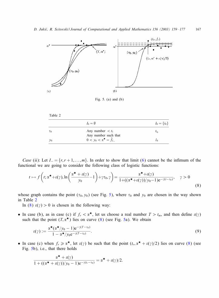
Fig. 5. (a) and (b)

Table 2

I0 = ∅ I0 = {i0}�0 Any number ¡t1 ti0

Any number such thaty0 0¡y0¡? = QfI− l0

Case (ii): Let I−= {r; r+1; : : : ; m}. In order to show that limit (6) cannot be the inKmum of thefunctional we are going to consider the following class of logistic functions:

t �→ f(t; ?+$(�); ln

(? + $(�)

y0−1)+��0; �

)=

?+$(�)1+((?+$(�))=y0−1)e−�(t−�0)

; �¿ 0

(8)

whose graph contains the point (�0; y0) (see Fig. 5), where �0 and y0 are chosen in the way shownin Table 2In (8) $(�)¿ 0 is chosen in the following way:

• In case (b), as in case (c) if fr ¡?, let us choose a real number T ¿ tm, and then deKne $(�)such that the point (T; ?) lies on curve (8) (see Fig. 5a). We obtain

$(�) :=?(?=y0 − 1)e−�(T−�0)

1− ?=y0e−�(T−�0): (9)

• In case (c) when fr¿ ?, let $(�) be such that the point (tr ; ? + $(�)=2) lies on curve (8) (seeFig. 5b), i.e., that there holds

? + $(�)1 + ((? + $(�))=y0 − 1)e−�(tr−�0)

= ? + $(�)=2:

168 D. Juki+c, R. Scitovski / Journal of Computational and Applied Mathematics 156 (2003) 159–177

By solving the previous equality we obtain

$(�) =4?(? − y0)

−3? + y0[1 + e�(tr−�0)] +√8?(y0 − ?) + [− 3? + y0(1 + e�(tr−�0)]2

: (10)

Note that lim�→∞ $(�) = 0 and

lim�→∞f

(t; ? + $(�); ln

(? + $(�)

y0− 1)+ ��0; �

)=

0; t ¡ �0;

y0; t = �0;

?; t ¿ �0:

(11)

For the corresponding weighted sum of squares

F(? + $(�); ln

(? + $(�)

y0− 1)+ ��0; �

)

=∑

i∈I+∪I0∪I−pi

? + $(�)

1 + ( ?+$(�)y0

− 1)e−�(ti−�0)− fi

2

:= %(�)

there holds

lim�→∞%(�) =

∑i∈I+

pif2i +∑i∈I0

pi(l0 − fi)2 +∑i∈I−

pi(? − fi)2: (12)

The derivative of the function % is

d%d�(�) = 2

m∑i=1

pi

[? + $(�)

1 + ((? + $(�))=y0 − 1)e−�(ti−�0)− fi

]1

[1 + ((? + $(�))=y0 − 1)e−�(ti−�0)]2

×[$′(�)

(1− e−�(ti−�0)

)+ (? + $(�))

(? + $(�)

y0− 1)e−�(ti−�0)(ti − �0)

]: (13)

Case (b). Since I− = {r; : : : ; m}, we have I0 = {r − 1}, �0 = tr−1 and I+ = {1; : : : ; r − 2}.Let us consider the expression

1 + ((? + $(�))=y0 − 1)e−�(tr−2−�0)

2[$′(�)(1− e−�(tr−2−�0)) + (? + $(�))((? + $(�))=y0 − 1)e−�(tr−2−�0)(tr−2 − �0)]d%d�(�)

= SI+(�) + SI−(�); (14)

where

SI+(�) :=r−2∑i=1

pi

[? + $(�)

1 + ((? + $(�))=y0 − 1)e−�(ti−�0)− fi

] [1 + ( ?+$(�)y0− 1)e−�(tr−2−�0)]

[1 + ( ?+$(�)y0

− 1)e−�(ti−�0)]2

×[

$′(�)(1− e−�(ti−�0)) + (? + $(�))((? + $(�))=y0 − 1)e−�(ti−�0)(ti − �0)$′(�)(1− e−�(tr−2−�0)) + (? + $(�))((? + $(�))=y0 − 1)e−�(tr−2−�0)(tr−2 − �0)

]

D. Juki+c, R. Scitovski / Journal of Computational and Applied Mathematics 156 (2003) 159–177 169

SI−(�) :=m∑i=r

pi

[? + $(�)

1 + ((? + $(�))=y0 − 1)e−�(ti−�0)− fi

][1 + ((? + $(�))=y0 − 1)e−�(tr−2−�0)][1 + ((? + $(�))=y0 − 1)e−�(ti−�0)]2

×[

$′(�)(1− e−�(ti−�0)) + (? + $(�))((? + $(�))=y0 − 1)e−�(ti−�0)(ti − �0)$′(�)(1− e−�(tr−2−�0)) + (? + $(�))((? + $(�))=y0 − 1)e−�(tr−2−�0)(tr−2 − �0)

]:

In this case

SI−(�) :=m∑i=r

pi

? + $(�)

1 +(? + $(�)

y0− 1)e−�(ti−�0)

− fi

× [e�(tr−2−�0) + ((? + $(�))=y0 − 1)][1 + ((? + $(�))=y0 − 1)e−�(ti−�0)]2

e−�(tr−2−�0)

× [$′(�)e�(ti−�0) + (? + $(�))((? + $(�))=y0 − 1)(ti − �0)− $′(�)]e−�(ti−�0)

[$′(�)e�(tr−2−�0) + (? + $(�))((? + $(�))=y0 − 1)(tr−2 − �0)− $′(�)]e−�(tr−2−�0)

=m∑i=r

pi

[? + $(�)

1 + ((? + $(�))=y0 − 1)e−�(ti−�0)− fi

][e�(tr−2−�0) + ((? + $(�))=y0 − 1)][1 + ((? + $(�))=y0 − 1)e−�(ti−�0)]2

× $′(�) + [(? + $(�))((? + $(�))=y0 − 1)(ti − �0)− $′(�)]e−�(ti−�0)

[$′(�)e�(tr−2−�0) + (? + $(�))((? + $(�))=y0 − 1)(tr−2 − �0)− $′(�)]�→∞→ 0

and

SI+(�) :=r−2∑i=1

pi

[? + $(�)

1 + ((? + $(�))=y0 − 1)e−�(ti−�0)− fi

]

× [e�(tr−2−�0) + ((? + $(�))=y0 − 1)]e−�(tr−2−�0)

[e�(ti−�0) + ((? + $(�))=y0 − 1)]2e−2�(ti−�0)

× [$′(�)e�(ti−�0) + (? + $(�))((? + $(�))=y0 − 1)(ti − �0)− $′(�)]e−�(ti−�0)

[$′(�)e�(tr−2−�0) + (? + $(�))((? + $(�))=y0 − 1)(tr−2 − �0)− $′(�)]e−�(tr−2−�0)

=r−2∑i=1

pi

[? + $(�)

1 + ((? + $(�))=y0 − 1)e−�(ti−�0)− fi

][e�(tr−2−�0) + ((? + $(�))=y0 − 1)][e�(ti−�0) + ((? + $(�))=y0 − 1)]2

× [$′(�)e�(ti−�0) + (? + $(�))((? + $(�))=y0 − 1)(ti − �0)− $′(�)][$′(�)e�(tr−2−�0) + (? + $(�))((? + $(�))=y0 − 1)(tr−2 − �0)− $′(�)]

e�(ti−�0)

�→∞→ − pr−2fr−2:

170 D. Juki+c, R. Scitovski / Journal of Computational and Applied Mathematics 156 (2003) 159–177

Since the denominator of (14) is strictly negative for su5ciently large positive �, we concludethat d%=d�(�) is strictly positive whenever � is large enough. Therefore, there is a real number �0such that the function % is strictly increasing on interval (�0;∞). Hence, for every �′ ∈ (�0;∞) wehave

F(? + $(�); ln

(? + $(�)

y0− 1)+ �′�0; �′

)=%(�′)¡ lim

�→∞%(�) =∑i∈I+

pif2i +∑i∈I0

pi(l0 − fi)2

+∑i∈I−

pi(? − fi)2 = limn→∞F(n; n; �n):

This means that limit (6) cannot be the inKmum of the functional F .Case (c): In this case I0 = ∅ and I−= {1; : : : ; m} (i.e., r=1) or I0 = {1} and I−= {2; : : : ; m} (i.e.,

r = 2).Furthermore,

%(�) =∑

i∈I0∪I−pi

[? + $(�)

1 + ((? + $(�))=y0 − 1)e−�(ti−�0)− fi

]2: (15)

Let us also show that

%(�)¡ lim�→∞%(�) =

∑i∈I0

pi(l0 − fi)2 +∑i∈I−

pi(? − fi)2 (16)

for each large enough real number �, which would mean that limit (6) cannot be the inKmum ofthe functional F .(c1) If fr ¡?, let us consider the expression

S(�) :=1 + ((? + $(�))=y0 − 1)e−�(tr−�0)

2[$′(�)(1− e−�(tr−�0)) + (? + $(�))((? + $(�))=y0 − 1)e−�(tr−�0)(tr − �0)]d%d�(�)

=m∑i=r

pi

[? + $(�)

1 + ((? + $(�))=y0 − 1)e−�(ti−�0)− fi

]

× [e�(tr−ti) + ((? + $(�))=y0 − 1)e−�(ti−�0)][1 + ((? + $(�))=y0 − 1)e−�(ti−�0)]2

e−�(tr−ti)

× [$′(�)e�(ti−�0) + (? + $(�))((? + $(�))=y0 − 1)(ti − �0)− $′(�)]e−�(ti−�0)

[$′(�)e�(tr−�0) + (? + $(�))((? + $(�))=y0 − 1)(tr − �0)− $′(�)]e−�(tr−�0)

=m∑i=r

pi

[?+$(�)

1+((? + $(�))=y0−1)e−�(ti−�0)− fi

][e�(tr−ti)+((?+$(�))=y0−1)e−�(ti−�0)][1+((?+$(�))=y0−1)e−�(ti−�0)]2

× [$′(�)e�(ti−�0) + (? + $(�))((? + $(�))=y0 − 1)(ti − �0)− $′(�)]

[$′(�)e�(tr−�0) + (? + $(�))((? + $(�))=y0 − 1)(tr − �0)− $′(�)]:

D. Juki+c, R. Scitovski / Journal of Computational and Applied Mathematics 156 (2003) 159–177 171

Since

lim�→∞ $′(�) = lim

�→∞−?(?=y0 − 1)e−�(T−�0)(T − �0)

[1− ?=y0e−�(T−�0)]2= 0

and

lim�→∞ $′(�)e�(ti−�0) = lim

�→∞−?(?=y0 − 1)e−�(T−ti)(T − �0)

[1− ?=y0e−�(T−�0)]2= 0; i = r; : : : ; m;

we obtain lim�→∞ S(�) =pr(? −fr)¿ 0. Since the denominator of S(�) strictly positive for su5-ciently large �, we conclude that d%=d�(�)¿ 0 is strictly positive for a large enough real number �,i.e., the function % is strictly increasing. Therefore, %(�)¡ lim�→∞ %(�) for each large enough realnumber �.(c2) If fr ¿?, then $(�) is deKned by (10), wherefrom

$′(�) =−4y0?(? − y0)e�(tr−�0)(tr − �0)√

8?(y0 − ?) + [− 3? + y0(1 + e�(tr−�0)]2

× 1

−3? + y0[1 + e�(tr−�0)] +√8?(y0 − ?) + [− 3? + y0(1 + e�(tr−�0)]2

:

From (15) we obtain

S(�) :=1

2[$′(�)(1− e−�(tr−�0)) + (? + $(�))((? + $(�))=y0 − 1)e−�(tr−�0)(tr − �0)]d%d�(�)

=m∑i=r

pi

[? + $(�)

1 + ((? + $(�))=y0 − 1)e−�(ti−�0)− fi

]1

[1 + ((? + $(�))=y0 − 1)e−�(ti−�0)]2

× [$′(�)e�(ti−�0) + (? + $(�))((? + $(�))=y0 − 1)(ti − �0)− $′(�)]e−�(ti−�0)

[$′(�)e�(tr−�0) + (? + $(�))((? + $(�))=y0 − 1)(tr − �0)− $′(�)]e−�(tr−�0)

=m∑i=r

pi

[? + $(�)

1 + ((? + $(�))=y0 − 1)e−�(ti−�0)− fi

]1

[1 + ((? + $(�))=y0 − 1)e−�(ti−�0)]2

×$′(�)e�(tr−�0) + [(? + $(�))((? + $(�))=y0 − 1)(ti − �0)− $′(�)]e−�(ti−tr)

$′(�)e�(tr−�0) + [(? + $(�))((? + $(�))=y0 − 1)(tr − �0)− $′(�)]:

Since lim�→∞ $′(�) = 0 and

lim�→∞ $′(�)e�(tr−�0) =−2?

(?

y0− 1)(tr − �0)

then

lim�→∞ S(�) = pr(? − fr) + 2

m∑i=r+1

pi(? − fi) =m∑

i=r+1

pi(? − fi) =−pr(? − fr)¿ 0:

The denominator of S(�) is strictly positive, so that arguing similarly as in case (c1), one can showthat %(�)¡ lim�→∞ %(�) for every large enough real number �.

172 D. Juki+c, R. Scitovski / Journal of Computational and Applied Mathematics 156 (2003) 159–177

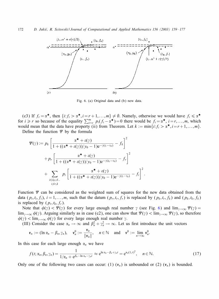
Fig. 6. (a) Original data and (b) new data.

(c3) If fr = ?, then {i:fi ¿?; i= r+1; : : : ; m} �= ∅. Namely, otherwise we would have fi6 ?

for i¿ r so because of the equality∑m

i=r pi(fi−?)=0 there would be fi=?, i= r; : : : ; m, whichwould mean that the data have property (ii) from Theorem. Let k := min{i:fi ¿?; i=r+1; : : : ; m}.DeKne the function ' by the formula

'(�) :=pk

[? + $(�)

1 + ((? + $(�))=y0 − 1)e−�(tr−�0)− fk

]2

+pr

[? + $(�)

1 + ((? + $(�))=y0 − 1)e−�(tk−�0)− fr

]2

+∑

i∈I0∪I−i =r; k

pi

[? + $(�)

1 + ((? + $(�))=y0 − 1)e−�(ti−�0)− fi

]2:

Function ' can be considered as the weighted sum of squares for the new data obtained from thedata (pi; ti; fi), i=1; : : : ; m, such that the datum (pr; tr ; fr) is replaced by (pk; tr ; fk) and (pk; tk ; fk)is replaced by (pr; tk ; fr).Note that %(�)¡'(�) for every large enough real number � (see Fig. 6) and lim�→∞'(�) =

lim�→∞ %(�). Arguing similarly as in case (c2), one can show that '(�)¡ lim�→∞'(�), so therefore%(�)¡ lim�→∞ %(�) for every large enough real number �.(III) Consider the case n → ∞ and 2n + �2n → ∞. Let us Krst introduce the unit vectors�n := (ln n − n; �n); �0n :=

�n‖�n‖ ; n∈N and �0 := lim

n→∞ �0n:

In this case for each large enough n we have

f(t; n; n; �n) =1

1=n + en−ln n−�nt≈ eln n−n+�nt = e�n(1; t)

T; n∈N: (17)

Only one of the following two cases can occur: (1) (�n) is unbounded or (2) (�n) is bounded.

D. Juki+c, R. Scitovski / Journal of Computational and Applied Mathematics 156 (2003) 159–177 173

(III.1) Suppose (�n) is unbounded, i.e., ‖�n‖ → ∞.(a) If �0 ∈ S1 \ l−, then there exists i0 ∈{1; : : : ; m} such that �0uTi0 ¿ 0. Therefore,

limn→∞ �nu

Ti0 = lim

n→∞ ‖�n‖�0nuTi0 =∞:

Then from (17) we would obtain limn→∞ F(n; n; �n)=∞. So, in this case the functional F cannotattain its inKmum F?.(b) Let �0 ∈ l−. Since �n ¿ 0, �0 �= v01.If �0 ∈ l− \ {v01; v0m}, then �0uTi ¡ 0, i = 1; : : : ; m, (see Fig. 2) and

limn→∞ �nu

Ti = lim

n→∞ ‖�n‖�0nuTi =−∞; i = 1; : : : ; m:

By means of (17) we obtain limn→∞ F(n; n; �n) =∑m

i=1 pif2i .If �0 = v0m, then �0uTi ¡ 0, i = 1; : : : ; m − 1, (see Fig. 2), from where by (17) we obtain

limn→∞ F(n; n; �n)¿∑m−1

i=1 pif2i .In considerations under (II.1) we have shown that there exists a point in B, in which the functional

F attains a value which is smaller than∑m−1

i=1 pif2i . This means that in this way (�0 ∈ l−) the

functional F cannot attain its inKmum.(III.2) Consider the case (�n) = (ln n − n; �n) is bounded. Let (ln n − n; �n)→ (ln b0; c0). Note

that c0¿ 0, because �n ¿ 0, n∈N. By means of (17) we obtain

limn→∞F(n; n; �n) =

m∑i=1

pi(b0ec0ti − fi)2= : F2:

If c0 = 0, then

F2 =m∑i=1

pi(bo − fi)2¿m∑i=1

pi( Qf − fi)2 where Qf =∑m

i=1 pifi∑mi=1 pi

:

In considerations under case (c) in II.2(ii), we have shown that there exists a point in B, in whichthe functional F attains a value which is smaller than

∑mi=1 pi( Qf − fi)2.

Hence, we can further assume that c0¿ 0.(a) Consider the case

∑mi=1 pi(b0ec0ti −fi)2¿ inf (b;c)∈R2+

∑mi=1 pi(becti −fi)2. Let (b′; c′)∈R2+ be

a point such that∑m

i=1 pi(b′ec′ti − fi)2¡

∑mi=1 pi(b0ec0ti − fi)2. Then (see proof of the Lemma 1)

lim→∞F(; ln − ln b′; c′) =

m∑i=1

pi(b′ec′ti − fi)2¡

m∑i=1

pi(b0ec0ti − fi)2 = limn→∞F(n; n; �n);

which means that in this way the functional F cannot attain its inKmum.(b) It remains to consider the case

∑mi=1 pi(b0ec0ti − fi)2 = inf (b;c)∈R2+

∑mi=1 pi(becti − fi)2. Let

i0 ∈{1; : : : ; m} be such that b0ec0ti0 − fi0 ¿ 0. Since not all the data lie on the exponential curve,according to Lemma 2 there exists such i0.In order to show that in this way the functional F cannot attain its inKmum either, we are going to

consider the class of logistic functions whose graph contains two points (ti0 ; boec0ti0 ) and (�0; boec0�0)

174 D. Juki+c, R. Scitovski / Journal of Computational and Applied Mathematics 156 (2003) 159–177

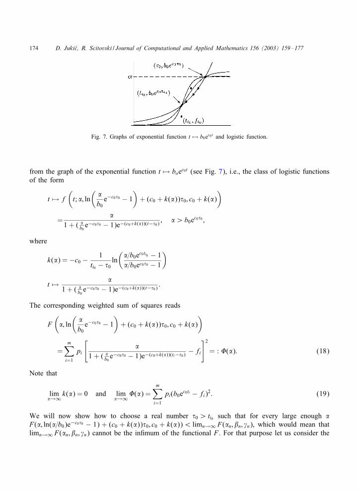
Fig. 7. Graphs of exponential function t �→ b0ec0t and logistic function.

from the graph of the exponential function t �→ boec0t (see Fig. 7), i.e., the class of logistic functionsof the form

t �→ f(t; ; ln

(b0e−c0�0 − 1

)+ (c0 + k())�0; c0 + k()

)

=

1 + ( b0e−c0�0 − 1)e−(c0+k())(t−�0)

; ¿b0ec0�0 ;

where

k() =−c0 − 1ti0 − �0

ln(=b0ec0ti0 − 1=b0ec0�0 − 1

)

t �→ 1 + (

b0e−c0�0 − 1)e−(c0+k())(t−�0)

:

The corresponding weighted sum of squares reads

F(; ln

(b0e−c0�0 − 1

)+ (c0 + k())�0; c0 + k()

)

=m∑i=1

pi

[

1 + ( b0e−c0�0 − 1)e−(c0+k())(ti−�0)

− fi

]2= : �(): (18)

Note that

lim→∞ k() = 0 and lim

→∞�() =m∑i=1

pi(b0ec0ti − fi)2: (19)

We will now show how to choose a real number �0¿ti0 such that for every large enough F(; ln(=b0)e−c0�0 − 1) + (c0 + k())�0; c0 + k())¡ limn→∞ F(n; n; �n), which would mean thatlimn→∞ F(n; n; �n) cannot be the inKmum of the functional F . For that purpose let us consider the

D. Juki+c, R. Scitovski / Journal of Computational and Applied Mathematics 156 (2003) 159–177 175

derivative of the function �:

d�()d

=2m∑i=1i =i0

pi

[

1 + ( b0e−c0�0 − 1)e−(c0+k())(ti−�0)

− fi

]

× 1[1 + (

b0e−c0�0 − 1)e−(c0+k())(ti−�0)]2

×[1−

(1 +

b0(

b0e−c0ti0 − 1)(e

−c0ti0 − e−c0�0)ti − �0ti0 − �0

)e−(c0+k())(ti−�0)

]:

It is easy to show that

lim→∞

(2d�()d

)=2b20

m∑i=1i =i0

pi(b0ec0ti − fi)e2c0ti

×[1−

(1 + (e−c0ti0 − e−c0�0)

ti − �0ti0 − �0

ec0ti0)e−c0(ti−�0)

]: (20)

According to (3) there holds

m∑i=1i =i0

pi(b0ec0ti − fi)ec0ti =−pi0(b0ec0ti0 − fi0)e

c0ti0

m∑i=1i =i0

pi(b0ec0ti − fi)ec0ti ti =−pi0(b0ec0ti0 − fi0)e

c0ti0 ti0

so (20) goes into

lim→∞

(2d�()d

)=2b20

m∑i=1i =i0

pi(b0ec0ti − fi)e2c0ti

+2b20pi0(b0ec0ti0 − fi0)e

c0(ti0+�0)[1 + (e−c0ti0 − e−c0�0)ec0ti0 ]:

For �0 let us take any large enough real number such that lim→∞ (2 d�()=d)¿ 0. Note that thereexists such �0. For �0 chosen in such a way there holds d�()=d¿ 0. This means that there existsa real number 0 such that the function � is strictly increasing in the interval (0;∞). Therefore,

176 D. Juki+c, R. Scitovski / Journal of Computational and Applied Mathematics 156 (2003) 159–177

for every ∈ (0;∞) there holds

F(; ln

(b0e−c0�0 − 1

)+ (c0 + k())�0; c0 + k()

)

=�()¡ lim→∞�() =

m∑i=1

pi(b0ec0ti − fi)2

= limn→∞F(n; n; �n);

which means that in this way the functional F cannot attain its inKmum.Therefore, the sequence (n; n; �n) is bounded. By the Bolzano–Weierstrass’ theorem we can

now assume that it is convergent (otherwise we take convergent subsequences). Let (n; n; �n) →(?; ?; �?).If ? = 0, then F(0; ?; �?) =

∑mi=1 pif2i . In considerations under (II.1) it has been shown that

here exists a point at which the functional F attains a smaller value. Thus, ? �= 0. If �? = 0,F(?; ?; 0)¿

∑mi=1 pi(fi − Qf)2, where Qf =

∑mi=1 pifi=

∑mi=1 pi. In considerations under case (c)

in (II.2) (ii) it has been shown that there exists a point at which the functional F attains a smallervalue. Thus, ? �= 0 and �? �= 0. i.e., (?; ?; �?)∈B. By continuity of the functional F we haveinf (;; �)∈B F(; ; �) = F(?; ?; �?). This completes the proof of Theorem 1.

Remark 2. The generalized logistic function

f(t; ; ; �; )) =

(1 + e−�)t)1=); ; �; )¿ 0; ∈R (21)

is the solution of the so-called Nelder’s model (see [13]):

y′ = �y[1−

(y

))]; ; �; )¿ 0; ∈R: (22)

The parameter )¿ 0 is called the asymmetry coe5cient. For )=1 model (22) becomes the logisticmodel (1). If we take that the asymmetry coe5cient ) is a known constant, by simulating proofsit can be easily shown that then there holds the statement Theorem 1 for the generalized logisticfunction (21) as well.

References

[1] A. BjSorck, Numerical Methods for Least Squares Problems, SIAM, Philadelphia, 1996.[2] E.Z. Demidenko, Optimization and Regression, Nauka, Moscow, 1989 (in Russian).[3] E.Z. Demidenko, Is this the least squares estimate? Biometrika 87 (2000) 437–452.[4] J.E. Dennis, R.B. Schnabel, Numerical Methods for Unconstrained Optimization and Nonlinear Equations, SIAM,

Philadelphia, 1996.[5] C.J. Easingwood, Early product life cycle forms for infrequently purchased major products, Internat. J. Res. Marketing

4 (1987) 3–9.[6] P.E. Gill, W. Murray, M.H. Wright, Practical Optimization, Academic Press, London, 1981.[7] R.C. Jain, R. Agrawal, K.N. Singh, A within year growth model for crop yield forecasting, Biomed. J. 34 (1992)

501–511.

D. Juki+c, R. Scitovski / Journal of Computational and Applied Mathematics 156 (2003) 159–177 177

[8] D. Juki+c, R. Scitovski, The existence of optimal parameters of the generalized logistic function, Appl. Math. Comput.77 (1996) 281–294.

[9] D. Juki+c, R. Scitovski, Existence results for special nonlinear total least squares problem, J. Math. Anal. Appl. 226(1998) 348–363.

[10] D. Juki+c, R. Scitovski, The best least squares approximation problem for a 3-parametric exponential regression model,ANZIAM J. 42 (2000) 254–266.

[11] D. Juki+c, R. Scitovski, H. SpSath, Partial linearization of one class of the nonlinear total least squares problem byusing the inverse model function, Computing 62 (1999) 163–178.

[12] R. Lewandowsky, Prognose und Informationssysteme und ihre Anwendungen, Walter de Gruyter, Berlin, New York,1980.

[13] J.A. Nelder, The Ktting of a generalization of the logistic curve, Biometrics (1961) 89–100.[14] D.A. Ratkowsky, Handbook of Nonlinear Regression Models, Marcel Dekker, New York, 1990.[15] T.A. Stukel, Generalized logistic models, J. Amer. Stat. Assoc. 83 (1988) 426–431.[16] P.F. Verhulst, Notice sur la loi que la population suit dans son accroissement, Math. Phys. 10 (1838) 113.[17] E.O. Voit, M.A. Savageau, Analytical solutions to a generalized growth equation, J. Math. Anal. Appl. 103 (1984)

380–386.