The Finite Mixture Partial Least SquaresApproach - Methodology and Application

Christian M. Ringle, Sven Wende, and Alexander Will1

University of Hamburg - School of Business, Economics and Social Sciencesc.ringle|s.wende|a.will@smartpls.de

1 Introduction

Structural equation modeling (SEM) and path modeling with latent vari-ables (LVP) are applied in modern marketing research to measure complexcause-effect relationships [6, 19]. Covariance structure analysis (CSA) [12] andpartial least squares analysis (PLS) [13] constitute the two corresponding, yetdifferent, statistical techniques for estimating such models. A typical researchissue in SEM and LVP is the measurement of customer satisfaction [7], whichis closely related to the requirement of identifying distinctive customer seg-ments [10].

In SEM, segmentation can be achieved based on the heterogeneity of scoresfor latent variables in the structural (inner) model. Jedidi et al. (1997) addressthis field of research and propose a procedure that blends finite mixture mod-els and the expectation-maximization (EM) algorithm [14, 15, 21]. However,the original technique extends CSA and is inappropriate for PLS because ofmethodological assumptions [5]. Therefore, Hahn et al. (2002) propose thefinite mixture partial least squares (FIMIX-PLS) approach that is stronglyconnected to the maximum likelihood (ML) theory [4]. According to theirproposal, a finite mixture procedure is joined with an EM-algorithm specif-ically regarding the ordinary least squares (OLS)-based predictions of PLS.Hahn et al. (2002), the developers of FIMIX-PLS, present a formal descriptionand discussion of this methodology, the aspects of model identification andan interpretation of results.

2 Methodology

The first methodological step is to estimate path models by applying the basicPLS algorithm for LVP [13]. FIMIX-PLS is then employed using the predictedscores of latent variables and their modified presentation of relationships inthe inner (structural) model:

2 Christian M. Ringle, Sven Wende, and Alexander Will

Bηi + Γξi = ζi (1)

Segment specific heterogeneity of path models is concentrated in the esti-mated relationships between latent variables. FIMIX-PLS captures this het-erogeneity. The segment specific distributional function is defined as follows,assuming that ηi is distributed as a finite mixture of conditional multivariatenormal densities fi|k(·):

ηi ∼K∑

k=1

ρkfi|k(ηi|ξi, Bk, Γk, Ψk) (2)

Substituting fi|k(ηi|ξi, Bk, Γk, Ψk) results in the following equation:

ηi ∼K∑

k=1

ρk

[|Bk|

M√

2π√|Ψk|

e−12 (Bkηi+Γkξi)

′Ψ−1k

(Bkηi+Γkξi))

](3)

It is sufficient to assume multivariate normal distribution of ηi becauseendogenous variables ηi are a function of exogenous variables ξi in the innermodel. Equations (4) and (5) represent an EM-formulation of the likelihoodfunction and the log-likelihood (lnL) as the corresponding objective functionfor maximization:

L =∏

i

∏k

[ρkf(ηi|ξi, Bk, Γk, Ψk)]zik (4)

lnL =∑

i

∑k

zikln(f(ηi|ξi, Bk, Γk, Ψk)) +∑

i

∑k

zikln(ρk) (5)

The EM-algorithm is used to maximize the likelihood in this model inorder to ensure convergence. The ’expectation’ of equation (5) is calculatedin the E-step, where zik is 1 if subject i belongs to class k (or 0 otherwise).The segment size ρk, the parameters ξi, Bk, Γk and Ψk of the conditionalprobability function are given, and provisional estimates (expected values)for zik are computed as follows according to Bayes’ theorem:

E(zik) = Pik =ρkfi|k(ηi|ξi, Bk, Γk, Ψk)∑K

k=1 ρkfi|k(ηi|ξi, Bk, Γk, Ψk)(6)

Equation (5) is maximized in the M-step. Initially, new mixing proportionsρk are calculated by the average of adjusted expected values Pik that resultfrom the previous E-step:

ρk =∑I

i=1 Pik

I(7)

Thereafter, optimal parameters for Bk, Γk and Ψk are determined by inde-pendent OLS regressions (one for each relationship between latent variables

The Finite Mixture Partial Least Squares Approach 3

in the structural model). ML estimators of coefficients and variances are as-sumed to be identical to OLS predictions. The following equations are appliedto obtain the regression parameters for latent endogenous variables:

Ymi = ηmi (8)

Xmi = (Emi, Nmi)′ (9)

Emi ={{ξ1, ..., ξAm} , Am ≥ 1, am = 1, ..., Am ∧ ξam is regressor of m

∅ else (10)

Nmi ={{η1, ..., ηBm

} , Bm ≥ 1, bm = 1, ..., Bm ∧ ηbmis regressor of m

∅ else (11)

The closed form OLS analytic formula for τmk and ωmk is expressed asfollows:

τmk = ((γammk), (βbmmk))′ =[∑

i Pik(X ′miXmi)]

−1 [∑

i Pik(X ′miYmi)]

(12)

ωmk = cell (m×m) of Ψk =∑

i Pik(Ymi −Xmiτmk)(Ymi −Xmiτmk)′

Iρk(13)

The M-step determines new mixing proportions. Independent OLS regres-sions are used in the next E-step iteration to improve the outcomes for Pik.Based on an a priori specified convergence criterion, the EM-algorithm stopswhen the lnL hardly improves (see figure 1). However, the stop is more a mea-sure of lack of progress than a measure of convergence, and there is evidencethat the algorithm is often stopped too early [21].

When applying FIMIX-PLS, the EM-algorithm monotonically increaseslnL and converges towards an optimum [8]. Experience shows that FIMIX-PLS frequently stops in local optimum solutions. The cause of this is thatthe likelihood becomes multimodal so that the algorithm becomes sensitive tothe starting values [21]. Moreover, the problem of convergence in local optimaseems to increase in relevance whenever component densities are not wellseparated. The number of parameters estimated is large and the informationembedded in each observation is limited. This causes a relatively weak updateof the membership probabilities in the E-step.

Some examples of simple strategies for escaping local optima include be-ginning the EM-algorithm from a wide range of (random) starting values orusing various clustering procedures, such as k-means, to obtain an appro-priate initial partition of data. If alternative initializations (starting values)of the algorithm result in different local optima, then the solution with the

4 Christian M. Ringle, Sven Wende, and Alexander Will

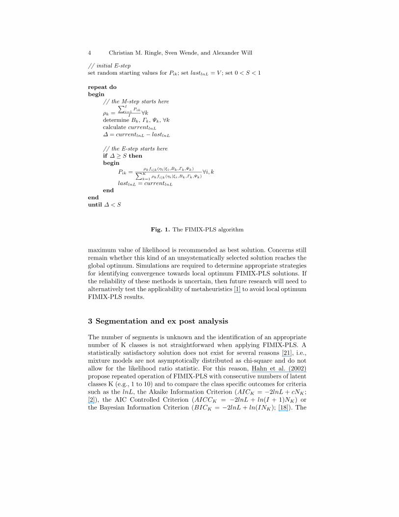
// initial E-stepset random starting values for Pik; set lastlnL = V ; set 0 < S < 1

repeat dobegin

// the M-step starts here

ρk =

∑I

i=1Pik

I∀k

determine Bk, Γk, Ψk, ∀kcalculate currentlnL

∆ = currentlnL − lastlnL

// the E-step starts hereif ∆ ≥ S thenbegin

Pik =ρkfi|k(ηi|ξi,Bk,Γk,Ψk)∑K

k=1ρkfi|k(ηi|ξi,Bk,Γk,Ψk)

∀i, k

lastlnL = currentlnL

endenduntil ∆ < S

Fig. 1. The FIMIX-PLS algorithm

maximum value of likelihood is recommended as best solution. Concerns stillremain whether this kind of an unsystematically selected solution reaches theglobal optimum. Simulations are required to determine appropriate strategiesfor identifying convergence towards local optimum FIMIX-PLS solutions. Ifthe reliability of these methods is uncertain, then future research will need toalternatively test the applicability of metaheuristics [1] to avoid local optimumFIMIX-PLS results.

3 Segmentation and ex post analysis

The number of segments is unknown and the identification of an appropriatenumber of K classes is not straightforward when applying FIMIX-PLS. Astatistically satisfactory solution does not exist for several reasons [21], i.e.,mixture models are not asymptotically distributed as chi-square and do notallow for the likelihood ratio statistic. For this reason, Hahn et al. (2002)propose repeated operation of FIMIX-PLS with consecutive numbers of latentclasses K (e.g., 1 to 10) and to compare the class specific outcomes for criteriasuch as the lnL, the Akaike Information Criterion (AICK = −2lnL + cNK ;[2]), the AIC Controlled Criterion (AICCK = −2lnL + ln(I + 1)NK) orthe Bayesian Information Criterion (BICK = −2lnL + ln(INK); [18]). The

The Finite Mixture Partial Least Squares Approach 5

results of these heuristic measures provide evidence about an appropriatenumber of latent classes. Moreover, an entropy statistic [16], limited between0 and 1, indicates the degree of separation in the individually estimated classprobabilities.

ENK = 1−[∑

i

∑k −Pikln(Pik)]Iln(K)

(14)

The quality of separation of the derived classes will improve the higherENK is. Values of EN that are above 0.5 will result in estimates for Pik

that permit unambiguous segmentation. This criterion is especially relevant,e.g., for identifying different types of customers in the field of marketing.Furthermore, estimates of class specific relationships in the inner model needto provide statistically reasonable values after segmentation.

Given these assumptions, FIMIX-PLS is only applicable for additionalanalytic purposes, if the segments are interpretable. For this reason, Hahnet al. (2002) suggest an ex post analysis of the estimated probabilities ofmembership using an approach proposed by Ramaswamy et al. (1993) toidentify explanatory variables that allow further interpretation of the finalsegments. This kind of characterization of FIMIX-PLS results is essential forthe methodology and its applicability.

The findings of this new approach can be used to group data (e.g., into’young customers’ and ’old customers’) and to calculate the LVP for eachsegment (set of data). The following examples, which use experimental dataand empirical data, document this approach.

4 Example using experimental data

SmartPLS 2.0 [17] is the first statistical software application for (graphical)path modeling with latent variables employing both the basic PLS algorithm[13] as well as FIMIX-PLS capabilities for the kind of segmentation proposedby Hahn et al. (2002). Applying this statistical software module to experi-mental data for a marketing-related path model demonstrates the potentialsof the methodology for PLS-based research. Our hypothetical model is com-prised of one endogenous latent variable Satisfaction and two exogenous latentvariables Price and Quality in the structural model.

• Price-oriented customers (segment 1)This segment is characterized by a strong relationship between Price andSatisfaction and a weak relationship between Quality and Satisfaction.

• Quality-oriented customers (segment 2)This segment is characterized by a strong relationship between Qualityand Satisfaction and a weak relationship between Price and Satisfaction.

Each latent exogenous variable (Price and Quality) consists of seven re-flective indicator-variables, and the latent endogenous variable (Satisfaction)

6 Christian M. Ringle, Sven Wende, and Alexander Will

measured by two manifest variables in a reflective measurement model. Ac-cording to the scheme in table 1, the underlying case values of the manifestvariables are generated on a scale ranging from 1 to 7. For instance, thecase values 1 to 20 of the manifest indicators Price1 to Price7, Satisfaction1and Satisfaction2 are normally distributed random numbers, with µ = 6 andσ = 0.1. The case values 1 to 20 of the manifest indicators Quality1 to Qual-ity7 are normally distributed random numbers, with µ = 4 and σ = 1.

Case Price Quality Satisfaction

1− 20 µ = 6.0 / σ = 0.1 µ = 4.0 / σ = 1.0 µ = 6.0 / σ = 0.121− 40 µ = 4.0 / σ = 1.0 µ = 6.0 / σ = 0.1 µ = 6.0 / σ = 0.141− 60 µ = 2.0 / σ = 0.1 µ = 4.0 / σ = 1.0 µ = 2.0 / σ = 0.161− 80 µ = 4.0 / σ = 1.0 µ = 2.0 / σ = 0.1 µ = 2.0 / σ = 0.1

Table 1. Data generation scheme

The standard PLS procedure is executed to measure the path model basedon the experimental data for manifest indicator variables. FIMIX-PLS usesthe results to process the latent variable scores in the inner model for twosegments. The standard PLS inner model weights in table 2 show that bothconstructs Price and Quality have a relatively high effect on Satisfaction andresult in a substantial R2 of 0.932. An overall goodness of fit (GoF) measure- that is limited between 0 and 1 - is proposed as the geometric mean of theaverage communality (outer model) and the average R2 (inner model) [20]:

GoF =√

communality ·R2 =√

0.865 · 0.932 = 0.898 (15)

However, it is misleading to interpret these excellent estimates for a pathmodel. The application of FIMIX-PLS permits additional analyses that leadto different conclusions.

Price → Satisfaction Quality → Satisfaction

Standard PLS 0.7 0.7FIMIX-PLS segment 1 0.7 0.0FIMIX-PLS segment 2 0.0 0.7

Table 2. Inner model weights

According to the FIMIX-PLS results presented in table 2, both a prioricreated segments are identified in the experimental set of data, i.e., segment 1shows a strong effect of Price on Satisfaction and a week relationship betweenQuality and Satisfaction, and segment 2 shows a strong effect of Quality onSatisfaction and a week relationship between Price and Satisfaction. As aconsequence of the experimental design, segment specific regression variances

The Finite Mixture Partial Least Squares Approach 7

are very low for the latent endogenous variable Satisfaction (0.001 for segment1 and 0.002 for segment 2). This results in corresponding outcomes for R2

that nearly equal one. Cases 1 − 20 and cases 41 − 60 are perfectly assignedto segment 1, and cases 21 − 40 and cases 61 − 80 are perfectly assignedto segment 2 (Pik has either a value of 0 or 1 for the final segmentation).Consequently, EN has a value of 1.0 indicating perfect separation of these twoa priori created (distinctive) segments.

5 Marketing example using empirical data

FIMIX-PLS is often not as straightforward as demonstrated in the foregoingexample using experimental data if researchers use empirical data and do nothave a priori segmentation assumptions. Extensive use of FIMIX-PLS withempirical data in future research ought to furnish additional findings aboutthe methodology and its applicability. For this reason, we apply the techniqueto a marketing related path model and to empirical data from Gruner + Jahr’s’Brigitte Communication Analysis 2002’. Gruner + Jahr is one of the leadingpublishers of printed magazines in Germany. They have been conducting theirCommunication Analysis survey every other year since 1984. In the survey,over 5,000 women answer questions on brands in different product categoriesand questions regarding their personality. The women represent a cross sectionof the German female population.

Answers to questions on the Benetton fashion brand name (on a fourpoint scale from ’low’ to ’high’) are selected in order to use the survey as amarketing-related example of FIMIX-PLS-based customer segmentation. Weassume that Benetton’s aggressive and provocative advertising in the 1990sresulted in a lingering customer heterogeneity that is more distinctive andeasier to identify compared with other fashion brands in this survey (e.g.,Esprit or S.Oliver).

LVP is designed to demonstrate the applicability of FIMIX-PLS in thefield of marketing. The scope of this article does not include a presentation oftheoretically substantiated hypotheses and PLS-based empirical confirmationof them (see for example [9]). We therefore create a reduced path model forBenetton’s brand preference that consists of one latent endogenous ’BRANDPREFERENCE’ variable, and two latent exogenous variables, ’IMAGE’ and’PERSON’, in the structural model. Figure 2 illustrates our inner model, theouter models of LVP that they reflect, and the manifest variables employed.PLS is applied for estimating the path model using the SmartPLS 2.0 softwareapplication.

We follow the suggestions given by Chin (1998) for arriving at a brief eval-uation of results. All relationships in the reflective measurement models haveexcellent factor loadings (the smallest loading has a value of 0.795). Moreover,the average variance extracted (AVE) and ρc are at relatively high levels (seesection 7.2). The latent exogenous ’IMAGE’ variable (weight of 0.423) exhibits

8 Christian M. Ringle, Sven Wende, and Alexander Will

Fig. 2. The brand preference model

a strong relationship to the latent endogenous ’BRAND PREFERENCE’ vari-able. The influence of the latent exogenous ’PERSON’ variable is considerablyweaker (weight of 0.174). Both relationships are statistically significant (seethe results of the bootstrapping procedure in section 7.2). R2 of ’BRANDPREFERENCE’ equals 0.239 and is at a moderate level for PLS path mod-els. This value is mainly determined by Benetton’s ’IMAGE’. The ’PERSON’variable is not as relevant but exhibits a statistically significant influence. Theaverage communality of the three reflective measurement models is relativelyhigh, so that R2 of the latent endogenous ’BRAND PREFERENCE’ variablemainly causes (only) a moderate GoF outcome:

GoF =√

communality ·R2 =√

0.748 · 0.239 = 0.423 (16)

The FIMIX-PLS module of SmartPLS 2.0 is applied for customer seg-mentation based on the estimated scores for latent variables. Table 3 showsheuristic FIMIX-PLS evaluation criteria for alternative numbers of classes K.According to these results, the choice of two latent classes seems to be ap-propriate for customer segmentation purposes, especially in terms of EN. OurEN result of 0.501 also reaches a proper level compared to the EN of 0.43 thatHahn et al. (2002) present for an FIMIX-PLS application. Their presentationis the only one found thus far in English language academic literature.

Table 4 presents the FIMIX-PLS results for two latent classes. In a largesegment (size of 0.809), the explained variance of the latent endogenous’BRAND PREFERENCE’ variable is at a relatively weak level for PLS mod-els (R2 = 0.108). This variance is explained by the latent exogenous ’IMAGE’variable, with its weight of 0.343, and the latent exogenous ’PERSON’ vari-

The Finite Mixture Partial Least Squares Approach 9

Number of latent classes lnL AIC BIC AICC EN

Aggregate (K = 1) −569, 461 1152.922 1181.593 1181.609 1.000K = 2 −713.233 1448.466 1493.520 1493.545 0.501K = 3 −942.215 1954.431 2097.784 2097.863 0.216K = 4 −1053.389 2192.793 2450.830 2450.972 0.230K = 5 −1117.976 2441.388 2846.874 2847.097 0.214

Table 3. Model selection

able, with its weight of 0.177. A smaller segment (size of 0.191) has a relativelyhigh R2 for ’BRAND PREFERENCE’ (value of 0.930). The influence of the’PERSON’ variable does not change much for this segment. However, theweight of the ’IMAGE’ variable is more than twice as high and has a value of0.759. This result reveals that the preference for Benetton is explained to ahigh degree whenever the image of this brand is far more important than theindividuals’ personality.

K = 1 K = 2

Segment size 0.809 0.191R2 (for ’BRAND PREFERENCE’) 0.108 0.930Path ’IMAGE’ to ’BRAND PREFERENCE’ 0.343 0.759Path ’PERSON’ to ’BRAND PREFERENCE’ 0.177 0.170

Table 4. Disaggregate results (solution for two latent classes)

The next step in FIMIX-PLS involves the necessity to identify a certainvariable that characterizes customer segments that have been formed. We im-plemented an ex post analysis of the estimated probabilities of membershipin line with the suggestions of Hahn et al. (2002). The most significant ex-planatory variables among the several indicators examined are: ’I AM VERYINTERESTED IN THE LATEST FASHION TRENDS’, ’I GET INFORMA-TION ABOUT CURRENT FASHION FROM MAGAZINES FOR WOMEN’,’BRAND NAMES ARE VERY IMPORTANT FOR SPORTS WEAR’ and ’ILIKE TO BUY FASHION DESIGNERS’ PERFUMES’ (t-statistics rangingfrom 1.462 to 2.177). These variables may be appropriate for explaining thesegmentation of customers into two classes.

Table 5 shows PLS results using the ’I LIKE TO BUY FASHION DE-SIGNERS’ PERFUMES’ variable for an a priori customer segmentation intotwo classes. Both outcomes for segment-specific LVP estimations satisfy therelevant criteria for model evaluation [3] (see section 7.3). Segment 1 repre-sents customers that are not interested in fashion designers’ perfumes (size of0.223). By contrast, segment 2 (size of 0.777) represents customers that areattracted to Benetton who would enjoy using this fashion brand’s productsin other product categories, such as perfumes. From a marketing viewpoint,

10 Christian M. Ringle, Sven Wende, and Alexander Will

these customers are very important to fashion designers who are intending tocreate brand extensions.

Segment 1 Segment 2

GoF 0.387 0.470R2 (for ’BRAND PREFERENCE’) 0.204 0.323’IMAGE’ → ’BRAND PREFERENCE’ 0.394 0.562’PERSON’ → ’BRAND PREFERENCE’ 0.164 0.104

Table 5. A priori segmentation based on ’I LIKE TO BUY FASHION DESIGNERS’PERFUMES’

Besides their applicability to explaining the FIMIX-PLS segmentation forthe structural model, the variables identified in the ex post analysis do notoffer much potential for a meaningful a priori segmentation, except for the ’ILIKE TO BUY FASHION DESIGNERS’ PERFUMES’ variable. The otherfour variables with high t-statistics do not result in different measurementsfor segment specific path models when segmented a priori into two classes.

We consider reasonable alternatives and test the ’CUSTOMERS’ AGE’variable for an a priori segmentation of Benetton’s brand preference LVP.The ex post analysis of FIMIX-PLS results does not furnish evidence for therelevance of this variable (t-statistic = 0.690). Yet when creating a customersegment for females older than 28 years (segment 1; segment size: 0.793) andfor female consumers between ages of 15 and 28 years (segment 2; segment size:0.207), we achieve a result that is nearly identical to the a priori segmentationusing ’I LIKE TO BUY FASHION DESIGNERS’ PERFUMES’ (see table 6;the evaluated model [3] reveals that the PLS model estimates are acceptablefor each segment, see section 7.4). However, this variable and ’AGE’ are nothighly correlated (correlation coefficient: −0.166).

Segment 1 Segment 2

GoF 0.355 0.521R2 (for ’BRAND PREFERENCE’) 0.172 0.356’IMAGE’ → ’BRAND PREFERENCE’ 0.364 0.559’PERSON’ → ’BRAND PREFERENCE’ 0.158 0.110

Table 6. A priori segmentation based on ’CUSTOMERS’ AGE’

The findings that we present depict problems in identifying interpretablevariables for an a priori segmentation of data. We therefore select several po-tential explanatory variables to create different kinds and numbers of customersegments before specifically estimating their LVP. These results reveal thatvariables, which are indicated as significant throughout the ex post analysis,do not necessarily provide for enhanced a priori segmentation. However, our

The Finite Mixture Partial Least Squares Approach 11

tests do confirm the appropriateness of two classes for a priori segmentation asindicated by FIMIX-PLS. Using larger numbers of latent classes causes PLSmodel estimations with insignificant relationships within the structural modelor relatively low values of R2 for the latent endogenous ’BRAND PREFER-ENCE’ variable.

The example that uses empirical data demonstrates that FIMIX-PLS reli-ably identifies a suitable number of customer segments, if heterogeneity existswithin the structural model. These kinds of findings, which result in segmentspecific LVP estimations, provide a platform for acquiring further differenti-ated PLS path modeling conclusions. However, an ex post analysis is essentialin terms of methodology and offers various potentials for future research.

6 Summary

FIMIX-PLS allows us to capture unobserved heterogeneity in the estimatedscores for latent variables in path models by grouping data. This is advanta-geous to a priori segmentation because homogeneous segments are explicitlygenerated for the inner model relationships. The procedure is broadly appli-cable in business research. For example, marketing-related path modeling canexploit this approach for distinguishing certain groups of customers.

In the first example involving experimental data, FIMIX-PLS reliably iden-tifies and separates the two a priori created segments of price- and quality-oriented customers. The second example of a marketing-related path modelfor Benetton’s brand preference is based on empirical data, and it also demon-strates that FIMIX-PLS reliably identifies an appropriate number of customersegments if distinctive groups of customers exist that result in heterogeneitywithin the inner model. In this case, FIMIX-PLS enables us to identify: (1)a large segment of ’more mature’ female customers that shows similar resultswhen compared to the original model estimation and (2) a smaller segment of’young’ female customers that reveals a strong relationship between ’IMAGE’and ’BRAND PREFERENCE’.

We accordingly conclude that the methodology offers capabilities to ex-tend and further differentiate PLS-based analyses of LVP. The most importantfact within this context is that poor standard PLS results for the overall setof data, caused by the heterogeneity of estimates in the structural model,may result in good estimates of the inner relationships and substantial val-ues for R2 of latent endogenous variables after segmentation. However, anaccurate ex post analysis is essential for this kind of methodology to ensure asuitable characterization of the formed groups for further interpretation pur-poses and additional conclusions. Such FIMIX-PLS related analyses must beconducted by trial and error testing routines until future research presentsreliable procedures. Extensive simulations with experimental data and broaduse of empirical data are required to further illustrate the applicability ofFIMIX-PLS.

12 Christian M. Ringle, Sven Wende, and Alexander Will

7 Appendix

7.1 Description of symbols

Am number of exogenous variables as regressors in regression mam exogenous variable am with am = 1, ..., Am

Bm number of endogenous variables as regressors in regression mbm endogenous variable bm with bm = 1, ..., Bm

γammk regression coefficient of am in regression m for class kβbmmk regression coefficient of bm in regression m for class kτmk ((γammk), (βbmmk))′ vector of the regression coefficientsωmk cell (m×m) of Ψk

c constant factorfi|k(·) probability for case i given a class k and parameters (·)I number of cases or observationsi case or observation i with i = 1, ..., IJ number of exogenous variablesj exogenous variable j with j = 1, ..., JK number of classesk class or segment k with k = 1, ...,KM number of endogenous variablesm endogenous variable m with m = 1, ...,MNk number of free parameters defined as (K − 1) + KR + KMPik probability of membership of case i to class kR number of predictor variables of all regressions in the inner modelS stop or convergence criterionV large negative numberXmi case values of the regressors for regression m of individual iYmi case values of the regressant for regression m of individual izik zik = 1, if the case i belongs to class k; zik = 0 otherwiseζi random vector of residuals in the inner model for case iηi vector of endogenous variables in the inner model for case iξi vector of exogenous variables in the inner model for case iB M ×M path coefficient matrix of the inner modelΓ M × J path coefficient matrix of the inner model∆ difference of currentlnL and lastlnL

Bk M ×M path coefficient matrix of the inner model for latent class kΓk M × J path coefficient matrix of the inner model for latent class kΨk M ×M matrix for latent class k containing the regression variancesρ (ρ1, ..., ρK), vector of the K mixing proportions of the finite mixtureρk mixing proportion of latent class k

The Finite Mixture Partial Least Squares Approach 13

7.2 PLS results for the ’BRAND PREFERENCE’ path model

PLS results for the reflective measurement models

Image Person B.P.I have a clear impression of this brand 0.860

This brand can be trusted 0.899Is modern and up to date 0.795

Represents a great style of living 0.832Fashion is a way to express who I am 0.801

I often talk about fashion 0.894A brand name is very important to me 0.850

I am interested in the latest trends 0.831Sympathy 0.944

Brand usage 0.930

AV E and ρc for the latent variables

AV E ρc

Image 0.710 0.910Person 0.725 0.922B.P. 0.881 0.937

PLS results for the structural model and the GoF

R2 of the latent endogenous ’BRAND PREFERENCE’ variable = 0.239,GoF = 0.423. Bootstrapping, 500 samples, construct level changes.

Image → B.P. Person → B.P.Original estimation 0.423 0.174

Mean of all bootstrapping sample 0.428 0.174Standard deviation 0.041 0.036

t-statistic 10.361 4.875

7.3 PLS results for segment 1 based upon ’I LIKE TO BUY...’

This segment with a size of 0.223 represents customers that are not interestedin fashion designers’ perfumes.

14 Christian M. Ringle, Sven Wende, and Alexander Will

PLS results for the reflective measurement models

Image Person B.P.I have a clear impression of this brand 0.851

This brand can be trusted 0.894Is modern and up to date 0.783

Represents a great style of living 0.821Fashion is a way to express who I am 0.761

I often talk about fashion 0.878A brand name is very important to me 0.851

I am interested in the latest trends 0.823Sympathy 0.949

Brand usage 0.930

AV E and ρc for the latent variables

AV E ρc

Image 0.703 0.904Person 0.687 0.898B.P. 0.882 0.938

PLS results for the structural model and the GoF

R2 of the latent endogenous ’BRAND PREFERENCE’ variable = 0.204,GoF = 0.387. Bootstrapping, 500 samples, construct level changes.

Image → B.P. Person → B.P.Original estimation 0.394 0.164

Mean of all bootstrapping sample 0.394 0.173Standard deviation 0.041 0.037

t-statistic 9.562 4.492

7.4 PLS results for segment 2 based upon ’I LIKE TO BUY...’

This segment with a size of 0.777 represents customers that are attracted bythe fashion brand and would enjoy using this brand for items of other productcategories like perfumes.

The Finite Mixture Partial Least Squares Approach 15

PLS results for the reflective measurement models

Image Person B.P.I have a clear impression of this brand 0.873

This brand can be trusted 0.906Is modern and up to date 0.832

Represents a great style of living 0.870Fashion is a way to express who I am 0.788

I often talk about fashion 0.645A brand name is very important to me 0.747

I am interested in the latest trends 0.718Sympathy 0.906

Brand usage 0.934

AV E and ρc for the latent variables

AV E ρc

Image 0.758 0.926Person 0.528 0.816B.P. 0.847 0.917

PLS results for the structural model and the GoF

R2 of the latent endogenous ’BRAND PREFERENCE’ variable = 0.323,GoF = 0.470. Bootstrapping, 500 samples, construct level changes.

Image → B.P. Person → B.P.Original estimation 0.562 0.104

Mean of all bootstrapping sample 0.564 0.106Standard deviation 0.034 0.063

t-statistic 15.020 1.662

7.5 PLS results for segment 1 based upon customers’ age

This segment with a size of 0.793 represents women who are older than 28years.

16 Christian M. Ringle, Sven Wende, and Alexander Will

PLS results for the reflective measurement models

Image Person B.P.I have a clear impression of this brand 0.860

This brand can be trusted 0.879Is modern and up to date 0.777

Represents a great style of living 0.807Fashion is a way to express who I am 0.769

I often talk about fashion 0.894A brand name is very impoertant to me 0.867

I am interested in the latest trends 0.831Sympathy 0.936

Brand usage 0.925

AV E and ρc for the latent variables

AV E ρc

Image 0.692 0.900Person 0.708 0.906B.P. 0.866 0.928

PLS results for the structural model and the GoF

R2 of the latent endogenous variable ’BRAND PREFERENCE’ = 0.172,GoF = 0.355. Bootstrapping, 500 samples, construct level changes.

Image → B.P. Person → B.P.Original estimation 0.364 0.158

Mean of all bootstrapping sample 0.368 0.164Standard deviation 0.041 0.034

t-statistic 8.796 4.639

7.6 PLS results for segment 2 based upon customers’ age

This segment with a size of 0.209 represents women who are between 15 and28 years.

The Finite Mixture Partial Least Squares Approach 17

PLS results for the reflective measurement models

Image Person B.P.I have a clear impression of this brand 0.850

This brand can be trusted 0.928Is modern and up to date 0.888

Represents a great style of living 0.897Fashion is a way to express who I am 0.849

I often talk about fashion 0.834A brand name is very important to me 0.752

I am interested in the latest trends 0.818Sympathy 0.958

Brand usage 0.940

AV E and ρc for the latent variables

AV E ρc

Image 0.794 0.939Person 0.663 0.887B.P. 0.900 0.948

PLS results for the structural model and the GoF

R2 of the latent endogenous ’BRAND PREFERENCE’ variable = 0.356,GoF = 0.521. Bootstrapping, 500 samples, construct level changes.

Image → B.P. Person → B.P.Original estimation 0.559 0.110

Mean of all bootstrapping sample 0.558 0.116Standard deviation 0.031 0.034

t-statistic 17.931 3.218

References

1. Emile Aarts and Jan K. Lenstra. Local search in combinatorial optimization.Princeton University Press, Princeton et al., 2003.

2. Hirotugu Akaike. A new look at statistical model identification. IEEE Trans-action on Automatic Control, 19:328–347, 1974.

3. Wynne W. Chin. The partial least squares approach to structural equation mod-eling. In George A. Marcoulides, editor, Modern methods for business research,pages 295–358. Lawrence Erlbaum Associates, Mahwah, 1998.

4. Scott R. Eliason. Maximum likelihood estimation: Logic and practice. SagePublications, Newbury Park et al., 2000.

5. Claes Fornell and Fred L. Bookstein. Two structural equation models: LISRELand PLS applied to consumer exit-voice theory. Journal of Marketing Research,XIX:440–452, 1982.

18 Christian M. Ringle, Sven Wende, and Alexander Will

6. Claes Fornell and David F. Larcker. Structural equation models with unob-servable variables and measurement error: Algebra and statistics. Journal ofMarketing Research, XVIII:328–388, 1981.

7. Peter Hackl and Anders H. Westlund. On structural equation modeling forcustomer satisfaction measurement. Total Quality Management, 11:820–825,2000.

8. Carsten Hahn, Michael D. Johnson, Andreas Herrmann, and Frank Huber. Cap-turing customer heterogeneity using a finite mixture PLS approach. Schmalen-bach Business Review, 54:243–269, 2002.

9. Karl-Werner Hansmann and Christian M. Ringle. Enterprise networks andstrategic success. In Theresia Theurl, editor, Competitive advantage of the co-operatives’ networks, pages 131–152. Shaker Verlag, Aachen, 2005.

10. Barry Ip and Gabriel Jacobs. Segmentation of the games market using multi-variate analysis. Journal of Targeting, Measurement & Analysis for Marketing,13:275–287, 2005.

11. Kamel Jedidi, Harsharanjeet S. Jagpal, and Wayne S. DeSarbo. Finite-fixturestructural equation models for response-based segmentation and unobservedheterogeneity. Marketing Science, 16:39–59, 1997.

12. Karl G. Joreskog. Structural analysis of covariance and correlation matrices.Psychometrika, 43:443–477, 1978.

13. Jan-Bernd Lohmoller. Latent variable path modeling with partial least squares.Physica-Verlag, Heidelberg, 1989.

14. Geoffrey J. McLachlan and Kaye E. Basford. Mixture models: Inference andapplications to clustering. Marcel Dekker, New York, 1988.

15. Geoffrey J. McLachlan and Thriyambakam Krishnan. The EM algorithm andextensions. John Wiley & Sons, Chichester, 2004.

16. Venkatram Ramaswamy, Wayne S. DeSarbo, David J. Reibstein, and William T.Robinson. An empirical pooling approach for estimating marketing mix elastic-ities with PIMS data. Marketing Science, 12:103–124, 1993.

17. Christian M. Ringle, Sven Wende, and Alexander Will. SmartPLS 2.0 (beta).http://www.smartpls.de, 2005.

18. Gideon Schwarz. Estimating the dimensions of a model. Annals of Statistics,6:461–464, 1978.

19. Jan-Benedict Steenkamp and Hans Baumgartner. On the use of structural equa-tion models for marketing modeling. International Journal of Research in Mar-keting, 17:195–202, 2000.

20. Michel Tenenhaus, Vincenzo E. Vinzi, Yves-Marie Chatelin, and Carlo Lauro.PLS path modeling. Computational Statistics & Data Analysis, 48:159–205,2005.

21. Michel Wedel and Wagner Kamakura. Market segmentation: Conceptual andmethodological foundations. Kluwer Academic Publishers, Boston et al., 2000.