THE USE OF PARTIAL LEAST SQUARES PATH MODELING IN INTERNATIONAL MARKETING

THE USE OF PARTIAL LEAST

SQUARES PATH MODELING IN

INTERNATIONAL MARKETING

Jorg Henseler, Christian M. Ringle and

Rudolf R. Sinkovics

The advent of structural equation modeling (SEM) with latent variables haschanged the nature of research in international marketing and management.Researchers acknowledge the possibilities of distinguishing betweenmeasurement and structural models and explicitly taking measurementerror into account. As Gefen, Straub, and Boudreau (2000, p. 6) point out,‘‘SEM has become de rigueur in validating instruments and testing linkagesbetween constructs.’’ They furthermore distinguish between two families ofSEM techniques: covariance-based techniques, as represented by LISREL,and variance-based techniques, of which partial least squares (PLS) pathmodeling is the most prominent representative.

PLS has been used by a growing number of researchers from variousdisciplines such as strategic management (e.g., Hulland, 1999), managementinformation systems (e.g., Dibbern, Goles, Hirschheim, & Jayatilaka, 2004),e-business (e.g., Pavlou & Chai, 2002), organizational behavior (e.g.,Higgins, Duxbury, & Irving, 1992), marketing (e.g., Reinartz, Krafft, &Hoyer, 2004), and consumer behavior (e.g., Fornell & Robinson, 1983).Since 1987, for instance, more than 20 studies using PLS have beenpublished in five top-tier marketing journals (Eggert, 2007) – the majority in

New Challenges to International Marketing

Advances in International Marketing, Volume 20, 277–319

Copyright r 2009 by Emerald Group Publishing Limited

All rights of reproduction in any form reserved

ISSN: 1474-7979/doi:10.1108/S1474-7979(2009)0000020014

277

dx.doi.org/10.1108/S1474-7979(20)09000-0020014

dx.doi.org/10.1108/S1474-7979(20)09000-0020014

JORG HENSELER ET AL.278

the last six years. PLS is the method of choice for success factor studies inmarketing (Albers, 2009) and for estimating the various national customersatisfaction index models (e.g., Fornell, 1992). The PLS methodology hasalso achieved an increasingly popular role in empirical research ininternational marketing, which may represent an appreciation of distinctivemethodological features of PLS. As of March 2008, more than 30 articles oninternational marketing using PLS were published in double-blind reviewedjournals. However, these publications show a rather large variability in theway how PLS is applied and how its outcomes are reported. In manyinstances, the rationale for choosing PLS among a possible set of alternativeanalytical techniques is not made explicit.

Although several articles offer guidance for the use of covariance-basedstructural equation modeling (CBSEM) in international marketing (e.g.,Steenkamp & Baumgartner, 1998; Malhotra, 2001; Iacobucci, Grisaffe,Duhachek, & Marcati, 2003), there are no similar subject-specific guidelinesfor the use of PLS. While there are general recommendations for the use ofPLS (e.g., Hulland, 1999), the specific requirements and typical researchproblems of international marketing have not been addressed yet. Our mainaims are to shed light on PLS path modeling as an SEM technique, to revealthe strengths and weaknesses of PLS in general, and to deliver guidelines forits use in international marketing in particular.

1. APPLICATIONS OF PLS PATH MODELING

IN INTERNATIONAL MARKETING

In order to determine the status quo of PLS path modeling in internationalmarketing research, we conducted an exhaustive literature review. Anevaluation of double-blind reviewed journals through important academicpublishing databases (e.g., ABI/Inform, Elsevier ScienceDirect, EmeraldInsight, Google Scholar, PsycINFO, Swetswise) revealed that more than30 academic articles in the domain of international marketing (in a broadsense) used PLS path modeling as means of statistical analysis. We assessedwhat the main motivation for the use of PLS was in respect of each article.Moreover, we checked for applications of PLS in combination with one ormore additional methods, and whether the main reason for conducting anyadditional method(s) was mentioned.

Table 1 lists all the identified academic articles that use PLS as a methodof analysis in the context of international marketing. Green and Ryans

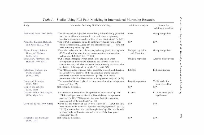
Table 1. Studies Using PLS Path Modeling in International Marketing Research.

Study Motivation for Using PLS Path Modeling Additional Analysis Reason for

Additional Analysis

Acedo and Jones (2007, JWB) ‘‘The PLS technique is justified where theory is insufficiently grounded

and the variables or measures do not conform to a rigorously

specified measurement model, or fit a certain distribution’’ (p. 242)

t-test Group comparison

Ainuddin, Beamish, Hulland,

and Rouse (2007, JWB)

‘‘Use of PLS is especially suited to exploratory studies such as this,

where the measures [ . . . ] are new and the relationships [ . . . ] have not

been previously tested’’ (p. 56)

N/A N/A

Alpert, Kamins, Sakano,

Onzo, and Graham

(2001, IMR)

‘‘Formative indicators can only be analyzed using partial least squares

(PLS), and not by using the more common structural equation

technique of LISREL’’ (p. 177–178)

Multiple regression

and Chow test

Group comparison

Birkinshaw, Morrison, and

Hulland (1995, SMJ)

‘‘PLS is most appropriate when sample sizes are small, when

assumptions of multivariate normality and interval scaled data

cannot be made, and when the researcher is primarily concerned with

prediction of the dependent variable’’ (pp. 646–647)

Multiple regression Analysis of subgroups

Calantone, Graham, and

Mintu-Wimsatt

(1998, IJRM)

‘‘The PLS parameter estimates better reveal the strength and direction

(i.e., positive vs. negative) of the relationships among variables

compared to correlation coefficients’’ (p. 28), ‘‘PLS avoids

parameters estimation biases common in regression analysis’’ (p. 28)

LISREL Path significances

Festge and Schwaiger

(2007, AIM)

‘‘The researcher’s focus is placed on the explanation of an endogenous

construct’’ (p. 192)

Logistic regression Verify model for

binary variables

Gerpott and Jakopin

(2005, SBR)

Not explicitly mentioned N/A N/A

Graham, Mintu, and Rodgers

(1994, Mgmt.Sc.)

‘‘Parameters can be estimated independent of sample size’’ (p. 79),

‘‘PLS avoids parameter estimation biases inherent in regression

analysis’’ (p. 80), ‘‘PLS provides the most flexibility regarding

measurement of the constructs’’ (p. 80)

LISREL In order to test path

significances

Green and Ryans (1990, JPIM) ‘‘Given that the purpose of this study is to predict [ . . . ], PLS has thus

been chosen as the structural equation modeling approach’’ (p. 53),

‘‘[PLS] is more robust with small sample sizes’’ (p. 53), ‘‘the data do

not have to be multivariate normal because of the fixed point

estimation’’ (p. 53)

N/A N/A

Holzmuller and Stottinger

(1996, JIM)


Partia

lLeast

Squares

Path

Modelin

gin

Intern

atio

nalMarketin

g279

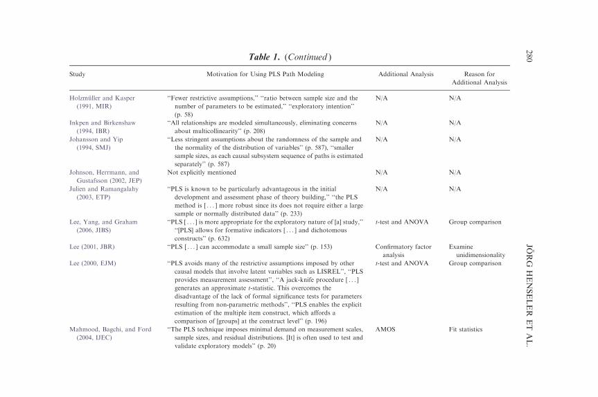
Table 1. (Continued )

Study Motivation for Using PLS Path Modeling Additional Analysis Reason for

Additional Analysis

Holzmuller and Kasper

(1991, MIR)

‘‘Fewer restrictive assumptions,’’ ‘‘ratio between sample size and the

number of parameters to be estimated,’’ ‘‘exploratory intention’’

(p. 58)

N/A N/A

Inkpen and Birkenshaw

(1994, IBR)

‘‘All relationships are modeled simultaneously, eliminating concerns

about multicollinearity’’ (p. 208)

N/A N/A

Johansson and Yip

(1994, SMJ)

‘‘Less stringent assumptions about the randomness of the sample and

the normality of the distribution of variables’’ (p. 587), ‘‘smaller

sample sizes, as each causal subsystem sequence of paths is estimated

separately’’ (p. 587)

N/A N/A

Johnson, Herrmann, and

Gustafsson (2002, JEP)


Julien and Ramangalahy

(2003, ETP)

‘‘PLS is known to be particularly advantageous in the initial

development and assessment phase of theory building,’’ ‘‘the PLS

method is [ . . . ] more robust since its does not require either a large

sample or normally distributed data’’ (p. 233)

N/A N/A

Lee, Yang, and Graham

(2006, JIBS)

‘‘PLS [ . . . ] is more appropriate for the exploratory nature of [a] study,’’

‘‘[PLS] allows for formative indicators [ . . . ] and dichotomous

constructs’’ (p. 632)

t-test and ANOVA Group comparison

Lee (2001, JBR) ‘‘PLS [ . . . ] can accommodate a small sample size’’ (p. 153) Confirmatory factor

analysis

Examine

unidimensionality

Lee (2000, EJM) ‘‘PLS avoids many of the restrictive assumptions imposed by other

causal models that involve latent variables such as LISREL’’, ‘‘PLS

provides measurement assessment’’, ‘‘A jack-knife procedure [ . . . ]

generates an approximate t-statistic. This overcomes the

disadvantage of the lack of formal significance tests for parameters

resulting from non-parametric methods’’, ‘‘PLS enables the explicit

estimation of the multiple item construct, which affords a

comparison of [groups] at the construct level’’ (p. 196)

t-test and ANOVA Group comparison

Mahmood, Bagchi, and Ford

(2004, IJEC)

‘‘The PLS technique imposes minimal demand on measurement scales,

sample sizes, and residual distributions. [It] is often used to test and

validate exploratory models’’ (p. 20)

AMOS Fit statistics

JORG

HENSELER

ET

AL.

280

Mintu-Wimsatt and Graham

(2004, JAMS)

‘‘PLS is a more rigorous approach [ . . . ] compared to correlation and

regression analyses’’ (p. 351), ‘‘PLS [ . . . ] avoids small sample size

problems,’’ ‘‘PLS minimizes biases associated with [ . . . ]

dichotomous and ordinal measures’’ (p. 352)

N/A N/A

Money (2004, JBR) In order to validate regression results N/A N/A

Money and Graham

(1999, JIBS)

N/A LISREL Regression &

Chow Test

Path significances

group comparison

Nakamura, Shaver, and Yeung

(1996, IJIO)


Nijssen and Douglas

(2008, JIM)

‘‘PLS can deal effectively with formative scales, is distribution free, and

is a powerful instrument for analyzing small samples’’ (p. 95)

N/A N/A

O’Cass and Fenech (2003,

EJM)

‘‘[PLS] circumvent[s] the necessity for the multivariate normal

assumption’’ (p. 377)

N/A N/A

Pavlou and Chai (2002, JECR) ‘‘PLS allows [ . . . ] a simultaneous analysis of both whether the

hypothesized relationships at the theoretical level are empirically

acceptable, and also how well the measures relate to each construct,’’

‘‘[t]he ability to include multiple measures for each construct,’’ ‘‘the

nature of [ . . . ] measures,’’ ‘‘the small sample size’’ (p. 246)

N/A N/A

Pullman, Granzin, and Olsen

(1997, IBR)

‘‘The objective of PLS is explanation of the relationships and prediction

of the criterion variables of the model’’ (p. 221)

N/A N/A

Pinto, Rodrıguez Escudero,

and Gutıerrez Cillan

(2008, IMM)

‘‘Avoiding any distributional assumption of the observed variables’’

(p. 160), ‘‘the sample size required in PLS is much smaller’’ (p. 160),

‘‘PLS can handle both types of measurement models, reflective and

formative’’ (p. 160)

N/A N/A

Singh, Fassott, Chao, and

Hoffmann (2006a, IMR)

‘‘PLS [ . . . ] uses distribution-free assumptions, [ . . . ] especially when

independence of observations is not stipulated’’ (p. 89)

N/A N/A

Singh, Fassott, Zhao, and

Boughton (2006b, JCB)


Stottinger and Holzmuller

(2001, MIR)


Tsang (2002, SMJ) ‘‘PLS is particularly suitable for data analysis during the early stage of

theory development where the theoretical model and its measures are

not well formed’’ (p. 841)

t-test Group comparison

Venaik, Midgley, and

Devinney (2005, JIBS)

‘‘At an early stage of development [ . . . ] the regression based approach

of PLS is considered more appropriate than covariance-based

methods such as LISREL,’’ applicable when a multivariate normal

distribution can not be assured, small sample size in combination

with a complex model including second-order constructs, formative

indicators (p. 665)

N/A N/A

Partia

lLeast

Squares

Path

Modelin

gin

Intern

atio

nalMarketin

g281


(1990) published the first study using PLS in international marketing.Although there were several articles in the 1990s, the popularity of PLSseems to have largely increased in the new millennium. Journals thatpublished PLS applications in the international marketing domain are(journal abbreviation and number of studies in parentheses):

� Advances in International Marketing (AIM; 1)� Entrepreneurship Theory and Practice (ETP; 1)� European Journal of Marketing (EJM; 2)� Industrial Marketing Management (IMM; 1)� International Business Review (IBR; 2)� International Journal of Electronic Commerce (IJEC; 1)� International Journal of Industrial Organization (IJIO; 1)� International Journal of Research in Marketing (IJRM; 1)� International Marketing Review (IMR; 2)� Journal of Business Research (JBR; 2)� Journal of Consumer Behaviour (JCR; 1)� Journal of Economic Psychology (JEP; 1)� Journal of Electronic Commerce Research (JECR; 1)� Journal of International Business Studies (JIBS; 3)� Journal of International Marketing (JIM; 2)� Journal of Product Innovation Management (JPIM; 1)� Journal of the Academy of Marketing Science (JAMS; 1)� Journal of World Business (JWB; 2)� Management International Review (MIR; 2)� Management Science (Mgmt.Sc.; 1)� Schmalenbach Business Review (SBR; 1)� Strategic Management Journal (SMJ; 3)

Our first analysis of these 33 studies provides some evidence of theincreasing popularity of PLS path modeling within the research community.The analysis also points to the authors’ motivation for the use of thisparticular statistical method. Many researchers argue that the goal of theirstudies is in line with particular strengths of PLS path modeling. The mostimportant motivations are exploration and prediction, as PLS pathmodeling is recommended in an early stage of theoretical development inorder to test and validate exploratory models. Another powerful feature ofPLS path modeling is that it is suitable for prediction-oriented research.Thereby, the methodology assists researchers who focus on the explanationof endogenous constructs. The characteristics of PLS path modeling, which

Partial Least Squares Path Modeling in International Marketing 283

researchers regard as relevant for their studies on international marketing,can be summarized as follows:

� PLS delivers latent variable scores, i.e. proxies of the constructs, which aremeasured by one or several indicators (manifest variables).� PLS path modeling avoids small sample size problems and can thereforebe applied in some situations when other methods cannot.� PLS path modeling can estimate very complex models with many latentand manifest variables.� PLS path modeling has less stringent assumptions about the distributionof variables and error terms.� PLS can handle both reflective and formative measurement models.

However, there are several arguments regarding the characteristicsof PLS path modeling that should be treated with caution: PLS pathmodeling does not have less stringent assumptions about the representa-tiveness of the sample. Sometimes, PLS path modeling is implicitlypresumed to be the only method that can cope with formative indicators(cf. Chin, 1998); however, LISREL also has this ability (cf. Jarvis,MacKenzie, & Podsakoff, 2003). Although comparisons of methods providesome evidence of PLS’ favorable behavior in light of multicollinearity(cf. Gustafsson & Johnson, 2004), PLS does not resist multicollinearity.Since PLS determines measurement models (in Mode B) as well as structuralmodels by means of multiple regressions, PLS estimates can be subject tomulticollinearity problems, too.

Our review furthermore discloses that some studies use PLS pathmodeling in combination with other analysis techniques such as t-tests,ANOVA, and CBSEM. Yet, these methods are not always a suitable choice.If, for instance, PLS was selected because of its distribution-free character, itwould be inconsequent to introduce distributional assumptions in anotheranalysis such as t-test or ANOVA, or to rely on criteria derived fromCBSEM’s chi-square statistic. This finding provides evidence that eitherPLS path modeling lacks important features, which makes the use ofadditional analyses necessary, or that researchers are not aware of therespective extensions of PLS path modeling. In particular, the findingsunderpin the strong need for a PLS-based approach to multigroup analysis(MGA) in international marketing in order to compare model parametersacross groups such as countries or cultures.

The remainder of this chapter is organized as follows: In the followingSection 2, we describe the working principle of PLS path modeling anddiscuss the characteristics of PLS in detail in order to assist research of


international marketing to distinguish between facts and fiction about PLSpath modeling. Section 3 addresses the assessment of PLS path modelingresults, which represents a key area of concern when applying themethodology. Five issues are covered: Sections 3.1 and 3.2 provide anoverview of the use of PLS path modeling for the assessment of reflectiveand formative measurement models, respectively. Section 3.3 presents theavailable criteria for evaluating the structural model. Section 3.4 presentsand discusses the use of bootstrapping for determining confidence intervalsand the significance of PLS path modeling estimates. As a courtesy tointernational marketing’s need to compare model parameters acrosscountries, Section 3.5 proposes a new PLS-based approach for groupcomparisons based on bootstrapping. Finally, Section 4 sums up the keyfindings and draws conclusions.

2. PLS PATH MODELING

PLS is a family of alternating least squares algorithms, or ‘‘prescriptions,’’which extend principal component and canonical correlation analysis. Themethod was designed by Wold (1974, 1982, 1985) for the analysis of highdimensional data in a low-structure environment and has undergone variousextensions and modifications. This chapter builds on Wold’s (1982) basicalgorithmic design and some extensions developed by Lohmoller (1989).

2.1. The Nature of PLS Path Models

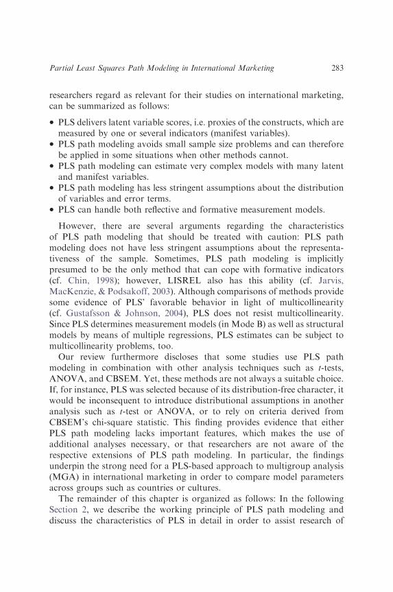
PLS path models are formally defined by two sets of linear equations: theinner model and the outer model. The inner model specifies the relationshipsbetween unobserved or latent variables, whereas the outer model specifiesthe relationships between a latent variable and its observed or manifestvariables. The various literatures do not always employ the sameterminology. For instance, publications addressing CBSEM (e.g., Rigdon,1998) often refer to structural models and measurement models or(observed) indicator variables; whereas those focusing on PLS pathmodeling (e.g., Lohmoller, 1989) use the terms inner model and outermodel or manifest variables for similar elements of the causal model. Fig. 1depicts an example of a PLS path model.

In order to simplify the notation of the model and in line with conventionaldescriptions of PLS, we assume that latent and manifest variables are

�1

�2

�3

�4

x11

x12

x13

x21

x22

x23

x24

x31

x32

x41

x42

x43

�31

�32

�41

�42

�43

�1

�2InnerModel

Outer Model(Here: Formative Mode)

Outer Model(Here: Reflective Mode)

Fig. 1. Example of a PLS Path Model.


standardized so that the location parameters can be discarded in thefollowing equations. The inner model for relationships between latentvariables can be written as:

x ¼ Bxþ z (1)

where x is the vector of latent variables, B denotes the matrix of coefficientsof their relationships, and z represents the inner model residuals. The basicPLS design assumes a recursive inner model that is subject to predictorspecification. Thus, the inner model constitutes a causal chain system (i.e.with uncorrelated residuals and without correlations between the residualterm of a certain endogenous latent variable and its explanatory latentvariables). Predictor specification reduces Eq. (1) to:

ðxjxÞ ¼ Bx (2)

PLS path modeling includes two different kinds of outer models: reflective(Mode A) and formative (Mode B) measurement models. The selection of acertain outer mode is subject to theoretical reasoning (Diamantopoulos &Winklhofer, 2001).

The reflective mode has causal relationships from the latent variable tothe manifest variables in its block. Thus, each manifest variable in a certainmeasurement model is assumed to be generated as a linear function of itslatent variables and the residual e:

Xx ¼ Lxxþ �x (3)


where L represents the loading (pattern) coefficients. The outer relationshipsare also subject to predictor specification – implying that there are nocorrelations between the outer residuals and the latent variable of the sameblock – that reduces Eq. (3) to:

ðXxjxÞ ¼ Lxx (4)

The formative mode of a measurement model has causal relationshipsfrom the manifest variables to the latent variable. For those blocks, thelinear relationships are given as follows:

x ¼ PxXx þ �x (5)

In the formative mode, predictor specification is also in effect, reducingEq. (5) to:

ðxjXxÞ ¼ PxXx (6)

Moreover, it is important to see that the terms ‘‘formative’’ and‘‘reflective,’’ as well as the connotation which is associated with theclassification of ‘‘causal’’ and ‘‘effect,’’ point at a difference between thecharacterization of the latent variable measurement models’ mode.Although a latent variable was originally considered an exact linearcombination of its indicators for formative indicator specifications, a causalindicator specification – the original term for these indicators – may be moregeneral in that it holds both in the case of an exact linear combination, aswell as when the indicators do not completely determine the latent variable(Bollen, 1989). In this chapter, we consistently use the terms ‘‘formative’’and ‘‘reflective’’ measurement models – in the way they are described, forexample, by Jarvis et al. (2003). It must be noted, though, that while we usethe terms ‘‘reflective’’ and ‘‘formative’’ constructs to refer to latent variablesthat are measured with reflective or formative indicators, ‘‘strictly speaking,it is the (observable) measures (i.e. the indicators) that are being modeled asreflective or formative and not the (unobservable) constructs as such’’(Diamantopoulos, 2006, p. 15). The following section introduces thebasic PLS algorithm, which starts with the data matrix of manifest variablesand successively computes the latent variable scores and all unknownrelationships.


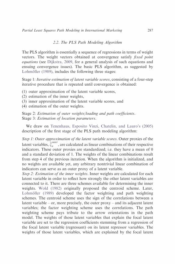
2.2. The PLS Path Modeling Algorithm

The PLS algorithm is essentially a sequence of regressions in terms of weightvectors. The weight vectors obtained at convergence satisfy fixed pointequations (see Dijkstra, 2009, for a general analysis of such equations andensuing convergence issues). The basic PLS algorithm, as suggested byLohmoller (1989), includes the following three stages:

Stage 1: Iterative estimation of latent variable scores, consisting of a four-stepiterative procedure that is repeated until convergence is obtained:

(1) outer approximation of the latent variable scores,(2) estimation of the inner weights,(3) inner approximation of the latent variable scores, and(4) estimation of the outer weights.

Stage 2: Estimation of outer weights/loading and path coefficients.Stage 3: Estimation of location parameters.

We draw on Tenenhaus, Esposito Vinzi, Chatelin, and Lauro’s (2005)description of the first stage of the PLS path modeling algorithm:

Step 1: Outer approximation of the latent variable scores. Outer proxies of the

latent variables, xouter

n , are calculated as linear combinations of their respectiveindicators. These outer proxies are standardized; i.e. they have a mean of 0and a standard deviation of 1. The weights of the linear combinations resultfrom step 4 of the previous iteration. When the algorithm is initialized, andno weights are available yet, any arbitrary nontrivial linear combination ofindicators can serve as an outer proxy of a latent variable.Step 2: Estimation of the inner weights. Inner weights are calculated for eachlatent variable in order to reflect how strongly the other latent variables areconnected to it. There are three schemes available for determining the innerweights. Wold (1982) originally proposed the centroid scheme. Later,Lohmoller (1989) developed the factor weighting and path weightingschemes. The centroid scheme uses the sign of the correlations between alatent variable – or, more precisely, the outer proxy – and its adjacent latentvariables; the factor weighting scheme uses the correlations. The pathweighting scheme pays tribute to the arrow orientations in the pathmodel. The weights of those latent variables that explain the focal latentvariable are set to the regression coefficients stemming from a regression ofthe focal latent variable (regressant) on its latent repressor variables. Theweights of those latent variables, which are explained by the focal latent


variable, are determined in a similar manner as in the factor weightingscheme. Regardless of the weighting scheme, a weight of zero is assigned toall nonadjacent latent variables.Step 3: Inner approximation of the latent variable scores. Inner proxies of

the latent variables, xinner

n , are calculated as linear combinations of the outerproxies of their respective adjacent latent variables, using the afore-determined inner weights.Step 4: Estimation of the outer weights. The outer weights are calculatedeither as the covariances between the inner proxy of each latent variable andits indicators (in Mode A, reflective), or as the regression weights resultingfrom the ordinary least squares regression of the inner proxy of each latentvariable on its indicators (in Mode B, formative).

These four steps are repeated until the change in outer weights betweentwo iterations drops below a predefined limit. The algorithm terminates afterstep 1, delivering latent variable scores for all latent variables. Loadings andinner regression coefficients are then calculated in a straightforward way,given the constructed indices and using Eqs. (4) and (5). In order todetermine the path coefficients, for each endogenous latent variable a(multiple) linear regression is conducted.

2.3. Methodological Characteristics

Methodological literature on PLS path modeling or publications on causalmodeling applications that utilize the PLS path modeling approach usuallyrefer to certain advantageous features of this technique (e.g., Fornell &Bookstein, 1982; Joreskog & Wold, 1982; Dijkstra, 1983; Lohmoller, 1989;SchneeweiX, 1991; Falk & Miller, 1992). The popularity of PLS pathmodeling among scientists and practitioners is rooted in four genuinecharacteristics: First, instead of solely drawing on the common reflectivemode, the PLS path modeling algorithm allows the unrestricted computa-tion of cause–effect relationship models that employ both reflective andformative measurement models (Diamantopoulos & Winklhofer, 2001).Second, PLS can be used to estimate path models when sample sizes aresmall (Chin & Newsted, 1999). Third, PLS path models can be very complex(i.e. consist of many latent and manifest variables) without leading toestimation problems (Wold, 1985). PLS path modeling is methodologicallyadvantageous to CBSEM whenever improper or nonconvergent results arelikely to occur (i.e. Heywood cases; see Krijnen, Dijkstra, & Gill, 1998).


Furthermore, with more complex models, the number of latent and manifestvariables may be high in relation to the number of observations. Fourth,PLS path modeling can be used when distributions are highly skewed(Bagozzi, 1994), or the independence of observations is not assured,because, as Fornell (1982, p. 443) has argued, ‘‘there are no distributionalrequirements.’’ All four characteristics are discussed in detail.

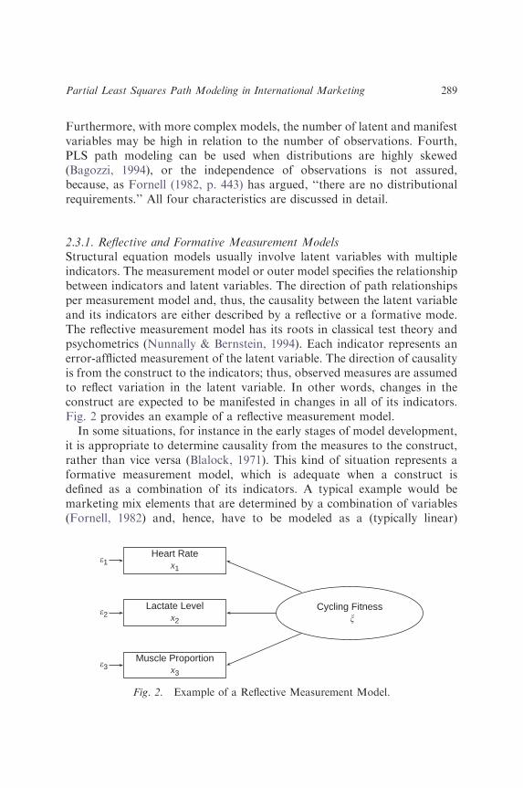
2.3.1. Reflective and Formative Measurement ModelsStructural equation models usually involve latent variables with multipleindicators. The measurement model or outer model specifies the relationshipbetween indicators and latent variables. The direction of path relationshipsper measurement model and, thus, the causality between the latent variableand its indicators are either described by a reflective or a formative mode.The reflective measurement model has its roots in classical test theory andpsychometrics (Nunnally & Bernstein, 1994). Each indicator represents anerror-afflicted measurement of the latent variable. The direction of causalityis from the construct to the indicators; thus, observed measures are assumedto reflect variation in the latent variable. In other words, changes in theconstruct are expected to be manifested in changes in all of its indicators.Fig. 2 provides an example of a reflective measurement model.

In some situations, for instance in the early stages of model development,it is appropriate to determine causality from the measures to the construct,rather than vice versa (Blalock, 1971). This kind of situation represents aformative measurement model, which is adequate when a construct isdefined as a combination of its indicators. A typical example would bemarketing mix elements that are determined by a combination of variables(Fornell, 1982) and, hence, have to be modeled as a (typically linear)

Cycling Fitness�

Heart Ratex1

Lactate Levelx2

Muscle Proportionx3

�1

�2

�3

Fig. 2. Example of a Reflective Measurement Model.

Cycling Fitness�

Trainingx1

Nutritionx2

Drug Abusex3

�

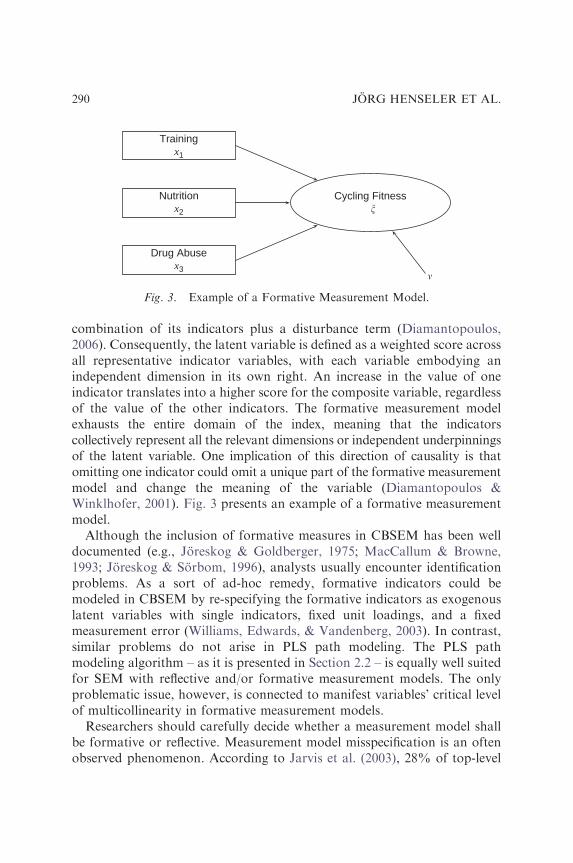
Fig. 3. Example of a Formative Measurement Model.


combination of its indicators plus a disturbance term (Diamantopoulos,2006). Consequently, the latent variable is defined as a weighted score acrossall representative indicator variables, with each variable embodying anindependent dimension in its own right. An increase in the value of oneindicator translates into a higher score for the composite variable, regardlessof the value of the other indicators. The formative measurement modelexhausts the entire domain of the index, meaning that the indicatorscollectively represent all the relevant dimensions or independent underpinningsof the latent variable. One implication of this direction of causality is thatomitting one indicator could omit a unique part of the formative measurementmodel and change the meaning of the variable (Diamantopoulos &Winklhofer, 2001). Fig. 3 presents an example of a formative measurementmodel.

Although the inclusion of formative measures in CBSEM has been welldocumented (e.g., Joreskog & Goldberger, 1975; MacCallum & Browne,1993; Joreskog & Sorbom, 1996), analysts usually encounter identificationproblems. As a sort of ad-hoc remedy, formative indicators could bemodeled in CBSEM by re-specifying the formative indicators as exogenouslatent variables with single indicators, fixed unit loadings, and a fixedmeasurement error (Williams, Edwards, & Vandenberg, 2003). In contrast,similar problems do not arise in PLS path modeling. The PLS pathmodeling algorithm – as it is presented in Section 2.2 – is equally well suitedfor SEM with reflective and/or formative measurement models. The onlyproblematic issue, however, is connected to manifest variables’ critical levelof multicollinearity in formative measurement models.

Researchers should carefully decide whether a measurement model shallbe formative or reflective. Measurement model misspecification is an oftenobserved phenomenon. According to Jarvis et al. (2003), 28% of top-level


marketing articles use misspecified measurement models in SEM applica-tions. A substantial number of latent variables in these studies wereinappropriately specified by treating formative measurement models as ifthey were reflective. Misspecification of measurement models can biasinner model parameter estimation and lead to incorrect assessments ofrelationships (Jarvis et al., 2003). The decision to use either formative orreflective indicators for a construct should be based on the nature of thecausal relationship between the indicators and the latent variables inthe measurement model (Bollen, 1989). The most suitable approach toavoid misspecification of measurement models in SEM is to consider theconceptual discussion of the differences between formative and reflectivemeasurement models by, e.g., Howell, Breivik, and Wilcox (2000a, 2007b);Bagozzi (2007); Bollen (2007); Bollen and Lennox (1991); Diamantopoulosand Winklhofer (2001); Edwards and Bagozzi (2000), as well as theC-OAR-SE procedure (Rossiter, 2002) and the design rules for determiningthe specific type of measurement model put forward by Jarvis et al. (2003).Notwithstanding this theoretic foundation, there are only a few endeavorsin the academic business literature that stress statistical techniques forthe assessment of formative measurement models in PLS path models.For instance, Bollen and Ting’s (1993) confirmatory tetrad analysis (CTA)results are used in SEM (e.g., Bollen & Ting, 2000) to assess whethermanifest variables in the measurement model are independent determinantsof a latent variable rather than its reflections in an effect indicator scale.Gudergan, Ringle, Wende, and Will (2008) show that PLS path modelingassumptions are consistent with the CTA procedure and, thereby, provide amore rigorous foundation for evaluating whether or not empirical datasupport a reflective indicator specification rather than a formative indicatorspecification.

2.3.2. Sample SizeThe sample size argument has its roots in the considerable obstacles facedwhen conducting CBSEM with small samples. A substantial number ofsimulation studies on CBSEM compare alternative discrepancy functionsand their estimation bias, accuracy, and robustness with respect to samplesize. Boomsma and Hoogland (2001), for example, conclude that there arenonconvergence problems and improper CBSEM solutions in smallsamples (e.g., 200 or fewer cases). These authors provide evidence thatCBSEM – depending on the selected discrepancy function and the modelcomplexity – requires several hundred or even thousands of observations.


In contrast, the sample size can be considerably smaller in PLS pathmodeling. For example, ‘‘there can be more variables than observations andthere may be a small amount of data that are missing completely atrandom’’ (Tenenhaus et al., 2005, p. 202). Wold (1989) illustrates the lowsample size requirement by analyzing a path model based on a data setconsisting of 10 observations and 27 manifest variables. A rule of thumb forrobust PLS path modeling estimations suggests that the sample size be equalto the larger of the following (Barclay, Higgins, & Thompson, 1995): (1) tentimes the number of indicators of the scale with the largest number offormative indicators, or (2) ten times the largest number of structural pathsdirected at a particular construct in the inner path model. Chin and Newsted(1999) present a Monte Carlo simulation study on PLS with small samples.They find that the PLS path modeling approach can provide informationabout the appropriateness of indicators at sample size as low as 20. Thisstudy confirms the consistency at large on loading estimates with increasednumbers of observations and numbers of manifest variables per measure-ment model.

As a result of these peculiarities, researchers and practitioners use PLSpath modeling, instead of CBSEM, when the sample size is relatively low.However, this persistent belief in publications and research that support theclaim that PLS is more efficient at small sample size is inadvertentlymisleading the research community as it asks for accuracy instead ofstatistical power. Goodhue, Lewis, and Thompson (2006, p. 9) argue thatstatistical significance is a primary consideration and accuracy a secondaryone: ‘‘without statistical significance, accuracy contributes no scientificknowledge.’’ Their findings suggest that PLS does not have an advantage interms of detecting statistical significance in small sample sizes. Furthermore,Goodhue et al. (2006) find no evidence that PLS with bootstrappingprovides more statistical power than CBSEM with small sample sizes. Thegenerally accepted ten times rule of thumb for the minimum sample size inPLS analyses can lead to unacceptably low levels of statistical power. It isonly in the case of a strong effect size (and high reliability) that rule ofthumb may lead to acceptable power. However, the authors provide strongevidence that the ten-times-rule does not take into account effect size,reliability, the number of indicators, or other factors which are known toaffect power. Thus, the recommendations on acceptable PLS sample sizemight be misleading.

The choice of an appropriate sample size depends on more than themagnitude of the relationship or the desired level of power. It is evident that‘‘a researcher must consider the distributional characteristics of the data,


potential missing data, the psychometric properties of the variablesexamined, and the magnitude of the relationships considered beforedeciding on an appropriate sample size to use or to ensure that a sufficientsample size is actually available to study the phenomena of interest’’(Marcoulides & Saunders, 2006, p. VI). Marcoulides and Saunders offerother warnings that clearly echo those presented in the CBSEM literature.For instance, SchneeweiX (2001) addresses the magnitude of standard errorsin PLS path modeling estimators resulting from not using enoughobservations (consistency) and indicators for each latent variable (consist-ency at large). This research provides closed form equations to determinethe magnitude of finite item bias relative to the number of indicators used ina model. SchneeweiX (2001, p. 310) indicates that item bias is generally smallwhen reflective measurement models involve many indicators, ‘‘each with asizable loading and an error which is small and uncorrelated (or only slightlycorrelated) with other error variables.’’

Goodhue et al. (2006) stress that even though PLS path modeling seemsto have no special abilities at small sample size, its performance, in terms ofstatistical power, is equal to other techniques for normally distributed data.In their view, PLS path modeling is still a convenient and powerfultechnique that is appropriate for many research situations such as complexresearch models with sample sizes that would be too small for CBSEMtechniques. They therefore note that ‘‘[u]nfortunately PLS does not provideresearchers with a magic bullet for achieving adequate statistical power atsmall sample sizes’’ (Goodhue et al., 2006, p. 10). In a similar vain,Marcoulides and Saunders (2006, p. VIII) state that ‘‘PLS is not a silverbullet to be used with samples of any size!’’ Thus, researchers must ensurethat the sample size is large enough to support the conclusions – the PLS-related rule of thumb might work well in some instances, but in others itmight fail miserably.

2.3.3. Model ComplexitySome CBSEM discrepancy functions (e.g., GFI and AGFI) decline as modelcomplexity increases (i.e. more observed variables or more constructs), andthey may be inappropriate for more complex models (Anderson & Gerbing,1984). For example, Boomsma and Hoogland (2001) experimentally variedthe model complexity (number of estimated parameters) and the number ofdegrees of freedom and found that the more parameters to be estimated, themore nonconvergence and improper solutions will occur, or – from aninformation point of view – the larger the estimation requirements, the moreinformation is needed. However, sample size has a primary effect: With


increasing numbers of observations, there is a decreasing occurrence ofnonconvergence and improper solutions. According to these authors’simulation study results, if the sample size and the factor loadings are aboutthe same, more complications are expected regarding nonconvergence andimproper solutions as model complexity increases: ‘‘It was shown thatanswers to these questions are conditional on data and model characteristicsalike. In practice, however, applied researchers often do not know the dataand the model characteristics before data collection and analysis. In newareas of applied research, especially when measurement instruments are in adeveloping stage, little is known about distributional characteristics ofobserved variables. Also, in phases of model exploration there areuncertainties about the complexity of the ‘‘final models,’’ about the numberof reliable indicators and the size of factor loadings. It is evident that withbetter measurements and stronger theoretical foundations of modelstructures, it becomes much easier to make proper decisions on the choiceof estimators and the planning of sample size’’ (Boomsma & Hoogland, 2001,p. 22). This quote stresses the complementary character of PLS in respect ofCBSEM in theory testing, especially with respect to the issues of modelcomplexity when the model building proceeds from simple to more complexmodels. PLS is considered better suited to explain complex relationships(Fornell, 1982; Fornell, Lorange, & Roos, 1990). Wold (1985, pp. 589–590)has therefore stated that ‘‘PLS comes to the fore in larger models, when theimportance shifts from individual variables and parameters to packages ofvariables and aggregate parameters. [...] In large, complex models with latentvariables PLS is virtually without competition.’’ Moreover, the PLSalgorithm allows for a considerable increase in model complexity and, hence,a noticeable reduction in the distance between subject matter analysis andstatistical technique in domains with continuous access to reliable data.

2.3.4. On the Robustness of Parameter EstimatesAlthough several authors argue that the PLS path modeling approach offerscertain advantages when compared to covariance-based methods (Chin,1998; Fornell, 1982), others provide notes of caution on the subject of thisdiscussion (Marcoulides & Saunders, 2006). However, literature on theformal comparison of CBSEM and PLS is rare (cf. Dijkstra, 1983;McDonald, 1996). Only few simulation studies analyze the parameterestimations of both methodologies, thereby uncovering certain peculiaritiesregarding their behavior in applications. Researchers and practitionersrequire this information when selecting an appropriate means for estimatinga particular SEM with their collected data.


A primary Monte Carlo simulation study by Vilares, Almeida, andCoelho (2009) analyzes the effects of two assumptions on the performanceof CBSEM and PLS: the symmetry of the distribution and the reflectivemodeling of the indicators. These authors compare both methods’performance when these assumptions hold and when they are violated; forinstance, when the distribution of the observations is skewed and someindicators follow a formative scheme. In their base model (reflective modelwith symmetric data), the quality of the two estimation methods is verysimilar, especially for the estimation of outer loadings. The Vilares et al.(2009) study sustains the phenomenon of outer loading overestimation byPLS and more conservative outcomes for inner path model relationships,whereas the Maximum Likelihood (ML) method shows exactly the oppositetendency, with overestimation of the path coefficients and a generalunderestimation of the indicator loadings. However, when a formativelatent variable is introduced, the PLS method demonstrates higherrobustness compared to CBSEM. The same kind of finding holds withskewed data results. Accordingly, the authors conclude that in case ofskewed data, PLS estimates are better than ML estimates, in terms of bothbias and precision. The ML estimators seem to be more sensitive to thevarious potential deficiencies in the data and model specification.

The research by Vilares et al. (2009) analyzes formative measurementmodels in that it draws on reflective loadings results, thus depicting asituation of measurement model misspecification (Jarvis et al., 2003).Another Monte Carlo simulation study by Ringle, Wilson, and Gotz (2007)compares the performance of CBSEM and PLS for formative exogenouslatent variables in a causal model. Both methodologies provide estimates forthe simulated sets of data that are very close to the population parameterswhen averaged. Although CBSEM estimates in the formative measurementand the structural model significantly decrease in accuracy and robustness inrespect of nonnormal data, the performance of reflective measurementmodels’ estimations is not seriously affected by these changed datacharacteristics. Ringle et al. (2007) reveal similar results for PLS pathmodeling, but the decline in accuracy and robustness is considerably lowercompared to CBSEM. On the basis of these findings, we can conclude thatin the normal data scenario, CBSEM provides accurate and robustparameter estimates that are equal or superior in comparison to PLSestimates, no matter what measurement models are used. However, if thepremises for the application of CBSEM are violated, such as regarding therequired minimum number of observations for robust model estimations orthe multivariate normality assumption for some CBSEM discrepancy


functions, the PLS approach offers robust approximations. It must be notedthough that, in general, PLS parameter estimates are less than optimalregarding bias and consistency. The estimates will be asymptotically correctunder the condition of consistency at large, i.e. both a large sample size andlarge numbers of indicators per latent variable (Joreskog & Wold, 1982).

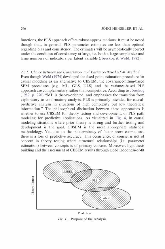
2.3.5. Choice between the Covariance- and Variance-Based SEM MethodEven though Wold (1974) developed the fixed-point estimation procedure forcausal modeling as an alternative to CBSEM, the covariance-fitting-basedSEM procedures (e.g., ML, GLS, ULS) and the variance-based PLSapproach are complementary rather than competitive. According to Joreskog(1982, p. 270) ‘‘ML is theory-oriented, and emphasizes the transition fromexploratory to confirmatory analysis. PLS is primarily intended for causal-predictive analysis in situations of high complexity but low theoreticalinformation.’’ The philosophical distinction between these approaches iswhether to use CBSEM for theory testing and development, or PLS pathmodeling for predictive applications. As visualized in Fig. 4, in causalmodeling situations where prior theory is strong and further testing anddevelopment is the goal, CBSEM is the most appropriate statisticalmethodology. Yet, due to the indeterminacy of factor score estimations,there is a loss of predictive accuracy. This occurrence, of course, is not ofconcern in theory testing where structural relationships (i.e. parameterestimation) between concepts is of primary concern. Moreover, hypothesisbuilding and the assessment of CBSEM results through global goodness-of-fit

The

ory

Test

ing

Prediction

LISREL

PLS

ANN

Fig. 4. Purpose of the Analysis.


criteria further emphasizes the theory-testing, rather than theory-building,character of this methodology (Anderson & Gerbing, 1988).

In research settings with predictive scope, weak theory, and no need foran understanding of underlying relationships, artificial neural networks(ANN) may be useful. This approach creates artificial neurons and theirinterrelations in the hidden layer that connects the input and output data, inorder, for example, to improve predictivity without necessarily creating amodel of theoretical meaning. Yet, Hsu, Chen, and Hsieh (2006) find thattheir ANN-based SEM technique is similar to PLS path modeling.

Using the iterative estimation technique as described in Section 3.2, thePLS path modeling approach calculates latent variable scores as exact linearcombinations of the observed measures. Thereby, the approach avoids theindeterminacy problem and provides an exact definition of componentscores (Fornell, 1982). The PLS approach is adequate for causal modelingapplications whose purpose is prediction and/or theory building. AlthoughPLS path modeling can be used for theory confirmation, it assumes that allmeasured variance is useful for explanation in applications (e.g., Sarkar,Echambadi, Cavusgil, & Aulakh, 2001) and indicates the causal relation-ships with significant effect. Thus, parameter estimates are obtained basedon the ability to minimize the residual variances of dependent variables(both latent and observed variables). An assessment of these PLS estimationoutcomes – for example, by standard errors that are obtained throughbootstrapping (see Section 3.4) – builds on the evaluation of partial pathmodel structures. PLS’ lack of a global optimization function andconsequently measures of global goodness of model fit definitely limits theuse of PLS for theory testing.

A researcher must arrive at a decision on the causal model analysis withlatent variables in order to select an appropriate statistical technique.Instead of using the model to explain the covariation among all indicators,which is the objective of CBSEM, PLS path modeling maximizes theexplained variance of all dependent variables and, thus, supports prediction-oriented goals. Although the CBSEM and PLS path modeling methodol-ogies differ from a statistical point of view, PLS estimates may representgood proxies of the CBSEM results. If CBSEM premises are violated, suchas distributional assumptions, minimum sample size, or maximum modelcomplexity, and related methodological matters arise, such as Heywoodcases, an inability to converge to a solution, parameters that are outsidereasonable limits, and large standard errors regarding parameter estimates(Rindskopf, 1984), PLS path modeling may represent a reasonablemethodological alternative for theory testing.


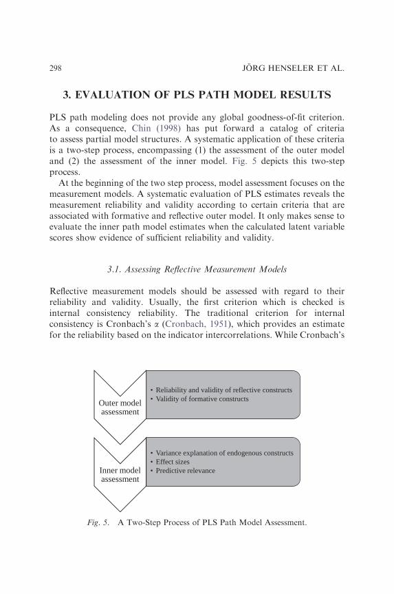
3. EVALUATION OF PLS PATH MODEL RESULTS

PLS path modeling does not provide any global goodness-of-fit criterion.As a consequence, Chin (1998) has put forward a catalog of criteriato assess partial model structures. A systematic application of these criteriais a two-step process, encompassing (1) the assessment of the outer modeland (2) the assessment of the inner model. Fig. 5 depicts this two-stepprocess.

At the beginning of the two step process, model assessment focuses on themeasurement models. A systematic evaluation of PLS estimates reveals themeasurement reliability and validity according to certain criteria that areassociated with formative and reflective outer model. It only makes sense toevaluate the inner path model estimates when the calculated latent variablescores show evidence of sufficient reliability and validity.

3.1. Assessing Reflective Measurement Models

Reflective measurement models should be assessed with regard to theirreliability and validity. Usually, the first criterion which is checked isinternal consistency reliability. The traditional criterion for internalconsistency is Cronbach’s a (Cronbach, 1951), which provides an estimatefor the reliability based on the indicator intercorrelations. While Cronbach’s

Outer model assessment

• Reliability and validity of reflective constructs• Validity of formative constructs

Inner model assessment

• Variance explanation of endogenous constructs• Effect sizes• Predictive relevance

Fig. 5. A Two-Step Process of PLS Path Model Assessment.


a assumes that all indicators are equally reliable, PLS prioritizes indicatorsaccording to their reliability, resulting in a more reliable composite.As Cronbach’s a tends to provide a severe underestimation of the internalconsistency reliability of latent variables in PLS path models, it ismore appropriate to apply a different measure, the composite reliabilityrc (Werts, Linn, & Joreskog, 1974). The composite reliability takes intoaccount that indicators have different loadings, and can be interpreted inthe same way as Cronbach’s a. No matter which particular reliabilitycoefficient is used, an internal consistency reliability value above 0.7 in earlystages of research and values above 0.8 or 0.9 in more advanced stages ofresearch are regarded as satisfactory (Nunnally & Bernstein, 1994), whereasa value below 0.6 indicates a lack of reliability.

As the reliability of indicators varies, the reliability of each indicatorshould be assessed. Researchers postulate that a latent variable shouldexplain a substantial part of each indicator’s variance (usually at least 50%).Accordingly, the absolute correlations between a construct and each of itsmanifest variables (i.e. the absolute standardized outer loadings) should behigher than 0.7 (�

ffiffiffiffiffiffiffi0:5p

). Moreover, some psychometrists (e.g., Churchill,1979) recommend eliminating reflective indicators from measurementmodels if their outer standardized loadings are smaller than 0.4. Takinginto account PLS’ characteristic of consistency at large, one should becareful when eliminating indicators. Only if an indicator’s reliability is lowand eliminating this indicator goes along with a substantial increase ofcomposite reliability, it makes sense to discard this indicator.

For the assessment of validity, two validity subtypes are usually examined:the convergent validity and the discriminant validity. Convergent validitysignifies that a set of indicators represents one and the same underlyingconstruct, which can be demonstrated through their unidimensionality.Fornell and Larcker (1981) suggest using the average variance extracted(AVE) as a criterion of convergent validity. An AVE value of at least 0.5indicates sufficient convergent validity, meaning that a latent variable is ableto explain more than half of the variance of its indicators on average(e.g., Gotz, Liehr-Gobbers, & Krafft, 2009). Discriminant validity is a rathercomplementary concept: Two conceptually different concepts should exhibitsufficient difference (i.e. the joint set of indicators is expected not to beunidimensional). In PLS path modeling, two measures of discriminantvalidity have been put forward: The Fornell–Larcker criterion and the cross-loadings. The Fornell–Larcker criterion (Fornell & Larcker, 1981) postulatesthat a latent variable shares more variance with its assigned indicators thanwith any other latent variable. In statistical terms, the AVE of each latent

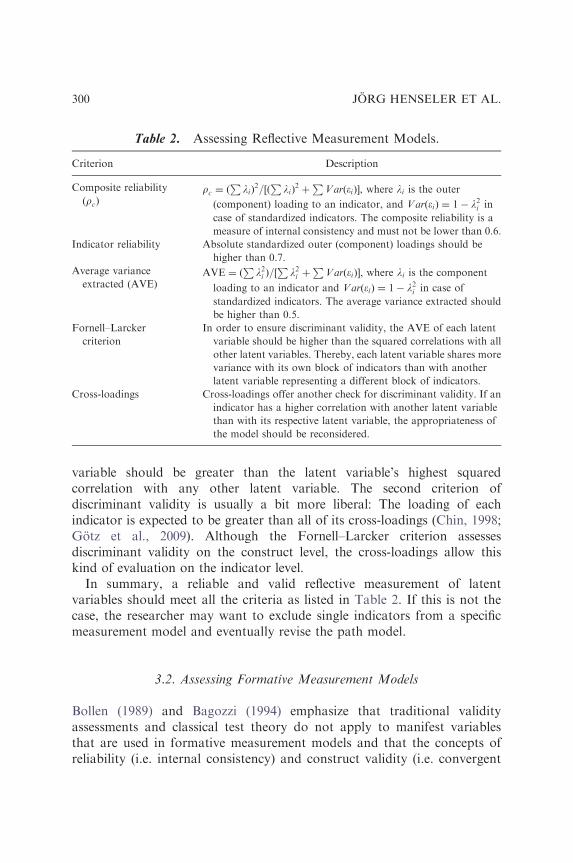
Table 2. Assessing Reflective Measurement Models.

Criterion Description

Composite reliability

(rc)rc ¼ ð

PliÞ2=½ð

PliÞ2 þ

PVarð�iÞ�, where li is the outer

(component) loading to an indicator, and Varð�iÞ ¼ 1� l2i in

case of standardized indicators. The composite reliability is a

measure of internal consistency and must not be lower than 0.6.

Indicator reliability Absolute standardized outer (component) loadings should be

higher than 0.7.

Average variance

extracted (AVE)AVE ¼ ð

Pl2i Þ=½

Pl2i þ

PVarð�iÞ�, where li is the component

loading to an indicator and Varð�iÞ ¼ 1� l2i in case of

standardized indicators. The average variance extracted should

be higher than 0.5.

Fornell–Larcker

criterion

In order to ensure discriminant validity, the AVE of each latent

variable should be higher than the squared correlations with all

other latent variables. Thereby, each latent variable shares more

variance with its own block of indicators than with another

latent variable representing a different block of indicators.

Cross-loadings Cross-loadings offer another check for discriminant validity. If an

indicator has a higher correlation with another latent variable

than with its respective latent variable, the appropriateness of

the model should be reconsidered.


variable should be greater than the latent variable’s highest squaredcorrelation with any other latent variable. The second criterion ofdiscriminant validity is usually a bit more liberal: The loading of eachindicator is expected to be greater than all of its cross-loadings (Chin, 1998;Gotz et al., 2009). Although the Fornell–Larcker criterion assessesdiscriminant validity on the construct level, the cross-loadings allow thiskind of evaluation on the indicator level.

In summary, a reliable and valid reflective measurement of latentvariables should meet all the criteria as listed in Table 2. If this is not thecase, the researcher may want to exclude single indicators from a specificmeasurement model and eventually revise the path model.

3.2. Assessing Formative Measurement Models

Bollen (1989) and Bagozzi (1994) emphasize that traditional validityassessments and classical test theory do not apply to manifest variablesthat are used in formative measurement models and that the concepts ofreliability (i.e. internal consistency) and construct validity (i.e. convergent


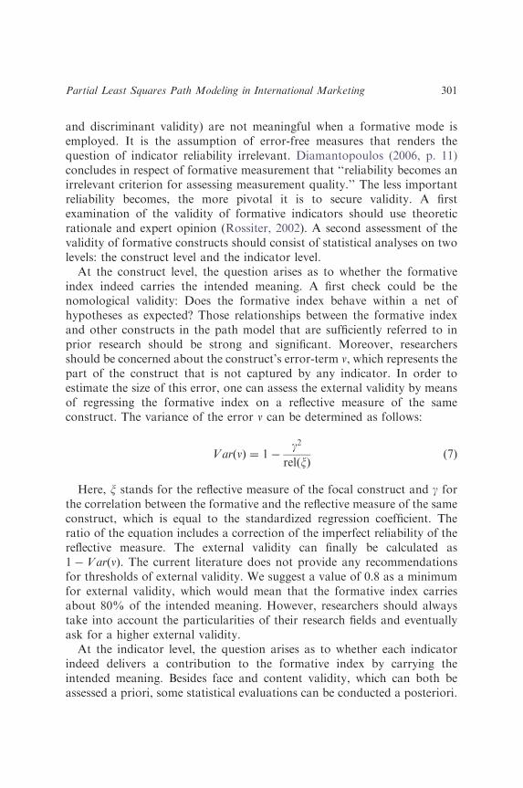
and discriminant validity) are not meaningful when a formative mode isemployed. It is the assumption of error-free measures that renders thequestion of indicator reliability irrelevant. Diamantopoulos (2006, p. 11)concludes in respect of formative measurement that ‘‘reliability becomes anirrelevant criterion for assessing measurement quality.’’ The less importantreliability becomes, the more pivotal it is to secure validity. A firstexamination of the validity of formative indicators should use theoreticrationale and expert opinion (Rossiter, 2002). A second assessment of thevalidity of formative constructs should consist of statistical analyses on twolevels: the construct level and the indicator level.

At the construct level, the question arises as to whether the formativeindex indeed carries the intended meaning. A first check could be thenomological validity: Does the formative index behave within a net ofhypotheses as expected? Those relationships between the formative indexand other constructs in the path model that are sufficiently referred to inprior research should be strong and significant. Moreover, researchersshould be concerned about the construct’s error-term n, which represents thepart of the construct that is not captured by any indicator. In order toestimate the size of this error, one can assess the external validity by meansof regressing the formative index on a reflective measure of the sameconstruct. The variance of the error n can be determined as follows:

VarðnÞ ¼ 1�g2

relðxÞ(7)

Here, x stands for the reflective measure of the focal construct and g forthe correlation between the formative and the reflective measure of the sameconstruct, which is equal to the standardized regression coefficient. Theratio of the equation includes a correction of the imperfect reliability of thereflective measure. The external validity can finally be calculated as1� Var nð Þ. The current literature does not provide any recommendationsfor thresholds of external validity. We suggest a value of 0.8 as a minimumfor external validity, which would mean that the formative index carriesabout 80% of the intended meaning. However, researchers should alwaystake into account the particularities of their research fields and eventuallyask for a higher external validity.

At the indicator level, the question arises as to whether each indicatorindeed delivers a contribution to the formative index by carrying theintended meaning. Besides face and content validity, which can both beassessed a priori, some statistical evaluations can be conducted a posteriori.


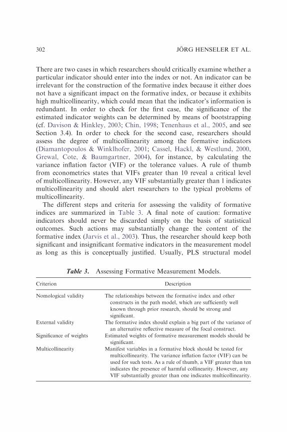
There are two cases in which researchers should critically examine whether aparticular indicator should enter into the index or not. An indicator can beirrelevant for the construction of the formative index because it either doesnot have a significant impact on the formative index, or because it exhibitshigh multicollinearity, which could mean that the indicator’s information isredundant. In order to check for the first case, the significance of theestimated indicator weights can be determined by means of bootstrapping(cf. Davison & Hinkley, 2003; Chin, 1998; Tenenhaus et al., 2005, and seeSection 3.4). In order to check for the second case, researchers shouldassess the degree of multicollinearity among the formative indicators(Diamantopoulos & Winklhofer, 2001; Cassel, Hackl, & Westlund, 2000,Grewal, Cote, & Baumgartner, 2004), for instance, by calculating thevariance inflation factor (VIF) or the tolerance values. A rule of thumbfrom econometrics states that VIFs greater than 10 reveal a critical levelof multicollinearity. However, any VIF substantially greater than 1 indicatesmulticollinearity and should alert researchers to the typical problems ofmulticollinearity.

The different steps and criteria for assessing the validity of formativeindices are summarized in Table 3. A final note of caution: formativeindicators should never be discarded simply on the basis of statisticaloutcomes. Such actions may substantially change the content of theformative index (Jarvis et al., 2003). Thus, the researcher should keep bothsignificant and insignificant formative indicators in the measurement modelas long as this is conceptually justified. Usually, PLS structural model

Table 3. Assessing Formative Measurement Models.


Nomological validity The relationships between the formative index and other

constructs in the path model, which are sufficiently well

known through prior research, should be strong and

significant.

External validity The formative index should explain a big part of the variance of

an alternative reflective measure of the focal construct.

Significance of weights Estimated weights of formative measurement models should be

significant.

Multicollinearity Manifest variables in a formative block should be tested for

multicollinearity. The variance inflation factor (VIF) can be

used for such tests. As a rule of thumb, a VIF greater than ten

indicates the presence of harmful collinearity. However, any

VIF substantially greater than one indicates multicollinearity.


estimates hardly alter after performing an elimination of insignificant orhighly collinear formative indicators, providing further support for thedecision to retain such indicators in the PLS path model. In the case ofmulticollinearity, indicator weight estimates can be distorted. This factrequires researchers to be particularly cautious when interpreting indicatorweights as a sign of indicator importance.

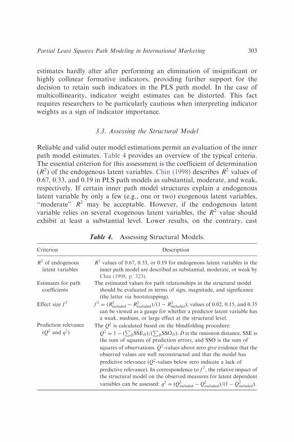
3.3. Assessing the Structural Model

Reliable and valid outer model estimations permit an evaluation of the innerpath model estimates. Table 4 provides an overview of the typical criteria.The essential criterion for this assessment is the coefficient of determination(R2) of the endogenous latent variables. Chin (1998) describes R2 values of0.67, 0.33, and 0.19 in PLS path models as substantial, moderate, and weak,respectively. If certain inner path model structures explain a endogenouslatent variable by only a few (e.g., one or two) exogenous latent variables,‘‘moderate’’ R2 may be acceptable. However, if the endogenous latentvariable relies on several exogenous latent variables, the R2 value shouldexhibit at least a substantial level. Lower results, on the contrary, cast

Table 4. Assessing Structural Models.


R2 of endogenous

latent variables

R2 values of 0.67, 0.33, or 0.19 for endogenous latent variables in the

inner path model are described as substantial, moderate, or weak by

Chin (1998, p. 323).

Estimates for path

coefficients

The estimated values for path relationships in the structural model

should be evaluated in terms of sign, magnitude, and significance

(the latter via bootstrapping).

Effect size f 2 f 2 ¼ ðR2included � R2

excludedÞ=ð1� R2includedÞ; values of 0.02, 0.15, and 0.35

can be viewed as a gauge for whether a predictor latent variable has

a weak, medium, or large effect at the structural level.

Prediction relevance

(Q2 and q2)

The Q2 is calculated based on the blindfolding procedure:

Q2 ¼ 1� ðP

DSSEDÞ=ðP

DSSODÞ. D is the omission distance, SSE is

the sum of squares of prediction errors, and SSO is the sum of

squares of observations. Q2-values above zero give evidence that the

observed values are well reconstructed and that the model has

predictive relevance (Q2-values below zero indicate a lack of

predictive relevance). In correspondence to f 2, the relative impact of

the structural model on the observed measures for latent dependent

variables can be assessed: q2 ¼ ðQ2included �Q2

excludedÞ=ð1�Q2includedÞ.


doubts regarding the theoretical underpinnings and demonstrate that themodel is incapable to explain the endogenous latent variable(s).

The individual path coefficients of the PLS structural model can beinterpreted as standardized beta coefficients of ordinary least squaresregressions. Structural paths, whose sign is in keeping with a prioripostulated algebraic signs, provide a partial empirical validation of thetheoretically assumed relationships between latent variables. Paths thatpossess an algebraic sign contrary to expectations do not support the apriori formed hypotheses. In order to determine the confidence intervals ofthe path coefficients and statistical inference, resampling techniques such asbootstrapping should be used (cf. Tenenhaus et al., 2005, and see Section3.4). Another important evaluation of direct and indirect relationships ofthe predecessor of a certain endogenous latent variable involves the analysisof mediating (Helm, Eggert, & Garnefeld, 2009) and moderating effects(Henseler & Fassott, 2009). Researchers and practitioners using PLS pathmodeling should first assess their hypothesized path model of direct effectsand then conduct additional analyses involving mediating and moderatingeffects to learn, for instance, more about possible spurious effects orsuppressor effects.

Albers (2009) proposes a new paradigm for success factor studies inmarketing. The significance of highly plausible direct inner path modelrelationships is no longer of interest to researchers and practitioners.Rather, the sum of the direct effect and all indirect effects of a particularlatent variable on another (the total effect) should be the subject ofevaluation for further interpretation. This new paradigm copes with afrequent observation in PLS path modeling that the standardized inner pathmodel coefficients decline with an increased number of indirect relation-ships, especially when mediating latent variables have a suppressor effect onthe direct path. Consequently, considerable direct relationships may becomeinsignificant after including additional indirect relationships. In suchinstances, the total effect should remain at a relatively constant, sizeablelevel and thus provide more reasonable grounds for conclusions on the innerpath model relationships.

For each effect in the path model, one can evaluate the effect size bymeans of Cohen’s (1988) f 2. The effect size f 2 is calculated as the increase inR2 relative to the proportion of variance of the endogenous latent variablethat remains unexplained. According to Cohen (1988), f 2 values of 0.02,0.15, and 0.35 signify small, medium, and large effects, respectively.

Another assessment of the structural model involves the model’scapability to predict. The predominant measure of predictive relevance is


Stone-Geisser’s Q2 (Stone, 1974; Geisser, 1975), which can be measuredusing blindfolding procedures (Tenenhaus et al., 2005). The Stone–Geissercriterion postulates that the model must be able to provide a prediction ofthe endogenous latent variable’s indicators. The technique represents asynthesis of function fitting and cross-validation. As Chin (1998) pointsout, ‘‘the prediction of observables or potential observables is of muchgreater relevance than the estimator of what are often artificialconstruct-parameters’’ (p. 320). Wold (1982) argues that the sample reusetechnique – especially the blindfolding procedure to obtain the cross-validated redundancy (instead of the cross-validated communality) – fits thePLS path modeling approach like ‘‘hand in glove.’’

The blindfolding procedure is only applied to endogenous latent variablesthat have a reflective measurement model operationalization. If this valuefor a certain endogenous latent variable is larger than zero, its explanatoryvariables provide predictive relevance. In analogy to the effect-size f 2

evaluation, the relative impact of the predictive relevance can be assessed bymeans of the measure q2: values of 0.02, 0.15, and 0.35 reveal a small,medium, or large predictive relevance of a certain latent variable, thusexplaining the endogenous latent variable under evaluation.

3.4. Bootstrapping

The nonparametric bootstrap (Davison & Hinkley, 2003; Efron &Tibshirani, 1993) procedure can be used in PLS path modeling to provideconfidence intervals for all parameter estimates, building the basis forstatistical inference. In general, the bootstrap technique provides an estimateof the shape, spread, and bias of the sampling distribution of a specificstatistic. Bootstrapping treats the observed sample as if it represents thepopulation. The procedure creates a large, pre-specified number ofbootstrap samples (e.g., 5,000). Each bootstrap sample should have thesame number of cases as the original sample. Bootstrap samples are createdby randomly drawing cases with replacement from the original sample.

PLS estimates the path model for each bootstrap sample. The obtainedpath model coefficients form a bootstrap distribution, which can be viewedas an approximation of the sampling distribution. The bootstrappinganalysis allows for the statistical testing of the hypothesis H0 : w ¼ 0 (w canbe any parameter estimated by PLS) against the alternative hypothesis H1 :wa 0 at mþ n� 2 degrees of freedom (where m is the number of PLSestimates for w in the original sample, which is 1; n is the number of


bootstrap estimates for w, e.g., 5,000). The PLS results for all bootstrapsamples provide the mean value and standard error for each path modelcoefficient. This information permits a student’s t-test to be performed forthe significance of path model relationships. Chin (1998) proposes using thefollowing test statistic for PLS:

temp ¼w

seðwÞ(8)

whereby temp represents the empirical t-value, w the original PLS estimate ofa certain path coefficient, and seðwÞ its bootstrapping standard error. Thestudent’s t-distribution table provides the critical t-value at given a-levelsand the respective number of degrees of freedom.

Instead of just reporting the significance of a parameter, it would be morevaluable to report the confidence interval. If a confidence interval for anestimated path coefficient w does not include zero, the hypothesis that wequals zero is rejected. Testing with confidence intervals is advantageous, asit provides more information about the estimate of w. Shaffer (1995, p. 575)remarks that ‘‘if the hypothesis is not rejected, the power of the procedurecan be gauged by the width of the interval.’’

In order to determine the confidence interval of a model parameter, saya path coefficient, one has to recognize that the bootstrapping proceduregenerates a distribution T of w. However, significance testing needs toaccount for the distribution of T under H0, which is the null distributionof T. This distribution is essential for performing the test since it providesthe basis for determining the p-value. If the null distribution is unknown, theasymptotic normality of the test statistic is commonly assumed. Althoughnonparametric alternatives can be obtained through bootstrapping, thisapproach overlooks the possibility that the data could be generated underthe alternative hypothesis H1 : ya y0.

This problem can be addressed by examining the statistical correspon-dence between tests of significance and confidence intervals when the nullhypothesis concerns a particular parameter value (Gudergan et al., 2008).Bootstrapping confidence intervals are well established (Efron & Tibshirani,1993; Davison & Hinkley, 2003). If the bootstrap estimates of bias andvariance are denoted by bB and vB, then the corresponding approximate1� a (two-tailed) confidence interval is:

t� bB � v1=2B z1�a=2 (9)

where bB ¼ �wB � w, the difference of the mean value of w for all bootstrapsand the original PLS estimation of that path coefficient. A null hypothesis


H0 : w ¼ 0 is accepted (or rejected) at a given level a, if the correspondingð1� aÞ confidence interval includes (or does not include) the parametervalue y0. The bias-corrected bootstrap confidence interval in Eq. (9)provides a basis to account for the aforementioned problem and, thus, canbe used as an appropriate means to test the significance of PLS-estimatedpath coefficients (Gudergan et al., 2008).

In PLS path modeling, the latent variable scores may have different signsif, for examples, estimation A uses an alternative outer weights initializationof the algorithm (say, þLV1) compared with estimation B (in this case,�LV2). Still, the absolute LV-values of both estimations usually representequivalent solutions, i.e. þLV1j j ¼ �LV2j j (for a discussion on this signindeterminacy of PLS see Wold, 1985). This sign indeterminacy of PLSlatent variable scores may also result in arbitrary sign changes during thebootstrap path model estimations. Such occurrence of sign changes ‘‘pull’’the mean value of bootstrapping results (e.g., for parameter w) toward zeroand, thereby, bias the bootstrap standard error upward. Arbitrary signchanges systematically reduce the value of temp and, thus, the possibility ofthe rejection of H0 at a given a level. The standard error of estimatesincreases dramatically without any real meaning if the sign changes are notproperly taken into account (Tenenhaus et al., 2005). Rather than nottreating sign changes in the bootstrapping results, we suggest using theindividual sign change option. The working principle is as follows: If a PLSpath coefficient estimation for a bootstrap subsample shows a different signcompared with the original path model estimation, the procedure reversesthe sign of that path coefficient in the bootstrapping subsample. Thus, thesigns in the outer and inner models of each resample are made consistentwith the signs in the original sample in order to avoid these sign-change-related problems.

3.5. Group Comparisons and Other Advances in PLS Analyses

A threat to the validity of SEM results may lie in the heterogeneity ofobservations. The level of observed or unobserved heterogeneity can lead tospurious or suppressor effects, and generally to misinterpretations. Typically,researchers in international marketing are well aware of the heterogeneity ofobservations; that is, different population parameters are likely for differentsubpopulations such as countries or cultures. Although cross-cultural orcross-national differences are related to observed heterogeneity, there canalso be unobserved heterogeneity, which cannot be attributed to any


predetermined variable. Similar to ignoring observed heterogeneity due tocountries or cultures, unobserved heterogeneity represents a serious problemin respect of interpreting PLS results (Ringle, 2006).

Our review of PLS path modeling applications in international marketinggives a mixed picture regarding the examination of heterogeneity. Although asignificant number of studies take observed heterogeneity into account bymeans of multigroup comparisons, none of the studies accounts forunobserved heterogeneity. However, there are several PLS-based approachesto detect unobserved heterogeneity. Analytical techniques such as finitemixture partial least squares (FIMIX-PLS; Hahn, Johnson, Herrmann, &Huber, 2002; Ringle, Sarstedt, & Mooi, 2009a; Ringle, Wende, & Will,2009b) or the recently developed PLS typological alternatives (e.g., EspositoVinzi, Ringle, Squillacciotti, & Trinchera, 2007; Ringle & Schlittgen, 2007)are becoming mandatory for evaluating PLS path modeling results. Usingthese techniques, researchers can either confirm that their results are notdistorted by unobserved heterogeneity or identify thus far neglected variablesthat describe the uncovered data segments.

As soon as conceptual deliberations or methods such as FIMIX-PLSsuggest different models for different subgroups, PLS-based multigroupanalysis (MGA) should be conducted. In MGA, a population parameter b ishypothesized to differ for two subpopulations: bð1Þa bð2Þ. Referring to PLSpath modeling, researchers would for instance ask whether one could concludedifferences in population parameters from the differences in path coefficients.

The primary approach for group comparisons is a t-test, as described byKeil et al. (2000). These authors suggest using the standard errors obtainedfrom bootstrapping as the input for a parametric test. After having exposedthe subsamples to separate bootstrap analyses and having made parametricassumptions about the distributions of the parameter standard errors, onecan calculate the following statistic for the difference in paths betweengroups (Keil et al., 2000):

t ¼bð1Þ � bð2Þffiffiffiffiffiffiffiffiffiffiffiffiffiffiffiffiffiffiffiffiffiffiffiffiffiffiffiffiffiffiffiffiffiffiffiffiffiffiffiffiffiffiffiffiffiffiffiffiffiffiffiffiffiffiffiffiffiffiffiffiffiffiffiffiffiffiffiffiffiffiffiffiffiffiffiffiffiffiffiffiffiffiffiffiffiffiffiffiffiffiffiffiffiffi

ðnð1Þ � 1Þ2

nð1Þ þ nð2Þ � 2seðbð1ÞÞ2 þ

ðnð2Þ � 1Þ2

nð1Þ þ nð2Þ � 2seðbð2ÞÞ2

s ffiffiffiffiffiffiffiffiffiffiffiffiffiffiffiffiffiffiffi1

nð1Þþ

1

nð2Þ

r (10)

This statistic is asymptotically t-distributed with nð1Þ þ nð2Þ � 2 degrees offreedom. The subsample-specific path coefficients are denoted as b, the sizesof the subsamples as n, and the path coefficient standard errors as resultingfrom bootstrapping as se.


Chin and Dibbern (2009) cast doubt on whether this approach ofmultigroup comparison with its inherent distributional assumptions fits toPLS path modeling, which is generally regarded as being distribution-free.In line with these doubts, we present an alternative approach to PLS-basedgroup comparisons that does not rely on distributional assumptions, asinitially proposed by Henseler (2007). The working principle of the novelPLS-MGA approach is as follows: First, the subsamples to be comparedare exposed to separate bootstrap analyses, and the bootstrap outcomesserve as a basis for the hypothesis tests of group differences. Instead ofrelying on distributional assumptions, the new approach evaluates theobserved distribution of the bootstrap outcomes. Given two subsampleswith parameter estimates (e.g., a path coefficient), bð1Þ and bð2Þ, the condi-tional probability Pðbð1Þ4bð2Þjbð1Þ � bð2ÞÞ has to be determined. Here, bð1Þ

and bð2Þ represent the true population parameters of population 1 and 2.A researcher would like to be sure that P is below a specified a-level beforeconcluding that bð1Þ is greater than bð2Þ.

If researchers know the parameter estimates of two subsamples frombootstrapping, they can easily verify how probable a difference inparameters between two subpopulations is and hence test their hypothesiswith the following equation:

Pðbð1Þ4bð2Þjbð1Þ � bð2ÞÞ ¼ 1�X8j;i

Y 2 �bð1Þ� bð1Þj � 2 �b

ð2Þþ bð2Þi

� �J2

(11)

In this equation, J denotes the number of bootstrap samples, bð1Þj and b

ð2Þi

the bootstrap parameter estimates, �bð1Þ

and �bð2Þ

the means of the focalparameters over the bootstrap samples, and Y the unit step function, whichhas a value of 1 if its argument exceeds 0, otherwise 0. The superscript inparentheses marks the respective group. This equation states that J2 (i.e. allpossible) comparisons of bootstrap parameters have to be made. In fact, thisapproach can be seen as a Mann–Whitney–Wilcoxon test (Wilcoxon, 1947;Mann & Whitney, 1947) applied to the bootstrap-values corrected for theoriginal parameter values.

PLS-MGA does not require any distributional assumptions and is simpleto apply by using the bootstrap outputs that are generated by the prevailingPLS implementations such as SmartPLS (Ringle, Wende, & Will, 2005). Theway of determining the probability whether a population parameter differsacross two sub-populations is unique to this new approach. Researchers caneasily conduct the final calculations with available spreadsheet software suchas MS Excel (a sample spreadsheet can be obtained from the first author).


Besides the aforementioned methodological advances for addressing therequirement to capture unobserved heterogeneity, recent developments inthe evaluation of PLS path modeling results focus on the problem ofmeasurement model misspecification. Bucic and Gudergan (2004) use a PLSapplication to demonstrate the significant consequences of misspecificationfor path model estimates. The seven criteria that have been put forwardby Jarvis et al. (2003) permit an a priori examination of the outer mode.In addition, a confirmatory tetrad measurement model analysis of PLS(CTA-PLS; Gudergan et al., 2008) provides a statistical test to evaluate theouter measurement model a posteriori.

Statistical support is there for specifying not only the measurement modelbut also the structural model. Research by Marcoulides (2003) and Wilson,Callaghan, Ringle, and Henseler (2007) addresses the inner path modelspecification search to uncover superior structures and more appropriateinner relationship directions.

Additional advances on the subject of evaluating path modeling resultsinvolve the development of global goodness-of-fit criteria. The PLSgoodness-of-fit proposal by Tenenhaus et al. (2005) is the geometric meanof the average communalities (outer measurement model) and the averageR2 of endogenous latent variables, and is normed between 0 and 1, where ahigher value represents better path model estimations. However, while thiscriterion has only been applied in few applications (e.g., Esposito Vinziet al., 2007) and has not been systematically analyzed in simulation studies,it is restricted to reflective outer models and may be subject to systematicimprovement by means of path model modifications/manipulations. Futuredevelopments in this line of research may combine PLS and ML CBSEMglobal goodness-of-fit criteria. This procedure is well established in CBSEMfor the asymptotic distribution-free estimators (ADF), which—like PLS—does not follow distributional assumptions that allow the global goodness-of-fit to be computed. Consequently, researchers and practitioners shouldnote the substantial link between CBSEM and PLS path modeling for whichthe literature has called over the last decades.

4. SUMMARY AND CONCLUSION

In international marketing research, both CBSEM and PLS provide apowerful framework for estimating causal models with latent variablesand systems of simultaneous equations with measurement errors. CBSEMand PLS path modeling constitute two complementary, yet distinctive,


statistical techniques for estimating parameters of conceptual models.A critical review of the PLS application in international marketing revealsthat this methodology has increased in popularity, especially for multigroupanalyses of PLS results for different nations. Our paper illustrates thePLS path modeling methodology and typical criteria for the assessmentof results. Moreover, we introduce several advances in evaluating PLSmodel estimations, such as a novel approach for multigroup comparison(PLS-MGA).

PLS is based on least squares estimation with the primary objective beingto maximize the explanation of variance in a structural equation model’sdependent constructs. Joreskog and Wold (1982, p. 270) suggest that ‘‘PLSis primarily intended for causal-predictive analysis in situations of highcomplexity but low theoretical information’’. In contrast, the primarymeasures used in CBSEM are overall goodness-of-fit measures that assesshow well the hypothesized model fits the observed data. The modelestimation is theory-oriented and emphasizes the confirmatory, rather thanthe exploratory, analysis. Consequently, in international marketingresearch, CBSEM should be used either to empirically confirm a systemof hypotheses that underlie a causal model or to test and compare results foralternative theoretically established causal models. The prediction-orientedPLS method, on the contrary, does not require strong theory and can beused as a theory-building method (Gefen et al., 2000). PLS offers excellentcapabilities for work with small samples and formative measurement, as themethodology is sufficient for most success factor (cause indicator) analysesin international marketing research. Moreover, complementary analyticaltechniques such as FIMIX-PLS for uncovering unobserved heterogeneity ormultigroup PLS analysis may provide further differentiated path modelingresults that allow for more precise interpretation. The review of PLS studiesin international marketing reveals that few studies conduct multigroupanalyses to identify differences in path coefficients across subgroups. Nostudy has addressed the potentially serious problems of ignoring unobservedheterogeneity (Ringle, 2006). Owing to the severity of the consequences ofneglecting unobserved heterogeneity, such additional analyses shouldbecome a standard means of evaluating PLS path modeling results,especially in international marketing research.

A final concern refers to the choice of SEM method. There may besituations in which CBSEM is preferable, in other situations PLS may bepreferable. Moreover, there may be situations where using CBSEM isdesirable but unobtainable, for example, due to violations in some keyCBSEM assumptions (e.g., regarding sample size, distribution, and model


identification); in such cases, PLS may provide a realistic alternative toCBSEM. Some authors also critically point out that both CBSEM and PLSfollow the classical test theory paradigm, while especially for internationalmarketing applications alternative methodologies following the probabil-istic test theory may be advisable (Ewing, Salzberger, & Sinkovics, 2005).All in all, the findings of our paper are deemed to help researchers ininternational marketing to adopt a more holistic perspective and to makeinformed decisions about the SEM method based on the nature and keyobjectives of their study.

REFERENCES

Acedo, F. J., & Jones, M. V. (2007). Speed of internationalization and entrepreneurial

cognition: Insights and a comparison between international new ventures, exporters and

domestic firms. Journal of World Business, 42(3), 236–252.

Ainuddin, R. A., Beamish, P. W., Hulland, J. S., & Rouse, M. J. (2007). Resource attributes and

firm performance in international joint ventures. Journal of World Business, 42(1), 47–60.

Albers, S. (2009). PLS and success factor studies in marketing. In: V. Esposito Vinzi,

W. W. Chin, J. Henseler & H. Wang (Eds), Handbook of partial least squares: Concepts,

methods, and applications. Berlin: Springer (in print).

Alpert, F., Kamins, M., Sakano, T., Onzo, N., & Graham, J. (2001). Retail buyer beliefs,

attitude, and behavior toward pioneer and me-too follower brands. International

Marketing Review, 18(2), 160–187.

Anderson, J. C., & Gerbing, D. W. (1984). The effect of sampling error on convergence,

improper solutions, and goodness of fit indices for maximum likelihood confirmatory

factor analysis. Psychometrika, 49(2), 155–173.

Anderson, J. C., & Gerbing, D. W. (1988). Structural equation modeling in practice: A review

and recommended two-step approach. Psychological Bulletin, 103(3), 411–423.

Bagozzi, R. P. (1994). In: Principles of marketing research (pp. 317–385). Oxford: Blackwell.

Bagozzi, R. P. (2007). On the meaning of formative measurement and how it differs from

reflective measurement: Comment on Howell, Breivik, and Wilcox (2007). Psychological

Methods, 12(2), 229–237.

Barclay, D. W., Higgins, C., & Thompson, R. (1995). The partial least squares approach to

causal modeling: Personal computer adoption and use as illustration. Technology

Studies, 2(2), 285–309.

Birkinshaw, J., Morrison, A., & Hulland, J. (1995). Structural and competitive determinants of

a global integration strategy. Strategic Management Journal, 16(8), 637–655.

Blalock, H. M. (1971). Causal models in the social sciences. Chicago, IL: Aldine-Atherton.

Bollen, K. A. (1989). Structural equations with latent variables. New York, NY: Wiley.

Bollen, K. A. (2007). Interpretational confounding is due to misspecification, not to type of

indicator: Comment on Howell, Breivik, and Wilcox (2007). Psychological Methods,

12(2), 219–228.


Bollen, K. A., & Lennox, R. (1991). Conventional wisdom on measurement: A structural

equation perspective. Psychological Bulletin, 110(2), 305–314.

Bollen, K. A., & Ting, K. (1993). Confirmatory tetrad analysis. Sociological Methodology, 23,

147–175.

Bollen, K. A., & Ting, K. (2000). A tetrad test for causal indicators. Psychological Methods, 5(1),

3–22.

Boomsma, A., & Hoogland, J. J. (2001). The robustness of LISREL modeling revisited. In:

R. Cudeck, S. du Toit & D. Sorbom (Eds), Structural equation modeling: Present and

future (pp. 139–168). Chicago, IL: Scientific Software International.

Bucic, T., & Gudergan, S. P. (2004). The impact of organizational settings on creativity and

learning in alliances. Management, 7(3), 257–273.

Calantone, R. J., Graham, J. L., & Mintu-Wimsatt, A. (1998). Problem-solving approach in an

international context: Antecedents and outcomes. International Journal of Research in

Marketing, 15(1), 19–35.

Cassel, C. M., Hackl, P., & Westlund, A. H. (2000). On measurement of intangible assets:

A study of robustness of partial least squares. Total Quality Management, 11(7), 897–907.

Chin, W. W. (1998). The partial least squares approach to structural equation modeling. In:

G. A. Marcoulides (Ed.), Modern Methods for Business Research (pp. 295–358).

Mahwah, NJ: Lawrence Erlbaum Associates.

Chin, W. W., & Dibbern, J. (2009). A permutation based procedure for multi-group (PLS)

analysis: Results of tests of differences on simulated data. In: V. Esposito Vinzi,

W. W. Chin, J. Henseler & H. Wang (Eds), Handbook of partial least squares: Concepts,

methods and applications in marketing and related fields. Springer (In press).

Chin, W. W., & Newsted, P. R. (1999). Structural equation modeling analysis with small

samples using partial least squares. In: R. H. Hoyle (Ed.), Statistical strategies for small

sample research (pp. 307–342). Thousand Oaks, CA: Sage.

Churchill, G. A. (1979). A paradigm for developing better measures of marketing constructs.

Journal of Marketing Research, 16(1), 64–73.

Cohen, J. (1988). Statistical power analysis for the behavioral sciences (2nd ed.). Hillsdale, NJ:

Lawrence Erlbaum Associates.

Cronbach, L. J. (1951). Coefficient alpha and the internal structure of tests. Psychometrika,

16(3), 297–334.

Davison, A. C., & Hinkley, D. V. (2003). Bootstrap methods and their application (2nd ed.).

New York, NY: Cambridge University Press.

Diamantopoulos, A. (2006). The error term in formative measurement models: Interpretation

and modeling implications. Journal of Modelling in Management, 1(1), 7–17.

Diamantopoulos, A., & Winklhofer, H. (2001). Index construction with formative indicators:

An alternative to scale development. Journal of Marketing Research, 38(2), 269–277.

Dibbern, J., Goles, T., Hirschheim, R. A., & Jayatilaka, B. (2004). Information systems

outsourcing: A survey and analysis of the literature. The Data Base for Advances in

Information Systems, 35(4), 6–102.

Dijkstra, T. K. (1983). Some comments on maximum likelihood and partial least squares

methods. Journal of Econometrics, 22(1/2), 67–90.

Dijkstra, T. K. (2009). Latent variables and indices: HermanWold’s basic design and partial least

squares. In: V. Esposito Vinzi, W. W. Chin, J. Henseler & H. Wang (Eds), Handbook of

partial least squares: Concepts, methods, and applications. Berlin: Springer (in print).


Edwards, J. R., & Bagozzi, R. P. (2000). On the nature and direction of relationships between

constructs and measures. Psychological Methods, 5(2), 155–174.

Efron, B., & Tibshirani, R. J. (1993). An introduction to the bootstrap. New York, NY:

Chapman Hall.

Eggert, A. (2007). Getting your PLS research published: A personal and interpersonal

perspective. In: Proceedings of the academy of marketing science 2007 world marketing

congress, July 11–14, Verona, Italy.

Esposito Vinzi, V., Ringle, C. M., Squillacciotti, S., & Trinchera, L. (2007). Capturing and

treating unobserved heterogeneity by response based segmentation in PLS path

modeling: A comparison of alternative methods by computational experiments. ESSEC

Research Center Working Paper 07019, ESSEC Business School Paris-Singapore, Paris.

Ewing, M. T., Salzberger, T., & Sinkovics, R. R. (2005). An alternate approach to assessing

cross-cultural measurement equivalence in advertising research. Journal of Advertising,

34(1), 17–36.

Falk, R. F., & Miller, N. B. (1992). A primer for soft modeling. Akron, OH: University of Akron

Press.

Festge, F., & Schwaiger, M. (2007). The drivers of customer satisfaction with industrial goods:

An international study. In: C. R. Taylor & D.-H. Lee (Eds), Advances in international

marketing (Vol. 18, pp. 179–207). Amsterdam: Elsevier.

Fornell, C. (1982). A second generation of multivariate analysis: An overview. In: C. Fornell

(Ed.), A second generation of multivariate analysis (Vol. 1, pp. 1–21). New York, NY:

Praeger.

Fornell, C. (1992). A national customer satisfaction barometer: The Swedish experience.

Journal of Marketing, 56(1), 6–21.

Fornell, C., & Bookstein, F. (1982). A comparative analysis of two structural equation models:

LISREL and PLS applied to market data. In: C. Fornell (Ed.), A second generation of

multivariate analysis (Vol. 1, pp. 289–323). New York, NY: Praeger.

Fornell, C., & Larcker, D. F. (1981). Structural equation models with unobservable variables

and measurement error: Algebra and statistics. Journal of Marketing Research, 18(3),

328–388.

Fornell, C., Lorange, P., & Roos, J. (1990). The cooperative venture formation process: A

latent variable structural modeling approach. Management Science, 36(10), 1246–1255.

Fornell, C., & Robinson, W. T. (1983). Industrial organization and consumer satisfaction/

dissatisfaction. Journal of Consumer Research, 9(4), 403–412.

Gefen, D., Straub, D. W., & Boudreau, M.-C. (2000). Structural equation modelling and

regression: Guidelines for research practice. Communications of the Association for

Information Systems, 4(7), 1–78.

Geisser, S. (1975). A predictive approach to the random effect model. Biometrika, 61(1), 101–107.

Gerpott, T., & Jakopin, N. (2005). International marketing standardization and financial

performance of mobile network operators – An empirical analysis. Schmalenbach

Business Review, 57(3), 198–228.

Goodhue, D., Lewis, W., & Thompson, R. (2006). PLS, small sample size, and statistical power

in MIS research. In: HICSS ‘06: Proceedings of the 39th annual Hawaii international

conference on system sciences, IEEE Computer Society, Washington, DC, pp. 202.2,

CD-ROM, 10 pages.

Gotz, O., Liehr-Gobbers, K., & Krafft, M. (2009). Evaluation of structural equation models

using the partial least squares (PLS) approach. In: V. Esposito Vinzi, W. W. Chin,


J. Henseler & H. Wang (Eds), Handbook of partial least squares: Concepts, methods, and

applications. Berlin: Springer (in print).

Graham, J. L., Mintu, A. T., & Rodgers, W. (1994). Explorations of negotiation behaviors in

ten foreign cultures using a model developed in the United States. Management Science,

40(1), 72–95.

Green, D. H., & Ryans, A. B. (1990). Entry strategies and market performance: Causal modeling

of a business simulation. Journal of Product Innovation Management, 7(1), 45–58.

Grewal, R., Cote, J. A., & Baumgartner, H. (2004). Multicollinearity and measurement error in

structural equation models: Implications for theory testing. Marketing Science, 23(4),

519–529.

Gudergan, S. P., Ringle, C. M., Wende, S., & Will, A. (2008). Confirmatory tetrad analysis for

evaluating the mode of measurement models in PLS path modeling. Journal of Business

Research, (in print).

Gustafsson, A., & Johnson, M. D. (2004). Determining attribute importance in a service

satisfaction model. Journal of Service Research, 7(2), 124–141.

Hahn, C., Johnson, M. D., Herrmann, A., & Huber, F. (2002). Capturing customer heterogeneity

using a finite mixture PLS approach. Schmalenbach Business Review, 54(3), 243–269.

Helm, S., Eggert, A., & Garnefeld, I. (2009). Modelling the impact of corporate reputation on

customer satisfaction and loyalty using PLS. In: V. Esposito Vinzi, W. W. Chin,

J. Henseler & H. Wang (Eds), Handbook of partial least squares: Concepts, methods, and

applications. Berlin: Springer (in print).

Henseler, J. (2007). A new and simple approach to multi-group analysis in partial least

squares path modeling. In: H. Martens, T. Næs & M. Martens (Eds), PLS’07

international symposium on PLS and related methods – causalities explored by indirect

observation (pp. 104–107). Norway: Matforsk, As.

Henseler, J., & Fassott, G. (2009). Testing moderating effects in PLS path models: An

illustration of available procedures. In: V. Esposito Vinzi, W. W. Chin, J. Henseler &

H. Wang (Eds), Handbook of partial least squares: Concepts, methods, and applications.

Berlin: Springer (in print).

Higgins, C. A., Duxbury, L. E., & Irving, R. H. (1992). Work-family conflict in the dual-career

family. Organizational Behavior and Human Decision Processes, 51(1), 51–75.

Holzmuller, H. H., & Kasper, H. (1991). On a theory of export performance: Personal and

organizational determinants of export trade activities observed in small and medium-

sized firms. Management International Review, 31(Special Issue), 45–70.

Holzmuller, H. H., & Stottinger, B. (1996). Structural modeling of success factors in exporting:

Cross-validation and further development of an export performance model. Journal of

International Marketing, 4(2), 29–55.

Howell, R. D., Breivik, E., & Wilcox, J. B. (2007a). Is formative measurement really

measurement? Reply to Bollen (2007) and Bagozzi (2007). Psychological Methods, 12(2),

238–245.

Howell, R. D., Breivik, E., & Wilcox, J. B. (2007b). Reconsidering formative measurement.

Psychological Methods, 12(2), 205–218.

Hsu, H.-H., Chen, W.-H., & Hsieh, M.-J. (2006). Robustness testing of PLS, LISREL, EQS

and ANN-based SEM for measuring customer satisfaction. Total Quality Management

and Business Excellence, 17(3), 355–372.

Hulland, J. S. (1999). Use of partial least squares (PLS) in strategic management research:

A review of four recent studies. Strategic Management Journal, 20(4), 195–204.


Iacobucci, D., Grisaffe, D., Duhachek, A., & Marcati, A. (2003). FAC-SEM: A methodology

for modeling factorial structural equations models, applied to cross-cultural and cross-

industry drivers of customer evaluations. Journal of Service Research, 6(1), 3–23.

Inkpen, A. C., & Birkenshaw, J. (1994). International joint ventures and performance: An

interorganizational perspective. International Business Review, 3(3), 201–217.

Jarvis, C. B., MacKenzie, S. B., & Podsakoff, P. M. (2003). A critical review of construct

indicators and measurement model misspecification in marketing and consumer

research. Journal of Consumer Research, 30(2), 199–218.

Johansson, J. K., & Yip, G. S. (1994). Exploiting globalization potential: U.S. and Japanese

strategies. Strategic Management Journal, 15(8), 579–601.

Johnson, M. D., Herrmann, A., & Gustafsson, A. (2002). Comparing customer satisfaction

across industries and countries. Journal of Economic Psychology, 23(6), 749–769.

Joreskog, K. G. (1982). The LISREL approach to causal model-building in the social

sciences. In: K. G. Joreskog & H. O. Wold (Eds), Systems under indirect observation,

Part I (pp. 81–100). Amsterdam: North-Holland.

Joreskog, K. G., & Goldberger, A. S. (1975). Estimation of a model with multiple indicators

and multiple causes of a single latent variable. Journal of the American Statistical

Association, 70(351), 631–639.

Joreskog, K. G., & Sorbom, D. (1996). LISREL 8: Structural equation modeling with the

SIMPLIS command language. Chicago, IL: Scientific Software International.

Joreskog, K. G., & Wold, H. O. (Eds). (1982). The ML and PLS technique for modelling with

latent variables: Historical and comparative aspects. In: Systems under indirect

oberservation, Part I (pp. 263–270). Amsterdam: North-Holland.

Julien, P. A., & Ramangalahy, C. (2003). Competitive strategy and performance of exporting

SMEs: An empirical investigation of the impact of their export information search and

competencies. Entrepreneurship Theory and Practice, 27(3), 227–245.

Keil, M., Tan, B. C., Wei, K.-K., Saarinen, T., Tuunainen, V., & Wassenaar, A. (2000). A cross-

cultural study on escalation of commitment behavior in software projects. Management

Information Systems Quarterly, 24(2), 299–325.

Krijnen, W. P., Dijkstra, T. K., & Gill, R. D. (1998). Conditions for factor (in) determinacy in

factor analysis. Psychometrika, 63(4), 359–367.

Lee, D. Y. (2000). Retail bargaining behaviour of American and Chinese customers. European

Journal of Marketing, 34(1/2), 190–206.

Lee, D. Y. (2001). Power, conflict and satisfaction in IJV supplier – Chinese distributor

channels. Journal of Business Research, 52(2), 149–160.

Lee, K.-H., Yang, G., & Graham, J. L. (2006). Tension and trust in international business

negotiation: American executives negotiating with Chinese executives. Journal of

International Business Studies, 37(5), 623–641.

Lohmoller, J.-B. (1989). Latent variable path modeling with partial least squares. Heidelberg:

Physica.

MacCallum, R. C., & Browne, M. W. (1993). The use of causal indicators in covariance

structure models: Some practical issues. Psychological Bulletin, 114(3), 533–541.

Mahmood, M. A., Bagchi, K., & Ford, T. C. (2004). On-line shopping behavior: Cross-country

empirical research. International Journal of Electronic Commerce, 9(1), 9–30.

Malhotra, N. K. (2001). Guest editorial: Cross-cultural marketing research in the twenty-first

century. International Marketing Review, 18(3), 230–234.


Mann, H. B., & Whitney, D. R. (1947). On a test of whether one of two random variables is

stochastically larger than the other. Annals of Mathematical Statistics, 18(1), 50–60.

Marcoulides, G. A. (2003). PLS model specification searches using optimization algorithms. In:

M. Vilares, M. Tenenhaus, P. S. Coelho, V. Esposito Vinzi & A. Morineau (Eds), PLS

and related methods: Proceedings of the PLS’03 international symposium (pp. 75–86).

Paris: Decisia.

Marcoulides, G. A., & Saunders, C. (2006). PLS: A silver bullet? Management Information

Systems Quarterly, 30(2), III–IX.

McDonald, R. P. (1996). Path analysis with composite variables. Multivariate Behavioral

Research, 31(2), 239–270.

Mintu-Wimsatt, A., & Graham, J. L. (2004). Testing a negotiation model on Canadian

anglophone and Mexican exporters. Journal of the Academy of Marketing Science, 32(3),

345–356.

Money, R. B. (2004). Word-of-mouth promotion and switching behavior in Japanese

and American business-to-business service clients. Journal of Business Research, 57(3),

297–305.

Money, R. B., & Graham, J. L. (1999). Salesperson performance, pay, and job satisfaction:

Tests of a model using data collected in the United States and Japan. Journal of


Nakamura, M., Shaver, J. M., & Yeung, B. (1996). An empirical investigation of joint venture

dynamics: Evidence from US–Japan joint ventures. International Journal of Industrial

Organization, 14(4), 521–541.

Nijssen, E. J., & Douglas, S. P. (2008). Consumer world-mindedness, social-mindedness and

store image. Journal of International Marketing, 16(3), 84–107.

Nunnally, J. C., & Bernstein, I. H. (1994). Psychometric theory (3rd ed.). New York, NY:

McGraw-Hill.

O’Cass, A., & Fenech, T. (2003). Web retailing adoption: Exploring the nature of internet users

web retailing behaviour. Journal of Retailing and Consumer Services, 10(2), 81–94.

Pavlou, P. A., & Chai, L. (2002). What drives electronic commerce across cultures? A cross-

cultural empirical investigation of the theory of planned behaviour. Journal of Electronic

Commerce Research, 3(4), 240–253.

Pinto, J. R., Rodrıguez Escudero, A. I., & Gutıerrez Cillan, J. (2008). Order, positioning, scope

and outcomes of market entry. Industrial Marketing Management, 37(2), 154–166.

Pullman, M. E., Granzin, K. L., & Olsen, J. E. (1997). The efficacy of cognition-and emotion-

based ‘‘buy domestic’’ appeals: Conceptualization, empirical test, and managerial

implications. International Business Review, 6(3), 209–231.

Reinartz, W., Krafft, M., & Hoyer, W. D. (2004). The customer relationship management

process: Its measurement and impact on performance. Journal of Marketing Research,

41(3), 293–305.

Rigdon, E. E. (1998). Structural equation modeling. In: G. A. Marcoulides (Ed.), Modern

methods for business research (pp. 251–294). Mahwah, NJ: Lawrence Erlbaum Associates.

Rindskopf, D. (1984). Structural equation models. Sociological Methods and Research, 13(1),

109–119.

Ringle, C. M. (2006). Segmentation for path models and unobserved heterogeneity: The finite

mixture partial least squares approach. Research Papers on Marketing and Retailing 35,

University of Hamburg, Hamburg.


Ringle, C. M., Sarstedt, M., & Mooi, E. A. (2009a). Response-based segmentation using finite

mixture partial least squares: Theoretical foundations and an application to American

customer satisfaction index data. Annals of Information Systems, in print.

Ringle, C. M., & Schlittgen, R. (2007). A genetic algorithm segmentation approach for

uncovering and separating groups of data in PLS path modeling. In: H. Martens,

T. Næs & M. Martens (Eds), PLS’07 International symposium on PLS and related

methods – causalities explored by indirect observation (pp. 75–78). Norway: Matforsk, As.

Ringle, C. M., Wende, S., & Will, A. (2005). SmartPLS 2.0 M3. Available at http://

www.smartpls.de

Ringle, C. M., Wende, S., & Will, A. (2009b). The finite mixture partial least squares approach:

Methodology and application. In: V. Esposito Vinzi, W. W. Chin, J. Henseler & H. Wang

(Eds), Handbook of partial least squares: Concepts, methods, and applications. Berlin:

Springer (in print).

Ringle, C. M., Wilson, B., & Gotz, O. (2007). A Monte Carlo robustness study on formative

measurement model specification in CBSEM and PLS. In: H. Martens, T. Næs &

M. Martens (Eds), PLS’07 international symposium on PLS and related methods –

Causalities explored by indirect observation (pp. 108–111). Norway: Matforsk, As.

Rossiter, J. R. (2002). The C-OAR-SE procedure for scale development in marketing.

International Journal of Research in Marketing, 19(4), 305–335.

Sarkar, M. B., Echambadi, R., Cavusgil, S. T., & Aulakh, P. S. (2001). The influence of

complementarity, compatibility, and relationship capital on alliance performance.

Journal of the Academy of Marketing Science, 29(4), 358–373.

SchneeweiX, H. (1991). Models with latent variables: LISREL versus PLS. Statistica

Neerlandica, 45(2), 145–157.

SchneeweiX, H. (2001). Consistency at large in models with latent variables. In: K. Haagen,

D. J. Bartholomew & M. Deistler (Eds), Statistical modelling and latent variables

(pp. 299–320). Amsterdam: North-Holland.

Shaffer, J. P. (1995). Multiple hypothesis testing. Annual Review of Psychology, 46, 561–584.

Singh, N., Fassott, G., Chao, M. C., & Hoffmann, J. A. (2006a). Understanding international

web site usage: A cross-national study of German, Brazilian, and Taiwanese online

consumers. International Marketing Review, 23(1), 83–97.

Singh, N., Fassott, G., Zhao, H., & Boughton, P. (2006b). A cross-cultural analysis of German,

Chinese and Indian consumers perception of web site adaptation. Journal of Consumer

Behaviour, 5(1), 56–68.

Steenkamp, J.-B., & Baumgartner, H. (1998). Assessing measurement invariance in cross-

national consumer research. Journal of Consumer Research, 25(1), 78–90.

Stone, M. (1974). Cross-validatory choice and assessment of statistical predictions. Journal of

the Royal Statistical Society, 36, 111–147.

Stottinger, B., & Holzmuller, H. (2001). Cross national stability of an export performance

model: A comparative study of Austria and the US. Management International Review,

41(1), 7–28.

Tenenhaus, M., Esposito Vinzi, V., Chatelin, Y.-M., & Lauro, C. (2005). PLS path modeling.

Computational Statistics & Data Analysis, 48(1), 159–205.

Tsang, E. (2002). Acquiring knowledge by foreign partners from international joint ventures in

a transition economy: Learning-by-doing and learning myopia. Strategic Management

Journal, 23(9), 835–854.

http://www.smartpls.de

http://www.smartpls.de


Venaik, S., Midgley, D. F., & Devinney, T. M. (2005). Dual paths to performance: The impact

of global pressures on MNC subsidiary conduct and performance. Journal of


Vilares, M. J., Almeida, M. H., & Coelho, P. S. (2009). Comparison of likelihood and PLS

estimators for structural equation modeling: A simulation with customer satisfaction

data. In: V. Esposito Vinzi, W. W. Chin, J. Henseler & H. Wang (Eds), Handbook of

partial least squares: Concepts, methods, and applications. Berlin: Springer (in print).

Werts, C. E., Linn, R. L., & Joreskog, K. G. (1974). Intraclass reliability estimates: Testing

structural assumptions. Educational and Psychological Measurement, 34(1), 25–33.

Wilcoxon, F. (1947). Probability tables for individual comparisons by ranking methods.

Biometrics, 3(3), 119–122.

Williams, L. J., Edwards, J. R., & Vandenberg, R. J. (2003). Recent advances in causal

modeling methods for organizational and management research. Journal of Manage-

ment, 29(6), 903–936.

Wilson, B., Callaghan, W., Ringle, C. M., & Henseler, J. (2007). Exploring causal path

directionality for a marketing model using Cohen’s path method. In: H. Martens,

T. Næs & M. Martens (Eds), PLS’07 international symposium on PLS and related

methods – Causalities explored by indirect observation (pp. 57–61). Norway: Matforsk, As.

Wold, H. O. (1974). Causal flows with latent variables: Partings of the ways in the light of

NIPALS modeling. European Economic Review, 5(1), 67–86.

Wold, H. O. (1982). Soft modeling: The basic design and some extensions. In: K. G. Joreskog &

H. O. Wold (Eds), Systems under indirect observations, Part II (pp. 1–54). Amsterdam:

North-Holland.

Wold, H. O. (1985). Partial least squares. In: S. Kotz & N. L. Johnson (Eds), Encyclopedia of

statistical sciences (Vol. 6, pp. 581–591). New York, NY: Wiley.

Wold, H. O. (1989). Introduction to the second generation of multivariate analysis. In:

H. O. Wold (Ed.), Theoretical empiricism: A general rationale for scientific model-building

(pp. VIII–XL). New York, NY: Paragon House.

THE USE OF PARTIAL LEAST SQUARES PATH MODELING IN INTERNATIONAL MARKETING

Documents

Transcript of THE USE OF PARTIAL LEAST SQUARES PATH MODELING IN INTERNATIONAL MARKETING