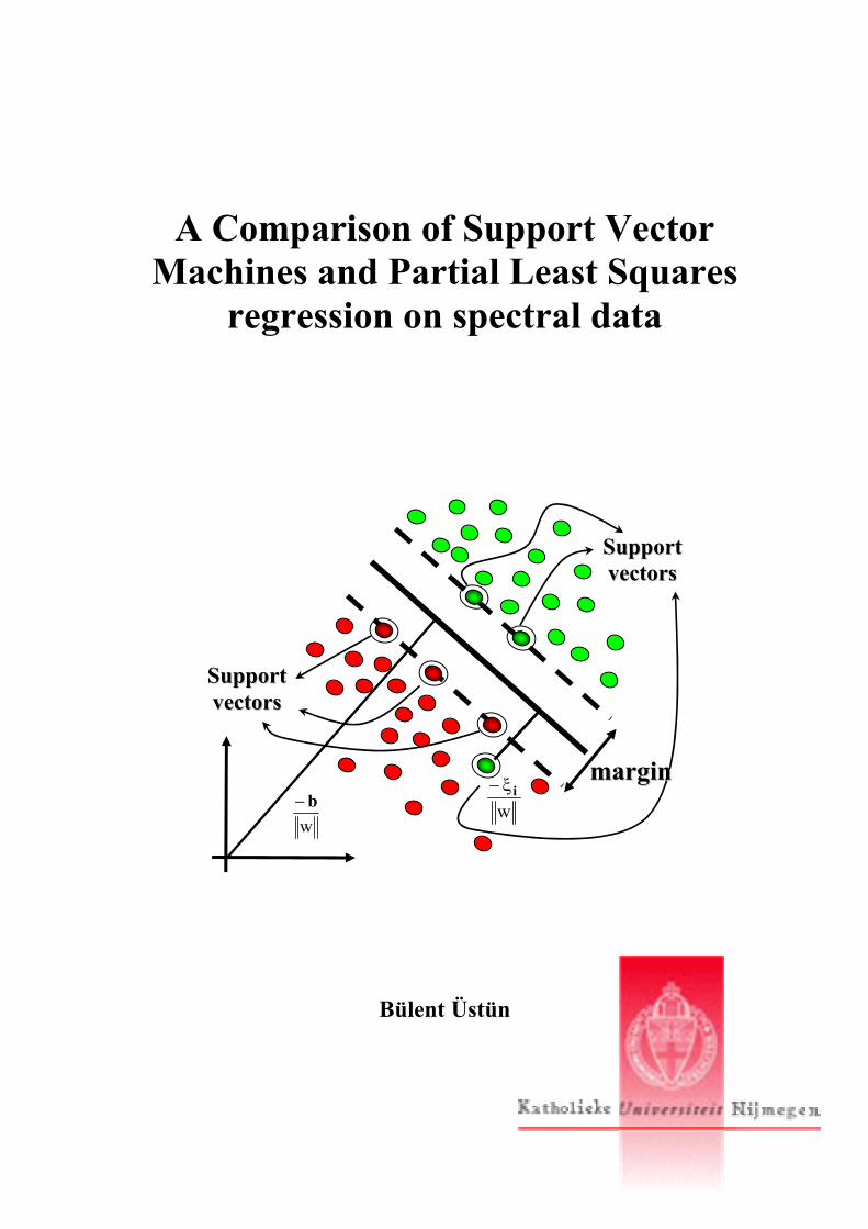
A Comparison of Support Vector

Machines and Partial Least Squares regression on spectral data

Bülent Üstün

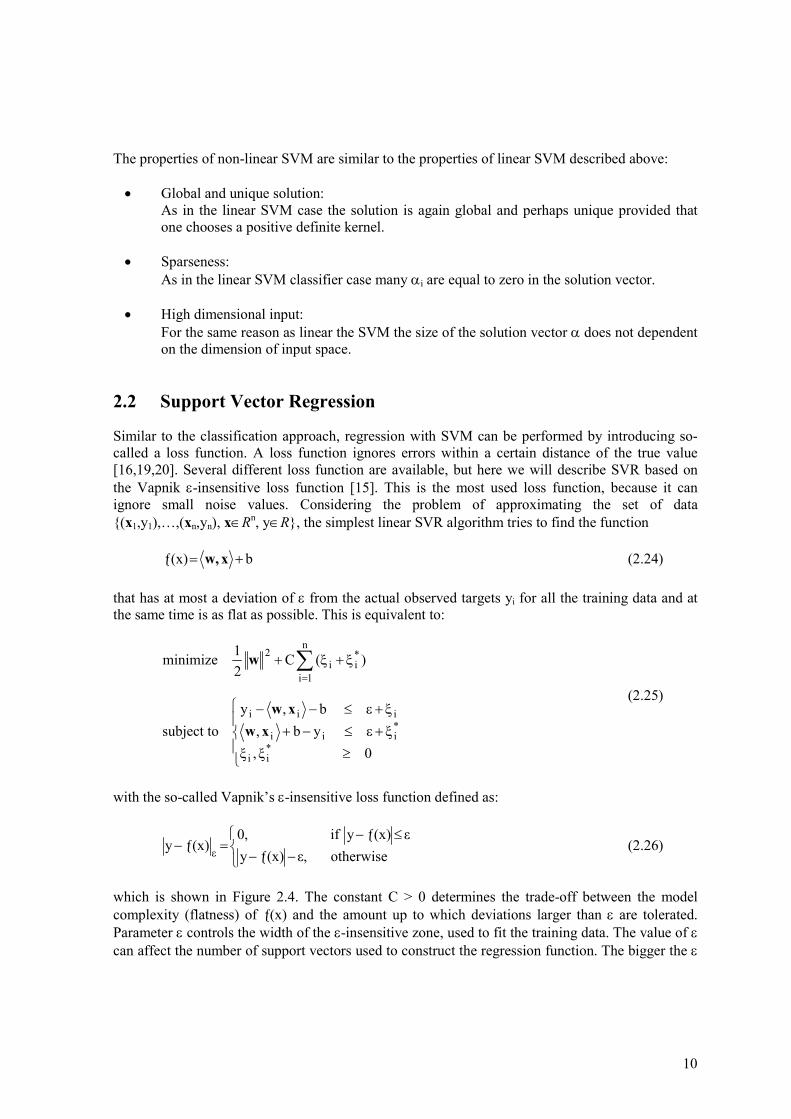
SSuuppppoorrtt vveeccttoorrss

SSuuppppoorrtt vveeccttoorrss

wiξ−

wb−

mmaarrggiinn

A Comparison of Support Vector Machines and Partial Least Squares

regression on spectral data

Bülent Üstün Department of Analytical Chemistry 21 August 2003 Supervisor: Uwe Thissen

Samenvatting

Het gebruik van spectroscopische methoden, zoals Raman en Nabij InfraRood (NIR), in combinatie met chemometrische technieken is sterk toegenomen. Deze worden voornamelijk gebruikt in industriële processen ter kwaliteitscontrole van producten, bijv. concentratie bepaling van chemische componenten. Een van de meest gebruikte chemometrische technieken voor spectrale data analyse is Partial Least Squares (PLS) regressie. Een relatief nieuwe techniek is Support Vector Regression (SVR). Deze heeft een aantal belangrijke eigenschappen die het gebruik ervan aantrekkelijk maken, zoals het vinden van niet-lineaire, algemene oplossingen en de eenvoudige modellering van hoog dimensionale data. In dit verslag worden de prestaties van PLS en SVR met elkaar vergeleken aan de hand van vier spectrale data sets, die enkele specifieke problemen bevatten, zoals niet-lineariteit en piekverschuivingen. Verder is er onderzoek gedaan naar verschillende methoden om de optimale instellingen van SVR parameters te vinden. Daarnaast is er een vergelijking gemaakt tussen SVR en Least Squares-SVR (LS-SVR). Uit de resultaten is gebleken dat SVR in de meeste gevallen betere resultaten levert dan PLS. In de praktijk blijkt echter dat LS-SVR betere resultaten levert dan SVR, omdat de rekentijd korter is, zodat de verschillende parameters veel nauwkeuriger te optimaliseren zijn.

Abstract

In the process industry on-line spectroscopic methods, like Raman and Near Infrared (NIR), in combination with regression tools are increasingly used to measure quality characteristics of products, e.g. concentrations of chemical constituents. One of the most widely used regression techniques is Partial Least Squares (PLS) and a relatively new, not yet widely used, technique is Support Vector Regression (SVR). The latter has some important advantages, such as its ability to find non-linear, global solutions and its ability to work with high dimensional input vectors. This report compares the performances of SVR with PLS for four spectral data sets, in which some specific modelling difficulties are included, such as non-linearity and peak shifts. Furthermore, a study is done on different methods to optimize the user-defined SVR parameters. Also the performance of LS-SVR is compared with SVR. From the experimental results, it can be concluded that SVR outperforms PLS in most of the cases. Additionally, LS-SVR has a shorter computing time than SVR. This leads to more precise optimization of the user-defined parameters and thus better results.

Contents

Samenvatting Abstract Contents 1 Introduction .................................................................................................................................. 2

1.1 The aim of this report ............................................................................................................... 2 1.2 Roadmap................................................................................................................................... 3

2 Support Vector Machines ............................................................................................................ 4

2.1 Support Vector Classification.................................................................................................. 4 2.2 Support Vector Regression.................................................................................................... 10 2.3 Least Squares Support Vector Machines............................................................................... 14

3 Experimental............................................................................................................................... 18

3.1 Data sets used ........................................................................................................................ 18 3.1.1 Raman spectra of polymer yarns (data set A)................................................................. 18 3.1.2 Raman spectra of polymer yarns (data set B) ................................................................. 20 3.1.3 Raman spectra of copolymerizations (data set C) .......................................................... 21 3.1.4 Near infrared spectra of ternary mixtures (data set D) ................................................... 22

3.2 Software................................................................................................................................. 23 3.3 Performance........................................................................................................................... 23

4 Results and Discussion ............................................................................................................... 24

4.1 Comparison of SVR parameter tuning techniques ................................................................ 24 4.1.1 Grid search tuning ........................................................................................................... 24 4.1.2 Practical selection of C and ε........................................................................................... 25 4.1.3 Conclusion....................................................................................................................... 25

4.2 Comparing SVR to PLS ........................................................................................................ 26 4.2.1 Data set A ....................................................................................................................... 26 4.2.2 Data set B........................................................................................................................ 28 4.2.3 Data set C........................................................................................................................ 31

4.3 Comparing PLS to SVR and LS-SVR................................................................................... 34 4.3.1 Data set D ....................................................................................................................... 34

5 Conclusion.................................................................................................................................. 40 Bibliography.................................................................................................................................... 42 Appendix ......................................................................................................................................... 44

A.1 Influence of ε and C on regression function .......................................................................... 44

1

2

1 Introduction

Spectroscopic techniques, e.g. Raman and Near InfraRed (NIR) spectroscopy, in combination with chemometric analysis have proved to be a powerful analytical tool for analysing on-line industrial processes. Using spectroscopic techniques on-line is especially possible due to their short measurement time. For this reason they are replacing standard and slow off-line laboratory analysis. Spectral data contain a large amount of information, which is partly hidden because the data are too complex to be easily interpreted. Chemometric analysis helps to visualise the information contained in the spectral data. In many industrial processes, Partial Least Squares (PLS) is the most used chemometric tool for correlating spectra to reference data, such as product characteristics. The reason to use PLS is because of its simplicity, speed, relative good performance and easy accessibility. However, PLS is not well suited for modelling strong non-linearities between the spectra and reference data. Recently, Support Vector Regression (SVR) emerged as an alternative regression tool. SVR is a derivation of Support Vector Machines (SVM), introduced by Vapnik [1]. SVMs were originally developed for classification purposes. The advantages of SVR are its ability to model non-linear relations, it results in a global and usually unique solution, it finds a general solution avoiding overtraining and the solution found is sparse. Often, Neural Networks (NNs) are used and considered to be good non-linear regression methods for spectra such as Raman or NIR (e.g. [2-4]). However, compared to NNs, SVR has the advantage that it leads to a global model which is capable of dealing efficiently with high dimensional input vectors. In contrast, the number of weights of the NNs is very high in cases with high dimensional input vectors. Furthermore, these weights are optimizing iteratively and this procedure is repeated with different initial settings, which might lead to non-global solutions. Another regression tool is Least Squares SVR (LS-SVR) which is a reformulation of SVR [5]. SVR solves regression problem by means of quadratic programming (QP). LS-SVR solves the regression problem by a set of linear equations, which is easier to use than QP. For this reason LS-SVR has a shorter computing time, as compared to SVR.

1.1 The aim of this report

The main aim of this report is to test the performance of SVR for monitoring (semi-) industrial processes using Raman and NIR spectra, measured on-line. Because usually PLS is used for many industrial processes, the performance of both PLS and SVR are compared on basis of four spectral data sets. Some of these data sets represent specific modelling difficulties, such as peak shifts and non-linearity. No comparison is made with NNs because of the theoretical disadvantages which are described above. Furthermore, a comparison is made between two different methods to optimize the SVR (this is done on the first data set). Additionally, the performance of LS-SVR as an alternative to SVR is assessed on the last data set. The first data set contains Raman spectra of polymer yarns [6]. These spectra are used to predict 4 structural and 3 physical properties of yarns. In the literature, wavelength selection is applied by using Simulated Annealing (SA) [7] to improve the PLS prediction of the selected yarn properties. Besides the comparison of the performance of SVR with PLS without wavelength selection, also a comparison of SVR with PLS with wavelength selection is made. The latter is done, because it is

3

known that SVR is easier to use and less time-consuming than PLS in combination with wavelength selection by using SA. The second data set also contains Raman spectra of polymer yarns [8]. In contrast to the first data set, these spectra are used to predict only 6 physical yarn properties. Two physical yarn properties of both data sets are similar. The third data set contains Raman spectra of three solution copolymerizations of Butyl Acrylate (BA) and Styrene (Sty) [9], which are used to predict the concentrations of BA and Sty. The spectra include small peak shifts induced by on/off switching of the laser and the repositioning of the grating, which distort the spectra. Witjes et al. [9], have applied peak shift correction on this data set to improve the ability of PLS to predict the concentrations of BA and Sty. Besides the comparison of the performance of SVR with PLS, also the influence of peak shift correction on SVR is investigated. The fourth data set consist of NIR spectra for the prediction of ethanol, water and 2-propanol concentrations in a ternary mixture [10]. The spectra are non-linear influenced by temperature variations. In the literature, several methods have been proposed to reduce this temperature dependency [10-13]. In this report, these results are compared with those of SVR.

1.2 Roadmap

This report is organized as follows. Chapter 2 explains the theory of SVM classification (SVC) and regression (SVR) as introduced by Vapnik [1] and LS-SVR introduced by Suykens et al.[5]. Chapter 3 describes the experimental part, which includes the description of the data sets, the software and the performance criterion used. The experimental results are analyzed and discussed in Chapter 4. Finally, some concluding remarks are made in Chapter 5. The influence of the SVR parameters on the quality of the solution is presented in the Appendix.

4

2 Support Vector Machines

Support Vector Machines (SVM) have been developed by Vapnik (1995) [1] and have been successfully applied to a number of classification problems [14,15]. Additionally, SVMs can also be applied for regression purposes [15-17]. Some advantages of SVM in comparison with other methods leads to: (1) a global and perhaps unique solution, (2) a general solution and thus avoiding overtraining, (3) a sparse solution and (4) non-linear relations can be modelled. Although, in this report the performance of Support Vector Regression (SVR) is compared with Partial Least Squares (PLS), it is useful first to understand Support Vector Classification (SVC). With SVC, the basic idea of SVM can be shown easily and helps understanding the theory of SVR. Therefore this chapter starts by describing SVC. Next, SVR based on the Vapnik ε-insensitive loss function will be described. In the last section a brief overview of LS-SVR is given. A more detailed description of SVC, SVR and LS-SVR can be found in [1,5,14-20].

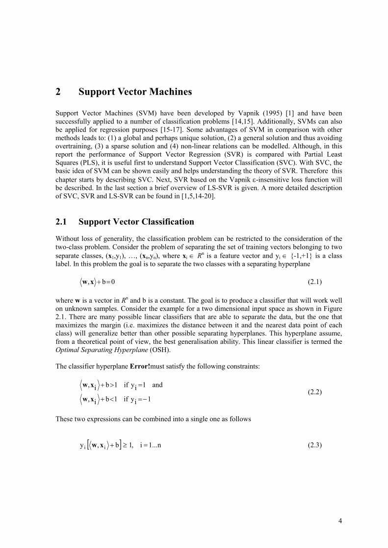
2.1 Support Vector Classification

Without loss of generality, the classification problem can be restricted to the consideration of the two-class problem. Consider the problem of separating the set of training vectors belonging to two separate classes, (x1,y1), …, (xn,yn), where xi ∈ Rn is a feature vector and yi ∈ -1,+1 is a class label. In this problem the goal is to separate the two classes with a separating hyperplane

0b, =+xw (2.1) where w is a vector in Rn and b is a constant. The goal is to produce a classifier that will work well on unknown samples. Consider the example for a two dimensional input space as shown in Figure 2.1. There are many possible linear classifiers that are able to separate the data, but the one that maximizes the margin (i.e. maximizes the distance between it and the nearest data point of each class) will generalize better than other possible separating hyperplanes. This hyperplane assume, from a theoretical point of view, the best generalisation ability. This linear classifier is termed the Optimal Separating Hyperplane (OSH). The classifier hyperplane Error!must satisfy the following constraints:

1iy if1bi,

and1iy if1bi,

−=<+

=>+

xw

xw (2.2)

These two expressions can be combined into a single one as follows

[ ] ...n1i,1b,y ii =≥+xw (2.3)

5

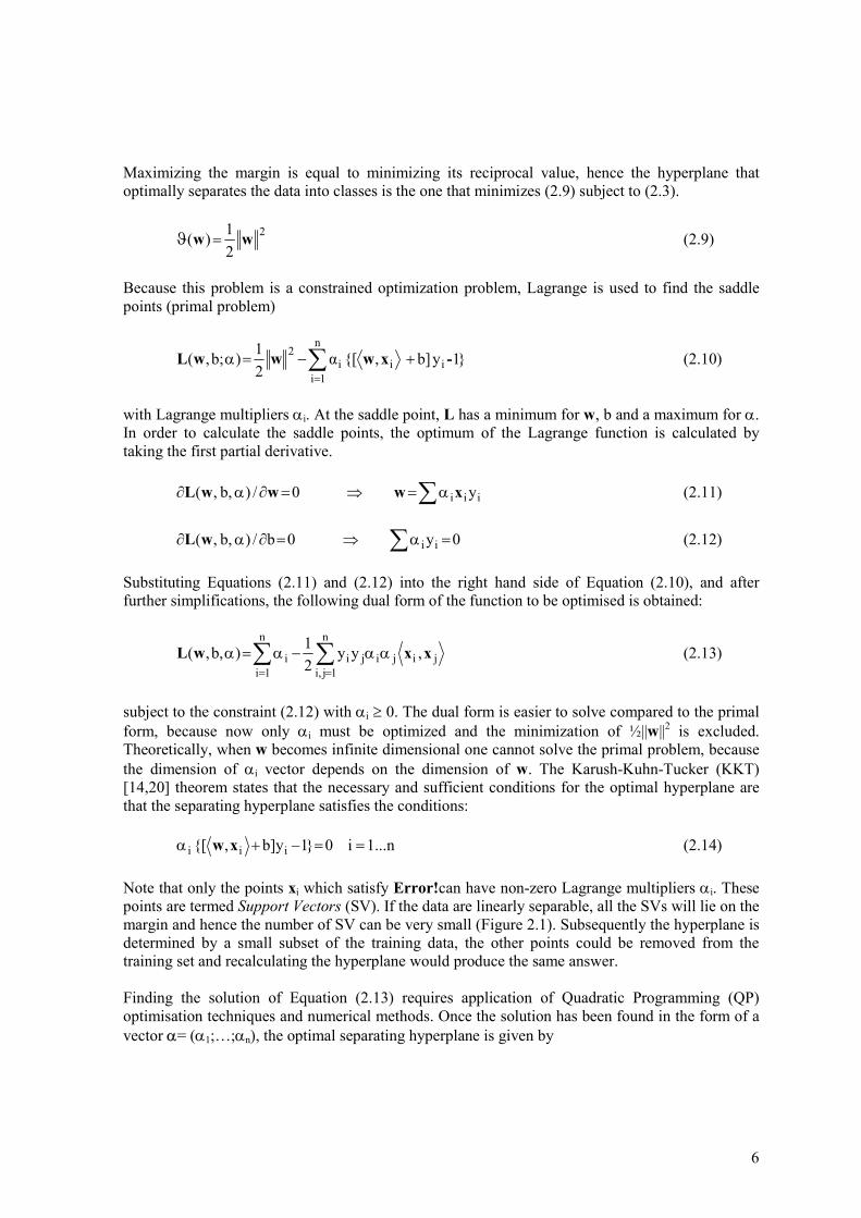
Figure 2.1 Classification of two separable classes. The white and black dots represent samples of the two classes. Left, several possible separating hyperplanes are shown, which are able to separate those two classes. Right, the optimal separating hyperplane (OSH). The dashed lines identify the margin and the points on the margin are called support vectors (circle). The distance from the origin to the OSH is given by (-b/||w||). The distance d(w,b;x) of a point x to the hyperplane (w,b) is,

wxw

xwdb,

)b;,+

=( (2.4)

The optimal hyperplane is given by maximizing the margin, ρ(w,b), subject to Equation (2.3). This margin is given by,

)b;,(min)b;,(minb), j

1jy:jxi

1iy:ixxwdxwdw

−==+=ρ( (2.5)

w

xw

wxw

wb,

minb,

minb),j

1jy:jx

i

1iy:ix

++

+=ρ

−==( (2.6)

www

1min

1minb),

1jy:jx1iy:ix

−+=ρ

−==( (2.7)

ww 2b), =ρ( (2.8)

Support vectors

Support vectors

OSH

margin

wb−

6

Maximizing the margin is equal to minimizing its reciprocal value, hence the hyperplane that optimally separates the data into classes is the one that minimizes (2.9) subject to (2.3).

2

21)( ww =ϑ (2.9)

Because this problem is a constrained optimization problem, Lagrange is used to find the saddle points (primal problem)

1yb],[α21)b;,( i

n

1iii

2 -xwwwL +−=α ∑=

(2.10)

with Lagrange multipliers αi. At the saddle point, L has a minimum for w, b and a maximum for α. In order to calculate the saddle points, the optimum of the Lagrange function is calculated by taking the first partial derivative.

∑α=⇒=∂α∂ iii y0/) b, ,( xwwwL (2.11)

∑ =α⇒=∂α∂ 0y0b/) b, ,( iiwL (2.12) Substituting Equations (2.11) and (2.12) into the right hand side of Equation (2.10), and after further simplifications, the following dual form of the function to be optimised is obtained:

∑ ∑= =

αα−α=αn

1i

n

1ji,jijijii ,yy

21)b,,( xxwL (2.13)

subject to the constraint (2.12) with αi ≥ 0. The dual form is easier to solve compared to the primal form, because now only αi must be optimized and the minimization of ½||w||2 is excluded. Theoretically, when w becomes infinite dimensional one cannot solve the primal problem, because the dimension of αi vector depends on the dimension of w. The Karush-Kuhn-Tucker (KKT) [14,20] theorem states that the necessary and sufficient conditions for the optimal hyperplane are that the separating hyperplane satisfies the conditions:

1...ni01b]y,[ iii ==−+α xw (2.14)

Note that only the points xi which satisfy Error!can have non-zero Lagrange multipliers αi. These points are termed Support Vectors (SV). If the data are linearly separable, all the SVs will lie on the margin and hence the number of SV can be very small (Figure 2.1). Subsequently the hyperplane is determined by a small subset of the training data, the other points could be removed from the training set and recalculating the hyperplane would produce the same answer. Finding the solution of Equation (2.13) requires application of Quadratic Programming (QP) optimisation techniques and numerical methods. Once the solution has been found in the form of a vector α= (α1;…;αn), the optimal separating hyperplane is given by

7

][21bandy sr

sviii xxwxw +−=α=∑ (2.15)

where xr and xs are any Support Vectors (SV) from each class. The classifier can then be constructed as:

)bysign(b)sign((x)

SViii∑ +α=+=ƒ xxxw ,, (2.16)

The solution from SVM given by Equation (2.13) has a number of interesting properties: • Global and Unique solution:

The matrix related to the quadratic term α is positive definite or positive semi definite. In case that the matrix is positive definite (all eigenvalues strictly positive) the solution α to this problem is global and unique. If the matrix is positive semi definite (all eigenvalues positive but zero eigenvalues possible) then the solution is global but not necessary unique.

• Sparseness:

SVM condense all the relevant training data to the solution in the support vectors (αi ≠ 0). This reduces the size of the training data, because the other points (αi = 0) can be removed.

• High dimensional input:

By introducing the inner product Error!in Equation (2.13), the size of the solution vector α does not further be dependent on the dimension of the input space (i.e., the number of object versus variables). However, in case of the primal problem, Equation (2.10), the size of the solution vector α will depend on the dimension of input space. This means that for a high dimensional input it is prefered to solve the dual problem.

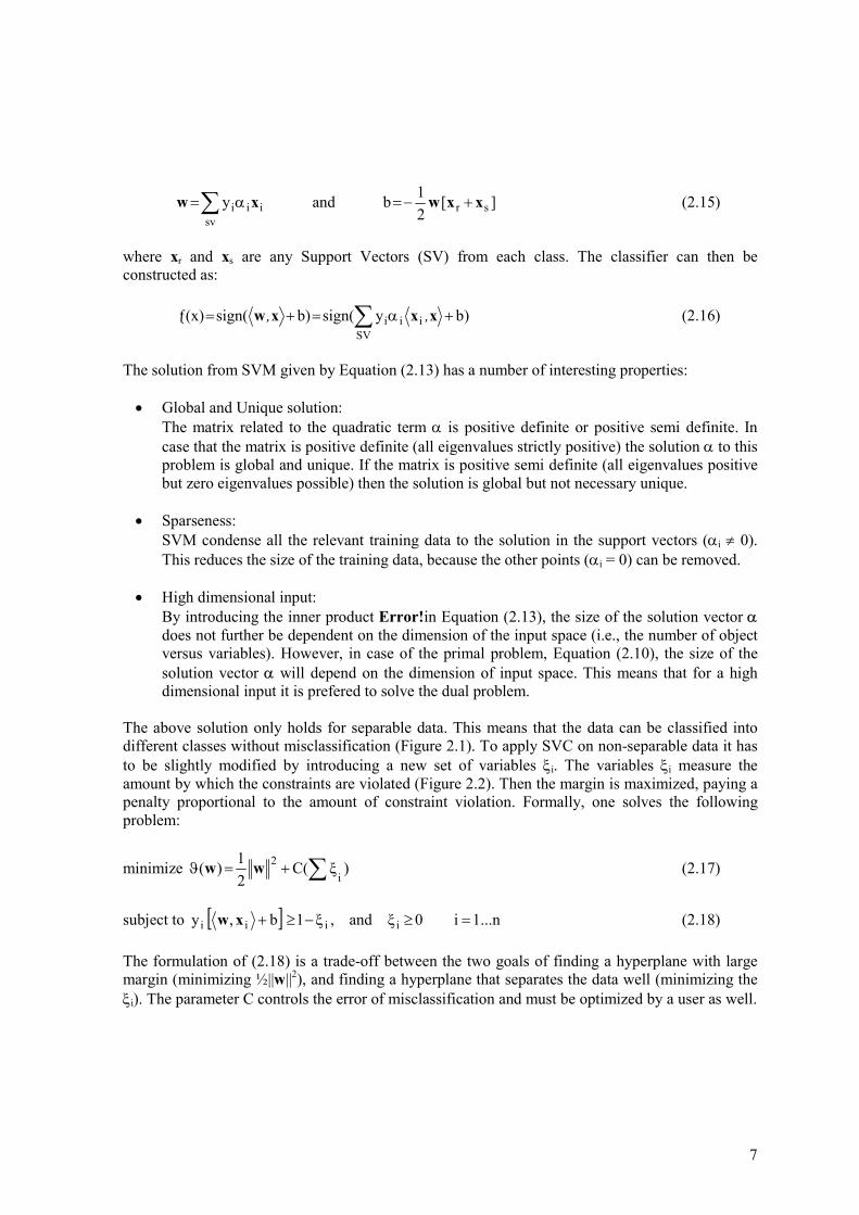
The above solution only holds for separable data. This means that the data can be classified into different classes without misclassification (Figure 2.1). To apply SVC on non-separable data it has to be slightly modified by introducing a new set of variables ξi. The variables ξi measure the amount by which the constraints are violated (Figure 2.2). Then the margin is maximized, paying a penalty proportional to the amount of constraint violation. Formally, one solves the following problem:

minimize )ξC(21)(

i2 ∑+=ϑ ww (2.17)

subject to [ ] ...n1i0ξand,1b,y iiii =≥ξ−≥+xw (2.18) The formulation of (2.18) is a trade-off between the two goals of finding a hyperplane with large margin (minimizing ½||w||2), and finding a hyperplane that separates the data well (minimizing the ξi). The parameter C controls the error of misclassification and must be optimized by a user as well.

8

Figure 2.2 Classification of two non-separable classes. The white and black dots represent samples of the two classes. In case of separable data, each class is located completely on one side of the OSH. In this case there is one misclassification, which will be measured by ξi. The distance between the OSH and misclassification is given by (-ξi/||w||). The first term at the right hand of Equation (2.17) controls the separability of the classifier (OSH with a large margin). On the other hand, the second term controls the accuracy of the classifier for misclassifications. In order to solve the optimization problem in Equation (2.17), the Lagrangian is again constructed as follows:

∑∑∑===

ξ−ξ+−+−ξ+=αn

1iiiii

n

1iii

n

1ii

2 µ1yb],[α)C(21)b;,( xwwwL (2.19)

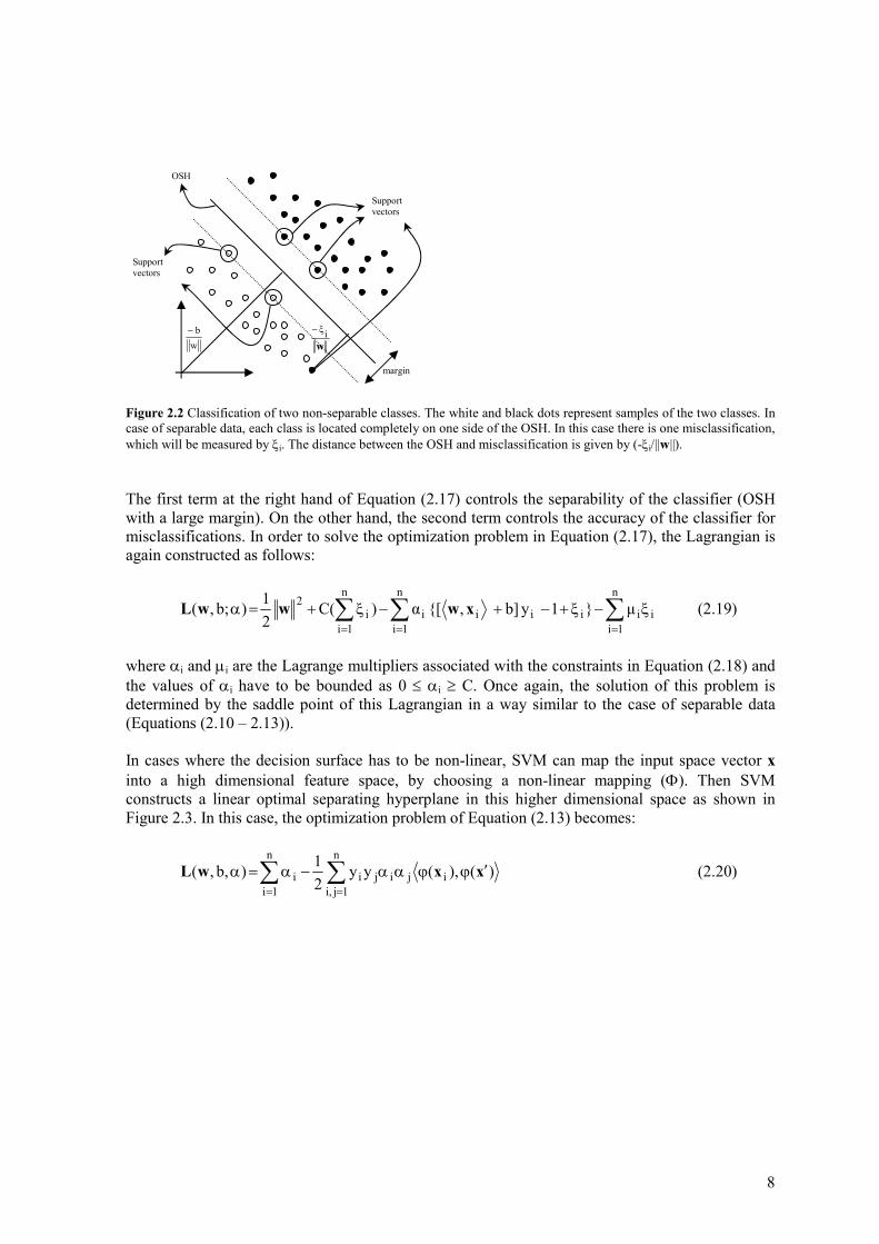
where αi and µi are the Lagrange multipliers associated with the constraints in Equation (2.18) and the values of αi have to be bounded as 0 ≤ αi ≥ C. Once again, the solution of this problem is determined by the saddle point of this Lagrangian in a way similar to the case of separable data (Equations (2.10 – 2.13)). In cases where the decision surface has to be non-linear, SVM can map the input space vector x into a high dimensional feature space, by choosing a non-linear mapping (Φ). Then SVM constructs a linear optimal separating hyperplane in this higher dimensional space as shown in Figure 2.3. In this case, the optimization problem of Equation (2.13) becomes:

∑ ∑= =

′ϕϕαα−α=αn

1i

n

1ji,ijijii )(),(yy

21)b,,( xxwL (2.20)

Support vectors

Support vectors

OSH

margin

wb−

wiξ−

9

Figure 2.3 Mapping of the input space to a feature space to construct a linear OSH. Left, the original input space of two classes, which are not linear separable. Right, the mapping of the input space to a feature space, which makes it possible to separate in a linear way the two classes. Clearly, if the feature space is high dimensional, the dot product (ϕ(xi)·ϕ(x΄j)) of equation (2.20) will be very expensive to compute. In some cases, however, there is a simple kernel (K) that can replace this mapping efficiently. It is therefore convenient to introduce the so called kernel function:

)(),()( ii xxxxK ′ϕϕ=, (2.21)

Using the kernel function the optimization problem comes down to:

( )

∑

∑ ∑=≥

αα−α=α= =

0yα and 0α subject to

,yy21)b,,(

iii

n

1i

n

1ji,ijijii xxKwL

(2.22)

where Error! is the kernel function performing the non-linear mapping into the feature space. Solving the above equation determines the Lagrangian multipliers and a classifier implanting the optimal separating hyperplane in the feature space is given by,

( ) )b,ysign((x)

SViii∑ +α=ƒ xxK (2.23)

Consequently, everything that has been derived concerning the linear case is also applicable for a non-linear case by using a suitable kernel instead of the dot product. The choice of kernel to fit non-linear data into a linear feature space depends on the structure of the data. Some commonly used kernels are:

1. The Radial Basic Function kernel )222(||exp),K( σ−= /||yx-yx (where the kernel width σ is user-defined)

2. The polynomial kernel ( )d1,),K( += yxyx (where the degree of the polynomial, d, is user-defined)

ϕ(x2)

ϕ(x1)

x

x x

x

x

x

x

x xx xx

Φ

x1

x2

10

The properties of non-linear SVM are similar to the properties of linear SVM described above: • Global and unique solution:

As in the linear SVM case the solution is again global and perhaps unique provided that one chooses a positive definite kernel.

• Sparseness:

As in the linear SVM classifier case many αi are equal to zero in the solution vector. • High dimensional input:

For the same reason as linear the SVM the size of the solution vector α does not dependent on the dimension of input space.

2.2 Support Vector Regression

Similar to the classification approach, regression with SVM can be performed by introducing so-called a loss function. A loss function ignores errors within a certain distance of the true value [16,19,20]. Several different loss function are available, but here we will describe SVR based on the Vapnik ε-insensitive loss function [15]. This is the most used loss function, because it can ignore small noise values. Considering the problem of approximating the set of data (x1,y1),…,(xn,yn), x∈Rn, y∈R, the simplest linear SVR algorithm tries to find the function

b(x) +=ƒ xw, (2.24)

that has at most a deviation of ε from the actual observed targets yi for all the training data and at the same time is as flat as possible. This is equivalent to:

≥ξ+ε≤−+ξ+ε≤−−

ξ+ξ+ ∑=

0 ξ,ξ yb, b,y

subject to

)(C21minimize

*ii

*iii

iii

n

1i

*ii

2

xwxw

w

(2.25)

with the so-called Vapnik’s ε-insensitive loss function defined as:

−ƒ−≤ƒ−

=ƒ− ε otherwiseε,(x)yε(x)y if,0

(x)y (2.26)

which is shown in Figure 2.4. The constant C > 0 determines the trade-off between the model complexity (flatness) of ƒ(x) and the amount up to which deviations larger than ε are tolerated. Parameter ε controls the width of the ε-insensitive zone, used to fit the training data. The value of ε can affect the number of support vectors used to construct the regression function. The bigger the ε

11

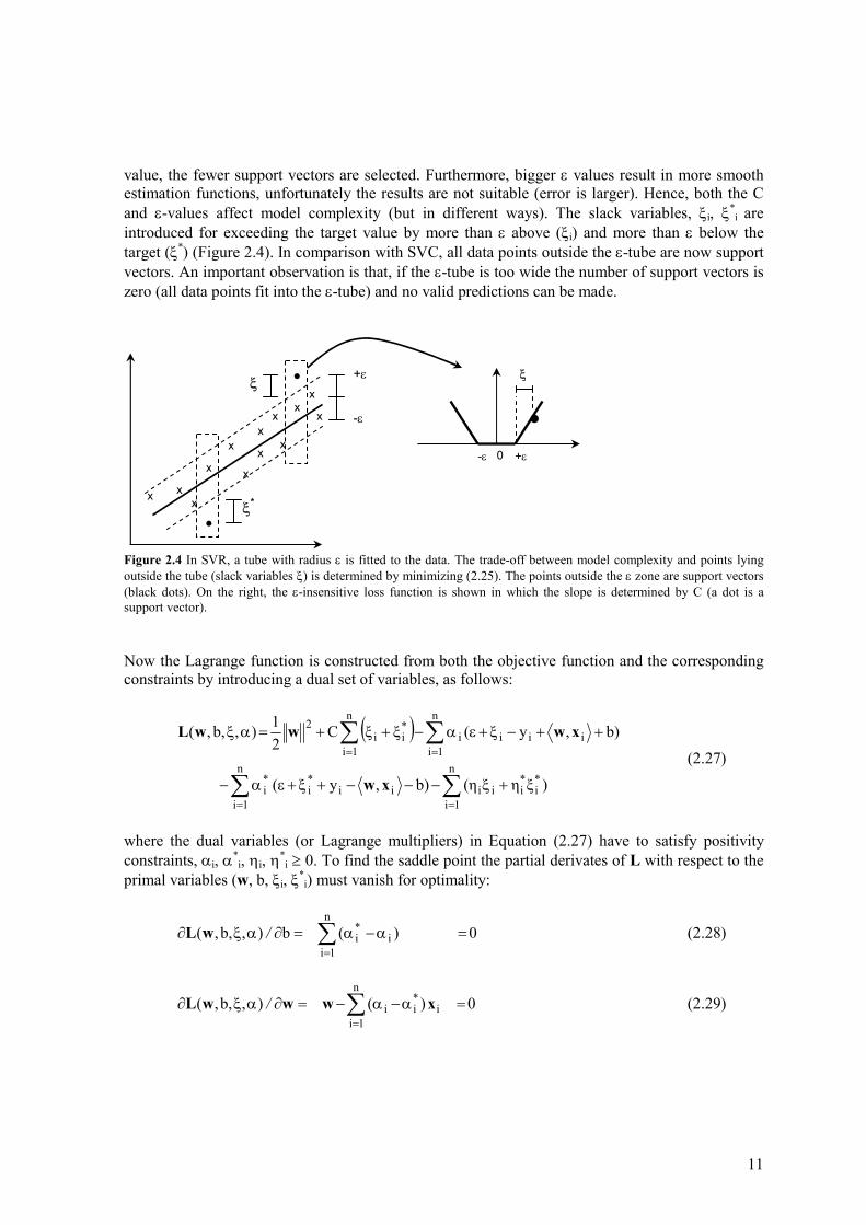
value, the fewer support vectors are selected. Furthermore, bigger ε values result in more smooth estimation functions, unfortunately the results are not suitable (error is larger). Hence, both the C and ε-values affect model complexity (but in different ways). The slack variables, ξi, ξ*

i are introduced for exceeding the target value by more than ε above (ξi) and more than ε below the target (ξ*) (Figure 2.4). In comparison with SVC, all data points outside the ε-tube are now support vectors. An important observation is that, if the ε-tube is too wide the number of support vectors is zero (all data points fit into the ε-tube) and no valid predictions can be made.

Figure 2.4 In SVR, a tube with radius ε is fitted to the data. The trade-off between model complexity and points lying outside the tube (slack variables ξ) is determined by minimizing (2.25). The points outside the ε zone are support vectors (black dots). On the right, the ε-insensitive loss function is shown in which the slope is determined by C (a dot is a support vector). Now the Lagrange function is constructed from both the objective function and the corresponding constraints by introducing a dual set of variables, as follows:

( )

∑ ∑

∑∑

= =

==

+ξ−−−+ξ+εα−

++−ξ+εα−++=αξ

n

1i

n

1i

*i

*iiiii

*i

*i

n

1iiiii

n

1i

*ii

2

)ξη(ηb),y(

b),y(ξξC21),b,,(

xw

xwwwL

(2.27)

where the dual variables (or Lagrange multipliers) in Equation (2.27) have to satisfy positivity constraints, αi, α*

i, ηi, η*i ≥ 0. To find the saddle point the partial derivates of L with respect to the

primal variables (w, b, ξi, ξ*i) must vanish for optimality:

0)(b),b,,(n

1ii

*i =α−α=∂αξ∂ ∑

=

/wL (2.28)

0)(),b,,(n

1ii

*ii =α−α−=∂αξ∂ ∑

=

xwwwL / (2.29)

+ε

-ε x

x

x

x

xx

x

x x x

x

•

x x

ξ

+ε -ε 0

•

ξ

• ξ*

12

* without and with variablesdenotes(*)

(*)i

(*)i

(*)

0ηC),b,,( =−α−=ξ∂αξ∂ /wL (2.30)

Substituting (2.28), (2.30) into (2.27) lets the terms in b and ξ vanish. Finally substituting (2.29) into (2.27) yields the dual optimization problem. This is shown in (2.31).

∈αα

=α−α

α−α+α−αε−

α−αα−α−

∑

∑ ∑

∑

= =

=

C][0,,

0)(subject to

)(y)(

,))((21

maximize

*ii

n

i

*ii

n

1i

n

1i

*iii

*ii

n

1ji,ji

*jj

*ii xx

(2.31)

In Equation (2.31) the dual variables ηi, η*

i were already eliminated through condition (2.30). Once αi and α*

i are determined from (2.31), the desired vectors can now be found as:

∑ ∑= =

+α−=ƒα−α=n

1i

n

1ii

*iii

*ii b)(α(x) thereforeand)( xxxw , (2.32)

The factor b (offset) can be calculated as follows:

C)(0,for ,yb

C)(0,for ,yb

*iii

iii

∈αε−−=

∈αε−−=

xw

xw (2.33)

Similarly to the non-linear SVC approach, a non-linear mapping kernel (K) can be used to map the data into a higher dimensional feature space where linear regression is performed. In this case, the regression function is given by,

( )∑=

+α−=ƒn

1ii

*ii b)(α(x) xxK , (2.34)

The properties of this solution are comparable with the results of classification. The solution is global and unique provided that the chosen kernel is positive definite. As in the classifier case, the solution is sparse. In comparison with non-linear SVC, non-linear SVR contains one more tuning parameter. Namely, ε of Vapnik’s ε-insensitive loss function. In the Appendix some illustrations are given on the effect of changing ε and C for a sinc function and the corresponding support vectors.

13

It is well known that SVR generalization performance depends on a good set of parameters C, ε and the kernel setting (σ in case of RBF or d in case of polynomial kernels), which must be defined by the user. The problem of optimal parameter selection is further complicated by the fact that SVM model complexity (and hence its generalization performance) depends on all three parameters (interaction of the kernel setting, ε and C on the regression model). This means that separately tuning of each parameter is not feasible to find the optimal regression model. Several methods for tuning of these parameters are reported in literature. Most widely, grid search by using leave-n-out cross-validation method, described here below, is used [16,19]. The main idea behind this method is to find the optimal parameters that minimize the prediction error of the regression model. The prediction error can be estimated by leave-n-out cross-validation on the training set. For the current study, a leave-10-out cross-validation has been used. Unfortunately, it is very time-consuming. SVR tuning - Grid search algorithm: 1. For each set of values of the parameters, leave-10-out cross-validation on the training set is

performed to predict the prediction error (RMSECV). 2. Select the set of values of the parameters that produced the model that gave the smallest

prediction error (optimal parameter settings). 3. Train the model with the optimal parameter settings with the whole training set and test it

with a test set (test is not used for training). Another method, a practical one [21], calculates the values of ε and C directly from the training data. In this approach, the value of C is chosen as:

)3σy,3σymax(C yy |||| −+= (2.35)

where y is the mean and σy is the standard deviation of the training set. The value of ε is calculated as:

30 n sets data largefor n(n)ln τσε

30 n sets data smallfor nσε

>=

≤=

(2.36)

where σ is the standard deviation of the training set, n is number of samples in the training set and τ is a constant that also has to be defined by the user. However, when applying this approach to the data in this report there are two important issues: 1. It is known that there is an interaction of the parameters C, ε and kernel setting on the

regression model. The question to be answered remains: How acceptable are the values of C and ε obtained according to this method?

14

2. The data sets used in this report are large (n > 30), and thus the second part of equation (2.36) must be used for selecting ε. In this case, the τ must be tuned. So, no reduction in tunable parameters is obtained.

2.3 Least Squares Support Vector Machines

Least Squares Support Vector Machines (LS-SVM) is a reformulation of the principles of SVM, which involves equality instead of inequality constraints. Furthermore, LS-SVR uses the least squares loss function instead of the ε-insensitive loss function. In this way, the solution follows from a linear KKT [14,20] system instead of a computationally hard QP problem [1,14,19,20]. In consideration of the aim of this report, LS-SVR is discussed in this section in relation to ε-insensitive SVR. A more detailed description of LS-SVR theory can be found in [5]. In contrast to SVC and SVR, the formulations of LS-SVR are shown directly in ‘mapped form’. In case of LS-SVR, one considers the following optimization problem in primal form:

,b)(xysubject to

21

21minimize

iiT

i

n

1i

2i

2

e

e

++ϕ=

γ+ ∑=

w

w (2.37)

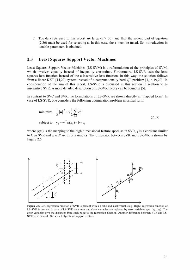
where ϕ(xi) is the mapping to the high dimensional feature space as in SVR, γ is a constant similar to C in SVR and ei ∈ R are error variables. The difference between SVR and LS-SVR is shown by Figure 2.5.

Figure 2.5 Left, regression function of SVR is present with a ε tube and slack variables ξi. Right, regression function of LS-SVR is present. In case of LS-SVR the ε tube and slack variables are replaced by error variables ei ∈ e1…e7. The error variables give the distances from each point to the regression function. Another difference between SVR and LS-SVR is, in case of LS-SVR all objects are support vectors.

+ε

-ε

x

x

x x

x

•ξ

• ξ*

x

x

x

x

x

x

x

e6

e2

e7 e5

e4e3

e1

15

The regression function is again given by:

b(x)(x) T +ϕ=ƒ w (2.38) Similar to SVR, it is more efficient to solve the dual problem instead of primal problem (2.37) in case of high dimensional data. Therefore, the Lagrangian is constructed:

∑∑==

−++ϕα−γ+=αn

1iiii

Ti

n

1i

2i

2 yb)(x21

21),b,,( eee wwwL (2.39)

The optimum of this function can be derived by:

==−++ϕ→=α∂α∂

=γ=α→=∂α∂

=α→=∂α∂

ϕα=→=∂α∂

∑

∑

=

=

n1,...,i0yb)(x0) ,b,,(

n1,...,i0) ,b,,(

00b) ,b,,(

)(x0) ,b,,(

iiiT

i

iii

n

1ii

n

1iii

e/e

ee/e

/e

/e

wwL

wL

wL

wwwL

(2.40)

After elimination of the variables w and e one gets the following solution:

=

α

γΙ+Ωυ

υ

y0b

110 T

/ (2.41)

where y=[y1;…;yn], 1υ=[1;…1], α=[α1;…αn] and Ωij=ϕ(xi)Tϕ(xj)=K(xi,xj) for i,j=1;…;n. In this case, the regression function of SVR given by Equation (2.33) becomes now:

∑=

+=ƒn

1ii

(*)i bα(x) xxK , (2.42)

where α(*)

i and b are the solution to the linear system (2.41). Some properties of LS-SVR are: • It is has a short computing time. Therefore it is easier to optimize.

• It gives a global and possibly unique solution:

The dual problem of LS-SVR corresponds to solve a linear KKT system which is a square system [5] with a unique solution if the matrix has full rank.

16

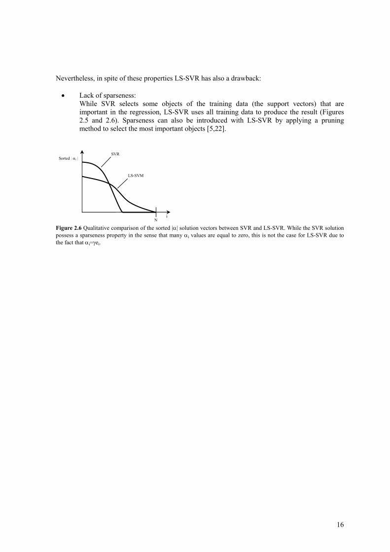
Nevertheless, in spite of these properties LS-SVR has also a drawback: • Lack of sparseness:

While SVR selects some objects of the training data (the support vectors) that are important in the regression, LS-SVR uses all training data to produce the result (Figures 2.5 and 2.6). Sparseness can also be introduced with LS-SVR by applying a pruning method to select the most important objects [5,22].

Figure 2.6 Qualitative comparison of the sorted |α| solution vectors between SVR and LS-SVR. While the SVR solution possess a sparseness property in the sense that many αi values are equal to zero, this is not the case for LS-SVR due to the fact that αi=γei.

N

Sorted | αi |

i

SVR

LS-SVM

17

18

3 Experimental

3.1 Data sets used

To compare the performance between PLS and SVR, four spectral data sets are used. Three of these data sets consist of Raman spectra (data sets A, B and C) and one consist of Near-InfraRed (NIR) spectra (data set D). Data set B is a ‘real world’ industrial data set, the other ones originate from published papers [6,9,10]. The reason to use these data sets is that some different approaches are used in original papers to improve the results of PLS, such as wavelength selection, peak shift correction and modelling of non-linear data. In this report it is investigated if these approaches are also important in case of SVR. Besides the performance between PLS and SVR, the two SVR parameter tuning methods, described in section 2.2, are compared by using data set A. Furthermore, data set D is used to compare the performance of LS-SVR and SVR.

3.1.1 Raman spectra of polymer yarns (data set A)

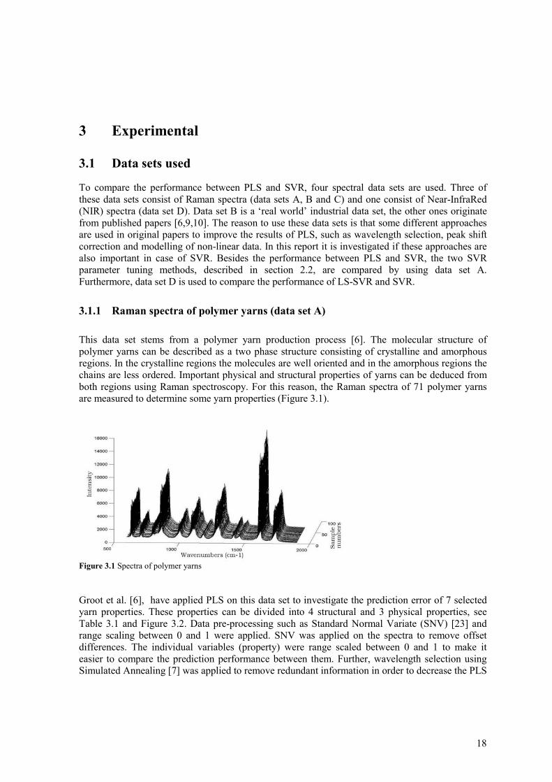
This data set stems from a polymer yarn production process [6]. The molecular structure of polymer yarns can be described as a two phase structure consisting of crystalline and amorphous regions. In the crystalline regions the molecules are well oriented and in the amorphous regions the chains are less ordered. Important physical and structural properties of yarns can be deduced from both regions using Raman spectroscopy. For this reason, the Raman spectra of 71 polymer yarns are measured to determine some yarn properties (Figure 3.1).

Figure 3.1 Spectra of polymer yarns Groot et al. [6], have applied PLS on this data set to investigate the prediction error of 7 selected yarn properties. These properties can be divided into 4 structural and 3 physical properties, see Table 3.1 and Figure 3.2. Data pre-processing such as Standard Normal Variate (SNV) [23] and range scaling between 0 and 1 were applied. SNV was applied on the spectra to remove offset differences. The individual variables (property) were range scaled between 0 and 1 to make it easier to compare the prediction performance between them. Further, wavelength selection using Simulated Annealing [7] was applied to remove redundant information in order to decrease the PLS

19

prediction error. The prediction error of each variable was obtained by calculating the leave-one-out cross-validation (RMSECV) value, due to the small size of the data set (71 spectra). From this study it is concluded that wavelength selection is able to decrease the PLS prediction error. This approach however has the drawback that wavelength selection is a time-consuming process. For this reason, SVR without wavelength selection is applied on this data set to compare its performance with that of PLS (with and without wavelength selection). To compare the results of SVR with that of the original paper, the same data pre-processing as the original paper is used. The prediction error is again calculated by means of leave-one-out cross-validation. Table 3.1 The 7 selected polymer yarn properties

Variables Description ASAR Average Size of Amorphous Region*

VFCR Volume Fraction of Crystalline Region*

AOF Amorphous Orientation Factor*

CLDF Contour Length Distribution Factor*

BT Breaking Tenacity of the yarn**

EAB Elongation At Break (EAB)**

TASE 5 Tenacity At a Specific Elongation of 5% (TASE 5)**

* Structural properties ** Physical properties

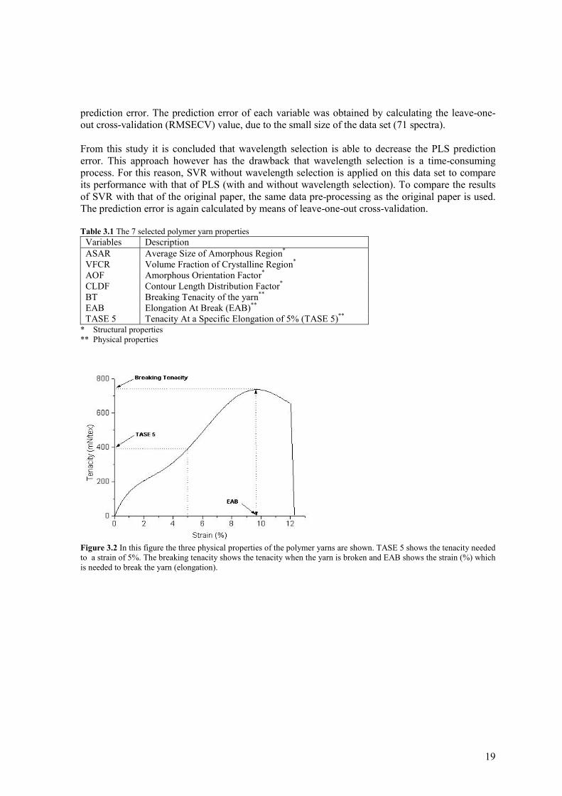
Figure 3.2 In this figure the three physical properties of the polymer yarns are shown. TASE 5 shows the tenacity needed to a strain of 5%. The breaking tenacity shows the tenacity when the yarn is broken and EAB shows the strain (%) which is needed to break the yarn (elongation).

20

3.1.2 Raman spectra of polymer yarns (data set B)

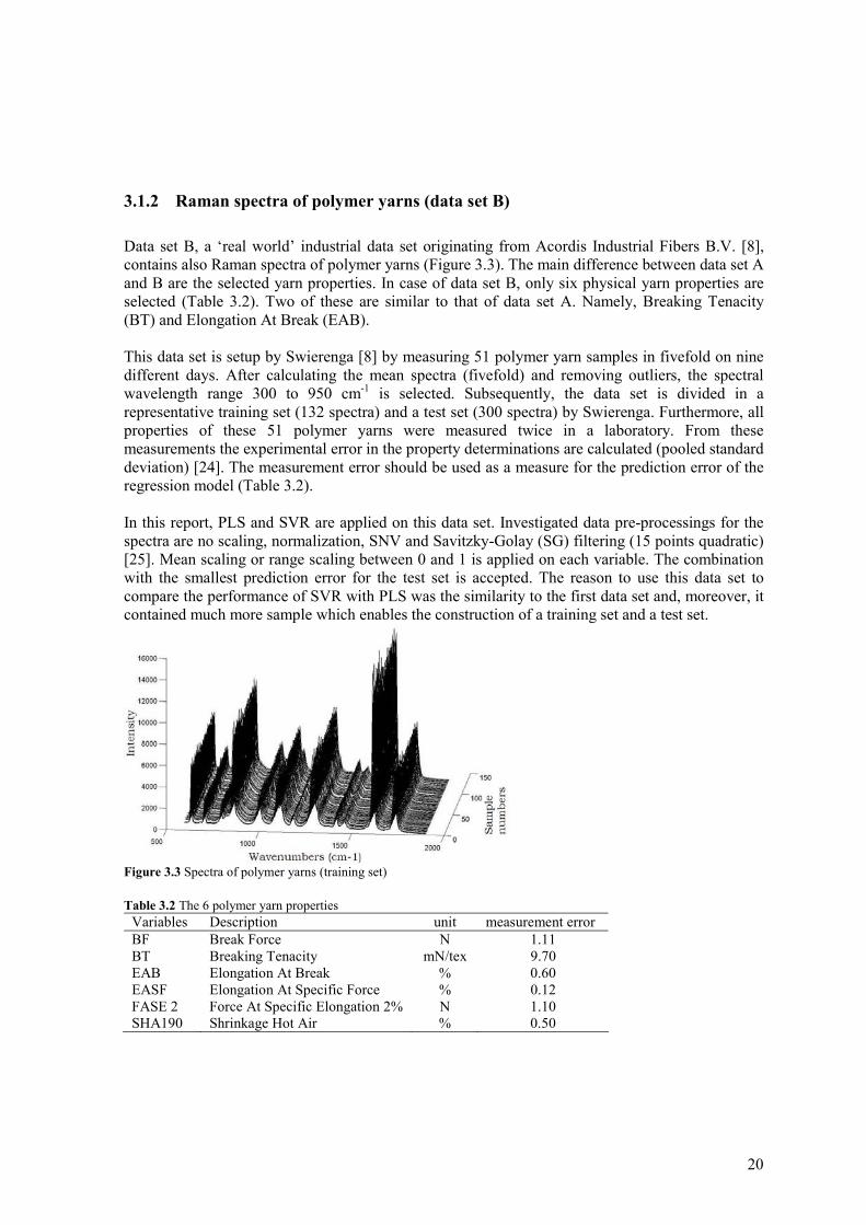
Data set B, a ‘real world’ industrial data set originating from Acordis Industrial Fibers B.V. [8], contains also Raman spectra of polymer yarns (Figure 3.3). The main difference between data set A and B are the selected yarn properties. In case of data set B, only six physical yarn properties are selected (Table 3.2). Two of these are similar to that of data set A. Namely, Breaking Tenacity (BT) and Elongation At Break (EAB). This data set is setup by Swierenga [8] by measuring 51 polymer yarn samples in fivefold on nine different days. After calculating the mean spectra (fivefold) and removing outliers, the spectral wavelength range 300 to 950 cm-1 is selected. Subsequently, the data set is divided in a representative training set (132 spectra) and a test set (300 spectra) by Swierenga. Furthermore, all properties of these 51 polymer yarns were measured twice in a laboratory. From these measurements the experimental error in the property determinations are calculated (pooled standard deviation) [24]. The measurement error should be used as a measure for the prediction error of the regression model (Table 3.2). In this report, PLS and SVR are applied on this data set. Investigated data pre-processings for the spectra are no scaling, normalization, SNV and Savitzky-Golay (SG) filtering (15 points quadratic) [25]. Mean scaling or range scaling between 0 and 1 is applied on each variable. The combination with the smallest prediction error for the test set is accepted. The reason to use this data set to compare the performance of SVR with PLS was the similarity to the first data set and, moreover, it contained much more sample which enables the construction of a training set and a test set.

Figure 3.3 Spectra of polymer yarns (training set) Table 3.2 The 6 polymer yarn properties

Variables Description unit measurement error BF Break Force N 1.11 BT Breaking Tenacity mN/tex 9.70 EAB Elongation At Break % 0.60 EASF Elongation At Specific Force % 0.12 FASE 2 Force At Specific Elongation 2% N 1.10 SHA190 Shrinkage Hot Air % 0.50

21

3.1.3 Raman spectra of copolymerizations (data set C)

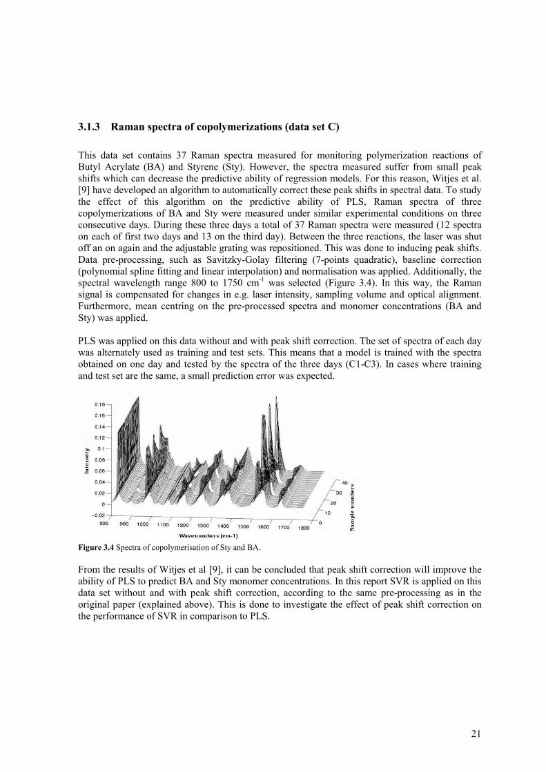
This data set contains 37 Raman spectra measured for monitoring polymerization reactions of Butyl Acrylate (BA) and Styrene (Sty). However, the spectra measured suffer from small peak shifts which can decrease the predictive ability of regression models. For this reason, Witjes et al. [9] have developed an algorithm to automatically correct these peak shifts in spectral data. To study the effect of this algorithm on the predictive ability of PLS, Raman spectra of three copolymerizations of BA and Sty were measured under similar experimental conditions on three consecutive days. During these three days a total of 37 Raman spectra were measured (12 spectra on each of first two days and 13 on the third day). Between the three reactions, the laser was shut off an on again and the adjustable grating was repositioned. This was done to inducing peak shifts. Data pre-processing, such as Savitzky-Golay filtering (7-points quadratic), baseline correction (polynomial spline fitting and linear interpolation) and normalisation was applied. Additionally, the spectral wavelength range 800 to 1750 cm-1 was selected (Figure 3.4). In this way, the Raman signal is compensated for changes in e.g. laser intensity, sampling volume and optical alignment. Furthermore, mean centring on the pre-processed spectra and monomer concentrations (BA and Sty) was applied. PLS was applied on this data without and with peak shift correction. The set of spectra of each day was alternately used as training and test sets. This means that a model is trained with the spectra obtained on one day and tested by the spectra of the three days (C1-C3). In cases where training and test set are the same, a small prediction error was expected.

Figure 3.4 Spectra of copolymerisation of Sty and BA. From the results of Witjes et al [9], it can be concluded that peak shift correction will improve the ability of PLS to predict BA and Sty monomer concentrations. In this report SVR is applied on this data set without and with peak shift correction, according to the same pre-processing as in the original paper (explained above). This is done to investigate the effect of peak shift correction on the performance of SVR in comparison to PLS.

22

3.1.4 Near infrared spectra of ternary mixtures (data set D)

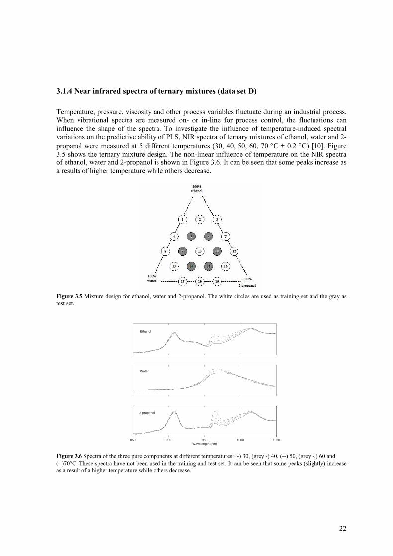
Temperature, pressure, viscosity and other process variables fluctuate during an industrial process. When vibrational spectra are measured on- or in-line for process control, the fluctuations can influence the shape of the spectra. To investigate the influence of temperature-induced spectral variations on the predictive ability of PLS, NIR spectra of ternary mixtures of ethanol, water and 2-propanol were measured at 5 different temperatures (30, 40, 50, 60, 70 °C ± 0.2 °C) [10]. Figure 3.5 shows the ternary mixture design. The non-linear influence of temperature on the NIR spectra of ethanol, water and 2-propanol is shown in Figure 3.6. It can be seen that some peaks increase as a results of higher temperature while others decrease.

Figure 3.5 Mixture design for ethanol, water and 2-propanol. The white circles are used as training set and the gray as test set.

Ethanol

Water

850 900 950 1000 1050Wavelength (nm)

2-propanol

Figure 3.6 Spectra of the three pure components at different temperatures: (-) 30, (grey -) 40, (--) 50, (grey -.) 60 and (-.)70°C. These spectra have not been used in the training and test set. It can be seen that some peaks (slightly) increase as a result of a higher temperature while others decrease.

23

Wülfert et al. [10], have applied baseline correction and mean scaling on the spectra to remove the instrumental baseline drift and selected the spectral region of 850 to 1050 cm-1. Furthermore, mean scaling was applied on the mole fractions of each chemical component separately. Next, the data set was divided into a training set (13 spectra) and a test set (6 spectra), for each temperature, to perform different PLS approaches (Figure 3.5). This data set is used to compare the performance of SVR with the existing PLS approaches of this data set. SVR can be expected to be a good candidate for this problem due to its ability to find non-linear solution and its good generalisation ability. In additionally, LS-SVR is also performed on this data set to compare its performance with SVR. The same pre-processing on the spectra as original paper [10] is used for SVR and LS-SVR. On the mole fractions, a selection of no scaling, mean scaling and range scaling (0-1) is used. The scaling with the smallest prediction error for the training set by leave-one-out cross-validation is accepted.

3.2 Software

The PLS models are calculated using PLS (simpls) Toolbox version 2.1. SVR and LS-SVR are calculated using the Matlab SVM Toolbox developed by Gunn [15] and LS-SVMlab1.5 Toolbox developed by Suykens [26]. Both toolboxes can be obtained from http://www.kernel-machines.org. All Toolboxes work under Matlab (The Mathworks, Inc.).

3.3 Performance

The Root-Mean-Square-Error (RMSE) is used as performance criterion in cross-validation (RMSECV) and also for predicting the test set (RMSEP). The RMSE value is defined by:

n

)yy(RMSE

n

1i

2ii∑

=

−

=

ˆ (3.1)

where ŷi and yi are the predicted and real values of sample i of the n samples respectively.

24

4 Results and Discussion

This chapter starts with a comparison of the two approaches for SVR parameter tuning methods as described before. Next, the PLS and SVR regression results of each data set are presented. In case of data sets A, C and D, PLS is performed to verify wether the results of published papers could be reproduced by our software. Only if these PLS results are similar to that of original papers, these results are not shown in this report. Data set B, does not originate from a paper and therefore PLS is performed to compare with SVR. Finally, the results of LS-SVR on data set D are shown. SVR and LS-SVR were applied using first the RBF-kernel function, because it is most widely used in literature [14-16,21]. If it is not possible to reduce the prediction error by a RBF-kernel the polynomial kernel was used.

4.1 Comparison of SVR parameter tuning techniques

In this section the two SVR parameter tuning methods, the grid search and the one based on the ‘rules’ (see section 2.2), are compared. The method based on the rules is easy and fast, but probably it fails, because of the interaction between the different parameters. In contrast, the grid search method takes into account these interactions, therefore it has to be expected that it will perform better. Both methods are tested on data set A, because at the start of this study this data set was only available. This work is carried out with a RBF kernel on pre-processed data according to original paper [6]. On basis of this comparison a SVR parameter tuning method is chosen, which will be used in the remaining part of this report.

4.1.1 Grid search tuning

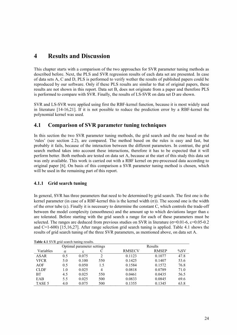
In general, SVR has three parameters that need to be determined by grid search. The first one is the kernel parameter (in case of a RBF-kernel this is the kernel width (σ)). The second one is the width of the error tube (ε). Finally it is necessary to determine the constant C, which controls the trade-off between the model complexity (smoothness) and the amount up to which deviations larger than ε are tolerated. Before starting with the grid search a range for each of these parameters must be selected. The ranges are deduced from previous studies on SVR in literature (σ=0.01-6, ε=0.05-0.2 and C=1-600) [15,16,27]. After range selection grid search tuning is applied. Table 4.1 shows the results of grid search tuning of the three SVR parameters, as mentioned above, on data set A. Table 4.1 SVR grid search tuning results.

Optimal parameter settings Results Variables σ ε C RMSECV RMSEP %SV

ASAR 0.5 0.075 2 0.1123 0.1077 47.8 VFCR 5.0 0.100 550 0.1425 0.1407 53.6 AOF 0.5 0.050 1.5 0.1584 0.1572 76.8 CLDF 1.0 0.025 4 0.0818 0.0789 71.0 BT 4.5 0.025 550 0.0461 0.0435 56.5 EAB 5.5 0.025 500 0.0833 0.0845 69.6 TASE 5 4.0 0.075 500 0.1355 0.1345 63.8

25

4.1.2 Practical selection of C and ε

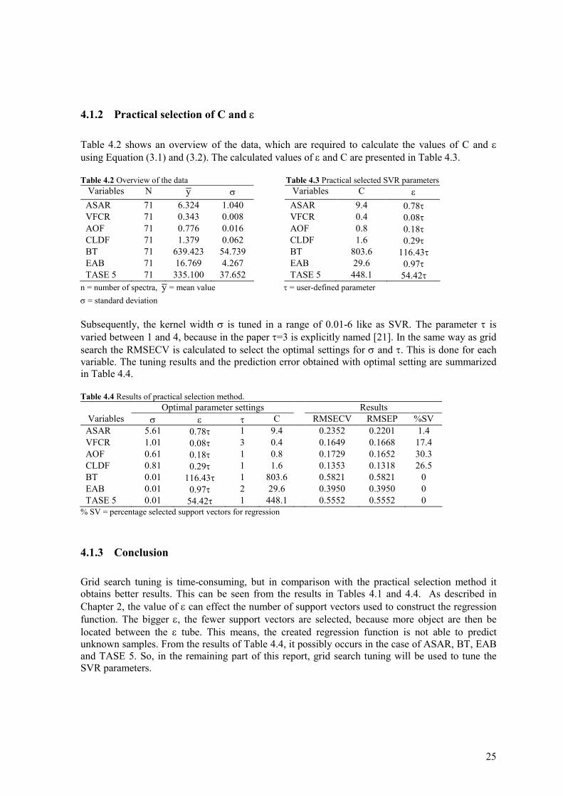
Table 4.2 shows an overview of the data, which are required to calculate the values of C and ε using Equation (3.1) and (3.2). The calculated values of ε and C are presented in Table 4.3. Table 4.2 Overview of the data Table 4.3 Practical selected SVR parameters

Variables N y σ Variables C ε ASAR 71 6.324 1.040 ASAR 9.4 0.78τ VFCR 71 0.343 0.008 VFCR 0.4 0.08τ AOF 71 0.776 0.016 AOF 0.8 0.18τ CLDF 71 1.379 0.062 CLDF 1.6 0.29τ BT 71 639.423 54.739 BT 803.6 116.43τ EAB 71 16.769 4.267 EAB 29.6 0.97τ TASE 5 71 335.100 37.652 TASE 5 448.1 54.42τ

n = number of spectra, y = mean value τ = user-defined parameter σ = standard deviation Subsequently, the kernel width σ is tuned in a range of 0.01-6 like as SVR. The parameter τ is varied between 1 and 4, because in the paper τ=3 is explicitly named [21]. In the same way as grid search the RMSECV is calculated to select the optimal settings for σ and τ. This is done for each variable. The tuning results and the prediction error obtained with optimal setting are summarized in Table 4.4. Table 4.4 Results of practical selection method.

Optimal parameter settings Results Variables σ ε τ C RMSECV RMSEP %SV ASAR 5.61 0.78τ 1 9.4 0.2352 0.2201 1.4 VFCR 1.01 0.08τ 3 0.4 0.1649 0.1668 17.4 AOF 0.61 0.18τ 1 0.8 0.1729 0.1652 30.3 CLDF 0.81 0.29τ 1 1.6 0.1353 0.1318 26.5 BT 0.01 116.43τ 1 803.6 0.5821 0.5821 0 EAB 0.01 0.97τ 2 29.6 0.3950 0.3950 0 TASE 5 0.01 54.42τ 1 448.1 0.5552 0.5552 0

% SV = percentage selected support vectors for regression

4.1.3 Conclusion

Grid search tuning is time-consuming, but in comparison with the practical selection method it obtains better results. This can be seen from the results in Tables 4.1 and 4.4. As described in Chapter 2, the value of ε can effect the number of support vectors used to construct the regression function. The bigger ε, the fewer support vectors are selected, because more object are then be located between the ε tube. This means, the created regression function is not able to predict unknown samples. From the results of Table 4.4, it possibly occurs in the case of ASAR, BT, EAB and TASE 5. So, in the remaining part of this report, grid search tuning will be used to tune the SVR parameters.

26

4.2 Comparing SVR to PLS

4.2.1 Data set A

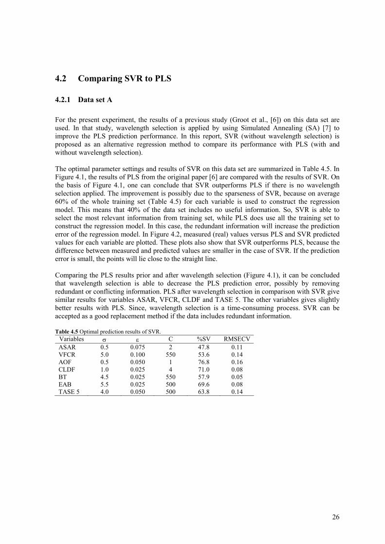
For the present experiment, the results of a previous study (Groot et al., [6]) on this data set are used. In that study, wavelength selection is applied by using Simulated Annealing (SA) [7] to improve the PLS prediction performance. In this report, SVR (without wavelength selection) is proposed as an alternative regression method to compare its performance with PLS (with and without wavelength selection). The optimal parameter settings and results of SVR on this data set are summarized in Table 4.5. In Figure 4.1, the results of PLS from the original paper [6] are compared with the results of SVR. On the basis of Figure 4.1, one can conclude that SVR outperforms PLS if there is no wavelength selection applied. The improvement is possibly due to the sparseness of SVR, because on average 60% of the whole training set (Table 4.5) for each variable is used to construct the regression model. This means that 40% of the data set includes no useful information. So, SVR is able to select the most relevant information from training set, while PLS does use all the training set to construct the regression model. In this case, the redundant information will increase the prediction error of the regression model. In Figure 4.2, measured (real) values versus PLS and SVR predicted values for each variable are plotted. These plots also show that SVR outperforms PLS, because the difference between measured and predicted values are smaller in the case of SVR. If the prediction error is small, the points will lie close to the straight line. Comparing the PLS results prior and after wavelength selection (Figure 4.1), it can be concluded that wavelength selection is able to decrease the PLS prediction error, possibly by removing redundant or conflicting information. PLS after wavelength selection in comparison with SVR give similar results for variables ASAR, VFCR, CLDF and TASE 5. The other variables gives slightly better results with PLS. Since, wavelength selection is a time-consuming process. SVR can be accepted as a good replacement method if the data includes redundant information. Table 4.5 Optimal prediction results of SVR.

Variables σ ε C %SV RMSECV ASAR 0.5 0.075 2 47.8 0.11 VFCR 5.0 0.100 550 53.6 0.14 AOF 0.5 0.050 1 76.8 0.16 CLDF 1.0 0.025 4 71.0 0.08 BT 4.5 0.025 550 57.9 0.05 EAB 5.5 0.025 500 69.6 0.08 TASE 5 4.0 0.050 500 63.8 0.14

27

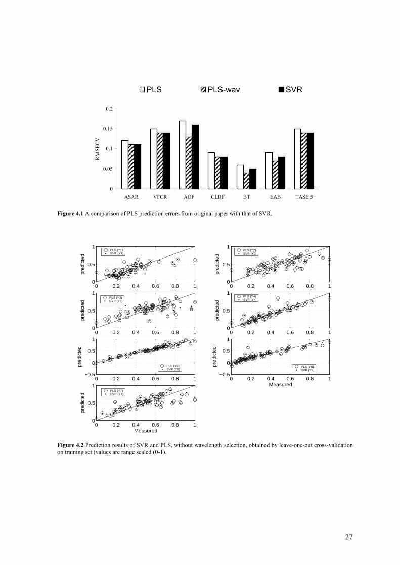
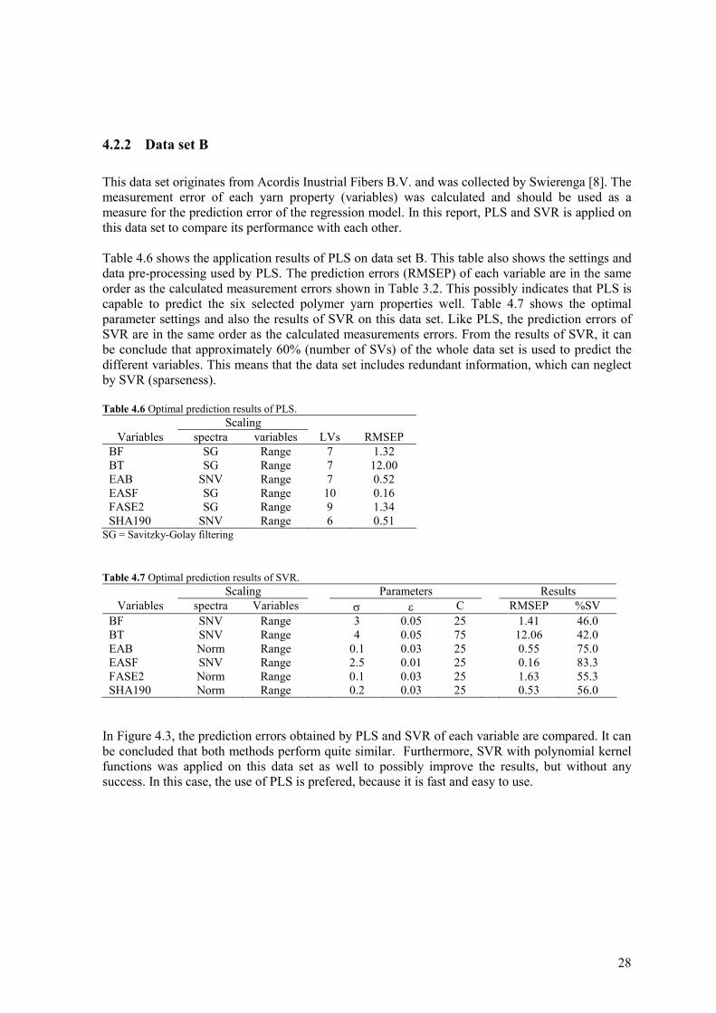
0

0.05

0.1

0.15

0.2

ASAR VFCR AOF CLDF BT EAB TASE 5

RM

SEC

VPLS PLS-wav SVR

Figure 4.1 A comparison of PLS prediction errors from original paper with that of SVR.

0 0.2 0.4 0.6 0.8 10

0.5

1

pred

icte

d

PLS (Y1)SVR (Y1)

0 0.2 0.4 0.6 0.8 10

0.5

1

pred

icte

d

PLS (Y2)SVR (Y2)

0 0.2 0.4 0.6 0.8 10

0.5

1

pred

icte

d

PLS (Y3)SVR (Y3)

0 0.2 0.4 0.6 0.8 10

0.5

1

pred

icte

d

PLS (Y4)SVR (Y4)

0 0.2 0.4 0.6 0.8 1−0.5

0

0.5

1

pred

icte

d

PLS (Y5)SVR (Y5)

0 0.2 0.4 0.6 0.8 1−0.5

0

0.5

1

Measured

pred

icte

d

PLS (Y6)SVR (Y6)

0 0.2 0.4 0.6 0.8 10

0.5

1

Measured

pred

icte

d

PLS (Y7)SVR (Y7)

Figure 4.2 Prediction results of SVR and PLS, without wavelength selection, obtained by leave-one-out cross-validation on training set (values are range scaled (0-1).

28

4.2.2 Data set B

This data set originates from Acordis Inustrial Fibers B.V. and was collected by Swierenga [8]. The measurement error of each yarn property (variables) was calculated and should be used as a measure for the prediction error of the regression model. In this report, PLS and SVR is applied on this data set to compare its performance with each other. Table 4.6 shows the application results of PLS on data set B. This table also shows the settings and data pre-processing used by PLS. The prediction errors (RMSEP) of each variable are in the same order as the calculated measurement errors shown in Table 3.2. This possibly indicates that PLS is capable to predict the six selected polymer yarn properties well. Table 4.7 shows the optimal parameter settings and also the results of SVR on this data set. Like PLS, the prediction errors of SVR are in the same order as the calculated measurements errors. From the results of SVR, it can be conclude that approximately 60% (number of SVs) of the whole data set is used to predict the different variables. This means that the data set includes redundant information, which can neglect by SVR (sparseness). Table 4.6 Optimal prediction results of PLS.

Scaling Variables spectra variables LVs RMSEP

BF SG Range 7 1.32 BT SG Range 7 12.00 EAB SNV Range 7 0.52 EASF SG Range 10 0.16 FASE2 SG Range 9 1.34 SHA190 SNV Range 6 0.51

SG = Savitzky-Golay filtering Table 4.7 Optimal prediction results of SVR.

Scaling Parameters Results Variables spectra Variables σ ε C RMSEP %SV

BF SNV Range 3 0.05 25 1.41 46.0 BT SNV Range 4 0.05 75 12.06 42.0 EAB Norm Range 0.1 0.03 25 0.55 75.0 EASF SNV Range 2.5 0.01 25 0.16 83.3 FASE2 Norm Range 0.1 0.03 25 1.63 55.3 SHA190 Norm Range 0.2 0.03 25 0.53 56.0

In Figure 4.3, the prediction errors obtained by PLS and SVR of each variable are compared. It can be concluded that both methods perform quite similar. Furthermore, SVR with polynomial kernel functions was applied on this data set as well to possibly improve the results, but without any success. In this case, the use of PLS is prefered, because it is fast and easy to use.

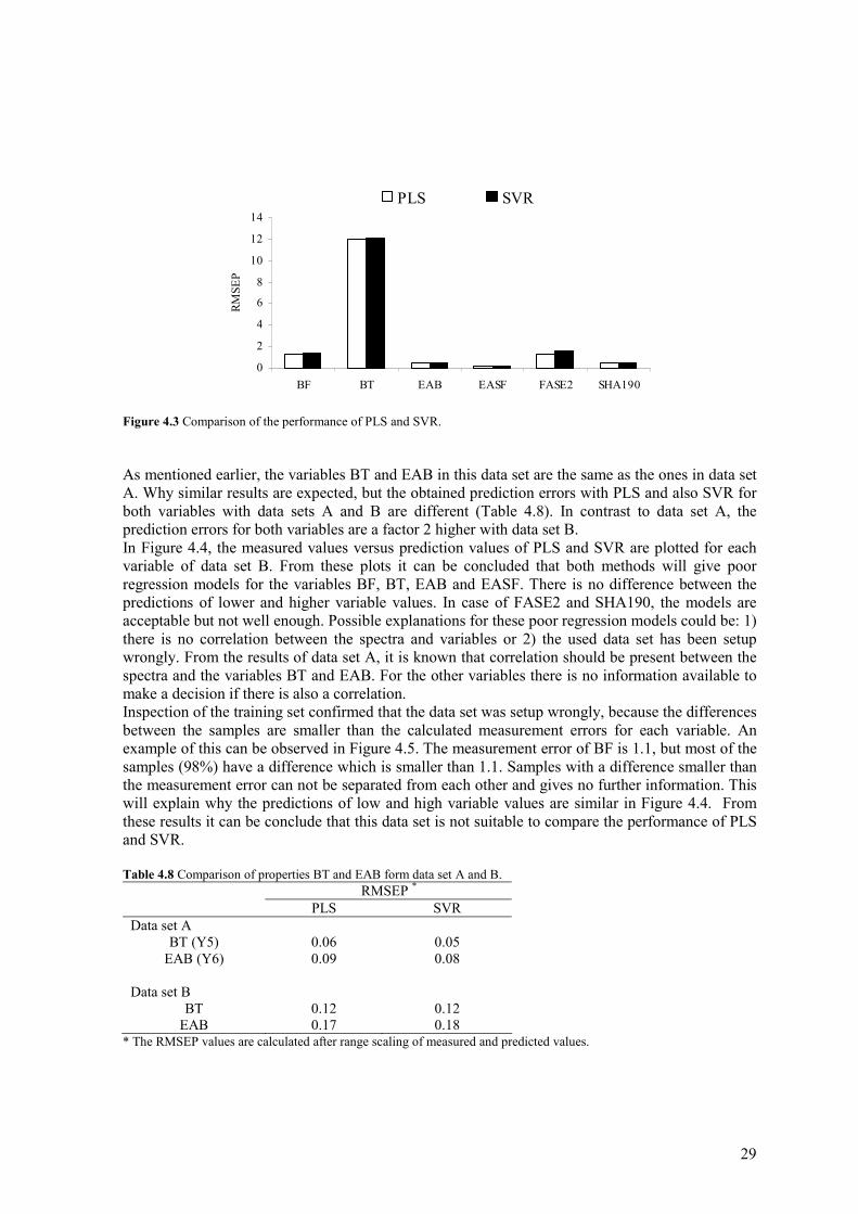
29

0

2

4

6

8

10

12

14

BF BT EAB EASF FASE2 SHA190

RMSE

P

PLS SVR

Figure 4.3 Comparison of the performance of PLS and SVR. As mentioned earlier, the variables BT and EAB in this data set are the same as the ones in data set A. Why similar results are expected, but the obtained prediction errors with PLS and also SVR for both variables with data sets A and B are different (Table 4.8). In contrast to data set A, the prediction errors for both variables are a factor 2 higher with data set B. In Figure 4.4, the measured values versus prediction values of PLS and SVR are plotted for each variable of data set B. From these plots it can be concluded that both methods will give poor regression models for the variables BF, BT, EAB and EASF. There is no difference between the predictions of lower and higher variable values. In case of FASE2 and SHA190, the models are acceptable but not well enough. Possible explanations for these poor regression models could be: 1) there is no correlation between the spectra and variables or 2) the used data set has been setup wrongly. From the results of data set A, it is known that correlation should be present between the spectra and the variables BT and EAB. For the other variables there is no information available to make a decision if there is also a correlation. Inspection of the training set confirmed that the data set was setup wrongly, because the differences between the samples are smaller than the calculated measurement errors for each variable. An example of this can be observed in Figure 4.5. The measurement error of BF is 1.1, but most of the samples (98%) have a difference which is smaller than 1.1. Samples with a difference smaller than the measurement error can not be separated from each other and gives no further information. This will explain why the predictions of low and high variable values are similar in Figure 4.4. From these results it can be conclude that this data set is not suitable to compare the performance of PLS and SVR. Table 4.8 Comparison of properties BT and EAB form data set A and B.

RMSEP *

PLS SVR Data set A

BT (Y5) 0.06 0.05 EAB (Y6) 0.09 0.08

Data set B

BT 0.12 0.12 EAB 0.17 0.18

* The RMSEP values are calculated after range scaling of measured and predicted values.

30

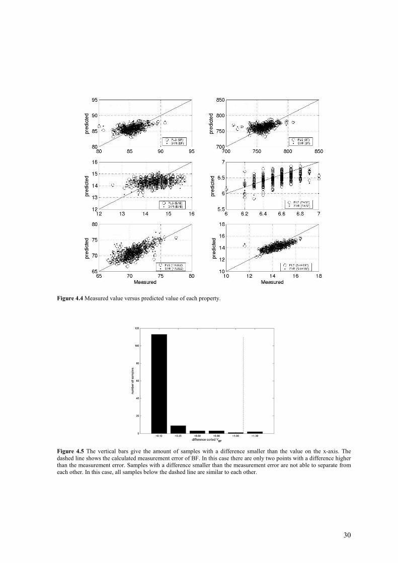
Figure 4.4 Measured value versus predicted value of each property.

Figure 4.5 The vertical bars give the amount of samples with a difference smaller than the value on the x-axis. The dashed line shows the calculated measurement error of BF. In this case there are only two points with a difference higher than the measurement error. Samples with a difference smaller than the measurement error are not able to separate from each other. In this case, all samples below the dashed line are similar to each other.

31

4.2.3 Data set C

Data set C, which consist Raman spectra of three copolymerizations of Butyl Acrylate (BA) and Styrene (Sty) measured on three separate days, contains some peak shifts [9]. These peak shifts were caused by on/off switching of the laser between the three reactions and repositioning of the adjustable grating. The peak shifts lead to a poor PLS prediction of the BA and Sty concentrations. This was the reason why Witjes et al. [9], have applied a simple algorithm to correct these peak shifts to improve the PLS prediction. The aim of this investigation was to develop an algorithm to correct peak shifts in spectra to make a robust PLS model. In this report, data set C is used to investigate the performance of SVR in case of peak shifts in comparison to PLS. The experimental PLS results of data set C are not completely comparable with that of the original paper [9] if C1 is used as training set, see Figure 4.6. The experimental PLS model will give mainly lower RMSEP values for C1 (BA) and higher values for C2 (Sty) and C3 (Sty) without peak correction. C1, C2 and C3 are the data collected on the first, second and third day. After peak correction, lower RMSEP values for C1, C2 and C3 for BA and Sty are obtained by training with C1. No reason can be found for these differences. It’s a challenge, the experimental PLS result will be used to compare it with SVR, because it has smaller or comparable RMSEP values compared to the original paper [9]. SVR is applied on this data set by using the RBF and polynomial kernels. The RBF kernel gives the best results of these two kernel functions. The optimal parameter settings of SVR with a RBF kernel are shown in Table 4.9. Table 4.9 Optimal settings of SVR in case of RBF kernel for BA and Sty.

Without peak shift correction After peak shift correction σ ε C σ ε C

BA C1 0.5 0.005 300 0.5 0.005 400 C2 0.5 0.005 100 1.0 0.005 500 C3 1.0 0.005 500 0.5 0.005 100

Sty

C1 1.0 0.005 5 1.0 0.005 5 C2 0.5 0.005 5 0.5 0.005 5 C3 1.0 0.005 5 0.5 0.005 5

A comparison of the PLS and SVR results are shown in Figure 4.7. From this figure it can be conclude that the PLS results are mostly improved after peak shift. Like PLS, the results of SVR will be improved after peak shifts correction. From this it can be concluded that the performance of SVR is also affected by peak shifts, and it is necessary to correct for it. PLS in comparison with SVR without peak shift correction shows that in some cases PLS and other cases SVR gives good results, indicating that differ methods perform equally well over the full range of parameters. After peak shift correction, the results of PLS are slightly better or comparable with that of SVR. So, PLS by using peak shift correction is the prefered method to predict BA and Sty concentrations.

32

Figure 4.6 Comparison of PLS results. A: calibrated with C1 without peak correction, B: calibrated with C1 after peak correction, C: calibrated with C2 without peak correction, D: calibrated with C2 after peak correction, E: calibrated with C3 without peak correction, F: calibrated with C3 after peak correction. C1-C3 are the spectra measured on day 1, 2 and 3.

0

1

2

3

4

5

6

C1 C2 C3

RM

SEP

PLS BA (lit) PLS BA (exp) PLS Sty (lit) PLS Sty (exp)

0

0.5

1

1.5

2

2.5

C1 C2 C3

RM

SEP

PLS BA (lit) PLS BA (exp) PLS Sty (lit) PLS Sty (exp)

0

0.5

1

1.5

2

2.5

C1 C2 C3

RM

SEP

PLS BA (lit) PLS BA (exp) PLS Sty (lit) PLS Sty (exp)

0

0.5

1

1.5

2

2.5

3

3.5

4

C1 C2 C3

RM

SEP

PLS BA (lit) PLS BA (exp) PLS Sty (lit) PLS Sty (exp)

0

0.5

1

1.5

2

2.5

C1 C2 C3

RM

SEP

PLS BA (lit) PLS BA (exp) PLS Sty (lit) PLS Sty (exp)

00.5

11.5

22.5

33.5

44.5

5

C1 C2 C3

RM

SEP

PLS BA (lit) PLS BA (exp) PLS Sty (lit) PLS Sty (exp)

A B

C D

E F

33

Figure 4.7 Comparison of PLS and SVR RMSEP values. A: calibrated with C1 to predict BA, B: calibrated with C1 to predict Sty, C: calibrated with C2 to predict BA, D: calibrated with C2 to predict Sty, E: calibrated with C3 to predict BA, F: calibrated with C3 to predict Sty.

0

1

2

3

4

5

6

C1 C2 C3

RMSE

P

PLS (without) SVR (without) PLS after SVR (after)

0

1

2

3

4

5

C1 C2 C3

RMSE

P

PLS (without) SVR (without) PLS after SVR (after)

0

1

2

3

4

5

C1 C2 C3

RMSE

P

PLS (without) SVR (without) PLS after SVR (after)

0

1

2

3

C1 C2 C3

RMSE

P

PLS (without) SVR (without) PLS after SVR (after)

0

1

2

C1 C2 C3

RMSE

P

PLS (without) SVR (without) PLS after SVR (after)

0

1

2

3

C1 C2 C3

RMSE

P

PLS (without) SVR (without) PLS after SVR (after)

A B

C D

E F

34

4.3 Comparing PLS to SVR and LS-SVR

4.3.1 Data set D

This data set was setup by Wülfert et al. [10] to study the influence of temperature fluctuations on the predictive ability of PLS on spectral data. For this reason, different local and global PLS models are applied on this data set by Wülfert et al. [10]. Local models are based on a training set of one temperature and global models are based on all temperatures. In case of local models, it is necessary to know the temperature of the new samples in the prediction step to choose the appropriate local model. With one global model for all temperatures, it is not necessary to know the temperature of a new sample to be predicted or that of the training set samples. In following publications, several different methods are applied on this data set to decrease the temperature influence to improve the performance of PLS [10-13]. Wülfert et al. [11], have applied different methods to decrease the temperature influence by explicitly including the temperature into the PLS model. Additionally, a method was presented to isolate temperature contributions by projecting the spectra on several wavelet basis functions. Furthermore, Continuous Piecewise Direct Standardization (CPDS) has been applied to correct for non-linear temperature effects on spectra before performing PLS [12]. Finally, robust variables selection was performed using Uninformative Variable Elimination (UVE). Robust variable selection using SA was also performed by Swierenga et al. [13]. By using the mentioned PLS based approaches, it was not completely possible to model the non-linear relations that exist between temperature and spectral variation. The main reason for this is that the PLS procedure works essentially by finding linear combinations of the spectral variables. In this report, SVR is applied on this data set as an alternative regression method. It is expect that SVR will perform well on this data set, because of its ability to find non-linear solutions and its good generalisation ability. Furthermore, LS-SVR is applied on this data set to compare its performance with SVR. Figure 4.8 shows the comparison between the experimental PLS results and the PLS results from the original paper [10]. It can be seen that there are some differences in RMSEP values. These differences can be caused by differences in baseline correction. The PLS results of the original paper will be used to compare it with SVR, because these have smaller RMSEP values except the global ethanol and 2-propanol models.

0.0000

0.0050

0.0100

0.0150

0.0200

0.0250

ethanol water 2-propanol

RM

SEP

PLS local (lit.) PLS local (exp.)PLS global (lit.) PLS global (exp.)

Figure 4.8 Comparison of the experimental PLS results (exp.) with the PLS results of original paper (lit).

35

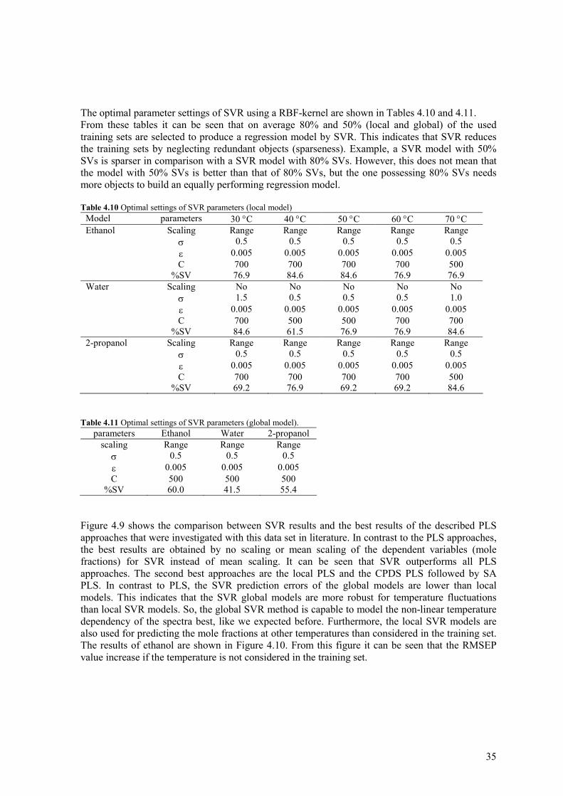
The optimal parameter settings of SVR using a RBF-kernel are shown in Tables 4.10 and 4.11. From these tables it can be seen that on average 80% and 50% (local and global) of the used training sets are selected to produce a regression model by SVR. This indicates that SVR reduces the training sets by neglecting redundant objects (sparseness). Example, a SVR model with 50% SVs is sparser in comparison with a SVR model with 80% SVs. However, this does not mean that the model with 50% SVs is better than that of 80% SVs, but the one possessing 80% SVs needs more objects to build an equally performing regression model. Table 4.10 Optimal settings of SVR parameters (local model)

Model parameters 30 °C 40 °C 50 °C 60 °C 70 °C Ethanol Scaling Range Range Range Range Range σ 0.5 0.5 0.5 0.5 0.5 ε 0.005 0.005 0.005 0.005 0.005 C 700 700 700 700 500 %SV 76.9 84.6 84.6 76.9 76.9 Water Scaling No No No No No σ 1.5 0.5 0.5 0.5 1.0 ε 0.005 0.005 0.005 0.005 0.005 C 700 500 500 700 700 %SV 84.6 61.5 76.9 76.9 84.6 2-propanol Scaling Range Range Range Range Range σ 0.5 0.5 0.5 0.5 0.5 ε 0.005 0.005 0.005 0.005 0.005 C 700 700 700 700 500 %SV 69.2 76.9 69.2 69.2 84.6

Table 4.11 Optimal settings of SVR parameters (global model).

parameters Ethanol Water 2-propanol scaling Range Range Range

σ 0.5 0.5 0.5 ε 0.005 0.005 0.005 C 500 500 500

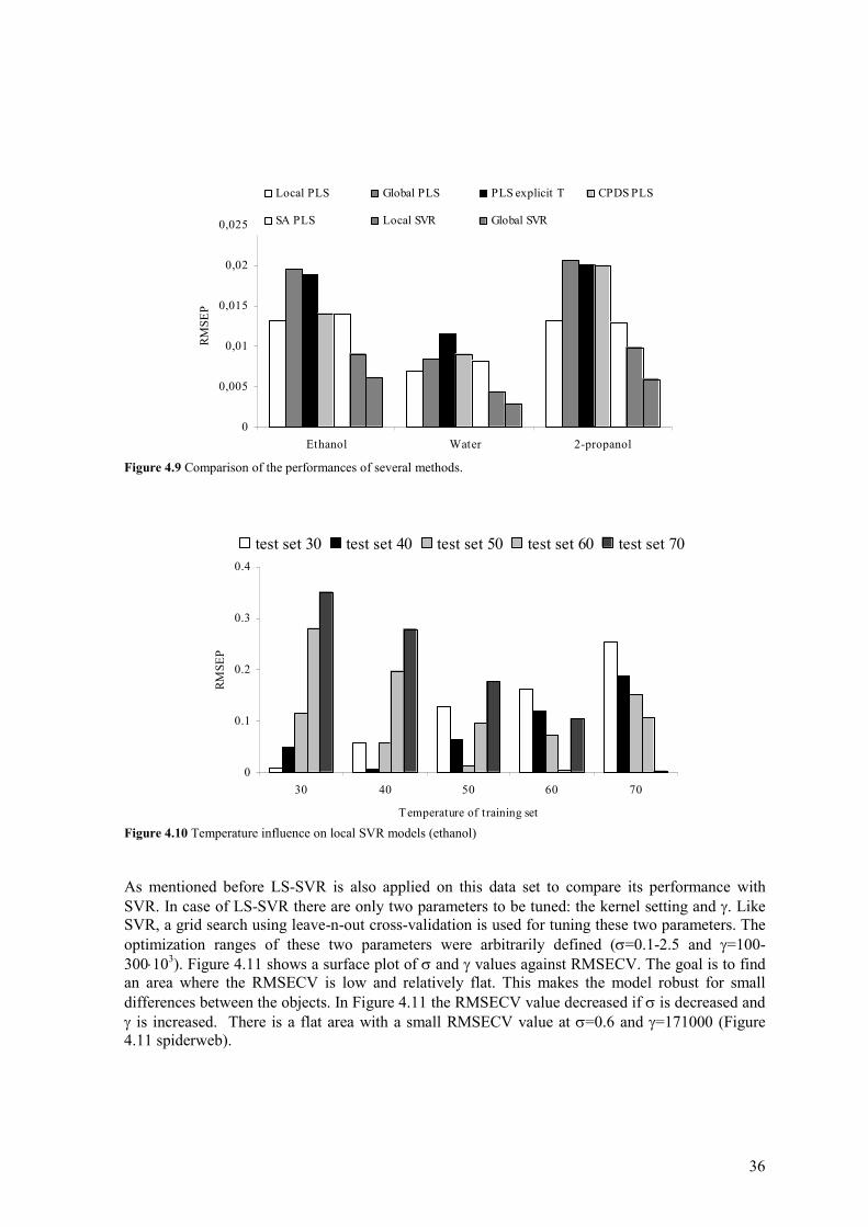
%SV 60.0 41.5 55.4 Figure 4.9 shows the comparison between SVR results and the best results of the described PLS approaches that were investigated with this data set in literature. In contrast to the PLS approaches, the best results are obtained by no scaling or mean scaling of the dependent variables (mole fractions) for SVR instead of mean scaling. It can be seen that SVR outperforms all PLS approaches. The second best approaches are the local PLS and the CPDS PLS followed by SA PLS. In contrast to PLS, the SVR prediction errors of the global models are lower than local models. This indicates that the SVR global models are more robust for temperature fluctuations than local SVR models. So, the global SVR method is capable to model the non-linear temperature dependency of the spectra best, like we expected before. Furthermore, the local SVR models are also used for predicting the mole fractions at other temperatures than considered in the training set. The results of ethanol are shown in Figure 4.10. From this figure it can be seen that the RMSEP value increase if the temperature is not considered in the training set.

36

0

0,005

0,01

0,015

0,02

0,025

Ethanol Water 2-propanol

RMSE

PLocal PLS Global PLS PLS explicit T CPDS PLS

SA PLS Local SVR Global SVR

0

0.1

0.2

0.3

0.4

30 40 50 60 70

Temperature of training set

RMSE

P

test set 30 test set 40 test set 50 test set 60 test set 70

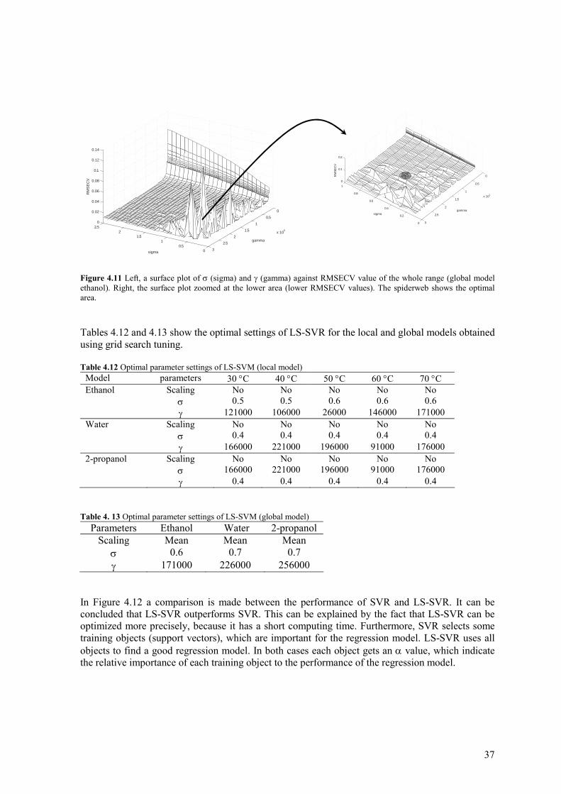
Figure 4.9 Comparison of the performances of several methods. Figure 4.10 Temperature influence on local SVR models (ethanol) As mentioned before LS-SVR is also applied on this data set to compare its performance with SVR. In case of LS-SVR there are only two parameters to be tuned: the kernel setting and γ. Like SVR, a grid search using leave-n-out cross-validation is used for tuning these two parameters. The optimization ranges of these two parameters were arbitrarily defined (σ=0.1-2.5 and γ=100-300⋅103). Figure 4.11 shows a surface plot of σ and γ values against RMSECV. The goal is to find an area where the RMSECV is low and relatively flat. This makes the model robust for small differences between the objects. In Figure 4.11 the RMSECV value decreased if σ is decreased and γ is increased. There is a flat area with a small RMSECV value at σ=0.6 and γ=171000 (Figure 4.11 spiderweb).

37

0

0.2

0.4

0.6

0.8

1

0

0.5

1

1.5

2

2.5

3

x 105

0

0.1

0.2

sigmagamma

RM

SE

CV

00.5

11.5

22.5

0

0.5

1

1.5

2

2.5

3

x 105

0

0.02

0.04

0.06

0.08

0.1

0.12

0.14

sigma

gamma

RM

SE

CV

Figure 4.11 Left, a surface plot of σ (sigma) and γ (gamma) against RMSECV value of the whole range (global model ethanol). Right, the surface plot zoomed at the lower area (lower RMSECV values). The spiderweb shows the optimal area. Tables 4.12 and 4.13 show the optimal settings of LS-SVR for the local and global models obtained using grid search tuning. Table 4.12 Optimal parameter settings of LS-SVM (local model)

Model parameters 30 °C 40 °C 50 °C 60 °C 70 °C Ethanol Scaling No No No No No σ 0.5 0.5 0.6 0.6 0.6 γ 121000 106000 26000 146000 171000 Water Scaling No No No No No σ 0.4 0.4 0.4 0.4 0.4 γ 166000 221000 196000 91000 176000 2-propanol Scaling No No No No No σ 166000 221000 196000 91000 176000 γ 0.4 0.4 0.4 0.4 0.4

Table 4. 13 Optimal parameter settings of LS-SVM (global model)

Parameters Ethanol Water 2-propanol Scaling Mean Mean Mean

σ 0.6 0.7 0.7 γ 171000 226000 256000

In Figure 4.12 a comparison is made between the performance of SVR and LS-SVR. It can be concluded that LS-SVR outperforms SVR. This can be explained by the fact that LS-SVR can be optimized more precisely, because it has a short computing time. Furthermore, SVR selects some training objects (support vectors), which are important for the regression model. LS-SVR uses all objects to find a good regression model. In both cases each object gets an α value, which indicate the relative importance of each training object to the performance of the regression model.

38

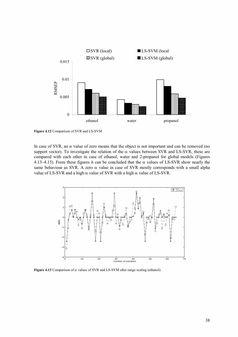
0

0.005

0.01

0.015

ethanol water propanol

RM

SEP

SVR (local) LS-SVM (localSVR (global) LS-SVM (global)

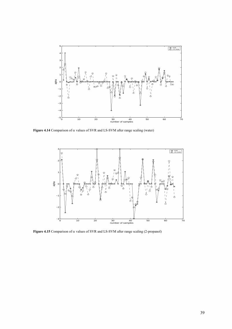
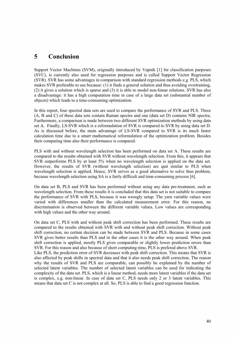
Figure 4.12 Comparison of SVR and LS-SVM In case of SVR, an α value of zero means that the object is not important and can be removed (no support vector). To investigate the relation of the α values between SVR and LS-SVR, these are compared with each other in case of ethanol, water and 2-propanol for global models (Figures 4.13–4.15). From these figures it can be concluded that the α values of LS-SVR show nearly the same behaviour as SVR. A zero α value in case of SVR mostly corresponds with a small alpha value of LS-SVR and a high α value of SVR with a high α value of LS-SVR.

0 10 20 30 40 50 60 70−4

−3

−2

−1

0

1

2

3

number of samples

alpha

SVRLS−SVM

Figure 4.13 Comparison of α values of SVR and LS-SVM after range scaling (ethanol)

39

0 10 20 30 40 50 60 70−5

−4

−3

−2

−1

0

1

2

3

4

5

number of samples

alph

a

SVRLS−SVM

Figure 4.14 Comparison of α values of SVR and LS-SVM after range scaling (water)

0 10 20 30 40 50 60 70−3

−2

−1

0

1

2

3

number of samples

alpha

SVRLS−SVM

Figure 4.15 Comparison of α values of SVR and LS-SVM after range scaling (2-propanol)

40

5 Conclusion

Support Vector Machines (SVM), originally introduced by Vapnik [1] for classification purposes (SVC), is currently also used for regression purposes and is called Support Vector Regression (SVR). SVR has some advantages in comparison with standard regression methods e.g. PLS, which makes SVR preferable to use because: (1) it finds a general solution and thus avoiding overtraining, (2) it gives a solution which is sparse and (3) it is able to model non-linear relations. SVR has also a disadvantage: it has a high computation time in case of a large data set (substantial number of objects) which leads to a time-consuming optimization. In this report, four spectral data sets are used to compare the performance of SVR and PLS. Three (A, B and C) of these data sets contain Raman spectra and one (data set D) contains NIR spectra. Furthermore, a comparison is made between two different SVR optimization methods by using data set A. Finally, LS-SVR which is a reformulation of SVR is compared to SVR by using data set D. As is discussed before, the main advantage of LS-SVR compared to SVR is its much faster calculation time due to a smart mathematical reformulation of the optimization problem. Besides their computing time also their performance is compared. PLS with and without wavelength selection has been performed on data set A. These results are compared to the results obtained with SVR without wavelength selection. From this, it appears that SVR outperforms PLS by at least 5% when no wavelength selection is applied on the data set. However, the results of SVR (without wavelength selection) are quit similar to PLS when wavelength selection is applied. Hence, SVR serves as a good alternative to solve thus problem, because wavelength selection using SA is a fairly difficult and time-consuming process [6]. On data set B, PLS and SVR has been performed without using any data pre-treatment, such as wavelength selection. From these results it is concluded that this data set is not suitable to compare the performance of SVR with PLS, because it was wrongly setup. The yarn variable values were varied with differences smaller than the calculated measurement error. For this reason, no discrimination is observed between the different variable values. Low values are corresponding with high values and the other way around. On data set C, PLS with and without peak shift correction has been performed. These results are compared to the results obtained with SVR with and without peak shift correction. Without peak shift correction, no certain decision can be made between SVR and PLS. Because in some cases SVR gives better results than PLS and in the other cases it is the other way around. When peak shift correction is applied, mostly PLS gives comparable or slightly lower prediction errors than SVR. For this reason and also because of short computing time, PLS is prefered above SVR. Like PLS, the prediction error of SVR decreases with peak shift correction. This means that SVR is also affected by peak shifts in spectral data and that it also needs peak shift correction. The reason why the results of SVR and PLS are comparable, can possibly be explained by the number of selected latent variables. The number of selected latent variables can be used for indicating the complexity of the data set. PLS, which is a linear method, needs more latent variables if the data set is complex, e.g. non-linear. In case of data set C, PLS needs only 2 or 3 latent variables. This means that data set C is not complex at all. So, PLS is able to find a good regression function.

41

The SVR results of the last data set (data set D) are compared with results, obtained from literature, of the different PLS based methods. From this, it appears that the global SVR models outperform all PLS based methods from literature by at least 50% in prediction error. So, SVR is capable to model implicitly non-linear relations between spectra and temperature. However, the prediction error of local SVR models increases by prediction of mole fractions with other temperatures. Therefore it can be concluded that the performance of local SVR models are still affected by temperature variations in spectral data (not robust). The second goal of this report was to investigate the two different SVR optimization methods described in literature. By considering the results of the two described SVR optimization methods, grid search tuning is selected as the best method. The reasons to select the grid search method are: it produces better results than the practical rule-based selection method and the practical method is not always able to find a regression function (zero support vectors). A drawback of the grid search method is that it is time-consuming. The final goal of this report was to compare the performance and speed of LS-SVR with SVR. Considering the results of LS-SVR an SVR on data set D, it can be concluded that the performance of LS-SVR is better than SVR. This can be explained by the advantages of LS-SVR, because a short computing time makes it possible to optimize the model more precisely. Furthermore, the α values which are responsible to select support vectors in case of SVR are comparable with that of LS-SVR. An α value of zero (no support vectors) in case of SVR correspond to small α value for LS-SVR and a high α value of SVR correspond to a high α value of LS-SVR. So, in case of data set D, there is no effect seen on the loss of sparseness of LS-SVR. In case of LS-SVR, there is no ε parameter of the ε-insensitive loss function, which needs to be optimized. The ε is special in giving zero penalties to small noise values, because the influence of noise disappears if the noise level is smaller than ε. Finally, the effect of γ of LS-SVR is comparable with C from SVR, but these differ in magnitude of values. For example, the prediction error obtained with C=300 for SVR is comparable with γ=150000 for LS-SVR. In general, it can be concluded that SVR and LS-SVR will give better results than PLS in case of presence of non-linear phenomena in spectral data. However, there are no general rules to make a decision when SVR, LS-SVR or PLS can applied on spectral data. To select the best method of these three, one needs to try them all. It is advisable to try LS-SVR before SVR, because of short computing time. However, in the presence of noise it may be better to use SVR, because of the ε boundary which eliminates part of the influence of noise present in the measured data.

42

Bibliography

1. V. Vapnik, The Nature of Statistical Learning Theory. 1995, New York: Springer,USA. 2. V. Centner, J. Verdú-Andrés, B. Walczak, D. Jouan-Rimbaud, F. Pasti, R. Paoppi, D.L.

Massart, O.E. De Noord, Comparison of multivariate calibration techniques applied to experimental NIR data sets. Applied spectroscopy, 2000. 54: p. 608-623.

3. F. Despagne, D.L. Massart, P. Chabot, Development of a robust calibration model for non-

linear in-line process data. Analytical Chemistry, 2000. 72: p. 1657-1665. 4. F. Estienne, D.L. Massart, Multivariate calibration width Raman data using fast principal

component regression and partial least squares methods. Analytica Chimica Acta, 2001. 450: p. 123-129.

5. J.A.K. Sukykens, T. van Gestel, J. De Brabanter, B. De Moor and J. Vandewalle, Least

Squares Support Vector Machines. 2002, London,UK: World Scientific Publishing Co. Pte. Ltd.

6. P.J. de Groot, H. Swierenga, G.J. Postma,W.J.Melsen and L.M.C. Buydens, Effect on PLS

prediction of yarn properties combining Raman and Infrared measurements and applying wavelength selection. Applied Spectroscopy, 2003. 57(6): p. 642-648.

7. U. Horchner, J.H. Kalivas, Further investigation on a comparative study of simulated

annealing and genetic algorithm for wavelength selection. Analytica Chimica Acta, 1995. 311: p. 1-13.

8. H. Swierenga (2003), Acordis Industrial Fibers B.V.: Persenol communication, Arnhem the

Netherlands. 9. H. Witjes, M.van den Brink, W.J.Melssen and L.M.C. Buydens, Automatic correction of

peak shifts in Raman spectra before PLS regression. Chemometrics and Intelligent Laboratory Systems, 2000. 52: p. 105-116.

10. F.Wülfert, W. Th. Kok and A.K. Smilde, Influence of temperature on vibrational spectra

and consequence for predictive ability of multivariate models. Analytical Chemistry, 1998. 70: p. 1761-1767.

11. F. Wülfert, W.T.K., O. E. de Noord, A. K. Smilde, Linear techniques to correct for

temperature-induced spectral variation in multivariate calibration. Chemometrics and Intelligent Laboratory Systems, 2000. 51: p. 189-200.

12. F. Wülfert, W.T. Kok, O.E. de Noord, A.K. Smilde, Correction of temperature-induced

spectral variation by continuous piecewise direct standardization. Analytical Chemistry, 2000. 72: p. 1639-1644.

43

13. H. Swierenga, F. Wülfert, O.E. de Noord, A.P. de Weijer, A.K. Smilde, L.M.C. Buydens, Development of robust calibration models in near infra-red spectrometric applications. Analytica Chimica Acta, 2000. 411: p. 121-135.

14. C.J.C Burges, A tutorial on support vector machines for pattern recognition, 1998. 15. S.R. Gunn, Support vector machines for classification and regression, 1997, University of

Southampton,UK. 16. B. Schölkopf, A.J. Smola, A tutorial on support vector regression, Neurocolt Technical

report NC-TR-98-030, 1998, University of London,UK. 17. A. J. Smola, Learning with Kernels, PH.D. thesis, 1998, Technische Universität Berlin. 18. K.R. Müller, S. Mika, G. Rätsch, B. Schölkopf, An introduction to kernel-based learning

Algorithms. IEEE Transactions on neural networks, 2001. 12: p. 181-202. 19. B. Schölkopf, A.J. Smola, Learning with kernels. 2002, London, GB: The MIT Press. 20. N. Cristianini, J. Shawe-Taylor, An introduction to support vector machines. 2000:

Cambridge Universtity Press,UK. 21. V. Cherkassky, Y. Ma, Practical selection of SVM parameters and noise estimation for

SVM regression. 2002, University of Minnesota: Minneapolis, USA. 22. B.J. de Kruif, T.J.A. de Vries, Pruning error minimization in least squares support vector

machines. IEEE Transactions on neural networks, 2003. 14: p. 696-702. 23. Q. Guo, W. Wu, D.L. Massart, The robust normal variate transform for pattern recognition

with near-infrared data. Analytica Chimica Acta, 1999. 382: p. 87-103. 24. D.L. Massart, B.G.M. Vanderginste, L.M.C. Buydens,S. de Jong,P. Lewi and J. Smeyers-

Verbeke, Handbook of Chemometrics and Qualimetrics, Part A. 1997, Amsterdam: Elsevier,NL.

25. D.L. Massart, B.G.M. Vanderginste, L.M.C. Buydens, S. de Jong, P. Lewi and J. Smeyers-

Verbeke, Handbook of Chemometrics and Qualimetrics,Part B. 1997, Amsterdam: Elsevier,NL.

26. J.A.K. Sukykens, K. Pelckmans, T. van Gestel, J. De Brabanter, L. Lukas, B. Hamers, B.

De Moor, J. Vandewalle, LS-SVM Toolbox, version 1.5, http://www.esat.kuleuven.ac.be/sista/lssvmlab/, 2003: Leuven, Belgium.

27. A. Demiriz, C. Breneman, M. Embrechts, Support Vector Machine Regression in

Chemometrics. Computing Science and Statistics, 2001. 33: p. 289-296.

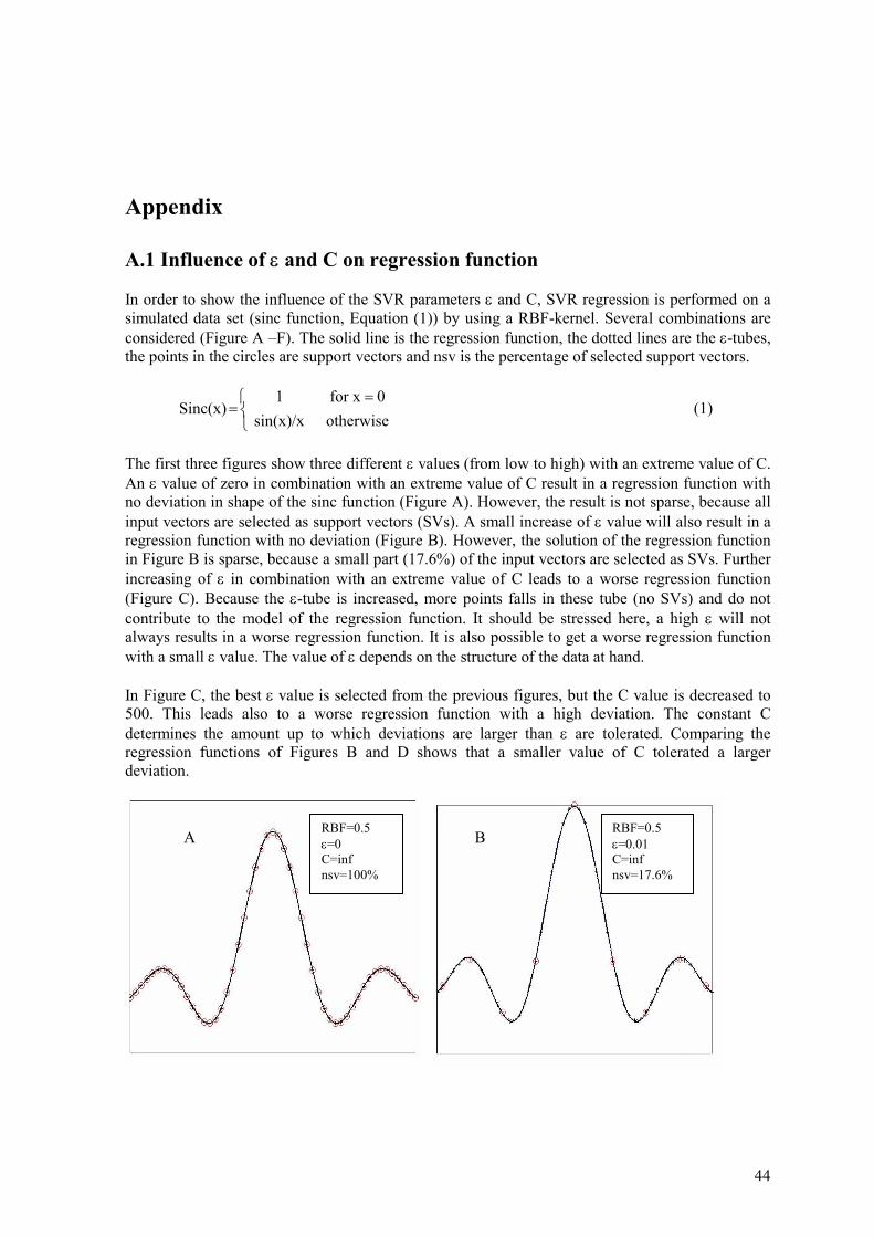
44

Appendix

A.1 Influence of ε and C on regression function

In order to show the influence of the SVR parameters ε and C, SVR regression is performed on a simulated data set (sinc function, Equation (1)) by using a RBF-kernel. Several combinations are considered (Figure A –F). The solid line is the regression function, the dotted lines are the ε-tubes, the points in the circles are support vectors and nsv is the percentage of selected support vectors.

=

=otherwisesin(x)/x

0for x1Sinc(x) (1)

The first three figures show three different ε values (from low to high) with an extreme value of C. An ε value of zero in combination with an extreme value of C result in a regression function with no deviation in shape of the sinc function (Figure A). However, the result is not sparse, because all input vectors are selected as support vectors (SVs). A small increase of ε value will also result in a regression function with no deviation (Figure B). However, the solution of the regression function in Figure B is sparse, because a small part (17.6%) of the input vectors are selected as SVs. Further increasing of ε in combination with an extreme value of C leads to a worse regression function (Figure C). Because the ε-tube is increased, more points falls in these tube (no SVs) and do not contribute to the model of the regression function. It should be stressed here, a high ε will not always results in a worse regression function. It is also possible to get a worse regression function with a small ε value. The value of ε depends on the structure of the data at hand. In Figure C, the best ε value is selected from the previous figures, but the C value is decreased to 500. This leads also to a worse regression function with a high deviation. The constant C determines the amount up to which deviations are larger than ε are tolerated. Comparing the regression functions of Figures B and D shows that a smaller value of C tolerated a larger deviation.

A B RBF=0.5 ε=0 C=inf nsv=100%

RBF=0.5 ε=0.01 C=inf nsv=17.6%

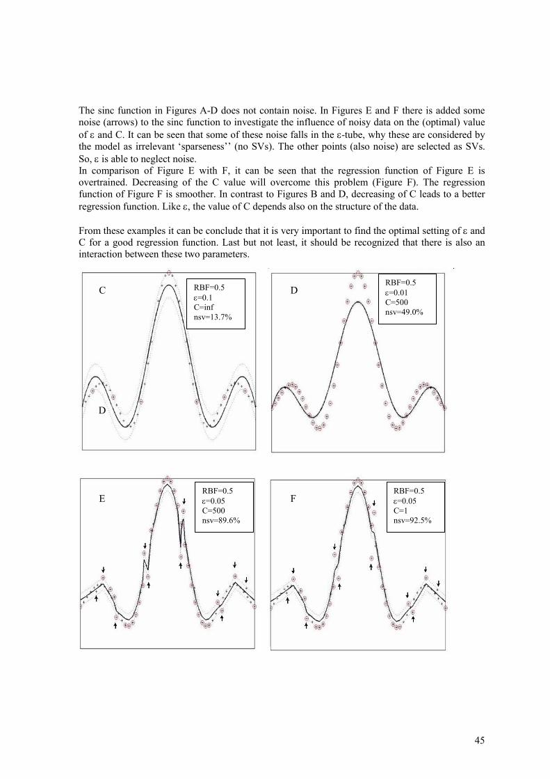
45

The sinc function in Figures A-D does not contain noise. In Figures E and F there is added some noise (arrows) to the sinc function to investigate the influence of noisy data on the (optimal) value of ε and C. It can be seen that some of these noise falls in the ε-tube, why these are considered by the model as irrelevant ‘sparseness’’ (no SVs). The other points (also noise) are selected as SVs. So, ε is able to neglect noise. In comparison of Figure E with F, it can be seen that the regression function of Figure E is overtrained. Decreasing of the C value will overcome this problem (Figure F). The regression function of Figure F is smoother. In contrast to Figures B and D, decreasing of C leads to a better regression function. Like ε, the value of C depends also on the structure of the data. From these examples it can be conclude that it is very important to find the optimal setting of ε and C for a good regression function. Last but not least, it should be recognized that there is also an interaction between these two parameters.

D

C D

E F

RBF=0.5 ε=0.1 C=inf nsv=13.7%

RBF=0.5 ε=0.01 C=500 nsv=49.0%

RBF=0.5 ε=0.05 C=500 nsv=89.6%

RBF=0.5 ε=0.05 C=1 nsv=92.5%