Computational Mechanicshttps://doi.org/10.1007/s00466-018-1661-y

ORIG INAL PAPER

High order exact geometry finite elements for seven-parameter shellswith parametric and implicit reference surfaces

M. H. Gfrerer1 ·M. Schanz2

Received: 24 April 2018 / Accepted: 23 November 2018© The Author(s) 2018

AbstractWe present high order surface finite element methods for the linear analysis of seven-parameter shells. The special featureof these methods is that they work with the exact geometry of the shell reference surface which can be given parametricallyby a global map or implicitly as the zero level-set of a level set function. Furthermore, a special treatment of singularparametrizations is proposed. For the approximation of the shell displacement parameters we have implemented arbitraryorder hierarchical shape functions on quadrilateral and triangular meshes. The methods are verified by a convergence analysisin numerical experiments.

Keywords Shells · Surface finite elements · Exact geometry · Implicit geometry · Higher order

1 Introduction

Due to their efficient load-carrying capabilities, shell struc-tures enjoy widespread use in a variety of engineering appli-cations. Therefore, a huge amount of research work has beendevoted to the development of shell models (e.g. [11,15]),their formal justification (e.g. [12–14]), as well as to the real-ization of numerical methods (e.g. [8,9]). It is well knownthat shell structures are sensitive to geometric imperfec-tions [30]. Even worse, the approximation of the geometryleads to wrong solutions in some situations, see the plateparadox investigated e.g. in [2]. Furthermore, e.g., in con-tact problems an exact description of smooth geometriesis of interest. Among others, these examples motivated usto develop shell finite element methods based on the exactgeometry. Therefore, the literature review concentrates ongeometry representation.

Usually, the exact geometry is approximated. In the sim-plest case, planar facet elements are deployed. However,those elements can only poorly represent curved structures

B M. Schanzm.schanz@tugraz.at

1 Felix Klein Zentrum für Mathematik, University ofKaiserslautern, Paul Ehrlich Strasse 31, 67663 Kaiserslautern,Germany

2 Institute of Applied Mechanics, Graz University ofTechnology, Technikerstrasse 4, 8010 Graz, Austria

and are not reliable due to a missing bending–stretching cou-pling on the element level. In order to represent the geometrymore accurately high order (often quadratic) shape functionsare used. To our best knowledge, exact geometry methodsfor shell analysis are restricted to the case where the exactgeometry is parametrically defined. A finite element methodwhich allows for arbitrary parametrizations is described in[1]. Therein, the field approximation based on Lagrangeelements is applied to a seven-parameter shell theory con-sidering geometrical nonlinearities and functionally gradedshells. However, the actual computation of the arising inte-grals is carried out by symbolic algebra subroutines writtenin MAPLE. In [31], an exact geometry method based on theblending function method is presented. Furthermore, in thework [29] a finite element method for geometrically non-linear problems is developed. Therein, the exact geometryof the shell is captured by an initial deformation of a flatreference configuration. However, since most CAD systemsuse NURBS functions, it is reasonable to restrict the inputparametrizations for the shell analysis to NURBS [10]. Thishas the advantage that the parametrization is given as a prod-uct of basis functions and coefficients. Thus, derivatives areeasily computed if the derivatives of the basis functions areknown. Following the concept of Isogemetric Analysis, shellfinite elements based on different shellmodelswere proposedin [5,23,24,28] among others. Therein, the reference surfaceis described by NURBS, just as the field approximation.

123

Computational Mechanics

Shell problems can also be seen as one application of themore general concept of partial differential equations definedon surfaces.Wemention [17] for an overview of related finiteelementmethods. Toour best knowledge thefirst exact geom-etry method for the Laplace–Beltrami operator on implicitlydefined surfaces was presented in [16]. Therein, the exactgeometry of closed smooth surfaces is parametrized over aspace triangulation by means of the closest point projection.Recently, a directional mapping based on predefined searchdirections was considered to construct high order geometryapproximations [20,25]. In [22], the search direction has beentailored such that the exact geometry of smooth surfaces withboundaries is available in the finite element analysis.

In the present paper we consider shells with parametri-cally and implicitly defined reference surfaces. For both casesexact geometry finite element methods are presented. Forimplicitly defined shells the reference surface is parametrizedover a space triangulation following the developments pre-sented in [22]. Thus, the implicit setting is reformulatedto the parametrized setting. The curvature of the referencesurface is necessary within the considered variational for-mulation, and so are the second order partial derivatives ofthe parametrization. In the case of a parametrically definedsurface they are obtained by automatic differentiation basedon hyper-dual numbers [19]. For the case of an implicitlydefined surface,wederive a formula such that only the secondorder derivatives of the level-set function φ are needed. Asa shell model we use a displacement based seven-parametermodel accounting for stretching, bending, shear deforma-tions, and through-the-thickness stretching (see [1,7,15]).Werestrict ourselves to a linear elastic analysis, i.e. small dis-placements, small rotations, small strains, and Hooke’s law.The discretization of the shell deformation is done by meansof high order hierarchical H1-conforming shape functions.Our implementation allows for arbitrary polynomial orders.Since our formulation is displacement based, various lockingphenomena (membrane, shear and thickness locking) occur,which can be seen in the examples in Sect. 4. Therefore, thelow order methods are very inefficient. Albeit the presenceof locking effects, the proposed methods converge to correctsolutions. Using high order shape functions reduces the lock-ing effects and offers high convergence rates. Nevertheless,in many practical examples this approach might be not veryefficient, see e.g. [29] for a quadratic element with a efficientdisplacement based formulation. As a further novelty, wepropose a strategy for the modification of the shape functionsto tackle singular parametrizations where the determinant ofthe metric vanishes on some part of the geometry. Followinga similar strategy developed in the context of IsogeometricAnalysis [33], we modify the ansatz space by combining andskipping basis functions.

2 Differential geometry and shell model

In this section, we recall the differential geometry of thin-walled structures and introduce the displacement basedseven-parameter shell model. First, the geometry of the ref-erence surface is presented. Then, the reference surface isextended to the three-dimensional shell volume, for whichwe present the geometric relations. In a next step, thethree-dimensional shell problem is introduced. Finally, thekinematics are restricted to a seven-parameter shell model.We remark that the differential geometry in the context ofthin-walled structures is exhaustively discussed in [3] and[11], among others.

The underlying assumption in shell analysis is that thecomputational domain Ω ⊂ R

3 has a small extension in onecoordinate compared to the two others. Thus, we assume thatΩ is located around a two-dimensional reference surface Ω .

2.1 Reference surface

In the present paper, we consider shell reference surfaceswhich are given parametrically or implicitly. In the formercase we have a parametrization g : U ⊂ R

2 → Ω availablewith given U . In the latter case, the reference surface is givenas the zero-level set of a functionφ : R3 → R inside a cuboidB

Ω = {x ∈ B| φ(x) = 0}. (1)

For this setting, the normal vector to the surface is given by

n(x) = ∇φ(x)||∇φ(x)|| . (2)

In the numerical method, we will make use of a piecewiseparametrization of the exact surface over a space triangu-lation. Therefore, the implicit description of the referencesurface is turned into a parametric one. Thus, we considerthe differential geometry of a parametrized surface in therest of this section.

Given the parametrization g, we can define the two covari-ant base vectorsGα := ∂g

∂θα , which span the tangent plane toΩ . Here and in the following, Greek indices take the values1 and 2 and Latin indices the values 1, 2, 3. With the basevectors we can define the unit normal vector

n = G1 × G2

||G1 × G2||, (3)

and the covariant coefficients of the metric Gαβ = Gα ·Gβ . The contravariant coefficients of the metric are given by

[Gαβ ] = [Gαβ ]−1, where [Gαβ ] is the coefficientmatrix. Thecontravariant base vectors can than be computed by G

α =

123

Computational Mechanics

Fig. 1 Parametrization of theshell. The parameter space onthe left is mapped to the physicalspace on the right. The referencesurface is parametrized by g,whereas the shell volume isparametrized by g

θ1

θ2

θ3

g, g

e1

e2e3

G1

G2

n

GαβGβ . Here, and in the following, the Einstein summation

convention applies. Whenever an index occurs once in anupper position and in a lower positionwe sumover this index.Due to the definition of the normal vector as a unit vector,we have n · n = 1. Taking the derivative with respect toθα , yields ∂

∂θα (n · n) = n,α · n + n · n,α = 0. Thus, thederivatives of the normal vector are in the tangent plane ofthe surface. Expressing the derivatives of the normal vectortrough a linear combination of the tangent vectors yields

n,α = −hβαGβ, (4)

with

hαβ = −Gα · n,β and hβα = G

βγhαγ . (5)

These relations are known as the Weingarten equations,first established in [34]. The functions hαβ = hβα are thecoefficients of the second fundamental form. Furthermore,H = 1

2hγγ is the mean curvature and K = h11h

22 − h21h

12 is

the Gaussian curvature of the surface.

2.2 Geometry of the shell volume

In this section, we assume that we have a parametrization g ofthe reference surface Ω available. Then the parametrizationof the shell volume Ω is given by

g : (U × T ) ⊂ R3 → Ω ⊂ R

3

(θ1, θ2) × θ3 �→ g(θ1, θ2, θ3) = g(θ1, θ2) + θ3 n,

(6)

with the interval T = [−t/2, t/2], where t is the thickness ofthe shell. The geometric setting is illustrated in Fig. 1. Thefirst two base vectors in the shell volume are related to thebase vectors at the reference surface by

Gα = μβαGβ, (7)

where μβα =

(δβα − θ3hβ

α

)are the components of the shifter

tensor and δβα is the Kronecker delta. Furthermore, G3 = n.

Thus, the covariant components of the metric are given by

Gαβ = μγα μ

ϕβ Gγ ϕ = Gαβ − 2 (θ3) hαβ + (θ3)2 hαγ h

γβ ,

Gα3 = G3α = 0, G33 = 1,

(8)

and the determinant of the metric is

dG =det([Gi j ]) =(1 − 2 (θ3) H + (θ3)2 K

)2det([Gαβ ]).

(9)

The components of the contravariant metric are

[Gαβ ] = [Gαβ ]−1

= adj([Gαβ ]) − 2 θ3 adj([hαβ ]) + (θ3)2adj([hαγ hγβ ])

det([Gαβ ]) (1 − 2Hθ3 + K (θ3)2

)2Gα3 = G3α = 0, G33 = 1,

(10)

where

adj([Gαβ ]) =[G22 −G12

−G12 G11

](11)

is the adjugate matrix of [Gαβ ].

2.3 The 3D shell problem

Wecontinuewith the statement of the three-dimensional shellproblem, which is considered in the present paper to be aproblem of linearized elasticity on shell-like domainsΩ withboundaryΓ . The three-dimensional elasticity problem reads:Find u : Ω → R

3 such that

123

Computational Mechanics

∇ · σσσ + b = 0 in Ω,

σσσ = C : εεε in Ω,

εεε = 1

2

(∇u + (∇u)�

)in Ω,

u = uD on ΓD,

t = tN on ΓN .

(12)

Here, σσσ is the stress tensor, b the bodyforce, C the elasticitytensor, εεε the strain tensor, uD the given Dirichlet datum onΓD , and tN the givenNeumann datum onΓN .We require thatΓ = ΓD ∪ ΓN andΓD ∩ ΓN = ∅.Moreover, we assume thatΓD is a subset of the lateral part of the boundaryΓ .We remarkthat all quantities with a tilde over them are defined on Ω

without reference to a specific parametrization. Furthermore,we have the following coordinate-free displacement-basedvariational formulation of (12): Find u ∈ V such that

∫

Ωεεε(v) : C : εεε(u) dx =

∫

Ωv · b dx +

∫

ΓN

v · tN dsx ∀ v ∈ V0,

(13)

with V = {u ∈ [H1(Ω)]3 | u = uD on ΓD} and V0 = {v ∈[H1(Ω)]3 | v = 0 on ΓD}.

In order to solve (13),we rewrite the problem inparametriccoordinates. Instead of solving for u(x), x ∈ Ω , we seek thedisplacement field u(θ1, θ2, θ3) = u(g(θ1, θ2, θ3)) definedon the parametric space. This change of variables applies toall quantities analogously. In the present paper, we employ alinear isotropic material law, where the contravariant compo-nents of the elasticity tensor C = C

i jkl Gi ⊗G j ⊗Gk ⊗Gl

for a shell-like body are given by

Cαβγϕ = λGαβGγ ϕ + μ

(GαγGβϕ + GαϕGβγ

),

Cαβ33 = C

33αβ = λGαβ,

C3α3β = C

3αβ3 = Cα33β = C

α3β3 = μGαβ,

C3αβγ = C

α3βγ = Cαβ3γ = C

αβγ 3 = 0,

C333α = C

33α3 = C3α33 = C

α333 = 0,

C3333 = λ + 2μ.

(14)

The Lamé constants are denoted with λ and μ.

2.4 Seven-parameter shell model

Up to this point, no approximation of the three-dimensionalproblem has been introduced. In this section, we introducethe seven-parameter shell model [1,7,15] by restricting thethrough-the-thickness kinematics of the shell to be of theform

u(θ1, θ2, θ3) = Vb(θ3)

(1)ui (θ

1, θ2) ei + Vt (θ3)

(2)ui (θ

1, θ2) ei

+Vn(θ3)

(n)u (θ1, θ2) n, (15)

where we made use of the following through-the-thicknessfunctions

Vb(θ3) = t − 2 θ3

2 t,

Vt (θ3) = t + 2 θ3

2 t,

Vn(θ3) = 1 − 4(θ3)2

t2.

(16)

In (15), we have introduced the seven parameters(1)ui (θ1, θ2),

(2)ui (θ1, θ2), and

(n)u (θ1, θ2), which depend only on the posi-

tion on the reference surface. While(1)ui physically represent

the Cartesian components of the displacement vector at the

bottom surface (at θ3 = −t/2),(2)ui represent the Cartesian

components of the displacement vector at the top surface (at

θ3 = t/2). The seventh parameter(n)u (θ1, θ2) is included in

order to circumvent Poisson thickness locking [6]. Insert-ing (15) into the kinematic relations for the linearized straintensor εεε = εi j Gi ⊗ G j yields

εαβ = 1

2J iς

(μς

α

(Vb

(1)ui,β + Vt

(2)ui,β

)

+μςβ

(Vb

(1)ui,α + Vt

(2)ui,α

))− μς

αhςβVn(n)u ,

εα3 = ε3α = 1

2

(1

tμς

α Jiς

((2)ui − (1)

ui

)

+ J i3

(Vb

(1)ui,α + Vt

(2)ui,α

)+ Vn

(n)u,α

),

ε33 = 1

tJ i3

((2)ui − (1)

ui

)− 8(θ3)

t2(n)u ,

(17)

with J il = Gl · ei . From the expression of ε33 we see that themodel can represent constant and linear normal strain statesthrough the thickness.

3 Finite element method

In this section, we describe the developed finite elementmethods. The methods used for parametrically and implic-itly defined shells differ from each other. However, in bothcases, we employ the reference element technique for theconstruction of hierarchical H1-conforming shape functionsof arbitrary degree [32]. These element shape functions arepieced together to FEM basis functions by establishing a

123

Computational Mechanics

Fig. 2 Mappings for theparametric shell

ξ

η Φe

θ1

θ2

g

e1

e2e3

connectionbetween local andglobal degrees of freedom.Fur-thermore, we use tensor-product (degenerated for triangles)Gauss–Legendre quadrature rules on the reference elementfor the integral evaluation. For shape functions of degree p,(p+1)2 in-plane quadrature points are used on each element,whereas three quadrature points for the integration acrossthe thickness are employed. In the following,Φe denotes thelocal linear element mapping. The discretization of the seven

parameters

{(1)ui ,

(2)ui ,

(n)u

}∈ [H1(U )]3 ×[H1(U )]3 × H1(U )

introduced in (15) is done by means of

{(1)ui ,

(2)ui ,

(n)u

}≈

{(1)uh|i ,

(2)uh|i ,

(n)uh

}=

nS∑l=1

{(1)uil ,

(2)uil ,

(n)ul

}Nl(θ

1, θ2),

(18)

where

{(1)uil ,

(2)uil ,

(n)ul

}are 7nS unknown coefficients and Nl

are the FEM basis functions.

3.1 FEM for shells defined by singularparametrizations

In this section, we describe the finite element method for thecase where the parametrization g of the reference surface isexplicitly available. The geometry mappings for this methodare depicted in Fig. 2. We use a quadrilateralization of theparametric plane U . In (13), the derivatives of g up to secondorder show up. In the present work we use an automaticdifferentiation schema based on an augmented algebra. Tothis end, a hyper-dual number class has been implementedproviding operator overloading [19].

Special care has to be taken of singular parametrizations,where the determinant of the metric vanishes on some partof the geometry. In particular, we focus on the case whereone side of the boundary is mapped to a single point in thereal space. In this case, the stiffness matrix does not need toexist.Wemodify the ansatz space by combining and skippingbasis functions. In the framework of Isogeometric Analysis,a similar strategy was considered in [33]. For presentational

purposes, we assume that the boundary at the line θ1 = 0 inthe parameter space is mapped to a single point P0 in the realspace,

g(0, θ2) = P0. (19)

Obviously,

G2 = 0 for θ1 = 0, (20)

and the determinant of the metric is zero at the whole lineθ1 = 0. We assume that apart from the line θ1 = 0 theparametrization is regular. Furthermore, it is assumed that

G11 > 0 and that the Laurent expansion of G22√⟨

Gαβ

⟩about

θ1 = 0 is of the form

G22√⟨

Gαβ

⟩ = a−1(θ2)

θ1+

∞∑i=0

(θ1)i ai (θ2). (21)

Investigation on the existence of

∫

Ω

∇vh · ∇vh dx =∫

U((vh,1)

2G11 + 2vh,1vh,2G12

+ (vh,2)2G22)

√⟨Gαβ

⟩dθ (22)

leads to the following modifications of the shape functions:

1. All vertex-based shape functions related to the verticeson θ1 = 0 are added up to one single shape function.

2. All edge-based shape functions related to the edges onθ1 = 0 are removed, i.e. the respective degrees of free-dom are constrained to zero in the implementation.

3. No modification of the cell-based shape functions ismade.

The problematic term is

(vh,2)2 G22

√⟨Gαβ

⟩ = (vh,2)2 a−1(θ

2)

θ1+higher order terms.

(23)

123

Computational Mechanics

Fig. 3 Mappings Φe, a, andge = a ◦ Φe between thereference triangle τ R , theelement τe ∈ Th , and a(τe)

θ1

θ2

(0, 0) (1, 0)

(0, 1)

τR

Φe ge

a

τe a(τe)

We remark that vh are polynomials. The integral (22) existsif vh,2 = 0 holds, i.e.vh has to be constant with respect to θ2

or vh = 0 on θ1 = 0. Writing

vh,2 =p∑

i=0

p∑j=0

ai j (θ1)i (θ2) j , (24)

the integral does not exist if any a0 j �= 0. The non-vanishingfunctions on θ1 = 0 are related to the nodes and edges there.All cell-based shape functions vanish on the boundary. Afunction vh which is constant with respect to θ2 can be con-structed summing up all node-based functions. This givesone new shape function. The edge-based shape functions areof higher order with respect to θ2 on θ1 = 0, they are thuseliminated.

3.2 FEM for implicitly defined shells

In the case of an implicitly defined reference surface, theparametrization g over a flat parameter domain is not explic-itly available. Therefore, the exact geometry is parametrizedover a space triangulation Th . To this end, we follow the strat-egy developed in [22]. The geometric concept is illustratedfor the example of a sphere in Fig. 3. As a starting point weassume that a triangulation in space Th close to the exactsurface is available. For each triangle τe ∈ Th we have thestandard affine mapping Φe which maps the reference trian-gle τR to τe. We denote the piecewise flat surface defined bythe triangulation by Ωh . In order to lift a point x ∈ Ωh to theexact surface we introduce the mapping a in the followingimplicit way

a : Ωh → Ω

x �→ a(x) = x + r(x) s(x) such that φ(a(x)) = 0.

(25)

Here, s(x) are predefined search directions. The mapping ais implicitly defined because r(x) is not explicitly knownand has to be computed in each evaluation of a such thatφ(a(x)) = 0. We specify the search directions in (25) asfollows. Let V denote the set of all vertices of Th . We set

sv(x) = ∇φ(x)||∇φ(x)|| for x ∈ V, (26)

where ∇φ is the usual gradient of the level-set function φ inR3. To preserve the exact geometry, we apply a modification

at the vertices on the boundary of B. Thus, we set

sv(x) ={sv(x) − (sv(x) · n∂B(x))n∂B(x) for x ∈ V ∩ ∂B

sv(x) else,

(27)

where n∂B are the normal vectors to ∂B. Then the searchdirection field s(x) defined on Ωh is obtained by linearinterpolation of sv(x). Thus, the search direction field sis given as a linear finite element function. We remarkthat the mapping (25) requires the solution of a non-linearroot finding problem, which is numerically realized withthe Newton–Raphson method. We obtain an element-wiseparametrization ge of Ω over the reference element τ R by

123

Computational Mechanics

ge : τ R → Ω

(θ1, θ2) �→ a(Φe(θ1, θ2)).

(28)

The evaluation of the integrals in (13) requires x =ge(θ1, θ2), the base vectors Gα and the coefficients of thesecond fundamental form hαβ . All other geometric quanti-ties can be computed from them by algebraic operations. Theformula

Gα = Φe,α − Φe

,α · n + r s,α · ns · n s + r s,α (29)

for the computation of the base vectors can be found in [22].Taking into account the dependencies

n(x) = n(ge(θ1, θ2)) = n(θ1, θ2) (30)

the chain rule results in

n,β = ∇n · Gβ. (31)

Together with (5) the coefficients of the second fundamentalform can be computed by

hαβ = −Gα · (∇n · Gβ). (32)

For the gradient of the normal vector we have

∇n = ∇∇φ

||∇φ|| − ∇φ ⊗ ∇φ

||∇φ||3 = ∇∇φ − n ⊗ n||∇φ|| . (33)

Thus, we have to provide the second order derivatives of thelevel-set function φ in the implementation.

In order to clarify the explanations on the implicit method,we remark that the space triangulation represents an interme-diate step in the method and does not define the geometry.The key ingredient of the implicit method is the mapping adefined in (25), which maps the space triangulation to theexact geometry. However, this mapping is only implicitlydefined and a one dimensional root finding problem has tobe solved for the evaluation. This is no problem because theintegrals are approximated by quadrature. Thus, only a point-wise evaluation is necessary.

4 Numerical results

In this section, we demonstrate the correct implementation ofthe developedmethods and their capabilities. The verificationexamples are based on the method of manufactured solutionsin order to have exact solutions to compare with. As an errormeasure we use

eu =√

∑ ∫

Ω

({(1)ui ,

(2)ui ,

(n)u

}

M−

{(1)ui ,

(2)ui ,

(n)u

}

h

)2

dx,

(34)

where

{(1)ui ,

(2)ui ,

(n)u

}

Mis the exact manufactured solution and

{(1)ui ,

(2)ui ,

(n)u

}

hthe numerical solution. In (34), the sum has to

be understood over the seven shell model parameters.

4.1 Verification example for a parametricallydefined shell

In order to verify the implementation, we employ the methodof manufactured solutions, which has been demonstrated in[21] for parametrically defined surfaces. In this example, weuse the reference surface defined by the parametrization

x = 2θ1θ2 + 2θ1 − θ2

3,

y = −θ1θ2 + 2θ1 + 2θ2

3,

z = 2θ1θ2 − θ1 + 2θ2

3,

(35)

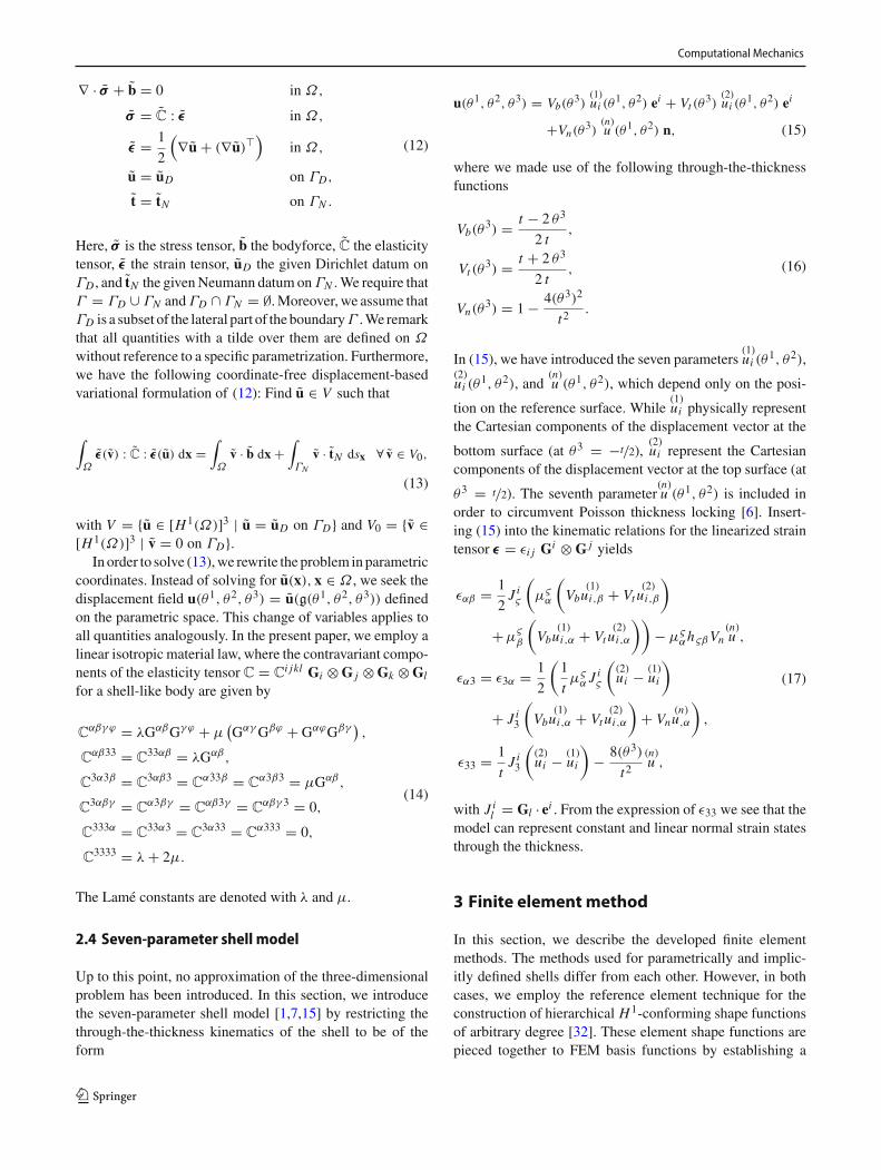
and (θ1, θ2) ∈ [0, 0.56]× [0, 0.65], see Fig. 4. The shell hasthe thickness t = 0.01. The Young’s modulus is E = 8 ·104,whereas Poisson’s ration is ν = 0.25. We study the con-vergence of the method under uniform mesh refinement. Weremark that we have checked the convergence for differentdisplacement fields. Here, we present the results for the pre-

scribed solution(1)u1 = cos(20 θ1),

(1)u2 = 0,

(1)u3 = sin(10 θ2),

(2)u1 = sin(10 θ1 θ2),

(2)u2 = 0,

(2)u3 = 0, and

(n)u = sin(10 θ1 θ2).

A regular mesh obtained by uniform subdivision of theparameter space into 2 × 2 = 4 elements represents refine-ment level 0. We get the subsequent refinement levels byuniform subdivision of the previous level. The results of theconvergence study are depicted in Fig. 5. We observe opti-mal convergence rates, i.e.O(h p+1)-convergence, where his a characteristic element length.

4.2 Verification example for an implicitly definedshell

The implementation of the FEM for an implicitly definedshell is verified. To this end, we consider a manufacturedsolution on a torus. The geometry of the considered surfaceis defined by the zero level-set of the function

φ(x, y, z) = d(x, y, z) =√

(√x2 + z2 − R)2 + y2 − r ,

r = 0.4, R = 0.8, (36)

123

Computational Mechanics

Fig. 4 Geometry and bodyforce at the mid-surface of the verifictionexample for the parametrically defined shell

0 1 2 3 4 5 6 710 -12

10 -10

10 -8

10 -6

10 -4

10 -2

10 0

10 2

Fig. 5 Convergence results for the parametrically defined shell

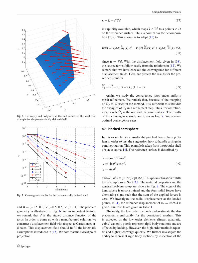
and B = [−1.5, 0.3] × [−0.5, 0.5] × [0, 1.1]. The problemgeometry is illustrated in Fig. 6. As an important feature,we remark that d is the signed distance function of thetorus. In order to come up with a manufactured solution, weconstruct a displacement field with respect to Cartesian coor-dinates. This displacement field should fulfill the kinematicassumptions introduced in (15).We note that the closest pointprojection

x = x − d ∇d (37)

is explicitly available, which maps x ∈ R3 to a point x ∈ Ω

on the reference surface. Thus, a point x has the decomposi-tion (x, d). This allows us to adapt (15) to

u(x) = Vb(d)(1)ui (x) ei +Vt (d)

(2)ui (x) ei +Vn(d)

(n)u (x) ∇d,

(38)

since n = ∇d. With the displacement field given in (38),the source terms follow easily from the relations in (12). Weremark that we have checked the convergence for differentdisplacement fields. Here, we present the results for the pre-scribed solution

(2)u1 = (1)

u1 = (0.3 − x) z (1.1 − z). (39)

Again, we study the convergence rates under uniformmesh refinement. We remark that, because of the mappingof Ωh to Ω used in the method, it is sufficient to subdividethe triangles of Th in a refinement step. Thus, for all refine-ment levels Ωh is the one and the same surface. The resultsof the convergence study are given in Fig. 7. We observeoptimal convergence rates.

4.3 Pinched hemisphere

In this example, we consider the pinched hemisphere prob-lem in order to test the suggestion how to handle a singularparametrization. This example is taken from the popular shellobstacle course [4]. The reference surface is described by

x = cos θ1 cos θ2,

y = sin θ1 cos θ2,

z = sin θ2,

(40)

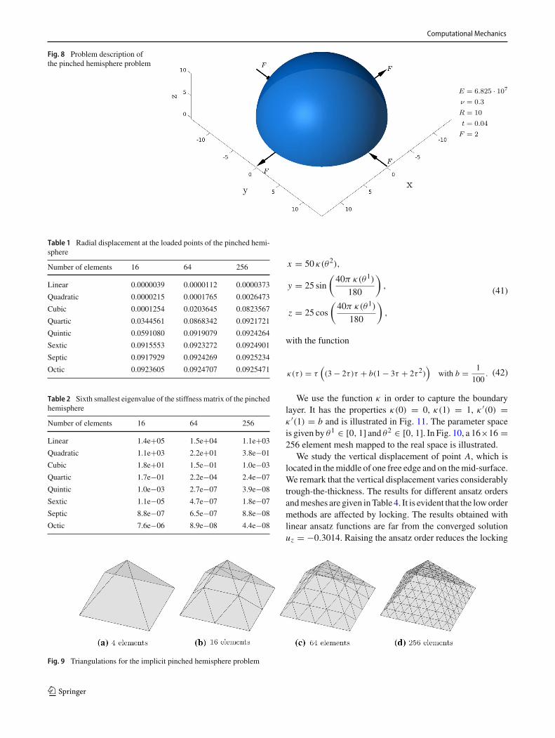
and (θ1, θ2) ∈ [0, 2π ]×[0, π/2]. This parametrization fulfillsthe assumptions in Sect. 3.1. The material properties and thegeneral problem setup are shown in Fig. 8. The edge of thehemisphere is unconstrained and the four radial forces havealternating signs such that the sum of the applied forces iszero. We investigate the radial displacement at the loadedpoints. In [4], the reference displacement of ur = 0.0924 isgiven. Our results are given in Table 1.

Obviously, the low order methods underestimate the dis-placement significantly for the considered meshes. Thisis expected as the low order elements (linear, quadratic,cubic) can only poorly represent rigid body rotations and areaffected by locking. However, the high order methods (quar-tic and higher) converge quickly. We further investigate theability to represent rigid body motions by inspection of the

123

Computational Mechanics

Fig. 6 Triangulations for thedeformed torus example: thebase triangulation (upper left),the mapped triangulation (upperright), side view (lower left),and top view (lower right)

0 1 2 3 410 -14

10 -12

10 -10

10 -8

10 -6

10 -4

10 -2

Fig. 7 Convergence results for the implicitly defined shell. Refinementlevel 0 is the base triangulation

eigenvalues of the stiffnessmatrix. The three rigid body trans-lations can be represented exactly by the elements, resultingin three zero (up to numerical round-off errors) eigenvalues.As the rigid body rotations are only approximated the nextthree eigenvalues are nonzero. The sixth smallest eigenval-ues for different meshes and polynomial orders are given inTable 2. As expected they decrease rapidly with increasingpolynomial order.

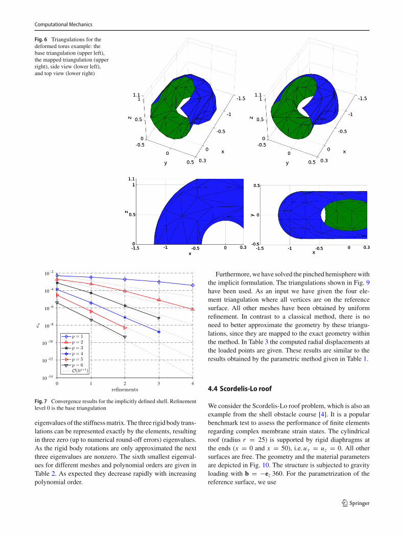
Furthermore, we have solved the pinched hemispherewiththe implicit formulation. The triangulations shown in Fig. 9have been used. As an input we have given the four ele-ment triangulation where all vertices are on the referencesurface. All other meshes have been obtained by uniformrefinement. In contrast to a classical method, there is noneed to better approximate the geometry by these triangu-lations, since they are mapped to the exact geometry withinthe method. In Table 3 the computed radial displacements atthe loaded points are given. These results are similar to theresults obtained by the parametric method given in Table 1.

4.4 Scordelis-Lo roof

We consider the Scordelis-Lo roof problem, which is also anexample from the shell obstacle course [4]. It is a popularbenchmark test to assess the performance of finite elementsregarding complex membrane strain states. The cylindricalroof (radius r = 25) is supported by rigid diaphragms atthe ends (x = 0 and x = 50), i.e.uy = uz = 0. All othersurfaces are free. The geometry and the material parametersare depicted in Fig. 10. The structure is subjected to gravityloading with b = −ez 360. For the parametrization of thereference surface, we use

123

Computational Mechanics

Fig. 8 Problem description ofthe pinched hemisphere problem

E = 6.825 · 107

ν = 0.3

R = 10

t = 0.04

F = 2

Table 1 Radial displacement at the loaded points of the pinched hemi-sphere

Number of elements 16 64 256

Linear 0.0000039 0.0000112 0.0000373

Quadratic 0.0000215 0.0001765 0.0026473

Cubic 0.0001254 0.0203645 0.0823567

Quartic 0.0344561 0.0868342 0.0921721

Quintic 0.0591080 0.0919079 0.0924264

Sextic 0.0915553 0.0923272 0.0924901

Septic 0.0917929 0.0924269 0.0925234

Octic 0.0923605 0.0924707 0.0925471

Table 2 Sixth smallest eigenvalue of the stiffness matrix of the pinchedhemisphere

Number of elements 16 64 256

Linear 1.4e+05 1.5e+04 1.1e+03

Quadratic 1.1e+03 2.2e+01 3.8e−01

Cubic 1.8e+01 1.5e−01 1.0e−03

Quartic 1.7e−01 2.2e−04 2.4e−07

Quintic 1.0e−03 2.7e−07 3.9e−08

Sextic 1.1e−05 4.7e−07 1.8e−07

Septic 8.8e−07 6.5e−07 8.8e−08

Octic 7.6e−06 8.9e−08 4.4e−08

x = 50 κ(θ2),

y = 25 sin

(40π κ(θ1)

180

),

z = 25 cos

(40π κ(θ1)

180

),

(41)

with the function

κ(τ) = τ((3 − 2τ)τ + b(1 − 3τ + 2τ2)

)with b = 1

100. (42)

We use the function κ in order to capture the boundarylayer. It has the properties κ(0) = 0, κ(1) = 1, κ ′(0) =κ ′(1) = b and is illustrated in Fig. 11. The parameter spaceis given by θ1 ∈ [0, 1] and θ2 ∈ [0, 1]. In Fig. 10, a 16×16 =256 element mesh mapped to the real space is illustrated.

We study the vertical displacement of point A, which islocated in themiddle of one free edge and on themid-surface.We remark that the vertical displacement varies considerablytrough-the-thickness. The results for different ansatz ordersandmeshes are given inTable 4. It is evident that the lowordermethods are affected by locking. The results obtained withlinear ansatz functions are far from the converged solutionuz = −0.3014. Raising the ansatz order reduces the locking

Fig. 9 Triangulations for the implicit pinched hemisphere problem

123

Computational Mechanics

Table 3 Radial displacement atthe loaded points of the pinchedhemisphere

Number of elements 4 16 64 256

Linear 0.0000011 0.0000035 0.0000134 0.0000526

Quadratic 0.0000062 0.0000398 0.0005833 0.0075576

Cubic 0.0000322 0.0011217 0.0262481 0.0877841

Quartic 0.0002854 0.0125512 0.0878863 0.0923755

Quintic 0.0016276 0.0607160 0.0922467 0.0924516

Sextic 0.0058856 0.0894647 0.0924056 0.0924764

Septic 0.0224888 0.0920513 0.0924452 0.0924957

Octic 0.0572128 0.0923485 0.0924647 0.0925141

E = 4.32 · 108

ν = 0

R = 25

L = 50

t = 0.25

Fig. 10 Problem description of the Scordelis-Lo roof problem

0 0.2 0.4 0.6 0.8 1

0

0.2

0.4

0.6

0.8

1

τ

κ( τ)

Fig. 11 The function κ for capturing the boundary layer

phenomena. Without resorting to other techniques to reducethe locking, we advise to use at least quartic ansatz functions.In [27], a reference value uz = −0.3024 for the verticaldisplacement at point A is reported. For a shell model basedon equivalent seven-parameter kinematics, uz = −0.3008 iscomputed in [18]. Therefore, our results are in accordancewith the values found in literature.

4.5 Gyroid

In this example, we consider the deformation of a shell struc-ture where the reference surface is part of a gyroid, seeFig. 12.An approximation of a gyroid is given by the level-setfunction

φ(x, y, z) = sin(x) cos(y) + sin(y) cos(z) + sin(z) cos(x).

(43)

The considered shell lies in B = [0, 2]× [−0.5, 0.5]×[−0.5, 0.5]. The shell structure is fixed at the plane x = 0.We assume a thickness t = 0.03.

We study the static deformation due to a volume loadb = ez 107. To this end, we use three different surfacemeshes, which are depicted in Fig. 13. The coarsest meshis obtained by theMarching Cubes Algorithm [26] and meshsmoothing. The other two meshes are obtained by uniformrefinement of the coarsest mesh. We remark that, in the anal-ysis, each mesh is mapped to the exact surface by meansof (28). Table 5 illustrates the convergence of the verticaldisplacement uz at the point [2, 0.5,−0.25]. Obviously, theresults obtained by linear ansatz functions underestimate thedeformation tremendously for the considered meshes. Theuse of quadratic ansatz functions reduces the locking con-siderably. In view of the results obtained by the octic ansatzfunctions, we can accept a converged value of uz = 1.8812.

5 Conclusion

In this paper, high order finite element methods for shellanalysis have been presented. The underlying shell modelis a displacement based seven-parameter model. As a spe-cial feature, the methods incorporate the exact geometry ofparametrically and implicitly defined reference surfaces. Wehave shown the capabilities of the methods in five examples.In order to assess the convergence behavior, the method ofmanufactured solutions has been utilized. In all numerical

123

Computational Mechanics

Table 4 Vertical displacementat point A of the Scordelis-Loroof

Number of elements 4 16 64 256

Linear −0.0026073 −0.0016144 −0.0044508 −0.0126987

Quadratic −0.0019732 −0.0305159 −0.1354229 −0.2741197

Cubic −0.0301026 −0.2470338 −0.2968267 −0.3012622

Quartic −0.1675085 −0.2967069 −0.3012862 −0.3014015

Quintic −0.2888778 −0.3012049 −0.3013835 −0.3014021

Sextic −0.2979929 −0.3013161 −0.3014014 −0.3014026

Septic −0.3014056 −0.3013603 −0.3014014 −0.3014026

Octic −0.3012498 −0.3013926 −0.3014021 −0.3014026

Fig. 12 Geometry of the gyroid problem

experiments, we observe optimal convergence rates in theasymptotic range.

In the present work we used a purely displacement basedformulation. Thus, various locking phenomena reduce theefficiency of the method when using low order approxi-mations. In order to reduce locking phenomena, we haveresorted to high order shape functions (our implementationallows for arbitrary high order). As thismight be not very effi-

Table 5 Vertical displacement uz at the point [2, 0.5,−0.25]Number of elements 136 544 2176

Linear 0.0118106 0.0332828 0.1055900

Quadratic 0.1694172 0.9005433 1.7152640

Cubic 1.2274694 1.8430397 1.8793713

Quartic 1.7745119 1.8788403 1.8808718

Quintic 1.8726206 1.8804255 1.8811317

Sextic 1.8784737 1.8809134 1.8812070

Septic 1.8802114 1.8811026 1.8812299

Octic 1.8807253 1.8811810 1.8812370

cient in many examples, it would be interesting to developlow order locking-free elements based on the exact geometryin future work.

Moreover, the use of a seven-parameter shell modelallowed us to use H1-conforming ansatz and test spaces.This might not be appropriate for other shell models likeKirchhoff–Love typemodels or Reissner–Mindlin typemod-els. In the former, typically, H2-conforming elements areneeded, whereas in the latter elements are necessary provid-ing a vector field tangential to the surface. The developmentof such elements for implicitly defined shells should receivefurther attention.

Fig. 13 Three triangulations of the considered gyroid surface

123

Computational Mechanics

Acknowledgements Open access funding provided byGrazUniversityof Technology.

Open Access This article is distributed under the terms of the CreativeCommons Attribution 4.0 International License (http://creativecommons.org/licenses/by/4.0/), which permits unrestricted use, distribution,and reproduction in any medium, provided you give appropriate creditto the original author(s) and the source, provide a link to the CreativeCommons license, and indicate if changes were made.

References

1. Arciniega R, Reddy J (2007) Tensor-based finite element for-mulation for geometrically nonlinear analysis of shell structures.Comput Methods Appl Mech Eng 196(4):1048–1073

2. Babuška I, Pitkäranta J (1990) The plate paradox for hard and softsimple support. SIAM J Math Anal 21(3):551–576

3. BasarY,KrätzigWB (1985)Mechanik der Flächentragwerke: The-orie, Berechnungsmethoden, Anwendungsbeispiele. Vieweg

4. Belytschko T, Stolarski H, Liu WK, Carpenter N, Ong JS (1985)Stress projection for membrane and shear locking in shell finiteelements. Comput Methods Appl Mech Eng 51(1):221–258

5. Benson D, Bazilevs Y, Hsu MC, Hughes T (2010) Isogeometricshell analysis: the Reissner–Mindlin shell. Comput Methods ApplMech Eng 199(5):276–289

6. Bischoff M, Ramm E (1997) Shear deformable shell elements forlarge strains and rotations. Int J NumerMethods Eng 40(23):4427–4449

7. BischoffM, RammE (2000) On the physical significance of higherorder kinematic and static variables in a three-dimensional shellformulation. Int J Solids Struct 37(46–47):6933–6960

8. Bischoff M, Bletzinger KU, Wall W, Ramm E (2004) Models andfinite elements for thin-walled structures. In: Stein E, de Borst R,Hughes T (eds) Encyclopedia of computational mechanics, chap3, vol 2. Wiley Online Library, New York, pp 59–137

9. Chapelle D, Bathe KJ (2010) The finite element analysis of shells.Springer, Berlin

10. Cho M, Roh HY (2003) Development of geometrically exact newshell elements based on general curvilinear co-ordinates. Int JNumer Methods Eng 56(1):81–115

11. Ciarlet PG (2006) An introduction to differential geometry withapplications to elasticity, vol 78. Springer, Berlin

12. Ciarlet PG, Lods V (1996) Asymptotic analysis of linearly elasticshells. I. Justification of membrane shell equations. Arch RationMech Anal 136(2):119–161

13. Ciarlet PG, Lods V (1996) Asymptotic analysis of linearly elasticshells. III. Justification of Koiter’s shell equations. Arch RationMech Anal 136(2):191–200

14. Ciarlet PG, Lods V, Miara B (1996) Asymptotic analysis of lin-early elastic shells. II. Justification of flexural shell equations. ArchRation Mech Anal 136(2):163–190

15. Dauge M, Faou E, Yosibash Z (2004) Plates and shells: asymptoticexpansions and hierarchic models. In: Stein E, de Borst R, HughesT (eds) Encyclopedia of computational mechanics, chap 8, vol 2.Wiley Online Library, New York, pp 199–236

16. Demlow A (2009) Higher-order finite element methods and point-wise error estimates for elliptic problems on surfaces. SIAM JNumer Anal 47(2):805–827

17. DziukG, Elliott C (2013) Finite elementmethods for surface PDEs.Acta Numer 22:289–396

18. Echter R, Oesterle B, Bischoff M (2013) A hierarchic family ofisogeometric shell finite elements. Comput Methods Appl MechEng 254:170–180

19. Fike JA, Alonso JJ (2011) The development of hyper-dual numbersfor exact second-derivative calculations. In: 49th AIAA aerospacesciences meeting including the new horizons forum and aerospaceexposition, Orlando, Florida

20. Fries TP, SchöllhammerD (2017)Higher-ordermeshing of implicitgeometries part II: approximations onmanifolds. ComputMethodsAppl Mech Eng 326:270–297

21. Gfrerer MH, Schanz M (2017) Code verification examples basedon the method of manufactured solutions for Kirchhoff–Love andReissner–Mindlin shell analysis. Eng Comput. https://doi.org/10.1007/s00366-017-0572-4

22. GfrererMH, SchanzM (2018)A high-order FEMwith exact geom-etry description for the Laplacian on implicitly defined surfaces.Int J Numer Methods Eng. https://doi.org/10.1002/nme.5779

23. Hosseini S, Remmers JJ, Verhoosel CV, Borst R (2013) An isogeo-metric solid-like shell element for nonlinear analysis. Int J NumerMethods Eng 95(3):238–256

24. Kiendl J, Bletzinger KU, Linhard J, Wüchner R (2009) Isogeomet-ric shell analysis with Kirchhoff–Love elements. Comput MethodsAppl Mech Eng 198(49):3902–3914

25. Lehrenfeld C (2016) High order unfitted finite element methods onlevel set domains using isoparametric mappings. Comput MethodsAppl Mech Eng 300:716–733

26. LorensenW, Cline H (1987) Marching cubes: a high resolution 3Dsurface construction algorithm. In: Proceedings of the 14th annualconference on computer graphics and interactive techniques,ACM,New York, NY, USA, SIGGRAPH’87, pp 163–169

27. Macneal RH, Harder RL (1985) A proposed standard set of prob-lems to test finite element accuracy. FiniteElemAnalDes1(1):3–20

28. Oesterle B, Sachse R, Ramm E, Bischoff M (2017) Hierarchicisogeometric large rotation shell elements including linearizedtransverse shear parametrization.ComputMethodsApplMechEng321:383–405

29. Pimenta PM, Campello EMB (2009) Shell curvature as an initialdeformation: a geometrically exact finite element approach. Int JNumer Methods Eng 78(9):1094–1112

30. Ramm E, Wall W (2004) Shell structures—a sensitive interrela-tion between physics and numerics. Int J Numer Methods Eng60(1):381–427

31. Rank E, Düster A, Nübel V, Preusch K, Bruhns O (2005) Highorder finite elements for shells. Comput Methods Appl Mech Eng194(21):2494–2512

32. Schöberl J, Zaglmayr S (2005) High order Nédélec elements withlocal complete sequence properties. Compel 24(2):374–384

33. Takacs T, Jüttler B (2011) Existence of stiffnessmatrix integrals forsingularly parameterized domains in isogeometric analysis. Com-put Methods Appl Mech Eng 200(49):3568–3582

34. Weingarten J (1861) Ueber eine Klasse auf einander abwickelbarerFlächen. J Reine Angew Math 59:382–393

Publisher’s Note Springer Nature remains neutral with regard to juris-dictional claims in published maps and institutional affiliations.

123