Seven Lessonsin

Program Design

Norman RamseyTufts University

Contents

Introduction: Why program design? 1

1 Proof systems and program design 31.1 Formal judgment and sequents. . . . . . . . . . . . . . . . . . . . . . . . . . . . . . . . . . . . . . . . . . . . . . . . . . 31.2 Proofs and inference rules . . . . . . . . . . . . . . . . . . . . . . . . . . . . . . . . . . . . . . . . . . . . . 31.3 Five proof systems . . . . . . . . . . . . . . . . . . . . . . . . . . . . . . . . . . . . . . . . . . . . . . . . . 41.4 From proof system to algebraic specification . . . . . . . . . . . . . . . . . . . . . . . . . . . . . . . . . . . 41.5 From algebraic laws to recursive function . . . . . . . . . . . . . . . . . . . . . . . . . . . . . . . . . . . . 61.6 Complete process examples . . . . . . . . . . . . . . . . . . . . . . . . . . . . . . . . . . . . . . . . . . . . 71.7 Mistakes to avoid in algebraic laws . . . . . . . . . . . . . . . . . . . . . . . . . . . . . . . . . . . . . . . . 9

2 Scheme values and more algebraic laws 112.1 Describing µScheme data . . . . . . . . . . . . . . . . . . . . . . . . . . . . . . . . . . . . . . . . . . . . . 112.2 Laws for µScheme data . . . . . . . . . . . . . . . . . . . . . . . . . . . . . . . . . . . . . . . . . . . . . . 122.3 More uses of algebraic laws . . . . . . . . . . . . . . . . . . . . . . . . . . . . . . . . . . . . . . . . . . . . 122.4 Common issues using algebraic laws with Scheme . . . . . . . . . . . . . . . . . . . . . . . . . . . . . . . . 14

3 Higher-order functions 153.1 Designing with functions as arguments . . . . . . . . . . . . . . . . . . . . . . . . . . . . . . . . . . . . . . 153.2 Designing with functions as results . . . . . . . . . . . . . . . . . . . . . . . . . . . . . . . . . . . . . . . . 15

4 ML types and pattern matching 194.1 Design steps . . . . . . . . . . . . . . . . . . . . . . . . . . . . . . . . . . . . . . . . . . . . . . . . . . . . . 19

Syntax help for Standard ML 23

5 Program design with typing rules 255.1 Overall program design . . . . . . . . . . . . . . . . . . . . . . . . . . . . . . . . . . . . . . . . . . . . . . 255.2 Design steps for one function . . . . . . . . . . . . . . . . . . . . . . . . . . . . . . . . . . . . . . . . . . . 255.3 Translating rules to code . . . . . . . . . . . . . . . . . . . . . . . . . . . . . . . . . . . . . . . . . . . . . . 26

6 Program design with abstract data types 316.1 Creator, producer, observer, mutator . . . . . . . . . . . . . . . . . . . . . . . . . . . . . . . . . . . . . . . 316.2 Representation, abstraction, invariant . . . . . . . . . . . . . . . . . . . . . . . . . . . . . . . . . . . . . . 316.3 Two examples . . . . . . . . . . . . . . . . . . . . . . . . . . . . . . . . . . . . . . . . . . . . . . . . . . . . 326.4 Suggestions . . . . . . . . . . . . . . . . . . . . . . . . . . . . . . . . . . . . . . . . . . . . . . . . . . . . . 326.5 How design steps are affected . . . . . . . . . . . . . . . . . . . . . . . . . . . . . . . . . . . . . . . . . . . 33

7 Program design with objects 357.1 Designing with abstraction . . . . . . . . . . . . . . . . . . . . . . . . . . . . . . . . . . . . . . . . . . . . 357.2 How design steps are affected . . . . . . . . . . . . . . . . . . . . . . . . . . . . . . . . . . . . . . . . . . . 357.3 Laws for double dispatch . . . . . . . . . . . . . . . . . . . . . . . . . . . . . . . . . . . . . . . . . . . . . . 37

Acknowledgements 39

iii

Steps

1. Forms of data. Using the descriptions given to you,understand the forms of the data that will be in-put to the function. Forms might be described byproof rules, by list of cases, or even by a type def-inition. However they are described, the forms ofdata must be distinguishable by writing code.

2. Example inputs. For each form of data, write anexample input which has that form. Every form ofdata needs an example.

3. Function’s name. If it’s not already given to you,choose a name for the function. Use a noun, verb,or property, as described in the general codingrubric, under “Naming.”

4. Function’s contract. If it’s not already given to you,write the function’s contract: in a simple, clearsentence, what should the function return, as de-termined by its argument(s)?

5. Example results. Look the example inputs frompart 2. On each example, what should the functionreturn? Write your answer as a check-expect orcheck-assert unit test.

6. Algebraic laws. Generalize the example unit teststo algebraic laws. Some values in the examples willturn into variables. This step may be hard.

7. Code case analysis. Looking at only the left-handsides of the algebraic laws, start coding the body ofthe function. The function should begin by askingthe input data, “How were you formed?,” whichtells the code which algebraic law to follow. Codeone case per algebraic law. Distinguish cases usingif-expressions.

8. Code results. Finish the function. For each case,ask the input, “From what parts, if any, were youformed?” Then, using the right-hand side of thecorresponding algebraic law, compute the results.

9. Revisit tests. Revisit the unit tests. First, look atthem. Do they test every form of input? If thefunction’s result is Boolean, add new tests so thatyou have both a “true” and a “false” test for eachform of input.Next, run them. If there are any test failures, lookat the algebraic laws first.

Rationale

1. The shape of the data determines the shape of thecode. This idea, popularized by Fred Brooks inThe Mythical Man-Month, applies to many pro-gramming languages and paradigms. It has beenknown since the 1960s.

2. Examples are the easiest place to start, and theyare what people learn from.

3. A meaningful name is critical to code review. Bywriting it early, you clarify what you are aimingfor.

4. Contracts aren’t just useful in code review: writ-ing the contract first is a form of “design first, codelater,” which you may have practiced in Comp 40.And the contract can help alert you to a designthat is too complex; if your contract isn’t simple,your code may be hard to get right.If you’ve been taught to think of a contract only asdocumentation you write after the fact, you may besurprised at how much you get out of a “contractfirst” approach.

5. Writing down results on example inputs ensuresthat we know where we’re going. If something isgoing to be wrong, misunderstood, or confusing,we want to identify it early—for example, beforewe start coding the wrong function.Writing examples as unit tests gives the inter-preter the job of checking that everything worksas expected—every time. If anything goes wrongwith your code, you want the bug to manifest as afailed unit test.

6. Algebraic laws are the single most powerful toolyou will learn in Comp 105. They occupy a mid-dle ground between vague English and executablecode, where they simplify both coding and review.

7. Case analysis is always the enemy. This step showsyou where you must have it.

8. This step reduces the coding task to a bite-sizedpiece involving one case at a time.

9. Adding test cases for both “true” and “false” resultsfinds many bugs, as does actually running the unittests.

A nine-step design process for functions

Introduction: Why program design?

One reason to get a university education in computerscience, as opposed to training at a boot camp or acode academy, is to prepare yourself to write codefrom scratch using a language you’ve never seen before.To succeed at such a task, it helps to deploy program-ming techniques that transcend language. Instead ofspitting out fragments of code you saw somewhere, or“debugging a blank screen,” you can tackle new pro-gramming tasks using a systematic design process.

If this booklet is your first encounter with a system-atic design process, it may look overly detailed, bureau-cratic, or even pedantic. Fortunately, bureaucracy hasits limits. It should help to know that it plays threeroles:

• A systematic process is necessary only when some-thing is hard. If things are going great and youjust write down code that works, you don’t needa systematic process. The time to apply processis when you’re stuck, or something goes wrong, oryou need help, or simply when you feel that gettingyour code to work takes too much time.If you approach our teaching assistants for helpwith programming or debugging, they will askabout your design process.

• A systematic process is tiresome to learn—thereare a lot of steps to keep in mind—but if you canmaster it to a point where you can apply it withoutthinking, it is surprisingly helpful. You get thebenefits without any marginal cost.You are not expected to reach that level of mas-tery this semester, but I encourage you to applykey parts of the process, such as unit tests and alge-braic laws, to your work outside of this class. Manystudents report excellent results applying system-atic design on internship, for example.

• A systematic process is learned by applying it toeasy problems—typically problems that could eas-ily be solved without a systematic process. Suchapplications of systematic design might seem point-less, but there is a point: when you are readyto tackle a hard problem like a Boolean-formulasolver, you have the tools.You will be expected to demonstrate parts of yourdesign process, especially unit tests and algebraiclaws, on some very simple problems—sometimes sosimple that systematic design seems like overkill.The goal is not to solve an easy problem; the goalis to learn design.

The design process we use is founded on one key tech-nique: understand your input data, then let the shape ofyour input data determine the shape of your code. Thistechnique was suggested in the 1970s by Brooks, devel-oped into an industrial design method in the 1980s byJackson, and refined for beginning programmers in the1990s by Flatt, Felleisen, Findler, and Krishnamurthi.In this series of lessons, we look at data defined by in-duction, generalize data examples to algebraic laws, andturn algebraic laws into code. Inspired by an estab-lished industry practice called test-driven development,we also generalize data examples into test cases.

Our full design process is shown on the facing page.The steps are not just for beginners: professional soft-ware engineers value effective use of names, contracts(and their associated algebraic laws), and unit tests.

Each lesson in the book applies the process in a dif-ferent context: usually a form of data, a language, orboth. You’ll learn how to work with natural numbers;with lists, trees, and other symbolic expressions; withhigher-order functions; with pattern matching; withtypes; with proof systems; with abstract datatypes; andwith objects.

1

1. Proof systems and program design

In this lesson, we start to develop our code-from-datatechnique by examining five inductive definitions of thenatural numbers, then looking at recursive functionsthat we derive using the definitions. The lesson intro-duces proof systems for describing forms of data, alge-braic laws for specifying behavior, and complete exam-ples of our design process for going from data to lawsto code. This lesson explores only proofs, laws, andfunctions that compute with natural numbers.

1.1 Formal judgment and sequents

A regular person says something like “7 is a naturalnumber.” A semanticist1 also says “7 is a natural num-ber,” but when they write it down, they write somethinglike this:

⊢ 7 nat.

Roughly speaking, what they mean is, “without havingto make any assumptions, I claim that 7 is a naturalnumber.” The notation is an example of a sequent frommathematical logic, and the general form is like this:

context ⊢ statement.

A context usually contains assumptions, and because7 is a natural number regardless of assumptions, thesequent “ ⊢ 7 nat” doesn’t need any assumptions.

A sequent is just one form of formal judgment, whichis how a semanticist states a claim precisely. Formaljudgments play a major role in the second homework(and in programming languages more generally), andsequents are used to express judgments in type systems,which we study in mid-semester.

When we speak a sequent out loud, we don’t usu-ally pronounce the ⊢ symbol, but when we need to talkabout the symbol, we call it “the turnstile.”

1.2 Proofs and inference rules

A sequent is just a claim. As in real life, some claims aregood, like “7 is a natural number,” but some claims arebad, like “the square root of 2 is a natural number.”We’d like to distinguish good claims from bad ones.Truth is always good, but truth is often impossible toestablish. Instead, we focus on provability. To prove ajudgment, as opposed to just stating it, we use a proofsystem. If the proof system is designed properly, all

1Someone who studies the meanings of languages.

provable claims are true, and therefore, no false claimsare provable. For example, I can write “ ⊢

√2 nat,” but

I’d better not be able to prove it. (Not all true claimsare provable; if you have heard of “Gödel’s incomplete-ness theorem,” it constructs a claim that is true but notprovable.)

The proof systems we use are composed of inferencerules. An inference rule can be identified by its longhorizontal line. Below the line you will find a singlejudgment, the conclusion. Above the line you will findsome number of judgments, called premises. The rulemeans “if you can prove every premise (above the line),you may apply this rule, after which you are consideredto have proven the conclusion (below the line).” For ex-ample, if you can prove that m is a natural number, youcan also prove that m+1 is a natural number. The ruleis called Successor:

Successor⊢P m nat

⊢P (m+ 1) nat

The capital P dangling off the turnstile is a way to labelthis rule as belonging to a particular proof system—oneof five in the lesson.

A good way to read the Successor rule is, “if youwant to prove that m+1 is a natural number, you firsthave to prove that m is a natural number.” This readingis good because it’s like writing a recursive function:if you want to compute a function of m+ 1, you mightfirst recursively call the function on m.2 This trick ispretty good, and it covers every natural number exceptzero (the only one that can’t be written in the formm+ 1, where m is also a natural number). But zero isalso a natural number, and it needs a proof rule:

Zero⊢P 0 nat

Another good way to read this rule is this “if you wantto prove that 0 is a natural number, there’s nothingelse you have to prove first—you’re done.” It’s a bit likewriting a recursive function: when you see an argumentof 0, you don’t have to make a recursive call.

2Perhaps you are more accustomed to think “if I want tocompute a function of n, I might first recursively call the functionon n − 1.” I like this thinking, but I wouldn’t want to write theSuccessor rule this way. When writing a specification like this,we use m and m+ 1 because then the rule works for any naturalnumber m—the rule is not restricted to, say, natural numbersgreater than zero.

3

1.3 Five proof systems

When you write a recursive function on natural num-bers, you have a lot of ways to structure the recursion.Ideally, the recursive structure of your function followsfrom the structure you use to describe the numbers.And a structure for describing natural numbers can beexpressed in a proof system. This lesson presents fiveexample proof systems. All except the last are basedon numbering systems; the last is based on parity (evenversus odd).

Peano numerals

The simplest and most standard way to characterize thenatural numbers uses axioms posited by mathematicianGiuseppe Peano: a natural number is either zero oris the successor of some other natural number. Youmay have studied these axioms in math class. Hereis Peano’s characterization presented as a formal proofsystem, identified with a subscript P on the turnstile.The rules are the two rules you’ve already seen, butunder different names:

PeanoZero⊢P 0 nat

Successor⊢P m nat

⊢P (m+ 1) nat

Binary ``numbers''

Computer scientists say “binary number,” but a math-ematician would balk—the binary system is a numera-tion system, and a “binary number” is just a numeral.A natural number is either zero or is twice a naturalnumber m plus a bit b.

BinaryZero⊢B 0 nat

BinaryNat⊢B m nat ⊢ b bit⊢B (2×m+ b) nat

A bit is either zero or one:BitZero

⊢ 0 bitBitOne

⊢ 1 bit

Bits are bits regardless of proof system, so when I write⊢ 0 bit or ⊢ 1 bit, I don’t decorate the turnstile.

A decimal system for arithmetic

The decimal (also called Arabic) numerals have a proofsystem very similar to “binary numbers.” A naturalnumber is either zero or is ten times a natural number mplus a decimal digit d.

DecimalZero⊢D 0 nat

DecimalNat⊢D m nat ⊢ d digit⊢D (10×m+ d) nat

Proving that d is a digit requires ten highly repetitiverules:

Digit0⊢ 0 digit

Digit1⊢ 1 digit

Digit2⊢ 2 digit

Digit3⊢ 3 digit

Digit4⊢ 4 digit

Digit5⊢ 5 digit

Digit6⊢ 6 digit

Digit7⊢ 7 digit

Digit8⊢ 8 digit

Digit9⊢ 9 digit

This proof system is great for guiding implementationsof arithmetic on natural numbers, including addition,subtraction, multiplication, and division.

A decimal system for numeration

The Decimal proof system is useful for arithmetic, butit is not at all good for looking at properties of numer-als. For example, if you want to know if a number nis represented by a numeral that is all 4’s, you shouldavoid the Decimal system.3 Instead, you should preferthis DecNumeral system:

DecNumeralDigit⊢ d digit⊢DN d nat

DecNumeralNat

⊢DN m natm = 0 ⊢ d digit⊢DN (10×m+ d) nat

Parity

This strange little proof system relies on numbers beingeven or odd. It says that a natural number is zero, orit’s one, or it’s two plus another natural number:

EvenParity⊢E 0 nat

OddParity⊢E 1 nat

SameParity⊢E m nat

⊢E (m+ 2) nat

This system captures the the insight that 0 is even,1 is odd, and whenever m is even or odd, so is m+ 2.

1.4 From proof system to algebraicspecification

A proof system is a starting point for designing recursivefunctions. Design begins by looking at the forms of nat-ural numbers as they appear in the conclusions of the

3Using the Decimal system would have the same effect aswriting every numeral with a leading zero.

4

Proof system Left-hand sidePeano (f 0) = · · ·

(f (m+ 1)) = · · ·Binary (f 0) = · · ·

(f (2×m+ b)) = · · ·Decimal (f 0) = · · ·(arithmetic) (f (10×m+ d)) = · · ·Decimal (f d) = · · ·(numeration) (f (10×m+ d)) = · · ·Parity (f 0) = · · ·

(f 1) = · · ·(f (m+ 2)) = · · ·

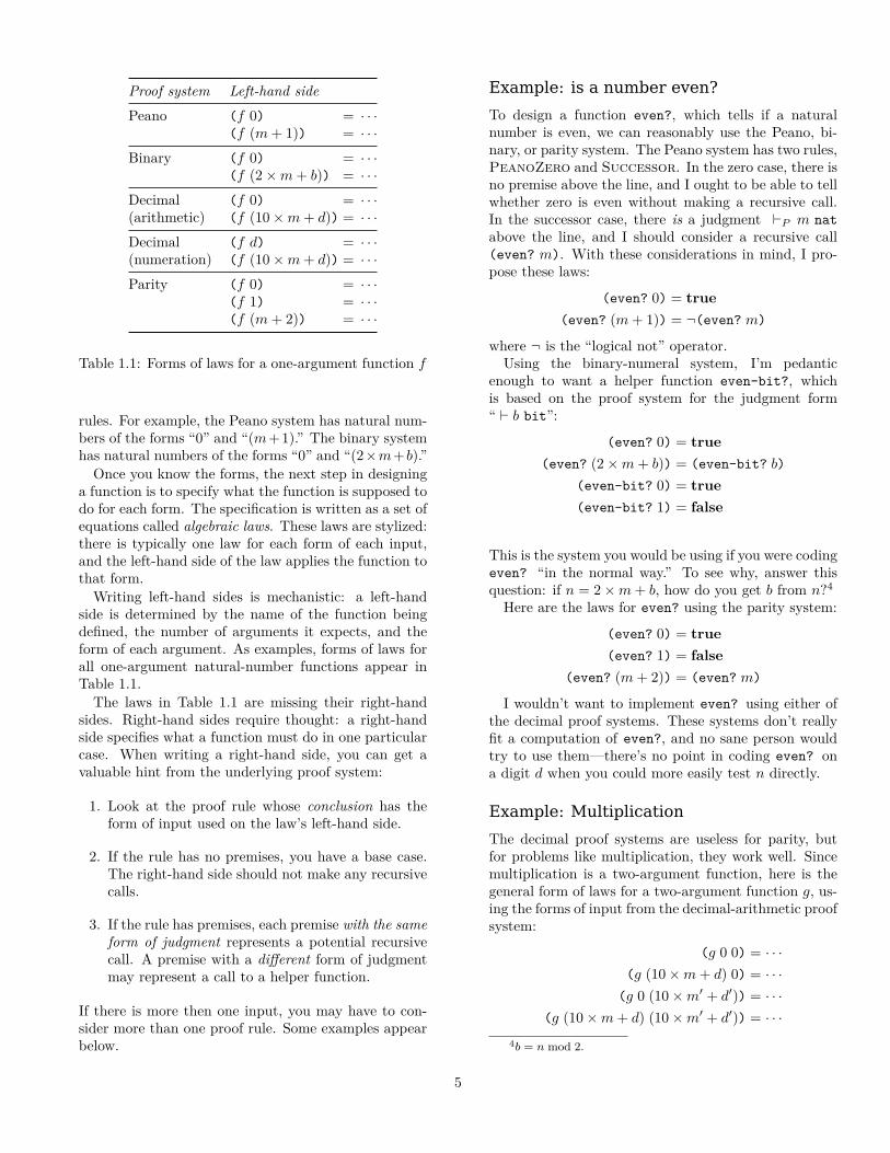
Table 1.1: Forms of laws for a one-argument function f

rules. For example, the Peano system has natural num-bers of the forms “0” and “(m+1).” The binary systemhas natural numbers of the forms “0” and “(2×m+b).”

Once you know the forms, the next step in designinga function is to specify what the function is supposed todo for each form. The specification is written as a set ofequations called algebraic laws. These laws are stylized:there is typically one law for each form of each input,and the left-hand side of the law applies the function tothat form.

Writing left-hand sides is mechanistic: a left-handside is determined by the name of the function beingdefined, the number of arguments it expects, and theform of each argument. As examples, forms of laws forall one-argument natural-number functions appear inTable 1.1.

The laws in Table 1.1 are missing their right-handsides. Right-hand sides require thought: a right-handside specifies what a function must do in one particularcase. When writing a right-hand side, you can get avaluable hint from the underlying proof system:

1. Look at the proof rule whose conclusion has theform of input used on the law’s left-hand side.

2. If the rule has no premises, you have a base case.The right-hand side should not make any recursivecalls.

3. If the rule has premises, each premise with the sameform of judgment represents a potential recursivecall. A premise with a different form of judgmentmay represent a call to a helper function.

If there is more then one input, you may have to con-sider more than one proof rule. Some examples appearbelow.

Example: is a number even?

To design a function even?, which tells if a naturalnumber is even, we can reasonably use the Peano, bi-nary, or parity system. The Peano system has two rules,PeanoZero and Successor. In the zero case, there isno premise above the line, and I ought to be able to tellwhether zero is even without making a recursive call.In the successor case, there is a judgment ⊢P m natabove the line, and I should consider a recursive call(even? m). With these considerations in mind, I pro-pose these laws:

(even? 0) = true(even? (m+ 1)) = ¬(even? m)

where ¬ is the “logical not” operator.Using the binary-numeral system, I’m pedantic

enough to want a helper function even-bit?, whichis based on the proof system for the judgment form“ ⊢ b bit”:

(even? 0) = true(even? (2×m+ b)) = (even-bit? b)

(even-bit? 0) = true(even-bit? 1) = false

This is the system you would be using if you were codingeven? “in the normal way.” To see why, answer thisquestion: if n = 2×m+ b, how do you get b from n?4

Here are the laws for even? using the parity system:

(even? 0) = true(even? 1) = false

(even? (m+ 2)) = (even? m)

I wouldn’t want to implement even? using either ofthe decimal proof systems. These systems don’t reallyfit a computation of even?, and no sane person wouldtry to use them—there’s no point in coding even? ona digit d when you could more easily test n directly.

Example: Multiplication

The decimal proof systems are useless for parity, butfor problems like multiplication, they work well. Sincemultiplication is a two-argument function, here is thegeneral form of laws for a two-argument function g, us-ing the forms of input from the decimal-arithmetic proofsystem:

(g 0 0) = · · ·(g (10×m+ d) 0) = · · ·

(g 0 (10×m′ + d′)) = · · ·(g (10×m+ d) (10×m′ + d′)) = · · ·

4b = n mod 2.

5

Proof system Form of n Test for form Parts n is formed fromPeano 0 n = 0

(m+ 1) n = 0 m = n− 1

Binary 0 n = 0(2×m+ b) n = 0 m = ndiv 2 b = n mod 2

Decimal 0 n = 0(arithmetic) (10×m+ d) n = 0 m = ndiv 10 d = n mod 10

Decimal d n < 10 d = n(numerals) (10×m+ d) n ≥ 10 m = ndiv 10 d = n mod 10

Parity 0 n = 01 n = 1(m+ 2) n = 0 ∧ n = 1 m = n− 2

Table 1.2: Identifying the form of n and extracting its parts

The laws for multiplication are

(* 0 0) = 0

(* (10×m+ d) 0) = 0

(* 0 (10×m′ + d′)) = 0

(* (10×m+ d) (10×m′ + d′)) =

100×m×m′ + 10× (m× d′ +m′ × d) + d× d′

Example: ``All fours''

Suppose I want to write a function all-fours?, whichtells me if an argument’s decimal representation usesonly the digit 4. That is, it likes arguments 4, 44, 444,and so on. I don’t want the Decimal system, since 0 isthe wrong base case. Instead, I want DecimalNat:

(all-fours? d) = (d = 4)

(all-fours? (10×m+ d)) = (all-fours? m) ∧ d = 4,

where ∧ is the “logical and” symbol.

1.5 From algebraic laws to recursivefunction

When the algebraic laws are complete, we write thecode. Conceptually, the code emerges in response tothree questions:

1. We ask of each input, how were you formed? (Ex-ample answer: 10×m+ d.)

2. Once we know the form of an input, we proceed toask from what parts were you formed? (Exampleanswer: from m and d, where m = ndiv 10 andd = n mod 10.)

3. Finally, when we know how each input was formedand from what parts, we can ask which algebraiclaw applies and what does the law say we are sup-posed to do with the parts? (Example answer: makea recursive call on m and check if d = 4.)

The first two questions can be answered using the testsand equations shown in Table 1.2. The third question isanswered by selecting the algebraic law whose left-handside has the right form, then using the right-hand side.

Detailed example

As a first example, let’s implement function is_even,in C, using the parity system. Here are the laws:

(is_even 0) = true(is_even 1) = false

(is_even (m+ 2)) = (is_even m)

Table 1.2 shows that we can distinguish the forms of nusing tests for 0 and 1, so the first draft of our functionuses if statements to distinguish three cases: one foreach law.

bool is_even (unsigned n) {if (n == 0) {...

} else if (n == 1) {...

} else {...

}}

In the first two cases, n isn’t formed from any otherparts, and we can knock off the cases by filling in theright-hand sides of the laws:

6

bool is_even (unsigned n) {if (n == 0) {return true;

} else if (n == 1) {return false;

} else {...

}}

In the final case, the law mentions m, which is computedas n− 2:

bool is_even (unsigned n) {if (n == 0) {return true;

} else if (n == 1) {return false;

} else {unsigned m = n - 2;...

}}

With m computed, we use the right-hand side of the lawto write a recursive call:

bool is_even (unsigned n) {if (n == 0) {

return true;} else if (n == 1) {

return false;} else {

unsigned m = n - 2;return is_even(m);

}}

In practice, I probably would not bother with m in thethird case, writing instead is_even(n-2).

Condensed example

As another example, suppose I want to design a functionthat sums the natural numbers from 0 to n. I choosethe Peano proof system, and I write these laws:

(sumto 0) = 0

(sumto (m+ 1)) = (sumto m)+ (m+ 1)

I distinguish case n = 0 from case n = (m+1) by testingn = 0, and when n = (m + 1), I get the “part” m bycomputing m = n− 1:

int sumto(unsigned n) { // not testedif (n == 0} {return 0;

} else {return sumto(n - 1) + n;

}}

In this code, I don’t bother with an explicit m.

1.6 Complete process examples

The preceding sections of this handout look at proofsystems, forms of data, and algebraic laws, which arethe technical core of our recommended software pro-cess. This section works two more examples, showingall 9 steps of the complete process.

Design of a factorial function

1. Understand the forms of data. To design a factorialfunction, I choose the Peano system, with forms 0and (m + 1). Choosing the right system is notalways obvious, but I’ve written factorial functionsbefore, and I know the Peano system will work.

2. Write a sample input for each form. My exampleinput of form 0 is 0, and my example input of form(m+ 1) is 4.

3. Choose a name. I choose the name factorial.This name is a noun that describes what the func-tion returns.

4. Write the contract. The contract is trivial, pedan-tic, and boring. It says

;; (factorial n) returns n factorial,;; sometimes written "n!", where n;; is a natural number

In practice, I would write this function without acontract—the name alone is contract enough.

5. Write examples. My examples:

(check-expect (factorial 0) 1)(check-expect (factorial 4) 24)

6. Generalize to algebraic laws. The zero case is al-ready an algebraic law:

(factorial 0) == 1

For the successor case, the Peano proof system hasjudgment ⊢ m nat above the line, so I’ll be lookingto make a recursive call with m. I write

7

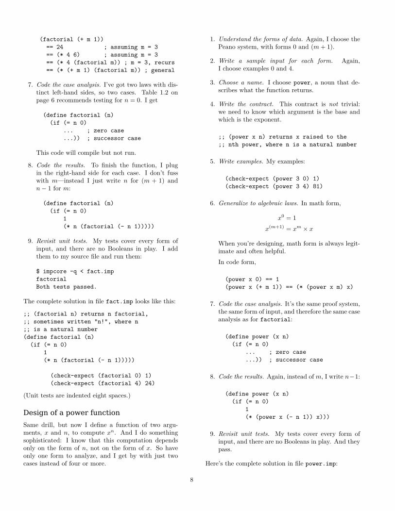
(factorial (+ m 1))== 24 ; assuming m = 3== (* 4 6) ; assuming m = 3== (* 4 (factorial m)) ; m = 3, recurs== (* (+ m 1) (factorial m)) ; general

7. Code the case analysis. I’ve got two laws with dis-tinct left-hand sides, so two cases. Table 1.2 onpage 6 recommends testing for n = 0. I get

(define factorial (n)(if (= n 0)

... ; zero case

...)) ; successor case

This code will compile but not run.

8. Code the results. To finish the function, I plugin the right-hand side for each case. I don’t fusswith m—instead I just write n for (m + 1) andn− 1 for m:

(define factorial (n)(if (= n 0)

1(* n (factorial (- n 1)))))

9. Revisit unit tests. My tests cover every form ofinput, and there are no Booleans in play. I addthem to my source file and run them:

$ impcore -q < fact.impfactorialBoth tests passed.

The complete solution in file fact.imp looks like this:

;; (factorial n) returns n factorial,;; sometimes written "n!", where n;; is a natural number(define factorial (n)(if (= n 0)

1(* n (factorial (- n 1)))))

(check-expect (factorial 0) 1)(check-expect (factorial 4) 24)

(Unit tests are indented eight spaces.)

Design of a power function

Same drill, but now I define a function of two argu-ments, x and n, to compute xn. And I do somethingsophisticated: I know that this computation dependsonly on the form of n, not on the form of x. So haveonly one form to analyze, and I get by with just twocases instead of four or more.

1. Understand the forms of data. Again, I choose thePeano system, with forms 0 and (m+ 1).

2. Write a sample input for each form. Again,I choose examples 0 and 4.

3. Choose a name. I choose power, a noun that de-scribes what the function returns.

4. Write the contract. This contract is not trivial:we need to know which argument is the base andwhich is the exponent.

;; (power x n) returns x raised to the;; nth power, where n is a natural number

5. Write examples. My examples:

(check-expect (power 3 0) 1)(check-expect (power 3 4) 81)

6. Generalize to algebraic laws. In math form,

x0 = 1

x(m+1) = xm × x

When you’re designing, math form is always legit-imate and often helpful.In code form,

(power x 0) == 1(power x (+ m 1)) == (* (power x m) x)

7. Code the case analysis. It’s the same proof system,the same form of input, and therefore the same caseanalysis as for factorial:

(define power (x n)(if (= n 0)

... ; zero case

...)) ; successor case

8. Code the results. Again, instead of m, I write n−1:

(define power (x n)(if (= n 0)

1(* (power x (- n 1)) x)))

9. Revisit unit tests. My tests cover every form ofinput, and there are no Booleans in play. And theypass.

Here’s the complete solution in file power.imp:

8

;; (power x n) returns x raised to the;; nth power, where n is a natural number(define power (x n)(if (= n 0)

1(* (power x (- n 1)) x)))

(check-expect (power 3 0) 1)(check-expect (power 3 4) 81)

1.7 Mistakes to avoid in algebraic laws

An algebraic law sits halfway between a mathemati-cal statement and a function definition. When you arewriting a law for function f , here are some mistakes toavoid:

• A left-hand side is not an application of f .

• On a left-hand side, f is applied to something thatis not a form of data. For example, m/b or (/ m b).

• There is a permissible form of data that does notmatch the left-hand side of any law.

• A law’s right-hand side mentions a variable thatdoes not appear on the left-hand side. (This mis-take is just like trying to use an undeclared variablein a C++ function.)

In addition to these basic mistakes, people who are firstlearning to code with algebraic laws often make threeother, more subtle mistakes. The more subtle mistakesreflect confusion about what a variable in a law standsfor: an actual parameter or a part of an actual parame-ter? When a variable stands for a part of a parameter,trouble sometimes follows.

In the first subtle mistake, the right-hand side of alaw uses a variable that is intended to stand for a formalparameter, but the parameter doesn’t actually appearon the left. For example,

(has-digit? (10 * m + d) d2) ==(has-digit? (/ n 10) d2), where d2 != d

The n on the right-hand side is not specified—it couldbe anything. This mistake is a special case of the fourth

bullet above, and I can see what’s going on: the left-hand side specifies the parts of the first parameter, butthe right-hand side uses n to name the parameter itself.What’s meant by (/ n 10) is actually m.

To avoid this mistake, remember this rule: The right-hand side of an algebraic law may use any variable thatappears on the left-hand side, and only those variables.

In the second subtle mistake, a right-hand side mis-uses a variable from the left as if it were the argument,rather than a part of the argument. Here’s an examplefor function (power x n):

(power x (+ m 1)) == (* (power x (- m 1)) x)

The variable m is already meant to be one less than theargument: m = n − 1. The right-hand side of the lawincorrectly applies to m the operation that is meant tobe applied to n.

In the third subtle mistake, a name like m is used inthe algebraic laws to stand for a part of an argument,but in the code to stand for the entire argument. Here’san example:

;; (has-digit? (+ (* 10 m) d) d) == 1;; (has-digit? (+ (* 10 m) d) d2) == ...;; ...

(define has-digit? (m d2)...) ;; cases 1 & 2:

;; m == (+ (* 10 m) d)???

Each part is technically correct by itself, but mixing thetwo is just too confusing: the argument can’t be m and10×m+d. To avoid this mistake, make sure each namestands consistently either for an argument or for a partof an argument, but not both.

9

2. Scheme values and more algebraic laws

Now we remove the training wheels and start workingwith more structured data. This lesson presents thebare bones of programming with µScheme values, in-cluding lists and S-expressions, using proof systems andalgebraic laws. We apply the same design techniques asbefore, but with new forms of data.

This lesson also introduces a wider world of alge-braic laws, distinguishing algorithmic laws from non-algorithmic properties. When coding from scratch,you must learn to make your laws algorithmic.

2.1 Describing µScheme data

The first section of this lesson revisits the ideas in thenatural-number lesson, but for some common forms ofµScheme data.

Proof systems for µScheme data

As noted in Figure 2.1 on page 93 of Programming Lan-guages: Build, Prove, and Compare, a µScheme valueis either an atom, a function, or a cons cell. A “fullygeneral S-expression” is any of these except a function.We could write a proof system like this:

⊢ v symbol⊢ v gsx

⊢ n number⊢ n gsx ⊢ #t gsx

⊢ #f gsx ⊢ '() gsx⊢ v1 gsx ⊢ v2 gsx⊢ (cons v1 v2) gsx

We could define “list of A’s” using the proof systemfrom section 2.4, which starts on page 109 of the text-book:

EmptyList'() ∈ LIST(A)

ConsLista ∈ A as ∈ LIST(A)

(cons a as) ∈ LIST(A)

On your homework I’ll ask you to define “nonemptylist of A’s.”

We could define “ordinary” S-expression using justideas 1 and 2 from Figure 2.1 on page 93. The notation

of that last rule gets a little dodgy:⊢ n number⊢ n osx ⊢ #t osx ⊢ #f osx

vs ∈ LIST(osx)⊢ vs osx

Writing LIST(osx) is flagrant abuse of notation.There’s a better way.

An informal alternative

Proof systems are great for describing the structureof natural numbers, as well as more complex struc-tures like computations. But for describing simplerdata structures, we don’t need the expressive power ofproof systems, and it’s often difficult to come up withgood judgment forms—that’s where we got into trou-ble above. As an alternative, we can write an inductivedefinition informally. We name the set we’re trying todefine, and we list all the ways that data in the set couldbe formed. Examples follows.

A fully general S-expression is one of the following:• A symbol• A number• A Boolean• The empty list '()• (cons v1 v2), where v1 and v2 are fully general S-

expressionsA list of A’s is one of the following:

• The empty list '()• (cons a as), where a is an A and as is a list of A’s

An ordinary S-expression is one of the following:• A symbol• A number• A Boolean• A list of ordinary S-expressionsIt is frequently useful to expand that last bullet. It is

equally true that an ordinary S-expression is one of thefollowing:

• A symbol• A number• A Boolean• The empty list '()• (cons v vs), where v is an ordinary S-expression

and vs is a list of ordinary S-expressions

11

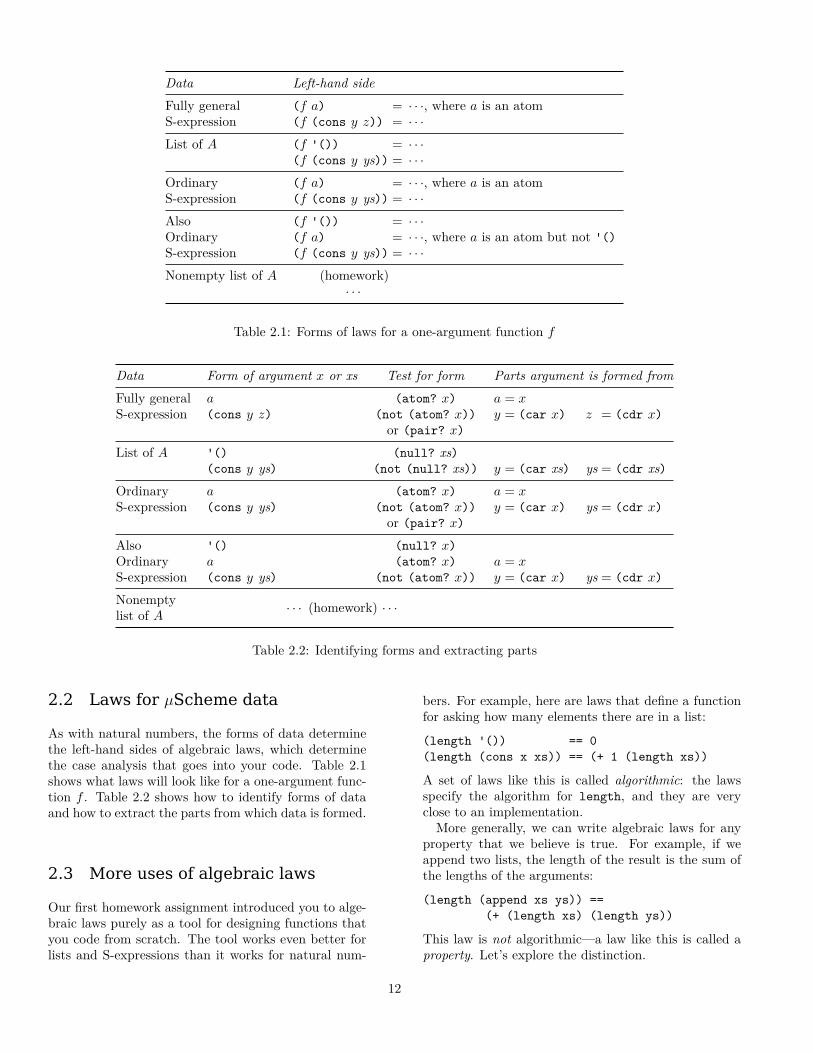
Data Left-hand sideFully general (f a) = · · ·, where a is an atomS-expression (f (cons y z)) = · · ·List of A (f '()) = · · ·

(f (cons y ys)) = · · ·Ordinary (f a) = · · ·, where a is an atomS-expression (f (cons y ys)) = · · ·Also (f '()) = · · ·Ordinary (f a) = · · ·, where a is an atom but not '()S-expression (f (cons y ys)) = · · ·Nonempty list of A (homework)

· · ·

Table 2.1: Forms of laws for a one-argument function f

Data Form of argument x or xs Test for form Parts argument is formed fromFully general a (atom? x) a = xS-expression (cons y z) (not (atom? x)) y = (car x) z = (cdr x)

or (pair? x)

List of A '() (null? xs)(cons y ys) (not (null? xs)) y = (car xs) ys = (cdr xs)

Ordinary a (atom? x) a = xS-expression (cons y ys) (not (atom? x)) y = (car x) ys = (cdr x)

or (pair? x)

Also '() (null? x)Ordinary a (atom? x) a = xS-expression (cons y ys) (not (atom? x)) y = (car x) ys = (cdr x)

Nonemptylist of A · · · (homework) · · ·

Table 2.2: Identifying forms and extracting parts

2.2 Laws for µScheme data

As with natural numbers, the forms of data determinethe left-hand sides of algebraic laws, which determinethe case analysis that goes into your code. Table 2.1shows what laws will look like for a one-argument func-tion f . Table 2.2 shows how to identify forms of dataand how to extract the parts from which data is formed.

2.3 More uses of algebraic laws

Our first homework assignment introduced you to alge-braic laws purely as a tool for designing functions thatyou code from scratch. The tool works even better forlists and S-expressions than it works for natural num-

bers. For example, here are laws that define a functionfor asking how many elements there are in a list:

(length '()) == 0(length (cons x xs)) == (+ 1 (length xs))

A set of laws like this is called algorithmic: the lawsspecify the algorithm for length, and they are veryclose to an implementation.

More generally, we can write algebraic laws for anyproperty that we believe is true. For example, if weappend two lists, the length of the result is the sum ofthe lengths of the arguments:

(length (append xs ys)) ==(+ (length xs) (length ys))

This law is not algorithmic—a law like this is called aproperty. Let’s explore the distinction.

12

Understanding and using algorithmic laws

To identify a set of laws as algorithmic, learn to recog-nize these hallmarks:

• Each left-hand side is a function to be defined, ap-plied to one or more arguments, where each argu-ment is either a variable or a form of data. In thelength example, both '() and (cons x xs) areforms of data.

• In an algorithmic set of laws, each law is mutu-ally exclusive with the others. That is, given anyparticular input, at most one law applies. Mutualexclusion is accomplished either using mutually ex-clusive forms of data, like '() and (cons x xs), orby using mutually exclusive side conditions.(In rare cases, algorithmic laws can overlap: thereare inputs for which more than one law could apply.In such cases, all applicable right-hand sides mustproduce the same result. These cases are sufficientlyrare that I don’t present an example.)

• Collectively, an algorithmic set of laws accounts forevery input that is permitted by a function’s con-tract. If an input is permissible, there must be alaw that applies.

• In every recursive call on every right-hand side,some input is getting smaller.

Algorithmic laws are used for these purposes:

• Algorithmic laws are used primarily to design andimplement functions.

• Algorithmic laws can also be used to test functions.

Understanding and using properties

Technically, every law in an algorithmic set is also aproperty. But not every property is an algorithmic law.To identify a property law as non-algorithmic, learn torecognize these hallmarks:

• On a left-hand side, a function is applied to theresult of another function. For example, in thelength property, length is applied to the resultof append.

• Properties might not be mutually exclusive, andthey needn’t account for every permissible input.

Properties have many more uses than algebraic laws,including these purposes:

• Properties are used for testing. Substitute a per-missible value for each variable in the property, andcheck that equality holds. For example, here’s aproperty we use to test arithmetic in Smalltalk:

(* 2 n) == (+ n n)

We can test this property with any natural num-ber n.Here’s a property about lists that is useful only fortesting:

(permutation? (cons x (cons y zs))(cons y (cons x zs))) == #t

Good tooling for programming languages fre-quently includes random, automated, property-based testing based on substituting randomly gen-erated values for variables in properties.

• Properties are used for refactoring, which meansrewriting code to improve its structure, withoutchanging its semantics. A good example is codesimplification. Many of the properties found in sec-tion 2.5 of the textbook, like this append-cons law,can be used to simplify code:

(append (cons x '()) xs) == (cons x xs)

• Properties are used for code improvement, whichmeans rewriting code to improve its performance,without changing its semantics. (Code improve-ment is often called “optimization.”) Some of theproperties found in section 2.5 of the textbook, likethis append-append law, can be used to improveperformance:

(append (append xs ys) zs) ==(append xs (append ys zs))

• Properties are used for specification, especially ofabstract data types. Programmers may use proper-ties to say how an abstraction behaves without say-ing how it is implemented. Here’s a typical prop-erty from an abstraction of sets:

(member? x (add-element x xs)) == #t

The property says that if we add an element x toany set, then x is a member of the resulting set.

13

2.4 Common issues using algebraiclaws with Scheme

Below are some issues you might run into when writingalgebraic laws for Scheme functions.

Correct use of variables

A common mistake is to write laws thinking that vari-ables are mutually exclusive with other forms of data.They aren’t. When you write a variable, you are sayingimplicitly, “this could be any form of data, and I don’tcare which.” In other words, when you write a variablein an argument position, you are promising not to lookand see how the argument was formed. In particular,when you write a variable, you are promising never toapply null?, car, or cdr to that variable.

Here’s an example of this common mistake:

(sublist? xs '()) == #f ;; WRONG(sublist? '() ys) == #t... more cases below ...

The student who wrote these laws meant for xs andys meant to be nonempty. But a variable could beany list, including the empty list. In this example, ifboth xs and ys are empty, the laws give inconsistent re-sults. That’s how we’re certain that something is wrong.Here’s a correct version, in which every argument is ei-ther explicitly empty or explicitly nonempty.

(sublist? (cons w ws) '()) == #f ;; RIGHT(sublist? '() (cons z zs)) == #t... more cases below ...

These left-hand sides can’t possibly be confused.This version can be refined by observing that in the

original set, the problem lies with the first law. The law(sublist? '() ys) == #t is actually good: the emptylist is a sublist of any list ys, whether ys is empty ornot. So we could write the laws this way:

(sublist? (cons w ws) '()) == #f ;; RIGHT(sublist? '() ys) == #t ;; SPLENDID... more cases below ...

The advantage of this final specification is that we mightthen have to consider fewer alternatives in the “morecases below.”

Breaking S-expression inputs down by cases

Quite often it’s useful to define an ordinary S-expressionas one of the following:

• The empty list

• (cons z zs), where z is an S-expression and zs isa list of S-expressions

• a, where a is an atom but not the empty list

A common mistake here is to forget the side conditionon a. Here are some mistaken laws for counting thenumber of atoms in an ordinary S-expression:

(atom-count '()) = 0(atom-count (cons z zs)) =

(+ (atom-count z) (atom-count zs))(atom-count a) = 1 ;; WRONG

The last law needs a side condition:

(atom-count a) = 1,where a is a non-null atom ;; RIGHT

You can't break a function down by cases

Some of the problems on the homework, like takewhile,dropwhile, and arg-max, take functions as inputs.You can’t break a function down by cases, becausethere’s no way to ask a function how it was formed.All you can do with a function is apply it. How, then,should a function appear in an algebraic law? As a vari-able. Here’s an example for takewhile, which takes twoarguments, a predicate p? and a list of values. A func-tion has one case and a list has two, and multipliedtogether there are two in total:

(takewhile p? '()) = ...(takewhile p? (cons x xs)) = ...

That’s not the end of the story, however: once we haveboth p? and an x that we could apply p? to, we couldhave extra cases depending on whether (p? x) is true orfalse. Those cases would be written as side conditions.

One final example: function arg-max takes a functionand a nonempty list of values. The laws for arg-max willhave one case for the function input (just a variable),and other cases for the nonempty list. (Finding theforms of a nonempty list is a homework problem.)

14

3. Higher-order functions

In addition to “constructed data” (cons), Scheme alsohas first-class, nested functions. This key feature, whichoriginated with Scheme, is now used prominently insuch scripting languages as JavaScript, Python, Lua,and Perl. Functions are not quite like other forms ofdata, but they still participate in the design process.Functions that appear as arguments are handled some-what like other forms of data; functions that appear asresults are different. The details are explained in thislesson.

3.1 Designing with functions as argu-ments

In a principled design process, here’s how we work withfunction arguments:

1. Forms of data. A function is unlike any other formof data so far, in this way: you can’t interrogatea function to ask how it was made or from whatparts. Instead,

All you can do with a function is apply it.

However, we can and do use information about afunction’s contract as a proxy for its form. Step 1of the design process is therefore to identify whatis important about the function’s contract. Usu-ally what’s most important involves the numberof parameters and sometimes the types of the pa-rameters and result. Here are some ways to thinkabout the form of a function:

• Takes one argument• Takes two arguments• Takes one argument, returns a Boolean• Takes two arguments, returns a Boolean• Takes one argument, returns a function• Takes two arguments, returns a result that is

like the second argument

2. Example inputs. Once you’ve identified the formof a function, you can come up with examples.The best examples are familiar functions, like thosefrom the initial basis.

abs ; one arg+ ; two argssymbol? ; one arg, returns Boolean< ; two args, returns Boolean

curry ; one arg, returns functioncons ; two args, result like 2nd

3, 4, 5. When functions are used as arguments, steps 3 to 5are unchanged.

6. Algebraic laws. Forms of algebraic laws are as be-fore: on the left-hand side, the function being de-fined is applied to arguments. What’s different isthere can be no case analysis on an argument that isa function. The only thing you can do with a func-tion is apply it. Case analysis on other argumentsproceeds as usual.

7. Code case analysis. Because we can’t do case anal-ysis on a function, the presence of a function asan argument doesn’t change the way we code caseanalysis. Case analysis on non-function argumentsproceeds as usual.

8, 9. When functions are used as arguments, steps8 and 9 are unchanged.

3.2 Designing with functions as re-sults

When a function returns another function as a result,the design process is affected more broadly. That’s be-cause we can’t do much with a function result. In par-ticular, we can’t compare a function result with anotherfunction result—all we can do is apply it. If we want totest or specify a function result, we have to test or spec-ify what happens when we apply the function to some-thing. The central principle is this:

Two functions are equal if and only if whenthey are applied to equal arguments, they re-turn equal results.

Here’s how this principle affects our design process.

1, 2. We’re talking about results, not inputs, so the storyabout forms of data and inputs is unchanged.

3, 4. Naming and contracts are unchanged.

5. Example results. Example results may or may notbe helpful here—it depends whether the expectedresult has a well-known name. Here’s a case whereexample results are helpful: function flip takes atwo-argument function as argument and returns afunction that is like the argument function, except

15

the result function expects its arguments in the op-posite order. A couple of good example results are

(flip <) == >(flip >=) == <=

With these examples, we got lucky. More com-monly, the result doesn’t have a name. For exam-ple, we don’t have a name for (flip append).While you can sometimes find examples to be equalto a function result, you can always construct ex-amples about what a function result is applied to.This design technique is reliable, and it might looklike this:

((flip <) 3 4) == #f((flip <=) 3 4) == #f((flip append) '(a b c) '(1 2 3)) ==

'(1 2 3 a b c)

This general form of example has three parts:

a) The function being designed, flip, is appliedto arguments, producing a result.

b) The result is itself applied to (more) argu-ments.

c) The result of the result (the whole applica-tion) is equal to something.

6. Algebraic laws. Right-hand sides of algebraic lawsdon’t change, but left-hand sides do. When a func-tion returns a function, the left-hand side is nowgoing to include at least two applications, just likethe example results in step 5.

a) The function being designed is applied to vari-ables and/or forms of data.

b) The result of the function being designed isthen applied to more variables and/or formsof data.

As examples, here are the laws for every predefinedµScheme function that returns a function as a re-sult:

((o f g) x) == (f (g x))((uncurry f) x y) == ((f x) y)

If the result of a result is also a function, we keepapplying until we get to a point where we haveresults that can be tested for equality:

(((curry f) x) y) == (f x y);; *three* applications on left!

7. Code left-hand side. When a function returns afunction, this step changes a bit. The key changeis that we code one function for every applicationon the left-hand side. The outermost function canbe coded using either define or lambda. Innerfunctions are coded using lambda.One possibly confusing point:

The innermost application in the lawcorresponds to the outermost define orlambda in the definition.

That’s because in the law, the innermost applica-tion is evaluated first, but in the definition, theoutermost lambda is evaluated first. Let’s see howit works.In the law for ((o f g) x), we have two nestedapplications:

(o f g) = result(result x) = (f (g x))

That result is going to become an anonymouslambda.First step in the code: innermost application fromthe left-hand side:

(define o (f g); law: (result x) == (f (g x))... result function ...)

Next step of the left-hand side: result function ex-pects x as an argument:

(define o (f g); law: (result x) == (f (g x))

(lambda (x) ... right-hand side ...))

And leaping ahead to step 8:

(define o (f g); law: (result x) == (f (g x))

(lambda (x) (f (g x))))

Here’s the same development for uncurry:

(define uncurry (f); law: (result x y) = ((f x) y)... result function ...)

And finishing the left-hand side with lambda:

(define uncurry (f); law: (result x y) = ((f x) y)(lambda (x y) ... RHS ...))

16

And leaping ahead to step 8:

(define uncurry (f); law: (result x y) = ((f x) y)(lambda (x y) ((f x) y)))

8. Code results. The code for a final result on a right-hand side is written in the same way as usual, butwe’ll find it inside at least one additional lambda.

9. In order to test a function’s result, we have to applyit to something. Here is one bad example accom-panied by three good ones:

(check-expect (flip <) >) ;; USELESS(check-expect ((flip <) 3 4) (> 3 4)) ;; GOOD(check-expect ((flip <) 3 3) (> 3 3)) ;; GOOD(check-expect ((flip <) 3 2) (> 3 2)) ;; GOOD

17

4. ML types and pattern matching

This lesson sketches how to apply our design processto ML, a language with types and pattern matching.Popular languages with these features include Haskell,Elm, OCaml, Reason, F♯, Erlang, and Scala. More ob-scure languages include Agda, Idris, and Coq/Gallina.

This lesson is followed by a page of syntax help.

4.1 Design steps

Our design method is affected by the introductions ofconstructed data and types.

1. Forms of data for numbers and functions are as inScheme. But forms of data for lists, pairs, tuples,trees, and other constructed data are determinedby primitive types and user-defined types, includ-ing algebraic datatypes. These forms are shown inTable 4.1 on the next page, as patterns.Patterns are the technical name for the phrasesthat appear as function arguments on the left-handsides of algebraic laws—so you already know howto program with them. But to define them care-fully, here are ML’s rules for patterns:

• Any variable, as in x, is a pattern.• The “wildcard,” as in _ (underscore), is a pat-

tern• A sequence of patterns separated by com-

mas and wrapped in round brackets, as in(l, x, r), is a tuple pattern.

• The empty tuple () is a pattern.• A sequence of patterns separated by com-

mas and wrapped in square brackets, as in[x1, x2, x3], is a list pattern.

• The empty list [] is a pattern.• A value constructor by itself, as in nil or

NONE, is a pattern.• A value constructor applied to a pattern, as

in SOME x, is a pattern.• An infix value constructor placed between

patterns, as in x :: xs, is a pattern.1

• A sequence of pattern bindings separated bycommas and wrapped in curly brackets, as in{ ps1 = s, ps2 = s' }, is a record pattern.

1Confusingly, “fixity” is a local property of a name, not aproperty of the value constructor itself.

• A literal number, as in 1852, is a pattern.• A literal string, as in "frogs", is a pattern.• A literal character, as in #"f", is a pattern.

A key feature of ML is that you get to definenew forms of data, using the datatype definition.For example, a binary tree of machine integers:

datatype inttree= ILEAF| INODE of inttree * int * inttree

2. Example inputs include what you would expectfrom Scheme: numbers written using numeric liter-als, and anonymous lambda functions written usingfn, as in (fn (x, y) => y + 1). ML also has stringliterals.In addition, examples of constructed data areformed using the pattern rules: if a pattern hasno variables or wildcards, it specifies a value:

(105, "hello")[2, 3, 5, 7, 11]SOME 33

3. Function names are limited. In ML, you may useeither “symbolic” characters like <, ?, +, and so on,or you may use alphanumeric characters2 with anunderscore, but you may not use both in the samename. Symbolic characters may be combined intoarbitrarily long names, such as <=> or /*/.ML offers a design choice not available in Scheme:function names can be “infix.” Predefined functionslike mod, o, and + all have infix names, as does thevalue constructor ::. The fixity of names can bechanged by an infix or nonfix definition form.It’s especially common for symbolic names to bemade infix.Infix names like :: and + can’t be used as first-classvalues; when you write an infix name, ML thinksyou mean to apply it. But there is a workaround:putting the reserved word op in front of any infix

2The ASCII quote mark, here pronounced “prime,” counts asalphanumeric, as in x', pronounced “x-prime.”

19

Type of e Patterns Test in definition Test in expression Types of partscase e

'a list [] fun f [] = · · · of [] => · · ·x :: xs | f (x :: xs) = · · · | x :: xs => · · · x : 'a, xs : 'a list

case e'a option NONE fun f NONE = · · · of NONE => · · ·

SOME x | f (SOME x) = · · · | SOME x => · · · x : 'a

case eorder LESS fun f LESS = · · · of LESS => · · ·

EQUAL | f EQUAL = · · · of EQUAL => · · ·GREATER | f GREATER = · · · of GREATER => · · ·

case eint 0 fun f 0 = · · · of 0 => · · ·

n | f n = · · · | n => · · · n : int

let val (x, y) = e'a * 'b (x, y) fun f (x, y) = · · · in · · · x : 'a, y : 'b

end

let val (x, y, z) = e'a * 'b * 'c (x, y, z) fun f (x, y, z) = · · · in · · · x : 'a, y : 'b, z : 'c

end

{ f1 : 'a { f1 = x fun f { f1 = x let val { f1 = x x : 'a, f2 : 'b , f2 = y , f2 = y , f2 = y y : 'b, f3 : 'c , f3 = z , f3 = z , f3 = z z : 'c· · · , ... , ... , ... } = e

} } } = · · · in · · ·(record) (“f1” is short for “field 1”, and so on) end

case e'a tree LEAF fun f (LEAF) = · · · of LEAF => · · ·(homework) NODE(l,x,r) | f (NODE(l,x,r)) = · · · | NODE(l,x,r) => · · · l : 'a tree, x : 'a

r : 'a tree

case eµScheme LITERAL v fun f (LITERAL v) = · · · of LITERAL v => · · · v : valueexp VAR x | f (VAR x) = · · · | VAR x => · · · x : name(page 312) SET (x, e) | f (SET (x, e)) = · · · | SET (x, e) => · · · x : name, e : exp

......

......

Table 4.1: Identifying forms and extracting parts (ML builtins and 105 types)

20

name turns it into a nonfix name, which you canuse as a value. Here are two classic examples:

fun sum ns = foldl op + 0 nsfun prod ns = foldl op * 1 ns

4. Function contracts are now enhanced: every func-tion has a most general type. We consider the typeto be part of the function’s contract. The typeis enforced by the compiler. In many cases, likeList.all and List.exists, the name and thetype form a sufficient contract all by themselves.

5. Example results and test cases work using thesame ideas as in µScheme (“check-expect,” “check-assert,” and “check-error”), but the mechanismsare different. Compared with µScheme, ML’s unittesting is verbose and awkward. But there is onesmall compensation: unlike µScheme, ML indicateschecked run-time errors using exceptions. This fea-ture makes it possible to check for the presence ofa particular exception, like Subscript, Empty, orOverflow. In µScheme, that’s not possible.

6. Algebraic laws are as helpful as ever. They mustrespect types. We will also develop a new designmethod that helps with writing right-hand sides ofalgebraic laws. The new method is based on types,and when we are ready to study types in detail,it will be presented in class.

7. Coding case analysis is much simpler than inScheme: for case analysis over constructed data,we just use pattern matching. This feature makesthe code look an awful lot like the algebraic laws.For case analysis of natural numbers or machineintegers, we can often use partial pattern match-ing (one or more cases of interest, followed by acatchall case).

8. Coding results uses the same design methods asin Scheme. But in ML, both the concrete syntaxand the abstract syntax are different from Scheme.Here are the key differences in the abstract syntaxand our use of it:

• In ML, the let form uses definitions and hasa similar semantics to Scheme’s let*. Directrecursion is accomplished by using fun, andmutual recursion by using and.

• ML has a case form for pattern matching inan expression. (But usually we will patternmatch in the fun definition form.)

• Deconstruction of input data is always doneby pattern matching. ML has functions likecar, cdr, and null?, but they are used rarely,and only by experts.

9. Revisiting tests has the same intellectual content,but it’s much more fussy to code. To run yourtests, you’ll need to study the Unit interface thatis described in the guide to learning ML.

21

Syntax help for Standard ML

Standard ML is a full language, not simplified for teach-ing, and an exhaustive syntax summary would be over-whelming. This section presents the key syntactic toolsthat you will use most frequently. It is not exhaustive!

ML has four major syntactic categories. From thetop down:

d Definitionsp Patternse Expressionsτ Types

These categories are related like this:

• Definitions sit at the top, and they contain bothpatterns and expressions. A typical definition formhas a pattern on the left and an expression on theright. The definition of a Curried function mayhave multiple patterns on the left.The val form you already know is present, but in-stead of just a name on the left, it can take anypattern.The define form you already know is a specialcase of fun, but fun is more typically used withpatterns, to express algebraic laws directly.There are two kinds of type definitions: type ab-breviations (type) and fresh, algebraic data types(datatype). Both are called “types,” and both def-inition forms contain types.

• Patterns are new. They are one of the two maininteresting features of ML, and they are describedin detail in Lesson 4 above. Patterns may containtypes, but they usually don’t—we put types in pat-terns only when we’re debugging.

• Expressions resemble those that you already know,except for the let form. ML’s let form con-tains definitions, not Scheme’s name-value bind-ings. And unlike Scheme’s let, which binds allnames simultaneously, ML’s let evaluates defini-tions in sequence, like Scheme’s let*.Expressions may contain definitions and types. Ex-pressions commonly contain definitions (any letform), but they rarely contain types—we put typesin expressions only when we’re debugging.

• Types are more general than the types you knowfrom C and C++. We will study types at length.

To summarize the common forms of the categorieslisted above, I use these symbols for nonterminals:

x, f Name (of a variable or function)k Literal (like 7 or #"a")K Name of a value constructort Name of a type

Using these symbols, here are some examples of themost commonly used forms of ML syntax:

p ⇒ x∣∣ k ∣∣ (p1, p2)

∣∣ (p1, p2, p3)| []

∣∣ p1 :: p2∣∣ [p1,p2, …, pn]

| NONE∣∣ SOME p

∣∣ LESS ∣∣ EQUAL ∣∣ GREATER| K

∣∣ K p

e ⇒ x∣∣ k ∣∣ (e1, e2)

∣∣ (e1, e2, e3)| []

∣∣ e1 :: e2∣∣ [e1,e2, …, en]

| NONE∣∣ SOME e

∣∣ LESS ∣∣ EQUAL ∣∣ GREATER| K

∣∣ K e

| e e · · ·| if e1 then e2 else e3| let d · · · in e end| (case e of p1 => e1 | p2 => e2 | · · · )| raise e

∣∣ (e1 handle p => e)| e1 andalso e2

∣∣ e1 orelse e2

d ⇒ val p = e| val (x1, x2) = e (overlooked special case)| fun f p1 = e1 | f p2 = e2 | · · ·| fun f p1 · · · = e1 | f p2 · · · = e2 | · · ·| exception K| exception K of τ| type t = τ| type 'a t = τ| datatype t = K1 of τ1 | K2 of τ2 | · · ·| datatype t = K1 | · · ·| datatype 'a t = K1 of τ1 | K2 of τ2 | · · ·| datatype 'a t = K1 | · · ·

τ ⇒ int∣∣ string ∣∣ bool ∣∣ char

| τ list∣∣ τ option

| τ1 * τ2∣∣ τ1 * τ2 * τ3

| τ1 -> τ2| 'a

∣∣ 'b ∣∣ 'c

23

5. Program design with typing rules

One reason to use formal proofs (for operational seman-tics and type systems) is that proof rules often tell ushow to write code. We can approach the coding taskthe same way we approach other coding tasks: we canstart by viewing a proof as data and each proof rule asa form of data. But if the goal is to translate a type sys-tem (or any other proof system) into code, we are betteroff specializing the design process to write the transla-tion directly. This lesson presents a suitably specializedprocess, which you will use for two assignments: typechecking and type inference.

The special process for turning rules into code, evenmore than other processes, is ultimately meant to beinternalized and abbreviated. It is possible to com-plete all the homework successfully without masteringthe process, but if you do master it, you will find your-self writing clean code, fluently. Your coding will bedriven primarily by questions like “what do I know?”,“what can I compute from what I know?”, and “whatdo I want to compute next.” If you reach this level offluency, you will not need to leave evidence of your de-sign process, and you will not need to follow the codingsuggestions to the letter.

5.1 Overall program design

When we code up a type system or other proof sys-tem, every judgment form is implemented by a function.A judgment form is a logical statement, amounting to“a claim is provable.” A function implementing a judg-ment form follows one of two models:

• Every metavariable in the judgment form is an in-put to the function, and the function returns aBoolean that answers the question, “is this claimprovable?”Example: judgment x ∈ domΓ. Both x and Γare inputs, so the function takes a name and anenvironment and returns a Boolean. This is thefunction isBound from the ML homework.Example: judgment τ1 ≡ τ2. Both τ1 and τ2 areinputs, so the function takes two types and returnsa Boolean. This is the function eqType from thetype-systems chapter.

• Some metavariables are inputs and some are out-puts. The function tries to compute values for theoutput metavariables such that the whole judgmentis provable. If it succeeds, it returns those values.If it fails, it raises an exception.

Example: judgment ∆,Γ ⊢ e : τ . The inputs are ∆,Γ, and e, and the output is τ . This is the functiontypeof from the type-systems homework.To give an example of typeof, I assume I’m usingthe environments from the initial basis. If, in ad-dition, I pass the input expression (+ 2 2), typeofwill succeed and will return type int. If I pass(+ 2 #t), typeof will fail by raising the exceptionTypeError.To identify functions like this, I frequently write ajudgment form with boxes around the outputs, asin “∆,Γ ⊢ e : τ .”

To implement a type checker, a type inferencer, an-other static analyzer, or even an interpreter, you im-plement all the judgment forms. Here are some keyquestions:

• What function will each judgment form be imple-mented by? What are the inputs and the outputs?

• What are the proof rules for the judgment formsI implement? What judgments do those proof rulesuse?

• Which judgment forms are already implementedfor me? Perhaps in the book?

• Which judgment forms do I have to implement?

The answers are different for each different type system,but many of the answers are found in the book:

Typed Impcore Table 6.2 on page 347Typed µScheme Table 6.5 on page 376nano-ML Table 7.3 on page 443

5.2 Design steps for one function

To design a function that implements a judgment form,we follow the usual design steps:

1. Forms of data. Key data types found in type sys-tems are

Γ Type environment∆ Kind environmentC Equality constraint (inference only)e Abstract syntaxτ Typeσ Type scheme (Hindley-Milner only)α Type variable

25

Like the judgment forms, these forms of data andtheir ML representations are shown in the tableson pages 347, 376, and 443.Not all of these data are broken down by cases:

• Environments are never broken down bycases.

• Types are not usually broken down by cases,except when implementing a constraint solverfor type inference.

• Type schemes have only one form, butwhen instantiating polymorphic values, typeschemes are deconstructed. (Instantiation isimplemented in the book.)

• Equality constraints and abstract syntax,when consumed, are broken down by cases.

2. Example inputs. To write examples of abstract syn-tax, we use concrete syntax. (Writing abstract syn-tax is what concrete syntax is for!) When possible,we do the same with types, which also have a con-crete syntax.

3. Function name. To form names, we usually usenouns like “type” or verbs like “elaborate,” “eval-uate,” “substitute,” “conjoin,” or “solve.” Or someother name that is connected with the proof sys-tem. Function names are often given by one of thetables on pages 347, 376, and 443.

4. Function contract. This is a key step. At an ab-stract level, all the contracts are the same: “im-plement a judgment.” But it helps to be concrete.Example: judgment form C,Γ ⊢ e : τ from nano-ML. Here’s the function and its contract:

val typeof : exp * type_env -> ty * conCalling typeof (e,Γ) returns (τ, C) suchthat C,Γ ⊢ e : τ . Constraint C is notguaranteed to be solvable.1

To help us remember a function’s contract, we canwrite the corresponding judgment form with boxesaround the outputs: C ,Γ ⊢ e : τ .

5. Example results. While it is possible to write exam-ple inputs and results directly as ML values, this

1The inputs and outputs to type inference are a frequentsource of confusion. Examples of other type systems, as wellas operational semantics, suggest the heuristic, “inputs on theleft, outputs on the right.” But that’s not how logic works—theheuristic is wrong. The logical structure of a sequent is

context ⊢ claim.

In type inference, one of the outputs of the algorithm is the con-straint C. This constraint, which is part of the context, expressesthe assumptions that have to be made in order for term e to betypable.

level of work can usually be avoided. For mosttype-checking tasks, try this method:

• Whenever possible, use the environments ininitial basis.

• When necessary, extend the initial environ-ment with just one or two definitions.

• Write example inputs (expressions and defi-nitions) using the concrete syntax of TypedImpcore, Typed µScheme, or nano-ML. Writeexample outputs likewise.

• Turn the examples into unit tests using thecheck-type, check-principal-type, andcheck-type-error forms.

When implementing the proof system for the con-straint solver, there is no concrete syntax for con-straints. Fortunately, the ML syntax for writingconstraints is not too painful. So to design theconstraint solver, write example inputs and resultsas you learned to do when coding the first ML as-signment.

6, 7, 8. Algebraic laws and code. Experienced type-systemhackers can code a type system from inference rulesalone. But while you are learning, you are betteroff following the step-by-step translation procedureoutlined below. This procedure is the one you wantto internalize.

9. Revisit unit tests. To test a type checker, use con-crete syntax with unit-test forms in source code,as described in step 5 above. To test the nano-MLconstraint solver, use Unit functions to embed unittests inside your interpreter.

5.3 Translating rules to code

To implement a type system or other proof system,you organize the rules by the form of the judgmentthat appears in the conclusion. All the rules that con-clude the same form are implemented by the same func-tion. So for example, if you consult the table 6.5 onpage 376, you’ll see that the Typed µScheme type sys-tem needs you to write two functions: typeof andelabdef. The corresponding forms of concluding judg-ment are ∆,Γ ⊢ e : τ and ⟨d,∆,Γ⟩ → Γ′ . You’llfind the corresponding collections of rules summarizedin Figures 6.12 and 6.13 on pages 405 and 406. (Not ev-erything is in the summaries; in particular, the rules forliteral values are found only at the beginning of sec-tion 6.6.5, which starts on page 370.)

Now you know the function you are implementing, itsinputs and outputs, and the collection of rules that spec-ifies the implementation. Your next step is to break therules down by forms of data, which is to say the forms

26

of the abstract syntax in the conclusions of the rules.For typeof, this is expression syntax; for elabdef, thisis definition syntax. For each form of syntax, expectone or more rules. In our case, we’re expecting exactlyone rule per form of syntax—systems with more thanrule are not hard to implement, but they are beyondthe scope of this lesson.

To finish the job, you translate each rule into code.Code produced by beginners looks quite different fromcode produced by experts, but the expert’s code reflectsthe same thought process as the beginner’s—the codeis just streamlined. This lesson teaches you to writebeginner’s code. But because you’ll see expert code inlecture and in the model solutions, the lesson also addsnotes about what experts do.

In a beginner’s code, every right-hand side (whethera law or direct to ML code) takes the form of a let ex-pression, with bindings and a body. The let expressionis developed using the custom design process embodiedin these steps:

(A) In your chosen rule, identify all the judgmentsabove the line. Put them on a list of unprovedjudgments. (The expert knows exactly which judg-ments are proved and unproved at every point inthe code, but the judgments might not need to bewritten down.)

(B) In each unproved judgment, identify (1) what func-tion implements the judgment and (2) which partsof the judgment are inputs and which parts are out-puts. Draw a box around each output. (The expertknows at a glance what function implements eachjudgment and what the inputs and outputs are.)

(C) Look at all the variables that appear in output po-sitions in unproved judgments. If any variable ap-pears in more than one such position, all thoseoutputs must be equivalent. In the original ruleand the list of unproved judgments, rename out-puts until all output variables have unique names,and introduce equality or equivalence constraints.If you are writing type inference, return the newconstraints from the function. If you are writinga type checker, add equivalence judgments to yourlist of unproved judgments. (The expert may leapdirectly to new constraints or new judgments, with-out doing the intervening renaming step.)

(D) Look at all the literals or expressions that appear inoutput positions in unproved judgments. In a typechecker, these are likely to be types like bool orτ1 → τ2. These also must be renamed, and equal-ity or equivalence constraints must be introduced.(Again, the expert may leap directly to suitableconstraints, without the renaming step.)

(E) Once every judgment above the line has only vari-ables in output positions, and no variable appearsin more than one output position, you are readyto write code to discharge the unproved judg-ments. You will need to keep track of the avail-able metavariables. These include any inputs tothe judgment below the line—and their parts—plusany metavariables introduced in the let bindings—of which you don’t have any yet.As long as there is an unproved judgment, re-peat the following step: find an unproved judgmentwhose inputs are all available. Now as a beginner,implement that judgment in one of two ways:

• If the judgment has any outputs, add a letbinding that calls the function:

val output-pattern = f inputs• If the judgment has no outputs, add a trivial

binding that confirms the judgment is prov-able, and if not, raises an exception.2

val () =if f inputs then()

elseraise TypeError message

(The expert finds a judgment in exactly the sameway, but the expert may know at a glance whichmetavariables are available and can therefore eas-ily choose a judgment whose inputs are available.But the expert’s code may be much more heavilycondensed than a beginner’s code: an expert maynot always bind a call’s result in a val, and anexpert is quite likely to combine the Boolean testand the exception raising into a conditional thatappears in the body of the outer let.)Once the judgment is implemented:

• Cross it off the list of unproved judgments.• Note that its outputs, if any, are now avail-

able.

Beginners and experts alike continue repeating thisstep until there are no more unproved judgments.

(F) Once all the unproved judgments have been dealtwith, return to the judgment below the line. Lookat the outputs. Every output should either be anavailable variable or should be formed from avail-able variables. Use these variables to make the out-put, and place it in the body of the let. (An ex-pert carries out the same process, but if the rule is

2If your proof system has more than one rule per syntacticform, as in an interpreter for an operational semantics, for exam-ple, you would not raise an exception. Instead, you would try thenext rule. Once you’ve tried all possible rules, then you raise theexception.

27

simple enough, the expert may choose simply to re-turn a result without the administrative overheadof a let.)

Complete example

Let’s demonstrate the process with the If rule:

∆,Γ ⊢ e1 : bool ∆,Γ ⊢ e2 : τ ∆,Γ ⊢ e3 : τ

∆,Γ ⊢ If(e1, e2, e3) : τ

(A) We have these unproved judgments:

∆,Γ ⊢ e1 : bool∆,Γ ⊢ e2 : τ

∆,Γ ⊢ e3 : τ

(B) Each of the unproved judgments is implemented bytypeof. The inputs are ∆, Γ, e1, e2, and e3, andthe outputs are bool and τ .

(C) The variable τ appears in two output positions inunproved judgments. I rename the second positionτ3, and I introduce the type-equivalence judgementτ ≡ τ3.My original rule now looks like this:

∆,Γ ⊢ e1 : bool ∆,Γ ⊢ e2 : τ ∆,Γ ⊢ e3 : τ3τ ≡ τ3

∆,Γ ⊢ If(e1, e2, e3) : τ

and the unproved judgements look like this:

∆,Γ ⊢ e1 : bool∆,Γ ⊢ e2 : τ

∆,Γ ⊢ e3 : τ3

τ ≡ τ3

(D) Next, I spot bool in an output position. I rewriteit to τ1. My original rule now looks like this:

∆,Γ ⊢ e1 : τ1 ∆,Γ ⊢ e2 : τ ∆,Γ ⊢ e3 : τ3τ ≡ τ3 τ1 ≡ bool∆,Γ ⊢ If(e1, e2, e3) : τ

and the unproved judgements look like this:

∆,Γ ⊢ e1 : τ1

∆,Γ ⊢ e2 : τ

∆,Γ ⊢ e3 : τ3

τ ≡ τ3

τ1 ≡ bool

(E) All of my unproved judgments have only variablesin output positions (τ1, τ , and τ3), and no vari-able appears in more than one output position.I’m ready to start discharging them.

The type system has only one rule for If, so I’mgoing to code it directly in one clause of a clausaldefinition for typeof. That clause begins some-thing like this:

fun typeof (IFX (e1, e2, e3), Delta, Gamma) = ...

And my available variables are ∆, Γ, e1, e2, and e3.Time to start proving judgments. Variables areavailable for any of the first three unproved judg-ments. I start with the first.

• Judgment ∆,Γ ⊢ e1 : τ1 has output τ1, soI add this definition form to my let bindings:

val tau_1 = typeof (e1, Delta, Gamma)

This binding adds τ1 to my list of availablevariables.

• Now that τ1 is available, I can discharge theunproved judgment τ1 ≡ bool. This judg-ment doesn’t have any outputs, so I have totest it to see if it is provable. From Table 6.5,the corresponding function is eqType. I addthis definition form to my let bindings:

val () =if eqType (tau_1, booltype) then()

elseraise TypeError "...message..."

• I now discharge the second unproved judg-ment ∆,Γ ⊢ e2 : τ with this binding:

val tau = typeof (e2, Delta, Gamma)

• And I discharge the third unproved judgment∆,Γ ⊢ e3 : τ3 with this binding:

val tau_3 = typeof (e3, Delta, Gamma)

• With variables τ and τ3 finally available, I candischarge the last unproved judgment, τ ≡ τ3:

val () =if eqType (tau, tau_3) then()

elseraise TypeError "...message..."

• Finally, I return to the judgment below theline, ∆,Γ ⊢ If(e1, e2, e3) : τ . The outputis τ , so tau is what I return in the body ofthe let.

With all steps complete, here’s my full implementationof the If rule, in beginner’s style:

28

fun typeof (IFX (e1, e2, e3), Delta, Gamma) =let val tau_1 = typeof (e1, Delta, Gamma)

val () =if eqType (tau_1, booltype) then()

elseraise TypeError "...message..."

val tau = typeof (e2, Delta, Gamma)val tau_3 = typeof (e3, Delta, Gamma)val () =if eqType (tau, tau_3) then()

elseraise TypeError "...message..."

in tauend

And here’s the code I might write as an expert, startingwith an internal function ty that reduces the bureau-cracy of the repeated calls to typeof. I also combinebindings; I change name tau to tau_2; and to make iteasier to write good error messages, I invert conditionson the ifs:

fun typeof (IFX (e1, e2, e3), Delta, Gamma) =let fun ty e = typeof(e, Delta, Gamma)

val (tau_1, tau_2, tau_3) =(ty e1, ty e2, ty e3)

in if not (eqType (tau_1, booltype)) thenraise TypeError "...message..."

else if not (eqType (tau_2, tau_3)) thenraise TypeError "...message..."

elsetau_2

end

Summary of the steps

You’ll repeat these steps for every rule, so it’s worthhaving a short summary:

(A) List unproved judgments.(B) Know function names; box the outputs.(C) Rename duplicated output variables.(D) Introduce variables for output literals.(E) Discharge each unproved judgment:

• Find a judgment whose inputs are available.• If it has outputs, val bind them.• It if has no outputs, confirm it returns true

or raise an exception.(F) Return the outputs from the rule’s conclusion (the

judgment below the line).

29

6. Program design with abstract data types

Our 9-step design process is intended for functions. Ab-stract data types introduce new problems, which aredealt with by means of abstraction functions and invari-ants. While you will have seen these ideas in Comp 15and possibly in Comp 40, you may not have gotten thevocabulary. So this chapter sketches the main ideas,with the vocabulary. It also explains how to extendand apply our design process to client code (outside ofa type’s module) and implementation code (inside of atype’s module).

6.1 Creator, producer, observer, mu-tator

Following a taxonomy of Barbara Liskov, operations onan abstract data type are classified as creators, produc-ers, observers, or mutators. This classification is ex-plained in Programming Languages: Build, Prove, andCompare, in section 2.5.2 on page 113. It informs boththe design of interfaces and the design of the client codethat uses those interfaces.

6.2 Representation, abstraction, in-variant

The new idea here is data abstraction: we have a rep-resentation that lives in the world of code, and an ab-straction that lives in the world of ideas. This ideapervades Comp 40, and you may also have encounteredit in Comp 15. “We can’t put a student in the com-puter, but we can put a representation of a student inthe computer.”

For the classic data structures we study in Comp 15,the world of ideas is usually the world of mathematicalideas, like sets, sequences, and finite maps. For morepractical system-building, the world of ideas is usuallythe outside world of problems we’re trying to solve: stu-dents, images, games, or what have you. In all cases,there are some steps you follow before you can startdesigning functions:

(a) Identify the abstraction.(b) Choose the data you will use to represent the ab-

straction. This choice is often informed by desiresabout the cost model. For example, if you wantconstant-time lookup, you might choose a hash ta-ble.

(c) Explain the mapping from the representation to theabstraction. This mapping is called the abstractionfunction and is written A.

(d) Design invariants that restrict the representation.Invariants sometimes also support the cost model.

In data-structures class, you study implementationsof well-known abstractions like sets, sequences, andfinite maps (also known as “tables” or “dictionar-ies”). In real systems, designing new, useful abstrac-tions is often hard. A new abstraction typically goesthrough multiple iterations of refinement or even re-design. In Comp 105, we avoid this part of the designprocess—the abstractions have been designed for you,and your role is to come up with good representations.

Choosing a representation may or may not be hard.In data-structures class, you learn about proven, effec-tive representations. These representations are foundin books, and the same representations are used in realsystems. But when you’re designing a representationfor a new, system-specific abstraction—like a two-playergame, for example—you will have to fall back on yourown ideas.

Once you’ve chosen a representation, you write anabstraction function and a representation invariant.These elements play different roles:

• An abstraction function tells us what each valuestands for, so we can be confident we are imple-menting a module’s operations according to theircontracts. An abstraction function need be definedonly on representations that satisfy the invariant!As an example, the abstraction function for a bi-nary search tree usually just accumulates all thevalues held at all of the nodes.The role of the abstraction function is to make sureyour representation works, and to help you under-stand how to implement each function. The func-tion’s contract is written in terms of the abstraction(“in the world of ideas”), but its code operates onthe representation (“in the world of code”). To ar-gue that a function’s contract is fulfilled by its im-plementation, you use the abstraction function tomap the representations of arguments and resultsup to their corresponding abstractions.

• A representation invariant tells us what is trueabout the representations we encounter at runtime. It could be something as simple as “the list

31

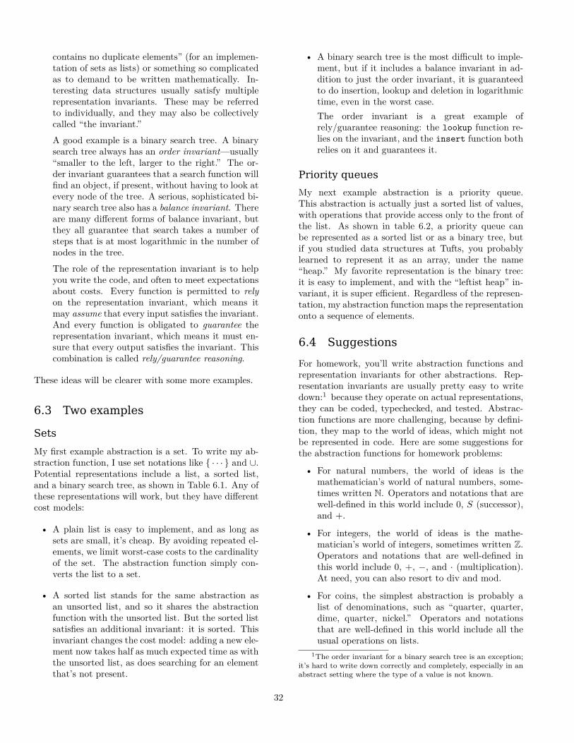
contains no duplicate elements” (for an implemen-tation of sets as lists) or something so complicatedas to demand to be written mathematically. In-teresting data structures usually satisfy multiplerepresentation invariants. These may be referredto individually, and they may also be collectivelycalled “the invariant.”A good example is a binary search tree. A binarysearch tree always has an order invariant—usually“smaller to the left, larger to the right.” The or-der invariant guarantees that a search function willfind an object, if present, without having to look atevery node of the tree. A serious, sophisticated bi-nary search tree also has a balance invariant. Thereare many different forms of balance invariant, butthey all guarantee that search takes a number ofsteps that is at most logarithmic in the number ofnodes in the tree.The role of the representation invariant is to helpyou write the code, and often to meet expectationsabout costs. Every function is permitted to relyon the representation invariant, which means itmay assume that every input satisfies the invariant.And every function is obligated to guarantee therepresentation invariant, which means it must en-sure that every output satisfies the invariant. Thiscombination is called rely/guarantee reasoning.

These ideas will be clearer with some more examples.

6.3 Two examples

Sets

My first example abstraction is a set. To write my ab-straction function, I use set notations like { · · · } and ∪.Potential representations include a list, a sorted list,and a binary search tree, as shown in Table 6.1. Any ofthese representations will work, but they have differentcost models:

• A plain list is easy to implement, and as long assets are small, it’s cheap. By avoiding repeated el-ements, we limit worst-case costs to the cardinalityof the set. The abstraction function simply con-verts the list to a set.

• A sorted list stands for the same abstraction asan unsorted list, and so it shares the abstractionfunction with the unsorted list. But the sorted listsatisfies an additional invariant: it is sorted. Thisinvariant changes the cost model: adding a new ele-ment now takes half as much expected time as withthe unsorted list, as does searching for an elementthat’s not present.

• A binary search tree is the most difficult to imple-ment, but if it includes a balance invariant in ad-dition to just the order invariant, it is guaranteedto do insertion, lookup and deletion in logarithmictime, even in the worst case.The order invariant is a great example ofrely/guarantee reasoning: the lookup function re-lies on the invariant, and the insert function bothrelies on it and guarantees it.

Priority queues

My next example abstraction is a priority queue.This abstraction is actually just a sorted list of values,with operations that provide access only to the front ofthe list. As shown in table 6.2, a priority queue canbe represented as a sorted list or as a binary tree, butif you studied data structures at Tufts, you probablylearned to represent it as an array, under the name“heap.” My favorite representation is the binary tree:it is easy to implement, and with the “leftist heap” in-variant, it is super efficient. Regardless of the represen-tation, my abstraction function maps the representationonto a sequence of elements.

6.4 Suggestions

For homework, you’ll write abstraction functions andrepresentation invariants for other abstractions. Rep-resentation invariants are usually pretty easy to writedown:1 because they operate on actual representations,they can be coded, typechecked, and tested. Abstrac-tion functions are more challenging, because by defini-tion, they map to the world of ideas, which might notbe represented in code. Here are some suggestions forthe abstraction functions for homework problems:

• For natural numbers, the world of ideas is themathematician’s world of natural numbers, some-times written N. Operators and notations that arewell-defined in this world include 0, S (successor),and +.

• For integers, the world of ideas is the mathe-matician’s world of integers, sometimes written Z.Operators and notations that are well-defined inthis world include 0, +, −, and · (multiplication).At need, you can also resort to div and mod.

• For coins, the simplest abstraction is probably alist of denominations, such as “quarter, quarter,dime, quarter, nickel.” Operators and notationsthat are well-defined in this world include all theusual operations on lists.

1The order invariant for a binary search tree is an exception;it’s hard to write down correctly and completely, especially in anabstract setting where the type of a value is not known.

32

Abstraction OperationsSet At minimum, empty/new, insert, delete,

member?; possibly also empty?, size,union, inter, diff

Representation Invariant Abstraction FunctionList No element is repeated. A([]) = { }

A(x::xs) = {x} ∪ A(xs)Sorted list No element is repeated; elements are sorted. (Same as list.)Binary search tree No element is repeated; smaller elements

are in left subtrees; larger elements are inright subtrees; perhaps some sort of balanceinvariant.

A(EMPTY) = { }A(NODE(l,x,r)) = A(l) ∪ {x} ∪ A(r)

Table 6.1: Representations of sets

Abstraction OperationsPriority queue At minimum, empty/new, insert, empty?,

and delete-min; possibly also size,find-min, merge

Representation Invariant Abstraction FunctionList List is sorted with the smallest element at

the front (inefficient unless small).A(xs) = xs

Array Element at index i is not larger than theelements at indices 2i and 2i+ 1, if any.

A(a) = sort(a)

Binary tree Element at node is not larger than elementsat left and right child, if any.

A(EMPTY) = [ ]

A(NODE(l,x,r)) = x :: merge(A(l),A(r))

Leftist heap Binary tree, with the additional invariantthat every left subtree is at least as high asthe corresponding right subtree.

(Same as binary tree.)

Table 6.2: Representations of priority queues

• For players, the abstractions are X and O.

6.5 How design steps are affected

Abstract data types affect the design process becauseof two changes:

• Contracts for functions are written for the ab-straction (“in the world of ideas”), but the func-tions themselves are written for the representation(“in the world of code”).

• Outside its defining module, an abstract type hasno forms of data.

The implications are explored below.

Design steps for client code

Outside an abstract type’s module, code is called aclient of the module. Here’s how each step of the designprocess works in client code:

1. Forms of data. Manifest types have exposed repre-sentations, so client code works with them just asusual.

Abstract types don’t give access to the forms ofdata. If you’re a client and you’re consuming ab-stract data, you’ll typically be calling observers—sometimes mutators. And to make new abstractvalues, you’ll use creators and producers.

33

A value of abstract type is a little bit analogous toa function: all you can do with it is what’s in theinterface.

2. Example inputs. Example inputs can be made onlyby calling creators, producers, and sometimes mu-tators. (Mutation makes testing harder.)

3. Functions’ names. Nothing changes.

4. Functions’ contracts. The client’s own contractsmay mention the abstraction or may even be writ-ten in terms of the abstraction. The client doesn’tknow about the representation—which is mostlythe point.

5. Example results. Any example results of abstracttype have to be expressed indirectly, again us-ing creators, producers, and sometimes mutators.(Mutation makes testing harder.)

6. Algebraic laws. When client code consumes a valueof abstract type, it can’t have one algebraic lawper form of data—an abstract type has only oneform of data. Instead, to decide on a law, you canuse side conditions from an observer, or you caneven break an observed value down by forms of itsdata. For example, in the Abstract Game Solver,it’s useful to write laws for the advice function bybreaking down the list of legal moves.

7. Case analysis. You can’t do case analysis on avalue of abstract type directly. But you may beable to do case analysis on the results of calling anobserver in the interface.

8. Coding results. Right-hand sides are coded asusual.

9. Revisit unit tests. Unit tests can be written asusual. To construct values for use in unit tests,you can call creators and producers (and possiblymutators) for the abstract type.Unit testing has a pitfall: before writing unit tests,we have to know how to compare test results forequality. A well-designed abstraction will includean equality-testing function, but unit tests oftentry to use a built-in equality, which may or maynot work. In particular, the built-in equality de-fined by Standard ML works on representations,not abstractions, and it may say two values aredifferent when they should actually be consideredthe same.

Design steps for implementations

Inside an abstract type’s module, code has completeaccess to the representation. Here’s how each step ofthe design process works in an implementation:

1. Forms of data. The implementation has completeaccess to the representation, so forms of data areavailable as usual.

2. Example inputs. Example inputs can be writtenas usual—but care must be taken to be sure thatevery example input satisfies the representation in-variant.

3. Function’s names. Nothing changes.

4. Function’s contracts. The contract of each functionis given in the interface, and it is written in termsof the abstraction. But the function itself is writtenin terms of the representation. To be confident thateach function fulfills its contract, you must definethe function with the type’s abstraction functionin mind.Also, each exported function2 has these amend-ments added to its contract:

• Every input of abstract type satisfies the rep-resentation invariant for that type.

• Every output of abstract type must satisfy therepresentation invariant for that type.

Private functions may, if they wish, deal with argu-ments and results that don’t satisfy the represen-tation invariant. Indeed, one common use of pri-vate functions is to re-establish an invariant beforereturning a result. Each private function’s rela-tionship to and action on representation invariantsmust be documented in its contract.

5. Example results. Example results can be writtenas usual, as can unit tests.

6. Algebraic laws. Algebraic laws can be written asusual.

7. Case analysis. Case analysis can be based on alge-braic laws as usual.

8. Coding. Right-hand sides are coded as usual.

9. Revisit unit tests. Unit tests can be written asusual.

2A function is exported if it is visible in the interface that isbeing implemented. C++ calls these functions “public.”

34

7. Program design with objects

Like abstract data types, objects demand that we adaptour 9-step design process, which is intended for func-tions. This lesson explains the adaptations, focusing onthe effects of dynamic dispatch and the limitations onaccess to representation. It also discusses each step inthe design process, and it shows how to convert alge-braic laws to double dispatch.

In order to use this lesson effectively, you should re-fresh your memory on the basic 9-step process describedin the introduction, as well as the preceding lesson (de-sign with abstract data types), on which this one builds.

7.1 Designing with abstraction

Many ideas from abstract data types also work withobjects:

• Barbara Liskov’s taxonomy of creators, producers,observers, and mutators (Ramsey, section 2.5.2 onpage 113) is equally useful for both abstract datatypes and objects.

• Whether an abstraction is implemented using ab-stract data types or objects, abstraction functionsand invariants continue to play a key role.

• Contracts for methods are written for the ab-straction (“in the world of ideas”), but the meth-ods themselves are written for the representation(“in the world of code”).

• Like an abstract data type outside its defining mod-ule, an object has only one form of data, which isopaque.

• Whether data abstraction is implemented using ab-stract data types or objects, program design is es-sentially interface design. This aspect of programdesign is beyond the scope of Comp 105—in 105,we work with interfaces that are given to us.

These similarities help, but our design and coding areaffected by these key differences:

• With either form of abstraction, our 9-step designprocess is useful for designing each piece of the ab-straction. But the pieces are different: with ab-stract data types, each piece is a function thatsits inside a module. With objects, each piece isa method that sits inside a class definition.

• Abstract data types give access to the representa-tion of every value of abstract type, including pa-rameters to all functions. This access comes withan obligation to understand and respect the invari-ant. Objects give access only to the representationof the receiver. Each argument must be treatedas an abstraction and dealt with by sending mes-sages in its public protocol. (If the argument issupposed to be “like” the receiver, it can also besent messages from the private protocol that theyhave in common.) This difference is discussed fur-ther in the textbook in section 10.7, which startson page 670.

• With objects, interfaces are designed not just beused by clients, but also to be inherited from bysubclasses.

• An abstract data type can have any kind of rep-resentation: an algebraic type, a tuple, or evena function, for example. An object can have onlyone kind of representation: a collection of namedinstance variables.

• A function that expects a value of abstract typecan be used only with values of that type. But amethod that expects an object of a given class canbe used with objects of any class, provided thoseobjects mimic the protocol of the class that themethod is expecting. This mimicry, which is a keyfeature of object-oriented systems, is called behav-ioral subtyping or sometimes “duck typing.”

7.2 How design steps are affected

Our design process is most heavily influenced by twoaspects of object-orientation:

• Dynamic dispatch changes the way we identifyforms of data and the way we code case analysis.Case analysis in particular is so changed that youmay not recognize it as “coding.” In particular,we never ask an object, “how were you made?”

• Information hiding denies access to the representa-tions of other objects, even if we know everythingabout their class. In other words, only the receiverof a message knows from what parts it was made.We never ask an argument object, “from what partswere you made?”

35

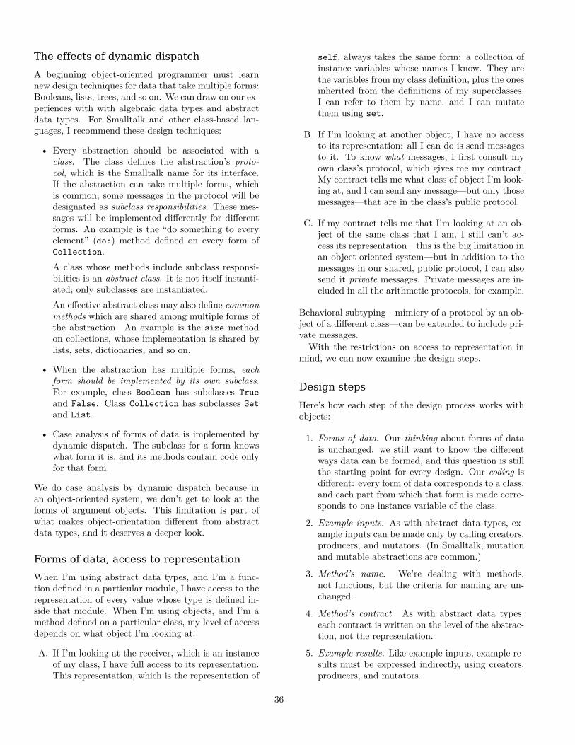
The effects of dynamic dispatch

A beginning object-oriented programmer must learnnew design techniques for data that take multiple forms:Booleans, lists, trees, and so on. We can draw on our ex-periences with with algebraic data types and abstractdata types. For Smalltalk and other class-based lan-guages, I recommend these design techniques:

• Every abstraction should be associated with aclass. The class defines the abstraction’s proto-col, which is the Smalltalk name for its interface.If the abstraction can take multiple forms, whichis common, some messages in the protocol will bedesignated as subclass responsibilities. These mes-sages will be implemented differently for differentforms. An example is the “do something to everyelement” (do:) method defined on every form ofCollection.A class whose methods include subclass responsi-bilities is an abstract class. It is not itself instanti-ated; only subclasses are instantiated.An effective abstract class may also define commonmethods which are shared among multiple forms ofthe abstraction. An example is the size methodon collections, whose implementation is shared bylists, sets, dictionaries, and so on.

• When the abstraction has multiple forms, eachform should be implemented by its own subclass.For example, class Boolean has subclasses Trueand False. Class Collection has subclasses Setand List.

• Case analysis of forms of data is implemented bydynamic dispatch. The subclass for a form knowswhat form it is, and its methods contain code onlyfor that form.

We do case analysis by dynamic dispatch because inan object-oriented system, we don’t get to look at theforms of argument objects. This limitation is part ofwhat makes object-orientation different from abstractdata types, and it deserves a deeper look.

Forms of data, access to representation

When I’m using abstract data types, and I’m a func-tion defined in a particular module, I have access to therepresentation of every value whose type is defined in-side that module. When I’m using objects, and I’m amethod defined on a particular class, my level of accessdepends on what object I’m looking at:

A. If I’m looking at the receiver, which is an instanceof my class, I have full access to its representation.This representation, which is the representation of

self, always takes the same form: a collection ofinstance variables whose names I know. They arethe variables from my class definition, plus the onesinherited from the definitions of my superclasses.I can refer to them by name, and I can mutatethem using set.

B. If I’m looking at another object, I have no accessto its representation: all I can do is send messagesto it. To know what messages, I first consult myown class’s protocol, which gives me my contract.My contract tells me what class of object I’m look-ing at, and I can send any message—but only thosemessages—that are in the class’s public protocol.

C. If my contract tells me that I’m looking at an ob-ject of the same class that I am, I still can’t ac-cess its representation—this is the big limitation inan object-oriented system—but in addition to themessages in our shared, public protocol, I can alsosend it private messages. Private messages are in-cluded in all the arithmetic protocols, for example.

Behavioral subtyping—mimicry of a protocol by an ob-ject of a different class—can be extended to include pri-vate messages.

With the restrictions on access to representation inmind, we can now examine the design steps.

Design steps

Here’s how each step of the design process works withobjects:

1. Forms of data. Our thinking about forms of datais unchanged: we still want to know the differentways data can be formed, and this question is stillthe starting point for every design. Our coding isdifferent: every form of data corresponds to a class,and each part from which that form is made corre-sponds to one instance variable of the class.

2. Example inputs. As with abstract data types, ex-ample inputs can be made only by calling creators,producers, and mutators. (In Smalltalk, mutationand mutable abstractions are common.)

3. Method’s name. We’re dealing with methods,not functions, but the criteria for naming are un-changed.

4. Method’s contract. As with abstract data types,each contract is written on the level of the abstrac-tion, not the representation.

5. Example results. Like example inputs, example re-sults must be expressed indirectly, using creators,producers, and mutators.

36

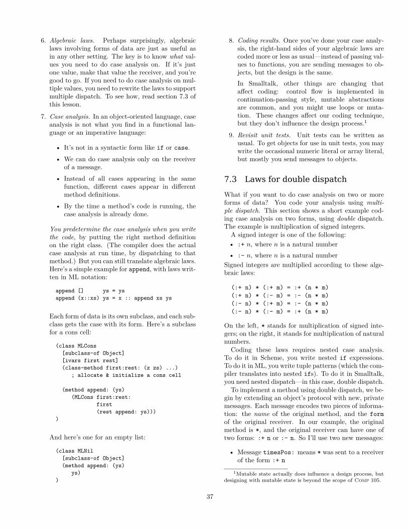
6. Algebraic laws. Perhaps surprisingly, algebraiclaws involving forms of data are just as useful asin any other setting. The key is to know what val-ues you need to do case analysis on. If it’s justone value, make that value the receiver, and you’regood to go. If you need to do case analysis on mul-tiple values, you need to rewrite the laws to supportmultiple dispatch. To see how, read section 7.3 ofthis lesson.

7. Case analysis. In an object-oriented language, caseanalysis is not what you find in a functional lan-guage or an imperative language:

• It’s not in a syntactic form like if or case.• We can do case analysis only on the receiver

of a message.• Instead of all cases appearing in the same

function, different cases appear in differentmethod definitions.

• By the time a method’s code is running, thecase analysis is already done.

You predetermine the case analysis when you writethe code, by putting the right method definitionon the right class. (The compiler does the actualcase analysis at run time, by dispatching to thatmethod.) But you can still translate algebraic laws.Here’s a simple example for append, with laws writ-ten in ML notation:

append [] ys = ysappend (x::xs) ys = x :: append xs ys

Each form of data is its own subclass, and each sub-class gets the case with its form. Here’s a subclassfor a cons cell:

(class MLCons[subclass-of Object][ivars first rest](class-method first:rest: (z zs) ...)

; allocate & initialize a cons cell

(method append: (ys)(MLCons first:rest:

first(rest append: ys)))

)

And here’s one for an empty list:

(class MLNil[subclass-of Object](method append: (ys)

ys))

8. Coding results. Once you’ve done your case analy-sis, the right-hand sides of your algebraic laws arecoded more or less as usual—instead of passing val-ues to functions, you are sending messages to ob-jects, but the design is the same.In Smalltalk, other things are changing thataffect coding: control flow is implemented incontinuation-passing style, mutable abstractionsare common, and you might use loops or muta-tion. These changes affect our coding technique,but they don’t influence the design process.1

9. Revisit unit tests. Unit tests can be written asusual. To get objects for use in unit tests, you maywrite the occasional numeric literal or array literal,but mostly you send messages to objects.

7.3 Laws for double dispatch

What if you want to do case analysis on two or moreforms of data? You code your analysis using multi-ple dispatch. This section shows a short example cod-ing case analysis on two forms, using double dispatch.The example is multiplication of signed integers.

A signed integer is one of the following:• :+ n, where n is a natural number• :- n, where n is a natural number

Signed integers are multiplied according to these alge-braic laws:

(:+ n) * (:+ m) = :+ (n * m)(:+ n) * (:- m) = :- (n * m)(:- n) * (:+ m) = :- (n * m)(:- n) * (:- m) = :+ (n * m)

On the left, * stands for multiplication of signed inte-gers; on the right, it stands for multiplication of naturalnumbers.

Coding these laws requires nested case analysis.To do it in Scheme, you write nested if expressions.To do it in ML, you write tuple patterns (which the com-piler translates into nested ifs). To do it in Smalltalk,you need nested dispatch—in this case, double dispatch.

To implement a method using double dispatch, we be-gin by extending an object’s protocol with new, privatemessages. Each message encodes two pieces of informa-tion: the name of the original method, and the formof the original receiver. In our example, the originalmethod is *, and the original receiver can have one oftwo forms: :+ n or :- n. So I’ll use two new messages:

• Message timesPos: means * was sent to a receiverof the form :+ n

1Mutable state actually does influence a design process, butdesigning with mutable state is beyond the scope of Comp 105.

37

• Message timesNeg: means * was sent to a receiverof the form :- n

Using these messages, I write “laws of dispatch:”

(:+ n) * A = (A timesPos: (:+ n))(:- n) * A = (A timesNeg: (:- n))

In these laws, there’s no case analysis on the argu-ment A. The only case analysis is on :+ n versus :- n,which should be coded by dynamic dispatch of * on theclass of the receiver. We implement the * method bysending timesPos: or timesNeg: to the argument A.

To design timesPos: and timesNeg:, we need laws.To get them, we combine the dispatch laws with theoriginal laws for *. We start by expanding the dis-patch laws, noting that argument A can take two forms.I make two copies of each dispatch law—one where A is:+ m, and one when A is :- m:

(:+ n) * (:+ m) = ((:+ m) timesPos: (:+ n))(:+ n) * (:- m) = ((:- m) timesPos: (:+ n))

(:- n) * (:+ m) = ((:+ m) timesNeg: (:- n))(:- n) * (:- m) = ((:- m) timesNeg: (:- n))

By design, the expanded dispatch laws have the sameleft-hand sides as the original laws for *. So the corre-sponding right-hand sides must be equal:

((:+ m) timesPos: (:+ n)) = :+ (n * m)((:- m) timesPos: (:+ n)) = :- (n * m)

((:+ m) timesNeg: (:- n)) = :- (n * m)((:- m) timesNeg: (:- n)) = :+ (n * m)

Now I can write one method definition for each law.Here are two of the four:(method timesPos: (plus-n) ; self is :+ m(LargePositiveInteger

withMagnitude:(magnitude * (plus-n magnitude))))

(method timesPos: (plus-n) ; self is :- m(LargeNegativeInteger

withMagnitude:(magnitude * (plus-n magnitude))))

Which method goes on which class? You figure it out.

38

Acknowledgements

The design process presented in this monograph is adirect descendant of the six-step “design recipe” devel-oped by Felleisen, Findler, Flatt, and Krishnamurthi(second edition, 2018). The process and some individ-ual lessons also draw on the work of Tony Hoare onabstract data types, the work of John Guttag and Jean-nette Wing on algebraic specification, and the work ofWill Cook on data abstraction.

The first draft of Lesson 1 was written by Nate Bragg.

39