Perspectives on Projective Geometry
591
J¨ urgen Richter-Gebert Perspectives on Projective Geometry A Guided Tour through Real and Complex Geometry (Draft Version) October 3, 2010 Springer
-
Upload
khangminh22 -
Category
Documents
-
view
0 -
download
0
Transcript of Perspectives on Projective Geometry

Jurgen Richter-Gebert
Perspectives on Projective
Geometry
A Guided Tour through Real and Complex Geometry
(Draft Version)
October 3, 2010
Springer

About This Book
Let no one ignorant of geometry enter here!
Entrance to Plato’s academy
Once or twice she had peeped into the book her sister wasreading, but it had no pictures or conversations in it, “andwhat is the use of a book,” thought Alice, “without pictures orconversations?”
Lewis Carroll,Alice’s Adventures in Wonderland
Geometry is the mathematical discipline that deals with the interrelationsof objects in the plane, in space, or even in higher dimensions. Practicinggeometry comes in very different flavors. More than any other mathematicaldiscipline, the field of geometry ranges from the very concrete and visual tothe very abstract and fundamental. In the one extreme, geometry deals withvery concrete objects such as points, lines, circles, and planes and studiesthe interrelations between them. On the other side, geometry is a benchmarkfor logical rigor, the elegance of axiom systems, and logical chains of proof.There is a third way of thinking about geometry that stands alongside the vi-sual and the logic-based approaches: the algebraic treatment. Here algebraicstructures such as vectors, matrices, and equations are used to form a kind ofparallel world, in which each geometric object and relation has an algebraicmanifestation. Also in this parallel world the considerations may be veryconcrete and algorithmic or very abstract and functorial. This book explains
v
vi
how to treat the fundamental objects of geometry with appropriate alge-braic methods. Many of the techniques presented this book have their rootsin the work of the great geometers of the nineteenth century like Plucker,Grassmann, Mobius, Klein, and Poincare (to mention only a few).
The algebraic representations are, however, more by far than a way toexpress geometric objects by numbers. Very often, finding the right algebraicstructure unveils the “true” nature of a geometric concept. It may open newperspectives and deep insights on matters that seemed elementary at firstsight and help to generalize, connect, interpret, visualize, understand. Thisis what this book is about. Its ultimate aim is to present the beauty thatlies in the rich interplay of geometric structures and their algebraic counter-parts. A warning should be issued right at the beginning. It is relatively easyto transform geometric objects into algebraic ones. For instance, points inthe plane may be easily represented by their xy-coordinates. However, these“naive” approaches to representing geometric objects are very often not thosethat lead to far-reaching conclusions. Often it is useful to introduce more so-phisticated algebraic methods that may seem more abstract at first sight butare more powerful and elegant later on. Guided by these more abstract andelegant structures, it may even happen that one is willing to modify the orig-inal concept of the geometric first-class citizens (say points or lines) and forinstance add some new type of (more abstract) objects. When we talk abouthomogeneous coordinates, one of the most fundamental concepts of this book,exactly this will happen. We will first see that in the plane very elementaryoperations such as computing the line through two points and computingthe intersection of two lines can be very elegantly expressed if lines as wellas points are represented by three-dimensional coordinates (where nonzeroscalar multiples are identified). Having a closer look at the relation of planarpoints and their three-dimensional representing vectors, we will observe thatcertain vectors do not represent points in the real Euclidean plane. This mo-tivates the search for a geometric interpretation of these nonexistent points.It turns out that they may be interpreted as “points that are infinitely faraway.” We then will extend the usual two-dimensional plane by these newpoints at infinity and obtain a richer and more elegant geometric system: thesystem of projective geometry.
In a certain sense this way of thinking is quite similar to the work ofchemists at the time when periodic table of the elements was about to bediscovered. Based on the elements known so far, they looked for ways toexplain their behavior. At some point they spotted a structure and certainsymmetry principles into which all the known chemical elements could be fit-ted (the periodic table of the elements). However, some places in the periodictable did not correspond to known elements. It became soon more reasonableto claim the existence of these undiscovered elements than to give up theinner beauty and explanatory power of the periodic table. Later on, all ele-ments whose existence had been conjectured were indeed discovered. The role
vii
of “discovering elements” in mathematics is played by the “interpretation ofconcepts.” We will meet such situations quite often in this book.
The spirit of this book. In a sense, this book is much more about the“how” than about the “what” in geometry. The reader will recognize thatvery often we will study very simple objects and their relations. Elementaryobjects such as points, lines, circles, conics, angles, and distances are thereal first-class citizens in our approach. Also, the operations we study willbe quite elementary: intersecting two lines, intersecting a line and a conic,calculating tangents, etc. Most of these operations may in principle be per-formed with some advanced high-school mathematics. Regardless of that, ouremphasis will be on structures that at the same time allow us to express thefundamental objects as well as the operations on them in a most elegantway. So the algebraic representation of an object never stands alone; it al-ways is related to the operations that should be performed with the object.As mentioned before, these advanced representations often lead to new in-sights and broaden our understanding of the seemingly well-known objects.In this respect our philosophy here is very close to Felix Klein’s famous book“Elementary Mathematics From an Advanced Standpoint.”
When reading this book, the reader will find that the definitions and con-cepts are more important than the theorems. Very often the same (sometimeselementary) theorems are re-proved with different approaches. A topic thatwill show up over and over again is the question of how elegantly and gener-alizably these proofs can be performed by the various methods. I hope thatthe reader will find these multiple perspectives on related topics a good wayto get a deeper understanding of what is going on.
A little history. As mentioned before, many of the techniques in this bookgo back to what could be called the golden age of geometry, the hundred yearsbetween 1790 and 1890. In this period, starting with Gaspard Monge manyfundamental geometric concepts were discovered that went far beyond Eu-clid’s Elements (which until then dominated geometric thinking). Many ofthese new concepts were intimately related to the underlying algebraic struc-tures. In that period, algebra and geometry underwent a kind of coevolution,inspiring and enhancing each other. Projective geometry turned out to beone of the most fundamental structures that at the same time had the mostelegant algebraic representation. The concepts of linear and multilinear alge-bra were developed in close connection to their geometric significance. Thedevelopment culminated in the revolutionary discovery of what now is called“hyperbolic geometry”: a geometric structure that violates the fifth postu-late of Euclid and still is logically on an equal footing to his geometry. Atits time, this discovery was so revolutionary that C.F. Gauss, who was oneof the main protagonists in this discovery and at the same time one of theworld’s leading mathematicians, kept it a secret and never published any-thing on that topic. (We will dedicate several chapters to this topic.) The
viii
key to an elegant treatment of hyperbolic geometry again lies in projectiveapproaches. Nowadays, hyperbolic geometry is a well-established, amazinglyrich mathematical subject with flourishing connections to many other fields,such as topology, group theory, number theory, combinatorics, numerics, andmany more.
Unfortunately, in the nineteenth century, the field of geometry grew per-haps a bit too fast. Many books with many pictures, many theorems, andmany proofs of varying mathematical quality were published. Some of theproofs heavily relied on pictorial reasoning. At some time around the turnof the century, a point was reached where it was difficult to say which ofthese results were to be trusted and which were not. As a kind of antitheticaldevelopment, this time was the beginning of a school of new and so far un-matched mathematical rigor. David Hilbert was one of the leading figures inthe progress of rewriting all geometry from scratch in order to place it on areliable and safe foundation. His book “Grundlagen der Geometrie” (Foun-dations of Geometry) [58] starts with an axiom system that even fixed gapsin Euclid’s axioms and postulates to develop a watertight building of geome-try. Hilbert’s famous saying that one must be able to say “tables, chairs, beermugs” each time in place of “points, lines, planes” refers to the demand thatan axiom system must be completely formal and not at all depend on imagi-nation. By this strict approach he and several other mathematicians triggereda development in which geometry was treated as a purely formal science. Thehardliners of this program claimed that pictures, and in particular pictorialreasoning, had to be abandoned from geometry books.1
This development was a kind of catharsis for geometry, and many impor-tant and subtle points were revealed in that time (from 1900 to approximately1970). However, this formal approach also had its disadvantages. There is afamous half-joking quotation from Johann Wolfgang von Goethe about math-ematical abstractions:
Mathematicians are a kind of Frenchmen; whatever you say to them they translateinto their own language, and forthwith it is something entirely different.
Something like this happened to geometry in the time of rigorous abstraction.Abstraction opened mathematicans’ eyes to many far-reaching concepts, suchas alternative axiom systems, algebraic geometry, and combinatorial gener-alizations. At the same time, it changed the concept of what was considereda first-class mathematical citizen. Germs, schemes, matroids, and configura-tion spaces became more important than (the old-fashioned) points, lines,and planes.
By this process many important concepts were almost forgotten. Largeparts of the still valuable “old geometry” were no longer taught at the uni-versities. The following personal anecdote shall exemplify this. It was around1993 when I gave a talk at KTH (Kungliska Tekniska Hogskolan) in Sweden,
1 It is a kind of historical irony that Hilbert, jointly with Cohn-Vossen, wrote a beautifuland highly visual book entitled “Geometry and the Imagination” [59].
ix
where I mentioned a certain (and I think really cool) way to construct the fociof an ellipse by just drawing certain four (complex) tangents and intersectingthem (see Figure 19.6). After the talk, a much older colleague came to meand said, “Oh, I am so glad. I thought that today nobody remembered thisconstruction and that I might be one of the last ones who knew it.” In fact,I learned this construction from a book of Blaschke from the 1940s [6], and Ihardly know a modern textbook in which it is taught. Perhaps this was oneof the points at which I decided to write this book.
Geometry and Computers. Since the 1970s, the role of geometric rea-soning has again undergone a structural change. The reason for this is thatcomputers, and in particular computer graphics, have played a more andmore important role. This has had an effect in two directions. On the onehand, in order to obtain good visualizations (also in nonmathematical fieldssuch as CAD, animated movies, games) it is essential to have a good and far-reaching modeling of the objects that should be visualized, be it the newestautomobile design, the dinosaurs in Jurassic Park, or chemical molecules.For such visualizations, even on a very elementary level the elegant treat-ment of primitives such as points, lines, and circles becomes a key issue. Onthe other hand, the computer became a tool that allowed mathematicians tovisualize abstract concepts and to do exact research on a level that is stillquite visual. In particular, computers have made it possible to interact di-rectly with mathematical (and in particular with geometric) structures. Allthese developments brought a more concrete and more algorithmic treatmentof geometry again to the mathematical world’s attention. In fact, it turnedout that many concepts related to nineteenth-century geometry are highlyappropriate for dealing with geometric structures in a computational way.
I myself began my research career at a time (around 1985) at which com-putational methods were seriously entering the everyday work of mathemati-cians. From then until now I have gone through a chain of topics that defi-nitely shaped the selection of topics in this book. For me, an amazing experi-ence was that this chain went from quite abstract concepts in combinatorialgeometry to more and more elementary (or let us rather say fundamental)concepts and questions. Following these experiences it became more and moreclear that the key to an elegant treatment of geometric structures lies in agood algebraic representation and goes straight to the heart of ninetheenthcentury geometry. Since many of these topics I was working on form a kindof “knowledge base” for this book, I will briefly mention this chain. I startedworking on the structural and computational treatment of so-called realiz-ability questions on combinatorial geometry (we will meet this topic brieflyin Section 27.2). In this area it turned out that invariant theoretic and pro-jective methods (see Chapter 6 and Chapter 7) are fundamental. In fact (andthis was part of my own PhD thesis), these methods could be used to im-plement algorithms that were able to generate “readable algebraic proofs”for many geometric incidence theorems (see Chapter 15) and by this can
x
form the basis of a kind of geometric expert system. After implementing thisprover, I had the desire to have a nice interactive input device for geomet-ric configurations that could be used to feed the prover. What started as asmall seemingly simple project turned out to be a task that is still occupyingquite a substantial fraction of my research work. The original demands forthis input interface were comparatively simple. The user should be able touse the mouse to construct geometric configurations containing points, lines,circles, conics, etc. After the construction is finished it should be possible tograb basis elements with the mouse, move them, and watch the constructionchange according to the rules of the construction. If the configuration encodesan incidence theorem, it should be possible to ask the prover for a proof ofit. My experience in combinatorial geometry and invariant theory made itimmediately clear that such a system, if it should be elegant, must be basedon projective methods, since they have the nice feature of eliminating manyspecial cases. What started at this time (a first prototypical project was un-dertaken together with Henry Crapo in 1992) for me turned out to be anongoing search for elegant structures to represent the fundamental objectsin geometry. In a sense, this book tells about half of this story. In 1996 Istarted the development of a less prototypical system for dynamic geometry(Cinderella), jointly with Ulrich Kortenkamp [112, 113]. In this system wetried to represent the geometric objects in a way that allows for a smoothimplementation of geometric primitive operations. One can read the presentbook as a guide to the representation of these objects and operations. Onefundamental breakthrough in the Cinderella project was the discovery thatin order to get a continuous dynamic behavior of the geometric elements it isnecessary to embed the whole situation in an ambient complex space and ina sense navigate on Riemann surfaces (see [72, 73, 74]). This is the other halfof the story, on which we will only very briefly touch in the very last sectionof the very last chapter. To tell it in full length would require another book.
Applications, beauty, pictures, and formulas: This book is intendedto serve two purposes. On the one hand, it should be very “hands-on” andpurposely focuses on elementary objects such as points, lines, circles, conics,and their interrelations. The reader will find many concrete and directly ap-plicable formulas and recipes for performing operations, measurements, andtransformations on them. On the other hand, the book is intended to com-municate some of the inner beauty of the subject. For me it is one of the mostbeautiful mathematical topics, with many amazing twists, surprises, and sub-tleties and still of fundamental importance for many practical applications.
Although this book presents many such explicit algebraic and algorith-mic methods for performing primitive operations, the observant reader mayrecognize that in this book there are comparatively few long algebraic deriva-tions and calculations. This is intimately related to the approach of workingon a conceptual level. We will try to derive conceptual setups that make ex-plicit calculations superfluous whenever possible. By this we are close to the
xi
philosophy of one of the most important persons in nineteenth century ge-ometry, Julius Plucker. Felix Klein, who was his direct student, wrote abouthim:
In der Pluckerschen Geometrie wird die bloße Kombination von Gleichungen ingeometrische Auffassung ubersetzt und ruckwarts durch letztere die analytische Op-eration geleitet. Rechnung wird nach Moglichkeit vermieden, dabei eine bis zur Vir-tuositat gesteigerte Beweglichkeit der inneren Anschauung, der geometrischen Aus-deutung vorliegender analytischer Gleichungen ausgebildet und in reichem Maßeverwendet.
Or in the translation by M. Ackermann:
In Plucker’s geometry the bare combination of equations is translated into geomet-rical terms, and the analytic operations are led back through the geometric. Com-putation is avoided as far as possible; but by doing this, a mobility, heightened tothe point of virtuosity, of inner intuition of the geometric interpretation of givenanalytic equations, is cultivated and extensively applied.
Many of the formulas and derivations that are given here are not only usedto do a formal derivation that takes one from a statement A to a statementB. Rather than, that formulas very often have a structural component. Manyof them have interesting symmetry properties, a certain rhythm, so to speak.It is perhaps advisable that the reader pause at some point and meditate abit on this inner structure and symmetry of some of the formulas.
In the book you will also find many pictures, diagrams, and illustrations(so hopefully Alice will find it useful after all). They are intended to illustrateand not to replace the proofs and concepts that are presented. As with theformulas, while reading the book it is highly recommended that one spend asubstantial amount of time looking closely at some of the pictures. A pictureis worth a thousand words, and not everything that one might see and observein the pictures is also in the text. So I recommend that the reader take sometime for meditation on the pictures, their hidden symmetry structures, theirspatial interpretations, their dynamic behavior.
Why this book? One might wonder why one should take the effort towrite a 550-page book about projective geometry that contains so much “oldgeometry.” There are several reasons, and I will try to explain a few of them.
My experience over the past few years: As already mentioned, much of myown work has been tightly related to the representation of geometric objectson a computer. In the area of automated theorem-proving as in the area ofdynamic geometry, the classical approaches turned out to be extremely useful.Homogeneous coordinates, invariant theoretic methods, Grassmann-Plucker-Relations, Cayley-Klein geometries and many other topics that are centralin this book were the key for understanding and implementing versatile andflexible tools. This book gives a selection of those topics that I found mosthelpful either from a structural point of view (how things are related) or froma pragmatic point of view (what is needed for implementations). Furthermore,
xii
many aspects have been added to the purely classical viewpoint that hopefullygive some new interrelations between the topics.
Backing up knowledge: I had to learn many of these concepts from the oldoriginal literature. Mathematical language changes over time, and sometimesit takes quite a bit of decoding to understand what some concept in someoriginal paper really means. Although much of the old mathematics maybe still valuable from a modern point of view, it might become increasinglyinaccessible. In particular, if (as in the case of classical projective geometry)some concepts are no longer regularly taught at universities, they enter a self-reinforcing loop of fading from commonly available knowledge. Fortunately,the advent of computer visualization has made classical projective geometryagain an important topic. However, many of the deeper concepts are stillaccessible only to the experts. A few months ago I had a discussion withmy colleague Tim Hoffmann on this topic, and in the discussion we founda nice metaphor for what is going on. Writing about classical topics in amodern language is like copying films from video-tape to DVDs. The oldmedia still exist; however, it becomes increasingly unlikely that they are used.It needs a refreshing copy procedure that takes the data/knowledge to aformat accessible by modern readers (i.e. DVD players). So part of this bookproject is a kind of backup process. Still I can truly recommend to everyone toread at least once Felix Klein’s Vorlesungen uber nicht-euklidische Geometrie[68] or Plucker’s System der analytischen Geometrie [100].
The audience: This book is intentionally written in a style that shouldbe accessible to students who have basically finished their elementary linearalgebra course. It should be accessible to mathematicians as well as computerscientists and physicists. Most of the topics of this book are presented in arelatively self-contained way. So it should be even possible for the geometrynovice to profit from reading it.
A guided tour: Here is a brief summary of the topics you will meet in thefollowing chapters. Except for Chapter 1 (which is a bit special, as you willsee), this book is divided into three parts. The first part is entitled “Projec-tive Geometry” and deals with the very fundamental objects and concepts.Projective spaces are introduced, first on an axiomatic level (Chapter 2)and then in direct relation to spaces related to real geometry (“real” in thesense of the real numbers R). Homogeneous coordinates are introduced as themain tool to deal with projective geometry on an algebraic level (Chapter 3).Their transformations are also studied. In particular, it is shown how vari-ous transformations can all be handled by a unified framework. Chapter 4deals with first simple invariants under these transformations. Cross-ratiosare prominently introduced. They will form the foundation of many inves-tigations of the later chapters. Chapter 5 is perhaps the theoretically mostcomplicated chapter of the first part. There we show that projective trans-formations can as well be characterized by certain invariant properties (for

xiii
instance collinearity). This chapter could be skipped on first reading. Chap-ters 6 and 7 demonstrate the importance of determinants in this context. Itis sketched how one could alternatively build up the framework of projectivegeometry by taking determinants instead of points as first-class citizens.
The second part is entitled “Working and Playing with Geometry.” Inthis part a selection of topics is presented that can be nicely treated withprojective concepts. In a way, this part is also largely about the “flexibilityof thinking” in Plucker’s sense. There we try to demonstrate the concep-tual power of projective geometry and homogeneous coordinates. Chapter 8introduces more elaborate invariants. Chapters 9 to 11 deal intensively withconics. These chapters are of fundamental importance for the rest of the bookand should not be skipped. Chapter 12 explains how the concepts general-ize to higher dimensions. Chapters 13 and 14 are in a sense special again.They introduce a beautiful method of dealing with projective geometry ona diagrammatic level. In this language, each formula can be expressed by agraphical diagram. Algebraic derivations translate to graph manipulations.These two chapters can be skipped at first reading; however, skipping themmeans to miss many beautiful concepts. Chapter 15 finally tries to presentall previously mentioned concepts in a combined way and highlights sev-eral interesting geometric incidence theorems and invariant-theoretic provingmethods.
The third part is entitled “Measurements.” It deals with a fundamentalproblem that remains after the first two parts. Over the real numbers, projec-tive geometry and homogeneous coordinates are a powerful system. However,they have one great disadvantage. The only concepts that can be dealt withare those that are stable under projective transformations. This implies thatsuch elementary geometric operations as measuring a distance and measuringan angle have no direct analogue in real projective geometry. Also, such fun-damental objects as circles are not objects of real projective geometry. Thisproblem has a beautiful resolution. Performing projective geometry over thecomplex numbers allows for the utilization of the geometric properties of thisnumber field. Since multiplication by complex numbers of unit length corre-sponds to a rotation and rotations implicitly encode distances, this impliesthat using complex numbers allows one to express measurements in projectivegeometry. We will see that, for instance, circles can be expressed as specialconics that pass through two special complex points I and J. Adding thesetwo points to projective geometry will essentially allow us to perform Eu-clidean operations. The entire third part is about the utilization of complexnumbers for performing measurements. Chapter 16 gives a brief introductionto the geometry of complex numbers. Chapter 17 introduces the complexprojective line, a first structure in which cocircularity can be expressed in apurely projective framework. Chapter 18 merges the structure of the real pro-jective plane and the complex projective line to give a system that combinesthe advantages of both spaces. Chapter 19 gives many concrete examples ofhow this general philosophy applies to various Euclidean concepts. Chapters
xiv
20 to 26 deal with a bold generalization of this approach. It is shown howmeasurements can be based on projective calculations with respect to a conic.There all three branches (projective invariants, conics, and complex numbers)are combined to form the very general framework of Cayley-Klein geometries.Chapter 20 introduces the basic concepts. Chapter 21 introduces the generalframework for measurements. Chapters 22 and 23 deal with various specialgeometric properties and theorems in these spaces. The historically very im-portant topic of hyperbolic geometry is a special Cayley-Klein geometry. Wededicate Chapters 24 to 26 to it as the representation of hyperbolic elemen-tary geometry. Hyperbolic geometry turns out to be a so-called nondegenerateCayley-Klein geometry. This gives it various symmetry properties not sharedby general Cayley-Klein geometries.
Finally, in Chapter 27 we briefly mention a few topics that demonstratehow projective geometry influences other parts of mathematics, among themalgebraic geometry, combinatorics, quantum information theory, and dynamicgeometry.
I want to thank!It has taken what seems to me like an eternity to complete this book, therewere many people involved in reading through the drafts in its various stages.Some of them commented, some of them corrected, some of them protested(at the right places) some of them encouraged. I am sure that I will forgetto mention many of them by name here. So first of all a great thank you toeveryone who gave me any kind of feedback on the manuscript during thelast six years.
There are some people who were very active in the final stages of thismanuscript. They corrected numerous typos, improved my written englishand went through some index battles in the formulas. Among them wereMichael Schmid, Thorsten Orendt, Johann Hartl, Susanne Apel, HermannVogel, Tim Hoffmann, Peter Lebmeir and Vanessa Krummeck, Martin vonGagern. A special thank goes to Oswald Giering who went through large partsof the manuscript and made very valuable mathematical comments. Threepeople deserve a very great Thank You during the final phase of writingthe book. David Kramer and Stephan Lembach took the pain to go throughthe entire (pre-)final version of the manuscript and tried to correct all thespalling2, punctation, formula layout, unidiomatic use of terms and so on. Thethird person is Jutta Niebauer who was incredibly patient while entering allthese piles of corrections into my original the TEX files.
Drawings are essential for this book and most of the drawings have beencreated with suitable software. A great thank you goes to Ulrich Kortenkampmy coauthor of the Cinderella project. Writing the software and the book is atightly interwoven process and I guess without our mathematical discussionson the software several sections of this book would never have been written.In Section 26.5 you will see beautiful pictures of hyperbolic ornaments. They
2 I wrote this acknowledgement after they finisched their work.

xv
have been produced with the software project morenaments by Martin vonGagern (using hand drawn sketches of myself as input) . Also this projectwas essential for shaping some of the mathematics presented in this book.
I cannot count the mathematical discussions I have had with colleaguesand students on various topics of this book. Many students who attended myclasses on Projective Geometry helped to clarify several mathematical andstylistic issues. Many of them definitely helped to clarify the exposition. I amespecially grateful to those of them who encouraged me to leave the bookin its present rather explanatory style. They convinced me that even todaystudents are willing to read fat books and that it is worse to approach thesame topic from very different directions. Discussions with colleagues werealso essential I here just want to mention a few of the main players that haveconsciously or unconsciously contributed to the book in its present form3:Gunter Ziegler, Jim Blinn, Jurgen Bokowski, Bernd Sturmfels, Henry Crapo,Walter Whiteley, Ulrich Kortenkamp, AleXX Below, Martin von Gagern. Aspecial thank you goes to Anders Bjorner, who in the very premature stagesof this project encouraged me to write this book. Perhaps here I should alsomention two other mathematicians from whom I learned a lot although Iwill here on earth unfortunately never have the chance to meet them: JuliusPlucker and Felix Klein.
Publishing this book at Springer Verlag means a lot to me. I am veryhappy to be able to collaborate with Martin Peters and Ruth Allewelt. Theyalways were friendly and remained patient although writing this book tookmuch longer than promised.
My greatest, warmest and foremost thanks go to the one person thatinfluenced me most during my entire life. Without the love, encouragement,deep understanding, patience and believe of my wife Ingrid all other thingswould mean nothing at all. Thank you!
A special thank goes also to my daughter Angie. I am surprised that sheis still willing to give stylistic advice on so many fine points. Her fresh andmodern look on things helped to improve the layout and graphical appearanceat many places.
A final thanks goes to Jimmy our new “family member.” He helped me tostay grounded in the very final stages of the manuscript.
3 i.e. I learned from them a lot.

Contents
1 Pappos’s Theorem: Nine Proofs and Three Variations . . . . 31.1 Pappos’s Theorem and Projective Geometry . . . . . . . . . . . . . . . 41.2 Euclidean Versions of Pappos’s Theorem . . . . . . . . . . . . . . . . . . 61.3 Projective Proofs of Pappos’s Theorem . . . . . . . . . . . . . . . . . . . . 131.4 Conics . . . . . . . . . . . . . . . . . . . . . . . . . . . . . . . . . . . . . . . . . . . . . . . . 191.5 More Conics . . . . . . . . . . . . . . . . . . . . . . . . . . . . . . . . . . . . . . . . . . . 221.6 Complex Numbers and Circles . . . . . . . . . . . . . . . . . . . . . . . . . . . 241.7 Finally... . . . . . . . . . . . . . . . . . . . . . . . . . . . . . . . . . . . . . . . . . . . . . . 29
Part I Projective Geometry
2 Projective Planes . . . . . . . . . . . . . . . . . . . . . . . . . . . . . . . . . . . . . . . . . 352.1 Drawings and Perspectives . . . . . . . . . . . . . . . . . . . . . . . . . . . . . . . 362.2 The Axioms . . . . . . . . . . . . . . . . . . . . . . . . . . . . . . . . . . . . . . . . . . . 402.3 The Smallest Projective Plane . . . . . . . . . . . . . . . . . . . . . . . . . . . 43
3 Homogeneous Coordinates . . . . . . . . . . . . . . . . . . . . . . . . . . . . . . . . 473.1 A Spatial Point of View . . . . . . . . . . . . . . . . . . . . . . . . . . . . . . . . . 473.2 The Real Projective Plane with Homogeneous Coordinates . . 493.3 Joins and Meets . . . . . . . . . . . . . . . . . . . . . . . . . . . . . . . . . . . . . . . . 523.4 Parallelism . . . . . . . . . . . . . . . . . . . . . . . . . . . . . . . . . . . . . . . . . . . . 553.5 Duality . . . . . . . . . . . . . . . . . . . . . . . . . . . . . . . . . . . . . . . . . . . . . . . 563.6 Projective Transformations . . . . . . . . . . . . . . . . . . . . . . . . . . . . . . 583.7 Finite Projective Planes . . . . . . . . . . . . . . . . . . . . . . . . . . . . . . . . . 64
4 Lines and Cross-Ratios . . . . . . . . . . . . . . . . . . . . . . . . . . . . . . . . . . . 674.1 Coordinates on a Line . . . . . . . . . . . . . . . . . . . . . . . . . . . . . . . . . . . 684.2 The Real Projective Line . . . . . . . . . . . . . . . . . . . . . . . . . . . . . . . . 694.3 Cross-Ratios (a First Encounter) . . . . . . . . . . . . . . . . . . . . . . . . . 724.4 Elementary Properties of the Cross-Ratio . . . . . . . . . . . . . . . . . . 74
xvii
xviii Contents
5 Calculating with Points on Lines . . . . . . . . . . . . . . . . . . . . . . . . . . 795.1 Harmonic Points . . . . . . . . . . . . . . . . . . . . . . . . . . . . . . . . . . . . . . . 805.2 Projective Scales . . . . . . . . . . . . . . . . . . . . . . . . . . . . . . . . . . . . . . . 825.3 From Geometry to Real Numbers . . . . . . . . . . . . . . . . . . . . . . . . . 835.4 The Fundamental Theorem . . . . . . . . . . . . . . . . . . . . . . . . . . . . . . 865.5 A Note on Other Fields . . . . . . . . . . . . . . . . . . . . . . . . . . . . . . . . . 885.6 Von Staudt’s Original Constructions . . . . . . . . . . . . . . . . . . . . . . 895.7 Pappos’s Theorem . . . . . . . . . . . . . . . . . . . . . . . . . . . . . . . . . . . . . . 91
6 Determinants . . . . . . . . . . . . . . . . . . . . . . . . . . . . . . . . . . . . . . . . . . . . . 936.1 A “Determinantal” Point of View . . . . . . . . . . . . . . . . . . . . . . . . . 946.2 A Few Useful Formulas . . . . . . . . . . . . . . . . . . . . . . . . . . . . . . . . . . 956.3 Plucker’s µ . . . . . . . . . . . . . . . . . . . . . . . . . . . . . . . . . . . . . . . . . . . . 966.4 Invariant Properties . . . . . . . . . . . . . . . . . . . . . . . . . . . . . . . . . . . . 996.5 Grassmann-Plucker Relations . . . . . . . . . . . . . . . . . . . . . . . . . . . . 102
7 More on Bracket Algebra . . . . . . . . . . . . . . . . . . . . . . . . . . . . . . . . 1097.1 From Points to Determinants . . . . . . . . . . . . . . . . . . . . . . . . . . . . 1097.2 . . . and Back . . . . . . . . . . . . . . . . . . . . . . . . . . . . . . . . . . . . . . . . . . . 1127.3 A Glimpse of Invariant Theory . . . . . . . . . . . . . . . . . . . . . . . . . . . 1157.4 Projectively Invariant Functions . . . . . . . . . . . . . . . . . . . . . . . . . . 1207.5 The Bracket Algebra . . . . . . . . . . . . . . . . . . . . . . . . . . . . . . . . . . . . 121
Part II Working and Playing with Geometry
8 Quadrilateral Sets and Liftings . . . . . . . . . . . . . . . . . . . . . . . . . . . 1298.1 Points on a Line . . . . . . . . . . . . . . . . . . . . . . . . . . . . . . . . . . . . . . . . 1298.2 Quadrilateral Sets . . . . . . . . . . . . . . . . . . . . . . . . . . . . . . . . . . . . . . 1318.3 Symmetry and Generalizations of Quadrilateral Sets . . . . . . . . 1348.4 Quadrilateral Sets and von Staudt . . . . . . . . . . . . . . . . . . . . . . . . 1368.5 Slope Conditions . . . . . . . . . . . . . . . . . . . . . . . . . . . . . . . . . . . . . . . 1378.6 Involutions and Quadrilateral Sets . . . . . . . . . . . . . . . . . . . . . . . . 139
9 Conics and Their Duals . . . . . . . . . . . . . . . . . . . . . . . . . . . . . . . . . . . 1459.1 The Equation of a Conic . . . . . . . . . . . . . . . . . . . . . . . . . . . . . . . . 1459.2 Polars and Tangents . . . . . . . . . . . . . . . . . . . . . . . . . . . . . . . . . . . . 1499.3 Dual Quadratic Forms . . . . . . . . . . . . . . . . . . . . . . . . . . . . . . . . . . 1549.4 How Conics Transform . . . . . . . . . . . . . . . . . . . . . . . . . . . . . . . . . . 1569.5 Degenerate Conics . . . . . . . . . . . . . . . . . . . . . . . . . . . . . . . . . . . . . . 1579.6 Primal-Dual Pairs . . . . . . . . . . . . . . . . . . . . . . . . . . . . . . . . . . . . . . 159
10 Conics and Perspectivity . . . . . . . . . . . . . . . . . . . . . . . . . . . . . . . . . 16710.1 Conic through Five Points . . . . . . . . . . . . . . . . . . . . . . . . . . . . . . . 16710.2 Conics and Cross-Ratios . . . . . . . . . . . . . . . . . . . . . . . . . . . . . . . . . 17010.3 Perspective Generation of Conics . . . . . . . . . . . . . . . . . . . . . . . . . 17210.4 Transformations and Conics . . . . . . . . . . . . . . . . . . . . . . . . . . . . . 175
Contents xix
10.5 Hesse’s “Ubertragungsprinzip” . . . . . . . . . . . . . . . . . . . . . . . . . . . 17810.6 Pascal’s and Brianchon’s Theorems . . . . . . . . . . . . . . . . . . . . . . . 18310.7 Harmonic points on a conic . . . . . . . . . . . . . . . . . . . . . . . . . . . . . . 185
11 Calculating with Conics . . . . . . . . . . . . . . . . . . . . . . . . . . . . . . . . . . 18711.1 Splitting a Degenerate Conic . . . . . . . . . . . . . . . . . . . . . . . . . . . . . 18811.2 The Necessity of “If” Operations . . . . . . . . . . . . . . . . . . . . . . . . . 19111.3 Intersecting a Conic and a Line . . . . . . . . . . . . . . . . . . . . . . . . . . 19211.4 Intersecting Two Conics . . . . . . . . . . . . . . . . . . . . . . . . . . . . . . . . . 19411.5 The Role of Complex Numbers . . . . . . . . . . . . . . . . . . . . . . . . . . . 19711.6 One Tangent and Four Points . . . . . . . . . . . . . . . . . . . . . . . . . . . . 200
12 Projective d-space . . . . . . . . . . . . . . . . . . . . . . . . . . . . . . . . . . . . . . . . 20712.1 Elements at Infinity . . . . . . . . . . . . . . . . . . . . . . . . . . . . . . . . . . . . . 20812.2 Homogeneous Coordinates and Transformations . . . . . . . . . . . . 20912.3 Points and Planes in 3-Space . . . . . . . . . . . . . . . . . . . . . . . . . . . . . 21112.4 Lines in 3-Space . . . . . . . . . . . . . . . . . . . . . . . . . . . . . . . . . . . . . . . . 21412.5 Joins and Meets: A Universal System . . . . . . . . . . . . . . . . . . . . . 21712.6 . . . And How to Use It . . . . . . . . . . . . . . . . . . . . . . . . . . . . . . . . . . 220
13 Diagram Techniques . . . . . . . . . . . . . . . . . . . . . . . . . . . . . . . . . . . . . . 22513.1 From Points, Lines, and Matrices to Tensors . . . . . . . . . . . . . . . 22613.2 A Few Fine Points . . . . . . . . . . . . . . . . . . . . . . . . . . . . . . . . . . . . . . 22913.3 Tensor Diagrams . . . . . . . . . . . . . . . . . . . . . . . . . . . . . . . . . . . . . . . 23013.4 How Transformations Work . . . . . . . . . . . . . . . . . . . . . . . . . . . . . . 23213.5 The δ-tensor . . . . . . . . . . . . . . . . . . . . . . . . . . . . . . . . . . . . . . . . . . . 23413.6 ε-Tensors . . . . . . . . . . . . . . . . . . . . . . . . . . . . . . . . . . . . . . . . . . . . . . 23513.7 The ε-δ Rule . . . . . . . . . . . . . . . . . . . . . . . . . . . . . . . . . . . . . . . . . . . 23713.8 Transforming ε-Tensors . . . . . . . . . . . . . . . . . . . . . . . . . . . . . . . . . 23913.9 Invariants of Line and Point Configurations . . . . . . . . . . . . . . . . 243
14 Working with diagrams . . . . . . . . . . . . . . . . . . . . . . . . . . . . . . . . . . . 24514.1 The Simplest Property: A Trace Condition . . . . . . . . . . . . . . . . 24614.2 Pascal’s Theorem . . . . . . . . . . . . . . . . . . . . . . . . . . . . . . . . . . . . . . . 24814.3 Closed ε-Cycles . . . . . . . . . . . . . . . . . . . . . . . . . . . . . . . . . . . . . . . . 25014.4 Conics, Quadratic Forms, and Tangents . . . . . . . . . . . . . . . . . . . 25414.5 Diagrams in RP
3 . . . . . . . . . . . . . . . . . . . . . . . . . . . . . . . . . . . . . . . 25714.6 The ε-δ-rule in Rank 4 . . . . . . . . . . . . . . . . . . . . . . . . . . . . . . . . . . 26014.7 Co- and Contravariant Lines in Rank 4 . . . . . . . . . . . . . . . . . . . . 26114.8 Tensors versus Plucker Coordinates . . . . . . . . . . . . . . . . . . . . . . . 263
15 Configurations, Theorems, and Bracket Expressions . . . . . . 26715.1 Desargues’s Theorem . . . . . . . . . . . . . . . . . . . . . . . . . . . . . . . . . . . 26815.2 Binomial Proofs . . . . . . . . . . . . . . . . . . . . . . . . . . . . . . . . . . . . . . . . 27015.3 Chains and Cycles of Cross-Ratios . . . . . . . . . . . . . . . . . . . . . . . . 27515.4 Ceva and Menelaus . . . . . . . . . . . . . . . . . . . . . . . . . . . . . . . . . . . . . 277
xx Contents
15.5 Gluing Ceva and Menelaus Configurations . . . . . . . . . . . . . . . . . 28315.6 Furthermore . . . . . . . . . . . . . . . . . . . . . . . . . . . . . . . . . . . . . . . . . . . 289
Part III Measurements
16 Complex Numbers: A Primer . . . . . . . . . . . . . . . . . . . . . . . . . . . . . 29516.1 Historical Background. . . . . . . . . . . . . . . . . . . . . . . . . . . . . . . . . . . 29616.2 The Fundamental Theorem . . . . . . . . . . . . . . . . . . . . . . . . . . . . . . 29916.3 Geometry of Complex Numbers . . . . . . . . . . . . . . . . . . . . . . . . . . 30016.4 Euler’s Formula . . . . . . . . . . . . . . . . . . . . . . . . . . . . . . . . . . . . . . . . 30216.5 Complex Conjugation . . . . . . . . . . . . . . . . . . . . . . . . . . . . . . . . . . . 305
17 The Complex Projective Line . . . . . . . . . . . . . . . . . . . . . . . . . . . . . 30917.1 CP
1 . . . . . . . . . . . . . . . . . . . . . . . . . . . . . . . . . . . . . . . . . . . . . . . . . . 30917.2 Testing Geometric Properties . . . . . . . . . . . . . . . . . . . . . . . . . . . . 31017.3 Projective Transformations . . . . . . . . . . . . . . . . . . . . . . . . . . . . . . 31317.4 Inversions and Mobius Reflections . . . . . . . . . . . . . . . . . . . . . . . . 31817.5 Grassmann-Plucker-Relations . . . . . . . . . . . . . . . . . . . . . . . . . . . . 32017.6 Intersection Angles . . . . . . . . . . . . . . . . . . . . . . . . . . . . . . . . . . . . . 32217.7 Stereographic Projection . . . . . . . . . . . . . . . . . . . . . . . . . . . . . . . . 324
18 Euclidean Geometry . . . . . . . . . . . . . . . . . . . . . . . . . . . . . . . . . . . . . . 32718.1 The points I and J . . . . . . . . . . . . . . . . . . . . . . . . . . . . . . . . . . . . . 32818.2 Cocircularity . . . . . . . . . . . . . . . . . . . . . . . . . . . . . . . . . . . . . . . . . . . 32918.3 The Robustness of the Cross-Ratio . . . . . . . . . . . . . . . . . . . . . . . 33118.4 Transformations . . . . . . . . . . . . . . . . . . . . . . . . . . . . . . . . . . . . . . . . 33218.5 Translating Theorems . . . . . . . . . . . . . . . . . . . . . . . . . . . . . . . . . . . 33618.6 More Geometric Properties . . . . . . . . . . . . . . . . . . . . . . . . . . . . . . 33718.7 Laguerre’s Formula . . . . . . . . . . . . . . . . . . . . . . . . . . . . . . . . . . . . . 34018.8 Distances . . . . . . . . . . . . . . . . . . . . . . . . . . . . . . . . . . . . . . . . . . . . . . 343
19 Euclidean Structures from a Projective Perspective . . . . . . . 34719.1 Mirror Images . . . . . . . . . . . . . . . . . . . . . . . . . . . . . . . . . . . . . . . . . . 34819.2 Angle Bisectors . . . . . . . . . . . . . . . . . . . . . . . . . . . . . . . . . . . . . . . . 34919.3 Center of a Circle . . . . . . . . . . . . . . . . . . . . . . . . . . . . . . . . . . . . . . 35219.4 Constructing the Foci of a Conic . . . . . . . . . . . . . . . . . . . . . . . . . 35419.5 Constructing a Conic by Foci . . . . . . . . . . . . . . . . . . . . . . . . . . . . 35819.6 Triangle Theorems . . . . . . . . . . . . . . . . . . . . . . . . . . . . . . . . . . . . . . 36019.7 Hybrid Thinking . . . . . . . . . . . . . . . . . . . . . . . . . . . . . . . . . . . . . . . 366
20 Cayley-Klein Geometries . . . . . . . . . . . . . . . . . . . . . . . . . . . . . . . . . 37320.1 I and J Revisited . . . . . . . . . . . . . . . . . . . . . . . . . . . . . . . . . . . . . . . 37420.2 Measurements in Cayley-Klein Geometries . . . . . . . . . . . . . . . . . 37520.3 Nondegenerate Measurements along a Line . . . . . . . . . . . . . . . . 37720.4 Degenerate Measurements along a Line . . . . . . . . . . . . . . . . . . . . 38420.5 A Planar Cayley-Klein Geometry . . . . . . . . . . . . . . . . . . . . . . . . . 387
Contents xxi
20.6 A Census of Cayley-Klein Geometries . . . . . . . . . . . . . . . . . . . . . 39120.7 Coarser and Finer Classifications . . . . . . . . . . . . . . . . . . . . . . . . . 396
21 Measurements and Transformations . . . . . . . . . . . . . . . . . . . . . . 39721.1 Measurements vs. Oriented Measurements . . . . . . . . . . . . . . . . . 39821.2 Transformations . . . . . . . . . . . . . . . . . . . . . . . . . . . . . . . . . . . . . . . . 39921.3 Getting Rid of X and Y . . . . . . . . . . . . . . . . . . . . . . . . . . . . . . . . . 40521.4 Comparing Measurements . . . . . . . . . . . . . . . . . . . . . . . . . . . . . . . 40621.5 Reflections and Pole/Polar Pairs . . . . . . . . . . . . . . . . . . . . . . . . . 41121.6 From Reflections to Rotations . . . . . . . . . . . . . . . . . . . . . . . . . . . . 417
22 Cayley-Klein Geometries at Work . . . . . . . . . . . . . . . . . . . . . . . . 42322.1 Orthogonality . . . . . . . . . . . . . . . . . . . . . . . . . . . . . . . . . . . . . . . . . . 42422.2 Constructive versus Implicit Representations . . . . . . . . . . . . . . . 42722.3 Commonalities and Differences . . . . . . . . . . . . . . . . . . . . . . . . . . . 42922.4 Midpoints and Angle Bisectors . . . . . . . . . . . . . . . . . . . . . . . . . . . 43122.5 Trigonometry . . . . . . . . . . . . . . . . . . . . . . . . . . . . . . . . . . . . . . . . . . 437
23 Circles and Cycles . . . . . . . . . . . . . . . . . . . . . . . . . . . . . . . . . . . . . . . . 44323.1 Circles via Distances . . . . . . . . . . . . . . . . . . . . . . . . . . . . . . . . . . . . 44423.2 Relation to the Fundamental Conic . . . . . . . . . . . . . . . . . . . . . . . 44623.3 Centers at Infinity . . . . . . . . . . . . . . . . . . . . . . . . . . . . . . . . . . . . . . 44823.4 Organizing Principles . . . . . . . . . . . . . . . . . . . . . . . . . . . . . . . . . . . 45023.5 Cycles in Galilean Geometry . . . . . . . . . . . . . . . . . . . . . . . . . . . . . 459
24 Non-Euclidean Geometry: A Historical Interlude . . . . . . . . . 46524.1 The Inner Geometry of a Space . . . . . . . . . . . . . . . . . . . . . . . . . . 46624.2 Euclid’s Postulates . . . . . . . . . . . . . . . . . . . . . . . . . . . . . . . . . . . . . 46824.3 Gauss, Bolyai, and Lobachevsky . . . . . . . . . . . . . . . . . . . . . . . . . . 47024.4 Beltrami and Klein . . . . . . . . . . . . . . . . . . . . . . . . . . . . . . . . . . . . . 47424.5 The Beltrami-Klein Model . . . . . . . . . . . . . . . . . . . . . . . . . . . . . . . 47624.6 Poincare . . . . . . . . . . . . . . . . . . . . . . . . . . . . . . . . . . . . . . . . . . . . . . 479
25 Hyperbolic Geometry . . . . . . . . . . . . . . . . . . . . . . . . . . . . . . . . . . . . . 48325.1 The Staging Ground . . . . . . . . . . . . . . . . . . . . . . . . . . . . . . . . . . . . 48325.2 Hyperbolic Transformations . . . . . . . . . . . . . . . . . . . . . . . . . . . . . . 48525.3 Angles and Boundaries . . . . . . . . . . . . . . . . . . . . . . . . . . . . . . . . . . 48725.4 The Poincare Disk . . . . . . . . . . . . . . . . . . . . . . . . . . . . . . . . . . . . . . 48925.5 CP
1 Transformations and the Poincare Disk . . . . . . . . . . . . . . . 49625.6 Angles and Distances in the Poincare Disk . . . . . . . . . . . . . . . . . 501
26 Selected Topics in Hyperbolic Geometry . . . . . . . . . . . . . . . . . . 50526.1 Circles and Cycles in the Poincare Disk . . . . . . . . . . . . . . . . . . . 50526.2 Area and Angle Defect . . . . . . . . . . . . . . . . . . . . . . . . . . . . . . . . . . 50926.3 Thales and Pythagoras . . . . . . . . . . . . . . . . . . . . . . . . . . . . . . . . . . 51426.4 Constructing Regular n-Gons . . . . . . . . . . . . . . . . . . . . . . . . . . . . 517
xxii Contents
26.5 Symmetry Groups . . . . . . . . . . . . . . . . . . . . . . . . . . . . . . . . . . . . . . 519
27 What We Did Not Touch . . . . . . . . . . . . . . . . . . . . . . . . . . . . . . . . . 52527.1 Algebraic Projective Geometry . . . . . . . . . . . . . . . . . . . . . . . . . . . 52527.2 Projective Geometry and Discrete Mathematics . . . . . . . . . . . . 53127.3 Projective Geometry and Quantum Theory . . . . . . . . . . . . . . . . 53827.4 Dynamic Projective Geometry . . . . . . . . . . . . . . . . . . . . . . . . . . . 546
References . . . . . . . . . . . . . . . . . . . . . . . . . . . . . . . . . . . . . . . . . . . . . . . . . . . . 557
Index . . . . . . . . . . . . . . . . . . . . . . . . . . . . . . . . . . . . . . . . . . . . . . . . . . . . . . . . . 563

Overture

1
Pappos’s Theorem: Nine Proofs andThree Variations
Bees, then, know just this fact which is of service to them-selves, that the hexagon is greater than the square and thetriangle and will hold more honey for the same expenditure ofmaterial used in constructing the different figures. We, how-ever, claiming as we do a greater share in wisdom than bees,will investigate a problem of still wider extent, namely, that,of all equilateral and equiangular plane figures having an equalperimeter, that which has the greater number of angles is al-ways greater, and the greatest plane figure of all those whichhave a perimeter equal to that of the polygons is the circle.
Pappos of Alexandria, ca. 340 CE
Everything in the world is strange and marvelous to well-openeyes.
Jose Ortega y GassetOrtega y Gasset, Jose
We will begin our journey through projective geometry in a slightly uncommonway. We will have a very close look at one particular geometric theorem—namely The hexagon theorem of Pappos. Pappos of Alexandria lived around290–350 CE and was one of the last great Greek geometers of antiquity.He was the author of several books (some of them are unfortunately lost)that covered large parts of the mathematics known at that time. Amongother topics, his work addressed questions in mechanics, dealt with the vol-ume/circumference properties of circles, and even gave a solution to the angletrisection problem (with the additional help of a conic). The reader may takethis first chapter as a kind of overture to the remainder of the book in whichseveral topics that are important later on are introduced. Without any harmone can also skip this chapter on first reading and come back to it later.
3
4 1 Pappos’s Theorem: Nine Proofs and Three Variations
X Y Z
AB C
A
B
Z Y
C
X
B
A Z
X
C Y
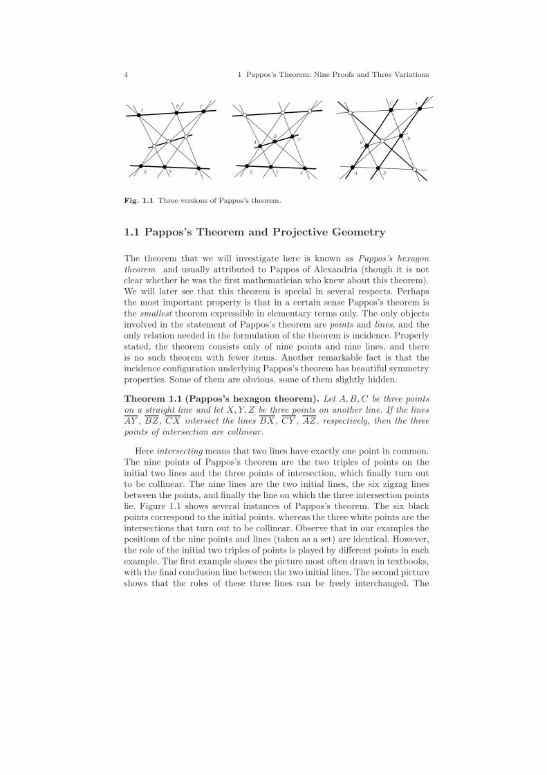
Fig. 1.1 Three versions of Pappos’s theorem.
1.1 Pappos’s Theorem and Projective Geometry
The theorem that we will investigate here is known as Pappos’s hexagontheorem and usually attributed to Pappos of Alexandria (though it is notclear whether he was the first mathematician who knew about this theorem).We will later see that this theorem is special in several respects. Perhapsthe most important property is that in a certain sense Pappos’s theorem isthe smallest theorem expressible in elementary terms only. The only objectsinvolved in the statement of Pappos’s theorem are points and lines, and theonly relation needed in the formulation of the theorem is incidence. Properlystated, the theorem consists only of nine points and nine lines, and thereis no such theorem with fewer items. Another remarkable fact is that theincidence configuration underlying Pappos’s theorem has beautiful symmetryproperties. Some of them are obvious, some of them slightly hidden.
Theorem 1.1 (Pappos’s hexagon theorem). Let A,B,C be three pointson a straight line and let X,Y, Z be three points on another line. If the linesAY , BZ, CX intersect the lines BX, CY , AZ, respectively, then the threepoints of intersection are collinear.
Here intersecting means that two lines have exactly one point in common.The nine points of Pappos’s theorem are the two triples of points on theinitial two lines and the three points of intersection, which finally turn outto be collinear. The nine lines are the two initial lines, the six zigzag linesbetween the points, and finally the line on which the three intersection pointslie. Figure 1.1 shows several instances of Pappos’s theorem. The six blackpoints correspond to the initial points, whereas the three white points are theintersections that turn out to be collinear. Observe that in our examples thepositions of the nine points and lines (taken as a set) are identical. However,the role of the initial two triples of points is played by different points in eachexample. The first example shows the picture most often drawn in textbooks,with the final conclusion line between the two initial lines. The second pictureshows that the roles of these three lines can be freely interchanged. The
1.1 Pappos’s Theorem and Projective Geometry 5
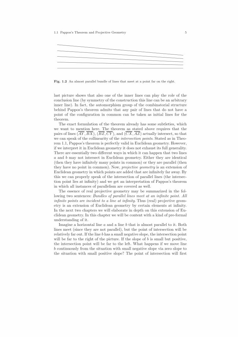
Fig. 1.2 An almost parallel bundle of lines that meet at a point far on the right.
last picture shows that also one of the inner lines can play the role of theconclusion line (by symmetry of the construction this line can be an arbitraryinner line). In fact, the automorphism group of the combinatorial structurebehind Pappos’s theorem admits that any pair of lines that do not have apoint of the configuration in common can be taken as initial lines for thetheorem.
The exact formulation of the theorem already has some subtleties, whichwe want to mention here. The theorem as stated above requires that thepairs of lines (AY ,BX), (BZ,CY ), and (CX,AZ) actually intersect, so thatwe can speak of the collinearity of the intersection points. Stated as in Theo-rem 1.1, Pappos’s theorem is perfectly valid in Euclidean geometry. However,if we interpret it in Euclidean geometry it does not exhaust its full generality.There are essentially two different ways in which it can happen that two linesa and b may not intersect in Euclidean geometry. Either they are identical(then they have infinitely many points in common) or they are parallel (thenthey have no point in common). Now, projective geometry is an extension ofEuclidean geometry in which points are added that are infinitely far away. Bythis we can properly speak of the intersection of parallel lines (the intersec-tion point lies at infinity) and we get an interpretation of Pappos’s theoremin which all instances of parallelism are covered as well.
The essence of real projective geometry may be summarized in the fol-lowing two sentences: Bundles of parallel lines meet at an infinite point. Allinfinite points are incident to a line at infinity. Thus (real) projective geom-etry is an extension of Euclidean geometry by certain elements at infinity.In the next two chapters we will elaborate in depth on this extension of Eu-clidean geometry. In this chapter we will be content with a kind of pre-formalunderstanding of it.
Imagine a horizontal line a and a line b that is almost parallel to it. Bothlines meet (since they are not parallel), but the point of intersection will berelatively far out. If the line b has a small negative slope, the intersection pointwill be far to the right of the picture. If the slope of b is small but positive,the intersection point will be far to the left. What happens if we move lineb continuously from the situation with small negative slope via zero slope tothe situation with small positive slope? The point of intersection will first
6 1 Pappos’s Theorem: Nine Proofs and Three Variations
A
B
C
Z Y X
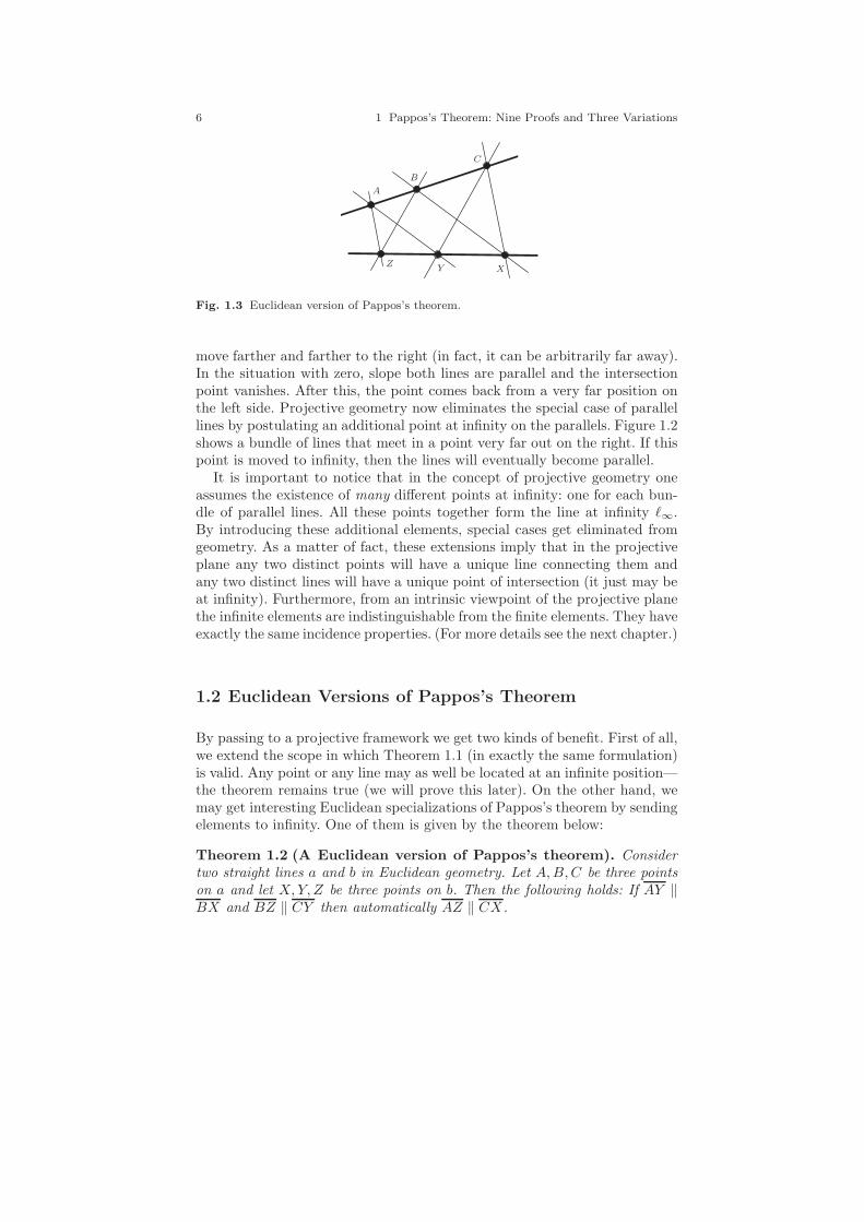
Fig. 1.3 Euclidean version of Pappos’s theorem.
move farther and farther to the right (in fact, it can be arbitrarily far away).In the situation with zero, slope both lines are parallel and the intersectionpoint vanishes. After this, the point comes back from a very far position onthe left side. Projective geometry now eliminates the special case of parallellines by postulating an additional point at infinity on the parallels. Figure 1.2shows a bundle of lines that meet in a point very far out on the right. If thispoint is moved to infinity, then the lines will eventually become parallel.
It is important to notice that in the concept of projective geometry oneassumes the existence of many different points at infinity: one for each bun-dle of parallel lines. All these points together form the line at infinity ℓ∞.By introducing these additional elements, special cases get eliminated fromgeometry. As a matter of fact, these extensions imply that in the projectiveplane any two distinct points will have a unique line connecting them andany two distinct lines will have a unique point of intersection (it just may beat infinity). Furthermore, from an intrinsic viewpoint of the projective planethe infinite elements are indistinguishable from the finite elements. They haveexactly the same incidence properties. (For more details see the next chapter.)
1.2 Euclidean Versions of Pappos’s Theorem
By passing to a projective framework we get two kinds of benefit. First of all,we extend the scope in which Theorem 1.1 (in exactly the same formulation)is valid. Any point or any line may as well be located at an infinite position—the theorem remains true (we will prove this later). On the other hand, wemay get interesting Euclidean specializations of Pappos’s theorem by sendingelements to infinity. One of them is given by the theorem below:
Theorem 1.2 (A Euclidean version of Pappos’s theorem). Considertwo straight lines a and b in Euclidean geometry. Let A,B,C be three pointson a and let X,Y, Z be three points on b. Then the following holds: If AY ‖BX and BZ ‖ CY then automatically AZ ‖ CX.

1.2 Euclidean Versions of Pappos’s Theorem 7
A
B
Z Y
C
X
αβ
γ
ℓ∞
A
B
Z Y
C
X
αβγ
Fig. 1.4 Euclidean version of Pappos’s theorem with points at infinity and line at infinityadded (left). The straight version (right).
For a drawing of this theorem see Figure 1.3. Figure 1.4 illustrates how theparallelism of lines is translated to the projective setup. If AY ‖ BX thenthese two lines intersect (projectively) at a point γ at infinity. Similarly we getan infinite intersection α for BZ ‖ CY . Pappos’s theorem (in its projectiveversion) states that γ and α and the intersection β of AZ with CX arecollinear. Since γ and α span the line ℓ∞ at infinity, AZ and CX must beparallel as well. In other words, the conclusion line (i.e. the line that encodesthe final conclusion of the theorem) has been sent to infinity. The drawingon the right shows a straightened version of the situation with the conclusionline at a finite location. Observe the similarity of the combinatorics. Once wehave introduced the concept of projective transformation, we will see that bya suitable transformation we can send any instance of Pappos’s theorem tothe above situation. Thus our Euclidean version is essentially equivalent tothe full Pappos’s theorem and not just a special case of it.
We will start our collection of proofs with two proofs of Theorem 1.2.It should be remarked in advance that most of our proofs will be algebraicand rely on translations of geometric facts to algebraic identities. There isa general problem with algebraic proofs: one should never divide by zero!This seemingly obvious fact leads to many difficulties and misunderstandingswhen geometric theorems are concerned. Very often, proofs work perfectly ingeneric situations in which no points or lines coincide or additional collineari-ties occur, but in certain degenerate cases they may break down. In fact, manyalgebraic proofs given in geometry textbooks suffer from this (d)effect and awhole branch of current ongoing research deals with the proper treatment ofnondegeneracy conditions. The very statement of Theorem 1.1 carries non-degeneracy conditions in stating that the three crucial pairs of lines shouldactually intersect.
8 1 Pappos’s Theorem: Nine Proofs and Three Variations
A
B
C
Z Y X
O
P
Q
R S
O
|OP ||OQ| =
|OR||OS|
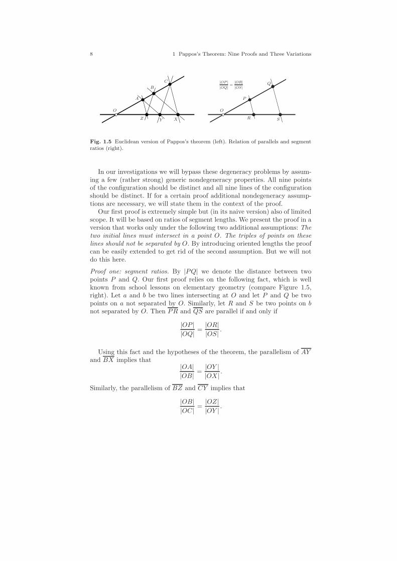
Fig. 1.5 Euclidean version of Pappos’s theorem (left). Relation of parallels and segmentratios (right).
In our investigations we will bypass these degeneracy problems by assum-ing a few (rather strong) generic nondegeneracy properties. All nine pointsof the configuration should be distinct and all nine lines of the configurationshould be distinct. If for a certain proof additional nondegeneracy assump-tions are necessary, we will state them in the context of the proof.
Our first proof is extremely simple but (in its naive version) also of limitedscope. It will be based on ratios of segment lengths. We present the proof in aversion that works only under the following two additional assumptions: Thetwo initial lines must intersect in a point O. The triples of points on theselines should not be separated by O. By introducing oriented lengths the proofcan be easily extended to get rid of the second assumption. But we will notdo this here.
Proof one: segment ratios. By |PQ| we denote the distance between twopoints P and Q. Our first proof relies on the following fact, which is wellknown from school lessons on elementary geometry (compare Figure 1.5,right). Let a and b be two lines intersecting at O and let P and Q be twopoints on a not separated by O. Similarly, let R and S be two points on bnot separated by O. Then PR and QS are parallel if and only if
|OP ||OQ| =
|OR||OS| .
Using this fact and the hypotheses of the theorem, the parallelism of AYand BX implies that
|OA||OB| =
|OY ||OX | .
Similarly, the parallelism of BZ and CY implies that
|OB||OC| =
|OZ||OY | .

1.2 Euclidean Versions of Pappos’s Theorem 9
Since none of the six points are allowed to coincide with O, none of thedenominators in the above expression are zero. Multiplying the two left sidesof the equations and the two right sides of the equations and canceling theterms |OB| and |OY |, we obtain
|OA||OC| =
|OZ||OX | .
This in turn is equivalent to the fact that AZ and CX are parallel. ⊓⊔
At first sight the above proof seems to be very simple and elegant: Multiplytwo equations, cancel out terms, and get the result. Unfortunately, it hasseveral drawbacks. One of the main problems is that we translated parallelisminto ratios of lengths of segments. This translation works correctly only if thedecisive points are not separated by the intersection of the lines. One cancircumvent this problem by considering oriented line segments. The sign ofthe ratios used in our proof will be negative if the points are separated byO, and positive otherwise. However, to make this formally correct one shouldprovide a case-by-case analysis that proves that the signs really have thedesired behavior. A closer look shows that the proof is problematic, since weintroduced the auxiliary point O and we made the proof dependent on itsexistence. The complete proof breaks down if the lines a and b are paralleland point O does not exist at all. In fact, the Euclidean version of Pappos’stheorem does not at all depend on these special position requirements. Thefollowing proof uses only the six points of Theorem 1.2. However, we will needthree slightly less trivial facts concerning polynomials and oriented areas oftriangles and quadrangles.
Fact 1: Oriented triangle area.For three points A,B,C with coordinates (ax, ay), (bx, by), and (cx, cy) we
can express the oriented area of the triangle ∆(A,B,C) by a polynomial inthe coordinates. To be more specific, the desired polynomial is
1
2det
ax bx cxay by cy1 1 1
=
1
2(axby + bxcy + cxay − axcy − bxay − cxby).
In fact, the specific shape of this polynomial is not important for our nextproof. What is more important is the meaning of oriented: If the sequence ofpoints (A,B,C) is in counterclockwise order, then the area will be calculatedwith positive sign. If they are in clockwise order, we will get a negative sign.If the three points are collinear, then the triangle vanishes and the area willbe zero. We will denote the triangle area by area(A,B,C).
Fact 2: Oriented quadrangle area.The oriented area of a quadrangle (A,B,C,D) can be defined as
10 1 Pappos’s Theorem: Nine Proofs and Three Variations
A
BC
DA
B
C
D
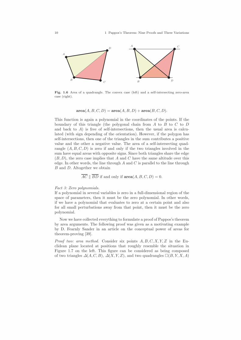
Fig. 1.6 Area of a quadrangle. The convex case (left) and a self-intersecting zero-area
case (right).
area(A,B,C,D) = area(A,B,D) + area(B,C,D).
This function is again a polynomial in the coordinates of the points. If theboundary of this triangle (the polygonal chain from A to B to C to Dand back to A) is free of self-intersections, then the usual area is calcu-lated (with sign depending of the orientation). However, if the polygon hasself-intersections, then one of the triangles in the sum contributes a positivevalue and the other a negative value. The area of a self-intersecting quad-rangle (A,B,C,D) is zero if and only if the two triangles involved in thesum have equal areas with opposite signs. Since both triangles share the edge(B,D), the zero case implies that A and C have the same altitude over thisedge. In other words, the line through A and C is parallel to the line throughB and D. Altogether we obtain
AC ‖ BD if and only if area(A,B,C,D) = 0.
Fact 3: Zero polynomials.If a polynomial in several variables is zero in a full-dimensional region of thespace of parameters, then it must be the zero polynomial. In other words,if we have a polynomial that evaluates to zero at a certain point and alsofor all small perturbations away from that point, then it must be the zeropolynomial.
Now we have collected everything to formulate a proof of Pappos’s theoremby area arguments. The following proof was given as a motivating exampleby D. Fearnly Sander in an article on the conceptual power of areas fortheorem-proving [39].
Proof two: area method. Consider six points A,B,C,X, Y, Z in the Eu-clidean plane located at positions that roughly resemble the situation inFigure 1.7 on the left. This figure can be considered as being composedof two triangles ∆(A,C,B), ∆(X,Y, Z), and two quadrangles (B, Y,X,A)
1.2 Euclidean Versions of Pappos’s Theorem 11
A
C Z
Y
X
BA
B
Z Y
C
X
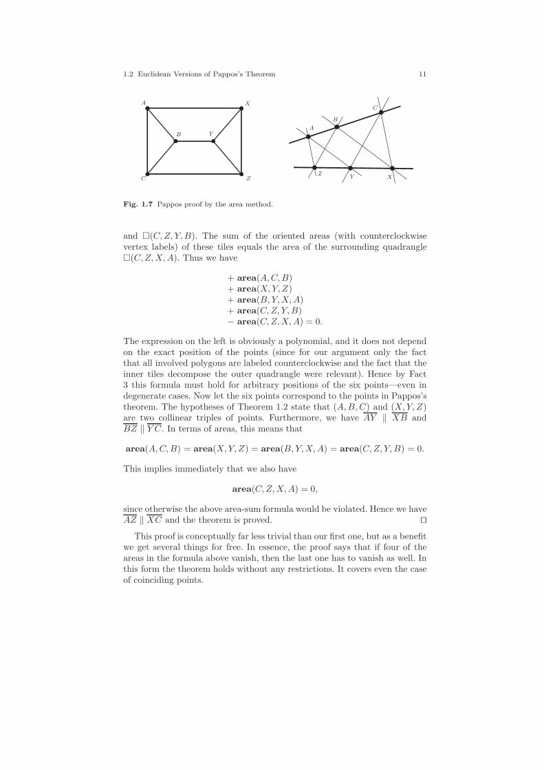
Fig. 1.7 Pappos proof by the area method.
and (C,Z, Y,B). The sum of the oriented areas (with counterclockwisevertex labels) of these tiles equals the area of the surrounding quadrangle(C,Z,X,A). Thus we have
+ area(A,C,B)+ area(X,Y, Z)+ area(B, Y,X,A)+ area(C,Z, Y,B)− area(C,Z,X,A) = 0.
The expression on the left is obviously a polynomial, and it does not dependon the exact position of the points (since for our argument only the factthat all involved polygons are labeled counterclockwise and the fact that theinner tiles decompose the outer quadrangle were relevant). Hence by Fact3 this formula must hold for arbitrary positions of the six points—even indegenerate cases. Now let the six points correspond to the points in Pappos’stheorem. The hypotheses of Theorem 1.2 state that (A,B,C) and (X,Y, Z)are two collinear triples of points. Furthermore, we have AY ‖ XB andBZ ‖ Y C. In terms of areas, this means that
area(A,C,B) = area(X,Y, Z) = area(B, Y,X,A) = area(C,Z, Y,B) = 0.
This implies immediately that we also have
area(C,Z,X,A) = 0,
since otherwise the above area-sum formula would be violated. Hence we haveAZ ‖ XC and the theorem is proved. ⊓⊔
This proof is conceptually far less trivial than our first one, but as a benefitwe get several things for free. In essence, the proof says that if four of theareas in the formula above vanish, then the last one has to vanish as well. Inthis form the theorem holds without any restrictions. It covers even the caseof coinciding points.
12 1 Pappos’s Theorem: Nine Proofs and Three Variations
A
C
BP
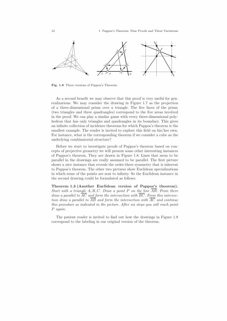
Fig. 1.8 Three versions of Pappos’s Theorem.
As a second benefit we may observe that this proof is very useful for gen-eralizations. We may consider the drawing in Figure 1.7 as the projectionof a three-dimensional prism over a triangle. The five faces of the prism(two triangles and three quadrangles) correspond to the five areas involvedin the proof. We can play a similar game with every three-dimensional poly-hedron that has only triangles and quadrangles in its boundary. This givesan infinite collection of incidence theorems for which Pappos’s theorem is thesmallest example. The reader is invited to explore this field on his/her own.For instance, what is the corresponding theorem if we consider a cube as theunderlying combinatorial structure?
Before we start to investigate proofs of Pappos’s theorem based on con-cepts of projective geometry we will present some other interesting instancesof Pappos’s theorem. They are drawn in Figure 1.8. Lines that seem to beparallel in the drawings are really assumed to be parallel. The first pictureshows a nice instance that reveals the order-three symmetry that is inherentto Pappos’s theorem. The other two pictures show Euclidean specializationsin which some of the points are sent to infinity. So the Euclidean instance inthe second drawing could be formulated as follows.
Theorem 1.3 (Another Euclidean version of Pappos’s theorem).Start with a triangle A,B,C. Draw a point P on the line AB. From theredraw a parallel to AC and form the intersection with BC. From this intersec-tion draw a parallel to AB and form the intersection with AC and continuethis procedure as indicated in the picture. After six steps you will reach pointP again.
The patient reader is invited to find out how the drawings in Figure 1.8correspond to the labeling in our original version of the theorem.
1.3 Projective Proofs of Pappos’s Theorem 13
1.3 Projective Proofs of Pappos’s Theorem
In this section we want to present proofs in which (in contrast to the lastsection) we make no particular use of parallelism. All proofs in this sectionwill rely on the collinearity properties of points only. In this respect theseproofs are projective in nature, since incidence and collinearity are genuineprojective concepts, while parallels are not.
The main algebraic tool used in this section is homogeneous coordinates,which will be introduced in much detail in later chapters. In contrast tothe usual (x, y)-coordinates in the plane, homogeneous coordinates presentpoints in the plane by three coordinates (x, y, z). Coordinate vectors that dif-fer only by a nonzero scalar multiple are considered to be equivalent. The zerovector (0, 0, 0) is excluded from consideration. Thus the nonzero points in aone-dimensional subspace of R
3 represent the same point. A usual Euclideanplane H can be embedded in a homogeneous framework in the following way.Embed H as an affine subspace of R3 that does not contain the origin. Eachpoint p of H corresponds to the one-dimensional subspace Vp spanned by pand may be represented by any nonzero vector of Vp. Conversely, each homo-geneous vector (x, y, z) spans a subspace V(x,y,z). In general, this subspaceintersects the embedded plane H at some point p. This is the point that cor-responds to (x, y, z). It may happen that V(x,y,z) does not intersect H (thishappens whenever the subspace is parallel to H). Then there is no Euclideanpoint associated to (x, y, z). In this case this homogeneous coordinate vec-tor represents an infinite point (see Chapter 3 for details). Thus the finiteand the infinite points can be represented by homogeneous coordinates in acompletely generalized manner.
Collinearity of points in H translates to the fact that the three points inR3 lie in a single plane (the plane spanned by the corresponding line and theorigin of R3). Thus if A = (x1, y1, z1), B = (x2, y2, z2), and C = (x3, y3, z3)are homogeneous coordinates of points, then one can test collinearity bychecking the condition
det
x1 y1 z1x2 y2 z2x3 y3 z3
= 0.
This condition works for finite as well as for infinite points. The followingproof is based on this observation.
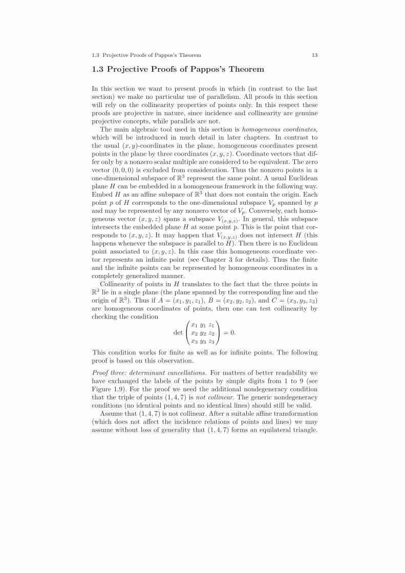
Proof three: determinant cancellations. For matters of better readability wehave exchanged the labels of the points by simple digits from 1 to 9 (seeFigure 1.9). For the proof we need the additional nondegeneracy conditionthat the triple of points (1, 4, 7) is not collinear. The generic nondegeneracyconditions (no identical points and no identical lines) should still be valid.
Assume that (1, 4, 7) is not collinear. After a suitable affine transformation(which does not affect the incidence relations of points and lines) we mayassume without loss of generality that (1, 4, 7) forms an equilateral triangle.

14 1 Pappos’s Theorem: Nine Proofs and Three Variations
1
3
7
6
4
2
5
98
1 1 0 02 a b c3 d e f4 0 1 05 g h i6 j k l7 0 0 18 m n o9 p q r
[1, 2, 3] = 0 =⇒ ce=bf[1, 5, 9] = 0 =⇒ iq=hr[1, 6, 8] = 0 =⇒ ko=ln[2, 4, 9] = 0 =⇒ ar=cp[2, 6, 7] = 0 =⇒ bj=ak[3, 4, 8] = 0 =⇒ fm=do[3, 5, 7] = 0 =⇒ dh=eg[4, 5, 6] = 0 =⇒ gl=ij
[7, 8, 9] = 0 ⇐= mq=np
Fig. 1.9 Determinant cancellation for Pappos’s theorem.
Now we embed the plane in which our configuration resides into three-spacein such a way that the points 1, 4, and 7 are at the three-dimensional unitvectors (1, 0, 0), (0, 1, 0), and (0, 0, 1).
Since the configuration is now embedded in R3, each point is representedby three-dimensional (homogeneous) coordinates. Three points P,Q,R in ourpicture are collinear if and only if the determinant of the 3×3 matrix formedby their coordinates is zero. We abbreviate this determinant by [PQR]. Thematrix in Figure 1.9 represents the coordinates of the configuration.
The letters in the matrix represent the coordinates of the remaining points.The generic nondegeneracy assumptions imply that none of the letters canbe 0. This can be seen as follows. The triple of points (3, 4, 7) cannot becollinear, since otherwise two of the configuration lines would coincide. How-ever, the determinant formed by these points equals exactly a. Thus we get
0 6= det
a b c0 1 00 0 1
= a.
A similar argument works for each of the other variables.With our special choice of coordinates, each of the eight collinearities of
the hypotheses can be expressed as the vanishing of a certain 2 × 2 sub-determinant of the coordinate matrix. If we write down all these equations(compare Figure 1.9), multiply all left sides, and multiply all right sides,we are left with another equation mq = np, which translates back to thecollinearity of (7, 8, 9). By our nondegeneracy assumptions, all variables in-volved in the proof will be nonzero; therefore the cancellation process is fea-sible. ⊓⊔
A proof that is essentially based on this structure first appeared in [14].This proof carries remarkable symmetric structures concerning the cancella-tion patterns among the determinants. Structurally, it reduces to the facts
1.3 Projective Proofs of Pappos’s Theorem 15
that all collinearities correspond to 2 × 2 determinants and that each letteroccurs on the left as well as on the right. The first fact is highly dependenton the choice of our basis, since only the zeros in the unit vectors are allowedto express each of the collinearities as a 2 × 2 determinant.
One can circumvent this problem by an even more abstract approach. In-stead of dealing with concrete coordinates of points, we may deal with generalproperties of determinants. A fundamental role in this context is played bythe Grassmann-Plucker-Relations. These relations state that for arbitraryfive points A,B,C,D,E in the projective plane the following relation holdsamong the determinants of the homogeneous coordinates:
[ABC][ADE] − [ABD][ACE] + [ABE][ACD] = 0.
This remarkable identity is of fundamental importance for projective geom-etry, and we will dedicate a large part of Chapter 6 to it. For now we takethe identity as an algebraic fact. On it we base our next proof.
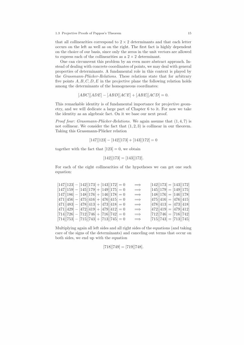
Proof four: Grassmann-Plucker-Relations. We again assume that (1, 4, 7) isnot collinear. We consider the fact that (1, 2, 3) is collinear in our theorem.Taking this Grassmann-Plucker relation
[147][123]− [142][173] + [143][172] = 0
together with the fact that [123] = 0, we obtain
[142][173] = [143][172].
For each of the eight collinearities of the hypotheses we can get one suchequation:
[147][123]− [142][173] + [143][172] = 0 =⇒ [142][173] = [143][172][147][159]− [145][179] + [149][175] = 0 =⇒ [145][179] = [149][175][147][186]− [148][176] + [146][178] = 0 =⇒ [148][176] = [146][178][471][456]− [475][416] + [476][415] = 0 =⇒ [475][416] = [476][415][471][483]− [478][413] + [473][418] = 0 =⇒ [478][413] = [473][418][471][429]− [472][419] + [479][412] = 0 =⇒ [472][419] = [479][412][714][726]− [712][746] + [716][742] = 0 =⇒ [712][746] = [716][742][714][753]− [715][743] + [713][745] = 0 =⇒ [715][743] = [713][745]
Multiplying again all left sides and all right sides of the equations (and takingcare of the signs of the determinants) and canceling out terms that occur onboth sides, we end up with the equation
[718][749] = [719][748].
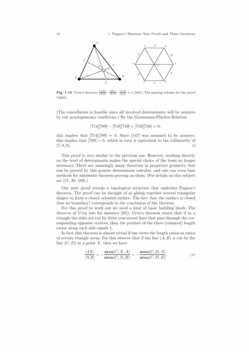
16 1 Pappos’s Theorem: Nine Proofs and Three Variations
AB
C
Z
YD
X 1
1
1
2
2
23
A
A B
B
C
C
Fig. 1.10 Ceva’s theorem|AX||XB|
· |BY ||Y C|
· |CZ||ZA|
= 1 (left). The pasting scheme for the proof
(right).
(The cancellation is feasible since all involved determinants will be nonzeroby our nondegeneracy conditions.) By the Grassmann-Plucker-Relation
[714][789]− [718][749] + [719][748] = 0,
this implies that [714][789] = 0. Since [147] was assumed to be nonzero,this implies that [789] = 0, which in turn is equivalent to the collinearity of(7, 8, 9). ⊓⊔
This proof is very similar to the previous one. However, working directlyon the level of determinants makes the special choice of the basis no longernecessary. There are amazingly many theorems in projective geometry thatcan be proved by this generic determinant calculus, and one can even basemethods for automatic theorem-proving on them. (For details on this subjectsee [15, 30, 109].)
Our next proof reveals a topological structure that underlies Pappos’stheorem. The proof can be thought of as gluing together several triangularshapes to form a closed oriented surface. The fact that the surface is closed(has no boundary) corresponds to the conclusion of the theorem.
For this proof to work out we need a kind of basic building block: Thetheorem of Ceva (see for instance [28]). Ceva’s theorem states that if in atriangle the sides are cut by three concurrent lines that pass through the cor-responding opposite vertices, then the product of the three (oriented) lengthratios along each side equals 1.
In fact, this theorem is almost trivial if one views the length ratios as ratiosof certain triangle areas. For this observe that if the line (A,B) is cut by theline (C,D) at a point X , then we have
|AX ||XB| = −area(C,X,A)
area(C,X,B)= −area(C,D,A)
area(C,D,B), (∗)
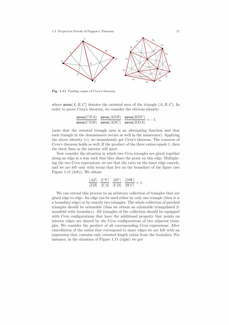
1.3 Projective Proofs of Pappos’s Theorem 17
A
C
B
D
X
Y
Z
V
W
a1
b1
a2
b2
a3b3
a4
b4
a5
b5
a6
b6
Fig. 1.11 Pasting copies of Ceva’s theorem.
where area(A,B,C) denotes the oriented area of the triangle (A,B,C). Inorder to prove Ceva’s theorem, we consider the obvious identity
area(CDA)
area(CDB)· area(ADB)
area(ADC)· area(BDC)
area(BDA)= −1
(note that the oriented triangle area is an alternating function and thateach triangle in the denominator occurs as well in the numerator). Applyingthe above identity (∗), we immediately get Ceva’s theorem. The converse ofCeva’s theorem holds as well: If the product of the three ratios equals 1, thenthe three lines in the interior will meet.
Now consider the situation in which two Ceva triangles are glued togetheralong an edge in a way such that they share the point on this edge. Multiply-ing the two Ceva expressions, we see that the ratio on the inner edge cancels,and we are left only with terms that live on the boundary of the figure (seeFigure 1.11 (left)). We obtain
|AZ||ZB| ·
|CY ||Y A| ·
|BV ||V D| ·
|DW ||WC| = 1.
We can extend this process to an arbitrary collection of triangles that areglued edge to edge. An edge can be used either by only one triangle (then it isa boundary edge) or by exactly two triangles. The whole collection of patchedtriangles should be orientable (thus we obtain an orientable triangulated 2-manifold with boundary). All triangles of the collection should be equippedwith Ceva configurations that have the additional property that points oninterior edges are shared by the Ceva configurations of two adjacent trian-gles. We consider the product of all corresponding Ceva expressions. Aftercancellation of the ratios that correspond to inner edges we are left with anexpression that contains only oriented length ratios from the boundary. Forinstance, in the situation of Figure 1.11 (right) we get

18 1 Pappos’s Theorem: Nine Proofs and Three Variations
Fig. 1.12 Creating Pappos’s theorem from six copies of Ceva’s theorem.
a1
b1· a2
b2· a3
b3· a4
b4· a5
b5· a6
b6= 1.
The inner part of the structure cancels completely and does not contributeto the product on the boundary. Now, if we have a collection of triangles thathas nothing more than a triangular boundary (i.e., a 2-manifold with a singletriangular hole), then the Ceva condition on the whole is automatically satis-fied, and we can paste in a final triangle that carries a Ceva configuration. Inother words, if we have an orientable triangulated 2-manifold without bound-ary and we have a Ceva configuration on all triangles but one (such that theedge points are shared), then a Ceva configuration can automatically be puton the final triangle. This is an incidence theorem. We now will show thatusing the right manifold, Pappos’s theorem can be put in exactly this form.
Proof five: pasting copies of Ceva’s theorem. Consider six triangles that arearranged as in Figure 1.10 on the right. Furthermore, identify opposite edgesof the hexagon as indicated in the drawing. This can be done by placing thesix triangles one over the other (think of the hexagon as made of paper andfold it appropriately) and gluing together corresponding opposite edges. Nowplace a Ceva configuration on each of the edges in a way such that whenevertwo triangles meet at an edge, the corresponding two points on this edge areidentified. Our considerations above show that if the edge points are locatedsuch that five of the triangles carry proper Ceva configurations, then the lastCeva configuration is satisfied automatically. The figure in the middle showsthe situation after all the triangle edges have been identified. Observe thatthe points on the edges of the outer triangle as well as the edges themselvesdo not contribute to the incidence theorem. What is left after these elementsare deleted is exactly a drawing of Pappos’s theorem. ⊓⊔
A proof very similar to this was given by H.S.M. Coxeter and S.L. Gre-itzer [28]. Their proof was based on Menelaus configurations instead of Cevaconfigurations but is essentially similar. In [110] one can find an elaboratetreatment of the question of which geometric theorems can be proved bysimilar manifold arguments.
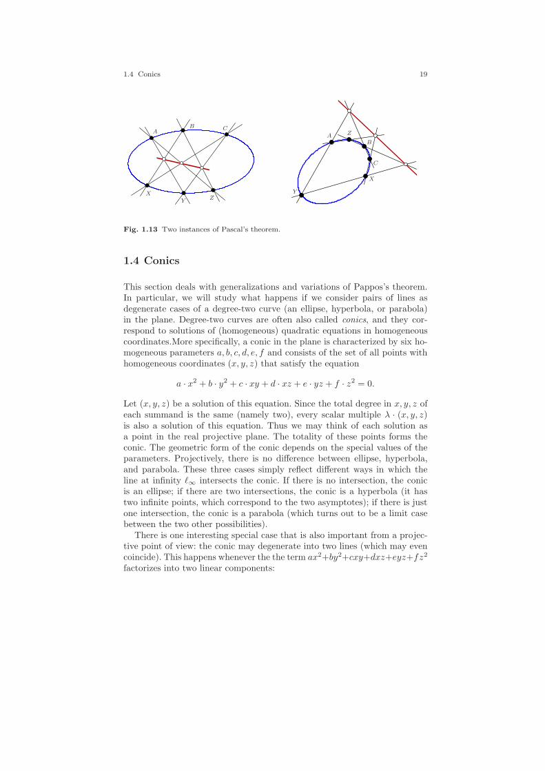
1.4 Conics 19
AB C
XY Z
AB
C
X
Y
Z
Fig. 1.13 Two instances of Pascal’s theorem.
1.4 Conics
This section deals with generalizations and variations of Pappos’s theorem.In particular, we will study what happens if we consider pairs of lines asdegenerate cases of a degree-two curve (an ellipse, hyperbola, or parabola)in the plane. Degree-two curves are often also called conics, and they cor-respond to solutions of (homogeneous) quadratic equations in homogeneouscoordinates.More specifically, a conic in the plane is characterized by six ho-mogeneous parameters a, b, c, d, e, f and consists of the set of all points withhomogeneous coordinates (x, y, z) that satisfy the equation
a · x2 + b · y2 + c · xy + d · xz + e · yz + f · z2 = 0.
Let (x, y, z) be a solution of this equation. Since the total degree in x, y, z ofeach summand is the same (namely two), every scalar multiple λ · (x, y, z)is also a solution of this equation. Thus we may think of each solution asa point in the real projective plane. The totality of these points forms theconic. The geometric form of the conic depends on the special values of theparameters. Projectively, there is no difference between ellipse, hyperbola,and parabola. These three cases simply reflect different ways in which theline at infinity ℓ∞ intersects the conic. If there is no intersection, the conicis an ellipse; if there are two intersections, the conic is a hyperbola (it hastwo infinite points, which correspond to the two asymptotes); if there is justone intersection, the conic is a parabola (which turns out to be a limit casebetween the two other possibilities).
There is one interesting special case that is also important from a projec-tive point of view: the conic may degenerate into two lines (which may evencoincide). This happens whenever the the term ax2+by2+cxy+dxz+eyz+fz2
factorizes into two linear components:
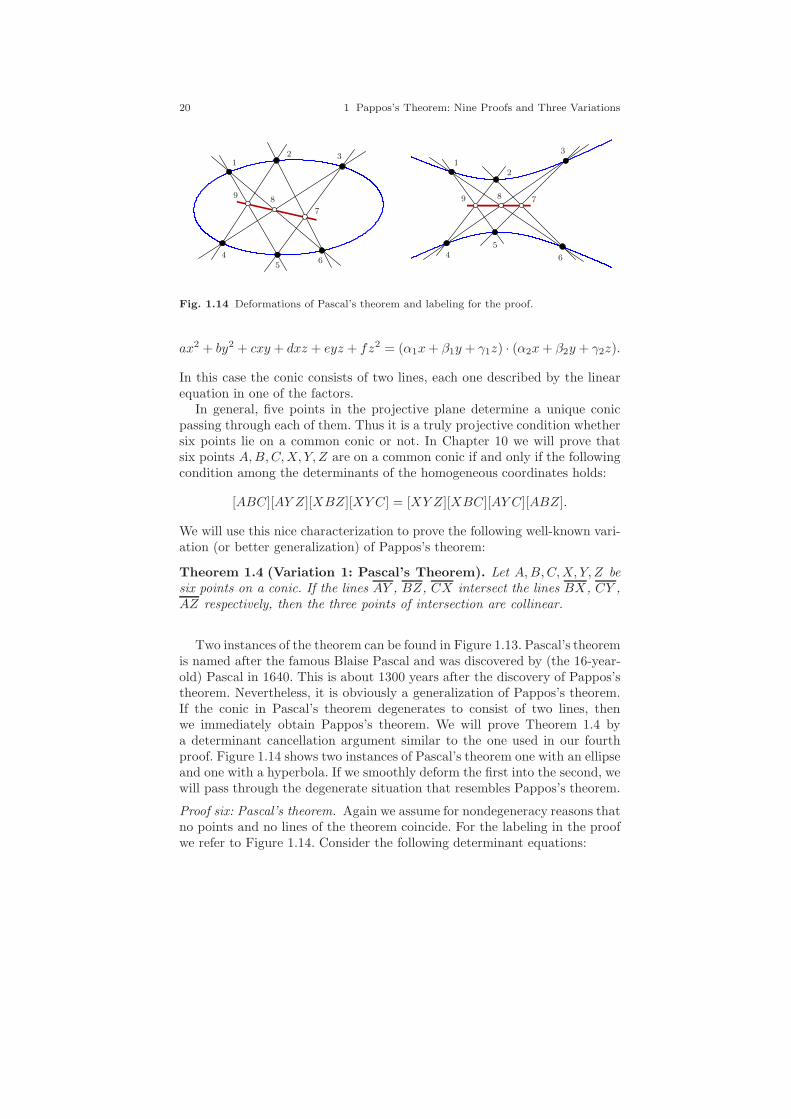
20 1 Pappos’s Theorem: Nine Proofs and Three Variations
12 3
45
6
98
7
12
3
45
6
9 8 7
Fig. 1.14 Deformations of Pascal’s theorem and labeling for the proof.
ax2 + by2 + cxy + dxz + eyz + fz2 = (α1x+ β1y + γ1z) · (α2x+ β2y + γ2z).
In this case the conic consists of two lines, each one described by the linearequation in one of the factors.
In general, five points in the projective plane determine a unique conicpassing through each of them. Thus it is a truly projective condition whethersix points lie on a common conic or not. In Chapter 10 we will prove thatsix points A,B,C,X, Y, Z are on a common conic if and only if the followingcondition among the determinants of the homogeneous coordinates holds:
[ABC][AY Z][XBZ][XYC] = [XY Z][XBC][AY C][ABZ].
We will use this nice characterization to prove the following well-known vari-ation (or better generalization) of Pappos’s theorem:
Theorem 1.4 (Variation 1: Pascal’s Theorem). Let A,B,C,X, Y, Z besix points on a conic. If the lines AY , BZ, CX intersect the lines BX, CY ,AZ respectively, then the three points of intersection are collinear.
Two instances of the theorem can be found in Figure 1.13. Pascal’s theoremis named after the famous Blaise Pascal and was discovered by (the 16-year-old) Pascal in 1640. This is about 1300 years after the discovery of Pappos’stheorem. Nevertheless, it is obviously a generalization of Pappos’s theorem.If the conic in Pascal’s theorem degenerates to consist of two lines, thenwe immediately obtain Pappos’s theorem. We will prove Theorem 1.4 bya determinant cancellation argument similar to the one used in our fourthproof. Figure 1.14 shows two instances of Pascal’s theorem one with an ellipseand one with a hyperbola. If we smoothly deform the first into the second, wewill pass through the degenerate situation that resembles Pappos’s theorem.
Proof six: Pascal’s theorem. Again we assume for nondegeneracy reasons thatno points and no lines of the theorem coincide. For the labeling in the proofwe refer to Figure 1.14. Consider the following determinant equations:

1.4 Conics 21
conic: ⇒ [125] [136] [246] [345] = + [126] [135] [245] [346][159] = 0 =⇒ [157] [259] = − [125] [597][168] = 0 =⇒ [126] [368] = + [136] [268][249] = 0 =⇒ [245] [297] = − [247] [259][267] = 0 =⇒ [247] [268] = − [246] [287][348] = 0 =⇒ [346] [358] = + [345] [368][357] = 0 =⇒ [135] [587] = − [157] [358][987] = 0 ⇐= [287] [597] = + [297] [587]
The first line encodes that the points 1, . . . , 6 lie on a conic. The next sixlines are consequences of Grassmann-Plucker-Relations and the six collinear-ity hypotheses of our theorem. If we multiply all expressions on the left and allexpressions on the right and cancel determinants that occur on both sides, weend up with the last expression, which (under the nondegeneracy assumptionthat [157] 6= 0) implies the desired collinearity of (7, 8, 9). ⊓⊔
Similar to Pappos’s theorem, there is a variety of reformulations and spe-cializations. A nice reformulation is the following: If a hexagon is inscribed ina conic in the projective plane, then the opposite sides of the hexagon meet inthree collinear points. Or if one prefers a Euclidean variant of this in which theconclusion line is sent to infinity, one could state the following: If a hexagonis inscribed in a conic and two pairs of opposite edges are parallel, then sois the third pair. There is another nice way to derive even more incidencetheorems from Pascal’s theorem. Assume that the conic has a fixed position.If two of the points in Pascal’s theorem that are joined by a line continu-ously approach each other until they meet, their joining line will in the limitcase become a tangent to the conic at the position where the two points arelocated. Thus we obtain as limit cases situations in which also tangents areinvolved (observe that tangents are proper concepts of projective geometry).
Instances of degenerate versions are given in Figure 1.15. The leftmostpicture shows a smallest degenerate situation. The label 15 symbolizes thatpoints 1 and 5 are identified. The labeling is consistent with the labeling inFigure 1.14. The join of 1 and 5 becomes the tangent at the point 15. One canalso read the construction in the reverse direction. If a conic C and a point15 on it are given, then one can construct the tangent at 15 by choosing fourarbitrary points 2, 3, 4, 6 on C and constructing the joins and intersections asgiven by the picture to arrive finally at point 9 another point on the tangent.This fact was also known to Pascal, and is one of the main applicationsof his theorem. The second picture shows in essence the same situation asthe first one. However, here the point 15 has been sent to infinity and thecorresponding tangent is located at the line at infinity. By this the conicbecomes a parabola, and the two other lines through 15 become parallel tothe symmetry axis of the parabola. Now the theorem reads as follows: Start
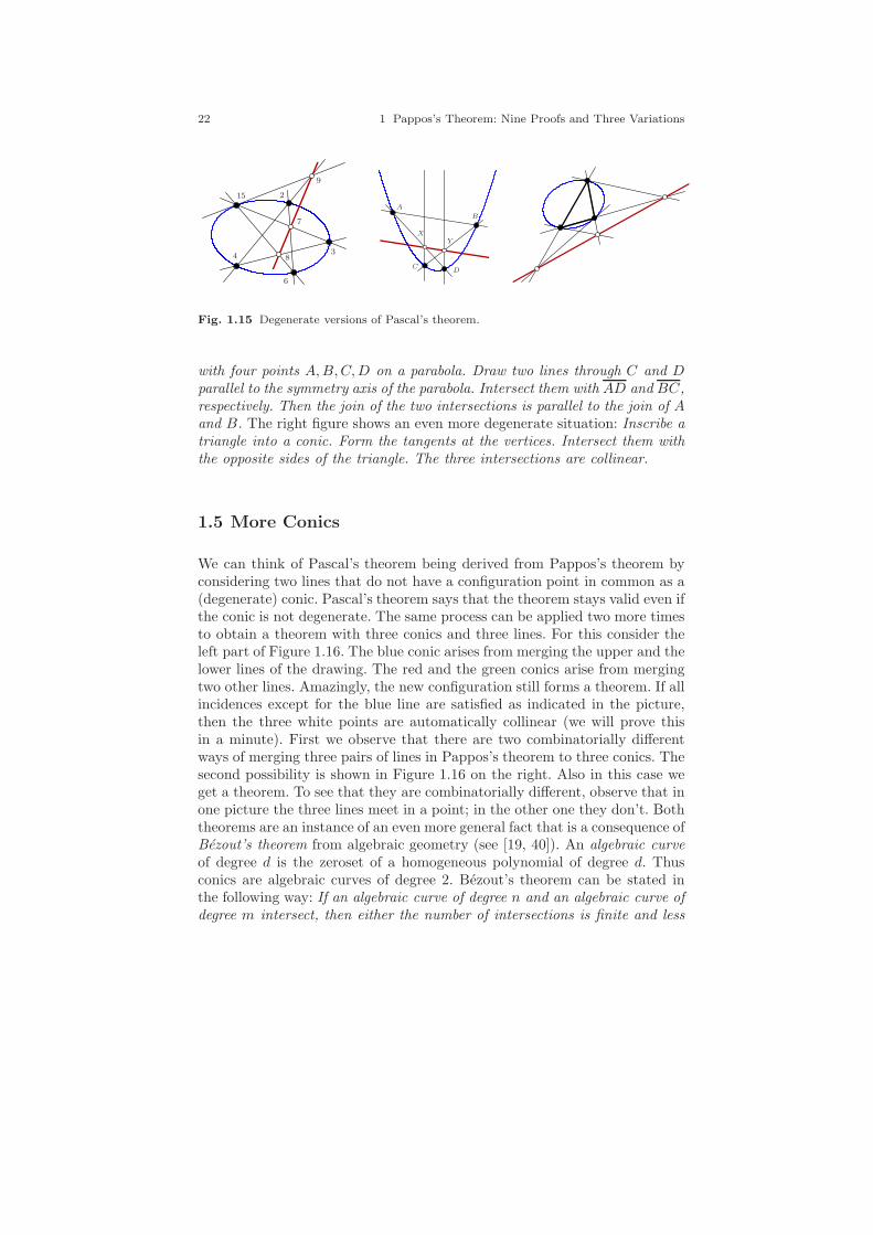
22 1 Pappos’s Theorem: Nine Proofs and Three Variations
15 2
3
6
4
9
7
8
A
B
XY
CD
Fig. 1.15 Degenerate versions of Pascal’s theorem.
with four points A,B,C,D on a parabola. Draw two lines through C and Dparallel to the symmetry axis of the parabola. Intersect them with AD and BC,respectively. Then the join of the two intersections is parallel to the join of Aand B. The right figure shows an even more degenerate situation: Inscribe atriangle into a conic. Form the tangents at the vertices. Intersect them withthe opposite sides of the triangle. The three intersections are collinear.
1.5 More Conics
We can think of Pascal’s theorem being derived from Pappos’s theorem byconsidering two lines that do not have a configuration point in common as a(degenerate) conic. Pascal’s theorem says that the theorem stays valid even ifthe conic is not degenerate. The same process can be applied two more timesto obtain a theorem with three conics and three lines. For this consider theleft part of Figure 1.16. The blue conic arises from merging the upper and thelower lines of the drawing. The red and the green conics arise from mergingtwo other lines. Amazingly, the new configuration still forms a theorem. If allincidences except for the blue line are satisfied as indicated in the picture,then the three white points are automatically collinear (we will prove thisin a minute). First we observe that there are two combinatorially differentways of merging three pairs of lines in Pappos’s theorem to three conics. Thesecond possibility is shown in Figure 1.16 on the right. Also in this case weget a theorem. To see that they are combinatorially different, observe that inone picture the three lines meet in a point; in the other one they don’t. Boththeorems are an instance of an even more general fact that is a consequence ofBezout’s theorem from algebraic geometry (see [19, 40]). An algebraic curveof degree d is the zeroset of a homogeneous polynomial of degree d. Thusconics are algebraic curves of degree 2. Bezout’s theorem can be stated inthe following way: If an algebraic curve of degree n and an algebraic curve ofdegree m intersect, then either the number of intersections is finite and less

1.5 More Conics 23
Fig. 1.16 Generalizations of Pascal’s Theorem
than or equal to n ·m, or the curves intersect in infinitely many points andshare a component. Now we can prove the following very strong statement:
Theorem 1.5 (Variation 2: Cayley-Bacharach-Chasles theorem). LetA and B be two curves of degree three intersecting in nine proper points. Ifsix of these points are on a conic, the remaining three points are collinear.
Proof seven: algebraic curves. Let A and B be the curves and let pA(x, y, z)and pB(x, y, z) be the corresponding homogeneous polynomials of degreethree. Bezout’s theorem implies that if the two curves A and B have onlyfinitely many points in common, then they can have at most nine points ofintersection. Call them 1, . . . , 9. And assume that 1, . . . , 6 are on a conic Cwith polynomial pC . We will prove that 7, 8, 9 are collinear. Consider a linearcombination pµ = pA+µ ·pB of the two polynomials for some real parameterµ. The polynomial pµ has the following properties. First it is again a degree-three polynomial. Second, it passes through all nine points 1, . . . , 9 (each ofthese points is a zero of both pA and pB, so it is also a zero of any linear com-bination of them). Now consider an additional point q on the conic C distinctfrom 1, . . . , 6. There is a µ such that pµ also passes through q (to find µ wejust have to solve a linear equation pA(q) + µpB(q) = 0). Consider pµ withthis specific value µ. The curve pµ passes through 1, . . . , 6 and through q.Thus it shares these seven points with the conic C. Bezout’s theorem impliesthat pµ must have C as one component. Thus we have pµ = pC · L with alinear equation L (otherwise pµ cannot have degree three). This implies thatthe points 7, 8, 9 are all contained in the line described by the linear equationL. ⊓⊔
The situation of the theorem is sketched in Figure 1.17. This theorem wasindependently discovered by several people. Most probably Chasles was thefirst to discover this theorem, in a slightly more general version in 1885. As sooften in mathematics, the theorem is usually attributed to others, in this casenamely to Cayley and to Bacharach, who published similar results later than
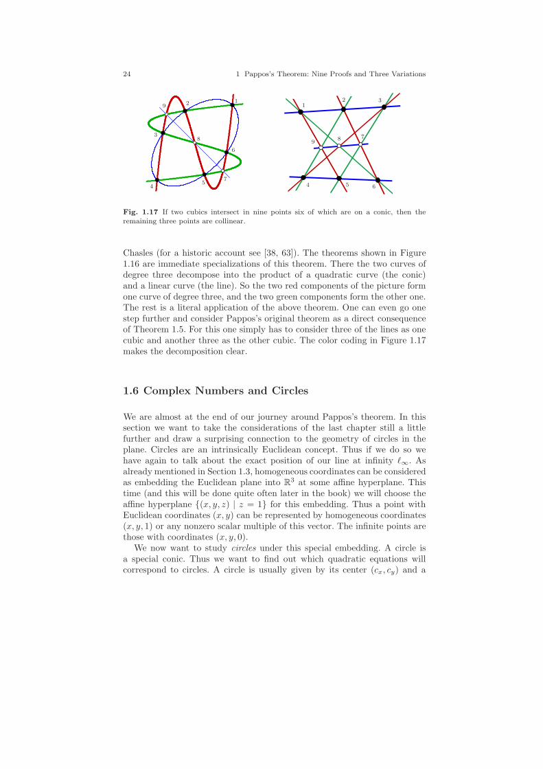
24 1 Pappos’s Theorem: Nine Proofs and Three Variations
12
6
5
3
9
7
8
4
98
4 5
7
6
12 3
Fig. 1.17 If two cubics intersect in nine points six of which are on a conic, then theremaining three points are collinear.
Chasles (for a historic account see [38, 63]). The theorems shown in Figure1.16 are immediate specializations of this theorem. There the two curves ofdegree three decompose into the product of a quadratic curve (the conic)and a linear curve (the line). So the two red components of the picture formone curve of degree three, and the two green components form the other one.The rest is a literal application of the above theorem. One can even go onestep further and consider Pappos’s original theorem as a direct consequenceof Theorem 1.5. For this one simply has to consider three of the lines as onecubic and another three as the other cubic. The color coding in Figure 1.17makes the decomposition clear.
1.6 Complex Numbers and Circles
We are almost at the end of our journey around Pappos’s theorem. In thissection we want to take the considerations of the last chapter still a littlefurther and draw a surprising connection to the geometry of circles in theplane. Circles are an intrinsically Euclidean concept. Thus if we do so wehave again to talk about the exact position of our line at infinity ℓ∞. Asalready mentioned in Section 1.3, homogeneous coordinates can be consideredas embedding the Euclidean plane into R3 at some affine hyperplane. Thistime (and this will be done quite often later in the book) we will choose theaffine hyperplane (x, y, z) | z = 1 for this embedding. Thus a point withEuclidean coordinates (x, y) can be represented by homogeneous coordinates(x, y, 1) or any nonzero scalar multiple of this vector. The infinite points arethose with coordinates (x, y, 0).
We now want to study circles under this special embedding. A circle isa special conic. Thus we want to find out which quadratic equations willcorrespond to circles. A circle is usually given by its center (cx, cy) and a
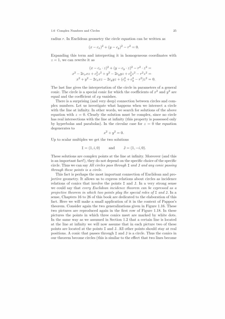
1.6 Complex Numbers and Circles 25
radius r. In Euclidean geometry the circle equation can be written as
(x− cx)2 + (y − cy)
2 − r2 = 0.
Expanding this term and interpreting it in homogeneous coordinates withz = 1, we can rewrite it as
(x− cx · z)2 + (y − cy · z)2 − r2 · z2 =
x2 − 2cxxz + c2xz2 + y2 − 2cyyz + c2yz
2 − r2z2 =
x2 + y2 − 2cxxz − 2cyyz + (c2x + c2y − r2)z2 = 0.
The last line gives the interpretation of the circle in parameters of a generalconic. The circle is a special conic for which the coefficients of x2 and y2 areequal and the coefficient of xy vanishes.
There is a surprising (and very deep) connection between circles and com-plex numbers. Let us investigate what happens when we intersect a circlewith the line at infinity. In other words, we search for solutions of the aboveequation with z = 0. Clearly the solution must be complex, since no circlehas real intersections with the line at infinity (this property is possessed onlyby hyperbolas and parabolas). In the circular case for z = 0 the equationdegenerates to
x2 + y2 = 0.
Up to scalar multiples we get the two solutions
I = (1, i, 0) and J = (1,−i, 0).
These solutions are complex points at the line at infinity. Moreover (and thisis an important fact!), they do not depend on the specific choice of the specificcircle. Thus we can say All circles pass through I and J and any conic passingthrough these points is a circle.
This fact is perhaps the most important connection of Euclidean and pro-jective geometry. It allows us to express relations about circles as incidencerelations of conics that involve the points I and J. In a very strong sensewe could say that every Euclidean incidence theorem can be expressed as aprojective theorem in which two points play the special roles of I and J. In asense, Chapters 16 to 26 of this book are dedicated to the elaboration of thisfact. Here we will make a small application of it in the context of Pappos’stheorem. Consider again the two generalizations given in Figure 1.16. Thesetwo pictures are reproduced again in the first row of Figure 1.18. In thesepictures the points in which three conics meet are marked by white dots.In the same way as we assumed in Section 1.2 that a certain line is locatedat the line at infinity we will now assume that in each picture two of thesepoints are located at the points I and J. All other points should stay at realpositions. A conic that passes through I and J is a circle. Thus the conics inour theorem become circles (this is similar to the effect that two lines become
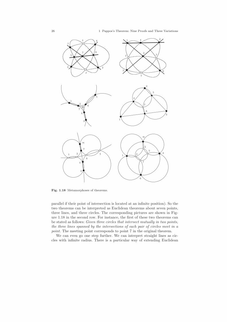
26 1 Pappos’s Theorem: Nine Proofs and Three Variations
1
I 4
3
J
2
57 6
1 4 2
5
7
6
3I
J
12
3
4
5
6
7
1
2
3
4
6
5
7
1 2
7
4
∞
5
6
3
14
6
7
35
2
∞
Fig. 1.18 Metamorphoses of theorems.
parallel if their point of intersection is located at an infinite position). So thetwo theorems can be interpreted as Euclidean theorems about seven points,three lines, and three circles. The corresponding pictures are shown in Fig-ure 1.18 in the second row. For instance, the first of these two theorems canbe stated as follows: Given three circles that intersect mutually in two points,the three lines spanned by the intersections of each pair of circles meet in apoint. The meeting point corresponds to point 7 in the original theorem.
We can even go one step further. We can interpret straight lines as cir-cles with infinite radius. There is a particular way of extending Euclidean
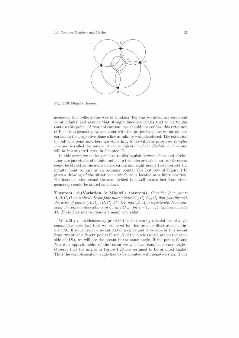
1.6 Complex Numbers and Circles 27
AE
B
F
CG
H
D
Fig. 1.19 Miquel’s theorem.
geometry that reflects this way of thinking. For this we introduce one point∞ at infinity and assume that straight lines are circles that in particularcontain this point. (A word of caution: one should not confuse this extensionof Euclidean geometry by one point with the projective plane we introducedearlier. In the projective plane a line at infinity was introduced. The extensionby only one point used here has something to do with the projective complexline and is called the one-point compactification of the Euclidean plane andwill be investigated later, in Chapter 17.
In this setup we no longer have to distinguish between lines and circles.Lines are just circles of infinite radius. In this interpretation our two theoremscould be stated as theorems on six circles and eight points (we interpret theinfinite point ∞ just as an ordinary point). The last row of Figure 1.18gives a drawing of the situation in which ∞ is located at a finite position.For instance, the second theorem (which is a well-known fact from circlegeometry) could be stated as follows.
Theorem 1.6 (Variation 3: Miquel’s theorem). Consider four pointsA,B,C,D on a circle. Draw four more circles C1, C2, C3, C4 that pass throughthe pairs of points (A,B), (B,C), (C,D), and (D,A), respectively. Now con-sider the other intersections of Ci and Ci+1 for i = 1, . . . , 4 (indices modulo4). These four intersections are again cocircular.
We will give an elementary proof of this theorem by calculations of anglesums. The basic fact that we will need for this proof is illustrated in Fig-ure 1.20. If we consider a secant AB of a circle and if we look at this secantfrom two other different points C and D of the circle (which are on the sameside of AB), we will see the secant in the same angle. If the points C andD are at opposite sides of the secant we will have complementary angles.Observe that the angles in Figure 1.20 are assumed to be oriented angles.Thus the complementary angle has to be counted with negative sign. If one
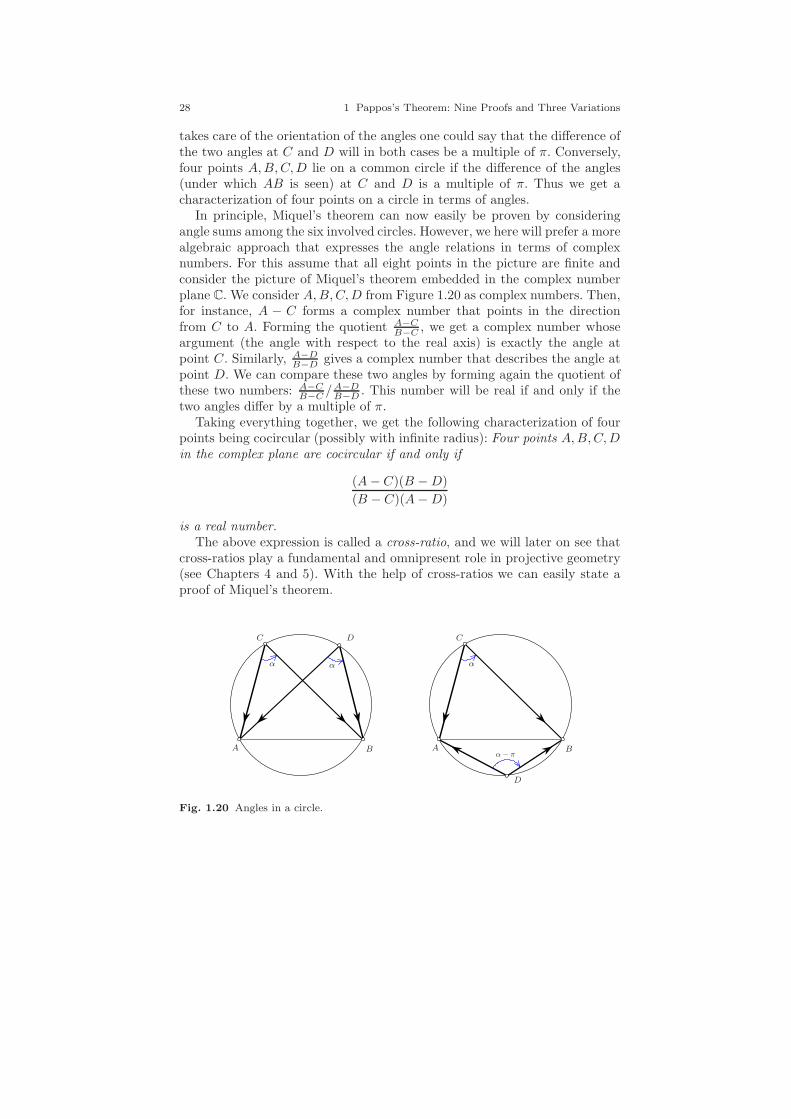
28 1 Pappos’s Theorem: Nine Proofs and Three Variations
takes care of the orientation of the angles one could say that the difference ofthe two angles at C and D will in both cases be a multiple of π. Conversely,four points A,B,C,D lie on a common circle if the difference of the angles(under which AB is seen) at C and D is a multiple of π. Thus we get acharacterization of four points on a circle in terms of angles.
In principle, Miquel’s theorem can now easily be proven by consideringangle sums among the six involved circles. However, we here will prefer a morealgebraic approach that expresses the angle relations in terms of complexnumbers. For this assume that all eight points in the picture are finite andconsider the picture of Miquel’s theorem embedded in the complex numberplane C. We consider A,B,C,D from Figure 1.20 as complex numbers. Then,for instance, A − C forms a complex number that points in the directionfrom C to A. Forming the quotient A−C
B−C , we get a complex number whoseargument (the angle with respect to the real axis) is exactly the angle atpoint C. Similarly, A−D
B−D gives a complex number that describes the angle atpoint D. We can compare these two angles by forming again the quotient ofthese two numbers: A−C
B−C /A−DB−D . This number will be real if and only if the
two angles differ by a multiple of π.Taking everything together, we get the following characterization of four
points being cocircular (possibly with infinite radius): Four points A,B,C,Din the complex plane are cocircular if and only if
(A− C)(B −D)
(B − C)(A−D)
is a real number.The above expression is called a cross-ratio, and we will later on see that
cross-ratios play a fundamental and omnipresent role in projective geometry(see Chapters 4 and 5). With the help of cross-ratios we can easily state aproof of Miquel’s theorem.
A B
C D
α α
A B
C
D
α
α− π
Fig. 1.20 Angles in a circle.

1.7 Finally... 29
Proof eight: cross-ratio cancellations. Assume that the quadruples of points(A,B,C,D), (A,B,E, F ), (B,C, F,G), (C,D,G,H), (D,A,H,E) are cocir-cular. From this we obtain that the following cross-ratios are all real:
(A−B)(C−D)(C−B)(A−D) ,
(F−B)(A−E)(A−B)(F−E) ,
(C−B)(F−G)(F−B)(C−G) ,
(H−D)(C−G)(C−D)(H−G) ,
(A−D)(H−E)(H−D)(A−E) .
Multiplying all these numbers and canceling terms that occur in the numer-ator as well as in the denominator, we are left with the expression
(F −G)(H − E)
(H −G)(F − E).
Since this expression is the product of real numbers, it must itself be real. Byour above observations this expresses exactly the cocircularity of (E,F,G,H),which is the conclusion of our theorem. ⊓⊔
1.7 Finally...
We will end this section with an almost trivial proof of Pappos’s theorem inits full generality by simply expanding an algebraic term. Still we need a littlepreparation for this. Again consider the original points of Pappos’s theoremexpressed in homogeneous coordinates. Thus we assume that the drawingplaneH is again embedded in R3 at a position that does not contain the originof R3. As before, each point p is represented by a three-dimensional vector(x, y, z). This time we will take all points of R
3 − (0, 0, 0) into account.For this we identify the vector (x, y, z) with all of its nonzero scalar multiples(λx, λy, λz), λ 6= 0. By this R3−(0, 0, 0) is divided into equivalence classes.Each equivalence class represents a point of the projective plane. A pointof the drawing plane H can be represented by its actual (x, y, z) positionor by any nonzero scalar multiple of it. Conversely, for a point (x, y, z) ofR3 − (0, 0, 0) we consider the line l(x,y,z) through it and the origin. Thepoint in H that is represented by (x, y, z) is the intersection of l(x,y,z) andH . If this intersection does not exist, (x, y, z) represents an infinite point.
In this setup a straight line g in H may be considered a two-dimensionallinear space spanned by the elements of g and the origin of R3. Such a linemay by represented by a linear equation
(x, y, z) ∈ R3 − (0, 0, 0) | ax+ by + cz = 0
given by parameters (a, b, c) ∈ R3 − (0, 0, 0). Thus points as well as linesare represented by nonzero vectors in R3. A line g is incident to a point p ifand only if the standard scalar product 〈p, g〉 is zero.
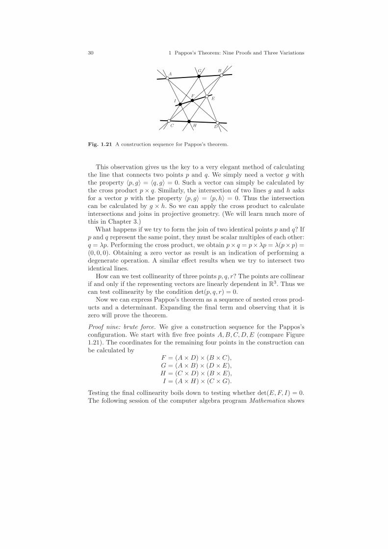
30 1 Pappos’s Theorem: Nine Proofs and Three Variations
AB
C D
EF
G
H
I
Fig. 1.21 A construction sequence for Pappos’s theorem.
This observation gives us the key to a very elegant method of calculatingthe line that connects two points p and q. We simply need a vector g withthe property 〈p, g〉 = 〈q, g〉 = 0. Such a vector can simply be calculated bythe cross product p× q. Similarly, the intersection of two lines g and h asksfor a vector p with the property 〈p, g〉 = 〈p, h〉 = 0. Thus the intersectioncan be calculated by g × h. So we can apply the cross product to calculateintersections and joins in projective geometry. (We will learn much more ofthis in Chapter 3.)
What happens if we try to form the join of two identical points p and q? Ifp and q represent the same point, they must be scalar multiples of each other:q = λp. Performing the cross product, we obtain p× q = p×λp = λ(p× p) =(0, 0, 0). Obtaining a zero vector as result is an indication of performing adegenerate operation. A similar effect results when we try to intersect twoidentical lines.
How can we test collinearity of three points p, q, r? The points are collinearif and only if the representing vectors are linearly dependent in R3. Thus wecan test collinearity by the condition det(p, q, r) = 0.
Now we can express Pappos’s theorem as a sequence of nested cross prod-ucts and a determinant. Expanding the final term and observing that it iszero will prove the theorem.
Proof nine: brute force. We give a construction sequence for the Pappos’sconfiguration. We start with five free points A,B,C,D,E (compare Figure1.21). The coordinates for the remaining four points in the construction canbe calculated by
F = (A×D) × (B × C),G = (A×B) × (D × E),H = (C ×D) × (B × E),I = (A×H) × (C ×G).
Testing the final collinearity boils down to testing whether det(E,F, I) = 0.The following session of the computer algebra program Mathematica shows

1.7 Finally... 31
an evaluation of these expressions. All output except for the final result hasbeen suppressed. The final “0” proves Pappos’s theorem.
What does this evaluation indeed prove? It shows that when we performthe construction sequence independently of the initial choice of the coordi-nates of A,B,C,D,E, the final determinant will be zero. This may happenfor two different reasons. Either during the construction sequence we runinto a degenerate situation (such as the intersection of identical lines) thatintroduce a zero vector as an intermediate result. Or all operations were valid(this will be the case for almost every instance) and the final points E,F, Iare indeed collinear. ⊓⊔
A word of caution: The last proof is very general and seems to be straight-forward. Still, the help of a computer is essential here. Performing the cal-culations by hand would require one to perform all cross products and toevaluate the final determinant. The final term has altogether 15456 sum-mands of degree 15. They can be canceled in pairs, which gives the finalresult.


Part I
Projective Geometry


2
Projective Planes
Moge dieses Buchlein dazu beitragen den Schatz geo-metrischer Schonheit [. . .] uber unsere Zeit hinwegzuretten.
W. Blaschke, Projektive Geometrie 1949
The basis of all investigations in this book will be projective geometry.Although projective geometry has a tradition of more than 400 years, itgives a fresh look at many problems, even today. One could even saythat the essence of this book is to view many well-known geometric ef-fects/setups/statements/environments from a projective viewpoint.
One of the usual approaches to projective geometry is the axiomatic one(see for instance [3, 25, 44, 58]). There, in the spirit of Euclid, a few axiomsare set up and a projective geometry is defined as any system that satisfiesthese axioms. We will very briefly meet this approach in this chapter. Themain part of this book will, however, be much more concrete and “down toearth.” We will predominantly study projective geometries that are definedover a specific coordinate field (most prominently the real numbers R orthe complex numbers C). This gives us the chance to directly investigatethe interplay of geometric objects (points, lines, circles, conics, . . .) and thealgebraic structures (coordinates, polynomials, determinants, . . .) that areused to represent them. The largest part of the book will be about surprisinglyelegant ways of expressing geometric operations or relations by algebraicformulas (see also [26]). We will in particular focus on understanding thegeometry of real and of complex spaces. In the same way as the concept ofcomplex numbers explains many of the seemingly complicated effects for realsituations (for instance in calculus, algebra, or function theory), studying thecomplex projective world will give surprising insights into the geometry overthe real numbers (which to a large extent governs our real life).
35
36 2 Projective Planes
The usual study of Euclidean geometry leads to a treatment of specialcases at a very early stage. Two lines may intersect or not depending onwhether they are parallel or not. Two circles may intersect or not dependingon their radii and on the position of their midpoints. In fact, these two effectsalready lead to a variety of special cases in constructions and theorems all overEuclidean geometry. The treatment of these special cases often unnecessarilyobscures the beauty of the underlying structures. Our aim in this book is toderive statements and formulas that are elegant and general, and carry asmuch geometric information as possible. In particular, we will try to reducethe necessity of treating special cases to a minimum. Here we do not strivefor complicated formulas but for formulas that carry much structural insightand often simplicity. In a sense, this book is written in the spirit of JuliusPlucker (1801–1868), who was, as Felix Klein (1849–1925) expressed it [69],a master of “reading in the equations.”
Starting from the usual Euclidean plane we will see that there are two es-sential extensions needed to bypass thespecial situations described in the lastparagraph. First, one has to introduce elements at infinity. These elementsat infinity will nicely unify special cases that come from parallel situations.Second (in the third part of this book), we will study the geometry over com-plex numbers, since they allow us also to treat intersections of circles thatare disjoint from each other in real space.
2.1 Drawings and Perspectives
• In the Garden of Eden, God is giving Adam a geometrylesson: “Two parallel lines intersect at infinity. It can’tbe proven but I’ve been there.”
• If parallel lines meet at infinity, infinity must be a verynoisy place with all those lines crashing together!
Two math jokes from a website
It was one of the major achievements of the Renaissance period of paintingto understand the laws of perspective drawing. If one tries to produce a two-dimensional image of a three-dimensional object (say a cube or a pyramid),the lines of the drawing cannot be in arbitrary position. Lines that are parallelin the original scene must either be parallel or meet in a finite point. Linesthat meet in a point in the original scene have either to meet in a point in thedrawing or they may become parallel in the picture for very special choicesof the viewpoint. The artists of that time (among others Durer, Leonardoda Vinci and Raphael) used these principles to produce (for the standards ofthat time) stunningly realistic-looking images of buildings, towns, and other

2.1 Drawings and Perspectives 37
Fig. 2.1 A page of Durer’s book Underweysung der Messung, mit dem Zirkel unnRichtscheyt, in Linien, Ebenen unn gantzen corporen.
scenes. The principles developed at this time still form the basis of mostcomputer-created photorealistic images. The basic idea is simple. To producea two-dimensional drawing of a three-dimensional scene, fix the position ofthe canvas and the position of the viewer’s eye in space. For each point onthe canvas consider a line from the viewer’s eye through this point and plota dot according to the object that your ray meets first (compare Figure 2.1).
By this procedure a line in object space is in general mapped to a line inthe picture. One may think of this process in the following way: Any point inobject space is connected to the viewpoint by a line. The intersection of thisline with the canvas gives the image of the point. For any line in object spacewe consider the plane spanned by this line and the viewpoint (if the line doesnot pass through the viewpoint this plane is unique). The intersection of thisplane and the canvas plane is the image of the line. This simple constructionprinciple implies that—almost obviously—incidences of points and lines arepreserved by the mapping process and that lines are again mapped to lines.Parallelism, orthogonality, distances, and angles, however, are not preservedby this process. So it may happen that lines that were parallel in object spaceare mapped to concurrent lines in the image space. Two pictures by the Dutch

38 2 Projective Planes
Fig. 2.2 Two copperplates of the dutch graphic artist M.C. Escher with auxiliary linesdemonstrating the strong perspectivity.
artist M.C. Escher in which these construction principles are carried out ina very strict sense are reproduced in Figure 2.21.
A first systematic treatment of the mathematical laws of perspective draw-ings was undertaken by the French architect and engineer Girard Desar-gues (1591–1661) [32] and later by his student Blaise Pascal (1623–1662).
They laid foundations of the discipline that we today call projective ge-ometry. Unfortunately, many of their geometric investigations had not beenanticipated by the mathematicians of their time, since approximately at thesame time Rene Descartes (1596–1650) published his groundbreaking workLa geometrie, which for the first time intimately related the concepts of alge-bra and geometry by introducing a coordinate system (this is why we speakof “Cartesian coordinates”). It was almost 150 years later that large partsof projective geometry were rediscovered by the Frenchman Gaspard Monge(1746–1818), who was, among other occupations, draftsman, lecturer, min-ister and a strong supporter of Napoleon Bonaparte and his revolution. Hismathematical investigations had very practical backgrounds, since they wereat least partially directly related to mechanics, architecture, and military ap-plications. In 1799 Monge wrote a book [89] on what we today would callconstructive or descriptive geometry. This discipline deals with the problemof making exact two-dimensional construction sketches of three-dimensionalobjects. Monge introduced a method (which in essence is still used today byarchitects and mechanical engineers) of providing different interrelated per-
1 M.C. Escher’s “Delft: Town Hall” c©2010 The M.C. Escher Company-Holland. All rightsreserved.—M.C. Escher’s “Tower of Babel” c©2010 The M.C. Escher Company-Holland.All rights reserved. www.mcescher.com.
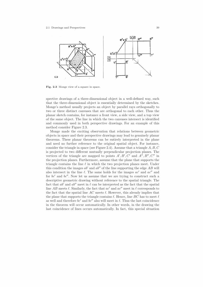
2.1 Drawings and Perspectives 39
Fig. 2.3 Monge view of a square in space.
spective drawings of a three-dimensional object in a well-defined way, suchthat the three-dimensional object is essentially determined by the sketches.Monge’s method usually projects an object by parallel rays orthogonally totwo or three distinct canvases that are orthogonal to each other. Thus theplanar sketch contains, for instance a front view, a side view, and a top viewof the same object. The line in which the two canvases intersect is identifiedand commonly used in both perspective drawings. For an example of thismethod consider Figure 2.3.
Monge made the exciting observation that relations between geometricobjects in space and their perspective drawings may lead to genuinely planartheorems. These planar theorems can be entirely interpreted in the planeand need no further reference to the original spatial object. For instance,consider the triangle in space (see Figure 2.4). Assume that a triangle A,B,Cis projected to two different mutually perpendicular projection planes. Thevertices of the triangle are mapped to points A′, B′, C′ and A′′, B′′, C′′ inthe projection planes. Furthermore, assume that the plane that supports thetriangle contains the line ℓ in which the two projection planes meet. Underthis condition the images ab′ and ab′′ of the line supporting the edge AB willalso intersect in the line ℓ. The same holds for the images ac′ and ac′′ andfor bc′ and bc′′. Now let us assume that we are trying to construct such adescriptive geometric drawing without reference to the spatial triangle. Thefact that ab′ and ab′′ meet in ℓ can be interpreted as the fact that the spatialline AB meets ℓ. Similarly, the fact that ac′ and ac′′ meet in ℓ corresponds tothe fact that the spatial line AC meets ℓ. However, this already implies thatthe plane that supports the triangle contains ℓ. Hence, line BC has to meet ℓas well and therefore bc′ and bc′′ also will meet in ℓ. Thus the last coincidencein the theorem will occur automatically. In other words, in the drawing thelast coincidence of lines occurs automatically. In fact, this special situation
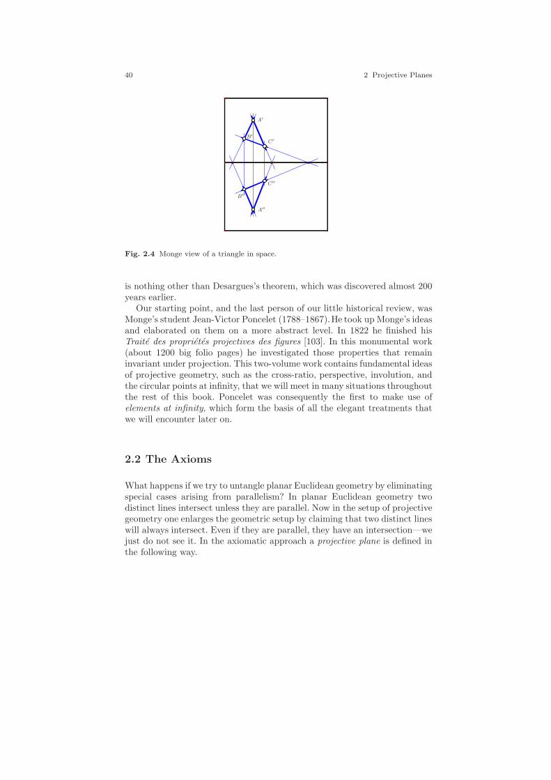
40 2 Projective Planes
A′
B′
C′
A′′
B′′
C′′
Fig. 2.4 Monge view of a triangle in space.
is nothing other than Desargues’s theorem, which was discovered almost 200years earlier.
Our starting point, and the last person of our little historical review, wasMonge’s student Jean-Victor Poncelet (1788–1867).He took up Monge’s ideasand elaborated on them on a more abstract level. In 1822 he finished hisTraite des proprietes projectives des figures [103]. In this monumental work(about 1200 big folio pages) he investigated those properties that remaininvariant under projection. This two-volume work contains fundamental ideasof projective geometry, such as the cross-ratio, perspective, involution, andthe circular points at infinity, that we will meet in many situations throughoutthe rest of this book. Poncelet was consequently the first to make use ofelements at infinity, which form the basis of all the elegant treatments thatwe will encounter later on.
2.2 The Axioms
What happens if we try to untangle planar Euclidean geometry by eliminatingspecial cases arising from parallelism? In planar Euclidean geometry twodistinct lines intersect unless they are parallel. Now in the setup of projectivegeometry one enlarges the geometric setup by claiming that two distinct lineswill always intersect. Even if they are parallel, they have an intersection—wejust do not see it. In the axiomatic approach a projective plane is defined inthe following way.
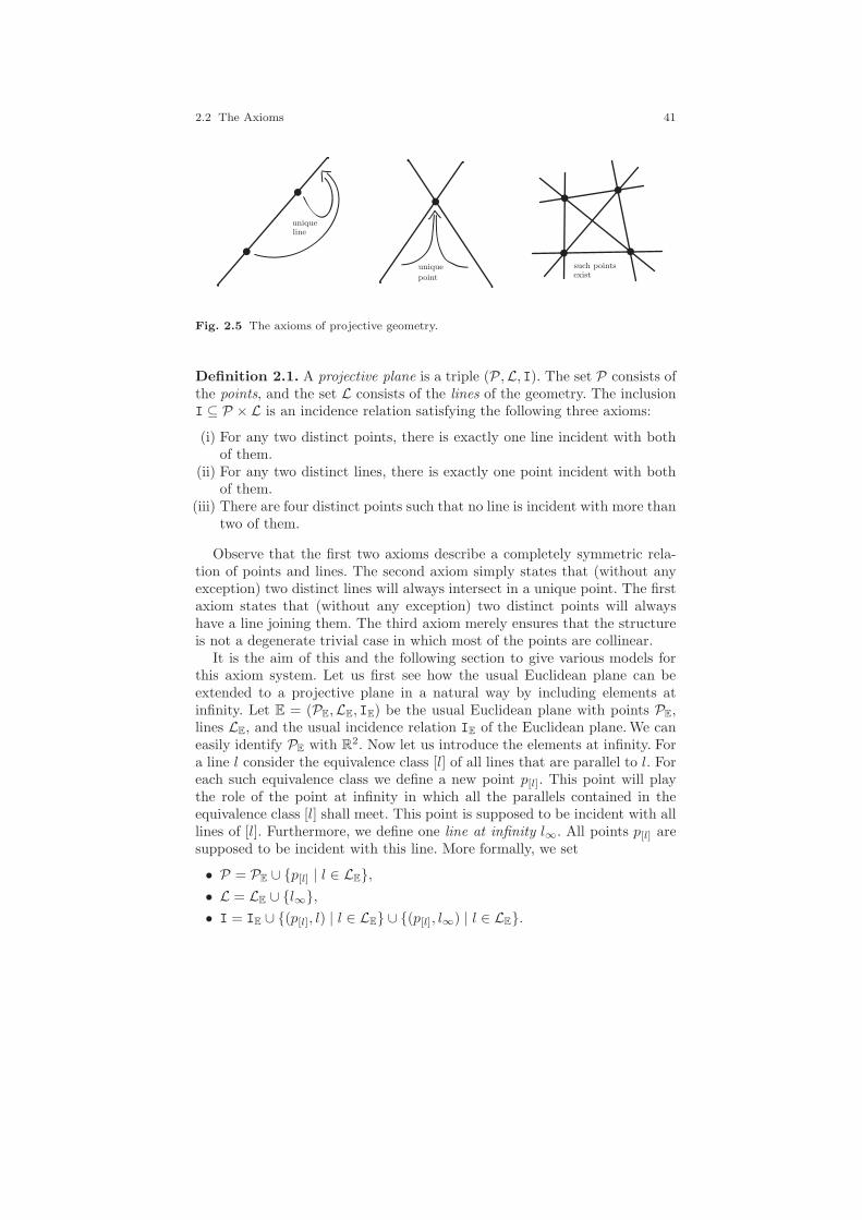
2.2 The Axioms 41
uniqueline
unique
point
such pointsexist
Fig. 2.5 The axioms of projective geometry.
Definition 2.1. A projective plane is a triple (P ,L, I). The set P consists ofthe points, and the set L consists of the lines of the geometry. The inclusionI ⊆ P × L is an incidence relation satisfying the following three axioms:
(i) For any two distinct points, there is exactly one line incident with bothof them.
(ii) For any two distinct lines, there is exactly one point incident with bothof them.
(iii) There are four distinct points such that no line is incident with more thantwo of them.
Observe that the first two axioms describe a completely symmetric rela-tion of points and lines. The second axiom simply states that (without anyexception) two distinct lines will always intersect in a unique point. The firstaxiom states that (without any exception) two distinct points will alwayshave a line joining them. The third axiom merely ensures that the structureis not a degenerate trivial case in which most of the points are collinear.
It is the aim of this and the following section to give various models forthis axiom system. Let us first see how the usual Euclidean plane can beextended to a projective plane in a natural way by including elements atinfinity. Let E = (PE,LE, IE) be the usual Euclidean plane with points PE,lines LE, and the usual incidence relation IE of the Euclidean plane. We caneasily identify PE with R2. Now let us introduce the elements at infinity. Fora line l consider the equivalence class [l] of all lines that are parallel to l. Foreach such equivalence class we define a new point p[l]. This point will playthe role of the point at infinity in which all the parallels contained in theequivalence class [l] shall meet. This point is supposed to be incident with alllines of [l]. Furthermore, we define one line at infinity l∞. All points p[l] aresupposed to be incident with this line. More formally, we set
• P = PE ∪ p[l] | l ∈ LE,• L = LE ∪ l∞,• I = IE ∪ (p[l], l) | l ∈ LE ∪ (p[l], l∞) | l ∈ LE.
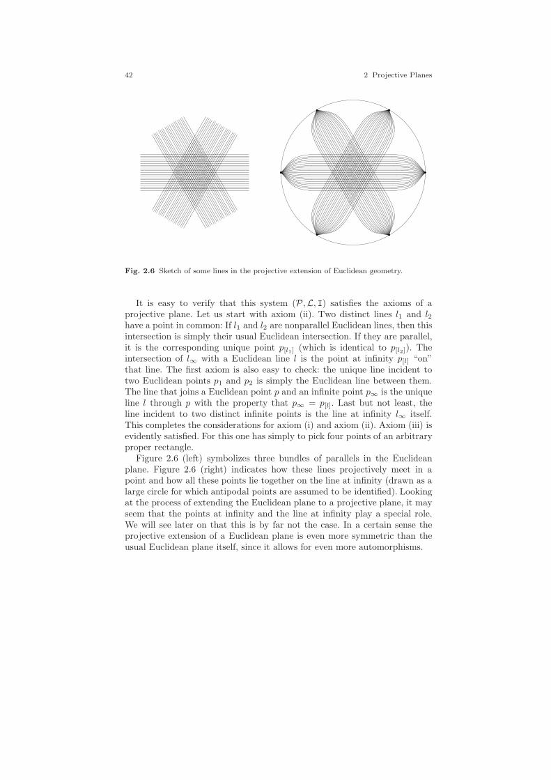
42 2 Projective Planes
Fig. 2.6 Sketch of some lines in the projective extension of Euclidean geometry.
It is easy to verify that this system (P ,L, I) satisfies the axioms of aprojective plane. Let us start with axiom (ii). Two distinct lines l1 and l2have a point in common: If l1 and l2 are nonparallel Euclidean lines, then thisintersection is simply their usual Euclidean intersection. If they are parallel,it is the corresponding unique point p[l1] (which is identical to p[l2]). Theintersection of l∞ with a Euclidean line l is the point at infinity p[l] “on”that line. The first axiom is also easy to check: the unique line incident totwo Euclidean points p1 and p2 is simply the Euclidean line between them.The line that joins a Euclidean point p and an infinite point p∞ is the uniqueline l through p with the property that p∞ = p[l]. Last but not least, theline incident to two distinct infinite points is the line at infinity l∞ itself.This completes the considerations for axiom (i) and axiom (ii). Axiom (iii) isevidently satisfied. For this one has simply to pick four points of an arbitraryproper rectangle.
Figure 2.6 (left) symbolizes three bundles of parallels in the Euclideanplane. Figure 2.6 (right) indicates how these lines projectively meet in apoint and how all these points lie together on the line at infinity (drawn as alarge circle for which antipodal points are assumed to be identified). Lookingat the process of extending the Euclidean plane to a projective plane, it mayseem that the points at infinity and the line at infinity play a special role.We will see later on that this is by far not the case. In a certain sense theprojective extension of a Euclidean plane is even more symmetric than theusual Euclidean plane itself, since it allows for even more automorphisms.
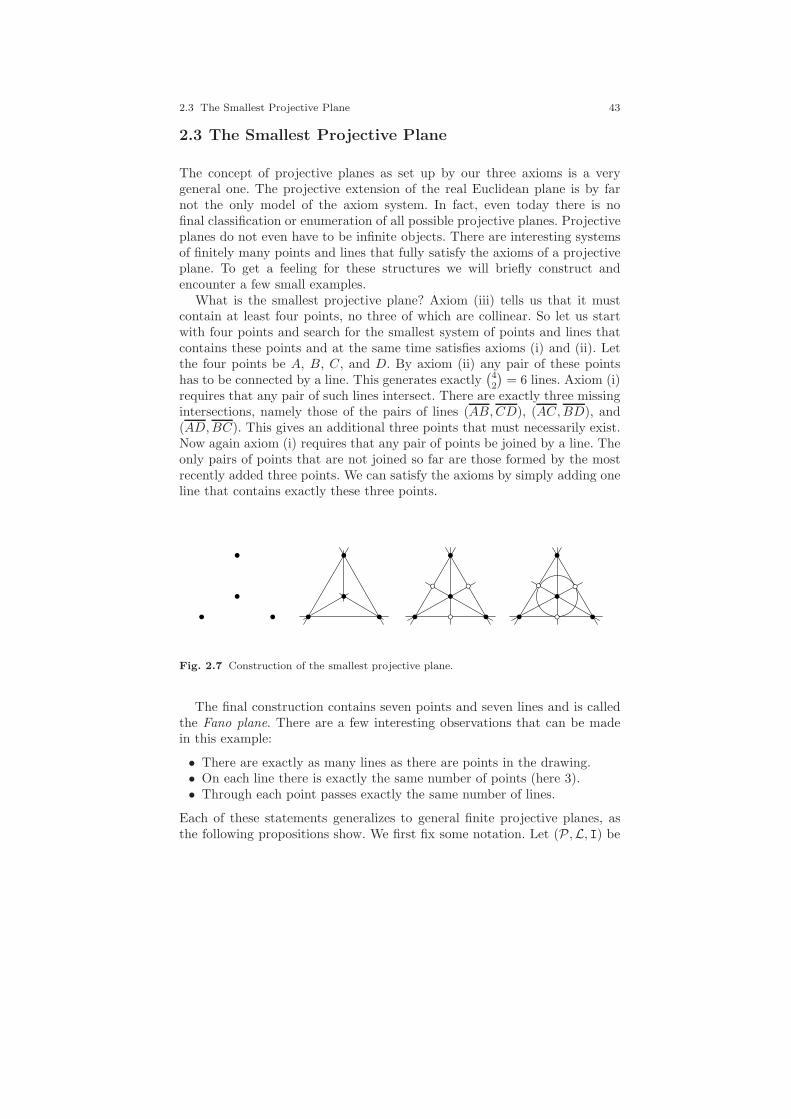
2.3 The Smallest Projective Plane 43
2.3 The Smallest Projective Plane
The concept of projective planes as set up by our three axioms is a verygeneral one. The projective extension of the real Euclidean plane is by farnot the only model of the axiom system. In fact, even today there is nofinal classification or enumeration of all possible projective planes. Projectiveplanes do not even have to be infinite objects. There are interesting systemsof finitely many points and lines that fully satisfy the axioms of a projectiveplane. To get a feeling for these structures we will briefly construct andencounter a few small examples.
What is the smallest projective plane? Axiom (iii) tells us that it mustcontain at least four points, no three of which are collinear. So let us startwith four points and search for the smallest system of points and lines thatcontains these points and at the same time satisfies axioms (i) and (ii). Letthe four points be A, B, C, and D. By axiom (ii) any pair of these pointshas to be connected by a line. This generates exactly
(42
)= 6 lines. Axiom (i)
requires that any pair of such lines intersect. There are exactly three missingintersections, namely those of the pairs of lines (AB,CD), (AC,BD), and(AD,BC). This gives an additional three points that must necessarily exist.Now again axiom (i) requires that any pair of points be joined by a line. Theonly pairs of points that are not joined so far are those formed by the mostrecently added three points. We can satisfy the axioms by simply adding oneline that contains exactly these three points.
Fig. 2.7 Construction of the smallest projective plane.
The final construction contains seven points and seven lines and is calledthe Fano plane. There are a few interesting observations that can be madein this example:
• There are exactly as many lines as there are points in the drawing.• On each line there is exactly the same number of points (here 3).• Through each point passes exactly the same number of lines.
Each of these statements generalizes to general finite projective planes, asthe following propositions show. We first fix some notation. Let (P ,L, I) be
44 2 Projective Planes
a projective plane. For a line l ∈ L let p(l) = p ∈ P∣∣ pIl be the points
on l, and for a point p ∈ P let l(p) = l ∈ L∣∣ pIl be the lines through p.
Furthermore, we agree on a few linguistic conventions. Since in a projectiveplane the line l that is at the same time incident to two points p and q is byaxiom (i) uniquely determined, we will use a language that is more functionalthan set-theoretic and simply speak of the join of the two points. We willexpress this join operation by p∨q or by join(p, q). Similarly, we will call theunique point incident with two lines l and m the meet or intersection of theselines and denote the corresponding operation by l ∧m or by meet(l,m). Wealso say that a line l contains a point p if it is incident with it.
Lemma 2.1. If for p, q ∈ P and l,m ∈ L we have pIl, qIl, pIm, and qIm,then either p = q or l = m.
Proof. Assume that pIl, qIl, pIm, and qIm. If p 6= q, axiom (i) implies thatl = m. Conversely, if l 6= m, axiom (ii) implies that p = q. ⊓⊔
Lemma 2.2. Every line of a projective plane is incident with at least threepoints.
Proof. Let l ∈ L be any line of the projective plane and assume to thecontrary that l does contain fewer than three points. Let a, b, c, and d be thepoints of axiom (iii). Assume without loss of generality that a and b are noton l. Consider the lines a∨ b, a∨ c, a∨d. Since these all pass through a, theymust be distinct by axiom (iii) and must by Lemma 2.1 have three distinctintersections with l. ⊓⊔
Lemma 2.3. For every point p there is at least one line not incident with p.
Proof. Let p be any point. Let l and m be arbitrary lines. Either one of themdoes not contain p (then we are done), or we have p = l ∧ m. By the lastlemma there is a point pl on l distinct from p, and a point pm on m distinctfrom p. The join of these two points cannot contain p, since this would violateaxiom (i). ⊓⊔
Theorem 2.1. Let (P ,L, I) be a projective plane with finite sets P and L.Then there exists a number n ∈ N such that |p(l)| = n+ 1 for any l ∈ L and|l(p)| = n+ 1 for any p ∈ P.
Proof. Let l and m be two distinct lines. Assume that l contains k points. Wewill prove that both lines contain the same number of points. Let p = l ∧mbe their intersection and let ℓ be a line through p distinct from l and m.Now consider a point q on ℓ distinct from p, which exists by Lemma 2.2. Leta1, a2, . . . , an = p(l) − p be the points on l distinct from p and consider
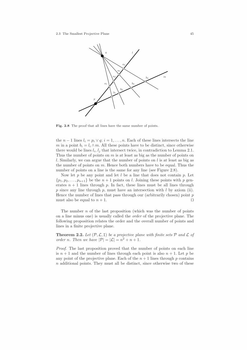
2.3 The Smallest Projective Plane 45
a1
a2
a3
a4
b1
b2
b3
b4
l
m
p
q
Fig. 2.8 The proof that all lines have the same number of points.
the n− 1 lines li = pi ∨ q; i = 1, . . . , n. Each of these lines intersects the linem in a point bi = li ∧m. All these points have to be distinct, since otherwisethere would be lines li, lj that intersect twice, in contradiction to Lemma 2.1.Thus the number of points on m is at least as big as the number of points onl. Similarly, we can argue that the number of points on l is at least as big asthe number of points on m. Hence both numbers have to be equal. Thus thenumber of points on a line is the same for any line (see Figure 2.8).
Now let p be any point and let l be a line that does not contain p. Letp1, p2, . . . , pn+1 be the n+ 1 points on l. Joining these points with p gen-erates n + 1 lines through p. In fact, these lines must be all lines throughp since any line through p, must have an intersection with l by axiom (ii).Hence the number of lines that pass through our (arbitrarily chosen) point pmust also be equal to n+ 1. ⊓⊔
The number n of the last proposition (which was the number of pointson a line minus one) is usually called the order of the projective plane. Thefollowing proposition relates the order and the overall number of points andlines in a finite projective plane.
Theorem 2.2. Let (P ,L, I) be a projective plane with finite sets P and L oforder n. Then we have |P| = |L| = n2 + n+ 1.
Proof. The last proposition proved that the number of points on each lineis n + 1 and the number of lines through each point is also n + 1. Let p beany point of the projective plane. Each of the n+ 1 lines through p containsn additional points. They must all be distinct, since otherwise two of these
46 2 Projective Planes
lines intersect twice. We have altogether (n+ 1) · n+ 1 = n2 + n+ 1 points.A similar count proves that the number of lines is the same. ⊓⊔
So far we have met two examples of a projective plane. One is the finiteFano plane of order 2; the other (infinite example) was the projective exten-sion of the real Euclidean plane. Our next chapter will show that both can beconsidered as special examples of a construction that generates a projectiveplane for every number field.

3
Homogeneous Coordinates
Ich habe bei den folgenden Entwicklungen nur die Absichtgehabt [...] zu zeigen, dass die neue Methode [...] zum Be-weise einzelner Satze und zur Darstellung allgemeiner Theo-rien sich sehr geschmeidig zeigt.
Julius Plucker, Ueber ein neues Coordinatensystem, 1829
3.1 A Spatial Point of View
Let K be any field.1. And let K3 be the vector space of dimension three overthis field. We will prove that if we consider the one-dimensional subspaces ofK
3 as points and the two-dimensional subspaces as lines, then we obtain aprojective plane by defining incidence as subspace containment.
We will prove this fact by creating a more concrete coordinate representa-tion of the one- and two-dimensional subspaces of K3. This will allow us tocalculate with these objects easily. For this we first form equivalence classesof vectors by identifying all vectors v ∈ K3 that differ by a nonzero multiple:
[v] := v′ ∈ K3 | v′ = λ · v for λ ∈ K \ 0.
The set of all such equivalence classes could be denoted by K3\(0,0,0)
K\0 : all
nonzero vectors modulo scalar nonzero multiples. Replacing a vector by its
1 This is almost the only place in this book where we will refer to an arbitrary field K Allother considerations will be much more “down to earth” and refer to specific fields—mostlythe real numbers R or the complex numbers C.
47

48 3 Homogeneous Coordinates
equivalence class preserves many interesting structural properties. In par-ticular, two vectors v1, v2 are orthogonal if their scalar product vanishes:〈v1, v2〉 = 0. This relation remains stable if we replace the two vectors by anyvectors taken from the corresponding equivalence classes. We define orthog-onality of equivalence classes [p] and [l] in a canonic way by
[p] ⊥ [l] ⇐⇒ 〈p, l〉 = 0.
Now we set PK = K3\(0,0,0)
K\0 and let LK = K3\(0,0,0)
K\0 as well (we consider
PK and LK as disjoint copies of the same kind of space). Furthermore, wedefine the incidence relation IK ⊆ PK × LK for [p] ∈ P and [l] ∈ L by
[p] IK [l] ⇐⇒ [p] ⊥ [l].
Before we prove that the triple (PK,LK, IK) is indeed a projective plane, weclarify what this has to do with one- and two-dimensional subspaces. Thereis a bijection of the set of one-dimensional subspaces of K3 and PK. Eachsubspace can be represented by a single nonzero vector p in it. In fact, exactlyall vectors in the equivalence class [p] represent the same one-dimensionalsubspace. We observe, that [p] itself is this subspace with the zero vectortaken out. A two-dimensional vector space (x, y, z) | ax + by + cz = 0in K
3 is in our setup represented by its normal vector (a, b, c). Since normalvectors that differ only by a scalar multiple describe the same two-dimensionalsubspace, the set LK is appropriate for representing them. Finally, a one-dimensional subspace represented by [p] is contained in a two-dimensionalsubspace represented by [l] if and only if [p] ⊥ [l]. This is consistent with ourincidence operator IK.
Theorem 3.1. With the above definitions and notation for any field K, thetriple (PK,LK, IK) is a projective plane.
Proof. We simply have to verify the three axioms. Let [p] and [q] be twodistinct elements in PK. In order to verify axiom (i) we must prove that thereis a vector l that is simultaneously orthogonal to p and q. Furthermore, wemust show that all nonzero vectors with this property must be scalar multiplesof l. Since [p] and [q] are distinct, the vectors (p1, p2, p3) and (q1, q2, q3) donot differ just by a nonzero scalar multiple. In other words, the matrix
(p1 p2 p3
q1 q2 q3
)
has rank 2. Thus the solution space of
(p1 p2 p3
q1 q2 q3
)l1l2l3
=
(00
)
3.2 The Real Projective Plane with Homogeneous Coordinates 49
is one-dimensional. This is exactly the desired claim. For any nonzero solution(l1, l2, l3) of this system the equivalence class [(l1, l2, l3)] is the desired join ofthe points.
In a completely similar way, we can verify axiom (ii), which states that forany pair of distinct lines there is exactly one point incident to both.
For axiom (iii) observe that any field K must contain a zero element anda one element. It is easy to check that the equivalence classes of the four vec-tors (0, 0, 1), (0, 1, 1), (1, 0, 1), and (1, 1, 1) satisfy the requirements of non-collinearity of axiom (iii). ⊓⊔
Although the message of the last theorem is simple, it is perhaps the cen-tral point of this entire book. It is the link of geometry and algebra. Itspower stems from the fact that we can recover our construction of projec-tively extending the Euclidean plane directly in the representation of pointsby three-dimensional vectors. This will be shown in the next section. This rep-resentation of points as well as lines of a projective plane by three-dimensionalvectors is called homogeneous coordinates. We will later on see that the ad-jective homogeneous is very appropriate, since these coordinates at the sametime unify the role of usual lines and the line at infinity and give three co-ordinates of K3 a completely symmetric interpretation. We will see that byintroducing this coordinate system we can easily deal with the Euclideanplane and its projective extension (the points and the line at infinity) in acompletely algebraic manner.
The use of homogeneous coordinates can be considered an extensionof barycentric coordinates, which were introduced by August FerdinandMobius (1790–1868). Homogeneous coordinates were first introduced byJulius Plucker in his article “Ueber ein neues Coordinatensystem” in 1830[99]. There he writes
Ich habe bei den folgenden Entwicklungen nur die Absicht gehabt [...] zu zeigen, dassdie neue Methode [...] zum Beweise einzelner Satze und zur Darstellung allgemeinerTheorien sich sehr geschmeidig zeigt.2
In fact, it is this elegance that we will encounter repeatedly throughout thisbook. I hope that after finishing this book the reader will finally agree onPlucker’s point of view.
3.2 The Real Projective Plane with HomogeneousCoordinates
Let us now analyze how the projective extension of the Euclidean planefits into the picture of homogeneous coordinates. For this we start with a
2 My intention for making the following developments was to demonstrate that this newmethod turns out to be very pliable for proving specific theorems or for representing generaltheories.
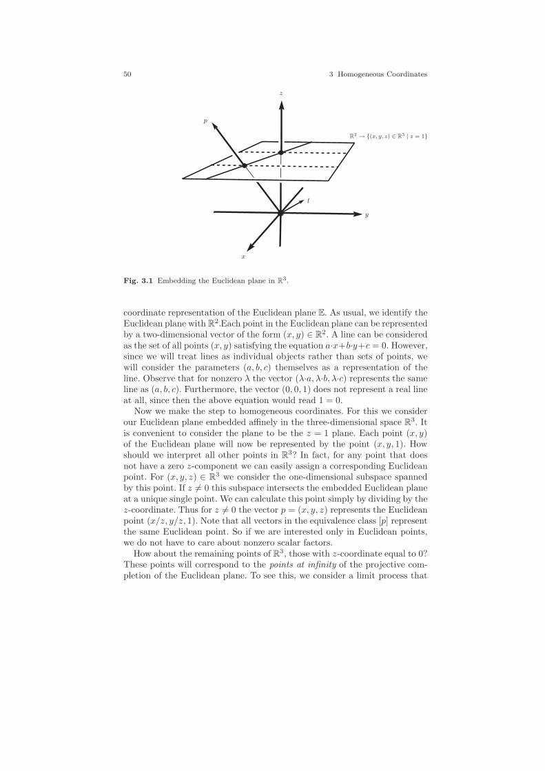
50 3 Homogeneous Coordinates
y
x
z
p
l
R2 → (x, y, z) ∈ R3 | z = 1
Fig. 3.1 Embedding the Euclidean plane in R3.
coordinate representation of the Euclidean plane E. As usual, we identify theEuclidean plane with R2.Each point in the Euclidean plane can be representedby a two-dimensional vector of the form (x, y) ∈ R2. A line can be consideredas the set of all points (x, y) satisfying the equation a·x+b·y+c = 0. However,since we will treat lines as individual objects rather than sets of points, wewill consider the parameters (a, b, c) themselves as a representation of theline. Observe that for nonzero λ the vector (λ·a, λ·b, λ·c) represents the sameline as (a, b, c). Furthermore, the vector (0, 0, 1) does not represent a real lineat all, since then the above equation would read 1 = 0.
Now we make the step to homogeneous coordinates. For this we considerour Euclidean plane embedded affinely in the three-dimensional space R3. Itis convenient to consider the plane to be the z = 1 plane. Each point (x, y)of the Euclidean plane will now be represented by the point (x, y, 1). Howshould we interpret all other points in R3? In fact, for any point that doesnot have a zero z-component we can easily assign a corresponding Euclideanpoint. For (x, y, z) ∈ R3 we consider the one-dimensional subspace spannedby this point. If z 6= 0 this subspace intersects the embedded Euclidean planeat a unique single point. We can calculate this point simply by dividing by thez-coordinate. Thus for z 6= 0 the vector p = (x, y, z) represents the Euclideanpoint (x/z, y/z, 1). Note that all vectors in the equivalence class [p] representthe same Euclidean point. So if we are interested only in Euclidean points,we do not have to care about nonzero scalar factors.
How about the remaining points of R3, those with z-coordinate equal to 0?These points will correspond to the points at infinity of the projective com-pletion of the Euclidean plane. To see this, we consider a limit process that
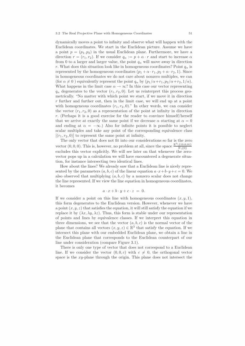
3.2 The Real Projective Plane with Homogeneous Coordinates 51
dynamically moves a point to infinity and observe what will happen with theEuclidean coordinates. We start in the Euclidean picture. Assume we havea point p = (p1, p2) in the usual Euclidean plane. Furthermore, we have adirection r = (r1, r2). If we consider qα := p + α · r and start to increase αfrom 0 to a larger and larger value, the point qα will move away in directionr. What does this situation look like in homogeneous coordinates? Point qα isrepresented by the homogeneous coordinates (p1 +α · r1, p2 +α · r2, 1). Sincein homogeneous coordinates we do not care about nonzero multiples, we can(for α 6= 0 ) equivalently represent the point qα by (p1/α+r1, p2/α+r2, 1/α).What happens in the limit case α→ ∞? In this case our vector representingqα degenerates to the vector (r1, r2, 0). Let us reinterpret this process geo-metrically. “No matter with which point we start, if we move it in directionr further and further out, then in the limit case, we will end up at a pointwith homogeneous coordinates (r1, r2, 0).” In other words, we can considerthe vector (r1, r2, 0) as a representation of the point at infinity in directionr. (Perhaps it is a good exercise for the reader to convince himself/herselfthat we arrive at exactly the same point if we decrease α starting at α = 0and ending at α = −∞.) Also for infinite points it is possible to neglectscalar multiples and take any point of the corresponding equivalence class[(r1, r2, 0)] to represent the same point at infinity.
The only vector that does not fit into our considerations so far is the zero
vector (0, 0, 0). This is, however, no problem at all, since the space R3\(0,0,0)
R\0excludes this vector explicitly. We will see later on that whenever the zero-vector pops up in a calculation we will have encountered a degenerate situa-tion, for instance intersecting two identical lines.
How about the lines? We already saw that a Euclidean line is nicely repre-sented by the parameters (a, b, c) of the linear equation a ·x+b ·y+c = 0. Wealso observed that multiplying (a, b, c) by a nonzero scalar does not changethe line represented. If we view the line equation in homogeneous coordinates,it becomes
a · x+ b · y + c · z = 0.
If we consider a point on this line with homogeneous coordinates (x, y, 1),this form degenerates to the Euclidean version. However, whenever we havea point (x, y, z) that satisfies the equation, it will still satisfy the equation if wereplace it by (λx, λy, λz). Thus, this form is stable under our representationof points and lines by equivalence classes. If we interpret this equation inthree dimensions, we see that the vector (a, b, c) is the normal vector of theplane that contains all vectors (x, y, z) ∈ R3 that satisfy the equation. If weintersect this plane with our embedded Euclidean plane, we obtain a line inthe Euclidean plane that corresponds to the Euclidean counterpart of ourline under consideration (compare Figure 3.1).
There is only one type of vector that does not correspond to a Euclideanline. If we consider the vector (0, 0, c) with c 6= 0, the orthogonal vectorspace is the xy-plane through the origin. This plane does not intersect the

52 3 Homogeneous Coordinates
embedded Euclidean plane. However all points at infinity (remember, theyhave the form (x, y, 0)) are orthogonal to this vector, since 0·x+0·y+c·0 = 0.We call this line the line at infinity. It is incident to all points at infinity.
Let us summarize what we have achieved so far. In Section 2.2 we discussedhow we can extend the Euclidean plane by introducing elements at infinity:one point at infinity for each direction and one global line at infinity thatcontains all these points. Now we have a concrete coordinate representation ofthese objects. The Euclidean points correspond to points of the form (x, y, 1);the infinite points correspond to points of the form (x, y, 0). The Euclideanlines have the form (a, b, c) with a 6= 0 or b 6= 0 (or both). The line at infinityhas the form (0, 0, 1). All the vectors are considered modulo nonzero scalarmultiples. We will refer to this setup of the real projective plane later on asRP
2. This notion stands for Real Projective 2-dimensional space. Later on wewill also deal with spaces such as RP
1, RPd, CP
1, CP2.
From the three-dimensional viewpoint the distinction of infinite and finiteelements is completely unnatural: all elements are simply represented by vec-tors. This resembles the situation in the axiom system for projective planes.There we also do not distinguish between finite and infinite elements. Thisdistinction is only a kind of artifact that arises when we interpret the Eu-clidean plane in a projective setup. In a sense, if we consider the projectiveplane as an extension of the Euclidean plane, we break the nice symmetry ofprojective planes by (artificially) singling out one line to play the role of theline at infinity. Nevertheless, it is a very fruitful exercise to interpret Euclideantheorems in a projective framework or to interpret projective theorems in aEuclidean framework. Usually, a whole group of theorems in Euclidean ge-ometry corresponds to just one theorem in projective geometry and turns outto be just different specializations for different lines at infinity. We will makethese kinds of investigations very often in the following chapters, and we willsee how nicely projective geometry generalizes different Euclidean concepts.
3.3 Joins and Meets
This section is dedicated to a way of easily carrying out elementary operationsin geometry by algebraic calculation. In Chapter 2 we saw that the axiomsystem for projective planes immediately motivates two operations, the joinof two points and the meet of two lines. We will now get to know the algebraiccounterparts of these operations. From now on we will (by slight abuse ofnotation) no longer explicitly refer to the equivalence classes of points thatarise from multiplication by nonzero scalars. Rather than that we will dothe calculations with explicit representatives of these classes. Essentially alloperations that will be described can be simply carried out on this level ofrepresentatives. So, from now on the reader should always have in mind thatthe vectors (x, y, z) and (λx, λy, λz) represent the same geometric point.

3.3 Joins and Meets 53
The crucial point for representing the join and meet operations alge-braically is that if (in homogeneous coordinates) the point (x, y, z) is con-tained in the line (a, b, c), the equation
a · x+ b · y + c · z = 0
holds. If the equation holds, then these two vectors are orthogonal. Now, iftwo points p = (p1, p2, p3) and q = (q1, q2, q3) are given, then the coordinatesl = (l1, l2, l3) of a line incident to both points must be orthogonal to bothvectors p and q. In Section 3.1 we argued that there is a solution to thisproblem by explicitly writing down a system of two linear equations. However,there is also a way to obtain a specific solution explicitly. For this considerthe vector-product operator “×” from linear algebra. This operator is definedas follows:
p1
p2
p3
×
q1q2q3
=
+p2q3 − p3q2−p1q3 + p3q1+p1q2 − p2q1
.
An easy calculation shows that this operator generates a vector that is si-multaneously orthogonal to p and q. For instance, for p we get, after termexpansion,
p1 · (p2q3 − p3q2) + p2 · (−p1q3 + p3q1) + p3 · (p1q2 − p2q1) = 0.
(We will soon see a more structural approach to the vector product thatexplains this relation.) Thus we can express the join operation of two pointssimply by the cross product:
meet(p, q) := p× q.
We can deal in a completely similar fashion with the problem of intersectingtwo lines l = (l1, l2, l3) and m = (m1,m2,m3). A point that is simultaneouslyincident with both lines must be represented by a vector that is orthogonalto both l and m. We can generate such a vector simply by forming the vectorproduct. Thus we get
join(l,m) := l×m.
It is instructive to see these operators in work at a Euclidean example. LetA,B,C,D (see Figure 3.2, left) be four points in the Euclidean plane givenby the following (Euclidean) coordinates:
A = (1, 1),B = (3, 2),C = (3, 0),D = (4, 1).
What are the coordinates of the intersection of the lines AB and CD? Thehomogeneous coordinates of the points are A = (1, 1, 1), B = (3, 2, 1), C =

54 3 Homogeneous Coordinates
(3, 0, 1), D = (4, 1, 1). We can calculate the homogeneous coordinates of thetwo lines simply by taking the vector products:
lAB = (1, 1, 1)× (3, 2, 1)= (1 · 1 − 1 · 2,−1 · 1 + 1 · 3, 1 · 2 − 1 · 3)= (−1, 2,−1),
lCD = (3, 0, 1)× (4, 1, 1)= (0 · 1 − 1 · 1,−3 · 1 + 1 · 4, 3 · 1 − 0 · 4)= (−1, 1, 3).
The meet E of these lines is again calculated by the vector product:
E = (−1, 2,−1)× (−1, 1, 3)= (2 · 3 − (−1) · 1,−(−1) · 3 + (−1) · (−1), (−1) · 1 − 2 · (−1))= (7, 4, 1).
These are the homogeneous coordinates of the Euclidean point (7, 4). (Thefact that the z-coordinate turned out to be 1 was, in fact, only a luckycoincidence. In general we would have to divide by this coordinate to getthe Euclidean values.) It is somehow amazing that with a projective point ofview we get an explicit and straightforward way to calculate with joins andintersections. The calculations even automatically take care of the coordinatesif elements at infinity are involved. We consider the same example but nowwith point D located at (5, 1) (see Figure 3.2, right). The calculation abovebecomes
lAB = (1, 1, 1) × (3, 2, 1)= (1 · 1 − 1 · 2,−1 · 1 + 1 · 3, 1 · 2 − 1 · 3)= (−1, 2,−1),
lCD = (3, 0, 1) × (5, 1, 1)= (0 · 1 − 1 · 1,−3 · 1 + 1 · 5, 3 · 1 − 0 · 5)= (−1, 2, 3).
E = (−1, 2,−1)× (−1, 2, 3)= (2 · 3 − (−1) · 2,−(−1) · 3 + (−1) · (−1), (−1) · 2 − 2 · (−1))= (8, 4, 0).
Point E is now an infinite point, since its z-coordinate is zero. In particular,it its the infinite point in direction (8, 4) (or equivalently in direction (2, 1)).This is the point in which the two parallel lines meet.
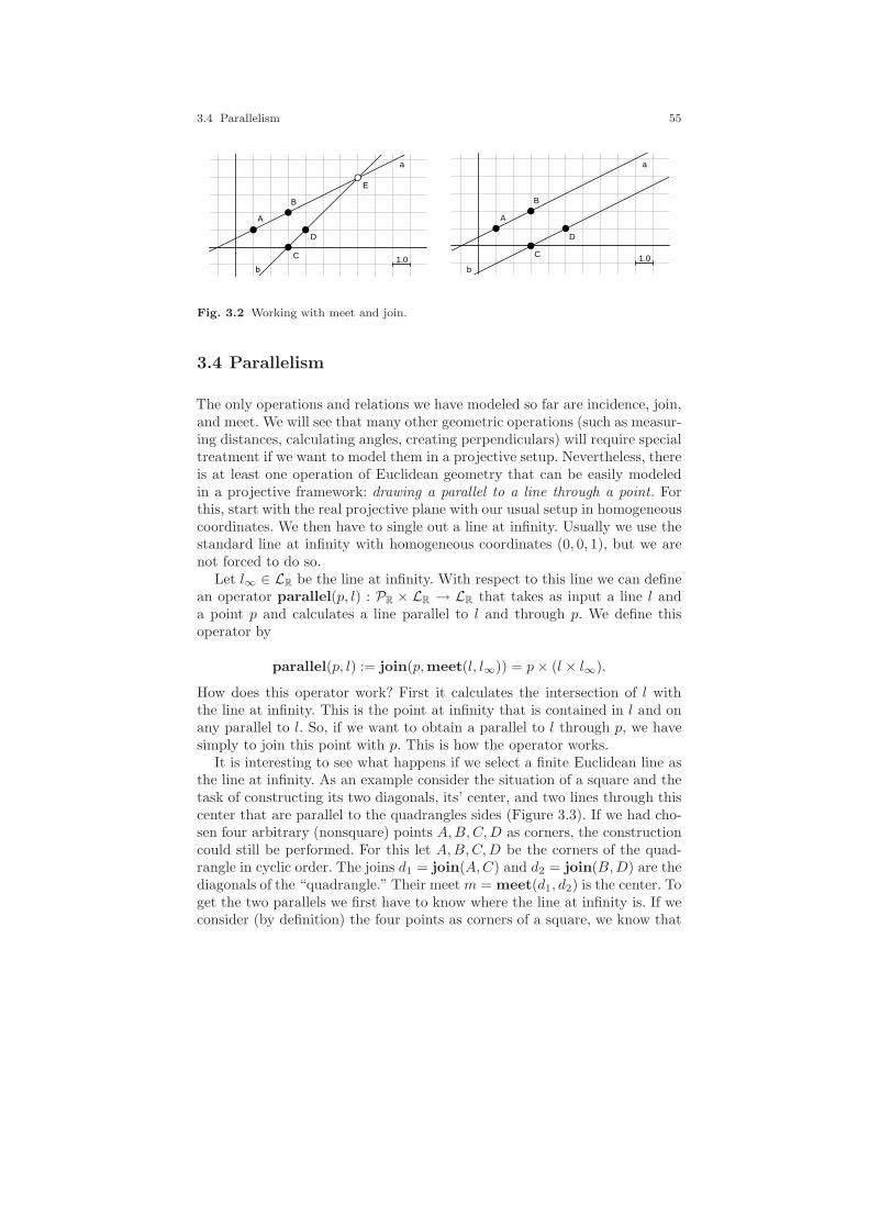
3.4 Parallelism 55
1.0
A
B
C
D
E
a
b1.0
A
B
C
D
a
b
Fig. 3.2 Working with meet and join.
3.4 Parallelism
The only operations and relations we have modeled so far are incidence, join,and meet. We will see that many other geometric operations (such as measur-ing distances, calculating angles, creating perpendiculars) will require specialtreatment if we want to model them in a projective setup. Nevertheless, thereis at least one operation of Euclidean geometry that can be easily modeledin a projective framework: drawing a parallel to a line through a point. Forthis, start with the real projective plane with our usual setup in homogeneouscoordinates. We then have to single out a line at infinity. Usually we use thestandard line at infinity with homogeneous coordinates (0, 0, 1), but we arenot forced to do so.
Let l∞ ∈ LR be the line at infinity. With respect to this line we can definean operator parallel(p, l) : PR × LR → LR that takes as input a line l anda point p and calculates a line parallel to l and through p. We define thisoperator by
parallel(p, l) := join(p,meet(l, l∞)) = p× (l × l∞).
How does this operator work? First it calculates the intersection of l withthe line at infinity. This is the point at infinity that is contained in l and onany parallel to l. So, if we want to obtain a parallel to l through p, we havesimply to join this point with p. This is how the operator works.
It is interesting to see what happens if we select a finite Euclidean line asthe line at infinity. As an example consider the situation of a square and thetask of constructing its two diagonals, its’ center, and two lines through thiscenter that are parallel to the quadrangles sides (Figure 3.3). If we had cho-sen four arbitrary (nonsquare) points A,B,C,D as corners, the constructioncould still be performed. For this let A,B,C,D be the corners of the quad-rangle in cyclic order. The joins d1 = join(A,C) and d2 = join(B,D) are thediagonals of the “quadrangle.” Their meet m = meet(d1, d2) is the center. Toget the two parallels we first have to know where the line at infinity is. If weconsider (by definition) the four points as corners of a square, we know that
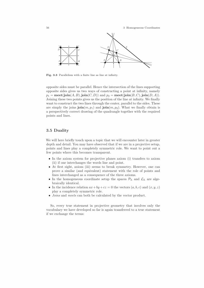
56 3 Homogeneous Coordinates
D C
A B
D
C
A B
q
Fig. 3.3 Parallelism with a finite line as line at infinity.
opposite sides must be parallel. Hence the intersection of the lines supportingopposite sides gives us two ways of constructing a point at infinity, namelyp1 = meet(join(A,B), join(C,D)) and p2 = meet(join(B,C), join(D,A)).Joining these two points gives us the position of the line at infinity. We finallywant to construct the two lines through the center, parallel to the sides. Theseare simply the joins join(m, p1) and join(m, p2). What we finally obtain isa perspectively correct drawing of the quadrangle together with the requiredpoints and lines.
3.5 Duality
We will here briefly touch upon a topic that we will encounter later in greaterdepth and detail. You may have observed that if we are in a projective setup,points and lines play a completely symmetric role. We want to point out afew points where this becomes transparent.
• In the axiom system for projective planes axiom (i) transfers to axiom(ii) if one interchanges the words line and point.
• At first sight, axiom (iii) seems to break symmetry. However, one canprove a similar (and equivalent) statement with the role of points andlines interchanged as a consequence of the three axioms.
• In the homogeneous coordinate setup the spaces PK and LK are alge-braically identical.
• In the incidence relation ax+ by+ cz = 0 the vectors (a, b, c) and (x, y, z)play a completely symmetric role.
• Joins and meets can both be calculated by the vector product.
So, every true statement in projective geometry that involves only thevocabulary we have developed so far is again transferred to a true statementif we exchange the terms:
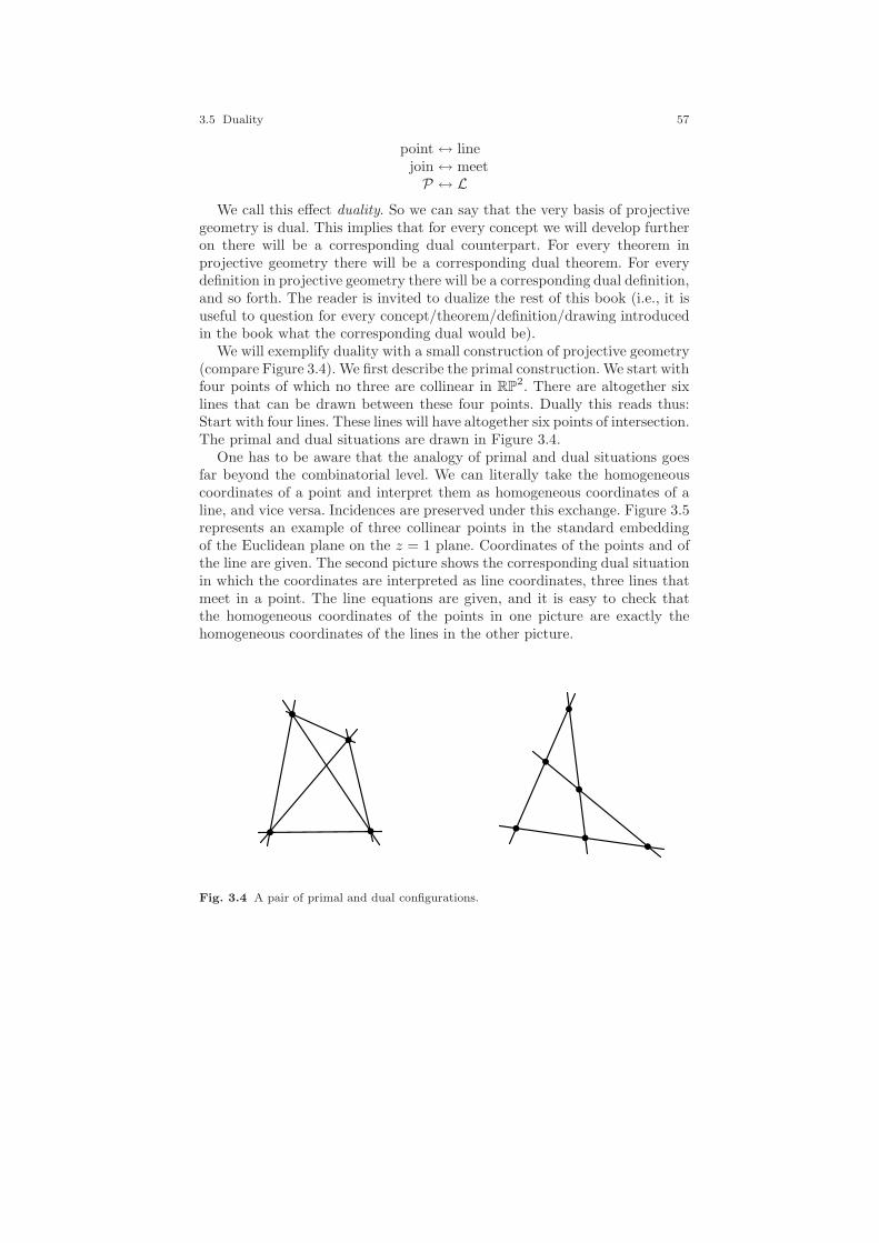
3.5 Duality 57
point ↔ linejoin ↔ meetP ↔ L
We call this effect duality. So we can say that the very basis of projectivegeometry is dual. This implies that for every concept we will develop furtheron there will be a corresponding dual counterpart. For every theorem inprojective geometry there will be a corresponding dual theorem. For everydefinition in projective geometry there will be a corresponding dual definition,and so forth. The reader is invited to dualize the rest of this book (i.e., it isuseful to question for every concept/theorem/definition/drawing introducedin the book what the corresponding dual would be).
We will exemplify duality with a small construction of projective geometry(compare Figure 3.4). We first describe the primal construction. We start withfour points of which no three are collinear in RP
2. There are altogether sixlines that can be drawn between these four points. Dually this reads thus:Start with four lines. These lines will have altogether six points of intersection.The primal and dual situations are drawn in Figure 3.4.
One has to be aware that the analogy of primal and dual situations goesfar beyond the combinatorial level. We can literally take the homogeneouscoordinates of a point and interpret them as homogeneous coordinates of aline, and vice versa. Incidences are preserved under this exchange. Figure 3.5represents an example of three collinear points in the standard embeddingof the Euclidean plane on the z = 1 plane. Coordinates of the points and ofthe line are given. The second picture shows the corresponding dual situationin which the coordinates are interpreted as line coordinates, three lines thatmeet in a point. The line equations are given, and it is easy to check thatthe homogeneous coordinates of the points in one picture are exactly thehomogeneous coordinates of the lines in the other picture.
Fig. 3.4 A pair of primal and dual configurations.
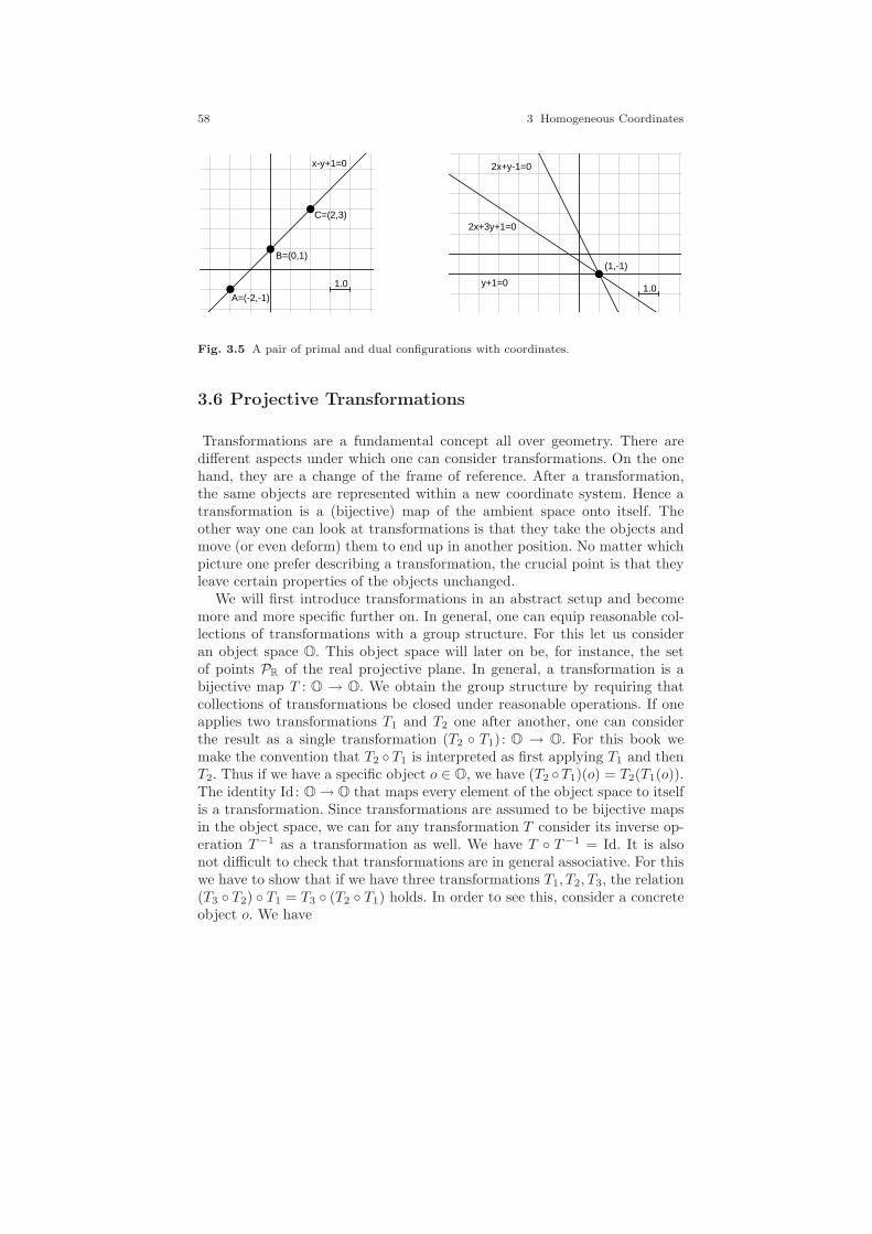
58 3 Homogeneous Coordinates
1.0
A=(-2,-1)
B=(0,1)
C=(2,3)
x-y+1=0
1.0
(1,-1)
2x+y-1=0
y+1=0
2x+3y+1=0
Fig. 3.5 A pair of primal and dual configurations with coordinates.
3.6 Projective Transformations
Transformations are a fundamental concept all over geometry. There aredifferent aspects under which one can consider transformations. On the onehand, they are a change of the frame of reference. After a transformation,the same objects are represented within a new coordinate system. Hence atransformation is a (bijective) map of the ambient space onto itself. Theother way one can look at transformations is that they take the objects andmove (or even deform) them to end up in another position. No matter whichpicture one prefer describing a transformation, the crucial point is that theyleave certain properties of the objects unchanged.
We will first introduce transformations in an abstract setup and becomemore and more specific further on. In general, one can equip reasonable col-lections of transformations with a group structure. For this let us consideran object space O. This object space will later on be, for instance, the setof points PR of the real projective plane. In general, a transformation is abijective map T : O → O. We obtain the group structure by requiring thatcollections of transformations be closed under reasonable operations. If oneapplies two transformations T1 and T2 one after another, one can considerthe result as a single transformation (T2 T1) : O → O. For this book wemake the convention that T2 T1 is interpreted as first applying T1 and thenT2. Thus if we have a specific object o ∈ O, we have (T2 T1)(o) = T2(T1(o)).The identity Id: O → O that maps every element of the object space to itselfis a transformation. Since transformations are assumed to be bijective mapsin the object space, we can for any transformation T consider its inverse op-eration T−1 as a transformation as well. We have T T−1 = Id. It is alsonot difficult to check that transformations are in general associative. For thiswe have to show that if we have three transformations T1, T2, T3, the relation(T3 T2) T1 = T3 (T2 T1) holds. In order to see this, consider a concreteobject o. We have

3.6 Projective Transformations 59
((T3 T2) T1)(o) = (T3 T2)(T1(o))
= T3(T2(T1(o))
= T3((T2 T1)(o))
= (T3 (T2 T1))(o).
Taking all this together, one obtains the properties that ensure that we havea group structure.
Let us be a little more concrete and consider the usual transformations ofEuclidean geometry (we will now recall a few facts from linear algebra). Forthis let R2 again represent the coordinates of the Euclidean plane. The pointsof the Euclidean plane will be our objects; thus R2 plays the role of the objectspace. The usual transformations in Euclidean geometry are translations,rotations, reflections, and glide reflections. These transformations can easilybe expressed by algebraic operations. A translation by a vector (tx, ty) canbe written as (
xy
)7→(x+ txy + ty
).
A rotation about the origin by an angle α can be written as
(xy
)7→(
cos(α) sin(α)− sin(α) cos(α)
)·(xy
).
A rotation about an arbitrary point (rx, ry) can be written as
(xy
)7→(
cos(α) sin(α)− sin(α) cos(α)
)·(x− rxy − ry
)+
(rxry
).
Reflections and glide reflections have a similar representation. Any of theabove Euclidean transformations can be written in the form
p 7→ M(p− v) + w
for suitable choices of a 2 × 2 matrix M and vectors v and w. For rota-tions the matrix M has to be a rotation matrix. This means it has the form(
cos(α) sin(α)− sin(α) cos(α)
). For reflections or glide reflections the matrix must be a re-
flection matrix of the form
(cos(α) sin(α)sin(α) − cos(α)
). The group of Euclidean transfor-
mations leaves fundamental properties and relations within the object spaceinvariant. For instance, if p and q are Euclidean points, then the distancebetween them is the same before or after a Euclidean transformation. Alsothe absolute values of angles are not altered by Euclidean transformations. Ingeneral, the shape and size of an object is not altered by a Euclidean transfor-mation. If one maps a circle (or line, or quadrangle) pointwise by a Euclideantransformation, one ends up again with a circle (or line, or quadrangle) ofthe same size. It may just have moved to another location.

60 3 Homogeneous Coordinates
In the above formM(p−v)+w, one may allow for more general transforma-tions (where M is any invertible 2× 2 matrix). By this one can also describescalings, similarities, and affine transformations. In this case the group oftransformations becomes larger and the set of properties that is not alteredby these transformations becomes smaller. For instance, similarities will stillpreserve the absolute value of angles but no longer distances. An affine trans-formation will not even preserve angles. However, an affine transformationstill maps a pair of parallel lines to another pair of parallel lines.
From the point of view of computer implementations it is inherently diffi-cult and error-prone to calculate with the above representation of Euclideantransformations. The fact that the rotational or reflectional part is expressedby a matrix multiplication while the translational part is expressed by a vec-tor addition makes it cumbersome to calculate the inverses or the compositionof two transformations. Again we get a structurally much clearer approach ifwe focus on a projective setup and an approach via homogeneous coordinates.
If we represent a Euclidean point (x, y) by homogeneous coordinates(x, y, 1), we can express rotations as well as translations by a multiplica-tion by a 3 × 3 matrix. Translations take the following form (assuming for amoment that the z-coordinate is chosen to be 1):
xy1
7→
1 0 tx0 1 ty0 0 1
·
xy1
=
x+ txy + ty
1
.
Rotations about the origin can be expressed thus:
xy1
7→
cos(α) sin(α) 0− sin(α) cos(α) 0
0 0 1
·
xy1
.
Applying two transformations in succession is now nothing but multiplica-tion of the corresponding matrices. Inverting a transformation correspondsto matrix inversion. One should notice that the above matrices were chosenin a way that a vector with z-coordinate equal to one is again mapped toa vector with z-coordinate equal to one. Hence, the first two entries of thehomogeneous coordinate vector directly show the Euclidean position of themapped point (in our standard embedding). From a conceptual point of view,it is, even if one deals only with Euclidean transformations, often much moreuseful to work in this more general representation, since here translations,rotations, and reflections arise in a unified way. Moreover, we will gain evenmore advantage from this representation, since it is the key to an even widerclass of transformations: the projective transformations. First, if we considermatrices with nonzero determinant of the form
3.6 Projective Transformations 61
a b cd e f0 0 1
,
then we get all affine planar transformations. Still we have not used the wholefreedom of an invertible 3 × 3 matrix. A general projective transformation isa multiplication by an invertible 3 × 3 matrix
a b cd e fg h i
.
We now want to investigate the properties of such a general type of pro-jective transformation. We first make a notational convention. Since for anyp ∈ R3 \ (0, 0, 0) the product of a 3 × 3 matrix M and any member of theequivalence class [p] ends up within the same equivalence class [M · p], theaction of M on these equivalence classes is well defined. Thus we can simplyinterpret M as acting on our object space (of equivalence classes) PR. Thuswe can interpret the multiplication by M on the level of representatives taken
from R3 \ (0, 0, 0) or on the level of equivalence classes R3\(0,0,0)
R\0 . Thus
for a projective point in [p] ∈ PR we will write M · [p] and mean by this theprojective point [M · p].
Since in the context of projective geometry the input vector and the outputvector of our matrix multiplication are determined only up to multiplicationby a nonzero scalar, the matrices M and λM represent the same projectivetransformation (for nonzero λ). Thus we have overall only eight degrees offreedom that determine such a transformation.
One fundamental property of projective transformations is given by thefollowing statement.
Theorem 3.2. A projective transformation maps collinear points to collinearpoints.
Proof. It suffices to prove the theorem for a generic triple of points. Let[a], [b], [c] ∈ PR be three collinear points represented by homogeneous coor-dinates a, b, c. In this case there exists a line [l] ∈ LR with 〈l, a〉 = 〈l, b〉 =〈l, c〉 = 0. We assume that all homogeneous coordinates are represented bycolumn vectors. We have to show that under these conditions the points rep-resented by a′ = M · a, b′ = M · b, c′ = M · c, are also collinear. For thissimply consider the line [l′] represented by l′ := (M−1)T l. We have
〈l′, a′〉 = (l′)Ta′ = ((M−1)T l)TMa = lT ((M−1)T )TMa = lTa = 〈l, a〉 = 0.
A similar calculation applies also to the other two points. Thus the linerepresented by l′ is simultaneously incident to all three points represented bya′, b′ and, c′. Hence these points are collinear. ⊓⊔
62 3 Homogeneous Coordinates
Implicitly, the calculations in the last proof describe how a projective trans-formation M : PR → PR represented by a 3 × 3 matrix M acts on the spaceof lines LR. The homogeneous coordinates of a line must be mapped in sucha way that incidences of points and lines are preserved under the mapping.This implies that a line has to be mapped according to l 7→ (M−1)T l. If pand l are incident before a transformation, they will be incident after thetransformation as well.
In fact, the property of Theorem 3.2 is characteristic of projective trans-formations over the field of real numbers. One can prove the following:
Theorem 3.3. If Φ : PR → PR is any bijective map that preserves thecollinearity of points, then Φ can be expressed as multiplication by a 3 × 3matrix.
In fact, this theorem is so crucial that it is sometimes called the fundamentaltheorem of projective geometry. Its proof is a bit subtle, and requires someelementary results from field theory. The proof makes use of the fact thatthe real numbers do not have any field automorphisms except the identity.The generalization of the above theorem to arbitrary fields involves a properdiscussion of field automorphisms. A proof will be postponed to Section 5,where we will discuss the relations of projective geometry and elementaryarithmetic operations. For now, we will collect more properties of projectivetransformations that can be expressed as multiplication by a 3 × 3 matrix.
The most fundamental property of projective transformations that we willneed (which is also of invaluable practical importance) is the following fact.
Theorem 3.4. Let [a], [b], [c], [d] ∈ PR be four points of which no three arecollinear and let [a′], [b′], [c′], [d′] ∈ PR be another four points of which nothree are collinear then there exists a 3× 3 matrix M such that [M ·a] = [a′],[M · b] = [b′], [M · c] = [c′], and [M · d] = [d′].
Proof. We assume that a, b, c, d, a′, b′, c′, d′ ∈ R3 are representatives of thecorresponding equivalence classes. We first prove the theorem for the specialcase that a = (1, 0, 0), b = (0, 1, 0), c = (0, 0, 1), and d = (1, 1, 1). Sincethe columns of a matrix are the images of the unit vectors, the matrix musthave the form (λ · a′, µ · b′, τ · c′). (In other words, the image of a must be amultiple of vector a′ and so forth.) Hence the image of d is λ ·a′ +µ ·b′+τ ·c′.This must be a multiple of d′. We have only to adjust the parameters λ, µ, τaccordingly. For this we have to solve the system of linear equations
| | |a′ b′ c′
| | |
·
λµτ
=
|d′
|
.
This system is solvable, by our nondegeneracy assumptions (a′, b′, c′ are notcollinear). Furthermore, none of the parameters is zero (as a consequence of

3.6 Projective Transformations 63
Fig. 3.6 The image of a grid under a projective transformation.
the remaining nondegeneracy assumptions). This proves the theorem for thespecial case.
In order to prove the general case of the theorem one uses the above factto find a transformation T1 that maps (1, 0, 0), (0, 1, 0), (0, 0, 1), (1, 1, 1) toa, b, c, d, and to find a transformation T2 that maps (1, 0, 0), (0, 1, 0), (0, 0, 1),(1, 1, 1) to a′, b′, c′, d′. The desired transformation is then T2 · T−1
1 . ⊓⊔
Remark 3.1. (A note on implementations): The last theorem is not only oftheoretical interest. The proof gives also a practical recipe for calculating aprojective transformation that maps a, b, c, d to a′, b′, c′, d′ (as usual up toscalar multiple). The basic operations that are required for this are matrixmultiplication and matrix inversion. One has simply to follow the differentcalculation steps in the above proof.
The fact that projective transformations preserve collinearities and inci-dences of points and lines relates them intimately to the topic of perspectivelycorrect drawings. Figure 3.6 shows a drawing of a checkerboard-like grid andfour circles and its image under a projective transformation. The projec-tively transformed picture is completely determined by the image of fourcorner points. Observe that, for instance, the grid points along the diagonalsare again collinear in the transformed image. One can also see that anglesand distances are not preserved under a projective transformation. Not evenratios of distances are preserved: an equidistant chain of points in the originalpicture will in general no longer be equidistant after the projective transfor-mation (later on, we will see that cross-ratios are preserved under projectivetransformations). We also see that circles are not necessarily mapped to cir-cles again. The picture also indicates that tangency relations of curves arepreserved under projective transformations.
Throughout the entire book we will very often return to the topic of pro-jective transformations under various aspects.
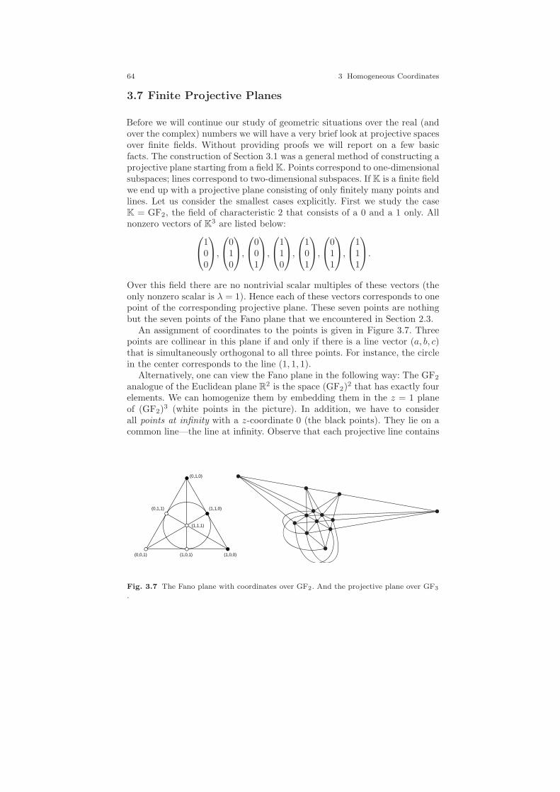
64 3 Homogeneous Coordinates
3.7 Finite Projective Planes
Before we will continue our study of geometric situations over the real (andover the complex) numbers we will have a very brief look at projective spacesover finite fields. Without providing proofs we will report on a few basicfacts. The construction of Section 3.1 was a general method of constructing aprojective plane starting from a field K. Points correspond to one-dimensionalsubspaces; lines correspond to two-dimensional subspaces. If K is a finite fieldwe end up with a projective plane consisting of only finitely many points andlines. Let us consider the smallest cases explicitly. First we study the caseK = GF2, the field of characteristic 2 that consists of a 0 and a 1 only. Allnonzero vectors of K3 are listed below:
100
,
010
,
001
,
110
,
101
,
011
,
111
.
Over this field there are no nontrivial scalar multiples of these vectors (theonly nonzero scalar is λ = 1). Hence each of these vectors corresponds to onepoint of the corresponding projective plane. These seven points are nothingbut the seven points of the Fano plane that we encountered in Section 2.3.
An assignment of coordinates to the points is given in Figure 3.7. Threepoints are collinear in this plane if and only if there is a line vector (a, b, c)that is simultaneously orthogonal to all three points. For instance, the circlein the center corresponds to the line (1, 1, 1).
Alternatively, one can view the Fano plane in the following way: The GF2
analogue of the Euclidean plane R2 is the space (GF2)2 that has exactly four
elements. We can homogenize them by embedding them in the z = 1 planeof (GF2)
3 (white points in the picture). In addition, we have to considerall points at infinity with a z-coordinate 0 (the black points). They lie on acommon line—the line at infinity. Observe that each projective line contains
(0,1,0)
(0,0,1) (1,0,0)
(0,1,1) (1,1,0)
(1,0,1)
(1,1,1)
Fig. 3.7 The Fano plane with coordinates over GF2. And the projective plane over GF3
.
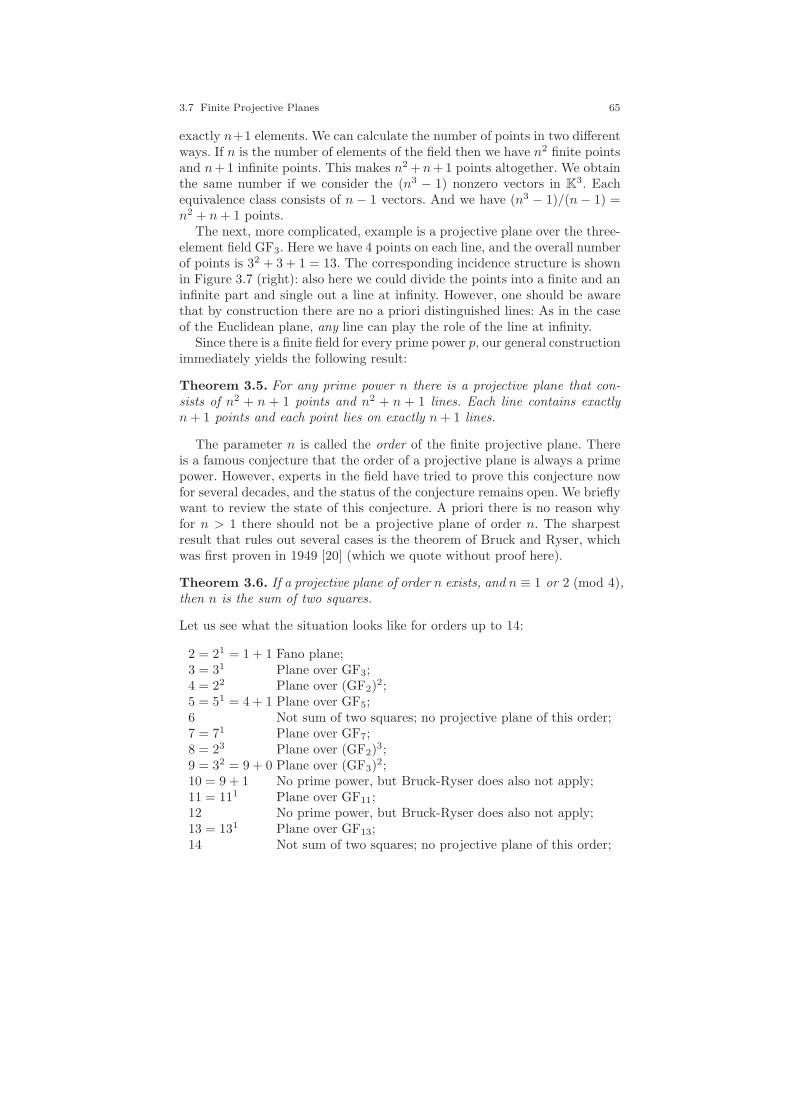
3.7 Finite Projective Planes 65
exactly n+1 elements. We can calculate the number of points in two differentways. If n is the number of elements of the field then we have n2 finite pointsand n+1 infinite points. This makes n2 +n+1 points altogether. We obtainthe same number if we consider the (n3 − 1) nonzero vectors in K3. Eachequivalence class consists of n− 1 vectors. And we have (n3 − 1)/(n− 1) =n2 + n+ 1 points.
The next, more complicated, example is a projective plane over the three-element field GF3. Here we have 4 points on each line, and the overall numberof points is 32 + 3 + 1 = 13. The corresponding incidence structure is shownin Figure 3.7 (right): also here we could divide the points into a finite and aninfinite part and single out a line at infinity. However, one should be awarethat by construction there are no a priori distinguished lines: As in the caseof the Euclidean plane, any line can play the role of the line at infinity.
Since there is a finite field for every prime power p, our general constructionimmediately yields the following result:
Theorem 3.5. For any prime power n there is a projective plane that con-sists of n2 + n + 1 points and n2 + n + 1 lines. Each line contains exactlyn+ 1 points and each point lies on exactly n+ 1 lines.
The parameter n is called the order of the finite projective plane. Thereis a famous conjecture that the order of a projective plane is always a primepower. However, experts in the field have tried to prove this conjecture nowfor several decades, and the status of the conjecture remains open. We brieflywant to review the state of this conjecture. A priori there is no reason whyfor n > 1 there should not be a projective plane of order n. The sharpestresult that rules out several cases is the theorem of Bruck and Ryser, whichwas first proven in 1949 [20] (which we quote without proof here).
Theorem 3.6. If a projective plane of order n exists, and n ≡ 1 or 2 (mod 4),then n is the sum of two squares.
Let us see what the situation looks like for orders up to 14:
2 = 21 = 1 + 1 Fano plane;3 = 31 Plane over GF3;4 = 22 Plane over (GF2)
2;5 = 51 = 4 + 1 Plane over GF5;6 Not sum of two squares; no projective plane of this order;7 = 71 Plane over GF7;8 = 23 Plane over (GF2)
3;9 = 32 = 9 + 0 Plane over (GF3)
2;10 = 9 + 1 No prime power, but Bruck-Ryser does also not apply;11 = 111 Plane over GF11;12 No prime power, but Bruck-Ryser does also not apply;13 = 131 Plane over GF13;14 Not sum of two squares; no projective plane of this order;

66 3 Homogeneous Coordinates
The table reveals two interesting values of the order for which the Theoremof Bruck and Ryser does not rule out the existence of a projective plane, nordoes our field construction apply: the orders 10 and 12.
The case of order 10 was settled in 1989 by H.W.C. Lam, L. Thiel, andS. Swiercz [78, 79]. They proved the nonexistence of a projective plane oforder 10 by a clever but in essence still brute-force computer proof. Theexhaustive computer proof took the equivalent of 2000 hours on a Cray 1supercomputer. (In order to get an impression of the problem state it in thefollowing way: Mark the places in a 111 × 111 array such that the followingconditions are satisfied: In each row and each column there are exactly 11marks. Furthermore, each pair of rows must have exactly one mark in thesame column.)
The case of order 12 is still wide open. No method seems to be known tobreak down the difficulty of enumerating all possible cases to a reasonablesize that would fit on contemporary computing devices.
One might wonder whether the only way to obtain a finite projective planeis via our field construction. This is not the case. The first case for which suchnonstandard planes occur is that of order nine. There are 4 nonisomorphicprojective planes of this order. There are even 193 (known) finite projectiveplanes of order 25. A general method of classification seems to be far beyondreach.
4
Lines and Cross-Ratios
Upside downboy you turn me
inside outand round and round
Song text, Diana Ross
At this stage of this monograph we enter a significant didactic problem.There are three concepts that are intimately related and that unfold their fullpower only if they play together. These concepts are performing calculationswith geometric objects, determinants and determinant algebra, and geometricincidence theorems. The reader should understand that in a beginner’s textthat makes few assumptions about prior knowledge, these concepts mustbe introduced sequentially. Therefore we will sacrifice some mathematicalbeauty for clarity of exposition. Still, we highly recommend that the followingchapters be read (at least) twice, so that the reader may obtain an impressionof the interplay of the different concepts.
This and the next section are dedicated to the relationship between RP2
and calculations in the underlying field R. For this we will first find methodsto relate points in a projective plane to the coordinates over R. Then wewill show that elementary operations like addition and multiplication can bemimicked in a purely geometric fashion. Finally, we will use these facts toderive interesting statements about the structure of projective planes andprojective transformations.
67
68 4 Lines and Cross-Ratios
4.1 Coordinates on a Line
Assume that two distinct points [p] and [q] in PR are given. How can wedescribe the set of all points on the line through these two points? It is clearthat we can implicitly describe them by first calculating the homogeneouscoordinates of the line through p and q and then selecting all points that areincident to this line. However, there is also a very direct and explicit way ofdescribing these points, as the following lemma shows:
Lemma 4.1. Let [p] and [q] be two distinct points in PR. The set of all pointson the line through these points is given by
[λ · p+ µ · q]∣∣ λ, µ ∈ R with λ or µ nonzero.
Proof. The proof is an exercise in elementary linear algebra. For λ, µ ∈ R
(with λ or µ nonzero) let r = λ · p+ µ · q be a representative of a point. Wehave to show that this point is on the line through [p] and [q]. In other words,we must prove that 〈λ ·p+µ ·q, p× q〉 = 0. This is an immediate consequenceof the arithmetic rules for the scalar and vector products. We have
〈λ · p+ µ · q, p× q〉 = 〈λ · p, p× q〉 + 〈µ · q, p× q〉= λ〈p, p× q〉 + µ〈q, p× q〉= λ · 0 + µ · 0= 0.
The first two equations hold by multilinearity of the scalar product. The thirdequation comes from the fact that 〈p, p× q〉 and 〈q, p× q〉 are always zero.
Conversely, assume that [r] is a point on the line spanned by [p] and [q].This means that there is a vector l ∈ R3 with
〈l, p〉 = 〈l, q〉 = 〈l, r〉 = 0.
The points [p] and [q] are distinct, and thus p and q are linearly independent.Consider the matrix M with row vectors p, q, r. This matrix cannot have fullrank, since the product M · l is the zero vector. Thus r must lie in the spanof p and q. Since r itself is not the zero vector, we have a representation ofthe form r = λ · p+ µ · q with λ or µ nonzero. ⊓⊔
The last proof is simply an algebraic version of the geometric fact thatwe consider a line as the linear span of two distinct points on it. In theform r = λ · p + µ · q we can simultaneously multiply both parameters λand µ by the same factor α and still obtain the same point [r]. If one of thetwo parameters is nonzero we can normalize this parameter to 1. Using thisfact we can express almost all points on the line through [p] and [q] by theexpression λ · p + q; λ ∈ R. The only point we miss is [p] itself. Similarly,
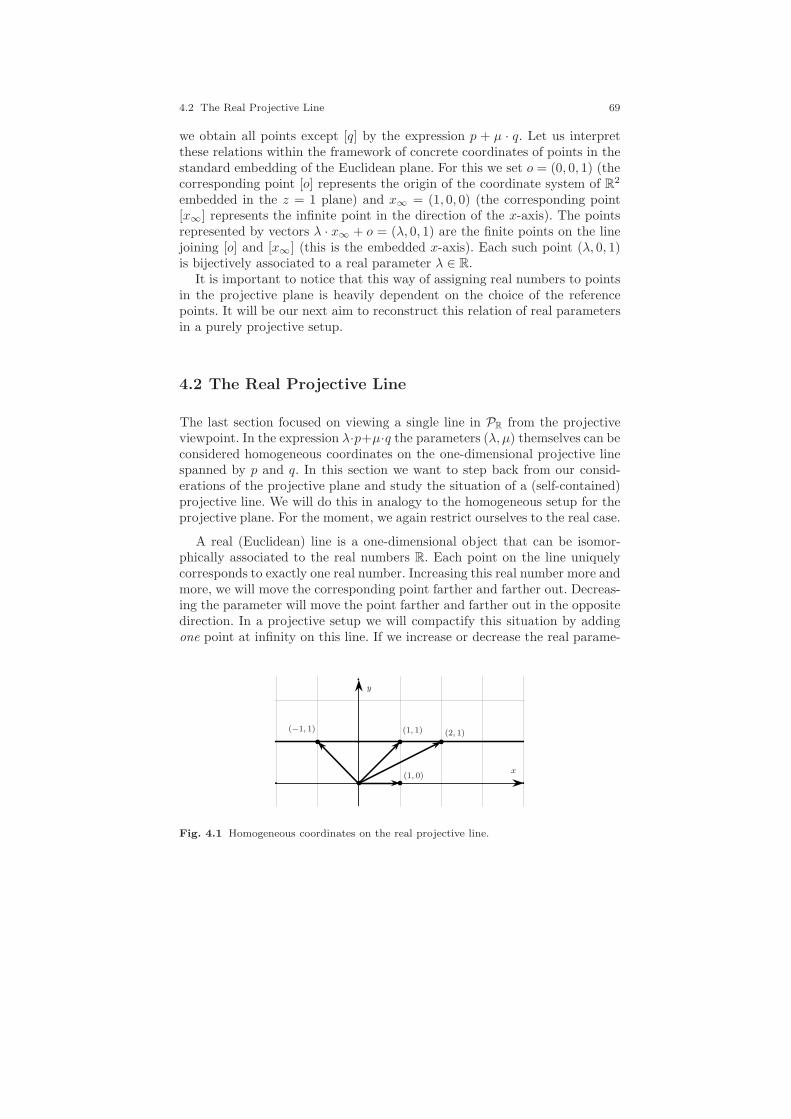
4.2 The Real Projective Line 69
we obtain all points except [q] by the expression p + µ · q. Let us interpretthese relations within the framework of concrete coordinates of points in thestandard embedding of the Euclidean plane. For this we set o = (0, 0, 1) (thecorresponding point [o] represents the origin of the coordinate system of R2
embedded in the z = 1 plane) and x∞ = (1, 0, 0) (the corresponding point[x∞] represents the infinite point in the direction of the x-axis). The pointsrepresented by vectors λ · x∞ + o = (λ, 0, 1) are the finite points on the linejoining [o] and [x∞] (this is the embedded x-axis). Each such point (λ, 0, 1)is bijectively associated to a real parameter λ ∈ R.
It is important to notice that this way of assigning real numbers to pointsin the projective plane is heavily dependent on the choice of the referencepoints. It will be our next aim to reconstruct this relation of real parametersin a purely projective setup.
4.2 The Real Projective Line
The last section focused on viewing a single line in PR from the projectiveviewpoint. In the expression λ·p+µ·q the parameters (λ, µ) themselves can beconsidered homogeneous coordinates on the one-dimensional projective linespanned by p and q. In this section we want to step back from our consid-erations of the projective plane and study the situation of a (self-contained)projective line. We will do this in analogy to the homogeneous setup for theprojective plane. For the moment, we again restrict ourselves to the real case.
A real (Euclidean) line is a one-dimensional object that can be isomor-phically associated to the real numbers R. Each point on the line uniquelycorresponds to exactly one real number. Increasing this real number more andmore, we will move the corresponding point farther and farther out. Decreas-ing the parameter will move the point farther and farther out in the oppositedirection. In a projective setup we will compactify this situation by addingone point at infinity on this line. If we increase or decrease the real parame-
(−1, 1) (1, 1) (2, 1)
(1, 0)x
y
Fig. 4.1 Homogeneous coordinates on the real projective line.
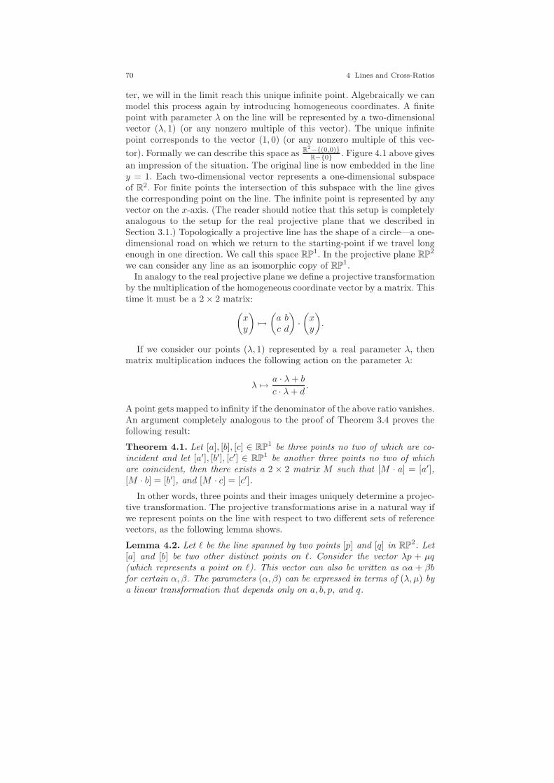
70 4 Lines and Cross-Ratios
ter, we will in the limit reach this unique infinite point. Algebraically we canmodel this process again by introducing homogeneous coordinates. A finitepoint with parameter λ on the line will be represented by a two-dimensionalvector (λ, 1) (or any nonzero multiple of this vector). The unique infinitepoint corresponds to the vector (1, 0) (or any nonzero multiple of this vec-
tor). Formally we can describe this space as R2−(0,0)R−0 . Figure 4.1 above gives
an impression of the situation. The original line is now embedded in the liney = 1. Each two-dimensional vector represents a one-dimensional subspaceof R2. For finite points the intersection of this subspace with the line givesthe corresponding point on the line. The infinite point is represented by anyvector on the x-axis. (The reader should notice that this setup is completelyanalogous to the setup for the real projective plane that we described inSection 3.1.) Topologically a projective line has the shape of a circle—a one-dimensional road on which we return to the starting-point if we travel longenough in one direction. We call this space RP
1. In the projective plane RP2
we can consider any line as an isomorphic copy of RP1.
In analogy to the real projective plane we define a projective transformationby the multiplication of the homogeneous coordinate vector by a matrix. Thistime it must be a 2 × 2 matrix:
(xy
)7→(a bc d
)·(xy
).
If we consider our points (λ, 1) represented by a real parameter λ, thenmatrix multiplication induces the following action on the parameter λ:
λ 7→ a · λ+ b
c · λ+ d.
A point gets mapped to infinity if the denominator of the above ratio vanishes.An argument completely analogous to the proof of Theorem 3.4 proves thefollowing result:
Theorem 4.1. Let [a], [b], [c] ∈ RP1 be three points no two of which are co-
incident and let [a′], [b′], [c′] ∈ RP1 be another three points no two of which
are coincident, then there exists a 2 × 2 matrix M such that [M · a] = [a′],[M · b] = [b′], and [M · c] = [c′].
In other words, three points and their images uniquely determine a projec-tive transformation. The projective transformations arise in a natural way ifwe represent points on the line with respect to two different sets of referencevectors, as the following lemma shows.
Lemma 4.2. Let ℓ be the line spanned by two points [p] and [q] in RP2. Let
[a] and [b] be two other distinct points on ℓ. Consider the vector λp + µq(which represents a point on ℓ). This vector can also be written as αa + βbfor certain α, β. The parameters (α, β) can be expressed in terms of (λ, µ) bya linear transformation that depends only on a, b, p, and q.

4.2 The Real Projective Line 71
a
b
p
a′
b′
p′
o
Fig. 4.2 Projective scales under projections.
Proof. Theorem 4.1 ensures that the point represented by λp + µq can alsobe expressed in the form αa+ βb. Since p is in the span of a and b, it can bewritten as p = αpa+ βpb. Similarly, q can be written as q = αqa+ βqb. Thusthe expression λp+ µq can be written as λ(αpa+ βpb) + µ(αqa+ βqb). Thuswe have
αa+ βb = (αpλ+ αqµ)a+ (βpλ+ βqµ)b.
Since a and b are linearly independent, we have
(αβ
)=
(αp αqβp βq
)·(λµ
).
⊓⊔
Finally, we want to describe how perspectivities from one line to anotherinduce projective maps on the coordinates of the lines. For this let ℓ and ℓ′
be two lines and let o be a projection point not incident to either of them.Furthermore, assume that [a] and [b] are points on ℓ and that [a′] and [b′] arethe corresponding projected images in a projection through o from ℓ to ℓ′.The situation is illustrated in Figure 4.2. With these settings we obtain thefollowing:
Lemma 4.3. There exists a number τ ∈ R such that the image of a pointαa+ βb under the projection is α′a′ + β′b′, with (α′, β′) = (ατ, β).
Proof. One way to geometrically express the desired result is to say that theline (αa+ βb)× (α′a′ + β′b′) is incident to o. This happens if and only if thescalar product of o and this line is zero. In this case we have

72 4 Lines and Cross-Ratios
0 = 〈(αa+ βb) × (α′a′ + β′b′), o〉= 〈(αa× α′a′) + (βb× β′b′) + (αa× β′b′) + (βb× α′a′), o〉= αα′〈(a× a′), o〉 + ββ′〈(b × b′), o〉 + αβ′〈(a× b′), o〉 + βα′〈(b × a′), o〉= αβ′〈(a× b′), o〉 + βα′〈(b× a′), o〉.
The first and second equalities just expand the cross product by distributivity.The third equality holds since o is on a× a′ and o is on b× b′. The last linebeing equal to zero can also be written as
α
β·(−〈(a× b′), o〉〈(b× a′), o〉
)=α′
β′ .
Setting τ = − 〈(a×b′),o〉〈(b×a′),o〉 gives the desired claim. ⊓⊔
4.3 Cross-Ratios (a First Encounter)
In the previous sections we have seen that many geometric magnitudes(among them seemingly natural magnitudes such as distances and ratios ofdistances) do not remain invariant under projective transformations.
Cross-ratios are the simplest magnitudes that are invariant under pro-jective transformations. Cross-ratios will play an important role throughouteach of the following chapters.
Before we introduce cross-ratios, we will set up a little notation that willhelp us to abbreviate many of the formulas we will have to consider from nowon. If a =
(a1
a2
)and b =
(b1b2
)are two-dimensional vectors, we will use
[a, b] := det
(a1 b1a2 b2
)
as an abbreviation for the determinant of the 2 × 2 matrix formed by thesetwo vectors. We will also use
[a, b, c] := det
a1 b1 c1a2 b2 c2a3 b3 c3
as an abbreviation of a 3 × 3 determinant if a, b, c are three-dimensionalvectors. The reader should be careful not to confuse these brackets with thenotation we use for equivalence classes.
A cross-ratio is assigned to an ordered quadruple of points on a line. Wefirst restrict ourselves to the case of calculating the cross-ratio for four pointsin RP
1. Later on we will define the cross-ratio for four arbitrary points on aline in the projective plane RP
2.

4.3 Cross-Ratios (a First Encounter) 73
We first define the cross-ratio on the level of homogeneous coordinates andthen prove that the cross-ratio actually depends only on the projective pointsrepresented by these coordinates.
Definition 4.1. Let a, b, c, d be four nonzero vectors in R2. The cross-ratio(a, b; c, d) is the following magnitude:
(a, b; c, d) :=[a, c][b, d]
[a, d][b, c].
We will now show that the value of the cross-ratio does not change undervarious transformations.
Lemma 4.4. For any real nonzero parameters λa, λb, λc, λd ∈ R we have
(a, b; c, d) = (λaa, λbb;λcc, λdd).
Proof. Since [p, q] represents a determinant with columns p and q, we have[λpp, λqq] = λpλq[p, q]. Applying this to the definition of cross-ratios, we get
[λaa, λcc][λbb, λdd]
[λaa, λdd][λbb, λcc]=λaλbλcλd[a, c][b, d]
λaλbλcλd[a, d][b, c]=
[a, c][b, d]
[a, d][b, c].
Canceling all the λ’s is feasible, since they were assumed to be nonzero. Theequality of the leftmost and the rightmost terms is exactly the claim. ⊓⊔
This lemma proves that it makes sense to speak of the cross-ratio
([a], [b]; [c], [d])
of four points in RP1, since the concrete choices of the representatives are
irrelevant for the value of the cross-ratio. Cross-ratios are also invariant underprojective transformations, as the following lemma shows:
Lemma 4.5. Let M be a 2 × 2 matrix with nonvanishing determinant andlet a, b, c, d be four vectors in R2. Then we have
(a, b; c, d) = (M · a,M · b;M · c,M · d).
Proof. We have [M · p,M · q] = det(M) · [p, q]. This gives:
[M · a,M · c][M · b,M · d][M · a,M · d][M · b,M · c] =
det(M)2[a, c][b, d]
det(M)2[a, d][b, c]=
[a, c][b, d]
[a, d][b, c].
Canceling all determinants is feasible, since M was assumed to be invertible.The equality of the leftmost and the rightmost terms is exactly the claim. ⊓⊔

74 4 Lines and Cross-Ratios
Taking the last two lemmas together highlights a remarkable robustnessof the cross-ratio. Not only is it independent of the vectors representing thepoints. It is invariant even under projective transformations. This in turnhas the consequence that if we have a line in RP
2 with two points p and qsuch that the points on the line are represented by λp + µq, the cross-ratioof four points on this line can be calculated using the parameters (λ, µ) asone-dimensional homogeneous coordinates. The value of this cross-ratio iswell defined according to Lemma 4.2, Lemma 4.4, and Lemma 4.5.
Thus we have encountered our first genuine projective measure: the cross-ratio. From now on we will only very rarely have to distinguish between apoint [p] in projective space and its representation in homogeneous coordi-nates. The reason is that whenever we want to link projective entities tomeasures we can do this via cross-ratios. If no confusion can arise we willfrom now on identify a point [p] with the homogeneous coordinate vectorp representing it. Whenever we speak of the point p we mean the equiva-lence class [p], and if we speak of the vector p we mean the element of Rd
representing it.
4.4 Elementary Properties of the Cross-Ratio
In this section we will collect a few elementary facts that are useful wheneverone calculates with cross-ratios.
Cross-ratios and the real numbers line: Readers already familiarwith cross-ratios may have noticed that our approach to cross-ratios is notthe one taken most often by textbooks. Usually cross-ratios are introduced byexpressions concerning the oriented distances of points on a line. For referencewe will briefly also present this approach.
For this let ℓ be any line and let a, b, c, d be four points on this line. Weassume that ℓ is equipped with an orientation (a preferred direction) and wedenote by |a, b| the directed (Euclidean) distance from a to b (this means that|a, b| = −|b, a|). If ℓ represents the real number line, each point a correspondsto a number xa ∈ R and we can simply set |a, b| = xb−xa. Now the cross-ratiois usually defined as
(a, b; c, d) =|a, c||a, d|
/ |b, c||b, d| .
(In German literature the cross-ratio is called Doppelverhaltnis: a “ratio ofratios.”) It is easy to see that this definition agrees with our setup for allfinite points a, b, c, d. We can introduce homogeneous coordinates
(a1
),(b1
),(
c1
)and
(d1
)for the points. The determinant then becomes
det
(a b1 1
)= a− b = −|a, b|.
4.4 Elementary Properties of the Cross-Ratio 75
An easy calculation shows the identity of both setups. Compared to thisapproach via oriented lengths the approach taken in the last section has theadvantage that it also treats infinite points correctly. Sometimes the formabove provides a nice shortcut for calculating the cross-ratio for finite points.
For some positions of the input values the cross-ratio becomes infinite.This happens whenever either a and d coincide or b and c coincide. It willlater on turn out to be useful not to consider this as an unpleasant specialcase. We simply can consider the results of the cross-ratio themselves aspoints on a projectively closed line. The infinite value is then nothing but arepresentation of the infinite point. If we assume in this interpretation thatthree of the entries (say a, b, and c) are distinct and fixed, then the map
d 7→ (a, b; c, d)
itself becomes a projective transformation. If one wants to calculate withinfinite numbers, the following rules will be consistent with all operationsthroughout this book:
1/∞ = 0; 1/0 = ∞; 1 + ∞ = ∞.
Permutations of cross-ratios: The cross-ratio is not independent of theorder of the entries. However, if we know the cross-ratio (a, b; c, d) = λ, we canreconstruct the cross-ratio for any permutation of a, b, c, and d. We obtainthe following theorem:
Theorem 4.2. Let a, b, c, d be four points on a projective line with cross-ratio(a, b; c, d) = λ. Then we have
(i) (a, b; c, d) = (b, a; d, c) = (c, d; a, b) = (d, c; b, a),
(ii) (a, b; d, c) = 1/λ,
(iii) (a, c; b, d) = 1 − λ,
(iv) the values for the remaining permutations area consequence of these three rules.
Proof. Statement (i) is clear from Definition 4.1 and the anticommutativityof the determinant. Statement (ii) is obvious from the definition, since it justexchanges numerator and denominator.
Statement (iii) requires a little elementary calculation. The expression wewant to prove is
(a, c; b, d) = 1 − (a, b; c, d).
On the determinant level this reads
[a, b][c, d]
[a, d][c, b]= 1 − [a, c][b, d]
[a, d][b, c].

76 4 Lines and Cross-Ratios
Multiplying by [a, d][b, c], this translates to
[a, b][c, d] − [a, c][b, d] + [a, d][b, c] = 0.
Since the cross-ratio is invariant under projective transformations, we mayassume that all points are finite and we can represent them by numbers λa,λb, λc, and λd. The determinants then become differences, and our expressionreads
(λa − λb)(λc − λd) − (λa − λc)(λb − λd) + (λa − λd)(λb − λc) = 0.
Expanding all terms, we get
(λaλc + λbλd − λaλd − λbλc)
−(λaλb + λcλd − λaλd − λcλb)
+(λaλb + λdλc − λaλc − λdλb) = 0.
This is obviously true, since all summands cancel.
Finally, it is obvious that we can generate all possible permutations ofpoints by application of the three rules. The first rule allows us to bringany letter to the front position. The second and third equations describe twospecific transpositions from which all permutations of the last three letterscan be generated. ⊓⊔
Remark 4.1. If (a, b; c, d) = λ, the six values of the cross-ratio for permuta-tions of these points are
λ,1
λ, 1 − λ,
1
1 − λ,
λ
1 − λ,
1 − λ
λ.
In particular, these six functions form a group isomorphic to S3.
Cross-ratios and perspectivities: We now want to demonstrate howcross-ratios are invariant under geometric projections. This is an immedi-ate corollary of the fact that projections induce a projective transformation(Lemma 4.3) and the invariance of the cross-ratio under projective transfor-mations:
Corollary 4.1. Let o be a point and let ℓ and ℓ′ be two lines not passingthrough o. If four points a, b, c, d on ℓ are projected by the viewpoint o to fourpoints a′, b′, c′, d′ on ℓ′, then the cross-ratios satisfy (a, b; c, d) = (a′, b′; c′, d′).
This corollary justifies another concept. We can assign to any quadruple oflines that pass through one point o a cross-ratio. We can assign this cross-ratioin the following way. We cut the four lines by an arbitrary line ℓ (not througho). The four points of intersection define a cross-ratio. The last corollary
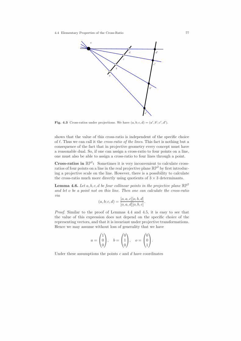
4.4 Elementary Properties of the Cross-Ratio 77
a
b
c
d
a′
b′
c′
d′
o
Fig. 4.3 Cross-ratios under projections. We have (a, b; c, d) = (a′, b′; c′, d′).
shows that the value of this cross-ratio is independent of the specific choiceof ℓ. Thus we can call it the cross-ratio of the lines. This fact is nothing but aconsequence of the fact that in projective geometry every concept must havea reasonable dual. So, if one can assign a cross-ratio to four points on a line,one must also be able to assign a cross-ratio to four lines through a point.
Cross-ratios in RP2: Sometimes it is very inconvenient to calculate cross-
ratios of four points on a line in the real projective plane RP2 by first introduc-
ing a projective scale on the line. However, there is a possibility to calculatethe cross-ratio much more directly using quotients of 3 × 3 determinants.
Lemma 4.6. Let a, b, c, d be four collinear points in the projective plane RP2
and let o be a point not on this line. Then one can calculate the cross-ratiovia
(a, b; c, d) =[o, a, c][o, b, d]
[o, a, d][o, b, c].
Proof. Similar to the proof of Lemmas 4.4 and 4.5, it is easy to see thatthe value of this expression does not depend on the specific choice of therepresenting vectors, and that it is invariant under projective transformations.Hence we may assume without loss of generality that we have
a =
100
, b =
010
, o =
001
.
Under these assumptions the points c and d have coordinates

78 4 Lines and Cross-Ratios
c =
c1c20
, d =
d1
d2
0
.
All determinants reduce to 2 × 2 determinants, and the theorem follows im-mediately. ⊓⊔

5
Calculating with Points on Lines
Newsgroups: sci.math
Subject: Re: I'm looking for axioms and proof in math texts
Date: 6 Aug 2003 02:53:12 -0700
From: [email protected] (prometheus666)
[...]
and being passing familiar with the number line -- I'm sure if I don't
say passing familiar somebody here will say, "You have to know vector
tensor shmelaculus in 15 triad synergies to really understand the
number line. It's not even called that, it's called the real
torticular space." or something to that effect --
[...]
Found on the WWW
In the previous section we have seen that cross-ratios form a universal linkfrom projective geometry to the underlying coordinate field. In this chapterwe want to elaborate more on this topic. We will see that one can recoverthe structure of the real numbers from the purely geometric setup of the realprojective plane.
A line has (seemingly) far less geometric structure than the plane. In theplane there can be collinear and non collinear points, and we have seen thatcollinearity is a crucial property that is invariant under projective transforma-tions. On a line all triples of points are automatically collinear, so we cannothope for this to be a crucial characterizing property of projective transforma-tions. The simplest nontrivial property that is invariant under a projectivetransformation on a line is the specific value of the cross-ratio of a quadrupleof points. It will be the ultimate goal of this chapter to show that a map thatfixes a certain value for the cross-ratio of four points automatically fixes allcross-ratios and will automatically be a projective transformation. From therewe will prove Theorem 3.3, which claims that any bijective transformation inRP
2 that preserves collinearity is automatically a projective transformation.
79
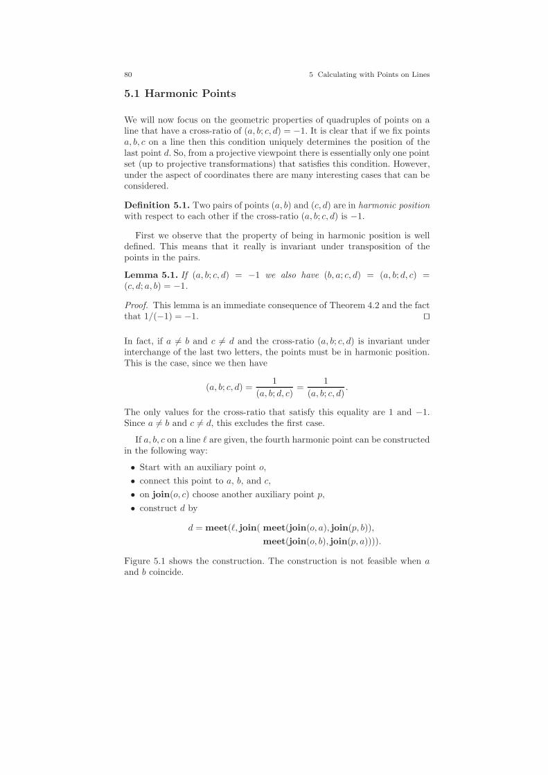
80 5 Calculating with Points on Lines
5.1 Harmonic Points
We will now focus on the geometric properties of quadruples of points on aline that have a cross-ratio of (a, b; c, d) = −1. It is clear that if we fix pointsa, b, c on a line then this condition uniquely determines the position of thelast point d. So, from a projective viewpoint there is essentially only one pointset (up to projective transformations) that satisfies this condition. However,under the aspect of coordinates there are many interesting cases that can beconsidered.
Definition 5.1. Two pairs of points (a, b) and (c, d) are in harmonic positionwith respect to each other if the cross-ratio (a, b; c, d) is −1.
First we observe that the property of being in harmonic position is welldefined. This means that it really is invariant under transposition of thepoints in the pairs.
Lemma 5.1. If (a, b; c, d) = −1 we also have (b, a; c, d) = (a, b; d, c) =(c, d; a, b) = −1.
Proof. This lemma is an immediate consequence of Theorem 4.2 and the factthat 1/(−1) = −1. ⊓⊔
In fact, if a 6= b and c 6= d and the cross-ratio (a, b; c, d) is invariant underinterchange of the last two letters, the points must be in harmonic position.This is the case, since we then have
(a, b; c, d) =1
(a, b; d, c)=
1
(a, b; c, d).
The only values for the cross-ratio that satisfy this equality are 1 and −1.Since a 6= b and c 6= d, this excludes the first case.
If a, b, c on a line ℓ are given, the fourth harmonic point can be constructedin the following way:
• Start with an auxiliary point o,
• connect this point to a, b, and c,
• on join(o, c) choose another auxiliary point p,
• construct d by
d = meet(ℓ, join( meet(join(o, a), join(p, b)),
meet(join(o, b), join(p, a)))).
Figure 5.1 shows the construction. The construction is not feasible when aand b coincide.
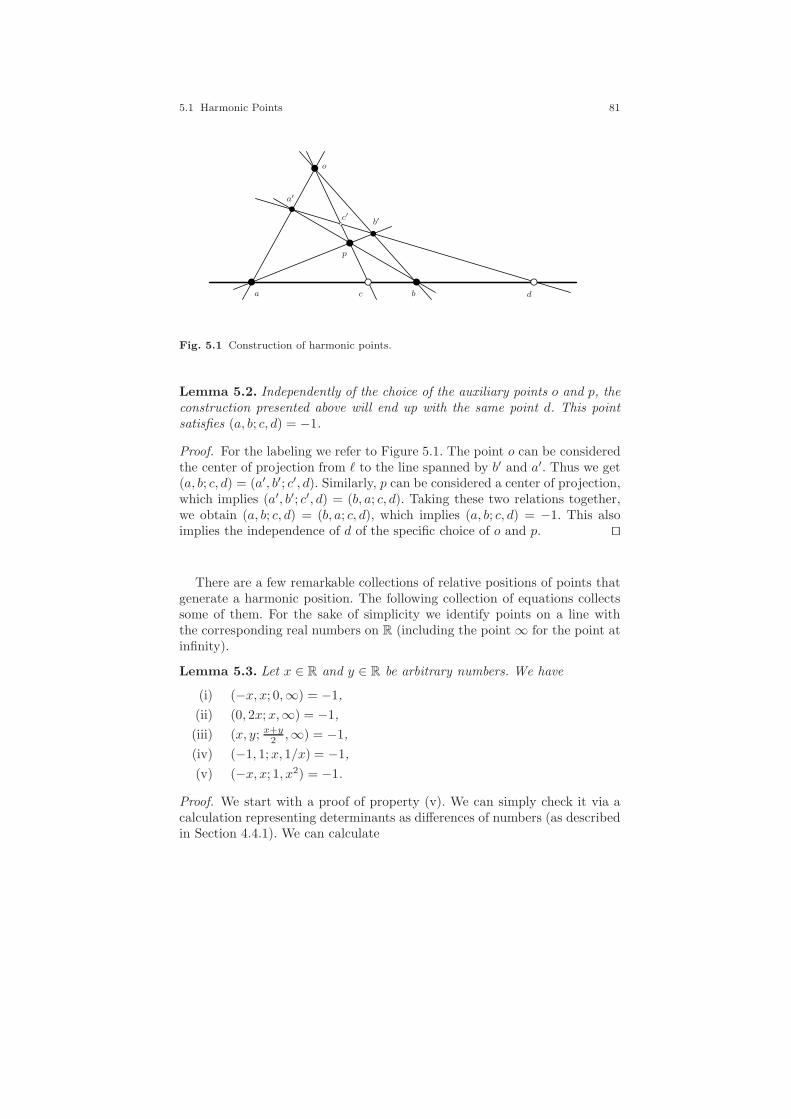
5.1 Harmonic Points 81
a bc
a′
b′c′
d
o
p
Fig. 5.1 Construction of harmonic points.
Lemma 5.2. Independently of the choice of the auxiliary points o and p, theconstruction presented above will end up with the same point d. This pointsatisfies (a, b; c, d) = −1.
Proof. For the labeling we refer to Figure 5.1. The point o can be consideredthe center of projection from ℓ to the line spanned by b′ and a′. Thus we get(a, b; c, d) = (a′, b′; c′, d). Similarly, p can be considered a center of projection,which implies (a′, b′; c′, d) = (b, a; c, d). Taking these two relations together,we obtain (a, b; c, d) = (b, a; c, d), which implies (a, b; c, d) = −1. This alsoimplies the independence of d of the specific choice of o and p. ⊓⊔
There are a few remarkable collections of relative positions of points thatgenerate a harmonic position. The following collection of equations collectssome of them. For the sake of simplicity we identify points on a line withthe corresponding real numbers on R (including the point ∞ for the point atinfinity).
Lemma 5.3. Let x ∈ R and y ∈ R be arbitrary numbers. We have
(i) (−x, x; 0,∞) = −1,
(ii) (0, 2x;x,∞) = −1,
(iii) (x, y; x+y2 ,∞) = −1,
(iv) (−1, 1;x, 1/x) = −1,
(v) (−x, x; 1, x2) = −1.
Proof. We start with a proof of property (v). We can simply check it via acalculation representing determinants as differences of numbers (as describedin Section 4.4.1). We can calculate
82 5 Calculating with Points on Lines
(−x− 1)(x− x2)
(−x− x2)(x − 1)=x(−x− 1)(1 − x)
x(−1 − x)(x − 1)= −1.
Statement (iv) is a consequence of statement (v); it arises by dividingall entries by x (this is a projective transformation and does not changethe cross-ratio). Statement (i) can be considered a limit case of (iv) if x →0. Statement (ii) arises from (i) by adding x to all entries (this is again aprojective transformation). Statement (iii) arises from (i) also by scaling andshifting. ⊓⊔
5.2 Projective Scales
We now fix three distinct points on a line, and call them 0, 1, and ∞. Everypoint x on the line can be associated with a unique cross-ratio (0,∞;x,1).This construction allows us to equip the line with a scale that behaves “asif” point 0 were the origin, 1 were a unit point, and point ∞ were infinitelyfar away. In particular we have the following:
Lemma 5.4. The following equations hold:
(i) (0,∞;0,1) = 0,
(ii) (0,∞;1,1) = 1,
(iii) (0,∞;∞,1) = ∞.
Proof. The lemma is a direct application of the definition of the cross-ratio. ⊓⊔
The next lemma shows that the cross-ratios with respect to these threepoints can be used to reconstruct the coordinates of a point from its geometriclocation. For this we set 0, 1, and ∞ to the positions 0, 1, and ∞ on a realnumber line.
Lemma 5.5. Assume that we have the specific homogeneous coordinates0 = (0, 1), 1 = (1, 1), ∞ = (1, 0), x = (x, 1) for x ∈ R. Then we have(0,∞;x,1) = x.
Proof. We can proof this fact by direct calculation:
(0,∞;x,1) =
det
(0 x1 1
)det
(1 10 1
)
det
(0 11 1
)det
(1 x0 1
) = x.
⊓⊔
5.3 From Geometry to Real Numbers 83
If we single out three distinct points on a line, we can always consider thema projective basis and refer all measurements to these three points. By thiswe can assign to every point on the line a real number. The resulting numberis then invariant under projective transformations. In a way this is like re-constructing the original scenery from a perspectively distorted photographif the original positions of three points are given.
5.3 From Geometry to Real Numbers
From 1850 to 1856 the mathematician Karl Georg Christian von Staudt(1798–1867) published a series of books under the title Beitrage zur Ge-ometrie der Lage. In these books von Staudt develops a completely synthetic(this means there are no calculations) setup for projective geometry. In hissetup for projective geometry he works on a similar axiomatic level as Eucliddid for Euclidean geometry. One of the major achievements of von Staudt’swork was to provide a method that starts with a purely projective setup andreconstructs an underlying algebraic structure. In particular, he was able toreconstruct the field structure of the underlying coordinate field from prop-erties of geometric constructions.
We will not follow exactly these lines of thought here.1 However, we willdemonstrate how intimately the concepts of real numbers, cross-ratios, andprojective transformations are interwoven. In particular, we will provide thepromised proof of Theorem 3.3, which claims that whenever we have a bijec-tive map in RP
2 that maps collinear points to collinear points, then it mustbe a projective transformation. We will even work a little harder and providethe proof for a similar fact on the projective line from which Theorem 3.3will easily follow.
Theorem 5.1. Let τ : RP1 → RP
1 be a bijective map with the property thatharmonic quadruples of points are mapped to harmonic quadruples of points.Then τ is a projective transformation.
We subdivide the proof of this rather strong theorem into several smallerparts. A bijective map with the property that harmonic quadruples of pointsare mapped to harmonic quadruples of points will be called a harmonic map.Our strategy will be first to show that harmonic maps are very rigid objects.We will see that harmonic maps that preserve the base points of a projectivescale will induce a field automorphism. For this we will first fix a projectivescale 0, 1, and ∞ on RP
1. We can identify each point x of RP1 \ ∞ by its
real coordinate (0,∞;x,1) ∈ R. If τ : RP1 → RP
1 is any bijective map withτ(∞) = ∞, this induces a bijection fτ : R → R according to
τ(p) = q ⇐⇒ fτ ((0,∞; p,1)) = (0,∞; q,1).
1 In fact, our approach closely follows Blaschke’s presentation in [6].
84 5 Calculating with Points on Lines
The behavior of f is mainly determined by the fact that τ is harmonic:
Lemma 5.6. Let τ be a harmonic map that in addition satisfies τ(0) = 0,τ(1) = 1, τ(∞) = ∞. Then the function fτ : R → R satisfies the followingrelations:
(i) fτ (0) = 0,
(ii) fτ (1) = 1,
(iii) fτ (x+y
2 ) = fτ (x)+fτ (y)2 ,
(iv) fτ (2x) = 2fτ (x),
(v) fτ (x+ y) = fτ (x) + fτ (y),
(vi) fτ (−x) = −fτ (x),(vii) fτ (x
2) = fτ (x)2,
(viii) fτ (x · y) = fτ (x) · fτ (y).
Proof. We can prove the statements in order. In doing so, we make heavyuse of the fact that if the positions of points a, b, c on a line are fixed, thenthe fourth harmonic point d is determined uniquely. Within this proof wewill freely identify points on RP
1 and the corresponding real numbers withrespect to the basis 0,1,∞.
Statements (i) and (ii) are direct reformulations of the facts that τ(0) = 0and τ(1) = 1. Statement (iii) holds for the following reason. For any x, ythe pairs of points (x, y) and ((x + y)/2,∞) are in harmonic position (com-pare Lemma 5.3 (iii)). Thus if we apply a harmonic map the image pairs(f(x), f(y)) and (f((x + y)/2), f(∞)) are harmonic again. Since we have
f(∞) = ∞, the point f((x+ y)/2) must be fτ (x)+fτ (y)2 . Several of the other
statements follow by similar reasoning. In these cases we refer only to thecorresponding harmonic sets. Statement (iv) holds, since the pair (0, 2x) isharmonic with the pair (x,∞). Statement (v) is now a consequence of (iii)and (iv). Statement (vi) is a consequence of (v) and (i). Statement (vii) holds,since (−x, x; 1, x2) is harmonic together with (ii) and (vi). Statement (viii)requires a little calculation. By (vii), (v), and (iv) we can conclude that
fτ (x)2 + 2fτ (x · y) + fτ (y)
2 = fτ (x2) + 2fτ (x · y) + fτ (y
2)
= fτ (x2 + 2xy + y2)
= fτ ((x + y)2)
= (fτ (x+ y))2
= fτ (x)2 + 2fτ (x) · fτ (y) + fτ (y)
2.
Comparing the first and the last expressions in this chain of equalities, weobtain fτ (x · y) = fτ (x) · fτ (y). ⊓⊔

5.3 From Geometry to Real Numbers 85
The most important statements in the last theorem were the facts thatwe have fτ (x + y) = fτ (x) + fτ (y) and fτ (x · y) = fτ (x) · fτ (y). In otherwords, the function fτ is a field automorphism of R. However, the only fieldautomorphism of R is the identity, as the next lemma shows:
Lemma 5.7. Let f : R → R be a function that satisfies f(x+y) = f(x)+f(y)and f(x · y) = f(x) · f(y). Then f is the identity.
Proof. Since 0 is the only element in R that satisfies x + x = x and wehave f(0) + f(0) = f(0 + 0) = f(0), we must have f(0) = 0. Similarly,f(1) ·f(1) = f(1 ·1) = f(1) implies f(1) = 1. Now consider an integer n ∈ N.We can write n = 1 + 1 + · · · + 1︸ ︷︷ ︸
n-times
and obtain
f(n) = f(1 + 1 + · · · + 1︸ ︷︷ ︸n-times
) = f(1) + f(1) + · · · + f(1)︸ ︷︷ ︸n-times
= 1 + 1 + · · · + 1︸ ︷︷ ︸n-times
= n.
The fact that f(x · y) = f(x) · f(y) implies that for any rational numberq = n/m, n,m ∈ N, we have f(q) = q, since q is the only number thatsatisfies the equation f(m) · q = f(n) and we have f(n) = n and f(m) = m.For similar reasons we have f(−x) = −f(x) for any x ∈ R.
Now the key observation is that one can characterize positivity in R bymultiplication. A number is positive if it can be written as x2 for x 6= 0. Thusfrom f(x2) = f(x)2 we obtain that f maps positive numbers to positivenumbers. This implies that x < y implies f(x) < f(y) (to see this, observethat x < y is equivalent to y − x > 0).
If f were not the identity, then we could find a real number a such thatf(a) 6= a. Then we would have either a < f(a) or a > f(a). Consider the firstcase. Since the set of rational numbers is dense in R, the open interval (a, f(a))contains a rational number q. This leads to a contradiction to the order-preservation property of f , since we then have a < q, but f(a) > q = f(q).The case a > f(a) is analogous. ⊓⊔
Taking together Lemma 5.6 and Lemma 5.7, we can finally prove Theorem5.1, the fact that harmonic maps can be expressed by matrix multiplication.
Proof of Theorem 5.1. Assume that ψ : RP1 → RP
1 is a harmonic map.The special points 0, 1, and ∞ are mapped by ψ to some points 0′, 1′,and ∞′. Theorem 4.1 implies that there exists a projective transformationφ : RP
1 → RP1 with φ(0′) = 0, φ(1′) = 1, φ(∞′) = ∞. The composition
τ : RP1 → RP
1 defined by τ(x) = φ(ψ(x)) is again a harmonic map, whichin addition leaves 0, 1, and ∞ invariant. By Lemma 5.6 it induces a fieldautomorphism on R, which (by Lemma 5.7) can only be the identity. Thus τitself must have been the identity map. This in turn implies that the originalharmonic map ψ must be the inverse of the projective transformation φ.Hence it is itself a projective transformation. ⊓⊔

86 5 Calculating with Points on Lines
5.4 The Fundamental Theorem
Theorem 5.1 is of fundamental importance. It links a structural geometricconcept (harmonic point quadruples) to the algebraic structure of the under-lying field: On the level of coordinates every harmonic map can be expressedas a matrix multiplication. Von Staudt originally went even one step further:He started with an incidence system that satisfies the axioms of a projec-tive plane and required the additional presence of another incidence property(namely that Pappos’s theorem holds within the incidence structure) and re-constructed an underlying field K from this incidence structure. One can show
that the original projective plane is isomorphic to K3−(0,0,0)
K−0 . We will not
prove this here. For a proof of this fact see for instance [44, 58, 3]. However,we will explain later the relevance of Pappos’s theorem in this context: Thepresence of Pappos’s theorem results in the commutativity of the underlyingfield.
Theorem 5.1 is a one-dimensional counterpart of Theorem 3.3, for whichwe still have not presented a proof. This theorem states that in RP
2 anybijective map that maps collinear points to collinear points can be expressedby a projective transformation. We will obtain this in a similar way as The-orem 5.1. However, we will have to find a way to encode two-dimensionalpositions in terms of cross-ratios. A harmonic map in RP
2 is any bijectionthat maps harmonic points on a line to harmonic points (perhaps on anotherline). A collineation in RP
2 will be any bijection that maps collinear points tocollinear points. It is obvious that a harmonic map is a collineation (collinearpoints are mapped to collinear points). However, the opposite is also true:
Lemma 5.8. Any collineation in RP2 is a harmonic map.
Proof. Consider four harmonic points a, b, c, d on some line l. By Lemma 5.2there exist four auxiliary points not on l that form (together with a, b, c, d) theincidence pattern of Figure 5.1. Under a collineation this incidence patternis mapped to an incidence pattern with the same combinatorial structure.This implies that (again by Lemma 5.2) the image points are harmonic aswell. ⊓⊔
We now use two values of cross-ratios in RP2 as “coordinates” for two-
dimensional points. For this we single out a projective basis in RP2 consisting
of four distinct points 0, ∞x, ∞y, and 1. These four points will play the roleof the origin, an infinite point on the x-axis, an infinite point on the y-axis,and a point with coordinates (1, 1) respectively. Furthermore, we define
1x = meet(join(0,∞x), join(1,∞y))
and1y = meet(join(0,∞y), join(1,∞x)).
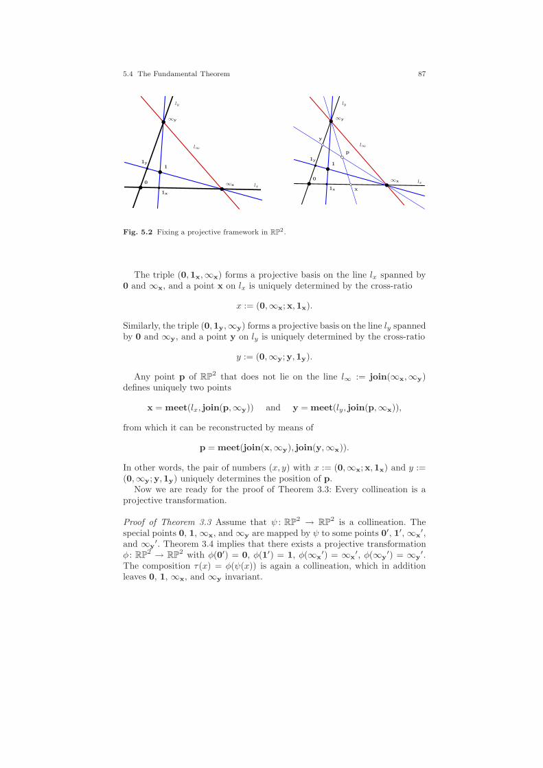
5.4 The Fundamental Theorem 87
1
0
1x
1y
∞x
∞y
l∞
lx
ly
1
0
1x
1y
∞x
∞y
l∞
lx
ly
x
y
p
Fig. 5.2 Fixing a projective framework in RP2.
The triple (0,1x,∞x) forms a projective basis on the line lx spanned by0 and ∞x, and a point x on lx is uniquely determined by the cross-ratio
x := (0,∞x;x,1x).
Similarly, the triple (0,1y,∞y) forms a projective basis on the line ly spannedby 0 and ∞y, and a point y on ly is uniquely determined by the cross-ratio
y := (0,∞y;y,1y).
Any point p of RP2 that does not lie on the line l∞ := join(∞x,∞y)
defines uniquely two points
x = meet(lx, join(p,∞y)) and y = meet(ly, join(p,∞x)),
from which it can be reconstructed by means of
p = meet(join(x,∞y), join(y,∞x)).
In other words, the pair of numbers (x, y) with x := (0,∞x;x,1x) and y :=(0,∞y;y,1y) uniquely determines the position of p.
Now we are ready for the proof of Theorem 3.3: Every collineation is aprojective transformation.
Proof of Theorem 3.3 Assume that ψ : RP2 → RP
2 is a collineation. Thespecial points 0, 1, ∞x, and ∞y are mapped by ψ to some points 0′, 1′, ∞x
′,and ∞y
′. Theorem 3.4 implies that there exists a projective transformationφ : RP
2 → RP2 with φ(0′) = 0, φ(1′) = 1, φ(∞x
′) = ∞x′, φ(∞y
′) = ∞y′.
The composition τ(x) = φ(ψ(x)) is again a collineation, which in additionleaves 0, 1, ∞x, and ∞y invariant.

88 5 Calculating with Points on Lines
By Lemma 5.6 it induces a field automorphism on R, which (by Lemma 5.7)can only be the identity. Thus τ itself must have been the identity map onthe lines lx and ly. Our above considerations imply that all points of RP
2
that are not on l∞ must be invariant. As a consequence, all points on l∞must be invariant as well (any such point can be encoded as the intersectionof l∞ and a line through two points not on l∞). Thus τ is the identity. Thisin turn implies that the original harmonic map ψ must be the inverse of theprojective transformation φ. Hence it is itself a projective transformation. ⊓⊔
5.5 A Note on Other Fields
The last three sections established a close connection of the field that un-derlies a projective geometry and projective transformations. In our ap-proach we entirely focused on the real projective plane. Almost all our con-structions (such as projective transformations, cross-ratios, harmonic points,collineations) could as well be carried out over arbitrary fields. However, withrespect to the fundamental theorem a little care is necessary.
One crucial ingredient for Theorem 5.1 and Theorem 3.3 was to derivea field automorphism from a harmonic map. The fact that R has onlyhave the trivial field automorphism translates into the statement that everycollineation can be expressed as a matrix multiplication. Over other fields(such as C) we have nontrivial field automorphisms. These field automor-phisms induce collineations that cannot be expressed as a projective trans-formation. Let us focus for a moment on the complex projective plane CP
2. In
complete analogy to RP2 we can define this space by PC = C
2−(0,0,0)C−0 and
LC = C2−(0,0,0)
C−0 . A point (x, y, z) is on a line (a, b, c) if a ·x+ b ·y+ c · z = 0.
Matrix multiplications are again the projective transformations and inducecollineations. However, over C we have additional collineations. We obtain thesimplest such collineation by taking the map that assigns to each coordinateentry its complex conjugate:
(x, y, z) 7→ (x, y, z) and (a, b, c) 7→ (a, b, c).
We have a · x+ b · y + c · z = 0 ⇐⇒ a · x+ b · y + c · z = 0.The generalization of the fundamental theorem that applies to all fields
can be stated as follows.
Theorem 5.2. Let τ : KP1 → KP
1 be a collineation. Then τ can be factoredas φ ψ, where φ is a projective transformation and ψ is induced by a fieldautomorphism.
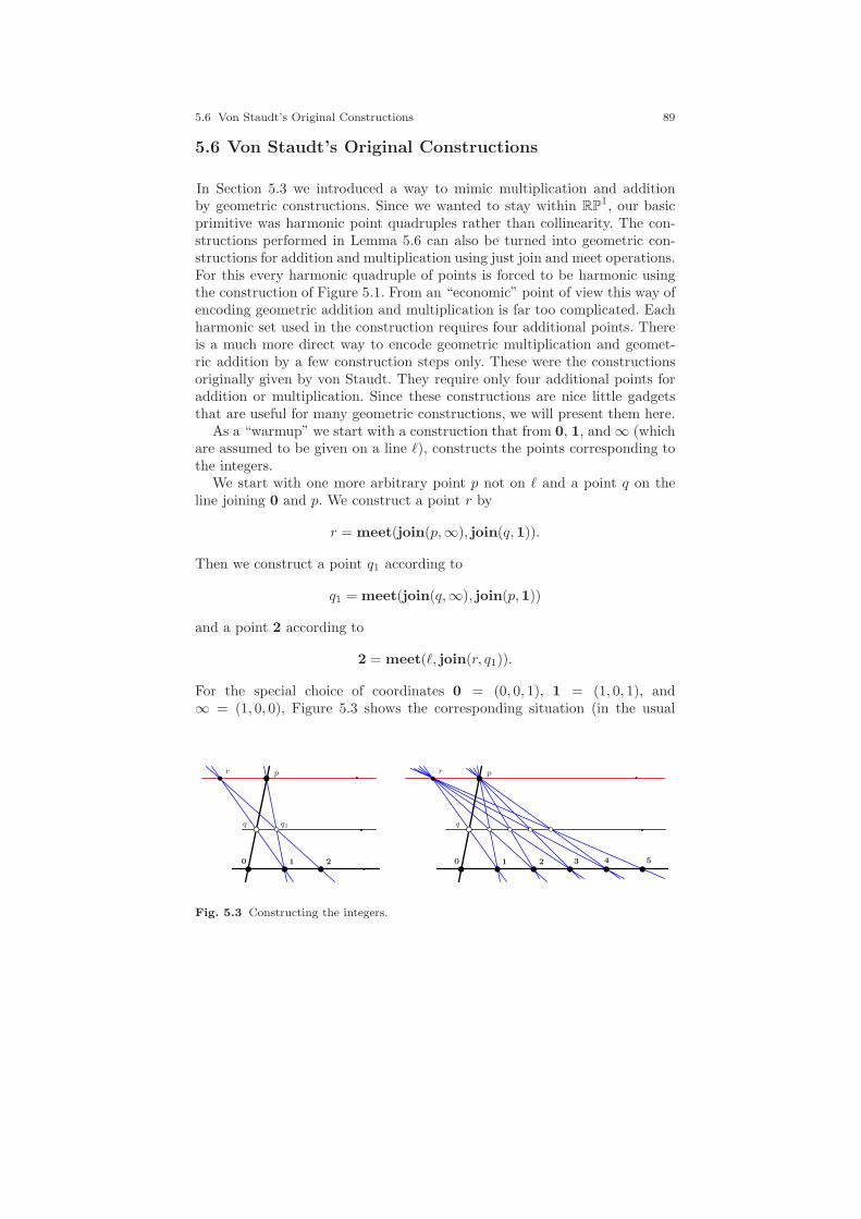
5.6 Von Staudt’s Original Constructions 89
5.6 Von Staudt’s Original Constructions
In Section 5.3 we introduced a way to mimic multiplication and additionby geometric constructions. Since we wanted to stay within RP
1, our basicprimitive was harmonic point quadruples rather than collinearity. The con-structions performed in Lemma 5.6 can also be turned into geometric con-structions for addition and multiplication using just join and meet operations.For this every harmonic quadruple of points is forced to be harmonic usingthe construction of Figure 5.1. From an “economic” point of view this way ofencoding geometric addition and multiplication is far too complicated. Eachharmonic set used in the construction requires four additional points. Thereis a much more direct way to encode geometric multiplication and geomet-ric addition by a few construction steps only. These were the constructionsoriginally given by von Staudt. They require only four additional points foraddition or multiplication. Since these constructions are nice little gadgetsthat are useful for many geometric constructions, we will present them here.
As a “warmup” we start with a construction that from 0, 1, and ∞ (whichare assumed to be given on a line ℓ), constructs the points corresponding tothe integers.
We start with one more arbitrary point p not on ℓ and a point q on theline joining 0 and p. We construct a point r by
r = meet(join(p,∞), join(q,1)).
Then we construct a point q1 according to
q1 = meet(join(q,∞), join(p,1))
and a point 2 according to
2 = meet(ℓ, join(r, q1)).
For the special choice of coordinates 0 = (0, 0, 1), 1 = (1, 0, 1), and∞ = (1, 0, 0), Figure 5.3 shows the corresponding situation (in the usual
r p
q q1
0 1 2
r p
q
0 1 2 3 4 5
Fig. 5.3 Constructing the integers.
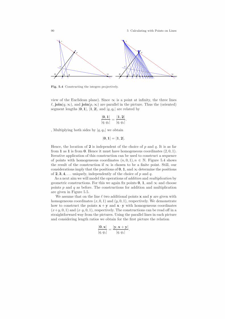
90 5 Calculating with Points on Lines
r
p
q
0 1 2 ∞
r
p
q
0 1 2 3∞
Fig. 5.4 Constructing the integers projectively.
view of the Euclidean plane). Since ∞ is a point at infinity, the three linesℓ, join(q,∞), and join(p,∞) are parallel in the picture. Thus the (oriented)segment lengths |0,1|, |1,2|, and |q, q1| are related by
|0,1||q, q1|
=|1,2||q, q1|
.
, Multiplying both sides by |q, q1| we obtain
|0,1| = |1,2|.
Hence, the location of 2 is independent of the choice of p and q. It is as farfrom 1 as 1 is from 0. Hence it must have homogeneous coordinates (2, 0, 1).Iterative application of this construction can be used to construct a sequenceof points with homogeneous coordinates (n, 0, 1), n ∈ N. Figure 5.4 showsthe result of the construction if ∞ is chosen to be a finite point. Still, ourconsiderations imply that the positions of 0, 1, and ∞ determine the positionsof 2,3,4, . . . uniquely, independently of the choice of p and q.
As a next aim we will model the operations of addition and multiplication bygeometric constructions. For this we again fix points 0, 1, and ∞ and choosepoints p and q as before. The constructions for addition and multiplicationare given in Figure 5.5.
We assume that on the line ℓ two additional points x and y are given withhomogeneous coordinates (x, 0, 1) and (y, 0, 1), respectively. We demonstratehow to construct the points x + y and x · y with homogeneous coordinates(x+y, 0, 1) and (x·y, 0, 1), respectively. The constructions can be read off in astraightforward way from the pictures. Using the parallel lines in each pictureand considering length ratios we obtain for the first picture the relation
|0,x||q, q1|
=|y,x + y||q, q1|
.

5.7 Pappos’s Theorem 91
x y x + y0
p
q
r
q1
1 x y x · y0
p
q
r
q1
s
Fig. 5.5 Geometric addition and multiplication.
Thus the distance from 0 to x is the same as the distance from y to x + y.This implies the desired relation for addition. For the picture on the right weobtain the relations
|0,1||0,x| =
|p, s||r, p| =
|0,y||0,x · y| .
The first relation comes from the relations induced by the lines passingthrough q, the second comes from the lines passing through q1; Comparingthe first and the third terms gives the desired relation.
If we alter the role of the points, the same configurations can be used toperform geometric subtraction or geometric division. By combining severalvon Staudt constructions, the evaluation of arbitrary quotients of polynomialscan be modeled geometrically.
5.7 Pappos’s Theorem
As a final topic of this chapter, we want to demonstrate the important rolethat is played by Pappos’s theorem in relation to underlying fields of a pro-jective plane. We will see that Pappos’s theorem is equivalent to the commu-tativity of the underlying field. To see this, we will have a closer look at thevon Staudt constructions for addition and multiplication.
If we interchange the roles of x and y in the von Staudt addition (seeFigure 5.5 left) we end up with a drawing that has exactly the same combi-natorics. This implies the commutativity of addition. This is not the case forvon Staudt multiplication. Figure 5.6 overlays different constructions for thepoint x · y. The blue lines are exactly the same as presented as “von Staudtmultiplication” in the last section. The green construction corresponds to the“von Staudt multiplication” for y · x (the roles of x and y are interchanged).The black lines belong to both constructions. Since over real numbers themultiplication is commutative and we have x · y = y · x, both constructions

92 5 Calculating with Points on Lines
1 x y x · y = y · x0
p
q
r
q1
q2
st
1 x y x · y = y · x0
p
q
r
q1
q2
st
Fig. 5.6 Commutativity of multiplication and Pappos’s theorem.
must result in the same point. This fact can be interpreted as a purely geo-metric incidence theorem (without ever referring to algebra).
In fact, the decisive incidence theorem that hides behind commutativityof multiplication is nothing but Pappos’s theorem (recall the first chapter ofthis book). In Figure 5.6 the nine lines that correspond to Pappos’s theo-rem are drawn in bold, and the nine points are emphasized in red.t If we lookback at the collection of proofs for Pappos’s theorem that we presented in thefirst chapter of this book, then we will recognize that each of these proofs atone point made use of commutativity of the underlying coordinate field. Thereason for this is that the presence of Pappos’s theorem in a projective planeimplies that the plane can be considered as (PK,LK, IK) for some (commu-tative) field K. Projective planes in which Pappos’s theorem holds are calledPappian planes. With this terminology we can reformulate the above fact inthe following manner:
Theorem 5.3. A projective plane is Pappian if and only if it is of the form(PK,LK, IK) for some field K.
We do not prove this theorem here (for proofs see [44, 58, 3]), since themain focus of this book is not the distinction of projective planes that comefrom fields from those that do not come from fields. All projective planesused hereinafter will come from a field, and hence we can (and will) freelymake use of Pappos’s theorem.
6
Determinants
One person’s constant is another person’s variable.
Susan Gerhart
While the previous chapters had their focus on the exploration of the logi-cal and structural properties of projective planes, this chapter will focus onthe following question: What is the easiest way to calculate with geometry?Many textbooks on geometry introduce coordinates (or homogeneous coor-dinates) and base all analytic computations on calculations on this level. Ananalytic proof of a geometric theorem is carried out in the parameter space.For a different parameterization of the theorem the proof may look entirelydifferent.
In this chapter we will see that this way of thinking is very often notthe most economical one. The reason for this is that the coordinates of ageometric object are in a way a basis-dependent artifact and carry not onlyinformation on the geometric object but also on the relation of this object tothe basis of the coordinate system. For instance, if a point is represented by itshomogeneous coordinates (x, y, z), we have encoded its relative position to aframe of reference. From the perspective of projective geometry the perhapsmost important fact that one can say about the point is simply that it isa point. All other properties are not projectively invariant. Similarly, if weconsider three points p1 = (x1, y1, z1), p2 = (x2, y2, z2), p3 = (x3, y3, z3), thestatement that these points are collinear reads
x1y2z3 + x2y3z1 + x3y1z2 − x1y3z2 − x2y1z3 − x3y2z1 = 0,
a 3×3 determinant. Again from a structural point of view this expression is fartoo complicated. It would be much better to encode the collinearity directlyinto a short algebraic expression and deal with this. The simplest way to
93

94 6 Determinants
do this is to change the role of primary and derived algebraic objects. If weconsider the determinants themselves as “first-class citizens,” the statementof collinearity simply reads det(p1, p2, p3) = 0, where the determinant isconsidered an unbreakable unit rather than just a shorthand for the aboveexpanded formula. In this chapter we will explore the roles determinants playwithin projective geometry. For further reading on this fascinating topic werecommend [16, 33, 126, 132].
6.1 A “Determinantal” Point of View
Before we start with the treatment of determinants on a more general level wewill review and emphasize the role of determinants in topics we have treatedso far.
One of our first encounters of determinants occurred when we expressedthe collinearity of points in homogeneous coordinates. Three points p1, p2, p3
are collinear in RP2 if and only if det(p1, p2, p3) = 0. One can interpret this
fact either geometrically (if p1, p2, p3 are collinear, then the correspondingvectors of homogeneous coordinates are coplanar) or algebraically (if p1, p2, p3
are collinear, then the system of linear equations 〈p1, l〉 = 〈p2, l〉 = 〈p3, l〉 = 0has a nontrivial solution l 6= (0, 0, 0)). Dually, we can say that the determinantof three lines l1, l2, l3 vanishes if and only if these lines have a point in common(this point may be at infinity).
A second instance in which determinants played a less obvious role oc-curred when we calculated the join of two points p and q by the cross productp× q. We will give an algebraic interpretation of this. If (x, y, z) is any pointon the line p ∨ q, then it satisfies
det
p1 p2 p3
q1 q2 q3x y z
= 0.
If we develop the determinant by the last row, we can rewrite this as
det
(p2 p3
q2 q3
)· x− det
(p1 p3
q1 q3
)· y + det
(p1 p2
q1 q2
)· z = 0.
Or expressed as a scalar product,
⟨(det
(p2 p3
q2 q3
),− det
(p1 p3
q1 q3
), det
(p1 p2
q1 q2
)), (x, y, z)
⟩= 0.
We can geometrically reinterpret this equation by saying that
(det
(p2 p3
q2 q3
),− det
(p1 p3
q1 q3
), det
(p1 p2
q1 q2
))
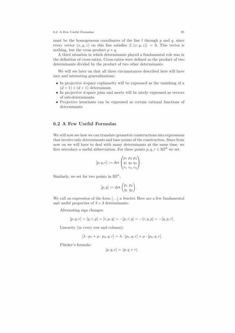
6.2 A Few Useful Formulas 95
must be the homogeneous coordinates of the line l through p and q, sinceevery vector (x, y, z) on this line satisfies 〈l, (x, y, z)〉 = 0. This vector isnothing, but the cross product p× q.
A third situation in which determinants played a fundamental role was inthe definition of cross-ratios. Cross-ratios were defined as the product of twodeterminants divided by the product of two other determinants.
We will see later on that all three circumstances described here will havenice and interesting generalizations:
• In projective d-space coplanarity will be expressed as the vanishing of a(d+ 1) × (d+ 1) determinant.
• In projective d-space joins and meets will be nicely expressed as vectorsof sub-determinants.
• Projective invariants can be expressed as certain rational functions ofdeterminants.
6.2 A Few Useful Formulas
We will now see how we can translate geometric constructions into expressionsthat involve only determinants and base points of the construction. Since fromnow on we will have to deal with many determinants at the same time, wefirst introduce a useful abbreviation. For three points p, q, r ∈ RP
2 we set
[p, q, r] := det
p1 p2 p3
q1 q2 q3r1 r2 r3
.
Similarly, we set for two points in RP1,
[p, q] := det
(p1 p2
q1 q2
).
We call an expression of the form [. . .] a bracket. Here are a few fundamentaland useful properties of 3 × 3 determinants:
Alternating sign changes:
[p, q, r] = [q, r, p] = [r, p, q] = −[p, r, q] = −[r, q, p] = −[q, p, r].
Linearity (in every row and column):
[λ · p1 + µ · p2, q, r] = λ · [p1, q, r] + µ · [p2, q, r].
Plucker’s formula:[p, q, r] = 〈p, q × r〉.
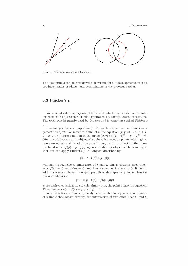
96 6 Determinants
l1
l2
c1
c2
q
q
Fig. 6.1 Two applications of Plucker’s µ.
The last formula can be considered a shorthand for our developments on crossproducts, scalar products, and determinants in the previous section.
6.3 Plucker’s µ
We now introduce a very useful trick with which one can derive formulasfor geometric objects that should simultaneously satisfy several constraints.The trick was frequently used by Plucker and is sometimes called Plucker’sµ.
Imagine you have an equation f : Rd → R whose zero set describes ageometric object. For instance, think of a line equation (x, y, z) 7→ a · x+ b ·y + c · z or a circle equation in the plane (x, y) 7→ (x − a)2 + (y − b)2 − r2.Often one is interested in objects that share intersection points with a givenreference object and in addition pass through a third object. If the linearcombination λ · f(p) + µ · g(p) again describes an object of the same type,then one can apply Plucker’s µ. All objects described by
p 7→ λ · f(p) + µ · g(p)
will pass through the common zeros of f and g. This is obvious, since when-ever f(p) = 0 and g(p) = 0, any linear combination is also 0. If one inaddition wants to have the object pass through a specific point q, then thelinear combination
p 7→ g(q) · f(p) − f(q) · g(p)is the desired equation. To see this, simply plug the point q into the equation.Then one gets g(q) · f(q) − f(q) · g(q) = 0.
With this trick we can very easily describe the homogeneous coordinatesof a line ℓ that passes through the intersection of two other lines l1 and l2

6.3 Plucker’s µ 97
and through a third point q by
〈l2, q〉l1 − 〈l1, q〉l2.
Testing whether this line passes through q yields
〈〈l2, q〉l1 − 〈l1, q〉l2, q〉 = 〈l2, q〉〈l1, q〉 − 〈l1, q〉〈l2, q〉 = 0,
which is obviously true. Later on we will make frequent use of this trickwhenever we need a fast and elegant way to calculate a specific geometricobject. We will now use Plucker’s µ to calculate intersections of lines spannedby points.
What is the intersection of the two lines spanned by the point pairs (a, b)and (c, d)? On the one hand, the point has to be on the line a ∨ b; thus itmust be of the form λ ·a+µ · b. It also has to be on c∨d; hence it must be ofthe form ψ · c+φ ·d. Identifying these two expressions and solving for λ, µ, ψ,and φ would be one possibility to solve the problem. But we can directly readoff the right parameters using (a dual version of) Plucker’s µ. The propertythat encodes that a point p is on the line c ∨ d is simply [c, d, p] = 0. Thuswe immediately obtain that the point
[c, d, b] · a− [c, d, a] · b
must be the desired intersection. This point is obviously on a ∨ b, and it ison c ∨ d, since we have
[c, d, [c, d, b] · a− [c, d, a] · b] = [c, d, b] · [c, d, a] − [c, d, a] · [c, d, b] = 0.
We could equivalently have applied the calculation with the roles of a ∨ band c ∨ d interchanged. Then we can express the same point as
[a, b, d] · c− [a, b, c] · d.
In fact, it is not a surprise that these two expressions end up at identicalpoints. We will later on, in Section 6.5, see that this is just a reformulationof the well-known Cramer’s rule for solving systems of linear equations.
How can we express the condition that three lines a ∨ b, c ∨ d, e ∨ f meetin a point? For this we simply have to test whether the intersection p of a∨ band c ∨ d, is on e ∨ f . We can do this by testing whether the determinant ofthese three points is zero. Plugging in the formula for p, we get
[e, f, [c, d, b] · a− [c, d, a] · b] = 0.
After expansion by multilinearity, we obtain
[c, d, b][e, f, a] − [c, d, a][e, f, b] = 0.

98 6 Determinants
a
b
c
d
[a, b, d] · c− [a, b, c] · d
a
b
c
de
f
[c, d, b][e, f, a] − [c, d, a][e, f, b] = 0
Fig. 6.2 Conditions for lines meeting in a point.
This is the algebraic condition for the three lines meeting in a point. Takinga look at the above formula, we should pause and make a few observations:
• The first and most important observation is that we could write such aprojective condition as a polynomial of determinants evaluating to zero.
• In the formula, each term has the same number of determinants.
• Each letter occurs equally often in each term.
All three observations extend very well to much more general cases. In orderto see this, we will have first to introduce the notion of projectively invariantproperties.
Before we do this we want to use this formula to obtain (another) beautifulproof for Pappos’s theorem. Consider the drawing of Pappos’s theorem inFigure 6.3 (observe the nice 3-fold symmetry). We can state Pappos’s theoremin the following way: If for six points a, . . . , f in the projective plane the linesa ∨ d, c ∨ b, e ∨ f meet and the lines c ∨ f , e ∨ d, a ∨ b meet, then also e ∨ b,a ∨ f , c ∨ d meet. The two hypotheses can be expressed as
[b, c, e][a, d, f ] = [b, c, f ][a, d, e],
[c, f, b][d, e, a] = [c, f, a][d, e, b].
Using the fact that a cyclic shift of the points of a 3 × 3 bracket does notchange its sign, we observe that the first term of the second equation isidentical to the second term of the first equation. So we obtain
[f, a, c][e, b, d] = [f, a, d][e, b, c]
Which is exactly the desired conclusion of Pappos’s theorem.

6.4 Invariant Properties 99
b
c
d
e
f
a
Fig. 6.3 Pappos’s theorem, once more.
6.4 Invariant Properties
How can we algebraically characterize that a certain property of a pointconfiguration is invariant under projective transformations? Properties ofsuch type are for instance three lines being concurrent or six points a, . . . , fsuch that a ∨ b, c ∨ d, e ∨ f meet.
In general, properties of this type can be expressed as functions in the (ho-mogeneous) coordinates of the points that have to be zero when the propertyholds. Being invariant means that a property holds for a point configurationP if and only if it also holds for any projective transformation of P . Moreformally, let us express the point configuration P by a matrix whose columnsare the homogeneous coordinates of n points p1, . . . , pn:
P =
p1x p2x . . . pnxp1y p2y . . . pnyp1z p2z . . . pnz
.
A projective transformation is then simply represented by left-multiplicationby a 3× 3 invertible matrix T . A projectively invariant property should alsobe invariant when we replace a vector pi by a scalar multiple λi · pi. We canexpress the scaling of the points by right multiplication of P by an invertiblediagonal matrix D. All matrices obtained from P via
T · P ·D
represent essentially the same projective configuration. A projectively invari-ant property is any property of P that is invariant under such a transfor-
100 6 Determinants
mation. Very often, our invariant properties will be polynomials being zero,but for now we want to keep things more general and consider any map thatassociates to P a Boolean value. The matrix P can be considered an elementof R3·n. Thus we make the following definition:
Definition 6.1. A projectively invariant property of n points in the real pro-jective plane is a map f : R3·n → true, false such that for all invertiblereal 3 × 3 matrices T ∈ GL(R, 3) and n× n invertible real diagonal matricesD ∈ diag(R, n), we have
f(P ) = f(T · P ·D).
In a canonical way we can identify each predicate P ⊆ X on a space Xwith its characteristic function f : X → true, false, where f(x) evaluatesto true if and only if x ∈ P . Thus we can equivalently speak of projectivelyinvariant predicates.
In this sense, for instance, [a, b, c] = 0 defines a projectively invariantproperty of three points a, b, c in the real projective plane. Also the propertythat we encountered in the last section,
[c, d, b][e, f, a] − [c, d, a][e, f, b] = 0,
which encodes the fact that three lines a ∨ b, c ∨ d, e ∨ f meet in a point, isprojectively invariant. Before we state a more general theorem we will analyzewhy this relation is invariant from an algebraic point of view. Transformingthe points by a projective transformation T results in replacing the pointsa, . . . , f with T · a, . . . , T · f . Scaling the homogeneous coordinates results inreplacing a, . . . , f by λa · a, . . . , λf · f with nonzero λ’s. Thus if P encodesthe point configuration, then the overall effect of T · P ·D on the expression[c, d, b][e, f, a] − [c, d, a][e, f, b] can be written as
[λc · T · c, λd · T · d, λb · T · b][λe · T · e, λf · T · f, λa · T · a]− [λc · T · c, λd · T · d, λa · T · a][λe · T · e, λf · T · f, λb · T · b].
Since [T · p, T · q, T · r] = det(T ) · [p, q, r], the above expression simplifies to
(det(T )2 · λa · λb · λc · λd · λe · λf ) · ([c, d, b][e, f, a]− [c, d, a][e, f, b]).
All λ’s were nonzero and T was assumed to be invertible. Hence the expression[c, d, b][e, f, a]−[c, d, a][e, f, b] is zero if and only if the above expression is zero.Observe that it was important that each summand of the bracket polynomialhad exactly the same number of brackets. This made it possible to factor outa factor det(T )2. Furthermore, in each summand each letter occurred equallyoften. This made it possible to factor out the λ’s.
This example is a special case of a much more general fact, namely thatall multihomogeneous bracket polynomials define projectively invariant prop-erties.
6.4 Invariant Properties 101
Definition 6.2. Let P = (p1, p2, , . . . , pn) ∈ (R3)n represent a point config-uration of n points. A bracket monomial on P is an expression of the form
[a1,1, a1,2, a1,3] · [a2,1, a2,2, a2,3] · · · · · [ak,1, ak,2, ak,3],
where each aj,k is one of the points pi. The degree deg(pi,M) of a pointpi in a monomial is the total number of occurrences of pi in M . A bracketpolynomial on P is a sum of bracket monomials on P . A bracket polynomialQ = M1 + · · · + Ml with monomials M1, . . . ,Ml is multihomogeneous if foreach point pi we have
deg(pi,M1) = · · · = deg(pi,Ml).
In other words, a bracket polynomial is multihomogeneous if each pointoccurs in each summand the same number of times. We can make an anal-ogous definition for points on a projective line. The only difference there isthat we have to deal with brackets of length 2 instead of length 3.
As a straightforward generalization of our observations on the multiho-mogeneous bracket polynomial [c, d, b][e, f, a] − [c, d, a][e, f, b] we obtain thefollowing theorem:
Theorem 6.1. Let Q(P ) be a multihomogeneous bracket polynomial on npoints P = (p1, p2, . . . , pn) ∈ (R3)n. Then Q(P ) = 0 defines a projectivelyinvariant property.
Proof. Since Q is multihomogeneous, each of the summands contains thesame number (say 3k) of points. Therefore each summand is the product ofk brackets. Thus we have for any projective transformation T the relation
Q(T · P ) = det(T )k ·Q(P ).
Furthermore, the degree of the point pi is the same (say di) in each monomial.Scaling the points by scalars λ1 · · · · · λd can be expressed as multiplicationby the diagonal matrix D = diag(λ1 · · · · · λn). Since each bracket is linear ineach point entry, the scaling induces the following action on Q:
Q(P ·D) = λd11 · · · · · λdnn ·Q(P ).
Overall, we obtain
Q(T · P ·D) = det(T )k · λd11 · · · · · λdnn ·Q(P ).
The factors preceding Q(P ) are all nonzero, since T is invertible and onlynonzero λi are allowed. Hence Q(T · P · D) is zero if and only if Q(P ) iszero. ⊓⊔
Clearly, a similar statement also holds for points on the projective line (and2 × 2 brackets) and also for projective planes over other fields.
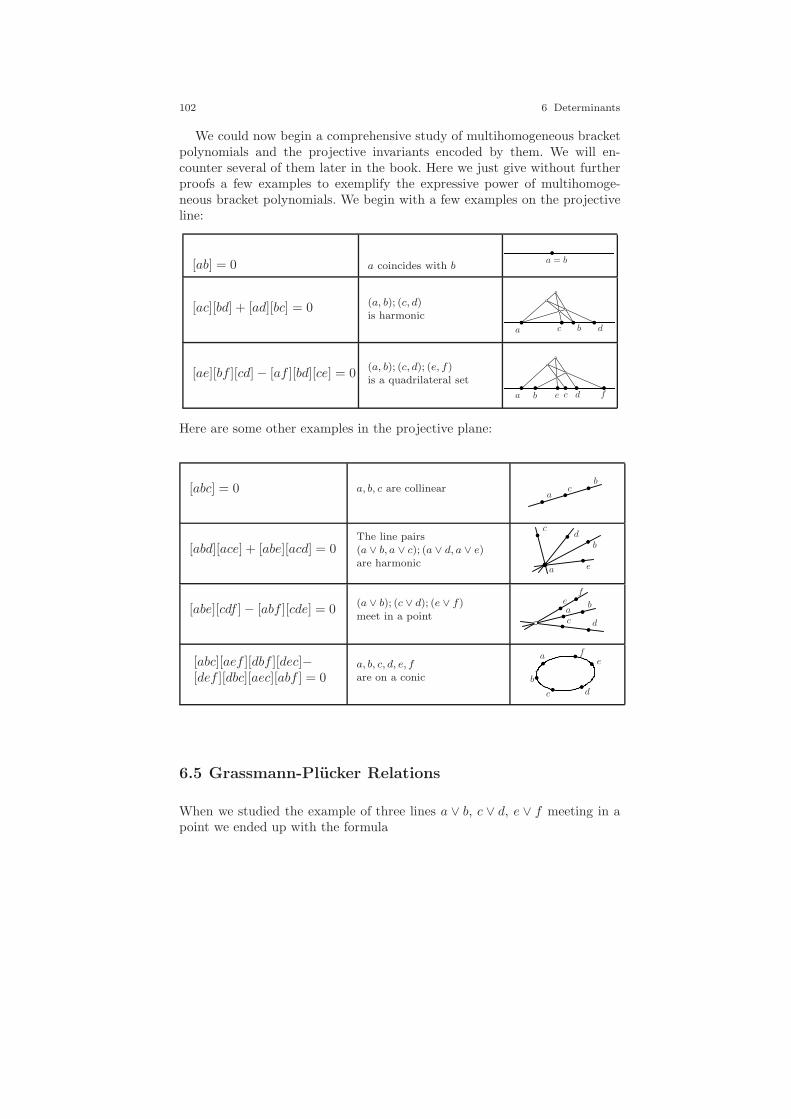
102 6 Determinants
We could now begin a comprehensive study of multihomogeneous bracketpolynomials and the projective invariants encoded by them. We will en-counter several of them later in the book. Here we just give without furtherproofs a few examples to exemplify the expressive power of multihomoge-neous bracket polynomials. We begin with a few examples on the projectiveline:
[ab] = 0 a coincides with ba = b
[ac][bd] + [ad][bc] = 0 (a, b); (c, d)is harmonic
a bc d
[ae][bf ][cd] − [af ][bd][ce] = 0(a, b); (c, d); (e, f)is a quadrilateral set
a b c de f
Here are some other examples in the projective plane:
[abc] = 0 a, b, c are collineara
bc
[abd][ace] + [abe][acd] = 0The line pairs(a ∨ b, a ∨ c); (a ∨ d, a ∨ e)are harmonic
a
b
cd
e
[abe][cdf ] − [abf ][cde] = 0(a ∨ b); (c ∨ d); (e ∨ f)
meet in a pointa
b
c
fe
d
[abc][aef ][dbf ][dec]−[def ][dbc][aec][abf ] = 0
a, b, c, d, e, fare on a conic
a
b
c
ef
d
6.5 Grassmann-Plucker Relations
When we studied the example of three lines a ∨ b, c ∨ d, e ∨ f meeting in apoint we ended up with the formula

6.5 Grassmann-Plucker Relations 103
[c, d, b][e, f, a] − [c, d, a][e, f, b] = 0.
A closer look at this formula shows that the line a ∨ b plays a special rolecompared to the other two lines. Its points are distributed over the brackets,while the points of the other lines always occur in one bracket. The symmetryof the original property implies that there are two more essentially differentways to encode the property in a bracket polynomial:
[a, b, c][e, f, d]−[a, b, d][e, f, c] = 0 and [a, b, e][c, d, f ]−[a, b, f ][c, d, e] = 0.
The reason for this is that there are multi-homogeneous bracket polynomialsthat will always evaluate to zero no matter where the points of the configu-ration are placed. These special polynomials are of fundamental importancewhenever one makes calculations in which several determinants are involved.The relations in question are the Grassmann-Plucker-Relations. In principle,such relations exist in any dimension. However, as usual in our exposition wewill mainly focus on the case of the projective line and the projective plane,i.e., 2 × 2 and 3 × 3 brackets. We start with the 2 × 2 case. We state therelations on the level of vectors rather than on the level of projective points.
Theorem 6.2. For any vectors a, b, c, d ∈ R2 the following equation holds:
[a, b][c, d] − [a, c][b, d] + [a, d][b, c] = 0.
Proof. If one of the vectors is the zero vector, the equation is trivially true.Thus we may assume that each of the vectors represents a point of the pro-jective line. Since [a, b][c, d] − [a, c][b, d] + [a, d][b, c] is a multihomogeneousbracket polynomial, we may assume that all vectors are (if necessary aftera suitable projective transformation) finite points and normalized to vectors(λa
1
), . . . ,
(λd
1
). The determinants then become simply differences. Rewriting
the term gives
(λa − λb)(λc − λd) − (λa − λc)(λb − λd) + (λa − λd)(λb − λc) = 0.
Expanding all terms, we get equivalently
(λaλc + λbλd − λaλd − λbλc)−(λaλb + λcλd − λaλd − λcλb)+(λaλb + λdλc − λaλc − λdλb) = 0.
The last equation can be easily checked. ⊓⊔
Grassmann-Plucker-Relations can be interpreted in many equivalent waysand, thereby this link several branches of geometry and invariant theory. Wewill here present three more interpretations (or proofs if you want).
1. Determinant expansion: The Grassmann-Plucker-Relation [a, b][c, d]−[a, c][b, d] + [a, d][b, c] = 0 can be considered a determinant expansion. For
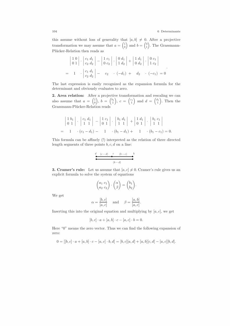
104 6 Determinants
this assume without loss of generality that [a, b] 6= 0. After a projective
transformation we may assume that a =(
10
)and b =
(01
). The Grassmann-
Plucker-Relation then reads as∣∣∣∣1 00 1
∣∣∣∣ ·∣∣∣∣c1 d1
c2 d2
∣∣∣∣ −∣∣∣∣1 c10 c2
∣∣∣∣ ·∣∣∣∣0 d1
1 d2
∣∣∣∣ +
∣∣∣∣1 d1
0 d2
∣∣∣∣ ·∣∣∣∣0 c11 c2
∣∣∣∣
= 1 ·∣∣∣∣c1 d1
c2 d2
∣∣∣∣ − c2 · (−d1) + d2 · (−c1) = 0
.
The last expression is easily recognized as the expansion formula for thedeterminant and obviously evaluates to zero.
2. Area relation: After a projective transformation and rescaling we can
also assume that a =(
10
), b =
(b11
), c =
(c11
)and d =
(d11
). Then the
Grassmann-Plucker-Relation reads
∣∣∣∣1 b10 1
∣∣∣∣ ·∣∣∣∣c1 d1
1 1
∣∣∣∣ −∣∣∣∣1 c10 1
∣∣∣∣ ·∣∣∣∣b1 d1
1 1
∣∣∣∣ +
∣∣∣∣1 d1
0 1
∣∣∣∣ ·∣∣∣∣b1 c11 1
∣∣∣∣
= 1 · (c1 − d1) − 1 · (b1 − d1) + 1 · (b1 − c1) = 0.
This formula can be affinely (!) interpreted as the relation of three directedlength segments of three points b, c, d on a line:
d c b(c− d) (b− c)
(b − d)
3. Cramer’s rule: Let us assume that [a, c] 6= 0. Cramer’s rule gives us anexplicit formula to solve the system of equations
(a1 c1a2 c2
)·(αβ
)=
(b1b2
).
We get
α =[b, c]
[a, c]and β =
[a, b]
[a, c].
Inserting this into the original equation and multiplying by [a, c], we get
[b, c] · a+ [a, b] · c− [a, c] · b = 0.
Here “0” means the zero vector. Thus we can find the following expansion ofzero:
0 = [[b, c] · a+ [a, b] · c− [a, c] · b, d] = [b, c][a, d] + [a, b][c, d] − [a, c][b, d].

6.5 Grassmann-Plucker Relations 105
This is exactly the Grassmann-Plucker-Relation.
What happens in dimension 3 (i.e., the projective plane)? First of all, weobtain a consequence of the Grassmann-Plucker-Relation on the line whenwe add the same point to any bracket:
Theorem 6.3. For any vectors a, b, c, d, x ∈ R3 the following equation holds:
[x, a, b][x, c, d] − [x, a, c][x, b, d] + [x, a, d][x, b, c] = 0.
Proof. Assuming without loss of generality that x = (1, 0, 0) reduces all de-terminants of the expression to 2 × 2 determinants, any of the above proofstranslates literally. ⊓⊔
In the projective plane we get another Grassmann-Plucker-Relation thatinvolves four instead of three summands.
Theorem 6.4. For any vectors a, b, c, d, e, f ∈ R3 the following equationholds:
[a, b, c][d, e, f ]− [a, b, d][c, e, f ] + [a, b, e][c, d, f ]− [a, b, f ][c, d, e] = 0.
Proof. Applying Cramer’s rule to the solution of a 3 × 3 equation
| | |c d e| | |
·
αβγ
=
|f|
,
we can prove the identity
[f, d, e] · c+ [c, f, e] · d+ [c, d, f ] · e = [c, d, e] · f.
Rearranging the terms yields
[d, e, f ] · c− [c, e, f ] · d+ [c, d, f ] · e− [c, d, e] · f = 0.
Inserting this expansion of the zero vector 0 into [a, b, 0] = 0 yields (afterexpanding the terms by multilinearity) the desired relation. ⊓⊔
Again, we can also interpret this equation in many different ways. Set-ting (a, b, c) to the unit matrix the Grassmann-Plucker-Relation encodes thedevelopment of the 3 × 3 determinant (d, e, f) by the first column. We get
˛
˛
˛
˛
˛
˛
1 0 0
0 1 0
0 0 1
˛
˛
˛
˛
˛
˛
·
˛
˛
˛
˛
˛
˛
d1 e1 f1d2 e2 f2d3 e3 f3
˛
˛
˛
˛
˛
˛
−
˛
˛
˛
˛
˛
˛
1 0 d10 1 d20 0 d3
˛
˛
˛
˛
˛
˛
·
˛
˛
˛
˛
˛
˛
0 e1 f10 e2 f21 e3 f3
˛
˛
˛
˛
˛
˛
+
˛
˛
˛
˛
˛
˛
1 0 e10 1 e20 0 e3
˛
˛
˛
˛
˛
˛
·
˛
˛
˛
˛
˛
˛
0 d1 f10 d2 f21 d3 f3
˛
˛
˛
˛
˛
˛
−
˛
˛
˛
˛
˛
˛
1 0 f10 1 f20 0 f3
˛
˛
˛
˛
˛
˛
·
˛
˛
˛
˛
˛
˛
0 d1 e10 d2 e21 d3 e3
˛
˛
˛
˛
˛
˛
= 1 ·
˛
˛
˛
˛
˛
˛
d1 e1 f1d2 e2 f2d3 e3 f3
˛
˛
˛
˛
˛
˛
− d3 ·
˛
˛
˛
˛
e1 f1e2 f2
˛
˛
˛
˛
+ e3 ·
˛
˛
˛
˛
d1 f1d2 f2
˛
˛
˛
˛
− f3 ·
˛
˛
˛
˛
d1 e1d2 e2
˛
˛
˛
˛
= 0.

106 6 Determinants
c
d
f
− c
e
f
+
d
e
f
− c
d
e= 0
Fig. 6.4 Grassmann-Plucker-Relation as area formulas.
Observe that we can express each minor of the determinant [d, e, f ] as asuitable bracket that involves a, b, c. This point will later be of fundamentalimportance.
There is also a nice interpretation that generalizes the “area viewpoint.”The determinant ∣∣∣∣∣∣
a1 b1 c1a2 b2 c21 1 1
∣∣∣∣∣∣
calculates twice the oriented area ∆(a, b, c) of the affine triangle a, b, c. Aftera suitable projective transformation the Grassmann-Plucker-Relation reads
˛
˛
˛
˛
˛
˛
1 0 c10 1 c20 0 1
˛
˛
˛
˛
˛
˛
˛
˛
˛
˛
˛
˛
d1 e1 f1d2 e2 f21 1 1
˛
˛
˛
˛
˛
˛
−
˛
˛
˛
˛
˛
˛
1 0 d10 1 d20 0 1
˛
˛
˛
˛
˛
˛
˛
˛
˛
˛
˛
˛
c1 e1 f1c2 e2 f21 1 1
˛
˛
˛
˛
˛
˛
+
˛
˛
˛
˛
˛
˛
1 0 e10 1 e20 0 1
˛
˛
˛
˛
˛
˛
˛
˛
˛
˛
˛
˛
c1 d1 f1c2 d2 f21 1 1
˛
˛
˛
˛
˛
˛
−
˛
˛
˛
˛
˛
˛
1 0 f10 1 f20 0 1
˛
˛
˛
˛
˛
˛
˛
˛
˛
˛
˛
˛
c1 d1 e1c2 d2 e21 1 1
˛
˛
˛
˛
˛
˛
= 0.
In terms of triangle areas this equation reads as
∆(d, e, f) −∆(c, e, f) +∆(c, d, f) −∆(c, d, e) = 0.
This formula has again a direct geometric interpretation in terms of affineoriented areas of triangles. Assume that c, d, e, f are any four points in theaffine plane. The convex hull of these four points can be covered in two waysby triangles spanned by three of the points. These two possibilities mustboth result in the same total (oriented) area. This is the Grassmann-Plucker-Relation.
Using Grassmann-Plucker-Relations we can easily explain why the prop-erty that a ∨ b, c ∨ d, e ∨ f meet can be expressed either by
[a, b, e][c, d, f ] − [a, b, f ][c, d, e] = 0
or by[a, b, c][e, f, d] − [a, b, d][e, f, c] = 0.
Adding the two expressions yields
[a, b, c][e, f, d] − [a, b, d][e, f, c] + [a, b, e][c, d, f ] − [a, b, f ][c, d, e] = 0,

6.5 Grassmann-Plucker Relations 107
which is exactly a Grassmann-Plucker-Relation. Hence this equation must bezero, which proves the equivalence of the above two expressions.

7
More on Bracket Algebra
Algebra is generous; she often gives more than is asked of her.
D’Alembert (1717–1783)
The last chapter demonstrated that determinants (and in particular multiho-mogeneous bracket polynomials) are of fundamental importance in express-ing projectively invariant properties. In this chapter we will alter our pointof view. What if our “first-class citizens” were not the points of a projectiveplane but the values of determinants generated by them? We will see thatwith the use of Grassmann-Plucker-Relations we will be able to recover aprojective configuration from its values of determinants.
We will start our treatment by considering vectors in R3 rather than con-
sidering homogeneous coordinates of points in RP2. This has the advantage
that we can neglect the (only technical) difficulty that the determinant valuesvary when the coordinates of a point are multiplied by a scalar.
While reading this chapter the reader should constantly bear in mind thatall concepts presented in this chapter generalize to arbitrary dimensions. Stillwe will concentrate on the case of vectors in R2 and in R3 to keep thingsconceptually as simple as possible.
7.1 From Points to Determinants . . .
Assume that we are given a configuration of n vectors in R3 arranged in amatrix:
P =
| | | . . . |p1 p2 p3 . . . pn| | | . . . |
.
109
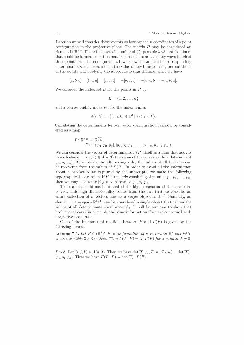
110 7 More on Bracket Algebra
Later on we will consider these vectors as homogeneous coordinates of a pointconfiguration in the projective plane. The matrix P may be considered anelement in R
3·n. There is an overall number of(n3
)possible 3×3 matrix minors
that could be formed from this matrix, since there are as many ways to selectthree points from the configuration. If we know the value of the correspondingdeterminants we can reconstruct the value of any bracket using permutationsof the points and applying the appropriate sign changes, since we have
[a, b, c] = [b, c, a] = [c, a, b] = −[b, a, c] = −[a, c, b] = −[c, b, a].
We consider the index set E for the points in P by
E = 1, 2, . . . , n
and a corresponding index set for the index triples
Λ(n, 3) := (i, j, k) ∈ E3 | i < j < k.
Calculating the determinants for our vector configuration can now be consid-ered as a map
Γ : R3·n → R(n
3),P 7→ ([p1, p2, p3], [p1, p2, p4], . . . , [pn−2, pn−1, pn]).
We can consider the vector of determinants Γ (P ) itself as a map that assignsto each element (i, j, k) ∈ Λ(n, 3) the value of the corresponding determinant[pi, pj, pk]. By applying the alternating rule, the values of all brackets canbe recovered from the values of Γ (P ). In order to avoid all the informationabout a bracket being captured by the subscripts, we make the followingtypographical convention. If P is a matrix consisting of columns p1, p2, . . . , pn,then we may also write [i, j, k]P instead of [pi, pj , pk].
The reader should not be scared of the high dimension of the spaces in-volved. This high dimensionality comes from the fact that we consider anentire collection of n vectors now as a single object in Rn·3. Similarly, an
element in the space R(n3) may be considered a single object that carries the
values of all determinants simultaneously. It will be our aim to show thatboth spaces carry in principle the same information if we are concerned withprojective properties.
One of the fundamental relations between P and Γ (P ) is given by thefollowing lemma:
Lemma 7.1. Let P ∈ (R3)n be a configuration of n vectors in R3 and let Tbe an invertible 3× 3 matrix. Then Γ (T ·P ) = λ · Γ (P ) for a suitable λ 6= 0.
Proof. Let (i, j, k) ∈ Λ(n, 3): Then we have det(T ·pi, T ·pj , T ·pk) = det(T ) ·[pi, pj, pk]. Thus we have Γ (T · P ) = det(T ) · Γ (P ). ⊓⊔
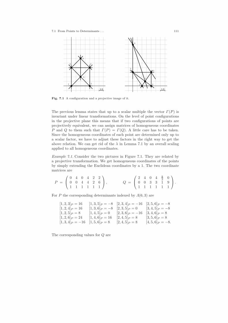
7.1 From Points to Determinants . . . 111
1.0
1 2
3 4
5
6
1.0
1 2
34
5
6
Fig. 7.1 A configuration and a projective image of it.
The previous lemma states that up to a scalar multiple the vector Γ (P ) isinvariant under linear transformations. On the level of point configurationsin the projective plane this means that if two configurations of points areprojectively equivalent, we can assign matrices of homogeneous coordinatesP and Q to them such that Γ (P ) = Γ (Q). A little care has to be taken.Since the homogeneous coordinates of each point are determined only up toa scalar factor, we have to adjust these factors in the right way to get theabove relation. We can get rid of the λ in Lemma 7.1 by an overall scalingapplied to all homogeneous coordinates.
Example 7.1. Consider the two pictures in Figure 7.1. They are related bya projective transformation. We get homogeneous coordinates of the pointsby simply extending the Euclidean coordinates by a 1. The two coordinatematrices are
P =
0 4 0 4 2 20 0 4 4 2 61 1 1 1 1 1
, Q =
2 4 0 4 83 0
0 0 3 3 1 91 1 1 1 1 1
.
For P the corresponding determinants indexed by Λ(6, 3) are
[1, 2, 3]P = 16 [1, 3, 5]P = −8 [2, 3, 4]P = −16 [2, 5, 6]P = −8[1, 2, 4]P = 16 [1, 3, 6]P = −8 [2, 3, 5]P = 0 [3, 4, 5]P = −8[1, 2, 5]P = 8 [1, 4, 5]P = 0 [2, 3, 6]P = −16 [3, 4, 6]P = 8[1, 2, 6]P = 24 [1, 4, 6]P = 16 [2, 4, 5]P = 8 [3, 5, 6]P = 8[1, 3, 4]P = −16 [1, 5, 6]P = 8 [2, 4, 5]P = 8 [4, 5, 6]P = −8.
The corresponding values for Q are

112 7 More on Bracket Algebra
[1, 2, 3]Q = 6 [1, 3, 5]Q = −4 [2, 3, 4]Q = −16 [2, 5, 6]Q = −8[1, 2, 4]Q = 6 [1, 3, 6]Q = −12 [2, 3, 5]Q = 0 [3, 4, 5]Q = −8[1, 2, 5]Q = 2 [1, 4, 5]Q = 0 [2, 3, 6]Q = −24 [3, 4, 6]Q = 24[1, 2, 6]Q = 18 [1, 4, 6]Q = 24 [2, 4, 5]Q = 4 [3, 5, 6]Q = 16[1, 3, 4]Q = −12 [1, 5, 6]Q = 8 [2, 4, 5]Q = 12 [4, 5, 6]Q = −16.
At first sight these two collections of values seem not to be very related.However, if we simply choose different homogeneous coordinates for the pointin the second picture, such as
r1 = 4 · q1, r2 = 4 · q2, r3 = 2 · q3, r4 = 2 · q4, r5 = 3 · q5, r6 = 1 · q6,
we get
[1, 2, 3]R = 192 [1, 3, 5]R = −96 [2, 3, 4]R = −192 [2, 5, 6]R = −96[1, 2, 4]R = 192 [1, 3, 6]R = −96 [2, 3, 5]R = 0 [3, 4, 5]R = −96[1, 2, 5]R = 96 [1, 4, 5]R = 0 [2, 3, 6]R = −192 [3, 4, 6]R = 96[1, 2, 6]R = 288 [1, 4, 6]R = 192 [2, 4, 5]R = 96 [3, 5, 6]R = 96[1, 3, 4]R = −192 [1, 5, 6]R = 96 [2, 4, 5]R = 96 [4, 5, 6]R = −96.
This is exactly 12 times the values of the determinants obtained from P . It isalso instructive to check the Grassmann-Plucker-Relations for a few specialcases. For instance, we should have
[1, 2, 3]P [4, 5, 6]P−[1, 2, 4]P [3, 5, 6]P+[1, 2, 5]P [3, 4, 6]P−[1, 2, 6]P [3, 4, 5]P = 0.
This can easily be verified:
16 · (−8) − 16 · 8 + 8 · 8 − 24 · (−8) = −128 − 128 + 64 + 192 = 0.
7.2 . . . and Back
We will now focus on the other direction. To what extent do the values ofΓ (P ) already determine the entries of P? Let us first start with two obser-vations.
Observation 1: The elements in Γ (P ) are not independent of eachother. This comes from the fact that the entries at least have to satisfythe Grassmann-Plucker-Relations.Observation 2: The elements in Γ (P ) can determine P only up to alinear transformation. This is the statement of Lemma 7.1.
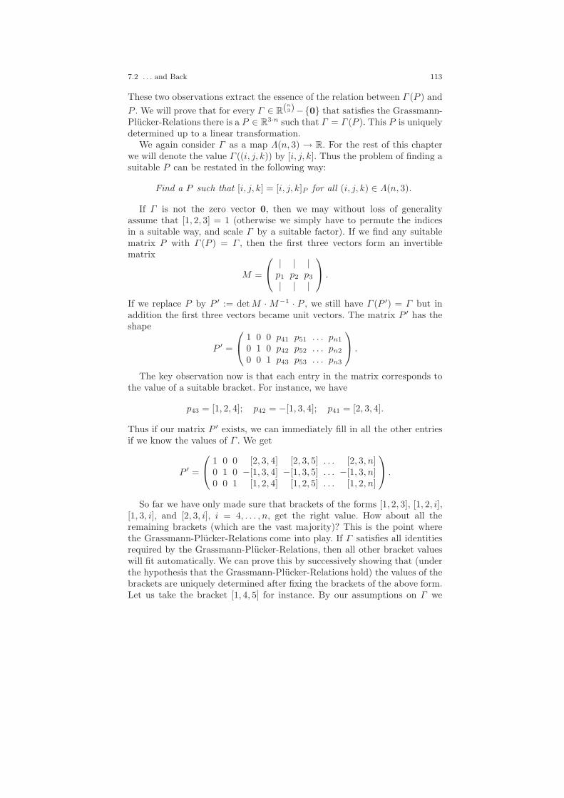
7.2 . . . and Back 113
These two observations extract the essence of the relation between Γ (P ) and
P . We will prove that for every Γ ∈ R(n3)−0 that satisfies the Grassmann-
Plucker-Relations there is a P ∈ R3·n such that Γ = Γ (P ). This P is uniquelydetermined up to a linear transformation.
We again consider Γ as a map Λ(n, 3) → R. For the rest of this chapterwe will denote the value Γ ((i, j, k)) by [i, j, k]. Thus the problem of finding asuitable P can be restated in the following way:
Find a P such that [i, j, k] = [i, j, k]P for all (i, j, k) ∈ Λ(n, 3).
If Γ is not the zero vector 0, then we may without loss of generalityassume that [1, 2, 3] = 1 (otherwise we simply have to permute the indicesin a suitable way, and scale Γ by a suitable factor). If we find any suitablematrix P with Γ (P ) = Γ , then the first three vectors form an invertiblematrix
M =
| | |p1 p2 p3
| | |
.
If we replace P by P ′ := detM ·M−1 · P , we still have Γ (P ′) = Γ but inaddition the first three vectors became unit vectors. The matrix P ′ has theshape
P ′ =
1 0 0 p41 p51 . . . pn1
0 1 0 p42 p52 . . . pn2
0 0 1 p43 p53 . . . pn3
.
The key observation now is that each entry in the matrix corresponds tothe value of a suitable bracket. For instance, we have
p43 = [1, 2, 4]; p42 = −[1, 3, 4]; p41 = [2, 3, 4].
Thus if our matrix P ′ exists, we can immediately fill in all the other entriesif we know the values of Γ . We get
P ′ =
1 0 0 [2, 3, 4] [2, 3, 5] . . . [2, 3, n]0 1 0 −[1, 3, 4] −[1, 3, 5] . . . −[1, 3, n]0 0 1 [1, 2, 4] [1, 2, 5] . . . [1, 2, n]
.
So far we have only made sure that brackets of the forms [1, 2, 3], [1, 2, i],[1, 3, i], and [2, 3, i], i = 4, . . . , n, get the right value. How about all theremaining brackets (which are the vast majority)? This is the point wherethe Grassmann-Plucker-Relations come into play. If Γ satisfies all identitiesrequired by the Grassmann-Plucker-Relations, then all other bracket valueswill fit automatically. We can prove this by successively showing that (underthe hypothesis that the Grassmann-Plucker-Relations hold) the values of thebrackets are uniquely determined after fixing the brackets of the above form.Let us take the bracket [1, 4, 5] for instance. By our assumptions on Γ we
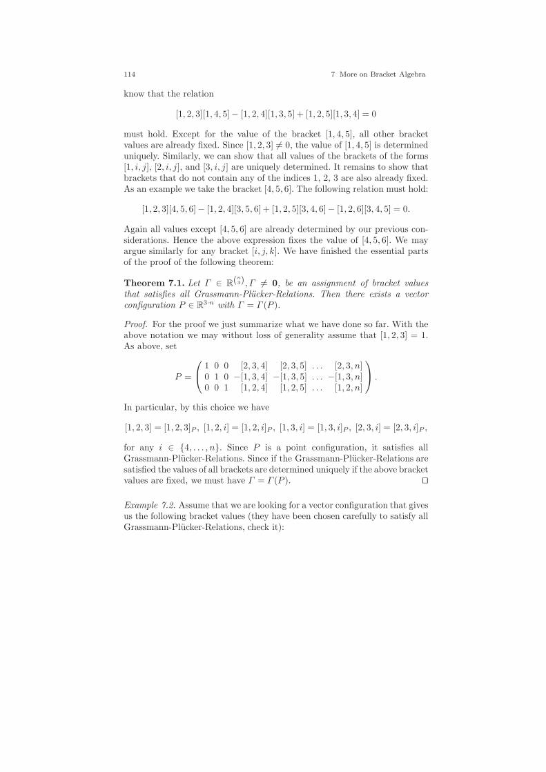
114 7 More on Bracket Algebra
know that the relation
[1, 2, 3][1, 4, 5]− [1, 2, 4][1, 3, 5] + [1, 2, 5][1, 3, 4] = 0
must hold. Except for the value of the bracket [1, 4, 5], all other bracketvalues are already fixed. Since [1, 2, 3] 6= 0, the value of [1, 4, 5] is determineduniquely. Similarly, we can show that all values of the brackets of the forms[1, i, j], [2, i, j], and [3, i, j] are uniquely determined. It remains to show thatbrackets that do not contain any of the indices 1, 2, 3 are also already fixed.As an example we take the bracket [4, 5, 6]. The following relation must hold:
[1, 2, 3][4, 5, 6]− [1, 2, 4][3, 5, 6] + [1, 2, 5][3, 4, 6]− [1, 2, 6][3, 4, 5] = 0.
Again all values except [4, 5, 6] are already determined by our previous con-siderations. Hence the above expression fixes the value of [4, 5, 6]. We mayargue similarly for any bracket [i, j, k]. We have finished the essential partsof the proof of the following theorem:
Theorem 7.1. Let Γ ∈ R(n3), Γ 6= 0, be an assignment of bracket values
that satisfies all Grassmann-Plucker-Relations. Then there exists a vectorconfiguration P ∈ R3·n with Γ = Γ (P ).
Proof. For the proof we just summarize what we have done so far. With theabove notation we may without loss of generality assume that [1, 2, 3] = 1.As above, set
P =
1 0 0 [2, 3, 4] [2, 3, 5] . . . [2, 3, n]0 1 0 −[1, 3, 4] −[1, 3, 5] . . . −[1, 3, n]0 0 1 [1, 2, 4] [1, 2, 5] . . . [1, 2, n]
.
In particular, by this choice we have
[1, 2, 3] = [1, 2, 3]P , [1, 2, i] = [1, 2, i]P , [1, 3, i] = [1, 3, i]P , [2, 3, i] = [2, 3, i]P ,
for any i ∈ 4, . . . , n. Since P is a point configuration, it satisfies allGrassmann-Plucker-Relations. Since if the Grassmann-Plucker-Relations aresatisfied the values of all brackets are determined uniquely if the above bracketvalues are fixed, we must have Γ = Γ (P ). ⊓⊔
Example 7.2. Assume that we are looking for a vector configuration that givesus the following bracket values (they have been chosen carefully to satisfy allGrassmann-Plucker-Relations, check it):
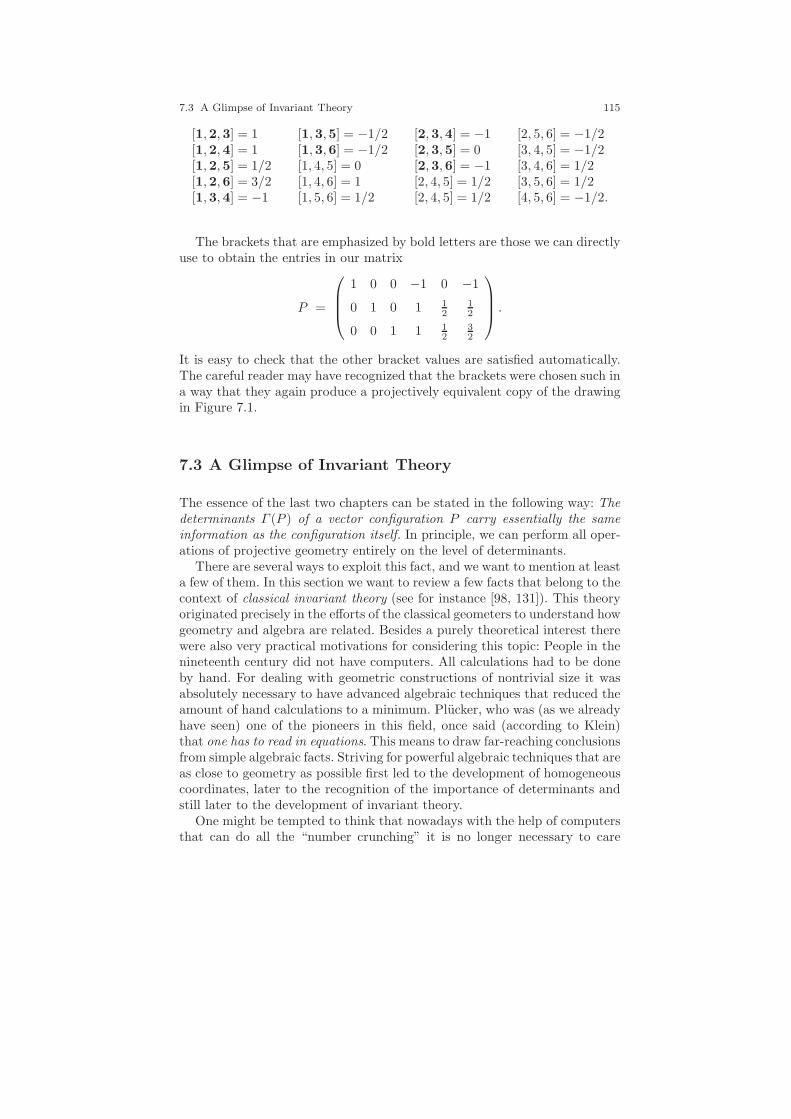
7.3 A Glimpse of Invariant Theory 115
[1,2,3] = 1 [1,3,5] = −1/2 [2,3,4] = −1 [2, 5, 6] = −1/2[1,2,4] = 1 [1,3,6] = −1/2 [2,3,5] = 0 [3, 4, 5] = −1/2[1,2,5] = 1/2 [1, 4, 5] = 0 [2,3,6] = −1 [3, 4, 6] = 1/2[1,2,6] = 3/2 [1, 4, 6] = 1 [2, 4, 5] = 1/2 [3, 5, 6] = 1/2[1,3,4] = −1 [1, 5, 6] = 1/2 [2, 4, 5] = 1/2 [4, 5, 6] = −1/2.
The brackets that are emphasized by bold letters are those we can directlyuse to obtain the entries in our matrix
P =
1 0 0 −1 0 −1
0 1 0 1 12
12
0 0 1 1 12
32
.
It is easy to check that the other bracket values are satisfied automatically.The careful reader may have recognized that the brackets were chosen such ina way that they again produce a projectively equivalent copy of the drawingin Figure 7.1.
7.3 A Glimpse of Invariant Theory
The essence of the last two chapters can be stated in the following way: Thedeterminants Γ (P ) of a vector configuration P carry essentially the sameinformation as the configuration itself. In principle, we can perform all oper-ations of projective geometry entirely on the level of determinants.
There are several ways to exploit this fact, and we want to mention at leasta few of them. In this section we want to review a few facts that belong to thecontext of classical invariant theory (see for instance [98, 131]). This theoryoriginated precisely in the efforts of the classical geometers to understand howgeometry and algebra are related. Besides a purely theoretical interest therewere also very practical motivations for considering this topic: People in thenineteenth century did not have computers. All calculations had to be doneby hand. For dealing with geometric constructions of nontrivial size it wasabsolutely necessary to have advanced algebraic techniques that reduced theamount of hand calculations to a minimum. Plucker, who was (as we alreadyhave seen) one of the pioneers in this field, once said (according to Klein)that one has to read in equations. This means to draw far-reaching conclusionsfrom simple algebraic facts. Striving for powerful algebraic techniques that areas close to geometry as possible first led to the development of homogeneouscoordinates, later to the recognition of the importance of determinants andstill later to the development of invariant theory.
One might be tempted to think that nowadays with the help of computersthat can do all the “number crunching” it is no longer necessary to care

116 7 More on Bracket Algebra
about sophisticated algebraic techniques, since calculations on the coordinatelevel can be carried out automatically. In fact, exactly the opposite is thecase. The rise of computational power has led to a considerable demandfor sophisticated techniques for performing geometric calculations. There areseveral reasons for this (and we will list only a few of them):
• With computers it is possible to deal with really huge geometric situationsthat were not previously within reach. So still it is necessary to computeefficiently.
• Practical applications in computer-aided design, robotics, computer vi-sion, and structural mechanics lead to problems that are at the core ofprojective geometry, and the algebraic techniques that are used there haveto be appropriate for the problem. (For instance, consider an autonomousrobot that has to use pictures taken by a video camera to obtain an innermodel of the environment. This corresponds to the problem of lifting atwo-dimensional projective scene to a three-dimensional one.)
• Symbolic calculations on the coordinate level very soon lead to a combi-natorial explosion, since usually every single multiplication of two poly-nomials doubles the number of summands involved.
• The rise of computers opened the new discipline of “automatic deduc-tion in geometry” (see [45, 115, 133, 60, 17]). There one is, for instance,interested in automatically generating proofs for geometric theorems. Inorder to be able to retranslate the automatically generated proof intogeometric statements one has finally to reinterpret algebraic terms geo-metrically. This is much easier if the algebraic statements are “close” togeometry.
Our investigations of the last two sections showed that brackets form afunctional basis for projective invariants. To make this notion a bit moreprecise, we first slightly broaden the scope of Definition 6.1, in which we in-troduced projectively invariant properties. To avoid technical difficulties thatarise from configurations that do not have full rank, we call a configurationof points given by homogeneous coordinates P ∈ R3·n proper if P has rank3. If P is not proper, then all points of P lie on a line, or even collapse to asingle point.
Definition 7.1. Let M be an arbitrary set. A projective invariant of n pointsin the real projective plane is a map f : R3·n →M such that for all invertiblereal 3 × 3 matrices T ∈ GL(R, 3) and n× n invertible real diagonal matricesD ∈ diag(R, n) and for any proper configuration P , we have
f(P ) = f(T · P ·D).
In this definition the image range M is taken to be an arbitrary set. IfM is the set true, false, then f is a projectively invariant property as

7.3 A Glimpse of Invariant Theory 117
introduced in Definition 6.1. If M = R∪∞, then f measures some numberthat is invariant under projective transformations (such as the cross-ratio, forinstance). We now want to study under what circumstances one can generateone projective invariant from others. For this we introduce the concept of afunctional basis.
Definition 7.2. A collection fi : R3·n → Mi, i = 1, . . . , k, of functions is afunctional basis of the set of all projective invariants if for every projectiveinvariant f : R
3·n →M , there is a function
m : M1 × · · · ×Mk →M
such that for all X ∈ R3·n we have
f(X) = m(f1(X), . . . , fk(X)).
In other words, if f1, . . . , fk is a functional basis then it completely suf-fices to know the values of these functions to calculate the value of any otherinvariant. We can also understand the concept of functional basis on an al-gorithmic level. For every invariant f there exists an algorithm A that takesthe values of f1, . . . , fk as input and calculates the value of f . The last twosections essentially prove the following theorem:
Theorem 7.2. The entries of the determinant vector Γ (P ) form a functionalbasis for all projective invariants.
Proof (sketch). Let f be any invariant and let P be an arbitrary properconfiguration of points. Since P is proper, at least one entry of Γ := Γ (P ) isnonzero (this means that at least one determinant does not vanish). Thus wecan use the techniques of Section 7.2 to calculate a configuration P ′ := P ′(Γ )that is projectively equivalent to P . Thus we must have f(P ′(Γ )) = f(P ),which proves the claim. ⊓⊔
This theorem is a weak version of a much deeper algebraic fact that isknown as the first fundamental theorem of projective invariant theory (see[131, 126]). Theorem 7.2 states only that we can compute any invariant if weknow the values of the brackets. It does not state that the algebraic structureof an invariant is preserved by any means. The first fundamental theoremin addition guarantees that the algebraic type of an invariant is essentiallypreserved.
Unfortunately, at this point we have to pay a price for calculating with ho-mogeneous coordinates. Since we do not distinguish homogeneous coordinatesthat differ only by a scalar multiple, we have to take care of these equivalenceclasses in a corresponding algebraic setup. Any polynomial in the entries ofthe matrix P ∈ R3·n is thus not invariant under rescaling of the homoge-neous coordinates. This implies that the category of polynomials is not the

118 7 More on Bracket Algebra
appropriate one for talking about projective invariants. There are essentiallytwo ways out of this dilemma. Both involve quite a few technical difficulties.The first is to introduce the concept of a relative invariant polynomial. Sucha polynomial f(P ) is not an invariant in the sense of Definition 7.1. Ratherthan being strictly invariant, one requires that the action of T ∈ GL(R, 3)and D ∈ diag(R, n) change f(T · P ·D) in a very predictable way. If D hasdiagonal entries λ1, . . . , λk, then f is called a relative invariant if there areexponents τ1, . . . , τn, τ such that
f(T · P ·D) = det(T )τ · λτ11 · · · · · λτnn · f(P ).
This means that rescaling and transforming only results in a controllablefactor that essentially depends only on the number of times a point is involvedin the function f .
The other way out is to change the category of functions under considera-tion and not consider polynomials as the important functions. The simplestcategory of functions in which projective invariants arise is that of rationalfunctions that are quotients of polynomials. We already have encounteredsuch types of invariants. The cross-ratio is the simplest instance of such aninvariant. We will follow this path a little later.
For now we want to state at least one version of the first fundamentaltheorem that avoids all these technical difficulties for the price of not directlymaking a statement about projective geometry [131]. Our version of the firstfundamental theorem is formulated on the level of vector configurations. Thusthis time we distinguish vectors that differ by scalar multiples. Furthermore,we have to restrict the set of allowed transformations to those that havedeterminant one (this means we have to study group actions of SL(R, 3);this still includes all projective transformations).
Theorem 7.3. Let f : R3·n → R be a polynomial with the property that forevery T ∈ SL(R, 3) and every P ∈ R3·n we have
f(P ) = f(T · P ).
Then f can be expressed as a polynomial in the 3× 3 sub-determinants of P .
So, the first fundamental theorem does not state that every invariant canbe expressed in terms of the determinants. It states that every polynomialinvariant can be expressed as a polynomial in the determinants.To understandthe power of this statement we want to emphasize that by this theorem,usually rather long and involved formulas on the level of coordinates (i.e.,the entries of P ) will factor into small and geometrically understandablepolynomials on the level of brackets. We will not prove the first fundamentaltheorem here since the proof requires some nontrivial and extensive technicalmachinery. (A proof of this classical theorem may be found, for instance, in[131], in [33], or in [126].) However, we at least want to give an example thatdemonstrates the power of the statement.
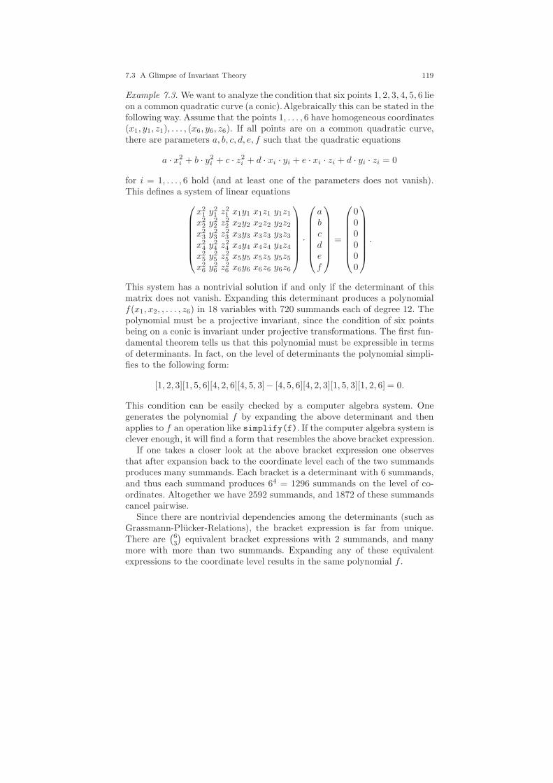
7.3 A Glimpse of Invariant Theory 119
Example 7.3. We want to analyze the condition that six points 1, 2, 3, 4, 5, 6 lieon a common quadratic curve (a conic).Algebraically this can be stated in thefollowing way. Assume that the points 1, . . . , 6 have homogeneous coordinates(x1, y1, z1), . . . , (x6, y6, z6). If all points are on a common quadratic curve,there are parameters a, b, c, d, e, f such that the quadratic equations
a · x2i + b · y2
i + c · z2i + d · xi · yi + e · xi · zi + d · yi · zi = 0
for i = 1, . . . , 6 hold (and at least one of the parameters does not vanish).This defines a system of linear equations
x21 y
21 z
21 x1y1 x1z1 y1z1
x22 y
22 z
22 x2y2 x2z2 y2z2
x23 y
23 z
23 x3y3 x3z3 y3z3
x24 y
24 z
24 x4y4 x4z4 y4z4
x25 y
25 z
25 x5y5 x5z5 y5z5
x26 y
26 z
26 x6y6 x6z6 y6z6
·
abcdef
=
000000
.
This system has a nontrivial solution if and only if the determinant of thismatrix does not vanish. Expanding this determinant produces a polynomialf(x1, x2, , . . . , z6) in 18 variables with 720 summands each of degree 12. Thepolynomial must be a projective invariant, since the condition of six pointsbeing on a conic is invariant under projective transformations. The first fun-damental theorem tells us that this polynomial must be expressible in termsof determinants. In fact, on the level of determinants the polynomial simpli-fies to the following form:
[1, 2, 3][1, 5, 6][4, 2, 6][4, 5, 3]− [4, 5, 6][4, 2, 3][1, 5, 3][1, 2, 6] = 0.
This condition can be easily checked by a computer algebra system. Onegenerates the polynomial f by expanding the above determinant and thenapplies to f an operation like simplify(f). If the computer algebra system isclever enough, it will find a form that resembles the above bracket expression.
If one takes a closer look at the above bracket expression one observesthat after expansion back to the coordinate level each of the two summandsproduces many summands. Each bracket is a determinant with 6 summands,and thus each summand produces 64 = 1296 summands on the level of co-ordinates. Altogether we have 2592 summands, and 1872 of these summandscancel pairwise.
Since there are nontrivial dependencies among the determinants (such asGrassmann-Plucker-Relations), the bracket expression is far from unique.There are
(63
)equivalent bracket expressions with 2 summands, and many
more with more than two summands. Expanding any of these equivalentexpressions to the coordinate level results in the same polynomial f .
120 7 More on Bracket Algebra
The first fundamental theorem can be proved constructively by providingan explicit algorithm that takes a polynomial
f(P ) ∈ R[x1,1, x1,2, x1,3, . . . , xn,1, xn,2, xn,3] =: R[X]
on the coordinate level as input and produces a polynomial in the bracketsof the points 1, . . . , n whenever f is an invariant. Here X abbreviates thecollection of all indeterminates on the coordinate level. One strategy for thisis to introduce a generic basis of three independent points e1, e2, e3. Underthe assumption of invariance of f one may without loss of generality assumethat these three vectors are the three unit vectors. Thus each variable on thecoordinate level can be expressed as a bracket that involves two unit vectorsand one point of the configuration. So we can rewrite f as a polynomial b(. . .)in these brackets. Now the difficult part of the proof begins. One can showthat using Grassmann-Plucker-Relations, b can be rewritten in the form
b = [e1, e2, e3]τ · b′(. . .).
Here b′(. . .) is a bracket polynomial that involves only points 1, . . . , n. Since[e1, e2, e3]
τ is constantly 1, the polynomial b′(. . .) must be the desired bracketpolynomial. The reader interested in a formal proof that follows these linesis referred to [126].
A general problem in the translation of coordinate polynomials to bracketpolynomials is that one has almost no control on the length of the resultingbracket polynomial. It is still a difficult open research problem to provide ef-ficient algorithms that generate bracket expressions of provably short length.
7.4 Projectively Invariant Functions
In geometry one is often interested in measuring certain values of geometricconfigurations (lengths, angles, etc.). As we have seen, lengths and angles arenot invariant under projective transformations. Thus they are not a reason-able measure within the framework of projective geometry. In contrast, it isappropriate to study functions f : RP
2 → R ∪ ∞ that are projectively in-variant in the sense of Definition 7.1. Here we will focus on rational functionsthat are projectively invariant.
We have already met one of these functions: the cross-ratio. If we re-consider the proofs of Lemmas 4.4 (invariance under rescaling homogeneouscoordinates) and 4.5 (invariance under projective transformations), we imme-diately see how to obtain other projectively invariant rational functions. Thecrucial property is that in the numerator and in the denominator we havemultihomogeneous functions with the same degree for any letter. Under theseconditions, rescaling factors of homogeneous coordinates and determinants ofprojective transformations will cancel perfectly.

7.5 The Bracket Algebra 121
We will see later on (in Part III of this book) how to express angles anddistances as invariant functions that relate projective objects with specialpoints or lines (such as the line at infinity).
Under mild nondegeneracy assumptions it can be shown that every rationalprojectively invariant function can be expressed as a rational function incross-ratios. The proof of this fact essentially reconstructs the coordinatesof the configuration (up to projective equivalence) from the cross-ratios (bytechniques similar to those of Section 5.4). Then the invariant functions cansimply be expanded in terms of cross-ratios. A formal proof may be found in[18].
7.5 The Bracket Algebra
In this section we want to change our point of view and again consider thebrackets as “first-class citizens” in preference to coordinates. We have seen inSections 7.1 and 7.2 that brackets carry all information that is necessary toreconstruct a configuration up to projective equivalence. Furthermore, Sec-tion 7.3 showed that as a consequence of this we can compute any projectiveinvariant from the values of the brackets. In particular, Example 7.3 indi-cated that expressing projective invariants on the level of brackets leads toconsiderably shorter expressions compared to the coordinate level. Moreover,the bracket expressions are often much easier to interpret geometrically thanthe coordinate expression.
Taking all this into account, it would be a wise strategy to drop the co-ordinate level completely and model the entire setup of projective geometryover R on the level of brackets.
For this we will in this chapter consider the brackets [a, b, c] themselves asindeterminates that may take any value in R. The set of all brackets on npoints is abbreviated
B := [i, j, k]∣∣ i, j, k ∈ E, E = 1, . . . , n.
The polynomial ring R[B] contains all polynomials that we can possibly writewith those brackets (remember, the brackets are now variables, not determi-nants). If the brackets really came from the determinants of a vector config-uration they would be far from independent. There would be many relationsamong them: a bracket that contains a repeated letter would have to be zero,the brackets would satisfy the alternating determinant rules, and, last but notleast, the brackets would have to satisfy the Grassmann-Plucker-Relations.
We can take these dependencies into account by factoring out the corre-sponding relations from the ring R[B].
Definition 7.3. We define the following three ideals in the ring R[B]:
122 7 More on Bracket Algebra
• Irepeat :=⟨[i, j, k] ∈ B
∣∣ i = j or i = k or j = k⟩,
• Ialtern :=⟨[λ1, λ2, λ3]+σ(π)[λπ(1), λπ(2), λπ(3)]
∣∣λ1, λ2, λ3 ∈ E, σ ∈ S3⟩,
• IGP :=⟨[a, b, c][d, e, f ]− [a, b, d][c, e, f ]+ [a, b, e][c, d, f ]− [a, b, f ][c, d, e]
∣∣
a, b, c, d, e, f ∈ E⟩.
In this expression π is a permutation of three elements, and σ(π) is its sign.The bracket ring BR is the ring R[B] factored modulo these three ideals:
BR := R[B]/⟨Irepeat ∪ Ialtern ∪ IGP
⟩.
Thus the bracket ring is defined in a way that brackets with repeated lettersare automatically zero (this is forced by Irepeat). Furthermore, alternatingdeterminant rules are forced by Ialtern, and finally, the Grassmann-Plucker-Relations are forced by IGP. See [132] for a more elaborate treatment ofthe bracket ring. Bracket polynomials that are identical in BR turn out toexpand to the same expression when we replace the brackets by the corre-sponding determinants. In order to formulate this precisely, we introduce aring homomorphism
Φ : R(B) → R[X]
that models the expansion of brackets. This homomorphism is uniquely de-termined by its action on the brackets
Φ([i, j, k]) := det(xi, xj , xk).
We now can prove the following theorem:
Theorem 7.4. Let f, g be two polynomials in R(B) such that f ≡ g in thebracket ring. Then Φ(f) = Φ(g).
Proof. If f ≡ g in the bracket ring, then there is a polynomial h ∈⟨Irepeat ∪
Ialtern ∪ IGP
⟩such that f = g + h in R[B]. Applying the operator Φ to both
sides, we obtain
Φ(f) = Φ(g + h) = Φ(g) + Φ(h) = Φ(g).
The last equation holds since every polynomial in the ideals Irepeat, Ialtern, IGP
expands to zero under Φ by definition. ⊓⊔
The converse of the above theorem is true as well:
Theorem 7.5. Let f, g be two polynomials in R(B) with Φ(f) = Φ(g). Thenf − g ∈
⟨Irepeat ∪ Ialtern ∪ IGP
⟩.
Equivalently, we can state this theorem also by saying that every bracketpolynomial f ∈ R(B) with Φ(f) = 0 is automatically in the ideal
7.5 The Bracket Algebra 123
⟨Irepeat ∪ Ialtern ∪ IGP
⟩.
This theorem is also known as the second fundamental theorem of invarianttheory: All bracket polynomials that are identical to zero for all point config-urations are generated by our three ideals. If we, a little less formally, identifybracket symbols according to the rules
[i, j, k] = [j, k, i] = [k, i, j] = −[i, k, j] = −[k, j, i] = −[j, i, k],
we can also express this theorem by saying that every bracket expressionf(B) that vanishes on all configurations can be written as
f =∑
mi · γi,
where the γi are Grassmann-Plucker-Relations.

Part II
Working and Playing with Geometry


127
Need to play is the mother of all invention.
Kristina Brenneman, Portland Tribune, 2005
You’ve achieved success in your field when you don’t knowwhether what you’re doing is work or play.
Warren Beatty (b. 1937)
So far, we have prepared a solid basis for projective geometry with a strongemphasis on relationship to algebra. Now it is time to explore how theseconcepts interact in several contexts. It is the aim of the following few chaptersto demonstrate how a bracket-oriented point of view makes it algebraicallyeasy to describe, prove, and even generate interesting geometric facts. Wealso want to investigate how homogeneous coordinates can be used to expressgeometric calculations in an elegant fashion.
The material used in the following sections is intentionally taken fromdifferent areas of projective geometry. However, especially the chapters onquadrilateral sets and on conics will play an important role later on. Through-out these chapters we will also try to introduce several standard techniquesfor proving geometric facts on the level of bracket algebra.

8
Quadrilateral Sets and Liftings
The mathematics of rhythm are universal.They don’t belong to any particular culture
John McLaughlin
In this chapter we will focus on an important concept of projective geom-etry: quadrilateral sets. On the one hand, these configurations can be con-sidered a generalization of harmonic points. On the other hand, they have aclose relation-ship to the liftability of lower-dimensional point configurationsto prescribed higher-dimensional scenarios. Their algebraic counterparts alsoexpose highly symmetric (almost rhythmic) structures coming from the in-terplay of the six intersections of four lines.
8.1 Points on a Line
We will begin our studies with the algebraic consequences of having n pointson a line. Any bracket formed by three collinear points will automatically bezero. Via Grassmann-Plucker-Relations, this vanishing bracket causes otherrelations among the other (nonzero) brackets.(From now on, we will freely omitthe commas in brackets whenever no confusion can arise in order to make theformulas a bit more compact and readable; thus we may write [abc] insteadof [a, b, c]). Consider the three-summand Grassmann-Plucker-Relation
[abc][axy] − [abx][acy] + [aby][acx] = 0.
129
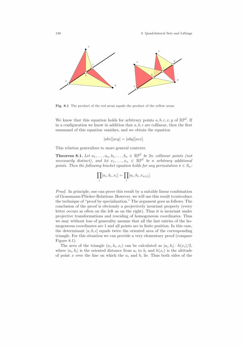
130 8 Quadrilateral Sets and Liftings
a
b
c
x
y a
b
c
dx
y
z
Fig. 8.1 The product of the red areas equals the product of the yellow areas.
We know that this equation holds for arbitrary points a, b, c, x, y of RP2. If
in a configuration we know in addition that a, b, c are collinear, then the firstsummand of this equation vanishes, and we obtain the equation
[abx][acy] = [aby][acx].
This relation generalizes to more general contexts:
Theorem 8.1. Let a1, . . . , an, b1, . . . , bn ∈ RP2 be 2n collinear points (not
necessarily distinct), and let x1, . . . , xn ∈ RP2 be n arbitrary additional
points. Then the following bracket equation holds for any permutation π ∈ Sn:
∏
i
[ai, bi, xi] =∏
i
[ai, bi, xπ(i)].
Proof. In principle, one can prove this result by a suitable linear combinationof Grassmann-Plucker-Relations. However, we will use this result to introducethe technique of “proof by specialization.” The argument goes as follows. Theconclusion of the proof is obviously a projectively invariant property (everyletter occurs as often on the left as on the right). Thus it is invariant underprojective transformations and rescaling of homogeneous coordinates. Thuswe may without loss of generality assume that all the last entries of the ho-mogeneous coordinates are 1 and all points are in finite position. In this case,the determinant [a, b, c] equals twice the oriented area of the correspondingtriangle. For this situation we can provide a very elementary proof (compareFigure 8.1).
The area of the triangle (ai, bi, xi) can be calculated as |ai, bi| · h(xi)/2,where |ai, bi| is the oriented distance from ai to bi and h(xi) is the altitudeof point x over the line on which the ai and bi lie. Thus both sides of the
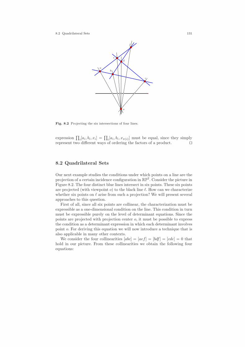
8.2 Quadrilateral Sets 131
a
e
f
d
b
c
o
Fig. 8.2 Projecting the six intersections of four lines.
expression∏i[ai, bi, xi] =
∏i[ai, bi, xπ(i)] must be equal, since they simply
represent two different ways of ordering the factors of a product. ⊓⊔
8.2 Quadrilateral Sets
Our next example studies the conditions under which points on a line are theprojection of a certain incidence configuration in RP
2. Consider the picture inFigure 8.2. The four distinct blue lines intersect in six points. These six pointsare projected (with viewpoint o) to the black line ℓ. How can we characterizewhether six points on ℓ arise from such a projection? We will present severalapproaches to this question.
First of all, since all six points are collinear, the characterization must beexpressible as a one-dimensional condition on the line. This condition in turnmust be expressible purely on the level of determinant equations. Since thepoints are projected with projection center o, it must be possible to expressthe condition as a determinant expression in which each determinant involvespoint o. For deriving this equation we will now introduce a technique that isalso applicable in many other contexts.
We consider the four collinearities [abc] = [aef ] = [bdf ] = [cde] = 0 thathold in our picture. From these collinearities we obtain the following fourequations:

132 8 Quadrilateral Sets and Liftings
[abc] = 0 =⇒ [abe][bcf ][cad] = [abf ][bcd][cae]
[aef ] = 0 =⇒ [aeo][afb] = [aeb][afo]
[bfd] = 0 =⇒ [bfo][bdc] = [bfc][bdo]
[cde] = 0 =⇒ [cdo][cea] = [cda][ceo]
The last three are direct consequences of Grassmann-Plucker-Relations.The first equation is an application of Theorem 8.1. Multiplying all left sidesand all right sides and canceling determinants that appear on both sides(those that are not underlined), we arrive at the equation
[aeo][bfo][cdo] = [afo][bdo][ceo].
This is the desired characterization. Since in each bracket the point o isinvolved, we can also read this expression as a rank-2 expression of the cor-responding projections on the line.
Before we study the symmetry of this bracket expression we will have alook at two other ways of deriving this formula.
Consider the picture in Figure 8.3 left. There the point of projection hasbeen moved to infinity. We want to give an affine argument from which wecan generate the desired formula. This time we will directly head for therank-2 formula: Under what conditions are six points a, b, c, d, e, f on a lineliftable to the blue incidence configuration? We want a nontrivial lifting, inwhich not all lines are identical. We furthermore assume that points whoselifted images should be collinear do not coincide on the line.Similar questionsarise in the field of scene analysis, a branch of projective geometry in whichquadrilateral sets and bracket algebra play a fundamental role [29, 31].
We assume that the points that are involved have homogeneous (rank-2)coordinates (xa, 1), . . . , (xf , 1). A lifting of the six points corresponds to anassignment of an altitude ha, . . . , hf to each of the points. Assume that wehave such a lifting such that the lifted points a, b, c are collinear. The liftedpoints have homogeneous coordinates (xa, 1, ha), (xb, 1, hb), (xc, 1, hc). Theircollinearity is expressed as
0 = det
xa 1 haxb 1 hbxc 1 hc
= [ab]hc − [ac]hb + [bc]ha.
We get similar expressions for the other four lines. In a lifting these fourconditions have to be satisfied simultaneously. Thus any lifting correspondsto a solution of the linear system of equations
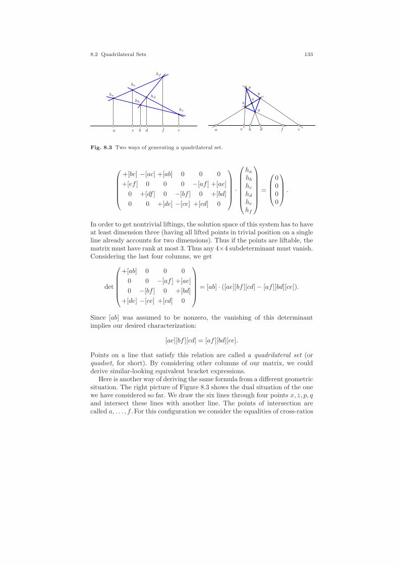
8.2 Quadrilateral Sets 133PSfrag
a b cde f
ha
he
hbhd
hf
hc
x
y
p
q
a e b f cd
o
Fig. 8.3 Two ways of generating a quadrilateral set.
+[bc] −[ac] +[ab] 0 0 0
+[ef ] 0 0 0 −[af ] +[ae]
0 +[df ] 0 −[bf ] 0 +[bd]
0 0 +[de] −[ce] +[cd] 0
·
hahbhchdhehf
=
0000
.
In order to get nontrivial liftings, the solution space of this system has to haveat least dimension three (having all lifted points in trivial position on a singleline already accounts for two dimensions). Thus if the points are liftable, thematrix must have rank at most 3. Thus any 4×4 subdeterminant must vanish.Considering the last four columns, we get
det
+[ab] 0 0 0
0 0 −[af ] +[ae]
0 −[bf ] 0 +[bd]
+[de] −[ce] +[cd] 0
= [ab] · ([ae][bf ][cd] − [af ][bd][ce]).
Since [ab] was assumed to be nonzero, the vanishing of this determinantimplies our desired characterization:
[ae][bf ][cd] = [af ][bd][ce].
Points on a line that satisfy this relation are called a quadrilateral set (orquadset, for short). By considering other columns of our matrix, we couldderive similar-looking equivalent bracket expressions.
Here is another way of deriving the same formula from a different geometricsituation. The right picture of Figure 8.3 shows the dual situation of the onewe have considered so far. We draw the six lines through four points x, z, p, qand intersect these lines with another line. The points of intersection arecalled a, . . . , f . For this configuration we consider the equalities of cross-ratios

134 8 Quadrilateral Sets and Liftings
(a, c; e, d) = (a, y;x, o) = (a, b; f, d).
The first equality comes from projection through point p; the second is aconsequence of projection through q. Expanding the cross-ratios, we get
[ae][cd]
[ad][ce]=
[af ][bd]
[ad][bf ].
Canceling [ad] and multiplying by the denominators, we get the desired equa-tion
[ae][bf ][cd] = [ce][af ][bd].
8.3 Symmetry and Generalizations of Quadrilateral Sets
The quadrilateral set configuration has interesting inner structures. In ourlabeling there are three pairs of points (a, d), (b, e), and (c, f) such that thepoints of each pair do not share a line of the configuration. Every line of thecomplete quadrilateral is obtained by selecting exactly one point from eachof the pairs. For instance, the line (a, b, c) takes the first point of each of thepairs. In our expression
[ae][bf ][cd] = [ce][af ][bd],
the line (a, b, c) plays a special role. The two monomials of the expressionare formed by three brackets, and each of these brackets contains exactly onepoint of the line and one other point such that they do not form one of thethree pairs above. For each line we get exactly one such characterization ofthe quadrilateral set.
Besides the four lines in our original quadrilateral set there are alsofour other lines that can be formed by taking exactly one point from eachof the pairs. These lines (d, e, f), (a, b, f), (b, c, d), and (a, c, e) describethe associated complete quadrilateral to our original one. The symmetry of[ae][bf ][cd] = [ce][af ][bd] also implies that this expression is as well a char-acterization of the quadrilateral set generated by the associated completequadrilateral. The situation is illustrated in Figure 8.4 left. The blue partof the picture is our original quadrilateral set configuration, the green partis the complementary one. In particular, if we interchange the roles of twopoints in one of the pairs (a, d), (b, e), (c, f), then we transfer the completequadrilateral into its associated one. This implies that the triple of pairs char-acterizes the quadrilateral set. The right part of Figure 8.4 is an illustrationof obtaining a quadrilateral set by projection or by intersection. Both pic-tures represent projective incidence theorems. If all coincidences except thelast one are satisfied, then the last one is satisfied automatically.
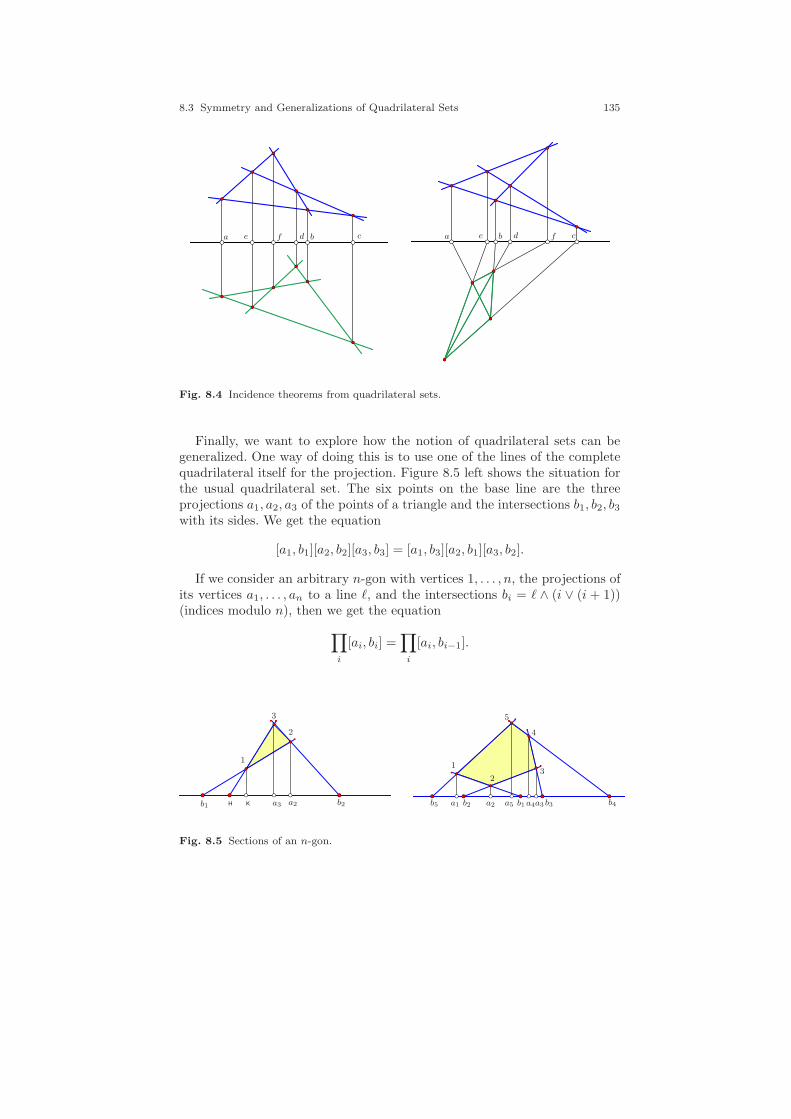
8.3 Symmetry and Generalizations of Quadrilateral Sets 135
a b cde f a b cde f
Fig. 8.4 Incidence theorems from quadrilateral sets.
Finally, we want to explore how the notion of quadrilateral sets can begeneralized. One way of doing this is to use one of the lines of the completequadrilateral itself for the projection. Figure 8.5 left shows the situation forthe usual quadrilateral set. The six points on the base line are the threeprojections a1, a2, a3 of the points of a triangle and the intersections b1, b2, b3with its sides. We get the equation
[a1, b1][a2, b2][a3, b3] = [a1, b3][a2, b1][a3, b2].
If we consider an arbitrary n-gon with vertices 1, . . . , n, the projections ofits vertices a1, . . . , an to a line ℓ, and the intersections bi = ℓ ∧ (i ∨ (i + 1))(indices modulo n), then we get the equation
∏
i
[ai, bi] =∏
i
[ai, bi−1].
H K a3 a2b1 b2
1
2
3
a1 a2 a3a4a5 b1b2b5 b4b3
1
23
4
5
Fig. 8.5 Sections of an n-gon.
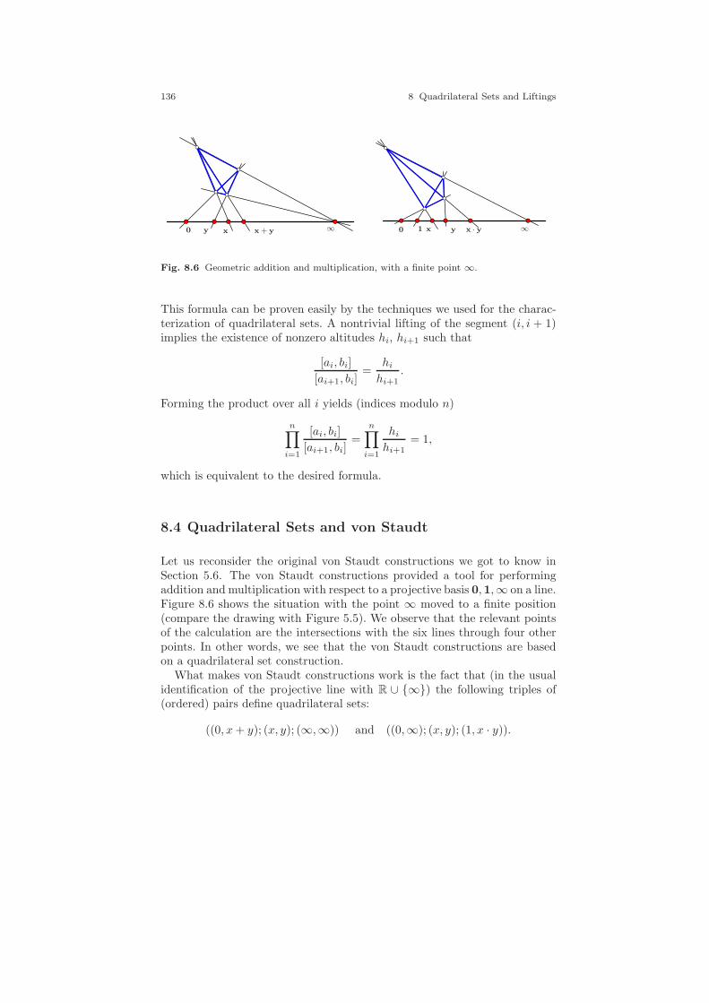
136 8 Quadrilateral Sets and Liftings
y x x + y0 ∞ 1 x y x · y0 ∞
Fig. 8.6 Geometric addition and multiplication, with a finite point ∞.
This formula can be proven easily by the techniques we used for the charac-terization of quadrilateral sets. A nontrivial lifting of the segment (i, i + 1)implies the existence of nonzero altitudes hi, hi+1 such that
[ai, bi]
[ai+1, bi]=
hihi+1
.
Forming the product over all i yields (indices modulo n)
n∏
i=1
[ai, bi]
[ai+1, bi]=
n∏
i=1
hihi+1
= 1,
which is equivalent to the desired formula.
8.4 Quadrilateral Sets and von Staudt
Let us reconsider the original von Staudt constructions we got to know inSection 5.6. The von Staudt constructions provided a tool for performingaddition and multiplication with respect to a projective basis 0,1,∞ on a line.Figure 8.6 shows the situation with the point ∞ moved to a finite position(compare the drawing with Figure 5.5). We observe that the relevant pointsof the calculation are the intersections with the six lines through four otherpoints. In other words, we see that the von Staudt constructions are basedon a quadrilateral set construction.
What makes von Staudt constructions work is the fact that (in the usualidentification of the projective line with R ∪ ∞) the following triples of(ordered) pairs define quadrilateral sets:
((0, x+ y); (x, y); (∞,∞)) and ((0,∞); (x, y); (1, x · y)).
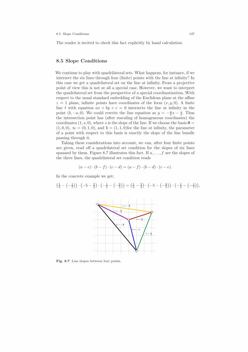
8.5 Slope Conditions 137
The reader is invited to check this fact explicitly by hand calculation.
8.5 Slope Conditions
We continue to play with quadrilateral sets. What happens, for instance, if weintersect the six lines through four (finite) points with the line at infinity? Inthis case we get a quadrilateral set on the line at infinity. From a projectivepoint of view this is not at all a special case. However, we want to interpretthe quadrilateral set from the perspective of a special coordinatization. Withrespect to the usual standard embedding of the Euclidean plane at the affinez = 1 plane, infinite points have coordinates of the form (x, y, 0). A finiteline ℓ with equation ax + by + c = 0 intersects the line at infinity in thepoint (b,−a, 0). We could rewrite the line equation as y = −a
bx − cb . Thus
the intersection point has (after rescaling of homogeneous coordinates) thecoordinates (1, s, 0), where s is the slope of the line. If we choose the basis 0 =(1, 0, 0), ∞ = (0, 1, 0), and 1 = (1, 1, 0)for the line at infinity, the parameterof a point with respect to this basis is exactly the slope of the line bundlepassing through it.
Taking these considerations into account, we can, after four finite pointsare given, read off a quadrilateral set condition for the slopes of six linesspanned by them. Figure 8.7 illustrates this fact. If a, . . . , f are the slopes ofthe three lines, the quadrilateral set condition reads
(a− e) · (b− f) · (c− d) = (a− f) · (b − d) · (c− e).
In the concrete example we get:
(13 −
(− 1
7
))·(−5 − 5
2
)·(− 1
2 −(− 6
5
))=(
13 − 5
2
)·(−5 −
(− 6
5
))·(− 1
2 −(− 1
7
)),
a = 13
b = −4
c = − 12
d = − 65
e = − 17
f = 52
Fig. 8.7 Line slopes between four points.
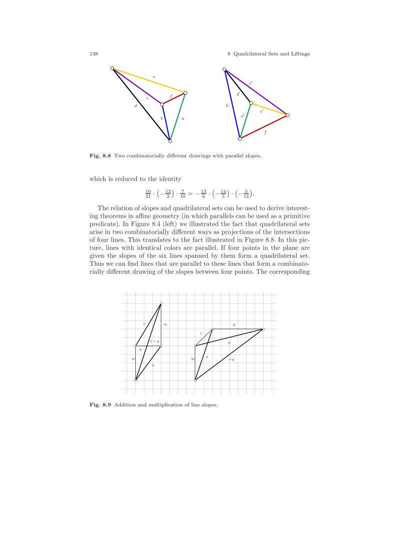
138 8 Quadrilateral Sets and Liftings
ʼ
ʼ
ʼ
ʼ
ʼ
ʼ
aa
b
b
c
cd
d
e
e
f
f
Fig. 8.8 Two combinatorially different drawings with parallel slopes.
which is reduced to the identity
1021 ·
(− 13
2
)· 7
10 = − 136 ·(− 14
5
)·(− 5
14
).
The relation of slopes and quadrilateral sets can be used to derive interest-ing theorems in affine geometry (in which parallels can be used as a primitivepredicate). In Figure 8.4 (left) we illustrated the fact that quadrilateral setsarise in two combinatorially different ways as projections of the intersectionsof four lines. This translates to the fact illustrated in Figure 8.8. In this pic-ture, lines with identical colors are parallel. If four points in the plane aregiven the slopes of the six lines spanned by them form a quadrilateral set.Thus we can find lines that are parallel to these lines that form a combinato-rially different drawing of the slopes between four points. The corresponding
1
0
0
x
x
y
y
x·y
x+ y
∞∞
∞
Fig. 8.9 Addition and multiplication of line slopes.
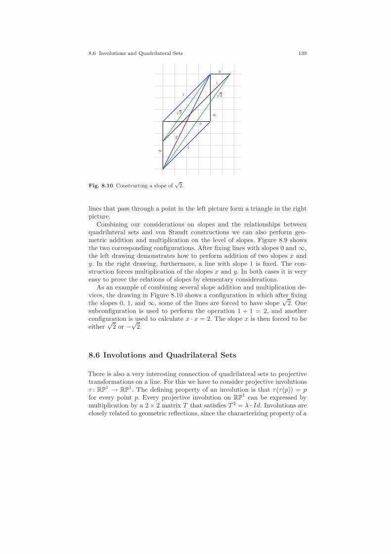
8.6 Involutions and Quadrilateral Sets 139
1
1
1
0
0
√2
√2
2
∞
∞
Fig. 8.10 Constructing a slope of√
2.
lines that pass through a point in the left picture form a triangle in the rightpicture.
Combining our considerations on slopes and the relationships betweenquadrilateral sets and von Staudt constructions we can also perform geo-metric addition and multiplication on the level of slopes. Figure 8.9 showsthe two corresponding configurations. After fixing lines with slopes 0 and ∞,the left drawing demonstrates how to perform addition of two slopes x andy. In the right drawing, furthermore, a line with slope 1 is fixed. The con-struction forces multiplication of the slopes x and y. In both cases it is veryeasy to prove the relations of slopes by elementary considerations.
As an example of combining several slope addition and multiplication de-vices, the drawing in Figure 8.10 shows a configuration in which after fixingthe slopes 0, 1, and ∞, some of the lines are forced to have slope
√2. One
subconfiguration is used to perform the operation 1 + 1 = 2, and anotherconfiguration is used to calculate x · x = 2. The slope x is then forced to beeither
√2 or −
√2.
8.6 Involutions and Quadrilateral Sets
There is also a very interesting connection of quadrilateral sets to projectivetransformations on a line. For this we have to consider projective involutionsτ : RP
1 → RP1. The defining property of an involution is that τ(τ(p)) = p
for every point p. Every projective involution on RP1 can be expressed by
multiplication by a 2× 2 matrix T that satisfies T 2 = λ · Id. Involutions areclosely related to geometric reflections, since the characterizing property of a

140 8 Quadrilateral Sets and Liftings
Fig. 8.11 Pairs of orthogonal slopes: The altitudes meet in a point.
reflection is that the mirror image of the mirror image is the original again.We now get the following result:
Theorem 8.2. Let τ : RP1 → RP
1 be a projective involution that is not theidentity and let a, b, c be arbitrary points in RP
1. Then the pairs
(a, τ(a)), (b, τ(b)), (c, τ(c))
form a quadrilateral set.
Proof. Since T is an involution, we have T 2 = λ · Id. This implies det(T )2 =det(T 2) = det((λ · Id)) = λ2. Hence det(T ) is either +λ or −λ. We will firstexclude the case det(T ) = λ. For this, the fact that T is a 2 × 2 matrix is
crucial. Let T =(α βγ δ
). We then get
T 2 =
(α2 + βγ αβ + βδαγ + δγ γβ + δ2
)=
(λ 00 λ
).
This can be satisfied only if either α = −δ or γ = β = 0. The first caseleads to det(T ) = −λ (check it). The second case implies α2 = δ2. Sinceagain τ was assumed not to be the identity, this case implies α = −δ, whichagain implies (together with β = γ = 0) the equation det(T ) = −λ. We nowconsider the monomial
[a, T b][b, T c][c, T a].
Applying the transformation T to each of the points of this monomial trans-fers this monomial to
[Ta, T 2b][Tb, T 2c][Tc, T 2a] = [Ta, λb][Tb, λc][Tc, λa] = −λ3[b, T a][c, T b][a, T c].
On the other hand, the transferred monomial must satisfy the equation
[Ta, T 2b][Tb, T 2c][Tc, T 2a] = (det(T ))3[a, T b][b, T c][c, T a].
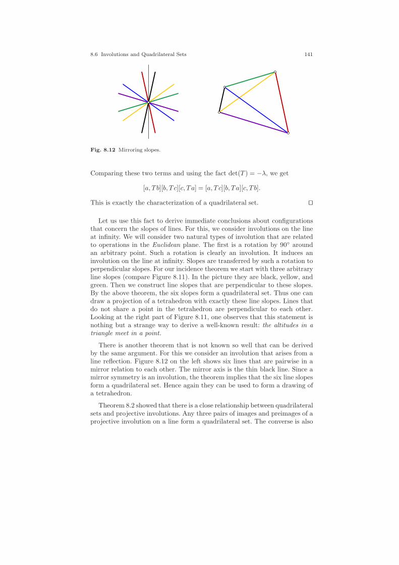
8.6 Involutions and Quadrilateral Sets 141
Fig. 8.12 Mirroring slopes.
Comparing these two terms and using the fact det(T ) = −λ, we get
[a, T b][b, T c][c, T a] = [a, T c][b, T a][c, T b].
This is exactly the characterization of a quadrilateral set. ⊓⊔
Let us use this fact to derive immediate conclusions about configurationsthat concern the slopes of lines. For this, we consider involutions on the lineat infinity. We will consider two natural types of involution that are relatedto operations in the Euclidean plane. The first is a rotation by 90 aroundan arbitrary point. Such a rotation is clearly an involution. It induces aninvolution on the line at infinity. Slopes are transferred by such a rotation toperpendicular slopes. For our incidence theorem we start with three arbitraryline slopes (compare Figure 8.11). In the picture they are black, yellow, andgreen. Then we construct line slopes that are perpendicular to these slopes.By the above theorem, the six slopes form a quadrilateral set. Thus one candraw a projection of a tetrahedron with exactly these line slopes. Lines thatdo not share a point in the tetrahedron are perpendicular to each other.Looking at the right part of Figure 8.11, one observes that this statement isnothing but a strange way to derive a well-known result: the altitudes in atriangle meet in a point.
There is another theorem that is not known so well that can be derivedby the same argument. For this we consider an involution that arises from aline reflection. Figure 8.12 on the left shows six lines that are pairwise in amirror relation to each other. The mirror axis is the thin black line. Since amirror symmetry is an involution, the theorem implies that the six line slopesform a quadrilateral set. Hence again they can be used to form a drawing ofa tetrahedron.
Theorem 8.2 showed that there is a close relationship between quadrilateralsets and projective involutions. Any three pairs of images and preimages of aprojective involution on a line form a quadrilateral set. The converse is also
142 8 Quadrilateral Sets and Liftings
true. For this we first observe that if a projective map in RP1 interchanges
two points, then it will automatically be an involution.
Lemma 8.1. Let τ : RP1 → RP
1 be a projective transformation with τ(a) =a′ and τ(a′) = a for distinct points a and a′. Then τ is an involution.
Proof. Without loss of generality we may (after a suitable projective trans-
formation) assume that a =(
10
)and a′ =
(01
). Thus the matrix T that
represents τ must have the form T =(
0 αβ 0
)for nonzero parameters α and β.
Calculating T 2, we get
T 2 =
(αβ 00 αβ
)= αβ
(1 00 1
).
Thus T 2 represents the identity map on RP1. ⊓⊔
With this lemma it is easy to prove that every quadrilateral set inducesan involution.
Theorem 8.3. Let a, b, c be three distinct points in RP1. Let a′b′c′ be three
additional points. If (a, a′); (b, b′); (c, c′) forms a quadrilateral set, then theprojective map τ uniquely defined by τ(a) = a′, τ(b) = b′, τ(c) = c′ is aninvolution.
Proof. If a = a′, b = b′, c = c′, then τ must be the identity, which is triviallyan involution. Thus at least one of the pairs consists of different points.Assume without loss of generality that a and a′ are distinct. Consider theuniquely defined transformation τ that satisfies τ(a) = a′, τ(a′) = a, τ(b) =b′. By Lemma 8.1 this transformation will be an involution. Thus it sufficesto show that τ(c) = c′. Theorem 8.2 implies that
(a, τ(a)), (b, τ(b)), (c, τ(c))
form a quadrilateral set. Using our knowledge about τ , we see that
(a, a′), (b, b′), (c, τ(c))
is a quadrilateral set. Since five points of a quadrilateral set determine thesixth one uniquely, we must have that τ(c) = c′. This proves the theorem. ⊓⊔
So to every quadrilateral set we can associate in a natural way an involu-tion. It is a remarkable fact that the two fixed points of the involution are inharmonic position to all point pairs in the quadrilateral set.
If T represents a projective transformation, then the eigenvectors of Tcorrespond to the fixed points of the transformation. For every eigenvector pof T we have Tp = λp, and p is mapped to itself. If T is a 2× 2 matrix, thenit may have either two real or two complex conjugate eigenvectors (up to
8.6 Involutions and Quadrilateral Sets 143
scalar multiples). If the eigenvectors are real, then they correspond to pointsin RP
1 that are invariant under T .
Theorem 8.4. Let τ be the involution associated to the points of a quadri-lateral set (a, a′; b, b′, c, c′). Assume that τ has two distinct real fixed points pand q. Then the point pairs (p, q) and (a, a′) form a harmonic set.
Proof. If τ is an involution, then (a, τ(a); p, τ(p); q, τ(q)) is a quadrilateralset. Using our knowledge of the definition of τ and the fixed point propertiesof p and q, we see that (a, a′; p, p; q, q) is a quadrilateral set. Thus we have[a, p][p, q][q, a′] = [a, q][p, a′][q, p]. Using the distinctness of p and q we cancancel [p, q] from this expression and are left with [a, p][q, a′] = −[a, q][p, a′],which is exactly the characterization for a harmonic pair of point pairs. ⊓⊔
Clearly, in the same way the pair of points (p, q) is also harmonic withrespect to (b, b′) and to (c, c′). This leads us to a nice characterization offixed points of τ . If τ is an involution associated to (a, a′; b, b′; c, c′), thenthe fixed points of τ are exactly those two points that are simultaneouslyharmonic to all three point pairs of the quadrilateral set. In fact, any twoof the point pairs of the quadrilateral set determine the position of p and quniquely. The fact that (p, q) are also harmonic with respect to the last pairis exactly the quadrilateral set condition.
There is a little subtlety concerning the existence of the fixed points thatwill become relevant later in this book: The fixed points need not be real.We saw that the fixed points correspond to the eigenvectors of the matrix Tthat represents τ . If this matrix has complex eigenvalues (like the involution(
0 1−1 0
)), then the eigenvectors are also complex (and cannot become real by
multiplication by a real scalar). In such a case the transformation has no realfixed points. This case geometrically is related to “rotation-like” transforma-tions τ such as the 90 rotation we used in Figure 8.11. The case in whichreal fixed points exist is related to “reflection-like” transformations, such asthe mirror-image operation we used in Figure 8.12.


9
Conics and Their Duals
You always admire what you really don’t understand.
Blaise Pascal
So far, we have dealt almost exclusively with situations in which onlypoints and lines were involved. Geometry would be quite a pure topic if thesewere the only objects to be treated. Large parts of classical elementary geom-etry deal with constructions involving circles. The most elementary drawingtools treated by Euclid (the straightedge and the compass) contain a toolfor generating circles. In a sense, so far we have dealt with the straightedgealone. Unfortunately, circles are not a concept of projective geometry. Thiscan easily be seen by observing that the shape of a circle is not invariantunder projective transformations. If you look at a sheet of paper on which acircle is drawn from a skew angle, you will see an ellipse. In fact, projectivetransformations of circles include ellipses, hyperbolas, and parabolas. Theyare subsumed under the term conic sections, or conics, for short. Conics arethe concept of projective geometry that comes closest to the concept of circlesin Euclidean geometry. It is the purpose of this section to give a purely pro-jective treatment of conics. Later on, we will see how certain specializationsprovide interesting insights into the geometry of circles.
9.1 The Equation of a Conic
Let us start with the unit circle in the Euclidean plane:
(x, y) ∈ R2 | x2 + y2 = 1.
145
146 9 Conics and Their Duals
In this section we will investigate which shapes can arise if we transform thiscircle projectively. For this we again consider the Euclidean plane embeddedat the z = 1 plane of R
3 and represented by homogeneous coordinates (anyother affine embedding not containing the origin would serve as well andwould lead to the same result). Thus the points of the circle correspondto points with homogeneous coordinates (x, y, 1) with x2 + y2 = 1. Takinginto account that homogeneous coordinates are specified only up to a scalarmultiple, we may rewrite this condition in a more general way as points(x, y, z) with x2 + y2 = z2. Setting z = 1, we obtain the original formula.According to the fact that every term of the expression x2 + y2 = z2 isquadratic, a vector (x, y, z) satisfies this expression if (λx, λy, λz), λ 6= 0,satisfies it. We may rewrite the quadratic equation as
(x, y, z) ·
1 0 00 1 00 0 −1
·
xyz
= 0.
Thus the homogeneous coordinate vectors that satisfy this equation areexactly those that represent points of our circle. We now want to transformthese points projectively. Applying a projective transformation to the pointscan be carried out by replacing both occurrences of the vector p = (x, y, z) bya transformed vector M · p. Thus we obtain that a projectively transformedunit circle can be expressed algebraically as the solutions of the equation
((x, y, z) ·MT ) ·
1 0 00 1 00 0 −1
· (M ·
xyz
) = 0,
where M is a real 3 × 3 matrix with nonzero determinant. Multiplying thethree matrices in the middle of this expression, we are led to an equation
(x, y, z) ·
a b db c ed e f
·
xyz
= 0, (∗)
for suitable parameters a, b, c, d, e, f . Observe that the matrix in the middleis necessarily symmetric. Expanding the above product expression yields thefollowing quadratic equation:
a · x2 + c · y2 + f · z2 + 2b · xy + 2d · xz + 2e · yz = 0.
We call such an expression of the form pTAp a quadratic form (regardless ofwhether the matrix A is symmetric). The set of points that satisfies such anequation will be called a conic. In a sense we are working on three differentlevels when we speak about matrices, quadratic forms, and conics. Beforewe continue, we want to clarify this relationship. Let A be a 3 × 3 matrixwith entries in some field K. The associated quadratic form is a homogeneous
9.1 The Equation of a Conic 147
quadratic function QA : K3 → K defined by
QA(p) = pTAp.
It is important to notice that different matrices may lead to the samequadratic form. This can be seen by expanding
QA = (x, y, z) ·
a b1 d2
b2 c e1d1 e2 f
·
xyz
to
QA = a · x2 + c · y2 + f · z2 + (b1 + b2) · xy + (d1 + d2) · xz + (e1 + e2) · yz.
Observe that the quadratic form associated to a matrix depends only on thediagonal entries and the sums of matrix entriesAij+Aji. For every potentiallynonsymmetric matrix A, the matrix (A+ AT )/2 creates the same quadraticform:
QA = Q(A+AT )/2.
We call this process symmetrization. Furthermore, it is also clear that forevery homogeneous quadratic polynomial f(x, y, z), a (symmetric) matrix Awith QA(x, y, z) = f(x, y, z) also exists.
The conics themselves are the third level with which we have to deal.They consist of all points in PK for which a quadratic form vanishes. Theconic associated to a matrix (or quadratic form) is
CA = [p] ∈ PK | pTAp = 0.
Since the expression pTAp = 0 is stable under scalar multiplication of p bya nonzero scalar, we will, by common abuse of notation, work as usual onthe level of homogeneous coordinates and omit the brackets [. . .]. How muchinformation about the matrix A is still present in the conic in a sense dependson the underlying field. Over R it may, for instance, happen that a conic (suchas the solution set of x2 + y2 + z2 = 0) has no nonzero solutions at all. Insuch a case there are still complex solutions. We will deal with them later.
We return to the case of a projectively transformed circle and the quadraticform described in equation (∗). In this case the parameters a, . . . , f are notcompletely independent. Sylvester’s law of inertia from linear algebra tells usthat the signature of the eigenvalues must be the same as in the matrix
1 0 00 1 00 0 −1

148 9 Conics and Their Duals
and that this is the only restriction.1
If we allow general real parameters in equation (∗), we can classify thedifferent cases by the signature of the eigenvalues. Since the quadratic formsof the matrices A and −A describe identical point sets, we may identifya signature vector with its negative. Thus we end up with five essentiallydifferent cases of signatures:
(+,+,−), (+,+,+), (+,−, 0), (+,+, 0), (+, 0, 0).
Each of these cases describes a geometric situation that cannot be trans-formed projectively into any of the other cases. The case of a circle cor-responds to the first entry in the list. The last three cases correspond todegenerate conics (the determinant of A is zero), and the second case corre-sponds to a situation like x2 +y2 +z2 = 0, in which we have no real solutionsat all (but where complex solutions still exist). Before we clarify the geo-metric meaning of the other four cases in detail, we will have a closer lookat the circular case. Projectively, all quadratic forms with eigenvalue signa-ture (+,+,−) have to be considered as isomorphic (they are the projectiveimages of a unit circle). However, if we fix a certain embedding of the Eu-clidean plane into R3 (say the standard z = 1 embedding) and by this singleout a specific line at infinity, then we may classify them also with respectto Euclidean motions. In fact, there is an infinite variety of forms of conicsthat are inequivalent under Euclidean transformations. Still there is a veryuseful (and well-known) coarser classification if we just count the intersec-tions of the conic with the line at infinity. Intersecting the quadratic form ofa projectively transformed circle
a · x2 + c · y2 + f · z2 + 2b · xy + 2d · xz + 2e · yz = 0
and the line at infinity (i.e., setting z = 0) leaves us with the equation
a · x2 + c · y2 + 2b · xy = 0.
This homogeneous quadratic equation may lead to zero, one, or two solu-tions up to scalar multiples. The three cases are shown in Figure 9.1. Theycorrespond to the well-known cases of ellipses, parabolas, and hyperbolas.Thus one could say that a parabola is a conic that touches the line at in-finity, while a hyperbola has two points at infinity. The three cases can bealgebraically distinguished by considering the discriminant of the equationa · x2 + c · y2 + 2b · xy = 0. The sign of the discriminant turns out to be thesign of the determinant
det
(a bb c
).
1 Sylvester’s law of inertia states that if M is nonsingular, then A and MTAM have thesame signature of eigenvalues for any symmetric matrix A. Furthermore, this is the onlyrestriction on the coefficients of the symmetric matrix MTAM .

9.2 Polars and Tangents 149
ℓ∞ ℓ∞ ℓ∞
ellipse parabola hyperbola
Fig. 9.1 The possible images of a circle.
If this sign is negative we are in the hyperbolic case. If it is zero, we get aparabola, and if it is positive, we get an ellipse.
9.2 Polars and Tangents
For the moment we will stick to the case of nondegenerate conics that areprojective images of a circle. Our next task will be to calculate a tangentto such a conic. For this we first need an algebraic characterization of a linebeing tangent to a conic. There are essentially two ways of doing this. Thefirst is related to concepts of differential geometry: A line is tangent to aconic if at a point of intersection it has the same slope as the conic. Theother approach is intersection-theoretic and uses the fact that we know thata conic is a quadratic curve: A line is tangent to a conic if it has exactly onepoint in common with it. The first approach is slightly more general, since italso covers the case of degenerated conics. Still we want to follow the secondapproach, since it fits smoothly into the concepts introduced so far, and wewill generalize it later.
Before we will start investigating the intersection properties of lines andconics we have to recall a few facts concerning homogeneous quadratic equa-tions. First consider the quadratic equation:
150 9 Conics and Their Duals
(λ, µ) ·(a bb c
)·(λµ
)= a · λ2 + 2b · λµ+ c · µ2 = 0.
Clearly if (λ, µ) is a solution then any scalar multiple of it is a solution aswell. If we as usual consider equivalence classes [(λ, µ)] of solutions modulononzero scalars, this quadratic equation will have zero, one, or two solutions ifat least one of the parameters a, b, c does not vanish. In this case the numberof solutions depends on the sign of the determinant
det
(a bb c
).
If the sign is zero we get exactly one solution; if it is negative we get twosolutions; if it is positive we get no real solutions but two complex solutions.If all parameters a, b, c are zero, any (λ, µ) ∈ R
2 will be a solution.The second fact we need is that a quadratic form QA(p) may factor into
two linear terms. Then it has the form 〈p, l〉 · 〈p, g〉 for two suitable vectors land g. The quadratic form may then be written as QlgT (p), since we have
pT(lgT)p =
(pT l) (gT p
)= 〈p, l〉 · 〈p, g〉.
Furthermore, if the corresponding conic contains a line with homogeneouscoordinates l, then the quadratic form must necessarily factor to the aboveform for suitable g.
In order to approach the calculation of a tangent, we will study the possibletypes of intersections of a line given by a linear combination of two points aand b on it and a conic given by a symmetric matrix A. In what follows allcoordinates of points and lines will be given by homogeneous coordinates, andwe will frequently identify the points with their coordinate representations.
Lemma 9.1. Let A be a symmetric real 3×3 matrix and let l be a line λa+µbgiven by two distinct points a and b. Then points q on the line that satisfyqTAq = 0 correspond to the solutions of the homogeneous system
(λ, µ) ·(
(aTAa) (bTAa)(bTAa) (bTAb)
)·(λµ
)= 0.
In particular, we get exactly two (real or complex) solutions (up to scalarmultiples) if and only if the determinant of the above matrix does not vanish.
Proof. The proof goes simply by expansion of the formula (λa+µb)TA(λa+µb) = 0, which describes the common points of the line and the quadraticform. Expanding it, we get
(λ, µ) ·(
(aTAa) (bTAa)(aTAb) (bTAb)
)·(λµ
)= 0,
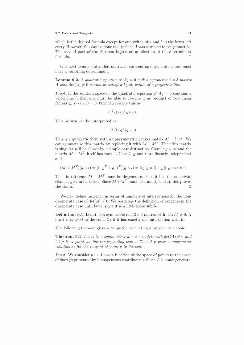
9.2 Polars and Tangents 151
which is the desired formula except for one switch of a and b in the lower leftentry. However, this can be done easily, since A was assumed to be symmetric.The second part of the theorem is just an application of the discriminantformula. ⊓⊔
Our next lemma states that matrices representing degenerate conics musthave a vanishing determinant.
Lemma 9.2. A quadratic equation qTAq = 0 with a symmetric 3× 3 matrixA with det(A) 6= 0 cannot be satisfied by all points of a projective line.
Proof. If the solution space of the quadratic equation qTAq = 0 contains awhole line l, then one must be able to rewrite it as product of two linearfactors 〈p, l〉 · 〈p, g〉 = 0. One can rewrite this as
(qT l) · (gT q) = 0.
This in turn can be interpreted as
qT (l · gT )q = 0.
This is a quadratic form with a nonsymmetric rank-1 matrix M = l · gT . Wecan symmetrize this matrix by replacing it with M +MT . That this matrixis singular will be shown by a simple case distinction. Case 1: g = λl and thematrix M +MT itself has rank 1. Case 2: g and l are linearly independentand
(M +MT )(g × l) = (l · gT + g · lT )(g × l) = l〈g, g × l〉 + g〈l, g × l〉 = 0.
Thus in this case M + MT must be degenerate, since it has the nontrivialelement g× l in its kernel. Since M+MT must be a multiple of A, this provesthe claim. ⊓⊔
We now define tangency in terms of numbers of intersections for the non-degenerate case of det(A) 6= 0. We postpone the definition of tangents in thedegenerate case until later, since it is a little more subtle.
Definition 9.1. Let A be a symmetric real 3× 3 matrix with det(A) 6= 0. Aline l is tangent to the conic CA if it has exactly one intersection with it.
The following theorem gives a recipe for calculating a tangent to a conic.
Theorem 9.1. Let A be a symmetric real 3 × 3 matrix with det(A) 6= 0 andlet p be a point on the corresponding conic. Then A·p gives homogeneouscoordinates for the tangent at point p to the conic.
Proof. We consider p 7→ A·p as a function of the space of points to the spaceof lines (represented by homogeneous coordinates). Since A is nondegenerate,

152 9 Conics and Their Duals
p
∗A(p)
p
∗A(p)
p
∗A(p)
Fig. 9.2 Images under polarity.
this map is bijective. First we show that the point p and the line l := A·pcoincide. For this, simply observe, that
〈p, l〉 = 〈p,A·p〉 = pTAp = 0.
Now assume that there was a second point q that is on l as well as on the conicrepresented by A. If p and q represent different points, then λp+µq must havemore than one intersection with the conic. In this case we have the followingthree equations: pTAp = 0 (point p is on the conic), qTAq = 0 (point q ison the conic), qTAp = 0 (point q is on l). Forming a linear combination ofthe first and the last equations yields (λp + µq)TAp = 0 for arbitrary λ, µ.Combining the second and the last yields qTA(λp + µq) = 0, which (by thesymmetry of A) gives (λp+ µq)TAq = 0. Another combination shows that
(λp+ µq)TA(λp + µq) = 0.
This proves that all linear combinations of p and q must be on the conicas well. Thus either p and q both represent the same point (and all linearcombinations are also identical to this point) or the conic contains the entireline λp+ µq. The latter cannot happen by Lemma 9.2, since A was assumedto be nondegenerate. ⊓⊔
The last theorem gives a very simple recipe to calculate the homogeneouscoordinates of a tangent l to a point p on a conic pTAp = 0: simply calculatel = Ap! This function is also defined if p is not on the conic. The map p 7→ Apis called a polarity, and it has various interesting properties. Figure 9.2 showsthree drawings of a point and its polar line with respect to an ellipse.Observethat if the point is inside the ellipse, the corresponding polar lies entirelyoutside. If the point is outside the conic, then the polar intersects the conicin two points. In the limit situation when the point is on the ellipse. thepolar is the tangent at this point. We want to investigate the properties ofpolarities in some detail.
Definition 9.2. Let A be a symmetric 3 × 3 matrix with det(A) 6= 0. Themap
∗A : PR → LR,p 7→ Ap,
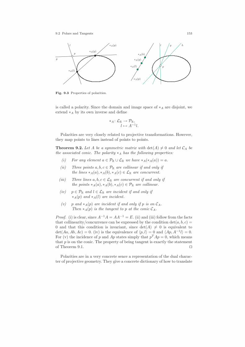
9.2 Polars and Tangents 153
p
∗A(p)l
g
∗A(l)
∗A(g)
p
∗A(p)
l g h
∗A(h)
∗A(g)
∗A(l)
Fig. 9.3 Properties of polarities.
is called a polarity. Since the domain and image space of ∗A are disjoint, weextend ∗A by its own inverse and define
∗A : LR → PR,l 7→ A−1l.
Polarities are very closely related to projective transformations. However,they map points to lines instead of points to points.
Theorem 9.2. Let A be a symmetric matrix with det(A) 6= 0 and let CA bethe associated conic. The polarity ∗A has the following properties:
(i) For any element a ∈ PR ∪ LR we have ∗A(∗A(a)) = a.
(ii) Three points a, b, c ∈ PR are collinear if and only ifthe lines ∗A(a), ∗A(b), ∗A(c) ∈ LR are concurrent.
(iii) Three lines a, b, c ∈ LR are concurrent if and only ifthe points ∗A(a), ∗A(b), ∗A(c) ∈ PR are collinear.
(iv) p ∈ PR and l ∈ LR are incident if and only if∗A(p) and ∗A(l) are incident.
(v) p and ∗A(p) are incident if and only if p is on CA.Then ∗A(p) is the tangent to p at the conic CA.
Proof. (i) is clear, since A−1A = AA−1 = E. (ii) and (iii) follow from the factsthat collinearity/concurrence can be expressed by the condition det(a, b, c) =0 and that this condition is invariant, since det(A) 6= 0 is equivalent todet(Aa,Ab,Ac) = 0. (iv) is the equivalence of 〈p, l〉 = 0 and 〈Ap,A−1l〉 = 0.For (v) the incidence of p and Ap states simply that pTAp = 0, which meansthat p is on the conic. The property of being tangent is exactly the statementof Theorem 9.1. ⊓⊔
Polarities are in a very concrete sence a representation of the dual charac-ter of projective geometry. They give a concrete dictionary of how to translate
154 9 Conics and Their Duals
statements of projective geometry into their dual statements. For every non-degenerate matrix A we obtain such a dictionary. For a point p we will calll = Ap the polar of p. Likewise, p is called the pole of l.
Algebraically, multiplication by A (or A−1) is the simplest way to carryout a polarity. However, property (v) of the previous theorem gives us anotherpossibility to construct a polar of a point p geometrically if we are able toconstruct a tangent to a conic. This is particularly easy if the point p is“outside” the conic (i.e., the polar of p intersects the conic in two points).Then we simply have to draw the two tangents of p to the conic. The pointswhere they touch the conic are the poles of these lines. If we join these twopoints, then we get the polar of the original point. Figure 9.3 on the left showsthis procedure. Algebraically, this construction is explained by the fact that ifp is a point and l and g are two lines through this point, then by Theorem 9.2(iv) the line ∗A(p) is incident to the points ∗A(l) and ∗A(g). Since l and gare the tangents, then by Theorem 9.2 (v) the polars are the correspondingtouching points.
We can also reverse the construction in different ways. If the line ∗A(p)is given, we can construct its pole p by intersection of the two tangents.Furthermore, if, for instance, in a computer geometry system a method forcalculating the polar and pole is available (multiplication by A or A−1) and ifit is possible to intersect a conic with a line, then this can be used to constructthe tangents through a point p to a conic. Simply intersect the polar of thepoint with the conic and join the intersections with point p.
Figure 9.3 on the right demonstrates that concurrent lines lead to collinearpoles. This property is also the key to constructing the polar of a point“inside” a conic. For this, one must simply draw two lines incident to thepoint, construct their poles, and join them.
So far, we have used the terms “inside” and “outside” of a conic in akind of informal way by always drawing images of an ellipse. In fact, one canformalize this concept by referring to the number of intersections of the conicwith the corresponding polar.
Definition 9.3. For a 3 × 3 symmetric matrix A with det(A) 6= 0, a pointa is inside the conic defined by pTAp = 0 if the conic does not intersect thepolar ∗A(a). If the polar intersects the conic in two (real) points, then thepoint a is outside the conic (compare Figure 9.4).
9.3 Dual Quadratic Forms
In Chapters 2 and 3 we learned that projective geometry is a dual theory.The roles of points and lines, meets and joins, etc. are interchangeable. Inthe previous section we saw how we can make the duality explicit using a
9.3 Dual Quadratic Forms 155
Fig. 9.4 Inside an ellipse and inside a hyperbola.
polarity with respect to a conic. There must also be a dual counterpart ofthe concept of a conic. This will be defined in this section. Again we will dealwith the nondegenerate case first.
A conic consists of all points p that satisfy an equation pTAp = 0. The setof all tangents to this conic can be described as Ap | pTAp = 0. We candescribe this set of homogeneous coordinates for lines directly as a quadraticform by the following observation:
pTAp = pTAA−1Ap = pTATA−1Ap = (Ap)TA−1(Ap).
The right side of the equation explains how the set of tangent lines of a conicmay be directly interpreted as the zero set of a quadratic form with matrixA−1. Thus we obtain that the set of all tangents is described by
C∗A := [l] ∈ LR | lTAl = 0.
In this expression we replaced the inverse A−1 by the adjoint A = A−1 ·det(A) of the matrix A, which is (for a symmetric matrix) defined by
a b db c ed e f
=
+
∣∣∣∣c ee f
∣∣∣∣ −∣∣∣∣b ed f
∣∣∣∣ +
∣∣∣∣b cd e
∣∣∣∣
−∣∣∣∣b de f
∣∣∣∣ +
∣∣∣∣a dd f
∣∣∣∣ −∣∣∣∣a bd e
∣∣∣∣
+
∣∣∣∣b dc e
∣∣∣∣ −∣∣∣∣a db e
∣∣∣∣ +
∣∣∣∣a bb c
∣∣∣∣
.
Compared to the inverse, the adjoint has the advantage that it is also com-putable if A is not invertible, since it avoids division by the determinant.
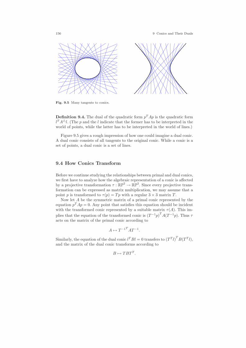
156 9 Conics and Their Duals
Fig. 9.5 Many tangents to conics.
Definition 9.4. The dual of the quadratic form pTAp is the quadratic formlTAl. (The p and the l indicate that the former has to be interpreted in theworld of points, while the latter has to be interpreted in the world of lines.)
Figure 9.5 gives a rough impression of how one could imagine a dual conic.A dual conic consists of all tangents to the original conic. While a conic is aset of points, a dual conic is a set of lines.
9.4 How Conics Transform
Before we continue studying the relationships between primal and dual conics,we first have to analyze how the algebraic representation of a conic is affectedby a projective transformation τ : RP
2 → RP2. Since every projective trans-
formation can be expressed as matrix multiplication, we may assume that apoint p is transformed to τ(p) = Tp with a regular 3 × 3 matrix T .
Now let A be the symmetric matrix of a primal conic represented by theequation pTAp = 0. Any point that satisfies this equation should be incidentwith the transformed conic represented by a suitable matrix τ(A). This im-
plies that the equation of the transformed conic is (T−1p)TA(T−1p). Thus τ
acts on the matrix of the primal conic according to
A 7→ T−1TAT−1.
Similarly, the equation of the dual conic lTBl = 0 transfers to (T T l)TB(T T l),
and the matrix of the dual conic transforms according to
B 7→ TBT T .

9.5 Degenerate Conics 157
To summarize: the primal matrix A is affected by left and right applicationof T−1, while the dual matrix is affected by left and right application of T .
Since A (resp. B) is a symmetric matrix, it is in particular possible tochoose a suitable transformation matrix T such that τ(A) (resp. τ(B)) isa diagonal matrix. For this, the matrix T may even be chosen to be or-thogonal (i.e., T TT = E. The diagonal entries are the eigenvalues of A(resp. B). By choosing T appropriately, the diagonal entries of A′ = τ(A) =diag(α1, α2, α3) may occur in any order.
We may even apply a further transformation by a diagonal matrix S by
computing A′′ = (S−1TA′S−1) if we set
Sii :=
√|αi| if αi 6= 0,
1 if αi = 0.
Then A′′ is a diagonal matrix whose entries are in +1,−1, 0. As a directconsequence we obtain the following:
Theorem 9.3. Every planar conic is projectively equivalent to a conic of theform σ1x
2 + σ2y2 + σ3z
2 = 0 with σi ∈ +1,−1, 0 for i ∈ 1, 2, 3.
9.5 Degenerate Conics
So far, we have considered mainly conics that came from invertible matricesA. In this case there is a one-to-one correspondence between conics and theirduals. We will now study the degenerate case. We first study the possiblecases in the world of primal conics which correspond to point sets. For aclassification we have again to study the different signatures of eigenvaluesthat we met in Section 9.1:
(+,+,−), (+,+,+), , (+,−, 0) (+,+, 0), (+, 0, 0).
Theorem 9.3 tells us that these are up to projective equivalence all cases thatcan arise. The first case corresponds to the class of real nondegenerate conics,which we have studied previously. The second case is still not degenerate, butthe corresponding conic consists entirely of complex points. The last threecases lead to situations with vanishing determinant and have to be considereddegenerate conics. Up to projective equivalence they may be represented bythe following quadratic forms:
x2 − y2 = 0, x2 + y2 = 0, x2 = 0.
The first case consists of all points (x, y, z) for which |x| = |y|. Thus up toscalar multiple the points are of the form (1, 1, α), (1,−1, α), or (0, 0, 1). Thefirst and second types of these vectors describe two lines each with one pointmissing, and the last vector describes the missing intersection point of the
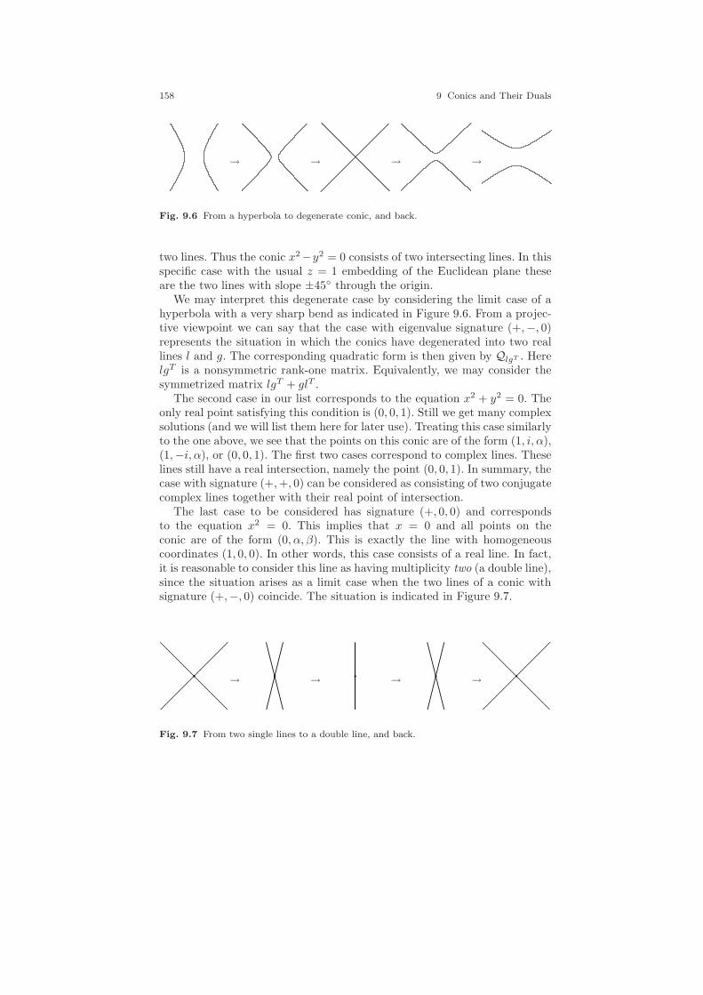
158 9 Conics and Their Duals
→ → → →
Fig. 9.6 From a hyperbola to degenerate conic, and back.
two lines. Thus the conic x2−y2 = 0 consists of two intersecting lines. In thisspecific case with the usual z = 1 embedding of the Euclidean plane theseare the two lines with slope ±45 through the origin.
We may interpret this degenerate case by considering the limit case of ahyperbola with a very sharp bend as indicated in Figure 9.6. From a projec-tive viewpoint we can say that the case with eigenvalue signature (+,−, 0)represents the situation in which the conics have degenerated into two reallines l and g. The corresponding quadratic form is then given by QlgT . HerelgT is a nonsymmetric rank-one matrix. Equivalently, we may consider thesymmetrized matrix lgT + glT .
The second case in our list corresponds to the equation x2 + y2 = 0. Theonly real point satisfying this condition is (0, 0, 1). Still we get many complexsolutions (and we will list them here for later use). Treating this case similarlyto the one above, we see that the points on this conic are of the form (1, i, α),(1,−i, α), or (0, 0, 1). The first two cases correspond to complex lines. Theselines still have a real intersection, namely the point (0, 0, 1). In summary, thecase with signature (+,+, 0) can be considered as consisting of two conjugatecomplex lines together with their real point of intersection.
The last case to be considered has signature (+, 0, 0) and correspondsto the equation x2 = 0. This implies that x = 0 and all points on theconic are of the form (0, α, β). This is exactly the line with homogeneouscoordinates (1, 0, 0). In other words, this case consists of a real line. In fact,it is reasonable to consider this line as having multiplicity two (a double line),since the situation arises as a limit case when the two lines of a conic withsignature (+,−, 0) coincide. The situation is indicated in Figure 9.7.
→ → → →
Fig. 9.7 From two single lines to a double line, and back.

9.6 Primal-Dual Pairs 159
→ → → →
Fig. 9.8 Tangents of a hyperbola.
9.6 Primal-Dual Pairs
What happens to tangents in the process of degeneration? Figure 9.8 showsthe situation as a kind of continuous process. A hyperbola is deformed suchthat the deformation passes through a situation in which the conic degener-ates into two real lines. The green lines in the pictures are tangents of theconic. First note that the tangents in the first picture all are “outside” theconic. When the conic becomes more degenerate, the tangents seem to accu-mulate in the center of the conic. In the degenerate situation, in which theconic consists of two lines, there are indeed many lines that have only oneintersection with the conic. They all pass through the singular point at whichthe two lines meet. After the degenerate situation, the hyperbola “switchesits branches” (left/right to top/bottom). Again the tangents are outside thehyperbola, but they now occupy a different region of the projective plane.The degenerate situation is a kind of intermediate stage, in which tangentsin both regions are possible. Our tangency concept of Definition 9.1 did notcover the degenerate case.
For the degenerate case of a conic consisting of two lines it is reasonableto consider all lines through the point of intersection as tangents, includingthe two lines of the conic themselves. Algebraically, this can be done quiteelegantly and explicitly, again by considering the adjoint of the correspondingmatrix.
Theorem 9.4. Let A be the symmetric 3 × 3 matrix corresponding to a de-generate conic CA consisting of two distinct lines g and h. Then the adjointA has the property that the lines passing through the intersection g × h areexactly those that satisfy lTAl = 0.
Proof. This theorem can be proved using the following formula, whichholds for arbitrary three-dimensional vectors g = (g1, g2, g3)
T and h =(h1, h2, h3)
T :(ghT + hgT ) = −(g × h)(g × h)T .
First observe that this formula can be proved simply by expanding the termson both sides of the expression and comparing the entries of the resulting3 × 3 matrices (this is left to the patient reader).

160 9 Conics and Their Duals
The left side of the equation is the adjoint of the symmetric matrix repre-senting a degenerate conic consisting of the lines g and h. If g and h representdistinct vectors, then g × h = p represents their point of intersection. Thusthe right side has the form −ppT . Now assume that a line l is incident to p.Then we have lT (−ppT )l = −(lTp)(pT l) = 0. Conversely, if a line satisfieslT (−ppT )l = 0, then we have (lT p)2 = 0. Thus l must be incident to p asclaimed in the theorem. ⊓⊔
The previous theorem together with the fact that for a nondegeneratematrix A the inverse is a multiple of the adjoint allows us to nicely combinethe description of polars for both cases. In both cases we can consider thedual as the following set of lines:
[l] ∈ LR | lTAl = 0.
In the case of a degenerate primal conic, the dual describes all points thatpass through the double point in which the two lines intersect.
So far, we have not treated the case in which the conic degenerates intojust one line (we may consider this a double line). Algebraically, this case ischaracterized by the property that the symmetric matrix A has rank 1 and isof the form A = ggT . It also corresponds to the eigenvalue signature (+, 0, 0).In this case the adjoint is simply the zero matrix and no longer carries anygeometric information. In fact, in this case it is reasonable (and as we willlater see, highly useful) to blow up the situation and assign information byattaching a suitable matrix to the dual.
Since the situation is a little subtle, we will approach it from several per-spectives. First of all, we consider a deformation of a conic that passes throughthe situation of a double line. For this, consider the drawing in Figure 9.9,which has been reproduced from the brilliant book by Felix Klein Vorlesun-gen uber nicht-euklidische Geometrie (1925) [68]. There we see a sequenceof pictures. The first shows an ellipse. This ellipse is squeezed horizontallyuntil it becomes extremely thin. We can model this situation by consider-ing the equation αx2 + y2 − αz2 = 0 with α moving from 0.5 to 0. In thelimit situation all tangents seem to pass through the two “endpoints” of thesqueezed ellipse. If we deform α further (from 0 to −0.5), the conic becomesa hyperbola. Again close to the limit case all tangents seem to pass throughthe two special points. In the limit case α = 0 the conic consists of just thedoubly covered x-axis. On this axis two points play a special role.
We can reinterpret this situation in terms of dual conics. What is thedual of a conic that consists of two distinct lines and a double point wherethey meet? Dualizing this description word by word, we see that the dual ofsuch a conic must consist of two distinct points and a double line that joinsthem. This is exactly what we see in Klein’s drawing. Algebraically, the dualconic may be represented by a single quadratic form lTBl = 0 with a rank-2symmetric matrix B. Its dual is described by the matrix B. The quadraticform pTAp = 0 describes exactly the double line through the two points.
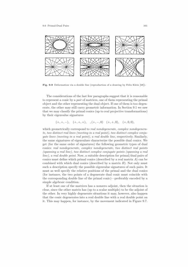
9.6 Primal-Dual Pairs 161
Fig. 9.9 Deformation via a double line (reproduction of a drawing by Felix Klein [68]).
The considerations of the last few paragraphs suggest that it is reasonableto represent a conic by a pair of matrices, one of them representing the primalobject and the other representing the dual object. If one of them is too degen-erate, the other may still carry geometric information. In Section 9.1 we sawthat we may classify the primal conics (up to real projective transformations)by their eigenvalue signatures
(+,+,−), (+,+,+), , (+,−, 0) (+,+, 0), (+, 0, 0),
which geometrically correspond to real nondegenerate, complex nondegenera-te, two distinct real lines (meeting in a real point), two distinct complex conju-gate lines (meeting in a real point), a real double line, respectively. Similarly,the same signatures of eigenvalues characterize the possible dual conics. Weget (for the same order of signatures) the following geometric types of dualconics: real nondegenerate, complex nondegenerate, two distinct real points(spanning a real line), two distinct complex conjugate points (spanning a realline), a real double point. Now, a suitable description for primal/dual pairs ofconics must define which primal conics (described by a real matrix A) can becombined with which dual conics (described by a matrix B). Not only mustsuch a description specify the possible eigenvalue signatures of such pairs. Itmust as well specify the relative positions of the primal and the dual conics(for instance, the two points of a degenerate dual conic must coincide withthe corresponding double line of the primal conic)—preferably encoded by asimple algebraic condition.
If at least one of the matrices has a nonzero adjoint, then the situation isclear, since the other matrix has (up to a scalar multiple) to be the adjoint ofthe other. In very highly degenerate situations it may, however, also happenthat the conic degenerates into a real double line with a real double point onit. This may happen, for instance, by the movement indicated in Figure 9.7.
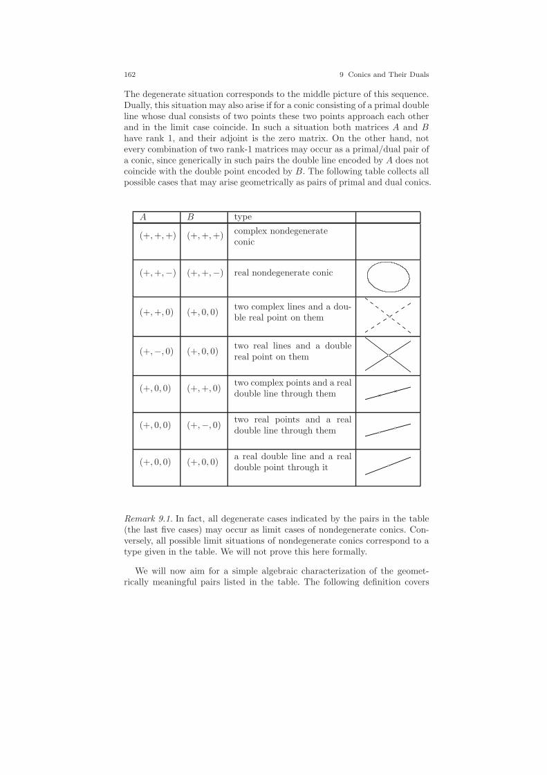
162 9 Conics and Their Duals
The degenerate situation corresponds to the middle picture of this sequence.Dually, this situation may also arise if for a conic consisting of a primal doubleline whose dual consists of two points these two points approach each otherand in the limit case coincide. In such a situation both matrices A and Bhave rank 1, and their adjoint is the zero matrix. On the other hand, notevery combination of two rank-1 matrices may occur as a primal/dual pair ofa conic, since generically in such pairs the double line encoded by A does notcoincide with the double point encoded by B. The following table collects allpossible cases that may arise geometrically as pairs of primal and dual conics.
A B type
(+,+,+) (+,+,+) complex nondegenerateconic
(+,+,−) (+,+,−) real nondegenerate conic
(+,+, 0) (+, 0, 0)two complex lines and a dou-ble real point on them
(+,−, 0) (+, 0, 0)two real lines and a doublereal point on them
(+, 0, 0) (+,+, 0)two complex points and a realdouble line through them
(+, 0, 0) (+,−, 0)two real points and a realdouble line through them
(+, 0, 0) (+, 0, 0)a real double line and a realdouble point through it
Remark 9.1. In fact, all degenerate cases indicated by the pairs in the table(the last five cases) may occur as limit cases of nondegenerate conics. Con-versely, all possible limit situations of nondegenerate conics correspond to atype given in the table. We will not prove this here formally.
We will now aim for a simple algebraic characterization of the geomet-rically meaningful pairs listed in the table. The following definition covers
9.6 Primal-Dual Pairs 163
also the above-mentioned highly degenerate case, in which the primal conicdegenerates into a double line and the dual conic degenerates into a doublepoint on this line.2 Compared to the formula in Theorem 9.4, it is an implicitrather than an explicit description.
Definition 9.5. A primal/dual pair of conics is given by a pair (A,B) of realsymmetric nonzero 3 × 3 matrices such that there exists a factor λ ∈ R withAB = λE (here E is the usual unit matrix).
By looking at this definition it is not clear at all that it exactly characterizesall possible cases. To see this, we have to do a little work. We break theargument into a sequence of small lemmas that cover all important properties.
Lemma 9.3. Being a primal/dual pair is a projectively invariant property.
Proof. Assume that (A,B) is a primal/dual pair. Thus there is a λ withAB = λE. Let τ be a projective transformation that transforms points byp 7→ Tp. This transformation maps the primal conic A according to A 7→T−1TAT−1. The matrix of the dual conic B is mapped according to B 7→TBT T . Applying τ to both objects in the expressionA·B, we get τ(A)·τ(B) =
T−1TAT−1TBT T = T−1TABT T = T−1TλET T = λE. ⊓⊔
Lemma 9.4. If det(A) 6= 0, then (A,B) is a primal/dual pair if and only ifB is a nonzero multiple of A−1.
Proof. Let det(A) 6= 0. Then for every nonzero 3 × 3 matrix B, the productAB is not the zero matrix. If (A,B) is a primal pair, then AB = λE withλ 6= 0. Hence B must be a multiple of A−1. Conversely, if B is a multiple ofA−1, then AB = λE. ⊓⊔
The previous lemma tells us that at least in the nondegenerate case, theprimal/dual pairs correspond to a pair of corresponding primal and dualconics. We now show that all other primal/dual pairs characterize exactlythose pairs of primal and dual conics that arise as limit cases of nondegeneratesituations. For the proper treatment of the nondegenerate cases we have tobe aware of the following two subtleties related to the question of real vs.complex coordinate entries and the fact that matrices and vectors differingby nonzero scalar multiples represent the same geometric object. We willalways assume that the matrices A and B have real entries. Still, it mayhappen that, for instance, a primal matrix A decomposes into two complex
conjugate lines, since llT
+ llT is real. We will also have to express real rank-1matrices A by expressions of the type A = llT . For this it may happen thatalthough A is real, l must be chosen to be complex. For instance, consider the
2 The concept of primal/dual pairs given in Definition 9.5 nicely generalizes to an appropri-ate concept even in higher dimensions. The reader is invited to figure out the correspondingtheory for three-dimensional or even higher-dimensional cases by analogy.

164 9 Conics and Their Duals
matrix A with the only nonzero element −1 in the upper left corner. For adecomposition A = llT we must choose either l = (i, 0, 0)T or l = (−i, 0, 0)T .Still, l represents a real point, since it is a scalar multiple of (1, 0, 0)T . Similarproblems may arise by decomposing a rank-two matrix with no negativeeigenvalues into a pair of real lines. Since matrices differing only by a nonzeroscalar multiple represent the same geometric object, we may easily bypassthis problem by the following general assumption, which we make from nowon whenever necessary:
Both matrices in a primal/dual pair (A,B) should have at least onepositive eigenvalue.
Since (A,B) is a primal/dual pair if and only if (−A,B) or (A,−B) is, thisassumption can be made without any loss of generality.
Lemma 9.5. If A describes a conic consisting of two distinct lines g and lthen (A,B) is a primal/dual pair if and only if B is a multiple of ppT , withp = g × l.
Proof. If A encodes a primal conic consisting of two distinct lines l and g,then up to a scalar multiple, the matrix A equals glT + lgT . This matrix hasrank 2, so the product with another matrix B can never be the unit matrixE. Thus for the primal/dual pair (A,B) we have AB = 0 (here 0 denotes thezero matrix). In this case B has rank 1, since every column of B must lie inthe (one-dimensional) kernel of A. Thus B is of the form ppT for a suitablep ∈ C3. We get
0 = AB =(glT + lgT
) (ppT
)= glTppT + lgT ppT =
(lT p)gpT +
(gT p
)lpT .
To derive the desired result we have to inspect the expression above. Sincel and g represent distinct lines, the matrices gpT and lpT do not differ justby a scalar multiple. They also are nonzero, since none of the vectors p, g, lis zero. Hence this expression can be the zero matrix only if lT p = gT p = 0.Thus p must be incident to both l and m. Hence it is a multiple of g × l.
If, conversely,B = ppT for a point p incident to l and g, then the expressionAB = (lT p)gpT + (gT p)lpT vanishes. ⊓⊔
Remark 9.2. As said before, we may assume that the point B has a singlepositive eigenvalue and thus p in the above lemma can be chosen to be com-pletely real. We also want to point out that the above argument also coversthe case that l and g have complex conjugate coordinates.
Obviously this lemma also has also a corresponding dual statement thatcovers the case of a matrix B describing a dual conic consisting of two distinct(perhaps complex conjugate) points. The dual statement of the lemma thenclaims that the matrix A describes a doubly covered real line l through thesetwo points.
9.6 Primal-Dual Pairs 165
We now analyze what the property of being a primal/dual pair tells us ifwe know that the matrix A describes a conic that consists of a single (doublycounted) line l. In this case, A is a rank-1 matrix of the form llT .
Lemma 9.6. Let A = llT describe a conic consisting of a real double line l.
(i) If (A,B) is a primal/dual pair, then B is of the form pqT + qpT , withlT p = 0 and lT q = 0 for suitable p, q ∈ C3. If further, B has at least onepositive eigenvalue, then p and q may be chosen either to be both real oras complex conjugates (in particular, p and q may coincide).
(ii) If a real symmetric matrix B is of the form pqT + qpT , with lT q = 0 andlT q = 0, then (A,B) is a primal/dual pair.
Proof. We start with statement (i). If A = llT for a line l, then A has rank 1.Let us assume that (A,B) is a primal/dual pair. Then AB can never be theunit matrix. Thus if (A,B) is a primal/dual pair, then we must have AB = 0.This implies that B has at most rank 2 but is still nonzero. Hence at leastone eigenvalue of B (say λ3) is zero and at least one eigenvalue (say λ1) isnonzero. Since B is by definition real and symmetric, it has an orthonormalbasis a1, a2, a3 of eigenvectors. Thus we have Bai = λiai and
aTi aj =
1 if i = j,0 if i 6= j.
(9.2)
We now consider the two points
p =
√λ1a1 +
√−λ2a2
2and q =
√λ1a1 −
√−λ2a2
2.
A simple calculation (expand and cancel) shows, that
X := pqT + qpT = λ1a1aT1 + λ2a2a
T2 .
Using (9.2), we get
Xa1 = λ1a1aT1 a1 + λ2a2a
T2 a1 = 1 · λ1a1 + 0 · λ2a1 = λ1a1,
Xa2 = λ1a1aT1 a2 + λ2a2a
T2 a2 = 0 · λ1a1 + 1 · λ2a1 = λ2a2,
Xa3 = λ1a1aT1 a3 + λ2a2a
T2 a3 = 0 · λ1a1 + 0 · λ2a1 = 0.
Thus X acts on a1, a2, a3 exactly as B does. Hence B = X = pqT + qpT .In order to see that lTp = 0 and lT q = 0, consider the expression 0 =
AB = llt(pqT + qpT ). If p and q represent two different points, then weare in the situation of the dual of Lemma 9.6, and lT p = lT q = 0 followsfrom this statement. Otherwise, p is a multiple of q and then B = αppT forsuitable nonzero α. Then 0 = AB = αllT ppT = (lT p)lpT . Since both l andp are nonzero, this can happen only if lT p = 0. If we furthermore assume

166 9 Conics and Their Duals
that without loss of generality λ1 is positive then we get the following threepossible geometric situations:
• If λ2 > 0 then p and q are complex conjugates,
• If λ2 < 0 then p and q are real and distinct,
• If λ2 = 0 then p = q is real.
To prove (ii) assume that B = pqT + qpT with lT p = lT q = 0. ExpandingAB and using lT p = lT q = 0 immediately proves AB = 0; hence (A,B) is aprimal/dual pair. ⊓⊔
Summarizing the results of the previous lemmas we yields the followingtheorem:
Theorem 9.5. If (A,B) is a primal/dual pair, then we have one of the ge-ometric situations listed in the table on page 162. Conversely, if A and Bdescribe any of the cases in this table, then (A,B) is a primal/dual pair.
Proof. The two nondegenerate cases are covered by Lemma 9.4. The fivedegenerate cases are covered by Lemma 9.5 and Lemma 9.6. ⊓⊔
Remark 9.3. The reader might wonder why we have devoted such a longsection to the proper treatment of the degenerate cases of conics and theadmissible primal/dual pairs of matrices. We will see that they become ofcrucial importance in Chapters 20 to 24, when we deal with different Cayley-Klein geometries. We will see that each of the cases in our table of primal/dualpairs leads to a different type of “metric geometry” with quite specific andvery interesting properties.
10
Conics and Perspectivity
Some people have a mental horizon of radius zero and call ittheir point of view.
Attributed variously to David Hilbert,Albert Einstein and Leonhard Euler
In the previous chapter we treated conics more or less as isolated objects. Wedefined points on them and lines tangent to them. Now we want to investigatevarious geometric and algebraic properties of conics. In particular, we will seehow we can treat conics on the level of bracket algebra.
10.1 Conic through Five Points
We begin by calculating a conic through a given set of points. For this,consider the quadratic equation that defines a conic:
a · x2 + b · y2 + c · z2 + d · xy + e · xz + f · yz = 0.
This equation has six parameters a, . . . , f.1 Multiplying all of them simultane-ously by the same nonzero scalar leads to the same conic. Thus the parametervector (a, . . . , f) behaves like a vector of homogeneous coordinates. Countingdegrees of freedom shows that in general it will take five points to uniquelydetermine a conic. To find the parameters for a conic through five pointspi = (xi, yi, zi), i = 1, . . . , 5, we simply have to solve the following linearsystem of equations:
1 Compared to Section 9.1 we have relabeled the parameters and put the factor 2 of themixed terms into the parameters.
167

168 10 Conics and Perspectivity
x21 y
21 z
21 x1y1 x1z1 y1z1
x22 y
22 z
22 x2y2 x2z2 y2z2
x23 y
23 z
23 x3y3 x3z3 y3z3
x24 y
24 z
24 x4y4 x4z4 y4z4
x25 y
25 z
25 x5y5 x5z5 y5z5
·
abcdef
=
00000
.
If this system has a full rank of 5, then there is a (up to scalar multiple)unique solution (a, . . . , f) that defines the corresponding conic. If more thanthree points are simultaneously collinear or if two points coincide, the rankof the system may be lower than 5. This corresponds to the situation thatthere is more than one conic passing through the given set of points. Thismethod of determining the parameter vector (a, . . . , f) is mathematicallyelegant. However it is computationally expensive. We first have to calculatethe squared parameters and then have to solve a 5 × 6 system of equations.
There is also another way to calculate such a conic more or less directly.This way will also give us additional structural insight into the geometry andunderlying algebra of a conic. In preparation we have to understand how tocalculate a degenerate conic that consists of two lines with homogeneous coor-dinates g and h. A degenerate conic must be represented by a quadratic formpTAp = 0 that vanishes if p is on either of the lines. The (nonsymmetrized)matrix of such a quadratic form is simply given by
A = ghT .
This can be easily seen, since the quadratic form
pTAp = pT (ghT )p = (pT g)(hT p) = 〈p, g〉〈p, h〉
vanishes if one of the two scalar products on right side vanishes. This in turncorresponds geometrically to the situation in which p is on g or on h.
Assume that the line g is spanned by two points labeled 1 and 2 and thatline h is spanned by two points labeled 3 and 4. Then we have g = 1× 2 andh = 3 × 4. The quadratic form becomes
〈p, 1 × 2〉〈p, 3 × 4〉 = 0.
We may as well express this term as the product of two determinants
[p, 1, 2][p, 3, 4] = 0.
Each factor describes a linear condition on the point p. The product calculatesthe conjunction between the two expressions.
Now assume that we want to describe the set of conics that pass through forpoints 1, . . . , 4 in general position. Clearly, there are many conics that satisfythis condition. The corresponding system of linear equations consists of fourequations in six variables. Hence the solution space will be two-dimensional.
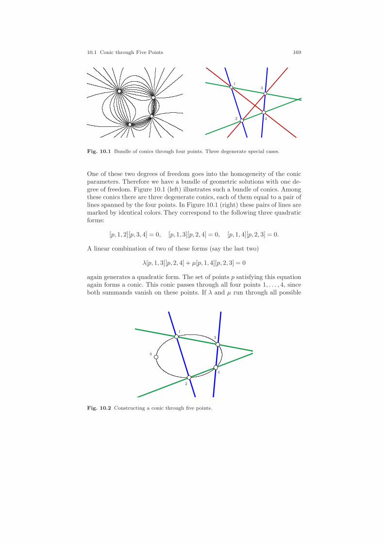
10.1 Conic through Five Points 169
13
2 4
Fig. 10.1 Bundle of conics through four points. Three degenerate special cases.
One of these two degrees of freedom goes into the homogeneity of the conicparameters. Therefore we have a bundle of geometric solutions with one de-gree of freedom. Figure 10.1 (left) illustrates such a bundle of conics. Amongthese conics there are three degenerate conics, each of them equal to a pair oflines spanned by the four points. In Figure 10.1 (right) these pairs of lines aremarked by identical colors. They correspond to the following three quadraticforms:
[p, 1, 2][p, 3, 4] = 0, [p, 1, 3][p, 2, 4] = 0, [p, 1, 4][p, 2, 3] = 0.
A linear combination of two of these forms (say the last two)
λ[p, 1, 3][p, 2, 4] + µ[p, 1, 4][p, 2, 3] = 0
again generates a quadratic form. The set of points p satisfying this equationagain forms a conic. This conic passes through all four points 1, . . . , 4, sinceboth summands vanish on these points. If λ and µ run through all possible
1
3
2
4
q
Fig. 10.2 Constructing a conic through five points.

170 10 Conics and Perspectivity
values we obtain all the conics in the bundle through the four points. Applyingthe technique of Plucker’s µ (compare Section 6.3), we can adjust these valuessuch that the resulting conic passes through another given point q. For thiswe simply have to choose
λ = [q, 1, 4][q, 2, 3]; µ = −[q, 1, 3][q, 2, 4].
The resulting conic equation can be written as
[q, 1, 4][q, 2, 3][p, 1, 3][p, 2, 4]− [q, 1, 3][q, 2, 4][p, 1, 4][p, 2, 3] = 0.
Observe that this equation is a multihomogeneous bracket polynomial that isquadratic in each of the six involved points. Figure 10.2 illustrates the situa-tion. We can also interpret it as a bracket condition encoding the (projectivelyinvariant) property that six points 1, . . . , 4, p, q are on a conic (compare Sec-tion 6.4 and Section 7.3). We will return to this interpretation in the nextsection.
But first we will give the procedure for calculating the symmetric matrixfor the conic through the five points 1, 2, 3, 4, q. We give it as a kind of simplecomputer program:
1: g1 := 1 × 3;
2: g2 := 2 × 4;
3: h1 := 1 × 4;
4: h2 := 2 × 3;
5: G := g1gT2 ;
6: H := h1hT2 ;
7: M := qTHqG− qTGqH ;
8: A := M +MT .
The matrix A assigned in the last line of the program contains the sym-metrized matrix.
10.2 Conics and Cross-Ratios
Let us return to the equation
[q, 1, 4][q, 2, 3][p, 1, 3][p, 2, 4]− [q, 1, 3][q, 2, 4][p, 1, 4][p, 2, 3] = 0, (∗)
which characterizes whether six points are on a conic. First observe that thisequation is highly symmetric. For each bracket in one term, its complement(the bracket consisting of the other three letters) is in the other term. The
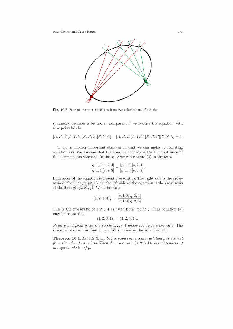
10.2 Conics and Cross-Ratios 171
1
2 34
q
p
Fig. 10.3 Four points on a conic seen from two other points of a conic.
symmetry becomes a bit more transparent if we rewrite the equation withnew point labels:
[A,B,C][A, Y, Z][X,B,Z][X,Y,C] − [A,B,Z][A, Y,C][X,B,C][X,Y, Z] = 0.
There is another important observation that we can make by rewritingequation (∗). We assume that the conic is nondegenerate and that none ofthe determinants vanishes. In this case we can rewrite (∗) in the form
[q, 1, 3][q, 2, 4]
[q, 1, 4][q, 2, 3]=
[p, 1, 3][p, 2, 4]
[p, 1, 4][p, 2, 3].
Both sides of the equation represent cross-ratios. The right side is the cross-ratio of the lines p1, p2, p3, p4; the left side of the equation is the cross-ratioof the lines q1, q2, q3, q4. We abbreviate
(1, 2; 3, 4)q :=[q, 1, 3][q, 2, 4]
[q, 1, 4][q, 2, 3].
This is the cross-ratio of 1, 2, 3, 4 as “seen from” point q. Thus equation (∗)may be restated as
(1, 2; 3, 4)q = (1, 2; 3, 4)p.
Point p and point q see the points 1, 2, 3, 4 under the same cross-ratio. Thesituation is shown in Figure 10.3. We summarize this in a theorem:
Theorem 10.1. Let 1, 2, 3, 4, p be five points on a conic such that p is distinctfrom the other four points. Then the cross-ratio (1, 2; 3, 4)p is independent ofthe special choice of p.
172 10 Conics and Perspectivity
We will later on see that this theorem is very closely related to the exteriorangle theorem for circles, which states that in a circle a fixed secant is seenfrom an arbitrary point on the circle under the same angle (modulo π).
The previous theorem enables us to speak of the cross-ratio of four pointson a fixed conic as long as no more than two of the points (1, 2, 3, 4) coincideand we can speak of a cross-ratio at all. For this we simply choose an arbi-trary point p that does not coincide with 1, 2, 3, 4 and take the cross-ratio(1, 2; 3, 4)p.
The theorem is useful under many aspects. In particular, it is useful toparameterize classes of objects. We will investigate two of these applications.First assume that the points 1, 2, 3, 4 are fixed. The previous theorem statesthat for a fixed conic C, the value of (1, 2; 3, 4)p is independent of the choiceof p. Thus it can be considered as a characteristic number that singles outthe specific conic C from all other conics through the four points. Thus wecan take this number as a kind of coordinate for the conic within the one-dimensional bundle of conics through 1, 2, 3, 4. In fact, if we do so the threespecial degenerate conics in this bundle (compare Figure 10.1) correspond tothe values 0, 1, and ∞.
In the second application we fix the conic itself as well as the positionof the points 1, 2, 3. The point p may be an arbitrary point on the conicwhose exact position is not relevant for the calculations as long as it doesnot coincide with the other points. If point 4 takes all possible positions onthe conic, then the value of (1, 2; 3, 4)p takes all possible values of R ∪ ∞,since the line p, 4 takes all possible positions through p. Thus we can use thecross-ratio (1, 2; 3, 4)p to characterize the position of 4 with respect to 1, 2, 3on the conic. The three special values 0, 1, and ∞ are assumed when 4 isidentical to 1, 3, 2, respectively. In this setup we may consider the conic itselfas a model of the real projective line. The three points 1, 2, 3 above play therole of a projective basis on this line with respect to which we measure thecross-ratio. In this model it is obvious that the topological structure of thereal projective line is a circle.
10.3 Perspective Generation of Conics
The considerations of the last section can be reversed in order to create conicsby perspective bundles of lines. For this we consider the points p and q ascenters of two bundles of lines that are projectively related to each other.Forming the intersections of corresponding lines from each bundle creates alocus of points that all have to lie on a single conic.
To formalize this fact (in particular to deal with the special cases) we haveto refine our notion of projective transformations slightly.
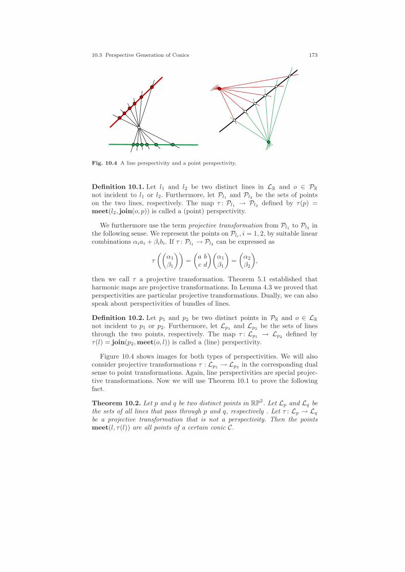
10.3 Perspective Generation of Conics 173
Fig. 10.4 A line perspectivity and a point perspectivity.
Definition 10.1. Let l1 and l2 be two distinct lines in LR and o ∈ PR
not incident to l1 or l2. Furthermore, let Pl1 and Pl2 be the sets of pointson the two lines, respectively. The map τ : Pl1 → Pl2 defined by τ(p) =meet(l2, join(o, p)) is called a (point) perspectivity.
We furthermore use the term projective transformation from Pl1 to Pl2 inthe following sense. We represent the points on Pli , i = 1, 2, by suitable linearcombinations αiai + βibi. If τ : Pl1 → Pl2 can be expressed as
τ
((α1
β1
))=
(a bc d
)(α1
β1
)=
(α2
β2
),
then we call τ a projective transformation. Theorem 5.1 established thatharmonic maps are projective transformations. In Lemma 4.3 we proved thatperspectivities are particular projective transformations. Dually, we can alsospeak about perspectivities of bundles of lines.
Definition 10.2. Let p1 and p2 be two distinct points in PR and o ∈ LR
not incident to p1 or p2. Furthermore, let Lp1 and Lp2 be the sets of linesthrough the two points, respectively. The map τ : Lp1 → Lp2 defined byτ(l) = join(p2,meet(o, l)) is called a (line) perspectivity.
Figure 10.4 shows images for both types of perspectivities. We will alsoconsider projective transformations τ : Lp1 → Lp2 in the corresponding dualsense to point transformations. Again, line perspectivities are special projec-tive transformations. Now we will use Theorem 10.1 to prove the followingfact.
Theorem 10.2. Let p and q be two distinct points in RP2. Let Lp and Lq be
the sets of all lines that pass through p and q, respectively . Let τ : Lp → Lqbe a projective transformation that is not a perspectivity. Then the pointsmeet(l, τ(l)) are all points of a certain conic C.
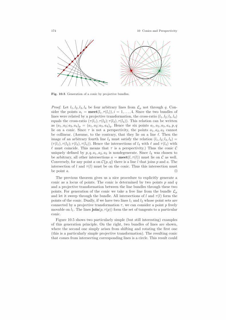
174 10 Conics and Perspectivity
Fig. 10.5 Generation of a conic by projective bundles.
Proof. Let l1, l2, l3, l4 be four arbitrary lines from Lp not through q. Con-sider the points ai = meet(li, τ(li)), i = 1, . . . , 4. Since the two bundles oflines were related by a projective transformation, the cross-ratio (l1, l2; l3, l4)equals the cross-ratio (τ(l1), τ(l2); τ(l3), τ(l4)). This relation can be writtenas (a1, a2; a3, a4)p = (a1, a2; a3, a4)q. Hence the six points a1, a2, a3, a4, p, qlie on a conic. Since τ is not a perspectivity, the points a1, a2, a3 cannotbe collinear. (Assume, to the contrary, that they lie on a line ℓ. Then theimage of an arbitrary fourth line l4 must satisfy the relation (l1, l2; l3, l4) =(τ(l1), τ(l2); τ(l3), τ(l4)). Hence the intersections of l4 with ℓ and τ(l4) withℓ must coincide. This means that τ is a perspectivity.) Thus the conic Cuniquely defined by p, q, a1, a2, a3 is nondegenerate. Since l4 was chosen tobe arbitrary, all other intersections a = meet(l, τ(l)) must lie on C as well.Conversely, for any point a on Cp, q there is a line l that joins p and a. Theintersection of l and τ(l) must be on the conic. Thus this intersection mustbe point a. ⊓⊔
The previous theorem gives us a nice procedure to explicitly generate aconic as a locus of points. The conic is determined by two points p and qand a projective transformation between the line bundles through these twopoints. For generation of the conic we take a free line from the bundle Lpand let it sweep through the bundle. All intersections of l and τ(l) form thepoints of the conic. Dually, if we have two lines l1 and l2 whose point sets areconnected by a projective transformation τ , we can consider a point p freelymovable on l1. The lines join(p, τ(p)) form the set of tangents to a particularconic.
Figure 10.5 shows two particularly simple (but still interesting) examplesof this generation principle. On the right, two bundles of lines are shown,where the second one simply arises from shifting and rotating the first one(this is a particularly simple projective transformation). The resulting conicthat comes from intersecting corresponding lines is a circle. This result could
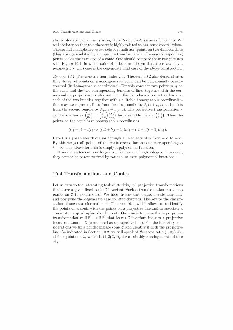
10.4 Transformations and Conics 175
also be derived elementarily using the exterior angle theorem for circles. Wewill see later on that this theorem is highly related to our conic constructions.The second example shows two sets of equidistant points on two different lines(they are again related by a projective transformation). Joining correspondingpoints yields the envelope of a conic. One should compare these two pictureswith Figure 10.4, in which pairs of objects are shown that are related by aperspectivity. This case is the degenerate limit case of the above construction.
Remark 10.1. The construction underlying Theorem 10.2 also demonstratesthat the set of points on a nondegenerate conic can be polynomially param-eterized (in homogeneous coordinates). For this consider two points p, q onthe conic and the two corresponding bundles of lines together with the cor-responding projective transformation τ . We introduce a projective basis oneach of the two bundles together with a suitable homogeneous coordinatiza-tion (say we represent lines from the first bundle by λpl1 + µpl2 and pointsfrom the second bundle by λqm1 + µqm2). The projective transformation τ
can be written as(λq
µq
)=(a bc d
)(λp
µp
)for a suitable matrix
(a bc d
). Thus the
points on the conic have homogeneous coordinates
(tl1 + (1 − t)l2) × ((at+ b(t− 1))m1 + (ct+ d(t− 1))m2).
Here t is a parameter that runs through all elements of R from −∞ to +∞.By this we get all points of the conic except for the one corresponding tot = ∞. The above formula is simply a polynomial function.
A similar statement is no longer true for curves of higher degree. In general,they cannot be parameterized by rational or even polynomial functions.
10.4 Transformations and Conics
Let us turn to the interesting task of studying all projective transformationsthat leave a given fixed conic C invariant. Such a transformation must mappoints on C to points on C. We here discuss the nondegenerate case onlyand postpone the degenerate case to later chapters. The key to the classifi-cation of such transformations is Theorem 10.1, which allows us to identifythe points on a conic with the points on a projective line and to associate across-ratio to quadruples of such points. Our aim is to prove that a projectivetransformation τ : RP
2 → RP2 that leaves C invariant induces a projective
transformation on C (considered as a projective line). For the following con-siderations we fix a nondegenerate conic C and identify it with the projectiveline. As indicated in Section 10.2, we will speak of the cross-ratio (1, 2; 3, 4)Cof four points on C, which is (1, 2; 3, 4)p for a suitably nondegenerate choiceof p.
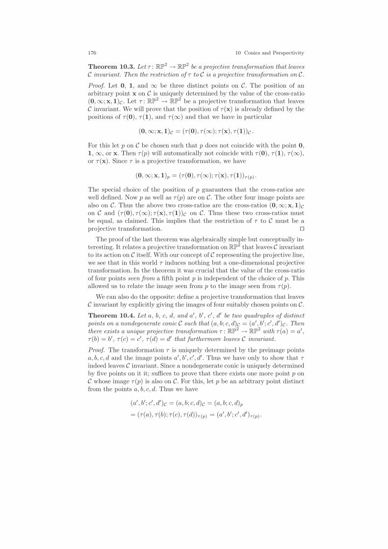
176 10 Conics and Perspectivity
Theorem 10.3. Let τ : RP2 → RP
2 be a projective transformation that leavesC invariant. Then the restriction of τ to C is a projective transformation on C.Proof. Let 0, 1, and ∞ be three distinct points on C. The position of anarbitrary point x on C is uniquely determined by the value of the cross-ratio(0,∞;x,1)C . Let τ : RP
2 → RP2 be a projective transformation that leaves
C invariant. We will prove that the position of τ(x) is already defined by thepositions of τ(0), τ(1), and τ(∞) and that we have in particular
(0,∞;x,1)C = (τ(0), τ(∞); τ(x), τ(1))C .
For this let p on C be chosen such that p does not coincide with the point 0,1, ∞, or x. Then τ(p) will automatically not coincide with τ(0), τ(1), τ(∞),or τ(x). Since τ is a projective transformation, we have
(0,∞;x,1)p = (τ(0), τ(∞); τ(x), τ(1))τ(p) .
The special choice of the position of p guarantees that the cross-ratios arewell defined. Now p as well as τ(p) are on C. The other four image points arealso on C. Thus the above two cross-ratios are the cross-ratios (0,∞;x,1)Con C and (τ(0), τ(∞); τ(x), τ(1))C on C. Thus these two cross-ratios mustbe equal, as claimed. This implies that the restriction of τ to C must be aprojective transformation. ⊓⊔
The proof of the last theorem was algebraically simple but conceptually in-teresting. It relates a projective transformation on RP
2 that leaves C invariantto its action on C itself. With our concept of C representing the projective line,we see that in this world τ induces nothing but a one-dimensional projectivetransformation. In the theorem it was crucial that the value of the cross-ratioof four points seen from a fifth point p is independent of the choice of p. Thisallowed us to relate the image seen from p to the image seen from τ(p).
We can also do the opposite: define a projective transformation that leavesC invariant by explicitly giving the images of four suitably chosen points on C.
Theorem 10.4. Let a, b, c, d, and a′, b′, c′, d′ be two quadruples of distinctpoints on a nondegenerate conic C such that (a, b; c, d)C = (a′, b′; c′, d′)C. Thenthere exists a unique projective transformation τ : RP
2 → RP2 with τ(a) = a′,
τ(b) = b′, τ(c) = c′, τ(d) = d′ that furthermore leaves C invariant.
Proof. The transformation τ is uniquely determined by the preimage pointsa, b, c, d and the image points a′, b′, c′, d′. Thus we have only to show that τindeed leaves C invariant. Since a nondegenerate conic is uniquely determinedby five points on it it; suffices to prove that there exists one more point p onC whose image τ(p) is also on C. For this, let p be an arbitrary point distinctfrom the points a, b, c, d. Thus we have
(a′, b′; c′, d′)C = (a, b; c, d)C = (a, b; c, d)p
= (τ(a), τ(b); τ(c), τ(d))τ(p) = (a′, b′; c′, d′)τ(p).
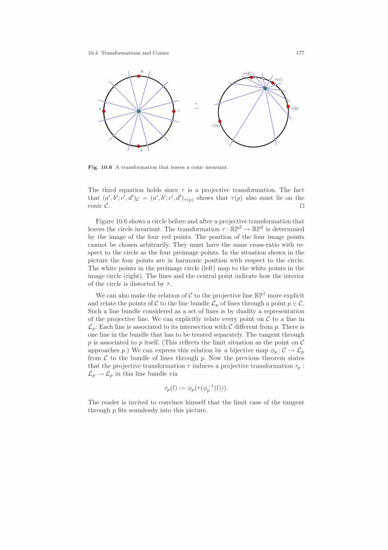
10.4 Transformations and Conics 177
a
b
c
d
τ→
τ(a)
τ(b)
τ(c)
τ(d)
Fig. 10.6 A transformation that leaves a conic invariant.
The third equation holds since τ is a projective transformation. The factthat (a′, b′; c′, d′)C = (a′, b′; c′, d′)τ(p) shows that τ(p) also must lie on theconic C. ⊓⊔
Figure 10.6 shows a circle before and after a projective transformation thatleaves the circle invariant. The transformation τ : RP
2 → RP2 is determined
by the image of the four red points. The position of the four image pointscannot be chosen arbitrarily. They must have the same cross-ratio with re-spect to the circle as the four preimage points. In the situation shown in thepicture the four points are in harmonic position with respect to the circle.The white points in the preimage circle (left) map to the white points in theimage circle (right). The lines and the central point indicate how the interiorof the circle is distorted by τ .
We can also make the relation of C to the projective line RP1 more explicit
and relate the points of C to the line bundle Lp of lines through a point p ∈ C.Such a line bundle considered as a set of lines is by duality a representationof the projective line. We can explicitly relate every point on C to a line inLp: Each line is associated to its intersection with C different from p. There isone line in the bundle that has to be treated separately. The tangent throughp is associated to p itself. (This reflects the limit situation as the point on Capproaches p.) We can express this relation by a bijective map φp : C → Lpfrom C to the bundle of lines through p. Now the previous theorem statesthat the projective transformation τ induces a projective transformation τp :Lp → Lp in this line bundle via
τp(l) := φp(τ(φ−1p (l))).
The reader is invited to convince himself that the limit case of the tangentthrough p fits seamlessly into this picture.

178 10 Conics and Perspectivity
a
b
c
d
ef g
h
i
j
k
p
φℓp(c)φp(d) φp(e) φp(f)φp(h) φp(g) φp(h) φp(i) φp(j)
φp(p)
ℓ
Fig. 10.7 Projection of a conic onto RP1.
Figure 10.7 illustrates the relation of the points on the conic to the linebundle. In addition to the line bundle, the picture also shows an additionalline ℓ that is intersected with every line of the bundle. So the points on theconic are also in one-to-one correspondence to the points on ℓ. The pictureexemplifies also how this relation of points on the conic to points on the lineis closely related to the classical stereographic projection, a relation that willbecome much more important later. It is remarkable how important it is thatthe point p is really placed on the conic. If it were inside the conic we wouldget a two-to-one relation between points on the conic and lines in the bundleLp. If the point p were outside the conic, not all lines of the bundle wouldintersect the conic at all. An intersection of a line and a conic corresponds tosolving a quadratic equation. The fact that we consider a bundle at a pointon the conic implies that we already know one of the two solutions of thisquadratic equation. Thus solving the quadratic equation in principle can bereduced to a linear problem by factoring out the already known solution.The linearity is the deeper reason why there is a one-to-one correspondencebetween C and the lines in the bundle.
Let us close this section with a remark on the group structure of theset of those transformations that leave C invariant. Theorem 10.3 can beinterpreted in the following way: The group of all projective transformationsthat leaves a nondegenerate conic invariant is isomorphic to the group ofprojective transformations of RP
1.
10.5 Hesse’s “Ubertragungsprinzip”
The last sections have made it clear that we can identify a nondegenerateconic with a projective line. In this section we will go one step further. Wewill demonstrate a way how one can interpret arbitrary lines and points
10.5 Hesse’s “Ubertragungsprinzip” 179
of RP2 as suitable objects on the projective line. This allows us to represent
statements in the two-dimensional world of RP2 by corresponding statements
of certain objects on the projective line. The idea of this translation goes backto an article by Otto Hesse from 1866 [57]. Hesse was mainly interested inquestions of invariant theory and studied several ways to linearize objects ofhigher degree. In his works around 1866 he was interested in generalizing theconcept of duality. Duality allows us to derive for every theorem of projectivegeometry a corresponding dual theorem just by applying a dictionary thattranslates “point” by “line,” “line” by “point,” “intersection” by “meet,” andso forth. In the same spirit Hesse formulated a principle that allowed himto derive a one-dimensional theorem from any two-dimensional theorem ofprojective geometry. He gave his principle the name “Ubertragungsprinzip.”A reasonable translation of this term could be “transfer principle.”
His work had far-reaching consequences. It was used by Klein in his famousErlanger Programm [65] to demonstrate the concept of equivalent geometries.It inspired further work and many interesting generalizations. Some of thesegeneralizations had an important impact on the classification of Lie algebrasand even on quantum theory. For a more elaborate treatment of this fascinat-ing topic see [56]. In this book we will use the transfer principle for derivingelegant bracket expressions for geometric configurations involving conics andlines.
In his original work Hesse related points in RP2 to solutions of one-
dimensional quadratic forms. We will take a slightly more visual approachthat allows us to represent the solutions of the quadratic forms directly asintersections of a conic with a line. As before, we consider a nondegenerateconic C as an image of a projective line. Now to a line l in RP
2 we associateits two points of intersection with C. A word of caution is necessary. First ofall, not all lines will have two intersections with C. This corresponds to thesituation that Hesse studied, solutions of arbitrary quadratic forms with realcoefficients. There may be two real solutions, two complex solutions (whichare conjugates), or one (double) real solution. The three cases correspondto the situations in which the line intersects in two, in no, or in one point,respectively. To state Hesse’s ideas in full generality we have also to deal withthe complex solutions. This will be our first careful investigation of complexsituations in projective geometry. Thus to treat Hesse’s transfer principleproperly, we must talk about CP
1 instead of RP1. However, the only objects
we have to consider are pairs of points (p, q) that are either both real orcomplex conjugates (p = q) or coincide (p = q). Figure 10.8 illustrates thethree cases. For the following considerations one may either consider thesecomplex elements (all algebraic considerations work straightforwardly) or as-sume (for convenience) that the conic is large enough such that all lines underconsideration intersect it in at least one point.
A line l that intersects the conic C in two (real or complex) points p1 andp2 is represented by the pair HC(l) := (p1, p2). If l is tangent to the conic atpoint p, we represent it by the pair HC(l) := (p, p). In all our considerations

180 10 Conics and Perspectivity
p1
p2
p
l1
H(l1) = (p1, p2)
l2
H(l1) = (p, p)
l3
H(l1) = (q, q)
Fig. 10.8 Hesse’s transfer principle for lines. Each line is associated to a pair of points.In case the line does not intersect the conic, the points are complex and conjugates.
related to Hesse’s transfer principle the order of the points within such a pairwill be irrelevant. Nevertheless, it is important to speak of pairs rather thansets to cover also the situation of a double point (p, p).
If lines are represented by pairs of points, what is the corresponding rep-resentation of a point of RP
2? In Hesse’s transfer principle points wouldbe represented by projective transformations on the projective line that arefurthermore involutions (i.e., τ2 = Id). Such a transformation is derived inthe following way. For a point p not on C we take two arbitrary distinctlines l and m through p that intersect C and consider the pairs of pointsHC(l) = (a1, a2) and HC(m) = (b1, b2). These four points are distinct, andsince they lie on a nondegenerate conic, no three of them are collinear. Thusthere is a unique projective transformation τ : RP
2 → RP2 that simultane-
ously interchanges a1 with a2 and b1 with b2. In particular, this transforma-tion leaves l, m, and p invariant. Furthermore, we have (by Theorem 4.2)(a1, a2; b1, b2)C = (a2, a1; b2, b1)C . This in turn implies by Theorem 10.3 thatτ leaves the conic C invariant. Such a projective transformation induces byTheorem 10.2 a corresponding transformation τp on C considered as RP
1.This is the object to which p is translated. The crucial fact in the definitionof τp is that it depends only on the choice of p but is independent of theparticular choice of l and m. We will not follow this line of thought here.
The reason for this is that we want to bypass a certain technical problemrelated to expressing a point p by a projective transformation τp. If the pointp is on the conic C, then the above construction does not lead to a properprojective transformation, since a1 and b1 (or b2) become identical. Insteadof introducing a concrete object that represents a point, we will characterizeconcurrence of lines k, l, m directly by a relation between the corresponding

10.5 Hesse’s “Ubertragungsprinzip” 181
point pairs HC(k), HC(l),and HC(m). This characterization also covers thedegenerate cases in which the coincident point lies on C.
Theorem 10.5. Let C be a conic and let k, l, m be lines in RP2. To exclude
the complex case we assume that they intersect or touch the conic. If k, l, mare concurrent, then (HC(k);HC(l);HC(m)) form a quadrilateral set.
We will prove this theorem by restriction to a remarkable special case bya suitable projective transformation. This special case was communicated byYuri Matiyasevich (private communication), who discovered this remarkableconfiguration as a high-school student. Matiyasevich’s configuration is a kindof geometric gadget for performing multiplications. He used this gadget togive a geometric construction for the prime numbers. We formulate it in thereal Euclidean plane:
Lemma 10.1. Let x and y be two real numbers. The join of the points(−x, x2) and (y, y2) crosses the y-axis at the point (0, x · y).
Proof. We can prove this by direct calculation when we show that the threepoints are collinear.
det
−x y 0x2 y2 xy1 1 1
= −x · y2 + y · xy − (−x) · xy − y · x2 = 0.
⊓⊔Figure 10.9 gives an impression of how the parabola-multiplication device
works. For our purposes we must also cover the degenerate case y = −x.Then the join becomes a tangent and we obtain the following:
Lemma 10.2. Let x be a real number. Then the tangent at (−x, x2) to theparabola y = x2 crosses the y-axis at the point (0,−x2).
Proof. This can also easily be checked by direct calculation. The tangent hasslope −2x; hence the tangent has equation f(t) = a − 2xt. Resolving for agives x2 = a− 2x(−x). Thus a must be −x2. ⊓⊔
Now, what has Matiyasevich’s gadget to do with Hesse’s transfer principle?The parabola plays the role of the conic. The points on the conic are verticallyprojected onto the x-axis. Thus the x-axis is the representation of RP
1 thatis isomorphic to the points on the conic (the unique infinite point of theparabola corresponds to the point at infinity of the x-axis). The line shownin Figure 10.9 intersects the conic in two points (the green and the blue ones).They are associated to their x-value by the projection. Thus the green andblue points on the x-axis correspond to the Hesse pair that represents theline. Now we are ready to prove Theorem 10.5 (which is essentially Hesse’stransfer principle) as a simple application of Matiyasevich’s construction.

182 10 Conics and Perspectivity
1
10
9
8
7
6
5
3
2
1
5 4 3 2 0 654321
4
11
Fig. 10.9 Multiplication of two real numbers using a parabola.
Proof of Theorem 10.5: Since three tangents of a conic C never intersect inone point, at least one of the lines must meet the conic in two points. Aftera suitable projective transformation we may assume that the conic p is theparabola y = x2 (in Euclidean coordinates) and that one of the lines (sayk) is the y-axis. We identify the x-axis together with its point at infinity∞ with the RP
1 associated to the conic. The corresponding mapping goesvia vertical projection. Thus k is mapped to HC(k) = (0,∞). Now assumethat the other two lines l and m intersect the y-axis at the same point asrequired by the theorem. Let the corresponding point pairs on the x-axis beHC(l) = (lx, ly) and HC(m) = (mx,my). Since the two lines in the theoremintersect the y-axis in the same point, we can consider them as two instancesof Matiyasevich’s construction, and we get
(−lx) · (ly) = (−mx) · (my).
This expression can be used to prove the corresponding quadset relation. Forthis we introduce homogeneous coordinates
(lx1
),
(ly1
),
(mx
1
),
(my
1
),
(01
),
(10
)
and calculate the characteristic quadset equation of Section 8.2. For the sixpoints (lx, ly;mx,my; 0,∞) being a quadset we must show that
[lx,∞][mx, ly][0,my] = [lx,my][mx,∞][0, ly].
This expands to
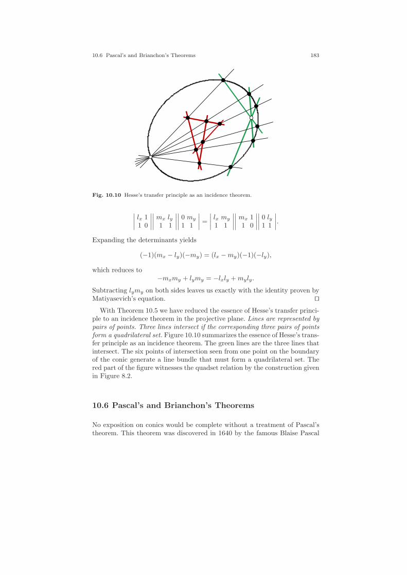
10.6 Pascal’s and Brianchon’s Theorems 183
Fig. 10.10 Hesse’s transfer principle as an incidence theorem.
∣∣∣∣lx 11 0
∣∣∣∣∣∣∣∣mx ly1 1
∣∣∣∣∣∣∣∣0 my
1 1
∣∣∣∣ =
∣∣∣∣lx my
1 1
∣∣∣∣∣∣∣∣mx 11 0
∣∣∣∣∣∣∣∣0 ly1 1
∣∣∣∣.
Expanding the determinants yields
(−1)(mx − ly)(−my) = (lx −my)(−1)(−ly),
which reduces to−mxmy + lymy = −lxly +myly.
Subtracting lymy on both sides leaves us exactly with the identity proven byMatiyasevich’s equation. ⊓⊔
With Theorem 10.5 we have reduced the essence of Hesse’s transfer princi-ple to an incidence theorem in the projective plane. Lines are represented bypairs of points. Three lines intersect if the corresponding three pairs of pointsform a quadrilateral set. Figure 10.10 summarizes the essence of Hesse’s trans-fer principle as an incidence theorem. The green lines are the three lines thatintersect. The six points of intersection seen from one point on the boundaryof the conic generate a line bundle that must form a quadrilateral set. Thered part of the figure witnesses the quadset relation by the construction givenin Figure 8.2.
10.6 Pascal’s and Brianchon’s Theorems
No exposition on conics would be complete without a treatment of Pascal’stheorem. This theorem was discovered in 1640 by the famous Blaise Pascal
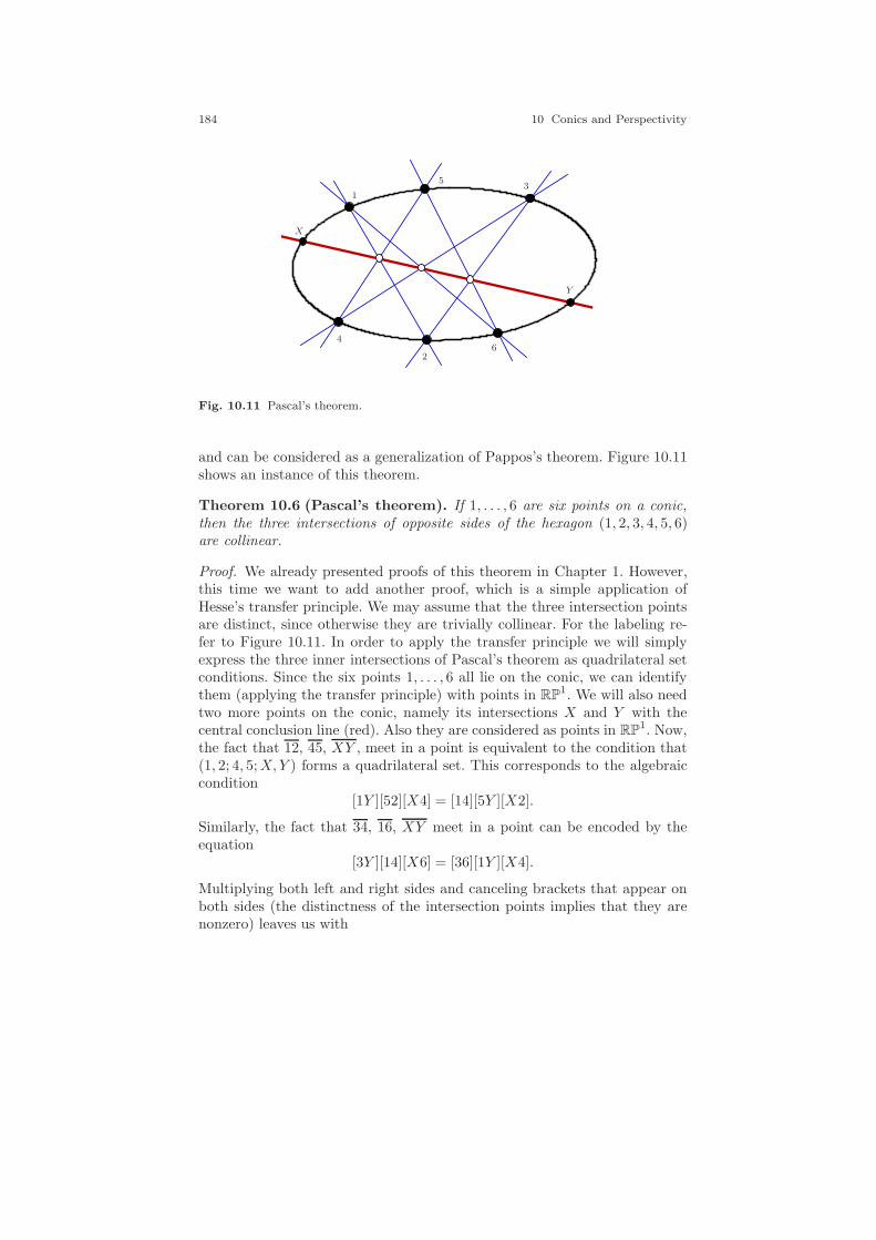
184 10 Conics and Perspectivity
1
53
4
26
X
Y
Fig. 10.11 Pascal’s theorem.
and can be considered as a generalization of Pappos’s theorem. Figure 10.11shows an instance of this theorem.
Theorem 10.6 (Pascal’s theorem). If 1, . . . , 6 are six points on a conic,then the three intersections of opposite sides of the hexagon (1, 2, 3, 4, 5, 6)are collinear.
Proof. We already presented proofs of this theorem in Chapter 1. However,this time we want to add another proof, which is a simple application ofHesse’s transfer principle. We may assume that the three intersection pointsare distinct, since otherwise they are trivially collinear. For the labeling re-fer to Figure 10.11. In order to apply the transfer principle we will simplyexpress the three inner intersections of Pascal’s theorem as quadrilateral setconditions. Since the six points 1, . . . , 6 all lie on the conic, we can identifythem (applying the transfer principle) with points in RP
1. We will also needtwo more points on the conic, namely its intersections X and Y with thecentral conclusion line (red). Also they are considered as points in RP
1. Now,the fact that 12, 45, XY , meet in a point is equivalent to the condition that(1, 2; 4, 5;X,Y ) forms a quadrilateral set. This corresponds to the algebraiccondition
[1Y ][52][X4] = [14][5Y ][X2].
Similarly, the fact that 34, 16, XY meet in a point can be encoded by theequation
[3Y ][14][X6] = [36][1Y ][X4].
Multiplying both left and right sides and canceling brackets that appear onboth sides (the distinctness of the intersection points implies that they arenonzero) leaves us with
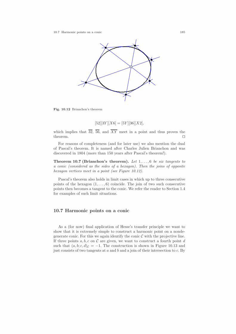
10.7 Harmonic points on a conic 185
Fig. 10.12 Brianchon’s theorem
[52][3Y ][X6] = [5Y ][36][X2],
which implies that 32, 56, and XY meet in a point and thus proves thetheorem. ⊓⊔
For reasons of completeness (and for later use) we also mention the dualof Pascal’s theorem. It is named after Charles Julien Brianchon and wasdiscovered in 1804 (more than 150 years after Pascal’s theorem!).
Theorem 10.7 (Brianchon’s theorem). Let 1, . . . , 6 be six tangents toa conic (considered as the sides of a hexagon). Then the joins of oppositehexagon vertices meet in a point (see Figure 10.12).
Pascal’s theorem also holds in limit cases in which up to three consecutivepoints of the hexagon (1, . . . , 6) coincide. The join of two such consecutivepoints then becomes a tangent to the conic. We refer the reader to Section 1.4for examples of such limit situations.
10.7 Harmonic points on a conic
As a (for now) final application of Hesse’s transfer principle we want toshow that it is extremely simple to construct a harmonic point on a nonde-generate conic. For this we again identify the conic C with the projective line.If three points a, b, c on C are given, we want to construct a fourth point dsuch that (a, b; c, d)C = −1. The construction is shown in Figure 10.13 andjust consists of two tangents at a and b and a join of their intersection to c. By
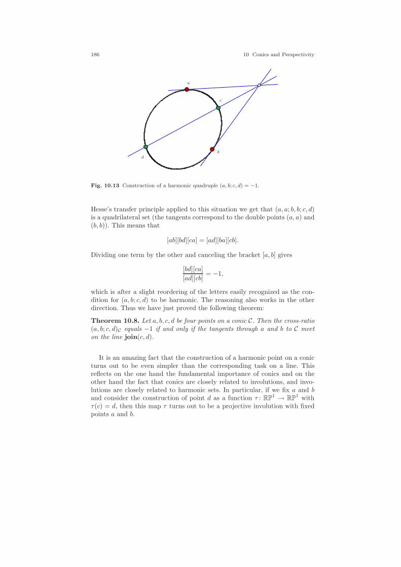
186 10 Conics and Perspectivity
a
b
c
d
Fig. 10.13 Construction of a harmonic quadruple (a, b; c, d) = −1.
Hesse’s transfer principle applied to this situation we get that (a, a; b, b; c, d)is a quadrilateral set (the tangents correspond to the double points (a, a) and(b, b)). This means that
[ab][bd][ca] = [ad][ba][cb].
Dividing one term by the other and canceling the bracket [a, b] gives
[bd][ca]
[ad][cb]= −1,
which is after a slight reordering of the letters easily recognized as the con-dition for (a, b; c, d) to be harmonic. The reasoning also works in the otherdirection. Thus we have just proved the following theorem:
Theorem 10.8. Let a, b, c, d be four points on a conic C. Then the cross-ratio(a, b; c, d)C equals −1 if and only if the tangents through a and b to C meeton the line join(c, d).
It is an amazing fact that the construction of a harmonic point on a conicturns out to be even simpler than the corresponding task on a line. Thisreflects on the one hand the fundamental importance of conics and on theother hand the fact that conics are closely related to involutions, and invo-lutions are closely related to harmonic sets. In particular, if we fix a and band consider the construction of point d as a function τ : RP
1 → RP1 with
τ(c) = d, then this map τ turns out to be a projective involution with fixedpoints a and b.
11
Calculating with Conics
We [Kaplansky and Halmos] share a love of linear algebra. Ithink it is our conviction that we’ll never understand infinite-dimensional operators until we have a decent mastery of finitematrices. And we share a philosophy about linear algebra: wethink basis-free, we write basis-free, but when the chips aredown we close the office door and compute with matrices likefury.
Irving Kaplanskyin Paul Halmos: Celebrating 50 Years of Mathematics
A major part of classical elementary geometry was concerned with thequestion of which constructions can be carried out with a straightedge andcompass. The decisive primitive operations here are connecting two points bya line, drawing a circle with a radius given by two other points, and markingintersections of objects as new points. In our projective framework we do nothave circles, but still can consider elementary constructions with the objectswe have studied so far (points, lines, and conics). Since we are interestedin particular in calculating with geometric objects, we in particular want toknow how we can compute the results of geometric primitive operations if theparameters of the involved objects are given. So far, we can roughly associatethe classical straightedge/compass operations with our projective operationsin the following way:
• connecting two points by a line corresponds to the join operation andcan be carried out by a cross product,
• intersecting two lines corresponds to the meet operation and is also carriedout by the cross product,
• constructing a circle from two points can be associated to our constructionof a conic by five points as described in Section 10.1.
187
188 11 Calculating with Conics
Furthermore, we had additional operations for
• constructing polars of points and lines with respect to a conic (this in-cluded the calculation of a tangent),
• transforming points/lines/conics by projective transformations,
• calculating the matrix of the dual of a given conic.
So far we do not have an algebraic equivalent of the classical operationsof intersecting a line and a circle and of intersecting two circles. This chapteris (among others) dedicated to this task. We will develop algebraic methodsfor intersecting conics with lines and conics with conics. Clearly, these op-erations can be carried out by solving corresponding systems of polynomialequations. However, we will try to make the calculations for these operationsas natural as possible in the framework of homogeneous coordinates and ma-trix representations for conics. This chapter is meant as a collection of recipesfor such kinds of primitive operations. Many of these recipes are used in theimplementation of the dynamic geometry program Cinderella [112].
11.1 Splitting a Degenerate Conic
Before we turn our attention to the problem of intersecting a conic with otherobjects we will study how it is possible to derive homogeneous coordinatesfor the two lines of a degenerate conic from the matrix of a conic. This willturn out to be a useful operation later on.
Assume that a conic CA is given by a symmetric matrix A such that asusual, CA = p | pTAp = 0. If the conic is degenerate and consists of twolines or of one double line, then A will not have full rank. Thus we candetermine a degenerate situation by testing det(A) = 0. If a conic consists oftwo distinct lines with homogeneous coordinates g and h, then its symmetric(rank-2) matrix A can be written as A = ghT +hgT (up to a scalar multiple).The matrices ghT and hgT would in principle generate the same conic, butthey are not symmetric. However, knowing one of these matrices (for instanceghT ) would be equivalent to knowing the homogeneous coordinates of the twolines, since the columns of this matrix are just scalar multiples of g and therows are just scalar multiples of h. Any nonzero column (resp. row) couldserve as homogeneous coordinates for g (resp. h). This can be seen easily byobserving that the disjunction of the conditions 〈p, h〉 = 0 and 〈p, g〉 = 0 canbe written as
0 = 〈p, g〉 · 〈p, h〉 = (pT g)(hT p) = pT (ghT )p.
So, splitting a degenerate conic into its two lines essentially corresponds tofinding a rank-1 matrix B that generates the same conic as A. The quadraticform is linear in the corresponding matrix (i.e., we have pT (A + B)p =
11.1 Splitting a Degenerate Conic 189
pTAp + pTBp). Furthermore, those matrices for which the quadratic formis identically zero are exactly the skew-symmetric matrices (those withAT = −A). All in all, for decomposing a symmetric degenerate matrix Ainto two lines we have to find a skew-symmetric matrix B such that A + Bhas rank 1. Thus in our case we have to find parameters λ, µ, and τ suchthat the following matrix sum has rank 1:
a b db c ed e f
+
0 τ −µ−τ 0 λµ −λ 0
.
The determinant of every 2 × 2 submatrix of a rank-1 matrix must vanish.Thus necessary conditions for the parameters are
∣∣∣∣a b+ τ
b− τ c
∣∣∣∣ = 0;
∣∣∣∣a d− µ
d+ µ f
∣∣∣∣ = 0;
∣∣∣∣c e+ λ
e− λ f
∣∣∣∣ = 0.
Resolving for λ, τ , and µ gives
τ2 = −∣∣∣∣a bb c
∣∣∣∣; µ2 = −∣∣∣∣a dd f
∣∣∣∣; λ2 = −∣∣∣∣c ee f
∣∣∣∣.
This determines the parameters λ, µ, and τ up to their sign. In principleone could test all eight possibilities to find a suitable choice that makes theentire matrix a rank-1 matrix. However, there is also a more direct way ofcalculating the values with their correct sign. For this we associate to theparameter vector p = (λ, µ, τ)T the skew-symmetric matrix
Mp :=
0 τ −µ−τ 0 λµ −λ 0
.
Left multiplication by the matrix Mp encodes performing a cross productwith the vector p. A simple calculation shows that for any three-dimensionalvector q we have
Mp · q = p× q.
Lemma 11.1. Let A be a rank-2 symmetric 3×3 matrix that defines a conicconsisting of two distinct lines. Let p be the point of intersection of theselines. Then for a suitable factor α the matrix A+ αMp has rank 1.
Proof. Let g and h be homogeneous coordinates for the two lines. We mayassume that these coordinates are scaled such that A has the form ghT +hgT .The intersection of these lines is g × h. We have for a suitable factor α theequation g × h = αp. If we consider the difference ghT − hgT , we obtain theskew-symmetric matrix
190 11 Calculating with Conics
ghT − hgT =
0 g1h2 − g2h1 g1h3 − g3h1
g2h1 − g1h2 0 g2h3 − g3h2
g3h1 − g1h3 g3h2 − g2h3 0
.
Comparison of coefficients shows that this matrix is nothing other thanMg×h. Thus we obtain
ghT − hgT = Mg×h = Mαp = αMp.
With this we obtain
A+ αMp = (ghT + hgT ) + (ghT − hgT ) = 2ghT .
Thus the result must have the desired rank-1 form, and the theorem isproven. ⊓⊔
In particular, if for specific coordinates g and h we have A = ghT + hgT
and p = g × h, we can choose the factor α = 1 and obtain
A−Mp = 2hgT .
If we instead add the matrices, we obtain A + Mp = 2ghT . The previouslemma allows us to calculate the corresponding rank-1 matrix if a symmetricmatrix of a degenerate conic is given. However, it has one big disadvantage:We know neither p nor α in advance. There are several circumstances (we willencounter them later) in which we, for instance, know p in advance. However,it is also possible to calculate p from the matrix A without too much effort.For this we have to use the formula
(ghT + hgT ) = −(g × h)(g × h)T ,
which we already used in Section 9.5. The matrix B = (g × h)(g × h)T isa rank-1 matrix ppT with p = g × h. Thus each row/column of this matrixis a scalar multiple of p. Furthermore, the diagonal entries of this matrixcorrespond to the squared coordinate values of g × h. Thus one can extractthe coordinates of g × h by searching for a nonzero diagonal entry of B, sayBi,i, and set p = Bi/
√Bi,i, where Bi denotes the ith column of B. With this
assignment we can calculate the matrix A+Mp, which gives either 2ghT or2hgT depending on the sign of the square root. Altogether, we can summarizethe procedure of splitting a matrix A that describes a conic consisting of twodistinct lines.:
1: B := A;
2: Let i be the index of a nonzero diagonal entry of B;
3: β =√Bi,i;
4: p = Bi/β, where Bi is the ith column of B;
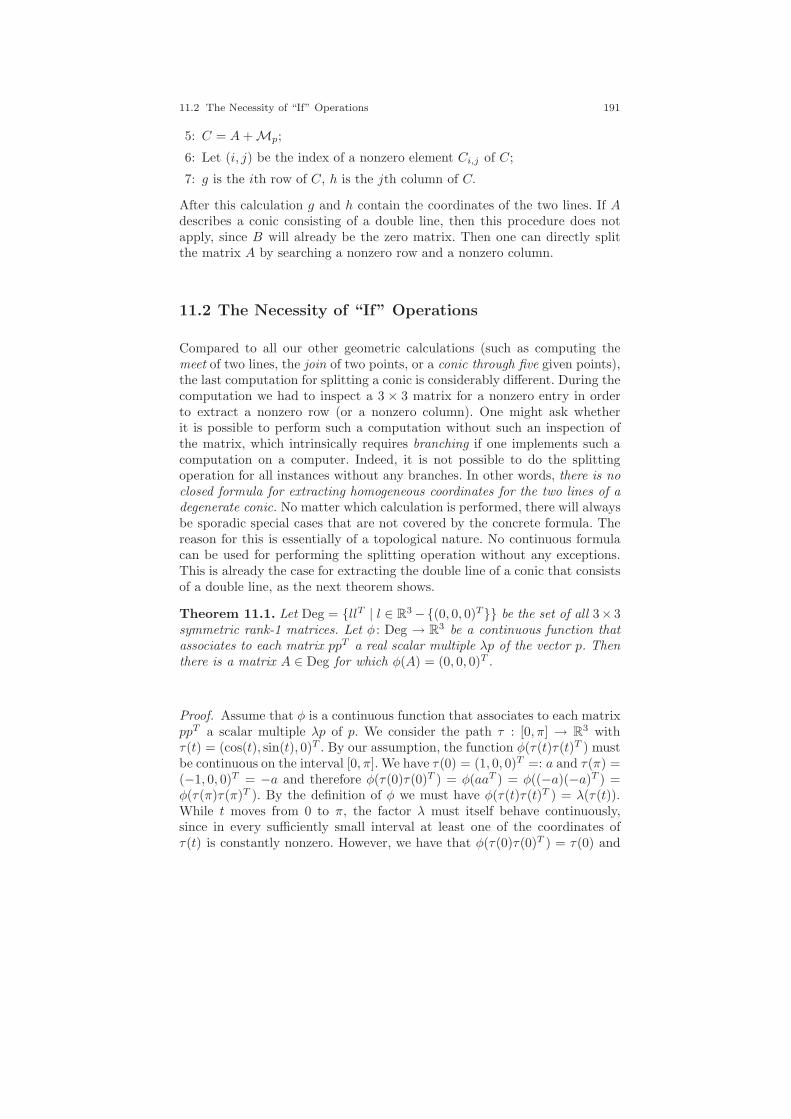
11.2 The Necessity of “If” Operations 191
5: C = A+ Mp;
6: Let (i, j) be the index of a nonzero element Ci,j of C;
7: g is the ith row of C, h is the jth column of C.
After this calculation g and h contain the coordinates of the two lines. If Adescribes a conic consisting of a double line, then this procedure does notapply, since B will already be the zero matrix. Then one can directly splitthe matrix A by searching a nonzero row and a nonzero column.
11.2 The Necessity of “If” Operations
Compared to all our other geometric calculations (such as computing themeet of two lines, the join of two points, or a conic through five given points),the last computation for splitting a conic is considerably different. During thecomputation we had to inspect a 3 × 3 matrix for a nonzero entry in orderto extract a nonzero row (or a nonzero column). One might ask whetherit is possible to perform such a computation without such an inspection ofthe matrix, which intrinsically requires branching if one implements such acomputation on a computer. Indeed, it is not possible to do the splittingoperation for all instances without any branches. In other words, there is noclosed formula for extracting homogeneous coordinates for the two lines of adegenerate conic. No matter which calculation is performed, there will alwaysbe sporadic special cases that are not covered by the concrete formula. Thereason for this is essentially of a topological nature. No continuous formulacan be used for performing the splitting operation without any exceptions.This is already the case for extracting the double line of a conic that consistsof a double line, as the next theorem shows.
Theorem 11.1. Let Deg = llT | l ∈ R3 −(0, 0, 0)T be the set of all 3× 3symmetric rank-1 matrices. Let φ : Deg → R3 be a continuous function thatassociates to each matrix ppT a real scalar multiple λp of the vector p. Thenthere is a matrix A ∈ Deg for which φ(A) = (0, 0, 0)T .
Proof. Assume that φ is a continuous function that associates to each matrixppT a scalar multiple λp of p. We consider the path τ : [0, π] → R3 withτ(t) = (cos(t), sin(t), 0)T . By our assumption, the function φ(τ(t)τ(t)T ) mustbe continuous on the interval [0, π]. We have τ(0) = (1, 0, 0)T =: a and τ(π) =(−1, 0, 0)T = −a and therefore φ(τ(0)τ(0)T ) = φ(aaT ) = φ((−a)(−a)T ) =φ(τ(π)τ(π)T ). By the definition of φ we must have φ(τ(t)τ(t)T ) = λ(τ(t)).While t moves from 0 to π, the factor λ must itself behave continuously,since in every sufficiently small interval at least one of the coordinates ofτ(t) is constantly nonzero. However, we have that φ(τ(0)τ(0)T ) = τ(0) and

192 11 Calculating with Conics
φ(τ(π)τ(π)T ) = φ(τ(0)) = −τ(π). Since λ was assumed to be real this impliesby the intermediate value theorem that for at least one parameter t0 ∈ [0, π]we must have λ = 0. ⊓⊔
The matrix llT that corresponds to the point p for which we have φ(llT ) =(0, 0, 0)T = 0 · p does not lead to a meaningful nondegenerate evaluation ofφ. The interpretation of this fact is a little subtle. It means that on thecoordinate level there is no continuous way of extracting the double lineof a conic CA from a symmetric rank-1 matrix A. On the other hand, theconsiderations of the last sections show that on the level of geometric objectsthere is a way to extract the coordinates of the line l from the matrix llT whichmust be necessarily continuous in the topology of our geometric objects.There is just no way of doing these computations without using branchingwithin the calculations. This was reflected by the fact that we explicitly hadto search for nonzero entries in our 3 × 3 matrices.
In fact, the effect treated in this section is just the beginning of a longstory that leads to the conclusion that elementary geometry and effects fromcomplex function theory (such as monodromy, multivalued functions) areintimately interwoven. We will return to these issues in the very final sectionof this book.
11.3 Intersecting a Conic and a Line
After all this preparatory work the final task of this chapter turns out to berelatively simple. We want to calculate the intersection of a conic given by asymmetric 3 × 3 matrix A and a line given by its homogeneous coordinatesl. Clearly the task is in essence nothing but solving a quadratic equation.However, we want to perform the operation that is as closely as possiblerelated to the coordinate representation. For this we will use the operationof splitting a matrix that represents a degenerate conic as introduced inSection 11.1 as a basic building block. Essentially, the square root needed tosolve a quadratic equation will be the one required for this operation.
Our aim will be to derive a closed formula for the degenerate conic thatconsists of the line l as double line and whose dual consists of the two pointsof intersection. Such a conic is given by a pair of matrices (A,B), where Ais a rank-1 symmetric matrix and describes the double line l and where B isa symmetric rank-2 matrix with B = A that describes the dual conic andwith this the position of the two points of intersection. Splitting the matrixB yields the two points of intersection.
So, how do we derive the matrix B? We will characterize the matrix viaits properties. Let p and q be the two (not necessarily distinct) intersectionpoints. The quadratic form mTBm must have the property that it vanishesfor exactly those lines m that pass through (at least) one of the points p andq. A matrix with these properties is given by

11.3 Intersecting a Conic and a Line 193
p
q
l
Fig. 11.1 Intersecting a conic and a line: Consider the line as a conic consisting of adouble line and two points on it.
B = MTl AMl.
To see this, we calculate the quadratic form mTBm. Using the propertyMlm = l ×m, we get
mTBm = mTMTl AMlm = (Mlm)TA(Mlm) = (l ×m)TA(l ×m).
The right side of this chain of equations can be interpreted as follows: l×mcalculates the intersection of l and m. The condition (l×m)TA(l×m) testswhether this intersection is also on the conic CA. Thus as claimed, MT
l AMl
is the desired matrix B. It is the matrix of a dual conic describing two pointson l. Splitting this matrix finally gives the intersections in question.
Compared to Section 11.1 we are this time in the dual situation. We wantto split a matrix of a dual conic into two points. For this we have to transformit into an equivalent rank-1 matrix (one that defines the same conic) byadding a skew-symmetric matrix. For the splitting procedure we do not haveto apply the full machinery of Section 11.1. This time we are in the goodsituation that we already know the skew-symmetric matrix up to a multiple.It must be the matrix Ml, since l was by definition the join of the twointersection points. Thus the desired rank-1 matrix has the form
MTl AMl + αMl
for a suitably chosen factor α. This factor must be chosen in a way that theresulting matrix has rank 1. The parameter α can be simply determined byconsidering a suitable 2 × 2 submatrix of the resulting matrix.
All in all, the procedure of calculating the intersections of a line l and aconic given by A can be described as follows (without loss of generality weassume that the last coordinate entry of l = (λ, µ, τ)T is nonzero):
1: B = MTl AMl;

194 11 Calculating with Conics
2: α = 1τ
√−∣∣∣ B1,1, B1,2
B1,2 B2,2
∣∣∣;
3: C = B + αMl;
4: Let (i, j) be the index of a nonzero element Ci,j of C;
5: p is the ith row of C, q is the jth column of C.
The choice of α in the second row ensures that the matrix C will have rank 1.The particular sign of α is irrelevant, since a sign change would result ininterchanging the points p and q. If the entry τ of l were zero, one would haveto take a different 2 × 2 matrix for determining the value of α. It is also aremarkable fact that if for some reason one is not interested in the individualcoordinates of p and q but is interested in treating them as a pair, thenall necessary information is already encoded in the matrix B. Furthermore,notice that for the calculation of the individual coordinates it is necessary touse a square-root operation just once. This is unavoidable, since intersectinga conic and a line can be used to solve a quadratic equation.
11.4 Intersecting Two Conics
Now, we want to intersect two conics. For this we will use the considera-tions of the last sections as auxiliary primitives and will reduce the problemof intersecting two conics to the problem of intersecting a conic with a line.Intersecting a conic and a line as considered in the previous section was essen-tially equivalent to solving a quadratic equation. Therefore it was necessaryto use at least one square root operation. This will no longer be the case forthe intersection of two conics. There the situation will be worse. Generally,two conics will have four more or less independent intersections. This indi-cates that it is necessary to solve a polynomial equation of degree four for theintersection operation. However, we will present a method that requires usto solve only a cubic (degree-3) equation. This results from the fact that in acertain sense the algebraic difficulty of solving degree-three and degree-fourequations is essentially the same.
The idea for calculating the intersection of two conics is very simple. Weassume that the two conics CA and CB are represented by matrices A and B.It is helpful for the following considerations to assume that the two conicshave four real intersections. However, all calculations presented here can becarried out as well over the complex numbers. All linear combinations λA+µBof the matrices represent conics that pass through the same four points ofintersection as the original matrices. In the bundle of conics λA+µB | λ, µ ∈R we now search for suitable parameters λ and µ such that the matrix λA+µB is degenerate. After this we split the degenerate conic by the procedure
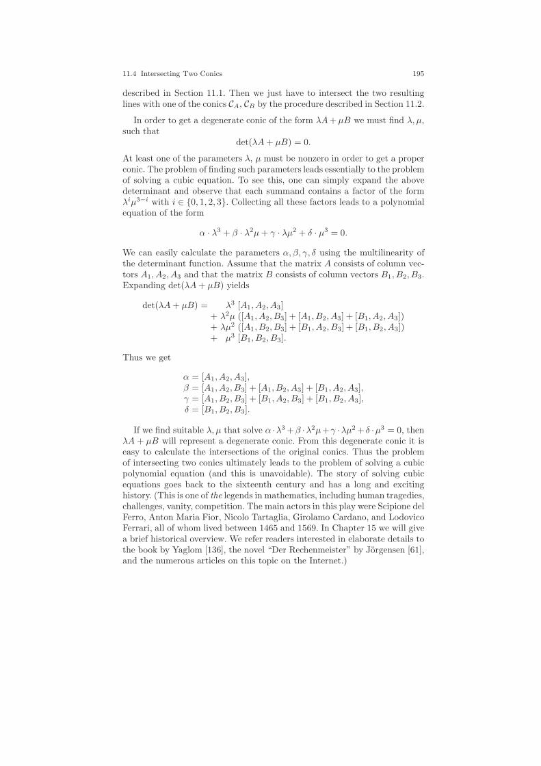
11.4 Intersecting Two Conics 195
described in Section 11.1. Then we just have to intersect the two resultinglines with one of the conics CA, CB by the procedure described in Section 11.2.
In order to get a degenerate conic of the form λA+µB we must find λ, µ,such that
det(λA+ µB) = 0.
At least one of the parameters λ, µ must be nonzero in order to get a properconic. The problem of finding such parameters leads essentially to the problemof solving a cubic equation. To see this, one can simply expand the abovedeterminant and observe that each summand contains a factor of the formλiµ3−i with i ∈ 0, 1, 2, 3. Collecting all these factors leads to a polynomialequation of the form
α · λ3 + β · λ2µ+ γ · λµ2 + δ · µ3 = 0.
We can easily calculate the parameters α, β, γ, δ using the multilinearity ofthe determinant function. Assume that the matrix A consists of column vec-tors A1, A2, A3 and that the matrix B consists of column vectors B1, B2, B3.Expanding det(λA+ µB) yields
det(λA+ µB) = λ3 [A1, A2, A3]+ λ2µ ([A1, A2, B3] + [A1, B2, A3] + [B1, A2, A3])+ λµ2 ([A1, B2, B3] + [B1, A2, B3] + [B1, B2, A3])+ µ3 [B1, B2, B3].
Thus we get
α = [A1, A2, A3],β = [A1, A2, B3] + [A1, B2, A3] + [B1, A2, A3],γ = [A1, B2, B3] + [B1, A2, B3] + [B1, B2, A3],δ = [B1, B2, B3].
If we find suitable λ, µ that solve α ·λ3 +β ·λ2µ+γ ·λµ2 + δ ·µ3 = 0, thenλA + µB will represent a degenerate conic. From this degenerate conic it iseasy to calculate the intersections of the original conics. Thus the problemof intersecting two conics ultimately leads to the problem of solving a cubicpolynomial equation (and this is unavoidable). The story of solving cubicequations goes back to the sixteenth century and has a long and excitinghistory. (This is one of the legends in mathematics, including human tragedies,challenges, vanity, competition. The main actors in this play were Scipione delFerro, Anton Maria Fior, Nicolo Tartaglia, Girolamo Cardano, and LodovicoFerrari, all of whom lived between 1465 and 1569. In Chapter 15 we will givea brief historical overview. We refer readers interested in elaborate details tothe book by Yaglom [136], the novel “Der Rechenmeister” by Jorgensen [61],and the numerous articles on this topic on the Internet.)

196 11 Calculating with Conics
For our purposes we will confine ourselves to a direct way for solving a cubicequation. Our procedure has three nice features compared to usual solutionsof cubic equations. It works in the homogeneous setting where we ask forvalues of λ and µ instead of just a one-variable version that does not handle“infinite” cases properly. It needs to calculate exactly one square root andexactly one cube root, and we will not have to take care which specific rootsof all complex possibilities we take. It works on the original cubic equation(most solutions presented in the literature work only for a reduced equationwhere β = 0).
All calculations in our procedure have to be carried out over the complexnumbers, since it may happen that intermediate results are no longer real.For the computation we will need one of the cube roots of unity as a constant.We abbreviate it by
ω = −1
2+ i ·
√3
4.
A reasonable procedure for solving the equation
α · λ3 + β · λ2µ+ γ · λµ2 + δ · µ3 = 0
is given by the following sequence of operations (don’t ask why the parametersand formulas work; it’s a long story):
1: W = −2β3 + 9αβγ − 27α2δ;
2: D = −β2γ2 + 4αγ3 + 4β3δ − 18αβγδ + 27α2δ3;
3: Q = W − α√
27D;
4: R = 3√
4Q;
5: L = (2β2 − 6αγ,−β,R)T ;
6: M = 3α(R, 1, 2)T ;
The two vectors L and M are the key to finding the three solutions forthe final computation of λ and µ. For this we have to compute
ω 1 ω2
1 1 1ω2 1 ω
L1
L2
L3
=
λ1
λ2
λ3
,
ω 1 ω2
1 1 1ω2 1 ω
M1
M2
M3
=
µ1
µ2
µ3
.
The pairs (λ1, µ1), (λ2, µ2), and (λ3, µ3) are the three solutions of the cubicequation. In Step 4 of the above procedure we have to choose a specific cuberoot. If R is one cube root, the other two cube roots are ωR and ω2R. Thereader is invited to convince himself that no matter which of these cube rootswe take, we obtain the same set of solutions (in fact they are permuted).Similarly, if we change the sign of the square root in Step 3, two of thesolutions are interchanged.
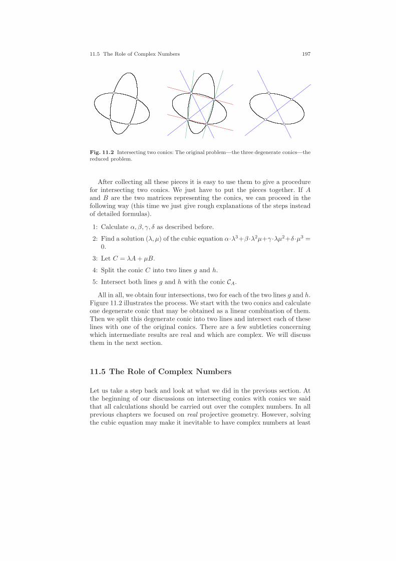
11.5 The Role of Complex Numbers 197
Fig. 11.2 Intersecting two conics: The original problem—the three degenerate conics—thereduced problem.
After collecting all these pieces it is easy to use them to give a procedurefor intersecting two conics. We just have to put the pieces together. If Aand B are the two matrices representing the conics, we can proceed in thefollowing way (this time we just give rough explanations of the steps insteadof detailed formulas).
1: Calculate α, β, γ, δ as described before.
2: Find a solution (λ, µ) of the cubic equation α·λ3+β ·λ2µ+γ ·λµ2+δ ·µ3 =0.
3: Let C = λA+ µB.
4: Split the conic C into two lines g and h.
5: Intersect both lines g and h with the conic CA.
All in all, we obtain four intersections, two for each of the two lines g and h.Figure 11.2 illustrates the process. We start with the two conics and calculateone degenerate conic that may be obtained as a linear combination of them.Then we split this degenerate conic into two lines and intersect each of theselines with one of the original conics. There are a few subtleties concerningwhich intermediate results are real and which are complex. We will discussthem in the next section.
11.5 The Role of Complex Numbers
Let us take a step back and look at what we did in the previous section. Atthe beginning of our discussions on intersecting conics with conics we saidthat all calculations should be carried out over the complex numbers. In allprevious chapters we focused on real projective geometry. However, solvingthe cubic equation may make it inevitable to have complex numbers at least

198 11 Calculating with Conics
as an intermediate result (if the value of D calculated in step two of our cubicequation procedure becomes negative).
We first discuss what it means to have a real object in the framework ofhomogeneous coordinates. In all our considerations so far we have agreed toidentify coordinate vectors that differ only by a scalar multiple. If we workwith complex coordinates we will do essentially the same. However, this timewe will also allow complex multiples. We will call a coordinate vector p “real”if there is a (perhaps complex) scalar s such that s·p has only real coordinates.In this sense the vector (1+2i, 3+6i,−2−4i)T represents a real object, sincewe can divide by 1 + 2i and obtain the real vector (1, 3,−2)T . Similarly,the vector (1, i, 0) is a proper complex vector, since no matter by whichnonzero number we multiply it, at least one of the entries will be complex.It is an amazing fact that we may get real objects from calculations withproper complex objects. Consider the following calculation, which could beconsidered the join of two proper complex points:
1 + 2i3 + i1 − i
×
1 − 2i3 − i1 + i
=
8i−6i10i
= 2i ·
4−35
.
The coordinates of the result are complex, but they still represent the realobject (4,−3, 5)T . The reason for this is that in this example we took the joinof two complex conjugate points. More generally, we get for a point p + iq,with real vectors p and q,
(p+ iq) × (p− iq) = p× p+ (iq) × p+ p× (−iq) + (iq) × (−iq) = 2i(q × p).
The join (meet) of two conjugate complex points (lines) is a real geometricobject. This perfectly fits in our geometric intuition. Imagine you intersecta line l with a conic CA. If the line is entirely outside the conic, they do nothave real intersections. As algebraic solution we get two complex conjugatepoints. Joining these two points, we get the real line l again. Generally, whenwe deal with homogeneous coordinates we will call an object real if there isa scalar multiple that simultaneously makes all entries real. We will applythis definition to points, lines, conics, transformations and also to bundles ofobjects parameterized by homogeneous coordinates.
Now let us return to the problem of intersecting conics. If we have tworeal conics CA and CB, then the parameters α, . . . , δ for the cubic equationwill be real as well. A cubic equation in C has three solutions (if necessarycounted with multiplicity). Except for degenerate cases in which two or allthree of these solutions coincide, we will have one of the following two cases:Either all these three solutions are real or just one of the solutions is real andthe other two are complex conjugates. In any case we will have at least onereal solution. The term “real solution” in the homogeneous setup in which weidentify scalar multiples of (λ, µ) means that there is a scalar s that makes
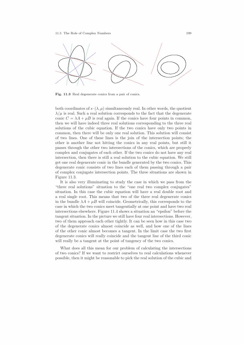
11.5 The Role of Complex Numbers 199
Fig. 11.3 Real degenerate conics from a pair of conics.
both coordinates of s ·(λ, µ) simultaneously real. In other words, the quotientλ/µ is real. Such a real solution corresponds to the fact that the degenerateconic C = λA + µB is real again. If the conics have four points in common,then we will have indeed three real solutions corresponding to the three realsolutions of the cubic equation. If the two conics have only two points incommon, then there will be only one real solution. This solution will consistof two lines. One of these lines is the join of the intersection points; theother is another line not hitting the conics in any real points, but still itpasses through the other two intersections of the conics, which are properlycomplex and conjugates of each other. If the two conics do not have any realintersection, then there is still a real solution to the cubic equation. We stillget one real degenerate conic in the bundle generated by the two conics. Thisdegenerate conic consists of two lines each of them passing through a pairof complex conjugate intersection points. The three situations are shown inFigure 11.3.
It is also very illuminating to study the case in which we pass from the“three real solutions” situation to the “one real two complex conjugates”situation. In this case the cubic equation will have a real double root anda real single root. This means that two of the three real degenerate conicsin the bundle λA + µB will coincide. Geometrically, this corresponds to thecase in which the two conics meet tangentially at one point and have two realintersections elsewhere. Figure 11.4 shows a situation an “epsilon” before thetangent situation. In the picture we still have four real intersections. However,two of them approach each other tightly. It can be seen how in this case twoof the degenerate conics almost coincide as well, and how one of the linesof the other conic almost becomes a tangent. In the limit case the two firstdegenerate conics will really coincide and the tangent line of the third conicwill really be a tangent at the point of tangency of the two conics.
What does all this mean for our problem of calculating the intersectionsof two conics? If we want to restrict ourselves to real calculations wheneverpossible, then it might be reasonable to pick the real solution of the cubic and

200 11 Calculating with Conics
proceed with this one. Then we finally have to intersect two real lines with aconic. Still it may happen that one or both of the lines do not intersect theconic in real points. However, whenever we have real intersection points wewill find them by this procedure by intersecting a real line and a real conic.
If we think of implementing such an operation in a computer program,it may also be the case that the underlying math library can properly dealwith complex numbers (it should anyway for solving the cubic equation). Insuch a case we do not have to explicitly pick a real solution. We can take anysolution we want. If we by accident pick a complex solution, then we will geta complex degenerate conic, which splits into two complex lines. However,intersecting the lines with one of the original conics will result in the correctintersections. If the correct intersections turn out to be real points, then it justmay be necessary to extract a common complex factor from the homogeneouscoordinates.
11.6 One Tangent and Four Points
As a final example of a computation we want to derive a procedure thatcalculates a conic that passes through four points and at the same timeis tangent to a line (see Figure 11.5 for the two possible solutions for aninstance of such a problem). Based on the methods we have developed sofar, there are several ways to approach this construction problem. Perhapsthe most straightforward is to construct a fifth point on the conic and then
Fig. 11.4 An almost degenerate situation.

11.6 One Tangent and Four Points 201
calculate the conic through these five points. This fifth point may be chosenon the line itself. Then it must be at the position where the resulting conictouches the line. Generally, there are two possible positions for such a point,corresponding to the two possible conics that satisfy the tangency conditions.
The crucial observation that allows us to calculate these two points is thefact that pairs of points that are generated by intersecting all possible conicsthrough four given points with a line l are the pairs of points of a projectiveinvolution on the line. For this, recall that the conics through four pointsA,B,C,D have the form
Cλ := p | (A,B;C,D)p = λ,
where λ may take an arbitrary value in R ∪ ∞. For each such conic thereexists a pair of points on l that are as well on Cλ. These pairs of points maybe both real, both complex, or coinciding. If the points coincide, then we areexactly in the tangent situation. Let pλ, qλ be the pair of such points onthe conic Cλ. Then we have the following:
Lemma 11.2. There is a projective involution τ on l such that for any λ ∈R ∪ ∞ we have τ(pλ) = qλ.
Proof. Instead of giving an algebraic proof we will directly use a geomet-ric argument. With the help of Pascal’s theorem we can construct the pointqλ from A,B,C,D, and pλ without explicit knowledge of the conic Cλ. Fig-ure 11.6 shows the construction. The black and white elements of the picturedepend only on A,B,C,D and pλ. Starting with the point pλ we have to
Fig. 11.5 Conics through four points and tangent to a line.
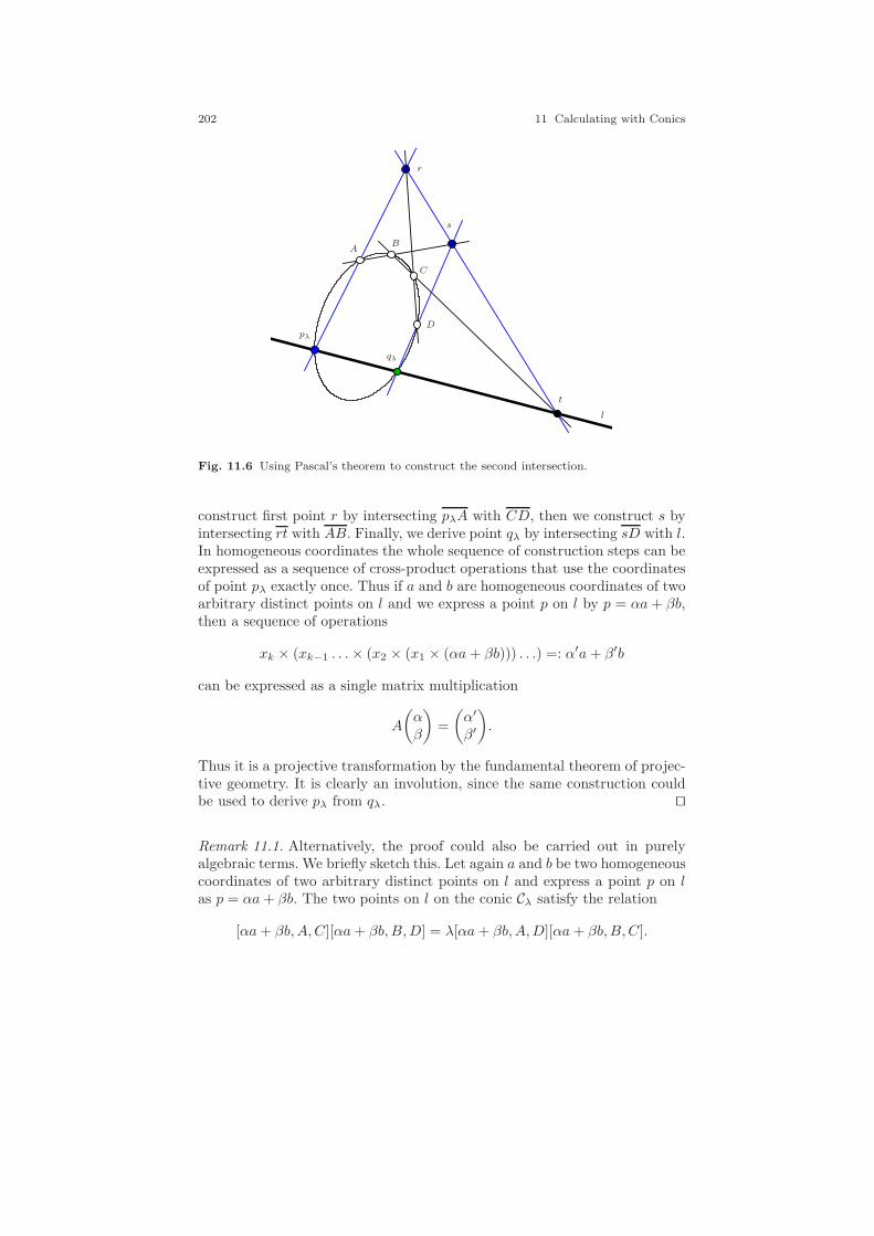
202 11 Calculating with Conics
B
D
C
A
l
pλ
qλ
r
s
t
Fig. 11.6 Using Pascal’s theorem to construct the second intersection.
construct first point r by intersecting pλA with CD, then we construct s byintersecting rt with AB. Finally, we derive point qλ by intersecting sD with l.In homogeneous coordinates the whole sequence of construction steps can beexpressed as a sequence of cross-product operations that use the coordinatesof point pλ exactly once. Thus if a and b are homogeneous coordinates of twoarbitrary distinct points on l and we express a point p on l by p = αa+ βb,then a sequence of operations
xk × (xk−1 . . .× (x2 × (x1 × (αa+ βb))) . . .) =: α′a+ β′b
can be expressed as a single matrix multiplication
A
(αβ
)=
(α′
β′
).
Thus it is a projective transformation by the fundamental theorem of projec-tive geometry. It is clearly an involution, since the same construction couldbe used to derive pλ from qλ. ⊓⊔
Remark 11.1. Alternatively, the proof could also be carried out in purelyalgebraic terms. We briefly sketch this. Let again a and b be two homogeneouscoordinates of two arbitrary distinct points on l and express a point p on las p = αa+ βb. The two points on l on the conic Cλ satisfy the relation
[αa+ βb,A,C][αa+ βb,B,D] = λ[αa+ βb,A,D][αa+ βb,B,C].
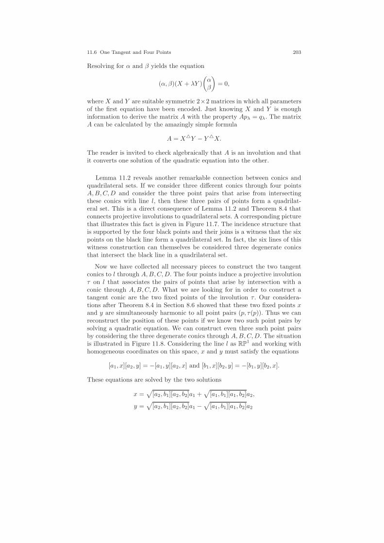
11.6 One Tangent and Four Points 203
Resolving for α and β yields the equation
(α, β)(X + λY )
(αβ
)= 0,
where X and Y are suitable symmetric 2×2 matrices in which all parametersof the first equation have been encoded. Just knowing X and Y is enoughinformation to derive the matrix A with the property Apλ = qλ. The matrixA can be calculated by the amazingly simple formula
A = XY − Y X.
The reader is invited to check algebraically that A is an involution and thatit converts one solution of the quadratic equation into the other.
Lemma 11.2 reveals another remarkable connection between conics andquadrilateral sets. If we consider three different conics through four pointsA,B,C,D and consider the three point pairs that arise from intersectingthese conics with line l, then these three pairs of points form a quadrilat-eral set. This is a direct consequence of Lemma 11.2 and Theorem 8.4 thatconnects projective involutions to quadrilateral sets. A corresponding picturethat illustrates this fact is given in Figure 11.7. The incidence structure thatis supported by the four black points and their joins is a witness that the sixpoints on the black line form a quadrilateral set. In fact, the six lines of thiswitness construction can themselves be considered three degenerate conicsthat intersect the black line in a quadrilateral set.
Now we have collected all necessary pieces to construct the two tangentconics to l through A,B,C,D. The four points induce a projective involutionτ on l that associates the pairs of points that arise by intersection with aconic through A,B,C,D. What we are looking for in order to construct atangent conic are the two fixed points of the involution τ . Our considera-tions after Theorem 8.4 in Section 8.6 showed that these two fixed points xand y are simultaneously harmonic to all point pairs (p, τ(p)). Thus we canreconstruct the position of these points if we know two such point pairs bysolving a quadratic equation. We can construct even three such point pairsby considering the three degenerate conics through A,B,C,D. The situationis illustrated in Figure 11.8. Considering the line l as RP
1 and working withhomogeneous coordinates on this space, x and y must satisfy the equations
[a1, x][a2, y] = −[a1, y][a2, x] and [b1, x][b2, y] = −[b1, y][b2, x].
These equations are solved by the two solutions
x =√
[a2, b1][a2, b2]a1 +√
[a1, b1][a1, b2]a2,
y =√
[a2, b1][a2, b2]a1 −√
[a1, b1][a1, b2]a2
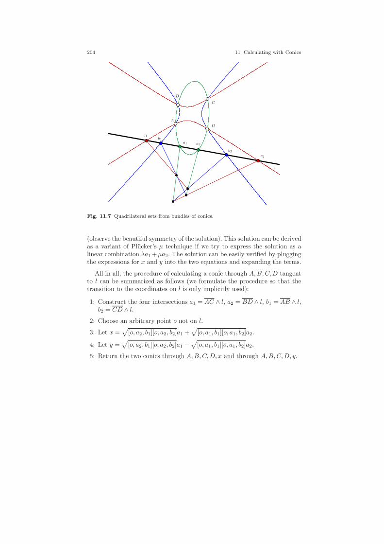
204 11 Calculating with Conics
A
B
C
D
a1 a2
b1
b2
c1
c2
Fig. 11.7 Quadrilateral sets from bundles of conics.
(observe the beautiful symmetry of the solution). This solution can be derivedas a variant of Plucker’s µ technique if we try to express the solution as alinear combination λa1 +µa2. The solution can be easily verified by pluggingthe expressions for x and y into the two equations and expanding the terms.
All in all, the procedure of calculating a conic through A,B,C,D tangentto l can be summarized as follows (we formulate the procedure so that thetransition to the coordinates on l is only implicitly used):
1: Construct the four intersections a1 = AC ∧ l, a2 = BD ∧ l, b1 = AB ∧ l,b2 = CD ∧ l.
2: Choose an arbitrary point o not on l.
3: Let x =√
[o, a2, b1][o, a2, b2]a1 +√
[o, a1, b1][o, a1, b2]a2.
4: Let y =√
[o, a2, b1][o, a2, b2]a1 −√
[o, a1, b1][o, a1, b2]a2.
5: Return the two conics through A,B,C,D, x and through A,B,C,D, y.

11.6 One Tangent and Four Points 205
B
A
C
D
a1 a2b1 b2 c1 c2x y
Fig. 11.8 The final construction.

12
Projective d-space
Es ist wunschenswert, daß neben der Euklidischen Methodeneuere Methoden der Geometrie in den Unterricht auf Gym-nasien eingefuhrt werden.
Felix Klein, 1868One of the “Theses” of his thesis defense
Mathematics is a game played according to certain simplerules with meaningless marks on paper.
David Hilbert
Different topic! So far, we have dealt almost exclusively with projective geom-etry of the line and of the plane. We explored the tight and very often elegantrelationships between geometric objects and their algebraic representations.Our central issues were:
• Introducing elements at infinity to bypass many special cases of ordinaryEuclidean geometry,
• representing geometric objects by homogeneous coordinates,• performing algebraic operations directly on geometric objects (via homo-
geneous coordinates),• performing transformations by matrix multiplication,• duality,• expressing geometric relations by bracket expressions.
The close interplay of homogeneous coordinates, finite and infinite ele-ments, and linear algebra made it possible to express geometric relations byvery elegant algebraic expressions. This chapter deals with generalizations ofthese concepts to higher dimensions.
207

208 12 Projective d-space
Fig. 12.1 A projectively correct cube.
Here we will just scratch the surface—in the hope that the reader might geta rough impression of the beauty and richness of the entire theory. It wouldbe easy to fill another 600 pages with an in-depth study of projective geom-etry in higher dimensions. We will restrict ourselves here to representationsof basic objects (points, lines, planes, and transformations) and elementaryoperations (join and meet). Most often we will not give explicit proofs andconfine ourselves with the general concepts.
12.1 Elements at Infinity
The three-dimensional projective space carries many similarities to the two-dimensional projective plane. Similarly to our treatment of the two-dimen-sional case we will start with our investigations by considering the usualEuclidean space R3. Like the Euclidean plane, this space is full of specialcases. Planes may, for instance, be parallel or meet in a line. Similarly tothe treatment of the projective plane we will extend the usual space R3 byelements at infinity to get rid of many of these special cases. For every bundleof parallel lines of R3 we introduce one point at infinity. The totality of allpoints in R3 together with these infinite points forms the set of points of thethree-dimensional projective space.
As usual, certain subsets of these points will be considered (projective)lines, and (since we are in the three-dimensional case) there will also besubsets that are considered projective planes. For every finite line l of R3
there is a unique point at infinity corresponding to the parallel bundle ofthis line. The finite part of l together with this point is considered a line

12.2 Homogeneous Coordinates and Transformations 209
in projective space. In addition, there are many lines that lie entirely at aninfinite position.
For this consider a usual finite plane h. This plane is extended by allinfinite points of lines that are contained in h. The extended plane is nothingbut a usual projective plane. All infinite points of this plane form a line atinfinity. This line consists entirely of infinite points. Every ordinary plane ofR3 is extended by such a unique line at infinity.
There is one object we have not yet covered in our collection of points,lines, and planes. All infinite points taken together again form a projectiveplane: the plane at infinity. The lines of this plane are all the infinite lines.We could say that the real projective three-space may be considered to beR3 extended by a projective plane at infinity in the same way as we may saythat the real projective plane is R2 together with a line at infinity.
In a way, this distinction of finite and infinite objects is confusing andunnecessary. It is just meant as a dictionary to connect concepts of ordi-nary Euclidean space to concepts of projective space. As one may expect theprojective space is much more homogeneous and symmetric than the usualEuclidean space. The projective space is governed by the following incidenceproperties (which are again analogues of the corresponding axioms of theprojective plane):
• Any two points span a unique line as long as they do not coincide.• Any three points span a unique plane as long as they are not collinear.• Any two planes meet in a unique line as long as they do not coincide.• Any three planes meet in a unique point as long as they do not meet in a
line.• Any pair of point and line span a unique plane as long as the point is not
on the line.• Any pair of plane and line meet in a unique point as long as the line is
not contained in the plane.
It will be the task of the next few sections to express these operations ofjoin and meet in a suitable way that also generalizes to higher dimensions.
12.2 Homogeneous Coordinates and Transformations
How do we represent these elements algebraically? Essentially the process issimilar to the setup in the projective plane. Points in projective three-spaceare represented by nonzero four-dimensional vectors. They are the homo-geneous coordinates of the points. Nonzero scalar multiples of the vectorsare identified. In other words, we may represent the points of the projectivethree-space as
RP3 =
R4 − (0, 0, 0, 0)TR − 0 .
210 12 Projective d-space
In the standard embedding we may “imagine” the Euclidean R3 embed-ded in R
4 as an affine space parallel to the (x, y, z, 0)T space of R4. If this is
too hard to imagine, then one can also proceed purely formally. In the stan-dard embedding a point (x, y, z)T ∈ R3 is represented by a four-dimensionalvector (x, y, z, 1)T ∈ R4. Nonzero scalar multiples are identified. The infinitepoints are exactly those nonzero vectors of the form (x, y, z, 0)T . They donot correspond to Euclidean points. Vectors of the form (x, y, z, 0)T may alsobe interpreted as homogeneous coordinates of the usual projective plane byignoring the last entry.
Thus we can literally say that RP3 consists of R
3 (the homogeneous vec-tors (x, y, z, 1)T ) and a projective plane at infinity (the homogeneous vectors(x, y, z, 0)T ). We may also interpret this process inductively and consider theprojective plane itself as composed of the Euclidean plane R2 (the vectors(x, y, 1, 0)T ) and a line at infinity (the vectors (x, y, 0, 0)T ). The line may beconsidered a Euclidean line (the vectors (x, 1, 0, 0)T ) and finally a point atinfinity (represented by (1, 0, 0, 0)T ).
The objects dual to points in RP3 will be planes. Similarly to points,
planes will also be represented by four-dimensional vectors. In Euclideanterms we may consider the vector (a, b, c, d)T as representing the parametersthat describe the affine plane (x, y, z) ∈ R
3 | ax+by+cz+d = 0. As usual,nonzero scalar multiples of the vector represent the same geometric object.If we interpret the equation in a setup of homogeneous coordinates, a point(x, y, z, w)T is incident to a plane (a, b, c, d)T if and only if
ax+ by + cz + dw = 0.
As in the two-dimensional setup, incidence is simply expressed by a scalarproduct being zero. The plane at infinity has homogeneous coordinates(0, 0, 0, 1)T .
Finding a plane that passes through three given points pi = (xi, yi, zi, wi),i = 1, 2, 3, thus translates to the task of solving a linear equation:
x1 y1 z1 w1
x2 y2 z2 w2
x3 y3 z3 w3
abcd
=
000
.
In the next section we will deal with methods of performing this calcula-tion explicitly. However, before we do so we will consider transformations inthis homogeneous projective setup. The situation here is almost completelyanalogous to the two-dimensional case. A transformation is represented by asimple matrix multiplication. This time we need a 4× 4 matrix. The cases ofusual affine transformations in R3 are again covered by special transformation

12.3 Points and Planes in 3-Space 211
matrices in which certain entries are zero. The following matrices representa linear transformation of R3 with matrix A, a pure translation, a generalaffine transformation, and a general projective transformation, respectively:
A000
0 0 0 1
,
1 0 0 tx0 1 0 ty0 0 1 tz0 0 0 1
,
• • • •• • • •• • • •0 0 0 1
,
• • • •• • • •• • • •• • • •
.
A “•” stands for an arbitrary number. In every case we must assume thatthe determinant of the matrix is nonzero.
Such a transformation T maps a point p to the associated image point. Thecorresponding transformation that applies to the homogeneous coordinatesof a plane is (as in the two-dimensional case) given by (T−1)T . By this choiceincidence of points and planes is preserved by projective transformations:
〈p, h〉 = 0 ⇐⇒ 〈Tp, (T−1)Th〉 = 0.
Instead of the transposed inverse (T−1)T it is also possible to use the trans-posed adjoint (T)T , since they differ by only a scalar factor.
Remark 12.1. A word of caution: One should consider the setup of presentingpoints and planes by four-dimensional vectors and expressing coincidence bythe standard scalar product as a kind of interim solution that will be replacedby something more powerful later on. The problem that we will have to facesoon is that lines will be represented by six-dimensional vectors and we haveto create a notational system that handles points, lines, and planes in aunified way. For this we will have to give up the concept of indexing a vectorentry with the position where it is placed in a vector. We will return to thisissue in Section 12.4.
12.3 Points and Planes in 3-Space
The task of this section is to give a closed formula for calculating the homo-geneous coordinates of a plane spanned by three points. The correspondingtwo-dimensional situation is governed by the cross product operation. Theline through two points p, q could be calculated by
l = p× q =
p1
p2
p3
×
q1q2q3
=
+
∣∣∣∣p2 q2p3 q3
∣∣∣∣
−∣∣∣∣p1 q1p3 q3
∣∣∣∣
+
∣∣∣∣p1 q1p2 q2
∣∣∣∣
.

212 12 Projective d-space
The entries of the coordinates of the line are the 2 × 2 subdeterminants ofthe matrix
p1 q1p2 q2p3 q3
.
One way of explaining this effect is to observe that an arbitrary point λp+µqon this line must have a zero scalar product with l. We obtain
〈λp+ µq, l〉 = λ〈p, l〉 + µ〈q, l〉 = λdet(p, p, q) + µ det(q, p, q).
The last equation holds since if we plug the expression for l into 〈a, l〉, weobtain the determinant det(a, p, q), as one can easily see if one develops thisdeterminant by the first column.
In a similar way we can obtain the coordinates of a plane h through threepoints p, q, r in RP
3. We get
h = join(p, q, r) :=
+
∣∣∣∣∣∣
p2 q2, r2p3 q3, r3p4 q4, r4
∣∣∣∣∣∣
−
∣∣∣∣∣∣
p1 q1, r1p3 q3, r3p4 q4, r4
∣∣∣∣∣∣
+
∣∣∣∣∣∣
p1 q1, r1p2 q2, r2p4 q4, r4
∣∣∣∣∣∣
−
∣∣∣∣∣∣
p1 q1, r1p2 q2, r2p3 q3, r3
∣∣∣∣∣∣
.
So the coordinates are the 3 × 3 subdeterminants of the matrix
p1 q1 r1p2 q2 r2p3 q3 r3p4 q4 r4
.
Equipped with alternating signs, they give the plane through these threepoints. The argument for the correctness of this calculation is the same asin the two-dimensional case. If we consider an arbitrary point a, then thedevelopment of the determinant
det
a1 p1 q1 r1a2 p2 q2 r2a3 p3 q3 r3a4 p4 q4 r4

12.3 Points and Planes in 3-Space 213
by the first column is just the scalar product 〈a, h〉 for the above definitionof h. If a is spanned by p, q, and r, then this determinant becomes zero (thepoint a is on h). If the point is not spanned by p, q, and r, then the columnsare linearly independent and the determinant is nonzero. Thus a is not onh. Geometrically speaking, we compute a vector h that is simultaneouslyorthogonal to all three vectors p, q, and r.
It may happen that the above operation (taking the four 3 × 3 subdeter-minants of the 4 × 3 matrix) results in a zero vector. However, this couldhappen only if the three column vectors were linearly dependent. In this casethe three points do not span a plane. Geometrically, there are several possi-bilities how this can happen. Either all points coincide (then the matrix hasrank 1) or the points lie on a unique common line (then the matrix has rank2). In both cases we have a degenerate situation in which the plane throughthe points is not uniquely determined.
As in the planar case, the procedure described here covers all possiblecases of finite and infinite points. For instance, a plane through two finitepoints p and q and one infinite point r is the unique plane that contains theline pq and parallels in direction of r (as long as r is not on pq, which is adegenerate situation). The plane through three infinite points is the plane atinfinity itself.
The same trick can also be used to calculate a point that is simultaneouslycontained in three planes. Let h, g, f be the homogeneous coordinates of threeplanes in RP
3. Assume that the three planes do not have a line in common.In this case the planes contain a unique common point. The coordinates ofthis point can be calculated as the 3 × 3 subdeterminants of the matrix
h1 g1 f1h2 g2 f2h3 g3 f3h4 g4 f4
equipped with alternating signs. As in the dual case, degenerate cases resultin a zero vector. All special cases resulting, from finite or infinite points areautomatically covered as well. For instance, if h and g are two finite planesand f is the plane at infinity, then the resulting point is the point at infinityon the intersection of h and g.
There is one more or less obvious but remarkable fact that we want tomention for further reference. If p, q, and r span a plane h and if a, b, and cspan the same plane, then the join operation that calculates the plane fromthree points may have different results for p, q, and r and for a, b, and c.However, the two results may differ at most by a non-zero scalar multiple.One may view this result as a consequence of the fact that the plane h isuniquely determined and thus vectors representing it only may differ by ascalar multiple. However, one can obtain it also directly from the fact thatthe operation join(p, q, r) is linear in each argument and anticommutative.

214 12 Projective d-space
Each of the points a, b, c is a linear combination of p, q, and r. So, if we, forinstance, replace p by a, we obtain
join(a, q, r) = join(λp+ µq + τr, q, r)= λ · join(p, q, r) + µ · join(q, q, r) + τ · join(r, q, r)= λ · join(p, q, r).
As a consequence of antisymmetry, terms with repeated letters can be can-celed.
12.4 Lines in 3-Space
Now comes the tricky part. What is the good way of representing lines ofprojective space? One could say that the answer to this question was, afterintroduction of homogeneous coordinates, one of the major breakthroughsof nineteenth-century geometry. More or less, the answer was independentlydiscovered by at least two people. Perhaps the first was Hermann GuntherGrassmann (1809–1877). In his work on Lineare Ausdehnungslehre [46] from1844 he laid at the same time the basis for our modern linear algebra as wellas for multilinear algebra. One of the essential parts was a formal methodthat made it possible to directly operate with points, lines, planes, etc. Un-fortunately, Grassmann developed a kind of completely new mathematicalterminology and notation to deal with these kinds of objects. This causedhim to be more or less completely ignored by his contemporaries, and hisideas did not become common mathematical knowledge until he completelyrewrote his book and published a second version [47] in 18621.
The second person involved was Julius Plucker (whom we have already metfrequently in this book). Not aware of Grassmann’s work, in 1868 he publishedthe first part of Neue Geometrie des Raumes, gegrundet auf die Betrachtungder geraden Linie als Raumelement [101] (New Geometry of space, basedon the straight line as space element) but died before the second part wascomplete. Felix Klein at this time was his assistant and essentially completedPlucker’s thoughts in his doctoral dissertation [64].
From a modern perspective the basic ideas are a straightforward gener-alization of our considerations in the previous section. Nevertheless, theseideas opened whole new branches of mathematics starting from projective
1 The first edition of his book was of about 900 copies, from of about 600 were pulpedsince they simply could not be sold. The remaining 300 books were given away for freeto anyone who showed interest. In his second edition, Grassmann expresses his regretthat people do not take the time to follow another person’s thoughts. It is little knownamong mathematicians that Grassmann was much more famous in his time for his workson Indo-Germanic linguistics. He published the first German translation of the Rig-Veda(an ancient indian document), and his Indo-German dictionaries are still in use today.
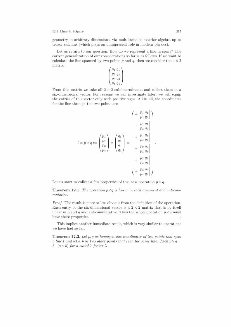
12.4 Lines in 3-Space 215
geometry in arbitrary dimensions, via multilinear or exterior algebra up totensor calculus (which plays an omnipresent role in modern physics).
Let us return to our question: How do we represent a line in space? Thecorrect generalization of our considerations so far is as follows. If we want tocalculate the line spanned by two points p and q, then we consider the 4 × 2matrix
p1 q1p2 q2p3 q3p4 q4
.
From this matrix we take all 2 × 2 subdeterminants and collect them in asix-dimensional vector. For reasons we will investigate later, we will equipthe entries of this vector only with positive signs. All in all, the coordinatesfor the line through the two points are
l = p ∨ q :=
p1
p2
p3
p4
∨
q1q2q3q4
=
+
∣∣∣∣p1 q1p2 q2
∣∣∣∣
+
∣∣∣∣p1 q1p3 q3
∣∣∣∣
+
∣∣∣∣p1 q1p4 q4
∣∣∣∣
+
∣∣∣∣p2 q2p3 q3
∣∣∣∣
+
∣∣∣∣p2 q2p4 q4
∣∣∣∣
+
∣∣∣∣p3 q3p4 q4
∣∣∣∣
.
Let us start to collect a few properties of this new operation p ∨ q.
Theorem 12.1. The operation p∨q is linear in each argument and anticom-mutative.
Proof. The result is more or less obvious from the definition of the operation.Each entry of the six-dimensional vector is a 2 × 2 matrix that is by itselflinear in p and q and anticommutative. Thus the whole operation p∨ q musthave these properties. ⊓⊔
This implies another immediate result, which is very similar to operationswe have had so far.
Theorem 12.2. Let p, q be homogeneous coordinates of two points that spana line l and let a, b be two other points that span the same line. Then p∨ q =λ · (a ∨ b) for a suitable factor λ.
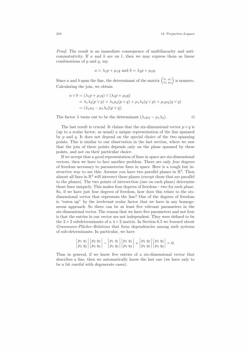
216 12 Projective d-space
Proof. The result is an immediate consequence of multilinearity and anti-commutativity. If a and b are on l, then we may express them as linearcombinations of p and q, say
a = λ1p+ µ1q and b = λ2p+ µ2q.
Since a and b span the line, the determinant of the matrix(λ1 µ1
λ2 µ2
)is nonzero.
Calculating the join, we obtain
a ∨ b = (λ1p+ µ1q) ∨ (λ2p+ µ2q)
= λ1λ2(p ∨ p) + λ1µ2(p ∨ q) + µ1λ2(q ∨ p) + µ1µ2(q ∨ q)= (λ1µ2 − µ1λ2)(p ∨ q).
The factor λ turns out to be the determinant (λ1µ2 − µ1λ2). ⊓⊔
The last result is crucial. It claims that the six-dimensional vector p∨ q is(up to a scalar factor, as usual) a unique representation of the line spannedby p and q. It does not depend on the special choice of the two spanningpoints. This is similar to our observation in the last section, where we sawthat the join of three points depends only on the plane spanned by thesepoints, and not on their particular choice.
If we accept that a good representation of lines in space are six-dimensionalvectors, then we have to face another problem. There are only four degreesof freedom necessary to parameterize lines in space. Here is a rough but in-structive way to see this: Assume you have two parallel planes in R
3. Thenalmost all lines in R3 will intersect these planes (except those that are parallelto the planes). The two points of intersection (one on each plane) determinethose lines uniquely. This makes four degrees of freedom—two for each plane.So, if we have just four degrees of freedom, how does this relate to the six-dimensional vector that represents the line? One of the degrees of freedomis “eaten up” by the irrelevant scalar factor that we have in any homoge-neous approach. So there can be at least five relevant parameters in thesix-dimensional vector. The reason that we have five parameters and not fouris that the entries in our vector are not independent. They were defined to bethe 2× 2 subdeterminants of a 4× 2 matrix. In Section 6.5 we learned aboutGrassmann-Plucker-Relations that form dependencies among such systemsof sub-determinants. In particular, we have
∣∣∣∣p1 q1p2 q2
∣∣∣∣∣∣∣∣p3 q3p4 q4
∣∣∣∣−∣∣∣∣p1 q1p3 q3
∣∣∣∣∣∣∣∣p1 q1p4 q4
∣∣∣∣+∣∣∣∣p2 q2p3 q3
∣∣∣∣∣∣∣∣p2 q2p4 q4
∣∣∣∣ = 0.
Thus in general, if we know five entries of a six-dimensional vector thatdescribes a line, then we automatically know the last one (we have only tobe a bit careful with degenerate cases).
12.5 Joins and Meets: A Universal System . . . 217
Conversely, if we have a vector l = (a, b, c, d, e, f)T that satisfies the equa-tion af − be+ cd = 0, Theorem 7.1 implies that there are two vectors p and qwith l = p ∨ q. Vectors that satisfy such a condition are called decomposable.
12.5 Joins and Meets: A Universal System . . .
Before we play around with line coordinates in space we will first clear upour notation and present a universal system that is capable of dealing withpoints, lines and planes in a unified way. The situation is even better: we willpresent a system that is capable of dealing with linear objects in arbitraryprojective spaces of any dimension. This will be a direct generalization of thethree-dimensional case.
The main problem so far is that points and planes are represented by four-dimensional vectors, while lines are represented by six-dimensional vectors.So a priori it is not clear how to define operators that work reasonably onarbitrary collections of such objects. The key observation here is to give upthe idea that the coordinate entries belong to certain positions in a vector. Itwill be much more useful to associate meaningful labels to the different entriesof a vector. In the three-dimensional case these labels will be the subsets ofthe set 1, 2, 3, 4. There are exactly four one-element subsets; they will labelthe coordinate entries of a point. There are six two-element subsets; they willlabel the entries of a line. And there are four three-element subsets and theywill be used to label the coordinate entries of a plane. So points and planesare both represented by four-dimensional vectors, but they have explicitlydifferent meanings.
It is also reasonable to include the empty set and the full set 1, 2, 3, 4in our system. We will learn about their meaning soon. If we consider the num-bers of subsets sorted by their cardinality, we obtain the sequence 1, 4, 6, 4, 1,which is simply a sequence of binomial coefficients—the fifth row of Pascal’striangle.
We will (at least partially) follow Grassmann’s footprints in order to seehow the whole system of join and meet operations arises. In modern terms,Grassmann states that if we want to work in projective (d − 1)-dimensionalgeometry, we have to fix first of all a system of d units
e1, e2, e3, . . . , ed
that are by definition independent. You may think of them as the d-dimensional unit vectors and associate the corresponding projective pointsto them. These units are in a sense the most fundamental geometric objects,and any other objects will be expressible in terms of units, real numbers,and admissible operations. Furthermore, it is allowed to form products of
218 12 Projective d-space
units. These products are assumed to be anticommutative and linear in bothfactors. Thus we have
eiej = −ejei if i 6= j and eiei = 0.
Products of k units are called rank-k units. Thus e1, . . . , ed are rank-1 units,e1e2, . . . , ed−1ed are rank-2 units, and so forth. Furthermore it is allowed toform products and sums of objects. A geometric object of rank-k is a linearcombination of several rank-k units. One may think of rank-k objects as rep-resenting a (k − 1)-dimensional linear object in the corresponding projectivespace.
Let us see how these simple rules automatically create a system in whichmultiplication corresponds to well-known arithmetic operations. Let us startwith the first nontrivial case d = 2. Rank-1 objects (points) are simply linearcombinations
λ1e1 + λ2e2.
Up to sign change there is only one nonvanishing rank-2 unit, namely e1e2 =−e2e1. The product of two points turns out to be
(λ1e1 + λ2e2)(µ1e1 + µ2e2)
= λ1µ1e1e1 + λ1µ2e1e2 + λ2µ1e2e1 + λ2µ2e2e2
= (λ1µ2 − λ2µ1)e1e2,
which is up to the factor e1e2 just the determinant of the points. Productsof more than three points will always vanish completely.
Next is d = 3. We have three units e1, e2, e3 and (up to sign) three rank-2units e1e2, e1e3, e2e3. Calculating the product of two points, we get
(λ1e1 + λ2e2 + λ3e3)(µ1e1 + µ2e2 + µ3e3)
= . . . expression with nine summands . . .
= (λ1µ2 − λ2µ1)e1e2 + (λ1µ3 − λ3µ1)e1e3 + (λ2µ3 − λ3µ2)e2e3,
which is essentially the cross product of the two points expressed as a linearcombination of rank-2 units. Thus the join operation of two points pops outautomatically (except for the sign change in the middle entry). If we proceed,we see that the product of three points turns out to be
(λ1e1 + λ2e2 + λ3e3)(µ1e1 + µ2e2 + µ3e3)(τ1e1 + τ2e2 + τ3e3)
= . . . expression with 27 summands . . .
= (λ1µ2τ3 + λ2µ3τ1 + λ3µ1τ2 − λ1µ3τ2 − λ3µ2τ1 − λ2µ1τ3)e1e2e3,
which is just the determinant of the point coordinates times e1e2e3.If we proceed in a similar manner, then we find out that for d = 4 the points
are represented by four-dimensional objects. The products of two points is alinear combination of the six rank-2 units whose coefficients are exactly the

12.5 Joins and Meets: A Universal System . . . 219
entries of our join operation;
(λ1e1 + λ2e2 + λ3e3 + λ4e4)(µ1e1 + µ2e2 + µ3e3 + µ4e4)
= . . . expression with 16 summands . . .
= +(λ1µ2 − λ2µ1)e1e2 + (λ1µ3 − λ3µ1)e1e3 + (λ1µ4 − λ4µ1)e1e4+(λ2µ3 − λ3µ2)e2e3 + (λ2µ4 − λ4µ2)e2e4 + (λ3µ4 − λ4µ3)e3e4.
(Now you see where the positive signs come from.) The product of threepoints gives the coordinates of the plane expressed in rank-3 units. Finally,the product of four points creates the determinant of the coordinate vectorsof the points times the rank-4 unit e1e2e3e4.
We see that all the ei in our expressions carry essentially no information.
The only thing that counts are the indices. Furthermore, the only combina-tions of indices that really contribute are those with nonrepeating letters,and it suffices to consider one unit for every subset of indices. Thus we cango ahead and say that a rank-k object is a vector with
(dk
)entries labeled
by the k-element subsets of 1, 2, . . . , d. We identify these subsets with thesequences of k ordered elements taken from 1, 2, . . . , d =: Ed. Thus theindex set of a k-flat (this is a (k − 1)-dimensional linear object) in RP
d−1 is
Λ(d, k) := (i1, . . . , ik) ∈ Ekd | i1 < i2 < · · · < ik.
To further distinguish the Grassmann operation from ordinary multiplicationwe introduce the symbol “∨” and call this the join operation. In general thejoin operation can be determined by the following rules. If we are working inRP
d−1, we can take the join of a k-flat P and an m-flat Q if k +m ≤ d. IfR = P ∨Q, then R is indexed by the elements of Λ(d, k +m). For an indexλ ∈ Λ(d, k +m) we can calculate the corresponding entry of R according tothe formula
Rλ =∑
λ=µ∪τµ∈Λ(d,k)
τ∈Λ(d,m)
sign(µ, τ)PµQτ .
Here sign(µ, τ) is defined to be 1 or −1 depending on the parity of trans-positions needed to sort the sequence (µ, τ). We will see in the next sectionhow this formula is used in practice. It allows us to calculate the join of twoarbitrary objects as long as the sum of their ranks does not exceed d. Theabove formula filters exactly those terms that do not cancel in the Grassmannproduct.
In a similar fashion we can define a meet operation. We will not develophere the theory behind the exact definition. It is essentially defined in a waythat represents the dual of the join operation. If we work in RP
d−1, we areallowed to take the meet of a k-flat P and an m-flat Q whenever k +m ≥ d.We abbreviate the meet operator by “∧”. If R = P ∧ Q, then R is indexed

220 12 Projective d-space
by the elements of Λ(d, k +m− d). For an index λ ∈ Λ(d, k +m− d) we cancalculate the corresponding entry of R according to the formula
Rλ =∑
λ=µ∩τµ∈Λ(d,k)
τ∈Λ(d,m)
sign(µ\λ, τ\λ)PµQτ .
12.6 . . . And How to Use It
In this section we will see what can be done with join and meet operationsand how they are calculated in practice. We will restrict our considerationsto d = 4, the spatial case. Everything carries over in a straightforward wayto higher (and lower) dimensions. First of all, we will start with a kind ofsymbolic table that exemplifies the dimensions of the objects involved underjoin and meet operations. For the join we obtain
point ∨ point = line,
point ∨ line = plane,
point ∨ plane = number,
line ∨ line = number,
point ∨ point ∨ point = plane,
point ∨ point ∨ line = number,
point ∨ point ∨ point ∨ point = number.
Every operation results in either a vector or a number. Whenever a zero vec-tor or the number zero occurs as result, this indicates a degenerate situationin which the objects are dependent. For instance, usually the join of a pointand a line results in the plane spanned by the point and the line. However,if the point is on the line, then the join results in the zero vector. The con-secutive join of four points results in a number, and this number is just thedeterminant of the matrix formed by the vectors of the points as columnvectors. If the points are coplanar, then this join returns the number zero.The join of two lines is zero if the two lines coincide. The join of a point anda plane is a number. In principle, this number is just the scalar product ofthe point and the plane. It is zero whenever the point is on the plane.
The meet operator performs the dual operations. Again the occurrence ofa zero or a zero vector indicates a degenerate situation. In detail, the meetscan be used to perform the following operations:
12.6 . . . And How to Use It 221
plane ∧ plane = line,
plane ∧ line = point,
plane ∧ point = number,
line ∧ line = number,
plane ∧ plane ∧ plane = point,
plane ∧ plane ∧ line = number,
plane ∧ plane ∧ plane ∧ plane = number.
Again it should be mentioned that all operations based on join and meet fullysupport all elements of projective geometry. Thus in the standard embeddingof R
3 elements at infinity are also processed correctly. For instance, the meetof two parallel planes results in a line at infinity. To achieve a standard em-bedding we have to make a choice of which the vectors e1, . . . , e4 is chosenfor homogenization purposes. If we choose e4 for this purpose, we may rep-resent a point (x, y, z) ∈ R3 as xe1 + ye2 + ze3 + e4. The plane at infinitythen corresponds to e1e2e3. The notation is much more familiar if we simplyrepresent the objects with associated labels. A Euclidean point (x, y, z) anda Euclidean plane (x, y, z)t | ax + by + cz + d = 0 then correspond to thetwo vectors
1 x2 y3 z4 1
and
123 −d124 c134 −b234 a
.
The minus signs in the plane coordinates are used to compensate the signchanges caused by the join operator. The join operation of these two objectsresults in a single number (labeled by “1234”); this number is simply calcu-lated as ax + by + cz + d, as desired. It is zero if the point and the planecoincide.
Let us perform a more elaborate example with concrete coordinates. Letus first calculate the join of two points:
1 32 −23 44 1
∨
1 −32 33 54 1
=
12 3·3 − (−2)·(−3)13 3·5 − 4·(−3)14 3·1 − 1·(−3)23 (−2)·5 − 4·324 (−2)·1 − 1·334 4·1 − 1·5
=
12 313 2714 623 −2224 −534 −1
.
The result is a six-dimensional vector representing a line. In particular,this vector must satisfy the Grassmann-Plucker-Relation. The Grassmann-Plucker-Relation for a line l can be simply expressed as l ∨ l = 0 (where 0 isthe zero vector). This has a direct geometric interpretation: a line is incidentto itself. In our example, we get
222 12 Projective d-space
3·(−1) − 27·(−5) + 6·(−22) = −3 + 135 − 132 = 0,
as expected. We proceed by forming the meet of this line with some plane.The result is the point where the plane intersects the line:
12 313 2714 623 −2224 −534 −1
∧
123 4124 2134 1234 5
=
1 3·1 − 27·2 + 6·42 3·5 − (−22)·2 + (−5)·43 27·5 − (−22)·1 + (−1)·44 6·5 − (−5)·1 + (−1)·2
=
1 −272 393 1534 33
.
If everything went right with our calculation, the resulting point must lie onthe plane itself. Thus the join of the point and the plane must be simply zero.We obtain
1 −272 393 1534 33
∨
123 4124 2134 1234 5
=
(1234 (−27)·5 − 39·1 + 153·2 − 33·4
)= 0.
We finally will have a closer look at the representation of infinite lines(in the usual embedding of R3 in RP
3). There are two ways to derive a lineat infinity: either we join two infinite points or we meet two parallel planes.Either way leads to the same characterization of infinite lines, though thesituations may be interpreted slightly differently from a geometric point ofview. Joining two infinite points. we obtain
1 x1
2 y13 z14 0
∨
1 x2
2 y23 z24 0
=
12 x1y2 − x2y113 x1y3 − x3y114 023 x2y3 − x3y224 034 0
.
A line is infinite if the only nonzero entries are those not involving the label4. We also see that if we restrict the line to the labels 12, 13, and 23, thenthe join of infinite points behaves like a cross product.
Two planes are parallel if they differ only in the 123entry. The meet of twoparallel planes is an infinite line:
123 d1
124 c134 b234 a
∧
123 d2
124 c134 b234 a
=
12 d1c− d2c13 d1b− d2b14 cb− bc23 d1a− d2a24 ca− ac34 ba− ab
= (d1 − d2) ·
12 c13 b14 023 a24 034 0
.
12.6 . . . And How to Use It 223
Again, as expected, the 14, 24, and 34 entries are zero. The other threeentries encode up to the usual sign changes the common normal vectors ofthe planes. The factor d1 − d2 can be interpreted in the following way. If theplanes coincide then d1 = d2 and the meet operation results in a zero vector.


13
Diagram Techniques
Notation, Notation, Notation.
Title of a book by Jim Blinn, 2002
We just reduced all of geometry to tensor multiplication (well,almost all). And there are no embarrassing transposes. Row-ness and column-ness is superseded by the more general con-cept of covariant and contravariant indices. Plus we can feelreally cool by sharing notation with General Relativity.
Jim Blinn, 1992
It sometimes happens that reading a mathematical article sheds a completelynew light on subjects that one considered “personally well-under stood.” Soit happened to me when I did some research related to solving cubic equa-tions and stumbled across a series of papers written by the computer sci-entist Jim Blinn. The series was essentially about the expressive power oftensor calculus applied to geometry [8, 9, 10, 11]. I always hated workingwith tensors and avoided them wherever possible, because tensor notationtends either to be very abstract or to clutter all the essential information ofa formula into indices and indices of indices and indices of indices of indices.Jim Blinn’s papers were different. There tensor formulas were encoded asdiagrams, and suddenly all those terrible index battles became geometricallymeaningful structures. Moreover, this approach gives a unifying setup fortreating points, lines, planes, hyperplanes, transformations, quadratic forms,algebraic curves, and surfaces in all dimensions. Everything becomes a ten-sor, and every projective invariant becomes a diagram. The bookkeeping ofhow to combine the coordinate entries of the tensors (for instance to derive
225

226 13 Diagram Techniques
the Plucker coordinates of a line) is completely driven by the structure of thediagrams. It is the aim of this chapter to give a brief introduction to thesemethods. As before, we want to remain as explicit as possible. We will firsttranslate the objects of our previous investigations to tensors and then trans-late tensor formulas to tensor diagrams. The mathematically trained readermay excuse that we again focus on concrete objects and focus on tensorsgiven by concrete coordinate values rather than taking the (more modern)abstract point of view: “A tensor is an abstract element of a tensor space,. . .”
13.1 From Points, Lines, and Matrices to Tensors
So far, we have dealt with several types of objects. In RP2 we had points
and lines. In RP3 we had points, lines, and planes, and so on. Furthermore,
there were transformations (represented by d × d matrices) and quadraticforms (also represented by d×d matrices). Our typical operations were scalarproducts (to determine coincidences), and cross products (for join and meet),exterior products, and matrix multiplications from the left and from theright, depending on the context. Our previous chapter introduced exteriorproducts as a generalization of join and meet operations for the price thatthe bookkeeping of how to perform the operations became a little complicated(compare Section 12.5).
We will now (as a first step) consider all these objects as particular typesof tensors, and we will consider all operations as multiplication of tensorswith tensors. For this, let us look at a few of these operations from a very el-ementary perspective, in which we neglect the difference of rows and columnsin matrices and vectors and represent all geometric quantities as arrays ofnumbers and where we rebuild all elementary operations from scratch. Letus consider the rank-three case RP
2 first. A point p has homogeneous coor-dinates (p1, p2, p3); a line l has coordinates (l1, l2, l3); the scalar product ofthe points and the line is
3∑
i=1
pili.
A transformation matrix T is a 3 × 3 array of numbers with entries tij . Theproduct of T and the point p is in elementary terms
t11 t12 t12t21 t22 t22t31 t32 t33
·
p1
p2
p3
=
∑3i=1 pit1i∑3i=1 pit2i∑3i=1 pit3i
.
The evaluation of the quadratic form pTAp turns out to be
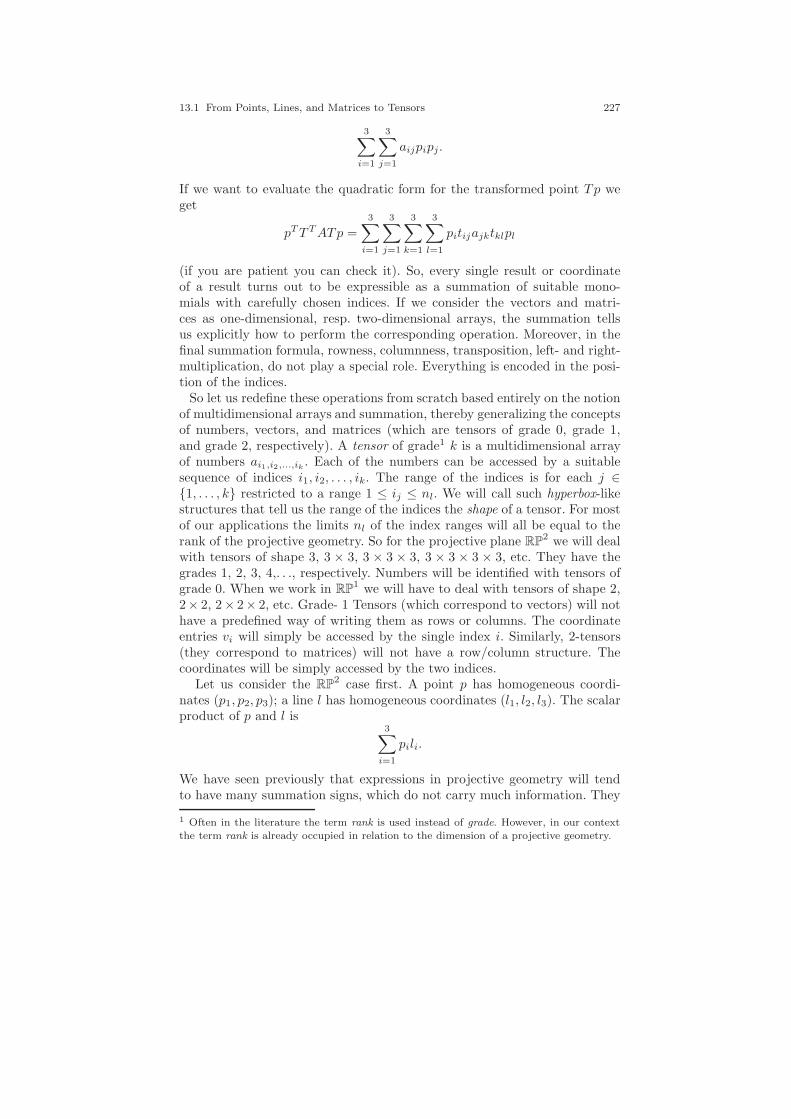
13.1 From Points, Lines, and Matrices to Tensors 227
3∑
i=1
3∑
j=1
aijpipj.
If we want to evaluate the quadratic form for the transformed point Tp weget
pTT TATp =
3∑
i=1
3∑
j=1
3∑
k=1
3∑
l=1
pitijajktklpl
(if you are patient you can check it). So, every single result or coordinateof a result turns out to be expressible as a summation of suitable mono-mials with carefully chosen indices. If we consider the vectors and matri-ces as one-dimensional, resp. two-dimensional arrays, the summation tellsus explicitly how to perform the corresponding operation. Moreover, in thefinal summation formula, rowness, columnness, transposition, left- and right-multiplication, do not play a special role. Everything is encoded in the posi-tion of the indices.
So let us redefine these operations from scratch based entirely on the notionof multidimensional arrays and summation, thereby generalizing the conceptsof numbers, vectors, and matrices (which are tensors of grade 0, grade 1,and grade 2, respectively). A tensor of grade1 k is a multidimensional arrayof numbers ai1,i2,...,ik . Each of the numbers can be accessed by a suitablesequence of indices i1, i2, . . . , ik. The range of the indices is for each j ∈1, . . . , k restricted to a range 1 ≤ ij ≤ nl. We will call such hyperbox-likestructures that tell us the range of the indices the shape of a tensor. For mostof our applications the limits nl of the index ranges will all be equal to therank of the projective geometry. So for the projective plane RP
2 we will dealwith tensors of shape 3, 3 × 3, 3 × 3 × 3, 3 × 3 × 3 × 3, etc. They have thegrades 1, 2, 3, 4,. . ., respectively. Numbers will be identified with tensors ofgrade 0. When we work in RP
1 we will have to deal with tensors of shape 2,2× 2, 2× 2× 2, etc. Grade- 1 Tensors (which correspond to vectors) will nothave a predefined way of writing them as rows or columns. The coordinateentries vi will simply be accessed by the single index i. Similarly, 2-tensors(they correspond to matrices) will not have a row/column structure. Thecoordinates will be simply accessed by the two indices.
Let us consider the RP2 case first. A point p has homogeneous coordi-
nates (p1, p2, p3); a line l has homogeneous coordinates (l1, l2, l3). The scalarproduct of p and l is
3∑
i=1
pili.
We have seen previously that expressions in projective geometry will tendto have many summation signs, which do not carry much information. They
1 Often in the literature the term rank is used instead of grade. However, in our contextthe term rank is already occupied in relation to the dimension of a projective geometry.

228 13 Diagram Techniques
just tell us from where to where an index runs, but this is already specified bythe shape of the tensors. So, let us drop the summation signs in our notation.We use a formal trick that is known as Einstein’s summation convention. Ifwe want to sum over an index, then the index should occur exactly twice in aformula, and it should be used once as a subscript and once as a superscript.Thus our scalar product may be simply written as
pili.
In a similar fashion we can represent transformation matrices as grade-2tensors.
Using Einstein’s summation convention we can write the multiplication ofa matrix by a vector (the classical matrix multiplication) as
tijpi.
We should step back for a moment and check that we indeed get the rightresults. If we set qj = tijpi, the three entries of qj evaluate to
q1 =
3∑
i=1
ti1pi, q2 =
3∑
i=1
ti2pi, q3 =
3∑
i=1
ti3pi,
which are exactly the components of the result of usual matrix multiplication.The upper and lower indices have one additional semantic meaning. We
have seen that lines were equipped with upper indices, whereas points wereequipped with lower indices. In a sense, all lower indices will turn out to be“pointlike” and all upper indices will turn out to be “linelike.” In products oftensors indices with the same letter occur only between an upper and a lowerentry. Thus in the product tijpi, the point p is connected via the index i tothe transformation matrix. The only index not “eaten up” by the summationis the lower index j; thus the result is again a pointlike object.
In our previous investigation into conics (Sections 9 to 11), quadratic formswere represented by a 3 × 3 matrix A. Evaluation of a quadratic form at apoint was done by the product pTAp. In the context of tensors, the matrixA is different from a transformation matrix T . While the product of T withp is again a point, the product of A with p must be linelike so that it can beconnected to another point. In other words, it must be possible to connectthe quadratic form represented by A to two points. Thus the matrix A isrepresented as a grade-2 tensor with two upper indices, aij . The evaluationof the quadratic form can be written as
aijpipj .
Observe that the order of the tensors becomes completely irrelevant, sincethe summation is completely driven by the distribution of the indices. We canalso go one step further and combine points, transformations, and quadratic
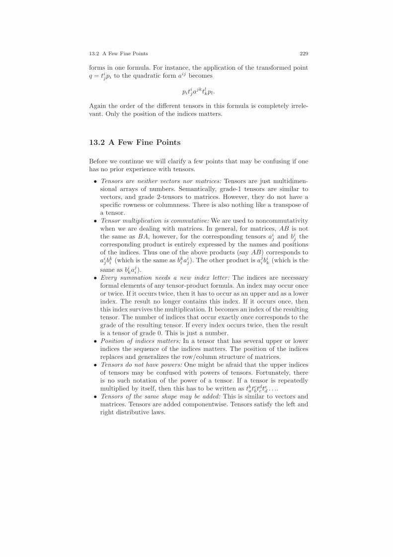
13.2 A Few Fine Points 229
forms in one formula. For instance, the application of the transformed pointq = tijpi to the quadratic form aij becomes
pitijajktlkpl.
Again the order of the different tensors in this formula is completely irrele-vant. Only the position of the indices matters.
13.2 A Few Fine Points
Before we continue we will clarify a few points that may be confusing if onehas no prior experience with tensors.
• Tensors are neither vectors nor matrices: Tensors are just multidimen-sional arrays of numbers. Semantically, grade-1 tensors are similar tovectors, and grade 2-tensors to matrices. However, they do not have aspecific rowness or columnness. There is also nothing like a transpose ofa tensor.
• Tensor multiplication is commutative: We are used to noncommutativitywhen we are dealing with matrices. In general, for matrices, AB is notthe same as BA, however, for the corresponding tensors aij and bij thecorresponding product is entirely expressed by the names and positionsof the indices. Thus one of the above products (say AB) corresponds toaijb
ki (which is the same as bki a
ij). The other product is ajib
ik (which is the
same as bikaji ).
• Every summation needs a new index letter: The indices are necessaryformal elements of any tensor-product formula. An index may occur onceor twice. If it occurs twice, then it has to occur as an upper and as a lowerindex. The result no longer contains this index. If it occurs once, thenthis index survives the multiplication. It becomes an index of the resultingtensor. The number of indices that occur exactly once corresponds to thegrade of the resulting tensor. If every index occurs twice, then the resultis a tensor of grade 0. This is just a number.
• Position of indices matters: In a tensor that has several upper or lowerindices the sequence of the indices matters. The position of the indicesreplaces and generalizes the row/column structure of matrices.
• Tensors do not have powers: One might be afraid that the upper indicesof tensors may be confused with powers of tensors. Fortunately, thereis no such notation of the power of a tensor. If a tensor is repeatedlymultiplied by itself, then this has to be written as tbat
cbtdc ted . . ..
• Tensors of the same shape may be added: This is similar to vectors andmatrices. Tensors are added componentwise. Tensors satisfy the left andright distributive laws.
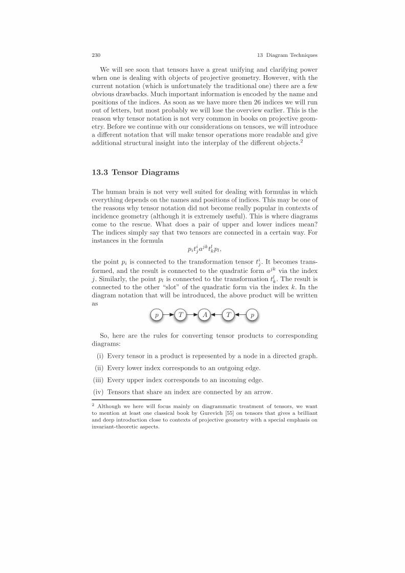
230 13 Diagram Techniques
We will see soon that tensors have a great unifying and clarifying powerwhen one is dealing with objects of projective geometry. However, with thecurrent notation (which is unfortunately the traditional one) there are a fewobvious drawbacks. Much important information is encoded by the name andpositions of the indices. As soon as we have more then 26 indices we will runout of letters, but most probably we will lose the overview earlier. This is thereason why tensor notation is not very common in books on projective geom-etry. Before we continue with our considerations on tensors, we will introducea different notation that will make tensor operations more readable and giveadditional structural insight into the interplay of the different objects.2
13.3 Tensor Diagrams
The human brain is not very well suited for dealing with formulas in whicheverything depends on the names and positions of indices. This may be one ofthe reasons why tensor notation did not become really popular in contexts ofincidence geometry (although it is extremely useful). This is where diagramscome to the rescue. What does a pair of upper and lower indices mean?The indices simply say that two tensors are connected in a certain way. Forinstances in the formula
pitijajktlkpl,
the point pi is connected to the transformation tensor tij . It becomes trans-
formed, and the result is connected to the quadratic form ajk via the indexj. Similarly, the point pl is connected to the transformation tlk. The result isconnected to the other “slot” of the quadratic form via the index k. In thediagram notation that will be introduced, the above product will be writtenas
pp T TA
So, here are the rules for converting tensor products to correspondingdiagrams:
(i) Every tensor in a product is represented by a node in a directed graph.
(ii) Every lower index corresponds to an outgoing edge.
(iii) Every upper index corresponds to an incoming edge.
(iv) Tensors that share an index are connected by an arrow.
2 Although we here will focus mainly on diagrammatic treatment of tensors, we wantto mention at least one classical book by Gurevich [55] on tensors that gives a brilliantand deep introduction close to contexts of projective geometry with a special emphasis oninvariant-theoretic aspects.
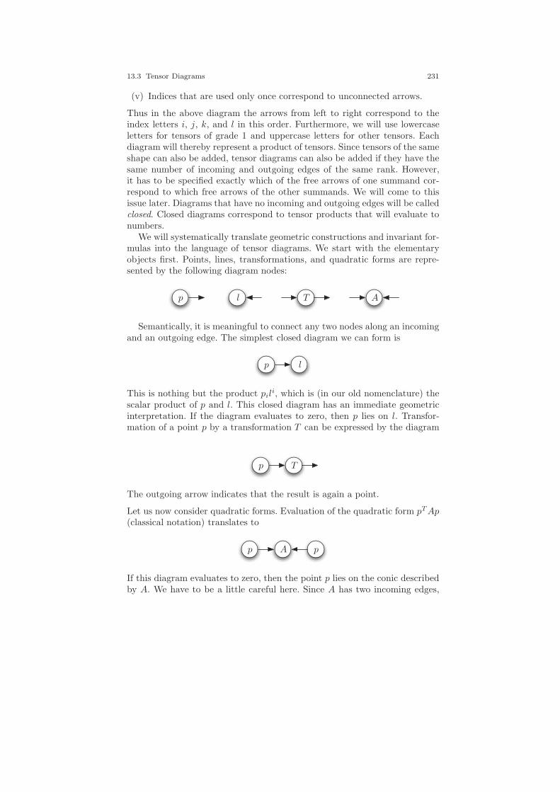
13.3 Tensor Diagrams 231
(v) Indices that are used only once correspond to unconnected arrows.
Thus in the above diagram the arrows from left to right correspond to theindex letters i, j, k, and l in this order. Furthermore, we will use lowercaseletters for tensors of grade 1 and uppercase letters for other tensors. Eachdiagram will thereby represent a product of tensors. Since tensors of the sameshape can also be added, tensor diagrams can also be added if they have thesame number of incoming and outgoing edges of the same rank. However,it has to be specified exactly which of the free arrows of one summand cor-respond to which free arrows of the other summands. We will come to thisissue later. Diagrams that have no incoming and outgoing edges will be calledclosed. Closed diagrams correspond to tensor products that will evaluate tonumbers.
We will systematically translate geometric constructions and invariant for-mulas into the language of tensor diagrams. We start with the elementaryobjects first. Points, lines, transformations, and quadratic forms are repre-sented by the following diagram nodes:
p l T A
Semantically, it is meaningful to connect any two nodes along an incomingand an outgoing edge. The simplest closed diagram we can form is
p l
This is nothing but the product pili, which is (in our old nomenclature) the
scalar product of p and l. This closed diagram has an immediate geometricinterpretation. If the diagram evaluates to zero, then p lies on l. Transfor-mation of a point p by a transformation T can be expressed by the diagram
p T
The outgoing arrow indicates that the result is again a point.
Let us now consider quadratic forms. Evaluation of the quadratic form pTAp(classical notation) translates to
p pA
If this diagram evaluates to zero, then the point p lies on the conic describedby A. We have to be a little careful here. Since A has two incoming edges,
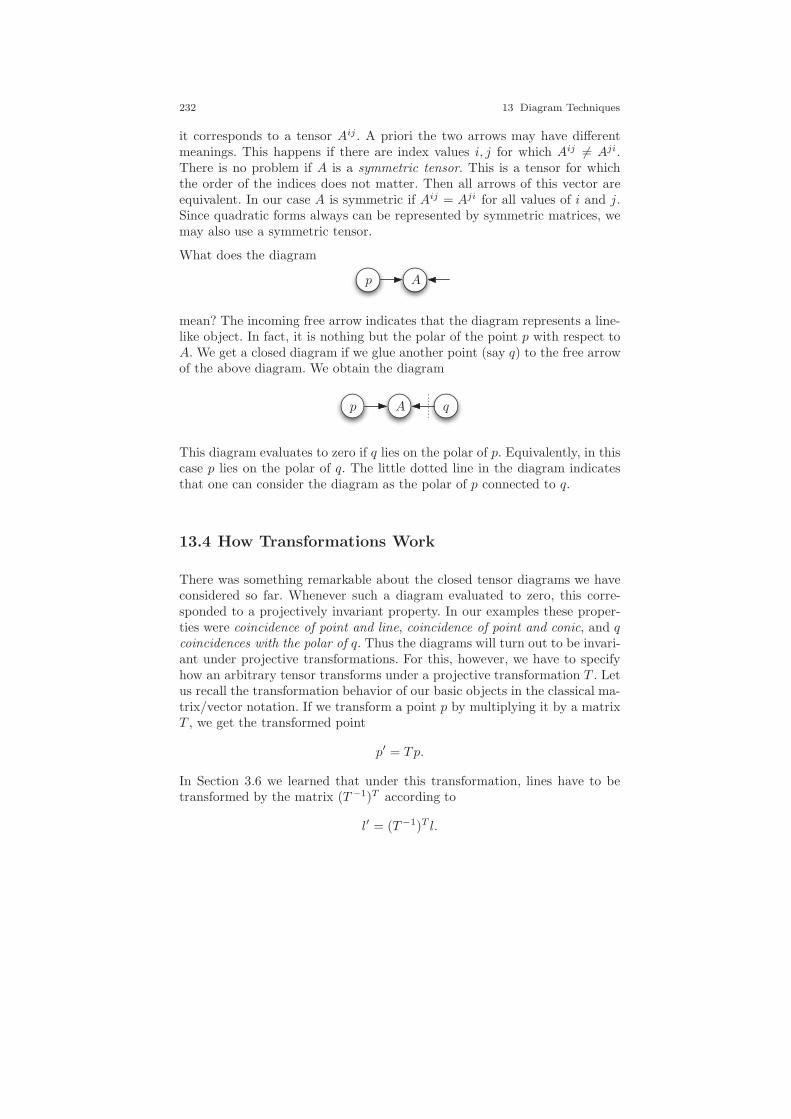
232 13 Diagram Techniques
it corresponds to a tensor Aij . A priori the two arrows may have differentmeanings. This happens if there are index values i, j for which Aij 6= Aji.There is no problem if A is a symmetric tensor. This is a tensor for whichthe order of the indices does not matter. Then all arrows of this vector areequivalent. In our case A is symmetric if Aij = Aji for all values of i and j.Since quadratic forms always can be represented by symmetric matrices, wemay also use a symmetric tensor.
What does the diagram
p A
mean? The incoming free arrow indicates that the diagram represents a line-like object. In fact, it is nothing but the polar of the point p with respect toA. We get a closed diagram if we glue another point (say q) to the free arrowof the above diagram. We obtain the diagram
p qA
This diagram evaluates to zero if q lies on the polar of p. Equivalently, in thiscase p lies on the polar of q. The little dotted line in the diagram indicatesthat one can consider the diagram as the polar of p connected to q.
13.4 How Transformations Work
There was something remarkable about the closed tensor diagrams we haveconsidered so far. Whenever such a diagram evaluated to zero, this corre-sponded to a projectively invariant property. In our examples these proper-ties were coincidence of point and line, coincidence of point and conic, and qcoincidences with the polar of q. Thus the diagrams will turn out to be invari-ant under projective transformations. For this, however, we have to specifyhow an arbitrary tensor transforms under a projective transformation T . Letus recall the transformation behavior of our basic objects in the classical ma-trix/vector notation. If we transform a point p by multiplying it by a matrixT , we get the transformed point
p′ = Tp.
In Section 3.6 we learned that under this transformation, lines have to betransformed by the matrix (T−1)T according to
l′ = (T−1)T l.
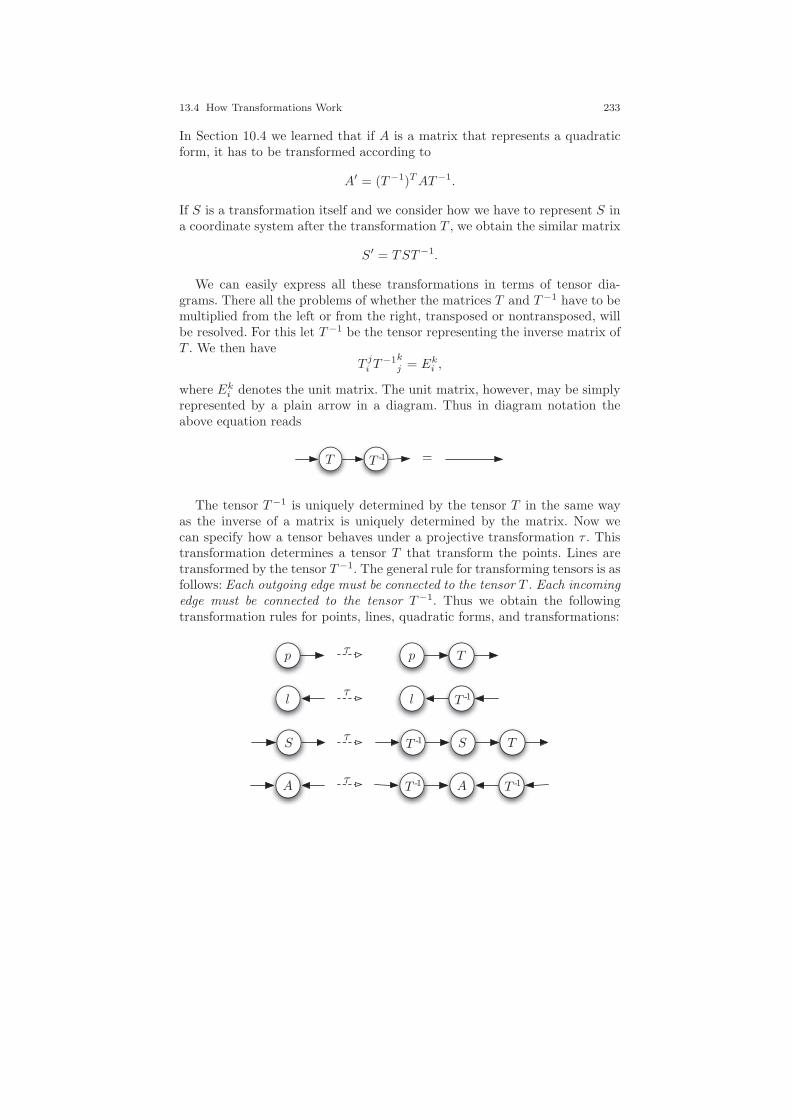
13.4 How Transformations Work 233
In Section 10.4 we learned that if A is a matrix that represents a quadraticform, it has to be transformed according to
A′ = (T−1)TAT−1.
If S is a transformation itself and we consider how we have to represent S ina coordinate system after the transformation T , we obtain the similar matrix
S′ = TST−1.
We can easily express all these transformations in terms of tensor dia-grams. There all the problems of whether the matrices T and T−1 have to bemultiplied from the left or from the right, transposed or nontransposed, willbe resolved. For this let T−1 be the tensor representing the inverse matrix ofT . We then have
T ji T−1k
j = Eki ,
where Eki denotes the unit matrix. The unit matrix, however, may be simplyrepresented by a plain arrow in a diagram. Thus in diagram notation theabove equation reads
T T -1 =
The tensor T−1 is uniquely determined by the tensor T in the same wayas the inverse of a matrix is uniquely determined by the matrix. Now wecan specify how a tensor behaves under a projective transformation τ . Thistransformation determines a tensor T that transform the points. Lines aretransformed by the tensor T−1. The general rule for transforming tensors is asfollows: Each outgoing edge must be connected to the tensor T . Each incomingedge must be connected to the tensor T−1. Thus we obtain the followingtransformation rules for points, lines, quadratic forms, and transformations:
p p
l l
τ
τ
τ
τ
S S
A A
T
T
T -1T -1
T -1
T -1
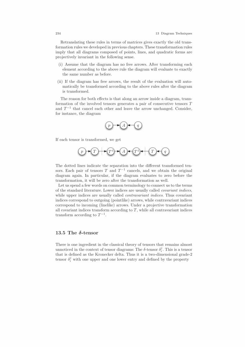
234 13 Diagram Techniques
Retranslating these rules in terms of matrices gives exactly the old trans-formation rules we developed in previous chapters. These transformation rulesimply that all diagrams composed of points, lines, and quadratic forms areprojectively invariant in the following sense.
(i) Assume that the diagram has no free arrows. After transforming eachelement according to the above rule the diagram will evaluate to exactlythe same number as before.
(ii) If the diagram has free arrows, the result of the evaluation will auto-matically be transformed according to the above rules after the diagramis transformed.
The reason for both effects is that along an arrow inside a diagram, trans-formation of the involved tensors generates a pair of consecutive tensors Tand T−1 that cancel each other and leave the arrow unchanged. Consider,for instance, the diagram
p qA
If each tensor is transformed, we get
p qA TT T -1T -1
The dotted lines indicate the separation into the different transformed ten-sors. Each pair of tensors T and T−1 cancels, and we obtain the originaldiagram again. In particular, if the diagram evaluates to zero before thetransformation, it will be zero after the transformation as well.
Let us spend a few words on common terminology to connect us to the termsof the standard literature. Lower indices are usually called covariant indices,while upper indices are usually called contravariant indices. Thus covariantindices correspond to outgoing (pointlike) arrows, while contravariant indicescorrespond to incoming (linelike) arrows. Under a projective transformationall covariant indices transform according to T , while all contravariant indicestransform according to T−1.
13.5 The δ-tensor
There is one ingredient in the classical theory of tensors that remains almostunnoticed in the context of tensor diagrams: The δ-tensor δji . This is a tensorthat is defined as the Kronecker delta. Thus it is a two-dimensional grade-2tensor δji with one upper and one lower entry and defined by the property
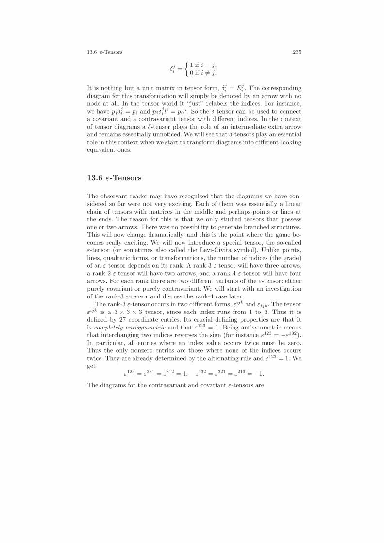
13.6 ε-Tensors 235
δji =
1 if i = j,0 if i 6= j.
It is nothing but a unit matrix in tensor form, δji = Eji . The correspondingdiagram for this transformation will simply be denoted by an arrow with nonode at all. In the tensor world it “just” relabels the indices. For instance,we have pjδ
ji = pi and pjδ
ji li = pil
i. So the δ-tensor can be used to connecta covariant and a contravariant tensor with different indices. In the contextof tensor diagrams a δ-tensor plays the role of an intermediate extra arrowand remains essentially unnoticed. We will see that δ-tensors play an essentialrole in this context when we start to transform diagrams into different-lookingequivalent ones.
13.6 ε-Tensors
The observant reader may have recognized that the diagrams we have con-sidered so far were not very exciting. Each of them was essentially a linearchain of tensors with matrices in the middle and perhaps points or lines atthe ends. The reason for this is that we only studied tensors that possessone or two arrows. There was no possibility to generate branched structures.This will now change dramatically, and this is the point where the game be-comes really exciting. We will now introduce a special tensor, the so-calledε-tensor (or sometimes also called the Levi-Civita symbol). Unlike points,lines, quadratic forms, or transformations, the number of indices (the grade)of an ε-tensor depends on its rank. A rank-3 ε-tensor will have three arrows,a rank-2 ε-tensor will have two arrows, and a rank-4 ε-tensor will have fourarrows. For each rank there are two different variants of the ε-tensor: eitherpurely covariant or purely contravariant. We will start with an investigationof the rank-3 ε-tensor and discuss the rank-4 case later.
The rank-3 ε-tensor occurs in two different forms, εijk and εijk. The tensorεijk is a 3 × 3 × 3 tensor, since each index runs from 1 to 3. Thus it isdefined by 27 coordinate entries. Its crucial defining properties are that itis completely antisymmetric and that ε123 = 1. Being antisymmetric meansthat interchanging two indices reverses the sign (for instance ε123 = −ε132).In particular, all entries where an index value occurs twice must be zero.Thus the only nonzero entries are those where none of the indices occurstwice. They are already determined by the alternating rule and ε123 = 1. Weget
ε123 = ε231 = ε312 = 1, ε132 = ε321 = ε213 = −1.
The diagrams for the contravariant and covariant ε-tensors are
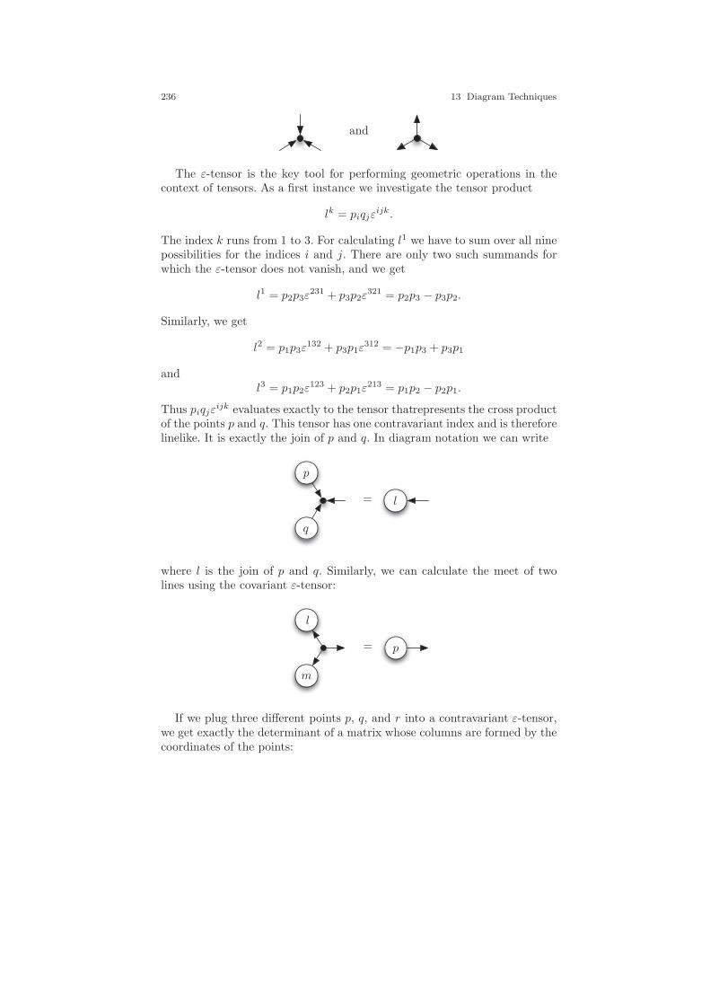
236 13 Diagram Techniques
and
The ε-tensor is the key tool for performing geometric operations in thecontext of tensors. As a first instance we investigate the tensor product
lk = piqjεijk.
The index k runs from 1 to 3. For calculating l1 we have to sum over all ninepossibilities for the indices i and j. There are only two such summands forwhich the ε-tensor does not vanish, and we get
l1 = p2p3ε231 + p3p2ε
321 = p2p3 − p3p2.
Similarly, we get
l2 = p1p3ε132 + p3p1ε
312 = −p1p3 + p3p1
andl3 = p1p2ε
123 + p2p1ε213 = p1p2 − p2p1.
Thus piqjεijk evaluates exactly to the tensor thatrepresents the cross product
of the points p and q. This tensor has one contravariant index and is thereforelinelike. It is exactly the join of p and q. In diagram notation we can write
p
q
l=
where l is the join of p and q. Similarly, we can calculate the meet of twolines using the covariant ε-tensor:
p
m
l
=
If we plug three different points p, q, and r into a contravariant ε-tensor,we get exactly the determinant of a matrix whose columns are formed by thecoordinates of the points:
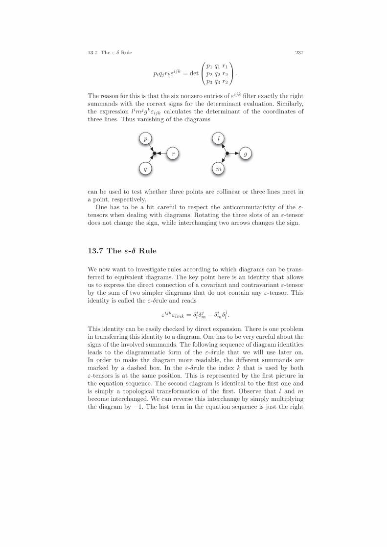
13.7 The ε-δ Rule 237
piqjrkεijk = det
p1 q1 r1p2 q2 r2p3 q3 r2
.
The reason for this is that the six nonzero entries of εijk filter exactly the rightsummands with the correct signs for the determinant evaluation. Similarly,the expression limjgkεijk calculates the determinant of the coordinates ofthree lines. Thus vanishing of the diagrams
p
q
r
m
l
g
can be used to test whether three points are collinear or three lines meet ina point, respectively.
One has to be a bit careful to respect the anticommutativity of the ε-tensors when dealing with diagrams. Rotating the three slots of an ε-tensordoes not change the sign, while interchanging two arrows changes the sign.
13.7 The ε-δ Rule
We now want to investigate rules according to which diagrams can be trans-ferred to equivalent diagrams. The key point here is an identity that allowsus to express the direct connection of a covariant and contravariant ε-tensorby the sum of two simpler diagrams that do not contain any ε-tensor. Thisidentity is called the ε-δrule and reads
εijkεlmk = δilδjm − δimδ
jl .
This identity can be easily checked by direct expansion. There is one problemin transferring this identity to a diagram. One has to be very careful about thesigns of the involved summands. The following sequence of diagram identitiesleads to the diagrammatic form of the ε-δrule that we will use later on.In order to make the diagram more readable, the different summands aremarked by a dashed box. In the ε-δrule the index k that is used by bothε-tensors is at the same position. This is represented by the first picture inthe equation sequence. The second diagram is identical to the first one andis simply a topological transformation of the first. Observe that l and mbecome interchanged. We can reverse this interchange by simply multiplyingthe diagram by −1. The last term in the equation sequence is just the right
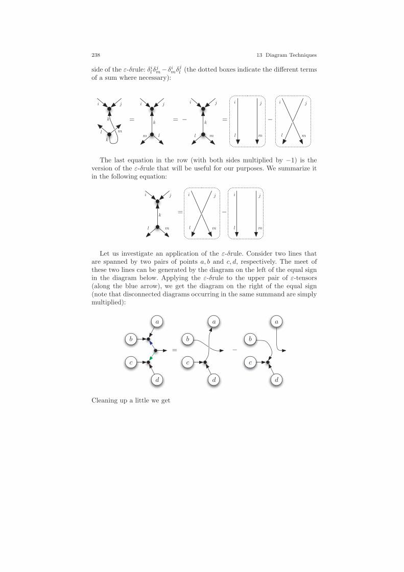
238 13 Diagram Techniques
side of the ε-δrule: δilδjm−δimδjl (the dotted boxes indicate the different terms
of a sum where necessary):
iiiii jjjjj
kk
k
k
lllll
mm mmm
−− ===
The last equation in the row (with both sides multiplied by −1) is theversion of the ε-δrule that will be useful for our purposes. We summarize itin the following equation:
i ii j jj
k
l ll mm m
−=
Let us investigate an application of the ε-δrule. Consider two lines thatare spanned by two pairs of points a, b and c, d, respectively. The meet ofthese two lines can be generated by the diagram on the left of the equal signin the diagram below. Applying the ε-δrule to the upper pair of ε-tensors(along the blue arrow), we get the diagram on the right of the equal sign(note that disconnected diagrams occurring in the same summand are simplymultiplied):
aaa
bbb
ccc
ddd
−=
Cleaning up a little we get

13.8 Transforming ε-Tensors 239
aa bb
cc dd
−
In terms of bracket algebra this diagram means nothing but
[acd]b− [bcd]a.
This this is exactly the bracket expression for this situation we derived inSection 6.3 using Pluckers µ. Equivalently, we could have performed thesame split along the green arrow. Then we would get the following equivalentexpression for the meet:
aa
bb c
c d
d
−
Since both expressions must be equivalent, we can also combine them intoone equation and obtain
a a a a
b b
b b
c
c
c c
d
d d d
−− + 0=
This is just Cramer’s rule as we encountered it in Section 6.6. Pluggingthe join of two points e and f into all open arrows, we get the four-summandGrassmann-Plucker-Relation.
13.8 Transforming ε-Tensors
We have seen that diagrams containing ε-tensors also create geometricallymeaningful expressions. The deep reason for this is that ε-tensors behavewell under projective transformations. Applying a projective transformationto an ε-tensor simply results in a tensor that is a multiple of the ε-tensor.The scaling factor is the determinant of the transformation matrix. Thus wehave
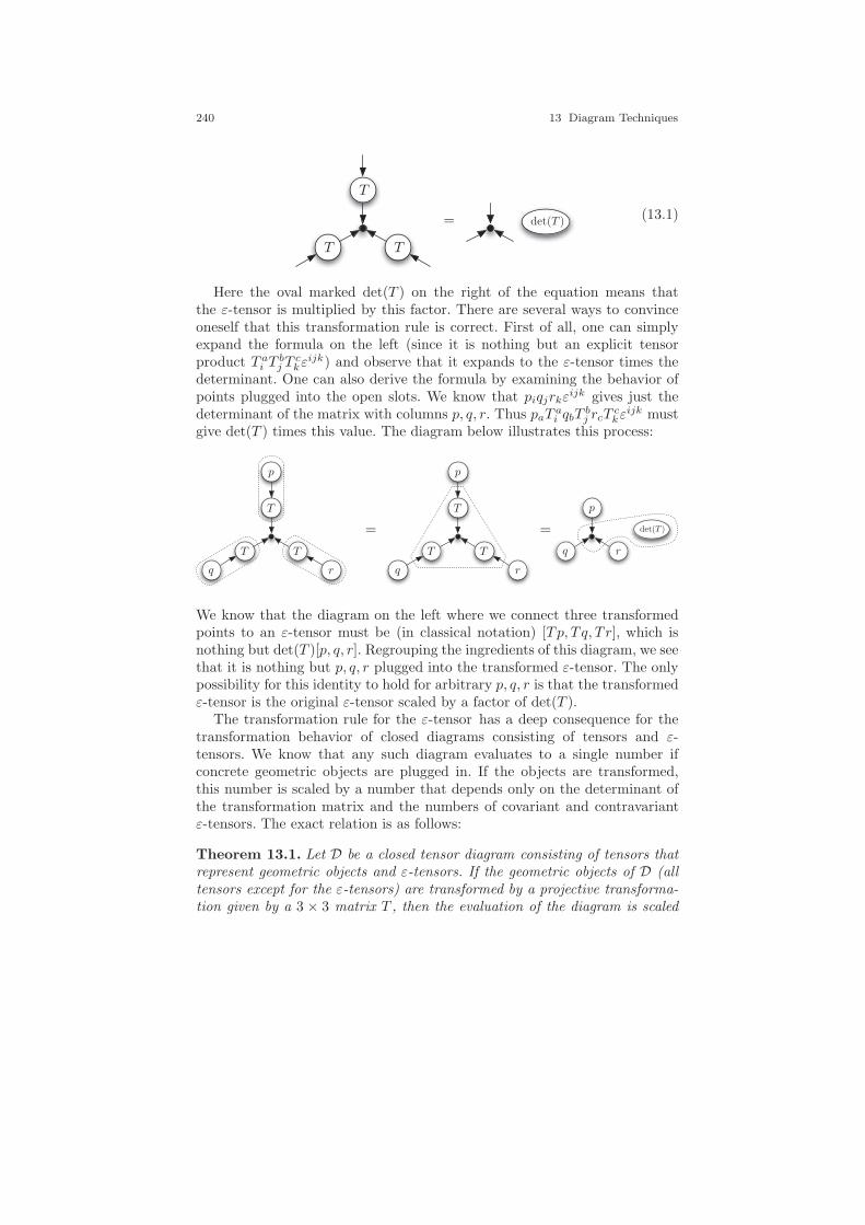
240 13 Diagram Techniques
T
T
T
det(T )= (13.1)
Here the oval marked det(T ) on the right of the equation means thatthe ε-tensor is multiplied by this factor. There are several ways to convinceoneself that this transformation rule is correct. First of all, one can simplyexpand the formula on the left (since it is nothing but an explicit tensorproduct T ai T
bj T
ckεijk) and observe that it expands to the ε-tensor times the
determinant. One can also derive the formula by examining the behavior ofpoints plugged into the open slots. We know that piqjrkε
ijk gives just thedeterminant of the matrix with columns p, q, r. Thus paT
ai qbT
bj rcT
ckεijk must
give det(T ) times this value. The diagram below illustrates this process:
T
T
TT
T
T
p
pp
q
r
rr
det(T )==
We know that the diagram on the left where we connect three transformedpoints to an ε-tensor must be (in classical notation) [Tp, T q, T r], which isnothing but det(T )[p, q, r]. Regrouping the ingredients of this diagram, we seethat it is nothing but p, q, r plugged into the transformed ε-tensor. The onlypossibility for this identity to hold for arbitrary p, q, r is that the transformedε-tensor is the original ε-tensor scaled by a factor of det(T ).
The transformation rule for the ε-tensor has a deep consequence for thetransformation behavior of closed diagrams consisting of tensors and ε-tensors. We know that any such diagram evaluates to a single number ifconcrete geometric objects are plugged in. If the objects are transformed,this number is scaled by a number that depends only on the determinant ofthe transformation matrix and the numbers of covariant and contravariantε-tensors. The exact relation is as follows:
Theorem 13.1. Let D be a closed tensor diagram consisting of tensors thatrepresent geometric objects and ε-tensors. If the geometric objects of D (alltensors except for the ε-tensors) are transformed by a projective transforma-tion given by a 3 × 3 matrix T , then the evaluation of the diagram is scaled

13.8 Transforming ε-Tensors 241
by a factor det(T )k, where k is the difference of covariant and contravariantε-tensors.
Proof. Rather than giving a strictly formal proof, we confine ourselves hereto a “proof by example” that exemplifies the main principles in diagramnotation. We consider the following diagram, which consists of four points,one line, and three ε-tensors (two of them are contravariant and two of themare covariant):
p
q r
s
l
How does the evaluation change if we transform the geometric objectsby a projective transformation given by the pair (T, T−1)? Covariant arrows(our points) of geometric objects have to be transformed by T , contravariantarrows (our lines) have to be transformed by T−1, and we obtain
T
TT
T
T -1p
q r
s
l
For evaluating this diagram we “blow up” the interior arrows by replacingthem by a pair of transformations T -1 T . After this procedure our dia-gram looks as follows:
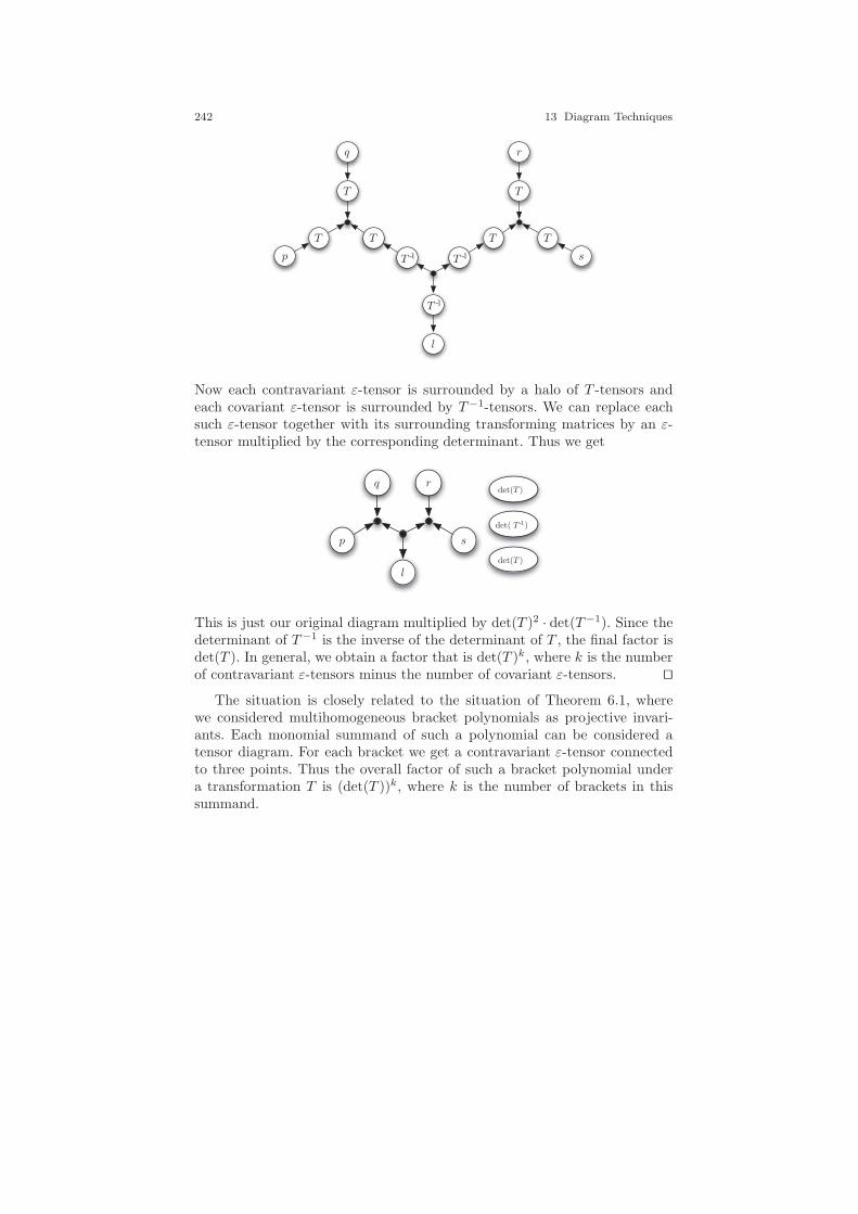
242 13 Diagram Techniques
TT T
TT
T
T -1T -1
T -1
p
q r
s
l
Now each contravariant ε-tensor is surrounded by a halo of T -tensors andeach covariant ε-tensor is surrounded by T−1-tensors. We can replace eachsuch ε-tensor together with its surrounding transforming matrices by an ε-tensor multiplied by the corresponding determinant. Thus we get
p
q r
s
ldet(T )
det(T )
det( T -1)
This is just our original diagram multiplied by det(T )2 · det(T−1). Since thedeterminant of T−1 is the inverse of the determinant of T , the final factor isdet(T ). In general, we obtain a factor that is det(T )k, where k is the numberof contravariant ε-tensors minus the number of covariant ε-tensors. ⊓⊔
The situation is closely related to the situation of Theorem 6.1, wherewe considered multihomogeneous bracket polynomials as projective invari-ants. Each monomial summand of such a polynomial can be considered atensor diagram. For each bracket we get a contravariant ε-tensor connectedto three points. Thus the overall factor of such a bracket polynomial undera transformation T is (det(T ))k, where k is the number of brackets in thissummand.
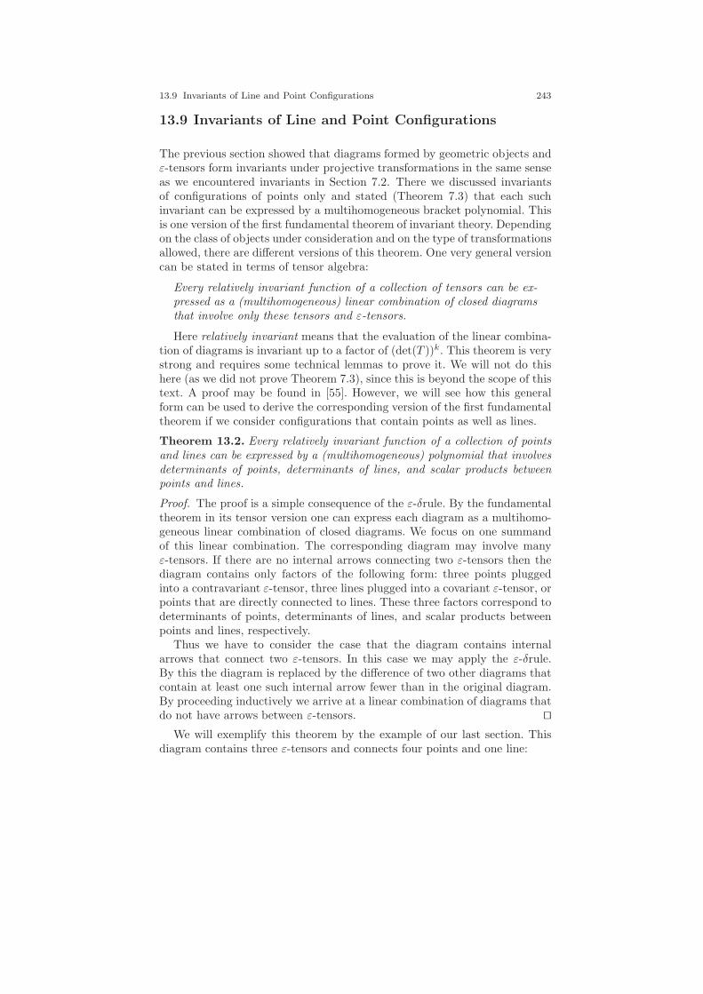
13.9 Invariants of Line and Point Configurations 243
13.9 Invariants of Line and Point Configurations
The previous section showed that diagrams formed by geometric objects andε-tensors form invariants under projective transformations in the same senseas we encountered invariants in Section 7.2. There we discussed invariantsof configurations of points only and stated (Theorem 7.3) that each suchinvariant can be expressed by a multihomogeneous bracket polynomial. Thisis one version of the first fundamental theorem of invariant theory. Dependingon the class of objects under consideration and on the type of transformationsallowed, there are different versions of this theorem. One very general versioncan be stated in terms of tensor algebra:
Every relatively invariant function of a collection of tensors can be ex-pressed as a (multihomogeneous) linear combination of closed diagramsthat involve only these tensors and ε-tensors.
Here relatively invariant means that the evaluation of the linear combina-tion of diagrams is invariant up to a factor of (det(T ))k. This theorem is verystrong and requires some technical lemmas to prove it. We will not do thishere (as we did not prove Theorem 7.3), since this is beyond the scope of thistext. A proof may be found in [55]. However, we will see how this generalform can be used to derive the corresponding version of the first fundamentaltheorem if we consider configurations that contain points as well as lines.
Theorem 13.2. Every relatively invariant function of a collection of pointsand lines can be expressed by a (multihomogeneous) polynomial that involvesdeterminants of points, determinants of lines, and scalar products betweenpoints and lines.
Proof. The proof is a simple consequence of the ε-δrule. By the fundamentaltheorem in its tensor version one can express each diagram as a multihomo-geneous linear combination of closed diagrams. We focus on one summandof this linear combination. The corresponding diagram may involve manyε-tensors. If there are no internal arrows connecting two ε-tensors then thediagram contains only factors of the following form: three points pluggedinto a contravariant ε-tensor, three lines plugged into a covariant ε-tensor, orpoints that are directly connected to lines. These three factors correspond todeterminants of points, determinants of lines, and scalar products betweenpoints and lines, respectively.
Thus we have to consider the case that the diagram contains internalarrows that connect two ε-tensors. In this case we may apply the ε-δrule.By this the diagram is replaced by the difference of two other diagrams thatcontain at least one such internal arrow fewer than in the original diagram.By proceeding inductively we arrive at a linear combination of diagrams thatdo not have arrows between ε-tensors. ⊓⊔
We will exemplify this theorem by the example of our last section. Thisdiagram contains three ε-tensors and connects four points and one line:
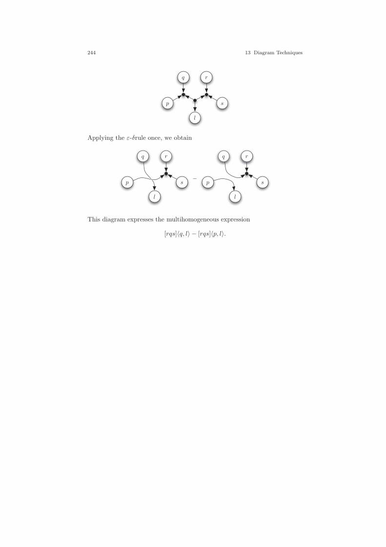
244 13 Diagram Techniques
p
q r
s
l
Applying the ε-δrule once, we obtain
pp
qq rr
ss
ll
−
This diagram expresses the multihomogeneous expression
[rqs]〈q, l〉 − [rqs]〈p, l〉.
14
Working with diagrams
When the proofs, the figure,were ranged in columns before me,
When I was shown the charts and diagrams,to add, divide, and measure them,. . .
Two lines of a poem by Walt Whitman (1819–1892)
The value of diagram techniques even at this rudimentarylevel should be clear by now: it is easier to visualize where sim-plifications may be found in a complicated network by search-ing for a reducible linkage than by examining a complicatedalgebraic expression.
Geoffrey E. Stedman,Diagram Techniques in Group Theory (1990)
So much for the preliminaries. Now let us come to the real stuff about dia-grams. In this chapter we will investigate more advanced applications of ten-sors and diagrams. In particular, we will link tensor diagrams more closely togeometric theorems and concepts we encountered in previous chapters. Theinvariant character of closed diagrams and the ε-δ rule will play a prominentrole in this context. Moreover, we will revisit the theorems of Pappos andPascal once again.
245
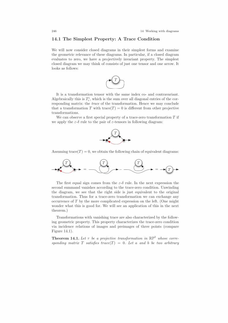
246 14 Working with diagrams
14.1 The Simplest Property: A Trace Condition
We will now consider closed diagrams in their simplest forms and examinethe geometric relevance of these diagrams. In particular, if a closed diagramevaluates to zero, we have a projectively invariant property. The simplestclosed diagram we may think of consists of just one tensor and one arrow. Itlooks as follows:
T
It is a transformation tensor with the same index co- and contravariant.Algebraically this is T ii , which is the sum over all diagonal entries of the cor-responding matrix: the trace of the transformation. Hence we may concludethat a transformation T with trace(T ) = 0 is different from other projectivetransformations.
We can observe a first special property of a trace-zero transformation T ifwe apply the ε-δ rule to the pair of ε-tensors in following diagram:
T
Assuming trace(T ) = 0, we obtain the following chain of equivalent diagrams:
T
TTT
− ==
The first equal sign comes from the ε-δ rule. In the next expression thesecond summand vanishes according to the trace-zero condition. Unwindingthe diagram, we see that the right side is just equivalent to the originaltransformation. Thus for a trace-zero transformation we can exchange anyoccurrence of T by the more complicated expression on the left. (One mightwonder what this is good for. We will see an application of this in the nexttheorem.)
Transformations with vanishing trace are also characterized by the follow-ing geometric property. This property characterizes the trace-zero conditionvia incidence relations of images and preimages of three points (compareFigure 14.1).
Theorem 14.1. Let τ be a projective transformation in RP2 whose corre-
sponding matrix T satisfies trace(T ) = 0. Let a and b be two arbitrary
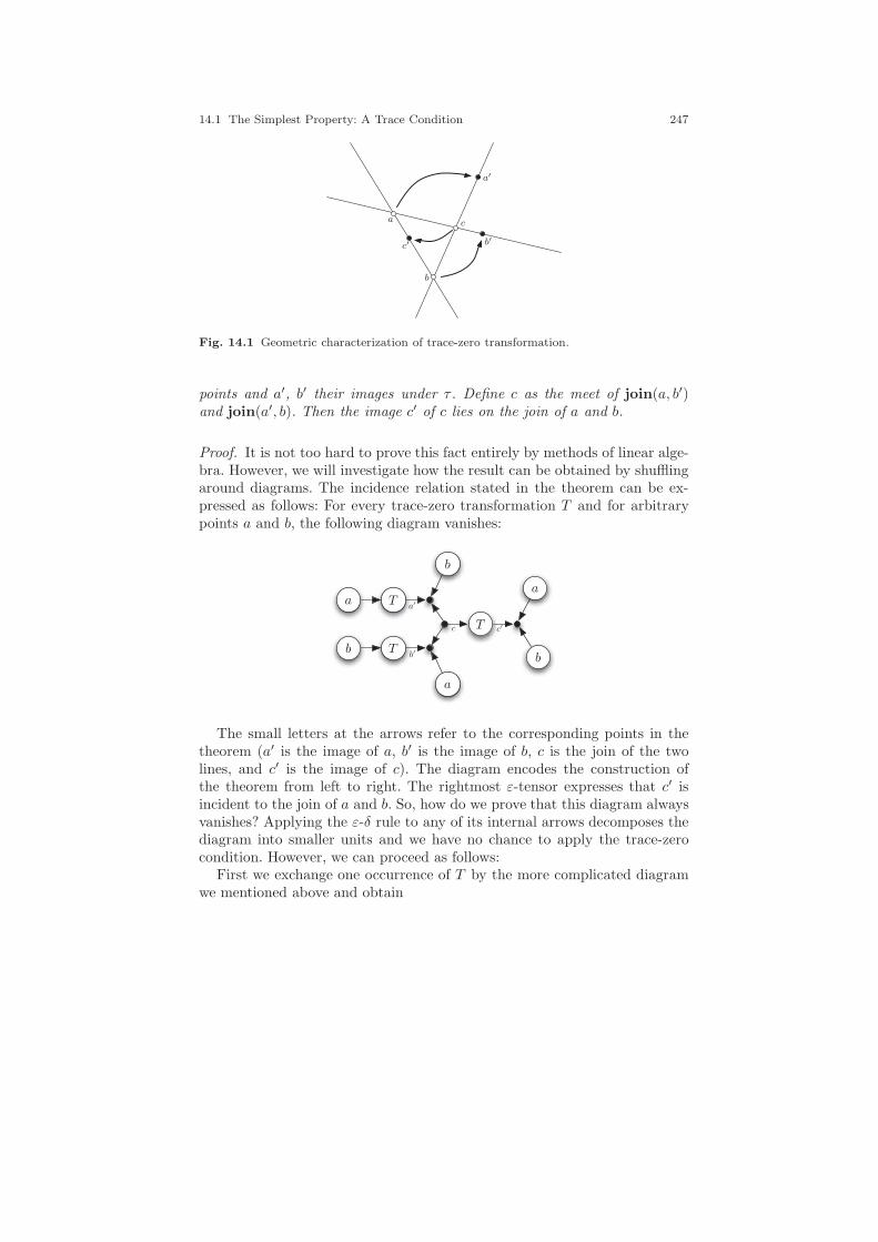
14.1 The Simplest Property: A Trace Condition 247
a
b
c
a′
b′c′
Fig. 14.1 Geometric characterization of trace-zero transformation.
points and a′, b′ their images under τ . Define c as the meet of join(a, b′)and join(a′, b). Then the image c′ of c lies on the join of a and b.
Proof. It is not too hard to prove this fact entirely by methods of linear alge-bra. However, we will investigate how the result can be obtained by shufflingaround diagrams. The incidence relation stated in the theorem can be ex-pressed as follows: For every trace-zero transformation T and for arbitrarypoints a and b, the following diagram vanishes:
aa
a
bb
b
c
a′
b′
c′T
T
T
The small letters at the arrows refer to the corresponding points in thetheorem (a′ is the image of a, b′ is the image of b, c is the join of the twolines, and c′ is the image of c). The diagram encodes the construction ofthe theorem from left to right. The rightmost ε-tensor expresses that c′ isincident to the join of a and b. So, how do we prove that this diagram alwaysvanishes? Applying the ε-δ rule to any of its internal arrows decomposes thediagram into smaller units and we have no chance to apply the trace-zerocondition. However, we can proceed as follows:
First we exchange one occurrence of T by the more complicated diagramwe mentioned above and obtain
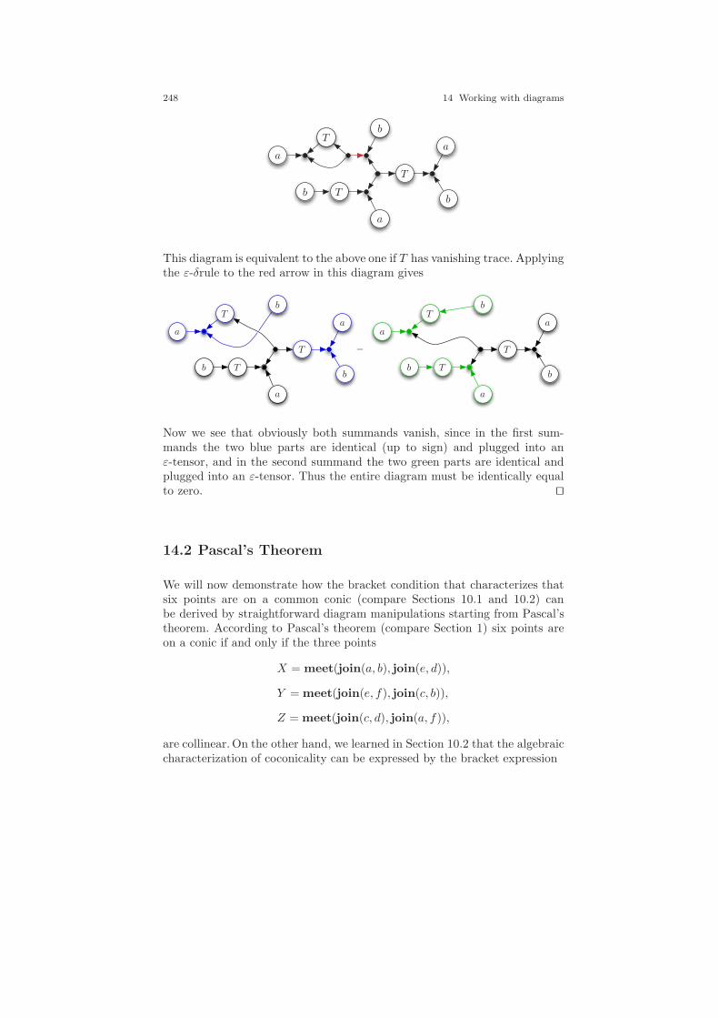
248 14 Working with diagrams
aa
a
bb
bT
T
T
This diagram is equivalent to the above one if T has vanishing trace. Applyingthe ε-δrule to the red arrow in this diagram gives
aa
a
aa
a
bb
b
bb
bT
T
T
T
T
T
−
Now we see that obviously both summands vanish, since in the first sum-mands the two blue parts are identical (up to sign) and plugged into anε-tensor, and in the second summand the two green parts are identical andplugged into an ε-tensor. Thus the entire diagram must be identically equalto zero. ⊓⊔
14.2 Pascal’s Theorem
We will now demonstrate how the bracket condition that characterizes thatsix points are on a common conic (compare Sections 10.1 and 10.2) canbe derived by straightforward diagram manipulations starting from Pascal’stheorem. According to Pascal’s theorem (compare Section 1) six points areon a conic if and only if the three points
X = meet(join(a, b), join(e, d)),
Y = meet(join(e, f), join(c, b)),
Z = meet(join(c, d), join(a, f)),
are collinear. On the other hand, we learned in Section 10.2 that the algebraiccharacterization of coconicality can be expressed by the bracket expression
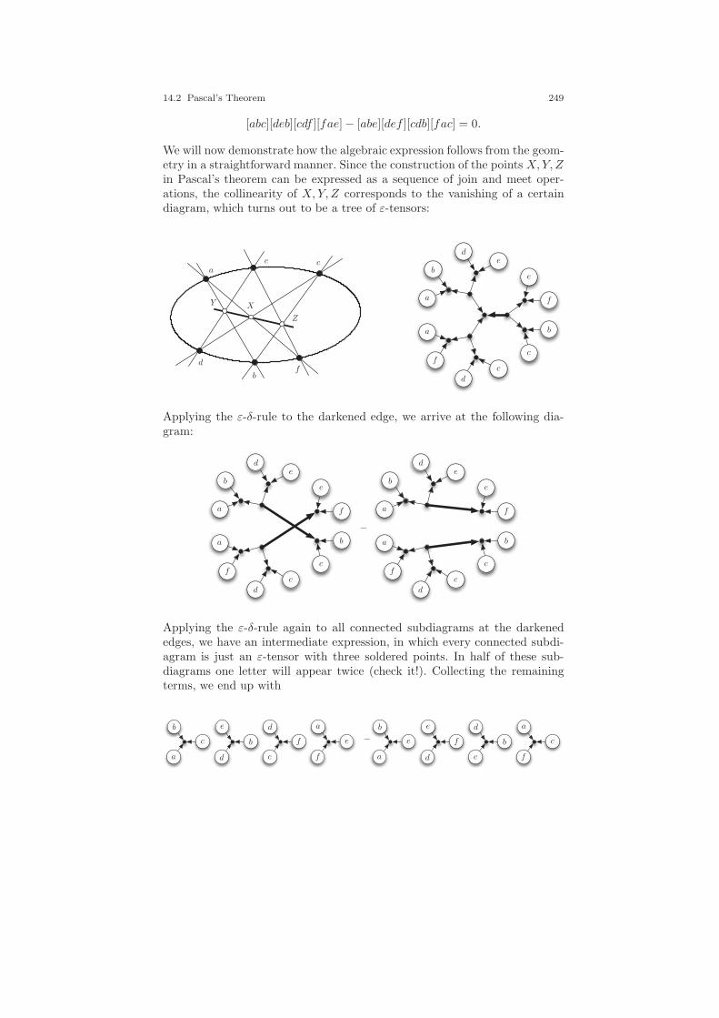
14.2 Pascal’s Theorem 249
[abc][deb][cdf ][fae]− [abe][def ][cdb][fac] = 0.
We will now demonstrate how the algebraic expression follows from the geom-etry in a straightforward manner. Since the construction of the points X,Y, Zin Pascal’s theorem can be expressed as a sequence of join and meet oper-ations, the collinearity of X,Y, Z corresponds to the vanishing of a certaindiagram, which turns out to be a tree of ε-tensors:
ae c
d
bf
Y X
Z
a
a
b
b
c
c
d
de
e
f
f
Applying the ε-δ-rule to the darkened edge, we arrive at the following dia-gram:
a
a
a
a
b
b
b
b
c
c
c
c
d
d
d
de
e
e
e
f
f
f
f
−
Applying the ε-δ-rule again to all connected subdiagrams at the darkenededges, we have an intermediate expression, in which every connected subdi-agram is just an ε-tensor with three soldered points. In half of these sub-diagrams one letter will appear twice (check it!). Collecting the remainingterms, we end up with
a
a
a
a
b
b
b
b
c
cc
c
d
d
d
d
e
ee
e
f
f
f
f −

250 14 Working with diagrams
This is exactly the characterization of coconicality we were heading after:
[abc][deb][cdf ][fae]− [abe][def ][cdb][fac] = 0.
Conversely (if one assumes this expression as given), one can read the di-agrammatic calculations in the opposite directions and interpret them as aproof of Pascal’s theorem.
14.3 Closed ε-Cycles
As a further example let us consider closed rings of ε-tensors (alternately co-and contravariant) and investigate their geometric meaning under variousaspects. Since all our arrows are directed, the number of ε-tensors has to beeven, in order to get a closed cycle:
. . .
As a first instance, we will consider the meaning of a 2-cycle. This littlegadget will turn out to be useful as an auxiliary calculation that will be neededin order to simplify the diagrams later on. The calculation is presented in thefollowing diagram and explains how double arrows between ε-tensors can bereplaced by a single arrow and a factor:
= = = =−− 3 −2 (14.1)
The first equality is just a topological deformation; the second is an applica-tion of the ε-δ rule. The third equality is due to the fact that the closed loop
= δii = 3 is nothing but the trace of the unit matrix (here the dimensionenters the calculation as a number).
Let us now consider larger cycles. Each of these cycles has an alternat-ing sequence of incoming and outgoing arrows along the boundary. We willanalyze the cases in which we attach points and lines in an alternating man-ner. The vanishing of such a cycle encodes a projective condition that mustbe fulfilled by the points and lines that are involved. For each cycle we will
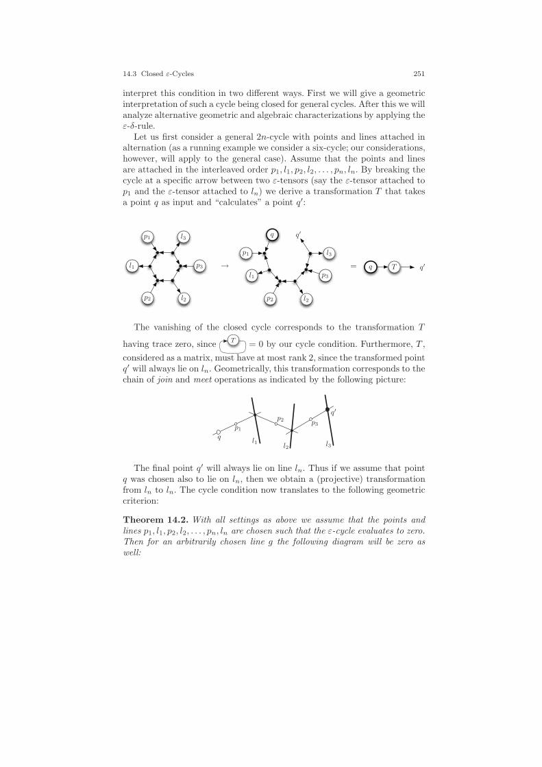
14.3 Closed ε-Cycles 251
interpret this condition in two different ways. First we will give a geometricinterpretation of such a cycle being closed for general cycles. After this we willanalyze alternative geometric and algebraic characterizations by applying theε-δ-rule.
Let us first consider a general 2n-cycle with points and lines attached inalternation (as a running example we consider a six-cycle; our considerations,however, will apply to the general case). Assume that the points and linesare attached in the interleaved order p1, l1, p2, l2, . . . , pn, ln. By breaking thecycle at a specific arrow between two ε-tensors (say the ε-tensor attached top1 and the ε-tensor attached to ln) we derive a transformation T that takesa point q as input and “calculates” a point q′:
p1
p1
p2p2
p3
p3
l1
l1
l2l2
l3
l3
q
q
q′
q′
T→ =
The vanishing of the closed cycle corresponds to the transformation T
having trace zero, since T = 0 by our cycle condition. Furthermore, T ,
considered as a matrix, must have at most rank 2, since the transformed pointq′ will always lie on ln. Geometrically, this transformation corresponds to thechain of join and meet operations as indicated by the following picture:
p1
p2 p3
l1l2 l3
q
q′
The final point q′ will always lie on line ln. Thus if we assume that pointq was chosen also to lie on ln, then we obtain a (projective) transformationfrom ln to ln. The cycle condition now translates to the following geometriccriterion:
Theorem 14.2. With all settings as above we assume that the points andlines p1, l1, p2, l2, . . . , pn, ln are chosen such that the ε-cycle evaluates to zero.Then for an arbitrarily chosen line g the following diagram will be zero aswell:
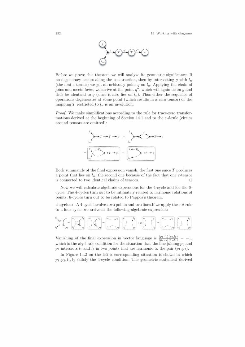
252 14 Working with diagrams
g
g
ln
q q′ q′′
TT
Before we prove this theorem we will analyze its geometric significance. Ifno degeneracy occurs along the construction, then by intersecting g with ln(the first ε-tensor) we get an arbitrary point q on ln. Applying the chain ofjoins and meets twice, we arrive at the point q′′, which will again lie on g andthus be identical to q (since it also lies on ln). Thus either the sequence ofoperations degenerates at some point (which results in a zero tensor) or themapping T restricted to ln is an involution.
Proof. We make simplifications according to the rule for trace-zero transfor-mations derived at the beginning of Section 14.1 and to the ε-δ-rule (circlesaround tensors are omitted):
g
g
g
g
g
g
g
g
lnln
lnln
T
T
TT
TT
TT
−=
=
Both summands of the final expression vanish, the first one since T producesa point that lies on ln, the second one because of the fact that one ε-tensoris connected to two identical chains of tensors. ⊓⊔
Now we will calculate algebraic expressions for the 4-cycle and for the 6-cycle. The 4-cycles turn out to be intimately related to harmonic relations ofpoints; 6-cycles turn out to be related to Pappos’s theorem.
4-cycles: A 4-cycle involves two points and two lines.If we apply the ε-δ-ruleto a four-cycle, we arrive at the following algebraic expression:
l1l1l1l1l1l1l1l1
l2l2l2l2l2l2l2l2 p1p1p1p1p1p1p1p1
p2p2p2p2p2p2p2p2
−− ++ === 2
Vanishing of the final expression in vector language is 〈p1,l1〉〈p2,l2〉〈p1,l2〉〈p2,l1〉 = −1,
which is the algebraic condition for the situation that the line joining p1 andp2 intersects l1 and l2 in two points that are harmonic to the pair (p1, p2).
In Figure 14.2 on the left a corresponding situation is shown in whichp1, p2, l1, l2 satisfy the 4-cycle condition. The geometric statement derived
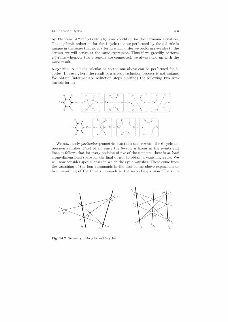
14.3 Closed ε-Cycles 253
by Theorem 14.2 reflects the algebraic condition for the harmonic situation.The algebraic reduction for the 4-cycle that we performed by the ε-δ-rule isunique in the sense that no matter in which order we perform ε-δ-rules to thearrows, we will arrive at the same expression. Thus if we greedily performε-δ-rules whenever two ε-tensors are connected, we always end up with thesame result.
6-cycles: A similar calculation to the one above can be performed for 6-cycles. However, here the result of a greedy reduction process is not unique.We obtain (intermediate reduction steps omitted) the following two irre-ducible forms:
l1l1l1l1l1
l2l2l2l2l2
l3l3l3l3l3 p1p1p1p1p1
p2p2p2p2p2
p3p3p3p3p3 −−−=
l1l1l1l1
l2l2l2l2
l3l3l3l3 p1p1p1p1
p2p2p2p2
p3p3p3p3 −−=
We now study particular geometric situations under which the 6-cycle ex-pression vanishes. First of all, since the 6-cycle is linear in the points andlines, it follows that for every position of five of the elements there is at leasta one-dimensional space for the final object to obtain a vanishing cycle. Wewill now consider special cases in which the cycle vanishes. These come fromthe vanishing of the four summands in the first of the above expansions orfrom vanishing of the three summands in the second expansion. The sum-
l1l2
p1
p2
q
l1l2
p1
p2
l3
p3
q
Fig. 14.2 Geometry of 4-cycles and 6-cycles.
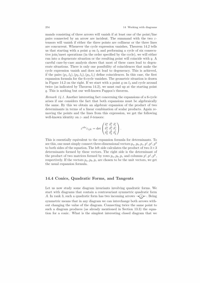
254 14 Working with diagrams
mands consisting of three arrows will vanish if at least one of the point/linepairs connected by an arrow are incident. The summand with the two ε-tensors will vanish if either the three points are collinear or the three linesare concurrent. Whenever the cycle expression vanishes, Theorem 14.2 tellsus that starting with a point q on l3 and performing a cycle of six consecu-tive join/meet operations (in the order specified by the cycle), we will eitherrun into a degenerate situation or the resulting point will coincide with q. Acareful case-by-case analysis shows that most of these cases lead to degen-erate situations. There is only one possibility of coincidences that make thecycle expression vanish and does not lead to degeneracy. This is achieved,if the pairs (p1, l2), (p2, l3), (p3, l1) define coincidences. In this case, the firstexpansion formula for the 6-cycle vanishes. The geometric situation is drawnin Figure 14.2 on the right. If we start with a point q on l3 and cycle aroundtwice (as indicated by Theorem 14.2), we must end up at the starting pointq. This is nothing but our well-known Pappos’s theorem.
Remark 14.1. Another interesting fact concerning the expansions of a 6-cyclearises if one considers the fact that both expansions must be algebraicallythe same. By this we obtain an algebraic expansion of the product of twodeterminants in terms of a linear combination of scalar products. Again re-moving the points and the lines from this expression, we get the followingwell-known identity on ε- and δ-tensors:
εabcεijk = det
δai δ
bi δ
ci
δaj δbj δ
cj
δak δbk δ
ck
.
This is essentially equivalent to the expansion formula for determinants. Tosee this, one must simply connect three-dimensional vectors pa, pb, pc, p
i, pj, pk
to both sides of the equation. The left side calculates the product of two 3×3determinants formed by these vectors. The right side is the determinant ofthe product of two matrices formed by rows pa, pb, pc and columns pi, pj, pk,respectively. If the vectors pa, pb, pc are chosen to be the unit vectors, we getthe usual expansion formula.
14.4 Conics, Quadratic Forms, and Tangents
Let us now study some diagram invariants involving quadratic forms. Westart with diagrams that contain a contravariant symmetric quadratic formA. In rank 3, such a quadratic form has two incoming arrows A . Being
symmetric means that in any diagram we can interchange both arrows with-out changing the value of the diagram. Connecting twice the same point tosuch a diagram produces (as already mentioned in Section 13.3) the equa-tion for a conic. What is the simplest interesting closed diagram that we
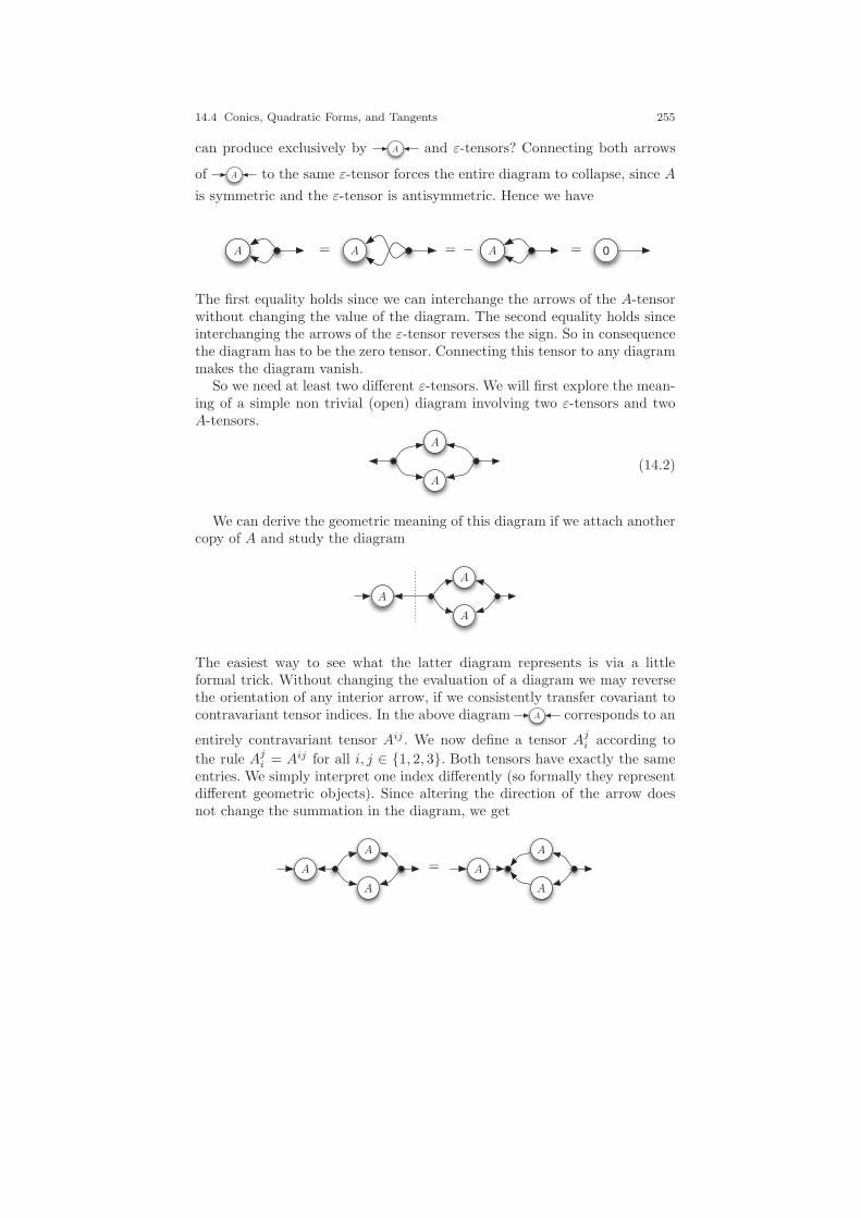
14.4 Conics, Quadratic Forms, and Tangents 255
can produce exclusively by A and ε-tensors? Connecting both arrows
of A to the same ε-tensor forces the entire diagram to collapse, since A
is symmetric and the ε-tensor is antisymmetric. Hence we have
0AAA − ===
The first equality holds since we can interchange the arrows of the A-tensorwithout changing the value of the diagram. The second equality holds sinceinterchanging the arrows of the ε-tensor reverses the sign. So in consequencethe diagram has to be the zero tensor. Connecting this tensor to any diagrammakes the diagram vanish.
So we need at least two different ε-tensors. We will first explore the mean-ing of a simple non trivial (open) diagram involving two ε-tensors and twoA-tensors.
A
A
(14.2)
We can derive the geometric meaning of this diagram if we attach anothercopy of A and study the diagram
A
A
A
The easiest way to see what the latter diagram represents is via a littleformal trick. Without changing the evaluation of a diagram we may reversethe orientation of any interior arrow, if we consistently transfer covariant tocontravariant tensor indices. In the above diagram A corresponds to an
entirely contravariant tensor Aij . We now define a tensor Aji according to
the rule Aji = Aij for all i, j ∈ 1, 2, 3. Both tensors have exactly the sameentries. We simply interpret one index differently (so formally they representdifferent geometric objects). Since altering the direction of the arrow doesnot change the summation in the diagram, we get
A
A
A
A
A
A
=
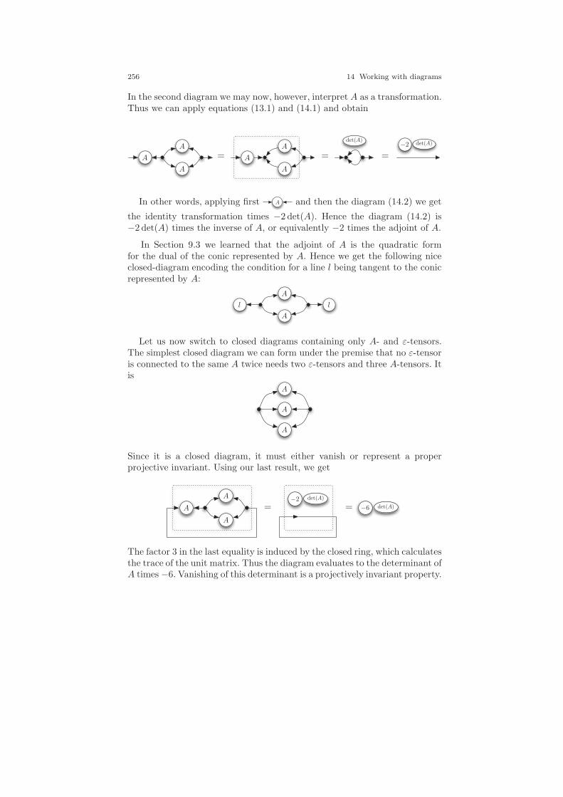
256 14 Working with diagrams
In the second diagram we may now, however, interpret A as a transformation.Thus we can apply equations (13.1) and (14.1) and obtain
A
A
A
A
A
A
===
det(A)det(A) −2
In other words, applying first A and then the diagram (14.2) we get
the identity transformation times −2 det(A). Hence the diagram (14.2) is−2 det(A) times the inverse of A, or equivalently −2 times the adjoint of A.
In Section 9.3 we learned that the adjoint of A is the quadratic formfor the dual of the conic represented by A. Hence we get the following niceclosed-diagram encoding the condition for a line l being tangent to the conicrepresented by A:
A
A
l l
Let us now switch to closed diagrams containing only A- and ε-tensors.The simplest closed diagram we can form under the premise that no ε-tensoris connected to the same A twice needs two ε-tensors and three A-tensors. Itis
A
A
A
Since it is a closed diagram, it must either vanish or represent a properprojective invariant. Using our last result, we get
A
A
A
== det(A)
det(A)
−6
−2
The factor 3 in the last equality is induced by the closed ring, which calculatesthe trace of the unit matrix. Thus the diagram evaluates to the determinant ofA times −6. Vanishing of this determinant is a projectively invariant property.
14.5 Diagrams in RP3 257
14.5 Diagrams in RP3
How does the machinery of tensor diagrams generalize to other dimensions?As one might expect, most concepts can be carried over in a most naturalway.However, already in RP
3 there are some nice twists that enter the gameaccording to the fact that the most natural representation of a line in RP
3 isby its six-dimensional Plucker vector. In what follows we will briefly sketchsome of the most crucial effects. The reader should always be aware that weonly scratch the surface and will leave aside many fascinating aspects of thissubject. For a more elaborate treatment we recommend [8].
We start with the obvious parts. As we saw in Section 12, the points inRP
3 have to be represented by four-dimensional vectors. They in turn arerepresented by a covariant tensor of grade 1 with four entries. In a diagramsuch a point is simply represented by a node p with one outgoing arrow.
Similarly, a plane is represented by a contravariant tensor of grade 1 withfour entries, diagrammatically expressed by a node h with one incoming
arrow. Incidence of a point p and a plane h corresponds to vanishing ofthe diagram p h . Transformations are grade-two tensors T ji of shape
4 × 4 with the entries of the corresponding transformation matrix and thediagrammatic notation T .
Matters start to become interesting as soon as ε-tensors are involved.For applications in RP
3 (i.e., rank 4) these are completely antisymmetric4 × 4 × 4 × 4 tensors. There is a completely covariant version εijkl and acompletely contravariant version εijkl. As in rank 3, they are defined by theproperty that they are completely antisymmetric and ε1234 = ε1234 = 1. Theonly coordinate entries are 0, 1, and −1. There are exactly 24 nonzero entriesthat appear at those places for which all indices i, j, k, l differ. If e1, . . . , e4are the four unit vectors in R4, then we get a nice and easily memorizabledescription of the coordinate entries of the ε-tensors by
εijkl = εijkl = det(ei, ej , ek, el).
In this equation the indices are not merely placeholders but concrete entries(i, j, k, l) ∈ i, j, k, j4. Now, what is a good diagrammatic representations ofεijkl and εijkl? Each such tensor must be represented by a node with fouroutgoing, resp. four incoming, arrows. Since the ε-tensors are completely an-tisymmetric, interchanging of two indices (i.e., arrows) induces a sign-switch.In fact, a perfect representation for these tensors would be to embed the dia-grams in three-dimensional space and let the four arrows point from the cen-ter to the four vertices of a tetrahedron. Rotations of this three-dimensionaldiagram node would not affect the sign, while a mirror reflection of the nodewould result in a sign inversion. This is elegant, but we do not want to cookup three-dimensional diagrams here, in order not to overstress the geometrybehind the diagrams. We want to keep them as close to usual graphs with
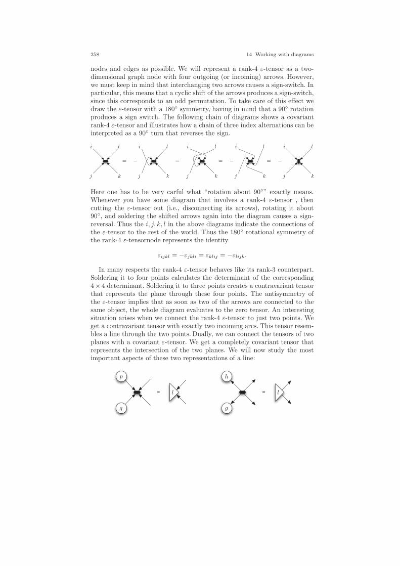
258 14 Working with diagrams
nodes and edges as possible. We will represent a rank-4 ε-tensor as a two-dimensional graph node with four outgoing (or incoming) arrows. However,we must keep in mind that interchanging two arrows causes a sign-switch. Inparticular, this means that a cyclic shift of the arrows produces a sign-switch,since this corresponds to an odd permutation. To take care of this effect wedraw the ε-tensor with a 180 symmetry, having in mind that a 90 rotationproduces a sign switch. The following chain of diagrams shows a covariantrank-4 ε-tensor and illustrates how a chain of three index alternations can beinterpreted as a 90 turn that reverses the sign.
iiiii
jjjjj kkkkk
lllll
= = −= −= −
Here one has to be very carful what “rotation about 90” exactly means.Whenever you have some diagram that involves a rank-4 ε-tensor , thencutting the ε-tensor out (i.e., disconnecting its arrows), rotating it about90, and soldering the shifted arrows again into the diagram causes a sign-reversal. Thus the i, j, k, l in the above diagrams indicate the connections ofthe ε-tensor to the rest of the world. Thus the 180 rotational symmetry ofthe rank-4 ε-tensornode represents the identity
εijkl = −εjkli = εklij = −εlijk.
In many respects the rank-4 ε-tensor behaves like its rank-3 counterpart.Soldering it to four points calculates the determinant of the corresponding4× 4 determinant. Soldering it to three points creates a contravariant tensorthat represents the plane through these four points. The antisymmetry ofthe ε-tensor implies that as soon as two of the arrows are connected to thesame object, the whole diagram evaluates to the zero tensor. An interestingsituation arises when we connect the rank-4 ε-tensor to just two points. Weget a contravariant tensor with exactly two incoming arcs. This tensor resem-bles a line through the two points. Dually, we can connect the tensors of twoplanes with a covariant ε-tensor. We get a completely covariant tensor thatrepresents the intersection of the two planes. We will now study the mostimportant aspects of these two representations of a line:
= =
p
q
h
g
ll
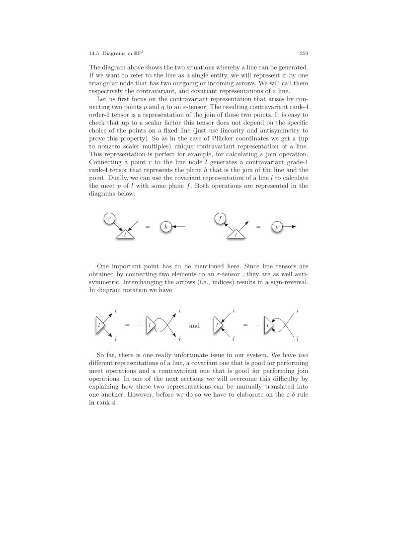
14.5 Diagrams in RP3 259
The diagram above shows the two situations whereby a line can be generated.If we want to refer to the line as a single entity, we will represent it by onetriangular node that has two outgoing or incoming arrows. We will call themrespectively the contravariant, and covariant representations of a line.
Let us first focus on the contravariant representation that arises by con-necting two points p and q to an ε-tensor. The resulting contravariant rank-4order-2 tensor is a representation of the join of these two points. It is easy tocheck that up to a scalar factor this tensor does not depend on the specificchoice of the points on a fixed line (just use linearity and antisymmetry toprove this property). So as in the case of Plucker coordinates we get a (upto nonzero scaler multiples) unique contravariant representation of a line.This representation is perfect for example, for calculating a join operation.Connecting a point r to the line node l generates a contravariant grade-1rank-4 tensor that represents the plane h that is the join of the line and thepoint. Dually, we can use the covariant representation of a line l to calculatethe meet p of l with some plane f . Both operations are represented in thediagrams below:
r
h
l
=
f
p
l
=
One important point has to be mentioned here. Since line tensors areobtained by connecting two elements to an ε-tensor , they are as well anti-symmetric. Interchanging the arrows (i.e., indices) results in a sign-reversal.In diagram notation we have
ii
jj
ll = − and
ii
jj
ll = −
So far, there is one really unfortunate issue in our system. We have twodifferent representations of a line, a covariant one that is good for performingmeet operations and a contravariant one that is good for performing joinoperations. In one of the next sections we will overcome this difficulty byexplaining how these two representations can be mutually translated intoone another. However, before we do so we have to elaborate on the ε-δ-rulein rank 4.

260 14 Working with diagrams
14.6 The ε-δ-rule in Rank 4
In Section 13.6 we learned the ε-δ-rule for rank-3 tensors. In usual tensorlanguage it reads as
εijαεlmα = δilδjm − δimδ
jl = det
(δil δjlδim δjm
).
This expression straightforwardly generalizes to higher ranks. In particular,for the rank-4 case we get
εijkαεmnrα = det
δim δjm δkmδin δjn δknδir δjr δkr
.
We will not prove this here, since the proof is mainly an index and coeffi-cient battle that can be obtained by brute-force expansion of the implicitsummation.
Remark 14.2. Although we will not prove this ε-δ-rule here, we will point outthe resemblance to the formula we observed in Remark 14.1. While the for-mula there was essentially the factorization formula for determinants of theproduct of two matrices, the general ε-δ-rule may be considered an expressionof the famous Cauchy-Binet formula. This formula expresses the determinantof an n×m and an m×n matrix as a summation over products of two deter-minants of corresponding minors of the two matrices. The ε-δ-rule generatesexactly this formula, where the summation is implicitly generated by thesummation over the indices shared by both ε-tensors.
Diagrammatically the rank-4 ε-δ-rule translates to the identity presentedbelow. (As always, one should be aware of the fact that the signs and theorientations of the ε-tensors require a careful translation process.)
iiiiiii jjjjjjj kkkkkkk
nnnnnnn mmmmmmm rrrrrrr
α = ++ −−−
We will also need another version of the ε-δ-rule that expands the termεijβαεmnβα. Also, here we could obtain the formula by brute force expansion
(we get (−2)(δilδjm− δimδjl )). Instead, this time we will show how this formula
is derived directly by diagram calculations from the previous one. We simplyhave to solder the two exits k and r in all subdiagrams. We get
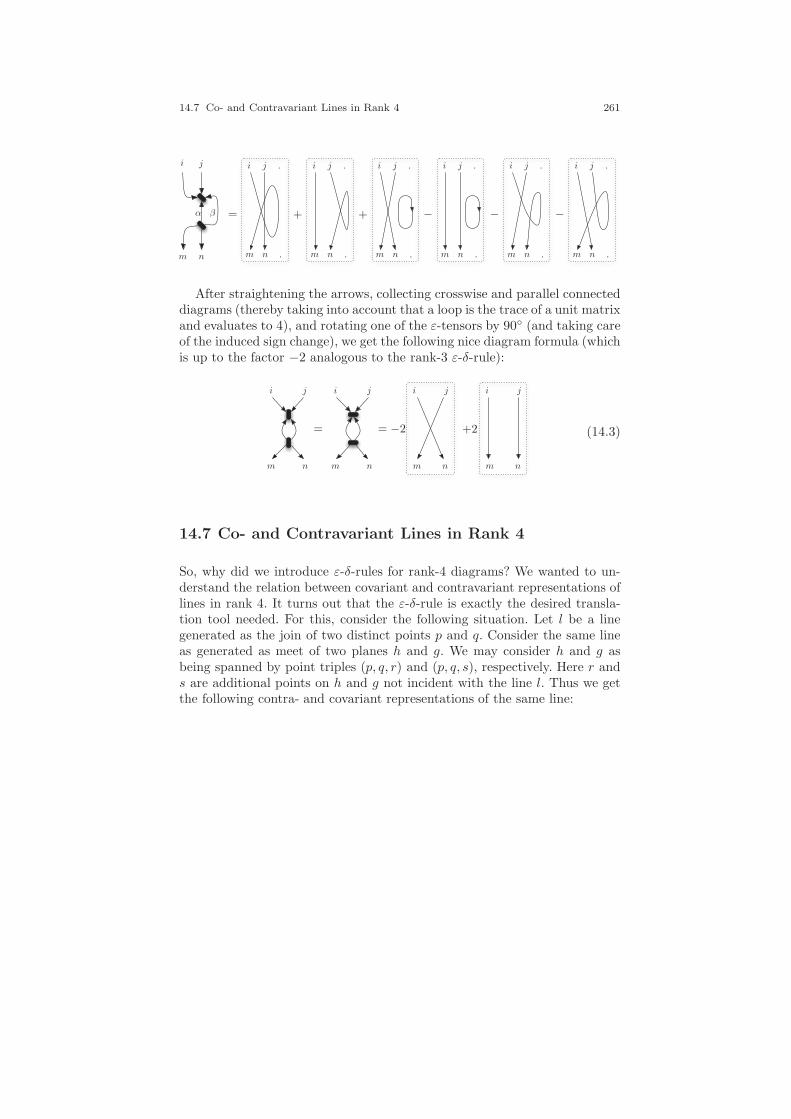
14.7 Co- and Contravariant Lines in Rank 4 261
.
.
.
.
.
.
.
.
.
.
.
.
iiiiiii jjjjjjj
nnnnnnn mmmmmmm
βα = ++ −−−
After straightening the arrows, collecting crosswise and parallel connecteddiagrams (thereby taking into account that a loop is the trace of a unit matrixand evaluates to 4), and rotating one of the ε-tensors by 90 (and taking careof the induced sign change), we get the following nice diagram formula (whichis up to the factor −2 analogous to the rank-3 ε-δ-rule):
i iiij jjj
n nnnm mmm
= = +2−2 (14.3)
14.7 Co- and Contravariant Lines in Rank 4
So, why did we introduce ε-δ-rules for rank-4 diagrams? We wanted to un-derstand the relation between covariant and contravariant representations oflines in rank 4. It turns out that the ε-δ-rule is exactly the desired transla-tion tool needed. For this, consider the following situation. Let l be a linegenerated as the join of two distinct points p and q. Consider the same lineas generated as meet of two planes h and g. We may consider h and g asbeing spanned by point triples (p, q, r) and (p, q, s), respectively. Here r ands are additional points on h and g not incident with the line l. Thus we getthe following contra- and covariant representations of the same line:
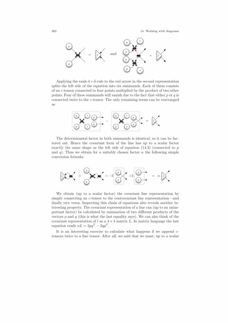
262 14 Working with diagrams
p
q
l= andp
p
q
q
r
s
l=
Applying the rank-4 ε-δ-rule to the red arrow in the second representationsplits the left side of the equation into six summands. Each of them consistsof an ε-tensor connected to four points multiplied by the product of two otherpoints. Four of these summands will vanish due to the fact that either p or q isconnected twice to the ε-tensor. The only remaining terms can be rearrangedas
p
p
p
pq
q
q
q rr
ss
l=−
The determinantal factor in both summands is identical, so it can be fac-tored out. Hence the covariant form of the line has up to a scalar factorexactly the same shape as the left side of equation (14.3) (connected to pand q). Thus we obtain for a suitably chosen factor α the following simpleconversion formula:
ppp
qqq
ll === −2 +2 α
We obtain (up to a scalar factor) the covariant line representation bysimply connecting an ε-tensor to the contravariant line representation—anddually vice versa. Inspecting this chain of equations also reveals another in-teresting property. The covariant representation of a line can (up to an unim-portant factor) be calculated by summation of two different products of thevectors p and q (this is what the last equality says). We can also think of thecovariant representation of l as a 4× 4 matrix L. In matrix language the lastequation reads αL = 2pqT − 2qpT .
It is an interesting exercise to calculate what happens if we append ε-tensors twice to a line tensor. After all, we said that we must, up to a scalar

14.8 Tensors versus Plucker Coordinates 263
factor, get a copy of the line tensor we started with. By applying the ε-δ-ruleto the double link of the ε-tensors we obtain
= = llll −2 +2 +4
The last equality is a consequence of the antisymmetry of the l tensor. Thustransforming a contravariant tensor by appending a chain of two ε-tensorsresults in multiplication by a factor of 4.
14.8 Tensors versus Plucker Coordinates
If we compare the representation of lines by tensors with the representation oflines by Plucker coordinates, at first sight there is an amazing structural dif-ference. While the Plucker coordinates of a line l were six-dimensional vectors(g12, g13, g14, g23, g24, g34)
T that satisfy the Grassmann-Plucker-Relations
g12g34 − g13g24 + g14g23 = 0,
the tensor representation looks quite different. A 4 × 4 tensor representsessentially a matrix M with 16 different entries. However, both the covariantand contravariant representations of the line tensor are antisymmetric. If Mis such a matrix we have M = −MT . This implies that each of the fourdiagonal entries vanishes.
Furthermore, the lower left triangle determines the complete shape of thematrix. This makes exactly six free entries. As in the case of Plucker coordi-nates! The matrix M has the structure
M =
0 −a −b −ca 0 −d −eb d 0 −fc e f 0
.
We will briefly analyze how these entries relate to the Plucker coordinates ofa line. For this we have to go down to the coordinate level once again. Letp = (p1, p2, p3, p4)
T and q = (q1, q2, q3, q4)T be two points that span the line
l. The Plucker coordinates of l then are gij =∣∣∣ pi qi
pj qj
∣∣∣. Let lij = εαβijpαqβ
be the contravariant tensor that represents l and let lij = piqj − pjqi be thecovariant representation of the line. We then get for specific values of i and j
lij = sign(i, j, α, β)
∣∣∣∣pα qαpβ qβ
∣∣∣∣ and lij =
∣∣∣∣pi qipj qj
∣∣∣∣ ,
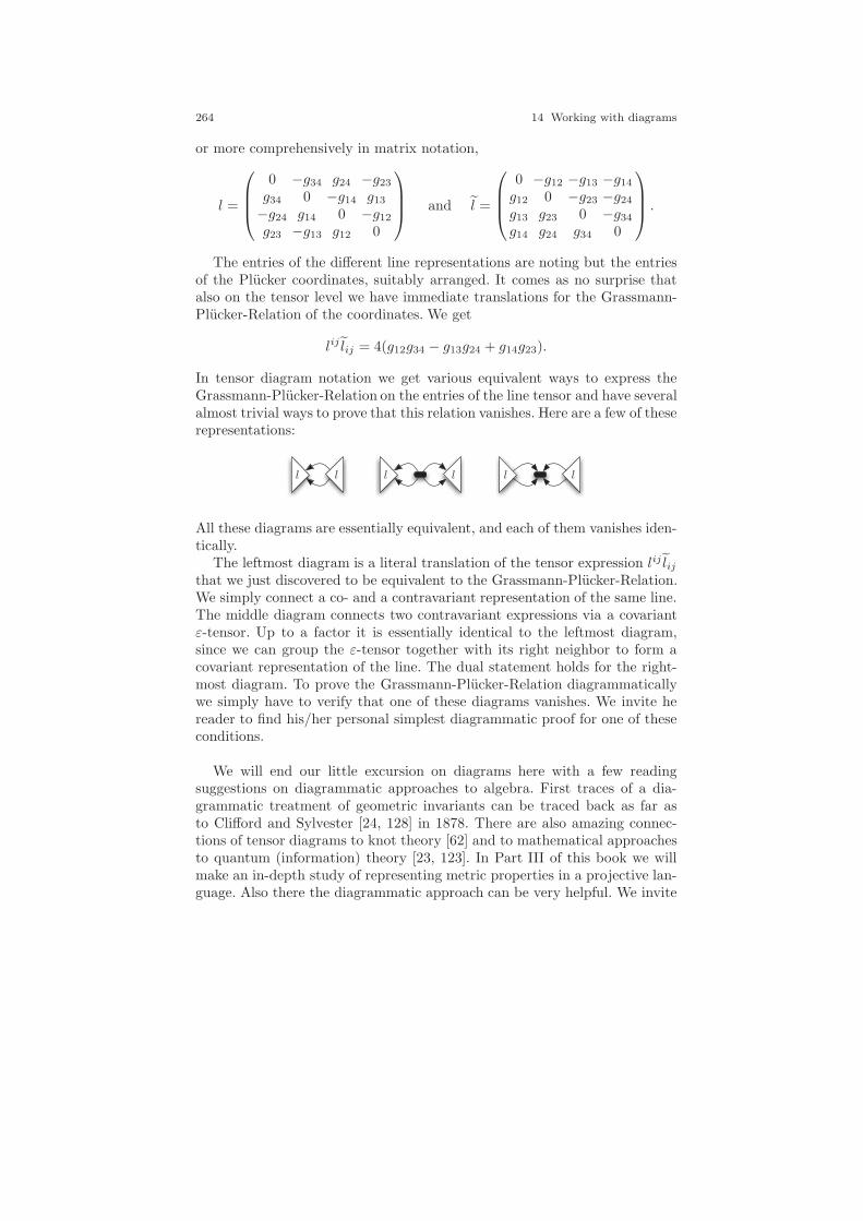
264 14 Working with diagrams
or more comprehensively in matrix notation,
l =
0 −g34 g24 −g23g34 0 −g14 g13−g24 g14 0 −g12g23 −g13 g12 0
and l =
0 −g12 −g13 −g14g12 0 −g23 −g24g13 g23 0 −g34g14 g24 g34 0
.
The entries of the different line representations are noting but the entriesof the Plucker coordinates, suitably arranged. It comes as no surprise thatalso on the tensor level we have immediate translations for the Grassmann-Plucker-Relation of the coordinates. We get
lij lij = 4(g12g34 − g13g24 + g14g23).
In tensor diagram notation we get various equivalent ways to express theGrassmann-Plucker-Relation on the entries of the line tensor and have severalalmost trivial ways to prove that this relation vanishes. Here are a few of theserepresentations:
llllll
All these diagrams are essentially equivalent, and each of them vanishes iden-tically.
The leftmost diagram is a literal translation of the tensor expression lij lijthat we just discovered to be equivalent to the Grassmann-Plucker-Relation.We simply connect a co- and a contravariant representation of the same line.The middle diagram connects two contravariant expressions via a covariantε-tensor. Up to a factor it is essentially identical to the leftmost diagram,since we can group the ε-tensor together with its right neighbor to form acovariant representation of the line. The dual statement holds for the right-most diagram. To prove the Grassmann-Plucker-Relation diagrammaticallywe simply have to verify that one of these diagrams vanishes. We invite hereader to find his/her personal simplest diagrammatic proof for one of theseconditions.
We will end our little excursion on diagrams here with a few readingsuggestions on diagrammatic approaches to algebra. First traces of a dia-grammatic treatment of geometric invariants can be traced back as far asto Clifford and Sylvester [24, 128] in 1878. There are also amazing connec-tions of tensor diagrams to knot theory [62] and to mathematical approachesto quantum (information) theory [23, 123]. In Part III of this book we willmake an in-depth study of representing metric properties in a projective lan-guage. Also there the diagrammatic approach can be very helpful. We invite

14.8 Tensors versus Plucker Coordinates 265
the reader who is (after digesting at least Chapters 16–19) interested in thisdirection to have a look at the articles [83, 84].


15
Configurations, Theorems, andBracket Expressions
Beauty depends on size as well as symmetry.
Aristotle (384–322 BCE), Poetics
Characteristic of Weyl was an aesthetic sense which domi-nated his thinking on all subjects. He once said to me, half-joking, ”My work always tried to unite the true with the beau-tiful; but when I had to choose one or the other, I usuallychose the beautiful. (Hermann Weyl (1885–1955))
F. Dyson, in Nature, March 10, 1956
This section is devoted to several specific examples of theorems and con-figurations in projective geometry. Clearly, our considerations in Chapter 5demonstrated that there is an infinite variety of incidence theorems in realprojective geometry.Any polynomial identity like (x+ y)2 = x2 +2 ·x ·y+ y2
can be translated into an incidence theorem via von Staudt constructions.For this, one models every elementary addition or multiplication by a suit-able subconfiguration. The equality in the equation translates to a final co-incidence of two lines that forms the conclusion of the theorem. Figure 15.1shows a suitable geometric construction for the equation above (lines thatappear to be parallel are assumed to be parallel).
Clearly, most of the incidences obtained in this way will be very boring,since they represent only more or less trivial facts about algebraic expressions.In fact, the simplest algebraic expressions will surprisingly lead to nicer geo-metric theorems than the complicated ones. For instance, we saw in Section5.7 that Pappos’s theorem expresses the equation x · y = y · x.
267

268 15 Configurations, Theorems, and Bracket Expressions
0 1 x x2y y2xy 2xy x2 + 2xyx+y (x+y)2=x2+2xy+y2
Fig. 15.1 An incidence theorem from (x+ y)2 = x2 + 2 · x · y + y2.
It is unreasonable to try to find a formal notion of mathematical beauty,but nevertheless many geometric theorems are considered to be beautifulmathematical objects. Typically there are several (interrelated) ingredientsthat make a geometric theorem a nice result:
• simplicity (it is easy to state the theorem),• symmetry (are there repeated patterns),• surprising conclusions (is the conclusion somehow unexpected),• size (the fewer hypotheses the better),• generalizability (does the theorem extend to a whole class of objects).
In this section we want to explore several theorems and configurations thatare expressible in terms of projective geometry. In particular, we will explorerelations to bracket expressions and explore their combinatorial symmetriesand the symmetries of the corresponding bracket expressions. We will alsouse this section to demonstrate several techniques that are useful in relatinggeometric scenarios to algebraic expressions. Several times we will provide dif-ferent proofs for the same facts in order to demonstrate different approaches.I hope the reader will share the appreciation of the mathematical beauty ofmany of these structures.1
15.1 Desargues’s Theorem
The first theorem we will meet is an incidence theorem similar to Pappos’stheorem. However, in contrast, it requires 10 points and 10 lines. Each point
1 Some of the proofs presented here already occurred in the introductory Chapter 1, wherewe explored different approaches to Pappos’s theorem. For matters of completeness theyare also included in this chapter.
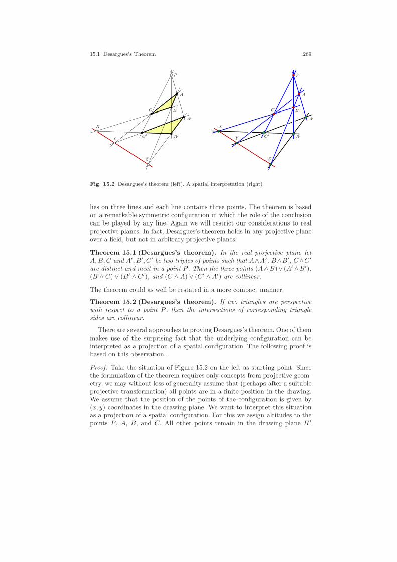
15.1 Desargues’s Theorem 269
P
A
BC
A′
B′C′
X
Z
Y
P
A
BC
A′
B′C′
X
Z
Y
Fig. 15.2 Desargues’s theorem (left). A spatial interpretation (right)
lies on three lines and each line contains three points. The theorem is basedon a remarkable symmetric configuration in which the role of the conclusioncan be played by any line. Again we will restrict our considerations to realprojective planes. In fact, Desargues’s theorem holds in any projective planeover a field, but not in arbitrary projective planes.
Theorem 15.1 (Desargues’s theorem). In the real projective plane letA,B,C and A′, B′, C′ be two triples of points such that A∧A′, B∧B′, C∧C′
are distinct and meet in a point P . Then the three points (A∧B)∨ (A′ ∧B′),(B ∧ C) ∨ (B′ ∧C′), and (C ∧A) ∨ (C′ ∧A′) are collinear.
The theorem could as well be restated in a more compact manner.
Theorem 15.2 (Desargues’s theorem). If two triangles are perspectivewith respect to a point P , then the intersections of corresponding trianglesides are collinear.
There are several approaches to proving Desargues’s theorem. One of themmakes use of the surprising fact that the underlying configuration can beinterpreted as a projection of a spatial configuration. The following proof isbased on this observation.
Proof. Take the situation of Figure 15.2 on the left as starting point. Sincethe formulation of the theorem requires only concepts from projective geom-etry, we may without loss of generality assume that (perhaps after a suitableprojective transformation) all points are in a finite position in the drawing.We assume that the position of the points of the configuration is given by(x, y) coordinates in the drawing plane. We want to interpret this situationas a projection of a spatial configuration. For this we assign altitudes to thepoints P , A, B, and C. All other points remain in the drawing plane H ′
270 15 Configurations, Theorems, and Bracket Expressions
(compare Figure 15.2 (right)). We may interpret the situation as follows: Weconsider three planes in space which meet in a point P . Any pair of theseplanes meet in a line that passes through P . There are three of these lines.On each line we take a pair of points. We label these pairs (A,A′), (B,B′),and (C,C′). The three points A, B, and C span a plane H , and the threepoints A′, B′, and C′ span a plane H ′ (this is the drawing plane). Thesetwo planes meet in a line. The four points A,A′, B, and B′ are on one of thethree initial planes. The intersection of this plane, H , and H ′ is the point Zthat also lies on ℓ. Similarly, the points X and Y lie on ℓ, which proves thetheorem. ⊓⊔
The method of proof used here can be nicely generalized to prove othertheorems.Furthermore, it gives a nice insight into the combinatorial structureof the underlying configuration of Desargues’s theorem. The spatial situationconsists altogether of five planes (the initial three planes together with Hand H ′), all ten intersections of pairs of these planes (the lines of the config-uration), and all ten intersections of triples of these planes (the points of theconfiguration). The projection of the lines and planes forms the planar De-sargues’s configuration. This demonstrates that the configuration possesses avery high degree of symmetry. In fact the combinatorial automorphism grouphas 120 elements and is isomorphic to S5 the group of all permutations offive elements.
In the next sections we will see also different algebraic proofs of Desargues’stheorem that essentially make use of bracket calculations.
15.2 Binomial Proofs
The following proof technique is very far-reaching. It translates the hypothe-ses and the conclusion of the theorem into multihomogeneous bracket poly-nomials. The conclusion is then algebraically composed from the polynomialsof the hypotheses. Binomial proofs are now special in the respect that thecancellation patterns between the algebraic terms are particularly simple.Many proofs that can be found in classical literature on projective geometryfollow exactly the pattern we present here. The way we will approach bino-mial proofs here has the advantage that one can even use them to implementautomatic provers for geometric theorems.Binomial proofs were first studiedin the context of oriented matroids [15] and were later used in the context ofautomated theorem-proving [30, 109].
The theorems we will consider are (on the first level) those whose hy-potheses and conclusions can be expressed as collinearity conditions of points.Furthermore, we will also have to deal with nondegeneracy conditions thatprevent our configurations from being too special. Algebraically, the nonde-generacy conditions prevent us from dividing by zero. The nondegeneracyconditions will always be such that certain points are not allowed to be
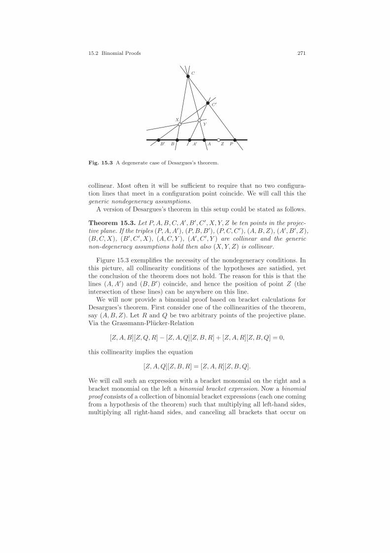
15.2 Binomial Proofs 271
P
XY
C
C′
BB′ A′ A Z
Fig. 15.3 A degenerate case of Desargues’s theorem.
collinear. Most often it will be sufficient to require that no two configura-tion lines that meet in a configuration point coincide. We will call this thegeneric nondegeneracy assumptions.
A version of Desargues’s theorem in this setup could be stated as follows.
Theorem 15.3. Let P,A,B,C,A′, B′, C′, X, Y, Z be ten points in the projec-tive plane. If the triples (P,A,A′), (P,B,B′), (P,C,C′), (A,B,Z), (A′, B′, Z),(B,C,X), (B′, C′, X), (A,C, Y ), (A′, C′, Y ) are collinear and the genericnon-degeneracy assumptions hold then also (X,Y, Z) is collinear.
Figure 15.3 exemplifies the necessity of the nondegeneracy conditions. Inthis picture, all collinearity conditions of the hypotheses are satisfied, yetthe conclusion of the theorem does not hold. The reason for this is that thelines (A,A′) and (B,B′) coincide, and hence the position of point Z (theintersection of these lines) can be anywhere on this line.
We will now provide a binomial proof based on bracket calculations forDesargues’s theorem. First consider one of the collinearities of the theorem,say (A,B,Z). Let R and Q be two arbitrary points of the projective plane.Via the Grassmann-Plucker-Relation
[Z,A,B][Z,Q,R] − [Z,A,Q][Z,B,R] + [Z,A,R][Z,B,Q] = 0,
this collinearity implies the equation
[Z,A,Q][Z,B,R] = [Z,A,R][Z,B,Q].
We will call such an expression with a bracket monomial on the right and abracket monomial on the left a binomial bracket expression. Now a binomialproof consists of a collection of binomial bracket expressions (each one comingfrom a hypothesis of the theorem) such that multiplying all left-hand sides,multiplying all right-hand sides, and canceling all brackets that occur on
272 15 Configurations, Theorems, and Bracket Expressions
both sides gives a bracket binomial that corresponds to the conclusion of thetheorem.
Proof. Binomial proof for Desargues’s theorem. The following collection ofbinomials does the job for Desargues’s theorem:
[CY A] = 0 =⇒ [CY B][CAX ] = [CY X ][CAB]
[ABX ] = 0 =⇒ [ABC][AXP ] = [ABP ][AXC][PA′A] = 0 =⇒ [PA′X ][PAB] = [PA′B][PAX ][PCC′] = 0 =⇒ [PCZ][PC′B′] = [PCB′][PC′Z][C′ZB′] = 0 =⇒ [C′ZP ][C′B′A′] = [C′ZA′][C′B′P ][A′Y C′] = 0 =⇒ [A′Y B′][A′C′Z] = [A′Y Z][A′C′B′][PBB′] = 0 =⇒ [PBA′][PB′C] = [PBC][PB′A′][CBZ] = 0 =⇒ [CBP ][CZY ] = [CBY ][CZP ]
[A′B′X ] = 0 =⇒ [A′B′P ][A′XY ] = [A′B′Y ][A′XP ]
Each row corresponds to one of the hypotheses. The binomial equation is(via a suitable Grassmann-Plucker-Relation) a consequence of one of thehypotheses. Multiplying all left sides and all right sides gives a binomialequation that has 18 brackets on the left and 18 brackets on the right. Takinginto account the alternating determinant rules, one observes that all butfour brackets (the underlined ones) occur on both sides. Canceling thesebrackets, we are left with the expression [Y XA′][Y ZC] = [Y XC][Y ZA′].The cancellation process requires that none of the brackets that is canceledbe zero. This, in turn, is established by our nondegeneracy assumptions. Usingagain a Grassmann-Plucker-Relation, one can conclude that
[Y XA′][Y ZC] = [Y XC][Y ZA′] =⇒ [Y XZ] = 0 or [Y CA′] = 0.
The collinearity of (Y,C,A′) would violate our nondegeneracy assump-tions. Thus finally the points (X,Y, Z) must be collinear. ⊓⊔
In Chapter 1 we presented a similar proof of Pappos’s theorem. The crucialpoint in finding such a proof is the translation of collinearities to binomialexpressions. There is a lot of freedom in this translation. First observe thatfor each triple of collinear points one of the points plays a special role in theGrassmann-Plucker-Relation. Furthermore, there are two other configurationpoints that are needed for the Grassmann-Plucker-Relation. They must bechosen from the remaining points. Thus if the theorem involves n points,there are altogether 3 ·
(n−2
2
)possibilities to translate a collinearity into a
binomial expression. For each collinearity in the hypotheses one has to findone (or more) suitable representations such that a combination of all binomialexpressions can be translated into the conclusion. If a “brute-force” approachwere the only way to find such a proof, one would end up with a computa-tionally rather hard problem. Fortunately, the problem can be translated intoa linear problem by considering the exponent vectors. In this setup one hasto test whether a representation of the conclusion lies in the (linear) span
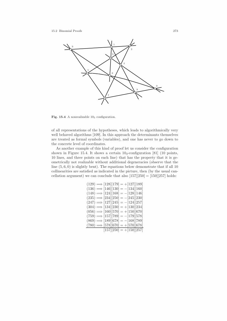
15.2 Binomial Proofs 273
1
2
3
4
5
6
7
8
9
0
Fig. 15.4 A nonrealizable 103 configuration.
of all representations of the hypotheses, which leads to algorithmically verywell behaved algorithms [109]. In this approach the determinants themselvesare treated as formal symbols (variables), and one has never to go down tothe concrete level of coordinates.
As another example of this kind of proof let us consider the configurationshown in Figure 15.4. It shows a certain 103-configuration [81] (10 points,10 lines, and three points on each line) that has the property that it is ge-ometrically not realizable without additional degeneracies (observe that theline (5, 6, 0) is slightly bent). The equations below demonstrate that if all 10collinearities are satisfied as indicated in the picture, then (by the usual can-cellation argument) we can conclude that also [157][250] = [150][257] holds:
(129) =⇒ [128][179] = +[127][189](136) =⇒ [146][130] = −[134][160](148) =⇒ [124][168] = −[128][146](235) =⇒ [234][250] = −[245][230](247) =⇒ [127][245] = −[124][257](304) =⇒ [134][230] = +[130][234](056) =⇒ [160][570] = +[150][670](759) =⇒ [157][789] = −[179][578](869) =⇒ [189][678] = −[168][789](780) =⇒ [578][670] = +[570][678]
[157][250] = +[150][257]
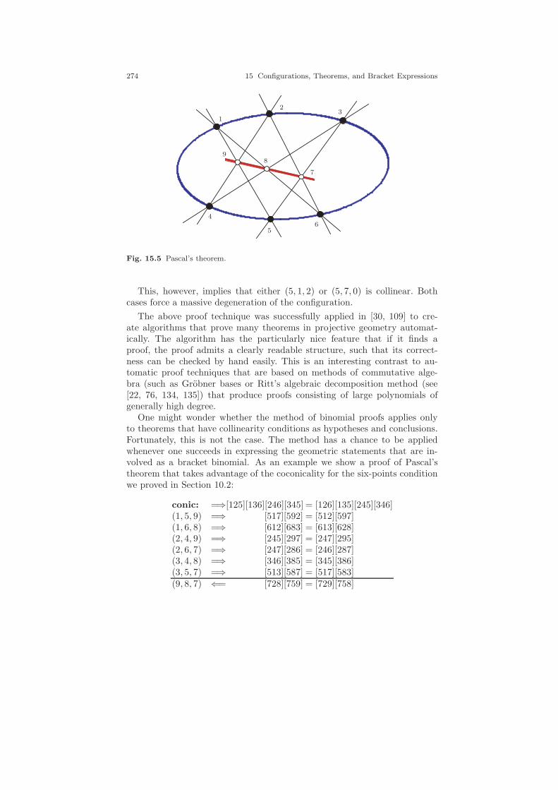
274 15 Configurations, Theorems, and Bracket Expressions
1
23
4
56
98
7
Fig. 15.5 Pascal’s theorem.
This, however, implies that either (5, 1, 2) or (5, 7, 0) is collinear. Bothcases force a massive degeneration of the configuration.
The above proof technique was successfully applied in [30, 109] to cre-ate algorithms that prove many theorems in projective geometry automat-ically. The algorithm has the particularly nice feature that if it finds aproof, the proof admits a clearly readable structure, such that its correct-ness can be checked by hand easily. This is an interesting contrast to au-tomatic proof techniques that are based on methods of commutative alge-bra (such as Grobner bases or Ritt’s algebraic decomposition method (see[22, 76, 134, 135]) that produce proofs consisting of large polynomials ofgenerally high degree.
One might wonder whether the method of binomial proofs applies onlyto theorems that have collinearity conditions as hypotheses and conclusions.Fortunately, this is not the case. The method has a chance to be appliedwhenever one succeeds in expressing the geometric statements that are in-volved as a bracket binomial. As an example we show a proof of Pascal’stheorem that takes advantage of the coconicality for the six-points conditionwe proved in Section 10.2:
conic: =⇒[125][136][246][345] = [126][135][245][346](1, 5, 9) =⇒ [517][592] = [512][597](1, 6, 8) =⇒ [612][683] = [613][628](2, 4, 9) =⇒ [245][297] = [247][295](2, 6, 7) =⇒ [247][286] = [246][287](3, 4, 8) =⇒ [346][385] = [345][386](3, 5, 7) =⇒ [513][587] = [517][583](9, 8, 7) ⇐= [728][759] = [729][758]
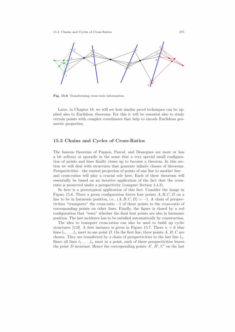
15.3 Chains and Cycles of Cross-Ratios 275
A
B
C
D
A′
B′
C′
D′
Fig. 15.6 Transforming cross-ratio information.
Later, in Chapter 18, we will see how similar proof techniques can be ap-plied also to Euclidean theorems. For this it will be essential also to studycertain points with complex coordinates that help to encode Euclidean geo-metric properties.
15.3 Chains and Cycles of Cross-Ratios
The famous theorems of Pappos, Pascal, and Desargues are more or lessa bit solitary or sporadic in the sense that a very special small configura-tion of points and lines finally closes up to become a theorem. In this sec-tion we will deal with structures that generate infinite classes of theorems.Perspectivities—the central projection of points of one line to another line—and cross-ratios will play a crucial role here. Each of these theorems willessentially be based on an iterative application of the fact that the cross-ratio is preserved under a perspectivity (compare Section 4.4.3).
So here is a prototypical application of this fact. Consider the image inFigure 15.6. There a green configuration forces four points A,B,C,D on aline to be in harmonic position, i.e., (A,B;C,D) = −1. A chain of perspec-tivities “transports” the cross-ratio −1 of these points to the cross-ratio ofcorresponding points on other lines. Finally, the figure is closed by a redconfiguration that “tests” whether the final four points are also in harmonicposition. The last incidence has to be satisfied automatically by construction.
The idea to transport cross-ratios can also be used to build up cyclicstructures [119]. A first instance is given in Figure 15.7. There n = 6 bluelines l1, . . . , ln meet in one point D. On the first line, three points A, B, C arechosen. They are transferred by a chain of perspectivities to the last line ln.Since all lines l1, . . . , ln meet in a point, each of these perspectivities leavesthe point D invariant. Hence the corresponding points A′, B′, C′ on the last

276 15 Configurations, Theorems, and Bracket Expressions
line must be such that (A,B;C,D) = (A′, B′;C′, D). Now consider the meetP of the two lines join(A,A′) and join(C,C′). Forming a perspective fromln to l1 through P maps A′ to A, B′ to B, and D to D. Thus (since the cross-ratio of the four corresponding points is identical) it must also map C′ to C.In other words, join(C′, C) also passes through P . Clearly, this constructionproduces a theorem for any integer n.
There is another nice variant of this construction. For this consider the leftdrawing in Figure 15.8. Start with an odd number n of (blue) lines l1, . . . , lnthat meet in one common point O. On each of these lines li choose a pointpi (black) that will serve as a projection center of a perspectivity. Now startwith a point A1 on l1 and i = 1 and form a perspectivity through pi+(n−1)/2
on li+(n−1)/2. Call the new point A2 and proceed with this projection processiteratively by an index shift of 1. After wrapping around twice, one ends up ata point A2n+1 that coincides with A1. This theorem was originally discoveredby Armin Saam [118]. In principle, it is possible also to prove this theoremby a “transfer of cross-ratio” argument. This argument is subdivided intotwo steps. One of them is technically easy; the other is not. Assume thatone moves the point A1 in the drawing along l1 toward the center O of theconfiguration. Alternatingly even and odd Ai will move inward and outwardwith respect to the center O. In particular, the other point on l1 (the pointA(n+1)/2) will move in the opposite direction of A1. Eventually, there is aposition C where the moved points A1 and A(n+1)/2 coincide (this was the
AB C
D
A′
B′
C′
l1
l2 l3
l4
l5
l6
P
Fig. 15.7 Cycles of cross-ratios.

15.4 Ceva and Menelaus 277
O
A1
A2
A3
A4
A5
A6
A7
A8
A9
A10
l1
l2
l3
l4l5
p1
p2
p3
p4 p5
A1
A6
C
O
Fig. 15.8 Saam’s theorem.
easy part). Now one can observe that the original points A1 and A(n+1)/2 arein harmonic position to C and O (hard part!). The rest of the proof is easilydone by “transfer of cross-ratio.” We will not work out this proof in detail.Instead, we will postpone to Section 15.5 a more elegant proof that avoidsthe hard part and even generates a generalization of the theorem.
The theorems of this section were essentially based on chains or one-dimensional cycles of perspectivities. In what follows we will elaborate onthe idea of cyclic structures. However, we will generalize the concept to cy-cles on two-dimensional manifolds. For this we will first, in the next section,study small configurations that serve as basic building blocks for the man-ifolds. In Section 15.5 we will show how the building blocks can be gluedtogether to generate interesting theorems.
15.4 Ceva and Menelaus
In this section we deal with two structurally very simple theorems: the the-orems of Ceva and Menelaus (see [28]). At first sight, they have the flavorof Euclidean, resp. affine, theorems, since they involve ratios (and not cross-ratios) of lengths along the sides of a triangle. However, a slightly closerinspection of these theorems reveals their projective nature. Moreover, onthe level of bracket algebra the proofs of these theorems are almost trivial.Nonetheless, these theorems turn out to be of key importance for under-

278 15 Configurations, Theorems, and Bracket Expressions
A BX
P
A BX
P
Q
A
B
C
X
Y
Z
a1
b1
a2 b2
a3
b3
Fig. 15.9 Oriented length ratios and segment cuts in a triangle.
standing the structures of other projective and Euclidean incidence theorems[110].2
We begin our considerations with the Euclidean version of these theo-rems. For both theorems the notion of oriented distance ratio is crucial. LetA,X,B ∈ R be three points on the real number line. Then the oriented
distance ratio |A,X||X,B| is defined as
|A,X ||X,B| =
A−X
X −B.
Similarly, we can define the oriented length ratio for an arbitrary line byconsidering this line as the real number line R. If X is between A and Bthen this ratio is positive; if X is outside the line segment A,B then the ratiois negative. For calculating the oriented distance ratio we can equivalentlycalculate the ratio of ordinary distances and equip it with the appropriatesign. It is important to notice that the sign of the distance ratio can beassigned in a reasonable way only if the three points that are involved lie ona common line. All cases that we will consider will be of this type.
There is also a way to express the oriented length ratio by quotients oforiented triangle areas. For this let ∆(A,B, P ) be the oriented area of atriangle (A,B, P ). The sign is positive if the points are in counterclockwiseorder and negative if they are in clockwise order. Let us assume for a momentthatA,B, P are in the standard embedding with last homogeneous coordinatebeing 1. Then we have ∆(A,B, P ) = 1
2 [A,B, P ]. Since the triangle area can
be calculated by |A,B|·hP
2 , where hP is the altitude of P over the side (A,B),we get for the oriented distance ratios
|A,X ||X,B| =
∆(A,X, P )
∆(X,B, P )=
[A,X, P ]
[X,B, P ]. (15.1)
2 Interesting generalizations of the theorems of Ceva and Menelaus have been intensivelystudied by Grunbaum and Shephard [51, 52, 53, 54, 120].

15.4 Ceva and Menelaus 279
A B
C
Z
YD
X
A B
C
Z
Y
X
Ceva’s Thm:|AX||XB|
· |BY ||Y C|
· |CZ||ZA|
= 1 Menelaus’s Thm:|AX||XB|
· |BY ||YC|
· |CZ||ZA|
= −1
Fig. 15.10 Theorems of Ceva and Menelaus.
Here P is an arbitrary point not on the line (A,B) (compare Figure 15.9(left)). Notice that the sign turns out to be automatically correct. We willalso need another expression for the oriented distance ratios. For this assumethat Q is another point on the line (X,P ) distinct from P , again in thestandard embedding. We then have X = (1 − λ)P + λQ, and obtain
|A,X ||X,B| =
[A,X, P ]
[X,B, P ]=
[A, (1 − λ)P + λQ,P ]
[(1 − λ)P + λQ,B, P ]=
[A,Q, P ]
[Q,B, P ]. (15.2)
We will need (15.1) and (15.2) later.
The theorems of Ceva and Menelaus now deal with triangles (A,B,C) forwhich each of the sides is dissected by one of the points X,Y, Z. In whatfollows we will always assume that X is the cutting point for the segment(A,B), that Y is the cutting point for (B,C), and that Z is the cutting pointfor (C,A). We also assume that none of the points involved coincides withanother (compare Figure 15.9 (right)). The product
|AX ||XB| ·
|BY ||Y C| ·
|CZ||ZA| (15.3)
is now the first-class citizen in the theorems of Ceva and Menelaus; they areillustrated in Figure 15.10.
Theorem 15.4 (Ceva’s theorem). If in a triangle (A,B,C), with cuttingpoints X,Y, Z as above, the lines (A, Y ), (B,Z), and (C,X) are concurrent,then we have
|AX ||XB| ·
|BY ||Y C| ·
|CZ||ZA| = 1.
Theorem 15.5 (Menelaus’s theorem). If in a triangle (A,B,C), withcutting points X,Y, Z as above, the points X,Y, Z are collinear, then we have

280 15 Configurations, Theorems, and Bracket Expressions
|AX ||XB| ·
|BY ||Y C| ·
|CZ||ZA| = −1.
Before presenting proofs of these two theorems we will first explore theirprojective nature. For this consider the following bracket formula on the pointsA,B,C,X, Y, Z and one additional point P in generic position.
[PAX ]
[PXB]· [PBY ]
[PY C]· [PCZ]
[PZA]. (15.4)
By our considerations in Chapter 6 this is clearly a projective invariantfunction, since it is the quotient of two multihomogeneous bracket polynomi-als with same multidegree. On the other hand, we may assume that each ofthe points is represented in standard homogeneous coordinates with the lastcoordinate entry being 1. Then the brackets correspond to oriented triangleareas and we get by applying 15.1,
|AX ||XB| ·
|BY ||Y C| ·
|CZ||ZA| =
[PAX ]
[PXB]· [PBY ]
[PY C]· [PCZ]
[PZA].
In other words, the above expression (15.3) looks as if it were a Euclideanexpression (since it involves quotients of segment lengths) but is indeed aprojective invariant. Applying a projective transformation does not alter thevalue of (15.3). If we deal only with the bracket expression, we may even dropthe assumption that the points are in the standard embedding. The theoremsof Ceva and Menelaus deal with special cases of the values of the expression(15.3): the cases +1 and −1.
We will give two different proofs of each of the two theorems. The firstproof for the two theorems will take direct advantage of the fact that (15.4)is a projective invariant. The second proof will present an explicit bracketcancellation pattern. We refer to Figure 15.10 for the labeling.
First proof of Ceva’s theorem: The observation that the product of the ratiosis a projective invariant gives an almost trivial proof of Ceva’s theorem. Sinceby a projective transformation four points in general position can be mappedto four other arbitrary points in general position, we can freely adjust thepositions of A,B,C,D in the drawing. Thus it is sufficient to verify Ceva’stheorem just for one special case. By far the simplest situation is an equilat-eral triangle with sides cut by the symmetry axes. There the three orienteddistance ratios are all equal to 1 and their product is 1 as well. ⊓⊔First proof of Menelaus’s theorem: A proof in the same spirit can be givenfor Menelaus’s theorem. A projective transformation carries exactly enoughfreedom to adjust the three corners of the triangles and the secant line. Thusverifying one example suffices to prove the theorem. A suitable example isgiven in Figure 15.11. There the calculation is

15.4 Ceva and Menelaus 281
A
C
B
X
YZ
Fig. 15.11 Proof by example.
|AX ||XB| ·
|BY ||Y C| ·
|CZ||ZA| =
6
−2· 2
2· 1
3= −1.
⊓⊔
Second proof of Ceva’s theorem: Our second proof of Ceva’s theorem relies onthe equality (15.2). In order to prove Ceva’s theorem we consider the obviousidentity
[ACD]
[CBD]· [BAD]
[ACD]· [CBD]
[BAD]= 1,
(note that each determinant in the denominator occurs as well in the nu-merator). This expression again is a projective invariant. Applying (15.2) weget.
|AX ||XB| ·
|BY ||Y C| ·
|CZ||ZA| =
([ACD]
[CBD]
)·(
[BAD]
[ACD]
)·(
[CBD]
[BAD]
)= 1
which proves Ceva’s theorem. ⊓⊔Second proof of Menelaus’s theorem: Similarly, a proof of Menelaus’s theoremis derived. For this consider the special line as being generated by two pointsD and E. We have
[ADE]
[BDE]· [BDE]
[CDE]· [CDE]
[ADE]= 1.
Applying the identity (15.2) and taking into account the alternating deter-minant rules, we get
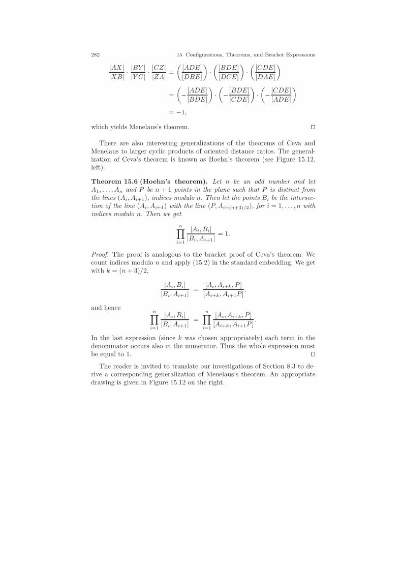
282 15 Configurations, Theorems, and Bracket Expressions
|AX ||XB| ·
|BY ||Y C| ·
|CZ||ZA| =
([ADE]
[DBE]
)·(
[BDE]
[DCE]
)·(
[CDE]
[DAE]
)
=
(− [ADE]
[BDE]
)·(− [BDE]
[CDE]
)·(− [CDE]
[ADE]
)
= −1,
which yields Menelaus’s theorem. ⊓⊔
There are also interesting generalizations of the theorems of Ceva andMenelaus to larger cyclic products of oriented distance ratios. The general-ization of Ceva’s theorem is known as Hoehn’s theorem (see Figure 15.12,left):
Theorem 15.6 (Hoehn’s theorem). Let n be an odd number and letA1, . . . , An and P be n + 1 points in the plane such that P is distinct fromthe lines (Ai, Ai+1), indices modulo n. Then let the points Bi be the intersec-tion of the line (Ai, Ai+1) with the line (P,Ai+(n+3)/2), for i = 1, . . . , n withindices modulo n. Then we get
n∏
i=1
|Ai, Bi||Bi, Ai+1|
= 1.
Proof. The proof is analogous to the bracket proof of Ceva’s theorem. Wecount indices modulo n and apply (15.2) in the standard embedding. We getwith k = (n+ 3)/2,
|Ai, Bi||Bi, Ai+1|
=[Ai, Ai+k, P ]
[Ai+k, Ai+1P ],
and hencen∏
i=1
|Ai, Bi||Bi, Ai+1|
=n∏
i=1
[Ai, Ai+k, P ]
[Ai+k, Ai+1P ].
In the last expression (since k was chosen appropriately) each term in thedenominator occurs also in the numerator. Thus the whole expression mustbe equal to 1. ⊓⊔
The reader is invited to translate our investigations of Section 8.3 to de-rive a corresponding generalization of Menelaus’s theorem. An appropriatedrawing is given in Figure 15.12 on the right.

15.5 Gluing Ceva and Menelaus Configurations 283
A1
A2
A3
A4A5
B1
B2
B3
B4
B5
P
A1
A2
A3
A4A5
B1
B2
B3
B4
B5
Fig. 15.12 Hoehn’s theorem and the generalized Menelaus theorem for n = 5.
15.5 Gluing Ceva and Menelaus Configurations
The World Serpent was an enormous snake which wrappedaround the world and bit his own tail.
The legend of Thor
The reason why we spend so much time on the theorems of Ceva and Menelausis that according to their simple structure they are ideal basic building blocksfor more complicated statements. What is missing so far is a kind of glue tolink several copies of Ceva’s or Menelaus’s configurations. Indeed, gluing themturns out to be an extremely natural (and powerful) process [110]. For thisconsider two different Ceva configurations that are identified along one edgesuch that the special point on the edge is shared by both configurations.Before we do so, we fix several naming conventions. When in the future wetalk about the “Cevaexpression” (or “Menelausexpression”) for the triangleA,B,C, the letters A, B, and C are assumed to be ordered as in (15.3). Theordering A,C,B would generate the reciprocal expression. Furthermore, wewill call the points X , Y , and Z the edge points of the configuration. Thepoints A, B, and C will be called the vertices of the configuration. Point Din a Ceva configuration will be called the Ceva point, and the secant line ina Menelaus configuration is the Menelaus line.
Now consider the situation in which two triangles that are equipped witha Ceva configuration share an edge and the corresponding edge point on this
edge (see the Figure 15.13). The triangle A,B,C yields a relation |AZ||ZB| ·
|BX||XC| ·
|CY ||Y A| = 1, while the triangle C,B,D yields |CX|
|XB| ·|BV ||V D| ·
|DW ||YW | = 1. The quotient
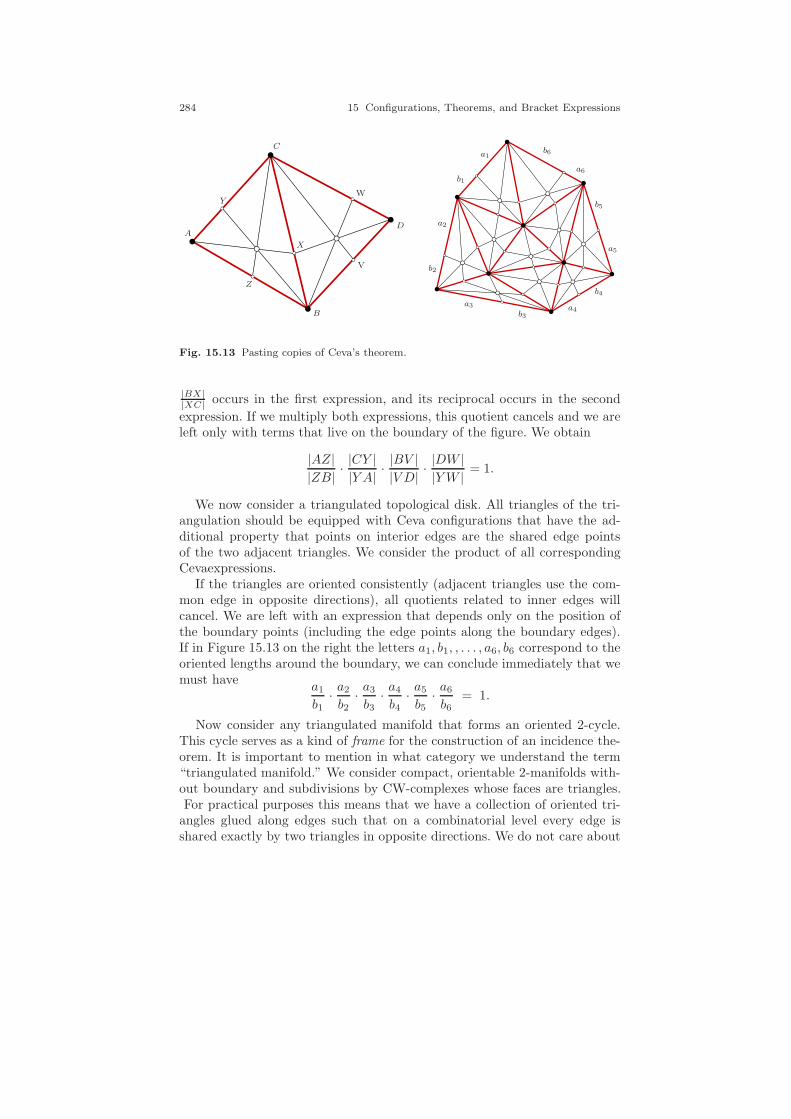
284 15 Configurations, Theorems, and Bracket Expressions
A
C
B
D
X
Y
Z
V
W
a1
b1
a2
b2
a3b3
a4
b4
a5
b5
a6
b6
Fig. 15.13 Pasting copies of Ceva’s theorem.
|BX||XC| occurs in the first expression, and its reciprocal occurs in the second
expression. If we multiply both expressions, this quotient cancels and we areleft only with terms that live on the boundary of the figure. We obtain
|AZ||ZB| ·
|CY ||Y A| ·
|BV ||V D| ·
|DW ||YW | = 1.
We now consider a triangulated topological disk. All triangles of the tri-angulation should be equipped with Ceva configurations that have the ad-ditional property that points on interior edges are the shared edge pointsof the two adjacent triangles. We consider the product of all correspondingCevaexpressions.
If the triangles are oriented consistently (adjacent triangles use the com-mon edge in opposite directions), all quotients related to inner edges willcancel. We are left with an expression that depends only on the position ofthe boundary points (including the edge points along the boundary edges).If in Figure 15.13 on the right the letters a1, b1, , . . . , a6, b6 correspond to theoriented lengths around the boundary, we can conclude immediately that wemust have
a1
b1· a2
b2· a3
b3· a4
b4· a5
b5· a6
b6= 1.
Now consider any triangulated manifold that forms an oriented 2-cycle.This cycle serves as a kind of frame for the construction of an incidence the-orem. It is important to mention in what category we understand the term“triangulated manifold.” We consider compact, orientable 2-manifolds with-out boundary and subdivisions by CW-complexes whose faces are triangles.For practical purposes this means that we have a collection of oriented tri-
angles glued along edges such that on a combinatorial level every edge isshared exactly by two triangles in opposite directions. We do not care about
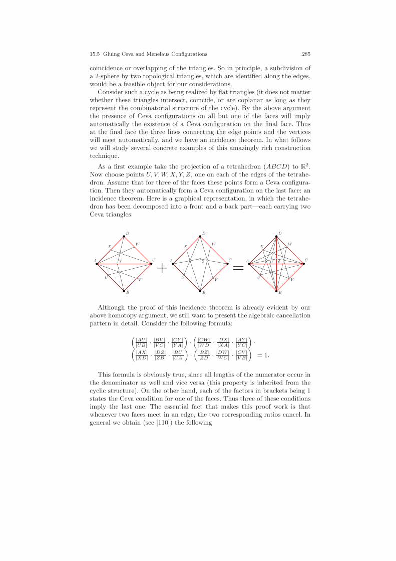
15.5 Gluing Ceva and Menelaus Configurations 285
coincidence or overlapping of the triangles. So in principle, a subdivision ofa 2-sphere by two topological triangles, which are identified along the edges,would be a feasible object for our considerations.
Consider such a cycle as being realized by flat triangles (it does not matterwhether these triangles intersect, coincide, or are coplanar as long as theyrepresent the combinatorial structure of the cycle). By the above argumentthe presence of Ceva configurations on all but one of the faces will implyautomatically the existence of a Ceva configuration on the final face. Thusat the final face the three lines connecting the edge points and the verticeswill meet automatically, and we have an incidence theorem. In what followswe will study several concrete examples of this amazingly rich constructiontechnique.
As a first example take the projection of a tetrahedron (ABCD) to R2.Now choose points U, V,W,X, Y, Z, one on each of the edges of the tetrahe-dron. Assume that for three of the faces these points form a Ceva configura-tion. Then they automatically form a Ceva configuration on the last face: anincidence theorem. Here is a graphical representation, in which the tetrahe-dron has been decomposed into a front and a back part—each carrying twoCeva triangles:
A C
D
B
UV
WX
Y
+A C
D
B
UV
WX
Z
=A C
D
B
UV
WX
Y Z
Although the proof of this incidence theorem is already evident by ourabove homotopy argument, we still want to present the algebraic cancellationpattern in detail. Consider the following formula:
(|AU||UB| ·
|BV ||V C| ·
|CY ||Y A|
)·(
|CW ||WD| ·
|DX||XA| ·
|AY ||Y C|
)·
(|AX||XD| ·
|DZ||ZB| ·
|BU||UA|
)·(
|BZ||ZD| ·
|DW ||WC| ·
|CV ||V B|
)= 1.
This formula is obviously true, since all lengths of the numerator occur inthe denominator as well and vice versa (this property is inherited from thecyclic structure). On the other hand, each of the factors in brackets being 1states the Ceva condition for one of the faces. Thus three of these conditionsimply the last one. The essential fact that makes this proof work is thatwhenever two faces meet in an edge, the two corresponding ratios cancel. Ingeneral we obtain (see [110]) the following
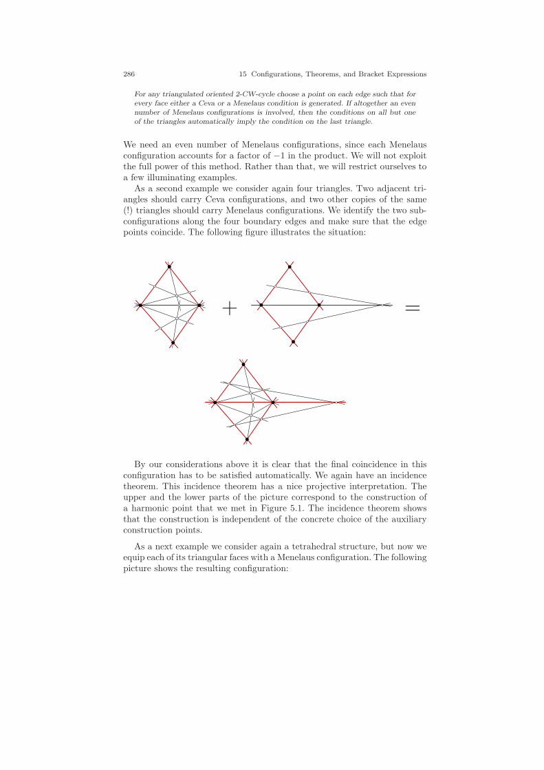
286 15 Configurations, Theorems, and Bracket Expressions
For any triangulated oriented 2-CW-cycle choose a point on each edge such that forevery face either a Ceva or a Menelaus condition is generated. If altogether an evennumber of Menelaus configurations is involved, then the conditions on all but oneof the triangles automatically imply the condition on the last triangle.
We need an even number of Menelaus configurations, since each Menelausconfiguration accounts for a factor of −1 in the product. We will not exploitthe full power of this method. Rather than that, we will restrict ourselves toa few illuminating examples.
As a second example we consider again four triangles. Two adjacent tri-angles should carry Ceva configurations, and two other copies of the same(!) triangles should carry Menelaus configurations. We identify the two sub-configurations along the four boundary edges and make sure that the edgepoints coincide. The following figure illustrates the situation:
+ =
By our considerations above it is clear that the final coincidence in thisconfiguration has to be satisfied automatically. We again have an incidencetheorem. This incidence theorem has a nice projective interpretation. Theupper and the lower parts of the picture correspond to the construction ofa harmonic point that we met in Figure 5.1. The incidence theorem showsthat the construction is independent of the concrete choice of the auxiliaryconstruction points.
As a next example we consider again a tetrahedral structure, but now weequip each of its triangular faces with a Menelaus configuration. The followingpicture shows the resulting configuration:
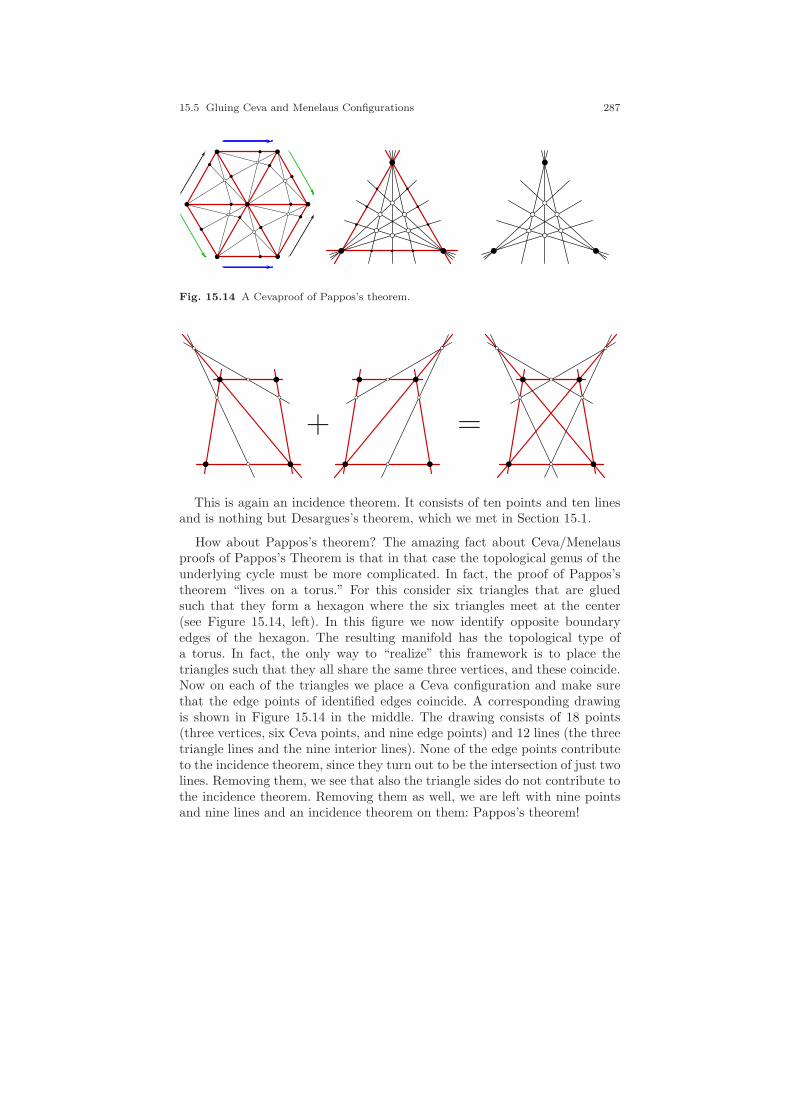
15.5 Gluing Ceva and Menelaus Configurations 287
Fig. 15.14 A Cevaproof of Pappos’s theorem.
+ =
This is again an incidence theorem. It consists of ten points and ten linesand is nothing but Desargues’s theorem, which we met in Section 15.1.
How about Pappos’s theorem? The amazing fact about Ceva/Menelausproofs of Pappos’s Theorem is that in that case the topological genus of theunderlying cycle must be more complicated. In fact, the proof of Pappos’stheorem “lives on a torus.” For this consider six triangles that are gluedsuch that they form a hexagon where the six triangles meet at the center(see Figure 15.14, left). In this figure we now identify opposite boundaryedges of the hexagon. The resulting manifold has the topological type ofa torus. In fact, the only way to “realize” this framework is to place thetriangles such that they all share the same three vertices, and these coincide.Now on each of the triangles we place a Ceva configuration and make surethat the edge points of identified edges coincide. A corresponding drawingis shown in Figure 15.14 in the middle. The drawing consists of 18 points(three vertices, six Ceva points, and nine edge points) and 12 lines (the threetriangle lines and the nine interior lines). None of the edge points contributeto the incidence theorem, since they turn out to be the intersection of just twolines. Removing them, we see that also the triangle sides do not contribute tothe incidence theorem. Removing them as well, we are left with nine pointsand nine lines and an incidence theorem on them: Pappos’s theorem!
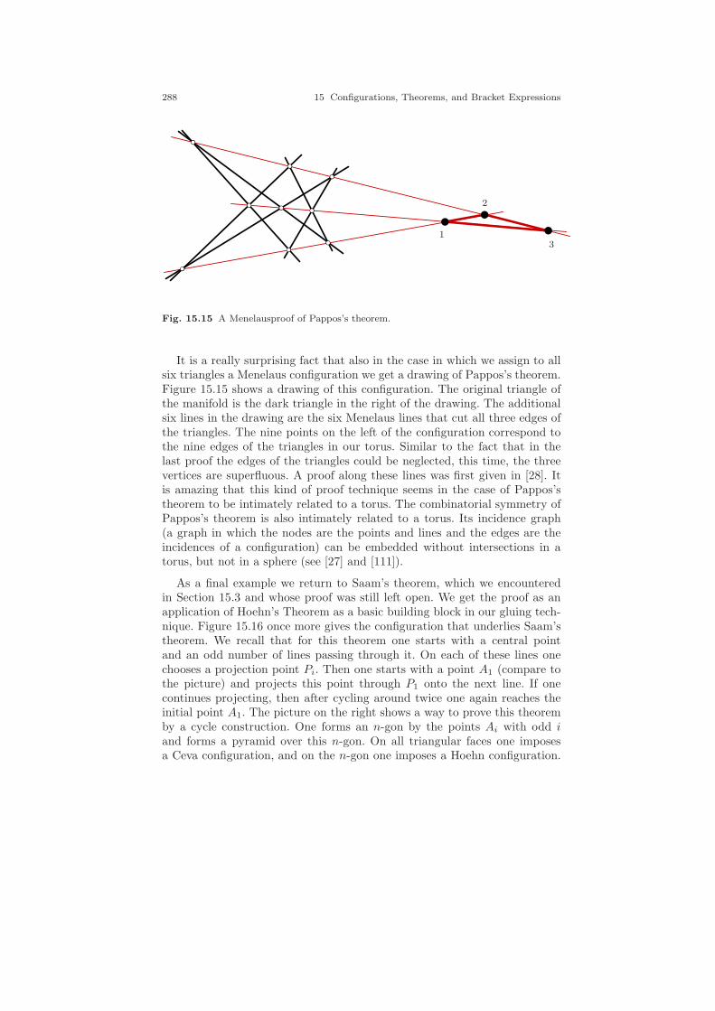
288 15 Configurations, Theorems, and Bracket Expressions
1
2
3
Fig. 15.15 A Menelausproof of Pappos’s theorem.
It is a really surprising fact that also in the case in which we assign to allsix triangles a Menelaus configuration we get a drawing of Pappos’s theorem.Figure 15.15 shows a drawing of this configuration. The original triangle ofthe manifold is the dark triangle in the right of the drawing. The additionalsix lines in the drawing are the six Menelaus lines that cut all three edges ofthe triangles. The nine points on the left of the configuration correspond tothe nine edges of the triangles in our torus. Similar to the fact that in thelast proof the edges of the triangles could be neglected, this time, the threevertices are superfluous. A proof along these lines was first given in [28]. Itis amazing that this kind of proof technique seems in the case of Pappos’stheorem to be intimately related to a torus. The combinatorial symmetry ofPappos’s theorem is also intimately related to a torus. Its incidence graph(a graph in which the nodes are the points and lines and the edges are theincidences of a configuration) can be embedded without intersections in atorus, but not in a sphere (see [27] and [111]).
As a final example we return to Saam’s theorem, which we encounteredin Section 15.3 and whose proof was still left open. We get the proof as anapplication of Hoehn’s Theorem as a basic building block in our gluing tech-nique. Figure 15.16 once more gives the configuration that underlies Saam’stheorem. We recall that for this theorem one starts with a central pointand an odd number of lines passing through it. On each of these lines onechooses a projection point Pi. Then one starts with a point A1 (compare tothe picture) and projects this point through P1 onto the next line. If onecontinues projecting, then after cycling around twice one again reaches theinitial point A1. The picture on the right shows a way to prove this theoremby a cycle construction. One forms an n-gon by the points Ai with odd iand forms a pyramid over this n-gon. On all triangular faces one imposesa Ceva configuration, and on the n-gon one imposes a Hoehn configuration.
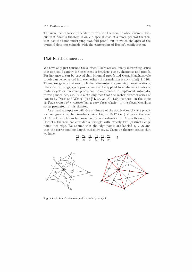
15.6 Furthermore . . . 289
The usual cancellation procedure proves the theorem. It also becomes obvi-ous that Saam’s theorem is only a special case of a more general theoremthat has the same underlying manifold proof, but in which the apex of thepyramid does not coincide with the centerpoint of Hoehn’s configuration.
15.6 Furthermore . . .
We have only just touched the surface. There are still many interesting issuesthat one could explore in the context of brackets, cycles, theorems, and proofs.For instance it can be proved that binomial proofs and Ceva/Menelauscycleproofs can be converted into each other (the translation is not trivial) [1, 110].There are generalizations to higher dimensions; symmetry considerations;relations to liftings; cycle proofs can also be applied to nonlinear situations;finding cycle or binomial proofs can be automated to implement automaticproving machines, etc. It is a striking fact that the rather abstract series ofpapers by Dress and Wenzel (see [34, 35, 36, 87, 130]) centered on the topicof Tutte groups of a matroid has a very close relation to the Ceva/Menelaussetup presented in this chapter.
As a final example we will give a glimpse of the application of cycle proofsfor configurations that involve conics. Figure 15.17 (left) shows a theoremof Carnot, which can be considered a generalization of Ceva’s theorem. InCarnot’s theorem we consider a triangle with exactly two (distinct) edgepoints per edge. We assume that the edge points are labeled 1, . . . , 6 andthat the corresponding length ratios are ai/bi. Carnot’s theorem states thatwe have
a1
b1· a2
b2· a3
b3· a4
b4· a5
b5· a6
b6= 1
OP1
P2
P3
P4
P5A1
A2
A3
A4
A5
A6
A7A8
A9
A10
Fig. 15.16 Saam’s theorem and its underlying cycle.
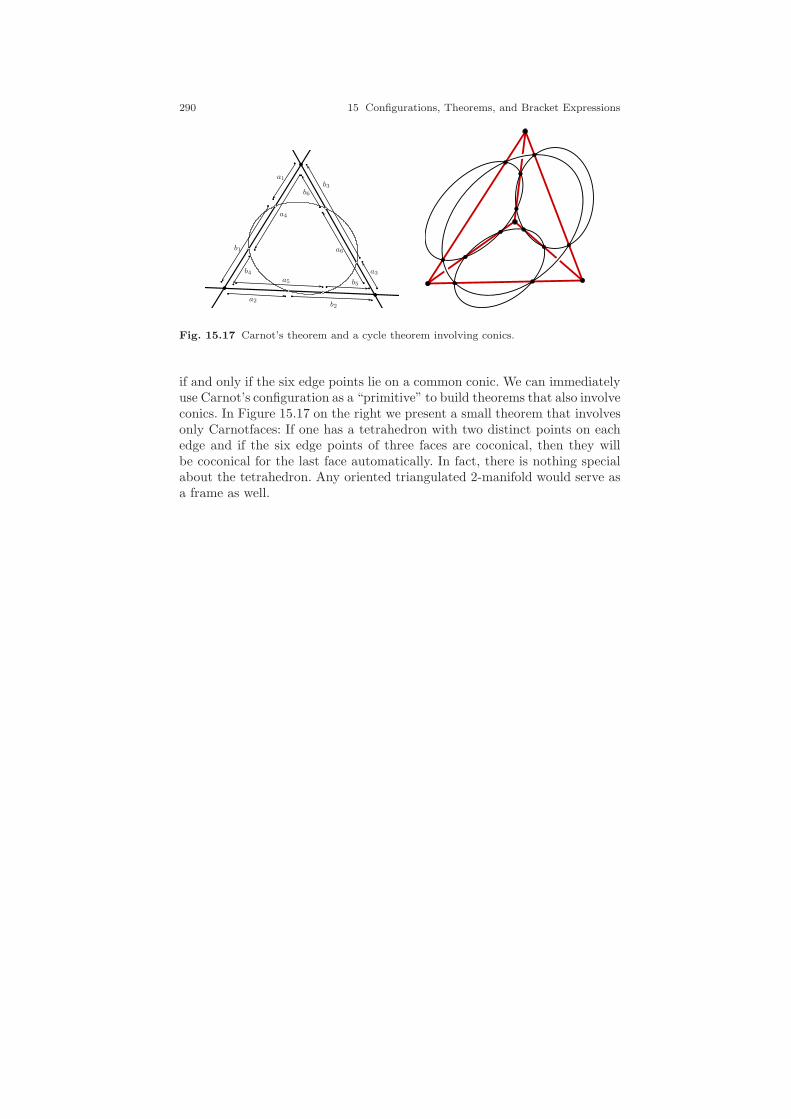
290 15 Configurations, Theorems, and Bracket Expressions
a1
a2
a3
a4
a5
a6b1
b2
b3
b4
b5
b6
Fig. 15.17 Carnot’s theorem and a cycle theorem involving conics.
if and only if the six edge points lie on a common conic. We can immediatelyuse Carnot’s configuration as a “primitive” to build theorems that also involveconics. In Figure 15.17 on the right we present a small theorem that involvesonly Carnotfaces: If one has a tetrahedron with two distinct points on eachedge and if the six edge points of three faces are coconical, then they willbe coconical for the last face automatically. In fact, there is nothing specialabout the tetrahedron. Any oriented triangulated 2-manifold would serve asa frame as well.

Part III
Measurements

293
Calvin and Hobbes Copyright 1988 Watterson. Used by permission of Universal Press Syndicate. All rights reserved.
Bill Watterson, Calvin and Hobbes, 1988
Perhaps the most annoying thing about our current setup for projective ge-ometry is the fact that concepts that one usually immediately associates withgeometry (such as circles, distances, and angles) do not have an immediatecorrespondence. We obtained a very beautiful algebraic system for dealingwith geometry, but we paid a high price. Many interesting and nice resultsfrom geometry cannot even be expressed by our language developed so far.Essentially most concepts that belong to Euclidean geometry were abandonedfrom our setup. We could talk about conic sections, but not about circles.We could measure cross-ratios but not distances; we could intersect arbitrarypairs of lines, but we lost the notion of angles.
Thus it is, for instance, impossible to formulate a simple statement like“The altitudes in a triangle meet in a point”, since we do not have a conceptof perpendicularity. We also do not have any equivalents to Thales’ theoremor the Pythagorean theorem, since we cannot speak about circles and righttriangles. It would seem then that we have developed a beautiful algebraicsystem at the price of giving up Euclidean geometry!

294
Here comes the good news: This is not true at all—there is a beautifulsystem that allows us to express all Euclidean concepts and magnitudes ina purely projective framework. Thus we can perform all nice operations ofprojective geometry and still retain the expressive power and richness ofEuclidean geometry. Things are even better: if we properly understand howto incorporate Euclidean geometry into projective geometry we will see thatEuclidean geometry is just a special case of several other ways to embed othergeometries. If we then play with the parameters, we will see that there is awhole variety of other geometries expressible in a similar (and algebraicallysmooth) manner. Euclidean geometry will just be a special case of a muchricher system. The larger system will contain prominent inhabitants such ashyperbolic geometry and relativistic space-time geometry.
It is the purpose of this part of the book to develop this general theory.As before, we will pay special attention to the question of how geometricprimitive operations can be carried out in the most general and at the sametime the simplest way. The key to everything will be the proper use of complexnumbers.
16
Complex Numbers: A Primer
The Divine Spirit found a sublime outlet in that wonder ofanalysis, that portent of the ideal world, that amphibian be-tween being and not-being, which we call the imaginary rootof negative unity.
Gottfried Wilhelm Leibniz, 1702
So far, almost all our considerations have dealt with real projective geometry.The main reason for this is that we wanted to stay with all our considerationsas concrete and close to imagination as possible. Nevertheless, almost allconsiderations we have made so far carry over in a straightforward way toother underlying fields. Only in very rare cases are small twists necessary,and if so, they result from one of the following two facts:
• Depending on the field, certain equations may be solvable or not.• Other fields may have other field automorphisms.
We now will be interested in particular in projective geometry over thecomplex numbers. Since the complex numbers are algebraically closed (everypolynomial equation is solvable over the complex numbers), objects will haveintersections in general. For instance, over the complex numbers there isalways an intersection of a conic and a line, in contrast to the real case inwhich we may have situations in which the two objects do not intersect. Thisis the first benefit we will get from the use of complex numbers. They willhelp in our efforts to exclude special cases.
Compared to real numbers, the complex numbers have more field automor-phisms. Besides the identity (the only automorphism of the real numbers),there is also the automorphism that sends x+ iy to x− iy.
295

296 16 Complex Numbers: A Primer
automorphism!of a field This automorphism corresponds to complex conju-gation.1 Considering this fact under the light of the fundamental theoremof projective geometry (compare Section 5.4), we see that over the complexnumbers there will be harmonic maps and collineations that do not corre-spond to a matrix multiplication but come from complex conjugation. Wewill have to deal with this difference later.
This section is meant as a very brief introduction to complex numbers.Here we will highlight all ingredients we will need later. Readers who alreadyfeel very familiar with complex numbers can skip this chapter with no harm.
16.1 Historical Background
The historical roots of complex numbers are closely related to the task offinding solutions to polynomial equations [137]. It is an interesting fact thatcomplex numbers were first discovered in the context of cubic rather thanquadratic equations. Roughly, the story goes as follows:quadratic equationequation!quadratic In antiquity it was known how to solve quadratic equa-tions x2 + px+ q = 0. The solution is given by the well-known formula
x1/2 = −p2±√p2
4− q.
It was clear that there are instances in which no (real) solution would bepossible due to the fact that the square of a (real) number is always positive.So for instance, the equation x2 = −1 was considered unsolvable.
Since then it remained a major open question how to generalize the solu-tion of the quadratic equation to the next more complicated case, the cubicequation.cubic equationequation!cubic In fact, it took several hundred years until a solution was found(in the sixteenth century), and one can say that the developments triggeredby the discovery of this formula form the initial point of what one wouldconsider “modern mathematics.” The history around the discovery of thesolution (we already used a variant of it in Section 11.4 when we intersectedtwo conics) is exciting, full of personal tragedy, amusing—a prototype of amathematical “crime story” on priority disputes. Again, since this is not abook on the history of mathematics we will only briefly outline the basic plotand refer to history books for details [48, 137]. We also recommend the novel[61]. Briefly, Scipione del Ferro was essentially the first to solve (a specialcase of) the general cubic equation x3 + ax2 + bx + c = 0 around 1515.
1 These are the only continuous automorphisms of C. Indeed, in the presence of the axiomof choice there are also uncountably many wild automorphisms of C.

16.1 Historical Background 297
Unfortunately, he did not publish his result during his lifetime (he died in1526). However, he told the solution to his scholar and relative Anton MariaFior (a more or less mediocre mathematician).After Scipione’s death, AntonMaria Fior challenged the mathematician Nicolo Tartaglia (1499–1557) to amathematical tournament (which were quite common at this time). Tartagliawas the best-known mathematician in Italy at this time and practiced inVenice. Such a tournament consisted of 30 mathematical challenges, whichwere given from either opponent to the other. Somehow, Tartaglia found outthat Fior knew the secret of how to solve cubic equations. Tartaglia suspectedcorrectly that all challenges he had to face would involve cubic equations. Hefigured out how to solve (a special case of) the cubic equation by himselfand won the tournament handily—he solved all 30 problems within 2 hours.At that time another Italian mathematician, Girolamo Cardano (1501–1576)was working on a book that covered the mathematical knowledge known atthe time (Tartaglia had a similar project). Cardano importuned Tartagliato reveal his formula so that he could include it in his book. Tartaglia firstresisted, but after several attempts, he agreed to tell him the formula underthe condition that Cardano would not publish the formula in his own book.Cardano even vowed not to tell Tartaglia’s formula in speech or in writing.However, a few years later Cardano found out that Tartaglia was not the firstto have solved the cubic equation. Therefore, he felt released from the vowand included Tartaglia’s formula in his book Ars magna (1545). Cardano evengeneralized the solution and was able to solve all special cases of the equation.For Tartaglia this was a great shock, and he began a long and public priorityfight with Cardano. The solution formula was until recently always called“Cardano’s formula.” In recent years (and after some historical research) itis more common to call it the “del Ferro/Tartaglia/Cardano formula.”
As we will see, despite all the priority disputes, Cardano made a contri-bution in this context that is perhaps more important than the solution ofcubic equations itself. Tartaglia’s general formula for solving the cubic equa-tion x3 +px+q = 0 (every cubic equation can be easily transformed into thisform) can in modern terms be formulated as:
x =3
√
− q2
+
√q2
4+p3
27+
3
√
− q2−√q2
4+p3
27.
For instance, if one wants to find a solution of x3 − 24x− 72 = 0, one gets
298 16 Complex Numbers: A Primer
x =3
√−−72
2 +√
722
4 + (−243)27 +
3
√−−72
2 −√
722
4 + (−243)27
= 3√
36 +√
1296 − 512 + 3√
36 −√
1296− 512
= 3√
36 + 28 + 3√
36 − 28
= 3√
64 + 3√
8
= 4 + 2
= 6.
And indeed, x = 6 is a solution of the cubic equation: 63 − 24 · 6 − 72 =216 − 144 − 72 = 0.
Now, it is clear that every cubic equation of the above form must haveat least one solution, since as x runs from −∞ to +∞, the cubic itself runscontinuously from −∞ to +∞ and therefore has to pass through zero. Un-fortunately, Tartaglia’s formula applied in a naive way does not always leadto a solution. Consider, for instance, the problem x3 − 15x − 4 = 0. If weproceed in the same way as before, we get
x =3
√−−4
2 +√
42
4 + (−153)27 +
3
√−−4
2 −√
42
4 + (−153)27
= 3√
2 +√
4 − 125 + 3√
2 −√
4 − 125
= 3√
2 +√−121 + 3
√2 −
√−121
= . . .
. . . and we are stuck! What should one do with the term√−121? There is
no number (at least for del Ferro and Tartaglia) whose square is −121. Nev-ertheless, there must be a solution of the cubic (in contrast to the quadraticcase, where nobody saw a reason for searching for a solution of x2 = −1).This was the place where Cardano made his brilliant innovation. He simplywent on calculating, assuming that one could take the term
√−1 as a purely
formal expression with which one could do arithmetic. It behaves almost likea usual number but must be used subject to the rule
√−1 ·
√−1 = −1. If we
do so, we can continue the above calculation
3√
2 +√−121 + 3
√2 −
√−121
= 3√
2 + 11√−1 + 3
√2 − 11
√−1
= . . .
. . . and now we need two numbers a and b with the property that a3 =2 + 11
√−1 and b3 = 2 − 11
√−1. In fact, a = 2 +
√−1 and b = 2 −
√−1 do
the job (check it!) and we can proceed:

16.2 The Fundamental Theorem 299
Fig. 16.1 Function plots of the two cubic polynomials (x3 −24x−72)/50 and (x3−15x−4)/50.
3√
2 +√−1 + 3
√2 −
√−1
= (2 + 11√−1) + (2 − 11
√−1)
= 4.
Et voila, right before the last equation the mysterious√−1 disappears again,
and we end up with a nice, real (and correct) solution x = 4. Testing theresult we obtain 43 − 15 · 4 − 4 = 64 − 60 − 4 = 0.
In “modern times” things have been smoothed out. A new symbol “i” wasintroduced that plays the role of the mysterious
√−1 and behaves subject to
i2 = −1. This number i is usually called the imaginary unit. We now usuallyconsider C = R[i] as a field extension of the real numbers, so that we canconsider complex numbers as numbers of the form x+ i ·y. Complex numbersplay a great unifying role in modern mathematics. With their help, seeminglyunrelated effects and topics may be interpreted as different sides of the samecoin. We will have a brief look at some of them.
16.2 The Fundamental Theorem
The fundamental theorem of algebra is a great example for the unifying powerof complex numbers. Complex numbers were originally introduced to performthe calculations to solve cubic equations. However, they also generalize thestructure of the solution set. A view to the solution set of cubic equation fromthe “real perspective” tells us that they will have one, two, or three solutions,depending on the values of their parameters. From a “complex perspective”one can prove that a cubic x3 +ax2 +bx+c can always be written in the form(x−x1)(x−x2)(x−x3), where x1, x2, x3 are three (possibly complex) numbers.Since this expression is zero if and only if x itself equals one of these numbers,x1, x2, x3 must be solutions of the cubic equation x3+ax2+bx+c = 0. Thus ina certain sense we could say that a cubic equation always has three solutions.
300 16 Complex Numbers: A Primer
They may occur with a multiplicity if the same linear expression is used morethan once in the expression (x− x1)(x− x2)(x− x3).
This is a special case of a much more general theorem: the fundamentaltheorem of algebra. This theorem states that every polynomial
f(x) = xn + an−1xn−1 + · · · + a1x+ a0
of degree n may be written as a product of n linear factors
(x− x1) · (x− x2) · · · · · (x− xn).
The numbers x1, . . . , xn are all solutions of the equation f(x) = 0. Thesenumbers may be real or complex, and they may occur with a certain multi-plicity in the product expression.
Thus not only do complex numbers help to solve quadratic and cubicequations, they also allow one to find all solutions of arbitrary polynomials.The fundamental theorem is by far not easy to prove, and both proofs ofthis theorem first known (one by Gauss and one by d’Alembert) turned outto have some minor flaws.2 It is important to mention that the fundamentaltheorem of algebra does not tell how to find the solutions of a polynomialequation. It only states their existence.
Applied to geometric problems, the fundamental theorem has many im-portant consequences concerning the intersection multiplicity of geometricobjects. It gives us the right to speak of intersections of objects even if wedo not see them. Thus a line and a nondegenerate conic will always have twointersections, either real or complex. These two intersections coincide if theline is tangent to the conic. Similarly, two conics will in general have fourpoints of intersection. Again these intersections may coincide.
16.3 Geometry of Complex Numbers
One of the most important aspects in relation to our investigations will bea geometric interpretation of complex numbers. A complex number a + i · bmay be associated to the point (a, b) in the real plane R2. Thus we may iden-tify the field of complex numbers C with the real Euclidean plane R2. Everystatement about complex numbers immediately possesses a geometric coun-terpart. It is amazing that this (from a modern perspective almost obvious)interpretation was made quite a while after the invention of complex num-bers. The geometric interpretation was first published by Caspar Wessel in1799 (this is about 250 years after complex numbers were introduced!). Later,
2 In fact, in 1799 Gauss published a proof in response to d’Alembert’s proof, since hethought that this proof was not rigorous. However Gauss’s proof (based on a topologicalargument) also contained some flaws. Perhaps the first complete and correct proof wasgiven in 1816 by Gauss.
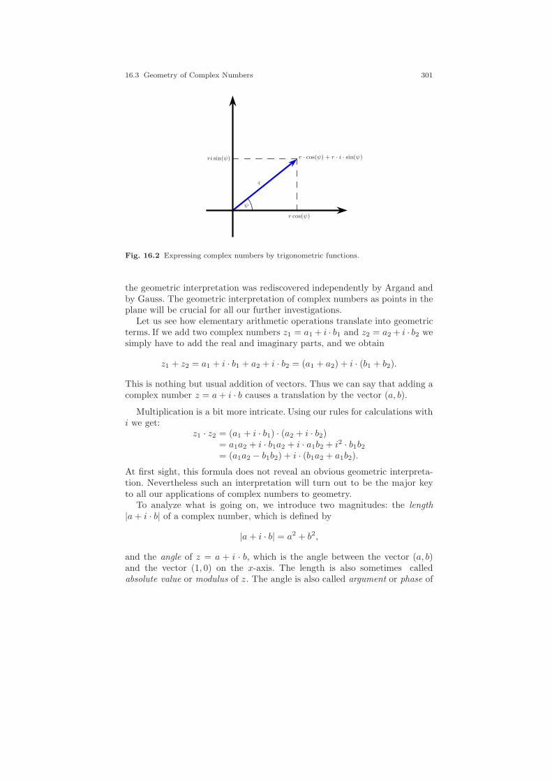
16.3 Geometry of Complex Numbers 301
r
ri sin(ψ)
r cos(ψ)
r · cos(ψ) + r · i · sin(ψ)
ψ
Fig. 16.2 Expressing complex numbers by trigonometric functions.
the geometric interpretation was rediscovered independently by Argand andby Gauss. The geometric interpretation of complex numbers as points in theplane will be crucial for all our further investigations.
Let us see how elementary arithmetic operations translate into geometricterms. If we add two complex numbers z1 = a1 + i · b1 and z2 = a2 + i · b2 wesimply have to add the real and imaginary parts, and we obtain
z1 + z2 = a1 + i · b1 + a2 + i · b2 = (a1 + a2) + i · (b1 + b2).
This is nothing but usual addition of vectors. Thus we can say that adding acomplex number z = a+ i · b causes a translation by the vector (a, b).
Multiplication is a bit more intricate. Using our rules for calculations withi we get:
z1 · z2 = (a1 + i · b1) · (a2 + i · b2)= a1a2 + i · b1a2 + i · a1b2 + i2 · b1b2= (a1a2 − b1b2) + i · (b1a2 + a1b2).
At first sight, this formula does not reveal an obvious geometric interpreta-tion. Nevertheless such an interpretation will turn out to be the major keyto all our applications of complex numbers to geometry.
To analyze what is going on, we introduce two magnitudes: the length|a+ i · b| of a complex number, which is defined by
|a+ i · b| = a2 + b2,
and the angle of z = a + i · b, which is the angle between the vector (a, b)and the vector (1, 0) on the x-axis. The length is also sometimes calledabsolute value or modulus of z. The angle is also called argument or phase of
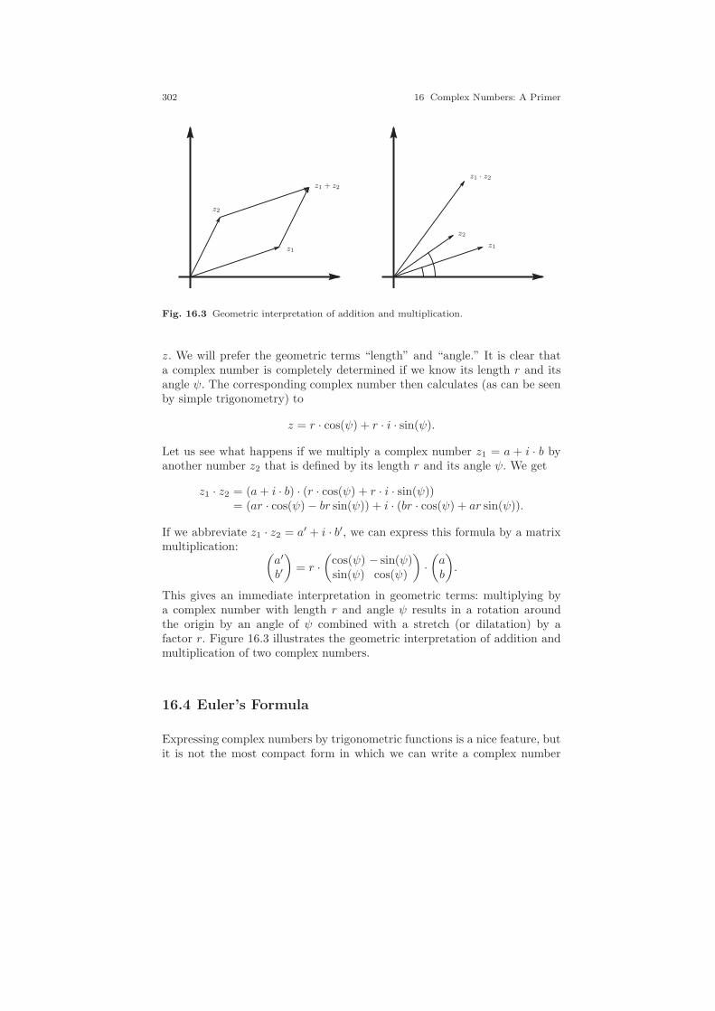
302 16 Complex Numbers: A Primer
z1
z2
z1 + z2
z1
z2
z1 · z2
Fig. 16.3 Geometric interpretation of addition and multiplication.
z. We will prefer the geometric terms “length” and “angle.” It is clear thata complex number is completely determined if we know its length r and itsangle ψ. The corresponding complex number then calculates (as can be seenby simple trigonometry) to
z = r · cos(ψ) + r · i · sin(ψ).
Let us see what happens if we multiply a complex number z1 = a + i · b byanother number z2 that is defined by its length r and its angle ψ. We get
z1 · z2 = (a+ i · b) · (r · cos(ψ) + r · i · sin(ψ))= (ar · cos(ψ) − br sin(ψ)) + i · (br · cos(ψ) + ar sin(ψ)).
If we abbreviate z1 · z2 = a′ + i · b′, we can express this formula by a matrixmultiplication: (
a′
b′
)= r ·
(cos(ψ) − sin(ψ)sin(ψ) cos(ψ)
)·(ab
).
This gives an immediate interpretation in geometric terms: multiplying bya complex number with length r and angle ψ results in a rotation aroundthe origin by an angle of ψ combined with a stretch (or dilatation) by afactor r. Figure 16.3 illustrates the geometric interpretation of addition andmultiplication of two complex numbers.
16.4 Euler’s Formula
Expressing complex numbers by trigonometric functions is a nice feature, butit is not the most compact form in which we can write a complex number

16.4 Euler’s Formula 303
given by angle and length. There is a beautiful formula known as Euler’sformula that closely relates trigonometric functions, complex numbers, andthe exponential function. One way to express this formula is
eix = cos(x) + i · sin(x).
If x is a real number, this means that the exponential of the purely imaginarynumber ix can be expressed as combination of cos(x), which forms the realpart, and i · sin(x), which forms the imaginary part. In this form the formulawas published by Euler in 1748 (although it was discovered earlier by RogerCotes in 1714). Since the geometric interpretation of complex numbers wasnot known at this time, both Cotes and Euler considered this result a purelyanalytical statement.
When trying to interpret this formula, we encounter an important diffi-culty: What is eix? How should we define the result of an analytic functionapplied to a complex argument? The short answer to this goes as follows:Whenever a function is expressible as a formal power series, one can use thispower series to evaluate the function also for complex arguments, as long asit converges. In particular, the functions ex, sin(x), and cos(x) have formalpower series that converge for all complex numbers. These power series are
ex = 1 + x + x2
2! + x3
3! + x4
4! + x5
5! + x6
6! + x7
7! + · · · ,
sin(x) = x − x3
3! + x5
5! − x7
7! + · · · ,
cos(x) = 1 − x2
2! + x4
4! − x6
6! + · · · .
Comparing the entries of these power series, we observe a striking similarityof the summands of the three power series. Up to sign changes, all summandsof ex occur in sin(x) or cos(x). So, how do we get the signs right? This iswhere the number i enters the game. If we expand the function eix, we seethat depending on the power of the summand, the summand occurs eitherwith a factor i (for even powers) or not (for odd powers). By the rule i2 = −1also the signs are altered according to a very regular pattern. In detail, weget
eix = 1 + ix + (ix)2
2! + (ix)3
3! + (ix)4
4! + (ix)5
5! + (ix)6
6! + (ix)7
7! + . . .
= 1 + ix − x2
2! − ix3
3! + x4
4! + ix5
5! − x6
6! − ix7
7! + · · · ,
i sin(x) = ix − ix3
3! + ix5
5! − ix7
7! + · · · ,
cos(x) = 1 − x2
2! + x4
4! − x6
6! + · · · .
We have printed the power series for cos(x) and i sin(x) for reference purposes.We see that eix splits into these two functions. So we have
eix = cos(x) + i · sin(x).
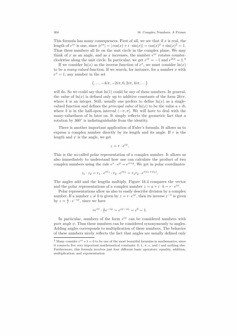
304 16 Complex Numbers: A Primer
This formula has many consequences. First of all, we see that if x is real, thelength of eix is one, since |eix| = | cos(x) + i · sin(x)| = cos(x)2 + sin(x)2 = 1.Thus these numbers all lie on the unit circle in the complex plane. We maythink of x as an angle, and as x increases, the number eix rotates counter-clockwise along the unit circle. In particular, we get eiπ = −1 and e2iπ = 1.3
If we consider ln(x) as the inverse function of ex, we must consider ln(x)to be a many-valued function. If we search, for instance, for a number x withex = 1, any number in the set
. . . ,−4iπ,−2iπ, 0, 2iπ, 4iπ, . . .
will do. So we could say that ln(1) could be any of these numbers. In general,the value of ln(x) is defined only up to additive constants of the form 2kiπ,where k is an integer. Still, usually one prefers to define ln(x) as a single-valued function and defines the principal value of ln(x) to be the value a+ ib,where b is in the half-open interval (−π, π]. We will have to deal with themany-valuedness of ln later on. It simply reflects the geometric fact that arotation by 360 is indistinguishable from the identity.
There is another important application of Euler’s formula. It allows us toexpress a complex number directly by its length and its angle. If r is thelength and ψ is the angle, we get
z = r · eiψ.
This is the so-called polar representation of a complex number. It allows usalso immediately to understand how one can calculate the product of twocomplex numbers using the rule ex · ey = ex+y. We get in polar coordinates
z1 · z2 = r1 · eiψ1 · r2 · eiψ2 = r1r2 · ei(ψ1+ψ2).
The angles add and the lengths multiply. Figure 16.4 compares the vectorand the polar representations of a complex number z = a+ i · b = r · eiψ.
Polar representations allow us also to easily describe division by a complexnumber. If a number z 6= 0 is given by z = r ·eiψ, then its inverse z−1 is givenby z = 1
r · e−iψ, since we have
reiψ · 1r e
−iψ = eiψ−iψ = e0 = 1.
In particular, numbers of the form eiψ can be considered numbers withpure angle ψ. Thus these numbers can be considered synonymously to angles.Adding angles corresponds to multiplication of these numbers. The behaviorof these numbers nicely reflects the fact that angles are usually defined only
3 Many consider eiπ+1 = 0 to be one of the most beautiful formulas in mathematics, sinceit connects five very important mathematical constants: 0, 1, π, e, and i and nothing else.
Furthermore, this formula involves just four different basic operators: equality, addition,multiplication, and exponentiation.
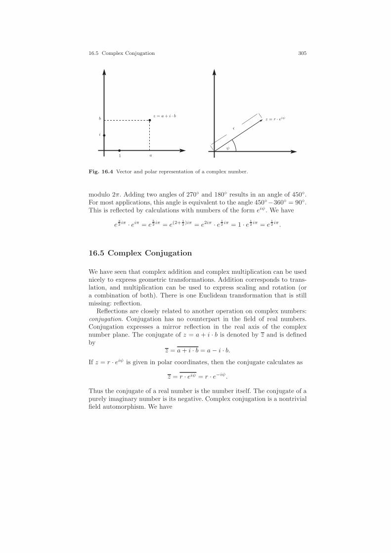
16.5 Complex Conjugation 305
1
i
a
bz = a+ i · b
r
ψ
z = r · eiψ
Fig. 16.4 Vector and polar representation of a complex number.
modulo 2π. Adding two angles of 270 and 180 results in an angle of 450.For most applications, this angle is equivalent to the angle 450−360 = 90.This is reflected by calculations with numbers of the form eiψ. We have
e32iπ · eiπ = e
52iπ = e(2+
12)iπ = e2iπ · e 1
2iπ = 1 · e 1
2iπ = e
12iπ .
16.5 Complex Conjugation
We have seen that complex addition and complex multiplication can be usednicely to express geometric transformations. Addition corresponds to trans-lation, and multiplication can be used to express scaling and rotation (ora combination of both). There is one Euclidean transformation that is stillmissing: reflection.
Reflections are closely related to another operation on complex numbers:conjugation. Conjugation has no counterpart in the field of real numbers.Conjugation expresses a mirror reflection in the real axis of the complexnumber plane. The conjugate of z = a + i · b is denoted by z and is definedby
z = a+ i · b = a− i · b.If z = r · eiψ is given in polar coordinates, then the conjugate calculates as
z = r · eiψ = r · e−iψ.
Thus the conjugate of a real number is the number itself. The conjugate of apurely imaginary number is its negative. Complex conjugation is a nontrivialfield automorphism. We have

306 16 Complex Numbers: A Primer
z = a+ ib
z = a− ib
Fig. 16.5 Complex conjugation.
z1 + z2 = z1 + z2 and z1 · z2 = z1 · z2.
The first equation follows immediately from the vector representation; thesecond follows immediately from the polar representation. In respect of thefundamental theorem of projective geometry this means that in complex pro-jective spaces we will have harmonic maps or collinearities that do not comefrom projective transformations. If we consider only continuous automor-phisms, complex conjugation is the only nontrivial field automorphism ofC, so that we do not get too many types of continuous harmonic maps orcollineations.
There are a few facts on complex conjugation that should be mentioned,since they will turn out to be useful later. The first couple of facts concernthe relation of complex conjugates to the elementary arithmetic operations:
• Adding a number z to its own conjugate, we obtain twice the real partof the number:
z + z = (a+ ib) + (a− ib) = 2a.
• Subtracting z from z, we obtain twice the imaginary part of the number:
z − z = (a+ ib) − (a− ib) = 2ib.
• Multiplying z by z, we obtain the square of the absolute value of z:
z · z = reiψ · re−iψ = r2eiψ−iψ = r2e0 = r2.
• Dividing z by z, we obtain the number that has length 1 and twice theangle of z:
z/z = reiψ/re−iψ = eiψ+iψ = e2iψ .
It is a remarkable fact that complex conjugates and the four arithmeticoperations are so closely related to the parameters of a complex number. We
16.5 Complex Conjugation 307
will make use of this later on. In particular, the third equation implies thatone can define the absolute value of a complex number by |z| =
√z · z.
Another important fact is that if we have a polynomial f(x) =∑n
i=0 aixi
with real parameters ai, then as mentioned before, not all zeros of this poly-nomial may be real. However, if we have a complex root z of this polynomial,then z will also be a root. This can be seen easily by evaluating f(z):
f(z) =
n∑
i=0
aizi =
n∑
i=0
ai zi =
n∑
i=0
aizi =
n∑
i=0
aizi = 0 = 0.
The second equality holds since the ai were assumed to be real and hence wehave ai = ai.
The proof strategy we have used here may be viewed as a special case of amore general concept. If we have any complex function f(z1, z2, . . . , zn) thatis composed only of the four arithmetic operations and complex conjugation,then we will automatically have
f(z1, z2, . . . , zn) = f(z1, z2, . . . , zn).

17
The Complex Projective Line
The shortest route between two truths in the real domainpasses through the complex domain.
Jacques Salomon Hadamard (1865–1963)
Now we will study the simplest case of a complex projective space: the com-plex projective line. We will see that even this case has already very richgeometric interpretations. The close relation of complex arithmetic opera-tions to geometry allows us to express geometric properties by nice algebraicstructures. In particular, this case will be the first example of a projectivespace in which we will be able to properly deal with circles.
17.1 CP1
Let us recall how we introduced the real projective line. We took the one-dimensional space R, considered it as a Euclidean line, and added one pointat infinity. Topologically, we obtained a circle. The best way to express theelements of the real projective line algebraically was to introduce homoge-neous coordinates. For this we associated to each number x ∈ R the vector(x, 1)T and identified nonzero scalar multiples. Finally, we identified the vec-tor (1, 0)T (and all its non-zero multiples) with the point at infinity. We endedup with the space
RP1 =
R2 − (0, 0)TR − 0 .
We will do exactly the same for the complex numbers! To obtain thecomplex projective line we start with all the numbers in C. We associate every
309
310 17 The Complex Projective Line
number z ∈ C with the vector (z, 1)T and identify nonzero scalar multiples.By this we associate all vectors of the form (a, b)T ; b 6= 0, to a number inC. What is left is the vector (1, 0)T and all its nonzero multiples. They willrepresent a unique point at infinity. All in all, we obtain the space CP
1 definedby
CP1 =
C2 − (0, 0)TC − 0 .
This space is isomorphic to all complex numbers together with one point atinfinity.
What is the dimension of this space? In a sense, this depends on the pointof view. From the perspective of real numbers, the complex plane C is atwo-dimensional object, since it requires two real parameters to specify theobjects of C. Hence one would say that also CP
1 is a real-two-dimensionalobject, since it differs from C just by one point. On the other hand, from acomplex perspective, C is just a one-dimensional object. It contains just one(complex) parameter. Since R is the real number line, one could consider C
the complex number line. Thus C is complex-one-dimensional, and so is CP1.
This is the reason why we call the space CP1 the complex projective line!
There is another issue important to mention in this context. Identifyingvectors that differ only by a nonzero scalar this time also includes multiplica-tion by complex numbers. Thus (1, 2)T , (3i, 6i)T , (2+ i, 4+2i)T all representthe same point. From every point represented by (a, b)T with b 6= 0 we canreconstruct the corresponding number of C by multiplication by 1/b. Thedehomogenized number is then a/b ∈ C. We will also frequently identify CP
1
with the space C := C ∪ ∞. As in the case of real numbers, we use thestandard rules for arithmetic operations with ∞:
1/∞ = 0; 1/0 = ∞; 1 + ∞ = ∞; ∞ + ∞ = ∞.
17.2 Testing Geometric Properties
We will now identify the finite part of the complex projective line (i.e., C
as a part of CP1) with the Euclidean plane R2 and investigate how certain
geometric properties can be expressed in terms of algebraic expressions inC. Most of these tests will, however, not correspond to projectively invariantproperties in CP
1.We will first express the property that two vectors associated to two com-
plex numbers z1 and z2 point in the same (or in the opposite) direction. Forthis we simply have to calculate the quotient z1/z2. Using polar coordinates,we get (if z2 6= 0)
z1/z2 = (r1eiψ1/r2e
iψ2) = (r1/r2)ei(ψ1−ψ2).
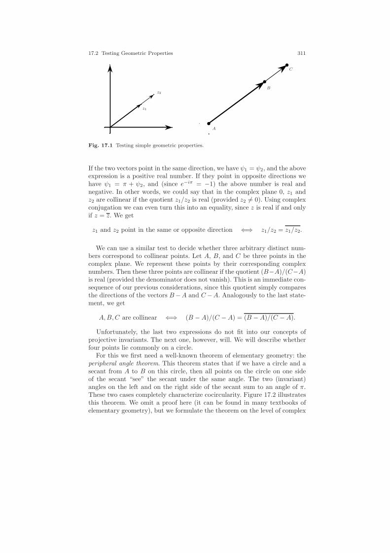
17.2 Testing Geometric Properties 311
z1
z2
A
B
C
Fig. 17.1 Testing simple geometric properties.
If the two vectors point in the same direction, we have ψ1 = ψ2, and the aboveexpression is a positive real number. If they point in opposite directions wehave ψ1 = π + ψ2, and (since e−iπ = −1) the above number is real andnegative. In other words, we could say that in the complex plane 0, z1 andz2 are collinear if the quotient z1/z2 is real (provided z2 6= 0). Using complexconjugation we can even turn this into an equality, since z is real if and onlyif z = z. We get
z1 and z2 point in the same or opposite direction ⇐⇒ z1/z2 = z1/z2.
We can use a similar test to decide whether three arbitrary distinct num-bers correspond to collinear points. Let A, B, and C be three points in thecomplex plane. We represent these points by their corresponding complexnumbers. Then these three points are collinear if the quotient (B−A)/(C−A)is real (provided the denominator does not vanish). This is an immediate con-sequence of our previous considerations, since this quotient simply comparesthe directions of the vectors B−A and C−A. Analogously to the last state-ment, we get
A,B,C are collinear ⇐⇒ (B −A)/(C −A) = (B −A)/(C −A).
Unfortunately, the last two expressions do not fit into our concepts ofprojective invariants. The next one, however, will. We will describe whetherfour points lie commonly on a circle.
For this we first need a well-known theorem of elementary geometry: theperipheral angle theorem. This theorem states that if we have a circle and asecant from A to B on this circle, then all points on the circle on one sideof the secant “see” the secant under the same angle. The two (invariant)angles on the left and on the right side of the secant sum to an angle of π.These two cases completely characterize cocircularity. Figure 17.2 illustratesthis theorem. We omit a proof here (it can be found in many textbooks ofelementary geometry), but we formulate the theorem on the level of complex
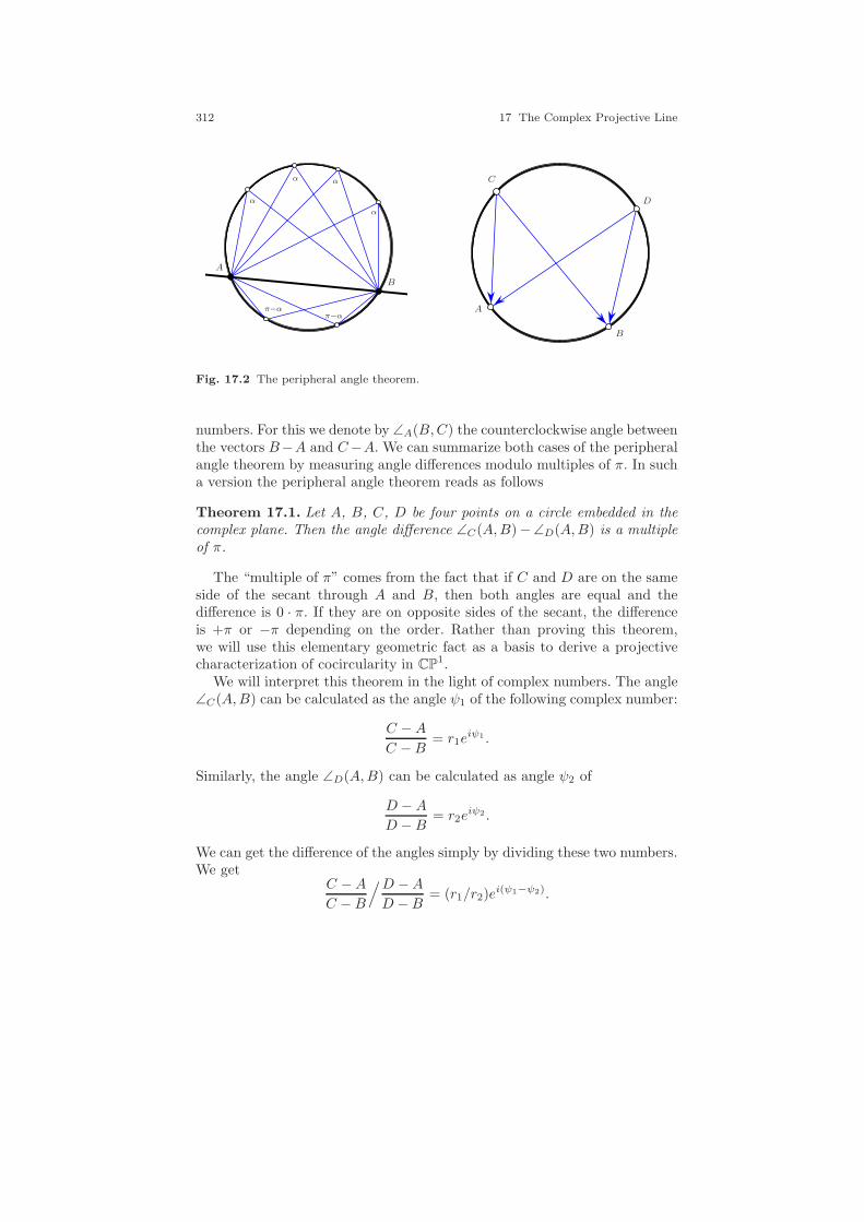
312 17 The Complex Projective Line
α
αα
α
π−απ−α
A
B
A
B
C
D
Fig. 17.2 The peripheral angle theorem.
numbers. For this we denote by ∠A(B,C) the counterclockwise angle betweenthe vectors B−A and C−A. We can summarize both cases of the peripheralangle theorem by measuring angle differences modulo multiples of π. In sucha version the peripheral angle theorem reads as follows
Theorem 17.1. Let A, B, C, D be four points on a circle embedded in thecomplex plane. Then the angle difference ∠C(A,B)−∠D(A,B) is a multipleof π.
The “multiple of π” comes from the fact that if C and D are on the sameside of the secant through A and B, then both angles are equal and thedifference is 0 · π. If they are on opposite sides of the secant, the differenceis +π or −π depending on the order. Rather than proving this theorem,we will use this elementary geometric fact as a basis to derive a projectivecharacterization of cocircularity in CP
1.We will interpret this theorem in the light of complex numbers. The angle
∠C(A,B) can be calculated as the angle ψ1 of the following complex number:
C −A
C −B= r1e
iψ1 .
Similarly, the angle ∠D(A,B) can be calculated as angle ψ2 of
D − A
D −B= r2e
iψ2 .
We can get the difference of the angles simply by dividing these two numbers.We get
C −A
C −B
/D −A
D −B= (r1/r2)e
i(ψ1−ψ2).

17.3 Projective Transformations 313
Since the angle difference is a multiple of π by the peripheral angle theorem,this number must be real. Now, the amazing fact is this: the expression onthe left is nothing but a cross-ratio in the complex projective plane. Thus wecan say that if the four points are on a circle, this cross-ratio (A,B;C,D) isa real number. The converse is also “almost” true; we have only to includethe special case that the circle may have infinite radius and degenerate toa line. It is easy to check that if A,B,C,D are collinear, the cross-ratio isreal as well. As usual, in our considerations we have to consider ∞ as a realnumber as well. The cross-ratio assumes this value if either C = B or D = A.All in all, we obtain the following beautiful theorem, which highlights theclose relationship between complex projective geometry and the geometry ofcircles.
Theorem 17.2. Four points in CP1 are cocircular or collinear if and only if
the cross-ratio (A,B;C,D) is in R ∪ ∞.We can even be more specific about the sign of the cross-ratio:
Theorem 17.3. If for four noncoinciding cocircular points in CP1 the pair
(A,B) cyclically separates the pair (C,D), then (A,B;C,D) < 0. If (A,B)does not separate (C,D), then (A,B;C,D) > 0.
Proof. We have seen that the cross-ratio calculates as
C −A
C −B
/D −A
D −B= (r1/r2)e
i(ψ1−ψ2),
where ψ1 and ψ2 are the angles under which C and D see the segment A,B.If C and D are on the same side of the segment A,B, then these angles areidentical and we get ei(ψ1−ψ2) = e0 = 1, which implies a positive cross-ratio.If C and D are on different sides, then the angles differ by π or by −π.In both cases this gives ei(ψ1−ψ2) = e±iπ = −1, which implies a negativecross-ratio. ⊓⊔
17.3 Projective Transformations
A projective transformation in CP1 can (as in the real case) be expressed
by a matrix multiplication. If the vector (z1, z2)T ∈ C2 represents a point in
CP1 by homogeneous coordinates, then a projective transformation can be
expressed asτ : CP
1 → CP1,
(z1z2
)7→(a bc d
)(z1z2
).
As usual, the matrix must be nondegenerate. All entries can be complex.Matrices differing only by a nonzero scalar multiple represent the same pro-
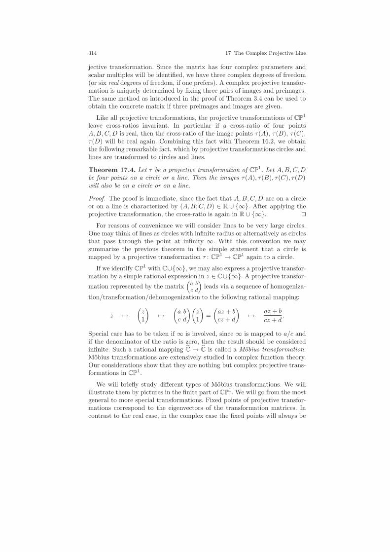
314 17 The Complex Projective Line
jective transformation. Since the matrix has four complex parameters andscalar multiples will be identified, we have three complex degrees of freedom(or six real degrees of freedom, if one prefers). A complex projective transfor-mation is uniquely determined by fixing three pairs of images and preimages.The same method as introduced in the proof of Theorem 3.4 can be used toobtain the concrete matrix if three preimages and images are given.
Like all projective transformations, the projective transformations of CP1
leave cross-ratios invariant. In particular if a cross-ratio of four pointsA,B,C,D is real, then the cross-ratio of the image points τ(A), τ(B), τ(C),τ(D) will be real again. Combining this fact with Theorem 16.2, we obtainthe following remarkable fact, which by projective transformations circles andlines are transformed to circles and lines.
Theorem 17.4. Let τ be a projective transformation of CP1. Let A,B,C,D
be four points on a circle or a line. Then the images τ(A), τ(B), τ(C), τ(D)will also be on a circle or on a line.
Proof. The proof is immediate, since the fact that A,B,C,D are on a circleor on a line is characterized by (A,B;C,D) ∈ R ∪ ∞. After applying theprojective transformation, the cross-ratio is again in R ∪ ∞. ⊓⊔
For reasons of convenience we will consider lines to be very large circles.One may think of lines as circles with infinite radius or alternatively as circlesthat pass through the point at infinity ∞. With this convention we maysummarize the previous theorem in the simple statement that a circle ismapped by a projective transformation τ : CP
1 → CP1 again to a circle.
If we identify CP1 with C∪∞, we may also express a projective transfor-
mation by a simple rational expression in z ∈ C∪∞. A projective transfor-
mation represented by the matrix„
a bc d
«
leads via a sequence of homogeniza-
tion/transformation/dehomogenization to the following rational mapping:
z 7→(z1
)7→
(a bc d
)(z1
)=
(az + bcz + d
)7→ az + b
cz + d.
Special care has to be taken if ∞ is involved, since ∞ is mapped to a/c andif the denominator of the ratio is zero, then the result should be consideredinfinite. Such a rational mapping C → C is called a Mobius transformation.Mobius transformations are extensively studied in complex function theory.Our considerations show that they are nothing but complex projective trans-formations in CP
1.
We will briefly study different types of Mobius transformations. We willillustrate them by pictures in the finite part of CP
1. We will go from the mostgeneral to more special transformations. Fixed points of projective transfor-mations correspond to the eigenvectors of the transformation matrices. Incontrast to the real case, in the complex case the fixed points will always be
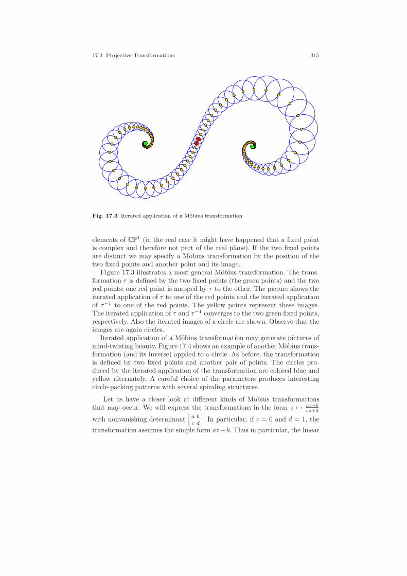
17.3 Projective Transformations 315
Fig. 17.3 Iterated application of a Mobius transformation.
elements of CP1 (in the real case it might have happened that a fixed point
is complex and therefore not part of the real plane). If the two fixed pointsare distinct we may specify a Mobius transformation by the position of thetwo fixed points and another point and its image.
Figure 17.3 illustrates a most general Mobius transformation. The trans-formation τ is defined by the two fixed points (the green points) and the twored points: one red point is mapped by τ to the other. The picture shows theiterated application of τ to one of the red points and the iterated applicationof τ−1 to one of the red points. The yellow points represent these images.The iterated application of τ and τ−1 converges to the two green fixed points,respectively. Also the iterated images of a circle are shown. Observe that theimages are again circles.
Iterated application of a Mobius transformation may generate pictures ofmind-twisting beauty. Figure 17.4 shows an example of another Mobius trans-formation (and its inverse) applied to a circle. As before, the transformationis defined by two fixed points and another pair of points. The circles pro-duced by the iterated application of the transformation are colored blue andyellow alternately. A careful choice of the parameters produces interestingcircle-packing patterns with several spiraling structures.
Let us have a closer look at different kinds of Mobius transformationsthat may occur. We will express the transformations in the form z 7→ az+b
cz+d
with nonvanishing determinant˛
˛
˛
˛
a bc d
˛
˛
˛
˛
. In particular, if c = 0 and d = 1, the
transformation assumes the simple form az+ b. Thus in particular, the linear
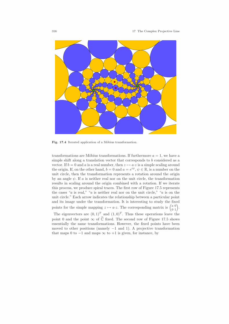
316 17 The Complex Projective Line
Fig. 17.4 Iterated application of a Mobius transformation.
transformations are Mobius transformations. If furthermore a = 1, we have asimple shift along a translation vector that corresponds to b considered as avector. If b = 0 and a is a real number, then z 7→ a·z is a simple scaling aroundthe origin. If, on the other hand, b = 0 and a = eiψ, ψ ∈ R, is a number on theunit circle, then the transformation represents a rotation around the originby an angle ψ. If a is neither real nor on the unit circle, the transformationresults in scaling around the origin combined with a rotation. If we iteratethis process, we produce spiral traces. The first row of Figure 17.5 representsthe cases “a is real,” “a is neither real nor on the unit circle,” “a is on theunit circle.” Each arrow indicates the relationship between a particular pointand its image under the transformation. It is interesting to study the fixed
points for the simple mapping z 7→ a·z. The corresponding matrix is„
a 00 1
«
.
The eigenvectors are (0, 1)T and (1, 0)T . Thus these operations leave the
point 0 and the point ∞ of C fixed. The second row of Figure 17.5 showsessentially the same transformations. However, the fixed points have beenmoved to other positions (namely −1 and 1). A projective transformationthat maps 0 to −1 and maps ∞ to +1 is given, for instance, by
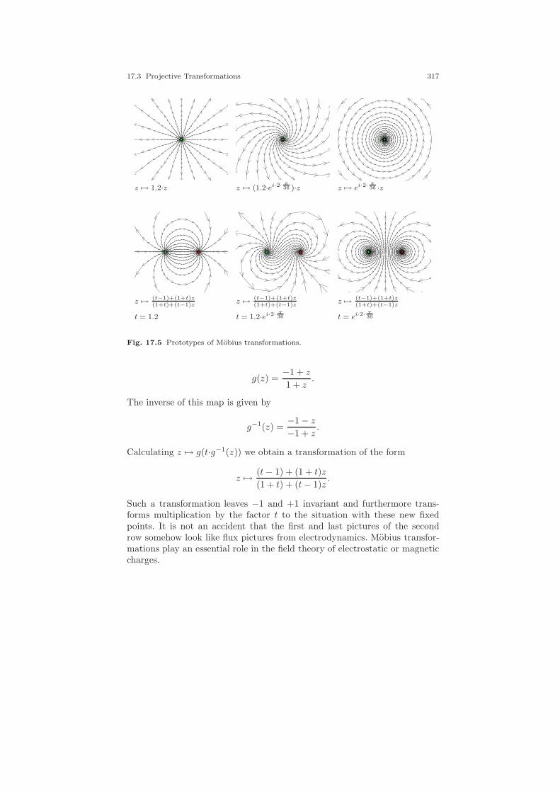
17.3 Projective Transformations 317
z 7→ 1.2·z z 7→ (1.2·ei·2· π36 )·z z 7→ ei·2·
π36 ·z
z 7→ (t−1)+(1+t)z(1+t)+(t−1)z
z 7→ (t−1)+(1+t)z(1+t)+(t−1)z
z 7→ (t−1)+(1+t)z(1+t)+(t−1)z
t = 1.2 t = 1.2·ei·2· π36 t = ei·2·
π36
Fig. 17.5 Prototypes of Mobius transformations.
g(z) =−1 + z
1 + z.
The inverse of this map is given by
g−1(z) =−1 − z
−1 + z.
Calculating z 7→ g(t·g−1(z)) we obtain a transformation of the form
z 7→ (t− 1) + (1 + t)z
(1 + t) + (t− 1)z.
Such a transformation leaves −1 and +1 invariant and furthermore trans-forms multiplication by the factor t to the situation with these new fixedpoints. It is not an accident that the first and last pictures of the secondrow somehow look like flux pictures from electrodynamics. Mobius transfor-mations play an essential role in the field theory of electrostatic or magneticcharges.

318 17 The Complex Projective Line
17.4 Inversions and Mobius Reflections
There is one subtle but important point in the theory of transformations inCP
1 that we have neglected so far. Our considerations of Chapter 5 differ-entiated between harmonic maps and projective transformations. Over RP
1
these two concepts coincide. The fundamental theorem of projective geome-try, however, states that harmonic maps are the more general concept.Everyharmonic map can be expressed by a field automorphism followed by a pro-jective transformation. In fact, unlike R, the field C possesses a nontrivialfield automorphism: complex conjugation. And this is the only one. Thusin addition to projective transformations, complex conjugation z 7→ z alsoleaves the set of circles invariant. Geometrically, this is not very surprising,since complex conjugation just resembles a mirror reflection in the real axis.The surprising fact is that such simple operations like reflection are not at allcovered by projective transformations in CP
1. In a certain sense all Mobiustransformations will be orientation-preserving.
The characteristic magnitude preserved by Mobius transformations can beconsidered a kind of “circle sidedness predicate.” To make this precise wedefine what we mean by the positive side of a circle in CP
1. To be precisehere we must consider oriented circles defined by three points A,B,C. Wedenote such an oriented circle by ©(A,B,C). Such an oriented circle consistsof the circle through A,B,C together with some orientation information. Onemay think of this orientation as a rotational sense on the boundary such thatwe traverse the three points in the order A,B,C (if the circle degeneratesinto a line, it may happen that one has to pass through infinity when onetraverses A,B,C in this order). At every point of the circle’s boundary onemay think of an arrow indicating the rotational sense. Now we rotate thesearrows counterclockwise by 90. The rotated arrows point to the side of thecircle that we call its “positive side.” It is important to notice that by thisdefinition the positive side may be either the interior or the exterior of thecircle, depending on the order of A,B,C. If the circle degenerates to a line,then one of the two half-spaces defined by the line becomes positive, and theother one becomes negative, again depending on the order of A,B,C.
There is also an easy algebraic characterization of the positive side of thecircle. We will take this as the formal definition.
Definition 17.1. Let A,B,C be three points in CP1. The positive side of
the circle ©(A,B,C) defined by A,B,C is the set
p ∈ CP1 | the imaginary part of (A,B;C, p) is positive .
Thus the imaginary part of the cross-ratio specifies the sides of the circle. Itis positive on the positive side, zero on the boundary, and negative on thenegative side. The reader may convince himself that this definition agreeswith our geometric definition. Now it is immediate to see that we have thefollowing theorem:
17.4 Inversions and Mobius Reflections 319
Theorem 17.5. Let A,B,C be three points of CP1 and let τ be a projective
transformation in CP1. Then τ maps the positive side of ©(A,B,C) to the
positive side of ©(τ(A), τ(B), τ(C)).
Proof. The proof is immediate. Since τ is a projective transformation, inparticular it preserves the sign of the imaginary part of cross-ratios. ⊓⊔
Thus we may say that projective geometry in CP1 deals not only with cir-
cles, but with oriented circles. Projective transformations map the positivesides of oriented circles to the positive sides of other oriented circles. Hencethere cannot be a projective transformation that leaves the real axis point-wise invariant and interchanges its upper and lower half-spaces. Likewise,there cannot be a projective transformation that leaves a circle invariant andinterchanges its interior and its exterior.
Complex conjugation z 7→ z helps to add these kinds of transformationsto our geometric system. It leaves the real axis (which is a special “circle”with infinite radius) invariant. But it interchanges its positive and negativesides.
A general harmonic map is a field automorphism followed by a projectivetransformation. Hence we may express those harmonic maps that are notprojective transformations in the form
z 7→ a·z + b
c·z + d;
∣∣∣∣a bc d
∣∣∣∣ 6= 0.
We will call a map of this kind an anti-Mobius transformation. Anti-Mobiustransformations preserve cocircularity but they interchange sidedness. In fact,every anti-Mobius transformation has a circle that as a whole stays invariantunder the transformation. Its interior and its exterior will be interchanged. Wewill not prove this here. Instead, we will restrict ourselves to a few importantexamples of such maps with geometric significance.
One of those maps we already encountered, z 7→ z, is the reflection in thereal axis. Another important map of this kind is given by
ι : CP1 → CP
1,z 7→ 1
z .
This map is known as inversion in the unit circle. It leaves points on thecomplex unit circle point-wise invariant and interchanges the interior and theexterior of this circle. The map ι is an involution, since ι(ι(z)) = z, as an easycomputation shows. The origin is mapped to the point ∞. This operation issometimes also called circlereflection. However, one should be aware that thisoperation does not represent a map that mimics optical reflection in a circle.Reflections in other circles can also be expressed easily using conjugationwith a Mobius transformation τ . If τ maps the unit circle to another circleC, then z 7→ τ(ι(τ−1(z))) is the inversion in the circle C.
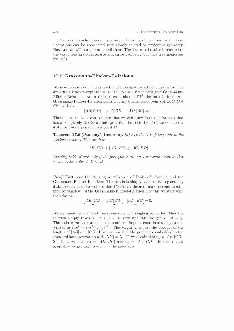
320 17 The Complex Projective Line
The area of circle inversion is a very rich geometric field and by our con-siderations can be considered very closely related to projective geometry.However, we will not go into details here. The interested reader is referred tothe vast literature on inversive and circle geometry (for nice treatments see[28, 49]).
17.5 Grassmann-Plucker-Relations
We now return to our main track and investigate what conclusions we maydraw from bracket expressions in CP
1. We will first investigate Grassmann-Plucker-Relations. As in the real case, also in CP
1 the rank-2 three-termGrassmann-Plucker-Relation holds. For any quadruple of points A,B,C,D ∈CP
1 we have[AB][CD] − [AC][BD] + [AD][BC] = 0.
There is an amazing consequence that we can draw from this formula thathas a completely Euclidean interpretation. For this, by |AB| we denote thedistance from a point A to a point B.
Theorem 17.6 (Ptolemy’s theorem). Let A,B,C,D be four points in theEuclidean plane. Then we have
|AB||CD| + |AD||BC| ≥ |AC||BD|.
Equality holds if and only if the four points are on a common circle or linein the cyclic order A,B,C,D.
Proof. First note the striking resemblance of Ptolemy’s formula and theGrassmann-Plucker-Relations. The brackets simply seem to be replaced bydistances. In fact, we will see that Ptolemy’s theorem may be considered akind of “shadow” of the Grassmann-Plucker-Relation. For this we start withthe relation
[AB][CD]︸ ︷︷ ︸α
− [AC][BD]︸ ︷︷ ︸γ
+ [AD][BC]︸ ︷︷ ︸β
= 0.
We represent each of the three summands by a single greek letter. Thus therelation simply reads α − γ + β = 0. Rewriting this, we get α + β = γ.These three variables are complex numbers. In polar coordinates they can bewritten as rαe
iψα , rβeiψβ , rγe
iψγ . The length rα is just the product of thelengths of [AB] and [CD]. If we assume that the points are embedded in thestandard homogenization with [XY ] = X−Y , we obtain that rα = |AB||CD|.Similarly, we have rβ = |AD||BC| and rγ = |AC||BD|. By the triangleinequality we get from α+ β = γ the inequality
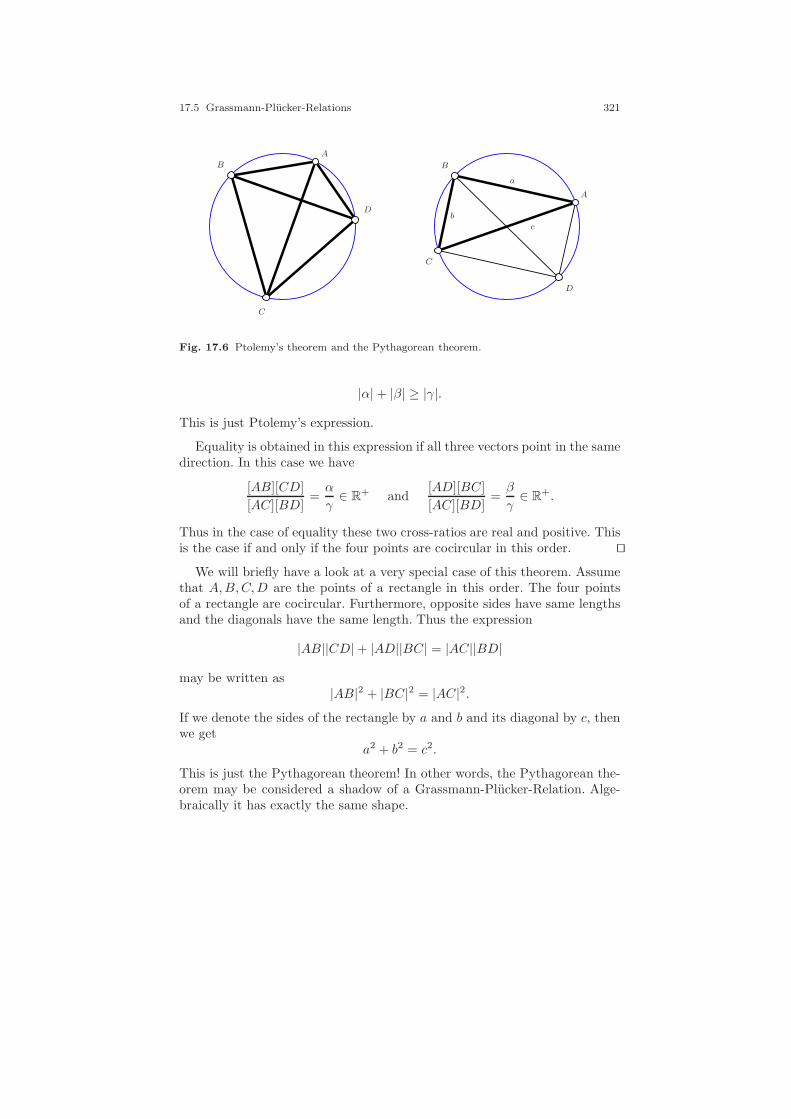
17.5 Grassmann-Plucker-Relations 321
A
B
C
D
A
B
C
D
b
a
c
Fig. 17.6 Ptolemy’s theorem and the Pythagorean theorem.
|α| + |β| ≥ |γ|.
This is just Ptolemy’s expression.
Equality is obtained in this expression if all three vectors point in the samedirection. In this case we have
[AB][CD]
[AC][BD]=α
γ∈ R
+ and[AD][BC]
[AC][BD]=β
γ∈ R
+.
Thus in the case of equality these two cross-ratios are real and positive. Thisis the case if and only if the four points are cocircular in this order. ⊓⊔
We will briefly have a look at a very special case of this theorem. Assumethat A,B,C,D are the points of a rectangle in this order. The four pointsof a rectangle are cocircular. Furthermore, opposite sides have same lengthsand the diagonals have the same length. Thus the expression
|AB||CD| + |AD||BC| = |AC||BD|
may be written as|AB|2 + |BC|2 = |AC|2.
If we denote the sides of the rectangle by a and b and its diagonal by c, thenwe get
a2 + b2 = c2.
This is just the Pythagorean theorem! In other words, the Pythagorean the-orem may be considered a shadow of a Grassmann-Plucker-Relation. Alge-braically it has exactly the same shape.
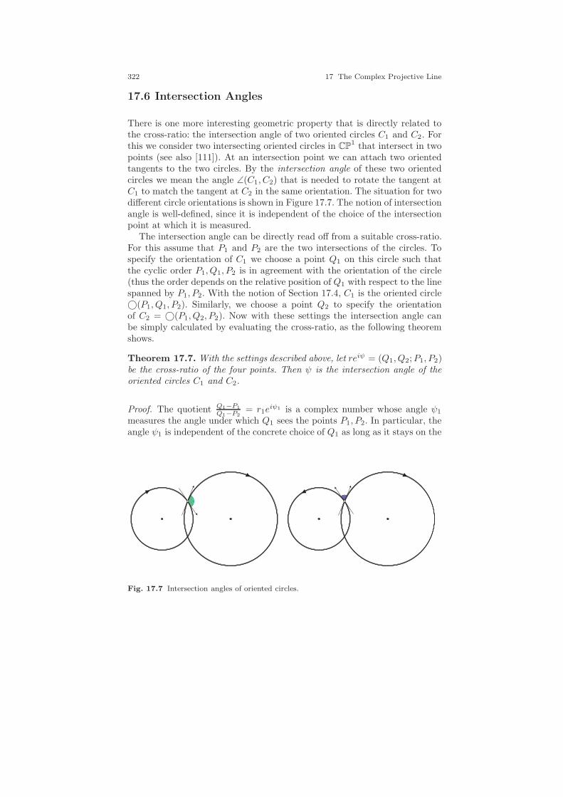
322 17 The Complex Projective Line
17.6 Intersection Angles
There is one more interesting geometric property that is directly related tothe cross-ratio: the intersection angle of two oriented circles C1 and C2. Forthis we consider two intersecting oriented circles in CP
1 that intersect in twopoints (see also [111]). At an intersection point we can attach two orientedtangents to the two circles. By the intersection angle of these two orientedcircles we mean the angle ∠(C1, C2) that is needed to rotate the tangent atC1 to match the tangent at C2 in the same orientation. The situation for twodifferent circle orientations is shown in Figure 17.7. The notion of intersectionangle is well-defined, since it is independent of the choice of the intersectionpoint at which it is measured.
The intersection angle can be directly read off from a suitable cross-ratio.For this assume that P1 and P2 are the two intersections of the circles. Tospecify the orientation of C1 we choose a point Q1 on this circle such thatthe cyclic order P1, Q1, P2 is in agreement with the orientation of the circle(thus the order depends on the relative position of Q1 with respect to the linespanned by P1, P2. With the notion of Section 17.4, C1 is the oriented circle©(P1, Q1, P2). Similarly, we choose a point Q2 to specify the orientationof C2 = ©(P1, Q2, P2). Now with these settings the intersection angle canbe simply calculated by evaluating the cross-ratio, as the following theoremshows.
Theorem 17.7. With the settings described above, let reiψ = (Q1, Q2;P1, P2)be the cross-ratio of the four points. Then ψ is the intersection angle of theoriented circles C1 and C2.
Proof. The quotient Q1−P1
Q1−P2= r1e
iψ1 is a complex number whose angle ψ1
measures the angle under which Q1 sees the points P1, P2. In particular, theangle ψ1 is independent of the concrete choice of Q1 as long as it stays on the
Fig. 17.7 Intersection angles of oriented circles.

17.6 Intersection Angles 323
P1
P2
Q1Q2
C1
C2
Fig. 17.8 Computing the intersection angle.
same side of join(P1, P2). A similar statement holds for Q2 that sees P1, P2
under the angle ψ2. Thus the angle ψ1 − ψ2 of the cross-ratio
Q1 − P1
Q1 − P2
/Q2 − P1
Q2 − P2= r1e
iψ1/r2eiψ2 = rei(ψ1−ψ2)
depends only on the two circles and their orientation and not on the particularchoice of Q1, Q2. To see that ψ1 − ψ2 indeed equals the intersection angle ofthe two circles we now consider the limit case in which Q1, Q2 asymptoticallyapproach P1. The cross-ratio may also be written
Q1 − P1
Q1 − P2· Q2 − P2
Q2 − P1=Q1 − P1
Q2 − P1︸ ︷︷ ︸=a
· Q2 − P2
Q1 − P2︸ ︷︷ ︸=b
.
In the limit case the term a in this expression has an angle identical to theintersection angle, since the numerator and the denominator describe complexnumbers that have the same directions as the oriented tangents at P1. Theterm b has an angle of zero, since the point P2 is distinct from P1 that isasymptotically approached by both Q1 and Q2. Hence the overall expressionof the cross-ratio has an angle equal to the intersection angle. ⊓⊔
Figure 17.8 demonstrates how the intersection angle is composed from thetwo angles at Q1 and Q2. Since cross-ratios remain invariant under Mobiustransformations, we immediately get the following consequence.
Corollary 17.1. The intersection angle of oriented circles is invariant underMobius transformations.
Remark 17.1. With a similar argument one can prove that anti-Mobius trans-formations reverse all intersection angles.
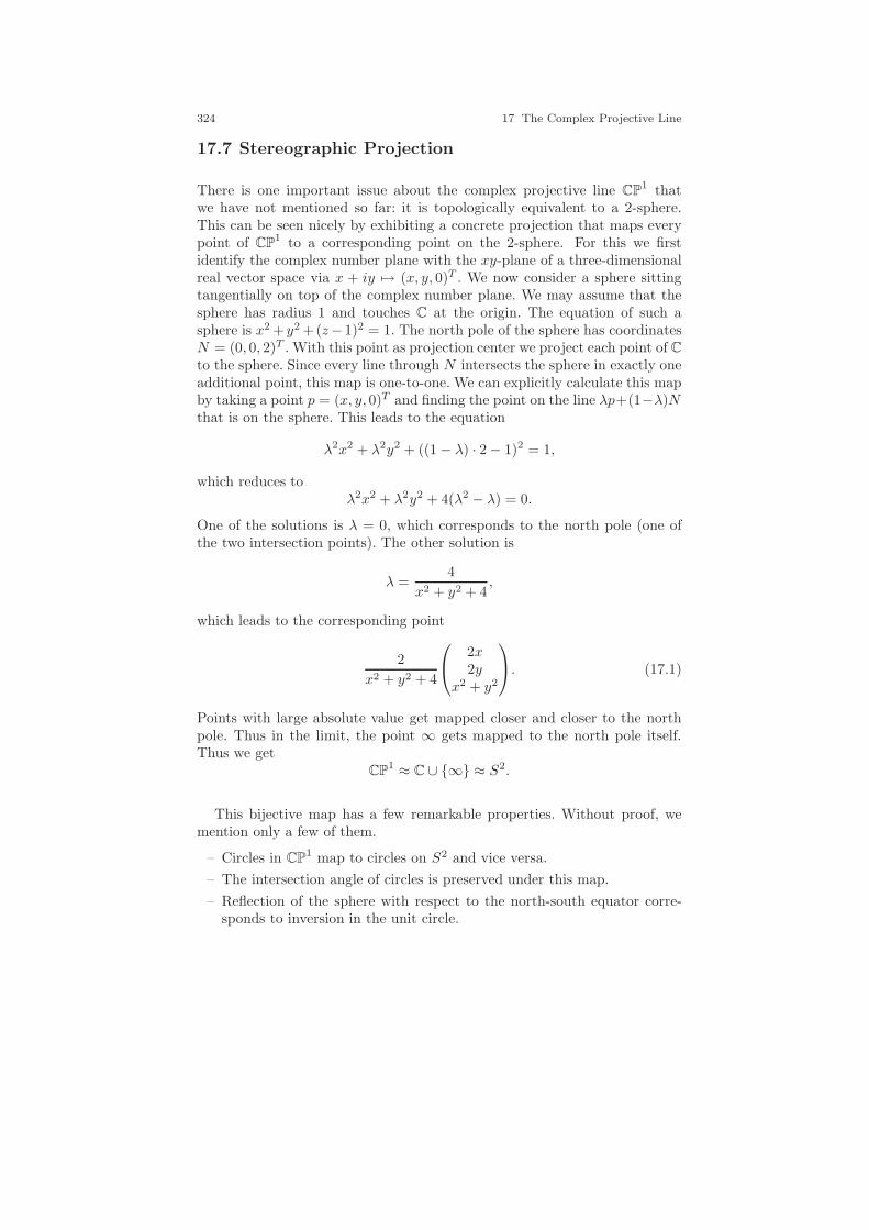
324 17 The Complex Projective Line
17.7 Stereographic Projection
There is one important issue about the complex projective line CP1 that
we have not mentioned so far: it is topologically equivalent to a 2-sphere.This can be seen nicely by exhibiting a concrete projection that maps everypoint of CP
1 to a corresponding point on the 2-sphere. For this we firstidentify the complex number plane with the xy-plane of a three-dimensionalreal vector space via x + iy 7→ (x, y, 0)T . We now consider a sphere sittingtangentially on top of the complex number plane. We may assume that thesphere has radius 1 and touches C at the origin. The equation of such asphere is x2 + y2 +(z−1)2 = 1. The north pole of the sphere has coordinatesN = (0, 0, 2)T . With this point as projection center we project each point of C
to the sphere. Since every line through N intersects the sphere in exactly oneadditional point, this map is one-to-one. We can explicitly calculate this mapby taking a point p = (x, y, 0)T and finding the point on the line λp+(1−λ)Nthat is on the sphere. This leads to the equation
λ2x2 + λ2y2 + ((1 − λ) · 2 − 1)2 = 1,
which reduces toλ2x2 + λ2y2 + 4(λ2 − λ) = 0.
One of the solutions is λ = 0, which corresponds to the north pole (one ofthe two intersection points). The other solution is
λ =4
x2 + y2 + 4,
which leads to the corresponding point
2
x2 + y2 + 4
2x2y
x2 + y2
. (17.1)
Points with large absolute value get mapped closer and closer to the northpole. Thus in the limit, the point ∞ gets mapped to the north pole itself.Thus we get
CP1 ≈ C ∪ ∞ ≈ S2.
This bijective map has a few remarkable properties. Without proof, wemention only a few of them.
– Circles in CP1 map to circles on S2 and vice versa.
– The intersection angle of circles is preserved under this map.
– Reflection of the sphere with respect to the north-south equator corre-sponds to inversion in the unit circle.
17.7 Stereographic Projection 325
Fig. 17.9 Stereographic projection.
– Mobius transformations can be considered as mapping CP1 to the sphere,
then rotating the sphere, scaling it, moving it to a new still tangentialposition, and finally projecting from the north pole of the moved sphereback to CP
1.
For a more elaborate treatment of stereographic projection that in partic-ular highlights the relations between projective geometry, complex numbers,matrix groups, and quaternions, we recommend [111].

18
Euclidean Geometry
Dieses schone Resultat [...] blieb aber lange unbeachtet, ver-mutlich, weil sich die Geometer an den Gedanken gewohnthatten, daß Metrik und projektive Geometrie in keinerBeziehung zueinander standen.
Felix Klein about Laguerre’s formula,Vorlesungen uber Nicht-Euklidische Geometrie, 1928
In this chapter we will merge two different worlds: CP1 and RP
2. Both can beconsidered as representing a real two-dimensional plane. They have differentalgebraic structures, and they both represent different compactifications ofthe Euclidean plane: For RP
2 we added a line at infinity. For CP1 we added
a point at infinity. Both spaces have different weaknesses and strengths.In the first two parts of the book we learned that RP
2 is very well suitedfor dealing, for instance, with incidences of lines and points, with conics intheir general form, and with cross-ratios. We did not have a proper way totalk about circles, angles, and distances in RP
2. The previous two chaptersintroduced CP
1. This space was very good for dealing with cocircularity andalso for dealing with angles. However, lines were poorly supported by CP
1.They had to be considered circles with infinite radius, and they were not evenprojectively invariant objects.
We will now introduce an algebraic system that is capable of mergingadvantages of both worlds. We will end up with a framework in which weexpress all Euclidean properties by projectively invariant expressions.
327

328 18 Euclidean Geometry
18.1 The points I and J
The key to expressing Euclidean properties in projective geometry is as simpleas it is powerful. We have to introduce two special points. All Euclideanproperties will be expressed as projectively invariant expressions in whichthese two points play a special role. There are several possibilities for thechoice of these points. However, there is a special choice for the two pointsunder which all formulas become very simple and elegant. The points are
I =
−i10
and J =
i10
.
Strictly speaking, these points are not even members of RP2, since they have
complex coordinates. We will consider them formally as members of CP2. All
algebraic calculations will be carried out in CP2 (we use homogeneous coor-
dinates with complex coordinate entries). However, the initial elements andthe results of our calculations will usually be in RP
2. All our considerationswill refer to the standard embedding of the Euclidean plane R2 into RP
2 by
(xy
)7→
xy1
.
Thus as usual, the line at infinity will have coordinates l∞ = (0, 0, 1)T . Wewill start by collecting a few useful properties of the points I and J.
I and J span the line at infinity: The points I and J both are on l∞, sincethey have a zero in their last entry. Since they are two different points, theyeven span l∞:
−i10
×
i10
=
00
−2i
= −2i
001
.
I and J can transfer finite points from RP2 to C: Consider a point p with
homogeneous coordinates (a, b, 1)T in RP2. In the Euclidean plane this point
would represent the point (a, b)T . In the complex plane it would representthe point a+ ib. Now consider the 3 × 3 determinant [p, I, l∞]. We get
[p, I, l∞] =
∣∣∣∣∣∣
a −i 0b 1 01 0 1
∣∣∣∣∣∣= a+ ib.
Similarly, we get the conjugate a+ ib:

18.2 Cocircularity 329
[p, J, l∞] =
∣∣∣∣∣∣
a i 0b 1 01 0 1
∣∣∣∣∣∣= a− ib.
I and J can express determinants in CP1 as determinants in RP
2: We con-sider also the standard embedding in CP
1:
z 7→(z1
).
Now take two points p1 and p2 in RP2 represented by vectors (a1, b1, 1)T
and (a2, b2, 1)T . In CP1 they would represent points p1 = (a1 + ib1, 1) and
p2 = (a2 + ib2, 1). Considering the determinant [p1, p2, I], we get
[p1, p2, I] =
∣∣∣∣∣∣
a1 a2 −ib1 b2 11 1 0
∣∣∣∣∣∣= a2 − ib1 − a1 + ib2
= (a2 + ib2) − (a1 + ib1)
= [p2, p1].
And similarly we get the conjugate
[p1, p2, J] = [p2, p1].
Thus the use of I and J allows us to express determinants of CP1 (and their
conjugates) as determinants of RP2 involving I and J. The fact that we rely
on the standard embedding in both worlds will not harm us later on, since inboth worlds we will have to deal only with projectively invariant conditions.
The last property is crucial. It is the key to translating projective invariantsof CP
1 to projective invariants of RP2.
18.2 Cocircularity
Let us begin applying I and J to express Euclidean properties. The strategyhere will be:
• Express the property in CP1 as bracket identity.
• Translate the identity bracket by bracket to RP2 (using I and J).
• Consider the translated identity as a projective invariant in RP2.
330 18 Euclidean Geometry
One of the most fundamental invariants of CP1 is cocircularity. Four points
of CP1 are cocircular if their cross-ratio is real. Assume that we are given
four points A,B,C,D in RP2 (with respect to the standard embedding).
We consider their corresponding counterparts in CP1, the complex points
A, B, C, D. It is easy to express cocircularity in terms of A, B, C, D. Thepoints are cocircular if
[AC][BD]
[AD][BC]∈ R,
or equivalently
[AC][BD]
[AD][BC]=
([AC][BD]
[AD][BC]
).
Expressing the brackets in RP2, we get
[ACI][BDI]
[ADI][BCI]=
[ACJ][BDJ]
[ADJ][BCJ].
We can also multiply by the denominators to obtain a projectively invariantpolynomial equation:
[ACI][BDI][ADJ][BCJ] = [ACJ][BDJ][ADI][BCI].
Summarizing, we get the following characterization of cocircularity:
Theorem 18.1. The points A,B,C,D in RP2 are cocircular if
[ACI][BDI][ADJ][BCJ] = [ACJ][BDJ][ADI][BCI].
Comparing the above bracket expression with the expression derived inSection 10.2 that characterizes whether six points are on a conic, we observethat the expression
[ACI][BDI][ADJ][BCJ] = [ACJ][BDJ][ADI][BCI]
expresses the fact that A,B,C,D, I, J lie on a common conic (each pointoccurs quadratically on either side). Thus we can reformulate the previoustheorem as follows:
Theorem 18.2. The points A,B,C,D in RP2 are cocircular if A,B,C,D, I, J
are on a common conic.
Or in other words: Circles are conics through I and J!
This last fact can also be derived in a different way. If we consider the(Euclidean) equation of a circle with midpoint (mx,my) and radius r,
(x −mx)2 + (x−my)
2 = r2,
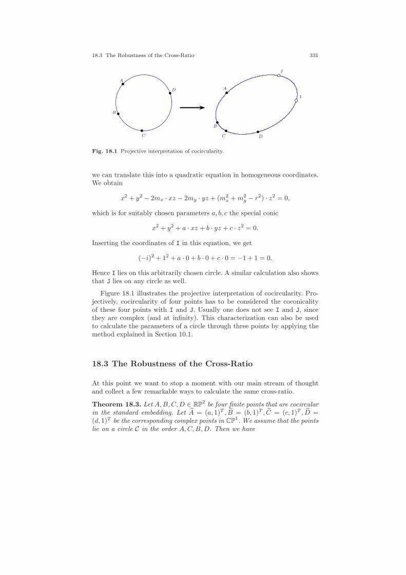
18.3 The Robustness of the Cross-Ratio 331
A
B
C
D A
B
C D
I
J
Fig. 18.1 Projective interpretation of cocircularity.
we can translate this into a quadratic equation in homogeneous coordinates.We obtain
x2 + y2 − 2mx · xz − 2my · yz + (m2x +m2
y − r2) · z2 = 0,
which is for suitably chosen parameters a, b, c the special conic
x2 + y2 + a · xz + b · yz + c · z2 = 0.
Inserting the coordinates of I in this equation, we get
(−i)2 + 12 + a · 0 + b · 0 + c · 0 = −1 + 1 = 0.
Hence I lies on this arbitrarily chosen circle. A similar calculation also showsthat J lies on any circle as well.
Figure 18.1 illustrates the projective interpretation of cocircularity. Pro-jectively, cocircularity of four points has to be considered the coconicalityof these four points with I and J. Usually one does not see I and J, sincethey are complex (and at infinity). This characterization can also be usedto calculate the parameters of a circle through three points by applying themethod explained in Section 10.1.
18.3 The Robustness of the Cross-Ratio
At this point we want to stop a moment with our main stream of thoughtand collect a few remarkable ways to calculate the same cross-ratio.
Theorem 18.3. Let A,B,C,D ∈ RP2 be four finite points that are cocircular
in the standard embedding. Let A = (a, 1)T , B = (b, 1)T , C = (c, 1)T , D =(d, 1)T be the corresponding complex points in CP
1. We assume that the pointslie on a circle C in the order A,C,B,D. Then we have
332 18 Euclidean Geometry
(A,B;C,D)C = (A, B; C, D) =|a− c| · |b− d||a− d| · |b− c| .
The first equality also holds for an arbitrary order of the points.
Proof. We first prove the first equality. The expression (A,B;C,D)C is thewell-defined cross-ratio (A,B;C,D)P of the four points seen from a pointP on the conic (compare Theorem 10.1). In the proof of Theorem 10.1 theparticular choice of the underlying field is irrelevant. Thus we can in particularset P = I. Using the relation [p1, p2, I] = [p2, p1] that relates the pointsin RP
2 to their complex counterparts, we immediately get (A,B;C,D)C =
(A,B;C,D)I = (A, B; C, D).Now for the second equality: a, b, c, d are the complex numbers representing
the four points in C in the standard embedding of the complex projective line.The difference of two such numbers a, c has polar coordinates a−c = ra,ce
iψa,c
with ra,c = |a−c|. We define the radii and angles of the remaining differences
similarly. Then the cross-ratio (A, B; C, D) becomes
[AC][BD]
[AD][BC]=
(a− c)(b − d)
(a− d)(b − c)=ra,crb,dra,drb,c
· eiψa,ceiψb,d
eiψa,deiψb,c︸ ︷︷ ︸=−1
.
The sign −1 of the phase part of this expression is implied by Theorem 17.3and the assumption that A,B separates C,D in the circle. All in all, we get
(A, B; C, D) =[AC] · [BD]
[AD] · [BC]= −ra,c · rb,d
ra,d · rb,c,
which is the claimed equality. ⊓⊔This theorem allows us to interpret the cross-ratio of four cocircular points
in various ways: as cross-ratios in the complex projective line, as cross-ratiosof four points on a circle, and as cross-ratios of absolute values of distances.
18.4 Transformations
Before we discuss further examples of expressing Euclidean properties in pro-jective terms we will have a brief look at the “philosophy” behind the ap-proach of Section 18.2. Our way of expressing cocircularity by a projectivelyinvariant expression relied heavily on the standard embedding of Euclideangeometry into projective geometry (as well in RP
2 as in CP1). This standard
embedding caused the particular choice of the coordinates for I and J. Thecrucial property of I and J is that they, considered as a pair, remain invari-ant under certain transformations (in particular under Euclidean transfor-mations). At this point we have to be a little careful to specify exactly which
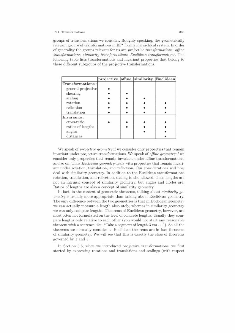
18.4 Transformations 333
groups of transformations we consider. Roughly speaking, the geometricallyrelevant groups of transformations in RP
2 form a hierarchical system. In orderof generality the groups relevant for us are projective transformations, affinetransformations, similarity transformations, Euclidean transformations. Thefollowing table lists transformations and invariant properties that belong tothese different subgroups of the projective transformations.
projective affine similarity EuclideanTransformations :
general projective •shearing • •scaling • • •rotation • • • •reflection • • • •translation • • • •
Invariants :cross-ratio • • • •ratios of lengths • • •angles • •distances •
We speak of projective geometry if we consider only properties that remaininvariant under projective transformations. We speak of affine geometry if weconsider only properties that remain invariant under affine transformations,and so on. Thus Euclidean geometry deals with properties that remain invari-ant under rotation, translation, and reflection. Our considerations will nowdeal with similarity geometry. In addition to the Euclidean transformationsrotation, translation, and reflection, scaling is also allowed. Thus lengths arenot an intrinsic concept of similarity geometry, but angles and circles are.Ratios of lengths are also a concept of similarity geometry.
In fact, in the context of geometric theorems, talking about similarity ge-ometry is usually more appropriate than talking about Euclidean geometry.The only difference between the two geometries is that in Euclidean geometrywe can actually measure a length absolutely, whereas in similarity geometrywe can only compare lengths. Theorems of Euclidean geometry, however, aremost often not formulated on the level of concrete lengths. Usually they com-pare lengths only relative to each other (you would not start any reasonabletheorem with a sentence like: “Take a segment of length 3 cm . . .”). So all thetheorems we normally consider as Euclidean theorems are in fact theoremsof similarity geometry. We will see that this is exactly the class of theoremsgoverned by I and J.
In Section 3.6, when we introduced projective transformations, we firststarted by expressing rotations and translations and scalings (with respect
334 18 Euclidean Geometry
to the standard embedding) as multiplication by a 3 × 3 matrix. There weobtained the following forms for each of the transformations, respectively:
cos(α) sin(α) 0− sin(α) cos(α) 0
0 0 1
;
1 0 tx0 1 ty0 0 1
;
s 0 00 s 00 0 1
.
A matrix that performs an orientation-preserving similarity transformation(a combined rotation, translation, and scaling) has the general form
c s a−s c b0 0 1
.
Similarly, a general orientation-reversing similarity transformation has theform
c s as −c b0 0 1
.
In both cases we must require c2 + s2 6= 0 for having a nonzero determinant.
Theorem 18.4. With respect to the standard embedding, orientation-preservingsimilarity transformations are exactly those matrices that leave I and J in-variant. Orientation-reversing similarity transformations are exactly thosematrices that interchange I and J.
Proof. Applying an orientation-preserving similarity transformation S to I,we get
S · I =
c s a−s c b0 0 1
·
−i10
=
−ic+ sis+ c
0
= (c+ is)
−i10
= (c+ is)I.
The scalar c + is is nonzero, since c2 + s2 6= 0. Similarly, we obtain thatS · J = (c + is) · J. For an orientation-reversing similarity transformation Rthe calculation is similar. We get
R · I =
c s as −c b0 0 1
·
−i10
=
−ic+ s−is− c
0
= (−c− is)
i10
= (−c− is)J.
Again similarly we get R · J = (−c− is)I.Now we conversely assume thatM is a matrix that leaves I invariant. Since
M is assumed to be a matrix that represents a projective transformation ofRP
2, we may assume that M has real entries. We then have M · I = λI. Wenow successively determine constraints on the entries of M . We first considerthe first two entries of the last row of M :
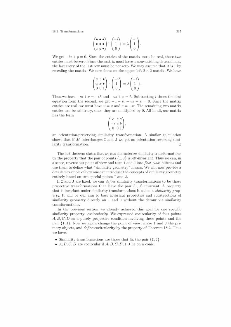
18.4 Transformations 335
• • •• • •x y •
·
−i10
= λ
−i10
.
We get −ix+ y = 0. Since the entries of the matrix must be real, these twoentries must be zero. Since the matrix must have a nonvanishing determinant,the last entry of the last row must be nonzero. We may assume that it is 1 byrescaling the matrix. We now focus on the upper left 2 × 2 matrix. We have
u v •w x •0 0 1
·
−i10
= λ
−i10
.
Thus we have −ui+ v = −iλ and −wi+ x = λ. Subtracting i times the firstequation from the second, we get −u − iv − wi + x = 0. Since the matrixentries are real, we must have u = x and v = −w. The remaining two matrixentries can be arbitrary, since they are multiplied by 0. All in all, our matrixhas the form
c s a−s c b0 0 1
,
an orientation-preserving similarity transformation. A similar calculationshows that if M interchanges I and J we get an orientation-reversing simi-larity transformation. ⊓⊔
The last theorem states that we can characterize similarity transformationsby the property that the pair of points I, J is left-invariant. Thus we can, ina sense, reverse our point of view and turn I and J into first-class citizens anduse them to define what “similarity geometry” means. We will now provide adetailed example of how one can introduce the concepts of similarity geometryentirely based on two special points I and J.
If I and J are fixed, we can define similarity transformations to be thoseprojective transformations that leave the pair I, J invariant. A propertythat is invariant under similarity transformations is called a similarity prop-erty. It will be our aim to base invariant properties and constructions ofsimilarity geometry directly on I and J without the detour via similaritytransformations.
In the previous section we already achieved this goal for one specificsimilarity property: cocircularity. We expressed cocircularity of four pointsA,B,C,D as a purely projective condition involving these points and thepair I, J. Now we again change the point of view, make I and J the pri-mary objects, and define cocircularity by the property of Theorem 18.2. Thuswe have:
• Similarity transformations are those that fix the pair I, J.• A,B,C,D are cocircular if A,B,C,D, I, J lie on a conic.

336 18 Euclidean Geometry
PSfrag
A
B C
D
E
F G
H
A
B
C
D
E
F
G
H
I
J
Fig. 18.2 Miquel’s theorem and its projective interpretation.
Based on these definitions we can derive the statement
• Cocircularity is invariant under similarity transformations.
Proof. A proof of this fact would look as follows: Assume that A,B,C,D arecocircular (thus A,B,C,D, I, J lie on a conic) and assume that τ : RP
2 → RP2
is a similarity transformation. We will prove that τ(A), τ(B), τ(C), τ(D) arecocircular as well. Since τ is a projective transformation and being on a conicis a projectively invariant property, the six points τ(A), τ(B), τ(C), τ(D),τ(I), and τ(J) are on a conic as well.
Since τ is a similarity transformation either we have τ(I) = I and τ(J) = J
or we have τ(I) = J and τ(J) = I. In either case this implies that τ(A), τ(B),τ(C), τ(D), I, and J are on a conic, which means that τ(A), τ(B), τ(C), τ(D),are cocircular. ⊓⊔
At first sight such reasoning may seem to be unnaturally complicated.However, it is conceptually very nice, since we reduced the concept of co-circularity entirely to the introduction of two special points I and J and toprojective invariants, without even referring to the particular coordinates ofI and J. If we choose special coordinates I = (−i, 1, 0)T and J = (i, 1, 0)T ,then (with respect to the standard embedding) this setup specializes to ourusual picture of similarity transformations and cocircularity.
18.5 Translating Theorems
The considerations of the last section show that behind every theorem ofsimilarity geometry (or Euclidean geometry) there lies a projective truth.We will exemplify this by a nice theorem that needs cocircularity as the onlypredicate.

18.6 More Geometric Properties 337
Theorem 18.5 (Miquel’s theorem). Let A,B,C,D,E, F,G,H be eightdistinct points in the Euclidean plane such that the following quadruples arecocircular: (A,B,C,D), (A,B,E, F ), (B,C, F,G), (C,D,G,H), (D,A,H,E).Then (E,F,G,H) will be cocircular as well.
Proof. We will present a proof of Miquel’s theorem based on projective in-variants. The hypotheses of the theorem imply that the following sextupleslie on common conics: (A,B,C,D, I, J), (A,B,E, F, I, J), (B,C, F,G, I, J),(C,D,G,H, I, J), (D,A,H,E, I, J). This produces the following five bracketequations:
[CDJ][ABJ][BCI][ADI] = [ABI][CDI][ADJ][BCJ],[ABI][AEJ][BFJ][EFI] = [ABJ][BFI][AEI][EFJ],[BCJ][BFI][CGI][FGJ] = [BCI][BFJ][CGJ][FGI],
[CDI][CGJ][GHI][DHJ] = [CDJ][CGI][GHJ][DHJ],[ADJ][AEI][EHJ][DHI] = [ADI][AEJ][EHI][DHJ].
All brackets in these expressions will be nonzero, since they always involvetwo distinct finite points and either I or J. Multiplying all left sides and allrights sides and canceling brackets that appear on both sides, we derive theequation
[EFI][FGJ][EHJ][GHI] = [EFJ][FGI]EHI][GHJ].
This expression is exactly the condition that also (E,F,G,H, I, J) are on aconic. And this implies the cocircularity of (E,F,G,H). ⊓⊔
Our proof did not refer (except for nondegeneracy assumptions) to thecoordinates of I and J. The bracket argument also proves a correspondingpurely projective theorem about eight points and six conics, where I and J
are located at real and finite positions. The corresponding theorem is shownin Figure 18.2 on the right. The labeling is consistent with the labeling ofMiquel’s theorem on the left.
18.6 More Geometric Properties
Our next aim is to derive projective conditions for other concepts of simi-larity geometry. We start with perpendicularity. We want to characterize theproperty that for three points A,B,C the lines AB and AC are perpendicularto each other. If we associate the three points with the corresponding pointsof the complex number plane A, B, and C, then we can represent the aboverelation as an algebraic condition. For this we have to certify that the anglebetween the complex numbers A − B and A − C is 90. This is the case ifand only if

338 18 Euclidean Geometry
A
B
C
I
J
A
l
ml∞
L
M
Fig. 18.3 Projective interpretation of orthogonality.
A− B
A− C∈ iR.
This in turn translates to the equation
A− B
A− C= −
(A− B
A− C
).
As before, we reinterpret this equation in RP2 with the help of I and J. We
get[ABI]
[ACI]= − [ABJ]
[ACJ].
Slightly reordering the terms, we get
−1 =[ABI][ACJ]
[ACI][ABJ]= (B,C; I, J)A.
We can formulate this characterization in the following result.
Theorem 18.6. The lines AB and AC are orthogonal if and only if the pairsof lines (AB,AC) and (AI, AJ) are in harmonic position.
Alternatively, we can speak directly of orthogonal lines by considering theirintersections with the line at infinity in relation to I and J:
Theorem 18.7. Two lines l and m are orthogonal if and only if their inter-sections with the line at infinity L = l× l∞ and M = m× l∞ are in harmonicposition with I and J.
Proof. Assume that l and m are orthogonal and that A is their intersection.Let B be a point on l and let C be a point on m. The cross-ratio (B,C; I, J)Ais the same as the cross-ratio (L,M ; I, J). Hence by Theorem 18.6, the pointpairs L,M and I, J are in harmonic position.
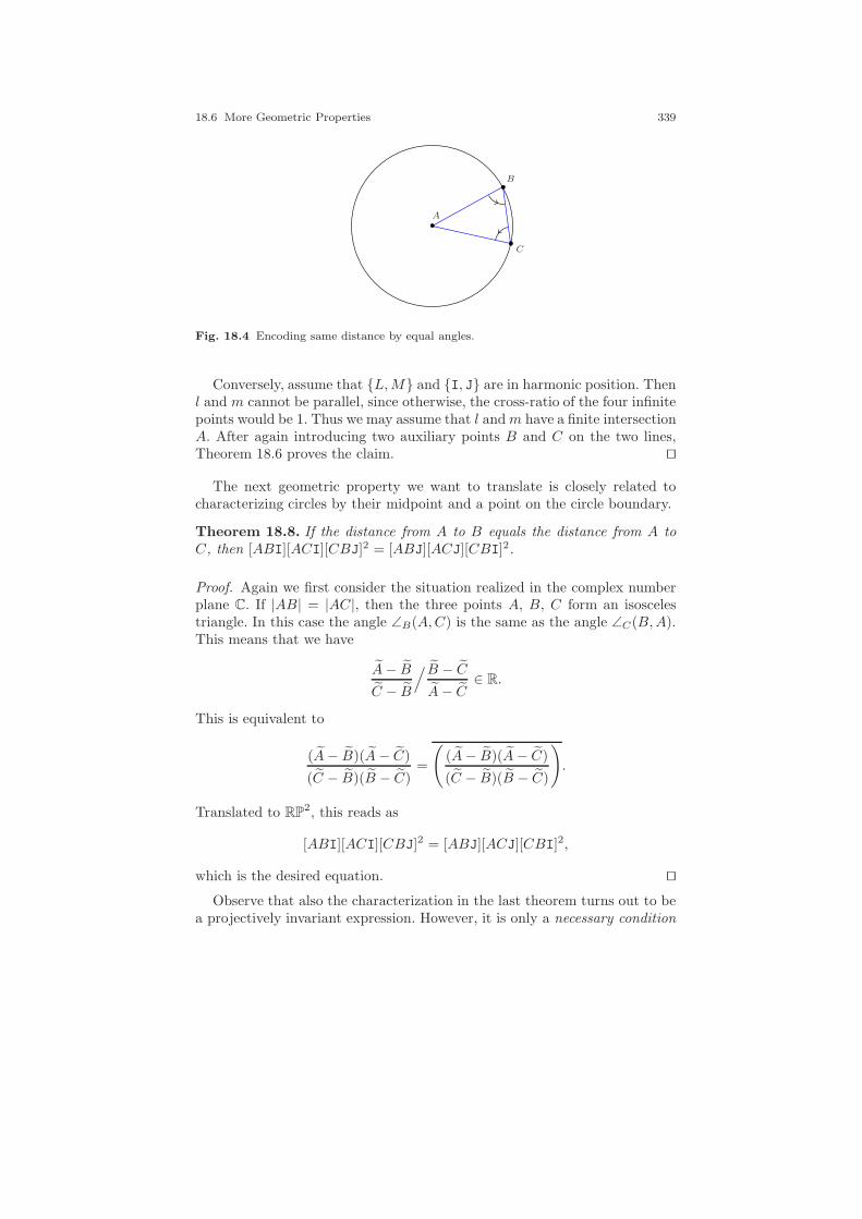
18.6 More Geometric Properties 339
A
B
C
Fig. 18.4 Encoding same distance by equal angles.
Conversely, assume that L,M and I, J are in harmonic position. Thenl and m cannot be parallel, since otherwise, the cross-ratio of the four infinitepoints would be 1. Thus we may assume that l andm have a finite intersectionA. After again introducing two auxiliary points B and C on the two lines,Theorem 18.6 proves the claim. ⊓⊔
The next geometric property we want to translate is closely related tocharacterizing circles by their midpoint and a point on the circle boundary.
Theorem 18.8. If the distance from A to B equals the distance from A toC, then [ABI][ACI][CBJ]2 = [ABJ][ACJ][CBI]2.
Proof. Again we first consider the situation realized in the complex numberplane C. If |AB| = |AC|, then the three points A, B, C form an isoscelestriangle. In this case the angle ∠B(A,C) is the same as the angle ∠C(B,A).This means that we have
A− B
C − B
/ B − C
A− C∈ R.
This is equivalent to
(A− B)(A− C)
(C − B)(B − C)=
((A− B)(A− C)
(C − B)(B − C)
).
Translated to RP2, this reads as
[ABI][ACI][CBJ]2 = [ABJ][ACJ][CBI]2,
which is the desired equation. ⊓⊔Observe that also the characterization in the last theorem turns out to be
a projectively invariant expression. However, it is only a necessary condition

340 18 Euclidean Geometry
for |AB| = |AC|. The point A occurs quadratically in this expression. Thuswe may expect a conic section as locus for A if B and C are fixed. In fact,this conic consists of two lines. One is the median of B and C; the other isthe join of B and C. The equation is satisfied if A is on one of these lines.Thus the case of A being the midpoint of a circle through B and C is onlyone situation in which the above expression vanishes. The other is a being onthe join of B and C. Later in this section we will also learn about a necessaryand sufficient characterization of |AB| = |AC|.
18.7 Laguerre’s Formula
So far we have used I and J only to express properties that are invariant undersimilarity transformations. We can even go one step further and performmeasurements using I and J.
In Section 4 we learned that the simplest way to extract projectively in-variant data from point configurations is by calculating cross-ratios. We willnow use cross-ratios in combination with I and J to mimic measurements ina projective setup. The key result (which has also many beautiful general-izations, as we will see later) is Laguerre’s formula. It was found in 1851 byEdmond Laguerre when he was just 19 years old [77, 68]. It allows one tomeasure the angle between two lines. Before we state Laguerre’s formula wewill clarify what exactly we mean by the angle between two lines l and m.Let us assume first that these two lines intersect in a single finite point O ofthe Euclidean plane. By the angle ∠(l,m) from l to m we mean the angle bywhich l has to be rotated counterclockwise around O until it coincides withm. Thereby the angle between two distinct lines will always lie in the openinterval between 0 and π. If lines coincide or are parallel, then the angle be-tween them is 0. Alternatively one could say that the angle between l and mcorresponds to the angle about which l has to be rotated so that its directioncoincides with that of m. One might expect that angles should be measuredbetween 0 and 2π. However, this makes no sense for unoriented lines. Nowwe are ready to state Laguerre’s formula.
Theorem 18.9. Let l and m be two finite lines of RP2 and let L = l × l∞
and M = m× l∞ be the corresponding intersections with the line at infinity.Then the angle between l and m is (modulo π)
1
2i· ln((M,L; I, J)
).
Proof. The proof of this surprising result is straightforward using the methodof transferring geometric properties from RP
2 to C. Let l = (l1, l2, l3)T and
m = (m1,m2,m3)T be the homogeneous coordinates of the lines. Then L and

18.7 Laguerre’s Formula 341
M have the coordinates L = (l2,−l1, 0)T and M = (m2,−m1, 0)T . The firsttwo entries of these vectors are normal vectors to the two lines. The angle ofthese normal vectors (modulo π) is exactly the angle between the two lines.We translate the normal vectors to two corresponding complex numbers
zl = l2 − i·l1 = rl·eiψl and zm = m2 − i·m1 = rm·eiψm .
The angle ψm −ψl modulo π is exactly the angle we are looking for. We canextract this angle by forming the following ratio:
zm · zlzm · zl
=rm·eiψm · rl·e−iψl
rm·e−iψm · rl·eiψl=eiψm · e−iψl
e−iψm · eiψl= e2i(ψm−ψl).
In the last expression the absolute values of zl and zm cancel, since eachnumber (or its conjugate) is used in the numerator and in the denominator.Our considerations of Section 18.1 show that we have
zl = [L, I, l∞]; zl = [L, J, l∞]; zm = [M, I, l∞]; zm = [M, J, l∞].
Using these determinants to express the above expression, we get
(M,L; I, J) =[M, I, l∞][L, J, l∞]
[M, J, l∞][L, I, l∞]=zm · zlzm · zl
= e2i(ψm−ψl).
Resolving for the desired angle, we get
ψm − ψl =1
2i· ln((M,L; I, J)
),
which is exactly Laguerre’s formula. ⊓⊔
Laguerre’s formula relates the properties of angles to the properties ofcross-ratios in a surprising way. We will collect a few of these properties:
Measurement modulo π: The fact that angles between lines are measuredmodulo π is reflected in the fact that the natural logarithm function is uniqueonly modulo a factor of 2πi (we have ea = ea+2πi) together with the factor12i in Laguerre’s formula.
Real lines generate real angles: At first it is surprising that La-guerre’s formula indeed produces only real values. If fact, if the lines havereal coordinates, then the numerator and the denominator of (M,L; I, J) =[M,I,l∞][L,J,l∞][M,J,l∞][L,I,l∞] are complex conjugates. Dividing two conjugate numbers pro-
duces a complex number on the unit circle. Its logarithm is purely imaginary.This is compensated by the factor 1
2i .
Interchange of lines reverses angle: We must have ∠(l,m) = −∠(m, l)modulo π. Interchanging L and M transforms the cross-ratio to its inverse:

342 18 Euclidean Geometry
(L,M ; I, J) = 1/(M,L; I, J). Since ln(a) = − ln(1/a) modulo 2πi, this pro-duces the desired sign change.
Angles are additive: If we have three lines h, l,m we must have ∠(l,m)+∠(m,h) = ∠(l, h) modulo π. This formula expresses the multiplicativity ofthe cross-ratio. We have
(M,L; I, J) · (H,M ; I, J) =[M, I, l∞][L, J, l∞]
[M, J, l∞][L, I, l∞]· [H, I, l∞][M, J, l∞]
[H, J, l∞][M, I, l∞]
=[H, I, l∞][L, J, l∞]
[H, J, l∞][L, I, l∞]
= (H,L; I, J).
By ln(a · b) = ln(a) + ln(b) modulo 2πi this translates to additivity ofangles.
Orientation-preserving similarity transformations leave angles in-variant: If τ is an orientation-preserving similarity transformation, wemust have ∠(l,m) = ∠(τ(l), τ(m)) (here we interpret τ(l) as the correspond-ing action of τ on a line by multiplication of the inverse transformation ma-trix). To see this identity, we calculate
(M,K, I, J) = (τ(M), τ(K); τ(I), τ(J))
= (τ(M), τ(K); I, J).
Hence the angle is the same after the transformation.
Orientation-reversing similarity transformations reverse angles:If τ is an orientation-reversing similarity transformation, we must have∠(l,m) = −∠(τ(l), τ(m)). We get
(M,K, I, J) = (τ(M), τ(K); τ(I), τ(J))
= (τ(M), τ(K); J, I)
= 1/(τ(M), τ(K); I, J),
which produces (via the logarithm) the reversed angle.
One should also observe that Laguerre’s formula contains as a specialcase the characterization of right angles. If l and m are orthogonal, then∠(l,m) = π
2 . Since eiπ = −1, this translates via Laguerre’s formula to thecondition (M,L; I, J) = −1. This is exactly our characterization given inTheorem 18.7.
18.8 Distances 343
18.8 Distances
Using I and J we can also express distances between two points P and Q inEuclidean geometry. This formula is a little bit “tricky,” and we will presentit here without a strictly formal proof. First of all, we cannot expect toexpress the distance purely as a projectively invariant formula only involvingP , Q, I, and J, since distance is not an invariant of similarity geometry. Theonly thing we can hope for is that we obtain a formula that compares thedistance between P and Q to the distance between two reference points A
and B. Thus we will compute a formula for |P,Q||A,B| . If the distance |A,B| is
normalized to be the unit length, we will have a formula for the distance oftwo arbitrary points. We will finally have an invariant expression in the sixpoints A,B, P,Q, I, J.
For two points P = (p1, p2) and Q = (q1, q2) in the Euclidean plane R2,we usually calculate the distance via Pythagorean theorem:
|P,Q| =√
(p1 − q1)2 + (p2 − q2)2.
We will first express this formula in terms of determinants and then enlargethis formula to get a projectively invariant expression. Again we assume thatP and Q have homogeneous coordinates with respect to the standard embed-ding. Thus we have P = (p1, p2, 1)T and Q = (q1, q2, 1)T . We now considerthe expression
√[P,Q, I][P,Q, J]. Expanding this term, we get
√√√√√
∣∣∣∣∣∣
p1 q1 −ip2 q2 11 1 0
∣∣∣∣∣∣
∣∣∣∣∣∣
p1 q1 ip2 q2 11 1 0
∣∣∣∣∣∣=√
((q1 − p1) + i(q2 − p2)) · ((q1 − p1) − i(q2 − p2))
=√
(p1 − q1)2 + (p2 − q2)2
= |P,Q|.
This is exactly the desired distance. Unfortunately, the expression
√[P,Q, I][P,Q, J]
is not at all a projective invariant. The following expression, however, is:
√[P,Q, I][P,Q, J][A, I, J][B, I, J]√[A,B, I][A,B, J][P, I, J][Q, I, J]
= |PQ|.
This expression indeed is a projective invariant (each letter occurs with thesame power in numerator and denominator). Furthermore, for the case ofthe standard embedding and |A,B| = 1 we get exactly the right distancefunction (as the following comparison of terms shows):

344 18 Euclidean Geometry
|P,Q|︷ ︸︸ ︷√[P,Q, I][P,Q, J]
−2i︷ ︸︸ ︷[A, I, J]
−2i︷ ︸︸ ︷[B, I, J]√
[A,B, I][A,B, J]︸ ︷︷ ︸1
[P, I, J]︸ ︷︷ ︸−2i
[Q, I, J]︸ ︷︷ ︸−2i
= |P,Q|.
All in all we get the following result:
Theorem 18.10. The Euclidean distance |P,Q| between two points P and Qcan be calculated by
√[P,Q, I][P,Q, J][A, I, J][B, I, J]√[A,B, I][A,B, J][P, I, J][Q, I, J]
,
if |A,B| = 1 is a reference length.
It is also instructive to inspect this formula more closely. The occurrenceof the square-root function expresses that it makes sense to speak of distancesonly up to a global sign. We can also compare the last result to the formuladerived in Theorem 18.8, where we expressed a necessary condition for theproperty |AB| = |AC|. Theorem 18.10 contains this situation as special case.If we set P = A and Q = C and square the expression of Theorem 18.10, weget
1 =
(√[A,C, I][A,C, J][A, I, J][B, I, J]√[A,B, I][A,B, J][A, I, J][C, I, J]
)2
=[A,C, I][A,C, J][A, I, J]2[B, I, J]2
[A,B, I][A,B, J][A, I, J]2[C, I, J]2
=[A,C, I][A,C, J][B, I, J]2
[A,B, I][A,B, J][C, I, J]2.
This is also a necessary condition for |AB| = |AC|. In the formula
1 =[A,C, I][A,C, J][B, I, J]2
[A,B, I][A,B, J][C, I, J]2(18.1)
the points A, B, and C occur quadratically. If we fix two of the points, thenthe locus for the remaining one must be a conic. The conic for B is the circlewith center A and perimeter point C. Similarly, the conic for B is the circlewith center A and perimeter point B. The conic for A turns out to consistof two lines. One of the lines is the median of B and C; the other is the lineat infinity (as a simple calculation shows). If we combine the equation
[A,C, I][A,C, J][B, I, J]2 = [A,B, I][A,B, J][C, I, J]2

18.8 Distances 345
with the equation of Theorem 18.8,
[A,B, I][A,C, I][C,B, J]2 = [A,B, J][A,C, J][C,B, I]2,
by multiplying left and right sides we get
[A,C, I]2[C,B, J]2[B, I, J]2 = [A,B, J]2[C,B, I]2[C, I, J]2.
Taking the square root on both sides, we arrive at
[A,C, I][C,B, J][B, I, J] = ±[A,B, J][C,B, I][C, I, J].
After choosing the right sign in this expression, it turns out to be a necessaryand sufficient condition for |AB| = |AC|. The formula that characterizes thiscase is
[A,C, I][C,B, J][B, I, J] = −[A,B, J][C,B, I][C, I, J].
Observe that A occurs linearly in this formula, and both B and C occurquadratically.

19
Euclidean Structures from a ProjectivePerspective
Projective geometry does not start where elementary Geome-try leaves off; that is to say, it does not presuppose any of theresults of elementary Geometry. It stands by itself, and is de-veloped logically from its own initial propositions. The readerwill find, however, that the two subjects are not entirely un-connected, for it will appear that elementary Geometry is aparticular case of Projective Geometry. As a consequence ofthe fact that it is not dependent on elementary Geometry hemust not expect to find that the initial propositions are famil-iar to him from what he already knows. Indeed, it is only at theend of the development that he will see elementary Geometry
emerging. But it must not be supposed that the only aim ofProjective Geometry is to establish the results of elementaryGeometry; it does this incidentally, but at the same time itshows them in their true perspective, for it shows clearly whatplaces in the hierarchy of Geometry this and other Geometriesoccupy.
C.W. O’Hara and D.R. Ward,An Introduction to Projective Geometry, 1937
In the previous chapter we laid the foundations for representing Euclideanconcepts (transformations, angles, distances, orthogonality, cocircularity . . .)in a projective framework. In this chapter we will apply these concepts. Wewill give a loose and by no means complete collection of interesting construc-tions/calculations/theorems in Euclidean geometry that can be nicely carriedout in our projective framework. Here we will strictly follow the concept that
Euclidean geometry is projective geometry together with I and J.
347
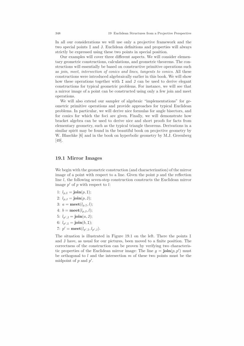
348 19 Euclidean Structures from a Projective Perspective
In all our considerations we will use only a projective framework and thetwo special points I and J. Euclidean definitions and properties will alwaysstrictly be expressed using these two points in special position.
Our examples will cover three different aspects. We will consider elemen-tary geometric constructions, calculations, and geometric theorems. The con-structions will essentially be based on constructive primitive operations suchas join, meet, intersection of conics and lines, tangents to conics. All theseconstructions were introduced algebraically earlier in this book. We will showhow these operations together with I and J can be used to derive elegantconstructions for typical geometric problems. For instance, we will see thata mirror image of a point can be constructed using only a few join and meetoperations.
We will also extend our sampler of algebraic “implementations” for ge-ometric primitive operations and provide approaches for typical Euclideanproblems. In particular, we will derive nice formulas for angle bisectors, andfor conics for which the foci are given. Finally, we will demonstrate howbracket algebra can be used to derive nice and short proofs for facts fromelementary geometry, such as the typical triangle theorems. Derivations in asimilar spirit may be found in the beautiful book on projective geometry byW. Blaschke [6] and in the book on hyperbolic geometry by M.J. Greenberg[49].
19.1 Mirror Images
We begin with the geometric construction (and characterization) of the mirrorimage of a point with respect to a line. Given the point p and the reflectionline l, the following seven-step construction constructs the Euclidean mirrorimage p′ of p with respect to l:
1: lp,I = join(p, I);
2: lp,J = join(p, J);
3: a = meet(lp,I, l);
4: b = meet(lp,J, l);
5: lp′,J = join(a, J);
6: lp′,I = join(b, I);
7: p′ = meet(lp′,I, lp′,J).
The situation is illustrated in Figure 19.1 on the left. There the points I
and J have, as usual for our pictures, been moved to a finite position. Thecorrectness of the construction can be proven by verifying two characteris-tic properties of the Euclidean mirror image: The line g = join(p, p′) mustbe orthogonal to l and the intersection m of these two points must be themidpoint of p and p′.
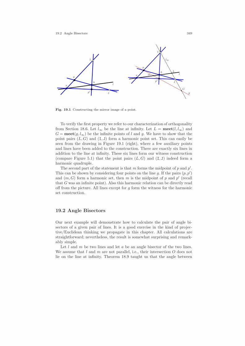
19.2 Angle Bisectors 349
PSfrag
ba
p
p′
I
J
l
ba
p
p′
I
J
l
l∞
g
mL
G
Fig. 19.1 Constructing the mirror image of a point.
To verify the first property we refer to our characterization of orthogonalityfrom Section 18.6. Let l∞ be the line at infinity. Let L = meet(l, l∞) andG = meet(g, l∞) be the infinite points of l and g. We have to show that thepoint pairs (L,G) and (I, J) form a harmonic point set. This can easily beseen from the drawing in Figure 19.1 (right), where a few auxiliary pointsand lines have been added to the construction. There are exactly six lines inaddition to the line at infinity. These six lines form our witness construction(compare Figure 5.1) that the point pairs (L,G) and (I, J) indeed form aharmonic quadruple.
The second part of the statement is that m forms the midpoint of p and p′.This can be shown by considering four points on the line g. If the pairs (p, p′)and (m,G) form a harmonic set, then m is the midpoint of p and p′ (recallthat G was an infinite point). Also this harmonic relation can be directly readoff from the picture. All lines except for g form the witness for the harmonicset construction.
19.2 Angle Bisectors
Our next example will demonstrate how to calculate the pair of angle bi-sectors of a given pair of lines. It is a good exercise in the kind of projec-tive/Euclidean thinking we propagate in this chapter. All calculations arestraightforward; nevertheless, the result is somewhat surprising and remark-ably simple.
Let l and m be two lines and let a be an angle bisector of the two lines.We assume that l and m are not parallel, i.e., their intersection O does notlie on the line at infinity. Theorem 18.9 taught us that the angle between

350 19 Euclidean Structures from a Projective Perspective
l
m
a−
a+
O
Fig. 19.2 Angle bisectors of two lines.
two lines can be calculated as 12i · ln((L,M ; I, J)) with L and M being the
intersections of l and m with the line at infinity l∞. Let A be the intersectionof a with l∞. Then a is an angle bisector if and only if
(L,A; I, J) = (A,M ; I, J). (19.1)
Finding the correct position for A solves the problem of calculating the anglebisector: it is then simply join(A,O).
Now let P be an arbitrary point not on l∞ that we can use to express thecross-ratios in terms of 3× 3 determinants. Then on the bracket level, (19.1)reads
[P,L, I][P,A, J]
[P,L, J][P,A, I]=
[P,A, I][P,M, J]
[P,A, J][P,M, I],
or equivalently,
[P,L, I][P,M, I][P,A, J]2 = [P,M, J][P,L, J][P,A, I]2.
The point A is on l∞ = join(I, J). Thus for suitable λ and µ we have A =λI + µJ. Inserting this into the bracket expression, we get
[P,L, I][P,M, I][P, λI + µJ, J]2 = [P,M, J][P,L, J][P, λI + µJ, I]2.
And after expanding and removing brackets with identical letters, we have
[P,L, I][P,M, I][P, λI, J]2 = [P,M, J][P,L, J][P, µJ, I]2.
Extracting λ and µ leads to
λ2[P,L, I][P,M, I][P, I, J]2 = µ2[P,M, J][P,L, J][P, J, I]2.
Thus after canceling [P, J, I]2, we get
λ2[P,L, I][P,M, I] = µ2[P,M, J][P,L, J],

19.2 Angle Bisectors 351
and a suitable choice for λ and µ is
λ = ±√
[P,L, J][P,M, J] and µ = ±√
[P,L, I][P,M, I].
Inserting this into A = λI + µJ, we get the nicely symmetric formula
A± =√
[P,L, J][P,M, J] · I±√
[P,L, I][P,M, I] · J.
The choice of the sign corresponds to the fact that two lines in generalhave two angle bisectors. It is also easy to check that the two possible anglebisectors are orthogonal to each other, since for an arbitrary pair of pointsof the forms A+ = λI + µJ and A− = λI− µJ we get
(A+, A−; I, J)P =[PA+, I, ][P,A−, J]
[P,A+, J][P,Ai, I]
=[PλI + µJ, I, ][P, λI − µJ, J]
[P, λI + µJ, J][P, λI− µJ, I]
=[PµJ, I, ][P, λI, J]
[P, λI, J][P,−µJ, I]= −1.
Summarizing these results, we have the following theorem:
Theorem 19.1. With the notation as above, the angle bisectors of l and mmay be calculated by join(A,O) with
A± =√
[P,L, J][P,M, J] · I±√
[P,L, I][P,M, I] · J.
The two angle bisectors are perpendicular to each other.
It is also interesting to see what being an angle bisector means alge-braically. We will consider the slightly more general case in which we wantto test whether for four lines l,m, a, b the angle enclosed between l and aequals the angle enclosed between b and m. Setting a = b, we obtain thespecial case of an angle bisector. We again let L,M,A,B be the correspond-ing intersections of the lines with l∞. From Laguerre’s formula we obtain thecondition
(L,A; I, J) = (B,M ; I, J).
We may permute the entries on the left and right side, of this equation con-sistently and still obtain the same condition. For instance, we get
(L, I;A, J) = (B, I;M, J).
Again using a suitably generic point P distinct from l∞, we may write theabove equation on the level of brackets as
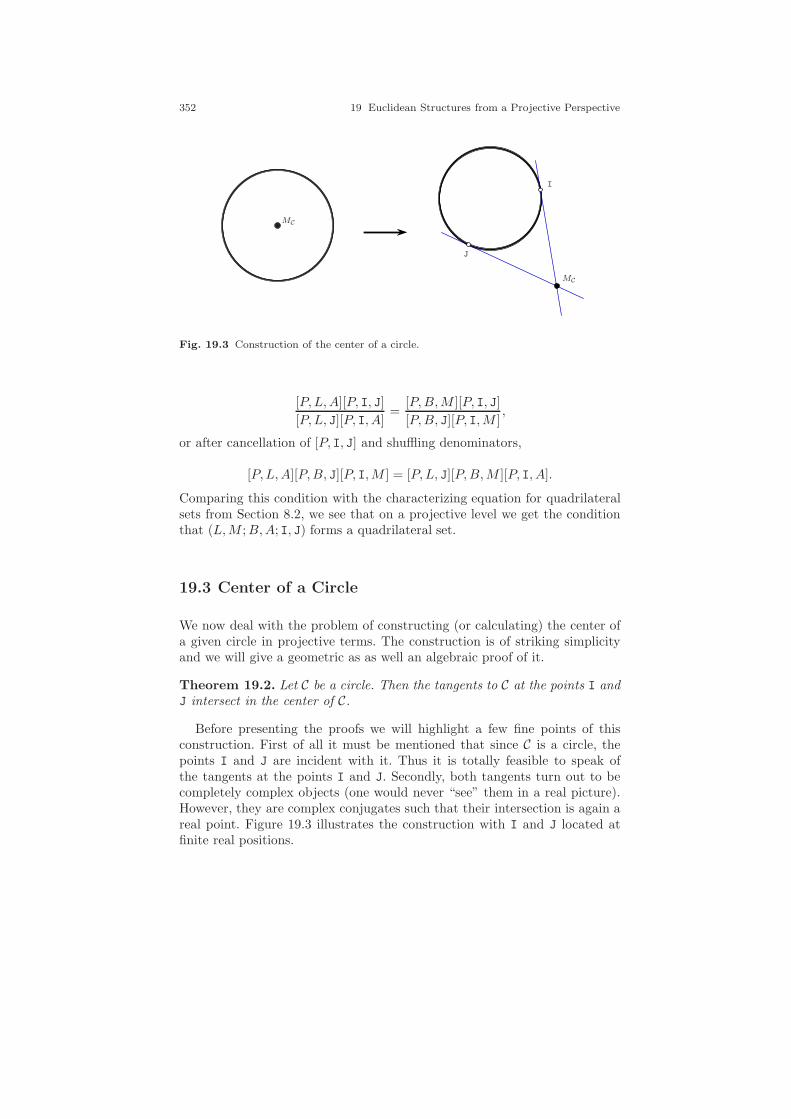
352 19 Euclidean Structures from a Projective Perspective
MC
I
J
MC
Fig. 19.3 Construction of the center of a circle.
[P,L,A][P, I, J]
[P,L, J][P, I, A]=
[P,B,M ][P, I, J]
[P,B, J][P, I,M ],
or after cancellation of [P, I, J] and shuffling denominators,
[P,L,A][P,B, J][P, I,M ] = [P,L, J][P,B,M ][P, I, A].
Comparing this condition with the characterizing equation for quadrilateralsets from Section 8.2, we see that on a projective level we get the conditionthat (L,M ;B,A; I, J) forms a quadrilateral set.
19.3 Center of a Circle
We now deal with the problem of constructing (or calculating) the center ofa given circle in projective terms. The construction is of striking simplicityand we will give a geometric as as well an algebraic proof of it.
Theorem 19.2. Let C be a circle. Then the tangents to C at the points I andJ intersect in the center of C.
Before presenting the proofs we will highlight a few fine points of thisconstruction. First of all it must be mentioned that since C is a circle, thepoints I and J are incident with it. Thus it is totally feasible to speak ofthe tangents at the points I and J. Secondly, both tangents turn out to becompletely complex objects (one would never “see” them in a real picture).However, they are complex conjugates such that their intersection is again areal point. Figure 19.3 illustrates the construction with I and J located atfinite real positions.

19.3 Center of a Circle 353
Algebraically, this construction can also be translated into a very simplecalculation. Let Q be the matrix of the quadratic form that represents C. Thetangents at I and J can be calculated by Q · I and Q · J. Their intersectionis simply
MC = (Q · I) × (Q · J).
Algebraic proof: A simple calculation verifies that MC is indeed the centerof the circle. We assume that C has a center with Euclidean coordinates(mx,my)
T . The circle equation then is of the form
(x −mx)2 + (x−my)
2 = r2.
The corresponding matrix of the quadratic form is
Q =
1 0 −mx
0 1 −my
−mx −my α
for a suitable α. By expanding (QI) × (QJ), we get
(QI) × (QJ) =
0
@
1 0 −mx0 1 −my
−mx −my α
1
A
0
@
−i10
1
A ×
0
@
1 0 −mx0 1 −my
−mx −my α
1
A
0
@
i10
1
A
=
0
@
−i1
imx −my
1
A ×
0
@
i1
−imx −my
1
A
=
0
@
−2imx−2imy−2i
1
A
= −2i
0
@
mxmy1
1
A.
This proves that this point is the center of the circle. ⊓⊔An even simpler geometric argument can be used as well to show the
midpoint property. For this recall that for three collinear points A,B,M ona line l we can characterize the fact that M is the midpoint of A and B bythe condition that (A,B;M,L) are in harmonic position (here L is again theintersection of l and l∞). Thus the center M of a circle C is characterized bythe following property. For a line l that passes through M let A and B be theintersections of l and C and let L be the intersection of l and l∞. The pointM is the center of the circle if for any such line, (A,B;M,L) are in harmonicposition.Geometric proof: Let M be the intersection of the two tangents at I and J.The only thing we have to prove is that for an arbitrary line l through M

354 19 Euclidean Structures from a Projective Perspective
A
B
L
a
b
l
M
m
l∞
I
J
Fig. 19.4 Proving the midpoint property.
the points (A,B;L,M) as defined above are in harmonic position. Refer toFigure 19.4 for the labeling. In Section 10.7 we saw that in this situationevery point P on the circle sees the points (A,B; I, J) in harmonic relation.This means that the connecting lines from P to these points are in harmonicrelation. In particular, this is the case for P = I. Thus the lines (a, b; l∞,m)in Figure 19.4 are in harmonic relation. Hence the points (A,B;L,M) areharmonic, since they are the intersections of the line l with the four linesa, b, l∞,m. ⊓⊔
19.4 Constructing the Foci of a Conic
The previous construction has a remarkable generalization. With the help ofI and J it is possible to construct the foci of a conic by just drawing fourtangents and intersecting them. In fact, projectively speaking, this construc-tion is an appropriate way to define foci of conics (and then checking thatthe definition agrees with the classical one). To appreciate the followingconstruction we first need a characterizing property of foci in classical terms.An ellipse has the property that there are two so-called foci. These are twopoints F1 and F2 inside the ellipse with the following geometric property.If a light ray is emitted from F1 and reflected at the conic’s boundary, thereflected light ray passes through F2. Figure 19.5 (left) shows a collectionof light rays emitted from one of the foci, and the corresponding reflectedrays. In the drawing on the right one single light ray and its reflection areshown. Reflection at the conic means that at the position at which the rayhits the conic, we may locally consider a tangent to the conic as a planar

19.4 Constructing the Foci of a Conic 355
m
P
F1 F2
Fig. 19.5 Definition of the foci of a conic.
mirror. Thus the supporting lines of the original ray and the reflected oneare mirror symmetric with respect to this tangent. A similar characterizationalso holds for a hyperbola. A hyperbola also has two foci, with the propertythat if a ray is emitted from F1, then the supporting line of the reflected rayis incident with F2. In the case of a circle the two foci will coincide with thecenter.
We will now give a projective construction involving I and J that createsfocal points with exactly the property described above. In order to get anondegenerate construction we will assume (for the moment) that the conicunder consideration C is not a circle. We will see later on that the constructionalso covers this case. If C is not a circle, then I and J are not coincident with it.Thus we can draw two tangents i1 and i2 from I at the conic C. Similarly, wecan draw two tangents j1 and j2 from J. The intersections of these tangentsturn out to be foci (see Figure 19.6).
F2
F1
G1
G2
F2
F1
I
J
Fig. 19.6 Construction of foci using I and J.
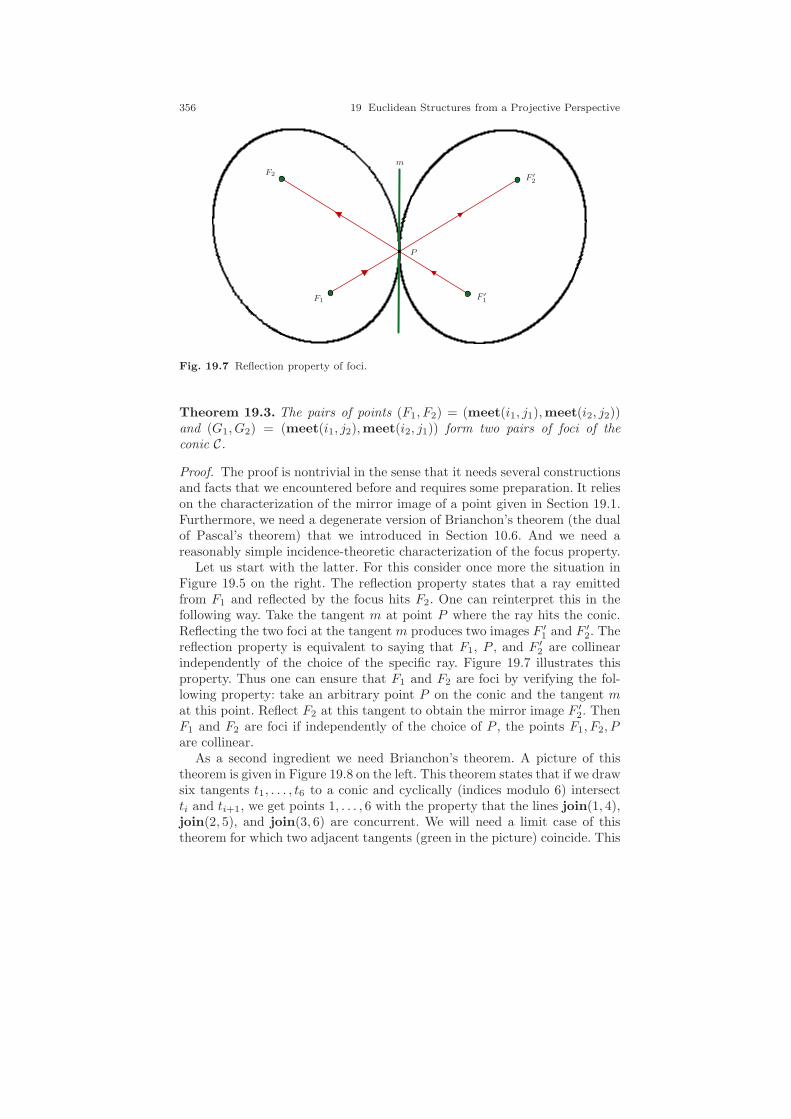
356 19 Euclidean Structures from a Projective Perspective
F ′1
F ′2
F1
F2
m
P
Fig. 19.7 Reflection property of foci.
Theorem 19.3. The pairs of points (F1, F2) = (meet(i1, j1),meet(i2, j2))and (G1, G2) = (meet(i1, j2),meet(i2, j1)) form two pairs of foci of theconic C.
Proof. The proof is nontrivial in the sense that it needs several constructionsand facts that we encountered before and requires some preparation. It relieson the characterization of the mirror image of a point given in Section 19.1.Furthermore, we need a degenerate version of Brianchon’s theorem (the dualof Pascal’s theorem) that we introduced in Section 10.6. And we need areasonably simple incidence-theoretic characterization of the focus property.
Let us start with the latter. For this consider once more the situation inFigure 19.5 on the right. The reflection property states that a ray emittedfrom F1 and reflected by the focus hits F2. One can reinterpret this in thefollowing way. Take the tangent m at point P where the ray hits the conic.Reflecting the two foci at the tangent m produces two images F ′
1 and F ′2. The
reflection property is equivalent to saying that F1, P , and F ′2 are collinear
independently of the choice of the specific ray. Figure 19.7 illustrates thisproperty. Thus one can ensure that F1 and F2 are foci by verifying the fol-lowing property: take an arbitrary point P on the conic and the tangent mat this point. Reflect F2 at this tangent to obtain the mirror image F ′
2. ThenF1 and F2 are foci if independently of the choice of P , the points F1, F2, Pare collinear.
As a second ingredient we need Brianchon’s theorem. A picture of thistheorem is given in Figure 19.8 on the left. This theorem states that if we drawsix tangents t1, . . . , t6 to a conic and cyclically (indices modulo 6) intersectti and ti+1, we get points 1, . . . , 6 with the property that the lines join(1, 4),join(2, 5), and join(3, 6) are concurrent. We will need a limit case of thistheorem for which two adjacent tangents (green in the picture) coincide. This
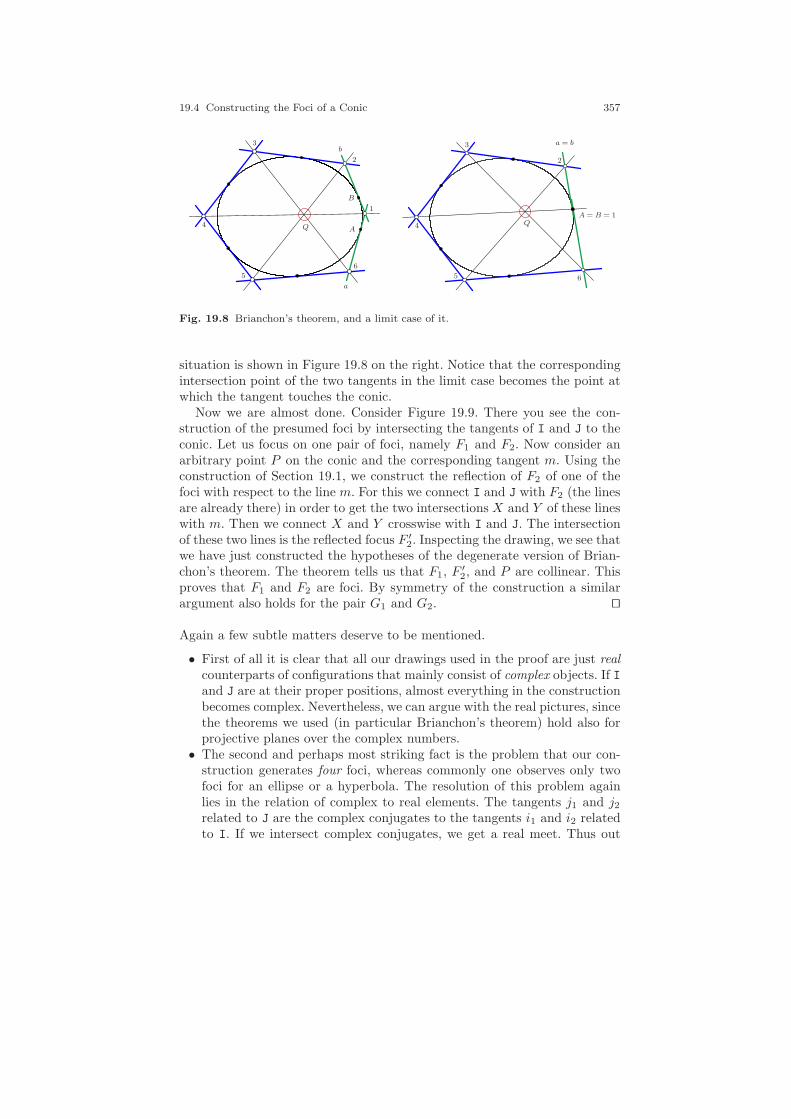
19.4 Constructing the Foci of a Conic 357
1
2
3
4
5
6
a
b
A
B
Q
2
3
4
5 6
Q
a = b
A = B = 1
Fig. 19.8 Brianchon’s theorem, and a limit case of it.
situation is shown in Figure 19.8 on the right. Notice that the correspondingintersection point of the two tangents in the limit case becomes the point atwhich the tangent touches the conic.
Now we are almost done. Consider Figure 19.9. There you see the con-struction of the presumed foci by intersecting the tangents of I and J to theconic. Let us focus on one pair of foci, namely F1 and F2. Now consider anarbitrary point P on the conic and the corresponding tangent m. Using theconstruction of Section 19.1, we construct the reflection of F2 of one of thefoci with respect to the line m. For this we connect I and J with F2 (the linesare already there) in order to get the two intersections X and Y of these lineswith m. Then we connect X and Y crosswise with I and J. The intersectionof these two lines is the reflected focus F ′
2. Inspecting the drawing, we see thatwe have just constructed the hypotheses of the degenerate version of Brian-chon’s theorem. The theorem tells us that F1, F
′2, and P are collinear. This
proves that F1 and F2 are foci. By symmetry of the construction a similarargument also holds for the pair G1 and G2. ⊓⊔
Again a few subtle matters deserve to be mentioned.
• First of all it is clear that all our drawings used in the proof are just realcounterparts of configurations that mainly consist of complex objects. If Iand J are at their proper positions, almost everything in the constructionbecomes complex. Nevertheless, we can argue with the real pictures, sincethe theorems we used (in particular Brianchon’s theorem) hold also forprojective planes over the complex numbers.
• The second and perhaps most striking fact is the problem that our con-struction generates four foci, whereas commonly one observes only twofoci for an ellipse or a hyperbola. The resolution of this problem againlies in the relation of complex to real elements. The tangents j1 and j2related to J are the complex conjugates to the tangents i1 and i2 relatedto I. If we intersect complex conjugates, we get a real meet. Thus out
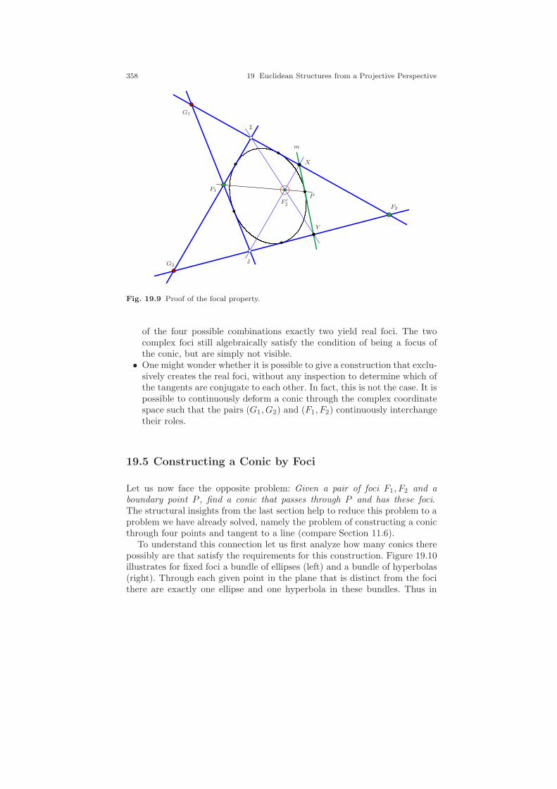
358 19 Euclidean Structures from a Projective Perspective
F1
F2
G1
G2
F ′2
P
m
X
Y
I
J
Fig. 19.9 Proof of the focal property.
of the four possible combinations exactly two yield real foci. The twocomplex foci still algebraically satisfy the condition of being a focus ofthe conic, but are simply not visible.
• One might wonder whether it is possible to give a construction that exclu-sively creates the real foci, without any inspection to determine which ofthe tangents are conjugate to each other. In fact, this is not the case. It ispossible to continuously deform a conic through the complex coordinatespace such that the pairs (G1, G2) and (F1, F2) continuously interchangetheir roles.
19.5 Constructing a Conic by Foci
Let us now face the opposite problem: Given a pair of foci F1, F2 and aboundary point P , find a conic that passes through P and has these foci.The structural insights from the last section help to reduce this problem to aproblem we have already solved, namely the problem of constructing a conicthrough four points and tangent to a line (compare Section 11.6).
To understand this connection let us first analyze how many conics therepossibly are that satisfy the requirements for this construction. Figure 19.10illustrates for fixed foci a bundle of ellipses (left) and a bundle of hyperbolas(right). Through each given point in the plane that is distinct from the focithere are exactly one ellipse and one hyperbola in these bundles. Thus in
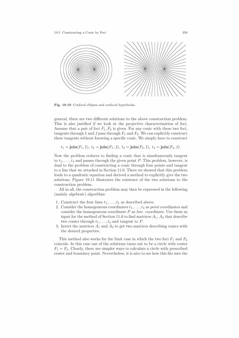
19.5 Constructing a Conic by Foci 359
Fig. 19.10 Confocal ellipses and confocal hyperbolas.
general, there are two different solutions to the above construction problem.This is also justified if we look at the projective characterization of foci.Assume that a pair of foci F1, F2 is given. For any conic with these two foci,tangents through I and J pass through F1 and F2. We can explicitly constructthese tangents without knowing a specific conic. We simply have to construct
t1 = join(F1, I), t2 = join(F1, J), t3 = join(F2, I), t4 = join(F2, J).
Now the problem reduces to finding a conic that is simultaneously tangentto t1, . . . , t4 and passes through the given point P . This problem, however, isdual to the problem of constructing a conic through four points and tangentto a line that we attacked in Section 11.6. There we showed that this problemleads to a quadratic equation and derived a method to explicitly give the twosolutions. Figure 19.11 illustrates the existence of the two solutions to theconstruction problem.
All in all, the construction problem may then be expressed in the following(mainly algebraic) algorithm:
1. Construct the four lines t1, . . . , t4 as described above.2. Consider the homogeneous coordinates t1, . . . , t4 as point coordinates and
consider the homogeneous coordinate P as line coordinate. Use them asinput for the method of Section 11.6 to find matrices A1, A2 that describetwo conics through t1, . . . , t4 and tangent to P .
3. Invert the matrices A1 and A2 to get two matrices describing conics withthe desired properties.
This method also works for the limit case in which the two foci F1 and F2
coincide. In this case one of the solutions turns out to be a circle with centerF1 = F2. Clearly, there are simpler ways to calculate a circle with prescribedcenter and boundary point. Nevertheless, it is nice to see how this fits into the
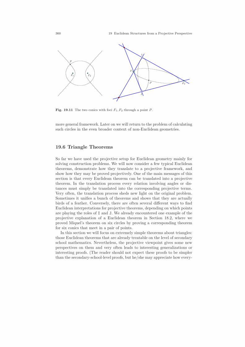
360 19 Euclidean Structures from a Projective Perspective
F1 F2
P
F1
F2P
I
J
Fig. 19.11 The two conics with foci F1, F2 through a point P .
more general framework. Later on we will return to the problem of calculatingsuch circles in the even broader context of non-Euclidean geometries.
19.6 Triangle Theorems
So far we have used the projective setup for Euclidean geometry mainly forsolving construction problems. We will now consider a few typical Euclideantheorems, demonstrate how they translate to a projective framework, andshow how they may be proved projectively. One of the main messages of thissection is that every Euclidean theorem can be translated into a projectivetheorem. In the translation process every relation involving angles or dis-tances must simply be translated into the corresponding projective terms.Very often, the translation process sheds new light on the original problem.Sometimes it unifies a bunch of theorems and shows that they are actuallybirds of a feather. Conversely, there are often several different ways to findEuclidean interpretations for projective theorems, depending on which pointsare playing the roles of I and J. We already encountered one example of theprojective explanation of a Euclidean theorem in Section 18.2, where weproved Miquel’s theorem on six circles by proving a corresponding theoremfor six conics that meet in a pair of points.
In this section we will focus on extremely simple theorems about triangles:those Euclidean theorems that are already treatable on the level of secondaryschool mathematics. Nevertheless, the projective viewpoint gives some newperspectives on them and very often leads to interesting generalizations orinteresting proofs. (The reader should not expect these proofs to be simplerthan the secondary-school-level proofs, but he/she may appreciate how every-
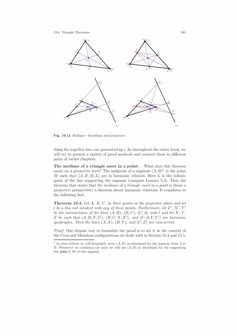
19.6 Triangle Theorems 361
B
C
A
Y
Z
X
M
B
C
A
Y
Z
X
B
C
A
Y
Z
X
Y ′
Z′
X′M
l∞
B
C
A
Y
Z
X
Y ′
Z′
X′
l∞
Fig. 19.12 Medians—Euclidean and projective.
thing fits together into our general setup.) As throughout the entire book, wewill try to present a variety of proof methods and connect them to differentparts of earlier chapters.
The medians of a triangle meet in a point: What does this theoremmean on a projective level? The midpoint of a segment (A,B)1 is the pointM such that (A,B;M,L) are in harmonic relation. Here L is the infinitepoint of the line supporting the segment (compare Lemma 5.3). Thus thetheorem that states that the medians of a triangle meet in a point is (from aprojective perspective) a theorem about harmonic relations. It translates tothe following fact.
Theorem 19.4. Let A, B, C, be three points in the projective plane and letl be a line not incident with any of these points. Furthermore, let Z ′, X ′, Y ′
be the intersections of the lines (A,B), (B,C), (C,A) with l and let X, Y ,Z be such that (A,B;Z,Z ′), (B,C;X,X ′), and (C,A;Y, Y ′) are harmonicquadruples. Then the lines (A,X), (B, Y ), and (C,Z) are concurrent.
Proof. One elegant way to formulate the proof is to set it in the context ofthe Ceva and Menelaus configurations we dealt with in Section 15.4 and 15.5.
1 In what follows we will frequently write (A,B) as shorthand for the segment from A toB. Whenever no confusion can arise we will use (A,B) as shorthand for the supportingline join(A,B) of this segment.
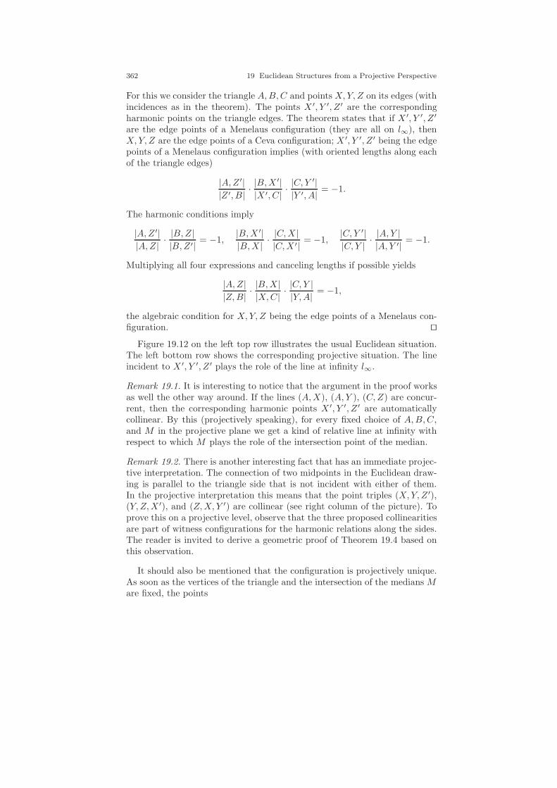
362 19 Euclidean Structures from a Projective Perspective
For this we consider the triangle A,B,C and points X,Y, Z on its edges (withincidences as in the theorem). The points X ′, Y ′, Z ′ are the correspondingharmonic points on the triangle edges. The theorem states that if X ′, Y ′, Z ′
are the edge points of a Menelaus configuration (they are all on l∞), thenX,Y, Z are the edge points of a Ceva configuration; X ′, Y ′, Z ′ being the edgepoints of a Menelaus configuration implies (with oriented lengths along eachof the triangle edges)
|A,Z ′||Z ′, B| ·
|B,X ′||X ′, C| ·
|C, Y ′||Y ′, A| = −1.
The harmonic conditions imply
|A,Z ′||A,Z| · |B,Z|
|B,Z ′| = −1,|B,X ′||B,X | ·
|C,X ||C,X ′| = −1,
|C, Y ′||C, Y | · |A, Y |
|A, Y ′| = −1.
Multiplying all four expressions and canceling lengths if possible yields
|A,Z||Z,B| ·
|B,X ||X,C| ·
|C, Y ||Y,A| = −1,
the algebraic condition for X,Y, Z being the edge points of a Menelaus con-figuration. ⊓⊔
Figure 19.12 on the left top row illustrates the usual Euclidean situation.The left bottom row shows the corresponding projective situation. The lineincident to X ′, Y ′, Z ′ plays the role of the line at infinity l∞.
Remark 19.1. It is interesting to notice that the argument in the proof worksas well the other way around. If the lines (A,X), (A, Y ), (C,Z) are concur-rent, then the corresponding harmonic points X ′, Y ′, Z ′ are automaticallycollinear. By this (projectively speaking), for every fixed choice of A,B,C,and M in the projective plane we get a kind of relative line at infinity withrespect to which M plays the role of the intersection point of the median.
Remark 19.2. There is another interesting fact that has an immediate projec-tive interpretation. The connection of two midpoints in the Euclidean draw-ing is parallel to the triangle side that is not incident with either of them.In the projective interpretation this means that the point triples (X,Y, Z ′),(Y, Z,X ′), and (Z,X, Y ′) are collinear (see right column of the picture). Toprove this on a projective level, observe that the three proposed collinearitiesare part of witness configurations for the harmonic relations along the sides.The reader is invited to derive a geometric proof of Theorem 19.4 based onthis observation.
It should also be mentioned that the configuration is projectively unique.As soon as the vertices of the triangle and the intersection of the medians Mare fixed, the points

19.6 Triangle Theorems 363
C
A
B T
R
S
W
U
V
t
rs
w
u
v
H
l∞
Fig. 19.13 Quadrilateral set condition.
meet(join(A,B), join(X,Y )) and meet(join(B,C), join(Y, Z))
determine the position of l∞.Desargues’s theorem applied to the two triangles(A,B,C) and (X,Y, Z) implies that meet(join(A,C), join(X,Z)) is also onl∞.
The altitudes of a triangle meet in a point: In contrast to the previ-ous theorem, the meeting of the altitudes makes a reference to explicit angles.Altitudes are orthogonal to the sides of the triangle. Thus in the projec-tivization I and J also play a role. This time we will express the projectiveversion entirely on the level of line slopes or, equivalently, on the level inter-section points on the line at infinity. In Section 8.2 we learned that six linesr, s, t, u, v, w whose intersections R, . . . ,W with the line at infinity are knownmay support the edges of a projected tetrahedron (i.e. a Ceva configuration)if and only if (R,U ;S, V ;T,W ) forms a quadrilateral set. Refer to Figure19.13 for the labeling. Algebraically, this means that on the line at infinitythe following projectively invariant bracket relation holds (with respect to anarbitrary basis on l∞):
[R,W ][S,U ][T, V ] = [R, V ][S,W ][T, U ]. (19.2)
This criterion can be nicely used to characterize the concurrence of threelines that pass through the triangle vertices. We will apply it to the alti-tudes. Characterizing orthogonality is the point at which I and J enter thegame. If the lines r and u are orthogonal, this means that (I, J;R,U) form aharmonic quadruple. Similarly, u, v, w being altitudes implies that (I, J;S, V )and (I, J;T,W ) are in harmonic position as well. Thus we get the equations
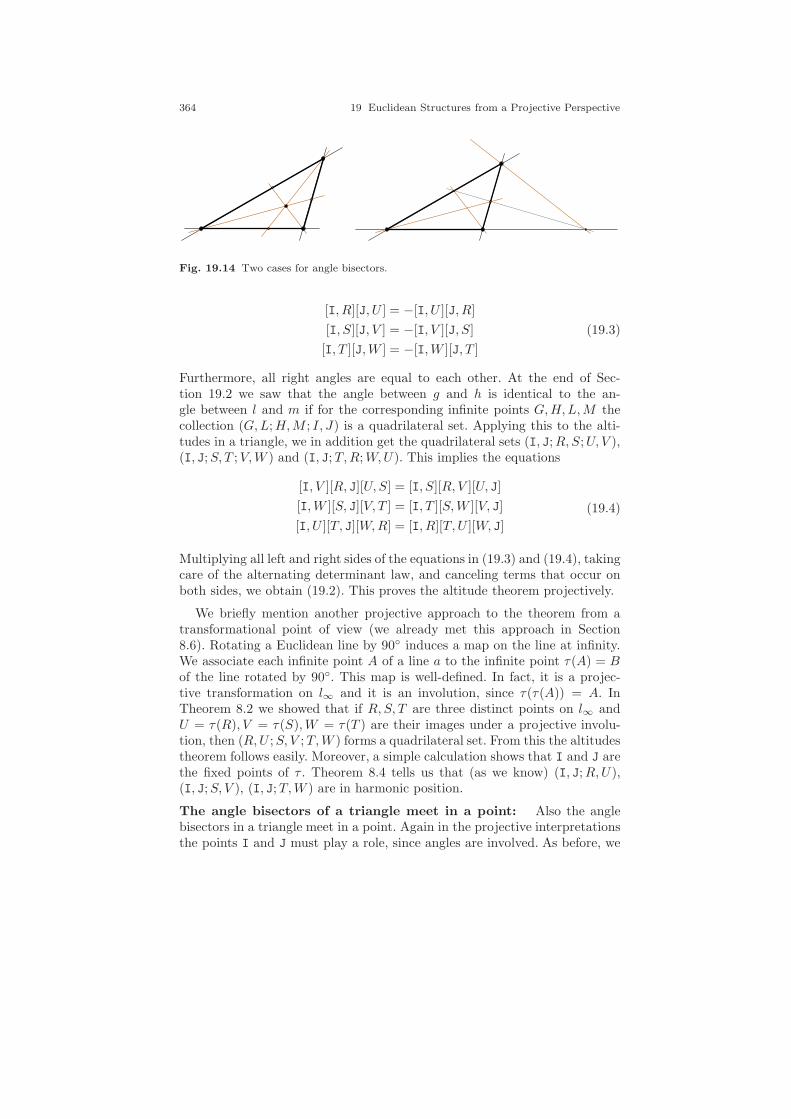
364 19 Euclidean Structures from a Projective Perspective
Fig. 19.14 Two cases for angle bisectors.
[I, R][J, U ] = −[I, U ][J, R]
[I, S][J, V ] = −[I, V ][J, S]
[I, T ][J,W ] = −[I,W ][J, T ]
(19.3)
Furthermore, all right angles are equal to each other. At the end of Sec-tion 19.2 we saw that the angle between g and h is identical to the an-gle between l and m if for the corresponding infinite points G,H,L,M thecollection (G,L;H,M ; I, J) is a quadrilateral set. Applying this to the alti-tudes in a triangle, we in addition get the quadrilateral sets (I, J;R,S;U, V ),(I, J;S, T ;V,W ) and (I, J;T,R;W,U). This implies the equations
[I, V ][R, J][U, S] = [I, S][R, V ][U, J]
[I,W ][S, J][V, T ] = [I, T ][S,W ][V, J]
[I, U ][T, J][W,R] = [I, R][T, U ][W, J]
(19.4)
Multiplying all left and right sides of the equations in (19.3) and (19.4), takingcare of the alternating determinant law, and canceling terms that occur onboth sides, we obtain (19.2). This proves the altitude theorem projectively.
We briefly mention another projective approach to the theorem from atransformational point of view (we already met this approach in Section8.6). Rotating a Euclidean line by 90 induces a map on the line at infinity.We associate each infinite point A of a line a to the infinite point τ(A) = Bof the line rotated by 90. This map is well-defined. In fact, it is a projec-tive transformation on l∞ and it is an involution, since τ(τ(A)) = A. InTheorem 8.2 we showed that if R,S, T are three distinct points on l∞ andU = τ(R), V = τ(S),W = τ(T ) are their images under a projective involu-tion, then (R,U ;S, V ;T,W ) forms a quadrilateral set. From this the altitudestheorem follows easily. Moreover, a simple calculation shows that I and J arethe fixed points of τ . Theorem 8.4 tells us that (as we know) (I, J;R,U),(I, J;S, V ), (I, J;T,W ) are in harmonic position.
The angle bisectors of a triangle meet in a point: Also the anglebisectors in a triangle meet in a point. Again in the projective interpretationsthe points I and J must play a role, since angles are involved. As before, we

19.6 Triangle Theorems 365
encode the relevant line slopes by the intersection points with the line atinfinity. For the labeling we again refer to Figure 19.13. If line W is an anglebisector of the lines r and s, this implies (according to Section 19.2) that(I, J;R,S;W,W ) is a quadrilateral set. Applying this fact to all three anglebisectors, we obtain the three conditions
[I,W ][R, J][W,S] = [I, S][R,W ][W, J]
[I, U ][S, J][U, T ] = [I, T ][S,U ][U, J]
[I, V ][T, J][V,R] = [I, R][T, V ][V, J]
(19.5)
One might expect that multiplying left and right sides and canceling as usualgives the desired result. Unfortunately, not a single bracket cancels. However,there is a nice trick that provides three more equations that make thingscancel. The roles of I and J are interchangeable in the quadrilateral setrelations. This implies that we also get the following three equations:
[J,W ][R, I][W,S] = [J, S][R,W ][WI]
[J, U ][S, I][U, T ] = [J, T ][S,U ][U, I]
[J, V ][T, I][V,R] = [J, R][T, V ][V, I]
(19.6)
Multiplying left and right sides of (19.5) and (19.6) and canceling bracketsnow leaves us with the equation
([W,S][U, T ][V,R])2 = ([R,W ][S,U ][T, V ])2.
Thus we can conclude that either
[R, V ][S,W ][T, U ] = +[R,W ][S,U ][T, V ] or
[R, V ][S,W ][T, U ] = −[R,W ][S,U ][T, V ]
is true. The first equation describes the quadrilateral set equation we arelooking for. The second equation encodes the fact that the intersectionsmeet(r, u), meet(s, v), and meet(t, w) are collinear. In fact, with the givenhypotheses this is the best we could hope for, since any pair of lines hastwo angle bisectors. If we made a proper choice, they are collinear; otherwise(in half of the possible cases), we get the collinearity condition. Figure 19.14illustrates the two possible cases for one given triangle.
The Euler line: The intersection of the medians M , the intersection ofthe altitudes H (called the orthocenter), and the circumcenter O are alwayscollinear. They lie on the so-called Euler line (see Figure 19.15 (left)). Froma projective viewpoint it turns out that this theorem is a direct consequenceof Desargues’s theorem. To see this, first observe that for the Euler line the-orem it is not necessary to draw all three altitudes, all three medians, andall three perpendicular bisectors. Two of each suffice to determine the threeintersection points O, M , and H . Figure 19.15 (right) shows a drawing in

366 19 Euclidean Structures from a Projective PerspectivePSfrag
B
C
M
A
HO
Y
Z
X
B
C
M
A
HO
Y X
Fig. 19.15 The Euler line.
which only two of each type of lines are drawn. Furthermore, a line betweenthe two midpoints X and Y is drawn. From our considerations about medians(Remark 19.2) we know that this line is parallel to A,B. Also, the perpendic-ular bisectors are parallel to the sides of the altitudes associated to the sameside of the triangle. Hence, the three sides of the red triangle are parallel tothe three sides of the green triangle. So they meet at three points that alllie on the line at infinity. Desargues’s theorem now tells us that in this casethe two triangles must be perspective with respect to a point. Thus the linejoin(O,H) must pass through the intersection of join(A,X) and join(B, Y ).
19.7 Hybrid Thinking
The world is neither Euclidean nor projective—it simply is. We may look atit only through certain filters of perception. In the final section of this chapterwe want to demonstrate how a kind of hybrid thinking, where one takes a pro-jective or Euclidean viewpoint, whichever seems to be more appropriate, canlead to interesting proofs and generalizations of theorems. Again, one couldfill a whole book with this. We here will limit ourselves to one example only,namely the nine-point circle, which is one of the more advanced theorems inelementary triangle geometry.2 The theorem is kind of surprising. However,
2 In fact, I have to admit that I personally hate these overcrowded elementary geometricdrawings that show up in many textbooks dealing with advanced triangle geometry. WhenI started to think about this section I thought, It would be nice to include also some-thing about the nine-point circle of a triangle. Starting thinking on this, I was trapped!The mutual relations and correspondences are so nice, surprising, and overwhelming thatI continued to produce exactly the same kind of overcrowded pictures over and over onmy computer. The situation got even worse when I started to think about possible pro-jectivizations of these relations. New theorems and relations, beautiful configurations, andnice relaxations showed up every minute, many more than would fit into single chapter

19.7 Hybrid Thinking 367
A B
C
D
E
F
P Q
R
H XY
Z
Fig. 19.16 Nine-point circle.
it is not too difficult to prove. It states that in any triangle the midpoints ofthe sides, the feet of the altitudes, and the midpoints of the segments thatjoin the orthocenterH with each vertex all lie on a common circle (see Figure19.16). A standard (Euclidean) proof technique of this result goes along thefollowing lines: The crucial observation is that the line that joins the mid-points in a triangle is parallel to the third side of the triangle. (We will needthis fact frequently later on and simply refer to it as (M).This implies that(Y,R) as well as (Z,Q) is parallel to (A,H). Also (R,Q) is parallel to (B,C)and hence orthogonal to (Y,R). Taking these statements together, one canconclude that (Y,R,Q,Z) is a rectangle. Thus its vertices lie on a circle. Sim-ilarly, one can prove that (X,Q, P, Y ) and (Z,P,R,X) are rectangles. Thisimplies that all midpoints (the blue points in the drawing) P,Q,R,X, Y, Zare on a circle. Since (Y,R,Q,Z) is a rectangle, the segment (Y,Q) is a diam-eter of the circle. Thales’ theorem implies that also the foot point E (a greenpoint) must be on the circle. Similarly, F and D are on the circle. The rightside of Figure 19.16 illustrates the two ingredients necessary for this proof.
At first sight this argument is far from being projective. However, everysingle step can be carefully translated to a projective argument (try it), andwe end up with a rather lengthy projective proof. This is not what we areaiming for. Instead, this time we are aiming for a closely related, thoughdifferent, projective theorem. This theorem will show that many of the co-incidences of the nine-point circle are still true after the hypotheses of thetheorem are somehow relaxed.By this we want to demonstrate how one couldapproach a theorem with a projective eye and how this may lead to interestingEuclidean and projective variants, relaxations, and generalizations (for evenmore variants see also [95]). We try to use arguments, based on our (so far)well-understood projective concepts like Desargues’s theorem (Section 15.1),
of this book. Here I will present a small collection of some of them. I tried to separatedifferent statements into several hopefully not so overcrowded pictures.
368 19 Euclidean Structures from a Projective Perspective
A B
C
P Q
R
H
XY
Z A B
C
P
Q
R
H
XY
Z
Fig. 19.17 The midpoints are on a conic.
Pascal’s theorem (Section 10.6), and Hesse’s transfer principle (Section 10.5).Our fundamental relaxation is that the points H will no longer be requiredto be the orthocenter—it may just be an arbitrary point that is not on a linesupporting the triangle’s edges.
Observation 1: Midpoints are on a conic. From a projective point ofview the first interesting relation occurs already on the level of the midpointsX,Y, Z, P,Q,R in the configuration. Constructing a midpoint is not depen-dent on the points I and J. It is an affine but not a genuinely Euclideanoperation. Thus if we start with the points A,B,C, and H , we may suspectthat even then the six midpoints of pairs of such points lie on a conic. HereH is assumed to be an arbitrary point and not necessarily the orthocenter.(We may not expect that the midpoints still lie on a circle, since I and J
are not contained in the hypotheses.) In fact, this conjecture turns out tobe true and not hard to prove at all. Figure 19.17 (left) shows the theoremand adds a few lines (red lines in the right picture) that immediately providea proof. (We may think projectively and still draw Euclidean pictures andare aware of the special role of the line at infinity.) By fact (M) we knowthat (Y,R) and (A,H) are parallel (i.e., they meet at the line at infinity)and that (Z,Q) and (A,H) are parallel. Hence (Y,R) and (Z,Q) meet at theline at infinity. Similarly, the pair of lines (Y, P ) and (X,Q) are parallel, aswell as (Z,P ) and (X,R). In other words, in the drawing the red lines forma hexagon with opposite sides being parallel. This in turn can be used as thehypotheses for Pascal’s theorem, which then implies that X,Y, Z, P,Q,R areon a conic. Observe that this argument used only the parallelism of the redand green lines (the former altitudes) in the picture.
Observation 2: The hexagon is symmetric. There is one more propertythat attracts attention when we look at Figure 19.17 (right). The hexagon ispoint-symmetric. In other words, if one joins opposite points of the hexagon,then the three resulting segments meet in the center of symmetry of thehexagon (see the blue lines in Figure 19.18, left). How can this be proved?Again a projective argument helps immediately. Similarly to what we didbefore, we can (now using parallelism to the black triangle edges and fact

19.7 Hybrid Thinking 369
A B
C
P
Q
R
H
XY
Z A B
C
P
Q
R
H
XY
Z
Fig. 19.18 Segments between opposite midpoints intersect.
(M)) show that in Figure 19.18 (right) the sides of the orange triangle areparallel to the sides of the red triangle. Desargues’s theorem implies thatthey are perspective with respect to each other. This forces that the bluelines meet in the point of perspectivity.
Observation 3: Also the foot points are on the conic. Now comes anamazing and remarkable observation. The conic through the six midpoints,passes also through the foot points D,E, F where the green lines (the for-mer altitudes) hit the triangle edges. Figure 19.19 illustrates the effect. Thisstatement is by far not as easy to prove as the previous ones. In the literature,only proofs involving loci of polars with respect to pencils of conics seem to beavailable (compare [95]). We here want to follow a more incidence-geometricapproach and base the proof on Hesse’s principle of transfer (see in particularFigure 10.10).
Hesse’s principle of transfer states that if we have six points on a conicsuch that the lines spanned by pairs of them are concurrent, then the condi-tion of a seventh point being on the conic is characterized by the fact thatit sees the six points in a quadrilateral set relation. We are in the lucky sit-
AB
C
D
E
F
P
Q
R
H
XY
Z
Fig. 19.19 Foot points are on the conic.
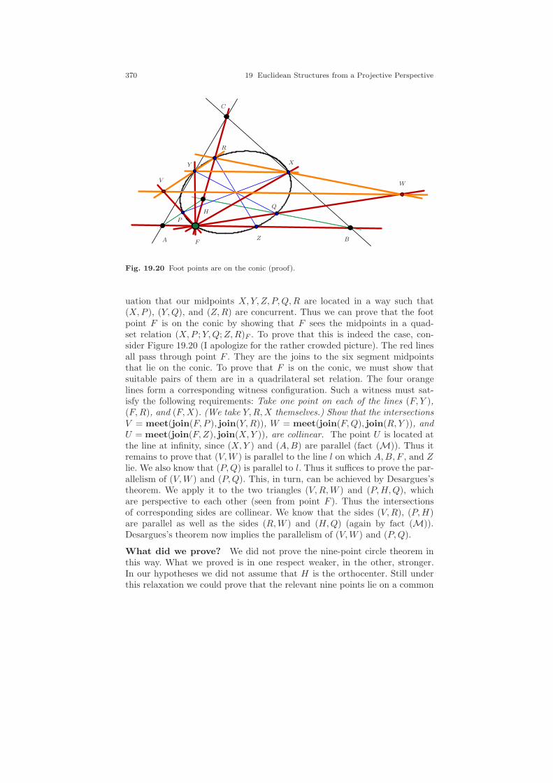
370 19 Euclidean Structures from a Projective Perspective
A B
C
F
P
Q
R
H
XY
Z
VW
Fig. 19.20 Foot points are on the conic (proof).
uation that our midpoints X,Y, Z, P,Q,R are located in a way such that(X,P ), (Y,Q), and (Z,R) are concurrent. Thus we can prove that the footpoint F is on the conic by showing that F sees the midpoints in a quad-set relation (X,P ;Y,Q;Z,R)F . To prove that this is indeed the case, con-sider Figure 19.20 (I apologize for the rather crowded picture). The red linesall pass through point F . They are the joins to the six segment midpointsthat lie on the conic. To prove that F is on the conic, we must show thatsuitable pairs of them are in a quadrilateral set relation. The four orangelines form a corresponding witness configuration. Such a witness must sat-isfy the following requirements: Take one point on each of the lines (F, Y ),(F,R), and (F,X). (We take Y,R,X themselves.) Show that the intersectionsV = meet(join(F, P ), join(Y,R)), W = meet(join(F,Q), join(R, Y )), andU = meet(join(F,Z), join(X,Y )), are collinear. The point U is located atthe line at infinity, since (X,Y ) and (A,B) are parallel (fact (M)). Thus itremains to prove that (V,W ) is parallel to the line l on which A,B, F , and Zlie. We also know that (P,Q) is parallel to l. Thus it suffices to prove the par-allelism of (V,W ) and (P,Q). This, in turn, can be achieved by Desargues’stheorem. We apply it to the two triangles (V,R,W ) and (P,H,Q), whichare perspective to each other (seen from point F ). Thus the intersectionsof corresponding sides are collinear. We know that the sides (V,R), (P,H)are parallel as well as the sides (R,W ) and (H,Q) (again by fact (M)).Desargues’s theorem now implies the parallelism of (V,W ) and (P,Q).
What did we prove? We did not prove the nine-point circle theorem inthis way. What we proved is in one respect weaker, in the other, stronger.In our hypotheses we did not assume that H is the orthocenter. Still underthis relaxation we could prove that the relevant nine points lie on a common
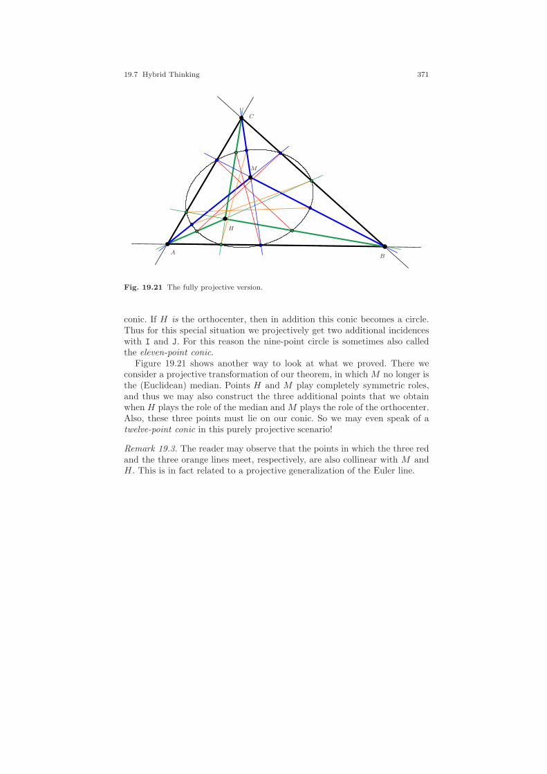
19.7 Hybrid Thinking 371
AB
C
H
M
Fig. 19.21 The fully projective version.
conic. If H is the orthocenter, then in addition this conic becomes a circle.Thus for this special situation we projectively get two additional incidenceswith I and J. For this reason the nine-point circle is sometimes also calledthe eleven-point conic.
Figure 19.21 shows another way to look at what we proved. There weconsider a projective transformation of our theorem, in which M no longer isthe (Euclidean) median. Points H and M play completely symmetric roles,and thus we may also construct the three additional points that we obtainwhen H plays the role of the median and M plays the role of the orthocenter.Also, these three points must lie on our conic. So we may even speak of atwelve-point conic in this purely projective scenario!
Remark 19.3. The reader may observe that the points in which the three redand the three orange lines meet, respectively, are also collinear with M andH . This is in fact related to a projective generalization of the Euler line.

20
Cayley-Klein Geometries
It ain’t necessarily so.
George and Ira Gershwin
We started out developing projective geometry for two reasons: It was al-gebraically nice and it helped us to get rid of the treatment of many spe-cial situations that are omnipresent in Euclidean geometry. Then, to expressEuclidean geometry in a projective setup, we needed the help of complexnumbers, our special points I and J, cross-ratios, and Laguerre’s formula.Wenow come to another pivot point in our explanations: We will see that ourtreatment of Euclidean geometry in a projective framework is only a specialcase of a variety of other reasonable geometries. One might ask what it meansto be a geometry in that context. For us it means that there are notions ofpoints, lines, incidence, distances, and angles with a certain reasonable inter-play. Besides Euclidean geometry, among those geometries there are quite afew prominent examples, such as hyperbolic geometry, elliptic geometry, andrelativistic space-time geometry.
In all these geometries the fundamental notions of measurement are basedon a conic that plays the role of infinitely distant elements. The type of conicdetermines the type of geometry we get. So the classification of conics weprovided in Section 9.5 will play a crucial role in this context.
It is difficult to recommend particular places in the mathematical literaturewhere one can dive into this subject more deeply. Many modern texts arefairly abstract, and the classical texts may be difficult to access. I personallylike best the classical book by Klein [68] and his original papers “On the so-called non-Euclidean geometry” from 1872 [66] and 1874 [67]. The first oneis translated and reprinted in [125]. More modern treatments may be foundin [91, 75]. A very accessible exposition may be found in [3].
373
374 20 Cayley-Klein Geometries
20.1 I and J Revisited
As we saw in Section 18.7, the measurement of angles in Euclidean geometryis expressed by Laguerre’s formula:
∠(l,m) =1
2i· ln((L,M ; I, J)
),
with L andM being the infinite points of l and m. It is the aim of this chapterto generalize this formula. One might think that this generalization willbe carried out by generalizing the way that the elements are arithmeticallyconnected by cross-ratios and logarithms. But actually it will be the elementsthat enter the formula themselves that are subject to the generalization. Forthis, observe that we may consider the pair of points (I, J) a degenerate dualconic consisting of the two complex conjugate points I and J. The setup forgeneral Cayley-Klein geometries will be to admit a general conic instead ofI and J.
To see how this will work, we reexamine I and J, now interpreted as aconic. In Chapter 9 we learned that a dual conic may degenerate into a pairof points (either real or complex conjugate). In the case that these two pointsdo not coincide, the corresponding primal conic must be the doubly coveredline that connects these two points. In the case of I and J, a correspondingprimal/dual pair Ceuc = (A,B) of matrices (in the sense of Definition 9.5) isgiven by
A =
0 0 00 0 00 0 1
= B∆ and B =
1 0 00 1 00 0 0
.
Here B is the matrix that describes the degenerate dual quadratic formlTBl = 0; A describes the primal form pTAp = 0. The primal equation(which describes which points are on the conic) pTAp = 0 with p = (x, y, z)T
becomes z2 = 0. The points that satisfy this equation are all those of the form(x, y, 0), i.e., the points on the line at infinity (doubly covered). The solutionsof the dual equation (which describes which lines are tangent to the conic)lTBl = 0 with l = (a, b, c)T must satisfy a2 + b2 = 0. Up to a scalar multi-ple these are all lines of the form (−i, 1, α) =: iα and (i, 1, α) := jα with afree parameter α. These are two bundles of lines through two different points,namely I and J. Lines of the form iα satisfy 〈I, iα〉 = (−i)·(−i)+1·1+0·α = 0and pass through I. Lines of the form jα satisfy 〈J, jα〉 = i · i+1 ·1+0 ·α= 0and pass through J. The tangents of a point p to the conic Ceuc are the twolines join(p, I) and join(p, J). Thus we can reinterpret Laguerre’s formulafor calculating the angle between two lines in the following way:
Assume that the lines l and m meet at a point p. Construct the twotangents t1 and t2 from p to Ceuc. The angle between l and m is then
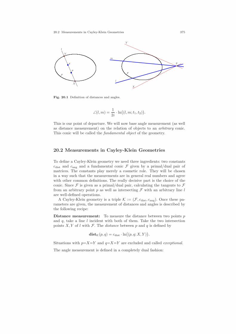
20.2 Measurements in Cayley-Klein Geometries 375
p
q
l
F
X
Y
p
l
m
F
X
Y
Fig. 20.1 Definition of distances and angles.
∠(l,m) =1
2i· ln((l,m; t1, t2)
).
This is our point of departure. We will now base angle measurement (as wellas distance measurement) on the relation of objects to an arbitrary conic.This conic will be called the fundamental object of the geometry.
20.2 Measurements in Cayley-Klein Geometries
To define a Cayley-Klein geometry we need three ingredients: two constantscdist and cang and a fundamental conic F given by a primal/dual pair ofmatrices. The constants play merely a cosmetic role. They will be chosenin a way such that the measurements are in general real numbers and agreewith other common definitions. The really decisive part is the choice of theconic. Since F is given as a primal/dual pair, calculating the tangents to Ffrom an arbitrary point p as well as intersecting F with an arbitrary line lare well-defined operations.
A Cayley-Klein geometry is a triple K := (F , cdist, cang). Once these pa-rameters are given, the measurement of distances and angles is described bythe following recipe:
Distance measurement: To measure the distance between two points pand q, take a line l incident with both of them. Take the two intersectionpoints X,Y of l with F . The distance between p and q is defined by
distK(p, q) = cdist · ln((p, q;X,Y )
).
Situations with p=X=Y and q=X=Y are excluded and called exceptional.
The angle measurement is defined in a completely dual fashion:

376 20 Cayley-Klein Geometries
Angle measurement: To measure the angle between two lines l and mtake a point p incident with both of them. Take the two tangents X,Y fromp to F . The angle between l and m is defined by
angK(l,m) = cang · ln((l,m;X,Y )
).
Situations with l=X=Y and m=X=Y are excluded and called exceptional.
The geometric position of the elements involved is illustrated in Figure 20.1.Let us point out a few subtleties of these two definitions of measurement.
• The distance measurement remains well-defined even if the two pointsp and q coincide. If this happens, any line l through them will give ameasurement of the form cdist·ln
((p, p;X,Y )
)= cdist ·ln(1) = 0. Similarly,
the angle of coinciding lines is also zero.• In many practical situations it may make sense to define distance and
angles as the absolute values of the measurements defined above. Wewill make this precise later on. The situation is similar to the situationin the usual Euclidean plane. There along one line it makes sense tospeak of oriented distances. However, if one measures distances in theplane without reference to a particular line, it is reasonable to switch toabsolute values.
• There are two ambiguities in the definitions of measurement. Firstly, theorder of the elements X,Y is not specified. Interchanging their roles al-ters the sign of the measurement (one more reason to consider absolutevalues). Secondly, on a function theoretic level the logarithm is a multi-valued function. It is determined only up to multiples of 2πi. We will seethat for all practical purposes we can deal nicely with these ambiguities.
• Perhaps the most important point is that the elements X,Y may eitherbe real, coincide, or be complex conjugates. Each of these three possibil-ities leads to a qualitatively different behavior of the measurement. Thepictures in Figure 20.1 represent the situation in which X and Y are dis-tinct and real. We get a complex situation for the distance measurementif line l does not intersect the conic. We get a complex situation for theangle measurement if the lines l and m intersect inside the conic.
• In the definition we will explicitly allow the fundamental conic to becompletely complex. Thus equations like x2 + y2 + z2 = 0 are completelysuitable fundamental objects. (In fact, they will lead to very interestinggeometries.)
• If F is a degenerate conic, then it may happen that X and Y coincidefor all distance or angle measurements. In that case we get, for instance,a degenerate length measurement of the form cdist · ln
((p, q;X,X)
)=
cdist · ln(1) = 0. We will dedicate an entire section to the treatment ofsuch degenerate cases.
• It may happen that in the cross-ratio (p, q;X,Y ) = [p,X ][q, Y ]/[p, Y ][q,X ]both the denominator and the numerator become zero and p and q do not
20.3 Nondegenerate Measurements along a Line 377
coincide (for instance if q = X = Y ). Then the evaluation of the cross-ratio is of the form 0/0. The corresponding length (resp. angle) is thenan undefined value. We call such point pairs (or line pairs) exceptional.
We will soon see how all these subtleties fit nicely into the picture as a whole.In a sense, each of them makes the whole theory a bit more beautiful.
20.3 Nondegenerate Measurements along a Line
We will first study how the above notion of distance applies to the points ofone single line. Let l be this line and let X and Y be the two intersections ofthis line with the fundamental conic F . While restricting the measurementsto the line l we keep these two points fixed during the entire section. Sincethe definitions of distance and angle measurement are completely dual, thecorresponding dual statements apply analogously for angle measurement.
Since the logarithm has to be considered a multivalued function that isdetermined only modulo 2πi, all equations on distance measurement thatfollow have to be considered to be true modulo cdist2πi. Analogously, anglemeasurements are determined only modulo cang2πi.
1
Theorem 20.1. Let K := (F , cdist, cang) be a Cayley-Klein geometry and letl be an arbitrary line that intersects F in two distinct points X,Y . For twopoints p and q on l we set distK(p, q) = cdist · ln
((p, q;X,Y )
). Then (modulo
cdist2πi) we get for points p, q, r on l,
(i) distK(p, p) = 0,
(ii) distK(p, q) = −distK(q, p),
(iii) distK(p, q) + distK(q, r) = distK(p, r).
Proof. (i): For cross-ratios we have (p, p;X,Y ) = 1. This implies
distK(p, p) = cdist · ln((p, p;X,Y )
)= cdist · ln
(1) = 0.
(ii): For cross-ratios the relation (p, q;X,Y ) = 1/(q, p;X,Y ) holds. Hence weget
distK(p, q) = cdist · ln((p, q;X,Y )
)
= −cdist · ln(1/(p, q;X,Y )
)
= −cdist · ln((q, p;X,Y )
)
= −distK(q, p).
1 We know this effect from the usual angle measurement. Given two (unoriented) lines, theangle between them is determined only modulo π. This agrees with Laguerre’s formula,where cang = 1/2i.
378 20 Cayley-Klein Geometries
(iii): For cross-ratios the relation (p, q;X,Y ) · (q, r;X,Y ) = (p, r;X,Y ) holds.Hence we get
distK(p, r) = cdist · ln((p, r;X,Y )
)
= cdist · ln((p, q;X,Y ) · (q, r;X,Y )
)
= cdist · ln((p, q;X,Y )) + cdist · ln
((q, r;X,Y )
)
= distK(p, q) + distK(q, r)
⊓⊔We see that the logarithm turns the multiplicative properties of cross-ratios
into additive properties of distances. Along a fixed line it makes perfect senseto speak of oriented distances, and the above statements in essence introducea distance scale along such a line. As soon as a point p on l is singled out, onecan consistently measure the position of all other points on l with respect top by the value of distK(p, r). This is in a sense similar to the situation on thereal number line, where one can also measure distances as soon as an originis fixed (in fact, there is a subtle difference between these two pictures, whichwe will encounter later on). We now want to analyze how this measurementbehaves qualitatively. The intersections of l with the fundamental conic ariseas the solutions of a quadratic equation. Thus up to equivalence by realprojective transformations we have to consider only three different cases:
(a) X,Y are real and distinct,(b) X,Y are complex conjugates,(c) X,Y are identical and real.
We will first focus on the cases (a) and (b).
Case (a) – hyperbolic measurement: For this we fix two points X =(−1, 1) and Y = (1, 1) on the projective line l. We will study the measurementbetween points (p, 1) and (q, 1). Since all our considerations will be restrictedto the line l, we may simply identify a point (x, 1) with the number x andcalculate the cross-ratio by quotients of differences between these numbers.The measurement between two points p and q with respect to X and Y thenbecomes
dist(p, q) = cdist · ln(
(p+ 1)(q − 1)
(p− 1)(q + 1)
).
In particular, if we set p = 0 to be the origin, we get the distance function
dist(0, q) = cdist · ln(
(1 − q)
(1 + q)
).
The expression in the logarithm is positive whenever q is in the open intervalfrom −1 to 1. If p traverses this interval continuously then the logarithm inthe above formula will traverse values from ∞ to −∞. More generally, the

20.3 Nondegenerate Measurements along a Line 379
π/2
−π/2
1−1
disthyp(0, x)
distell(0, x)
x
Fig. 20.2 Distance functions for hyperbolic and elliptic measurement.
function ln(
(p+1)(q−1)(p−1)(q+1)
)is real-valued if (along the real projective (!) line l)
the points p and q are not separated by −1 and 1. It is complex or infiniteotherwise.
We now come to a particular choice of the constant cdist. A reasonabledistance measure should behave in a way such that points that are “near”each other (and not separated by −1 or by 1) have a small real distance. Sincein such a proximity situation the logarithm is real-valued, we can achievethis by choosing cdist to be a real number. One particularly nice choice is tochoose this number such that locally for very small numbers q the functiondist(0, q) is asymptotically close to q itself (i.e., around 0 it approximatesthe usual Euclidean measurement on the real number line). Considering thederivative
d dist(0, q)
d q= cdist ·
d ln(
(1−q)(1+q)
)
d q= cdist ·
2
q2 − 1,
we see that by setting cdist = −1/2 we get the desired local approximationbehavior around q = 0. Although all other constants lead to essentially iso-morphic measurements, we will continue with this special setting and define
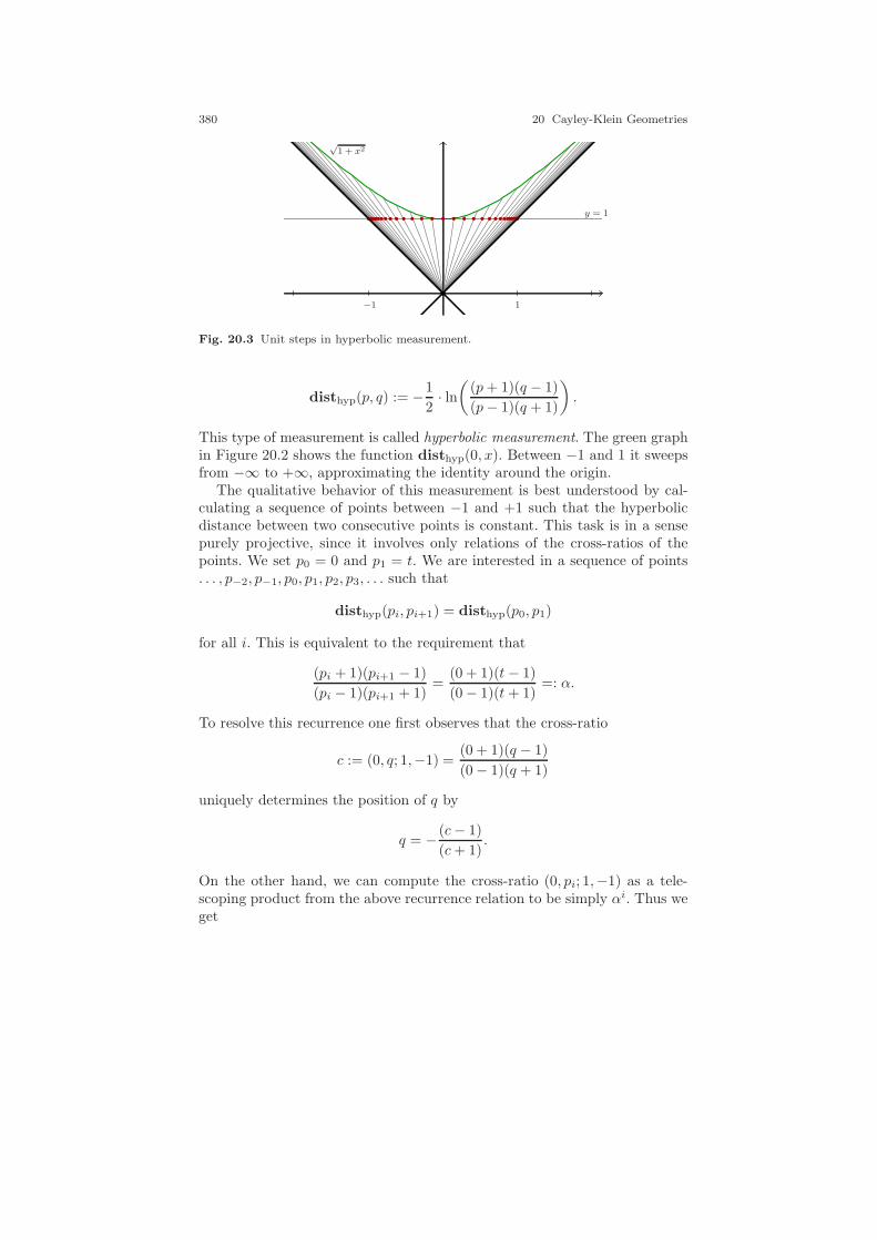
380 20 Cayley-Klein Geometries
√1 + x2
y = 1
1−1
Fig. 20.3 Unit steps in hyperbolic measurement.
disthyp(p, q) := −1
2· ln(
(p+ 1)(q − 1)
(p− 1)(q + 1)
).
This type of measurement is called hyperbolic measurement. The green graphin Figure 20.2 shows the function disthyp(0, x). Between −1 and 1 it sweepsfrom −∞ to +∞, approximating the identity around the origin.
The qualitative behavior of this measurement is best understood by cal-culating a sequence of points between −1 and +1 such that the hyperbolicdistance between two consecutive points is constant. This task is in a sensepurely projective, since it involves only relations of the cross-ratios of thepoints. We set p0 = 0 and p1 = t. We are interested in a sequence of points. . . , p−2, p−1, p0, p1, p2, p3, . . . such that
disthyp(pi, pi+1) = disthyp(p0, p1)
for all i. This is equivalent to the requirement that
(pi + 1)(pi+1 − 1)
(pi − 1)(pi+1 + 1)=
(0 + 1)(t− 1)
(0 − 1)(t+ 1)=: α.
To resolve this recurrence one first observes that the cross-ratio
c := (0, q; 1,−1) =(0 + 1)(q − 1)
(0 − 1)(q + 1)
uniquely determines the position of q by
q = − (c− 1)
(c+ 1).
On the other hand, we can compute the cross-ratio (0, pi; 1,−1) as a tele-scoping product from the above recurrence relation to be simply αi. Thus weget
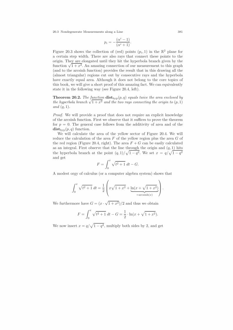
20.3 Nondegenerate Measurements along a Line 381
pi = − (αi − 1)
(αi + 1).
Figure 20.3 shows the collection of (red) points (pi, 1) in the R2 plane fora certain step width. There are also rays that connect these points to theorigin. They are elongated until they hit the hyperbola branch given by thefunction
√1 + x2. An amazing connection of our measurement to this graph
(and to the arcsinh function) provides the result that in this drawing all the(almost triangular) regions cut out by consecutive rays and the hyperbolahave exactly equal area. Although it does not belong to the core topics ofthis book, we will give a short proof of this amazing fact. We can equivalentlystate it in the following way (see Figure 20.4, left).
Theorem 20.2. The function disthyp(p, q) equals twice the area enclosed bythe hyperbola branch
√1 + x2 and the two rays connecting the origin to (p, 1)
and (q, 1).
Proof. We will provide a proof that does not require an explicit knowledgeof the arcsinh function. First we observe that it suffices to prove the theoremfor p = 0. The general case follows from the additivity of area and of thedisthyp(p, q) function.
We will calculate the area of the yellow sector of Figure 20.4. We willreduce the calculation of the area F of the yellow region plus the area G ofthe red region (Figure 20.4, right). The area F +G can be easily calculatedas an integral. First observe that the line through the origin and (q, 1) hits
the hyperbola branch at the point (q, 1)/√
1 − q2. We set x = q/√
1 − q2
and get
F =
∫ x
0
√t2 + 1 dt−G.
A modest orgy of calculus (or a computer algebra system) shows that
∫ x
0
√t2 + 1 dt =
1
2
x√
1 + x2 + ln(x+√
1 + x2)︸ ︷︷ ︸=arcsinh(x)
.
We furthermore have G = (x ·√
1 + x2)/2 and thus we obtain
F =
∫ x
0
√t2 + 1 dt−G =
1
2· ln(x+
√1 + x2).
We now insert x = q/√
1 − q2, multiply both sides by 2, and get
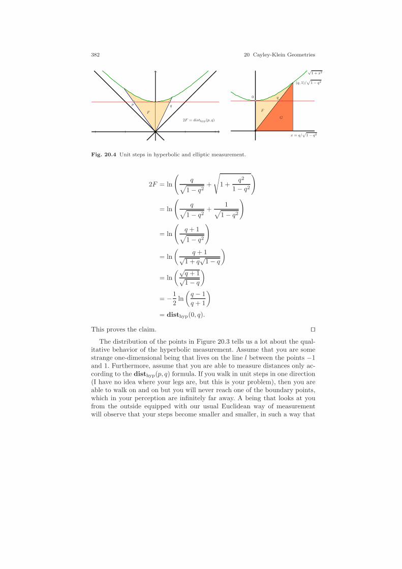
382 20 Cayley-Klein Geometries
p q
F
2F = disthyp(p, q)
(q, 1)/p
1 − q2
x = q/p
1 − q2
q0
F
G
√1 + x2
Fig. 20.4 Unit steps in hyperbolic and elliptic measurement.
2F = ln
(q√
1 − q2+
√1 +
q2
1 − q2
)
= ln
(q√
1 − q2+
1√1 − q2
)
= ln
(q + 1√1 − q2
)
= ln
(q + 1√
1 + q√
1 − q
)
= ln
(√q + 1√1 − q
)
= −1
2ln
(q − 1
q + 1
)
= disthyp(0, q).
This proves the claim. ⊓⊔The distribution of the points in Figure 20.3 tells us a lot about the qual-
itative behavior of the hyperbolic measurement. Assume that you are somestrange one-dimensional being that lives on the line l between the points −1and 1. Furthermore, assume that you are able to measure distances only ac-cording to the disthyp(p, q) formula. If you walk in unit steps in one direction(I have no idea where your legs are, but this is your problem), then you areable to walk on and on but you will never reach one of the boundary points,which in your perception are infinitely far away. A being that looks at youfrom the outside equipped with our usual Euclidean way of measurementwill observe that your steps become smaller and smaller, in such a way that
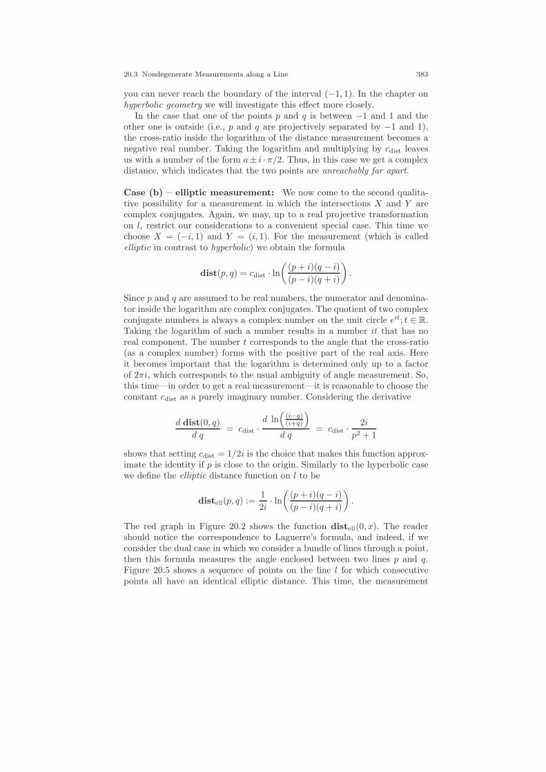
20.3 Nondegenerate Measurements along a Line 383
you can never reach the boundary of the interval (−1, 1). In the chapter onhyperbolic geometry we will investigate this effect more closely.
In the case that one of the points p and q is between −1 and 1 and theother one is outside (i.e., p and q are projectively separated by −1 and 1),the cross-ratio inside the logarithm of the distance measurement becomes anegative real number. Taking the logarithm and multiplying by cdist leavesus with a number of the form a± i ·π/2. Thus, in this case we get a complexdistance, which indicates that the two points are unreachably far apart.
Case (b) – elliptic measurement: We now come to the second qualita-tive possibility for a measurement in which the intersections X and Y arecomplex conjugates. Again, we may, up to a real projective transformationon l, restrict our considerations to a convenient special case. This time wechoose X = (−i, 1) and Y = (i, 1). For the measurement (which is calledelliptic in contrast to hyperbolic) we obtain the formula
dist(p, q) = cdist · ln(
(p+ i)(q − i)
(p− i)(q + i)
).
Since p and q are assumed to be real numbers, the numerator and denomina-tor inside the logarithm are complex conjugates. The quotient of two complexconjugate numbers is always a complex number on the unit circle eit; t ∈ R.Taking the logarithm of such a number results in a number it that has noreal component. The number t corresponds to the angle that the cross-ratio(as a complex number) forms with the positive part of the real axis. Hereit becomes important that the logarithm is determined only up to a factorof 2πi, which corresponds to the usual ambiguity of angle measurement. So,this time—in order to get a real measurement—it is reasonable to choose theconstant cdist as a purely imaginary number. Considering the derivative
d dist(0, q)
d q= cdist ·
d ln(
(i−q)(i+q)
)
d q= cdist ·
2i
p2 + 1
shows that setting cdist = 1/2i is the choice that makes this function approx-imate the identity if p is close to the origin. Similarly to the hyperbolic casewe define the elliptic distance function on l to be
distell(p, q) :=1
2i· ln(
(p+ i)(q − i)
(p− i)(q + i)
).
The red graph in Figure 20.2 shows the function distell(0, x). The readershould notice the correspondence to Laguerre’s formula, and indeed, if weconsider the dual case in which we consider a bundle of lines through a point,then this formula measures the angle enclosed between two lines p and q.Figure 20.5 shows a sequence of points on the line l for which consecutivepoints all have an identical elliptic distance. This time, the measurement
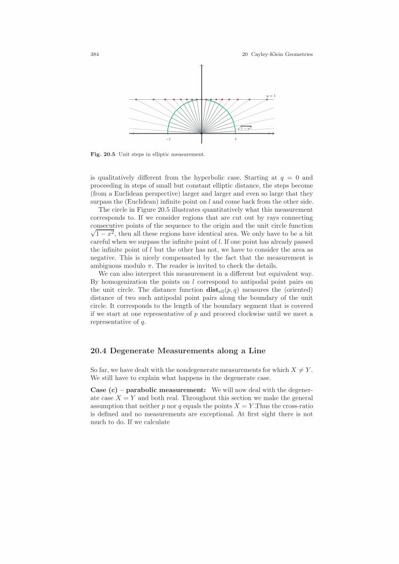
384 20 Cayley-Klein Geometries
√1 − x2
y = 1
1−1
Fig. 20.5 Unit steps in elliptic measurement.
is qualitatively different from the hyperbolic case. Starting at q = 0 andproceeding in steps of small but constant elliptic distance, the steps become(from a Euclidean perspective) larger and larger and even so large that theysurpass the (Euclidean) infinite point on l and come back from the other side.
The circle in Figure 20.5 illustrates quantitatively what this measurementcorresponds to. If we consider regions that are cut out by rays connectingconsecutive points of the sequence to the origin and the unit circle function√
1 − x2, then all these regions have identical area. We only have to be a bitcareful when we surpass the infinite point of l. If one point has already passedthe infinite point of l but the other has not, we have to consider the area asnegative. This is nicely compensated by the fact that the measurement isambiguous modulo π. The reader is invited to check the details.
We can also interpret this measurement in a different but equivalent way.By homogenization the points on l correspond to antipodal point pairs onthe unit circle. The distance function distell(p, q) measures the (oriented)distance of two such antipodal point pairs along the boundary of the unitcircle. It corresponds to the length of the boundary segment that is coveredif we start at one representative of p and proceed clockwise until we meet arepresentative of q.
20.4 Degenerate Measurements along a Line
So far, we have dealt with the nondegenerate measurements for whichX 6= Y .We still have to explain what happens in the degenerate case.
Case (c) – parabolic measurement: We will now deal with the degener-ate case X = Y and both real. Throughout this section we make the generalassumption that neither p nor q equals the points X = Y .Thus the cross-ratiois defined and no measurements are exceptional. At first sight there is notmuch to do. If we calculate
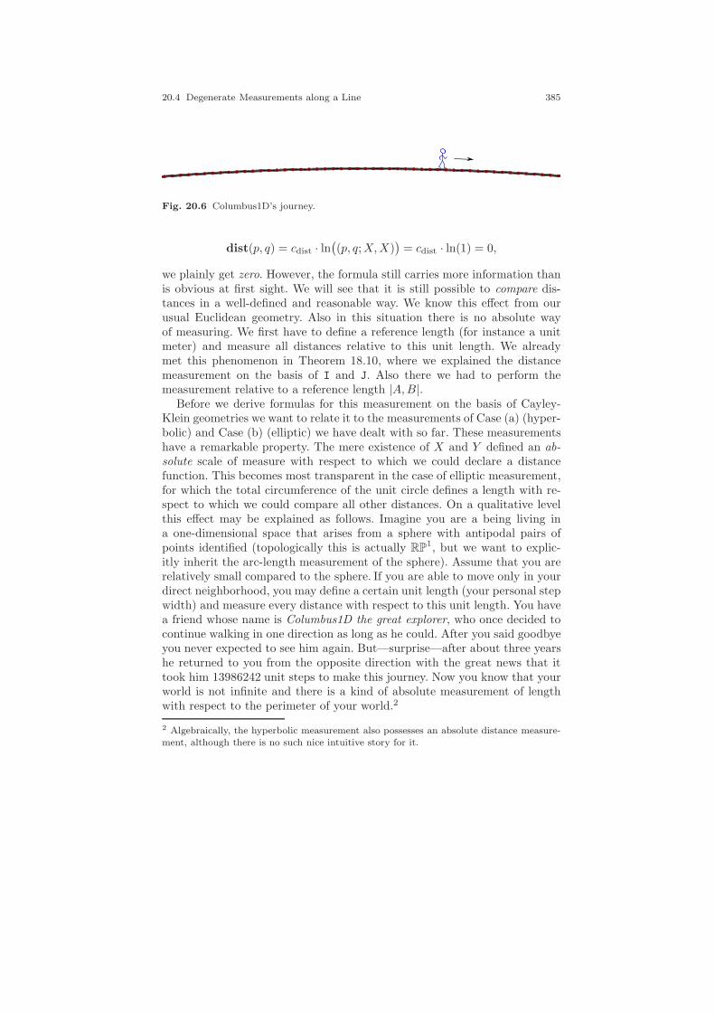
20.4 Degenerate Measurements along a Line 385
Fig. 20.6 Columbus1D’s journey.
dist(p, q) = cdist · ln((p, q;X,X)
)= cdist · ln(1) = 0,
we plainly get zero. However, the formula still carries more information thanis obvious at first sight. We will see that it is still possible to compare dis-tances in a well-defined and reasonable way. We know this effect from ourusual Euclidean geometry. Also in this situation there is no absolute wayof measuring. We first have to define a reference length (for instance a unitmeter) and measure all distances relative to this unit length. We alreadymet this phenomenon in Theorem 18.10, where we explained the distancemeasurement on the basis of I and J. Also there we had to perform themeasurement relative to a reference length |A,B|.
Before we derive formulas for this measurement on the basis of Cayley-Klein geometries we want to relate it to the measurements of Case (a) (hyper-bolic) and Case (b) (elliptic) we have dealt with so far. These measurementshave a remarkable property. The mere existence of X and Y defined an ab-solute scale of measure with respect to which we could declare a distancefunction. This becomes most transparent in the case of elliptic measurement,for which the total circumference of the unit circle defines a length with re-spect to which we could compare all other distances. On a qualitative levelthis effect may be explained as follows. Imagine you are a being living ina one-dimensional space that arises from a sphere with antipodal pairs ofpoints identified (topologically this is actually RP
1, but we want to explic-itly inherit the arc-length measurement of the sphere). Assume that you arerelatively small compared to the sphere. If you are able to move only in yourdirect neighborhood, you may define a certain unit length (your personal stepwidth) and measure every distance with respect to this unit length. You havea friend whose name is Columbus1D the great explorer, who once decided tocontinue walking in one direction as long as he could. After you said goodbyeyou never expected to see him again. But—surprise—after about three yearshe returned to you from the opposite direction with the great news that ittook him 13986242 unit steps to make this journey. Now you know that yourworld is not infinite and there is a kind of absolute measurement of lengthwith respect to the perimeter of your world.2
2 Algebraically, the hyperbolic measurement also possesses an absolute distance measure-ment, although there is no such nice intuitive story for it.

386 20 Cayley-Klein Geometries
Intuitively speaking, the degenerate measurement caseX = Y is about thesituation in which you have a sphere of infinite radius and Columbus1D will infact never return. For dealing with the degenerateX = Y case analytically wewill, for the moment, drop our assumption that X and Y are fixed. Instead,we will consider them as members of a continuous family of measurements (weblow up the world). For this we consider the quadratic equation αx2−y2 = 0and assume that X,Y are the homogeneous coordinates of the solutions ofthis equation. For α = 1 we get the situation of the hyperbolic case Xhyp =(−1, 1)T and Yhyp = (1, 1)T . For α = −1 we get the situation of the ellipticcaseXell = (−i, 1)T and Yell = (i, 1)T . In the general case we get the solutions(1,±√
α)T . If the parameter α is moved continuously from 1 to −1, we startwith the pair of points (Xhyp, Yhyp). Then they move away from the originin opposite directions. They will coincide for α = 0 at the infinite point of l.After this they continue as complex conjugates, to finally reach the position(Xell, Yell) for α = −1. We now consider the measurement between two points(0, 1) and (q, 1), both different from (1, 0). We consider the behavior of thelogarithm
ln
∣∣∣∣0 11 −√
α
∣∣∣∣∣∣∣∣q 11√α
∣∣∣∣∣∣∣∣0 11√α
∣∣∣∣∣∣∣∣q 11 −√
α
∣∣∣∣
= ln
(q√α− 1
−q√α− 1
)= ln(q
√α− 1) − ln(−q
√α− 1).
We now want to compare the distance measure generated by this expressionwith the measurement from (0, 1) to a fixed point (a, 1) that will play therole of the unit length. The relation of these two measurements (notice thatcdist cancels) is
fa(α, q) :=ln(q
√α− 1) − ln(−q√α− 1)
ln(a√α− 1) − ln(−a√α− 1)
.
For α = 0 this gives an undefined expression 0/0. However, we may stillconsider the limit situation limα→0 fa(α, q). This limit value can be easilycalculated using the L’Hospital’s rule. For this we differentiate the numeratorand denominator of fa(α, q) with respect to α and divide the two expressions(we omit the boring details of the calculation):
limα→0
fa(α, q) = limα→0
q√α(αq2−1)
a√α(αa2−1)
= limα→0
q(αa2 − 1
)
a(αq2 − 1)=q
a.
In the limit case the comparison of the two Cayley-Klein measures turns outto be just a comparison of the usual Euclidean distances. In other words,performing a relative measurement with respect to a unit length convergesto the usual Euclidean measurement of lengths.
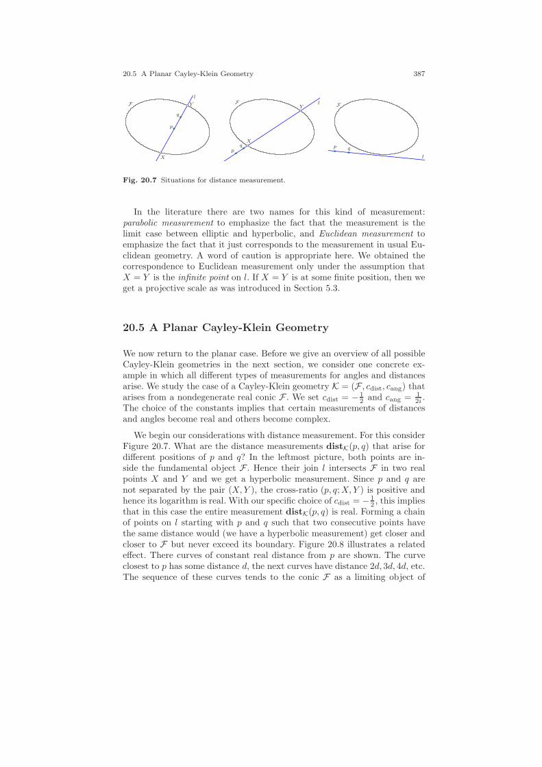
20.5 A Planar Cayley-Klein Geometry 387
p
q
X
Y
l
F
pqX
YlF
p q
l
F
Fig. 20.7 Situations for distance measurement.
In the literature there are two names for this kind of measurement:parabolic measurement to emphasize the fact that the measurement is thelimit case between elliptic and hyperbolic, and Euclidean measurement toemphasize the fact that it just corresponds to the measurement in usual Eu-clidean geometry. A word of caution is appropriate here. We obtained thecorrespondence to Euclidean measurement only under the assumption thatX = Y is the infinite point on l. If X = Y is at some finite position, then weget a projective scale as was introduced in Section 5.3.
20.5 A Planar Cayley-Klein Geometry
We now return to the planar case. Before we give an overview of all possibleCayley-Klein geometries in the next section, we consider one concrete ex-ample in which all different types of measurements for angles and distancesarise. We study the case of a Cayley-Klein geometry K = (F , cdist, cang) thatarises from a nondegenerate real conic F . We set cdist = − 1
2 and cang = 12i .
The choice of the constants implies that certain measurements of distancesand angles become real and others become complex.
We begin our considerations with distance measurement. For this considerFigure 20.7. What are the distance measurements distK(p, q) that arise fordifferent positions of p and q? In the leftmost picture, both points are in-side the fundamental object F . Hence their join l intersects F in two realpoints X and Y and we get a hyperbolic measurement. Since p and q arenot separated by the pair (X,Y ), the cross-ratio (p, q;X,Y ) is positive andhence its logarithm is real. With our specific choice of cdist = − 1
2 , this impliesthat in this case the entire measurement distK(p, q) is real. Forming a chainof points on l starting with p and q such that two consecutive points havethe same distance would (we have a hyperbolic measurement) get closer andcloser to F but never exceed its boundary. Figure 20.8 illustrates a relatedeffect. There curves of constant real distance from p are shown. The curveclosest to p has some distance d, the next curves have distance 2d, 3d, 4d, etc.The sequence of these curves tends to the conic F as a limiting object of
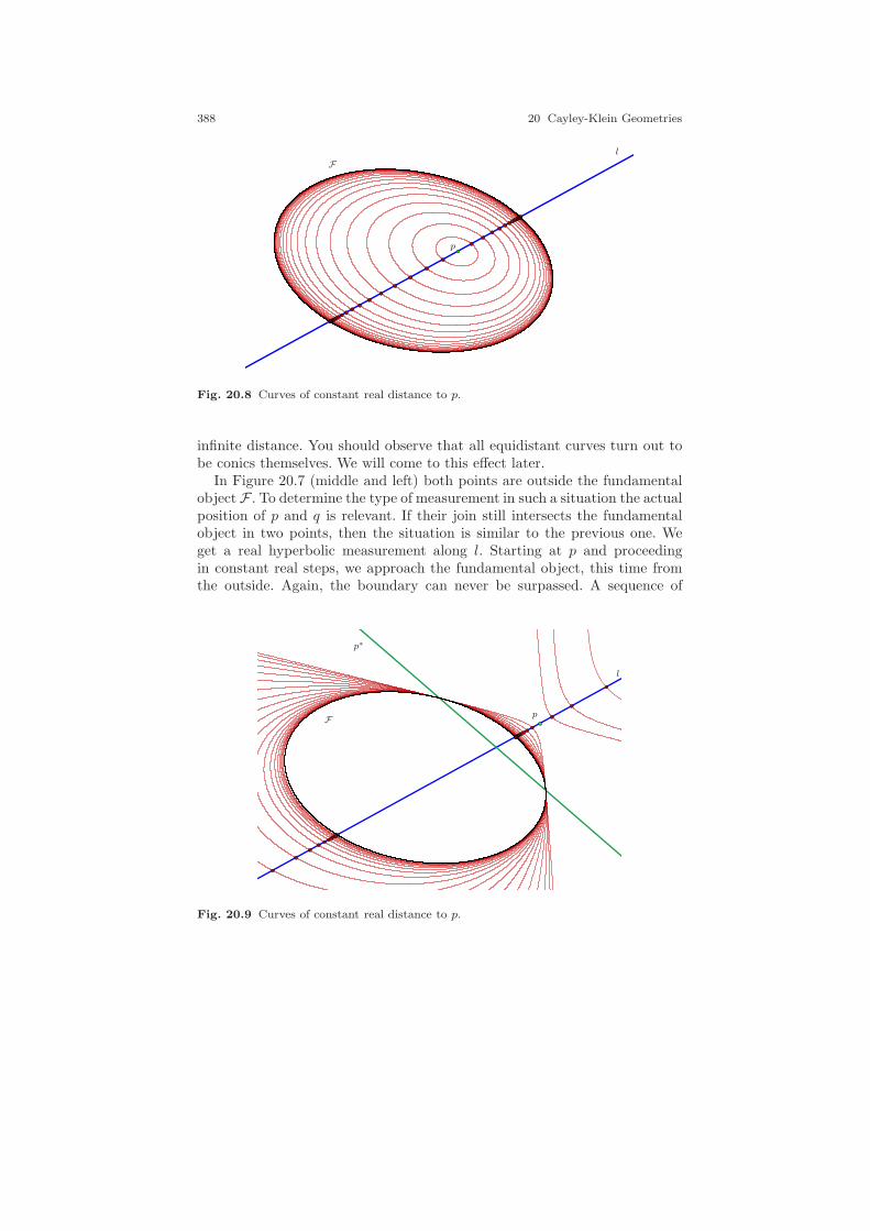
388 20 Cayley-Klein Geometries
p
l
F
Fig. 20.8 Curves of constant real distance to p.
infinite distance. You should observe that all equidistant curves turn out tobe conics themselves. We will come to this effect later.
In Figure 20.7 (middle and left) both points are outside the fundamentalobject F . To determine the type of measurement in such a situation the actualposition of p and q is relevant. If their join still intersects the fundamentalobject in two points, then the situation is similar to the previous one. Weget a real hyperbolic measurement along l. Starting at p and proceedingin constant real steps, we approach the fundamental object, this time fromthe outside. Again, the boundary can never be surpassed. A sequence of
p
l
p∗
F
Fig. 20.9 Curves of constant real distance to p.

20.5 A Planar Cayley-Klein Geometry 389
p
l
p∗
F
Fig. 20.10 Curves of constant purely imaginary distance to p.
curves of constant distance to p is shown in Figure 20.9. The situation isqualitatively different if l does not intersect the fundamental object. Thenthe points X and Y are no longer real. They become complex conjugates andwe get an elliptic measurement along l. The cross-ratio (p, q;X,Y ) then willbe a complex number on the unit circle, and its logarithm will be of the formi · t, t ∈ R. With our choice of the constant cdist we get a distance that ispurely imaginary. Proceeding in constant (imaginary) steps away from p willultimately make a cycle along the projective line l. Qualitatively this is anelliptic measurement as described, for instance, in Figure 20.5. Figure 20.10shows a sequence of curves of constant imaginary distance from p.
At this point the reader should observe two important facts (which we willprove later): All curves of constant distance are again conics. These conicshave two points of tangency with the fundamental objects. They are thesame for every such conic, namely the intersections of the polar of p withrespect to F with F itself. One might wonder what happens to this tangencyfor the curves shown in Figure 20.8, in which the curves do not touch thefundamental object. Well, they still do! The points of tangency only becomecomplex in this case, so that we do not see them.
We have left out two interesting cases for the position of p and q so far.First, it may happen that one point is inside and the other is outside. Inthis case the cross-ratio (p, q;X,Y ) is real and negative. We then will get alogarithm of the type a+ i · π, an entirely complex number, which indicatesthat q is unreachable from q by real steps. It may also happen that l is tangentto the fundamental object F . In this case we get a parabolic measurementon the line l in the sense of Section 20.5.
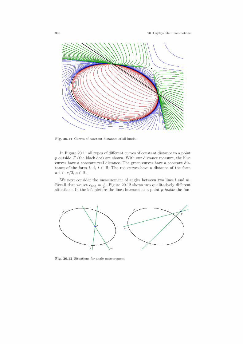
390 20 Cayley-Klein Geometries
Fig. 20.11 Curves of constant distances of all kinds.
In Figure 20.11 all types of different curves of constant distance to a pointp outside F (the black dot) are shown. With our distance measure, the bluecurves have a constant real distance. The green curves have a constant dis-tance of the form i · t, t ∈ R. The red curves have a distance of the forma+ i · π/2, a ∈ R.
We next consider the measurement of angles between two lines l and m.Recall that we set cang = 1
2i . Figure 20.12 shows two qualitatively differentsituations. In the left picture the lines intersect at a point p inside the fun-
p
l m
Fp
l
m
F
Fig. 20.12 Situations for angle measurement.
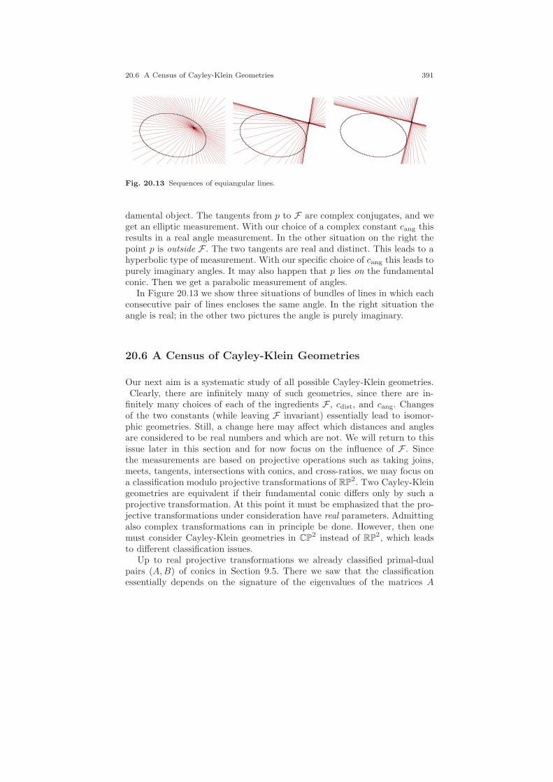
20.6 A Census of Cayley-Klein Geometries 391
Fig. 20.13 Sequences of equiangular lines.
damental object. The tangents from p to F are complex conjugates, and weget an elliptic measurement. With our choice of a complex constant cang thisresults in a real angle measurement. In the other situation on the right thepoint p is outside F . The two tangents are real and distinct. This leads to ahyperbolic type of measurement. With our specific choice of cang this leads topurely imaginary angles. It may also happen that p lies on the fundamentalconic. Then we get a parabolic measurement of angles.
In Figure 20.13 we show three situations of bundles of lines in which eachconsecutive pair of lines encloses the same angle. In the right situation theangle is real; in the other two pictures the angle is purely imaginary.
20.6 A Census of Cayley-Klein Geometries
Our next aim is a systematic study of all possible Cayley-Klein geometries.Clearly, there are infinitely many of such geometries, since there are in-
finitely many choices of each of the ingredients F , cdist, and cang. Changesof the two constants (while leaving F invariant) essentially lead to isomor-phic geometries. Still, a change here may affect which distances and anglesare considered to be real numbers and which are not. We will return to thisissue later in this section and for now focus on the influence of F . Sincethe measurements are based on projective operations such as taking joins,meets, tangents, intersections with conics, and cross-ratios, we may focus ona classification modulo projective transformations of RP
2. Two Cayley-Kleingeometries are equivalent if their fundamental conic differs only by such aprojective transformation. At this point it must be emphasized that the pro-jective transformations under consideration have real parameters. Admittingalso complex transformations can in principle be done. However, then onemust consider Cayley-Klein geometries in CP
2 instead of RP2, which leads
to different classification issues.Up to real projective transformations we already classified primal-dual
pairs (A,B) of conics in Section 9.5. There we saw that the classificationessentially depends on the signature of the eigenvalues of the matrices A
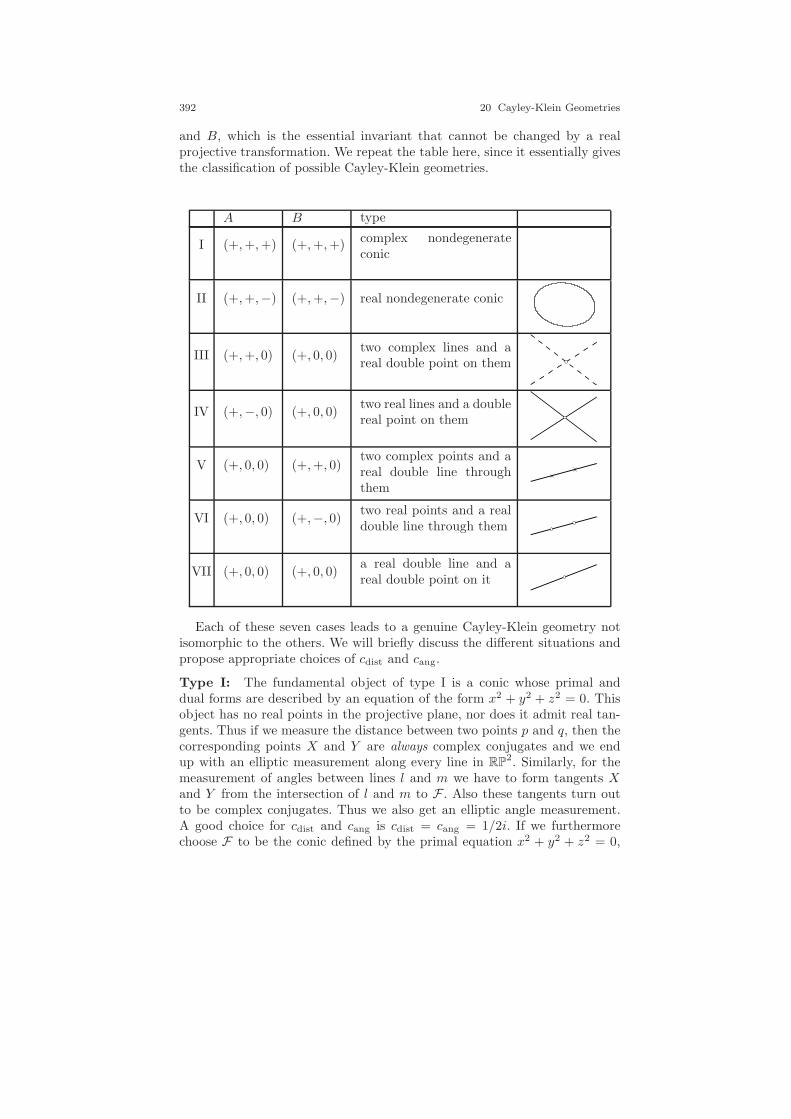
392 20 Cayley-Klein Geometries
and B, which is the essential invariant that cannot be changed by a realprojective transformation. We repeat the table here, since it essentially givesthe classification of possible Cayley-Klein geometries.
A B type
I (+,+,+) (+,+,+)complex nondegenerateconic
II (+,+,−) (+,+,−) real nondegenerate conic
III (+,+, 0) (+, 0, 0)two complex lines and areal double point on them
IV (+,−, 0) (+, 0, 0)two real lines and a doublereal point on them
V (+, 0, 0) (+,+, 0)two complex points and areal double line throughthem
VI (+, 0, 0) (+,−, 0)two real points and a realdouble line through them
VII (+, 0, 0) (+, 0, 0)a real double line and areal double point on it
Each of these seven cases leads to a genuine Cayley-Klein geometry notisomorphic to the others. We will briefly discuss the different situations andpropose appropriate choices of cdist and cang.
Type I: The fundamental object of type I is a conic whose primal anddual forms are described by an equation of the form x2 + y2 + z2 = 0. Thisobject has no real points in the projective plane, nor does it admit real tan-gents. Thus if we measure the distance between two points p and q, then thecorresponding points X and Y are always complex conjugates and we endup with an elliptic measurement along every line in RP
2. Similarly, for themeasurement of angles between lines l and m we have to form tangents Xand Y from the intersection of l and m to F . Also these tangents turn outto be complex conjugates. Thus we also get an elliptic angle measurement.A good choice for cdist and cang is cdist = cang = 1/2i. If we furthermorechoose F to be the conic defined by the primal equation x2 + y2 + z2 = 0,

20.6 A Census of Cayley-Klein Geometries 393
p
q
l
p
l
m
Fig. 20.14 Distance and angle measurement in the spherical model of elliptic geometry.
this leads to the following geometric situation: If we interpret the projec-tive plane RP
2 as the points (x, y, z) on the unit sphere x2 + y2 + z2 = 1with antipodal points identified, then the above Cayley-Klein measurementcan be interpreted in the following way: The distance between two points pand q is the spherical distance between representatives of them on the unitsphere. The angle between two lines is the spherical angle between the twogreat circles that correspond to the lines. The maximal distance between twopoints is π, which is the semiperimeter of an equator on the unit ball. Themaximal angle between two lines is π as well. This geometry is usually calledelliptic geometry. It should not be confused with the closely related sphericalgeometry for which antipodal points on the sphere are not identified.
Type II: Here we have a geometry where (up to isomorphism) the primalfundamental object has the form x2 +y2−z2 = 0. This is the real unit circle.In a sense, this is the most complicated Cayley-Klein geometry, since alldifferent kinds of measurements may arise as well for distances as for angles.We dealt with this geometry at length in the previous section. The choice ofcdist and cang depends on what measurements one wants to be real. We willlater see that a particularly interesting situation arises if one limits oneself tothe interior of the unit circle only. In this case the distance between two pointswill always lead to a hyperbolic measurement, and cdist = −1/2 is a goodchoice. If one considers only angles of lines that intersect inside the unit circle,then angle measurement results in an elliptic situation. Hence, cang = 1/2iis a good choice. From a certain perspective this restriction to the interioris a reasonable choice. Imagine you are a being inside the circle. There is noway for you to get out of there by real step width only. Your universe is theinterior, which seems infinite to you. We will dedicate the entire Chapter 25and Chapter 26 to this situation. It is called hyperbolic geometry. However,one should be aware that from the perspective of Cayley-Klein geometries,hyperbolic geometry is only a substructure of a larger ambient situation.
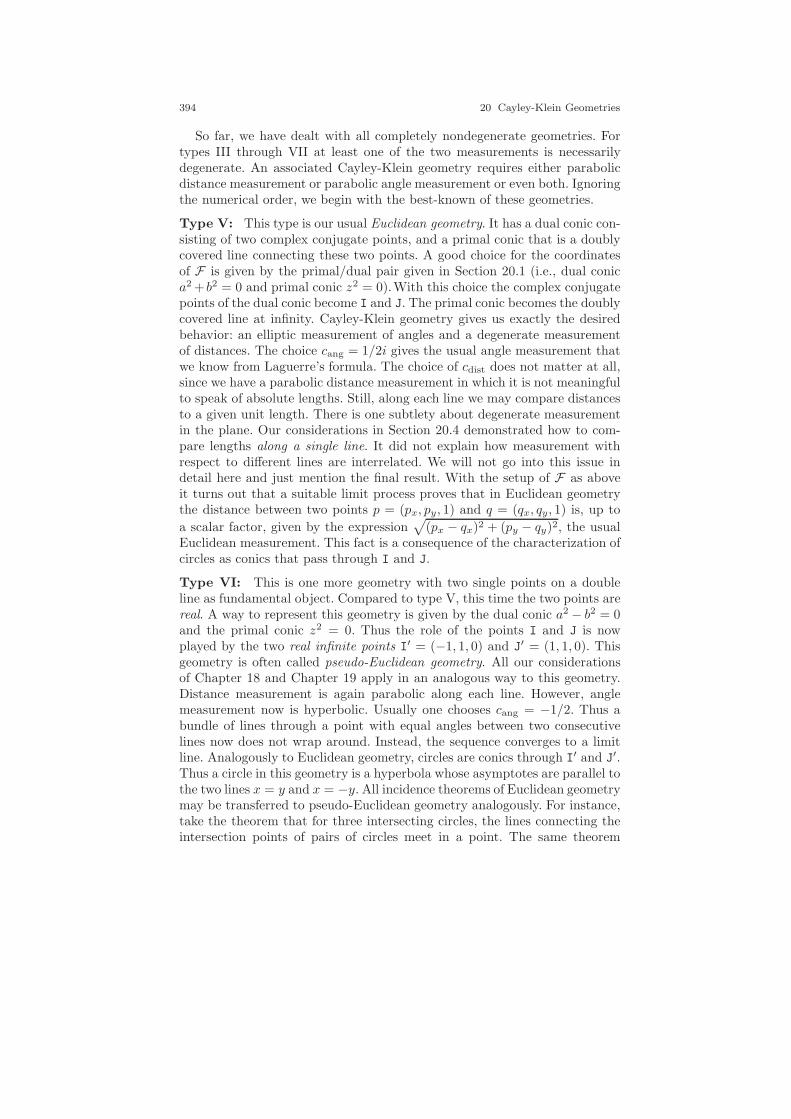
394 20 Cayley-Klein Geometries
So far, we have dealt with all completely nondegenerate geometries. Fortypes III through VII at least one of the two measurements is necessarilydegenerate. An associated Cayley-Klein geometry requires either parabolicdistance measurement or parabolic angle measurement or even both. Ignoringthe numerical order, we begin with the best-known of these geometries.
Type V: This type is our usual Euclidean geometry. It has a dual conic con-sisting of two complex conjugate points, and a primal conic that is a doublycovered line connecting these two points. A good choice for the coordinatesof F is given by the primal/dual pair given in Section 20.1 (i.e., dual conica2 + b2 = 0 and primal conic z2 = 0).With this choice the complex conjugatepoints of the dual conic become I and J. The primal conic becomes the doublycovered line at infinity. Cayley-Klein geometry gives us exactly the desiredbehavior: an elliptic measurement of angles and a degenerate measurementof distances. The choice cang = 1/2i gives the usual angle measurement thatwe know from Laguerre’s formula. The choice of cdist does not matter at all,since we have a parabolic distance measurement in which it is not meaningfulto speak of absolute lengths. Still, along each line we may compare distancesto a given unit length. There is one subtlety about degenerate measurementin the plane. Our considerations in Section 20.4 demonstrated how to com-pare lengths along a single line. It did not explain how measurement withrespect to different lines are interrelated. We will not go into this issue indetail here and just mention the final result. With the setup of F as aboveit turns out that a suitable limit process proves that in Euclidean geometrythe distance between two points p = (px, py, 1) and q = (qx, qy, 1) is, up to
a scalar factor, given by the expression√
(px − qx)2 + (py − qy)2, the usualEuclidean measurement. This fact is a consequence of the characterization ofcircles as conics that pass through I and J.
Type VI: This is one more geometry with two single points on a doubleline as fundamental object. Compared to type V, this time the two points arereal. A way to represent this geometry is given by the dual conic a2 − b2 = 0and the primal conic z2 = 0. Thus the role of the points I and J is nowplayed by the two real infinite points I′ = (−1, 1, 0) and J′ = (1, 1, 0). Thisgeometry is often called pseudo-Euclidean geometry. All our considerationsof Chapter 18 and Chapter 19 apply in an analogous way to this geometry.Distance measurement is again parabolic along each line. However, anglemeasurement now is hyperbolic. Usually one chooses cang = −1/2. Thus abundle of lines through a point with equal angles between two consecutivelines now does not wrap around. Instead, the sequence converges to a limitline. Analogously to Euclidean geometry, circles are conics through I′ and J′.Thus a circle in this geometry is a hyperbola whose asymptotes are parallel tothe two lines x = y and x = −y. All incidence theorems of Euclidean geometrymay be transferred to pseudo-Euclidean geometry analogously. For instance,take the theorem that for three intersecting circles, the lines connecting theintersection points of pairs of circles meet in a point. The same theorem
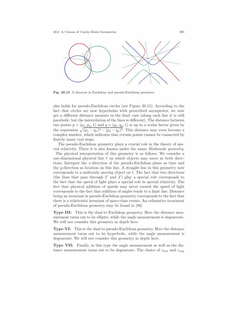
20.6 A Census of Cayley-Klein Geometries 395
Fig. 20.15 A theorem in Euclidean and pseudo-Euclidean geometry.
also holds for pseudo-Euclidean circles (see Figure 20.15). According to thefact that circles are now hyperbolas with prescribed asymptotes, we nowget a different distance measure in the limit case (along each line it is stillparabolic, but the interrelation of the lines is different). The distance betweentwo points p = (px, py, 1) and q = (qx, qy, 1) is up to a scalar factor given by
the expression√
(px − qx)2 − (py − qy)2. This distance may even become acomplex number, which indicates that certain points cannot be connected byfinitely many real steps.
The pseudo-Euclidean geometry plays a crucial role in the theory of spe-cial relativity. There it is also known under the name Minkowski geometry.The physical interpretation of this geometry is as follows. We consider a
one-dimensional physical line ℓ on which objects may move in both direc-tions. Interpret the x-direction of the pseudo-Euclidean plane as time andthe y-direction as location on this line. A straight line in this geometry nowcorresponds to a uniformly moving object on ℓ. The fact that two directions(the lines that pass through I′ and J′) play a special role corresponds tothe fact that the speed of light plays a special role in special relativity. Thefact that physical addition of speeds may never exceed the speed of lightcorresponds to the fact that addition of angles tends to a limit line. Distancebeing an invariant in pseudo-Euclidean geometry corresponds to the fact thatthere is a relativistic invariant of space-time events. An exhaustive treatmentof pseudo-Euclidean geometry may be found in [86].
Type III: This is the dual to Euclidean geometry. Here the distance mea-surement turns out to be elliptic, while the angle measurement is degenerate.We will not consider this geometry in depth here.
Type VI: This is the dual to pseudo-Euclidean geometry. Here the distancemeasurement turns out to be hyperbolic, while the angle measurement isdegenerate. We will not consider this geometry in depth here.
Type VII: Finally, in this type the angle measurement as well as the dis-tance measurement turns out to be degenerate. The choice of cdist and cang
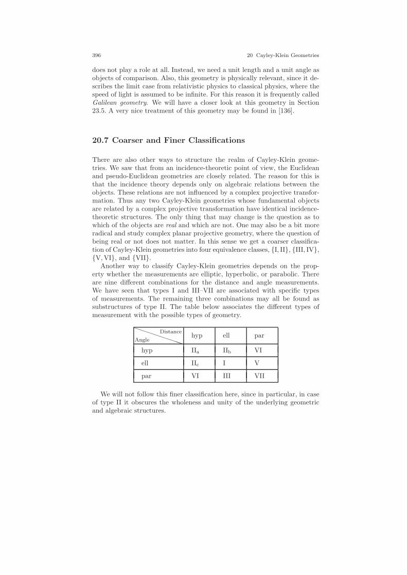
396 20 Cayley-Klein Geometries
does not play a role at all. Instead, we need a unit length and a unit angle asobjects of comparison. Also, this geometry is physically relevant, since it de-scribes the limit case from relativistic physics to classical physics, where thespeed of light is assumed to be infinite. For this reason it is frequently calledGalilean geometry. We will have a closer look at this geometry in Section23.5. A very nice treatment of this geometry may be found in [136].
20.7 Coarser and Finer Classifications
There are also other ways to structure the realm of Cayley-Klein geome-tries. We saw that from an incidence-theoretic point of view, the Euclideanand pseudo-Euclidean geometries are closely related. The reason for this isthat the incidence theory depends only on algebraic relations between theobjects. These relations are not influenced by a complex projective transfor-mation. Thus any two Cayley-Klein geometries whose fundamental objectsare related by a complex projective transformation have identical incidence-theoretic structures. The only thing that may change is the question as towhich of the objects are real and which are not. One may also be a bit moreradical and study complex planar projective geometry, where the question ofbeing real or not does not matter. In this sense we get a coarser classifica-tion of Cayley-Klein geometries into four equivalence classes, I, II, III, IV,V,VI, and VII.
Another way to classify Cayley-Klein geometries depends on the prop-erty whether the measurements are elliptic, hyperbolic, or parabolic. Thereare nine different combinations for the distance and angle measurements.We have seen that types I and III–VII are associated with specific typesof measurements. The remaining three combinations may all be found assubstructures of type II. The table below associates the different types ofmeasurement with the possible types of geometry.
PP
PP
PP
PPAngle
Distancehyp ell par
hyp IIa IIb VI
ell IIc I V
par VI III VII
We will not follow this finer classification here, since in particular, in caseof type II it obscures the wholeness and unity of the underlying geometricand algebraic structures.
21
Measurements and Transformations
Projective geometry is all geometry.
Arthur Cayley, as cited by F. Klein
While in the last chapter we have focused on measurement aspects and re-lated analytic issues, we will return to more qualitative relations of objectsin a Cayley-Klein geometry. In this and the next chapter we will mainlystudy the projective nature of Cayley-Klein geometries. This chapter focuseson aspects concerning transformations, their (projective) invariants, and thebehavior of measurements under these transformations. The next chaptertreats geometric objects and their elementary geometric properties, includ-ing some elementary geometric theorems. Although Cayley-Klein geometriesunify several rather different types of geometric playgrounds in a commonprojective framework, each type of geometry (in the sense of Section 20.6)has its very special properties. This is due to the fact that the degenera-cies of the fundamental conic of the geometry lead to degeneracies in therelevant geometric constructions. For this reason we will sometimes have toperform a special case analysis for the different types of Cayley-Klein geome-tries. Sometimes one general definition covers a certain effect (for instancereflection) in all types of geometries. Still it may be instructive to considerits particular specialization to certain geometries. Since we do not want tobecome too encyclopedic, we will confine ourselves to highlighting only someof the interesting situations. For any statement and concept we will makeclear to which types of geometries it applies and under which circumstancesdegenerate situations arise. Since again the relevant concepts are quite inter-woven, we recommend reading this and the following chapter at least twice.Some relations may become clear only at second reading.
397
398 21 Measurements and Transformations
21.1 Measurements vs. Oriented Measurements
Before considering transformations and transformation groups, we will clarifyhow the measurements defined in the last chapter can be interpreted entirelyin a projective framework. Since we now want to compare distances (resp.angles) among arbitrary points (resp. lines) in a Cayley-Klein geometry, wewill first have to deal with the various ambiguities of the measurements.
Considering the projective aspects of Cayley-Klein geometries, one im-portant aspect comes into play: If we consider the distance measurementdistK(p, q) = cdist · ln
((p, q;X,Y )
), each possible value of the cross-ratio
(p, q;X,Y ) leads to a different value of distK(p, q) modulo 2πicdist. Thus anyqualitative relation between distances (like distK(p, q) = distK(r, s)) can al-ready be expressed on the level of cross-ratios. A similar statement holds forangle measurements. In a sense, applying the logarithm is a convenient wayto translate the (multiplicative) projective world of cross-ratios into the (ad-ditive) world of distance and angle measurement we are used to. Moreover,the multiplications by constants are used to make things even more famil-iar insofar as we get real measurements whenever we are expecting them.Nevertheless, staying directly on the level of the projectively invariant cross-ratios has its advantages. First of all, from a projective viewpoint, taking thelogarithm is just an unnecessary “cosmetic isomorphism.” Secondly, takingthe logarithm even introduces (unnecessary) ambiguities of the measurementmodulo 2πicdist (resp. 2πicang) that are not essential for the theory.
If we want to operate on the level of cross-ratios instead of measurements,we have to face a formal problem whose solution is essential for making precisestatements later on. In our definition of the measurements distK(p, q), besidesthe intrinsic ambiguity of the logarithm there was another serious ambiguitythat we did not really care about so far. In Section 20.3 we learned thatif we restrict distance measurements to one single line (resp. restrict anglemeasurement to one single line bundle), it is possible to fix a priori theelements X and Y and thereby arrive at oriented measurements.
This is no longer the case if we do measurements without referring to an apriori chosen line (resp. bundle). If we want to measure the distance betweentwo points p and q we first have to construct the points X and Y . There isno reasonable way to prefer one order of the points X and Y over the other.Hence in performing the distance measurement, one might either get
d = cdist · ln((p, q;X,Y )
)or − d = cdist · ln
((p, q;Y,X)
).
One might be tempted to resolve this problem by simply referring insteadto the absolute value of a measurement. However, this approach has twoproblems. Firstly, the result of a measurement may well be a complex number.By taking its absolute value one loses not only the information about its signbut also about its direction, which is unnecessarily coarse. Secondly, we willtry to express as many geometric properties as possible directly on the level

21.2 Transformations 399
of cross-ratios and not on the level of distances (or angles). For the cross-ratiothe sign change of the measurement corresponds to the reciprocal connection(p, q;X,Y ) = 1/(p, q;Y,X). In order to deal with these ambiguities properlywe will introduce two special equivalence classes (this is slightly uncommon inthe literature on Cayley-Klein geometries, but it resolves the situation mostappropriately). We set
≀≀ x ≀≀ := x,−x and ≀≀ x ≀≀ := x, 1/x.Thus for comparing unoriented distances, an expression like
≀≀ distK(p, q) ≀≀ = ≀≀ distK(r, s) ≀≀
is a reasonable formulation. To compare two cross-ratios where the order ofX,Y is undetermined,
≀≀ (p, q;X,Y ) ≀≀ = ≀≀ (r, s;X,Y ) ≀≀
is a good shorthand. Alternatively, one could use squared distances only and,on the level of cross-ratios, a function that symmetrically uses a cross-ratioand its inverse. We will do this later on, too. However, for the moment weprefer the above notation since, it is a bit closer to the fundamental definitionof measurement.
21.2 Transformations
Cayley-Klein geometries are projective geometries equipped with certain ad-ditional measurements for distances and angles. While a projective trans-formation is a transformation that leaves fundamental projective propertiesinvariant (incidences, tangencies, etc.), a transformation in a Cayley-Kleingeometry in addition preserves distance and angle measurement.
Since Cayley-Klein geometries make it eventually necessary to deal alsowith complex elements, we will first briefly specify the setup in which ob-jects and transformations are considered in this context. Ultimately, we wantto make statements about the real projective plane RP
2 equipped with themeasurements of a Cayley-Klein geometry. Thus the only transformations wewill consider are projective transformations τ of the real projective plane.They are represented by a pair of real nondegenerate matrices (T, T−1) thatare used to transform geometric elements. In homogeneous coordinates apoint p is transformed according to τ(p) = T · p; A line l is transformedby τ(l) = (T−1)T · l (compare Section 3.6). A primal quadratic form A istransformed by τ(A) = (T−1)TAT−1, and a dual quadratic form B is trans-formed by τ(B) = TBT T (compare Section 10.4). As usual, we must identifynonscalar multiples of matrices and vectors.
400 21 Measurements and Transformations
In all our operations we will admit the following objects as input elements:
• All points, lines, and primal or dual quadratic forms of RP2.
• The primal and dual fundamental object of the Cayley-Klein geometry.
We admit arbitrary projectively reasonable operations between these objects,no matter whether they result in real or complex elements. This is in the samespirit as our treatment of Euclidean geometry in Chapter 18 and Chapter 19,in which we also had to face the problem that intermediate construction ele-ments may become complex. Whenever we speak of transformational invari-ance of a certain property we limit ourselves to real projective transformationmatrices (still they might be applied to complex objects).
We are now going to define motion in a Cayley-Klein geometry K :=(F , cdist, cang). Here as usual F is given as a primal/dual pair of matrices(A,B). There are two possible ways to approach the concept of motion. Thefirst approach asks for those projective transformations that leave the dis-tance and angle measurements invariant. However, in the case of degeneratemeasurements of both distances and angles (as they appear in Galilean ge-ometries) one would unavoidably have to consider also degenerate measure-ments, which makes things more complicated. The second approach definesK-motions as those projective transformations that leave the fundamental ob-ject F invariant. As a consequence, such transformations also leave distancesand angles invariant. We will follow this second approach.
Definition 21.1. Let K be a Cayley-Klein geometry whose fundamental ob-ject F is defined by the primal/dual pair of matrices (A,B). Let τ be aprojective transformation in RP
2. We call τ a K-motion if it leaves both Aand B invariant.
Theorem 21.1. Let τ be a K-motion. Then we have
(i) ≀≀ distK(p, q) ≀≀ = ≀≀ distK(τ(p), τ(q)) ≀≀ for all points p and q,
(ii) ≀≀ angK(l,m) ≀≀ = ≀≀ angK(τ(l), τ(m)) ≀≀ for all lines l and m.
Proof. We start with the proof of (i). Without loss of generality we mayassume that the distance measurement is not degenerate (i.e., the primal conicis not a double line), since otherwise all distance measurements distK(p, q)are zero anyway. Let p and q be two arbitrary points in RP
2 and let τ be aK-motion. Let l be a line to which both p and q are incident. Then τ(l) is aline incident to both τ(p) and τ(q). Now let X and Y be the intersection ofl with the fundamental conic F and let X ′ and Y ′ be the intersection of τ(l)with the fundamental conic F (in any order). The distance measurement ofp and q depends on (p, q;X,Y ), while the distance measurement of τ(p) andτ(q) depends on (τ(p), τ(q);X ′, Y ′). Since projective transformations preserveincidence relations and F is mapped to itself under τ we have either
X ′ = τ(X) and Y ′ = τ(Y )
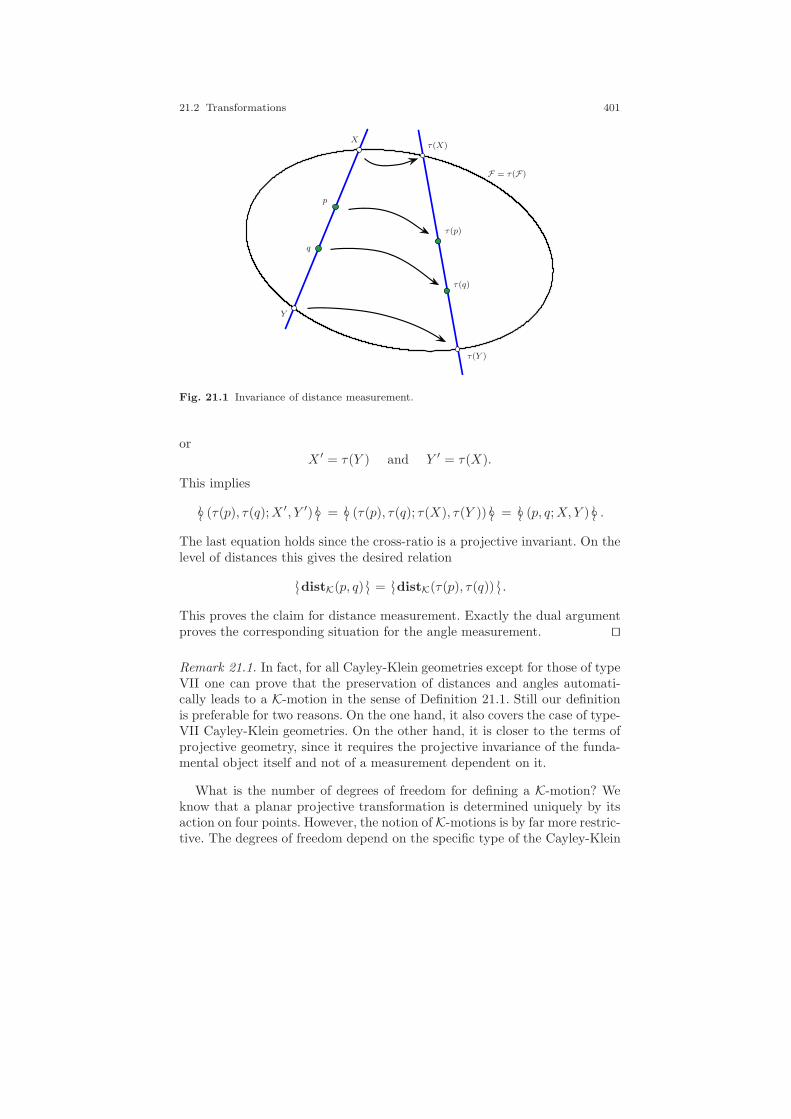
21.2 Transformations 401
p
q
X
Y
τ(p)
τ(q)
τ(X)
τ(Y )
F = τ(F)
Fig. 21.1 Invariance of distance measurement.
orX ′ = τ(Y ) and Y ′ = τ(X).
This implies
≀≀ (τ(p), τ(q);X ′, Y ′) ≀≀ = ≀≀ (τ(p), τ(q); τ(X), τ(Y )) ≀≀ = ≀≀ (p, q;X,Y ) ≀≀ .
The last equation holds since the cross-ratio is a projective invariant. On thelevel of distances this gives the desired relation
≀≀ distK(p, q) ≀≀ = ≀≀ distK(τ(p), τ(q)) ≀≀ .
This proves the claim for distance measurement. Exactly the dual argumentproves the corresponding situation for the angle measurement. ⊓⊔
Remark 21.1. In fact, for all Cayley-Klein geometries except for those of typeVII one can prove that the preservation of distances and angles automati-cally leads to a K-motion in the sense of Definition 21.1. Still our definitionis preferable for two reasons. On the one hand, it also covers the case of type-VII Cayley-Klein geometries. On the other hand, it is closer to the terms ofprojective geometry, since it requires the projective invariance of the funda-mental object itself and not of a measurement dependent on it.
What is the number of degrees of freedom for defining a K-motion? Weknow that a planar projective transformation is determined uniquely by itsaction on four points. However, the notion of K-motions is by far more restric-tive. The degrees of freedom depend on the specific type of the Cayley-Klein

402 21 Measurements and Transformations
geometry: the more degenerate the fundamental object is, the more degreesof freedom we have. Considering the number of degrees of freedom, we maydistinguish three different situations: the nondegenerate cases, the singly de-generate cases, and the doubly degenerate cases.
Nondegenerate cases: For types I and II, the fundamental object con-sists of a nondegenerate conic (real or complex). Since in the nondegeneratecase the primal conic given by the matrix A uniquely defines the dual conicB = A−1, it is sufficient to study those transformations that leave the matrixA invariant. Without loss of generality we may choose the transformationmatrix T to have determinant det(T ) = 1. Thus we are looking for transfor-mations T ∈ SL(R, 3) such that (T−1)TAT−1 = A. One could consider this apurely algebraic problem. At first sight, the problem seems to be identical forboth nondegenerate geometries. However, the requirement that the entriesof the transformation matrix have to be real-valued results in two differenttransformation groups. We study the two situations of type I (elliptic case)and type II (hyperbolic case) Cayley-Klein geometries separately, since bothof them lead to interesting geometric structures.
Type I, the elliptic case: In this situation up to isomorphism the matrix Amay be chosen to be the unit matrix E. The invariance property then reads
(T−1)TT−1 = E.
This, in turn, is exactly the definition of an orthogonal matrix (the inverseis the transpose). Such a matrix T ∈ O(3) describes either a rotation or areflection in R3. We can immediately interpret this fact geometrically. Wemay represent each point p ∈ RP
2 by an antipodal pair of points on theunit sphere in R3. Now an elliptic transformation is a rotation or a reflectionof this sphere. This is nicely consistent with the fact that elliptic measure-ment may be interpreted as spherical distances and angles on this sphere(compare Figure 20.13). The number of degrees of freedom for this trans-formation group is exactly three, corresponding to the degrees of freedom ofa rotation or reflection in R3. There is an important difference between theelliptic transformation group and the matrix group O(3). In the elliptic trans-formation group, according to the projective setup, the matrices T and −Tare identified. Therefore O(3) is a double cover of the elliptic transformationgroup.
Type II, the hyperbolic case: The fundamental conic F of a Cayley-Klein ge-ometry of type II is a real nondegenerate conic. This gives us the possibilityto describe these transformations directly in terms of projective geometry.In Section 10.4 we studied projective transformations that leave a given realnondegenerate conic invariant. Recall that the points on the primal funda-mental object may be considered an isomorphic image of a one-dimensionalprojective line under stereographic projection (compare Figure 10.7). Theset of projective transformations that leave a nondegenerate conic invariant
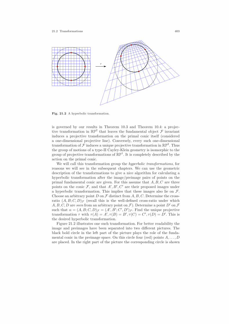
21.2 Transformations 403
τ
Fig. 21.2 A hyperbolic transformation.
is governed by our results in Theorem 10.3 and Theorem 10.4: a projec-tive transformation in RP
2 that leaves the fundamental object F invariantinduces a projective transformation on the primal conic itself (considereda one-dimensional projective line). Conversely, every such one-dimensionaltransformation of F induces a unique projective transformation in RP
2. Thusthe group of motions of a type-II Cayley-Klein geometry is isomorphic to thegroup of projective transformations of RP
1. It is completely described by theaction on the primal conic.
We will call this transformation group the hyperbolic transformations, forreasons we will see in the subsequent chapters. We can use the geometricdescription of the transformations to give a nice algorithm for calculating ahyperbolic transformation after the image/preimage pairs of points on theprimal fundamental conic are given. For this assume that A,B,C are threepoints on the conic F , and that A′, B′, C′ are their proposed images undera hyperbolic transformation. This implies that these images also lie on F .Choose an arbitrary pointD on F distinct from A,B,C. Determine the cross-ratio (A,B;C,D)F (recall this is the well-defined cross-ratio under whichA,B,C,D are seen from an arbitrary point on F). Determine a point D′ on Fsuch that α = (A,B;C,D)F = (A′, B′;C′, D′)F . Find the unique projectivetransformation τ with τ(A) = A′, τ(B) = B′, τ(C) = C′, τ(D) = D′. This isthe desired hyperbolic transformation.
Figure 21.2 illustrates one such transformation. For better readability theimage and preimages have been separated into two different pictures. Theblack bold circle in the left part of the picture plays the role of the funda-mental conic in the preimage space. On this circle four (red) points A, . . . ,Dare placed. In the right part of the picture the corresponding circle is shown
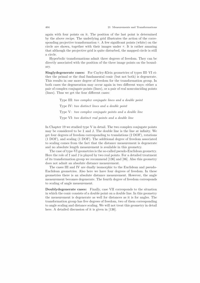
404 21 Measurements and Transformations
again with four points on it. The position of the last point is determinedby the above recipe. The underlying grid illustrates the action of the corre-sponding projective transformation τ . A few significant points (white) on thecircle are shown, together with their images under τ . It is rather amazingthat although the projective grid is quite disturbed, the mapped circle is stilla circle.
Hyperbolic transformations admit three degrees of freedom. They can bedirectly associated with the position of the three image points on the bound-ary.
Singlydegenerate cases: For Cayley-Klein geometries of types III–VI ei-ther the primal or the dual fundamental conic (but not both) is degenerate.This results in one more degree of freedom for the transformation group. Inboth cases the degeneration may occur again in two different ways: either apair of complex conjugate points (lines), or a pair of real noncoinciding points(lines). Thus we get the four different cases:
Type III: two complex conjugate lines and a double point
Type IV: two distinct lines and a double point
Type V: two complex conjugate points and a double line
Type VI: two distinct real points and a double line
In Chapter 19 we studied type V in detail. The two complex conjugate pointsmay be considered to be I and J. The double line is the line at infinity. Weget four degrees of freedom corresponding to translations (2 DOF), rotations(1 DOF), and scaling (1 DOF). The additional degree of freedom associatedto scaling comes from the fact that the distance measurement is degenerateand no absolute length measurement is available in this geometry.
The case of type-VI geometries is the so-called pseudo-Euclidean geometry.Here the role of I and J is played by two real points. For a detailed treatmentof its transformation group we recommend [136] and [86]. Also this geometrydoes not admit an absolute distance measurement.
The cases III and IV are dually isomorphic to the Euclidean and pseudo-Euclidean geometries. Also here we have four degrees of freedom. In thesegeometries there is an absolute distance measurement. However, the anglemeasurement becomes degenerate. The fourth degree of freedom correspondsto scaling of angle measurement.
Doublydegenerate cases: Finally, case VII corresponds to the situationin which the conic consists of a double point on a double line. In this geometrythe measurement is degenerate as well for distances as it is for angles. Thetransformation group has five degrees of freedom, two of them correspondingto angle scaling and distance scaling. We will not treat this geometry in detailhere. A detailed discussion of it is given in [136].
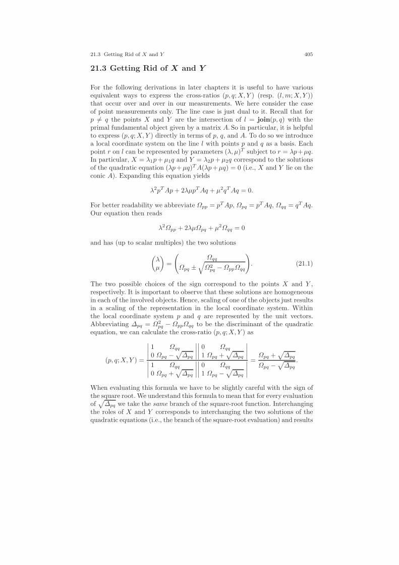
21.3 Getting Rid of X and Y 405
21.3 Getting Rid of X and Y
For the following derivations in later chapters it is useful to have variousequivalent ways to express the cross-ratios (p, q;X,Y ) (resp. (l,m;X,Y ))that occur over and over in our measurements. We here consider the caseof point measurements only. The line case is just dual to it. Recall that forp 6= q the points X and Y are the intersection of l = join(p, q) with theprimal fundamental object given by a matrix A. So in particular, it is helpfulto express (p, q;X,Y ) directly in terms of p, q, and A. To do so we introducea local coordinate system on the line l with points p and q as a basis. Eachpoint r on l can be represented by parameters (λ, µ)T subject to r = λp+µq.In particular, X = λ1p+ µ1q and Y = λ2p+ µ2q correspond to the solutionsof the quadratic equation (λp+µq)TA(λp+µq) = 0 (i.e., X and Y lie on theconic A). Expanding this equation yields
λ2pTAp+ 2λµpTAq + µ2qTAq = 0.
For better readability we abbreviate Ωpp = pTAp, Ωpq = pTAq, Ωqq = qTAq.Our equation then reads
λ2Ωpp + 2λµΩpq + µ2Ωqq = 0
and has (up to scalar multiples) the two solutions
(λµ
)=
(Ωqq
Ωpq ±√Ω2pq −ΩppΩqq
). (21.1)
The two possible choices of the sign correspond to the points X and Y ,respectively. It is important to observe that these solutions are homogeneousin each of the involved objects. Hence, scaling of one of the objects just resultsin a scaling of the representation in the local coordinate system. Withinthe local coordinate system p and q are represented by the unit vectors.Abbreviating ∆pq = Ω2
pq − ΩppΩqq to be the discriminant of the quadraticequation, we can calculate the cross-ratio (p, q;X,Y ) as
(p, q;X,Y ) =
∣∣∣∣1 Ωqq0 Ωpq −
√∆pq
∣∣∣∣∣∣∣∣0 Ωqq1 Ωpq +
√∆pq
∣∣∣∣∣∣∣∣1 Ωqq0 Ωpq +
√∆pq
∣∣∣∣∣∣∣∣0 Ωqq1 Ωpq −
√∆pq
∣∣∣∣=Ωpq +
√∆pq
Ωpq −√∆pq
.
When evaluating this formula we have to be slightly careful with the sign ofthe square root. We understand this formula to mean that for every evaluationof√∆pq we take the same branch of the square-root function. Interchanging
the roles of X and Y corresponds to interchanging the two solutions of thequadratic equations (i.e., the branch of the square-root evaluation) and results

406 21 Measurements and Transformations
in taking the inverse of the cross-ratio, as expected. The situation ∆pq = 0corresponds to the case that X and Y coincide. We know that in the caseof an exceptional measurement (and only in this case) the cross-ratio (andhence also this expression) assumes the form 0/0. It is instructive to analyzethe geometric situation in the exceptional case. Then we have X = Y , whichmeans that ∆pq = 0 and thus the join of p and q is tangent to the fundamentalconic. In addition, either p = X or q = X . Without loss of generality weassume that p = X . Thus the tangent join(p, q) is the polar of p, and q lieson this polar. This means that Ωpq is also zero.
21.4 Comparing Measurements
The formula we just derived expresses the cross-ratio (p, q;X,Y ) directly interms of the quadratic form Ω. If one wants to test whether the distance froma to b equals the distance from p to q, one can do this directly by testing
Ωab +√∆ab
Ωab −√∆ab
=Ωpq +
√∆pq
Ωpq −√∆pq
without calculating the intersections of the lines ab and pq with the funda-mental conic. There are several other versions of such comparisons that giveadditional geometric (and algebraic) insight. We will briefly consider a fewof them.
Since the order of X and Y in a measurement is not previously specifiedin the cross-ratio, (p, q;X,Y ) is on an equal footing with its inverse. We canaccount for that fact by applying a function to
α =Ωpq +
√∆pq
Ωpq −√∆pq
that treats α and 1/α symmetrically. A particularly interesting choice is
α 7→ 1
2
(√α+
1√α
)=α+ 1
2√α
=: f(α).
After applying this transformation and a few elementary calculations, we get
f
(Ωpq +
√∆pq
Ωpq −√∆pq
)=
Ωpq√ΩppΩqq
=: β.
Still there is some ambiguity in this formula, since we introduced a square rootwhose sign we did not specify. We will take care of that in a minute. Beforethis, we will inspect the above formula and discuss its geometric significance.

21.4 Comparing Measurements 407
For this we consider the following formula, which connects the logarithm andthe (arc) cosine function:
ln(α) = 2i arccos
(α+ 1
2√α
).
(This function follows from the Euler formula eix = cos(x) + i · sin(x) =cos(x) + i ·
√1 − (cos(x))2 and a few elementary calculations.) The expres-
sion under the arccos(. . .) function exactly corresponds to our transformingfunction f(α). Thus we get (for cdist = 1/2i)
dist(p, q) =1
2iln((p, q;X,Y )) = arccos
(Ωpq√ΩppΩqq
).
This formula is remarkable, since it nicely generalizes a well-known fact to ar-bitrary Cayley-Klein geometries. The well-known fact is that we can measurethe angle between two vectors p and q in R3 by the following formula:
cos(∠p, q) :=〈p, q〉√
〈p, p〉〈q, q〉.
This formula is exactly our general formula applied to elliptic geometry inthe standard representation where A is the unit matrix. In this case we getΩp,q = pTAq = pT q = 〈p, q〉. The sign ambiguity resembles the fact thatthere is some ambiguity on the direction in which the angle is measured. Asimilar (completely dual) statement also holds for angle measurement.
Still there are some other nice representations for the comparison of mea-surements. The above representation has two major drawbacks. Firstly, thesquare root in the function introduces a sign ambiguity. Secondly, the for-mula is usable only for nondegenerate measurements. If A is a rank-1 matrix(A = llT ) then the expression β always evaluates to 1. This simply meansthat for degenerate measurements all point pairs have the same degeneratedistance zero. There is an amazing trick with which we can use the same(projectively invariant) formula for comparison of measurements for the de-generate and for the nondegenerate case. In principle, this trick encapsulatesthe limit argument that we made in Section 20.4 by using a suitable replace-ment for the discriminant ∆pq. Let us first deal with the first problem, thesign ambiguity. For this we simply square the expression β. It turns out thatit is even better to transform according to
β 7→ β2 − 1 =: g(β).
We get
g
(Ωpq√ΩppΩqq
)=Ω2pq −ΩppΩqq
ΩppΩqq=
∆pq
ΩppΩqq=: Φpq . (21.2)
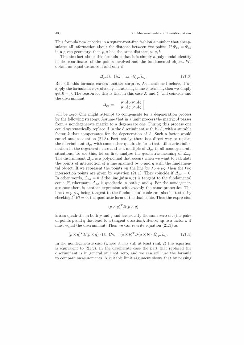
408 21 Measurements and Transformations
This formula now encodes in a square-root-free fashion a number that encap-sulates all information about the distance between two points. If Φpq = Φabin a given geometry, then p, q has the same distance as a, b.
The nice fact about this formula is that it is simply a polynomial identityin the coordinates of the points involved and the fundamental object. Weobtain an equal distance if and only if
∆pqΩaaΩbb = ∆abΩppΩqq . (21.3)
But still this formula carries another surprise. As mentioned before, if weapply the formula in case of a degenerate length measurement, then we simplyget 0 = 0. The reason for this is that in this case X and Y will coincide andthe discriminant
∆pq = −∣∣∣∣pTAp pTAqpTAq qTAq
∣∣∣∣
will be zero. One might attempt to compensate for a degeneration processby the following strategy. Assume that in a limit process the matrix A passesfrom a nondegenerate matrix to a degenerate one. During this process onecould systematically replace A in the discriminant with k ·A, with a suitablefactor k that compensates for the degeneration of A. Such a factor wouldcancel out in equation (21.3). Fortunately, there is a direct way to replacethe discriminant ∆pq with some other quadratic form that still carries infor-mation in the degenerate case and is a multiple of ∆pq in all nondegeneratesituations. To see this, let us first analyze the geometric meaning of ∆pq.The discriminant ∆pq is a polynomial that occurs when we want to calculatethe points of intersection of a line spanned by p and q with the fundamen-tal object. If we represent the points on the line by λp + µq, then the twointersection points are given by equation (21.1). They coincide if ∆pq = 0.In other words, ∆pq = 0 if the line join(p, q) is tangent to the fundamentalconic. Furthermore, ∆pq is quadratic in both p and q. For the nondegener-ate case there is another expression with exactly the same properties. Theline l = p × q being tangent to the fundamental conic can also be tested bychecking lTBl = 0, the quadratic form of the dual conic. Thus the expression
(p× q)TB(p× q)
is also quadratic in both p and q and has exactly the same zero set (the pairsof points p and q that lead to a tangent situation). Hence, up to a factor k itmust equal the discriminant. Thus we can rewrite equation (21.3) as
(p× q)TB(p× q) ·ΩaaΩbb = (a× b)TB(a× b) ·ΩppΩqq. (21.4)
In the nondegenerate case (where A has still at least rank 2) this equationis equivalent to (21.3). In the degenerate case the part that replaced thediscriminant is in general still not zero, and we can still use the formulato compare measurements. A suitable limit argument shows that by passing
21.4 Comparing Measurements 409
from a nondegenerate to the degenerate case with rank A being 1, everythingbehaves continuously and the above equation corresponds to the test for equaldistance in the degenerate case.
In the case that p and q are in located such that an exceptional measure-ment arises, both expressions (p × q)TB(p × q) and ΩppΩqq vanish, so thatformula (21.4) is satisfied independently of the position of a and b. As alreadymentioned, this case does not allow for a reasonable distance measurement.
We want to explore the geometric and invariant-theoretic meaning of theabove equation in the degenerate case. The interesting situation arises whenthe primal conic described by A degenerates to a double line. Then B mighthave either rank 2 or rank 1. We analyze the case in which B has rank 2.In this case B describes two distinct points on the double line. We will callthese two points I and J for the moment, to remind ourselves of the specialrole played by the points I and J in Euclidean geometry. In the standardembedding of Euclidean geometry we have I = I and J = J. The dual conicis described by the matrix B = IJ
T + JIT . The primal conic is described by
the matrix A = (I × J)(I × J)T . Plugging this into our condition for equalmeasurement, we get
(p× q)T (IJT + JIT )(p× q) · aT (I × J)(I × J)T a · bT (I × J)(I × J)T b
= (a× b)T (IJT + JIT )(a× b) · pT (I × J)(I × J)T p · qT (I × J)(I × J)T q.
At first sight this looks frightening, but let us analyze the different parts ofthis formula. We get
(p× q)T (IJT )(p× q) = ((p× q)T I) · (JT (p× q)) = [pqI][pqJ]
and(p× q)T (JIT )(p× q) = ((p× q)T J) · (IT (p× q)) = [pqJ][pqI].
Hence(p× q)T (IJT + JI
T )(p× q) = 2[pqI][pqJ].
Furthermore, we get
aT (I × J)(I × J)T a = (aT (I × J)) · ((I × J)T a) = [aIJ]2.
We get similar translations for the other subexpressions involved. Thus theentire large equation translates to
[pqI][pqJ][aIJ]2[bIJ]2 = [abI][abJ][pIJ]2[qIJ]2.
This is exactly expression (18.1), which we obtained in Section 18.8, nowgeneralized to general Cayley-Klein geometries with a degenerate primal ma-trix and a rank-2 dual matrix. For reversed roles of a degenerate angle andnondegenerate distance measurement a corresponding dual formula applies.
Thus instead of considering the function Φpq we consider the function
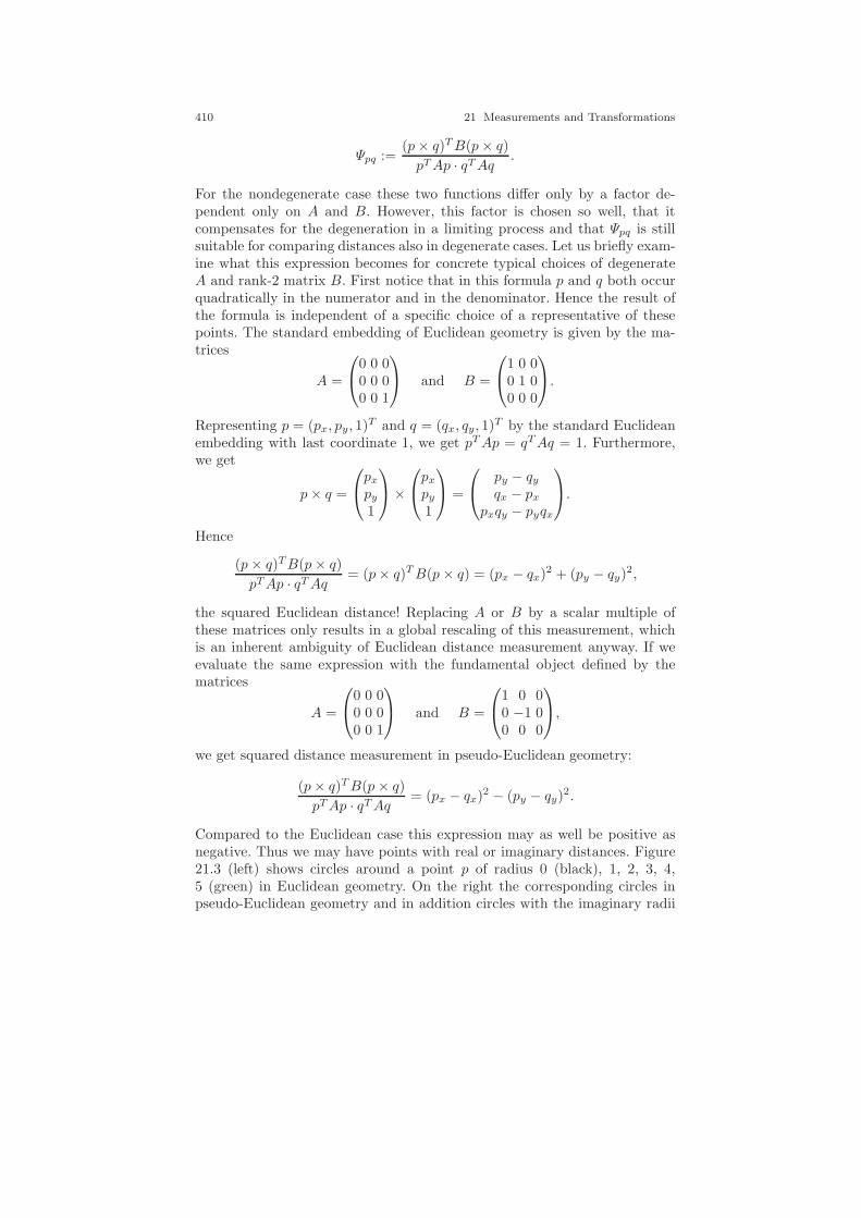
410 21 Measurements and Transformations
Ψpq :=(p× q)TB(p× q)
pTAp · qTAq .
For the nondegenerate case these two functions differ only by a factor de-pendent only on A and B. However, this factor is chosen so well, that itcompensates for the degeneration in a limiting process and that Ψpq is stillsuitable for comparing distances also in degenerate cases. Let us briefly exam-ine what this expression becomes for concrete typical choices of degenerateA and rank-2 matrix B. First notice that in this formula p and q both occurquadratically in the numerator and in the denominator. Hence the result ofthe formula is independent of a specific choice of a representative of thesepoints. The standard embedding of Euclidean geometry is given by the ma-trices
A =
0 0 00 0 00 0 1
and B =
1 0 00 1 00 0 0
.
Representing p = (px, py, 1)T and q = (qx, qy, 1)T by the standard Euclideanembedding with last coordinate 1, we get pTAp = qTAq = 1. Furthermore,we get
p× q =
pxpy1
×
pxpy1
=
py − qyqx − px
pxqy − pyqx
.
Hence
(p× q)TB(p× q)
pTAp · qTAq = (p× q)TB(p× q) = (px − qx)2 + (py − qy)
2,
the squared Euclidean distance! Replacing A or B by a scalar multiple ofthese matrices only results in a global rescaling of this measurement, whichis an inherent ambiguity of Euclidean distance measurement anyway. If weevaluate the same expression with the fundamental object defined by thematrices
A =
0 0 00 0 00 0 1
and B =
1 0 00 −1 00 0 0
,
we get squared distance measurement in pseudo-Euclidean geometry:
(p× q)TB(p× q)
pTAp · qTAq = (px − qx)2 − (py − qy)
2.
Compared to the Euclidean case this expression may as well be positive asnegative. Thus we may have points with real or imaginary distances. Figure21.3 (left) shows circles around a point p of radius 0 (black), 1, 2, 3, 4,5 (green) in Euclidean geometry. On the right the corresponding circles inpseudo-Euclidean geometry and in addition circles with the imaginary radii
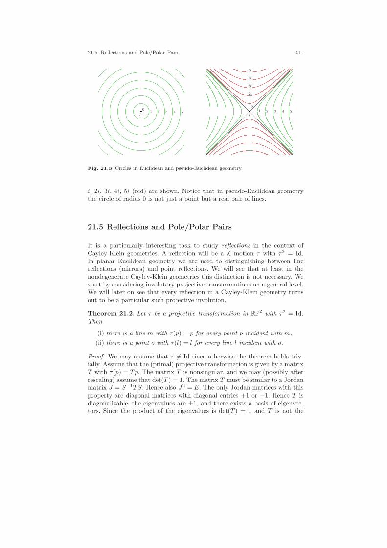
21.5 Reflections and Pole/Polar Pairs 411
01 2 3 4 5
p
01 2 3 4 5
i
2i
3i
4i
5i
p
Fig. 21.3 Circles in Euclidean and pseudo-Euclidean geometry.
i, 2i, 3i, 4i, 5i (red) are shown. Notice that in pseudo-Euclidean geometrythe circle of radius 0 is not just a point but a real pair of lines.
21.5 Reflections and Pole/Polar Pairs
It is a particularly interesting task to study reflections in the context ofCayley-Klein geometries. A reflection will be a K-motion τ with τ2 = Id.In planar Euclidean geometry we are used to distinguishing between linereflections (mirrors) and point reflections. We will see that at least in thenondegenerate Cayley-Klein geometries this distinction is not necessary. Westart by considering involutory projective transformations on a general level.We will later on see that every reflection in a Cayley-Klein geometry turnsout to be a particular such projective involution.
Theorem 21.2. Let τ be a projective transformation in RP2 with τ2 = Id.
Then
(i) there is a line m with τ(p) = p for every point p incident with m,
(ii) there is a point o with τ(l) = l for every line l incident with o.
Proof. We may assume that τ 6= Id since otherwise the theorem holds triv-ially. Assume that the (primal) projective transformation is given by a matrixT with τ(p) = Tp. The matrix T is nonsingular, and we may (possibly afterrescaling) assume that det(T ) = 1. The matrix T must be similar to a Jordanmatrix J = S−1TS. Hence also J2 = E. The only Jordan matrices with thisproperty are diagonal matrices with diagonal entries +1 or −1. Hence T isdiagonalizable, the eigenvalues are ±1, and there exists a basis of eigenvec-tors. Since the product of the eigenvalues is det(T ) = 1 and T is not the
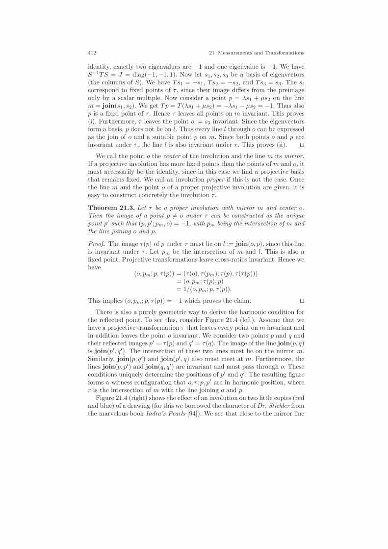
412 21 Measurements and Transformations
identity, exactly two eigenvalues are −1 and one eigenvalue is +1. We haveS−1TS = J = diag(−1,−1, 1). Now let s1, s2, s3 be a basis of eigenvectors(the columns of S). We have Ts1 = −s1, Ts2 = −s2, and Ts3 = s3. The sicorrespond to fixed points of τ , since their image differs from the preimageonly by a scalar multiple. Now consider a point p = λs1 + µs2 on the linem = join(s1, s2). We get Tp = T (λs1 + µs2) = −λs1 − µs2 = −1. Thus alsop is a fixed point of τ . Hence τ leaves all points on m invariant. This proves(i). Furthermore, τ leaves the point o := s3 invariant. Since the eigenvectorsform a basis, p does not lie on l. Thus every line l through o can be expressedas the join of o and a suitable point p on m. Since both points o and p areinvariant under τ , the line l is also invariant under τ . This proves (ii). ⊓⊔
We call the point o the center of the involution and the line m its mirror.If a projective involution has more fixed points than the points of m and o, itmust necessarily be the identity, since in this case we find a projective basisthat remains fixed. We call an involution proper if this is not the case. Oncethe line m and the point o of a proper projective involution are given, it iseasy to construct concretely the involution τ .
Theorem 21.3. Let τ be a proper involution with mirror m and center o.Then the image of a point p 6= o under τ can be constructed as the uniquepoint p′ such that (p, p′; pm, o) = −1, with pm being the intersection of m andthe line joining o and p.
Proof. The image τ(p) of p under τ must lie on l := join(o, p), since this lineis invariant under τ . Let pm be the intersection of m and l. This is also afixed point. Projective transformations leave cross-ratios invariant. Hence wehave
(o, pm; p, τ(p)) = (τ(o), τ(pm); τ(p), τ(τ(p)))= (o, pm; τ(p), p)= 1/(o, pm; p, τ(p)).
This implies (o, pm; p, τ(p)) = −1 which proves the claim. ⊓⊔There is also a purely geometric way to derive the harmonic condition for
the reflected point. To see this, consider Figure 21.4 (left). Assume that wehave a projective transformation τ that leaves every point on m invariant andin addition leaves the point o invariant. We consider two points p and q andtheir reflected images p′ = τ(p) and q′ = τ(q). The image of the line join(p, q)is join(p′, q′). The intersection of these two lines must lie on the mirror m.Similarly, join(p, q′) and join(p′, q) also must meet at m. Furthermore, thelines join(p, p′) and join(q, q′) are invariant and must pass through o. Theseconditions uniquely determine the positions of p′ and q′. The resulting figureforms a witness configuration that o, r; p, p′ are in harmonic position, wherer is the intersection of m with the line joining o and p.
Figure 21.4 (right) shows the effect of an involution on two little copies (redand blue) of a drawing (for this we borrowed the character of Dr. Stickler fromthe marvelous book Indra’s Pearls [94]). We see that close to the mirror line
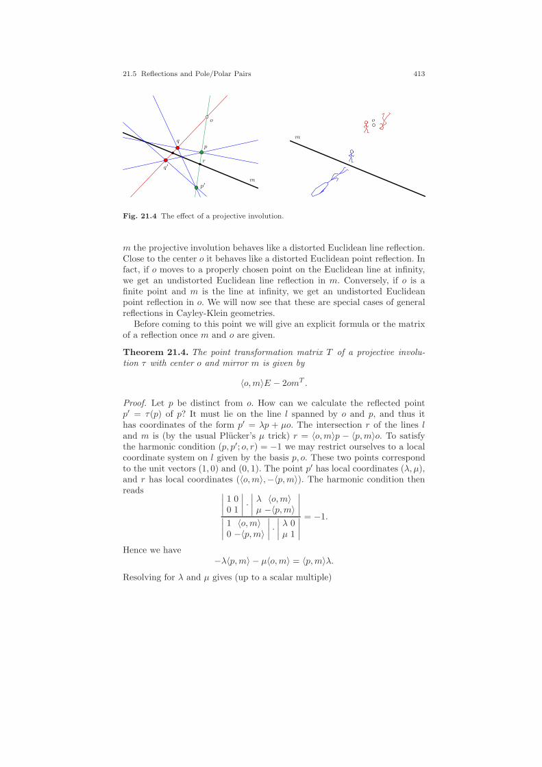
21.5 Reflections and Pole/Polar Pairs 413
m
o
pq
p′
q′r
m
o
Fig. 21.4 The effect of a projective involution.
m the projective involution behaves like a distorted Euclidean line reflection.Close to the center o it behaves like a distorted Euclidean point reflection. Infact, if o moves to a properly chosen point on the Euclidean line at infinity,we get an undistorted Euclidean line reflection in m. Conversely, if o is afinite point and m is the line at infinity, we get an undistorted Euclideanpoint reflection in o. We will now see that these are special cases of generalreflections in Cayley-Klein geometries.
Before coming to this point we will give an explicit formula or the matrixof a reflection once m and o are given.
Theorem 21.4. The point transformation matrix T of a projective involu-tion τ with center o and mirror m is given by
〈o,m〉E − 2omT .
Proof. Let p be distinct from o. How can we calculate the reflected pointp′ = τ(p) of p? It must lie on the line l spanned by o and p, and thus ithas coordinates of the form p′ = λp + µo. The intersection r of the lines land m is (by the usual Plucker’s µ trick) r = 〈o,m〉p − 〈p,m〉o. To satisfythe harmonic condition (p, p′; o, r) = −1 we may restrict ourselves to a localcoordinate system on l given by the basis p, o. These two points correspondto the unit vectors (1, 0) and (0, 1). The point p′ has local coordinates (λ, µ),and r has local coordinates (〈o,m〉,−〈p,m〉). The harmonic condition thenreads ∣∣∣∣
1 00 1
∣∣∣∣ ·∣∣∣∣λ 〈o,m〉µ −〈p,m〉
∣∣∣∣∣∣∣∣1 〈o,m〉0 −〈p,m〉
∣∣∣∣ ·∣∣∣∣λ 0µ 1
∣∣∣∣= −1.
Hence we have−λ〈p,m〉 − µ〈o,m〉 = 〈p,m〉λ.
Resolving for λ and µ gives (up to a scalar multiple)
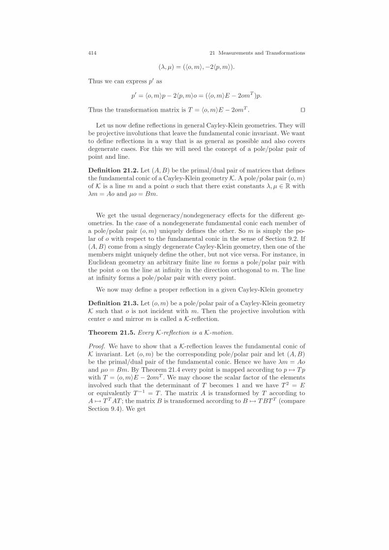
414 21 Measurements and Transformations
(λ, µ) = (〈o,m〉,−2〈p,m〉).
Thus we can express p′ as
p′ = 〈o,m〉p− 2〈p,m〉o = (〈o,m〉E − 2omT )p.
Thus the transformation matrix is T = 〈o,m〉E − 2omT . ⊓⊔
Let us now define reflections in general Cayley-Klein geometries. They willbe projective involutions that leave the fundamental conic invariant. We wantto define reflections in a way that is as general as possible and also coversdegenerate cases. For this we will need the concept of a pole/polar pair ofpoint and line.
Definition 21.2. Let (A,B) be the primal/dual pair of matrices that definesthe fundamental conic of a Cayley-Klein geometry K. A pole/polar pair (o,m)of K is a line m and a point o such that there exist constants λ, µ ∈ R withλm = Ao and µo = Bm.
We get the usual degeneracy/nondegeneracy effects for the different ge-ometries. In the case of a nondegenerate fundamental conic each member ofa pole/polar pair (o,m) uniquely defines the other. So m is simply the po-lar of o with respect to the fundamental conic in the sense of Section 9.2. If(A,B) come from a singly degenerate Cayley-Klein geometry, then one of themembers might uniquely define the other, but not vice versa. For instance, inEuclidean geometry an arbitrary finite line m forms a pole/polar pair withthe point o on the line at infinity in the direction orthogonal to m. The lineat infinity forms a pole/polar pair with every point.
We now may define a proper reflection in a given Cayley-Klein geometry
Definition 21.3. Let (o,m) be a pole/polar pair of a Cayley-Klein geometryK such that o is not incident with m. Then the projective involution withcenter o and mirror m is called a K-reflection.
Theorem 21.5. Every K-reflection is a K-motion.
Proof. We have to show that a K-reflection leaves the fundamental conic ofK invariant. Let (o,m) be the corresponding pole/polar pair and let (A,B)be the primal/dual pair of the fundamental conic. Hence we have λm = Aoand µo = Bm. By Theorem 21.4 every point is mapped according to p 7→ Tpwith T = 〈o,m〉E − 2omT . We may choose the scalar factor of the elementsinvolved such that the determinant of T becomes 1 and we have T 2 = Eor equivalently T−1 = T . The matrix A is transformed by T according toA 7→ T TAT ; the matrix B is transformed according to B 7→ TBT T (compareSection 9.4). We get
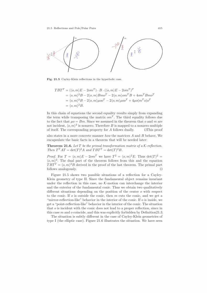
21.5 Reflections and Pole/Polar Pairs 415
m
o
m
o
Fig. 21.5 Cayley-Klein reflections in the hyperbolic case.
TBT T = (〈o,m〉E − 2omT ) ·B · (〈o,m〉E − 2omT )T
= 〈o,m〉2B − 2〈o,m〉BmoT − 2〈o,m〉omTB + 4omTBmoT
= 〈o,m〉2B − 2〈o,m〉µooT − 2〈o,m〉µooT + 4µo(mT o)oT
= 〈o,m〉2B.
In this chain of equations the second equality results simply from expandingthe term while transposing the matrix omT . The third equality follows dueto the fact that µo = Bm. Since we assumed in the theorem that o and m arenot incident, 〈o,m〉2 is nonzero. Therefore B is mapped to a nonzero multipleof itself. The corresponding property for A follows dually. ⊓⊔This proof
also states in a more concrete manner how the matrices A and B behave. Weencapsulate the basic facts in a theorem that will be needed later:
Theorem 21.6. Let T be the primal transformation matrix of a K-reflection.Then T TAT = det(T )2A and TBT T = det(T )2B.
Proof. For T = 〈o,m〉E − 2omT we have T 2 = 〈o,m〉2E. Thus det(T )2 =〈o,m〉2. The dual part of the theorem follows from this and the equationTBT T = 〈o,m〉2B derived in the proof of the last theorem. The primal partfollows analogously. ⊓⊔
Figure 21.5 shows two possible situations of a reflection for a Cayley-Klein geometry of type II. Since the fundamental object remains invariantunder the reflection in this case, no K-motion can interchange the interiorand the exterior of the fundamental conic. Thus we obtain two qualitativelydifferent situations depending on the position of the center o with respectto the conic. If o is outside the conic, then m cuts the conic, and we get a“mirror-reflection-like” behavior in the interior of the conic. If o is inside, weget a “point-reflection-like” behavior in the interior of the conic. The situationthat o is incident with the conic does not lead to a proper reflection, since inthis casem and o coincide, and this was explicitly forbidden by Definition21.3.
The situation is subtly different in the case of Cayley-Klein geometries oftype I (the elliptic case). Figure 21.6 illustrates the situation. We have seen

416 21 Measurements and Transformations
m
o
Fig. 21.6 Cayley-Klein reflections in the spherical case.
that (up to projective equivalence) this geometry is nicely represented byconsidering the sphere with antipodal pairs identified as a double cover ofthe projective plane. Cayley-Klein measurement then corresponds to lengthmeasurement with geodesics (shortest paths on the sphere). The fact that inelliptic geometry antipodal pairs of the sphere are identified implies that onthe sphere every object is present twice. The antipodal object occurs withreversed orientation. A K-reflection corresponds to a reflection in a greatcircle of the sphere. There is no distinction of point and line reflection inthis geometry! A reflection with respect to the line m may equally well beachieved by a rotation of 180 with respect to the pole o.
In Euclidean geometry a K-reflection leads again to two different situa-tions. If the line m is finite, the point o lies on the fundamental object (theline at infinity) and we get a line reflection. If o is finite then m is necessarilythe line at infinity and we get a point reflection. The reader is invited towork out the different situations that may arise in the other Cayley-Kleingeometries.
We have seen that depending on the degree of degeneration of a Cayley-Klein geometry we obtain different degrees of freedom for the associatedtransformations. While the nondegenerate geometries (types I and II) admitthree degrees of freedom, the singly degenerate types (types III to VI) ad-mit four degrees of freedom. Finally, the doubly degenerate geometry (typeVII) admits five degrees of freedom. In types I and II every K-motion leavesdistances and angles invariant. In types III and VI there exist in addition K-motions that alter the angle. In types V and VI there exist K-motions thatalter the distance (for instance scalings in Euclidean geometry). In type VIIthere exist K-motions that alter both angles and distances. Now, reflections
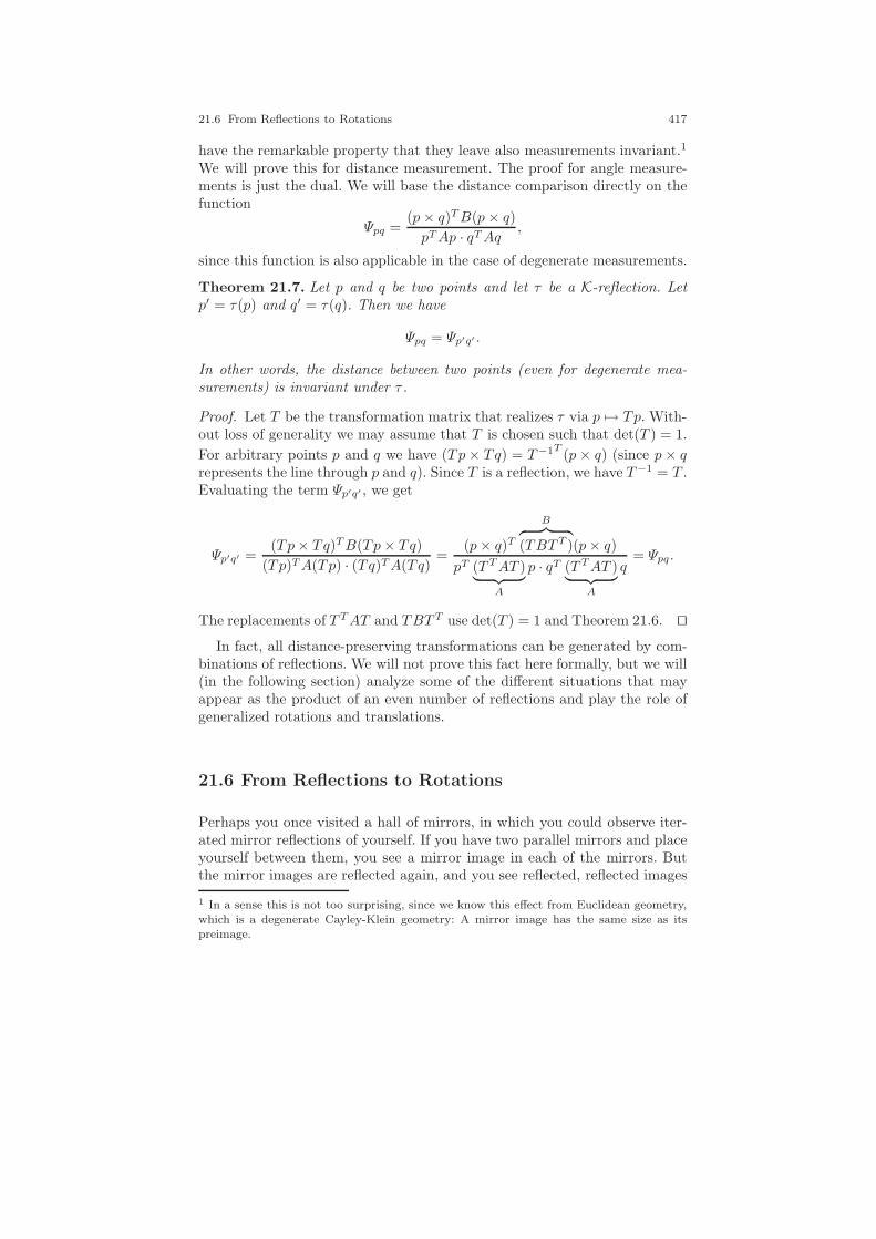
21.6 From Reflections to Rotations 417
have the remarkable property that they leave also measurements invariant.1
We will prove this for distance measurement. The proof for angle measure-ments is just the dual. We will base the distance comparison directly on thefunction
Ψpq =(p× q)TB(p× q)
pTAp · qTAq ,
since this function is also applicable in the case of degenerate measurements.
Theorem 21.7. Let p and q be two points and let τ be a K-reflection. Letp′ = τ(p) and q′ = τ(q). Then we have
Ψpq = Ψp′q′ .
In other words, the distance between two points (even for degenerate mea-surements) is invariant under τ .
Proof. Let T be the transformation matrix that realizes τ via p 7→ Tp. With-out loss of generality we may assume that T is chosen such that det(T ) = 1.
For arbitrary points p and q we have (Tp× Tq) = T−1T (p× q) (since p× qrepresents the line through p and q). Since T is a reflection, we have T−1 = T .Evaluating the term Ψp′q′ , we get
Ψp′q′ =(Tp× Tq)TB(Tp× Tq)
(Tp)TA(Tp) · (Tq)TA(Tq)=
(p× q)T
B︷ ︸︸ ︷(TBT T )(p× q)
pT (T TAT )︸ ︷︷ ︸A
p · qT (T TAT )︸ ︷︷ ︸A
q= Ψpq.
The replacements of T TAT and TBT T use det(T ) = 1 and Theorem 21.6. ⊓⊔In fact, all distance-preserving transformations can be generated by com-
binations of reflections. We will not prove this fact here formally, but we will(in the following section) analyze some of the different situations that mayappear as the product of an even number of reflections and play the role ofgeneralized rotations and translations.
21.6 From Reflections to Rotations
Perhaps you once visited a hall of mirrors, in which you could observe iter-ated mirror reflections of yourself. If you have two parallel mirrors and placeyourself between them, you see a mirror image in each of the mirrors. Butthe mirror images are reflected again, and you see reflected, reflected images
1 In a sense this is not too surprising, since we know this effect from Euclidean geometry,which is a degenerate Cayley-Klein geometry: A mirror image has the same size as itspreimage.
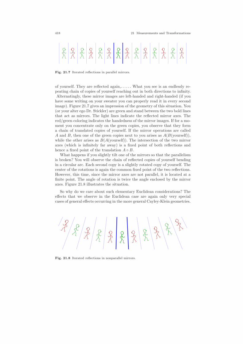
418 21 Measurements and Transformations
Fig. 21.7 Iterated reflections in parallel mirrors.
of yourself. They are reflected again,. . . . . . What you see is an endlessly re-peating chain of copies of yourself reaching out in both directions to infinity.Alternatingly, these mirror images are left-handed and right-handed (if you
have some writing on your sweater you can properly read it in every secondimage). Figure 21.7 gives an impression of the geometry of this situation. You(or your alter ego Dr. Stickler) are green and stand between the two bold linesthat act as mirrors. The light lines indicate the reflected mirror axes. Thered/green coloring indicates the handedness of the mirror images. If for a mo-ment you concentrate only on the green copies, you observe that they forma chain of translated copies of yourself. If the mirror operations are calledA and B, then one of the green copies next to you arises as A(B(yourself)),while the other arises as B(A(yourself)). The intersection of the two mirroraxes (which is infinitely far away) is a fixed point of both reflections andhence a fixed point of the translation A B.
What happens if you slightly tilt one of the mirrors so that the parallelismis broken? You will observe the chain of reflected copies of yourself bendingin a circular arc. Each second copy is a slightly rotated copy of yourself. Thecenter of the rotations is again the common fixed point of the two reflections.However, this time, since the mirror axes are not parallel, it is located at afinite point. The angle of rotation is twice the angle enclosed by the mirroraxes. Figure 21.8 illustrates the situation.
So why do we care about such elementary Euclidean considerations? Theeffects that we observe in the Euclidean case are again only very specialcases of general effects occurring in the more general Cayley-Klein geometries.
Fig. 21.8 Iterated reflections in nonparallel mirrors.
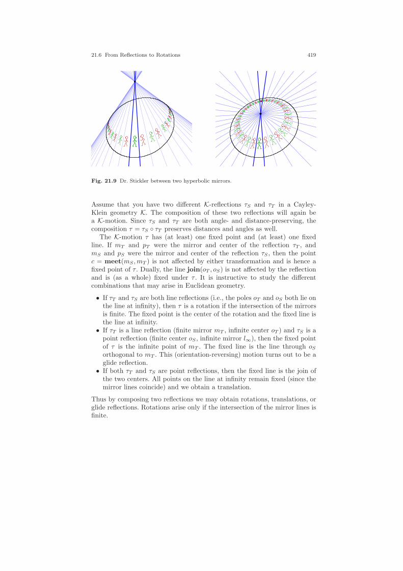
21.6 From Reflections to Rotations 419
Fig. 21.9 Dr. Stickler between two hyperbolic mirrors.
Assume that you have two different K-reflections τS and τT in a Cayley-Klein geometry K. The composition of these two reflections will again bea K-motion. Since τS and τT are both angle- and distance-preserving, thecomposition τ = τS τT preserves distances and angles as well.
The K-motion τ has (at least) one fixed point and (at least) one fixedline. If mT and pT were the mirror and center of the reflection τT , andmS and pS were the mirror and center of the reflection τS , then the pointc = meet(mS ,mT ) is not affected by either transformation and is hence afixed point of τ . Dually, the line join(oT , oS) is not affected by the reflectionand is (as a whole) fixed under τ . It is instructive to study the differentcombinations that may arise in Euclidean geometry.
• If τT and τS are both line reflections (i.e., the poles oT and oS both lie onthe line at infinity), then τ is a rotation if the intersection of the mirrorsis finite. The fixed point is the center of the rotation and the fixed line isthe line at infinity.
• If τT is a line reflection (finite mirror mT , infinite center oT ) and τS is apoint reflection (finite center oS , infinite mirror l∞), then the fixed pointof τ is the infinite point of mT . The fixed line is the line through oSorthogonal to mT . This (orientation-reversing) motion turns out to be aglide reflection.
• If both τT and τS are point reflections, then the fixed line is the join ofthe two centers. All points on the line at infinity remain fixed (since themirror lines coincide) and we obtain a translation.
Thus by composing two reflections we may obtain rotations, translations, orglide reflections. Rotations arise only if the intersection of the mirror lines isfinite.
420 21 Measurements and Transformations
The situation becomes more involved (or better, “less commonly known”)in the other Cayley-Klein geometries. We will briefly have a look at what hap-pens for Cayley-Klein geometries of type II for which the fundamental conicis nondegenerate and real. Figure 21.9 illustrates two qualitatively differentscenarios. Again the two mirror lines are drawn as bold blue lines. In the leftpicture the two mirror lines intersect outside the fundamental conic. Withinthe line bundle through the intersection of the mirrors we have a hyperbolicangle measurement. This results in an endless chain of reflected mirror im-ages reaching out to both sides and never approaching the boundary. If youwere Dr. Stickler, for you the situation would look much like the situation be-tween two parallel Euclidean mirrors—endless repetition in both directions.However, projectively the situation is slightly different, since the two limitingiterations never will touch each other, as they did in the Euclidean case. In asense, we could call such a transformation composed of the two reflections ahyperrotation—a rotation whose rotation center is “more than infinitely faraway” (see Chapter 23). Such a hyperrotation has a single fixed line thatpasses through the interior of the fundamental object. This is a remarkabledifference to the Euclidean case of parallel mirrors, where a translation hasinfinitely many fixed lines.
The right picture represents the situation in which the intersection of themirror line is in the finite region. The angle measurement around the intersec-tion of the mirrors is elliptic. Here the situation is much like the Euclideancase of nonparallel mirrors. If in addition the angle is a divisor of the fullcircle, the chain of reflections closes up and the group generated by the tworeflections is finite. This is the situation shown in the picture. The composi-tion of the two reflections is called a rotation. This operation also has a fixedline. However, this line is outside the horizon. It is the polar of the rotationcenter.
In between these two cases lies the situation in which the intersection ofthe mirrors is on the boundary of the fundamental object. This case is evenmore like the situation of Euclidean parallel mirrors, since now the limitingpictures in both directions again meet in a single point.
Remark 21.2. It should be finally mentioned that in many interesting sit-uations the transformation τ = τT τS can be considered a member of acontinuous family of distance-preserving K-motions that connects τ continu-ously with the identity transformation (as in Euclidean geometry, for whicha rotation or translation can be considered a continuous process of movingan object to a new position). We briefly discuss this in type-II geometries.There the mirror uniquely determines the center of a reflection, which makesthings a little easier. Take τT and τS to be reflections with axis mT and mS .Consider the continuous family of reflections τλ with axis (1− λ)mT + λmS .As λ moves from 0 to 1, the reflection τT τλ interpolates between the iden-tity and τ . As long as throughout this process τλ is always admissible (i.e.,the mirror is not a tangent to the fundamental conic), we get the desiredcontinuous family of transformations.

21.6 From Reflections to Rotations 421

22
Cayley-Klein Geometries at Work
Diese Uberlegung gibt uns ein schones Beispiel dafur, wie diedualen Satze der elliptischen Geometrie beim Ubergang zur
euklidischen Geometrie in Trummer fallen.
Felix Klein on the angle bisector theorem,Vorlesungen uber Nicht-Euklidische Geometrie, 1928
Based on the measurement in a Cayley-Klein geometry, we can now definespecific geometric objects and relations. For instance a circle may be definedas the set of all points that have a constant distance to a given point. Beingorthogonal may be defined as a certain angle relation between two lines. Ineach type of a Cayley-Klein geometry the objects and relations will have veryspecific properties. In this chapter we will deal with aspects of elementarygeometry in the context of Cayley-Klein geometries. Following the spirit ofthis book, we will again focus on (algebraic and geometric representationsof) geometric primitive operations, on incidence theorems, and on invarianceproperties. Again we try to present the definitions and statements in a waythat they apply as generally as possible to degenerate Cayley Klein geome-tries. Still some statements may break down if the geometric configurationsor the underlying geometry becomes too degenerate. Since we do not wantto spend most of the exposition mainly with pathological degenerate cases,we will base our definitions whenever possible on constructive approachesthat allow us to explicitly calculate the objects involved. The reader shouldbe aware that this chapter is by far more about the “how” than about the“what.” The ways theorems are interpreted and proved is more central thanthe theorems themselves. Nice treatments of elementary geometric theoremsmay also be found in [49, 86, 136].
423
424 22 Cayley-Klein Geometries at Work
22.1 Orthogonality
We start with the notion of orthogonality.In Euclidean geometry two distinctlines l and m are considered orthogonal if the oriented angle ∠(l,m) is iden-tical to the oriented angle ∠(m, l). To transfer this notion into the contextof Cayley-Klein geometries, assume that p is the intersection of l and m andthat X and Y are the two tangents from p to the fundamental object. Thuswe are looking for a line with the property (l,m;X,Y ) = (m, l;X,Y ) 6= 1.Using the fact that interchanging the roles of l and m inverts the cross-ratio,we see that this can be the case only if (m, l;X,Y ) = −1. As usual, X and Yare the two tangents of p to the fundamental conic. In order to cover also de-generate cases of coinciding lines in which both numerator and denominatorof the cross-ratio vanish, we prefer the following characterization.
Definition 22.1. Two distinct lines l and m are orthogonal in the Cayley-Klein geometry K if (with notions as above)
[h, l,X ][h,m, y] = −[h, l, Y ][h,m,X ] (22.1)
for a line h not through the intersection p of l and m.
We will now derive an equivalent more concise algebraic definition fortwo lines l and m being orthogonal that directly relates orthogonality tothe fundamental conic. For this we introduce a local coordinate system onthe line bundle around p with l and m as a basis. Every line through p isexpressible as a linear combination λl + µm. In particular, X and Y havesuch a representation. In Section 21.3 we made a consideration dual to thisin order to eliminate the points X and Y in a distance measurement. Now wewant to do exactly the same with the lines X and Y . By an argument exactlydual to the content of Section 21.3 we can prove that with the abbreviationsΘll = lTBl, Θlm = lTBm, Θmm = mTBm, and ∆ = Θ2
lm − ΘllΘmm, thecondition (22.1) is equivalent to
Θlm +√∆ = −Θlm +
√∆.
The expressions on the left and the negative of the expression on the right ofthis equation represent the numerator and the denominator of the cross-ratio.From this we easily get the following theorem.
Theorem 22.1. Let K be a Cayley-Klein geometry and let B be the matrixrepresenting the dual fundamental conic. Then a pair of distinct lines l,m isorthogonal in K if lTBm = 0.
Proof. In the expression Θlm +√∆ = −Θlm +
√∆ the term
√∆ cancels. So
it is equivalent to 0 = Θlm = lTBm, as claimed. ⊓⊔We can use this condition also in the case of coinciding lines l and m.
In this case lTBm = 0 means that l = m is a tangent to the fundamental
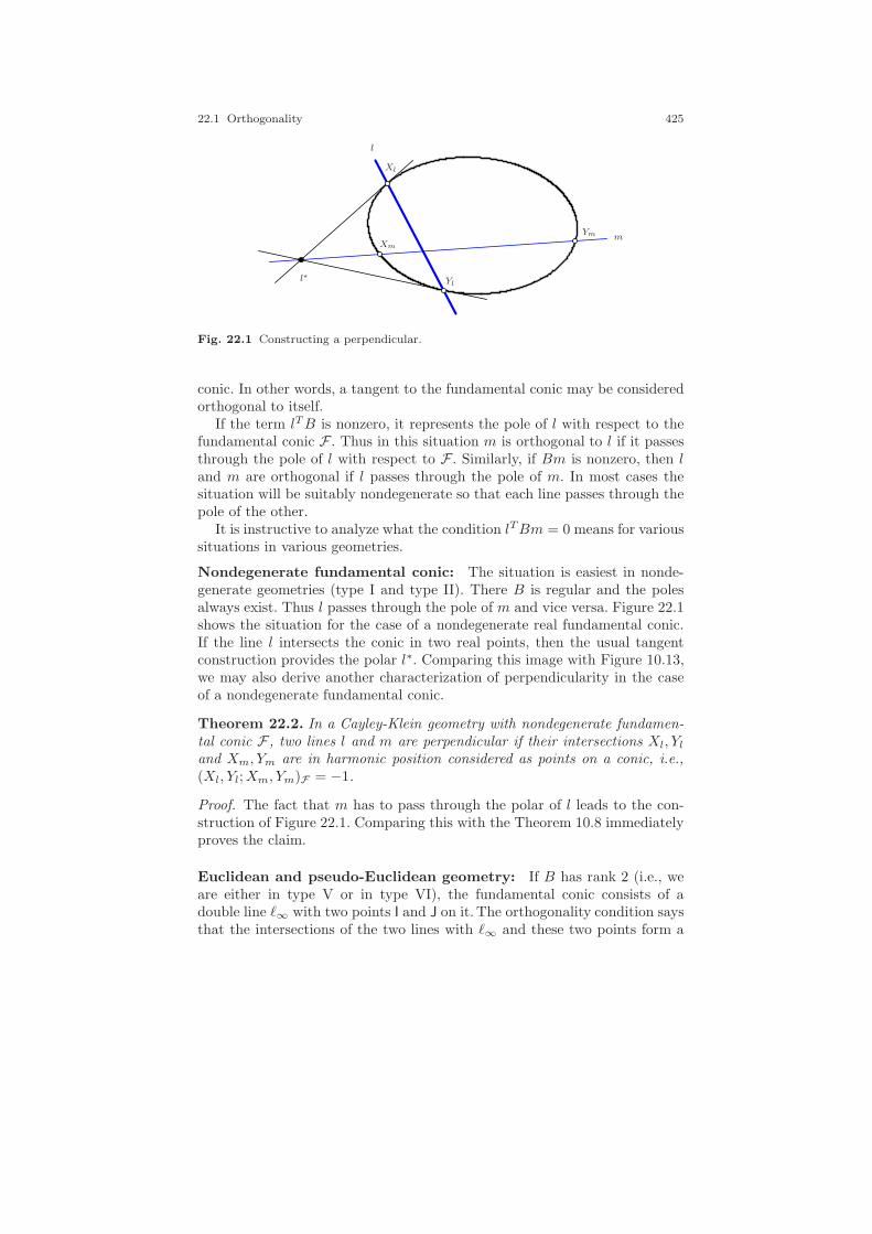
22.1 Orthogonality 425
l
m
Xl
Yl
Xm
Ym
l∗
Fig. 22.1 Constructing a perpendicular.
conic. In other words, a tangent to the fundamental conic may be consideredorthogonal to itself.
If the term lTB is nonzero, it represents the pole of l with respect to thefundamental conic F . Thus in this situation m is orthogonal to l if it passesthrough the pole of l with respect to F . Similarly, if Bm is nonzero, then land m are orthogonal if l passes through the pole of m. In most cases thesituation will be suitably nondegenerate so that each line passes through thepole of the other.
It is instructive to analyze what the condition lTBm = 0 means for varioussituations in various geometries.
Nondegenerate fundamental conic: The situation is easiest in nonde-generate geometries (type I and type II). There B is regular and the polesalways exist. Thus l passes through the pole of m and vice versa. Figure 22.1shows the situation for the case of a nondegenerate real fundamental conic.If the line l intersects the conic in two real points, then the usual tangentconstruction provides the polar l∗. Comparing this image with Figure 10.13,we may also derive another characterization of perpendicularity in the caseof a nondegenerate fundamental conic.
Theorem 22.2. In a Cayley-Klein geometry with nondegenerate fundamen-tal conic F , two lines l and m are perpendicular if their intersections Xl, Yland Xm, Ym are in harmonic position considered as points on a conic, i.e.,(Xl, Yl;Xm, Ym)F = −1.
Proof. The fact that m has to pass through the polar of l leads to the con-struction of Figure 22.1. Comparing this with the Theorem 10.8 immediatelyproves the claim.
Euclidean and pseudo-Euclidean geometry: If B has rank 2 (i.e., weare either in type V or in type VI), the fundamental conic consists of adouble line ℓ∞ with two points I and J on it. The orthogonality condition saysthat the intersections of the two lines with ℓ∞ and these two points form a

426 22 Cayley-Klein Geometries at Work
harmonic quadruple. As expected, this agrees nicely with the characterizationof Euclidean orthogonality we derived in Theorem 18.6. In pseudo-Euclideangeometry the two points I and J are real. A line passing through these pointsis self-orthogonal.
There is one interesting case covered by lTBm = 0 that is still missing:The double line ℓ∞ is orthogonal to every other line l. This is the case sinceBℓ∞ = (IJT +JI
T )ℓ∞ = 0. In this situation the pole of l is no longer uniquelyspecified.
The remaining cases: In all other cases the matrix B has rank 1 and isof the form B = qqT . The point q is the double point representing the dualfundamental object. The situation lTBm = 0 can arise only if either l or mis incident with q. Thus if one line does not pass through q, then in case oforthogonality the other must pass through q. The point q is the pole of everyline that does not already pass through it.
We now turn to simple theorems involving orthogonality. In the case thatthe expression Bl is not zero, it represents the pole of l with respect tothe fundamental conic. Then we get, for instance, an easy explicit method toconstruct a perpendicular to l through a given point p. Expressed in algebraicterms this reads as:
1: Construct the pole l∗ = B · l of l.
2: Join l∗ with p.
As an application of expressing perpendicularity in a Cayley-Klein geom-etry we will show that also in a Cayley-Klein geometry the altitudes of atriangle meet in a point. A corresponding picture for a nondegenerate funda-mental conic F is shown in Figure 22.2. The three black points in the interiorare the vertices of the triangle. Its sides are the lines l1, l2, l3. The polars ofthese lines are shown in corresponding colors. Joining the polars with thecorresponding opposite vertices results in the three altitudes that meet in apoint. Essentially this theorem of metric character is again translated into anentirely projective statement. We could provide geometric proofs for the non-degenerate and the degenerate cases. However, we prefer to give an algebraicproof that simultaneously covers both cases.
Theorem 22.3. Let K be a Cayley-Klein geometry with dual fundamentalconic B and let l1, l2, l3 be the sides of a triangle. If Bl1, Bl2, and Bl3 areall nonzero, then the altitudes of the triangle are uniquely defined and meetin one point.
Proof. Let l1, l2, l3 be the lines supporting the sides of the triangle and let Bbe the matrix of the dual fundamental conic. The polars of the lines are givenby Bl1, Bl2, Bl3. The altitude h1 to line l1 thus can be uniquely (!) written ash1 = join(meet(l2, l3), Bl1). In terms of cross products this can be expressed

22.2 Constructive versus Implicit Representations 427
l1
l2
l3
l∗1
l∗2
l∗3
Fig. 22.2 The altitudes meet in a point.
as (l2× l3)×Bl1. Applying the identity (v1×v2)×v3 = 〈v1, v3〉v2−〈v2, v3〉v1,we get
h1 = 〈l2, Bl1〉l3 − 〈l3, Bl1〉l2.Similarly, we get
h2 = 〈l3, Bl2〉l1 − 〈l1, Bl2〉l3,h3 = 〈l1, Bl3〉l2 − 〈l2, Bl3〉l1.
Now we want to prove that h1, h2, h3 are concurrent. Thus we want to ex-pand the determinant [h1, h2, h3]. Since each row in this expression has twosummands, this expansion has eight summands. However, it is easy to checkthat all terms involving a left term and a right term of the above equationsmust vanish identically, since two rows become linearly dependent. Thus weget
[h1, h2, h3] = +[〈l2, Bl1〉l3, 〈l3, Bl2〉l1, 〈l1, Bl3〉l2]−[〈l3, Bl1〉l2, 〈l1, Bl2〉l3, 〈l2, Bl3〉l1] = 0.
This proves the claim. ⊓⊔
22.2 Constructive versus Implicit Representations
One might wonder how important the nondegeneracy assumptions “Bl1, Bl2,and Bl3 are all nonzero” in Theorem 22.3 were. In fact, we formulated thetheorem in a way that kept us on the safe side. Let us now explore to whatextent a statement like the following is true:
428 22 Cayley-Klein Geometries at Work
Let l1, l2, l3 be lines that support the three sides of a triangle and letg1, g2, g3 be three lines such that li and gi for i = 1, . . . , 3 are orthogonaland gi passes through the vertex meet(lj , lk) with i, j, k = 1, 2, 3 fori = 1, . . . , 3 (i.e., the gi are altitudes). Then g1, g2, g3 have a point incommon.
Compared to Theorem 22.3 this statement characterizes orthogonality onlyimplicitly via the equations lTi Bgi = 0. This statement is not true in general,but still many cases not covered by Theorem 22.3 turn out to be true. Letus explore the different situations. If all poles exist, the statement is true asa consequence of Theorem 22.3. Let us first consider the case of Euclideangeometry. The only situation not already covered is the case that one of thelines (say l1) is the line at infinity (every finite line has a unique pole). Inthis case two of the triangles vertices (those incident with l1) are the infinitepoints of l2 and l3. The altitude g2 of l2 passes through the pole of l2 (thisis an infinite point) and through the infinite point of l3. Hence this altitudeis the line at infinity. Similarly, g3 is also the line at infinity. This impliesthat no matter what g1 is, the three altitudes have a point in common. Thusthe above statement also holds in general in the Euclidean plane. The sameargument applies to pseudo-Euclidean geometry.
In the remaining cases the dual conic is a double point q. As long as thethree lines l1, l2, l3 do not pass through this point, they have a unique polar(the point q itself), and Theorem 22.3 applies and proves that the altitudesmeet. Actually, they will meet in the double point itself. What happens ifone or more lines go through the double point? In the case of only one line(say l1) the two altitudes g2 and g3 must still go through q. Since also l1 goesthrough q, the two altitudes g2 and g3 must coincide with l1, and again thestatement is true.
There are not many cases left, but now the statement finally breaks apartif at least two of the lines li (say l1 and l2) pass through the double point q.In this case every line g1 is orthogonal to l1 and every line g2 is orthogonalto l2. Thus no matter where g3 is, these lines can be chosen in a way thatthe three altitudes do not meet.
This is what Felix Klein meant in the quotation used as the epigraph to thischapter when he said that “theorems fall to pieces” if the underlying geometryis too degenerate. What makes the theorem remain true in so many cases andfinally collapse in the last mentioned case? The deep reason for this is thateach the “good” cases could be considered a limiting case of a nondegeneratesituation. However, in the last case we forced the poles of l1 and l2 to move todifferent places and still represent a double-point degeneracy. This can neverhappen as a limiting case of a sequence of nondegenerate situations.
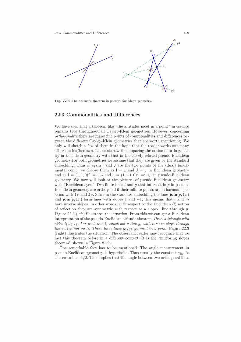
22.3 Commonalities and Differences 429
g
l
l1
l2
l3
g1
g3
g3
Fig. 22.3 The altitudes theorem in pseudo-Euclidean geometry.
22.3 Commonalities and Differences
We have seen that a theorem like “the altitudes meet in a point” in essenceremains true throughout all Cayley-Klein geometries. However, concerningorthogonality there are many fine points of commonalities and differences be-tween the different Cayley-Klein geometries that are worth mentioning. Weonly will sketch a few of them in the hope that the reader works out manyothers on his/her own. Let us start with comparing the notion of orthogonal-ity in Euclidean geometry with that in the closely related pseudo-Euclideangeometry.For both geometries we assume that they are given by the standardembedding. Thus if again I and J are the two points of the (dual) funda-mental conic, we choose them as I = I and J = J in Euclidean geometryand as I = (1, 1, 0)T =: IP and J = (1,−1, 0)T =: JP in pseudo-Euclideangeometry. We now will look at the pictures of pseudo-Euclidean geometrywith “Euclidean eyes.” Two finite lines l and g that intersect in p in pseudo-Euclidean geometry are orthogonal if their infinite points are in harmonic po-sition with IP and JP . Since in the standard embedding the lines join(p, IP )and join(p, IP ) form lines with slopes 1 and −1, this means that l and mhave inverse slopes. In other words, with respect to the Euclidean (!) notionof reflection they are symmetric with respect to a slope-1 line through p.Figure 22.3 (left) illustrates the situation. From this we can get a Euclideaninterpretation of the pseudo-Euclidean altitude theorem. Draw a triangle withsides l1, l2, l3. For each line li construct a line gi with inverse slope throughthe vertex not on li. These three lines g1, g2, g3 meet in a point. Figure 22.3(right) illustrates the situation. The observant reader may recognize that wemet this theorem before in a different context. It is the “mirroring slopestheorem” shown in Figure 8.12.
One remarkable fact has to be mentioned. The angle measurement inpseudo-Euclidean geometry is hyperbolic. Thus usually the constant cdist ischosen to be −1/2. This implies that the angle between two orthogonal lines

430 22 Cayley-Klein Geometries at Work
MP
Q
S
M
P
Q
S
Fig. 22.4 Thales’ theorem in pseudo-Euclidean geometry.
is the complex number −iπ/2. In fact, in pseudo-Euclidean geometry it is notpossible to move a line into one of its orthogonals by any sequence of finiterotations (i.e., those with a real rotation angle). Figure 22.4 shows anotherinteresting instance of a theorem that remains true in pseudo-Euclidean ge-ometry: Thales’s theorem.In this geometry circles are (Euclidean) hyperbolaswhose asymptotes have slopes 1 and −1. Thales’ theorem states that eachpoint S on a circle “sees” the endpoints P and Q of any diameter of the circlein a right angle.
Let us now turn to hyperbolic geometry (i.e., we have a real nondegen-erate fundamental object). Perhaps one of the most striking and importantdifferences to Euclidean geometry is the one indicated in Figure 22.5. Therea pentagon is shown. Every side of the pentagon is incident with the poles ofthe two adjacent sides. Hence the edges of the pentagon meet orthogonallyat the corner. We get a pentagon with five right vertex angles. Indeed, it ispossible for every n ≥ 5 to have n-gons with only right angles. We will have
Fig. 22.5 A hyperbolic pentagon with only right angles.
22.4 Midpoints and Angle Bisectors 431
a closer look at this important phenomenon later when we discuss hyperbolicgeometry.
22.4 Midpoints and Angle Bisectors
Two other interesting geometric primitive operations are the constructionof midpoints and of angle bisectors. In Cayley-Klein geometries these twoconcepts are intimately related, since one is the dual of the other. The reasonthat these concepts are not obviously dual in Euclidean geometry (there aretwo angular bisectors of a pair of lines but only one midpoint of a pair ofpoints) is that there the fundamental conic itself is not self-dual and inducesqualitatively different behavior for angles and for distances.
Let us begin with the consideration of midpoints of two points p and q ina general Cayley-Klein geometry. We first treat the case of a nondegeneratedistance measurement given by a primal matrix A of rank 2 at least. Againwe abbreviate Ωpq = pTAq. Let p and q be arbitrary points. A midpoint1 ofp and q is a point on the line l = join(p, q) with distK(p,m) = distK(m, q).Here the distance measurement is considered an oriented measurement withrespect to the line l. Thus if X and Y are the two points where l meets thefundamental object, we are looking for a point m such that
(p,m;X,Y ) = (m, q;X,Y ).
We will now explicitly calculate the solutions of this equation. While perform-ing the calculation we will have to make a few nondegeneracy assumptions—we will remove them in later considerations wherever possible. The cross-ratioequation above is equivalent to
(p,X ;m,Y ) = (m,X ; q, Y ). (22.2)
This equation is obtained by permuting the two middle letters on each side ofthe equation. For the moment we will assume that p and q are distinct points.So we can introduce a local coordinate system on l by representing every pointλp+µq by the coordinates (λ, µ). By multiplying by the denominators of thecross-ratios and canceling [X,Y ] we can now write condition (22.2) as thebracket expression
[p,m][m,Y ][X, q] = [m, q][p, Y ][X,m]. (22.3)
We set m = λp+ µq and try to find the (λ, µ) that satisfy the equation. Weget the following condition:
[p, λp+ µq][λp+ µq, Y ][X, q] = [λp+ µq, q][p, Y ][X,λp+ µq].
1 Note that we deliberately do not speak of the midpoint.
432 22 Cayley-Klein Geometries at Work
Expanding, eliminating brackets with double letters, collecting terms, andcanceling the nonzero factor [p, q] yields
µ2[X, q][q, Y ] = λ2[p, Y ][X, p].
Now we use the fact that in Section 21.3 we found that X,Y are representedin the form λp+ µq by the two points
(Ωqq
Ωpq ±√Ω2pq −ΩppΩqq
).
Furthermore, p corresponds to (1, 0) and p to (0, 1). Plugging in these values,the above condition yields
µ2Ω2qq = λ2(Ω2
pq − (Ω2pq −ΩppΩqq)).
Canceling Ωqq once on each side, we get
µ2Ωqq = λ2Ωpp.
Thus we get the amazingly simple formula
m =√Ωqq · p±
√Ωpp · q. (22.4)
Let us for a moment analyze the nondegeneracy assumptions that enteredthis calculation. There were three of them. In the very last step we dividedby Ωqq . In fact, this is not much of a restriction, since there is a completelyanalogous way of deriving the result by dividing by Ωpp. However, it is essen-tial that at least one of these expressions is nonzero. Otherwise, expression(22.4) would be identically zero. The second nondegeneracy assumption wasthat p and q are distinct points. So let us see what happens to (22.4) if pand q are identical. Evaluating the expression with the “+” sign results inthe point p again (which is a reasonable choice for the midpoint of p andp). Evaluating the expression with the “−” sign results in the zero vector,a sign of degeneracy. Finally, we assumed that the distance measurement isnondegenerate. This means that X and Y are distinct and we can divide by[X,Y ]. We made use of this when we derived the bracket expression (22.3).However, this expression is still meaningful for coinciding points X and Y . IfX and Y coincide, then this equation becomes
[p,m][m,X ][X, q] = [m, q][p,X ][X,m].
This condition is satisfied either if X and m coincide or if (m,X ; p, q) are aharmonic quadruple. This agrees with our usual interpretation of midpointsin a degenerate distance measurement. For instance, in Euclidean geometrythe midpoint of p and q is the harmonic conjugate of the infinite point X
22.4 Midpoints and Angle Bisectors 433
on join(p, q) with respect to the pair (p, q); and there is another point thathas the same distance to p and q, namely X itself. Thus we can without anyproblem use our derivations (and in particular the nice formula (22.4)) alsofor a degenerate distance measurement.
It is an amazing fact that by this point of view we also obtain two pointsthat deserve the name midpoint of p and q in Euclidean geometry. The or-dinary midpoint and the corresponding infinite point on join(p, q). We willbriefly inspect how formula (22.4) behaves for degenerate distance measure-ments. In this case the matrix A has rank 1. Thus it is of the form A = ℓℓT ,where ℓ represents the line that plays the role of the line at infinity. Expression(22.4) becomes
m =√qT ℓℓT q · p±
√pT ℓℓT p · q = 〈q, ℓ〉 · p± 〈q, ℓ〉 · q.
The formula 〈q, ℓ〉 · p + 〈q, ℓ〉 · q gives the usual midpoint. The expression〈q, ℓ〉 · p − 〈q, ℓ〉 · q can be interpreted as Plucker’s µ trick for calculating apoint on ℓ and on join(p, q). Thus the second midpoint is, as expected, theintersection of join(p, q) with the line at infinity. This point has the samedistance to p and q: it is infinitely far away.
We also want to mention the following important relation between the twomidpoints of p and q.
Theorem 22.4. Let m+ and m− be the two midpoints of p and q. Then thepairs (p, q) and (m+,m−) are in harmonic relation.
Proof. Expanding the condition for harmonicity
[p,m+][q,m−] + [p,m−][q,m+] = 0
yields under the use of m+ = λp+ µq and m− = λp− µq
[p,m+][q,m−] + [p,m−][q,m+]
= [p, λp+ µq][q, λp− µq] + [p, λp− µq][q, λp+ µq]
= −µλ[p, q][q, p] + µλ[p, q][q, p]
= 0,
which is obviously true. ⊓⊔
Remark 22.1. The observant reader should notice that we did essentially thesame calculation earlier, namely when we proved in Section 19.3 that the twoEuclidean angle bisectors of a line pair are perpendicular.
Let us turn to a generalization of the Euclidean “the medians meet in a point”theorem. We will see that from the six possible midpoints of the points of a
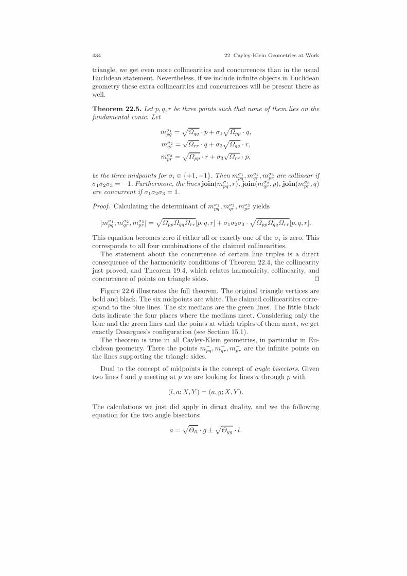
434 22 Cayley-Klein Geometries at Work
triangle, we get even more collinearities and concurrences than in the usualEuclidean statement. Nevertheless, if we include infinite objects in Euclideangeometry these extra collinearities and concurrences will be present there aswell.
Theorem 22.5. Let p, q, r be three points such that none of them lies on thefundamental conic. Let
mσ1pq =
√Ωqq · p+ σ1
√Ωpp · q,
mσ2qr =
√Ωrr · q + σ2
√Ωqq · r,
mσ3pr =
√Ωpp · r + σ3
√Ωrr · p,
be the three midpoints for σi ∈ +1,−1. Then mσ1pq ,m
σ2qr ,m
σ3pr are collinear if
σ1σ2σ3 = −1. Furthermore, the lines join(mσ1pq , r), join(mσ2
qr , p), join(mσ3pr , q)
are concurrent if σ1σ2σ3 = 1.
Proof. Calculating the determinant of mσ1pq ,m
σ2qr ,m
σ3pr yields
[mσ1
pq ,mσ2
qr ,mσ3
pr ] =√ΩppΩqqΩrr[p, q, r] + σ1σ2σ3 ·
√ΩppΩqqΩrr[p, q, r].
This equation becomes zero if either all or exactly one of the σi is zero. Thiscorresponds to all four combinations of the claimed collinearities.
The statement about the concurrence of certain line triples is a directconsequence of the harmonicity conditions of Theorem 22.4, the collinearityjust proved, and Theorem 19.4, which relates harmonicity, collinearity, andconcurrence of points on triangle sides. ⊓⊔
Figure 22.6 illustrates the full theorem. The original triangle vertices arebold and black. The six midpoints are white. The claimed collinearities corre-spond to the blue lines. The six medians are the green lines. The little blackdots indicate the four places where the medians meet. Considering only theblue and the green lines and the points at which triples of them meet, we getexactly Desargues’s configuration (see Section 15.1).
The theorem is true in all Cayley-Klein geometries, in particular in Eu-clidean geometry. There the points m−
pq,m−qr,m
−pr are the infinite points on
the lines supporting the triangle sides.
Dual to the concept of midpoints is the concept of angle bisectors. Giventwo lines l and g meeting at p we are looking for lines a through p with
(l, a;X,Y ) = (a, g;X,Y ).
The calculations we just did apply in direct duality, and we the followingequation for the two angle bisectors:
a =√Θll · g ±
√Θgg · l.
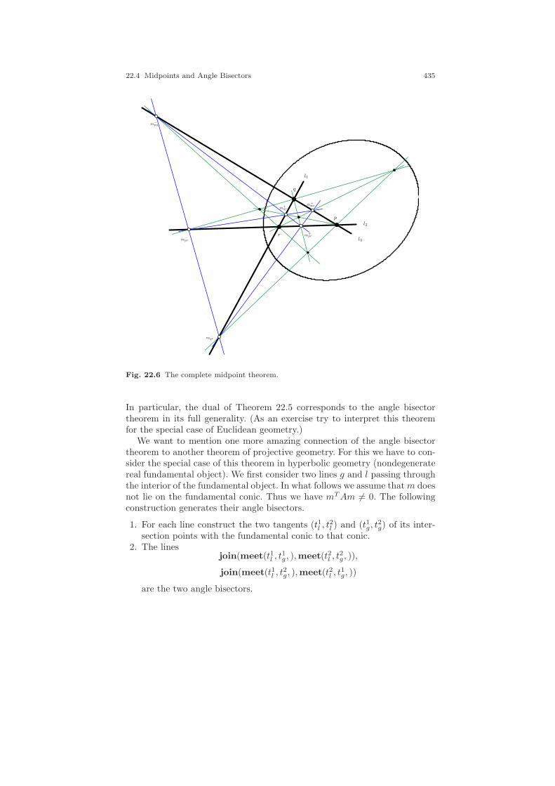
22.4 Midpoints and Angle Bisectors 435
l1
l2
l3
p
q
r
m+pq
m−pq
m+qr
m−qr
m+pr
m−pr
Fig. 22.6 The complete midpoint theorem.
In particular, the dual of Theorem 22.5 corresponds to the angle bisectortheorem in its full generality. (As an exercise try to interpret this theoremfor the special case of Euclidean geometry.)
We want to mention one more amazing connection of the angle bisectortheorem to another theorem of projective geometry. For this we have to con-sider the special case of this theorem in hyperbolic geometry (nondegeneratereal fundamental object). We first consider two lines g and l passing throughthe interior of the fundamental object. In what follows we assume thatm doesnot lie on the fundamental conic. Thus we have mTAm 6= 0. The followingconstruction generates their angle bisectors.
1. For each line construct the two tangents (t1l , t2l ) and (t1g, t
2g) of its inter-
section points with the fundamental conic to that conic.2. The lines
join(meet(t1l , t1g, ),meet(t2l , t
2g, )),
join(meet(t1l , t2g, ),meet(t2l , t
1g, ))
are the two angle bisectors.
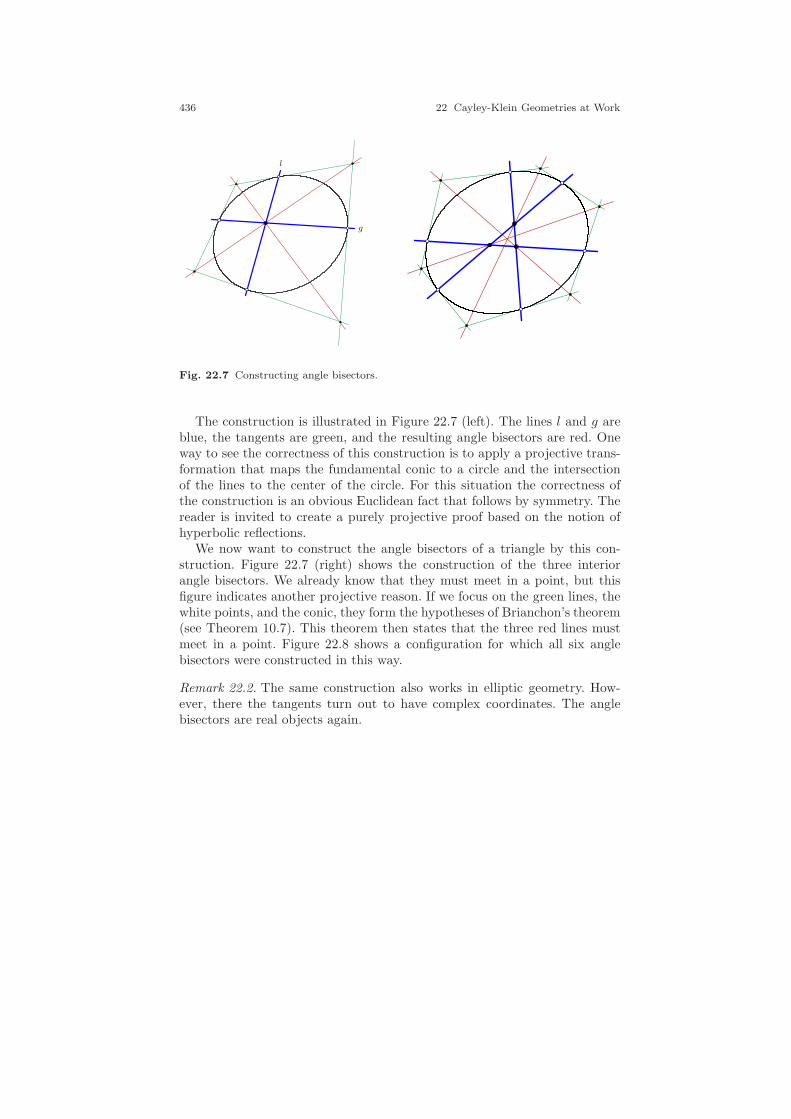
436 22 Cayley-Klein Geometries at Work
l
g
Fig. 22.7 Constructing angle bisectors.
The construction is illustrated in Figure 22.7 (left). The lines l and g areblue, the tangents are green, and the resulting angle bisectors are red. Oneway to see the correctness of this construction is to apply a projective trans-formation that maps the fundamental conic to a circle and the intersectionof the lines to the center of the circle. For this situation the correctness ofthe construction is an obvious Euclidean fact that follows by symmetry. Thereader is invited to create a purely projective proof based on the notion ofhyperbolic reflections.
We now want to construct the angle bisectors of a triangle by this con-struction. Figure 22.7 (right) shows the construction of the three interiorangle bisectors. We already know that they must meet in a point, but thisfigure indicates another projective reason. If we focus on the green lines, thewhite points, and the conic, they form the hypotheses of Brianchon’s theorem(see Theorem 10.7). This theorem then states that the three red lines mustmeet in a point. Figure 22.8 shows a configuration for which all six anglebisectors were constructed in this way.
Remark 22.2. The same construction also works in elliptic geometry. How-ever, there the tangents turn out to have complex coordinates. The anglebisectors are real objects again.
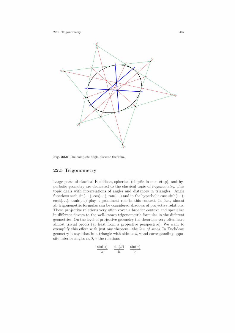
22.5 Trigonometry 437
Fig. 22.8 The complete angle bisector theorem.
22.5 Trigonometry
Large parts of classical Euclidean, spherical (elliptic in our setup), and hy-perbolic geometry are dedicated to the classical topic of trigonometry. Thistopic deals with interrelations of angles and distances in triangles. Anglefunctions such sin(. . .), cos(. . .), tan(. . .) and in the hyperbolic case sinh(. . .),cosh(. . .), tanh(. . .) play a prominent role in this context. In fact, almostall trigonometric formulas can be considered shadows of projective relations.These projective relations very often cover a broader context and specializein different flavors to the well-known trigonometric formulas in the differentgeometries. On the level of projective geometry the theorems very often havealmost trivial proofs (at least from a projective perspective). We want toexemplify this effect with just one theorem—the law of sines. In Euclideangeometry it says that in a triangle with sides a, b, c and corresponding oppo-site interior angles α, β, γ the relations
sin(α)
a=
sin(β)
b=
sin(γ)
c

438 22 Cayley-Klein Geometries at Work
hold (with interior angles always measured with positive sign). There is acorresponding theorem in elliptic geometry (which we for a moment consideras geometry on the sphere, ignoring the identification of antipodal points). Weconsider a sphere of radius 1, so that the total circumference is 2π. If we havea spherical triangle with (geodesic) side lengths a, b, c and and correspondingopposite interior angles α, β, γ, the relation
sin(α)
sin(a)=
sin(β)
sin(b)=
sin(γ)
sin(c)
holds. In hyperbolic geometry (we will learn more about hyperbolic geometryin Chapter 24) the corresponding formula assumes the shape
sin(α)
sinh(a)=
sin(β)
sinh(b)=
sin(γ)
sinh(c).
The occurrence of the sinh(. . .) function reflects the fact that the lengthmeasurement on a hyperbolic line is hyperbolic.
In what follows we will first connect the trigonometric functions to theirprojective counterparts. We will see that all three formulas are just incarna-tions of the same projective theorem. Then we will provide a conceptuallysimple proof for this underlying projective theorem. To avoid the sign ambi-guity that arises from measuring angles and distances in a certain directionwe will consider squares of the fractions in the above expressions.
Already in Section 21.4 we connected trigonometric functions to our pro-jective ways of measuring. We will briefly redo this here in a self-containedway in order to cover as well the case of the sinh(. . .) function. For this recallthat
sin(x) :=eix − e−ix
2i, sinh(x) :=
ex − e−x
2.
In Section 20.3 we introduced the standard constants 1/2i and −1/2 as scalingfactors for elliptic, resp. hyperbolic, measurements. Using these constants, weobtain for an elliptically measured size α = (1/2i) · ln(Ξ) (with Ξ playingthe role of the cross-ratio)
sin(α) = sin
(1
2i· ln(Ξ)
)
=ei
12i
·ln(Ξ) − e−i12i
·ln(Ξ)
2i
=e
12·ln(Ξ) − e−
12·ln(Ξ)
2i
=
√Ξ − 1/
√Ξ
2i.

22.5 Trigonometry 439
Analogously, for sinh(α) in a hyperbolic measurement α = (−1/2) · ln(Ξ) weget
sinh(α) =1/
√Ξ −
√Ξ
2.
This is up to a factor the same expression. So, how can we interpret the term√Ξ − 1/
√Ξ? In order to be able to neglect the sign right away we instead
consider (√Ξ−1/
√Ξ)2 = Ξ+1/Ξ−2. In the following considerations we refer
to distance measurements; angle measurements are completely analogous. InSection 21.3 we proved that for a (distance) measurement between p and qthe involved cross-ratio is
Ξ = (p, q;X,Y ) =Ωpq +
√∆pq
Ωpq −√∆pq
.
Inserting this in the expression Ξ + 1/Ξ − 2 and abbreviating Ω := Ωpq and∆ = ∆pq, we get
Ξ + 1/Ξ − 2 =Ω +
√∆
Ω −√∆
+Ω −
√∆
Ω +√∆
− 2
=2Ω2 + 2∆
Ω2 −∆− 2
=4∆
Ω2 −∆
=4∆pq
ΩppΩqq.
This is (up to the factor of 4) exactly the function Φpq that we defined inSection 21.4 in equation (21.2). There we also showed that this function (againup to a constant factor depending only on A and B) equals the expression
Ψpq =(p× q)TB(p× q)
pTAp · qTAq .
This expression was also used as a squared distance measurement for degen-erate Cayley-Klein geometries. Thus the expression Ψpq can be interpreted inthree different ways. Up to a constant scalar factor it is . . .
. . . (sin(distK(p, q)))2 in an elliptic distance measurement,
. . . (sinh(distK(p, q)))2 in a hyperbolic distance measurement,
. . . the squared length in a degenerate length measurement.
Corresponding dual statements for angle measurements hold for the expres-sion
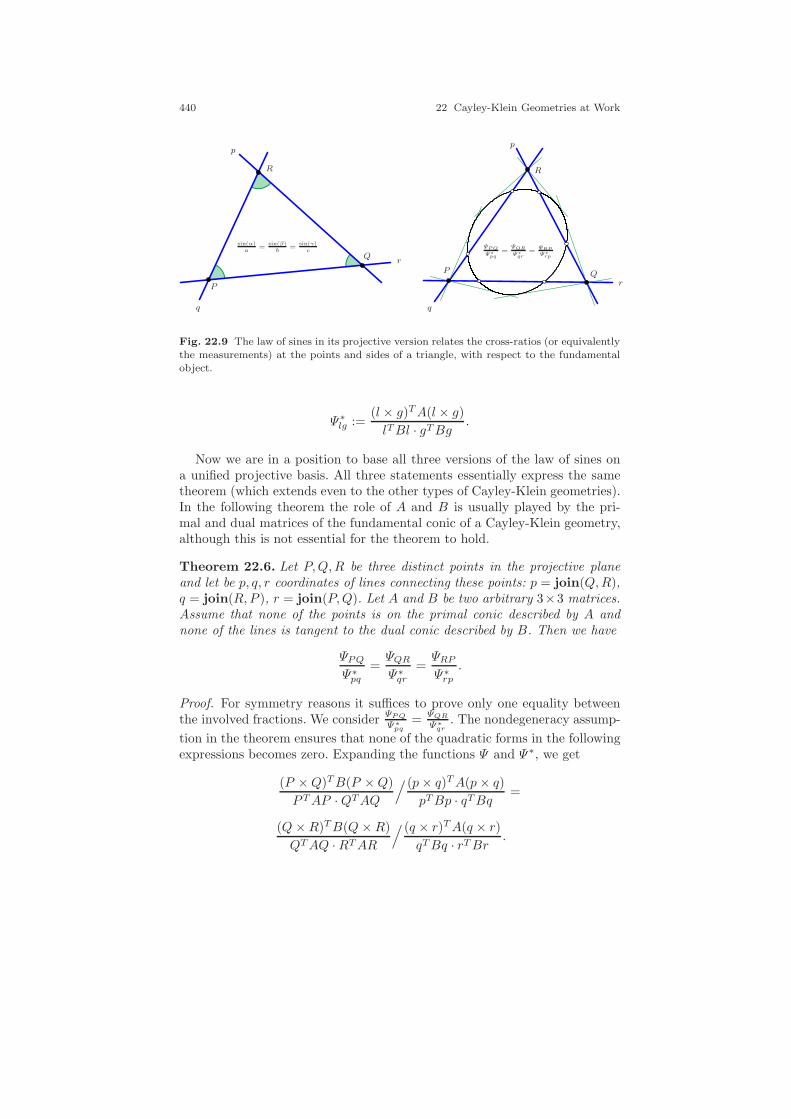
440 22 Cayley-Klein Geometries at Work
P
Q
R
p
q
r
sin(α)a
=sin(β)b
=sin(γ)c
P Q
R
p
q
r
ΨP Q
Ψ∗
pq=
ΨQR
Ψ∗
qr= ΨRP
Ψ∗
rp
Fig. 22.9 The law of sines in its projective version relates the cross-ratios (or equivalentlythe measurements) at the points and sides of a triangle, with respect to the fundamentalobject.
Ψ∗lg :=
(l × g)TA(l × g)
lTBl · gTBg .
Now we are in a position to base all three versions of the law of sines ona unified projective basis. All three statements essentially express the sametheorem (which extends even to the other types of Cayley-Klein geometries).In the following theorem the role of A and B is usually played by the pri-mal and dual matrices of the fundamental conic of a Cayley-Klein geometry,although this is not essential for the theorem to hold.
Theorem 22.6. Let P,Q,R be three distinct points in the projective planeand let be p, q, r coordinates of lines connecting these points: p = join(Q,R),q = join(R,P ), r = join(P,Q). Let A and B be two arbitrary 3×3 matrices.Assume that none of the points is on the primal conic described by A andnone of the lines is tangent to the dual conic described by B. Then we have
ΨPQΨ∗pq
=ΨQRΨ∗qr
=ΨRPΨ∗rp
.
Proof. For symmetry reasons it suffices to prove only one equality betweenthe involved fractions. We consider
ΨPQ
Ψ∗
pq=
ΨQR
Ψ∗
qr. The nondegeneracy assump-
tion in the theorem ensures that none of the quadratic forms in the followingexpressions becomes zero. Expanding the functions Ψ and Ψ∗, we get
(P ×Q)TB(P ×Q)
PTAP ·QTAQ/(p× q)TA(p× q)
pTBp · qTBq =
(Q×R)TB(Q×R)
QTAQ ·RTAR/ (q × r)TA(q × r)
qTBq · rTBr .
22.5 Trigonometry 441
Rewriting this into multiplicative form and canceling terms that occur on theleft and on the right, we are left with
(P ×Q)TB(P ×Q) · pTBp · RTAR · (q × r)TA(q × r) =
PTAP · (p× q)TA(p× q) · (Q×R)TB(Q×R) · rTBr.
Notice that each letter involved occurs equally often on the left and on theright of the equation. So multiplying any of them by a nonzero scalar factordoes not change the truth of the equation. Now we can use the fact that thereare certain incidence relations between the points and lines. We have
r = join(P,Q); R = meet(p, q); p = join(Q,R); P = join(q, r).
In fact, it is possible to choose the scaling of the homogeneous coordinatessuch that we have
r = P ×Q; R = p× q; p = Q×R; P = q × r.
We will encapsulate the proof of this nice little fact in a lemma after this proof.Inserting these relations into our above expression, we get the replacements
rT
︷ ︸︸ ︷(P ×Q)T B
r︷ ︸︸ ︷(P ×Q) ·pTBp ·RTAR ·
PT
︷ ︸︸ ︷(q × r)T A
P︷ ︸︸ ︷(q × r) =
PTAP · (p× q)T︸ ︷︷ ︸RT
A (p× q)︸ ︷︷ ︸R
· (Q×R)T︸ ︷︷ ︸pT
B (Q×R)︸ ︷︷ ︸p
·rTBr,
which leaves us with
rTBr · pTBp ·RTAR · PTAP = PTAP ·RTAR · pTBp · rTBr.
Obviously every quadratic form on the left occurs also on the right, whichproves the theorem. ⊓⊔
Although the proof contains quite a number of letters and symbols, thereader should be aware of the fact that it is structurally extremely simple.After the replacement of the crossproducts we have only a simple cancellationargument. In essence, it boils down to a strategy of the form, Formulate thetheorem in the appropriate form—see immediately that it is true. Further-more, the proved fact is by far more general than the usual law of sines. Iteven applies to matrices A and B that have nothing to do with each other.
Still we have to prove the little lemma required for the theorem.
Lemma 22.1. For three distinct points P,Q,R of a triangle and the threelines p, q, r supporting the sides, let
r = join(P,Q); R = meet(p, q); p = join(Q,R); P = join(q, r).
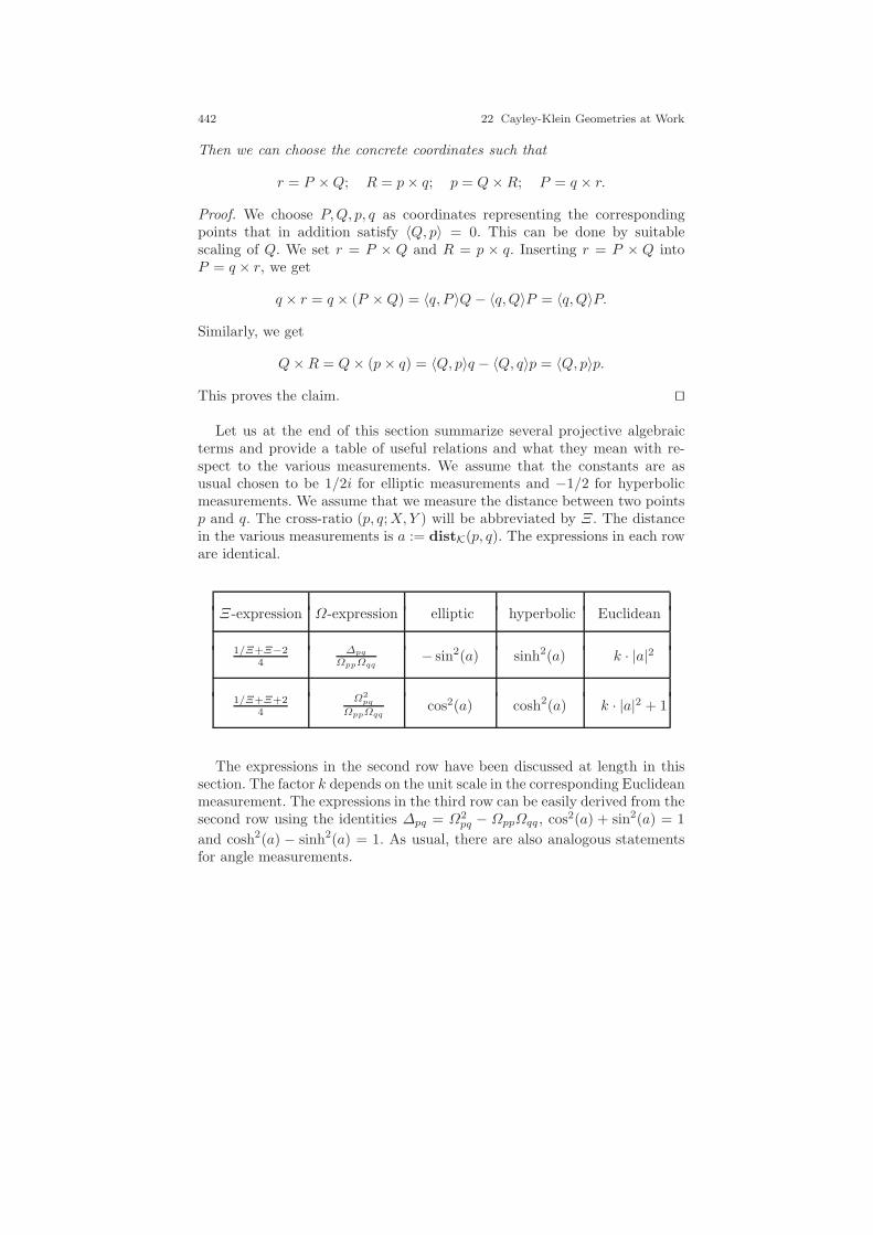
442 22 Cayley-Klein Geometries at Work
Then we can choose the concrete coordinates such that
r = P ×Q; R = p× q; p = Q×R; P = q × r.
Proof. We choose P,Q, p, q as coordinates representing the correspondingpoints that in addition satisfy 〈Q, p〉 = 0. This can be done by suitablescaling of Q. We set r = P × Q and R = p × q. Inserting r = P × Q intoP = q × r, we get
q × r = q × (P ×Q) = 〈q, P 〉Q− 〈q,Q〉P = 〈q,Q〉P.
Similarly, we get
Q×R = Q× (p× q) = 〈Q, p〉q − 〈Q, q〉p = 〈Q, p〉p.
This proves the claim. ⊓⊔
Let us at the end of this section summarize several projective algebraicterms and provide a table of useful relations and what they mean with re-spect to the various measurements. We assume that the constants are asusual chosen to be 1/2i for elliptic measurements and −1/2 for hyperbolicmeasurements. We assume that we measure the distance between two pointsp and q. The cross-ratio (p, q;X,Y ) will be abbreviated by Ξ. The distancein the various measurements is a := distK(p, q). The expressions in each roware identical.
Ξ-expression Ω-expression elliptic hyperbolic Euclidean
1/Ξ+Ξ−24
∆pq
ΩppΩqq− sin2(a) sinh2(a) k · |a|2
1/Ξ+Ξ+24
Ω2pq
ΩppΩqqcos2(a) cosh2(a) k · |a|2 + 1
The expressions in the second row have been discussed at length in thissection. The factor k depends on the unit scale in the corresponding Euclideanmeasurement. The expressions in the third row can be easily derived from thesecond row using the identities ∆pq = Ω2
pq − ΩppΩqq , cos2(a) + sin2(a) = 1
and cosh2(a) − sinh2(a) = 1. As usual, there are also analogous statementsfor angle measurements.

23
Circles and Cycles
Do not disturb my circles.
Archimedes of Syracuse(287–212 BCE)
Let us come to another interesting class of geometric objects: circles.Speaking about circles in general Cayley-Klein geometries first raises a con-ceptual issue. Euclidean circles have several geometric properties on whichone could base a more general definition. They are. . .
. . . objects of constant distance to a given point m—the circle’s center,
. . . objects that have the property that every incident point “sees” a givensegment with endpoints on the circle under the same (directed) angle,
. . . objects that admit a continuous group of isometries under which anypoint on the object can be mapped to any other.
At first sight it is not at all clear that these properties are all equivalent fordifferent Cayley-Klein geometries (in fact, they are not). So, what are rea-sonable properties on which one should base a general definition of a circle?Closely related to this question is, again, the problem of degenerate situa-tions.Questions like “Should one admit centers on the line at infinity?” “Howshould one deal with degenerate measurements?” arise naturally in this con-text. In fact, it turns out that (with a proper treatment of infinite radii)the above concepts are equivalent only for Euclidean and pseudo-Euclideangeometry. For different reasons these properties begin to diverge in all othergeometries. We here will again take a road that is on the pragmatic side andforms a compromise between conceptual understanding and easily accessibleconcrete calculational formulas. We first will stick mainly to the first property
443
444 23 Circles and Cycles
(constant distance to the center). At the end of this chapter we will discussalternative definitions and dedicate a short section to the subtleties of circlesin type-VII (Galilean) geometries.
23.1 Circles via Distances
So for now let us take the obvious definition and define circles to be objectsof constant distance to a given point m, the circle’s center. We start ourinvestigations by expressing this property in terms of the quadratic forms Aand B of the primal/dual pair of the fundamental conic F of the geometry. InSection 21.4 we showed that (also for degenerate measurements) the function
Ψpq :=(p× q)TB(p× q)
pTAp · qTAq (23.1)
is bijectively related to the distance between p and q: different values of Ψpqmean different distances and vice versa. Applying this to the case of circleswith center m, we see that a circle is the set of points p for which
(m× p)TB(m× p) = k ·mTAm · pTAp (23.2)
for some constant k. There is one important difference between the two formu-las (23.1) and (23.2). By rewriting (23.1) in the form (23.2) we have silentlydealt with the case of exceptional measurements between m and p. In (23.1)they lead simply to an undefined expression 0/0. In (23.2) they lead to equa-tions of the form 0 = 0, independently of the choice of k. Thus if m, isa proposed center and e is an exceptional point with respect to m then eautomatically lies on every circle around m. We know this effect from Eu-clidean geometry. The points I and J are exceptional with respect to everycenter m, their distance to any m is undetermined, and every circle passesthrough them. Depending on the fundamental conic F and on the positionof m relative to it, the exceptional points with respect to m may be real orcomplex.
Equation (23.2) imposes a quadratic condition on p. Thus in particular acircle (including the exceptional points with respect to m) is a special conic.We can make the quadratic condition more explicit if we rewrite the p ×moperator using matrix multiplication. For m = (x, y, z)T we set
M :=
0 z −y−z 0 xy −x 0
and get m× p = M · p (we used this trick already in Section 11.1). Therebyand with k′ = k ·mTAm, equation (23.2) becomes

23.1 Circles via Distances 445
pTMTBMp = k′ · pTAp.
Equivalently for suitable λ and µ we can rewrite this equation as
pT (λ ·MTBM + µ · A)︸ ︷︷ ︸Cλ,µ
p = 0.
The λ, µ notion has the advantage that (as commonly in projective geom-etry) we can also deal with the case k′ = ∞ in a clean way. The matrixCλ,µ represents the quadratic form of the circle. The circles with center mare parameterized by the homogeneous coordinates (λ, µ). We get two ex-treme situations C1,0 = MTBM and C0,1 = A. The first quadratic formpTC1,0p = pTMTBMp = 0 encodes the geometric condition that the linep ×m is tangent to the fundamental conic. For the other extreme situationthe equation pTC0,1p = pTAp = 0 simply says that p is on the fundamentalconic. It is illustrative to analyze the corresponding radii for these extremesituations. We have to do this for degenerate and non-degenerate distancemeasurement separately.
If the measurement is degenerate, we have seen at the end of Section 21.4that Ψmp itself is (up to a scalar normalization factor) the squared distancemeasure. For a point with pTMTBMp = 0 the numerator of Ψmp becomeszero. Thus the circle represented by C1,0 is a circle with radius 0. For apoint with pTAp = 0 the denominator of Ψmp becomes zero. Thus the circlerepresented by C0,1 is a circle with radius 1/0 = ∞.
The situation is the same in the nondegenerate case, although there thereasoning is slightly different. For a point p on pTMTBMp = 0 the linejoin(m, p) is tangent to the fundamental conic. Thus the distance measure-ment is degenerate, since X and Y will coincide and we get a distance ofzero. A point p with pTAp = 0 is on the fundamental conic. Thus it coincideswith X or Y and the distance measurement will become infinite.
In both cases the different circles Cλ,µ with center m can be considered alinear interpolation between a circle with zero radius and a circle with infiniteradius around m. If, for instance, we want to create a circle with center mand through a given point p, then we can calculate its coordinates by theusual Plucker’s µ trick and obtain immediately the following result:
Theorem 23.1. Let K be a Cayley-Klein geometry and let m be a point noton the fundamental conic of K. Let p be an arbitrary point not on the funda-mental conic. Then the set of all points q having the same distance to m asp united with the points exceptional with respect to m is a conic given by thequadratic equation qTXq = 0 with
X = (pTAp) ·MTBM − (pTMTBMp) ·A.
Proof. Let k be the constant such that
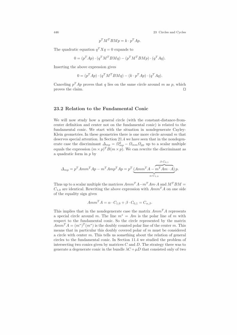
446 23 Circles and Cycles
pTMTBMp = k · pTAp.
The quadratic equation qTXq = 0 expands to
0 = (pTAp) · (qTMTBMq) − (pTMTBMp) · (qTAq).
Inserting the above expression gives
0 = (pTAp) · (qTMTBMq) − (k · pTAp) · (qTAq).
Canceling pTAp proves that q lies on the same circle around m as p, whichproves the claim. ⊓⊔
23.2 Relation to the Fundamental Conic
We will now study how a general circle (with the constant-distance-from-center definition and center not on the fundamental conic) is related to thefundamental conic. We start with the situation in nondegenerate Cayley-Klein geometries. In these geometries there is one more circle around m thatdeserves special attention. In Section 21.4 we have seen that in the nondegen-erate case the discriminant ∆mp = Ω2
mp − ΩmmΩpp up to a scalar multiple
equals the expression (m× p)TB(m× p). We can rewrite the discriminant asa quadratic form in p by
∆mp = pTAmmTAp−mTAmpTAp = pT (AmmTA−
β·C0,1︷ ︸︸ ︷mTAm · A)︸ ︷︷ ︸
α·C1,0
p.
Thus up to a scalar multiple the matricesAmmTA−mTAm·A andMTBM =C1,0 are identical. Rewriting the above expression with AmmTA on one sideof the equality sign gives
AmmTA = α · C1,0 + β · C0,1 = Cα,β .
This implies that in the nondegenerate case the matrix AmmTA representsa special circle around m. The line m∗ = Am is the polar line of m withrespect to the fundamental conic. So the circle represented by the matrixAmmTA = (m∗)T (m∗) is the doubly counted polar line of the center m. Thismeans that in particular this doubly covered polar of m must be considereda circle with center m. This tells us something about the relation of generalcircles to the fundamental conic. In Section 11.4 we studied the problem ofintersecting two conics given by matrices C and D. The strategy there was togenerate a degenerate conic in the bundle λC+µD that consisted only of two
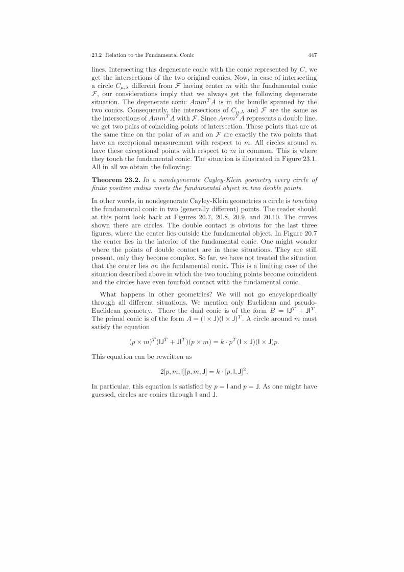
23.2 Relation to the Fundamental Conic 447
lines. Intersecting this degenerate conic with the conic represented by C, weget the intersections of the two original conics. Now, in case of intersectinga circle Cµ,λ different from F having center m with the fundamental conicF , our considerations imply that we always get the following degeneratesituation. The degenerate conic AmmTA is in the bundle spanned by thetwo conics. Consequently, the intersections of Cµ,λ and F are the same asthe intersections of AmmTA with F . Since AmmTA represents a double line,we get two pairs of coinciding points of intersection. These points that are atthe same time on the polar of m and on F are exactly the two points thathave an exceptional measurement with respect to m. All circles around mhave these exceptional points with respect to m in common. This is wherethey touch the fundamental conic. The situation is illustrated in Figure 23.1.All in all we obtain the following:
Theorem 23.2. In a nondegenerate Cayley-Klein geometry every circle offinite positive radius meets the fundamental object in two double points.
In other words, in nondegenerate Cayley-Klein geometries a circle is touchingthe fundamental conic in two (generally different) points. The reader shouldat this point look back at Figures 20.7, 20.8, 20.9, and 20.10. The curvesshown there are circles. The double contact is obvious for the last threefigures, where the center lies outside the fundamental object. In Figure 20.7the center lies in the interior of the fundamental conic. One might wonderwhere the points of double contact are in these situations. They are stillpresent, only they become complex. So far, we have not treated the situationthat the center lies on the fundamental conic. This is a limiting case of thesituation described above in which the two touching points become coincidentand the circles have even fourfold contact with the fundamental conic.
What happens in other geometries? We will not go encyclopedicallythrough all different situations. We mention only Euclidean and pseudo-Euclidean geometry. There the dual conic is of the form B = IJ
T + JIT .
The primal conic is of the form A = (I × J)(I × J)T . A circle around m mustsatisfy the equation
(p×m)T (IJT + JIT )(p×m) = k · pT (I × J)(I × J)p.
This equation can be rewritten as
2[p,m, I][p,m, J] = k · [p, I, J]2.
In particular, this equation is satisfied by p = I and p = J. As one might haveguessed, circles are conics through I and J.
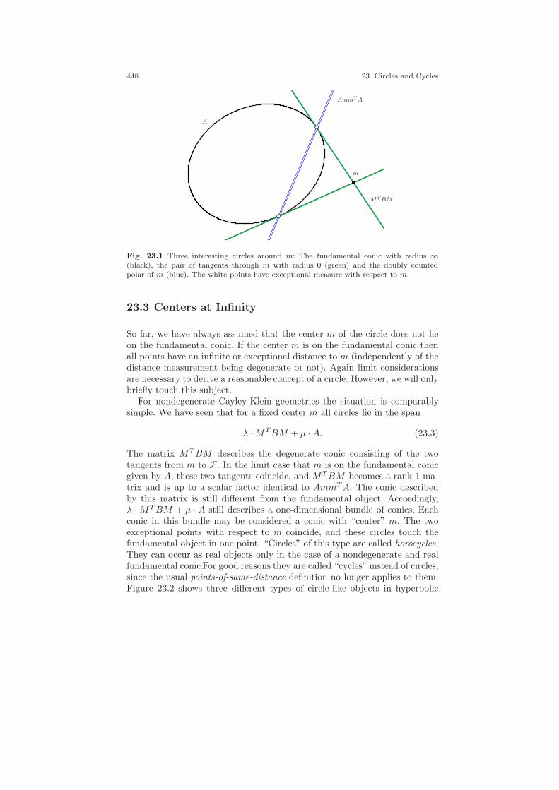
448 23 Circles and Cycles
m
A
MTBM
AmmTA
Fig. 23.1 Three interesting circles around m: The fundamental conic with radius ∞(black), the pair of tangents through m with radius 0 (green) and the doubly countedpolar of m (blue). The white points have exceptional measure with respect to m.
23.3 Centers at Infinity
So far, we have always assumed that the center m of the circle does not lieon the fundamental conic. If the center m is on the fundamental conic thenall points have an infinite or exceptional distance to m (independently of thedistance measurement being degenerate or not). Again limit considerationsare necessary to derive a reasonable concept of a circle. However, we will onlybriefly touch this subject.
For nondegenerate Cayley-Klein geometries the situation is comparablysimple. We have seen that for a fixed center m all circles lie in the span
λ ·MTBM + µ · A. (23.3)
The matrix MTBM describes the degenerate conic consisting of the twotangents from m to F . In the limit case that m is on the fundamental conicgiven by A, these two tangents coincide, and MTBM becomes a rank-1 ma-trix and is up to a scalar factor identical to AmmTA. The conic describedby this matrix is still different from the fundamental object. Accordingly,λ ·MTBM + µ · A still describes a one-dimensional bundle of conics. Eachconic in this bundle may be considered a conic with “center” m. The twoexceptional points with respect to m coincide, and these circles touch thefundamental object in one point. “Circles” of this type are called horocycles.They can occur as real objects only in the case of a nondegenerate and realfundamental conic.For good reasons they are called “cycles” instead of circles,since the usual points-of-same-distance definition no longer applies to them.Figure 23.2 shows three different types of circle-like objects in hyperbolic

23.3 Centers at Infinity 449
m1m2
m3
F
p
Fig. 23.2 Three types of hyperbolic cycles. A circle (blue), a horocycle (red), and ahypercycle (green).
geometry (the general term is cycle). The blue object is a usual circle. Thecorresponding center m1 lies inside the fundamental conic. All points on thecircle have real distance to the center. The circle has no real intersectionswith the fundamental conic. The red cycle is a horocycle. There the two con-tact points with the fundamental conic coincide. This means that it touchesthe fundamental conic of order 4. The center m2 lies on (!) the cycle. Allpoints of the cycle have an infinite distance to the center. However, this isno longer a characterizing property for them. Finally, the green cycle is a so-called hypercycle. Its center m3 is outside the fundamental conic. It touchesthe fundamental conic in the two points that have exceptional measure withrespect to m3. All points on the hypercycle have complex distance to thecenter.
The situation is slightly more complicated in the case of Euclidean orpseudo-Euclidean geometry. We study the situation in the standard embed-ding of Euclidean; geometry, the situation for pseudo-Euclidean geometry isanalogous. The fundamental conic and a point m = (a, b, c)T are given by
m =
abc
, A =
0 0 00 0 00 0 1
, and B =
1 0 00 1 00 0 0
.
We get
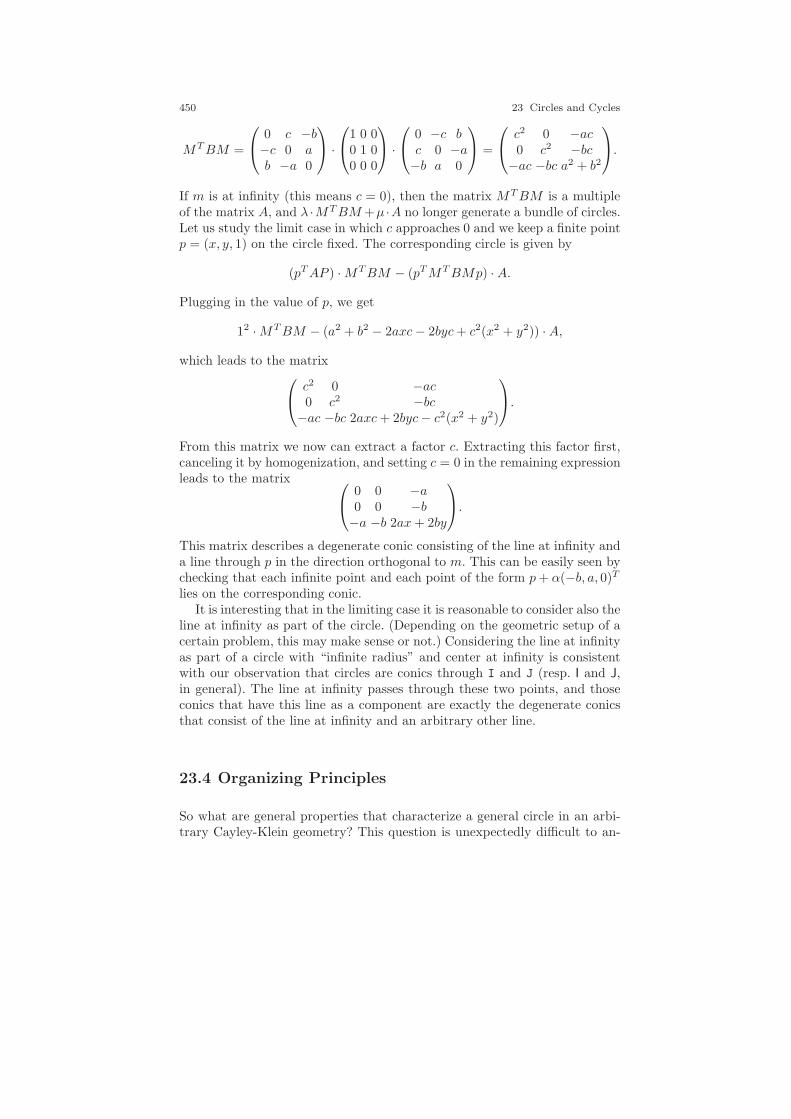
450 23 Circles and Cycles
MTBM =
0 c −b−c 0 ab −a 0
·
1 0 00 1 00 0 0
·
0 −c bc 0 −a−b a 0
=
c2 0 −ac0 c2 −bc
−ac −bc a2 + b2
.
If m is at infinity (this means c = 0), then the matrix MTBM is a multipleof the matrix A, and λ ·MTBM +µ ·A no longer generate a bundle of circles.Let us study the limit case in which c approaches 0 and we keep a finite pointp = (x, y, 1) on the circle fixed. The corresponding circle is given by
(pTAP ) ·MTBM − (pTMTBMp) · A.
Plugging in the value of p, we get
12 ·MTBM − (a2 + b2 − 2axc− 2byc+ c2(x2 + y2)) ·A,
which leads to the matrixc2 0 −ac0 c2 −bc
−ac −bc 2axc+ 2byc− c2(x2 + y2)
.
From this matrix we now can extract a factor c. Extracting this factor first,canceling it by homogenization, and setting c = 0 in the remaining expressionleads to the matrix
0 0 −a0 0 −b−a −b 2ax+ 2by
.
This matrix describes a degenerate conic consisting of the line at infinity anda line through p in the direction orthogonal to m. This can be easily seen bychecking that each infinite point and each point of the form p+ α(−b, a, 0)T
lies on the corresponding conic.It is interesting that in the limiting case it is reasonable to consider also the
line at infinity as part of the circle. (Depending on the geometric setup of acertain problem, this may make sense or not.) Considering the line at infinityas part of a circle with “infinite radius” and center at infinity is consistentwith our observation that circles are conics through I and J (resp. I and J,in general). The line at infinity passes through these two points, and thoseconics that have this line as a component are exactly the degenerate conicsthat consist of the line at infinity and an arbitrary other line.
23.4 Organizing Principles
So what are general properties that characterize a general circle in an arbi-trary Cayley-Klein geometry? This question is unexpectedly difficult to an-

23.4 Organizing Principles 451
swer, since it depends a bit on the point of view and the properties that onewants to generalize. We will discuss here only some approaches and collect afew general properties that all cycles (this is what we will call the generaliza-tions of circles) should have. Some of the issues will be touched only briefly,since they are closely related to differential geometry and we do not want todevelop here the necessary differential-geometric machinery. In what follows,we will use the more general name cycle for circle-like objects and reserve theword circle strictly for the points-with-contant-distance-to-center definition.
Cycles as limiting cases: We have seen that in the nondegenerate cases(geometries of type I and type II and finite center) it is clear what a circleshould look like. It is the set of all points having a fixed distance from thecenter m together with the points that have exceptional measure with respectto m, or in algebraic terms the points p that satisfy the equation
pTMTBMp = k · pTAp.
Perhaps the most reasonable definition for a general cycle is to say thatthese are all objects that arise as a continuous limit case of a sequence ofnondegenerate circles. During the limiting process the matrices A and Bmay approach the matrices of a degenerate Cayley-Klein geometry and/orthe point m may approach a position on the fundamental conic.
One might wonder why there is any difficulty at all, since we alreadycharacterized circles with infinitely distant centers in Section 23.3 for differentgeometries and from there derived general definitions of a cycle in these cases.We obtained there:
• In hyperbolic and elliptic geometry circles are conics that have tangentialcontact with the fundamental conic in two points (that may be complex).If the center is on the fundamental conic, these points of contact maycoincide and generate an osculation of order four.
• In Euclidean and pseudo-Euclidean geometry cycles are conics throughI and J, the two special points on the (degenerate) fundamental conic.This definition also covers the case of an infinitely distant center. Then thecycle degenerates into two lines one of which is the (primal) fundamentalconic itself.
One can prove (we will not do this here) that by these characterizationsall limiting cases in these geometries are properly covered. So all that isleft is the case of dual Euclidean and dual pseudo-Euclidean geometry andthe case of doublydegenerate (Galilean) geometry. In fact, the definition fordual Euclidean and dual pseudo-Euclidean geometry can be easily dealt withby dualizing the second of the above characterizations (we will see this in aminute). However, in the case of Galilean geometry the concepts of circles andcycles break apart seriously. We will come back to this issue in Section 23.5in some detail. But we will now at least roughly state what happens.
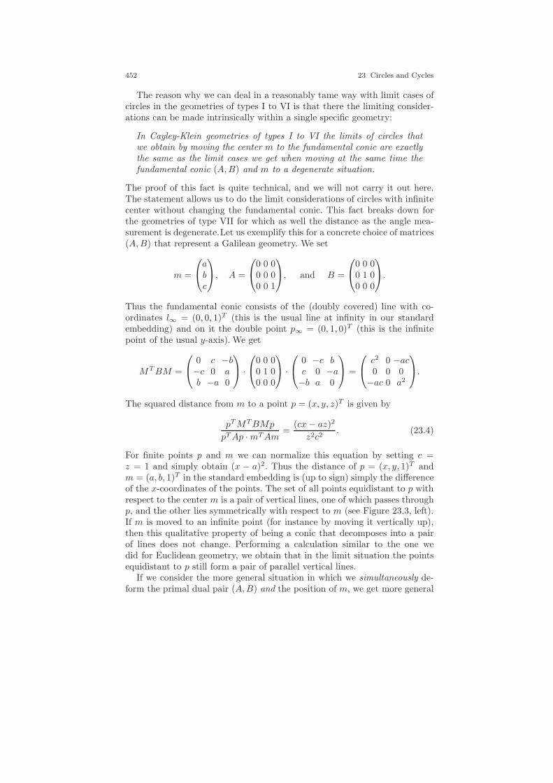
452 23 Circles and Cycles
The reason why we can deal in a reasonably tame way with limit cases ofcircles in the geometries of types I to VI is that there the limiting consider-ations can be made intrinsically within a single specific geometry:
In Cayley-Klein geometries of types I to VI the limits of circles thatwe obtain by moving the center m to the fundamental conic are exactlythe same as the limit cases we get when moving at the same time thefundamental conic (A,B) and m to a degenerate situation.
The proof of this fact is quite technical, and we will not carry it out here.The statement allows us to do the limit considerations of circles with infinitecenter without changing the fundamental conic. This fact breaks down forthe geometries of type VII for which as well the distance as the angle mea-surement is degenerate.Let us exemplify this for a concrete choice of matrices(A,B) that represent a Galilean geometry. We set
m =
abc
, A =
0 0 00 0 00 0 1
, and B =
0 0 00 1 00 0 0
.
Thus the fundamental conic consists of the (doubly covered) line with co-ordinates l∞ = (0, 0, 1)T (this is the usual line at infinity in our standardembedding) and on it the double point p∞ = (0, 1, 0)T (this is the infinitepoint of the usual y-axis). We get
MTBM =
0 c −b−c 0 ab −a 0
·
0 0 00 1 00 0 0
·
0 −c bc 0 −a−b a 0
=
c2 0 −ac0 0 0
−ac 0 a2
.
The squared distance from m to a point p = (x, y, z)T is given by
pTMTBMp
pTAp ·mTAm=
(cx− az)2
z2c2. (23.4)
For finite points p and m we can normalize this equation by setting c =z = 1 and simply obtain (x − a)2. Thus the distance of p = (x, y, 1)T andm = (a, b, 1)T in the standard embedding is (up to sign) simply the differenceof the x-coordinates of the points. The set of all points equidistant to p withrespect to the center m is a pair of vertical lines, one of which passes throughp, and the other lies symmetrically with respect to m (see Figure 23.3, left).If m is moved to an infinite point (for instance by moving it vertically up),then this qualitative property of being a conic that decomposes into a pairof lines does not change. Performing a calculation similar to the one wedid for Euclidean geometry, we obtain that in the limit situation the pointsequidistant to p still form a pair of parallel vertical lines.
If we consider the more general situation in which we simultaneously de-form the primal dual pair (A,B) and the position of m, we get more general

23.4 Organizing Principles 453
m
p
dd
Fig. 23.3 A Galilean circle vs. a Galilean cycle.
conics. For this we consider a primal/dual pair of matrices
A =
0 0 00 0 00 0 1
and B =
k 0 00 1 00 0 0
.
If the parameter k traverses the interval [−1, 1], we move continuously fromthe situation of pseudo-Euclidean geometry (k < 0) via the degenerate caseof Galilean geometry (k = 0) to the Euclidean case (k > 0). The points I
and J are the solutions of k · x2 + y2 = 0 and z = 0. In the first situationI and J are real. In the process of deformation they approach each other.They coincide for k = 0 with I = J = (0, 1, 0)T = p∞, and branch off ascomplex conjugates when k enters the positive region. We now consider thesituation of a circle through three finite points p, q, r. We could make theeffort to perform the rather tedious explicit calculation, but we may alsoargue directly in geometric terms. For each choice of k 6= 0 the correspondingcircle is the unique conic through the five points p, q, r, I, J. Throughout thedeformation process the line join(I, J) stably remains l∞ = (0, 0, 1)T , theprimal fundamental conic. In the limiting case k = 0 the points I and J
coincide, and the conic through the five points becomes a conic throughp, q, r and p∞ = I = J tangent to l∞. Figure 23.4 illustrates this passage forthe situation in which l∞ and p∞ were moved to finite positions. The middlepicture corresponds to the case of Galilean geometry. If, as in our originalchoice of the fundamental conic, l∞ = (0, 0, 1)T and p∞ = (0, 1, 0)T , thenin the pseudo-Euclidean case cycles look like (usual) hyperbolas, since theyintersect l∞ twice. In the Euclidean case they look like (usual) ellipses, sincethey do not intersect l∞, and in the Galilean case they look like parabolasof the form y = β(x − α)2 + γ, since they touch l∞ at the point p∞. Thus

454 23 Circles and Cycles
p q
r
p∞
I J
p q
r
I = J = p∞
p q
r
p∞
Fig. 23.4 Limiting case for a Galilean cycle.
each parabola with vertical symmetry axis corresponds to a cycle of Galileangeometry. As special limiting cases we here again get degenerate parabolasthat either consist of two vertical lines (these are the circles) or consist of l∞and an arbitrary other line. Figure 23.3 (right) shows one possible cycle.
One might wonder what these general parabola-shaped cycles have to dowith ordinary circles in Galilean geometry. For instance, one might be in-terested in the question, “where is the center?” In fact, a careful analysisshows what happens to the center: it moved to the position p∞, and indeedthis point has the same distance to all points of a parabola. The distanceis infinite. However, this is no longer a characterizing property. Later, inSection 23.5, we will learn about other surprising (and more illuminating)properties that are shared by a circle and a parabola.
Duality of circles: We now want to highlight another property of generalcycles. The attribute of being a circle carries some nice duality properties.Knowing only about Euclidean geometry, these duality properties are usuallyobscured by the fact that the fundamental conics of this geometry is not self-dual. The duality properties are best observed in self-dual geometries wherethe primal and dual fundamental conic have the same degree of degeneracy(these are hyperbolic, elliptic, and Galilean geometry). So let us start ourinvestigations with the definition of a usual (nondegenerate) circle and dualizeit word by word.
Primal: A circle is a curve consisting of all points that have a fixedconstant distance to a given center.
Dual: A dual circle is a curve all of whose tangents have a fixed constantangle to a given line.
At first sight it is not evident whether and if so how these primal anddual circles are related. It turns out that for nondegenerate geometries bothdefinitions describe exactly the same class of objects. For every circle we finda suitable line with respect to which it is a dual circle. We can even be morespecific. If m is the center of the circle, then its dual m∗ = Am with respectto the fundamental conic of the geometry is the line that appears in the dualcircle definition. By switching to algebraic terms we may right away includethe case of circles with infinite radius. The following theorem formalizes this

23.4 Organizing Principles 455
m
m∗
α
m
m∗
α
Fig. 23.5 The (oriented) angle of tangents to a circle with the polar of the center isconstant.
duality. We recall that for nondegenerate geometries the matrix of a circlewith center m can be written as a linear combination α ·AmmTA+ β ·A. Acircle with infinite radius corresponds to (α, β) = (0, 1). Analogously, a dualcircle can be described by a linear combination α′ ·B(m∗)(m∗)TB + β′ ·B.
Theorem 23.3. Let (A,B) be the primal/dual pair of a nondegenerate Cayley-Klein geometry. Let m be a point and let X = α · AmmTA + β · A be thematrix representing a circle with center m. Then the line m∗ = Am has theproperty that for suitable α′, β′ the matrix X ′ := α′ ·BmmTB+β′ ·B satisfiesX ·X ′ = µE for some parameter µ (and hence X ′ describes a conic dual tothe circle X).
Proof. We prove this theorem by directly multiplying X and X ′, therebyderiving conditions for α′ and β′. Since we are in the nondegenerate case, wemay without loss of generality assume that B = A−1. We thus havem∗ = Amand m = Bm∗. The matrices X and X ′ may be rewritten as
X = α(m∗)(m∗)T + βA and X ′ = α′mmT + β′A−1.
The case (α, β) = (0, 1) immediately leads to the condition (α′, β′) = (0, 1).Since only the ratio of the parameter pair (α, β) is relevant, we can (in orderto deal with the remaining cases) without loss of generality set α = 1. Thefollowing calculation shows that we find a suitable pair (α′, β′) also for α′ = 1.In this case we get

456 23 Circles and Cycles
X ·X ′ = ((m∗)(m∗)T + βA) · (mmT + β′A−1)
= (m∗)(m∗)TmmT + βAmmT + β′(m∗)(m∗)TA−1 + ββ′AA−1
= ((m∗)Tm)(m∗)mT + β(m∗)mT + β′(m∗)mT + ββ′E
= ((m∗)Tm+ β + β′)︸ ︷︷ ︸=:0
(m∗)mT + ββ′E.
The condition (m∗)Tm + β + β′ = 0 can be easily satisfied by settingβ′ = −β − mTAm. Thus (α′, β′) = (1,−β − mTAm) is the choice whoseexistence is claimed by the theorem. ⊓⊔
This theorem also implies that the tangents to a circle form a constantangle with the polar of the center of the circle. Figure 23.5 illustrates thistheorem for a hyperbolic circle (left) and for an elliptic circle (right). Theelliptic picture is as usual represented on the sphere that is a double cover ofthe projective plane. There the theorem becomes an almost obvious geometricfact. The figure consisting of the center, the circle, and the polar of the centerforms an object that has a rotational symmetry whose axis is the line joiningthe two antipodal representations of the center. Any tangents to the circlecan be moved into each other by a simple rotation around this axis. Thus theangle under which they meet the polar must be constant, since it remainsinvariant under the continuous rotation.
What happens to this duality relation in Euclidean geometry? The polarof any finite point is the line at infinity.Every finite line cuts the line at infinityunder the constant angle π/2. Thus in particular, all tangents to a circle cutthe polar of the center under this angle. Unfortunately, the situation is verydegenerate. This has the consequence that the definition of a dual cycle by alltangents having a fixed angle with respect to a line describes only pathologicalsituations. If the line is finite, then all lines cutting this line at a constantangle form a bundle of parallels. The conic that has those tangents consistsof a single point at infinity. If it is the line at infinity, the only angle thatmay occur is π/2. Thus the bundle of lines meeting at this angle consists ofall finite lines and does no longer describe the tangents of a conic. The samereasoning applies to pseudo-Euclidean geometry.
Our last consideration also tells us something important about cycles indual Euclidean or dual pseudo-Euclidean geometry. There the primal defini-tion via centers contains only pathological examples. In these geometries itis more reasonable to base the definition of a cycle on the dual situation andto prefer “midlines” to centers.
Curves of constant curvature: Here comes another definition of a cyclethat one often finds in the literature.
In any geometry a cycle is a curve of constant curvature.

23.4 Organizing Principles 457
m1m2
m3
F
p
Fig. 23.6 Bicycling with constant curvature.
Curvature is a notion related to differential geometry. Roughly speaking, fora smooth curve it describes the amount of turn at each point while the curveis traversed. If you have a constant turn while you traverse, you will travelon a cycle. A good way of imagining local curvature is to assume that thecurve is a road that you travel on a bicycle. The amount of local curvaturecorresponds to the angle of your handlebar at each moment. If you fix thehandlebar of your bicycle at a certain angle, you will travel along a circularpath. This includes the limiting case of fixing the handlebar at a straightposition (frontwheel aligned to rearwheel) that takes you on a straight linearroad.
In contrast to our previous characterizations, the cycle definition via cur-vature does not a priori state the existence of a center (or a midline), nor doesit state that the resulting curve has the shape of a conic. It uses only localdifferential properties, and the concrete shape and the existence of centerscan be derived as secondary properties. However, one has to be very careful,since this local definition introduces some subtle (but extremely important)differences to the concepts we introduced in our previous sections. Very oftenin the literature these differences are overlooked or ignored leading to partialmisunderstandings, at least for the novice in the field. Since we here do notwant to develop all the necessary tools from differential geometry, we explainthese differences on a more phenomenological level.
Compared to our more algebraic language, this more local differential ge-ometric approach has some remarkable differences. They already become vis-ible in Euclidean geometry. For the special case of a handlebar fixed in thestraight position this definition gives us the line as a cycle, but does not con-tain the line at infinity as a component. The situation becomes more drastic

458 23 Circles and Cycles
in hyperbolic geometry. For this we refer to Figure 23.6 (this figure is veryclosely related to Figure 23.2, in which we described the qualitatively differenttypes of circles). Imagine you start your bicycling trip at point p. You mayfix your handlebar at a position that gives you just the right amount of turnto traverse the blue circle. What will happen? With this fixed curvature youwill traverse the blue circle round and round. You may start again this timefixing the handlebar to traverse the red curve (the horocycle). What will hap-pen? While you traverse the curve you will get closer and closer to the pointwhere the horocycle touches the fundamental conic. However, you will neverreach it, since in the metric of the corresponding Cayley-Klein geometry thepath to this point has infinite length. If we look at the situation “from theoutside,” your bike seems to shrink as it approaches the boundary (like thefishes in an Escher circle limit picture). You yourself will never recognize thisshrinking process, since during your trip all parts of the environment (trees,houses, your eye, your brain) will shrink as well in the same proportionalamount. By starting from point p in the opposite direction with the sameturning angle you may still traverse the other part of the curve that is belowpoint p. Although the red curve is still connected in the inner topology ofyour habitat, it is topologically different from the blue circle. It seems like aline infinite in both directions. The situation becomes even more drastic whenyou travel along the green curve. Again you will never be able to tour beyondthe points where the green curve touches the fundamental conic. However,this time this prevents you from reaching a whole part of the green curve.The segment (dimmed green) between the two touching points that does notcontain p is not reachable by traveling on a curve with constant curvature.Similarly, if you started on this dimmed green part you would never by ableto reach the other part by traveling with the corresponding constant curva-ture. If we define a cycle via the local curvature property, we must considerthe green curve as two different unconnected cycles. In our algebraic setupwe treated it as one cycle, since both branches lie on the same conic. We willreturn to this issue later when we speak about hyperbolic geometry.
We will briefly mention that the effect we just explained is also very muchrelated to generating circular shapes by a sequence of iterated reflections. Ifyou look back at Figure 21.9, you observe that the feet of Dr. Stickler in thehall of mirrors stand on a circular path. If the two mirror axes meet insidethe fundamental conic, this path will be a full circle. If they meet outside,then the mirror images will appear on only one branch of the cycle. We mayconsider the transformations of the green copies of Dr. Stickler as a kind ofdiscrete version of the bicycle metaphor. To get from one green copy to thenext, Dr. Stickler must take a step of constant width and then turn aroundby a constant angle.1
1 In a sense, this is a kind of Cayley-Klein-turtle-graphics: move forward—turn—moveforward—turn—move forward—turn—. . .
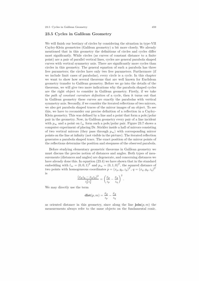
23.5 Cycles in Galilean Geometry 459
23.5 Cycles in Galilean Geometry
We will finish our bestiary of circles by considering the situation in type-VIICayley-Klein geometries (Galilean geometry) a bit more closely. We alreadymentioned that in this geometry the definitions of circles and cycles differmost significantly. While circles (as curves of constant distance to a finitepoint) are a pair of parallel vertical lines, cycles are general parabola shapedcurves with vertical symmetry axis. There are significantly more cycles thancircles in this geometry. The general equation of such a parabola has threefree parameters; the circles have only two free parameters. Furthermore (ifwe include limit cases of parabolas), every circle is a cycle. In this chapterwe want to show how several theorems that are well known for Euclideangeometry transfer to Galilean geometry. Before we go into the details of thetheorems, we will give two more indications why the parabola shaped cyclesare the right object to consider in Galilean geometry. Firstly, if we takethe path of constant curvature definition of a cycle, then it turns out thatin Galilean geometry these curves are exactly the parabolas with verticalsymmetry axis. Secondly, if we consider the iterated reflections of two mirrors,we also get parabola shaped traces of the mirror images of an object. To seethis, we have to reconsider our precise definition of a reflection in a Cayley-Klein geometry. This was defined by a line and a point that form a pole/polarpair in the geometry. Now, in Galilean geometry every pair of a line incidentwith p∞ and a point on l∞ form such a pole/polar pair. Figure 23.7 shows acomputer experiment of placing Dr. Stickler inside a hall of mirrors consistingof two vertical mirrors (they pass through p∞) with corresponding mirrorpoints on the line at infinity (not visible in the picture). The iterated reflectiongenerates a parabola shaped trace. The exact position of the mirror points ofthe reflections determine the position and steepness of the observed parabola.
Before studying elementary geometric theorems in Galilean geometry wemust discuss the precise notion of distances and angles. Both types of mea-surements (distances and angles) are degenerate, and concerning distances wehave already done this. In equation (23.4) we have shown that in the standardembedding with l∞ = (0, 0, 1)T and p∞ = (0, 1, 0)T , the squared distance oftwo points with homogeneous coordinates p = (xp, yp, zp)
T , q = (xq , yq, zq)T
is(xpzq − xqzp)
2
z2pz
2q
=
(xpzp
− xqzq
)2
.
We may directly use the term
dist(p,m) =xpzp
− xqzq
as oriented distance in this geometry, since along the line join(p,m) themeasurements always refer to the same objects on the fundamental conic.

460 23 Circles and Cycles
Fig. 23.7 Dr. Stickler in a Galilean mirror cabinet.
Since the fundamental conic is self-dual (point p∞ incident to line l∞) weget a corresponding formula for angles between lines. If l = (al, bl, cl) andg = (ag, bg, cg) are given, then a similar calculation shows that the (oriented)angle is
ang(l, g) =albl
− agbg.
Bearing in mind that in the standard embedding the line l has the equationx · al + y · bl + cl = 0, which (if l is nonvertical) is equivalent to
y = −albl
· x− clbl,
we see that (up to a sign change) the Galilean angle of two lines is justthe difference of their slopes. Since Galilean geometry is a rather degenerateenvironment, the distance and angle measurement turn out to be performablewithout much calculation. For the moment we may make our life a littleeasier and strip off our projective framework and directly express Galileanmeasurements in unusual R2 coordinates. For this we will simply ignore pointsat infinity (i.e., points on l∞), and ignore vertical lines (i.e., lines throughp∞)as well. 2. In this simplified framework the points p and q are given bythe two-dimensional coordinates p = (xp, yp) and q = (xq, yq). The lines land g are represented by equations y = kl · x + rl and y = kg · x + rg. Theformulas for distance and included angle then simply become
2 In a sense, we are dealing for a moment with Galilean geometry in the same way wedealt with Euclidean geometry before projective geometry was invented.
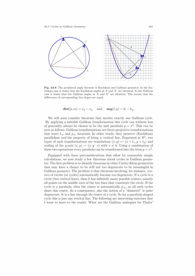
23.5 Cycles in Galilean Geometry 461
AB
X
X′
α
α
A
B
X
X′
12
−1
1
− 12
Fig. 23.8 The peripheral angle theorem in Euclidean and Galilean geometry. In the Eu-clidean case it states that the Euclidean angles at X and X′ are identical. In the Galileancase it states that the Galilean angles at X and X′ are identical. This means that thedifferences of corresponding line slopes are equal.
dist(p,m) = xp − xq and ang(l, g) = kl − kg.
We will soon consider theorems that involve exactly one Galilean cycle.By applying a suitable Galilean transformation this cycle can without loss
of generality always be chosen to be the unit parabola y = x2. This can beseen as follows. Galilean transformations are those projective transformationsthat leave l∞ and p∞ invariant. In other words, they preserve (Euclidean)parallelism and the property of being a vertical line. Expressed in R2, twotypes of such transformations are translations (x, y) 7→ (x + tx, y + ty) andscaling of the y-axis (x, y) 7→ (x, y · s) with s 6= 0. Using a combination ofthese two operations every parabola can be transformed into the form y = x2.
Equipped with these preconsiderations that allow for reasonably simplecalculations, we now study a few theorems about cycles in Galilean geome-try. The first problem is to identify theorems in other Cayley-Klein geometriesthat may have a chance to be still not too degenerate to be meaningful inGalilean geometry. The problem is that theorems involving, for instance, cen-ters of circles (or cycles) automatically become too degenerate. If a cycle is acircle (two vertical lines), then it has infinitely many possible centers, namelyall points on the middle axes of the two lines that constitute the circle. If thecycle is a parabola, then the center is automatically p∞, so all such cyclesshare this center. As a consequence, also the notion of a “diameter” is quitedegenerate. It is a line through the center of a cycle. So for a parabola shapedcycle this is just any vertical line. The following are interesting exercises thatI want to leave to the reader. What are the Galilean analogues for Thales’
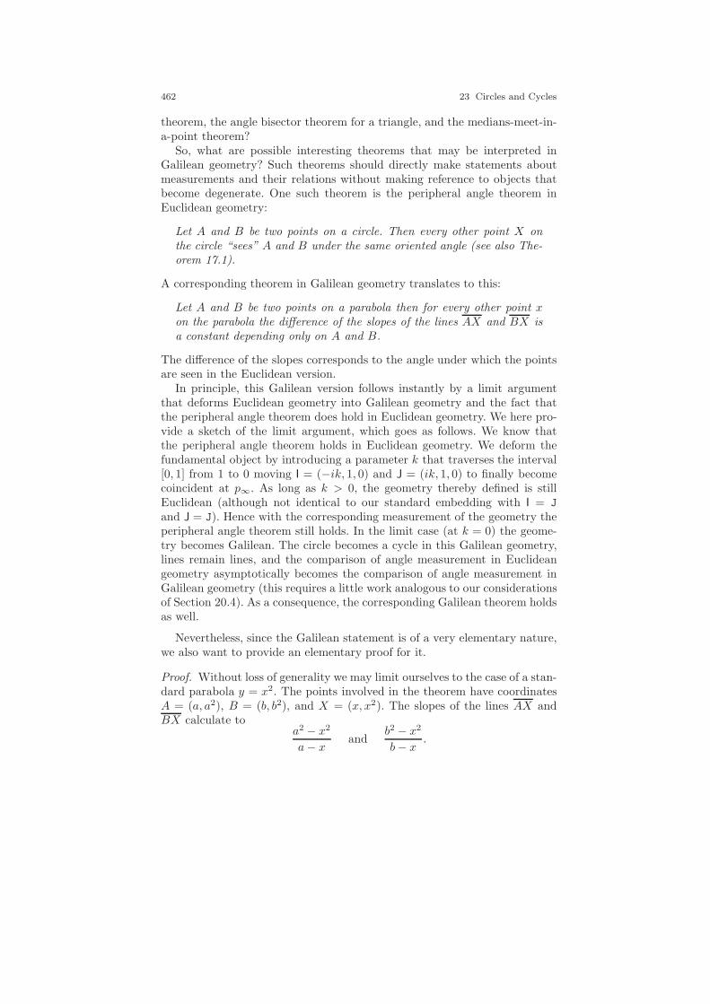
462 23 Circles and Cycles
theorem, the angle bisector theorem for a triangle, and the medians-meet-in-a-point theorem?
So, what are possible interesting theorems that may be interpreted inGalilean geometry? Such theorems should directly make statements aboutmeasurements and their relations without making reference to objects thatbecome degenerate. One such theorem is the peripheral angle theorem inEuclidean geometry:
Let A and B be two points on a circle. Then every other point X onthe circle “sees” A and B under the same oriented angle (see also The-orem 17.1).
A corresponding theorem in Galilean geometry translates to this:
Let A and B be two points on a parabola then for every other point xon the parabola the difference of the slopes of the lines AX and BX isa constant depending only on A and B.
The difference of the slopes corresponds to the angle under which the pointsare seen in the Euclidean version.
In principle, this Galilean version follows instantly by a limit argumentthat deforms Euclidean geometry into Galilean geometry and the fact thatthe peripheral angle theorem does hold in Euclidean geometry. We here pro-vide a sketch of the limit argument, which goes as follows. We know thatthe peripheral angle theorem holds in Euclidean geometry. We deform thefundamental object by introducing a parameter k that traverses the interval[0, 1] from 1 to 0 moving I = (−ik, 1, 0) and J = (ik, 1, 0) to finally becomecoincident at p∞. As long as k > 0, the geometry thereby defined is stillEuclidean (although not identical to our standard embedding with I = J
and J = J). Hence with the corresponding measurement of the geometry theperipheral angle theorem still holds. In the limit case (at k = 0) the geome-try becomes Galilean. The circle becomes a cycle in this Galilean geometry,lines remain lines, and the comparison of angle measurement in Euclideangeometry asymptotically becomes the comparison of angle measurement inGalilean geometry (this requires a little work analogous to our considerationsof Section 20.4). As a consequence, the corresponding Galilean theorem holdsas well.
Nevertheless, since the Galilean statement is of a very elementary nature,we also want to provide an elementary proof for it.
Proof. Without loss of generality we may limit ourselves to the case of a stan-dard parabola y = x2. The points involved in the theorem have coordinatesA = (a, a2), B = (b, b2), and X = (x, x2). The slopes of the lines AX andBX calculate to
a2 − x2
a− xand
b2 − x2
b− x.
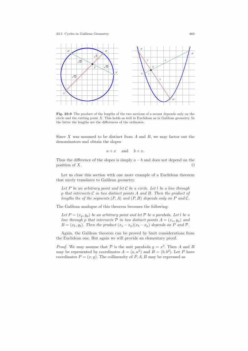
23.5 Cycles in Galilean Geometry 463
A
B
X
A′
B′
√50
√8
√20
√20
A
B
X
A′
B′
1
62
3
Fig. 23.9 The product of the lengths of the two sections of a secant depends only on thecircle and the cutting point X. This holds as well in Euclidean as in Galilean geometry. Inthe latter the lengths are the differences of the ordinates.
Since X was assumed to be distinct from A and B, we may factor out thedenominators and obtain the slopes
a+ x and b+ x.
Thus the difference of the slopes is simply a− b and does not depend on theposition of X . ⊓⊔
Let us close this section with one more example of a Euclidean theoremthat nicely translates to Galilean geometry.
Let P be an arbitrary point and let C be a circle. Let l be a line throughp that intersects C in two distinct points A and B. Then the product oflengths the of the segments (P,A) and (P,B) depends only on P and C.
The Galilean analogue of this theorem becomes the following:
Let P = (xp, yp) be an arbitrary point and let P be a parabola. Let l be aline through p that intersects P in two distinct points A = (xa, ya) andB = (xb, yb). Then the product (xa−xp)(xb−xp) depends on P and P.
Again, the Galilean theorem can be proved by limit considerations fromthe Euclidean one. But again we will provide an elementary proof.
Proof. We may assume that P is the unit parabola y = x2. Then A and Bmay be represented by coordinates A = (a, a2) and B = (b, b2). Let P havecoordinates P = (x, y). The collinearity of P,A,B may be expressed as
464 23 Circles and Cycles
0 = det
a b xa2 b2 y1 1 1
= ab2+by+a2x−ay−ba2−b2x = (ab+y−(b+a)x)(b−a).
Dividing by (b − a) (the points A and B are distinct) gives
(ab+ y − (b+ a)x) = 0. (23.5)
Now we consider the product (a− x)(b− x), which is claimed to be constantby the theorem. Expanding gives
(a− x)(b − x) = ab− x(a+ b) + x2.
Subtracting (23.5) from this expression, which means subtracting zero, gives
(a− x)(b − x) = −y + x2. (23.6)
Thus the product depends only on x and y, as claimed by the theorem. ⊓⊔There is a remarkable connection of this theorem to a theorem we already
proved earlier. Lemma 10.1 provided a kind of mechanical multiplicationdevice based on a parabola (see also Figure 10.9). The theorem we just provedcan be directly used to demonstrate that this multiplication device worksproperly. Lemma 10.1 just corresponds to the special case x = 0 in whichequation (23.6) becomes a · b = −y.
24
Non-Euclidean Geometry: A HistoricalInterlude
Some of the men stood talking in this room, and at the rightof the door a little knot had formed round a small table, thecenter of which was the mathematics student, who was ea-gerly talking. He had made the assertion that one could drawthrough a given point more than one parallel to a straight line;Frau Hagenstrom had cried out that this was impossible, andhe had gone on to prove it so conclusively that his hearers
were constrained to behave as though they understood.
Thomas Mann, Little Herr Friedemann
History will teach us nothing.
Sting
Imagine you are a two-dimensional being living in the interior of a real non-degenerate fundamental conic of a Cayley-Klein geometry. All your mea-surements (distances and angles) are done with respect to this Cayley-Kleingeometry, and you have no knowledge of the fact that your world is embeddedin some larger space (the projective plane in which the Cayley-Klein geome-try is defined). One day your dog, your ruler, and you decide to take a long,long walk always following the same direction.How would that feel? In a senseit would not feel very exciting, and this is indeed an exciting thing. The threeof you simply go on without anything remarkable happening. A person fromthe outside observing you will see you all getting smaller and smaller as youapproach the boundary of the fundamental object. With your legs shrinking,your step size (observed from the outside) is getting smaller and smaller, too.Every single step will be very small compared to your current distance to the
465
466 24 Non-Euclidean Geometry: A Historical Interlude
boundary. You yourself will recognize nothing of this change of size. Togetherwith you your dog, your shoes, your ruler, everything shrinks by the sameamount. So when in regular intervals of time you measure the size of yourdog (this is an old habit of yours), it neither shrinks nor grows. What doesmeasuring mean? Well, you take your ruler and compare it to the length ofyour dog. Your dog was three times as long as your ruler when you startedyour trip and it is so every time you redo the measurement. So who coulddaresay that something has changed?
24.1 The Inner Geometry of a Space
In this little story there are two observers: you inside the conic and a personlooking from the outside. Both describe the same situation in different terms.You from the inside observe an infinite space. The person from the outsideobserves you constantly shrinking within a finite space. Both descriptions areperfectly legitimate. Yours describes the inner geometry of the space you livein. The person outside describes the scenario he sees in terms of the geometryhe lives in (and perhaps as an irony of fate his world is also embedded in somestrange way into a larger space he does not know about).
Do you as an inhabitant of the interior of the conic have any chance to findout that the world you live in is indeed the finite interior of a conic? Does thisquestion even make sense? In a way yes, in a way no, and a good answer tothese questions becomes philosophical sooner or later. You as a being in yourworld have very good reasons to call it infinite in every direction. However,your intellect (after quite a lot of mathematical thought) may tell you thatthere are ways to realize your world (to find a model for it consistent withyour experiences) in a way that it fits into the finite region of the interiorof a conic. However, in order to make some predictions about the geometricbehavior of your habitat it does not matter which way you describe it. Soboth standpoints (the inside/infinite view and the outside/finite view) maybe equally appropriate as long as they make the same predictions about whatwill happen.
We have seen in the previous chapters that compared to the Euclideangeometry we learn in school (and which is perhaps—at least locally—thegeometry of the space we are living in), the geometry in a general Cayley-Klein geometry may be significantly different (one may have, for instance,hyperbolic angle measurement, so that it is not possible to turn around one’sown axis and face the same direction again). But what is it like inside thenondegenerate and real conic? There angle measurement is elliptic as we areused to from Euclidean geometry: turning around by 360 brings you back toyour old position. Distance measurement is in a good sense infinite in eachdirection, as in Euclidean geometry. However, the differences to Euclideangeometry come into play whenever distance and angle measurements interact.
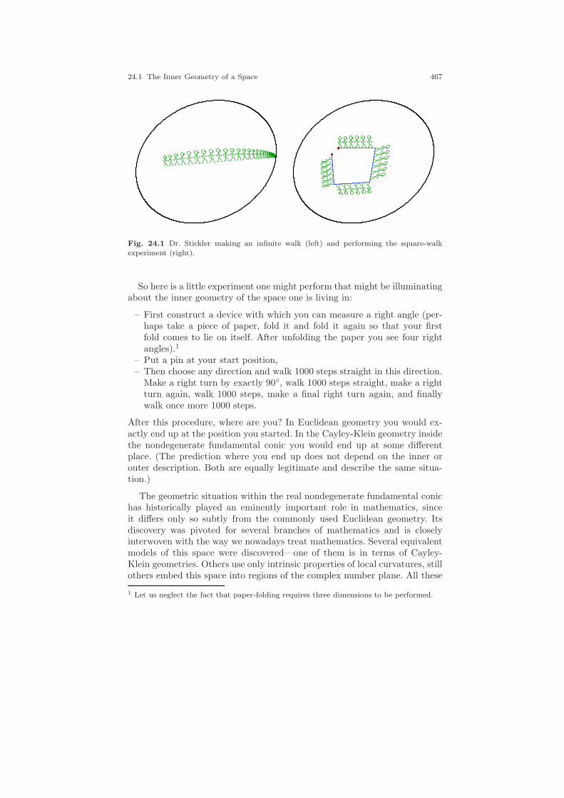
24.1 The Inner Geometry of a Space 467
Fig. 24.1 Dr. Stickler making an infinite walk (left) and performing the square-walkexperiment (right).
So here is a little experiment one might perform that might be illuminatingabout the inner geometry of the space one is living in:
– First construct a device with which you can measure a right angle (per-haps take a piece of paper, fold it and fold it again so that your firstfold comes to lie on itself. After unfolding the paper you see four rightangles).1
– Put a pin at your start position,– Then choose any direction and walk 1000 steps straight in this direction.
Make a right turn by exactly 90, walk 1000 steps straight, make a rightturn again, walk 1000 steps, make a final right turn again, and finallywalk once more 1000 steps.
After this procedure, where are you? In Euclidean geometry you would ex-actly end up at the position you started. In the Cayley-Klein geometry insidethe nondegenerate fundamental conic you would end up at some differentplace. (The prediction where you end up does not depend on the inner orouter description. Both are equally legitimate and describe the same situa-tion.)
The geometric situation within the real nondegenerate fundamental conichas historically played an eminently important role in mathematics, sinceit differs only so subtly from the commonly used Euclidean geometry. Itsdiscovery was pivoted for several branches of mathematics and is closelyinterwoven with the way we nowadays treat mathematics. Several equivalentmodels of this space were discovered—one of them is in terms of Cayley-Klein geometries. Others use only intrinsic properties of local curvatures, stillothers embed this space into regions of the complex number plane. All these
1 Let us neglect the fact that paper-folding requires three dimensions to be performed.
468 24 Non-Euclidean Geometry: A Historical Interlude
approaches are equally legitimate, since they all lead to the same qualitativeresults. The Cayley-Klein approach has the advantage to embed this specialgeometry into a larger system of other possible geometries.
This chapter is perhaps a bit different from the others in this book andoffers more philosophical and historical background dealing with the natureof space and the nature of geometry. Still we here can only scratch the surfaceand advise the reader to consult some of the really brilliant books and paperson this topic. We here want to recommend four books that provide interestinginsights in the history of development of these ideas. The very wellwrittenbook of Marvin Jay Greenberg on hyperbolic geometry [49] dedicates entirechapters to the historical and philosophical aspects of hyperbolic geometry.The books by Jeremy Gray Worlds out of nothing [48] and by Isaak Moisee-vich Yaglom Felix Klein and Sophus Lie—Evolution of the Idea of Symmetryin the Nineteenth Century [137] tell essentially the entire story of the de-velopment of hyperbolic geometry, including the origins of modern algebraand projective geometry. Finally, F. Klein’s Development of mathematics inthe 19th century [69, 70] gives a kind of first-hand treatment of the subject.Although it sometimes lacks the distance of a historian, it gives very deepinsights into important streams of thought of these times.
24.2 Euclid’s Postulates
In the books (the Elements) that Euclid wrote around 300 BCE about math-ematics and geometry, he tried to lay a rigorous foundation of the mattershe was writing about. Compared to modern standards there are still a fewgaps in his reasoning, but he came pretty close. In a sense, his treatment ofmathematics served as a blueprint for the way we do mathematics nowadays:Base your formal treatment on axioms and definitions; then do admissibleformal reasoning to derive theorems based only on these axioms, definitions,and things you have already proved. Thus ultimately the proof of every sin-gle theorem can be traced back to your axioms, definitions, and logicallyadmissible reasoning steps.
In Euclid’s treatment of geometry, after specifying the objects (points,segments, circles), which he treats in very general terms by sentences like“A point is that which has no part” etc.), he describes the relations betweenthese objects by a set of five axioms, often called his postulates:
1. A straight line segment can be drawn joining any two points.
2. Any straight line segment can be extended indefinitely in a straight line.
3. Given any straight line segment, a circle can be drawn having the segmentas radius and one endpoint as center.
4. All right angles are congruent.
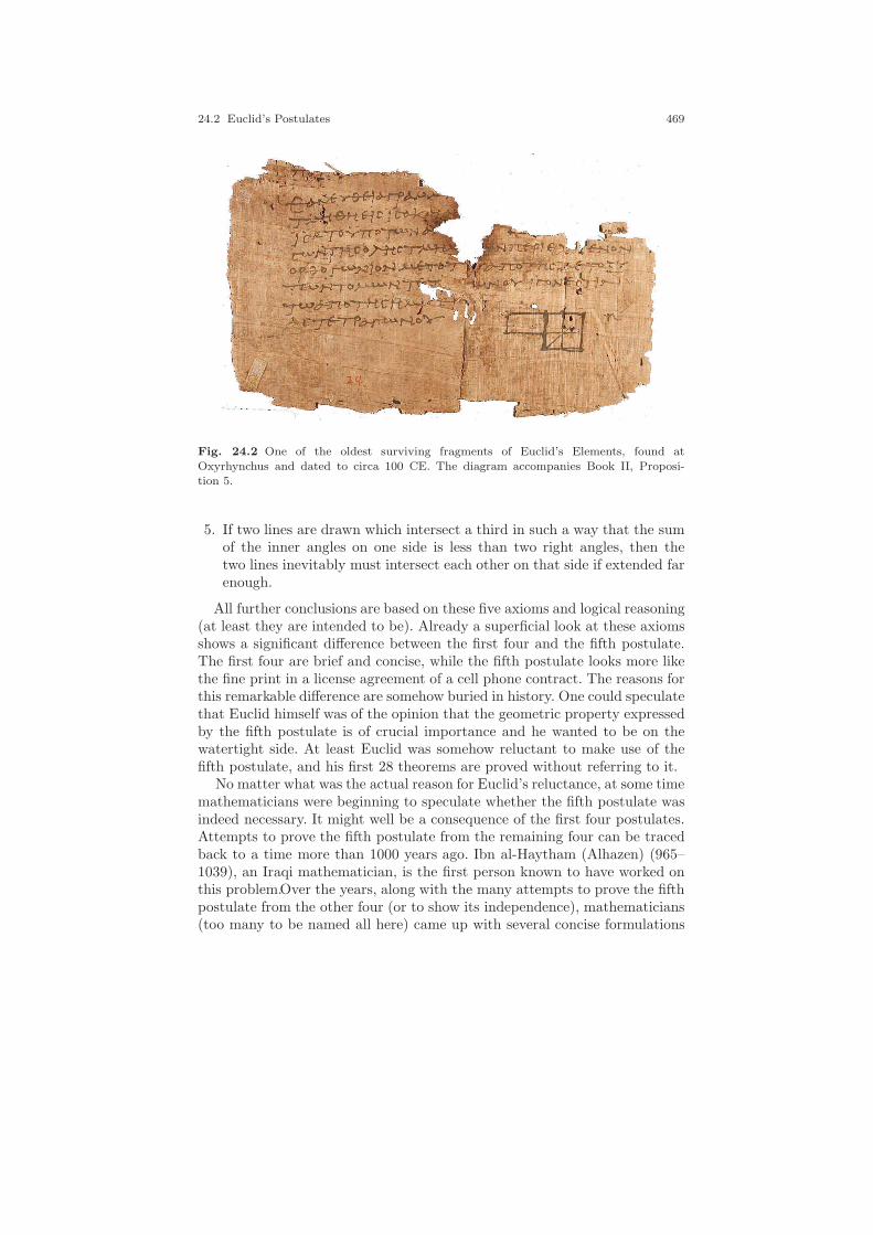
24.2 Euclid’s Postulates 469
Fig. 24.2 One of the oldest surviving fragments of Euclid’s Elements, found at
Oxyrhynchus and dated to circa 100 CE. The diagram accompanies Book II, Proposi-tion 5.
5. If two lines are drawn which intersect a third in such a way that the sumof the inner angles on one side is less than two right angles, then thetwo lines inevitably must intersect each other on that side if extended farenough.
All further conclusions are based on these five axioms and logical reasoning(at least they are intended to be). Already a superficial look at these axiomsshows a significant difference between the first four and the fifth postulate.The first four are brief and concise, while the fifth postulate looks more likethe fine print in a license agreement of a cell phone contract. The reasons forthis remarkable difference are somehow buried in history. One could speculatethat Euclid himself was of the opinion that the geometric property expressedby the fifth postulate is of crucial importance and he wanted to be on thewatertight side. At least Euclid was somehow reluctant to make use of thefifth postulate, and his first 28 theorems are proved without referring to it.
No matter what was the actual reason for Euclid’s reluctance, at some timemathematicians were beginning to speculate whether the fifth postulate wasindeed necessary. It might well be a consequence of the first four postulates.Attempts to prove the fifth postulate from the remaining four can be tracedback to a time more than 1000 years ago. Ibn al-Haytham (Alhazen) (965–1039), an Iraqi mathematician, is the first person known to have worked onthis problem.Over the years, along with the many attempts to prove the fifthpostulate from the other four (or to show its independence), mathematicians(too many to be named all here) came up with several concise formulations
470 24 Non-Euclidean Geometry: A Historical Interlude
equivalent to the fifth postulate in the presence of the other four. Here welist a few of them:
a. At most one line can be drawn through any point not on a given lineparallel to the given line in a plane.
b. The sum of the angles in every triangle is 180.
c. There exists a triangle whose angles add up to 180.
d. There exists a pair of similar, but not congruent, triangles.
e. If three angles of a quadrilateral are right angles, then the fourth angleis also a right angle.
f. There exists a quadrilateral of which all angles are right angles.
g. In a right-angled triangle, the square of the hypotenuse equals the sumof the squares of the other two sides (Pythagorean theorem).
h. There is no upper limit to the area of a triangle.
The first of these formulations is often called the parallel postulate, and ittraces back to John Playfair (1748–1819). Formulations b. to d. demonstratethat the problem is intimately related to the angular sum of a triangle. For-mulations e. and f. show that our walk in a square experiment from the lastchapter was ultimately a test for the truth of the fifth postulate. Formulationg. shows that the Pythagorean theorem is essentially equivalent to the fifthpostulate, and finally formulation h. shows that the area of a triangle will bebounded if the contrary of the fifth postulate holds.
24.3 Gauss, Bolyai, and Lobachevsky
Surprisingly, the problem of the independence of the fifth postulate was notresolved to full satisfaction until approximately between 1820 and 1882, andthe Cayley-Klein geometries we discuss in in this book play a crucial role inthis development. The story is long, surprisingly emotional, involves personalfate and has several surprising twists. Here we will give only a brief outlineof what happened in the final and crucial years.
The main actors in this part of mathematical history were CarlFriedrich Gauss (1777–1855), Janos Bolyai (1802–1860), Nikolai IvanovichLobachevsky (1792–1856), Eugenio Beltrami (1835–1900), Felix ChristianKlein (1849–1925) and Jules Henri Poincare (1854–1912). One should alsomention Farkas Bolyai (1775–1856), the father of Janos, because of his per-sonal involvement and the fact that he somehow formed a bridge betweenGauss and his own son.
In short, the story can be told as follows. In the first half of the nineteenthcentury several mathematicians were attempting to show that the parallel
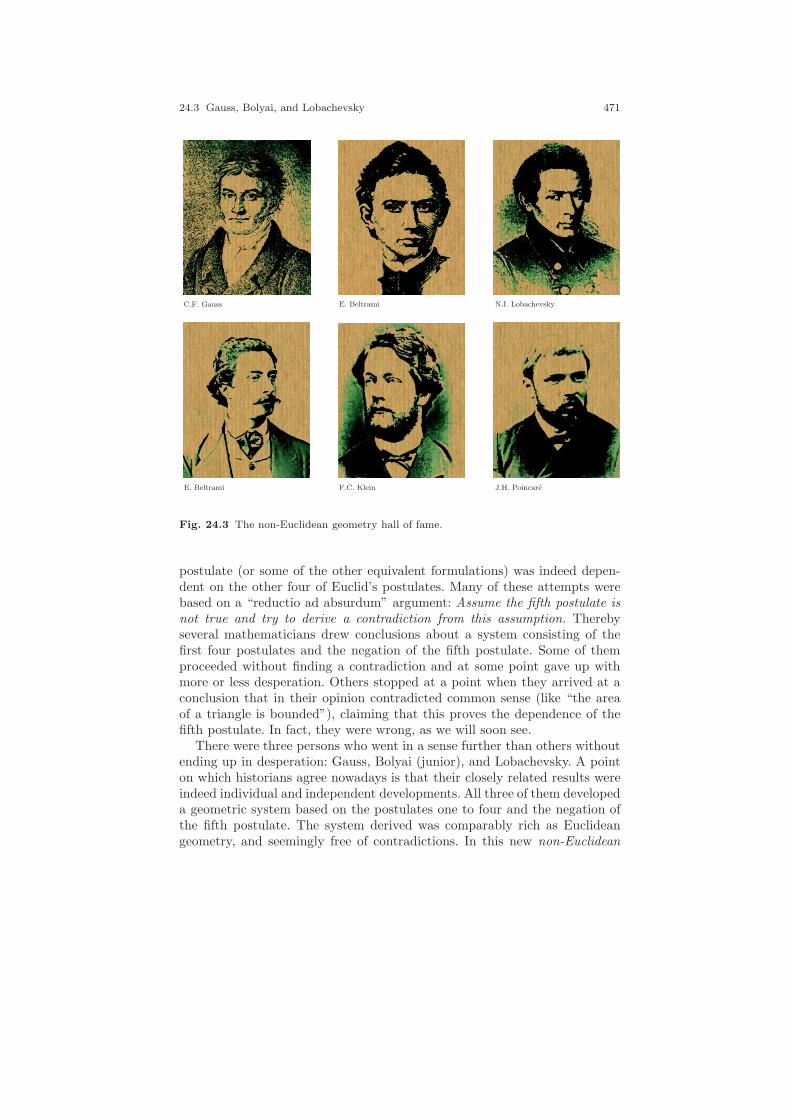
24.3 Gauss, Bolyai, and Lobachevsky 471
C.F. Gauss N.I. Lobachevsky
E. Beltrami
E. Beltrami
F.C. Klein J.H. Poincare
Fig. 24.3 The non-Euclidean geometry hall of fame.
postulate (or some of the other equivalent formulations) was indeed depen-dent on the other four of Euclid’s postulates. Many of these attempts werebased on a “reductio ad absurdum” argument: Assume the fifth postulate isnot true and try to derive a contradiction from this assumption. Therebyseveral mathematicians drew conclusions about a system consisting of thefirst four postulates and the negation of the fifth postulate. Some of themproceeded without finding a contradiction and at some point gave up withmore or less desperation. Others stopped at a point when they arrived at aconclusion that in their opinion contradicted common sense (like “the areaof a triangle is bounded”), claiming that this proves the dependence of thefifth postulate. In fact, they were wrong, as we will soon see.
There were three persons who went in a sense further than others withoutending up in desperation: Gauss, Bolyai (junior), and Lobachevsky. A pointon which historians agree nowadays is that their closely related results wereindeed individual and independent developments. All three of them developeda geometric system based on the postulates one to four and the negation ofthe fifth postulate. The system derived was comparably rich as Euclideangeometry, and seemingly free of contradictions. In this new non-Euclidean
472 24 Non-Euclidean Geometry: A Historical Interlude
geometry there were perfectly reasonable notions of elementary geometry,differential geometry, mechanics, etc. Many Euclidean theorems had a non-Euclidean analogue that was often related to the corresponding Euclideanone by just a small but essential twist.
The way the three mathematicians dealt with their results was quite dif-ferent. Gauss was perhaps the first person who was convinced that there isan equally justified non-Euclidean geometry. However, he was reluctant topublish anything on this topic. He was afraid of the at that time dominantphilosophical school of Immanuel Kant. One of Kant’s fundamental state-ments in his epistemology was that the properties of a straight line are apriori clear and cannot be further discussed. Starting an intellectual disputeabout non-Euclidean geometry would exactly mean to discuss the very mean-ing of a straight line. Nevertheless, to the outside world there was indeed someevidence that Gauss was well aware of all the subtleties around the parallelpostulate. As the leading mathematician of his day he often received letterswith supposed proofs of the dependence of Euclid’s fifth postulate. On theseoccasions he often responded very soon, pointing the finger to the place ofthe logical flaw in the supposed argumentation. Still, during his lifetime hedid not publish anything on this subject.
Farkas Bolyai, the father of Janos Bolyai, was a school friend of Gauss.Farkas himself was deeply committed to the problem of the parallel postulateand worked on it for several decades (without real success). When his sontold him that he was as well planing to spend significant time working on theparallel postulate, the father beseeched him not to do so. To get an impressionhow emotionally tense the subject was, here is an excerpt from a letter FarkasBolyai wrote to his son Janos trying to prevent him from doing research onthe parallel postulate. For those readers capable of reading German I includethe full original passage, which may be found, for instance, in [104]. Afterthis I include an abridged translation that can be found in [49].
Du darfst die Parallelen auf jenem Wege nicht versuchen; ich kenne diesen Weg bisan sein Ende. Auch ich habe diese bodenlose Nacht durchmessen, jedes Licht, jedeFreude meines Lebens sind in ihr ausgeloscht worden; ich beschwore Dich bei Gott!Lass die Lehre von den Parallelen in Frieden. Du sollst davor denselben Abscheuhaben, wie vor einem liederlichen Umgang, sie kann Dich um all Deine Muße, umdie Gesundheit, um Deine Ruhe und um Dein ganzes Lebensgluck bringen. Diesegrundlose Finsternis wurde vielleicht tausend Newtonsche Riesenturme verschlingen,es wird nie auf Erden hell werden, und das armselige Menschengeschlecht wird nie et-was vollkommen Reines haben, selbst die Geometrie nicht; es ist in meiner Seele einetiefe und ewige Wunde. Behut Dich Gott, dass diese sich (bei Dir) je so tief hinein-nagen mochte. Diese raubt einem die Lust zur Geometrie, zum irdischen Leben.Ich hatte mir vorgenommen, mich fur die Wahrheit aufzuopfern; ich ware bereitgewesen, zum Martyrer zu werden, damit ich nur die Geometrie von diesem Makelgereinigt dem menschlichen Geschlecht ubergeben konnte. Schauderhafte, riesige Ar-beiten habe ich vollbracht, habe bei weitem Besseres geleistet als bisher (geleistetwurde), aber keine vollkommene Befriedigung habe ich je gefunden. Hier aber giltes: Si paullum a summo discessit, vergit ad imum. Ich bin zuruckgekehrt, als ichdurchschaut habe, dass man den Boden dieser Nacht von der Erde aus nicht erre-
24.3 Gauss, Bolyai, and Lobachevsky 473
ichen kann, ohne Trost, mich selbst und das ganze Geschlecht bedauernd. Lerne anmeinem Beispiel; indem ich die Parallelen kennen wollte, blieb ich unwissend, diesehaben mir all die Blumen meines Lebens und meiner Zeit weggenommen. Hier stecktsogar die Wurzel aller meiner spateren Fehler, und es hat darauf aus den hauslichenGewolken geregnet. Wenn ich die Parallelen hatte entdecken konnen, so ware ich einEngel geworden, wenn es auch niemand gewusst hatte, dass ich sie gefunden habe.. . . Versuche es nicht, Du wirst es nie zeigen, dass je mit den unaufhorlichen Ein-biegungen desselben Maßes die untere Gerade geschnitten werde, es steckt in diesermateria ein ewig in sich zuruckdrehender circulus - ein Labyrinth, das einen immerhineinlockt -, wer sich hineinbegibt, verarmt, wie ein Schatzgraber, und bleibt un-wissend. Solltest Du auf was fur immer ein absurdum geraten, alles ist umsonst. Du
kannst es nicht als ein Axiom hinstellen. . . . Die Saulen des Herkules stehen in diesenGegenden, gehe nicht um einen einzigen Schritt weiter, sonst bist Du verloren.
And here the abridged translation:
You must not attempt this approach to parallels. I know this way to its very end. Ihave traversed this bottomless night, which extinguished all light and joy of my life. Ientreat you, leave the science of parallels alone . . . I thought I would sacrifice myselffor the sake of the truth. I was ready to become a martyr who would remove theflaw from geometry and return it purified to mankind. I accomplished monstrous,enormous labors; my creations are far better than those of others and yet I have notachieved complete satisfaction. For here it is true that si paullum a summo discessit,vergit ad imum. I turned back when I saw that no man can reach the bottom of thisnight. I turned back unconsoled, pitying myself and all mankind. . . do not go anystep further; otherwise, you are lost.
Janos Bolyai did not stop. He continued and developed the above-mentionedrich system of non-Euclidean geometry. After he convinced his father that hehad indeed gone further in this subject than other contemporary mathemati-cians, his father sent his son’s notes to his youth friend Gauss. He wanted tolet Gauss approve (or disapprove) the mathematical thoughts of his son andto get advice how to proceed. Gauss answered in a letter, of which here is anextract (again in German):
Jetzt uber die Arbeiten deines Sohnes.—Wenn ich damit anfange, das ich solche nichtloben darf, so wirst Du wohl einen Augenblick stutzen, aber ich kann nicht anders;
sie loben hieße mich selbst zu loben, denn der ganze Inhalt der Schrift, der Weg, denDein Sohn eingeschlagen hat, und die Resultate, zu denen er gefuhrt ist, kommen fastdurchgehends mit meinen eigenen, zum Teile schon seit 20–25 Jahren angestelltenMeditationen berein. In der Tat bin ich dadurch auf das Außerste uberrascht. – MeinVorsatz war, bei meinen Lebzeiten gar nichts bekannt werden zu lassen. Die meistenMenschen haben gar nicht den rechten Sinn fur das, worauf es dabei ankommt,und ich habe nur wenige Menschen gefunden, die das was ich ihnen mitteilte mitbesonderem Interesse aufnahmen. Um das zu konnen, muß man erst recht lebendiggefuhlt haben, was eigentlich fehlt, und daruber sind die meisten Menschen ganzunklar. Dagegen war meine Absicht mit der Zeit alles zu Papier zu bringen, daßes mit mir dereinst nicht unterginge. – Sehr bin ich also uberrascht, daß geradeder Sohn meines alten Freundes es ist, der mir auf eine so merkwurdige Art zuvorgekommen ist.
Abridged translation:
474 24 Non-Euclidean Geometry: A Historical Interlude
If I commenced by saying that I am unable to praise this work, you would certainlybe surprised for a moment. But I cannot say otherwise. To praise it would be topraise myself. Indeed the whole contents of the work, the path taken by your son,the results to which he is led, coincide almost entirely with my meditations, whichhave occupied my mind partly for the last thirty or thirty-five years. So I remainedquite stupefied. So far as my own work is concerned, of which up till now I haveput little on paper, my intention was not to let it be published during my lifetime.. . . I have found very few people who could regard with any special interest whatI communicated to them on this subject. . . .it was my idea to write down all thislater so that at least it should not perish with me. It is therefore a pleasant surprisefor me that I am spared this trouble, and I am very glad that it is just the son of
my old friend, who takes the precedence of me in such a remarkable manner.
Finally Janos Bolyai could publish his explorations as an appendix in abook written by his father.
The third person who arrived at essentially the same system was N.I. Lo-bachevsky, a mathematics professor at the university of Kazan, in Russia.He as well started to derive conclusions from the negated parallel postu-late and made perhaps the furthest-reaching investigations of differential-geometric structures in his non-Euclidean geometry. In a letter Gauss also ex-pressed great appreciation of the work of Lobachevsky. Not seldom is the termLobachevskian Geometry used synonymously with the term non-Euclideangeometry.
The story continues. The two Bolyais falsely believed that Lobachevskywas a pseudonym of Gauss under which he incognito had published histhoughts on non-Euclidean geometry2. And unfortunately, neither Bolyai norLobachevsky received recognition of their work until Gauss died in 1855. WithGauss’s death his private letters became public, and with them also a wealthof private thoughts of the world’s leading mathematician on the subject ofnon-Euclidean geometry, including references to Bolyai and Lobachevsky.During their lifetimes only few mathematicians knew about the groundbreak-ing work of these two mathematical revolutionaries.
24.4 Beltrami and Klein
So what was the achievement of the three protagonists of our last section?They went further than others in deriving consequences of the negated par-allel postulate. By this they developed a system of geometric terms at least
2 This almost curious fact is mentioned in Klein’s historical book [69] and can be tracedback to a text Bemerkungen ueber Nicolaus Lobatschefskijs Untersuchungen zur Theorieder Parallellinien Bolyai wrote around 1851. There he writes: “Fur noch wahrscheinlicheraber halte ich, daß der ohnedem an Schatzen so reiche Koloß Gauss es nicht ertragen kon-
nte, daß ihm jemand auch in dieser Sache zuvorgekommen sei, und, da er dies durchausnicht mehr verhindern konnte, das Werk selbst bearbeitet hat und unter LobatschefskijsNamen hat herausgeben lassen.” Further details on this fascinating part of the story maybe found in [122].
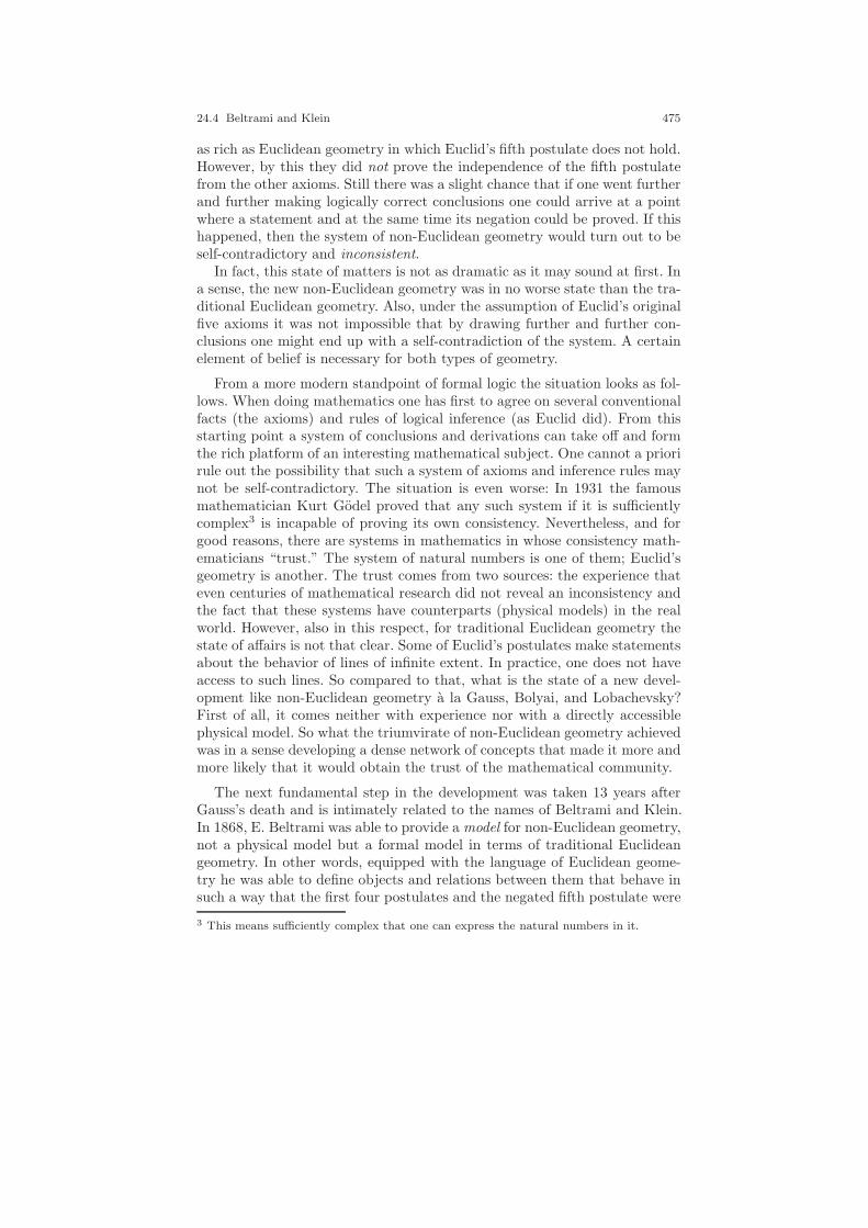
24.4 Beltrami and Klein 475
as rich as Euclidean geometry in which Euclid’s fifth postulate does not hold.However, by this they did not prove the independence of the fifth postulatefrom the other axioms. Still there was a slight chance that if one went furtherand further making logically correct conclusions one could arrive at a pointwhere a statement and at the same time its negation could be proved. If thishappened, then the system of non-Euclidean geometry would turn out to beself-contradictory and inconsistent.
In fact, this state of matters is not as dramatic as it may sound at first. Ina sense, the new non-Euclidean geometry was in no worse state than the tra-ditional Euclidean geometry. Also, under the assumption of Euclid’s originalfive axioms it was not impossible that by drawing further and further con-clusions one might end up with a self-contradiction of the system. A certainelement of belief is necessary for both types of geometry.
From a more modern standpoint of formal logic the situation looks as fol-lows. When doing mathematics one has first to agree on several conventionalfacts (the axioms) and rules of logical inference (as Euclid did). From thisstarting point a system of conclusions and derivations can take off and formthe rich platform of an interesting mathematical subject. One cannot a priorirule out the possibility that such a system of axioms and inference rules maynot be self-contradictory. The situation is even worse: In 1931 the famousmathematician Kurt Godel proved that any such system if it is sufficientlycomplex3 is incapable of proving its own consistency. Nevertheless, and forgood reasons, there are systems in mathematics in whose consistency math-ematicians “trust.” The system of natural numbers is one of them; Euclid’sgeometry is another. The trust comes from two sources: the experience thateven centuries of mathematical research did not reveal an inconsistency andthe fact that these systems have counterparts (physical models) in the realworld. However, also in this respect, for traditional Euclidean geometry thestate of affairs is not that clear. Some of Euclid’s postulates make statementsabout the behavior of lines of infinite extent. In practice, one does not haveaccess to such lines. So compared to that, what is the state of a new devel-opment like non-Euclidean geometry a la Gauss, Bolyai, and Lobachevsky?First of all, it comes neither with experience nor with a directly accessiblephysical model. So what the triumvirate of non-Euclidean geometry achievedwas in a sense developing a dense network of concepts that made it more andmore likely that it would obtain the trust of the mathematical community.
The next fundamental step in the development was taken 13 years afterGauss’s death and is intimately related to the names of Beltrami and Klein.In 1868, E. Beltrami was able to provide a model for non-Euclidean geometry,not a physical model but a formal model in terms of traditional Euclideangeometry. In other words, equipped with the language of Euclidean geome-try he was able to define objects and relations between them that behave insuch a way that the first four postulates and the negated fifth postulate were
3 This means sufficiently complex that one can express the natural numbers in it.
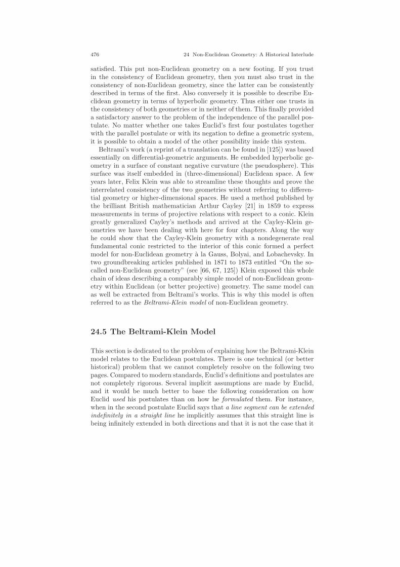
476 24 Non-Euclidean Geometry: A Historical Interlude
satisfied. This put non-Euclidean geometry on a new footing. If you trustin the consistency of Euclidean geometry, then you must also trust in theconsistency of non-Euclidean geometry, since the latter can be consistentlydescribed in terms of the first. Also conversely it is possible to describe Eu-clidean geometry in terms of hyperbolic geometry. Thus either one trusts inthe consistency of both geometries or in neither of them. This finally provideda satisfactory answer to the problem of the independence of the parallel pos-tulate. No matter whether one takes Euclid’s first four postulates togetherwith the parallel postulate or with its negation to define a geometric system,it is possible to obtain a model of the other possibility inside this system.
Beltrami’s work (a reprint of a translation can be found in [125]) was basedessentially on differential-geometric arguments. He embedded hyperbolic ge-ometry in a surface of constant negative curvature (the pseudosphere). Thissurface was itself embedded in (three-dimensional) Euclidean space. A fewyears later, Felix Klein was able to streamline these thoughts and prove theinterrelated consistency of the two geometries without referring to differen-tial geometry or higher-dimensional spaces. He used a method published bythe brilliant British mathematician Arthur Cayley [21] in 1859 to expressmeasurements in terms of projective relations with respect to a conic. Kleingreatly generalized Cayley’s methods and arrived at the Cayley-Klein ge-ometries we have been dealing with here for four chapters. Along the wayhe could show that the Cayley-Klein geometry with a nondegenerate realfundamental conic restricted to the interior of this conic formed a perfectmodel for non-Euclidean geometry a la Gauss, Bolyai, and Lobachevsky. Intwo groundbreaking articles published in 1871 to 1873 entitled “On the so-called non-Euclidean geometry” (see [66, 67, 125]) Klein exposed this wholechain of ideas describing a comparably simple model of non-Euclidean geom-etry within Euclidean (or better projective) geometry. The same model canas well be extracted from Beltrami’s works. This is why this model is oftenreferred to as the Beltrami-Klein model of non-Euclidean geometry.
24.5 The Beltrami-Klein Model
This section is dedicated to the problem of explaining how the Beltrami-Kleinmodel relates to the Euclidean postulates. There is one technical (or betterhistorical) problem that we cannot completely resolve on the following twopages. Compared to modern standards, Euclid’s definitions and postulates arenot completely rigorous. Several implicit assumptions are made by Euclid,and it would be much better to base the following consideration on howEuclid used his postulates than on how he formulated them. For instance,when in the second postulate Euclid says that a line segment can be extendedindefinitely in a straight line he implicitly assumes that this straight line isbeing infinitely extended in both directions and that it is not the case that it

24.5 The Beltrami-Klein Model 477
topologically may close up to form a circle. He uses this implicit assumption,for instance, when he proves that the exterior angle in a triangle is alwayslarger than each of its opposite interior angles. There are several more implicitassumptions on the notions of betweenness, the character of congruence, andso forth.
A strict (in modern standards) axiomatic treatment of what we call Eu-clidean geometry was done as late as 1899 in David Hilbert’s book Grundlagender Geometrie [58]. Hilbert there presented a set of 20 axioms forming a wa-tertight basis for Euclidean geometry. He later on also formulated a similarset of axioms for projective geometry and for non-Euclidean geometry.4 Sowhen we here want to see how the Beltrami-Klein model is indeed a modelof Euclidean geometry it would be by far more appropriate to relate it toHilbert’s axioms than to Euclid’s postulates. We will not do this here andrefer to other books for this topic [48]. We will content ourselves with a briefand commented version of Euclid’s postulates and their relationship to theBeltrami-Klein model.
In principle, within the preceding chapters we have done all preparationsto explain the Beltrami-Klein model in comparatively simple terms. So, whatdo we want? We need a geometric system whose objects are lines, planes, andcircles, equipped with a notion of measurement for distances and angles, thatsatisfies the first four of Euclid’s postulates and the negation of the fifth. So,here it is: We start with a nondegenerate real conic in the projective plane.For reasons of simplicity and without loss of generality we choose the unitcircle F defined by x2 + y2 = 1. This has the advantage that all points wewill consider now are part of the usual Euclidean plane, and by this it is notexplicitly necessary to refer to projective geometry and elements at the lineat infinity. The points of our geometry are all interior points of the unit circle.The lines of the geometry are the (nonempty) intersections of an ordinaryline with the interior of the unit circle. Distance measurement and anglemeasurement are those of the Cayley Klein geometry K = (F ,−1/2,−1/2i).With respect to this measurement we can define, in agreement with Euclid’sdefinitions, 5 that a circle is the set of all points having constant distancefrom another point. Furthermore, we define that an angle between two linesis right if the two angles to the left and to the right of one of the lines andon the same side of the other have equal size.
Equipped with these definitions, we will now analyze how this system ofgeometric objects relates to Euclid’s postulates. For this we take the intrinsicviewpoint. We argue as a being that lives inside the reality of the interior ofthe unit circle equipped with the Cayley-Klein measurement.
4 It is an interesting fact that in Hilbert’s axioms the term circle is not at all used ordefined. Circles in this setup are secondary objects whose definition is based on the axioms
of measurement and incidence.5 We have not reproduced all these 23 definitions here.
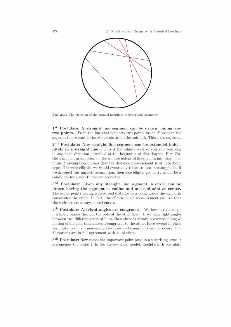
478 24 Non-Euclidean Geometry: A Historical Interlude
p
l
Fig. 24.4 The violation of the parallel postulate in hyperbolic geometry.
1st Postulate: A straight line segment can be drawn joining anytwo points. From the line that connects two points inside F we take thesegment that connects the two points inside the unit disk. This is the segment.
2nd Postulate: Any straight line segment can be extended indefi-nitely in a straight line This is the infinite walk of you and your dogin one fixed direction described at the beginning of this chapter. Here Eu-clid’s implicit assumption on the infinite extent of lines comes into play. Thisimplicit assumption implies that the distance measurement is of hyperbolictype. If it were elliptic, we would eventually return to our starting point. Ifwe dropped this implicit assumption, then also elliptic geometry would be acandidate for a non-Euclidean geometry
3rd Postulate: Given any straight line segment, a circle can bedrawn having the segment as radius and one endpoint as center.The set of points having a fixed real distance to a point inside the unit diskconstitutes the circle. In fact, the elliptic angle measurement ensures thatthese circles are always closed curves.
4th Postulate: All right angles are congruent. We have a right angleif a line g passes through the pole of the other line l. If we have right anglesbetween two different pairs of lines, then there is always a corresponding Kmotion of one pair that makes it congruent to the other. Here several implicitassumptions on continuous rigid motions and congruence are necessary. TheK-motions are in full agreement with all of them.
5th Postulate: Now comes the important point (and in a surprising sense itis somehow the easiest). In the Cayley-Klein model, Euclid’s fifth postulate
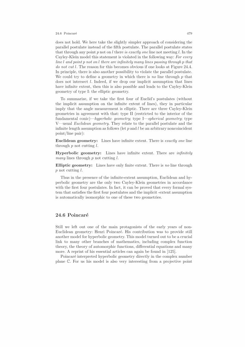
24.6 Poincare 479
does not hold. We here take the slightly simpler approach of considering theparallel postulate instead of the fifth postulate. The parallel postulate statesthat through any point p not on l there is exactly one line not meeting l. In theCayley-Klein model this statement is violated in the following way: For everyline l and point p not on l there are infinitely many lines passing through p thatdo not cut l. The reason for this becomes obvious if one looks at Figure 24.4.In principle, there is also another possibility to violate the parallel postulate.We could try to define a geometry in which there is no line through p thatdoes not intersect l. Indeed, if we drop our implicit assumption that lineshave infinite extent, then this is also possible and leads to the Cayley-Kleingeometry of type I: the elliptic geometry.
To summarize, if we take the first four of Euclid’s postulates (withoutthe implicit assumption on the infinite extent of lines), they in particularimply that the angle measurement is elliptic. There are three Cayley-Kleingeometries in agreement with that: type II (restricted to the interior of thefundamental conic)—hyperbolic geometry; type I—spherical geometry; typeV—usual Euclidean geometry. They relate to the parallel postulate and theinfinite length assumption as follows (let p and l be an arbitrary noncoincidentpoint/line pair):
Euclidean geometry: Lines have infinite extent. There is exactly one linethrough p not cutting l.
Hyperbolic geometry: Lines have infinite extent. There are infinitelymany lines through p not cutting l.
Elliptic geometry: Lines have only finite extent. There is no line throughp not cutting l.
Thus in the presence of the infinite-extent assumption, Euclidean and hy-perbolic geometry are the only two Cayley-Klein geometries in accordancewith the first four postulates. In fact, it can be proved that every formal sys-tem that satisfies the first four postulates and the implicit -extent assumptionis automatically isomorphic to one of these two geometries.
24.6 Poincare
Still we left out one of the main protagonists of the early years of non-Euclidean geometry: Henri Poincare. His contribution was to provide stillanother model for hyperbolic geometry. This model turned out to be a cruciallink to many other branches of mathematics, including complex functiontheory, the theory of automorphic functions, differential equations and manymore. A reprint of his essential articles can again be found in [125].
Poincare interpreted hyperbolic geometry directly in the complex numberplane C. For us his model is also very interesting from a projective point
480 24 Non-Euclidean Geometry: A Historical Interlude
of view. While the Beltrami-Klein model is best understood embedded inthe two-dimensional real projective space RP
2, the Poincare model is bestunderstood embedded in the one-dimensional complex projective space CP
1.In the Poincare disk model of the hyperbolic plane the region of relevantpoints is as in the Beltrami-Klein model restricted to the interior points of acircle (one may again choose the unit circle for convenience). The hyperboliclines are circular arcs that meet the unit circle orthogonally. We will give adetailed description of the Poincare disk model later in the next chapters.Here we just collect a few of the essential features.6
At first sight one might wonder why it would be advantageous to representhyperbolic lines by circular arcs. In fact, losing straightness of lines is only asmall drawback compared to the advantages of the Poincare disk model. Theimportant point is that the Poincare disk model is conformal. This meansthat it represents intersection angles in an unperturbed way. In this modelthe hyperbolic angle under which two hyperbolic lines meet corresponds ex-actly to the angle under which the associated two circular arcs meet. As aconsequence of conformality, circles are represented by proper circles in thePoincare disk model. The feature of conformality is also the reason that thismodel and with it hyperbolic geometry plays a fundamental role in complexfunction theory.
There is a very simple relationship between the Poincare disk model andthe Beltrami-Klein model. For both geometries let the points be those in theinterior of the unit circle. We may identify the interior of the unit disk inCP
1 with the interior of the unit disk in RP2 as usual by the map x + iy 7→
(x, y, 1)T . Now, if z with ‖z‖ < 1 is a point in the Poincare disk and w isthe corresponding point in the Beltrami-Klein model, then these points arerelated by
z 7→ 2z
1 + ‖z‖2= w and w 7→ w
1 +√
1 − ‖w‖2= z.
Thus the Poincare disk is only a deformed copy of the Beltrami-Kleindisk. The deformation function is centrally symmetric. In moving from theBeltrami-Klein model to the Poincare model the interior of the disk is shrunkand the boundary is blown up.Visually, this is a very good feature, since weget a higher “resolution” at the boundary, which thereby contains most ofthe hyperbolic plane. Visually it is also very pleasant that intersection anglesof objects appear at their proper geometric size.
As an example of the visual advantages of the Poincare model considerFigure 24.5. It shows an identical arrangement of infinitely many lines in
6 In the literature one frequently also finds the Poincare half-plane model, where the activepoints are all points above the real axis of C and the lines are circular arcs that meet thereal axis orthogonally. From a projective viewpoint this model is exactly equivalent to thedisk model, since any open half-plane can be mapped to any interior of a circle by a CP
1
transformation. This map preserves the set of lines and circles and the intersection angleof these objects.

24.6 Poincare 481
Fig. 24.5 Comparing the Beltrami-Klein representation and the Poincare representationof an arrangement of lines.
both models (left Beltrami-Klein, right Poincare). The arrangement of linescuts out a tessellation of the hyperbolic plane constituted of infinitely manypentagons with only right angles at the corners (yes, such weird things existin the hyperbolic plane). Notice that in the Poincare model one can at thesame time perceive much more detail of the tessellation and directly see thatthe vertices of the pentagons are rectangular.
Which of the two models is preferable under algebraic aspects depends alot on the concrete circumstances. Later on, we will give a dictionary thathelps to translate concepts from one model into the other.

25
Hyperbolic Geometry
To infinity . . . and beyond!
Buzz Lightyear (Toy Story, Disney)
Back to mathematics! This chapter is dedicated to several interesting topicsin hyperbolic geometry. With our previous knowledge on the real projectiveplane RP
2, on the complex projective line CP1, and of Cayley-Klein geome-
tries we have an ideal departure point to explain several hyperbolic effectsfrom an elegant and advanced standpoint. In particular, we will work out therelations between the Beltrami-Klein model and the Poincare disk model.Compared to the general considerations in Chapters 20–23 we are now in asomewhat better situation. When we dealt with general Cayley-Klein geome-tries we spent a lot of our efforts on the treatment of case distinctions thatarose from the various degrees of degeneracy of the fundamental conic. Thealgebraic structure became easier the less degenerate the fundamental conicwas. Now we will deal only with one particular Cayley-Klein geometry, whichin addition is nondegenerate.
25.1 The Staging Ground
In everything that follows we refer to the Cayley-Klein geometry defined bythe following parameters. The fundamental conic F = (A,B) is given by
A =
1 0 00 1 00 0 −1
and B =
1 0 00 1 00 0 −1
.
483
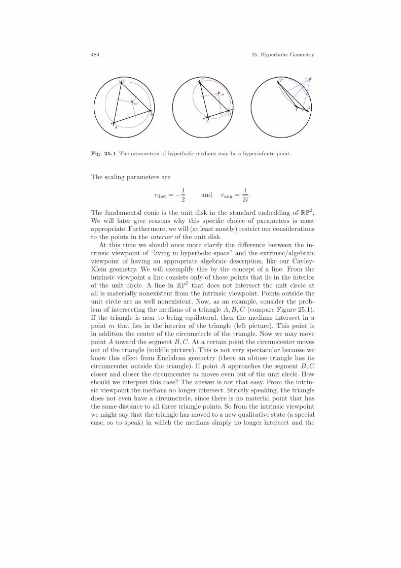
484 25 Hyperbolic Geometry
A
B
C
m
A
B
C
m
A B
Cm
Fig. 25.1 The intersection of hyperbolic medians may be a hyperinfinite point.
The scaling parameters are
cdist = −1
2and cang =
1
2i.
The fundamental conic is the unit disk in the standard embedding of RP2.
We will later give reasons why this specific choice of parameters is mostappropriate. Furthermore, we will (at least mostly) restrict our considerationsto the points in the interior of the unit disk.
At this time we should once more clarify the difference between the in-trinsic viewpoint of “living in hyperbolic space” and the extrinsic/algebraicviewpoint of having an appropriate algebraic description, like our Cayley-Klein geometry. We will exemplify this by the concept of a line. From theintrinsic viewpoint a line consists only of those points that lie in the interiorof the unit circle. A line in RP
2 that does not intersect the unit circle atall is materially nonexistent from the intrinsic viewpoint. Points outside theunit circle are as well nonexistent. Now, as an example, consider the prob-lem of intersecting the medians of a triangle A,B,C (compare Figure 25.1).If the triangle is near to being equilateral, then the medians intersect in apoint m that lies in the interior of the triangle (left picture). This point isin addition the center of the circumcircle of the triangle. Now we may movepoint A toward the segment B,C. At a certain point the circumcenter movesout of the triangle (middle picture). This is not very spectacular because weknow this effect from Euclidean geometry (there an obtuse triangle has itscircumcenter outside the triangle). If point A approaches the segment B,Ccloser and closer the circumcenter m moves even out of the unit circle. Howshould we interpret this case? The answer is not that easy. From the intrin-sic viewpoint the medians no longer intersect. Strictly speaking, the triangledoes not even have a circumcircle, since there is no material point that hasthe same distance to all three triangle points. So from the intrinsic viewpointwe might say that the triangle has moved to a new qualitative state (a specialcase, so to speak) in which the medians simply no longer intersect and the

25.2 Hyperbolic Transformations 485
circumcircle disappears. Were we to do so, hyperbolic geometry would sufferfrom the treatment of many many case distinctions.
Now it may happen that a clever mathematician in the hyperbolic worldcomes along and says, Well, the intersection of the medians may disappear inour world, but if we introduce a suitable algebraic structure to coordinatizeour points and lines (namely homogeneous coordinates) and if we furthermoredescribe our angle measurement by a certain formula (Cayley-Klein geome-try), then we may think of our world as realized within a certain object (theunit disk). If we do all that, then I can say that it is reasonable to extend ourlines even further than their infinity points to, let’s call it hyperinfinite points.In this representation two lines always intersect, and it makes total sense al-ways to speak of the intersection of the medians. They may intersect at finite,infinite, or hyperinfinite points. There is always also a circumcenter. If it isa hyperinfinite point, its distance to the triangle vertices becomes complex.But who cares, I am a mathematician and I am allowed to do abstractions.
In a sense, the situation is similar to the introduction of infinite pointsin Euclidean geometry. One may either accept that there are many case dis-tinctions or accept that there is a nicer algebraic system that gets rid of thespecial cases for the price of being more abstract and by adding elementsthat have no material counterpart. So also from an intrinsic viewpoint it istotally legitimate to represent hyperbolic geometry in terms of Cayley-Kleingeometries and their measurements. This means simply to allow for infiniteand hyperinfinite elements and using the corresponding algebraic represen-tations.
In what follows we will denote the interior of the unit circle by H andthe unit circle itself by H. The interior H is the staging ground to which werelate all our geometric considerations. However, we will freely make use ofits nice algebraic representation in RP
2.
25.2 Hyperbolic Transformations
After these quite philosophical considerations we will return to concrete cal-culations. We will start with a topic we already touched in Section 21.2:hyperbolic transformation. In our setup with the unit circle as fundamentalobject these are exactly those projective transformations in RP
2 that leavethe unit circle invariant. Fixing the images of three points A,B,C ∈ H on theunit circle determines such a hyperbolic transformation τ uniquely. The imagepoints A′, B′, C′ ∈ H must also lie on the unit circle. The matrix of the hyper-bolic transformation can be calculated in the following way. The three pointsA,B,C determine a projective scale on H. Every other point D on H has aunique and well-defined cross-ratio (A,B;C,D)P under which it is seen froma generic point P on H. So we can determine the unique position D on H suchthat (A,B;C,D)P = −1. Similarly, we get a unique point D′ in harmonic

486 25 Hyperbolic Geometry
p
l
τ(p)τ(l)
Fig. 25.2 Moving a point to the center of H.
position to A′, B′, C′. The hyperbolic transformation is the unique projectivetransformation that maps A,B,C,D to the corresponding primed points (seealso Figure 21.2). We recall that our Theorems 10.3 and 10.4 imply that thisprocedure indeed generates a map that leaves H invariant and that the groupof all such transformations is isomorphic to the group of projective transfor-mations of the real projective line RP
1. Since we will quite frequently referto the cross-ratio of four points A,B,C,D on H seen from a generic otherpoint P , we abbreviate this cross-ratio by (A,B;C,D)H := (A,B;C,D)P .Theorem 10.1 ensures that this value is independent of the specific choice ofP and hence well-defined. It is easy to show that a hyperbolic transformationautomatically also maps H to H.
Theorem 25.1. Let τ be a projective transformation that maps H to H.Then it also maps H to itself bijectively.
Proof. Since projective transformations are automatically bijections, the onlything we have to prove is that under τ the image of every point p ∈ H is againin H. For this we choose two arbitrary lines l and g through p. Since p is inthe interior of the unit disk, the lines l and g intersect H in two pairs of pointsAl, Bl and Ag, Bg, respectively. Since the two lines intersect in the interiorof H, the intersections with g and l alternate when traversing H cyclically.This in turn implies that the cross-ratio (Al, Bl;Ag, Bg) is negative. Hencealso the cross-ratio (τ(Al), τ(Bl); τ(Ag), τ(Bg)) is negative. Thus the imagepoints alternate as well. Accordingly also τ(l) and τ(p) intersect in the interiorof the unit disk. This implies τ(p) ∈ H. ⊓⊔
We now study the transitivity properties of hyperbolic transformation.
25.3 Angles and Boundaries 487
Theorem 25.2. Let p ∈ H and l be a point and a line incident to each other.Then there exists a hyperbolic transformation τ such that τ(p) = (0, 0, 1)T isthe origin and τ(l) = (0, 1, 0) is the x-axis.
Proof. We can base the proof on the observation of Theorem 22.2 that statesthat in the case of a nondegenerate fundamental conic two lines l and m areorthogonal if and only if their intersections with the fundamental conic arein harmonic position. Thus we may take the line l and its unique hyperbolicperpendicular through p, the line g. Then the intersections Al, Bl, Ag, and Bgwith H are in harmonic position: (Al, Bl;Ag, Bg)H = −1. The intersectionsAh,Bh of the (horizontal) x-axis with H and the intersections Av,Bv of the(vertical) y-axis with H are also in harmonic position. Thus the hyperbolictransformation τ with τ(Al) = Ah, τ(Bl) = Bh, τ(Ag) = Av automaticallysatisfies τ(Bg) = Bv. By this l is mapped to the x-axis and g is mappedto the y-axis. Furthermore, p (the intersection of l and g) is mapped by thistransformation to the origin (the intersection of the x-axis and the y-axis). ⊓⊔
This theorem enables us to do many of the following derivations withoutloss of generality for the special case that a certain point p is located atthe center of the hyperbolic disk. Furthermore, it shows that any pair ofcoincident point and line in H can be mapped to any other such pair in H.An illustration of the construction in the proof is given in Figure 25.2.
25.3 Angles and Boundaries
The theorem we just proved has another advantage related to angle measure-ment. For lines through the origin the angle measurement agrees with theusual Euclidean angle measurement, as the following theorem shows. Thusby the previous theorem we may always move to a situation with a compar-atively simple angle measurement.
Theorem 25.3. Let l and m be two lines that pass through the origin (0, 0, 1).Let αE be the Euclidean angle between them and αH the hyperbolic anglebetween them. Then |αE | = |αH |.
Proof. In our standard representation of hyperbolic geometry the measure-ment of angles between two lines l and m through a point p is by definitiongiven as
1
2i· ln(l,m;X,Y ).
Here X and Y are the tangents through p to the fundamental conic. Thesetangents are the lines that connect p to the intersections of the polar of p(with respect to H) with the fundamental conic H. In the standard embeddingthe polar of the origin with respect to the unit circle is the line at infinityl∞ = (0, 0, 1)T . The intersection of this line with any circle (in particular with
488 25 Hyperbolic Geometry
the unit circle) is I and J. Hence for measurements of angles between linesthrough p we have X = I and Y = J, or vice versa. Thus up to a possiblesign change the angle measurement agrees with Laguerre’s formula (Theorem18.9) and hence is just the Euclidean measurement. ⊓⊔
Remark 25.1. We have seen in Section 22.3 that if we perform measurementonly for lines through one point p, then we may without any problem talkabout oriented angle measurement. Since in this case the two tangents Xand Y are always the same, we can fix their roles once and forall. Now it ispossible to prove the following fact. Assume you move a point pt continuouslyparameterized by a parameter t ∈ [0, 1] such that pt always stays in H. Themotion of pt induces two continuous pathsXt and Yt of the two correspondingtangents. In principle, it may happen that for a round trip with p0 = p1 thetwo tangents may interchange their roles (this is, for instance, possible in ananalogous situation in elliptic geometry). However, if pt stays inside H, thetwo tangents Xt and Yt will never coincide, and as a consequence one hasX0 = X1 and Y0 = Y1 (the argument for this is not totally trivial and involvessome elementary topology). From this it can be shown that for an arbitraryendpoint p1 the order of the tangents is independent of the concrete path.Thus we may transfer the oriented angle measurement in a unique way to aglobally consistent oriented angle measurement on all of H. The hyperbolicplane is orientable!
We now will give an explicit method for calculating the angle between twooriented lines. By this we mean the absolute value of the angle that is neededto rotate one of the lines to match the other in the same orientation. Thefact that four points on the unit circle are in harmonic position if and only ifthe lines joining alternating pairs of them are perpendicular is only a specialcase of the following theorem. The theorem allows us to calculate the angledirectly from the intersection of the two lines with the unit circle.
Theorem 25.4. Let l and m be two oriented lines intersecting H in pointsAl, Bl, resp. Am, Bm. The lines are assumed to be oriented from B to A.Then the hyperbolic angle between l and m can be calculated as
2 arctan
(√−(Al, Bl;Am, Bm)H
).
Proof. We first prove the theorem for the special case that the intersectionof the two lines passes through the origin. Then we have a situation as shownin Figure 25.3. We consider the rectangle whose vertices are the intersec-tions of the two lines with the unit circle. By Theorem 18.3 and the factthat on the unit circle the points Al, Bl separate Am, Bm, the cross-ratio(Al, Bl;Am, Bm)H can be calculated as −a·a′
b·b′ , where a, a′, b, b′ are the lengthsof the sides of the rectangle. Since a = a′ and b = b′, the cross-ratio becomes

25.4 The Poincare Disk 489
ml
Al
Bl
Am
Bm
a
b
a′
b′α
α2
Fig. 25.3 Determining an angle from boundary points.
(Al, Bl;Am, Bm)H = −a2
b2= −(tan(α/2))2.
The last equation holds since the (Euclidean) angle at Bm shown in thepicture is half the angle between l and m. The tangent of this angle is exactlya/b. This proves
α = 2 arctan
(√−(Al, Bl;Am, Bm)H
)
for the special case of lines that intersect in the origin.Now assume that l and m are arbitrary intersecting lines. By Theo-
rem 25.2 there is a hyperbolic transformation τ that moves the intersectionof these two lines to the origin. This transformation leaves the cross-ratio(Al, Bl;Am, Bm)H as well as the angle α invariant, which proves the theo-rem. ⊓⊔
25.4 The Poincare Disk
We now introduce the Poincare disk model for hyperbolic geometry. Forthis we again consider a unit circle around the origin as the staging ground.However, this time we interpret it as a circle in the complex number plane C.Again it is highly appropriate to compactify C and right away consider thecomplex projective line CP
1 where the point at infinity has been added. As inRP
2 the region outside the unit circle helps us to understand the underlying
490 25 Hyperbolic Geometry
geometric and algebraic structure of the model. However, in this model theregion outside the unit circle will play a fundamentally different role fromthat in the Beltrami-Klein model. Inside the unit disk both models are onlydeformed images of one another. The following lists give a dictionary of howobjects of the hyperbolic plane are modeled in the Poincare disk model.Roughly speaking, the . . .
. . . points of the hyperbolic plane are represented by all points inside the unitcircle,
. . . lines of the hyperbolic plane are represented by circular arcs inside theunit circle that intersect the unit circle orthogonally,
. . . hyperbolic transformations are those Mobius transformations and thoseanti-Mobius transformations (compare Section 17.4) that leave the unitcircle invariant.
Furthermore, the Poincare disk has several advantages related to measure-ments. In the Poincare disk model the . . .
. . . hyperbolic angle between two lines is the (Euclidean) intersection anglebetween the corresponding circular arcs,
. . . circles (as loci of real(!) constant distance to a point) are represented byEuclidean circles,
. . . hyperbolic distances can still be calculated as the logarithm of a certaincross-ratio.
In what follows (if not explicitly stated otherwise), by a circle in CP1 we
will always mean either a usual circle or a circle with infinite radius (i.e., aline). Lines are those circles that pass through the infinite point ∞ of CP
1.The possibility to translate terms from the Beltrami-Klein model that residesin RP
2 and that is based essentially on linear structures to the Poincare diskmodel that resides in CP
1 and that is based essentially on circular structuresin such a nice way comes from a rich interplay and network of conceptsrelating the two worlds. Again we will here give only a rough impression ofthis rich topic. Projective geometry allows us to formulate many concepts onan advanced structural level. However, it will also be helpful to apply somesimple theorems from elementary geometry in this context.
We first aim at a proof that both models indeed represent structures thatare isomorphic inside the unit circle. What do we have to do for this? In theBeltrami-Klein model a hyperbolic line is represented by a line segment athat connects two points of H. In the Poincare disk model the correspondingline is represented by a circular arc a′ that connects the same two points.In addition, a′ has to intersect the unit circle orthogonally. This requirementmakes a′ uniquely defined. We now must verify that this way of mapping linesbetween the two models leads to a consistent specification for the mapping ofpoints. A point p in the Poincare disk model may be uniquely specified as theintersection of two distinct lines a and b that contain it. The correspondingcircular arcs a′ and b′ associated to these two lines again have a unique
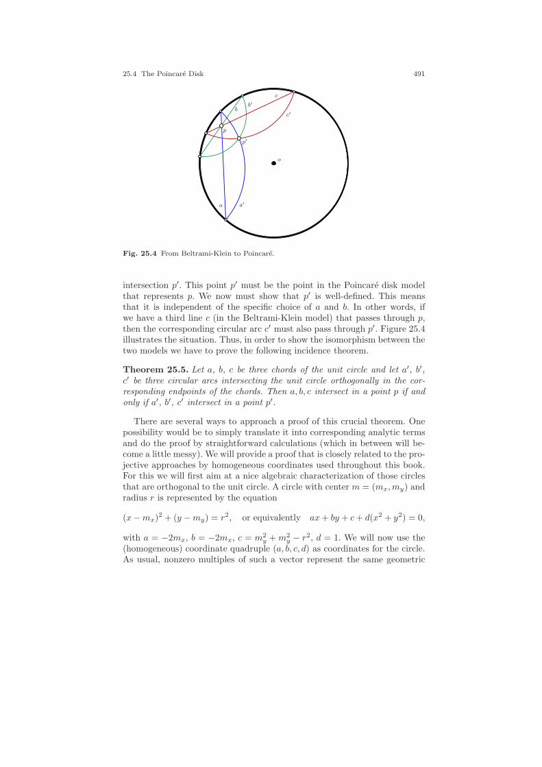
25.4 The Poincare Disk 491
a
b
c
a′
b′
c′
p
p′
o
Fig. 25.4 From Beltrami-Klein to Poincare.
intersection p′. This point p′ must be the point in the Poincare disk modelthat represents p. We now must show that p′ is well-defined. This meansthat it is independent of the specific choice of a and b. In other words, ifwe have a third line c (in the Beltrami-Klein model) that passes through p,then the corresponding circular arc c′ must also pass through p′. Figure 25.4illustrates the situation. Thus, in order to show the isomorphism between thetwo models we have to prove the following incidence theorem.
Theorem 25.5. Let a, b, c be three chords of the unit circle and let a′, b′,c′ be three circular arcs intersecting the unit circle orthogonally in the cor-responding endpoints of the chords. Then a, b, c intersect in a point p if andonly if a′, b′, c′ intersect in a point p′.
There are several ways to approach a proof of this crucial theorem. Onepossibility would be to simply translate it into corresponding analytic termsand do the proof by straightforward calculations (which in between will be-come a little messy). We will provide a proof that is closely related to the pro-jective approaches by homogeneous coordinates used throughout this book.For this we will first aim at a nice algebraic characterization of those circlesthat are orthogonal to the unit circle. A circle with center m = (mx,my) andradius r is represented by the equation
(x−mx)2 + (y −my) = r2, or equivalently ax+ by + c+ d(x2 + y2) = 0,
with a = −2mx, b = −2mx, c = m2y +m2
y − r2, d = 1. We will now use the(homogeneous) coordinate quadruple (a, b, c, d) as coordinates for the circle.As usual, nonzero multiples of such a vector represent the same geometric
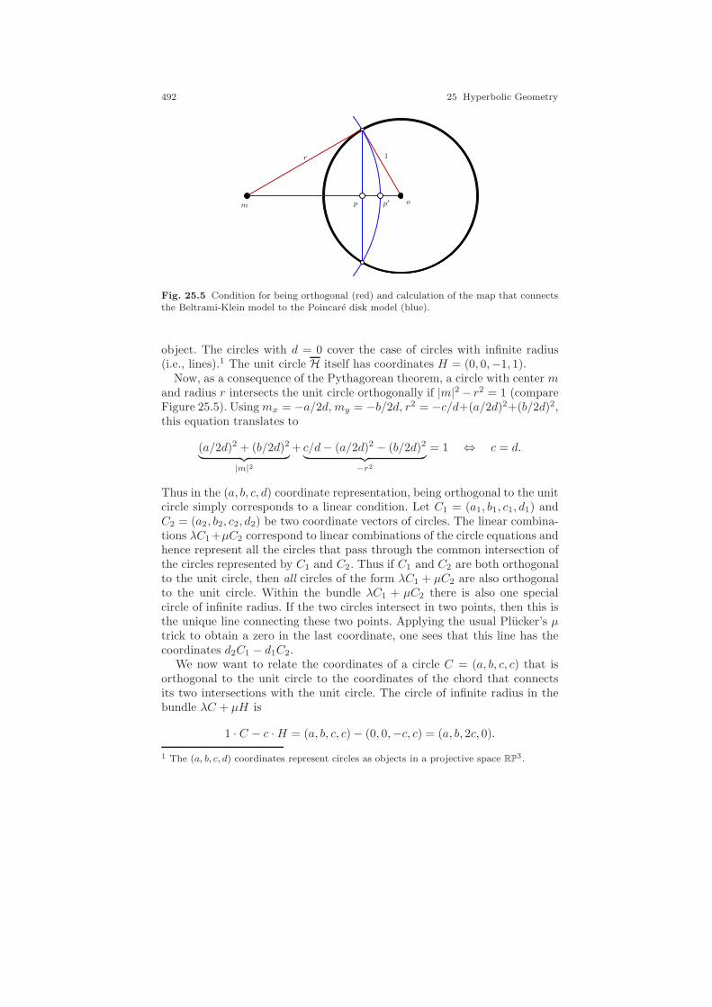
492 25 Hyperbolic Geometry
om p p′
1r
Fig. 25.5 Condition for being orthogonal (red) and calculation of the map that connectsthe Beltrami-Klein model to the Poincare disk model (blue).
object. The circles with d = 0 cover the case of circles with infinite radius(i.e., lines).1 The unit circle H itself has coordinates H = (0, 0,−1, 1).
Now, as a consequence of the Pythagorean theorem, a circle with center mand radius r intersects the unit circle orthogonally if |m|2 − r2 = 1 (compareFigure 25.5). Usingmx = −a/2d,my = −b/2d, r2 = −c/d+(a/2d)2+(b/2d)2,this equation translates to
(a/2d)2 + (b/2d)2︸ ︷︷ ︸|m|2
+ c/d− (a/2d)2 − (b/2d)2︸ ︷︷ ︸−r2
= 1 ⇔ c = d.
Thus in the (a, b, c, d) coordinate representation, being orthogonal to the unitcircle simply corresponds to a linear condition. Let C1 = (a1, b1, c1, d1) andC2 = (a2, b2, c2, d2) be two coordinate vectors of circles. The linear combina-tions λC1+µC2 correspond to linear combinations of the circle equations andhence represent all the circles that pass through the common intersection ofthe circles represented by C1 and C2. Thus if C1 and C2 are both orthogonalto the unit circle, then all circles of the form λC1 + µC2 are also orthogonalto the unit circle. Within the bundle λC1 + µC2 there is also one specialcircle of infinite radius. If the two circles intersect in two points, then this isthe unique line connecting these two points. Applying the usual Plucker’s µtrick to obtain a zero in the last coordinate, one sees that this line has thecoordinates d2C1 − d1C2.
We now want to relate the coordinates of a circle C = (a, b, c, c) that isorthogonal to the unit circle to the coordinates of the chord that connectsits two intersections with the unit circle. The circle of infinite radius in thebundle λC + µH is
1 · C − c ·H = (a, b, c, c) − (0, 0,−c, c) = (a, b, 2c, 0).
1 The (a, b, c, d) coordinates represent circles as objects in a projective space RP3.
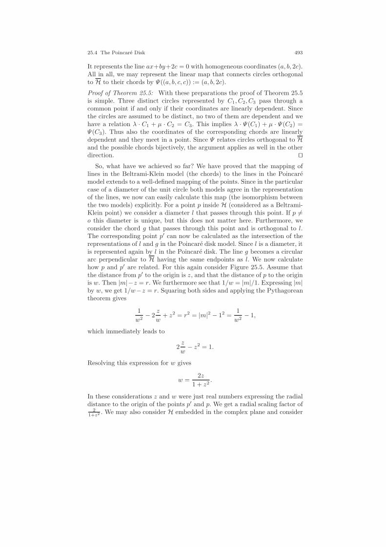
25.4 The Poincare Disk 493
It represents the line ax+by+2c = 0 with homogeneous coordinates (a, b, 2c).All in all, we may represent the linear map that connects circles orthogonalto H to their chords by Ψ((a, b, c, c)) := (a, b, 2c).
Proof of Theorem 25.5: With these preparations the proof of Theorem 25.5is simple. Three distinct circles represented by C1, C2, C3 pass through acommon point if and only if their coordinates are linearly dependent. Sincethe circles are assumed to be distinct, no two of them are dependent and wehave a relation λ · C1 + µ · C2 = C3. This implies λ · Ψ(C1) + µ · Ψ(C2) =Ψ(C3). Thus also the coordinates of the corresponding chords are linearlydependent and they meet in a point. Since Ψ relates circles orthogonal to Hand the possible chords bijectively, the argument applies as well in the otherdirection. ⊓⊔
So, what have we achieved so far? We have proved that the mapping oflines in the Beltrami-Klein model (the chords) to the lines in the Poincaremodel extends to a well-defined mapping of the points. Since in the particularcase of a diameter of the unit circle both models agree in the representationof the lines, we now can easily calculate this map (the isomorphism betweenthe two models) explicitly. For a point p inside H (considered as a Beltrami-Klein point) we consider a diameter l that passes through this point. If p 6=o this diameter is unique, but this does not matter here. Furthermore, weconsider the chord g that passes through this point and is orthogonal to l.The corresponding point p′ can now be calculated as the intersection of therepresentations of l and g in the Poincare disk model. Since l is a diameter, itis represented again by l in the Poincare disk. The line g becomes a circulararc perpendicular to H having the same endpoints as l. We now calculatehow p and p′ are related. For this again consider Figure 25.5. Assume thatthe distance from p′ to the origin is z, and that the distance of p to the originis w. Then |m|−z = r. We furthermore see that 1/w = |m|/1. Expressing |m|by w, we get 1/w−z = r. Squaring both sides and applying the Pythagoreantheorem gives
1
w2− 2
z
w+ z2 = r2 = |m|2 − 12 =
1
w2− 1,
which immediately leads to
2z
w− z2 = 1.
Resolving this expression for w gives
w =2z
1 + z2.
In these considerations z and w were just real numbers expressing the radialdistance to the origin of the points p′ and p. We get a radial scaling factor of
21+z2 . We may also consider H embedded in the complex plane and consider
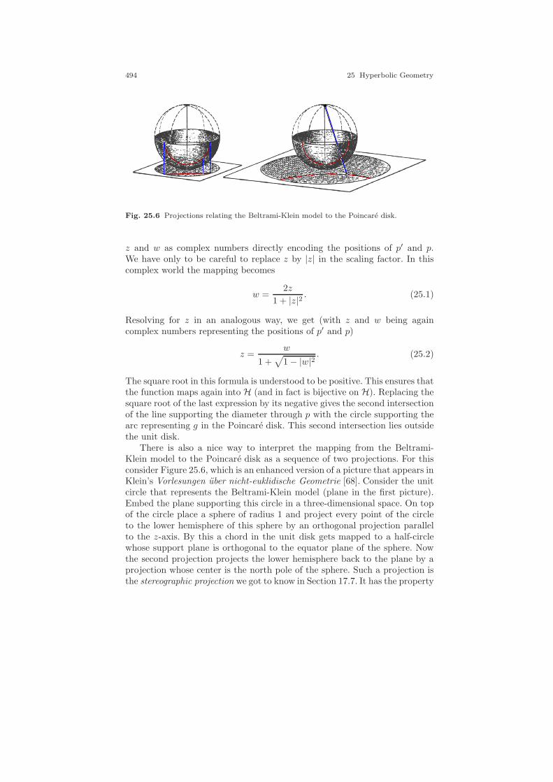
494 25 Hyperbolic Geometry
Fig. 25.6 Projections relating the Beltrami-Klein model to the Poincare disk.
z and w as complex numbers directly encoding the positions of p′ and p.We have only to be careful to replace z by |z| in the scaling factor. In thiscomplex world the mapping becomes
w =2z
1 + |z|2 . (25.1)
Resolving for z in an analogous way, we get (with z and w being againcomplex numbers representing the positions of p′ and p)
z =w
1 +√
1 − |w|2. (25.2)
The square root in this formula is understood to be positive. This ensures thatthe function maps again into H (and in fact is bijective on H). Replacing thesquare root of the last expression by its negative gives the second intersectionof the line supporting the diameter through p with the circle supporting thearc representing g in the Poincare disk. This second intersection lies outsidethe unit disk.
There is also a nice way to interpret the mapping from the Beltrami-Klein model to the Poincare disk as a sequence of two projections. For thisconsider Figure 25.6, which is an enhanced version of a picture that appears inKlein’s Vorlesungen uber nicht-euklidische Geometrie [68]. Consider the unitcircle that represents the Beltrami-Klein model (plane in the first picture).Embed the plane supporting this circle in a three-dimensional space. On topof the circle place a sphere of radius 1 and project every point of the circleto the lower hemisphere of this sphere by an orthogonal projection parallelto the z-axis. By this a chord in the unit disk gets mapped to a half-circlewhose support plane is orthogonal to the equator plane of the sphere. Nowthe second projection projects the lower hemisphere back to the plane by aprojection whose center is the north pole of the sphere. Such a projection isthe stereographic projection we got to know in Section 17.7. It has the property
25.4 The Poincare Disk 495
that it maps circles to circles and preserves intersection angles of circles. Thestereographic projection maps the equator to unit circle 2H scaled the by afactor of two. The arcs intersecting the equator orthogonally are mapped toarcs that intersect 2H orthogonally. Scaling down the region 2H by a factorof 2 leaves us with our version of the Poincare disk. To see that this is indeedthe right mapping, consider a point (x, y, 0)T in the Poincare disk embeddedin R2. Scaling by a factor of 2 gives (2x, 2y, 0)T . Mapping this point to thesphere by stereographic projection via formula (17.1) results in
2x2y0
7→ 2
x2 + y2 + 1
xy
x2 + y2
.
Projecting down to the plane exactly results in
1
x2 + y2 + 1
2x2y0
.
Omitting the last coordinate, this is our formula (25.1) that relates the pointsof the Poincare disk to the points in the Beltrami-Klein model.
The scaling factor of the map (25.1) for points close to the center is asymp-totically 2. This means that objects close to the center in the Poincare diskmodel appear half the size that they appear in the Beltrami-Klein model.They thereby leave more space for the other objects that are squeezed closeto the boundary. Thus the Poincare disk model appears visually more bal-anced, an effect that we could observe for instance in Figure 24.5.
In our translation process one final point deserves to be mentioned: therole of the exterior of H in the Poincare disk model. Referring once more toFigure 25.6, we see that in the second projection the upper hemisphere of thesphere is mapped to the outside of the Poincare disk. The vertical projectionthat relates the Beltrami-Klein model to the sphere produces in essence twointersections: one at the lower hemisphere and one at the upper hemisphere.Thus projecting also the upper hemisphere to CP
1, each point inside H inthe Beltrami-Klein model is related to two points in CP
1, one point inside theunit disk and one point outside the unit disk. They correspond to the choice ofthe sign of the square root in (25.2). Both representing points w
1+√
1−|w|2and
w
1−√
1−|w|2have the same direction with respect to the origin but different
distances. In fact, the radii are reciprocal, as the following calculation shows.The product of the distances of these two points to the origin evaluates to
|w|1 +
√1 − |w|2
· |w|1 −
√1 − |w|2
=|w|2
1 − (1 − |w|2) = 1.

496 25 Hyperbolic Geometry
Both of them are related by an inversion in the unit circle z 7→ 1z . Thus the
outside of the Poincare disk is just a mirror image (by reflection in the unitcircle) of the inside. The points outside the unit circle in the Beltrami-Kleinmodel have no direct counterpart in the Poincare disk.
25.5 CP1 Transformations and the Poincare Disk
So far, we have defined hyperbolic transformations only in the world of theBeltrami-Klein model. They are the projective RP
2 transformations τ thatleave the unit circle as a whole invariant.Via the isomorphism of the Poincaredisk and the Beltrami-Klein model (explicitly given by equations (25.1) and(25.2)), the map τ induces an action τ in the Poincare disk model. The map τis the corresponding hyperbolic transformation in the Poincare disk model. Itwill turn out that these hyperbolic transformations τ in the Poincare disk areexactly those Mobius transformations and anti-Mobius transformations thatleave the unit circle invariant. The reason for this nice interplay of (certain)RP
2 projective transformations and (certain) CP1 projective transformations
is that a hyperbolic transformation must leave the unit circle as a wholeinvariant. In both cases this induces a transformation of the points on theunit circle that is a projective transformation on the points of H.
Since the situation involves simultaneously several interpretations of thesame objects in different mathematical spaces, it may become quite confus-ing. To avoid this confusion we will first specify these different spaces andtheir interrelations. Most of these relations have already been established inprevious chapters.
The relation of RP2 and CP
1: We identify the finite part of both spacesby the map (x, y, 1)T 7→ (x + iy, 1). In particular, this map relates the unitcircle and its interior in both spaces bijectively. We will use the same symbolsH and H for the unit circle and its interior in both spaces. As before, for apoint p ∈ RP
2 we will denote its counterpart in CP1 by p.
The unit circle in RP2 and its relation to RP
1: The unit circle H isa special conic satisfying the (homogeneous) equation x2 + y2 − z2 = 0. InSection 10.2 we learned that we can bijectively relate each nondegenerateconic to the space RP
1 by (stereographically) projecting its points to a line(compare Figure 10.7). Equivalently, this bijection can also be calculated bya cross-ratio with respect to the conic. For this we consider R ∪ ∞ as acopy of RP
1 and define a specific bijection Ψ : H → R ∪ ∞ = RP1. We fix
three mutually different points 0,1,∞ on the conic and for every other pointx = (x, y, 1)T on the conic calculate
Ψ(x) := (0,∞;x,1)H.

25.5 CP1 Transformations and the Poincare Disk 497
eτ
Fig. 25.7 A hyperbolic transformation.
In a natural way we may call a map f : H → H a projective map if thecomposition Ψ f Ψ−1 is a projective transformation on RP
1. Theorem 10.3states that every projective transformation on RP
2 that leaves H invariantinduces a projective map (a RP
1 action) on the points of H.
The unit circle in CP1 and its relation to RP
1: We can also relate theunit circle in CP
1 in a natural way to the real projective line. For this we alsofix three points 0, 1, ∞ on H and consider the map Φ : H → R∪∞ = RP
1
defined byΦ(x) := (0, ∞; x, 1),
the cross-ratio this time considered over CP1. This expression maps into
R∪ ∞ since four cocircular points in CP1 always produce a real or infinite
cross-ratio. In fact, Theorem 18.3 tell us that both ways to relate the unitcircle to RP
1 are identical. We have
Ψ(x) = (0,∞;1,x)H = (0, ∞; 1, x) = Φ(x). (25.3)
We may even interpret the map Φ as a projective map that sends the circleH to the real points RP
1 = (a, b)T |a, b,∈ R − (0, 0)T in CP1 by sending
0 7→ (0, 1)T , 1 7→ (1, 1)T , and ∞ 7→ (1, 0)T . Again in a natural way wemay call a map f : H → H a projective map if Φ f Φ−1 is a projectivetransformation on RP
1. By the equivalence of the two cross-ratios in equation(25.3) the two concepts of projective transformations on H are equivalent.
Now, a projective transformation τ ′ in CP1 that leaves H invariant can be
interpreted as a projective transformation on the points of H (considered asa RP
1) via Φ τ ′ Φ−1. Figure 25.7 illustrates the effect of a projective CP1
transformation that leaves the unit circle invariant. Notice that the grid oflines is mapped to a grid of circular arcs. The map induces a transformationon the unit circle itself. This transformation is projective. The specific trans-
498 25 Hyperbolic Geometry
formation in Figure 25.7 has been chosen such that the image of three pointsis exactly the same as in the RP
2 transformation shown in Figure 21.2. Thisimplies that both maps agree on the unit circle.Moreover, and this is important for us, we get the following lemma.
Lemma 25.1. Let f : H → H be a projective map. Then this map can beuniquely extended to a projective transformation τ ′ in CP
1.
Proof. Let f : H → H be a projective map on H. This implies that the mapg := Φ f Φ−1 is a projective map RP
1 → RP1 on the usual projective
line. Thus g can be represented by a 2 × 2 matrix with real coefficients. Wemay interpret this map as a projective map g : CP
1 → CP1. We now can pull
back this CP1 action to H by setting τ ′ = Φ−1 g Φ. In other words, every
projective map on H can be written as a 2×2 matrix and by this interpretedas a projective map on CP
1. ⊓⊔
After these conceptual considerations we are ready to prove that hyper-bolic transformations in the Poincare disk are either Mobius or anti-Mobiustransformations. For a given hyperbolic transformation τ (in the Beltrami-Klein model) we want to compute the corresponding effect in the Poincaredisk model, i.e., the map τ . In principle, this could be done by directly cal-culating the effect of a projective transformation under a conjugation bythe transformation equations (25.1) and (25.2). However, we again can avoidthese rather tedious calculations by performing some structural analysis ofthe situation. Within the Poincare disk model we may compute the imageunder τ of a point p inside H by the following alternative procedure.
1: Take two distinct circular arcs l and g intersecting H orthogonally (twoPoincare lines) that both pass through p.
2: The two arcs intersect H in two pairs of points (Al, Bl) and (Ag, Bg).
3: Take the images (τ(Al), τ(Bl)) and (τ(Ag), τ(Bg)) of these point pairsunder τ (this is the same image as under τ (l)).
4: They determine two new circular arcs τ(l) and τ (g) (orthogonal to H)inside H. These are the images of l and g in the Poincare model.
5: Their intersection corresponds to the image τ (p) of p.
This can be used to prove the following theorem.
Theorem 25.6. Let τ be a hyperbolic transformation. If τ preserves the ori-entation of H, then τ is the unique Mobius transformation that agrees with τon H. If τ reverses the orientation of H then τ is a composition of the uniqueMobius transformation that agrees with τ on H followed by a circle inversionin the unit circle.
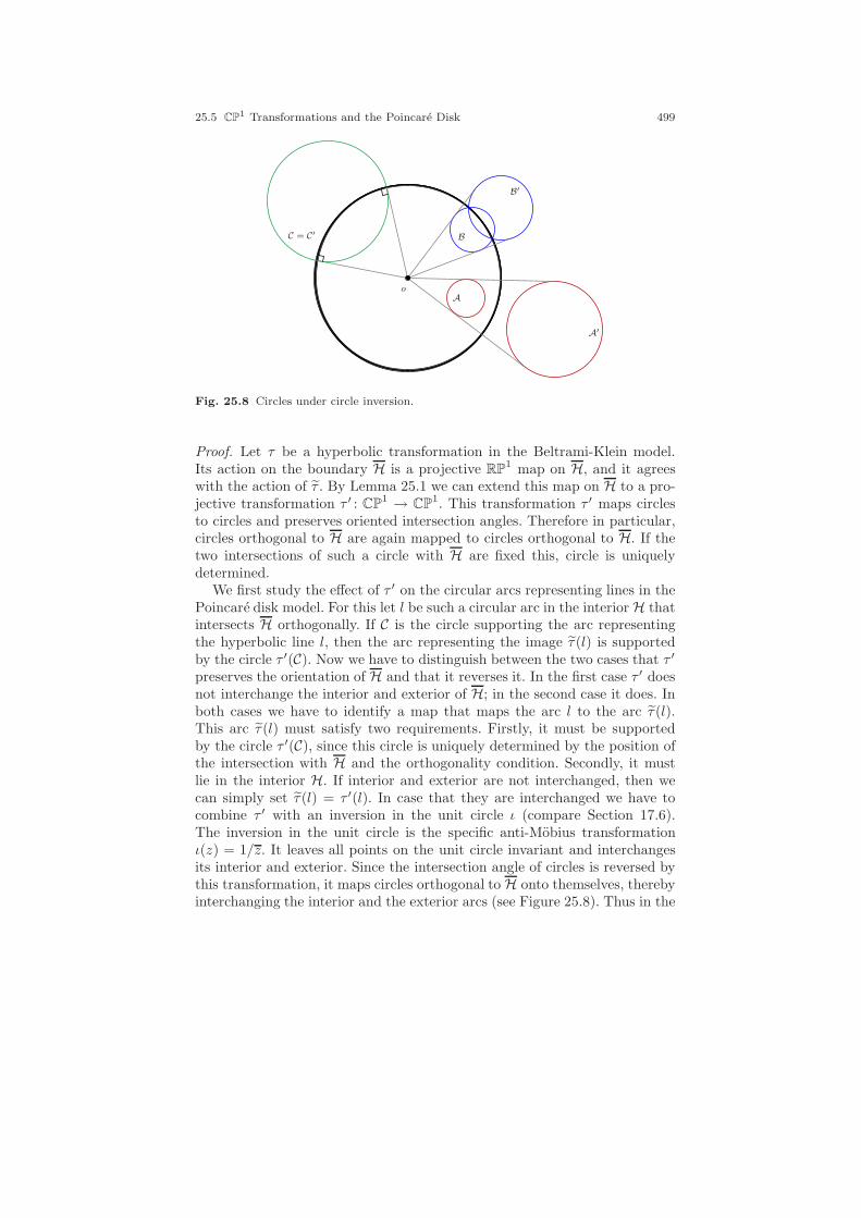
25.5 CP1 Transformations and the Poincare Disk 499
oA
BC = C′
A′
B′
Fig. 25.8 Circles under circle inversion.
Proof. Let τ be a hyperbolic transformation in the Beltrami-Klein model.Its action on the boundary H is a projective RP
1 map on H, and it agreeswith the action of τ . By Lemma 25.1 we can extend this map on H to a pro-jective transformation τ ′ : CP
1 → CP1. This transformation τ ′ maps circles
to circles and preserves oriented intersection angles. Therefore in particular,circles orthogonal to H are again mapped to circles orthogonal to H. If thetwo intersections of such a circle with H are fixed this, circle is uniquelydetermined.
We first study the effect of τ ′ on the circular arcs representing lines in thePoincare disk model. For this let l be such a circular arc in the interior H thatintersects H orthogonally. If C is the circle supporting the arc representingthe hyperbolic line l, then the arc representing the image τ (l) is supportedby the circle τ ′(C). Now we have to distinguish between the two cases that τ ′
preserves the orientation of H and that it reverses it. In the first case τ ′ doesnot interchange the interior and exterior of H; in the second case it does. Inboth cases we have to identify a map that maps the arc l to the arc τ (l).This arc τ (l) must satisfy two requirements. Firstly, it must be supportedby the circle τ ′(C), since this circle is uniquely determined by the position ofthe intersection with H and the orthogonality condition. Secondly, it mustlie in the interior H. If interior and exterior are not interchanged, then wecan simply set τ (l) = τ ′(l). In case that they are interchanged we have tocombine τ ′ with an inversion in the unit circle ι (compare Section 17.6).The inversion in the unit circle is the specific anti-Mobius transformationι(z) = 1/z. It leaves all points on the unit circle invariant and interchangesits interior and exterior. Since the intersection angle of circles is reversed bythis transformation, it maps circles orthogonal to H onto themselves, therebyinterchanging the interior and the exterior arcs (see Figure 25.8). Thus in the
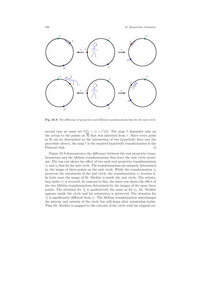
500 25 Hyperbolic Geometry
A
B
C
A′A′
B′
B′
C′ C′
τ1 τ2
A
B
C
A′
A′
B′
B′
C′ C′
τ ′1 τ ′2
Fig. 25.9 The difference of projective and Mobius transformations that fix the unit circle.
second case we must set τ (l) = (ι τ ′)(l). The map τ depended only onthe action to the points on H that was inherited from τ . Since every pointin H can be determined as the intersection of two hyperbolic lines (see theprocedure above), the map τ is the required hyperbolic transformation in thePoincare disk. ⊓⊔
Figure 25.9 demonstrates the difference between the real projective trans-formations and the Mobius transformations that leave the unit circle invari-ant. The top row shows the effect of two such real projective transformationsτ1 and τ2 that fix the unit circle. The transformations are uniquely determinedby the image of three points on the unit circle. While the transformation τ2preserves the orientation of the unit circle, the transformation τ1 reverses it.In both cases the image of Dr. Stickler is inside the unit circle. The orienta-tion under τ1 is reversed. In contrast to this, the lower row shows the effect ofthe two Mobius transformations determined by the images of the same threepoints. The situation for τ ′2 is qualitatively the same as for τ2. Dr. Sticklerappears inside the circle and his orientation is preserved. The situation forτ ′1 is significantly different from τ1. The Mobius transformation interchangesthe interior and exterior of the circle but still keeps their orientation stable.Thus Dr. Stickler is mapped to the exterior of the circle with his original ori-
25.6 Angles and Distances in the Poincare Disk 501
entation. The map τ ′1 followed by a circle inversion ι would be the hyperbolictransformation that corresponds to τ1 in the Poincare disk model.
25.6 Angles and Distances in the Poincare Disk
The hard part of the work is done. From what we have established so far itis relatively easy to determine the computation of angles and distances di-rectly in the Poincare disk model. The fact that hyperbolic transformationsare essentially expressed by Mobius transformations and anti-Mobius trans-formations helps to transfer (without loss of generality) the measurement toalmost trivial situations. We start with angles between hyperbolic lines. Wehave seen that lines in the Poincare model correspond to circular arcs insideH orthogonal to the unit circle. We again consider angles between orientedlines as in Section 25.3. First of all, the formula for computing the anglesfrom the intersections of lines with the unit circle from Theorem 25.4 stillapplies to the Poincare disk, since it agrees with the Beltrami-Klein modelalong the unit circle. From this we also see that the situation is most trivialfor lines through the origin.
Lemma 25.2. Let l and g be two oriented hyperbolic lines in the Poincaredisk that pass through the origin. Then the angle between them is exactly theEuclidean angle between them.
Proof. Hyperbolic lines through the origin in the Poincare model are juststraight diameters of the unit circle. Thus the representation of lines throughthe origin is the same as in the Beltrami-Klein model, and the lemma followsby Theorem 25.3. ⊓⊔
The property of Mobius transformations to preserve the intersection anglesof circles helps to transfer this result to arbitrary intersection of hyperboliclines.
Theorem 25.7. Let l and g be two arbitrary intersecting oriented hyperboliclines in the Poincare disk. Then the angle between them is exactly the Eu-clidean intersection angle between the corresponding Euclidean arcs.
Proof. Apply a hyperbolic transformation τ that maps the intersection ofthe two lines under consideration to the origin (such a transformation existsby Theorem 25.2). The construction in the proof of this theorem allowedus to choose this transformation to be order-preserving. In the Poincaredisk model this corresponds to a Mobius transformation by Theorem 25.6.The preservation of intersection-angles property of Mobius transformations(Corollary17.1) ensures that the intersection angles of the circular arcs beforeand after the transformation are identical. Finally, Lemma 25.2 ensures thatthe intersection angle matches the Euclidean intersection angle. ⊓⊔

502 25 Hyperbolic Geometry
Fig. 25.10 Angle between lines in the Poincare disk.
This gives us an important property of the Poincare disk model: The an-gles are represented conformally. One can simply measure the Euclidean in-tersection angle between the circular arcs that represent the lines to get thehyperbolic intersection angle between the lines. Figure 25.10 illustrates thesituation.
It is also instructive to figure out how the hyperbolic distance betweentwo points can be calculated directly in the Poincare disk model. For this weuse the transformation (25.1) and relate certain cross-ratios in the Beltrami-Klein model (i.e. in RP
2) and in the Poincare disk (i.e., in CP1). We again
pull back to a situation that is algebraically nicely accessible.
Lemma 25.3. Let P and Q be two points on the x-axis in the Poincare disk.Then the hyperbolic distance between P and Q is | ln((P,Q;X,Y ))|, where Xand Y are the two intersections of the x-axis with the unit circle.
Proof. We may represent the points by their x-coordinates p and q. By for-mula (25.1) the corresponding points P ′ and Q′ in the Beltrami-Klein modelare also on the x-axis and have coordinates p′ = 2p
1+p2 and q′ = 2q1+q2 . The
absolute value of the hyperbolic distance is given by
∣∣∣∣1
2ln ((P ′, Q′;X ;Y ))
∣∣∣∣ =
∣∣∣∣1
2ln
((p′ − 1)(q′ + 1)
(p′ + 1)(q′ − 1)
)∣∣∣∣ .
Inserting the expression for p′ in (p′−1)(p′+1) gives
p′ − 1
p′ + 1=
2p− 1 − p2
1 + p2· 1 + p2
2p+ 1 + p2=
(p− 1
p+ 1
)2
.
25.6 Angles and Distances in the Poincare Disk 503
A similar expression holds for q, and we obtain
(p′ − 1)(q′ + 1)
(p′ + 1)(q′ − 1)=
((p− 1)(q + 1)
(p+ 1)(q − 1)
)2
.
This shows that(P ′, Q′;X,Y ) = (P,Q;X,Y )2.
Inserting this in the distance formula yields
∣∣∣∣1
2ln ((P ′, Q′;X,Y ))
∣∣∣∣ =
∣∣∣∣1
2ln((P,Q;X,Y )2
)∣∣∣∣ = |ln ((P,Q;X,Y ))| .
This is what is claimed by the theorem. ⊓⊔We again can use this result to get a general method to calculate distances
in the Poincare model.
Theorem 25.8. Let P and Q be two arbitrary points in the Poincare disk.Then the hyperbolic distance between P and Q is | ln((P,Q;X,Y ))|, where Xand Y are the intersections of the hyperbolic line through P and Q with theunit circle.
Proof. Let P and Q be two arbitrary points in the Poincare disk. By Theo-rem 25.2 there is a hyperbolic transformation that maps them to two pointsτ(P ) and τ(Q) on the x-axis. This transformation is a Mobius transforma-tion τ that fixes the unit circle, and hence X and Y get mapped to twopoints τ(X) and τ(Y ) that are the intersections X ′ and Y ′ of the x-axiswith the unit circle. Thus we have (P,Q;X,Y ) = (τ(P ), τ(Q); τ(X), τ(Y )) =(τ(P ), τ(Q);X ′, Y ′), and Lemma 25.3 can be applied to finally prove thetheorem. ⊓⊔
It is an amazing fact that when calculating the hyperbolic distance inthe Poincare model via the cross-ratio in CP
1 the factor 1/2 in the distanceformula has to be dropped, in order to be consistent with the Beltrami-Kleinmodel.

26
Selected Topics in HyperbolicGeometry
Out of nothing I created a strangenew universe!
Janos Bolyai
After having mastered the basics of hyperbolic geometry, having learned howto calculate distances and angles, perform transformations, represent it intwo different models, a whole world of interesting topics opens, by far morethan can be covered here in this book. We now want to focus on a few ofthese topics that are of particular beauty and show specific relationships toour projective approaches to hyperbolic geometry.
26.1 Circles and Cycles in the Poincare Disk
Without going too much into detail we want to explain a few effects concern-ing circles and cycles in the Poincare disk model. For this we again have todistinguish carefully between different types of cycles, a topic we already en-countered in Chapter 23.We here should again recall that the points outsidethe unit disk in the Beltrami-Klein model do not have a proper counterpartin the Poincare disk. For this reason we will prominently consider those cy-cles that have a nonempty intersection with the interior of the unit disk (inthe Beltrami-Klein model). As developed in Section 23.3, these cycles fallinto three classes. Members of the the first class will be called proper realcircles. They are a set of points inside the unit disk that have a real hy-perbolic distance to a center m inside the unit disk. In the Beltrami-Klein
505

506 26 Selected Topics in Hyperbolic Geometry
Fig. 26.1 Circles and cycles in the Beltrami-Klein model and the Poincare disk.
model they correspond to conics that have two complex contact points withour fundamental conic—the unit circle.
Other cycles that may have nonempty intersection with the interior of theunit disk are the hypercycles and the horocycles. Horocycles have a centerthat lies on the unit circle. In the Beltrami-Klein model they are conics thatosculate with the unit circle of order four (i.e. the two contact points coincide).The distance of the cycle points to such a center is always infinite and cannotbe used as a characterizing property for the points on the cycle. Hypercyclesare those conics that have a center outside the unit circle. They have ordertwo contact with the unit circle in two real points. The distance of the pointsof the cycle to the center is a complex number. Summarizing, one can say thatin the Beltrami-Klein model, cycles are conics that have contact to the unitcircle in two points that may be distinct complex conjugates, distinct realpoints, or real and coinciding points. All three types of curves have constantcurvature, except for the points where they meet the unit circle.
How are these types of cycles represented in the Poincare model? Fig-ure 26.1 shows three cycles: a proper real circle (blue), a horocycle (red),and a hypercycle (green) in the Beltrami-Klein model and the correspondingcycles in the Poincare model. If possible also the centers are indicated. Weonce more recall our discussion from Section 23.4 concerning the questionwhether a hypercycle should be considered one cycle or two cycles. Therewere good reasons for both of these viewpoints. The reason to consider thehypercycle to be two cycles comes from the differential geometric viewpoint:It is impossible to get from one half to the other by a finite journey alongthe circle in hyperbolic space. Both branches are curves of constant curva-ture of infinite length. The reason to consider them to be one branch camefrom the algebraic treatment. The entire cycle should be an algebraicallyclosed curve: a complete conic. We will see that both viewpoints again havetheir counterparts in the Poincare disk model. First we will briefly explain
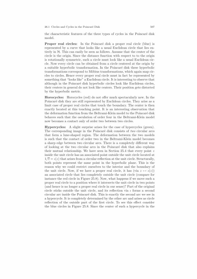
26.1 Circles and Cycles in the Poincare Disk 507
the characteristic features of the three types of cycles in the Poincare diskmodel.
Proper real circles: In the Poincare disk a proper real circle (blue) isrepresented by a curve that looks like a usual Euclidean circle that lies en-tirely in H. This can easily be seen as follows. Assume that the center of thecircle is the origin. Since the distance function with respect to to the originis rotationally symmetric, such a circle must look like a usual Euclidean cir-cle. Now every circle can be obtained from a circle centered at the origin bya suitable hyperbolic transformation. In the Poincare disk these hyperbolictransformations correspond to Mobius transformations, which again map cir-cles to circles. Hence every proper real circle must in fact be represented bysomething that “looks like” a Euclidean circle. It is interesting to observe thatalthough in the Poincare disk hyperbolic circles look like Euclidean circles,their centers in general do not look like centers. Their position gets distortedby the hyperbolic metric.
Horocycles: Horocycles (red) do not offer much spectacularly new. In thePoincare disk they are still represented by Euclidean circles. They arise as alimit case of proper real circles that touch the boundary. The center is thenexactly located at this touching point. It is an interesting observation thatthe deformation function from the Beltrami-Klein model to the Poincare diskbehaves such that the osculation of order four in the Beltrami-Klein modelnow becomes a contact only of order two between two circles.
Hypercycles: A slight surprise arises for the case of hypercycles (green).The corresponding image in the Poincare disk consists of two circular arcsthat form a lune-shaped region. The deformation between the two modelsis such that the contact of order two in the Beltrami-Klein model becomesa sharp edge between two circular arcs. There is a completely different wayof looking at the two circular arcs in the Poincare disk that also explainstheir mutual relationship. We have seen in Section 25.4 that every point zinside the unit circle has an associated point outside the unit circle located at1/z = ι(z) that arises from a circular reflection at the unit circle. Structurally,both points represent the same point in the hyperbolic plane. This is thereason why we could restrict ourselves to the interior and the boundary ofthe unit circle. Now, if we have a proper real circle, it has (via z 7→ ι(z))an associated circle that lies completely outside the unit circle (compare forinstance the red circle in Figure 25.8). Now, what happens if we move such aproper real circle to a position where it intersects the unit circle in two points(and hence is no longer a proper real circle in our sense)? Part of the originalcircle sticks outside the unit circle, and its reflection via ι forms a secondcircular arc inside the Poincare disk. This is exactly the second arc we see ina hypercycle. It is completely determined by the other arc and arises as circlereflection of the outside part of the first circle. To see this effect considerthe blue circles in Figure 25.8. Since the center of such a hypercycle in the

508 26 Selected Topics in Hyperbolic Geometry
Fig. 26.2 Four A-circles through three points.
Beltrami-Klein model lies outside the unit circle, it has no visual counterpartin the Poincare model.
So we see that the two branches of a hypercycle in the Poincare disk modelindeed translate into two distinct (though closely related) circular arcs. Letus finally exemplify how the different viewpoints of what is a circle sensiblyinfluence some of the fundamental statements of elementary geometry. InEuclidean geometry we are used to the fact that through three finite pointsthere always passes a unique circle. What is the counterpart of this in hyper-bolic geometry? This depends on your definition of what is a cycle. Let ustake two extreme positions. We first formulate them in the Beltrami-Kleinmodel. Let us call an A-circle (A for algebraic) for a given center m any conicdescribed by the matrix
λ ·MTBM + µ ·A(compare Equation (23.3)), that is, the complete conic that corresponds toa circle, a horocycle or a hypercycle. Let us call a C-circle (C for curvature)any curve of constant curvature that arises from starting at a point insidethe unit disk and following with the same curvature in both directions. Thusthe hypercycles get cut into two branches. In the Poincare disk the A-circlescorrespond to full (Euclidean) circles in the closure of H and pairs of circulararcs that are related by ι as described above. The C-circles arise simply asintersections of ordinary Euclidean circles with the interior H of the unitcircle. For three points A,B,C inside H we now have the following:
There is exactly one C-circle through these three points. As long asA,B,C are not on a hyperbolic line, there are exactly four A-circlesthrough these three points.
In the Poincare model the unique C-circle arises as the intersection of theunique Euclidean circle through A,B,C with H. The four A-circles arise
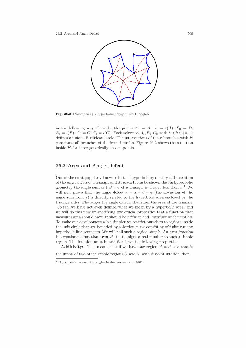
26.2 Area and Angle Defect 509
Fig. 26.3 Decomposing a hyperbolic polygon into triangles.
in the following way. Consider the points A0 = A, A1 = ι(A), B0 = B,B1 = ι(B), C0 = C, C1 = ι(C). Each selection Ai, Bj, Ck with i, j, k ∈ 0, 1defines a unique Euclidean circle. The intersections of these branches with Hconstitute all branches of the four A-circles. Figure 26.2 shows the situationinside H for three generically chosen points.
26.2 Area and Angle Defect
One of the most popularly known effects of hyperbolic geometry is the relationof the angle defect of a triangle and its area: It can be shown that in hyperbolicgeometry the angle sum α + β + γ of a triangle is always less then π.1 Wewill now prove that the angle defect π − α − β − γ (the deviation of theangle sum from π) is directly related to the hyperbolic area enclosed by thetriangle sides. The larger the angle defect, the larger the area of the triangle.So far, we have not even defined what we mean by a hyperbolic area, and
we will do this now by specifying two crucial properties that a function thatmeasures area should have. It should be additive and invariant under motion.To make our development a bit simpler we restrict ourselves to regions insidethe unit circle that are bounded by a Jordan curve consisting of finitely manyhyperbolic line segments. We will call such a region simple. An area functionis a continuous function area(R) that assigns a real number to such a simpleregion. The function must in addition have the following properties.
Additivity: This means that if we have one region R = U ∪ V that is
the union of two other simple regions U and V with disjoint interior, then
1 If you prefer measuring angles in degrees, set π = 180.

510 26 Selected Topics in Hyperbolic Geometry
π αα β
Fig. 26.4 Calculating the area of special hyperbolic triangles.
area(R) = area(U) + area(V ).
Motion invariance: If τ is a hyperbolic transformation and a R a simpleregion, we require
area(R) = area(τ(R)).
Any function that satisfies these properties will be called an area function.We will now outline a stream of arguments that shows that the above twoproperties already determine the area function up to a constant multiplicativefactor and directly relate it to the angle deficit.
Triangles are enough: It can be proved that every simple region can bedecomposed as a union of triangles. The additivity property implies that anarea function is completely specified if its values on all triangles are deter-mined (compare Figure 26.3). Thus it is now our task to determine the areaof a triangle. In hyperbolic geometry the shape of a triangle is completelydetermined by its three vertex angles. Thus up to a motion (that leaves thearea invariant) we can talk of the triangle ∆α,β,γ with vertex angles α, β, γ.We will now investigate how additivity and motion invariance restrict thefunction area(∆α,β,γ). In particular, we will also admit triangles whose ver-tices are on the unit circle. The corresponding vertex angle at such a vertexis 0. All accompanying pictures for the following explanations will be in thePoincare disk model, since there it is possible to directly perceive the vertexangles.
The infinite triangle ∆0,0,0: We will start by fixing the area functionfor one specific triangle. Conceptually, there are two extremes that are agood starting point for such a convention: infinitesimally small triangles andthe largest triangles possible. In fact, we want infinitesimally small regionsof the hyperbolic plane to behave asymptotically like the Euclidean plane.Accordingly, our definition of length measurement
|dist(p, q)| =
∣∣∣∣−1
2ln(p, q,X, Y )
∣∣∣∣

26.2 Area and Angle Defect 511
determines the area of infinitesimally small triangles. We want (if possible) toconstruct our area function such that a right triangle whose legs have lengtha has the area a2/2 as a → 0. Starting with this assumption is a possibleway to go, but leads to rather messy calculations. We will go the other wayaround and fix the area for a triangle that is as large as possible and atthe end show that our choice is consistent with the above requirement forinfinitesimal triangles. The largest triangle possible is a triangle all of whosevertices are “at infinity” (i.e., they are on the unit circle). For such a triangleall vertex angles are 0. We define
area(∆0,0,0) := π.
We will see that this choice uniquely determines all other triangle areas. It isclear that all triangles with all vertices on the unit circle are hyperbolicallycongruent, since a projective RP
1 transformation on the unit circle can mapevery triple of points to every other one. The left picture in Figure 26.4illustrates such an infinite triangle.
Triangles of shape ∆α,0,0: We next determine the area for triangles withall but one vertex at infinity (see Figure 26.4 in the middle). The functionf(α) := area(∆α,0,0) should be continuous in α. Furthermore it should satisfyf(0) = π (the area of the infinite triangle) and f(π) = 0 (a degenerate trianglehas zero area). Figure 26.4 (right) reveals another important identity of thefunction f . It must satisfy
f(α) + f(β) = f(α+ β) + π.
This can easily be seen by considering the quadrangle Q formed by the fourvertices in this pictures decomposed in two different ways.
Taking the derivative of both sides with respect to α, we get
f ′(α) = f ′(α+ β),
which implies that f ′(α) is constant and hence f(α) must be a linear function.Together with f(0) = π and f(π) = 0 this implies
area(∆α,0,0) = π − α.
Triangles of general shape ∆α,β,γ: Now it is easy to determine the areaof a general triangle ∆α,β,γ . For this consider Figure 26.5. It shows how theinfinite triangle can be decomposed into a triangle of shape ∆α,β,γ and threeother triangles of shapes ∆π−α,0,0, ∆π−β,0,0, and ∆π−γ,0,0. The additivityproperty implies that
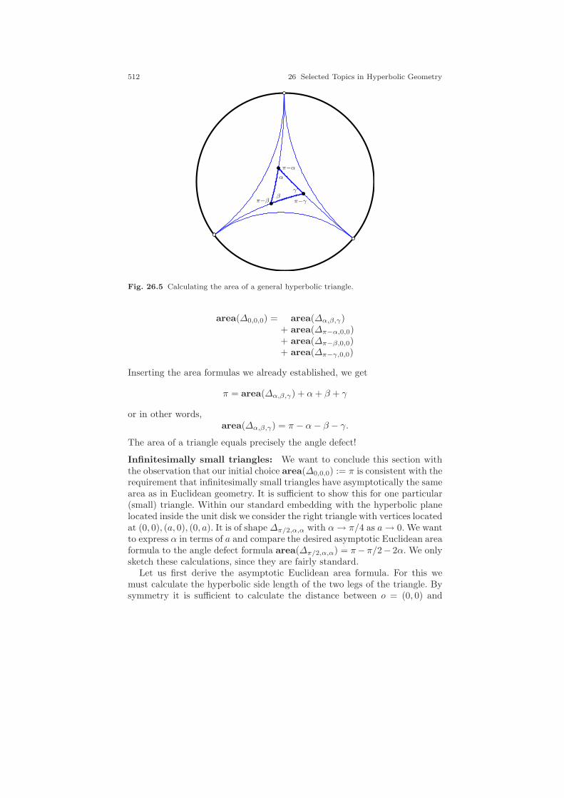
512 26 Selected Topics in Hyperbolic Geometry
α
βγ
π−α
π−β π−γ
Fig. 26.5 Calculating the area of a general hyperbolic triangle.
area(∆0,0,0) = area(∆α,β,γ)+ area(∆π−α,0,0)+ area(∆π−β,0,0)+ area(∆π−γ,0,0)
Inserting the area formulas we already established, we get
π = area(∆α,β,γ) + α+ β + γ
or in other words,area(∆α,β,γ) = π − α− β − γ.
The area of a triangle equals precisely the angle defect!
Infinitesimally small triangles: We want to conclude this section withthe observation that our initial choice area(∆0,0,0) := π is consistent with therequirement that infinitesimally small triangles have asymptotically the samearea as in Euclidean geometry. It is sufficient to show this for one particular(small) triangle. Within our standard embedding with the hyperbolic planelocated inside the unit disk we consider the right triangle with vertices locatedat (0, 0), (a, 0), (0, a). It is of shape ∆π/2,α,α with α→ π/4 as a→ 0. We wantto express α in terms of a and compare the desired asymptotic Euclidean areaformula to the angle defect formula area(∆π/2,α,α) = π− π/2− 2α. We onlysketch these calculations, since they are fairly standard.
Let us first derive the asymptotic Euclidean area formula. For this wemust calculate the hyperbolic side length of the two legs of the triangle. Bysymmetry it is sufficient to calculate the distance between o = (0, 0) and
26.2 Area and Angle Defect 513
p = (a, 0). For the line supporting these two points we get X = (−1, 0) andY = (1, 0). Thus we get with choice of our constant cdist = −1/2 (which nowreally enters as a significant constant)
disthyp(o, p) = −1/2 ln
(1 − a
1 + a
).
We already studied this function in Section 20.3. Figure 20.2 shows a plotof this function that demonstrates that for small a this function is asymp-totically close to the identity (this is how cdist was chosen). Thus in theasymptotic situation we can replace the hyperbolic distance simply by a it-self. So we get a right triangle whose legs (asymptotically) are of length a.The corresponding Euclidean area function for such a triangle is a2/2. Wenow must show that asymptotically the angle defect approximates closelythis value. The value of α can be calculated from a by the formula
cos(α) =Θlm√ΘllΘmm
,
with l = (0, 1, 0)T and m = (−1,−1, a) being the homogeneous coordinatesof a leg and the hypotenuse. Inserting in the above formula gives
α = arccos
(1√
2 − a2
)
Inserting this in the angle deficit formula yields
area(∆π/2,α,α) =π
2− 2 arccos
(1√
2 − a2
).
By standard techniques from a first-year calculus course it can be shown thatfor as a→ 0 we have
a2
2≈ π
2− 2 arccos
(1√
2 − a2
).
It is an amazing effect (and one of the beautiful coincidences that makemathematics a fascinating subject) that the choice area(∆0,0,0) := π of thearea of the largest possible triangle leads to the simplest possible formulasfor the area in general and even leads to formulas for very small trianglesthat approximate the Euclidean area function.

514 26 Selected Topics in Hyperbolic Geometry
4040
90
Fig. 26.6 The peripheral angle configuration (left and middle) and Thales’ theorem inhyperbolic geometry (right).
26.3 Thales and Pythagoras
As we did in Chapter 19 for Euclidean geometry, we now want to have abrief look at elementary geometry in the hyperbolic plane from a projectiveperspective.We already supplied many results in this direction in Chapter 22on the level of general Cayley-Klein geometries. There we proved theoremson altitudes, angle bisectors, medians and an analogue of the law of sinesfor triangles. We here will look at some of the peculiarities that are more orless special to hyperbolic geometry.2 We will focus on two well-known theo-rems from Euclidean geometry and look for their counterparts in hyperbolicgeometry: The theorems of Thales and Pythagoras.
Thales’ theorem can be considered a special case of the peripheral angletheorem for circles. The peripheral angle theorem states that (modulo π)every point of a circle sees a fixed chord under a fixed angle. Thales’ theoremis the special case in which the chord becomes a diameter and the angle is aright angle. Let us first see what still remains of the peripheral angle theoremin hyperbolic geometry. The left and middle pictures of Figure 26.6 show (inthe Beltrami-Klein model) a segment (black) and the locus of all points thatsee this segment under a hyperbolic angle of 40. The left picture illustratesthat the locus is topologically still of the type of a circle. However, metricallyit is not a circle at all, not even a conic. It turns out to be a branch ofan algebraic curve of degree four. The light curve shown in this picture isthe locus of points that see the segment under an angle of −40. This locusforms another branch of the same curve. The picture in the middle showsthe analogous situation of a segment that intersects the fundamental conic.Algebraically, for this situation it is still feasible to speak of the locus ofall points that see the segment under an angle of 40. In this case the twobranches merge and form a more complicated curve. The picture on the right
2 To be more precise, it would perhaps be better to say “are more or less special toCayley-Klein geometries with nondegenerate fundamental conic,” since on the algebraicside hyperbolic and elliptic geometry are essentially equivalent and each statement in onegeometry has its counterpart in the other.
26.3 Thales and Pythagoras 515
now shows the locus of all points that see the segment under a right angle(this is the case of a hyperbolic analogue of Thales’ theorem). In this case thetwo branches of the curve overlap and form one curve of degree 2: a conic.Thus Thales’ theorem survives in the following restricted form, and with aprojective way of thinking it is almost trivial to prove it.
Theorem 26.1 (Hyperbolic Thales). The points that see a given segmentin hyperbolic geometry under a right angle all lie (in the Beltrami-Kleinmodel) on a conic.
Proof. Let A and B be the two endpoints of the segment. Let l be a linethrough A. We calculate the (unique) line through B perpendicular to l. Thisis g = B × l∗ with l∗ being the polar of l with respect to the fundamentalconic. If we consider the two line bundles LA and LB through A and B andequip each of them with a projective basis, then the transition from l to g isjust a projective transformation. Theorem 10.2 implies that the locus of allintersections of l and g is a conic. ⊓⊔
Let us stay with right triangles and come to a hyperbolic version of perhapsthe most famous theorem in geometry: the Pythagorean theorem. The essenceof the Pythagorean theorem is that it allows one to calculate the side lengthof the hypotenuse of a right triangle from the side lengths of the two legs. Inhyperbolic geometry the Pythagorean theorem takes the following surprisingform:
Theorem 26.2 (Hyperbolic Pythagoras). Let a, b, c be the three hyper-bolic side lengths of a hyperbolic right triangle with c being the hypotenuseand a, b being the legs. Then
cosh(a) · cosh(b) = cosh(c).
Proof. We will again attempt to prove this theorem in essentially projectiveterms. By this we will also see more projective reformulations of the samestatement. Recall from Section 22.5 (see the summary table there at the end)that with respect to hyperbolic distance measurement we have
cosh2(dist(p, q)) =Ω2pq
ΩppΩqq.
We assume that the three vertices of the triangle are p, q, r such that c =dist(p, q) and the right angle is at point r. Since for real x the functioncosh(x) is always positive, the statement of the theorem is equivalent to
cosh2(a) · cosh2(b) = cosh2(c).
Applying the above identity, this translates to

516 26 Selected Topics in Hyperbolic Geometry
Ω2qr
ΩppΩrr·
Ω2rq
ΩrrΩqq=
Ω2pq
ΩppΩqq.
Canceling terms that occur on both sides and clearing denominators gives
Ω2pr ·Ω2
rq = Ω2pq ·Ω2
rr.
Thus we are done if we prove
Ωpr ·Ωrq = Ωpq ·Ωrr,
or equivalently(pTAr) · (rTAq) = (pTAq) · (rTAr), (26.1)
for a triangle p, q, r with right angle at r. The condition for the orthogonal-ity of the lines join(r, p) and join(r, q) can according to Theorem 22.1 beexpressed by
(r × p)TB(r × q) = 0. (26.2)
Proving the hyperbolic Pythagorean theorem thus results in proving theequivalence of equations (26.1) and (26.2). Perhaps the simplest and mostdirect proof of this equivalence goes via the use of tensor diagrams (see Chap-ter 13 and Chapter14). So we will make one small exception to our rule notto use diagram techniques. The matrix B may be chosen to be the adjointA∆ of the primal fundamental conic A. Thus the diagram of (r×p)TB(r× q)is given by
A
A
rr
p q
Here the dotted part plays the role of B = A∆. Applying the ε-δ-rule reducesthis diagram to
−A
A
A
A
rrrr
pp qq
which is nothing but twice the diagram
A
A
r
r
p
q
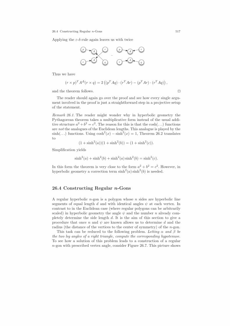
26.4 Constructing Regular n-Gons 517
Applying the ε-δ-rule again leaves us with twice
−A
A
A
A
r
r
r
r
pp
Thus we have
(r × p)TA∆(r × q) = 2((pTAq) · (rTAr) − (pTAr) · (rTAq)
),
and the theorem follows. ⊓⊔The reader should again go over the proof and see how every single argu-
ment involved in the proof is just a straightforward step in a projective setupof the statement.
Remark 26.1. The reader might wonder why in hyperbolic geometry thePythagorean theorem takes a multiplicative form instead of the usual addi-tive structure a2 + b2 = c2. The reason for this is that the cosh(. . .) functionsare not the analogues of the Euclidean lengths. This analogue is played by thesinh(. . .) functions. Using cosh2(x) − sinh2(x) = 1, Theorem 26.2 translatesto
(1 + sinh2(a))(1 + sinh2(b)) = (1 + sinh2(c)).
Simplification yields
sinh2(a) + sinh2(b) + sinh2(a) sinh2(b) = sinh2(c).
In this form the theorem is very close to the form a2 + b2 = c2. However, inhyperbolic geometry a correction term sinh2(a) sinh2(b) is needed.
26.4 Constructing Regular n-Gons
A regular hyperbolic n-gon is a polygon whose n sides are hyperbolic linesegments of equal length d and with identical angles ψ at each vertex. Incontrast to in the Euclidean case (where regular polygons can be arbitrarilyscaled) in hyperbolic geometry the angle ψ and the number n already com-pletely determine the side length d. It is the aim of this section to give aprocedure that once n and ψ are known allows us to determine d and theradius (the distance of the vertices to the center of symmetry) of the n-gon.
This task can be reduced to the following problem. Letting α and β bethe two leg angles of a right triangle, compute the corresponding hypotenuse.To see how a solution of this problem leads to a construction of a regularn-gon with prescribed vertex angle, consider Figure 26.7. This picture shows

518 26 Selected Topics in Hyperbolic Geometry
α
β
c
a
b
α
β
c
γ
Fig. 26.7 A hexagon with only right angles decomposed into right triangles.
a hexagon (thus n = 6) all whose vertex angles are ψ = 90. It can bedecomposed into a ring of 12 = 2n right triangles. The two leg angles areπ/n = 30 for those angles that meet in the center of the hexagon andβ = ψ/2 = 45 for the angle that meets at the vertex of the n-gon. Conversely,a collection of 2n right triangles with leg-corner angles β = ψ/2 and α = π/ncan be used to assemble an n-gon with vertex angle ψ.
So, how can we solve the above problem and construct the length c ofthe hypotenuse from α and β? This is a relatively simple task if apply somehyperbolic trigonometry. For the labeling we refer to Figure 26.7 (right).From the Pythagorean theorem we know that
cosh(a) · cosh(b) = cosh(c).
We can rewrite this as
sinh2(a) + sinh2(b) + sinh2(a) sinh2(b) = sinh2(c).
Furthermore, the sine theorem tells us that
sin(α)
sinh(a)=
sin(β)
sinh(b)=
sin(γ)
sinh(c).
Since γ = 90, we have sin(γ) = 1, and we get
sin(α) sinh(c) = sinh(a) and sin(β) sinh(c) = sinh(b).
26.5 Symmetry Groups 519
Inserting this in the above equation gives
sin2(α) sinh2(c) + sin2(β) sinh2(c) + sin2(α) sin2(β) sinh4(c) = sinh2(c).
Canceling sinh2(c) yields
sin2(α) + sin2(β) + sin2(α) sin2(β) sinh2(c) = 1.
Resolving for the remaining sinh2(c) gives
sinh2(c) =1 − sin2(α) − sin2(β)
sin2(α) sin2(β)=
1
tan2(α) tan2(β)− 1.
The above equation is a consequence of simple trigonometric identities. Giventhe last identity, it is an easy task to compute the length c of the hypotenusec from the two angles α and β.
The fact that the angle sum in a hyperbolic triangle is always less than180 is reflected by the following fact. Let p and q be the endpoints of thehypotenuse c. They are both inside the unit disk (the fundamental conic) ifthe cross-ratio Ξ = (p, q;X,Y ) is positive. Since sinh(c) = (1/Ξ +Ξ − 2)/4,the term sinh(c) must be positive for the hypotenuse to lie entirely in theunit disk. This implies that in this case 1
tan2(α) tan2(β) − 1 must be positive.
This is the case only if |α| + |β| < 45.
26.5 Symmetry Groups
No exposition on hyperbolic geometry would be complete without mention-ing the fascinating symmetry properties regular hyperbolic tesselations canhave. The reason for this richness of structure comes from the fact that inthe hyperbolic plane one can have polygons all of whose vertex angles arearbitrary small divisors of 360. Consider, for instance a regular hyperbolicpentagon whose vertex angles are all 90. One can take four such pentagonsand arrange them such that they meet tightly in a common vertex, like thesquares in a Euclidean checkerboard. One can infinitely repeat this processand fill the entire hyperbolic plane with an infinite collection of such right-angled pentagons, four of them meeting at every vertex. Figure 26.8 showssuch an arrangement where in addition the pentagons are colored alternatelyblack and white. It is possible to create such a tiling with arbitrary hyperbolicright-angled n-gons. The considerations of our last section imply that suchn-gons exist whenever n > 4. We then only have to choose α = 180/n andβ = 45. Such tilings by regular n-gons are not only restricted to right angles.As long as the parameters n and β satisfy 360/n+ ψ < 90 and ψ = 2β isa divisor of 360, the corresponding polygon will seamlessly tile the hyper-
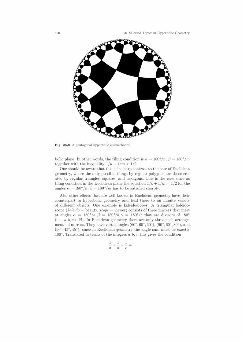
520 26 Selected Topics in Hyperbolic Geometry
Fig. 26.8 A pentagonal hyperbolic checkerboard.
bolic plane. In other words, the tiling condition is α = 180/n, β = 180/mtogether with the inequality 1/n+ 1/m < 1/2.
One should be aware that this is in sharp contrast to the case of Euclideangeometry, where the only possible tilings by regular polygons are those cre-ated by regular triangles, squares, and hexagons. This is the case since astiling condition in the Euclidean plane the equation 1/n+1/m = 1/2 for theangles α = 180/n, β = 180/m has to be satisfied sharply.
Also other effects that are well known in Euclidean geometry have theircounterpart in hyperbolic geometry and lead there to an infinite varietyof different objects. One example is kaleidoscopes. A triangular kaleido-scope (kaleido = beauty, scope = viewer) consists of three mirrors that meetat angles α = 180/a, β = 180/b, γ = 180/c that are divisors of 180
(i.e., a, b, c ∈ N). In Euclidean geometry there are only three such arrange-ments of mirrors. They have vertex angles (60, 60, 60), (90, 60, 30), and(90, 45, 45), since in Euclidean geometry the angle sum must be exactly180. Translated in terms of the integers a, b, c, this gives the condition
1
a+
1
b+
1
c= 1.
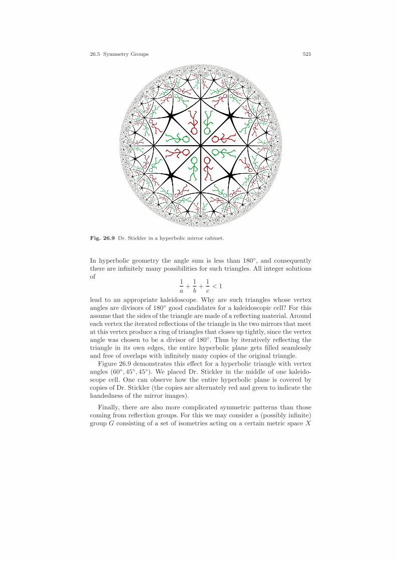
26.5 Symmetry Groups 521
Fig. 26.9 Dr. Stickler in a hyperbolic mirror cabinet.
In hyperbolic geometry the angle sum is less than 180, and consequentlythere are infinitely many possibilities for such triangles. All integer solutionsof
1
a+
1
b+
1
c< 1
lead to an appropriate kaleidoscope. Why are such triangles whose vertexangles are divisors of 180 good candidates for a kaleidoscopic cell? For thisassume that the sides of the triangle are made of a reflecting material. Aroundeach vertex the iterated reflections of the triangle in the two mirrors that meetat this vertex produce a ring of triangles that closes up tightly, since the vertexangle was chosen to be a divisor of 180. Thus by iteratively reflecting thetriangle in its own edges, the entire hyperbolic plane gets filled seamlesslyand free of overlaps with infinitely many copies of the original triangle.
Figure 26.9 demonstrates this effect for a hyperbolic triangle with vertexangles (60, 45, 45). We placed Dr. Stickler in the middle of one kaleido-scope cell. One can observe how the entire hyperbolic plane is covered bycopies of Dr. Stickler (the copies are alternately red and green to indicate thehandedness of the mirror images).
Finally, there are also more complicated symmetric patterns than thosecoming from reflection groups. For this we may consider a (possibly infinite)group G consisting of a set of isometries acting on a certain metric space X
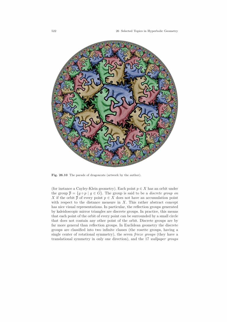
522 26 Selected Topics in Hyperbolic Geometry
Fig. 26.10 The parade of dragoncats (artwork by the author).
(for instance a Cayley-Klein geometry). Each point p ∈ X has an orbit underthe group p = g p | g ∈ G. The group is said to be a discrete group onX if the orbit p of every point p ∈ X does not have an accumulation pointwith respect to the distance measure in X . This rather abstract concepthas nice visual representations. In particular, the reflection groups generatedby kaleidoscopic mirror triangles are discrete groups. In practice, this meansthat each point of the orbit of every point can be surrounded by a small circlethat does not contain any other point of the orbit. Discrete groups are byfar more general than reflection groups. In Euclidean geometry the discretegroups are classified into two infinite classes (the rosette groups, having asingle center of rotational symmetry), the seven frieze groups (they have atranslational symmetry in only one direction), and the 17 wallpaper groups

26.5 Symmetry Groups 523
(they have translatorial symmetry in two directions). Most prominent arethe 17 wallpaper groups forming the mathematical basis of most symmetricplanar geometric structures, such as the ornamental patterns of Islamic artand many drawings by the famous Dutch artist M.C. Escher. A fundamentalregion of such a group is a connected subset F of X such that the orbits of Fform a disjoint union of X . In Euclidean geometry the wallpaper groups areexactly those with a finite fundamental region. In a wallpaper ornament eachfundamental region could be considered a tile whose symmetric repetitionaccording to the rules of the group forms the entire ornament.
Also here the structure in hyperbolic geometry is by far richer. The ana-logues of the Euclidean wallpaper groups are those discrete hyperbolic groupshaving a finite fundamental region, and (no surprise) there are infinitely manyof them. (The structure has a fascinating richness.) Figure 26.10 shows sucha hyperbolic ornament, a hyperbolic tiling where each of the tiles is ani-mal shaped and all the tiles fit seamlessly together to cover the hyperbolicplane. Recall that in the hyperbolic plane each of these animals indeed hasexactly the same size and shape. Notice also the subtle color symmetries ofthis drawing.3
3 Figures 26.8, 26.9, 26.10 were generated with the software morenaments, which is partof a joint project of Martin von Gagern and the author of this book [43, 42].

27
What We Did Not Touch
This is not the end. It is not even the beginning of the end.But it is, perhaps, the end of the beginning
Winston Churchill
This book now comes to an end, and it became considerably fatter thanoriginally intended. Still there are many interesting, amazing, deep, esthetictopics that we did not touch at all. This final chapter is intended to give avery brief overview of a loose selection of topics that I think are among themost fascinating ones among them.
27.1 Algebraic Projective Geometry
Throughout this book we have dealt mainly with linear objects (lines, planes,flats) and quadratic objects (conics). Many fascinating effects occur when onedeals with algebraic curves of higher degree in a projective framework. Newtypes of incidence theorems, interesting singularities, and a surprising theoryof duality arise (see for instance [19, 40]). Also the interplay of complexand real parts of curves becomes an interesting subject. We will scratch thesurface of a few of these topics. An algebraic curve is the solution set of ahomogeneous polynomial equation in three variables x, y, z. For instance, analgebraic cubic (a curve of degree three) is the set of all points (x, y, z)T thatsatisfy an equation
p1x3+p2x
2y+p3x2z+p4xy
2+p5xyz+p6xz2+p7y
3+p8y2z+p9yz
2+p10z3 = 0.
525
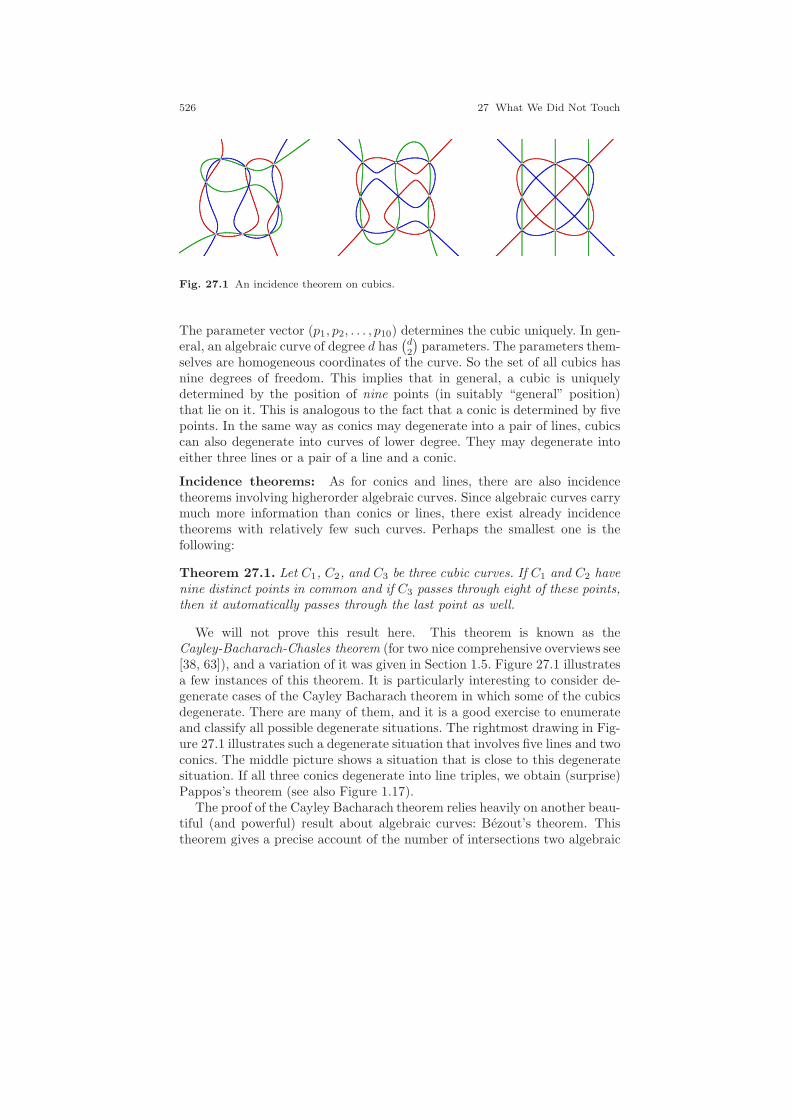
526 27 What We Did Not Touch
Fig. 27.1 An incidence theorem on cubics.
The parameter vector (p1, p2, . . . , p10) determines the cubic uniquely. In gen-eral, an algebraic curve of degree d has
(d2
)parameters. The parameters them-
selves are homogeneous coordinates of the curve. So the set of all cubics hasnine degrees of freedom. This implies that in general, a cubic is uniquelydetermined by the position of nine points (in suitably “general” position)that lie on it. This is analogous to the fact that a conic is determined by fivepoints. In the same way as conics may degenerate into a pair of lines, cubicscan also degenerate into curves of lower degree. They may degenerate intoeither three lines or a pair of a line and a conic.
Incidence theorems: As for conics and lines, there are also incidencetheorems involving higherorder algebraic curves. Since algebraic curves carrymuch more information than conics or lines, there exist already incidencetheorems with relatively few such curves. Perhaps the smallest one is thefollowing:
Theorem 27.1. Let C1, C2, and C3 be three cubic curves. If C1 and C2 havenine distinct points in common and if C3 passes through eight of these points,then it automatically passes through the last point as well.
We will not prove this result here. This theorem is known as theCayley-Bacharach-Chasles theorem (for two nice comprehensive overviews see[38, 63]), and a variation of it was given in Section 1.5. Figure 27.1 illustratesa few instances of this theorem. It is particularly interesting to consider de-generate cases of the Cayley Bacharach theorem in which some of the cubicsdegenerate. There are many of them, and it is a good exercise to enumerateand classify all possible degenerate situations. The rightmost drawing in Fig-ure 27.1 illustrates such a degenerate situation that involves five lines and twoconics. The middle picture shows a situation that is close to this degeneratesituation. If all three conics degenerate into line triples, we obtain (surprise)Pappos’s theorem (see also Figure 1.17).
The proof of the Cayley Bacharach theorem relies heavily on another beau-tiful (and powerful) result about algebraic curves: Bezout’s theorem. Thistheorem gives a precise account of the number of intersections two algebraic

27.1 Algebraic Projective Geometry 527
x2 + y3 − y2 = 0 x2 + y3 = 0 x2 + y3 + y2 = 0
Fig. 27.2 Singularities of a cubic
curves can have. Here one has to be careful to get the right concept of inter-sections and intersection multiplicity. For instance, the point at which a linetouches a conic in tangential position has to be counted as a double inter-section, since an ε-perturbation of the situation immediately generates twointersections. Also, complex intersections and intersections at infinity have tobe counted. So here again it is inevitable to have a framework that is bothprojective and complex: see [19]. With such an advanced understanding ofthe concept of intersection, Bezout’s theorem can be stated as follows:
Theorem 27.2. Two algebraic curves of degree n and m either meet in n ·m points (counted with correct multiplicity) or have a whole component incommon.
We have encountered several special cases of this theorem already. Twolines meet in one point, a line and a conic meet in two points, and two conicsmeet in four points. Concerning cubics we now see that a general line meetsa cubic in three points (this corresponds to the fact that a polynomial ofdegree three has three solutions), a conic meets a cubic in six points, and twocubics meet in nine points.
Special points on curves: Algebraic curves may have very interestingpoints with special properties. We have seen only one type of such specialpoints: a conic may intersect itself in a point if the conic degenerates intotwo lines. Already starting with degree three, other interesting special pointsoccur. For this consider Figure 27.2, in which several interesting examplesare shown. All curves shown there are of degree three and in fact belongto a one-parameter continuous family of curves (implicit equations of thecurves in inhomogeneous coordinates are given). In the first picture thecurve intersects itself. Such a situation in which one part of the curve passestransversally through another part of the curve is called a simple singularityor double point. For every nonsingular point of the curve it is possible toassign a unique tangent. This is no longer the case for a double point. In acertain sense (which involves the technique of a blowup of a singularity) onecan assign two well-defined tangents at this point of the curve, one for everysmooth branch of the curve passing through it. The second picture shows thelimit situation, in which the loop that exists in the first picture is just about
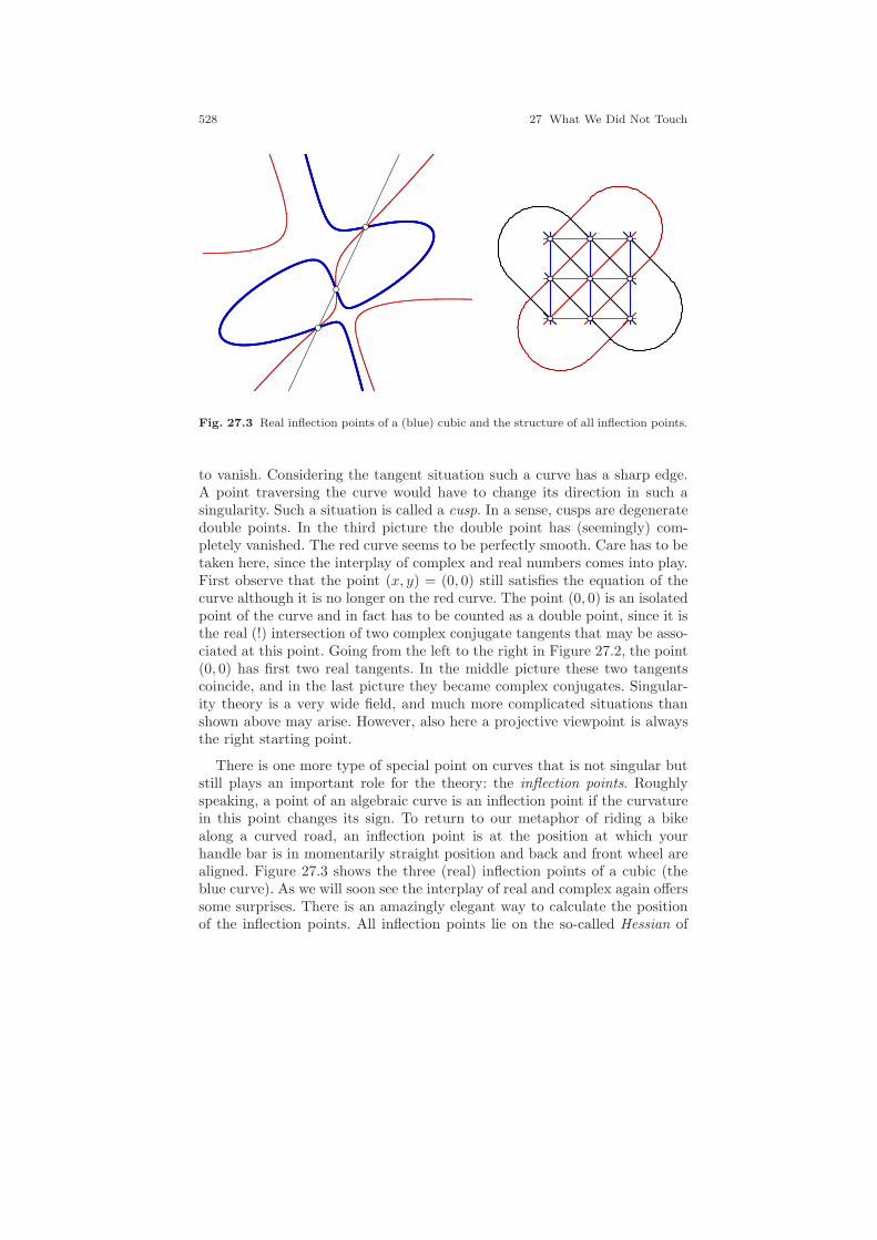
528 27 What We Did Not Touch
Fig. 27.3 Real inflection points of a (blue) cubic and the structure of all inflection points.
to vanish. Considering the tangent situation such a curve has a sharp edge.A point traversing the curve would have to change its direction in such asingularity. Such a situation is called a cusp. In a sense, cusps are degeneratedouble points. In the third picture the double point has (seemingly) com-pletely vanished. The red curve seems to be perfectly smooth. Care has to betaken here, since the interplay of complex and real numbers comes into play.First observe that the point (x, y) = (0, 0) still satisfies the equation of thecurve although it is no longer on the red curve. The point (0, 0) is an isolatedpoint of the curve and in fact has to be counted as a double point, since it isthe real (!) intersection of two complex conjugate tangents that may be asso-ciated at this point. Going from the left to the right in Figure 27.2, the point(0, 0) has first two real tangents. In the middle picture these two tangentscoincide, and in the last picture they became complex conjugates. Singular-ity theory is a very wide field, and much more complicated situations thanshown above may arise. However, also here a projective viewpoint is alwaysthe right starting point.
There is one more type of special point on curves that is not singular butstill plays an important role for the theory: the inflection points. Roughlyspeaking, a point of an algebraic curve is an inflection point if the curvaturein this point changes its sign. To return to our metaphor of riding a bikealong a curved road, an inflection point is at the position at which yourhandle bar is in momentarily straight position and back and front wheel arealigned. Figure 27.3 shows the three (real) inflection points of a cubic (theblue curve). As we will soon see the interplay of real and complex again offerssome surprises. There is an amazingly elegant way to calculate the positionof the inflection points. All inflection points lie on the so-called Hessian of
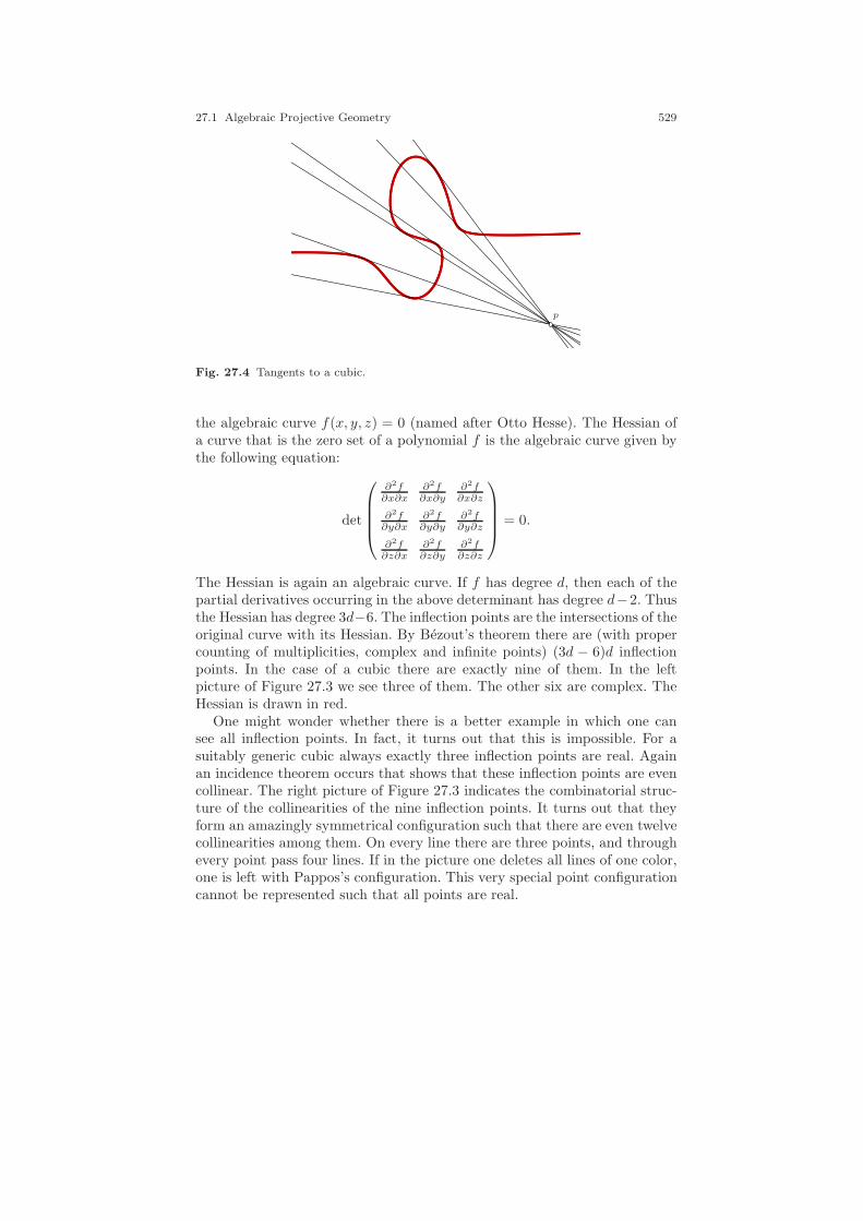
27.1 Algebraic Projective Geometry 529
p
Fig. 27.4 Tangents to a cubic.
the algebraic curve f(x, y, z) = 0 (named after Otto Hesse). The Hessian ofa curve that is the zero set of a polynomial f is the algebraic curve given bythe following equation:
det
∂2f∂x∂x
∂2f∂x∂y
∂2f∂x∂z
∂2f∂y∂x
∂2f∂y∂y
∂2f∂y∂z
∂2f∂z∂x
∂2f∂z∂y
∂2f∂z∂z
= 0.
The Hessian is again an algebraic curve. If f has degree d, then each of thepartial derivatives occurring in the above determinant has degree d−2. Thusthe Hessian has degree 3d−6. The inflection points are the intersections of theoriginal curve with its Hessian. By Bezout’s theorem there are (with propercounting of multiplicities, complex and infinite points) (3d − 6)d inflectionpoints. In the case of a cubic there are exactly nine of them. In the leftpicture of Figure 27.3 we see three of them. The other six are complex. TheHessian is drawn in red.
One might wonder whether there is a better example in which one cansee all inflection points. In fact, it turns out that this is impossible. For asuitably generic cubic always exactly three inflection points are real. Againan incidence theorem occurs that shows that these inflection points are evencollinear. The right picture of Figure 27.3 indicates the combinatorial struc-ture of the collinearities of the nine inflection points. It turns out that theyform an amazingly symmetrical configuration such that there are even twelvecollinearities among them. On every line there are three points, and throughevery point pass four lines. If in the picture one deletes all lines of one color,one is left with Pappos’s configuration. This very special point configurationcannot be represented such that all points are real.
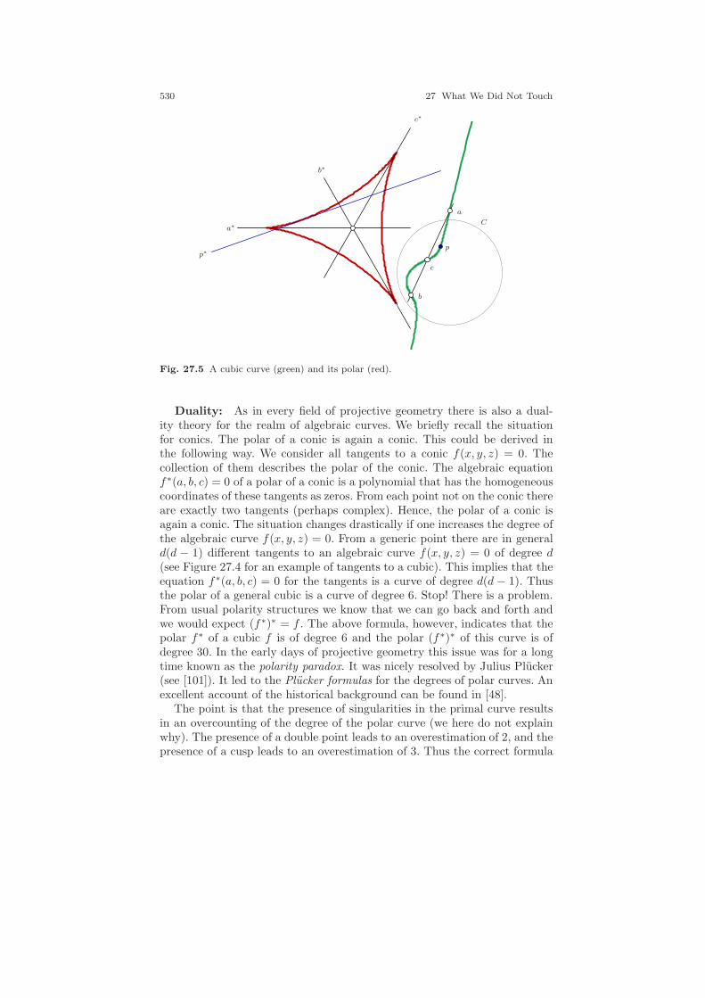
530 27 What We Did Not Touch
p
a
b
c
p∗
a∗
b∗
c∗
C
Fig. 27.5 A cubic curve (green) and its polar (red).
Duality: As in every field of projective geometry there is also a dual-ity theory for the realm of algebraic curves. We briefly recall the situationfor conics. The polar of a conic is again a conic. This could be derived inthe following way. We consider all tangents to a conic f(x, y, z) = 0. Thecollection of them describes the polar of the conic. The algebraic equationf∗(a, b, c) = 0 of a polar of a conic is a polynomial that has the homogeneouscoordinates of these tangents as zeros. From each point not on the conic thereare exactly two tangents (perhaps complex). Hence, the polar of a conic isagain a conic. The situation changes drastically if one increases the degree ofthe algebraic curve f(x, y, z) = 0. From a generic point there are in generald(d − 1) different tangents to an algebraic curve f(x, y, z) = 0 of degree d(see Figure 27.4 for an example of tangents to a cubic). This implies that theequation f∗(a, b, c) = 0 for the tangents is a curve of degree d(d − 1). Thusthe polar of a general cubic is a curve of degree 6. Stop! There is a problem.From usual polarity structures we know that we can go back and forth andwe would expect (f∗)∗ = f . The above formula, however, indicates that thepolar f∗ of a cubic f is of degree 6 and the polar (f∗)∗ of this curve is ofdegree 30. In the early days of projective geometry this issue was for a longtime known as the polarity paradox. It was nicely resolved by Julius Plucker(see [101]). It led to the Plucker formulas for the degrees of polar curves. Anexcellent account of the historical background can be found in [48].
The point is that the presence of singularities in the primal curve resultsin an overcounting of the degree of the polar curve (we here do not explainwhy). The presence of a double point leads to an overestimation of 2, and thepresence of a cusp leads to an overestimation of 3. Thus the correct formula
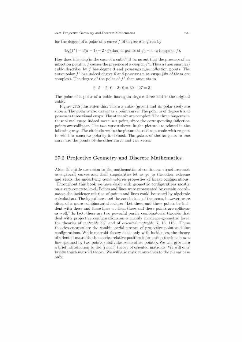
27.2 Projective Geometry and Discrete Mathematics 531
for the degree of a polar of a curve f of degree d is given by
deg(f∗) = d(d− 1) − 2 · #(double points of f) − 3 · #(cusps of f).
How does this help in the case of a cubic? It turns out that the presence of aninflection point in f causes the presence of a cusp in f∗. Thus a (non singular)cubic describe, by f has degree 3 and possesses nine inflection points. Thecurve polar f∗ has indeed degree 6 and possesses nine cusps (six of them arecomplex). The degree of the polar of f∗ then amounts to
6 · 5 − 2 · 0 − 3 · 9 = 30 − 27 = 3.
The polar of a polar of a cubic has again degree three and is the originalcubic.
Figure 27.5 illustrates this. There a cubic (green) and its polar (red) areshown. The polar is also drawn as a point curve. The polar is of degree 6 andpossesses three visual cusps. The other six are complex. The three tangents inthese visual cusps indeed meet in a point, since the corresponding inflectionpoints are collinear. The two curves shown in the picture are related in thefollowing way. The circle shown in the picture is used as a conic with respectto which a concrete polarity is defined. The polars of the tangents to onecurve are the points of the other curve and vice versa.
27.2 Projective Geometry and Discrete Mathematics
After this little excursion to the mathematics of continuous structures suchas algebraic curves and their singularities let us go to the other extremeand study the underlying combinatorial properties of linear configurations.Throughout this book we have dealt with geometric configurations mostly
on a very concrete level. Points and lines were represented by certain coordi-nates; the incidence relation of points and lines could be tested by algebraiccalculations. The hypotheses and the conclusions of theorems, however, wereoften of a more combinatorial nature: “Let these and these points be inci-dent with these and these lines . . . then these and these points are collinearas well.” In fact, there are two powerful purely combinatorial theories thatdeal with projective configurations on a mainly incidence-geometric level:the theories of matroids [92] and of oriented matroids [7, 13, 116]. Thesetheories encapsulate the combinatorial essence of projective point and lineconfigurations. While matroid theory deals only with incidences, the theoryof oriented matroids also carries relative position information (such as how aline spanned by two points subdivides some other points). We will give herea brief introduction to the (richer) theory of oriented matroids. We will onlybriefly touch matroid theory. We will also restrict ourselves to the planar caseonly.

532 27 What We Did Not Touch
1
2
3
4
5
+00−0
++00+
00+0−
0+++0
0+0++
+++00
+++−−
1
2
3
45
+00−0
++00+
00+0−
0+++0
0+0++
+++00
+++−−
Fig. 27.6 An arrangement of points and some of its covectors (left) and the dual situation,an arrangement of lines and its covectors (right). In the primal case covectors correspond to
point partitions by hyperplanes; in the dual case they correspond to signatures of regions.
The theory of oriented matroids has several facets, and in fact it was“invented” independently at several places by researchers working in projec-tive geometry, linear programming [2], graph theory, topology [41], structuralchemistry, computational geometry [71], and polytope theory [80]. In all thesedifferent fields certain combinatorial axiom systems were found to be at thecore of the research problems. Later on, it turned out that all these differentaxiom systems were essentially cryptomorphic (this means that the terms ofeach one of them could be translated into the terms of the others), whichmade oriented matroids a useful link between quite different branches ofmathematics. We will here briefly sketch different approaches and give hintsto why they are equivalent.
A common feature of many of the different approaches to oriented matroidtheory is that they are most easily expressed when one considers oriented pro-jective geometry (see [124]) instead of projective geometry. In projective ge-ometry we express points by homogeneous coordinates where nonzero scalarmultiples are considered to be equivalent. In contrast to this, in oriented pro-jective geometry one considers only positive scalar multiples to be equivalent.So in a sense we study points on the sphere S2 ⊃ R3, and in contrast to in ourusual setup, this time we do not identify antipodal points. It is relatively easyto get from oriented projective geometry to projective geometry by formingsuitable 2-element equivalence classes. If we want to think projectively, wemay consider each point in the projective plane to be equipped with a “+” ora “−” sign encoding its orientation. We now consider a sequence of vectorsV = (v1, . . . , vn) ∈ R3·n (they may represent oriented points in the projectiveplane). From these vectors we will now extract combinatorial information invarious ways.
Covectors of V : We first study the so-called covectors of V . They encodeall possible ways in which an (oriented) line can separate the set of points
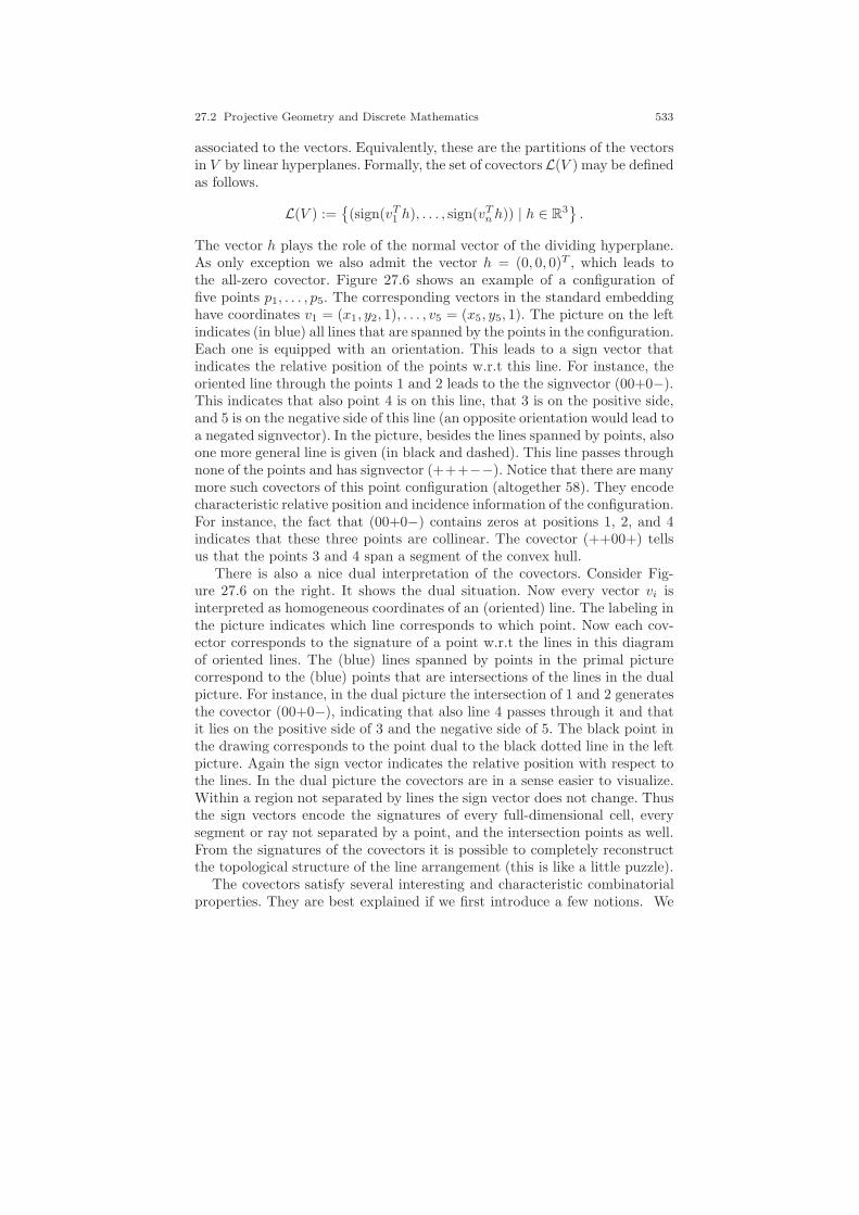
27.2 Projective Geometry and Discrete Mathematics 533
associated to the vectors. Equivalently, these are the partitions of the vectorsin V by linear hyperplanes. Formally, the set of covectorsL(V ) may be definedas follows.
L(V ) :=(sign(vT1 h), . . . , sign(vTnh)) | h ∈ R
3.
The vector h plays the role of the normal vector of the dividing hyperplane.As only exception we also admit the vector h = (0, 0, 0)T , which leads tothe all-zero covector. Figure 27.6 shows an example of a configuration offive points p1, . . . , p5. The corresponding vectors in the standard embeddinghave coordinates v1 = (x1, y2, 1), . . . , v5 = (x5, y5, 1). The picture on the leftindicates (in blue) all lines that are spanned by the points in the configuration.Each one is equipped with an orientation. This leads to a sign vector thatindicates the relative position of the points w.r.t this line. For instance, theoriented line through the points 1 and 2 leads to the the signvector (00+0−).This indicates that also point 4 is on this line, that 3 is on the positive side,and 5 is on the negative side of this line (an opposite orientation would lead toa negated signvector). In the picture, besides the lines spanned by points, alsoone more general line is given (in black and dashed). This line passes throughnone of the points and has signvector (+++−−). Notice that there are manymore such covectors of this point configuration (altogether 58). They encodecharacteristic relative position and incidence information of the configuration.For instance, the fact that (00+0−) contains zeros at positions 1, 2, and 4indicates that these three points are collinear. The covector (++00+) tellsus that the points 3 and 4 span a segment of the convex hull.
There is also a nice dual interpretation of the covectors. Consider Fig-ure 27.6 on the right. It shows the dual situation. Now every vector vi isinterpreted as homogeneous coordinates of an (oriented) line. The labeling inthe picture indicates which line corresponds to which point. Now each cov-ector corresponds to the signature of a point w.r.t the lines in this diagramof oriented lines. The (blue) lines spanned by points in the primal picturecorrespond to the (blue) points that are intersections of the lines in the dualpicture. For instance, in the dual picture the intersection of 1 and 2 generatesthe covector (00+0−), indicating that also line 4 passes through it and thatit lies on the positive side of 3 and the negative side of 5. The black point inthe drawing corresponds to the point dual to the black dotted line in the leftpicture. Again the sign vector indicates the relative position with respect tothe lines. In the dual picture the covectors are in a sense easier to visualize.Within a region not separated by lines the sign vector does not change. Thusthe sign vectors encode the signatures of every full-dimensional cell, everysegment or ray not separated by a point, and the intersection points as well.From the signatures of the covectors it is possible to completely reconstructthe topological structure of the line arrangement (this is like a little puzzle).
The covectors satisfy several interesting and characteristic combinatorialproperties. They are best explained if we first introduce a few notions. We
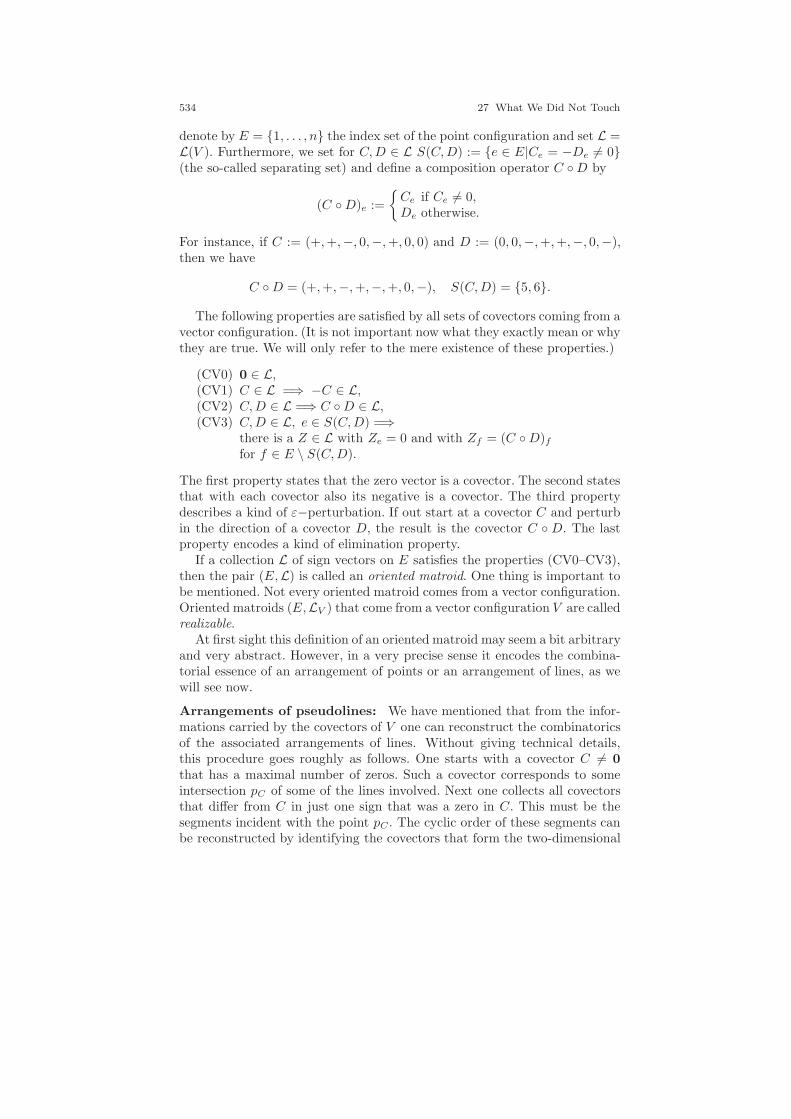
534 27 What We Did Not Touch
denote by E = 1, . . . , n the index set of the point configuration and set L =L(V ). Furthermore, we set for C,D ∈ L S(C,D) := e ∈ E|Ce = −De 6= 0(the so-called separating set) and define a composition operator C D by
(C D)e :=
Ce if Ce 6= 0,De otherwise.
For instance, if C := (+,+,−, 0,−,+, 0, 0) and D := (0, 0,−,+,+,−, 0,−),then we have
C D = (+,+,−,+,−,+, 0,−), S(C,D) = 5, 6.
The following properties are satisfied by all sets of covectors coming from avector configuration. (It is not important now what they exactly mean or whythey are true. We will only refer to the mere existence of these properties.)
(CV0) 0 ∈ L,(CV1) C ∈ L =⇒ −C ∈ L,(CV2) C,D ∈ L =⇒ C D ∈ L,(CV3) C,D ∈ L, e ∈ S(C,D) =⇒
there is a Z ∈ L with Ze = 0 and with Zf = (C D)ffor f ∈ E \ S(C,D).
The first property states that the zero vector is a covector. The second statesthat with each covector also its negative is a covector. The third propertydescribes a kind of ε−perturbation. If out start at a covector C and perturbin the direction of a covector D, the result is the covector C D. The lastproperty encodes a kind of elimination property.
If a collection L of sign vectors on E satisfies the properties (CV0–CV3),then the pair (E,L) is called an oriented matroid. One thing is important tobe mentioned. Not every oriented matroid comes from a vector configuration.Oriented matroids (E,LV ) that come from a vector configuration V are calledrealizable.
At first sight this definition of an oriented matroid may seem a bit arbitraryand very abstract. However, in a very precise sense it encodes the combina-torial essence of an arrangement of points or an arrangement of lines, as wewill see now.
Arrangements of pseudolines: We have mentioned that from the infor-mations carried by the covectors of V one can reconstruct the combinatoricsof the associated arrangements of lines. Without giving technical details,this procedure goes roughly as follows. One starts with a covector C 6= 0that has a maximal number of zeros. Such a covector corresponds to someintersection pC of some of the lines involved. Next one collects all covectorsthat differ from C in just one sign that was a zero in C. This must be thesegments incident with the point pC . The cyclic order of these segments canbe reconstructed by identifying the covectors that form the two-dimensional
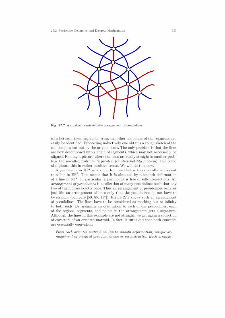
27.2 Projective Geometry and Discrete Mathematics 535
Fig. 27.7 A smallest nonstretchable arrangement of pseudolines.
cells between these segments. Also, the other endpoints of the segments caneasily be identified. Proceeding inductively one obtains a rough sketch of thecell complex cut out by the original lines. The only problem is that the linesare now decomposed into a chain of segments, which may not necessarily bealigned. Finding a picture where the lines are really straight is another prob-lem: the so-called realizability problem (or stretchability problem). One couldalso phrase this in rather intuitive terms. We will do this now.
A pseudoline in RP2 is a smooth curve that is topologically equivalent
to a line in RP2. This means that it is obtained by a smooth deformation
of a line in RP2. In particular, a pseudoline is free of self-intersections. An
arrangement of pseudolines is a collection of many pseudolines such that anytwo of them cross exactly once. Thus an arrangement of pseudolines behavesjust like an arrangement of lines only that the pseudolines do not have tobe straight (compare [50, 85, 117]). Figure 27.7 shows such an arrangementof pseudolines. The lines have to be considered as reaching out to infinityto both ends. By assigning an orientation to each of the pseudolines, eachof the regions, segments, and points in the arrangement gets a signature.Although the lines in this example are not straight, we get again a collectionof covectors of an oriented matroid. In fact, it turns out that both conceptsare essentially equivalent:
From each oriented matroid an (up to smooth deformation) unique ar-rangement of oriented pseudolines can be reconstructed. Each arrange-

536 27 What We Did Not Touch
ment of oriented pseudolines generates the covectors of an oriented ma-troid.
The arrangement in Figure 27.7 is a nonstretchable one. The reason forthis is Pappos’s theorem. This can be seen as follows. If one compares thisarrangement of pseudolines with the lines of Pappos’s theorem as shown inFigure 6.3, one recognizes in essence the same structure with one significantdifference. The coincidence of the three red lines has been perturbed andreplaced by a triangle. Still, each of the red lines meets the others in exactlyone point—but they do not all meet in a single point. Assume that all pseu-dolines were realized by straight lines, then Pappos’s theorem would implythat also the three red lines had to be concurrent—a contradiction.
In fact, it turns out that this example with nine lines is the smallest non-stretchable arrangement of pseudolines. All arrangements with eight or fewerpseudolines are indeed stretchable.
Chirotopes: Here comes another approach to oriented matroids againbased on vectors and on the algebraic properties of determinants.
Let again V = (v1, . . . , vn) ∈ R3·n be a collection of vectors (consideredas oriented homogeneous coordinates of a point configuration with n points).Let En = 1, . . . , n be the index set of the points. We define a map χV :E3 → −1, 0,+1 according to
χV (i, j, k) = sign(det(vi, vj , vk)).
Thus to each triple (i, j, k) we assign the orientation of the basis given bythe vectors vi, vj , vj if they are linearly independent; otherwise, we assign 0.Such a map is called a chirotope of V . It is sufficient to provide the valuesfor strictly ordered sequences of indices. The rest is determined by the alter-nating determinant rules. For instance, the chirotope for the configuration inFigure 27.6 is determined by the following list of signs:
χ(1, 2, 3) = +, χ(1, 2, 4) = 0, χ(1, 2, 5) = −, χ(1, 3, 4) = −, χ(1, 3, 5) = −,χ(1, 4, 5) = −, χ(2, 3, 4) = −, χ(2, 3, 5) = 0, χ(2, 4, 5) = −, χ(3, 4, 5) = −.
From the chirotope χV the set of covectors LV can be reconstructed. Con-versely, if on fixes the sign of only one basis in χV , the signs of the remainingbases are determined by LV .
What are the conditions that a given sign list χ corresponds to thecovectors of a general oriented matroid? It turns out that this questionis closely related to the Grassmann-Plucker-Relations. In general, a mapχ : E3 → −1, 0,+1 is called a chirotope if it satisfies the following twoproperties.
(Chi0) The map is alternating.(Chi1) It is in “no obvious contradiction” to the Grassmann-Plucker-Relations.

27.2 Projective Geometry and Discrete Mathematics 537
The first statement means that interchanging two indices reverses the sign.The second slightly loosely formulated statement means the following. Con-sider a specific Grassmann-Plucker-Relation; as an example we take
[1, 2, 3][1, 4, 5]− [1, 2, 4][1, 3, 5] + [1, 2, 5][1, 3, 4] = 0.
The chirotope χ now proposes a sign for each of the brackets. By this we candeduce the signs of the summands. There would be an obvious contradictionto this equation if one summand turned out to be positive and no othersummand compensated for this by being negative. This is not allowed tohappen for any Grassmann-Plucker-Relation.
It turns out that whenever the map χ is a chirotope, then it is consistentwith an oriented matroid and vice versa. Thus chirotopes, arrangements ofpseudolines, and oriented matroids are essentially the same objects.
Realizability: There are many fascinating theorems on oriented matroidsand still many interesting research areas. We want to briefly mention oneof the most fascinating concepts, the realizability problem (see [7, 16, 50]).It is perhaps most easily stated in terms of chirotopes. Given a chirotopeχ, when does it come from a vector configuration χ = χV ? In a sense, theaxiomatization of chirotopes rules out the “stupidest reasons” for a sign mapE3 → −1, 0,+1 not to come from a vector configuration. At least it mustbe alternating, since it is modeling the behavior of determinants. And itmust at least be consistent with the Grassmann-Plucker-Relations. Theseare exactly the two chirotope axioms. They are checkable in polynomial time.Since planar Grassmann-Plucker-Relations involve at most six points, we canalso say that we require that at least all subconfigurations with at most sixpoints be realizable.
From this point on, things get amazingly hard. It turns out that this lo-cal realizability implies that the smallest nonrealizable chirotope comes froma perturbed Pappos’s configuration. In fact, every nonrealizable chirotopeis related to some perturbed incidence theorem. Thus knowing about non-realizable oriented matroids means knowing about incidence theorems. Theproof methods for incidence theorems from Chapter 15 had their origins inautomated nonrealizability proofs for chirotopes (see [15, 105]).One can evenprove (and this is a famous theorem in oriented matroid theory) the so-calleduniversality theorem:
Deciding whether a chirotope is realizable is as hard as solving
an arbitrary system of polynomial inequalities and equations.
At the core of the proof of this theorem are the von Staudt constructionswe used in Chapter 5 to encode addition and multiplication on the levelof projective incidence configurations (for details see [96, 97, 107, 121]). Alsowith projective methods a similar statement can be proved for the realizationspaces of polytopes [106, 108].
538 27 What We Did Not Touch
27.3 Projective Geometry and Quantum Theory
It is always an amazing phenomenon when a mathematical field has applica-tions to subjects that at the first sight seem to be not related at all to it.Manyof the methods presented in this book have very close relationsships to variousbranches of physics (among them quite modern ones). For instance, Cayley-Klein geometries can be used as a very good framework to model space-timecoordinate systems (and their invariants) in special relativity theory. A bitmore surprising is the relation of projective geometry to quantum physics.Again we can give only a glimpse of the subject. For matters of brevity welimit ourselves to the rather restricted area of quantum information theory(see for instance [90]). This subject deals with the concept of informationon the quantum level. While in the usual framework of information theorythe fundamental unit of information is a bit (a single 0/1 decision), in quan-tum information theory the fundamental unit of information is a qubit (shortfor quantumbit). A carrier of such a single piece of information can be, forinstance, an elementary particle such as an electron or a photon.
Qubits and CP1: As a first step we have to clarify how an electron or a
photon can carry information. For this we have to deal with quantum statesand measurements.A quantum state completely describes the physical prop-erties of an elementary particle such as an electron or a photon. Typicallythese states can be expressed as the (complex) superposition of several mutu-ally exclusive elementary states. These elementary states will be representedby an orthogonal basis of vectors. For the situation we are interested in, theelectron spin, we will need two such elementary states. In the physics litera-ture these base states are usually denoted by |0〉 and |1〉. The superpositionis
|ψ〉 = α0|0〉 + α1|1〉.Here α0, α1 ∈ C. For reasons related to the measurement of quantum prop-erties one furthermore requires |α0|2 + |α1|2 = 1. From a mathematical pointof view we can simply identify the base states with two unit vectors of CP
2
and get
|ψ〉 = α0|0〉 + α1|1〉 = α0
(10
)+ α1
(01
)=
(α0
α1
).
The normalization |α0|2 + |α1|2 = 1 says that the vector length of |ψ〉 con-sidered as composed of four real components (the two real and imaginaryparts of α0 and α1) is normalized to 1. In addition (also due to the proper-ties of measurements explained later), states that differ only by a complexunit eit, t ∈ R, are considered to represent the same state: |ψ〉 ∼ eit|ψ〉.From a projective point of view, after considering states differing by a phaseshift to be equivalent, the normalization is superfluous. We may equally wellrepresent a state simply by a linear combination α0|0〉 + α1|1〉 and identifynonzero complex multiples. So a state vector is nothing but an element of

27.3 Projective Geometry and Quantum Theory 539
CP1. Nevertheless, the normalization will be technically helpful when we con-
sider measurements later on. This identification of states and points in CP1
can be made very concrete for the case of an electron spin or photon polariza-tion. For reasons of brevity we will restrict ourselves to the case of electronspin (and by neglecting the photon miss another geometrically fascinatinginterpretation of qubits).
In the case of the electron, the state |ψ〉 encodes all information about thespin of the electron. The spin is a quantum phenomenon that has no classicalanalogue. Nevertheless, a good way (at least good enough for our purposes)to think about it is to visualize the electron as a spinning sphere. The spincorresponds to the direction of the rotation axes. Since the rotation has adirection, also the axis is directed by a kind of right-hand rule (the fingersindicate the rotation and the thumb points in the direction of the axis).1 Sothe spin is essentially a point on the unit sphere. A vector connecting theorigin to this point indicates the directed axis. This is the moment whenprojective geometry comes into play. In Section 17.7 we have seen how thecomplex projective line CP
1 can be identified with the unit sphere via stereo-graphic projection (see Figure 17.9). As a consequence of this interpretation,by stereographic projection two basic states |0〉 and |1〉 correspond to two op-posite directions of the spin pointing to the southpole and to the northpole.More generally, any pair of antipodal points on the projected sphere becomesa pair of homogeneous coordinates whose inner product vanishes.
The linear combinations of the basic states α0|0〉+α1|1〉 resemble the spaceof all possible states. For instance, all states of the form 1√
2(eit|0〉 + α1|1〉)
with t ∈ R represent electron spins whose rotation axis meets the equator,the great circle of all points halfway between the north and southpoles.
To understand why firstly the normalization |α0|2+|α1|2 = 1 and secondlythe identification of states differing only by a phase make sense, it is essentialto understand the measurement process that transfers quantum states in clas-sical observables. It is one of the fundamental properties of quantum statesthat they are not directly accessible by classical observations. They only in-fluence the probability of the outcome of certain measurements. In the caseof the electron spin, the situation is as follows. Typically, when measuring theelectron spin one has to decide before the measurement with respect to whichaxis one wants to measure. So when an electron is exhibited to a measuringdevice, the device performs the measurement and outputs “yes” or “no” de-pending on the direction of the spin of the electron. If the electron spin pointsin the direction of the measurement, the answer is surely “yes.” If it pointsin the opposite direction of the measurement, the answer is surely “no.” Forall other spin directions the probability of a “yes” a or “no” depends on theproximity of the spin direction and the measurement direction. Measurementshave the strange property that after the measurement, the electron is indeed
1 Do not think about all the other properties one would classically associate to a rotationsuch like speed and acceleration. The electron spin just has a direction; that’s it.

540 27 What We Did Not Touch
measure
YES
NO
Fig. 27.8 Measurement of electron spin.
in the state that has been measured. Thus the measurement influences thequantum state of the electron.2 Figure 27.8 roughly illustrates this process.An electron with an arbitrary spin enters the measurement device that testsfor a spin pointing upward. After it leaves the device there are two possibleresults of the measurement. Either the output is “yes” and the spin thenreally points upward, or the output is “no” and the spin then really pointsdownward.
Mathematically speaking, measurements are expressed in a similar way asstates. A measurement is a linear combination of two directions
〈φ| = β0〈0| + β1〈1|
of two mutually exclusive unit states 〈0| = (1, 0), 〈1| = (0, 1). Note that thistime we use row vectors. We make an important twist to the representationof states. The complex numbers β0 and β1 are the complex conjugates of thenumbers α0 and α1 that would encode the same direction as a spin. So if|ψ〉 = α0|0〉 + α1|1〉 is the state (i.e., direction) of a spin, then
〈ψ| = α0〈0| + α1〈1| = (α0, α1)
encodes the measurement in exactly the same direction. In other words, di-rections of measurement are represented by the Hermitian conjugates of thecorresponding directions of states. The Hermitian conjugate is derived by si-
2 Do not try to understand in classical terms how this can happen. It is one of the (moreharmless) mysteries of quantum mechanics.
27.3 Projective Geometry and Quantum Theory 541
multaneously transposing and conjugating. If we denote the Hermitian con-jugate of a vector v by v†, then we get 〈ψ| = |ψ〉†.
The states 〈0| = (1, 0) and 〈1| = (0, 1) represent opposite directions inthe measurement space. Again every other direction can be expressed as alinear combination of the basis states. The probability that a measurement〈φ| responds with “yes” to a state |ψ〉 is calculated by
|〈φ|·|ψ〉|2 = |α0β0|2 + |α1β1|2.
Measuring a state |ψ〉 = α0|0〉 + α1|1〉 with respect to its own direction 〈ψ|results in the probability
|〈ψ|·|ψ〉|2 = α0α0 + α1α1 = |α0|2 + |α1|2 = 1.
This a posteriori justifies the normalization |α0|2 + |α1|2 = 1 and |β0|2 +|β1|2 = 1. Also an easy calculation shows that a phase shift (i.e., replacing|ψ〉 by eit|ψ〉) does not influence the probability of the measurement, and bythis will have no effect on the classical world.
Let us see what happens if one measures one of the equatorial states |ψ〉 =1√2(eit|0〉+α1|1〉) with respect to the south direction 〈1|. For the probability
of getting “yes” we get
|〈1|·|ψ〉|2 =
(1√2
)2
(|0 · 1|2 + |1 · eit|)2 =1
2.
This corresponds to the physically reasonable fact that measurements of anequatorial spin with respect to the south direction produces a “yes” equallyoften as it produces a “no.”
There is one important point on possible local transformations of a qubit.Our choice of the basis |0〉, |1〉 was somehow random. We could equally wellhave chosen a pair of other opposite directions as basis. In other words thereare some basis transformations of the mathematical representation that donot alter the physical reality. Let |0〉 = α0|0〉+α1|1〉 be one such state (with|α0|2 + |α1|2 = 1). Then |1〉 = −α1|0〉+α1|1〉 represents the state with oppo-site spin direction. Thus a basis transformation from the (|0〉, |1〉)-basis to the
(|0〉, |1〉)-basis is given by a transformation matrix(α0 −α1
α1 α0
). This is a matrix
from the matrix group SU(2) of unitary matrices with determinant 1. Suchan SU(2) matrix can also be used to describe rotation of the measurementdevice. From a projective point of view such transformations are nothingbut special projective transformations of CP
1. Similarly to the fact that wecould describe hyperbolic transformations in the Poincare model by certainCP
1 transformations, the SU(2) transformations represent transformations ofelliptic geometry in a suitable CP
1 representation.
One note on notation. From a mathematical point of view the states andthe measurements are nothing but a fancy notation for column and row vec-
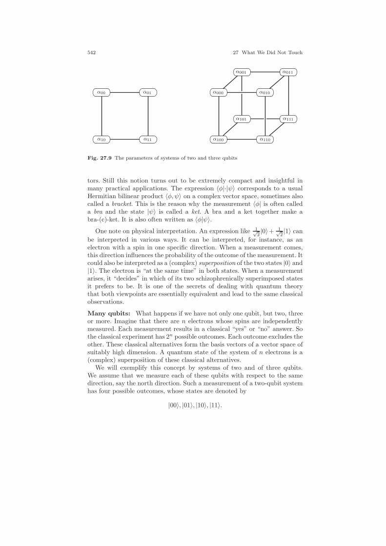
542 27 What We Did Not Touch
α00 α01
α10 α11
α000 α010
α100 α110
α001 α011
α101 α111
Fig. 27.9 The parameters of systems of two and three qubits
tors. Still this notion turns out to be extremely compact and insightful inmany practical applications. The expression 〈φ|·|ψ〉 corresponds to a usualHermitian bilinear product 〈φ, ψ〉 on a complex vector space, sometimes alsocalled a bracket. This is the reason why the measurement 〈φ| is often calleda bra and the state |ψ〉 is called a ket. A bra and a ket together make abra-(c)-ket. It is also often written as 〈φ|ψ〉.
One note on physical interpretation. An expression like 1√2|0〉+ 1√
2|1〉 can
be interpreted in various ways. It can be interpreted, for instance, as anelectron with a spin in one specific direction. When a measurement comes,this direction influences the probability of the outcome of the measurement. Itcould also be interpreted as a (complex) superposition of the two states |0〉 and|1〉. The electron is “at the same time” in both states. When a measurementarises, it “decides” in which of its two schizophrenically superimposed statesit prefers to be. It is one of the secrets of dealing with quantum theorythat both viewpoints are essentially equivalent and lead to the same classicalobservations.
Many qubits: What happens if we have not only one qubit, but two, threeor more. Imagine that there are n electrons whose spins are independentlymeasured. Each measurement results in a classical “yes” or “no” answer. Sothe classical experiment has 2n possible outcomes. Each outcome excludes theother. These classical alternatives form the basis vectors of a vector space ofsuitably high dimension. A quantum state of the system of n electrons is a(complex) superposition of these classical alternatives.
We will exemplify this concept by systems of two and of three qubits.We assume that we measure each of these qubits with respect to the samedirection, say the north direction. Such a measurement of a two-qubit systemhas four possible outcomes, whose states are denoted by
|00〉, |01〉, |10〉, |11〉.
27.3 Projective Geometry and Quantum Theory 543
The superposition of these states is given by
|ψ〉 = α00|00〉+ α01|01〉 + α10|10〉 + α11|11〉.
Since the outcomes are mutually exclusive, we may again represent them asmutually orthogonal unit vectors and get
|ψ〉 =
α00
α01
α10
α11
.
As before, we have to assume that this vector is normalized, i.e., we have|α00|2 + |α01|2 + |α10|2 + |α11|2 = 1. The obvious combinatorics of the indicesof the four different entries indicates that it might be reasonable to arrangethese indices not as a vector but as a matrix:
|ψ〉 =
(α00 α01
α10 α11
).
Again a common phase shift is irrelevant. This together with the normal-ization implies once more that we may equivalently skip normalization andphase-shifting and instead consider the states that differ by a complex scalarto be equivalent. Thus the state space is nothing but CP
3.If we perform the same considerations with three instead of two qubits, we
will get eight possible classical outcomes of the measurements. We will haveeight controlling (complex) parameters. This time it is best to locate theseeight parameters at the eight vertices of a cube. Again complex multiplesrepresent the same state and we get a projective space CP
7 as state space.One might consider such a state, as a 2×2×2 tensor (in fact tensor diagramtechniques are rather common in quantum physics [23, 123]).
So a system of n qubits is described by a 2n-dimensional vector repre-senting the complex (homogeneous) coordinates. It can also considered a2 × 2 × · · · × 2 tensor. From an information-theoretic viewpoint this is re-markable. A single qubit is an element of CP
1 and by this has in essenceone complex parameter. A system of two qubits is an element of CP
3 and hasthree complex parameters. A system of three qubits is an element of CP
7 andhas essentially seven complex parameters. So the collection of the parts car-ries significantly (exponentially) more information than all individual partstaken together.
What does this mean and how could this happen? The key to this seem-ingly paradoxical situation is a concept called entanglement, which has noclassical counterpart at all. We again start our explanations with the two-qubit case. Consider some kind of particle decay that emits two electrons inopposite directions. The two electrons form a 2-qubit quantum ensemble, andtheir quantum state is described by |ψ〉 = α00|00〉+α01|01〉+α10|10〉+α11|11〉.
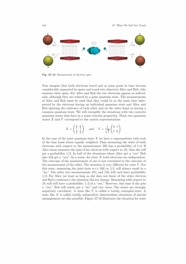
544 27 What We Did Not Touch
„
0 11 0
«
YESYES
NONO
Fig. 27.10 Measurement of electron spin.
Now imagine that both electrons travel and at some point in time becomeconsiderably separated by space and reach two observers Alice and Bob, whomeasure their spins. For Alice and Bob the two electrons appear as individ-uals, although they are related by a joint quantum state. The measurementsof Alice and Bob must be such that they could be at the same time inter-preted by the electrons having an individual quantum state and Alice andBob ignoring the existence of each other and on the other hand as having acommon quantum state. We will exemplify the situations with two concretequantum states that have in a sense extreme properties. These two quantumstates X and Y correspond to the matrix representations
X =
(12
12
12
12
)and Y =
1√2
(0 1
1 0
).
In the case of the joint quantum state X we have a superposition with eachof the four basis states equally weighted. Thus measuring the state of bothelectrons with respect to the measurement 〈00| has a probability of 1/4. IfAlice alone measures the spin of her electron with respect to 〈0|, then she willget a probability 1/2. In half of the situations where Alice get a “yes” Bobalso will get a “yes.” In a sense, for state X both electrons are independent.The outcome of the measurement of one is not correlated to the outcome ofthe measurement of the other. The situation is very different for state Y . Forthis state, measuring the joint state w.r.t 〈00| or 〈11| will always result in a“no.” The other two measurements 〈01| and 〈10| will each have probability1/2. For Alice (at least as long as she does not know of the other electronand Bob’s existence), the situation did not change. Measuring with respect to〈0| will still have a probability 1/2 of a “yes.” However, this time if she getsa “yes,” Bob will surely get a “no” and vice versa. The states are stronglynegatively correlated. A state like Y is called a totally entangled state. Astate like X is called totally independent. Intermediate situations of partialentanglement are also possible. Figure 27.10 illustrates the situation for state

27.3 Projective Geometry and Quantum Theory 545
Y . A measurement of both electrons results either in situation of the twoyellow electrons or in the situation of the two red electrons.
One might say, “So what, where is the problem? Both electrons alreadyhave their spin when they leave their particle source, like two coins in twoclosed boxes that are opened only when the measurement is performed. Theoutcome of measurement of the electrons is governed by some hidden vari-ables.” Although from a classical perspective this seems to be a reasonableexplanation, one can show that this is definitely not the case. This effect isknown as the Einstein-Podolsky-Rosen paradox (EPR) and has been con-firmed by experiments [37, 12]. The outcome of the measurement by Alice isreally completely undetermined unless the measurement has been performed.By some mysterious principle of nonlocality, the outcome of the measurementis somehow transported to Bobs measurement device and influences his mea-surement. How this happens is still an open problem.3
Entanglement invariants: Understanding the mathematics of entangle-ment brings us again back to projective geometry and invariant theory (see[127]). We here will be able to give only a rough sketch of what happens.We again start with the 2-qubit case. The transformations acting on thecombined space of the two electron spins within the space CP
3 is given byall matrix operations in SU(4). This is a certain subgroup of all projectivetransformations of CP
3. Compared to this, Alice and Bob have only very re-stricted influence on the state space. Each of them can act with an SU(2) ontheir individual electrons. Thus after the electrons have been separated, onlySU(2) × SU(2) ⊂ SU(4) actions are possible. Alice’s action corresponds to aleft multiplication of the state matrix with an SU(2) matrix. Bob’s action cor-responds to a right multiplication of the matrix with an SU(2) matrix. Suchactions cannot change the degree of entanglement. For instance, it can beshown that for state Y , if Alice decides to measure her electron with respectto another basis, there is a corresponding basis for Bob such that he still willalways get the opposite answer to Alice’s. Similarly, in case of state X thereis no choice of the bases such that the measurements become correlated.
In fact, it turns out that completely independent states correspond torank-1 state matrices (α0|0〉 + α1|1〉)(β0|0〉 + β1|1〉)T . They are always com-pletely unentangled. The rank-1 property cannot be influenced by the localperturbations. It turns out that the absolute value of the determinant ofthe state matrix is an entanglement invariant. It cannot be altered by localtransformations. After normalization this absolute value of the determinantcan take values between 0 and 1. The state X results in a value of 0 (nonen-tangled); the value Y results in a value 1 (fully entangled). The space of allnonentangled states forms a conic in the state space CP
3.The situation becomes more complicated if more than two qubits are in-
volved. In principle, one is interested in all
3 Do not try to understand in classical terms how this can happen. It is one of the (lessharmless) mysteries of quantum mechanics.
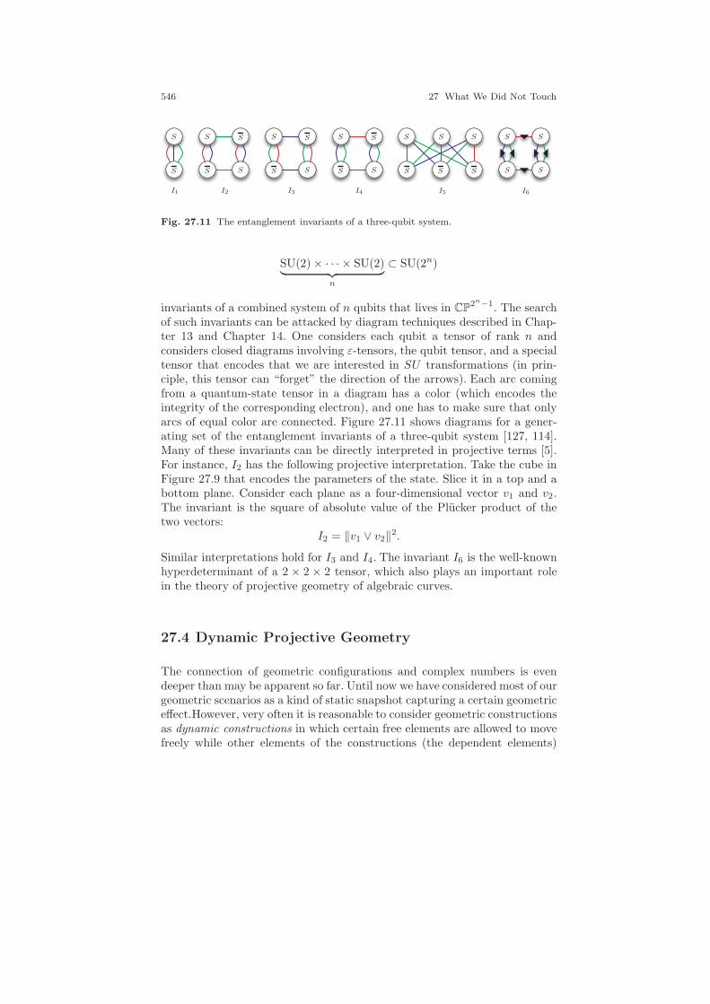
546 27 What We Did Not Touch
S S S
S
S
S
S
S
S
S
S
S
SS
SS S
S
S
S
S
S
SS
I1 I2 I3 I4 I5 I6
Fig. 27.11 The entanglement invariants of a three-qubit system.
SU(2) × · · · × SU(2)︸ ︷︷ ︸n
⊂ SU(2n)
invariants of a combined system of n qubits that lives in CP2n−1. The search
of such invariants can be attacked by diagram techniques described in Chap-ter 13 and Chapter 14. One considers each qubit a tensor of rank n andconsiders closed diagrams involving ε-tensors, the qubit tensor, and a specialtensor that encodes that we are interested in SU transformations (in prin-ciple, this tensor can “forget” the direction of the arrows). Each arc comingfrom a quantum-state tensor in a diagram has a color (which encodes theintegrity of the corresponding electron), and one has to make sure that onlyarcs of equal color are connected. Figure 27.11 shows diagrams for a gener-ating set of the entanglement invariants of a three-qubit system [127, 114].Many of these invariants can be directly interpreted in projective terms [5].For instance, I2 has the following projective interpretation. Take the cube inFigure 27.9 that encodes the parameters of the state. Slice it in a top and abottom plane. Consider each plane as a four-dimensional vector v1 and v2.The invariant is the square of absolute value of the Plucker product of thetwo vectors:
I2 = ‖v1 ∨ v2‖2.
Similar interpretations hold for I3 and I4. The invariant I6 is the well-knownhyperdeterminant of a 2 × 2 × 2 tensor, which also plays an important rolein the theory of projective geometry of algebraic curves.
27.4 Dynamic Projective Geometry
The connection of geometric configurations and complex numbers is evendeeper than may be apparent so far. Until now we have considered most of ourgeometric scenarios as a kind of static snapshot capturing a certain geometriceffect.However, very often it is reasonable to consider geometric constructionsas dynamic constructions in which certain free elements are allowed to movefreely while other elements of the constructions (the dependent elements)
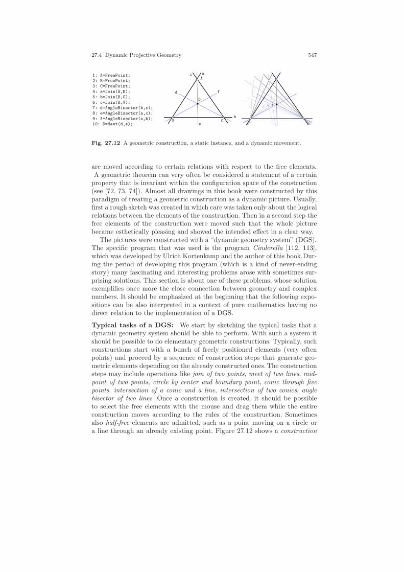
27.4 Dynamic Projective Geometry 547
1: A=FreePoint;2: B=FreePoint;
3: C=FreePoint;4: a=Join(A,B);5: b=Join(B,C);
6: c=Join(A,V);7: d=AngleBisector(b,c);
8: e=AngleBisector(a,c);9: f=AngleBisector(a,b);10: D=Meet(d,e);
A
B C
D
a
b
c
d
e
f
Fig. 27.12 A geometric construction, a static instance, and a dynamic movement.
are moved according to certain relations with respect to the free elements.A geometric theorem can very often be considered a statement of a certain
property that is invariant within the configuration space of the construction(see [72, 73, 74]). Almost all drawings in this book were constructed by thisparadigm of treating a geometric construction as a dynamic picture. Usually,first a rough sketch was created in which care was taken only about the logicalrelations between the elements of the construction. Then in a second step thefree elements of the construction were moved such that the whole picturebecame esthetically pleasing and showed the intended effect in a clear way.
The pictures were constructed with a “dynamic geometry system” (DGS).The specific program that was used is the program Cinderella [112, 113],which was developed by Ulrich Kortenkamp and the author of this book.Dur-ing the period of developing this program (which is a kind of never-endingstory) many fascinating and interesting problems arose with sometimes sur-prising solutions. This section is about one of these problems, whose solutionexemplifies once more the close connection between geometry and complexnumbers. It should be emphasized at the beginning that the following expo-sitions can be also interpreted in a context of pure mathematics having nodirect relation to the implementation of a DGS.
Typical tasks of a DGS: We start by sketching the typical tasks that adynamic geometry system should be able to perform. With such a system itshould be possible to do elementary geometric constructions. Typically, suchconstructions start with a bunch of freely positioned elements (very oftenpoints) and proceed by a sequence of construction steps that generate geo-metric elements depending on the already constructed ones.The constructionsteps may include operations like join of two points, meet of two lines, mid-point of two points, circle by center and boundary point, conic through fivepoints, intersection of a conic and a line, intersection of two conics, anglebisector of two lines. Once a construction is created, it should be possibleto select the free elements with the mouse and drag them while the entireconstruction moves according to the rules of the construction. Sometimesalso half-free elements are admitted, such as a point moving on a circle ora line through an already existing point. Figure 27.12 shows a construction
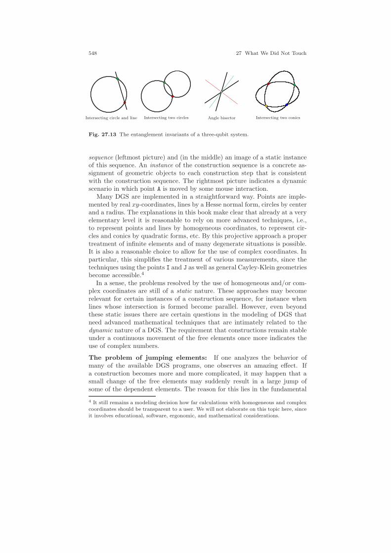
548 27 What We Did Not Touch
Intersecting circle and line Intersecting two circles Angle bisector Intersecting two conics
Fig. 27.13 The entanglement invariants of a three-qubit system.
sequence (leftmost picture) and (in the middle) an image of a static instanceof this sequence. An instance of the construction sequence is a concrete as-signment of geometric objects to each construction step that is consistentwith the construction sequence. The rightmost picture indicates a dynamicscenario in which point A is moved by some mouse interaction.
Many DGS are implemented in a straightforward way. Points are imple-mented by real xy-coordinates, lines by a Hesse normal form, circles by centerand a radius. The explanations in this book make clear that already at a veryelementary level it is reasonable to rely on more advanced techniques, i.e.,to represent points and lines by homogeneous coordinates, to represent cir-cles and conics by quadratic forms, etc. By this projective approach a propertreatment of infinite elements and of many degenerate situations is possible.It is also a reasonable choice to allow for the use of complex coordinates. Inparticular, this simplifies the treatment of various measurements, since thetechniques using the points I and J as well as general Cayley-Klein geometriesbecome accessible.4
In a sense, the problems resolved by the use of homogeneous and/or com-plex coordinates are still of a static nature. These approaches may becomerelevant for certain instances of a construction sequence, for instance whenlines whose intersection is formed become parallel. However, even beyondthese static issues there are certain questions in the modeling of DGS thatneed advanced mathematical techniques that are intimately related to thedynamic nature of a DGS. The requirement that constructions remain stableunder a continuous movement of the free elements once more indicates theuse of complex numbers.
The problem of jumping elements: If one analyzes the behavior ofmany of the available DGS programs, one observes an amazing effect. Ifa construction becomes more and more complicated, it may happen that asmall change of the free elements may suddenly result in a large jump ofsome of the dependent elements. The reason for this lies in the fundamental
4 It still remains a modeling decision how far calculations with homogeneous and complexcoordinates should be transparent to a user. We will not elaborate on this topic here, sinceit involves educational, software, ergonomic, and mathematical considerations.

27.4 Dynamic Projective Geometry 549
ω
ω/2
ω/4
ω/8
Fig. 27.14 In iterated angle bisector.
nature of certain geometric primitive operations. Some operations, such asintersecting a line with a circle, intersecting two circles, calculating the anglebisector of two lines, and intersecting two conics, are intrinsically ambiguous.In these cases the input elements do not uniquely determine the output ele-ments. Intersecting a circle with a line in general has two solutions, as wellas intersecting a circle and a circle. Two lines have two angle bisectors. Twoconics in general intersect in four different points. We dealt with each of theseprimitives in the context of this book. For the first three cases a square-rootoperation (which carries an intrinsic ambiguity) is involved in the computa-tion of the output (compare Section 11.3 and Section 19.2). For intersectionof two conics solving a polynomial of degree three and square roots are in-volved (compare Section 11.4). Figure 27.13 shows some instances of theseambiguous operations together with the different outputs of the primitiveoperations (indicated by different colors).
For an initial instance of a geometric construction in a DGS it is usuallyclear (by user interaction) which of the several outputs of an ambiguousoperation has to be taken. However, when the free points of a constructionare dragged, the computer has to decide which of the outputs for ambiguousoperations has to be taken. It may happen that the computer makes a decisionin which a dependent element suddenly jumps from one position to the other.
One might think that there are appropriate simple heuristics that depend-ing on the position of the free elements allow one to chose the dependentelements such that no such discontinuous jumping arises. In fact, one canprove by a relatively simple argument that every implementation that avoidsdiscontinuous behavior of the dependent elements must take the history ofthe movement into account [74]. For this consider Figure 27.14. It shows theiteration of an angle bisector. The red line is the angle bisector of the twoblack lines (one of them is the x-axis). The green line is the angle bisector ofthe red line and the x-axis. The blue line is the angle bisector of the green
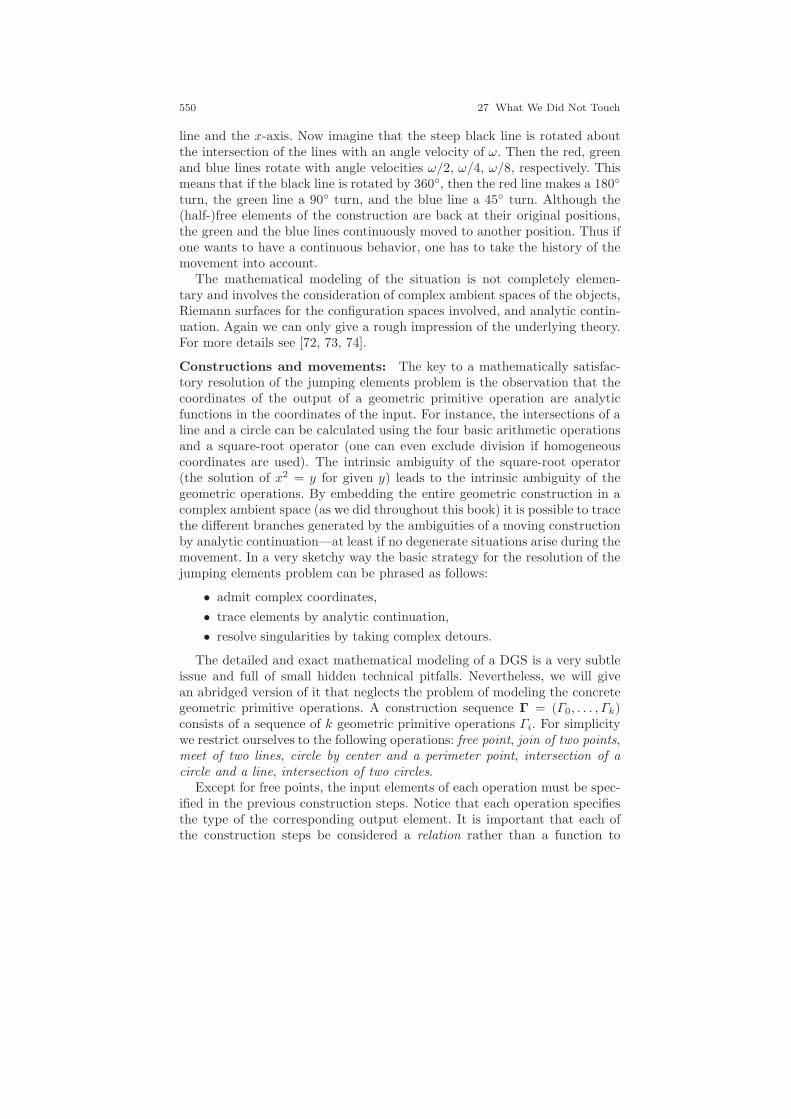
550 27 What We Did Not Touch
line and the x-axis. Now imagine that the steep black line is rotated aboutthe intersection of the lines with an angle velocity of ω. Then the red, greenand blue lines rotate with angle velocities ω/2, ω/4, ω/8, respectively. Thismeans that if the black line is rotated by 360, then the red line makes a 180
turn, the green line a 90 turn, and the blue line a 45 turn. Although the(half-)free elements of the construction are back at their original positions,the green and the blue lines continuously moved to another position. Thus ifone wants to have a continuous behavior, one has to take the history of themovement into account.
The mathematical modeling of the situation is not completely elemen-tary and involves the consideration of complex ambient spaces of the objects,Riemann surfaces for the configuration spaces involved, and analytic contin-uation. Again we can only give a rough impression of the underlying theory.For more details see [72, 73, 74].
Constructions and movements: The key to a mathematically satisfac-tory resolution of the jumping elements problem is the observation that thecoordinates of the output of a geometric primitive operation are analyticfunctions in the coordinates of the input. For instance, the intersections of aline and a circle can be calculated using the four basic arithmetic operationsand a square-root operator (one can even exclude division if homogeneouscoordinates are used). The intrinsic ambiguity of the square-root operator(the solution of x2 = y for given y) leads to the intrinsic ambiguity of thegeometric operations. By embedding the entire geometric construction in acomplex ambient space (as we did throughout this book) it is possible to tracethe different branches generated by the ambiguities of a moving constructionby analytic continuation—at least if no degenerate situations arise during themovement. In a very sketchy way the basic strategy for the resolution of thejumping elements problem can be phrased as follows:
• admit complex coordinates,
• trace elements by analytic continuation,
• resolve singularities by taking complex detours.
The detailed and exact mathematical modeling of a DGS is a very subtleissue and full of small hidden technical pitfalls. Nevertheless, we will givean abridged version of it that neglects the problem of modeling the concretegeometric primitive operations. A construction sequence Γ = (Γ0, . . . , Γk)consists of a sequence of k geometric primitive operations Γi. For simplicitywe restrict ourselves to the following operations: free point, join of two points,meet of two lines, circle by center and a perimeter point, intersection of acircle and a line, intersection of two circles.
Except for free points, the input elements of each operation must be spec-ified in the previous construction steps. Notice that each operation specifiesthe type of the corresponding output element. It is important that each ofthe construction steps be considered a relation rather than a function to
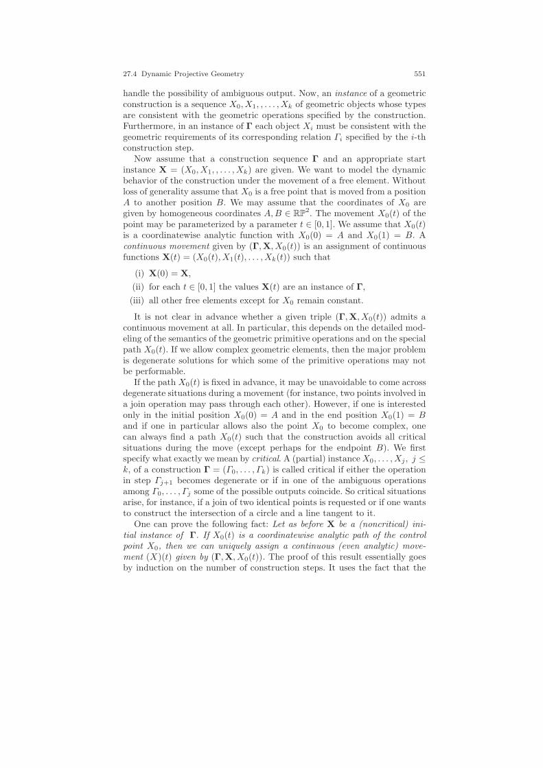
27.4 Dynamic Projective Geometry 551
handle the possibility of ambiguous output. Now, an instance of a geometricconstruction is a sequence X0, X1, , . . . , Xk of geometric objects whose typesare consistent with the geometric operations specified by the construction.Furthermore, in an instance of Γ each object Xi must be consistent with thegeometric requirements of its corresponding relation Γi specified by the i-thconstruction step.
Now assume that a construction sequence Γ and an appropriate startinstance X = (X0, X1, , . . . , Xk) are given. We want to model the dynamicbehavior of the construction under the movement of a free element. Withoutloss of generality assume that X0 is a free point that is moved from a positionA to another position B. We may assume that the coordinates of X0 aregiven by homogeneous coordinates A,B ∈ RP
2. The movement X0(t) of thepoint may be parameterized by a parameter t ∈ [0, 1]. We assume that X0(t)is a coordinatewise analytic function with X0(0) = A and X0(1) = B. Acontinuous movement given by (Γ,X, X0(t)) is an assignment of continuousfunctions X(t) = (X0(t), X1(t), . . . , Xk(t)) such that
(i) X(0) = X,
(ii) for each t ∈ [0, 1] the values X(t) are an instance of Γ,
(iii) all other free elements except for X0 remain constant.
It is not clear in advance whether a given triple (Γ,X, X0(t)) admits acontinuous movement at all. In particular, this depends on the detailed mod-eling of the semantics of the geometric primitive operations and on the specialpath X0(t). If we allow complex geometric elements, then the major problemis degenerate solutions for which some of the primitive operations may notbe performable.
If the path X0(t) is fixed in advance, it may be unavoidable to come acrossdegenerate situations during a movement (for instance, two points involved ina join operation may pass through each other). However, if one is interestedonly in the initial position X0(0) = A and in the end position X0(1) = Band if one in particular allows also the point X0 to become complex, onecan always find a path X0(t) such that the construction avoids all criticalsituations during the move (except perhaps for the endpoint B). We firstspecify what exactly we mean by critical. A (partial) instanceX0, . . . , Xj, j ≤k, of a construction Γ = (Γ0, . . . , Γk) is called critical if either the operationin step Γj+1 becomes degenerate or if in one of the ambiguous operationsamong Γ0, . . . , Γj some of the possible outputs coincide. So critical situationsarise, for instance, if a join of two identical points is requested or if one wantsto construct the intersection of a circle and a line tangent to it.
One can prove the following fact: Let as before X be a (noncritical) ini-tial instance of Γ. If X0(t) is a coordinatewise analytic path of the controlpoint X0, then we can uniquely assign a continuous (even analytic) move-ment (X)(t) given by (Γ,X, X0(t)). The proof of this result essentially goesby induction on the number of construction steps. It uses the fact that the
552 27 What We Did Not Touch
branches of the output of any geometric primitive operation can be calcu-lated by analytic functions (for details see [74]). By the absence of criticalsituations it is always possible to distinguish the branches of an ambiguousoperation. To stay with the example of intersecting a line and a circle: if nocritical situations are involved, the two intersections never coincide (however,they might become complex). By this every noncritical movement of the lineand the circle can be used to reconstruct a unique path for the two branches ofpossible intersections. The assumption of being noncritical is essential to geta uniqueness of the branches of the intersection. If the line becomes tangentto the circles, the two branches will eventually meet.
So the main issue becomes the avoidance of critical points. As long as weare interested only in the initial point and in the endpoint of X0(t) we havesufficient freedom to chose the path such that all critical points are avoided.For this we consider the linear interpolation
X0(t) := (1 − λ(t)) · A+ λ(t) · B,
where now λ : [0, 1] → C is an analytic function with λ(0) = 0 and λ(1) = 1on the interval [0, 1]. It is possible—by methods of complex function theory—to prove that λ can always be chosen in a way such that the resulting pathof the construction is noncritical for t ∈ [0, 1). In fact, the critical situationsarise only as pointlike singularities in C, the space in which λ is defined.For that reason it is always possible to circumvent critical situations by asuitable complex detour. Allowing complex values for X0(t) is essential. Ifone requires λ(t) to be real, it may be unavoidable to pass through criticalsituations.
One might wonder why one allows the free choice of a path X0(t) andeven with complex coordinates. This resembles very much the informationsituation in a real dynamic geometry system implemented on a computer. Indragging a free point, the only information on the user input is the mouseinteraction. This information, however, consists of a sequence of discrete sam-pling points (the mouse-drag information). The above strategy uses this free-dom to interpolate this information by noncritical analytic paths. All in all,this method allows for a continuous movement of the dependent elementsfor any specific mouse movement and by this resolves the jumping elementsproblem.
A simple example: We will end with a minimal example that illustratesthe complex tracing process. We consider a unit circle c and a vertical line lwhose position is controlled by some free point (it is easy to construct such asituation in a DGS). We want to analyze the behavior of the two intersectionpoints. Since all relevant elements stay finite, it is admissible to do the analysisby considering the usual Euclidean xy-coordinates. The points of the circle areall points (x, y) | x2 + y2 = 1. Let la be the vertical line with x-coordinatea. The two intersections of c and la have the coordinates p± = (a,±
√1 − a2).
For all a in the open interval (−1, 1) we have two real solutions. For a = ±1 we
27.4 Dynamic Projective Geometry 553
1 2 3 4 5 6 7 8
0 2
−e−itπ + 1
singularity
C
detour
Fig. 27.15 Intersections of a vertical line and a circle under a movement (left). The spaceof the controlling parameter of the line (right).
have critical situations. For all other a the two intersections have a complexy-coordinate. If we move the controlling parameter a continuously from 0 to2 along the real axis, we will necessarily pass through the critical situation ata = 1. However, we may take a detour through complex space (for instancea = −e−itπ + 1, t ∈ [0, 1]) that easily avoids the singularity. Inserting thispath into the y-coordinate of p±, we get
y = ±√
(1 − (−e−itπ + 1)2 = ±√−e−2itπ + 2e−itπ.
The expression under the square root describes a cycloid (the sum of twocyclic motions) whose absolute value is always greater than or equal to 1. So
Re(x)
Re(y)
Im(y)
Fig. 27.16 The intersections of a line and a circle with complex y-coordinate. The leftpicture shows the situation for a real path of a; the right picture shows the path of theintersections under a controlling path a(t) = 1 + cos(t) + ib sin(t), t ∈ [0, π], for variousvalues of b.
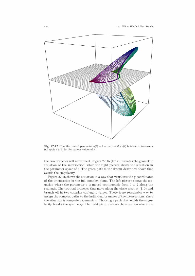
554 27 What We Did Not Touch
Fig. 27.17 Now the control parameter a(t) = 1 + cos(t) + ib sin(t) is taken to traverse afull cycle t ∈ [0, 2π] for various values of b.
the two branches will never meet. Figure 27.15 (left) illustrates the geometricsituation of the intersection, while the right picture shows the situation inthe parameter space of a. The green path is the detour described above thatavoids the singularity.
Figure 27.16 shows the situation in a way that visualizes the y-coordinatesof the intersection in the full complex plane. The left picture shows the sit-uation where the parameter a is moved continuously from 0 to 2 along thereal axis. The two real branches that move along the circle meet at (1, 0) andbranch off in two complex conjugate values. There is no reasonable way toassign the complex paths to the individual branches of the intersections, sincethe situation is completely symmetric. Choosing a path that avoids the singu-larity breaks the symmetry. The right picture shows the situation where the

27.4 Dynamic Projective Geometry 555
parameter a is moved along a closed path a(t) = 1+cos(t)+ib sin(t), t ∈ [0, 2π]for the values of b ∈ 1
20 ,220 , . . . ,
1920 , 1.
Finally, Figure 27.17 demonstrates what happens if the control parametera describes a full round trip around the singularity. It is a remarkable factthat in this case, such a circular path of the control parameter causes the twointersections to continuously interchange their roles, without ever meeting.

References
1. S. Apel, & J. Richter-Gebert, Cancellation patterns in Atutonated Geometric The-orem Proving, extended abstract ADG 2010, 14p, 2010.
2. A. Bachem & W. Kern, Linear Programming Duality. An Introduction to OrientedMatroids, Universitext, Springer-Verlag, Berlin Heidelberg 1992.
3. H. Behnke, F. Bachmann, K. Fladt, & H. Kunle, (Eds.), Grundzuge der Mathe-matik – Band II Geometrie, Vandenhoeck & Ruprecht, Gottingen, 1971. Also avail-able as translated version Fundamentals of Mathematics Vol. 2, Geometry, MIT Press,1974.
4. A. Below, V. Krummeck, & J. Richter-Gebert, Matroids with complex coefficients– phirotopes and their realizations in rank 2, in Discrete and Computational Geometry– The Goodman-Pollack Festschrift B. Aronov, S. Basu, J. Pach, M. Sharir (eds),Algorithms and Combinatorics 25, Springer Verlag, Berlin (2003), pp. 205-235.
5. R. Bischoff, Geometry of Qubits, Diploma Thesis, ETH Zurich (2003)6. W. Blaschke: Projective Geometry, Birkhauser, Basel, 1954.7. A. Bjorner, M. Las Vergnas, B. Sturmfels, N. White, G. M. Ziegler, Oriented
Matroids, Cambridge University Press 1993, second ed. 19998. J.F. Blinn, Lines in space,
Computer Graphics and Applications, IEEEPart 1: The 4D cross product, Volume 23, Issue 2 (March-April 2003) 84-91,Part 2: The line formulation, Volume 23, Issue 3 (May-June 2003) 72-79,Part 3: The two matrices, Volume 23, Issue 4 (July-Aug. 2003) 96-101,
Part 4: Back to the diagrams, Volume 23, Issue 5 (Sept.-Oct. 2003) 84-93,Part 5: A tale of two lines, Volume 23, Issue 6 (Nov.-Dec. 2003) 84-97,Part 6: Our Friend the Hyperbolic Paraboloid, Volume 24, Issue 3 (May-Jun 2004)92-100,Part 7: The Algebra of Tinkertoys, Volume 24, Issue 4 (July-Aug. 2004) 96-102,Part 8: Line(s) through four lines, Volume 24, Issue 5 (Sept.-Oct. 2004) 100-106.
9. J.F. Blinn, Polynomial discriminants,Computer Graphics and Applications, IEEEPart 1: Matrix magic, Volume 20, Issue 6 (Nov.-Dec. 2000) 94-98,Part 2: Tensor diagrams, Volume 21, Issue 1 (Jan-Feb 2001) 86-92.
10. J.F. Blinn, Quartic discriminants and tensor invariants, Computer Graphics andApplications, IEEE Volume 22, Issue 2 (March-April 2002) 86-91.
11. J.F. Blinn, Uppers and downers,Computer Graphics and Applications, IEEEPart 1: Volume 12, Issue 2 (March 1992) 85-91,Part 2: Volume 12, Issue 3 (May 1992) 80-85.
557
558 References
12. D. Bohm, A. Aharonov, Discussion of Experimental Proof for the Paradox of Ein-stein, Rosen and Podolsky, Phys. Rev. 108 (1957), 1070 – 107.
13. J. Bokowski Oriented matroids, Chapter 2.5 in: Handbook of Convex Geometry (eds.P. Gruber, J. Wills), North-Holland, Amsterdam, 1993, 555-602.
14. J. Bokowski, J. Richter & B. Sturmfels, Nonrealizability proofs in computationalgeometry, Discrete Comput. Geometry, 5, (1990), 333–350.
15. J. Bokowski, & J. Richter, On the finding of final polynomials, Europ. J. Combi-natorics, 11, (1990), 21–34.
16. J. Bokowski & B. Sturmfels, Computational Synthetic Geometry, Lecture Notes inMathematics 1355, Springer-Verlag, Berlin Heidelberg 1989.
17. F. Botana & T. Recio, (eds.), Automated Deduction in Geometry - ADG 2006
Revised Papers, LNAI 4969. Springer-Verlag, Berlin Heidelberg, 2008.18. M. Boutin & G. Kemper, On Reconstructing Configurations of Points in P 2 from
a Joint Distribution of Invariants, Appl. Algebra Engrg. Comm. Comput. 15 (2005),361–39.
19. E. Brieskorn & H. Knorrer, Plane Algebraic Curves, Birkhauser Verlag Basel, 1986.20. R. H. Bruck & H. J. Ryser, The non-existence of certain finite projective planes,
Can. J. Math. 1 (1949), p. 88–93.21. A. Cayley, Sixth Memoire upon Quantics, Philosophical Transactions of the Royal
Society of London, 159, (1859), p. 61–91.22. S.C. Chou, Mechanical Geometry Theorem Proving, D. Reidel Publishing Company,
Dodrecht, Holland, 1988.23. P. Cvitanovic, Group Theory Birdtracks, Lie’s, and Exceptional Groups, Princeton
University Press (2008).24. W. Clifford, Extract of a Letter to Mr. Sylvester from Prof. Clifford of University
College, Am. J. Math., vol. 1, 1878, pp. 126-128.25. H.S.M. Coxeter, Projective Geometry, Springer, New York, Berlin, 1994 (orig. 1963).26. H.S.M. Coxeter, The Real Projective Plane, Springer, New York, 1992 (orig. 1949).27. H.S.M. Coxeter, The Beauty of Geometry: Twelve Essays, Dover 1968.28. H.S.M. Coxeter & S.L. Greitzer, Geometry Revisited, Mathematical Association
of America, Washington, DC, 1967.29. H. Crapo, Invariant-Theoretic Methods in Scene Analysis and Structural Mechanics,
J. Symb. Comput., 11, (1991), 523–548.30. H. Crapo & J. Richter-Gebert, Automatic proving of geometric theorems, in: “In-
variant Methods in Discrete and Computational Geometry”, Neil White ed., KluwerAcademic Publishers, Dodrecht, (1995), 107–139.
31. H. Crapo & J. Ryan, Spatial realizations of linear scenes, Structural Topology, 13,(1986), 33–68.
32. G. Desargues, Oeuvres de Desargues reunies at analysees par M. Poudra, 2 vols,1864, Paris.
33. P. Doubilet, G.-C. Rota & J. Stein, On the foundations of combinatorial theory.IX., Combinatorial methods in invariant theory, Studies in Appl. Math. 53 (1974),185–216.
34. A.W.M. Dress & W. Wenzel, Endliche Matroide mit Koeffizienten, Bayreuth. Math.Scr., 24 (1978), 94–123.
35. A.W.M. Dress & W. Wenzel, Geometric Algebra for Combinatorial Geometries,Adv. in Math. 77 (1989), 1–36.
36. A.W.M. Dress & W. Wenzel, Grassmann-Plucker Relations and Matroids with Co-efficients, Adv. in Math. 86 (1991), 68–110.
37. A. Einstein, B. Podolsky & N. Rosen, Can quantum-mechanical description ofphysical reality be considered complete? Physical Review, 41 (1935), 777 – 180.
38. D. Eisenbud, M. Green, & J. Harris, Cayley-Bacharach Theorems and Conjectures,Bulletin (New Series) of the AMS 33, 3, (1996), 295–324.
References 559
39. D. Fearnley-Sander, Plane Euclidian Reasoning, in Gao, X.-S., Yang L.& Wang,D. (eds.), Automated Deduction in Geometry - ADG 1998 Proceedings. LNAI 1669.Springer-Verlag, Berlin Heidelberg, 1999, 86-110.
40. G. Fischer, Plane algebraic curves, Student Mathematical Library, 15, AmericanMathematical Society, 2001.
41. J. Folkman & J. Lawrence, Oriented matroids, J. Combinatorial Theory Ser. B 25
(1978), 199-236.42. M. v. Gagern, Morenaments, www.morenaments.de.43. M. v. Gagern & J. Richter-Gebert, Hyperbolization of Euclidean Ornaments, In
The Anders Bjorner Festschrift, Hultman, A., Linusson, S., Ziegler, G.M (eds) TheElectronic Journal of Combinatorics 16 (2009), R12.
44. L.E. Garner, An Outline of Projective Geometry, North Holland, New York, Oxford,1981.
45. X.-S. Gao, L. Yang & D. Wang, (eds.), Automated Deduction in Geometry - ADG1998 Proceedings, LNAI 1669. Springer-Verlag, Berlin Heidelberg, 1999.
46. H. Graßmann, Die lineare Ausdehnungslehre, Verlag Otto Wigand Leipzig 1844, 2.Aufl., 1878.
47. H. Graßmann, Die Ausdehnungslehre, Berlin 1862.48. J. Gray, Worlds Out of Nothing: A Course in the History of Geometry in the 19th
Century, Springer Undergraduate Mathematics Series, Springer 2006.49. M.J. Greenberg, Euclidean and non-Euclidean Geometries, (3rd ed.), Freeman and
Company, New York, 1996 (orig. 1974).50. B. Grunbaum, Arrangements and Spreads, Amer. Math. Soc. Regional Conference
Series in Mathematics 10, Rhode Island 1972.51. B. Grunbaum & G.C. Shephard, Ceva, Menelaus, and the Area Principle, Mathe-
matics Magazine, 68 (1995), 254–268.52. B. Grunbaum & G.C. Shephard, A new Ceva-type theorem, Math. Gazette 80 (1996),
492–500.53. B. Grunbaum & G.C. Shephard, Ceva, Menelaus, and Selftransversality, Geometriae
Dedicata, 65 (1997), 179–192.54. B. Grunbaum & G.C. Shephard, Some New Transversality Properties, Geometriae
Dedicata, 71 (1998), 179–208.55. G.B. Gurevich, Foundations of the Theory of Algebraic Invariants, P. Noordhoff,
Groningen (1964).56. Th. Hawkins, Hesses’s principle of transfer and the representation of lie algebras
Archive for History of Exact Sciences, 39, 1, 1988, 41–73.57. L.O. Hesse, Ein Uebertragungsprinzip, JI. fur reine u. angew. Math., 66, (1866), 15-
21.58. D. Hilbert, Grundlagen der Geometrie, Leipzig 1899, reprinted Teubner, Stuttgart
1999.59. D. Hilbert & S. Cohn-Vossen, Geometry and the Imagination, original Anschauliche
Geometrie, Springer 1932, reprinted, AMS Chelsea Publishing, 1999.60. H. Hong & D.Wang (eds.), Automated Deduction in Geometry - ADG 2004 Revised
Papers, LNAI 3763. Springer-Verlag, Berlin Heidelberg, 2006.61. D. Jorgensen, Der Rechenmeister, Aufbau dv, 1999.62. L. Kauffman, Knots and Physics: Series on Knots and Everything (Series on Knots
and Everything, Vol.1), World Scientific Publishing Co Pte Ltd, 1991.63. G. Katz, Curves in Cages: An Algebro-Geometric Zoo, American Mathematical
Monthly, 113, Number 9, 2006 , 777-791.64. F. Klein, Uber die Transformationen der allgemeinen Gleichung des zweiten Grades
zwischen Linien-Coordinaten auf eine canonische Form, Inauguraldissertation, Bonn,1968.
65. F. Klein, Das Erlanger Programm : Vergleichende Betrachtungen ber neuere ge-ometrische Forschungen, 1871, reprinted in Verlag Harry Deutsch, Frankfurt/ Main1995.
560 References
66. F. Klein, Uber die so-genannte nicht-euklidische Geometrie, Mathematische Annalen,4 (1871), 573–625.
67. F. Klein, Uber die so-genannte nicht-euklidische Geometrie, Mathematische Annalen,6 (1873), 112–145.
68. F. Klein, Vorlesungen uber nicht-euklidische Geometrie, Springer, Berlin, reprinted1968 (orig. 1928).
69. F. Klein, Vorlesungen uber die Entwicklung der Mathematik im 19. Jahrhundert,Springer, Heidelberg, 1928.
70. F. Klein, Development of mathematics in the 19th century (1928), reprinted andtranslated in Math Science Press, 1970.
71. D. E. Knuth, Axioms and Hulls, Lecture Notes in Computer Science 606, Springer-Verlag, Berlin Heidelberg 1992.
72. U. Kortenkamp, Foundations of dynamic geometry, PhD-thesis, ETH Zurich, 1999,http://www.inf.fu-berlin.de/∼kortenka/Papers/diss.pdf.
73. U. Kortenkamp & J. Richter-Gebert, Complexity issues in dynamic geometry, In
Festschrift in the honor of Stephen Smale’s 70th birthday, M. Rojas, F. Cucker (eds.),World Scientific, pp 355–404, (2002).
74. U. Kortenkamp and J. Richter-Gebert: Grundlagen dynamischer Geometrie, Ze-ichnung - Figur - Zugfigur (2001) 123-144.
75. G. Kowol, Projektive Geometrie und Cayley-Klein Geometrien der Ebene,Birkhauser, 2009.
76. B. Kutzler & S. Stifter, On the application of Buchberger’s algorithm to automatedgeometry theorem proving, J. Symb. Comput., 2, (1986), 389–297
77. E. Laguerre, Sur la theorie des foyers, Nouv. Ann. Math., 12 (1853) 57–66.78. C. W. H. Lam, L. H. Thiel & S. Swiercz, The Non-existence of Finite Projective
Planes of Order 10, Canad. J. Math., 41 (1989), 1117–1123.79. C. W. H. Lam, L. H. Thiel, and S. Swiercz, The search for a finite projective planes
of order 10, Amer. Math. Monthly., 98 (1991), 305–318.80. M. Las Vergnas, Convexity in oriented matroids, J. Combinatorial Theory, Ser. B
29 (1980), 231–243.81. R. Lauffer, Die nichtkonstruierbare Konfiguration (103), Math. Nachr., 11, (1954),
303–304.82. P. Lebmeir & J. Richter-Gebert, Recognition of Computationally Constructed Loci,
Lecture Notes in Computer Science/Artificial Intelligence, Vol. 4869 (2007) 52–68.83. P. Lebmeir & J. Richter-Gebert, Rotations, Translations and Symmetry Detection
for Complexified Curves, Computer Aided Geometric Design (special issue ClassicalTechniques for Applied Geometry), 25, 2008, 707–719.
84. P. Lebmeir & J. Richter-Gebert: Diagrams, tensors and geometric reasoning, Dis-crete Comput. Geom. 42, No. 2, (2009), 305–334.
85. F. Levi, Die Teilung der projektiven Ebene durch Gerade oder Pseudogerade, Ber.Math.-Phys. Kl. Sachs. Akad. Wiss., 78 (1926), 256-267.
86. D. Liebscher, Einsteins Relativitatstheorie und die Geometrien der Ebene, TeubnerVerlag, 1999.
87. S.B. Maurer, Matroid basis graphs I, J. Combin. Theory B, 26 (1979), 159–173.88. J. Edmonds & A. Mandel, Topology of oriented matroids, Ph.D. Thesis of A. Mandel,
University of Waterloo 1982, 333 pages.89. G. Monge, Traite de geometrie descriptive, 1811, Paris.90. M. Nielsen & I. Chuang, Quantum Computation and Quantum Information, Cam-
bridge University Press, 2000.91. A.L. Onishchik & R. Sulanke, Projective and Cayley-Klein Geometries, Springer
Monographs in Mathematics Springer, 2006.92. J. Oxley, Matroid Theory, Oxford University Press, Oxford 1992.93. R. MacPherson, & M. McConnell, Classical projective geometry and modular vari-
eties, in Algebraic Analysis, Geometry and Number Theory: Proceedings of the JAMIInaugural Conference, ed. Jun-Ichi Igusa, Hohn Hopkins U. Press, (1989), 237–290.
References 561
94. D. Mumford, C. Series & D. Wright, Indras Pearls – the Vision of Felix Klein,Cambridge University Press 2002.
95. C.W. O’Hara & D.R. Ward, An Introduction to Projektive Geometry, Oxford at theClarendon Press, 1937.
96. N.E. Mnev, The universality theorems on the classification problem of configurationvarieties and convex polytopes varieties, in: Viro, O.Ya. (ed.): Topology and Geometry— Rohlin Seminar, Lecture Notes in Mathematics 1346, Springer, Heidelberg 1988,527–544.
97. N.E. Mnev, The universality theorems on the oriented matroid stratification of thespace of real matrices, in: Applied Geometry and Discrete Mathematics – The Vic-tor Klee Festschrift (P. Gritzmann, B. Sturmfels, eds.), DIMACS Series in Discrete
Mathematics and Theoretical Computer Science, Amer. Math. Soc., Providence, RI,6 (1991), 237–243.
98. P. J. Olver, Classical Invariant Theory, London Mathematical Society Student Texts44, Cambridge: Cambridge University Press, 1999.
99. J. Plucker, Uber ein neues Coordinatensystem, Journal fur reine und angewandteMathematik, 5, (1830), 1–36.
100. J. Plucker, System der analytischen Geometrie, Berlin, 1935.101. J. Plucker, System der algebraischen Curven, Bonn, 1939.102. J. Plucker, Neue Geometrie des Raumes gegrndet auf die Betrachtung der geraden
Linie als Raumelement, Teubner, Leibzig, 1868.103. J.V. Poncelet, Traite des proprietes projectives des figures, Gauthier-Villars, Paris
1822.104. H. Reichhardt, Gauss und die Anfange der nicht-euklidischen Geometrie, B.G.
Teubner ; Wien ; New York : Distributed by Springer, c1985.105. J. Richter, Kombinatorische Realisierbarkeitskriterien fur orientierte Matroide,
Mitteilungen Math. Seminar Gießen 194 (1989).106. J. Richter-Gebert, Realization Spaces of Polytopes, Lecture Notes in Mathematics
1643, Springer, Heidelberg 1996.107. J. Richter-Gebert, Mnev’s universality theorem revisited, Proceedings of the
Seminaire Lotharingien de Combinatorie 1995, 211–225.108. J. Richter-Gebert, Universality Theorems for Oriented Matroids and Polytopes,
Contemporary Mathematics, 223, 1999, 269–292.109. J. Richter-Gebert, Mechanical theorem proving in projective geometry, Annals of
Mathematics and Artificial Intelligence 13 (1995), 139–172.110. J. Richter-Gebert, Meditations on Ceva’s Theorem, In The Coxeter Legacy: Re-
flections and Projections (Eds. Chandler Davis & Eric Ellers, American MathematicalSociety, Fields Institute), 227–254, 2006.
111. J. Richter-Gebert & Th.Orendt, Geometriekalkule, Springer, 2009.112. J. Richter-Gebert & U. Kortenkamp, Cinderella - The interactive geometry soft-
ware, Springer 1999.113. J. Richter-Gebert & U. Kortenkamp, Cinderella - The interactive geometry soft-
ware, 2006 http://www.cinderella.de.114. J. Richter-Gebert & P. Lebmeir, Diagrams, tensors and geometric reasoning. Dis-
crete Comput. Geom. 42, No. 2, (2009), 305-334.115. J. Richter-Gebert & D.Wang (eds.), Automated Deduction in Geometry - ADG
2000 Revised Papers, LNAI 2061. Springer-Verlag, Berlin Heidelberg, 2001.116. J. Richter-Gebert & G.M. Ziegler, Oriented Matroids, CRC Handbook on “Dis-
crete and Computational Geometry” (J.E. Goodman, J. O’Rourke, eds.) CRC Press,Boca Raton, New York, (1997), 111–132.
117. G. Ringel, Teilungen der Ebene durch Geraden oder topologische Geraden, Math.Zeitschrift 64 (1956), 79-102.
118. A. Saam, Ein neuer Schließungssatz fur die projektive Ebene, Journal of Geometry29 (1987), 36–42.
562 References
119. A. Saam, Schließungssatze als Eigenschaften von Projektivitaten, Journal of Geom-etry 32 (1988), 86–130.
120. G.C. Shephard, Cyclic Product Theorems for Polygons (I) Constructions using Cir-cles, Discrete Comput. Geom., 24 (2000), 551-571.
121. P. Shor, Stretchability of pseudolines is NP–hard, in: Applied Geometry and Dis-crete Mathematics – The Victor Klee Festschrift (P. Gritzmann, B. Sturmfels, eds.),DIMACS Series in Discrete Mathematics and Theoretical Computer Science, Amer.Math. Soc., Providence, RI, 4 (1991), 531–554.
122. P. Stackel ed., Geometrische Untersuchungen mit Untersttzung der UngarischenAkademie der Wissenschaften, Magyar Tudomanyos Akademia, Leipzig, Berlin: B.G.Teubner, 1913.
123. G.E. Stedman, Diagram techniques in group theory, Cambridge University Press,New York, 1990.
124. J. Stolfi, Oriented Projective Geometry, Academic Press, 1991.125. J. Stilwell, Sources of Hyperbolic Geometry, (History of Mathematics, V. 10),
American Mathematical Society, 1996.126. B. Sturmfels: Algorithms in Invariant Theory, Springer-Verlag Wien New York,
1993.127. A. Sudbery, On local invariants of three-qubit states, J. Phys. A, 34:643–652, 2000.
(quant-ph/0001116).128. J. Sylvester, On an Application of the New Atomic Theory to the Graphical Rep-
resentation of the Invariants and Covariants of Binary Quantics, with Three Appen-dices, Am. J. Math., vol. 1, 1878, pp. 64–125.
129. B. L. van der Waerden, Zur algebraischen Geometrie. XV. Losung des Charakter-istikenproblems fur Kegelschnitte, Mathematische Annalen, 115,1938, 645–655.
130. W. Wenzel, A Group-Theoretic Interpretation of Tutte’s Homotopy Theory, Adv.in Math. 77 (1989), 27–75.
131. H. Weyl, The Classical Groups, Princeton University Press, Princeton, New Jersey,1939.
132. N. White, The Bracket Ring of Combinatorial Geoemtry I, Transactions AMS 202
(1975), 79–95.133. Winkler, F. (ed), Automated Deduction in Geometry - ADG 2002 Revised Papers,
LNAI 2930. Springer-Verlag, Berlin Heidelberg, 2004.134. W.T. Wu, On the decision problem and the mechanization of theorem-proving in
elementary geometry, Contemp. Math. 29, (1984), 213–234.135. W.T. Wu, Basic principles of mechanical theorem proving in elementary geometries,
J. Syst. Sci. Math. Sci., 4, (1984), 207–235.136. I.M. Yaglom, A simple non-Euclidean geometry and its physical basis : an ele-
mentary account of Galilean geometry and the Galilean principle of relativity,, AbeShenitzer (trans.), Springer-Verlag New York, 1979.
137. I.M. Yaglom, Felix Klein and Sophus Lie - Evolution of the Idea of Symmetry in theNineteenths Century, Birkhauser, Boston, Basel, 1988.
138. G. M. Ziegler, Lectures on Polytopes, Graduate Texts in Mathematics 152,Springer-Verlag, New York 1995; Updates, corrections, and more available per WWWfrom http://www.math.tu-berlin.de/∼ziegler

Index
C, 293–305CP
1, 307–323, 475, 534
RP1, 69–78
RP2, 47–66, 475
RP3, 207–215, 255–263
RPd, 215–221
a priori knowledge, 468
absolute distance measurement, 383
absolute value, 299addition, 90, 134, 299
additivity, 505adjoint, 153, 254
affine geometry, 331affine transformation, 59, 331
algebraic curve, 23, 521
algebraic geometry, 521altitudes of a triangle, 138, 361, 422
ambiguous operations, 544analytic path, 547
angle, 27, 309, 320, 331, 433Euclidean, 338
angle bisector, 347, 545
angle bisectors of a triangle, 362, 427, 430angle defect, 505
angle measurementhyperbolic, 483, 497
in Cayley-Klein Geometries, 373angle sum, 465
anti-commutative, 213
anti-Mobius transformation, 317, 494Archimedes of Syracuse, 439
area, 9, 104, 105, 128, 465, 467hyperbolic, 505
area method, 10Argand, Jean-Robert, 299
argument, 299
Aristotle, 265arrangement
of lines, 529of pseudolines, 530
asymptote, 19
automated proving, 114, 268automorphism
of a field, 84, 88, 317axioms
of oriented matroids, 530of Euclidean geometry, 464, 473
of projective plane, 40
Bezout’s theorem, 22, 522Bacharach, I., 23
basis
functional, 114projective, 82, 86
Beatty, Warren, 125Beltrami, Eugenio, 466, 471
Beltrami-Klein model, 471, 479bicycle, 453
binomial proof, 268, 335
Blaschke, Wilhelm, 35, 83, 346Blinn, Jim, 223
blowup, 523Bolyai, Farkas, 466, 468
Bolyai, Janos, 466, 468, 501bracket, 72, 95–101, 107, 127, 269, 327
ring, 120
bracket algebra, 119bracket monomial, 100
bracket polynomial, 116, 118multi-homogeneous, 100, 240
Brenneman, Kristina, 125Brianchon’s theorem, 181, 354
Brianchon, Charles Julien, 183
563
564 Index
Bruck and Ryser
Theorem of, 65
calculation
of projective transformation, 63calculation of
angleCayley-Klein, 373
Euclidean, 338hyperbolic, 484
in Poincare disk, 497angle bisector, 347
angle bisector in Cayley-Kleingeometries, 430
center of a circle, 350
circle through three points, 329conic from foci, 356conic through five points, 168
conic through four points and tangent toa line, 203
distance
Cayley-Klein, 373Euclidean, 341
in Poincare disk, 498dual conic, 153
foci of a conic, 352harmonic point, 80
intersection of conic and line, 191intersection of three planes, 211
intersection of two conics, 194join, 53join in RP
3, 213, 256
join in RPd, 215
meet, 53
meet in RPd, 215
midpoint in Cayley-Klein geometries,429
mirror image, 346parallel, 55
perpendicular, 335, 420plane through three points, 208
projective transformation, 62splitted conic, 188tangent, 149, 252
transformed conic, 154transformed line, 61
transformed point, 61calculations
symbolic, 114Calvin and Hobbes, 291
cancellation, 13, 29, 268–287Cardano, Girolamo, 193, 295
Carnot’s theorem, 287Carroll, Lewis, v
Cayley, Arthur, 23, 395, 472
Cayley-Bacharach-Chasles theorem, 23,522
Cayley-Klein geometries, 371–460
census of Cayley-Klein geometries, 389
center, 444of a circle, 350
of a hyperbolic circle, 503Ceva configuration, 17, 360
Ceva’s theorem, 16, 275
Ceva-Menelaus proof, 275Chasles, Michael, 23
checkerboard, 515chirotope, 532
Churchill, Winston, 521Cinderella, 186, 543
circle, 24, 143, 309, 328, 350, 464, 486
in Cayley-Klein Geometries, 439–460in hyperbolic geometry, 473, 501
nine point, 364through three points, 329, 504
circle inversion, 317, 494
circle limit picture, 454, 518circlereflection, 317
Clifford, William Kingdon, 262closed ε-cycle, 248
closed diagrams, 229cocircularity, 28, 309, 319, 327, 333
coconicality, 168, 246, 272, 328
collinearity, 13, 79, 94, 309collineation, 86
Columbus1D, 383columnness, 225
combinatrics, 527
commutativity, 91, 265complex conjugate, 303
complex conjugate objects, 196complex detour, 548
complex distance, 381complex function theory, 476, 548
complex number plane, 299, 475, 485
complex numbers, 24, 35, 88, 195, 293–305,308, 475, 544
complex projective line, 307
computational geometry, 527computer aided design, 114
computer algebra, 30, 117
computer vision, 114configuration, 98, 107, 108, 115
configuration space, 543conformal, 476
conic, 19, 116, 143–203, 252, 352, 372, 511as equidistant curve, 387
classification, 146, 155, 160

Index 565
degenerate, 20, 155, 167, 186
non-degenerate, 147splitting of a, 186–192
through five points, 165twelve-point, 369
conjugate, 327conjugation, 303, 316
construction sequence, 544continuity, 545continuous function, 189
contravariant index, 232coordinate matrix, 107
coordinate ring, 119coordinates
homogeneous, 13, 50, 74, 107, 115, 208,308
Cotes, Roger, 301
covariant index, 232covector, 528
Coxeter, Harold Scott Macdonald, 18Cramer’s rule, 97, 104
Cray, 65cross product, 30, 53, 95, 187, 234
cross-ratio, 28, 63, 72–78, 80, 95, 115, 118,131, 168, 173, 329, 338, 373, 403, 420,482
chains of, 273in CP
1, 311, 316, 330
in RP1, 72
in RP2, 77
of lines, 76on a circle, 330
on a conic, 170, 330permutations of indices, 75
seen from a point, 78, 169cubic, 23, 521
solving a, 193cubic equation, 192
curvature, 453, 502curve
algebraic, 23, 521cubic, 23, 521
curves
equidistant, 386cusp, 523
CW-complex, 282cycle, 444, 501
in Galilean geometry, 457
d’Alembert, Jean-Baptiste le Rond, 107,298
Durer, Alfred, 36
da Vinci, Leonardo, 36degenerate measurement, 382, 439
degree, 525
delta tensor, 233Desargues’s Theorem
spatial interpretation, 268Desargues’s theorem, 40, 266, 284, 363, 367Desargues, Girard, 38
Descartes, Rene, 38descriptive geometry, 38
determinant, 9, 13, 72, 94–107, 109, 149,210, 217, 234, 252, 327
determinant vector, 108, 115
diagramsclosed, 229
diagrams of tensors, 228differential geometry, 453
dimension, 36, 52, 308discrete mathematics, 527distance, 337, 433, 440
Euclidean, 341oriented, 276
distance measurementhyperbolic, 497
in Cayley-Klein Geometries, 373in hyperbolic geometry, 473
distances, 331division, 302dog, 461
Doppelverhaltnis, 74double line, 190
double point, 523dragoncat, 519
Dress, Andreas, 287dual
of a conic, 160of Pascal’s theorem, 183of a circle, 450
of a conic, 153, 190, 254of a degenerate conic, 190
of a quadratic form, 153of an algebraic curve, 525
duality, 56, 152, 177, 357, 373of concurrence and collinearity, 94
of distances and angles, 373of join and meet, 56, 218of midpoint and angular bisector, 427
of point and line, 56of points and planes, 208
dynamic geometry, 542–551
eigenvalue, 145
eigenvector, 314Einstein’s summation convention, 226
Einstein, Albert, 165Einstein-Podolsky-Rosen paradox, 541

566 Index
electron, 534
electrostatic charge, 315elementary geometry, 467
elements at infinity, 41, 206elimination property, 530
ellipse, 19, 147, 352elliptic geometry, 371, 391, 475elliptic measurement, 381
elliptic transformation group, 400entanglement, 540
entanglement invariant, 541epsilon tensor, 233
epsilon tensorsof rank 4, 255
epsilon-delta rule, 235, 257, 258equation
cubic, 23, 192
quadratic, 19, 144, 165, 190equidistant curves, 386
equivalence class, 41, 47Erlanger Programm, 177
Escher, Maurits Cornelius, 38, 454, 518Euclid, 464
Euclid’s postulates, 464Euclidean angle, 338
Euclidean distance, 341Euclidean geometry, 5, 36, 291, 325–369,
371, 392, 425, 443, 452Euclidean invariant, 327
Euclidean measurement, 384Euclidean plane, 41, 50, 143, 219
Euclidean transformation, 58, 331Euler line, 363
Euler’s Formula, 301, 404Euler, Leonhard, 165, 301
exceptional situation, 374, 404, 445
Fano plane, 43, 64
Fearnly Sander, Desmond, 10Ferrari, Lodovico, 193
field, 35, 47, 84, 88finite, 64
fifth postulate, 465finite projective plane, 44, 63Fior, Anton Maria, 193, 295
first fundamental theorem of invarianttheory, 115
fixed point, 313
foci of a conic, 352focus, 352, 356
free elements, 543function
continuous, 189multivalued, 375
projectively invariant, 118
rational, 116functional basis, 114
fundamental object, 373, 386, 420, 442fundamental theorem of algebra, 297
fundamental theorem of invariant theoryfirst, 115second, 120
fundamental theorem of projectivegeometry, 62, 86
Godel, Kurt, 471von Gagern, Martin, 519
Galilean geometry, 394, 440, 448, 455Gauss, Carl Friedrich, 298, 466
generic nondegeneracy assumptions, 269geometric construction, 543geometric properties, 335
geometryGalilean, 455
similarity, 331affine, 331
Cayley-Klein, 371–460descriptive, 38
dynamic, 542–551elliptic, 371, 391, 475
Euclidean, 5, 36, 291, 325–369, 371, 392,425, 443, 452
Galilean, 394, 440, 448
hyperbolic, 371, 391, 426, 461–519Minkowski, 393projective, 35, 38
pseudo-Euclidean, 392, 425, 443, 452real projective, 5
relativistic space-time, 371, 393spherical, 391
Gerhard, Susan, 93Gershwin, George, 371
Gershwin, Ira, 371grade of a tensor, 225
graph theory, 527Grassmann product, 217Grassmann, Hermann Gunther, 212
Grassmann-Plucker-Relation, 15, 102–106,110–113, 127, 214, 237, 262, 269, 532
in CP1, 318
Gray, Jeremy, 464Greenberg, Marvin Jay, 346, 464
Greitzer, Samuel, L., 18Grobner bases, 272
group, 58, 482, 515discrete, 518
group of elliptic transformations, 400group of hyperbolic transformations, 400

Index 567
Hadamard, Jacques Salomon, 307
harmonic map, 83, 86
harmonic points, 80, 83
construction of, 81
on a conic, 183
harmonic position, 80, 250, 284, 336, 347,359, 361, 410, 420, 428
Hesse’s transfer principle, 177, 365
Hessian, 525
Hilbert, David, 165, 205, 473
Hoehn’s theorem, 280
homogeneous coordinates, 13, 50, 74, 107,115
in CP1, 308
in RP3, 208
in RPd, 215
horocycle, 444, 454, 502
hyperbola, 19, 147, 352
hyperbolic geometry, 371, 391, 426,461–519
hyperbolic measurement, 376
hyperbolic transformation, 481, 492–499
hyperbolic transformation group, 400
hypercycle, 444, 454, 502
hyperdeterminant, 542
hyperinfinite point, 481
hyperrotation, 418
I and J, 25, 326–343, 346, 350, 372
Ibn al-Haytham, 465
if-operation, 189
imaginary unit, 297
incidence, 40, 229
incidence relation, 40, 48
incidence theorem, 12, 18, 25, 67, 92, 132,181, 265–288, 521, 527
Euclidean, 275
index set, 108
indices
contravariant, 232
covariant, 232
linelike, 226
of a tensor, 226
pointlike, 226
inflection point, 524
inner geometry, 462, 480
inside, 150
instance, 544
intermediate value theorem, 189
intersection
of circle and line, 545
of conic and line, 190
of two conics, 192
invariant, 72, 98–102, 114, 115, 230, 241,327, 541
relative, 116invariant predicate, 100invariant theory, 113inversion, 316, 317
inversve geometry, 317involution, 137–141, 184iterated reflections, 416
join, 44, 49, 52, 207, 234, 346in RP
3, 213, 256in RP
d, 215
jumping elements, 544
kaleidoscope, 516Kant, Immanuel, 468
Kaplansky, Irving, 185Klein, Felix, 36, 158, 177, 205, 212, 325,
371, 419, 424, 464, 466, 471, 490knot theory, 262Kortenkamp, Ulrich, 543
Laguerre’s formula, 325, 338, 372, 484Laguerre, Edmond, 338Lam, H.W.C., 65
law of sines, 433, 510Levi-Civita symbol, 233Lie algebra, 177
lifting, 130Lightyear, Buzz, 479line, 40, 51
at infinity, 5, 42, 51, 135, 325, 439, 448
complex projective, 307in RP
3, 212, 257oriented, 529projective, 127, 134
real projective, 68, 69, 307line arrangement, 529line reflection, 413
line segmentoriented, 9
linear programming, 527linear transformation, 313
linelike indices, 226Lobachevsky, Nikolai Ivanovich, 466, 470logarithm, 338, 373
Mobius Reflections, 316Mobius transformation, 313, 492
iterated, 313
Mobius, August Ferdinand, 49magnetic charge, 315manifold, 16

568 Index
triangulated, 17, 282
manifold proofs, 282Mann, Thomas, 461map
harmonic, 83, 86Matiyasevich, Yuri, 179matrix, 144, 224
coordinate, 107rank, 186, 407
skew symmetric, 187transformation, 60, 331
matroid, 287, 527
McLaughlin, John, 127measurement, 338, 341
elliptic, 381
in Cayley-Klein geometries, 373degenerate, 382, 439Euclidean, 384
hyperbolic, 376in quantum theory, 535
nondegenerate, 375oriented, 396, 427, 484parabolic, 382
mechanics, 467medians of a triangle, 359, 430meet, 44, 52, 207, 234, 346
in RPd, 215
Menelaus configuration, 18, 360
Menelaus’s theorem, 275midpoint, 337, 427Minkowski geometry, 393
Miquel’s theorem, 27, 334mirror image, 346modulus, 299
Monge, Gaspard, 38motion invariance, 505multi-homogeneous bracket polynomials,
100, 240
multilinearity, 96, 213multiplication, 90, 134, 179, 299
multivalued function, 375
n-gon, 513nine point circle, 364nondegeneracy conditions, 7, 269
generic, 8nondegenerate measurement, 375
O’Hara, C.W., 345
observation, 535observer, 462order, 45, 65, 66
orientation, 320oriented area, 9, 128
oriented distance, 276
oriented matroid, 527–533oriented matroid axioms, 530
oriented measurement, 396, 427oriented surface, 16
orthogonal projection, 490orthogonality, 48, 335, 361, 420
in pseudo-Euclidean geometry, 421
outside, 150
Pappian plane, 92Pappos of Alexandria, 3
Pappos’s Theorem, 4–31Euclidean version, 6
Pappos’s theorem, 91, 98, 251, 265, 285,522, 531
parabola, 19, 147, 179, 449, 455parabolic measurement, 382
parallel, 5, 36, 42, 54parallel postulate, 466, 474
parameterizationrational, 173
Pascal’s Theoremdegenerate version, 21
Euclidean versions, 21Pascal’s theorem, 20, 181, 199, 246, 272,
366
Pascal’s triangle, 215Pascal, Blaise, 20, 38, 143, 181
pentagon, 426, 515peripheral angle theorem, 309, 510permutation, 75
perspective drawing, 36perspectivity, 71, 76, 170
phase, 534photon, 534
Plucker formulas, 526Plucker vector, 255
Plucker’s µ, 96, 167, 237, 441, 488Plucker’s formula, 96
Plucker, Julius, 36, 47, 49, 96, 113, 212plane
at infinity, 207
Euclidean, 41, 50, 143, 219finite projective, 44, 63
in RP3, 207
Pappian, 92
projective, 41real projective, 49
smallest projective, 43Plato, v
Playfair, John, 466Poincare disk model, 475, 479, 485, 497,
501

Index 569
Poincare half plane model, 475
Poincare, Henri, 466, 475point, 40, 50, 464
at infinity, 6, 27, 42, 50, 70, 308, 322,325, 448
hyperinfinite, 481on a line, 68, 127
point configuration, 98, 107, 115point reflection, 413
pointlike indices, 226
pointsantipodal, 528
polar, 147, 230polar representation, 302
polarization, 534pole, 421
pole-polar pair, 409
polynomial, 10, 116cubic, 23
multi-homogeneous, bracket, 100, 240polytope theory, 527
Poncelet, Jean-Victor, 40
power series, 301predicate, 100
primal-dual pair, 157–164, 389, 412, 440classification, 160
prime numbers, 179prism, 12
projection, 76
orthogonal, 490stereographic, 175, 322, 490
projective basis, 82, 86, 170projective geometry, 35, 38
fundamental theorem of, 62, 86
oriented, 528projective invariant, 114, 230, 241, 327, 395
projective line, 68, 134complex, 307
projective plane, 41axioms, 40
finite, 44, 63
over a field, 48projective scale, 82
on a conic, 170projective space, 205
projective transformation, 57, 60, 70, 99,109, 137, 154, 171, 173, 331, 482
in RP3, 209
projectively invariant conditions, 327
projectively invariant function, 118projectively invariant properties, 98–102
proof by specialization, 128properties
projectively invariant, 98–102
proving
automated, 114, 268pseudo-Euclidean geometry, 392, 425, 443,
452pseudoline arrangement, 530
pseudosphere, 472Ptolemy’s theorem, 318Pythagorean theorem, 319, 465, 488, 510
quadratic equation, 19, 165, 190
quadratic form, 144, 229, 403quadrilateral set, 129–141, 178, 201, 350,
359, 361quantum information theory, 534–542
qubit, 534
rank, 186, 407rank of a tensor, 225Raphael, 36
ratio, 8, 17rational function, 116rational parameterization, 173
ratios of lengths, 331ray, 354real numbers, 35, 69, 83, 84, 88
real projective geometry, 5real projective line, 68, 307real projective plane, 49
realizability problem, 531, 533realizable, 530rectangle, 319
reflection, 139, 303, 331, 346, 354in Cayley-Klein geometries, 409
relative position, 529
relativistic space-time geometry, 371, 393Renaissance, 36Riemann surface, 546right angle, 426, 462, 464
ring, 119bracket, 120
Ritt’s algebraic decomposition, 272
robotics, 114rosette group, 518Ross, Diana, 67
rotation, 58, 300, 313, 331, 426in Cayley-Klein geometries, 416
rowness, 225
ruler, 461
Saam’s theorem, 274Saam, Armin, 274scalar product, 211
scaleprojective, 82

570 Index
scaling, 313, 331
scene analysis, 130Scipione del Ferro, 193, 295
second fundamental theorem of invarianttheory, 120
segment, 464separation
on a circle, 330set
harmonic, 80, 250quadrilateral, 129–141, 178, 201
shearing, 331
sidedness, 316sign, 147, 389, 528
signature, 146, 389similarity, 59, 300, 313, 331
similarity geometry, 331similarity transformation, 331
simplicity, 266
singularity, 523, 548skew symmetric, 187
slope, 135space
projective, 205, 255special cases, 36, 189
sphere, 322, 535
spherical geometry, 391spin, 534
splitting a conic, 186–192square root, 546
state, 534entangled, 540
independent, 540
von Staudt, Karl Georg Christian, 83Stedman, Geoffrey E., 243
stereographic projection, 175, 322, 490, 535Sting, 461
straight line, 468stretchability problem, 531
structural chemistry, 527
structural mechanics, 114summation convention
Einstein’s, 226supercomputer, 65
superposition, 534surface of negative curvature, 472
Swiercz, S., 65
Sylvester’s law of inertia, 146Sylvester, James Joseph, 262
symbolic calculations, 114symmetrization
of a matrix, 145symmetry, 132, 266
symmetry group, 515
tangent, 21, 63, 147–152, 184, 198, 252,346, 350
Tartaglia, Nicolo, 193, 295tensor, 225, 539
grade of, 225
tensor calculus, 223–263tensor diagrams, 228–263, 542
in RP3, 255
Thales’s theorem, 426, 510
Theorem of
Carnot, 287Desargues, 266, 284
Hoehn, 280Pascal, 366
Pythagoras, 319, 465
Bezout, 22, 522Brianchon, 181, 354
Bruck and Ryser, 65Cayley-Bacharach-Chasles, 23, 522
Ceva, 16, 275
Desargues, 40, 363, 367Menelaus’, 275
Miquel, 27, 334Pappos, 4–31, 91, 98, 251, 265, 285, 522,
531
Pascal, 20, 181, 199, 246, 272
Ptolemy, 318Pythagoras, 488, 510
Saam, 274Thales, 426, 510
Thiel, L., 65
tiling, 515topology, 527
trace, 244transformation, 57–63
affine, 59, 331
anti-Mobius, 317, 494Euclidean, 58, 331
hyperbolic, 481, 492–499in Cayley-Klein geometries, 395–419
leaving a conic invariant, 173
linear, 108, 313Mobius, 313, 492
of ε-tensors, 237of a conic, 154
of a line, 61of a point, 61
of a tensor, 230
projective, 57, 60, 70, 99, 109, 137, 154,171, 173, 209, 331, 482
in CP1, 311, 492
similarity, 331with vanishing trace, 244
transformation matrix, 60, 331

Index 571
transitivity properties, 482translation, 58, 299, 313, 331transposition, 225triangle, 465, 505triangle theorems, 358–364
in Cayley-Klein geometries, 422–432triangulated manifold, 17, 282trigonometric function, 301trigonometry, 433–438
hyperbolic, 514Tutte group, 287
twelve-point conic, 369
unit circle, 143, 476, 480unit steps
elliptic, 382hyperbolic, 378
universality theorem, 533
vector, 528vector configuration, 108vector space, 47von Staudt constructions, 83, 89, 134, 265,
533
wallpaper group, 518Ward, D.R., 345Watterson, Bill, 291
Wenzel, Walter, 287Wessel, Caspar, 299Weyl, Hermann, 265Whitman, Walt, 243
Yaglom, Isaak Moiseevich, 464