Optimizing the Evaluation of Finite Element Matrices

SIAM J. SCI. COMPUT. c© 2005 Society for Industrial and Applied MathematicsVol. 27, No. 3, pp. 741–758

OPTIMIZING THE EVALUATION OF FINITE ELEMENTMATRICES∗

ROBERT C. KIRBY† , MATTHEW KNEPLEY‡ , ANDERS LOGG§ , AND

L. RIDGWAY SCOTT¶

Abstract. Assembling stiffness matrices represents a significant cost in many finite elementcomputations. We address the question of optimizing the evaluation of these matrices. By findingredundant computations, we are able to significantly reduce the cost of building local stiffness matri-ces for the Laplace operator and for the trilinear form for Navier–Stokes operators. For the Laplaceoperator in two space dimensions, we have developed a heuristic graph algorithm that searches forsuch redundancies and generates code for computing the local stiffness matrices. Up to cubics, weare able to build the stiffness matrix on any triangle in less than one multiply-add pair per entry. Upto sixth degree, we can do it in less than about two pairs. Preliminary low-degree results for Poissonand Navier-Stokes operators in three dimensions are also promising.

Key words. finite element, compiler, variational form

AMS subject classifications. 65D05, 65N15, 65N30

DOI. 10.1137/040607824

1. Introduction. It has often been observed that the formation of the matri-ces arising from finite element methods over unstructured meshes takes a substantialamount of time and is one of the primary disadvantages of finite elements over finitedifferences. Here, we will show that the standard algorithm for computing finite ele-ment matrices by integration formulae is far from optimal and will present a techniquethat can generate algorithms with considerably fewer operations even than well-knownprecomputation techniques.

From fairly simple examples with Lagrangian finite elements, we will presenta novel optimization problem and present heuristics for the automatic solution ofthis problem. We demonstrate that the stiffness matrix for the Laplace operatorcan be computed in about one multiply-add pair per entry in two dimensions upto cubics, and about two multiply-add pairs up to degree 6. Low-order examples inthree dimensions suggest similar possibilities, which we intend to explore in the future.More important, the techniques are not limited to linear problems—in fact, we showthe potential for significant optimizations for the nonlinear term in the Navier–Stokesequations. These results seem to have lower flop counts than even the best quadraturerules for simplices.

∗Received by the editors May 4, 2004; accepted for publication (in revised form) April 22, 2005;published electronically November 15, 2005.

http://www.siam.org/journals/sisc/27-3/60782.html†Department of Computer Science, University of Chicago, Chicago, IL 60637-1581 (kirby@cs.

uchicago.edu).‡Division of Mathematics and Computer Science, Argonne National Laboratory, 9700 Cass Ave.,

Argonne, IL 60439-4844 ([email protected]). This author’s work was supported by the Mathe-matical, Information, and Computational Sciences Division subprogram of the Office of AdvancedScientific Computing Research, Office of Science, U.S. Department of Energy, under contract W-31-109-Eng-38.

§Toyota Technological Institute at Chicago, University Press Building, 1427 East 60th St., SecondFloor, Chicago, IL 60637 ([email protected]).

¶The Computation Institute and Departments of Computer Science and Mathematics, Universityof Chicago, Chicago, IL 60637-1581 ([email protected]).

741

742 R. C. KIRBY, M. KNEPLEY, A. LOGG, AND L. R. SCOTT

Our long-term goal is to develop a “form compiler” for finite element methods.Such a compiler will map high-level descriptions of the variational problem and finiteelement spaces into low-level code for building the algebraic systems. Currently, theSundance project [21, 20] and the DOLFIN project [10] are developing run-time C++systems for the assembly variational forms. Recent work in the PETSc project [18]is leading to compilation of variational forms into C code for building local matrices.Our work here complements these ideas by suggesting compiler optimizations for suchcodes that would greatly enhance the run-time performance of the matrix assembly.

Automating tedious but essential tasks has proven remarkably successful in manyareas of scientific computing. Automatic differentiation of numerical code has allowedcomplex algorithms to be used reliably [5]. Indeed the family of automatic differen-tiation tools [1] that automatically produce efficient gradient, adjoint, and Hessianalgorithms for existing code has been invaluable in enabling optimal control calcula-tions and Newton-based nonlinear solvers.

2. Matrix evaluation by assembly. Finite element matrices are assembledby summing the constituent parts over each element in the mesh. This is facilitatedthrough the use of a numbering scheme called the local-to-global index. This index,ι(e, λ), relates the local (or element) node number, λ ∈ L, on a particular element, in-dexed by e, to its position in the global node ordering [4]. This local-to-global indexingworks for Lagrangian finite elements, but requires generalizations for other familiesof elements. While this generalization is required for assembly, our techniques foroptimizing the computation over each element can still be applied in those situations.

We may write a finite element function f in the form∑e

∑λ∈L

fι(e,λ)φeλ,(2.1)

where fi denotes the “nodal value” of the finite element function at the ith node inthe global numbering scheme and {φe

λ : λ ∈ L} denotes the set of basis functions onthe element domain Te. By definition, the element basis functions, φe

λ, are extendedby zero outside Te. In many important cases, we can relate all of the “element” basisfunctions φe

λ to a fixed set of basis functions on a “reference” element, T , via somemapping of T to Te. This mapping could involve changing both the “x” values andthe “φ” values in a coordinated way, as with the Piola transform [2], or it could beone whose Jacobian is nonconstant, as with tensor-product elements or isoparametricelements [4]. But for a simple example, we assume that we have an affine mapping,ξ → Jξ + xe, of T to Te:

φeλ(x) = φλ

(J−1(x− xe)

).

The inverse mapping x → ξ = J−1(x− xe) has as its Jacobian

J−1mj =

∂ξm∂xj

,

and this is the quantity which appears in the evaluation of the bilinear forms. Ofcourse, det J = 1/det J−1.

The assembly algorithm utilizes the decomposition of a variational form as a sumover “element” forms

a(v, w) =∑e

ae(v, w),

OPTIMIZING EVALUATION OF FINITE ELEMENT MATRICES 743

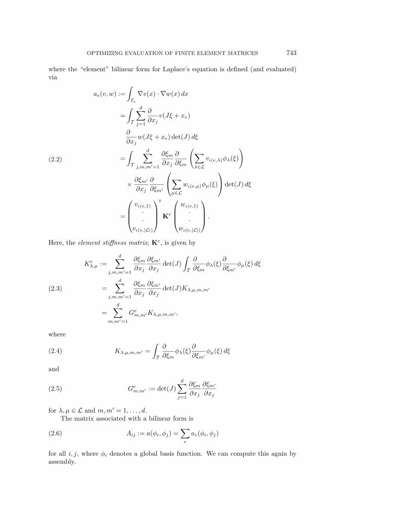
where the “element” bilinear form for Laplace’s equation is defined (and evaluated)via

ae(v, w) :=

∫Te

∇v(x) · ∇w(x) dx

=

∫T

d∑j=1

∂

∂xjv(Jξ + xe)

∂

∂xjw(Jξ + xe) det(J) dξ

=

∫T

d∑j,m,m′=1

∂ξm∂xj

∂

∂ξm

(∑λ∈L

vι(e,λ)φλ(ξ)

)

× ∂ξm′

∂xj

∂

∂ξm′

⎛⎝∑μ∈L

wι(e,μ)φμ(ξ)

⎞⎠det(J) dξ

=

⎛⎜⎜⎝vι(e,1)

··

vι(e,|L|)

⎞⎟⎟⎠t

Ke

⎛⎜⎜⎝wι(e,1)

··

wι(e,|L|)

⎞⎟⎟⎠ .

(2.2)

Here, the element stiffness matrix, Ke, is given by

Keλ,μ :=

d∑j,m,m′=1

∂ξm∂xj

∂ξm′

∂xjdet(J)

∫T

∂

∂ξmφλ(ξ)

∂

∂ξm′φμ(ξ) dξ

=

d∑j,m,m′=1

∂ξm∂xj

∂ξm′

∂xjdet(J)Kλ,μ,m,m′

=

d∑m,m′=1

Gem,m′Kλ,μ,m,m′ ,

(2.3)

where

Kλ,μ,m,m′ =

∫T

∂

∂ξmφλ(ξ)

∂

∂ξm′φμ(ξ) dξ(2.4)

and

Gem,m′ := det(J)

d∑j=1

∂ξm∂xj

∂ξm′

∂xj(2.5)

for λ, μ ∈ L and m,m′ = 1, . . . , d.The matrix associated with a bilinear form is

Aij := a(φi, φj) =∑e

ae(φi, φj)(2.6)

for all i, j, where φi denotes a global basis function. We can compute this again byassembly.


First, set all the entries of A to zero. Then loop over all elements e and localelement numbers λ and μ and compute

Aι(e,λ),ι(e,μ)+ = Keλ,μ =

∑m,m′

Gem,m′Kλ,μ,m,m′ ,(2.7)

where Gem,m′ are defined in (2.5). One can imagine trying to optimize the computation

of each

Keλ,μ =

∑m,m′

Gem,m′Kλ,μ,m,m′ ,(2.8)

but each such term must be computed separately. We consider this optimization insection 3.

3. Computing the Laplacian stiffness matrix with general elements.The tensor Kλ,μ,m,n can be presented as an |L| × |L| matrix of d × d matrices, aspresented in Table 3.1 for the case of quadratics in two dimension. The entries ofresulting matrix Ke can be viewed as the dot (or Frobenius) product of the entries ofK and Ge. That is,

Keλ,μ = Kλ,μ : Ge.(3.1)

The key point is that certain dependencies among the entries of K can be used tosignificantly reduce the complexity of building each Ke. For example, the four 2 × 2matrices in the upper-left corner of Table 3.1 have only one nonzero entry, and sixothers in K are zero. There are significant redundancies among the rest. For example,K3,1 = −4K4,1, so once K4,1 : Ge is computed, K3,1 : Ge may be computed by onlyone additional operation.

By taking advantage of these simplifications, we see that each Ke for quadraticsin two dimensions can be computed with at most 18 floating point operations (see sec-tion 3.2) instead of 288 floating point operations using the straightforward definition,an improvement of a factor of 16 in computational complexity.

The tensor Kλ,μ,m,n for the case of linears in three dimensions is presented inTable 3.2. Each Ke can be computed by computing the three row sums of Ge, thethree column sums, and the sum of one of these sums. We also have to negate all ofthe column and row sums, leading to a total of 20 floating point operations insteadof 288 floating point operations using the straightforward definition, an improvementof a factor of nearly 15 in computational complexity. Using symmetry of Ge (rowsums equal column sums) we can reduce the computation to only 10 floating pointoperations, leading to an improvement of nearly 29.

We leave it as an exercise to work out the reductions in computation that can bedone for the case of linears in two dimensions.

3.1. Algorithms for determining reductions. Obtaining reductions in com-putation can be done systematically as follows. It may be useful to work in rationalarithmetic and keep track of whether terms are exactly zero and determine commondivisors. However, floating point representations may be sufficient in many cases. Wecan start by noting which submatrices are zero, which ones have only one nonzeroelement, and so forth. Next, we find arithmetic relationships among the submatrices,as follows.

Determining whether

Kλ,μ = cKλ′,mu′(3.2)


Table 3.1

The tensor K for quadratics represented as a matrix of 2 × 2 matrices.

3 0 0 -1 1 1 -4 -4 0 4 0 00 0 0 0 0 0 0 0 0 0 0 00 0 0 0 0 0 0 0 0 0 0 0-1 0 0 3 1 1 0 0 4 0 -4 -41 0 0 1 3 3 -4 0 0 0 0 -41 0 0 1 3 3 -4 0 0 0 0 -4-4 0 0 0 -4 -4 8 4 0 -4 0 4-4 0 0 0 0 0 4 8 -4 -8 4 00 0 0 4 0 0 0 -4 8 4 -8 -44 0 0 0 0 0 -4 -8 4 8 -4 00 0 0 -4 0 0 0 4 -8 -4 8 40 0 0 -4 -4 -4 4 0 -4 0 4 8

Table 3.2

The tensor K (multiplied by four) for piecewise linears in three dimensions represented as amatrix of 3 × 3 matrices.

1 0 0 0 1 0 0 0 1 -1 -1 -10 0 0 0 0 0 0 0 0 0 0 00 0 0 0 0 0 0 0 0 0 0 00 0 0 0 0 0 0 0 0 0 0 01 0 0 0 1 0 0 0 1 -1 -1 -10 0 0 0 0 0 0 0 0 0 0 00 0 0 0 0 0 0 0 0 0 0 00 0 0 0 0 0 0 0 0 0 0 01 0 0 0 1 0 0 0 1 -1 -1 -1-1 0 0 0 -1 0 0 0 -1 1 1 1-1 0 0 0 -1 0 0 0 -1 1 1 1-1 0 0 0 -1 0 0 0 -1 1 1 1

requires just simple linear algebra. We think of these as vectors in d2-dimensionalspace and just compute the angle between the vectors. If this angle is zero, then (3.2)holds. Again, if we assume that we are working in rational arithmetic, then c couldbe determined as a rational number.

Similarly, a third vector can be written in terms of two others by considering itsprojection on the first two. That is,

Kλ,μ = c1Kλ1,μ1 + c2Kλ2,μ2(3.3)

if and only if the projection of Kλ,μ onto the plane spanned by Kλ1,μ1 and Kλ2,μ2 isequal to Kλ,μ.

Higher-order relationships can be determined similarly by linear algebra as well.Note that any d2 + 1 entries Kλ,μ will be linearly dependent, since they are in d2-dimensional space. Thus we might only expect lower-order dependencies to be usefulin reducing the computational complexity.

We can then form graphs that represent the computation of Ke in (3.1). Thegraphs have d2 nodes representing Ge as inputs and |L| × |L| nodes representingthe entries of Ke as outputs. Internal edges and nodes represent computations andtemporary storage. The inputs to a given computation come directly from Ge orindirectly from other internal nodes in the graph.

The computation represented in (2.7) would correspond to a dense graph in whicheach of the input nodes is connected directly to all |L| × |L| output nodes. It will bepossible to attempt to reduce the complexity of the computation by finding sparse


graphs that represent equivalent computations.We can generate interesting graphs by analyzing the entries of Kλ,μ for relation-

ships as described above. It would appear useful to consider• entries Kλ,μ which have only one nonzero element,• entries Kλ,μ which have 2 ≤ k � d2 nonzero elements,• entries Kλ,μ which are scalar multiples of other elements,• entries Kλ,μ which are linear combinations of other elements,

and so forth. For each graph representing the computation of Ke, we have a precisecount of the number of floating point operations, and we can simply minimize thetotal number over all graphs generated by the above heuristics. Our examples indicatethat computational simplifications consisting of an order of magnitude or more canbe achieved.

We have developed a code called FErari (Finite Element ReARrangements ofIntegrals or Finite Element Rearrangement to Automatically Reduce Instructions) tocarry out such optimizations automatically. We describe this in detail in section 4.3.This code linearizes the graph representation discussed above, taking a particularevaluation path that is based on heuristics chosen to approximate optimal evaluation.We have used it to show that for classes of elements, significant improvements incomputational efficiency are available.

3.2. Computing K for quadratics. Here we give a detailed algorithm forcomputing K for quadratics. Thus we have

6 ∗Ke =

⎛⎜⎜⎜⎜⎜⎜⎝3G11 −G12 γ11 γ0 4G12 0−G21 3G22 γ22 0 4G21 γ1

γ11 γ22 3(γ11 + γ22) γ0 0 γ1

γ0 0 γ0 γ2 −γ3 − 8G22 γ3

4G21 4G12 0 −γ3 − 8G22 γ2 −γ3 − 8G11

0 γ1 γ1 γ3 −γ3 − 8G11 γ2

⎞⎟⎟⎟⎟⎟⎟⎠,

(3.4)

where the Gij ’s are the inputs and the intermediate quantities γi are defined andcomputed from

γ0 = − 4γ11,

γ1 = − 4γ22,

γ2 =4G1221 + 8G1122 = γ3 + 8γ12 = 8(G12 + γ12),

γ3 =4G1221 = 4γ21 = 8G12,

(3.5)

where we use the notation Gijk� := Gij + Gk�, and finally, the γij ’s are(γ11 = G11 + G12 = G1112 γ12 = G11 + G22 = G1122

γ21 = G12 + G21 = G1221 γ22 = G12 + G22 = G1222

).(3.6)

Let us distinguish different types of operations. The above formulas involve (a)negation, (b) multiplication of integers and floating point numbers, and (c) additionsof floating point numbers. Since the order of addition is arbitrary, we may assumethat the operations (c) are commutative (although changing the order of evaluationmay change the result). Thus we have G1222 = G2212 and so forth. The symmetry ofG implies that G1112 = G1121 and G2122 = G1222. The symmetry of G implies thatKe is also symmetric, by inspection, as it must be from the definition.


The computation of the entries of Ke proceeds as follows. The computations in(3.6) are done first and require only four (c) operations, or three (c) operations andone (b) operation (γ21 = 2G12). Next, the γi’s are computed via (3.5), requiring four(b) operations and one (c) operation. Finally, the matrix Ke is completed, via three(a) operations, seven (b) operations, and three (c) operations. This makes a total ofthree (a) operations, twelve (b) operations, and three (c) operations. Thus only 18operations are required to evaluate Ke, compared with 288 operations via the formula(2.8).

It is clear that there may be other algorithms with the same amount of work(or less) since there are many ways to decompose some of the submatrices in termsof others. Finding (or proving) the absolute minimum may be difficult. Moreover,the metric for minimization should be run time, not some arbitrary way of countingoperations. Thus the right way to utilize the ideas we are presenting may be toidentify sets of ways to evaluate finite element matrices. These could then be testedon different systems (architectures plus compilers) to see which is the best. It isamusing that it takes fewer operations to compute Ke than it does to write it down,so it may be that memory traffic should be considered in an optimization algorithmthat seems to be the most efficient algorithm.

4. Evaluation of general multilinear forms. General multilinear forms canappear in finite element calculations. As an example of a trilinear form, we considerthat arising from the first-order term in the Navier–Stokes equations. Though ad-ditional issues arise over bilinear forms, many techniques carry over to give efficientalgorithms.

The local version of the form is defined by

ce(u;v,w) :=

∫Te

u · ∇v(x) · w(x) dx

=

∫Te

d∑j,k=1

uj(x)∂

∂xjvk(x)wk(x) dx

=

∫T

d∑j,k=1

uj(Jξ + xe)∂

∂xjvk(Jξ + xe)wk(Jξ + xe) det(J) dξ

=

∫T

d∑j,k,m=1

(∑λ∈L

uι(e,λ)j φλ(ξ)

)∂ξm∂xj

⎛⎝∑μ∈L

vι(e,μ)k

∂

∂ξmφμ(ξ)

⎞⎠

×

⎛⎝∑ρ∈L

wι(e,ρ)k φρ(ξ)

⎞⎠det(J) dξ

=d∑

j,k,m=1

∑λ,μ,ρ∈L

uι(e,λ)j

∂ξm∂xj

vι(e,μ)k w

ι(e,ρ)k det(J)

×∫Tφλ(ξ)

∂

∂ξmφμ(ξ)φρ(ξ) dξ.

(4.1)


Thus we have found that

ce(u,v,w) =

d∑j,k=1

∑λ,μ,ρ∈L

uι(e,λ)j v

ι(e,μ)k w

ι(e,ρ)k

×d∑

m=1

∂ξm∂xj

det(J)

∫Tφλ(ξ)

∂

∂ξmφμ(ξ)φρ(ξ) dξ

=

d∑j,k=1

∑λ,μ,ρ∈L

uι(e,λ)j v

ι(e,μ)k w

ι(e,ρ)k

d∑m=1

∂ξm∂xj

det(J)Nλ,μ,ρ,m,

(4.2)

where

Nλ,μ,ρ,m :=

∫Tφλ(ξ)

∂

∂ξmφμ(ξ)φρ(ξ) dξ.(4.3)

To summarize, we have

ce(u,v,w) =

d∑j,k=1

∑λ,μ,ρ∈L

uι(e,λ)j v

ι(e,μ)k w

ι(e,ρ)k Ne

λ,μ,ρ,j

=

d∑k=1

∑μ,ρ∈L

vι(e,μ)k w

ι(e,ρ)k

d∑j=1

∑λ∈L

uι(e,λ)j Ne

λ,μ,ρ,j ,

(4.4)

where the element coefficients Neλ,μ,ρ,j are defined by

Neλ,μ,ρ,j :=

d∑m=1

∂ξm∂xj

det(J)Nλ,μ,ρ,m. =:

d∑m=1

GmjNλ,μ,ρ,m,(4.5)

where Gmj := ∂ξm∂xj

det(J). Recall that J is the Jacobian above, and J−1 is its inverse,

and (J−1

)m,j

=∂ξm∂xj

.

Note that both Nλ,μ,ρ,(·) and Neλ,μ,ρ,(·) can be thought of as d-vectors. Moreover

Neλ,μ,ρ,(·) = det(J)Nλ,μ,ρ,(·)J

−1.

Also note that Nλ,μ,ρ,(·) = Nρ,μ,λ,(·), so that considerable storage reduction could bemade if desired.

The matrix C defined by Cij = c(u, φi, φj) can be computed using the assemblyalgorithm as follows. First, note that C can be written as a matrix of dimension|L| × |L| with entries that are d× d diagonal blocks. In particular, let Id denote thed × d identity matrix. Now set C to zero, loop over all elements, and update thematrix by

Cι(e,μ),ι(e,ρ)+ =Id

d∑j=1

∑λ∈L

uι(e,λ)j Ne

λ,μ,ρ,j

=Id

d∑m,j=1

Gmj

(∑λ∈L

uι(e,λ)j Nλ,μ,ρ,m

)=Id

∑m,λ∈L

γmλNλ,μ,ρ,m

(4.6)


for all μ and ρ, where

γmλ =

d∑j=1

Gmjuι(e,λ)j .(4.7)

It thus appears that the computation of C can be viewed as similar in form to (3.1),and similar optimization techniques applied. In fact, we can introduce the notationKe,u, where

Ke,uμ,ρ =

∑m,λ∈L

γmλNλ,μ,ρ,m.(4.8)

Then the update of C is done in the obvious way with Ke,u.

4.1. Trilinear forms with piecewise linears. For simplicity, we may considerthe piecewise linear case. Here, the standard mixed formulations are not inf-sup stable,but the trilinear form is still an essential part of the well-known family of stabilizedmethods [8, 11] that do admit equal-order piecewise linear discretizations. Moreover,our techniques could as well be used with the nonconforming linear element [6], whichdoes admit an inf-sup condition when paired with piecewise constant pressures.

In the piecewise linear case, (4.3) simplifies to

Nλ,μ,ρ,m :=∂φμ

∂ξm

∫Tφλ(ξ)φρ(ξ) dξ.(4.9)

We can think of Nλ,μ,ρ,m defined from two matrices Nλ,μ,ρ,m = Dμ,mFλ,ρ, where

Dμ,m :=∂φμ

∂ξm=

⎛⎝1 00 11 1

⎞⎠ (d = 2) and

⎛⎜⎜⎝1 0 00 1 00 0 11 1 1

⎞⎟⎟⎠ (d = 3)(4.10)

and

Fλ,ρ :=

∫Tφλ(ξ)φρ(ξ) dξ.(4.11)

The latter matrix is easy to determine. In the piecewise linear case, we can computeintegrals of products using the quadrature rule that is based on edge midpoints (withequal weights given by the area of the simplex divided by the number of edges). Thusthe weights are ω = 1/6 for d = 2 and ω = 1/24 for d = 3. Each of the values φλ(ξ)is either 1

2 or zero, and the products are equal to 14 or zero. For the diagonal terms

λ = ρ, the product is nonzero on d edges, so Fλ,λ = 1/12 for d = 2 and 1/32 ford = 3. If λ �= ρ, then the product φλ(ξ)φρ(ξ) is nonzero for exactly one edge (the oneconnecting the corresponding vertices), so Fλ,ρ = 1/24 for d = 2 and 1/96 for d = 3.Thus we can describe the matrices F in general as having d on the diagonals, 1 onthe off-diagonals, and scaled by 1/24 for d = 2 and 1/96 for d = 3. Thus

F =1

4(d + 1)!

⎛⎜⎜⎝d 1 · · · 11 d · · · 1· · · · · ·1 1 · · · d

⎞⎟⎟⎠

=d− 1

4(d + 1)!Id+1 +

1

4(d + 1)!

⎛⎜⎜⎝1 1 · · · 11 1 · · · 1· · · · · ·1 1 · · · 1

⎞⎟⎟⎠(4.12)


Table 4.1

The tensor N (multiplied by 96) for piecewise linears in three dimensions represented as amatrix of 4 × 3 matrices.

3 1 1 1 0 0 0 0 0 0 0 0 3 1 1 10 0 0 0 3 1 1 1 0 0 0 0 3 1 1 10 0 0 0 0 0 0 0 3 1 1 1 3 1 1 11 3 1 1 0 0 0 0 0 0 0 0 1 3 1 10 0 0 0 1 3 1 1 0 0 0 0 1 3 1 10 0 0 0 0 0 0 0 1 3 1 1 1 3 1 11 1 3 1 0 0 0 0 0 0 0 0 1 1 3 10 0 0 0 1 1 3 1 0 0 0 0 1 1 3 10 0 0 0 0 0 0 0 1 1 3 1 1 1 3 11 1 1 3 0 0 0 0 0 0 0 0 1 1 1 30 0 0 0 1 1 1 3 0 0 0 0 1 1 1 30 0 0 0 0 0 0 0 1 1 1 3 1 1 1 3

for d = 2 or 3, where Id denotes the d × d identity matrix. Note that for a given d,the matrices in (4.12) are d + 1 × d + 1 in dimension.

The tensor N for linears in three dimensions is presented in Table 4.1. We seenow a new ingredient for computing the entries of Ke,u from the matrix γm,λ. Define

γm =∑4

λ=1 γm,λ for m = 1, 2, 3, and then γm,λ = 2γm,λ + γm for m = 1, 2, 3 andλ = 1, 2, 3, 4. Then

Ke,u =

⎛⎜⎜⎝γ11 γ21 γ31 γ11 + γ21 + γ31

γ12 γ22 γ32 γ12 + γ22 + γ32

γ13 γ23 γ33 γ13 + γ23 + γ33

γ14 γ24 γ34 γ14 + γ24 + γ34

⎞⎟⎟⎠.(4.13)

However, note that the γm’s are not computations that would have appeared directlyin the formulation of Ke,u but are intermediary terms that we have defined for con-venience and efficiency. This requires 39 operations, instead of 384 operations using(4.8).

4.2. Algorithmic implications. The example in section 4 provides guidancefor the general case. First of all, we see that the “vector” space of the evaluationproblem (4.8) can be arbitrary in size. In the case of the trilinear form in Navier–Stokes equations considered there, the dimension is the spatial dimension times thedimension of the approximation (finite element) space. High-order finite elementapproximations [14] could lead to very high-dimensional problems. Thus we need tothink about looking for a relationship among the “computational vectors” in high-dimensional spaces, e.g., up to several hundred in extreme cases. The example insection 4.1 is the lowest order case in three space dimensions, and it requires a twelve-dimensional space for the complexity analysis.

Second, it will not be sufficient just to look for simple combinations to deter-mine optimal algorithms, as discussed in section 3.1. The example in section 4.1shows that we need to think of this as an approximation problem. We need to lookfor vectors (matrices) which closely approximate a set of vectors that we need tocompute. The vectors V1 = (1, 1, 1, 1, 0, . . . , 0), V2 = (0, 0, 0, 0, 1, 1, 1, 1, 0, 0, 0, 0),V3 = (0, . . . , 0, 1, 1, 1, 1) are each edit-distance one from four vectors we need to com-pute. The quantities γm represent the computations (dot-product) with Vm. Thequantities γmλ are simple perturbations of γ which require only two operations toevaluate. A simple rescaling can reduce this to one operation.


Table 4.2

Summary of results for FErari on triangular Lagrange elements.

Order Entries Base MAPs FErari MAPs1 6 24 72 21 84 153 55 220 454 120 480 1765 231 924 4436 406 1624 867

Edit distance is a useful measure for approximating the computational complexitydistance, since it provides an upper-bound on the number of computations it takes toget from one vector to another. Thus we need to add this type of optimization to thetechniques listed in section 3.1.

4.3. The FErari system. The algorithms discussed in sections 3.1 and 4.2 havebeen implemented in a prototype system which we call FErari (Finite Element ReAR-rangements of Integrals or Finite Element Rearrangement to Automatically ReduceInstructions). We have used it to build optimized code for the local stiffness matricesfor the Laplace operator using Lagrange polynomials of up to degree six. While thereis no perfect metric to predict efficiency of implementations due to differences in ar-chitecture, we have taken a simple model to measure improvement due to FErari. Aparticular algorithm could be tuned by hand, common divisors in rational arithmeticcould be sought, and more care could be taken to order the operations to maximizeregister usage. Before discussing the implementation of FErari more precisely, wepoint to Table 4.2 to see the levels of optimization detected. In the table, “Entries”refers to the number of entries in the upper triangle of the (symmetric) matrix. “BaseMAPs” refers to the number of multiply-add pairs if we were not to detect dependen-cies at all, and “FErari MAPs” is the number of multiply-add pairs in the generatedalgorithm. Although we gain only about a factor of two for the higher-order cases, weare automatically generating algorithms with fewer multiply-add pairs than entriesfor linears, quadratics, and cubics.

FErari builds a graph of dependencies among the tensors Kλ,μ in several stages.We now describe each of these stages, what reductions they produce in assemblingKe, and how much they cost to perform. We start by building the tensors {Kλ,μ}for 1 ≤ λ ≤ dimPk and λ ≤ μ ≤ dimPk using FIAT (FInite element AutomaticTabulator) [15]. In discussing algorithmic complexity of our heuristics below, we shalllet n be the size of this set. Throughout, we are typically using “greedy” algorithmsthat quit when they find a dependency. Also, the order in which these stages areperformed matters, as if a dependency for a tensor found at one stage, will not markit again later.

As we saw earlier, sometimes Kλ,μ = 0. In this case, (Ke)λ,μ = 0 as well for anye, so these entries cost nothing to build. Searching for uniformly zero tensors can bedone in n operations. While we found that three tensors vanish for quadratics andcubics, none do for degrees four through six.


Table 4.3

Results of FErari on Lagrange elements of degrees 1 through 6.

Order Entries Zero Eq Eq t 1 Entry Col Ed1 Ed2 LC Default Cost1 6 0 0 0 3 0 2 0 1 0 72 21 3 2 3 4 2 5 1 1 0 153 55 3 17 0 5 8 12 5 5 0 454 120 0 23 0 7 2 25 30 25 8 1765 231 0 18 0 13 5 41 71 45 38 4436 406 0 27 0 17 7 59 139 61 96 867

Next, if two tensors Kλ,μ and Kλ′,μ′ are equal, then their dot product into Ge willalso be equal. So, we mark Kλ′,μ′ as depending on Kλ,μ. Naively, searching throughthe nonzero tensors is an O(n2) process, but can be reduced to O(n log(n)) operationsby inserting the tensors into a binary tree using lexicographic ordering of the entriesof the tensors. The fourth column of Table 4.3 titled “Eq” shows the number of suchdependencies that FErari found.

As a variation on this theme, if Kλ,μ = (Kλ′,μ′)t, then Kλ,μ : Ge = (Kλ′,μ′ : Ge)since Ge is symmetric. Hence, once (Ke)λ,μ is computed, (Ke)λ′,μ′ is free. We mayalso search for these dependencies among nonzero tensors that are not already markedas equal to another tensor in O(n log(n)) time by building a binary tree. In thiscase, we compare by lexicographically ordering the components of the symmetric partof each tensor (recall the symmetric part of K is K+Kt

2 ). Equality of symmetric partsis necessary but not sufficient for two matrices to be transposes of each other. So, if ourinsertion into the binary tree reveals an entry with the same symmetric part, we thenperform an additional check to see if the two are indeed transposes. Unfortunately, wefound such dependencies only for quadratics, where we found three. This is indicatedin the fifth column of Table 4.3, titled “Eq t.”

So far, we have focused on finding and marking tensors that can be dotted into Ge

with no work (perhaps once some other dot product has been performed). Now, weturn to ways of finding tensors whose dot product with Ge can be computed cheaply.The first such way is to find unmarked tensors Kλ,μ with only one nonzero entry.This may be trivially performed in O(n) time. The sixth column of Table 4.3, titled“1 Entry,” shows the number of such tensors for each polynomial degree.

If there is a constant α such that Kλ′,μ′ = αKλ,μ, then Kλ′,μ′ : Ge = αKλ,μ : Ge

and hence may be computed in a single multiply. Moreover, colinearity among theremaining tensors may be found in O(n log(n)) time by a binary tree and lexicographicordering of an appropriate normalization. To this end, we divide each (nonzero) tensorby its Frobenius norm and ensure that its first nonzero entry is positive. If insertioninto the binary tree gives equality under this comparison, then we mark the tensorsas colinear. The numbers of such dependencies found for each degree is seen in the“Col” column of Table 4.3.

Next, we seek tensors that are close together in edit distance, differing only inone or two entries. Then, the difference between the dot products can be computedcheaply. For each unmarked tensor, we look for a marked tensor that is edit-distanceone away. We iterate this process until no more dependencies are found, then searchfor dependencies among the remainders. We repeat this process for things that areedit-distance two apart. In general, this process seems to be O(n2). Table 4.3 hastwo columns, titled “Ed1” and “Ed2,” showing the number of tensors we were ableto mark in such a way.


from Numeric import zeros

G=zeros(4,"d")

def K(K,jinv):

detinv = 1.0/(jinv[0,0]*jinv[1,1] - jinv[0,1]*jinv[1,0])

G[0] = ( jinv[0,0]**2 + jinv[1,0]**2 ) * detinv

G[1] = ( jinv[0,0]*jinv[0,1]+jinv[1,0]*jinv[1,1] ) * detinv

G[2] = G[1]

G[3] = ( jinv[0,1]**2 + jinv[1,1]**2 ) * detinv

K[1,1] = 0.5 * G[0]

K[1,0] = -0.5 * G[1]- K[1,1]

K[2,1] = 0.5 * G[2]

K[2,0] = -0.5 * G[3]- K[2,1]

K[0,0] = -1.0 * K[1,0] + -1.0 * K[2,0]

K[2,2] = 0.5 * G[3]

K[0,1] = K[1,0]

K[0,2] = K[2,0]

K[1,2] = K[2,1]

return K

Fig. 4.1. Generated code for computing the stiffness matrix for linear basis functions.

If a tensor is a linear combination of two other tensors, then its dot product can becomputed in two multiply-add pairs. This is an expensive search to perform (O(n3)),since we have to search through pairs of tensors for each unmarked tensor. However,we do seem to find quite a few linear combinations, as seen in the “LC” column ofTable 4.3. Any remaining tensors are marked as “Default” in which case they arecomputed by the standard four multiply-add pairs.

After building the graph of dependencies, we topologically sort the vertices. Thisgives an ordering for which, if vertex u depends on vertex v, then v occurs before u,an essential feature for generating code. We currently generate Python code for easein debugging and integrating with the rest of our computational system, but we couldjust as easily generate C or Fortran. In fact, in the future we hope to generate notonly particular code, but abstract syntax as in PETSc 3.0.

One interesting feature of the generated code is that it is completely unrolled—noloops are done. This leads to relatively large functions, but sets up the code to a pointwhere the compiler really only needs to handle register allocation. In Figure 4.1, wepresent the generated code for computing linears.

4.4. Code verification. In general,the question of verifying a code’s correct-ness is difficult. In this case, we have taken an existing Poisson solver and replacedthe function to evaluate the local stiffness matrix with FErari-generated code. Thecorrect convergence rates are still observed, and the stiffness matrices and computedsolutions agree to machine precision. However, in the future, we hope to generateoptimized code for new, complicated forms where we do not have an existing verifiedimplementation, and the general question of verifying such codes is beyond the scopeof this present work.

5. Computing a matrix via quadrature. The computations in equations(2.6)–(2.7) can be computed via quadrature as


Aι(e,λ),ι(e,μ)+ =∑ξ∈Ξ

ωξ∇φλ(ξ) · (Ge∇φμ(ξ))

=∑ξ∈Ξ

ωξ

d∑m,n=1

φλ,m(ξ)Gem,nφμ,n(ξ)

=

d∑m,n=1

Gem,n

∑ξ∈Ξ

ωξφλ,m(ξ)φμ,n(ξ)

=

d∑m,n=1

Gem,nKλ,μ,m,n,

(5.1)

where the coefficients Kλ,μ,m,n are analogous to those defined in (2.3), but here theyare defined by quadrature:

Kλ,μ,m,n =∑ξ∈Ξ

ωξφλ,m(ξ)φμ,n(ξ).(5.2)

(The coefficients are exactly those of (2.3) if the quadrature is exact.)The right strategy for computing a matrix via quadrature would thus appear to be

to compute the coefficients Kλ,μ,m,n first using (5.2), and then proceeding as before.However, there is a different strategy associated with quadrature when we want onlyto compute the action of the linear operator associated with the matrix and not thematrix itself (cf. [16]).

6. Other approaches. We have presented one approach to optimize the compu-tation of finite element matrices. Other approaches have been suggested for optimizingcode for scientific computation. The problem that we are solving can be representedas a sparse-matrix-times-full-matrix multiply, KG, where the dimensions of K are,for example, |L|2 × d2 for Laplace’s equation in d dimensions using a (local) finiteelement space L. For the nonlinear term in Navier–Stokes equations, the dimensionsof K become |L|2 × d|L|. The first dimension of G of course matches the second of K,but the second dimension of G is equal to the number of elements in the mesh. Thusit is worthwhile to do significant precomputation on K.

At a low level, ATLAS [26] works with operations such as loop unrolling, cacheblocking, etc. This type of optimization would not find the reductions in computationthat FErari does, since the latter identifies more complex algebraic structures. In thissense, our work is more closely aligned with that of FLAME [7] which works withoperations such as rank updates, triangular solves, etc. The BeBOP group has alsoworked on related issues in sparse matrix computation [22, 24, 23, 25, 12]. Our workcould be described as utilizing a sparsity structure in a matrix representation, andit can be written as multiplying a sparse matrix times a very large set of (relativelysmall) vectors (the columns of G). This is the reverse of the case considered in theSPARSITY system [13], where multiplying a sparse matrix times a small number oflarge vectors is considered.

Clearly the ideas we present here could be coupled with these approaches togenerate improved code. The novelty of our work resides in the precomputation thatis applied to evaluate the action of K. In this way, it resembles the reorganization ofcomputation done for evaluation of polynomials or matrix multiply [17].

7. Timing results. We performed several experiments for the Poisson problemwith piecewise linear and piecewise quadratic elements. We set up a series of meshesusing the mesh library in DOLFIN [10]. These meshes contained between 2048 and


524288 triangles. We timed computation of local stiffness matrices by several tech-niques; inserting them into a sparse PETSc matrix [3], multiplying the matrix ontoa vector, and solving the linear system. All times were observed to be linear in thenumber of triangles, so we report all data as time per million triangles. All computa-tions were performed on a Linux workstation with a 3 GHz Pentium 4 processor with2 GB of RAM. All our code was compiled using gcc with “−O3” optimization.

Our goal is to assess the efficacy and relevance of our proposed optimizations.Solver technology has been steadily improving over the last several decades, withmultigrid and other optimal strategies being found for wider classes of problems.When such efficient solvers are available, the cost of assembling the matrices (bothcomputing local stiffness matrices and inserting them into the global matrix) is muchmore important. This is especially true in geometric multigrid methods in whicha stiffness matrix can be built on each of a sequence of nested meshes, but only afew iterations are required for convergence. To factor out the choice of solver, weconcentrate first on the relative costs of building local stiffness matrices, insertingthem into the global matrix, and applying the matrix to a vector.

We used four strategies for computing the local stiffness matrices: numericalquadrature, tensor contractions (four flops per entry), tensor contractions with zerosomitted (this code was generated by the FEniCS form compiler [19]), and the FErari-optimized code translated into C. For both linear and quadratic elements, the costof building all of the local stiffness matrices and inserting them into the global sparsematrix was comparable (after storage had been preallocated). In both situations,computing the matrix-vector product is an order of magnitude faster than computingthe local matrices and inserting them into the global matrix. These costs, all measuredas seconds to process one million triangles, are given in Table 7.1 and plotted inFigure 7.1 using log scale for time.

We may draw several conclusions from this. First, precomputing the referencetensors leads to a large performance gain over numerical quadrature. Beyond this,additional benefits are included by omitting the zeros, and more still by doing theFErari optimizations. We seem to have optimized the local computation to the pointwhere it is constrained by read-write to cache rather than by floating point optimiza-tion. Second, these optimizations reveal a new bottleneck: matrix insertion. Thismotivates either studying whether we may improve the performance of insertion intothe global sparse matrix or else implementing matrix-free methods.

While the FErari optimizations are highly successful for building the matrices,there is still quite a bit of solver overhead to contend with. We used GMRES (bound-ary conditions were imposed in a way that broke symmetry) preconditioned by theBoomerAMG method of HYPRE [9]. For both linear and quadratic elements, theKrylov solver converged with only three iterations. However, the cost of buildingand applying the AMG preconditioner is very large. Using numerical quadrature,building local stiffness matrices accounted for between five and nine percent of thetotal run time (building the local-to-global mapping, computing geometry tensors,computing local stiffness matrices, sorting and inserting local matrices into the globalmatrix, creating and applying the AMG preconditioner, and computing the Kryloviterations). Keeping everything else constant and switching to the FErari optimizedcode, building local stiffness matrices took less than one percent of the total time.Geometric multigrid algorithms tend to be much more efficient, and we conjecturethat the cost of building local matrices would be even more important in this case.


Table 7.1

Seconds to process one million triangles: local stiffness matrices, global matrix insertion, andmatrix-vector product.

Quadrature Tensor FFC FErari Assemble MatvecLinear 0.3802 0.0725 0.0535 0.0513 0.4762 0.0177

Quadratic 2.0000 0.3367 0.1517 0.1506 1.9342 0.1035

Quadrature

Tensor

FFC

FErari

Insertion

Matvec

0.0100

0.1000

1.0000

10.0000

Time (s)

Seconds per million triangles

Linear

Quadratic

Fig. 7.1. Seconds to process one million triangles: local stiffness matrices, global matrix inser-tion, and matrix-vector product.

8. Conclusions. The determination of local element matrices involves a novelproblem in computational complexity. There is a mapping from (small) geometrymatrices to “difference stencils” that must be computed. We have demonstrated thepotential speed-up available with simple low-order methods. We have suggested byexamples that it may be possible to automate this to some degree by solving abstractgraph optimization problems.

Acknowledgments. We thank the FEniCS team, and Todd Dupont, JohanHoffman, and Claes Johnson in particular, for substantial suggestions regarding thispaper.

REFERENCES

[1] A. A. Albrecht, P. Gottschling, and U. Naumann, Markowitz-type heuristics for computingJacobian matrices efficiently, in International Conference on Computational Science, PartII, Lecture Notes in Comput. Sci. 265 Springer, Berlin, 2003, pp. 575–584.

[2] D. N. Arnold, D. Boffi, and R. S. Falk, Quadrilateral H(div) finite elements, SIAM J.Numer. Anal., 42 (2005), pp. 2429–2491.


[3] S. Balay, K. Buschelman, V. Eijkhout, W. D. Gropp, D. Kaushik, M. G. Knepley, L. C.

McInnes, B. F. Smith, and H. Zhang, PETSc Users Manual, Tech. Report ANL-95/11,Revision 2.1.5, Argonne National Laboratory, Argonne, IL, 2004.

[4] S. C. Brenner and L. R. Scott, The Mathematical Theory of Finite Element Methods, 2nded., Springer-Verlag, New York, 2002.

[5] K. A. Cliffe and S. J. Tavener, Implementation of extended systems using symbolic algebra,in Continuation Methods in Fluid Dynamics, D. Henry and A. Bergeon, eds., Notes Numer.Fluid Mech. 74, Vieweg, Braunschweig, 2000, pp. 81–92.

[6] M. Crouzeix and P.-A. Raviart, Conforming and nonconforming finite element methods forsolving the stationary Stokes equations. I, Rev. Francaise Automat. Informat. RechercheOperationnelle Ser. Rouge, 7 (1973), pp. 33–75.

[7] J. A. Gunnels, F. G. Gustavson, G. M. Henry, and R. A. van de Geijn, FLAME: Formallinear algebra methods environment, Trans. Math. Software, 27 (2001), pp. 422–455.

[8] P. Hansbo and A. Szepessy, A velocity-pressure streamline diffusion finite element methodfor the incompressible Navier-Stokes equations, Comput. Methods Appl. Mech. Engrg., 84(1990), pp. 175–192.

[9] V. Henson and U. Yang, BoomerAMG: A parallel algebraic multigrid solver and precondi-tioner, Appl. Numer. Math., 41 (2002), pp. 155–177.

[10] J. Hoffman and U. Yang, DOLFIN: Dynamic Object Oriented Library for Finite ElementComputation, Tech. Report 2002-6, Chalmers Finite Element Preprint Series, ChalmersUniversity, Goteborg, Sweden, 2002, http://www.fenics.org/dolfin.

[11] T. J. R. Hughes, L. P. Franca, and M. Balestra, A new finite element formulation forcomputational fluid dynamics. V. Circumventing the Babuska-Brezzi condition: A stablePetrov-Galerkin formulation of the Stokes problem accommodating equal-order interpola-tions, Comput. Methods Appl. Mech. Engrg., 59 (1986), pp. 85–99.

[12] E.-J. Im and K. A. Yelick, Optimizing sparse matrix computations for register reuse in SPAR-SITY, in Proceedings of the International Conference on Computational Science, (SanFrancisco, CA), Lecture Notes in Comput. Sci. 2073, Springer, New York, 2001, pp. 127–136.

[13] E.-J. Im, K. A. Yelick, and R. Vuduc, SPARSITY: Framework for optimizing sparse matrix-vector multiply, Int. J. High Performance Comput. Appl., 18 (2004), pp. 135–158.

[14] H. Juarez, L. R. Scott, R. Metcalfe, and B. Bagheri, Direct simulation of freely rotatingcylinders in viscous flows by high-order finite element methods, Comput. & Fluids, 29(2000), pp. 547–582.

[15] R. C. Kirby, Algorithm 839: FIAT, a new paradigm for computing finite element basis func-tions, ACM Trans. Math. Software, 30 (2004), pp. 502–516.

[16] R. C. Kirby, M. Knepley, and L. Scott, Evaluation of the Action of Finite Element Oper-ators, Tech. report TR-2004-07, Department of Computer Science, University of Chicago,Chicago, IL, 2004.

[17] D. E. Knuth, The Art of Computer Programming, Volume 2: Seminumerical Algorithms, 3rded., Addison-Wesley, Reading, MA, 1997.

[18] Argonne National Laboratory, PETSc-CS Alphan, http://www-unix.mcs.anl.gov/petsc/petsc-3/.

[19] A. Logg, FFC: The FEniCS Form Compiler, http://www.fenics.org/ffc.[20] K. Long, Sundance rapid prototyping tool for parallel PDE optimization, in Large-Scale PDE-

Constrained Optimization, Lecture Notes in Comput. Sci. Engrg. 30, Springer, Berlin, 2003,pp. 331–341.

[21] K. Long, Sundance, 2003, http://csmr.ca.sandia.gov/∼krlong/sundance.html.[22] R. Vuduc, J. Demmel, and J. Bilmes, Statistical models for empirical search-based perfor-

mance tuning, Int. J. High Performance Comput. Appl., 18 (2004), pp. 65–94.[23] R. Vuduc, J. W. Demmel, K. A. Yelick, S. Kamil, R. Nishtala, and B. Lee, Performance

optimizations and bounds for sparse matrix-vector multiply, in Proceedings of Supercom-puting, Baltimore, MD, IEEE, Piscataway, NJ, 2002, pp. 1–35.

[24] R. Vuduc, A. Gyulassy, J. W. Demmel, and K. A. Yelick, Memory hierarchy optimizationsand bounds for sparse ATAx, in Proceedings of the ICCS Workshop on Parallel LinearAlgebra, P. M. A. Sloot, D. Abramson, A. V. Bogdanov, J. J. Dongarra, A. Y. Zomaya,and Y. E. Gorbachev, eds., (Melbourne, Australia), Lecture Notes in Comput. Sci. 2660,Springer, New York, 2003, pp. 705–714.


[25] R. Vuduc, S. Kamil, J. Hsu, R. Nishtala, J. W. Demmel, and K. A. Yelick, Automaticperformance tuning and analysis of sparse triangular solve, presented at the Workshop onPerformance Optimization via High-Level Languages and Libraries, in conjunction with the16th International Conference on Supercomputing (ICS), ACM, New York, 2002. Availableonline at http://www.cs.berkeley.edu/˜richie/research/pubs.html

[26] R. C. Whaley, A. Petitet, and J. J. Dongarra, Automated empirical optimization of soft-ware and the ATLAS project, Parallel Computing, 27 (2001), pp. 3–35. Also available onlineas University of Tennessee LAPACK Working Note 147, UT-CS-00-448 at www.netlib.org/lapack/lawns/downloads.

Optimizing the Evaluation of Finite Element Matrices

Documents

Transcript of Optimizing the Evaluation of Finite Element Matrices