Introduction to Finite-Element-Methods In Electromagnetism
56
Nathan S. Froemming ([email protected]) Northern Illinois University, PHYS 790D Tue 08 Oct 2019 Introduction to Finite-Element-Methods In Electromagnetism
-
Upload
khangminh22 -
Category
Documents
-
view
3 -
download
0
Transcript of Introduction to Finite-Element-Methods In Electromagnetism
Nathan S. Froemming ([email protected])Northern Illinois University, PHYS 790DTue 08 Oct 2019
Introduction to Finite-Element-Methods In Electromagnetism

08 Oct 2019 Nathan S. Froemming | Introduction to Finite-Element Methods in Electromagnetism
Main Goal for Today….
• Be able to understand, setup, and solve basic problems in electrostatics and magnetostatics using finite-element methods, e.g. “Finite Element Method Magnetics” (FEMM), on your local Windows/Linux/Mac computer
�2
(quick real-time example)

08 Oct 2019 Nathan S. Froemming | Introduction to Finite-Element Methods in Electromagnetism
Outline
• Overview LaPlace’s equation and solutions- Cauchy-Riemann equations; Connection to electromagnetism (EM)- Conformal mappings- Shortcomings• Finite-Element methods and codes (OPERA, COMSOL, FEMM, …)• Getting FEMM setup on your local machine• FEMM electric example- Problem setup: Electric dipole/quadrupole- How to extract the potential/E-field from FEMM• FEMM magnetic example (next time)- Problem setup: H-dipole, quadrupole (more challenging)- How to extract the potential/B-field from FEMM• Pro Tips And Tricks (next time)- Scripting in `lua` and `python`; Jupyter notebooks; WebPlotDigitizer; etc.• Conclusions
�3

08 Oct 2019 Nathan S. Froemming | Introduction to Finite-Element Methods in Electromagnetism
• I am Prof. Syphers’ postdoc. I am stationed at Fermilab, and I work closely with Accelerator Division (AD) and the Muon g-2 Experiment (E989)
But first, A Few Quick Words About Me….
�4
Example Finite-Element Field

08 Oct 2019 Nathan S. Froemming | Introduction to Finite-Element Methods in Electromagnetism
• [Accelerator] Physics has many applications elsewhere, e.g. medicine
• The ability to perform high-level data analysis is always sought after!
�5
I’ll Also Try To Talk About The Bigger Picture Along The Way

Date Presenter I Presentation Title �6
Outline
• Overview LaPlace’s equation and solutions- Cauchy-Riemann equations; Connection to electromagnetism (EM)- Conformal mappings- Shortcomings• Finite-Element methods and codes (OPERA, COMSOL, FEMM, …)• Getting FEMM setup on your local machine• FEMM electric example- Problem setup: Electric dipole/quadrupole- How to extract the potential/E-field from FEMM• FEMM magnetic example (next time)- Problem setup: H-dipole, quadrupole (more challenging)- How to extract the potential/B-field from FEMM• Pro Tips And Tricks (next time)- Scripting in `lua` and `python`; Jupyter notebooks; WebPlotDigitizer; etc.• Conclusions
08 Oct 2019 Nathan S. Froemming | Introduction to Finite-Element Methods in Electromagnetism
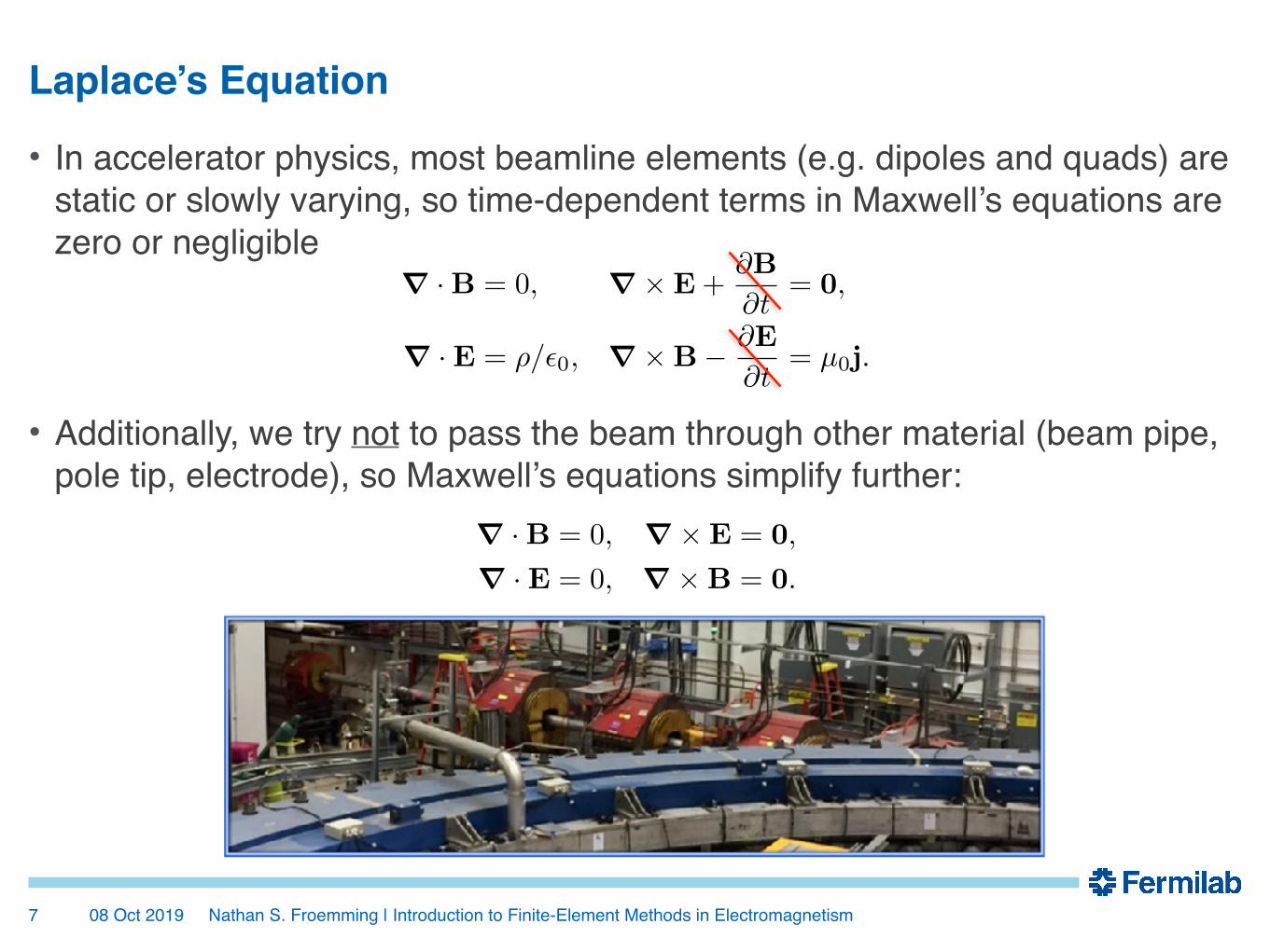
Laplace’s Equation
• In accelerator physics, most beamline elements (e.g. dipoles and quads) are static or slowly varying, so time-dependent terms in Maxwell’s equations are zero or negligible
• Additionally, we try not to pass the beam through other material (beam pipe, pole tip, electrode), so Maxwell’s equations simplify further:
�7
r ·B = 0, r⇥E+@B
@t= 0,
r ·E = ⇢/✏0, r⇥B� @E
@t= µ0j.
<latexit sha1_base64="lZatgnEh6MY1lExicLGHsTdBfFw=">AAADcXicjVLfa9swEFbsbe28X+m2lzE2REPKoFtqpw/rS6FsBPbYwdIWohBk+ZxolSVPkgvB+Hn/3976T+xl/8BkJyVb00IPhE7f6e6++7g4F9zYMLxsef69+w82Nh8Gjx4/efqsvfX8xKhCMxgyJZQ+i6kBwSUMLbcCznINNIsFnMbnn+v46QVow5X8Zuc5jDM6lTzljFoHTbZaP7sBiWHKZQk/igasAiKVLLIY9FWICj6VkFQBdkZiJRIzz9xVEkljQStMWKIsLkmc4k8V3jnE4Xt8q+3cUsPyDMyiyKDCu5ikmrKS5FRbTsVV9WqF2KZVg4eVa0jIXQgOmiyiZwrvYQK54cIpURO+AzE33YcbiQ3WiZGsmISL6PeqFxCQyUrJ5rWSvDtpd8Je2Bhed6Kl00FLO560f5FEsSIDaZmgxoyiMLfjsmbABLgGhYGcsnM6hZFzJXUzjMtmYyrcdUiCU6XdkRY36L8ZJc1MrYL7mVE7M9djNXhTbFTY9GBccpkXFiRbNEoLp4jC9frhhGtgVsydQ5nmjitmM+rktG5JAydCdH3kdeek34v2e/2v/c7RwVKOTfQabaN3KEIf0RH6go7RELHWb++l98Z76/3xX/nY31589VrLnBfoP/N3/wLhNg4i</latexit>
r ·B = 0, r⇥E = 0,
r ·E = 0, r⇥B = 0.<latexit sha1_base64="2+dpAhh0ZybsVKx2R2ykjADYBEg=">AAAC8niclVJNaxQxGM6MH13Hr60evQQXiwdZZtaDvQilUvBYwW0Lm2VJMu9sQzPJmLxTWIb5GV48KOLVX+PNf2N2dtDaKugLIU+e93nzfiSi0spjmn6P4mvXb9zcGtxKbt+5e+/+cPvBkbe1kzCVVlt3IrgHrQxMUaGGk8oBL4WGY3H2au0/PgfnlTVvcVXBvORLowolOQZqsR0NmIClMg28qzuqZcaauhTgkt7DtVoayNuEBmPC6tyvyrA1zHCheUuZzC3ShomC7rd05yVNn1G68xctqhL8RnzQiTuYtiGEsX9JcfA/KfYvphgnDEz+q5/u9LPvxXCUjtPO6FWQ9WBEejtcDL+x3Mq6BINSc+9nWVrhvOEOldQQrq89VFye8SXMAjQ8VDVvuidr6ZPA5LSwLiyDtGMvRjS89Ou+grLkeOov+9bkn3yzGovdeaNMVSMYuUlU1Jqipev3p7lyIFGvAuDSqVArlafccYnhlyRhCNnllq+Co8k4ez6evJmM9nb7cQzII/KYPCUZeUH2yGtySKZERjZ6H32MPsUYf4g/x1820jjqYx6S3yz++gNf3uiL</latexit>

08 Oct 2019 Nathan S. Froemming | Introduction to Finite-Element Methods in Electromagnetism
Laplace’s Equation
• The curl equations imply the field may be derived from a potential,
• The divergence equations then imply Laplace’s equation,
• Also, don’t forget about these 3 copies of Laplace’s equation,
• Laplace’s equation is all over the place! We should spend some time trying to understand how to solve it….
�8
r · {E,B} = r · (�r{Ve, Vm}) = �r2{Ve, Vm} = 0.<latexit sha1_base64="vc3pMI/sd5TMQ+2oeGQUsaZqBuo=">AAACgnicdVHdSsMwFE7r1Dn/pl56ExyCitZ2Cu5CQRTBywluCsssaZpqME1Kkgqj9EF8Le98Gs3mLpybB0I+vh9yck6UcaaN73867lxlfmGxulRbXlldW69vbHa1zBWhHSK5VI8R1pQzQTuGGU4fM0VxGnH6EL1eD/WHN6o0k+LeDDLaT/GzYAkj2FgqrL+jSPJYD1J7FUjgiOMSIhJLA1FRoCiBN+UhHIGrEpXwAv4f2DuaqRXdkB7Cbpiict/mZ5memhM26/K9sN7wPX9UcBoEY9AA42qH9Q8US5KnVBjCsda9wM9Mv8DKMMJpWUO5phkmr/iZ9iwUOKW6X4xGWMJdy8QwkcoeYeCI/Z0ocKqHPVtnis2L/qsNyVlaLzdJq18wkeWGCvLzUJJzaCQc7gPGTFFi+MACTBSzvULyghUmxm6tZocQ/P3yNOg2veDEa96dNi5b43FUwTbYAXsgAGfgEtyCNugAAr6cXcdzjt2Ke+AG7smP1XXGmS0wUe75N9qFwYI=</latexit>
r⇥B = r⇥ (r⇥A) = r(r ·A)�r2A = 0 ) �r2A = 0<latexit sha1_base64="WJ3nuWYPdjvGvCdGK94hIDJneHQ=">AAAC+HicjVJNbxMxEPUuXyVASeHIZdQIqRwa7aZI9IJUyoVjQU1bKRuiWa83seq1F3sWFFb7S3rhAEJc+Snc+Dc42yCgjYCRLD/PvDcejyctlXQURd+D8MrVa9dvrN3s3Lp9Z/1ud+PekTOV5WLIjTL2JEUnlNRiSJKUOCmtwCJV4jg9fb6IH78V1kmjD2leinGBUy1zyZG8a7IRrCepUZmbF36rE42pwgYSkoVwUCdpDvsNwFOAv9C2/pXiWfPIp1jBWq3kmaFfwu1VwteDn4S2uBZHHidvKsySV3I6I7TWvGvPANv/nWLS7UX9qDW4DOIl6LGlHUy635LM8KoQmrhC50ZxVNK4RkuSK9F0ksqJEvkpTsXIQ42+K+O6/bgGHnpPBrmxfmmC1vu7osbCLar2zAJp5i7GFs5VsVFF+e64lrqsSGh+flFeKSADiymATFrBSc09QG6lrxX4DC1y8rPS8U2ILz75Mjga9OOd/uDl497e7rIda+wB22RbLGZP2B57wQ7YkPGgCs6Cj8Gn8H34IfwcfjmnhsFSc5/9YeHXHw7m7rU=</latexit>
(Coulomb gauge)0
r⇥ {E,B} = 0 ) {E,B} = �r{Ve, Vm}.<latexit sha1_base64="MtHvbltQGwWhFPg4ONguVkh3pOo=">AAACc3icdZFLb9QwEMed8CrLawGJSw+MuiBxaFdJQaIXpAqExLEgdltpvYomjrNr1bGDPQGtonwBPh43vgUX7nize4C2jGT55//MaB7Oa608JcnPKL52/cbNWzu3B3fu3rv/YPjw0dTbxgk5EVZbd5ajl1oZOSFFWp7VTmKVa3man79b+0+/SueVNZ9pVct5hQujSiWQgpQNv/Pc6sKvqnC13GCusQNOqpIeeNvyvIT33T708LbjHbzZcNIB8C8NFvyTWiwJnbPf+vf/sg6uLNROM7kP06zi3TgbjpJx0htchnQLI7a1k2z4gxdWNJU0JDR6P0uTmuYtOlJCy27AGy9rFOe4kLOABsNQ87bfWQfPg1JAaV04hqBX/85osfLrbkNkhbT0F31r8SrfrKHyaN4qUzckjdgUKhsNZGH9AVAoJwXpVQAUToVeQSzRoaDwTYOwhPTiyJdhejhOX44PP74aHR9t17HDdtkee8FS9podsw/shE2YYL+iJ9HTCKLf8W68Fz/bhMbRNucx+8figz9d9Lya</latexit>

08 Oct 2019 Nathan S. Froemming | Introduction to Finite-Element Methods in Electromagnetism
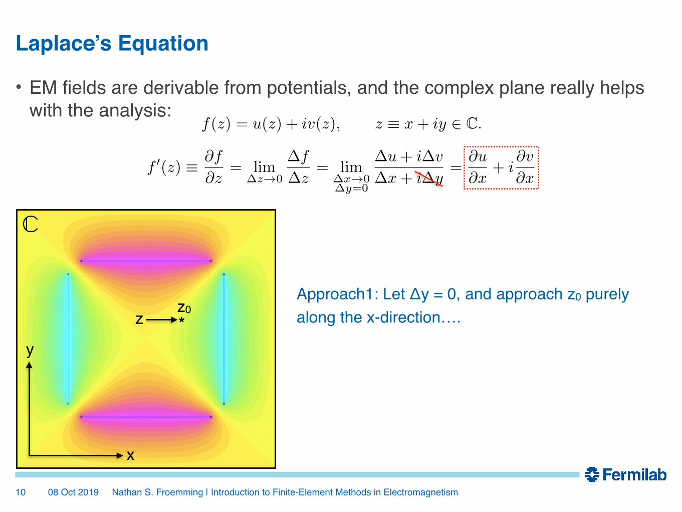
• EM fields are derivable from potentials. The complex plane really helps with the analysis…
�9
Laplace’s Equation
f(z) = u(z) + iv(z), z ⌘ x+ iy 2 C.<latexit sha1_base64="CR26TOkeoX8PUsTI0iyAwntjX0I=">AAACJ3icbVDLSgNBEJz1GeMr6tFLYxAUJexGwVyUQC4eFYwGsiHMTmZ1cHZ2M49gsuRvvPgrXgQV0aN/4mzMQaMFwxRV3XR3BQlnSrvuhzM1PTM7N59byC8uLa+sFtbWL1VsJKF1EvNYNgKsKGeC1jXTnDYSSXEUcHoV3NYy/6pHpWKxuND9hLYifC1YyAjWVmoXTsKdwS4cg8m+PWDQs2QfwO92De4ADMCnXcN6cJe5ffCZAD/C+iYI0tqw1C4U3ZI7Avwl3pgU0Rhn7cKz34mJiajQhGOlmp6b6FaKpWaE02HeN4ommNzia9q0VOCIqlY6unMI21bpQBhL+4SGkfqzI8WRUv0osJXZimrSy8T/vKbRYaWVMpEYTQX5HhQaDjqGLDToMEmJ5n1LMJHM7grkBktMtI02b0PwJk/+Sy7LJe+gVD4/LFYr4zhyaBNtoR3koSNURafoDNURQffoEb2gV+fBeXLenPfv0iln3LOBfsH5/AJUtqID</latexit>
f 0(z) ⌘ @f
@z= lim
�z!0
�f
�z= lim
�x!0�y!0
�u+ i�v
�x+ i�y<latexit sha1_base64="CfZUSiahoOkUQz9/A/WFxw7wMW4=">AAACuXicbVFdaxNBFJ1dv2r8ivroy8UgVoSwW6UWpFDQBx8rmLaQCeHu5G4z7exH5yO4WfY/im/+G2eTDa2pF4Y5nHvOnZkzSamksVH0Jwjv3L13/8HOw96jx0+ePus/f3FiCqcFjUShCn2WoCElcxpZaRWdlZowSxSdJpdf2v7pgrSRRf7DViVNMjzPZSoFWk9N+7/St7vLdwCcrpxc+D3VKGpeorYSFaTNNV42AIdeoWQ2rflXUhZhCdwWEDUb35ptXV2/6UFXhxuncYmxKC43mp/rGZxDR1Td0K2pDt6D3GgWzbX9Bl010/4gGkargtsg7sCAdXU87f/ms0K4jHIrFBozjqPSTur20UJR0+POUOmvi+c09jDHjMykXiXfwBvPzCAttF+5hRV701FjZkyVJV6ZoZ2b7V5L/q83djY9mNQyL52lXKwPSp0CH0z7jTCTmoRVlQcotPR3BTFHn5b1n93zIcTbT74NTvaG8Yfh3vePg6ODLo4d9oq9ZrssZp/YEfvGjtmIiWA/4AEFafg5xHAeXqylYdB5XrJ/KjR/ATuU0iI=</latexit>
z0*
ℂ
x
y
Suppose we have a particle here. We need to know the field (since F = q(E + v x B)), so we need to calculate a derivative of the potential
08 Oct 2019 Nathan S. Froemming | Introduction to Finite-Element Methods in Electromagnetism�10
• EM fields are derivable from potentials, and the complex plane really helps with the analysis:
Laplace’s Equation
f(z) = u(z) + iv(z), z ⌘ x+ iy 2 C.<latexit sha1_base64="CR26TOkeoX8PUsTI0iyAwntjX0I=">AAACJ3icbVDLSgNBEJz1GeMr6tFLYxAUJexGwVyUQC4eFYwGsiHMTmZ1cHZ2M49gsuRvvPgrXgQV0aN/4mzMQaMFwxRV3XR3BQlnSrvuhzM1PTM7N59byC8uLa+sFtbWL1VsJKF1EvNYNgKsKGeC1jXTnDYSSXEUcHoV3NYy/6pHpWKxuND9hLYifC1YyAjWVmoXTsKdwS4cg8m+PWDQs2QfwO92De4ADMCnXcN6cJe5ffCZAD/C+iYI0tqw1C4U3ZI7Avwl3pgU0Rhn7cKz34mJiajQhGOlmp6b6FaKpWaE02HeN4ommNzia9q0VOCIqlY6unMI21bpQBhL+4SGkfqzI8WRUv0osJXZimrSy8T/vKbRYaWVMpEYTQX5HhQaDjqGLDToMEmJ5n1LMJHM7grkBktMtI02b0PwJk/+Sy7LJe+gVD4/LFYr4zhyaBNtoR3koSNURafoDNURQffoEb2gV+fBeXLenPfv0iln3LOBfsH5/AJUtqID</latexit>
z0*
ℂ
x
y
z
f 0(z) ⌘ @f
@z= lim
�z!0
�f
�z= lim
�x!0�y=0
�u+ i�v
�x+ i�y=
@u
@x+ i
@v
@x<latexit sha1_base64="gzBLkCB5unjWRULFbOXEw3ZCkr8=">AAADB3icbVJNS9xQFH2JtrXTD8d2WQoXB9EiDIkW6kYQ2oVLCx0VJsPw8uZFH758+D4GZ0J2bvpXunFhkW77F7rrv+nNTIJm7IWQw7nn3Jdz88JMCm0876/jLi0/efps5XnrxctXr1fba2+OdWoV4z2WylSdhlRzKRLeM8JIfpopTuNQ8pPw4nPZPxlzpUWafDOTjA9iepaISDBqkBquOe8BK9rcmn4ACPilFWN8R4qyPMioMoJKiIp7PC0A9lEhRTzMgy9cGgpTCEwKXlH75mzpqvpFC6rar53ahtpQdlFrruYzggAqYoJar1iYaWEbRK0YF/dmpGtf47BmEPsgyBUG2YZyWlMzbmiG7Y7X9WYFj4FfgQ6p6mjY/hOMUmZjnhgmqdZ938vMIC8HMsmLVmA1zzA3PeN9hAmNuR7ks/9YwAYyI4hShU9iYMY+dOQ01noSh6iMqTnXi72S/F+vb020N8hFklnDEzY/KLIScOXlpYCRUJwZOUFAmRL4rcDOKe7F4NVp4RL8xciPwfFO19/t7nz92DnYq9axQt6RdbJFfPKJHJBDckR6hDnXzg/n1vnpfndv3Dv311zqOpXnLWmU+/sfdrHtdw==</latexit>
Approach1: Let Δy = 0, and approach z0 purely along the x-direction….
08 Oct 2019 Nathan S. Froemming | Introduction to Finite-Element Methods in Electromagnetism�11
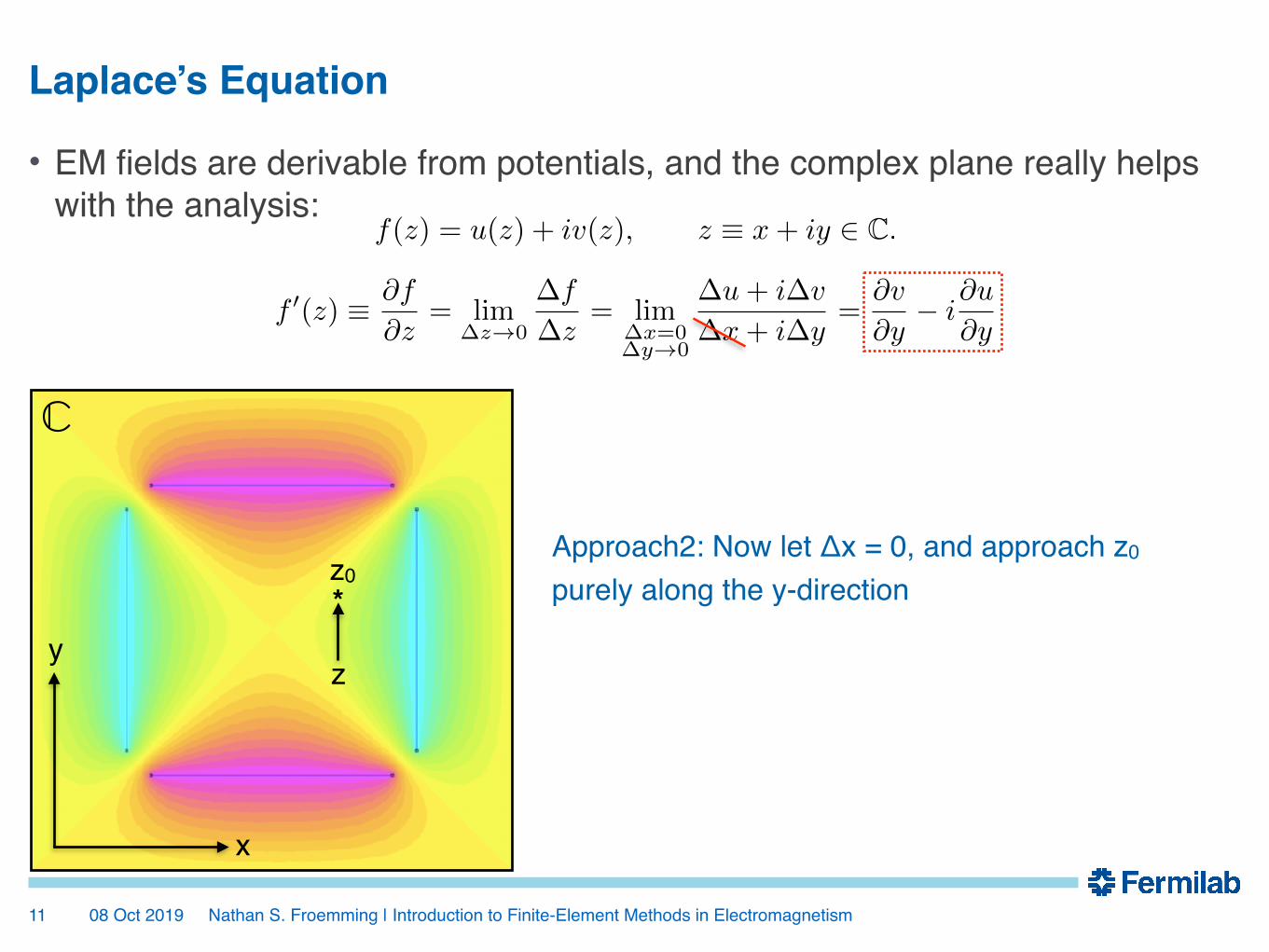
• EM fields are derivable from potentials, and the complex plane really helps with the analysis:
Laplace’s Equation
f(z) = u(z) + iv(z), z ⌘ x+ iy 2 C.<latexit sha1_base64="CR26TOkeoX8PUsTI0iyAwntjX0I=">AAACJ3icbVDLSgNBEJz1GeMr6tFLYxAUJexGwVyUQC4eFYwGsiHMTmZ1cHZ2M49gsuRvvPgrXgQV0aN/4mzMQaMFwxRV3XR3BQlnSrvuhzM1PTM7N59byC8uLa+sFtbWL1VsJKF1EvNYNgKsKGeC1jXTnDYSSXEUcHoV3NYy/6pHpWKxuND9hLYifC1YyAjWVmoXTsKdwS4cg8m+PWDQs2QfwO92De4ADMCnXcN6cJe5ffCZAD/C+iYI0tqw1C4U3ZI7Avwl3pgU0Rhn7cKz34mJiajQhGOlmp6b6FaKpWaE02HeN4ommNzia9q0VOCIqlY6unMI21bpQBhL+4SGkfqzI8WRUv0osJXZimrSy8T/vKbRYaWVMpEYTQX5HhQaDjqGLDToMEmJ5n1LMJHM7grkBktMtI02b0PwJk/+Sy7LJe+gVD4/LFYr4zhyaBNtoR3koSNURafoDNURQffoEb2gV+fBeXLenPfv0iln3LOBfsH5/AJUtqID</latexit>
z0*
ℂ
x
yz
Approach2: Now let Δx = 0, and approach z0 purely along the y-direction
f 0(z) ⌘ @f
@z= lim
�z!0
�f
�z= lim
�x=0�y!0
�u+ i�v
�x+ i�y=
@v
@y� i
@u
@y<latexit sha1_base64="Y+rgA4nQtnrtfPlc1bk1zhEyZgs=">AAADB3icbVLLbtNAFB2bV0h5pLBESFdEiCJEZJdKZFOpEixYFom0leIoGk/G7SjjB/OI6ljeseFX2LAAIbb8Ajv+huvEVuu0Vxr5zLnn3Jl7PWEmhTae989xb9y8dftO52536979Bw9724+OdGoV4yOWylSdhFRzKRI+MsJIfpIpTuNQ8uNw/q7KHy+40iJNPpk845OYniYiEowapKbbzlPAiF7sLF8CBPyzFQv8RoqyIsioMoJKiMoLvCwB9lEhRTwtgvdcGgpLCEwKXtn41mzlqvNlF+rYb5zahtpQNm8055jyggDqbV6X3Khp4RWIRrMoL8xIN87WYe1GFpcaybGR11BVa2tsSzPt9b2Btwq4Cvwa9Ekdh9Pe32CWMhvzxDBJtR77XmYmRVWQSV52A6t5hn3TUz5GmNCY60mx+o8lPEdmBlGqcCUGVuxlR0FjrfM4RGVMzZnezFXkdbmxNdFwUogks4YnbH1QZCXgjKtHATOhODMyR0CZEnhXYGcU52Lw6XRxCP5my1fB0e7AfzPY/bjXPxjW4+iQJ+QZ2SE+eUsOyAdySEaEOV+cb84P56f71f3u/nJ/r6WuU3sek1a4f/4Ddvftew==</latexit>
08 Oct 2019 Nathan S. Froemming | Introduction to Finite-Element Methods in Electromagnetism�12
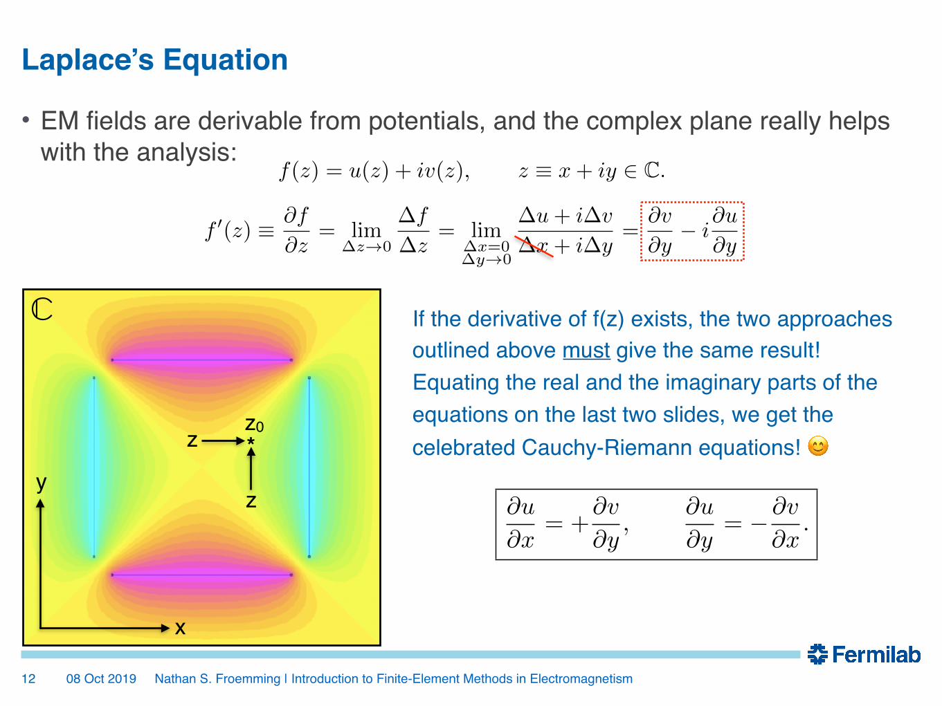
• EM fields are derivable from potentials, and the complex plane really helps with the analysis:
Laplace’s Equation
f(z) = u(z) + iv(z), z ⌘ x+ iy 2 C.<latexit sha1_base64="CR26TOkeoX8PUsTI0iyAwntjX0I=">AAACJ3icbVDLSgNBEJz1GeMr6tFLYxAUJexGwVyUQC4eFYwGsiHMTmZ1cHZ2M49gsuRvvPgrXgQV0aN/4mzMQaMFwxRV3XR3BQlnSrvuhzM1PTM7N59byC8uLa+sFtbWL1VsJKF1EvNYNgKsKGeC1jXTnDYSSXEUcHoV3NYy/6pHpWKxuND9hLYifC1YyAjWVmoXTsKdwS4cg8m+PWDQs2QfwO92De4ADMCnXcN6cJe5ffCZAD/C+iYI0tqw1C4U3ZI7Avwl3pgU0Rhn7cKz34mJiajQhGOlmp6b6FaKpWaE02HeN4ommNzia9q0VOCIqlY6unMI21bpQBhL+4SGkfqzI8WRUv0osJXZimrSy8T/vKbRYaWVMpEYTQX5HhQaDjqGLDToMEmJ5n1LMJHM7grkBktMtI02b0PwJk/+Sy7LJe+gVD4/LFYr4zhyaBNtoR3koSNURafoDNURQffoEb2gV+fBeXLenPfv0iln3LOBfsH5/AJUtqID</latexit>
z0*
ℂ
x
yz
If the derivative of f(z) exists, the two approaches outlined above must give the same result! Equating the real and the imaginary parts of the equations on the last two slides, we get the celebrated Cauchy-Riemann equations! 😊z
@u
@x= +
@v
@y,
@u
@y= �@v
@x.
<latexit sha1_base64="2owLUGfQJOwUEvUHNQ0D4XofXZ0=">AAACjnicjVFdS8MwFE3r16xfVR99CQ5BUEc7RYcyHPiyxwlOhbWMNE1dWPphkspK6c/xD/nmvzHdCuoU8UDgcO+5J8m5XsKokJb1rukLi0vLK7VVY219Y3PL3N65F3HKMenjmMX80UOCMBqRvqSSkceEExR6jDx445uy//BCuKBxdCezhLgheopoQDGSqjQ0Xx0vnhA/N2AFJ+AI506CuKSIwbT45JMCwjaER3OSly+SrDhWFs/PKfL/45jNHE/+cJwUDaMYmnWrYU0BfxK7InVQoTc03xw/xmlIIokZEmJgW4l089ITM1IYTipIgvAYPZGBohEKiXDzaZwFPFAVHwYxVyeScFr9OpGjUIgs9JQyRHIk5ntl8bfeIJVBy81plKSSRHh2UZAyKGNY7gb6lBMsWaYIwpyqt0I8QioaqTZoqBDs+S//JPfNhn3aaN6e1TutKo4a2AP74BDY4AJ0QBf0QB9gbU2ztUvtSjf1c72tX8+kulbN7IJv0Lsf51jDKA==</latexit>
f 0(z) ⌘ @f
@z= lim
�z!0
�f
�z= lim
�x=0�y!0
�u+ i�v
�x+ i�y=
@v
@y� i
@u
@y<latexit sha1_base64="Y+rgA4nQtnrtfPlc1bk1zhEyZgs=">AAADB3icbVLLbtNAFB2bV0h5pLBESFdEiCJEZJdKZFOpEixYFom0leIoGk/G7SjjB/OI6ljeseFX2LAAIbb8Ajv+huvEVuu0Vxr5zLnn3Jl7PWEmhTae989xb9y8dftO52536979Bw9724+OdGoV4yOWylSdhFRzKRI+MsJIfpIpTuNQ8uNw/q7KHy+40iJNPpk845OYniYiEowapKbbzlPAiF7sLF8CBPyzFQv8RoqyIsioMoJKiMoLvCwB9lEhRTwtgvdcGgpLCEwKXtn41mzlqvNlF+rYb5zahtpQNm8055jyggDqbV6X3Khp4RWIRrMoL8xIN87WYe1GFpcaybGR11BVa2tsSzPt9b2Btwq4Cvwa9Ekdh9Pe32CWMhvzxDBJtR77XmYmRVWQSV52A6t5hn3TUz5GmNCY60mx+o8lPEdmBlGqcCUGVuxlR0FjrfM4RGVMzZnezFXkdbmxNdFwUogks4YnbH1QZCXgjKtHATOhODMyR0CZEnhXYGcU52Lw6XRxCP5my1fB0e7AfzPY/bjXPxjW4+iQJ+QZ2SE+eUsOyAdySEaEOV+cb84P56f71f3u/nJ/r6WuU3sek1a4f/4Ddvftew==</latexit>
08 Oct 2019 Nathan S. Froemming | Introduction to Finite-Element Methods in Electromagnetism�13
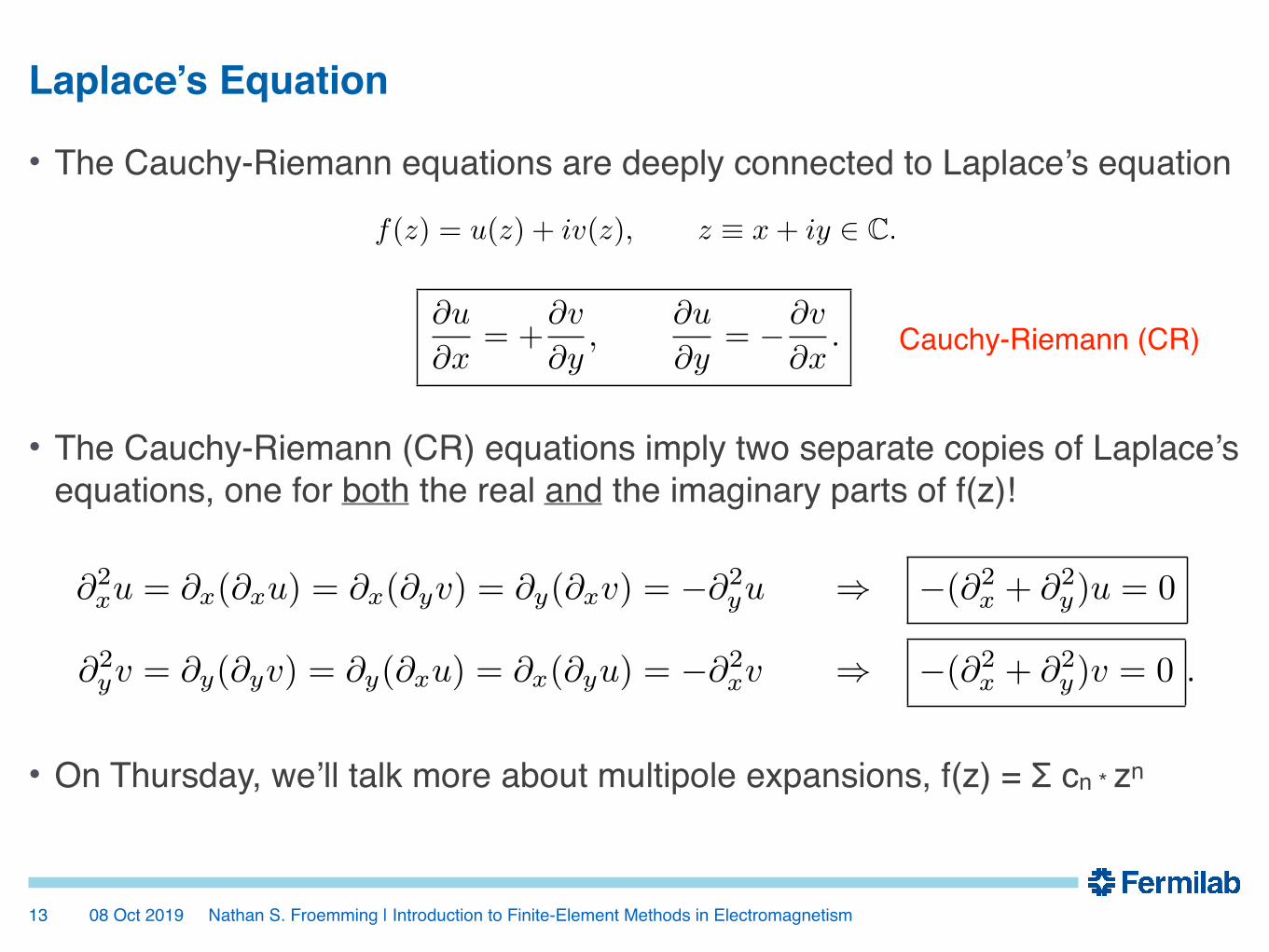
• The Cauchy-Riemann equations are deeply connected to Laplace’s equation
• The Cauchy-Riemann (CR) equations imply two separate copies of Laplace’s equations, one for both the real and the imaginary parts of f(z)!
• On Thursday, we’ll talk more about multipole expansions, f(z) = Σ cn * zn
Laplace’s Equation
f(z) = u(z) + iv(z), z ⌘ x+ iy 2 C.<latexit sha1_base64="CR26TOkeoX8PUsTI0iyAwntjX0I=">AAACJ3icbVDLSgNBEJz1GeMr6tFLYxAUJexGwVyUQC4eFYwGsiHMTmZ1cHZ2M49gsuRvvPgrXgQV0aN/4mzMQaMFwxRV3XR3BQlnSrvuhzM1PTM7N59byC8uLa+sFtbWL1VsJKF1EvNYNgKsKGeC1jXTnDYSSXEUcHoV3NYy/6pHpWKxuND9hLYifC1YyAjWVmoXTsKdwS4cg8m+PWDQs2QfwO92De4ADMCnXcN6cJe5ffCZAD/C+iYI0tqw1C4U3ZI7Avwl3pgU0Rhn7cKz34mJiajQhGOlmp6b6FaKpWaE02HeN4ommNzia9q0VOCIqlY6unMI21bpQBhL+4SGkfqzI8WRUv0osJXZimrSy8T/vKbRYaWVMpEYTQX5HhQaDjqGLDToMEmJ5n1LMJHM7grkBktMtI02b0PwJk/+Sy7LJe+gVD4/LFYr4zhyaBNtoR3koSNURafoDNURQffoEb2gV+fBeXLenPfv0iln3LOBfsH5/AJUtqID</latexit>
@u
@x= +
@v
@y,
@u
@y= �@v
@x.
<latexit sha1_base64="2owLUGfQJOwUEvUHNQ0D4XofXZ0=">AAACjnicjVFdS8MwFE3r16xfVR99CQ5BUEc7RYcyHPiyxwlOhbWMNE1dWPphkspK6c/xD/nmvzHdCuoU8UDgcO+5J8m5XsKokJb1rukLi0vLK7VVY219Y3PL3N65F3HKMenjmMX80UOCMBqRvqSSkceEExR6jDx445uy//BCuKBxdCezhLgheopoQDGSqjQ0Xx0vnhA/N2AFJ+AI506CuKSIwbT45JMCwjaER3OSly+SrDhWFs/PKfL/45jNHE/+cJwUDaMYmnWrYU0BfxK7InVQoTc03xw/xmlIIokZEmJgW4l089ITM1IYTipIgvAYPZGBohEKiXDzaZwFPFAVHwYxVyeScFr9OpGjUIgs9JQyRHIk5ntl8bfeIJVBy81plKSSRHh2UZAyKGNY7gb6lBMsWaYIwpyqt0I8QioaqTZoqBDs+S//JPfNhn3aaN6e1TutKo4a2AP74BDY4AJ0QBf0QB9gbU2ztUvtSjf1c72tX8+kulbN7IJv0Lsf51jDKA==</latexit>
@2xu = @x(@xu) = @x(@yv) = @y(@xv) = �@2
yu ) �(@2x + @2
y)u = 0
@2yv = @y(@yv) = @y(@xu) = @x(@yu) = �@2
xv ) �(@2x + @2
y)v = 0 .<latexit sha1_base64="JXuxb9IdPOTQ98oIYZvLUnUyYsc=">AAADy3icpVLLbtNAFJ3YPIp5pbBkMyJKlAo1csKCbpAqsekGqSDSVopDNB7fJKOOx2YeaYzJkh9kx5I/YeyY1nUBIXElS8fn3NeZmTDlTGnf/95y3Fu379zduefdf/Dw0eP27pMTlRhJYUwTnsizkCjgTMBYM83hLJVA4pDDaXj+ptBPVyAVS8QHnaUwjclCsDmjRFtqttv60fWCEBZM5PDJlOQmEIkwcQiyEghnCwHRxsM2gpRIzQifrT+OsMG497rO9a8gNnsY/0HM8KohZvXKSty/UrezbL7dMeoF79liqYmUyUVJFEovCJM1RDne79dXfFHvsWdsWx9vbJ/gupliwKphJvvnff/q1DTNrLez/tvM6peZgReAiC6vqfy5vEyvO2t3/IFfBr4JhhXooCqOZ+1vQZRQE4PQlBOlJkM/1dO8GE05bLzAKEgJPScLmFgoSAxqmpdvcYO7lonwPJH2ExqXbL0iJ7FSWRzazJjopWpqBfk7bWL0/GCaM5EaDYJuB80NxzrBxcPGEZNANc8sIFQyuyumSyIJ1fb5e/YQhk3LN8HJaDB8ORi9G3UOD6rj2EHP0HPUR0P0Ch2iI3SMxog6R45wLpy1+9ZV7mf3yzbVaVU1T9G1cL/+BFMvL28=</latexit>
Cauchy-Riemann (CR)
08 Oct 2019 Nathan S. Froemming | Introduction to Finite-Element Methods in Electromagnetism
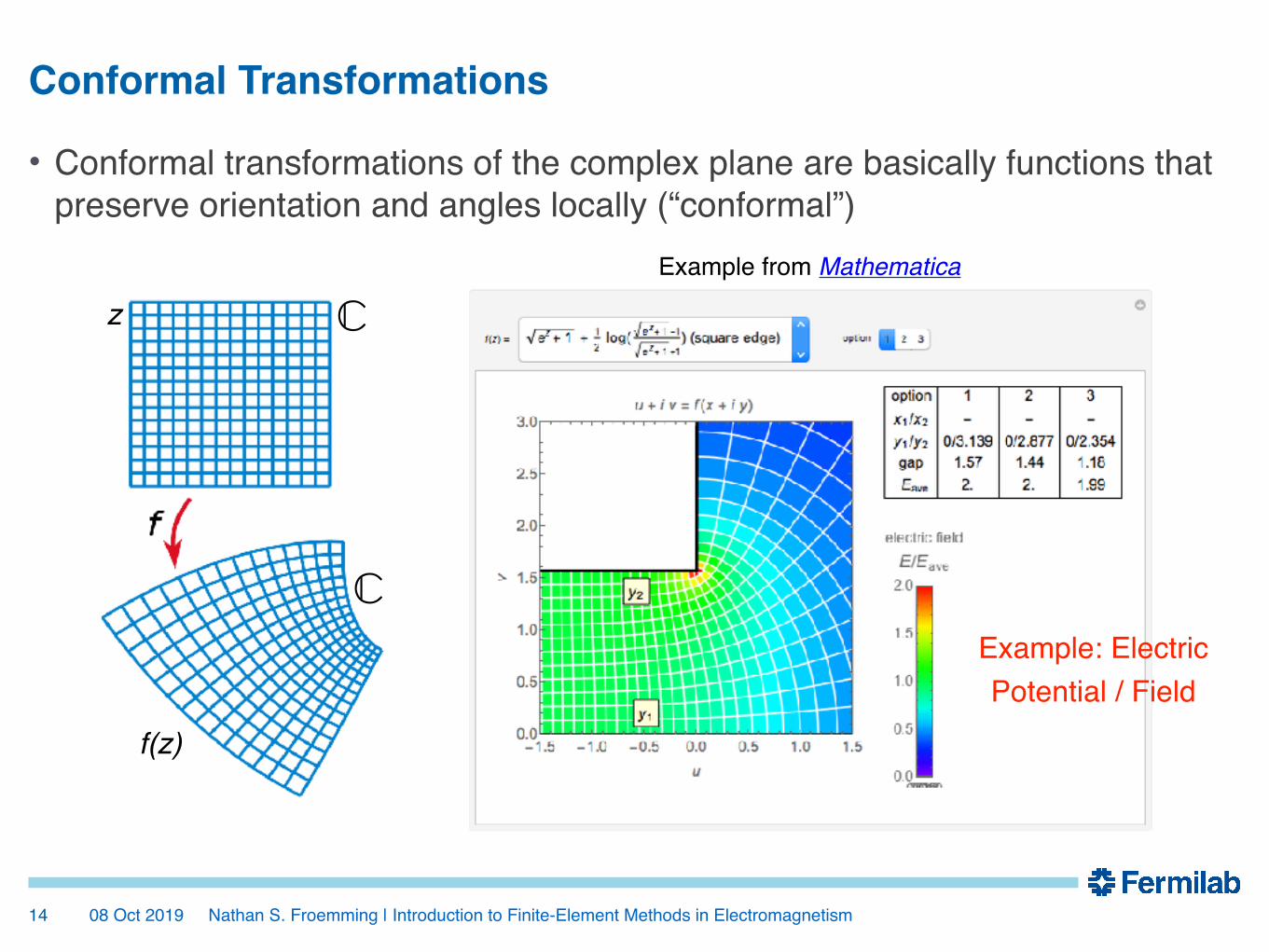
Conformal Transformations
• Conformal transformations of the complex plane are basically functions that preserve orientation and angles locally (“conformal”)
�14
Example from Mathematica
z
f(z)
ℂ
ℂExample: ElectricPotential / Field

08 Oct 2019 Nathan S. Froemming | Introduction to Finite-Element Methods in Electromagnetism
• Mathematical expressions quickly get out of control. Limited to all but this simplest cases. Nowadays, with computers, we can do much more….
�15
Conformal transformations (i.e. math equations on paper) were basically superseded by numerical methods on computers c. 1960-1970
Conformal Transformations => Finite-Element Methods

08 Oct 2019 Nathan S. Froemming | Introduction to Finite-Element Methods in Electromagnetism
Finite-Element Methods (FEM)?
• Essentially, (FEM) “puts differential equations on a grid/mesh” and solves numerically with computers (fluid flow, heat flow, stress/strain, electromagnetism, etc.)
�16
“Finite Elements”(a.k.a. “mesh”)
08 Oct 2019 Nathan S. Froemming | Introduction to Finite-Element Methods in Electromagnetism
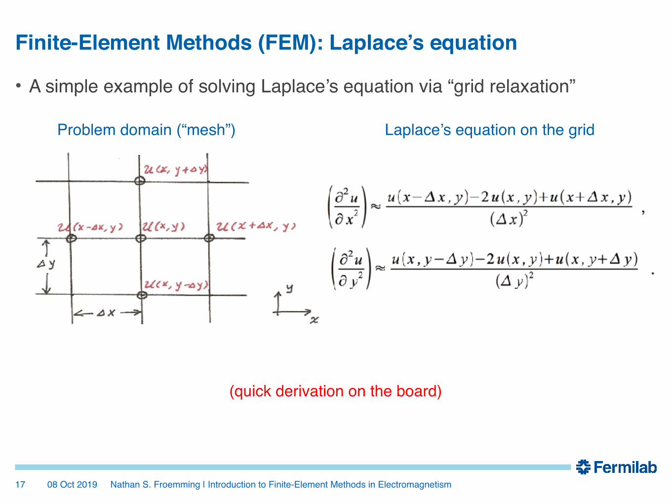
• A simple example of solving Laplace’s equation via “grid relaxation”
�17
Finite-Element Methods (FEM): Laplace’s equation
Problem domain (“mesh”) Laplace’s equation on the grid
(quick derivation on the board)
08 Oct 2019 Nathan S. Froemming | Introduction to Finite-Element Methods in Electromagnetism
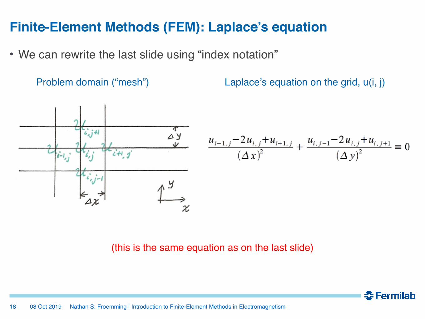
• We can rewrite the last slide using “index notation”
�18
Finite-Element Methods (FEM): Laplace’s equation
Problem domain (“mesh”) Laplace’s equation on the grid, u(i, j)
(this is the same equation as on the last slide)

08 Oct 2019 Nathan S. Froemming | Introduction to Finite-Element Methods in Electromagnetism
• Let Δx = Δy = 1 for simplicity. Then the solution at u(i, j) is just the average value of its neighbors!
�19
Finite-Element Methods (FEM): Laplace’s equation
Ask to see Prof.Syphers’ notebook :)

08 Oct 2019 Nathan S. Froemming | Introduction to Finite-Element Methods in Electromagnetism�20
Outline
• Overview LaPlace’s equation and solutions- Cauchy-Riemann equations; Connection to electromagnetism (EM)- Conformal mappings- Shortcomings• Finite-Element methods and codes (OPERA, COMSOL, FEMM, …)• Getting FEMM setup on your local machine• FEMM electric example- Problem setup: Electric dipole/quadrupole- How to extract the potential/E-field from FEMM• FEMM magnetic example (next time)- Problem setup: H-dipole, quadrupole (more challenging)- How to extract the potential/B-field from FEMM• Pro Tips And Tricks (next time)- Scripting in `lua` and `python`; Jupyter notebooks; WebPlotDigitizer; etc.• Conclusions
08 Oct 2019 Nathan S. Froemming | Introduction to Finite-Element Methods in Electromagnetism
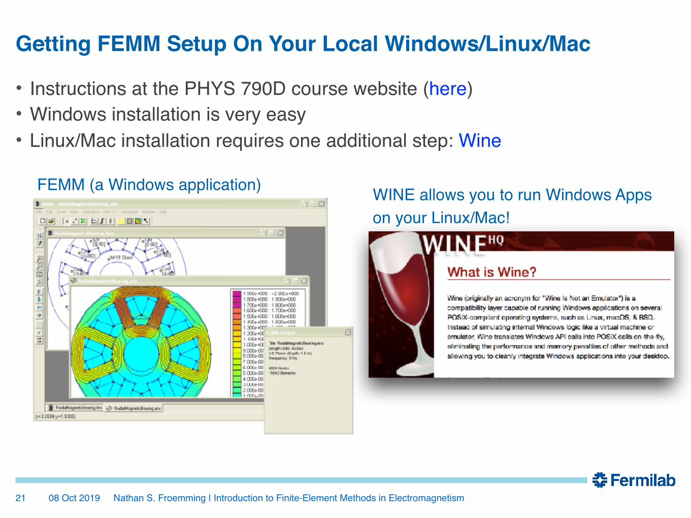
Getting FEMM Setup On Your Local Windows/Linux/Mac
• Instructions at the PHYS 790D course website (here)• Windows installation is very easy• Linux/Mac installation requires one additional step: Wine
�21
FEMM (a Windows application) WINE allows you to run Windows Apps on your Linux/Mac!

08 Oct 2019 Nathan S. Froemming | Introduction to Finite-Element Methods in Electromagnetism
• Electric problems are easier to setup in FEMM, so that’s where we’ll start• Two simple examples: (1) electric dipole, (2) electric quadrupole
�22
Electric storage ring: EDM measurements Example electric dipole FEMM simulation
E-fieldWe’ll look at
straight/curved longitudinal axes
FEMM Tutorial: Electrostatics

08 Oct 2019 Nathan S. Froemming | Introduction to Finite-Element Methods in Electromagnetism
FEMM Tutorial: Electrostatics
• Here we go! Start FEMM and create a new “Electrostatics Problem”
�23
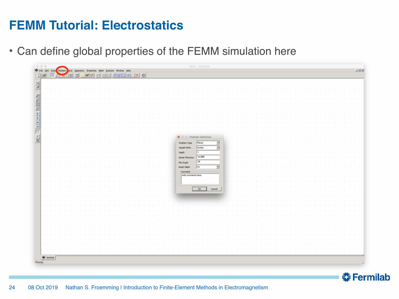
08 Oct 2019 Nathan S. Froemming | Introduction to Finite-Element Methods in Electromagnetism
• Can define global properties of the FEMM simulation here
�24
FEMM Tutorial: Electrostatics
08 Oct 2019 Nathan S. Froemming | Introduction to Finite-Element Methods in Electromagnetism
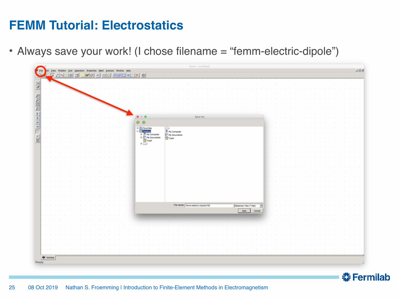
• Always save your work! (I chose filename = “femm-electric-dipole”)
�25
FEMM Tutorial: Electrostatics

08 Oct 2019 Nathan S. Froemming | Introduction to Finite-Element Methods in Electromagnetism
• Build a “vacuum chamber” shape. Start by defining corners & edges
�26
Add 4 corner points at {±10, ±10} by pressing <TAB> and entering
(x, y) coordinates
FEMM Tutorial: Electrostatics
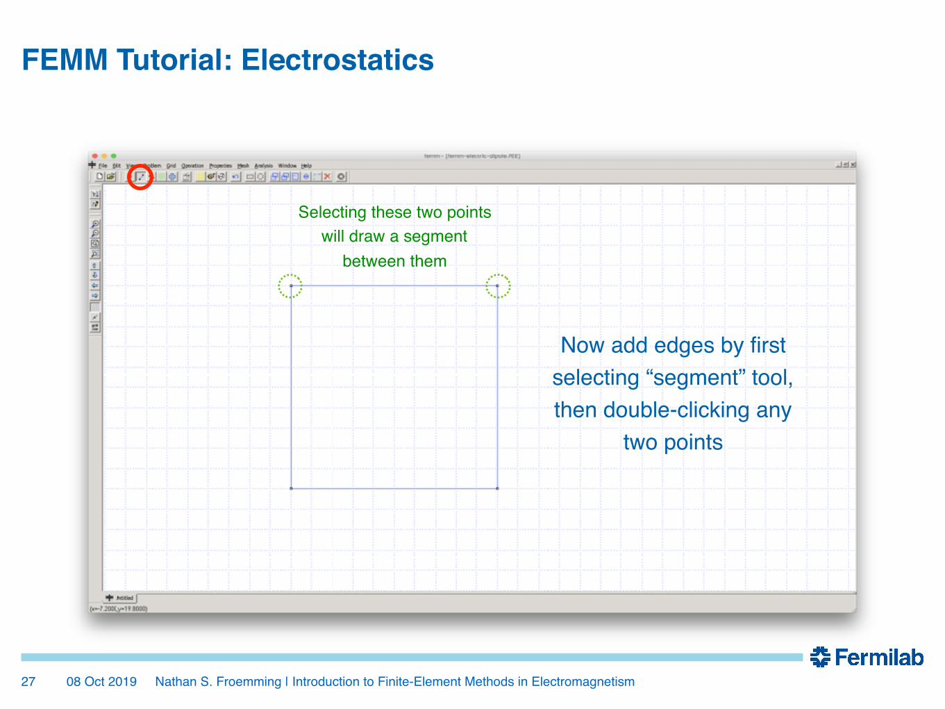
08 Oct 2019 Nathan S. Froemming | Introduction to Finite-Element Methods in Electromagnetism�27
Now add edges by first selecting “segment” tool, then double-clicking any
two points
Selecting these two points will draw a segment
between them
FEMM Tutorial: Electrostatics
08 Oct 2019 Nathan S. Froemming | Introduction to Finite-Element Methods in Electromagnetism
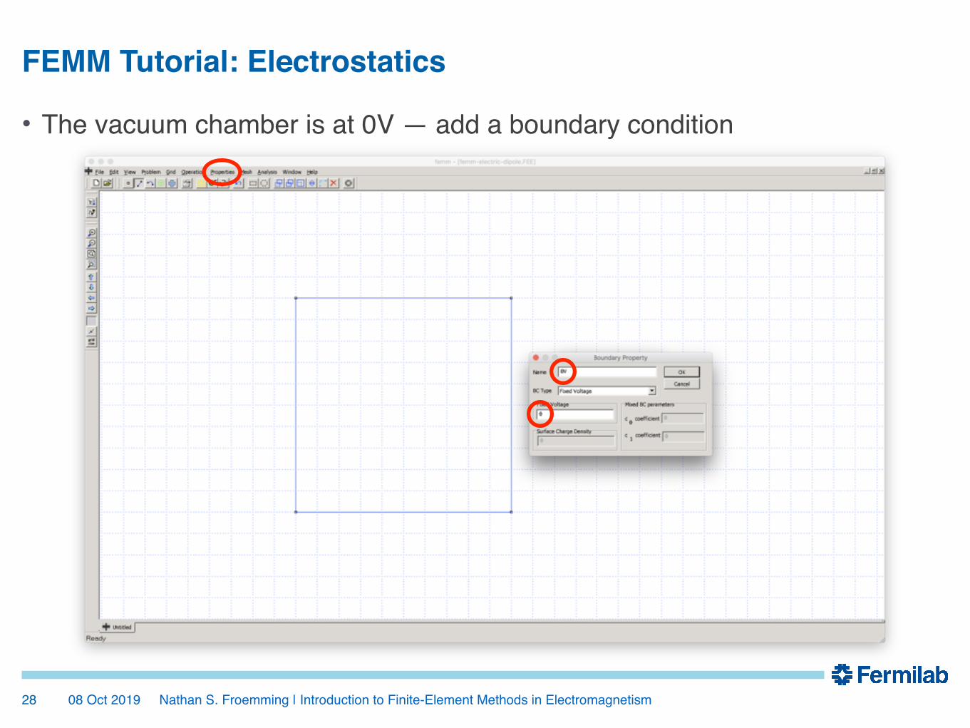
• The vacuum chamber is at 0V — add a boundary condition
�28
FEMM Tutorial: Electrostatics

08 Oct 2019 Nathan S. Froemming | Introduction to Finite-Element Methods in Electromagnetism
• The vacuum chamber is at 0V — add a boundary condition
�29
Select line segments, press <SPACE BAR>, add boundary condition
FEMM Tutorial: Electrostatics
08 Oct 2019 Nathan S. Froemming | Introduction to Finite-Element Methods in Electromagnetism
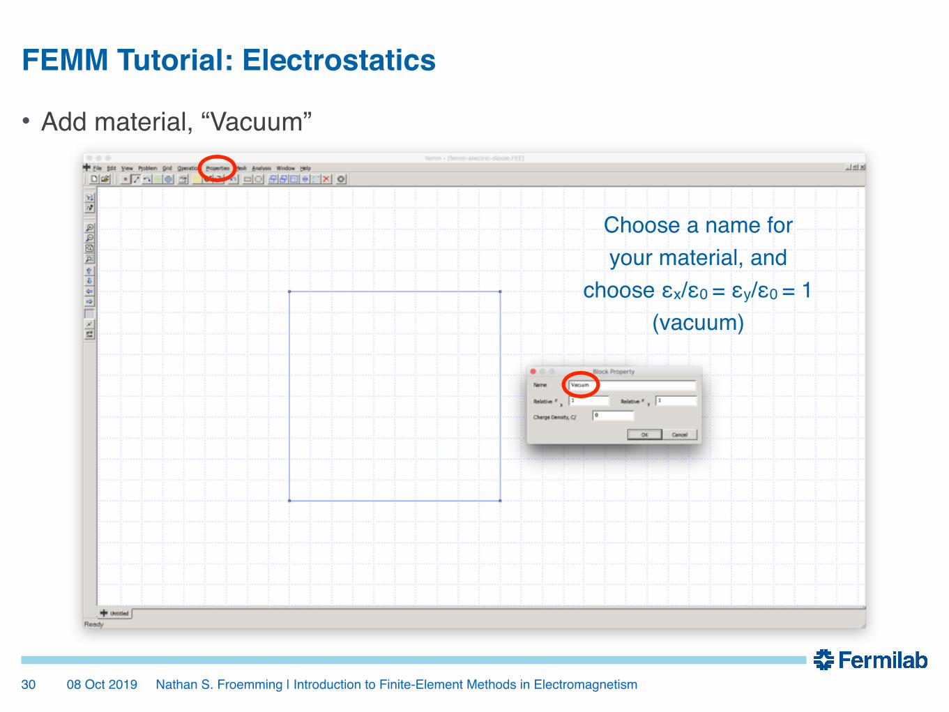
• Add material, “Vacuum”
�30
Choose a name for your material, and
choose εx/ε0 = εy/ε0 = 1 (vacuum)
FEMM Tutorial: Electrostatics
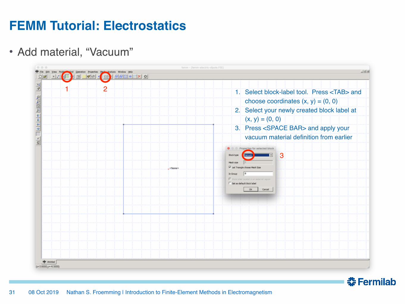
08 Oct 2019 Nathan S. Froemming | Introduction to Finite-Element Methods in Electromagnetism
• Add material, “Vacuum”
�31
1. Select block-label tool. Press <TAB> and choose coordinates (x, y) = (0, 0)
2. Select your newly created block label at (x, y) = (0, 0)
3. Press <SPACE BAR> and apply your vacuum material definition from earlier
1 2
3
FEMM Tutorial: Electrostatics

08 Oct 2019 Nathan S. Froemming | Introduction to Finite-Element Methods in Electromagnetism
• Create the “outer electrode” by first drawing a line segment
�32
I chose electrode vertices (x, y) = (5, ±5) cm
FEMM Tutorial: Electrostatics

08 Oct 2019 Nathan S. Froemming | Introduction to Finite-Element Methods in Electromagnetism
• Define the potential for the outer electrode, e.g. +1kV
�33
FEMM Tutorial: Electrostatics

08 Oct 2019 Nathan S. Froemming | Introduction to Finite-Element Methods in Electromagnetism
• Apply potential to outer electrode, e.g. +1kV
�34
Select line segments, press <SPACE BAR>, add boundary condition
FEMM Tutorial: Electrostatics

08 Oct 2019 Nathan S. Froemming | Introduction to Finite-Element Methods in Electromagnetism
• Now create the “inner electrode” by drawing a line, as before
�35
Same steps as before. I chose (x, y) = (-5, ±5) cm
for vertices
FEMM Tutorial: Electrostatics

08 Oct 2019 Nathan S. Froemming | Introduction to Finite-Element Methods in Electromagnetism
• Define the potential for the inner electrode, e.g. -1kV
�36
FEMM Tutorial: Electrostatics

08 Oct 2019 Nathan S. Froemming | Introduction to Finite-Element Methods in Electromagnetism
• Apply potential to inner electrode, e.g. -1kV
�37
Select line segments, press <SPACE BAR>, add boundary condition
FEMM Tutorial: Electrostatics

08 Oct 2019 Nathan S. Froemming | Introduction to Finite-Element Methods in Electromagnetism
• Mesh, analyze, and see the results!
�38
1. Run mesh generator (mesh icon, yellow)2. Run analysis (gear icon)3. View results (glasses icon)
1, 2, 3
FEMM Tutorial: Electrostatics

08 Oct 2019 Nathan S. Froemming | Introduction to Finite-Element Methods in Electromagnetism
• This is what you should see. If not, I can help!
�39
FEMM Tutorial: Electrostatics

08 Oct 2019 Nathan S. Froemming | Introduction to Finite-Element Methods in Electromagnetism
• Suppose we want the E-field in the horizontal midplane….
�40
FEMM Tutorial: Electrostatics
Same steps as before: Define a line via 2 points
(press <TAB>). Can hover mouse to see coordinates
listed at lower left.

08 Oct 2019 Nathan S. Froemming | Introduction to Finite-Element Methods in Electromagnetism
• Now make a plot by clicking the “plot” icon. Can export to text file….
�41
FEMM Tutorial: Electrostatics
08 Oct 2019 Nathan S. Froemming | Introduction to Finite-Element Methods in Electromagnetism
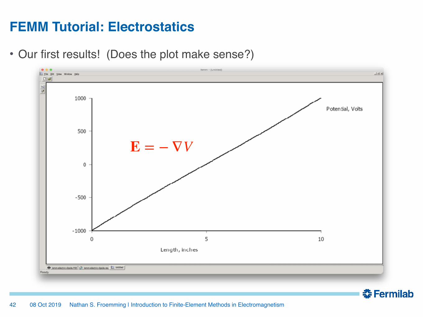
• Our first results! (Does the plot make sense?)
�42
E = − ∇V
FEMM Tutorial: Electrostatics

08 Oct ‘19 Nathan S. Froemming | Introduction to Finite Element Method Magnetics (FEMM)
• Now we’ll modify the dipole to make a quadrupole. Always save your work!
�43
FEMM Tutorial: Electrostatics
08 Oct 2019 Nathan S. Froemming | Introduction to Finite-Element Methods in Electromagnetism
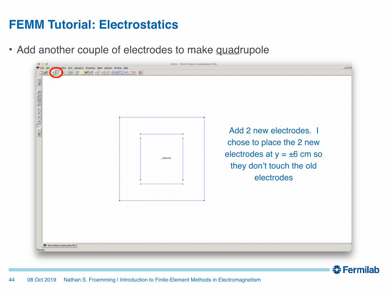
• Add another couple of electrodes to make quadrupole
�44
FEMM Tutorial: Electrostatics
Add 2 new electrodes. I chose to place the 2 new
electrodes at y = ±6 cm so they don’t touch the old
electrodes

08 Oct 2019 Nathan S. Froemming | Introduction to Finite-Element Methods in Electromagnetism�45
FEMM Tutorial: Electrostatics
Move old electrodes slightly for symmetry using the “move” tool

08 Oct 2019 Nathan S. Froemming | Introduction to Finite-Element Methods in Electromagnetism
• Set electrode voltages for vertical focusing of positively-charged particles
�46
FEMM Tutorial: Electrostatics
Apply the correct voltages for vertical focusing of
positively charged particles
08 Oct 2019 Nathan S. Froemming | Introduction to Finite-Element Methods in Electromagnetism
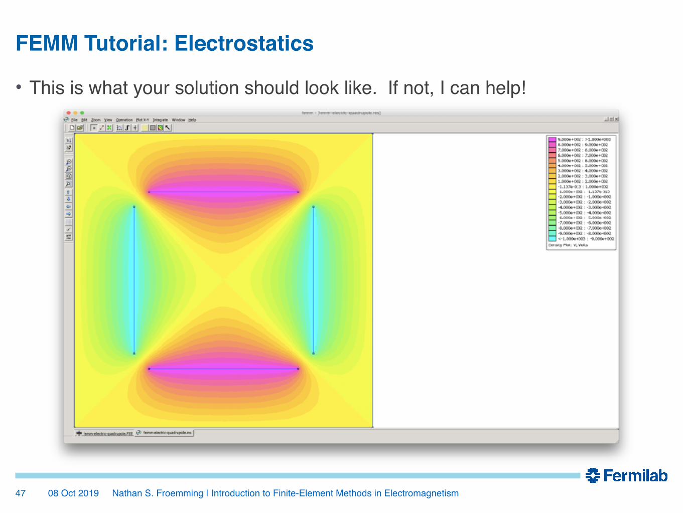
• This is what your solution should look like. If not, I can help!
�47
FEMM Tutorial: Electrostatics

08 Oct 2019 Nathan S. Froemming | Introduction to Finite-Element Methods in Electromagnetism
• Plot the potential in the horizontal midplane. (Does it make sense?)
�48
FEMM Tutorial: Electrostatics
Same steps as before: Define a line via 2 points
(press <TAB>). Can hover mouse to see coordinates
listed at lower left.

08 Oct 2019 Nathan S. Froemming | Introduction to Finite-Element Methods in Electromagnetism
• Plot the potential in the horizontal midplane. (Does it make sense?)
�49
FEMM Tutorial: Electrostatics

08 Oct 2019 Nathan S. Froemming | Introduction to Finite-Element Methods in Electromagnetism
• What about a curved longitudinal axis, i.e. cylindrical symmetry?
�50
FEMM Tutorial: Electrostatics
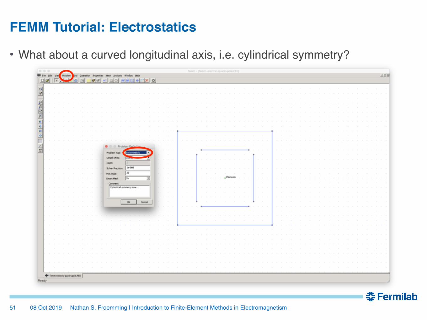
08 Oct 2019 Nathan S. Froemming | Introduction to Finite-Element Methods in Electromagnetism
• What about a curved longitudinal axis, i.e. cylindrical symmetry?
�51
FEMM Tutorial: Electrostatics

08 Oct 2019 Nathan S. Froemming | Introduction to Finite-Element Methods in Electromagnetism
• Does the new solution (with cylindrical symmetry) look any different?
�52
FEMM Tutorial: Electrostatics

08 Oct 2019 Nathan S. Froemming | Introduction to Finite-Element Methods in Electromagnetism
• Plot the potential in the horizontal midplane
�53
FEMM Tutorial: Electrostatics
Same steps as before: Define a line via 2 points
(press <TAB>). Can hover mouse to see coordinates
listed at lower left.
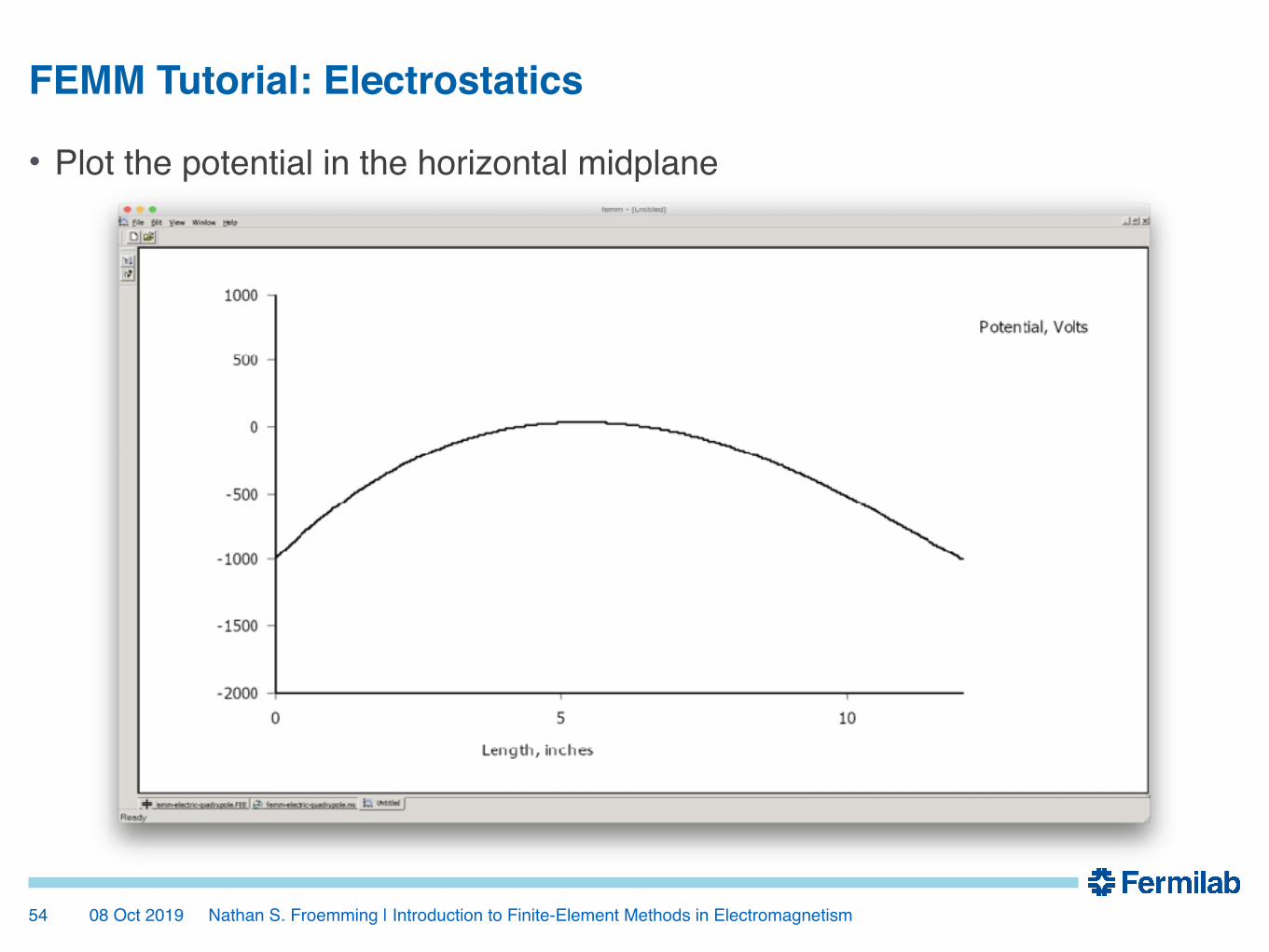
08 Oct 2019 Nathan S. Froemming | Introduction to Finite-Element Methods in Electromagnetism
• Plot the potential in the horizontal midplane
�54
FEMM Tutorial: Electrostatics
08 Oct 2019 Nathan S. Froemming | Introduction to Finite-Element Methods in Electromagnetism
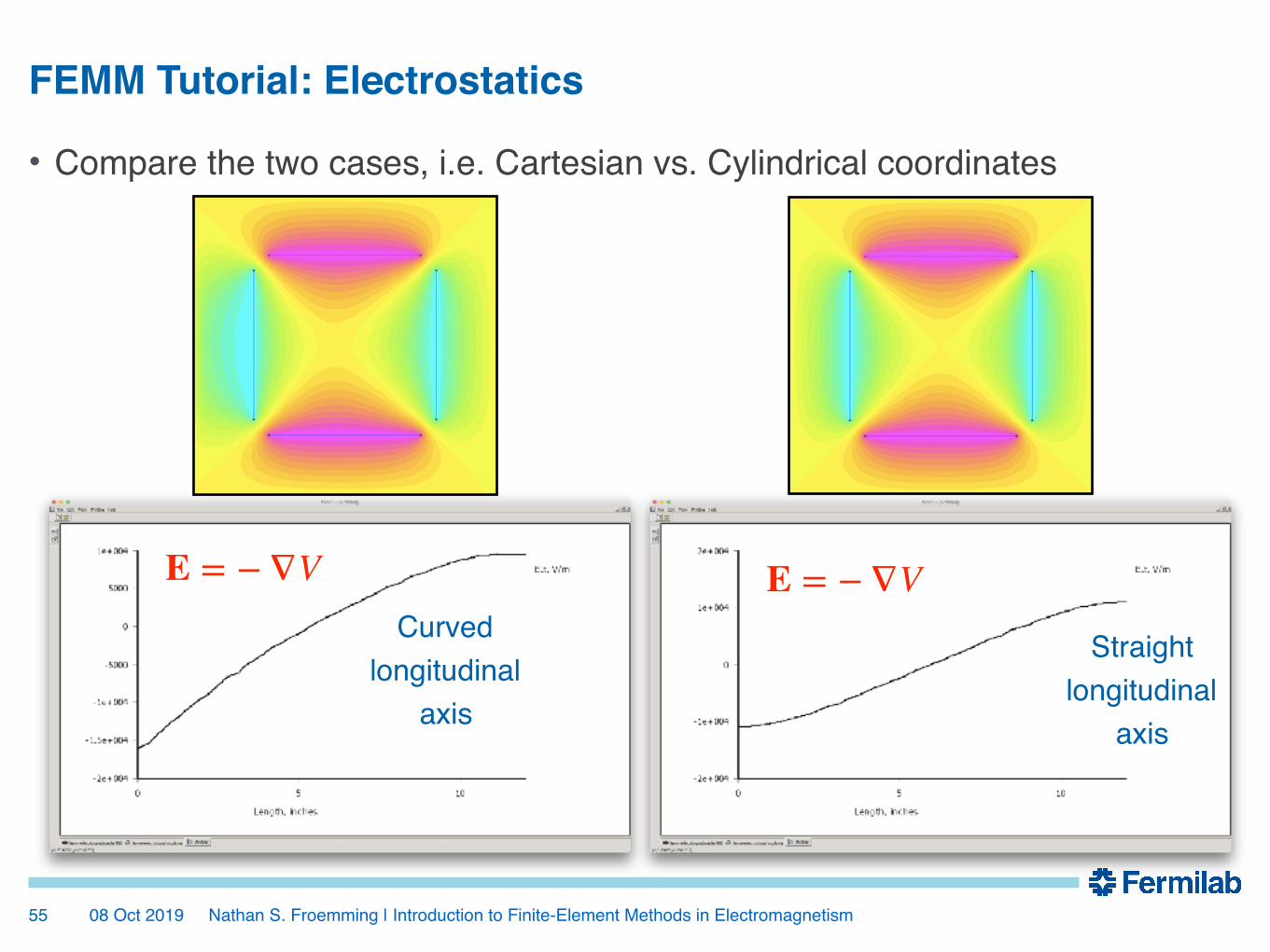
• Compare the two cases, i.e. Cartesian vs. Cylindrical coordinates
�55
E = − ∇VCurved
longitudinal axis
Straight longitudinal
axis
E = − ∇V
FEMM Tutorial: Electrostatics

08 Oct 2019 Nathan S. Froemming | Introduction to Finite-Element Methods in Electromagnetism�56
That’s All For Today — See You On Thursday!
• Overview LaPlace’s equation and solutions- Cauchy-Riemann equations; Connection to electromagnetism (EM)- Conformal mappings- Shortcomings• Finite-Element methods and codes (OPERA, COMSOL, FEMM, …)• Getting FEMM setup on your local machine• FEMM electric example- Problem setup: Electric dipole/quadrupole- How to extract the potential/E-field from FEMM• FEMM magnetic example (next time)- Problem setup: H-dipole, quadrupole (more challenging)- How to extract the potential/B-field from FEMM• Pro Tips And Tricks (next time)- Scripting in `lua` and `python`; Jupyter notebooks; WebPlotDigitizer; etc.• Conclusions