A SYMMETRICAL FINITE ELEMENT MODEL FOR - CORE

1

Rail vehicle dynamic response to the nonlinear physical in-service model of its secondary suspension hydraulic dampers W.L. Wanga, b*, D.S. Yuc, Q.H. Qinb, S. Iwnickid

a School of Mechanical Engineering, Dongguan University of Technology, Dongguan 523808, P. R. of China b State Key Laboratory for Strength and Vibration of Mechanical Structures, Xi’an Jiaotong University, Xi’an 710049, P. R. of China c Anhui Xingrui Gear Transmission Co., Ltd, Lu’an 237161, P. R. of China d Institute of Railway Research, University of Huddersfield, Huddersfield HD1 3DH, UK

Abstract

A full nonlinear physical in-service model was built for a rail vehicle secondary suspension hydraulic damper with

shim-pack-type valves. In the modelling process, a shim pack deflection theory with an equivalent-pressure correction factor

was proposed and the Finite Element Analysis (FEA) approach was assisted. Followed bench test results validated the

damper model over its full velocity range, and thus also proved the proposed shim pack deflection theory and the FEA-based

parameter identification approach are effective. The validated full damper model was then incorporated into a detailed

vehicle dynamics simulation to study how its key in-service parameter variations influence the secondary suspension related

vehicle system dynamics. The obtained nonlinear physical in-service damper model and the vehicle dynamic response

characteristics in this study could be used in product design optimisation and nonlinear optimal specification of high-speed

rail hydraulic dampers.

Keywords: Nonlinear modelling; hydraulic damper; shim pack deflection; FEA; in-service parameter; rail vehicle secondary

suspension; ride comfort; curve negotiation stability

1. Introduction

The secondary suspension of a passenger rail vehicle usually employs both vertical and several lateral

hydraulic dampers, which play important roles in the carbody vibration reduction, ride comfort improvement and

curve negotiation stabilization. For hydraulic dampers are in practice very nonlinear devices (see Mellado et al.

[1] and Wang et al. [2]), with characteristics which are sensitive to the in-service conditions and could have

unpredictable and significant influences on the vehicle system dynamics (see Wang et al. [3]), as speeds and

loads increase in modern rail vehicles, these effects become more significant, so it is important to include exact

representation of damper parameters for vehicle system dynamics study.

In related works, Kasteel et al. [4] and Farjoud et al. [5] built detailed nonlinear physical models for

hydraulic dampers with shim stacks and orifices. Simms et al. [6] and Calvo et al. [7] performed simulations on

the effects of damper characteristics on road vehicle dynamics, the macro damper models used include which

has symmetric or asymmetric performance, which has simple linear or piecewise linear or linear with hysteresis

performance; Park et al. [8] carried out sensitivity analysis of suspension parameters on high-speed train * Corresponding author at: School of Mechanical Engineering, Dongguan University of Technology, Dongguan 523808, Guangdong Province, PR China. Tel.: +86 769 22861122.

E-mail address: [email protected] (W.L. Wang).

CORE Metadata, citation and similar papers at core.ac.uk

Provided by University of Huddersfield Repository

https://core.ac.uk/display/80693055?utm_source=pdf&utm_medium=banner&utm_campaign=pdf-decoration-v1

2

dynamics, using commercial Multibody System (MBS) dynamics simulation software Vampire and Design of

Experiments (DoE) approach, however, the hydraulic damper model used is a simple linear model which

contains only one parameter, i.e., the damping coefficient.

In rail vehicle design studies, Shieh et al. [9] and He et al. [10] also used the simple linear hydraulic damper

model for suspension optimization; Hao et al. [11], however, used the linear Maxwell damper model, i.e., a

linear damping coefficient in series with a linear stiffness (see [12]), in the multi-objective optimization search,

and obtained better results; Wang et al. [13] proposed a full nonlinear damper model concept which includes

most of the in-service parameters and a detailed physical model was built, the nonlinear in-service damper model

was then successfully used for the optimal specification of a locomotive axle-box hydraulic damper for vibration

reduction and track-friendliness (see Wang et al. [14]).

Nomenclature Aa pressure acting area on a shim or shim pack (m2) B1~B5 constant coefficients C damping coefficient (N s/m) Cd1, Cd2 discharge coefficients Ce equivalent-pressure correction factor Cw deflection coefficient of a shim or shim pack (m6/N) C1~C5 constant coefficients E elastic modulus (Pa) F, Fb, Fr damping force, bending force, damper saturation force (N) Ke, Krubber, Kw effective stiffness, rubber attachment stiffness, bending stiffness (N/m) Mb bending torque (Nm) P, Pb, Pe working pressure, reservoir back pressure, equivalent pressure (Pa) Qvalve flow through the valve system (m3/s) R (m) railway curve radius (m) RMS_Ay root mean square centrifugal acceleration of the carbody (m/s2) RMS_Dc root mean square derailment coefficient RMS_Fy root mean square wheelset-rail lateral shift force (N) RMS_Wn root mean square total wear number (N) T oil temperature (℃) V, Vr vehicle speed (km/h), damper saturation speed (m/s) Wzy, Wzz lateral and vertical ride index dc diameter of the constant orifice (m) h, he, shim thickness, equivalent thickness of a shim pack (m) p1~pn pressures acting on the shims of a shim pack (Pa) r, rn, rw radius, clamping radius and free radius of a shim (m) s damper displacement (m) t time (s) v damper velocity (m/s) w(r) disk deflection in terms of the radius (m) xr(t) actual instantaneous displacement of the damper (m) 2a small clearance between a damper and its two fixing seats (m) ε0 entrained air ratio of oil (%) ν poisson’s ratio ρ instantaneous density of oil (kg/m3)

3

For the research of how actual in-service parameters of the secondary suspension hydraulic dampers affect

high-speed rail vehicle system dynamics is not adequate, in this work, a detailed nonlinear physical in-service

model was built for a secondary suspension vertical hydraulic damper with shim-pack-type valves, in the

modelling process, a shim pack deflection theory with an equivalent-pressure correction factor was proposed and

the Finite Element Analysis (FEA) approach was assisted in the parameter identification; Followed comparison

of simulation and test results prove that the established damper model captured the nonlinear damping

characteristics over its full velocity range. The validated full damper model was then used for a detailed MBS

simulation of a locomotive dynamic response to the in-service parameter variations of its secondary suspension

hydraulic dampers. The obtained nonlinear in-service damper model and vehicle dynamic response could be

instructive in product design optimization and optimal specification of modern rail vehicle hydraulic dampers.

2. Nonlinear physical in-service damper model

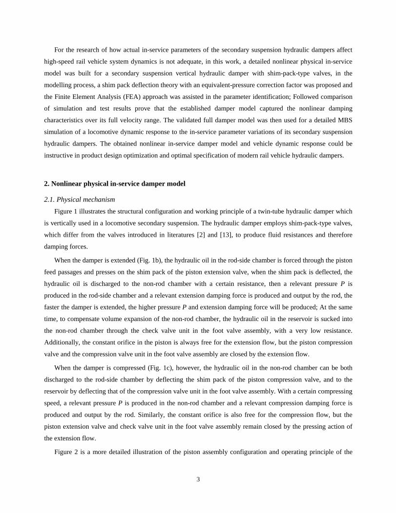
2.1. Physical mechanism Figure 1 illustrates the structural configuration and working principle of a twin-tube hydraulic damper which

is vertically used in a locomotive secondary suspension. The hydraulic damper employs shim-pack-type valves,

which differ from the valves introduced in literatures [2] and [13], to produce fluid resistances and therefore

damping forces.

When the damper is extended (Fig. 1b), the hydraulic oil in the rod-side chamber is forced through the piston

feed passages and presses on the shim pack of the piston extension valve, when the shim pack is deflected, the

hydraulic oil is discharged to the non-rod chamber with a certain resistance, then a relevant pressure P is

produced in the rod-side chamber and a relevant extension damping force is produced and output by the rod, the

faster the damper is extended, the higher pressure P and extension damping force will be produced; At the same

time, to compensate volume expansion of the non-rod chamber, the hydraulic oil in the reservoir is sucked into

the non-rod chamber through the check valve unit in the foot valve assembly, with a very low resistance.

Additionally, the constant orifice in the piston is always free for the extension flow, but the piston compression

valve and the compression valve unit in the foot valve assembly are closed by the extension flow.

When the damper is compressed (Fig. 1c), however, the hydraulic oil in the non-rod chamber can be both

discharged to the rod-side chamber by deflecting the shim pack of the piston compression valve, and to the

reservoir by deflecting that of the compression valve unit in the foot valve assembly. With a certain compressing

speed, a relevant pressure P is produced in the non-rod chamber and a relevant compression damping force is

produced and output by the rod. Similarly, the constant orifice is also free for the compression flow, but the

piston extension valve and check valve unit in the foot valve assembly remain closed by the pressing action of

the extension flow.

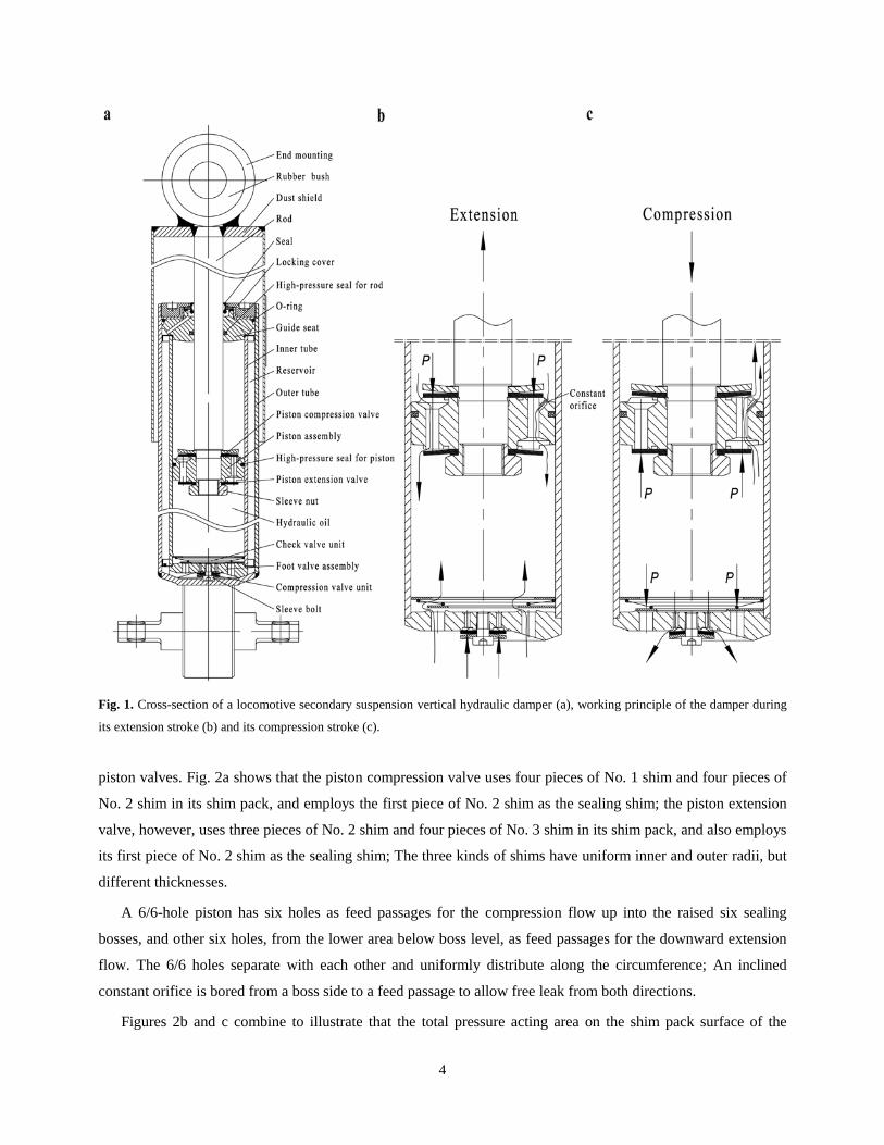
Figure 2 is a more detailed illustration of the piston assembly configuration and operating principle of the

4

Fig. 1. Cross-section of a locomotive secondary suspension vertical hydraulic damper (a), working principle of the damper during

its extension stroke (b) and its compression stroke (c).

piston valves. Fig. 2a shows that the piston compression valve uses four pieces of No. 1 shim and four pieces of

No. 2 shim in its shim pack, and employs the first piece of No. 2 shim as the sealing shim; the piston extension

valve, however, uses three pieces of No. 2 shim and four pieces of No. 3 shim in its shim pack, and also employs

its first piece of No. 2 shim as the sealing shim; The three kinds of shims have uniform inner and outer radii, but

different thicknesses.

A 6/6-hole piston has six holes as feed passages for the compression flow up into the raised six sealing

bosses, and other six holes, from the lower area below boss level, as feed passages for the downward extension

flow. The 6/6 holes separate with each other and uniformly distribute along the circumference; An inclined

constant orifice is bored from a boss side to a feed passage to allow free leak from both directions.

Figures 2b and c combine to illustrate that the total pressure acting area on the shim pack surface of the

5

Fig. 2. Exploded view of the piston assembly (a), cross-section and schematic pressure acting areas on the surface of the sealing

shim (No. 2 shim) (b), operating principle of the piston compression valve (c) and that of the piston extension valve (d).

piston compression valve, is the sum of the six projected areas of the six bosses on the sealing shim; In each

projected area, the central circular is a uniform-pressure acting area, and the irregular area outside the circle is a

nonlinear-decreasing-pressure acting area with zero marginal pressure. Fig. 2c shows that the shim pack will be

deflected against the rigid backing plate by the pressing action of the compression flow, and therefore discharge

the compression flow.

Operating principle of the piston extension valve (Fig. 2d) is similar to that of the piston compression valve,

the extension flow acting area and pressure distribution law on the shim pack, are the same as that of the

compression flow on the shim pack of the piston compression valve.

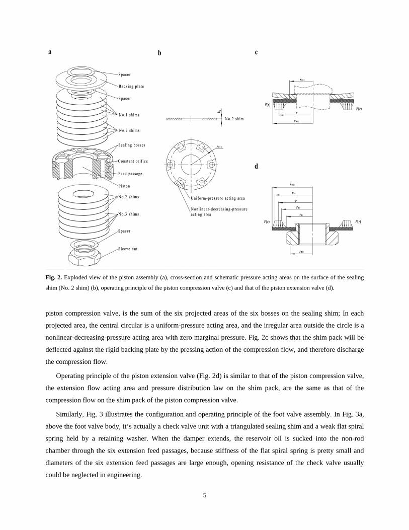
Similarly, Fig. 3 illustrates the configuration and operating principle of the foot valve assembly. In Fig. 3a,

above the foot valve body, it’s actually a check valve unit with a triangulated sealing shim and a weak flat spiral

spring held by a retaining washer. When the damper extends, the reservoir oil is sucked into the non-rod

chamber through the six extension feed passages, because stiffness of the flat spiral spring is pretty small and

diameters of the six extension feed passages are large enough, opening resistance of the check valve usually

could be neglected in engineering.

6

Fig. 3. Exploded view of the foot valve assembly (a), cross-section and schematic pressure acting areas on the surface of the sealing

shim (No. 4 shim) (b) and operating principle of the compression valve unit in the foot valve assembly (c).

When the damper is compressed, however, the compression flow closes the check valve first, thus, it can

only be forced through the central perforation of the check valve shim and into the six small compression feed

passages inside the inner edge seal, and press on the shim pack of the compression valve unit below the foot

valve body. As shown in Fig. 3a, the compression valve unit uses eight pieces of No. 4 shim in its shim pack,

and employs the first piece of No. 4 shim as the sealing shim.

Figures 3b and c combine to illustrate that there are three annulus areas on the surface of the sealing shim.

the middle larger annulus area is subjected to a continuous and uniform pressure, and the other two smaller

annulus areas are both subjected to continuous but nonlinear-decreasing pressures with zero marginal values. Fig.

3c shows that the shim pack will be deflected against the rigid backing plate by the compression flow, and

therefore discharge the compression flow.

2.2. Nonlinear modelling

2.2.1 Modelling scheme

This study borrows the nonlinear in-service damper model concept proposed in literature [13]. The proposed

nonlinear in-service damper model, which includes a nonlinear hydraulic damping element, a tandem stiffness of

oil, rubber bushes and fixing seats, and a small clearance element, is more detailed than the Maxwell [12]

damper model and proved to be more suitable for modern high-speed transit problems.

The approaches for modelling the damper motions and forces, the variable oil properties and the flow losses

of the secondary suspension vertical hydraulic damper, are similar to that introduced in [13]; For the valve

7

system configuration and operating mechanism are very different from that in previous papers, the valve system

dynamics has to be solved in specialty.

Figures 2b, c and d show that the pressure acting areas on the piston valve shim packs are discrete. In each

discrete acting area, the area outside the central circle is irregular, and the nonlinear-decreasing-pressure law

acting on it is hard to calculate; Although the pressure acting areas on the compression valve unit in the foot

valve assembly are continuous, as shown in Figs. 3b and c, the nonlinear-decreasing-pressure laws on the inner

and outer annuli are also difficult to solve. To be practical and cost-effective in engineering problem solving,

here employs the following modelling scheme.

(1) Theoretically solve out the shim pack deflection under a uniform pressure; Define an equivalent-pressure

correction factor for the same law to estimate the shim pack deflection under non-uniform pressure conditions.

(2) Calculate the shim pack deflections under the above two pressure conditions respectively, by using the

FEA approach; Validate the theoretical law of the shim pack deflection under a uniform pressure, then identify

the equivalent-pressure correction factor for estimating the shim pack deflection under real pressure conditions.

(3) Model the pressure-flow characteristics of the valve system.

2.2.2 Modelling the shim pack deflection

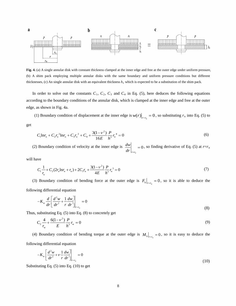
Figure 4a illustrates the bending model of a single annular disk with a constant thickness h, when clamped at

the inner edge rn and free at the outer edge rw and under a uniform pressure P. In the polar coordinate system

with the pole at the disk centre and polar radius coincides with the disk radius r, a curved surface differential

equation depicting the elastic deflection w(r) of the annular disk, can be deduced [15, 16] as

2 2

w 2 2

1 1d d dw dwK Pdr r dr dr r dr

+ + =

(1)

Where the bending stiffness Kw of the annular disk is given by 3

w 212(1 )EhK

ν=

− (2)

Eq. (2) indicates that for a given annular disk, the bending stiffness is a constant. General solution of Eq. (1) is given by

2 21 2 3 4( ) ln lnw r C r C r r C r C w∗= + + + + (3)

Where the sum of the first four members is the general solution of the corresponding homogeneous equation of

Eq. (1) and w* is a particular solution of Eq. (1). Because Kw and P are all independent of r, as shown in Eq. (1),

if assuming that w*=C5r4, then, substituting w*=C5r4 into Eq. (1) and solving out to get 2

4 43

w

3(1 )64 16

P Pw r rK E h

ν∗ −= = (4)

Thus, the general solution of Eq. (1) can be further described as

22 2 4

1 2 3 4 3

3(1 )( ) ln ln16

Pw r C r C r r C r C rE hν−

= + + + + (5)

8

Fig. 4. (a) A single annular disk with constant thickness clamped at the inner edge and free at the outer edge under uniform pressure,

(b) A shim pack employing multiple annular disks with the same boundary and uniform pressure conditions but different

thicknesses, (c) An single annular disk with an equivalent thickness he which is expected to be a substitution of the shim pack.

In order to solve out the constants C1, C2, C3 and C4 in Eq. (5), here deduces the following equations

according to the boundary conditions of the annular disk, which is clamped at the inner edge and free at the outer

edge, as shown in Fig. 4a.

(1) Boundary condition of displacement at the inner edge isn

( ) 0r r

w r=

= , so substituting rn into Eq. (5) to

get 2

2 2 41 n 2 n n 3 n 4 n3

3(1 )ln ln 016

PC r C r r C r C rE hν−

+ + + + = (6)

(2) Boundary condition of velocity at the inner edge is n

0r r

dwdr =

= , so finding derivative of Eq. (5) at r=rn

will have 2

31 2 n n n 3 n n3

n

1 3(1 )(2 ln ) 2 04

PC C r r r C r rr E h

ν−+ + + + = (7)

(3) Boundary condition of bending force at the outer edge is w

b 0r r

F=

= , so it is able to deduce the

following differential equation

w

2

w 2

1 0r r

d d w dwKdr dr r dr

=

− + =

(8) Thus, substituting Eq. (5) into Eq. (8) to concretely get

2

2 w3w

4 6(1 ) 0PC rr E h

ν−+ = (9)

(4) Boundary condition of bending torque at the outer edge is w

b 0r r

M=

= , so it is easy to deduce the

following differential equation

w

2

w 2

1 0r r

d w dwKdr r dr

ν=

− + =

(10) Substituting Eq. (5) into Eq. (10) to get

9

22

1 2 w 3 w2 3w

( 1) 3(1 )(3 )[2( +1)ln ( 3)] 2 ( +1) 04

PC C r C rr E h

ν ν νν ν ν − − +

+ + + + + =

(11)

Combining Eqs. (6), (7), (9) and (11) to solve out the constant coefficients C1~C4 of the general solution of

the homogeneous equation of Eq. (1), as

( )2

n1 2 2 3 3

4

r PC B B BB h

= − + +

(12)

2 1 3

PC Bh

=

(13)

( )2 33 3

42B B PC

B h+ =

(14)

and ( ) ( )22 3 n n

4 5 2 n 34

2ln 1ln

2B B r r PC B B r

B h + − = + +

(15)

Where the constant coefficients B1~B5 are

( )2 2w

1

3 12

rB

Eν −

= −

(16)

( ) ( )2 2 2

n 2n2 w n

3 12ln 1

2 2r rB r r

Eν −

= − +

(17)

( )( ) ( )

2 4w

3 w

3 1 ( 3)2 1 ln2 1 2

rB r

Eν ννν

− + = + + −

(18)

( )( )

2 24 w n

11

B r rνν

+= − −

(19)

and ( ) ( )2 2 2 2n w n n

5

3 1 8 ln16

r r r rB

Eν − −

=

(20)

Therefore, the general solution Eq. (5) can be further described as

22 2 4

1 2 3 4 3

w 3

3(1 )( ) ln ln16

Pw r C r C r r C r C rE h

PCh

ν −= + + + +

=

(21)

Where

( ) ( ) ( )

( ) ( )

2 22 34 2 n

w 1 2 2 34 4

22 3 n n

5 2 n4

3 1ln ln

16 2

2ln 1ln

2

B B rC r B r r B B B rE B B

B B r rB B r

B

ν− + = + + − + +

+ −

+ + +

(22)

10

Equation (22) indicates that, for a given annular disk, for parameters rn, rw, E and ν are all constants, Cw is a

function only of the radius r, in other words, Cw is independent of the pressure P and the disk thickness h. Thus,

Cw is an intrinsic characteristics of the disk and thus named as the disk deflection coefficient.

Thus, for a shim pack employs multiple annular disks with the same rn, rw, E and ν but different thicknesses

h1, h2, … hn, as shown in Fig. 4b, if assuming that a single annular disk, with the same rn, rw, E and ν but an

equivalent thickness he (Fig. 4c), could be a substitution of the shim pack in Fig. 4b, then it has

1 2 nw w w w3 3 3 3

1 2 n e

( ) ...p p p Pw r C C C Ch h h h

= = = = = (23)

and b 1 a 2 a n a a...F p A p A p A PA= + + + = (24)

Eq. (23) indicates that in Figs. 4b and c, every disk has the same deflection coefficient Cw and the same disk

deflection; Eq. (24), however, indicates that the sum of the bending forces of all the disks (Fig. 4b) equals to the

bending force of the equivalent disk (Fig. 4c).

Therefore, combining Eqs. (23) and (24) to solve out the deflection of a shim pack, as

w 3

e

( ) Pw r Ch

= (25)

Where 3 3 33e 1 2 n...h h h h= + + + (26)

By referring to Eq. (26), the equivalent thicknesses of the shim packs of the piston extension valve, the piston

compression valve and the compression valve unit in the foot valve assembly, are deduced as

3 33e1 2 33 4h h h= + (27)

3 33e2 1 24( )h h h= + (28)

and 33e3 4 48 2h h h= = (29)

Equation (25) is able to perform the deflection calculation of a shim pack under a uniform pressure; however,

to perform that of a shim pack under complex pressure conditions demonstrated in Figs. 2 and 3, here uses the

following estimation equation

e ew w e w3 3 3

e e e

( )( ) P C P Pw r C C C Ch h h

= = = (30)

Eq. (30) assumes that the deflection of a shim pack under non-uniform pressures equals to that of the same shim

pack under an equivalent uniform pressure Pe, so if defining Pe=CeP, then Ce is an equivalent-pressure

correction factor.

2.2.3 Validation and parameter identification of the shim pack deflection theory using FEA approach

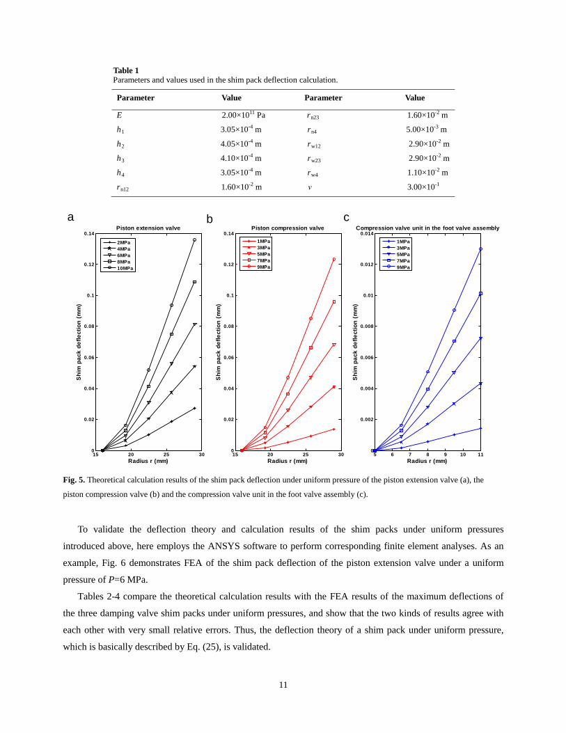
Based on Eq. (25) and the parameters and values list in Table 1, the shim pack deflections under uniform

pressures of the three damping valves are calculated and shown in Fig. 5; Fig. 5 demonstrates the nonlinear

elastic deflecting behaviour of the shim packs under uniform pressures.

11

Table 1 Parameters and values used in the shim pack deflection calculation.

Parameter Value Parameter Value

E 2.00×1011 Pa rn23 1.60×10-2 m

h1 3.05×10-4 m rn4 5.00×10-3 m

h2 4.05×10-4 m rw12 2.90×10-2 m

h3 4.10×10-4 m rw23 2.90×10-2 m

h4 3.05×10-4 m rw4 1.10×10-2 m

rn12 1.60×10-2 m ν 3.00×10-1

15 20 25 300

0.02

0.04

0.06

0.08

0.1

0.12

0.14Piston extension valve

Radius r (mm)

Shi

m p

ack

defle

ctio

n (m

m)

15 20 25 300

0.02

0.04

0.06

0.08

0.1

0.12

0.14Piston compression valve

Radius r (mm)

Shi

m p

ack

defle

ctio

n (m

m)

5 6 7 8 9 10 110

0.002

0.004

0.006

0.008

0.01

0.012

0.014Compression valve unit in the foot valve assembly

Radius r (mm)

Shi

m p

ack

defle

ctio

n (m

m)

2MPa4MPa6MPa8MPa10MPa



ba c

Fig. 5. Theoretical calculation results of the shim pack deflection under uniform pressure of the piston extension valve (a), the

piston compression valve (b) and the compression valve unit in the foot valve assembly (c).

To validate the deflection theory and calculation results of the shim packs under uniform pressures

introduced above, here employs the ANSYS software to perform corresponding finite element analyses. As an

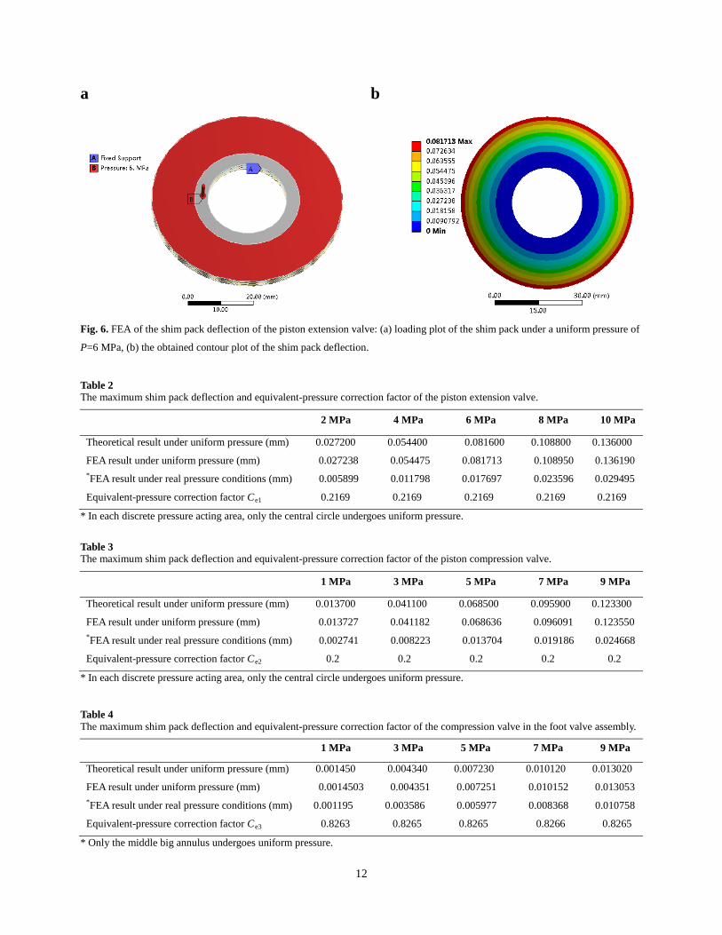
example, Fig. 6 demonstrates FEA of the shim pack deflection of the piston extension valve under a uniform

pressure of P=6 MPa.

Tables 2-4 compare the theoretical calculation results with the FEA results of the maximum deflections of

the three damping valve shim packs under uniform pressures, and show that the two kinds of results agree with

each other with very small relative errors. Thus, the deflection theory of a shim pack under uniform pressure,

which is basically described by Eq. (25), is validated.

12

a b

Fig. 6. FEA of the shim pack deflection of the piston extension valve: (a) loading plot of the shim pack under a uniform pressure of

P=6 MPa, (b) the obtained contour plot of the shim pack deflection.

Table 2 The maximum shim pack deflection and equivalent-pressure correction factor of the piston extension valve.

2 MPa 4 MPa 6 MPa 8 MPa 10 MPa

Theoretical result under uniform pressure (mm) 0.027200 0.054400 0.081600 0.108800 0.136000

FEA result under uniform pressure (mm) 0.027238 0.054475 0.081713 0.108950 0.136190 *FEA result under real pressure conditions (mm) 0.005899 0.011798 0.017697 0.023596 0.029495

Equivalent-pressure correction factor Ce1 0.2169 0.2169 0.2169 0.2169 0.2169

* In each discrete pressure acting area, only the central circle undergoes uniform pressure.

Table 3 The maximum shim pack deflection and equivalent-pressure correction factor of the piston compression valve.





* In each discrete pressure acting area, only the central circle undergoes uniform pressure.

Table 4 The maximum shim pack deflection and equivalent-pressure correction factor of the compression valve in the foot valve assembly.





* Only the middle big annulus undergoes uniform pressure.

13

To identify the equivalent-pressure correction factor Ce defined in Eq. (30), here continues to perform FEA

of the deflections of the three valve shim packs under real pressure conditions as that illustrated in Figs. 2 and 3.

As examples, Fig. 7 demonstrates the loading plots and the obtained deflection contour plots of the shim

packs of the piston extension valve and the compression valve unit in the foot valve assembly.

Fig. 7a shows that the piston extension valve shim pack is subjected to six identical discrete pressure

loadings. In each pressure acting area, the central circle undergoes a uniform pressure of P=2 MPa, and the outer

rectangle undergoes an assumed quadratic nonlinear-decreasing pressure from P=2 MPa to zero. Fig. 7a is

actually an approximate loading model of the piston extension valve shim pack, however, for the area outside the

central circle is small, Fig. 7a might not lose accuracy in engineering calculation.

a b

c d

Fig. 7. FEA of shim pack deflection under non-uniform pressure conditions: the loading plot (a) and the obtained deflection contour

plot (b) of the piston extension valve shim pack; the loading plot (c) and the obtained deflection contour plot (d) of the shim pack of

the compression valve unit in the foot valve assembly.

14

Similarly, Fig. 7c, shows the approximate loading conditions of the shim pack of the compression valve unit

in the foot valve assembly. The middle big annulus is subjected to a uniform pressure of P=3 MPa, and the small

outer annulus is subjected to an assumed quadratic nonlinear-decreasing pressure from P=3 MPa to zero, for the

inner annulus is pressed against the rigid backing plate, it is fixed in the analysis.

Tables 2-4 also list the concrete FEA results of the maximum deflections of the three damping valve shim

packs under approximate real pressure conditions. Thus, by using Eq. (30) and the datum in Tables 2-4, it is easy

to identify the equivalent-pressure correction factors for the three damping valves, if using the mean value, then

it has Ce1=0.2169, Ce2=0.2 and Ce3=0.8265.

2.2.4 Pressure-flow characteristics of the valve system

With the validated and parameter identified shim pack deflection theory, and by referring to Figs. 1-3, it is

easy to write the dynamic pressure-flow characteristics of the damping valve system, as

w23

w12

1 2 1 22

d1 c d2 w23 e1 w r3e1

1 2 1 22

valve d1 c d2 w12 e2 w 3e2

d2 w4

2 2+ 2 , if ( ) 0,4

2 2+ 24

+ 2

r r

r r

PC d P C r C C P x th

PQ C d P C r C C Ph

C r

π πr r

π πr r

π

=

=

≥

=

w4

1 2

e3 w b r3e3

2 ( ) , if ( ) 0.r rPC C P P x t

h r=

− <

(31)

Where the back pressure in the reservoir Pb was given in [13].

2.3. Experimental validation Damping characteristics of the hydraulic damper was simulated by using the established nonlinear physical

in-service model, the simulated key results are shown in Figs. 8, 9 and Table 5. In the simulation, the discharge

coefficient of the constant orifice Cd1 was specified to be 0.72 because the length to diameter ratio [17, 18] of the

orifice is between 0.5 and 4, the discharge coefficient of the shim packs Cd2 was specified to be 0.61 because the

deflected shim packs are actually sharp-edged hydraulic valve ports [17, 18]; The diameters of the rod, the piston

and the constant orifice are 28 mm, 69.8 mm and 2 mm, respectively; Additionally, values of some key

parameters are set to be that in normal conditions, such as the hydraulic oil temperature T=45℃, the entrained

air ratio [13] of oil at atmospheric pressure ε0=0.05%, the accumulated clearance at damper ends 2a=0 mm, and

the rubber attachment stiffness of damper Krubber=6×106 N/m.

For comparison, the bench test results of a sample secondary suspension vertical hydraulic damper are also

shown in Figs. 8, 9 and Table 5. The sampled hydraulic damper has just been repaired after a 2×105 kM service

journey.

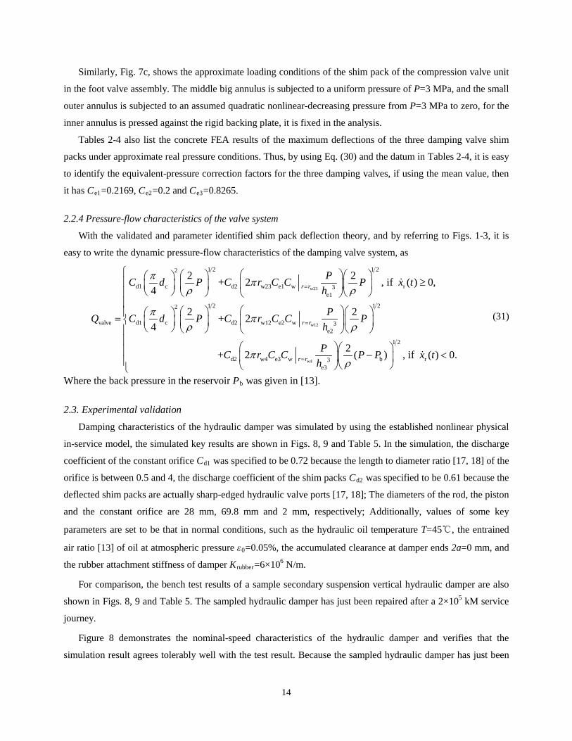
Figure 8 demonstrates the nominal-speed characteristics of the hydraulic damper and verifies that the

simulation result agrees tolerably well with the test result. Because the sampled hydraulic damper has just been

15

-30 -20 -10 0 10 20 30-1.5

-1

-0.5

0

0.5

1

1.5 x 104

Displacement [mm]

Dam

ping

forc

e [N

]

-0.1 -0.05 0 0.05 0.1-1.5

-1

-0.5

0

0.5

1

1.5 x 104

Velocity [m/s]D

ampi

ng fo

rce

[N]

SimulationTest

ba

Fig. 8. Nominal-speed force vs. displacement (F-s) characteristics (a) and force vs. velocity (F-v) characteristics (b) of the

secondary suspension vertical hydraulic damper, with a harmonic excitation of displacement amplitude ± 24.875 mm, frequency

0.64 Hz and velocity amplitude ± 0.1 m/s (other conditions: T=45℃, ε0=0.05%, 2a=0 mm, Krubber=6×106 N/m).

-30 -20 -10 0 10 20 30-2.5

-2

-1.5

-1

-0.5

0

0.5

1

1.5

2

2.5 x 104

Displacement [mm]

Dam

ping

forc

e [N

]

-0.3 -0.2 -0.1 0 0.1 0.2 0.3-2.5

-2

-1.5

-1

-0.5

0

0.5

1

1.5

2

2.5 x 104

Velocity [m/s]

Dam

ping

forc

e [N

]

SimulationTest

a b

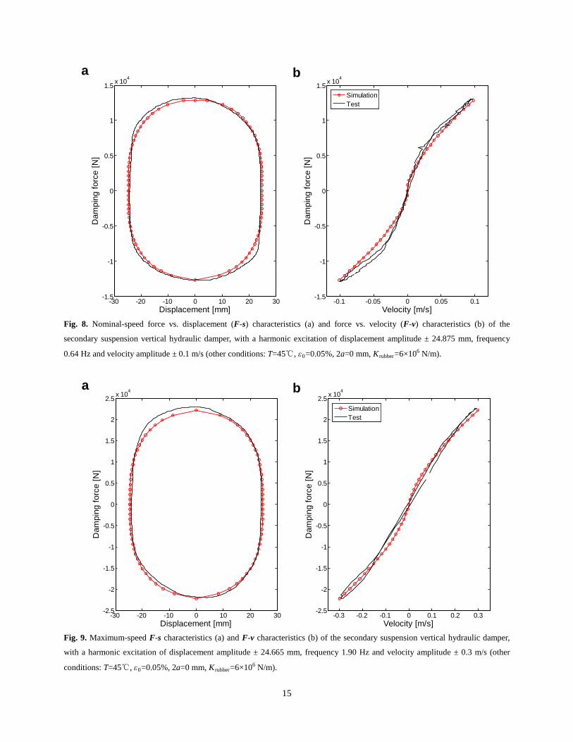
Fig. 9. Maximum-speed F-s characteristics (a) and F-v characteristics (b) of the secondary suspension vertical hydraulic damper,

with a harmonic excitation of displacement amplitude ± 24.665 mm, frequency 1.90 Hz and velocity amplitude ± 0.3 m/s (other

conditions: T=45℃, ε0=0.05%, 2a=0 mm, Krubber=6×106 N/m).

16

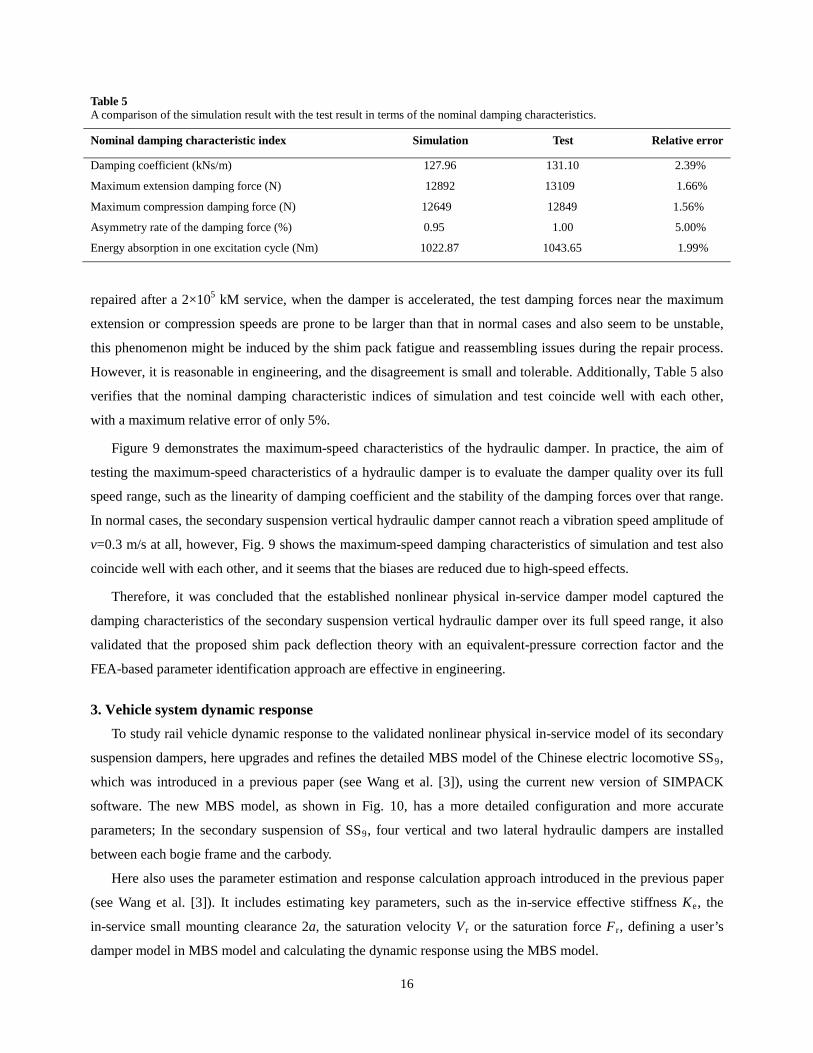
Table 5 A comparison of the simulation result with the test result in terms of the nominal damping characteristics.

Nominal damping characteristic index Simulation Test Relative error

Damping coefficient (kNs/m) 127.96 131.10 2.39%

Maximum extension damping force (N) 12892 13109 1.66%

Maximum compression damping force (N) 12649 12849 1.56%

Asymmetry rate of the damping force (%) 0.95 1.00 5.00%

Energy absorption in one excitation cycle (Nm) 1022.87 1043.65 1.99%

repaired after a 2×105 kM service, when the damper is accelerated, the test damping forces near the maximum

extension or compression speeds are prone to be larger than that in normal cases and also seem to be unstable,

this phenomenon might be induced by the shim pack fatigue and reassembling issues during the repair process.

However, it is reasonable in engineering, and the disagreement is small and tolerable. Additionally, Table 5 also

verifies that the nominal damping characteristic indices of simulation and test coincide well with each other,

with a maximum relative error of only 5%.

Figure 9 demonstrates the maximum-speed characteristics of the hydraulic damper. In practice, the aim of

testing the maximum-speed characteristics of a hydraulic damper is to evaluate the damper quality over its full

speed range, such as the linearity of damping coefficient and the stability of the damping forces over that range.

In normal cases, the secondary suspension vertical hydraulic damper cannot reach a vibration speed amplitude of

v=0.3 m/s at all, however, Fig. 9 shows the maximum-speed damping characteristics of simulation and test also

coincide well with each other, and it seems that the biases are reduced due to high-speed effects.

Therefore, it was concluded that the established nonlinear physical in-service damper model captured the

damping characteristics of the secondary suspension vertical hydraulic damper over its full speed range, it also

validated that the proposed shim pack deflection theory with an equivalent-pressure correction factor and the

FEA-based parameter identification approach are effective in engineering.

3. Vehicle system dynamic response To study rail vehicle dynamic response to the validated nonlinear physical in-service model of its secondary

suspension dampers, here upgrades and refines the detailed MBS model of the Chinese electric locomotive SS9,

which was introduced in a previous paper (see Wang et al. [3]), using the current new version of SIMPACK

software. The new MBS model, as shown in Fig. 10, has a more detailed configuration and more accurate

parameters; In the secondary suspension of SS9, four vertical and two lateral hydraulic dampers are installed

between each bogie frame and the carbody.

Here also uses the parameter estimation and response calculation approach introduced in the previous paper

(see Wang et al. [3]). It includes estimating key parameters, such as the in-service effective stiffness Ke, the

in-service small mounting clearance 2a, the saturation velocity Vr or the saturation force Fr, defining a user’s

damper model in MBS model and calculating the dynamic response using the MBS model.

17

Fig. 10. MBS model for simulating the Chinese electric locomotive SS9 dynamics.

3.1. Dynamic response on tangent track

3.1.1 Dynamic response to vertical damper parameter variations

Figure 11 shows the stochastic damping characteristics of a secondary suspension vertical hydraulic damper

when simulating the vehicle dynamics on tangent track. The small clearance 2a between the damper and its two

fixing seats is assumed to be 1 mm, which is common in engineering due to structural clearance and lack of

maintenance, so the stochastic F-s performance demonstrates 1 mm dead zone.

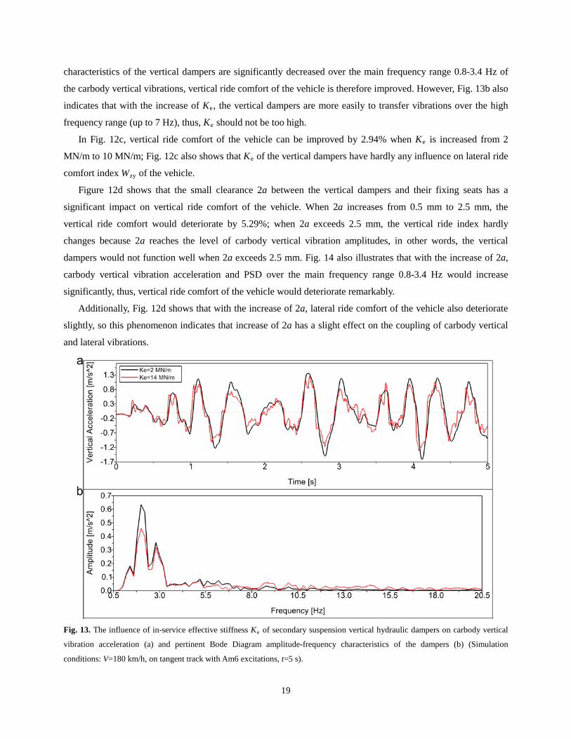
Figure 12 gives the results of vehicle ride comfort indices on tangent track versus key parameter variations of

its secondary suspension vertical hydraulic dampers. Figs. 12a and b show that vertical ride index Wzz increases

(it means the vertical ride comfort is getting worse) with the increase of damping coefficient C and saturation

velocity Vr of the vertical dampers, so both C and Vr should be appropriately specified, their values should be

neither too low which mean being insufficient for vibration reduction, nor too high which are prone to transfer

high frequency vibrations; In Fig. 12b, when Vr exceeds 0.05 m/s, which cannot be reached by the maximum

vertical vibration speed of the carbody, Wzz does not change any more, in other words, if Vr was specified too

high, saturation capability of the damper would not function well, and excessive damping forces would not be

relieved; Figs. 12a and b also show that both C and Vr of the vertical dampers have hardly any influences on

lateral ride comfort index Wzy of the vehicle.

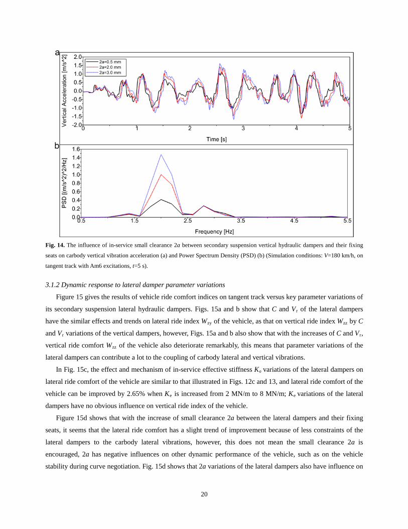
Figure 12c demonstrates that Wzz decreases (it means the vertical ride comfort is getting better) with the

increase of in-service effective stiffness Ke of the vertical dampers, and this effect can be easily interpreted by

Fig. 13. Fig. 13a shows that vertical vibration of the carbody is apparently reduced with the increase of Ke, thus,

vertical ride comfort of the vehicle is improved; Bode Diagram amplitude-frequency characteristics of the

vertical dampers, as shown in Fig. 13b, also illustrate that with the increase of Ke , vibration transfer

18

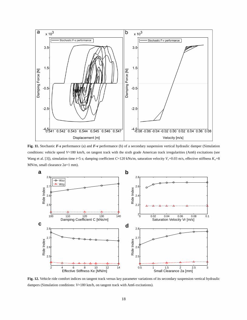
Fig. 11. Stochastic F-s performance (a) and F-v performance (b) of a secondary suspension vertical hydraulic damper (Simulation

conditions: vehicle speed V=180 km/h, on tangent track with the sixth grade American track irregularities (Am6) excitations (see

Wang et al. [3]), simulation time t=5 s; damping coefficient C=120 kNs/m, saturation velocity V r=0.03 m/s, effective stiffness Ke=8

MN/m, small clearance 2a=1 mm).

100 110 120 130 140

2.5

2.6

2.7

2.8

Damping Coefficient C [kNs/m]

Rid

e In

dex

0 0.02 0.04 0.06 0.08 0.12

2.2

2.4

2.6

2.8

Saturation Velocity Vr [m/s]

Rid

e In

dex

2 4 6 8 10 12 14

2.5

2.6

2.7

2.8

Effective Stiffness Ke [MN/m]

Rid

e In

dex

0.5 1 1.5 2 2.5 3

2.5

2.6

2.7

2.8

Small Clearance 2a [mm]

Rid

e In

dex

WzzWzy

d

ba

c

Fig. 12. Vehicle ride comfort indices on tangent track versus key parameter variations of its secondary suspension vertical hydraulic

dampers (Simulation conditions: V=180 km/h, on tangent track with Am6 excitations).

19

characteristics of the vertical dampers are significantly decreased over the main frequency range 0.8-3.4 Hz of

the carbody vertical vibrations, vertical ride comfort of the vehicle is therefore improved. However, Fig. 13b also

indicates that with the increase of Ke, the vertical dampers are more easily to transfer vibrations over the high

frequency range (up to 7 Hz), thus, Ke should not be too high.

In Fig. 12c, vertical ride comfort of the vehicle can be improved by 2.94% when Ke is increased from 2

MN/m to 10 MN/m; Fig. 12c also shows that Ke of the vertical dampers have hardly any influence on lateral ride

comfort index Wzy of the vehicle.

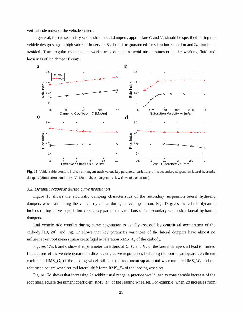
Figure 12d shows that the small clearance 2a between the vertical dampers and their fixing seats has a

significant impact on vertical ride comfort of the vehicle. When 2a increases from 0.5 mm to 2.5 mm, the

vertical ride comfort would deteriorate by 5.29%; when 2a exceeds 2.5 mm, the vertical ride index hardly

changes because 2a reaches the level of carbody vertical vibration amplitudes, in other words, the vertical

dampers would not function well when 2a exceeds 2.5 mm. Fig. 14 also illustrates that with the increase of 2a,

carbody vertical vibration acceleration and PSD over the main frequency range 0.8-3.4 Hz would increase

significantly, thus, vertical ride comfort of the vehicle would deteriorate remarkably.

Additionally, Fig. 12d shows that with the increase of 2a, lateral ride comfort of the vehicle also deteriorate

slightly, so this phenomenon indicates that increase of 2a has a slight effect on the coupling of carbody vertical

and lateral vibrations.

Fig. 13. The influence of in-service effective stiffness Ke of secondary suspension vertical hydraulic dampers on carbody vertical

vibration acceleration (a) and pertinent Bode Diagram amplitude-frequency characteristics of the dampers (b) (Simulation

conditions: V=180 km/h, on tangent track with Am6 excitations, t=5 s).

20

Fig. 14. The influence of in-service small clearance 2a between secondary suspension vertical hydraulic dampers and their fixing

seats on carbody vertical vibration acceleration (a) and Power Spectrum Density (PSD) (b) (Simulation conditions: V=180 km/h, on

tangent track with Am6 excitations, t=5 s).

3.1.2 Dynamic response to lateral damper parameter variations

Figure 15 gives the results of vehicle ride comfort indices on tangent track versus key parameter variations of

its secondary suspension lateral hydraulic dampers. Figs. 15a and b show that C and Vr of the lateral dampers

have the similar effects and trends on lateral ride index Wzy of the vehicle, as that on vertical ride index Wzz by C

and Vr variations of the vertical dampers, however, Figs. 15a and b also show that with the increases of C and Vr,

vertical ride comfort Wzz of the vehicle also deteriorate remarkably, this means that parameter variations of the

lateral dampers can contribute a lot to the coupling of carbody lateral and vertical vibrations.

In Fig. 15c, the effect and mechanism of in-service effective stiffness Ke variations of the lateral dampers on

lateral ride comfort of the vehicle are similar to that illustrated in Figs. 12c and 13, and lateral ride comfort of the

vehicle can be improved by 2.65% when Ke is increased from 2 MN/m to 8 MN/m; Ke variations of the lateral

dampers have no obvious influence on vertical ride index of the vehicle.

Figure 15d shows that with the increase of small clearance 2a between the lateral dampers and their fixing

seats, it seems that the lateral ride comfort has a slight trend of improvement because of less constraints of the

lateral dampers to the carbody lateral vibrations, however, this does not mean the small clearance 2a is

encouraged, 2a has negative influences on other dynamic performance of the vehicle, such as on the vehicle

stability during curve negotiation. Fig. 15d shows that 2a variations of the lateral dampers also have influence on

21

vertical ride index of the vehicle system.

In general, for the secondary suspension lateral dampers, appropriate C and Vr should be specified during the

vehicle design stage, a high value of in-service Ke should be guaranteed for vibration reduction and 2a should be

avoided. Thus, regular maintenance works are essential to avoid air entrainment in the working fluid and

looseness of the damper fixings.

70 80 90 100 110

2

2.2

2.4

2.6


Rid

e In

dex

0 0.02 0.04 0.06 0.08 0.1

2

2.2

2.4

2.6


Rid

e In

dex

2 4 6 8 10 12

2

2.2

2.4

2.6


Rid

e In

dex

0.5 1 1.5 2 2.5 3

2

2.2

2.4

2.6


Rid

e In

dex

WzzWzy

a

c

b

d

Fig. 15. Vehicle ride comfort indices on tangent track versus key parameter variations of its secondary suspension lateral hydraulic

dampers (Simulation conditions: V=180 km/h, on tangent track with Am6 excitations).

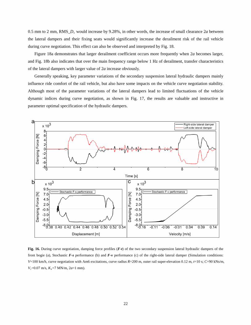
3.2. Dynamic response during curve negotiation

Figure 16 shows the stochastic damping characteristics of the secondary suspension lateral hydraulic

dampers when simulating the vehicle dynamics during curve negotiation; Fig. 17 gives the vehicle dynamic

indices during curve negotiation versus key parameter variations of its secondary suspension lateral hydraulic

dampers.

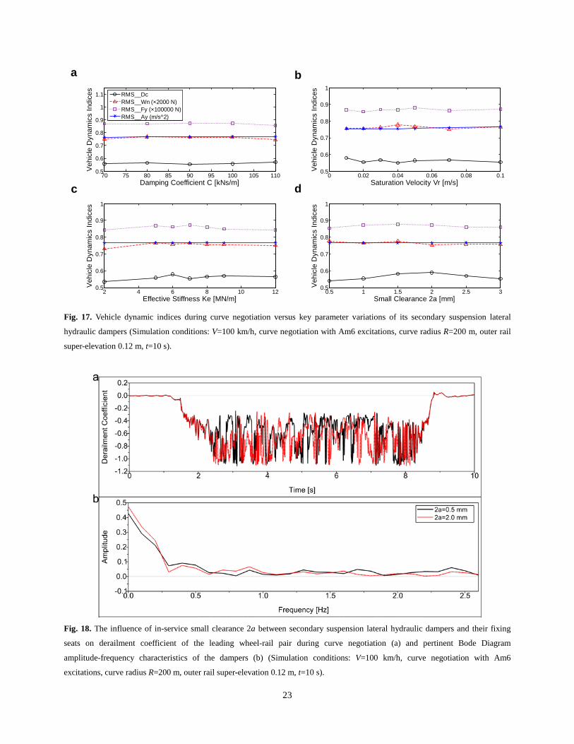
Rail vehicle ride comfort during curve negotiation is usually assessed by centrifugal acceleration of the

carbody [19, 20], and Fig. 17 shows that key parameter variations of the lateral dampers have almost no

influences on root mean square centrifugal acceleration RMS_Ay of the carbody.

Figures 17a, b and c show that parameter variations of C, Vr and Ke of the lateral dampers all lead to limited

fluctuations of the vehicle dynamic indices during curve negotiation, including the root mean square derailment

coefficient RMS_Dc of the leading wheel-rail pair, the root mean square total wear number RMS_Wn and the

root mean square wheelset-rail lateral shift force RMS_Fy of the leading wheelset.

Figure 17d shows that increasing 2a within usual range in practice would lead to considerable increase of the

root mean square derailment coefficient RMS_Dc of the leading wheelset. For example, when 2a increases from

22

0.5 mm to 2 mm, RMS_Dc would increase by 9.28%, in other words, the increase of small clearance 2a between

the lateral dampers and their fixing seats would significantly increase the derailment risk of the rail vehicle

during curve negotiation. This effect can also be observed and interpreted by Fig. 18.

Figure 18a demonstrates that larger derailment coefficient occurs more frequently when 2a becomes larger,

and Fig. 18b also indicates that over the main frequency range below 1 Hz of derailment, transfer characteristics

of the lateral dampers with larger value of 2a increase obviously.

Generally speaking, key parameter variations of the secondary suspension lateral hydraulic dampers mainly

influence ride comfort of the rail vehicle, but also have some impacts on the vehicle curve negotiation stability.

Although most of the parameter variations of the lateral dampers lead to limited fluctuations of the vehicle

dynamic indices during curve negotiation, as shown in Fig. 17, the results are valuable and instructive in

parameter optimal specification of the hydraulic dampers.

Fig. 16. During curve negotiation, damping force profiles (F-t) of the two secondary suspension lateral hydraulic dampers of the

front bogie (a), Stochastic F-s performance (b) and F-v performance (c) of the right-side lateral damper (Simulation conditions:

V=100 km/h, curve negotiation with Am6 excitations, curve radius R=200 m, outer rail super-elevation 0.12 m, t=10 s; C=90 kNs/m,

V r=0.07 m/s, Ke=7 MN/m, 2a=1 mm).

23

70 75 80 85 90 95 100 105 1100.5

0.6

0.7

0.8

0.9

1

1.1


Veh

icle

Dyn

amic

s In

dice

s

0 0.02 0.04 0.06 0.08 0.10.5

0.6

0.7

0.8

0.9

1


Veh

icle

Dyn

amic

s In

dice

s

2 4 6 8 10 120.5

0.6

0.7

0.8

0.9

1


Veh

icle

Dyn

amic

s In

dice

s

0.5 1 1.5 2 2.5 30.5

0.6

0.7

0.8

0.9

1


Veh

icle

Dyn

amic

s In

dice

s

RMS__DcRMS__Wn (×2000 N)RMS__Fy (×100000 N)RMS__Ay (m/s^2)

a

c

b

d

Fig. 17. Vehicle dynamic indices during curve negotiation versus key parameter variations of its secondary suspension lateral

hydraulic dampers (Simulation conditions: V=100 km/h, curve negotiation with Am6 excitations, curve radius R=200 m, outer rail

super-elevation 0.12 m, t=10 s).

Fig. 18. The influence of in-service small clearance 2a between secondary suspension lateral hydraulic dampers and their fixing

seats on derailment coefficient of the leading wheel-rail pair during curve negotiation (a) and pertinent Bode Diagram

amplitude-frequency characteristics of the dampers (b) (Simulation conditions: V=100 km/h, curve negotiation with Am6

excitations, curve radius R=200 m, outer rail super-elevation 0.12 m, t=10 s).

24

4. Conclusions (1) A detailed nonlinear physical in-service model was built assisted by FEA approach for the secondary

suspension vertical hydraulic damper with shim-pack-type valves, followed comparison of simulation and test

results proves the established damper model captured the nonlinear damping characteristics over a full velocity

range, and thus also proves that the proposed shim pack deflection theory with an equivalent-pressure correction

factor and the FEA-based parameter identification approach are effective.

(2) Key in-service parameter variations of the vertical damper mainly influence the vertical ride comfort, and

that of the lateral damper mainly influence the lateral ride comfort. However, most of the parameter variations of

the lateral damper contribute a lot to the coupling of carbody lateral and vertical vibrations, and therefore have

also significant influences on the vertical ride comfort. Additionally, key in-service parameter variations of the

lateral damper also have some impacts on the vehicle curve negotiation stability.

(3) Both C and V r of the secondary suspension hydraulic dampers should be optimally specified, their values

should be neither too low nor too high; a high value of in-service Ke should be always guaranteed for vibration

reduction and 2a should be always avoided. Thus, regular maintenance works are essential to avoid air

entrainment in the working fluid and looseness of the damper fixings.

The nonlinear physical in-service damper model and the vehicle dynamic response characteristics obtained in

this research could be used in product design optimisation and optimal specification of high-speed rail hydraulic

dampers.

Acknowledgement

The authors thank financial supports from the National Natural Science Foundation of China (NSFC) under

Grant No. 11572123 and the State Key Laboratory for Strength and Vibration of Mechanical Structures of China

under Project No. SV2016-KF-05.

References

[1] A.C. Mellado, E. Gómez, J. Viñolas, Advances on railway yaw damper characterisation exposed to small displacements, Int. J.

Heavy Veh. Syst. 13 (4) (2006) 263–280.

[2] W.L. Wang, Y. Huang, X.J. Yang, G.X. Xu, Nonlinear parametric modeling of a high-speed rail hydraulic yaw damper with

series clearance and stiffness, Nonlinear Dyn. 65 (1–2) (2011) 13–34.

[3] W.L. Wang, D.S. Yu, Y. Huang, Z. Zhou, R. Xu, A locomotive’s dynamic response to in-service parameter variations of its

hydraulic yaw damper, Nonlinear Dyn. 77 (4) (2014) 1485–1502.

[4] R.V. Kasteel, C.G. Wang, L.X. Qian, J.Z. Liu, G.H. Ye, A new shock absorber model for use in vehicle dynamics studies, Veh.

Syst. Dyn. 43 (9) (2005) 613–631.

[5] A. Farjoud, M. Ahmadian, M. Craft, W. Burke, Nonlinear modeling and experimental characterization of hydraulic dampers:

effects of shim stack and orifice parameters on damper performance, Nonlinear Dyn. 67 (2) (2012) 1437–1456.

[6] A. Simms, D. Crolla, The influence of damper properties on vehicle dynamic behavior, SAE Paper, 2002–01–0319.

[7] J.A. Calvo, B. López-Boada, J.L.S. Román, A. Gauchía, Influence of a shock absorber model on vehicle dynamic simulation,

25

Proc. Inst. Mech. Eng. Part D: J. Automob. Eng. 223 (2) (2009) 189–202.

[8] C.K. Park, Y.G. Kim, D.S. Bae, Sensitivity analysis of suspension characteristics for Korean high speed train, J. Mech. Sci.

Tech. 23 (2009) 938–941.

[9] N.C. Shieh, C.L. Lin, Y.C. Lin, K.Z. Liang, Optimal design for passive suspension of a light rail vehicle using constrained

multiobjective evolutionary search, J. Sound Vib. 285(1–2) (2005) 407–424.

[10] Y.P. He, J. Mcphee, Multidisciplinary optimization of multibody systems with application to the design of rail vehicles,

Multibody Syst. Dyn. 14 (2005) 111–135.

[11] J.H. Hao, J. Zeng, P.B. Wu, Vertical stochastic vibration reduction and suspension parameters optimization of a railway

passenger car, J. China Railway Society 28(6) (2006) 35–40. (In Chinese)

[12] European Standard: Railway Applications – Suspension Components – Hydraulic Dampers, EN 13802:2013.

[13] W.L. Wang, D.S. Yu, Z. Zhou, In-service parametric modelling a rail vehicle’s axle-box hydraulic damper for high-speed

transit problems, Mech. Syst. Signal Process. 62–63 (2015) 517–533.

[14] W.L. Wang, D.S. Yu, S. Iwnicki, Nonlinear optimal specification of a locomotive axle-box hydraulic damper for vibration

reduction and track-friendliness, Proceedings of the 24th Symposium of the International Association for Vehicle System

Dynamics, pp. 1471-1480, August 17-21, 2015, Graz, Austria.

[15] A.P. Boresi, K.P. Chong, J.D. Lee, Elasticity in Engineering Mechanics (3rd edition), John Wiley & Sons, INC., Hoboken,

New Jersey, USA, 2011.

[16] C.C. Zhou, Theory and Design of Automotive Shock Absorber, Beijing University Press, Beijing, China, 2012. (In Chinese)

[17] M.G. Rabie, Fluid Power Engineering. The McGraw-Hill Companies, Inc., New York, USA, 2009.

[18] J.C. Dixon, The Shock Absorber Handbook, John Wiley & Sons, Ltd., West Sussex, England, 2007.

[19] Chinese Railway Society Standard, Evaluation methods and criteria for dynamics performance test of railway locomotives,

TB/T 2360-93, 1993. (In Chinese)

[20] S. Iwnicki, Handbook of Railway Vehicle Dynamics, Taylor & Francis Group, Abingdon, England, 2006.

A SYMMETRICAL FINITE ELEMENT MODEL FOR - CORE

Documents

Transcript of A SYMMETRICAL FINITE ELEMENT MODEL FOR - CORE