Linear dependency between ε and the input noise in ε-support vector regression

544 IEEE TRANSACTIONS ON NEURAL NETWORKS, VOL. 14, NO. 3, MAY 2003

Linear Dependency Between� and the Input Noise in�-Support Vector Regression

James T. Kwok and Ivor W. Tsang

Abstract—In using the -support vector regression ( -SVR)algorithm, one has to decide a suitable value for the insensitivityparameter . Smola et al. considered its “optimal” choice bystudying the statistical efficiency in a location parameter estima-tion problem. While they successfully predicted a linear scalingbetween the optimal and the noise in the data, their theoreticallyoptimal value does not have a close match with its experimentallyobserved counterpart in the case of Gaussian noise. In this paper,we attempt to better explain their experimental results by studyingthe regression problem itself. Our resultant predicted choice ofis much closer to the experimentally observed optimal value, whileagain demonstrating a linear trend with the input noise.

Index Terms—Support vector machines (SVMs), support vectorregression.

I. INTRODUCTION

I N recent years, the use of support vector machines (SVMs)on various classification and regression problems have been

increasingly popular. SVMs are motivated by results fromstatistical learning theory and, unlike other machine learningmethods, their generalization performance does not dependon the dimensionality of the problem [3], [24]. In this paper,we focus on regression problems and consider the-supportvector regression (-SVR) algorithm [4], [20] in particular. The-SVR has produced the best result on a timeseries prediction

benchmark [11], as well as showing promising results in anumber of different applications [7], [12], [22].

One issue about-SVR is how to set the insensitivity param-eter . Data-resampling techniques such as cross-validation canbe used [11], though they are usually very expensive in termsof computation and/or data. A more efficient approach is to usea variant of the SVR algorithm called-support vector regres-sion ( -SVR) [17]. By using another parameterto trade off

with model complexity and training accuracy,-SVR allowsthe value of to be automatically determined. Moreover, it canbe shown that represents an upper bound on the fraction oftraining errors and a lower bound on the fraction of supportvectors. Thus, in situations where some prior knowledge on thevalue of is available, using -SVR may be more convenientthan -SVR. Another approach is to consider the theoretically“optimal” choice of . Smolaet al.[19] tackled this by studyingthe simpler location parameter estimation problem and derivedthe asymptotically optimal choice ofby maximizing statistical

Manuscript received February 13, 2002; revised November 13, 2002.The authors are with the Department of Computer Science, Hong Kong

University of Science and Technology, Clear Water Bay, Hong Kong (e-mail:[email protected]; [email protected]).

Digital Object Identifier 10.1109/TNN.2003.810604

efficiency. They also showed that this optimal value scales lin-early with the noise in the data, which is confirmed in the exper-iment. However, in the case of Gaussian noise, their predictedvalue of this optimal does not have a close match with theirexperimentally observed value.

In this paper, we attempt to better explain their experimentalresults. Instead of working on the location parameter estimationproblem as in [19], our analysis will be based on the original-SVR formulation. The rest of this paper is organized as fol-

lows. Brief introduction to the-SVR is given in Section II. Theanalysis of the linear dependency betweenand the input noiselevel is given in Section III, while the last section gives someconcluding remarks.

II. -SVR

In this section, we introduce some basic notations for-SVR.Interested readers are referred to [3], [20], [24] for more com-plete reviews.

Let the training set be , with inputand output . In -SVR, is first mapped to ina Hilbert space (with inner product ) via a nonlinear map

. This space is often called thefeature spaceand its dimensionality is usually very high (sometimes infinite).Then, a linear function is constructed in

such that it deviates least from the training data according toVapnik’s -insensitive loss function

ifotherwise

while at the same time is as “flat” as possible (i.e., is assmall as possible). Mathematically, this means

minimize

subject to (1)

where is a user-defined constant. It is well known that (1) canbe transformed to the following quadratic programming (QP)problem:

maximize

(2)

1045-9227/03$17.00 © 2003 IEEE

KWOK AND TSANG: LINEAR DEPENDENCY 545

subject to

and

However, recall that the dimensionality of and thus also ofand , is usually very high. Hence, in order for this

approach to be practical, a key characteristic of-SVR andkernel methods in general, is that one can obtainin (2) without having to explicitly obtain and first.This is achieved by using akernelfunction such that

(3)

For example, the -order polynomial kernelcorresponds to a map into the space spanned by

all products of exactly order of [24]. More generally, itcan be shown that any function satisfying Mercer’s theoremcan be used as kernel and each will have an associated mapsuch that (3) holds [24]. Computationally,-SVR (and kernelmethods in general) also has the important advantage that onlyquadratic programming1 and not nonlinear optimization, isinvolved. Thus, the use of kernels provides an elegant nonlineargeneralization of many existing linear algorithms [2], [3], [10],[16].

III. L INEAR DEPENDENCY BETWEEN AND THE

INPUT NOISE PARAMETER

In order to derive a linear dependency betweenand the scaleparameter of the input noise model, Smolaet al.[19] consideredthe simpler problem of estimating the univariate location param-eter from a set of data points

Here, s are i.i.d. noise belonging to some distribution .Using the Cramer-Rao information inequality for unbiased es-timators, the maximum likelihood estimator ofwith an “op-timal” value of was then obtained by maximizing its statisticalefficiency.

In this paper, instead of working on the location parameterestimation problem, we study the regression problem of esti-mating the (possibly multivariate) weight parametergiven aset of , with

(4)

Here, follows distribution and follows distribu-tion . The corresponding density function onis denoted

. Notice that the bias term has beendropped here for simplicity and this is equivalent to assumingthat the s have zero mean. Moreover, using the notation inSection II, in general one can replacein (4) byin feature space and thus recovers the original-SVR setting.Besides, while the work in [19] is based on maximum likelihoodestimation, it is now well known that-SVR is related instead to

1The SVM problem can also be formulated as a linear programming problem[9], [18] instead of a quadratic programming problem.

maximuma posteriori(MAP) estimation. As discussed in [14],[20], [21], the -insensitive loss function leads to the followingprobability density function on

(5)

Notice that [14], [20], [21] do not have the factorin (5), butis introduced here to play the role of controlling the noise level2

[6]. With the Gaussian prior3 on

and on applying the Bayes rule,, we obtain

const (6)

On setting , the optimization problem in (1) can beinterpreted as finding the MAP estimate ofat given values of

and .

A. Estimating the Optimal Values ofand

In general, the MAP estimate in (6) depends on the partic-ular training set and a closed-form solution is difficult to obtain.To simplify the analysis, we replace in(6) by its expectation

Equation (6) thus becomes

const (7)

On setting its partial derivative with respect toto zero, it canbe shown that has to satisfy

(8)

2To be more precise, we will show in Section III-B that the optimal value of� is inversely proportional to the noise level of the input noise model.

3In this paper,� and� are regarded as hyperparameters while� is treated as aconstant. Thus, dependence on� will not be explicitly mentioned in the sequel.


To find suitable values for the hyperparametersand , we usethe method of type II maximum likelihood prior4 (ML-II) inBayesian statistics [1]. The ML-II solutions ofand are thosethat maximize , which can be obtained by integratingout

where is the width of the integrand andmeasures the posterior uncertainty of. Assuming that the con-tributions due to are comparable at different values ofand, maximizing with respect to and thus becomes

maximizing . This is the same as maximizing, or approximately. Differentiating

(7) with respect to and and then using (8), we have

(9)

and

(10)

respectively. Setting (9) and (10) to zero, we obtain

(11)

4Notice that MacKay’s evidence framework [8], which has been popularlyused in the neural networks community, is computationally equivalent to theML-II method.

and

(12)

These can then be used to solve forand .

B. Applications to Some Common Noise Models

Recall that the -insensitive loss function implicitly corre-sponds to the noise model in (5). Of course, in cases where theunderlying noise model of a particular data set is known, theloss function should be chosen such that it has a close matchwith this known noise model, while at the same time ensuringthat the resultant optimization problem can still be solved ef-ficiently. It is thus possible that the-insensitive loss functionmay not be best. For example, when the noise model is knownto be Gaussian, the corresponding loss function is the squaredloss function and the resultant model becomes a regularizationnetwork [5], [13].5 However, an important advantage of-SVRusing the -insensitive loss function, just like SVMs using thehinge loss in classification problems, is that sparseness of thedual variables can be ensured. On the contrary, sparseness willbe lost if the squared loss function is used instead. Thus, even forGaussian noise, the-insensitive loss function is sometimes stilldesirable and the resultant performance is often very competi-tive. In this section, by solving (11) and (12), we will show thatthere is always a linear relationship between the optimal valueof and the noise level, even when the true noise model is dif-ferent from (5). As in [19], three commonly used noise models,namely the Gaussian, Laplacian, and uniform models, will bestudied.

1) Gaussian Noise:For the Gaussian noise model

where is the standard deviation. Defineand

. It can be shown that (11) and (12)reduce to

erfc erfc(13)

and

erfc erfc

(14)

where erfc is the complementaryerror function [15]. Substituting (13) into (14) and after per-forming the integration,6 it can be shown thatalways appearsas the factor in the solution and, thus, there is always a linearrelationship between the optimal values ofand .

5This is sometimes also called the least-squares SVM [23] in the SVM liter-ature.

6Here, the integration is performed by using the symbolic math toolbox ofMatlab.


Fig. 1. Objective functionh(�=�) to be minimized in the case of Gaussian noise.

If we assume that

(15)

and also that the variation of with is small,7 then maximizingin (7) is effectively the same as minimizing

, which is the same as minimizing8

erfc

erfc

(16)

7Notice that from (8), we have

@w

@�=

�

�NI+ xx p w x� �jx

+ p w x+ �jx p(x)dx

� x p w x � �jx

�p w x+ �jx p(x)dx

whereI is the identity matrix.@w=@� thus involves the difference of two verysimilar terms and will be small.

8More detailed derivations are in the Appendix.

A plot of is shown in Fig. 1. Its minimum can be obtainednumerically as

(17)

By substituting (15), (17) into (29), we can also obtain theoptimal value of as . This confirms the role of

in controlling the noise variance, as mentioned in Section III.In the following, we repeat an experiment in [19] to verify

this ratio of . The target function to be learned issinc . The training set consists of 200s drawn inde-

pendently from a uniform distribution on [1, 1] and the corre-sponding outputs have Gaussian noise added. Testingerror is obtained by directly integrating the squared differencebetween the true target function and the estimated function overthe range [ 1, 1]. As in [19], the model selection problem forthe regularization parameter in (1) is side-stepped by alwayschoosing the value of that yields the smallest testing error.The whole experiment is repeated 40 times and the spline kernelwith an infinite number of knots is used.

Fig. 2 shows the linear relationship of obtainedfrom the experiment. This is close to the value ofobtained in the experiment in [19] and is also in good agreementwith our predicted ratio of . In comparison, thetheoretical results in [19] suggest the “optimal” choice of

.2) Laplacian Noise:Next, we consider the Laplacian noise

model

Here, we only consider the simpler case whenis one-dimen-sional, with uniform density over the range [ , ] (i.e.,


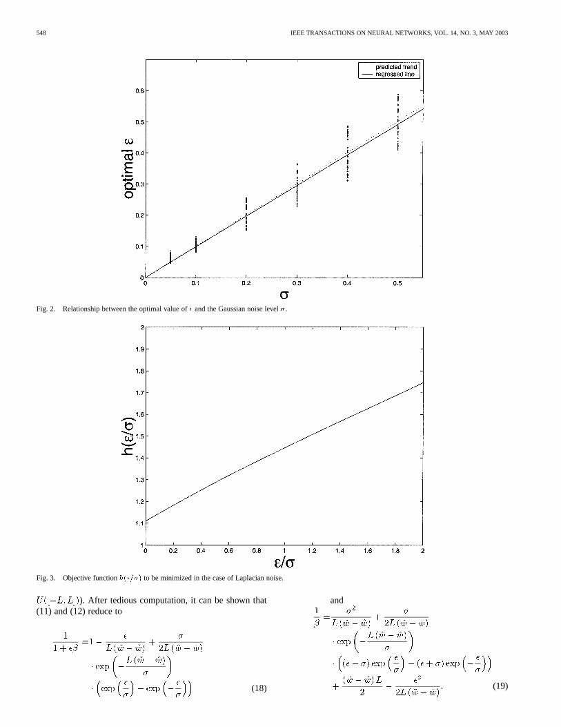
Fig. 2. Relationship between the optimal value of� and the Gaussian noise level�.

Fig. 3. Objective functionh(�=�) to be minimized in the case of Laplacian noise.

). After tedious computation, it can be shown that(11) and (12) reduce to

(18)

and

(19)


(a)

(b)

Fig. 4. Relationship between the optimal value of� and the Laplacian noise level�. (a) One-dimensionalx: (b) Two-dimensionalx:

Substituting (19) back into (18), we notice again thatalwaysappears in the factor and thus there is always a linear rela-tionship between the optimal value ofand under the Lapla-cian noise. Recall that the variance for the uniform distribution

is and that for the exponential distribution9

9The density function of the exponential distribution� � Expon(�) isp(�) = � exp(��) (where� > 0; � � 0).

is . As in Section III-B1, we considerand assume that

. With , we also obtain .Consequently

(20)


Fig. 5. Scenario whenL > � + �= ~w � w in the case of uniform noise.

and hence

(21)

Analogous to Section III-B1, by plugging in (18), (19), and (21),it can be shown that the problem reduces to minimizing (Fig. 3)as shown in the equation at the bottom of the page. Again, thesolution can be obtained numerically as , which was alsoobtained in [19]. Notice that this is intuitively correct as the den-sity function in (5) degenerates to the Laplacian density when

. Moreover, we can also obtain the optimal value ofas, again showing that is inversely proportional

to the noise level of the Laplacian noise model.To verify the ratio of , we repeat the experiment in Sec-

tion III-B1 but with the Laplacian noise instead. More-over, as our analysis applies only whenis one dimensional,we also investigate experimentally the optimal value ofin thetwo-dimensional case. The ratios obtained for the one- and two-dimensional cases are and , respec-tively (Fig. 4), which are close to our prediction of .

3) Uniform Noise: Finally, we consider the uniform noisemodel

(22)

whereifotherwise.

is the indicator function.

Again, we only consider the simpler case whenis one-dimen-

sional, with uniform density over the range [ , ]. Moreover,only the case whenwill be discussed here. Derivation for the case when

is similar. Whereas, for(i.e., ), the corresponding SVR solution willbe very poor (Fig. 5) and thus usually not the case of interest.

It can be shown that (11) and (12) reduce to

and

(23)

Combining and simplifying, we have. Substituting back into (23), we

obtain

(24)

Again, we notice that always appears in the factor and,thus, there is also a linear relationship between the optimal valueof and in the case of uniform noise.

As in Section III-BI, consider and assumethat . Using (20) again,we obtain . On substituting back into (24) andproceed as in Section III-BI, we obtain, after tedious computa-tion, . This is intuitively correct since the density function


(a)

(b)

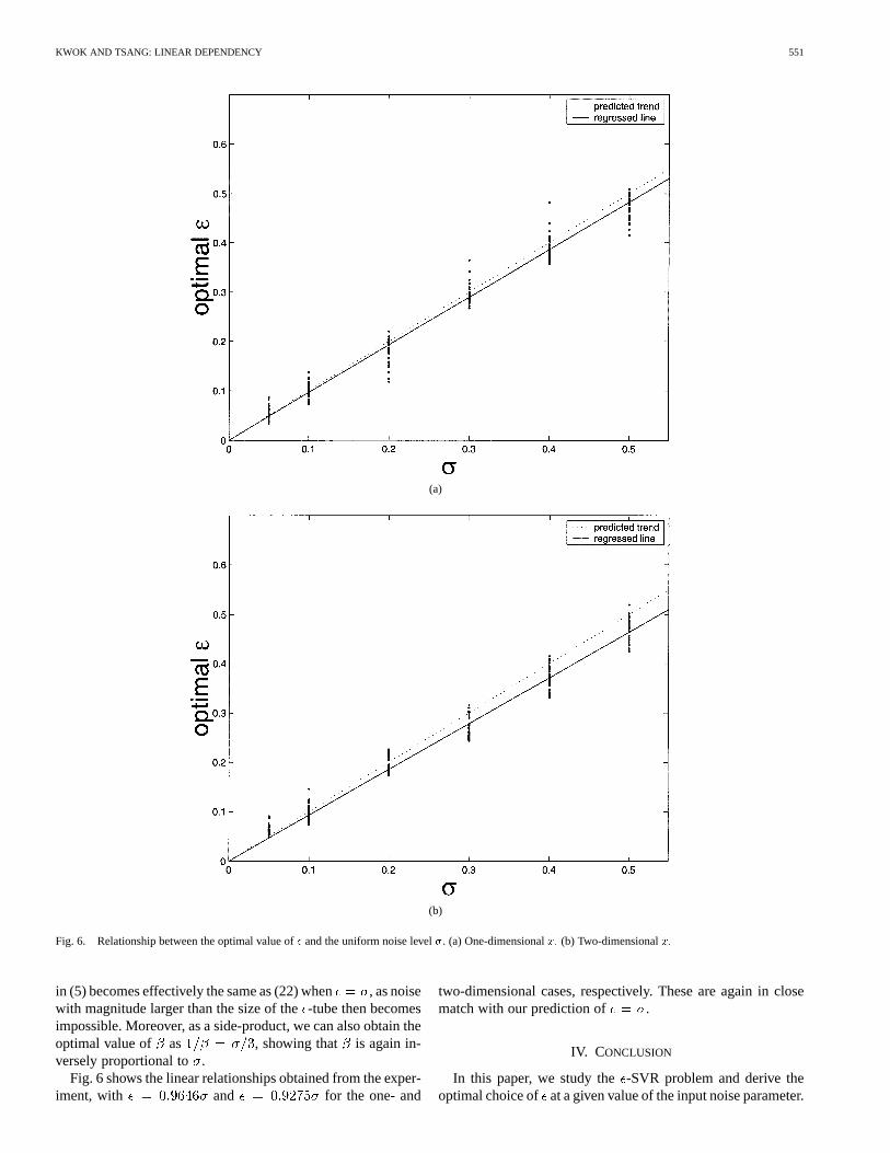
Fig. 6. Relationship between the optimal value of� and the uniform noise level�. (a) One-dimensionalx: (b) Two-dimensionalx:

in (5) becomes effectively the same as (22) when , as noisewith magnitude larger than the size of the-tube then becomesimpossible. Moreover, as a side-product, we can also obtain theoptimal value of as , showing that is again in-versely proportional to .

Fig. 6 shows the linear relationships obtained from the exper-iment, with and for the one- and

two-dimensional cases, respectively. These are again in closematch with our prediction of .

IV. CONCLUSION

In this paper, we study the-SVR problem and derive theoptimal choice of at a given value of the input noise parameter.


While the results in [19] considered only the problem of locationparameter estimation using maximum likelihood, our analysisis based on the original-SVR formulation and corresponds toMAP estimation. Consequently, our predicted ratio of inthe case of Gaussian noise is much closer to the experimentallyobserved optimal value. Besides, we accord with [19] in that

scales linearly with the scale parameter under the Gaussian,Laplacian, and uniform noise models.

In order to apply these linear dependency results in practicalapplications, one has to first arrive at an estimate of the noiselevel . One way to obtain this is by using Bayesian methods(e.g., [6]). In the future, we will investigate the integration ofthese two and also its applications in some real-world prob-lems. Besides, the work here is also useful in designing sim-ulation experiments. Typically, a researcher/practitioner may beexperimenting a new technique on-SVR, while not directly ad-dressing the issue of finding the optimal value of. The resultshere can then be used to ascertain that a suitable value/range of

has been chosen in the simulation. Finally, our analyses underthe Laplacian and uniform noise models are restricted to the casewhen the input is one dimensional and with uniform densityover a certain range. Extensions to the multivariate case and toother noise models will also be investigated in the future.

APPENDIX

Recall the following notations introduced in Section III-B1:

In the following, we will use the second-order Taylor series ex-pansions for erfc and

erfc erfc

(25)

(26)

Using (25), (13) then becomes

erfc erfc

erfc

erfc

(27)

Similarly, using (26), (14) becomes

erfc erfc

erfc erfc

erfc erfc

Using (13) and (25), this simplifies to (28), shown at the bottomof the page, from which we obtain

(29)

Substituting (27) into (28) and simplifying, we have

erfc

(30)

(28)


Now, maximizing in (7) is thus the same as minimiz-ing . Substituting in(15), (27), (29), and (30), this becomes minimizingin (16).

REFERENCES

[1] J. O. Berger,Statistical Decision Theory and Bayesian Analysis, 2nd ed,ser. Springer Series in Statistics. New York: Springer-Verlag, 1985.

[2] V. Cherkassky and F. Mulier,Learning From Data: Concepts, Theoryand Methods. New York: Wiley, 1998.

[3] N. Cristianini and J. Shawe-Taylor,An Introduction to Support VectorMachines. New York: Cambridge Univ. Press, 2000.

[4] H. D. Drucker, C. J. C. Burges, L. Kaufman, A. Smola, and V. Vapnik,“Support vector regression machines,” inAdvances in Neural Informa-tion Processing Systems 9, M. C. Mozer, M. I. Jordan, and T. Petsche,Eds. San Mateo, CA: Morgan Kaufmann, 1997, pp. 155–161.

[5] T. Evgenious, M. Pontil, and T. Poggio, “Regularization networks andsupport vector machines,” inAdvances in Computational Mathematics,1999.

[6] M. H. Law and J. T. Kwok, “Bayesian support vector regression,” inProc. 8th Int. Workshop Artificial Intelligence Statistics, Key West, FL,2001, pp. 239–244.

[7] Y. Li, S. Gong, and H. Liddell, “Support vector regression and classi-fication based multi-view face detection and recognition,” inProc. 4thIEEE Int. Conf. Face Gesture Recognition, Grenoble, France, 2000, pp.300–305.

[8] D. J. C. MacKay, “Bayesian interpolation,”Neural Comput., vol. 4, no.3, pp. 415–447, May 1992.

[9] O. L. Mangasarian and D. R. Musicant, “Robust linear and supportvector regression,”IEEE Trans. Pattern Anal. Machine Learning, vol.22, Sept. 2000.

[10] K.-R. Müller, S. Mika, G. Rätsch, K. Tsuda, and B. Schölkopf, “Anintroduction to kernel-based learning algorithms,”IEEE Trans. NeuralNetworks, vol. 12, pp. 181–202, Mar. 2001.

[11] K. R. Müller, A. J. Smola, G. Rätsch, B. Schölkopf, J. Kohlmorgen,and V. Vapnik, “Predicting time series with support vector machines,”in Proc. Int. Conf. Artificial Neural Networks, 1997, pp. 999–1004.

[12] C. Papageorgiou, F. Girosi, and T. Poggio, “Sparse correlation kernelreconstruction,” inProc. Int. Conf. Acoust., Speech, Signal Processing,Phoenix, AZ, 1999, pp. 1633–1636.

[13] T. Poggio and F. Girosi,A Theory of Networks for Approximation andLearning. Cambridge, MA: MIT Press, 1989.

[14] M. Pontil, S. Mukherjee, and F. Girosi,On the Noise Model of SupportVector Machine Regression. Cambridge, MA: MIT Press, 1998.

[15] W. H. Press, S. A. Teukolsky, W. T. Vetterling, and B. P. Flannery,Numerical Recipes in C, 2nd ed. New York: Cambridge Univ. Press,1992.

[16] B. Schölkopf, C. Burges, and A. e. Smola,Advances in KernelMethods—Support Vector Learning. Cambridge, MA: MIT Press,1998.

[17] B. Schölkopf, A. Smola, and R. C. Williamson, “New support vectoralgorithms,”Neural Comput., vol. 12, no. 4, pp. 1207–1245, 2000.

[18] A. Smola, B. Schölkopf, and G. Rätsch, “Linear programs for automaticaccuracy control in regression,” inProc. Int. Conf. Artificial Neural Net-works, 1999, pp. 575–580.

[19] A. J. Smola, N. Murata, B. Schölkopf, and K.-R. Müller, “Asymptoti-cally optimal choice of�-loss for support vector machines,” inProc. Int.Conf. Artificial Neural Networks, 1998, pp. 105–110.

[20] A. J. Smola and B. Schölkopf, “A Tutorial on Support Vector Regres-sion,” Royal Holloway College, London, U.K., NeuroCOLT2 Tech. Rep.NC2-TR-1998-030, 1998.

[21] A. J. Smola, B. Schölkopf, and K.-R. Müller, “General cost functions forsupport vector regression,” inProc. Australian Congr. Neural Networks,1998, pp. 78–83.

[22] M. Stitson, A. Gammerman, V. N. Vapnik, V. Vovk, C. Watkins, andJ. Weston, “Support vector regression with ANOVA decompositionkernels,” in Advances in Kernel Methods—Support Vector Learning,B. Schölkopf, C. Burges, and A. Smola, Eds. Cambridge, MA: MITPress, 1999.

[23] J. A. K. Suykens, “Least squares support vector machines for classifica-tion and nonlinear modeling,” inProc. 7th Int. Workshop Parallel Ap-plications Statistics Economics, 2000, pp. 29–48.

[24] V. Vapnik, Statistical Learning Theory. New York: Wiley, 1998.

James T. Kwok received the Ph.D. degree incomputer science from the Hong Kong Universityof Science and Technology in 1996. He then joinedthe Department of Computer Science, Hong KongBaptist University as an Assistant Professor. Hereturned to the Hong Kong University of Scienceand Technology in 2000 and is now an AssistantProfessor in the Department of Computer Science.His research interests include kernel methods,artificial neural networks, pattern recognition andmachine learning.

Ivor W. Tsang received his B.Eng. degree in com-puter science from the Hong Kong University of Sci-ence and Technology (HKUST) in 2001. He is cur-rently a master student in HKUST. He was the HonorOutstanding student in 2001. His research interestsinclude machine learning and kernel methods.

Linear dependency between ε and the input noise in ε-support vector regression

Documents

Transcript of Linear dependency between ε and the input noise in ε-support vector regression