Performance Dependency of Secondary

Buyouts on Primary Buyouts

Tjark C. Eschenroder1, Thomas Hartmann-Wendels2

University of Cologne

Department of Bank Management

Abstract

Secondary buyouts (SBOs) represent more than 50 percent of the total private equity (PE)

buyout activities. However, in academia and practise, a potential underperformance of SBOs

compared to primary buyouts (PBOs) is discussed. Therefore, it is all the more important to

further understand how the value in SBOs is driven and what makes a potential SBO attractive

to look at in a due diligence process. This paper describes the dependency of SBOs on the

preceding PBOs based on a dataset of 295 PBOs with their consecutive SBOs. It analyses

the impact of the performance of a portfolio company during a PBO on the performance of

the following SBO and derives value drivers and their influence on the SBO. Based on the

performance of the value drivers during the PBO five criteria are identified for a pre-selection

of SBOs. There is not a single perfect strategy for all SBOs, but the value drivers during the

SBO differ strongly depending on the identified selection criteria. Generally, general partners

(GPs) do not only use complimentary skillsets, i.e. they do something completely different

across buyout rounds. Additionally, they work on similar value drivers but with a different

focus than the previous investor, i.e. they work differently on similar areas of improvement.

First Version: December 20, 2018

This Version: August 20, 2019

JEL Classification: G11, G23, G24, G34

Keywords: Private Equity, Secondary Buyout, Value Drivers, Investment Selection

Contact: The authors can be contacted via the following means

1 eschenroeder@wiso-uni-koeln.de or 0049 0 221 470 6575

2 hartmann-wendels@wiso-uni-koeln.de or 0049 0 221 470 4479

1 Introduction

After the downturn of the private equity (PE) market during the global financial crisis PE is

growing significantly ever since. PE funds are getting bigger and large amounts of committed

money is available. This success however, puts general partners (GPs) in a conflict. On the

one hand, GPs are facing a shortage of attractive investment targets. On the other hand, GPs

are forced to exit their portfolio companies within the lifespan of the tendered fund. Due to

this market design, secondary buyouts (SBOs) seem to represent a solution to the scacity of

investment opportunities as their share of total buyouts is steadily growing. SBOs are leveraged

buyouts (LBOs) in which one PE investor sells his portfolio company to another PE investor.

As shown in Figure 1, the share of the SBO transaction volume on the total PE transaction

volume grew since 2010 and reaches 52 percent in 2018, both in the EU and the US market.

During an LBO the PE investor creates value by using financial and operational engineering.

After the closing the deal, the agenda of GPs is to optimse the portfolio company with respect

to short-term and mid-term time horizons. Thus at first glance, a second investor should not be

able to achieve abnormal investment returns as the value creation potential is already captured

by the first PE investor (e.g. Jenkinson & Sousa (2015), Wang (2012), Bonini (2015)). However,

PE investors may decide to acquire companies directly from other financial investors. There

are several attempts on explaining the investment rational of SBOs. For example Jenkinson &

Sousa (2015) mention complimentary skill sets of the GPs, time pressure to sell the portfolio

company early, marketing the successful sale of portfolio companies for future fund raising and

usage of favourable debt market conditions as possible explanations. Another used argument is

that both the primary buyout (PBO) and the SBO are successful as the organisational structure

of PE is superior to non-PE organisational structures (Jensen (1989)) and, thus, SBOs may still

provide sufficient returns to investors. Nevertheless, the dependency between the two buyout

rounds may further prove the advantages of SBOs. These analyses may provide criteria on how

to achieve successful SBOs.

Following these findings, we provide empirical guidance for investing into successful SBO

investments. First, we analyse the value drivers in PBOs and SBOs to understand how the total

value creation is composed and whether value is driven differently amongst the individual buy-

out rounds. Second, after the identification of value drivers, we are able to study dependencies

of value drivers across the buyout rounds. Do any value drivers during the PBO have an impact

on the value creation during the SBO? Answering this question leads to certain characteristics

that are favourable for the engagement in an SBO, thus identifying selection criteria for poten-

tially successful SBOs. Third, once selection criteria are identified, a GP needs to understand

what to focus on during the SBO based on the development during the PBO. Thus, we analyse

the value drivers dependent on the identified selection criteria.

We find that the value drivers differ among buyout rounds. PBO investors primarily focus

on company growth, profitability improvement, and boosting innovation to create value. In

contrast, SBO investor focus more on increasing profitability and efficiency gains. We are able

to identify five selection criteria for target selection that drive value creation during the SBO.

1

Companies with a lower value creation during the PBO compared to its close peers are generally

preferred for SBOs. On the one hand, portfolio companies with a great company growth and

profitability development, in terms of EBITDA margin, are favoured. On the other hand, good

SBO targets demonstrate weak efficiency during the PBO and, consequently, also an inferior

development of return on assets compared to its close peers. The value drivers dependent

on these selection criteria differ quite substantially. We confirm the findings of Jenkinson &

Sousa (2015) that complimentary skill sets exist, i.e. that GPs focus on something completely

different across buyout rounds. Exemplary, the SBO investor improves profitability after the

PBO investor has focussed on company growth. However, we also find that this is not the

only way to create value in SBOs. SBO investors also do something similar as the previous

PBO investor but with a different approach than the PBO investor. For example, the PBO

investor works on profitability by improving the EBITDA margin, whereas the SBO investors

also focusses on profitability but rather works on the improvement of return on assets. However,

an SBO investor does not simply apply the same mechanics as was done during the PBO.

This paper contributes to the literature in the following ways. Most studies about PE

performance and SBO performance consider PBO and SBO autonomously (e.g. Achleitner &

Figge (2014), Degeorge et al. (2016)). In our opinion, for a rigorous analysis it is crucial to

consider two consecutive deals rather than any two independent deals because the dependencies

are measured between two back-to-back buyouts rather than individual, independent buyouts.

Otherwise the underlying data may suffer from a random selection of individual PBOs and

SBOs. To our knowledge, only Bonini (2015) analyses the operating performance of two se-

quential deals and aims to find reasons for investing into consecutive private equity transactions.

This paper does not suffer as much from selection bias as others. By using both public data

providers and private data from a large fund of fund manager, we make sure that unsuccessful

PE deals are also included. Furthermore, the full length of the holding period of back-to-back

buyouts is considered. Most importantly, based on fundamental data it is the first paper that

identifies selection criteria and company profiles that are suitable for successful SBOs. We are

able to give advice on what to do during SBOs dependent on the individual selection criteria

to make the buyout successful.

This paper is structured as follows. The following chapter describes the dataset and its

preparation in detail. Chapter three presents the summary statistics of the dataset. The

following three chapters explain the hypotheses of the three consecutive research questions,

the underlying methodology for the analyses, and present the empirical findings of this study.

Finally, the conclusion can be found in the last chapter.

2

2 Data Sample

2.1 Explanation of the Data Sample, the Peer Group and the Un-

derlying Variables

Many studies about PE, and especially about SBOs, face tremendous problems gathering suf-

ficient observations for reasonable analyses. Firstly, compared to other transactions, PE deals

cover relatively fewer deals. Secondly, many PE transactions are taken privately, which does

not require the financial investor to disclose financial information in many countries. Thirdly,

due to the construction of PE and the underlying holding periods of portfolio companies, many

transactions during the last few years cannot be considered as the financial investor has not

yet exited the investment. This is especially critical for our study as we use two consecutive

PE deals and thus we can only consider PBOs with an early exit. Lastly, data providers are

strongly dependent on financial investors publishing the news of acquiring and exiting their

investment, which is also not always the case.

Our original dataset consists of PE portfolio companies, which are located in the United

Kingdom (UK). The UK is a very active PE market and, therefore, provides a significant

amount of observations. In contrast to the USA, most of the companies in the UK need to

publish their full financial accounts, which enables operative analyses on a more detailed level.

We used several data providers to retrieve an initial list of all buyouts that are labelled

as “secondary buyout” and “financial buyout”. These data were collected from Capital IQ,

Thomson Reuters Eikon, Prequin, Mergermarket and private information from a large fund of

fund manager. The list of SBOs includes the names of the portfolio companies that the PE

companies invested in and the date of the investment entry and most of the time the investment

exit. We eliminated all buyouts that are in fact tertiary buyouts or any other financial buyouts

that occurred after the SBO. Most data providers start the portfolio company search in 1996

and companies need at least one year to publish their financial accounts in a timely manner.

Therefore, the portfolio companies had their PBO no earlier than 1996 and their SBO exit no

later than 2017. We chose those dates as the time horizon needs to be as large as possible to

guarantee a sufficient number of observations. Per definition of the consecutive deal analysis,

the PBO investment exit date is equal to the SBO investment entry date. After matching for

company keys and company name, only few companies had the full date information for the

first transaction date (at PBO entry), for the second transaction date (at PBO exit/at SBO

entry), and for the third transaction date (at SBO exit). However, for most companies at least

one out of the three dates was still missing. Thus, we hand-collected the missing dates, if

available, from the financial investor’s websites or other official transaction publications.

We then retrieved accounting information for the underlying portfolio companies for the

fiscal years which are the closest to the first, second, and third transaction date, respectively.

On the one hand, collecting data only for the fiscal year before the entry date and for the

fiscal year after the exit date covers the full time span of the deal but if the entry date and

the respective fiscal year are too far apart mayor early improvements of the GP may not be

3

recognized in the analysis. On the other hand, collecting data for the fiscal year after the entry

date and for the fiscal year before the exit date may not cover the full value creation of the

specific buyout. We assume that using the closest fiscal year to the transaction date provides

the lowest bias possible. For most private companies in the UK, only the balance sheet and

the P&L are published and for some rarer cases the cash flow statement is also published.

The reason to track both of those financial statement’s items is to combine the static view of

the balance sheet with operative, dynamic measures of the P&L statement. Furthermore, we

retrieved the number of fulltime employees if available. Table 1 provides an overview of all the

retrieved financial information. Ideally 23 variables and ratios have been retrieved, however,

that strongly depends on the availability and depth of the financial information. Even if not

the full information were available the observation was kept in the sample. Multicollinearity

for the observed variables should not be a problem as can be inferred from the low correlations

in Table 2.

- Table 1 about here -

The final sample consists of 295 companies. We were able to collect accounting data at the

three transaction dates within the setting of consecutive PE deals. This means that we collected

information about 590 investments, thus having access to a maximum of 885 transactions per

variable. Obviously due to the depth of the available information the number of observations

for individual variables may differ significantly.

- Table 2 about here -

As explained in the following section a peer group is needed for both calculating the relevant

performance measures and the valuation of our sample companies. The peer group consists of

public companies from the UK and the USA. Obviously for our UK sample it is reasonable to

use a UK peer group. Due to the fact that we apply an accurate matching procedure over a

large time horizon, our potential peer group needs to be very large. The peer group’s quality

can be improved by enlarging the dataset with other countries that share similar investment

characteristics. Especially for bigger companies, such as buyout companies, other countries

that share a similar investment market should suffice for an improved comparison (Schreiner

(2009)). The American market should therefore serve well as an enlargement of the UK peer

group as the PE markets are quite similar. We used Compustat database to retrieve data for all

companies that were listed from 1996 to 2017 on the UK and US equity markets. Additionally,

we were able to retrieve the same accounting information as for the sample firms.

2.2 Preparation of the Dataset

2.2.1 Valuation of Sample Companies

The analysis aims to identify the value drivers of the intrinsic value creation. Thus, the equity

valuation needs to be considered. For several reasons, we chose to value the equity of our sample

companies ourselves by using multiple valuation techniques. For most PE transactions the deal

4

values are not published or at least the value at either entry or exit is missing. Only using

those deals, for which deal values are available, would decrease the total number of observations

drastically. From our point of view the pricing of transaction values is determined by many

factors that do not directly inherit the private equity core activity. Such factors include price

influencers, e.g. negotiation skills of the PE firms (Achleitner et al. (2011)) or random shifts in

the demand and supply of potential target companies. In fact, we have been trying to isolate

the operational value creation and thus created a fair market value of the sample’s companies

using public market data. We assumed that the success of a buyout is a combination of several

drivers and thus analysed the combined effect of those drivers, expressed as multiple valuations

on certain key accounting information. The multiple valuation has the advantage that the

observed companies’ valuation seems to be more homogenous throughout time, which enables

good comparability as small unobservable, firm specific drivers may be included over the time

period of the two consecutive deals. Lastly, multiple valuation shares the same fundament

as comprehensive valuations and thus provide a good groundwork for deal values (Liu et al.

(2002)). Although these market values may differ slightly from actual deal values, they serve

well as tendencies of the actual price and are assumed to be quite accurate.

Accordingly, we used trading multiples rather than transaction multiples for the valuation

of our sample companies. Most importantly, using transaction multiples would again provide

us with price distortion, e.g. in form of transaction fees, possible synergy effects between

the target and the acquiring firm and liquidity premia. Thus, for determining purely the

operational success, transaction multiples do not seem to provide a reasonable valuation basis.

Choosing transaction multiples, we would need to use PE transaction to truly capture all the PE

mechanics. A lack of suitable observations may be a problem in that case, too. We, therefore,

favoured trading multiples in our study. Within the category of trading multiples several studies

analyse the differences between forecasting multiples, trailing multiples and the combination of

both of them. Forecasting multiples are those multiples that are based on forecasted accounting

information, such as the consensus of broker reports’ forecasts. Those forecasting multiples lead

to the lowest valuation error (Liu et al. (2002)). Unfortunately, broker reports are not available

in the necessary quantity for private companies. We decided to not forecast the financial

information ourselves, as we feel that such a forecast would lead to a too subjective outcome.

As a result, trailing multiples seem to be the right choice for valuing the sample’s companies.

Trailing multiples are those multiples that are based on past fundamental data. Several studies

aim to identify both the stand-alone accuracy of the multiple valuations and of the combination

of several multiple valuations. Amongst others sales, EBITDA, earnings and equity book value

multiples perform the best. Liu et al. (2002) find that those multiples perform very well and

are not much weaker than forecasting multiples. They analyse the effects of cash flow multiples

and find that they perform significantly worse than the above mentioned multiples. For some

observations it may be reasonable to implement industry-specific multiples. However, due to

the various and detailed industry specifications of our sample, it would not be feasible as most

companies do not publish the necessary information. Therefore, sales, EBITDA, earnings and

5

book equity multiples seemed to be the best choice for a sufficient multiple valuation.

The identification of the best possible peer group is a crucial process for optimising the

valuation accuracy. Therefore, our identification process and the underlying matching pro-

cess underwent a complex and detailed structure. The matching procedure followed the LBO

matching procedures of Guo et al. (2011) to apply a pre-performance matching, i.e. finding

suitable matches before the activity of the PE investor begins. Generally, we matched our sam-

ple portfolio companies with the listed companies from the peer group. The pre-performance

matching was done twice, before the PBO as well as before the SBO. With this process we reset

the benchmark of the underlying observations. Many other studies apply an industry-size-year

matching as this process is supposed to identify the most similar companies available (Barber

& Lyon (1996)). However, we assumed that sometimes matching for industry, size, and year

as proposed is not enough. Ceteris paribus, a company that is very profitable should perform

differently compared to a company that is specified as a loss company, and thus develop dif-

ferently. Therefore, we followed the idea of Bhojraj & Lee (2002) and included a measure of

profitability, namely the EBITDA margin, in our matching process. For every sample company,

the matching process results in the five closest peer companies. First of all, the sample com-

pany’s year of transaction has to be exactly the same as the trading year of the peer company

in order to eliminate time effects. Secondly, as we track the development of both the sample

and peer group companies, the peer firm still needed to be listed at the end of the PE firm’s

buyout. Thirdly, the companies needed to have a similar size at the beginning of the buyout as

a proxy for a similar development within the business lifecycle (Alford (1992)). Thus, a peer

group company may not deviate more than 50 percent in total assets from the sample firm.

Fourthly, the companies should have a similar profitability. The peers do not deviate more

than 25 percentage points in EBITDA margin and should have the same sign of the EBITDA

margin. Both of these cut-off points were chosen by us to represent a reasonable comparison.

The profitability interval is slightly lower compared to the size interval because the margin is

usually centered around an industry average anyways, whilst the size is not necssarily bound

to an industry benchmark. Lastly, the companies needed to be in the same industry for all

the other premises to be comparable. Out of the standard industry classification codes, GICS

codes perform the best for a reasonable valuation (Bhojraj et al. (2003)). We followed Alford

(1992) as we matched by the most detailed industry code at the beginning. If there are less

than five matches per sample firm, we reduced the depth of the industry codes until every

PE portfolio company has at least five matches. If there were more than five matches per

portfolio company, the five peers which had the most similar size were selected. A good peer

group should have enough observations to smoothen the results, but too many observations

may distort the results. Pereiro (2002) and Schreiner (2009) show that a peer group should

consist of 2 to 10 peers. We followed Bhojraj & Lee (2002) and find the five most similar peers,

as this is in accordance with the leading literature. Due to the nature of the dataset and the

corresponding possible peer group, the geographic matching occured between the UK and the

US. A single country-matching would be superior but usually the number of similar compa-

6

nies in each year and industry is very limited, thus there is no harm to increase the potential

comparable companies by comparing to similar economies as well (Schreiner (2009)).

After the identification of the correct peers for each sample company, the peer group mul-

tiples needed to be estimated. First of all, we extracted the accounting data of the peer group

which are matched with the three transaction dates of the sample companies. The accounting

data for the peer group have the same fiscal year as in the sample data collection, i.e. the

closest fiscal year to the transaction date. For every match we calculated the multiples of sales,

EBITDA, earnings, and equity book value based on the market capitalisation of the respective

companies. After the calculation of the individual value for all peer group companies, these

values needed to be aggregated. Herrmann & Richter (2003) find that using the arithmetic

mean would lead to an overestimation of the valuation and thus distort the valuation. They as

well as Baker & Ruback (1999) instead propose that the median is a very good way to aggre-

gate these valuations. Thus, we chose to use the median values. Ultimately, we got the median

values for sales, EBITDA, earnings and book equity multiples of the portfolio companies that

we wanted to value.

The actual valuation was simply done by multiplying the peer group’s multiple values with

the sample company’s respective accounting data. This process provided four company values

as each multiple valuation was done independently of each other. As the companies are quite

similar by the nature of the matching process, we applied an arithmetic mean to find the average

company equity value among all the multiple valuations.

After the valuation of our sample companies’ equity we retrieved as many actual deal values

as possible for those sample companies in order to validate these valuation. We were able to

retrieve 136 actual transaction values of our given sample. A mean test between the actual

observation and the valuations was performed. Both our initial sample and the actual deal

values were not significantly different from each other, already indicating that the valuation

was not too far off. Further, we regress the value of the self-valued companies on the actual

transaction prices in order to see whether our estimates performed well at predicting the actual

transaction price. With a coefficient of 0.9333 and a R-squared of 0.85 the company valuations

seem to be a very good fit and thus may be used for further analysis.

2.2.2 Variable Calculation

Our study focusses on the development of both the overall company growth, but also the growth

of all the observed financial information. Generally, when calculating growth two categories

of measurements arise. Those variables that always stay positive can be calculated with the

compound annual growth rate (CAGR),

CAGRi,t(X) = (xi,txi,t−k

)1/k − 1 (1)

with xi,t being the variable of interest at time t of company i, and k being the holding period

of the investment.

7

As the nominator and denominator will always be positive, it is possible to distinguish a

positive growth from a negative growth. In the underlying analysis the growth of the company

value, total assets, equity, number of full-time employees and sales are calculated with the

CAGR.

Other variables may become negative over the investment period. For these values the

CAGR is mathematically not feasible. For that reason we chose to calculate the yearly growth

ratios by dividing the total change in the underlying ratio by the length of the holding period

in years.

Growthi,t(X) = (xi,t − xi,t−k

t− k) (2)

with xi,t being the variable of interest at time t of company i, and k being the holding period

of the investment.

Winsorising is a commonly used method in the related literature to adjust the underlying

data for thorough and generally applicable studies. All the relevant fundamental data were

winsorised at the 1 percent and 99 percent level as only a few observations strongly distorted

the results. This approach is in accordance with other studies in the research field of PE (e.g.

Achleitner & Figge (2014)).

We further chose to use the absolute excess development rather than simply analysing the

companies’ performance isolated. Especially, for investment purposes it is more important how

a company performs in comparison to its peers and the industry it operates in. Although

a certain performance indicator may be high in absolute terms it does not mean that the

company is well managed as it may underperform its close peer group. Therefore, similar to

Bonini (2015), we calculated the difference between all variables of the underlying portfolio

company and the corresponding variables of its peer group as follows.

di,p = (xi −mp) (3)

where xi is the performance indicator x for company i, and m being the median of the perfor-

mance indicator of peer group p.

2.3 Variable Selection

This chapter presents the variables that were used in this paper. In the following, the mea-

surement of growth, profitability, financial engineering, liquidity, efficiency, and innovation are

explained.

The growth of a portfolio company is measured in two ways, namely total sales and equity

growth. The analysis of total sales growth is necessary for two reasons. Increasing sales either

represents a sufficient market share on the total market or it may indicate a growing industry.

8

Further, the growth of equity is analysed as it is a balance sheet position and thus provides

a more stable view on the development throughout the holding period than a profit and loss

account position.

The profitability is measured with four variables, namely the EBITDA margin, profit mar-

gin, return on equity, and return on assets. The first two variables measure the operating

earnings in comparison to the total sales. The EBITDA margin clearly identifies the operat-

ing earnings without considering any financing and accounting effects. Complimentary to this

measure, we use the profit margin because it also inherits the interest payments and taxes.

Usually, GPs are not able to strongly reduce the tax liabilities of the portfolio company, but

due to high leverage, interest payments may be very high. The other two profitability vari-

ables rather measure the earnings in contrast to the input of capital. They are also crucial to

analyse because they are more stable compared to pure profit and loss profitability measures.

Within this category of variables, we need to measure both asset and equity returns because

the amount of total assets and equity usually differ strongly in buyouts due to the financial

leverage.

The capital structure and financial engineering is measured with the development of the

financial leverage. The financial leverage is measured as the ratio of liabilities to equity. It

serves both well as explanatory variable and control variable of the capital structure.

Liquidity is measured with two variables, namely the cash ratio and the current ratio. The

cash ratio is measured as cash and cash equivalents over current liabilities. Especially for high

risk investments, such as buyouts, the availability of cash to pay off current liabilities directly,

seems to be a valid proxy for liquidity. The current ratio is defined as the current receivables

over current liabilities. This ratio measures a similar degree of liquidity but also considers other

assets, which shows how solvent a company is in the short-term.

This paper uses two proxies as part of the portfolio company’s efficiency. The inventory

sales ratio, which is defined as sales over inventory, measures the efficiency on how the inven-

tory is used to achieve certain sales. Generally, companies may aim to reduce the necessary

inventory whilst always having just enough inventory to keep the business running smoothly.

The receivables turnover ratio represents the efficiency of a company to convert receivables into

actual sales. It is defined as sales over receivables outstanding.

Innovation and asset structure are measured with the intangible asset ratio, which is the pro-

portion to intangible assets on total assets. It shows the degree of innovation and brand value,

as mostly patents and goodwill are incorporated in intangible assets. Also, it can serve well as

a control variable for asset structure, which may be important especially when considering the

recent development of digitalisation.

The control variables are manifold. First, we use credit spreads, the employment rate,

inflation rate, and GDP index as macroeconomic control variables. Second, as we consider the

growth of variables, we need to control for the length of the holding period to differentiate

between short-term and long-term value drivers. Third, total assets are used to control for

the size of the company. Fourth, we control for the risk of financial distress of the portfolio

9

company. As portfolio companies are not listed, a market price and its underlying volatility

cannot be observed. For that purpose, we choose to measure the risk of a company by analysing

its fundamental data as well. The Altman Z-score is a well-established measure to predict

financial distress and thus serves well as control variable of risk for private companies (Altman

(1968)). Lastly, we apply time and industry dummies.

3 Summary Statistics

Table 3 displays the summary statistics for the final dataset of 590 investments. For infor-

mational purposes all the statistics are split into three categories: the total sample, primary

buyouts and secondary buyouts. Mean T-tests and nonparametric equality-of-medians tests

are performed to recognise the differences in characteristics between PBOs and SBOs. The

statistics are divided into two panels: the company information at entry and the company

information developments. The observations are relatively well balanced, i.e. for most infor-

mation the full number of potential observations are available so that only few observations go

missing in further analysis.

- Table 3 about here -

The first panel covers the valuation, some fundamental data, and selected ratios to display

the operative and financial characteristics of the portfolio companies at the beginning of the

investment. Figure 2 provides an overview on the investment entry year. The valuation at entry

for the total sample has a mean of 60.8 million GBP. This is slightly lower than the deal values

in other studies. The size difference may arise from the specific country focus. Large deals are

also less likely to be bought twice by financial investors as those deals are quite rare anyway.

Thus, in this setting it is less likely to include those large companies twice. The valuation

at entry of PBOs is significantly greater in its mean with a weak significance compared to

entry valuation of SBOs, indicating that value is created throughout the primary buyout. The

medians of the two buyout types are significantly different from each other which clearly shows

that value is created in PBOs. As shown by the valuation CAGR all PE-backed companies

develop positively over time, again by construction, the fundamental data should be higher

at the entry of the SBO. However, the mean differences of the three ratios at entry of PBOs

and SBOs, namely return on equity, return on assets and the leverage, are not significantly

different from each other. Both return measures are very similar both in mean and median.

Both first round investors and second round investors start with a similar return on the invested

equity and assets. Although the operative earnings increase, the equity and assets invested to

achieve this return grow proportionally the same. Surprisingly, the mean leverage ratios at

entry are not significantly different from each other. The standard deviations of both means

are extremely high which clearly indicates that there are different approaches on how to use

leverage as a tool for value creation. The median tests show roughly the same results and thus

do not require further interpretation.

10

The second panel shows the development of the valuation, the aforementioned fundamental

data, and their ratios. Most variables’ means are not significantly different from another. This

suggests that neither investment type generally performs better or worse than the other. This

brings up the question which deal, PBO or SBO, outperforms in the respective fields. The

valuation CAGR is positive for both buyout types indicating that both buyouts create excess

value compared to its peer group. However, neither the mean nor the median are different from

another, showing that in this sample PBOs do not necessarily perform better than SBOs. The

mean growth of total assets and equity are significantly different from another which shows

that PE firms may bloat the balance sheet more during the PBO. Interestingly, the medians of

developments of sales, the EBITDA margin, the EBIT margin, the profit margin and total assets

are significantly different from each other and higher in PBOs, showing that for many deals

the development of the selected performance indicators are better during the first investment

round. The holding period for the total sample on average is 4.1 years. The mean holding

periods are not significantly different from another which might indicate that SBOs on average

do not follow the idea of having buying and selling pressure more than PBOs. Figure 3 further

represents the deviation of holding periods according to PBOs and SBOs.

4 Differing Value Drivers Across Buyout Rounds

Throughout the history of PE, portfolio companies generally faced two phases of buyout activity.

The first phase focussed on value creation through financial engineering. The second phase

made use of operational engineering. Nowadays, both financial and operational engineering are

applied to maximise the value creation within a buyout.

Jensen (1989) states that a buyout structure with high leverage allows the PE investors to

align management incentives and to create efficient and lean organisational structures. Other

studies further show that a high leverage reduces agency costs due to a high powered incentive

system (e.g. Jensen & Meckling (1976), Jensen (1986)). Korteweg (2010) finds that during

the early investment stages, PE investors often prefer high leverage as their optimal capital

structure. The evidence about leverage as value driver in SBOs is rather mixed. Achleitner &

Figge (2014) propose that all GPs may use similar skill sets for operational improvements and

therefore the only way to create additional return is by increasing the leverage. On the other

hand, Wang (2012) states that a successful PBO usually relies on an almost optimal capital

structure and therefore the second PE buyer should not change the leverage. For these partially

mixed reasons, we expect leverage to have at least a small positive effect on value creation in

both buyout rounds of our sample.

After a downturn in debt markets, financial investors had to reinvent their business model

and focused on operational performance enhancement rather than simply implementing finan-

cial engineering (Matthews et al. (2009)). GPs are more focussed on strategic and operative

decision-making and thus trying to improve the efficiency and profitability of the underlying

investment companies (De Fontenay (2014)). Operational engineering may come in form of im-

11

provements in production, cost structures, marketing, human resource management, inorganic

growth, repositioning in the market, or restructuring (Acharya et al. (2012), Lee et al. (2001),

Wright et al. (2001)). According to Perembetov et al. (2014), operational engineering and its

underlying improvements comprise about 51 percent of the total value creation in PE, whereas

financial engineering and multiple effects explain 31 percent and 18 percent, respectively. Gen-

erally, SBOs inherit some theoretical problems with respect to operational engineering. The

idea of PE is that either GPs are good at identifying and selecting strong performing companies

or they are able to optimise portfolio companies throughout the investment period. After the

completion of the holding period there should not be any or only little value creation poten-

tial left. Thus, after the PBO, the SBO should not be able to achieve a significantly more

additional value compared to the first buyout round. Achleitner & Figge (2014), however, find

that financial buyouts still offer potential for operational performance, such as sales growth

and margin expansion, which habe not developed during the PBOs. Therefore, SBOs do not

develop differently compared to PBOs.

Growth and expansion as value drivers should be relevant in buyout rounds, but probably

more during the PBO because during a PBO a lot of capital is invested into the portfolio

company to gain high market shares and expand quickly. Although SBO investors may also

try to grow the portfolio company, further and quick market growth may be more difficult to

achieve as marginal costs to achieve the growth are higher, resulting in a lower expected effect

of growth on value creation.

GPs do not only make use of expansive growth but also ultimately turn the previous growth

into profitable cashflows. Thus, we expect that an improvement in profitability has a positive

influence on value creation during both buyout rounds. However, this effect could be more

relevant during the SBO because the portfolio company is older and thus potentially further

developed in the business life cycle. After the growth period during the PBO, the SBO may

aim on streamlining the business as a following step.

PE investments belong to the illiquid investment class and, therefore, do not suffer from

any short-term goals from shareholders. The portfolio companies do not need to provide a huge

degree of liquidity, just enough to run the business smoothly. Shortages in liquidity may also

be covered by further capital injections by the financial sponsor. Thus, we expect that financial

sponsors focus less on the portfolio companies’ liquidity and, therefore, that there is a negative

effect of liquidity on value creation during the buyout rounds.

The growth and expansion of companies during buyout rounds leads to inflated balance

sheet positions (e.g. assets and equity). Consequently, efficiency ratios suffer as the input

variables may increase more than the output variables. The portfolio company is possibly

streamlined with respect to those measures during the SBO as part of the “fine-tuning” after

the implementation of main value drivers during the PBO. We, therefore, expect a positive

correlation with value growth during the SBO but an insignificant effect during the PBO.

During a PBO the PE firm may aim to invest heavily to foster growth, which may also

come in form of growth in intangible assets, representing mainly innovation (e.g. patents) and

12

brand value. The SBO investor can either make use of the increased level of innovation or

even further invest in research and development. Due to superior negotiation skills of PE firms

and the accompanying high exit price of the portfolio company (Achleitner et al. (2011)), it

is reasonable to assume an above average goodwill development for PBOs. Assuming similar

negotiation skills between PBO and SBO investors, the amount of goodwill should not change

a lot during the SBO. Thus, we expect a stronger increase of innovation and brand value during

the PBO and thus a greater effect on value creation.

4.1 Methodology

We analyse which determinants are related to value growth of the portfolio companies. As our

SBOs directly follow the PBOs, we are able to construct a determinant analysis in form of a

panel analysis. The model is defined as:

yit = α + β ∗Xit + γ ∗ Yt + ε (4)

where X describes the firm-specific variables and Y describes the macroeconomic variables for

firm i at transaction date t.

The potential main value drivers are commonly used by other papers and serve well as a

start of a determinant analysis. For that purpose, we include growth, profitability, leverage,

liquidity, eifficiency, and innovation in this model (e.g. Achleitner & Figge (2014), Bonini

(2015), Achleitner et al. (2011)). However, as we were able to retrieve the whole profit and

loss account and balance sheet we improve the analysis by including more detailed performance

measures. We analyse the excess growth of the individual characteristics compared to its

predefined peer group of public companies. We use a random-effects model, as the Hausmann-

test estimates between random and fixed effects are not significantly different from another

(Hausman (1978)). We assume that we control for most of the relevant characteristics and the

unobservable effects are rather small. Therefore, a random-effect model is also sensible from

an economic point of view.

Afterwards, we apply an OLS regression for both PBOs and SBO separately. This helps to

identify if value drivers are different in both buyout rounds. The variables and specification

are the same as in the panel regression.

4.2 Results

The determinant analyses consist each of three specifications which are displayed in Tables 4-6.

The base case specifications only consider the four multiples that were used to perform the

valuation of the observed company. Afterwards, in the second specifications, we further include

controls for the size, the holding period, the macroeconomic environment, the time, and the

main industry the company operates in. In the third specifications, we complete the regressions

by adding more detailed firm characteristics that should serve as value drivers.

13

The determinant analysis for all buyouts is a combination of the following two determinant

analyses about PBOs and SBOs. Table 4 shows the results of all buyouts for comparison. The

results are not further discussed as we rank the importance of the value drivers in PBO and

SBO separately higher than for all buyouts in general. We can confirm that the results for all

buyouts align with the PE literature.

- Table 4 about here -

Table 5 displays the determinant analysis of PBOs. The growth of a portfolio company is

a significant value driver for primary buyouts as both sales CAGR and equity growth have

positive and significant coefficients. Companies that expand their total sales and improve the

operative earnings margin are likely to increase their operative cash flows and thus create higher

value. Higher equity is equal to a greater intrinsic book value of the company. Further, those

companies that are able to increase their equity over time indicate a positive past performance

and higher stability, thus increasing the company value.

- Table 5 about here -

Profitability seems to play various roles for value drivers in PBOs. The EBITDA margin

is significant for all specifications and the profit margin for the last, most relevant, specifica-

tions as well. The coefficient of the EBITDA margin is in line with the previous finding that

ultimately, and in combination with sales increase, operative earnings and operative cash flows

may be increased. Interestingly, the profit margin coefficient is not significant for the first

two specifications but becomes weakly significant and negatively correlated to the company’s

valuation for the third specification. This observation indicates that portfolio companies that

aim to have a great profit margin, without considering the other value drivers, may have a

bad overall value development. Portfolio companies that aim to increase their profit margin

seem to perform worse at other value drivers, e.g. sacrificing the growth in sales for a higher

profitability margin. Furthermore, due to a strong leverage, portfolio companies tend to pay

high interest and thus portfolio companies may have negative net earnings. The return on

assets and equity are not significant, indicating that the necessary capital may work against

the increase in earnings.

In this sample, financial engineering does not seem to be relevant as the coefficient is not

statistically significant. However, this development of the financial leverage may be explained

because GPs aim to reduce the leverage towards the end of the holding period as can be inferred

as well from the summary statistics. Therefore, this explanation may be a reason why there is

not an effect on the value creation of a PBO portfolio company.

As expected, the developments of liquidity and efficiency do not influence the value creation

during the PBO. These findings however, need to be treated with caution because due to the

construction of this dataset, SBOs are the follow-up investors. Assuming that PE investors care

less about the underlying liquidity of companies compared to strategic buyers, PBO investors

do not focus as much on this measure because SBO investors simply may not regard these

developments as valid selection criteria.

14

PBOs seem to benefit from early innovation and improvement of goodwill. Companies

that increase the share of intangible assets in total assets have a stronger value growth. This

might be explained by the fact that those younger companies tend to focus more on intellectual

property generation or goodwill growth than companies with older and traditional thinking.

This finding needs to be treated with caution as well because the result can be heavily driven

by the increase from goodwill after the exit of the PBO when comparably there was less or no

goodwill incorporated before the PBO.

The results of the SBO value driver analysis are presented in Table 6. Growth seems to

be less important in SBOs than in PBOs. The sales CAGR is only significant for the first

specifications with a positive coefficient. The coefficient is slightly higher than in specifications

of the PBO, which may indicate that during the PBO the expansion of the business probably

comes at a lower cost as low hanging fruits can easily be collected.

- Table 6 about here -

The focus of profitability changes during SBOs compared to PBOs. The EBITDA margin

development is weakly significant and positive for the first and the third specification with a

slightly lower coefficient than in the PBO analysis. This finding is also as expected, as companies

with a positive development of a profitability experience superior operative earnings, thus

increasing the company value. However, the weaker effect of the EBITDA margin development

on value creation for SBOs compared to PBOs, indicates that the improvement comes along

with higher opportunity costs during the SBO than during the PBO. The return on assets is

positively correlated and significant with a very high coefficient, showing that the return on

assets is extremely important in SBOs. It seems that portfolio companies may become cost

efficient, in terms of EBITDA margin, during the PBO but lack the asset efficiency in order to

achieve that certain profitability. As shown in the t-test, total assets increase strongly during

the PBO. This increase seems to be too high in comparison to achieving certain earnings.

During an SBO the GP increases total assets significantly less than during a PBO, indicating

that total assets are not build up unnecessarily during an SBO and thus creating a better return

on assets metric.

Similar to the finding for PBOs, financial engineering does not have a statistically significant

effect on value creation during the SBO. This absence of significance is probably driven for the

same reason as for PBOs that the leverage is reduced towards the end of the holding period

anyways and thus the full effect cannot be observed.

In contrast to PBOs, in SBOs it is rather important to focus more on liquidity. One of

the two possible measures for liquidity, namely the current ratio, is significant with a positive

coefficient. This result indicates that financial sponsors should hold sufficient current assets to

cover all outstanding short-term payables. This is increasingly important when the SBO exits

via a strategic sale or through an IPO as liquidity is reasonably more important to non-PE

buyers. This reason also explains the difference between PBOs and SBOs for liquidity as value

driver during the holding period.

15

Efficiency gains throughout the SBO holding period also become increasingly important.

The inventory sales ratio is highly significant and negatively correlated, as expected. GPs

pursue inventory management and thus indicate that they can sell off their inventory quickly

or find ways of using the inventory more efficiently. This measure is also amplified through

the former analysis of the return on assets metric, as good inventory management reduces the

amount of necessary current assets to achieve a certain level of sales and ultimately operative

earnings.

The development of innovation is not significant for value creation during SBOs. As ex-

pected, innovation does not play a role in value creation for SBOs. As the overall valuation

creation is not superior for SBOs compared to PBOs, as can be inferred from the summary

statistics, an above-average development of goodwill will not be achieved at time of the exit.

Further, total assets increase significantly less during the SBO compared to the PBO, also

indicating that probably less growth in intangible assets can be recognized.

5 Selection Criteria for SBOs

The previous analysis shows that the value drivers differ across buyout rounds, but still do have

some similarities. The differences may be explained by two factors. First, the typical GP of

an SBO may prefer to implement other measures than the GP of a PBO. Second, and more

importantly, different action needs to be taken considering the state of the company at time

of the investment entry. Whereas PBOs stem from a less specialised and less streamlined field

of business, i.e. the non-PE backed background, SBO investors acquire companies that have

been in the hand of a GP before. Having the same PE driven mindset can serve beneficial

for SBOs because the business structures are very similar and many of the favourable traits

(such as governance engineering) are already implemented in the business. On the contrary,

the potential for value creation might be closed and only little or no potential to create value

exists.

Achleitner & Figge (2014) argue that SBOs are able to exploit gaps of value creation if

the optimisation process during the PBO could not been completed. The remaining potential

for SBOs may occur for several reasons. For example, there may not be enough time in the

lifespan of the funds and the portfolio company must be sold early before the GP could cover the

whole value creation potential (Jenkinson & Sousa (2011)). For marketing purposes during the

fund raising, some investments will be exited early to illustrate good performance to potential

investors (Wang (2012) Jenkinson & Sousa (2011)).

As this paper aims to truly identify the dependency of value creation, we take a closer look

at the value chain. As a first step, a good potential target needs to be identified. Identifying

good investment targets based on past performance indicators is also done in non-PE areas

of corporate finance (e.g. Capron & Shen (2007)). The selection of targets should not differ

between PE and non-PE in the way how the analysis is conducted. Therefore, we analyse the

effect of the portfolio company’s development during the PBO on the value creation during the

16

SBO. This approach helps to identify individual good traits of an SBO. The academic findings

on target selection from a PE perspective are unusually silent. Whereas Jenkinson & Sousa

(2015) describe in which situations SBOs are the best choice of exit, there is only little evidence

on the characteristics of the process from a buying perspective. Wang (2012) aims to answer

the question why to engage in an SBO rather than which company to select.

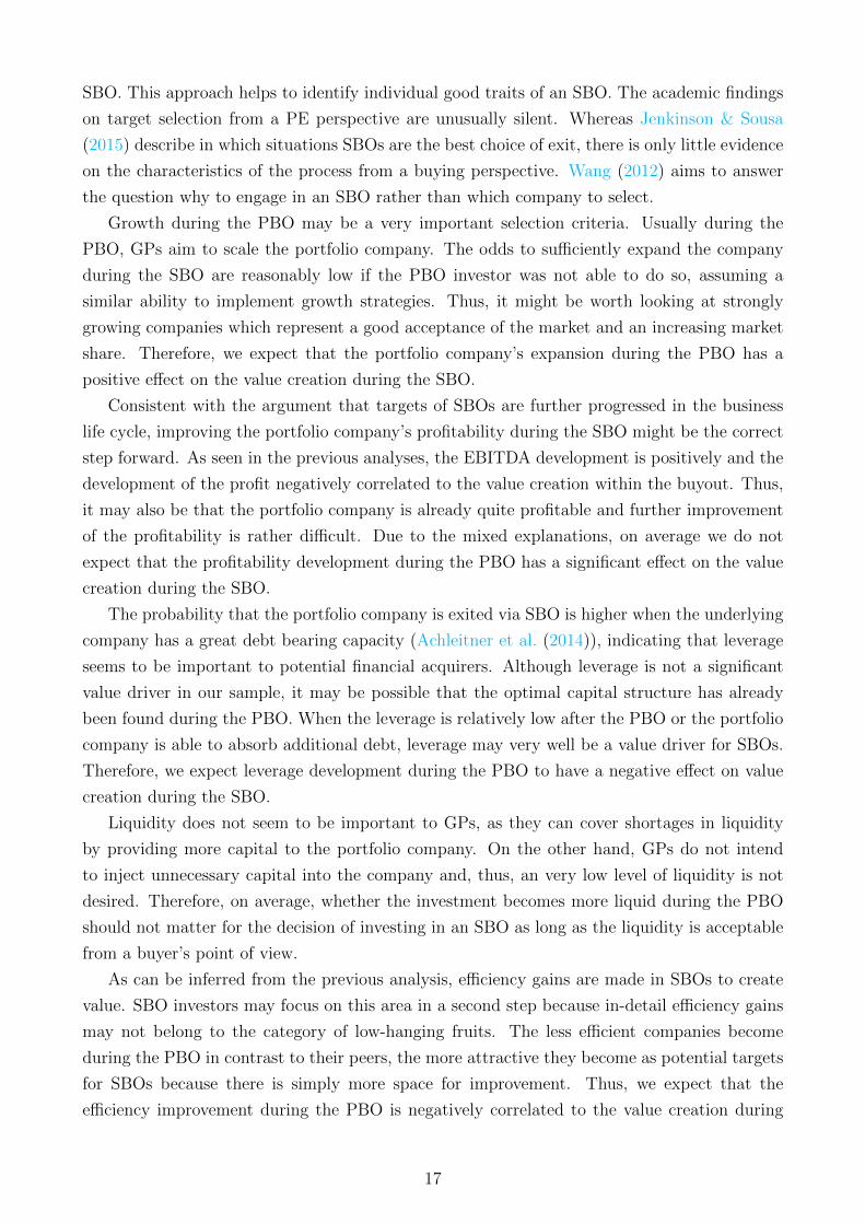
Growth during the PBO may be a very important selection criteria. Usually during the

PBO, GPs aim to scale the portfolio company. The odds to sufficiently expand the company

during the SBO are reasonably low if the PBO investor was not able to do so, assuming a

similar ability to implement growth strategies. Thus, it might be worth looking at strongly

growing companies which represent a good acceptance of the market and an increasing market

share. Therefore, we expect that the portfolio company’s expansion during the PBO has a

positive effect on the value creation during the SBO.

Consistent with the argument that targets of SBOs are further progressed in the business

life cycle, improving the portfolio company’s profitability during the SBO might be the correct

step forward. As seen in the previous analyses, the EBITDA development is positively and the

development of the profit negatively correlated to the value creation within the buyout. Thus,

it may also be that the portfolio company is already quite profitable and further improvement

of the profitability is rather difficult. Due to the mixed explanations, on average we do not

expect that the profitability development during the PBO has a significant effect on the value

creation during the SBO.

The probability that the portfolio company is exited via SBO is higher when the underlying

company has a great debt bearing capacity (Achleitner et al. (2014)), indicating that leverage

seems to be important to potential financial acquirers. Although leverage is not a significant

value driver in our sample, it may be possible that the optimal capital structure has already

been found during the PBO. When the leverage is relatively low after the PBO or the portfolio

company is able to absorb additional debt, leverage may very well be a value driver for SBOs.

Therefore, we expect leverage development during the PBO to have a negative effect on value

creation during the SBO.

Liquidity does not seem to be important to GPs, as they can cover shortages in liquidity

by providing more capital to the portfolio company. On the other hand, GPs do not intend

to inject unnecessary capital into the company and, thus, an very low level of liquidity is not

desired. Therefore, on average, whether the investment becomes more liquid during the PBO

should not matter for the decision of investing in an SBO as long as the liquidity is acceptable

from a buyer’s point of view.

As can be inferred from the previous analysis, efficiency gains are made in SBOs to create

value. SBO investors may focus on this area in a second step because in-detail efficiency gains

may not belong to the category of low-hanging fruits. The less efficient companies become

during the PBO in contrast to their peers, the more attractive they become as potential targets

for SBOs because there is simply more space for improvement. Thus, we expect that the

efficiency improvement during the PBO is negatively correlated to the value creation during

17

the SBO.

Innovation during the PBO may indicate strongly growing companies and thus align with

the growth hypothesis. At the same time, SBO investors may wish to invest in companies that

are not as innovative yet because already little investments may foster the value growth. Due

to these mixed explanations, we do not expect a significant effect of the degree of innovation

during the PBO on the development of the company value during the SBO.

5.1 Methodology

After understanding which value drivers are relevant in a general environment, we analyse if

and how the success in the second investment round is dependent on the development of the

performance drivers during the PBO. We calculate the possibility of an SBO being successful

depending on the success of the PBO. A deal is defined as successful when it produces a

superior company value development compared to its predefined peer group. Those companies

that have an above average development are assigned a ”1” in a binary variable setting. Due to

the assignment in the binary variable setting, we are able to calculate probabilities whether an

investment is going to be successful conditional on the outcome of the prior investment. This

overview provides a first idea whether there might be dependencies between the two buyout

stages. The conditional probabilities for each case are calculated as follows:

P (SBO|PBO) =P (SBO ∩ PBO)

SBO(5)

In addition, we use an OLS regression to determine whether the development during the PBO

has any influence on the value creation during the SBO. This analysis determines which com-

panies are suitable for an SBO. We regress the valuation development during the secondary

buyout conditional on the developments of the value drivers during the PBO. We use the value

drivers from the determinant analysis and use the following model specification:

yit(SBO) = α + β ∗Xit(PBO) + γ ∗ Yt + ε (6)

where y describes the company value growth of company i at time t during the SBO, X de-

scribes devlopment of the firm-specific variables during the PBO and Y describes the economic

variables.

5.2 Results

The probability tree in Figure 4 shows the success probabilities for all buyout rounds and the

conditional probabilities for all four cases after the SBO. In our sample there are more deals

that outperformed their peer group than deals that underperformed compared to their peer

group.

18

The conditional probabilities of the SBO being successful are similar with 64.9 percent

and 67.3 percent for a successful and unsuccessful PBOs, respectively. Thus, it seems that PE

investors themselves may perform superior compared to other shareholders and thus on average

foster the companies’ growth more than their peer group. However, after any development

of the PBO there are evidentially some differences between outperforming the market and

underperforming the market. The conditional probabilities show that there are slight differences

for the success of the SBO conditional on how the PBO performed. However, the differences are

not very large and thus we may need a more detailed analysis on how to engage in a successful

SBO. Therefore, in the following we analyse which companies are especially suitable for good

SBOs.

Table 7 summarises the results of the OLS regression. The evidence about dependency of

growth and expansion during the PBO is rather mixed. In all specifications the value growth

during the PBO has a negative influence on the value growth during the SBO with a high

significance. Those companies, which develop a higher company value during the PBO than

their competitors, perform worse during the SBO. This result follows the idea that most of value

creation potential is already used up during the PBO. This result corroborates the finding from

the conditional probabilities, but its extent is weaker as the conditional probabilities for success

are only in a binary variable setting and thus inherit less variation. This theory aligns with

the partially significant and negative coefficients in equity development during the PBO as a

measure of intrinsic value growth. The sales CAGR is at least for the last specification weakly

significant with a positive coefficient. Companies that grow rapidly represent products and

services that are promising or generally well-developing brands and thus indicate potential

further growth in the future. These results indicate that it is beneficial when the intrinsic value

of the company developed rather weakly during the PBO, whilst the market participation,

measured in sales, grows.

- Table 7 about here -

The results for SBO value creation based on the profitability development during the PBO is

also mixed. The EBITDA margin development during the PBO is statistically significant and

positively correlated to the value growth during the SBO. PE firms should invest into companies

having a good operative margin. Companies that could not be improved into more efficient

companies during the PBO may not improve the EBITDA margin during the SBO either as

some businesses are not possible to streamline further. In contrast to the EBITDA-margin, the

return on assets ratio is negatively and significantly correlated. We observe that it is important

to find companies that use their assets badly to reach a certain operating profit. This finding

aligns with the previous regression that return on assets is a very strong value driver for SBOs.

Therefore, it seems that portfolio companies should have great operating earnings but require

further fine-tuning according to asset usage. This finding is further backed by the inventory

sales ratio. According to this variable, PE firms should acquire companies that are bad at selling

off and managing their inventory, i.e. using parts of their assets inefficiently. Potentially, during

an SBO the GP can sell off the excessive inventory, thereby reducing its working capital and

19

thus improving its profitability with respect to the invested assets.

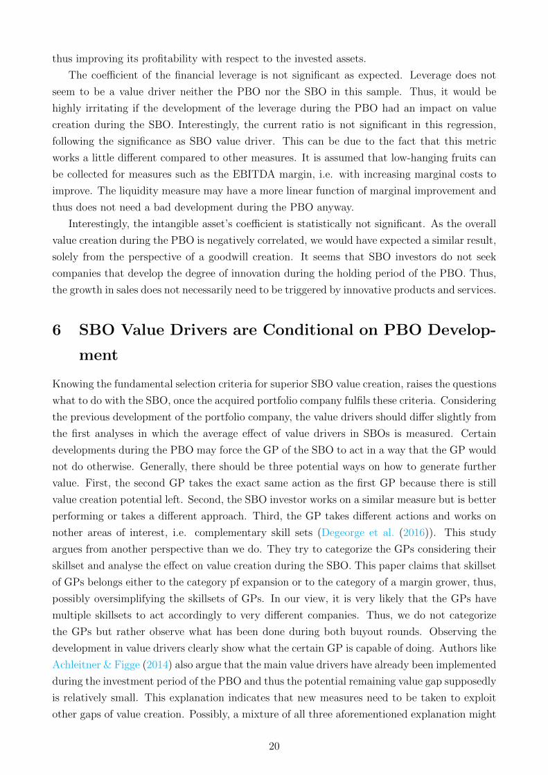
The coefficient of the financial leverage is not significant as expected. Leverage does not

seem to be a value driver neither the PBO nor the SBO in this sample. Thus, it would be

highly irritating if the development of the leverage during the PBO had an impact on value

creation during the SBO. Interestingly, the current ratio is not significant in this regression,

following the significance as SBO value driver. This can be due to the fact that this metric

works a little different compared to other measures. It is assumed that low-hanging fruits can

be collected for measures such as the EBITDA margin, i.e. with increasing marginal costs to

improve. The liquidity measure may have a more linear function of marginal improvement and

thus does not need a bad development during the PBO anyway.

Interestingly, the intangible asset’s coefficient is statistically not significant. As the overall

value creation during the PBO is negatively correlated, we would have expected a similar result,

solely from the perspective of a goodwill creation. It seems that SBO investors do not seek

companies that develop the degree of innovation during the holding period of the PBO. Thus,

the growth in sales does not necessarily need to be triggered by innovative products and services.

6 SBO Value Drivers are Conditional on PBO Develop-

ment

Knowing the fundamental selection criteria for superior SBO value creation, raises the questions

what to do with the SBO, once the acquired portfolio company fulfils these criteria. Considering

the previous development of the portfolio company, the value drivers should differ slightly from

the first analyses in which the average effect of value drivers in SBOs is measured. Certain

developments during the PBO may force the GP of the SBO to act in a way that the GP would

not do otherwise. Generally, there should be three potential ways on how to generate further

value. First, the second GP takes the exact same action as the first GP because there is still

value creation potential left. Second, the SBO investor works on a similar measure but is better

performing or takes a different approach. Third, the GP takes different actions and works on

nother areas of interest, i.e. complementary skill sets (Degeorge et al. (2016)). This study

argues from another perspective than we do. They try to categorize the GPs considering their

skillset and analyse the effect on value creation during the SBO. This paper claims that skillset

of GPs belongs either to the category pf expansion or to the category of a margin grower, thus,

possibly oversimplifying the skillsets of GPs. In our view, it is very likely that the GPs have

multiple skillsets to act accordingly to very different companies. Thus, we do not categorize

the GPs but rather observe what has been done during both buyout rounds. Observing the

development in value drivers clearly show what the certain GP is capable of doing. Authors like

Achleitner & Figge (2014) also argue that the main value drivers have already been implemented

during the investment period of the PBO and thus the potential remaining value gap supposedly

is relatively small. This explanation indicates that new measures need to be taken to exploit

other gaps of value creation. Possibly, a mixture of all three aforementioned explanation might

20

work in SBOs. Therefore, we expect differing value drivers depending on the various selection

criteria.

6.1 Methodology

Lastly, after identifying the characteristics for suitable targets it is crucial to know what to do

with the investment once it is acquired. During the analysis of the target selection we identified

five company specific characteristics that make the acquisition of the portfolio company reason-

able. These characteristics are lower company growth, strong sales growth, superior EBITDA

margin development, weaker development in return on assets, and improved inventory sales

ratio. We perform subsampling for all identified value drivers during the regressions for target

selection, e.g. if we identified a negative value driver in the previous question, we construct a

subsample consisting of all observations that underperform in that specific value driver com-

pared to its peer group. This way, we are able to analyse what to do with a portfolio company

if one of the previous selection criteria has occurred. We may be able to recognise similarities

in the required actions of the different subsamples to finally identify which performance drivers

to favour and therefore to increase the portfolio companies’ valuation as much as possible. In

this analysis, we look at those individual selection criteria separately. Thus, we apply an OLS

regression for all SBOs with different subsamples:

yit(SBO) = α + β ∗Xit(SBO) + γ ∗ Yt + ε (7)

where y describes the company value growth of company i at time t during the SBO, X describes

the firm-specific variables development during the SBO and Y describes the economic variables.

6.2 Results

The results are summarised in Table 8. The five specifications represent the subsamples ac-

cording to the significant variables from the previous question, namely valuation growth, sales

growth, EBITDA margin development, return on asset development and inventory sales ratio

development.

- Table 8 about here -

The first specification considers the subsample of all companies that underperformed in terms

of valuation growth during the PBO. It is hard to tell how this subsample of 106 companies

are characterised, as there are several value drivers during the PBO. The coefficient of the

EBITDA margin is significant but economically rather small compared to the profitability

coefficients from the previous analyses. The other specifications provide a better insight how

the acquired companies are characterised and are therefore more interesting to this study.

The second specification analyses the subsample for those companies that had a superior

sales development compared to its peers. Interestingly, the coefficient for sales is not signifi-

21

cant although we found some significance in the SBO determinant analysis. This observation

may indicate that GPs neglect the further excessive expansion of sales when a company grew

strongly. On the other hand, the equity growth has a positive and significant coefficient, indi-

cating that successful SBOs are able to channel their earnings into equity. The return on assets

is both significant and also highly positive, indicating that it is highly important to improve the

effective usage of the portfolio company’s assets in order to realise strong value growth. Thus,

GPs should focus to redirect the strong sales growth into a profitable operation in relation to

its invested assets. The leverage ratio development is significant with a negative coefficient

indicating that the proportion of liabilities to equity should decrease. It shows that financial

engineering is less relevant when the underlying company has strongly expanded before and

probably does not need further capital to generate additional value. Furthermore, it has the

effect to reduce the amount of total assets which aligns well with the reasoning about the

improvement in return on assets.

The third specification focuses on those companies whose excess EBITDA margin develop-

ment was positive, i.e. the company developed its operative earnings margin better than its

peer group during the PBO. The coefficient for sales growth is significant and positive, meaning

that PE firms should rather concentrate on expanding the portfolio company’s sales when the

operating structures already became leaner. The portfolio companies may benefit strongly as

for every additional unit in sales the operative earnings are relatively high. Again, the company

should aim to improve the effective utilisation of assets as the significant coefficient for return

on assets is very high positive. The size of the company at entry of the SBO, measured in

total assets, is significantly and positively correlated to value growth, but the coefficient is too

small to be economically relevant. Furthermore, the cash ratio is highly significant and positive,

showing that the PE firm needs to use their profitable situation to build up cash, which may

be used either to repay the high amount of debt or to invest.

The fourth specification includes those companies whose return on assets has not developed

as well as in other companies. These companies need to consider the growth of the company

and turn the company into a more profitable organisation to increase operating cash flows. It

seems that the inferior return on assets is driven by lower operative earnings. Interestingly, the

intangible asset ratio is significant and negatively correlated to value creation. It seems that

counteracting the inferior return on assets is achieved by the reduction of intangible assets as

they seem to be less effective in generating earnings, at least in the short-run and therefore

SBO investors reduce the level of intangible assets on total assets.

The last specification concerns those companies that developed the inventory sales ratio

stronger than their close competitors during the PBO, i.e. being worse at inventory management

than the peer group. In this specification, only the sales growth coefficient is significant and

positive. This indicates that rather than reducing the inventory for a certain level of sales,

higher sales should be targeted.

Very interestingly, companies are not only successful when they have additional skillsets as

previously assumed. First, they do apply additional skillsets, e.g. improving return on assets

22

during the SBO after sales growth during the PBO, and thereby do something different to

create further value in a consecutive buyout. Second, SBO investors work on a similar area of

value drivers, e.g. increasing profitability by improving return on assets, although profitability

was already focussed on during the PBO as the EBITDA margin has been improved strongly.

However, it seems that SBO investors do not simply continue the previous strategy by doing

the same over again in the second buyout round.

Generally, there are different types of characteristics that make PBO portfolio companies

interesting for an SBO. Our analysis shows that there is not just a single value driver for SBOs

but rather a combination of reactions to the operational development during the PBO. Often

the reasons for acquiring a company in an SBO are manifold and thus do not depend on one

single indicator. However, the different indicators give a good first insight on how to handle

companies in different economic and operational situations. The investors may decide to which

category the investment belongs, test whether the significant value drivers can be implemented,

and then decide accordingly.

7 Conclusion

With a dataset of 295 companies undergoing consecutive PBOs and SBOs this paper answers

three research questions. First, we analyse whether PBOs and SBOs have differing value drivers.

Second, we answer the question how a company should have developed during the PBO to be

suitable for an SBO. Third, we investigate the separate value drivers dependent on the previous

development of the portfolio company. Our paper contributes to the existing literature in many

ways. The dataset is different from most papers, as it considers consecutive deals rather than

PBO and SBO separately. Up to our knowledge this dataset is the largest and most detailed

one with this specific construction of back-to-back buyouts. The dataset thus enables a more

sensible way to analyse different sets of value drivers. Furthermore, as we hand-collect many

data items, we are able to analyse other characteristics, for example risk, that have not been

properly examined yet. It is also the first paper which does not only investigate the differences

between the two buyouts but rather looks at the dependency between the two buyout rounds

based on a fundamental analysis.

The descriptive summary indicates different value creation profiles of PBO and SBO. Like

many other studies, we see that the portfolio companies develop well operationally compared

to its non PE-backed peers. Interestingly, the mean differences between PBO and SBO are

not significant for most of the applied measures. However, the median differences of the same

measures are often significantly different from another, mostly with better medians for the

PBO. The mean for the valuation CAGR is greater for SBOs than for PBOs, whilst the median

value is greater in PBOs than in SBOs. This is the first indication that it is possible to create

more value during an SBO than during PBOs but there is simply much more volatility in

the operational success of an SBO. Thus, we look closer into the value creation of buyouts

and especially of SBOs. The dependency analyses help to identify mechanisms that promote

23

successful SBOs.

We find that dependencies between the operational performance of PBOs and the opera-

tional performance of SBOs exist. We identify five developments during the PBO that influence

the value creation during the SBO and thus serve well as selection criteria. The more value was

created during the PBO, the less attractive it becomes as potential target for an SBO. How-

ever, SBO investors should seek to invest into strongly expanding companies as these companies

represent promising markets and, by this, stronger pertinence. When a portfolio company’s

profitability developed well during the PBO it becomes favourable for SBO acquisitions, an

inferior return on assets on the other hand is favourable as it allows further fine-tuning during

the SBO. Lastly, the less a portfolio companies improves its efficiency during the PBO, the

higher the value creation during the SBO.

The required action taken by the SBO investors differs among the identified selection cri-

teria. Generally, two types of value drivers exist which are conditional on certain selection

criteria. First, we find supporting evidence that complimentary skillsets exist, e.g. when sales

is developed strongly during the PBO, SBO investors tend to improve the profitability of the

portfolio companies. Second, the SBO investors also work on similar measures as the PBO

investors but do it differently, e.g. although profitability is focussed on PBO, in terms of

EBITDA margin, the SBO investor still aims to work on the profitability, but rather focuses on

the improvement of the return on assets. SBO investors either need to set different objectives

for their performnce management compared to PBO investors or they concentrate on the same

objectives with a different approach. However, a simple continuation of the PBO strategy does

not create value during the SBO.

Future research may expand this study by further analysing the combination of these effects.

Whilst our study provides an initial overview on which companies to acquire and what to do

once they are acquired, these findings solely focus on individual effects. Usually, companies

are acquired for several reasons rather than just one. This directly effects the combination of

what to do with the portfolio company and may differ from what we found. Further, up to this

point, it is not clear which of the proposed dependencies provides the greatest success.

24

8 Appendix

Figure 1: Buyout Exits

Source: Based on PitchBook (2018a) and PitchBook (2018b).

Figure 2: Start Year Density

Note: This figure shows the density of the sample’s investment entry year.

Figure 3: Holding Period by Buyout

Note: This figure shows the densitiy of the holding periods in years during the PBO and

SBO, respectively.

Figure 4: Conditional Probability

PBO

SBO

P (N1 ∩N2) = 12, 2%

NotSuccessful32, 7%

P (N1 ∩ S2) = 25, 1%Succ

essful

67, 3%

NotSuccessful37, 3%

SBO

P (S1 ∩N2) = 22, 0%

NotSuccessful35, 1%

P (S1 ∩ S2) = 40, 7%Succ

essful

64, 9%

Successf

ul

62, 7%

Note: This figure shows the (conditional) success probabilities during the PBO and SBO.

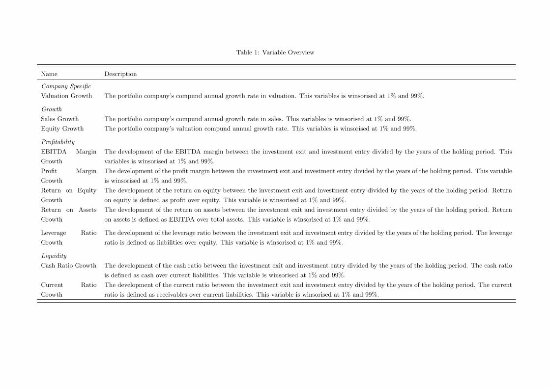
Table 1: Variable Overview

Name Description

Company Specific

Valuation Growth The portfolio company’s compund annual growth rate in valuation. This variables is winsorised at 1% and 99%.

Growth

Sales Growth The portfolio company’s compund annual growth rate in sales. This variables is winsorised at 1% and 99%.

Equity Growth The portfolio company’s valuation compund annual growth rate. This variables is winsorised at 1% and 99%.

Profitability

EBITDA Margin

Growth

The development of the EBITDA margin between the investment exit and investment entry divided by the years of the holding period. This

variables is winsorised at 1% and 99%.

Profit Margin

Growth

The development of the profit margin between the investment exit and investment entry divided by the years of the holding period. This variable

is winsorised at 1% and 99%.

Return on Equity

Growth

The development of the return on equity between the investment exit and investment entry divided by the years of the holding period. Return

on equity is defined as profit over equity. This variable is winsorised at 1% and 99%.

Return on Assets

Growth

The development of the return on assets between the investment exit and investment entry divided by the years of the holding period. Return

on assets is defined as EBITDA over total assets. This variable is winsorised at 1% and 99%.

Leverage Ratio

Growth

The development of the leverage ratio between the investment exit and investment entry divided by the years of the holding period. The leverage

ratio is defined as liabilities over equity. This variable is winsorised at 1% and 99%.

Liquidity

Cash Ratio Growth The development of the cash ratio between the investment exit and investment entry divided by the years of the holding period. The cash ratio

is defined as cash over current liabilities. This variable is winsorised at 1% and 99%.

Current Ratio

Growth

The development of the current ratio between the investment exit and investment entry divided by the years of the holding period. The current

ratio is defined as receivables over current liabilities. This variable is winsorised at 1% and 99%.

Table 1 Variable Overview – continued from previous page

Name Description

Efficiency

Inventory-Sales Ra-

tio Growth

The development of the inventory sales ratio between the investment exit and investment entry divided by the years of the holding period. This

variable is defined as stocks over sales. This variable is winsorised at 1% and 99%.

Receivables-

Turnover Ratio

Growth

The development of the receivables turnover ratio between the investment exit and investment entry divided by the years of the holding period.

The receivables turnover ratio is defined as sales over debtors. This variable is winsorised at 1% and 99%.

Intangible Asset

Growth

The development of the intangible asset ratio between the investment exit and investment entry divided by the years of the holding period. The

intangible asset ratio is defined as the proportion of intangible assets of total assets. This variable is winsorised at 1% and 99%.

Altman Z-Score

Development

The development of the Altman Z-score between the investment exit and investment entry divided by the years of the holding period.

Control Variables

SBO Dummy Dummy variable that indicates whether the deal is a secondary buyout. Variable is equal to one when the underlying deal is a secondary buyout.

Total Assets The portfolio company’s total assets including all fixed assets and current assets at the time of the respective transaction. This variables is

winsorised at 1% and 99%.

Start Year Dummy Dummy variables that indicate the entry year of the underlying deal.

Holding Period The time (in years) the investors holds the portfolio company during the first and second buyout, i.e. the time difference between the first and

second transaction date and the time difference between the second and third transaction date.

GICS Dummy Dummy variables that indicates the industry classification of the portfolio company. The classification is based on the 8-digit sub-industry GICS

code.

Market-Based

Inflation Rate The annual inflation rate at time of entry and exit of the underlying deal.

Credit spreads Difference between Moody’s BAA bond index (corporate bond index) and the risk-free UK government bond (risk-free rate)

Employment Rate The yearly employment rate in the UK; Employed Working People/Working People

GDP Index GDP Index Development with 1996=100

Note: The table above presents all variables and ratios that are used in the analysis of this paper. All development measures are calculated for both the PBO and

the SBO. When applicable, the absolute excess development compared to the close peer group is considered (see section 3.2.2.). The table includes company specific

information, deal-specific, and economic data.

Table 2: Cross-correlation table

Variables (1) (2) (3) (4) (5) (6) (7) (8) (9) (10) (11) (12) (13) (14) (15) (16) (17) (18)Valuation 1.000Sales 0.422 1.000EBITDA 0.421 0.466 1.000Profit 0.223 0.229 0.588 1.000Equity 0.086 -0.221 0.041 0.059 1.000Total Assets -0.088 -0.217 -0.113 -0.049 0.102 1.000Holding Period -0.194 -0.214 -0.022 0.036 0.076 -0.049 1.000Intangible Asset 0.105 0.131 0.099 0.029 -0.221 -0.130 -0.018 1.000Leverage Ratio -0.047 0.009 0.049 0.028 -0.003 0.100 -0.064 -0.033 1.000Current Cash 0.027 -0.057 0.015 0.043 0.012 -0.005 0.087 -0.025 -0.002 1.000Return on Equity 0.071 -0.012 0.010 0.150 -0.005 -0.055 0.000 0.006 0.045 0.015 1.000Return on Assets 0.238 0.127 0.327 0.412 0.023 -0.073 0.067 0.001 0.021 0.078 0.279 1.000Receivables Sales 0.040 0.185 0.224 0.338 0.000 -0.053 -0.028 -0.011 -0.032 -0.040 0.240 0.196 1.000Inventory Sales -0.280 -0.201 -0.193 -0.295 -0.003 -0.030 0.029 0.001 -0.001 -0.046 0.047 -0.044 -0.044 1.000Credit Spreads 0.078 0.008 0.005 -0.006 0.033 0.049 -0.190 0.016 0.003 -0.025 0.002 -0.074 0.008 -0.004 1.000Employment Rate -0.069 -0.025 -0.041 -0.041 -0.042 -0.029 0.023 0.008 -0.001 0.018 0.022 -0.002 0.014 0.067 -0.353 1.000Inflation Rate -0.006 -0.043 -0.003 -0.028 0.034 0.047 -0.018 0.023 0.040 0.026 -0.038 -0.042 -0.078 0.004 0.286 -0.528 1.000GDP Index 0.059 -0.053 0.049 0.023 0.015 0.048 -0.179 0.063 0.000 -0.034 0.014 -0.046 0.056 0.001 0.170 0.164 0.460 1.000

Note: The table above shows the correlation matrix of the variable developments used in this paper. The highest positive correlation is 0.588 between EBITDAdevelopment and profit development. On the opposite the highest negative correlation is -0.528 between inflation rate and employment rate. None of these variablesshould cause concern about multicollinearity.

Table 3: Summary

Panel A: Company Information at EntryTotal PBO SBO

Mean SD Median Obs Mean SD Median Obs Mean SD Median ObsValuation at Entry 60,801 98,030 26,432 590 52,784 98,481 19,979 295 68,818∗ 97,083 36,143∗∗∗ 295Sales at Entry 58,253 87,979 27,684 590 47,813 83,215 19,800 295 68,693∗∗ 91,452 36,056∗∗∗ 295EBITDA at Entry 7,926 16,954 3,412 590 6,588 17,988 2,288 295 9,263 15,771 4,958∗∗∗ 295Profit at Entry 3,079 7,922 1,492 590 1,740 7,082 745 295 4,418∗∗∗ 8,483 2,423∗∗∗ 295RoA at Entry 0.156 0.198 0.139 590 0.153 0.226 0.138 295 0.16 0.166 0.141 295Total Assets at Entry 82,872 176,586 26,966 590 65,562 145,864 19,987 295 100,182∗∗∗ 201,478 36,442∗∗∗ 295Equity at Entry 2,4116 61,813 5,442 590 19,029 54,307 3,491 295 29,204∗ 68,217 9,271∗∗∗ 295Leverage at Entry 2.35 52.3 1.601 587 1.441 58.6 1.816 293 3.36 45.3 1.389 294

Panel B: Company Information DevelopmentTotal PBO SBO

Mean SD Median Obs Mean SD Median Obs Mean SD Median ObsValuation CAGR 1.320 0.917 1.161 589 1.293 0.769 1.170 294 1.346 1.045 1.148 295Sales CAGR 1.245 0.617 1.112 589 1.289 0.613 1.162 294 1.2 0.62 1.088∗∗∗ 295EBITDA-Margin Dev 0.111 0.556 0.018 588 0.125 0.507 0.031 294 0.098 0.601 0.008∗∗∗ 294Profit-Margin Dev 0.086 0.412 0.014 589 0.09 0.387 0.022 294 0.082 0.436 0.005∗∗∗ 295RoA Dev -0.005 0.115 -0.001 587 -0.002 0.117 0.001 294 -0.009 0.113 -0.003 293Total Assets CAGR 1.202 0.388 1.133 588 1.268 0.455 1.179 294 1.136∗∗∗ 0.0291 1.094∗∗∗ 294Equity Dev 0.125 0.29 0.06 589 0.152 0.323 0.074 294 0.099∗ 0.251 0.055 295Leverage Dev 2.766 32.41 -0.055 585 3.734 37.166 -0.06 292 1.801 26.877 -0.047 293Holding Period 4.102 2.550 4 590 4.054 2.445 4 295 4.149 2.654 4 295

Note: The table above presents the dataset of 295 companies from the UK that have been tracked throughout the two consecutive buyouts, i.e. the PBO and the SBO.For most of those companies we were able to collect the balance sheet and P&L fundamental data at time of the transactions, speaking before the PBO, after the PBO,and after the SBO. The variables used in this study are defined in table 2. Absolute data are presented in thousands. Panel A displays the valuation and the operativeand financial characteristics of the buyouts at time of the investment entry. These fundamental data and ratios represent the basic data of the underlying portfoliocompany. Panel B illustrates the development of the valuation and the key characteristics throughout the holding period. The calculation of the respective developmentis also presented in table 1. The significance levels for the mean difference and median difference test between PBO and SBO are ***0.1%, **1% and *5%.

Table 4: Determinant Analysis: Total Buyouts

(1) (2) (3)Growth

SalesG 0.885∗∗∗ 0.881∗∗∗ 0.786∗∗∗

(0.00) (0.00) (0.00)EquityG 0.018∗∗∗ 0.022∗∗∗ 0.023∗∗∗

(0.00) (0.00) (0.00)Profitability

EBITDA marginG 0.788∗∗∗ 0.744∗∗∗ 0.754∗∗∗

(0.00) (0.00) (0.00)Profit marginG -0.040 0.008 -0.192∗

(0.61) (0.93) (0.04)Return on equityG 0.058

(0.08)Return on assetsG 2.007∗∗∗

(0.00)Leverage ratioG -0.002

(0.06)Liquidity

Cash ratioG -0.056(0.59)

Current ratioG 0.044(0.29)

EfficiencyReceivables Turnover RatioG -0.002

(0.27)Inventory Sales RatioG -0.195∗∗∗

(0.00)Altman z-scoreG 0.008

(0.57)Intangible asset ratioG 0.403∗

(0.02)log (total assets) 0.006 0.016

(0.80) (0.54)log (holding period) -0.120 -0.147∗

(0.06) (0.02)Macro controls NO YES YES

Time Dummy NO YES YES

Industry Dummy NO YES YES

Constant 0.095∗∗ 708.192 979.980∗

(0.01) (0.14) (0.04)Overall R2 0.264 0.396 0.467Number of Observations 588 588 572

Note: The table above shows the estimates of the panel OLS regression. For all three specifications, thedependent variable is the excess company value growth. The first specification represents the base case whichincludes the variables used in the valuation of the company. The second specification adds time controls,industry controls and selected macroeconomic variables. The third specification adds more company-specificvariables that influence the company value. The t-statistics are reported in parenthesis below the respectivecoefficients. The significance levels for all specifications are ***0.1%, **1% and *5%. The lower case G indicateswhether the variable is a measure of excess growth.

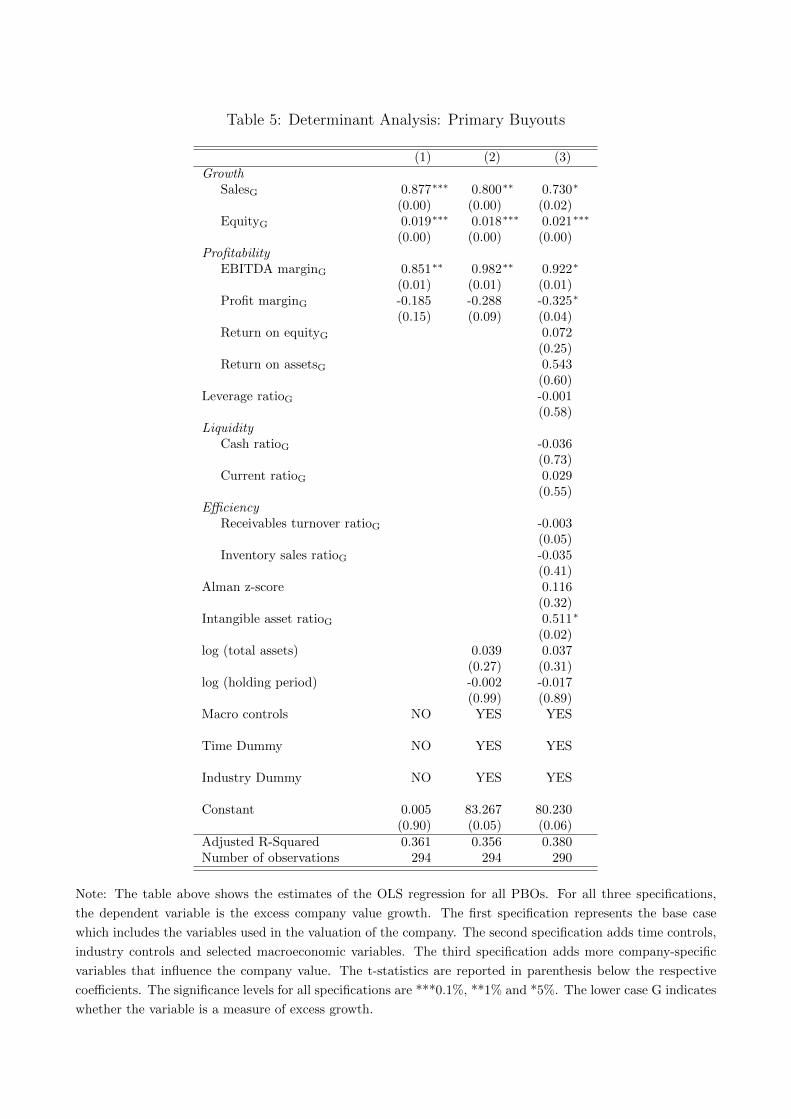
Table 5: Determinant Analysis: Primary Buyouts

(1) (2) (3)Growth

SalesG 0.877∗∗∗ 0.800∗∗ 0.730∗

(0.00) (0.00) (0.02)EquityG 0.019∗∗∗ 0.018∗∗∗ 0.021∗∗∗

(0.00) (0.00) (0.00)Profitability

EBITDA marginG 0.851∗∗ 0.982∗∗ 0.922∗

(0.01) (0.01) (0.01)Profit marginG -0.185 -0.288 -0.325∗

(0.15) (0.09) (0.04)Return on equityG 0.072

(0.25)Return on assetsG 0.543

(0.60)Leverage ratioG -0.001

(0.58)Liquidity

Cash ratioG -0.036(0.73)

Current ratioG 0.029(0.55)

EfficiencyReceivables turnover ratioG -0.003

(0.05)Inventory sales ratioG -0.035

(0.41)Alman z-score 0.116

(0.32)Intangible asset ratioG 0.511∗

(0.02)log (total assets) 0.039 0.037

(0.27) (0.31)log (holding period) -0.002 -0.017

(0.99) (0.89)Macro controls NO YES YES

Time Dummy NO YES YES

Industry Dummy NO YES YES

Constant 0.005 83.267 80.230(0.90) (0.05) (0.06)

Adjusted R-Squared 0.361 0.356 0.380Number of observations 294 294 290

Note: The table above shows the estimates of the OLS regression for all PBOs. For all three specifications,

the dependent variable is the excess company value growth. The first specification represents the base case

which includes the variables used in the valuation of the company. The second specification adds time controls,

industry controls and selected macroeconomic variables. The third specification adds more company-specific

variables that influence the company value. The t-statistics are reported in parenthesis below the respective

coefficients. The significance levels for all specifications are ***0.1%, **1% and *5%. The lower case G indicates

whether the variable is a measure of excess growth.

Table 6: Determinant Analysis: Secondary Buyouts

(1) (2) (3)Growth

SalesG 0.932∗∗ 0.786 0.636(0.00) (0.10) (0.22)

EquityG -0.002 -0.007 -0.000(0.82) (0.64) (1.00)

ProfitabilityEBITDA marginG 0.788∗ 0.733 0.863∗

(0.03) (0.06) (0.03)Profit marginG 0.069 0.155 -0.126

(0.75) (0.53) (0.28)Return on equityG 0.085

(0.41)Return on assetsG 3.829∗∗

(0.01)Leverage ratioG -0.003

(0.29)Liquiditiy

Cash ratioG -0.051(0.82)

Current ratioG 0.138∗

(0.03)Efficiency

Receivables turnover ratioG 0.026(0.11)

Inventory Sales RatioG -0.265∗∗∗

(0.00)Altman z-score -0.208

(0.09)Intangible asset ratioG -0.307

(0.67)log (total assets) -0.035 -0.044

(0.43) (0.32)log (holding period) -0.202 -0.267∗

(0.10) (0.05)Macro controls NO YES YES

Time Dummy NO YES YES

Industry Dummy NO YES YES

Constant 0.186∗∗∗ 1251.213 1917.697(0.00) (0.37) (0.14)

Adjusted R-Sqaured 0.216 0.183 0.287Number of observations 294 294 282

Note: The table above shows the estimates of the OLS regression for all PBOs. For all three specifications,the dependent variable is the excess company value growth. The first specification represents the base casewhich includes the variables used in the valuation of the company. The second specification adds time controls,industry controls and selected macroeconomic variables. The third specification adds more company-specificvariables that influence the company value. The t-statistics are reported in parenthesis below the respectivecoefficients. The significance levels for all specifications are ***0.1%, **1% and *5%. The lower case G indicateswhether the variable is a measure of excess growth.

Table 7: Target Selection

(1) (2) (3)Growth

ValuationPBO,G -0.345∗∗∗ -0.354∗∗∗ -0.318∗∗∗

(0.00) (0.00) (0.00)SalesPBO,G 0.222 0.276 0.394∗

(0.06) (0.14) (0.04)EquityPBO,G -0.474∗ -0.422∗ -0.330

(0.03) (0.03) (0.09)Profitability

EBITDA marginPBO,G 0.164∗ 0.145∗ 0.189∗

(0.03) (0.01) (0.04)Profit marginPBO,G -0.088 -0.025 -0.052

(0.35) (0.68) (0.60)Return on assetsPBO,G -0.295∗∗∗

(0.00)Return on equityPBO,G -0.001

(0.85)Leverage ratioPBO,G -0.000

(0.51)Liquidity

Cash ratioPBO,G 0.069(0.09)

Current ratioPBO,G -0.041(0.07)

EfficiencyReceivables turnover ratioPBO,G 0.001

(0.60)Inventory Sales RatioPBO,G 0.543∗∗∗

(0.00)Altman z-scorePBO,G 0.010

(0.73)Intangible asset ratioPBO,G -0.062

(0.66)log (holding period)PBO -0.132 -0.123

(0.07) (0.12)log (total assets)SBO -0.020 -0.040

(0.46) (0.10)Macro controls NO YES YES

Time Dummy NO YES YES

Industry Dummy NO YES YES

Constant 0.266∗∗∗ 2.773 4.570(0.00) (0.59) (0.37)

Adjusted R-Squared 0.062 0.136 0.292Number of observations 295 294 290

The table above shows the estimates of the OLS model regressing the excess valuation growth during the SBOon the excess variable developments during the PBO. The first specification represents the base case whichincludes the variables used in the valuation of the company. The second specification adds time controls,industry controls and selected macroeconomic variables. The third specification adds more company-specificvariables that influence the company value. The t-statistics are reported in parenthesis below the respectivecoefficients. The significance levels for all specifications are ***0.1%, **1% and *5%. The lower case G indicateswhether the variable is a measure of excess growth.

Table 8: SBO Value Drivers

(1) (2) (3) (4) (5)Valuation Sales EBITDA RoA Inventory

GrowthSalesSBO,G 0.004 0.413 0.980∗∗∗ 0.481∗∗ 0.531∗∗∗

(0.99) (0.10) (0.00) (0.00) (0.00)EquitySBO,G 0.780 0.474∗ 0.335 0.362 0.170

(0.10) (0.02) (0.30) (0.05) (0.61)Profitability

EBITDA marginSBO,G 0.047 0.075 -0.128 0.564∗∗ 0.208(0.84) (0.81) (0.26) (0.01) (0.18)

Profit marginSBO,G 0.202∗∗ 0.496 0.251 0.020 0.024(0.01) (0.19) (0.42) (0.48) (0.49)

Return on assetsSBO,G -0.713 1.918∗ 2.243∗∗ 0.057 0.005(0.70) (0.02) (0.01) (0.96) (1.00)

Return on equitySBO,G -0.010 0.026 0.003 0.023 0.011(0.66) (0.25) (0.79) (0.25) (0.50)

Leverage ratioSBO,G 0.001 -0.004∗ -0.003 0.000 -0.001(0.84) (0.03) (0.18) (0.91) (0.62)

LiquidityCash ratioSBO,G 0.028 0.085 0.034∗∗∗ -0.042 0.188

(0.06) (0.32) (0.00) (0.64) (0.34)Current ratioSBO,G -0.001 -0.013 0.000 -0.029 -0.038

(0.66) (0.52) (0.86) (0.47) (0.41)Efficiency

Inventory sales ratioSBO,G -1.621 -0.211 -0.118 -2.886 -3.147(0.55) (0.74) (0.83) (0.07) (0.06)

Receivables turnover ratioSBO,G 0.010 -0.058 -0.055 0.011 -0.039(0.30) (0.06) (0.09) (0.22) (0.07)

Altman z-score 0.088 -0.054 0.118 0.099 -0.281(0.23) (0.60) (0.06) (0.14) (0.08)

Intangible asset ratioSBO,G -0.083 0.084 0.002 -0.769∗∗ -0.124(0.54) (0.31) (0.99) (0.00) (0.63)

log (holding period)SBO,G -0.296 -0.071 -0.025 -0.084 -0.051(0.11) (0.28) (0.72) (0.31) (0.58)

log (total assets)SBO -0.000 -0.000 0.000∗ 0.000 -0.000(0.94) (0.56) (0.02) (0.56) (0.49)

Macro Controls YES YES YES YES YES

Time Dummy YES YES YES YES YES

Industry Dummy YES YES YES YES YES

Constant -0.581 7.520 3.729 2.002 -5.672(0.95) (0.11) (0.50) (0.80) (0.30)

Adjusted R-Squared 0.358 0.405 0.456 0.490 0.503Number of observations 106 205 171 135 141

Note: The table above shows the estimates of the OLS model regressing the excess valuation growth during theSBO on the excess variable developments during the SBO. All specifications include the base variables, timecontrols, industry controls, macroeconomic variables and additional company-specific variables. The specifica-tions are subsamples that represent the target selection criteria identified in the second research question. Thet-statistics are reported in parenthesis below the respective coefficients. The significance levels for all specifi-cations are ***0.1%, **1% and *5%. The lower case G indicates whether the variable is a measure of excessgrowth.

References

Acharya, V. V., Gottschalg, O., Hahn, M., & Kehoe, C. (2012). Corporate Governance and

Value Creation: Evidence from Private Equity. The Review of Financial Studies , 26 (2),

368–402.

Achleitner, A.-K., Braun, R., & Engel, N. (2011). Value Creation and Pricing in Buyouts:

Empirical Evidence from Europe and North America. Review of Financial Economics , 20 (4),

146–161.

Achleitner, A.-K., & Figge, C. (2014). Private Equity Lemons? Evidence on Value Creation

in Secondary Buyouts. European Financial Management , 20 (2), 406–433.

Achleitner, A.-K., Figge, C., & Lutz, E. (2014). Drivers of Value Creation in a Secondary

Buyout: The Acquisition of Brenntag by BC Partners. Qualitative Research in Financial

Markets , 6 (3), 278–301.

Alford, A. W. (1992). The Effect Of The Set Of Comparable Firms On The Accuracy Of The

Price Earnings Valuation Method. Journal of Accounting Research, 30 (1), 94–108.

Altman, E. I. (1968). Financial ratios, discriminant analysis and the prediction of corporate

bankruptcy. The journal of finance, 23 (4), 589–609.

Baker, M., & Ruback, R. S. (1999). Estimating Industry Multiples. Working Paper. Harvard

University .

Barber, B. M., & Lyon, J. D. (1996). Detecting Abnormal Operating Performance: The

Empirical Power and Specification of Test Statistics. Journal of Financial Economics , 41 (3),

359–399.

Bhojraj, S., & Lee, C. M. (2002). Who Is My Peer? A Valuation-Based Approach to the

Selection of Comparable Firms. Journal of Accounting Research, 40 (2), 407–439.

Bhojraj, S., Lee, C. M., & Oler, D. K. (2003). What’s My Line? A Comparison of Industry

Classification Schemes for Capital Market Research. Journal of Accounting Research, 41 (5),

745–774.

Bonini, S. (2015). Secondary Buyouts: Operating Performance and Investment Determinants.

Financial Management , 44 (2), 431–470.

Capron, L., & Shen, J.-C. (2007). Acquisitions of private vs. public firms: Private information,

target selection, and acquirer returns. Strategic management journal , 28 (9), 891–911.

De Fontenay, E. (2014). Private Equity Firms as Gatekeepers. Review of Banking & Financial

Law , 33 , 115-189.

Degeorge, F., Martin, J., & Phalippou, L. (2016). On Secondary Buyouts. Journal of Financial

Economics , 120 (1), 124–145.

Guo, S., Hotchkiss, E. S., & Song, W. (2011). Do Buyouts (Still) Create Value? The Journal

of Finance, 66 (2), 479–517.

Hausman, J. A. (1978). Specification Tests in Econometrics. Econometrica: Journal of the

Econometric Society , 46 (6), 1251–1271.

Herrmann, V., & Richter, F. (2003). Pricing with Performance-Controlled Multiples. Schmalen-

bach Business Review , 55 (3), 194–219.

Jenkinson, T., & Sousa, M. (2011). Why Do Private Equity Firms Sell to Each Others?

Working Paper, Said Business School, Oxford University .

Jenkinson, T., & Sousa, M. (2015). What Determines the Exit Decision for Leveraged Buyouts?

Journal of Banking & Finance, 59 , 399–408.

Jensen, M. C. (1986). Agency Cost of Free Cash Flow, Corporate Finance, and Takeovers. The

American Economic Review , 76 (2), 323–329.

Jensen, M. C. (1989). Eclipse of the Public Corporation. Harvard Business Review , 67 (5),

61-74.

Jensen, M. C., & Meckling, W. H. (1976). Theory of the Firm: Managerial Behavior, Agency

Costs and Ownership Structure. Journal of Financial Economics , 3 (4), 305-360.

Korteweg, A. (2010). The Net Benefits to Leverage. The Journal of Finance, 65 (6), 2137–2170.

Lee, C., Lee, K., & Pennings, J. M. (2001). Internal Capabilities, External Networks, and

Performance: A Study on Technology-Based Ventures. Strategic Management Journal , 22 (6),

615–640.

Liu, J., Nissim, D., & Thomas, J. (2002). Equity Valuation Using Multiples. Journal of

Accounting Research, 40 (1), 135–172.

Matthews, G., Bye, M., & Howland, J. (2009). Operational Improvement: The Key to Value

Creation in Private Equity. Journal of Applied Corporate Finance, 21 (3), 21–27.

Pereiro, L. E. (2002). Valuation of Companies in Emerging Markets: A Practical Approach

(Vol. 156). John Wiley & Sons.

Perembetov, K., Herger, I., Braun, R., & Puche, B. (2014). Value Creation in Private Equity.

Working Paper .

PitchBook. (2018a). EU PE Breakdown. Report .

PitchBook. (2018b). US PE Breakdown. Report .

Schreiner, A. (2009). Equity Valuation Using Multiples: An Empirical Investigation. Springer

Science & Business Media.

Wang, Y. (2012). Secondary Buyouts: Why Buy and at What Price? Journal of Corporate

Finance, 18 (5), 1306–1325.

Wright, M., Hoskisson, R. E., Busenitz, L. W., & Dial, J. (2001). Finance and Management

Buyouts: Agency versus Entrepreneurship Perspectives. Venture Capital: An International

Journal of Entrepreneurial Finance, 3 (3), 239–261.