1

Database dependency discovery:a machine learning approach

Peter A. FlachDepartment of Computer Science,University of Bristol,Bristol BS8 1UB, United Kingdom,Peter.Flach@bristol.ac.uk

Iztok SavnikFaculty of Computer and Information Science,University of Ljubljana,1000 Ljubljana, Slovenia,Iztok.Savnik@fri.uni-lj.si

Database dependencies, such as functional and multivalueddependencies, express the presence of structure in databaserelations, that can be utilised in the database design process.The discovery of database dependencies can be viewed as aninduction problem, in which general rules (dependencies) areobtained from specific facts (the relation). This viewpointhas the advantage of abstracting away as much as possiblefrom the particulars of the dependencies. The algorithms inthis paper are designed such that they can easily be gener-alised to other kinds of dependencies.Like in current approaches to computational induction suchas inductive logic programming, we distinguish between top-down algorithms and bottom-up algorithms. In a top-downapproach, hypotheses are generated in a systematic way andthen tested against the given relation. In a bottom-up ap-proach, the relation is inspected in order to see what depen-dencies it may satisfy or violate. We give algorithms for bothapproaches.

Keywords: Induction, attribute dependency, database re-verse engineering, data mining.

1. Introduction

Dependencies between attributes of a database re-lation express the presence of structure in that rela-tion, that can be utilised in the database design pro-cess. For instance, a functional dependencyX!Y ex-presses that the values of attributesX uniquely deter-mine the value of attributesY . The wayY depends

onX can thus be stored in a separate relation with at-tributesX [ Y . Furthermore,Y can be removed fromthe original relation, which can be reconstructed as thejoin of the two new relations overX . In this way theimplicit structure of the relation is made explicit. Infact, the relation betweenX andY does not need to befunctional: all that is needed for a lossless decomposi-tion is that the wayY depends onX is independent ofthe remaining attributes. This has led to the concept ofa multivalued dependencyX!!Y .

Traditionally, database dependencies were consid-ered to be part of the data model provided by thedatabase designer. However, they may also be re-trieved from the extensional data. One reason for do-ing so can be that the data model, or parts of it, hasbeen lost or is no longer accurate, so that some form ofreverse engineeringis required. Another reason maybe that certain dependencies were not foreseen by thedatabase designer, but do occur in practice. Once theyhave been discovered, they may be utilised for restruc-turing the database, as indicated above, but also forquery optimisation. In this paper we address this prob-lem of dependency discovery, understood as charac-terising the set of dependencies that are satisfied by agiven collection of data.1

Some previous work has been done on algorithmsfor dependency discovery, mostly restricted to discov-ery of functional dependencies [18, 14, 20, 13]. Inthis paper we propose some new algorithms for dis-covery of functional dependencies, and we study thenew problem of discovery of multivalued dependen-cies. The major contribution, however, is the elabora-tion of the connection between the problem of depen-dency discovery and the problem of inductive learningor learning from examples from the field of machinelearning. Through this novel perspective we are able1We avoid using the ambiguous term ‘dependency inference’,which has been used in the literature both for dependency discoveryand for the problem of constructing dependencies that are implied bygiven dependencies, which is not the problem we are dealing with inthis paper.

AI Communications 0 () 0ISSN 0921-7126 / $8.00 , IOS Press

2 Peter A. Flach and Iztok Savnik / Database dependency discovery: a machine learning approach

to develop our algorithms in a systematic and princi-pled way. Furthermore, the algorithms are formulatedin very general terms, relegating the particulars of thekind of dependency that is being induced to specificsub-procedures. As a consequence, the algorithms wedevelop can be adapted to discover other kinds of de-pendencies than the functional and multivalued depen-dencies considered in this paper.

This paper summarises and extends results from [6,28, 29, 7, 8, 30].

1.1. Overview of the paper

In Section 2 we review the main concepts and no-tation from the relational database model. Some ad-ditional insights are gained through a reformulation interms of clausal logic. Section 3 gives a brief introduc-tion to the field of computational induction, and indi-cates how database dependency discovery fits in. Sec-tion 4 is the main part of the paper, giving top-down,bi-directional, and bottom-up algorithms for inductionof functional and multivalued dependencies. The algo-rithms are formulated so that they can be easily adaptedto other kinds of dependencies. In Section 5 we discussimplementation details of the algorithms. In particular,we define a datastructure for succinct representationof large sets of functional dependencies. In Section 6we discuss relations of our results with other publishedwork, and in Section 7 we report some experimentalresults. Section 8 concludes.

2. Preliminaries

This section provides the theoretical backgroundsof database dependencies. In Section 2.1 we reviewthe main concepts and notation from the relationaldatabase model. In Section 2.2 we provide an alterna-tive, logical view, through which we derive some addi-tional theoretical results needed further on in the paper.

2.1. The relational model

Our notational conventions are close to [17]. Arelation scheme Ris an indexed set ofattributesA1; : : : ; An. Each attributeAi has adomainDi, 1 �i � n, consisting ofvalues. Domains are assumed tobe countably infinite. AtupleoverR is a mappingt :R ! S iDi with t(Ai) 2 Di, 1 � i � n. The valuesof a tuplet are usually denoted asht(A1); : : : ; t(An)iif the order of attributes is understood. Arelation on R

is a set of tuples overR. We will only consider finiterelations. Any expression that is allowed for attributesis extended, by a slight abuse of symbols, to sets of at-tributes, e.g., ifX is a subset ofR, t(X) denotes thesetft(A) j A 2 Xg. We will not distinguish betweenan attributeA and a setA containing only one attribute.A set of values for a set of attributesX is called anX-value. In general, attributes are denoted by upper-case letters (possibly subscripted) from the beginningof the alphabet; sets of attributes are denoted by upper-case letters (possibly subscripted) from the end of thealphabet; values of (sets of) attributes are denoted bycorresponding lowercase letters. Relations are denotedby lowercase letters (possibly subscripted) such asn,p, q, r, u; tuples are denoted byt, t1, t2, . . . . IfX andY are sets of attributes, their juxtapositionXY meansX [ Y . If S is a set,jSj denotes its cardinality.

Informally, a functional dependency from attributesX to attributesY expresses that theY -value of anytuple from a relation satisfying the functional depen-dency is uniquely determined by itsX-value. In otherwords, if two tuples in the relation have the sameX-value, they also have the sameY -value.

Definition 1 (Functional dependency)LetR be a re-lation scheme, and letX andY be subsets of attributesfromR. The expressionX!Y is a functional depen-dencyoverR (fd for short). If Y is a single attributethe fd is calledsimple.A pair of tuplest1 andt2 overR violatesa functionaldependencyX!Y if t1(X) = t2(X) and t1(Y ) 6=t2(Y ).A relation r overR violatesa functional dependencyX!Y if some pair of tuplest1 2 r andt2 2 r violatesX!Y ; t1 andt2 are calledwitnesses. r satisfiesan fdif r does not violate it.

The following properties are immediate from Defini-tion 1.

Proposition 1 (Properties of fds) (1) A relation sat-isfies a functional dependencyX!Y iff it satisfiesX!A for everyA 2 Y .(2) If a relation satisfies an fdX!Y , it also satisfiesany functional dependencyZ!Y withZ � X .(3) If a relation satisfies an fdX!Y , it also satisfiesany fdX!Y 0 with Y 0 = Y �X .(4) If a functional dependency is satisfied by a relationr, it is also satisfied by any relationr0 � r.(1) allows us, without loss of generality, to restrict at-tention to simple functional dependencies with a sin-

Peter A. Flach and Iztok Savnik / Database dependency discovery: a machine learning approach 3

gle dependent attribute. (2) indicates that functionaldependencies with minimal left-hand sides convey themost information. (3) indicates that left-hand side at-tributes are redundant on the right-hand side. (4) statesthat the set of functional dependencies satisfied by arelation decreases monotonically when the relation in-creases.

Multivalued dependencies generalise functional de-pendencies by stipulating that everyX-value deter-mines aset of possibleY -values. For instance, if arelation describes events that occur weekly during agiven period, this relation satisfies a multivalued de-pendency from day of week to date: given the day ofweek, we can determine the set of dates on which theevent occurs. For instance, if the Computer Sciencecourse and the Artificial Intelligence course are bothtaught on a Wednesday during the fall semester, andthere is a CS lecture on Wednesday September 7, whilethere is an AI lecture on Wednesday December 7, thenthere is also a CS lecture on the latter date and an AIlecture on September 7.

Definition 2 (Multivalued dependency) Let R be arelation scheme, letX andY be subsets of attributesfrom R, and letZ denoteR � XY . The expressionX!!Y is a multivalued dependencyoverR (mvd forshort).Given an mvdX!!Y , the tupledeterminedby a pairof tuplest1 and t2 overR is defined byt3(XY ) =t1(XY ) and t3(Z) = t2(Z). Given a relationr, apair of tuplest1 2 r andt2 2 r violatesa multivalueddependencyX!!Y if t1(X) = t2(X) and the tupledetermined byt1 andt2 is not inr.A relationr overR violatesa multivalued dependencyX!!Y if some pair of tuplest1 2 r and t2 2 r vio-latesX!!Y ; t1 andt2 are calledpositive witnesses,and the tuple determined by them is called anegativewitness. r satisfiesan mvd ifr does not violate it.

Thus, a relationr satisfies an mvdX!!Y if for ev-ery pair of tuplest1 2 r and t2 2 r such thatt1(X) = t2(X) the tuplet3 determined byt1 andt2 isin r as well. Note that by exchangingt1 andt2, thereshould also be a tuplet4 2 r with t4(XY ) = t2(XY )andt4(Z) = t1(Z). Furthermore, notice that a pair oftuples can only violate an mvd in the context of a par-ticular relation, while an fd can be violated by a pair oftuples in isolation. This difference has certain conse-quences for the induction algorithms developed in Sec-tion 4.

The following properties are immediate from Defi-nition 2.

Proposition 2 (Properties of mvds)(1) A relation sat-isfies a multivalued dependencyX!!Y iff it satisfiesX!!Z withZ = R�XY .(2) If a relation satisfies an mvdX!!Y , it also satis-fies any mvdZ!!Y withZ � X .(3) If a relation satisfies an mvdX!!Y , it also satis-fies any mvdX!!Y 0 with Y 0 = Y �X .(4) If a relation satisfies a functional dependencyX!Y , it also satisfies the multivalued dependencyX!!Y .

(1) states that mvds are pairwise equivalent. This givesus a sort of “normal form” which is however muchweaker than for fds: any mvdX!!Y partitions a rela-tion schemeR into three subsetsX , Y ,R�XY . Sucha partition is called adependency basisfor X [17]. Itcan be generalised to represent a set of mvds with iden-tical left-hand side. (2) and (3) demonstrate that, analo-gously to fds, multivalued dependencies with minimalleft-hand sides are most informative, and that left-handside attributes are redundant on the right-hand side. (4)states that functional dependencies are indeed specialcases of multivalued dependencies. Notice that Propo-sition 1 (4) does not extend to multivalued dependen-cies, since an mvd requires the existence of certain tu-ples in the relation. Thus, ifr satisfies a certain mvd,some subset ofr may violate it.

Functional dependencies and multivalued dependen-cies are jointly referred to asdependencies. The at-tributes found on the left-hand side of an attributedependency are calledantecedent attributes, thoseon the right-hand sideconsequent attributes. Theset of dependencies over a relation schemeR is de-notedDEPR. If r is a relation over relation schemeR, the set of dependencies satisfied byr is denotedDEPR(r). Single dependencies are denoted by Greeklowercase letters such as�, , �; sets of dependenciesare denoted by Greek uppercase letter such as�, , �.

As we see from Propositions 1 and 2, the setDEPR(r) contains a lot of redundancy. A cover ofDEPR(r) is a subset from which all other dependen-cies satisfied byr can be recovered. In order to de-fine this formally we need the notion of entailmentbetween (sets of) dependencies. In the database lit-erature (e.g. [17, 32, 19]) the entailment structure offunctional and multivalued dependencies is usually de-fined by means of inference rules like the following(cf. Proposition 1 (2), Proposition 2 (1,2)):

fromX!Y inferX!Z for Z � YfromX!!Y inferX!!Z for Z � Y

4 Peter A. Flach and Iztok Savnik / Database dependency discovery: a machine learning approach

fromX!!Y inferX!!R�XYIf we view dependencies as logical statements aboutthe tuples in a relation, as will be discussed in Section2.2 below, there is no need to axiomatise the entailmentstructure of functional and multivalued dependencies,as they are, so to speak, hardwired into the logical rep-resentation. A cover of a set of dependencies� is thussimply any subset that is satisfied by exactly the samerelations.

Definition 3 (Cover) LetR be a relation scheme, andlet � be a set of dependencies overR. � � is acoverof � if the set of relations overR satisfyingis equal to the set of relations overR satisfying�. Acover is minimal if for every proper subset� � ,there is a relation overR satisfying� but not.

We are usually interested in a cover ofDEPR(r),but sometimes we are also interested in a cover ofDEPR � DEPR(r), i.e. the set of dependencies thatare violated byr.2.2. The logical view

There is a well-known correspondence betweenstatements from the relational model and first-orderpredicate logic [5, 10, 27]. The basic idea is to interpretann-ary relationr as a Herbrand interpretation for ann-ary predicater. Given this Herbrand interpretation,we can translate a relational statement likeX!Y to alogical formula�, such thatr satisfies the relationalstatement if and only if the Herbrand interpretation isa model for�.

For instance, given a relationr with relationalschemeR = fA;B;C;Dg, the functional dependencyAC!D corresponds to the logical statement

D1=D2 :- r(A,B1,C,D1),r(A,B2,C,D2)

In words: if two tuples from relationr agree on theirAC-values, they also agree on theirD-value. Sim-ilarly, the multivalued dependencyA!!BD corre-sponds to the logical statement

r(A,B1,C2,D1) :- r(A,B1,C1,D1),r(A,B2,C2,D2)

In words: if two tuplest1 andt2 from relationr agreeon theirA-values, then there exists a third tuplet3 inthe relation which has the sameA-value ast1 andt2,while inheriting itsBD-values fromt1 and itsC-valuefrom t2.

We now proceed to define the logical analogues ofthe main relational concepts from Section 2.1. LetR = fA1; : : : ; Ang be a relation scheme with associ-ated domainsDi, 1 � i � n. With R we associate ann-ary predicater, and with each attributeAi we asso-ciate a countable set of typed variablesXi; Yi; Zi; : : :ranging over the values in domainDi.2Definition 4 (Clause) A relational atomis an expres-sion of the formr(X1; : : : ; Xn). An equality atomis an expression of the formXi = Yi. A literal isan atom or the negation of an atom. Aclauseis aset of literals, understood as a disjunction. Adefi-nite clauseis a clause with exactly one positive literal.Definite clauses are conveniently written in the formH:-B, whereH is the positive literal andB is a comma-separated list of the negative literals.

Definition 5 (Substitution) A substitutionis a map-ping from variables to values from their associated do-mains. Given a relationr, a substitutionsatisfiesanatomr(X1; : : : ; Xn) if the tuple resulting from apply-ing the substitution to the sequencehX1; : : : ; Xni isin r. A substitution satisfies an atomXi = Yi if bothvariables are mapped to the same value. Given a rela-tion r, a substitutionviolatesa clause if it satisfies allnegative atoms in the clause but none of the positiveatoms. A relationr satisfiesa clause if no substitutionviolates it.

Definition 6 (Dependencies in logic)LetX!A be afunctional dependency, then the associated logicalstatement isH:-B1,B2, constructed as follows.B1and B2 are two relational atoms that have identicalvariables for attributes inX , and different variablesotherwise.H is the equality literalA1=A2, whereA1andA2 are the variables associated with attributeAoccurring inB1 andB2, respectively.LetX!!Y be a multivalued dependency, then the as-sociated logical formula isL3:-L1,L2, constructedas follows. L1 andL2 are two relational atoms thathave identical variables for attributes inX , and differ-ent variables otherwise.L3 is the relational atom thathas the same variables for attributes inX asL1 andL2, the same variables for attributes inY asL1, andthe same variables asL2 for the remaining attributes.If � is a relational statement, then the correspondinglogical formula is denoted[[�]].2We adopt the Prolog convention of treating any string startingwith a capital as denoting a variable.

Peter A. Flach and Iztok Savnik / Database dependency discovery: a machine learning approach 5

The following Proposition is immediate from theabove construction.

Proposition 3 (Logical vs. relational view)Let R bea relation scheme,r a relation overR, and� a depen-dency.r satisfies dependency�, as defined in Defini-tions 1 and 2, if and only ifr satisfies formula[[�]], asdefined in Definitions 6 and 5.

As an illustration of the advantage of the logicalview, consider the multivalued dependencyA!!Cwhich is translated to the statement

r(A,B2,C1,D2) :- r(A,B1,C1,D1),r(A,B2,C2,D2)

By re-ordering the literals in the body of the latterclause and renaming the variables, it is readily seenthat it is in fact equivalent to the clause above repre-senting the mvdA!!BD. Thus, we see that the equiv-alence between mvd’sX!!Y andX!!R�XY isobtained as a logical consequence of the chosen rep-resentation, and does not need to be axiomatised sep-arately. It is easily checked that this holds true for allproperties stated in Propositions 1 and 2. Thus, a majoradvantage of the logical view is that meta-statementsabout attribute dependencies are much easier verified.

In particular, we will make use of the followingProposition.

Proposition 4 (Entailment) Let � and be two fdsor two mvds.� entails (that is, every relation thatsatisfies� also satisfies ) iff there is a substitution�such that[[�]]� = [[ ]].The substitution� will have the effect of unifying twovariables in the body of the clause, associated with thesame attribute. Translating the result back to a de-pendency, this corresponds to an extension of the an-tecedent.

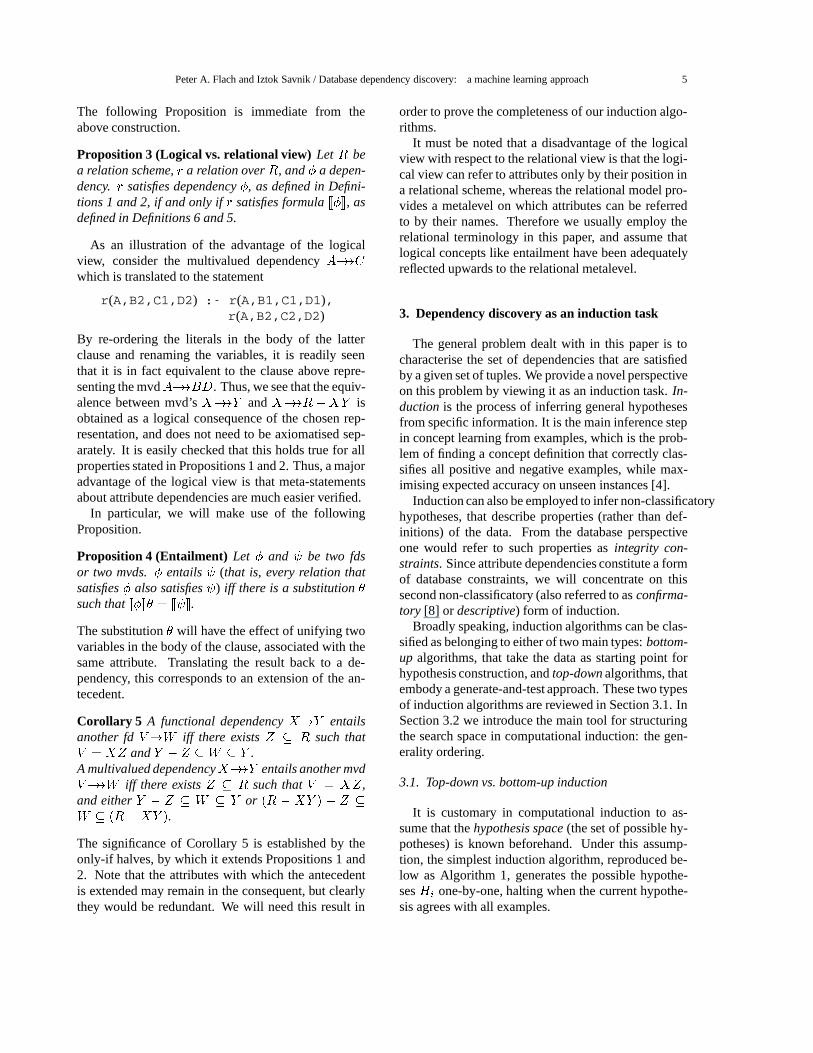
Corollary 5 A functional dependencyX!Y entailsanother fdV!W iff there existsZ � R such thatV = XZ andY � Z �W � Y .A multivalued dependencyX!!Y entails another mvdV!!W iff there existsZ � R such thatV = XZ,and eitherY � Z � W � Y or (R � XY ) � Z �W � (R�XY ).The significance of Corollary 5 is established by theonly-if halves, by which it extends Propositions 1 and2. Note that the attributes with which the antecedentis extended may remain in the consequent, but clearlythey would be redundant. We will need this result in

order to prove the completeness of our induction algo-rithms.

It must be noted that a disadvantage of the logicalview with respect to the relational view is that the logi-cal view can refer to attributes only by their position ina relational scheme, whereas the relational model pro-vides a metalevel on which attributes can be referredto by their names. Therefore we usually employ therelational terminology in this paper, and assume thatlogical concepts like entailment have been adequatelyreflected upwards to the relational metalevel.

3. Dependency discovery as an induction task

The general problem dealt with in this paper is tocharacterise the set of dependencies that are satisfiedby a given set of tuples. We provide a novel perspectiveon this problem by viewing it as an induction task.In-ductionis the process of inferring general hypothesesfrom specific information. It is the main inference stepin concept learning from examples, which is the prob-lem of finding a concept definition that correctly clas-sifies all positive and negative examples, while max-imising expected accuracy on unseen instances [4].

Induction can also be employed to infer non-classificatoryhypotheses, that describe properties (rather than def-initions) of the data. From the database perspectiveone would refer to such properties asintegrity con-straints. Since attribute dependencies constitute a formof database constraints, we will concentrate on thissecond non-classificatory (also referred to asconfirma-tory [8] or descriptive) form of induction.

Broadly speaking, induction algorithms can be clas-sified as belonging to either of two main types:bottom-up algorithms, that take the data as starting point forhypothesis construction, andtop-downalgorithms, thatembody a generate-and-test approach. These two typesof induction algorithms are reviewed in Section 3.1. InSection 3.2 we introduce the main tool for structuringthe search space in computational induction: the gen-erality ordering.

3.1. Top-down vs. bottom-up induction

It is customary in computational induction to as-sume that thehypothesis space(the set of possible hy-potheses) is known beforehand. Under this assump-tion, the simplest induction algorithm, reproduced be-low as Algorithm 1, generates the possible hypothe-sesHi one-by-one, halting when the current hypothe-sis agrees with all examples.

6 Peter A. Flach and Iztok Savnik / Database dependency discovery: a machine learning approach

Algorithm 1 (Enumerative induction)Input : an indexed set of hypothesesfHig,and a set of examplesE.Output : a hypothesisH agreeing withE.begin i := 0;

while Hi does not agree withEdo i := i+ 1 odoutput Hi

end.

In the case of dependency discovery,fHigwould be anenumeration of the set of attribute dependencies overa given relation. For any but the simplest hypothesisspace this naive approach is obviously infeasible. Themain problem is that, even if the enumeration is donein some systematic way, no information is extractedfrom it: every hypothesis is treated as if it were the firstone. If we view the algorithm as a search algorithm,the search space is totally flat: every hypothesis is animmediate descendant of the root node, so solutionsare only found at leaves of the search tree.

If solutions are to be found higher up in the searchspace, we need a strict partial order that structures thehypothesis space in a non-trivial way. For instance, inconcept learning from examples a suitable search or-der can be defined in terms of generality of the pos-sible concept definitions: more specific definitions areonly tried after the more general ones have been foundinappropriate (top-downalgorithms). We will furtherdiscuss the generality ordering in Section 3.2.

Bottom-up induction algorithms construct hypothe-ses directly from the data. They are less easily viewedas search algorithms, and are in some cases even deter-ministic. For instance, when inducing a definition fortheappend-predicate we may encounter the facts

append([a],[],[a])

and

append([1,2],[3,4],[1,2,3,4])

If we assume that these are generated by the sameclause, we can construct the clause head

append([A|B],C,[A|D])

by anti-unification, and then proceed to find appropri-ate restrictions for the variables. Since the data canbe viewed as extremely specific hypotheses, such al-gorithms climb the generality ordering from specific togeneral, and are thus in some sense dual to top-downalgorithms.

It should be noted that some algorithms, most no-tably those inducing classification rules, induce a sin-

gle possible hypotheses agreeing with the data, whileothers result in a description of the set of all hypothe-ses agreeing with the data. The latter holds for all al-gorithms in this paper. Alternatively, we can determinethe set of all hypothesesrefutedby the data, which canbe seen as a dual induction problem with the reversegenerality ordering.

3.2. The generality ordering

The generality ordering arose from work on con-cept learning from examples. Briefly,concept learningcan be defined as inferring an intensional definition ofa predicate from positive examples (ground instances)and negative examples (non-instances). The inductiontask is to construct a concept definition such that theextension of the defined predicate contains all of thepositive examples and none of the negative examples.This induces a natural generality ordering on the spaceof possible definitions: a predicate definition is said tobe more generalthan another if the extension of thefirst is a proper superset of the second.

Notice that this definition of generality refers to ex-tensions and is thus a semantical definition. For thegenerality ordering to be practically useful during thesearch for an appropriate hypothesis we need a syntac-tical analogue of this semantical concept. In theory itwould be desirable that the semantical and syntacticalgenerality ordering coincide, but in practice this idealis unattainable. Even if the set of all extensions formsa Boolean algebra, the syntactical hypothesis space isoften not more than a partially ordered set, possiblywith infinite chains. The complexity of the learningtask depends for a great deal on the algebraic structureof the hypothesis space that is reflected by the syntac-tical generality ordering.

In general, a predicate definition establishes bothsufficientandnecessaryconditions for concept mem-bership. In practice, however, the necessary conditionsare usually left implicit. This means that the hypothe-sis language is restricted to definite clauses, as is cus-tomary in inductive logic programming [23, 24, 2]. Itfurthermore means that the extension of the definedpredicate is obtained from the least Herbrand model ofits definition, using negation as failure. Consequently,one predicate definition is more general than anotherif the least Herbrand model of the first is a model ofthe second, which in fact means that the first logicallyentails the second.

For predicate definitions consisting of a single, non-recursive clause, logical entailment between predicate

Peter A. Flach and Iztok Savnik / Database dependency discovery: a machine learning approach 7

definitions is equivalent to�-subsumption: a clause�-subsumesanother if a substitution can be applied to thefirst, such that every literal occurs, with the appropri-ate sign, in the second.3 In the general case of recur-sive clauses�-subsumption is strictly weaker than log-ical entailment [11]. However, for the restricted lan-guage of attribute dependencies�-subsumption is quitesufficient, as demonstrated by Proposition 4. Notethat clauses representing attribute dependencies alwayshave the same number of literals.

In the last 15 years, an abundance of algorithms forinduction of predicate definitions in first-order clausallogic has been developed [23, 24, 2]. A top-down in-duction algorithm starts from a set of most general sen-tences, specialising when a sentence is found too gen-eral (i.e. it misclassifies a negative example). In def-inite clause logic, there are two ways to specialise aclause under�-subsumption: to apply a substitution,and to add a literal to the body. Alternatively, a bottom-up algorithm operates by generalising a few selectedexamples, for instance by applying some variant ofanti-unification.

As has been said before, in this paper we are inter-ested in non-classificatory induction. Contrasting withinduction of classification rules, induction of integrityconstraints does not allow for an interpretation in termsof extensions.4 We simply want to find the set of all hy-potheses that agree with the data. For instance, given arelationr we may want to find the setDEPR(r) of alldependencies satisfied byr. Another instance of thisproblem is the construction of a logical theory axioma-tising a given Herbrand modelm.

Even if there is no extensional relation between dataand hypothesis, the notion of logical entailment canagain be used to structure the search space, since weare usually interested in finding a cover of the set of allpossible hypotheses, which only needs to contain themost general integrity constraints satisfied by the data(see Definition 3). An important difference in compar-3This definition, and the term�-subsumption, was introduced inthe context of induction by Plotkin [25, 26]. In theorem proving theabove version is termed subsumption, whereas�-subsumption indi-cates a special case in which the number of literals of the subsumantdoes not exceed the number of literals of the subsumee [16].4An alternative view of induction of integrity constraints is ob-tained if we view the data (e.g. a database relation or a Herbrandmodel) as one example, i.e. a member of the extension of the setof satisfied integrity constraints, which re-establishes the extensionalinterpretation of generality [3]. A disadvantage of this alternativeview is that it reverses the intuitive relation between generality andentailment: an integrity constraint with more Herbrand models islogically weaker.

ison with induction of predicate definitions is that sat-isfaction of an integrity constraint does not depend onother sentences.5 This gives rise to a simple yet generaltop-down algorithm, that is given below as Algorithm2.

The most interesting differences, and the major con-tributions of the present paper, manifest itself whenconsidering bottom-up approaches to induction of in-tegrity constraints, that operate more in a data-drivenfashion. It is in general not possible to construct a sat-isfied integrity constraint from only a small subset ofthe data, because such a constraint may be violated byother parts of the data. It is however possible to con-struct, in a general and principled way, a number of de-pendencies that areviolatedby the data. Proceeding inthis way we can extract from the data, in one run, allthe information that is needed to construct a cover forthe set of satisfied dependencies. This makes a data-driven method more feasible than a top-down methodwhen the amount of data is relatively large. The detailscan be found below in Sections 4.2 and 4.3.

4. Algorithms for inducing dependencies

We are now ready to present the main induction al-gorithms for dependency discovery. The specifics of aparticular kind of dependency will as much as possi-ble be relegated to sub-procedures, in order to obtainspecifications of the top-level algorithms that are gen-erally applicable. We start with the conceptually sim-pler top-down algorithm in Section 4.1, followed bya bi-directional algorithm in Section 4.2, and a purebottom-up algorithm in Section 4.3.

4.1. A top-down induction algorithm

We want to find a cover ofDEPR(r) for a given re-lation r. The basic idea underlying the top-down ap-proach is that such a cover is formed by the most gen-eral elements ofDEPR(r). Therefore, the possibledependencies are enumerated from general to specific.For every dependency thus generated, we test whetherthe given relation satisfies it. If it does not, we scheduleall of its specialisations for future inspection; if it does,these specialisations are known to be satisfied also and5In contrast, when inducing a recursive predicate definitionwhatwe are constructing is asetof interrelated sentences, which is clearlymuch more complicated than the construction of several independentsentences.

8 Peter A. Flach and Iztok Savnik / Database dependency discovery: a machine learning approach

need not be considered. In the context of database de-pendencies, the process can be slightly optimised be-cause the witnesses signalling the violation of a depen-dency may indicate that some of its specialisations arealso violated. For instance, letR = fA;B;C;Dg, letr contain the tuplesha; b1; c; d1i andha; b2; c; d2i, andconsider the fdA!B which is violated byr. Its spe-cialisations areAC!B andAD!B, but the first ofthese is violated by the same pair of witnesses.

Algorithm 2 (Top-down induction of dependencies)Input : a relation schemeR and a relationr overR.Output : a cover ofDEPR(r).begin

DEPS :=;;Q := initialise(R);while Q 6= ;do D := next item from Q; Q := Q� D;

if some witnessest1; : : : ; tn fromr violate Dthen Q := Q [ spec(R,D,t1; : : : ; tn)elseDEPS := DEPS[ fDgfi

odoutput DEPS

end.

Algorithm 2 is basically an agenda-based search algo-rithm, specialising items on the agendaQ until theyare no longer violated byr. Notice that the thus con-structed setDEPS may still contain redundancies; anon-redundant cover may be constructed in some moreor less sophisticated way.

Algorithm 2 works for both functional and multival-ued dependencies; the only difference lies in the ini-talisation of the agenda, and the way dependencies areviolated and specialised. The correctness of the algo-rithm depends on the following conditions on the pro-cedurespec():

– every dependencyD0 returned byspec(D; t1; : : : ; tn)is a specialisation ofD, i.e.D entailsD0 butD0does not entailD;

– every dependency entailed byD and not violatedby r is entailed by some dependency returned byspec(D; t1; : : : ; tn).

The first condition is calledsoundnessof the special-isation procedure; the second condition is calledrela-tive completeness(it is not complete in the sense thatminimal specialisations ofD that are violated by thesame witnesses are not returned).

Theorem 6 Algorithm 2 returns a cover ofDEPR(r)if the procedureinitialise() returns the set of mostgeneral dependencies, and the procedurespec() issound and relatively complete.

Proof. LetDEPS be the set of dependencies returnedby Algorithm 2 when fed with relationr. Clearly,only dependencies not violated byr are included inDEPS. The algorithm halts because every depen-dency has only a finite number of specialisations. Itremains to prove that every dependency satisfied byris entailed by some dependency inDEPS. This fol-lows from the fact that the agenda is initialised withthe set of most general dependencies and the relativecompleteness of the specialisation procedure.

For functional dependencies the parameters of Al-gorithm 2 are instantiated as follows. By Proposition 1we can restrict attention to simple fds. In accordancewith Corollary 5 the agenda is initialised with;!Afor everyA 2 R. Furthermore, according to Defi-nition 1 an fdX!A is violated by two witnessest1andt2 that agree onX but not onA. Again accord-ing to Corollary 5,X!A must be specialised by ex-tending the antecedent; without compromising relativecompleteness we can ignoreA (since the fdXA!A istautological), and also any attribute on which the wit-nesses agree (since this specialised fd would be refutedby the same witnesses). This results in the followingrelatively complete specialisation algorithm.

Algorithm 3 (Specialisation of functional dependencies)Input : a relation schemeR, a functional dependencyX!A overR, and two witnessest1; t2 violatingX!A.Output : the non-trivial minimal specialisations ofX!Anot violated by the same witnesses.proc fd-spec

SPECS :=;;DIS := the set of attributes for whicht1 andt2 have different values;for eachB 2 DIS�Ado SPECS := SPECS[ XB!A od;output SPECS

endproc.

Theorem 7 Algorithm 3 is a sound and relatively com-plete specialisation algorithm.

Proof. Clearly,X!A entailsXB!A but not viceversa, which demonstrates soundness.LetV!W be a non-tautological fd entailed byX!A,then by Corollary 5V � X andW = A. If further-moreV!W is not contradicted by the same witnesses,then the witnesses do not agree on all attributes inV .Let B 6= A be an attribute on which they disagree,then Algorithm 3 will returnXB!A, which entailsV!W .

Peter A. Flach and Iztok Savnik / Database dependency discovery: a machine learning approach 9

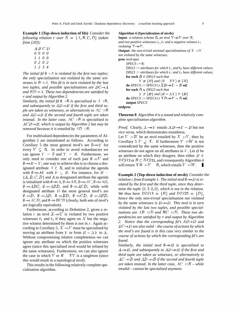
Example 1 (Top-down induction of fds) Consider thefollowing relation r overR = fA;B;C;Dg (takenfrom [20]):A B C D

0 0 0 01 1 0 00 2 0 21 2 3 4

The initial fd;!A is violated by the first two tuples;the only specialisation not violated by the same wit-nesses isB!A. This fd is in turn violated by the lasttwo tuples, and possible specialisations areBC!AandBD!A. These two dependencies are satisfied byr and output by Algorithm 2.Similarly, the initial fd;!B is specialised toA!B,and subsequently toAD!B if the first and third tu-ple are taken as witnesses, or alternatively toAC!BandAD!B if the second and fourth tuple are takeninstead. In the latter case,AC!B is specialised toACD!B, which is output by Algorithm 2 but may beremoved because it is entailed byAD!B.

For multivalued dependencies the parameters of Al-gorithm 2 are instantiated as follows. According toCorollary 5 the most general mvd’s are;!!Y forevery Y � R. In order to avoid redundancies wecan ignoreY = ; and Y = R. Furthermore, weonly need to consider one of each pair;!!Y and;!!R� Y ; one way to achieve this is to choose a des-ignated attributeA 2 R, and to initialise the agendawith ;!!AY with Y � R. For instance, forR =fA;B;C;Dg andA as designated attribute the agendais initialised with;!!A, ;!!AB, ;!!AC, ;!!AD,;!!ABC, ;!!ABD, and ;!!ACD; while withdesignated attributeD the most general mvd’s are;!!D, ;!!AD, ;!!BD, ;!!CD, ;!!ABD,;!!ACD, and;!!BCD (clearly, both sets of mvd’sare logically equivalent).

Furthermore, according to Definition 2, given a re-lation r an mvdX!!Y is violated by two positivewitnessest1 andt2 if they agree onX but the nega-tive witness determined by them is not inr. Again ac-cording to Corollary 5,X!!Y must be specialised bymoving an attribute fromY or from R � XY to X .Without compromising relative completeness we canignore any attribute on which the positive witnessesagree (since this specialised mvd would be refuted bythe same witnesses). Furthermore, we can also ignorethe case in whichY or R � XY is a singleton (sincethis would result in a tautological mvd).

This results in the following relatively complete spe-cialisation algorithm.

Algorithm 4 (Specialisation of mvds)Input : a relation schemeR, an mvdX!!Y overR,and two positive witnessest1; t2 and a negative witnesst3violatingX!!Y .Output : the non-trivial minimal specialisations ofX!!Ynot violated by the same witnesses.proc mvd-spec

SPECS :=;;DIS13 := attributes for whicht1 andt3 have different values;DIS23 := attributes for whicht2 andt3 have different values;for eachB 2 DIS13 such thatY 6= fBg and(R�XY ) 6= fBgdo SPECS := SPECS[ XB!!Y �B od;for eachB 2 DIS23 such thatY 6= fBg and(R�XY ) 6= fBgdo SPECS := SPECS[ XB!!Y �B od;output SPECS

endproc.

Theorem 8 Algorithm 4 is a sound and relatively com-plete specialisation algorithm.

Proof. Clearly,X!!Y entailsXB!!Y �B but notvice versa, which demonstrates soundness.Let V!!W be an mvd entailed byX!!Y , then byCorollary 5 V � X . If furthermoreV!!W is notcontradicted by the same witnesses, then the positivewitnesses do not agree on all attributes inV . LetB bean attribute on which they disagree, then eitherB 2DIS13 orB 2 DIS23, and consequently Algorithm 4will returnXB!!Y �B, which entailsV!!W .

Example 2 (Top-down induction of mvds)Consider therelationr from Example 1. The initial mvd;!!D is vi-olated by the first and the third tuple, since they deter-mine the tupleh0; 2; 0; 0i, which is not in the relation.We thus haveDIS13 = fBg andDIS23 = fDg,hence the only non-trivial specialisation not violatedby the same witnesses isB!!D. This mvd is in turnviolated by the last two tuples, and possible special-isations areAB!!D andBC!!D. These two de-pendencies are satisfied byr and output by Algorithm2. Notice that the corresponding fd’sAB!D andBC!D are also valid – the course of actions by whichthe mvd’s are found is in this case very similar to thecourse of actions by which the corresponding fd’s arefound.Similarly, the initial mvd;!!B is specialised toA!!B, and subsequently toAD!!B if the first andthird tuple are taken as witnesses, or alternatively toAC!!B andAD!!B if the second and fourth tupleare taken instead. In the latter case,AC!!B – whileinvalid – cannot be specialised anymore.

10 Peter A. Flach and Iztok Savnik / Database dependency discovery: a machine learning approach

4.2. A bi-directional induction algorithm

Algorithm 2 is a generate-and-test algorithm: it gen-erates dependencies from general to specific, testingeach generated dependency against the given relation.We now describe an alternative approach which dif-fers from the top-down approach in that the test phaseis conducted against the set of least generalviolateddependencies, rather than against the relation itself.The basic idea is to construct, for each pair of tu-ples, the least general dependencies for which the tu-ples are a pair of violating witnesses. For instance,let R = fA;B;C;Dg and consider the tuplest1 =ha; b1; c; d1i andt2 = ha; b2; c; d2i. The fd’sA!B,A!D, C!B, C!D, AC!B, andAC!D are allviolated byt1; t2; of these, the last two are least gen-eral. If we iterate over all pairs of tuples in relationr,we have constructed a cover for the set of dependen-cies that areviolatedby r; we will call such a cover anegative cover.6 Since the negative cover is calculatedin a bottom-up fashion, while the positive cover is cal-culated from the negative cover in a top-down manneras before, we call this thebi-directional induction al-gorithm.

The following procedure calculates this negativecover.

Algorithm 5 (Negative cover)Input : a relation schemeR and a relationr overR.Output : a cover of the dependencies violated byr.proc neg-cover

NCOVER :=;;for each pair of tuplest1; t2 fromrdo NCOVER := NCOVER[ violated(R,r,t1,t2) odoutput NCOVER

endproc.

In practice the proceduresneg-cover() andviolated()will be merged, in order to prevent addition of depen-dencies for which a less general version is already in-cluded in the negative cover.

The correctness of Algorithm 5 depends on the pro-cedureviolated(R; r; t1; t2), which calculates the setof dependencies for whicht1 andt2 are violating wit-nesses (the relationr is only needed in the case ofmultivalued dependencies). This procedure treats theattributes on which the tuples agree as antecedent at-tributes, and the remaining attributes as consequent at-tributes.6Negative covers are called anti-covers in [12].

Algorithm 6 (Violated fds)Input : a relation schemeR and two tuplest1; t2 overR.Output : the least general fd’s overR violated byt1; t2.proc fd-violated

VIOLATED := ;;DIS := attributes for whicht1 andt2 have different values;AGR :=R�DIS;for eachA 2 DISdo VIOLATED := VIOLATED[ AGR!A od;output VIOLATED

endproc.

Notice that the fd-initialisation procedure for the top-down approach is a special case of Algorithm 6, withDIS = R andAGR = ;.Theorem 9 Algorithm 6 correctly calculates the set ofleast general fd’s overR violated by two tuplest1 andt2.Proof. Clearly, any fd output by Algorithm 6 is vio-lated byt1 andt2. Conversely, letX!A be an fd vi-olated byt1 andt2, thenX � AGR andA 2 DIS,henceX!A entailsAGR!A which is output by Al-gorithm 6.

Example 3 (Negative cover for fds)Consider again therelationr from the previous examples:A B C D

0 0 0 01 1 0 00 2 0 21 2 3 4

For construction of the negative cover we have 6 pairsof tuples to consider.The first and second tuple result in violated fd’sCD!A andCD!B.The first and third tuple result in violated fd’sAC!BandAC!D.The first and fourth tuple result in violated fd’s;!A,;!B, ;!C, and;!D. (Notice that, if the negativecover is built incrementally by merging Algorithms 5and 6, as it is implemented in practice, the first, sec-ond, and fourth of these fd’s will be found redundantwhen compared with previously found fd’s.)The second and third tuple result in violated fd’sC!A, C!B, andC!D (which are all redundant incomparison with fd’s found earlier).The second and fourth tuple result in violated fd’sA!B,A!C , andA!D (of which only the second isnon-redundant).Finally, the third and fourth tuple result in violated fd’s

Peter A. Flach and Iztok Savnik / Database dependency discovery: a machine learning approach 11B!A,B!C, andB!D.A non-redundant negative cover consists of the follow-ing violated fd’s:B!A, CD!A, AC!B, CD!B,A!C,B!C, AC!D, andB!D.

For multivalued dependencies the proceduremvd-violated() is slightly more involved, since for a pairof positive witnesses and a possibly violated mvd weneed to consider one or both tuples determined by thepositive witnesses, and check whether these are indeednegative witnesses not contained inr.Algorithm 7 (Violated mvds)Input : a relation schemeR, a relationr overR,and two tuplest1; t2 overR.Output : the least general mvd’s violated byt1; t2 givenr.proc mvd-violated

VIOLATED := ;;DIS := attributes for whicht1 andt2 have different values;AGR :=R�DIS;A := some attribute in DIS;for eachZ � (DIS �A)do MVD := AGR!!AZ;t3 := tuple determined byt1; t2 given MVD;

if t3 62 rthen VIOLATED := VIOLATED[ MVDelset4 := tuple determined byt2; t1 given MVD;

if t4 62 rthen VIOLATED := VIOLATED[ MVDfi

fiod;output VIOLATED

endproc.

Note that the construction ofMVD in Algorithm 7 isagain a variant of the initialisation procedure for mvd’sin the top-down approach, by puttingDIS = R andAGR = ;.Theorem 10 Algorithm 7 correctly calculates the setof least general mvd’s overR violated by two tuplest1andt2 given relationr.Proof. Clearly any mvd added toV IOLATED is vi-olated byt1 and t2 given r. Conversely, letX!!Ybe an mvd violated byt1 and t2, thenX � AGR;therefore the tuples determined byr1 and t2 givenX!!Y are the same as determined byt1 andt2 givenAGR!!Y �AGR. Hence the latter mvd – which isentailed byX!!Y according to Corollary 5 – will beoutput by Algorithm 7.

Example 4 (Negative cover for mvds)We proceed withthe running example. For construction of the nega-tive cover for mvd’s we have 6 pairs of tuples to con-sider. We will assume that the designated attribute(Ain Algorithm 7) is always the lexicographically first at-tribute inDIS.For the first and second tuple we haveDIS = fA;BgandAGR = fC;Dg, hence withA as designated at-tribute the only potentially violated mvd isCD!!A.7The tuple determined by the first and second tuple inrgivenCD!!A is h0; 1; 0; 0i, which is indeed outsider, hence the mvd is added to the negative cover.The first and third tuple result in violated mvdAC!!B.The first and fourth tuple result in violated mvd’s;!!A, ;!!AB, ;!!AC, ;!!AD, ;!!ABC , ;!!ABD,and ;!!ACD. (Notice that only;!!ABD is non-redundant in the light of the mvd’s found previously.)The second and third tuple result in violated mvd’sC!!A,C!!AB, andC!!AD (which are all redun-dant).The second and fourth tuple result in violated mvd’sA!!B, A!!BC, andA!!BD (of which only thelast is non-redundant).Finally, the third and fourth tuple result in violatedmvd’sB!!A,B!!AC , andB!!AD.A non-redundant negative cover consists of the fol-lowing violated mvd’s:B!!A, CD!!A, AC!!B,A!!C,B!!C , andB!!D.

We can now give the main bi-directional algorithm.It starts with construction of the negative cover, andproceeds by specialising each dependency until noneof them entails any element of the negative cover.

Algorithm 8 (Bi-directional induction of dependencies)Input : a relation schemeR and a relationr overR.Output : a cover ofDEPR(r).begin

DEPS :=;;Q := initialise(R);NCOVER := neg-cover(R,r);while Q 6= ;do D := next item from Q; Q := Q� D;

if D entails some element ND in NCOVERthen Q := Q [ spec(D,ND)elseDEPS := DEPS[ fDgfi

odoutput DEPS

end.7With B as designated attribute it would be the logically equiva-lent mvdCD!!B.

12 Peter A. Flach and Iztok Savnik / Database dependency discovery: a machine learning approach

The procedurespec() is similar to the specialisationprocedures given above as Algorithms 3 and 4, withthe only distinction that specialisation is guided by adependencyND not to be entailed, rather than a pairor triple of violating witnesses; we omit the details.

The reader will notice that Algorithm 8 is in factquite similar to Algorithm 2, but there is an importantdifference: dependencies on the agenda are tested withrespect to the negative cover,without further referenceto the tuples inr. This bi-directional approach is morefeasible ifjrj is large compared tojRj.Theorem 11 Let r be a relation over schemeR, letNCOVER be the negative cover constructed by Algo-rithm 5, and letD be a dependency overR. D violatesr iff D entails some elementND of NCOVER.

Proof. (if) If ND 2 NCOVER, thenND is contra-dicted by some witnesses inr. If D entailsND, thenD is contradicted by the same witnesses, henceD isviolated byr.(only if) SupposeD is violated byr, then the depen-dencyND constructed from any witnesses by Algo-rithm 5 will be entailed byD.

In the light of Theorem 11, the correctness of Algo-rithm 8 follows from the correctness of Algorithm 2.

Corollary 12 Algorithm 8 returns a cover ofDEPR(r)if the procedureinitialise() returns the set of mostgeneral dependencies, and the procedurespec() issound and relatively complete.

Example 5 In Example 3 the following non-redundantnegative cover was found:B!A, CD!A, AC!B,CD!B, A!C , B!C , AC!D, andB!D. Theinitial fd ;!A entailsCD!A in the negative cover,and is therefore specialised toB!A. This fd is foundto be in the negative cover in the next iteration, and isspecialised toBC!A andBD!A. These two depen-dencies do not entail any element of the negative cover,and are output by Algorithm 8.In the case of mvds, in Example 4 the followingnon-redundant negative cover was found:B!!A,CD!!A, AC!!B, A!!C , B!!C , and B!!D.The initial mvd;!!B entailsAC!!B in the nega-tive cover, and is specialised toD!!B. In turn, thismvd entailsCD!!A in the negative cover, and is spe-cialised toAD!!B.

Notice that the agenda cannot be initialised withNCOVERbecause, although every most general satis-fied dependency is the specialisation of a violated de-pendency (otherwise it would not be most general), itmay not be the specialisation of aleast generalviolateddependency that is included in the negative cover.

Example 6 The most general satisfied fd’sBC!AandBD!A (see Example 1) are indeed specialisa-tions of an fd in the negative cover,viz. B!A. How-ever, the most general satisfied fdAD!B is not.Similarly, the most general satisfied mvd’sBC!!AandBD!!A (see Example 2) are indeed specialisa-tions of an mvd in the negative cover,viz. B!!A.However, the most general satisfied mvdD!!C is not.

4.3. A bottom-up induction algorithm

The pure bottom-up induction algorithm is a sim-ple variation on Algorithm 8. Instead of generating thepositive cover from the negative cover in a top-down,generate-and-test manner, we iterate once over the neg-ative cover, considering each least general violated de-pendency only once. Experimental results in Section7 demonstrate that this yields a considerable improve-ment in practice.

Algorithm 9 (Bottom-up induction of dependencies)Input : a relation schemeR and a relationr overR.Output : a cover ofDEPR(r).begin

DEPS := initialise(R);NCOVER := neg-cover(R,r);for each ND2 NCOVERdo TMP := DEPS;

for each D 2 DEPS entailing NDdo TMP := TMP� D [ spec(D,ND) odDEPS := TMP

odoutput DEPS

end.

The bottom-up algorithm thus contains two nestedloops, the outer one of which iterates over the nega-tive cover, ensuring that its elements are inspected onlyonce. Notice that by exchanging the two loops we ob-tain (more or less) the bi-directional algorithm again.

Example 7 In Example 3 the following non-redundantnegative cover was found:B!A, CD!A, AC!B,CD!B, A!C, B!C, AC!D, andB!D. B!Acauses specialisation of the initial fd;!A to C!AandD!A. The next element of the negative coverCD!A causes specialisation of these toBC!A andBD!A. AC!B causes specialisation of;!B toD!B, subsequently specialised toAD!B by virtueof the fourth element of the negative cover. Continua-tion of this process leads to construction of the positivecover in one iteration over the negative cover.

Peter A. Flach and Iztok Savnik / Database dependency discovery: a machine learning approach 13

5. Implementation

The algorithms described above have been imple-mented in two separate systems: the systemfdep forinduction of functional dependencies, and the programmdep which realizes algorithms for induction of mul-tivalued dependencies. The systemfdep is imple-mented in GNU C and has been used by the authors forthe discovery of functional dependencies from a vari-ety of domains.8 The programmdep is implementedin Sicstus Prolog. It serves as an experimental proto-type for the study of algorithms for the discovery ofmultivalued dependencies.

The programsfdep andmdep are described in thefollowing sub-sections. Section 5.1 presents the imple-mentation of the algorithms for induction of functionaldependencies. It includes the description of the datastructure which is used for storing sets of dependen-cies, as well as handling of missing values and noise.In Section 5.2 we present the main aspects of the pro-grammdep and some experiences obtained with theprototype. Experiments withfdep are described sep-arately in Seciont 7.

5.1. Algorithms for inducing functional dependencies

The top-down induction algorithm for functionaldependencies turned out to be computationally tooexpensive for inducing functional dependencies fromlarger relations. The main weakness of this algorithmis its method for testing the validity of the hypotheses;they are tested by considering all pairs of tuples fromthe input relation. The method for testing the validityof a functional dependency is considerably improvedin the bi-directional induction algorithm.

The bi-directional algorithm uses the same methodfor the enumeration of hypotheses as the top-downalgorithm: in both algorithms hypotheses (i.e., func-tional dependencies) are specialised until the valid de-pendencies are reached. The main improvements ofthe bi-directional algorithm are in the method for test-ing the validity of the dependencies, and for specialisa-tion of refuted functional dependencies. First, insteadof checking the hypotheses on the complete relation,they are tested using the negative cover (the set of mostspecific invalid dependencies). Secondly, the hypothe-ses are specialised in the bi-directional algorithm using8The system is available from thefdep homepage athttp://infolab.fri.uni-lj.si/˜savnik/fdep.html.

the invalid dependencies which are the cause for thecontradiction of the hypotheses.

Since every hypothesis is checked for its validity bysearching the negative cover, an efficient representa-tion of the set of dependencies is of significant impor-tance for the performance of the induction algorithm.The set of dependencies is represented infdep usinga data structure calledFD-tree which allows efficientuse of space for the representation of sets of dependen-cies, and at the same time provides fast access to the el-ements of the set. FD-tree is presented in the followingsub-section.

FD-tree is also used for the representation of the setof valid hypotheses which are the result of the algo-rithm. The valid hypotheses are added to the set as theyare generated by the enumeration based on specialisa-tion. Initially, the set of valid dependencies is empty.Each time a new valid dependency is generated, it isfirst tested against the existing set of valid dependen-cies. The valid hypothesis is added to the existing setof dependencies only if it is not covered by the existingset of dependencies. As in the case of the set of invaliddependencies representing the negative cover, efficientaccess to the elements of the set of valid dependenciesis important for the efficient performance of the algo-rithm.

A problem which appears with the bi-directionalalgorithm lies in the enumeration of the hypotheses.The hypotheses are enumerated from the most generalfunctional dependencies to more specific dependenciesas presented by Algorithm 8. The algorithm can beseen as performing depth-first search where the spe-cialisation of the refuted candidates is based on invaliddependencies from the negative cover. Ideally, each ofthe hypotheses would be enumerated and tested againstthe negative cover only once. However, since the in-valid dependencies are used for specialisation of re-futed hypotheses, the enumeration can not be guidedin a way which avoids testing some hypotheses morethan one time. This is one of the main reasons for abad performance of the algorithm for some domains.

Finally, the bottom-up algorithm has the best perfor-mance among the presented algorithms. As presentedin Algorithm 9, the bottom-up algorithm starts withthe positive cover which includes the most general de-pendencies. The positive cover is refined in each stepby considering only one invalid dependency. A sin-gle FD-tree is used for the representation of the posi-tive cover during the iteration through the invalid de-pendencies from the negative cover. In each step, onlythose dependencies from the positive cover which are

14 Peter A. Flach and Iztok Savnik / Database dependency discovery: a machine learning approach

refuted by the currently considered invalid dependen-cies are affected. Each of these dependencies is re-moved from the FD-tree (positive cover) and their spe-cialisations which are not contradicted by the currentlyconsidered invalid dependency are added to the sameFD-tree. Therefore, the algorithm generates only thosehypotheses which are actually needed to avoid the con-tradiction of the invalid dependency considered in onestep of the algorithm. In a way, this algorithm is theclosest approximation of the intuitive idea of comput-ing the positive cover by “inverting” the negative cover.In Section 7 we present empirical support for this anal-ysis.

5.1.1. Data structure for representing sets offunctional dependencies

Each of the presented algorithms for inductionof functional dependencies manipulates sets of validand/or invalid dependencies. In the previous sectionsit was assumed that covers for valid and invalid func-tional dependencies are represented simply as lists.In this section we introduce a data structure which isused for storing sets of functional dependencies andwhich allows efficient implementation of operationsfor searching more specific and more general depen-dencies of a given dependency.

To describe the data structure for representing setsof dependencies, we first introduce theantecedent tree.We assume that attributes are totally ordered, so thatfor each pair of attributesAi; Aj 2 R(i 6= j) we havethat eitherAi is higher thanAj or the opposite.

Definition 7 (Antecedent tree)Given a relation schemeR, anantecedent tree overR is a tree with the follow-ing properties:

1. every node of the tree, except the root node, is anattribute fromR;

2. the children of the nodeAi are higher attributes;and

3. the children of the root are all attributes.

Each path starting at the root of an antecedent treerepresents a set of attributes, that will be interpreted asthe antecedent of a functional dependency. The nodesof an antecedent tree are now labelled with sets of con-sequent attributes, as follows.

Definition 8 (FD-tree) Given a relation schemeR anda set of functional dependenciesF overR, theFD-treeof F is defined as follows: for every fdX!B 2 Fthere is a path representingX , and each node from the

A

B DB C

B

D EA

CBC C

C

A

C

ABC

C

B CEE

Fig. 1. An example of an FD-tree representing a set of functionaldependencies.

path is labelled by the consequent attributeB. For ev-ery attributeA 2 R, the unlabelled subtree consistingof all the nodes in FD-tree that includeA in its label iscalled theA-subtree.

Note that the dependencies composing theA-subtreecan be identified in the FD-tree by visiting a subtreeof nodes that are labelled by attributeA. An exampleof the FD-tree which is used for the representation ofthe set of functional dependenciesAB!C,ACE!B,AD!C,BDE!C, CE!A is presented in Figure 1.

There are two important operations on the FD-treewhich are used when generating the positive and neg-ative covers. The first operation can be defined asfollows: given an arbitrary dependency, search for amore specific dependency in the FD-tree. If the op-eration completes successfully, the result of the op-eration is amore specificdependency found in theset of dependencies. The second operation is similar:given an arbitrary dependency, it searches in the FD-tree for a dependency that is more general than the in-put dependency. The first operation is calledexists-specialisationand the secondexists-generalisation.Since both algorithms work in a similar manner onlythe operationexists-specialisationis detailed below asAlgorithm 10. The description of the operationexists-generalisationcan be found in [28].

Algorithm 10 (exists-specialisation)Input : the root of an FD-tree denoted asTnode, anda dependencyX!AOutput : a dependencyY!A from FD-tree that is morespecific thanX!A, if it existsfunction exists-specialisation( Tnode;X; Y;A ): boolean;begin

exists-specialisation := false;if X is emptythenY := Y + f Path fromTnode to arbitrary leaf

Peter A. Flach and Iztok Savnik / Database dependency discovery: a machine learning approach 15

of Tnode’s A-subtreeg;exists-specialisation := true;output Y!A;

elseX1 := first attribute from the listX;Y1 := last attribute from the listY ;foreachB 2 [(label(Y1) + 1) .. label(X1)]do if B = X1 thenX := X � fX1g fi;

if exists-specialisation( Tnode.child[B],X,Y + fBg,A )then exists-specialisation := true;

exit;fi;

od;fi;

end.

Algorithm 10 searches the FD-tree for a dependencyY!A that is more specific than the input dependencyX!A. Suppose that the antecedent of the input de-pendency is composed of attributesX1X2 : : : Xk andthe antecedent of the dependencyY!A is composedof attributesY1Y2 : : : Yl. The search process is com-pleted, if a path from the root to a leaf of theA-subtreeis found, such that the set of attributesY forming thepath includes the set of attributesX .

The core of Algorithm 10 can be described asfollows. Suppose that each attribute from the setfX1; : : : ; Xi�1g matches one of the nodes on the pathfrom the root of theA-subtree to the nodeYj�1. In thisstep, the algorithm searches for the descending node ofthe nodeYj�1 that would form the next attribute in thepathY . Only attributes in the range fromYj�1 to theattributeXi are considered. The reason for choosingthe lower bound of the range is obvious, since descend-ing nodes describe higher attributes. Similarly, there isno reason for investigating nodes that are higher thanthe attributeXi, since the attributeXi would be miss-ing in such a path. If the next attribute on the pathY isthe attributeXi, than the next attribute from the listX(Xi+1) is considered in the next step of the algorithm.In the case that the next attribute on the pathY is notthe attributeXi, it is assumed thatXi will be matchedlater in the subtree.

Empirical results suggested that the average timeneeded for the operationexists-specialisationdoes notexceedO(c � jRj), wherec is a constant between 1and 3.

5.1.2. Missing values and noisefdep incorporates simple mechanisms for handling

incomplete and/or incorrect data.9 First, theunknownattribute values are infdep treated as separate valueswhich do not match any of the legal attribute values.Hence, the unknown attribute values are not used whengenerating the negative cover. For example, the tuples[a1; b1; c1] and[a1; ?; c2] (‘?’ denotes unknown value),which have the schema(A;B;C), yield the invalid de-pendencyA!C . Since we do not know if dependen-ciesA!B andAB!C are valid (invalid), we simplydo not take them into account when the invalid depen-dencies contradicted by a given pair of tuples are enu-merated.

Secondly,fdep implements a simple method fortreating noisy data. During the generation of negativecover, the program counts the number of pairs of tu-ples which are the evidence for the contradiction of aninvalid functional dependency. The user can define athresholdT which represents a number of (permitted)contradictions of an functional dependency which aretreated as noise. Hence, if a functional dependency iscontradicted byN pairs of tuples, andN < T , thenwe treat this dependency to be valid. Infdep we usethe percentage to specify the number of permitted con-tradicting pairs of tuples. For example, if the thresholdfor the permitted contradicting pairs of tuples in a re-lation withn tuples isp, then the number of permittedcontradictions isn � (n� 1) � p=200. The experimentspresented below include some results obtained whenthe threshold is used for eliminating the noise in data.

5.2. Algorithms for inducing multivalueddependencies

The algorithms for induction of multivalued depen-dencies were implemented in a prototype written inSicstus Prolog; the prototype is referred to asmdep.The main intentions with the prototype were to studythe properties of the presented algorithms and, in par-ticular, to study the enumeration methods for the gen-eration of hypotheses (multivalued dependencies) andthe data structures for the representation of the sets ofmultivalued dependencies. This sub-section presentsthe work in progress.

For practical reasons, the multivalued dependenciesare in the prototype represented using the dependencybasis [1]. For a given set of attributesX , the depen-dency basis ofX with respect to the set of all multival-9See [15] for an approach to the related issue of approximate de-pendency inference.

16 Peter A. Flach and Iztok Savnik / Database dependency discovery: a machine learning approach

ued dependencies valid in a relation, writtenDB(X),is a set composed of pairwise disjoint sets of attributesfY1; : : : ; Yng such that the right-hand sideY of anarbitrary valid multivalued dependencyX!!Y is theunion of some sets fromDB(X). The definition of thedependency basis and the presentation of its propertiescan be found in [1, 32].

The most important reason for using the dependencybasis in our prototype is the efficient representationof dependencies. Namely, for a given left-hand sideof the multivalued dependency, there exists a singledependency basisDB(X) which determines all validmultivalued dependencies. As a consequence, a set ofmultivalued dependencies can be represented in a treewhich is defined similarly to the above presented FD-tree. Furthermore, the dependency basis can serve as asuitable base for the definition of a method for enumer-ating multivalued dependencies. A detailed descrip-tion of the use of the dependency basis in the algo-rithms for inducing multivalued dependencies is pre-sented in [30].

In comparison to the algorithms for discovery offunctional dependencies, in the multivalued case thespace of hypotheses is more complex in terms of therelationships among the hypotheses and in terms ofthe number of possible multivalued dependencies. Theprogrammdep can be used to induce multivalued de-pendencies from relations which contain up to 10 at-tributes and only few hundred of tuples. For exam-ple,mdep needs about 4 minutes on an HP4000 work-station to compute the satisfied multivalued dependen-cies from theLenses database[31] which includes 6attributes and 150 tuples. However, the results showthat the prototype can serve as a basis for the develop-ment of a system which can induce multivalued depen-dencies from larger relations.

6. Related work

Most of the published work on dependency discov-ery has been done by Mannila and co-workers, whoconcentrated on inferring functional dependencies [18,14, 20]. There are a number of resemblances betweenthe algorithms of Mannilaet al. and ours; however,their algorithms make more use of the particulars offunctional dependencies, and are thus less easily gen-eralised to other kinds of database constraints.

We will follow the survey in [20]. Algorithm 1 there,a naive algorithm enumerating and testing all possiblefd’s in no particular order, is similar to our enumeration

Algorithm 1, restricted to fd-discovery. This is naive inthe sense that it does not make use of the generality or-dering; like our Algorithm 1, it is intended as a startingpoint for further discussion, rather than as a practicallyfeasible algorithm.

Algorithm 2 bears some resemblance to our top-down Algorithm 2 restricted to fd’s; however, there aresome major differences. First of all, the algorithm ofMannila and Raiha assumes the consequent attribute tobe fixed. This can be done because for fd’s the hypoth-esis space consists of disconnected parts, one for eachconsequent attribute. However, this is not true in thegeneral case; for instance, it is not true for mvd’s. Run-ning the algorithm for each possible mvd consequentseparately would result in unnecessary duplication ofwork.

The most important difference between the two al-gorithms is that the loops iterating over all possible hy-potheses and over all possible pairs of violating tuplesare interchanged. In our Algorithm 2, we pop a possi-ble fd off the agenda and then iterate over all possiblepairs of tuples to see if this particular fd is satisfied. Incontrast, the algorithm of Mannila and Raiha consid-ers every possible pair of tuples in turn and updates theagenda accordingly. This means that their algorithmis in fact more of a bottom-up algorithm. It is hard tosee, however, how to generalise this algorithm to otherkinds of dependencies, since the test for satisfaction ofa dependency is not relegated to a subroutine (as in ourtop-down algorithm), but hardwired into the top-levelalgorithm itself.

The authors of [20] then proceed with an algorithmbased on transversals of hypergraphs. The algorithmemploys the notion of a necessary set, which seems tobe related to our negative cover. IfX!A is refuted bytwo tuplest1 and t2, then the fd must be specialisedby adding an attribute on whicht1 andt2 disagree tothe antecedent. Mannila and Raiha call the set of suchattributes anecessary setfor A. For every satisfied fdY!A, Y must contain at least one attribute of eachnecessary set forA. This means that we are only inter-ested inminimalnecessary sets, for which we computeminimal hitting sets (or transversals).

Example 8 Consider again the relationr from Exam-ple 1, originally from [20]:A B C D

0 0 0 01 1 0 00 2 0 21 2 3 4

Peter A. Flach and Iztok Savnik / Database dependency discovery: a machine learning approach 17

The minimal necessary sets forA areB andCD.The minimal necessary sets forB areA andD.The minimal necessary sets forC areBD andAD.The minimal necessary sets forD areB andAC.The most general dependencies are given by the mini-mal hitting sets:BC!A,BD!A,AD!B,AB!C,D!C, AB!D, andBC!D.

Clearly, the calculation of necessary sets is donebottom-up. There also seems to be some relation be-tween necessary sets and the negative cover, whichwas computed in Example 3 as consisting ofB!A,CD!A, AC!B, CD!B, A!C , B!C, AC!D,andB!D. The antecedents of the first two and lasttwo violated fd’s correspond to necessary sets, whilealso in the remaining cases there seems to be some re-lation. However, it should be noted that the calculationof a necessary set is is necessarily based on a differentpair of tuples than the calculation of the antecedent ofa violated fd, since in the first case the tuples are re-quired to disagree on the attributes, while in the lattercase they are required to agree. Further investigationsare needed on this point.

Finally, Mannila and Raiha give an algorithm forcomputing the most general satisfied dependenciesbased on consecutive sorts. This top-down algorithmis interesting because it maintains both a set of fd’sknown to be satisfied, and a set of fd’s known to beviolated, resembling our negative cover.

Recently, Mannila and Toivonen have generalisedthe fd-discovery problem to the problem of “finding allinteresting sentences” [21]. The problem is stated ingeneral terms:

given a databaser , a languageL for expressingproperties or defining subgroups of the data, and aninterestingness predicateq for evaluating whethera sentence� 2 L defines an interesting subclassof r . The task is to find the theory ofr with re-spect toL andq, i.e., the setTh(L; r; q) = f� 2L j q(r; �) is trueg.

This problem can be instantiated to finding all fd’sX!A over a relation schemeR that are satisfied by agiven relationr as follows:L = fX j X � Rg, andq(r;X) iff X!A is satisfied byr.

Mannila and Toivonen now give a general algorithmfor constructingTh(L; r; q) by employing aspeciali-sation relation� that is monotone with respect toq,i.e. if q(r; �) (� is interesting) and�0 � � (�0 is lessspecial than�), thenq(r; �0) (�0 is interesting). Giventhis specialisation relation, their algorithm enumeratessentences from general to specific in order to find all

sentences that satisfy the interestingness predicate. Inthe case of fd-discovery the specialisation relation ofMannila and Toivonen coincides10 with our generalityordering, so that their algorithm actually enumeratesfunctional dependencies from weak to strong, startingwith largest antecedents. Alternatively, one could rede-fine the interestingness predicate so thatq(r;X) standsfor “X!A is violated byr”. Consequently, the algo-rithm of Mannila and Toivonen would find the set ofviolated fd’s (the maximal negative cover).

Like our algorithms, the algorithm of Mannila andToivonen abstracts away from the particulars of theinduced sentences. One difference between their ap-proach and ours is that they don’t attempt to find acover for the set of interesting sentences, but simplyoutput all of them. It would however not be difficultto adapt their algorithm in this sense. Another differ-ence is that they only consider a generate-and-test ap-proach, since a bottom-up approach requires assump-tions about the nature of the induced sentences.

A slightly different approach to the discovery offunctional dependencies is taken by Huhtala and hiscolleagues [13]. Levelwise search [22] of the lattice ofattribute sets is used for the enumeration of hypotheses.When the algorithm is processing a set of attributesXthen all the dependenciesX �A!A, whereA 2 X ,are tested. Testing the validity of hypotheses is basedon partitions. A partition of r underX is the set ofequivalence classes of tuple identifiers defined with re-spect to the values of attributes fromX . The partitionsare built incrementally in accordance with the traversalof the search algorithm through the lattice. The actualtest of the validity of a hypothesis (functional depen-dency) is reduced to a simple comparison of the sizesof the partitions which are computed at the previouslevel and at the current level of the lattice.

In order to optimize the number of considered hy-potheses, the space of hypotheses is pruned. As inthe case of the computation of partitions, pruning inTANE algorithm takes advantage of the informationcomputed at the previous levels of the lattice. Thereis a slight difference betweenfdep and TANE in theway the search space is pruned.fdep uses the gen-erality ordering as the only means for pruning, whileTANE uses the generality ordering and some addi-tional criteria for pruning the search space. These cri-teria prune the dependenciesX!A, where an attribute10That is, while we call the most easily refuted dependencies‘most general’, they call the most easily satisfied sentences ‘mostgeneral’.

18 Peter A. Flach and Iztok Savnik / Database dependency discovery: a machine learning approachB 2 X depends on some subset ofX � B, and thedependencies which include a super-key on the left-hand side. Such dependencies are infdep filtered af-ter the complete positive cover is computed. The fil-tering algorithm simply removes all dependencies forwhich there exists a more general dependency in thepositive cover.

7. Experiments

In this section we describe some empirical results re-garding the efficiency of ourfdep system. The exper-iments were done on a set of databases including thedatabases available from the UCI Machine LearningRepository [31], and the set of medical databases orig-inating from University Medical Center at Universityof Ljubljana. All experiments were done on a PentiumII Personal Computer with 64MB of dynamic memory,operating under theLINUX operating system.

In Section 7.1 we describe our experiments to com-pare the different algorithms proposed in this paper. InSection 7.2 we compare the performance of two of ouralgorithms with TANE [13], currently the most effi-cient fd-discovery system to be found in the literature.In Section 7.3 we discuss the utility of the discoveredfds in some domains.

7.1. Comparison of the top-down, bi-directional andbottom-up fd-algorithms

The parameters which were observed in experimentsare: the number of relation tuplesjrj, the number ofattributesjRj describing the relation, the percentage ofpermitted contradicting pairs of tuplesct, the numberof dependencies in the negative covernneg , the numberof dependencies which form the positive cover11npos,the CPU time used for construction of the negativecovert1, the CPU timet2 used for construction of thepositive cover using the bi-directional algorithm, andthe CPU timet3 used for construction of the positivecover using the bottom-up algorithm. The top-down al-gorithm is not included in the experiments because thetime for the computation of a positive cover exceeds 2hours in all cases. The CPU time is measured using the11These covers are minimal in the sense that they don’t containtwo fds such that one entails the other, but some fds may be redun-dant because they are entailed by two or more other fds in the cover.Our cover is a positive border as defined by [22].

UNIX time command; we report the CPU time usedby a process.

The results of our experiments are presented in Ta-ble 1. The first thing to note is that the bottom-up algo-rithm significantly outperforms the bi-directional algo-rithm in all experiments. The main reason for this lies,as already stated above, in the method for the enumer-ation of the hypotheses. The enumeration used in thebottom-up algorithm considers each particular invaliddependency only once. Further, it generates only thosehypotheses which are necessary to avoid contradictionof each particular invalid dependency. The enumera-tion used in the bi-directional algorithm can be seen asdepth-first traversal of the space of hypotheses whichis organized in a lattice. Even though the specialisationof refuted dependencies is based on the invalid depen-dencies, which heavily reduces the number of gener-ated hypotheses, the same hypothesis can be generatedmore than once.

Secondly, in all experiments the time needed to com-pute the negative cover is greater than the time neededto compute the positive cover from the negative coverusing the bottom-up algorithm. Since generation of in-valid dependencies from a pair of tuples requires con-stant time, the complexity of the algorithm for the com-putation of the negative cover is dictated by the com-plexity of enumeration of all pairs of tuples from theinput relation which isO(n2) wheren is the number ofrelation tuples. For this reason, the algorithm may beof limited practical use for the discovery of dependen-cies from very large relations (depending on the num-ber and the type of attributes, as well).

Table 1 shows that in most cases, the time for com-puting the negative cover increases with the increaseof the noise threshold. One of the reasons for this isthe increased number of invalid dependencies in thenegative cover which appears because of the relaxedcondition for the invalid dependencies. In particular,the size of the negative cover increases when the ac-tual invalid dependencies are dispersed into a num-ber of more general invalid dependencies. Further-more, when the noise threshold is greater than zero,the time for computing the negative cover includes thetime used for eliminating “weak” invalid dependenciesfrom the negative cover. The most expensive operationinvolved in filtering of the negative cover is countingthe pairs of tuples which are the evidence for the con-tradiction of a given invalid dependency.

Furthermore, the time needed to compute the posi-tive cover from the negative cover depends consider-ably on the noise threshold. At the beginning, the time

Peter A. Flach and Iztok Savnik / Database dependency discovery: a machine learning approach 19

Domain jrj jRj ct nneg npos t1 t2 t3Rheumatology 362 17 0 507 1061 7.8 27.3 0.3Rheumatology 362 17 0.01 2625 3159 9.2 577.5 1.5Rheumatology 362 17 0.1 4970 5150 15.8 1859.1 2.0Rheumatology 362 17 1 4022 4326 40.5 509.4 1.2Rheumatology 362 17 3 2463 2967 60.9 133.0 0.6Rheumatology 362 17 5 1744 2249 70.8 50.6 0.4Primary tumor 339 18 0 141 224 4.7 1.75 0.1Primary tumor 339 18 0.01 1110 1971 4.8 651.9 1.4Primary tumor 339 18 0.1 4522 6355 9.1 19701.8 4.1Primary tumor 339 18 1 5789 6641 26.0 8998.1 3.0Primary tumor 339 18 3 3767 4965 42.6 2488.5 1.6Primary tumor 339 18 5 2142 3412 49.7 347.8 0.8Lymphography 148 19 0 883 2727 2.3 86.7 1.3Lymphography 148 19 0.01 1971 5490 2.6 564.9 2.9Lymphography 148 19 0.1 6362 13809 6.0 2285.4 6.5Lymphography 148 19 1 5952 11794 19.7 679.3 2.9Lymphography 148 19 3 2774 6053 28.8 117.5 1.0Lymphography 148 19 5 1590 3766 32.4 34.2 0.5Hepatitis 155 20 0 1151 4480 2.0. 110.9 1.4Hepatitis 155 20 0.01 1338 4597 2.1 199.0 1.4Hepatitis 155 20 0.1 1359 3327 2.9 250.6 0.9Hepatitis 155 20 1 2264 3206 5.9 166.8 1.4Hepatitis 155 20 3 2619 3820 10.1 305.8 1.5Hepatitis 155 20 5 2225 3480 12.8 250.5 1.1Wisconsin breast cancer 699 11 0 48 48 5.1 0.01 0.03Wisconsin breast cancer 699 11 0.01 58 108 5.1 0.02 0.04Wisconsin breast cancer 699 11 0.1 57 70 5.2 0.01 0.02Wisconsin breast cancer 699 11 1 120 187 5.3 0.02 0.07Wisconsin breast cancer 699 11 3 130 200 5.3 0.03 0.07Wisconsin breast cancer 699 11 5 112 227 5.3 0.01 0.08Annealing data 798 39 0 375 1584 13.0 17.6 0.3Annealing data 798 39 0.01 719 2007 13.6 52.8 0.5Annealing data 798 39 0.1 422 1504 14.3 9.1 0.25Annealing data 798 39 1 163 724 15.1 0.8 0.08Annealing data 798 39 3 90 497 15.7 0.4 0.04Annealing data 798 39 5 68 443 16.0 0.2 0.05

Table 1Comparison of the runtimes of the bi-directional and bottom-up fd-algorithms for various datasets, and the impact of the noise threshold on thesize of covers and on the computation time of algorithms.

increases very quickly as the algorithm treats a higherpercentage of contradicting tuples as noise. After this,the time for the computation of the positive coverslowly decreases (as the threshold increases). The in-crease of the computation time can be explained bythe increased number of functional dependencies in thepositive cover. Similarly as was the case for the neg-ative cover, the increase of the noise threshold causesthe increase of the number of specific valid depen-dencies which are otherwise contradicted by a smallnumber of pairs of relation tuples. In other words,the actual dependencies are dispersed into a number of(weaker) valid dependencies. The decrease of the com-putation time in the second phase is a consequence ofthe decreased number of invalid dependencies in thenegative cover as well as the shape of these invalid de-pendencies; only a small number of very specific in-

valid dependencies supported with the large numberof contradicting pairs of tuples remain in the negativecover. As a consequence, the positive cover contains asmall number of very general valid dependencies.

7.2. Comparison with TANE

The comparison of the performance of the bi-directional and bottom-up algorithms with the TANEalgorithm [13] for discovery of functional dependen-cies from relations is presented in Table 2. The TANEalgorithm was chosen for comparison because it ispublicly available as well as because of its perfor-mance – as presented in [13], the TANE algorithm per-forms better than most existing implementations of al-gorithms for discovery of functional dependencies. Ta-ble 2 presents two versions of the TANE algorithm: the

20 Peter A. Flach and Iztok Savnik / Database dependency discovery: a machine learning approach

Domain jrj jRj npos fdep: t1 + t2 fdep: t1 + t3 Tane Tane/MEM

Abalone data 4177 9 137 155.5 155.5 0.24 0.16Annealing data 798 39 1584 30.6 13.3 * *Hepatitis 155 20 4480 112.9 3.4 15.4 11.6Horse colic 300 28 81638 z 72.3 * *Lymphography 148 19 2727 89.0 3.6 23.6 20.1Primary tumor 339 18 224 6.4 4.8 29.0 28.6Rheumatology 362 17 1061 35.1 8.1 6.0 5.6Wisconsin breast cancer 699 11 48 5.2 5.2 0.25 0.22

Table 2Empirical comparison of algorithms. The symbolz denotes that the time for the computation of positive cover exceeds 2 hours. The asterixdenotes that the program is unable to compute the positive cover due to the amount of the system memory required.

version denotedTane which uses file representationof the relation, and the version denotedTane/MEMwhich represents relations in the dynamic memory.

The results show that the TANE algorithm performsbetter when the number of the attributes of the input re-lation is small. In the case of the Wisconsin breast can-cer and the Abalone data domains, the small number oftuples coincides with the small number of dependen-cies in the positive cover which results in a good per-formance of the levelwise algorithm. When the num-ber of attributes of the input relation increases, the per-formance offdep is better than the performance of theTANE algorithm. The reason for this lies in the largenumber of hypotheses which have to be considered bythe levelwise algorithm in the case that the numberof attributes is large – the set of generated hypothe-ses includes dependencies from the most general sen-tences to the most specific valid dependencies (positivecover). fdep performs good if the relation has largenumber of attributes, while, as pointed out in the previ-ous section, its performance depends considerably onthe number of tuples in the input relation.

7.3. Utility of dependencies

Knowledge discovery algorithms like the ones pre-sented in this paper typically output all valid rulesin a domain. This raises the question which of thediscovered rules are actually useful for a practicaltask. While this is not the topic of this paper, wehave started work on quantifying the novelty of rules.The novelty measure we used quantifies the extent towhich the null-hypothesis of statistical independencebetween antecedent and consequent of an fd should berejected. We used this heuristic to rank the induced fds.

Here are some of the highest ranked rules in severaldomains:Lymphography:

[block_lymph_c,regeneration,lym_nodes_enlar,no_nodes]->[block_lymph_s]

[lymphatics,by_pass,regeneration,lym_nodes_enlar]->[lym_nodes_dimin]

Primary tumor:[class,histologic_type,degree_of_diffe,brain,skin,neck]->[axillar]

[class,histologic_type,degree_of_diffe,bone_marrow,skin,neck]->[axillar]

[class,histologic_type,degree_of_diffe,bone,bone_marrow,skin]->[axillar]

Hepatitis:[liver_firm,spleen_palpable,spiders,ascites,bilirubin]->[class]

[liver_big,liver_firm,spiders,ascites,varices,bilirubin]->[class]

[anorexia,liver_firm,spiders,ascites,varices,bilirubin]->[class]

Wisconsin breast cancer:[uni_cell_size,se_cell_size,bare_nuclei,normal_nucleoli,mitoses]->[class]

[uni_cell_shape,marginal_adhesion,bare_nuclei,normal_nucleoli]->[class]

[uni_cell_size,marginal_adhesion,se_cell_size,bare_nuclei,normal_nucleoli]->[class]

Notice that in the last two domains the induced fds de-termine the class attribute. If we wanted to run a ma-chine learning algorithm to obtain a predictor for theclass attribute, such fds could be used to remove irrel-evant attributes.

8. Conclusions

In this paper we have addressed the problem ofdiscovering database dependencies from extensionaldata. We have approached this problem from a ma-chine learning perspective by viewing it as an induc-tion problem. This enabled us to employ a major toolfrom the computational induction field,viz. the gen-erality ordering. We have distinguished between top-down approaches, which embody a generate-and-testapproach, specialising dependencies that are found toogeneral, bottom-up approaches, that start by generalis-ing from the data, and bi-directional approaches, thatmix elements from the two. We have developed practi-cal algorithms, proved their correctness, and discussedtheir implementation. We have also presented exper-imental results, indicating that the pure top-down ap-proach is infeasible, and the pure bottom-up approachoutperforms the bi-directional approach. In compari-son with the TANE system, ourfdep system performsbetter for relations with many attributes.

Care has been taken so as to design the main al-gorithms as general as possible, pushing details about

Peter A. Flach and Iztok Savnik / Database dependency discovery: a machine learning approach 21

functional and multivalued dependencies to the lowerlevels of specialisation and generalisation routines. Inthis way, the algorithms may be adapted for other kindsof dependencies or constraints. We have compared ouralgorithms with other published algorithms for discov-ery of functional dependencies, and found that thereare similarities as well as differences. These differ-ences can partly be explained by our motivation to keepthe algorithms as flexible as possible, whereas algo-rithms designed by others were not intended to go be-yond fd-discovery. Yet, there does not seem to be amajor penalty to be paid for this flexibility in terms ofdecreased effectiveness.

We suspect that our bottom-up approach throughnegative covers is also applicable for other machinelearning tasks. For instance, suppose we know thathuman(john) is true butwoman(john) is false. Fromthis we can construct the clausewoman(X):-human(X),which is violated — we can consider it as a part of thenegative cover, and use it to construct a more specificclause such asman(X);woman(X):-human(X). An ini-tial attempt can be found in [9].

Acknowledgements

This work was partially supported by the EspritLong Term Research Project 20237 (Inductive LogicProgramming 2), the PECO Network ILPnet, and aJoint Project with Central/Eastern Europe funded bythe Royal Society. The work of Iztok Savnik has beensupported by Research Project J2-7627 financed bythe Ministry of Science and Technology, Republic ofSlovenia. The comments of two anonymous reviewershave been helpful.

References

[1] C. Beeri, ‘On the Membership Problem for Functional andMultivalued Dependencies in Relational Databases’,ACMTrans. on Database Systems5:3, 1980, pp. 241-259.

[2] L. De Raedt (ed.),Advances in Inductive Logic Programming,IOS Press, 1996.

[3] L. De Raedt, ‘Logical settings for concept-learning’,ArtificialIntelligence95:1, 1997, pp. 187-201.

[4] T.G. Dietterich, B. London, K. Clarkson & G. Dromey,‘Learning and inductive inference’,Handbook of ArtificialIntelligence, Vol. III, P. Cohen & E.A. Feigenbaum (eds.),William Kaufmann, 1982.

[5] R. Fagin, ‘Horn clauses and database dependencies’,J. ACM29, 1982, pp. 952-985.

[6] P.A. Flach, ‘Inductive characterisation of database relations’,Proc. Fifth Int. Symposium on Methodologies for IntelligentSystems ISMIS’90, Z.W. Ras, M. Zemankowa, M.L. Emrich(eds.), North-Holland, Amsterdam, 1990, pp. 371-378. AlsoITK Research Report No. 23, Tilburg University.

[7] P.A. Flach, ‘Predicate invention in Inductive Data Engi-neering’, Proc. European Conference on Machine LearningECML’93, P. Brazdil (ed.), Lecture Notes in Artificial Intelli-gence 667, Springer-Verlag, 1993, pp. 83-94.

[8] P.A. Flach,Conjectures — an inquiry concerning the logic ofinduction, PhD thesis, Tilburg University, 1995.

[9] P.A. Flach, ‘Normal forms for Inductive Logic Program-ming’, Proc. International Workshop on Inductive Logic Pro-gramming ILP’97, N. Lavrac and S. Dzeroski (eds.), LectureNotes in Artificial Intelligence 1297, Springer-Verlag, 1997,pp. 149-156.

[10] H. Gallaire, J. Minker & J.-M. Nicolas, ‘Logic and databases:a deductive approach’,Computing Surveys16:2, 1984,pp. 153-185.

[11] G. Gottlob, ‘Subsumption and implication’,Inf. Proc. Letters24, 1987, pp. 109-111.

[12] G. Gottlob & L. Libkin, ‘Investigations on Armstrong Rela-tions, Dependency Inference, and Excluded Functional De-pendencies’,Acta Cybernetica9:4, 1990, pp. 385-402.

[13] Y. Huhtala, J. Karkkainen, P. Porka & H. Toivonen,EfficientDiscovery of Functional and Approximate Dependencies Us-ing Partitions(Extended version), Report C-1997-79, Dept. ofComputer Science, University of Helsinki, 1997.

[14] M. Kantola, H. Mannila, K.-J. Raiha & H. Siirtola, ‘Dis-covering Functional and Inclusion Dependencies in Rela-tional Databases’,Int. Journal of Intelligent Systems7, 1992,pp. 591-607.

[15] J. Kivinen & H. Mannila, ‘Approximate inference of func-tional dependencies from relations’,TCS 149:1, 1995,pp. 129-149.

[16] D.W. Loveland & G. Nadathur, ‘Proof procedures for logicprogramming’,Handbook of Logic in Artificial Intelligenceand Logic Programming, Vol. 5, D.M. Gabbay, C.J. Hogger &J.A. Robinson (eds.), Oxford University Press, 1998, pp. 163-234.

[17] D. Maier, The theory of relational databases, Computer Sci-ence Press, Rockville, 1983.

[18] H. Mannila & K.-J. Raiha, ‘Dependency inference,Proc. 13thInt. Conf. on Very Large Databases, 1987, pp. 155-158.

[19] H. Mannila & K.-J. Raiha,The design of relational databases,Addison-Wesley, Wokingham, 1992.

[20] H. Mannila & K.-J. Raiha, ‘Algorithms for inferring func-tional dependencies from relations’,Data & Knowledge En-gineering12, 1994, pp. 83-99.

[21] H. Mannila & H. Toivonen, ‘On an algorithm for finding allinteresting sentences’,Proc. Cybernetics and Systems ’96,R. Trappl (ed.), 1996, pp. 973-978.

[22] H. Mannila & H. Toivonen,Levelwise search and borders oftheories in knowledge discovery, Report C-1997-8, Dept. ofComputer Science, University of Helsinki, 1997.

[23] S.H. Muggleton (ed.),Inductive Logic Programming, Aca-demic Press, 1992.

[24] S.H. Muggleton & L. De Raedt, ‘Inductive Logic Program-ming: theory and methods’,Journal of Logic Programming19-20, 1994, pp. 629-679.

[25] G. Plotkin, ‘A note on inductive generalisation’,Machine In-telligence 5, B. Meltzer & D. Michie (eds.), North-Holland,1970, pp. 153-163. 1970.

22 Peter A. Flach and Iztok Savnik / Database dependency discovery: a machine learning approach

[26] G. Plotkin, ‘A further note on inductive generalisation’, Ma-chine Intelligence 6, B. Meltzer & D. Michie (eds.), North-Holland, 1971, pp. 101-124.

[27] R. Reiter, ‘Towards a logical reconstruction of relationaldatabase theory’. InOn conceptual modelling: perspectivesfrom Artificial Intelligence, databases and programming lan-guages, M.L. Brodie, J.A Mylopoulos & J.W. Schmidt (eds.),Springer-Verlag, Berlin, 1984 pp. 191-233.

[28] I. Savnik, Induction of Functional Dependencies from Rela-tions, IJS Report 6681, Jozef Stefan Institute, 1993.

[29] I. Savnik & P.A. Flach, ‘Bottom-up induction of functionaldependencies from relations’,Proc. AAAI ’93 Workshop onKnowledge Discovery in Databases, G. Piatetsky-Shapiro(ed.), 1993, pp. 174-185.

[30] I. Savnik & P.A. Flach,Discovery of Multivalued Dependen-cies from Relations, Technical Report, Jozef Stefan Institute,in preparation.

[31] C.J. Merz, P.M. Murphy,UCI repository of machine learningdatabases, University of California, Dept. of Information andComputer Science, 1996.http://www.ics.uci.edu/˜mlearn/MLRepository.html

[32] J.D. Ullman, Principles of Database and Knowledge-BaseSystems, Volume 1, Computer Science Press, Rockville, 1988.