Virginia Commonwealth University Virginia Commonwealth University

VCU Scholars Compass VCU Scholars Compass

Theses and Dissertations Graduate School

2018

Penalized mixed-effects ordinal response models for high-Penalized mixed-effects ordinal response models for high-

dimensional genomic data in twins and families dimensional genomic data in twins and families

Amanda E. Gentry Virginia Commonwealth University

Follow this and additional works at: https://scholarscompass.vcu.edu/etd

Part of the Applied Statistics Commons, Biostatistics Commons, Categorical Data Analysis

Commons, Longitudinal Data Analysis and Time Series Commons, Medical Genetics Commons, Other

Applied Mathematics Commons, Other Public Health Commons, Personality and Social Contexts

Commons, Psychiatric and Mental Health Commons, Statistical Models Commons, and the Substance

Abuse and Addiction Commons

© The Author

Downloaded from Downloaded from https://scholarscompass.vcu.edu/etd/5575

This Dissertation is brought to you for free and open access by the Graduate School at VCU Scholars Compass. It has been accepted for inclusion in Theses and Dissertations by an authorized administrator of VCU Scholars Compass. For more information, please contact libcompass@vcu.edu.

c©Amanda Elswick Gentry 2018

All Rights Reserved

Penalized mixed-effects ordinal

response models for high-dimensional

genomic data in twins and families

A dissertation submitted in partial fulfillment of the requirements for the degree of Doctor

of Philosphy at Virginia Commonwealth University

Amanda Elswick Gentry

B.A. Mathematics, Bryan College, 2011

Advisor: Kellie J. Archer, Ph.D.

Professor and Chair

College of Public Health at The Ohio State University

July 2, 2018

Acknowledgement

Nelson Mandela said, “It always feels impossible until it’s done.” During the 959 days between

my admission to Ph.D. candidacy and my defense, I found this to be profoundly true. True for

myself, but mercifully, not those dearest and closest to me. In every great human endeavor,

there are those who surrender hope for the victory and those who do not. In my pursuit of

the PhD, my own small, personal endeavor, I lost confidence in my ability to cross the finish

line victoriously. When the weight of the impossible overwhelmed me, two people never gave

up on me, and their confidence on my behalf carried me to end. This thesis is dedicated

in whole to them, my husband, Taylor Gentry, and my Dad, Dr. R.K. Elswick, Jr. This

belongs to the three of us, equally.

Whatever I have achieved, I owe to innumerable others. They are too many to name and

their support too magnanimous for an acknowledgment here to do justice, but I’ll try.

Personally, I must thank:

Taylor, I love you and I like you. Thank you for not ever, ever, giving up on me.

Mom and Dad, I love you guys. You’re the best, most loving, supportive, generous, and

wise parents a child could hope for and I don’t deserve you.

Mom and Dad Gentry, I won the in-law lottery with you two and I couldn’t possibly love

you more or be more grateful for your selfless investment and faith in me.

Brothers and in-laws and grandparents and aunts and uncles and cousins, no one is

surrounded by more beautiful and loving family than I am and I love every single one of you.

Chaco, my sweetest, bravest, handsomest, borking-est, fur-son, thank you for waking up

to live every day like it’s the best day of your life.

My classmates, especially Rebecca Lehman, Keith Zirkle, Ed Glass, and Kyle Ferber,

thank you for being my first and most gracious collaborators. We all know that (with

ii

probability of exactly 1) I would not have passed my classes or made it here without your

help. You’ve earned (or will very soon earn) your own Ph.D.’s, but you also partially earned

this doctor’s Ph.D. for her too.

Susanna, you beautiful, rule-breaking moth, thank you for soup and beers and hikes and

tea and HBO and my couch and yours and a thousand big and small gestures of your kind

attention and care, my heart is full and grateful.

Keaton, you’re too small to understand how much your sweet, innocent love and unbridled

joy for life have nourished my spirit, but I owe you so much. Thanks to you and your family

for inviting me to share in your tiny, new life during my toughest days. You help me

remember what’s valuable in life.

Dr. Simpson and Dr. Lestmann, two of the greatest teacher-mathematicians on this

earth, thank you for teaching me to love math and for caring more about what kind of

person I became than how good I was at that math.

My dearest friends, you know who you are and all the words of encouragement and

dinners and desserts and coffees and alcohol we shared. You feed my soul.

Deeper and truer thanks than I have words to write, to Jesus. I believe that our lives are

directed by a good and sovereign Creator Redeemer and for His grace, I owe infinite debt.

Professionally, I must thank:

Dr. Kellie Archer, my advisor. Thanks for never tiring of explaining the obvious to me

over and over again. And thanks for believing for me that I would, indeed, make it to this

day. My highest professional goal is to one day be as talented and accomplished as you are.

My committee members, Dr. Mike Neale, Dr. Nathan Gillespie, Dr. Nitai Mukhopad-

hyay, and Dr. Guimin Gao, thank you for your time, expertise, and commitment. In

particular, thank you Nathan for your tireless investment in me. I appreciate the kind and

selfless way you took an interest in my success and gave of your time and efforts to promote

my development as a person and a scientist. And Dr. Neale, thank you for supporting me

under your R25; it was very generous of you and that support allowed me many incredible

iii

educational opportunities.

Dr. Nick Martin and everyone at QIMR, most especially Dr. Scott Gordon. Scott, you

have aided me with selfless attention and kindness, even though you had no obligation to

do so. I’ll endeavor to help every student that crosses my future path as graciously and

generously as you have helped me.

Dr. Leroy Thacker, my unofficial mentor. Thanks for listening and giving wise advice.

I’ve learned more (statistically and non-statistically) from you than you know and I’m so

grateful.

Russ, thanks for always listening.

Yvonne, there just aren’t words to do you justice. My Dad told me to listen to you

because you were always right. I admit that I didn’t believe you when you said you knew I

could make it to the end, but here we are and you were right. Also, way back in the summer

of 2012, I begged you not to retire before I finished and you refused to make promises, but

once again, here we are.

Mr. Harold Greenwald and the late Dr. Jan Chlebowski, even before I had cause for

contact with the office of the Associate Dean for Graduate Education at the School of

Medicine, I knew it well. You set a tone for conduct and an atmosphere for kindness and

excellence. I found myself in a few tight spots during my graduate career, but I knew that

Harold and Dr. Chlebowski would fight for my success. So many of us owe our achievements

to your tireless efforts on our behalf and your belief in our abilities, even when we doubted

ourselves. I’m grateful for you both. Rest in peace, Dr. Chlebowski, you left the school a

better place than you found it.

Dr. Todd Webb and Dr. Brien Riley, thanks for offering this brand-new Ph.D. a job and

believing that a newborn Biostatistician, with ever so much to learn, might one day have

something to offer your institute. I endeavor to be equal to your faith in me.

All my professors and collaborators, I appreciate all your investments.

To paraphrase Cheryl Strayed, “Your thesis has a birthday. You don’t know what it is yet.”

iv

I told myself this over and over through the long and frustrating nights and now, finally, we

know. It’s July 2, 2018.

v

Contents

1 Introduction 1

1.1 Motivation . . . . . . . . . . . . . . . . . . . . . . . . . . . . . . . . . . . . . 1

1.2 Data Description . . . . . . . . . . . . . . . . . . . . . . . . . . . . . . . . . 4

1.2.1 The Brisbane Longitudinal Twin Study and the Pathways to Cannabis

Use, Abuse, and Dependence Project . . . . . . . . . . . . . . . . . . 4

1.2.2 Drug Use Dataset . . . . . . . . . . . . . . . . . . . . . . . . . . . . . 4

1.2.3 Personality Data . . . . . . . . . . . . . . . . . . . . . . . . . . . . . 7

1.2.4 Genome-Wide Association Data . . . . . . . . . . . . . . . . . . . . . 9

1.2.5 Final Analysis Set . . . . . . . . . . . . . . . . . . . . . . . . . . . . 12

1.3 Currently Available Methods . . . . . . . . . . . . . . . . . . . . . . . . . . . 13

1.3.1 Biometric Twin Model . . . . . . . . . . . . . . . . . . . . . . . . . . 13

1.3.2 Regression Tests for Association . . . . . . . . . . . . . . . . . . . . . 15

1.3.3 Penalized Ordinal Regression Methods . . . . . . . . . . . . . . . . . 16

1.3.4 Mixed-Effects Ordinal Regression Methods . . . . . . . . . . . . . . . 20

2 No-penalty Subset 22

2.1 Introduction and Context . . . . . . . . . . . . . . . . . . . . . . . . . . . . 22

2.2 Motivating Data . . . . . . . . . . . . . . . . . . . . . . . . . . . . . . . . . 23

2.2.1 Primary Outcome of Interest . . . . . . . . . . . . . . . . . . . . . . . 23

2.2.2 Sample Description . . . . . . . . . . . . . . . . . . . . . . . . . . . . 24

vi

2.2.3 Methylation Data . . . . . . . . . . . . . . . . . . . . . . . . . . . . . 25

2.2.4 Data Pre-processing . . . . . . . . . . . . . . . . . . . . . . . . . . . 27

2.3 Background: Previously Described Methods . . . . . . . . . . . . . . . . . . 30

2.4 Data Filtering . . . . . . . . . . . . . . . . . . . . . . . . . . . . . . . . . . . 31

2.4.1 Likelihood Ratio Tests to Determine No-Penalty Subset . . . . . . . . 31

2.4.2 Likelihood Ratio Tests to Filter Methylation Data . . . . . . . . . . . 32

2.5 Proposed Method . . . . . . . . . . . . . . . . . . . . . . . . . . . . . . . . . 33

2.6 Simulation Study . . . . . . . . . . . . . . . . . . . . . . . . . . . . . . . . . 36

2.7 Application Results . . . . . . . . . . . . . . . . . . . . . . . . . . . . . . . . 37

2.8 Discussion . . . . . . . . . . . . . . . . . . . . . . . . . . . . . . . . . . . . . 40

2.9 Acknowledgements . . . . . . . . . . . . . . . . . . . . . . . . . . . . . . . . 41

3 Mixed-Model 42

3.1 Previous Research . . . . . . . . . . . . . . . . . . . . . . . . . . . . . . . . . 42

3.1.1 Additive genetic, common environmental, and unique environmental

components of cannabis use and dependence . . . . . . . . . . . . . . 42

3.1.2 Cannabis Initiation . . . . . . . . . . . . . . . . . . . . . . . . . . . . 43

3.1.3 Relationship between Cannabis and other substances . . . . . . . . . 43

3.2 Twin Models . . . . . . . . . . . . . . . . . . . . . . . . . . . . . . . . . . . 44

3.2.1 The Mixed Model . . . . . . . . . . . . . . . . . . . . . . . . . . . . . 44

3.2.2 The Mixed Model for Behavior Genetics Analysis . . . . . . . . . . . 46

3.3 Proposed Model . . . . . . . . . . . . . . . . . . . . . . . . . . . . . . . . . . 52

3.4 Alternate Model Formulations . . . . . . . . . . . . . . . . . . . . . . . . . . 61

3.5 Parameter Estimation . . . . . . . . . . . . . . . . . . . . . . . . . . . . . . 65

3.5.1 Model Evaluation . . . . . . . . . . . . . . . . . . . . . . . . . . . . . 67

4 Data Application 85

4.1 Final Analysis Set . . . . . . . . . . . . . . . . . . . . . . . . . . . . . . . . . 85

vii

4.2 Proposed Model Application . . . . . . . . . . . . . . . . . . . . . . . . . . . 90

4.2.1 Application, without JEPQ measure . . . . . . . . . . . . . . . . . . 90

4.2.2 Application, with JEPQ measures . . . . . . . . . . . . . . . . . . . . 95

4.2.3 Discussion of Proposed Model Results . . . . . . . . . . . . . . . . . 97

4.3 Single Locus Tests . . . . . . . . . . . . . . . . . . . . . . . . . . . . . . . . 98

5 Conclusion 100

5.1 Model Limitations . . . . . . . . . . . . . . . . . . . . . . . . . . . . . . . . 100

5.2 Future Directions . . . . . . . . . . . . . . . . . . . . . . . . . . . . . . . . . 101

A R Code 103

A.1 Code for creating the twinlist snp.RData object . . . . . . . . . . . . . . . 103

A.2 Code for creating the chr21filt.RData object . . . . . . . . . . . . . . . . . 104

A.3 Code for creating the simulated data for the original model . . . . . . . . . . 105

A.4 Code for creating the simulated data for the alternate model . . . . . . . . . 110

A.5 Code for the application SNP data filtering, Chr 9-22 . . . . . . . . . . . . . 115

A.6 Code for the application SNP data filtering, Chr 1-8 . . . . . . . . . . . . . . 116

A.7 Code to create the final set.RData object . . . . . . . . . . . . . . . . . . 118

A.8 Code to run the original proposed ACE model . . . . . . . . . . . . . . . . . 120

A.9 Code to run the original proposed AE model . . . . . . . . . . . . . . . . . . 127

A.10 Code to run the original proposed CE model . . . . . . . . . . . . . . . . . . 134

A.11 Code to run the alternate proposed model . . . . . . . . . . . . . . . . . . . 140

A.12 Code to setup the application data for the original proposed AE model . . . 146

A.13 Code to setup the application data for the alternate proposed AE model . . 149

viii

List of Figures

1.1 Histograms of scores for each JEPQ dimension . . . . . . . . . . . . . . . . . 8

1.2 Illustration of a SNP, a single nucleotide base difference that commonly occurs

in the human population89. . . . . . . . . . . . . . . . . . . . . . . . . . . . 9

1.3 Illustration of the possible pairings of two alleles on a chromosome to form

homozygous or heterozygous loci14. . . . . . . . . . . . . . . . . . . . . . . . 10

1.4 Illustration of the Infinium II technology interrogating three different loci on a

Beadchip array. Probe 1 has been covered in cytosine bases that have attached

and probe 3 has been covered by thymine bases that have attached and these

homozygous loci will emit predominantly green and red signals respectively.

Probe 2 is a heterozygous loci to which guamine and adenine bases have

attached and an approximately equally green and red signal will emit from

this probe. . . . . . . . . . . . . . . . . . . . . . . . . . . . . . . . . . . . . . 11

2.1 Illustration of the methylation process of a cytosine2. . . . . . . . . . . . . . 26

2.2 Boxplot of mean β values by percent GC content across all samples, for type

I probes. . . . . . . . . . . . . . . . . . . . . . . . . . . . . . . . . . . . . . . 28

2.3 Boxplot of mean β values by percent GC content across all samples, for type

II probes. . . . . . . . . . . . . . . . . . . . . . . . . . . . . . . . . . . . . . 29

2.4 Boxplot of β-values for CpG site cg19149522 (ZDHHC4), for all subjects, by

stage of cancer. . . . . . . . . . . . . . . . . . . . . . . . . . . . . . . . . . . 38

ix

2.5 Boxplot of β-values for CpG site cg16807687 (PCDH21), for all subjects, by

stage of cancer. . . . . . . . . . . . . . . . . . . . . . . . . . . . . . . . . . . 40

3.1 Simulation SNPs distributions . . . . . . . . . . . . . . . . . . . . . . . . . . 70

3.2 Histograms of the simulated logistic distributions of the sRE and serror com-

binations overlayed with the standard logistic . . . . . . . . . . . . . . . . . 72

3.3 Histograms of the simulated logistic distributions of the sRE and serror com-

binations overlayed with the standard logistic . . . . . . . . . . . . . . . . . 73

x

List of Tables

1.1 Ordinal scale for stem items. . . . . . . . . . . . . . . . . . . . . . . . . . . . 5

1.2 Drug use questionnaire participant sex by zygosity. . . . . . . . . . . . . . . 6

1.3 Number of same-sex twin pairs by zygosity. . . . . . . . . . . . . . . . . . . . 6

1.4 Number of subjects reporting level of tobacco, alcohol, and cannabis use by sex. 6

1.5 Mean and standard deviation of age of initiation for alcohol, tobacco, and

cannabis by sex. . . . . . . . . . . . . . . . . . . . . . . . . . . . . . . . . . . 7

1.6 Participants in the final application analysis set sex by zygosity. . . . . . . . 12

1.7 Number of subjects in the final application analysis set reporting level of

tobacco, alcohol, and cannabis use by sex. . . . . . . . . . . . . . . . . . . . 13

2.1 Criteria for breast cancer subtype classification and count for each category.

Note that breast cancer subtype classification typically considers proportion of

tumor cells positive for the Ki67 protein. This measurement was not collected

in our study and therefore could not be used for classification. . . . . . . . . 24

2.2 Demographic characteristics by stage of cancer. The medians are reported

for continuous variables (age and BMI) and the frequencies are reported for

categorical variables (race, smoking status, and prior surgery). . . . . . . . . 25

2.3 Frequencies of breast cancer subtype by stage of cancer. . . . . . . . . . . . . 25

2.4 LRT and resulting p-values from univariate cumulative logit models predicting

stage of cancer. . . . . . . . . . . . . . . . . . . . . . . . . . . . . . . . . . . 32

xi

2.5 AIC selected CpG sites listed with their chromosome, position, and associated

UCSC ref genes, where appropriate. . . . . . . . . . . . . . . . . . . . . . . . 39

2.6 Cross-tabulation of the observed (rows) versus predicted (columns) class for

the AIC and the fully-converged models. . . . . . . . . . . . . . . . . . . . . 40

3.1 Zygosity of twin pairs in the simulated dataset where MZFF and MZMM

denote MZ female-female and MZ male-male respectively, DZFF and DZMM

likewise indicate same-sex DZ pairs and DZMF denotes opposite sex DZ pairs. 68

3.2 Scale values used in the rlogis() function to generate the random effect and

random error terms for the simulations for the original model. . . . . . . . . 71

3.3 Variance parameters for the alternate model formulation simulation studies. 74

3.4 Number of non-zero parameters selected by the BIC- and AIC-selected full

ACE model and the restriced AE and CE models when β = 1. The value

in parentheses indicates how many of those non-zero parameters were true

parameters. . . . . . . . . . . . . . . . . . . . . . . . . . . . . . . . . . . . . 75

3.5 Predicted class for the AIC- and BIC-selected full ACE and restricted AE and

CE models when β = 1. . . . . . . . . . . . . . . . . . . . . . . . . . . . . . 77

3.6 Proportion of accurately predicted outcomes for the left-out fold for the BIC-

and AIC-selected full ACE model and the restriced AE and CE models when

β = 1. . . . . . . . . . . . . . . . . . . . . . . . . . . . . . . . . . . . . . . . 78

3.7 Intraclass correlation values for the simulated outcomes for MZ and DZ twins

and the estimated variance components of the BIC- and AIC-selected full

ACE and restricted AE and CE models when the true β parameters are all

set to equal 1. . . . . . . . . . . . . . . . . . . . . . . . . . . . . . . . . . . . 79

3.8 Number of non-zero parameters selected by the BIC- and AIC-selected models

when β = 1. The value in parentheses indicates how many of those non-zero

parameters were true parameters. . . . . . . . . . . . . . . . . . . . . . . . . 81

3.9 Predicted class for the AIC- and BIC-selected models when β = 1. . . . . . . 82

xii

3.10 Proportion of accurately predicted outcomes for the left-out fold for the BIC-

and AIC-selected models when β = 1. The value in parentheses indicates how

many of those non-zero parameters were true parameters. . . . . . . . . . . . 82

3.11 Intraclass correlation values for the simulated outcomes for MZ and DZ twins

and the estimated variance components of the BIC- and AIC-selected models

when the true β parameters are all set to equal 1. . . . . . . . . . . . . . . . 83

3.12 Estimated intra-class correlations for MZ and DZ twins and the estimated

variance components of the BIC- and AIC-selected models when the true β

parameters are all set to equal 1. . . . . . . . . . . . . . . . . . . . . . . . . 83

4.1 Participants in the final application analysis set sex by zygosity . . . . . . . 85

4.2 Number of typed and imputed SNPs in each chromosome in the original,

unfiltered dataset and in the variance filtered dataset. . . . . . . . . . . . . . 87

4.3 Number of subjects in the final application analysis set reporting level of

tobacco, alcohol, and cannabis use by sex. . . . . . . . . . . . . . . . . . . . 88

4.4 Parameter estimates and standard errors for a model fitting ordinal level of

cannbis by alcohol and nicotine use. . . . . . . . . . . . . . . . . . . . . . . . 89

4.5 BIC-selected original proposed AE model parameters when the personality

measures are excluded. . . . . . . . . . . . . . . . . . . . . . . . . . . . . . . 91

4.6 Non-zero parameters in each BIC-selected original proposed AE model when

the personality measures are excluded. . . . . . . . . . . . . . . . . . . . . . 92

4.7 BIC-selected alternate proposed model parameters when the personality mea-

sures are excluded. . . . . . . . . . . . . . . . . . . . . . . . . . . . . . . . . 93

4.8 Non-zero parameters in each BIC-selected alternate proposed model when the

personality measures are excluded. . . . . . . . . . . . . . . . . . . . . . . . 94

4.9 BIC-selected AE original proposed model parameters. . . . . . . . . . . . . . 95

4.10 Non-zero parameters in each BIC-selected original proposed AE model. . . . 96

4.11 BIC-selected alternate proposed model parameters. . . . . . . . . . . . . . . 96

xiii

4.12 Non-zero parameters in each BIC-selected alternate proposed model. . . . . . 97

4.13 Significant loci from the single locus association tests performed on each chro-

mosome, as determined by both Benjamini and Hochberg and Benjamini and

Yekuttieli FDR correction methods. . . . . . . . . . . . . . . . . . . . . . . . 99

xiv

AbstractPenalized mixed-effects ordinal response models for high-dimensional genomic data in

twins and families

Amanda Elswick Gentry, B.A.

A dissertation submitted in partial fulfillment of the requirements for the degree of Doctor

of Philosphy at Virginia Commonwealth University

Virginia Commonwealth University, 2018

Advisor: Kellie J. Archer, Ph.D.

Professor and Chair

College of Public Health at The Ohio State University

The Brisbane Longitudinal Twin Study (BLTS) was being conducted in Australia and wasfunded by the US National Institute on Drug Abuse (NIDA). Adolescent twins weresampled as a part of this study and surveyed about their substance use as part of thePathways to Cannabis Use, Abuse and Dependence project. The methods developed in thisdissertation were designed for the purpose of analyzing a subset of the Pathways data thatincludes demographics, cannabis use metrics, personality measures, and imputed genotypes(SNPs) for 493 complete twin pairs (986 subjects.) The primary goal was to determinewhat combination of SNPs and additional covariates may predict cannabis use, measuredon an ordinal scale as: “never tried,” “used moderately,” or “used frequently”. To conductthis analysis, we extended the ordinal Generalized Monotone Incremental ForwardStagewise (GMIFS) method for mixed models. This extension includes allowance for aunpenalized set of covariates to be coerced into the model as well as flexibility foruser-specified correlation patterns between twins in a family. The proposed methods areapplicable to high-dimensional (genomic or otherwise) data with ordinal response andspecific, known covariance structure within clusters.Keywords: ordinal regression, penalization, mixed models, twin modeling, cannabis use,GWAS, genomics

Chapter 1

Introduction

1.1 Motivation

The National Institute on Drug Abuse (NIDA) reported that only 36.1% of American high

school seniors perceive daily use of cannabis (marijuana) to be harmful103. This percentage

is representative of a trend; over the last several years, teens report less concern about the

dangers of cannabis use. In contrast, research continues to show that regular use of mari-

juana is associated with anxiety and depression and worsening of symptoms in those with

schizophrenia104. In answer to this public health concern, the NIDA has funded the Path-

ways to Cannabis Use, Abuse, and Dependence (Pathways) project to uncover, among other

things, the genetic and environmental factors influencing cannabis use among adolescents56.

This study utilizes data from the Brisbane Longitudinal Twin Study (BLTS) that sampled

thousands of Australian adolescents. Of primary research interest for this dissertation project

is determining what genetic variants, personality factors, and demographic measures are as-

sociated with ordinal level of cannabis use. From a statistical analysis perspective, detecting

these associations is not straight-forward since the covariate space is high-dimensional. Co-

variates include categorical measures (e.g. sex, zygosity), ordinal measures (e.g. alcohol

use), and continuous imputed allelic dosage values for over 8 million single nucleotide poly-

1

morphism (SNP) loci. Additionally, the sample population includes twins and their siblings,

resulting in correlations among observations for which the model must account.

These data modeling challenges (high-dimensionality, correlated observations, and an or-

dinal outcome) are not unique to the Pathways to Cannabis Use, Abuse, and Dependence

project. As high-throughput genomic technologies become less expensive and more accessi-

ble, more researchers are utilizing them. SNP arrays, as well as methylation profiles and gene

expression technologies produce thousands, or even millions of data values for each subject,

meaning that studies including these measures will nearly always face the problem of more

covariates than subjects in the sample. Clustered data, including family and longitudinal

data as specific cases, are also a common data structure in health-related research. Currently,

there is no available statistical method which can appropriately model the data to answer

some relevant research questions. The primary goal in this dissertation is to address some

portion of this gap in statistical knowledge and develop a modeling strategy to efficiently

analyze the Pathways data.

This dissertation research is described in the following chapters and sections:

• Chapter 1: Introduction

– In order to properly explain the motivation for this research, it is necessary to

present an overview of the motivating dataset. The introduction will therefore

include a full description of the BLTS and Pathways data as well as a survey

of currently available ordinal regression methods for handling high-dimensional

and/or correlated data.

• Chapter 2: No-Penalty Subset

– The first method developed applies to an ordinal-response, penalized regression

method designed to model high-dimensional data. Many of these penalized meth-

ods require that the full set of covariates be included in the penalized set, i.e.,

that the penalization scheme be allowed to select (or not select) any of the avail-

2

able predictors for the final model. This presents a challenge when some subset

of covariates are considered clinically relevant and investigators wish to ensure

they are included in a final predictive model. Our proposed method allows some

subset of covariates, a “no penalty”subset, to be coerced into the model.

• Chapter 3: Mixed Model

– The second and primary method developed is an ordinal-response, penalized

mixed-model with a random effect that accounts for the specific genetic correla-

tions between twins. By specifying the covariance structure between observations

in the same family (twin pair), the model is able to estimate the proportion of the

variance that may be attributed to genetic factors, shared environmental factors,

and/or subject-specific environmental factors. This proposed model includes a

no penalty subset, as developed in the previous chapter. Simulation studies are

conducted to evaluate the performance of the model.

• Chapter 4: Data Application

– This chapter includes an analysis of the primary, motivating data. The proposed

method is applied to the BLTS and Pathways data and the findings interpreted.

• Chapter 5: Conclusion and Future Directions

– The conclusion discusses the overall contribution the proposed method makes to

the field. Future research directions and goals are also presented.

3

1.2 Data Description

1.2.1 The Brisbane Longitudinal Twin Study and the Pathways

to Cannabis Use, Abuse, and Dependence Project

The Queensland Institute of Medical Research (QIMR) initiated the Brisbane Longitudinal

Twin Study (BLTS) in 1992. The BLTS sample includes Australian monozygotic (identical)

and dizygotic (fraternal) twins (3,408 total twins), their siblings (1,572 total individuals), and

their parents, representing 1,703 total families. Data collected since 1992 has focused on some

common diseases, such as melanoma and asthma, psychiatric conditions, such as anxiety,

depression, schizophrenia, and use and abuse of a range of both legal and illicit substances.

The US National Institute on Drug Abuse (NIDA) funded the Pathways to Cannabis Use,

Abuse, and Dependence (Pathways) project which collected data from the BLTS for the

purpose of discovering genetic and environmental factors associated with marijuana use

in adolescents56. As part of the Pathways project, alcohol and drug (including cannabis)

use was surveyed among BLTS Australian adolescent twins and their non-twin siblings.

Genome-wide association (GWA) data was collected for 8,809,012 typed and imputed single

nucleotide polymorphisms (SNPs), obtained via the Illumina 610k SNP array. In addition,

personality was measured with the Junior Eysenck Personality Questionnaire (JEPQ)46. We

will describe each of these three data collections, the drug use data, the SNP data, and the

personality data, in greater detail. It is important to note that the subset of participants

in each of these three data collections varies slightly; the final analysis will therefore include

fewer subjects (the subset that participated in all three data collections) that each dataset

contains individually.

1.2.2 Drug Use Dataset

Under funding from the NIH/NIDA Pathways project, BLTS subjects where administered

questionnaires surveying, among other things, their general health, activities, personality,

4

and drug and alcohol use. Participants were asked about each of the following substances:

Alcohol, Nicotine, Cannabis, Cocaine, Amphetamine-type stimulants, Inhalants, Sedatives

or Sleeping Pills, Hallucinogens, Opiods, Ecstasy, Ketamine, GHB or party drugs, and over-

the-counter and prescription Analgesics and Stimulants for non-medical purposes. Questions

about these substances asked about age of initiation, past three-month and lifetime use, as

well as any concurrent use of any of these substances with alcohol. For each of alcohol,

nicotine, and cannabis, measures referred to as “stem items” were calculated based on the

substance use questionnaire responses. If responses to Diagnostic and Statistical Manual of

Mental Disorders, version 4 and 5 (DSM-IV and DSM-V) use questions in each of these three

substance categories met certain criteria, then the DSM-IV/V abuse and dependence items

where administered to the participant. Participants were asked the abuse and dependence

item if they reported smoking at least 100 cigarettes in their lifetime, consuming five or more

drinks (for males) or four or more drinks (for females) at least once a week for a month or

more, or using marijuana at least six times in their lifetime for each of nicotine, alcohol, and

cannabis, respectively. The stem items for each of these three categories indicates use on an

ordinal scale as described in Table 1.1.

Ordinal Level Ordinal Description Explanation0 “Never tried” Never tried1 “Used moderately” Used, but not enough to meet the threshold

for use and dependence survey2 “Used frequently” Met or exceded use threshold

Table 1.1: Ordinal scale for stem items.

The drug use data are available for 3104 subjects, 2384 twins and 720 siblings. There

were 1360 male and 1744 female participants. The median age was 25 (mean 25.60), with

minimum of 18 and maximum of 38 (age not reported for 205 subjects). Table 1.2 below

shows a breakdown of twins by sex and zygosity.

5

MZ DZ (same sex) DZ (opposite sex) Siblings TotalFemale 564 (57.32%) 421 (57.12%) 356 (53.70%) 403 (55.97%) 1744 (56.19%)Male 420 (42.68%) 316 (42.88%) 307 (46.30%) 317 (44.03%) 1360 (43.81%)Total 984 737 663 720 3104

Table 1.2: Drug use questionnaire participant sex by zygosity.

Notice that Table 1.2 shows counts for individuals and not for pairs. In some cases, the

individual counts for twins may be odd numbers reflecting the fact that on some occassions,

only one twin from the pair chose to participate in the study. There were 429 complete

monozygotic (MZ) pairs, 577 complete DZ pairs, 313 complete same-sex dizygotic (DZ)

pairs and 264 complete opposite-sex DZ pairs. Table 1.3 below gives the full breakdown of

same-sex pairs.

MZ DZ (same sex)Female 255 (59.44%) 189 (60.38%)Male 174 (40.56%) 124 (39.62%)

Table 1.3: Number of same-sex twin pairs by zygosity.

Among the drug use questions were items asking participants if they had ever, in their

lifetime, used tobacco products, alcohol, and/or cannabis. A summary of these binary use

statistics, by sex, is given in Table 1.4 and includes the number of subjects who did not

respond to the question.

Female MaleTobacco Used 775 (44.44%) 744 (54.71%)

Never used 787 (45.13%) 437 (32.13%)Did not answer 182 (10.44%) 179 (13.16%)

Alcohol Used 1537 (88.13%) 1165 (85.66%)Never used 26 (1.49%) 16 (1.18%)Did not answer 181 (10.38%) 179 (13.16%)

Cannabis Used 830 (47.59%) 776 (57.06%)Never used 783 (44.90%) 442 (32.50%)Did not answer 131 (7.51%) 142(10.44%)

Table 1.4: Number of subjects reporting level of tobacco, alcohol, and cannabis use by sex.

If a participant indicated that they had used one of alcohol, tobacco, and/or cannabis,

6

then the participant was subsequently asked at what age they initiated this use. The mean

and standard deviation of the age of initiation for each of the three substances are given in

Table 1.5.

Female MaleAlcohol 15.97 (1.77) 15.71 (1.98)Tobacco 16.53 (2.53) 16.99 (3.05)Cannabis 17.83 (2.68) 17.66 (2.87)

Table 1.5: Mean and standard deviation of age of initiation for alcohol, tobacco, and cannabisby sex.

1.2.3 Personality Data

The Junior Eysenck Personality Questionnaire (JEPQ) was administered to a subset of the

study participants in order to measure personality. The JEPQ assesses personality along

three primary dimensions, neuroticism, psychoticism, and extroversion41. Neuroticism mea-

sures elements such as self-esteem, anxiety, and depression, psychoticism measures empathy

and sensitivy such that a high score would indicate a liability towards psychotic illnesses,

and extroversion is a general measure of “sociability”57, A lie scale is also measured by the

JEPQ; this scale is intended to detect a pattern of “socially desirable”responses41. Each

dimension is assessed via a series of Yes/No questions to which the participant may choose

to answer, “Yes”, “No”, or “I don’t know”. The “I don’t know” responses are coded as

missing while “Yes” is coded as 1 and “No” is coded as 0. Typically, the missing values are

imputed prior to analysis29. The JEPQ consists of 81 questions, 20 for neuroticism, 17 for

psychoticism, 24 for extroversion, and 20 for lie. Generally speaking, it is appropriate to

include and impute missing values for subjects missing no more than 1/3 of the responses

from each dimension. The highest proportion missingness for an individual participant from

our dataset was 0.15, 0.12, 0.17, and 0.15, for neuroticism, psychoticism, extroversion, and

lie, respectively. Given these low proportions of missingness by subject, it was reasonable not

to exclude any subject on the basis of missing responses. Where a response was missing, the

7

Neuroticism

Neuroticism Score

Fre

quen

cy

0 5 10 15 20

010

030

050

0Psychoticism

Psychoticism Score

Fre

quen

cy

5 10 15

020

060

0

Extroversion

Extroversion Score

Fre

quen

cy

5 10 15 20

020

060

0

Lie

Lie Score

Fre

quen

cy

5 10 15

020

040

060

0

Figure 1.1: Histograms of scores for each JEPQ dimension.

subject- and dimension-specific median was obtained. This subject and dimension-specific

median was rounded to the closest value (either 0 or 1), and that rounded value imputed

for the missing value. A total, dimension-specific score for each subject is then found by

summing the responses for each subject across each dimension. The distributions of the four

dimensions are given in Figure 1.1.

JEPQ scores were available for a total of 3563 subjects. Among those, 1909 also had

drug use data.

8

1.2.4 Genome-Wide Association Data

Gentic variants are of great interest in many research areas, including behavior genetics and

substance use research. Typically, genetic variants between individuals are measured by

Single Nucleotide Polymorphisms (SNPs). While all humans have over 99% of their DNA in

common, the small proportion of differences between humans DNA sequences are responsible

for the many of the visible and invisible differences between them. One genetic difference

often studied within human populations are SNPs. DNA is composed of 4 nucleotide bases,

adenine (A), thymine (T), cytosine (C), and guanine (G), arranged along two strands that

bind together in a specific way and coil to form the familiar double-helix shape. The specific

sequence of these 4 bases varies from person to person, however, as stated, 99% of the

sequence is the same for all humans. As illustrated in Figure 1.2, SNPs are the single

nucleotide base differences commonly occurring in the human population (generally speaking,

in greater than 1% of the population.) The figure shows a segment of one strand of DNA from

three individuals. These segments contain the same sequence of nucleotide bases everywhere

except for the location captured in the box labeled “SNP”, illustrating a single nucleotide

base difference that might occur along the sequences.

Figure 1.2: Illustration of a SNP, a single nucleotide base difference that commonly occursin the human population89.

9

It is approximated that there are around 10 million SNPs in the human genome. Humans

are diploid organisms and therefore have two complete sets of chromosomes. For each locus,

or location on the DNA strand, there are two copies. For SNPs, there are generally only two

possible alleles, or nucleotide base possibilities observed. One allele is often more commonly

observed in the population and is traditionally referred to as the “major allele”, while the

alternate form is referred to as the “minor allele”. And so, although more than two alleles

are possible for a given locus, for most loci, there are only two variations observed. Figure

1.3 shows the possible combinations of these alleles on a chromosome.

Figure 1.3: Illustration of the possible pairings of two alleles on a chromosome to formhomozygous or heterozygous loci14.

The two forms, in the figure, are denoted as “A” and “a”. When the two alleles are the

same, the form may be said to be homozygous and heterzygous when they are not. Genotype

is reported as the number of copies of the minor allele, therefore, considering “A” to be the

major allele, when two copies of the major allele are present, the genotype is 0. It is 1 when

both alleles are present and 2 when two copies of the minor allele appear.

As part of the Pathways project, subjects were genotyped using the Illumina 610K array.

The 610K utilizes Beadchip technology. This Beadchip array is comprised of beads which

are covered in DNA oligonucleotide probes. The appropriately named Human 610-Quad

array contains 4 arrays per slide and each array interrogates over 610,000 loci. Each 50bp

10

probe ends one base short of the loci, or SNP location, of interest and after the DNA is

hybridized to the array, fluorescent antibodies labeling single-base extensions are used to

stain the array59,73,74. The relative proportions of red and green at each locus indicates the

genotype for that locus. Illumina’s Infinium II technology is illustrated in Figure 1.4, which

shows three different probes and illustrates the nucleotide bases attaching to the end of the

probes and emitting their fluorescent dye signals.

Figure 1.4: Illustration of the Infinium II technology interrogating three different loci on aBeadchip array. Probe 1 has been covered in cytosine bases that have attached and probe 3has been covered by thymine bases that have attached and these homozygous loci will emitpredominantly green and red signals respectively. Probe 2 is a heterozygous loci to whichguamine and adenine bases have attached and an approximately equally green and red signalwill emit from this probe.

The Beadchip array directly types fewer than one million SNPs while there are estimated

to be approximately 10 million SNPs across the human genome. SNPs on the genome,

however, are not independent of one another. A phenomenon known as linkage disequilibrium

is defined as, “the nonrandom association between the alleles at two or more genetic loci in

a natural breeding population.”28 SNPs close together on the genome tend to be inherited

as a set, referred to as a haplotype. SNPs within a haplotype block have a certain, well-

studied correlation pattern. Large-scale projects, such as the International HapMap Project

were undertaken in order to create a map of the haplotype blocks present in the human

11

genome. Owing to this and other mapping projects, a small number of tag SNPs (around a

half-million or so) may be directly typed and several million more inferred, or imputed, with

a high degree of certainty. Software such as Plink114 leverage this haplotype and linkage

disequilibrium information to take the 610K array output and impute several million more

SNPs than the array is able to directly type. Because this imputation involves some level

of uncertainty, instead of reporting the imputed SNPs as hard call genotypes, the software

outputs imputed so-called “dosage”data. While hard call genotyping records a SNP as

having 0, 1, or 2 copies of the minor allele, the imputed dosage data gives a continuous value

between 0 and 2 as the estimated minor allele frequency. The genotype imputation for this

sample was accomplished with the University of Michigan’s Imputation Server34 which at

the time of imputation, implemented ShapeIt38 for the phasing step (haplotype estimation)

and minimac2 for the actual imputation52,70.

1.2.5 Final Analysis Set

The subset of subjects included in the final analysis is described here. In order to be included

in the final analysis, a subject had to be a member of a complete twin pair (complete data

had to be available for the co-twin), have taken the JEPQ, and have non-missing responses

for gender, zygosity, and the stem items for cannabis, alcohol, and nicotine. A total of 986

subjects (493 twin pairs) met these criteria. The distribution of participant sex and zygosity

is described in Table 1.6

MZ DZ (same sex) DZ (opposite sex) TotalFemale 218 (59.89%) 214 (59.78%) 132 (50%) 564 (57.20%)Male 146 (40.11%) 144 (40.22%) 132 (50%) 422 (42.80%)Total 364 358 264 986

Table 1.6: Participants in the final application analysis set sex by zygosity.

Table 1.7 shows the number and proportions of responses in each ordinal “stem” item, for

male and female participants. Recall that an ordinal level of use of “0” indicates never tried

or never used the substance, “1” indicates tried but did not use enough of the substance

12

to meet the threshold levels to be administered the use and dependence survey, and “2”

indicates used frequently.

Female Male TotalTobacco 0 258 (45.74%) 147 (34.83%) 405 (41.08%)

1 196 (34.75%) 150 (35.55%) 346 (35.09%)2 110 (19.50%) 125 (29.62%) 235 (23.83%)

Alcohol 0 13 (2.30%) 4 (0.95%) 17 (1.72%)1 247 (43.79%) 118 (27.96%) 365 (37.02%)2 304 (53.90%) 300 (71.09%) 604 (61.26%)

Cannabis 0 302 (53.55%) 167 (39.57%) 469 (47.57%)1 152 (26.95%) 80 (18.96%) 232 (23.53%)2 110 (19.50%) 175 (41.47%) 285 (28.90%)

Total 564 422 986

Table 1.7: Number of subjects in the final application analysis set reporting level of tobacco,alcohol, and cannabis use by sex.

1.3 Currently Available Methods

1.3.1 Biometric Twin Model

For decades, the classical twin design has been an important model in behavioral genetics and

it has traditionally been analyzed with the biometric twin model. We know that monozy-

gotic (MZ) twins, or “identical” twins, share essentially identical genomes, while dizygotic

(DZ) twins, or “fraternal” twins, share approximately 50% of their genomes. Knowledge of

these approximate proportions of shared DNA is extremely useful from a modeling perspec-

tive. Even without measured genotypes, the biometrical twin model implements structural

equation modeling methods to estimate proportions of phenotypic variance due to additive

genetic effects, unique environmental effects, and either shared environmental or dominance

genetic effects99. This approach is especially powerful given that twins reared together live

in the same shared environment and share a (approximately) known proportion of their

genes. The biometric model framework is comprehensive and flexible to effectively answer

carefully constructed questions concerning latent factors that affect phenotypic variance in

13

one or many variables at once; it may be used to parse out the true number and relationship

of latent genetic or environmental factors contributing to traits of interest.

The general biometric model for a continuous phenotype parses the variance of a pheno-

type according to the following formula115:

yij = µ+ Aij +Dij + Cij + εij,where (1.1)

yij is the observed phenotype for member j from family i,

µ is the overall mean,

Aij ∼ N(0, σ2A) is an additive genetic component,

Dij ∼ N(0, σ2D) is a dominance genetic component,

Cij ∼ N(0, σ2C) is a common environment component,

εij ∼ N(0, σ2E) is a unique (individual) environment component, and

these four variance components are mutually independent so that,

var(yij) = σ2A + σ2

C + σ2D + σ2

E.

This model, referred to as the ACDE model, is often fit as a path model under the framework

of structural equation modeling. The OpenMX software23,100,113 in R is the most popular

and effective means of fitting such a model. For many twin study samples, observations are

only available for pairs of MZ and DZ twins. When this is true, the model is not identifiable

because all four variance components cannot be simultaneously estimated. Generally, a

researcher may determine whether additive genetic or dominance genetics effects are more

likely to influence the phenotypic trait under study and choose to fit either an ACE or an

ADE model. Either an ACE or an ADE model may be indicated by examination of the

intracluster correlations (ICCs) of the phenotype or outcome of interest between MZ and

14

DZ pairs. Allowing r to indicate the ICC, the following equations show what sort of variance

components are likely to be influencing an outcome, based on comparisons between MZ and

DZ ICCs:

rMZ = rDZ, shared environment, (1.2)

rMZ = 2rDZ, additive genetics, (1.3)

rMZ > 2rDZ, additive genetics and dominance genetics, (1.4)

rDZ >1

2rMZ, additive genetics and shared environment. (1.5)

Variance components may be selectively dropped and nested models may be compared with

likelihood ratio tests. For example, if the shared environmental component is estimated to

be small, an AE model may be compared to an ACE model. One drawback of the biometric

approach is that it is not designed to accomodate a large number of covariates, such as

genome-wide SNP data.

1.3.2 Regression Tests for Association

When molecular genetic data are present, one of the simplest analyses is a single locus asso-

ciation test (SLAT). In the early days of single nucleotide polymorphism genotyping, SLAT

was the most common method for assessing quantitative trait loci. Under this framework,

each loci is entered as a covariate into a regression equation modeling a phenotype as the

outcome. As SNPs are typically typed or imputed to number in the thousands or even mil-

lions of loci, these were traditionally entered into a model one at a time so that each SNP

was tested individually. Then, these single-SNP model p-values were adjusted to account

for multiple testing24 using, for example, a Bonferroni correction77 or the Benjamini and

Hochberg false discovery rate (FDR) correction20. This approach was reliant on the theory

that a few SNPs with large effect size were driving many observable phenotypes. Although

this has been found to be true in some areas of research, success has also been found in

15

using multivariable models with sets of SNPs or genes predicting phenotypes25,98. In gen-

eral, as the research has matured, it has been concluded that most complex and/or common

diseases are likely to be caused by a larger number of SNPs with smaller effect, working in

concert45,83,137.

Around this same time, it was proposed that perhaps some combination of moderately

“suggestive” markers from the univariate SNP analyses might be used to identify some dis-

ease risk45. Even though such an approach was unlikely to identify a single SNP or very small

set of SNPs responsible for a given phenotype, the combination of information from many

SNPs might confer some information regarding the phenotype. Under these assumptions, the

polygenic risk score (PRS) approach was born. PRS analyses have been successful in psychi-

atric and behavior genetics in particular58 and have successfully created and applied scores

that explained significant proportions of genetic variance in substance use applications27,127.

Somewhat related to the idea of the PRS is the approach taken by GCTA. Genome-wide

Complex Trait Analysis (GCTA) is a GWAS data analysis software, first designed as a com-

putational tool for approximating the amount of phenotype variation explained by a large

number of SNPs all at once138,139. GCTA estimates the genetic relatedness matrices (GRMs)

explicitly for all individuals in the sample set and uses these to account for all genetic re-

latedness between subjects. The method fits all measured SNPs (either genome-wide or

chromosome-by-chromosome) as random effects in a regression model of a phentoype of in-

terest. It therefore estimates the proportion of phenotypic variance attributable to all (typed

or imputed) available SNP markers.

1.3.3 Penalized Ordinal Regression Methods

The PRS or GCTA approaches are not necessarily ideal for the research goals of the Pathways

study. It is of interest to parse out some subset or group of markers which may be predictive

of cannabis use, and neither PRS nor GCTA accomplish this task since they are not designed

with covariate selection in mind. GCTA in particular is based on the idea that all measured

16

SNPs will contribute to the phenotype of interest. One goal in analyzing the Pathways data is

to identify some set of SNPs that are related to cannabis use. As mentioned previously, given

the high-dimensional and correlated nature of the GWA data, this is not a task that is readily

accomplished with existing statistical methodology. The first of the modeling considerations

to address is the high-dimensional nature of the data. Many penalized regression methods

have been developed, some of which apply to the ordinal regression setting.

One popular regularization approach is ridge regression. Ridge regression introduces

an L2-penalty term to the regression equation and is therefore more useful for addressing

multicollinearity than dimension reduction68. The nature of the ridge penalty prevents any

coefficient estimate to shrink to exactly zero. Although a ridge penalty has been adapted

for ordinal regression39,87 and has been implemented for GWAS applications in quantitative

genetics,36 such a regularization scheme does not directly address the need for variable selec-

tion. The widely-used Least Absolute Skrinkage and Selection Operator (LASSO) method,

originally developed for linear regression, penalizes the likelihood by introducing an L1-

penalty into the regression equation122. With the LASSO penalty, sparsity is encouraged

and the coefficients of some covariates are allowed to shrink to exactly zero, making it a

useful tool for variable selection. The elastic net penalty was introduced as a combination

of the ridge regression and LASSO approaches; it includes both an L1- and an L2-penalty

term148.

The LASSO was applied to the Bayesian setting111 and the adaptive LASSO was devel-

oped to address the situations in which the LASSO solution is not consistent using adaptive

weights147. These have all been further expanded to methods such as the Bayesian adaptive

LASSO86 and later, the Bayesian adaptive LASSO for ordinal regression47. Other varia-

tions of the general L1- and L2-penalties have also been applied to unordered multinomial

models124,143. The Dantzig selector26 is another penalization scheme, similar to the LASSO,

that works by including in the likelihood formulation an L1-penalty term with specific con-

staints. The Dantzig selector was extended to allowing fitting of all generalized linear models

17

and concurrently modified to address overshrinkage common with the implementation of the

original Dantzig selector75.

The LASSO was extended to apply more broadly to generalized linear regression109.

This methodology included a fitting algorithm that calculated the full penalized solution

path and has been implemented in the R packages glmpath110 and glmnet49. One very

useful feature of glmpath is that the function allows the user to specify some subset of

covariates to be coerced into the model without penalization. The elastic net penalization

scheme (of which ridge regression and the LASSO are two special cases) may be found using

glmpath or glmnet via a linear, logistic, multinomial, Poisson, or Cox regression model and

the user may set the so-called “mixing parameter”to define the proportions of the L1- and

L2-penalty terms. Both packages implement fitting through slightly different algorithms,

although both use coordinate descent50. The glmpath and glmnet packages were both

extended for the continuation ratio method for ordinal outcomes in the glmpathcr9,12 and

glmnetcr8,12 packages, respectively. The ordinalNet package is another package that fits

an elastic net penalty via coordinate descent to ordinal response data using a variety of link

functions135,136.

A related penalized methodology is the Bayesian Sparse Linear Mixed Model (BSLMM)144,145,146.

Implemented in the software package GEMMA, the BSLMM is a so-called “hybrid” between

the linear mixed model and Bayesian variable selection regression models. Similar in nature

to the LASSO, BSLMM is based on the idea that some small, subset of variables may be

responsible for the outcome phenotype and the remaining variables are allowed to drop out

of the model alltogether. GEMMA does not, however, allow for ordinal response models.

Fitting Methods

Multiple methods for fitting the LASSO penalized model solution have been proposed and

some of these have led to the development of other penalized model forms. For example,

Least Angle Regression (LAR) was designed as an algorithm to solve the entire LASSO

18

solution path (i.e., the solution for every possible tuning parameter) simultaneously42. A

similar fitting algorithm, Incremental Forward Stagewise (IFS) also solves the entire LASSO

solution path for a continuous response, but does so in a smoother fashion by forcing the path

to be monotone64,123. A more general form of IFS, the Generalized Monotone Incremental

Stagewise Regression (GMIFS) method is an extension that allows for a binary response to

be modeled using a logistic regression framework64. Consider a general likehood of the form:

L(β) = −n∑i=1

[yi log(pi + (1− yi) log(1− pi)], (1.6)

where pi =exp(xiβ)

1 + exp(xiβ), (1.7)

and yi is a binary response for subject i, pi is the probability of response, xi is a vector of

penalized predictors and β is the associated vector of penalized coefficients. Then the X

matrix is augmented to include the negative version of itself, so that {X}, with dimensions

n× p, becomes {X : −X}, with dimensions n× 2p. The GMIFS is an “incremental” fitting

method, meaning that in every iteration, or fitting “step,”the algorithm updates a single

parameter estimate by a small, incremental amount. Augmenting the covariate space in this

way saves computation time because the calculation of the second derivative is not necessary

in order to determine if the parameter to be updated should be incremented in the positive

or negative direction. By avoiding the additional calculation to determine the direction of

the update, the model may be fit more efficiently. The GMIFS fits a penalized solution

according to the following algorithm:

Step 1: Start with β1, β2, ..., β2p = 0.

Step 2: Find the predictor xm with the largest negative gradient element, −δLδβ

.

Step 3: Update βm = βm + ε, where ε is some small increment, such as 0.01.

Step 4: Repeat steps 2-3 many times.

19

This was updated to allow for ordinal responses and the inclusion of an unpenalized set of

covariates11,55. The details of the method and its development appear in Chapter 2. This

work has been incorporated into the R package ordinalgmifs.

1.3.4 Mixed-Effects Ordinal Regression Methods

A second consideration for modeling the cannabis use data is the correlated nature of the

data. Observations and responses in twins are expected to show greater correlation than

would be expected between two otherwise unrelated subjects. Owing to this, standard

regression which assumes all observations to be independent of one another is inappropriate

for these data. The mixed-effects model offers a solution; while fixed-effects (fixed, but

unknown) estimates are made for most model covariates, a random-effect (that is, a varying)

effect term may be added for a family identifier covariate in order to account and adjust for

the expected correlation in the data between twins in the same family.

Many mixed-effects models have been developed and are available in various R packages.

Two popular linear mixed-effects model fitting packages are glmm82 and lme415,16. For ordinal

responses, the ordinal package provides a cumulative logit model that will fit one or two

random effects33. The mixor package fits general mixed-effects ordinal and binary response

models65. The Vignette associated with the package includes an example of how the package

may be used to fit separate random effects to account for zygosity when modeling twin data,

although the methodology extends only to families that include either one set of MZ or one

set of DZ twins10. The mixcat package offers ordinal regression with non-parametric random

effect distributions107. Bayesian mixed-effects regression is available in the arm package54.

Bayesian mixed-effects models for ordinal regression are implemented in both the MCMCpack

and MCMCglmm packages61,62,90,91. All of the methods mentioned in this section apply only to

the low-dimensional setting.

The penalization methods and R packages described are not a comprehensive list of all

available methods and software. They are, however, representative of currently available

20

models and techniques. At the time of this writing, no single method includes all the

capabilities desired in order to adequately describe and answer the research questions relating

to the cannabis use data, namely, a regularized ordinal regression model with mixed-effects

that allow specifically for a twin cluster situation. This dissertation work proposes one such

model. The next chapter presents the first portion of this work in which a penalized fitting

algorithm is adapted for ordinal response regression with inclusion of a no-penalty subset of

covariates. Chapter 3 incorporates this methodology into a mixed-effects ordinal regression

model which accounts for the specific familial correlations present in the cannabis use data.

21

Chapter 2

No-penalty Subset

2.1 Introduction and Context

Most penalized or regularized regression methods subject the full set of covariates to the

penalization scheme. In other words, in many cases, once a penalized fitting method is im-

plemented, the model is allowed to penalize the coefficients in an automated manner. It was

of interest to develop a penalized ordinal regression method that would allow some subset of

covariates to be coerced into the model without being subject to penalization. A so-called

“no-penalty” subset would be useful in a variety of modeling situations. In certain epidemio-

logical studies, for example, researchers prefer to include predictors such as age and/or sex in

population models. For the current application of interest, some measures are known to be

associated with cannabis use. Age of initiation of cannabis use has been found to be related

to greater use later in life116,130. It is also well understood that cannabis use is associated

with both alcohol and tobacco use5,108. For our analysis, it will therefore be advantageous to

utilize a model that allows certain variables to be adjusted for without penalization. At the

time of this portion of original work, no available method allowed for a no-penalty subset

in a regularized ordinal regression model. The research described in this chapter has been

published in Cancer Informatics under the title “Penalized Ordinal Regression Methods for

22

Predicting Stage of Cancer in High-Dimensional Covariate Spaces” in 2015 by Amanda El-

swick Gentry, Colleen K. Jackson-Cook, Debra E. Lyon, and Kellie J. Archer55. This portion

of the method was designed for the purpose of analyzing a methylation study conducted on

breast cancer patients. In the following chapter, this study itself, the proposed and published

method, and the application of the method to the study data are described in detail. This

work is incorporated into the model formulation proposed in Chapter 3 and applied to the

cannabis use data in Chapter 4.

2.2 Motivating Data

2.2.1 Primary Outcome of Interest

For our original paper, we worked with one dataset from a breast cancer study conducted

at Virginia Commonwealth University. The dataset included 73 women with breast cancer

and included baseline clinical and demographic covariates such as Estrogen-Receptor (ER),

Progesterone-Receptor (PR), and Human Epidermal Growth Factor Receptor 2 (HER2)

status, age, race (white or African American), prior breast cancer surgery (lumpectomy, seg-

mental, or simple surgery prior to study enrollment), and smoking status (currently smoking,

yes or no). The primary outcome of interest in this study was stage of cancer. Stage of can-

cer is a pathological description of a tumor and for breast cancer it considers the following:

size of tumor, number of cells in the tumor, location of tumor with respect to the chest wall

and skin, amount of cancer in mammary, axillary, and sentinal lymph nodes, the number of

lymph nodes involved, and the spread of cancer to other organs6. Stage of cancer typically

determines the course of therapy and is most often ascertained through a biopsy of the can-

cerous tissue. For stage of cancer, it may be of interest to predict which response level a

patient may exhibit, given some set of explanatory variables. Ordinal regression may be used

to model the probability of exhibiting a specific ordinal response, given some set of relevant

covariates. As previously discussed, most ordinal regression methods require either that the

23

sample size exceeds the number of features or that all covariate parameters be penalized.

For this project, the aim was to develop a method that allowed the model to penalize some

covariates without penalizing others (such as demographic covariates).

2.2.2 Sample Description

All 73 subjects in the study were women. The overall median age of the participants was

53 (minimum of 23, maximum of 71); 52 of the women were white and 21 were African-

American. ER, PR, and HER2 status were collapsed into a single, categorical measure of

breast cancer subtype,120 defined in Table 2.1; the number of patients in each category is

also given.

Subtype Number of PatientsLuminal A ER+ and/or PR+, HER2- 37Luminal B ER+ and/or PR+, HER2+ 8

Triple Negative ER-, PR-, HER2- 21HER2 Type ER-, PR-, HER2+ 7

Table 2.1: Criteria for breast cancer subtype classification and count for each category. Notethat breast cancer subtype classification typically considers proportion of tumor cells positivefor the Ki67 protein. This measurement was not collected in our study and therefore couldnot be used for classification.

Patients in this study had stages of cancer ranging from I to IIIA. The distributions of

age, BMI, race, smoking status, and prior surgery are shown for each cancer stage in Table

2.2.

24

Stage I IIA IIB IIIA Totaln=21 n=29 n=15 n=8 n=73

Age (median) 55 48 56 49 53BMI (median) 29.58 25.79 31.01 29.25 28.34Race (Black) 5/21 10/29 6/15 0/8 21/73Currently Smoking (Y) 3/21 5/29 6/15 1/8 15/73Prior Surgery (Y) 21/21 26/29 12/15 7/8 66/73

Table 2.2: Demographic characteristics by stage of cancer. The medians are reported forcontinuous variables (age and BMI) and the frequencies are reported for categorical variables(race, smoking status, and prior surgery).

The distribution of patients according to cancer subtype and stage is shown in Table 2.3.

Stage I IIA IIB IIIA Totaln=21 n=29 n=15 n=8 n=73

Luminal A 7 16 7 7 37Luminal B 2 3 3 0 8Triple Negative 11 7 2 1 21HER2 Type 1 3 3 0 7

Table 2.3: Frequencies of breast cancer subtype by stage of cancer.

2.2.3 Methylation Data

For this analysis, we had as covariates high-dimensional methylation data from the Illumina

Human Methylation 450K technology. The primary goal was to construct a model that

would allow us to use the methylation data and other relevent covariates to predict stage of

cancer in a sample of women with breast cancer. Methylation is an epigenetic event, which

alters gene expression without altering the DNA sequence itself. It is the process by which

a cytosine molecule on the DNA strand becomes a 5-methylcytosine through the addition

of a methyl group (as illustrated in Figure 2.1) or a 5-hydroxymethylcytosine through the

addition of a methyl group followed by a hydroxy group.

25

Figure 2.1: Illustration of the methylation process of a cytosine2.

Profound methylation changes are known to occur in the context of cancer; well-documented

changes include the hypermethylation of tumor-suppressor genes44 and the hypomethylation

of proto-oncogenes43. Specific patterns of methylation exhibited in tumors are thought to

not only detect cancer,17 but also predict tumor behavior18 and illuminate differences and

similarities across and within tumor types44. Jones and Laird stated that perhaps methy-

lation patterns in cells could serve as “a rough blueprint for the expression profile of that

cell”and envisioned that future development of science and technology might produce a use-

ful methylation analysis to generate a “DNA methylation fingerprint for a tumor biopsy.”78

Studies of methylation patterns in peripheral blood specimens from people diagnosed with

cancer have also shown alterations. Of particular relevance, DNA methylation analysis from

peripheral blood samples identified an association between methylation of the HYAL2 gene

and breast cancer,140 suggesting that methylation patterns in blood might be useful as a

screening tool for evaluating tumors in other tissues. Because epigenetic changes, such as

methylation, are reversible, identification of specific methylation changes occuring in specific

cancers may lead to targeted therapies to return normal function to the cells78. Given this

evidence, we hypothesized that differential methylation may be predictive of stage of cancer

in women with breast cancer.

26

2.2.4 Data Pre-processing

In this particular study, peripheral blood samples were collected at study entry and DNA

was subsequently extracted from these samples using standard methods, bisulphite con-

verted (Zymo Research EZ Methylation Kit), and hybridized to Illumina’s Human Methyla-

tion 450K array according to the manufacturer’s protocol. To assess assay reliability, some

samples were hybridized multiple times, resulting in a total of 82 methylation profiles.

The scanned arrays were processed using the minfi13 Bioconductor package in R to obtain

the β values for each probe, where βij represents proportion methylated for the ith probe

and the jth array, defined here as:

β =M

M + U + offset,where

M : Methylated signal for a given CpG site

U : Unmethylated signal for a given CpG site

offset: 100, to avoid division by small numbers22

Some pre-processing of the methylation data was necessary prior to statistical analysis.

Our first pre-processing step was to look at the distribution of β values by GC content (rel-

ative proportion of nucleotide bases, G and C). This is important because previous research

has established that methylation may not be accurately measured in regions of high GC

content84. Illumina’s design for the 450K array includes two separate assays, Type I and

Type II, for estimating methylation at a given locus. GC content was calculated as the

proportion of the probe sequence comprised of C’s and G’s and reported separately for Type

I and Type II design types. We then examined the boxplots of average β values (across

all samples) by GC content for each of the assay types separately. The resulting boxplots

were used to determine a GC proportion cutoff value beyond which methylation seems to no

longer be reliably measured. The choice of such a cutoff is clearly subjective, however, it is

27

important to remove the CpG sites beyond the cutoff because inclusion of unreliable probes

may distort the analysis.

The original, unfiltered data had 485,512 CpG sites. The boxplots of GC content by CpG

site (Figures 2.2 and 2.3) indicated that methylation may not be accurately measured beyond

42% for Type I probes or beyond 40% for Type II probes. After examining these boxplots,

we chose the more conservative of the two values and excluded CpG sites with greater than

40% GC content from further analysis. This GC content filtering criteria removed 52,077

CpG sites, leaving 433,435 CpG sites.

18 24 30 36 42 48 54 60 66

0.0

0.2

0.4

0.6

0.8

1.0

GC Content, Type I

Percentage

β

Figure 2.2: Boxplot of mean β values by percent GC content across all samples, for type Iprobes.

28

12 16 20 24 28 32 36 40 44 48 54

0.0

0.2

0.4

0.6

0.8

1.0

GC Content, Type II

Percentage

β

Figure 2.3: Boxplot of mean β values by percent GC content across all samples, for type IIprobes.

We also removed CpG sites within which there were known Single Nucleotide Polymor-

phisms (SNPs) according to the Illumina-provided annotation files22. There were 80,104

CpG sites that included SNPs, after these were removed, 353,331 CpG sites remained.

The Type I design includes two bead types for each CpG site, one which detects methy-

lated CpG sites and one which detects unmethylated CpG sites. The Type II design includes

a single bead with a two color readout; a different color is used to indicate whether the CpG

site is methylated or unmethylated. In 2011, Dedeurwaerder et al. examined the distribution

of β values produced by the Type I and Type II bead types used in the 450K technology37.

They noted that the distribution of β values from both bead types, across the whole array,

exhibited two distinct peaks, one close to 0 for the unmethylated CpGs and one close to 1

29

for the methylated CpGs. These peaks however, when modeled separately by bead type, did

not not align exactly; the peaks for the β values from the Type II beads were shifted inwards

when compared to the Type I beads. This shift is attributed to chemistry differences be-

tween the beads and is acknowledged by Illumina in a Tecnical Note for the 450K technology

on their website72. To correct this issue, we implemented the peak correction method by

Dedeurwaurder et al. on our β values as a preprocessing step; this method adjusts the Type

II peaks so that they align to the locations of the Type I peaks. The peak correction method

uses the M-values, the logit of the β values,

Mij = logβij

(1− βij).

Prior to the logit transformation and peak correction, we modified the β values slightly by

adding or subtracting 0.001 to any β values exactly equal to 0 or 1, respectively, in order

to prevent errors during the logit transformation. There were 1,742 βs exactly equal to zero

(while none were exactly equal to one). We imputed those equal to 0 to be 0.001 before

applying the logit transform.

Finally, there were five patients having n1 = 4, n2 = 4, n3 = 2, n4 = 2, and n5 = 2

hybridized samples each. For each of these patients, we averaged the final, peak-corrected

M-values across the replicate samples and used this single, mean signal for each of these

five patients in our analysis. All data analysis was conducted in R (version 3.1.0) utiliz-

ing the minfi13 (version 1.10.2), limma119 (version 3.16.8), VGAM (version 0.9-4)141, and

ordinalgmifs7 (version 1.0.2) packages. In our analysis, we used the 450K annotation file

version 1.21.

2.3 Background: Previously Described Methods

In genomic research, traditional modeling methods are often inappropriate. Traditional

ordinal regression methods, for example, require that the number of predictors (p) be smaller

30

than the sample size (n) and that the predictors be independent. After filtering, our breast

cancer study included 353,331 CpG sites and only 73 patients; such a situation, where

p� n, is typical when analyzing high-throughput genomic data. Furthermore, we know that

methylation levels of CpG sites in close proximity to one another are highly correlated. To

handle these challenges, we implemented penalized regression methods. Penalized regression

introduces bias into the model in exchange for reducing variability123. The resulting model

is sparse which is an attractive feature when we are dealing with an overly large predictor

space and are interested in producing a parsimonious model.

There are a variety of algorithms available for finding a penalized solution, as discussed in

Chapter 1. One particular algorithm of relevence for the development of our proposed model

is the Incremental Forward Stagewise (IFS) method, which provides the monotone Least

Absolute Shrinkage and Selection Operator (LASSO) solution in a linear regression setting64.

Hastie et al. modified and extended the IFS procedure, creating the Generalized Monotone

Incremental Forward Stagewise (GMIFS) method which provides a penalized solution in a

logistic regression setting64. Archer et al. further extended the GMIFS method to provide

the penalized solution in an ordinal regression setting11. In our work, we extended the

ordinal GMIFS algorithm to allow a subset of covariates to be included in the model without

penalization.

2.4 Data Filtering

2.4.1 Likelihood Ratio Tests to Determine No-Penalty Subset

This so-called no-penalty subset, the subset of demographic variables not penalized, is in-

cluded in the final model and the fitting algorithm is not allowed to shrink any of these

coefficients to 0. This no-penalty subset option is important in many scientific investigations

where some biologically-relevent demographic information should be retained in the model,

regardless of statistical significance ascribed to the given covariates. For our breast cancer

31

dataset, we fit univariate ordinal response models predicting stage for each of the following:

age, race, BMI, smoking status, prior surgery related to the management of breast cancer,

and subtype, to see which of these will be important for inclusion in the full ordinal model.

A likelihood ratio test (LRT) was conducted for each of the demographic covariates compar-

ing the intercepts-only model to each of the univariate models when fitting cumulative logit

models to predict stage of cancer. The results of these tests are given in Table 2.4.

Intercepts Age BMI Race Currently Prior SubtypeOnly Smoking Surgery

Deviance 188.72 187.57 188.70 188.69 187.56 185.70 179.91χ21 statistic 1.15 0.02 0.03 1.16 3.02 8.81*

P-Value 0.2834 0.8787 0.8611 0.2821 0.0824 0.0319

*χ23 statistic

Table 2.4: LRT and resulting p-values from univariate cumulative logit models predictingstage of cancer.

In the interest of developing a parsimonious model, we used a p-value cutoff of 0.05. At

this significance level, it was clear that only subtype (e.g. Luminal A; Luminal B; HER2+;

triple negative) was significantly related to stage of breast cancer in this univariate sense.

2.4.2 Likelihood Ratio Tests to Filter Methylation Data

Given the large number of CpG sites in the 450K array, we first filtered the M-values by

significance in order to reduce the number of penalized coefficients considered by the model.

We fit a model predicting stage with only the demographic covariates found to be important

from the previous LRTs and each of the CpG sites individually. We then conducted a series

of LRTs between the demographic-only model and each of the CpG site models. Using a

liberal p-value threhold of 0.25, we included in the penalized model only those CpG sites with

a p-value< 0.25. After excluding CpG sites with p-values greater than 0.25, 103,001 CpG

sites remained. Additionally, we removed CpG sites which were universally unmethylated

(β < 0.1) across all samples and those which were universally methylated (β > 0.9) in all

32

samples. Removing these CpG sites constituted no loss of information since all the samples

were either fully unmethylated or fully methylated. After excluding CpG sites for which β

was < 0.1 or > 0.9 in all samples, 27,110 CpG sites remained.

2.5 Proposed Method

The primary outcome measure of interest, as mentioned, was stage of cancer. Stage of cancer

is measured as 0-IV and may be further subdivided into 0, IA-B, IIA-B, IIIA-C, and IV.

The patients in our study, which focused on ascertaining participants with early stage breast

cancer, were classified as stage I (n=21), IIA (n=29), IIB (n=15), or IIIA (n=8); for this

application, therefore, the response is composed of C = 4 ordered classes. We constructed

a response matrix Y which was an n × C matrix representing class membership. Each of

i = 1, ..., n subjects may take one of c = 1, ..., C stages (ordinal levels), and the elements of

the matrix are

yic =

1, if observation i is in stage c

0, otherwise.

We also constructed a matrix of non-penalized predictors, W and a matrix of penalized

predictors, X. Using a cumulative logit model to model the C−1 logits of ordinal categories

at or below a given level, the probability of interest may be expressed as follows:

P (yi ≤ c | xi,wi) =exp(αc + xTi β + wT

i θ)

1 + exp(αc + xTi β + wTi θ)

,

where αc’s represent the intercepts and β and θ represent the coefficients for the penalized

and non-penalized predictors, respectively. The intercept terms are constrained such that

−∞ = α0 < α1 < ... < αC−1 < αC =∞. In this way, we modeled the conditional probability

that, given values of the demographic and methylation covariates, the cancer classification

33

for a patient would fall at or below a certain stage. The conditional probability that the

cancer classification would fall exactly at a certain stage may be written:

πc(xi,wi) = P (Yi = c | xi,wi)

=exp(αc + xTi β + wT

i θ)

1 + exp(αc + xTi β + wTi θ)− exp(αc−1 + xTi β + wT

i θ)

1 + exp(αc−1 + xTi β + wTi θ)

Therefore, the likelihood is given by:

L =n∏i=1

C∏c=1

πc(xi, wi)yic

and the log-likelihood is given by:

log(L) =n∑i=1

C∑c=1

yic log(πc(xi, wi))

which can be more formally expressed:

log(L) =n∑i

C∑c

yic log

(exp(αc + xTi β + wT

i θ)

1 + exp(αc + xTi β + wTi θ)− exp(αc−1 + xTi β + wT

i θ)

1 + exp(αc−1 + xTi β + wTi θ)

).

The specific steps of the modified GMIFS algorithm to obtain this solution are imple-

mented in the ordinalgmifs package in R7. We outline the steps for the cumulative logit

form of the model here.

1. Beginning at step s = 0,

Augment the X covariate space by appending the negative of the covariate space so

that X becomes [X : −X].*

*We augment the covariate space in this way so that we may avoid calculation of the

second derivative to determine the direction of the update.64

34

2. Set all of the β terms to 0 so that β(s)

= 0.

(The β vector is of length 2p)

3. Initialize the α terms as αc = logit(∑n

i=1

∑Cc=1

yicn

).

4. Holding the β terms fixed, update α and θ by maximum likelihood

5. Holding α and θ fixed, find m = argmin2p

− δδβp

(logL

)6. Update βs+1

m to be βsm + ε, where ε is some small value, such as ε = 0.01.

7. Repeat steps 4-6 until logL(s+1) − logL(s) < τ , where τ is some small value, such as

τ = 0.00001.

Once the algorithm converges, the parameter estimates achieved constitute the “converged

model.” For each step of the algorithm, we calculated the log likelihood, Akaike Information

Criterion (AIC), and the Bayesian Information Criterion (BIC) for the model at that iteration

of the algorithm. The AIC and BIC are measures of the relative quality or appropriateness of

a statistical model and are calculated as follows, for n observations, k estimated parameters

in the model, and a maximized likelihood value of L∗,

AIC = 2k − 2 log(L∗), and (2.1)

BIC = log(n)k − 2 log(L∗). (2.2)

AIC and BIC are fit criteria and the model with minimum AIC or BIC may be regarded

as the model that balances parsimony and minimization of the log-likelihood. Generally,

the minimum BIC model will be more parsimonious (contain fewer parameters) than the

minimum AIC model. For this application, we then extracted the parameter estimates at

the step that minimized the AIC.

The penalized covariates are given by x with β denoting the corresponding parameter

estimates. As indicated in item 2 of the algorithm, at the first step all the βs are set to zero.

35

For each consecutive step of the algorithm, only one β is updated by a very small incremental

amount. As indicated in items 5-6 of the algorithm, this β that is updated is that which

corresponds to the predictor having the largest negative derivative of the log-likelihood. After

a β has been updated, the thresholds and unpenalized predictors are estimated by maximum

likelihood keeping the β fixed (see item 4 of the algorithm). For this reason, some predictors

are penalized (x) while others are not penalized (w). The P penalized β estimates are found

when the log likelihood is minimized with respect to the following constraints:

β+p , β

−p ≥ 0 and

P∑p=1

(β+p + β−p ) ≤ s

The value of s is not specified by the user. Rather, each of the s values corresponds to

a specific solution64 so that both the AIC-slected and the converged model will have an

associated s value. Note that this method is an incremental forward stagewise method

which differs from preselecting a tuning parameter, or set of tuning parameters, against

which the model is fit then subsequently selecting the best fitting model by some model

fitting criterion.

For our selected model, we were interested in how the blood methylation values predicted

the stage of the actual tumor. For the non-zero coefficient estimates, we investigated whether

any of the differentially methylated loci had been previously associated with breast cancer

or other types of cancer.

2.6 Simulation Study

We also conducted a simulation study to further test the performance of the method. At

the time of this writing and publication, there existed no comparative method which fit a

penalized cumulative logit model so we had no method against which to test the GMIFS

cumulative logit model performance. For our simulation study, we used a sample size of 80

subjects, where 100 predictor variables were generated from a uniform distribution on the

36

[-1, 1] interval. Thereafter, the latent response, y?i for i = 1, . . . , 80, was generated using

the first four predictors (X1, . . . , X4) as covariates truly associated with the response where

the coefficients were (0.5, -0.5, 0.5, -0.5) and adding a Gaussian error term with mean 0

and standard deviation of 0.15. The observed response was generated by referencing the

probabilities of the generated latent response using a standard normal distribution where

the observed class was taken to be:

yi =

1 if P (y?i ) ≤ 0.25

2 if 0.25 < P (y?i ) ≤ 0.50

3 if 0.50 < P (y?i ) ≤ 0.75

4 if P (y?i ) > 0.75

. (2.3)

Thereafter, a cumulative logit GMIFS model was fit usingX1 as an unpenalized predictor and

X2, X3, X4 as penalized predictors and the AIC selected model was examined. This entire

process was repeated 50 times. Characteristics of the fitted models examined included: the

number of times the coefficients for X2, X3, andX4 were non-zero (true positive rate); the

number of times the coefficients for X5, . . . , X100 were non-zero (false positive rate); and the

misclassification rate.

Our simulation study indicated that the method performed well. The true positive rate

was 100% as all models returned non-zero coefficient estimates for X2, X3, andX4. The

median false positive rate was 5.2% (range 0 - 33%). The median misclassification rate was

13.75% (range 1.25 - 30.00%).

2.7 Application Results

The ordinal cumulative logit GMIFS model was fit to the subtype covariate, as a non-

penalized predictor, and to the M values for the 27,110 CpG sites, as penalized predictors.

37

I IIA IIB IIIA

0.5

0.6

0.7

0.8

0.9

Beta−values for methylation of cg19149552

Stage of cancer

β

Figure 2.4: Boxplot of β-values for CpG site cg19149522 (ZDHHC4), for all subjects, bystage of cancer.

The model attaining minimum AIC included 35 non-zero CpG sites (Table 2.5) while the

fully converged model estimated 107 non-zero CpG sites. Subsequently, we ran the model

again, this time filtering to exclude CpG sites with p-values greater than 0.05. Fitting the

same GMIFS model to this smaller set of CpG sites resulted in the exact same parameter

estimates and class predictions as the previous model, which used a p-value cutoff of 0.25.

Boxplots (Figures 2.4 and 2.5) are shown for the two CpG sites from Table 2.5 with the

largest absolute coefficient. The plots display the distribution of β values for all subjects

according to stage of cancer. The β values for cg19149522 (ZDHHC4) seem to be mono-

tonically decreasing while the β values for cg16807687 (PCDH21) seem to be monotonically

increasing.

The fully converged model predicted stage without error while the minimum AIC model

had an error rate of 15.1%. Table 2.6 shows the cross-tabulation of observed versus predicted

class. The fully converged model was without error, however, it included 107 non-zero

parameter estimates indicating that it is likely overfit. The AIC model was less accurate for

prediction, particularly for patients with stage IIIA cancer. This is likely due to the fact

38

CpG Site Chromosome Location (start) Location (end) UCSC Ref Genecg01393985 6 89927651 89927700 GABRR1cg02873991 12 25151263 25151312 C12orf77cg02990147 X 24329623 24329672 FAM48B2cg03478356 9 45726913 45726962 FAM27Acg03604519 X 70150242 70150291 SLC7A3cg03642328 11 69624925 69624974 FGF3cg04315214 1 2043799 2043848 PRKCZcg05898699 18 15197299 15197348cg06159404 10 43846376 43846425cg06618740 1 1100126 1100175cg07068358 16 25879737 25879786 HS3ST4cg07078747 12 34177660 34177709 ALG10cg07850592 1 231299396 231299445 TRIM67cg08314875 Y 15015601 15015650 DDX3Ycg08407901 21 43989901 43989950 SLC37A1cg08615372 19 18699234 18699283 C19orf60cg08833952 22 22469409 22469458cg09667394 1 78011748 78011797 AK5cg10139947 2 105274650 105274699cg10467557 13 21893614 21893663cg12386614 1 33608005 33608054cg12440927 7 157791673 157791722 PTPRN2cg13033971 13 46291925 46291974cg14468658 5 140723461 140723510 PCDHGA2, PCDHGA3, PCDHGA1cg14884760 22 50164389 50164438cg16807687 10 85973970 85974019 PCDH21cg19009644 3 10553211 10553260cg19149522 7 6616375 6616424 ZDHHC4cg19893664 14 105619634 105619683 JAG2cg20418394 10 72254335 72254384 KIAA1274cg21156276 9 4491869 4491918 SLC1A1cg24493834 6 129250963 129251012 LAMA2cg25099892 13 113313857 113313906 C13orf35cg26479305 12 52470979 52471028 C12orf44cg27161197 12 47224649 47224698

Table 2.5: AIC selected CpG sites listed with their chromosome, position, and associatedUCSC ref genes, where appropriate.

39

I IIA IIB IIIA

0.60

0.65

0.70

0.75

0.80

0.85

Beta−values for methylation of cg16807687

Stage of cancer

β

Figure 2.5: Boxplot of β-values for CpG site cg16807687 (PCDH21), for all subjects, bystage of cancer.

that our patient sample is unbalanced across the stages and is biased towards stages I-IIB.

AIC I IIA IIB IIIA Converged I IIA IIB IIIAI 20 1 0 0 I 21 0 0 0

IIA 0 29 0 0 IIA 0 29 0 0IIB 0 4 11 0 IIB 0 0 15 0

IIIA 0 0 6 2 IIIA 0 0 0 8

Table 2.6: Cross-tabulation of the observed (rows) versus predicted (columns) class for theAIC and the fully-converged models.

2.8 Discussion

In this Chapter, we described our published paper in which we presented an ordinal re-

sponse model for high-dimensional covariate spaces that allows for the inclusion of both

non-penalized and penalized covariates. While our simulations and case study were per-

formed using a cumulative logit model, this method can be applied to any cumulative link,

forward continuation ratio, backward continuation ratio, adjacent category, or stereotype

40

logit model using the ordinalgmifs R package7. While the fully converged model had

100% accuracy in predicting stage of cancer, there were several misclassifications for the

AIC selected model. This may be partially attributed to the imbalance and small class

size, particularly for stage IIIA. It should be noted that the fully converged model is likely

overfit and that classification of the training data used to fit the model is not the fairest

measure of predictive ability. A better assessment of model performance could be made via

cross-validation or bootstrapping. However, several of the CpG sites included in the models

were located within genes that have previously been associated with breast cancer. AK5,

PTPRN2, LAMA2, FGF3, SLC37A1, and SLC1A1 have all been previously associated with

breast cancer19,71,85,92,95,101,118. SLC7A3, PRKCZ, JAG2, GABRR1, DDX3Y and PCDHGA3

have been previously associated with other types of cancer48,76,79,93,102,105. Our results, which

agree with previously published results, indicate that methylation patterns of the tumor it-

self may impact methylation patterns present in peripheral blood. Development of a model

that can accurately predict stage of cancer from DNA methylation or other genomic profiles

from peripheral blood samples and demographic information may have important healthcare

implications.

2.9 Acknowledgements

Research reported in this chapter and the associated publication was supported by the

National Library of Medicine of the National Institutes of Health under Award Number

R01LM011169. Data collection was supported by the National Institute of Nursing Research

of the National Institutes of Health under Award Number R01NR012667. Support was also

provided under award number R25DA026119 from National Institute on Drug Abuse. The

content is solely the responsibility of the authors and does not necessarily represent the

official views of the National Institutes of Health.

41

Chapter 3

Mixed-Model

3.1 Previous Research

3.1.1 Additive genetic, common environmental, and unique envi-

ronmental components of cannabis use and dependence

Previous research has been conducted in cannabis use within the context of behavior genetics.

In 1998, one of the early classical twin design studies in cannabis use estimated 40% of the

variance in cannabis use among a sample of female twins was due to additive genetic factors

while 35% was due to common environmental factors81. The same study used AE models to

estimate the heritability of heavy use of cannabis at 79% and heritability of cannabis abuse

at 72%. The same year, another study used ACE models for cannabis use in both genders

and estimated additive genetic effects, common environmental effects, and individual effects

of 17%, 62%, and 21% respectively in males and 53%, 38%, and 10% in females125. In 2000,

a study of male twins indicated estimates of ACE factors of 33%, 34%, and 33% respectively

for cannabis use80. In the same study, AE models were used to estimate variance factors

for heavy use, abuse, and dependence and the additive genetic and shared environmental

factors were found to be 84% and 17%, 76% and 24%, and 58% and 42% for the three use

categories respectively.

42

Another study employed GCTA to investigate the association between common SNPs

and a factor score that represented liability to cannabis use disorder, as defined in the

DSM-V3. While they estimated that 21% of the phenotypic variance could be explained by

genomic factors, this estimate was not statistically significant. Additionally, they identified

11 SNPs on chromosome 17 which achieved nominal genome-wide significance for cannabis

use disorder although none of these met the established p-value threshold of 5× 10−8. This

agrees with previous research conducted in 2011 which had linked SNPs along chromosome

17 to DSM-IV cannabis dependence4.

3.1.2 Cannabis Initiation

A 2010 study implemented a traditional ACE model to estimate that 44% of liability to

cannabis initiation was due to genes, while 31% was attributed to shared environmental

factors and 24% to unique environmental factors128. In 2013, a study used GCTA138 to

estimate the proportion of variance in cannabis use initiation attributable to the combined

effect of all measured common SNPs126. It was discovered that only about 6% of the variance

in initiation could be explained by the common variants. While small, it should also be noted

that this study included 4,612 unrelated individuals but less than one million imputed SNPs.

Another study implemented GCTA to estimate that 25% of the variance observed in cannabis

initiation could be attributed to the cumulative effect of SNPs;94 the majority of these effects

were found in chromosomes 4 and 18. A SNP-based analysis of initiation conducted in the

same study found several suggestive SNPs contained within genes on chromosome 19 and a

SNP on chromosome 5 was found to be associated with age of initiation.

3.1.3 Relationship between Cannabis and other substances

Other research has indicated that dependence and addiction to substances such as cannabis,

alcohol, and tobacco may share some amount of “common liability.”One study capitalized

on this relationship by using GCTA to estimate the additive genetic portion of the variance

43

of dependence vulnerability, a summary score of dependence symptoms for alcohol, tobacco,

and a variety of illicit drugs, including cannabis106. The combined effect of all measured

SNPs was found to explain 36% of the variability in polysubstance dependence.

3.2 Twin Models

3.2.1 The Mixed Model

Another common approach to twin data analysis is the mixed model. Mixed models are

useful in longitudinal or repeated-measures modeling situations where a study participant

has, for example, the same test performed at multiple time points, such as a heart rate taken

at weekly appointments over several weeks. Mixed models are also applicable for clustered

data when, for example, study participants come from a similar unit (such as a family) or

share certain unmeasurable variables in common. For example, in a multisite clinical trial,

a mixed model might be used to adjust for unmeasured similarities among patients from

the same clinic location. In these cases, measurements over time within a single subject

or measurements between family members, the measurements cannot be assumed to be

independent of one another. Including a random effect in the regression equation allows the

model to account for this lack of independence. The general form of a mixed linear regression

model for clustered or longitudinal data is66:

yi = Xiβ + Ziui + εi,where (3.1)

yi is the ni × 1 response vector for cluster (or individual, in the longitudinal case) i

with j = 1, ..., ni observations on i = 1, ..., N total clusters,

Xi is an ni × p covariate matrix,

β is a p× 1 vector of fixed-effect regression parameters,

44

Zi is an ni × r design matrix for the random effects,

ui is an r × 1 vector of random cluster effects, and

εi is an ni × 1 error vector.

This parameterization allows for r random effects. Generally, there are 1-2 random effects

including a random, cluster-specific intercept and a random slope term. For longitudinal

analysis, the random slope typically models a time effect. Usually, it is assumed that εi ∼

N(0, σ2Ini) and ui ∼ N(0,Σi). The general idea behind the mixed model is to capture both

the correlation within observations in a cluster (or timepoints within an individual) and

between individuals in different clusters.

Kinship Matrix

When molecular genetic data is being modeled in a sample of related subjects, a kinship

matrix is often used to express the expected correlations between members of a single family.

Monozygotic twins may be expected to share all of their genes, since, as the name implies,

MZ twins developed from a single zygote. Dizygotic twins and full siblings are expected to

share approximately half of their genes, on average. These theoretical values are based on

an assumption of no inbreeding, i.e. assuming the parents are unrelated. As discussed in

Section 1.2.4 and shown in Figure 1.3, as diploid organisms, humans have two alleles at each

locus. The probability that two individuals have the same allele at a single locus is referred

to the “coefficient of kinship” or the “coefficient of coancestry” for those two individuals

and its theoretical value is based on genetic and probability theory. More specifically, the

coefficient of kinship is the probability that two related individuals share the same allele

“identical by descent” (IBD), meaning that they directly inherited the same allele. This is

easily understood in the context of a parent-child relationship; for example, a child receives

50% of its DNA from its father and 50% from its mother, so at conception, each parent

gives one of two alleles, for each genetic locus. With two possibilities from the mother and

45

two from the father, the probability that a child will share a locus IBD with one parent is

1/4132. Extending this logic, the coefficient of kinship between MZ twins is 1/2 and between

DZ twins or full siblings is 1/4.

The “additive genetic relationship” between two individuals describes the probability

that two alleles sampled between related individuals will be IBD for the same locus. This

additive genetic coefficient of relationship is twice the kinship coefficient and therefore is

often called the “double coancestry matrix”67. This additive genetic coefficient describes

the expected correlation then between SNP loci of related subjects and is 1 for MZ twins,

1/2 for DZ twins and siblings, and also 1/2 for parent-offspring pairs. The terms “kinship”

and “coancestry”matrices are used somewhat inconsistently interchangeably for the additive

genetic relationship matrix and often “kinship matrix” is used to describe either the true

kinship matrix (of kinship coefficients) or the double coancestry matrix.

3.2.2 The Mixed Model for Behavior Genetics Analysis

The application of the mixed model to twin data for genomic analysis is not new. In 2002,

Guo and Wang described a linear mixed model for clustered, genetically informative data60

which allowed for 5 types of relatedness (where relatedness is indicated by t), MZ twins (m),

DZ twins (d), siblings (f), half-siblings (h), and/or cousins (c), as follows:

yi = Xiβ + Ziu + ei,where, (3.2)

yi is the ni × 1 continuous response vector for the ni members of the ith family,

Xi is the ni× (p+ 1) matrix of p covariates and β is the (p+ 1)×1 vector of coefficient

estimates for the intercept plus p covariates,

Zi is the ni×5 matrix of relatedness indicators where, for a family with j members, the

jth row of Zi is given as (zj(m), zj(d), zj(f), zj(h), zj(c)) and the corresponding indicator is

1 where the individual is in each type of cluster

46

ui is the family-specific 5×1 vector of random effects given as (ui(m), ui(d), ui(f), ui(h), ui(c))

and is distributed asN(0,G), where G is a 5×5 diagonal matrix with (σ2u(m), σ

2u(d), σ

2u(f), σ

2u(h), σ

2u(c), )

and ei is an ni × 1 vector of random error components and is distributed as N(0,R),

where R is an M ×M diagonal matrix with kth diagonal element, rk =∑

t zk(t)σ2e(t)

and zk(t) represents the indicator for the t relationship types in the kth family group

and M =∑N

j=1 nj.

Then the within-cluster (or within-family) correlation may be calculated as: ρt =σ2u(t)

σ2u(t)

+σ2e(t)

.

The variances of the random effects are dependent on the type of genetic relatedness within

the family cluster because genetic theory expects that the within-cluster variance will be

generally smaller, the greater the genetic relatedness60. Guo and Wang also describe a more

complex model in which some of the environmental covariates (the xs) are also allowed to

have random effects. Regardless, the variances may be partitioned into additive genetic and

shared environmental components as follows:

h2x + c2

(md),x = ρ(m),x, (3.3)

1

2h2x + c2

(md),x = ρ(d),x, (3.4)

1

2h2x + c2

(f),x = ρ(f),x, (3.5)

1

4h2x + c2

(h),x = ρ(h),x, (3.6)

1

8h2x + c2

(c),x = ρ(c),x,where (3.7)

h2x is the heritability in the environment described by x and the c2

(t),x are the proportions of

the variance due to shared environment for the tth relationship type. The authors suggest

that this model may be fit using commercial software packages such as SAS and note that

one limitation of the model is that hypothesis testing for the h2 and c2 terms is not possible

under the given formulation.

The Guo and Wang method was applied and extended by Cho et al. in 200632. They used

the following mixed-model to estimate the heritability, shared environmental, and unshared

47

environmental components (ACE) of a variety of suicide risk factors:

yi = Xiβ + λiai + ci + ei,where (3.8)

yi is a vector of outcomes for j sibling in pair i,

Xi is a matrix of predictors,

β is a vector of predictor effects,

ai and ci are the genetic and shared environmental random effects, respectively, for

pair i,

λi = 1, for MZ pairs or√

1/2 for DZ pairs, and

ei is the random vector of residual terms.

Although the authors give no details regarding estimation methods or software used to fit

these models, they state that this model was estimated and compared to AE and CE models

via likelihood ratio tests.

Visscher, Benyamin, and White proposed a more detailed linear mixed model formulation

for twin and family data129. They formulate the traditional ACE model in the regression

framework as follows:

yi = µ+ apa(i) + ci +mi + ei (3.9)

= µ+ pairi +mi + ei,where (3.10)

yi is the continuous response vector for ni individuals from family group i,

µ is the overall mean of the response,

a represents additive genetic component and may be partitioned into effects inherited

from mother, from father, and deviation from those, so that ai = 1/2adad + 1/2amum +

48

mi = apa + mi where the adad and amum terms may be combined into the parental

average term, apa, and mi is the deviation from the parental average,

ci is the shared environmental component,

ei is a vector of length ni of the individual, non-shared environmental components (also

called the “residual” components),

and the pairi term respresents the combination of apa + ci, and is common between

both members of a twin pair.

According to this formulation, the covariance between the members of a twin pair is defined

as follows:

Cov(yij, yik) = mivar(Mi) + var(Pairi) (3.11)

= mi ∗ 1/2 ∗ var(Ai) + var(Pairi) (3.12)

= mi ∗ 1/2 ∗ var(Ai) + 1/2 ∗ var(Ai) + var(Ci) (3.13)

(where mi = 1 for MZ twins and 0 otherwise) (3.14)

= var(Ai) + var(Ci), for MZ twins, (3.15)

= 1/2 ∗ var(Ai) + var(Ci), for DZ twins. (3.16)

The authors point out that this model lends itself more readily to likelihood ratio testing

for significance of different variance terms than the Guo and Wang formulation60,129. For

example, testing an AE model against an ACE model is more straightforward using this

model. Model-fitting was demonstrated through residual maximum likelihood estimation in

the ASREML software.

Eaves et al.40 suggested an ordinal response model that combined elements of a psycho-

metric model and a model for individual differences. Their model describes the probability

of a response exceeding the kth out of K ordered categories on the jth item to follow the

49

cumulative logit distribution:

Pi,j,k =1

1 + exp[−βj(θi − αj,k)],where (3.17)

βj is the discriminating power of the jth item,

αj,k is the item difficulty, and

θ is the so-called latent trait and is hypothesized to comprise two components, a fixed

covariate effect and a random residual effect that captures individual differences so

that θi = ai+δi, where ai is age (in this application) and δi is a random effect assumed

to be N(0, σ2).

This model was fit using MCMC for Bayesian estimation with the Gibbs sampler. Although

few details were provided in this publication regarding the fitting procedure such as initial

values, it was stated that the model was fit in WinBUGS1.3, a Windows version of the BUGS

program.

Yu et al142. crafted a more complex model that accounts not only for familial relatedness

but also population structure. Their method was designed to handle a high degree of familial

relatedness and a moderate to high degree of population structure. The mixed-model is given

as:

y = Xβ + Sα + Qv + Zu + e,where (3.18)

y is an n× 1 vector of continuous phenotypic observations for all n subjects,

Xβ represents non-genetic fixed-effects and associated coefficient estimates,

Sα represents SNP effects,

Q is a matrix that accounts for population structure and is estimated via STRUCTURE

software; it relates y to v,

v is a vector of population effects,

50

Z is a design matrix,

u is a vector of random effects,

e is a vector of residuals,

Var(u) = 2KVg where K is an n × n matrix of relative kinship coefficients and Vg is

the genetic variance,

Var(e) = RVR where R is an n × n diagonal matrix with diagonal elements equal to

the reciprocal of the number of observations for which each phenotypic data point was

obtained and VR is the residual variance.

This model was fit using Proc Mixed in SAS and a software developed by the authors called

TASSEL.

More recently, Wang et al131. proposed a generalized linear mixed model formulation

that allows for estimation of fixed environmental effects, genetic variant effects, and variance

components for additive and dominance genetic effects, shared environments effects, and

individual effects. Their contribution specified a re-formulation of the traditional GLMM

that included a Cholesky decomposition of the random effects which allowed the model to be

fit using existing programs in SAS (proc “nlmixed”) or R (BRugs package) for the continuous

or dichotomous outcome cases. Their model is specified as follows:

g(µi) = m+ Ziα + x(gi)β + vi + ei,where (3.19)

g() is a known link function, and µi = E(yi|vi, ei) is an ni × 1 continuous or binary

response vector for the members of family i,

m is an intercept for the baseline,

Zi is a ni × p matrix of environmental covariates,

α is a p× 1 vector of fixed-effect estimates for the environmental effects,

51

x(gi) is a q × nj matrix of coded genotypes (the “g”here is not be confused with the

link function),

β is a p× 1 vector of fixed-effect estimates for the genetic effects,

vi is an ni×1 vector of random effects which is distributed N(0,Σi) for the ni members

of family i,

ei ∼ N(0, σ2c ), and ei⊥vi, and

Σi = 2Φiσ2A + ∆iσ

2D where Φi and ∆i are the kinship matrix (accounting for additive

genetic effects) and the matrix accounting for dominance genetic effects, respectively,

for family i.

This GLMM was re-formulated to incorporate the Cholesky decompositions of the kinship

and double coancestry matrices. A standard Cholesky decomposition may be used to define

2Φi = LΦiLᵀ

Φiand ∆i = L∆i

Lᵀ∆i

so that the random genetic effects for each family may be

re-parameterized as:

vi = LΦiai + L∆i

di,where (3.20)

ai = (ai1, ..., airi)ᵀ ∼ N(0, σ2

AIri)with ri = rank(Φi), and

di = (di1, ..., disi)ᵀ ∼ N(0, σ2

DIsi)with si = rank(∆i), so that

Cov(vi) = Cov(LΦiai + L∆i

di) = 2Φiσ2A + ∆iσ

2D = Σi.

3.3 Proposed Model

Of all the mixed-models available for complex, genomic data in families, none meets all of

our specific modeling needs. None of the models presented in section 3.2.2 are applicable in

high-dimensional scenarios. To answer the research questions of interest requires an ordinal

52

response mixed regression model that allows for a set of penalized variables, a set of unpenal-

ized variables, user-specified covariances for the random effects, and efficient implementation

in software. For this reason, we introduce the following model. The proposed cumulative

logit model for an ordinal response with C levels for the ith cluster or family is given as

follows:

log( γic

1− γic

)= log

(P (Yi ≤ c|Xi,wi, ui)

P (Yi > c|Xi,wi, ui)

)(3.21)

= αc + Xiβ + Wiθ + ziui, (3.22)

γic is an ni×1 vector of probabilities that the observation for each member from family

i will fall at or below level c of the outcome phenotype,

αc is the intercept for ordinal level c,

Xi is an ni × p matrix of penalized predictors for ni members in the ith family,

β is a p× 1 vector of fixed-effects parameters,

Wi is an ni × q matrix of unpenalized predictors for ni members in the ith family,

θ is a q × 1 vector of fixed-effects parameters,

zi is an ni × 1 design vector for the random effects, and

ui is a family-specific random effect and ziui ∼ N(0,Σi) where the form of Σi is

dependent on the structure of the ith family.

53

When the ith family contains one set of MZ twins, Σi is given as:

Σi = σ2A ∗Ki + σ2

C ∗

1 1

1 1

+ σ2E ∗ I2 (3.23)

= σ2A ∗

1 1

1 1

+ σ2C ∗

1 1

1 1

+ σ2E ∗

1 0

0 1

(3.24)

When the ith family contains one set of DZ twins, Σi is given as:

Σi = σ2A ∗Ki + σ2

C ∗

1 1

1 1

+ σ2E ∗ I2 (3.25)

= σ2A ∗

1 0.5

0.5 1

+ σ2C ∗

1 1

1 1

+ σ2E ∗

1 0

0 1

(3.26)

According to this specification, Ki is the theoretical kinship matrix and it is different for MZ

and DZ pairs. The kinship matrix is multiplied by the additive genetic variance term σ2A,

which is the same across all clusters. Similarly, the shared environmental variance term σ2C is

the same for all clusters (twin pairs, in this application.) The shared environmental variance

term is multiplied by the same matrix for both MZ and DZ pairs since twins, regardless of

zygosity, are assumed to share the same, communal environment. It represents individual,

non-shared variation and is estimated for each participant. This model was developed for

the purpose of application to the Pathways data from the BLTS participants. Although the

study population contains families of various sizes with both twins and non-twin siblings, we

will apply it only to complete twin pairs. The model and fitting method are valid for any

family size but so far, R code has been developed for fitting only complete twin pairs.

Then πc(Xij,Wij,ui) represents the probability that the response for the jth member of

the ith family falls into category c. Because the link function is cumulative, the individual

54

probabilities for all ordinal levels are found through subtraction and may be expressed:

πc(Xij,Wij,ui) = P (Yij ≤ c|Xij,Wij,ui)− P (Yij ≤ c− 1|Xij,Wij,ui) (3.27)

=exp(αc + Xijβ + Wijθ + ziui)

1 + exp(αc + Xijβ + Wijθ + ziui)− exp(αc−1 + Xijβ + Wijθ + ziui)

1 + exp(αc−1 + Xijβ + Wijθ + ziui)(3.28)

By definition, α0 = −∞ and αC =∞, therefore, when c = 1,

π1(Xij,Wij,ui) =exp(α1 + Xijβ + Wijθ + ziui)

1 + exp(α1 + Xijβ + Wijθ + ziui), (3.29)

because limα0→−∞

[ exp(α0 + Xijβ + Wijθ + ziui)

1 + exp(α0 + Xijβ + Wijθ + ziui)

]= 0. (3.30)

Similarly, when c = C,

π1(Xij,Wij,ui) = 1− exp(αC−1 + Xijβ + Wijθ + ziui)

1 + exp(αC−1 + Xijβ + Wijθ + ziui), (3.31)

because limαC→∞

[ exp(αC + Xijβ + Wijθ + ziui)

1 + exp(αC + Xijβ + Wijθ + ziui)

]= 1. (3.32)

The distribution of the random vector ui may be expressed as:

f(ui) =1

2π√|Σi|

exp[−1

2u′

iΣ−1i ui] (3.33)

It is worth noting here that the random effect ui is a random intercept and is the same for

all j members of the ith family. The random vector ui is of length j and may be re-expressed

as ui = ui ∗ ji, where ji is a vector of 1’s and is of length j. The distribution of the random

effect may therefore be expressed as:

f(ui) =1

2π√|Σi|

exp[−1

2u2i ∗ j

′

iΣ−1i ji] (3.34)

55

Then the conditional likelihood for family i is:

L∗i (α,β,θ,ui,Σi|Xi,Wi) =exp(−1

2u′iΣ−1i ui)

2π√|Σi|

ni∏j=1

C∏c=1

πc(Xij,Wij,ui)yijc . (3.35)

The marginal likelihood may be achieved by integrating out the random effect, ui. The

marginal likelihood for family i is:

1

2π√|Σi|

∫ [exp(−1

2u′

iΣ−1i ui)

ni∏j=1

C∏c=1

πc(Xij,Wij,ui)yijc]dui. (3.36)

As this integral has no closed form solution, we employ Gauss-Hermite quadrature to estimate

a solution. This quadrature rule estimates integrals of a general form in the following way35:

∫ ∞−∞

f(x) exp(−x2)dx ≈m∑i=1

wmf(zm), (3.37)

where the wm and the zm are the weights and abscissa (respectively) as dictated by the

Hermite polynomials35 and M represents the number of nodes, or points, being used. An

adaptive version of Gauss-Hermite quadrature involves a transformation which ensures that

the integrand will be sampled across the most suitable range of values88,97. Following the

derivations of Liu and Pierce, consider expressing:

∫ ∞−∞

f(x) exp(−x2)dx as

∫ ∞−∞

f(t)φ(t;µ, σ)dt, (3.38)

where φ(t;µ, σ) is an arbitrary normal density. The nodes zm are transformed to be located

at tm = µ+√

2σ2zm so (dtm =√

2σ2dzm) and the weights wm are modified to wm/√π. Then

µ is set to equal the mode of g(t) where,

g(ti) = exp(−1

2u′

iΣ−1i ui)

ni∏j=1

C∏c=1

πc(Xij,Wij,ui)yijc , (3.39)

56

the integrand from equation 3.36. And σ = 1j, where j = − δ2

δt2ilog g(ti)

∣∣∣ti=µ

and define:

h(ti) =g(ti)

φ(ti; µi, σi). (3.40)

And then,

∫ ∞−∞

g(ti)dti =

∫ ∞−∞

h(ti)(φ(ti; µi, σi))dti (3.41)

=

∫ ∞−∞

h(ti)1√

2σ2i π

exp(− (ti − µi)2

2σ2i

)dti (3.42)

≈M∑m=1

wm√πh(µi +

√2σ2

i zm) (3.43)

=M∑m=1

wm√π

g(µi +

√2σ2

i zm)

1√2σ2

i πexp

(− (ti−µi)2

2σ2i

) (3.44)

=M∑m=1

wm

√2σ2

i

g(µi +

√2σ2

i zm)

exp(−z2m)

(3.45)

=M∑m=1

wm

√2σ2

i exp(z2m)g(µi +

√2σ2

i zi) (3.46)

Applying this approximation to the likelihood stated above gives:

L∗i (α,β,θ,ui,Σi|Xi,Wi) ≈1

2π√|Σi|

M∑m=1

√2σ2

iwm exp(z2m)∗

exp(−(µi +

√2σ2

i zm)2

2j′

iΣ−1i ji)

ni∏j=1

C∏c=1

πc(Xij,Wij, (µi +

√2σ2

i zm))yijc

≈

√σ2i

π√

2|Σi|

M∑m=1

wm exp(z2m)∗

exp(−(µi +

√2σ2

i zm)2

2j′

iΣi−1ji)

ni∏j=1

C∏c=1

πc(Xij,Wij, (µi +

√2σ2

i zm))yijc . (3.47)

57

Note that the likelihood given above includes the i subscript on the µ and the σ2 since an

empirical Bayes estimate must be found for each cluster, i. The µi is the mode of g(ti),

the integrand from 3.36, for each family. It may be calculated by maximizing g(ti) or,

equivalently, minimizing -log(g(ti)) as follows:

µi = arg min− log(g(ti)) (3.48)

= arg min− log[

exp(−1

2u′

iΣ−1i ui)

ni∏j=1

C∏c=1

πc(Xij,Wij,ui)yijc]. (3.49)

Computation of this mode is made simpler and faster when the derivative is provided to the

optimization function. The derivative of the objective function log(g(t)) is shown below.

d

dui

[− log

(g(ti)

)]=

d

dui

[− log

(exp(−1

2u′

iΣ−1i ui)

ni∏j=1

C∏c=1

πc(Xij,Wij,ui)yijc)]

=d

dui

[− log

(exp(− u2

i

2σ2u

j′

iΣ−1i ji)

ni∏j=1

C∏c=1

πc(Xij,Wij,ui)yijc)]

=d

dui

[u2i

2j′

iΣ−1i ji −

ni∑j=1

C∑c=1

(yijclog

(πc(Xij,Wij,ui)

))]=

j′iΣ−1i ji2

· d

dui

(u2i

)−

ni∑j=1

C∑c=1

( yijcπc(Xij,Wij,ui)

· d

dui

(πc(Xij,Wij,ui)

))

Then, looking at just ddui

(πc(Xij,Wij,ui)

), and allowing the expression:

58

Xijβ + Wijθ + ziui be represented as ∗, we see:

d

dui

(πc(Xij ,Wij ,ui)

)=

d

dui

[exp(αc + ∗)

1 + exp(αc + ∗)− exp(αc−1 + ∗)

1 + exp(αc−1 + ∗)

]=

d

dui

[exp(αc + ∗)

1 + exp(αc + ∗)

]− d

dui

[exp(αc−1 + ∗)

1 + exp(αc−1 + ∗)

]=

ddui

[exp(αc + ∗)

](1 + exp(αc + ∗)

)−(

exp(αc + ∗))

ddui

[1 + exp(αc + ∗)

][1 + exp(αc + ∗)]2

−d

dui

[exp(αc−1 + ∗)

](1 + exp(αc−1 + ∗)

)−(

exp(αc−1 + ∗))

ddui

[1 + exp(αc−1 + ∗)

][1 + exp(αc−1 + ∗)]2

=d

dui

[exp(αc + ∗)

][1 + exp(αc + ∗)]2

−d

dui

[exp(αc−1 + ∗)

][1 + exp(αc−1 + ∗)]2

=exp(αc + ∗) d

dui

[αc + ∗

][1 + exp(αc + ∗)]2

−exp(αc−1 + ∗) d

dui

[αc−1 + ∗

][1 + exp(αc−1 + ∗)]2

=exp(αc + ∗) d

dui

[ziui

][1 + exp(αc + ∗)]2

−exp(αc−1 + ∗) d

dui

[ziui

][1 + exp(αc−1 + ∗)]2

=exp(αc + ∗)

[1 + exp(αc + ∗)]2− exp(αc−1 + ∗)

[1 + exp(αc−1 + ∗)]2

Then the full expression for ddui

[− log

(g(t)

)]may be expressed:

d

dui

[− log

(g(t)

)]=

j′

iΣ−1i ji2

· d

dui

(u2i)−

ni∑j=1

C∑c=1

yijc

(1

πc(Xij ,Wij ,ui)· d

dui

(πc(Xij ,Wij ,ui)

))

= uij′

iΣ−1i ji −

ni∑j=1

C∑c=1

yijc

(1

exp(αc+∗)1+exp(αc+∗) −

exp(αc−1+∗)1+exp(αc−1+∗)

· d

dui

(πc(Xij ,Wij ,ui)

))

= uij′

iΣ−1i ji −

ni∑j=1

C∑c=1

yijc

(1

exp(αc+∗)1+exp(αc+∗)2 −

exp(αc−1+∗)1+exp(αc−1+∗)

·( exp(αc + ∗)

[1 + exp(αc + ∗)]2− exp(αc−1 + ∗)

[1 + exp(αc−1 + ∗)]2))

.

59

Then when c = 2, ..., C − 1, the expression is:

= uij′iΣ−1i ji −

ni∑j=1

C∑c=1

yijc

([1 + exp(αc + ∗)][1 + exp(αc−1 + ∗)]

exp(αc + ∗)[1 + exp(αc−1 + ∗)]− exp(αc−1 + ∗)[1 + exp(αc + ∗)]

·exp(αc + ∗)[1 + exp(αc−1 + ∗)]2 − exp(αc−1 + ∗)[1 + exp(αc + ∗)]2

[1 + exp(αc + ∗)]2[1 + exp(αc−1 + ∗)]2

)

= uij′iΣ−1i ji −

ni∑j=1

C∑c=1

yijc

( exp(αc + ∗)[1 + exp(αc−1 + ∗)]2 − exp(αc−1 + ∗)[1 + exp(αc + ∗)]2

[exp(αc + ∗)− exp(αc−1 + ∗)][1 + exp(αc−1 + ∗)][1 + exp(αc + ∗)]

)

In the specific cases where c = 1 and c = C, the expression for

ddui

[− log

(g(t)

)]may be simplified. First, when c = 1 and α0 = −∞, see that

limα0→−∞

( exp(α0 + ∗)1 + exp(α0 + ∗)

)= 0.

Then1

πc(Xij,Wij,ui)=

1exp(αc+∗)

1+exp(αc+∗) −exp(αc−1+∗)

1+exp(αc−1+∗)

=1

exp(αc+∗)1+exp(αc+∗)

=1 + exp(αc + ∗)

exp(αc + ∗).

Also see that,

limα0→−∞

(exp(α0 + ∗)

[1 + exp(α0 + ∗)]2) = 0.

Then,

d

dui

(πc(Xij,Wij,ui)

)=( exp(αc + ∗)

[1 + exp(αc + ∗)]2− exp(αc−1 + ∗)

[1 + exp(αc−1 + ∗)]2)

=exp(αc + ∗)

[1 + exp(αc + ∗)]2.

Then the expression ddui

[− log

(g(t)

)]is simplified to:

= uij′

iΣ−1i ji −

ni∑j=1

yij11 + exp(α1 + ∗)

exp(α1 + ∗)· exp(α1 + ∗)

[1 + exp(α1 + ∗)]2

= uij′

iΣ−1i ji −

ni∑j=1

yij11 + exp(α1 + ∗)

,when c = 1 and α0 = −∞.

60

And, when c = C and αC =∞, see that

limαC→∞

( exp(αC + ∗)1 + exp(αC + ∗)

)= 1.

Then1

πc(Xij,Wij,ui)=

1exp(αc+∗)

1+exp(αc+∗) −exp(αc−1+∗)

1+exp(αc−1+∗)

=1

1− exp(αc−1+∗)1+exp(αc−1+∗)

= 1 + exp(αc−1 + ∗).

And see that,

limαC→∞

( exp(αC + ∗)[1 + exp(αC + ∗)]2

)= 0.

Then,

d

dui

(πc(xij,Wij,ui)

)=( exp(αc + ∗)

[1 + exp(αc + ∗)]2− exp(αc−1 + ∗)

[1 + exp(αc−1 + ∗)]2)

= − exp(αc−1 + ∗)[1 + exp(αc−1 + ∗)]2

Then the expression ddui

[− log

(g(t)

)]is simplified to:

= uij′

iΣ−1i ji −

ni∑j=1

yijC [1 + exp(αC−1 + ∗)] ·[− exp(αC−1 + ∗)

[1 + exp(αC−1 + ∗)]2]

= uij′

iΣ−1i ji −

ni∑j=1

−yijC(exp(αC−1 + ∗))1 + exp(αC−1 + ∗)

,when c = C and αC =∞.

These derivative calculations decrease computational burden, therefore decreasing the amount

of time it takes to find a solution.

3.4 Alternate Model Formulations

Our proposed mixed-model explicitly estimates the additive genetic, shared environmental,

and unique environental components of the variance, in keeping with the traditional additive

genetic assumptions in biometric model form. In many applications, however, one of either

61

the additive genetic or the shared environmental components will account for only a negligible

proportion of the total variance. In these cases, it is helpful to drop one of these terms (the

σ2a or the σ2

c ) and use a likelihood ratio test to determine its neccesity. The proposed model

was designed with this flexibility in mind and either the σ2a or the σ2

c may be easily dropped

in order to perform a likelihood ratio test.

The previously proposed model represents a mixed-effects regression formulation most

similar to that seen in much of the behavior genetics and other molecular genetics twin-

modeling literature. Many other mixed-model formulations, however, have been applied.

Hedeker and Gibbons suggested a general mixed-effects model with heterogeneous random

effect variance terms to account for correlations between twins in a pair66. Their logistic-

regression random-intercept model was given as follows:

log( pi

1− pi

)= Xiβ +

[MZi DZi

]σδ(MZ)

σδ(DZ)

θi,where (3.50)

pi is an ni × 1 vector of probabilities of response for the ni members of the ith twin

pair,

Xi is a ni×p matrix of covariates and β is the corresponding p×1 vector of fixed-effect

estimates,

MZi and DZi are dummy-coded variables indicating twin-pair status such that for

each pair,

[MZi DZi

]=

[1 0

], if MZ and

[MZi DZi

]=

[0 1

], if DZ, and

θi is a random effect with a standard normal distribution.

This model includes a single random effect, which contributes to model simplicity and ease

of estimation. The pre-multiplication by the separate MZ and DZ variance terms, however,

allows for different intraclass correlations between MZ and DZ twins. The two variances

terms are not constrained to be unequal, however the specification of the model allows them

to be different.

62

We modified this model to apply it to the high-dimensional, ordinal response setting as

follows:

log( γic

1− γic

)= log

(P (Yi ≤ c|Xi,wi,MZi, DZi, ui)

P (Yi > c|Xi,wi,MZi, DZi, ui)

)(3.51)

= αc + Xiβ + Wiθ +

[MZi DZi

]σu(MZ)

σu(DZ)

ui, (3.52)

αc,Xi,β,Wi, and θ are defined exactly as in Section 3.3, and the random effects

portion is defined as described in Equation 3.50.

This model may be fit similarly to the original proposed model, with a few modifications.

The random effect, ui, is assumed to be standard normal and its distribution may be given

as follows:

f(ui) =1√2π

exp−u2

i

2(3.53)

Then the conditional likelihood for family i is:

L∗i (α,β,θ,ui, σMZ , σDZ |Xi,Wi,MZi, DZi) =exp(−u2i

2)

√2π

ni∏j=1

C∏c=1

πc(Xij,Wij, ui,MZi, DZi)yijc .

(3.54)

Then as before, the marginal likelihood may be achieved by integrating out the random

effect, to yield:

1

2√

2π

∫ [exp(−u2

i )

ni∏j=1

C∏c=1

πc(Xij,Wij, ui,MZi, DZi)yijc]dui. (3.55)

As before, this integral also has no closed-form solution and we therefore employ adaptive

Gauss-Hermite quadrature to estimate a solution. This is applied in the same manner as

63

shown above so that the likelihood may be approximated as follows:

L∗i (α,β,θ,ui,Σi|Xi,Wi,MZi, DZi) ≈

√σ2i

π

M∑m=1

wm exp(z2m)∗

exp(−(µi +

√2σ2

i zm)2

2

ni∏j=1

C∏c=1

πc(Xij,Wij, (µi +

√2σ2

i zm),MZi, DZi)yijc . (3.56)

The µi is the mode of g(ti), the integrand from the approximated likelihood equation above,

for each family. It may be calculated by maximizing g(ti) or, equivalently, minimizing

− log(g(ti)) as follows:

µi = arg min− log(g(ti)) (3.57)

= arg min−[

exp(−u2

i

2)

ni∏j=1

C∏c=1

πc(Xij,Wij, ui,MZi, DZi)yijc]. (3.58)

Then, allowing the expression,

Xiβ + Wiθ +

[MZi DZi

]σu(MZ)

σu(DZ)

ui to be rexpressed as follows, (3.59)

Xiβ + Wiθ + (σMZMZi + σDZDZi)ui and represented by ∗, (3.60)

64

the derivative of − log(g(ti)) may be expressed as follows:

d

dui

[− log

(g(t)

)]=

d

dui

(u2i2

)−

ni∑j=1

C∑c=1

yijc

(1

πc(Xij ,Wij , ui,MZi, DZi)· d

dui

(πc(Xij ,Wij , ui,MZi, DZi)

))

= ui −ni∑j=1

C∑c=1

yijc

(1

exp(αc+∗)1+exp(αc+∗) −

exp(αc−1+∗)1+exp(αc−1+∗)

· d

dui

(πc(Xij ,Wij , ui,MZi, DZi)

))

= ui −ni∑j=1

C∑c=1

yijc

(1

exp(αc+∗)1+exp(αc+∗) −

exp(αc−1+∗)1+exp(αc−1+∗)

· exp(αc + ∗)(σMZMZi + σDZDZi)

1 + exp(αc + ∗)2− exp(αc−1 + ∗)(σMZMZi + σDZDZi)

1 + exp(αc−1 + ∗)2

)

3.5 Parameter Estimation

The optimx96 package in R may be used to optimize the expression for the original proposed

model in 3.48 or for the alternate model in 3.57 and find the empirical Bayes estimate

of µ. The optimx function will also estimate the Hessian matrix, which may be used to

estimate σ. Estimation of the Hessian matrix is possible when the derivative expressions,

as calculated previously in Section 3.3 and Section 3.4, are provided to the function call.

Once the µi’s and σ2i ’s have been found by the optimx function, they may be used in the

Gauss-Hermite quadrature procedure to approximate the marginal likelihood function. This

marginal likelihood may then be optimized to find the α, β, θ, σ2a, σ

2c , and σ2

e values for

the original proposed model or the α, β, θ, σ2u(MZ), and σ2

u(DZ) for the alternate model. The

marginal likelihood optimization is performed via the constrOptim function which estimates

parameters according to some set of linear constraints. For the original model, the constraints

are set so that α1 < ... < αC−1, σa > 0, σc > 0, and σe > 0.001. The constraint on σe is

enforced to prevent the variance/covariance matrix of the random effect from being singular.

65

For the alternate model, the constraints are set so that α1 < ... < αC−1, σu(MZ) > 0, and

σu(DZ) > 0.

The β estimates for the penalized covariates are estimated in a stepwise fashion. The

model is fit using a modified ordinal Generalized Monotone Incremental Forward Stagewise

(GMIFS) regression method. The original GMIFS64 was previously extended to allow for

ordinal responses and no-penalty subsets of covariates11 and further extended for ordinal

responses in a mixed-model framework to allow for clustered and longitudinal data69. Our

implementation of the GMIFS here includes a further extension which allows a mixed-model

with specified covariance structure to be fit. Before the modified GMIFS procedure begins,

the penalized covariate matrix X is expanded by appending the negative matrix to the

original. Then, for N family clusters,∑N

i=1 ni = Q total observations so that X with

dimensions Q × p becomes {X : −X} with dimensions Q × 2p after the expansion. We

augment the covariate space in this way so that we may avoid calculation of the second

derivative to determine the direction of the β update64. Then the fitting process proceeds

as follows:

• Step 0: Set all β estimates to zero, set σa = σc = 1, σe = 0.5 for the original proposed

model, or set σu(MZ) = 1 and σu(DZ) = 1 for the alternate model, set all u estimates

to 1, and set starting values for α and θ.

– Starting values for α, and θ are set via a 2-step process, first, all θ estimates are

set to 0 and the α-values are set such that αk = log∑k

c=1

∑Ni=1

∑njj=1

nijcQ

1−∑k

c=1

∑Ni=1

∑njj=1

nijcQ

• Step 1: Holding all other parameters fixed, find the Empirical Bayes estimate of u via

maximum likelihood.

• Step 2: Holding all other parameters fixed, estimate α, θ, and the variance param-

eters, either σa, σc, and σe or σu(MZ) and σu(DZ), using the adaptive Gauss-Hermite

quadrature procedure.

66

• Step 3: Identify the βm associated with the smallest negative gradient of the log like-

lihood, i.e. m = arg minp− ∂

∂βplogL.

• Step 4: If βm to be updated has a current estimate of 0 (i.e., it has not been updated

yet,) then repeat steps 1-3; if step 3 identifies the same β, then update it by adding

some small ε.

Otherwise, if βm 6= 0, then simply update it by adding some small ε.

• Step 5: Repeat steps 3-4 until the difference between sequential log likelihoods is

smaller than some small γ or until the total number of variables estimated in the

model exceeds Q/10, whichever comes first.

After the procedure finishes, the final β estimates are obtained by subtracting the estimates

for the {−X} from those for the {X} so that β = {β1, ..., βp} − {βp+1, ..., β2p}. The final

model, or the model as estimated by the final fitting step before the procedure was stopped

according to one of the two stopping criteria, may be an overfit model. The best model is

therefore be chosen according to some fit criteria; we chose to use AIC and BIC to select the

best fitting model. The full R code for fitting the ACE, AE, CE, and alternate models may

be found in Appendices A.8, A.9, A.10, and A.11 respectively.

3.5.1 Model Evaluation

Simulation Study Setup

To evaluate the performance of this proposed method, we performed several simulations

studies. For each simulation set-up, model performance was evaluated according to two gen-

eral aspects, feature selection and prediction. To assess feature selection, we reported the

number of predictors with truly non-zero coefficients that had non-zero coefficient estimates

in addition to the number of predictors with truly zero coefficients that had non-zero coeffi-

cient estimates. In this way, we can essentially measure the power and Type I error for the

variable selection procedure. When a particular β has a non-zero estimate, this means that

67

the associated covariate has been included in the model but when a β has a zero estimate,

this means that the associated covariate has been omitted from the model. To assess predic-

tion, we performed cross-validation and used the AIC and BIC-selected model parameters

to estimate the predicted class for the left out fold. While the models themselves include

random effects estimated for each cluster, the predicted responses are found using only the

fixed-effect regression parameters since the random effects cannot be estimated when the

response is not known. In this way, the predicted responses are a sort of average or mean

response for an observation with certain, known covariates.

Given the complex nature of SNP data and the correlation structure of such data for

twins, we chose not to generate SNP data for the purpose of our simulation studies. Instead,

we used actual SNP data from the Pathways project to simulate ordinal outcome data. The

subset of 1092 subjects (546 twin pairs) used in the simulation studies is composed of all

complete twin pairs for whom both SNP and drug use data were available. The R code that

created this subset is shown in Appendix Section A.1. The subset is limited to these subjects

since the zygosity of the twin pairs is needed to define the variance/covariance structure of

the twin pair and this zygosity information is available only in the drug use data set. To

simplify calculations, we randomly selected 46 pairs to remove from the training set, leaving

500 pairs (1000 subjects) in the training set. The zygosity of the 500 training pairs is given

in Table 3.1 below.

MZFF MZMM DZFF DZMM DZMF125 75 99 65 136

Table 3.1: Zygosity of twin pairs in the simulated dataset where MZFF and MZMM denoteMZ female-female and MZ male-male respectively, DZFF and DZMM likewise indicate same-sex DZ pairs and DZMF denotes opposite sex DZ pairs.

The proposed method is penalized in order to handle high-dimensional data, however, the

full SNP dataset is still too large for the model to accomodate. Even fitting the model on a

chromosome-by-chromosome basis is still intractable, considering that hundreds of thousands

of SNPs are measured on each chromosome. We therefore chose to fit the proposed model

68

to each chromosome individually, using a filtered set of SNPs from that chromosome. To

filter the data, we used the nearZeroVar() function from the R package caret51. This

function assesses variance according to two metrics, a frequency ratio and a distinct value

percentage. The frequency ratio (freqRatio value) is the ratio of the most common value to

the second most common value; the smaller this ratio, the greater the variance. The distinct

value percentage (percentUnique value) is the percentage of unique values out of the total

number of values; the higher this percentage, the greater the variance. Each of these is

calculated for each SNP on the chromosome. We then filtered out (i.e. removed) those SNPs

with both a freqRatio value at or above the 15th percentile and a percentUnique value

at or below the 85th percentile. In this way, the least informative SNPs, those with small

variance across all samples, may be removed. For the simulation studies, chromosome 21

was used. The full code creating this set may be found in Appendix Section A.2.

The original chromosome 21 dataset contains 118, 603 loci; after filtering, the trimmed

set contained 5602 loci, or approximately 4.72% of the original set. Full code for the data

simulation may be found in Appendix Section A.3 for the original model and Appendix

Section A.4 for the alternate model. From this filtered set, we randomly selected one primary

SNP and then several additional SNPs that were moderately correlated with it (correlation

absolute value of between 0.1 and 0.4) to serve as “true” predictors for the simulation study.

A total of 87 SNPs met this threshold for “moderate” correlation and 5 were randomly

chosen; together, these 6 SNPs represented the true parameters. Then, SNPs which were

highly correlated with these 6 SNPs (correlation absolute value of greater than 0.5) were

removed from the set; 38 such loci were removed. The final SNP set for the simulation study

therefore contained 5564, 6 of which were “true” predictors and the remaining 5558 were not

related to the ordinal response. Let these 6 SNPs in a matrix be represented by X∗ Figure

3.1 shows the dosage distribution across these 6 “true”predictor SNPs.

The random effect and the random error were generated differently for simulations test-

ing the original proposed model and the alternate model; denote these simulated random

69

Primary SNP 21:42525663

dosage

freq

0.0 0.5 1.0 1.5 2.0

010

030

050

0

Correlated SNP 21:42285237

dosage

freq

0.0 0.5 1.0 1.5 2.0

010

020

030

040

0

Correlated SNP 21:42750412

dosage

freq

0.5 1.0 1.5 2.0

020

040

060

0

Correlated SNP 21:42616731

dosage

freq

0.0 0.5 1.0 1.5 2.0

010

020

030

040

0

Correlated SNP 21:27330859

dosage

freq

0.0 0.5 1.0 1.5 2.0

010

030

050

0

Correlated SNP 21:38043108

dosage

freq

0.0 0.5 1.0 1.5 2.0

050

100

200

Figure 3.1: Simulation SNPs distributions.

70

variables as u∗ and ε∗. For the original model, they were generated using the rlogis()

function such that the sum of these two random variables (u∗ + ε∗), each assumed to be lo-

gistic distributed, would be approximately standard logistic distributed. Random variables

may be generated with the rlogis() function by specifying the mean, or the location, m,

and the variance, via a scale value, s, such that the variance is equal to π2s2

3. For each of

the original model simulations, m was set to 0 for both the random effect and random error

means. The s values were varied according to 15 combinations and are given in Table 3.2

below where sRE corresponds to the scale parameter for u∗ and serror corresponds to the scale

parameter for ε∗. As mentioned, the SNP data used for these simulations has an inherent

and complex correlation structure. These scale parameters were chosen in order to attempt

to approximate a range of ICC values between the MZ and DZ twins.

sRE 0.05 0.1 0.4 0.5 0.6 0.65 0.65 0.7 0.7 0.75 0.75 0.75 0.8 0.8 0.8

serror 0.9 0.8 0.85 0.9 0.95 0.35 0.3 0.9 0.25 0.25 0.2 0.1 0.9 0.2 0.1

Table 3.2: Scale values used in the rlogis() function to generate the random effect andrandom error terms for the simulations for the original model.

In order to determine whether or not the sum of these two logistic-distributed variables

were standard logistic distributed, we simulated 1000 random logistic values for each scale

parameter listed above. The histogram of the sum of the random variables (u∗+ε∗) for each

sRE and serror combination was then plotted and the overlayed with the standard logistic

pdf. These may be seen in Figures 3.2 and 3.3. Visual inspection indicated that the sum of

these two random variables was reasonably approximately standard logistic distributed.

For the alternate model, the simulated random effect, u∗, was generated as a standard

normal via the rnorm() function while the simulated error, ε∗, was generated as a standard

logistic via the rlogis() function where the scale parameter, s = 1. The simulated variance

terms, aMZ and aDZ , were varied according to the combinations shown in Table 3.3. These

values were chosen in order to achieve a small range of intracluster correlations between the

MZ and DZ pairs in the simulated datasets. It is important to note that aMZ and aDZ do

71

s(re) = 0.05, s(err) = 0.9

Den

sity

−6 −4 −2 0 2 4 6

0.00

0.10

0.20

0.30

s(re) = 0.1, s(err) = 0.8

Den

sity

−6 −4 −2 0 2 4 60.

000.

100.

200.

30

s(re) = 0.4, s(err) = 0.85

Den

sity

−6 −4 −2 0 2 4 6

0.00

0.10

0.20

0.30

s(re) = 0.5, s(err) = 0.9

Den

sity

−6 −4 −2 0 2 4 6

0.00

0.10

0.20

0.30

s(re) = 0.6, s(err) = 0.95

Den

sity

−6 −4 −2 0 2 4 6

0.00

0.10

0.20

0.30

s(re) = 0.65, s(err) = 0.35

Den

sity

−6 −4 −2 0 2 4 6

0.00

0.10

0.20

0.30

s(re) = 0.65, s(err) = 0.3

Den

sity

−6 −4 −2 0 2 4 6

0.00

0.10

0.20

0.30

s(re) = 0.7, s(err) = 0.9

Den

sity

−6 −4 −2 0 2 4 6

0.00

0.10

0.20

0.30

s(re) = 0.7, s(err) = 0.25

Den

sity

−6 −4 −2 0 2 4 6

0.00

0.10

0.20

0.30

Figure 3.2: Histograms of the simulated logistic distributions of the sRE and serror combina-tions overlayed with the standard logistic.

72

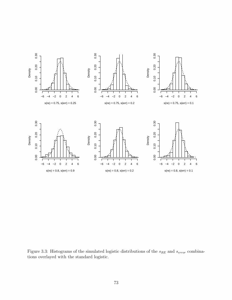
s(re) = 0.75, s(err) = 0.25

Den

sity

−6 −4 −2 0 2 4 6

0.00

0.10

0.20

0.30

s(re) = 0.75, s(err) = 0.2

Den

sity

−6 −4 −2 0 2 4 60.

000.

100.

200.

30

s(re) = 0.75, s(err) = 0.1

Den

sity

−6 −4 −2 0 2 4 6

0.00

0.10

0.20

0.30

s(re) = 0.8, s(err) = 0.9

Den

sity

−6 −4 −2 0 2 4 6

0.00

0.10

0.20

0.30

s(re) = 0.8, s(err) = 0.2

Den

sity

−6 −4 −2 0 2 4 6

0.00

0.10

0.20

0.30

s(re) = 0.8, s(err) = 0.1

Den

sity

−6 −4 −2 0 2 4 6

0.00

0.10

0.20

0.30

Figure 3.3: Histograms of the simulated logistic distributions of the sRE and serror combina-tions overlayed with the standard logistic.

73

not represent the true variances of the simulated datasets; these contribute to the complex

variance structure inherent in the SNPs chosen to simulate the outcome. The true ICC for

MZ and DZ twins in each dataset may be calculated from the simulated outcomes and are

given in Table 3.12.

aMZ 1 1 1.25 1.5 1.5 1.65 1.8 1.8aDZ 0.65 0.8 0.8 0.9 1.1 1 1.05 1.15

Table 3.3: Variance parameters for the alternate model formulation simulation studies.

For the simulation studies, all the β values for the 6 SNPs in X∗ were set to the same

value. For each of the 15 combinations of sre and serror in the original formulation and each

of the 8 combinations of aMZ and aDZ in the alternate formulation, the model was assessed

for β = {1, 1, 1, 1, 1, 1}. The linear portion, v∗ of the outcome was calculated as follows:

v∗i = X∗iβ + u∗i + ε∗i , for the original model, and, (3.61)

= X∗iβ + (aMZMZi + aDZDZi)u∗i + ε∗i , for the alternate model. (3.62)

Then these v∗ values are approximately evenly divided into three ordered categories using

quantiles such that

Qv∗(p) = {v∗|Pr(V ∗ ≤ v∗) = p}, (3.63)

indicates the pth percentile of v∗. Then each v∗i is transformed into an ordinal response, y∗i

as follows:

y∗i =

3 if v∗i < Qv∗(0.33)

2 if Qv∗(0.33) ≤ v∗i < Qv∗(0.66)

1 if v∗i ≥ Qv∗(0.66)

(3.64)

The full R code used to generate the simulation data is given in Appendix Section A.3 for

the original model and Appendix Section A.4 for the alternate model.

74

Simulation Study Results

Original Proposed Model The numbers of non-zero β parameters for the simulation

studies of the original proposed model are given in Table 3.4. For each combination of sRE

and serror, the number of parameters estimated by the AIC- and BIC-selected full ACE and

restricted AE and CE models are given. The value in each cell shows the total number of

non-zero β parameters estimated by that model and the adjacent value in parentheses shows

how many of the non-zero β’s are true non-zero β’s.

sRE serrorBIC model AIC model

ACE AE CE ACE AE CE0.05 0.9 3 (3) 2 (2) 3(3) 3 (3) 2 (3) 3 (3)0.1 0.8 29 (4) 6 (5) 30 (4) 45 (5) 46 (5) 45 (5)0.4 0.85 5 (4) 2 (2) 6 (4) 5(4) 2 (2) 45 (5)0.5 0.9 16 (5) 1 (1) 11 (4) 16 (5) 1(1) 18 (4)0.6 0.95 6 (2) 2 (2) 6 (2) 23 (5) 2 (2) 24 (5)0.65 0.35 29 (4) 6 (5) 30 (4) 45 (5) 46 (5) 45 (5)0.65 0.3 23 (4) 7 (5) 23 (4) 45 (5) 36 (5) 45 (5)0.7 0.9 2 (0) 1 (1) 2 (1) 44 (5) 1 (1) 44 (5)0.7 0.25 28 (4) 6 (5) 28 (4) 43 (5) 30 (5) 43 (5)0.75 0.25 1 (0) 5 (4) 2 (0) 40 (4) 46 (5) 40 (4)0.75 0.2 18 (2) 6 (4) 19 (2) 45 (4) 44 (5) 45 (4)0.75 0.1 41 (4) 8 (4) 41 (4) 45 (4) 46 (5) 45 (5)0.8 0.9 2 (0) 1 (1) 2 (1) 45 (5) 1 (1) 45 (5)0.8 0.2 1 (0 ) 5 (4) 1 (0) 45 (4) 36 (5) 44 (4)0.8 0.1 35 (4) 7 (5) 35 (4) 45 (5) 45 (5) 43 (5)

Table 3.4: Number of non-zero parameters selected by the BIC- and AIC-selected full ACEmodel and the restriced AE and CE models when β = 1. The value in parentheses indicateshow many of those non-zero parameters were true parameters.

From Table 3.4, we can see that none of the models were able to correctly identify all 6

of the true non-zero parameters, although a fair number of models were able to identify 5 of

them. While the AIC-selected models tend to perform better in terms of capturing more of

the true non-zero predictors, in most cases, they are overfit and include too many additional

parameters. The best selection without overfitting generally occurs in the BIC-selected AE

models, at least in cases where sRE is larger and serror is smaller (indicating greater ICC’s.)

75

The predicted response for the simulation studies of the original proposed model are

given in Table 3.5. For each combination of sRE and serror, the ordinal outcome predicted

by the AIC- and BIC-selected full ACE and restricted AE and CE models are given. For

each 3× 3 block of predicted responses, accurate predictions appear on the diagonal.

76

sRE serrorTrue BIC model AIC modelClass ACE AE CE ACE AE CE

0.05 0.91 21 3 7 0 31 0 21 3 7 21 3 7 0 31 0 21 3 72 13 4 13 0 30 0 13 4 13 13 4 13 0 30 0 13 4 133 8 4 19 0 31 0 8 3 20 8 4 19 0 31 0 8 3 20

0.1 0.81 2 29 0 20 8 3 2 29 0 4 27 0 16 11 4 4 27 02 0 26 4 9 8 13 0 26 4 1 23 6 7 11 12 1 23 63 0 21 10 0 8 23 0 21 10 0 19 12 0 8 23 0 19 12

0.4 0.851 21 5 5 30 0 1 21 4 6 21 5 5 30 0 1 16 11 42 10 3 17 27 0 1 8 5 6 10 3 17 27 0 1 5 12 133 6 6 19 25 0 1 5 8 18 6 6 19 25 0 1 2 8 21

0.5 0.91 20 5 6 0 31 0 3 27 1 20 5 6 0 31 0 12 17 22 8 5 17 0 30 0 0 27 1 8 5 17 0 30 0 1 22 73 5 5 21 0 31 0 0 25 6 5 5 21 0 31 0 0 18 13

0.6 0.951 0 31 0 0 31 0 0 31 0 9 19 3 0 31 0 19 4 82 0 30 0 0 30 0 0 30 0 1 22 7 0 30 0 7 8 153 0 31 0 0 31 0 0 31 0 0 18 13 0 31 0 4 6 21

0.65 0.351 2 29 0 20 8 3 2 29 0 4 27 0 16 11 4 4 27 02 0 26 4 9 8 13 0 26 4 1 23 6 7 11 12 1 23 63 0 21 10 0 8 23 0 21 10 0 19 12 0 8 23 0 19 12

0.65 0.31 0 21 0 20 8 3 0 31 0 4 27 0 18 10 3 4 27 02 0 28 2 8 8 14 0 27 3 2 22 6 7 10 13 2 22 63 0 30 1 0 7 24 0 29 2 0 18 13 0 8 23 0 18 13

0.7 0.91 0 31 0 0 30 1 0 31 0 12 16 3 0 30 1 12 16 32 0 30 0 0 25 5 0 30 0 2 22 6 0 25 5 2 22 63 0 31 0 0 25 6 0 31 0 1 15 15 0 25 6 1 15 15

0.7 0.251 0 20 1 21 6 4 0 30 3 3 26 2 16 11 4 2 27 22 0 29 1 8 10 12 0 29 1 2 26 2 8 10 12 1 27 23 0 27 4 0 7 24 0 27 4 0 20 11 0 8 23 0 21 10

0.75 0.251 0 31 0 21 6 4 0 29 2 0 31 0 16 11 4 0 29 22 0 30 0 9 8 13 0 28 2 0 30 0 6 12 12 0 28 23 0 31 0 0 7 24 0 29 2 0 31 0 0 8 23 0 29 2

0.75 0.21 0 31 0 20 6 5 0 31 0 2 26 3 15 11 5 2 26 32 0 30 0 10 9 11 0 30 0 1 28 1 8 11 11 1 28 13 0 30 1 0 7 24 0 30 1 0 22 9 0 7 24 0 22 9

0.75 0.11 2 28 1 20 6 5 2 28 1 3 27 1 16 12 3 2 28 12 0 28 2 5 12 13 0 28 2 0 28 2 6 12 12 0 28 23 0 27 4 0 7 24 0 27 4 0 27 4 0 8 23 0 27 4

0.8 0.91 0 31 0 0 30 1 0 31 0 8 22 1 0 30 1 8 22 12 0 30 0 0 25 5 0 30 0 8 22 1 0 25 5 8 22 13 0 31 0 0 25 6 0 31 0 0 23 8 0 25 6 0 23 8

0.8 0.21 0 31 0 20 6 5 0 31 0 2 27 2 15 12 4 2 27 22 0 30 0 11 7 12 0 30 0 1 29 0 7 12 11 1 29 03 0 30 1 0 7 24 0 31 0 0 23 8 1 7 23 0 23 8

0.8 0.11 0 28 3 21 6 4 0 28 3 3 25 3 17 9 5 2 26 32 0 29 1 9 8 13 0 29 1 1 28 1 10 8 12 1 28 13 0 27 4 0 8 23 0 27 4 0 24 7 0 9 22 0 25 6

Table 3.5: Predicted class for the AIC- and BIC-selected full ACE and restricted AE andCE models when β = 1.

The predicted outcomes for the 92 left-out subjects given in Table 3.5 may be summa-

77

rized by accuracy, i.e., the proportion of accurate predictions made by each model. These

accuracies are presented in Table 3.6.

sRE serrorBIC model AIC model

ACE AE CE ACE AE CE0.05 0.9 .370 .326 .489 .478 .326 .4890.1 0.8 .413 .554 .413 .424 .543 .4240.4 0.85 .467 .337 .478 .467 .337 .5330.5 0.9 .500 .326 .391 .500 .326 .5110.6 0.95 .326 .326 .326 .478 .326 .5220.65 0.35 .413 .554 .413 .424 .543 .4240.65 0.3 .315 .565 .315 .424 .554 .4240.7 0.9 .326 .337 .326 .533 .326 .5330.7 0.25 .359 .598 .359 .435 .533 .4240.75 0.25 .326 .576 .326 .326 .554 .3260.75 0.2 .326 .576 .337 .424 .543 .4240.75 0.1 .370 .609 .370 .380 .554 .3700.8 0.9 .326 .337 .326 .413 .337 .4130.8 0.2 .326 .554 .326 .424 .543 .4240.8 0.1 .359 .565 .359 .413 .511 .391

Table 3.6: Proportion of accurately predicted outcomes for the left-out fold for the BIC- andAIC-selected full ACE model and the restriced AE and CE models when β = 1.

In terms of prediction accuracy, none of the models perform particularly well, however, it

is important to remember that these predictions are made with only the fixed-effect portions

of the estimated models. The intraclass correlation values of the simulated data and the

variance estimates for the simulation studies of the original proposed model are given in

Table 3.7. For each combination of sRE and serror, the variance parameters estimated by the

AIC- and BIC-selected full ACE and restricted AE and CE models are given.

78

sRE serror ICCMZ ICCDZ modelσa σc σe

BIC AIC BIC AIC BIC AIC

0.05 0.9 0.372 0.129ACE 0 0 0.054 0.054 0.001 0.001AE 0.010 0.010 - - 0.001 0.001CE - - 0.011 0.011 0.001 0.001

0.1 0.8 0.395 0.144ACE 0 0 0.011 0.011 0.001 0.001AE 0.006 0.006 - - 0.001 0.001CE - - 1.918 1.640 0.001 0.001

0.4 0.85 0.438 0.183ACE 0 0 0.045 0.045 0.001 0.001AE 0.010 0.010 - - 0.001 0.001CE - - 0.034 0 0.001 0.001

0.5 0.9 0.446 0.228ACE 0 0 0.036 0.036 0.001 0.001AE 0.009 0.009 - - 0.001 0.001CE - - 1.027 0.769 0.001 0.001

0.6 0.95 0.446 0.233ACE 0 0 1.233 0.874 0.001 0.001AE 0.010 0.010 - - 0.001 0.001CE - - 1.251 0.041 0.001 0.001

0.65 0.35 0.812 0.450ACE 0 0 1.897 1.626 0.001 0.001AE 0.006 0.006 - - 0.001 0.001CE - - 1.918 1.640 0.001 0.001

0.65 0.3 0.832 0.482ACE 0 0 2.304 1.744 0.001 0.001AE 0.006 0.006 - - 0.001 0.001CE - - 2.271 1.774 0.001 0.001

0.7 0.9 0.509 0.299ACE 0 0 1.621 0.091 0.001 0.001AE 0.010 0.010 - - 0.001 0.001CE - - 1.614 0.886 0.001 0.001

0.7 0.25 0.847 0.515ACE 0 0 2.407 2.079 0.001 0.001AE 0.005 0.005 - - 0.001 0.001CE - - 2.402 2.138 0.001 0.001

0.75 0.25 0.861 0.555ACE 0 0 3.717 2.616 0.001 0.001AE 0.005 0.005 - - 0.001 0.001CE - - 3.714 2.630 0.001 0.001

0.75 0.2 0.898 0.563ACE 0 0 3.270 2.648 0.001 0.001AE 0.005 0.005 - - 0.001 0.001CE - - 3.278 2.651 0.001 0.001

0.75 0.1 0.926 0.632ACE 0 0 3.181 3.095 0.001 0.001AE 0.005 0.005 - - 0.001 0.001CE - - 3.183 3.106 0.001 0.001

0.8 0.95 0.556 0.334ACE 0 0 1.802 1.203 0.001 0.001AE 0.008 0.008 - - 0.001 0.001CE - - 1.780 1.190 0.001 0.001

0.8 0.2 0.898 0.627ACE 0 0 4.228 3.086 0.001 0.001AE 0.005 0.005 - - 0.001 0.001CE - - 4.245 3.133 0.001 0.001

0.8 0.1 0.918 0.649ACE 0 0 4.404 3.160 0.001 0.001AE 0.005 0.005 - - 0.001 0.001CE - - 3.426 3.227 0.001 0.001

Table 3.7: Intraclass correlation values for the simulated outcomes for MZ and DZ twins andthe estimated variance components of the BIC- and AIC-selected full ACE and restrictedAE and CE models when the true β parameters are all set to equal 1.

79

The comparison of intracluster correlations (as described in Equation 1.2) between the

simulated responses for the MZ and DZ twins indicate that either additive genetics or a

combination of additive genetics and shared environmental components are responsible for

the observed correlations in these scenarios. The full ACE models, however, estimate the

additive genetic component of the variance to be nearly zero in every case. The unique

environmental term is also estimated at nearly zero in every case; although it is estimated

at 0.001, this is an artifact of the estimation procedure since the σe is restricted to be at

least 0.001 in order to prevent singularity in the variance/covariance matrix. Without this

restriction, the estimated value of σe would shrink much closer to zero.

Overall, the original proposed model seems not to perform as optimally as hoped. Weigh-

ing the six models solutions (BIC- and AIC-selected models for each of the ACE, AE, and

CE formulations) against one another in terms of variable selection, prediction accuracy, and

variance estimation, the BIC-selected AE model appears to perform the best.

Given the estimated variance components, the estimated ICC for each model, the ICC

terms, could be calculated. For each model, the estimated ICC may be found as:

ICC =σ2a + σ2

c + σ2e

σ2a + σ2

c + σ2e + π2/3

, for MZs, and (3.65)

ICC =1/2σ2

a + σ2c + σ2

e

1/2σ2a + σ2

c + σ2e + π2/3

, for DZs. (3.66)

From the model-estimated variance parameters in Table 3.7, we see that the additive genetic

component of the variance is never very much greater than zero, resulting in a total random

effect variance of approximately zero for all the AE models. The ACE and CE models

estimate similar variances since the common environmental portion of the variance is driving

the estimates in both cases. The model-estimated ICC would therefore be the same for

both MZ and DZ twins because the shared environment is the only component contributing

significantly to the variance and this component is assumed to be the same for both types of

twin clusters. Based on these results, the model appears to be unable to properly parse out

80

and estimate the variance components. For this reason, the ICC terms were not calculated

or reported here.

Alternate Proposed Model The numbers of non-zero β parameters for the simulation

studies of the alternate proposed model are given in Table 3.8. For each combination of

aMZ and aDZ , the number of parameters estimated by the AIC- and BIC-selected models

are given. The value in each cell shows the total number of non-zero β parameters estimated

by that model and the adjacent value in parentheses shows how many of the non-zero β’s

are true non-zero β’s. The parameter values for aMZ and aDZ were chosen such that the

simulated ICCs would be similar to those simulation cases for which the original model

performed poorly in terms of variable selection.

aMZ aDZ BIC model AIC model1 0.65 5 (3) 35 (5)1 0.8 8 (5) 20 (5)

1.25 0.8 4 (3) 35 (5)1.5 0.9 13 (3) 41 (5)1.5 1.1 5 (3) 46 (5)1.65 1 14 (3) 46 (5)1.8 1.05 12 (3) 45 (5)1.8 1.15 14 (3) 46 (5)

Table 3.8: Number of non-zero parameters selected by the BIC- and AIC-selected modelswhen β = 1. The value in parentheses indicates how many of those non-zero parameterswere true parameters.

As with the original model, we observe from Table 3.8 that the AIC-selected model does

a better job of finding the true non-zero predictors, but it still overfitting in every case.

In comparison to the BIC-selected AE original proposed model, the BIC-selected alternate

model appears to perform variable selection more consistently, although not necessarily more

accurately in every case.

The predicted response for the simulation studies of the alternate proposed model are

given in Table 3.9. For each combination of aMZ and aDZ , the ordinal outcome predicted by

the AIC- and BIC-selected models are given. For each 3 × 3 block of predicted responses,

81

accurate predictions appear on the diagonal.

aMZ aDZ True Class BIC model AIC model

1 0.651 12 14 5 17 9 52 4 17 9 5 12 133 2 10 19 4 8 19

1 0.81 13 15 3 17 9 52 5 15 10 5 13 123 3 11 17 4 8 19

1.25 0.81 6 25 0 15 11 52 3 24 3 5 12 133 2 16 13 5 8 18

1.5 0.91 6 25 0 15 11 52 2 25 3 4 15 113 3 15 13 5 8 18

1.5 1.11 0 31 0 10 15 62 0 30 0 4 14 123 0 30 1 5 9 17

1.65 11 7 24 0 13 13 52 2 25 3 5 13 123 3 16 12 6 7 18

1.8 1.051 0 31 0 11 15 52 0 29 1 5 14 113 0 25 6 6 8 17

1.8 1.151 0 31 0 10 15 62 0 29 1 3 15 123 0 25 6 5 9 17

Table 3.9: Predicted class for the AIC- and BIC-selected models when β = 1.

The proportion of accurate predictions from Table 3.9 are summarized in Table 3.10.

aMZ aDZ BIC model AIC model1 0.65 .522 .5221 0.8 .489 .489

1.25 0.8 .467 .4891.5 0.9 .478 .5221.5 1.1 .337 .4461.65 1 .478 .4781.8 1.05 .380 .4561.8 1.15 .380 .456

Table 3.10: Proportion of accurately predicted outcomes for the left-out fold for the BIC-and AIC-selected models when β = 1. The value in parentheses indicates how many of thosenon-zero parameters were true parameters.

82

The proportion of accurately predicted outcomes appear more consistent but not neces-

sarily more accurate than those from the original proposed model.

The intraclass correlation values of the simulated data and the variance estimates for

the simulation studies of the original proposed model are given in Table 3.11. For each

combination of aMZ and aDZ , the variance parameters estimated by the AIC- and BIC-

selected models are given.

aMZ aDZ ICCMZ ICCDZBIC AIC

σMZ σDZ σMZ σDZ1 0.65 0.324 0.123 0.859 0.353 0.351 01 0.8 0.332 0.153 0.733 0.360 0.416 0

1.25 0.8 0.382 0.159 1.141 0.611 0.669 01.5 0.9 0.441 0.190 1.226 0.633 0.895 0.2111.5 1.1 0.425 0.221 1.334 1.028 0.661 0.4911.65 1 0.456 0.184 1.295 0.659 0.919 0.1321.8 1.05 0.500 0.207 1.687 0.853 1.212 0.2911.8 1.15 0.488 0.245 1.575 0.976 1.096 0.594

Table 3.11: Intraclass correlation values for the simulated outcomes for MZ and DZ twinsand the estimated variance components of the BIC- and AIC-selected models when the trueβ parameters are all set to equal 1.

aMZ aDZ ICCMZ ICCDZBIC AIC

ICCMZ ICCDZ ICCMZ ICCDZ

1 0.65 0.324 0.123 0.183 0.036 0.036 01 0.8 0.332 0.153 0.140 0.038 0.050 0

1.25 0.8 0.382 0.159 0.284 0.102 0.120 01.5 0.9 0.441 0.190 0.313 0.109 0.196 0.0131.5 1.1 0.425 0.221 0.351 0.243 0.117 0.0681.65 1 0.456 0.184 0.338 0.117 0.204 0.0051.8 1.05 0.500 0.207 0.464 0.181 0.309 0.0251.8 1.15 0.488 0.245 0.430 0.225 0.267 0.097

Table 3.12: Estimated intra-class correlations for MZ and DZ twins and the estimated vari-ance components of the BIC- and AIC-selected models when the true β parameters are allset to equal 1.

The ICC terms indicate the model-estimated ICC values. For each model, the estimated

83

ICCs are given as:

ICCMZ =σ2MZ

σ2MZ + π2/3

and ICCDZ =σ2MZ

σ2MZ + π2/3

, (3.67)

for MZ and DZ twins, respectively. From the results in Table 3.12, it’s clear that the BIC-

selected model performs better in terms of more accurately estimating the ICCs in MZ and

DZ twins. Although the estimates are below the true values in every case, they better

approximate the true values than the AIC-selected model estimates.

In this Chapter, we proposed a novel model formulation that met the requirements for

the data applications: penalization for the high-dimensional nature of the data and inclusion

of a no-penalty subset of covariates in an ordinal response mixed-model that allowed user-

specified covariance structures. This original proposed model did not perform optimally in

simulation studies; although variable selection was moderately effective in some cases, the

model was unable to properly parse out the additive genetic, common environmental, and

unique environmental portions of the variance in the random effect and in most cases, did

not predict with much greater than 50% accuracy. An alternate model was also proposed

and this model included all the features of the original model, with the exception of the

flexibility to specify partitioning of the covariance structure between twins. This model

performed better in simulation studies than the original model. Although it had similar

difficulty regarding prediction and BIC-selected models did not correctly identify as many

true predictors, it was more effective for approximating the covariance between twins.

84

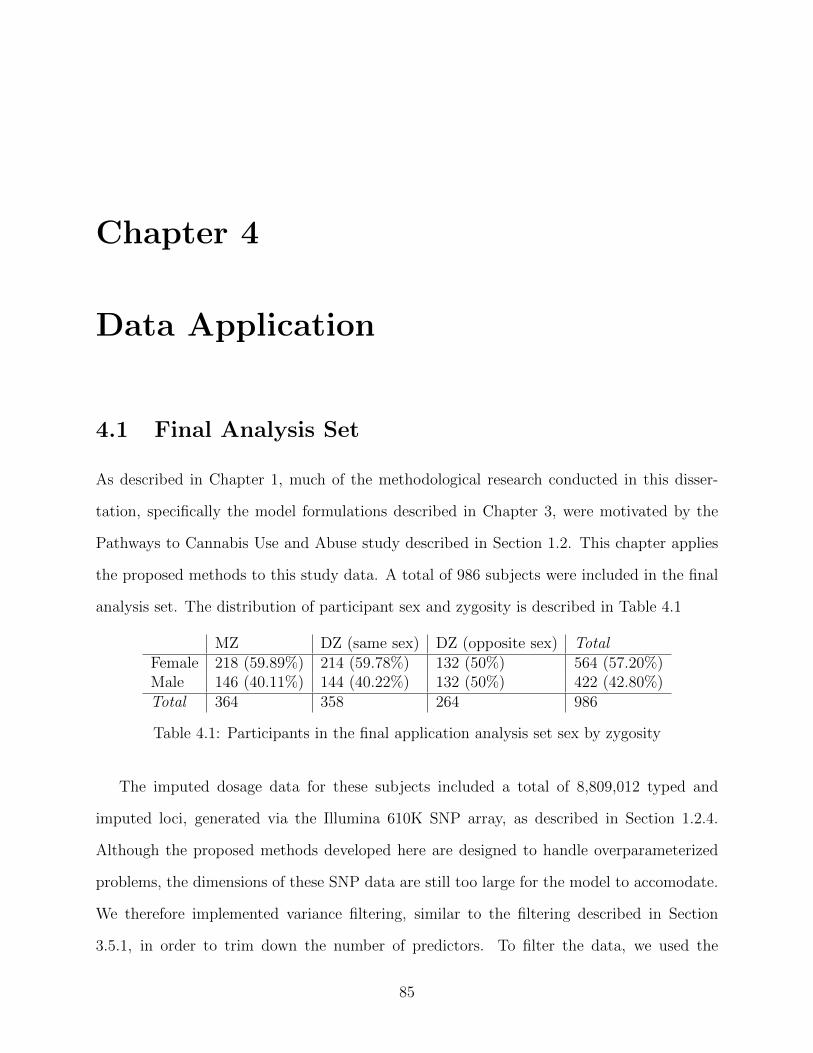
Chapter 4

Data Application

4.1 Final Analysis Set

As described in Chapter 1, much of the methodological research conducted in this disser-

tation, specifically the model formulations described in Chapter 3, were motivated by the

Pathways to Cannabis Use and Abuse study described in Section 1.2. This chapter applies

the proposed methods to this study data. A total of 986 subjects were included in the final

analysis set. The distribution of participant sex and zygosity is described in Table 4.1

MZ DZ (same sex) DZ (opposite sex) TotalFemale 218 (59.89%) 214 (59.78%) 132 (50%) 564 (57.20%)Male 146 (40.11%) 144 (40.22%) 132 (50%) 422 (42.80%)Total 364 358 264 986

Table 4.1: Participants in the final application analysis set sex by zygosity

The imputed dosage data for these subjects included a total of 8,809,012 typed and

imputed loci, generated via the Illumina 610K SNP array, as described in Section 1.2.4.

Although the proposed methods developed here are designed to handle overparameterized

problems, the dimensions of these SNP data are still too large for the model to accomodate.

We therefore implemented variance filtering, similar to the filtering described in Section

3.5.1, in order to trim down the number of predictors. To filter the data, we used the

85

nearZeroVar() function from the R package caret51. This function assesses variance ac-

cording to two metrics, a frequency ratio and a distinct value percentage. The frequency

ratio (freqRatio value) is the ratio of the most common value to the second most com-

mon value; the smaller this ratio, the greater the variance. The distinct value percentage

(percentUnique value) is the percentage of unique values out of the total number of val-

ues; the higher this percentage, the greater the variance. Each of these is calculated for

each SNP on the chromosome. We then filtered out (i.e. removed) those SNPs with both a

freqRatio value at or above the 5th percentile and a percentUnique value at or below the

95th percentile. In this way, the least informative SNPs, those with small variance across all

samples, may be removed. Although this level of filtering seems restrictive, it was necessary

in order to trim larger chromosomes down to a manageable size. Table 4.2 describes the

total number of loci for each chromosome before filtering and the number remaining after

the filtering procedure was implemented. The R code for filtering the SNP data is given in

Appendix A.5 (for chromosomes 9-22) and Appendix A.6 (for chromosomes 1-8).

86

Pre-filtering Post-FilteringChromosome SNP count SNP count

1 679,987 4,5192 740,798 5,6103 625,883 3,7904 642,278 4,5425 571,858 3,5666 580,647 3,8567 515,626 3,9498 492,689 2,9839 379,567 2,76610 448,105 2,85511 437,189 2,99612 424,387 2,91313 325,756 1,85814 290,063 2,55615 252,138 1,71516 276,413 3,75617 232,797 3,17418 253,621 1,86419 196,511 1,35420 199,361 1,25221 122,176 94222 121,162 2,296

8,809,012

Table 4.2: Number of typed and imputed SNPs in each chromosome in the original, unfiltereddataset and in the variance filtered dataset.

Before applying the proposed models to the application data, we determine which vari-

ables should be included in the no-penalty subset. As mentioned in Section 3.1.3, cannabis

use is often correlated with use of other substances such as nicotine and alcohol. Further-

more, these may share some genetic liability106. We therefore chose to include the stem

items for nicotine and alcohol in the no-penalty subject. The three stem items for the final

subject of subjects for the application analysis are summarized in Chapter 1, Table 1.7 and

repeated here, in Table 4.3

87

Female Male TotalTobacco 0 258 (45.74%) 147 (34.83%) 405 (41.08%)

1 196 (34.75%) 150 (35.55%) 346 (35.09%)2 110 (19.50%) 125 (29.62%) 235 (23.83%)

Alcohol 0 13 (2.30%) 4 (0.95%) 17 (1.72%)1 247 (43.79%) 118 (27.96%) 365 (37.02%)2 304 (53.90%) 300 (71.09%) 604 (61.26%)

Cannabis 0 302 (53.55%) 167 (39.57%) 469 (47.57%)1 152 (26.95%) 80 (18.96%) 232 (23.53%)2 110 (19.50%) 175 (41.47%) 285 (28.90%)

Total 564 422 986

Table 4.3: Number of subjects in the final application analysis set reporting level of tobacco,alcohol, and cannabis use by sex.

Because the “did not use” (0) category in the alcohol stem item contained so few subjects,

we chose to dichotomize this variable and combine ordinal levels of alcohol use into 0:“used

none to moderately”(original ordinal levels 0-1) and 1:“used frequently”(original ordinal level

2). The intracluster correlation between the ordinal level of cannabis use was estimated for

both twin types using the ICCest() function from the ICC R package133,134. The formula for

the ICCs are given as:

ICCMZ =σ2MZ

σ2MZ + π2/3

, and ICCDZ =σ2DZ

σ2DZ + π2/3

, (4.1)

for either MZ or DZ twins. The estimated ICCs were 0.667 for MZ twins and 0.304 for DZ

twins.

We used the modified alcohol stem item and the nicotine stem items to model the cannabis

stem item with a random intercept ordinal response model. We fit this model using the

clmm() function from the R package ordinal33. Although this function does not allow

separate random intercepts to be fit for MZ and DZ twins, it will model the data adequately

enough to obtain an idea of the significance of the association between cannabis and the

88

other stem items. The following model is fit using the ordinal package:

logit(γic)

= αc − walc1iβ1 − wnic1iβ2 − wnic2iβ3 + ui, where (4.2)

γic is an ni × 1 vector of the ni probabilities that each of the j responses in the ith

cluster will fall at or below the cth ordinal level of cannabis use,

αc are the intercepts,

walc1iβ1 represents the binary alcohol use item and its associated coefficient,

wnic1iβ2 represents an indicator for ordinal level 1 of nicotine use such that wnic1ij is

1 when nicotine use for the jth member of the ith cluster falls into ordinal category 1,

and 0 otherwise, and β2 is its associated coefficient. Likewise, wnic2i is an indicator

taking the value of 1 if nicotine use falls in the second category, and 0 otherwise, and

β3 is its associated coefficient,

and ui is the random intercept for cluster i.

The fitted model parameters are given in Table 4.4.

Parameter Estimate Standard Error P-Valueα0|1 0.953 0.1885α1|2 2.869 0.2445β1 -1.584 0.1951 < 0.0001β2 2.379 2.379 < 0.0001β3 3.877 0.3081 < 0.0001

Table 4.4: Parameter estimates and standard errors for a model fitting ordinal level of cannbisby alcohol and nicotine use.

The variance of the random intercept was estimated at 1.296. From the p-values shown in

Table 4.4, it’s clear that both alcohol use and cannabis use are associated with ordinal level

of cannabis use and we use these results to justify including them in the no-penalty subset

when modeling the application data with the proposed models. Not only are alcohol and

89

nicotine of interest when investigating cannabis use, we also see that they are statistically

associated in our present data. It is important to note that the model formulation stipulated

by the ordinal package subtracts the fixed effects from the intercept term. Our proposed

models add the fixed effects to the intercepts so that the signs are reversed.

4.2 Proposed Model Application

4.2.1 Application, without JEPQ measure

The original proposed model and the alternate proposed model were applied to the filtered

SNP data from the Pathways project. For every model application, model-selected genomic

loci were referenced in the Illumina 610 Quad manifest files (available online, from Illumina)

and any corresponding dbSNP indentifier (“rs-number’]rq) noted. Additionally, the Inte-

grative Genomics Viewer software (version 2.4.10)117,121 was used to lookup all identified

genomic loci and associated genes were listed, where applicable. As discussed in Section

3.5.1, the best performing formulation of the original model was the BIC-selected AE model

and the best performing formulation of the alternate model was the BIC-selected model.

These are therefore the two models we chose to apply. For each chromosome, ordinal level

of cannabis use was modeled with the dichotomized alcohol stem item and the nicotine stem

items included in the no-penalty subset and the SNPs for that chromosome. The R code

that sets up the application data for the models may be found in Appendices A.12 (for the

original proposed model) and A.13 (for the alternate model). The model parameters from

the original BIC-selected AE model are shown in Table 4.5.

90

Chr α0|1 α1|2 walc wnic1 wnic2 σa σe1 0.771 2.341 1.393 -1.939 -3.205 0.014 0.0012 0.771 2.341 1.393 -1.939 -3.205 0.014 0.0013 0.752 2.326 1.393 -1.947 -3.219 0.014 0.0014 0.755 2.324 1.395 -1.947 -3.214 0.014 0.0015 0.765 2.332 1.391 -1.926 -3.197 0.014 0.0016 0.765 2.332 1.391 -1.926 -3.197 0.014 0.0017 0.772 2.343 1.340 -1.193 -3.197 0.014 0.0018 0.945 2.517 1.403 -1.931 -3.194 0.014 0.0019 0.796 2.366 1.391 -1.937 -3.203 0.014 0.00110 0.764 2.335 1.394 -1.932 -3.204 0.014 0.00111 1.249 2.821 1.386 -1.927 -3.193 0.014 0.00112 0.770 2.339 1.394 -1.932 -3.204 0.014 0.00113 0.792 2.358 1.394 -1.920 -3.191 0.014 0.00114 0.751 2.321 1.393 -1.939 -3.209 0.014 0.00115 0.898 2.468 1.395 -1.926 -3.194 0.014 0.00116 0.829 2.399 1.398 -1.935 -3.203 0.014 0.00117 0.928 2.496 1.391 -1.916 -3.191 0.014 0.00118 0.875 2.444 1.400 -1.919 -3.185 0.014 0.00119 0.806 2.376 1.395 -1.937 -3.205 0.014 0.00120 0.756 2.320 1.401 -1.911 -3.183 0.014 0.00121 0.779 2.347 1.393 -1.922 -3.193 0.014 0.00122 0.955 2.523 1.389 -1.942 -3.210 0.014 0.001

Table 4.5: BIC-selected original proposed AE model parameters when the personality mea-sures are excluded.

The non-zero parameters chosen by the original proposed AE model are given in Table

4.6. The starred parameters indicate loci that were selected by both the original and the

alternate proposed model, applied below.

91

Chr No. predictors Non-zero predictors1 2 1:152310892 (RefSeq Gene FLG-AS1), 1:286382592 2 2:84058093*, 2:195942691*

3 23:123415781* (RefSeq Gene MYLK, rs820336),3:183015258* (RefSeq Gene MCF2L2)

4 2 4:4029928, 4:97403255 2 5:130689713 (RefSeq Gene CDC42SE2), 5:1586146076 2 6:30365740*, 6:24735937 2 7:72914811 (RefSeq Gene BAZ1B), 7:152415427*8 2 8:47716446, 8:137485507* (rs4909596)9 2 9:38488974*, 9:71344802 (RefSeq Gene PIP5K1B)10 2 10:65796140, 10:98539578

11 211:199673* (RefSeq Gene ODF3), 11:2415964* (RefSeq Gene CD81),11:117489521 (RefSeq Gene CD81)

12 2 12:10940426, 12:12716764*13 2 13:54698204, 13:22562993 (rs3129601)14 2 14:57027631, 14:103656062*15 2 15:98819843*, 15:4869673016 2 16:212328*, 16:8120992017 2 17:81069185*, 17:2911537918 2 18:77549734*, 18:1110951219 2 19:41339896*, 19:45523459 (RefSeq Gene RELB)20 2 20:56193258 (RefSeq Gene ZBP1), 20:19884764 (RefSeq Gene RIN2)

21 221:17707722 (RefSeq Gene MIR99AHG),21:18001708 (RefSeq Gene MIR99AHG)

22 2 22:20722220*, 22:23029263

Table 4.6: Non-zero parameters in each BIC-selected original proposed AE model when thepersonality measures are excluded.

The alternate proposed model was also applied to the application data. As before, for

each chromosome, ordinal level of cannabis use was modeled with the dichotomized alcohol

stem item and the nicotine stem items included in the no-penalty subset and the SNPs for

that chromosome. The model parameters from the alternate BIC-selected model are shown

in Table 4.7 and the associated selected loci given in Table 4.8.

92

Chr α0|1 α1|2 walc wnic1 wnic2 σMZ σDZ ICCMZ ICCDZ

1 1.253 3.288 1.641 -2.488 -4.055 1.727 1.177 0.476 0.2962 1.022 3.048 1.632 -2.474 -4.053 1.737 1.165 0.478 0.2923 1.015 3.041 1.632 -2.476 -4.054 1.733 1.166 0.477 0.2924 0.989 3.015 1.633 -2.478 -4.057 1.739 1.168 0.479 0.2935 0.994 3.023 1.635 -2.478 -4.061 1.752 1.169 0.483 0.2936 1.073 3.098 1.628 -2.468 -4.045 1.751 1.150 0.482 0.2877 1.218 3.239 1.657 -2.471 -4.036 1.723 1.137 0.474 0.2828 1.037 3.059 1.628 -2.468 -4.047 1.735 1.150 0.478 0.2879 1.037 3.062 1.634 -2.471 -4.045 1.737 1.158 0.478 0.29010 0.999 3.025 1.634 -2.475 -4.054 1.739 1.165 0.479 0.29211 1.121 3.143 1.628 -2.471 -4.046 1.731 1.150 0.477 0.28712 1.152 3.179 1.632 -2.468 -4.053 1.751 1.156 0.482 0.28913 0.992 3.018 1.633 -2.475 -4.054 1.740 1.165 0.479 0.29214 1.104 3.130 1.632 -2.475 -4.051 1.746 1.154 0.481 0.28815 1.080 3.105 1.632 -2.472 -4.051 1.735 1.159 0.478 0.29016 1.090 3.120 1.636 -2.482 -4.063 1.748 1.170 0.482 0.29417 0.989 3.015 1.633 -2.478 -4.058 1.739 1.168 0.479 0.29318 0.989 3.015 1.633 -2.475 -4.054 1.739 1.166 0.479 0.29219 1.127 3.151 1.628 -2.465 -4.047 1.733 1.155 0.477 0.28920 1.028 3.053 1.633 -2.474 -4.052 1.736 1.160 0.478 0.29021 1.094 3.119 1.637 -2.473 -4.055 1.747 1.152 0.481 0.28722 1.078 3.107 1.632 -2.479 -4.061 1.755 1.163 0.484 0.291

Table 4.7: BIC-selected alternate proposed model parameters when the personality measuresare excluded.

93

Chr No. predictors Non-zero predictors1 2 1:88298721, 1:989656212 2 2:84058093*, 2:195942691*

3 23:123415781* (RefSeq Gene MYLK, rs820336),3:183015258* (RefSeq Gene MCF2L2)

4 2 4:84288014, 4:1699919775 1 5:123768154 (RefSeq Gene LINC01170)6 2 6:30365740*, 6:90207007 2 7:152415427*, 7:1524200448 2 8:137485507* (rs4909596), 8:167295859 2 9:38488974*, 9:9903078 (RefSeq Gene PTPRD)10 1 10:122746804 (rs10886827)11 2 11:199673 (RefSeq Gene ODF3), 11:2415964 (RefSeq Gene CD81)12 2 12:51769773 (RefSeq Gene GALNT6), 12:12716764

13 213:112636548 (RefSeq Gene LINC00403),13:113744139 (RefSeq Gene MCF2L)

14 2 14:103656062*, 14:4454580815 2 15:23039087, 15:98819843*16 2 16:212328*, 16:588979017 2 17:80594 (RefSeq Gene RPH3AL), 17:81069185*18 1 18:77549734*19 2 19:41339896*, 19:2091545220 2 20:17837939, 20:2211622621 2 21:21426525, 21:35226135 (RefSeq Gene ITSN1, rs2249221)22 2 22:47648670, 22:20722220*

Table 4.8: Non-zero parameters in each BIC-selected alternate proposed model when thepersonality measures are excluded.

Of interest, the rs820336 variant within the MYLK gene on chromosome 3 has been pre-

viously associated with lung disease and asthma63. On chromosome 5, the BAZ1B gene was

identified as associated with some of the neurological symptoms in patients with Williams

Beuren syndrome53. The PTPRD gene on chromosome 9 has been associated with so-

cial conformity behavior31. Differential methylation of a CpG site within the MCF2L gene

on chromosome 13 was found to be associated with borderline personality disorder among

childhood mistreatment survivors112. Additionally, a rare deletion of a portion of a ring chro-

mosome 13 including the MCF2L gene was discovered in one case of a child with autism30.

94

4.2.2 Application, with JEPQ measures

It was of interest to include the JEPQ personality measures in the penalized set to determine

if these features were related to ordinal level of cannabis use. Both the original (BIC-selected

AE) and alternate (BIC-selected) models were applied in the same manner as described in

Section 4.2.1. Table 4.9 gives the model parameters for the original proposed BIC-selected

AE model when the JEPQ measures are included with the SNPs in the penalized set. For

this application, the models running on chromosomes 2, 7, 10, 12, 16-17, and 19-22 failed

to converge. Although a precise reason for failed convergence could not be determined, the

optimization procedure was unable to find a solution for the no-penalty subset and variance

parameters after several updates had been made to one or more of the β values for a variable

in the penalized set.

Chr α0|1 α1|2 walc wnic1 wnic2 σa σe1 1.968 3.568 1.302 −1.881 −3.131 0.015 0.0013 2.201 3.824 1.270 -1.848 -3.068 0.013 0.0014 2.167 3.767 1.283 -1.868 -3.109 0.013 0.0015 1.968 3.568 1.302 -1.881 -3.101 0.013 0.0016 1.874 3.470 1.316 -1.859 -3.102 0.013 0.0018 1.968 3.568 1.302 -1.881 -3.131 0.013 0.0019 1.874 3.470 1.316 -1.859 -3.102 0.013 0.00111 1.874 3.470 1.316 -1.859 -3.102 0.013 0.00112 2.003 3.599 1.302 -1.859 -3.098 0.013 0.00114 1.968 3.568 1.302 -1.881 -3.131 0.013 0.00115 1.874 3.470 1.316 -1.859 -3.102 0.013 0.00118 2.003 3.599 1.302 -1.859 -3.098 0.013 0.001

Table 4.9: BIC-selected AE original proposed model parameters.

Table 4.10 lists the non-zero predictors selected by the BIC-selected original proposed

AE model for each chromosome. The covariates listed in Table 4.10 are those selected by

the models shown in Table 4.9. The abbreviations “psy” and “ext” refer to the JEPQ

psychoticism and extroversion scores, respectively. The starred variables indicate loci that

were selected by both the original proposed model and the alternate proposed model (results

shown in Tables 4.11 and 4.12.) The loci indicated by “†” designate positions indicated in

95

both the penalized proposed model and the single locus tests (See Section 4.3).

Chr No. predictors Non-zero predictors1 2 psy, ext

3 4psy, ext, 3 : 142842195†∗ (RefSeq Gene CHST2, rs4149496),3:8652993 (rs2324665)

4 2 psy, ext5 2 psy, ext6 2 psy, ext8 2 psy, ext9 2 psy, ext11 2 psy, ext12 2 psy, ext14 2 psy, ext15 2 psy, ext18 2 psy, ext

Table 4.10: Non-zero parameters in each BIC-selected original proposed AE model.

The alternate proposed model was applied to the same data with the JEPQ measures

included in the penalized set. The BIC-selected alternate model parameter estimates are

shown for each chromosome in Table 4.11. Models for chromosomes 1-2, 7-8, 13, 16-17, and

21 failed to convergence in the same manner as the failed models shown in Table 4.9 above.

Chr α0|1 α1|2 walc wnic1 wnic2 σMZ σDZ ICCMZ ICCDZ

3 2.121 4.137 1.518 -2.308 -3.795 1.599 1.025 0.437 0.2424 2.279 4.320 1.555 -2.379 -3.911 1.664 1.145 0.457 0.2855 2.279 4.320 1.556 -2.379 -3.910 1.663 1.146 0.457 0.2856 2.294 4.335 1.556 -2.379 -3.911 1.664 1.148 0.457 0.2869 2.309 4.352 1.556 -2.380 -3.912 1.665 1.150 0.457 0.28710 2.210 4.248 1.545 -2.352 -3.861 1.617 1.121 0.443 0.27611 2.294 4.335 1.556 -2.380 -3.911 1.664 1.148 0.457 0.28612 2.288 4.330 1.556 -2.379 -3.910 1.663 1.147 0.457 0.28614 2.309 4.352 1.556 -2.381 -3.912 1.665 1.150 0.457 0.28715 2.289 4.330 1.556 -2.379 -3.910 1.663 1.147 0.457 0.28618 2.284 4.326 1.557 -2.380 -3.911 1.663 1.147 0.457 0.28619 2.303 4.347 1.557 -2.380 -3.911 1.664 1.150 0.457 0.28720 2.294 4.335 1.556 -2.380 -3.911 1.664 1.148 0.457 0.28622 2.309 4.352 1.556 -2.381 -3.912 1.665 1.150 0.457 0.287

Table 4.11: BIC-selected alternate proposed model parameters.

Table 4.12 lists the non-zero predictors selected by the BIC-selected alternate model for

96

each chromosome. The covariates listed in Table 4.12 are those selected by the models

shown in Table 4.11. The abbreviations “psy” and “ext” refer to the JEPQ psychoticism

and extroversion scores, respectively.

Chr No. predictors Non-zero predictors3 4 psy, ext, 3 : 142842195†∗ (RefSeq Gene CHST2, rs4149496), 3:1476152854 3 psy, ext, 4:1245577725 3 psy, ext, 5:541775116 3 psy, ext, 6:406418169 3 psy, ext, 9:9884551210 4 psy, ext, 10:82568684, 10:9852900211 3 psy, ext, 11:3877911612 3 psy, ext, 12:345473614 3 psy, ext, 14:10563658715 3 psy, ext, 15:2457614918 3 psy, ext, 18:195595119 3 psy, ext, 19:53076618 (RefSeq Gene ZNF701)20 3 psy, ext, 20:343542722 3 psy, ext, 22:20246081

Table 4.12: Non-zero parameters in each BIC-selected alternate proposed model.

The model results shown in Tables 4.10 and 4.12 seem to indicate that the JEPQ measures

may be overwhelming the SNP effects. Furthermore, many of the models failed to converge so

further investigation into the association between the JEPQ measures, SNPs, and cannabis

use in this setting is warranted.

4.2.3 Discussion of Proposed Model Results

The true intracluster correlations, as calculated from the cannabis use data for the 986

subjects in the analysis set, were estimated at 0.667 for MZ twins and 0.304 for DZ twins.

As seen in the simulation studies, the original proposed model estimates the random effect

variance components to be nearly zero and the ICCs could therefore not be accurately

measured. Also as seen in the simulation studies, the alternate proposed model estimates the

intracluster correlations consistently, but tends to underestimates these values. Excluding

the JEPQ features, the two model forms selected some, but not all of the same variables

97

from each chromosome. When the personality features were included in the penalized set,

the model chose extroversion and psychoticism as the primary features, however not all the

models on every chromosome converged when the problem was framed in this way.

4.3 Single Locus Tests

Because the proposed models did not perform as well as expected during simulation studies,

we chose to apply the single locus association test (SLAT) methodology to the application

dataset. Similar to the model fit in Equation 4.2, the SLATs are fit using the ordinal

package33 in R as follows:

logit(γic)

= αc − walc1iβ1 − wnic1iβ2 − wnic2iβ3 + snpabiβ4 + ui, where (4.3)

all parameters carry the same interpretation as in Equation 4.2, and

snpabi represents the bth SNP from the ath chromosome for subject i and β4 is its

associated coefficient.

The model above was fit once for each SNP on each chromosome. Because these models

were fit many times for each chromosome, it was necessary to correct for multiple testing.

(The exact number of tests performed for each chromosome may be seen in Table 4.2) A

p-value adjustment was made to the resulting p-values from every chromosome using both

the Benjamini and Hochberg20 (BH) and the Benjamini and Yekuttieli21 (BY) methods.

These adjustment methods control the false discovery rate (FDR), or the false positive rate,

and control it at a user-specified level. These adjustment methods are similar, although the

BY method is better suited to correlated variables. The FDR was set at 0.01 and Table

4.13 gives the significant hits from each of the chromosomes; only the chromosomes with

significant hits are included in the table.

98

Chr significant loci

3BY: -BH: 3 : 142842195† (RefSeq Gene CHST2, rs4149496), 3:142844453

16

BY: 16:268548701, 16:268553561, 16:19944471, 16:19953191, 16:19960751,16:84376551, 16:843765511BH: 16:26854329, 16:268543291, 16:268548701, 16:268553561, 16:291188651,16:1996075 (RefSeq Gene RPL3L), 16:19944471, 16:19953191, 16:19960751,16:84376551, 16:843765511

17BY: 17:252682671, 17:25334803:1BH: 17:805941 (RefSeq Gene NXN), 17:774678211, 17:252651301, 17:252682671,17:252769831, 17:25281651:1, 17:25284681:2, 17:252858031, 17:25334803:1

Table 4.13: Significant loci from the single locus association tests performed on each chromo-some, as determined by both Benjamini and Hochberg and Benjamini and Yekuttieli FDRcorrection methods.

Significant loci appeared only on chromosomes 3, 16, and 17 and 3:142842195 (RefSeq

Gene CHST2, rs4149496) was the only loci indentified by both the penalized methods and

the SLATs.

99

Chapter 5

Conclusion

In Chapter 1, we described the Pathways to Cannabis Use, Abuse and Dependence project,

which utilized data from the Bisbane Longitudinal Twin Study in order to investigate the

associations between substance use (particularly, the ordinal level of cannabis use) and SNPs

and personality features. A penalized regression-type model capable of handling the high-

dimensional data, the ordinal response, and the specific correlation pattern observed between

twins was not available to apply to the data. In Chapter 2, we described a penalized ordinal

regression fitting procedure that included a no-penalty subset, allowing the user to specify

some group of variable which may be coerced into the model. In Chapter 3, this model was

expanded in order to allow for user-specified covariance patterns between MZ and DZ twin

pairs so that different intracluster correlations might be calculated for each type of twin pair.

Finally, in Chapter 4, we applied the proposed models to the Pathways dataset and provide

some interpretation of the findings.

5.1 Model Limitations

The application of the proposed models to the Pathways data revealed some suggestive loci

of interest. None of the suggestive SNPs have previously been implicated in drug or alcohol

use studies. Given exploratory nature of the penalized regression analysis, it will of course

100

be necessary to further investigate and verify any findings. Additionally, when SNP effects

are small, as is typically seen for complex traits, sample sizes of tens of thousands or more

are needed in order to detect these effects. With a sample size of less than 1000 subjects in

our application, it is even more important to regard the results as suggestive, but impotant

initial pilot work into the study of genetic variants associated with drug use.

5.2 Future Directions

In its current form, the proposed model is applicable only to a single set of twins from

each family. The original proposed model form, however, was conceived as a general family-

cluster method. It will be straightforward to extend the model to allow for general kinship

matrices (of any size) to be used to specify the correlation structure within each family.

For application to the Pathways data, the first extension will be to include the sampled

siblings of the twin pairs from the BLTS data. The inclusion of additional family members

in the analysis will allow for more precise calculations of additive genetic and environmental

proportions of the variance.

The original proposed model was designed to model additive genetic, shared environmen-

tal, and individual environmental components of the variance with a single random effect.

The purpose of this choice was to keep the model as parsimonious and easily estimable as

possible. As discussed in Section 3.2.2 however, many other implementations of the mixed

model for behavior genetic applications fit a separate random effect for each of the partitions

of the total variance, additive genetic, shared environmental, and individual environmental.

Fitting additional random effects is more complex and requires more computing resources

but may result in better performance. Comparative performance may be evaluated by fitting

the same simulated dataset using our proposed, single random effect model and an extended,

multiple effect model, to see if addition random effects improve fit.

Multiple software programs have been developed which use measured genotypes to es-

101

timate the genetic relatedness matrix (GRM) between subjects in a sample. This GRM

may be regarded as a measured kinship matrix. Since the GRMs are calculated based on

the SNPs across the sample, they more accurately reflect the genetic relatedness between

subjects than the theoretical kinship matrix. It would be of interest to apply the proposed

methods using the estimated GRMs for each family cluster, as opposed to the theoretical

double coancestry matrices.

102

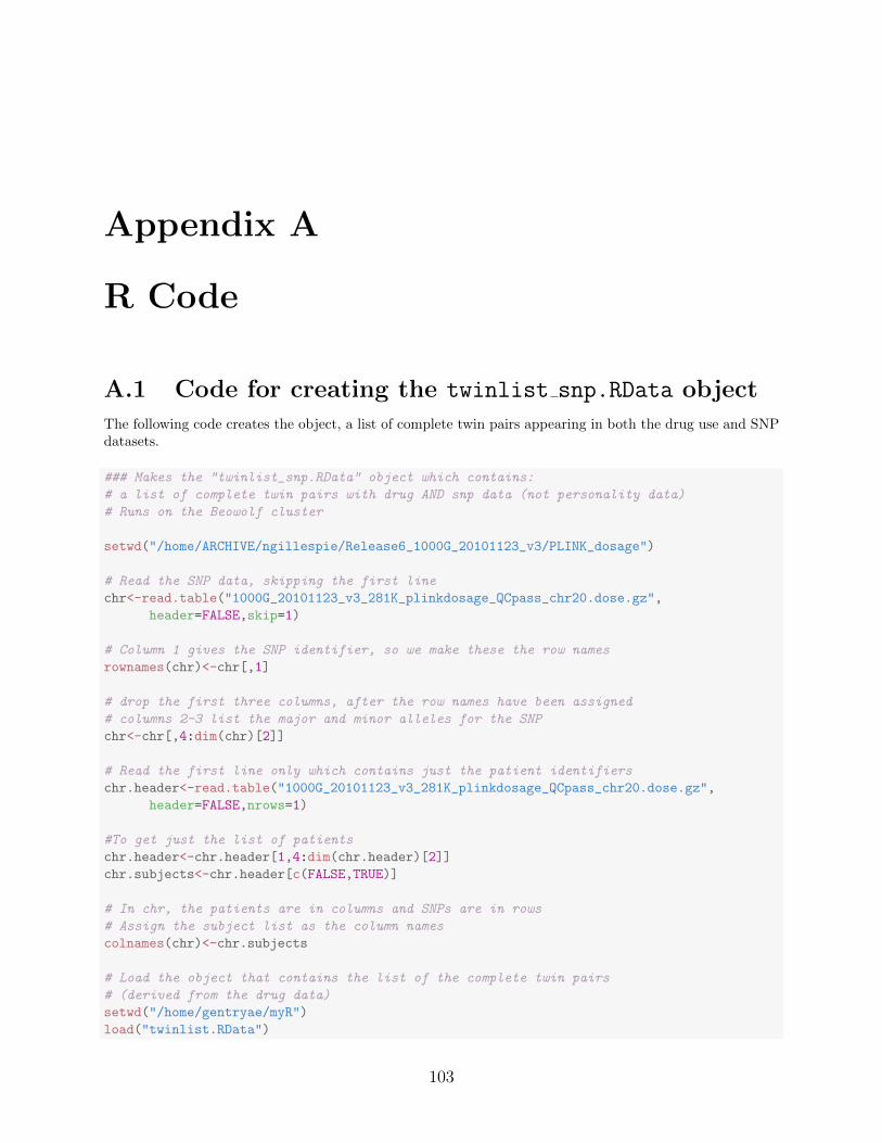
Appendix A

R Code

A.1 Code for creating the twinlist snp.RData object

The following code creates the object, a list of complete twin pairs appearing in both the drug use and SNPdatasets.

### Makes the "twinlist_snp.RData" object which contains:

# a list of complete twin pairs with drug AND snp data (not personality data)

# Runs on the Beowolf cluster

setwd("/home/ARCHIVE/ngillespie/Release6_1000G_20101123_v3/PLINK_dosage")

# Read the SNP data, skipping the first line

chr<-read.table("1000G_20101123_v3_281K_plinkdosage_QCpass_chr20.dose.gz",

header=FALSE,skip=1)

# Column 1 gives the SNP identifier, so we make these the row names

rownames(chr)<-chr[,1]

# drop the first three columns, after the row names have been assigned

# columns 2-3 list the major and minor alleles for the SNP

chr<-chr[,4:dim(chr)[2]]

# Read the first line only which contains just the patient identifiers

chr.header<-read.table("1000G_20101123_v3_281K_plinkdosage_QCpass_chr20.dose.gz",

header=FALSE,nrows=1)

#To get just the list of patients

chr.header<-chr.header[1,4:dim(chr.header)[2]]

chr.subjects<-chr.header[c(FALSE,TRUE)]

# In chr, the patients are in columns and SNPs are in rows

# Assign the subject list as the column names

colnames(chr)<-chr.subjects

# Load the object that contains the list of the complete twin pairs

# (derived from the drug data)

setwd("/home/gentryae/myR")

load("twinlist.RData")

103

# Drop the subjects that don't appear in the SNP set

twinpairs.only <- twinpairs.only[ twinpairs.only$subid %in% colnames(chr), ]

# Then we have to remove singletons again

identifier <- logical()

for (i in 1:dim(twinpairs.only)[1]){identifier[i]<- sum(twinpairs.only$familyid ==

twinpairs.only$familyid[i]) == 2

}twinpairs.only.snp <- twinpairs.only[identifier, ]

# Drop the subjects from the SNP set that aren't in the drug set

chr <- chr[ , colnames(chr) %in% twinpairs.only.snp$subid]

### And now, there is a list of complete twin pairs with SNP data

### We can output this list in order to use it in SNP filtering code

save(twinpairs.only.snp, file="twinlist_snp.RData")

A.2 Code for creating the chr21filt.RData object

The following code creates the object, a list of complete twin pairs appearing in both the drug use and SNPdatasets.

# Use the nearZerVar() function to filter chr 21 for the purpose of simulations

# Use the "twinlist_snp.RData" file to load the twinpairs.only.snp object

# that has the list of the complete twin pairs in both the drug and SNP data files

### Runs on the Beowolf cluster

###

setwd("/home/ARCHIVE/ngillespie/Release6_1000G_20101123_v3/PLINK_dosage")

# Read the SNP data, skipping the first line

chr<-read.table("1000G_20101123_v3_281K_plinkdosage_QCpass_chr21.dose.gz",

header=FALSE,skip=1)

# this object has dim 118,606 X 4,541

# Column 1 gives the SNP identifier, so we make these the row names

rownames(chr)<-chr[,1]

# drop the first three columns, after the row names have been assigned

# columns 2-3 list the major and minor alleles for the SNP

chr<-chr[,4:dim(chr)[2]]

# Read the first line only which contains just the patient identifiers

chr.header<-read.table("1000G_20101123_v3_281K_plinkdosage_QCpass_chr21.dose.gz",

header=FALSE,nrows=1)

#To get just the list of patients

chr.header<-chr.header[1,4:dim(chr.header)[2]]

chr.subjects<-chr.header[c(FALSE,TRUE)]

104

# In chr, the patients are in columns and SNPs are in rows

# Assign the subject list as the column names

colnames(chr)<-chr.subjects

# Load the subject list

setwd("/home/gentryae/myR")

load("twinlist_snp.RData")

# Subset the SNP data

chr <- chr[ , colnames(chr) %in% twinpairs.only.snp$subid]

# Run the filtering, outputting the metrics matrix

library(caret)

nzvchr21 <- nearZeroVar(t(chr), saveMetrics=TRUE)

save(nzvchr21, file="nzvchr21.Rdata")

# Keep the SNPs with freqRatio values in the bottom 15th percentile

# and percentUnique values in the top 85th percentile

# This will result in keeping approximately 5% of the SNPs on the chromosome

keep <- (nzvchr21$freqRatio < quantile(nzvchr21$freqRatio, 0.15) &

nzvchr21$percentUnique > quantile(nzvchr21$percentUnique, 0.85))

chr21filt <- chr[keep, ]

# Output the filtered SNP set

save(chr21filt, file="chr21filt.RData")

A.3 Code for creating the simulated data for the orig-

inal model

This particular example sets the σRE = 0.6 and σerror = 0.95, but these may be changed to produce thedata for any of the simulations for the original proposed model.

### Simulation Set-up

#setwd("/Users/taylorgentry/Documents/Amanda")

setwd("/home/gentryae/myR")

#setwd("/Users/AmandaGentry/Documents/Thesis")

# load the filtered chr21 SNP set

load("chr21filt.RData")

# load the object with the twin id's and zygosity info. from the list

load("twinlist_snp.RData")

# number of complete twin pairs for which there is SNP AND drug use data

# we have to use this subset because the zygosity information is contained

# within the drug use dataset the twinpairs.only.snp list has already been

# filtered to return this subset of subjects

no.sim.sub <- dim(twinpairs.only.snp)[1]

no.sim.pair <- no.sim.sub/2

### There are 1092 subjects in this set, we remove 46 random pairs for the

### simple purpose of working with a round number for the simulation

set.seed(1635)

# randomly select 46 family ID's and remove these from the training data

105

# We can use those 46 pairs as a test set

# subset the twinpairs.only.snp and the filtered chromosome objects

no.remove <- 46

no.train.sub <- no.sim.sub - (no.remove *2)

no.train.pair <- no.sim.pair - no.remove

keep <- !(twinpairs.only.snp$familyid %in%

sample(unique(twinpairs.only.snp$familyid), no.remove))

test <- !(keep)

twinpairs.only.test <- twinpairs.only.snp[test,]

chr21filt.test <- chr21filt[, colnames(chr21filt) %in%

twinpairs.only.test$subid]

twinpairs.only.snp <- twinpairs.only.snp[keep,]

chr21filt <- chr21filt[, colnames(chr21filt) %in% twinpairs.only.snp$subid]

# can double check that there's no overlap between the test and training sets

# sum(twinpairs.only.snp£subid %in% twinpairs.only.test£subid)

# the original SNP set from chromosome 21 contained 118603 SNPs

no.snps <- dim(chr21filt)[1]

prop.snps <- no.snps/118603

# to see the new distribution of zygosity in the training set

# table(twinpairs.only.snp£zygosity)

# no of MZFF

MZFF.sim <- sum(twinpairs.only.snp$zygosity == 1)/2

MZMM.sim <- sum(twinpairs.only.snp$zygosity == 2)/2

DZFF.sim <- sum(twinpairs.only.snp$zygosity == 3)/2

DZMM.sim <- sum(twinpairs.only.snp$zygosity == 4)/2

DZMF.sim <- (sum(twinpairs.only.snp$zygosity == 5) +

sum(twinpairs.only.snp$zygosity == 6))/2

# Original coding designates zygosity of 1 or 2 as MZ twins

# and zygosity of 3, 4, 5, or 6 as DZ twins

# For convenience, add an abbreviated zygosity column designating 0

# for MZ and 1 for DZ

twinpairs.only.snp$zyg.abr <- ifelse(twinpairs.only.snp$zygosity < 3,

0, 1)

# SNP 4000 has a nice distribution so we will choose it as the primary SNP

# see the distribution of this SNP

#hist(as.numeric(chr21filt[4000,]))

snp.choice<-4000

# Find the correlation between this SNP and every other SNP on the chromosome

cor.choice <- apply(chr21filt, 1, cor, as.numeric(chr21filt[snp.choice,]))

# Randomly select 5 other SNPs with abs(correlation) of between 0.1 and 0.4

set.seed(81092)

cor.with.4000 <- sample(which(abs(cor.choice)>0.1 & abs(cor.choice)<0.4), 5)

no.cor <- length(which(abs(cor.choice)>0.1 & abs(cor.choice)<0.4))

# see the correlations themselves

cor.choice[names(cor.choice) %in% rownames(chr21filt[cor.with.4000,])]

# Put these 6 SNPs in a matrix

selected<-c(rownames(chr21filt[4000,]),names(cor.with.4000))

# Find the correlations between each of these SNPs and every

# other SNP in the set

cor.mat<-matrix(data=NA, ncol=length(selected), nrow=dim(chr21filt[1]))

106

for (i in 1:length(selected)){cor.mat[, i] <- apply(chr21filt, 1, cor,

as.numeric(chr21filt[rownames(chr21filt) == selected[i],]))

}# assign rownames

rownames(cor.mat) <- rownames(chr21filt)

# Find SNPs highly correlated with the selected SNPs

cor.mat.ind <- abs(cor.mat) > 0.5

# Sum across to find the SNPs with correlation to any of the selected

# SNPs of greater than .5

cor.mat.ind2 <- apply(cor.mat.ind, 1, sum)

# Find the names of these SNPs

remove.snps <- names(which(cor.mat.ind2 >= 1))

# find the list of these correlated SNPs, minus the names of the 6

# "selected" SNPs

remove.snps1 <- !(remove.snps %in% selected)

# Find a subset of the SNPs to be removed, by name

remove.snps <- remove.snps[remove.snps1]

# Find the row numbers of these

remove.snps.rows <- which(rownames(chr21filt) %in% remove.snps)

# Remove these SNPs from the test and training sets

chr21filt <- chr21filt[-remove.snps.rows, ]

chr21filt.test <- chr21filt.test[-remove.snps.rows, ]

# the SNP table has subjects in columns, so we take the transpose

t.chr <- t(chr21filt)

t.chr.test <- t(chr21filt.test)

# reorder the SNP object so that it matches the

# twinpairs.only.snp object

# (the twinpairs.only.snp object is ordered according

# to ascending subject id)

t.chr <- t.chr[order(as.numeric(rownames(t.chr))), ]

t.chr.test <- t.chr.test[order(as.numeric(rownames(t.chr.test))), ]

# check that the twinpairs.only.snp object and the t.chr object

# are ordered the same

# all.equal(rownames(t.chr), as.character(twinpairs.only.snp£subid))

# all.equal(rownames(t.chr.test), as.character(twinpairs.only.test£subid))

# define the X matrix with the selected SNPs

no.final.snps <- dim(t.chr)[2]

no.false.pred <- dim(t.chr)[2] -6

X <- t.chr[, colnames(t.chr)%in%selected]

X.test <- t.chr.test[, colnames(t.chr.test)%in%selected]

# check that the ordering of X matches the twinpairs.only.snp ordering

# all.equal(rownames(X), as.character(twinpairs.only.snp£subid))

# all.equal(rownames(X.test), as.character(twinpairs.only.test£subid))

# Set the beta values

snp.betas <- rep(1,6)

# Generate the random intercept

u1mean <- 0

u1sd <- 0.6

set.seed(6981)

#u1 <- rnorm(500, u1mean, u1sd)

107

u1<- rlogis(500, u1mean, u1sd)

set.seed(6339)

#u1.test <- rnorm(46, u1mean, u1sd)

u1.test <- rlogis(46, u1mean, u1sd)

# append u to itself and add a temporary index from 1-500

u <- cbind(rep(1:500, 2), c(u1,u1))

u.test <- cbind(rep(1:46, 2), c(u1.test,u1.test))

# then order u according to the index and remove the index

# this is just the dumbest way I could think of to repeat each

# random intercept twice

u <- u[order(u[,1]),2 ]

u.test <- u.test[order(u.test[,1]),2 ]

sim <- cbind(twinpairs.only.snp, u)

sim.test <- cbind(twinpairs.only.test, u.test)

## Generate the random error/perturbations

sigmamean <- 0

sigmasd <- 0.95

set.seed(6480)

sigma = rlogis(dim(sim)[1], location = sigmamean, scale = sigmasd)

set.seed(6340)

sigma.test = rlogis(dim(sim.test)[1], location = sigmamean, scale = sigmasd)

z <- as.matrix(X) %*% snp.betas +

as.matrix(sim$u) +sigma

z.test <- as.matrix(X.test) %*% snp.betas +

as.matrix(sim.test$u.test) +sigma.test

y <- z

y[z < quantile(z,0.33)] <- 3

y[z >= quantile(z,0.33) & z < quantile(z,0.66)] <- 2

y[z >= quantile(z,0.66)] <- 1

ord.lev <- y

y.test <- z.test

y.test[z.test < quantile(z.test,0.33)] <- 3

y.test[z.test >= quantile(z.test,0.33) & z.test < quantile(z.test,0.66)] <- 2

y.test[z.test >= quantile(z.test,0.66)] <- 1

ord.lev.test <- y.test

############################################################DATA##

sim.training <- sim

ord.lev.training <- ord.lev

X.training <- X

t.chr.training <- t.chr

sim.test <- sim.test

ord.lev.test <- ord.lev.test

X.test <- X.test

t.chr.test <- t.chr.test

############################################################DATA##

# list the subjects individually

family.id <- as.numeric(sim.training$familyid)

108

# list the families (clusters)

family.list <- as.numeric(unique(sim.training$familyid))

family.size <- numeric(length=length(family.list))

for (i in 1:length(family.list)){family.size[i] <- sum(family.id == family.list[i])

}zygosity <- sim.training$zygosity

response <- ord.lev.training

### Define the penalized and unpenalized covariates

# Unpenalized

#w.mat <- as.matrix(sim£age)

#rownames(w.mat) <- sim£sim.subid

#colnames(w.mat) <- "age"

#Penalized

x.mat <- as.matrix(t.chr.training)

rownames(x.mat) <- sim.training$subid

colnames(x.mat) <- colnames(t.chr.training)

##################################################################

### Initialize the important stuff ###

epsilon <- 0.001

ordinal.level <- as.numeric(levels(as.factor(response)))

num.cat <- nlevels(as.factor(response))

# LATER - add an error message so that the function will not proceed

# if num.cat < 3

levels.response <- sort(unique(response))

# set the starting alpha and theta values

alpha <- vector(length=(num.cat-1), mode="numeric")

# set the alphas using the empirical values

for (ii in 1:(num.cat-1)){alpha[ii] <- sum(response == levels.response[ii]) / length(response)

}alpha <- log(cumsum(alpha)/(1 - cumsum(alpha)))[1:(num.cat - 1)]

#Theta <- rep(0, dim(w.mat)[2])

library(ordinal)

ord.model <- clm(as.factor(response) ~ 1, start=alpha)

alpha <- ord.model$alpha

#Theta <- ord.model£beta

# set the starting value for sigma.a and sigma.c, the variance of

# the random effect

sigma.a <- 1

sigma.c <- 1

sigma.e <- 0.5

# set starting beta values

beta <- rep(0, dim(x.mat)[2])

### Zygosity is defined: 1=MZFF, 2=MZMM, 3=DZFF, 4=DZMM, 5-6=DZFM

add.gens <- list()

com.env <- list()

uni.env <- list()

for (i in 1:length(family.list)) {com.env[[i]] <- matrix(1, nrow=family.size[i], ncol=family.size[i])

109

uni.env[[i]] <- diag(1, nrow=family.size[i], ncol=family.size[i])

add.gens[[i]] <- diag(1, nrow=family.size[i], ncol=family.size[i])

zyg <- zygosity[family.id == family.list[i]]

no.DZ.twins1 <- sum(zyg == 1)

no.DZ.twins2 <- sum(zyg == 2)

if (no.DZ.twins1 == 2){add.gens[[i]][which(zyg==1)[1], which(zyg==1)[2]] <- 1

add.gens[[i]][which(zyg==1)[2], which(zyg==1)[1]] <- 1

} else {add.gens[[i]]<- add.gens[[i]]

}

if (no.DZ.twins2 == 2){add.gens[[i]][which(zyg==2)[1], which(zyg==2)[2]] <- 1

add.gens[[i]][which(zyg==2)[2], which(zyg==2)[1]] <- 1

} else {add.gens[[i]]<- add.gens[[i]]

}

add.gens[[i]][add.gens[[i]]==0] <- 0.5

}levels <- sort(unique(response))

k <- length(unique(response))

# build the response matrix

Ymat <- matrix(0, nrow = length(response), ncol = k)

for (i in levels) {Ymat[which(response == i), which(levels == i)] <- 1

}z <- matrix(0, nrow = length(response), ncol = length(family.list))

for (i in (1:length(family.id))) {for (j in (1:length(family.list))){

z[i,j] <- ifelse(family.id[i] == family.list[j], 1, 0)

}}

n.GHQ.points <- 7

A.4 Code for creating the simulated data for the al-

ternate model

This particular example sets the aMZ = 1.5 and aDZ = 1.1, but these may be changed to produce the datafor any of the simulations for the alternate proposed model.

### Simulation Set-up

#setwd("/Users/taylorgentry/Documents/Amanda")

setwd("/home/gentryae/myR")

#setwd("/Users/AmandaGentry/Documents/Thesis")

# load the filtered chr21 SNP set

load("chr21filt.RData")

# load the object with the twin id's and zygosity info. from the list

110

load("twinlist_snp.RData")

delta <- matrix(c(1.5, 1.1), nrow=2)

snp.betas <- rep(1,6)

# number of complete twin pairs for which there is SNP AND drug use data

# we have to use this subset because the zygosity information is contained

# within the drug use dataset

# the twinpairs.only.snp list has already been filtered to return this

#subset of subjects

no.sim.sub <- dim(twinpairs.only.snp)[1]

no.sim.pair <- no.sim.sub/2

### There are 1092 subjects in this set, we remove 46 random pairs for the

# simple purpose of working with a round number for the simulation

set.seed(1635)

# randomly select 46 family ID's and remove these from the training data

# We can use those 46 pairs as a test set

# subset the twinpairs.only.snp and the filtered chromosome objects

no.remove <- 46

no.train.sub <- no.sim.sub - (no.remove *2)

no.train.pair <- no.sim.pair - no.remove

keep <- !(twinpairs.only.snp$familyid %in% sample(unique(twinpairs.only.snp$familyid),

no.remove))

test <- !(keep)

twinpairs.only.test <- twinpairs.only.snp[test,]

chr21filt.test <- chr21filt[, colnames(chr21filt) %in% twinpairs.only.test$subid]

twinpairs.only.snp <- twinpairs.only.snp[keep,]

chr21filt <- chr21filt[, colnames(chr21filt) %in% twinpairs.only.snp$subid]

# can double check that there's no overlap between the test and training sets

# sum(twinpairs.only.snp£subid %in% twinpairs.only.test£subid)

# Original coding designates zygosity of 1 or 2 as MZ twins

# and zygosity of 3, 4, 5, or 6 as DZ twins

# For convenience, add an abbreviated zygosity column designating 0 for

# MZ and 1 for DZ

twinpairs.only.snp$zyg.abr <- ifelse(twinpairs.only.snp$zygosity < 3,

0, 1)

# SNP 4000 has a nice distribution so we will choose it as the primary SNP

# see the distribution of this SNP

#hist(as.numeric(chr21filt[4000,]))

snp.choice<-4000

# Find the correlation between this SNP and every other SNP on the chromosome

cor.choice <- apply(chr21filt, 1, cor, as.numeric(chr21filt[snp.choice,]))

# Randomly select 5 other SNPs with abs(correlation) of between 0.1 and 0.4

set.seed(81092)

cor.with.4000 <- sample(which(abs(cor.choice)>0.1 & abs(cor.choice)<0.4), 5)

no.cor <- length(which(abs(cor.choice)>0.1 & abs(cor.choice)<0.4))

# see the correlations themselves

cor.choice[names(cor.choice) %in% rownames(chr21filt[cor.with.4000,])]

# Put these 6 SNPs in a matrix

selected<-c(rownames(chr21filt[4000,]),names(cor.with.4000))

# Find the correlations between each of these SNPs and every other SNP in the set

cor.mat<-matrix(data=NA, ncol=length(selected), nrow=dim(chr21filt[1]))

111

for (i in 1:length(selected)){cor.mat[, i] <- apply(chr21filt, 1, cor,

as.numeric(chr21filt[rownames(chr21filt) == selected[i],]))

}# assign rownames

rownames(cor.mat) <- rownames(chr21filt)

# Find SNPs highly correlated with the selected SNPs

cor.mat.ind <- abs(cor.mat) > 0.5

# Sum across to find the SNPs with correlation to any of the selected SNPs of

# greater than .5

cor.mat.ind2 <- apply(cor.mat.ind, 1, sum)

# Find the names of these SNPs

remove.snps <- names(which(cor.mat.ind2 >= 1))

# find the list of these correlated SNPs, minus the names of the 6 "selected" SNPs

remove.snps1 <- !(remove.snps %in% selected)

# Find a subset of the SNPs to be removed, by name

remove.snps <- remove.snps[remove.snps1]

# Find the row numbers of these

remove.snps.rows <- which(rownames(chr21filt) %in% remove.snps)

# Remove these SNPs from the test and training sets

chr21filt <- chr21filt[-remove.snps.rows, ]

chr21filt.test <- chr21filt.test[-remove.snps.rows, ]

# the SNP table has subjects in columns, so we take the transpose

t.chr <- t(chr21filt)

t.chr.test <- t(chr21filt.test)

# reorder the SNP object so that it matches the twinpairs.only.snp object

# (the twinpairs.only.snp object is ordered according to ascending subject id)

t.chr <- t.chr[order(as.numeric(rownames(t.chr))), ]

t.chr.test <- t.chr.test[order(as.numeric(rownames(t.chr.test))), ]

# check that the twinpairs.only.snp object and the t.chr object are ordered the same

# all.equal(rownames(t.chr), as.character(twinpairs.only.snp£subid))

# all.equal(rownames(t.chr.test), as.character(twinpairs.only.test£subid))

# define the X matrix with the selected SNPs

no.final.snps <- dim(t.chr)[2]

no.false.pred <- dim(t.chr)[2] -6

X <- t.chr[, colnames(t.chr)%in%selected]

X.test <- t.chr.test[, colnames(t.chr.test)%in%selected]

# check that the ordering of X matches the twinpairs.only.snp ordering

# all.equal(rownames(X), as.character(twinpairs.only.snp£subid))

# all.equal(rownames(X.test), as.character(twinpairs.only.test£subid))

# Create a zygosity vector that shows zygosity by INDIVIDUAL

zygosity <- twinpairs.only.snp$zygosity

zygosity.test <- twinpairs.only.test$zygosity

# create the zygosity indicator vector for each individual

zyg.ind2 <- matrix(nrow=length(zygosity), ncol=2)

zyg.ind2.test <- matrix(nrow=length(zygosity.test), ncol=2)

zyg.ind2[,1] <- ifelse(zygosity < 3, 1, 0)

zyg.ind2[,2] <- ifelse(zygosity > 2, 1, 0)

zyg.ind2.test[,1] <- ifelse(zygosity.test < 3, 1, 0)

zyg.ind2.test[,2] <- ifelse(zygosity.test > 2, 1, 0)

# Then create a zygosity vector that lists zygosity by FAMILY

112

zygosity.fam <- zygosity[c(TRUE, FALSE)]

zygosity.fam.test <- zygosity.test[c(TRUE, FALSE)]

### Zygosity is defined: 1=MZFF, 2=MZMM, 3=DZFF, 4=DZMM, 5-6=DZFM

# create the zygosity indicator vector for each family

zyg.ind <- matrix(nrow=length(zygosity.fam), ncol=2)

zyg.ind.test <- matrix(nrow=length(zygosity.fam.test), ncol=2)

zyg.ind[,1] <- ifelse(zygosity.fam < 3, 1, 0)

zyg.ind[,2] <- ifelse(zygosity.fam > 2, 1, 0)

zyg.ind.test[,1] <- ifelse(zygosity.fam.test < 3, 1, 0)

zyg.ind.test[,2] <- ifelse(zygosity.fam.test > 2, 1, 0)

# Generate the random intercept

u1mean <- 0

u1sd <- 1

set.seed(6981)

u1 <- rnorm(500, u1mean, u1sd)

#u1<- rlogis(500, u1mean, u1sd)

set.seed(6339)

u1.test <- rnorm(46, u1mean, u1sd)

#u1.test <- rlogis(46, u1mean, u1sd)

# append u to itself and add a temporary index from 1-500

u <- cbind(rep(1:500, 2), c(u1,u1))

u.test <- cbind(rep(1:46, 2), c(u1.test,u1.test))

# then order u according to the index and remove the index

# this is just the dumbest way I could think of to repeat each random intercept twice

u <- u[order(u[,1]),2 ]

u.test <- u.test[order(u.test[,1]),2 ]

sim <- cbind(twinpairs.only.snp, u)

sim.test <- cbind(twinpairs.only.test, u.test)

# Generate the sigma values

## Generate the random error/perturbations

sigmamean <- 0

sigmasd <- 1

set.seed(6480)

sigma = rlogis(dim(sim)[1], location = sigmamean, scale = sigmasd)

set.seed(6340)

sigma.test = rlogis(dim(sim.test)[1], location = sigmamean, scale = sigmasd)

z <- as.matrix(X) %*% snp.betas +

(zyg.ind2 %*% delta) * as.matrix(sim$u) + sigma

z.test <- as.matrix(X.test) %*% snp.betas +

(zyg.ind2.test %*% delta) * as.matrix(sim.test$u.test) +sigma.test

y <- z

y[z < quantile(z,0.33)] <- 3

y[z >= quantile(z,0.33) & z < quantile(z,0.66)] <- 2

y[z >= quantile(z,0.66)] <- 1

ord.lev <- y

y.test <- z.test

y.test[z.test < quantile(z.test,0.33)] <- 3

y.test[z.test >= quantile(z.test,0.33) & z.test < quantile(z.test,0.66)] <- 2

113

y.test[z.test >= quantile(z.test,0.66)] <- 1

ord.lev.test <- y.test

############################################################DATA##

sim.training <- sim

ord.lev.training <- ord.lev

X.training <- X

t.chr.training <- t.chr

sim.test <- sim.test

ord.lev.test <- ord.lev.test

X.test <- X.test

t.chr.test <- t.chr.test

############################################################DATA##

# list the subjects individually

family.id <- as.numeric(sim.training$familyid)

# list the families (clusters)

family.list <- as.numeric(unique(sim.training$familyid))

family.size <- numeric(length=length(family.list))

for (i in 1:length(family.list)){family.size[i] <- sum(family.id == family.list[i])

}

response <- ord.lev.training

x.mat <- as.matrix(t.chr.training)

rownames(x.mat) <- sim.training$subid

colnames(x.mat) <- colnames(t.chr.training)

##################################################################

### Initialize the important stuff ###

epsilon <- 0.001

ordinal.level <- as.numeric(levels(as.factor(response)))

num.cat <- nlevels(as.factor(response))

# LATER - add an error message so that the function will not proceed

# if num.cat < 3

levels.response <- sort(unique(response))

# set the starting alpha and theta values

alpha <- vector(length=(num.cat-1), mode="numeric")

# set the alphas using the empirical values

for (ii in 1:(num.cat-1)){alpha[ii] <- sum(response == levels.response[ii]) / length(response)

}alpha <- log(cumsum(alpha)/(1 - cumsum(alpha)))[1:(num.cat - 1)]

#Theta <- rep(0, dim(w.mat)[2])

library(ordinal)

ord.model <- clm(as.factor(response) ~ 1, start=alpha)

alpha <- ord.model$alpha

#Theta <- ord.model£beta

# set the starting value for sigma.mz and sigma.dz, the variance

# of the random effects

sigma <- matrix(c(2,1), nrow=2)

# set starting beta values

beta <- rep(0, dim(x.mat)[2])

114

levels <- sort(unique(response))

k <- length(unique(response))

# build the response matrix

Ymat <- matrix(0, nrow = length(response), ncol = k)

for (i in levels) {Ymat[which(response == i), which(levels == i)] <- 1

}z <- matrix(0, nrow = length(response), ncol = length(family.list))

for (i in (1:length(family.id))) {for (j in (1:length(family.list))){

z[i,j] <- ifelse(family.id[i] == family.list[j], 1, 0)

}}

n.GHQ.points <- 7

A.5 Code for the application SNP data filtering, Chr

9-22

This code runs on the QIMR HPC cluster when the SNP data is stored. This piece of code was used to filterthe chromosome 16 SNP data, but it was modified slightly in order to filter any one of chromosomes 9-22.The SNP data was stored in blocks on the HPC cluster; SNP data for chromosomes 9-22 were small enoughthat they could be read and filtered in a single group. Appendix Section A.6 shows the code used to filterSNP data for chromosomes 1-8.

# Runs on the QIMR HPC cluster

# Load the list of twins with outcome information

load("/mnt/lustre/working/lab_nickm/nathanG/AmandaThesis/twinlist.RData")

# SNP Data Folder

setwd("/mnt/lustre/reference/genepi/GWAS_release/Release8/Release8_HRCr1.1/PLINK_dosage")

# temp <- list.files(pattern="*poly.dose.gz")

temp <- list.files(pattern="^BlockPLINK_chr16[.].*poly.dose.gz$")

# Read the SNP data from the first block, skipping the first line

chr.header <- read.table("BlockPLINK_chr16.1_poly.dose.gz",header=FALSE,nrows=1)

#To get just the list of subjects, remove the first three columns

chr.header<-chr.header[1,4:dim(chr.header)[2]]

#The header line contains two fields for each subject, one field for family ID and the

# second for subject ID, so we remove the family ID field

chr.subjects<-chr.header[c(FALSE,TRUE)]

chr.subjects<-apply(chr.subjects, 2, as.character)

# Subset the list of subjects to include only the twins with this outcome information

# This will create a logical vector that can be used to subset the Block SNP files

subj.keep <- chr.subjects[chr.subjects %in% as.character(twinpairs.only$subid)]

rm(chr.header)

# Create the empty chrm object

chrm <- NULL

# Create the loop to read in each block, subset it, and append it

115

for (f in temp){

chr<-read.table(f,header=FALSE,skip=1)

# Column 1 gives the SNP identifier, so we make these the row names

rownames(chr)<-chr[,1]

# drop the first three columns, after the row names have been assigned

# columns 2-3 list the major and minor alleles for the SNP

chr<-chr[,4:dim(chr)[2]]

# In chr, the subjects are in columns and SNPs are in rows

# Assign the subject list as the column names

colnames(chr)<-chr.subjects

# Subset the chromosome object to contain the same subjects

chr.subset <- chr[, colnames(chr) %in% subj.keep]

rm(chr)

chrm <- rbind(chrm, chr.subset)

rm(chr.subset)

}

# load the caret library

library(caret)

# Run the filtering, outputting the metrics matrix

nzvchr16 <- nearZeroVar(t(chrm), saveMetrics=TRUE)

save(nzvchr16, file="/mnt/lustre/working/lab_nickm/nathanG/AmandaThesis/nzvchr16.Rdata")

# Keep the SNPs with freqRatio values in the bottom 15th percentile and percentUnique

# values in the top 85th percentile

### This will result in keeping approximately 5% of the SNPs on the chromosome

keep <- (nzvchr16$freqRatio < quantile(nzvchr16$freqRatio, 0.05) &

nzvchr16$percentUnique > quantile(nzvchr16$percentUnique, 0.95))

chr16filt <- chrm[keep, ]

# Output the filtered SNP set

save(chr16filt, file="/mnt/lustre/working/lab_nickm/nathanG/AmandaThesis/chr16filt.RData")

A.6 Code for the application SNP data filtering, Chr

1-8

This code runs on the QIMR HPC cluster when the SNP data is stored. This piece of code was used tofilter the chromosome 2 SNP data, but it was modified slightly in order to filter any one of chromosomes 1-8.The SNP data was stored in blocks on the HPC cluster; SNP data for chromosomes 1-8 were too large tobe filtered in a single group and two scripts were therefore needed in order to filter the data in two batches.Appendix Section A.5 shows the code used to filter SNP data for chromosomes 9-22.

# Runs on the QIMR HPC cluster

# Load the list of twins with outcome information

# Load the list of twins with outcome information

load("/mnt/lustre/working/lab_nickm/nathanG/AmandaThesis/twinlist.RData")

# SNP Data Folder

116

setwd("/mnt/lustre/reference/genepi/GWAS_release/Release8/Release8_HRCr1.1/PLINK_dosage")

# temp <- list.files(pattern="*poly.dose.gz")

temp <- list.files(pattern="^BlockPLINK_chr2[.].*poly.dose.gz$")

# chr2 has 68 blocks

temp <- temp[1:34]

# change to temp <- temp[35:68] for the second group

# Read the SNP data from the first block, skipping the first line

chr.header <- read.table("BlockPLINK_chr2.1_poly.dose.gz",header=FALSE,nrows=1)

#To get just the list of subjects, remove the first three columns

chr.header<-chr.header[1,4:dim(chr.header)[2]]

#The header line contains two fields for each subject, one field for family ID and the

# second for subject ID, so we remove the family ID field

chr.subjects<-chr.header[c(FALSE,TRUE)]

chr.subjects<-apply(chr.subjects, 2, as.character)

# Subset the list of subjects to include only the twins with this outcome information

# This will create a logical vector that can be used to subset the Block SNP files

subj.keep <- chr.subjects[chr.subjects %in% as.character(twinpairs.only$subid)]

rm(chr.header)

# Create the empty chrm object

chrm <- NULL

# Create the loop to read in each block, subset it, and append it

for (f in temp){

chr<-read.table(f,header=FALSE,skip=1)

# Column 1 gives the SNP identifier, so we make these the row names

rownames(chr)<-chr[,1]

# drop the first three columns, after the row names have been assigned

# columns 2-3 list the major and minor alleles for the SNP

chr<-chr[,4:dim(chr)[2]]

# In chr, the subjects are in columns and SNPs are in rows

# Assign the subject list as the column names

colnames(chr)<-chr.subjects

# Subset the chromosome object to contain the same subjects

chr.subset <- chr[, colnames(chr) %in% subj.keep]

rm(chr)

chrm <- rbind(chrm, chr.subset)

rm(chr.subset)

}

# load the caret library

library(caret)

# Run the filtering, outputting the metrics matrix

nzvchr2 <- nearZeroVar(t(chrm), saveMetrics=TRUE)

save(nzvchr2, file="/mnt/lustre/working/lab_nickm/nathanG/AmandaThesis/nzvchr2p1.Rdata")

# Keep the SNPs with freqRatio values in the bottom 15th percentile and percentUnique

# values in the top 85th percentile

### This will result in keeping approximately 5% of the SNPs on the chromosome

117

keep <- (nzvchr2$freqRatio < quantile(nzvchr2$freqRatio, 0.05) &

nzvchr2$percentUnique > quantile(nzvchr2$percentUnique, 0.95))

chr2filt <- chrm[keep, ]

# Output the filtered SNP set

save(chr2filt,

file="/mnt/lustre/working/lab_nickm/nathanG/AmandaThesis/chr2filtp1.RData")

# If the second group, save as:

#save(chr2filt,

# file="/mnt/lustre/working/lab_nickm/nathanG/AmandaThesis/chr2filtp2.RData")

A.7 Code to create the final set.RData object

# Runs locally

library(memisc)

# load the drug data from the .sav file

drug <- as.data.set(spss.system.file(

"/Users/AmandaGentry/Documents/Brisbane/NU321_8_16_16.sav"))

# save the data as a dataframe

drug <- as.data.frame(drug)

### Create a unique id field for each subject

# make a vector of possible twinid values, use up to 60 just to be safe

allowed.twinid <- c("01", "02", as.character(seq(from=50, to=60)))

# keep only the entries for which there is a valid twinid

drug <- drug[drug$twinid %in% allowed.twinid,]

# to get rid of any empty (invalid) factor levels, reapply the factor() function

drug$twinid <- factor(drug$twinid)

### For now, consider only twins

drug <- drug[drug$twinid %in% c("01","02"), ]

# and then get rid of the empty levels of twinid

drug$twinid <- factor(drug$twinid)

# Remove the subjects without any stem item

drug <- drug[ !is.na(drug$stem_ca), ]

drug <- drug[ !is.na(drug$stem_alc), ]

drug <- drug[ !is.na(drug$stem_nic), ]

# combine the familyid and twinid fields for a unique subject id

# these ID's are what already exist in the SNP data files

drug$subid <- as.numeric(paste(drug$familyid, drug$twinid, sep=""))

# To filter out singletons, we can just count the number of times each familyid appears,

# since sibs have already been removed

identifier <- logical()

for (i in 1:dim(drug)[1]){identifier[i]<- sum(drug$familyid == drug$familyid[i]) == 2

}

# Then use the identifier field to remove the singletons

118

drug <- drug[identifier, ]

dim(drug)

# load the personality data from the .sav file

jepq <- as.data.set(spss.system.file(

"/Users/AmandaGentry/Documents/Brisbane/JEPQ_170215_unlocked.sav"))

jepq <- as.data.frame(jepq)

# keep only the first visit data for now

jepq_v1<-jepq[jepq$visit==1,]

# Organize the JEPQ data

# 1=YES 2=NO

converter <- function(x){x<-ifelse(x==1, 1, ifelse(x==9, NA, 0))

return(x)

}#library(DescTools)

# psychoticism

psy <- c(3,7,12,15,19,23,30,32,35,39,42,46,50,54,57,63,72)

psy <- psy+2

jepq_v1[, psy] <- apply(jepq_v1[,psy], 2, converter)

sum.na.psy <- apply(is.na(jepq_v1[, psy]), 1, sum)

prop.na.psy <- sum.na.psy/length(psy)

max.na.psy <- max(prop.na.psy)

jepq_v1$psy.med <- round(apply(jepq_v1[, psy], 1, median, na.rm=TRUE))

for (i in 1:dim(jepq_v1)[1]){jepq_v1[i, psy][is.na(jepq_v1[i, psy])] <- jepq_v1$psy.med[i]

}jepq_v1$psy.score <- apply(jepq_v1[,psy], 1, sum)

# extroversion

ext <- c(1,5,9,13,17,21,25,28,33,37,41,44,48,52,56,58,61,65,67,70,74,76,79,81)

ext <- ext+2

jepq_v1[, ext] <- apply(jepq_v1[,ext], 2, converter)

sum.na.ext <- apply(is.na(jepq_v1[, ext]), 1, sum)

prop.na.ext <- sum.na.ext/length(ext)

max.na.ext <- max(prop.na.ext)

jepq_v1$ext.med <- round(apply(jepq_v1[, ext], 1, median, na.rm=TRUE))

for (i in 1:dim(jepq_v1)[1]){jepq_v1[i, ext][is.na(jepq_v1[i, ext])] <- jepq_v1$ext.med[i]

}jepq_v1$ext.score <- apply(jepq_v1[,ext], 1, sum)

# neuroticism

neu <- c(2,6,10,14,18,22,26,29,34,38,45,49,53,59,62,66,68,71,77,80)

neu <- neu+2

jepq_v1[, neu] <- apply(jepq_v1[,neu], 2, converter)

sum.na.neu <- apply(is.na(jepq_v1[, neu]), 1, sum)

prop.na.neu <- sum.na.neu/length(neu)

max.na.neu <- max(prop.na.neu)

jepq_v1$neu.med <- round(apply(jepq_v1[, neu], 1, median, na.rm=TRUE))

for (i in 1:dim(jepq_v1)[1]){jepq_v1[i, neu][is.na(jepq_v1[i, neu])] <- jepq_v1$neu.med[i]

}jepq_v1$neu.score <- apply(jepq_v1[,neu], 1, sum, na.rm=TRUE)

119

# lie

lie <- c(4,8,11,16,20,24,27,31,36,40,43,47,51,55,60,64,69,73,75,78)

lie <- lie+2

jepq_v1[, lie] <- apply(jepq_v1[,lie], 2, converter)

sum.na.lie <- apply(is.na(jepq_v1[, lie]), 1, sum)

prop.na.lie <- sum.na.lie/length(lie)

max.na.lie <- max(prop.na.lie)

jepq_v1$lie.med <- round(apply(jepq_v1[, lie], 1, median, na.rm=TRUE))

for (i in 1:dim(jepq_v1)[1]){jepq_v1[i, lie][is.na(jepq_v1[i, lie])] <- jepq_v1$lie.med[i]

}jepq_v1$lie.score <- apply(jepq_v1[,lie], 1, sum, na.rm=TRUE)

### Merge the drug and personality datasets keeping only the subjects in both

jepq_v1$subid <- jepq_v1$id

drug.jepq <- merge(drug, jepq_v1, by="subid")

# To filter out singletons, we can just count the number of times each familyid appears,

# since sibs have already been removed

identifier <- logical()

for (i in 1:dim(drug.jepq)[1]){identifier[i]<- sum(drug.jepq$familyid == drug.jepq$familyid[i]) == 2

}#check

sum(identifier) == dim(drug.jepq)[1]

load("/Users/AmandaGentry/Documents/Thesis/HPCdata/chr22filt.RData")

keep.dj <- as.character(drug.jepq$subid) %in% colnames(chr22filt)

drug.jepq <- drug.jepq[keep.dj, ]

identifier <- logical()

for (i in 1:dim(drug.jepq)[1]){identifier[i]<- sum(drug.jepq$familyid == drug.jepq$familyid[i]) == 2

}drug.jepq <- drug.jepq[identifier, ]

save(drug.jepq, file="final_set.RData")

A.8 Code to run the original proposed ACE model

This code fits the ACE original proposed model, without a no-penalty subset, a was applied only to simulateddata.

###########################################

### Function to find g(t) for each family i

### this representation of the g(t) function returns a scalar

### This technically finds the -log(g(t))

g.t <- function(u1, alpha, x.mat, beta, Ymat, add.gens, com.env,

uni.env, sigma.a, sigma.c, sigma.e, j){

120

bb <- matrix(nrow=dim(Ymat)[1], ncol=dim(Ymat)[2])

aa <- x.mat %*% beta + u1

bb[,1]<- exp(alpha[1] + aa)/(1 + exp(alpha[1] + aa))

bb[,2:(length(alpha))] <-

(exp(alpha[2:(length(alpha))] + aa)/

(1 + exp(alpha[2:(length(alpha))] + aa)) -

exp(alpha[1:(length(alpha)-1)] + aa)/

(1 + exp(alpha[1:(length(alpha)-1)] + aa)))

bb[,(length(alpha)+1)] <-

(1 - exp(alpha[length(alpha)] + aa)/(1 + exp(alpha[length(alpha)] + aa)))

sigmas <- (sigma.a^2 * add.gens + sigma.c^2 * com.env + sigma.e^2 * uni.env)

as.numeric( as.vector(((u1)^2)/2) %*% (t(j) %*% solve(sigmas) %*% j) -

sum(apply(Ymat * log(bb), 1, sum)))

}###########################################

### Function to find derivative(g(t))

### function returning a scalar

d.g.t <- function(u1, alpha, x.mat, beta, Ymat, add.gens, com.env,

uni.env, sigma.a, sigma.c, sigma.e, j){bb <- matrix(nrow=dim(Ymat)[1], ncol=dim(Ymat)[2])

aa <- x.mat %*% beta + u1

bb[,1]<- 1/(1 + exp(alpha[1] + aa))

bb[,2:(length(alpha))] <- (

(exp(alpha[2:(length(alpha))] + aa) *

(1 + exp(alpha[1:(length(alpha)-1)] + aa))^2) -

(exp(alpha[1:(length(alpha)-1)] + aa) *

(1 + exp(alpha[2:(length(alpha))] + aa))^2) ) /

(( exp(alpha[2:(length(alpha))] + aa) -

exp(alpha[1:(length(alpha)-1)] + aa) ) *

( (1 + exp(alpha[1:(length(alpha)-1)] + aa)) *

(1 + exp(alpha[2:(length(alpha))] + aa))) )

bb[,(length(alpha)+1)] <-

(-exp(alpha[length(alpha)] + aa)) / (1 + exp(alpha[length(alpha)] + aa))

sigmas <- (sigma.a^2 * add.gens + sigma.c^2 * com.env + sigma.e^2 * uni.env)

as.numeric( as.vector((u1)) %*% (t(j) %*% solve(sigmas) %*% j) -

sum(apply((bb * Ymat), 1, sum)))

}

###########################################

### Calculate the empirical Bayes estimates of the u1's

library(numDeriv)

library(optimx)

starting.u <- rep(1, length(family.list))

EB.u1 <- vector("numeric", length=length(family.list))

EB.Hessian <- vector("numeric", length=length(family.list))

EB.sigma.hat <- vector("numeric", length=length(family.list))

E.Bayes <- function(family.list, x.mat, Ymat, alpha, beta, sigma.a,

sigma.c, sigma.e, add.gens, com.env, uni.env, starting.u){optim.output <- vector("list", length=length(family.list))

for (i in 1:length(family.list)){# new.w.mat <- as.matrix(w.mat[which(z[ ,i] != 0),])

new.x.mat <- x.mat[which(z[ ,i] != 0),]

121

new.Ymat <- Ymat[which(z[ ,i] != 0),]

new.add.gens <- add.gens[[i]]

new.com.env <- com.env[[i]]

new.uni.env <- uni.env[[i]]

new.j <- rep(1, length=dim(new.add.gens)[1])

new.starting.u <- starting.u[i]

optim.output[[i]] <- optimx(par=new.starting.u, g.t, gr=d.g.t,

method="BFGS", hessian=TRUE,

alpha=alpha, x.mat=new.x.mat, beta=beta, Ymat=new.Ymat,

sigma.a=sigma.a, sigma.c=sigma.c, sigma.e=sigma.e,

add.gens=new.add.gens, com.env=new.com.env,

uni.env=new.uni.env, j=new.j)

EB.u1[i] <- optim.output[[i]]$p1

EB.Hessian[i] <- as.numeric(attr(optim.output[[i]],"details")[,"nhatend"])

EB.sigma.hat[i] <- 1/EB.Hessian[i]

}return(list(EB.u1 = EB.u1, EB.Hessian = EB.Hessian,

EB.sigma.hat = EB.sigma.hat))

}### Get the initial EB u1 values

E.Bayes.out <- E.Bayes(family.list=family.list, x.mat=x.mat,

Ymat=Ymat, alpha=alpha, beta=beta,

sigma.a=sigma.a, sigma.c=sigma.c, sigma.e=sigma.e,

add.gens=add.gens, com.env=com.env, uni.env=uni.env,

starting.u=starting.u)

###########################################

### Calculate the likelihood

library(glmmML)

library(Matrix)

nodes <- ghq(n.points = n.GHQ.points, modified = FALSE)$zeros

weights <- ghq(n.points = n.GHQ.points, modified = FALSE)$weights

LL.fxn <- function(par, EB.u1, EB.sigma.hat, n.GHQ.points, nodes,

weights, z, x.mat, beta, family.id, family.list, num.cat,

add.gens, com.env, uni.env){alpha <- par[1:length(alpha)]

sigma.a <- par[(length(alpha) + 1)]

sigma.c <- par[(length(alpha) + 2)]

sigma.e <- par[(length(alpha) + 3)]

### EB.u1 is a column vector of the empirical Bayes estimates of the u1's.

### EB.u1 is appended to itself to create a matrix with EB.u1 in each column and as

### many columns as n.GHQ.points.

### EB.sigma.hat is a column vector of the standard errors of the empirical Bayes

### estimates. After some manipulation, it's appended to itself n.GHQ.points times

### and then each column is multiple by the corresponding node.

### The resulting a matrix has no. of rows equal to the number of families/clusters

### and no. of columns equal to the number of nodes.

a <- (matrix(EB.u1, nrow=length(EB.u1), ncol=n.GHQ.points, byrow=FALSE) +

as.matrix(sqrt(2 * (EB.sigma.hat)^2)) %*% t(as.matrix(nodes)))

### Each column of aa is w*theta + x*beta + u1 for each node

### The large w-matrix, for all subjects, is multiplied by the theta vector and

### then appended to itself (i.e. repeated) n.GHQ.points times.

122

### The z matrix is multiple by the a matrix (from the above step) in order

### to repeat the appropriate rows of a so that it will have a row for each

### subject. (See that before this step, a has only one row for each family/cluster

### and we need to have each family's rows repeated to correspond to the number of

### members in that family.)

### The resulting matrix has no. of rows equal to number of subjects and no. of

### columns equal to the number of nodes.

aa <- matrix((x.mat %*% beta), nrow=dim(x.mat)[1],

ncol=n.GHQ.points, byrow=FALSE) +

z %*% a

### Create a matrix of alpha values

### Consider alpha as a row vector that's appended to itself n.GHQ.points-times.

alpha.mat <- matrix(alpha, nrow=length(family.id), ncol=length(alpha), byrow=TRUE)

### Create the sigma matrices

sigma.mats <- list()

for (i in 1:length(family.list)){sigma.mats[[i]] <- (sigma.a^2 * add.gens[[i]] +

sigma.c^2 * com.env[[i]] +

sigma.e^2 * uni.env[[i]])

}### Create a new list of the inverse of the sigma matrices.

i.sigmas <- lapply(sigma.mats, solve)

### Create a large, block-diagonal matrix of the inverse sigma matrices.

big.i.sigmas <- bdiag(i.sigmas)

### bb is Robj2

### For the likelihood calculation, we need the j'Sigma^(-1)j term for each

### family/cluster. Notice that regardless of the length of j and the

### dimensions of K, this will be a scalar. This can be

### accomplished by pre and post-multiplying the large block-diagonal

### inverse-kinships matrix by the z matrix.

bb <- diag(t(z) %*% big.i.sigmas %*% z)

### Create empty matrices for the loop calculation

pi.c <- matrix(nrow=length(family.id), ncol=num.cat)

final.pi.c <- vector("numeric", length=length(family.list))

likelihood.i <- matrix(nrow=length(family.list), ncol=n.GHQ.points)

### The loop calculates the individual pi.c's for each family/cluster,

### for each node.

for (i in 1:n.GHQ.points){### Build the pi.c matrix, with a row for each subject (j) and a column

# for each level (c)

pi.c[ ,1] <- exp(alpha.mat[ ,1] + aa[ ,i])/

(1 + exp(alpha.mat[ ,1] + aa[ ,i]))

pi.c[ , 2:(num.cat-1)] <- exp(alpha.mat[ ,2:(num.cat-1)] +

aa[ ,i])/(1 + exp(alpha.mat[ ,2:(num.cat-1)] + aa[ ,i])) -

exp(alpha.mat[ ,1:(num.cat-2)] + aa[ ,i])/

(1 + exp(alpha.mat[ ,1:(num.cat-2)] + aa[ ,i]))

pi.c[ , num.cat] <- 1 - exp(alpha.mat[ , num.cat-1]

+ aa[ ,i])/(1 + exp(alpha.mat[ , num.cat-1] + aa[ ,i]))

### Apply the exponent y_ijc and then take the product across all levels (c)

a.pi.c <- apply(pi.c^ Ymat, 1, prod) * z

### Change the zeros to ones so that the next multiplication step will work

a.pi.c[a.pi.c == 0] <- 1

final.pi.c <- apply(a.pi.c, 2, prod)

123

likelihood.i[ ,i] <- weights[i] * exp(nodes[i]^2) *

exp( -a[ ,i]^2 / 2 * bb) * final.pi.c

}### Sum over the nodes

likelihood.i <- apply(likelihood.i, 1, sum)

likelihood <- -sum(log(sqrt(EB.sigma.hat^2)/

(pi * sqrt(2 * as.numeric(lapply(sigma.mats,det)))) * likelihood.i))

return(likelihood)

}

### Estimate alpha, theta, and the sigmas

# build the constraint matrix that will ensure alpha1 < alpha2 < alpha3 < ...

ui <- matrix(0, nrow=(length(alpha)+2), ncol=(length(alpha) + 3 ))

for (j in 1:(length(alpha) - 1)){ui[j, j] <- -1

ui[j, j+1] <- 1

}for (j in (length(alpha)):(length(alpha) + 2)) {

ui[j, (j + 1)] <- 1

}ci <- c(rep(0, (length(alpha) + 1)), 0.001)

unpen.param <- constrOptim(theta=c(alpha, sigma.a, sigma.c, sigma.e),

f=LL.fxn, grad=NULL, ui=ui, ci=ci, EB.u1=E.Bayes.out$EB.u1,

EB.sigma.hat=E.Bayes.out$EB.sigma.hat, n.GHQ.points=n.GHQ.points,

nodes=nodes, weights=weights,

z=z, x.mat=x.mat, beta=beta, family.id=family.id,

family.list=family.list,

num.cat=num.cat, add.gens=add.gens, com.env=com.env,

uni.env=uni.env)

alpha <- unpen.param$par[1:length(alpha)]

sigma.a <- unpen.param$par[(length(alpha) + 1)]

sigma.c <- unpen.param$par[(length(alpha) + 2)]

sigma.e <- unpen.param$par[(length(alpha) + 3)]

likelihood.val <- unpen.param$value

diff.LL <- 0

beta.selection <- function(alpha, x.mat, beta, z, EB.u1, Ymat){# put the alphas into a matrix

alpha.mat <- matrix(alpha, nrow=dim(x.mat)[1],

ncol=length(alpha), byrow=TRUE)

# for convenience, construct the xB + wTHETA + zu portion of the equation

aa <- x.mat %*% beta + z %*% EB.u1

# find the negative partial derivative of the likelihood function

# with respect to the p'th variable of the x-matrix

deriv.beta.p <-

-t(x.mat) %*% (

Ymat[ ,1]/(1 + exp(alpha[1] + aa)) -

apply(

Ymat[ ,2:(dim(Ymat)[2] - 1)] *

(exp(alpha.mat[ ,2:dim(alpha.mat)[2]] +

alpha.mat[ ,1:(dim(alpha.mat)[2] - 1)] + 2 * aa) - 1 ) /

((1 + exp(alpha.mat[ ,2:dim(alpha.mat)[2]] + aa)) *

(1 + exp(alpha.mat[ ,1:(dim(alpha.mat)[2] - 1)]))), 1, sum) -

124

Ymat[ , dim(Ymat)[2]] * exp(alpha.mat[ ,dim(alpha.mat)[2]] + aa) /

(1 + exp(alpha.mat[ ,dim(alpha.mat)[2]] + aa))

)

# find which variable has the smallest negative gradient and save that

# coefficient value and also the position of that variable

update.beta.value <- min(deriv.beta.p, na.rm=TRUE)

update.beta.position <- which.min(deriv.beta.p)

# indicate whether or not a NEW beta is being added to the model

update.beta.position.opp <- ifelse( update.beta.position > (length(beta)/2),

update.beta.position - (length(beta)/2),

update.beta.position + (length(beta)/2))

new.beta <- ifelse( (beta[update.beta.position] == 0 &

beta[update.beta.position.opp] == 0),

1,

0)

# save these in a list to be output by the function

return(list( update.beta.value = update.beta.value,

update.beta.position = update.beta.position,

new.beta = new.beta))

}

# append the negative of x to itself

orig.x <- x.mat

x.mat <- cbind(x.mat, -1 * x.mat)

# initialize the betas

beta <- rep(0, dim(x.mat)[2])

# initialize step to 0

step <- 0

# set the number of unpenalized parameters

n.unpen <- length(alpha) + 3

# initialize a path matrices

beta.path <- matrix(c(beta,step), ncol=(dim(x.mat)[2] + 1), byrow=TRUE)

param.path <- matrix(c(alpha, sigma.a, sigma.c, sigma.e, n.unpen,

likelihood.val, diff.LL, step), nrow=1, byrow=TRUE)

alpha.names <- paste("alpha", as.character(c(1:length(alpha))), sep="")

colnames(param.path) <- c(alpha.names, "sigma.a", "sigma.c", "sigma.e",

"no. of param", "-log(L)", "diff in -LL", "step")

u1.path <- matrix(E.Bayes.out$EB.u1, nrow=1, byrow=TRUE)

sigma.hat.path <- matrix(E.Bayes.out$EB.sigma.hat, nrow=1, byrow=TRUE)

n.var.total <- n.unpen

### begin iterative portion

repeat{# define the object updt (don't want to use "update" bc that's a function in R)

# to be the list of the beta value and position of the beta to be updated

updt <- beta.selection(alpha=alpha, x.mat=x.mat, beta=beta,

z=z, EB.u1=E.Bayes.out$EB.u1, Ymat=Ymat)

if (updt$update.beta.value < 0) {# Is the beta to be added new?

# If yes, then re-estimate the alpha, Theta, sigma.u, and u's

# Then, update beta

if (updt$new.beta == 1){

125

# set the location of the beta that is to be added

# (the "maybe" beta)

maybe.beta <- updt$update.beta.position

# collapse beta back to the original

collapsed.beta <- beta[1:(dim(orig.x)[2])] -

beta[(dim(orig.x)[2] + 1):length(beta)]

# re-estimate unpenalized parameters alpha, Theta, and sigma.u

# append the new estimates to the matrix of the old estimates

unpen.param <- constrOptim(theta=c(alpha, sigma.a, sigma.c, sigma.e),

f=LL.fxn, grad=NULL, ui=ui, ci=ci,

EB.u1=E.Bayes.out$EB.u1, EB.sigma.hat=E.Bayes.out$EB.sigma.hat,

n.GHQ.points=n.GHQ.points,

nodes=nodes, weights=weights,

z=z, x.mat=x.mat, beta=beta, family.id=family.id,

family.list=family.list,

num.cat=num.cat, add.gens=add.gens, com.env=com.env,

uni.env=uni.env)

param.path <- rbind(param.path, c(unpen.param$par, n.var.total,

unpen.param$value,

(param.path[dim(param.path)[1],

(dim(param.path)[2] - 2)] - unpen.param$value),

step))

alpha <- unpen.param$par[1:length(alpha)]

sigma.a <- unpen.param$par[(length(alpha) + 1)]

sigma.c <- unpen.param$par[(length(alpha) + 2)]

sigma.e <- unpen.param$par[(length(alpha) + 3)]

# re-estimate the u1's (random effects)

# append the new estimates to the matrix of old estimates

starting.u <- E.Bayes.out$EB.u1

E.Bayes.out <- E.Bayes(family.list=family.list, x.mat=orig.x,

Ymat=Ymat, add.gens=add.gens, com.env=com.env,

uni.env=uni.env, alpha=alpha,

beta=collapsed.beta, sigma.a=sigma.a, sigma.c=sigma.c,

sigma.e=sigma.e,

starting.u = starting.u)

u1.path <- rbind(u1.path, E.Bayes.out$EB.u1)

sigma.hat.path <- rbind(sigma.hat.path, E.Bayes.out$EB.sigma.hat)

# NOW, re-asess to see if the same beta will be indicated

updt <- beta.selection(alpha=alpha, x.mat=x.mat, beta=beta,

z=z, EB.u1=E.Bayes.out$EB.u1, Ymat=Ymat)

# If the beta to be added is the same beta, then update that beta

if( updt$update.beta.position == maybe.beta ) {# update beta

beta[updt$update.beta.position] <-

beta[updt$update.beta.position] +

epsilon

beta.path <- rbind(beta.path, c(beta, step))

# increment the step since a new beta has been added

step <- step + 1

}} else {

# Otherwise, if the beta to be added is NOT new, then just add the beta

# update beta

126

beta[updt$update.beta.position] <- beta[updt$update.beta.position] +

epsilon

beta.path <- rbind(beta.path, c(beta,step))

# increment the step since a new beta has been added

step <- step + 1

}collapsed.beta <- beta[1:(dim(orig.x)[2])] +

beta[(dim(orig.x)[2] + 1):length(beta)]

n.var.total <- sum(collapsed.beta != 0) + n.unpen

if ( n.var.total >= length(family.list)/10 |

step == 10000 |

(param.path[dim(param.path)[1],

(dim(param.path)[2] - 1)] < 0.0001 & step > 10000)) {break

}} else {

break

}}

A.9 Code to run the original proposed AE model

This code fits the original proposed AE model, with a no-penalty subset, and what is shown here was appliedto the application dataset.

###########################################

### Function to find g(t) for each family i

### this representation of the g(t) function returns a scalar

### This technically finds the -log(g(t))

g.t <- function(u1, alpha, w.mat, Theta, x.mat, beta, Ymat,

add.gens, uni.env, sigma.a, sigma.e, j){bb <- matrix(nrow=dim(Ymat)[1], ncol=dim(Ymat)[2])

aa <- w.mat %*% Theta + x.mat %*% beta + u1

bb[,1]<- exp(alpha[1] + aa)/(1 + exp(alpha[1] + aa))

bb[,2:(length(alpha))] <- (exp(alpha[2:(length(alpha))] + aa)/

(1 + exp(alpha[2:(length(alpha))] + aa)) -

exp(alpha[1:(length(alpha)-1)] + aa)/

(1 + exp(alpha[1:(length(alpha)-1)] + aa)))

bb[,(length(alpha)+1)] <- (1 - exp(alpha[length(alpha)] + aa)/

(1 + exp(alpha[length(alpha)] + aa)))

sigmas <- (sigma.a^2 * add.gens + sigma.e^2 * uni.env)

as.numeric( as.vector(((u1)^2)/2) %*% (t(j) %*% solve(sigmas) %*% j) -

sum(apply(Ymat * log(bb), 1, sum)))

}

###########################################

### Function to find derivative(g(t))

### function returning a scalar

d.g.t <- function(u1, alpha, w.mat, Theta, x.mat, beta,

Ymat, add.gens, uni.env, sigma.a, sigma.e, j){

127

bb <- matrix(nrow=dim(Ymat)[1], ncol=dim(Ymat)[2])

aa <- w.mat %*% Theta + x.mat %*% beta + u1

bb[,1]<- 1/(1 + exp(alpha[1] + aa))

bb[,2:(length(alpha))] <- ( (exp(alpha[2:(length(alpha))] + aa) *

(1 + exp(alpha[1:(length(alpha)-1)] + aa))^2) -

(exp(alpha[1:(length(alpha)-1)] + aa) *

(1 + exp(alpha[2:(length(alpha))] + aa))^2) ) /

(( exp(alpha[2:(length(alpha))] + aa) -

exp(alpha[1:(length(alpha)-1)] + aa) ) *

( (1 + exp(alpha[1:(length(alpha)-1)] + aa)) *

(1 + exp(alpha[2:(length(alpha))] + aa))) )

bb[,(length(alpha)+1)] <- (-exp(alpha[length(alpha)] + aa)) /

(1 + exp(alpha[length(alpha)] + aa))

sigmas <- (sigma.a^2 * add.gens + sigma.e^2 * uni.env)

as.numeric( as.vector((u1)) %*% (t(j) %*% solve(sigmas) %*% j) -

sum(apply((bb * Ymat), 1, sum)))

}

###########################################

### Calculate the empirical Bayes estimates of the u1's

library(numDeriv)

library(optimx)

starting.u <- rep(1, length(family.list))

EB.u1 <- vector("numeric", length=length(family.list))

EB.Hessian <- vector("numeric", length=length(family.list))

EB.sigma.hat <- vector("numeric", length=length(family.list))

E.Bayes <- function(family.list, w.mat, x.mat, Ymat, alpha, Theta, beta, sigma.a,

sigma.e, add.gens, uni.env, starting.u){optim.output <- vector("list", length=length(family.list))

for (i in 1:length(family.list)){new.w.mat <- w.mat[which(z[ ,i] != 0),]

new.x.mat <- x.mat[which(z[ ,i] != 0),]

new.Ymat <- Ymat[which(z[ ,i] != 0),]

new.add.gens <- add.gens[[i]]

new.uni.env <- uni.env[[i]]

new.j <- rep(1, length=dim(new.add.gens)[1])

new.starting.u <- starting.u[i]

optim.output[[i]] <- optimx(par=new.starting.u, g.t, gr=d.g.t,

method="BFGS", hessian=TRUE,

alpha=alpha, w.mat=new.w.mat, x.mat=new.x.mat, Theta=Theta,

beta=beta, Ymat=new.Ymat,

sigma.a=sigma.a, sigma.e=sigma.e,

add.gens=new.add.gens, uni.env=new.uni.env, j=new.j)

EB.u1[i] <- optim.output[[i]]$p1

EB.Hessian[i] <- as.numeric(attr(optim.output[[i]],"details")[,"nhatend"])

EB.sigma.hat[i] <- 1/EB.Hessian[i]

}return(list(EB.u1 = EB.u1, EB.Hessian = EB.Hessian, EB.sigma.hat = EB.sigma.hat))

}### Get the initial EB u1 values

E.Bayes.out <- E.Bayes(family.list=family.list, w.mat=w.mat, x.mat=x.mat,

Ymat=Ymat, alpha=alpha, Theta=Theta, beta=beta,

128

sigma.a=sigma.a, sigma.e=sigma.e,

add.gens=add.gens, uni.env=uni.env, starting.u=starting.u)

###########################################

### Calculate the likelihood

library(glmmML)

library(Matrix)

nodes <- ghq(n.points = n.GHQ.points, modified = FALSE)$zeros

weights <- ghq(n.points = n.GHQ.points, modified = FALSE)$weights

LL.fxn <- function(par, EB.u1, EB.sigma.hat, n.GHQ.points, nodes, weights, w.mat,

z, x.mat, beta, family.id, family.list, num.cat, add.gens,

uni.env){alpha <- par[1:length(alpha)]

Theta <- par[(length(alpha) + 1):(length(alpha) + dim(w.mat)[2])]

sigma.a <- par[(length(alpha) + dim(w.mat)[2] + 1)]

sigma.e <- par[(length(alpha) + dim(w.mat)[2] + 2)]

### EB.u1 is a column vector of the empirical Bayes estimates of the u1's.

### EB.u1 is appended to itself to create a matrix with EB.u1 in each column and as

### many columns as n.GHQ.points.

### EB.sigma.hat is a column vector of the standard errors of the empirical Bayes

### estimates. After some manipulation, it's appended to itself n.GHQ.points times

### and then each column is multiple by the corresponding node.

### The resulting a matrix has no. of rows equal to the number of families/clusters

### and no. of columns equal to the number of nodes.

a <- (matrix(EB.u1, nrow=length(EB.u1), ncol=n.GHQ.points, byrow=FALSE) +

as.matrix(sqrt(2 * (EB.sigma.hat)^2)) %*% t(as.matrix(nodes)))

### Each column of aa is w*theta + x*beta + u1 for each node

### The large w-matrix, for all subjects, is multiplied by the theta vector and

### then appended to itself (i.e. repeated) n.GHQ.points times.

### The z matrix is multiple by the a matrix (from the above step) in order

### to repeat the appropriate rows of a so that it will have a row for each

### subject. (See that before this step, a has only one row for each family/cluster

### and we need to have each family's rows repeated to correspond to the number of

### members in that family.)

### The resulting matrix has no. of rows equal to number of subjects and no. of

### columns equal to the number of nodes.

aa <- matrix((w.mat %*% Theta + x.mat %*% beta), nrow=dim(w.mat)[1],

ncol=n.GHQ.points, byrow=FALSE) +

z %*% a

### Create a matrix of alpha values

### Consider alpha as a row vector that's appended to itself n.GHQ.points-times.

alpha.mat <- matrix(alpha, nrow=length(family.id), ncol=length(alpha), byrow=TRUE)

### Create the sigma matrices

sigma.mats <- list()

for (i in 1:length(family.list)){sigma.mats[[i]] <- (sigma.a^2 * add.gens[[i]] +

sigma.e^2 * uni.env[[i]])

}### Create a new list of the inverse of the sigma matrices.

i.sigmas <- lapply(sigma.mats, solve)

### Create a large, block-diagonal matrix of the inverse sigma matrices.

129

big.i.sigmas <- bdiag(i.sigmas)

### bb is Robj2

### For the likelihood calculation, we need the j'Sigma^(-1)j term for each

### family/cluster. Notice that regardless of the length of j and the

### dimensions of K, this will be a scalar. This can be

### accomplished by pre and post-multiplying the large block-diagonal

### inverse-kinships matrix by the z matrix.

bb <- diag(t(z) %*% big.i.sigmas %*% z)

### Create empty matrices for the loop calculation

pi.c <- matrix(nrow=length(family.id), ncol=num.cat)

final.pi.c <- vector("numeric", length=length(family.list))

likelihood.i <- matrix(nrow=length(family.list), ncol=n.GHQ.points)

### The loop calculates the individual pi.c's for each family/cluster,

### for each node.

for (i in 1:n.GHQ.points){### Build the pi.c matrix, with a row for each subject (j) and

# a column for each level (c)

pi.c[ ,1] <- exp(alpha.mat[ ,1] + aa[ ,i])/

(1 + exp(alpha.mat[ ,1] + aa[ ,i]))

pi.c[ , 2:(num.cat-1)] <- exp(alpha.mat[ ,2:(num.cat-1)] + aa[ ,i])/

(1 + exp(alpha.mat[ ,2:(num.cat-1)] + aa[ ,i])) -

exp(alpha.mat[ ,1:(num.cat-2)] + aa[ ,i])/

(1 + exp(alpha.mat[ ,1:(num.cat-2)] + aa[ ,i]))

pi.c[ , num.cat] <- 1 - exp(alpha.mat[ , num.cat-1]

+ aa[ ,i])/(1 + exp(alpha.mat[ , num.cat-1] + aa[ ,i]))

### Apply the exponent y_ijc and then take the product across all levels (c)

a.pi.c <- apply(pi.c^ Ymat, 1, prod) * z

### Change the zeros to ones so that the next multiplication step will work

a.pi.c[a.pi.c == 0] <- 1

final.pi.c <- apply(a.pi.c, 2, prod)

likelihood.i[ ,i] <- weights[i] * exp(nodes[i]^2) *

exp( -a[ ,i]^2 / 2 * bb) * final.pi.c

}### Sum over the nodes

likelihood.i <- apply(likelihood.i, 1, sum)

likelihood <- -sum(log(sqrt(EB.sigma.hat^2)/

(pi * sqrt(2 * as.numeric(lapply(sigma.mats,det)))) * likelihood.i))

return(likelihood)

}

### Estimate alpha, theta, and the sigmas

# build the constraint matrix that will ensure alpha1 < alpha2 < alpha3 < ...

ui <- matrix(0, nrow=(length(alpha)+1), ncol=(length(alpha) +

length(Theta) + 2 ))

for (j in 1:(length(alpha) - 1)){ui[j, j] <- -1

ui[j, j+1] <- 1

}for (j in (length(alpha)):(length(alpha) + 1)) {

ui[j, (j + length(Theta) + 1)] <- 1

}ci <- c(rep(0, (length(alpha))), 0.001)

130

unpen.param <- constrOptim(theta=c(alpha, Theta, sigma.a, sigma.e),

f=LL.fxn, grad=NULL, ui=ui, ci=ci,

EB.u1=E.Bayes.out$EB.u1, EB.sigma.hat=E.Bayes.out$EB.sigma.hat,

n.GHQ.points=n.GHQ.points,

nodes=nodes, weights=weights, w.mat=w.mat,

z=z, x.mat=x.mat, beta=beta, family.id=family.id,

family.list=family.list,

num.cat=num.cat, add.gens=add.gens, uni.env=uni.env)

alpha <- unpen.param$par[1:length(alpha)]

Theta <- unpen.param$par[(length(alpha) + 1):(length(Theta) +

length(alpha))]

sigma.a <- unpen.param$par[(length(alpha) + length(Theta) + 1)]

sigma.e <- unpen.param$par[(length(alpha) + length(Theta) + 2)]

likelihood.val <- exp(-unpen.param$value)

diff.LL <- 0

beta.selection <- function(alpha, x.mat, beta, w.mat, Theta, z, EB.u1, Ymat){# put the alphas into a matrix

alpha.mat <- matrix(alpha, nrow=dim(x.mat)[1], ncol=length(alpha), byrow=TRUE)

# for convenience, construct the xB + wTHETA + zu portion of the equation

aa <- x.mat %*% beta + w.mat %*% Theta + z %*% EB.u1

# find the negative partial derivative of the likelihood function

# with respect to the p'th variable

# of the x-matrix

deriv.beta.p <-

-t(x.mat) %*% (

Ymat[ ,1]/(1 + exp(alpha[1] + aa)) -

apply(

Ymat[ ,2:(dim(Ymat)[2] - 1)] *

(exp(alpha.mat[ ,2:dim(alpha.mat)[2]] +

alpha.mat[ ,1:(dim(alpha.mat)[2] - 1)] + 2 * aa) - 1 ) /

((1 + exp(alpha.mat[ ,2:dim(alpha.mat)[2]] + aa)) *

(1 + exp(alpha.mat[ ,1:(dim(alpha.mat)[2] - 1)]))),

1, sum) -

Ymat[ , dim(Ymat)[2]] * exp(alpha.mat[ ,dim(alpha.mat)[2]] + aa) /

(1 + exp(alpha.mat[ ,dim(alpha.mat)[2]] + aa))

)

# find which variable has the smallest negative gradient and save

# that coefficient value

# and also the position of that variable

update.beta.value <- min(deriv.beta.p, na.rm=TRUE)

update.beta.position <- which.min(deriv.beta.p)

# indicate whether or not a NEW beta is being added to the model

update.beta.position.opp <- ifelse( update.beta.position > (length(beta)/2),

update.beta.position - (length(beta)/2),

update.beta.position + (length(beta)/2))

new.beta <- ifelse(

(beta[update.beta.position] == 0 & beta[update.beta.position.opp] == 0),

1,

0)

# save these in a list to be output by the function

return(list( update.beta.value = update.beta.value,

131

update.beta.position = update.beta.position,

new.beta = new.beta))

}

# append the negative of x to itself

orig.x <- x.mat

x.mat <- cbind(x.mat, -1 * x.mat)

# initialize the betas

beta <- rep(0, dim(x.mat)[2])

# initialize step to 0

step <- 0

# set the number of unpenalized parameters

n.unpen <- length(alpha) + 2

# initialize a path matrices

beta.path <- matrix(c(beta,step), ncol=(dim(x.mat)[2] + 1), byrow=TRUE)

param.path <- matrix(c(alpha, Theta, sigma.a, sigma.e, n.unpen, likelihood.val,

diff.LL, step), nrow=1, byrow=TRUE)

alpha.names <- paste("alpha", as.character(c(1:length(alpha))), sep="")

colnames(param.path) <- c(alpha.names, colnames(w.mat), "sigma.a", "sigma.e",

"no. of param", "-log(L)", "diff in -LL", "step")

u1.path <- matrix(E.Bayes.out$EB.u1, nrow=1, byrow=TRUE)

sigma.hat.path <- matrix(E.Bayes.out$EB.sigma.hat, nrow=1, byrow=TRUE)

n.var.total <- n.unpen

### begin iterative portion

repeat{# define the object updt (don't want to use "update" bc that's a function in R)

# to be the list of the beta value and position of the beta to be updated

updt <- beta.selection(alpha=alpha, x.mat=x.mat, beta=beta, w.mat=w.mat,

Theta=Theta, z=z, EB.u1=E.Bayes.out$EB.u1, Ymat=Ymat)

if (updt$update.beta.value < 0) {# Is the beta to be added new?

# If yes, then re-estimate the alpha, Theta, sigma.u, and u's

# Then, update beta

if (updt$new.beta == 1){# set the location of the beta that is to be added

# (the "maybe" beta)

maybe.beta <- updt$update.beta.position

# collapse beta back to the original

collapsed.beta <- beta[1:(dim(orig.x)[2])] -

beta[(dim(orig.x)[2] + 1):length(beta)]

# re-estimate unpenalized parameters alpha, Theta, and sigma.u

# append the new estimates to the matrix of the old estimates

unpen.param <- constrOptim(theta=c(alpha, Theta, sigma.a, sigma.e),

f=LL.fxn, grad=NULL, ui=ui, ci=ci,

EB.u1=E.Bayes.out$EB.u1, EB.sigma.hat=E.Bayes.out$EB.sigma.hat,

n.GHQ.points=n.GHQ.points,

nodes=nodes, weights=weights, w.mat=w.mat,

z=z, x.mat=x.mat, beta=beta, family.id=family.id,

family.list=family.list,

num.cat=num.cat, add.gens=add.gens, uni.env=uni.env)

param.path <- rbind(param.path, c(unpen.param$par, n.var.total,

132

unpen.param$value,

(param.path[dim(param.path)[1],

(dim(param.path)[2] - 2)] -

unpen.param$value),

step))

alpha <- unpen.param$par[1:length(alpha)]

Theta <- unpen.param$par[(length(alpha) + 1):(length(Theta) +

length(alpha))]

sigma.a <- unpen.param$par[(length(alpha) + length(Theta) + 1)]

sigma.e <- unpen.param$par[(length(alpha) + length(Theta) + 2)]

# re-estimate the u1's (random effects)

# append the new estimates to the matrix of old estimates

starting.u <- E.Bayes.out$EB.u1

E.Bayes.out <- E.Bayes(family.list=family.list, w.mat=w.mat, x.mat=orig.x,

Ymat=Ymat, add.gens=add.gens, uni.env=uni.env, alpha=alpha,

Theta=Theta, beta=collapsed.beta, sigma.a=sigma.a,

sigma.e=sigma.e,

starting.u = starting.u)

u1.path <- rbind(u1.path, E.Bayes.out$EB.u1)

sigma.hat.path <- rbind(sigma.hat.path, E.Bayes.out$EB.sigma.hat)

# NOW, re-asess to see if the same beta will be indicated

updt <- beta.selection(alpha=alpha, x.mat=x.mat, beta=beta, w.mat=w.mat,

Theta=Theta, z=z, EB.u1=E.Bayes.out$EB.u1, Ymat=Ymat)

# If the beta to be added is the same beta, then update that beta

if( updt$update.beta.position == maybe.beta ) {# update beta

beta[updt$update.beta.position] <- beta[updt$update.beta.position] +

epsilon

beta.path <- rbind(beta.path, c(beta, step))

# increment the step since a new beta has been added

step <- step + 1

}} else {

# Otherwise, if the beta to be added is NOT new, then just add the beta

# update beta

beta[updt$update.beta.position] <- beta[updt$update.beta.position] +

epsilon

beta.path <- rbind(beta.path, c(beta,step))

# increment the step since a new beta has been added

step <- step + 1

}collapsed.beta <- beta[1:(dim(orig.x)[2])] +

beta[(dim(orig.x)[2] + 1):length(beta)]

n.var.total <- sum(collapsed.beta != 0) + n.unpen

if ( n.var.total >= length(family.list)/10 |

step == 500000 ) {break

}} else {

break

}}

133

A.10 Code to run the original proposed CE model

This code fits the original proposed CE model, without a no-penalty subset, as was applied only to thesimulated data.

###########################################

### Function to find g(t) for each family i

### this representation of the g(t) function returns a scalar

### This technically finds the -log(g(t))

g.t <- function(u1, alpha, x.mat, beta, Ymat, com.env, uni.env, sigma.c, sigma.e, j){bb <- matrix(nrow=dim(Ymat)[1], ncol=dim(Ymat)[2])

aa <- x.mat %*% beta + u1

bb[,1]<- exp(alpha[1] + aa)/(1 + exp(alpha[1] + aa))

bb[,2:(length(alpha))] <- (exp(alpha[2:(length(alpha))] + aa)/

(1 + exp(alpha[2:(length(alpha))] + aa)) -

exp(alpha[1:(length(alpha)-1)] + aa)/

(1 + exp(alpha[1:(length(alpha)-1)] + aa)))

bb[,(length(alpha)+1)] <- (1 - exp(alpha[length(alpha)] + aa)/

(1 + exp(alpha[length(alpha)] + aa)))

sigmas <- (sigma.c^2 * com.env + sigma.e^2 * uni.env)

as.numeric( as.vector(((u1)^2)/2) %*% (t(j) %*% solve(sigmas) %*% j) -

sum(apply(Ymat * log(bb), 1, sum)))

}

###########################################

### Function to find derivative(g(t))

### function returning a scalar

d.g.t <- function(u1, alpha, x.mat, beta, Ymat, com.env,

uni.env, sigma.c, sigma.e, j){bb <- matrix(nrow=dim(Ymat)[1], ncol=dim(Ymat)[2])

aa <- x.mat %*% beta + u1

bb[,1]<- 1/(1 + exp(alpha[1] + aa))

bb[,2:(length(alpha))] <- ( (exp(alpha[2:(length(alpha))] + aa) *

(1 + exp(alpha[1:(length(alpha)-1)] + aa))^2) -

(exp(alpha[1:(length(alpha)-1)] + aa) *

(1 + exp(alpha[2:(length(alpha))] + aa))^2) ) /

(( exp(alpha[2:(length(alpha))] + aa) -

exp(alpha[1:(length(alpha)-1)] + aa) ) *

( (1 + exp(alpha[1:(length(alpha)-1)] + aa)) *

(1 + exp(alpha[2:(length(alpha))] + aa))) )

bb[,(length(alpha)+1)] <- (-exp(alpha[length(alpha)] + aa)) /

(1 + exp(alpha[length(alpha)] + aa))

sigmas <- (sigma.c^2 * com.env + sigma.e^2 * uni.env)

as.numeric( as.vector((u1)) %*% (t(j) %*% solve(sigmas) %*% j) -

sum(apply((bb * Ymat), 1, sum)))

}###########################################

### Calculate the empirical Bayes estimates of the u1's

library(numDeriv)

library(optimx)

starting.u <- rep(1, length(family.list))

EB.u1 <- vector("numeric", length=length(family.list))

EB.Hessian <- vector("numeric", length=length(family.list))

EB.sigma.hat <- vector("numeric", length=length(family.list))

134

E.Bayes <- function(family.list, x.mat, Ymat, alpha, beta,

sigma.c, sigma.e, com.env, uni.env, starting.u){optim.output <- vector("list", length=length(family.list))

for (i in 1:length(family.list)){new.x.mat <- x.mat[which(z[ ,i] != 0),]

new.Ymat <- Ymat[which(z[ ,i] != 0),]

new.com.env <- com.env[[i]]

new.uni.env <- uni.env[[i]]

new.j <- rep(1, length=dim(new.com.env)[1])

new.starting.u <- starting.u[i]

optim.output[[i]] <- optimx(par=new.starting.u, g.t, gr=d.g.t,

method="BFGS", hessian=TRUE,

alpha=alpha, x.mat=new.x.mat, beta=beta, Ymat=new.Ymat,

sigma.c=sigma.c, sigma.e=sigma.e,

com.env=new.com.env, uni.env=new.uni.env, j=new.j)

EB.u1[i] <- optim.output[[i]]$p1

EB.Hessian[i] <- as.numeric(attr(optim.output[[i]],"details")[,"nhatend"])

EB.sigma.hat[i] <- 1/EB.Hessian[i]

}return(list(EB.u1 = EB.u1, EB.Hessian = EB.Hessian,

EB.sigma.hat = EB.sigma.hat))

}### Get the initial EB u1 values

E.Bayes.out <- E.Bayes(family.list=family.list, x.mat=x.mat,

Ymat=Ymat, alpha=alpha, beta=beta,

sigma.c=sigma.c, sigma.e=sigma.e,

com.env=com.env, uni.env=uni.env,

starting.u=starting.u)

###########################################

###########################################

### Calculate the likelihood

library(glmmML)

library(Matrix)

nodes <- ghq(n.points = n.GHQ.points, modified = FALSE)$zeros

weights <- ghq(n.points = n.GHQ.points, modified = FALSE)$weights

LL.fxn <- function(par, EB.u1, EB.sigma.hat, n.GHQ.points, nodes, weights,

z, x.mat, beta, family.id, family.list, num.cat, com.env, uni.env){alpha <- par[1:length(alpha)]

# Theta <- par[(length(alpha) + 1):(length(alpha) + dim(w.mat)[2])]

#sigma.a <- par[(length(alpha) + 1)]

sigma.c <- par[(length(alpha) + 1)]

sigma.e <- par[(length(alpha) + 2)]

### EB.u1 is a column vector of the empirical Bayes estimates of the u1's.

### EB.u1 is appended to itself to create a matrix with EB.u1 in each column and as

### many columns as n.GHQ.points.

### EB.sigma.hat is a column vector of the standard errors of the empirical Bayes

### estimates. After some manipulation, it's appended to itself n.GHQ.points times

### and then each column is multiple by the corresponding node.

### The resulting a matrix has no. of rows equal to the number of families/clusters

### and no. of columns equal to the number of nodes.

a <- (matrix(EB.u1, nrow=length(EB.u1), ncol=n.GHQ.points, byrow=FALSE) +

135

as.matrix(sqrt(2 * (EB.sigma.hat)^2)) %*% t(as.matrix(nodes)))

### Each column of aa is w*theta + x*beta + u1 for each node

### The large w-matrix, for all subjects, is multiplied by the theta vector and

### then appended to itself (i.e. repeated) n.GHQ.points times.

### The z matrix is multiple by the a matrix (from the above step) in order

### to repeat the appropriate rows of a so that it will have a row for each

### subject. (See that before this step, a has only one row for each family/cluster

### and we need to have each family's rows repeated to correspond to the number of

### members in that family.)

### The resulting matrix has no. of rows equal to number of subjects and no. of

### columns equal to the number of nodes.

aa <- matrix((x.mat %*% beta), nrow=dim(x.mat)[1], ncol=n.GHQ.points,

byrow=FALSE) +

z %*% a

### Create a matrix of alpha values

### Consider alpha as a row vector that's appended to itself n.GHQ.points-times.

alpha.mat <- matrix(alpha, nrow=length(family.id), ncol=length(alpha), byrow=TRUE)

### Create the sigma matrices

sigma.mats <- list()

for (i in 1:length(family.list)){sigma.mats[[i]] <- (#sigma.a^2 * add.gens[[i]] +

sigma.c^2 * com.env[[i]] +

sigma.e^2 * uni.env[[i]])

}### Create a new list of the inverse of the sigma matrices.

i.sigmas <- lapply(sigma.mats, solve)

### Create a large, block-diagonal matrix of the inverse sigma matrices.

big.i.sigmas <- bdiag(i.sigmas)

### bb is Robj2

### For the likelihood calculation, we need the j'Sigma^(-1)j term for each

### family/cluster. Notice that regardless of the length of j and the

### dimensions of K, this will be a scalar. This can be

### accomplished by pre and post-multiplying the large block-diagonal

### inverse-kinships matrix by the z matrix.

bb <- diag(t(z) %*% big.i.sigmas %*% z)

### Create empty matrices for the loop calculation

pi.c <- matrix(nrow=length(family.id), ncol=num.cat)

final.pi.c <- vector("numeric", length=length(family.list))

likelihood.i <- matrix(nrow=length(family.list), ncol=n.GHQ.points)

### The loop calculates the individual pi.c's for each family/cluster,

### for each node.

for (i in 1:n.GHQ.points){### Build the pi.c matrix, with a row for each subject (j)

#and a column for each level (c)

pi.c[ ,1] <- exp(alpha.mat[ ,1] + aa[ ,i])/

(1 + exp(alpha.mat[ ,1] + aa[ ,i]))

pi.c[ , 2:(num.cat-1)] <- exp(alpha.mat[ ,2:(num.cat-1)] + aa[ ,i])/

(1 + exp(alpha.mat[ ,2:(num.cat-1)] + aa[ ,i])) -

exp(alpha.mat[ ,1:(num.cat-2)] + aa[ ,i])/

(1 + exp(alpha.mat[ ,1:(num.cat-2)] + aa[ ,i]))

pi.c[ , num.cat] <- 1 - exp(alpha.mat[ , num.cat-1]

+ aa[ ,i])/

(1 + exp(alpha.mat[ , num.cat-1] + aa[ ,i]))

136

### Apply the exponent y_ijc and then take the product across all levels (c)

a.pi.c <- apply(pi.c^ Ymat, 1, prod) * z

### Change the zeros to ones so that the next multiplication step will work

a.pi.c[a.pi.c == 0] <- 1

final.pi.c <- apply(a.pi.c, 2, prod)

likelihood.i[ ,i] <- weights[i] * exp(nodes[i]^2) *

exp( -a[ ,i]^2 / 2 * bb) * final.pi.c

}### Sum over the nodes

likelihood.i <- apply(likelihood.i, 1, sum)

likelihood <- -sum(log(sqrt(EB.sigma.hat^2)/

(pi * sqrt(2 * as.numeric(lapply(sigma.mats,det)))) * likelihood.i))

return(likelihood)

}

### Estimate alpha, theta, and the sigmas

# build the constraint matrix that will ensure alpha1 < alpha2 < alpha3 < ...

ui <- matrix(0, nrow=(length(alpha)+1), ncol=(length(alpha) + 2 ))

for (j in 1:(length(alpha) - 1)){ui[j, j] <- -1

ui[j, j+1] <- 1

}for (j in (length(alpha)):(length(alpha) + 1)) {

ui[j, (j + 1)] <- 1

}ci <- c(rep(0, (length(alpha))), 0.001)

unpen.param <- constrOptim(theta=c(alpha, sigma.c, sigma.e),

f=LL.fxn, grad=NULL, ui=ui, ci=ci,

EB.u1=E.Bayes.out$EB.u1, EB.sigma.hat=E.Bayes.out$EB.sigma.hat,

n.GHQ.points=n.GHQ.points,

nodes=nodes, weights=weights,

z=z, x.mat=x.mat, beta=beta, family.id=family.id, family.list=family.list,

num.cat=num.cat, com.env=com.env, uni.env=uni.env)

alpha <- unpen.param$par[1:length(alpha)]

sigma.c <- unpen.param$par[(length(alpha) + 1)]

sigma.e <- unpen.param$par[(length(alpha) + 2)]

likelihood.val <- unpen.param$value

diff.LL <- 0

beta.selection <- function(alpha, x.mat, beta, z, EB.u1, Ymat){# put the alphas into a matrix

alpha.mat <- matrix(alpha, nrow=dim(x.mat)[1], ncol=length(alpha), byrow=TRUE)

# for convenience, construct the xB + wTHETA + zu portion of the equation

aa <- x.mat %*% beta + z %*% EB.u1

# find the negative partial derivative of the likelihood function with

# respect to the p'th variable

# of the x-matrix

deriv.beta.p <-

-t(x.mat) %*% (

Ymat[ ,1]/(1 + exp(alpha[1] + aa)) -

apply(

Ymat[ ,2:(dim(Ymat)[2] - 1)] *

(exp(alpha.mat[ ,2:dim(alpha.mat)[2]] +

137

alpha.mat[ ,1:(dim(alpha.mat)[2] - 1)] + 2 * aa) - 1 ) /

((1 + exp(alpha.mat[ ,2:dim(alpha.mat)[2]] + aa)) *

(1 + exp(alpha.mat[ ,1:(dim(alpha.mat)[2] - 1)]))),

1, sum) -

Ymat[ , dim(Ymat)[2]] * exp(alpha.mat[ ,dim(alpha.mat)[2]] + aa) /

(1 + exp(alpha.mat[ ,dim(alpha.mat)[2]] + aa))

)

# find which variable has the smallest negative gradient and

# save that coefficient value and also the position of that variable

update.beta.value <- min(deriv.beta.p, na.rm=TRUE)

update.beta.position <- which.min(deriv.beta.p)

# indicate whether or not a NEW beta is being added to the model

update.beta.position.opp <- ifelse( update.beta.position > (length(beta)/2),

update.beta.position - (length(beta)/2),

update.beta.position + (length(beta)/2))

new.beta <- ifelse(

(beta[update.beta.position] == 0 & beta[update.beta.position.opp] == 0),

1,

0)

# save these in a list to be output by the function

return(list( update.beta.value = update.beta.value,

update.beta.position = update.beta.position,

new.beta = new.beta))

}

# append the negative of x to itself

orig.x <- x.mat

x.mat <- cbind(x.mat, -1 * x.mat)

# initialize the betas

beta <- rep(0, dim(x.mat)[2])

# initialize step to 0

step <- 0

# set the number of unpenalized parameters

n.unpen <- length(alpha) + 2

# initialize a path matrices

beta.path <- matrix(c(beta,step), ncol=(dim(x.mat)[2] + 1), byrow=TRUE)

param.path <- matrix(c(alpha, sigma.c, sigma.e, n.unpen,

likelihood.val, diff.LL, step),

nrow=1, byrow=TRUE)

alpha.names <- paste("alpha", as.character(c(1:length(alpha))), sep="")

colnames(param.path) <- c(alpha.names, "sigma.c", "sigma.e","no. of param",

"-log(L)", "diff in -LL", "step")

u1.path <- matrix(E.Bayes.out$EB.u1, nrow=1, byrow=TRUE)

sigma.hat.path <- matrix(E.Bayes.out$EB.sigma.hat, nrow=1, byrow=TRUE)

n.var.total <- n.unpen

### begin iterative portion

repeat{# define the object updt (don't want to use "update" bc that's a function in R)

# to be the list of the beta value and position of the beta to be updated

updt <- beta.selection(alpha=alpha, x.mat=x.mat, beta=beta,

z=z, EB.u1=E.Bayes.out$EB.u1, Ymat=Ymat)

138

if (updt$update.beta.value < 0) {# Is the beta to be added new?

# If yes, then re-estimate the alpha, Theta, sigma.u, and u's

# Then, update beta

if (updt$new.beta == 1){# set the location of the beta that is to be added

# (the "maybe" beta)

maybe.beta <- updt$update.beta.position

# collapse beta back to the original

collapsed.beta <- beta[1:(dim(orig.x)[2])] -

beta[(dim(orig.x)[2] + 1):length(beta)]

# re-estimate unpenalized parameters alpha, Theta, and sigma.u

# append the new estimates to the matrix of the old estimates

unpen.param <- constrOptim(theta=c(alpha, sigma.c, sigma.e),

f=LL.fxn, grad=NULL, ui=ui, ci=ci,

EB.u1=E.Bayes.out$EB.u1, EB.sigma.hat=E.Bayes.out$EB.sigma.hat,

n.GHQ.points=n.GHQ.points,

nodes=nodes, weights=weights,

z=z, x.mat=x.mat, beta=beta, family.id=family.id,

family.list=family.list,

num.cat=num.cat, com.env=com.env, uni.env=uni.env)

param.path <- rbind(param.path, c(unpen.param$par, n.var.total,

unpen.param$value,

(param.path[dim(param.path)[1], (dim(param.path)[2] - 2)] -

unpen.param$value),

step))

alpha <- unpen.param$par[1:length(alpha)]

sigma.c <- unpen.param$par[(length(alpha) + 1)]

sigma.e <- unpen.param$par[(length(alpha) + 2)]

# re-estimate the u1's (random effects)

# append the new estimates to the matrix of old estimates

starting.u <- E.Bayes.out$EB.u1

E.Bayes.out <- E.Bayes(family.list=family.list, x.mat=orig.x,

Ymat=Ymat, com.env=com.env, uni.env=uni.env, alpha=alpha,

beta=collapsed.beta, sigma.c=sigma.c, sigma.e=sigma.e,

starting.u = starting.u)

u1.path <- rbind(u1.path, E.Bayes.out$EB.u1)

sigma.hat.path <- rbind(sigma.hat.path, E.Bayes.out$EB.sigma.hat)

# NOW, re-asess to see if the same beta will be indicated

updt <- beta.selection(alpha=alpha, x.mat=x.mat, beta=beta,

z=z, EB.u1=E.Bayes.out$EB.u1, Ymat=Ymat)

# If the beta to be added is the same beta, then update that beta

if( updt$update.beta.position == maybe.beta ) {# update beta

beta[updt$update.beta.position] <- beta[updt$update.beta.position] +

epsilon

beta.path <- rbind(beta.path, c(beta, step))

# increment the step since a new beta has been added

step <- step + 1

}} else {

# Otherwise, if the beta to be added is NOT new, then just add the beta

# update beta

139

beta[updt$update.beta.position] <- beta[updt$update.beta.position] +

epsilon

beta.path <- rbind(beta.path, c(beta,step))

# increment the step since a new beta has been added

step <- step + 1

}collapsed.beta <- beta[1:(dim(orig.x)[2])] +

beta[(dim(orig.x)[2] + 1):length(beta)]

n.var.total <- sum(collapsed.beta != 0) + n.unpen

if ( n.var.total >= length(family.list)/10 |

step == 10000 |

(param.path[dim(param.path)[1], (dim(param.path)[2] - 1)] <

0.0001 & step > 10000)) {break

}} else {

break

}}

A.11 Code to run the alternate proposed model

This code fits the alternate proposed model, with a no-penalty subset, and was applied to the applicationdataset.

###########################################

### Function to find g(t) for each family i

### this representation of the g(t) function returns a scalar

### This technically finds the -log(g(t))

g.t <- function(u1, alpha, w.mat, Theta, x.mat, beta, Ymat, sigma, zyg.ind){bb <- matrix(nrow=dim(Ymat)[1], ncol=dim(Ymat)[2])

aa <- w.mat %*% Theta + x.mat %*% beta + as.numeric(zyg.ind %*% sigma * u1)

bb[,1]<- exp(alpha[1] + aa)/(1 + exp(alpha[1] + aa))

bb[,2:(length(alpha))] <- (exp(alpha[2:(length(alpha))] + aa)/

(1 + exp(alpha[2:(length(alpha))] + aa)) -

exp(alpha[1:(length(alpha)-1)] + aa)/

(1 + exp(alpha[1:(length(alpha)-1)] + aa)))

bb[,(length(alpha)+1)] <- (1 - exp(alpha[length(alpha)] + aa)/

(1 + exp(alpha[length(alpha)] + aa)))

as.numeric( as.vector(((u1)^2)/2) -

sum(apply(Ymat * log(bb), 1, sum)))

}

###########################################

### Function to find derivative(g(t))

### function returning a scalar

d.g.t <- function(u1, alpha, w.mat, Theta, x.mat, beta, Ymat, sigma, zyg.ind){bb <- matrix(nrow=dim(Ymat)[1], ncol=dim(Ymat)[2])

aa <- w.mat %*% Theta + x.mat %*% beta + as.numeric(zyg.ind %*% sigma * u1)

bb[,1]<- as.numeric(zyg.ind %*% sigma)/(1 + exp(alpha[1] + aa))

140

bb[,2:(length(alpha))] <- as.numeric(zyg.ind %*% sigma) *

( (exp(alpha[2:(length(alpha))] + aa) *

(1 + exp(alpha[1:(length(alpha)-1)] + aa))^2) -

(exp(alpha[1:(length(alpha)-1)] + aa) *

(1 + exp(alpha[2:(length(alpha))] + aa))^2) ) /

(( exp(alpha[2:(length(alpha))] + aa) -

exp(alpha[1:(length(alpha)-1)] + aa) ) *

( (1 + exp(alpha[1:(length(alpha)-1)] + aa)) *

(1 + exp(alpha[2:(length(alpha))] + aa))) )

bb[,(length(alpha)+1)] <- (as.numeric(zyg.ind %*% sigma) *

-exp(alpha[length(alpha)] + aa)) /

(1 + exp(alpha[length(alpha)] + aa))

as.numeric( u1 - sum(apply((bb * Ymat), 1, sum)))

}

###########################################

### Calculate the empirical Bayes estimates of the u1's

library(numDeriv)

library(optimx)

starting.u <- rep(1, length(family.list))

EB.u1 <- vector("numeric", length=length(family.list))

EB.Hessian <- vector("numeric", length=length(family.list))

EB.sigma.hat <- vector("numeric", length=length(family.list))

E.Bayes <- function(family.list, w.mat, x.mat, Ymat, alpha, Theta, beta, sigma,

zyg.ind, starting.u){optim.output <- vector("list", length=length(family.list))

for (i in 1:length(family.list)){new.w.mat <- w.mat[which(z[ ,i] != 0),]

new.x.mat <- x.mat[which(z[ ,i] != 0),]

new.Ymat <- Ymat[which(z[ ,i] != 0),]

new.zyg.ind <- zyg.ind[i, ]

new.starting.u <- starting.u[i]

optim.output[[i]] <- optimx(par=new.starting.u, g.t, gr=d.g.t,

method="BFGS", hessian=TRUE,

alpha=alpha, w.mat=new.w.mat, x.mat=new.x.mat,

zyg.ind=new.zyg.ind,

Theta=Theta, beta=beta, Ymat=new.Ymat, sigma=sigma)

EB.u1[i] <- optim.output[[i]]$p1

EB.Hessian[i] <- as.numeric(attr(optim.output[[i]],"details")[,"nhatend"])

EB.sigma.hat[i] <- 1/EB.Hessian[i]

}return(list(EB.u1 = EB.u1, EB.Hessian = EB.Hessian,

EB.sigma.hat = EB.sigma.hat))

}### Get the initial EB u1 values

E.Bayes.out <- E.Bayes(family.list=family.list, w.mat=w.mat, x.mat=x.mat,

Ymat=Ymat, alpha=alpha, Theta=Theta, beta=beta,

sigma=sigma, zyg.ind=zyg.ind, starting.u=starting.u)

###########################################

### Calculate the likelihood

library(glmmML)

141

library(Matrix)

nodes <- ghq(n.points = n.GHQ.points, modified = FALSE)$zeros

weights <- ghq(n.points = n.GHQ.points, modified = FALSE)$weights

LL.fxn <- function(par, EB.u1, EB.sigma.hat, n.GHQ.points, nodes, weights, w.mat,

z, x.mat, beta, zyg.ind, family.id, family.list, num.cat){alpha <- par[1:length(alpha)]

Theta <- par[(length(alpha) + 1):(length(alpha) + dim(w.mat)[2])]

sigma <- par[(length(alpha) + dim(w.mat)[2] + 1):length(par)]

### EB.u1 is a column vector of the empirical Bayes estimates of the u1's.

### EB.u1 is appended to itself to create a matrix with EB.u1 in each column and as

### many columns as n.GHQ.points.

### EB.sigma.hat is a column vector of the standard errors of the empirical Bayes

### estimates. After some manipulation, it's appended to itself n.GHQ.points times

### and then each column is multiple by the corresponding node.

### The resulting a matrix has no. of rows equal to the number of families/clusters

### and no. of columns equal to the number of nodes.

a <- (matrix(EB.u1, nrow=length(EB.u1), ncol=n.GHQ.points, byrow=FALSE) +

as.matrix(sqrt(2 * (EB.sigma.hat)^2)) %*% t(as.matrix(nodes)))

### Each column of aa is w*theta + x*beta + u1 for each node

### The large w-matrix, for all subjects, is multiplied by the theta vector and

### then appended to itself (i.e. repeated) n.GHQ.points times.

### The z matrix is multiple by the a matrix (from the above step) in order

### to repeat the appropriate rows of a so that it will have a row for each

### subject. (See that before this step, a has only one row for each family/cluster

### and we need to have each family's rows repeated to correspond to the number of

### members in that family.)

### The resulting matrix has no. of rows equal to number of subjects and no. of

### columns equal to the number of nodes.

aa <- matrix((w.mat %*% Theta + x.mat %*% beta), nrow=dim(w.mat)[1],

ncol=n.GHQ.points, byrow=FALSE) +

z %*% (a * matrix(zyg.ind %*% sigma,

nrow=dim(zyg.ind)[1], ncol=n.GHQ.points, byrow=FALSE))

### Create a matrix of alpha values

### Consider alpha as a row vector that's appended to itself n.GHQ.points-times.

alpha.mat <- matrix(alpha, nrow=length(family.id), ncol=length(alpha), byrow=TRUE)

### Create empty matrices for the loop calculation

pi.c <- matrix(nrow=length(family.id), ncol=num.cat)

final.pi.c <- vector("numeric", length=length(family.list))

likelihood.i <- matrix(nrow=length(family.list), ncol=n.GHQ.points)

### The loop calculates the individual pi.c's for each family/cluster,

### for each node.

for (i in 1:n.GHQ.points){### Build the pi.c matrix, with a row for each subject (j)

# and a column for each level (c)

pi.c[ ,1] <- exp(alpha.mat[ ,1] + aa[ ,i])/

(1 + exp(alpha.mat[ ,1] + aa[ ,i]))

pi.c[ , 2:(num.cat-1)] <- exp(alpha.mat[ ,2:(num.cat-1)] +

aa[ ,i])/

(1 + exp(alpha.mat[ ,2:(num.cat-1)] + aa[ ,i])) -

exp(alpha.mat[ ,1:(num.cat-2)] + aa[ ,i])/

(1 + exp(alpha.mat[ ,1:(num.cat-2)] + aa[ ,i]))

142

pi.c[ , num.cat] <- 1 - exp(alpha.mat[ , num.cat-1] +

aa[ ,i])/

(1 + exp(alpha.mat[ , num.cat-1] + aa[ ,i]))

### Apply the exponent y_ijc and then take the product across all levels (c)

a.pi.c <- apply(pi.c^ Ymat, 1, prod) * z

### Change the zeros to ones so that the next multiplication step will work

a.pi.c[a.pi.c == 0] <- 1

final.pi.c <- apply(a.pi.c, 2, prod)

likelihood.i[ ,i] <- weights[i] * exp(nodes[i]^2) * exp( -a[ ,i]^2 / 2 ) *

final.pi.c

}### Sum over the nodes

likelihood.i <- apply(likelihood.i, 1, sum)

likelihood <- -sum(log(sqrt(EB.sigma.hat^2)/(sqrt(pi)) * likelihood.i))

return(likelihood)

}

### Estimate alpha, theta, and the sigmas

# build the constraint matrix that will ensure alpha1 < alpha2 < alpha3 < ...

# and the sigmas are non-negative

ui <- matrix(0, nrow=(length(alpha)+1), ncol=(length(alpha) +

length(Theta) + 2 ))

for (j in 1:(length(alpha) - 1)){ui[j, j] <- -1

ui[j, j+1] <- 1

}for (j in (length(alpha)):(length(alpha) + 1)) {

ui[j, (j + length(Theta) + 1)] <- 1

}ci <- c(rep(0, (length(alpha) + 1)))

unpen.param <- constrOptim(theta=c(alpha, Theta, sigma), f=LL.fxn,

grad=NULL, ui=ui, ci=ci,

EB.u1=E.Bayes.out$EB.u1, EB.sigma.hat=E.Bayes.out$EB.sigma.hat,

n.GHQ.points=n.GHQ.points,

nodes=nodes, weights=weights, w.mat=w.mat, zyg.ind=zyg.ind,

z=z, x.mat=x.mat, beta=beta, family.id=family.id,

family.list=family.list,

num.cat=num.cat)

alpha <- unpen.param$par[1:length(alpha)]

Theta <- unpen.param$par[(length(alpha) + 1):(length(Theta) +

length(alpha))]

sigma <- unpen.param$par[(length(alpha) +

length(Theta) + 1):length(unpen.param$par)]

likelihood.val <- exp(-unpen.param$value)

diff.LL <- 0

beta.selection <- function(alpha, x.mat, beta, w.mat, Theta,

sigma, zyg.ind, z, EB.u1, Ymat){# put the alphas into a matrix

alpha.mat <- matrix(alpha, nrow=dim(x.mat)[1],

ncol=length(alpha), byrow=TRUE)

# for convenience, construct the xB + wTHETA + zu portion of the equation

aa <- x.mat %*% beta + w.mat %*% Theta + z %*%

143

(EB.u1 * matrix(zyg.ind %*% sigma, nrow=dim(zyg.ind)[1],

ncol=1, byrow=FALSE))

# find the negative partial derivative of the likelihood function with

# respect to the p'th variable of the x-matrix

deriv.beta.p <-

-t(x.mat) %*% (

Ymat[ ,1]/(1 + exp(alpha[1] + aa)) -

apply(

Ymat[ ,2:(dim(Ymat)[2] - 1)] *

(exp(alpha.mat[ ,2:dim(alpha.mat)[2]] +

alpha.mat[ ,1:(dim(alpha.mat)[2] - 1)] + 2 * aa) - 1 ) /

((1 + exp(alpha.mat[ ,2:dim(alpha.mat)[2]] + aa)) *

(1 + exp(alpha.mat[ ,1:(dim(alpha.mat)[2] - 1)]))),

1, sum) -

Ymat[ , dim(Ymat)[2]] * exp(alpha.mat[ ,dim(alpha.mat)[2]] + aa) /

(1 + exp(alpha.mat[ ,dim(alpha.mat)[2]] + aa))

)

# find which variable has the smallest negative gradient and save that

# coefficient value and also the position of that variable

update.beta.value <- min(deriv.beta.p, na.rm=TRUE)

update.beta.position <- which.min(deriv.beta.p)

# indicate whether or not a NEW beta is being added to the model

update.beta.position.opp <- ifelse( update.beta.position > (length(beta)/2),

update.beta.position - (length(beta)/2),

update.beta.position + (length(beta)/2))

new.beta <- ifelse(

(beta[update.beta.position] == 0 & beta[update.beta.position.opp] == 0),

1,

0)

# save these in a list to be output by the function

return(list( update.beta.value = update.beta.value,

update.beta.position = update.beta.position,

new.beta = new.beta))

}

# append the negative of x to itself

orig.x <- x.mat

x.mat <- cbind(x.mat, -1 * x.mat)

# initialize the betas

beta <- rep(0, dim(x.mat)[2])

# initialize step to 0

step <- 0

# set the number of unpenalized parameters

n.unpen <- length(alpha) +length(Theta) + 2

# initialize a path matrices

beta.path <- matrix(c(beta,step), ncol=(dim(x.mat)[2] + 1), byrow=TRUE)

param.path <- matrix(c(alpha, Theta, sigma, n.unpen,

likelihood.val, diff.LL, step),

nrow=1, byrow=TRUE)

alpha.names <- paste("alpha", as.character(c(1:length(alpha))), sep="")

colnames(param.path) <- c(alpha.names, colnames(w.mat), "sigma.MZ", "sigma.DZ",

"no. of param", "-log(L)", "diff in -LL", "step")

144

u1.path <- matrix(E.Bayes.out$EB.u1, nrow=1, byrow=TRUE)

sigma.hat.path <- matrix(E.Bayes.out$EB.sigma.hat, nrow=1, byrow=TRUE)

n.var.total <- n.unpen

### begin iterative portion

repeat{# define the object updt (don't want to use "update" bc that's a function in R)

# to be the list of the beta value and position of the beta to be updated

updt <- beta.selection(alpha=alpha, x.mat=x.mat, beta=beta, w.mat=w.mat,

Theta=Theta, z=z, zyg.ind=zyg.ind, sigma=sigma,

EB.u1=E.Bayes.out$EB.u1, Ymat=Ymat)

if (updt$update.beta.value < 0) {# Is the beta to be added new?

# If yes, then re-estimate the alpha, Theta, sigma.u, and u's

# Then, update beta

if (updt$new.beta == 1){# set the location of the beta that is to be added

# (the "maybe" beta)

maybe.beta <- updt$update.beta.position

# collapse beta back to the original

collapsed.beta <- beta[1:(dim(orig.x)[2])] -

beta[(dim(orig.x)[2] + 1):length(beta)]

# re-estimate unpenalized parameters alpha, Theta, and sigma.u

# append the new estimates to the matrix of the old estimates

unpen.param <- constrOptim(theta=c(alpha, Theta, sigma), f=LL.fxn,

grad=NULL, ui=ui, ci=ci,

EB.u1=E.Bayes.out$EB.u1, EB.sigma.hat=E.Bayes.out$EB.sigma.hat,

n.GHQ.points=n.GHQ.points,

nodes=nodes, weights=weights, w.mat=w.mat,

z=z, x.mat=x.mat, beta=beta, family.id=family.id, family.list=family.list,

num.cat=num.cat, zyg.ind=zyg.ind)

param.path <- rbind(param.path, c(unpen.param$par, n.var.total, unpen.param$value,

(param.path[dim(param.path)[1], (dim(param.path)[2] - 2)] - unpen.param$value),

step))

alpha <- unpen.param$par[1:length(alpha)]

Theta <- unpen.param$par[(length(alpha) + 1):(length(Theta) + length(alpha))]

sigma <- unpen.param$par[(length(alpha) +

length(Theta) + 1):(length(alpha) + length(Theta) + 2)]

# re-estimate the u1's (random effects)

# append the new estimates to the matrix of old estimates

starting.u <- E.Bayes.out$EB.u1

E.Bayes.out <- E.Bayes(family.list=family.list, w.mat=w.mat, x.mat=orig.x,

Ymat=Ymat, alpha=alpha, Theta=Theta, zyg.ind=zyg.ind,

beta=collapsed.beta, sigma=sigma,

starting.u = starting.u)

u1.path <- rbind(u1.path, E.Bayes.out$EB.u1)

sigma.hat.path <- rbind(sigma.hat.path, E.Bayes.out$EB.sigma.hat)

# NOW, re-asess to see if the same beta will be indicated

updt <- beta.selection(alpha=alpha, x.mat=x.mat, beta=beta, w.mat=w.mat,

Theta=Theta, z=z, EB.u1=E.Bayes.out$EB.u1, Ymat=Ymat,

145

sigma=sigma, zyg.ind=zyg.ind)

# If the beta to be added is the same beta, then update that beta

if( updt$update.beta.position == maybe.beta ) {# update beta

beta[updt$update.beta.position] <- beta[updt$update.beta.position] +

epsilon

beta.path <- rbind(beta.path, c(beta, step))

# increment the step since a new beta has been added

step <- step + 1

}} else {

# Otherwise, if the beta to be added is NOT new, then just add the beta

# update beta

beta[updt$update.beta.position] <- beta[updt$update.beta.position] +

epsilon

beta.path <- rbind(beta.path, c(beta,step))

# increment the step since a new beta has been added

step <- step + 1

}collapsed.beta <- beta[1:(dim(orig.x)[2])] +

beta[(dim(orig.x)[2] + 1):length(beta)]

n.var.total <- sum(collapsed.beta != 0) + n.unpen

if ( n.var.total >= length(family.list)/10 |

step == 500000 |

(param.path[dim(param.path)[1], (dim(param.path)[2] - 1)] <

0.0001 & step > 100)) {break

}} else {

break

}}

A.12 Code to setup the application data for the origi-

nal proposed AE model

This code sets up the data to apply the original proposed AE model to the application data.

# Runs on the Beowolf cluster

# Load the drug and personality data

#load("/Users/AmandaGentry/Documents/Thesis/final_set.RData")

load("/home/gentryae/myR/final_set.RData")

# Load the filtered chromosome object

### For chr 9-22

load("/home/gentryae/myR/FiltChr/chr22filt.RData")

chr.subset <- chr22filt[,colnames(chr22filt) %in% as.character(drug.jepq$subid) ]

### For chr 1-8

load("/home/gentryae/myR/FiltChr/chr1filtp1.RData")

snps1 <- chr1filt

146

load("/home/gentryae/myR/FiltChr/chr1filtp2.RData")

snps2 <- chr1filt

snps <- rbind(snps1,snps2)

chr.subset <- snps[,colnames(snps) %in% as.character(drug.jepq$subid) ]

chr.subset <-data.frame(t(chr.subset))

chr.subset$subid <- as.numeric(rownames(chr.subset))

drug.jepq$stem_alc_bin <- ifelse(drug.jepq$stem_alc < 2, 1, 0)

drug.jepq$stem_nic1 <- ifelse(drug.jepq$stem_nic == 1, 1, 0)

drug.jepq$stem_nic2 <- ifelse(drug.jepq$stem_nic == 2, 1, 0)

drug.jepq.subset <- drug.jepq[, c("subid", "familyid", "zygosity",

"stem_ca", "stem_alc_bin", "stem_nic1", "stem_nic2")]

final <- merge(drug.jepq.subset, chr.subset, by="subid")

# list the subjects individually

family.id <- as.numeric(as.character(final$familyid))

# list the families (clusters)

family.list <- as.numeric(as.character(unique(family.id)))

family.size <- numeric(length=length(family.list))

for (i in 1:length(family.list)){family.size[i] <- sum(family.id == family.list[i])

}# Create a zygosity vector that shows zygosity by INDIVIDUAL

zygosity <- final$zygosity

# Then create a zygosity vector that lists zygosity by FAMILY

zygosity.fam <- zygosity[c(TRUE, FALSE)]

names(zygosity.fam) <- family.list

# create the MZ and DZ indicator vectors/columns

### Zygosity is defined: 1=MZFF, 2=MZMM, 3=DZFF, 4=DZMM, 5-6=DZFM

MZ <- ifelse(zygosity < 3, 1, 0)

DZ <- ifelse(zygosity > 2, 1, 0)

names(MZ) <- names(DZ) <- names(zygosity)

# create the zygosity indicator vector for each family

zyg.ind <- matrix(nrow=length(zygosity.fam), ncol=2)

zyg.ind[,1] <- ifelse(zygosity.fam < 3, 1, 0)

zyg.ind[,2] <- ifelse(zygosity.fam > 2, 1, 0)

rownames(zyg.ind) <- family.list

# Create the response vector from the Cannabis stem item

response <- final$stem_ca

names(response) <- final$subid

### Define the penalized and unpenalized covariates

# Unpenalized

w.mat <- as.matrix(final[,c("stem_alc_bin", "stem_nic1", "stem_nic2")])

rownames(w.mat) <- final$subid

#Penalized

x.mat <- as.matrix(final[,8:(dim(final)[2])])

rownames(x.mat) <- final$subid

147

##################################################################

### Initialize the important stuff ###

epsilon <- 0.001

ordinal.level <- as.numeric(levels(as.factor(response)))

num.cat <- nlevels(as.factor(response))

# LATER - add an error message so that the function will not proceed

# if num.cat < 3

levels.response <- sort(unique(response))

# set the starting alpha and theta values

alpha <- vector(length=(num.cat-1), mode="numeric")

# set the alphas using the empirical values

for (ii in 1:(num.cat-1)){alpha[ii] <- sum(response == levels.response[ii]) / length(response)

}alpha <- log(cumsum(alpha)/(1 - cumsum(alpha)))[1:(num.cat - 1)]

Theta <- rep(0, dim(w.mat)[2])

library(ordinal)

ord.model <- clm(as.factor(response) ~ w.mat, start=c(alpha, Theta))

alpha <- ord.model$alpha

Theta <- ord.model$beta

# set the starting value for sigma.a and sigma.c, the variance of the random effect

sigma.a <- 1

sigma.c <- 1

sigma.e <- 0.5

# set starting beta values

beta <- rep(0, dim(x.mat)[2])

### Zygosity is defined: 1=MZFF, 2=MZMM, 3=DZFF, 4=DZMM, 5-6=DZFM

add.gens <- list()

com.env <- list()

uni.env <- list()

for (i in 1:length(family.list)) {com.env[[i]] <- matrix(1, nrow=family.size[i], ncol=family.size[i])

uni.env[[i]] <- diag(1, nrow=family.size[i], ncol=family.size[i])

add.gens[[i]] <- diag(1, nrow=family.size[i], ncol=family.size[i])

zyg <- zygosity[family.id == family.list[i]]

no.DZ.twins1 <- sum(zyg == 1)

no.DZ.twins2 <- sum(zyg == 2)

if (no.DZ.twins1 == 2){add.gens[[i]][which(zyg==1)[1], which(zyg==1)[2]] <- 1

add.gens[[i]][which(zyg==1)[2], which(zyg==1)[1]] <- 1

} else {add.gens[[i]]<- add.gens[[i]]

}

if (no.DZ.twins2 == 2){add.gens[[i]][which(zyg==2)[1], which(zyg==2)[2]] <- 1

add.gens[[i]][which(zyg==2)[2], which(zyg==2)[1]] <- 1

} else {add.gens[[i]]<- add.gens[[i]]

}

add.gens[[i]][add.gens[[i]]==0] <- 0.5

148

}levels <- sort(unique(response))

k <- length(unique(response))

# build the response matrix

Ymat <- matrix(0, nrow = length(response), ncol = k)

for (i in levels) {Ymat[which(response == i), which(levels == i)] <- 1

}z <- matrix(0, nrow = length(response), ncol = length(family.list))

for (i in (1:length(family.id))) {for (j in (1:length(family.list))){

z[i,j] <- ifelse(family.id[i] == family.list[j], 1, 0)

}}

n.GHQ.points <- 7

A.13 Code to setup the application data for the alter-

nate proposed AE model

This code sets up the data to apply the original proposed AE model to the application data.

# Runs on the Beowolf cluster

# Load the drug and personality data

#load("/Users/AmandaGentry/Documents/Thesis/final_set.RData")

load("/home/gentryae/myR/final_set.RData")

# Load the filtered chromosome object

### For chr 9-22

load("/home/gentryae/myR/FiltChr/chr22filt.RData")

chr.subset <- chr22filt[,colnames(chr22filt) %in% as.character(drug.jepq$subid) ]

### For chr 1-8

load("/home/gentryae/myR/FiltChr/chr1filtp1.RData")

snps1 <- chr1filt

load("/home/gentryae/myR/FiltChr/chr1filtp2.RData")

snps2 <- chr1filt

snps <- rbind(snps1,snps2)

chr.subset <- snps[,colnames(snps) %in% as.character(drug.jepq$subid) ]

chr.subset <-data.frame(t(chr.subset))

chr.subset$subid <- as.numeric(rownames(chr.subset))

drug.jepq$stem_alc_bin <- ifelse(drug.jepq$stem_alc < 2, 1, 0)

drug.jepq$stem_nic1 <- ifelse(drug.jepq$stem_nic == 1, 1, 0)

drug.jepq$stem_nic2 <- ifelse(drug.jepq$stem_nic == 2, 1, 0)

drug.jepq.subset <- drug.jepq[, c("subid", "familyid", "zygosity",

"stem_ca", "stem_alc_bin", "stem_nic1", "stem_nic2")]

final <- merge(drug.jepq.subset, chr.subset, by="subid")

# list the subjects individually

149

family.id <- as.numeric(as.character(final$familyid))

# list the families (clusters)

family.list <- as.numeric(as.character(unique(family.id)))

# Create a zygosity vector that shows zygosity by INDIVIDUAL

zygosity <- final$zygosity

# Then create a zygosity vector that lists zygosity by FAMILY

zygosity.fam <- zygosity[c(TRUE, FALSE)]

names(zygosity.fam) <- family.list

# create the MZ and DZ indicator vectors/columns

### Zygosity is defined: 1=MZFF, 2=MZMM, 3=DZFF, 4=DZMM, 5-6=DZFM

MZ <- ifelse(zygosity < 3, 1, 0)

DZ <- ifelse(zygosity > 2, 1, 0)

names(MZ) <- names(DZ) <- names(zygosity)

# create the zygosity indicator vector for each family

zyg.ind <- matrix(nrow=length(zygosity.fam), ncol=2)

zyg.ind[,1] <- ifelse(zygosity.fam < 3, 1, 0)

zyg.ind[,2] <- ifelse(zygosity.fam > 2, 1, 0)

rownames(zyg.ind) <- family.list

# Create the response vector from the Cannabis stem item

response <- final$stem_ca

names(response) <- final$subid

### Define the penalized and unpenalized covariates

# Unpenalized

w.mat <- as.matrix(final[,c("stem_alc_bin", "stem_nic1", "stem_nic2")])

rownames(w.mat) <- final$subid

#Penalized

x.mat <- as.matrix(final[,8:(dim(final)[2])])

rownames(x.mat) <- final$subid

##################################################################

### Initialize the important stuff ###

epsilon <- 0.001

ordinal.level <- as.numeric(levels(as.factor(response)))

num.cat <- nlevels(as.factor(response))

# LATER - add an error message so that the function will not proceed

# if num.cat < 3

levels.response <- sort(unique(response))

# set the starting alpha and theta values

alpha <- vector(length=(num.cat-1), mode="numeric")

# set the alphas using the empirical values

for (ii in 1:(num.cat-1)){alpha[ii] <- sum(response == levels.response[ii]) / length(response)

}alpha <- log(cumsum(alpha)/(1 - cumsum(alpha)))[1:(num.cat - 1)]

Theta <- rep(0, dim(w.mat)[2])

library(ordinal)

ord.model <- clm(as.factor(response) ~ w.mat, start=c(alpha, Theta))

alpha <- ord.model$alpha

Theta <- ord.model$beta

# set the starting value for sigma.mz and sigma.dz, the variance of the random effects

150

sigma <- matrix(c(1,1), nrow=2)

# set starting beta values

beta <- rep(0, dim(x.mat)[2])

levels <- sort(unique(response))

k <- length(unique(response))

# build the response matrix

Ymat <- matrix(0, nrow = length(response), ncol = k)

for (i in levels) {Ymat[which(response == i), which(levels == i)] <- 1

}z <- matrix(0, nrow = length(response), ncol = length(family.list))

for (i in (1:length(family.id))) {for (j in (1:length(family.list))){

z[i,j] <- ifelse(family.id[i] == family.list[j], 1, 0)

}}

n.GHQ.points <- 7

151

Bibliography

[1] Illumina infinium human methylation 450k manifest, version 1.2. http://support.illumina.

com/downloads/humanmethylation450_15017482_v1-2_product_files.html, 2014. Accessed2014.07.22.

[2] Difference between DNA and histone methylation. http://www.differencebetween.com/

difference-between-dna-and-vs-histone-methylation/, 2017. Accessed 2018.04.03.

[3] Arpana Agrawal, Michael T. Lynskey, Kathleen K. Bucholz, Manav Kapoor, Laura Almasy,Daniella M. Dick, Howard J. Edenberg, Tatiana Foroud, Alison Goate, Dana B. Hancock, SarahHartz, Eric O. Johnson, Victor Hesselbrock, John R. Kramer, Samuel Kuperman, John I. Nurem-berger Jr., Marc Schuckit, and Laura J. Beirut. DSM-5 cannabis use disorder: A phenotypic andgenomic perspective. Drug and Alcohol Dependence, 134:362–369, 2014.

[4] Arpana Agrawal, Michael T. Lynskey, Anthony Hinrichs, Richard Grucza, Scott F. Saccone, RobertKreuger, Rosalind Neuman, William Howells, Sherri Fisher, Louis Fox, Robert Clonger, Danielle M.Dick, Kimberly F. Doheny, Howard J. Edenberg, Alison M. Goate, Victor Hesselbrock, Eric John-son, John Kramer, Samuel Kuperman, John I. Nurnberger Jr., Elizabeth Pugh, Marc Schuckit, JayTischfield, The GENEVA Consortium, John P. RIce, Kathleen K. Bucholz, and Laura J. Bierut. Agenomewide association study of DSM-IV cannabis dependence. Addiction Biology, 16(3):514–518,2011.

[5] Arpana Agrawal, Judy L. Silberg, Michael T. Lynskey, Hermine H. Maes, and Lindon J. Eaves. Mech-anisms underlying the lifetime co-occurrence of tobacco and cannabis use in adolescent and youngadult twins. Drug and Alcohol Dependence, 108(1-2):49–55, 2010.

[6] How is breast cancer staged? http://www.cancer.org/cancer/breastcancer/detailedguide/

breast-cancer-staging, 2014. Accessed 2014.11.19.

[7] Kellie J. Archer. ordinalgmifs: Ordinal Regression for High-dimensional Data, 2014. R package version1.0.2. http://CRAN.Rproject.org/package-ordinalgmifs.

[8] Kellie J. Archer. glmnetcr: Fit a Penalized Constrained Continuation Ratio Model for Predictingan Ordinal Response, 2017. R package version 1.0.3. http://www.cran.r-project.org/package=glmnetcr.

[9] Kellie J. Archer. glmpathcr: Fit a Penalized Constrained Continuation Ratio Model for Predictingan Ordinal Response, 2017. R package version 1.0.5. http://www.cran.r-project.org/package=glmpathcr.

[10] Kellie J. Archer, Donald Hedeker, Rachel Nordgren, and Robert D. Gibbons. mixor: An R packagefor Longitudinal and Clustered Ordinal Response Modeling. mixor R package vignette, available athttps://cran.r-project.org/web/packages/mixor/index.html.

[11] Kellie J. Archer, Jiayi Hou, Qing Zhou, Kyle Ferber, John G. Layne, and Amanda Elswick Gentry.ordinalgmifs: Ordinal regression for high-dimensional data. Cancer Informatics, 13:187–195, 2014.

152

[12] Kellie J. Archer and Andre A.A. Williams. L1 penalized continuation ratio models for ordinal responseprediction using high-dimensional datasets. Statistics in Medicine, 31(14):1464–1474, 2012.

[13] Martin J. Aryee, Andrew E. Jaffe, Hector Corrada-Bravo, Christine Ladd-Acosta, Andrew P. Fein-buerg, Kasper D. Hansen, and Rafael A. Irizarry. Minfi: a flexible and comprehensive bioconductorpackage for the analysis of infinium dna methylation microarrays. Bioinformatics, 30:1363–1369, 2014.

[14] Regina Bailey. Allele: A genetics definition. https://www.thoughtco.com/

allele-a-genetics-definition-373460, 2017. Accessed 2018.04.03.

[15] Douglas Bates, Martin Machler, Ben Bolker, and Steve Walker. Fitting linear mixed-effects modelsusing lme4. Journal of Statistical Software, 67(1):1–48, 2015.

[16] Douglas Bates, Martin Maechler, Ben Bolker, Steven Walker, Rune Haubo Bojesen Christensen, HenrikSingmann, Bin Dai, Fabian Scheipl, Gabor Grothendieck, and Peter Green. lme4: Linear Mixed-EffectsModels using ‘Eigen ’and S4, 2018. R package version 1.1-16. http://www.cran.r-project.org/package=lme4.

[17] Stephen B. Baylin, Steven A. Belinsky, and James G. Herman. Aberrant methylation of gene promotersin cancer - concepts, misconcepts, and promise. Journal of the National Cancer Institute, 92:1460–1461,2000.

[18] Stephen B. Baylin, Manel Esteller, Michael R. Rountree, Kurtis E. Bachman, Kornel Schuebel, andJames G. Herman. Aberrant patterns of dna methylation, chromatin formation and gene expressionin cancer. Human Molecular Genetics, 10:687–692, 2001.

[19] S G Beaudin, S Robilotto, and J Welsh. Comparative regulation of gene expression by 1,25-dihydroxyvitamin d3 in cells derived from normal mammary tissue and breast cancer. The Journal ofSteroid Biochemistry and Molecular Biology, 14, 2014.

[20] Yoav Benjamini and Yosef Hochberg. Controlling the false discovery rate: A practical and powerfulapproach to multiple testing. Journal of the Royal Statistical Society, Series B, 57(1):289–300, 1995.

[21] Yoav Benjamini and Daniel Yekutieli. The control of the false discovery rate in multiple testing underdependency. Annals of Statistics, 29(4):1165–1188, 2001.

[22] Marina Bibikova, Bret Barnes, Chan Tsan, Vincent Ho, Brandy Klotzle, Jennie M. Le, David Delano,Lu Zhang, Gary P. Schroth, Kevin L. Gunderson, Jian-Bing Fan, and Richard Shen. High density dnamethylation array with single cpg site resolution. Genomics, 98:288–295, 2011.

[23] Steven M. Boker, Michael C. Neale, Hermine H. Maes, Michael J. Wilde, Michael Spiegel, Timothy R.Brick, Ryne Estabrook, Timothy C. Bates, Paras Mehta, Timo von Oertzen, Ross J. Gore, Michael D.Hunter, Daniel C. Hackett, Julian Karch, Andreas M. Brandmaier, Joshua N. Pritikin, Mahsa Zahery,Robert M. Kirkpatrick, Yang Wang, Charles Driver, Massachusetts Institute of Technology, S. G.Johnson, Association for Computing Machinery, Dieter Kraft, Stefan Wilhelm, and Manjunath B G.OpenMx 2.7.17 User Guide, 2017.

[24] William S. Bush and Jason H. Moore. Chapter 11: Genome-wide association studies. PLOS Compu-tational Biology, 8(12):1–11, 2012.

[25] Min Cai, Hui Dai, Yongyong Qiu, Yang Zhao, Ruyang Zhang, Minjie Chu, Juncheng Dai, Zhibin Hu,Hongbing Shen, and Feng Chen. SNP set association analysis for genome-wide association studies.PLOSOne, 8(5), 2013.

[26] Emmanuel Candes and Terence Tao. The Dantzig selecter: Statistical estimation when p is muchlarger than n. The Annals of Statistics, 35(6):2313–2351, 2007.

153

[27] Caitlin E. Carey, Arpana Agrawal, Kathleen K. Bucholz, Sarah M. Hartz, Michael T. Lynskey, El-liot C. Nelson, Laura J. Bierut, and Ryan Bogdan. Associations between polygenic risk for psychiatricdisorders and substance involvement. Frontiers in Genetics, 7, 2016.

[28] Aravinda Chakravarti. Linkage disequilibrium. In Robert C. Elston, Jane M. Olson, and Lyle Palmer,editors, Biostatistical Genetics and Genetic Epidemiology, pages 472–475. John Wiley and Sons Ltd.,West Sussex, 2002.

[29] Benjamin P. Chapman, Alexander Weiss, Paul Barrett, and Paul Duberstein. Hierarchical structureof the eysenck personality inventory in a large population sample: Goldberg’s trait-tier mappingprocedure. Personality and Individual Differences, 54(4):479–484, 2013.

[30] Chariyawan Charalsawadi, Worathai Maisrikhaw, Verayuth Praphanphoj, Juthamas Wirojanan, Tip-pawan Hansakunachai, Rawiwan Roongpraiwan, Tasnawat Sombuntham, Nichara Ruangdaraganon,and Pornprot Limprasert. A case with a ring chromosome 13 in a cohort of 203 children with non-syndromic autism and review of the cytogenetic literature. Cytogenetic and Genome Research, 144:1–8,2014.

[31] Biqing Chen, Zijian Zhu, Yingying Wang, Xiaohu Ding, Xiaobo Guo, Mingguang He, Wan Fang, QinZhou, Shanbi Zhou, Jan Lei, Ailong Huang, Tingmei Chen, Dongsheng Ni, Yuping Gu, Jianing Liu,and Yi Rao. Nature vs. nurture in human sociality: multi-level genomic analyses of social conformity.Journal of Human Genetics, 63:605–619, 2018.

[32] Hyunsan Cho, Guang Guo, Bonita J. Iritani, and Denise Dion Hallfors. Genetic contribution to suicidalbehaviors and associated risk factors among adolescents in the U.S. Society for Prevention Research,7:303–311, 2006.

[33] Rune Haubo Bojeson Christensen. ordinal: Regression Models for Ordinal Data, 2015. R packageversion 2015.6-28. http://www.cran.r-project.org/package=ordinal.

[34] S Das, L Forer, S Schonherr, C Sidore, AE Locke, A Kwong, S Vrieze, EY Chew, S Levy, M McGue,D Schlessinger, D Stambolian, PR Loh, WG Iacono, A Swaroop, LJ Scott, F Cucca, F Kronenberg,M Boehnke, GR Abecasis, and C Fuchsberger. Next-generation genotype imputation service andmethods. Nature Genetics, 48(10):1284–1287, 2016.

[35] Philip J. Davis and Ivan Polonsky. Numerical Interpolation, Differentiation, and Integration, pages875–924. United States Department of Commerce, 1972.

[36] Ronald de Vlaming and Patrick J.F. Groenen. The current and future use of ridge regression forprediction in quantitative genetics. BioMed Research International, 2015, 2015.

[37] Sarah Dedeurwaerder, Matthieu Defrance, Emilie Calonne, Helene Denis, Christos Sotiriou, andFrancois Fuks. Evaluation of the infinium methylation 450k technology. Epigenomics, 3:771–784,2011.

[38] Olivier Delaneau, Jonathan Marchini, and Jean-Francois Zagury. A linear complexity phasing methodfor thousands of genomes. Nature Methods, 9(2):179–181, 2012.

[39] Stacia M. Desantis, E. Andres Houseman, and Brent A. Coull. A penalized latent class model forordinal data. Biostatistics, 9(2):249–262, 2008.

[40] Lindon Eaves, Judy Silberg, Debra Foley, Cynthia Bulik, Hermine Maes, Alaattin Erkanli, AdrianAngold, E. Jane Costello, and Carol Worthman. Genetic and environmental influences on the relativetiming of pubertal changes. Twin Research, 7(5):471–481, 2004.

[41] EDITS. https://www.edits.net/products/psychological-assessments/jepq.html.

154

[42] Bradley Efron, Trevor Hastie, Iain Johnstone, and Robert Tibshirani. Least angle regression. Annalsof Statistics, 32(2):407–499, 2004.

[43] Melanie Ehrlich. Dna methylation in cancer: too much, but also too little. Oncogene, 21:5400–5413,2002.

[44] Charis Eng, James G. Herman, and Stephen B. Baylin. A bird’s eye view of global methylation. NatureGenetics, 24:101–102, 2000.

[45] David M. Evans, Peter M. Visscher, and Naomi R. Wray. Harnessing the information contained withingenome-wide association studies to improve individual prediction of complex disease risk. Human andMolecular Genetics, 18(18):3525–3531, 2009.

[46] Sybil B. G. Eysenck. Manual of the Junior Eysenck Personality Inventory. University of London Press,1965.

[47] Xiang-Nan Feng, Hao-Tian Wu, and Xin-Yuan Song. Bayesian adaptive lasso for ordinal regressionwith latent variables. Sociological Methods and Research, 46(4):926–953, 2017.

[48] S Fransson, F Abel, P Kogner, T Martinsson, and K Ejeskar. Stage-dependent expression of pi3k/akt-pathway genes in neuroblastoma. International Journal of Oncology, 42:609–616, 2013.

[49] Jerome Friedman, Trevor Hastie, Noah Simon, Junyang Qian, and Rob Tibshirani. glmnet: Lassoand Elastic-Net Regularized Generalized Linear Models, 2017. R package version 2.0-13. http://www.cran.r-project.org/package=glmnet.

[50] Jerome Friedman, Trevor Hastie, and Rob Tibshirani. Regularization paths for generalized linearmodels via coordinate descent. Journal of Statistical Software, 33(1):1–22, 2010.

[51] Max Kuhn. Contributions from Jed Wing, Steve Weston, Andre Williams, Chris Keefer, Allan Engel-hardt, Tony Cooper, Zachary Mayer, Brenton Kenkel, the R Core Team, Michael Benesty, ReynaldLescarbeau, Andrew Ziem, Luca Scrucca, Yuan Tang, Can Candan, and Tyler Hunt. caret: Classifi-cation and Regression Training, 2017. R package version 6.0-77.

[52] Christian Fuchsberger, Goncalo R. Abecasis, and David A. Hinds. minimac2: faster genotype impu-tation. Bioinformatics, 31(5):782–784, 2015.

[53] Carmela Fusco, Lucia Micale, Bartolomeo Augello, Maria Teresa Pellico, Deny Menghini, Paolo Alfieri,Maria Cristina Digilio, Barbara Mandriani, Massimo Carella, Orazio Palumbo, Stefano Vicari, andGiuseppe Merla. Smaller and larger deletions of the Williams Beuren syndrome region implicate geneinvolved in mild facial phenotype, epilepsy and autistic traits. European Journal of Human Genetics,22:64–70, 2014.

[54] Andrew Gelman, Yu-Sung Su, Masanao Yajima, Jennifer Hill, Maria Grazia Pittau, Jouni Kerman,Tian Zheng, and Vincent Dorie. arm: Data Analysis Using Regression and Multilevel/HierarchicalModels, 2016. R package version 1.9-3. http://www.cran.r-project.org/package=arm.

[55] Amanda Elswick Gentry, Colleen K. Jackson-Cook, Debra E. Lyon, and Kellie J. Archer. Penalizedordinal regression methods for predicting stage of cancer in high-dimensional covariate spaces. CancerInformatics, 14(S2):201–208, 2015.

[56] Nathan A. Gillespie, Anjali K. Henders, Tracy A. Davenport, Daniel F. Hermens, Margie J. Wright,Nicholas G. Martin, and Ian B. Hickie. The Brisbane longitudinal twin study pathways to cannabisuse, abuse and dependence project: Current status, preliminary results and future directions. TwinResearch and Human Genetics, 16(1):21–33, 2013.

155

[57] Nathan A. Gillespie, Gu Zhu, David Evans, Sarah E. Medland, Margie J. Wright, and Nick G. Martin.A genome-wide scan for Eysenckian personality dimensions in adolescent twin sibships: Psychoticism,extraversion, neuroticism, and lie. Journal of Personality, 76(6):1415–1445, 2008.

[58] David Goldman. Polygenic risk scores in psychiatry. Biological Psychiatry, 82(10):698–699, 2017.

[59] Kevin L. Gunderson, Frank J. Steemers, Grace Lee, Leo G. Mendoza, and Mark S. Chee. A genome-wide scalable SNP genotyping assay using microarray technology. Nature Genetics, 37(5):549–554.

[60] Guang Guo and Jianmin Wang. The mixed or multilevel model for behavior genetic analysis. BehaviorGenetics, 32(1):37–49, 2002.

[61] Jarrod Hadfield. MCMCglmm:MCMC Generalised Linear Mixed Models, 2017. R package version 2.25.http://www.cran.r-project.org/package=MCMCglmm.

[62] Jarrod D Hadfield. Mcmc methods for multi-response generalized linear mixed models: The MCM-Cglmm R package. Journal of Statistical Software, 33(2):1–22, 2010.

[63] Yoo Jeong Han, Shwu-Fan Ma, Michael S. Wade, Carlos Flores, and Joe G.N. Garcia. An intronicMYLK variant associated with inflammatory lung disease regulates promoter activity of the smoothmuscle myosin light chain kinase isoform. Journal of Molecular Medicine, 90:299–308, 2012.

[64] Trevor Hastie, Jonathan Taylor, Robert Tibshirani, and Guenther Walther. Forward stagewise regres-sion and the monotone lasso. Electronic Journal of Statistics, 1:1–29, 2007.

[65] Donald Hedeker, Kellie J. Archer, Rachel Nordgren, and Robert D. Gibbons. mixor: Mixed-EffectsOrdinal Regression Analysis, 2015. R package version 1.0.3.

[66] Donald Hedeker and Robert D. Gibbons. Longitudinal Data Analysis. John Wiley and Sons, Inc.,2006.

[67] Philip W. Hedrick and Robert C. Lacy. Measuring relatedness between inbred individuals. Journal ofHeredity, 106(1):20–25, 2015.

[68] Arthur E. Hoerl and Robert W. Kennard. Ridge regression: Biased estimation for nonorthogonalproblems. Technometrics, 12(1):55–67, 1970.

[69] Jiaji Hou and Kellie J. Archer. Regularization method for predicting an ordinal response using lon-gitudinal high-dimensional genomic data. Statistical Applications in Genetics and Molecular Biology,14(1):93–111, 2015.

[70] Bryan Howie, Christian Fuchsberger, Matthew Stephews, Jonathan Marchini, and Goncalo R. Abeca-sis. Fast and accurate genotype imputation in genome-wide association studies through pre-phasing.Nature Genetics, 44(8):955–959, 2012.

[71] D Iacopetta, R Lappano, A R Cappello, M Madeo, E M De Francesco, A Santoro, R Curcio, L Capo-bianco, V Pezzi, M Maggliolini, and V Dolce. Slc37a1 gene expression is up-regulated by epidermalgrowth factor in breast cancer cells. Breast Cancer Research and Treatment, 122:755–764, 2010.

[72] Illumina, Inc. HumanMethylation450 BeadChip Achhieves Breadth of Coverage Using Two Infinium R©

Chemistries, March 2012. http://res.illumina.com/documents/products/technotes/technote_

hm450_data_analysis_optimization.pdf.

[73] Illumina Inc. https://youtu.be/lVG04dAAyvY.

[74] Illumina Inc. http://ycga.yale.edu/microarrays/illumina/applications/workflow_infinium_ii_65314_284_7301_v2.pdf.

156

[75] Gareth M. James and Peter Radchenko. A generalized Dantzig selector with shrinkage tuning.Biometrika, 96(2):323–337, 2009.

[76] R Januchowski, P Zawierucha, M Andrzejewska, M Rucinski, and M Zabel. Microarray-based de-tection and expression analysis of abc and slc transporters in drug-resistant ovarian cancer cell lines.Biomedicine and Pharmacotherapy, 67:240–245, 2013.

[77] Richard A. Johnson and Dean W. Wichern. Applied Multivariate Statistical Analysis. Pearson, 6edition, 2007.

[78] Peter A. Jones and Peter W. Laird. Cancer epigenetics comes of age. Nature Genetics, 21:163–167,1999.

[79] A S Karyagyna, M O Vassiliev, A S Ershova, R N Nurtdinov, and I S Lossey. Probe-level universalsearch (plus) algorithm for gender differentiation in affymetrix datasets. Journal of Bioinformaticsand Computational Biology, 8:553–577, 2010.

[80] Kenneth S. Kendler, Laura M. Karkowski, Michael C. Neale, and Carol A. Prescott. Illicit pyschoactivesubstance use, heavy use, abuse, and dependence in a us population-based sample of male twins.Archives of General Psychiatry, 57(3):261–269, 2000.

[81] Kenneth S. Kendler and Carol A. Prescott. Cannabis use, abuse, and dependence in a population-basedsample of female twins. American Journal of Psychiatry, 155(8):1016–1022, 1998.

[82] Christina Knudson. glmm: Generalized Linear Mixed Models via Monte Carlo Likelihood Approxima-tion, 2018. R package version 1.2.3. http://www.cran.r-project.org/package=glmm/.

[83] Chee Seng Ku, En Yun Loy, Yudi Pawitan, and Kee Seng Chia. The pursuit of genome-wide associationstudies: Where are we now? Journal of Human Genetics, 55:195–206, 2010.

[84] Pei Fen Kuan, Sijian Wang, Xin Zhou, and Haitao Chu. A statistical framework for illumina dnamethylation arrays. Bioinformatics, 26:2849–2855, 2010.

[85] Sunwoo Lee, Taejeong Oh, Hyuncheol Chung, Sunyoung Rha, Changjin Kim, Youngho Moon, Ben-jamin D. Hoehn, Dongjun Jeong, Seunghoon Lee, Namkyu Kim, Chanhee Park, Miae Yoo, and Sung-Whan An. Indentification of gabra1 and lama2 as new dna methylation markers in colorectal cancer.International Journal of Oncology, 40:889–898, 2012.

[86] Chenlei Leng, Minh-Ngoc Tran, and David Nott. Bayesian adaptive lasso. Annals of the Institute ofStatistical Mathematics, 66(2):221–244, 2014.

[87] J.M. Leski and N. Henzel. Generalized ordered linear regression with regularization. Bulletin of thePolish Academy of Sciences: Technical Sciences, 60(3):481–489, 2012.

[88] Qing Liu and Donald A. Pierce. A note on Gauss-Hermite quadrature. Biometrika, 81(3):624–629,1994.

[89] Annalisa Lonetti, Maria Chiara Fontana, Giovanni Martinelli, andIlaris Iacobucci. Single nucleotide polymorphisms as genomic mark-ers for high-throughput pharmacogenics. https://atlasofscience.org/

single-nucleotide-polymorphisms-as-genomic-markers-for-high-throughput-pharmacogenomic-studies/,2016. Accessed 2018.04.03.

[90] Andrew D. Martin, Kevin M. Quinn, and Jong Hee Park. MCMCpack: Markov chain monte carlo inR. Journal of Statistical Software, 42(9):22, 2011.

157

[91] Andrew D. Martin, Kevin M. Quinn, Jong Hee Park, Ghislain Vieilledent, Michael Malecki, andMatthew Blackwell. MCMCpack:Markoc Chain Monte Carlo (MCMC) Package, 2018. R packageversion 1.4-2. http://www.cran.r-project.org/package=MCMCpack.

[92] D Mefford and J Mefford. Stromal genes add prognostic information to proliferation and histoclinicalmarkers: a basis for the next generation of breast cancer gene signatures. PLoS One, 7:e37646, 2012.

[93] S Miller, H A Rogers, P Lyon, V Rand, M Adamowicz-Brice, S C Clifford, J T Hayden, S Dyer,S Pfister, A Korshunov, M A Brundler, J Lowe, B Coyle, and R G Grundy. Genome-wide molecu-lar characterization of central nervous system primitive neuroectodermal tumor and pineoblastoma.Neuro-oncology, 13:866–879, 2011.

[94] Camelia C. Minica, Conor V. Dolan, Jouke-Jan Hottenga, Rene Pool, The Genome of the Nether-lands Consortium, Iryna O. Fedko, Hamdi Mbarek, Charlotte Huppertz, Meike Bartels, Dorret I.Boomsma, and Jacqueline M. Vink. Heritability, snp- and gene-based analyses of cannabis use initia-tion and age at onset. Behavior Genetics, 45:503–513, 2015.

[95] Kazuaki Miyamoto, Takashi Fukutomi, Sadaki Askashi-Tanaka, Tadashi Hasegawa, Toshimasa Asa-hara, Takashi Sugimura, and Toshikazu Ushijima. Identification of 20 genes aberrantly methylated inhuman breast cancers. International Journal of Cancer, 116:407–414, 2005.

[96] John C. Nash and Ravi Varadhan. Unifying optimization algorithms to aid software system users:optimx for R. Journal of Statistical Software, 43(9):1–14, 2011.

[97] J.C. Naylor and A.F.M. Smith. Applications of a method for the efficient computation of posteriordistributions. Journal of the Royal Statistics Society, Series C, 31(3):214–225, 1982.

[98] Benjamin M. Neale and Pak C. Sham. The future of association studies: Gene-based analysis andreplication. American Journal of Human Genetics, 75:353–362, 2004.

[99] Michael C. Neale. Biometrical Models in Behavior Genetics, pages 15–33. Springer, 2009.

[100] Michael C. Neale, Michael D. Hunter, Joshua N. Pritikin, Mahsa Zahery, Timothy R. Brick, Robert M.Kickpatrick, Ryne Estabrook, Timothy C. Bates, Hermine H. Maes, and Steven M. Boker. OpenMx2.0: Extended structural equation and statistical modeling. Psychometrika, 81(2):535–549, 2016.

[101] S H Nordgard, F E Johansen, G I Alnaes, E Bucher, A C Syvanen, B Naume, A L Børresen-Dale,and V N Kristensen. Genome-wide analysis identifies 16q deletion associated with survival, molecularsubtypes, mrna expression, and germline haplotype in breast cancer patients. Genes, Chromosomes,and Cancer, 47:680–696, 2008.

[102] M Oczko-Wojciechowska, J Wloch, M Wiench, K Fujarewicz, K Simek, G Gala, E Gubala, S Szpak-Ulczok, and B Jarzab. Gene expression profile of medullary thyroid carcinoma–preliminary results.Endokrynologia Polska, 57:420–426, 2006.

[103] The NIH National Institute on Drug Abuse. Drug Facts: High School and Youth Trends, 2014.

[104] The NIH National Institute on Drug Abuse. NIDA Research Report Series: Marijuana, 2015.

[105] V Ory, E Tassi, L R Cavalli, G M Sharif, F Saenz, T Baker, M O Schmidt, S C Mueller, P AFurth, A Wellstein, and A T Riegel. The nuclear coactivator amplified in breast cancer 1 maintainstumor-initiating cells during development of ductal carcinoma in situ. Oncogene, 33:3033–3042, 2014.

[106] RHC Palmer, L Brick, NR Nugent, LC Bidwell, JE McGeary, VS Knopik, and MC Keller. Exam-ining the role of common genetic variants on alcohol, tobacco, cannabis, and illicit drug dependence.Addiction, 110(3):530–537, 2015.

158

[107] Georgios Papageorgiou and John Hinde. mixcat: Mixed effects cumulative link an dlogistic regresionmodels, 2012. R package version 1.0-3. http://www.cran.r-project.org/package=mixcat.

[108] Hilde Pape, Ingeborg Rossow, and Elisabet E. Storvoll. Under double influence: Assessment of si-multaneous alcohol and cannabis use in general youth populations. Drug and Alcohol Dependence,101(1-2):69–73, 2009.

[109] Mee Young Park and Trevor Hastie. L1-regularization path algorithm for generalized linear models.Journal of the Royal Statistical Society, Series B, 64(Part 4):659–677, 2007.

[110] Mee Young Park and Trevor Hastie. glmpath: L1 Regularization Path for Generalized Linear Modelsand Cox Proportional Hazards Model, 2018. R package version 0.98.

[111] Trevor Park and George Casella. The Bayesian Lasso. Journal of the American Statistical Association,103(482):681–686, 2008.

[112] J. Prados, L. Stenz, P. Courtet, P. Prada, R. Nicastro, W. Adouan, S. Guillaume, E. Olie, J.M.Aubry, A. Dayer, and N. Perroud. Borderline personality disorder and childhood maltreatment: agenome-wide methylation analysis. Genes, Brain, and Behavior, 14:177–188, 2015.

[113] Joshua N. Pritikin, Michael D. Hunter, and Steven M. Boker. Modular open-source software for ItemFactor Analysis. Educational and Psychological Measurement, 75(3):458–474, 2015.

[114] Shaun Purcell, Benjamin Neale, Kathe Todd-Brown, Lori Thomas, Manuel A. R. Ferreira, DavidBender, Julian Maller, Pamela Sklar, Paul I. W. de Bakker, Mark J. Daly, and Pak C. Sham. PLINK:A tool set for whole-genome association and population-based linkage analyses. The American Journalof Human Genetics, 81:559–575, 2007.

[115] S. Rabe-Hesketh, A. Skrondal, and H.K. Gjessing. Biometrical modeling of twin and family data usingstandard mixed model software. Biometrics, 64:280–288, 2008.

[116] Leah S. Richmond-Rakerd, Wendy S. Slutske, and Phillip K. Wood. Age of initiation and substance useprogression: A multivariate latent growth analysis. Psychology of Addictive Behaviors, 31(6):664–675,2017.

[117] James T. Robsinson, Helga Thorvaldsdottif, Wendy Winckler, Mitchell Guttman, Eric S. Lander, GadGetz, and Jill P. Mesirov. Integrative genomics viewer. Nature Biotechnology, 29:24–26, 2011.

[118] D Roy and G M Calaf. Allelic loss at chromosome 11q13 alters fgf3 gene expression in a human breastcancer progression model. Oncology Reports, 32:2445–2452, 2014.

[119] Gordon K Smyth. Limma: linear models for microarray data. In R. Gentleman, V. Carey, S. Dudoit,R. Irizarry, and W. Huber, editors, Bioinformatics and Computational Biology Solutions Using R andBioconductor, pages 397–420. Springer, New York, 2005.

[120] Breast cancer subtypes. http://ww5.komen.org/BreastCancer/SubtypesofBreastCancer.html,2014. Accessed 2014.11.25.

[121] Helga Thorvaldsdottir, James T. Robinson, and Jill P. Mesirov. Integrative genomics viewer (IGV):high-performace genomics data visualization and exploration. Briefings in Bioinformatics, (2):178–192,2013.

[122] Robert Tibshirani. Regression shrinkage and selection via the lasso. Journal of the Royal StatisticalSociety, Series B, 58(1):267–288, 1996.

[123] Trevor, Robert Tobshirani, and Jerome Friedman. The Elements of Statistical Learning: Data Mining,Inference, and Prediction. Springer, 2 edition, 2009.

159

[124] Gerhard Tutz, Wolfgang Pobnecker, and Lorenz Uhlmann. Variable selection in general multinomiallogit models. Computational Statistics and Data Analysis, 82:207–222, 2015.

[125] Marianne B.M. van den Bree, Eric O. Johnson, Michael C. Neale, and Roy W. Pickens. Genetic andenvironment influences on drug use and abuse/dependence in male and female twins. Drug and AlcoholDependence, 52:231–241, 1998.

[126] Karin J.H. Verweij, Anna A.E. Vinkhuyzen, Beben Benyamin, Michael T. Lynskey, Lydia Quaye,Arpana Agrawal, Scott D. Gordon, Grant W. Monetgomery, Pamela A.F. Madden, Andrew C. Heath,Timothy D. Spector, Nicholas G. Martin, and Sarah E. Medland. The genetic etiology of cannabis useinitiation: A meta-analysis of genome-wide association studies and a snp-based heritability estimation.Addiction Biology, 18(5):846–850, 2013.

[127] Jacqueline M. Vink, Jouke Jan Hottenga, Eco J.C. de Geus, Gonneke Willemsen, Michael C. Neale,Helena Furberg, and Dorret I. Boomsma. Polygenic risk scores for smoking: predictors for alcohol andcannabis use? Addiction, 109:1141–1151, 2014.

[128] Jacqueline M. Vink, Liselot M.C. Wolters, Michael C. Neale, and Dorret I. Boomsma. Heritability ofcannabis initiation in dutch adult twins. Addiction Behavior, 25(2):172–174, 2010.

[129] Peter M. Visscher, Beben Benyamin, and Ian White. The use of linear mixed models to estimatevariance components from data on twin pairs by maximum likelihood. Twin Research, 7(6):670–674,2004.

[130] Nora D. Volkow, Ruben D. Baler, Wilson M. Compton, and Susan R. B. Weiss. Adverse health effectsof marijuana use. New England Journal of Medicine, 370(23):2219–2227, 2014.

[131] Tao Wang, Peng He, Kwang Woo Ahn, Xujing Wang, Soumitra Ghosh, and Purushottam Laud. Are-formulation of generalized linear mixed models to fit family data in genetic association studies.Frontiers in Genetics, 6(120):1–10, 2015.

[132] Bruce S. Weir, Amy D. Anderson, and Amanda B. Hepler. Genetic relatedness analysis: modern dataand new challenges. nature Reviews Genetics, 7:771–780, 2006.

[133] Matthew Wolak. ICC:Facilitating Estimation of the Intraclass Correlation Coefficient, 2015. R packageversion 2.3.0 http://www.cran.r-project.org/package=ICC.

[134] Matthew E. Wolak, Daphne J. Fairbairn, and Yale R. Paulsen. Guidelines for estimating repeatability.Methods in Ecology and Evolution 3(1):129-137, 2012.

[135] Michael Wurm, Paul Rathouz, and Bret Hanlon. ordinalNet: Penalized Ordinal Regression, 2017. Rpackage version 2.4. https://CRAN.R-project.org/package=ordinalNet.

[136] Michael J. Wurm, Paul J. Rathouz, and Bret M. Hanlon. Regularized ordinal regression and theordinalNet R package. https://arxiv.org/abs/1706.05003v1, 2017.

[137] Jian Yang, Beben Benyamin, Brian P. McEvoy, Scott Gordon, Anjali K. Henders, Dale R. Nyholt,Pamela A. Madden, Andrew C. heath, Nicholas G. Martin, Grant W. Montgomery, Michael E. God-dard, and Peter M. Visscher. Commons SNPs explain a large proportion of the heritability for humanheight. Nature Genetics, 42(7):565–571, 2010.

[138] Jian Yang, S. Hong Lee, Michael E. Goddard, and Peter M. Visscher. Gcta: A tool for genome-widecomplex trait analysis. The American Journal of Human Genetics, 88(1):76–82, 2011.

[139] Jian Yang, Sang Hong Lee, Michael E. Goddard, and Peter M. Visscher. Genome-wide complex traitanalysis (GCTA): methods, data analyses, and interpretations. In Cedric Gondo, Julius van der Werf,and Ben Hayes, editors, Genome-wide association studies and genomic prediction, chapter volume1019, pages 215–236. Humana Press, Totowa, 2013.

160

[140] Rongxi Yang, Katrin Pfutze, Manuela Zucknick, Christian Sutter, Barbara Wappenschmidt, Fred-erik Marme, Bin Qu, Katarina Cuk, Christoph Engel, Sarah Schott, Andreas Schneeweiss, HermannBrenner, Rainer Claus, Christoph Plass, Peter Bugert, Markus Hoth, Christof Sohn, Rita Schmut-zler, Claus R. Bartram, and Barbara Burwinkel. Dna methylation array analyses identified breastcancer-associated hyal2 methylation in peripheral blood. International Journal of Cancer, 2014.

[141] Thomas W. Yee. VGAM: Vector Generalized Linear and Additive, 2014. R package version 0.9-4.http://CRAN.R-project.org/package=VGAM.

[142] Jianming Yu, Gael Pressoir, William H. Briggs, Irie Vroh Bi, Masanori Yamasaki, John F. Doebley,Michael D. McMullen, Brandon S. Gaut, Dahlia M Nielsen, James B. Holland, Stephen Kresovich, andEdward S. Buckler. A unified mixed-model method for association mapping that accounts for multiplelevels of relatedness. Nature Genetics, 38(2):203–208, 2006.

[143] Faisal Maqbool Zahid and Gerhard Tutz. Multinomial logit models with implicit variable selection.Advances in Data Analysis and Classification, 7(4):393–416, 2013.

[144] Xiang Zhou, Peter Carbonetto, and Matthew Stephens. Polygenic modeling with bayesian sparselinear mixed models. PLOS Genetics, 9(2):1–14, 2013.

[145] Xiang Zhou and Matthew Stephens. Genome-wide efficient mixed-model analysis for association stud-ies. Nature Genetics, 44(7):821–824, 2012.

[146] Xiang Zhou and Matthew Stephens. Efficient multivariate linear mixed model algorithms for genome-wide association studies. Nature Methods, 11(4):407–409, 2014.

[147] Hui Zou. The adaptive lasso and its oracle properties. Journal of the American Statistical Association,101(476):1418–1429, 2006.

[148] Hui Zou and Trevor Hastie. Regularization and variable selection via the elastic net. Journal of theRoyal Statistical Society Series B-Statistical Methodology, 67(Part 2):301–320, 2005.

161

Vita

Amanda Elswick GentryBorn May 9, 1989, Richmond, VAUS CitizenB.A. Mathematics, Bryan College, 2011

Means K, Gentry AE, Nguyen TT. Intravenous Continuous Infusion Versus Oral Immediate-Release Diltiazem for Acute Heart Rate Control. Western Journal of Emergency Medicine:Integrating Emergency Care with Population Health. Western Journal of Emergency Medicine,2018, Vol 19, Issue 2, pages 417-422. PMC5851520

Gillespie NA, Aggen SH, Gentry AE, Neale MC, Knudsen GP, Kreuger RF, South SC,Czajkowski N, Nesvag R, Ystrom E, Rosenstrom TH, Torvik FA, Reichborn-Kjennerud T,Kendler KS. Testing Genetic and Environmental Associations between Personality Disordersand Cocaine Use: A Population-Based Twin Study. Twin Research in Human Genetics,2018, Vol 21, Issue 1, pages 24-32.

Ameringer S, Elswick, Jr. RK, Menzies V, Robins JL, Starkweather A, Walter J, GentryAE, Jallo N. Psychometric Evaluation of the PROMIS Fatigue Short-Form across DiversePopulations. Nursing Research, 2016, Vol 65, Issue 4, pages 279-289. PMC4930004

Johnson RM, Vu NT, Griffin BP, Archer KJ, Gentry AE, Chalfant CE, and Park MA.The Alternative Splicing of Cytoplasmic Polyadenylation Element Binding Protein 2 DrivesAnoikis Resistance and the Metastasis of Triple Negative Breast Cancer. Journal of Biolog-ical Chemistry, 2015, Vol 290, Issue 42, pages 25,717-25,727. PMC4646214

Gentry AE, Jackson-Cook CK, Lyon DE, and Archer KJ. Penalized Ordinal RegressionMethods for Predicting Stage of Cancer in High-Dimensional Covariate Spaces. Cancer In-formatics, 2015, Vol 14, Suppl 2, pages 201-208. PMC444715

Archer KJ, Hou J, Zhou Q, Ferber K, Layne JG, and Gentry AE. ordinalgmifs: AnR Package for Ordinal Regression in High-dimensional Data Settings. Cancer Informatics,2014, Vol 10, Issue 13, pages 187-195. PMC4266195

162