arX

iv:0

912.

5200

v2 [

stat

.ME

] 3

0 Ju

n 20

10

PENALIZED COMPOSITE QUASI-LIKELIHOOD

FOR ULTRAHIGH-DIMENSIONAL VARIABLE SELECTION

BY JELENA BRADIC†∗, JIANQING FAN

†AND WEIWEI WANG

‡

† Department of Operations Research and Financial Engineering

Princeton University

and

‡ Biostatistics/Epidemiology/Research Design (BERD) Core

University of Texas Health Science Center at Houston

JUNE 30, 2010

Abstract

In high-dimensional model selection problems, penalized least-square approaches

have been extensively used. This paper addresses the question of both robustness and

efficiency of penalized model selection methods, and proposes a data-driven weighted

linear combination of convex loss functions, together with weighted L1-penalty. It is

completely data-adaptive and does not require prior knowledge of the error distribu-

tion. The weighted L1-penalty is used both to ensure the convexity of the penalty

term and to ameliorate the bias caused by the L1-penalty. In the setting with dimen-

sionality much larger than the sample size, we establish a strong oracle property of the

proposed method that possesses both the model selection consistency and estimation

efficiency for the true non-zero coefficients. As specific examples, we introduce a robust

method of composite L1-L2, and optimal composite quantile method and evaluate their

performance in both simulated and real data examples.

Key Words : Composite QMLE, LASSO, Model Selection, NP Dimensionality, Oracle

Property, Robust statistics, SCAD

∗This research was partially supported by NSF Grants DMS-0704337 and DMS- 0714554 and NIH

Grant R01-GM072611. The bulk of the work was conducted while Weiwei Wang was a postdoctoral fellow

at Princeton University.

1

1 Introduction

Feature extraction and model selection are important for sparse high dimensional data

analysis in many research areas such as genomics, genetics and machine learning. Motivated

by the need of robust and efficient high dimensional model selection method, we introduce

a new penalized quasi-likelihood estimation for linear model with high dimensionality of

parameter space.

Consider the estimation of the unknown parameter β in the linear regression model

Y = Xβ + ε, (1)

where Y = (Y1, · · · , Yn)T is an n-vector of response, X = (X1, · · · ,Xn)T is an n×p matrix

of independent variables with XTi being its i-th row, β = (β1, ..., βp)

T is a p-vector of

unknown parameters and ε = (ε1, ..., εn)T is an n-vector of i.i.d. random errors with mean

zero, independent of X. When the dimension p is high it is commonly assumed that only a

small number of predictors actually contribute to the response vector Y, which leads to the

sparsity pattern in the unknown parameters and thus makes variable selection crucial. In

many applications such as genetic association studies and disease classifications using high-

throughput data such as microarrays with gene-gene interactions, the number of variables

p can be much larger than the sample size n. We will refer to such problem as ultrahigh-

dimensional problem and model it by assuming log p = O(nδ) for some δ ∈ (0, 1). Following

Fan and Lv (2010), we will refer to p as a non-polynomial order or NP-dimensionality for

short.

Popular approaches such as LASSO (Tibshirani, 1996), SCAD (Fan and Li, 2001),

adaptive LASSO (Zou, 2006) and elastic-net (Zou and Zhang, 2009) use penalized least-

square regression:

β = argminβ

n∑

i=1

(Yi −XT

i β)2

+ n

p∑

j=1

pλ(|βj |). (2)

where pλ(·) is a specific penalty function. The quadratic loss is popular for its mathematical

beauty but is not robust to non-normal errors and presence of outliers. Robust regressions

such as the least absolute deviation and quantile regressions have recently been used in

variable selection techniques when p is finite (Wu and Liu, 2009; Zou and Yuan, 2008;

Li and Zhu, 2008). Other possible choices of robust loss functions include Huber’s loss

2

(Huber, 1964), Tukey’s bisquare, Hampel’s psi, among others. Each of these loss functions

performs well under a certain class of error distributions: quadratic loss is suitable for

normal distributions, least absolute deviation is suitable for heavy-tail distributions and

is the most efficient for double exponential distributions, Huber’s loss performs well for

contaminated normal distributions. However, none of them is universally better than all

others. How to construct an adaptive loss function that is applicable to a large collection

of error distributions?

We propose a simple and yet effective quasi-likelihood function, which replaces the

quadratic loss by a weighted linear combination of convex loss functions:

ρw =

K∑

k=1

wkρk, (3)

where ρ1, ..., ρK are convex loss functions and w1, ..., wK are positive constants chosen

to minimize the asymptotic variance of the resulting estimator. From the point of view

of nonparametric statistics, the functions ρ1, · · · , ρK can be viewed as a set of basis

functions, not necessarily orthogonal, used to approximate the unknown log-likelihood

function of the error distribution. When the set of loss functions is large, the quasi-

likelihood function can well approximate the log-likelihood function and therefore yield

a nearly efficient method. This kind of ideas appeared already in traditional statistical

inference with finite dimensionality (Koenker, 1984; Bai et al., 1992). We will extend it to

the sparse statistical inference with NP-dimensionality.

The quasi-likelihood function (3) can be directly used together with any penalty func-

tion such as Lp-penalty with 0 < p < 1 (Frank and Friedman, 1993), LASSO i.e. L1-

penalty (Tibshirani, 1996), SCAD (Fan and Li, 2001), hierarchical penalty (Bickel et al.,

2008), resulting in the penalized composite quasi-likelihood problem:

minβ

n∑

i=1

ρw(Yi −XTi β) + n

p∑

j=1

pλ(|βj |). (4)

Instead of using folded-concave penalty functions, we use the weighted L1- penalty of the

form

n

p∑

j=1

γλ(|β(0)j |)|βj |

3

for some function γλ and initial estimator β(0), to ameliorate the bias in L1-penalization

(Fan and Li, 2001; Zou, 2006; Fan and Lv, 2010) and to maintain the convexity of the

problem. This leads to the following convex optimization problem:

βw= argmin

β

n∑

i=1

ρw(Yi −XT

i β)+ n

p∑

j=1

γλ(|β(0)j |)|βj | (5)

When γλ(·) = p′λ(·), the derivative of the penalty function, (5) can be regarded as the local

linear approximation to problem (4) (Zou and Li, 2008). In particular, LASSO (Tibshirani,

1996) corresponds to γλ(x) = λ, SCAD reduces to (Fan and Li, 2001)

γλ(x) = λI(x ≤ λ) +(aλ− x)+(a− 1)λ

I(x > λ), (6)

and adaptive LASSO (Zou, 2006) takes γλ(x) = λ|x|−a where a > 0.

There is a rich literature in establishing the oracle property for penalized regression

methods, mostly for large but fixed p (Fan and Li, 2001; Zou, 2006; Yuan and Lin, 2007;

Zou and Yuan, 2008). One of the early papers on diverging p is the work by Fan and Peng

(2004) under conditions of p = O(n1/5). More recent works of the similar kind include

Huang et al. (2008), Zou and Zhang (2009), Xie and Huang (2009), which assume that the

number of non-sparse elements s is finite. When the dimensionality p is of polynomial

order, Kim et al. (2008) recently gave the conditions under which the SCAD estimator is

an oracle estimator. We would like to further address this problem when log p = O(nδ)

with δ ∈ (0, 1) and s = O(nα0) for α0 ∈ (0, 1), that is when the dimensionality is of

exponential order.

The paper is organized as follows. Section 2 introduces an easy to implement two-

step computation procedure. Section 3 proves the strong oracle property of the weighted

L1-penalized quasi-likelihood approach with discussion on the choice of weights and cor-

rections for convexity. Section 4 defines two specific instances of the proposed approach

and compares their asymptotic efficiencies. Section 5 provides a comprehensive simulation

study as well as a real data example of the SNP selection for the Down syndrome. Section

6 is devoted to the discussion. To facilitate the readability, all the proofs are relegated to

the Appendices A, B & C.

4

2 Penalized adaptive composite quasi-likelihood

We would like to describe the proposed two-step adaptive computation procedure and defer

the justification of the appropriate choice of the weight vector w to Section 3.

In the first step, one will get the initial estimate β(0)

using the LASSO procedure, i.e:

β(0)

= argminβ

n∑

i=1

(Yi −XT

i β)2

+ nλ

p∑

j=1

|βj |.

and estimate the residual vector ε0 = Y−Xβ(0)

(for justification see discussion following

Condition 2). The matrix M and vector a are calculated as follows:

Mkl =1

n

n∑

i=1

ψk(ε0i )ψl(ε

0i ), and ak =

1

n

n∑

i=1

∂ψk(ε0i ), (k, l = 1, ...,K),

where ψk(t) is a choice of the subgradient of ρk(t), ε0i is the i-th component of ε0, and

ak should be considered as a consistent estimator of E∂ψk(ε), which is the derivative of

Eψk(ε + c) at c = 0. For example, when ψk(x) = sgn(x), then Eψk(ε + c) = 1 − 2Fε(−c)and E∂ψk(ε) = 2fε(0). The optimal weight is then determined as

wopt = argminw≥0,aT

w=1wTMw. (7)

In the second step, one calculates the quasi maximum likelihood estimator (QMLE) using

weights wopt as

βa= argmin

β

n∑

i=1

ρwopt

(Yi −XT

i β)+ n

p∑

j=1

γλ(|β(0)j |)|βj |. (8)

Remark 1: Note that zero is not an absorbing state in the minimization problem (8).

Those elements that are estimated as zero in the initial estimate β(0) have a chance to

escape from zero, whereas those nonvanishing elements can be estimated as zero in (8).

Remark 2: The number of loss functions K is typically small or moderate in practice.

Problem (7) can be easily solved using a quadratic programming algorithm. The result-

ing vector wopt can have vanishing components, automatically eliminating inefficient loss

functions in the second step (8) and hence learning the best approximation of the unknown

log-likelihood function. This can lead to considerable computational gains. See Section 4

5

for additional details.

Remark 3: Problem (8) is a convex optimization problem when ρk’s are all convex and

γλ(|β(0)j |) are all nonnegative. This class of problems can be solved with fast and efficient

computational algorithms such as pathwise coordinate optimization (Friedman et al., 2008)

and least angle regression (Efron et al., 2004).

One particular example is the combination of L1 and L2 regressions, in which K = 2,

ρ1(t) = |t−b0| and ρ2(t) = t2. Here b0 denotes the median of error distribution ε. If the error

distribution is symmetric, then b0 = 0. If the error distribution is completely unknown,

b0 is unknown and can be estimated from the residual vector ε0i or being regarded as

an additional parameter and optimized together with β in (8). Another example is the

combination of multiple quantile check functions, that is,

ρk(t) = τk(t− bk)+ + (1 − τk)(t− bk)−,

where τk ∈ (0, 1) is a preselected quantile and bk is the τk-quantile of the error distribution.

Again, when bk’s are unknown, they can be estimated using the sample quantiles τk of the

estimated residuals ε0 or along with β in (8). See Section 4 for additional discussion.

3 Sampling properties and their applications

In this section, we plan to establish the sampling properties of estimator (5) under the

assumption that the number of parameters (true dimensionality) p and the number of

non-vanishing components (effective dimensionality) s = ‖β∗‖0 satisfy log p = O(nδ) and

s = O(nα0) for some δ ∈ (0, 1) and α0 ∈ (0, 1). Particular focus will be given to the

oracle property of Fan and Li (2001), but we will strengthen it and prove that estimator

(5) is an oracle estimator with overwhelming probability. Fan and Lv (2010) were among

the first to discuss the oracle properties with NP dimensionality using the full likelihood

function in generalized linear models with a class of folded concave penalties. We work on

a quasi-likelihood function and a class of weighted convex penalties.

3.1 Asymptotic properties

To facilitate presentation, we relegate technical conditions and the details of proofs to the

Appendix. We consider more generally the weighted L1-penalized estimator with nonneg-

6

ative weights d1, · · · , dp. Let

Ln(β) =

n∑

i=1

ρw(Yi −XT

i β)+ nλn

p∑

j=1

dj |βj | (9)

denote the penalized quasi-likelihood function. The estimator in (5) is a particular case of

(9) and corresponds to the case with dj = γλ(|β(0)j |)/λn.Without loss of generality, assume that parameter β∗ can be arranged in the form of

β∗ = (β∗1T ,0T )T , with β∗

1 ∈ Rs a vector of non-vanishing elements of β∗. Let us call

βo

= (βoT

1 ,0T )T ∈ Rp the biased oracle estimator, where βo

1 is the minimizer of Ln(β1,0)

in Rs and 0 is the vector of all zeros in Rp−s. Here, we suppress the dependence of βo

on

w and d = (d1, · · · , dp)T . The estimator βois called the biased oracle estimator, since the

oracle knows the true submodel M∗ = j : β∗j 6= 0, but nevertheless applies a penalized

method to estimate the non-vanishing regression coefficients. The bias becomes negligible

when the weights in the first part are zero or uniformly small (see Theorem 3.2). When

the design matrix S is non-degenerate, the function Ln(β1,0) is strictly convex and the

biased oracle estimator is unique, where S is a submatrix of X such that X = [S,Q] with

S and Q being n× s and n× (p− s) sub-matrices of X, respectively.

The following theorem shows that βo

is the unique minimizer of Ln(β) on the whole

space Rp with an overwhelming probability. As a consequence, βw

becomes the biased

oracle. We establish the following theorem under conditions on the non-stochastic vector

d (see Condition 2). It is also applicable to stochastic penalty weights as in (8); see the

remark following Condition 2.

Theorem 3.1 Under Conditions 1-4, the estimators βoand β

wexist and are unique on

a set with probability tending to one. Furthermore,

P (βw= β

o

) ≥ 1− (p− s) exp−cn(α0−2α1)++2α2

for a positive constant c.

For the previous theorem to be nontrivial, we need to impose the dimensionality re-

striction δ < (α0 − 2α1)+ + 2α2, where α1 controls the rate of growth of the correlation

coefficients between the matrices S and Q, the important predictors and unimportant

predictors (see Condition 5) and α2 ∈ [0, 1/2) is a non-negative constant, related to the

7

maximum absolute value of the design matrix [see Condition 4]. It can be taken as zero

and is introduced to deal with the situation where (α0 − 2α1)+ is small or zero so that

the result is trivial. The larger α2 is, the more stringent restriction is imposed on the

choice of λn. When the above conditions hold, the penalized composite quasi-likelihood

estimator βw

is equal to the biased oracle estimator βo

, with probability tending to one

exponentially fast.

Remark 4: The result of Theorem 3.1 is stronger than the oracle property defined in

Fan and Li (2001) once the properties of βoare established (see Theorem 3.2). It was

formulated by Kim et al. (2008) for the SCAD estimator with polynomial dimensional-

ity p. It implies not only the model selection consistency and but also sign consistency

(Zhao and Yu, 2006; Bickel et al., 2008, 2009):

P (sgn(βw) = sgn(β∗)) = P (sgn(β

o) = sgn(β∗)) → 1.

In this way, the result of Theorem 3.1 nicely unifies the two approaches in discussing the

oracle property in high dimensional spaces.

Let βw1 and β

w2 be the first s components and the remaining p − s components of

βw, respectively. According to Theorem 3.1, we have β

w2 = 0 with probability tending to

one. Hence, we only need to establish the properties of βw1.

Theorem 3.2 Under Conditions 1-5, the asymptotic bias of non-vanishing component

βw1 is controlled by Dn = maxdj : j ∈ M∗ with

‖βw1 − β∗

1‖2 = OP

√s(λnDn + n−1/2)

.

Furthermore, when 0 ≤ α0 < 2/3, βw1 possesses asymptotic normality:

bT (STS)1/2(βw1 − β∗

1

)D→ N

(0, σ2

w

)(10)

where b is a unit vector in Rs and

σ2w=

∑Kk,l=1wkwlE[ψk(ε)ψl(ε)](∑K

k=1wkE[∂ψk(ε)])2 . (11)

Since the dimensionality s depends on n, the asymptotic normality of βw1 is not well

8

defined in the conventional probability sense. The arbitrary linear combination bT βw1 is

used to overcome the technical difficulty. In particular, any finite component of βw1 is

asymptotically normal. The result in Theorem 3.2 is also equivalent to the asymptotic

normality of the linear combination BT βw1 stated in Fan and Peng (2004), where B is a

q × s matrix, for any given finite number q.

This theorem relates to the results of Portnoy (1985) in classical setting (corresponding

to p = s) where he established asymptotic normality of M -estimators when the dimension-

ality is not higher than o(n2/3).

3.2 Covariance Estimation

The asymptotic normality (10) allows us to do statistical inference for non-vanishing com-

ponents. This requires an estimate of the asymptotic covariance matrix of βw1. Let

ε = Y − ST βw1 be the residual and εi be its i-th component. A simple substitution

estimator of σ2w

is

σ2w=n∑K

k,l=1wkwl∑n

i=1 ψk(εi)ψl(εi)(∑K

k=1wk∑n

i=1 ∂ψk(εi))2 .

See also the remark proceeding (7). Consequently, by (10), the asymptotic variance-

covariance matrix of βw1 is given by

σ2w(STS)−1. (12)

Another possible estimator of the variance and covariance matrix is to apply the standard

sandwich formula. In Section 5, through simulation studies, we show that this formula has

good properties for both p smaller and larger than n (see Tables 3 and 4 and comments at

the end of Section 5.1).

3.3 Choice of weights

Note that only the factor σ2win equation (11) depends on the choice of w and it is invariant

to the scaling of w. Thus, the optimal choice of weights for maximizing efficiency of the

estimator βw1 is

wopt = argminw

wTMw s.t. aTw = 1, w ≥ 0 (13)

9

where M and a are defined in Section 2 using an initial estimator, independent of the

weighting scheme w.

Remark 5: The quadratic optimization problem (13) does not have a closed form solution,

but can easily be solved numerically for a moderate K. The above efficiency gain, over the

least-squares, could be better understood from the likelihood point of view. Let f(t) denote

the unknown error density. The most efficient loss function is the unknown log-likelihood

function, − log f(t). But since we have no knowledge of it, the set FK , consisting of convex

combinations of ρk(·)Kk=1 given in (3), could be viewed as a collection of basis functions

used to approximate it. The broader the set FK is, the better it can approximate the

log-likelihood function and the more efficient the estimator βain (8) becomes. Therefore,

we refer to ρw as the quasi-likelihood function.

3.4 One-step penalized estimator

The restriction of w ≥ 0 guarantees the convexity of ρw so that the problem (5) becomes

a convex optimization problem. However, this restriction may cause substantial loss of

efficiency in estimating βw1 (see Table 1). We propose a one-step penalized estimator

to overcome this drawback while avoiding non-convex optimization. Let β be the esti-

mator based on the convex combination of loss functions (5) and β1 be its nonvanishing

components. The one-step estimator is defined as

βosw1 = β1 −

[Ωn,w(β1)

]−1Φn,w(β1), β

osw2 = 0, (14)

where

Φn,w(β1) =

n∑

i=1

ψw(Yi − STi β1)Si,

Ωn,w(β1) =

n∑

i=1

∂ψw(Yi − STi β1)SiS

Ti .

Theorem 3.3 Under Conditions 1-5, if ‖β1 − β∗1‖ = Op(

√s/n), then the one-step esti-

mator βos

w(14) enjoys the asymptotic normality:

bT (STS)1/2(βos

w1 − β∗1

)D→ N

(0, σ2

w

), (15)

provided that s = o(n1/3), ∂ψ(·) is Lipchitz continous, and λmax(∑n

i=1 ‖S‖iSiSTi ) = O(n

√s),

10

where λmax(·) denote the maximum eigenvalue of a matrix and σ2w

are defined as in The-

orem 3.2.

The one-step estimator (14) overcomes the convexity restriction and is always well

defined, whereas (5) is not uniquely defined when convexity of ρw is ruined. Note that if

we remove the constraint of wk ≥ 0 (k = 1, ...,K), the optimal weight vector in (13) is

equal to

wopt = M−1a and σ2wopt

= (aTM−1a)−1.

This can be significantly smaller than the optimal variance obtained with convexity con-

straint, especially for multi-modal distributions (see Table 1).

The above discussion prompts a further improvement of the penalized adaptive compos-

ite quasi-likelihood in Section 2. Use (8) to compute the new residuals and new matrix M

and vector a. Compute the optimal unconstrained weight wopt = M−1a and the one-step

estimator (14).

4 Examples

In this section, we discuss two specific examples of penalized quasi-likelihood regression.

The proposed methods are complementary, in the sense that the first one is computationally

easy but loses some general flexibility while the second one is computationally intensive

but efficient in a broader class of error distributions.

4.1 Penalized Composite L1-L2 regression

First, we consider the combination of L1 and L2 loss functions, that is, ρ1(t) = |t− b0| andρ2(t) = t2. The nuisance parameter b0 is the median of the error distribution. Let β

L1−L2

w

denote the corresponding penalized estimator as the solution to the minimization problem:

argminβ,b0

w1

n∑

i=1

∣∣Yi − b0 −XTi β∣∣+ w2

n∑

i=1

(Yi −XT

i β)2

+ n

p∑

j=1

γλ(|β(0)j |)|βj |. (16)

11

If the error distribution is symmetric, then b0 = 0 and the minimization problem (16) can

be recast as a penalized weighted least square regression

argminβ

n∑

i=1

w1∣∣∣Yi −XTi β

(0)∣∣∣+ w2

(Yi −XT

i β)2

+ n

p∑

j=1

γλ(|β(0)j |)|βj |

which can be efficiently solved by pathwise coordinate optimization (Friedman et al., 2008)

or least angle regression (Efron et al., 2004).

If b0 6= 0, the penalized least-squares problem (16) is somewhat different from (5)

since we have an additional parameter b0. Using the same arguments, and treating b0 as

an additional parameter for which we solve in (16), we can show that the conclusions of

Theorems 3.2 and 3.3 hold with the asymptotic variance equal to

σ2L1−L2(w) =

w21/4 + w2

2σ2 +w2w1B

(w1f(b0) +w2)2 , (17)

where B = E[ε(I(ε > b0)− I(ε < b0))] and f(·) is the density of ε. This will hold when b0

is either known or unknown. Explicit optimization of (17) is not trivial and we go through

it as follows.

Since σ2L1−L2(w) is invariant to the scale of w, by setting w1/w2 = cσ, we have

σ2L1−L2(c) = σ2

c2/4 + 1 + aεc

(bεc+ 1)2. (18)

where aε = B/σ and bε = σf(b0). Note that

|B| ≤ E|ε|[I(ε > b0) + I(ε < b0)] ≤ σ.

Hence, |aε| ≤ 1 and c2/4 + 1 + aεc = (c/2 + aε)2 + 1− a2ε ≥ 0.

The optimal value of c over [0,∞) can be easily computed. If aεbε < 0.5, then the

optimal value is obtained at

cε = 2(2bε − aε)+/(1− 2aεbε). (19)

In particular, when 2bε ≤ aε, cε = 0, and the optimal choice is the least-squares estimator.

When aεbε = 0.5, if 2bε ≤ aε, then the minimizer is cε = 0. In all other cases, the minimizer

12

is cε = ∞ i.e. we are left to use L1 regression alone.

The above result shows the limitation of the convex combination, i.e. c ≥ 0. In many

cases, we are left alone with the least-squares or least absolute deviation regression without

improving efficiency. The efficiency can be gained and achieved by allowing negative weights

via the one-step technique as in Section 3.4. Let g(c) = (c2/4 + 1 + aεc)/(bεc + 1)2. The

function g(c) has a pole at c = −1/bε and a unique critical point

copt = 2(2bε − aε)/(1 − 2aεbε), (20)

provided that aεbε 6= 1/2. Consequently, the function g(c) can not have any local maximizer

(otherwise, from the local maximizer to the point c = −1/bε, there must exist a local

minimizer, which is also a critical point). Hence, the minimum value is attained at copt. In

other words,

minwσ2L1−L2

(w) = σ2 mincg(c) = dεσ

2, (21)

where

dε = g(copt) = (1− a2ε)/(4b2ε − 4aεbε + 1). (22)

Since the denominator can be written as (aε − 2bε)2 + (1− a2ε), we have dε ≤ 1, namely, it

outperforms the least-squares estimator, unless aε = 2bε. Similarly, it can be shown that

dε =1− a2ε

4b2ε[1− a2ε + (2aε − 1/bε)2/4]≤ 1

4b2ε,

namely, it outperforms the least absolute deviation estimation, unless aεbε = 1/2.

When error distribution is symmetric unimodal, bε ≥ 1/√12, according to Chapter

5 of Lehmann (1983). The worst scenario for the L1-regression in comparison with the

L2-regression is the uniform distribution (see Chapter 5, Lehmann (1983)), which has

the relatively efficiency of merely 1/3. For such uniform distribution, aε =√3/2 and

bε = 1/√12, dε = 3/4, and copt = −2/

√3. Hence, the best L1-L2 is 4 times better than L1

regression alone. More comparisons about the weighted L1-L2 combination with L1 and

least-squares are given in Table 1(Section 4.3).

4.2 Penalized Composite Quantile Regression

The weighted composite quantile regression (CQR) was first studied by Koenker (1984)

in classical statistical inference setting. Zou and Yuan (2008) used equally weighted CQR

13

(ECQR) for penalized model selection with p large but fixed. We show that the efficiency

of ECQR can be substantially improved by properly weighting and extend the work to

the case of p ≫ n. Consider K different quantiles, 0 < τ1 < τ2 < ... < τK < 1. Let

ρk(t) = τk(t − bk)+ + (1 − τk)(t − bk)−. The penalized composite quantile regression

estimator βcqr

is defined as the solution to the minimization problem

arg minb1,...,bk,β

K∑

k=1

wk

n∑

i=1

ρk(Yi −XT

i β)+ n

p∑

j=1

γλ(|β(0)j |)|βj |, (23)

where bk is the estimator of the nuisance parameter b∗k = F−1(τk), the τk-th quantile of

the error distribution. Note that b1, · · · , bK are nuisance parameters and the minimization

at (23) is done with respect to them too. After some algebra we can confirm that the

conclusions of Theorems 3.2 and 3.3 continue to hold with the asymptotic variance as

σ2cqr(w) =

∑Kk,k′=1wkwk′(min(τk, τk′)− τkτk′)(∑K

k=1wkf(F−1(τk)))2 . (24)

As shown in Koenker (1984) and Bickel (1973), when K → ∞, the optimally weighted

CQR (WCQR) is as efficient as the maximum likelihood estimator, always more efficient

than ECQR. Computationally, the minimization problem in equation (23) can be casted

as a large scale linear programming problem by expanding the covariate space with new

ancillary variables. Thus, it is computationally intensive to use too many quantiles. In

Section 4.3, we can see that usually no more than ten quantiles are adequate for WCQR

to approach the efficiency of MLE, whereas determining the optimal value of K in ECQR

seems difficult since the efficiency is not necessarily an increasing function of K (Table 2).

Also, some of the weights in wopt are zero, hence making WCQR method computationally

less intensive than ECQR. From our experience in large p and small n situations, this

reduction tends to be significant.

The optimal convex combination of quantile regression uses the weight

w+opt = argmin

w≥0,aTw=1w

TMw, (25)

where a = (f(F−1(τ1)), · · · , f(F−1(τK)))T and M is a K ×K matrix whose (i, j)-element

is min(τi, τj)− τiτj. The optimal combination of quantile regression, which is obtained by

14

using the one-step procedure, uses the weight

wopt = M−1a. (26)

Clearly, both combinations improve the efficiency of ECQR and the optimal combination

is most efficient among the three (see Table 1). When the error distributions are skewed

or multimodal, the improvement can be substantial.

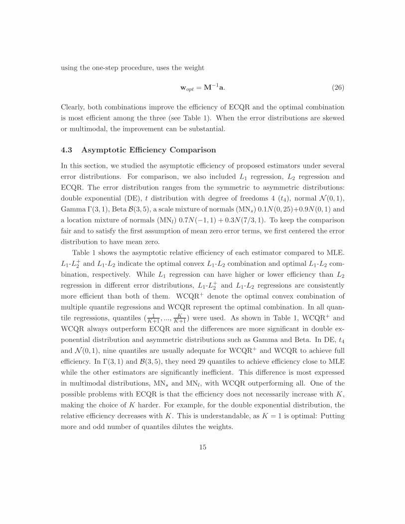
4.3 Asymptotic Efficiency Comparison

In this section, we studied the asymptotic efficiency of proposed estimators under several

error distributions. For comparison, we also included L1 regression, L2 regression and

ECQR. The error distribution ranges from the symmetric to asymmetric distributions:

double exponential (DE), t distribution with degree of freedoms 4 (t4), normal N (0, 1),

Gamma Γ(3, 1), Beta B(3, 5), a scale mixture of normals (MNs) 0.1N(0, 25)+0.9N(0, 1) and

a location mixture of normals (MNl) 0.7N(−1, 1) + 0.3N(7/3, 1). To keep the comparison

fair and to satisfy the first assumption of mean zero error terms, we first centered the error

distribution to have mean zero.

Table 1 shows the asymptotic relative efficiency of each estimator compared to MLE.

L1-L+2 and L1-L2 indicate the optimal convex L1-L2 combination and optimal L1-L2 com-

bination, respectively. While L1 regression can have higher or lower efficiency than L2

regression in different error distributions, L1-L+2 and L1-L2 regressions are consistently

more efficient than both of them. WCQR+ denote the optimal convex combination of

multiple quantile regressions and WCQR represent the optimal combination. In all quan-

tile regressions, quantiles ( 1K+1 , ...,

KK+1) were used. As shown in Table 1, WCQR+ and

WCQR always outperform ECQR and the differences are more significant in double ex-

ponential distribution and asymmetric distributions such as Gamma and Beta. In DE, t4

and N (0, 1), nine quantiles are usually adequate for WCQR+ and WCQR to achieve full

efficiency. In Γ(3, 1) and B(3, 5), they need 29 quantiles to achieve efficiency close to MLE

while the other estimators are significantly inefficient. This difference is most expressed

in multimodal distributions, MNs and MNl, with WCQR outperforming all. One of the

possible problems with ECQR is that the efficiency does not necessarily increase with K,

making the choice of K harder. For example, for the double exponential distribution, the

relative efficiency decreases with K. This is understandable, as K = 1 is optimal: Putting

more and odd number of quantiles dilutes the weights.

15

Table 1: Asymptotic relative efficiency compared to MLE

f(ε) DE t4 N (0, 1) Γ(3, 1) B(3, 5) MNs MNl

L1 1.00 0.80 0.63 0.29 0.41 0.61 0.35L2 0.50 0.35 1.00 0.13 0.68 0.05 0.14

L1-L+2 1.00♯ 0.85 1.00 0.34 0.68 0.61 0.63

L1-L2 1.00 0.85 1.00 0.44 0.80 0.61 0.63

ECQR K = 3 0.84 0.94 0.86 0.43 0.59 0.76 0.445 0.83 0.97 0.89 0.47 0.65 0.78 0.509 0.82 0.97 0.92 0.49 0.68 0.77 0.52

19 0.82 0.97 0.94 0.50 0.69 0.75 0.5429 0.83 0.97 0.95 0.51 0.71 0.76 0.54

WCQR+ K = 3 0.95† 0.94 0.87 0.51 0.61 0.76 0.605 0.96 0.97 0.91 0.59 0.70 0.78 0.699 0.97 0.98 0.95 0.69 0.78 0.79 0.77

19 0.98 0.99 0.98 0.80 0.86 0.80 0.8329 0.99 0.99 0.99 0.85 0.90 0.80 0.84

WCQR K = 3 0.95‡ 0.94 0.87 0.51 0.61 0.76 0.615 0.96 0.97 0.91 0.60 0.72 0.78 0.769 0.98 0.98 0.95 0.70 0.80 0.79 0.88

19 0.99 0.99 0.98 0.81 0.88 0.92 0.9529 0.99 0.99 0.99 0.86 0.92 0.93 0.97

16

Table 2: Optimal weights of convex composite quantile regression with K = 9 quantiles

f(ε) DE t4 N (0, 1) Γ(3,1) B(3,5) MNs MNl

Quantile1/10 0 0 0.20 0.56 0.39 0.06 0.362/10 0 0.12 0.11 0.15 0.10 0.23 0.113/10 0 0.14 0.09 0.08 0.11 0.17 0.104/10 0 0.14 0.08 0.06 0.05 0.10 0.015/10 1 0.16 0.06 0.05 0 0.14 06/10 0 0.14 0.08 0.04 0 0 07/10 0 0.14 0.09 0 0.05 0 08/10 0 0.12 0.11 0 0.09 0 09/10 0 0 0.20 0.05 0.20 0.30 0.29

In Table 2 we illustrate both the adaptivity of the proposed composite QMLE method-

ology and computational efficiency of WCQR+ over ECQR by showing the positions of

zero of the optimal nonnegative weight vector w+opt. For K = 9, only 1 quantile is needed

in the DE case, 5 and 6 quantiles are needed for MNl and MNs and 7 quantiles for t4,

Gamma and Beta. Only in the normal distribution, all 9 quantiles are used. Therefore,

WCQR+ can dramatically reduce the computational complexity of ECQR in large scale

optimization problems where p≫ n.

5 Finite Sample Study

5.1 Simulated example

In the simulation study, we consider the classical linear model for testing variable selection

methods used by Fan and Li (2001)

y = xTβ∗ + ε, x ∼ N(0,Σx), (Σx)i,j = (0.5)|i−j|.

The error vector varies from uni- to multi-modal and heavy to light tails distributions in

the same way as in Tables 1 and 2, and is centered to have mean zero. The data has

n = 100 observations. We considered two settings where p = 12 and p = 500, respec-

tively. In both settings, (β1, β2, β5) = (3, 1.5, 2) and the other coefficients are equal to

zero. We implemented penalized L1, L2, composite L1-L+2 , L1-L2, ECQR, WCQR+ and

WCQR using quantiles (10%, 20%, · · · , 90%). The local linear approximation of SCAD

17

penalty (6) was used and the tuning parameter in the penalty was selected using five fold

cross validation. We compared different methods by: (1) model error, which is defined as

ME(β) = (β−β∗)TE(XTX)(β−β∗); (2) the number of correctly classified non-zero coeffi-

cients , i.e. the true positive (TP); (3) the number of incorrectly classified zero coefficients,

i.e. the false positive (FP); (4) the multiplier σw of the standard error (SE)(12). A total

of 100 replications were performed and the median of model error (MME), the average of

TP and FP are reported in Table 3. The median model errors of oracle estimators were

calculated as the benchmark for comparison.

From the results presented in Table 3 and Table 4, we can see that penalized composite

L1-L+2 regression takes the smaller of the two model errors of L1 and L2 in all distributions

except in B(3, 5) where it outperforms both. As expected, optimal L1-L2 outperforms

L1-L+2 and brings a smaller number of FP, especially in multimodal and unsymmetric

distributions. Also, both L1-L+2 and L1-L2 perform reasonably well when compared to

ECQR, but with much less computational burden. WCQR+ and WCQR in both Tables 3

and 4 have smaller model errors and smaller number of false positives than ECQR. Similar

conclusions can be made from Figure 1, which compares the boxplots of the model errors

of the five methods (WCQR+ and L1 −L+2 are not shown) under different distributions in

the case of n = 100, p = 500. For p ≪ n in Table 3 we didn’t include LASSO estimator

since it behaves reasonably well in that setting. For p≫ n in Table 4, we included LASSO

estimator as a reference. Table 4 shows that LASSO has bigger model errors, more false

positives and higher standard errors (usually by a factor of 10) than any other five SCAD

based methods discussed.

In addition to the ME in Tables 3 and 4, we reported the multiplier σw of the asymptotic

variance (see equation (12)). Being the only part of SE that depends on the choice of

weights w and loss functions ρk, we explored it’s behavior when the dimensionality grows

from p≪ n to p≫ n. Both Tables 3 and 4 confirm the stability of the formula throughout

the two settings and all five CQMLEmethods. Only Lasso estimator being unable to specify

the correct sparsity set when p ≫ n, inflates σw for one order of magnitude compared to

other CQMLEs. Note that WCQR+ keeps the smallest value of σw and all L1-L2,L1-L+2 ,

WCQR and WCQR+ have smaller SEs than the classical L1, L2 or ECQR methods.

18

Table 3: Simulation results (n = 100, p = 12) where †, ‡ represent Median model error(MME) of the oracle and penalized estimator respectively

f(ε) DE t4 N (0, 3) Γ(3,1) B(3,5) MNs

L1 Oracle 0.029† 0.050 0.122 0.082 0.0010 0.043Penalized 0.035‡ 0.053 0.128 0.097 0.0011 0.051(TP, FP) (3,1.83) (3,0.8) (3,0.84) (3,1) (3,0.54) (3,0.93)SD×102 0.646 0.767 0.570 0.950 0.112 0.244

L2 Oracle 0.047 0.043 0.073 0.064 0.00056 0.083Penalized 0.059 0.054 0.106 0.100 0.0011 0.091(TP, FP) (3,0.82) (3,1.61) (3,1.89) (3,1.35) (3,3.76) (3,1.47)SD×102 0.779 0.762 0.485 0.869 0.129 0.179

L1-L+2 Oracle 0.036 0.043 0.070 0.070 0.00061 0.051

Penalized 0.037 0.049 0.102 0.099 0.00077 0.058(TP, FP) (3,2.49) (3,2.39) (3,1.97) (3,2.09) (3,2.42) (3,2.69)SD×101 0.717 0.702 0.518 0.876 0.095 0.169

L1-L2 Oracle 0.036 0.043 0.070 0.063 0.00060 0.051Penalized 0.037 0.049 0.102 0.078 0.00063 0.058(TP, FP) (3,2.49) (3,2.39) (3,1.97) (3,2.05) (3,2.42) (3,2.69)SD×102 0.717 0.702 0.518 0.846 0.075 0.169

ECQR Oracle 0.031 0.046 0.069 0.063 0.00065 0.033Penalized 0.042 0.046 0.107 0.074 0.00091 0.040(TP, FP) (3,1.88) (3,1.57) (3,2.04) (3,1.83) (3,1.88) (3,1.38)SD×102 0.654 0.562 0.488 0.813 0.087 0.177

WCQR+ Oracle 0.033 0.047 0.068 0.052 0.00065 0.036Penalized 0.039 0.041 0.100 0.054 0.00070 0.037(TP, FP) (3,0.55) (3,1.47) (3, 0.74) (3,0.61) (3,0.98) (3,0.62)SD×101 0.440 0.612 0.498 0.715 0.071 0.174

WCQR Oracle 0.033 0.047 0.068 0.048 0.00058 0.028Penalized 0.039 0.041 0.100 0.050 0.00062 0.030(TP, FP) (3,0.55) (3,1.47) (3, 0.74) (3,0.61) (3,0.98) (3,0.62)SD×101 0.440 0.612 0.498 0.650 0.061 0.132

19

Table 4: Simulation results (n = 100, p = 500) were †, ‡ are Median model error (MME)of oracle and penalized estimator respectively

f(ε) DE t4 N (0,3) Γ(3,1) B(3,5) MNs

Lasso Oracle 0.039† 0.039 0.035 0.0719 0.062 0.176Penalized 1.775‡ 1.759 8.687 2.662 1.808 6.497(TP,FP) (3,94.46) (3,94.26) (3,96.80) (3,95.59) (3,86.88) (3,96.55)SD×102 3.336 3.257 0.578 3.167 0.989 0.539

L1 Oracle 0.025 0.031 0.382 0.096 0.0094 0.281Penalized 0.035 0.039 1.342 0.131 0.0120 0.514(TP,FP) (3,4.53) (3,4.47) (3,5.32) (3,4.56) (3,8.10) (3,4.58)SD×102 0.268 0.274 0.144 0.461 0.215 0.101

L2 Oracle 0.035 0.043 0.207 0.078 0.0057 0.187Penalized 0.093 0.086 1.187 0.175 0.0073 0.764(TP,FP) (3,12.31) (3,10.64) (3,11.00) (3,8.02) (3,18.75) (3,16.93)SD×101 0.865 0.828 0.281 0.168 0.396 0.238

L1-L+2 Oracle 0.193 0.035 0.224 0.080 0.0061 0.195

Penalized 0.036 0.036 1.160 0.097 0.0077 0.576(TP,FP) (3,17.92) (3,12.58) (3,15.87) (3,15.43) (3,14.05) (3,17.92)SD×102 0.226 0.235 0.396 0.144 0.235 0.207

L1-L2 Oracle 0.035 0.035 0.224 0.079 0.0050 0.195Penalized 0.036 0.036 1.160 0.095 0.0069 0.576(TP,FP) (3,17.92) (3,12.58) (3,15.87) (3,15.43) (3,14.05) (3,17.92)SD×102 0.226 0.235 0.905 0.150 0.190 0.207

ECQR Oracle 0.029 0.024 0.252 0.057 0.0064 0.207Penalized 0.060 0.070 0.764 0.148 0.0118 0.599(TP,FP) (3,8.71) (3,8.43) (3,7.78) (3,9.59) (3,9.69) (3,8.91)SD×101 0.469 0.475 0.153 0.716 0.213 0.139

WCQR+ Oracle 0.028 0.027 0.223 0.050 0.0066 0.204Penalized 0.045 0.037 0.595 0.079 0.0076 0.368(TP,FP) (3,3.97) (3,3.76) (3, 3.93) (3,3.66) (3,4.85) (3,4.05)SD×101 0.244 0.266 0.112 0.273 0.120 0.084

WCQR Oracle 0.028 0.027 0.223 0.048 0.0048 0.160Penalized 0.045 0.037 0.595 0.062 0.0060 0.280(TP,FP) (3,3.97) (3,3.76) (3,3.93) (3,3.66) (3,4.85) (3,4.05)SD×101 0.224 0.219 0.112 0.180 0.110 0.060

20

L1 L2 L1−L2 ECQR WCQR

0

0.1

0.2

0.3

0.4

0.5

0.6

Val

ues

Double Exponential

L1 L2 L1−L2 ECQR WCQR

0

0.5

1

1.5

Val

ues

T4

L1 L2 L1−L2 ECQR WCQR

0

0.5

1

1.5

2

2.5

3

3.5

4

Val

ues

Normal

L1 L2 L1−L2 ECQR WCQR

0

0.5

1

1.5

Val

ues

Gamma

L1 L2 L1−L2 ECQR WCQR

0

0.01

0.02

0.03

0.04

0.05

0.06

0.07

Val

ues

Beta

L1 L2 L1−L2 ECQR WCQR

0

0.5

1

1.5

2

2.5

3

3.5

Val

ues

Mixture of Normals

Figure 1: Boxplots of Median model error (MME) of L1, L2, L1-L2, ECQR and WCQRmethods under different distributional settings with n = 100,p = 500

5.2 Real Data Example

In this section, we applied proposed methods to expression quantitative trait locus (eQTL)

mapping. Variations in gene expression levels may be related to phenotypic variations such

as susceptibility to diseases and response to drugs. Therefore, to understand the genetic

basis of gene expression, variation is an important topic in genetics. The availability of

genome-wide single nucleotide polymorphism (SNP) measurement has made it possible and

reasonable to perform the high resolution eQTL mapping on the scale of nucleotides. In

our analysis, we conducted the cis-eQTL mapping for the gene CCT8. This gene is located

within the Down Syndrome Critical Region on human chromosome 21, on the minus strand.

The over expression of CCT8 may be associated with Down syndrome phenotypes.

We used the SNP genotype data and gene expression data for the 210 unrelated indi-

viduals of the International HapMap project (International HapMap Consortium, 2003) ,

which include 45 Japanese in Tokyo, Japan, 45 Han Chinese in Beijing, China, 60 Utah

parents with ancestry from northern and western Europe (CEPH) and 60 Yoruba par-

ents in Ibadan, Nigeria and they are available in PLINK format (Purcell, et al 2007)

[http://pngu.mgh.harvard.edu/purcell/plink/]. We included in the analysis more than 2

21

million SNPs with minor allele frequency greater than 1% and missing data rate less than

5%. The gene expression data were generated by Illumina Sentrix Human-6 Expression

BeadChip and have been normalized (ith quantile normalization across replicates and me-

dian normalization across individuals) independently for each population (Stranger, et al

2007) [ftp://ftp.sanger.ac.uk/pub/genevar/].

Specifically, we considered the cis-candidate region to start 1 Mb upstream of the tran-

scription start site (TSS) of CCT8 and to end 1 Mb downstream of the transcription end

site (TES), which includes 1955 SNPs in Japanese and Chinese, 1978 SNPs in CEPH and

2146 SNPs in Yoruba. In the following analysis, we grouped Japanese and Chinese together

into the Asian population and analyzed the three populations Asian, CEPH and Yoruba

separately. The additive coding of SNPs (e.g. 0,1,2) was adopted and was treated as cate-

gorical variables instead of continuous ones to allow non-additive effects, i.e., two dummy

variables will be created for categories 1 and 2 respectively. The category 0 represents

the major, normal population. The missing SNP measurements were imputed as 0’s. The

response variable is the gene expression level of gene CCT8, measured by microarray.

In the first step, the ANOVA F-statistic was computed for each SNP independently

and a version of independent screening method of Fan and Lv (2008) was implemented.

This method is particularly computationally efficient in ultra-high dimensional problems

and here we retained the top 100 SNPs with the largest F-statistics. In the second step,

we applied to the screened data the penalized L2, L1, L1-L+2 , L1-L2, ECQR, WCQR+ and

WCQR with local linear approximation of SCAD penaly. All the four composite quantile

regressions used quantiles at (10%, ..., 90%). LASSO was used as the initial estimator and

the tuning parameter in both LASSO and SCAD penalty was chosen by five fold cross

validation. In all the three populations, the L1-L2 and L1-L+2 regressions reduced to L2

regression. This is not unexpected due to the gene expression normalization procedure. In

addition, WCQR reduced to WCQR+. The selected SNPs, their coefficients and distances

from transcription starting site (TSS) are summarized in Tables 5, 6 and 7.

In Asian population (Table 5), the five methods are reasonably consistent in not only

variables selection but also coefficients estimation (in terms of signs and order of magni-

tude). WCQR uses the weights (0.19, 0.11, 0.02, 0, 0.12, 0.09, 0.18, 0.19, 0.10). There are

four SNPs chosen by all the five methods. Two of them, rs2832159 and rs2245431, up-

regulate gene expression while rs9981984 and rs16981663 down-regulate gene expression.

The ECQR selects the largest set of SNPs while L1 regression selects the smallest set. In

CEPH population (Table 6), the five methods consistently selected the same seven SNPs

22

Table 5: eQTLs for gene CCT8 in Japanese and Chinese (n = 90). ** is the indicator forSNP equal to 2 and otherwise is the indicator for 1. SE of the estimates is reported in theparenthesis.

SNP L2 L1-L+2 L1 ECQR WCQR+ Distance from

L1-L2 WCQR TSS (kb)

rs16981663 -0.11 (0.03) -0.11 (0.03) -0.09 (0.04) -0.10 (0.03) -0.09 (0.03) -998rs16981663∗∗ 0.08 (0.06) 0.08 (0.06) 0.04 (0.06) -998rs9981984 -0.12 (0.03) -0.12 (0.03) -0.10 (0.04) -0.09 (0.03) -0.12 (0.03) -950rs7282280 0.05 (0.03) -231rs7282280∗∗ -0.07 (0.05) -231rs2245431∗∗ 0.33 (0.10) 0.33 (0.10) 0.36 (0.11) 0.37 (0.09) 0.38 (0.10) -89rs2832159 0.21 (0.04) 0.21 (0.04) 0.30 (0.04) 0.20 (0.04) 0.23 (0.04) 13rs1999321∗∗ 0.11 (0.07) 0.11 (0.07) 0.14 (0.07) 84rs2832224 0.07 (0.03) 0.07 (0.03) 0.06 (0.03) 0.04 (0.03) 86

with only ECQR choosing two additional SNPs. WCQR uses the weight (0.19, 0.21, 0, 0.04,

0.03, 0.07, 0.1, 0.21, 0.15). The coefficient estimations were also highly consistent. Deutsch

et al (2007) performed a similar cis-eQTL mapping for the gene CCT8 using the same

CEPH data as here. They considered a 100kb region surrounding the gene, which contains

41 SNPs. Using ANOVA with correction for multiple tests, they identified four eQTLs,

rs965951, rs2832159, rs8133819 and rs2832160, among which rs965951 possessing the small-

est p-value. Our analysis verified rs965951 to be an eQTL but did not find the other SNPs

to be associated with the gene expression of CCT8. In other words, conditioning on the

presence of SNP rs965951 the other three make little additional contributions. The anal-

ysis of Yoruba population yields a large number of eQTLs (Table 7). The ECQR again

selects the largest set of 44 eQTLs. The L1 regression selects 38 eQTLs. The L2 regres-

sion and WCQR both select 27 SNPs, 26 of which are the same. WCQR uses the weight

(0.1, 0, 0.17, 0.16, 0.11, 0.3, 0, 0, 0.16). The coefficients estimated by different methods are

mostly consistent (in terms of signs and order of magnitude), except that the coefficients

estimates for rs8134601, rs7281691, rs6516887 and rs2832159 by ECQR and L1 have dif-

ferent signs from those of L2 and WCQR. The eQTLs are almost all located within 500kb

upstream TSS or 500kb downstream TES (Figure 2) and mostly from 100kb upstream TSS

to 350 kb downstream TES.

23

Table 6: eQTLs for gene CCT8 in CEPH (n = 60). ** is the indicator for SNP equal to 2and otherwise is the indicator for 1. SE of the estimates is reported in the parenthesis.

SNP L2 L1-L+2 L1 ECQR WCQR+ Distance from

L1-L2 WCQR TSS (kb)

rs2831459 0.20 (0.07) 0.20 (0.07) 0.19 (0.08) 0.17 (0.07) 0.18 (0.07) -999rs7277536 0.18 (0.09) 0.18 (0.09) 0.09 (0.11) 0.14 (0.09) 0.23 (0.09) -672rs7278456∗∗ 0.36 (0.11) 0.36 (0.11) 0.21 (0.13) 0.40 (0.11) 0.35 (0.11) -663rs2248610 0.08 (0.04) 0.08 (0.04) 0.09 (0.05) 0.10 (0.05) 0.06 (0.05) -169rs965951 0.11 (0.05) 0.11 (0.05) 0.13 (0.06) 0.03 (0.06) 0.12 (0.05) -13rs3787662 0.12 (0.06) 0.12 (0.06) 0.08 (0.07) 0.13 (0.06) 0.12 (0.06) 78rs2832253 0.10 (0.07) 117rs2832332 0.08 (0.05) 382rs13046799 -0.16 (0.05) -0.16 (0.05) -0.14 (0.06) -0.14 (0.05) -0.16 (0.05) 993

Distance from the TSS

−500kb −400kb −300kb −200kb −100kb 0kb 100kb 200kb 300kb 400kb 500kb

Japanese and Chinese

CEPH

Yorub

Figure 2: Chromosome locations of identified eQTLs of the gene CCT8 with grey regionas the CCT8’s coding region. The eQTLs selected by any of the five methods are shown.

24

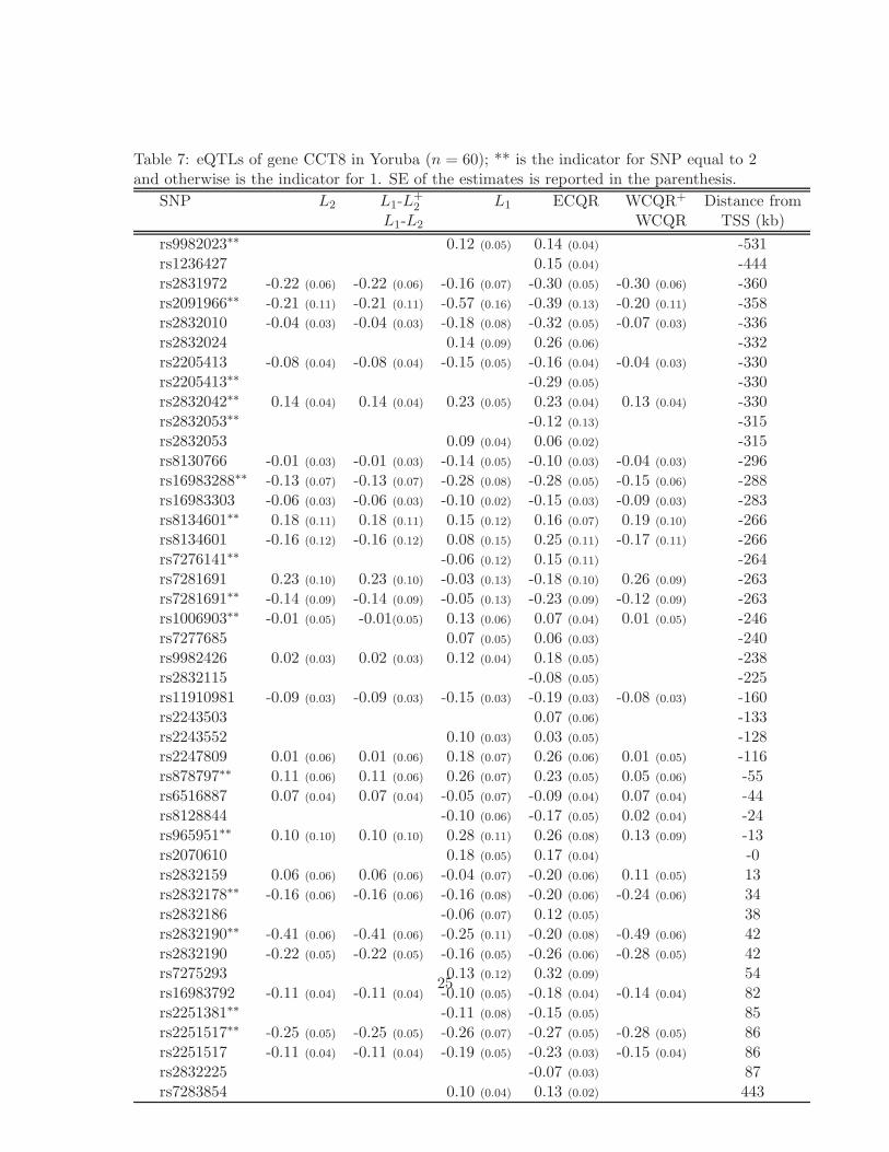
Table 7: eQTLs of gene CCT8 in Yoruba (n = 60); ** is the indicator for SNP equal to 2and otherwise is the indicator for 1. SE of the estimates is reported in the parenthesis.

SNP L2 L1-L+2 L1 ECQR WCQR+ Distance from

L1-L2 WCQR TSS (kb)

rs9982023∗∗ 0.12 (0.05) 0.14 (0.04) -531rs1236427 0.15 (0.04) -444rs2831972 -0.22 (0.06) -0.22 (0.06) -0.16 (0.07) -0.30 (0.05) -0.30 (0.06) -360rs2091966∗∗ -0.21 (0.11) -0.21 (0.11) -0.57 (0.16) -0.39 (0.13) -0.20 (0.11) -358rs2832010 -0.04 (0.03) -0.04 (0.03) -0.18 (0.08) -0.32 (0.05) -0.07 (0.03) -336rs2832024 0.14 (0.09) 0.26 (0.06) -332rs2205413 -0.08 (0.04) -0.08 (0.04) -0.15 (0.05) -0.16 (0.04) -0.04 (0.03) -330rs2205413∗∗ -0.29 (0.05) -330rs2832042∗∗ 0.14 (0.04) 0.14 (0.04) 0.23 (0.05) 0.23 (0.04) 0.13 (0.04) -330rs2832053∗∗ -0.12 (0.13) -315rs2832053 0.09 (0.04) 0.06 (0.02) -315rs8130766 -0.01 (0.03) -0.01 (0.03) -0.14 (0.05) -0.10 (0.03) -0.04 (0.03) -296rs16983288∗∗ -0.13 (0.07) -0.13 (0.07) -0.28 (0.08) -0.28 (0.05) -0.15 (0.06) -288rs16983303 -0.06 (0.03) -0.06 (0.03) -0.10 (0.02) -0.15 (0.03) -0.09 (0.03) -283rs8134601∗∗ 0.18 (0.11) 0.18 (0.11) 0.15 (0.12) 0.16 (0.07) 0.19 (0.10) -266rs8134601 -0.16 (0.12) -0.16 (0.12) 0.08 (0.15) 0.25 (0.11) -0.17 (0.11) -266rs7276141∗∗ -0.06 (0.12) 0.15 (0.11) -264rs7281691 0.23 (0.10) 0.23 (0.10) -0.03 (0.13) -0.18 (0.10) 0.26 (0.09) -263rs7281691∗∗ -0.14 (0.09) -0.14 (0.09) -0.05 (0.13) -0.23 (0.09) -0.12 (0.09) -263rs1006903∗∗ -0.01 (0.05) -0.01(0.05) 0.13 (0.06) 0.07 (0.04) 0.01 (0.05) -246rs7277685 0.07 (0.05) 0.06 (0.03) -240rs9982426 0.02 (0.03) 0.02 (0.03) 0.12 (0.04) 0.18 (0.05) -238rs2832115 -0.08 (0.05) -225rs11910981 -0.09 (0.03) -0.09 (0.03) -0.15 (0.03) -0.19 (0.03) -0.08 (0.03) -160rs2243503 0.07 (0.06) -133rs2243552 0.10 (0.03) 0.03 (0.05) -128rs2247809 0.01 (0.06) 0.01 (0.06) 0.18 (0.07) 0.26 (0.06) 0.01 (0.05) -116rs878797∗∗ 0.11 (0.06) 0.11 (0.06) 0.26 (0.07) 0.23 (0.05) 0.05 (0.06) -55rs6516887 0.07 (0.04) 0.07 (0.04) -0.05 (0.07) -0.09 (0.04) 0.07 (0.04) -44rs8128844 -0.10 (0.06) -0.17 (0.05) 0.02 (0.04) -24rs965951∗∗ 0.10 (0.10) 0.10 (0.10) 0.28 (0.11) 0.26 (0.08) 0.13 (0.09) -13rs2070610 0.18 (0.05) 0.17 (0.04) -0rs2832159 0.06 (0.06) 0.06 (0.06) -0.04 (0.07) -0.20 (0.06) 0.11 (0.05) 13rs2832178∗∗ -0.16 (0.06) -0.16 (0.06) -0.16 (0.08) -0.20 (0.06) -0.24 (0.06) 34rs2832186 -0.06 (0.07) 0.12 (0.05) 38rs2832190∗∗ -0.41 (0.06) -0.41 (0.06) -0.25 (0.11) -0.20 (0.08) -0.49 (0.06) 42rs2832190 -0.22 (0.05) -0.22 (0.05) -0.16 (0.05) -0.26 (0.06) -0.28 (0.05) 42rs7275293 0.13 (0.12) 0.32 (0.09) 54rs16983792 -0.11 (0.04) -0.11 (0.04) -0.10 (0.05) -0.18 (0.04) -0.14 (0.04) 82rs2251381∗∗ -0.11 (0.08) -0.15 (0.05) 85rs2251517∗∗ -0.25 (0.05) -0.25 (0.05) -0.26 (0.07) -0.27 (0.05) -0.28 (0.05) 86rs2251517 -0.11 (0.04) -0.11 (0.04) -0.19 (0.05) -0.23 (0.03) -0.15 (0.04) 86rs2832225 -0.07 (0.03) 87rs7283854 0.10 (0.04) 0.13 (0.02) 443

25

6 Discussion

In this paper, a robust and efficient penalized quasi-likelihood approach is introduced for

model selection with NP-dimensionality. It is shown that such an adaptive learning tech-

nique has a strong oracle property. As specific examples, two complementary methods

of penalized composite L1-L2 regression and weighted composite quantile regression are

introduced and they are shown to possess good efficiency and model selection consistency

in ultrahigh dimensional space. Numerical studies show that our method is adaptive to un-

known error distributions and outperforms LASSO (Tibshirani, 1996) and equally weighted

composite quantile regression (Zou and Yuan, 2008).

The penalized composite quasi-likelihood method can also be used in sure indepen-

dence screening (Fan and Lv, 2008; Fan and Song, 2010) or iterated version (Fan, et al,

2009), resulting in a robust variable screening and selection. In this case, the marginal

regression coefficients or contributions will be ranked and thresholded (Fan and Lv, 2008;

Fan and Song, 2010). It can also be applied to the aggregation problems of classification

(Bickel et al., 2009) where the usual L2 risk function could be replaced with composite

quasi-likelihood function. The idea can also be used to choose the loss functions in ma-

chine learning. For example, one can adaptively combine the hinge-loss function in the

support vector machine, the exponential loss in the AdaBoost, and the logistic loss func-

tion in logistic regression to yield a more efficient classifier.

Appendix A: Regularity Conditions

Let Dk be the set of discontinuity points of ψk(t), which is a subgradient of ρk. Assume that

the distribution of error terms Fε is smooth enough so that Fε(∪Kk=1Dk) = 0. Additional

regularity conditions on ψk are needed, as in Bai et al. (1992).

Condition 1 The function ψk satisfies E[ψk(ε1 + c)] = akc + o(|c|) as |c| → 0, for some

ak > 0. For sufficiently small |c|, gkl(c) = E[(ψk(ε1 + c) − ψk(ε1))(ψl(ε1 + c) − ψl(ε1))]

exists and is continuous at c = 0, where k, l = 1, ...,K. The error distribution satisfies the

following Cramer condition: E |ψw(εi)|m ≤ m!RKm−2, for some constants R and K.

This condition implies that Eψk(εi) = 0, which is an unbiased score function of pa-

rameter β. It also implies that E∂ψk(εi) = ak exists. The following two conditions are

26

important for establishing sparsity properties of parameter βw

by controlling the penalty

weighting scheme d and the regularization parameter λn.

Condition 2 Assume that Dn = maxdj : j ∈ M∗ = o(nα1−α0/2) and λnDn = O(n−(1+α0)/2).

In addition, lim inf mindj : j ∈ Mc∗ > 0.

The first statement is to ensure that the bias term in Theorem 3.2 is negligible. It

is needed to control the bias due to the convex penalty. The second requirement is to

make sure that the weights d in the second part are uniformly large so that the vanishing

coefficients are estimated as zero. It can also be regarded as a normalization condition,

since the actual weights in the penalty are λndj.The LASSO estimator will not satisfy the first requirement of Condition 2 unless

λn is small and α1 > α0/2. Nevertheless, under the sparse representation condition

(Zhao and Yu, 2006), Fan and Lv (2010) show that with probability tending to one, the

LASSO estimator is model selection consistent with ‖β1 − β∗1‖∞ = O(n−γ log n), when

the minimum signal β∗n = min|β∗j |, j ∈ M∗ ≥ n−γ log n. They also show that the same

result holds for the SCAD-type estimators under weaker conditions. Using one of them

as the initial estimator, the weight dj = γλ(β0j )/λ in (8) would satisfy Condition 2, on

a set with probability tending to one. This is due to the fact that with γλ(·) given by

(6), for j ∈ Mc∗, dj = γλ(0)/λ = 1, whereas for j ∈ M∗, dj ≤ γλ(β

∗n/2)/λ = 0, as long as

β∗n ≫ n−γ log n = O(λn). In other words, the results of Theorems 3.1 and 3.2 are applicable

to the penalized estimator (8) with data driven weights.

Condition 3 The regularization parameter λn ≫ n−1/2+(α0−2α1)+/2+α2 , where parameter

α1 is defined in Condition 5 and α2 ∈ [0, 1/2) is a constant, bounded by the restriction in

Condition 4.

We use the following notation throughout the proof. Let B be a matrix. Denote by

λmin(B) and λmax(B) the minimum and maximum eigenvalue of the matrix B when it is

a square symmetric matrix. Let ‖B‖ = λ1/2max(B

TB) be the operator norm and ‖B‖∞ the

largest absolute value of the elements in B. As a result, ‖ · ‖ is the Euclidean norm when

applied to a vector. Define ‖B‖2,∞ = max‖v‖2=1 ‖Bv‖∞.

27

Condition 4 The matrix STS satisfies C1n ≤ λmin(STS) ≤ λmax(S

TS) ≤ C2n for some

positive constants C1, C2. There exists ξ > 0 such that

n∑

i=1

(‖Si‖/n1/2)(2+ξ) → 0,

where STi is the i-th row of S. Furthermore, assume that the design matrix satisfies

||X||∞ = O(n1/2−(α0−2α1)+/2−α2) and maxj 6∈M∗‖X∗

j‖2 = O(n), where X∗j is the j-th col-

umn of X.

Condition 5 Assume that

supβ∈B(β∗

1,β∗

n)‖Qdiag∂ψ

w(β)S‖2,∞ = O(n1−α1).

maxβ∈B(β∗

1,β∗

n)λ−1min

(ST diag∂ψ

w(β)S

)= OP (n

−1),

where B(β∗1, β

∗n) is an s-dimensional ball centered at β∗

1 with radius β∗n and diag(∂ψw(β))

is the diagonal matrix with i-th element equal to ∂ψw(Yi − STi β).

Appendix B: Lemmas

Recall that X = (S,Q) and M∗ = 1, · · · , s is the true model.

Lemma 6.1 Under Conditions 2 and 4, the penalized quasi-likelihood Ln(β) defined by

(9) has a unique global minimizer β = (βT1 ,0

T )T , if

n∑

i=1

ψw

(Yi −XT

i β)Si + nλndM∗

sgn(β1) = 0, (B.1)

||z(β)||∞ < nλn, (B.2)

where z(β) = d−1Mc

∗

∑ni=1 ψw

(Yi −XT

i β)Qi, dM∗

and dMc∗stand for the subvectors of

d, consisting of its first s elements and the last p − s elements respectively, and sgn and

(the Hadamard product) in (B.1) are taken coordinatewise. Conversely, if β is a global

minimizer of Ln(β), then (B.1) holds and (B.2) holds with strict inequality replaced with

non-strict one.

28

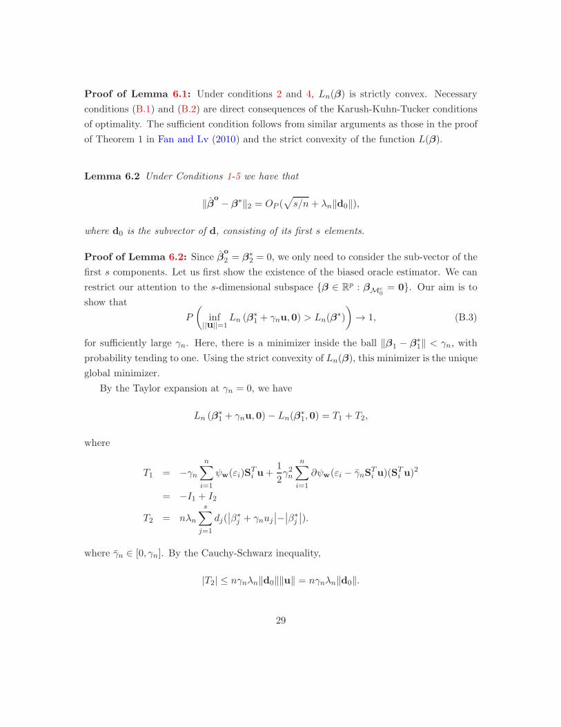
Proof of Lemma 6.1: Under conditions 2 and 4, Ln(β) is strictly convex. Necessary

conditions (B.1) and (B.2) are direct consequences of the Karush-Kuhn-Tucker conditions

of optimality. The sufficient condition follows from similar arguments as those in the proof

of Theorem 1 in Fan and Lv (2010) and the strict convexity of the function L(β).

Lemma 6.2 Under Conditions 1-5 we have that

‖βo − β∗‖2 = OP (√s/n+ λn‖d0‖),

where d0 is the subvector of d, consisting of its first s elements.

Proof of Lemma 6.2: Since βo

2 = β∗2 = 0, we only need to consider the sub-vector of the

first s components. Let us first show the existence of the biased oracle estimator. We can

restrict our attention to the s-dimensional subspace β ∈ Rp : βMc

0= 0. Our aim is to

show that

P

(inf

||u||=1Ln (β

∗1 + γnu,0) > Ln(β

∗)

)→ 1, (B.3)

for sufficiently large γn. Here, there is a minimizer inside the ball ‖β1 − β∗1‖ < γn, with

probability tending to one. Using the strict convexity of Ln(β), this minimizer is the unique

global minimizer.

By the Taylor expansion at γn = 0, we have

Ln (β∗1 + γnu,0)− Ln(β

∗1,0) = T1 + T2,

where

T1 = −γnn∑

i=1

ψw(εi)STi u+

1

2γ2n

n∑

i=1

∂ψw(εi − γnSTi u)(S

Ti u)

2

= −I1 + I2

T2 = nλn

s∑

j=1

dj(∣∣β∗j + γnuj

∣∣−∣∣β∗j∣∣).

where γn ∈ [0, γn]. By the Cauchy-Schwarz inequality,

|T2| ≤ nγnλn‖d0‖‖u‖ = nγnλn‖d0‖.

29

Note that for all ‖u‖ = 1, we have

|I1| ≤ γn‖n∑

i=1

ψw(εi)Si‖

and

E‖n∑

i=1

ψw(εi)Si‖ ≤(Eψ2

w(ε)

n∑

i=1

‖Si‖2)1/2

=(Eψ2

w(ε)tr(STS)

)1/2,

which is of order O(√ns) by Condition 4. Hence, I1 = Op(γn

√ns) uniformly in u.

Finally, we deal with I2. Let Hi(c) = inf |v|≤c∂ψw(εi − v). By Lemma 3.1 of Portnoy

(1984), we have

I2 ≥ γ2n

n∑

i=1

Hi(γn|STi u|)(ST

i u)2

≥ cγ2nn,

for a positive constant c. Combining all of the above results, we have with probability

tending to one that

Ln (β∗1 + γnu,0)− Ln(β

∗1,0) ≥ nγncγn −OP (

√s/n)− λn‖d0‖,

where the right hand side is larger than 0 when γn = B(√s/n+ λn‖d0‖) for a sufficiently

large B > 0. Since the objective function is strictly convex, there exists a unique minimizer

βo

1 such that

‖βo

1 − β∗1‖ = OP (

√s/n+ λn‖d0‖).

Lemma 6.3 Under the conditions of Theorem 3.2,

[bTAnb]−1/2

n∑

i=1

ψw(εi)bTSi

D→ N (0, 1) (B.4)

where An = Eψ2w(ε)STS .

30

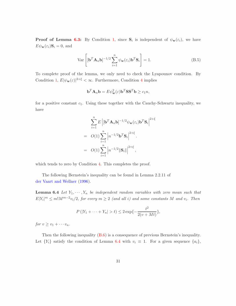
Proof of Lemma 6.3: By Condition 1, since Si is independent of ψw(εi), we have

Eψw(εi)Si = 0, and

Var

[[bTAnb]

−1/2n∑

i=1

ψw(εi)bTSi

]= 1. (B.5)

To complete proof of the lemma, we only need to check the Lyapounov condition. By

Condition 1, E|ψw(ε)|2+ξ <∞. Furthermore, Condition 4 implies

bTAnb = Eψ2w(ε)bTSSTb ≥ c1n,

for a positive constant c1. Using these together with the Cauchy-Schwartz inequality, we

have

n∑

i=1

E∣∣∣[bTAnb]

−1/2ψw(εi)bTSi

∣∣∣2+ξ

= O(1)

n∑

i=1

∣∣∣n−1/2bTSi

∣∣∣2+ξ

.

= O(1)

n∑

i=1

∣∣∣n−1/2‖Si‖∣∣∣2+ξ

,

which tends to zero by Condition 4. This completes the proof.

The following Bernstein’s inequality can be found in Lemma 2.2.11 of

der Vaart and Wellner (1996).

Lemma 6.4 Let Y1, · · · , Yn be independent random variables with zero mean such that

E|Yi|m ≤ m!Mm−2vi/2, for every m ≥ 2 (and all i) and some constants M and vi. Then

P (|Y1 + · · ·+ Yn| > t) ≤ 2 exp− t2

2(v +Mt),

for v ≥ v1 + · · · vn.

Then the following inequality (B.6) is a consequence of previous Bernstein’s inequality.

Let Yi satisfy the condition of Lemma 6.4 with vi ≡ 1. For a given sequence ai,

31

E|aiYi|m ≤ m!|aiM |m−2a2i /2. A direct application of Lemma 6.4 yields

P (|a1Y1 + · · ·+ anYn| > t) ≤ 2 exp− t2

2(∑n

i=1 a2i +M maxi |ai|t)

. (B.6)

Appendix C: Proofs of Theorems

Proof of Theorem 3.1: We only need to show that βois the unique minimizer of L(β)

in Rp on a set Ωn which has a probability tending to one. Since β

o1 already satisfies (B.1),

we only need to check (B.2).

We now define the set Ωn. Let

ξ = (ξ1, · · · , ξp)T =n∑

i=1

ψw

(Yi −XT

i β∗)Xi

and consider the event Ωn =∣∣∣∣∣∣ξMc

∗

∣∣∣∣∣∣∞

≤ un√n

with un being chosen later. Then, by

Condition 1 and Bernstein’s inequality, it follows directly from (B.6) that

P |ξj| > t ≤ 2 exp

− t2

2(‖X∗

j‖2R+ tK‖X∗j ||∞

),

where X∗j is the j-th column of X. Taking t = un

√n, we have

P|ξj| > un

√n≤ 2 exp

− u2n2(R‖X∗

j‖2/n+Kun‖X∗j ||∞/

√n)

≤ e−cu2n , (C.1)

for some positive constant c > 0, by Condition 4. Thus, by using the union bound, we

conclude that

P (Ωn) ≥ 1−∑

j∈Mc∗

P|ξj| > un

√n≥ 1− 2(p − s)e−cu2

n .

We now check whether (B.1) holds on the set Ωn. Let ψw(β) be the n-dimensional

vector with the i-th element ψw(Yi −XTi β). Then, by Condition 2

‖z(βo)‖∞ ≤

∥∥∥d−1Mc

∗

ξMc∗

∥∥∥∞

+∥∥∥d−1

Mc∗

QT [ψw(β

o)−ψ

w(β∗)]

∥∥∥∞

= O(n1/2un +

∥∥∥QTdiag(∂ψw(v))S(β

o1 − β∗

1)∥∥∥∞

)(C.2)

32

where v lies between βoand β∗

1. By Condition 5, the second term in (C.2) is bounded by

O(n1−α1)‖βo

1 − β∗1‖ = OP n1−α1(

√s/n+ λn‖d0‖),

where the equality follows from Lemma 6.2. By the choice of parameters,

(nλn)−1‖z(βo

)‖∞ = On−1/2λ−1n (un + n(α0−2α1)/2) +Dnn

α0/2−α1 = o(1),

by taking un = n(α0−2α1)+/2+α2 . Hence, by Lemma 6.1, βois the unique global minimizer.

Proof of Theorem 3.2: By Theorem 3.1, βw1 = β

o1 almost surely. It follows from

Lemma 6.2 that

‖βw1 − β∗

1‖ = OP √s(λnDn + 1/

√n).

This establishes the first part of the Theorem.

Let Qn(β1) =∑n

i=1 ψw(Yi − STi β1)Si. By Taylor’s expansion at the point β∗

1, we have

Qn(βw1) = Qn(β∗1) + ∂Qn(v)(βw1 − β∗

1),

where v lies between the points βw1 and β∗

1 and

∂Qn(v) = −n∑

i=1

∂ψw(Yi − STi v)SiS

Ti . (C.3)

By Lemma 6.2, ‖v− β∗1‖ ≤ ‖β

w1 − β∗1‖ = oP (1).

By using (B.2), we have

Qn(βw1) + nλnd0 sgn(βw1) = 0,

or equivalently,

βw1 − β

∗1 = −∂Qn(v)

−1Qn(β∗1)− ∂Qn(v)

−1nλnd0 sgn(βw1). (C.4)

Note that ‖d0 sgn(βw1)‖ = ‖d0‖. We have for any vector u,

∣∣∣uT∂Qn(v)−1d0 sgn(βw1)

∣∣∣ ≤ ‖∂Qn(v)−1‖ · ‖u‖ · ‖d0‖.

33

Consequently, for any unit vector b,

∥∥∥bT (STS)1/2∂Qn(v)−1d0 sgn(βw1)

∥∥∥ ≤ λ1/2max(STS)λ−1

min(∂Qn(v))√sDn

= OP (√s/nDn),

by using Conditions 4 and 5. This shows that the second term in (C.4), when multiplied

by the vector bT (STS)1/2 is of order

OP (√snλnDn) = oP (1),

by Condition 2. Therefore, we need to establish the asymptotic normality of the first term

in (C.4). This term is identical to the situation dealt by Portnoy (1985). Using his result,

the second conclusion of Theorem 3.2 follows. This completes the proof.

Proof of Theorem 3.3: First of all, by Taylor expansion,

Φn,w(β1) = Φn,w(β∗1) + Ωn,w(β1)(β1 − β∗

1), (C.5)

where β1 lies between β∗1 and β1. Consequently,

‖β1 − β1‖ ≤ ‖β∗1 − β1‖ = oP (1).

By the definition of the one step estimator (14) and (C.5), we have

βosw1 − β∗

1 = Ωn,w(β1)−1Φn,w(β

∗1) +Rn, (C.6)

where

Rn = Ωn,w(β1)−1Ωn,w(β1)− Ωn,w(β1)

(β1 − β∗

1).

We first deal with the remainder term. Note that

‖Rn‖ ≤∥∥∥Ωn,w(β1)−1

∥∥∥ ·∥∥∥Ωn,w(β1)− Ωn,w(β1)

∥∥∥ · ‖β1 − β∗1‖ (C.7)

and

Ωn,w(β1)− Ωn,w(β1) =n∑

i=1

fi(β1, β1)SiSTi , (C.8)

34

where fi(β1, β1) = ∂ψ(Yi − STi β1)− ∂ψ(Yi − ST

i β1). By the Liptchiz continuity, we have

|fi(β1, β1)| ≤ C‖Si‖ · ‖β1 − β1‖,

where C is the Liptchiz coefficient of ∂ψw(·). Let Is be the identity matrix of order s and

bn = λmax∑n

i=1 ‖Si‖SiSTi . By (C.8), we have

Ωn,w(β1)− Ωn,w(β1) ≤ C‖β1 − β1‖n∑

i=1

‖Si‖SiSTi ≤ C‖β1 − β1‖bnIs.

Hence, all of the eigenvalues of the matrix is no larger than C‖β1 − β1‖bn. Similarly, by

(C.8),

Ωn,w(β1)− Ωn,w(β1) ≥ −C‖β1 − β1‖n∑

i=1

‖Si‖SiSTi ≥ −C‖β1 − β1‖bnIs,

and all of its eigenvalue should be at least −C‖β1 − β1‖bn. Consequently,∥∥∥Ωn,w(β1)− Ωn,w(β1)

∥∥∥ ≤ C‖β1 − β1‖bn.

By Condition 5 and the assumption of β1, it follows from (C.7) that

‖Rn‖ = OP (s/n · bn/n) = OP (s3/2/n).

Thus, for any unit vector b,

bT (STS)1/2Rn ≤ λ1/2max(STS)‖Rn‖ = OP (s

3/2/n1/2) = oP (1).

The main term in (C.6) can be handled by using Lemma 6.3 and the same method as

Portnoy (1985). This completes the proof.

References

Bai, Z. D., Rao, C.R. and Wu, Y. (1992), M -estimation of multivariate linear regressionparameters under a convex discrepancy function, Stat. Sinica 2, 237–254.

35

Bickel, P. J. (1973), On some analogues to linear combinations of order statistics in thelinear model, Ann. Statist. 1, 597–616.

Bickel, P. J., Ritov, Y. and Tsybakov, A. B. (2008), Hierarchical selection of variables insparse high-dimensional regression, arXiv:0801.1158v1.

Bickel, P. J., Ritov, Y. and Tsybakov, A. B.(2009), Simultaneous analysis of lasso anddantzig selector, Ann. Statist. 37(4), 1705–1732.

Efron, B.,Hastie, T., Johnstone, I. and Tibshirani, R. (2004), Least angle regression, Ann.Statist. 32(2), 407–499.

Fan, J. and Li, R. (2001), Variable selection via nonconcave penalized likelihood and itsoracle properties, Journal of the American Statistical Association 96(456), 1348–1360.

Fan, J. and Lv, J. (2008), Sure independence screening for ultrahigh dimensional featurespace, Journal of the Royal Statistical Society, Series B: Methodological 70, 849–911.

Fan, J. and Lv, J. (2010), Properties of non-concave penalized likelihood with NP-dimensionality, submitted.

Fan, J., Samworth, R., and Wu, Y. (2009). Ultrahigh dimensional variable selection: be-yond the linear model. Journal of Machine Learning Research, 10, 1829-1853.

Fan, J. and Song, R. (2010). Sure Independence Screening in Generalized Linear Modelswith NP-Dimensionality. The Annals of Statistics, to appear.

Fan, J. and Peng, H. (2004), Nonconcave penalized likelihood with a diverging number ofparameters, Ann. Statist. 32(3), 928–961.

Frank, I. E. and Friedman, J. H. (1993), A Statistical view of some chemometrics regressiontools , Technometrics 35, 109–148.

Friedman, J. H., Hastie, T., Hofling, H. and Tibshirani, R.(2008), Pathwise coordinateoptimization, Ann. Appl. Statist. 1(2), 302–332.

Huang, J., Horowitz, J. L. and Ma, S. (2008), Asymptotic properties of bridge estimatorsin sparse high-dimensional regression models, Ann. Statist. 36(2), 587–613.

Huber, P. J. (1973), Robust estimation of location parameter, The Ann. of Math. Statist.35, 73–101.

Kim, Y., Choi, H. and Oh, H. (2008), Smoothly clipped absolute deviation on high dimen-sions, Journal of the American Statistical Association 103, 1656–1673.

Koenker, R. (1984), A note on L-estimates for linear models, Stats & Prob. Letters 2,323–325.

36

Lehmann, E. L. (1983), Theory of Point Estimation, John Wiley & Sons, 506.

Li, Y. and Zhu, J. (2008), L1-norm quantile regression, Journal of Computational andGraphical Statistics 17(1), 163–185.

Portnoy, S. (1984), Asymptotic behavior of M -estimators of p regression parameters whenp2/n is large. I. Consistency, Ann. Statist. 12, 1298–1309.

Portnoy, S. (1985), Asymptotic behavior of M -estimators of p regression parameters whenp2/n is large; II. Normal approximation. Ann. Statist. 13, 1403–1417.

Tibshirani, R. (1996), Regression shrinkage and selection via the lasso, Journal of the RoyalStatistical Society, Series B: Methodological 58, 267–288.

van der Vaart, A. W. and Wellner, Jon A. (1996), Weak Convergence and Empirical Pro-cesses, Springer-Verlag Inc. 0-387-94640-3,p 508.

Wu, Y. and Liu, Y. (2009), Variable selection in quantile regression, Stat. Sinica 37(2),801–817.

Xie, H. and Huang, J. (2009), SCAD-penalized regression in high-dimensional partiallylinear models, Ann. Statist. 37(2), 673-696.

Yuan, M. and Lin, Y. (2007), On the non-negative garrotte estimator, Journal of the RoyalStatistical Society, Series B: Statistical Methodology 69(2), 143–161.

Zhao, P. and Yu, B. (2006). On model selection consistency of Lasso. J. Machine LearningRes., 7, 2541–2567

Zou, H. (2006), The adaptive LASSO and its oracle properties, Journal of the AmericanStatistical Association 101(476), 1418–1429.

Zou, H. and Li, R. (2008), One-step sparse estimates in nonconcave penalized likelihoodmodels, Ann. Statist. 36(4), 1509-1533.

Zou, H. and Yuan, M. (2008), Composite Quantile Regression and the Oracle Model Se-lection Theory, Ann. Statist. 36(3), 1108–1126.

Zou, H. and Zhang, H. H. (2009), On the adaptive elastic-net with a diverging number ofparameters, Ann. Statist. 37(4), 1733–1751.

37