Survey Participation, Nonresponse Bias, Measurement Error Bias, and Total Bias

doi:10.1093 / poq / nfl038© The Author 2006. Published by Oxford University Press on behalf of the American Association for Public Opinion Research. All rights reserved. For permissions, please e-mail: [email protected].

Public Opinion Quarterly, Vol. 70, No. 5, Special Issue 2006, pp. 737–758

SURVEY PARTICIPATION, NONRESPONSE BIAS, MEASUREMENT ERROR BIAS, AND TOTAL BIAS

KRISTEN OLSON

Abstract A common hypothesis about practices to reduce surveynonresponse is that those persons brought into the respondent poolthrough persuasive efforts may provide data filled with measurementerror. Two questions flow from this hypothesis. First, does the meansquare error of a statistic increase when sample persons who are lesslikely to be contacted or cooperate are incorporated into the respondentpool? Second, do nonresponse bias estimates made on the respondents,using survey reports instead of records, provide accurate informationabout nonresponse bias? Using a unique data set, the Wisconsin DivorceStudy, with divorce records as the frame and questions about the frameinformation included in the questionnaire, this article takes a first lookinto these two issues. We find that the relationship between nonresponsebias, measurement error bias, and response propensity is statistic-specific and specific to the type of nonresponse. Total bias tends to belower on estimates calculated using all respondents, compared withthose with only the highest contact and cooperation propensities, andnonresponse bias analyses based on respondents yield conclusions simi-lar to those based on records. Finally, we find that error properties ofstatistics may differ from error properties of the individual variablesused to calculate the statistics.

KRISTEN OLSON is a graduate student in the program of survey methodology at the University ofMichigan. This article is part of the author’s doctoral dissertation research. The material is basedon work supported by the National Science Foundation under Grant no. SES-0620228. The authoris especially grateful to her committee—Bob Groves, T. E. Raghunathan, Rod Little, Yu Xie, andNorman Bradburn—for discussion and insight into the problem. Frauke Kreuter and Sonja Zinielprovided comments on an earlier draft that improved the article immensely. The author isindebted to Vaughn Call and Colter Mitchell for providing access to the Wisconsin DivorceStudy. The Wisconsin Divorce Study was funded by a grant (HD-31035 and HD32180–03) fromthe National Institute of Child Health and Human Development, the National Institutes of Health.The study was designed and carried out at the Center for Demography and Ecology at the Universityof Wisconsin–Madison and Brigham Young University under the direction of Vaughn Call andLarry Bumpass. Address correspondence to the author; e-mail: [email protected].

by guest on May 25, 2014

http://poq.oxfordjournals.org/D

ownloaded from

http://poq.oxfordjournals.org/

738 Olson

Introduction

Survey response rates in developed countries have fallen over the past threedecades (de Leeuw and de Heer 2002). Simultaneously, budgets for surveyshave risen dramatically as survey organizations have increased their efforts tocounteract this trend (Curtin, Presser, and Singer 2005). Increases in cost andeffort have been absorbed because the inferential paradigm of probabilitysampling demands 100 percent cooperation to guarantee the unbiasedness of asurvey estimate. Current best practices argue that researchers should attemptto maximize response rates and to minimize risk of nonresponse errors (Japecet al. 2000). However, recent research (Curtin, Presser, and Singer 2000;Keeter et al. 2000; Merkle and Edelman 2002) has called the traditional viewinto question by showing no strong relationship between nonresponse ratesand nonresponse bias (Groves 2006).

One hypothesis about practices involving nonresponse reduction is thatreluctant sample persons, successfully brought into the respondent poolthrough persuasive efforts, may provide data filled with measurement error(Biemer 2001; Cannell and Fowler 1963; Groves and Couper 1998). Twoquestions arise when this hypothesized relationship between low propensity torespond and measurement error holds. The first has to do with the quality of astatistic (e.g., means, correlation coefficients) calculated from a survey. Thatis, does the mean square error of a statistic increase when sample persons whoare less likely to be contacted or cooperate are incorporated into the respon-dent pool? An increase in mean square error could occur because (a) incorpo-rating the difficult to contact or reluctant respondents results in nononresponse bias in the final estimate, but measurement error does exist, or(b) nonresponse bias exists, but the measurement error in these reluctant ordifficult to contact respondents’ reports exceeds the nonresponse bias.

The second question has to do with methodological inquiries for detectingnonresponse bias. Although many types of analyses of nonresponse bias canbe conducted, four predominant approaches have been used: (1) comparingcharacteristics of the achieved sample, usually the demographic characteris-tics, with a benchmark survey (e.g., Duncan and Hill 1989), (2) comparingframe information for respondents and nonrespondents (e.g., Lin and Schaeffer1995), (3) simulating statistics based on a restricted version of the observedprotocol (e.g., Curtin, Presser, and Singer 2000), often called a “level ofeffort” analysis, and (4) mounting experiments that attempt to produce varia-tion in response rates across groups known to vary on a survey outcome ofinterest (Groves, Presser, and Dipko 2004). Findings from these studies showthat nonresponse bias varies across individual statistics within a survey and isrelatively larger on items central to the survey topic as described duringrespondent recruitment.

The focus of this article is on benchmark comparisons and level of effortcomparisons. Benchmark investigations compare a statistic from the survey



ownloaded from


Nonresponse Bias and Measurement Error Bias 739

with an externally available statistic for the same population, usually from ahigher response rate survey or from administrative records. Level of effortanalyses investigate the change in a statistic over increased levels of effort,taking change in the statistic to indicate the risk of nonresponse bias, and nochange to indicate the absence of risk. But if measurement error is correlatedwith level of effort (or response propensity), then an observed change or lackof change in the statistic may be due to measurement error and not to nonre-sponse bias (Groves 2006). Thus, traditional investigations of nonresponsebias based on respondent means may be misleading.

Specifically, in the presence of both measurement error and nonresponse,the bias of a sample mean can be decomposed into a nonresponse bias termand a measurement error bias term. For person i, a survey variable Yi with truevalues Ti, the joint effect of nonresponse and measurement error on the

respondent mean is , where a simple additive error

model pertains, , and is the covariance of the true values and theresponse propensity, p (Biemer 2001; Lessler and Kalsbeek 1992). The termsin the equation indicate nonresponse bias and measurement error bias, respec-tively. There is no nonresponse bias if all sampled units are equally likely torespond, and the only remaining problem is the measurement error bias(Lessler and Kalsbeek 1992). Comparisons of overall nonresponse bias andmeasurement error bias on survey statistics often show that measurement errorbias is at least as large as nonresponse bias, if not larger, and that these non-sampling errors often far outweigh any sampling errors (Assael and Keon1982; Biemer 2001; Lepkowski and Groves 1986; Schaeffer, Seltzer, andKlawitter 1991).

Similar to analyses described above for nonresponse bias, one approach tostudying the joint effects of nonresponse and measurement error is a “level ofeffort” analysis. Although this method is commonly used to understand non-response bias (e.g., Curtin, Presser, and Singer 2000), few studies have jointlyexamined the change in nonresponse bias and measurement error bias overincreasing levels of effort. In this type of nonresponse/measurement error study,survey responses are compared with records for those responses over increasinglevels of effort. Such comparisons are rare. Cannell and Fowler (1963) found thatthe number of hospital stays and length of the stay were misreported more oftenby those who responded to later follow-ups than to earlier follow-ups. Greaterdiscrepancies for later respondents were found on other topics (Huynh, Rupp,and Sears 2002; Stang and Jöckel 2005; Voigt et al. 2005) and as predictive ofsample attrition in panel studies (Bollinger and David 1995, 2001). Each of thesestudies indicates that measurement error increases for respondents who are moredifficult to recruit. Whether this difficulty was due to noncontact or noncoopera-tion, or the relative magnitude of measurement versus nonresponse error overincreased levels of effort, is often overlooked in these analyses.

Bias y p pi i

i 1

N

( ) ( )=

r pTp= +s e∑

ei

Y T= −i i

spT



ownloaded from


740 Olson

This article provides a first look into these two issues—whether the meansquare error of three different statistics changes (and whether the compositionof the mean square error changes) as lower propensity respondents are incor-porated into a survey estimate. The article also investigates the efficacy ofnonresponse bias studies using record data versus respondent reports. Aunique data set, the Wisconsin Divorce Study, which used divorce records asthe frame, asked questions about information contained on the frame in thequestionnaire, and has process data on call outcomes, is used to investigatethese issues.

Data

From August 1995 through October 1995 the University of Wisconsin–Madisonconducted the Wisconsin Divorce Study. This study was designed as an experi-mental comparison of mode effects on the quality of divorce date reports.Divorce certificates were extracted from four counties in Wisconsin from 1989and 1993, and a random sample from each year was selected. One member ofthe divorced couple was selected at random to be the respondent. Selectedpersons were randomly allocated to one of three initial modes: CATI, CAPI, andmail. Nonrespondents were followed up in a different mode—CATI and CAPInonrespondents had a mail follow-up, and mail nonrespondents were followedup by telephone. This article focuses on the CATI with mail follow-up subgroup.

Because of the time lapse between divorce and survey, sampled units weretracked extensively, and addresses were located for 85.2 percent of them. Per-sonalized letters asked the sampled person to participate in the “Life Eventsand Satisfaction Survey,” sponsored and carried out by the University ofWisconsin–Madison. The survey contained questions on satisfaction with lifeand relationships, marital and cohabitation history, childbearing history, educationand work history, satisfaction with current relationships, and demographics.Overall, the response rate (AAPOR RR1) for the CATI with mail follow-upmode was 71 percent, with a contact rate of 80.3 percent and a cooperationrate of 88.3 percent (table 1). Important process data, such as records of thecall attempts made by interviewers, were kept for each sampled unit, facilitatingour understanding of the participation process and making it possible to disen-tangle noncontact from refusal nonresponse bias.

Because this survey was not done for the purpose of estimating both nonre-sponse bias and measurement error bias, the data set has limitations for thepresent analysis. The most important limitation is that not all variables ofinterest in the survey are contained in the records. Additionally, records maycontain measurement errors, and the construct measured in the survey maydeviate slightly from the construct measured in the record. In particular,the frame consists of divorce certificate data on which only the divorce dateand child custody arrangements were recorded by an official body; all other



ownloaded from



information was provided by one of the two spouses in the divorcing couple.For this reason, the analyses here largely focus on the statistics calculatedusing the divorce date, a date used for administrative purposes and probablythe least sensitive to measurement error in the record.

FOCAL STATISTICS FOR NONRESPONSE BIAS AND MEASUREMENT ERROR BIAS

Three statistics—all means—are considered in these analyses. First, the length ofthe marriage is constructed from the difference between the divorce date and themarriage date. The length of marriage is calculated in number of months, themetric in which respondents were asked to report the dates in the questionnaire.1

The second statistic is constructed from the difference between the divorcedate and the date of the beginning of data collection. This statistic is also mea-sured in months. Thus, two of the three focal statistics use the same variablefor these analyses.

Finally, we look at the total number of marriages. Respondents were askedfor a count of the number of times they had been married.2 Marriages thatoccurred between the divorce in the record and the interview were excludedfrom this statistic.

Methods

The analyses proceed in four steps. First, we look at overall nonresponse biasby type of nonresponse (noncontact versus noncooperation) and measurementerror bias for the three statistics, all sample means, as described above. All esti-mates of nonresponse bias and measurement error bias are based on differences in

1. The questionnaire asked for each marriage, “In what month and year did your marriagebegin?” and, for each divorce, “In what month and year did you get divorced?”2. The question wording was “How many times have you been married?” and for the month andyear of each marriage. Reported marriages that occurred after the divorce date in the record weresubtracted from the number of times married.

Table 1. Final Disposition of Sample Cases

NOTE.—Nine deceased individuals and one respondent whosegender did not match the frame were removed from the sample.

n %

Interviews 523 71.0Refusal 51 6.9Contact, no resistance 18 2.4Noncontact 145 19.7

Total 737 100.0



ownloaded from


742 Olson

statistics. The measure of nonresponse bias is the difference between the meancalculated using the records on the entire frame and that calculated using onlythe respondent pool. Measurement error bias is estimated as the differencebetween the mean calculated on the complete cases (i.e., those with no item-missing data) from the survey reports and the mean calculated from the recorddata on all respondents. There is item nonresponse in the survey reports; wetake a “naive” analyst approach and ignore the missing data.3

Next, we estimate logistic regressions, using available auxiliary data andprocess data, predicting the probability of being contacted for the surveyand the probability of cooperating with the survey request, conditional oncontact.

The third step of the analyses examines how nonresponse bias and measure-ment error bias are associated with response propensity. To do this, we createfive roughly equal sized categories or strata from the estimated response pro-pensity scores. Changes in nonresponse bias and measurement error bias foreach statistic are examined as lower propensity respondents are incorporatedinto the estimate of the sample mean (i.e., the cumulative sample mean acrosspropensity strata). Finally, we examine how the total bias and the relativecomposition of errors change across propensity strata. That is, does the totalbias change, and does measurement error bias outweigh nonresponse bias aslower propensity respondents are incorporated into survey estimates?

Findings

NONRESPONSE BIAS: OVERALL

Nonresponse bias of a statistic results when the estimate calculated on therespondent pool differs from the value calculated on the entire population.Table 2 presents the means for the variables available on the frame for fivegroups: the entire sample,4 contacts, noncontacts, and interviews and nonco-operators (who are mostly refusals) among the contacted. The average lengthof marriage for the entire frame is 130.29 months, compared with 134.17months for the respondents, overestimating the population mean by 3 percent.5

3. This naive approach, the complete case analysis, has implications for understanding the mech-anism behind measurement error and for the estimate of the measurement error itself. Mech-anisms behind the misreporting of divorce status, item nonresponse (either don’t know or refusal),and inaccurate date reports are confounded in this analysis. Additionally, if the item nonrespon-dents or the false negatives on divorce status are meaningfully different on the variables of inter-est, we confound these compositional differences with misreports. However, the naive analystwould not have records at his or her disposal and would not be able to diagnose these problems.Thus, we feel that this complete case analysis is true to the nature of many analyses.4. One case was excluded because the respondent’s gender did not match the gender on the frame.

5. biasy y

yNRrespondent record frame

frame

=−,



ownloaded from



The average length of marriage for noncontacts (mean = 114.46) was signifi-cantly (p = .02) shorter than the average length of marriage for the interviewedcases, but there was no difference between the interviews and the noncoopera-tors (mean = 134.17, p = .99).

Differences between respondents and the frame for the time elapsedbetween the divorce and the interview are small—49.75 months for the frameversus 50.44 for the respondents, a 1.4 percent overestimate. Both noncontactsand noncooperators were divorced more recently than the interviewed cases(48.74, 46.68, and 50.44 months, respectively), although the differences arenot statistically significant. Interviewed cases had slightly fewer marriagesthan either the noncontacted or noncooperating sample units; the differencebetween interviews and noncontacts was statistically significant (p = .06).Thus, there does appear to be nonresponse bias on the sample means calcu-lated for these estimates, but the overall nonresponse bias is small.

MEASUREMENT ERROR BIAS: OVERALL

Although the frame was constructed such that all selected respondents hadbeen married and divorced, only 98 percent of the respondents reportedhaving been married and 92 percent of the respondents reported beingdivorced. This, in addition to item nonresponse on the survey, increases therisk of differences between the complete case analysis of the survey reportsand the records estimated on the entire respondent pool.

We consider the difference between complete case analyses on the respon-dents’ survey reports and records on the entire respondent pool to be the mea-surement error bias of the statistic. This difference varies by statistic. For

Table 2. Means by Stage of Sample Recruitment

NOTE.—Variation in N for the survey reports due to item nonresponse.

Length of Marriage (in

Months)

Number of Months Since

Divorce

Number of Previous

Marriages

N Mean SE Mean SE Mean SE

Record ValueTarget (full sample) 737 130.29 3.57 49.75 0.90 1.22 0.02Not Contacted 145 114.46 7.09 48.74 2.07 1.27 0.04Contacted 592 134.17 4.08 50.00 1.00 1.20 0.02Contacted, Not Interviewed 69 134.17 13.16 46.68 2.96 1.28 0.07Interviewed 523 134.17 4.29 50.44 1.06 1.20 0.02

Survey Report (complete cases) 429–520 133.92 4.79 55.74 1.62 1.21 0.02



ownloaded from


744 Olson

instance, the difference between the survey report for the length of marriage is133.9 months versus 134.2 months for the records for all respondents, a rela-tive difference of only 0.2 percent (see table 2).6 The report of the number ofmonths elapsed between the divorce and the interview is 10.4 percent higherthan that calculated from the records (55.7 from survey reports versus 50.4from the records). The number of marriages estimated from respondentreports is 1.21 marriages, compared with 1.20 estimated from the records forthe respondents, a 0.9 percent difference. For two statistics, the measurementerror bias is smaller than the nonresponse bias; in the third, the measurementerror bias is large relative to the nonresponse bias.

RESPONSE PROPENSITY MODELS

Response propensity is the theoretical probability that a sampled unit willbe contacted and will cooperate with a survey request. Many factors in asurvey protocol, as well as respondent traits, can influence response pro-pensity. Disentangling these effects requires multivariate modeling.Logistic regression models predicting contactability or cooperation can beused to create summary “response propensity scores” (i.e., the predictedprobability from the logistic regression model) that estimate how likelythe sampled unit is to participate in the survey, regardless of the actualoutcome. Propensity scores have a useful balancing property—conditionalon the propensity score, respondents and nonrespondents have equivalentdistributions on the observed characteristics entered into the model (Joffeand Rosenbaum 1999; Little 1986; Rosenbaum and Rubin 1984, 1985).Response propensity models are typically estimated when creatingweights for postsurvey adjustment. Their use in understanding the risk ofnonresponse bias is less well studied.

For these data, we estimate two models—a contact model and a cooperationmodel, conditional on contact. The dependent variable in the contact modelindicates that the sampled case was contacted in the CATI phase or explicitlyrefused or completed a mail survey. The dependent variable in the cooperationmodel indicates that the sampled case completed an interview in either phase.These models include three measures of level of effort. First, the number ofcall attempts before first contact in the CATI phase is available for all sampledcases, measured as the number of calls to first contact for the cases contactedin the CATI phase (mean = 4.29 calls, SE = 0.37) and the total number of callsfor the cases not contacted in the CATI phase (mean = 3.54 calls, SE = 0.83).7

6. .

7. Virtually all nonrespondents to the CATI phase were sent a mail questionnaire. Disentanglingnoncontact from refusal in a mail survey is difficult. We consider any case that explicitly returneda mail questionnaire or explicitly refused the mail questionnaire as being a final contact, even ifthey were not contacted in the CATI phase.

relative biasy y

MErespondent survey report divorce respond =

−, & _ eent record

respondent recordy,

,



ownloaded from



The range of call attempts is quite wide—some cases were never attempted bytelephone, only by mail8; other cases received up to 102 call attempts. Second,whether a sample case ever refused during the phone attempts (14 percent ofcontacted cases, SE = 1.44 percent), is available for all sampled cases. Protocoldecisions may be made based on both observable characteristics of the respon-dent, such as age, or on events that occur during the recruitment process, suchas persistent noncontacts, in addition to the specified protocol. It is possiblethat the number of call attempts to first contact reflects both protocol decisionsand respondent characteristics. A protocol decision permitted up to two refusalsbefore contact attempts in that mode were stopped. Ever refusing was notincluded in the contact model, as contact is necessary for a refusal to occur.Finally, all nonrespondents to the phone interview (49.6 percent of the samplecases) were sent a mail questionnaire. Because mail questionnaires followedthe phone attempts, they are an indicator of the sampled case having lowercontact and lower cooperation propensity (although the mailing itself does notcause these lower propensities).

Additional variables in the propensity models include frame variables thatwere not used in the construction of the statistics on which nonresponse biasand measurement error bias were measured. These variables include gender(51 percent female, SE = 1.8 percent) and education (some college or more—39.9 percent—versus high school or less—55.4 percent—versus educationmissing on frame—4.8 percent), whether the sampled person had been mar-ried in Wisconsin (74 percent, SE = 1.6 percent), and the number of childrenin the household at the time of separation (1.05 children, SE = 0.04). Thesevariables are included in the contact and cooperation models.

Clearly, inferences about the relationship between nonresponse bias, mea-surement error bias, and response propensity are sensitive to the specificationof the propensity model. However, level of effort analyses imply a propensitymodel with one predictor—for instance, the number of call attempts to a sam-pled household or a mode switch. A typical level of effort analysis impliesthat respondents with a high number of calls are more like nonrespondentsthan the rest of the respondents. The models in the present analysis use threemeasures of level of effort, as well as frame variables, to estimate responsepropensity, thus making weaker assumptions about the relationship betweennumber of calls and nonresponse bias than a one-variable level of effort analy-sis. We also estimate noncontact nonresponse propensity separately from non-cooperation nonresponse, a separation not typically made in level of effortanalyses.

8. While the protocol for the survey was CATI with mail follow-up, about 8 percent (n = 58) ofthe 737 sample units had no call records, indicating that the case was not called. One case had aresult code from the CATI phase of “refusal”; the remainder had a result code from the CATIphase indicating that there was not enough information to contact the case by telephone. Fifty-four of the 58 sampled units without call records were followed up by mail, and 18 returned themail questionnaire.



ownloaded from


746 Olson

Table 3 provides coefficients from each of these logistic regressions.The strongest predictors are the level of effort variables. The number ofcalls made before first contact to a household is positively related tocontact9 but not significantly related to cooperation. Interim refusals aresignificantly less likely to be final interviews than cases that did notrefuse. Persons who were sent a mail questionnaire have lower contact andcooperation propensity. Sample persons who were married in Wisconsinare more likely to be contacted than their married-elsewhere counterparts.

9. The relationship between number of calls to first contact and contact propensity is sensitive tothe inclusion of the cases whose call records indicate that no calls were made in the CATI phase,but were sent a mail survey. When the cases that received no calls in the CATI phase areexcluded, there is no difference in number of calls to first contact between the contacted anduncontacted cases.

Table 3. Response Propensity Models for Contact and Cooperation

+p < .10.*p < .05.**p < .01.***p < .001.****p < .0001.

Predicting Contact = 1

Predicting Cooperation = 1,

Conditional on Contact

Coefficient SE Coefficient SE

Intercept 2.7805**** 0.4485 4.1850**** 0.6395Frame Variables

Married in Wisconsin 0.6031* 0.2435 −0.2038 0.4244Number of children in household at time of separation

−0.00906 0.1016 0.3835* 0.1793

Some college or more versushigh school graduate or less

0.3781 0.2331 0.0530 0.3595

Missing education on frame −0.1730 0.5205 0.6161 0.8846Female respondent −0.1693 0.2126 0.4167 0.3485

Effort VariablesSent mail questionnaire −3.1937**** 0.3592 −2.0589**** 0.4521Log (number calls to first contact + 1)

0.4246*** 0.1379 −0.1558 0.1986

Ever refused — — −3.0860**** 0.3547N 737 592Percent Concordant 82.6 92.8Likelihood Ratio Chi-Square 185.87**** 187.24****



ownloaded from



The number of children in the household at the time of separation is signif-icantly positively related to cooperation.

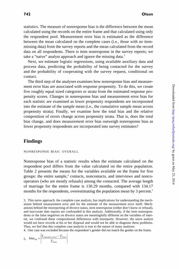
The predicted propensity scores were divided into five roughly equal-sizedgroups, ordered from low to high estimated contact or cooperation propensity(table 4).10 In a perfectly specified response propensity model, the actualresponse rate and the average estimated propensity for the groups will match.The overall estimated propensities are quite high—the top three groups ofcontact propensity are above 80 percent estimated likelihood of contact, andthe top four groups in cooperation propensity are above 90 percent estimatedlikelihood of cooperation. Of note, the bottom two contact propensity strataconsist entirely of mail respondents and the top two contact propensity strataconsist entirely of telephone respondents. Similarly, the bottom two coopera-tion propensity strata consist almost entirely of mail respondents (at least 88percent are mail respondents in these strata), and the top two cooperation pro-pensity strata consist entirely of telephone respondents.

RELATIONSHIP BETWEEN LIKELIHOOD OF CONTACT AND LIKELIHOOD OF COOPERATION

The next analyses examine changes in nonresponse bias and measurementerror bias by contact and cooperation propensity strata. One question is

10. Five propensity score subclasses are often found to be adequate for removing up to 90 percentof the bias in estimating causal effects (Rosenbaum and Rubin 1984). For the predicted contactpropensities, the five groups were calculated on both contacts and noncontacts so that differentnumbers of contacted cases are in each group. Similarly, the five groups for the cooperation pro-pensity were calculated on both interviews and noninterviews, among the contacted. Thus, thereare different numbers of cooperating cases in each group.

Table 4. Response Propensity Strata for Contact and Cooperation Models

Predicting Contact = 1Predicting Cooperation = 1,

Conditional on Contact

ResponsePropensityStratum

Actual Contact

Rate

Average Estimated Contact Propensity Actual

CooperationRate

Average Estimated Cooperation Propensity

Noncontacts Contacts Refusers Cooperators

% n % n % n % n % n % n

Low 51.4 148 50.6 72 53.3 76 51.7 118 42.8 57 63.1 61Group 2 69.4 147 65.6 45 66.2 102 91.6 119 90.5 10 92.0 109Group 3 83.3 144 81.9 24 88.7 120 99.2 118 96.7 1 98.1 117Group 4 99.4 154 97.9 1 97.5 153 100.0 121 — 0 98.9 121High 97.9 144 98.6 3 98.5 141 99.1 116 99.4 1 99.4 115



ownloaded from


748 Olson

whether the respondents in the high contact propensity stratum are also in thehigh cooperation propensity stratum—that is, are those who are easy to con-tact also likely to cooperate? If this is the case, then the two sets of analyseswill be redundant. There is a relationship between the two propensity stratadistributions (table 5, chi-square = 440.34, 16 df, p < .0001), but it is not a oneto one relationship (Spearman correlation = 0.51, asymptotic SE = 0.03). Forexample, only 16 percent of the respondents in the lowest contact propensitystratum were in the lowest cooperation propensity stratum, and only 15 percent ofthe respondents in the highest contact propensity stratum were in the highestcooperation propensity stratum.

RELATIONSHIP BETWEEN LIKELIHOOD OF CONTACT, LIKELIHOOD OF COOPERATION, AND NONRESPONSE BIAS

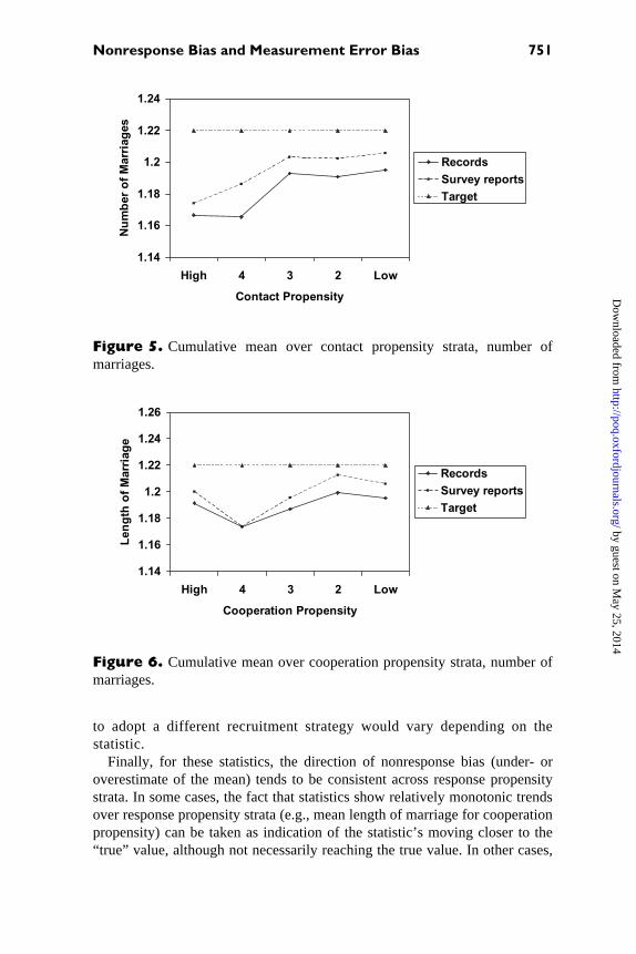
The critical question behind nonresponse reduction efforts is how the nonre-sponse bias of the estimate changes as respondents with lower propensity arerecruited into the survey. That is, do estimates based on the records changeover response propensities, and are estimates improved (i.e., lower nonre-sponse bias) by recruiting lower propensity sampled units into the respondentpool? Figures 1 through 6 present means cumulated over contact and coopera-tion propensity strata for the respondents. Moving from left to right on eachgraph indicates how the mean estimated on respondents changes based onadding lower propensity sample units into the respondent pool. The dottedline in each graph represents the target value, that is, the sample meanbased on the records. Differences between the solid line (the record meanbased on the respondents) and the dotted line indicate nonresponse bias for theunadjusted respondent mean. (The dashed line will be discussed in the nextsection.)

Table 5. Distribution of Predicted Cooperation Propensity Strata,Conditional on Contact, by Predicted Contact Propensity Strata among theCooperators

Predicted Contact Propensity

Predicted Cooperation Propensity

Low 2 3 4 High Total N

Low 16.13 75.81 8.06 0.00 0.00 100% 622 37.50 58.33 4.17 0.00 0.00 100% 723 18.18 17.17 7.07 13.13 44.44 100% 994 3.29 0.66 30.26 32.89 32.89 100% 152High 0.72 1.45 40.58 42.03 15.22 100% 138N 61 109 117 121 115 523



ownloaded from



Three observations can be made from the graphs. First, change in the sta-tistics across contact propensity strata is not the same as change in the statis-tics across cooperation propensity strata. This makes sense—therelationship between likelihood of contact and cooperation and survey vari-ables is likely to differ if different mechanisms produce contactability andcooperation. For instance, the mean length of marriage has an inverted “U”shape over contact propensity strata. On the other hand, the mean length ofmarriage calculated over cooperation propensity strata declines, movingcloser to the target value.

Figure 1. Cumulative mean over contact propensity strata, length of marriage.

021

521

031

531

041

541

051

woL234hgiH

ytisneporP tcatnoC

Leng

th o

f Mar

riage

sdroceRstroper yevruS

tegraT

Figure 2. Cumulative mean over cooperation propensity strata, length ofmarriage.

021

521

031

531

041

541

051

woL234hgiH

ytisneporP noitarepooC

Leng

th o

f Mar

riage


tegraT



ownloaded from


750 Olson

Second, the propensity stratum at which the mean calculated on therespondents is closest to the target value varies by statistic. For example,the nonresponse bias in the mean number of marriages based on respon-dent reports improves over all contact propensity strata, but the nonre-sponse bias in the mean number of months since divorce is negligible inalmost all cooperation propensity strata. Thus, if these three statistics werebeing monitored as part of a responsive design (Groves and Heeringa2006) with phases defined by response propensity, decisions about when

Figure 3. Cumulative mean over contact propensity strata, number ofmonths since divorce.

64

84

05

25

45

65

85

06

woL234hgiH

ytisneporP tcatnoC

Mon

ths

Sinc

e D

ivor

ce


tegraT

Figure 4. Cumulative mean over cooperation propensity strata, number ofmonths since divorce.

64

84

05

25

45

65

85

woL234hgiH


Mon

ths

Sinc

e D

ivor

ce


tegraT



ownloaded from



to adopt a different recruitment strategy would vary depending on thestatistic.

Finally, for these statistics, the direction of nonresponse bias (under- oroverestimate of the mean) tends to be consistent across response propensitystrata. In some cases, the fact that statistics show relatively monotonic trendsover response propensity strata (e.g., mean length of marriage for cooperationpropensity) can be taken as indication of the statistic’s moving closer to the“true” value, although not necessarily reaching the true value. In other cases,

Figure 5. Cumulative mean over contact propensity strata, number ofmarriages.

41.1

61.1

81.1

2.1

22.1

42.1

woL234hgiH

ytisneporP tcatnoC

Num

ber o

f Mar

riage

s


tegraT

Figure 6. Cumulative mean over cooperation propensity strata, number ofmarriages.

41.1

61.1

81.1

2.1

22.1

42.1

62.1

woL234hgiH


Leng

th o

f Mar

riage


tegraT



ownloaded from


752 Olson

this inference cannot be made (e.g., mean number of months since divorce forcooperation propensity).

EXAMINING NONRESPONSE BIAS USING RESPONDENT REPORTS

Having record values available for estimating nonresponse bias analyses israre. We now evaluate whether two common approaches to evaluating nonre-sponse bias based on respondent reports give us the same answer as that usingrecords. The first approach is one in which benchmark data are used to evalu-ate nonresponse bias properties of a statistic. The second approach is that dis-cussed above, in which movement of a statistic across propensity strata is usedto diagnose nonresponse bias. This is the propensity strata equivalent of alevel of effort simulation in which respondents recruited with greater levels ofeffort are removed from the respondent pool, and means from this truncateddistribution are compared with the full respondent mean (Curtin, Presser, andSinger 2000).

Assume that the mean for the entire sample based on the records is theobtained benchmark and that the difference between the mean based onrespondent reports and the benchmark is ascribed to nonresponse bias. Table 2shows that for length of marriage, the difference between the “benchmark”and the report-based mean is 3.63 months, compared with 3.88 months whenusing the records for the interviewed cases. The number of months sincedivorce shows a difference of 5.95 months when using the survey reports,compared with 0.65 months using the records. The mean number of marriagesis 0.01 marriages lower when using the survey reports, and 0.02 marriageslower than the benchmark when using the records. Thus, in two cases, thenonresponse bias estimate is actually smaller when using survey reportsinstead of records, but in one case, the nonresponse bias estimate is muchlarger relative to the using the records.

The second scenario is that available to most survey practitioners, inwhich the change in the respondent mean over different levels of effort isexamined. Differences between truncated distributions and the full respon-dent pool are taken as an indication of nonresponse bias (e.g., Curtin,Presser, and Singer 2000). The dashed line on figures 1–6 represents thisrespondent report-based mean. As when looking at the record-basedmeans above, as the dashed line moves from left to right on the graph,reports from respondents from lower propensity strata are incorporatedinto the estimate of the mean.

For all three statistics, the respondent mean calculated from the surveyreports tracks quite closely with the respondent mean calculated from therecords. Thus, conclusions drawn about whether inclusion of lower propensityrespondents improved the nonresponse bias properties of the statistic wouldbe similar, whether or not these estimates were based on respondent reports orrecord values. Importantly, although the conclusions are similar, the magnitudes



ownloaded from



of the estimates differ because the mean is shifted due to measurement errorbias in the respondent reports.

CHANGES IN MEASUREMENT ERROR BIAS AND NONRESPONSE BIAS BY LIKELIHOOD OF CONTACT AND COOPERATION

The discrepancy between nonresponse bias estimates based on the surveyreports and nonresponse bias estimates based on the records leads to threeimportant questions. First, does the difference between the estimate calculatedusing the respondent reports and that calculated from records change overresponse propensity strata? Second, does the total bias change over propensitystrata? Finally, does the relative contribution of nonresponse bias and mea-surement error bias change over propensity strata?

To answer the first question, we calculate the absolute measurement error

bias for each statistic as cumulated

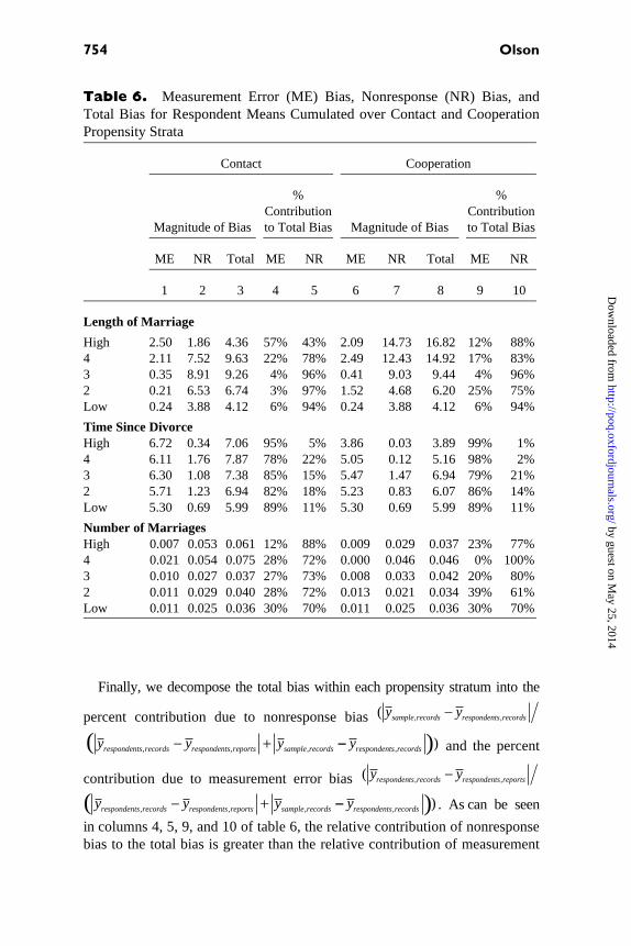
across strata. Columns 1 and 6 of table 6 clearly show that measurementerror bias is not constant across propensity strata. For two of the three statis-tics, measurement error bias decreases as lower contact propensity respon-dents are incorporated into the sample mean. On the other hand,measurement error bias increases as lower cooperation propensity respon-dents are incorporated into the sample mean for two of the three statistics,although the increase is not monotonic. For example, the cumulative meanlength of marriage, based on the survey reports, decreases in measurementerror bias as more reluctant and more difficult to contact cases are includedin the estimate of the sample mean. On the other hand, the measurementerror bias of the cumulative mean reported number of months since the (last)divorce increases across cooperation propensity strata, but decreases some-what across contact propensity strata.

To answer the second question, we examine the total absolute bias

. Columns 3 and 8of table 6 show that the total absolute bias increases between the first and sec-ond contact propensity strata, but then decreases across the remaining contactpropensity strata for all statistics. The total bias of the overall mean is lowerfor all statistics compared with the mean for the highest contact propensitystratum. This is not true for cooperation propensity. For mean length of mar-riage, total bias decreases as lower cooperation propensity respondents areincorporated into the sample mean. For another statistic, the mean time sincedivorce, total bias increases. Finally, for the mean number of marriages, thereis little change in the total bias as lower cooperation propensity respondentsare added to the estimate. For these statistics, converting low contact propen-sity cases appears to contribute more to reduction of total bias than convertinglow cooperation propensity cases.

( ), ,bias y yME respondent survey respondent record= −

( , , ,y y yrespondents records respondents reports sample records− + −− yrespondents records, )



ownloaded from


754 Olson

Finally, we decompose the total bias within each propensity stratum into the

percent contribution due to nonresponse bias

and the percent

contribution due to measurement error bias

. As can be seen

in columns 4, 5, 9, and 10 of table 6, the relative contribution of nonresponsebias to the total bias is greater than the relative contribution of measurement

Table 6. Measurement Error (ME) Bias, Nonresponse (NR) Bias, andTotal Bias for Respondent Means Cumulated over Contact and CooperationPropensity Strata

Contact Cooperation

Magnitude of Bias

% Contribution to Total Bias Magnitude of Bias

% Contribution to Total Bias

ME NR Total ME NR ME NR Total ME NR

1 2 3 4 5 6 7 8 9 10

Length of Marriage

High 2.50 1.86 4.36 57% 43% 2.09 14.73 16.82 12% 88%4 2.11 7.52 9.63 22% 78% 2.49 12.43 14.92 17% 83%3 0.35 8.91 9.26 4% 96% 0.41 9.03 9.44 4% 96%2 0.21 6.53 6.74 3% 97% 1.52 4.68 6.20 25% 75%Low 0.24 3.88 4.12 6% 94% 0.24 3.88 4.12 6% 94%

Time Since DivorceHigh 6.72 0.34 7.06 95% 5% 3.86 0.03 3.89 99% 1%4 6.11 1.76 7.87 78% 22% 5.05 0.12 5.16 98% 2%3 6.30 1.08 7.38 85% 15% 5.47 1.47 6.94 79% 21%2 5.71 1.23 6.94 82% 18% 5.23 0.83 6.07 86% 14%Low 5.30 0.69 5.99 89% 11% 5.30 0.69 5.99 89% 11%

Number of MarriagesHigh 0.007 0.053 0.061 12% 88% 0.009 0.029 0.037 23% 77%4 0.021 0.054 0.075 28% 72% 0.000 0.046 0.046 0% 100%3 0.010 0.027 0.037 27% 73% 0.008 0.033 0.042 20% 80%2 0.011 0.029 0.040 28% 72% 0.013 0.021 0.034 39% 61%Low 0.011 0.025 0.036 30% 70% 0.011 0.025 0.036 30% 70%

( , ,y ysample records respondents records−

( , , ,y y yrespondents records respondents reports sample records− + −− yrespondents records, ))

( , ,y yrespondents records respondents reports−

( , , ,y y yrespondents records respondents reports sample records− + −− yrespondents records, ))



ownloaded from



error bias for mean length of marriage and mean number of marriages acrossvirtually all contact and cooperation propensity strata. On the other hand,the relative contribution of measurement error bias outweighs the relativecontribution of nonresponse bias for the mean time elapsed since divorceacross all propensity strata. Of interest, mean length of marriage and meantime since divorce are two statistics that use the same question, but meanlength of marriage is dominated by nonresponse bias and mean time sincedivorce is dominated by measurement error bias. The contribution of mea-surement error bias to total bias decreases across contact propensity stratafor mean length of marriage and mean time since divorce, but increases forthe mean number of marriages across contact propensity strata. There is nodifference in the contribution of measurement error bias to total biasamong estimates that incorporate the bottom three contact propensitystrata. There is no clear trend in change of the contribution of measure-ment error bias to total bias across cooperation propensity strata for any ofthe three statistics.

Discussion and Conclusions

This analysis has five main findings. (1) Effects on the nonresponse bias of asurvey statistic from turning low propensity sample units into respondents arestatistic-specific and specific to the type of nonresponse (contact versus coop-eration). This is not a new finding but is worth reiterating. (2) What is new arethe findings on how these recruitment efforts are associated with the measure-ment error bias properties of the same statistics and how measurement errorbias affects diagnoses of nonresponse bias. (3) Limited support was found forthe suspicion that measurement error bias increases for estimates includingreluctant respondents. Such increases were found for two of the three statisticsinvestigated. (4) But, despite the increase in measurement error, total bias ofall three statistics decreased as a result of incorporating lower contact propen-sity cases, and for one statistic as a result of incorporating lower cooperationpropensity respondents. (5) Finally, this investigation showed that level ofeffort analyses came to similar (although not identical) conclusions whenbased on record data and on survey reports for the statistics and protocolinvestigated here.

Measurement error bias estimates for these three respondent means differedacross contact and cooperation propensity strata. The differences were some-times small relative to the estimate, and sometimes quite sizable. For two ofthe sample means, the contribution of nonresponse bias to total bias exceededthat due to measurement error bias over all propensity strata. For one samplemean, the relative contribution of nonresponse bias was much less than thecontribution due to measurement error bias. Thus, concerns that the errorproperties of a sample mean are dominated by measurement error bias after



ownloaded from


756 Olson

incorporating low propensity respondents into the sample pool are not consis-tently borne out. One important caveat is that the total bias changes over pro-pensity strata. Thus, the percent contribution of measurement error bias willnot necessarily increase when both measurement error bias and nonresponsebias increase. The relationship between nonresponse bias, measurement errorbias, and likelihood of response also clearly depends on which type of nonre-sponse propensity is considered.

In this study, methods of diagnosing nonresponse bias tended to givesimilar answers when either records or survey reports were used. The magni-tude of the estimate of nonresponse bias differed depending on the datasource, but the general direction of conclusions was quite similar for two ofthe three statistics considered. Replication of this analysis is clearly needed.

The difference between the error properties of a variable in a data set (orquestion in a questionnaire) and of a statistic such as a mean must be high-lighted. Two of the statistics used in this article use exactly the same question—the date of divorce. The length of marriage is the difference between thedivorce date and the marriage date. The time elapsed since divorce is the dif-ference between the divorce date and the first day of the field period. Both ofthese statistics use the divorce date variable but have dramatically differenterror properties. Mean length of marriage had little measurement error bias,whereas mean time elapsed since divorce was dominated by measurementerror bias. One hypothesis is that people are able to retrieve the length of asalient event, such as marriage, but not the individual dates that bound theevent. When a questionnaire demands the retrieval of two dates, individualsmay recall an approximate date that anchors the beginning of the event (e.g.,marriage date), and report a calculated end date (e.g., divorce date) using thisretrieved beginning date and length of the event (e.g., length of marriage).Further research on when and how combinations of variables change nonre-sponse and measurement error structures relative to the original variables isnecessary.

One critical element of this analysis is the mixed-mode design. Disentan-gling whether the mail and phone modes had different nonresponse bias andmeasurement error bias properties is important for understanding the findings.In this analysis, estimates made on the top two contact and cooperation pro-pensity strata are based solely on telephone respondents. Mail respondents areadded into the estimates for the next three strata. Previous research suggeststhat statistics calculated from self-administered modes may have differentmeasurement error properties than statistics calculated from interviewer-administered modes, at least for sensitive questions (e.g., Tourangeau andSmith 1996). Additionally, mixed-mode surveys are frequently done in thehope that respondents to the second mode will be different from respondentsto the first mode on the survey variables of interest (de Leeuw 2005). Thus,one would expect differences in both measurement error bias and nonresponsebias when looking at the two modes individually. We see some hints that this



ownloaded from



may be occurring. For example, measurement error bias drops dramaticallyfrom mean length of marriage calculated on the telephone respondents aloneto the same statistic calculated from phone and mail respondents. Nonre-sponse bias for mean length of marriage also tends to decrease. However, bothmeasurement error bias and nonresponse bias increase for mean time sincedivorce as lower cooperation propensity mail respondents are added. Furtherresearch into when and how mixed-mode designs are beneficial for meansquare error and how error structures change as a result of using more thanone mode is clearly needed. The sequencing of modes also is an importantquestion—had this investigation used a mail survey with a telephone follow-up,would similar changes in total error and the composition of error have beenobserved?

The results of this analysis are conditional on the variables included in thepropensity model. Similar analyses were conducted with two other modelspecifications. One model was identical to the model presented here butexcluded the mail questionnaire indicator; the other model replaced the totalnumber of calls to first contact with the total number of calls and replacedthe indicator for ever refusing with the total number of refusals. The conclu-sions from those analyses were similar to those presented here for the twostatistics involving dates, but conclusions for mean number of marriageswere somewhat more sensitive to model specification. The largest differ-ences between models for all three statistics occurred in the means calcu-lated for the highest contact and cooperation propensity strata. Thedifferences are suggestive of mode differences for the reported number ofmarriages, but future research on when and why the relationship betweentotal bias, nonresponse bias, measurement error bias, and response propen-sity changes when different predictors are included in the propensity modelis clearly needed.

References

The American Association for Public Opinion Research. 2006. Standard Definitions: Final Dis-positions of Case Codes and Outcome Rates for Surveys. 4th edition. Lenexa, Kansas: AAPOR.

Assael, Henry, and John Keon. 1982. “Nonsampling vs. Sampling Errors in Survey Research.”Journal of Marketing 46:114–23.

Biemer, Paul P. 2001. “Nonresponse Bias and Measurement Bias in a Comparison of Face to Faceand Telephone Interviewing.” Journal of Official Statistics 17:295–320.

Bollinger, Christopher R., and Martin H. David. 1995. “Sample Attrition and Response Error: DoTwo Wrongs Make a Right?” University of Wisconsin Center for Demography and Ecology.

———. 2001. “Estimation with Response Error and Nonresponse: Food Stamp Participation inthe SIPP.” Journal of Business and Economic Statistics 19:129–41.

Cannell, Charles F., and Floyd J. Fowler. 1963. “Comparison of a Self-Enumerative Procedureand a Personal Interview: A Validity Study.” Public Opinion Quarterly 27:250–64.

Curtin, Richard, Stanley Presser, and Eleanor Singer. 2000. “The Effects of Response RateChanges on the Index of Consumer Sentiment.” Public Opinion Quarterly 64:413–28.

———. 2005. “Changes in Telephone Survey Nonresponse over the Past Quarter Century.”Public Opinion Quarterly 69:87–98.



ownloaded from


758 Olson

de Leeuw, Edith. 2005. “To Mix or Not to Mix Data Collection Modes in Surveys.” Journal ofOfficial Statistics 21:233–55.

de Leeuw, Edith, and Wim de Heer. 2002. “Trends in Household Survey Nonresponse: A Longi-tudinal and International Perspective.” In Survey Nonresponse, ed. Robert M. Groves, Don A.Dillman, John L. Eltinge, and Roderick J. A. Little, pp. 41–54. New York: Wiley.

Duncan, Greg J., and Daniel H. Hill. 1989. “Assessing the Quality of Household Panel Data: TheCase of the Panel Study of Income Dynamics.” Journal of Business and Economic Statistics7:441–52.

Groves, Robert M. 2006. “Nonresponse Rates and Nonresponse Error in Household Surveys.”Public Opinion Quarterly 70:646–75.

Groves, Robert M., and Mick Couper. 1998. Nonresponse in Household Interview Surveys. NewYork: Wiley.

Groves, Robert M., and Steven G. Heeringa. 2006. “Responsive Design for Household Surveys:Tools for Actively Controlling Survey Errors and Costs.” Journal of the Royal StatisticalSociety, A 169:439–57.

Groves, Robert M., Stanley Presser, and Sarah Dipko. 2004. “The Role of Topic Interest inSurvey Participation Decisions.” Public Opinion Quarterly 68:2–31.

Huynh, Minh, Kalman Rupp, and James Sears. 2002. Working Paper 238: The Assessment of Sur-vey of Income and Program Participation (SIPP) Benefit Data Using Longitudinal Administra-tive Records. Washington, DC: U.S. Bureau of the Census.

Japec, Lilli, Antti Ahtiainen, Jan Hörngren, Håkan Lindén, Lars Lyberg, and Per Nilsson. 2000.Minska bortfallet. Sweden: Statistiska centralbyrån.

Joffe, Marshall M., and Paul R. Rosenbaum. 1999. “Invited Commentary: Propensity Scores.”American Journal of Epidemiology 150:327–33.

Keeter, Scott, Carolyn Miller, Andrew Kohut, Robert M. Groves, and Stanley Presser. 2000.“Consequences of Reducing Nonresponse in a National Telephone Survey.” Public OpinionQuarterly 64:125–48.

Lepkowski, James M., and Robert M. Groves. 1986. “A Mean Squared Error Model for Dual Frame,Mixed Mode Survey Design.” Journal of the American Statistical Association 81:930–37.

Lessler, Judith T., and William D. Kalsbeek. 1992. Nonsampling Error in Surveys. New York:Wiley.

Lin, I-Fen, and Nora Cate Schaeffer. 1995. “Using Survey Participants to Estimate the Impact ofNonparticipation.” Public Opinion Quarterly 59:236–58.

Little, Roderick J. A. 1986. “Survey Nonresponse Adjustments for Estimates of Means.” Interna-tional Statistical Review 54:139–57.

Merkle, Daniel, and Murray Edelman. 2002. “Nonresponse in Exit Polls: A Comprehensive Anal-ysis.” In Survey Nonresponse, ed. Robert M. Groves, Don A. Dillman, John L. Eltinge, andRoderick J. A. Little, pp. 243–57. New York: Wiley.

Rosenbaum, Paul R., and Donald B. Rubin. 1984. “Reducing Bias in Observational Studies UsingSubclassification on the Propensity Score.” Journal of the American Statistical Association79:516–24.

———. 1985. “Constructing a Control Group Using Multivariate Matched Sampling MethodsThat Incorporate the Propensity Score.” American Statistician 39:33–38.

Schaeffer, Nora Cate, Judith A. Seltzer, and Marieka Klawitter. 1991. “Estimating Nonresponseand Response Bias: Resident and Nonresident Parents’ Reports about Child Support.”Sociological Methods and Research 20:30–59.

Stang, Andreas, and Karl-Heinz Jöckel. 2005. “Letter to the Editor: The Authors Reply.” AmericanJournal of Epidemiology 161:403.

Tourangeau, Roger, and Tom W. Smith. 1996. “Asking Sensitive Questions: The Impact of DataCollection Mode, Question Format, and Question Context.” Public Opinion Quarterly 60:275–304.

Voigt, Lynda F., Denise M. Boudreau, Noel S. Weiss, Kathleen E. Malone, Christopher I. Li, andJanet R. Daling. 2005. “Letter to the Editor: RE: ‘Studies with Low Response Proportions MayBe Less Biased than Studies with High Response Proportions.’” American Journal of Epidemiology161:401–2.



ownloaded from


Survey Participation, Nonresponse Bias, Measurement Error Bias, and Total Bias

Documents

Transcript of Survey Participation, Nonresponse Bias, Measurement Error Bias, and Total Bias