Estimation of three-parameter exponentiated-Weibull distribution under type-II censoring
23
Journal of Statistical Planning and Inference 134 (2005) 350 – 372 www.elsevier.com/locate/jspi Estimation of three-parameter exponentiated-Weibull distribution under type-II censoring Umesh Singh, Pramod K. Gupta ∗ , S.K. Upadhyay Department of Statistics, Faculty of Science, Banaras Hindu University,Varanasi 221005, India Received 6 July 2003; accepted 29 April 2004 Available online 26 July 2004 Abstract The present article obtains the point estimators of the exponentiated-Weibull parameters when all the three parameters of the distribution are unknown. Maximum likelihood estimator generalized maximum likelihood estimator and Bayes estimators are proposed for three-parameter exponentiated- Weibull distribution when available sample is type-II censored. Independent non-informative types of priors are considered for the unknown parameters to develop generalized maximum likelihood estimator and Bayes estimators. Although the proposed estimators cannot be expressed in nice closed forms, these can be easily obtained through the use of appropriate numerical techniques. The perfor- mances of these estimators are studied on the basis of their risks, computed separately under LINEX loss and squared error loss functions through Monte-Carlo simulation technique. An example is also considered to illustrate the estimators. © 2004 Elsevier B.V.All rights reserved. MSC: primary 62F10, 62F15; secondary 62N01, 62N02 Keywords: Three-parameter exponentiated-Weibull distribution; Bayes estimators; Generalized maximum likelihood estimator; Maximum likelihood estimators; Non-informative prior; Type-II censoring; Square error loss function; LINEX loss function ∗ Corresponding author. Division of Biostatistics and Bioinformatics, National Health Research Institutes, 128, Yen-Chiu-Yuan Road, Sec. 2, Taipei 115 Taiwan. Tel.: +886-2-2653-4401(7665); fax: +886-2-2789-0253. E-mail address: [email protected] (Pramod K. Gupta). 0378-3758/$ - see front matter © 2004 Elsevier B.V. All rights reserved. doi:10.1016/j.jspi.2004.04.018
-
Upload
independent -
Category
Documents
-
view
5 -
download
0
Transcript of Estimation of three-parameter exponentiated-Weibull distribution under type-II censoring
Journal of Statistical Planning andInference 134 (2005) 350–372
www.elsevier.com/locate/jspi
Estimation of three-parameterexponentiated-Weibull distribution under type-II
censoring
Umesh Singh, Pramod K. Gupta∗, S.K. UpadhyayDepartment of Statistics, Faculty of Science, Banaras Hindu University, Varanasi 221005, India
Received 6 July 2003; accepted 29 April 2004Available online 26 July 2004
Abstract
The present article obtains the point estimators of the exponentiated-Weibull parameters whenall the three parameters of the distribution are unknown. Maximum likelihood estimator generalizedmaximum likelihood estimator and Bayes estimators are proposed for three-parameter exponentiated-Weibull distribution when available sample is type-II censored. Independent non-informative typesof priors are considered for the unknown parameters to develop generalized maximum likelihoodestimator and Bayes estimators. Although the proposed estimators cannot be expressed in nice closedforms, these can be easily obtained through the use of appropriate numerical techniques. The perfor-mances of these estimators are studied on the basis of their risks, computed separately under LINEXloss and squared error loss functions through Monte-Carlo simulation technique. An example is alsoconsidered to illustrate the estimators.© 2004 Elsevier B.V. All rights reserved.
MSC:primary 62F10, 62F15; secondary 62N01, 62N02
Keywords:Three-parameter exponentiated-Weibull distribution; Bayes estimators; Generalized maximumlikelihood estimator; Maximum likelihood estimators; Non-informative prior; Type-II censoring; Square errorloss function; LINEX loss function
∗ Corresponding author. Division of Biostatistics and Bioinformatics, National Health Research Institutes, 128,Yen-Chiu-Yuan Road, Sec. 2, Taipei 115 Taiwan. Tel.: +886-2-2653-4401(7665); fax: +886-2-2789-0253.
E-mail address:[email protected](Pramod K. Gupta).
0378-3758/$ - see front matter © 2004 Elsevier B.V. All rights reserved.doi:10.1016/j.jspi.2004.04.018

U. Singh et al. / Journal of Statistical Planning and Inference 134 (2005) 350–372 351
1. Introduction
A number of lifetime models have been suggested for analysis of lifetime data in theliterature by various authors see,Mann et al. (1974); Lawless (1982); Martz and Waller(1982); Sinha (1986)etc. Some of these models (particularly, exponential model andWeibullmodel) are widely discussed in the literature for the analysis of lifetime data. These modelsaccommodate either constant or monotone (increasing and decreasing) type of the hazardrates. But non-monotonic hazard functions such as unimodal shaped and bathtub shapedfunctions also arise in practice. For example, data in reliability analysis specially life cycle ofthe product often involve high initial hazard rates (Infant mortality) and eventual high hazardrates due to aging and wear-out in the end indicating a bathtub hazard rate. Non-monotonehazard rate is very common not only in the field of science and engineering but also in thefields of medical, biological ecological and space explorations.Therefore, modeling lifetimedata for non-monotonic hazard rates seems to be a growing interest. Various generalizationof the familiar models have been suggested to deal with non-monotonic hazard rates; e.g.generalized gamma, Weibull, Rayleigh and models suggested bySlymen and Lachenbruch(1984); Hjorth (1980); Prentice (1975); Rajarshi and Rajarshi (1988), etc. These generalizedmodels usually have many parameters and make the procedure of estimation of parametersso complicated. Even the standard procedures of statistical estimation such as method ofmaximum likelihood, method of moments and method of least square etc, often becomeintractable for these distributions especially in presence of censoring. SeeBain (1974);Hjorth (1980); Lawless (1982); Gore et al. (1986); Rajarshi and Rajarshi (1988); Mudholkaret al. (1995)for details. Apart from this, most of these models lack physical motivation.Hence, there has been a long felt need of having a model which can have natural relevance tothe data and involve minimum number of parameters so that besides accommodating non-monotonic hazard functions, it may provide easy implementation of standard statisticalinferential procedures in censored case also. In this context, exponentiated-Weibull familycan be considered as a suitable model, which was originally introduced byMudholkarand Srivastava (1993). Exponentiated-Weibull family is a simple generalization of well-known two-parameter Weibull family and is obtained by introducing one additional shapeparameter.The main feature of this family is that it allows bathtub shaped as well as unimodalhazard rates in addition to various monotone hazard rates. The distribution function andprobability density functions of exponentiated-Weibull family are
F (y) = (1 − exp
(−(y/�)�))�
, 0�y�∞ �, �,�> 0, (1.1)
f (y) = (��/�
)exp
(−(y/�)�)(y/�)�−1(1 − exp
(−(y/�)�))�−1
. (1.2)
Where� and� both are the shape parameters while� is scale parameter of the family. Adetailed discussion of three-parameter exponentiated-Weibull distribution (EWD) can behad fromMudholkar and Srivastava (1993); Mudholkar et al. (1995). Singh et al. (2002)has discussed the classical and Bayesian methods of parameter estimation for completesample case. It seems that estimation procedures for three-parameter EWD in presence ofcensoring have not been discussed. This paper is an attempt in this direction. For simplicity,we shall confine ourselves to type-II censored data only (seeLawless (1982)). Along with

352 U. Singh et al. / Journal of Statistical Planning and Inference 134 (2005) 350–372
maximum likelihood estimators (MLE) and generalized maximum likelihood estimators(GMLE), Bayes estimators have also been obtained.
It is well known that choice of loss function is an integral part of Bayesian estimationprocedures and squared error loss function (SELF) is frequently used (seeBox and Tiao(1973); Berger (1985)) due to its mathematical simplicity and relevance with classicalprocedures. But SELF is justified loss function only in those conditions where losses aresymmetric in nature. Hence, in-discernment use of SELF is not appropriate particularlyin these cases, where the losses are not symmetric. Such conditions are very common inengineering, medical and biomedical sciences. A number of asymmetric loss functionsmay be found in the literature but among these asymmetric losses, LINEX loss function(LLF) are dominantly and widely used because it is a natural extension of SELF. It wasoriginally introduced byVarian (1975)and got a lot of popularity due toZellner (1986).The mathematical form of LLF may simply be expressed as:
L (�) = b(ea� − a� − 1
), a �= 0, b > 0, (1.3)
where,a andb are respectively shape and scale parameters of the loss function given in(1.3), its asymmetric nature depends on shape parameter ‘a’. When value of ‘a’ is less thanzero, LLF gives more weight to under-estimation against over-estimation and the situationis reverse when value assigned to ‘a’ is greater than zero. If ‘a’ tends to zero LLF tendsto SELF. Uses of LLF have also been discussed by various authors includingBasu andEbrahimi (1991); Parsian (1990); Khatree (1992)etc. In this paper we shall obtain theBayes estimators under SELF and LLF both.
Succeeding section deals with the computational procedure to obtain the MLE of�, �and� of EWD. While Section 3 discusses the procedures to obtain the Bayes estimatorunder squared error loss function (BESF), Bayes estimator under LINEX loss function(BELF) and generalized maximum likelihood estimators (GMLE) for the parameters ofEWD. A simulated data set is considered to illustrate the proposed estimators in Section4. The estimators of�, � and� discussed in Sections 2 and 3 are not in nice closed forms,therefore, their simulated risks under SELF and LLF have been obtained in Section 5 tomake a detail comparison of their performances. The last section of the paper includes abrief conclusion and recommendation about the use of estimators of�, � and�.
2. Maximum likelihood estimators (MLE)
Let y = (y1, y2, . . . , yr ), wherey1�y2� · · · �yr be the observed lifetimes of the firstr components which fail in a random sample ofn components put on test. We assumethat the lifetimes of these components follow the distribution expressed in (1.2). Hence thelikelihood function of this setup can be written as:
l = n!(n − r)! (��/�)r
r∏i=1
exp(−(yi/�)�
) r∏i=1
(1 − exp
(−(yi/�)�))�−1
,
r∏i=1
(yi/�)�−1[1 − (
1 − exp(−(yr/�)�
))�]n−r
. (2.1)

U. Singh et al. / Journal of Statistical Planning and Inference 134 (2005) 350–372 353
To obtain the likelihood equations, we differentiate log of (2.1) with respect to the param-eters,�, � and� respectively and equate to zero. The resulting equations are as follows:
0=�L
��= r
�−
r∑i=1
(yi/�)� log(yi/�) + (� − 1)
×r∑
i=1
exp(−(yi/�)�)(yi/�)� log(yi/�)
(1 − exp(−(yi/�)�))+
r∑i=1
log(yi/�)
− (n − r)�(1 − exp(−(yr/�)�))�−1 exp(−(yr/�)�)(yr/�)� log(yr/�)[1 − (1 − exp(−(yr/�)�))�
] (2.2)
0=�L
��= r
�+
r∑i=1
log(1 − exp
(−(yi/�)�))
− (n − r)(1 − exp
(−(yr/�)�))� log
(1 − exp
(−(yr/�)�))
[1 − (
1 − exp(−(yr/�)�
))�] , (2.3)
0 = �L
��=� r
�−
r∑i=1
(yi/�)���
+ (� − 1
) r∑i=1
exp(−(yi/�)�
)(yi/�)��(
1 − exp(−(yi/�)�
))�
− (n − r) ��(1 − exp
(−(yr/�)�))�−1 exp
(−(yr/�)�)(yr/�)�
�[1 − (
1 − exp(−(yr/�)�
))�] . (2.4)
Eqs. (2.2)–(2.4) are nonlinear and analytical solutions are not possible. Therefore, to obtainthe solutions from these equations, we propose to use theNAG (1993)routine C05PCF,which is based on Newton Raphson type procedure. This procedure requires second-orderderivatives also, which can be obtained.
3. Bayes estimators
To develop the Bayes estimators of�, � and�, we consider independent non-informativetype of priors,g1(�), g2(�) andg3(�), given as,
g1 (�) = 1
c, 0< �< c, (3.1)
g2(�) = 1
�, �> 0, (3.2)
g3 (�) = 1
�, �> 0. (3.3)
354 U. Singh et al. / Journal of Statistical Planning and Inference 134 (2005) 350–372
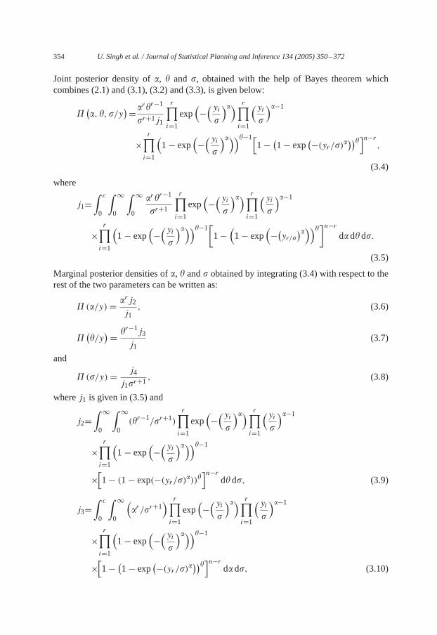
Joint posterior density of�, � and �, obtained with the help of Bayes theorem whichcombines (2.1) and (3.1), (3.2) and (3.3), is given below:
�(�, �,�/y
) =�r�r−1
�r+1j1
r∏i=1
exp(−
(yi
�
)�) r∏i=1
(yi
�
)�−1
×r∏
i=1
(1 − exp
(−
(yi
�
)�))�−1[1 − (
1 − exp(−(yr/�)�
))�]n−r
,
(3.4)
where
j1=∫ c
0
∫ ∞
0
∫ ∞
0
�r�r−1
�r+1
r∏i=1
exp(−
(yi
�
)�) r∏i=1
(yi
�
)�−1
×r∏
i=1
(1 − exp
(−
(yi
�
)�))�−1[1 −
(1 − exp
(−(
yr/�)�))�
]n−r
d� d� d�.
(3.5)
Marginal posterior densities of�, � and� obtained by integrating (3.4) with respect to therest of the two parameters can be written as:
� (�/y) = �r j2
j1, (3.6)
�(�/y
) = �r−1j3
j1(3.7)
and
� (�/y) = j4
j1�r+1 , (3.8)
wherej1 is given in (3.5) and
j2=∫ ∞
0
∫ ∞
0(�r−1/�r+1)
r∏i=1
exp(−
(yi
�
)�) r∏i=1
(yi
�
)�−1
×r∏
i=1
(1 − exp
(−
(yi
�
)�))�−1
×[1 − (1 − exp(−(yr/�)�))�
]n−r
d� d�, (3.9)
j3=∫ c
0
∫ ∞
0
(�r/�r+1
) r∏i=1
exp(−
(yi
�
)�) r∏i=1
(yi
�
)�−1
×r∏
i=1
(1 − exp
(−
(yi
�
)�))�−1
×[1 − (
1 − exp(−(yr/�)�
))�]n−r
d� d�, (3.10)

U. Singh et al. / Journal of Statistical Planning and Inference 134 (2005) 350–372 355
j4=∫ c
0
∫ ∞
0
(�r�r−1
) r∏i=1
exp(−
(yi
�
)�) r∏i=1
(yi
�
)�−1
×r∏
i=1
(1 − exp
(−
(yi
�
)�))�−1
×[1 − (
1 − exp(−(yr/�)�
))�]n−r
d� d�. (3.11)
3.1. Bayes estimators under squared error loss function (BESF)
Bayes estimators of parameters under SELF are nothing but the posterior mean of corre-sponding parameters. Hence the BESF�bs of � is simply expressed as:
�bs = E(�) = 1
j1
∫ c
0�� (�/y) d�.
After simplification it may be written as:
�bs = j5
j1, (3.12)
wherej1 is given in (3.5) and
j5=∫ c
0
∫ ∞
0
∫ ∞
0
�r+1�r−1
�r+1
r∏i=1
exp(−
(yi
�
)�) r∏i=1
(yi
�
)�−1
×r∏
i=1
(1 − exp
(−
(yi
�
)�))�−1
×[1 − (
1 − exp(−(yr/�)�
))�]n−r
d� d� d�. (3.13)
In a similar way, we can obtain the estimators�bs and�bs of � and�, respectively, as givenbelow:
�bs = j6
j1(3.14)
and
�bs = j7
j1, (3.15)
356 U. Singh et al. / Journal of Statistical Planning and Inference 134 (2005) 350–372
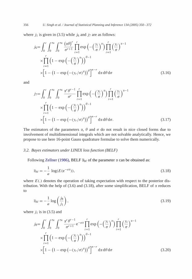
wherej1 is given in (3.5) whilej6 andj7 are as follows:
j6=∫ c
0
∫ ∞
0
∫ ∞
0
(��
)r
�r+1
r∏i=1
exp(−
(yi
�
)�) r∏i=1
(yi
�
)�−1
×r∏
i=1
(1 − exp
(−
(yi
�
)�))�−1
×[1 − (
1 − exp(−(yr/�)�
))�]n−r
d� d� d� (3.16)
and
j7=∫ c
0
∫ ∞
0
∫ ∞
0
�r�r−1
�r
r∏i=1
exp(−
(yi
�
)�) r∏i=1
(yi
�
)�−1
×r∏
i=1
(1 − exp
(−
(yi
�
)�))�−1
×[1 − (
1 − exp(−(yr/�)�
))�]n−r
d� d� d�. (3.17)
The estimators of the parameters�, � and � do not result in nice closed forms due toinvolvement of multidimensional integrals which are not solvable analytically. Hence, wepropose to use here 16-point Gauss quadrature formulae to solve them numerically.
3.2. Bayes estimators under LINEX loss function (BELF)
FollowingZellner (1986), BELF �bl of the parameter� can be obtained as:
�bl = −1
alog(E(e−a�)), (3.18)
whereE(.) denotes the operation of taking expectation with respect to the posterior dis-tribution. With the help of (3.6) and (3.18), after some simplification, BELF of� reducesto
�bl = −1
alog
(j8
j1
), (3.19)
wherej1 is in (3.5) and
j8=∫ c
0
∫ ∞
0
∫ ∞
0
�r�r−1
�r+1 e−a�r∏
i=1
exp(−
(yi
�
)�) r∏i=1
(yi
�
)�−1
×r∏
i=1
(1 − exp
(−
(yi
�
)�))�−1
×[1 − (
1 − exp(−(yr/�)�
))�]n−r
d� d� d� (3.20)
U. Singh et al. / Journal of Statistical Planning and Inference 134 (2005) 350–372 357
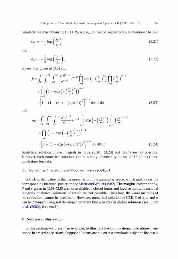
Similarly, we may obtain the BELF�bl and�bl of � and�, respectively, as mentioned below:
�bl = −1
alog
(j9
j1
)(3.21)
and
�bl = −1
alog
(j10
j1
), (3.22)
wherej1 is given in (3.5) and
j9=∫ c
0
∫ ∞
0
∫ ∞
0
�r�r−1
�r+1 e−a�r∏
i=1
exp(−
(yi
�
)�) r∏i=1
(yi
�
)�−1
×r∏
i=1
(1 − exp
(−
(yi
�
)�))�−1
×[1 − (
1 − exp(−(yr/�)�
))�]n−r
d� d� d� (3.23)
and
j10=∫ c
0
∫ ∞
0
∫ ∞
0
�r�r−1
�r+1 e−a�r∏
i=1
exp(−
(yi
�
)�) r∏i=1
(yi
�
)�−1
×r∏
i=1
(1 − exp
(−
(yi
�
)�))�−1
×[1 − (
1 − exp(−(yr/�)�
))�]n−r
d� d� d�. (3.24)
Analytical solution of the integrals in (3.5), (3.20), (3.23) and (3.24) are not possible.However, their numerical solutions can be simply obtained by the use of 16-points Gaussquadrature formula.
3.3. Generalized maximum likelihood estimators (GMLE)
GMLE is that value of the parameter within the parameter space, which maximizes thecorresponding marginal posterior, seeMartz and Waller (1982). The marginal posterior of�,� and� given in (3.6)–(3.8) are not available in closed forms and involve multidimensionalintegrals, analytical solutions of which are not possible. Therefore, the usual methods ofmaximization cannot be used here. However, numerical solution of GMLE of�, � and�can be obtained using self developed program that provides its global solutions (seeSinghet al. (2002), for details).
4. Numerical illustration
In this section, we present an example, to illustrate the computational procedures men-tioned in preceding sections. Suppose 10 items are put on test simultaneously; the life test is
358 U. Singh et al. / Journal of Statistical Planning and Inference 134 (2005) 350–372
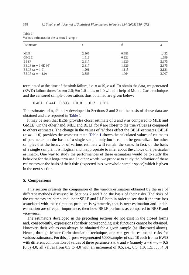
Table 1Various estimates for the censored sample
Estimators � � �
MLE 2.209 0.983 1.432GMLE 1.916 0.821 1.699BESF 2.817 1.826 2.375BELF (a= 1.0E-05) 2.817 1.826 2.375BELF (a = 1.0) 1.901 1.115 2.121BELF (a = −1.0) 3.386 1.064 3.007
terminated at the time of the sixth failure, i.e.n=10,r =6. To obtain the data, we generated(EWD) failure times for�=2.0;�=1.0 and�=2.0 with the help of Monte-Carlo techniqueand the censored sample observations thus obtained are given below:
0.401 0.441 0.893 1.010 1.012 1.362
The estimates of�, � and� developed in Sections 2 and 3 on the basis of above data areobtained and are reported inTable 1
It may be seen that BESF provides closer estimate of� and� as compared to MLE andGMLE. On the other hand, MLE and BELF for� are closer to the true values as comparedto others estimates. The change in the values of ‘a’ does effect the BELF estimates. BELF(a = −1.0) provides the worst estimate.Table 1shows the calculated values of estimatesof parameters on the basis of a single sample only but it cannot be generalized for othersamples that the behavior of various estimate will remain the same. In fact, on the basisof a single sample, it is illogical and inappropriate to infer about the choice of a particularestimator. One way to study the performances of these estimators would be to study thebehavior for their long-term use. In other words, we propose to study the behavior of theseestimators on the basis of their risks (expected loss over whole sample space) which is givenin the next section.
5. Comparisons
This section presents the comparison of the various estimators obtained by the use ofdifferent methods discussed in Sections 2 and 3 on the basis of their risks. The risks ofthe estimators are computed under SELF and LLF both in order to see that if the true lossassociated with the estimation problem is symmetric, that is over-estimation and under-estimation are of equal importance, then how BELF performs as compared to BESF andvice-versa.
The estimators developed in the preceding sections do not exist in the closed formsand, consequently, expressions for their corresponding risk functions cannot be obtained.However, their values can always be obtained for a given sample (as illustrated above).Hence, through Monte-Carlo simulation technique, one can get the estimated risks forvarious estimators. For this purpose we generated 5000 samples of size 10 each from a EWDwith different combination of values of three parameters�, � and� (namely�=�=�=0.5(0.5) 4.0, all values from 0.5 to 4.0 with an increment of 0.5, i.e., 0.5, 1.0, 1.5, . . . , 4.0)

U. Singh et al. / Journal of Statistical Planning and Inference 134 (2005) 350–372 359
so as to incorporate almost all the shapes of EWD. The various values of hyper-parameterconsideredc = 4 (2) 12. The values of shape parameter ‘a’ of LLF are taken to bea =−1.0and 1.0. Without loss of generality scale parameter ‘b’ of LLF is taken to 1.0 because achange in ‘b’ will not effect the trend of the risk. To see the effect ofr/n on the risks ofthe estimators, we have considered censoring fractions,r/n = 0.4 (0.2) 1.0. Risks of theproposed estimators are shown inFigs. S-5(1)–S-5(9)andFigs. L-5(1)–5(18). Each graphshows the risk of the estimator ony-axis and values of the corresponding parameter onx-axisfor fixed values of other parameters. It is important to mention here that scales ony-axis ofthe graphs are not same and it varies from figure to figure. From numerical results shown inFigs. S-5(1)–S-5(9)andFigs. L-5(1)–5(18)and those computed additionally but not shown(interested person may contact the authors for additional figures), we observe that the risksof the estimators of�, � and� slightly decrease asr/n increases without effecting the trendof the risks. Therefore, graphs have been shown forr/n = 0.4 only. Decrement in the riskof MLE ismore as compared to other estimators. Decrement in GMLE is only slightly lessthan that of MLE.
From the results, we have noted that risks of the estimators of� remain more or lessconstant for variation in the values ofc however, risks of estimators of� and� increaseasc increases. Although the increment in the magnitude of the risks, for considered rangeof c varies between 0.01 and 0.5 without effecting the relative positions of risks of variousestimators therefore, results are shown here only forc = 4.(a) Comparison of risk of estimators when under-estimation and over-estimation is of
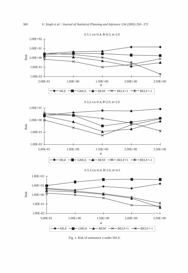
equal importance:Study of risks of proposed estimators show that risks of MLE and GMLEof �, in general, increase as� increases while risks of BESF and BELF (witha = 1.0) of �decrease initially up to� = 1.5 and then increase. But for small�, the risks of BELF (witha = −1.0) decrease as� increases. Risks of estimators of� also slightly decrease for largevalues of�. Risks of GMLE of� highly decrease as� increases (see, S-5(1)–S-5(3)).
Risks of all the estimators of� increases as� increases. Increment in the risk of MLE ishighest and BELF (witha = −1.0) shows smallest increment. Risks of other estimators of� show more increase within the range of� from 0.5 to 1.0 as compared to rest of the valuesof �, (seeFigs. S-5(4)–S-5(6)). Increment in the values of� or � show negligible effect onthe risks of estimators of�. It is also noted that the risks of BELF (witha =−1.0) decreasefor small censoring fractions.
Risks of estimators of� increase as� increases but the increment are noted to bevery small for all estimators. Risks of GMLE of� decrease for large values of� (seeFigs. S-5(7)–S-5(9)).
In general, Risks of MLE of� is highest for smallr/n. But for small�, risk of GMLEof � is large as compared to other estimators of� whereas BELF (witha = 1.0) of � givessmallest risk as compared to other estimators. It has been noted that risk of BELF (witha = −1.0) of � becomes smallest among all other estimators for��2.0. Risk of BESF of� is slightly higher than risk of BELF (witha = 1.0) (seeS-5(1)–S-5(3)).
Risks of BELF (witha =−1.0) of � has highest value while risk of BELF (witha = 1.0)of � gives smallest value as compared to other estimators of�. Risk of GMLE of � wasalso found smallest for small�. Risk of MLE of� is larger then those of GMLE, BESF andBELF (with a = 1.0) but smaller than the risk of BELF (witha = −1.0) (see figures fromS-5(4)–S-5(6)).
360 U. Singh et al. / Journal of Statistical Planning and Inference 134 (2005) 350–372
S-5.1 r/n=0.4; θ=0.5; σ=2.0
1.00E-02
1.00E-01
1.00E+00
1.00E+01
1.00E+02
5.00E-01 1.00E+00 1.50E+00 2.00E+00 2.50E+00
Ris
kR
isk
Ris
k
MLE GMLE BESF BELF=1 BELF=-1
S-5.2 r/n=0.4; θ=2.0; σ=2.0
1.00E-02
1.00E-01
1.00E+00
1.00E+01
5.00E-01 1.00E+00 1.50E+00 2.00E+00 2.50E+00
MLE GMLE BESF BELF=1 BELF=-1
S-5.3 r/n=0.4; θ=2.0; σ=0.5
1.00E-02
1.00E-01
1.00E+00
1.00E+01
1.00E+02
5.00E-01 1.00E+00 1.50E+00 2.00E+00 2.50E+00
MLE GMLE BESF BELF=1 BELF=-1
α
α
α
Fig. 1. Risk of estimators� under SELF.

U. Singh et al. / Journal of Statistical Planning and Inference 134 (2005) 350–372 361
S-5.4 r/n=0.4; α=0.5; σ=2.0
1.00E-02
1.00E-01
1.00E+00
1.00E+01
1.00E+02
5.00E-01 1.00E+00 1.50E+00 2.00E+00 2.50E+00
Ris
kR
isk
Ris
k
MLE GMLE BESF BELF=1 BELF=-1
S-5.5 r/n=0.4; α=2.0; σ=2.0
1.00E-02
1.00E-01
1.00E+00
1.00E+01
1.00E+02
5.00E-01 1.00E+00 1.50E+00 2.00E+00 2.50E+00
MLE GMLE BESF BELF=1 BELF=-1
S-5.6 r/n=0.4; α=2.0; σ=0.5
1.00E-02
1.00E-01
1.00E+00
1.00E+01
1.00E+02
5.00E-01 1.00E+00 1.50E+00 2.00E+00 2.50E+00
MLE GMLE BESF BELF=1 BELF=-1
θ
θ
θ
Fig. 2. Risk of estimators� under SELF.

362 U. Singh et al. / Journal of Statistical Planning and Inference 134 (2005) 350–372
S-5.7 r/n=0.4; α=0.5; θ=2.0
1.00E-02
1.00E-01
1.00E+00
1.00E+01
1.00E+02
1.00E+03
1.00E+04
5.00E-01 1.00E+00 1.50E+00 2.00E+00 2.50E+00
Ris
kR
isk
Ris
k
MLE GMLE BESF BELF=1 BELF=-1
S-5.8 r/n=0.4; α=2.0; θ=2.0
1.00E-02
1.00E-01
1.00E+00
1.00E+01
1.00E+02
1.00E+03
1.00E+04
5.00E-01 1.00E+00 1.50E+00 2.00E+00 2.50E+00
MLE GMLE BESF BELF=1 BELF=-1
S-5.9 r/n=0.4; α=2.0; θ=0.5
1.00E-02
1.00E-01
1.00E+00
1.00E+01
1.00E+02
1.00E+03
1.00E+04
5.00E-01 1.00E+00 1.50E+00 2.00E+00 2.50E+00
MLE GMLE BESF BELF=1 BELF=-1
σ
σ
σ
Fig. 3. Risk of estimators� under SELF.
U. Singh et al. / Journal of Statistical Planning and Inference 134 (2005) 350–372 363
L-5.1 r/n=0.4; θ=0.5; σ=2.0
1.00E-021.00E+001.00E+021.00E+041.00E+061.00E+081.00E+101.00E+121.00E+141.00E+16
5.00E-01 1.00E+00 1.50E+00 2.00E+00 2.50E+00
Ris
kR
isk
Ris
k
MLE GMLE BESF BELF
L-5.2 r/n=0.4; θ=2.0; σ=2.0
1.00E-02
1.00E-01
1.00E+00
1.00E+01
1.00E+02
5.00E-01 1.00E+00 1.50E+00 2.00E+00 2.50E+00
MLE GMLE BESF BELF
L-5.3 r/n=0.4; θ=2.0; σ=0.5
1.00E-02
1.00E-01
1.00E+00
1.00E+01
1.00E+02
1.00E+03
1.00E+04
1.00E+05
1.00E+06
5.00E-01 1.00E+00 1.50E+00 2.00E+00 2.50E+00
MLE GMLE BESF BELF
α
α
α
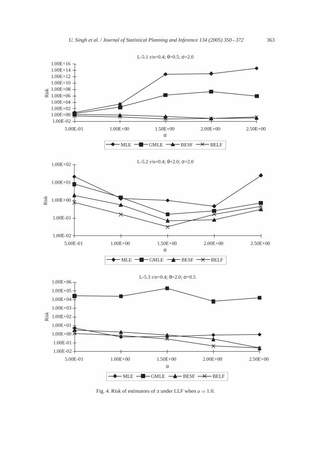
Fig. 4. Risk of estimators of� under LLF whena = 1.0.

364 U. Singh et al. / Journal of Statistical Planning and Inference 134 (2005) 350–372
L-5.4 r/n=0.4; α=0.5; σ=2.0
1.00E-02
1.00E-01
1.00E+00
1.00E+01
5.00E-01 1.00E+00 1.50E+00 2.00E+00 2.50E+00
Ris
kR
isk
Ris
k
MLE GMLE BESF BELF
L-5.5 r/n=0.4; α=2.0; σ=2.0
1.00E-02
1.00E-01
1.00E+00
1.00E+01
1.00E+02
1.00E+03
5.00E-01 1.00E+00 1.50E+00 2.00E+00 2.50E+00
MLE GMLE BESF BELF
L-5.6 r/n=0.4; α=2.0; σ=0.5
1.00E-03
1.00E-02
1.00E-01
1.00E+00
1.00E+01
5.00E-01 1.00E+00 1.50E+00 2.00E+00 2.50E+00
MLE GMLE BESF BELF
θ
θ
θ
Fig. 5. Risk of estimators of� under LLF whena = 1.0.
U. Singh et al. / Journal of Statistical Planning and Inference 134 (2005) 350–372 365
L-5.7 r/n=0.4; α=0.5;θ=2.0
1.00E-011.00E+011.00E+031.00E+051.00E+071.00E+091.00E+111.00E+131.00E+151.00E+171.00E+19
5.00E-01 1.00E+00 1.50E+00 2.00E+00 2.50E+00
Ris
kR
isk
Ris
k
MLE GMLE BESF BELF
L-5.8 r/n=0.4; α=2.0; θ=2.0
1.00E-03
1.00E-011.00E+011.00E+03
1.00E+051.00E+07
1.00E+09
1.00E+111.00E+131.00E+15
1.00E+17
5.00E-01 1.00E+00 1.50E+00 2.00E+00 2.50E+00
MLE GMLE BESF BELF
L-5.9 r/n=0.4; α=2.0; θ=0.5
1.00E-02
1.00E-01
1.00E+00
1.00E+01
1.00E+02
1.00E+03
1.00E+04
1.00E+05
1.00E+06
1.00E+07
5.00E-01 1.00E+00 1.50E+00 2.00E+00 2.50E+00
MLE GMLE BESF BELF
σ
σ
σ
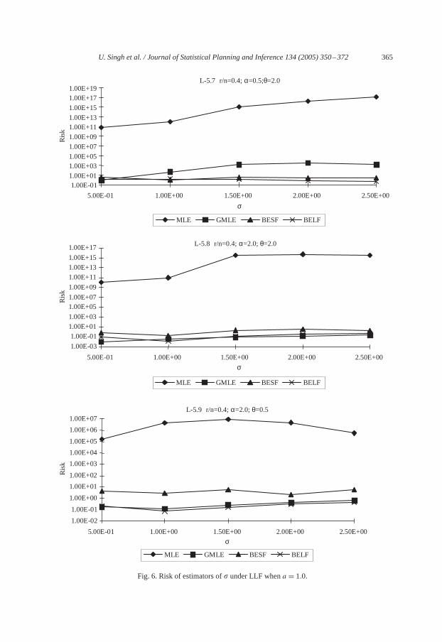
Fig. 6. Risk of estimators of� under LLF whena = 1.0.
366 U. Singh et al. / Journal of Statistical Planning and Inference 134 (2005) 350–372
L-5.10 r/n=0.4; θ=0.5; σ=2.0
1.00E-03
1.00E-02
1.00E-01
1.00E+00
1.00E+01
5.00E-01 1.00E+00 1.50E+00 2.00E+00 2.50E+00
Ris
kR
isk
Ris
k
MLE GMLE BESF BELF
L-5.11 r/n=0.4; θ=2.0; σ=2.0
1.00E-02
1.00E-01
1.00E+00
1.00E+01
5.00E-01 1.00E+00 1.50E+00 2.00E+00 2.50E+00
MLE GMLE BESF BELF
L-5.12 r/n=0.4; θ=2.0; σ=0.5
1.00E-02
1.00E-01
1.00E+00
1.00E+01
5.00E-01 1.00E+00 1.50E+00 2.00E+00 2.50E+00
MLE GMLE BESF BELF
α
α
α
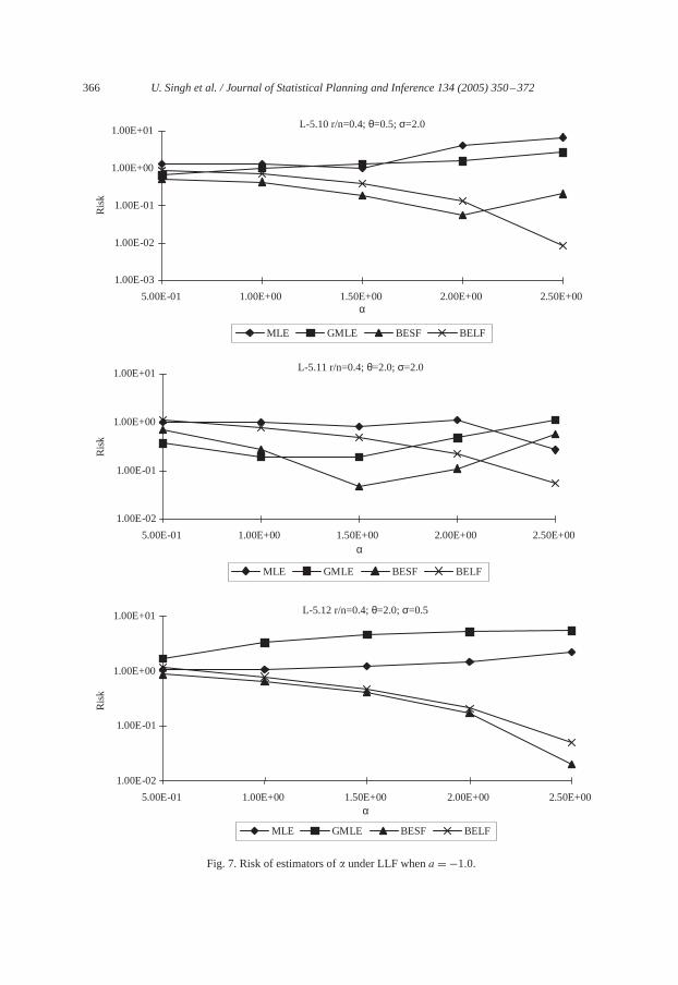
Fig. 7. Risk of estimators of� under LLF whena = −1.0.
U. Singh et al. / Journal of Statistical Planning and Inference 134 (2005) 350–372 367
L-5.13 r/n=0.4; α=0.5; σ=2.0
1.00E-02
1.00E-01
1.00E+00
1.00E+01
1.00E+02
5.00E-01 1.00E+00 1.50E+00 2.00E+00 2.50E+00
Ris
kR
isk
Ris
k
MLE GMLE BESF BELF
L5.14 r/n=0.4; α=2.0; σ=2.0
1.00E-02
1.00E-01
1.00E+00
1.00E+01
1.00E+02
5.00E-01 1.00E+00 1.50E+00 2.00E+00 2.50E+00
MLE GMLE BESF BELF
L-15 r/n=0.4; α=2.0; σ=0.5
1.00E-03
1.00E-02
1.00E-01
1.00E+00
1.00E+01
5.00E-01 1.00E+00 1.50E+00 2.00E+00 2.50E+00
MLE GMLE BESF BELF
θ
θ
θ
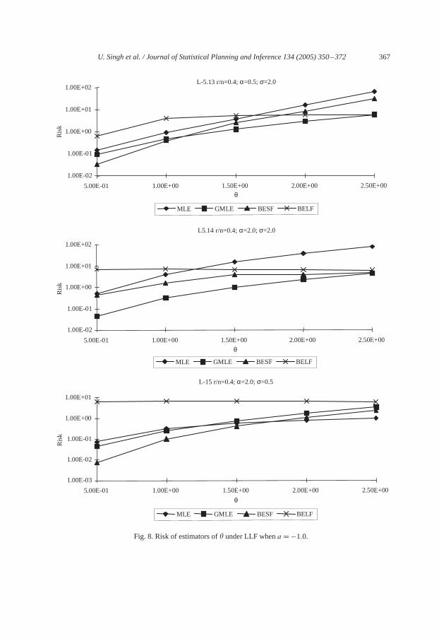
Fig. 8. Risk of estimators of� under LLF whena = −1.0.

368 U. Singh et al. / Journal of Statistical Planning and Inference 134 (2005) 350–372
L-5.16 r/n=0.4; α=0.5; θ=2.0
1.00E-01
1.00E+00
1.00E+01
1.00E+02
5.00E-01 1.00E+00 1.50E+00 2.00E+00 2.50E+00
MLE GMLE BESF BELF
L-5.17 r/n=0.4; α=2.0; θ=2.0
1.00E-03
1.00E-02
1.00E-01
1.00E+00
1.00E+01
1.00E+02
5.00E-01 1.00E+00 1.50E+00 2.00E+00 2.50E+00
MLE GMLE BESF BELF
L-5.18 r/n=0.4; α=2.0; θ=0.5
1.00E-02
1.00E-01
1.00E+00
1.00E+01
1.00E+02
5.00E-01 1.00E+00 1.50E+00 2.00E+00 2.50E+00
Ris
kR
isk
Ris
k
MLE GMLE BESF BELF
σ
σ
σ
Fig. 9. Risk of estimators of� under LLF whena = −1.0.
U. Singh et al. / Journal of Statistical Planning and Inference 134 (2005) 350–372 369
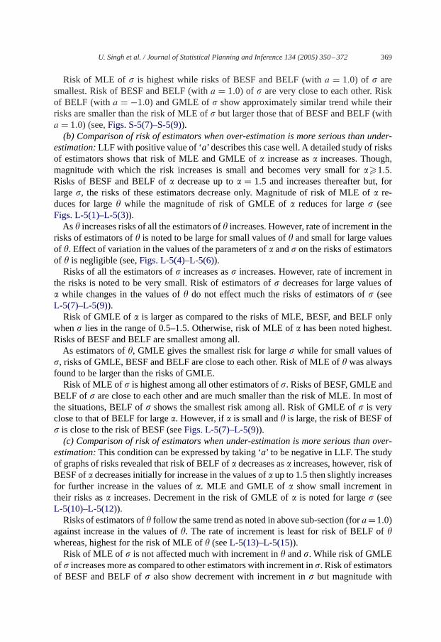
Risk of MLE of � is highest while risks of BESF and BELF (witha = 1.0) of � aresmallest. Risk of BESF and BELF (witha = 1.0) of � are very close to each other. Riskof BELF (with a = −1.0) and GMLE of� show approximately similar trend while theirrisks are smaller than the risk of MLE of� but larger those that of BESF and BELF (witha = 1.0) (see,Figs. S-5(7)–S-5(9)).(b) Comparison of risk of estimators when over-estimation is more serious than under-
estimation:LLF with positive value of ‘a’ describes this case well. A detailed study of risksof estimators shows that risk of MLE and GMLE of� increase as� increases. Though,magnitude with which the risk increases is small and becomes very small for��1.5.Risks of BESF and BELF of� decrease up to� = 1.5 and increases thereafter but, forlarge�, the risks of these estimators decrease only. Magnitude of risk of MLE of� re-duces for large� while the magnitude of risk of GMLE of� reduces for large� (seeFigs. L-5(1)–L-5(3)).
As� increases risks of all the estimators of� increases. However, rate of increment in therisks of estimators of� is noted to be large for small values of� and small for large valuesof �. Effect of variation in the values of the parameters of� and� on the risks of estimatorsof � is negligible (see,Figs. L-5(4)–L-5(6)).
Risks of all the estimators of� increases as� increases. However, rate of increment inthe risks is noted to be very small. Risk of estimators of� decreases for large values of� while changes in the values of� do not effect much the risks of estimators of� (seeL-5(7)–L-5(9)).
Risk of GMLE of � is larger as compared to the risks of MLE, BESF, and BELF onlywhen� lies in the range of 0.5–1.5. Otherwise, risk of MLE of� has been noted highest.Risks of BESF and BELF are smallest among all.
As estimators of�, GMLE gives the smallest risk for large� while for small values of�, risks of GMLE, BESF and BELF are close to each other. Risk of MLE of� was alwaysfound to be larger than the risks of GMLE.
Risk of MLE of � is highest among all other estimators of�. Risks of BESF, GMLE andBELF of � are close to each other and are much smaller than the risk of MLE. In most ofthe situations, BELF of� shows the smallest risk among all. Risk of GMLE of� is veryclose to that of BELF for large�. However, if� is small and� is large, the risk of BESF of� is close to the risk of BESF (seeFigs. L-5(7)–L-5(9)).(c) Comparison of risk of estimators when under-estimation is more serious than over-
estimation:This condition can be expressed by taking ‘a’ to be negative in LLF. The studyof graphs of risks revealed that risk of BELF of� decreases as� increases, however, risk ofBESF of� decreases initially for increase in the values of� up to 1.5 then slightly increasesfor further increase in the values of�. MLE and GMLE of � show small increment intheir risks as� increases. Decrement in the risk of GMLE of� is noted for large� (seeL-5(10)–L-5(12)).
Risks of estimators of� follow the same trend as noted in above sub-section (fora =1.0)against increase in the values of�. The rate of increment is least for risk of BELF of�whereas, highest for the risk of MLE of� (seeL-5(13)–L-5(15)).
Risk of MLE of � is not affected much with increment in� and�. While risk of GMLEof � increases more as compared to other estimators with increment in�. Risk of estimatorsof BESF and BELF of� also show decrement with increment in� but magnitude with

370 U. Singh et al. / Journal of Statistical Planning and Inference 134 (2005) 350–372
which risks increase is not large. Risks of estimators of� reduce for large values of� (seeL-5(16)–L-5(18)).
None of the estimators gives smallest risk in entire considered range. However, in most ofconsidered case, risk of BESF of� is either smallest or close to the smallest risk. However,if ��1.5 it is noted that the risk of MLE of� is less than the risk of BESF particularlywhen� is large. Risk of BELF of� decreases for increase in�. For large values of�, riskof BELF of � is smaller than that of BESF.
Risk of MLE of � is close to the risks of Bayes estimators of� for smallr/n and sometimes it is greater than the risks of Bayes estimator, particularly forr/n�0.6. Risk of BELFof � is highest while GMLE of� gives smallest risk when� is large. For small�, risk ofBESF of� gives smallest risk among all (seeL-5(13)–L-5(15)).
Risk of MLE of � is noted highest while risk of GMLE of� is found smallest. Risksof BESF and BELF of� lies between the risks of MLE of� and risk of GMLE of� (seeL-5(16)–L-5(18)).
6. Conclusions
From the above discussion, we see that the risks of BELF for� (with a = 1.0) are small-est or close to the risks of those estimators for which risk is smallest in the case whereunder-estimation and over-estimation are of equal importance or over-estimation is moreserious than the under-estimation. In these situations BESF also has a value close to thesmallest risk. It is also noted that GMLE, forr/n� 0.6 and� and� large, has risk closeto the risk of BELF and BESF. Hence, we may safely recommend BELF and BESF fortheir use in these cases. But when under-estimation is more serious than over-estimation,the risk of BESF, is in general smallest. However, ifr/n�0.6 and� and� both are large,the risk of GMLE was found to be least. On the other hand, ifr/n�0.6, ��1.5 and either� or � is large, MLE has smallest risk. Therefore, the use of BESF may be recommendedfor this situation but forr/n�0.6 and� and � large one may use GMLE. The use ofMLE may be recommended whenr/n�0.6, ��1.5 and at least one out of� and� islarge.
On the estimation of�, for the case when over-estimation and under-estimation are ofequal importance, risk of BELF (witha = 1.0) is often smallest. Risk of GMLE and BESF(when� is large and� is small) are also close to the risk of BELF. Therefore, BELF (witha = 1.0) may safely be used for estimation of�. However, when over-estimation is moreserious than the under-estimation BELF of� may be recommended for its use because riskof BELF of � is smallest or close to the risks of BESF and GMLE (when� and� both arelarge) which have smallest risks. If under-estimation is more serious than over-estimation,GMLE and BESF may be considered for their use because these provide smallest risk ascompared to other estimators.
If we consider the estimation of�, in the case when over-estimation and under-estimationare of equal importance or over-estimation is more serious than under-estimation then BELF(with a = 1.0) of � may be recommend for its use as compared to other estimators. This isbecause its risk is close to the risk of estimators which have smallest risks. In the condition,when under-estimation is more serious than over-estimation, use of GMLE of� is worth

U. Singh et al. / Journal of Statistical Planning and Inference 134 (2005) 350–372 371
recommending due to its smallest risk or closer to the risks of estimators, which havesmallest risks.
In brief, we may conclude that Bayes estimators (BESF and BELF) are found to per-form best in most of the situations. In the situations when these are not best, there isa marginal loss in the sense of risk. Hence, use of BESF and BELF may be safelyrecommended.
Acknowledgements
This research work of Pramod K. Gupta is financially supported by the Council of Sci-entific and Industrial Research, Government of India, through Senior Research Fellowship.We are highly grateful to the referees and Editors for their suggestions, which led to im-provement in the quality of the paper.
References
Bain, L.J., 1974. Analysis for the linear failure-rate life-testing distribution. Technometrics 16, 551–559.Basu, A.P., Ebrahimi, N., 1991. Bayesian approach to life testing and reliability estimation using asymmetric loss
function. J. Statist. Plann. Inference 29, 21–31.Berger, J.O., 1985. Statistical Decision Theory and Bayesian Analysis. Springer, New York.Box, G.E.P., Tiao, G.C., 1973. Bayesian Inference in Statistical Analysis. Addison-Wesley, Reading,
Massachusetts.Gore, A.P., Paranjape, S., Rajarshi, M.B., Gadgil, M., 1986. Some methods for summarizing survivorship data.
Biometrical J. 28, 557–586.Hjorth, U., 1980. A reliability distribution with increasing decreasing and bathtub-shaped failure rates.
Technometrics 22, 99–107.Khatree, R., 1992. Estimation of guarantee time and mean after warranty for two-parameter exponential failure
model. Austral. J. Statist. 342, 207–215.Lawless, J.F., 1982. Statistical Methods for Lifetime Data. Wiley, New York.Mann, N.R., Schafer, R.E., Singpurwalla, N.D., 1974. Methods for Statistical Analysis of Reliability and Life
Data. Wiley, New York.Martz, H.F., Waller, R.A., 1982. Bayesian Reliability Analysis. Wiley, New York.Mudholkar, G.S., Srivastava, D.K., 1993. Exponentiated Weibull family for analyzing bathtub failure-rate data.
IEEE Trans. Reliability 42, 299–302.Mudholkar, G.S., Srivastava, D.K., Freimer, M., 1995. Exponentiated Weibull family: a reanalysis of the bus motor
failure rate data. Technometrics 37, 436–445.NAG, 1993. Numerical Algorithms Group. Mark 16 Numerical Algorithms Group, Downers Grove, IllinoisParsian, A., 1990. On the admissibility of an estimator of a normal mean vector under a LINEX loss function.
Ann. Math. Statist. 42, 657–669.Prentice, R.L., 1975. Discrimination among some parametric models. Biometrika 62, 607–614.Rajarshi, S., Rajarshi, M.B., 1988. Bathtub distribution: a review. Commun. Statist. Theory Methods A13,
2597–2621.Singh, U., Gupta, P.K., Upadhyay, S.K., 2002. Estimation of exponentiatedWeibull shape parameters under LINEX
loss function. Commun. Statist. Simulation Comput. 31 (4), 523–537.Sinha, S.K., 1986. Reliability and Life Testing. Wiley Eastern Ltd., Delhi, India.Slymen, D.J., Lachenbruch, P.A., 1984. Survival distributions arising from two families and generated by
transformation. Commun. Statist. Theory. Methods A13, 1179–1201.

372 U. Singh et al. / Journal of Statistical Planning and Inference 134 (2005) 350–372
Varian, H.R., 1975. A Bayesian Approach to Real Estate Assessment. in: Stephen, E.F., Zellner, A. (Eds.),Studies in Bayesian Econometrics and Statistics in Honor of Leonard J. Savage. North-Holland, Amsterdam,pp. 195–208.
Zellner, A., 1986. Bayesian estimation and prediction using asymmetric loss function. J. Amer. Statist. Assoc. 81,446–451.