Energy SystDOI 10.1007/s12667-012-0050-4

O R I G I NA L PA P E R

An energy management system for off-grid powersystems

Daniel Zelazo · Ran Dai · Mehran Mesbahi

Received: 3 November 2011 / Accepted: 16 January 2012© Springer-Verlag 2012

Abstract Next generation power management at all scales will rely on the efficientscheduling and operation of both generating units and loads to maximize efficiencyand utility. The ability to schedule and modulate the demand levels of a subset ofloads within a power system can lead to more efficient use of the generating units.These methods become increasingly important for systems that operate indepen-dently of the main utility, such as microgrid and off-grid systems. This work ex-tends the principles of unit commitment and economic dispatch problems to off-gridpower systems where the loads are also schedulable. We propose a general optimiza-tion framework for solving the energy management problem in these systems. Animportant contribution is the description of how a wide range of sources and loads,including those with discrete states, non-convex, and nonlinear cost or utility func-tions, can be reformulated as a convex optimization problem using, for example, ashortest path description. Once cast in this way, solution are obtainable using a sub-gradient algorithm that also lends itself to a distributed implementation. The methodsare demonstrated by a simulation of an off-grid solar powered community.

Keywords Off-grid · Energy management · Lagrangian relaxation · Shortest-pathalgorithm

D. Zelazo (�)Institute for Systems Theory and Automatic Control, Universität Stuttgart, 70550 Stuttgart, Germanye-mail: daniel.zelazo@ist.uni-stuttgart.de

R. Dai · M. MesbahiDepartment of Aeronautics and Astronautics, University of Washington, Seattle, WA, 98195-2400,USA

R. Daie-mail: dairan@washington.edu

M. Mesbahie-mail: mesbahi@washington.edu

D. Zelazo et al.

NomenclatureG,L number of generating units, number of loadsG, L set of generating units, set of loadsT time horizonT set of time indicesi, j, t index for generating units, loads, and timegi(t), yj (t) power level of generating unit i ∈ G and demand of load

j ∈ L at time t ∈ Tx

gi (t), u

gi (t) state and control variables for generating unit i ∈ G at time

t ∈ Txlj (t), u

lj (t) state and control variables for load j ∈ L at time t ∈ T

fgi (gi(t), x

gi (t), u

gi (t)) dynamic evolution of generating unit variables for unit i ∈ G

f lj (yj (t), x

lj (t), u

lj (t)) dynamic evolution of load variables for load j ∈ L

Ci(gi(t), xgi (t), u

gi (t)) operating cost of generator unit i ∈ G at time t ∈ T

Uj (yj (t), xlj (t), u

lj (t)) utility of load j ∈ L at time t ∈ T

S gi (t), S l

j (t) abstract constraint set for generator unit i ∈ G and loadj ∈ L at time t ∈ T

X gi (t), U g

i (t) abstract constraint set for generator load state and controlvariables at t ∈ T

X lj (t), U l

j (t) abstract constraint set for load state and control variables att ∈ T

L(·), q(λ) Lagrangian and dual functionsλt , v(λt ), α Lagrange multiplier and sub-gradient at time t ∈ T , step size

1 Introduction

The push to modernize power systems towards a “smart” grid is driven by a varietyof factors including environmental compliance, economic advantage, and improvedreliability, robustness, and service. Indeed, the development of technologies and ap-plications related to smart grids is now a centerpiece for a clean-energy economyand initiative in both the United States and European Union [1, 2]. Precisely how asmart grid should look like and operate is now an active area of research in the powersystems community [3–6].

The ultimate success of a smart-grid infrastructure will depend on a decreasingdependence of consumers on the main power distribution network. A first step inthis direction is through the so-called microgrid. A microgrid contains various dis-tributed energy resources (i.e., wind turbines, photovoltaic arrays, fuel cells, gen-erators), energy storage devices (i.e., super-capacitors, batteries), and controllableloads [7]. A key feature of microgrids is their ability to operate autonomously, i.e.isolated from the main power grid. The success of a microgrid-type architecture de-pends not only on the development of new energy resources and storage capabilities,but equally on the ability to control and schedule these systems in a distributed man-ner [8]. Another challenge associated with microgrid is managing the import and

An energy management system for off-grid power systems

Fig. 1 Off-grid systems operate independently of a microgrid and smart grid architecture

export of power to the main distribution network. This relates to both the power bal-ance of the entire network and the economic bartering between the utility and themicrogrid [9, 10].

While much of the vision for smart and microgrids are aimed at large scale imple-mentation, many of the fundamental principles and techniques can also be adapted forsmaller-sized self-contained power systems. Such systems are referred to as off-gridsystems [11–13]. Off-grid systems inherit many similarities to microgrids, primar-ily regarding the ability to operate independently of the main grid; this is visualizedin Fig. 1. Off-grid systems can include small self-contained power systems such ashybrid and electrical vehicles (HEV) [14–16] and the “more electric aircraft” (MEA)pursued by the United States Air Force [17–19]. A larger scale version, including thescenario examined in this work, is that of smart homes and communities residing offthe main grid [10, 20, 21].

The main component of an off-grid system, therefore, is an effective energy man-agement system (see Fig. 1). The energy management system must coordinate thescheduling and operation of all the distributed generation sources in the system whilealso managing the efficient use of the loads. This should be done in a way that theoverall operating cost for generation is minimized and the utility obtained by theuser through the loads is maximized. Traditionally, the scheduling and operation oflarge scale power systems involves the solution of the unit commitment (UC) andeconomic dispatch (ED) problems. These problems determine an optimal scheduleand commitment level for each generating unit in a power system based on a setof constraints, including reserve power, operating parameters, and forecasted loadsover a finite time horizon. Many solution methods have been proposed includingLagrangian relaxation techniques and dynamic programming [22–26]. The mixed-integer linear programming (MILP) method applicable to small and medium sizedpower systems with linear models is another approach to search for the optimal con-

D. Zelazo et al.

tinuous and integer variables [27–29]. One of the difficulties related to this class ofproblems, however, is that the demand level is often not known precisely.

While this issue is perhaps unavoidable when considering large scale power sys-tems, the notion of unknown load demand levels for smaller scale power systemsmay not be as prevalent. In applications such as HEV and MEA, certain classes ofloads may follow very precise profiles for their demand level. Such loads, for exam-ple, avionics in an aircraft or a refrigerator in an off-grid home, may be critical tothe successful operation of the power system, while others, such as the environmen-tal control system, may follow looser demand profiles and have flexibility in theirdemand level. In this direction, we consider an extension of the economic dispatchand unit commitment problem to include the scheduling and operation of a subset ofloads within the power system. The notion of an optimal load demand pattern canbe considered as the “dual” problem to the ED and UC formulation; if generationof power is modeled as a fixed resource then indeed the scheduling of loads wouldfollow the same methodology. For ED and UC of power generation, the optimizationobjective is the minimization of the overall fuel and operating costs. For loads, weconsider the maximization of the load utility. The utility of certain loads is expectedto be highly dependent on the application, and the exact form of these utility func-tions may not have the same analytic foundation as for generation. A possible sourcefor these utility functions might be borrowed from microeconomic principles in theform of a demand curve or benefit function [30]. Such utility-based approaches havebeen considered for real-time pricing algorithms within a smart grid framework withquadratic or linear utility functions [31, 32]. In [33], an energy management systemfor smart homes aimed at maximizing the net benefit by end users is considered.The general problem of utility maximization has been studied for problems related tonetwork architecture and resource allocation [34, 35].

The notion of scheduling loads in a power system is not an entirely new idea.A common technique employed in self-contained power systems is load shedding.In many situations, such as in aircraft power systems, load shedding is based on aheuristic where loads are “ranked” according to a priority list [36, 37]; when there ismore demand than power available, loads at the bottom of the list are shed until thepower balance is restored. More sophisticated load shedding methods utilizing tech-niques from optimization have also been employed [38], but the fundamental notionof a priority is still utilized. Direct load control (DLC) is another attempt to controlthe load demand although the general approach is motivated by the capabilities ofthe generating units rather than the utility of the loads [39–41]. With the recognitionof the importance of smart grids, DLC has been revisited with a broader focus butis still faced with challenges such as the understanding the relationship between theconsumer and the supplier [30, 42–44].

The main contribution of this work, therefore, is the development of an energymanagement system for an off-grid power system. This work extends the principlesand techniques employed in traditional UC and ED problems to self-contained powersystems that also permit the scheduling of loads. Specifically, we formulate an opti-mization problem that minimizes the operating and generating costs of a distributedgeneration system while simultaneously maximizing the utility of the loads in thepower system. In the process of deriving the optimization model, we describe how

An energy management system for off-grid power systems

qualitative descriptions of generating units and loads can be mathematically mod-eled in a way that leads to tractable solution algorithms for solving the problem; thisgreatly generalizes the current methods used related to load control in off-grid sys-tems. The structure of the proposed model lends itself to a distributed implementationusing a sub-gradient algorithm. An important component of the algorithm describedhere is the use of a shortest path solution to solve component level sub-problemsbased on the qualitative description of each unit. The proposed distributed algorithmallows for parallel computation while maintaining stable calculation performancewith increasing number of electric components in the system. Furthermore, the qual-itative descriptions developed allows to consider a broader class of utility functions,including discrete, nonlinear, and non-convex (such as a priority-type utility), as com-pared to other solutions [31, 32]. Finally, the algorithm is easy to implement, leadingto a cheaper solution compared to that of commercial MILP software. A detailed dis-cussion of the advantages of a Lagrangian relaxation technique compared to MILP isgiven in [28, 29].

The outline of this paper is as follows. In Sect. 2 we first develop the power systemmodel employed in this work. This section includes a generic description of the gen-erating units and loads including their cost and utility functions along with their as-sociated constraints. The optimization model is also derived in Sect. 2 along with thecompanion dual problem. The description of the dual problem provides insights intoalternative descriptions of the model, that in turn, leads to tractable solution methods.In Sect. 2.1 we explore how a wide description of generating units and loads can beformulated into equivalent tractable problems. The description of a decentralized so-lution method for solving the model is presented in Sect. 3. A simulation example ofan off-grid solar powered community is provided in Sect. 4, and concluding remarksare given in Sect. 5.

2 An optimization framework for an energy management system

The general objective for a distributed generation system with schedulable loads is todetermine a schedule and commitment level for each generating unit and load suchthat the running costs of the generating units are minimized and the utility of the loadsare maximized.1 In addition to cost minimization and utility maximization, each unitmust also respect its own operating constraints and the aggregate power balance ofthe system.

Generally, the generating units and loads can contain systems with both continu-ous and discrete operating states. For example, a battery might be modeled to have aconstant charge and discharge rate. In this way, the variable gi(t), corresponding tothe battery power level, will be a discrete variable. In contrast, a generator can outputpower continuously, corresponding to gi(t) being a continuous variable. The con-tinuous or discrete nature of each element is encoded in the corresponding abstractconstraint sets for the units (described in the nomenclature section).

1At times we will also refer to the “disutility” of loads. In this way, we aim to minimize the disutility.

D. Zelazo et al.

In this direction, we can express the objective of the energy management systemthat we would like to minimize as,

J (g,y,xg,xl ,ug,ul) =T∑

t=1

(G∑

i=1

Ci

(gi(t), x

gi (t), u

gi (t)

)

−L∑

j=1

Uj

(yj (t), x

lj (t), u

lj (t)

))

. (2.1)

For notational simplicity we introduced the bold-faced vector notation; for exampleg(t) = [g1(t) · · · gG(t) ]T .

Remark 1 The cost minimization or utility maximization component of the objectivefunction (2.1) can be assigned a “priority” by introducing a scalar weight for eachterm. For example, assigning a weight of 0 to the utility maximization term corre-sponds to the cost function for a traditional ED and UC problem.

When considering an optimization framework for solving the scheduling and com-mitment problems, it is standard to assume certain properties for the objective func-tion (2.1). For example, convexity and continuity of the cost function (and concavityof the utility function) allow, through the tools of convex analysis, efficient solutionmethods in addition to strong guarantees on rates of convergence and optimality [45].However, in many qualitative descriptions of generating units and loads, such an idealmathematical description of their cost or utility might not be possible. Rather, thefunctions may have discontinuities and convexity or linearity might not be guaran-teed. Combined with the possibly discrete nature of the optimization variables, min-imization of (2.1) becomes computationally difficult. We will show in this sectionthat for certain forms of the cost and utility functions, equivalent representation ofthe objective can be derived that lead to tractable solution methods.

The optimization problem we aim to solve, which we call problem P , can now bestated as

ming,y,xg,xl ,ug,ul

J (g,y,xg,xl ,ug,ul ) (2.2)

s.t. (gi(t), xgi (t), u

gi (t)) ∈ Qg

i (t), ∀i ∈ G, t ∈ T (2.3)

(yj (t), xlj (t), u

lj (t)) ∈ Ql

j (t), ∀j ∈ L, t ∈ T (2.4)

xgi (t + 1) = f

gi (gi(t), x

gi (t), u

gi (t)), ∀i ∈ G, j ∈ L (2.5)

xlj (t + 1) = f l

j (yj (t), xlj (t), u

lj (t)), ∀i ∈ G, j ∈ L (2.6)

L∑

j=1

yj (t) =G∑

i=1

gi(t), ∀t ∈ T . (2.7)

We introduced a further notation for simplification, Qgi (t) = S g

i (t) × X gi (t) ×

U gi (t) and Ql

i (t) = S li (t) × X l

i (t) × U li (t). The constraints (2.5) and (2.6) represent

An energy management system for off-grid power systems

any dynamic descriptions of a unit, such as the decision to turn a unit on or off. Theconstraint (2.7) is the aggregate power balance equation of the power system. Notethat this constraint is the only coupling constraint in the problem P ; in the absenceof such a constraint the problem could be decomposed in a straightforward way, andmuch of the challenge in solving P stems from this constraint. It is also worth men-tioning that the power balance equation (2.7) assumes that the power system resideson a single power bus.

The dimension of this program is dependent on the time horizon, T = |T | and thenumber of generating units G and loads L. In this regard, the size of this problemis O(T (G + L)); the exact size will depend on the complexity of the dynamic andabstract constraints for each generating unit and load. Finally, we would like to re-emphasize that the model in (2.2), in its most general form, represents a non-linear,non-convex, and mixed-integer program.

Remark 2 The framework presented above provides, in general, a complete scheduleand commitment level for all units in the power system. However, certain scenariosmight require that a unit follow a nominal or desired state trajectory. Our earlierdiscussion also handles the situation where a nominal trajectory must be satisfied(for example, by specifying the constraint sets S g and S l as an equality constraint ateach time t). We also would like to highlight that our problem formulation implicitlyhandles a scenario where a nominal trajectory must be tracked, but the unit is allowedto deviate from that trajectory in some specified way. In particular, we note that thecost functions for each unit can be designed such that the error between a nominaltrajectory and the real trajectory is minimized (e.g., Ci(gi(t)) = (gi(t) − g(t))2 forsome reference trajectory g(t)). The constraint sets S g and S l would then capture theallowable deviations from the nominal trajectory (e.g., gi(t) ∈ [g(t) − ε, g(t) + ε]).

Before considering solution methods for the problem P , we first describe a fewclasses of units and their associated objective functions and constraint sets. We wouldlike to emphasize that the precise form of these functions is of paramount importancefor the development of a solution methodology.

2.1 Unit descriptions

A significant challenge in solving problem P is a precise description of the cost andutility functions, and the constraints of each unit (both dynamic and static). In thisdirection, we define here a few general classes of units.

2.1.1 Convex and continuous objective, 1 state (CC1)

This represents the simplest class of a generating unit or load. We assume the cost(utility) function is a convex (concave) and continuous function. While the generalform of the cost function (e.g. piecewise continuous or smooth) will ultimately dic-tate the appropriate solution method, this form allows for a traditional approach forfinding a solution method. For example, one might consider a piecewise-linear costcurve representing a progressively increasing cost as the output power increases. An

D. Zelazo et al.

example of a utility function for loads could be an α-fair utility curve commonly usedin network utility maximization problems [34].

The other defining property for units of this type relates to the number of statesrequired to describe its operation. Units that are ‘always on’ do not have to be sched-uled as there is no ability to change the state of the unit; for example, a refrigeratorin an off-grid home should be modeled as such a unit. Critical loads, such as avionicsin aircraft, can also be modeled in this way. Therefore, the dynamic constraints (2.5)and (2.6) are not needed.2 The only constraints these units must consider are the ab-stract constraint sets S g

i (t) and S lj (t) corresponding to the lower and upper bounds on

the power output (demand) level of the unit. In the absence of a dynamic constraint,the objective from the perspective of each unit is to minimize the cost of generation(maximize the load utility) while respecting the aggregate power balance constraintof the system.

2.1.2 Convex and continuous objective, n states (CCn)

A natural generalization of the class CC1 is to include multiple operating states de-scribing the operation of the unit. As with CC1, we assume the cost and utility func-tions are convex (concave) and continuous. The addition of multiple operating statesadds the scheduling component to problem P . This class of units perhaps describesthe most common types of units found in a self-contained power system. While theexact nature of each unit will require a customized model, we will show here a fewexamples to illustrate the general procedure. The following models represent exten-sions and variations to the basic models used in [22, 26].

Example 1 (On/Off units) The simplest example is for n = 2, corresponding to a unitthat can be switched on or off. This type of unit has dynamics of the form3

xg(t + 1) = ug(t), (2.8)

with x(t) ∈ X = {0,1} and u(t) ∈ U = {0,1}, for all t ∈ T . Here we associate thestate value x(t) = 0 to ‘off’ and x(t) = 1 to ‘on.’ Using this dynamic description weare also able to explicitly consider any costs associated with a state transition. Forexample, the cost function Ci(g(t), xg(t), ug(t)) (and utility Ui(y(t), xl(t), ul(t)))given in (2.1) can be decomposed to reflect transition costs in addition to generation(utility) costs. In this way, we can write the cost function as

C(g(t), xg(t), ug(t)

) = P g(g(t), xg(t)) + Sg(xg(t), ug(t)); (2.9)

the function is composed of a cost associated with generating power at a level g(t)

(and the state to ensure that when the device is ‘off’ there is no cost for generation),

2They can be included for completeness by defining, for example, xgi(t + 1) = f

gi

(gi (t), xgi(t),

ugi(t)) = 0.

3A similar formulation can be used for the loads.

An energy management system for off-grid power systems

and the cost of switching states in the next time interval.4 The associated cost for theload will have the similar form;

U(y(t), xl(t), ul(t)

) = P l(y(t), xl(t)) − Sl(xl(t), ul(t)); (2.10)

state-transition costs for loads are considered in the same way as for generators whichrequires those costs to be minimized, leading to the above form.

It is assumed for this class of units that the power variable g(t) (y(t)) is contin-uous, and the objective function P g (P l) is also continuous and convex (concave).That is, the constraint set S g(t) (S l(t)) should be described as a continuous interval.The transition cost will typically have the following form,

Sg(xg(t), ug(t)) =

⎧⎪⎪⎪⎨

⎪⎪⎪⎩

c1(t), if (xg(t), ug(t)) = (0,0)

c2(t), if (xg(t), ug(t)) = (0,1)

c3(t), if (xg(t), ug(t)) = (1,0)

c4(t), if (xg(t), ug(t)) = (1,1);(2.11)

the constants ci(t) should be non-negative and can in general be time varying. Exam-ples include standard electrical appliances such as lighting systems or a microwaveoven in an off-grid home.

Example 2 (Up/down time accumulation cost) Another example considers a unit withn = 2 states with a cost (utility) that is a function of the power level, transition states,and the cumulative time that the unit is ‘on’ or ‘off’. For example, when a dish washeror oven is scheduled for use, the utility obtained by the user could potentially bedegraded if the load must be turned off during its operation. The dynamics can bewritten as

xg(t + 1) ={

xg(t) + ug(t), if xg(t)ug(t) > 0

ug(t), if xg(t)ug(t) < 0,(2.12)

with xg(t) ∈ X = {−T , . . . ,−2,−1,1,2, . . . , T } and ug(t) ∈ U = {−1,1}, for allt ∈ T . Here we take positive values of xg(t) to denote the number of time steps theunit is ‘on’, and negative values for the number of time steps the unit is ‘off’. There-fore, the ‘on’ state corresponds to x(t) > 0, and ‘off’ to x(t) < 0. This is illustratedwith a state transition diagram shown in Fig. 2 (the diagram also includes minimumon and off time constraints, discussed below).

The cost function can be decomposed in a similar manner as in (2.9). As in theprevious example, this class of unit requires that the constraint variables S g(t) andS l(t) are continuous intervals. The cost function for such a setting would most natu-rally be described by a piece-wise continuous (and convex/concave) function. In thisway, the time that the unit is in the ‘on’ or ‘off’ state would constitute break-pointsfor the objective function.

4In this way, the transition cost reflects a change in state at time t to time (t + 1); the transition costcould similarly be defined to reflect the change from time (t − 1) to t , representing a slightly differentinterpretation for the total cost at time t .

D. Zelazo et al.

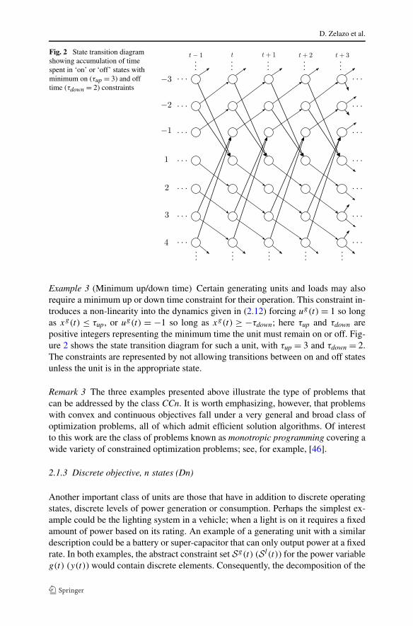
Fig. 2 State transition diagramshowing accumulation of timespent in ‘on’ or ‘off’ states withminimum on (τup = 3) and offtime (τdown = 2) constraints

Example 3 (Minimum up/down time) Certain generating units and loads may alsorequire a minimum up or down time constraint for their operation. This constraint in-troduces a non-linearity into the dynamics given in (2.12) forcing ug(t) = 1 so longas xg(t) ≤ τup, or ug(t) = −1 so long as xg(t) ≥ −τdown; here τup and τdown arepositive integers representing the minimum time the unit must remain on or off. Fig-ure 2 shows the state transition diagram for such a unit, with τup = 3 and τdown = 2.The constraints are represented by not allowing transitions between on and off statesunless the unit is in the appropriate state.

Remark 3 The three examples presented above illustrate the type of problems thatcan be addressed by the class CCn. It is worth emphasizing, however, that problemswith convex and continuous objectives fall under a very general and broad class ofoptimization problems, all of which admit efficient solution algorithms. Of interestto this work are the class of problems known as monotropic programming covering awide variety of constrained optimization problems; see, for example, [46].

2.1.3 Discrete objective, n states (Dn)

Another important class of units are those that have in addition to discrete operatingstates, discrete levels of power generation or consumption. Perhaps the simplest ex-ample could be the lighting system in a vehicle; when a light is on it requires a fixedamount of power based on its rating. An example of a generating unit with a similardescription could be a battery or super-capacitor that can only output power at a fixedrate. In both examples, the abstract constraint set S g(t) (S l(t)) for the power variableg(t) (y(t)) would contain discrete elements. Consequently, the decomposition of the

An energy management system for off-grid power systems

Fig. 3 State transition diagramfor a rechargeable battery

cost and utility functions will not posses the convexity and continuity properties ofthe previous classes of units.

Example 4 (Charging and discharging units) As an illustrative example, we con-sider a unit that can behave as either a generating unit or a load depending on itsstate. Rechargeable batteries and super-capacitors fall under this characterization.Figure 3 shows the state transition diagram for a rechargeable battery that has fourdiscrete states corresponding to being discharged, at 1/3 charge, 2/3 charge, andfully charged. Note that in this example the charge rate is different than the dischargerate; it requires two time steps to charge the unit to the next state (the dashed linein Fig. 3), whereas it is discharged in one time step (the solid black line in Fig. 3).Furthermore, the unit is also able to ‘hold’ its charge, as indicated by the grey arrowsin Fig. 3. The dynamic description of this model must keep track of how long theunit has been charging or discharging. Furthermore, we note that once the unit hascommitted to charging, it will not be available to discharge (or hold) until it is at thenext charge state. The dynamics for a generalized version can be written as

x(t + 1) =

⎧⎪⎨

⎪⎩

min(x(t) + u(t), Tc), if x(t)u(t) > 0

max(x(t) + rcrd

u(t),0), if x(t)u(t) < 0

x(t), if u(t) = 0,

(2.13)

where at each time step, x(t) ∈ {rc,2rc,3rc, . . . , Tc}. Here, Tc (assumed to be aninteger) is the time required to charge the unit from a discharged state to the fullycharged state, rc is the charge rate, and rd is the discharge rate. Note that this de-scription requires Tc to be an integer multiple of the charge rate rc . For the examplein Fig. 3, Tc = 6, rc = 2, and rd = 1. In this description, the state variable x(t) rep-resents the partial charge level of the unit. Here, x(t) ∈ X = {0,1,2, . . . , Tc} andu(t) ∈ U = {−1,0,1}. For n discrete charge states, x(t) = 0 corresponds to the fullydischarged state, x(t) = krc to k/n charge (for k = 1,2, . . . , n), and x(t) = Tc to thefully charged state.

The state transition costs can in general take the same form as (2.11). For thistype of unit, the objective function must be considered as a generating cost while itis discharging, and a utility when it is charging. In this way, the cost should be repre-sented as C(g(t), xg(t), ug(t)) = P(g(t), xg(t), ug(t)) + Sg(xg(t), ug(t)); although

D. Zelazo et al.

the unit can be considered as a load, we use the notation of the generating unit withthe book keeping requirement that when u(t) = −1 the unit should be treated as aload.

Another important observation relates to the precise form of the functionP(g(t), xg(t), ug(t)). In general, the utility function and cost function will be dif-ferent, and the objective can be written as

P(g(t), xg(t), ug(t)) =

⎧⎪⎨

⎪⎩

P g(g(t), xg(t)), u(t) = 1

P l(g(t), xg(t)), u(t) = −1

0, u(t) = 0.

(2.14)

We emphasize that as g(t) ∈ S g(t) is a discrete element, the functions P g(g(t), xg(t))

and P l(g(t), xg(t)) will be discontinuous and consequently non-convex.

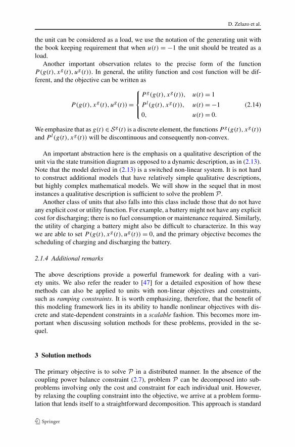
An important abstraction here is the emphasis on a qualitative description of theunit via the state transition diagram as opposed to a dynamic description, as in (2.13).Note that the model derived in (2.13) is a switched non-linear system. It is not hardto construct additional models that have relatively simple qualitative descriptions,but highly complex mathematical models. We will show in the sequel that in mostinstances a qualitative description is sufficient to solve the problem P .

Another class of units that also falls into this class include those that do not haveany explicit cost or utility function. For example, a battery might not have any explicitcost for discharging; there is no fuel consumption or maintenance required. Similarly,the utility of charging a battery might also be difficult to characterize. In this waywe are able to set P(g(t), xg(t), ug(t)) = 0, and the primary objective becomes thescheduling of charging and discharging the battery.

2.1.4 Additional remarks

The above descriptions provide a powerful framework for dealing with a vari-ety units. We also refer the reader to [47] for a detailed exposition of how thesemethods can also be applied to units with non-linear objectives and constraints,such as ramping constraints. It is worth emphasizing, therefore, that the benefit ofthis modeling framework lies in its ability to handle nonlinear objectives with dis-crete and state-dependent constraints in a scalable fashion. This becomes more im-portant when discussing solution methods for these problems, provided in the se-quel.

3 Solution methods

The primary objective is to solve P in a distributed manner. In the absence of thecoupling power balance constraint (2.7), problem P can be decomposed into sub-problems involving only the cost and constraint for each individual unit. However,by relaxing the coupling constraint into the objective, we arrive at a problem formu-lation that lends itself to a straightforward decomposition. This approach is standard

An energy management system for off-grid power systems

and is described in detail in, for example, [48]; we only provide a brief overviewhere.

To begin, we introduce the Lagrange multiplier λ ∈ RT and define the Lagrangian

function as

L(g,y,xg,xl ,ug,ul , λ) = J (g,y,xg,xl ,ug,ul )

+T∑

t=1

λt

(L∑

j=1

yj (t) −G∑

i=1

gi(t)

). (3.1)

From the Lagrangian (3.1) we can define the dual function as

q(λ) = ming,y,xg,xl ,ug,ul

L(g,y,xg,xl ,ug,ul , λ); (3.2)

the minimization problem (3.2) is subject to the constraints (2.3)–(2.6). The dualfunction lends an economic interpretation to the original problem P . The multiplierλ can be considered as a price per unit of power; when the power balance is positive(i.e., there is more demand than available power), the deficit must be purchased at acost of λ, whereas if the power balance is negative, the excess can be sold off at a rateof λ.

The most critical feature of the dual function (3.2) is it can be naturally decom-posed into subproblems corresponding to each unit as,

qi(λ) = minT∑

t=1

(Ci(gi(t), x

gi (t), u

gi (t)) − λtgi(t)

)(3.3)

qj (λ) = minT∑

t=1

(Uj (yj (t), x

lj (t), u

lj (t)) + λtyj (t)

). (3.4)

Thus, for a fixed value of λ, the problems (3.3) and (3.4) can be solved using anappropriate solver.

Remark 4 The above formulation suggests that each unit has associated with it theability to perform computation. Without any loss of generality, we note that the sub-problems can be solved at any designated “computation node.” This node may ingeneral solve more than one sub-problem; that is it is not a requirement that eachsub-problem is solved independently.

The dual function (3.2), in turn, is used to describe the dual optimization prob-lem to (2.2), which we term D. Therefore, using the decompositions shown in (3.3)and (3.4), we can express the dual problems for the generating units and loads as

maxλ

qi(λ), i ∈ G (3.5)

maxλ

qj (λ), j ∈ L. (3.6)

D. Zelazo et al.

It is a well-known result from optimization theory that the optimal value of theprimal problem P , which we denote as J ∗, constitutes an upper bound for the optimalvalue of the dual problem D, denoted as q∗ [45]; that is q∗ ≤ J ∗. We will discuss asolution method for solving the dual problem in the sequel, in addition to recoveringthe primal solution. Before we delve into the solution methods, we first describe howthe dual subproblems, as in (3.3) and (3.4), leads to tractable solution methods for avariety of unit definitions.

The solution method we use for solving the dual problem (3.5) relies on sub-gradient methods [48]. The general procedure involves iteratively updating the La-grange multiplier value λ in such a way as to maximize the dual function. At eachiteration and for a fixed value of λ, the subproblems (3.3) and (3.4) must be solved.It is important to emphasize that while the majority of the algorithmic work occursin parallel via the solution of each subproblem, the sub-gradient methods requires acoordination step to compute a sub-gradient and update the Lagrange multiplier.

First, we note that the t-th component of the sub-gradient of the dual function canbe expressed as

ν(λt ) =(

L∑

j=1

yj (t) −G∑

i=1

gi(t)

). (3.7)

The index t ranges over the entire time horizon, T . The sub-gradient, which providesan ascent direction for the dual problem, is precisely the power balance excess ordeficit.

Using the sub-gradient we are able to compute an ascent direction for the Lagrangemultiplier. Introducing the index k to denote the iteration step, we can compute theupdate as5

λk+1 = λk + αkν(λk). (3.8)

The parameter αk represents the step-size for the update at each iteration. The choiceof the step-size will have implications for both the absolute convergence properties ofthe algorithm and the speed of convergence. The precise choice is highly dependenton the particular application, and selection of this parameter should be approachedas a variable requiring iterative tuning. For this work, we consider a step size that isnon-summable and diminishing; that is for each iteration step k,

αk ≥ 0, limk→∞αk = 0, and

∞∑

k=1

αk = ∞.

The algorithm also requires a stopping criteria which will have implications forthe running speed as well as how “good” the solution is. There are some theoretical

5For an equality constraint, as in (2.7), the multiplier is unconstrained. If, however, the power balanceconstraint was written as an inequality constraint, the multiplier update (3.8) would have to be projectedonto the positive orthant.

An energy management system for off-grid power systems

justifications for choosing stopping conditions (and step-size rules) when an opti-mal solution to the problem is known a priori [48]. However, in the absence of thisknowledge a more ad hoc stopping criteria must be used. For example, in systemswhere the running time of the algorithm is critical, it may be advantageous to use afixed number of iterations. While this method may lead to less than desirable solu-tions, feasibility can still be guaranteed. Another possibility is to use a thresholdingtechnique, whereas if ‖λk+1 − λk‖ < ε, the algorithm stops.

As a final remark, we emphasize that this algorithm provides only asymptoticguarantees on convergence. In real implementations, use of a stopping criteria as sug-gested above will lead to a sub-optimal solution. Furthermore, we note that the abilityto reconstruct the global optimum from this algorithm will greatly depend on the spe-cific problem structure and the primal recovery step, that we discuss in Sect. 3.2.

3.1 Unit subproblems

As described above, at each iteration step of the sub-gradient algorithm, the sub-problems (3.3) and (3.4) must be solved. The classification of units given in Sect. 2.1will lead to insight on appropriate solution methods that we present here. It is im-portant to emphasize that one advantage of this method is the flexibility inherited forsolving each subproblem. Indeed, as shown in the following, certain sub-problemsmay admit specialized algorithms or even analytical solutions parameterized by thedual variables. The appropriate choice of the solution method will depend on the par-ticular problem instance, and we emphasize in this discussion the flexibility obtainedby considering a shortest-path formulation for many of the problem classes.

3.1.1 Convex and continuous objective, 1 state (CC1)

The sub-problem associated with this class must only consider the power generationor demand level for each unit. The sub-problems (3.3) and (3.4) reduce to

qi(λ) = mingi(t)∈S g

i (t)

T∑

t=1

(Ci(gi(t)) − λtgi(t)

), ∀i ∈ G (3.9)

qj (λ) = minyj (t)∈S l

j (t)

T∑

t=1

(Uj (yj (t)) + λtyj (t)

), ∀j ∈ L. (3.10)

Recall that for this class of units, the objective functions Ci(gi(t)) and Uj (yj (t)) arecontinuous and convex functions. Consequently, the sub-problems (3.9)–(3.10) arealso convex (concave) lending to efficient algorithms for finding their solutions. In themost general form, these functions fall under the class of convex programming andthe specific form of the objectives will dictate the appropriate solution method (e.g.,linear program or quadratic program). Furthermore, for certain classes of objectivefunctions analytic solutions can be computed a priori parameterized by the multipliervalue λ. In this way, the solution to these sub-problems can be efficiently computedwith minimal computational overhead.

D. Zelazo et al.

3.1.2 Convex and continuous objective, n states (CCn)

This class of units is the most closely related to units described in traditional EDand UTC literature [22–26]. The combination of the scheduling problem with thecommitment level of each unit is most readily solved using techniques from dynamicprogramming [49]. As in the case with the class CC1, the introduction of the term−λtgi(t) and λtyj (t) does not cause the objective function to lose its convexity prop-erties.

3.1.3 Discrete objective, n states (Dn)

Recall that the class Dn contains discrete decision variables with a discontinuous andnon-convex objective function description. This poses a computational challenge forsolving the sub-problems (3.3) and (3.4). Fortunately, the qualitative description ofthe unit’s operation via the state-transition diagram leads to insight on how to solvethe sub-problems.

To illustrate the procedure, we return to the rechargeable battery exampleof Sect. 2.1.3. We will assume that there is a constant operating cost when the super-capacitor is charging, and there is a constant utility for when it is discharging. Thecost functions specified in (2.14) have the form

P g(g(t), xg(t)) = γd and P l(g(t), xg(t)) = γc. (3.11)

The key observation here is the discrete nature of the power variable g(t) can betreated in the same way as the discrete state and decision variables. With such aperspective, tools from dynamic programming can be used. More intuitive, however,is the use of shortest path algorithms to solve the sub-problems [49]. Given the state-transition graph of Fig. 3 we must simply assign costs to each edge and then usean appropriate algorithm such as Dijkstra’s or the Bellman-Ford algorithm, to solvethe problem. What is important to note is the costs of certain edges will be time-dependent. For example, assume the constraint set for the power variable g(t) isS g = {−p,0,p} for all t ∈ T ; this corresponds to a constant charge and dischargerate when the battery is in the appropriate state. The decision to transition from afully discharged state at time t to the next charge state (which is reached at timet + 2), will incur a transition cost of Sg(0,1), obtain a utility of P l(−p,0) = γc , andpay a “phantom” price of λtp. The dashed line edge from Fig. 3 from time t to t + 2therefore gets assigned a cost of (Sg(0,1) − γc + λtp); note that the utility gained issubtracted from the total edge cost, as we would like to minimize the objective.

The shortest path approach to solving these subproblems also lends itself to amore transparent understanding of how the sub-gradient algorithm is working. Ateach iteration, the values of the multipliers get updated in such a way to solve thedual problem D. Consequently, the shortest path solution is expected to change ateach iteration as a result of the update equation (3.8), and this can be monitored tounderstand the impact of each unit on the aggregate solution.

Finally, we must “condition” the state transition diagram to accommodate theshortest path algorithm. A simple approach is to add a ‘Start’ node (labeled S) and a‘Terminal’ node (labeled T) to the graph, as shown in Fig. 4. Edges connecting these

An energy management system for off-grid power systems

Fig. 4 Shortest path graph for a rechargeable battery

augmented nodes can be used to specify initial and terminal operating states. For ex-ample, if the initial state is fully charged, then there should only be one edge leavingthe start node and connecting to the state corresponding to being fully charged. Sim-ilarly, if initial and final state conditions are to be determined via optimization, alledges can be included, possibly assigning additional costs reflecting those decisions.

As discussed in (3.3), the class Dn can also include units with no explicit cost orutility function associated with them. For example, in the supercapacitor example, wemight have γd = γc = 0. Note that this change does not affect the general procedure,and we note that the Lagrange multiplier still introduces a “phantom” price for theconsumption or production of power at a specified level. This most clearly illustratesthe hidden costs of, for example, charging or discharging a battery or supercapacitor.While no explicit cost is provided, there is an implicit cost incurred by the rest of thepower system in order to meet the state requirement of the unit.

3.2 Primal recovery

An important final step in the sub-gradient algorithm described above is the recoveryof the primal solution to the problem P from the solution of the dual problem D.Indeed, for special classes of optimization problems, such as those that are strictlyconvex, the recovery of the primal solution from the dual is a straight-forward proce-dure. In such cases, a convex combination of primal variables from the subproblemsare used to generate the primal solution [48]. For example, consider a scenario whereall generating units and loads are of the class CC1. At each iteration step in the sub-gradient algorithm, the sub-problems (3.3) and (3.4) must be solved. It can be shownthat in the limit, the primal solution can be obtained from a convex combination ofthe solution of from each iteration in the algorithm. To better illustrate this point, con-sider a generating unit with optimal commitment level g∗(t), and denote the optimalsolution of the k-th iteration in the sub-gradient algorithm as gk∗(t). Then the primalsolution can be expressed as [48]

g∗(t) = limk→∞

∑kr=1 αrgr∗(t)∑k

r=1 αr. (3.12)

D. Zelazo et al.

Note that when the variables are continuous, that is when the constraint sets S g(t) orS l(t) represent continuous intervals or box constraints, then the convex combinationwill be guaranteed to be feasible [45].

However, in the general set-up developed here, we do not have such properties.Clearly, the method used in (3.12) can not work when the primal variables are dis-crete; a convex combination of discrete points will not in general correspond to afeasible solution. In fact, even for linear programming examples, customized solu-tion methods must be employed for primal recovery, such as bundle methods [50].Furthermore, existing literature on primal recovery techniques for mixed integer non-linear programs is scarce. As a result, we propose a heuristic method for recoveringa feasible primal solution from the dual problem. Note that with this heuristic we areno longer able to make guarantees about the optimality of these solution, but ratheremphasize that feasibility is ensured.

The first important observation is that each subproblem guarantees that the solu-tions will be feasible in the absence of the power balance constraint (2.7). The mainchallenge for primal recovery, therefore, is that the power balance (2.7) is satisfied.In this direction, we propose to use a combination of the primal recovery techniqueshown in (3.12) with a load and source shedding heuristic.

As the classification of units suggest, the problem P will contain a combinationof both continuous and discrete variables representing the power generation and con-sumption of units, along with a set of discrete variables representing the state andcontrol variables for each unit. The primal recovery heuristic is described below. Wedenote by k∗ the last iteration count of the algorithm.

Algorithm 1 Primal Recovery Heuristic1. For each unit belonging to the class CC1 and CCn, construct the primal power

level variables gi(t) and yj (t) using (3.12). The state and control variables forthese units will be taken from the solution of the sub-problems (3.3) and (3.4) atthe last iteration step k∗.

2. For each unit belonging to the class Dn, use the solution for the power level vari-able and the state and control variables from the last iteration step; that is thevalues gi(t), x

gi (t), u

gi (t), yj (t), xl

j (t), and ulj (t) at iteration k∗.

3. Check the power balance constraint (2.7).4. If the power balance is satisfied, use that solution. Otherwise, begin shedding loads

or increasing power generation according to a predetermined priority list.

The last step in the procedure deserves some elucidation. One approach is to de-cide if the primal recovery should operate as a utility maximization priority, gener-ation cost priority, or aggregate cost priority (e.g., via the introduction of and ap-propriate choice of a weighting constant κ , discussed in Remark 1). For example, ifload utility has a greater overall importance to the operation of the power system,then when the power balance is not met, generation of power should be increasedwhen available. Similarly, if the generation cost is higher priority, than loads shouldbe shed or their demand level lowered when possible. In either situation, we find that

An energy management system for off-grid power systems

this procedure now relates to techniques related to load shedding heuristics and pri-ority assignments [36, 37, 39–44]. We would like to note that in our experience, thepower balance constraint is satisfied without the need for any additional shedding.

4 Simulation example: an off-grid solar powered community

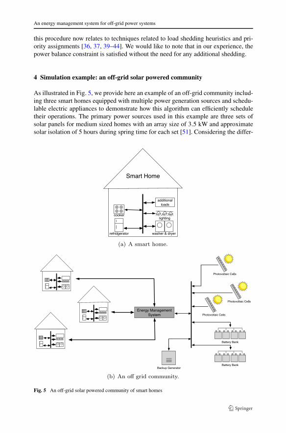
As illustrated in Fig. 5, we provide here an example of an off-grid community includ-ing three smart homes equipped with multiple power generation sources and schedu-lable electric appliances to demonstrate how this algorithm can efficiently scheduletheir operations. The primary power sources used in this example are three sets ofsolar panels for medium sized homes with an array size of 3.5 kW and approximatesolar isolation of 5 hours during spring time for each set [51]. Considering the differ-

Fig. 5 An off-grid solar powered community of smart homes

D. Zelazo et al.

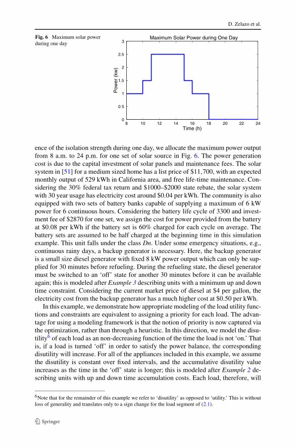
Fig. 6 Maximum solar powerduring one day

ence of the isolation strength during one day, we allocate the maximum power outputfrom 8 a.m. to 24 p.m. for one set of solar source in Fig. 6. The power generationcost is due to the capital investment of solar panels and maintenance fees. The solarsystem in [51] for a medium sized home has a list price of $11,700, with an expectedmonthly output of 529 kWh in California area, and free life-time maintenance. Con-sidering the 30% federal tax return and $1000–$2000 state rebate, the solar systemwith 30 year usage has electricity cost around $0.04 per kWh. The community is alsoequipped with two sets of battery banks capable of supplying a maximum of 6 kWpower for 6 continuous hours. Considering the battery life cycle of 3300 and invest-ment fee of $2870 for one set, we assign the cost for power provided from the batteryat $0.08 per kWh if the battery set is 60% charged for each cycle on average. Thebattery sets are assumed to be half charged at the beginning time in this simulationexample. This unit falls under the class Dn. Under some emergency situations, e.g.,continuous rainy days, a backup generator is necessary. Here, the backup generatoris a small size diesel generator with fixed 8 kW power output which can only be sup-plied for 30 minutes before refueling. During the refueling state, the diesel generatormust be switched to an ‘off’ state for another 30 minutes before it can be availableagain; this is modeled after Example 3 describing units with a minimum up and downtime constraint. Considering the current market price of diesel at $4 per gallon, theelectricity cost from the backup generator has a much higher cost at $0.50 per kWh.

In this example, we demonstrate how appropriate modeling of the load utility func-tions and constraints are equivalent to assigning a priority for each load. The advan-tage for using a modeling framework is that the notion of priority is now captured viathe optimization, rather than through a heuristic. In this direction, we model the disu-tility6 of each load as an non-decreasing function of the time the load is not ‘on.’ Thatis, if a load is turned ‘off’ in order to satisfy the power balance, the correspondingdisutility will increase. For all of the appliances included in this example, we assumethe disutility is constant over fixed intervals, and the accumulative disutility valueincreases as the time in the ‘off’ state is longer; this is modeled after Example 2 de-scribing units with up and down time accumulation costs. Each load, therefore, will

6Note that for the remainder of this example we refer to ‘disutility’ as opposed to ‘utility.’ This is withoutloss of generality and translates only to a sign change for the load segment of (2.1).

An energy management system for off-grid power systems

be modeled under the class Dn. The constraints for each load are also modeled asequality constraints; when a load is in the ‘on’ state it will demand a fixed level ofpower, and when it is ‘off’ it requires no power. The power demand constraint anddisutility values of the all load units from three homes are listed in Table 1, where P

denotes the power demand from each load referring to the example of [10], c repre-sents the disutility cost for being in the ‘off’ state during the fixed interval, t0 is theoperation request starting time and t is the requested duration time. The subscript1, 2 and 3 indicates the index of the home. The disutility cost is assigned accordingto the priority of the appliances in the daily life. Some units, i.e., the refrigerator andlighting system, will bring more inconvenience if purposely paused during a requesttime. For these units, we assign a higher disutility cost than the others to guaranteetheir normal operation provided there is enough power available. Other units, i.e., thedish washer, which is not urgent to be scheduled right upon request, is assigned lowerdisutility cost.

From the scenario description in Table 1, the overall daily energy demand requestfrom the small community is 61.73 kWh which is near the solar daily output capabil-ity of 52.5 kWh. Considering that some appliances, i.e., the washing machine and spindrier, may not be used everyday, the proposed generation system of a photovoltaic ar-ray, battery, and backup generator can generally meet the demand requirements ofthis community with three medium sized homes. However, during certain peak re-quest periods, i.e., in the mornings and evenings, conflicts can arise when there aremore load requests than available power; there will not be enough generating capa-bility from the solar source alone to supply the loads, especially when the maximumsolar power output is small due to isolation strength during those time intervals. It isexpected that the energy management system can efficiently schedule the operationto alleviate the demands during peak period and at the same time avoid shutting downany unit too long leading to increased disutility.

For this example we also implement a ‘receding horizon’ type of approach tosimulate the user-driven nature of the loads. We consider a moving time horizon forthe optimizer from the current request time to the end of the day (24 p.m.) witheach time step corresponding to 30 minute intervals. At the initial time, the algorithmdetermines the optimal schedule and allocation for each source and load. Here wepoint out that the optimizer can not anticipate that, for example, the dish washer fromhome 1 will turn on at 9 a.m. As a result, the optimizer uses the current requestlevel for each load and assumes it will be active until the end of its duration time.When a new load request is initiated, the optimizer must recompute the schedule andallocation for all units using the new state of the system. Otherwise, the generatedoptimal schedule will not change until the end of the day.

The Lagrange multipliers in the sub-gradient algorithm is initialized to zero andwe use αk(t) = 0.1√

k |ν(λk)| for the step-size αk in (3.8) to ensure the speed of conver-

gence is in a controlled scope. The optimal schedule for this scenario is illustrated inFig. 7 and Table 2 for the source’s power outputs and load’s operation histories, i.e.,starting time ts, ending time te and delayed time td, respectively.

From Fig. 7, we observe that solar sources, as the cheapest power supply unit inthis system, will provide as much power as required by the loads if the request is un-der its maximum power output limit. When the request is above solar source’s upper

D. Zelazo et al.

Tabl

e1

Con

stra

int,

disu

tility

and

oper

atio

nsc

enar

iofo

rlo

ads

Uni

tnam

eP

(kW

)c 1

($)

t01

(h)

t 1

(h)

c 2($

)t0

2(h

)

t 2(h

)c 3

($)

t03

(h)

t 3

(h)

Coo

ker

hob

30.

18

0.5

0.09

80.

50.

088.

50.

5

Mic

row

ave

1.7

0.1

80.

50.

09n/

an/

a0.

08n/

an/

a

Dis

hw

ashe

r1

0.00

29

10.

0018

9.5

10.

0016

111

Clo

thes

was

her

10.

029

1.5

0.01

8n/

an/

a0.

016

81

Vac

uum

robo

t1.

20.

002

90.

50.

0018

131

0.00

168

0.5

Dry

er2.

50.

0214

10.

018

n/a

n/a

0.01

612

1

Coo

ker

oven

50.

218

0.5

0.18

17.5

0.5

0.16

180.

5

Lig

htin

g0.

8450

186

5018

650

186

Des

ktop

0.3

3018

330

n/a

n/a

20n/

an/

a

Jacu

zzip

ump

1.8

0.05

191

0.04

519

10.

04n/

an/

a

Lap

top

0.1

2020

320

n/a

n/a

20n/

an/

a

Ref

rige

rato

r0.

310

024

100

2410

024

An energy management system for off-grid power systems

Fig. 7 Sources schedule and commitment levels

Table 2 Optimal schedule of loads operation

Unit name ts1 (h) te1 (h) td1 (h) ts2 (h) te2 (h) td2 (h) ts3 (h) te3 (h) td3 (h)

Cooker hob 8 8.5 0 8.5 9 0.5 9 9.5 0.5

Microwave 8 8.5 0 n/a n/a n/a n/a n/a n/a

Dish washer 10.5 11.5 1.5 10.5 11.5 1 11 12 0

Clothes washer 9.5 11 0.5 n/a n/a n/a 9.5 10.5 1.5

Vacuum robot 10 10.5 1 13 14 0 11 11.5 3

Spin dryer 14 15 0 n/a n/a n/a 12 13 0

Cooker oven 18 18.5 0 17.5 18 0 18 18.5 0

Lighting 18 24 0 18 24 0 18 24 0

Desktop 18 20 0 n/a n/a n/a n/a n/a n/a

Jacuzzi pump 19 20 0 20 21 1 n/a n/a n/a

Laptop 20 23 0 n/a n/a n/a n/a n/a n/a

Refrigerator 8 24 0 8 24 0 8 24 0

bound, the battery, as the second cheapest supply unit, will begin to output power orsome units are temporarily shut down until more power is available. For example,during the morning hours 8 a.m. to 10 a.m., when the solar source maximum poweroutput is low, the battery will supply the extra power required for some importantappliances, e.g. the cooker hob. However, when the solar power output is increasedduring noon and afternoon, the battery stores the extra generated energy after con-sumption. At the 18 p.m. mark, the aggregate requested power from the loads exceedthe battery supply limit, initiating the backup generator to supply power. However,since the backup generator can only supply power for 30 minute intervals, the opti-

D. Zelazo et al.

Fig. 8 Aggregate demandlevels and delivered power.Black colored bars indicateintervals when the load requestcould not be met andappropriate scheduling of thesources and loads are required

mizer must schedule the demand level of the loads to accommodate for the switchinglevel of available power. From the load operation history of Table 2, at the beginning,appliances having low disutility cost are shut down temporarily to let the more impor-tant appliances operate first with power supply coming from the solar source and thebattery, which avoids using the backup generator allowing both of them to operatesimultaneously. This behavior is due to the net benefit considered by both the costof running the backup generator and the utility lost for turning off some appliancestemporarily. The clothes washer, vacuum robot and dish washer, with lower assigneddisutility values, are purposely shut down until the solar power output level meetstheir requests. The Jacuzzi Pump request from home 2 at 19 p.m. is paused for 1 hourto avoid using the backup generator again.

In order to better illustrate the mediation function of the optimal algorithm amongall the units in the system, Fig. 8 shows how the aggregate available power is reducedduring peak load request time periods. In this plot, the grey bar is the power sup-ply and the black bar is the power request. When power supply can meet the powerrequest, the grey bar will cover the black bar. Otherwise, the grey bar is less thanthe black bar. Although the calculation time highly depends on the complexity ofthe shortest path models, the number of units, and the time horizon of the planningwindow, in this example with the prescribed scenario and parameters, the calculationtime of every new schedule running in Matlab is estimated to be less than 3 secondswhen all of the units shortest path solution are solved in sequence using a LenovoX201 laptop with intel i5 CPU and 4GB RAM. Therefore, if the shortest path so-lution for all the units are calculated parallel, we can expect to obtain the optimalsolution for each time interval in less than 1 second.

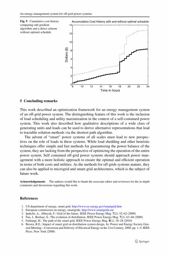
The performance of our algorithm is also compared with a direct scheme whichhas no schedule and will supply the requested power right at the proposed time inFig. 9; this solution will use the back-up generator regardless of cost. With the optimalschedule, the overall cost is greatly reduced from $12.86 to $8.42. With the optimalschedule, it will save approximate $133.2 in one month and $1598.4 in one year,which is not a trivial amount.

An energy management system for off-grid power systems

Fig. 9 Cumulative cost historycomparing sub-gradientalgorithm and a direct schemewithout optimal schedule

5 Concluding remarks

This work described an optimization framework for an energy management systemof an off-grid power system. The distinguishing feature of this work is the inclusionof load scheduling and utility maximization in the context of a self-contained powersystem. This work also described how qualitative descriptions of a wide class ofgenerating units and loads can be used to derive alternative representations that leadto tractable solution methods via the shortest path algorithm.

The advent of “smart” power systems of all scales must lead to new perspec-tives on the role of loads in these systems. While load shedding and other heuristictechniques offer simple and fast methods for guaranteeing the power balance of thesystem, they are lacking from the perspective of optimizing the operation of the entirepower system. Self contained off-grid power systems should approach power man-agement with a more holistic approach to ensure the optimal and efficient operationin terms of both costs and utilities. As the methods for off-grids systems mature, theycan also be applied to microgrid and smart-grid architectures, which is the subject offuture work.

Acknowledgements The authors would like to thank the associate editor and reviewers for the in-depthcomments and discussions regarding this work.

References

1. US department of energy, smart grid. http://www.oe.energy.gov/smartgrid.htm2. European commission on energy, smartgrids. http://www.smartgrids.eu/3. Ipakchi, A., Albuyeh, F.: Grid of the future. IEEE Power Energy Mag. 7(2), 52–62 (2009)4. Fan, J., Borlase, S.: The evolution of distribution. IEEE Power Energy Mag. 7(2), 63–68 (2009)5. Farhangi, H.: The path of the smart grid. IEEE Power Energy Mag. 8(1), 18–28 (2010)6. Brown, R.E.: Impact of smart grid on distribution system design. In: Power and Energy Society Gen-

eral Meeting—Conversion and Delivery of Electrical Energy in the 21st Century, 2008, pp. 1–4. IEEEPress, New York (2008)

D. Zelazo et al.

7. Hatziargyriou, N.: Microgrids [guest editorial]. IEEE Power Energy Mag. 6(3), 26–29 (2008)8. Katiraei, F., Iravani, R., Hatziargyriou, N., Dimeas, A.: Microgrids management. IEEE Power Energy

Mag. 6(3), 54–65 (2008)9. Thornley, V., Kemsley, R., Barbier, C., Nicholson, G.: User perception of demand side management.

In: SmartGrids for Distribution IET-CIRED, Frankfurt, Germany (2008)10. Zhang, D., Papageorgiou, L.G., Samsatli, N.J., Shah, N.: Optimal scheduling of smart homes energy

consumption with microgrid. In: Energy 2011: The First International Conference on Smart Grids,Green Communications and IT Energy-aware Technologies, no. c, pp. 70–75 (2011)

11. Misak, S., Prokop, L.: Off-grid power systems. In: 9th International Conference on Environment andElectrical Engineering, 2010, pp. 14–17. IEEE Press, New York (2010)

12. Muntean, N., Cornea, O., Petrila, D.: A new conversion and control system for a small off—grid windturbine. In: 12th International Conference on Optimization of Electrical and Electronic Equipment,2010, pp. 1167–1173. IEEE Press, New York (2010)

13. Leak, M.H., . Rashid, M.: Feasibility of off-grid residential power. In: CONIELECOMP 2011, 21stInternational Conference on Electrical Communications and Computers, pp. 14–17. IEEE Press, NewYork (2011)

14. Chan, C.C.: The state of the art of electric, hybrid, and fuel cell vehicles. Proc. IEEE 95(4), 704–718(2007)

15. Koot, M., Kessels, J., DeJager, B., Heemels, W., VandenBosch, P., Steinbuch, M.: Energy managementstrategies for vehicular electric power systems. IEEE Trans. Veh. Technol. 54(3), 771–782 (2005)

16. Davey, K., Longoria, R., Shutt, W., Carroll, J., Nagaraj, K., Park, J., Rosenwinkesl, T., Wu, W., Ara-postathis, A.: Reconfiguration in shipboard power systems. Am. Control Conf. 80(6), 064501 (2007)

17. Maldonado, M., Shah, N., Cleek, K., Walia, P., Korba, G.: Power Management and Distribution Sys-tem for a More-Electric Aircraft (MADMEL)-Program Status. IEEE Press, New York (2004)

18. Cloyd, J.: Status of the United States air force’s more electric aircraft initiative. IEEE Aerosp. Elec-tron. Syst. Mag. 13(4), 17–22 (1998)

19. Luongo, C.A., Masson, P.J., Nam, T., Mavris, D., Kim, H.D., Brown, G.V., Waters, M., Hall, D.: Nextgeneration more-electric aircraft: a potential application for HTS superconductors. IEEE Trans. Appl.Supercond. 19(3), 1055–1068 (2009)

20. Mohsenian-Rad, A.H., Leon-Garcia, A.: Optimal residential load control with price prediction in real-time electricity pricing environments. IEEE Trans. Smart Grid 1(2), 120–133 (2010)

21. Ricquebourg, V., Menga, D., Durand, D., Marhic, B., Delahoche, L., Loge, C.: The smart home con-cept: our immediate future. In: 1st IEEE International Conference on E-Learning in Industrial Elec-tronics, 2006, pp. 23–28. IEEE Press, New York (2006)

22. Bertsekas, D.P., Lauer, G.S., Sandell, N.R.J., Posbergh, T.A.: Optimal short-term scheduling of large-scale power systems. IEEE Trans. Autom. Control AC-28(1), 1–11 (1983)

23. Gruhl, J., Schweppe, F., Ruane, M.: Unit commitment scheduling of electric power systems. In: Sys-tem Engineering for Power: Status and Prospects, Henniker, NH, pp. 116–128 (1972)

24. Muckstadt, J., Koenig, S.: An application of Lagrangian relaxation to scheduling in power generationsystems. Oper. Res. 25(3), 387–403 (1977)

25. Kirchmayer, L.K.: Economic Operation of Power Systems. Wiley, New York (1958)26. Guan, X., Luh, P., Yan, H., Amalfi, J.: An optimization-based method for unit commitment. Electr.

Power Energy Syst. 14(1), 9–17 (1992)27. Ongsakul, W., Petcharaks, N.: Unit commitment by enhanced adaptive Lagrangian relaxation. IEEE

Trans. Power Syst. 19(1), 620–628 (2004)28. Papalexopoulos, A.: Optimization based methods for unit commitment: Lagrangian relaxation versus

general mixed integer programming. In: IEEE Power Engineering Society General Meeting (IEEECat. No. 03CH37491), 2003, pp. 1095–1100. IEEE Press, New York (2003)

29. Li, T., Shahidehpour, M.: Price-based unit commitment: a case of Lagrangian relaxation versus mixedinteger programming. IEEE Trans. Power Syst. 20(4), 2015–2025 (2005)

30. Joo, J.Y., Ilic, M.D.: A multi-layered adaptive load management (alm) system: Information exchangebetween market participants for efficient and reliable energy use. In: Transmission and DistributionConference and Exposition, 2010 IEEE PES, April, pp. 1–7 (2010)

31. Fahrioglu, M., Alvarado, F.: Using utility information to calibrate customer demand managementbehavior models. In: IEEE Power Engineering Society Winter Meeting. Conference Proceedings (Cat.No. 02CH37309), 2002, vol. 1, p. 26. IEEE Press, New York (2002)

32. Samadi, P., Mohsenian-Rad, A.-H., Schober, R., Wong, V.W.S., Jatskevich, J.: Optimal real-time pric-ing algorithm based on utility maximization for smart grid. In: First IEEE International Conferenceon Smart Grid Communications, 2010, pp. 415–420. IEEE Press, New York (2010)

An energy management system for off-grid power systems

33. Pedrasa, M.A.A., Spooner, T.D., MacGill, I.F.: Coordinated scheduling of residential distributed en-ergy resources to optimize smart home energy services. IEEE Trans. Smart Grid 1(2), 134–143 (2010)

34. Chiang, M., Low, S.H., Calderbank, A.R., Doyle, J.: Layering as optimization decomposition: a math-ematical theory of network architectures. Proc. IEEE 95(1), 255–312 (2007)

35. Nedic, A., Ozdaglar, A.: Subgradient methods in network resource allocation: Rate analysis. In: 42ndAnnual Conference on Information Sciences and Systems, 2008, pp. 1189–1194. IEEE Press, NewYork (2008)

36. Andrade, L., Tenning, C.: Design of Boeing 777 electric system. IEEE Aerosp. Electron. Syst. Mag.7(7), 4–11 (1992)

37. Huneault, M., Galiana, F.D.: A survey of the optimal power flow literature. IEEE Trans. Power Syst.6(2), 762–770 (1991)

38. Xu, D., Girgis, A.: Optimal load shedding strategy in power systems with distributed generation. In:IEEE Power Engineering Society Winter Meeting. Conference Proceedings (Cat. No. 01CH37194),no. C, 2001, pp. 788–793. IEEE Press, New York (2001)

39. Bhattacharyya, K., Crow, M.: A fuzzy logic based approach to direct load control. IEEE Trans. PowerSyst. 11(2), 708–714 (1996)

40. Cohen, A., Wang, C.: An optimization method for load management scheduling. IEEE Trans. PowerSyst. 3(2), 612–618 (1988)

41. Ng, K.H., Sheble, G.B.: Direct load control—a profit-based load management using linear program-ming. IEEE Trans. Power Syst. 13(2), 688–695 (1998)

42. Ramanathan, B., Vittal, V.: A framework for evaluation of advanced direct load control with minimumdisruption. IEEE Trans. Power Syst. 23(4), 1681–1688 (2008)

43. Widergren, S.E.: Demand or request: Will load behave? In: IEEE Power & Energy Society GeneralMeeting, 2009, pp. 1–5. IEEE Press, New York (2009)

44. Ruiz, N., Cobelo, I.N., Oyarzabal, J.: A direct load control model for virtual power plant management.IEEE Trans. Power Syst. 24(2), 959–966 (2009)

45. Boyd, S.P., Vandenberghe, L.: Convex Optimization. Cambridge University Press, Cambridge (2004)46. Rockafellar, R.T.: Network Flows and Monotropic Optimization. Wiley, New York (1984)47. Frangioni, A.: Solving nonlinear single-unit commitment problems with ramping constraints. Oper.

Res. 54, 775 (2006)48. Ruszczynski, A.: Nonlinear Optimization. Princeton University Press, Princeton (2006)49. Bertsekas, D.P.: Dynamic Programming and Optimal Control. Athena Scientific, Belmont (2007)50. Sherali, H., Choi, G.: Recovery of primal solutions when using subgradient optimization methods to

solve Lagrangian duals of linear programs. Oper. Res. Lett. 19(3), 105–113 (1996)51. Medium ac off grid solar powered system for your home. http://www.wholesalesolar.com/

solarpowersystems/medium-2-ac-home-off-grid-solar-power.html