
Validated real-time energy models for small-scale grid-connected PV-systems
9
Dublin Institute of Technology ARROW@DIT Articles Dublin Energy Lab 2010-07-01 Validated Real-time Energy Models for Small-Scale Grid-Connected PV-Systems Lacour Ayompe Dublin Institute of Technology, [email protected] Aidan Duffy Dublin Institute of Technology, aidan.duff[email protected] Sarah McCormack Trinity College, [email protected] Michael Conlon Dublin Institute of Technology, [email protected] is Article is brought to you for free and open access by the Dublin Energy Lab at ARROW@DIT. It has been accepted for inclusion in Articles by an authorized administrator of ARROW@DIT. For more information, please contact [email protected], [email protected]. is work is licensed under a Creative Commons Aribution- Noncommercial-Share Alike 3.0 License Recommended Citation Ayompe, L., Duffy, A., McCormack, S., Conlon, M.: Validated real-time energy models for small-scale grid-connected PV-systems, Energy, In Press, Corrected Proof, Available online 22 July 2010, ISSN 0360-5442, DOI: 10.1016/j.energy.2010.06.021.
Transcript of Validated real-time energy models for small-scale grid-connected PV-systems
Dublin Institute of TechnologyARROW@DIT
Articles Dublin Energy Lab
2010-07-01
Validated Real-time Energy Models for Small-ScaleGrid-Connected PV-SystemsLacour AyompeDublin Institute of Technology, [email protected]
Aidan DuffyDublin Institute of Technology, [email protected]
Sarah McCormackTrinity College, [email protected]
Michael ConlonDublin Institute of Technology, [email protected]
This Article is brought to you for free and open access by the Dublin EnergyLab at ARROW@DIT. It has been accepted for inclusion in Articles by anauthorized administrator of ARROW@DIT. For more information, pleasecontact [email protected], [email protected].
This work is licensed under a Creative Commons Attribution-Noncommercial-Share Alike 3.0 License
Recommended CitationAyompe, L., Duffy, A., McCormack, S., Conlon, M.: Validated real-time energy models for small-scale grid-connected PV-systems,Energy, In Press, Corrected Proof, Available online 22 July 2010, ISSN 0360-5442, DOI: 10.1016/j.energy.2010.06.021.

Dublin Energy Lab
Articles
Dublin Institute of Technology Year
Validated real-time energy models for
small-scale grid-connected PV-systems
Lacour Ayompe∗ Aidan Duffy†
Sarah McCormack‡ Michael Conlon∗∗
∗Dublin Institute of Technology, [email protected]†Dublin Institute of Technology, [email protected]‡Trinity College, [email protected]∗∗Dublin Institute of Technology, [email protected]
This paper is posted at ARROW@DIT.
http://arrow.dit.ie/dubenart/1

— Use Licence —
Attribution-NonCommercial-ShareAlike 1.0
You are free:
• to copy, distribute, display, and perform the work
• to make derivative works
Under the following conditions:
• Attribution.You must give the original author credit.
• Non-Commercial.You may not use this work for commercial purposes.
• Share Alike.If you alter, transform, or build upon this work, you may distribute theresulting work only under a license identical to this one.
For any reuse or distribution, you must make clear to others the license termsof this work. Any of these conditions can be waived if you get permission fromthe author.
Your fair use and other rights are in no way affected by the above.
This work is licensed under the Creative Commons Attribution-NonCommercial-ShareAlike License. To view a copy of this license, visit:
• URL (human-readable summary):http://creativecommons.org/licenses/by-nc-sa/1.0/
• URL (legal code):http://creativecommons.org/worldwide/uk/translated-license

Validated real-time energy models for small-scale grid-connected PV-systems
L.M. Ayompe a,*, A. Duffy a, S.J. McCormack b, M. Conlon c
aDepartment of Civil and Structural Engineering, School of Civil and Building Services, Dublin Institute of Technology, Bolton Street, Dublin 1, IrelandbDepartment of Civil, Structural and Environmental Engineering, Trinity College Dublin, Dublin 2, Irelandc School of Electrical Engineering Systems, Dublin Institute of Technology, Kevin St, Dublin 8, Ireland
a r t i c l e i n f o
Article history:Received 12 January 2010Received in revised form15 May 2010Accepted 19 June 2010Available online xxx
Keywords:Real-timeGrid-connected PV-systemEmpirical modelsPowerMicrogeneration
a b s t r a c t
This paper presents validated real-time energy models for small-scale grid-connected PV-systemssuitable for domestic application. The models were used to predict real-time AC power output from a PV-system in Dublin, Ireland using 30-min intervals of measured performance data between April 2009 andMarch 2010. Statistical analysis of the predicted results and measured data highlight possible sources oferrors and the limitations and/or adequacy of existing models, to describe the temperature and efficiencyof PV-cells and consequently, the accuracy of power prediction models. PV-system AC output powerpredictions using empirical models for PV-cell temperature and efficiency prediction showed lowerpercentage mean absolute errors (PMAEs) of 7.9e11.7% while non-empirical models had errors of10.0e12.4%. Cumulative errors for PV-system AC output power predictions were 1.3% for empiricalmodels and 3.3% for non-empirical models. The proposed models are suitable for predicting PV-systemAC output power at time intervals suitable for smart metering.
� 2010 Published by Elsevier Ltd.
1. Introduction
A domestic grid-connected PV-system is a type of installationwhere three major components are used: the PV-generator(comprising a number of PV-modules connected in series orparallel on a mounting structure); the inverter; DC and AC cablingand a conventional power line [1,2]. Inverters play a key role inenergy efficiency and reliability since they operate the PV-array atthe Maximum Power Point (MPP). Moreover, inverters convert theDC power generated by PV-modules into alternating current (AC) ofthe desired voltage and frequency (e.g. 230 V/50 Hz). Installationsof this type do not include batteries [3,4].
Most existing generic models for assessing the energy output ofPV-systems are lumped since they determine average daily,monthly or annual energy output. These models are adapted tosupport policies such as netmetering (applicable in Japan and someStates in America) where electricity is sold to the grid at the sameprice at which it is bought. Lumped models are also useful incountries where enhanced feed-in tariffs (high buy-back rates)apply such as in Germany, Spain, Italy, Greece and France. Lumpedmodels are, however, not adapted to analyse the real-time ordynamic performances of grid-connected PV-systems such as thosewhere support policies are based on paying for the excess (or spill)
electricity generated, which is fed into the utility grid (such as inother countries and Ireland). Moreover, they cannot cope withvariable electricity prices based on time of use, which is likely tobecome more common as smart metering becomes widelydeployed.
Smart meters provide much more precise information on elec-tricity consumed as well as the time of use. They are intelligenttwo-way communication devices with digital real-time powermeasurement. They offer the opportunity for remote operation andremote meter reading as well as the potential for real-time pricing,new tariff options and demand side management.
During the day when solar radiation is available, a grid-con-nected PV-system generates AC power. If the PV-system is installedin a domestic dwelling, the AC power is fed into the main electricaldistribution panel of the house fromwhich it can provide power tothe house for on-site consumption, the excess is supplied to theutility grid. Fig.1 shows representative plots of measured electricitygenerated from a 1.72 kWp PV-system located in Dublin, Ireland,average electricity consumption of a representative domesticdwelling in Ireland and the quantity of electricity exported andspilled to the grid on the 1st of June 2009.
The objective of this paper therefore, is, to develop a validatedreal-time mathematical model that predicts the electricity outputof small-scale grid-connected PV-systems. The model can be usedto generate time-stepped output data, which can be combinedwithdomestic demand data to predict the quantity of on-site electricityconsumption based on different users’ demand profiles.
* Corresponding author. Tel: þ353 14023940; fax: þ353 14022997.Q1E-mail address: [email protected] (L.M. Ayompe).
Contents lists available at ScienceDirect
Energy
journal homepage: www.elsevier .com/locate/energy
0360-5442/$ e see front matter � 2010 Published by Elsevier Ltd.doi:10.1016/j.energy.2010.06.021
Energy xxx (2010) 1e6
EGY2969_proof ■ 9 July 2010 ■ 1/6
Please cite this article in press as: Ayompe LM, et al., Validated real-time energy models for small-scale grid-connected PV-systems, Energy(2010), doi:10.1016/j.energy.2010.06.021
123456789
10111213141516171819202122232425262728293031323334353637383940414243444546474849505152535455
5657585960616263646566676869707172737475767778798081828384858687888990919293949596979899
100101102103104105106107108109110

2. PV output modelling
PV output modelling involves identifying all independent vari-ables and establishing their mathematical relationships with poweroutput. The variables identified include solar radiation; windspeed; ambient temperature; cell efficiency; cell temperature andmodule area.
Given that current smart metering practice is based on 30-minintervals, the mathematical representation of the PV-system wassimulated at 30-min intervals daily using measured data betweenApril 2009 and March 2010. In order to achieve this, it is necessaryto accurately predict the PV-cell temperature, which influences thecell efficiency. Once the cell efficiency and inverter efficiency at anygiven instant are accurately predicted, the PV-power equation isthen used to calculate the power output from the PV-system.
2.1. PV-cell temperature
The temperature of PV-cells is one of the most importantparameters used in assessing the performance of PV-systems and
their electricity output. The cell temperature depends on severalparameters such as the thermal properties of thematerials used, typeof cells, module configuration and local climate conditions [5,6].
A PV-module’s efficiency strongly depends on its cells’ operatingtemperature. PV-cell temperatures are very difficult to measuresince the cells are tightly encapsulated in order to protect themfrom environmental degradation. The temperature of the backsurface of PV-modules is commonly measured and used in place ofthe cell temperature with the assumption that these temperaturesclosely match [7].
From a mathematical point of view, correlations for PV-celloperating temperature (Tc) are either explicit in form, thus giving Tcdirectly, or implicit, i.e. involve variables such as cell efficiency orheat transfer coefficients, which themselves depend on Tc. In thelatter case, an iteration procedure is necessary to calculate the celltemperature [8]. Six models for PV-cell temperature evaluationwere identified from literature. They include five explicit and oneimplicit model, the latter comprising of a steady-state model.
2.1.1. Explicit correlationsThe explicit correlation models express the PV-cell temperature
as a function of ambient temperature, solar radiation, wind speedand other system parameters ignoring heat exchange dynamicsbetween the module and its environment. The first correlationexpresses the cell temperature of a PV-module Tc in Eq. (1) as [9]:
Tc ¼ Ta þ Gm
800ðNOCT� 20Þ
�1� hc
sa
�(1)
where, sa¼ 0.9 [10].A simplified model of Eq. (1) is given in Eq. (2) as [11,12]:
Tc ¼ Ta þ Gm
800ðNOCT� 20Þ (2)
Eq. (3) gives the simplest explicit correlation for the operatingtemperature of a PV-cell with the ambient temperature and inci-dent solar radiation flux [8]. Earlier reported values for hw were inthe range 0.02e0.04Wm�2 K�1 [13]. In this study, hw was deter-mined to be 0.018 Wm�2 K�1 using nonlinear regression analysison measured data.
Nomenclature
A area (m2)AM air massC heat capacity (J K�1)Gm in-plane solar radiation (Wm�2)hc forced convective heat transfer coefficient (Wm�2 K�1)hc,w convective heat transfer coefficient due to wind
(Wm�2 K�1)hr radiative heat transfer coefficient (Wm�2 K�1)nm number of modules_QG absorbed solar radiation (W)_Q r thermal losses by radiation (W)_Qc thermal losses by convection (W)NOCT normal operating cell temperature (45 �C)Pel electrical power (W)T temperature (�C)UL overall heat transfer coefficient (Wm�2 K�1)Vw wind speed (m s�1)PMAE percentage mean absolute error (%)
Subscriptsa ambientAC alternating currentc PV-cellDC direct currentinv inverterm moduleMPP maximum power pointn,c nominal cellPV photovoltaicr referenceSTC standard test conditionw wind
Greek symbolsa absorptivityb temperature coefficient of Pm of the PV-panel
(0.003 �C�1)h efficiency (%)s transmisivitys StefaneBoltzman’s constant (5.67� 10�8 Wm�2 K�4)e emissivity
-0.4
-0.3
-0.2
-0.1
0.0
0.1
0.2
0.3
0.4
0.5
00:0
0
01:0
0
02:0
0
03:0
0
04:0
0
05:0
0
06:0
0
07:0
0
08:0
0
09:0
0
10:0
0
11:0
0
12:0
0
13:0
0
14:0
0
15:0
0
16:0
0
17:0
0
18:0
0
19:0
0
20:0
0
21:0
0
22:0
0
23:0
0
Ene
rgy
(kW
h)
Time of day
Electricity demand PV generated electricity Difference
Energy spilled to grid
Energy imported from grid
Fig. 1. Representative daily domestic scale PV-system electricity generation anddemand.
L.M. Ayompe et al. / Energy xxx (2010) 1e62
EGY2969_proof ■ 9 July 2010 ■ 2/6
Please cite this article in press as: Ayompe LM, et al., Validated real-time energy models for small-scale grid-connected PV-systems, Energy(2010), doi:10.1016/j.energy.2010.06.021
111112113114115116117118119120121122123124125126127128129130131132133134135136137138139140141142143144145146147148149150151152153154155156157158159160161162163164165166167168169170171172173174175
176177178179180181182183184185186187188189190191192193194195196197198199200201202203204205206207208209210211212213214215216217218219220221222223224225226227228229230231232233234235236237238239240
Tc ¼ Ta þ Gmhw (3)
where, Tc and Ta are in degrees Kelvin.The PV-module temperature can also be determined using
Eq. (4) proposed by Tamizh Mani et al. in [14] given as:
Tc ¼ aþ bGm þ cTa þ dVw (4)
where, a, b, c and d are system-specific regression coefficients withvalues of �1.987, 0.02, 1.102 and�0.097, respectively, and R2 of 0.97determined using measured data from the Dublin site.
King in [8] proposed an expression for PV-cell temperaturegiven by Eq. (5) as:
Tc ¼ Ta þ Gm
GSTC
haV2
w þ bVw þ ci
(5)
where, a, b, and c are coefficients with values of 0.043, �1.652 and24.382, respectively, and R2 of 0.96, again determined usingmeasured data.
Other explicit correlations reported in literature [8] are based onfield performance data, which are site specific and, therefore, notapplicable in this case.
2.1.2. Steady-state analysisIn this approach it is assumed that, within a short-time period
(normally less than 1 h), the intensity of the incoming solar irra-diance and other parameters affecting the PV-module’s behaviourare constant. If the variation in the overall heat loss rates of the PV-module is small, then it can be assumed that the rate of heattransfer from the PV-module to the environment is steady and thetemperatures at each point of the PV-module are constant overa short-time period [7].
The equation for the PV-cell temperature operating understeady state is derived assuming that the incident energy on a solarcell is equal to the electrical energy output of the cell plus the sumof the energy losses due to convection and radiation. The resultingenergy balance equation is given as [15,16]:_QG � Pel � _Q r � _Qc ¼ 0 (6)
Substituting the relevant terms in Eq. (6) results in Eq. (7) givenas [17]:
saGmAc � hcGmAc � 2hrAcðTc � TaÞ � 2hcAcðTc � TaÞ ¼ 0 (7)
From Eq. (5), the PV-module temperature is given as:
Tc ¼ ðsa� hPVÞGm
2ðhr þ hcÞ þ Ta (8)
where, Tc and Ta are in degrees Kelvin.
2.1.3. Heat transfer coefficientsThe radiative heat transfer coefficient between the module front
and the sky, and themodule rear and the ground (hr) is given as [18]:
hr ¼ se�T2c þ T2a
�ðTc þ TaÞ (9)
The convective heat flow is dominated at the module front byforced convection driven by wind forces and at the module rear,depending on the installation situation, by free laminar or turbulentconvection. The convective heat transfer coefficient is given as [17]:
hc ¼ffiffiffiffiffiffiffiffiffiffiffiffiffiffiffiffiffiffiffiffiffiffiffiffiffiffiffih3c;w þ h3c;free
3q
(10)
hc;w ¼ 4:214þ 3:575Vw (11)
hc;free ¼ 1:78ðTc � TaÞ1=3 (12)
Because of the wide discrepancies in the value for hc, it isdifficult to choose a particular value. Duffie and Beckman [18]suggested the use of the expression for hc,w proposed by McA-dams [19] for flat plates exposed to outside winds:
hc;w ¼ 5:67þ 3:86Vw (13)
Nolay in [10] uses the following relationship:
hc;w ¼ 5:82þ 4:07Vw (14)
2.2. PV-cell and module efficiency
The most widely known model to predict the efficiency ofa PV-cell (hc) is given as [10,20]:
hc ¼ hn;c½1� bðTc � TrÞ þ glogðGm=1000Þ� (15)
where, Tr¼ 25 �C, g¼ 0.12.Most often Eq. (15) is given with g¼ 0 and it reduces to a linear
dependence of hc on temperature given as [10,16]:
hc ¼ hn;c½1� bðTc � 25Þ� (16)
The efficiency of solar cells can also be expressed as beingdependent on the incident solar radiation and cell temperature. Theefficiency at a particular irradiance or temperature is the result ofthe nominal efficiency minus the change in efficiency given as [2]:
hc ¼ hn;c
�1þ bln
�Gm
1000
�� bðTc � 25Þ
�(17)
Another expression for the cell efficiency assuming that thetransmittanceeabsorbance losses (sa/UL) are constant over therelevant operating temperature range is given as [21]:
hc ¼ hn;c
�1� 0:9b
Gm
800ðNOCT� 20Þ � bðTa � 25Þ
�(18)
Durisch et al. [22] developed a semi-empirical PV-cell efficiencymodel given as:
hc ¼ hn;ca�bGm
G0þ�Gm
G0
�c��dþ e
TcTr
þ fAMAM0
þ�AMAM0
�g�(19)
where, G0¼1000Wm�2, Tr¼ 25 �C, AM0¼1.5.The parameters a, b, c, d, e, f and g are regression coefficients
with values of 1.249, �0.241, 0.193, 0.244, �0.179, �0.037 and0.073, respectively, and R2 of 0.99 which were determined usingmeasured data from the Dublin site. The air mass (AM) is the ratioof the mass of air that the direct radiation has to traverse at anygiven time and location to the mass of air that it would traverse ifthe sun were at the zenith [23]. The air mass is calculated for anytime of day at any day of the year from the sun’s altitude F (indegrees) using the equation given as [24]:
AM ¼ 1=cosð90� FÞ (20)
The nominal efficiency (hn,c) of PV-cells is given as [2]:
hn;c ¼ PMPPðSTCÞAc � GSTC
(21)
The nominal efficiency of a PV-module is given as:
hn;m ¼ hn;c � PF (22)
The pack factor (PF) is the ratio of the total area of PV-cells (Ac)over the area of the PV-module (Am) and is given as [12]:
L.M. Ayompe et al. / Energy xxx (2010) 1e6 3
EGY2969_proof ■ 9 July 2010 ■ 3/6
Please cite this article in press as: Ayompe LM, et al., Validated real-time energy models for small-scale grid-connected PV-systems, Energy(2010), doi:10.1016/j.energy.2010.06.021
241242243244245246247248249250251252253254255256257258259260261262263264265266267268269270271272273274275276277278279280281282283284285286287288289290291292293294295296297298299300301302303304305
306307308309310311312313314315316317318319320321322323324325326327328329330331332333334335336337338339340341342343344345346347348349350351352353354355356357358359360361362363364365366367368369370
PF ¼ Ac
Am(23)
The measured PV-module efficiency is given as [18]:
hexp ¼ VDCIDCGmAm
(24)
2.3. PV-array power output
The DC power output from a PV-array is given as:
PDC ¼ nm � hn;c � hL � PF� Gm � Am (25)
hL accounts for losses that reduce power output from standardtest conditions (STCs). These losses include the difference of theoperating PV-cell temperature from the standard 25 �C, the devi-ation from the maximum power point, the ohmic losses of theconductors, the cleanness of the PV-module surface, the deviationof the solar irradiance from an ideal path in order to producea photoelectron in the cell (optical path deviation), the aging of thePV material, etc [25]. Kaushika and Rai [26] investigated mismatchlosses in solar photovoltaic cell networks while Mavromatakis et al.[25] presented expressions for reflection and difference in oper-ating PV-cell temperature losses. Due to the complexity of model-ling the individual losses, hL is often modelled using Eqs. (15)e(19)representing the terms that are multiplied by the nominal PV-cellefficiency (hn,c). Eq. (25) therefore reduces to
PDC ¼ nm � hc � PF � Gm � Am (26)
2.4. Inverter efficiency
The inverter efficiency is given as [9]:
hinv ¼ Pinv;nPPV;n
(27)
The normalised inverter output Pinv,n is given as a second-orderpolynomial by Peippo and Lund in [9] as:
Pinv;n ¼ k0 þ k1PPV;n þ k2P2PV;n (28)
where
PPV;n ¼ PPVPinv;rated
(29)
and
Pinv;n ¼ PinvPinv;rated
(30)
k0 is the normalised self-consumption loss, k1 is the linear effi-ciency coefficient and k2 is the coefficient for losses proportional toinput power squared as defined by Peippo and Lund in [9]. PPV,n andPinv,n are the normalised inverter input and output power, respec-tively. PPV and Pinv are the PV-array DC input and AC output from theinverter at any instant of time, respectively, while Pinv,rated is therated inverter input capacity. A regression analysis carried out onnormalised inverter input and output power yielded values for theconstants k0, k1 and k2 of �0.001, 0.926 and 0.004, respectively withR2 of 1.
2.5. PV-system power output
The PV-system AC power output is given as:
PAC ¼ hinvPDC (31)
Table 1Percentage mean absolute error (PMAE) for PV-cell temperature predictionsQ3 .
Eq. (1) Eq. (2) Eq. (3) Eq. (4) Eq. (5) Eq. (8)
PMAE 14.4 23.3 8.2 7.3 7.1 8.8
0
10
20
30
40
50
PV
-cel
l tem
pera
ture
(o C)
Time
Measured Modelled using Eq. 4 Modelled using Eq. 5
03/06/2009 04/06/2009 05/06/2009
Fig. 2. Measured and modelled PV-cell temperature.
Table 2PMAE for predicted PV-array power output.
Eq. (1) Eq. (2) Eq. (3) Eq. (4) Eq. (5) Eq. (8)
Eq. (15) 9.1 11.6 9.8 9.7 9.9 10.2Eq. (16) 12.5 15.4 13.4 13.3 13.4 13.8Eq. (17) 12.3 15.2 13.2 13.1 13.2 13.5Eq. (18) 11.4 12.0 11.2 11.3 11.3 11.5Eq. (19) 7.8 11.0 7.3 7.3 7.7 8.3
0
200
400
600
800
1000
1200
1400
1600
PV
-arr
ay m
axim
um p
ower
(W)
Time
Measured Modelled using Eqs. 1 & 15 Modelled using Eqs. 3 & 19
03/06/2009 04/06/2009 05/06/2009
Fig. 3. Measured and modelled PV-array maximum DC power output.
Table 3Percentage cumulative error for predicted PV-array output energy.
Eq. (1) Eq. (2) Eq. (3) Eq. (4) Eq. (5) Eq. (8)
Eq. (15) 2.5 6.5 3.8 3.8 3.8 4.2Eq. (16) 8.0 12.1 9.4 9.4 9.4 9.7Eq. (17) 7.7 11.8 9.1 9.0 9.0 9.4Eq. (18) 3.3 7.3 4.6 4.6 4.6 5.0Eq. (19) 2.3 6.7 0.7 0.6 0.6 1.4
L.M. Ayompe et al. / Energy xxx (2010) 1e64
EGY2969_proof ■ 9 July 2010 ■ 4/6
Please cite this article in press as: Ayompe LM, et al., Validated real-time energy models for small-scale grid-connected PV-systems, Energy(2010), doi:10.1016/j.energy.2010.06.021
371372373374375376377378379380381382383384385386387388389390391392393394395396397398399400401402403404405406407408409410411412413414415416417418419420421422423424425426427428429430431432433434435
436437438439440441442443444445446447448449450451452453454455456457458459460461462463464465466467468469470471472473474475476477478479480481482483484485486487488489490491492493494495496497498499500
3. Modelling
MatLab software was used to develop a programme to predictthe energy output from a trial PV installation using measuredweather data at 30-min intervals between April 2009 and March2010. At every given instant, the PV-cell temperature was modelledusing Eqs.(1)e(5) and (8). PV-array DC power and PV-system ACpower outputs were modelled using Eqs. (26) and (31),respectively.
3.1. PV-system description
The PV-system used to validate the above models consisted ofa 1.72 kWp PV-array composed of 8 modules covering a total area of10 m2 installed on a flat roof at the Focas Institute building, DublinInstitute of Technology, Dublin, Ireland. The 215 Wp Sanyo HIP-215NHE5 PV-modules are made of thin monocrystalline siliconwafer surrounded by ultra-thin amorphous silicon layers with anti-reflective coatings that maximized sunlight absorption [27]. Theunshaded modules were installed facing due south and inclined at53� to the horizontal corresponding to the local latitude of thelocation. The roof was approximately 12 m high and the moduleswere mounted on metal frames that were 1 m high.
A 1700 W AC power single-phase Sunny Boy inverter wasinstalled to convert the DC electricity from the PV-array to AC thatwas fed into the 220e240 V AC electrical network of the building.The data acquisition system consisted of a Sunny Boy 1700 inverter,Sunny SensorBox and Sunny WebBox. The Sunny SensorBox wasused to measure in-plane global solar radiation on the PV-modules.Additional sensors for measuring ambient temperature, windspeed and temperature at the back of the PV-module were con-nected to the SensorBox. The SensorBox and the inverter wereconnected to the SunnyWebBox via a serial RS485 link and a PowerInjector. Data was recorded at 5-minute intervals using theWebBox.
3.2. Data and results comparison
In order to quantify variations between predicted and measuredvalues, percentage mean absolute error (PMAE) was used. It eval-uates the percentage mean of the sum of absolute deviationsarising due to both over-estimation and under-estimation of indi-vidual observations. PMAE is given as:
PMAE ¼ 1N
XNi¼1
"ðCi �MiÞ2
Mi
#12
�100% (33)
N is the total number of observations while Ci and Mi are the ithcalculated and measured values, respectively.
3.3. Weather data
One year’s data collected at 5-min intervals between April 2009and March 2010 at the test site was aggregated to 30 min and usedfor model validation. The data composed of solar radiation, ambienttemperature, PV-module temperature, wind speed, PV-array DCcurrent, PV-array DC voltage and PV-system AC power output.
The monthly average daily total solar insolation varied between1.11 kWh/m2/day in December and 4.57 kWh/m2/day in June whilethe annual total measured in-plane solar insolation was1043.1 kWh/m2. The monthly average daily wind speed variedbetween 2.5 m/s in February and 6.6 m/s in November. Themonthly average ambient temperature varied between 6.0 �C inJanuary and 18.8 �C in August while the PV-module temperaturevaried between 8.8 �C in January and 23.8 �C in June. Maximumrecorded values for solar radiation, ambient temperature, PV-module temperature and wind speed were 1031.0 Wm�2, 27.0 �C,45.8 �C and 16.3 ms�1 in August, June, September and November,respectively.
4. Results and discussions
4.1. PV-cell temperature
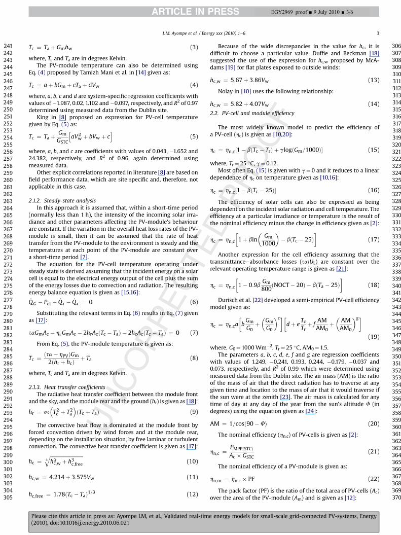
Table 1 presents PMAE for PV-cell temperature predictions usingthe models in Eqs. (1)e(5) and (8). The results show that theempirical models in Eqs. (4) and (5) produce the least PMAE of 7.3%and 7.1%, respectively.Wherefield trial data is not available to derivethe empirical coefficients, Eq. (1) can be used to predict the PV-celltemperature with a higher PMAE of 14.4%. Fig. 2 shows plots ofmeasured and modelled PV-cell temperature using Eqs. (4) and (5).It can be seen from Fig. 2 that the predicted PV-cell temperaturesshow good correlation with the measured data.
4.2. PV-array output power
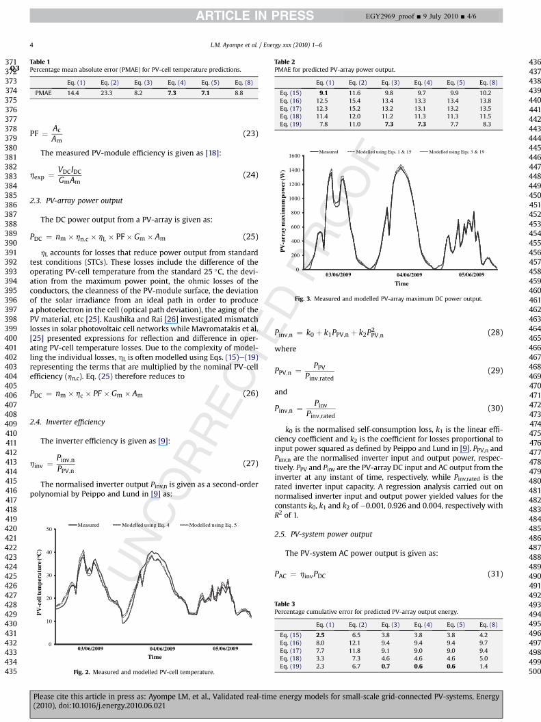
PMAE for predicted PV-array DC power output using PV-celltemperature models (Eqs. (1)e(5) and (8)) and modified PV-cellefficiency models (Eqs. (15)e(19)) are presented in Table 2. Theresults show that when field trial data is available to obtainregression coefficients, the empirical models for PV-cell tempera-ture (Eqs. (3) and (4)) and PV-cell efficiency (Eq. (19)) yield thelowest PMAE of 7.3%. Where only weather data is available, Eqs. (1)and (15) can be used to predict PV-array output power with PMAEof 9.1%. Fig. 3 shows plots of measured and modelled PV-arraymaximum DC output power. It can be seen that the predicted PV-array maximum output power shows good correlation with themeasured data.
0
200
400
600
800
1000
1200
1400
1600
PV
-sys
tem
max
imum
pow
er (W
)
Time
Measured Modelled using Eqs. 1 & 15 Modelled using Eqs. 3 & 19
03/06/2009 04/06/2009 05/06/2009
Fig. 4. Measured and modelled PV-system maximum AC power output.
Table 5Percentage cumulative error for predicted PV-system AC output energy.
Eq. (1) Eq. (2) Eq. (3) Eq. (4) Eq. (5) Eq. (8)
Eq. (15) 3.3 7.4 4.6 4.6 4.6 5.0Eq. (19) �1.6 7.5 1.4 1.3 1.4 2.2
Table 4PMAE for predicted PV-system AC output power.
Eq. (1) Eq. (2) Eq. (3) Eq. (4) Eq. (5) Eq. (8)
Eq. (15) 10.0 12.4 10.7 10.6 10.7 11.1Eq. (19) 8.4 11.7 7.9 7.9 8.3 9.0
L.M. Ayompe et al. / Energy xxx (2010) 1e6 5
EGY2969_proof ■ 9 July 2010 ■ 5/6
Please cite this article in press as: Ayompe LM, et al., Validated real-time energy models for small-scale grid-connected PV-systems, Energy(2010), doi:10.1016/j.energy.2010.06.021
501502503504505506507508509510511512513514515516517518519520521522523524525526527528529530531532533534535536537538539540541542543544545546547548549550551552553554555556557558559560561562563564565
566567568569570571572573574575576577578579580581582583584585586587588589590591592593594595596597598599600601602603604605606607608609610611612613614615616617618619620621622623624625626627628629630

Table 3 shows percentage cumulative errors for predicted PV-array output energy against the measured power output of1661.4 kWh. The empirical models in Eqs. (3)e(5) and (19) havepercentage cumulative errors of 0.6e0.7% while the non-empiricalmodels using Eqs. (1) and (15) have an error of 2.5%. Both models,however, tend to over-estimate PV-array power output duringsunrise.
4.3. PV-system AC output power
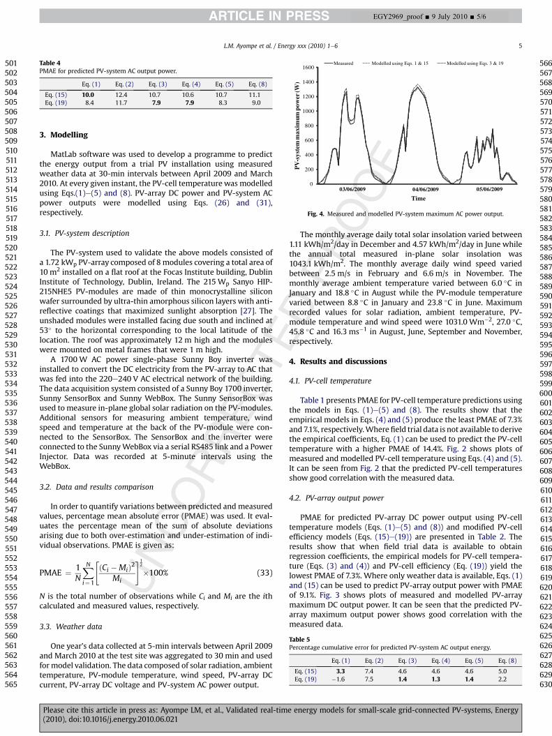
PMAE for PV-system AC power prediction using modelled PV-cell temperatures (Eqs. (1)e(5) and (8)) and PV-cell efficiency (Eqs.(15)e(19)) are shown in Table 4. The empirical models (Eqs. (3), (4)and (9)) give the lowest PMAE of 7.9% while the non-empiricalmodels (Eqs. (1) and (15)) yield a PMAE of 10%. Again the resultsshow that more accurate predictions are obtained when measuredPV-system performance data are used to generate empiricalmodels. Fig. 4 shows measured and modelled PV-system AC outputpower. It is seen in Fig. 4 that both the empirical and non-empiricalmodels show good agreement with measured data.
Table 5 presents percentage cumulative errors for PV-system ACenergy output prediction using PV-cell temperature models (Eqs.(1)e(5) and (8)) and PV-cell efficiency models (Eqs. (15) and (19))against the measured PV-system AC energy output of 1522.5 kWh.The empirical models (Eqs. (3)e(5) and (19)) result in over-esti-mations of 1.3e1.4% while the non-empirical models (Eqs. (1) and(15)) have an over-estimation error of 3.3%.
5. Conclusions
Introduction of smart meters in countries such as Ireland,Belgium and the UK which are currently trailing this technologywith a view of its widespread deployment necessitates moreaccurate prediction of PV-system power output within short-timeintervals such as 30 min. In this study, measured field performancedata for a domestic-scale grid-connected PV installation was usedto validate some of the widely quoted correlations in literatureemployed to model PV-cell temperature and efficiency for poweroutput prediction. The best prediction of PV-system AC outputpower was obtained using Eq. (4) for PV-cell temperature and Eq.(19) for PV-cell efficiency with percentage mean absolute andcumulative errors of 7.9% and 1.3%, respectively. Results show thatfor short-term PV-array power output prediction as is applicable tosmart metering, two options are available.
� Where field performance data of the PV-system is available,empirical models for PV-cell temperature (Eqs. (3) and (4)) andPV-cell efficiency (Eq. (19)) are to be used.
� Where field performance data of the PV-system is not available,the non-empirical models for PV-cell temperature (Eq. (1)) andPV-cell efficiency (Eq. (15)) are to be used.
In both cases, inverter performance data is required to modelthe PV-system AC power output. The proposed models should help
to establish the dynamic performance of PV-systems whencombined with time-of-day billing systems.
References Q2
[1] Spooner ED, Harbidge G. Review of international standards for grid connectedphotovoltaic systems. Renew Energy 2001;22(1-3):235e9.
[2] The German Solar Energy Society. Planning and installing photovoltaicsystems: a guide for installers, architects and engineers. UK: James and James;2006.
[3] Cramer G, Ibrahim M, Keinkauf W. PV system technologies: state-of-the-artand trends in decentralized electrification. Refocus; January/February 2004.
[4] Bernal-Agustín JL, Dufo-López R. Economical and environmental analysis ofgrid connected photovoltaic systems in Spain. Renew Energy 2006;31(8):1107e28.
[5] Alonso García MC, Balenzategui JL. Estimation of photovoltaic module yearlytemperature and performance based on nominal operation cell temperaturecalculations. Renew Energy 2004;29(12):1997e2010.
[6] Jones AD, Underwood CP. A thermal model for photovoltaic systems. SolarEnergy 2001;70(4):349e59.
[7] Trinuruk P, Sorapipatana C, Chenvidhya D. Estimating operating celltemperature of BIPV modules in Thailand. Renew Energy 2009;34(11):2515e23.
[8] Skoplaki E, Palyvos JA. Operating temperature of photovoltaic modules:a survey of pertinent correlations. Renew Energy 2009;34(1):23e9.
[9] Mondol JD, et al. Long-term validated simulation of a building integratedphotovoltaic system. Solar Energy 2005;78(2):163e76.
[10] Mattei M, et al. Calculation of the polycrystalline PV module temperatureusing a simple method of energy balance. Renew Energy 2006;31(4):553e67.
[11] Kymakis E, Kalykakis S, Papazoglou TM. Performance analysis of a grid con-nected photovoltaic park on the island of Crete. Energy Convers Manage2009;50(3):433e8.
[12] Markvart T, editor. Solar electricity. 2nd ed. , Chichester: John Wiley and Sons;2000.
[13] Buresch M. Photovoltaic energy systems. , New York: McGraw-Hill; 1983.[14] Chenni R, et al. A detailed modeling method for photovoltaic cells. Energy
2007;32(9):1724e30.[15] Ueda Y, et al. Performance analysis of various system configurations on
grid-connected residential PV systems. Solar Energy Mater Solar Cells2009;93(6-7):945e9.
[16] Kolhe M, et al. Analytical model for predicting the performance of photo-voltaic array coupled with a wind turbine in a stand-alone renewable energysystem based on hydrogen. Renew Energy 2003;28(5):727e42.
[17] Eicker U. Solar technologies for buildings. England: John Wiley and Sons;2003.
[18] Duffie JA, Beckman WA. Solar engineering of thermal processes. , New York:Wiley; 1991.
[19] McAdams WC, editor. Heat transmission. 3rd ed. , New York: McGraw-Hill;1954.
[20] Cucumo M, et al. Performance analysis of a 3 kW grid-connected photovoltaicplant. Renew Energy 2006;31(8):1129e38.
[21] Hove T. A method for predicting long-term average performance of photo-voltaic systems. Renew Energy 2000;21(2):207e29.
[22] Durisch W, et al. Efficiency model for photovoltaic modules and demonstra-tion of its application to energy yield estimation. Solar Energy Mater SolarCells 2007;91(1):79e84.
[23] Kalogirou SA. Solar energy engineering: processes and systems. , London:Elsevier; 2009.
[24] Durisch W, Lam KH, Close J. Efficiency and degradation of a copper indiumdiselenide photovoltaic module and yearly output at a sunny site in Jordan.Appl Energy 2006;83(12):1339e50.
[25] Mavromatakis F, et al. Modeling the photovoltaic potential of a site. RenewEnergy 2009;35(7):1387e90.
[26] Kaushika ND, Rai AK. An investigation of mismatch losses in solar photovoltaiccell networks. Energy 2007;32(5):755e9.
[27] Sanyo HIT photovoltaic module manual for HIP-215NHE5, HIP-210NHE5 andHIP-205NHE5. Available from: http://www.solarcentury.com/Residential-developers/Specifying-Solar/PV-Catalogue/HIP-215-NHE5-NHE-Series.
L.M. Ayompe et al. / Energy xxx (2010) 1e66
EGY2969_proof ■ 9 July 2010 ■ 6/6
Please cite this article in press as: Ayompe LM, et al., Validated real-time energy models for small-scale grid-connected PV-systems, Energy(2010), doi:10.1016/j.energy.2010.06.021
631632633634635636637638639640641642643644645646647648649650651652653654655656657658659660661662663664665666667668669670671672673674675676677678679680681682683684685686
687688689690691692693694695696697698699700701702703704705706707708709710711712713714715716717718719720721722723724725726727728729730731732733734735736737738739740741742