Optimal transport problems regularized by generic convex ...
Upload
independentCategory
view
0download
0
Time-Optimal Path Tracking for Robots
a Convex Optimization Approach
Diederik Verscheure, Dr. B. Demeulenaere,Prof. J. Swevers, Prof. J. De Schutter, Prof. M. Diehl
Katholieke Universiteit Leuven,Department of Mechanical Engineering,
PMA Division
16 maart 2008
Outline
1 IntroductionTime-optimal motion planning
2 Time-optimal path trackingProblem formulationExisting solution methods
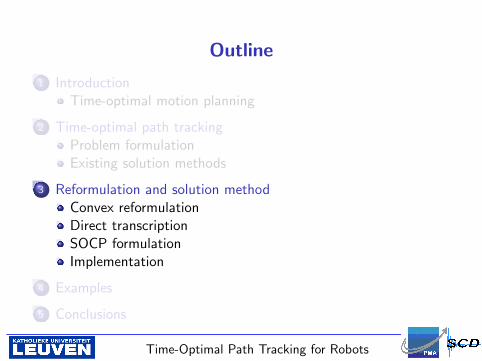
3 Reformulation and solution methodConvex reformulationDirect transcriptionSOCP formulationImplementation
4 Examples
5 Conclusions
Time-Optimal Path Tracking for Robots 2
Outline
1 IntroductionTime-optimal motion planning
2 Time-optimal path trackingProblem formulationExisting solution methods
3 Reformulation and solution methodConvex reformulationDirect transcriptionSOCP formulationImplementation
4 Examples
5 Conclusions
Time-Optimal Path Tracking for Robots 3
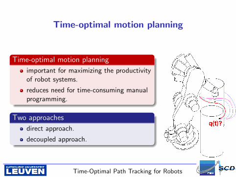
Time-optimal motion planning
Time-optimal motion planning
important for maximizing the productivityof robot systems.
reduces need for time-consuming manualprogramming.
Two approaches
direct approach.
decoupled approach.
Time-Optimal Path Tracking for Robots 4
Time-optimal motion planning
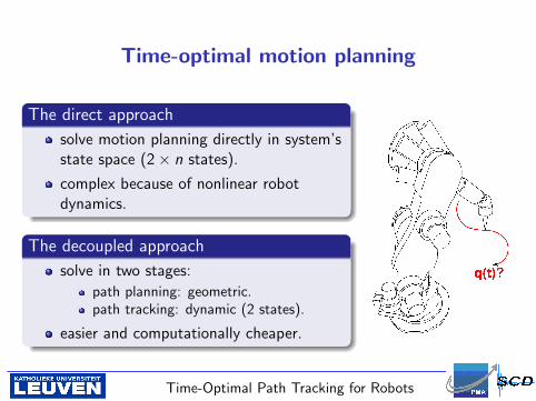
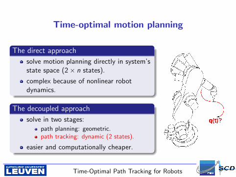
The direct approach
solve motion planning directly in system’sstate space (2× n states).
complex because of nonlinear robotdynamics.
The decoupled approach
solve in two stages:
path planning: geometric.path tracking: dynamic (2 states).
easier and computationally cheaper.
Time-Optimal Path Tracking for Robots 5
Time-optimal motion planning
The direct approach
solve motion planning directly in system’sstate space (2× n states).
complex because of nonlinear robotdynamics.
The decoupled approach
solve in two stages:
path planning: geometric.path tracking: dynamic (2 states).
easier and computationally cheaper.
Time-Optimal Path Tracking for Robots 5
Outline
1 IntroductionTime-optimal motion planning
2 Time-optimal path trackingProblem formulationExisting solution methods
3 Reformulation and solution methodConvex reformulationDirect transcriptionSOCP formulationImplementation
4 Examples
5 Conclusions
Time-Optimal Path Tracking for Robots 6
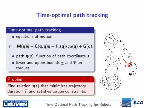
Time-optimal path tracking
Time-optimal path tracking
equations of motion
τ = M(q)q + C(q, q)q + Fs(q)sgn(q) + G(q),
path q(s), function of path coordinate s.
lower and upper bounds τ and τ ontorques.
Problem
Find relation s(t) that minimizes trajectoryduration T and satisfies torque constraints.
Time-Optimal Path Tracking for Robots 7
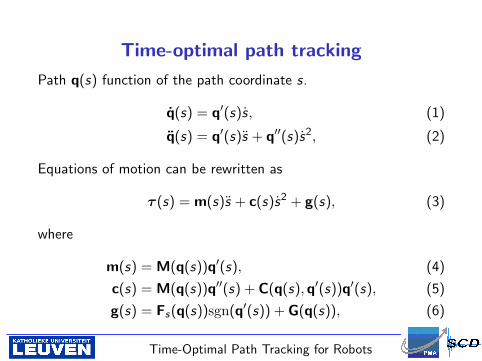
Time-optimal path tracking
Path q(s) function of the path coordinate s.
q(s) = q′(s)s, (1)
q(s) = q′(s)s + q′′(s)s2, (2)
Equations of motion can be rewritten as
τ (s) = m(s)s + c(s)s2 + g(s), (3)
where
m(s) = M(q(s))q′(s), (4)
c(s) = M(q(s))q′′(s) + C(q(s),q′(s))q′(s), (5)
g(s) = Fs(q(s))sgn(q′(s)) + G(q(s)), (6)
Time-Optimal Path Tracking for Robots 8
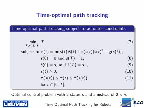
Time-optimal path tracking
Time-optimal path tracking subject to actuator constraints
minT ,s(·),τ (·)
T , (7)
subject to τ (t) = m(s(t))s(t) + c(s(t))s(t)2 + g(s(t)),
s(0) = 0 and s(T ) = 1, (8)
s(0) = s0 and s(T ) = sT , (9)
s(t) ≥ 0, (10)
τ (s(t)) ≤ τ (t) ≤ τ (s(t)), (11)
for t ∈ [0,T ].
Optimal control problem with 2 states s and s instead of 2× n.
Time-Optimal Path Tracking for Robots 9
Time-optimal path tracking
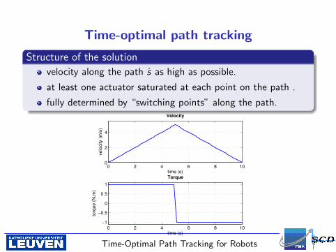
Structure of the solution
velocity along the path s as high as possible.
at least one actuator saturated at each point on the path .
fully determined by “switching points” along the path.
0 2 4 6 8 100
2
4
time (s)
velo
city (
m/s
)
Velocity
0 2 4 6 8 10
−1
−0.5
0
0.5
1
time (s)
torq
ue (
N.m
)
Torque
Time-Optimal Path Tracking for Robots 10
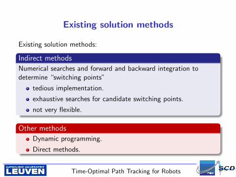
Existing solution methods
Existing solution methods:
Indirect methods
Numerical searches and forward and backward integration todetermine “switching points”
tedious implementation.
exhaustive searches for candidate switching points.
not very flexible.
Other methods
Dynamic programming.
Direct methods.
Time-Optimal Path Tracking for Robots 11
Outline
1 IntroductionTime-optimal motion planning
2 Time-optimal path trackingProblem formulationExisting solution methods
3 Reformulation and solution methodConvex reformulationDirect transcriptionSOCP formulationImplementation
4 Examples
5 Conclusions
Time-Optimal Path Tracking for Robots 12

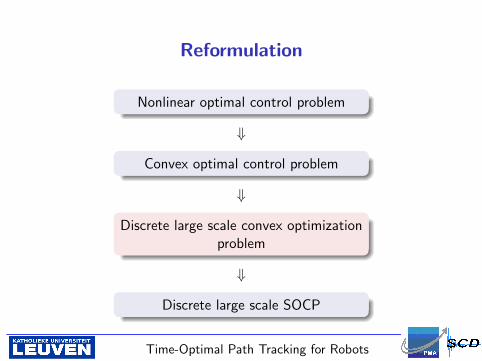
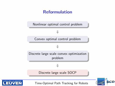
Reformulation
Nonlinear optimal control problem
⇓
Convex optimal control problem
⇓
Discrete large scale convex optimizationproblem
⇓
Discrete large scale SOCP
Time-Optimal Path Tracking for Robots 13
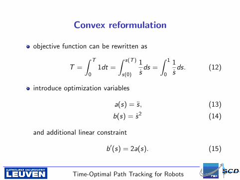
Convex reformulation
objective function can be rewritten as
T =
∫ T
01dt =
∫ s(T )
s(0)
1
sds =
∫ 1
0
1
sds. (12)
introduce optimization variables
a(s) = s, (13)
b(s) = s2 (14)
and additional linear constraint
b′(s) = 2a(s). (15)
Time-Optimal Path Tracking for Robots 14
Convex reformulation
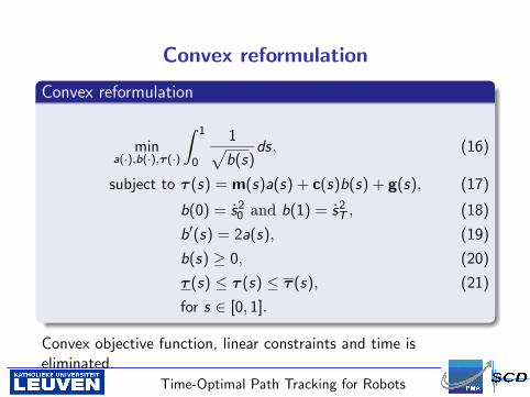
Convex reformulation
mina(·),b(·),τ (·)
∫ 1
0
1√b(s)
ds, (16)
subject to τ (s) = m(s)a(s) + c(s)b(s) + g(s), (17)
b(0) = s20 and b(1) = s2
T , (18)
b′(s) = 2a(s), (19)
b(s) ≥ 0, (20)
τ (s) ≤ τ (s) ≤ τ (s), (21)
for s ∈ [0, 1].
Convex objective function, linear constraints and time iseliminated.
Time-Optimal Path Tracking for Robots 15
Reformulation
Nonlinear optimal control problem
⇓
Convex optimal control problem
⇓
Discrete large scale convex optimizationproblem
⇓
Discrete large scale SOCP
Time-Optimal Path Tracking for Robots 16
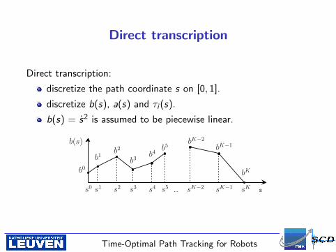
Direct transcription
Direct transcription:
discretize the path coordinate s on [0, 1].
discretize b(s), a(s) and τi (s).
b(s) = s2 is assumed to be piecewise linear.
... s sK
sK−1
sK−2
s5
s4
s3
s2
s1
s0
bK
bK−1
bK−2
b5
b4
b3
b2
b1
b0
b(s)
Time-Optimal Path Tracking for Robots 17
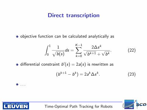
Direct transcription
objective function can be calculated analytically as∫ 1
0
1√b(s)
ds =K−1∑k=0
2∆sk
√bk+1 +
√bk
. (22)
differential constraint b′(s) = 2a(s) is rewritten as
(bk+1 − bk) = 2ak∆sk . (23)
. . .
Time-Optimal Path Tracking for Robots 18
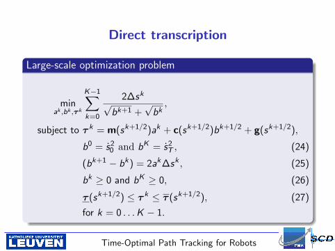
Direct transcription
Large-scale optimization problem
minak ,bk ,τ k
K−1∑k=0
2∆sk
√bk+1 +
√bk
,
subject to τ k = m(sk+1/2)ak + c(sk+1/2)bk+1/2 + g(sk+1/2),
b0 = s20 and bK = s2
T , (24)
(bk+1 − bk) = 2ak∆sk , (25)
bk ≥ 0 and bK ≥ 0, (26)
τ (sk+1/2) ≤ τ k ≤ τ (sk+1/2), (27)
for k = 0 . . .K − 1.
Time-Optimal Path Tracking for Robots 19
Reformulation
Nonlinear optimal control problem
⇓
Convex optimal control problem
⇓
Discrete large scale convex optimizationproblem
⇓
Discrete large scale SOCP
Time-Optimal Path Tracking for Robots 20
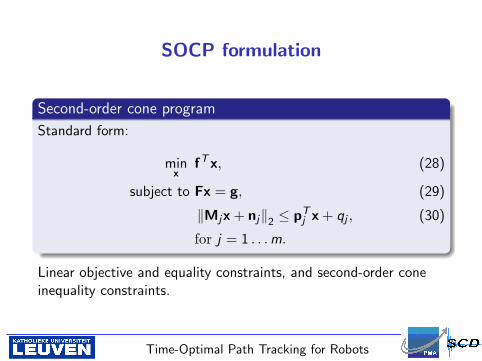
SOCP formulation
Second-order cone program
Standard form:
minx
fTx, (28)
subject to Fx = g, (29)
‖Mjx + nj‖2 ≤ pTj x + qj , (30)
for j = 1 . . .m.
Linear objective and equality constraints, and second-order coneinequality constraints.
Time-Optimal Path Tracking for Robots 21
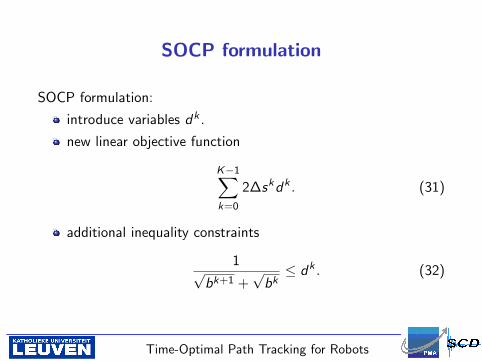
SOCP formulation
SOCP formulation:
introduce variables dk .
new linear objective function
K−1∑k=0
2∆skdk . (31)
additional inequality constraints
1√bk+1 +
√bk
≤ dk . (32)
Time-Optimal Path Tracking for Robots 22
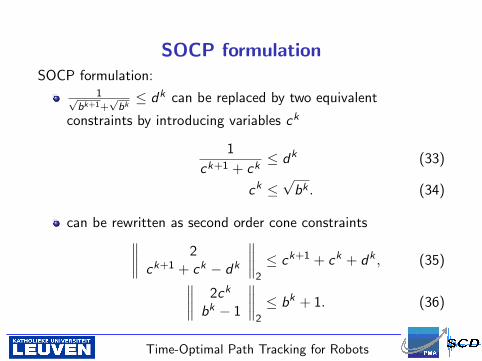
SOCP formulationSOCP formulation:
1√bk+1+
√bk≤ dk can be replaced by two equivalent
constraints by introducing variables ck
1
ck+1 + ck≤ dk (33)
ck ≤√
bk . (34)
can be rewritten as second order cone constraints∥∥∥∥ 2ck+1 + ck − dk
∥∥∥∥2
≤ ck+1 + ck + dk , (35)∥∥∥∥ 2ck
bk − 1
∥∥∥∥2
≤ bk + 1. (36)
Time-Optimal Path Tracking for Robots 23
SOCP formulation
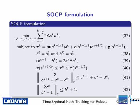
SOCP formulation
minak ,bk ,τ k ,ck ,dk
K−1∑k=0
2∆skdk , (37)
subject to τ k = m(sk+1/2)ak + c(sk+1/2)bk+1/2 + g(sk+1/2),
b0 = s20 and bK = s2
T , (38)
(bk+1 − bk) = 2ak∆sk , (39)
τ (sk+1/2) ≤ τ k ≤ τ (sk+1/2), (40)∥∥∥∥ 2ck+1 + ck − dk
∥∥∥∥2
≤ ck+1 + ck + dk , (41)∥∥∥∥ 2ck
bk − 1
∥∥∥∥2
≤ bk + 1. (42)
Time-Optimal Path Tracking for Robots 24
SOCP formulation
OK, but...
this sounds all very complicated...
and why should I care?
Easy and efficient
Once the (complicated) formulation is done, implementation is
very easy.
automatically efficient.
requires almost no optimization knowledge.
Time-Optimal Path Tracking for Robots 25
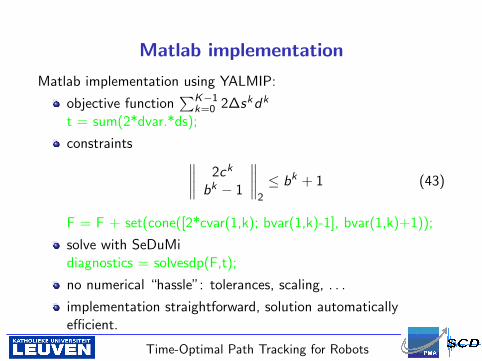
Matlab implementation
Matlab implementation using YALMIP:
objective function∑K−1
k=0 2∆skdk
t = sum(2*dvar.*ds);
constraints ∥∥∥∥ 2ck
bk − 1
∥∥∥∥2
≤ bk + 1 (43)
F = F + set(cone([2*cvar(1,k); bvar(1,k)-1], bvar(1,k)+1));
solve with SeDuMidiagnostics = solvesdp(F,t);
no numerical “hassle”: tolerances, scaling, . . .
implementation straightforward, solution automaticallyefficient.
Time-Optimal Path Tracking for Robots 26
Outline
1 IntroductionTime-optimal motion planning
2 Time-optimal path trackingProblem formulationExisting solution methods
3 Reformulation and solution methodConvex reformulationDirect transcriptionSOCP formulationImplementation
4 Examples
5 Conclusions
Time-Optimal Path Tracking for Robots 27
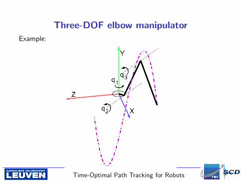
Three-DOF elbow manipulator
Example:
Time-Optimal Path Tracking for Robots 28
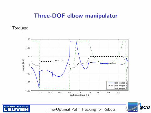
Three-DOF elbow manipulator
Torques:
0.1 0.2 0.3 0.4 0.5 0.6 0.7 0.8 0.9−150
−100
−50
0
50
100
150
path coordinate (−)
torq
ue (
N.m
)
joint torque 1joint torque 2joint torque 3
Time-Optimal Path Tracking for Robots 29
Three-DOF elbow manipulator
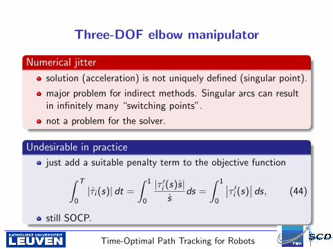
Numerical jitter
solution (acceleration) is not uniquely defined (singular point).
major problem for indirect methods. Singular arcs can resultin infinitely many “switching points”.
not a problem for the solver.
Undesirable in practice
just add a suitable penalty term to the objective function∫ T
0|τi (s)| dt =
∫ 1
0
|τ ′i (s)s|s
ds =
∫ 1
0
∣∣τ ′i (s)∣∣ ds, (44)
still SOCP.
Time-Optimal Path Tracking for Robots 30
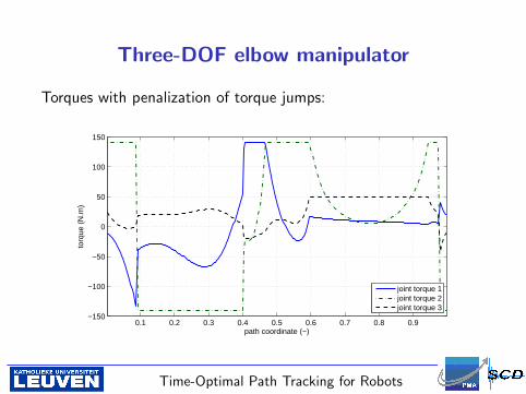
Three-DOF elbow manipulator
Torques with penalization of torque jumps:
0.1 0.2 0.3 0.4 0.5 0.6 0.7 0.8 0.9−150
−100
−50
0
50
100
150
path coordinate (−)
torq
ue (
N.m
)
joint torque 1joint torque 2joint torque 3
Time-Optimal Path Tracking for Robots 31
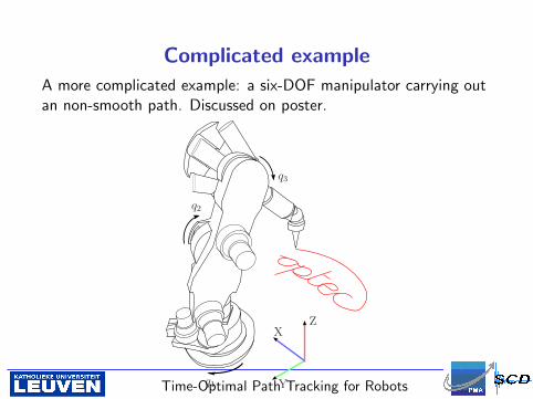
Complicated example
A more complicated example: a six-DOF manipulator carrying outan non-smooth path. Discussed on poster.
q1
q2
q3
X
Y
Z
Time-Optimal Path Tracking for Robots 32
Outline
1 IntroductionTime-optimal motion planning
2 Time-optimal path trackingProblem formulationExisting solution methods
3 Reformulation and solution methodConvex reformulationDirect transcriptionSOCP formulationImplementation
4 Examples
5 Conclusions
Time-Optimal Path Tracking for Robots 33
Conclusions
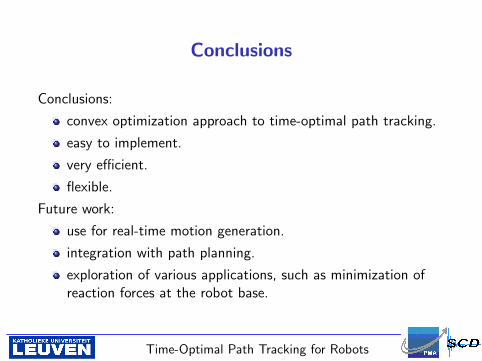
Conclusions:
convex optimization approach to time-optimal path tracking.
easy to implement.
very efficient.
flexible.
Future work:
use for real-time motion generation.
integration with path planning.
exploration of various applications, such as minimization ofreaction forces at the robot base.
Time-Optimal Path Tracking for Robots 34
Thank you for your attention
Thank you for your attention!
Comments/Suggestions/Questions?
Time-Optimal Path Tracking for Robots 35
Copyright © 2022 FDOKUMEN