3 May 2012 Submitted for publication c© The Authors

Discrete Mathematics, Algorithms and Applicationsc© World Scientific Publishing Company

FAT HEAPS WITHOUT REGULAR COUNTERS∗

AMR ELMASRYDepartment of Computer Engineering and Systems

Alexandria University, Egyptelmasry@mpi-inf.mpg.de

JYRKI KATAJAINENDepartment of Computer Science

University of Copenhagen, Denmark

jyrki@diku.dk

We introduce a variant of fat heaps that does not rely on regular counters, and still

achieves the optimal worst-case bounds: O(1) for find-min, insert and decrease, andO(logn) for delete and delete-min. Compared to the original, our variant is simpler toexplain, more efficient, and easier to implement. Experimental results suggest that ourimplementation is superior to structures, like run-relaxed heaps, that achieve the same

worst-case bounds, and competitive to structures, like Fibonacci heaps, that achieve thesame bounds in the amortized sense.

Keywords: Data structures; priority queues; decrease operation; regular counters.

Mathematics Subject Classification 2010: 68P05, 68W40, 68Q25, 11Z05

1. Introduction

Motivation. A numeral system is a notation for representing numbers using

symbols—digits—in a consistent manner. Operations such as modifying a specified

digit must obey the rules guarding the numeral system. These rules vary from simple

rules as, for example, allowing only two symbols in the digit set (binary system)

to more involved rules that constrain the relationship between digits. There is a

connection between numeral systems and data-structural design [5,17]. Relating

the number of objects of particular type in the data structure to the value of a digit

in the representation of a number may allow the performance of the operations on

such objects to be improved. Caveat that complex constraints might complicate the

structure and make the implementation impractical.

Formally, a counter representing a number d = (d0, d1, . . . , dℓ−1), where d0 is

the least significant digit and dℓ−1 the most significant digit (dℓ−1 6= 0), should

support the following two fundamental operations:

∗The results of this paper were presented at the 6th Workshop on Algorithms and Computationheld in Dhaka, Bangladesh in February 2012.

1

3 May 2012 Submitted for publication c© The Authors

2 Amr Elmasry and Jyrki Katajainen

d.increment(di): That is, perform ++di. At the data-structural level this means that

we insert an object of type i into the data structure.

d.decrement(di): That is, perform --di. At the data-structural level this means

that we delete an object of type i from the data structure.

When increasing a digit by one we may break the rules that guard the number

representation. Therefore, there should be a mechanism to normalize the represen-

tation after an increment. Also, before decreasing a digit by one, the value of that

digit can be zero so there should be a mechanism to create an object of that type

first. Sometimes we also need a mechanism to iterate over all non-zero digits in a

counter. To do this, we assume the availability of two additional operations:

d.first(): Return the smallest index i for which di 6= 0 in d; if no such digit exists,

the return value is unspecified.

d.empty(): Return true if there is no non-zero digit in d.

With the above-mentioned operations we can add a counter d′′ to another counter

d′ as follows:

while not d′′.empty()

di ← d′′.first()

d′′.decrement(di)

d′.increment(di)

Many data structures—such as worst-case-efficient finger trees [14], fat heaps

[15,16], fast meldable priority queues [1,11], and worst-case-optimal meldable pri-

ority queues [2,12]—rely on numeral systems and, as introduced, the application

of numeral systems seems to be essential. In a recent paper [11] we introduced the

strictly-regular numeral system, and showed how to use it to improve the constant

factors in the worst-case performance of the priority queue described in [1]. We ad-

vocated that numeral systems are important when developing worst-case-efficient

data structures, but we also warned against their overuse. To make the latter point

clear, we show in this paper that fat heaps can be implemented, within the same

asymptotic performance, without involved numeral systems.

Related work. In general, the most favoured priority queues are binary heaps

[19] and Fibonacci heaps [13]. Nevertheless, the asymptotic running times for binary

heaps are not optimal for all operations, and the bounds for Fibonacci heaps are

amortized. Many other priority-queue structures that are efficient in the worst-case

sense have been developed. In Table 1 we summarize the asymptotic performance

of the worst-case-efficient priority queues that are relevant for the present study.

Since the meld operation is seldom needed in applications, and as the struc-

tures described in [2,12] are complicated and impractical, run-relaxed heaps and

fat heaps are the structures of choice when worst-case constant-time decrease has

to be supported. Elsewhere it has been stated that the worst-case-efficient priority

3 May 2012 Submitted for publication c© The Authors

Fat Heaps Without Regular Counters 3

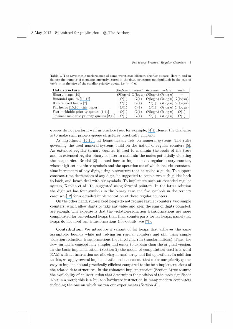
Table 1. The asymptotic performance of some worst-case-efficient priority queues. Here n and m

denote the number of elements currently stored in the data structures manipulated; in the case ofmeld m is the size of the smaller priority queue, i.e. m ≤ n.

Data structure find -min insert decrease delete meld

Binary heaps [19] O(log n) O(log n) O(log n) O(log n) –

Binomial queues [10,17] O(1) O(1) O(log n) O(log n) O(logm)Run-relaxed heaps [7] O(1) O(1) O(1) O(log n) O(logm)Fat heaps [15,16],[this paper] O(1) O(1) O(1) O(log n) O(logm)Fast meldable priority queues [1,11] O(1) O(1) O(log n) O(log n) O(1)Optimal meldable priority queues [2,12] O(1) O(1) O(1) O(log n) O(1)

queues do not perform well in practice (see, for example, [4]). Hence, the challenge

is to make such priority-queue structures practically efficient.

As introduced [15,16], fat heaps heavily rely on numeral systems. The rules

governing the used numeral systems build on the notion of regular counters [5].

An extended regular ternary counter is used to maintain the roots of the trees

and an extended regular binary counter to maintain the nodes potentially violating

the heap order. Brodal [2] showed how to implement a regular binary counter,

whose digit set has three symbols and the operation set of which includes constant-

time increments of any digit, using a structure that he called a guide. To support

constant-time decrements of any digit, he suggested to couple two such guides back

to back, and hence deal with six symbols. To implement such an extended regular

system, Kaplan et al. [15] suggested using forward pointers. In the latter solution

the digit set has four symbols in the binary case and five symbols in the ternary

case; see [12] for a detailed implementation of these regular counters.

On the other hand, run-relaxed heaps do not require regular counters; two simple

counters, which allow digits to take any value and keep the sum of digits bounded,

are enough. The expense is that the violation-reduction transformations are more

complicated for run-relaxed heaps than their counterparts for fat heaps; namely fat

heaps do not need run transformations (for details, see [7]).

Contribution. We introduce a variant of fat heaps that achieves the same

asymptotic bounds while not relying on regular counters and still using simple

violation-reduction transformations (not involving run transformations). Thus, the

new variant is conceptually simpler and easier to explain than the original version.

In the basic implementation (Section 2) the model of computation used is a word

RAM with an instruction set allowing normal array and list operations. In addition

to this, we apply several implementation enhancements that make our priority queue

easy to implement and practically efficient compared to the best implementations of

the related data structures. In the enhanced implementation (Section 3) we assume

the availability of an instruction that determines the position of the most significant

1-bit in a word; this is a built-in hardware instruction in many modern computers

including the one on which we ran our experiments (Section 4).

3 May 2012 Submitted for publication c© The Authors

4 Amr Elmasry and Jyrki Katajainen

2. Fat Heaps Simplified

Structure. A fat heap [15,16] is a forest of trinomial trees. A trinomial tree of

rank r is composed of three trinomial trees of rank r− 1, two of which are subtrees

of the root of the third tree. The rank is recorded at the root of the tree. A node

of rank r then has two children of rank 0, rank 1, . . . , rank r − 1. A single node

has rank 0. It follows that a trinomial tree of rank r has n = 3r nodes and its root

has 2r = 2 log3 n children. Similar to relaxed heaps [7], the trees are heap ordered,

i.e. an element associated with a node is not smaller than that associated with its

parent, except for some special nodes that may, but not necessarily, violate the heap

order; these nodes are called potential violation nodes. A fat heap storing n elements

consists of O(log n) trinomial trees, which may contain O(log n) violation nodes.

The children of a node are maintained in non-decreasing rank order forming

a child list. The roots of the trees are linked in a similar manner forming a root

list. Each node has two pointers to its siblings to keep it on one of these lists,

and a pointer to its last child. The right-sibling pointer of the last child points to

the parent. Additionally, each node stores its rank and a root-indicator bit that

distinguishes roots from other nodes.

The key issue in a fat heap is how to keep track of the roots and the violation

nodes, and how to make sure that their count never gets too high. In the original

articles [15,16] numeral systems were used for both of these purposes. Our point

here is to show that a much simpler tool, a resizable array collecting duplicates at

each rank, is enough in both cases.

Tree reductions. The rank of any tree in a fat heap that has n elements is at

most ⌊log3 n⌋. If the number of trees is larger than 2 ⌊log3 n⌋+ 2, there must be at

least three trees having the same rank. Three trinomial trees of rank r can be joined

in one of rank r+1 by making the root that has the smallest element the new root

and making the other two trees the last two subtrees of this root. This operation,

called a tree reduction, requires two element comparisons and six pointer updates.

Root inventory. In order to detect at which ranks we have more than two

trees, we maintain a root inventory which consists of two parts:

(1) a resizable array where the rth entry stores the number of trees of rank r as

well as a pointer to the first root of rank r, and

(2) a doubly-linked list on the entries of the array indicating the ranks at which

there are more than two trees.

Using this linked list and the array, three trees to be joined can be easily located.

See Section 3 for a different treatment that uses a bit vector, instead of the linked

list, to indicate the ranks at which there are more than two trees.

Violation inventory. For the violation nodes we use a similar arrangement.

The so-called violation inventory also has two parts:

3 May 2012 Submitted for publication c© The Authors

Fat Heaps Without Regular Counters 5

(1) a resizable array where the rth entry records the number of violation nodes of

rank r as well as a pointer to one violation node of rank r, and

(2) a doubly-linked list on the entries of the array indicating the ranks at which a

violation reduction is possible (details are given below).

See Section 3 for a different treatment that uses a bit vector.

To keep track of the violation nodes that have the same rank, we maintain a

doubly-linked list for each rank. We do this indirectly so that the list contains objects

each of which has a pointer to a priority-queue node, which has a pointer back to

this list object. We need the back pointer when a node becomes non-violating and

has to be in accordance removed from its list in constant time. Observe that in

their original form [15,16] fat heaps do not need this back pointer, as the number of

violation nodes per rank is a constant; this overhead is a drawback of our simplified

construction. On the other hand, similar to our treatment, run-relaxed heaps do

need these back pointers. See Section 3 for a different treatment that uses arena-

based memory management for the intermediate list objects; in effect, the storage

overhead at the priority-queue nodes can be reduced.

Storage requirements. Each priority-queue node has an element, a rank, a

root-indicator bit, and four pointers: two sibling pointers, a last-child pointer, and

a pointer to the violation inventory. The amount of storage used by the root and

violation inventories is O(log n).

Violation reductions. A violation reduction at rank r makes two rank-r vio-

lation nodes non-violating at the expense of possibly introducing one new violation

node at rank r + 1. The main task is to keep the number of violation nodes log-

arithmic. An implementation relying on a numeral system [15,16] achieves this by

guaranteeing that the number of violation nodes per rank is at most a constant.

To avoid run transformations [7], each of the two rank-r violation nodes involved

in a reduction must either be one of the last two children of its parent or have a

non-violating rank-(r+1) sibling. The aforementioned restriction is also guaranteed

when using a numeral system (the reductions are performed on violation nodes of

rank r whose count corresponds to a 2, which is followed by a 0 or 1 indicating that

at most one violation node of rank r + 1 exists).

We do not restrict the number of violation nodes per rank. Instead, similar to

run-relaxed heaps, we maintain the number of violation nodes below ⌊log3 n⌋ + 1.

Our first observation is that when the number of violation nodes becomes larger

than this, we can find a rank r such that there exist at least two violation nodes

of rank r and at most one violation node of rank r + 1; at such rank a violation

reduction is possible. This observation follows from the fact that a root cannot be

violating, and hence no violation nodes with the highest rank exist. Our second

observation is that we can efficiently keep track of ranks where violation reductions

are possible, using an array of double pointers and a doubly-linked list on which

these ranks appear in arbitrary order.

3 May 2012 Submitted for publication c© The Authors

6 Amr Elmasry and Jyrki Katajainen

When a non-violating rank-r node becomes violating or vice versa, it is a routine

matter to update the violation inventory in constant time. We also need to update

the doubly-linked list having the ranks for which violation reductions are possible.

This is done by first updating the number of violation nodes at rank r, then checking

the number of violation nodes at ranks r−1, r, r+1 within the corresponding array

entries. In accordance, we update the double pointers to maintain the doubly-linked

list. (Note that inserting a new rank-entry to this doubly-linked list is done by

adding the corresponding entity to the beginning of the list.) The details are simple

and are left for the reader. See Section 3 for a different treatment that uses bit

operations to detect at which ranks such a reduction would be possible.

Assume that we have two violation nodes u and v of rank r and at most one

violation node at rank r+1. If u is not one of the last two children of its parent, we

know that among the two siblings of u of rank r + 1 at most one can be violating.

Let p be a non-violating sibling of u of rank r + 1, and let x be one of the last two

children of p such that x is non-violating. We make u one of the last two children

of p by swapping the subtree rooted at u with the subtree rooted at x. Similarly,

we ensure that v is one of the last two children of its parent. Assume without loss

of generality that the element at the parent of u is not larger than that at the

parent of v. If u and v are not siblings, we swap the subtree rooted at u and the

subtree rooted at the rank-r sibling of v to make u and v children of the same

parent. Note that in this process no new violation nodes are created. Hereafter

we cut the three subtrees rooted at u, v, and their parent. We then join them in

one tree of rank r + 1 and attach that tree in the place of the subtree rooted at

the parent. Unless the root of the resulting tree is the root of the entire tree, its

node is made violating and added to the violation inventory. The benefit we gain is

that the last two children of the root of the resulting tree are now non-violating. In

total, each violation reduction requires at most three element comparisons and a few

pointer updates. To sum up, a violation reduction comprises three transformations:

cleaning transformation that makes a node one of the last two children of its parent,

gathering transformation that makes two violation nodes of the same rank siblings,

and splitting-rejoining transformation that removes two sibling violation nodes of

the same rank and possibly creates a violation node one level above—this reduces

the number of violation nodes by one or two. These transformations are illustrated

in pictorial form in Fig. 1.

Operations. When the tree- and violation-reduction procedures are available,

it is quite straightforward to implement the priority-queue operations. A summary

of these operations is given in pseudo-code form in Fig. 2.

find -min: All the other operations would maintain a pointer, called the minimum

pointer, to a node that stores the current minimum; this node can be a root

or a violation node. Hence, the operation can be easily supported in constant

time. See Section 3 for a slower version of this operation.

insert : The given node storing the new element is added to the root inventory. If the

3 May 2012 Submitted for publication c© The Authors

Fat Heaps Without Regular Counters 7

(1)u

U

r

p

r+1

x

X

r

cleaning u

x

X

r

p

r+1

u

U

r

(2)p

r+1

u

U

r

s

S

r

q

r+1

v

V

r

t

T

r

gathering u and v

p.element() ≤ q.element()

p

r+1

t

T

r

s

S

r

q

r+1

v

V

r

u

U

r

(3)q

r+1

v

V

r

u

U

r

splitting-rejoining q

r+1

rr

Fig. 1. Primitive transformations in violation reductions: (1) cleaning transformation, (2) gatheringtransformation, and (3) splitting-rejoining transformation. Violation nodes are drawn in grey and

ranks are written above the nodes.

3 May 2012 Submitted for publication c© The Authors

8 Amr Elmasry and Jyrki Katajainen

number of trees exceeds the threshold, their number is reduced by executing one

tree reduction. Since the new node may contain the current minimum, a further

check is done to ensure that the minimum pointer is up to date. In total, this

operation involves a constant amount of work including at most three element

comparisons (two for a tree reduction and one for the minimum-pointer update).

decrease: After making the element replacement, the accessed node is made vio-

lating (without any checks), and one violation reduction is executed if their

number exceeds the threshold. The new value is compared with the minimum,

and the minimum pointer is updated if necessary. Hence, this operation involves

a constant amount of work including at most four element comparisons (three

for a violation reduction and one for the minimum-pointer update).

delete: One way to accomplish this operation is to follow the strategy proposed

by Vuillemin [17] for binomial queues. First, all the ancestors of the deleted

node are visited and marked by traversing the present tree upwards until its

root is reached. Since we are only storing parent pointers for the last children,

a parent is reached by repeatedly accessing right-sibling pointers. Second, the

nodes are processed in a top-down fashion by starting from the root which is

made the current node. If the current node is the deleted node, it is discarded

and its children are inserted into the root inventory. This stops the downward

traversal. On the other hand, if the current node is an ancestor of the deleted

node, the tree rooted at it is split into three trinomial trees. After the split, the

root among these trees that is an ancestor of the deleted node is made the new

current node. The other two are inserted into the root inventory and the current

node is processed recursively. All the new roots added to the root inventory are

removed from the violation inventory since a root cannot be violating. During

the whole process, the number of trees increases by at most 2 log3 n+O(1) and

several tree reductions may be necessary. The number of element comparisons

involved in such tree reductions is at most 2 log3 n+ O(1). If the deleted node

contains the minimum, the new minimum is found by scanning all the roots

and violation nodes, and the minimum pointer is updated; this requires at

most 3 log3 n + O(1) element comparisons. As a result of a deletion n goes

down by 1. Thus, the number of violation nodes may exceed the threshold,

and a violation reduction may be necessary. In total, the number of element

comparisons performed by delete is at most 5 log3 n + O(1) ≈ 3.16 log2 n, and

the work done is O(log n). Note that the pseudo-code given in Fig. 2 adopts a

different implementation strategy, which is explained in Section 3, relying on

borrowing a node to replace the deleted node.

meld : Assume that the queues to be melded store m and n elements, and m ≤ n.

There are two tasks to be done: to merge the root inventories and to merge the

violation inventories. The first task is done by moving the roots, one by one,

from the smaller root inventory to the larger. Thereafter the number of trees

is reduced by repeated tree reductions until it is within the allowable threshold

(below 2 ⌊log3(n+m)⌋ + 2). The amount of work involved is proportional to

3 May 2012 Submitted for publication c© The Authors

Fat Heaps Without Regular Counters 9

the number of element comparisons performed, which is at most 2 log3 m +

O(1). For the second task the larger of the two resizable arrays is kept as the

basis of the violation inventory of the combined priority queue, and the other

array is disposed after all the violation nodes are moved from there to the

other inventory. Thereafter some violation reductions are executed to get the

number of violation nodes below the threshold. The amount of work involved

is proportional to the number of element comparisons performed, which is at

most 3 log3 m+O(1). In total, the number of element comparisons performed by

meld is at most 5 log3 m+O(1) ≈ 3.16 log2 m, and the work done is O(logm).

3. Implementation Enhancements

Genericity. We relied on policy-based design as recommended, for example,

in [4]. The implementation accepted several parameters, making it possible to

change policies in use whenever desired. The parameters passed included the type

of elements stored, comparison function used in element comparisons, nodes used

for encapsulating the elements, root inventory used for keeping track of the roots,

and violation inventory used for keeping track of the violation nodes.

Duplicate grouping. In principle we used almost identical arrangements when

implementing the two inventories. Both included a preallocated array that stored

pointers to the beginning of each duplicate list (roots or violation nodes of the same

rank), and two bit vectors: the occupancy vector that indicated the ranks where

there are at least one entity, and the surplus vector that indicated the ranks where

the number of entities equals or exceeds the boundary. Since there is a logarithmic

number of ranks, each of these bit vectors could be maintained in a single word.

There were four main differences between the two inventories:

(1) What was the boundary making a reduction possible? (three vs. two)

(2) How were reductions accomplished? (tree reduction vs. violation reduction)

(3) What was stored at the priority-queue nodes? (two linkage pointers vs. one back

pointer to the inventory)

(4) How were the duplicates linked? (direct linkage vs. indirect linkage)

The implemented root inventory kept the duplicates grouped, but the roots were

not fully sorted with respect to their ranks. Since the sibling pointers of the roots

were unused, we reused these pointers when linking the duplicates.

Arena. As for the doubly-linked lists that hold objects of the same ranks (see

Section 2), the implemented violation inventory used an extra preallocated array

that was used to store these objects. We call this array the arena, and the resulting

violation inventory arena-based. Yet another bit vector was used to keep track of

the free places on the arena. Each entry of the arena stored a pointer to the priority-

queue node it represents. In addition, each such entry stored two indexes to a next

3 May 2012 Submitted for publication c© The Authors

10 Amr Elmasry and Jyrki Katajainen

class: fat-heap

attributes:

roots: root inventoryviolations: violation inventorymin: minimum noden ∈ Z

method: construct()roots ← ∅violations ← ∅min ← nullptr

n← 0

method: find -min()return min

method: insert(p)p.make-singleton()roots.insert(p)roots.reduce()if p.element() < min.element()

min ← p

++n

method: decrease(p, v)p.element() ← v

violations.insert(p)violations.reduce(roots)if p.element() < min.element()

min ← p

method: borrow()p ← roots.first()roots.delete(p)for q ∈ p.children()

violations.delete(q)roots.insert(q)

p.make-singleton()--n

roots.reduce()violations.reduce(roots)return p

method: delete(p)q ← borrow()if p = q

return

violations.delete(p)for r ∈ p.children()

violations.delete(r)for i = 0 to p.rank()− 1

r1, r2 ← p.children(rank = i)q ← q.join(r1, r2)

p.replace(q, roots)p.make-singleton()violations.insert(q)violations.reduce(roots)if p 6= min

return

min ← roots.first()for r ∈ roots ∪ violations

if r.element() < min.element()min ← r

method: meld(other)if n < other .n

roots.swap(other .roots)violations.swap(other .violations)swap(min, other .min)swap(n, other .n)

while not other .roots.empty()p← other .roots.first()other .roots.delete(p)roots.insert(p)roots.reduce()

while not other .violations.empty()p← other .violations.first()other .violations.delete(p)violations.insert(p)violations.reduce(roots)

p← other .minif p.element() < min.element()

min ← p

n← n+ other .nother .n← 0

Fig. 2. Operations on a fat heap in pseudo-code. We assume that nodes support the op-erations element , children, rank , make-singleton, join, and replace which all have theirobvious meanings. Observe that p.replace(q, roots) takes two arguments: When p is replaced

by q, p can be a root, so it may be necessary to update the root inventory as well. In addition,we assume that both inventories support the operations empty, first , swap, insert , delete,and reduce. Of these, reduce applies one of the reductions once, if possible.

3 May 2012 Submitted for publication c© The Authors

Fat Heaps Without Regular Counters 11

and a previous entry of the same rank within the arena, if any. Now the back pointer

from the priority-queue node could be replaced by the index of the corresponding

entry in the arena. The index stored is called a violation index ; if a node is non-

violating, its violation index has some fixed predetermined value. The good news is

that the violation index, the root-indicator bit, and the rank each can be stored in

one byte, and hence all three can be stored in one word. Other than the data element,

including the sibling and child pointers, this sums up to four words per node. In

addition to saving storage and avoiding pointer manipulation, two important other

benefits of using the arena are improving cache efficiency and avoiding additional

memory allocation and deallocation.

Bit hacks. To perform a tree reduction, the surplus vector of the root inventory

is consulted to pick any rank where the threshold is reached (at least three roots

of that rank exist). This is realized by relying on an instruction that determines

the position of an arbitrary 1-bit in a word. For a violation reduction the situation

is more restricted. Actually, a rank having at least two violation nodes does not

indicate that a violation reduction is possible at that rank. We are looking for a

rank r where the threshold is reached (at least two violation nodes of that rank exist)

and in the meantime rank r+1 has at most one violation node. This is realized by

relying on an instruction that determines the position of the most significant 1-bit

in the surplus vector of the violation inventory. The use of this special instruction

is crucial, as the position of the most significant 1-bit always corresponds to a rank

where a violation reduction is possible.

Borrow-based delete. Following the advice given in [3,7] we did not implement

delete as explained in Section 2. Instead, we borrowed a node from the smallest tree

after splitting it up repeatedly, and then reconstructed the subtree that lost its

root by starting with the borrowed node and repeatedly joining the subtrees of the

deleted node. Before executing the joins, the deleted node and its children are all

removed from the violation inventory, if they were violating, since after the joins

they are no more violating. The new root of the reconstructed tree is made violating,

unless it is a root of an entire tree. As the final step, the minimum pointer is updated

if the current minimum was deleted.

For random deletions this modification would reduce the expected cost of

delete to a constant. To efficiently locate the smallest tree, we again used our bit-

manipulation tools to determine the position of the least significant 1-bit in the

occupancy vector of the root inventory.

Event-driven reductions. We chose to perform reductions in an aggressive

manner. Instead of maintaining exact counts for the number of trees and viola-

tion nodes and checking the thresholds per operation, we opted for performing

reductions after operations whenever possible. A tree reduction is performed by

every insert and delete if possible. A violation reduction is performed by every

decrease and delete if possible. During meld a tree reduction is performed after

every root move, and a violation reduction is performed after every violation-node

3 May 2012 Submitted for publication c© The Authors

12 Amr Elmasry and Jyrki Katajainen

move, if either is possible. It is worth mentioning that although our implementation

of delete may significantly increase the number of trees because of the borrowing

of the root of the smallest tree, performing only one tree reduction in insert and

delete would still guarantee that the number of trees is at most 2 ⌊log3 n⌋ + 2. In

fact, one can prove by induction a stronger bound; after each operation the number

of trees is at most 2 ⌊log3 n⌋+2−2ζ0− ζ1, where ζ0 is the number of ranks for each

of which no root with that rank exists and ζ1 is the number of ranks for each of

which exactly one root with that rank exists.

Slow minimum finding. In some applications it is advantageous to keep

find -min fast, while in other applications it is advantageous to support find -min

in logarithmic time and remove the burden of updating the minimum pointer from

other operations. To facilitate this we implemented a decorator that could transform

any priority queue supporting logarithmic find -min to one that supports constant-

time find -min; the only overhead caused is that each delete-min has to find the

minimum element before its removal instead of updating the minimum pointer after

the operation. Hence, we can support both variants in a flexible manner.

4. Experiments

Competitors. We implemented fat heaps as discussed in the previous section.

Our programs have been made part of the CPH STL (www.cphstl.dk), from where

we also picked three competitors for comparison. All of the existing implementations

of these data structures were highly tuned.

Run-relaxed weak queue [9]: This is a binary version of a run-relaxed heap [7],

which has the same worst-case behaviour as a fat heap. The design of run-

relaxed weak queues and fat heaps was similar; in principle, only the root and

violation inventories were implemented differently. The use of such policy-based

design is encouraged, for example, in [4], and the implementation of run-relaxed

weak queues that we used is documented in [8].

Fibonacci heap [13]: This priority queue has the same bounds (meld is even amort-

ized constant) as a fat heap but in the amortized sense. The variant of Fi-

bonacci heaps used was extremely lazy: insert , decrease, and delete operations

only appended some nodes to the root list and left all the actual work for the

forthcoming find -min operations (which had to consolidate the root list). Be-

cause of this laziness we do not expect any of the worst-case-efficient priority

queues to beat this variant for other than find -min and delete-min operations.

Binary heap [19]: The library implementation of binary heaps that we used is array-

based, except that elements were stored indirectly to retain referential integrity

as advised in [6, Chapter 6]. The bottom-up version of the heapify-down pro-

cedure was used to restore the heap order after deletion (see, e.g. [18]).

Implementation alternatives considered. We implemented the array-based

root inventory that keeps the roots of the same rank on doubly-linked lists as

3 May 2012 Submitted for publication c© The Authors

Fat Heaps Without Regular Counters 13

proposed in [7]. Additionally, we tested two other root-inventory implementations

that both relied on regular counters. The first alternative employed the special

regular counter proposed in [9], which supports digit injections and ejections at one

end and satellite-data updates at any position. The second alternative employed the

standard regular counter discussed in [5]. In all three alternatives bit vectors were

used to record the occupancy level at each rank. In our experiments all three types

of inventories worked well. Of the tested structures, our fat heap used the array-

based duplicate grouping, whereas the run-relaxed weak queue used the solution

based on the standard regular counter.

We tried three different violation-inventory realizations. The first was almost

identical to the array-based root inventory. Instead of storing roots the inventory

stored violation nodes, and in the nodes space for two additional pointers was re-

served to link duplicates. Interestingly, in spite of the larger memory footprint of

the nodes, this version worked well in practice. As we expected that the amount

of extra space used will be important in some applications, we also considered the

compact violation inventory described in [4] and the arena-based solution described

in Section 3. After some preliminary experiments, we decided to use the arena-based

solution both in our fat heap as well as in the run-relaxed weak queue implementa-

tions, since the more complex bit-packing techniques of [4] were a bit slower.

Lines of code. By looking at the code available at the repository of the CPH

STL we can quantitatively verify that a fat heap is simpler than a run-relaxed weak

queue (see Table 2). Even though the lines-of-code (LOC) metric may be considered

questionable, the numbers extracted clearly suggest that the transformations needed

for performing a violation reduction are simpler for fat heaps than for run-relaxed

weak queues. On the other hand, the LOC counts also suggest that the array-based

tree inventory and the numeral-system-based root inventory have about the same

complexity. Moreover, it is clear that both fat heaps and run-relaxed weak queues

require much more code than binary and Fibonacci heaps.

Environment. In our tests we used a laptop with the following configuration:

Processor: Intel R© CoreTM2 CPU P8700 @ 2.53GHz × 2

Memory: 3.8 GB

Cache: 3 MB, cache line 64 B, 12-way associative

Operating system: Ubuntu 11.10 (Linux kernel 3.0.0-19-generic-pae)

Compiler: g++ (gcc version 4.6.1)

Compiler options: -Wall -std=c++0x -O3

In all experiments the elements stored in the priority queues were of

type long long. The standard-library functions rand and random_shuffle were

used when generating random numbers and random permutations, and the function

clock when measuring the CPU time usage. All branch-misprediction and cache-

miss measurements were carried out using the simulators available in valgrind

(version 3.6.1). For a problem of size n, each experiment was repeated 107/n times

3 May 2012 Submitted for publication c© The Authors

14 Amr Elmasry and Jyrki Katajainen

Table 2. Approximative LOC counts for some priority-queue realizations in the CPH STL. Allcomments, lines only having a single parenthesis, debugging code, and assertions were excluded.

Data structure Component LOC

Fat heap kernel 136node 63root inventory 116violation inventory 277transformations 188Total 780

Run-relaxed weak queue kernel 146node 63root inventory 118violation inventory 277transformations 368Total 972

Fibonacci heap kernel 192node 104Total 296

Binary heap kernel 124node 43heapifier 38Total 205

(more time-consuming simulations only max{3, 105/n} times), each repetition us-

ing a different priority queue, and the mean over all test runs was reported. In our

experiments we used the logarithmic (slow) version of find -min for all the priority

queues under investigation, except (naturally) for binary heaps.

Homogeneous operation sequences. In our first set of experiments we con-

sidered the following operation sequences:

insertn: Starting from an empty structure perform n insert operations. The elem-

ents were given in decreasing order.

decreasen: Starting from a structure of size n, created by n insert operations fol-

lowed by one find -min operation, perform n decrease operations. Insertions were

performed in random order. The value of each element was decreased once and

the decreases were performed in value order, starting from the largest value,

such that the value of each element became smaller than the current minimum.

deleten: Starting from a structure of size n, created by n insert operations followed

by one find -min operation, perform n delete operations. The elements were

inserted in random order and deleted in the same order.

delete-minn: Starting from a structure of size n, created by n insert operations,

perform n delete-min operations. The elements were inserted in random order.

3 May 2012 Submitted for publication c© The Authors

Fat Heaps Without Regular Counters 15

We measured the work per operation by dividing the total work used for the

whole sequence by n. The work used for all initializations was excluded from the

measurement results. When analysing the performance of different priority queues

on these operation sequences, we considered three performance indicators: running

time, number of element comparisons, and number of pointer updates.

From the results in Tables 3–5, we can see that in our experimental setup bi-

nary heaps performed poorly for insert and decrease, and that Fibonacci heaps

were performing better than both fat heaps and run-relaxed weak queues as for

insert , decrease, and delete. The reason for this good behaviour is that the lazy

version of Fibonacci heaps postpones the actual work to find -min and delete-min.

Although fat heaps require more element comparisons than run-relaxed weak queues

per decrease, our fat-heap implementation was typically faster; this is due to the

simpler transformations, the avoidance of numeral-system complications, and other

implementation enhancements. For delete-min, the other priority queues were faster

than Fibonacci heaps; here Fibonacci heaps pay for the laziness of the other oper-

ations.

Heterogeneous operation sequences. In our second set of experiments we

considered intermixed operation sequences. One sequence of this type is composed

of rounds each having k decrease operations and ending with a minimum deletion.

We specifically studied the special sequence insertn(decreasek find -min delete)n.

This kind of sequence often appears in applications (e.g. in shortest-paths and

minimum-spanning-tree algorithms). We observed that once k was larger than a

small constant (5 in our experiments), the effect of decreases started being domi-

nating. For measuring the performance of different priority queues on this special

sequence, we considered three performance indicators: running time, number of

branch mispredictions, and number of cache misses.

The initial values were n distinct integers drawn from a consecutive range and

the elements were inserted in decreasing order. As to decreases, we selected a random

element for the target of each decrease and decreased the current value by n each

time. In particular, observe that the setup is a bit different from that used in the

previous experiments. In deletions, we deleted the minimum just found before the

deletion. The results of our experiments for the three performance measures are

displayed in Tables 6–8.

These experiments gave a consistent picture of the behaviour of the four data

structures: Binary heaps were the fastest, Fibonacci heaps came the second, run-

relaxed weak queues were the slowest, and fat heaps landed between Fibonacci

heaps and run-relaxed weak queues. Some divergences are possible, but in general

the behaviour of these data structures is predictable. The three advanced data

structures are less sensitive to the data values than to the sequence of operations. On

the other hand, as our experiments for homogeneous operation sequences showed,

binary heaps are more sensitive to the data values than the other structures.

3 May 2012 Submitted for publication c© The Authors

16 Amr Elmasry and Jyrki Katajainen

Table 3. Performance of fat heaps and their competitors for homogeneous operation sequences;average running time per operation (in nanoseconds).

Test Data structure n = 10 000 n = 100 000 n = 1000 000

insertn Fat heap 91 90 87Run-relaxed weak queue 103 102 101Fibonacci heap 71 70 68Binary heap 168 201 249

decreasen Fat heap 192 280 571Run-relaxed weak queue 222 281 560Fibonacci heap 10 41 144Binary heap 138 239 1 201

deleten Fat heap 233 253 285Run-relaxed weak queue 262 285 308Fibonacci heap 17 32 45Binary heap 56 80 246

delete-minn Fat heap 337 589 1 524Run-relaxed weak queue 287 509 1 586Fibonacci heap 506 867 2 088Binary heap 234 368 1 561

Table 4. Performance of fat heaps and their competitors for homogeneous operation sequences;

average number of element comparisons performed per operation.

Test Data structure n = 10 000 n = 100 000 n = 1000 000

insertn Fat heap 0.99 0.99 0.99Run-relaxed weak queue 0.99 0.99 0.99Fibonacci heap 0 0 0Binary heap 11.36 14.68 17.95

decreasen Fat heap 2.96 2.99 2.99Run-relaxed weak queue 1.98 1.99 1.99Fibonacci heap 0 0 0Binary heap 12.36 15.68 18.95

deleten Fat heap 3.06 3.14 3.17Run-relaxed weak queue 2.44 2.43 2.43Fibonacci heap 0 0 0Binary heap 2.54 2.59 2.61

delete-minn Fat heap 20.35 26.64 32.92Run-relaxed weak queue 16.40 21.31 26.23Fibonacci heap 16.23 21.22 26.20Binary heap 12.01 15.34 18.64

3 May 2012 Submitted for publication c© The Authors

Fat Heaps Without Regular Counters 17

Table 5. Performance of fat heaps and their competitors for homogeneous operation sequences;average number of pointer updates performed per operation.

Test Data structure n = 10 000 n = 100 000 n = 1000 000

insertn Fat heap 8.16 8.16 8.16Run-relaxed weak queue 6.49 6.49 6.49Fibonacci heap 7.99 7.99 8.00Binary heap 45.45 58.75 71.80

decreasen Fat heap 32.93 33.29 33.35Run-relaxed weak queue 17.00 17.23 17.23Fibonacci heap 9.68 9.68 9.68Binary heap 49.44 62.75 75.80

deleten Fat heap 40.39 41.31 41.65Run-relaxed weak queue 34.12 34.37 34.47Fibonacci heap 9.60 9.61 9.60Binary heap 10.20 10.43 10.48

delete-minn Fat heap 70.77 87.24 103.78Run-relaxed weak queue 67.86 85.45 101.68Fibonacci heap 138.70 178.62 218.24Binary heap 48.04 61.37 74.57

Table 6. Performance of fat heaps and their competitors for the sequence insertn(decreasek

find-min delete)n; average overall running time divided by n(k + log2n) (in nanoseconds).

k n Data structure n = 10 000 n = 100 000 n = 1000 000

k = 2 Fat heap 65 85 133Run-relaxed weak queue 68 87 140Fibonacci heap 42 64 99Binary heap 42 54 114

k = 4 Fat heap 91 120 197Run-relaxed weak queue 96 122 210Fibonacci heap 54 83 141Binary heap 41 54 127

k = 6 Fat heap 108 143 247Run-relaxed weak queue 117 147 263Fibonacci heap 60 93 169Binary heap 41 54 141

k = 8 Fat heap 122 160 288Run-relaxed weak queue 134 165 309Fibonacci heap 64 98 191Binary heap 41 55 156

3 May 2012 Submitted for publication c© The Authors

18 Amr Elmasry and Jyrki Katajainen

Table 7. Performance of fat heaps and their competitors for the sequence insertn(decreasek

find-min delete)n; average number of conditional branches executed and branch mispredictionsinduced, both divided by n(k + log

2n).

nData structure

n = 10 000 n = 100 000 n = 1000 000

k Branch|Mispred Branch|Mispred Branch|Mispred

k = 2 Fat heap 22.18 2.29 20.78 2.07 19.56 1.91Run-relaxed weak queue 38.30 3.02 35.25 2.75 32.81 2.54Fibonacci heap 14.68 2.10 14.35 1.95 13.97 1.85Binary heap 13.48 0.74 13.11 0.68 12.90 0.67

k = 4 Fat heap 25.57 2.77 24.23 2.53 22.95 2.36Run-relaxed weak queue 49.84 3.73 45.93 3.17 42.53 2.94Fibonacci heap 15.86 2.46 15.74 2.31 15.48 2.21Binary heap 12.05 0.63 11.78 0.59 11.63 0.59

k = 6 Fat heap 27.71 2.99 26.41 2.81 25.09 2.61Run-relaxed weak queue 58.34 4.32 53.89 3.99 49.92 3.68Fibonacci heap 16.23 2.53 16.19 2.41 15.99 2.32Binary heap 11.14 0.53 10.97 0.52 10.88 0.52

k = 8 Fat heap 29.28 3.20 28.04 2.95 26.70 2.76Run-relaxed weak queue 65.11 4.68 60.38 4.00 56.03 3.72Fibonacci heap 16.39 2.64 16.40 2.54 16.25 2.44Binary heap 10.46 0.47 10.37 0.47 10.33 0.48

Table 8. Performance of fat heaps and their competitors for the sequence insertn(decreasek

find-min delete)n; average number of memory references performed and cache misses incurred,

both divided by n(k + log2n).

nData structure

n = 10 000 n = 100 000 n = 1000 000

k Ref | Miss Ref | Miss Ref | Miss

k = 2 Fat heap 1.47 0.00 1.24 0.13 1.22 0.71Run-relaxed weak queue 1.31 0.00 1.39 0.16 1.23 0.73Fibonacci heap 1.11 0.00 1.16 0.14 1.15 0.65Binary heap 1.17 0.01 1.83 0.06 2.19 0.81

k = 4 Fat heap 2.22 0.00 2.11 0.14 2.11 1.18Run-relaxed weak queue 2.00 0.00 2.35 0.17 2.09 1.23Fibonacci heap 1.66 0.00 1.97 0.15 1.97 1.07Binary heap 1.35 0.01 2.02 0.06 2.20 0.96

k = 6 Fat heap 2.78 0.00 2.75 0.15 2.75 1.55Run-relaxed weak queue 2.51 0.00 3.05 0.19 2.70 1.62Fibonacci heap 2.06 0.00 2.54 0.15 2.51 1.41Binary heap 1.52 0.00 2.19 0.05 2.28 1.11

k = 8 Fat heap 3.21 0.00 3.26 0.16 3.26 1.86Run-relaxed weak queue 2.91 0.00 3.60 0.20 3.19 1.95Fibonacci heap 2.39 0.00 2.99 0.16 2.93 1.69Binary heap 1.67 0.00 2.37 0.05 2.43 1.26

3 May 2012 Submitted for publication c© The Authors

Fat Heaps Without Regular Counters 19

For the parameters n and k, we expect that during the execution of the special

sequence the number of nodes visited is proportional to n(k + log2 n). Therefore,

we have divided the observed numbers in Tables 6–8 by this value. The reported

rates can be interpreted as the number of clock tics, conditional branches, branch

mispredictions, memory references, and cache misses occurring when visiting a node.

The results on the number of conditional branches executed and branch mispre-

dictions induced complement those reported on the number of element comparisons

performed. We comment that a branch-misprediction rate of one half means that

the outcome of one specific branch is difficult to predict; that is, the prediction is

correct every other time. As suggested by the high branch and misprediction rates

reported in Table 7, the worst-case-efficient priority queues execute many other

branches than those related to element comparisons, and the outcome of many

of these branches is difficult to predict. One can also interpret the results on the

number of conditional branches as an indication that fat heaps are simpler than

run-relaxed weak queues, since the number of conditional branches is significantly

lower for them. The number of conditional branches executed by binary heaps was

close to that executed by Fibonacci heaps. However, the outcomes of these branches

were easier to predict; that is another explanation for why binary heaps are fast

in practical situations. As the cache-miss rates given in Table 8 indicate, the cache

misses started to occur first for large problem instances. For smaller instances the

whole data structure could be kept inside the cache. For the largest problem in-

stance, almost every other memory reference incurred a cache miss; this is typical

for this kind of pointer-based structures. Also, when the number of decreases being

executed increased, the three advanced data structures performed more memory

references than binary heaps. For fat heaps the memory-access locality seemed to

be a bit better compared to that for run-relaxed weak queues.

5. Conclusion

Progress. We expected first that Brodal’s guides [2] would be needed to im-

plement the extended regular counters. Later, we realized a simpler way of imple-

menting those counters [12]. Then we observed that the extended regular counters

are actually not needed, and that we only need the standard regular counters [5];

the point is that, for digit di, the general --di operation is not needed; it is enough

to support the operation: if di > 0: --di, which the standard regular counter can

handle efficiently. Finally, we ended up with the solution reported in this paper; fat

heaps can be implemented with similar counters to those used in run-relaxed heaps.

Summary. No knowledge of numeral systems is needed to understand the func-

tioning of our version of fat heaps. Thus, our description is conceptually simpler

than the original descriptions. A straightforward implementation of our simplified

fat heaps would require more space. However, for an arena-based inventory the

memory overhead is only one byte per element. Due to the alignment enforced by

most modern compilers, the space requirements of the two versions—the original

3 May 2012 Submitted for publication c© The Authors

20 Amr Elmasry and Jyrki Katajainen

and ours—are the same, i.e. 4n + O(log n) words plus the space used by the n

elements themselves. Also, the time complexity of all priority-queue operations is

the same for the two versions. Compared to run-relaxed heaps, the transformations

needed for reducing the number of potential violation nodes are simpler for fat

heaps; our lines-of-code counts and conditional-branch counts witness this clearly.

As far as we know, our fat-heap implementation is the first fully functional,

publicly available implementation. Our experiments showed that the actual runtime

performance of fat heaps is good. At the same time, fat heaps provide strict worst-

case guarantees for all priority-queue operations. However, in some cases, binomial

trees used by run-relaxed heaps are better than trinomial trees used by fat heaps;

and in typical applications data structures that are efficient in the average-case

sense or in the amortized sense can be faster.

Future work. One could look for answers to the following related questions:

• How does the asymptotically worst-case-efficient priority queues behave in ap-

plications where the worst-case efficiency is essential? For example, one may

study which priority queue to use in the parallel implementation of Dijkstra’s

shortest-paths algorithm discussed in [7].

• Our experiments showed that fat heaps perform more element comparisons than

run-relaxed weak queues. If element comparisons are expensive, this may make

fat heaps unattractive. Can one reduce the number of element comparisons

performed for fat heaps?

• Our experiments showed that the branch and cache behaviour of the worst-case-

efficient priority queues considered was far from optimal. Could the number of

cache misses and branch mispredictions be improved?

Source code

The programs used in the experiments are available via the home page of the CPH

STL (http://cphstl.dk/) in the form of a PDF document and a tar file.

References

[1] G. S. Brodal, Fast meldable priority queues, in Proc. 4th International Workshop onAlgorithms and Data Structures, Lecture Notes in Comput. Sci., Vol. 955 (Springer-Verlag 1995), pp. 282–290.

[2] G. S. Brodal, Worst-case efficient priority queues, in Proc. 7th Annual ACM-SIAMSymposium on Discrete Algorithms (ACM/SIAM 1996), pp. 52–58.

[3] M. R. Brown, Implementation and analysis of binomial queue algorithms, SIAM J.Comput. 7 (1978) 298–319.

[4] A. Bruun, S. Edelkamp, J. Katajainen, and J. Rasmussen, Policy-based benchmarkingof weak heaps and their relatives, in Proc. 9th International Symposium on Experi-mental Algorithms, Lecture Notes in Comput. Sci., Vol. 6049 (Springer-Verlag 2010),pp. 424–435.

3 May 2012 Submitted for publication c© The Authors

Fat Heaps Without Regular Counters 21

[5] M. J. Clancy and D. E. Knuth, A programming and problem-solving seminar, Tech-nical Report STAN-CS-77-606, Department of Computer Science (Stanford Univer-sity 1977).

[6] T. H. Cormen, C. E. Leiserson, R. L. Rivest, and C. Stein, Introduction to Algorithms,3nd edn. (The MIT Press 2009).

[7] J. R. Driscoll, H. N. Gabow, R. Shrairman, R. E. Tarjan, Relaxed heaps: An alter-native to Fibonacci heaps with applications to parallel computation, Commun. ACM31 (1988) 1343–1354.

[8] S. Edelkamp, A. Elmasry, and J. Katajainen, The weak-heap family of priority queuesin theory and praxis, Proc. 18th Computing: Australasian Theory Symposium, Con-ferences in Research and Practice in Information Technology, Vol. 128 (AustralianComputer Society, Inc. 2012), pp. 103–112.

[9] A. Elmasry, C. Jensen, and J. Katajainen, Relaxed weak queues: An alternativeto run-relaxed heaps, CPH STL Report 2005-2, Department of Computer Science(University of Copenhagen 2005).

[10] A. Elmasry, C. Jensen, and J. Katajainen, Multipartite priority queues, ACM Trans.Algorithms 5 (2008) 14:1–14:19.

[11] A. Elmasry, C. Jensen, and J. Katajainen, Strictly-regular number system and datastructures, in Proc. 12th Scandinavian Symposium and Workshops on Algorithm The-ory, Lecture Notes in Comput. Sci., Vol. 6139 (Springer-Verlag 2010), pp. 26–37.

[12] A. Elmasry and J. Katajainen, Worst-case optimal priority queues via extended regu-lar counters, Proc. 7th International Computer Science Symposium in Russia, LectureNotes in Comput. Sci., Vol. 7353 (Springer-Verlag 2012), pp. 130–142.

[13] M. L. Fredman and R. E. Tarjan, Fibonacci heaps and their uses in improved networkoptimization algorithms, J. ACM 34 (1987) 596–615.

[14] L. J. Guibas, E. M. McCreight, M. F. Plass, and J. R. Roberts, A new representationfor linear lists, in Proc. 9th Annual ACM Symposium on Theory of Computing (ACM1977), pp. 49–60.

[15] H. Kaplan, N. Shafrir, and R. E. Tarjan, Meldable heaps and Boolean union-find, inProc. 34th Annual ACM Symposium on Theory of Computing (ACM 2002), pp. 573–582.

[16] H. Kaplan and R. E. Tarjan, New heap data structures, Technical Report TR-597-99,Department of Computer Science (Princeton University 1999).

[17] J. Vuillemin, A data structure for manipulating priority queues, Commun. ACM 21

(1978) 309–315.[18] I. Wegener, Bottom-up-heapsort, a new variant of heapsort beating, on an average,

quicksort (if n is not very small), Theoret. Comput. Sci. 118 (1993) 81–98.[19] J. W. J. Williams, Algorithm 232: Heapsort, Commun. ACM 7 (1964) 347–348.