arX

iv:h

ep-t

h/02

1125

0v1

26

Nov

200

2

Preprint typeset in JHEP style - HYPER VERSION DFTT-38/2002

ROM2F/2002/28

DSF 23/2002

Classical gauge instantons from open strings

Marco Billo, Marialuisa Frau, Igor Pesando

Dipartimento di Fisica Teorica, Universita di Torino

Istituto Nazionale di Fisica Nucleare - sezione di Torino

via P. Giuria 1, I-10125 Torino

Francesco Fucito

Dipartimento di Fisica, Universita di Roma Tor Vergata

Istituto Nazionale di Fisica Nucleare - sezione di Roma 2

Via della Ricerca Scientifica, I-00133 Roma, Italy

Alberto Lerda

Dipartimento di Scienze e Tecnologie Avanzate

Universita del Piemonte Orientale, I-15100 Alessandria, Italy

Istituto Nazionale di Fisica Nucleare - sezione di Torino, Italy

Antonella Liccardo

Dipartimento di Scienze Fisiche, Universita di Napoli

Istituto Nazionale di Fisica Nucleare - sezione di Napoli

Complesso Universitario “Monte Sant’Angelo”, via Cintia, I-80126 Napoli, Italy

Abstract: We study the D3/D(−1) brane system and show how to compute instan-

ton corrections to correlation functions of gauge theories in four dimensions using

open string techniques. In particular we show that the disks with mixed boundary

conditions that are typical of the D3/D(−1) system are the sources for the classi-

cal instanton solution. This can then be recovered from simple calculations of open

string scattering amplitudes in the presence of D-instantons. Exploiting this fact we

also relate this stringy description to the standard instanton calculus of field theory.

Keywords: Instantons, D-branes, Open Strings.

Contents

1. Introduction 1

2. A review of the D3/D(-1) system 6

2.1 Broken and unbroken supersymmetries 7

2.2 Massless spectrum 8

3. Effective actions and ADHM measure on moduli space 13

4. The instanton solution from mixed disks 20

4.1 The gauge vector profile 20

4.2 Insertions of the translational zero-modes 25

5. The superinstanton profile 26

5.1 Unbroken supersymmetries 26

5.2 Broken supersymmetries 30

6. String amplitudes and instanton calculus 32

A. Notations and conventions 38

B. A short review of the ADHM construction and of zero modes

around an instanton background 41

C. Subleading order of the instanton profile in the α′ → 0 limit 45

1. Introduction

Recently a lot of effort has been put in investigating various properties of (supersym-

metric) field theories using string theory and in particular D-branes. At the same

time, a similar effort has been devoted to extend and “lift” to string theory many of

the methods that have been developed over the years to study field theories. As a

result of these investigations, a strong and fruitful relation between string and field

theory has been established.

Quite generally one can say that in the limit of infinite tension (α′ → 0) a

string theory reduces to an effective field theory with gauge interactions unified with

gravity. Even if the precise dictionary between string and field theory is not always

– 1 –

straightforward, the simple idea of taking α′ → 0 has been throroughly exploited to

investigate the perturbative sector of various field theories using string techniques

which, indeed, turned out to be very efficient computational tools (see e.g. Ref. [1]).

In this perturbative framework, one typically starts from string scattering amplitudes

computed on a Riemann surface Σ of a given topology. In general, a N -point string

amplitude AN is obtained from the correlation function among N vertex operators

Vφ1 , . . . , VφN, each of which describes the emission of a field φi of the string spectrum

from the world-sheet. Schematically, we have

AN =

∫

Σ

〈Vφ1 · · ·VφN〉Σ (1.1)

where the integral is over the positions of the vertex operators and the moduli of Σ

with an appropriate measure, and the symbol 〈 · · · 〉Σ denotes the vacuum expectation

value with respect to the (perturbative) vacuum represented by Σ.

Let us now focus on the simplest world-sheets, namely the sphere for closed

strings and the disk for open strings, and let us distinguish in the vertex Vφ the

polarization φ from the operator part by writing

Vφ = φ Vφ . (1.2)

Then, for any closed string field φclosed we have

〈 Vφ closed〉sphere = 0 , (1.3)

and for any open string field φopen we have

〈 Vφ open 〉disk = 0 . (1.4)

The relations (1.3) and (1.4) imply that the closed and open strings do not possess

tadpoles on the sphere and the disk respectively; hence these are the appropriate

world-sheets to describe the classical trivial vacua around which the ordinary per-

turbation theory is performed, but clearly they are inadequate to describe classical

non-perturbative backgrounds.

However, after the discovery of D-branes [2] the perspective has drastically

changed and nowadays also some non-perturbative properties can be studied in string

theory. The key point is that the Dp branes are p-dimensional extended configura-

tions of Type II and Type I string theory that, despite their non-perturbative nature,

admit a perturbative description. In fact, they can be represented by closed strings

in which the left and right movers are suitably identified [3]. Such an identification

is equivalent to insert a boundary on the closed string world-sheet and prescribe

suitable boundary reflection rules for the string coordinates [4]. Thus, the simplest

world-sheet topology for closed strings in the presence of a Dp brane is that of a disk

– 2 –

with (p+1) longitudinal and (9− p) transverse boundary conditions. Moreover, due

to the boundary reflection rules, on such a disk we have, in general,

〈 Vφ closed〉diskp

6= 0 . (1.5)

A Dp brane can also be represented by a boundary state |Dp〉, which is a non-

perturbative state of the closed string that inserts a boundary on the world-sheet

and enforces on it the appropriate identifications between left and right movers (for

a review on the boundary state formalism, see for example Ref. [5]). If we denote by

|φclosed〉 the physical state associated to the vertex operator Vφclosed, we can rewrite

(1.5) as follows

〈φ closed|Dp〉 6= 0 . (1.6)

Thus, the boundary state, or equivalently its corresponding disk, is a classical source

for the various fields of the closed string spectrum. In particular, it is a source for the

massless fields (like for instance the graviton hµν) which acquire a non-trivial profile

and therefore describe a non-trivial classical background. A precise relation between

such a background and the boundary state has been established in Refs. [6, 7].

There it has been shown that if one multiplies the massless tadpoles of |Dp〉 by free

propagators and then takes the Fourier transform, one gets the leading term in the

large distance expansion of the classical p-brane solutions carrying Ramond-Ramond

charges which are non-perturbative configurations of Type II or Type I supergravity.

For example, applying this procedure to the graviton tadpole

〈 Vhµν 〉diskp= 〈hµν |Dp〉 , (1.7)

one obtains the metric of the Dp brane in the large distance approximation from

which the complete supergravity solution can eventually be reconstructed. These

arguments show that in order to describe closed strings in a D-brane background it

is necessary to modify the boundary conditions of the string coordinates and, at the

lowest order, consider disks instead of spheres.

A natural question at this point is whether this approach can be generalized

to open strings, and in particular whether one can describe in this way the instan-

tons of four dimensional gauge theory. To show that this is possible is one of the

purposes of this paper. The crucial point is that the instantons of the (supersym-

metric) gauge theories in four dimensions are non-perturbative configurations which

admit a perturbative description within the realm of string theory. Thus, in a cer-

tain sense, they are the analogue for open strings of what the supergravity branes

with Ramond-Ramond charges are for closed strings. In this analysis a key role is

again played by the D-branes; this time, hovever, they are regarded from the open

string point of view, namely as hypersurfaces spanned by the string end-points on

which a (supersymmetric) gauge theory is defined. For definiteness, let us consider

– 3 –

a stack of N D3 branes of Type IIB string theory which support on their world-

volume a N = 4 supersymmetric Yang-Mills theory (SYM) with gauge group U(N)

(or SU(N) if we disregard the center of mass). Then, as shown in Refs. [8, 9], in

order to describe instantons of this gauge theory with topological charge k, one has

to introduce k D(−1) branes (D-instantons) and thus consider a D3/D(−1) brane

system. The role of D-instantons and their relation to the gauge theory instantons

have been intensively studied from many different points of view in the last years (see

for example Refs. [10, 11, 12, 14, 13, 15, 16, 17, 18]; for recent reviews on this subject

see Refs. [20, 21, 22] and references therein). In the D3/D(−1) brane system, be-

sides the ordinary perturbative gauge degrees of freedom represented by open strings

stretching between two D3 branes, there are also other degrees of freedom that are

associated to open strings with at least one end-point on the D-instantons. These

extra degrees of freedom are non-dynamical parameters which, at the lowest level,

can be interpreted as the moduli of the gauge (super)instantons in the ADHM con-

struction [23]. Furthermore, in the limit α′ → 0 the interactions of these parameters

reproduce exactly the ADHM measure on the instanton moduli space [22].

In this paper we further elaborate on this D-brane description of instantons

and show that it is not only an efficient book-keeping device to account for the

multiplicities and the transformation properties of the various instanton moduli, but

also a powerful tool to extract from string theory a detailed information on the

gauge instantons. First of all, we observe that the presence of different boundary

conditions for the open strings of the D3/D(−1) system implies the existence of

disks whose boundary is divided into different portions lying either on the D3 or

on the D(−1) branes (see for example Fig. 1). These disks, which we call mixed

Figure 1: The simplest mixed disk with two-boundary changing operators indicated by

the two crosses. The solid line represents the D3 boundary while the dashed line represents

the D(−1) boundary.

disks, are characterized by the insertion of at least two vertex operators associated

to excitations of strings that stretch between a D3 and a D(−1) brane (or viceversa),

and clearly depend on the parameters (i.e. the moduli) that accompany these mixed

vertex operators. Moreover, due to the change in the boundary conditions caused by

– 4 –

the mixed operators, in general one can expect that

〈 Vφ open 〉mixed disk 6= 0 . (1.8)

In this paper we will confirm this expectation and in particular show that the massless

fields of the N = 4 gauge vector multiplet propagating on the D3 branes have non-

trivial tadpoles on the mixed disks; for example, for the gauge potential Aµ, we will

find that

〈 VAµ 〉mixed disk 6= 0 . (1.9)

Furthermore, by taking the Fourier transform of these massless tadpoles after in-

cluding a propagator [6, 7], we find that the corresponding space-time profile is

precisely that of the classical instanton solution of the SU(N) gauge theory in the

singular gauge [24, 25]. For simplicity we show this only in the case of the D3/D(−1)

brane system in flat space, i.e. for instantons of the N = 4 supersymmetry, but a

similar analysis can be performed without difficulties also in orbifold backgrounds

that reduce the supersymmetry to N = 2 or N = 1.

We can therefore assert that the mixed disks are the sources for gauge fields with

an instanton profile, and thus, contrarily to the ordinary disks (see eq. (1.4)) they

are the appropriate world-sheets one has to consider in order to compute instanton

contributions to correlation functions within string theory. We believe that this fact

helps to clarify the analysis and the prescriptions presented in Refs. [11, 18] and

also provides the conceptual bridge necessary to relate the D-instanton techniques of

string theory with the standard instanton calculus in field theory.

This paper is organized as follows. In section 2 we review the main properties

of the D3/D(−1) brane system, discuss its supersymmetries and the spectrum of its

open string excitations. In section 3 we derive the effective action for the D3/D(−1)

brane system by taking the field theory limit α′ → 0 of string scattering amplitudes

on (mixed) disks. In this derivation we introduce also a string representation for the

auxiliary fields that linearize the supersymmetry transformation rules, and discuss

how the effective action of the D3/D(−1) system reduces to the ADHM measure on

the instanton moduli space by taking a suitable scaling limit. In section 4 we present

one of the main result of this paper, namely that the gauge vector field emitted from

a mixed disk with two boundary changing operators is exactly the leading term in the

large distance expansion of the classical instanton solution in the singular gauge. We

also discuss how the complete solution can be recovered by considering mixed disks

with more boundary changing insertions. In section 5 we complete our analysis by

considering the other components of the N = 4 vector multiplet and obtain the full

superinstanton solution from mixed disks. In the last section we show how instanton

contributions to correlation functions in gauge theories can be computed using string

theory methods, and also clarify the relation with the standard field theory approach.

Finally, in the appendices we list our conventions, give some more technical details

and briefly review the ADHM costruction of the superinstanton solution.

– 5 –

2. A review of the D3/D(-1) system

The k instanton sector of a four-dimensional N = 4 SYM theory with gauge group

SU(N) can be described by a bound state of N D3 and k D(−1) branes [8, 9]. In

this section we review the main properties of this brane system, and in particular

analyze its supersymmetries and the spectrum of its open string excitations.

In the D3/D(−1) system the string coordinates XM(τ, σ) and ψM(τ, σ) (M =

1, . . . , 10) obey different boundary conditions depending on the type of boundary.

Specifically, on the D(−1) brane we have Dirichlet boundary conditions in all direc-

tions, while on the D3 brane the longitudinal fields Xµ and ψµ (µ = 1, 2, 3, 4) satisfy

Neumann boundary conditions, and the transverse fields Xa and ψa (a = 5, . . . , 10)

obey Dirichlet boundary conditions. To fully define the system, it is necessary to

specify also the reflection rules of the spin fields SA, which transform as a Weyl

spinor of SO(10) (say with negative chirality). As explained for example in Ref. [3],

these reflection rules must be determined consistently from the boundary conditions

of the ψM’s. Introducing z = exp (τ + iσ) and z = exp (τ − iσ), and denoting with

a ˜ the right-moving part, it turns out that on the D(−1) boundary

SA(z) = ε SA(z)∣∣∣z=z

, (2.1)

while on the D3 boundary

SA(z) = ε′ (Γ0123S)A(z)∣∣∣z=z

. (2.2)

Here, ε and ε′ are signs that distinguish between branes and anti-branes. However,

only the relative sign εε′ is relevant, and thus we loose no generality in setting ε = 1

from now on.

Since the presence of the D3 branes breaks SO(10) to SO(4)×SO(6), we decom-

pose the spin fields SA as follows

SA →(Sα SA, S

α SA)

, (2.3)

where Sα (Sα) are SO(4) Weyl spinors of positive (negative) chirality, and SA (SA)

are SO(6) Weyl spinors of positive (negative) chirality which transform in the fun-

damental (anti-fundamental) representation of SU(4) ∼ SO(6) (see appendix A for

our conventions). Then, the D(−1) boundary conditions (2.1) become

Sα(z)SA(z) = Sα(z) SA(z)∣∣∣z=z

, Sα(z)SA(z) = Sα(z) SA(z)∣∣∣z=z

, (2.4)

while the D3 boundary conditions (2.2) become

Sα(z)SA(z) = ε′ Sα(z) SA(z)∣∣∣z=z

, Sα(z)SA(z) = −ε′ Sα(z) SA(z)∣∣∣z=z

. (2.5)

These reflection rules are essential in determining which supersymmetries are pre-

served or broken by the different branes.

– 6 –

2.1 Broken and unbroken supersymmetries

Let us recall that the charge q corresponding to a holomorphic current can be written

in terms of the left and right bulk charges Q and Q as

q = Q− Q =1

2πi

(∫dz j(z) −

∫dz j(z)

), (2.6)

where the z (z) integral is over a semicircle of constant radius in the upper (lower)

half complex plane. The charge q is conserved at the boundary if the following

condition

j(z) = j(z)∣∣∣z=z

(2.7)

holds. On the contrary, the other combination of bulk charges

q′ = Q+ Q =1

2πi

(∫dz j(z) +

∫dz j(z)

)(2.8)

is broken by the boundary conditions (2.7). In this case, when the integration con-

tours are deformed to real axis, the integrand does not vanish and thus it contributes

to q′ with the following amount∫

boundary

dx (j + j)

∣∣∣∣z=z≡x

. (2.9)

This corresponds to the integrated insertion on the boundary of the massless vertex

operator (j + j)(x) which describes the Goldstone field associated to the broken

symmetry generated by q′.

Let us now return to the D3/D(−1) system, and consider the bulk supercharges

QA =1

2πi

∫dz jA(z) , QA =

1

2πi

∫dz jA(z) , (2.10)

where jA (jA) is the left (right) supersymmetry current. In the (−1/2) picture, we

simply have

jA(z) = SA(z) e−12φ(z) (2.11)

(and similarly for the right moving current) where φ is the chiral boson of the su-

perghost fermionization formulas [26].

Decomposing the spin field as in (2.3), and using the reflection rules (2.4) and

(2.5), from the previous analysis it is easy to conclude that for ε′ = −1

• the charge QαA − QαA is preserved both on the D3 and on the D(−1) bound-

ary. Adopting the same notation as in [18], we denote by ξαA the fermionic

parameters of the supersymmetry transformations generated by this charge;

• the chargeQαA+QαA is broken on both types of boundaries. The corresponding

parameter is denoted by ραA;

– 7 –

• the charge QαA − QαA is preserved on the D(−1) boundary but is broken on

the D3 boundary. The corresponding parameter is denoted by ξαA;

• the charge QαA + QαA is preserved on the D3 boundary but is broken by the

D(−1). The corresponding parameter is denoted by ηαA.

If ε′ = 1, the chiralities get exchanged and the charges QαA−QαA and QαA +QαA are

respectively preserved and broken on both boundaries, while the charges QαA − QαA

and QαA + QαA are preserved only on the D(−1) boundary and on the D3 boundary

respectively. This exchange of chiralities is consistent with the fact that the two

cases ε′ = ∓1 correspond to instanton and anti-instanton configurations in the four-

dimensional gauge theory.

2.2 Massless spectrum

In the D3/D(−1) brane system there are four different kinds of open strings: those

stretching between two D3-branes (3/3 strings in the following), those having both

ends on a D(−1)-brane ((−1)/(−1) strings), and finally those which start on a D(−1)

and end on a D3 brane or vice-versa ((−1)/3 or 3/(−1) strings).

Let us first consider the 3/3 strings. In the NS sector at the massless level we

find a gauge vector Aµ and six scalars ϕa which can propagate in the four longitu-

dinal directions of the D3 brane. The corresponding vertex operators (in the (−1)

superghost picture) are

V(−1)A (z) = Aµ(p) V(−1)

Aµ (z; p) , (2.12)

V (−1)ϕ (z) = ϕa(p) V(−1)

ϕa (z; p) , (2.13)

where

V(−1)Aµ (z; p) =

1√2ψµ(z) e−φ(z) eipνXν(z) , (2.14)

V(−1)ϕa (z; p) =

1√2ψa(z) e−φ(z) eipνXν(z) (2.15)

with pν being the longitudinal incoming momentum. Here we have taken the conven-

tion that 2πα′ = 1; in the next section when we compute string scattering amplitudes

we will reinstate the appropriate dimensional factors.

In the R sector at the massless level we find two gauginos, ΛαA and ΛαA, that

have opposite SO(4) chirality and transform respectively in the fundamental and

anti-fundamental representation of SU(4). In the (−1/2) picture, the gaugino vertex

operators are

V(−1/2)Λ (z) = ΛαA(p) V(−1/2)

ΛαA (z; p) , (2.16)

V(−1/2)

Λ(z) = ΛαA(p) V(−1/2)

ΛαA(z; p) , (2.17)

– 8 –

where

V(−1/2)

ΛαA (z; p) = Sα(z)SA(z) e−12φ(z) eipνXν(z) , (2.18)

V(−1/2)

ΛαA(z; p) = Sα(z)SA(z) e−

12φ(z) eipνXν(z) . (2.19)

The massless fields introduced above form the N = 4 vector multiplet and are

connected to each other by the sixteen supersymmetry transformations which are

preserved on a D3 boundary and whose parameters are ξαA and ηαA, namely

δAµ = i ξαA (σµ)αβ Λ Aβ + i ηαA (σµ)αβ Λβ

A ,

δΛαA =i

2ηβA (σµν) α

β Fµν + i ξβB (σµ)βα (Σa)BA ∂µϕa ,

δΛαA =i

2ξβA (σµν)β

α Fµν − i ηβB (σµ)βα (Σa)BA ∂µϕa ,

δϕa = − i ξαA (Σa)AB ΛαB + i ηαA (Σa)AB Λ B

α , (2.20)

where σ and σ are the Dirac matrices of SO(4), and Σ and Σ are those of SO(6).

(see appendix A for our conventions).

The transformation laws (2.20) can be obtained by reducing to four dimensions

the supersymmetry transformations of the N = 1 SYM theory in ten dimensions.

However, they can also be obtained directly in the string formalism by using the

vertex operators (2.12)-(2.13) and computing their commutators with the supersym-

metry charges that are preserved on the D3 brane. For instance, taking the vertex

operator (2.16) for the gaugino ΛαA and the supersymmetry charge qαA ≡ QαA−QαA,

both in the (−1/2) picture, we have

[ξαA q

αA, V(−1/2)Λ (z)

]= ξαA

∮

z

dy

2πijαA(y)V

(−1/2)Λ (z)

= − ξαA ΛβB

∮

z

dy

2πi

(Sα(y)SA(y) e−

12φ(y)

) (Sβ(z)SB(z) e−

12φ(z) eipνXν(z)

)

=(− i ξαA (σµ)α

β ΛβA) 1√

2ψµ(z) e−φ(z) eipνXν(z) (2.21)

where in the last step we have used the contraction formulas (A.19). Comparing

with (2.12), we recognize in the last line of (2.21) the vertex operator of a gauge

boson with polarization

δξ Aµ = i ξαA (σµ)αβ Λ A

β (2.22)

in agreement with the first of eqs. (2.20). Thus, we can schematically write (2.21)

as follows [ξ q, VΛ

]= VδξA . (2.23)

By proceeding in this way with all other vertex operators, we can reconstruct the

entire transformation rules (2.20). Since in this approach the supersymmetry gener-

ators act on the vertex operators, and not on their polarizations, in order to derive

– 9 –

the transformation rule of a given field we have to work “backwards” and apply the

supercharges to the vertices of the fields which appear in the right hand side of the

supersymmetry transformations.

If one considers N coincident D3-branes, all vertex operators for the 3/3 strings

acquire N × N Chan-Paton factors T I and correspondingly all polarizations will

transform in the adjoint representation of U(N) (or SU(N)). In this case, the super-

symmetry transformation rules (2.20) must be modified accordingly, and in partic-

ular in the variation of the gauginos one must replace Fµν with the full non-abelian

field strength, the ordinary derivatives with the covariant ones and also add a term

proportional to[ϕa, ϕb

].

Let us now consider the (−1)/(−1) strings. Since now there are no longitudinal

Neumann directions, the states of these strings do not carry any momentum, and

thus they correspond more to moduli rather than to dynamical fields. In the NS

sector we find ten bosonic moduli. Even if they are all on the same footing, for

later purposes it is convenient to distinguish them into four aµ (corresponding to the

longitudinal directions of the D3 branes) and six χa (corresponding to the transverse

directions to the D3’s). Their vertex operators (in the (−1) superghost picture) read

V (−1)a (z) =

aµ

√2ψµ(z) e−φ(z) , (2.24)

V (−1)χ (z) =

χa

√2ψa(z) e−φ(z) . (2.25)

In the R sector of the (−1)/(−1) strings we find sixteen fermionic moduli which

are conventionally denoted by MαA and λαA, and correspond to the following vertex

operators (in the (−1/2) superghost picture)

V(−1/2)M (z) = MαA Sα(z)SA(z) e−

12φ(z) , (2.26)

V(−1/2)λ (z) = λαA Sα(z)SA(z) e−

12φ(z) . (2.27)

The moduli we have introduced so far are related to each other by the sixteen super-

symmetry transformations which are preserved on a D(−1) boundary. These can be

obtained by reducing to zero dimensions the N = 1 supersymmetry transformations

of the SYM theory in ten dimensions. However, since we will be ultimately interested

in discussing the instanton properties of the four-dimensional gauge theory living on

the D3 branes, we write only the moduli transformations which are preserved also

by a D3 boundary and whose parameters have been denoted by ξαA. They are

δξ aµ = i ξαA (σµ)αβ M A

β ,

δξ χa = − i ξαA (Σa)AB λα

B , (2.28)

δξ MαA = 0 , δξ λαA = 0 .

Also these supersymmetry transformations can be obtained by commuting the charge

qαA with the vertex operators of the various moduli, in complete analogy with what

– 10 –

we have shown in (2.21). For example, we have

[ξ q, VM

]= Vδξ a . (2.29)

If we consider a superposition of k D(−1) branes, the vertex operators (2.25)-

(2.27) acquire k × k Chan-Paton factors tU and the associated moduli an index in

the adjoint representation of U(k). Moreover, the supersymmetry transformations

of the fermionic moduli MαA and λαA get modified and become

δξ MαA = − ξβB (σµ)βα (Σa)BA [χa, aµ] , (2.30)

δξ λαA =1

2ξαB (Σab)B

A [χa, χb] +1

2ξβA (σµν)β

α [aµ, aν ] . (2.31)

Notice that these transformations being non linear in the moduli cannot be obtained

using the vertex operator approach previously discussed. However, in the next sec-

tion, we will show that this is actually possible after introducing suitable auxiliary

fields.

Finally, let us consider the 3/(−1) and (−1)/3 strings which are characterized

by the fact that four directions (those that are longitudinal to the D3 brane) have

mixed boundary conditions. These conditions forbid any momentum and imply that

in the NS sector the fields ψµ have integer-moded expansions with zero-modes that

represent the SO(4) Clifford algebra. Therefore, the massless states of this sector

are organized in two bosonic Weyl spinors of SO(4) which we denote by w and w

respectively. The chirality of these spinors is fixed by the GSO projection, and

depends on whether the D(−1) brane represents an instanton or an anti-instanton.

In the instanton case, i.e. for ε′ = −1 in (2.5), it turns out that w and w must

be anti-chiral, and thus the corresponding vertex operators (in the (−1) superghost

picture) are

V (−1)w (z) = wα ∆(z)Sα(z) e−φ(z) ,

V(−1)w (z) = wα ∆(z)Sα(z) e−φ(z) . (2.32)

Here ∆(z) and ∆(z) are the bosonic twist and anti-twist fields with conformal dimen-

sion 1/4, that change the boundary conditions of the Xµ coordinates from Neumann

to Dirichlet and vice-versa by introducing a cut in the world-sheet [27] 1.

1The fact that w and w must be anti-chiral can be understood by observing that the vertices

(2.32) are local with respect to the supercurrent jαA(z) associated to the only conserved super-

charges qαA of the D3/D(−1) strings. Indeed, using the OPE’s summarized in appendix A, we

have

jαA(z) V (−1)w (y) =

[Sα(z)SA(z) e−

1

2φ(z)

] [wβ ∆(y)Sβ(y) e−φ(y)

]

∼ 1

(z − y)

[wα ∆(y)SA(y) e−

3

2φ(y)

]+ · · ·

– 11 –

In the R sector of the 3/(−1) and (−1)/3 strings the fields ψµ have half-integer

mode expansions so that there are fermionic zero-modes only in the six common

transverse directions. Thus, the massless states of the R sector form two fermionic

Weyl spinors of SO(6) which we denote by µ and µ respectively. Again, it is the GSO

projection, together with the requirement of locality with respect to the conserved

supercurrent, that fixes the SO(6) chirality of µ and µ. The appropriate choice for in-

stanton configurations is that they must transform in the fundamental representation

of SU(4) so that their vertices (in the (−1/2) picture) are

V (−1/2)µ (z) = µA ∆(z)SA(z) e−

12φ(z) ,

V(−1/2)µ (z) = µA ∆(z)SA(z) e−

12φ(z) . (2.33)

In the presence of N D3 and k D(−1) branes, the vertices (2.32) and (2.33) acquire

Chan-Paton factors ζui and ζui transforming, respectively, in the bifundamental rep-

resentations N × k and N× k of the gauge groups.

The unbroken supersymmetries of the D3/D(−1) system act on w and µ by the

following transformations

δξ wα = − i ξαA µA , (2.34)

δξ µA = − 1√

2ξαB (Σa)BA wα χa , (2.35)

and similarly for wα and µA. The linear supersymmetry transformation (2.34) can

be obtained in the string operator formalism by commuting the charge qαA with the

vertex operator Vµ; indeed we have[ξ q, Vµ

]= Vδξ w . (2.36)

On the contrary, we have [ξ q, Vw

]= 0 , (2.37)

and to derive the non-linear transformation (2.35) from the string vertex operators

suitable auxiliary fields are required. Furthermore, the presence of w and w modifies

the supersymmetry transformation of λαA by a non-linear term

δξ λαA ∼ ξαA ww , (2.38)

which also requires auxiliary fields in order to be derived in the string operator

formalism. We conclude by mentioning that under the eight supercharges q′αA that

are preserved by the D3 branes but are broken by the D-instantons, the moduli w,

w, µ and µ are invariant and that [η q′, Vw] = 0.

where the ellipses stand for regular terms. If one had chosen the other chirality (corresponding to

chiral moduli wα and wα), one would have obtained a branch cut in the OPE with the supercurrent

jαA(z) and thus locality would have been spoiled. On the contrary, the chiral moduli would be local

with respect to the supercurrent jαA(z) that is conserved for an anti-instanton (i.e. for ε′ = −1 in

(2.5)).

– 12 –

3. Effective actions and ADHM measure on moduli space

In this section we compute the (tree-level) string amplitudes in the D3/D(−1) system

by using the vertex operators previously introduced, and discuss the field theory limit

α′ → 0 that yields the effective actions and the ADHM measure on the instanton

moduli space.

As a first example, let us consider the (color ordered) amplitude among one

gauge boson and two gauginos of the 3/3 strings. This is obtained by inserting the

vertex operators (2.12), (2.16) and (2.17) on a disk representing N D3 branes and is

given by

A(ΛAΛ) =⟨⟨V

(−1/2)

ΛV

(−1)A V

(−1/2)Λ

⟩⟩

≡ C4

∫ ∏i dzi

dV123

⟨V

(−1/2)

Λ(z1)V

(−1)A (z2)V

(−1/2)Λ (z3)

⟩. (3.1)

In this expression dVabc is the projective invariant volume element

dVabc =dza dzb dzc

(za − zb)(zb − zc)(zc − za)(3.2)

and the prefactor C4 represents the topological normalization of a disk amplitude

with the boundary conditions of a D3 brane. In general, the normalization Cp+1 for

disk amplitudes on a Dp brane can be determined using for example the unitarity

methods of Ref. [28], and if we take (2πα′)1/2 as the unit of length, it reads

Cp+1 =1

2π2α′2

1

xp+1 g2p+1

(3.3)

where gp+1 is the coupling constant of the (p + 1)-dimensional gauge theory living

on the brane world-volume which is given by

g2p+1 = 4π

(4π2α′

) p−32 gs (3.4)

in terms of the string coupling constant gs, and xp+1 is the Casimir invariant of the

fundamental representation of the gauge group of the Dp branes. Here we follow the

standard conventions and normalize the SU(N) generators T I on the D3 branes with

x4 = 1/2 , i.e.

Tr (T I T J) =1

2δIJ (3.5)

and the U(k) generators tU on the D-instantons with x0 = 1, i.e. 2

tr (tU tV ) = δUV . (3.6)

2In this way the one-instanton case (k = 1) can be simply obtained by removing the trace symbol

from all formulas without extra numerical factors.

– 13 –

With this choice we have

C4 =1

π2α′2

1

g2YM

(3.7)

where g2YM ≡ g2

4 = 4πgs is the gauge coupling constant of the four-dimensional SYM

theory, and

C0 =1

2π2α′2

1

g20

=2π

gs=

8π2

g2YM

(3.8)

Notice that the normalization C4 of a D3 amplitude is dimensionful, whereas the

normalization C0 of a D-instanton amplitude is dimensionless and equal to the action

of a gauge instanton.

To compute the amplitude (3.1), we must further remember that in section 2

all vertex operators have been written with the convention that 2πα′ = 1, and

thus suitable dimensional factors must be reinstated in the calculation. This can

be systematically done by rescaling all bosonic fields of the NS sector by a factor of

(2πα′)1/2 so that they acquire the canonical dimension of (length)−1, and by rescaling

all fermionic fields of the R sector by a factor of (2πα′)3/4 so that they acquire

the canonical dimension of (length)−3/2. Taking all these normalization factors into

account and using the contraction formulas of appendix A, we find

A(ΛAΛ) = − 2 i

g2YM

Tr(ΛαA A/

αβΛ A

β

)(3.9)

where the δ-function of momentum conservation is understood. The complete result

is obtained by adding to (3.9) all other inequivalent color orderings, and thus the

total coupling among two gauginos and one gauge boson is given by

− 2 i

g2YM

Tr(ΛαA

[A/

αβ, Λ A

β

]). (3.10)

All other interactions among the massless 3/3 string modes can be computed in a

similar way. After taking the limit α′ → 0 with gYM held fixed in all string amplitudes

and taking their Fourier transform, one finds that their 1PI parts are encoded in the

(euclidean) action of the N = 4 SYM theory 3

SSYM =1

g2YM

∫d4x Tr

1

2F 2

µν − 2 ΛαA 6Dαβ Λ Aβ + (Dµϕa)

2 − 1

2[ϕa, ϕb]

2

− i (Σa)AB ΛαA

[ϕa, Λ

αB

]− i (Σa)AB ΛαA

[ϕa,Λ

Bα

], (3.11)

which is invariant under the non-abelian version of the supersymmetry transforma-

tion rules (2.20).

3Remember that in Euclidean space the 1PI part of a scattering amplitude is equal to minus

the corresponding interaction term in the action. Moreover, the terms of higher order in α′ in the

scattering amplitudes represent string corrections to the standard field theory.

– 14 –

Let us now turn to the interactions among the (−1)/(−1) strings which are

obtained by evaluating correlation functions on disks representing k D(−1) branes.

For example, the color ordered coupling among λαA, aµ and MαA corresponds to

A(λaM) =⟨⟨V

(−1/2)λ V (−1)

a V(−1/2)M

⟩⟩(3.12)

where the vertex operators are given in (2.24), (2.26) and (2.27) with suitable factors

of 2πα′ inserted as discussed above in order to assign the canonical dimensions to

the various fields. In (3.12) the expectation value is computed in analogy with (3.1)

but now the overall normalization is C0 given in (3.8), as is appropriate for a disk

with a D(−1) boundary. After adding all color orderings, one finds that the total

coupling under consideration is

− i

g20

tr(λαA

[a/αβ , M A

β

])(3.13)

where the trace is now taken on the indices labeling the k D(−1) branes. Interestingly,

the various normalization coefficients have conspired to reproduce the (dimensionful)

coupling constant g0 with no other factors of α′ left over. If we proceed in a similar

way and take the field theory limit α′ → 0 with g0 held fixed, we find that all

irreducible couplings of the (−1)/(−1) strings are encoded in the effective action

S(−1) = Scubic + Squartic (3.14)

where

Scubic =i

g20

tr

λαA

[a/αβ,M A

β

]− 1

2(Σa)AB λαA

[χa, λ

αB

]− 1

2(Σa)AB M

αA[χa,M

Bα

]

(3.15)

and

Squartic = − 1

g20

tr

1

4[aµ, aν ]

2 +1

2[aµ, χa]

2 +1

4[χa, χb]

2

. (3.16)

This action, which is the reduction to zero dimensions of the N = 1 SYM action in

ten dimensions, vanishes in the abelian case of a single D(−1) brane, i.e. for k = 1.

It is interesting to observe that the quartic interactions in (3.16) can be decoupled

by means of auxiliary fields. In fact, Squartic is equivalent to

S ′ =1

g20

tr

1

2D 2

c +1

2Dc η

cµν [aµ, aν ] +

1

2Y 2

µa + Yµa [aµ, χa]

+1

4Z 2

ab +1

2Zab

[χa, χb

](3.17)

where η is the anti-self dual ’t Hooft symbol and D, Y and Z are auxiliary fields with

dimensions of (length)−2 which reproduce the quartic couplings of (3.16) after they

are eliminated through their equations of motion. It is worth remarking that, in order

– 15 –

to decouple the interaction tr [aµ, aν ]2, it is enough to introduce three independent

degrees of freedom which correspond to an antisymmetric tensor Dµν of a given

duality. For definiteness we have chosen this tensor to be anti-self dual and thus

have written Dµν = Dc ηcµν .

The cubic couplings of S ′ can be obtained in the string operator formalism by

introducing the following vertices for the auxiliary fields (in units of 2πα′ = 1)

V(0)D (z) =

1

2Dc η

cµν ψ

ν(z)ψµ(z) ,

V(0)Y (z) = Yµa ψ

a(z)ψµ(z) , (3.18)

V(0)Z (z) =

1

2Zab ψ

b(z)ψa(z) .

These NS vertices are written in the 0-superghost picture and, even if they are not

BRST invariant 4, they provide the correct structures and interactions. Fox example,

the (color-ordered) coupling among the auxiliary field D and two a’s is reproduced

by

A(Daa) =1

2

⟨⟨V

(0)D V (−1)

a V (−1)a

⟩⟩= − 1

2g20

tr(Dc η

cµν a

µ aν)

(3.19)

where a symmetry factor of 1/2 has been inserted to account for the presence of

two alike vertices, and the auxiliary field has been rescaled with (2πα′) to make it of

canonical dimension. All other cubic interactions of the action (3.17) can be obtained

in a similar way.

The vertex operators (3.18) are useful also because they linearize the supersym-

metry transformation rules of the various moduli which can therefore be obtained

completely within the string operator formalism. In fact, using the method described

in section 2, one can show for example that

[ξ q, VD

]= Vδξ λ (3.20)

where Vδξ λ is the vertex (2.27) with polarization

δξ λαA = − 1

4ξβA (σµν)β

αDc ηcµν . (3.21)

If the auxiliary fields Dc are eliminated through their equations of motion following

from S ′, then (3.21) reproduces exactly the last non-linear term in the supersymme-

try transformation rule (2.31). Similarly, the other terms in (2.31) and (2.30) can be

obtained by computing[ξ q, VZ

]and

[ξ q, VY

].

Let us now analyze the interactions of the (−1)/3 and 3/(−1) strings. In this

case the novelty is represented by the fact that the vertex operators (2.32) and (2.33)

4The lack of BRST invariance of the vertices (3.18) should not be regarded as a serious problem

since, when dealing with auxiliary fields, one is effectively working off-shell. Vertices similar to

those of (3.18) (but in the (−2) superghost picture) have been considered in Ref. [29].

– 16 –

contain the twist and anti-twist fields, ∆ and ∆, which change the boundary con-

ditions of the longitudinal coordinates Xµ. Thus, for consistency in any correlation

function a vertex operator of the (−1)/3 sector must always be accompanied by one

of the 3/(−1) sector. This gives rise to mixed disks whose boundary is divided into

an even number of portions with different boundary conditions 5. The simplest case

is the mixed disk represented in Fig. 1 where a pair of twist/anti-twist operators

divides its boundary in two portions with D3 and D(−1) boundary conditions re-

spectively. The topological normalization for the expectation value on such a mixed

disk is C0 given in (3.8), i.e. the normalization of the lowest brane.

Let us now consider a 3-point amplitude originating from the insertion of a

(−1)/(−1) state on a mixed disk, like for example

A(wλµ) =⟨⟨V (−1)

w V(−1/2)λ V

(−1/2)µ

⟩⟩. (3.22)

This correlation function can be computed in a straightforward manner by using the

OPE’s of appendix A, and the result is

A(wλµ) =2 i

g20

tr(w u

α λαA µ

Au

)(3.23)

where we have explicitly indicated also the index u of the fundamental representation

of SU(N) carried by the “twisted” moduli. Again all normalizations have conspired

to reconstruct the coupling constant g0 with no other factors of α′ left over. Thus,

this amplitude survives in the limit α′ → 0 with g0 fixed, and must be added to

the zero-dimensional effective action S(−1). Other terms of this effective action could

arise from amplitudes involving the vertex operators (3.18) of the auxiliary fields.

For example, we have

A(wDw) =⟨⟨V (−1)

w V(0)D V

(−1)w

⟩⟩

=1

2g20

ηcµν tr

(w u

α Dc wβu

)(σµν)α

β=

2 i

g20

tr (DcWc) (3.24)

where in the last step we have introduced the k × k matrices

(W c) ij = w ui

α (τ c)αβwβ

uj (3.25)

with τ c being the Pauli matrices. We remark in passing that the coupling (3.24)

modifies the field equations of Dc by a term proportional to Wc. Thus, when the

auxiliary fields are eliminated from the supersymmetry transformation rule (3.21),

the structure (2.38) can be reproduced.

5String amplitudes on mixed disks have been previously analyzed in Ref. [30, 31] to study the

gauge interactions of the non-BPS D-particles of the type IIB theory.

– 17 –

If we proceed systematically and compute all amplitudes on mixed disks which

survive in the field theory limit, we can reconstruct the following effective action for

w, w, µ and µ

S ′′ =2 i

g20

tr

(µA

uwu

α +wαuµAu

)λα

A−Dc Wc+

1

2(Σa)AB µ

Au µ

Buχa− iχa wαuwαuχa

.

(3.26)

Notice that the auxiliary fields Y and Z do not appear in this action. In fact, all

mixed amplitudes involving them vanish either at the string level, or in the field

theory limit. We point out that in analogy with what we have done before, also

the quartic interaction of (3.26) can be decoupled by introducing a pair of auxiliary

fields Xαa and Xαa. Their corresponding vertex operators, which are proportional to

Sαψa∆ and Sαψa∆ respectively, can be used to derive the non-linear supersymmetry

transformations rules (2.35) in the string operator formalism. However, since these

auxiliary fields do not play any other role, we will not introduce them in our analysis.

We can summarize our findings by saying that the total effective action for the

moduli produced by the D-instantons is given by

Smoduli = Scubic + S ′ + S ′′ . (3.27)

As we have thoroughly discussed, the zero-dimensional action (3.27) arises from string

scattering amplitudes on D(−1) branes in the limit α′ → 0 with g0 fixed, whereas

the four-dimensional SYM action (3.11) is obtained from string amplitudes on D3

branes in the limit α′ → 0 with gYM fixed. However, as is clear from (3.4), gYM and

g0 cannot be kept fixed at the same time: indeed, when α′ → 0 either gYM → 0 if

g0 is fixed, or g0 → ∞ if gYM is fixed. This simple fact shows that while a system

made of D3 and D(−1) branes is perfectly well-defined and stable at the string level,

its field theory limit, instead, is more subtle and requires some care. Since we are

interested in analyzing the four-dimensional SYM theory, we clearly must keep fixed

gYM when α′ → 0, and hence we should consider the zero-dimensional moduli action

in the strong coupling limit g0 → ∞. If we take this limit in a naive way, we obtain a

rather trivial result because the action (3.27), which is inversely proportional to g20,

becomes negligible and all effects of the D-instantons inside the D3 branes disappear.

However, there is another possibility that yields more interesting results: it consists

in taking g0 and (some of) the moduli to infinity. In particular, if we take

a =√

2 g0 a′ , χ = χ′ , M =

g0√2M ′ , λ = λ′ ,

D = D′ , Y =√

2 g0 Y′ , Z = g0 Z

′ , (3.28)

w =g0√2w′ , w =

g0√2w′ , µ =

g0√2µ′ , µ =

g0√2µ′ ,

and keep the primed variables fixed when g0 → ∞, we can easily see that the moduli

– 18 –

action (3.27) survives in the field theory limit, and becomes

Smoduli = tr

Y ′ 2

µa + 2 Y ′µa

[a′

µ, χ′a

]+

1

4Z ′ 2

ab + χ′a w

′αu w

′αuχ′a

+i

2(Σa)AB µ′A

u µ′Bu

χ′a − i

4(Σa)AB M

′αA[χ′

a,M′ Bα

]

+ i(µ′A

u w′ uα + w′

αu µ′Au

+[M ′βA

, a′βα

])λ′

αA

− iD′c

(W ′c + i ηc

µν

[a′

µ, a′

ν] ). (3.29)

If we integrate out the auxiliary fields Y ′ and Z ′, the action (3.29) reduces exactly to

the sum of the actions SK and SD defined in eqs. (10.70b) and (10.70c) of Ref. [22]

(up to a redefinition of χ′a → −iχ′

a). The action (3.29) provides the ADHM measure

on the moduli space of the k-instanton sector of the N = 4 SU(N) SYM theory; in

particular, the equations of motion for D′c are precisely the three non-linear ADHM

constraints

W ′c + i ηcµν

[a′

µ, a′

ν]= 0 , (3.30)

while the equations of motion for λ′αA are the fermionic constraints

µ′Au w

′ uα + w′

αu µ′Au

+[M ′βA

, a′βα

]= 0 (3.31)

of the ADHM construction. From now on, to avoid clutter we drop the ′ from all

moduli, but we keep the traditional notation for a′ and M ′ 6.

In this section we have explicitly reviewed that the D3/D(−1) system accomo-

dates all instanton moduli of a four-dimensional supersymmetric gauge theory. It

is worth pointing out, however, that the ADHM measure on moduli space does not

follow automatically from this construction. In fact, as we have shown, this measure

emerges only by taking the field theory limit of the D3/D(−1) system in a very

specific way, which includes a rescaling of some of the string moduli with the dimen-

sionful coupling g0, as indicated in (3.28), and the strong coupling limit g0 → ∞.6The procedure to obtain the ADHM measure that we have explained consists of two distinct

steps: the first is the field theory limit on the D(−1) branes, the second is the strong coupling limit

accompanied by a rescaling of the D(−1) fields which survive the first step. However, it is also

possible to obtain the ADHM measure directly in a single step. This can be done by using always

adimensional polarizations rescaled as follows

a =

(2gs

π

)1/2

sα a′ , χ = s−α χ′ , M =( gs

2π

)1/2

sα/2 M ′ , λ = s−3α/2 λ′ ,

D = s−2α D′ , Y =√

2Y ′ , Z = Z ′ ,

w =( gs

2π

)1/2

sα w′ , w =( gs

2π

)1/2

sα w′ , µ =( gs

2π

)1/2

sα/2 µ′ , µ =( gs

2π

)1/2

sα/2 µ′ ,

with α < 0, and then letting s → 0. It turns out that the action which survives in this limit is

precisely given by eq. (3.29). The standard dimensions of the ADHM moduli can then be recovered

by introducing suitable factors of (2πα′).

– 19 –

4. The instanton solution from mixed disks

The disk diagrams considered in the previous section do not exhaust all possibilities,

since there exhist also mixed disks with the emission of 3/3 strings. In this and the

following sections we explicitly analyze such mixed diagrams and show that they

are directly related to the classical instanton solutions of the four-dimensional SYM

theory. In particular we show that the D(−1) branes effectively act as a source for the

various fields of the gauge supermultiplet and that the (−1)/(−1) strings together

with the boundary changing operators associated to the 3/(−1) and (−1)/3 strings

provide the correct dependence of the instanton profile on the ADHM moduli. For

simplicity we will discuss in detail only the case of instanton number k = 1 in a

SU(N) gauge theory. However, no substantial changes occur in our analysis if one

considers higher values of k. Moreover, in the following we will set again 2πα′ = 1

since all dimensional factors cancel out in the final results.

4.1 The gauge vector profile

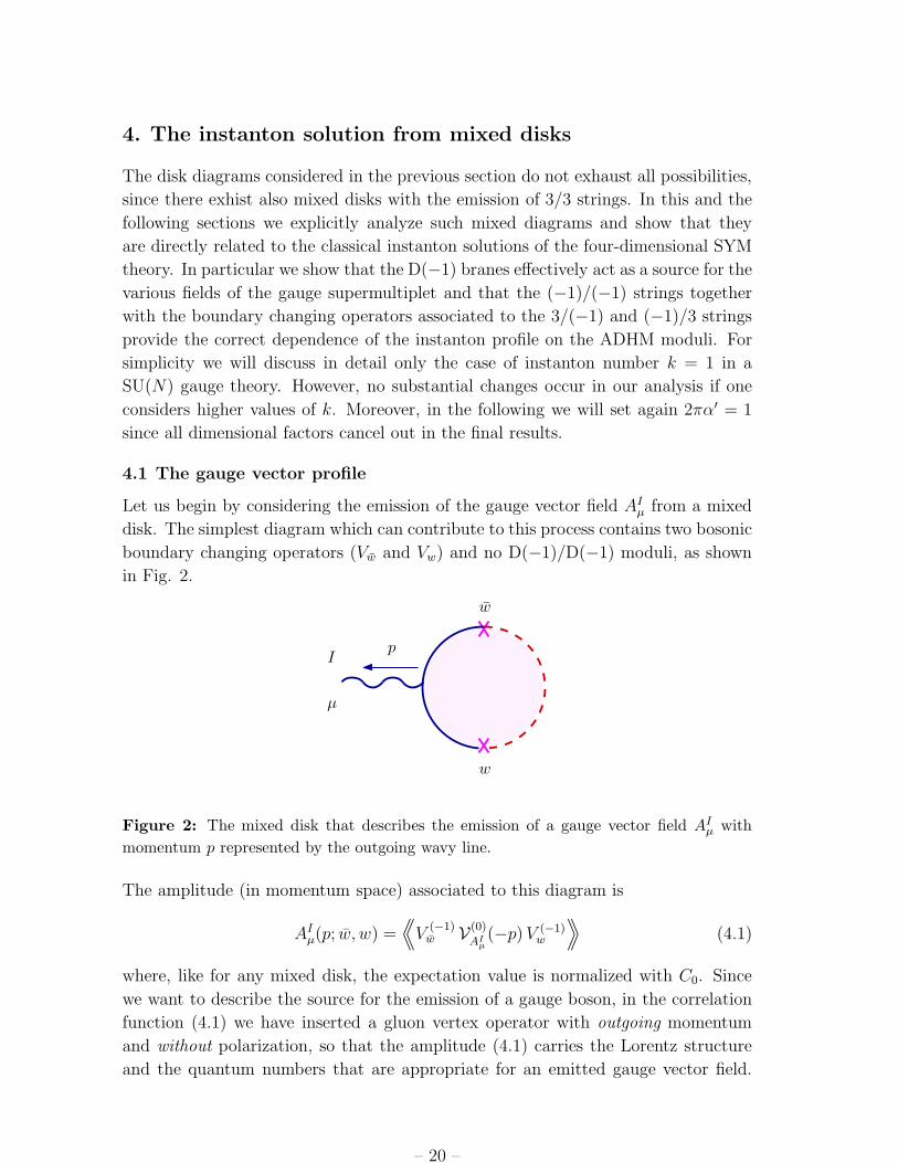
Let us begin by considering the emission of the gauge vector field AIµ from a mixed

disk. The simplest diagram which can contribute to this process contains two bosonic

boundary changing operators (Vw and Vw) and no D(−1)/D(−1) moduli, as shown

in Fig. 2.

I

µ

w

w

p

Figure 2: The mixed disk that describes the emission of a gauge vector field AIµ with

momentum p represented by the outgoing wavy line.

The amplitude (in momentum space) associated to this diagram is

AIµ(p; w, w) =

⟨⟨V

(−1)w V(0)

AIµ(−p)V (−1)

w

⟩⟩(4.1)

where, like for any mixed disk, the expectation value is normalized with C0. Since

we want to describe the source for the emission of a gauge boson, in the correlation

function (4.1) we have inserted a gluon vertex operator with outgoing momentum

and without polarization, so that the amplitude (4.1) carries the Lorentz structure

and the quantum numbers that are appropriate for an emitted gauge vector field.

– 20 –

Moreover, the gluon vertex is in the 0 superghost picture. This can be obtained by

performing a picture changing on the vertex (2.14) and reads

V(0)

AIµ(z;−p) = 2iT I (∂Xµ − i p · ψ ψµ) e−ip·X(z) (4.2)

where T I is the adjoint SU(N) Chan-Paton factor 7. The vertices for the w and w

moduli are instead in the (−1) superghost picture, and are given in (2.32). However,

due to the rescalings (3.28), an overall factor of (gs/2π)1/2 must be incorporated

in each of these vertices in order to interprete their polarizations as the w and w

moduli of the ADHM construction. Using the contraction formulas of appendix A,

and taking into account (see eq. (A.21)) that

⟨∆(z1) e−ip·X(z2) ∆(z3)

⟩= − e−ip·x0 (z1 − z3)

−1/2 (4.3)

where x0 denotes the location of the D-instanton inside the world-volume of the D3

branes (see also eq. (A.21)), one easily finds that the amplitude (4.1) is given by

AIµ(p; w, w) = i (T I)v

u pν ηc

νµ

(w u

α (τc)αβwβ

v

)e−ip·x0 ≡ i pν JI

νµ(w, w) e−ip·x0 (4.4)

where, in the last step, we have introduced the convenient notation JIνµ(w, w) for

the moduli dependence. Note that the various factors of gs and π’s coming from

the rescalings and from the normalization C0 of the mixed disk have canceled out

completely in this calculation.

As we have discussed before, the mixed disk of Fig. 2 represents the source in

momentum space for the emission of the gauge vector field in a non-trivial back-

ground. To obtain the space-time profile of this background, we simply have to take

the Fourier transform of the amplitude AIµ(p; w, w) after attaching to it the gluon

propagator δµν/p2. Thus, the classical field associated to the mixed disk of Fig. 2 is

AIµ(x) =

∫d4p

(2π)2AI

µ(p; w, w)1

p2eip·x

= − 2 (T I)vu

(w u

α (τc)αβwβ

v

)ηc

νµ

(x− x0)ν

(x− x0)4. (4.5)

This result can also be rewritten in terms of the antisymmetric “source” tensor JIνµ

as follows

AIµ(x) = JI

νµ(w, w)

∫d4p

(2π)2

ipν

p2eip·(x−x0) = JI

νµ(w, w) ∂νG(x− x0) (4.6)

where

G(x− x0) =

∫d4p

(2π)2

eip·(x−x0)

p2=

1

(x− x0)2(4.7)

7The overall factor of 2i, which is not determined by the picture changing, is fixed by requiring

the appropriate normalization of the three gluon amplitude.

– 21 –

is the scalar massless propagator in configuration space.

The gauge field AIµ(x) in (4.5) depends on the 4N moduli w u

α and wαu, up to

an overall phase redefinition w ∼ eiθw and w ∼ e−iθw, and on the position xµ0 of

the D-instanton inside the world-volume of the D3 branes. This amounts to 4N + 3

real parameters which are precisely those of the unconstrained instanton moduli

space in the ADHM construction. In fact, upon enforcing the three bosonic ADHM

constraints W c = 0 (see eq. (3.30) for k = 1), these parameters reduce exactly to the

4N moduli of the SU(N) instanton, namely the position of its center xµ0 , its size ρ

and the 4N −5 varibles that parametrize the coset space SU(N)/S[U(N −2)×U(1)]

and specify the orientation of a SU(2) subgroup inside SU(N). To see this explicitly,

let us define

2ρ2 ≡ wαu w

uα , (4.8)

and consider the three N ×N matrices

(tc)uv ≡ 1

2ρ2

(w u

α (τc)αβwβ

v

). (4.9)

Then, it is not difficult to show that these matrices generate a SU(2) subalgebra of

SU(N), i.e. [tc, td] = iǫcde te, provided the ADHM constraints W c = 0 are satisfied.

In conclusion, we can rewrite the gauge field (4.5) as follows

AIµ(x) = 4ρ2 Tr (T I tc) η

cµν

(x− x0)ν

(x− x0)4. (4.10)

In the case of SU(2) the indices I and c can be identified and, taking into account

the trace normalization, we obtain

Acµ(x) = 2ρ2 ηc

µν

(x− x0)ν

(x− x0)4. (4.11)

In this expression we recognize precisely the leading term in the large distance ex-

pansion (i.e. |x − x0| >> ρ) of the classical BPST SU(2) instanton [24, 25] with

center x0 and size ρ, in the so-called singular gauge, namely

Acµ(x) = 2ρ2 ηc

µν

(x− x0)ν

(x− x0)2[(x− x0)2 + ρ2

]

≃ 2ρ2 ηcµν

(x− x0)ν

(x− x0)4

(1 − ρ2

(x− x0)2+ . . .

). (4.12)

Notice that such a configuration has a self-dual field strength, despite the appearance

of the anti self-dual ’t Hooft symbols ηcµν .

More generally, from the mixed disk amplitude (4.5) with the ADHM constraint

(3.30) enforced, we can reconstruct the following anti-hermitian SU(N) connection

(Aµ(x))uv ≡ − iAµ(x)

I (T I)uv = w u

α (σνµ)αβwβ

v

(x− x0)ν

(x− x0)4, (4.13)

– 22 –

which is precisely the leading term in the large distance expansion of the one-

instanton connection of the ADHM construction [23] in the singular gauge

(Aµ(x))uv = w u

α (σνµ)αβwβ

v

(x− x0)ν

(x− x0)2[(x− x0)2 + ρ2

] . (4.14)

This analysis clarifies the interpretation of the string amplitude associated to the

mixed disk of Fig. 2. However, a few comments are in order. Firstly, we would like

to remark that the amplitude (4.1) is a 3-point function from the point of view of the

two dimensional conformal field theory on the string world sheet, but it should be

regarded instead as a 1-point function from the point of view of the four-dimensional

gauge theory on the D3 branes. Indeed, the two boundary changing operators Vw

and Vw in (4.1) just describe the non-dynamical parameters on which the background

depends, i.e. the size of the instanton and its orientation inside the gauge group. To

emphasize this point, we introduce the convenient notation

AIµ(p; w, w) =

⟨⟨VAI

µ(−p)

⟩⟩

D(w,w)(4.15)

where D(w, w) is the mixed disk produced by the insertion of Vw and Vw. Secondly,

the fact that the instanton connection is in the singular gauge should not come as

a surprise, but on the contrary it should be expected in this D-brane set-up. In

fact, as we have seen, the gauge instanton is produced by a D(−1) brane which is

a point-like object inside the D3 brane world-volume, and thus it is natural that

the instanton connection arising in this way exhibits a singularity at the location x0

of the D-instanton. We recall that in the singular gauge all non-trivial properties

of the instanton profile come entirely from the region near the singularity through

the embedding of a 3-sphere surrounding x0 into a SU(2) subgroup of SU(N). This

is to be contrasted with what happens in the regular gauge, where all non-trivial

properties of the instanton come instead from the asymptotic 3-sphere at infinity.

Furthermore, in the singular gauge the instanton field falls off as 1/x3 at large dis-

tances, thus guaranteeing the convergence of many integrals, like for example that

of the topological charge.

An obvious question to ask at this point is whether also the subleading terms in

the large distance expansion of the instanton solution can have a direct interpretation

in string theory. Since these higher-order terms contain higher powers of ρ2, they

are naturally associated to mixed disks with more insertions of boundary changing

operators. For example, the diagram one should consider to study the emission of

the vector field at the next-to-leading order is a mixed disk with two more vertices Vw

and Vw as shown in Fig. 3. However, extending the closed string analysis of Ref. [32]

to the present case, one can argue that in the limit α′ → 0 this diagram reduces to

a simpler one in which two first-order diagrams are sewn with a 3-gluon vertex of

the SYM theory, as shown in Fig. 4. In appendix C we will explicitly compute this

– 23 –

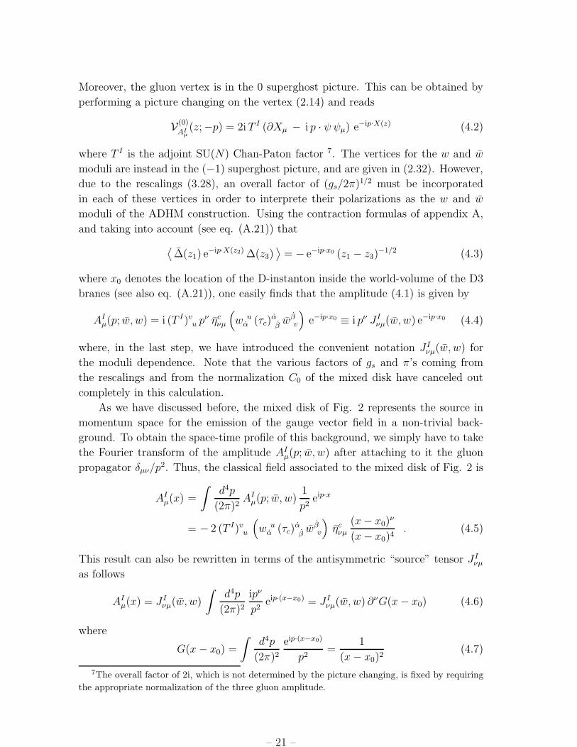
I

µ

w

w

w

wp

Figure 3: The mixed disk for the second order contribution to the gauge vector.

Iµ

w

w

w

w

p

q

p − q

Figure 4: In the field theory limit the mixed disk of Fig. 3 reduces to this configura-

tion which accounts for the second order term in the large-distance approximation of the

instanton solution for the gauge vector.

diagram and find that, for example for SU(2), the corresponding emitted gauge field

is

Acµ(x)(2) = −2ρ4ηc

µν

(x− x0)ν

(x− x0)6, (4.16)

that is exactly the second-order term in the large distance expansion of Acµ(x) in

(4.12). The higher order terms in this expansion can be in principle computed in a

similar manner and eventually the full instanton solution can be reconstructed. This

analysis shows that the relevant building block for the complete solution is actually

the leading term at large distance which corresponds to the “source” diagram of Fig.

2 whose evaluation, as we have seen, is extremely simple.

What we have described above is the open string analogue of the procedure

introduced in Refs. [6, 7] for closed strings. There, the so-called boundary states [5,

33] were recognized to be the sources for the various massless fields of the closed string

spectrum in a D-brane background, and the classical supergravity D-brane solutions

– 24 –

were obtained by taking the Fourier transform of the various tadpoles produced by

the boundary states. Similarly here, the mixed disks have been shown to be the

sources for the emission of open strings in a background whose profile is precisely

that of the classical gauge instanton. Just like the boundary state approach has been

very useful to obtain information on the classical geometry associated to complicated

D-brane configurations, also the present method based on the use of mixed disks

could play a very useful role in determining non-standard classical backgrounds of

the gauge theory.

4.2 Insertions of the translational zero-modes

It is a familiar fact that in the instanton background there are collective coordinates

associated to the presence of broken translational symmetries. From the string point

of view, these zero-modes describe the motion of the D-instanton within the D3

branes and correspond to the vertex operators of a′ (see eq. (2.24)) which, in the 0

superghost picture, are given by

V(0)a′ = a′µ ∂σX

µ . (4.17)

These vertex operators can be used to establish in a stringy way a relation between a′

and the instanton collective coordinate x0. Indeed, if one considers all disk diagrams

obtained from that of Fig. 2 by inserting any number of vertices V(0)a′ along the

D(−1) part of the boundary, and then resums the corresponding perturbative series,

one finds that all occurrences of x0 are replaced by x0 +a′. This fact could be proved

by adding to the action of the D(−1) open strings the following marginal deformation

along the boundary

δS =1

2πα′

∫dτ

[V

(0)a′ (σ = π, τ) − V

(0)a′ (σ = 0, τ)

]. (4.18)

However, it is quite difficult to treat this interaction in a non-perturbative way, since

it is not easy to find an exact solution of the new equations of motion for the string

coordinates with the required boundary conditions and regularity properties. For

this reason it is convenient to exploit the open-closed string duality and translate the

problem into the closed string language. This amounts to represent the D-instanton

localized at x0 with a boundary state |D(−1); x0〉 (see for example Ref. [33] for more

details) and to perform a world-sheet modular transformation that interchanges the

roles of σ and τ . Then, adding the marginal deformation (4.18) to the D(−1) open

strings is equivalent, in the closed string channel, to

P exp

(− i

2πα′

∫ π

0

dσ a′µ ∂τXµ

)|D(−1); x0〉 , (4.19)

as one can easily see by generalizing the discussion of Ref. [4]. Notice that the path

ordering is a consequence of the Chan-Paton factor that must be added to the vertex

– 25 –

operator (4.17) when k > 1. For k = 1 instead, the path ordering is trivial and the

expression (4.19) can be easily evaluated. In particular, one finds that the relevant

zero-more part is given by

e−i a′µpµ

δ4(x− x0) |p = 0〉 = δ4(x− x0 − a′) |p = 0〉 , (4.20)

which clearly shows that all occurrences of x0 are to be replaced by x0+a′, as desired.

For this reason in the following we will not distinguish any more between x0 and a′.

5. The superinstanton profile

The procedure we have discussed in the previous section can be easily extended to

the other components of the N = 4 vector multiplet, thus allowing to recover the full

superinstanton solution from mixed disks. Indeed, acting with the supersymmetry

transformations that are preserved also by the D(−1) branes, one can obtain from

the diagram of Fig. 2 those that describe the emission of the gauginos and the scalar

fields, and hence their classical profiles as function of the supermoduli. On the other

hand, acting with the supersymmetries that are broken by the D(−1) branes, one

can shift the supermoduli in the classical solution and account in this way for the

fermionic zero-modes of the superinstantons.

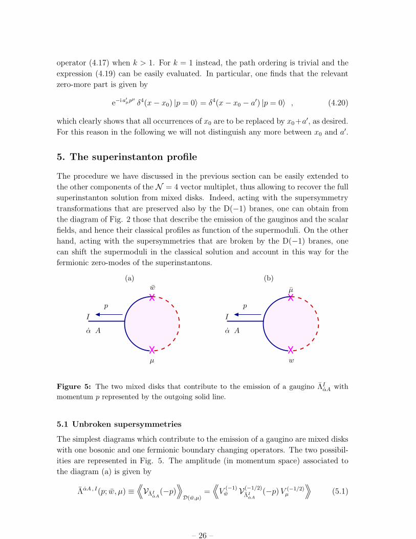
II

µ

µ

w

w

(a) (b)

α αA A

pp

Figure 5: The two mixed disks that contribute to the emission of a gaugino ΛIαA with

momentum p represented by the outgoing solid line.

5.1 Unbroken supersymmetries

The simplest diagrams which contribute to the emission of a gaugino are mixed disks

with one bosonic and one fermionic boundary changing operators. The two possibil-

ities are represented in Fig. 5. The amplitude (in momentum space) associated to

the diagram (a) is given by

ΛαA , I(p; w, µ) ≡⟨⟨VΛI

αA(−p)

⟩⟩

D(w,µ)=

⟨⟨V

(−1)w V(−1/2)

ΛIαA

(−p)V (−1/2)µ

⟩⟩(5.1)

– 26 –

where D(w, µ) is the mixed disk created by the insertion of Vw and Vµ, and is easily

evaluated to be

ΛαA , I(p; w, µ) = i (T I)vu µ

Au wαv e−ip·x0 . (5.2)

Notice again that in the amplitude (5.1) we have inserted a gaugino emission vertex

with outgoing momentum. Similarly, the amplitude corresponding to the diagram

(b) is

ΛαA , I(p; µ, w) ≡⟨⟨VΛI

αA(−p)

⟩⟩

D(w,µ)= i (T I)v

uwαu µA

v e−ip·x0 . (5.3)

An alternative method to compute these amplitudes is based on the use of the su-

persymmetries which are preserved both on the D3 and on the D(−1) boundary and

have been denoted by ξ q in section 2. Exploiting the fact that these supersymmetries

annihilate the vacuum, we have the following Ward identity

⟨⟨[ξ q , Vw

]VAI

µ(−p)Vµ

⟩⟩+

⟨⟨Vw

[ξ q ,VAI

µ(−p)

]Vµ

⟩⟩+

⟨⟨Vw VAI

µ(−p)

[ξ q , Vµ

]⟩⟩= 0 ,

(5.4)

where for simplicity we have understood the picture assignments 8. The only new

ingredient appearing in (5.4) is the commutator in the second term; this can be

computed from (4.2) and reads

[ξ q ,VAI

µ(−p)

]= ξβA pν (σνµ)β

α VΛIαA

(−p) . (5.5)

Then, using (2.36) and (2.37), we can rewrite the Ward identity (5.4) as follows

ξβA pν (σνµ)βα

⟨⟨Vw VΛI

αA(−p)Vµ

⟩⟩+

⟨⟨Vw VAI

µ(−p)Vδξw

⟩⟩= 0 (5.6)

which allows to obtain the gaugino amplitude in terms of the gauge boson amplitude

(4.4) with w replaced by its supersymmetry variation δξw given in (2.34). In this way

we can immediately get (5.2), and with a similar relation also (5.3) can be retrieved.

The space-time profile of the emitted gaugino is then obtained by taking the

Fourier transform of the sum of the amplitudes (5.2) and (5.3) multiplied by the free

fermion propagator i 6pβα/p2 ≡ i pν(σν)βα/p2, that is

ΛαA , I(x) =

∫d4p

(2π)2

(Λ A , I

β(p; w, µ) + Λ A , I

β(p; µ, w)

) i 6pβα

p2eip·x

= −2i (T I)vu

(w u

βµA

v + µAu wβv

)(σν)

βα (x− x0)ν

(x− x0)4. (5.7)

Just as the gauge field (4.10), also the gaugino (5.7) naturally arises in terms of un-

constrained parameters which become the instanton moduli when they are restricted

to satisfy the ADHM constraints (3.30) and (3.31). In particular, once the fermionic

8The latter are (−1/2), 0 and (−1) for Vµ, VAIµ

and Vw respectively, and (−1/2) for the super-

charges.

– 27 –

constraint (3.31) is imposed, it is immediate to extract from (5.7) the following

matrix-valued gaugino profile

(ΛαA(x))uv ≡ − i ΛαA , I(x) (T I)u

v = (σν)αβ

(wβu µA

v + µAu wβv

) (x− x0)ν

(x− x0)4. (5.8)

In this expression we recognize exactly the leading term in the large distance ex-

pansion of the gaugino instanton solution in the singular gauge (see for example

appendix B)

(ΛαA(x))uv = (σν)

αβ

(wβu µA

v + µAu wβv

) (x− x0)ν

√(x− x0)2

[(x− x0)2 + ρ2

]3. (5.9)

The subleading terms can be obtained from diagrams with more sources, in complete

analogy with what we did for the gauge field.

Let us now turn to the scalar components ϕIa of the N = 4 vector multiplet.

The simplest diagram which can describe their emission is a mixed disk with two

fermionic boundary changing operators, like the one represented in Fig. 6. The

I

µ

µ

a

p

Figure 6: The mixed disk describing the emission of an adjoint scalar ϕIa of momentum p

represented by the outgoing dashed line.

corresponding amplitude in momentum space is

ϕIa(p; µ, µ) ≡

⟨⟨VϕI

a(−p)

⟩⟩D(µ,µ)

=⟨⟨V

(−1/2)µ V(−1)

ϕIa

(−p)V (−1/2)µ

⟩⟩

= − i

2(T I)v

u (Σa)AB µBu µA

v e−ip·x0 (5.10)

where D(µ, µ) is the mixed disk created by the insertion of Vµ and Vµ. Defining

ϕAB =1

2√

2(Σa)AB ϕa , (5.11)

we can rewrite (5.10) as

ϕAB , I(p; µ, µ) = − i√2

(T I)vu µ

[Au µB]v e−ip·x0 (5.12)

– 28 –

where the square brackets mean antisymmetrization with weight one. Alternatively,

this result can be obtained from the Ward identity⟨⟨[

ξ q , Vµ

]VΛI

αA(−p)Vµ

⟩⟩+

⟨⟨Vµ

[ξ q ,VΛI

αA(−p)

]Vµ

⟩⟩+

⟨⟨Vµ VΛI

αA(−p)

[ξ q , Vµ

]⟩⟩= 0

(5.13)

which establishes a relation between the scalar and the gaugino amplitudes 9. Indeed,

working out the commutators, we find⟨⟨Vδξw VΛI

αA(−p)Vµ

⟩⟩− i ξα

B (Σa)BA⟨⟨Vµ VϕI

a(−p)Vµ

⟩⟩+

⟨⟨Vµ VΛI

αA(−p)Vδξw

⟩⟩= 0 ,

(5.14)

from which (5.12) easily follows upon using (5.2), (5.3) and (2.34).

The space-time profile of the adjoint scalars is obtained by taking the Fourier

transform of the amplitude (5.12) multiplied by the massless scalar propagator 1/p2,

namely

ϕAB , I(x) =

∫d4p

(2π)2ϕAB , I(p; µ, µ)

1

p2eip·x

= − i√2

(T I)vu µ

[Au µB]v

1

(x− x0)2. (5.15)

When the parameters are restricted to satisfy the ADHM constraints, this expression

represents the leading term of the adjoint scalars in the singular gauge. Moreover,

from (5.15) one can see that

(ϕAB(x))uv ≡ − iϕAB , I(x) (T I)u

v = − 1

2√

2

(µ[Au µB]

v −1

2µ[Ap µB]

p δuv

)1

(x− x0)2

(5.16)

with

||δuv|| =

(0[N−2]×[N−2] 0[N−2]×[2]

0[2]×[N−2] 1[2]×[2]

), (5.17)

which is indeed the leading term at large distance of the exact instanton solution (see

for example appendix B). As before, the subleading terms are given by diagrams

with more insertions of source terms.

We can summarize our findings by saying that the mixed disks with two boundary

changing operators represented in Figs. 2, 5 and 6 describe, respectively, the large

distance behavior in the instanton background of the vector AIµ, of the gaugino ΛI

αA

and of the scalars ϕIAB in the singular gauge, and that their space-time profiles can

be written as

AIµ(x) = JI

νµ ∂νG(x− x0) ,

ΛαA , I(x) = JA , I

β(σν)βα ∂νG(x− x0) , (5.18)

ϕAB , I(x) = JAB , I G(x− x0) ,9In eq. (5.13) all vertex operators, as well as the supersymmetry charges, are in the (−1/2)

picture.

– 29 –

where the scalar Green function G(x− x0) is defined in (4.7) and the various source

terms JIνµ, J

A , I

βand JAB , I are bilinear expressions in the instanton moduli which

can be read from (4.4), (5.2), (5.3) and (5.10) respectively. Moreover, taking into

account the fall-off at infinity of the various fields, one can easily realize that the

equations of motion that follow from the SYM action (3.11) in the Lorentz gauge

reduce at large distances simply to free equations i.e.

AIµ = 0 , ∂/αβ ΛαA , I = 0 , ϕAB , I = 0 , (5.19)

which indeed admit a solution of the form (5.18) in the presence of source terms.

5.2 Broken supersymmetries

Let us now consider the supersymmetries of the D3 branes which are broken by the

D-instantons, namely those that are generated by the charges q′αA ≡(QαA + QαA

)

(see section 2.1). As shown in (2.9), when one pulls the integration contour of a

charge operator to a boundary that does not preserve it, one obtains the integrated

emission vertex for the Goldstone field corresponding to the broken charge. In our

case, the goldstino associated to the breaking of q′αA by the D(−1) boundary is the

modulus M ′αA. Therefore, by acting with the broken supercharges q′αA on a given

instanton solution, one can modify it by shifting its supermoduli with M ′ dependent

terms. In particular, one can relate the “minimal” emission diagrams of Figs. 2, 5 and

6, that contain no D(−1)/D(−1) moduli, to diagrams which instead have additional

insertions of M ′ moduli [18]. Thus, the use of the broken supersymmetries allows us

to determine the M ′ dependence and complete the full superinstanton solution.

Let us see how this works in a specific example and consider the following Ward

identity⟨⟨[

M ′q′ , Vw

]VΛI

αA(−p)Vw

⟩⟩+

⟨⟨Vw

[M ′q′ ,VΛI

αA(−p)

]Vw

⟩⟩(5.20)

+⟨⟨Vw VΛI

αA(−p)

[M ′q′ , Vw

]⟩⟩= −

⟨⟨Vw VΛI

αA(−p)Vw

∫VM ′

⟩⟩.

Differently from the identities (5.4) and (5.13) associated to the preserved supersym-

metries, the right hand side of (5.20) is non-zero as a consequence of the fact that

the supercharge q′ is broken on the D(−1) boundary. A pictorial representation of

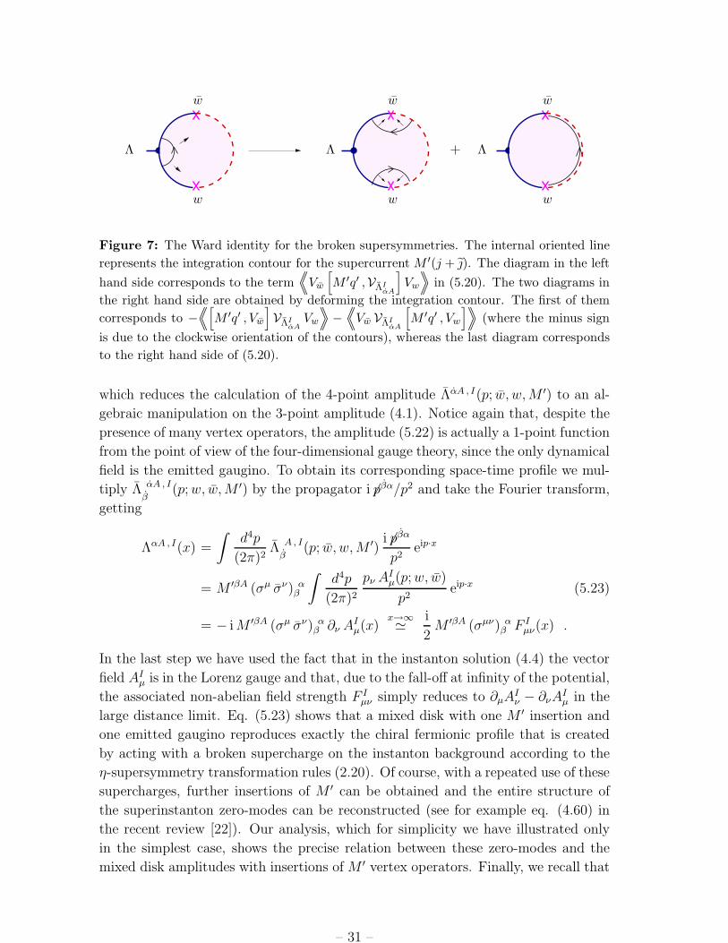
this Ward identity is provided in Fig. 7. Using the fact that the commutators of q′

with Vw and Vw vanish (as we already noticed at the end of section 2), and that[M ′q′,VΛI

αA(−p)

]= iM ′βA (σµ) α

β VAIµ(−p) , (5.21)

we can deduce from (5.20) the following relation

ΛαA , I(p; w, w,M ′) ≡⟨⟨VΛI

αA(−p)

⟩⟩D(w,w,M ′)

=⟨⟨Vw VΛI

αA(−p)Vw

∫VM ′

⟩⟩

= − iM ′βA (σµ) αβ AI

µ(p; w, w) , (5.22)

– 30 –

+

www

www

Λ ΛΛ

Figure 7: The Ward identity for the broken supersymmetries. The internal oriented line

represents the integration contour for the supercurrent M ′(j + ). The diagram in the left

hand side corresponds to the term⟨⟨

Vw

[M ′q′ ,VΛI

αA

]Vw

⟩⟩in (5.20). The two diagrams in

the right hand side are obtained by deforming the integration contour. The first of them

corresponds to −⟨⟨[

M ′q′ , Vw

]VΛI

αAVw

⟩⟩−

⟨⟨Vw VΛI

αA

[M ′q′ , Vw

]⟩⟩(where the minus sign

is due to the clockwise orientation of the contours), whereas the last diagram corresponds

to the right hand side of (5.20).

which reduces the calculation of the 4-point amplitude ΛαA , I(p; w, w,M ′) to an al-

gebraic manipulation on the 3-point amplitude (4.1). Notice again that, despite the

presence of many vertex operators, the amplitude (5.22) is actually a 1-point function

from the point of view of the four-dimensional gauge theory, since the only dynamical

field is the emitted gaugino. To obtain its corresponding space-time profile we mul-

tiply Λ αA , I

β(p;w, w,M ′) by the propagator i 6pβα/p2 and take the Fourier transform,

getting

ΛαA , I(x) =

∫d4p

(2π)2Λ A , I

β(p; w, w,M ′)

i 6pβα

p2eip·x

= M ′βA (σµ σν) αβ

∫d4p

(2π)2

pν AIµ(p;w, w)

p2eip·x (5.23)

= − iM ′βA (σµ σν) αβ ∂ν A

Iµ(x)

x→∞≃ i

2M ′βA (σµν) α

β F Iµν(x) .

In the last step we have used the fact that in the instanton solution (4.4) the vector

field AIµ is in the Lorenz gauge and that, due to the fall-off at infinity of the potential,

the associated non-abelian field strength F Iµν simply reduces to ∂µA

Iν − ∂νA

Iµ in the

large distance limit. Eq. (5.23) shows that a mixed disk with one M ′ insertion and

one emitted gaugino reproduces exactly the chiral fermionic profile that is created

by acting with a broken supercharge on the instanton background according to the

η-supersymmetry transformation rules (2.20). Of course, with a repeated use of these

supercharges, further insertions of M ′ can be obtained and the entire structure of

the superinstanton zero-modes can be reconstructed (see for example eq. (4.60) in

the recent review [22]). Our analysis, which for simplicity we have illustrated only

in the simplest case, shows the precise relation between these zero-modes and the

mixed disk amplitudes with insertions of M ′ vertex operators. Finally, we recall that

– 31 –

with the replacement

M ′αA → − ζ Aα (σµ)αβ a′µ (5.24)

one can account for the superconformal zero-modes of the N = 4 instanton solution

parametrized by the fermionic variables ζ .

6. String amplitudes and instanton calculus

In this section we want to explain what is the stringy procedure to compute in-

stanton corrections to scattering amplitudes in gauge theories and show its relation

with the standard instanton calculus of field theory. The key ingredient will be the

identification of the instanton solution with the string theory 1-point function on

mixed disks that we have proven in the previous sections. Exploiting this fact, we

will also be able to relate our approach to the analysis of the leading D-instantons

effects on scattering amplitudes that has been presented in Ref. [18]. Let us first

recall a few basic facts on the relation between string theory correlators, effective

actions and Green functions in field theory. As we have reviewed in section 3, the

tree-level scattering amplitude among n states of the 3/3 strings (which we denote

generically by φi) is given by 10

Aφ1...φn =⟨⟨Vφ1(p1) . . . Vφn(pn)

⟩⟩≡ φn(pn) . . . φ1(p1)

⟨⟨Vφ1(p1) . . .Vφn(pn)

⟩⟩(6.1)

where the correlator among the vertex operators is computed on a disk with D3

boundary conditions (see for example eq. (3.1)). By taking the limit α′ → 0 and

extracting the 1PI part, we obtain the following contribution to the effective action

−∫

d4p1

(2π)2. . .

d4pn

(2π)2φn(pn) . . . φ1(p1)

⟨⟨Vφ1(p1) . . .Vφn(pn)

⟩⟩∣∣∣1PI

α′→0, (6.2)

which, in turn, induces the following amputated Green function 11

⟨φ1(p1) . . . φn(pn)

⟩∣∣∣amput.

=⟨⟨Vφ1(−p1) . . .Vφn(−pn)

⟩⟩∣∣∣1PI

α′→0. (6.3)

If one computes the above correlators on world-sheets with more boundaries one

obtains the perturbative loop corrections to the effective action and Green functions.

We now want to investigate how the previous relations get modified by the pres-

ence of k D-instantons. In this case, as we have thoroughly explained, the correlators

of vertex operators receive contributions also from world-sheets with a part of their

boundary on the D-instantons, and specifically, at the lowest order in the string per-

turbation theory, from mixed disks. It is convenient to denote by D(M) the sum of

all disks with all possible insertions of the moduli M of the k instantons, as repre-

sented in Fig. 8. Each term in this sum corresponds to an amplitude with no vertex10Suitable symmetry factors must be included when not all field φi are different.11For simplicity, we assume that the propagators are 〈φi(p)φj(k)〉 = (2π)2δ4(p + k)

δij

p2 ; if this

does not happen, like for instance for the gauginos, appropriate changes are required, but these can

be straightforwardly implemented in our formulas.

– 32 –

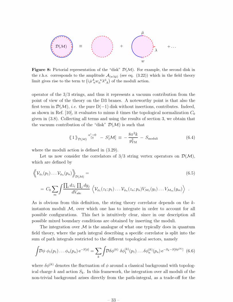
+ . . .≡D(M) +

µ

w

λ

Figure 8: Pictorial representation of the “disk” D(M). For example, the second disk in

the r.h.s. corresponds to the amplitude A(wλµ) (see eq. (3.22)) which in the field theory

limit gives rise to the term tr(i µA

uw uα λα

A

)of the moduli action.

operator of the 3/3 strings, and thus it represents a vacuum contribution from the

point of view of the theory on the D3 branes. A noteworthy point is that also the

first term in D(M), i.e. the pure D(−1) disk without insertions, contributes. Indeed,

as shown in Ref. [10], it evaluates to minus k times the topological normalization C0

given in (3.8). Collecting all terms and using the results of section 3, we obtain that

the vacuum contribution of the “disk” D(M) is such that

〈〈 1 〉〉D(M)

α′→0≃ − S[M] ≡ − 8π2k

g2YM

− Smoduli (6.4)

where the moduli action is defined in (3.29).

Let us now consider the correlators of 3/3 string vertex operators on D(M),

which are defined by

⟨⟨Vφ1(p1) . . .Vφn(pn)

⟩⟩D(M)

= (6.5)

= C0

∑

m

∫ ∏i dzi

∏j dyj

dVabc

⟨Vφ1(z1; p1) . . .Vφn(zn; pn)VM1(y1) . . . VMm(ym)

⟩.

As is obvious from this definition, the string theory correlator depends on the k-

instanton moduli M, over which one has to integrate in order to account for all

possible configurations. This fact is intuitively clear, since in our description all

possible mixed boundary conditions are obtained by inserting the moduli.

The integration over M is the analogue of what one typically does in quantum

field theory, where the path integral describing a specific correlator is split into the

sum of path integrals restricted to the different topological sectors, namely

∫Dφ φ1(p1) . . . φn(pn) e−S[φ] =

∑

k

∫Dδφ(k) δφ

(k)1 (p1) . . . δφ

(k)n (pn) e−Sk−S[δφ(k)] (6.6)

where δφ(k) denotes the fluctuation of φ around a classical background with topolog-

ical charge k and action Sk. In this framework, the integration over all moduli of the

non-trivial background arises directly from the path-integral, as a trade-off for the

– 33 –

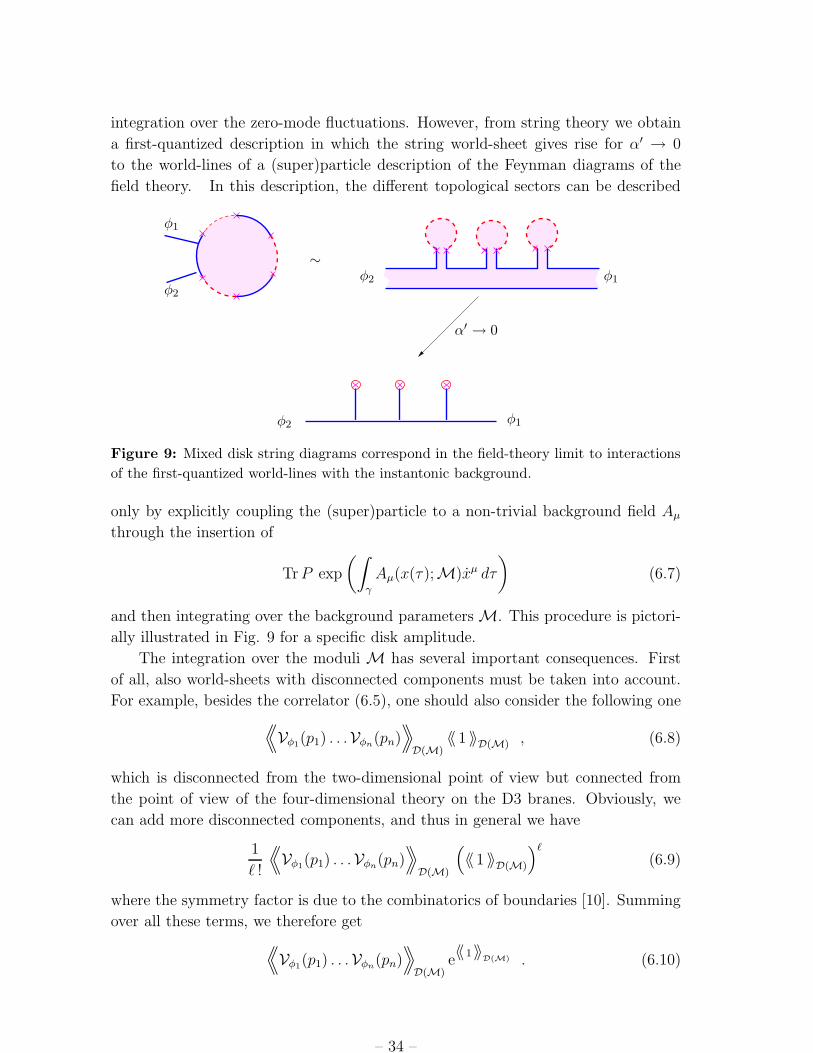
integration over the zero-mode fluctuations. However, from string theory we obtain

a first-quantized description in which the string world-sheet gives rise for α′ → 0

to the world-lines of a (super)particle description of the Feynman diagrams of the

field theory. In this description, the different topological sectors can be described

∼

α′ → 0

φ1

φ1

φ1

φ2

φ2φ2

Figure 9: Mixed disk string diagrams correspond in the field-theory limit to interactions

of the first-quantized world-lines with the instantonic background.

only by explicitly coupling the (super)particle to a non-trivial background field Aµ

through the insertion of

TrP exp

(∫

γ

Aµ(x(τ);M)xµ dτ

)(6.7)

and then integrating over the background parameters M. This procedure is pictori-

ally illustrated in Fig. 9 for a specific disk amplitude.

The integration over the moduli M has several important consequences. First

of all, also world-sheets with disconnected components must be taken into account.

For example, besides the correlator (6.5), one should also consider the following one⟨⟨Vφ1(p1) . . .Vφn(pn)

⟩⟩

D(M)〈〈 1 〉〉D(M) , (6.8)

which is disconnected from the two-dimensional point of view but connected from

the point of view of the four-dimensional theory on the D3 branes. Obviously, we

can add more disconnected components, and thus in general we have

1

ℓ !

⟨⟨Vφ1(p1) . . .Vφn(pn)

⟩⟩

D(M)

(〈〈 1 〉〉D(M)

)ℓ

(6.9)

where the symmetry factor is due to the combinatorics of boundaries [10]. Summing

over all these terms, we therefore get

⟨⟨Vφ1(p1) . . .Vφn(pn)

⟩⟩

D(M)e〈〈 1 〉〉

D(M) . (6.10)

– 34 –

However, this is not yet the full story. In fact, for the same arguments we should

also take into account diagrams in which the n vertex opertors Vφi(pi) are distributed

among various disconnected components. For example, besides the correlator (6.10)

we should also consider the following one⟨⟨Vφ1(p1)Vφ2(p2)

⟩⟩

D(M)

⟨⟨Vφ3(p3) . . .Vφn(pn)

⟩⟩

D(M)e〈〈 1 〉〉

D(M) . (6.11)

This contribution appears to be totally disconnected; however, it is connected with

respect to the φ’s because of the integration over the moduli M which all sit at the

same point where the stack of k D-instantons is located. Distributing the φ’s in all

possible ways, one generates various configurations which are compactly represented

in Fig. 10.

φ(1)1 φ

(1)2

φ(1)l1

φ(k)1 φ

(k)2

φ(k)lk

( )

. . .

+ . . .× 1 + + 12

D(M)D(M)D(M)

D(M)D(M)

Figure 10: A connected amplitude with n external Vφ vertex operators in a D-instanton

background receives contributions from topologically disconnected world-sheets, character-

ized by the insertion of li vertex operators for φ fields in each connected component, with∑i li = n.

Since each expectation value on D(M) is proportional to C0 ∝ g−1s (see eqs.

(6.5) and (3.8)), the dominant contribution for small gs is the one in which a single

vertex Vφ is inserted in each disk [11, 18], namely⟨⟨Vφ1(p1)

⟩⟩D(M)

· · ·⟨⟨Vφn(pn)

⟩⟩D(M)

e〈〈 1 〉〉

D(M) , (6.12)

whereas other terms, like for example (6.11), are subleading for small gs12. Moreover,

this correlator is clearly 1PI. Thus, we can conclude that in the field theory limit,

the dominant contribution to the amputated Green function of n fields of the 3/3

string sector in the presence of k D-instanton is given by (see Fig. 11)⟨φ1(p1) . . . φn(pn)

⟩∣∣∣D−inst.

amput.= (6.13)

=

∫dM

⟨⟨Vφ1(−p1)

⟩⟩D(M)

· · ·⟨⟨Vφn(−pn)

⟩⟩D(M)

e〈〈 1 〉〉

D(M)

∣∣∣∣α′→0

.

12Notice that world-sheets with higher Euler number can also give contributions to the sub-leading

orders.

– 35 –

φ1 φ2

φn

. . . D(M)D(M)D(M) e〈〈1〉〉

D(M)

Figure 11: The dominant contribution to an amplitude with n external Vφ vertex opera-

tors in a D-instanton background is a product of tadpoles.

Reinstating the propagators (see footnote 11) and Fourier transforming, we obtain

the following Green function in configuration space

⟨φ1(x1) . . . φn(xn)

⟩∣∣∣D−inst.

=

∫dM φdisk

1 (x1;M) · · · φdiskn (xn;M) e−S[M] (6.14)

where we have used (6.4) and defined

φdisk(x;M) =

∫d4p

(2π)2eip·x 1

p2

⟨⟨Vφ(−p)

⟩⟩D(M)

∣∣∣∣α′→0

. (6.15)

Using the results of sections 4 and 5 we can identify the right hand side of (6.15)

with the classical profile φcl(x;M) of the superinstanton solution for the field φ.

For example, the contributions from the simplest mixed disks, i.e. those with only

two insertions of boundary changing operators, account for the leading terms in the

large distance expansion of the superinstanton solution, as we have seen explicitly

for k = 1 in eqs. (4.5), (5.7) and (5.15). The contributions from mixed disks with

more boundary changing operators in the limit α′ → 0 account instead for the sub-

leading terms in the large distance expansion, as we have shown for the gauge field

in section 4 (see also appendix C). Thus, we can write

φ(x;M)disk = φcl(x;M) (6.16)

and conclude that the stringy prescription (6.14) of computing correlation functions

in the presence of D-instantons is exactly equivalent to the standard field theory

prescription of the instanton calculus

⟨φ1(x1) . . . φn(xn)

⟩∣∣∣inst.

=

∫dM φcl

1 (x1;M) · · · φcln (xn;M) e−S[M] . (6.17)

The effects of D-instantons on the scattering amplitudes of the gauge theory on

the D3 branes can be encoded by introducing new effective vertices for the 3/3 fields

φi’s which suitably modify the SYM action (see also Ref. [18]). These D-instanton

induced vertices originate from the amputated Green functions (6.13) upon including

the polarization fields for the external legs, and are clearly moduli dependent. At

– 36 –

fixed moduli, only the 1-point functions are irreducible and so the gauge effective

action induced by the D-instantons on the D3 branes will be

S(−1)/3 = −∑

φ

∫d4p

(2π)2φ(p)

⟨⟨Vφ(p)

⟩⟩D(M)

∣∣∣∣α′→0

(6.18)

where the sum is over all massless fields of the N = 4 vector multiplet. Since the

tadpoles⟨⟨Vφ(p)

⟩⟩

D(M)are generically of the form Jφ(M) eip·x0 (see for instance eqs.

(5.2) and (5.10)) 13, we can write this effective action simply as

S(−1)/3 = −∑

φ

φ(x0) Jφ(M) (6.19)

which manifestly shows that the 1-point functions on the mixed disks are sources

for the gauge fields at the instanton location. Using the expressions for the various

tadpoles computed in sections 4 and 5, it is easy to realize that

S(−1)/3 = − 1

2F I

µν(x0) Jµν , I(M) − ΛI

αA(x0) JαA , I(M) − ϕI

AB(x0) JAB , I(M) (6.20)

where the various sources are defined in (5.18). This expression represents the non-

abelian extension of the action given for example in Ref. [18, 19].

We think that our analysis clarifies the role played by D-instantons on the scat-

tering amplitudes of four-dimensional gauge theories already discussed in the litera-

ture. In particular we have shown that the stringy procedure to compute instanton

corrections to correlation functions reproduces in the field theory limit the standard

instanton calculus in virtue of the identification (6.16). We hope that these ideas

and techniques can be useful also for practical calculations in the N = 4 SYM theory

considered in this paper as well as in gauge theories with lower supersymmetries.

Acknowledgments

We thank Rodolfo Russo for useful discussions and exchange of ideas.

13For the gauge field AIµ there is also an explicit momentum factor, see eq. (4.4).

– 37 –

A. Notations and conventions

Notations: We use the following notations for indices:

• d = 10 vector indices: M,N, . . . ∈ 1, . . . , 10;

• d = 4 vector indices: µ, ν, . . . ∈ 1, . . . , 4;

• d = 6 vector indices: a, b, . . . ∈ 5, . . . , 10;

• chiral and anti-chiral spinor indices in d = 10: A and A;

• chiral and anti-chiral spinor indices in d = 4: α and α;

• spinor indices in d = 6: A and A in the fundamental and anti-fundamental of

SU(4) ≃ SO(6).

Our choice for the group indices is the following:

• SU(N) colour indices: I, J, . . . ∈ 1, . . . , N2 − 1;

• U(k) colour indices: U, V, . . . ∈ 1, . . . , k2;

• D3 indices: u, v, . . . ∈ 1, . . . , N;

• D(−1) indices: i, j, . . . ∈ 1, . . . , k;

• SU(2) adjoint indices: c, d, . . . ∈ 1, 2, 3.

d = 4 Clifford algebra: The Euclidean Lorentz group SO(4) ∼ SU(2)+ × SU(2)−is realized on spinors in terms of the matrices (σµ)αβ and (σµ)αβ with

σµ = (1,−i~τ ) , σµ = σ†µ = (1, i~τ) , (A.1)

where τ c are the ordinary Pauli matrices. They satisfy the Clifford algebra

σµσν + σν σµ = 2δµν 1 , (A.2)

and correspond to a Weyl representation of the γ-matrices,

γµ =

(0 σµ

σµ 0

)(A.3)

acting on the spinor

ψ =

(ψα

ψα

). (A.4)

– 38 –

Out of these matrices, the SO(4) generators are defined by

σµν =1

2(σµσν − σν σµ) , σµν =

1

2(σµσν − σνσµ) ; (A.5)

the matrices σµν are self-dual and thus generate the SU(2)+ factor; the anti-self-dual

matrices σµν generate instead the SU(2)− factor. Notice that the indices in the 2 of

SU(2)+ are denoted by α and those for the 2 of SU(2)− by α. The charge conjugation

matrix is block-diagonal in this Weyl basis:

C(4) =

(Cαβ 0

0 Cαβ

)=

(−εαβ 0

0 −εαβ

)(A.6)

with ε12 = ε12 = −ε12 = −ε12 = +1. Moreover we raise and lower spinor indices as

follows

ψα = εαβ ψβ , ψα = εαβ ψβ . (A.7)

’t Hooft symbols: The explicit mapping of a self-dual SO(4) tensor into the

adjoint representation of the SU(2)+ factor is realized by the ’t Hooft symbols ηcµν ;

the analogous mapping of an anti-self dual tensor into the adjoint of the SU(2)−subgroup is realized by ηc

µν . One has

(σµν)β

α = i ηcµν (τ c) β

α , (σµν)αβ

= i ηcµν (τ c)α

β. (A.8)

An explicit representation of the ’t Hooft symbols is given by

ηcµν = ηc

µν = εcµν , µ, ν ∈ 1, 2, 3,ηc

4ν = −ηc4ν = δc

ν , (A.9)

ηcµν = −ηc

νµ, ηcµν = −ηc

νµ .

From it one can easily see that

ηcµν η

d µν = 4 δcd , (A.10)

ηcµν η

cρσ = δµρ δνσ − δµσ δνρ + εµνρσ . (A.11)

Analogous formulas hold for the contractions of two η’s with a minus sign in the ε

term of (A.11).

d = 6 Clifford algebra: Taking advantage of the equivalence SO(6) ∼ SU(4),

upon which a positive (negative) chirality spinor corresponds to a fundamental (anti-

fundamental) SU(4) representation, we can represent the SO(6) spinor as

Λ =

(ΛA

ΛA

)(A.12)

– 39 –

on which the following gamma matrices act

Γa =

(0 Σa

Σa 0

). (A.13)

The matrices Σa and Σa realize the six-dimensional Clifford algebra

(Σa)AB(Σb)BC + (Σb)AB(Σa)BC = 2 δab δAC , (A.14)

(with (Σa)AB = (Σa BA)∗). An explicit realization can be given in terms of ’t Hooft

symbols

Σa =(η3, iη3, η2, iη2, η1, iη1

), Σa =

(−η3, iη3,−η2, iη2,−η1, iη1

). (A.15)

The charge conjugation matrix is off-diagonal in this chiral basis:

C(6) =

(0 C B

A

CAB 0

)=

(0 −i δ B

A

−i δAB 0

). (A.16)

d = 10 Clifford algebra: The ten-dimensional γ-matrices ΓM(10) and the charge

conjugation matrix C(10) are expressed in terms of the four- and six-dimensional

matrices as

Γµ(10) = γµ ⊗ 1 , Γa

(10) = γ5 ⊗ Γa ,

Γ11(10) = γ5 ⊗ Γ7 , C(10) = C(4) ⊗ C(6) , (A.17)

such that

C(10)ΓM(10)C

−1(10) = −ΓM T

(10) . (A.18)

Spin field correlators: From the general formulae of [34], by decomposing the

ten-dimensional fields into four-dimensional and six-dimensional ones, we can derive

the following “effective” OPE’s:

Sα(z)Sβ(w) ∼ 1√2

(σµ)αβ ψµ(w) , SA(z)SB(w) ∼ i δA

B

(z − w)3/4, (A.19)

Sα(z)S β(w) ∼ − εα β

(z − w)1/2, SA(z)SB(w) ∼ i√

2

(Σa)AB ψa(w)

(z − w)1/4,

Sα(z)Sβ(w) ∼ εαβ

(z − w)1/2, ψa(z)SA(w) ∼ 1√

2

(Σa)AB SB(w)

(z − w)1/2,

ψµ(z)Sα(w) ∼ 1√2

(σµ)αβ Sβ(w)

(z − w)1/2, ψa(z)SA(w) ∼ − 1√

2

(Σa)AB SB(w)

(z − w)1/2,

ψµψν(z)Sα(w) ∼ − 1

2

(σµν)αβS β(w)

(z − w), ψaψb(z)SA(w) ∼ 1

2

(Σab)AB S

B(w)

(z − w).

– 40 –

Other OPE’s which do not appear in (A.19) can be simply obtained by a suitable

change of the chiralities. From these OPE’s we can derive the following 3-point

functions which have been used in the main text

〈Sα(z1)ψµ(z2)Sβ(z3)〉 =1√2

(σµ)αβ(z1 − z2)

−1/2 (z2 − z3)−1/2 , (A.20)

〈Sα(z1)ψµψν(z2)Sβ(z3)〉 = −1

2(σµν)

αβ(z1 − z3)1/2 (z1 − z2)

−1 (z2 − z3)−1 ,

〈SA(z1)ψa(z2)S

B(z3)〉 =i√2

(Σa)AB (z1 − z2)−1/2 (z1 − z3)

−1/4 (z2 − z3)−1/2 ,

〈SA(z1)ψa(z2)SB(z3)〉 = − i√

2(Σa)AB (z1 − z2)

−1/2 (z1 − z3)−1/4 (z2 − z3)

−1/2 .

Twist field correlators: The (−1)/3 and the 3/(−1) strings have four Neumann-

Dirichlet directions, namely those along the world-volume of the D3 branes. Thus,

the string fields Xµ have twisted boundary conditions; this fact can be seen as due to

the presence of twist and anti-twist fields ∆(z) and ∆(z) that change the boundary

conditions from Neumann to Dirichlet and vice-versa by introducing a cut in the

world-sheet (see for example Ref. [27]). The twist fields ∆(z) and ∆(z) are bosonic

operators with conformal dimension 1/4 and their OPE’s are

∆(z1) ∆(z2) ∼ (z1 − z2)1/2 , ∆(z1) ∆(z2) ∼ − (z1 − z2)

1/2 , (A.21)

where the minus sign in the second correlator is again an “effective” rule to correctly

account for the space-time statistics in correlation functions.

B. A short review of the ADHM construction and of zero

modes around an instanton background

Following the notation of Refs. [22, 20], we begin by introducing the basic objects in

the ADHM construction of the SU(N) instanton solution in four dimensions, namely

the [N + 2k] × [2k] and [2k] × [N + 2k] matrices

∆(x) = a + b x , ∆(x) = a+ xb (B.1)

where xαβ = xµ (σµ)αβ and xαβ = xµ (σµ)αβ describe the position of the multi-

instanton center of mass, and all the remaining moduli are collected in the matrix

a (see formula (B.3) below). Finally, b is a [N + 2k] × [2k] matrix which can be

conveniently chosen to be

b =

(0

1[2k]×[2k]

), b = (0 , 1[2k]×[2k]) . (B.2)

– 41 –

The moduli space of the solutions to the self-dual equations of motion is characterized

in terms of the supercoordinates

a ≡(w ui

α

a′αβ li

), MA ≡

(µAui

M ′βAli

), (B.3)

which satisfy the bosonic and fermionic ADHM constraints

∆ ∆ = f−1k×k 1[2]×[2] , (B.4)

∆MA = MA ∆ (B.5)

with fk×k an invertible k × k matrix.

The solutions to the self-dual equations of motion for the various fields in the

N = 4 vector multiplet are given by

Aµ = U ∂µ U ,

ΛA = U(MAf b− b f MA

)U ,

ϕAB = − i

2√

2U

(MBf MA −MAf MB

)U

− i U ·(

0[N ]×[N ] 0[N ]×[2k]

0[2k]×[N ] L−1ΛAB[k]×[k] ⊗ 1[2]×[2]

)· U , (B.6)

in terms of the kernels U[N+2k]×[N ] and U[N ]×[N+2k] of the ADHM matrices ∆ and ∆.

In (B.6), the hatted gauge fields are taken to be anti-hermitian, ΛAB is the fermionic

bilinear

ΛAB =1

2√

2

(MAMB − MBMA

), (B.7)

and the operator L is defined as

L · Ω =1

2W 0,Ω + [aµ, [a

µ,Ω]] , (B.8)

with (W 0) ij = w ui

α wαuj .

For simplicity, from now on we concentrate on solutions with winding number

k = 1, which for SU(N) can be found starting from those for SU(2). For k = 1 the

ADHM constraints drastically simplify; indeed, the bosonic constraint (B.4) simply

reduces to

wαu w

uβ

= ρ2 δαβ

(B.9)

(see eq. (4.8)), which is solved by

||w uα || =

∣∣∣∣wαu

∣∣∣∣ = ρ T

(0[N−2]×[2]

1[2]×[2]

)(B.10)

where T ∈ SU(N)/SU(N − 2). This is just the standard SU(2) instanton solution

embedded inside the SU(N) in the lower right corner. The matrices T describe the

– 42 –

orientation of the SU(2) instanton inside SU(N) with SU(N − 2) being the stability

group of the SU(2) instanton solution. If we temporarily set T = 1, the vector field,

which solves the equations of motion in the singular gauge, can be written as

(Aµ)uv =

ρ2

x2 (x2 + ρ2)(σνµ)u

v xν , (B.11)

where

(σνµ) vu =

(0[N−2]×[N−2] 0[N−2]×[2]

0[2]×[N−2] (σνµ) βα

), (B.12)

and the center of the instanton has been set at x0 = 0 for simplicity. If we remove the

T = 1 constraint and shift the instanton center, we find the general SU(N) solution

Aµ = T Aµ T−1 which is given in (4.14). As we have also found in the main text, an

explicit representation of our embedding is given by the matrices in (4.9) where the

w uα ’s are chosen according to (B.10).

We now turn to the fermionic the zero modes. Their number is 2kNN and

obviously depends on the number of supersymmetries. For compatibility with the

rest of the paper we will discuss the N = 4 case. The N = 2 and N = 1 cases can

easily be deduced from our discussion by restricting the range of the capital latin

indices in the following to A,B = 1, 2 and A,B = 1 respectively. It is well-known

that in the SU(2) case the fermionic zero modes are in the adjoint representation

and that their explicit form can be found by acting with the supersymmetry charges

of the superconformal algebra on the instanton solution, leading to

ΛαA =i

2

(ηβA − ζ A

γ (σρ)γβ xρ

)(σµν) α

β Fµν . (B.13)

These solutions can be singled out also for arbitrary winding numbers k, since they

correspond to solutions of the constraint (B.5) in which the fermionic matrix MA is

taken to be proportional to the matrices a, b introduced in (B.1), namely

µAui = 0 , M ′βAij = bij η

βA , (B.14)

and

µAui = w uiα ζ αA , M ′βA

ij = −ζ Aα (σµ)αβ a′µij , (B.15)

for the supersymmetric and superconformal zero-modes respectively.

Besides the zero-modes (B.13), in the SU(N) case we have other 4N (N − 2)

fermionic zero-modes, which are the partners of the color rotations parametrized by

w uα ’s. They transform in the fundamental representation of the embedded SU(2) and

correspond to the 2(N−2) doublets in the decomposition of the adjoint representation

of SU(N) with respect to SU(2). For example, for SU(3) we have 8 = 3⊕ 2⊕ 2⊕ 1.

Since there are no solutions to the Dirac equation which are SU(2) singlets, and since

– 43 –

we already know the form (B.13) of the solution in the adjoint representation, we

simply have to recall the form of the SU(2) solutions in the fundamental. They are

ψαs =ρ ǫαs√

(x2 + ρ2)3(B.16)

where s = 1, 2 is an index which runs in the fundamental. The solutions for 2 are

obtained from those in (B.16) by raising the indices α and s. Let us now turn to

the SU(N) case and introduce the gauge invariant quantity (W αβ)j

i = wαui w

uj

β. By

definition, the infinitesimal gauge rotations which leave this quantity invariant are

those which satisfy

δwαui w

uj

β+ wα

ui δwuj

β= 0 . (B.17)

Using for δw and δw the transformations (2.35), from (B.17) we get

ξαA µ

Auiw

uj

β+ ξβA w

αui µ

Auj = 0 , (B.18)

from which we infer

µAui w

uj

β= 0 , wα

uiµAuj = 0 . (B.19)

For k = 1, given the choice Eq.(B.9), this implies µAu = (µA1 , . . . , µ

AN−2, 0, 0). Starting

from (B.16) we can now deduce the SU(N) formulae by replacing the index s in the

fundamental of SU(2) with an index v in the fundamental of SU(N), and adding

another index u to label the N − 2 different solutions. For convenience the range

of u will be extended to N . For consistency with our previous notation, we also

substitute ǫ with µ. Putting together doublets and anti-doublets, we finally find

(ΛαA)uv

∣∣∣reg.

=ρ√

(x2 + ρ2)3(µAu δα

v + εαu µAv) (B.20)

where εαu = (0, . . . , 0, εαβ) is a natural extension of the Levi-Civita symbol to our

case. To go to the singular gauge we perform a SU(N) gauge transformation extend-

ing the standard SU(2) one, i.e. g = xµσµ/√x2, to g′ = (0, . . . , 0, xµσ

µ)/√x2, and

get

(ΛαA)uv =

ρ√x2(x2 + ρ2)3

(µAu xαv + xαuµA

v) , (B.21)

where xαv = (0, . . . , 0, xµ (σµ)α

β).

At last we discuss the inhomogeneous solutions of the equations of motion for

the adjoint scalars ϕAB. These equations follow from the SYM action (3.11) 14 and

are

D2 ϕAB − 1√2ΛαA , Λ B

α + · · · = 0 , (B.22)

14We recall that the fields appearing in the SYM action (3.11) are hermitian, while the hatted

fields we are now considering are anti-hermitian; the precise relation between the two is given by

ϕAB = −i ϕAB and similarly for the other components of the supermultiplet.

– 44 –

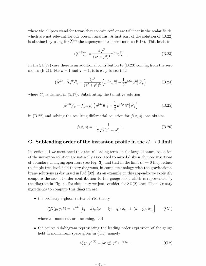
where the ellipses stand for terms that contain ΛαA or are trilinear in the scalar fields,

which are not relevant for our present analysis. A first part of the solution of (B.22)

is obtained by using for ΛαA the supersymmetric zero-modes (B.13). This leads to

(ϕAB)uv =

4√

2

(x2 + ρ2)2η[AuηB]

v . (B.23)

In the SU(N) case there is an additional contribution to (B.23) coming from the zero

modes (B.21). For k = 1 and T = 1, it is easy to see that

ΛαA , Λ Bα u

v =4ρ2

(x2 + ρ2)3

(µ[AuµB]

v −1

2µ[Ap µB]

p δuv

)(B.24)

where δuv is defined in (5.17). Substituting the tentative solution

(ϕAB)uv = f(x, ρ)

(µ[AuµB]

v −1

2µ[Ap µB]

p δuv

)(B.25)

in (B.22) and solving the resulting differential equation for f(x, ρ), one obtains

f(x, ρ) = − 1

2√

2(x2 + ρ2). (B.26)

C. Subleading order of the instanton profile in the α′ → 0 limit

In section 4.1 we mentioned that the subleading terms in the large distance expansion

of the instanton solution are naturally associated to mixed disks with more insertions

of boundary changing operators (see Fig. 3), and that in the limit α′ → 0 they reduce

to simple tree-level field theory diagrams, in complete analogy with the gravitational

brane solutions as discussed in Ref. [32]. As an example, in this appendix we explicitly

compute the second order contribution to the gauge field, which is represented by

the diagram in Fig. 4. For simplicity we just consider the SU(2) case. The necessary

ingredients to compute this diagram are:

• the ordinary 3-gluon vertex of YM theory

V cdeµνλ(p, q, k) = i εcde

[(q − k)µ δνλ + (p− q)λ δµν + (k − p)ν δλµ

](C.1)

where all momenta are incoming, and

• the source subdiagram representing the leading order expression of the gauge

field in momentum space given in (4.4), namely

Acµ(p; ρ)(1) = iρ2 ηc

νµ pν e−ip·x0 . (C.2)

– 45 –

The amplitude in Fig. 4 is then obtained by sewing two first-order diagrams to a

3-gluon vertex and reversing the sign of the momentum of the free gluon line to

describe an outgoing field. Taking into account a simmetry factor of 1/2, we have

Acµ(p; ρ)(2) =

1

2

∫d4q

(2π)2

[V cde

µνλ(−p, q, p− q)1

q2Ad

ν(q; ρ)(1) 1

(p− q)2Ae

λ(p− q; ρ)(1)]

=i

2ρ4 ǫcde ηd

σν ηeτλ e−ip·x0

∫d4q

(2π)2

1

q2(p− q)2qσ (p− q)τ ×

×[(p− 2q)µ δνλ + (q + p)λ δµν + (q − 2p)ν δλµ

](C.3)

where the momentum integral can be computed in dimensional regularization. To

obtain the space-time profile, we take the Fourier transform of Acµ(p; ρ)(2) multiplied

by 1/p2, and after some standard manipulations we find

(Acµ(x))(2) ≡ lim

d→4

∫ddp

(2π)d/2(Ac

µ(p; ρ))(2) 1

p2eip·x = −2ρ4ηc

µν

(x− x0)ν

(x− x0)6, (C.4)

which is exactly the second order term in eq. (4.12). The higher order terms in the

large distance expansion can in principle be computed in a similar manner and thus

the full instanton solution can eventually be reconstructed.

References

[1] Z. Bern, L.J. Dixon and D.A. Kosower, “Progress in one-loop QCD computations”,

Ann. Rev. Nucl. Part. Sci. 46 (1996) 109 [arXiv:hep-ph/9602280];

Z. Bern, “Perturbative quantum gravity and its relation to gauge theory”,

[arXiv:gr-qc/0206071], and references therein.

[2] J. Polchinski, “Dirichlet-branes and Ramond-Ramond charges,” Phys. Rev. Lett. 75

(1995) 4724 [arXiv:hep-th/9510017].

[3] J. Polchinski, “TASI lectures on D-branes”, [arXiv:hep-th/9611050]; C. V. Johnson,

“D-brane primer”, [arXiv:hep-th/0007170].

[4] C.G. Callan, C. Lovelace, C.R. Nappi and S.A. Yost, “Loop corrections to

superstring equations of motion”, Nucl. Phys. B 308 (1988) 221.

J. Polchinski and Y. Cai, “Consistency of open superstring theories”, Nucl. Phys. B

296 (1988) 91.

[5] P. Di Vecchia and A. Liccardo, “D branes in string theory. I”,

[arXiv:hep-th/9912161]; “D-branes in string theory. II”, [arXiv:hep-th/9912275].

[6] P. Di Vecchia, M. Frau, I. Pesando, S. Sciuto, A. Lerda and R. Russo, “Classical

p-branes from boundary state,” Nucl. Phys. B 507 (1997) 259

[arXiv:hep-th/9707068].

– 46 –

[7] P. Di Vecchia, M. Frau, A. Lerda and A. Liccardo, “(F,Dp) bound states from the

boundary state,” Nucl. Phys. B 565, 397 (2000) [arXiv:hep-th/9906214].

[8] E. Witten, “Bound states of strings and p-branes,” Nucl. Phys. B 460 (1996) 335

[arXiv:hep-th/9510135].

[9] M. R. Douglas, “Gauge fields and D-branes,” J. Geom. Phys. 28, 255 (1998)

[arXiv:hep-th/9604198]; “Branes within branes,” arXiv:hep-th/9512077.

[10] J. Polchinski, “Combinatorics of boundaries in string theory,” Phys. Rev. D 50

(1994) 6041 [arXiv:hep-th/9407031].

[11] M.B. Green and M. Gutperle, “Effects of D-instantons,” Nucl. Phys. B 498 (1997)

195, [arXiv:hep-th/9701093]; “D-particle bound states and the D-instanton

measure”, JHEP 9801 (1998) 005, [arXiv:hep-th/9711107]; “D-instanton partition

functions”, Phys. Rev. D 58 (1998) 046007, [arXiv:hep-th/9804123].

[12] T. Banks and M. B. Green, “Non-perturbative effects in AdS(5) x S**5 string theory

and d = 4 SUSY Yang-Mills”, JHEP 9805 (1998) 002, [arXiv:hep-th/9804170].

[13] C.S. Chu, P.M. Ho and Y.Y. Wu, “D-instanton in AdS(5) and instanton in

SYM(4)”, Nucl. Phys. B 541 (1999) 179, [arXiv:hep-th/9806103].

[14] I.I. Kogan and G. Luzon, “D-instantons on the boundary”, Nucl. Phys. B 539

(1999) 121, [arXiv:hep-th/9806197].

[15] M. Bianchi, M.B. Green, S. Kovacs and G. Rossi, “Instantons in supersymmetric

Yang-Mills and D-instantons in IIB superstring theory”, JHEP 9808(1998) 013,

[arXiv:hep-th/9807033].

[16] N. Dorey, V.V. Khoze, M.P. Mattis and S. Vandoren, “Yang-Mills instantons in the

large-N limit and the AdS/CFT correspondence”, Phys. Lett. B 442 (1998) 145,

[arXiv:hep-th/9808157]; [arXiv:hep-th/9808157]. N. Dorey, T.J. Hollowood,

V.V. Khoze, M.P. Mattis and S. Vandoren, “Multi-instantons and Maldacena’s

conjecture”, JHEP 9906 (1999) 023, [arXiv:hep-th/9810243].

[17] N. Dorey, T. J. Hollowood, V. V. Khoze, M. P. Mattis and S. Vandoren,

“Multi-instanton calculus and the AdS/CFT correspondence in N = 4

superconformal field theory”, Nucl. Phys. B 552 (1999) 88 [arXiv:hep-th/9901128].

[18] M.B. Green and M. Gutperle, “D-instanton induced interactions on a D3-brane,”

JHEP 0002 (2000) 014 [arXiv:hep-th/0002011].

[19] N. Dorey, T. J. Hollowood and V. V. Khoze, “Notes on soliton bound-state problems

in gauge theory and string theory”, [arXiv:hep-th/0105090].

[20] A.V. Belitsky, S. Vandoren and P. van Nieuwenhuizen, “Yang - Mills and D -

instantons”, Class. Quant. Grav. 17 (2000) 3521 [arXiv:hep-th/0004186].

– 47 –

[21] N. Dorey, T. J. Hollowood and V. V. Khoze, “A brief history of the stringy

instanton,” [arXiv:hep-th/0010015].

[22] N. Dorey, T. J. Hollowood, V. V. Khoze and M. P. Mattis, “The calculus of many

instantons,” [arXiv:hep-th/0206063].

[23] M. F. Atiyah, N. J. Hitchin, V. G. Drinfeld and Y. I. Manin, “Construction of

instantons”, Phys. Lett. A 65 (1978) 185.

[24] A. A. Belavin, A. M. Polyakov, A. S. Schwarz and Y. S. Tyupkin, “Pseudoparticle

solutions of the Yang-Mills equations,” Phys. Lett. B 59, 85 (1975).

[25] G. ’t Hooft, “Computation of the quantum effects due to a four-dimensional

pseudoparticle,” Phys. Rev. D 14, 3432 (1976) [Erratum-ibid. D 18, 2199 (1978)].

[26] D. Friedan, E. J. Martinec and S.H. Shenker, “Conformal invariance, supersymmetry

and string theory”, Nucl. Phys. B 271 (1986) 93.

[27] L.J. Dixon, J.A. Harvey, C. Vafa and E. Witten, “Strings on orbifolds”, Nucl. Phys.

B 261 (1985) 678; S. Hamidi and C. Vafa, “Interactions on orbifolds”, Nucl. Phys. B

279 (1987) 465.

[28] P. Di Vecchia, L. Magnea, A. Lerda, R. Russo and R. Marotta, “String techniques

for the calculation of renormalization constants in field theory”, Nucl. Phys. B 469

(1996) 235 [arXiv:hep-th/9601143].

[29] D. Polyakov, “BRST properties of new superstring states,” [arXiv:hep-th/0111227].

[30] A. Sen, “Type I D-particle and its interactions,” JHEP 9810, 021 (1998)

[arXiv:hep-th/9809111].

[31] L. Gallot, A. Lerda and P. Strigazzi, “Gauge and gravitational interactions of

non-BPS D-particles,” Nucl. Phys. B 586, 206 (2000) [arXiv:hep-th/0001049].

[32] M. Bertolini, P. Di Vecchia, M. Frau, A. Lerda, R. Marotta and R. Russo, “Is a

classical description of stable non-BPS D-branes possible?”, Nucl. Phys. B 590

(2000) 471, [arXiv:hep-th/0007097].

[33] M. Billo, P. Di Vecchia, M. Frau, A. Lerda, I. Pesando, R. Russo and S. Sciuto,

“Microscopic string analysis of the D0-D8 brane system and dual R-R states”, Nucl.

Phys. B 526 (1998) 199 [arXiv:hep-th/9802088].

[34] V.A. Kostelecky, O. Lechtenfeld, W. Lerche, S. Samuel and S. Watamura,

“Conformal techniques, bosonization and tree level string amplitudes”, Nucl. Phys.

B 288 (1987) 173.

– 48 –