SU (N) gauge theories in four dimensions: exploring the approach to N=∞

arX

iv:h

ep-l

at/0

1030

27v2

27

Jun

2001

Oxford OUTP-01-17P

SU(N) gauge theories in four dimensions :exploring the approach to N = ∞

B. Lucini and M. Teper

Theoretical Physics, University of Oxford, 1 Keble Road,

Oxford OX1 3NP, UK

Abstract.We calculate the string tension, σ, and some of the lightest glueball masses, mG, in3+1 dimensional SU(N) lattice gauge theories for 2 ≤ N ≤ 5. From the continuumextrapolation of the lattice values, we find that the mass ratios mG/

√σ appear to

show a rapid approach to the large–N limit, and, indeed, can be described all the waydown to SU(2) using just a leading O(1/N2) correction. We confirm that the smoothlarge–N limit we find, is obtained by keeping a constant ’t Hooft coupling. We alsocalculate the topological charge of the gauge fields. We observe that, as expected, thedensity of small-size instantons vanishes rapidly as N increases, while the topologicalsusceptibility appears to have a non-zero N = ∞ limit.

http://arXiv.org/abs/hep-lat/0103027v2

1 Introduction

How SU(N) gauge theories approach their N = ∞ limit, and what that limit is, isan interesting question [1] whose answer would represent a significant step towardsaddressing the same question in the context of QCD. Accurate lattice calculations in2+1 dimensions [2] show that in that case the approach is remarkably precocious inthat even N = 2 is close to N = ∞. Such calculations have to be very accurate, ofcourse, because for each value of N one has to perform a continuum extrapolation ofvarious mass ratios and then these are compared and extrapolated to N = ∞. ExistingD=3+1 calculations [3, 4, 5] are much too rough for this purpose even if their messageappears to be optimistic.

In this paper we present a calculation in 3+1 dimensions that is accurate enoughfor some conclusions to be drawn. This calculation is intended as an exploratory one,designed to see if a much more detailed and extensive calculation is warranted. Forthis reason we have limited ourselves to calculating just three masses in the (‘glueball’)spectrum: the lightest and first excited JPC = 0++ scalars, and the lightest 2++

tensor. We have also calculated the topological susceptibility and have obtained someinformation on the distribution of ‘instanton’ sizes so as to see how it evolves at largerN . We simultaneously investigate linear confinement, calculating the string tension.We do all this for SU(4) and SU(5) gauge theories and compare the results to whatone finds for SU(2) and SU(3). In fact, because the existing SU(2) calculations provedtoo inaccurate to be useful, we found that we had to redo SU(2) as well. We havealso chosen to perform our own SU(3) calculations (although this was not absolutelynecessary) so that when we compare results at various N in this paper, they will haveall been obtained with exactly the same methods.

For N > 3 there are, in addition, new stable strings that connect sources in represen-tations higher than the fundamental and we have calculated their string tensions. In [6]we presented our preliminary results on this topic. We have since somewhat increasedthe accuracy of those calculations as well as performing some similar, but much moreaccurate, calculations in D=2+1. We do not include these calculations in the presentpaper since they do not really belong to the question being addressed here, i.e. theapproach of SU(N) gauge theories to their N = ∞ limit. Instead we will present themelsewhere [7], as this will enable us to present in some detail the theoretical backgroundto the ideas involved. Here we simply remark that our previous conclusions [6] remainunchanged: in the D=3+1 SU(4) and SU(5) gauge theories the doubly charged stringhas a tension that is much less than twice that of the fundamental string, and it agrees,within fairly small errors, with the M(-theory)QCD conjecture made in [8]. However, aswe show in [7] our results also agree with old speculations about the ‘Casimir scaling’ ofstrings, a dependence that is manifested in leading-order Hamiltonian strong-couplingand which happens to be numerically quite close to the MQCD conjecture. This aspectwas not discussed in [6] but is explored in detail in [7]. Interest in Casimir scaling hasrecently revived [9, 10, 11] following recent studies of unstable higher representation

1

strings in SU(3) [9, 10]. In our much more accurate D=2+1 calculations it is clearthat these new stable string tensions, while being close to the MQCD conjecture, doin fact deviate from it. What we see is closer to Casimir scaling although here toothe agreement does not appear to be perfect. (Although there is some sign that thedeviations disappear quite rapidly with increasing N .) The fact that the strings wedeal with are stable removes ambiguities in interpreting string tensions of the unstableSU(3) strings and brings into sharp focus the possible relevance of Casimir scaling tothe dynamics of confinement [7].

In the next section we summarise the technical details of our lattice calculations. Wethen study the strong-to-weak coupling transition in the case of SU(4). The practicalreason for doing this is to demonstrate that the range of lattice spacings we shall use forour continuum extrapolation avoids this potential phase transition. However the natureof this transition is of interest in itself and it becomes more interesting as N increases.We discuss this in some detail. In Section 4 we present our results on glueball massesand the string tension in SU(2), SU(3), SU(4) and SU(5) gauge theories. We performthe continuum extrapolation of various mass ratios, compare their N -dependence andperform an extrapolation to N = ∞. We discuss what needs to be done better in futurecalculations. In Section 5 we ask whether our non-perturbative calculations supportthe usual diagrammatic expectation [1] that a smooth large-N limit is obtained bykeeping the ’t Hooft coupling λ ≡ g2N constant. We then turn to calculations of thetopological susceptibility and of the size distribution of the topological charges, witha view to clarifying the fate of topological fluctuations as N increases. We finish withsome concluding remarks.

We remark that a quite similar calculation of the physical properties of D=3+1SU(N) gauge theories is being carried out simultaneously elsewhere [12].

2 Lattice preliminaries

Our four dimensional lattice is hypercubic and has periodic boundary conditions. Thedegrees of freedom are SU(N) matrices, Ul, residing on the links, l, of the lattice. Inthe partition function the fields are weighted with expS where S is the standardplaquette action

S = −β∑

p

(

1 − 1

NReTr Up

)

, (1)

i.e. Up is the ordered product of the matrices on the boundary of the plaquette p. Forsmooth fields this action reduces to the usual continuum action with β = 2N/g2. Byvarying the inverse lattice coupling β we vary the lattice spacing a.

Our Monte Carlo mixes standard heat-bath and over-relaxation steps in the ratio1 : 4. These are implemented by updating SU(2) subgroups using the Cabibbo-Marinariprescription [13]. We use 3 subgroups in the case of SU(3), 6 for SU(4) and 10 for SU(5).As a check of efficient ergodicity we use the same algorithm to minimise the action and

2

we find that with this number of subgroups the SU(N) lattice action does decreasemore-or-less as effectively as in the SU(2) gauge theory.

Our typical lattice calculation, at a given value of β and for a given volume, involves105 Monte Carlo sweeps through the lattice. (For some of the coarser lattice spacings,where the correlation functions decrease most rapidly, we perform more sweeps.) Weperform calculations of correlation functions every 5’th such sweep. Calculations ofthe topological charge (whose details we leave to Section 6.1) are performed every 50sweeps.

We calculate correlations of gauge-invariant operators φ(t), which depend on fieldvariables within a given time-slice, t. The basic component of such an operator willtypically be the (traced) ordered product of the Ul matrices around some closed contourc. A contractible contour, such as the plaquette itself, is used for glueball operators. Anon-contractible closed contour, which winds around the spatial hyper-torus, projectsonto winding strings of fundamental flux. In the confining phase the theory is invariantunder a class of centre transformations that ensure that the overlap between suchcontractible and non-contractible operators is exactly zero. For our lattice action thecorrelation function of such an operator has good positivity properties, i.e. we canwrite

C(t) = 〈φ†(t)φ(0)〉 =∑

n

|〈Ω|φ|n〉|2 exp−Ent (2)

where |n〉 are the energy eigenstates, with En the corresponding energies, and |Ω〉 isthe vacuum state. If the operator has 〈φ〉 = 0 then the vacuum will not contribute tothis sum and we can extract the mass of the lightest state with the quantum numbersof φ, from the large-t exponential decay of C(t). To make the mass calculation moreefficient we use ~p = 0 operators. Note that on a lattice of lattice spacing a we willhave t = ant, where nt is an integer labelling the time-slices, so that what we actuallyobtain from eqn(2) is aEn, the energy in lattice units.

In practice a calculation using the simplest lattice string operator is inefficient be-cause the overlap onto the lightest string state is small and so one has to go to largevalues of t before the contribution of excited states has died away; and there the signaldisappears into the statistical noise. There are standard methods [14] for curing thisproblem, using blocked (smeared) link operators and variational techniques. This isdescribed in detail in, for example, [2]. In this exploratory study we use the simplestblocking technique [2] to produce blocked link matrices, and we form operators bymultiplying these blocked links around 1×1 and 1×2 contours. We take linear combi-nations which transform according to the cubic A++

1 and E++ representations, and thisallows us to extract JPC = 0++ and JPC = 2++ masses. To make the calculation moreefficient we use a variational criterion that determines the linear combination of ouroperators that has the best overlap onto the lightest 0++ and 2++ glueball states, andonto the first excited 0++ state. These standard techniques are described, for example,in [2].

For any given state we determine the best operator as described above. We then

3

attempt to fit the corresponding correlation function, normalised so that C(t = 0) = 1,with a single exponential in t. (Actually a cosh to take into account the temporalperiodicity.) We choose fitting intervals [t1, t2] where initially t1 is chosen to be t1 = 0and then is increased until an acceptable fit is achieved. The value of t2 is chosen sothat there are at least 3, and preferably 4, values of t being fitted. (Since our fittingfunction has two parameters.) Where t1 = 0 and the errors on C(t = a) are muchsmaller than the errors at t ≥ 2a, this procedure provides no significant evidence forthe validity of the exponential fit, and so we use the much larger error from C(t = 2a)rather than C(t = a). (This typically arises on the coarsest lattices and/or for verymassive states.) We ignore correlations between statistical errors at different t andattempt to compensate for this both by demanding a lower χ2 for the best acceptablefit and by not extending unnecessarily the fitting range. (Although in practice theerror on the best fit increases as we increase the fitting range, presumably because thecorrelation in t of the errors is modest and the decorrelation of the operator correlationsis less efficient as t increases.) The relatively rough temporal discretisation of manyof our calculations, means that, at the margins, there are inevitable ambiguities inthis procedure. These however decrease as a → 0. Once a fitting range is chosen, theerror on the mass is obtained by a Jack-knife procedure which deals correctly with anyerror correlations as long as the binned data are statistically independent. Typicallywe take 50 bins, each involving some 2000 sweeps. It is plausible that bins of this sizeare independent; however we have not stored our results in a sufficiently differentialform that we can calculate the autocorrelation functions so as to test this in detail. Acrude test is provided by recalculating the statistical errors using bins that are twiceas large. We find the errors are essentially unchanged, which provides some evidencefor the statistical independence of our original bins.

3 The strong–to–weak coupling transition

It has long been known that if we use the standard plaquette action then we find across-over between the strong and weak coupling regions, which is characterised by ananomalous dip in the mass of the lightest scalar glueball and a peak in the specific heat.This effect becomes more marked as we go from SU(2) to SU(3) and it is believed thatin the case of SU(N ≥ 4) one has an actual bulk phase transition in this cross-overregion. We want to locate the crossover to make sure that it does not interfere withour continuum extrapolations. We shall do so for the case of SU(4) where there havebeen rough estimates [3] that it is located in the region β ∈ [10.3, 10.5].

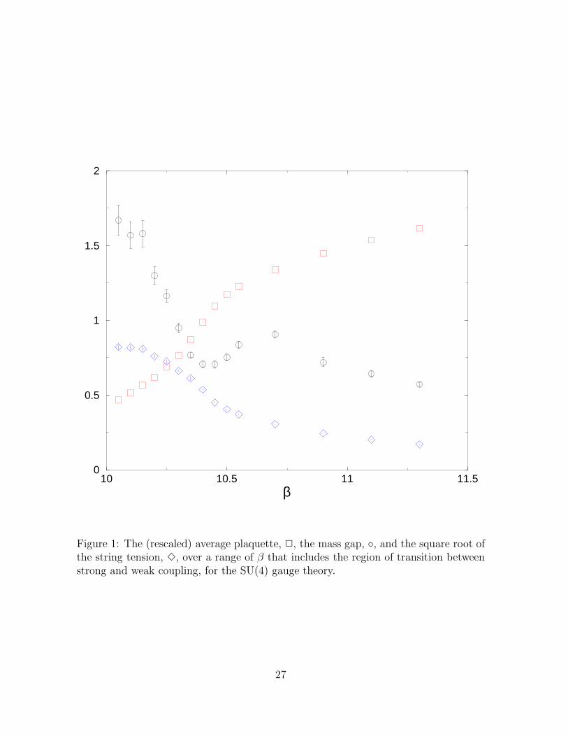
To locate the cross-over region we calculate the lightest scalar glueball mass, thestring tension and the plaquette, in the range of couplings β ∈ [10.0, 11.3]. Since wethink of the lattice spacing as increasing with β we would naively expect the value ofam, for any mass m, to decrease uniformly over this range. And indeed, as we see inFig.1, this is the case for the square root of the string tension, a

√σ. However, as we

4

see in Fig.1, this is not the case for the lightest scalar glueball, am0++ , which has astriking dip at β ∼ 10.4. We note that in this region the value of ds/dβ, where s isthe average plaquette, has a maximum, which tells us that there will be a peak in thespecific heat here. Taking into account that the dip in am0++ is superimposed on amontonically decreasing function, we estimate that the crossover is centered somewherein β ∈ [10.35, 10.40]. The calculations we shall use to extrapolate to the continuumlimit will all be well to the weak-coupling side of this value of β.

As far as the presence of an actual phase transition is concerned, we see no sign of astrong first order transition in that there appear to be no discontinuities in any of thequantities we calculate. We have not done the kind of finite volume study that mightreveal a second order transition; although at β = 10.30, where we have calculations ontwo volumes, there is no sign of the dip becoming deeper as the volume increases. Butwe emphasise that our calculations were not designed to locate a phase transition, andinstead were merely intended to identify the cross-over region.

Several reasons have been given in the past for a crossover or phase transition sepa-rating the strong and weak coupling regimes in SU(N) gauge theories. One explanationfocuses on string roughening (see [15, 16] and references therein): in strong couplingthe confining string is rigid, as though the transverse fluctuations were massive, whilein weak coupling we recover the usual continuum-like string with massless transversefluctuations. In the region of couplings where this mass vanishes the string becomesrough and the lattice theory should exhibit a cross-over [15, 16]. A quite different ap-proach [17] focuses on the different eigenvalue distributions that the plaquette matrixpossesses at strong and weak coupling. From this one can conclude [17] that thereis a third-order phase transition separating the strong and weak coupling regions atN = ∞ with, presumably, some kind of cross-over at finite but large N . A third ap-proach [18, 16] focuses on the phase structure in an extended coupling space, driven bythe condensation of various lattice topological objects [19, 20]. We will now commenton, and extend a little further, this last idea.

We start by considering SU(2). Suppose one generalises the lattice action in eqn(1)to

S = −β∑

p

(

1 − 1

NReTr Up

)

− βA

∑

p

(

1 − 1

N2 − 1ReTrA Up

)

, (3)

where TrA is the trace in the adjoint representation, and the Tr in the first termcontinues to be in the fundamental representation. This lattice theory has a non-trivial phase structure in the (β, βA) space of couplings [18, 16]. In particular thereis a phase transition line which ends in a critical point and this point approaches theWilson axis, βA = 0, as we go from SU(2) to SU(3). Moreover if one extrapolatesthis phase transition line one crosses the Wilson axis in the weak-to-strong couplingcrossover region. Since the mass gap vanishes at the critical point, its proximity to theWilson axis provides an explanation for the dip in the mass of the scalar glueball inthe region that characterises the transition from weak to strong coupling, and also the

5

fact that this dip deepens as we go from SU(2) to SU(3).The SU(2) phase structure described above is believed to be driven by the following

dynamics [19, 20]. If we multiply a link matrix by an element of the centre then this isinvisible to the adjoint piece of the action. Strings of plaquettes of flipped sign can bethought of as Z2 vortex lines. Such vortices may be closed or may end on Z2 monopoles.At small β and small βA there will be a vacuum condensate of both the Z2 vorticesand the Z2 monopoles. If we increase βA at β ∼ 0 the vortices remain condensed sincethe adjoint action does not feel their presence. However the monopoles will cease tocondense at some critical value of the coupling for the same entropy/action reason thatU(1) monopoles cease to be condensed in the D=3+1 U(1) theory beyond a certaincritical coupling. Thus there is a phase transition line extending to finite β from somepoint along the adjoint axis. Now if we go to large βA the plaquettes are all close to±1 and we have something close to a Z2 spin system. If we then increase β this isequivalent to increasing an external field that breaks the Z2 symmetry and at somepoint there is a phase transition to a phase where the (ultraviolet) Z2 vortices aresuppressed. So there is a phase transition line descending into the (β, βA) plane. Atsome point this coalesces with the other phase transition line and continues downwardstill it ends at the critical point. That it must end somewhere follows from the fact thatat large negative βA the plaquette traces are driven close to zero, and such a vacuumwill support neither Z2 vortices nor monopoles.

We note that although this kind of explanation sounds very particular to the simpleplaquette action, one should be able to generalise it to any loops; the crucial thing isthat we consider them in both the fundamental and adjoint representations. One mightwonder whether other representations might be relevant. It is clear however that therelevant topological objects are determined by the centre of the group and a loop in anySU(2) representation responds either like the fundamental or adjoint representation tocentre elements of the group. Thus the analysis possesses a qualitative universality.

In SU(3) the picture is essentially the same, but if we go to SU(4) things becomedifferent. Now we can introduce an extra k = 2 coupling, β2, corresponding to doubleflux plaquettes. Such plaquettes are insensitive to a factor eiπ = −1, just like theadjoint coupling. However the adjoint action is also insensitive to eiπ/2 fluxes. By theabove kind of argument we expect a similar phase structure in the SU(4) (β, βk=2)plane to the one we had in the SU(2) (β, βA) plane. Indeed we should now consider the(β, βk=2, βA) manifold of couplings, and there will be surfaces of phase transitions andlines of critical points which may approach the Wilson axis at more than one location.For higher SU(N) we have a (β, β2, β3, . . . , βA) space of couplings where the differentpieces of the action will be insensitive to different elements of the centre. That is tosay, to monopoles and vortices of various multiples of the basic ZN flux. There willbe a complex phase structure in this space, but since it involves the condensation ofultraviolet objects, one can in principle estimate the location of these transitions. Wedo not attempt to do so here. However we point out that these phase transitions would

6

naturally be related to the eigenvalue spectrum of the typical SU(N) plaquette. It isnot unreasonable to conjecture that the smooth N → ∞ limit of this complex phasestructure might be precisely the third-order phase transition discussed in [17].

Finally we remark that there is no sign of a cross-over, marked by a dip in the massgap, when we consider SU(N) gauge theories in D=2+1. Since the vacuum possessesall the topological objects described above, this might look like a counterexample tothe argument. In fact this is not so. The key observation is that in the D=2+1 U(1)theory there is no phase transition between strong and weak coupling: in contrast tothe D=3+1 case. This is because in D=2+1 the monopoles are instantons, while inD=3+1 they are objects with world lines. Thus the action/entropy balance is quitedifferent and leads to a quite different phase structure. This applies equally well to ZN

monopoles.

4 The spectrum and string tension

In Sections 4.1 and 4.2 we describe our calculations of the string tension and of themass spectrum respectively. We then discuss, in Section 4.3, what are the lessons welearn as to how to go about doing a much better calculation.

4.1 the string tension

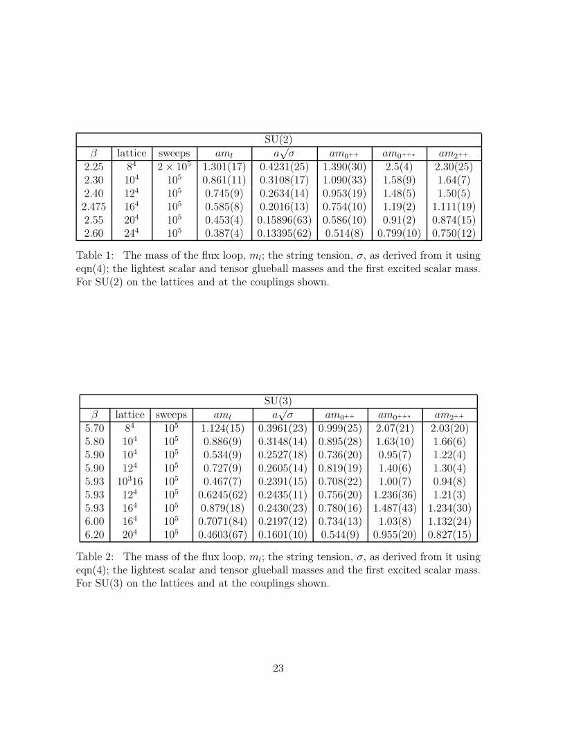
To calculate the (fundamental) string tension σ we construct string operators thatclose upon themselves through a spatial boundary. The correlation function of twosuch strings separated by a (Euclidean) time interval t will, for large enough t, decreaseexponentially ∝ exp(−mlt) where ml is the mass of the lightest periodic flux loop. Onthe lattice t = ant where nt labels the temporal time-slices, so what we obtain is thevalue of aml, the mass in lattice units. If the length of the loop is aL and if the theoryis linearly confining then a2σ = limL→∞ aml/L. Moreover the first correction to thislinear dependence is universal [21] if the infrared properties of the confining flux tubeare described by an effective string theory. If we further assume that the universalityclass is that of a simple (Nambu-Gotto) bosonic string (there is some evidence fromprevious SU(2) and SU(3) lattice calculations that points to this) and if we use thestring correction appropriate to our closed periodic string [22] then we find

aml = a2σL − π

3L(4)

once the flux loop is large enough. We shall use this expression to extract a2σ fromour lattice calculations of the flux loop mass aml.

As we have just remarked, in using eqn(4) we are assuming that we have linearconfinement in our SU(N) gauge theories, that the effective string theory describingthe infrared properties of the confining flux tube is in the Nambu-Gotto universality

7

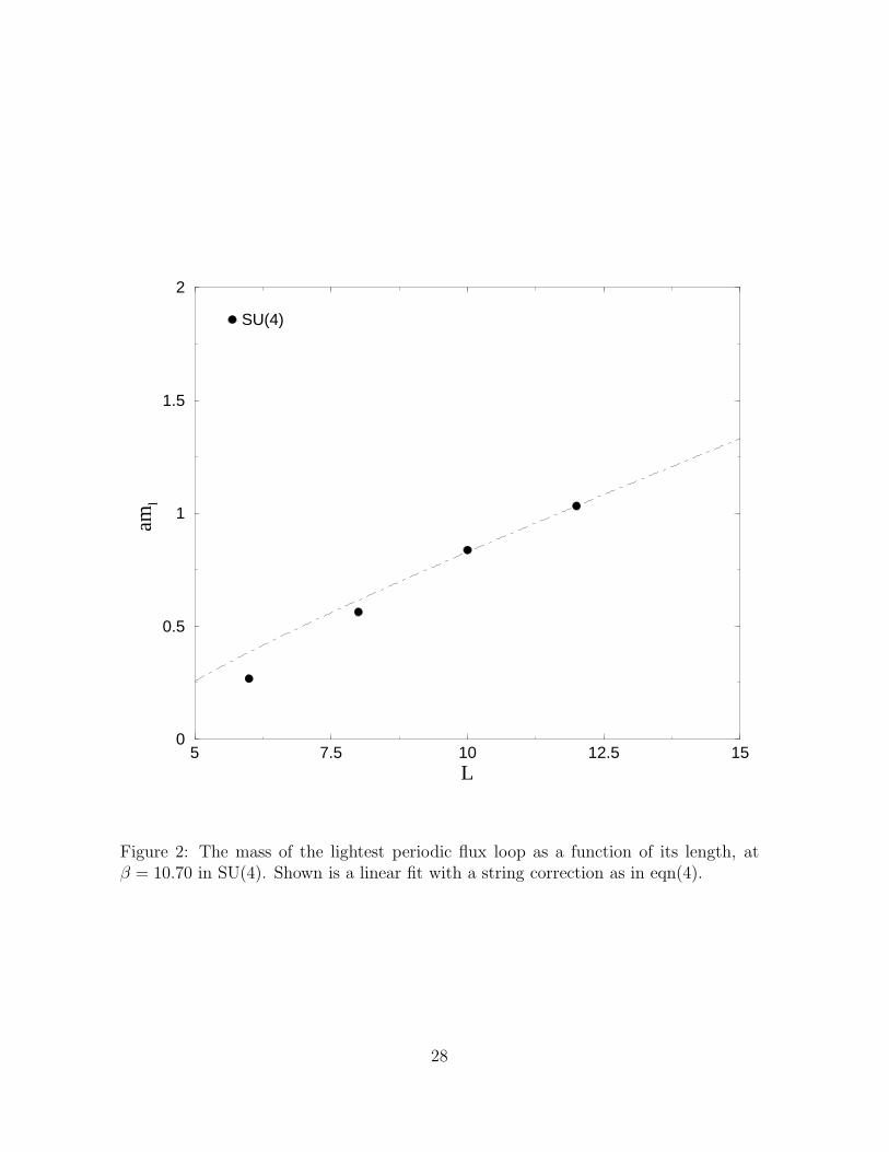
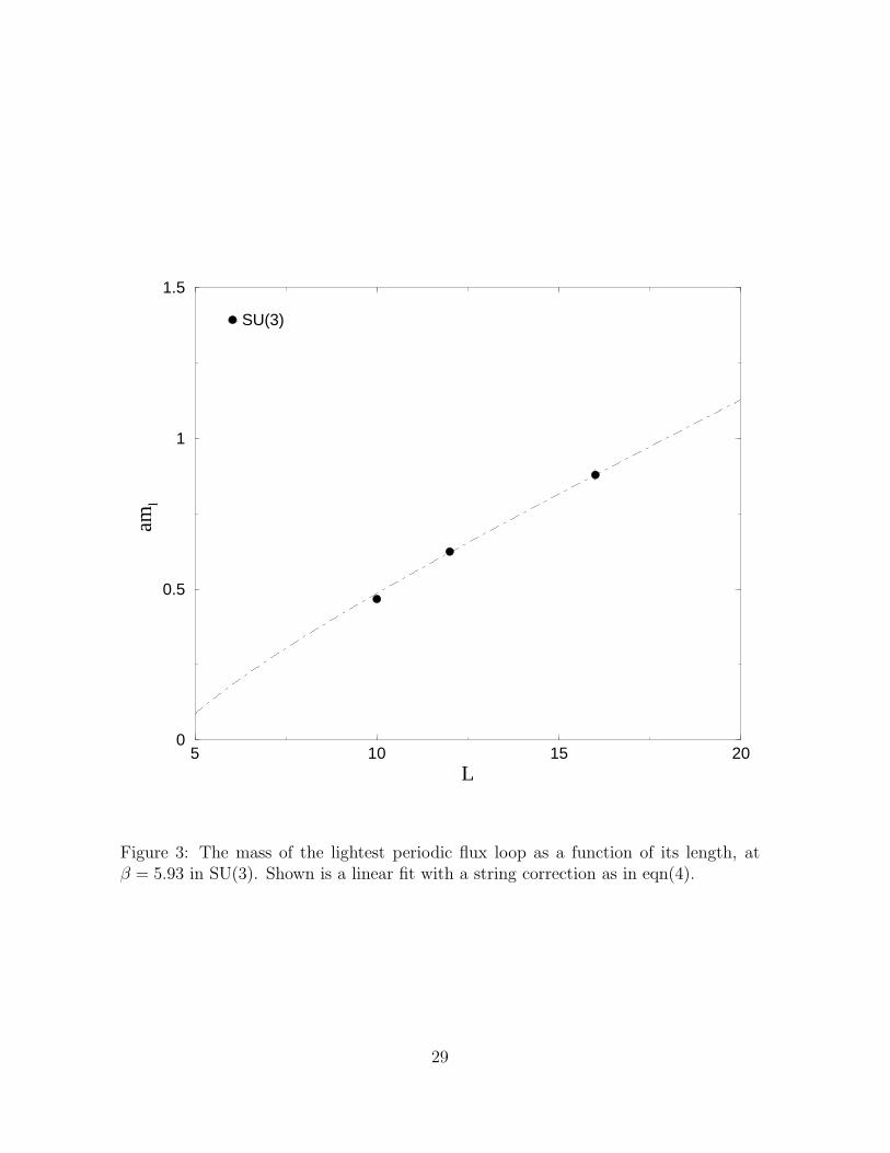
class, and that our string is in fact long enough for higher order corrections to benegligible. There is, of course, a great deal of numerical evidence, scattered throughthe literature, for linear confinement in the case of SU(2) and SU(3) as well as some(much weaker) evidence that the leading correction is as in eqn(4). To address theseissues for SU(N > 3) we show in Fig.2 how the value of aml varies with L in SU(4) ata particular value of a. In Fig.3 we perform a similar exercise for the case of SU(3). Weobserve that for SU(4), just as for SU(3), the mass aml increases roughly linearly withL: evidence for linear confinement. We also note that in both cases the deviation fromlinearity is consistent with eqn(4) for the largest two values of L and that in both casesthis occurs for distances aL ≥ 3/

√σ. If we equate the masses corresponding to these

longest two loops to aml = bL − c/L then we find c = 0.94 ± 0.41 and c = 0.76 ± 0.43for the SU(3) and SU(4) cases respectively. These values are consistent with the valuec = π/3 ≃ 1.05 assumed in eqn(4). We emphasise that, with only two values of Lfitting this correction, we cannot claim to have evidence for both the 1/L functionalform and for its coefficient. Rather we can say that if we assume the functional formthen we have some evidence that the bosonic string coefficient, as in eqn(4), is thecorrect one. This is thus a minimal finite size study (which we are in the process ofimproving upon [7]) but it does indicate that it should be safe, within our statisticalaccuracy, to use eqn(4) to extract a2σ as long as we do so for aL ≥ 3/

√σ.

We remark that although our determination of the string correction is not veryprecise, using periodic loops rather than Wilson loops is by far the better way to ap-proach this question. One reason is that the string correction has a larger coefficientin the former case; c = π/3 as compared to c = π/12 for Wilson loops. More im-portantly, with Wilson loops the string is attached to static sources which provide aCoulomb interaction. This has the same functional form as the string correction anddominates the potential at shorter distances. Thus in fits to the potential of the formV (r) = v + σr + c/r the value of c will be dominated by the short-distance Coulombinteraction rather than the long-distance string correction, unless one confines the fit-ting range to distances greater than, say, 1 fm. (Indeed, as we have seen, the periodicflux loop has to have a length r ≥ 3/

√σ ≃ 1.3fm if the leading string correction is to

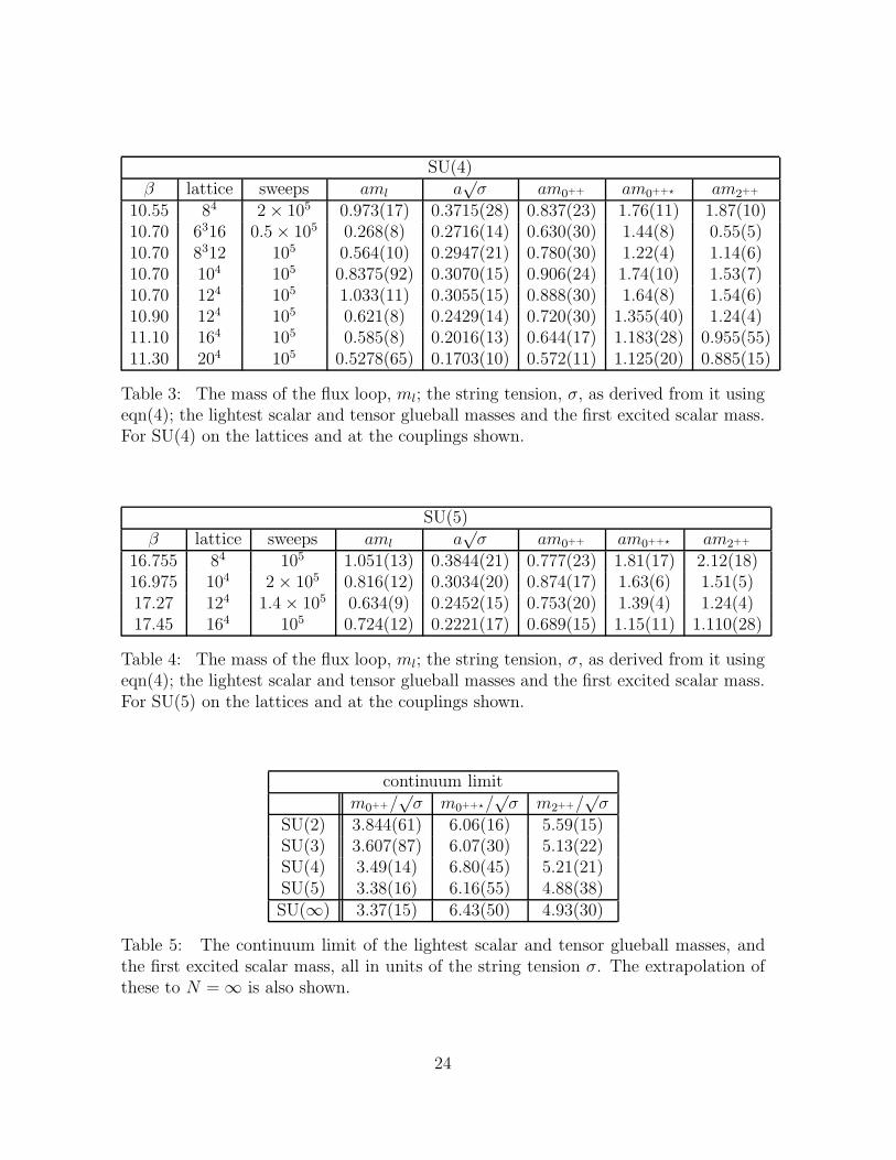
dominate.) This is a tough criterion for Wilson loop calculations and is rarely met.The loop masses and string tensions obtained in our SU(2), SU(3), SU(4) and SU(5)

lattice calculations are listed in Tables 1, 2, 3 and 4 respectively. In the various contin-uum extrapolations that we shall perform we shall only use string tensions calculatedon lattices that satisfy aL ≥ 3/

√σ and thus ones to which we believe the application

of eqn(4) is justified.

4.2 the mass spectrum

In addition to the string tension, we calculate the masses of the lightest scalar andtensor glueballs, as well as the mass of the first scalar excitation. These are obtainedfrom correlations of operators that are obtained by multiplying link matrices around

8

closed contractible loops. These masses are listed in Tables 1, 2, 3 and 4.The first question to ask is how large the spatial volume has to be for glueball finite

volume corrections to be negligible (at our level of statistical accuracy). To answer thisquestion we have performed mass calculations on a range of lattice volumes at β = 10.7in the case of SU(4) and at β = 5.93 in the case of SU(3). The masses are listed inTables 3 and 2 respectively. We observe that the lightest JPC = 0++ and 2++ glueballsappear to have reached (within errors) their infinite volume limit once aL

√σ ≥ 3. For

the excited 0++⋆ scalar the situation is less clear: it appears to be the case for SU(4)but apparently not for SU(3). We shall return to the probable cause of this in Section4.3 but for now we shall simply assume that it is safe to calculate glueball masses andthe string tension on lattice volumes that satisfy the constraint L ≥ 3/a

√σ.

We are interested in determining the N dependence of physical quantities in thecontinuum limit. We first note that if we form a dimensionless ratio of physical quan-tities then the lattice scale drops out, e.g. amG/a

√σ ≡ mG/

√σ. This ratio will of

course still possess lattice corrections. However the functional form of such correctionsis known. In particular for our simple plaquette action we expect the leading correctionto be O(a2). Thus for small enough a we expect the continuum limit to be approachedas

mG(a)√σ(a)

=mG(0)√

σ(0)+ ca2σ. (5)

We could use any mass µ in the correction term, since a2σ and a2µ2 differ at O(a4).We choose to use σ both for the correction term and in our dimensionless mass ratios,because it is the quantity we calculate most accurately and reliably. (In reality cin eqn(5) is a power series in g2(a). However, since the logarithmic variation of thecoupling is very small over our range of a, we follow usual practice and treat it as aconstant.)

Our procedure is therefore to fit our lattice ratios with eqn(5). We begin by includingall our calculated values. If the best fit is poor, we drop the coarsest value of a andre-attempt the fit – and so on. Following this procedure we obtain the continuum massratios listed in Table 5. We remark that the SU(2) and SU(3) values agree with thoseobtained previously, as reviewed for example in [4], and that our SU(2) mass ratios aremuch more accurate than earlier work, as expected.

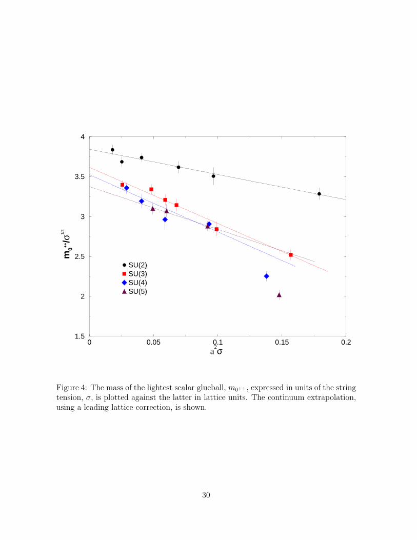
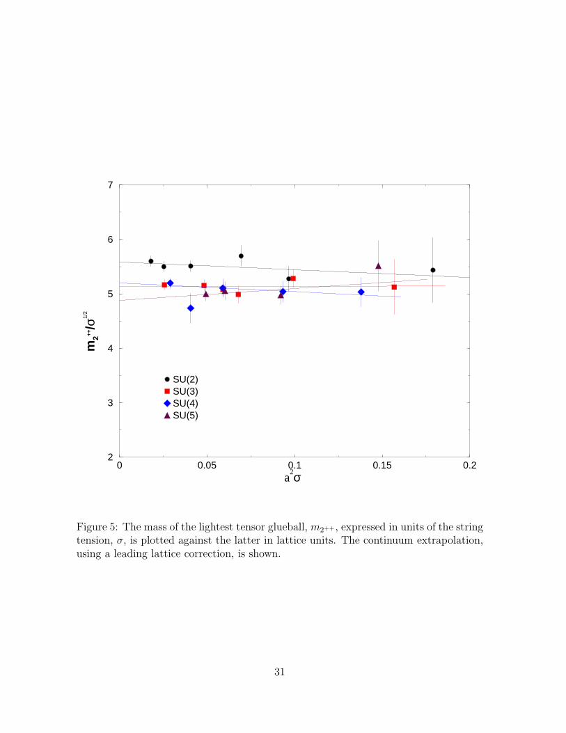
The best fits involved in the extrapolations of the lightest 0++ and 2++ glueballs arealmost always very good, and in any case never poor. They are shown, together withthe lattice ratios, in Fig.4 and Fig.5. We note the increasing influence as N increasesof the strong-to-weak coupling crossover on the mass of the 0++ at the coarsest latticespacing. For SU(5) the 0++⋆ fit is also good, and for SU(2) it is at least acceptable.However for SU(3) and SU(4) the best fits are very poor. In these cases we havequoted generous errors in an attempt not to be misleading. We believe we understandthe origin of these problems with the 0++⋆, and this is discussed in Section 4.3.

We are now in a position to discuss the N dependence of continuum SU(N) gauge

9

theories. We expect that once N is large enough, mass ratios will have a smooth limitwith a leading correction that is O(1/N2), i.e.

mG√σ

∣

∣

∣

∣

∣

N

=mG√

σ

∣

∣

∣

∣

∣

∞

+c

N2. (6)

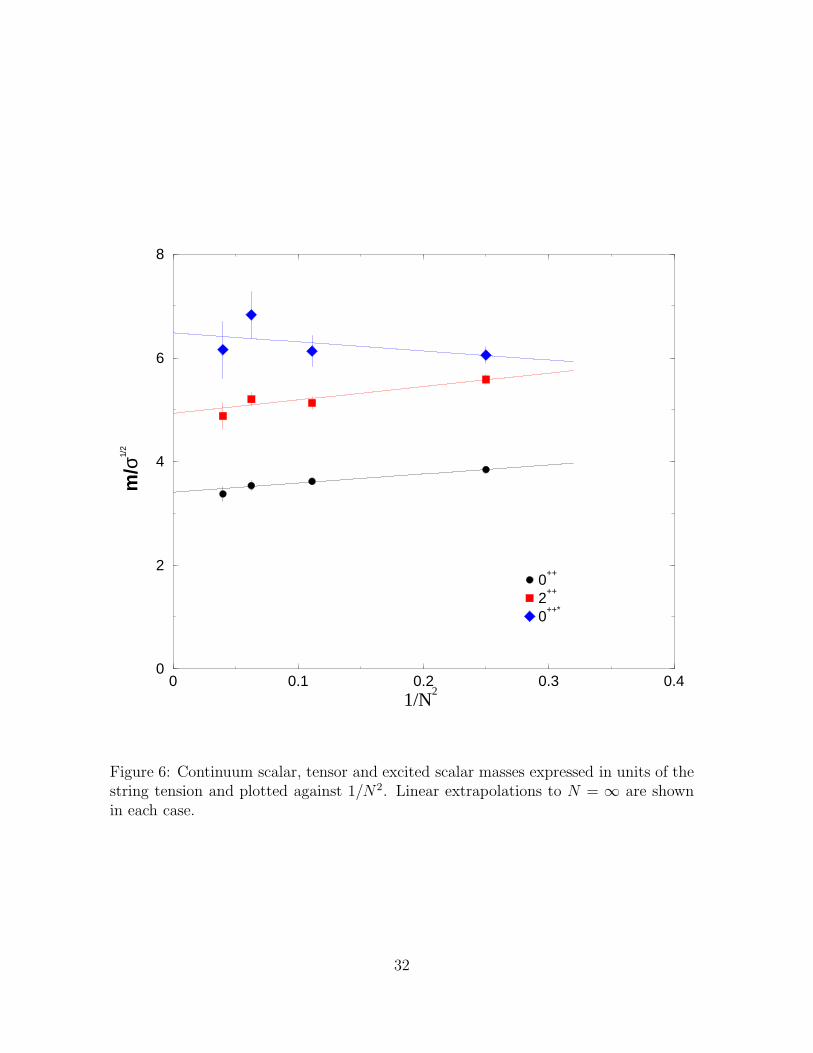
In Fig.6 we plot the continuum mass ratios against 1/N2. According to eqn.(6) once Nis sufficiently close to N = ∞ the mass ratios should fall on a straight line. Performinglinear fits we observe that in fact this is the case all the way down to N = 2. For the0++⋆ this is perhaps not so significant because the errors are so large; however in thecase of the 2++ and of the 0++ the errors are small and the result is striking.

Our best fits for N ≥ 2 are:

m0++√σ

= 3.37(15) +1.93(85)

N2(7)

m2++√σ

= 4.93(30) +2.6(1.9)

N2(8)

andm0++⋆√

σ= 6.43(50) − 1.5(2.6)

N2(9)

These relations give us the corresponding mass ratios not only for N = ∞ but for allvalues of N . The fact that we can fit these mass ratios with just the leading 1/N2

corrections all the way down to N = 2 and the fact that the coefficients are quite smallcan be summarised by saying that all SU(N) gauge theories are close to SU(∞), atleast as far as the low-lying mass spectrum is concerned.

4.3 discussion

Our above results provide a clear motivation for a much more detailed calculation.From what we have learned here, how should such a calculation proceed?

We have seen that there is a large gap to the first excited scalar state. The lessonis that if we want a detailed mass spectrum, many of the states will be quite heavyin lattice units. In this situation the best strategy is to use an anisotropic latticewith a fine temporal lattice spacing that allows a much finer resolution of the rapidlydecreasing correlation functions that correspond to heavy masses. This is an idea andtechnique with a long history [23] which has been used to impressive effect in recentcalculations of the SU(3) mass spectrum [24] (and also in calculations of the staticpotential [10]).

The first excited scalar has a mass m0++⋆ ≃ 2m0++ . This raises the question whetherit might not in fact be a two glueball scattering state with zero relative momentum.Within our present calculation we cannot answer this question with any certainty. Any

10

future calculation should include in the variational basis of operators explicit multi-glueball operators for all the scattering states, of various relative momenta, that areexpected to lie in the mass range of interest. In this way we can hope to identify andseparate bound states or resonances from the less interesting scattering states.

In addition to any bound states, resonances and scattering states, there are also extrastates which decouple in the infinite volume limit but which are not so heavy that theycan be ignored for the kind of volumes we are likely to use. These ‘torelon’ states (see [2]and references therein), which are composed of a periodic flux loop and its conjugate,have a mass that is about twice the mass of the single flux loop: mT ≃ 2ml. Thismass increases roughly linearly with the volume of course, but for much of the presentcalculations this happens to be close to m0++⋆ . Indeed the strong finite-size effects weobserve m0++⋆ to possess in our SU(3) study, suggests an occasional misidentificationwith such a torelon state. In the case of SU(3) and SU(4) the volumes are less constantthan in the case of SU(2) which suggests this as the reason for the poor continuumextrapolation. Again the solution to the problem is to include explicit torelon operatorsin the variational basis so as to make the explicit identification of these states possible.

The above discussion should however not be taken to imply that we have no faithin our estimate of the excited scalar mass. The reason is that our glueball operatorsinvolve the trace of a single loop, and we expect the overlap of both the torelon andtwo-glueball states on such operators to decrease rapidly with increasing N . Thus weare inclined to believe that what we observe in SU(5) is a genuine excited glueballstate, so that our large-N mass estimate should be quite reliable.

Our second observation, based on our tabulated masses, is that the errors on themasses appear to increase as we go from SU(2) to larger N . This could be a problemthat is intrinsic to such a calculation. One possible reason is that, as we shall see be-low, the sampling of different vacuum topological sectors becomes rapidly less ergodicas N increases. Another reason is that as N grows the path integral is increasinglydominated by the single ‘Master Field’ [1]. Our mass calculations are derived from thecorrelations in distant fluctuations about this Master Field and perhaps this methodbecomes inefficient at large N . (In which case it is an interesting question to ask howone might calculate the masses.) Because of its practical importance we have inves-tigated this question in detail. What we find is that the actual correlation functionsdo not display statistical errors that grow with N . This is good news: it means thatthe problem is not an intrinsic one. What happens is that our best operators have apoorer overlap onto the lightest states as N increases. This is more pronounced forthe flux loop than for the glueballs, and becomes more pronounced at smaller a in thelatter case. It may be useful to illustrate this with some explicit values. Consider theoverlap that appears in eqn(2), c2

n ≡ |〈Ω|φ|n〉|2, where we normalise∑

n c2n = 1. For the

best 0++ glueball operator the value of c2n varies, for our coarsest common value of a,

from ∼ 0.95 in SU(2) to ∼ 0.90 in SU(5). For the finest (common) values of a it variesfrom ∼ 0.92 to ∼ 0.85. For the periodic flux loop the corresponding variation of c2

n is

11

from ∼ 0.90 to ∼ 0.75 for both coarse and fine values of a. This behaviour suggeststhat the problem is with our simple blocking algorithm. A better strategy would beto intermingle smearing and blocking steps. In any case the lesson here is that a muchbetter calculation will require the construction of operators with better overlaps.

Another important issue concerns quantum numbers. Typically our operators fallinto representations of the cubic group. What we have called 0++ is actually the cubicA++

1 representation which also includes pieces of other continuum representations, suchas the 4++. For the lightest states one can identify criteria [2] which reassure us that ourcontinuum spin labelling is correct. However the ambiguity becomes larger for excitedstates. For example, one can ask whether our claimed 0++⋆ might not in fact be thelightest 4++. Since the higher-spin continuum representations are typically spreadbetween several representations of the cubic group, one approach to resolving theseambiguities is to search for corresponding degeneracies between states in different cubicrepresentations. However it is unlikely that one will, in practice, obtain these heaviermasses with sufficient accuracy to establish degeneracy unambiguously. (Which, inany case, only becomes exact for small a.) An alternative (or additional) strategy is toconstruct operators with approximate continuum rotational properties [25]. One canthen use the size of the overlap of the excited states onto such operators to determinewhat their likely quantum numbers are.

5 ’t Hooft coupling

The calculations in the previous Section indicate that SU(N) gauge theories have asmooth limit as N → ∞, that the theory remains confining, and that the approachis ‘precocious’ in the sense that even SU(2) appears to be within a modest O(1/N2)correction of SU(∞).

The analysis of diagrams [1] suggests that such a smooth limit should be achievedby keeping the ’t Hooft coupling, λ ≡ g2N , constant as N → ∞. We shall now see towhat extent this expectation can be addressed by our calculations.

Since the coupling runs, the ’t Hooft coupling is not a constant but will depend onthe length scale l on which it is defined, i.e. λ(l) ≡ g2(l)N . Thus we expect that if wefix the value of l in units of some quantity that partakes of the smooth large-N limit,such as the string tension, then λ(l) should have a smooth non-trivial limit as N → ∞.Now, we can define couplings in various ways, and one way is to use β = 2N/g2. Hereg2 is the lattice bare coupling and provides a definition of a coupling on the lengthscale a. Thus we define

λ(a) = g2(a)N = 2N2/β (10)

However it is well known that in our range of a this coupling is heavily influenced bylattice artifacts peculiar to the plaquette action, and that a much better coupling can

12

be obtained from it by the definition

λI(a) = g2I(a)N = 2N2/βI = 2N2/(β × 1

N〈ReTr Up〉) (11)

which may be regarded as a mean-field improved or tadpole improved version of β andλ(a) [26].

An aside. Ideally we would have wished to define a coupling on some scale l ≫ a sothat we could determine its behaviour at fixed l as a → 0 and then compare how thiscontinuum coupling varies with N . (For example one might use the coupling definitionin [27].) Using β, as we do, mixes in lattice corrections in an uncontrolled fashion.Transforming this to βI is known to remove a large part of the lattice corrections atsmall a. Nonetheless, the fact that these lattice corrections vary with the scale l,because of course l = a, will limit our ability to probe the interesting question of whathappens to the coupling on larger distance scales.

To test whether we get a smooth large-N limit by keeping λI(l = a) fixed, we needto choose a physical length scale in terms of which we keep l fixed. We shall choose1/√

σ since we have already seen that the ratio of√

σ to other masses has a smoothlarge-N limit. Thus our first expectation is that if we plot a

√σ against λI(a) then,

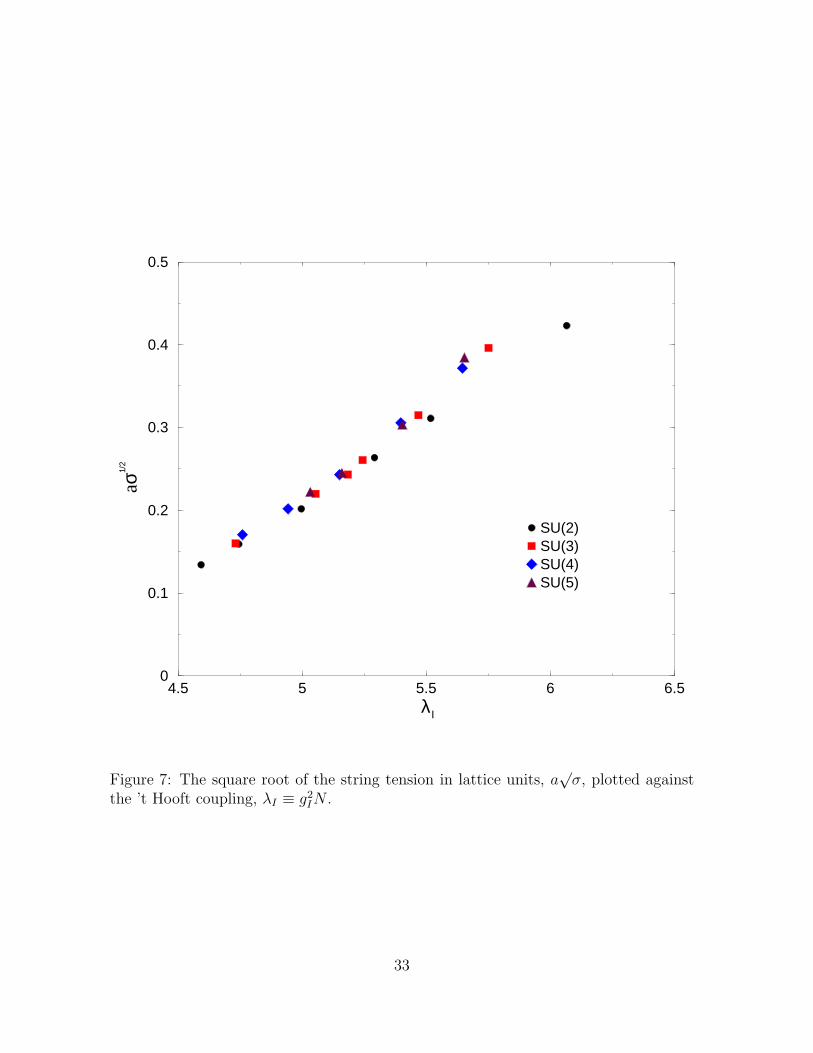
for large enough N , the calculated values should fall on a universal curve. In Fig.7 weplot all our calculated values of a

√σ, against the value of λI(a), for N = 2, 3, 4 and 5.

We observe that, within corrections which are small except at the largest value of a,we do indeed see a universal curve.

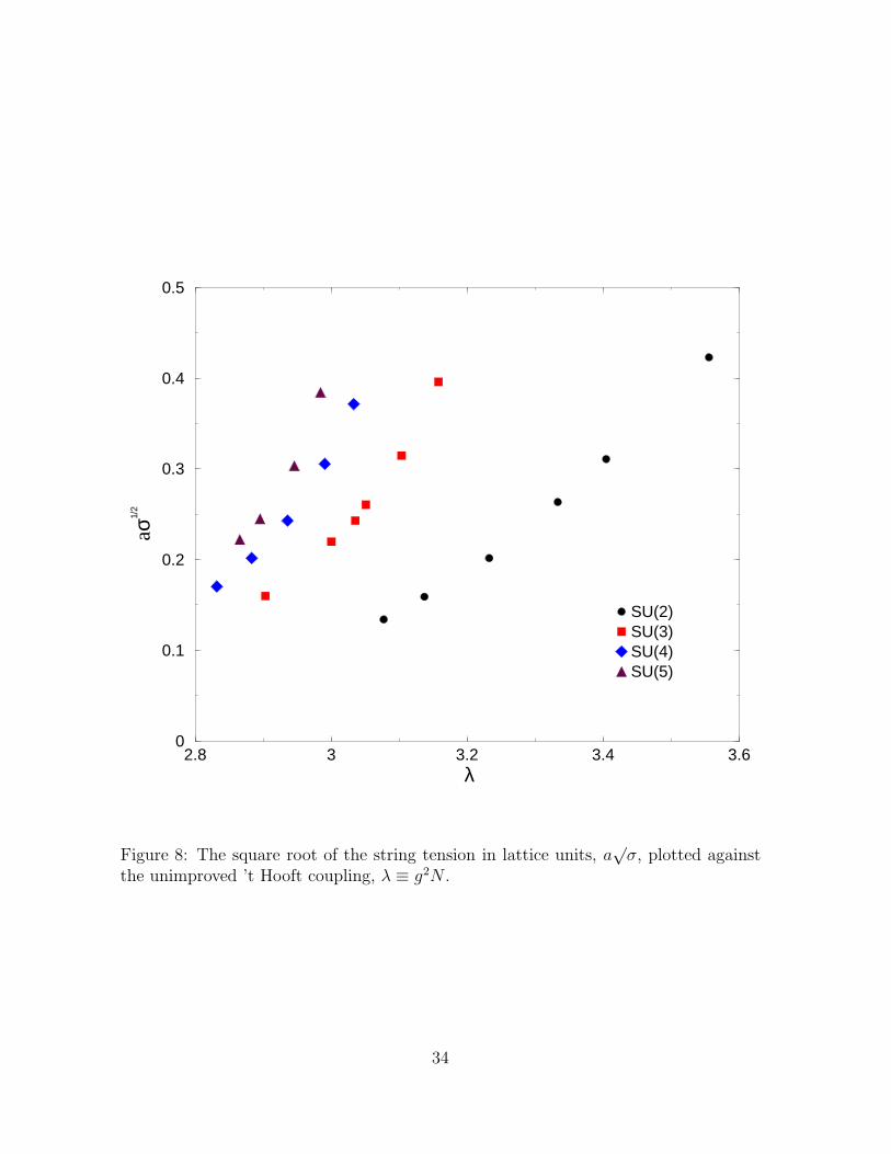
It is instructive to ask what would have happened if we had used eqn(10) ratherthan eqn(11) to define our running coupling. The answer is displayed in Fig.8. Herewe see how very large lattice corrections can easily hide the approach to large-N .

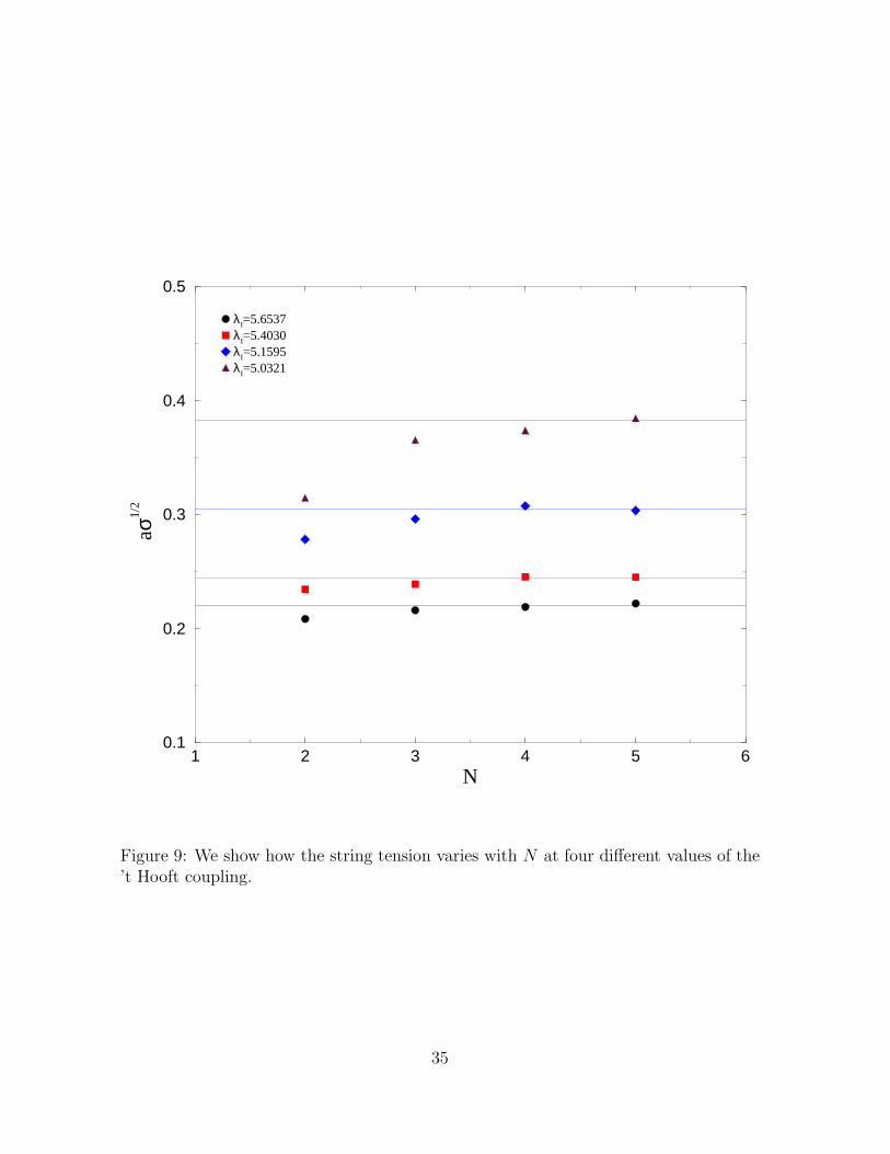
While Fig.7 makes the qualitative point, it is hard to make out the details of theapproach to the N = ∞ limit. To display this we start with each of our four SU(5)values of β and calculate the value of a

√σ obtained at the corresponding value of λI

for N = 2, 3, 4, 5. (To obtain these values for N 6= 5 requires some interpolation.) InFig.9 we show how the string tension varies with N at these four fixed values of the ’tHooft coupling. We see that at all values of a except the largest (where we are closeto the strong-to-weak coupling crossover) the string tension at fixed ’t Hooft couplingbecomes independent of N , within our errors, for N ≥ 4.

Once the coupling g2I (a) is small enough to be accurately given by its 2-loop pertur-

bative formula, we can replace the above analysis by simply extracting the scale ΛI

that appears in the 2-loop formula for the running coupling, and seeing if it also has asmooth large-N limit. We can use our calculations to illustrate how such an analysisproceeds, even though we do not really expect our couplings to be small enough for itto be very reliable. First we invert the 2-loop formula so as to obtain a in terms ofg2(a), and then we multiply both sides by

√σ to obtain

a√

σ =

√σ

ΛI

(

24π2

11

βI

N2

)51121

exp(

−12π2

11

βI

N2

)

. (12)

13

which gives us ΛI in units of a physical mass scale,√

σ, of the SU(N) gauge theory.Using this formula we can extract a value of

√σ/ΛI from each of our lattice calculations

of a√

σ. This value will receive O(a2) corrections in the usual way, but it will also receiveO(g2) perturbative corrections to the two-loop formula in eqn(12). These correctionswill vary by very little over our range of a and we would not be able to determinethem numerically. By contrast the O(a2) correction varies strongly so we can performa continuum extrapolation

√σ(a)

ΛeffI (a)

=

√σ(0)

ΛeffI (0)

+ ca2σ (13)

where ΛeffI is the value of ΛI renormalised by an unknown 1+O(g2

I) factor, where g2I is

the (approximately constant) value of g2I in our range of a. Performing the continuum

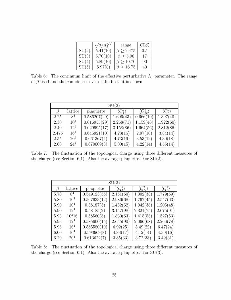
extrapolation in eqn(13) we obtain the values shown in Table 6. We note that thebest continuum fit is very poor in the case of SU(2), acceptable for SU(3) and goodfor SU(4) and SU(5). We then find that we obtain a good fit to these values using justthe expected leading O(1/N2) correction:

√σ

ΛeffI

= 6.05(9) − 2.65(85)

N2. (14)

That is to say, we find that the Λ parameter also appears to have a smooth limit asN → ∞. It is perhaps surprising how well this analysis has worked given the fact thatour values of g2

I(a) are not really that small.

6 Topology and instantons

A Euclidean continuum SU(N) gauge field on a hypertorus will possess an integertopological charge Q. The fluctuations of this charge may be characterised by thetopological susceptibility, χt ≡ 〈Q2〉/V , where V is the volume of space-time. In QCDone can argue [28] that these topological fluctuations make the η′ massive and so solvethe axial U(1) problem. In the large-N limit fermions decouple (for any non-zero quarkmass), so the vacuum topological fluctuations become the same as those of the SU(N)gauge theory. Thus in QCD at large-N and with Nf flavours, one can relate the massof the η′ to the topological susceptibility of the SU(N) gauge theory [29]:

χt ≃m2

η′f 2η′

2Nf

∼ (180 MeV )4. (15)

To obtain the value as (180 MeV )4 one assumes that corrections to this relation aresmall for SU(3) so that one can use the experimental values for mη′ and fη′ . (One alsoassumes the latter to be equal to fπ and one corrects eqn(15) for the small pseudoscalar

14

octet contribution.) There have been many lattice calculations of χt in SU(3) intendedto test the relation in eqn(15). The comparison turns out to be quite successful (see[30] for a review) but of course it only makes sense if the finite-N corrections are smallfor SU(3). We are not here in a position to estimate the corrections to the large-Nrelation m2

η′ ∝ 1/N , but we can check if the SU(3) topological susceptibility is close toits large-N limit, and we shall do so later in this section.

While one hopes that the fluctuations of the topological charge are not going tochange a great deal when one goes from N = 3 to N = ∞, the number density ofinstantons, by contrast, is expected to suffer a strong exponential suppression [31]:

D(ρ) ∝ e− 8π2

g2(ρ) = e−8π2

λ(ρ)N (16)

where ρ is the instanton size and λ ≡ g2N is the ’t Hooft coupling which is keptconstant as N → ∞. At first sight it is hard to see how χt can depend weakly on Nif the instanton density depends so strongly. One can see how this may be [32] if weinclude in our expression for D(ρ) the factor that arises from the various ways that anSU(2) subgroup may be embedded in SU(N):

D(ρ)dρ ∝ dρ

ρ

1

ρ4

b2

λ2(ρ)e−

8π2

λ(ρ)

N

. (17)

Here b is some known constant and we have also included the scale-invariant measure,and volume factor. We see that while at very small ρ, where λ(ρ) is small, therewill indeed be a strong exponential suppression of D(ρ) as N increases, this weakenswith increasing ρ. At the same time, as ρ increases (anti-)instantons will begin tooverlap and the effective action of an instanton will begin to decrease. As shown in[32] the small shift in the effective action calculated in [33] is sufficient to reversethe exponential large-N decay, at values of ρ where such an approximate dilute gascalculation remains plausible. Thus we expect [32] that while for very small ρ therewill be a rapid exponential suppression of D(ρ) with increasing N , this will weaken asρ increases, and indeed will cease entirely at some critical but still quite small value ofthe instanton size. We shall test this prediction in Section 6.3.

We have, in addition, specific expectations about the behaviour of D(ρ) as ρ → 0 atfixed N . Here one can do a reliable one-loop perturbative calculation around the verysmall instantons which gives

D(ρ) ∝ ρ11N

3−5. (18)

This will provide a test of our lattice calculations.

6.1 topology on the lattice

Here we briefly summarise some technical details of our lattice calculation of the topo-logical properties of the gauge fields. We use standard methods which are describedand referenced more fully in [30].

15

We start by observing that for smooth fields one can expand a plaquette matrix inthe (µ, ν) plane as Uµν(x) = 1 + a2Fµν(x) + O(a4). Thus for smooth fields one candefine a lattice topological charge density QL(x) as follows:

QL(x) =1

32π2εµνρσTrUµν(x)Uρσ(x) a→0−→ a4Q(x) (19)

where Q(x) is the continuum topological charge density.Typical lattice gauge fields are not smooth but are rough on all scales. So to apply

eqn(19) to a Monte Carlo generated lattice gauge field we first smoothen it by a pro-cess called ‘cooling’ [30]. This procedure is just like the Monte Carlo except that wechoose each link matrix so as to minimise the action (for each Cabibbo-Marinari SU(2)subgroup). In practice we shall always perform 20 complete cooling sweeps throughthe lattice.

Since the cooling algorithm changes only one link matrix at a time, the resultingdeformation of the fields is local. Thus the only way the topological charge can changeis by an ultraviolet instanton disappearing into a hypercube (or the reverse). For thephysical topological charge to change in this way, a charge on the scale ρ ∼ 0.5fm mustshrink, under the action of iterated cooling, to the scale ρ ∼ a. (Recall eqn(18) whichtells us that in practice the vacuum contains no very small instantons.) As a → 0this will take more and more cooling sweeps. In other words, as a → 0 the physicaltopological charge becomes stable under our 20 cooling sweeps.

While the total topological charge, Q, and hence the susceptibility χt = 〈Q2〉/V ,can be calculated reliably [30] in this way, it is much less clear how reliably one caninfer the location and sizes of instantons in the vacuum. This is partly because thecooling deforms the topological charge density but also because there are ambiguitiesin decomposing a distribution of topological charge into a ‘sum’ of instantons of var-ious sizes. We shall take the most naive approach here. After the 20 cooling sweepswe assume that any sufficiently pronounced peak in the QL(x) density is due to thepresence of an instanton. We infer the size of the instanton from the magnitude of thepeak using the classical continuum relation:

Qpeak =6

π2ρ4. (20)

In practice we apply a cutoff, and discard any peaks corresponding to ρ ≥ 10 (in latticeunits). In addition if there are two peaks of the same sign within a distance 2a of eachother, we keep only the sharper peak. In this way we try to avoid multiple counting ofpeaks with slightly deformed maxima. This instanton identification procedure is clearlymost reliable for smaller instantons, since they produce the most prominent peaks inthe topological charge density. However such instantons will have been deformed by thecooling and so we should not expect to do better than to identify some very qualitativefeatures of the instanton size distribution.

16

Returning to the total topological charge, we note that in practice QL =∑

x QL(x)need not be very close to an integer because there will often be topological chargeswhich are not very large and these will contribute significant O(a2/ρ2) corrections toQL. Since narrow instantons are easy to identify, and since the typical value of Q is notlarge, it is possible to correct for this. And indeed such corrections have been applied inmany past calculations (see for example [34]). Given our large number of calculationswe have chosen not to do this by hand (reliable but tedious) but have automatedthe process. Our algorithm looks at all the narrow instantons in the cooled latticefield and depending on their net charge we shift the real valued topological charge,which we shall call Qr(≡ QL), to one of the neighbouring integer values. We call thischarge QI . For the very coarsest values of a the results differ significantly from a morecareful individual examination (and so we should expect some disagreement with theolder calculations) but this difference rapidly disappears as a decreases. In practicethis difference will not affect our continuum limits in any way. Following previouscalculations [34], we also calculate a topological charge, QIc, which removes from QI

instantons that are sufficiently narrow that they might be affected by the lattice cut-off. In practice our criterion for what is narrow is that Qpeak ≥ 1/16π2. Using eqn(20)this corresponds to a cut-off size ρ ≃ 3. Both Qr and QIc are expected to suffer largerlattice spacing corrections than QI and so we will follow past practice [34] and use QI

to obtain our final continuum values of the topological susceptibility.In each of our lattice calculations (i.e. given volume and given β) we typically

calculate the topological charge on 2000 lattice gauge fields, spaced by 50 Monte Carlosweeps. This represents an increase by a factor of 5 to 10 in statistics over the olderSU(2) and SU(3) calculations [30] that use similar methods.

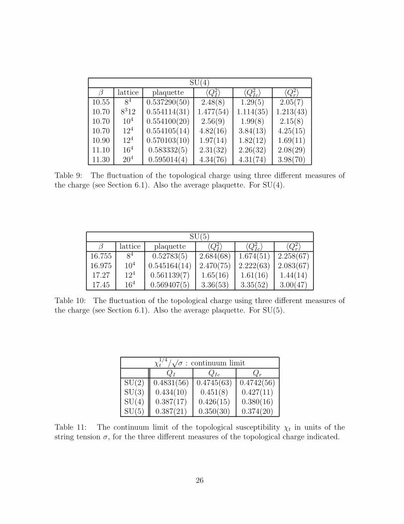
6.2 the topological susceptibility

We list our values of 〈Q2〉 in Tables 7 – 10. On a lattice of size L4 in lattice units,the topological susceptibility is a4χt = 〈Q2〉/L4. Since we expect Q = O(V ), χt shouldhave a finite limit as V → ∞. It is this finite limit we are interested in. To seehow large a volume we need to use in order that finite volume corrections should benegligible we have performed finite volume studies at β = 10.7 in the case of SU(4),and at β = 5.90, 5.93 in the case of SU(3). If we convert the values of QI listed inthe Tables to values of χt, we see that χt appears to decrease slightly with increasingvolume. Once the volume satisfies aL

√σ ≥ 3 (the case for the L = 10, 12 lattices at

β = 10.7) any finite volume effects seem to be within the 1 − 2% statistical errors.Thus almost all the volumes we shall use for our continuum extrapolations will satisfythis bound.

We see from the Tables that the values of QIc rapidly approach the values of QI asa → 0, and that this is more marked as N increases. This reflects the fact that smallinstantons are suppressed and, as we see in eqn(18), this suppression becomes moresevere as N grows. The values of Qr also approach QI as a → 0 but here there is

17

less variation with N . Having reassured ourselves that things are as expected, we shallfrom now use QI as our estimate of Q.

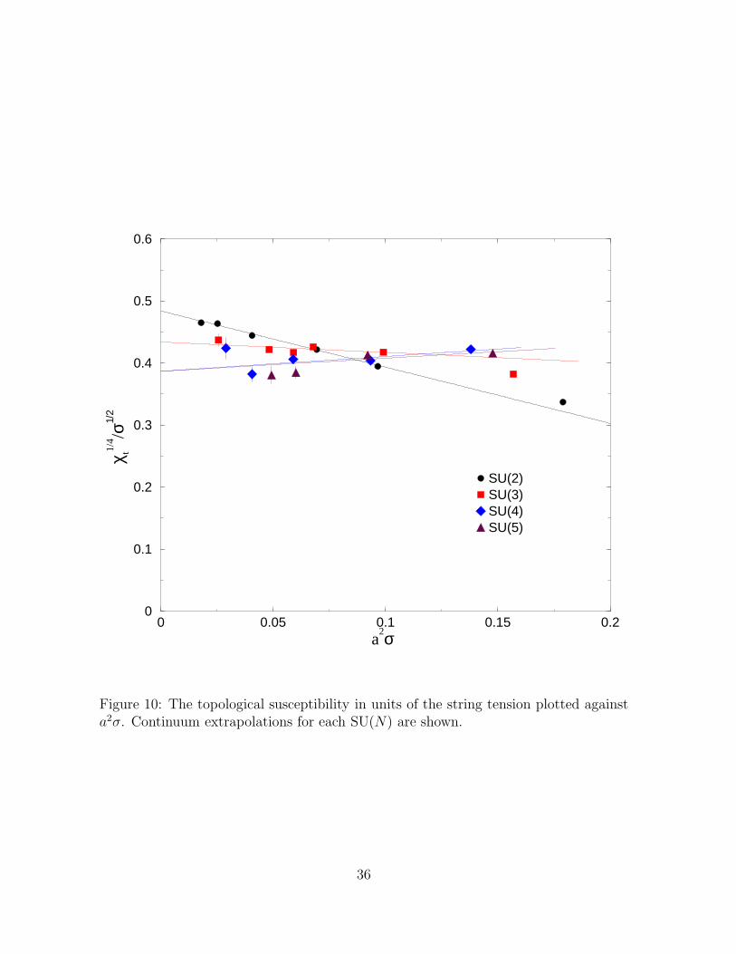
In Fig.10 we plot the dimensionless ratio χ1/4t /

√σ against a2σ. For sufficiently small

a we expect a dependence

χ14t (a)√σ(a)

=χ

14t (0)√σ(0)

+ ca2σ. (21)

so that a continuum extrapolation should be a simple stright line on our plot. We showtypical best fits of this kind.

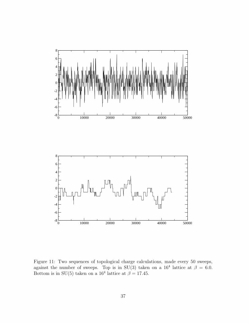
We see from Fig.10 that the SU(2) and SU(3) calculations are very precise and undergood control. As we increase N the errors on the values corresponding to smaller valuesof a become much larger, and the increasing scatter of points suggests that these errorestimates are becoming seriously underestimated. This is to be expected. The MonteCarlo changes Q by an instanton shrinking through small values of ρ down to ρ ∼ awhere it can vanish through the lattice. (Or the reverse process.) However eqn(18)tells us that the probability of a very small instanton goes rapidly to zero as N grows.Thus the lattice fields rapidly become constrained to lie in given topological sectorsand for this quantity the Monte Carlo rapidly ceases to be ergodic as N grows. This isillustrated in Fig.11. Here we show how the value of Q varies in two long Monte Carlosequences, the first in SU(3) and the second in SU(5). The lattice sizes are the sameas is the lattice spacing (within errors) when expressed in units of the string tension.Thus the sequences can be directly compared and it is apparent that the value of Qchanges much less frequently in SU(5) than in SU(3).

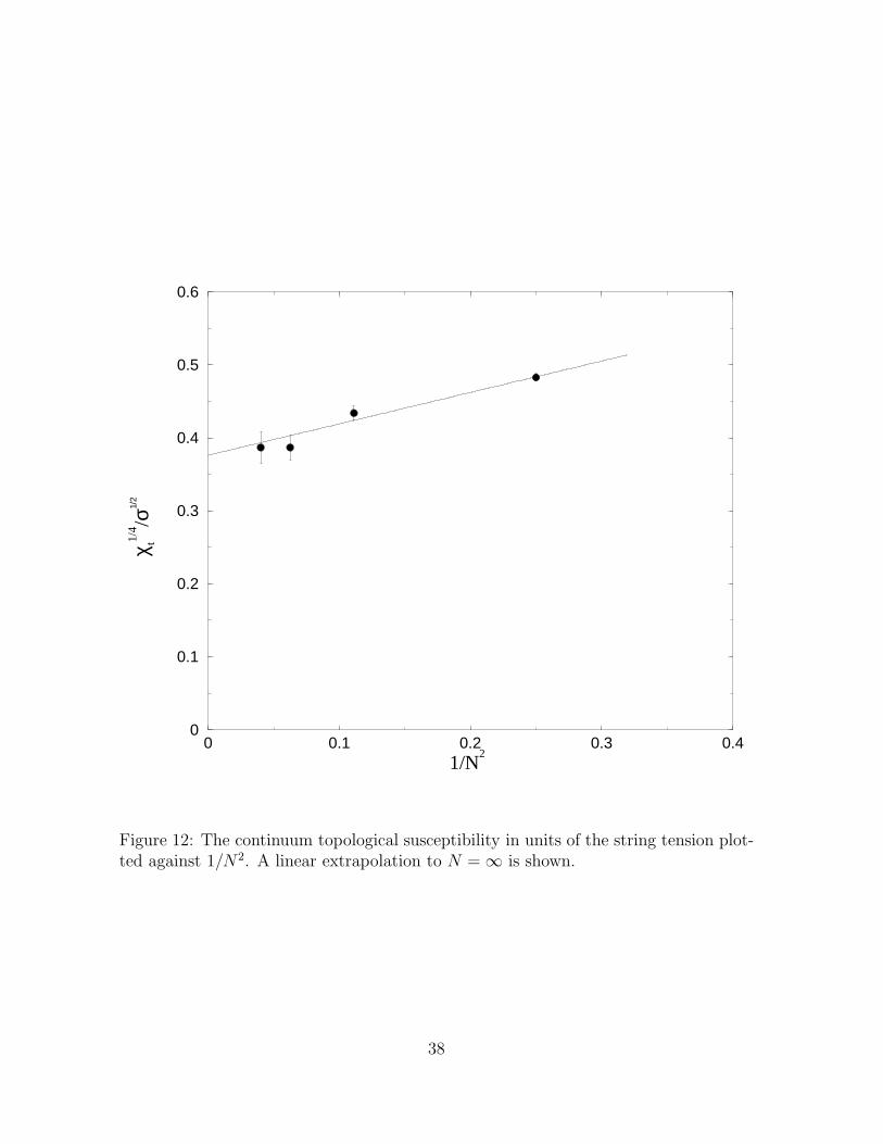
In Table 11 we list the continuum limit of χ1/4t /

√σ for each of our SU(N) groups.

In Fig.12 we plot these values against 1/N2. This is the expected leading large-Ncorrection, so an extrapolation to N = ∞ would be a straight line on this plot

χ14t√σ

∣

∣

∣

∣

∣

∣

N

=χ

14t√σ

∣

∣

∣

∣

∣

∣

∞

+c

N2. (22)

We show our best such fit in the plot:

χ14t√σ

= 0.376(20) +0.43(10)

N2. (23)

We see from this that the large-N corrections to the SU(3) susceptibility are indeedmodest. That is to say, if we express limN→∞ χt in physical units using

√σ ∼ 440 ±

38MeV [35] we obtain the value (165 ± 17MeV )4 for the large-N susceptibility – avalue that is consistent with our expectations [29] in eqn(15).

6.3 the instanton size distribution

In Fig.13 we plot the number density of topological charges against their size ρ. Wedo this for the 204 SU(2), SU(3) and SU(4) lattices. This is the calculation with the

18

smallest value of a common to these groups. (In fact the value of a√

σ varies a littleacross these calculations and we have rescaled the number density to take this intoaccount. We have not rescaled the horizontal ρ axis since here the effect is close tonegligible.)

We observe that the small-ρ tail disappears rapidly as N increases, just as we ex-pect. This implies, as we have already discussed, that our Monte Carlo must becomeineffective in exploring different topological charge sectors as N increases. We observethat the density D(ρ) appears to tend to a large-N limit where there are no chargesat all with ρ ≤ ρc. In lattice units ρc ∼ 5 − 6 which translates in physical units toρc ∼ 0.9/

√σ ∼ 0.4fm. The density then rises rapidly and takes non-zero values over a

range of ρ. The decrease at small ρ is very roughly consistent with being exponentialin N , as expected.

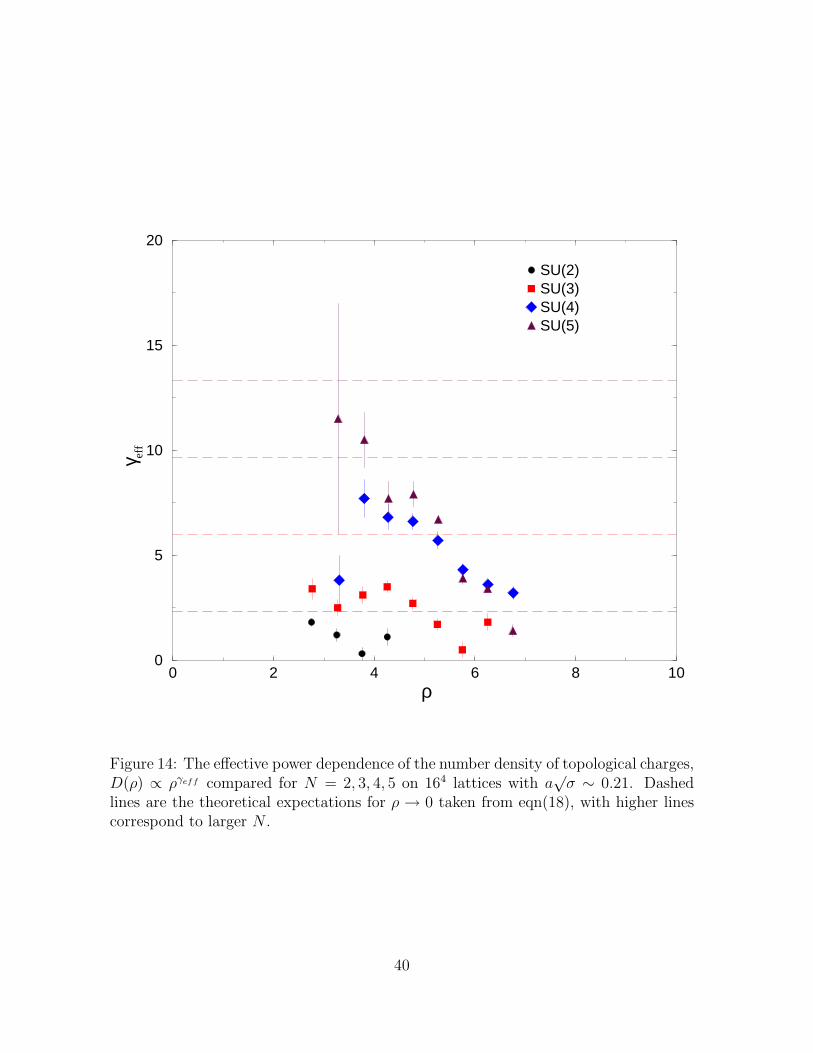
As remarked earlier, at small ρ one can make a reliable theoretical prediction forthe ρ–dependence of D(ρ). To test the prediction in eqn(18), we fit our calculateddistributions to the form

D(ρ) ∝ ργeff (ρ). (24)

The smallest a common to all our groups is on the 164 lattices. We extract D(ρ) andγeff from these calculations and plot the resulting values in Fig.14. We also plot in eachcase the power, from eqn(18), that we expect to observe for a ≪ ρ ≪ 0.5fm. Values ofρ satisfying these strong inequalities do not exist in our calculation. Nonetheless thereis an indication in Fig.14 that our values of γeff are indeed tending to the expectedvalues. This provides evidence that our number densities, while certainly somewhatdeformed by the cooling, do retain the main features of the true continuum densities.

7 Conclusions

We have seen, by explicit calculation, that SU(N) gauge theories in 3+1 dimensionsdo indeed appear to have a smooth large-N limit that is linearly confining. We findthat, as expected, the limit is achieved by keeping the ’t Hooft coupling, λ = g2N ,fixed. Remarkably we found that even SU(2) is close to SU(∞) in the sense that anumber of basic mass ratios can be described over all N using only a modest O(1/N2)correction. Thus a number of simple expressions, such as those in eqns(7–9) andeqn(23), elegantly encapsulate the corresponding physics for all values of N . Moreover,this greatly increases the plausibility of arguments that QCD is close to its large-Nlimit.

The purpose of our calculation was not to obtain the detailed physics of the SU(∞)theory, and for that reason we have not attempted to compare our results to thepredictions of recent analytic approaches (for example [36] or [37]). Rather our aimhas been to establish whether a detailed study is, in practice, possible. Clearly it is, andin Section 4.3 we pointed out some of the lessons we have learned concerning what willbe needed to make such a study successful. Nonetheless, our present study has revealed

19

the beginnings of an interesting N = ∞ glueball spectrum, with m2++ ≃ 1.5m0++ anda large excitation gap in the scalar sector, m0++⋆ ≃ 2m0++ . However we need a muchmore detailed spectrum if we are to be able to draw useful dynamical conclusions fromit.

We have also seen that the topological susceptibility acquires only small correctionswhen N is reduced from N = ∞ to N = 3. This provides an a posteriori justificationfor estimating this suceptibility using the experimental value of mη′ .

As described in the Introduction we shall address the interesting physics of the newnon-trivial k-strings that one encounters for N ≥ 4 in a parallel publication [7].

Acknowledgments

We thank L. Del Debbio and E. Vicari for interesting discussions. Our calculationswere carried out on Alpha Compaq workstations in Oxford Theoretical Physics, fundedby PPARC and EPSRC grants. One of us (BL) thanks PPARC for a postdoctoralfellowship.

References

[1] G. ’t Hooft, Nucl. Phys. B72 (1974) 461.E. Witten, Nucl. Phys. B160 (1979) 57.S. Coleman, 1979 Erice Lectures.A. Manohar, 1997 Les Houches Lectures, hep-ph/9802419.

[2] M. Teper, Phys. Rev. D59 (1999) 014512 (hep-lat/9804008).

[3] M. Teper, Phys. Lett. B397 (1997) 223 (hep-lat/9701003) and unpublished.

[4] M. Teper, hep-th/9812187.

[5] M. Wingate and S. Ohta, hep-lat/0006016; Nucl. Phys. Proc. Suppl. 83 (2000)381 (hep-lat/9909125).

[6] B. Lucini and M. Teper, Phys. Lett. B501 (2001) 128 (hep-lat/0012025).

[7] B. Lucini and M. Teper, in preparation.

[8] A. Hanany, M. J. Strassler and A. Zaffaroni, Nucl. Phys. B513 (1998) 87 (hep-th/9707244).M. J. Strassler, Nucl. Phys. Proc. Suppl. 73 (1999) 120 (hep-lat/9810059).

[9] S. Deldar, Phys. Rev. D62 (2000) 034509 (hep-lat/9911008).

20

http://arXiv.org/abs/hep-ph/9802419

http://arXiv.org/abs/hep-lat/9804008


http://arXiv.org/abs/hep-th/9812187








[10] G. Bali, Phys. Rev. D62 (2000) 114503 (hep-lat/0006022).

[11] V. I. Shevchenko and Yu. A. Simonov, Phys. Rev. Lett. 85 (2000) 1811 (hep-ph/0001299).Y. Koma, E. -M. Ilgenfritz, H. Toki and T. Suzuki, hep-ph/0103162.

[12] L. Del Debbio, H. Panagopoulos and E. Vicari, in progress.

[13] N. Cabibbo and E. Marinari, Phys. Lett. B119 (1982) 387.

[14] M. Teper, Phys. Lett. B183 (1987) 345.M. Albanese et al (APE Collaboration), Phys. Lett. B192 (1987) 163.

[15] J. Kogut, Rev. Mod. Phys. 55 (1983) 775.

[16] M. Creutz, Quarks, gluons and lattices (CUP, 1983).

[17] D. Gross and E. Witten, Phys. Rev. D21 (1980) 446.

[18] G. Bhanot and M. Creutz, Phys. Rev. D24 (1981) 3212.

[19] R. C. Brower, D. A. Kessler and H. Levine, Phys. Rev. Lett. 47 (1981) 621.R. C. Brower, D. A. Kessler, H. Levine, M. Nauenberg and T. Schalk, Phys. Rev.D26 (1982) 959.

[20] I. G. Halliday and A. Schwimmer, Phys. Lett. B101 (1981) 327; B102 (1981) 337.L. Caneschi, I. G. Halliday and A. Schwimmer, Nucl. Phys. B200 (1982) 409; Phys.Lett. B117 (1982) 427.

[21] M. Luscher, K. Symanzik and P. Weisz, Nucl. Phys. B173 (1980) 365.

[22] Ph. de Forcrand, G. Schierholz, H.Schneider and M. Teper, Phys. Lett. B160(1985) 137.

[23] K. Ishikawa, G. Schierholz and M. Teper, Z. Phys. C19 (1983) 327.

[24] C. Morningstar and M. Peardon, Phys. Rev. D56 (1997) 4043 (hep-lat/9704011);Phys. Rev. D60 (1999) 034509 (hep-lat/9901004).

[25] R. Johnson and M. Teper, Nucl. Phys. Proc. Suppl. 73 (1999) 267 (hep-lat/9808012).

[26] G. Parisi, in High Energy Physics - 1980 (AIP 1981).P. Lepage and P. Mackenzie, Phys. Rev. D48 (1993) 2250.P. Lepage, Schladming Lectures, hep-lat/9607076.

21










[27] M. Luscher, P. Weisz and R. Sommer, Nucl. Phys. B389 (1993) 247 (hep-lat/9207010).M. Luscher, Les Houches Lectures, hep-lat/9802029.

[28] G. ’t Hooft, Physics Reports 142 (1986) 357.

[29] E. Witten, Nucl. Phys. B156 (1979) 269.G. Veneziano, Nucl. Phys. B159 (1979) 213.

[30] M. Teper, Nucl. Phys. Proc. Suppl. 83 (2000) 146 (hep-lat/9909124).

[31] E. Witten, Nucl. Phys. B149 (1979) 285.

[32] M. Teper, Z. Phys. C5 (1980) 233.

[33] C. Callen, R. Dashen and D. Gross, Phys. Rev. D17 (1978) 2717; D19 (1979) 1826.

[34] M. Teper, Phys. Lett. 202B (1988) 553.

[35] M. Teper, Newton Inst. NATO-ASI School Lectures, 1997 (hep-lat/9711011).

[36] S. Dalley and B. van de Sande, Phys. Rev. D62 (2000) 014507 (hep-lat/9911035).

[37] O. Aharony, S. S. Gubser, J. Maldacena, H. Ooguri and Y. Oz, Phys. Rept. 323(2000) 183 (hep-th/9905111).

22








SU(2)β lattice sweeps aml a

√σ am0++ am0++⋆ am2++

2.25 84 2 × 105 1.301(17) 0.4231(25) 1.390(30) 2.5(4) 2.30(25)2.30 104 105 0.861(11) 0.3108(17) 1.090(33) 1.58(9) 1.64(7)2.40 124 105 0.745(9) 0.2634(14) 0.953(19) 1.48(5) 1.50(5)2.475 164 105 0.585(8) 0.2016(13) 0.754(10) 1.19(2) 1.111(19)2.55 204 105 0.453(4) 0.15896(63) 0.586(10) 0.91(2) 0.874(15)2.60 244 105 0.387(4) 0.13395(62) 0.514(8) 0.799(10) 0.750(12)

Table 1: The mass of the flux loop, ml; the string tension, σ, as derived from it usingeqn(4); the lightest scalar and tensor glueball masses and the first excited scalar mass.For SU(2) on the lattices and at the couplings shown.


√σ am0++ am0++⋆ am2++

5.70 84 105 1.124(15) 0.3961(23) 0.999(25) 2.07(21) 2.03(20)5.80 104 105 0.886(9) 0.3148(14) 0.895(28) 1.63(10) 1.66(6)5.90 104 105 0.534(9) 0.2527(18) 0.736(20) 0.95(7) 1.22(4)5.90 124 105 0.727(9) 0.2605(14) 0.819(19) 1.40(6) 1.30(4)5.93 10316 105 0.467(7) 0.2391(15) 0.708(22) 1.00(7) 0.94(8)5.93 124 105 0.6245(62) 0.2435(11) 0.756(20) 1.236(36) 1.21(3)5.93 164 105 0.879(18) 0.2430(23) 0.780(16) 1.487(43) 1.234(30)6.00 164 105 0.7071(84) 0.2197(12) 0.734(13) 1.03(8) 1.132(24)6.20 204 105 0.4603(67) 0.1601(10) 0.544(9) 0.955(20) 0.827(15)


23


√σ am0++ am0++⋆ am2++

10.55 84 2 × 105 0.973(17) 0.3715(28) 0.837(23) 1.76(11) 1.87(10)10.70 6316 0.5 × 105 0.268(8) 0.2716(14) 0.630(30) 1.44(8) 0.55(5)10.70 8312 105 0.564(10) 0.2947(21) 0.780(30) 1.22(4) 1.14(6)10.70 104 105 0.8375(92) 0.3070(15) 0.906(24) 1.74(10) 1.53(7)10.70 124 105 1.033(11) 0.3055(15) 0.888(30) 1.64(8) 1.54(6)10.90 124 105 0.621(8) 0.2429(14) 0.720(30) 1.355(40) 1.24(4)11.10 164 105 0.585(8) 0.2016(13) 0.644(17) 1.183(28) 0.955(55)11.30 204 105 0.5278(65) 0.1703(10) 0.572(11) 1.125(20) 0.885(15)



√σ am0++ am0++⋆ am2++

16.755 84 105 1.051(13) 0.3844(21) 0.777(23) 1.81(17) 2.12(18)16.975 104 2 × 105 0.816(12) 0.3034(20) 0.874(17) 1.63(6) 1.51(5)17.27 124 1.4 × 105 0.634(9) 0.2452(15) 0.753(20) 1.39(4) 1.24(4)17.45 164 105 0.724(12) 0.2221(17) 0.689(15) 1.15(11) 1.110(28)


continuum limitm0++/

√σ m0++⋆/

√σ m2++/

√σ

SU(2) 3.844(61) 6.06(16) 5.59(15)SU(3) 3.607(87) 6.07(30) 5.13(22)SU(4) 3.49(14) 6.80(45) 5.21(21)SU(5) 3.38(16) 6.16(55) 4.88(38)SU(∞) 3.37(15) 6.43(50) 4.93(30)

Table 5: The continuum limit of the lightest scalar and tensor glueball masses, andthe first excited scalar mass, all in units of the string tension σ. The extrapolation ofthese to N = ∞ is also shown.

24

√σ/Λeff

I range CL%SU(2) 5.41(10) β ≥ 2.475 0.5SU(3) 5.70(10) β ≥ 5.90 17SU(4) 5.89(10) β ≥ 10.70 90SU(5) 5.97(8) β ≥ 16.75 40

Table 6: The continuum limit of the effective perturbative ΛI parameter. The rangeof β used and the confidence level of the best fit is shown.

SU(2)β lattice plaquette 〈Q2

I〉〈Q2Ic〉〈Q2

r〉2.25 84 0.586207(29) 1.696(43) 0.666(19) 1.397(40)2.30 104 0.616955(29) 2.268(71) 1.159(46) 1.922(60)2.40 124 0.629995(17) 3.158(86) 1.664(56) 2.812(86)2.475 164 0.646921(10) 4.23(15) 2.97(10) 3.84(14)2.55 204 0.661367(4) 4.73(19) 3.53(12) 4.30(18)2.60 244 0.670009(3) 5.00(15) 4.22(14) 4.55(14)

Table 7: The fluctuation of the topological charge using three different measures ofthe charge (see Section 6.1). Also the average plaquette. For SU(2).


I〉〈Q2Ic〉〈Q2

r〉5.70 84 0.549123(56) 2.151(60) 1.002(38) 1.779(59)5.80 104 0.567633(12) 2.986(68) 1.767(45) 2.547(63)5.90 104 0.58187(3) 1.452(62) 1.042(38) 1.205(48)5.90 124 0.58185(2) 3.147(98) 2.321(75) 2.675(91)5.93 10316 0.58560(3) 1.830(63) 1.415(53) 1.527(53)5.93 124 0.585600(15) 2.655(90) 2.066(68) 2.266(78)5.93 164 0.585580(10) 6.92(25) 5.49(22) 6.47(24)6.00 164 0.593669(8) 4.83(17) 4.12(14) 4.30(16)6.20 204 0.613622(7) 3.85(33) 3.72(33) 3.49(31)


25


I〉〈Q2Ic〉〈Q2

r〉10.55 84 0.537290(50) 2.48(8) 1.29(5) 2.05(7)10.70 8312 0.554114(31) 1.477(54) 1.114(35) 1.213(43)10.70 104 0.554100(20) 2.56(9) 1.99(8) 2.15(8)10.70 124 0.554105(14) 4.82(16) 3.84(13) 4.25(15)10.90 124 0.570103(10) 1.97(14) 1.82(12) 1.69(11)11.10 164 0.583332(5) 2.31(32) 2.26(32) 2.08(29)11.30 204 0.595014(4) 4.34(76) 4.31(74) 3.98(70)



I〉〈Q2Ic〉〈Q2

r〉16.755 84 0.52783(5) 2.684(68) 1.674(51) 2.258(67)16.975 104 0.545164(14) 2.470(75) 2.222(63) 2.083(67)17.27 124 0.561139(7) 1.65(16) 1.61(16) 1.44(14)17.45 164 0.569407(5) 3.36(53) 3.35(52) 3.00(47)


χ1/4t /

√σ : continuum limit

QI QIc Qr

SU(2) 0.4831(56) 0.4745(63) 0.4742(56)SU(3) 0.434(10) 0.451(8) 0.427(11)SU(4) 0.387(17) 0.426(15) 0.380(16)SU(5) 0.387(21) 0.350(30) 0.374(20)

Table 11: The continuum limit of the topological susceptibility χt in units of thestring tension σ, for the three different measures of the topological charge indicated.

26

10 10.5 11 11.5β

0

0.5

1

1.5

2

Figure 1: The (rescaled) average plaquette, 2, the mass gap, , and the square root ofthe string tension, 3, over a range of β that includes the region of transition betweenstrong and weak coupling, for the SU(4) gauge theory.

27

5 7.5 10 12.5 15L

0

0.5

1

1.5

2

aml

SU(4)

Figure 2: The mass of the lightest periodic flux loop as a function of its length, atβ = 10.70 in SU(4). Shown is a linear fit with a string correction as in eqn(4).

28

5 10 15 20L

0

0.5

1

1.5

aml

SU(3)

Figure 3: The mass of the lightest periodic flux loop as a function of its length, atβ = 5.93 in SU(3). Shown is a linear fit with a string correction as in eqn(4).

29

0 0.05 0.1 0.15 0.2a

2σ

1.5

2

2.5

3

3.5

4

m0++

/σ1/

2

SU(2)SU(3)SU(4)SU(5)

Figure 4: The mass of the lightest scalar glueball, m0++ , expressed in units of the stringtension, σ, is plotted against the latter in lattice units. The continuum extrapolation,using a leading lattice correction, is shown.

30

0 0.05 0.1 0.15 0.2a

2σ

2

3

4

5

6

7

m2++

/σ1/

2


Figure 5: The mass of the lightest tensor glueball, m2++ , expressed in units of the stringtension, σ, is plotted against the latter in lattice units. The continuum extrapolation,using a leading lattice correction, is shown.

31

0 0.1 0.2 0.3 0.41/N

2

0

2

4

6

8

m/σ

1/2

0++

2++

0++*

Figure 6: Continuum scalar, tensor and excited scalar masses expressed in units of thestring tension and plotted against 1/N2. Linear extrapolations to N = ∞ are shownin each case.

32

4.5 5 5.5 6 6.5λΙ

0

0.1

0.2

0.3

0.4

0.5

aσ1/

2


Figure 7: The square root of the string tension in lattice units, a√

σ, plotted againstthe ’t Hooft coupling, λI ≡ g2

IN .

33

2.8 3 3.2 3.4 3.6λ

0

0.1

0.2

0.3

0.4

0.5

aσ1/

2


Figure 8: The square root of the string tension in lattice units, a√

σ, plotted againstthe unimproved ’t Hooft coupling, λ ≡ g2N .

34

1 2 3 4 5 6N

0.1

0.2

0.3

0.4

0.5

aσ1/

2

λI=5.6537λI=5.4030λI=5.1595λI=5.0321

Figure 9: We show how the string tension varies with N at four different values of the’t Hooft coupling.

35

0 0.05 0.1 0.15 0.2a

2σ

0

0.1

0.2

0.3

0.4

0.5

0.6

χ t1/4 /σ

1/2


Figure 10: The topological susceptibility in units of the string tension plotted againsta2σ. Continuum extrapolations for each SU(N) are shown.

36

0 10000 20000 30000 40000 50000-8

-6

-4

-2

0

2

4

6

8

0 10000 20000 30000 40000 50000-8

-6

-4

-2

0

2

4

6

8

Figure 11: Two sequences of topological charge calculations, made every 50 sweeps,against the number of sweeps. Top is in SU(3) taken on a 164 lattice at β = 6.0.Bottom is in SU(5) taken on a 164 lattice at β = 17.45.

37

0 0.1 0.2 0.3 0.41/N

2

0

0.1

0.2

0.3

0.4

0.5

0.6

χ t1/4 /σ

1/2

Figure 12: The continuum topological susceptibility in units of the string tension plot-ted against 1/N2. A linear extrapolation to N = ∞ is shown.

38

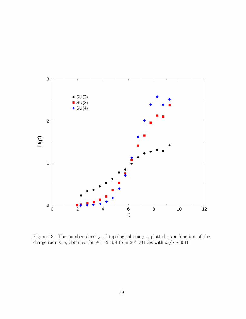
0 2 4 6 8 10 12ρ

0

1

2

3

D(ρ

)

SU(2)SU(3)SU(4)

Figure 13: The number density of topological charges plotted as a function of thecharge radius, ρ; obtained for N = 2, 3, 4 from 204 lattices with a

√σ ∼ 0.16.

39

0 2 4 6 8 10ρ

0

5

10

15

20

γ eff


Figure 14: The effective power dependence of the number density of topological charges,D(ρ) ∝ ργeff compared for N = 2, 3, 4, 5 on 164 lattices with a

√σ ∼ 0.21. Dashed

lines are the theoretical expectations for ρ → 0 taken from eqn(18), with higher linescorrespond to larger N .

40

SU (N) gauge theories in four dimensions: exploring the approach to N=∞

Documents

Transcript of SU (N) gauge theories in four dimensions: exploring the approach to N=∞