arX

iv:1

212.

2906

v1 [

hep-

th]

12

Dec

201

2

Dec 2012 ICTS-TIFR 2012/13TIFR/TH/12-47

A Study of U(N) Lattice Gauge Theory in2-dimensions

Spenta R. WadiaInternational Centre for Theoretical Sciences (ICTS-TIFR)

Tata Institute of Fundamental ResearchTIFR Centre Bldg, IISc Campus

Bangalore 560012 Indiaand

Dept of Theoretical PhysicsTata Institute of Fundamental ResearchHomi Bhabha Rd, Mumbai 500004 India

Abstract

This is an edited version of an unpublished 1979 EFI (U. Chicago) preprint

1

July, 1979 EFI 79/44

A Study of U(N) Lattice Gauge Theory in2-dimensions⋆

Spenta WadiaThe Enrico Fermi InstituteThe University of ChicagoChicago, Illinois, 60637

Abstract

The U(N) lattice gauge theory in 2-dimensions can be considered as thestatistical mechanics of a Coulomb gas on a circle in a constant electricfield. The large N limit of this system is discussed and compared with ex-act answers for finite N . Near the fixed points of the renormalization groupand especially in the critical region where one can define a continuum the-ory, computations in the thermodynamic limit (N → ∞) are in remarkableagreement with those for finite and small N . However, in the intermediatecoupling region the thermodynamic computation, unlike the one for finite N ,shows a continuous phase transition. This transition seems to be a pathol-ogy of the infinite N limit and in this simple model has no bearing on thephysical continuum limit.

⋆Work supported in part by the NSF: Grant No. PHY-78-01224.

2

Introduction

The 1/N expansion has proved very useful in studying the physical spec-trum of N component spin systems (σ-models) and several other tractablefield theories with large dimension of internal symmetry group, in two dim.1

It is used on the assumption that the qualitative, and, in certain cases, evenquantitative character of the spectrum is N independent. Then taking thelarge N limit enormously simplifies the computation since one can use acombination of a steepest descent and mean field approach in which eachcomponent of the spin interacts with the mean field of the other compo-nents.

For SU(N) color gauge theories of the strong interaction, the 1/N ex-pansion was introduced by ‘t Hooft2 who showed that in the Feynman graphexpansion of the theory to each order in g2N (fixed as N → ∞), the lead-ing contribution comes from planar diagrams. Diagrams with holes (quarkloops) and handles are suppressed by factors of 1/N and 1/N2 respectively.In this sense, the expansion in 1/N is analogous to the topological expansionof the dual model and as N → ∞ the mesonic and gluonic states appearas free particle states. Witten3 has recently incorporated baryons as soli-tons into this scheme and has enumerated and emphasized the qualitativeagreement between simple and basic aspects of hadronic spectroscopy andthe 1/N expansion. However, the computational difficulties of planar QCDremain intractable in the diagrammatic language of its formulation, thoughsome remarkable progress in the counting of planar diagrams for quartic andcubic vertices has been made by Brezin et al., using a WKB approach in1/N .4

Now in the statistical mechanics of N component spin systems the rela-tion of the large N limit to a mean field computation has received precisemathematical formulation by the introduction of a Lagrange multiplier asan auxiliary field. It is desirable to have an analogous formulation in thecase of QCD, which avoids direct encounters with the diagram technique.Further, it is desirable to evaluate the relevance of the large N limit. Thequestion is very simple: to what extent and in which domains of couplingis a thermodynamic computation in which N → ∞, relevant for the case offinite N .

We present in this paper a study of U(N) lattice gauge theories in 2-dimensions to clarify these questions. Our method follows studies in thestatistical theories of spectra and ref. (4).

3

In two dimensions, since plaquette variables are the independent ones,the partition function reduces to that of a random unitary matrix with N2

degrees of freedom. This in turn is the partition function of a Coulomb gas ona circle in a constant electric field E = 2β/N . The problem of computing thefree energy and other thermodynamic quantities as N → ∞ reduces to thesolution of a singular integral equation for the charge density, with a Cauchykernel. This problem is always exactly soluble. The solution depends on thestrength of the electric field E. For 0 ≤ E ≤ 1 there is no gap in the chargedistribution and the charge density is conjugate to the electric field. For1 ≤ E < ∞ the charge distribution has a gap and the problem reduces tothe Riemann-Hilbert problem for a simple arc in the plane. The appearanceof a gap in the charge density signals a continuous phase transition at E =1. An order parameter that measures the randomness of the system hasa constant value in the ‘strong coupling’ phase 0 ≤ E ≤ 1 and goes tozero for large E in the spin wave phase. The string constant is computedand a simple renormalization group used to discuss the physically relevantcontinuum limit.

The Coulomb gas partition function is also a Toeplitz determinant in-volving Bessel functions. For finite N it is obviously an analytic function ofthe temperature β. Taylor expansions around the fixed points β = 0 andβ = ∞ indicate an excellent agreement with the computation for N → ∞.To us, this agreement is far from self-evident. Near β = ∞, this can be seento result from a scaling argument.

An interesting mathematical corollary is that the problem of evaluatingToeplitz determinant of order N , can always be mapped to the problem ofa Coulomb gas on a circle, which in the N = ∞ limit is always exactlysoluble. Toeplitz determinants are encountered in the Ising model and theirevaluation is usually done by using Szego’s theorem (c.f. ref. (11)).

4

I. Equivalence of U(N) Gauge Theory in 2-dimensions to the Sta-

tistical Mechanics of a 1-dimensional Coulomb gas

The partition function of the U(N) lattice gauge theory is defined by5

Z(V,N, β) =∫

dµ exp

[

β∑

ρ

(U(P )−N)

]

(1)

dµ is a real measure over the gauge group elements at each link; the summa-tion over P is over all oriented plaquettes and U(P ) is a product of groupelements, in the fundamental representation, at the 4 oriented links of P .U+(P ) would be the group element associated with the links in the opposite

direction. β =1

g20is the temperature and V is the volume of the system in

lattice units.In two space-time dimensions it is possible to treat plaquette variables

as independent.6 A simple way to see this is to fix the axial gauge in Z: alltime-like links are chosen to be one and all space-like links at one particulartime ‘t0’ are chosen to be one. Since the time links are trivial the space-likelinks at time ‘t’ can be expressed as a unique product of a time ordered stringof independent plaquette variables, the expression for Z in (1) becomes anintegral over a single unitary matrix

Z =[∫

dUeβ[TrU+TrU+]]V

e−2βNV

Hence, the problem is reduced to the computation of the partition func-tion of a random unitary matrix with N2 real independent variables

z =∫

dUeβ(TrU+TrU+) (2)

Integration over the group U(N) is known.7 It is convenient to make a sep-aration of variables into group invariant and non-invariant parameters. LetR be the unitary matrix that brings U to diagonal form

U = R+DR, Dij = δijeiθj

R is arbitrary up to an invariant subgroup of U(N), hence, after appropriatechoice of gauge it depends on N2 −N parameters and

dU = CNdRN∏

i=1

dθi2π

∏

i<j

∣

∣

∣eiθi − eiθj∣

∣

∣

2(3)

5

Substituting (3) in (2) we get

z =1

N !

∫ 2π

0

N∏

i=1

dθi2π

e

N2

2β

N

N∑

i=1

1

Ncos θi + 2

∑

i<j

1

N2log |eiθi − eiθj |

(4)

The factor N ! appeared by choice of CN in (3) such that z = 1 for β = 0.Now define an action

−S =β

N

N∑

i=1

1

Ncos θi +

∑

i<j

1

N2log

∣

∣

∣eiθi − eiθj∣

∣

∣ (5)

then

z =1

N !

∫ 2π

0

N∏

i=1

dθi2π

e−2SN2

(6)

The action S = o(1) in N provided β/N = E/2 is a fixed parameter ofthe theory. If so, then for large N we can consider evaluating z by a WKBexpansion in the small parameter 1/N2.

The action S in (5) is essentially the electrostatic potential energy ofN charges of strength 1/N distributed on a unit circle in the plane, in thepresence of a constant electric field E/2 along the x-axis. The repulsivelogarithmic interaction tends to distribute the charge uniformly about thecircle and the electric field tends to drive all θi → 0. There is anotheranalogy with spin systems. Define a unit spin vector

~σi = (cos θi, sin θi)

then

−S =H

2

N∑

i=1

1

Nσxi +

∑

i<j

1

N2log (1− ~σi · ~σj)

which is the potential energy of unit spins equally spaced along the x-axis ina constant magnetic field H/2 = β/N . The logarithm represents a con-tinuous version of an anti-ferromagnetic coupling. In the absence of H ,〈~σn〉 =

(

cos 2πnN

, sin 2πnN

)

. In the rest of this paper we shall only considerthe electrostatic analogy.

6

II. WKB and Mean Field Calculation

If we define the free energy per degree of freedom f(E) by z = exp(N2f(E)),then we have the WKB expansion in 1/N2

f(E) = −2S0 +S1

N2+ 0

(

1

N4

)

(7)

S0 is the minimum value of the potential energy S and S1 is the result ofgaussian fluctuations around the most probable configuration that minimizesS. For the present, we shall be concerned with evaluating F (E) as N → ∞.

As we have noted, the point charges on the unit circle carry a charge

= 1/N . The interaction energy between two charges is 0(

1

N2

)

, which means

that they are very weakly coupled. However, the interaction energy of anyone charge in the mean field of the other N2 − N − 1 ≈ N2 charges is0(1). This motivates a mean field theory type computation7 in which oneintroduces a macroscopic charge density u(θ) ≥ 0, on the unit circle, suchthat u(θ)dθ/2π is the fraction of the number of charges between θ and θ+dθ.By definition

∫ 2π

0u(θ)

dθ

2π= 1 (8)

In this continuum limit as N → ∞ we have

−S[u] =E

2

∫ 2π

0

dθ

2πu(θ) cos θ + P

∫ 2π

0

dθ

2π

∫ 2π

0

dφ

2πu(θ) log |eiθ − eiφ|u(φ) (9)

P stands for the Cauchy principal value.The most probable charge distribution is a stationary point of (9) sub-

ject to the normalization (8). Hence, this distribution satisfies the followingsingular integral equation

E

2cos φ+ P

∫ 2π

0

dθ

2πu(θ) log |eiθ − eiφ| = λ

λ is a lagrange multiplier corresponding to (8). It represents the averagepotential at φ due to all the other charges, and it is φ independent. Takingφ derivatives we have

E sin φ = −P∫ 2π

0

dθ

2πu(θ) cot

(

θ − φ

2

)

(10)

7

which states that the tangential forces on the charge at φ due to all the othercharges balance the force of the electric field.

III. Solution of Integral Equation

Let us begin by assuming that the function u(θ) is smooth in the sensethat u′(θ) is continuous for 0 < θ < 2π. The solution to (10) can be im-mediately written down if we recall the Hilbert transform formula for thecircle:

If Φ(Z) is analytic for |Z| ≤ 1, then on the unit circle we have

Φ(eiθ) = Φ(Z = 0) +P

2πi

∫ 2π

0dθΦ(eiθ) cot

(

θ − φ

2

)

The choice Φ(Z) = 1 + EZ gives the correctly normalized solution

u(θ) = 1 + E cos θ (11)

The condition u(θ) ≥ 0 for 0 ≤ θ ≤ 2π, however, requires 0 ≤ E ≤ 1.When E = 0, u(θ) = 1 as expected; turning on the electric field along the

x-direction diminishes the density around θ = π and produces a crouchingof charge near θ = 0. Also u(θ) = u(−θ). Note that u(θ) is smooth andnever vanishes for E < 1. At E = 1 the distribution hits a zero at the singlepoint θ = π. This gives us a hint that as E starts exceeding the criticalvalue 1, there would start appearing a gap in the charge distribution aroundθ = π which would increase as a continuous and monotonic function of E,1 < E < ∞. In the following we shall establish this picture by solving theintegral equation (10) with the boundary condition that u(θ) = 0 outside theinterval −α < θ < α. For α 6= π we do not assume u(θ) to be smooth at theend points θ = α. The integral equation now becomes

E sin φ = −P∫ α

−α

dθ

2πu(θ) cot

(

θ − φ

2

)

∫ α

−α

dθ

2πu(θ) = 1 (12)

To solve (12) we introduce complex notation t = eiθ and t0 = eiφ. (12)becomes

E(t0 − t−10 ) =

P

πi

∫ t2

t1

dt

t

t + t0t− t0

u(t)

8

1

2π

∫ t2

t1

dt

itu(t) = 1, t1 = t⋆2 = e−iα (13)

Now the important point is that the normalization condition enables us towrite the integral equation in the form

E(t0 − t−10 ) =

P

πi

∫ t2

t1

dt

t− t02u(t)− 1

The kernel is Cauchy type and we have adapted the general formalism to solvesuch equations to our problem.9 One starts out by considering the function

Φ(z) =1

2πi

∫ t2

t1

dt

t

t+ z

t− zu(t) (14)

analytic in the plane cut by the (t1, t2). The direction of the arc is as-sumed counterclockwise. Denote the boundary values of this function as zapproaches a point t on the arc (t 6= t1, t2), from the left and right by Φ+(t)and Φ−(t) respectively. Then by the Plemelj formulae8 for the boundaryvalues of analytic functions we have

Φ+(t)− Φ−(t) = 2u(t) (15)

Φ+(t) + Φ−(t) =P

πi

∫ t2

t1

dξ

ξu(ξ)

ξ + t

ξ − t= E(t− t−1) (16)

Equation (16) specifies the Reimann-Hilbert problem for the arc (t1, t2): tofind an analytic function in the cut plane whose boundary values satisfy (16).In our case we have an additional condition to satisfy at z = ∞ which followsfrom the normalization of u(t),

Φ(∞) = −1 (17)

The discontinuity formula (15) (a reflection of Gauss’ law in electro-statics)implies that a solution to the Reimann-Hilbert problem solves the integralequation (13).

The function h(z) = [(z − t1)(z − t2)]1/2 clearly solves the homogeneous

problem φ+(t)+φ−(t) = 0 up to an entire function. This choice of the squareroot function vanishing at the end points leads to u(t1) = u(t2) = 0. Nowwrite

Φ(z) = h(z)H(z)

9

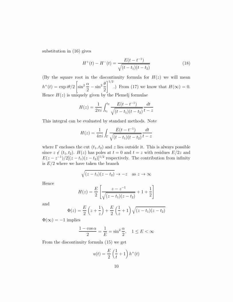
substitution in (16) gives

H+(t)−H−(t) =E(t− t−1)

√

(t− t1)(t− t2)(18)

(By the square root in the discontinuity formula for H(z) we will mean

h+(t) = exp iθ/2

[

sin2 α

2− sin2 θ

2

]1/2

.) From (17) we know that H(∞) = 0.

Hence H(z) is uniquely given by the Plemelj formulae

H(z) =1

2πi

∫ t2

t1

E(t− t−1)√

(t− t1)(t− t2)

dt

t− z

This integral can be evaluated by standard methods. Note

H(z) =1

4πi

∫

Γ

E(t− t−1)√

(t− t1)(t− t2)

dt

t− z

where Γ encloses the cut (t1, t2) and z lies outside it. This is always possiblesince z ǫ/ (t1, t2). H(z) has poles at t = 0 and t = z with residues E/2z andE(z − z−1)/2[(z − t1)(z − t2)]

1/2 respectively. The contribution from infinityis E/2 where we have taken the branch

√

(z − t1)(z − t2) → −z as z → ∞

Hence

H(z) =E

2

z − z−1

√

(z − t1)(z − t2)+ 1 +

1

2

and

Φ(z) =E

2

(

z +1

z

)

+E

2

(

1

z+ 1

)

√

(z − t1)(z − t2)

Φ(∞) = −1 implies

1− cosα

2=

1

E= sin2 α

2, 1 ≤ E < ∞

From the discontinuity formula (15) we get

u(t) =E

2

(

1

t+ 1

)

h+(t)

10

u(θ) = 2E cosθ

2

√

E−1 − sin2 θ

2≥ 0

We summarize the computation

u(θ) =

1 + E cos θ 0 ≤ E ≤ 1 (19a)

2E cosθ

2

√

E−1 − sin2 θ/2 1 ≤ E < ∞ (19b)

Our expectation for the appearance of a gap at θ = π beyond E = 1 isconfirmed; also the size of the gap 2α is a continuous and monotonic functionof E: 1/E = sin2 α/2.

IV. Computation of Thermodynamic Quanti-ties in the N → ∞ Limit

The appearance of the gap at E = 1 is reflected in the behavior of thethermodynamic functions. From (7) and (9) we have for the free energy perdegree of freedom

f(E) =

E2

40 ≤ E ≤ 1 (20a)

E − 1

2logE − 3

41 ≤ E < ∞ (20b)

f(E) and its first two derivatives are continuous at E = 1, indicating acontinuous phase transition at the point E = 1.

A useful order parameter9 that characterizes the phases is

R =N∑

i=1

1

Nsin2 θi =

1

NTr

[

U − U+

2i

]2

(21)

In the continuum approximation as N → ∞ we have

R(E) = limN→∞

〈 1N

N∑

i=1

sin2 θi〉 =∫ 2π

0

dθ

2πu(θ) sin2 θ (22)

Therefore

R(E) =

1/2 0 ≤ E ≤ 1

1

E− 1

2E21 ≤ E < ∞

(23)

11

R represents the average value of the sum of the squares of the y-co-ordinatesof the charges. R(E) and R′(E) are continuous at E = 1. In a sense, R is adisorder parameter because it is a measure of the randomness of the system.In the phase 0 ≤ E ≤ 1 where its expectation value is a constant, thedistribution of eigenvalues of the unitary matrix is truly random and theeigenvalues go over their entire range. We shall call this phase the randomphase (RP). In the phase 1 ≤ E < ∞ we see that for E ≫ 1, 〈R〉 ≈ 0; therandom distribution has continuously disappeared and the eigenvalues areconfined to a small region around U = 1. Also the eigenvalue density (196)for E ≫ 1 is written in scaled form

u(θ) ≈ 2√E

√

1− (√Eθ)2

4, |θ| ≤ 2√

E(24)

We call this phase the familiar spin wave phase (SWP). We are aware thatfor E >≈ 1, the term SWP is certainly not very appropriate.

V. The Wilson Loop

An important order parameter of the original U(N) theory is the Wilsonloop for a closed curve C,

W [C] =1

ZN

∫

dµTr

(

∏

ℓ

Uℓ

)

eβ(TrU+TrU+−N) (25)

Once more, because in two dimensions plaquette variables are the indepen-dent variables, we have for a simple curve

W (C) = ωA

ω =1

ZN

∫

dU(TrU)eβ(TrU+TrU+) (26)

A is the area enclosed by the curve in lattice units. In the diagonal repre-sentation

ω =

⟨

1

N

N∑

i=1

cos θi

⟩

(27)

which in the continuum approximation of the large N limit becomes

= limN→∞

⟨

1

N

N∑

i=1

cos θi

⟩

=∫ 2π

0

dθ

2πu(θ) cos θ.

12

Using (19) we have

WA =

(

E2

)A0 ≤ E ≤ 1

(

1− 12E

)A1 ≤ E < ∞

(28)

The string constant in lattice units is defined by

WA = e−A 1

4πα′

0

α0 =

− 1

4π

1

logE/20 ≤ E ≤ 1

− 1

4π

1

log(

1− 1

2E

) 1 ≤ E < ∞ (29)

it is the exact analogue of the correlation ‘length’ in spin systems. Up untilnow we have worked from the statistical mechanics point of view in whichthe basic unit of length is the lattice spacing ‘a’. In order to make contactwith field theory10 where the basic unit of length is usually set by the inverserenormalized mass we go over to laboratory units in which the string constanthas the dimension of area

α(a;E) = a2α0(E) (30)

This physical quantity is a renormalization group invariant i.e., if a → λa,λ > 0

α(λa;E) = α(a;Rλ(E)) (31)

Rλ(E) is the renormalized coupling. Then from (29) we have

Rλ(E) =

2(

E

2

)1/λ2

0 ≤ E ≤ 1

1

2

[

1−(

1− 1

2E

)1/λ2] 1 ≤ E < ∞ (32)

Now consider moving towards short distances, e.g., λ =1

2< 1. The recursion

formulae which follows from (32) have two trivial fixed points E⋆ = 0 and

13

E⋆ = ∞ and the flow is away from E⋆ = 0 towards E⋆ = ∞. Note thatE = 1 is not a fixed point. At the fixed points we have

α0(E⋆ = 0) = 0

α0(E⋆ = ∞) = ∞

Hence E⋆ = ∞ is the critical point of the statistical mechanics problemfor fixed a. In the neighborhood of the critical point E⋆ = ∞, the latticeconstant is an irrelevant parameter and it is possible to define a euclideaninvariant theory characterized by the adjustable parameter

αR = α(a → 0, E → E⋆)

From (29) we have for αR near the critical point

αR =Ea2

2π≡ ER

2π

In the field theory notationE

2=

β

N=

1

g20N, hence

αR =1

πN(g20/a2)

The renormalized parameter αR ranges from 0 to ∞, in contrast to the bareparameter α0 which ranges from 1/2π to ∞. This agrees with ‘t Hooft’scomputation2 of the same quantity in the Yang-Mills version of the theory.In fact, for the interaction energy of static quarks in the fundamental repre-sentation, we have

E(x1, x2) =1

4παR|x1 − x2|

x1 and x2 are the locations of the quarks in one dimension.

14

VI. Partition Function Near Critical Point

The partition function z in (6) can be written by expanding the cosineand the log in their respective power series. The action is

−2S = EN∑

i=1

cos θiN

+∑

i<j

1

N2log 2[1− cos(θi − θi)]

= EN∑

i=1

1

N

[

1− θ2i2!

+θ4i4!

· · ·]

+

∑

i<j

1

N2log(θi − θj)

2 −∑

i<j

1

N2

(θi − θj)2

3.4

Now performing a scale transformation

θi →√Eθi = ξi

we get

−2S = − 1

N

N∑

i=1

ξ2i /2 +1

N2

∑

i<j

log |ξi − ξj|2

+E − N(N − 1)

2N2logE +

∞∑

n=1

(

1

E

)θ(n)

[ξi]

θ(n) stands for the coefficient of 1/En, e.g.,

θ(1) =1

N

∑

i

ξ4i −1

N2

∑

i<j

(ξi − ξj)2

12

θ(2) = − 1

N

∑

i

ξ6i −1

N2

∑

i<j

(ξi − ξj)4

3.4.5.6· · · etc.

After scaling the measure factor we have

z = eN2(E−

1

2logE) 1

N !

∫ +∞

−∞

∏

i

dξi2π

∏

i

θ(√Eπ − |ξi|)

×eN2V · eN2

∑

∞

n=1

θ(n)

En(ξ)

15

V = − 1

N

N∑

i=1

ξ2i2

+1

N2

∑

i<j

log |ξi − ξj |2 (33)

The θ function in (33) is a cut-off that reflects the compactness of the gaugegroup.

So far, (33) is exact without approximation. In the large N limit, onecan once more consider a WKB expansion in 1/N2. Since this is the sameproblem as before except for a change of scale, we have, for the distributionof eigenvalues,

u(ξ) =1√Eu(ξ/

√E) = 2 cos

ξ

2√E

√

1− E sin2 ξ/2√E (34)

The function u above is given by (19b), since we are, ultimately, interestedin large values of E. Expanding, we have

u(ξ) =√

4− ξ2 +∞∑

n=1

Cn(ξ)

En, |ξ| ≤ 2, E ≫ 1

This means that the contribution of the terms involving the operators θ(n)(ξi)in (33), to the leading term in the WKB expansion in 1/N2, are negligiblenear critical point i.e., as E → ∞ (N.B. the large E limit is taken after thelarge N limit). Further, the cut-off in (33) is automatically repected, and wehave

z(E → E⋆) ≈ eN2(E−

1

2logE) 1

N !

∫

∞

−∞

∏

i

dξi2π

eN2V (35)

We now recall that ifH is aN×N hermetian matrix with N2 independentcomponents, the integration measure over H is defined by7

dH =N∏

i=1

dHii

∏

i<j

dHRijdH

Iij, Hij = HR

ij + iHIij (36)

Once more one can perform a separation of variables to extract those whichare left invariant by a unitary transformation. Let W be the unitary matrixthat diagonalizes H ,

H = W+h W, hij = δijξj

then

dH ∝ dW.N∏

i=1

dξi∏

i<j

|ξi − ξj|2

16

and (35) becomes

z ∝ eN2(E−logE/2)

∫

dHe−N2TrH2

(37)

Therefore, the partition function of the original gauge theory near criticalpoint is

Z = e−2NβV zV

∝ e−N2V logE/2[∫

dHe−N2TrH2

]V

∝[

∫

dH

(√E)N2

e−N2TrH2

]V

(38)

Expression (38) is what one expects to be proportional to the partition func-tion of the Yang-Mills version of the theory, which is defined in a spacetimevolume V by

ZYM ∝∫

∏

x,t

dA0dA1δ(A0(x, t))δ(A1(x, t0))e−

Tr

4g2

∫

VdxdtF 2

µν(39)

~Fµν is the field strength; g is the dimensional coupling constant. We havefixed the generalized axial gauge

A0(x, t) = 0

A1(x, t0) = 0

In this gauge one can express A1 uniquely in terms of the field strength

A1(x, t) =∫ t

t0F01(x, t

′)dt′ (40)

Making this change of variable in (39)

ZYM ∝∫

∏

x,t

dF (x, t)e−

1

2g2

∫

VdxdtTrF 2(x,t)

At this stage we can manipulate using a cut-off to write

ZYM ∝(∫

dFe−

a2

2g2TrF 2)V

17

dF is the integration measure of the Hermetian matrix F . Introducing thedimensionless coupling g20 = g2a2, which vanishes as a → 0, and the dimen-sionless matrix H = 2a2F/

√E; E = 2/g20N a fixed number as g0 → 0 and

N → ∞, we have

ZYM ∝(

∫

dH

(√E)N2

e−N2TrH2

)V

(41)

Hence the formal equivalence of (38) and (39) is established.Using entirely similar arguments it is easy to show that in the thermo-

dynamic limit of large N , near the critical point, the Wilson loop is givenby

W [C] =

[

1− 1

2E

⟨

1

N

N∑

i=1

ξ2i

⟩]A

(42)

⟨

1

N

N∑

i=1

ξ21

⟩

=

∫

∏

i

dξi2π

∏

i<j

|ξi − ξi|2N∑

i=1

ξ21/Ne−

N2

2

∑

i

ξ21/N

∫

∏

i

dξi2

∏

i<j

|ξi − ξi|2e−

N2

2

∑

i

ξ2i /N(43)

(N.B. to leading order in WKB

⟨

1

N

∑

i

ξ21

⟩

= 1, in agreement with 28). (42)

can be rewritten as an integral over a random Hermetian matrix H :

W [C] =[

1− 1

2E

⟨

1

NTrH2

⟩]A

(44)⟨

1NTrH2

⟩

=∫

dH(

1NTrH2

)

e−N2TrH2

∫

dHe−N2TrH2

(44) is exactly the expression for the Wilson loop in the Yang-Mills theory.The steps are similar to those which led from (39) to (41).

18

VII. Exact Computation of Partition Functionfor Fixed β and N

So far, we have studied the U(N) gauge theory in the limit N → ∞,holding the ratio E = 2β/N fixed. We now wish to compare these resultswith computations for finite N .

The partition function z can be expressed as a Toeplitz determinant.The trick lies in expressing the repulsive measure factor in (4) as a productof Vandermonde determinants

∏

i<j

(eiθi − eiθj )∏

i<j

(e−iθi − e−iθj ) = det V det V ⋆

Vℓm = eimθℓ (45)

det V =∑

J1···Jn

ǫJ1···JNV1J1···VNJN

Substituting (45) in (4) we have

z =1

N !

∑

J1···JN

ǫJ1···JN ǫK1···KN

∫ 2π

0

N∏

i=1

dθi2π

ei∑

ℓ

[(jℓ − kℓ)θℓ + 2β cos θℓ]

= detM (46)

Mij = Ii−j(2β) =∫ 2π

0

dθ

2πei(k−j)θ+2β cos θ

In(2β) is a Bessel function with imaginary argument11.It is clear that as long as N is finite, z is an analytic function of β. It

is also known that the U(N) gauge theory with finite N has only 2 trivialfixed points of the renormalization group6, β = 0 and β = ∞. As one goesto short distances, the coupling constant renormalizes to larger values andβ = ∞ is a critical point near which one can define a continuum theory.

From formula (26) we have, for the Wilson loop,

W [C] = ωA

ω(β,N) =1

2N

∂

∂βlog z (47)

It is instructive to compute ω(β,N) near the fixed points β = 0 and β = ∞.

19

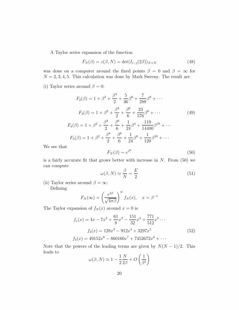
A Taylor series expansion of the function

FN(β) = z(β,N) = det(Ii−j(2β))N×N (48)

was done on a computer around the fixed points β = 0 and β = ∞ forN = 2, 3, 4, 5. This calculation was done by Mark Sweeny. The result are

(i) Taylor series around β = 0:

F2(β) = 1 + β2 +β4

2+

5

36β6 +

7

288β8 + · · ·

F3(β) = 1 + β2 +β4

2+

β6

6+

23

576β8 + · · · (49)

F4(β) = 1 + β2 +β4

2+

β6

6+

1

24β4 +

119

14400β10 + · · ·

F5(β) = 1 + β2 +β4

2+

β6

6+

1

24β8 +

1

120β10 + · · ·

We see thatFN (β) ∼ eβ

2

(50)

is a fairly accurate fit that grows better with increase in N . From (50) wecan compute

ω(β,N) ≃ β

N=

E

2(51)

(ii) Taylor series around β = ∞:Defining

FN (∞) =

(

e2β√4πβ

)N

fN(x), x = β−1

The Taylor expansion of fN(x) around x = 0 is

fx(x) = 4x− 7x2 +61

8x3 − 151

32x4 +

771

512x5 · · ·

f3(x) = 128x3 − 912x4 + 3297x5 (52)

f4(x) = 49152x6 − 860160x7 + 7452672x8 + · · ·Note that the powers of the leading terms are given by N(N − 1)/2. Thisleads to

ω(β,N) ≃ 1− 1

2

N

2β+O

(

1

β2

)

20

∼= 1− 1

2E, β ≫ 1 (53)

The small corrections are computable from (52). We note that this result isalso inferred from the exponential factor that scales z in (33). We do notknow a simple explanation for the linear fit in (51).

We see that the finite N results (51) and (53) near the fixed points exactlymatch the corresponding expressions (28) computed in the thermodynamiclimit of N → ∞.

VIII. Conclusion and Discussion

The analytic computation done in the large N limit holding E = 2β/Nfixed is in very good agreement with the computation for finite N , espe-cially near the fixed points and it is important to emphasize this agreementin the critical region which is the physically relevant one. The differenceis that while the computation for finite N involves analytic interpolationbetween weak and strong coupling the thermodynamic computation showsnon-analytic behavior at E = 1. Certainly this non-analyticity is a pathologyof the N = ∞ limit. We do not know whether the qualitative agreement ofthe two methods and even the anomaly at E = 1, is a feature of the theory inhigher dimensions which is vastly more complicated. It is desirable to expressthe summation of the planar diagrams in higher dimensions as a coupled setof integral equations in the mean field approximation.

We end with a final comment that the expression of the partition functionas a determinant implies that this theory has a fermionic representation.

Acknowledgement

I wish to thank Professor Yoichiro Nambu and Professor Leo Kadanofffor useful discussions and suggestions. I have also had some useful discus-sions with Nino Bralic, Tohru Eguchi, Mark Sweeny, Jorge Jose and DonWeingarten.

21

References

[1] See, for example: a) W.A. Bardeen, B.W. Lee and R.E. Schrock, Phys.Rev. D14, 985 (1976); b) E. Brezin, J.C. Le Guillou and J. Zinn-Justinin “Phase Transitions and Critical Phenomena”, Vol. 6, Edited by C.Domb and M.S. Green; c) S.K. Ma’s article in the same volume.

[2] G. ‘t Hooft, Nucl. Phys. B72, 461 (1974).G. ‘t Hooft, Nucl. Phys. B75, 461 (1975).

[3] E. Witten Havard Preprints HUTP-79/A007 and HUTP/79/A014.

[4] E. Brezin, C. Itzykson, G. Parisi and J.B. Zuber, Commun. Math.Phys. 59, 35 (1978).

[5] K.G. Wilson, Phys. Rev. D10, 2245 (1974); Erice Lecture notes 1975.

[6] J.M. Drouffe and C. Itzykson, Physics Reports 38C, No. 3 (1978).

[7] Integration over matrices has been extensively discussed in NuclearPhysics. See, e.g., F.J. Dyson, J. Math. Phys. 3, (1962) reprinted in‘Statistical Theories of Spectra: Fluctuations’ C. Porter (AcademicPress, 1965); ‘Random Matrices’, M.L. Mehta (Academic Press, 1967).

[8] ‘Singular Integral Equations’, N.I. Muskhelishvili (P. Noordhoof N.V.- Groningen - Holland).

[9] Suggested by L. Kadanoff.

[10] See, e.g., K.G. Wilson and J. Kogut, Phys. Reports 12C (1974). L.P.Kadanoff, Rev. Mod. Phys. 49, (1977).

[11] After this work was well begun we received a preprint on U(N) latticegauge theories by I. Bars and F. Green (IAS preprint) which also con-tains formula (40). In our notation they have computed the determinant

for small E =2β

N. We remark that in this limit the determinant can

be exactly computed using the classical theorem of Szego on Toeplitzdeterminant: For large N , fixed β

log det Ii−j(2β) ∼ Ng0 +∞∑

n=1

ngng−n = β2

22

gn =∫ 2π

0

dθ

2πeinθ log(e2β cos θ)

(See McCoy and Wu, ‘The Two Dimensional Ising Model [HardvardUniv. Press], for an extensive discussion).Other recent papers that discuss U(N) lattice theories: T. Eguchi(Chicago preprint EFI 79/22); D. Weingarten (Indiana preprint).

[12] I thank Mark Sweeny for responding with interest to do the computercalculation.

[13] While this work was going on and after the solutions of the integralequations were obtained we learnt of a similar work by D. J. Gross andE. Witten (Princeton preprint)

23