Supersymmetry breaking in two dimensions: The lattice N=1 Wess-Zumino model

arX

iv:h

ep-la

t/040

2007

v1 9

Feb

200

4

IFUP-TH 2004/09, UPRF-2004-02

Supersymmetry breaking in two dimensions:

the lattice N = 1 Wess-Zumino model

Matteo Beccaria∗

INFN, Sezione di Lecce, and Dipartimento di Fisica dell’Universita di Lecce,

Via Arnesano, ex Collegio Fiorini, I-73100 Lecce, Italy

Massimo Campostrini†

INFN, Sezione di Pisa, and Dipartimento di Fisica “Enrico Fermi” dell’Universita di Pisa,

Via Buonarroti 2, I-56125 Pisa, Italy

Alessandra Feo‡

Dipartimento di Fisica, Universita di Parma and INFN Gruppo Collegato di Parma,

Parco Area delle Scienze, 7/A, 43100 Parma, Italy

(Dated: February 9, 2004)

Abstract

We study dynamical supersymmetry breaking by non perturbative lattice techniques in a class of

two-dimensional N = 1 Wess-Zumino models. We work in the Hamiltonian formalism and analyze

the phase diagram by analytical strong-coupling expansions and explicit numerical simulations

with Green Function Monte Carlo methods.

PACS numbers: 12.60.Jv, 02.70.Ss

∗Electronic address: [email protected]†Electronic address: [email protected]‡Electronic address: [email protected]

1

http://arXiv.org/abs/hep-lat/0402007v1

I. INTRODUCTION

Supersymmetry (SUSY) is playing an increasingly relevant and unifying role in high

energy physics. From a purely theoretical point of view, SUSY is required for consistency

and finiteness in superstring theory; compactification and SUSY breaking mechanisms are

then needed in order to produce a low energy four-dimensional effective action with a residual

N = 1 SUSY. This constraint comes from the phenomenological side where the most popular

current extensions of the Standard Model are actually based on SUSY for at least two

reasons. First, supersymmetric Grand Unification theories are quite successful in predicting

SU(3) × SU(2) × U(1) gauge couplings unification [1], a fact that can be considered as the

main phenomenological motivation for SUSY [2]. Moreover, supersymmetric models solve

in a natural way the hierarchy problem [3] of matching the electroweak and GUT scales

without being spoiled by huge radiative corrections to Higgs masses.

However, many features of this scenario still need some clarification. Indeed, N = 1

SUSY is expected to be exact at the GUT scale around 1016 GeV, but must be broken in

the TeV region in order to account for the asymmetric mass textures that are currently

observed. In particular, this will be true if some superpartner with a mass of a few TeV will

be observed in the future LHC or Linear Collider experiments. In the model independent

analysis, the source of breaking is usually parametrized by a complete set of soft terms whose

origin remains however rather unexplained.

In several approaches, it is due to some kind of spontaneous breaking of SUSY in a

hidden sector and communicated to the MSSM particles producing the soft terms. As with

every dynamical symmetry breaking, non-perturbative techniques must be exploited and

the lattice regularization and renormalization programme is of course one of the main lines

of research. Indeed, the simultaneous introduction of infrared and ultraviolet cutoffs allows

for calculations, like strong-coupling expansions, that are quite complementary to the usual

weak-coupling perturbative analysis.

Beside this, when any known analytical treatment fails, lattice models can also be studied

by direct simulations that can provide, in principle, accurate numerical measurements.

In this paper, we address the problem of spontaneous supersymmetry breaking (S3B)

in a simple, but interesting, theoretical laboratory that is the class of Wess-Zumino (WZ)

two-dimensional models of chiral superfields with no vector multiplets. Preliminary results

2

on this subject can be found in [4]. Related studies of the two dimensional Wess-Zumino

model can be found in [5].

Despite their simplicity, these systems are nontrivial because in two dimensions super-

symmetry is not strong enough to predict the exact pattern of breaking, a situation that

must be compared with the four dimensional case where WZ models are expected to break

supersymmetry if and only if they do at tree level.

Unfortunately, as we shall discuss, lattice strong-coupling expansions provide useful in-

sights, but are unable to reliably predict the physics of the continuum theory and one must

resort to a numerical analysis.

Since S3B is closely related to the symmetry properties of the ground state, it appears to

be quite reasonable to adopt some kind of Hamiltonian formulation. Moreover, we will see

in the following that, if we wish to preserve a SUSY subalgebra, a conserved Hamiltonian

is crucial. However, the traditional algorithms for simulation of lattice field theories are

based on the Lagrangian formulation [6]. The main reason is the immediate probabilistic

interpretation of the partition function, at least for bosonic systems not suffering from a

sign or phase problem; this leads to a host of Monte Carlo algorithms, some of which are

extremely efficient. Of course, alternatives based on a more direct Hamiltonian formalism

do exist [7], but they are certainly less exploited in high energy physics where emphasis is

on Lagrangian symmetries, in particular Poincare invariance.

On the other hand, Hamiltonian methods has been used in Supersymmetric Discretized

Light-Cone Quantization (SDLCQ) [8] and also are widely exploited in non relativistic con-

texts [9] where the properties of the ground state are typically the simplest and first object

of investigation. Moreover, these techniques interlace the brute force numerical calculations

with analytical or physical insights about the structure of the ground state wave function,

a feature that is quite welcome in the study of S3B where we expect major changes to show

up at the phase transition.

Another important feature of our study concerns the fact that fermions, needed in su-

persymmetric models, are the major source of complications in the current approaches to

lattice simulations. In the Lagrangian approach quantum expectation values are computed

by summing over histories of the classical fields, following Feynman’s ideas. In the case of

fermions, these are Grassmann valued classical fields that cannot be analyzed by direct nu-

merical methods. The typical solution amounts to integrate them out and study the resulting

3

non-local bosonic model [10]. This can be nontrivial for a generic model and a recent de-

tailed account of this problem and whether it can be formulate successfully supersymmetric

theories on the lattice can be found in [11].

Instead, in the Hamiltonian approach, what is relevant is the algebra of the fields and

their conjugate momenta. From this point of view, fermions and bosons differ just by the

replacement of commutators by anticommutators and also by the structure of the state space,

finite dimensional for fermions in finite volume, infinite dimensional in the bosonic case.

Apparently, in the Hamiltonian approach, there is much more symmetry in the treatment

of fermions and bosons than in the Lagrangian approach.

Looking at the details of the simulation techniques, however, problems arise with Hamil-

tonian fermions due to the well known hard sign problem [12]. Roughly speaking, fermion

exchanges introduce problematic and unavoidable signs that often break in a substantial way

the probabilistic interpretation of quantum expectation values required to build a numerical

stochastic algorithm. This deep problem is somewhat milder in 1 + 1 dimensions where

specific equivalences between fermionic and bosonic fields can be established [13]. Also, the

topology of fermion dynamics is the simplest possible and helps in taming the sign prob-

lem. Actually, for several fermion models in 1 + 1 dimensions arising in Solid State theory,

like, e.g., Hubbard-like models, algorithms can be devised with no sign problem and good

efficiency as well as scaling properties [15].

The detailed plan of the paper is the following: in Sec. (II) we present the model and its

lattice Hamiltonian; in Sec. (III) we compute the first nontrivial order of the strong-coupling

expansion of the ground state energy; in Sec. (IV) we discuss the Renormalization Group

trajectories along which a continuum limit can be reached. In Sec. (V) we describe a Green

Function Monte Carlo algorithm. Finally, Sec. (VI) is devoted to present our numerical

results.

II. THE N = 1 WESS-ZUMINO MODEL IN 1 + 1 DIMENSIONS

A. Definition of the model and patterns of SUSY breaking

Let us consider the most general SUSY algebra in two dimensions. The generators are

split into fermionic and bosonic ones. The algebra with N left-handed fermionic generators

4

QALA=1,...,N and N right-handed fermionic generators QA

RA=1,...,N is denoted by (N, N).

The bosonic generators are the components of the two-momentum (P 0, P 1) and a set of

central charges TAB. The non trivial part of the algebra is

QAL , Q

BL = δAB(P 0 − P 1),

QAR, Q

BR = δAB(P 0 + P 1),

QAL , Q

BR = TAB.

In the left-right symmetric case with (N, N) = (1, 1), we denote

Q1,2 ≡ Q1R ±Q1

L, (2.1)

and find

Qa, Qb = 2(H 1 + Pσ1 + Tσ3)ab, (2.2)

where σi are the Pauli matrices, (P 0, P 1) ≡ (H,P ) and T ≡ T 11. The minimal realization

of this algebra requires a single real chiral multiplet with a real scalar component ϕ and a

Majorana fermion with components ψ1,2. The explicit form of the supercharges is

Q1,2 =∫dx

[p(x)ψ1,2(x) −

(∂ϕ

∂x± V (ϕ(x))

)ψ2,1(x)

], (2.3)

where p(x) is the momentum operator conjugate to ϕ(x). The central charge corresponds

to a topological quantum number [16]

T =∫dx∂ϕ

∂xV (ϕ). (2.4)

As usual with supersymmetric models, the structure of the Hamiltonian H guarantees that

the energy eigenstates have E ≥ 0 because

H =1

2(Q2

1 +Q22). (2.5)

Invariant states annihilated by both Qi coincide with the zero energy states and are thus

supersymmetric ground states; they must lie in the topologically trivial sector.

The problem of predicting the pattern of S3B is not easy. In principle, the form of

V (ϕ) is enough to determine whether supersymmetry is broken or not. At least at tree

level, one easily proves that supersymmetry is broken if and only if V has no zeros. In

two dimensions, however, these conclusion is generally false due to radiative corrections.

5

An analytic non-perturbative tool that can help in the analysis is the Witten index defined

as [23]

I = Tr(−1)F , (2.6)

where F is the fermion number. Since supersymmetry is not explicitly broken, contributions

from positive-energy bosonic and fermionic states cancel and

I = nBE=0 − nF

E=0. (2.7)

In finite volume, I is invariant under changes in V (ϕ) that do not modify its asymptotic

behaviour. In particular, it can be computed at weak coupling where each zero of V (ϕ) is

associated to a perturbative zero energy state. Thus, if V (ϕ) has an odd number of zeroes,

we find I 6= 0 and supersymmetry is unbroken. If, on the other hand, V (ϕ) has an even

number of zeroes, the associated perturbative vacua can contribute I with opposite signs

and, when I = 0, we cannot say anything. In particular, a nontrivial set of perturbative zero

energy states with I = 0 can receive instanton corrections due to tunneling lifting them to

positive energies breaking supersymmetry while leaving I = 0. In such cases, the behaviour

of the tunneling rate with increasing volume is crucial in answering the question of breaking.

An interesting example of this complicated scenario is discussed in Appendix A of Ref.

[23]. We quickly review the analysis since it will be important in the interpretation of our

results. When V (ϕ) = λ(ϕ2 + a2), the action of the WZ model is

S =∫d2x

(1

2(∂ϕ)2 +

i

2ψγ · ∂ψ − 1

2λ2(ϕ2 + a2)2 − 1

2λϕψψ

). (2.8)

For large positive a2 the index is zero because there are no zero-energy states. Due to a

special conjugation symmetry valid for this model in finite volume, the pattern of breaking is

invariant under a2 → −a2. This means that for negative a2, the two zeroes of V are bosonic

and fermionic and (finite volume) tunneling lifts their energy to a positive value. However,

in infinite volume and large negative a2, the narrow minimum of the potential is protected

from radiative corrections and generates an expectation value 〈ϕ〉 6= 0 signaling the SSB of

the Z2 symmmetry ϕ → −ϕ, ψ → γ5ψ. The fermion becomes massive and supersymmetry

must be unbroken due to the absence of a massless Goldstino.

The above discussion illustrates that an alternative non-perturbative analysis of the mod-

els with I = 0 is certainly welcome. In the following, we shall put the model on a space-time

lattice in order to exploit explicit numerical simulations as well as analytical strong-coupling

expansions.

6

B. Lattice Version of the Model

On the lattice it is impossible to maintain the full SUSY algebra and it is important to

understand what can be said by looking at subalgebras. If we consider one supercharge only,

for instance Q1, and find a state with Q1|s〉 = 0, we cannot say that it is a zero energy state

unless we know that it is in the T = 0 sector. On the other hand, if no states with Q1|s〉 = 0

are found in any topological sector, then supersymmetry is certainly broken.

Thus, even if we forget Q2, we can choose as a clear-cut signal of supersymmetry dynam-

ically breaking the lowest eigenvalue of the operator Q21: if it is positive, we have breaking.

The SUSY algebra (2.2) involves explicitely the generators of space and time infinitesimal

translations and is spoiled on the lattice. In the Lagrangian approach, both space and time

are discrete and SUSY is completely broken. In the Hamiltonian formulation, time remains

continuous and the D = 2 algebra is reduced to D = 1 and not totally lost. The full

two-dimensional algebra as well as Lorentz invariance are expected to be recovered in the

continuum limit.

A lattice version of the above model has been previously studied in Refs. [17, 18]. A

similar approach to Wess-Zumino models with N = 2 supersymmetry is discussed in Ref.

[19], and numerical investigations are reported in Ref. [20]. On each site of a spatial lattice

with L sites, we define a real scalar field ϕn together with its conjugate momentum pn such

that [pn, ϕm] = −iδn,m. The associated fermion is a Majorana fermion ψa,n with a = 1, 2

and ψa,n, ψb,m = δa,bδn,m , ψ†a,n = ψa,n. The fermionic charge

Q =L∑

n=1

[pnψ1,n −

(ϕn+1 − ϕn−1

2+ V (ϕn)

)ψ2,n

],

with arbitrary real function V (ϕ), (called prepotential in the following) can be used to define

a semi-positive definite lattice Hamiltonian

H = Q2. (2.9)

This Hamiltonian includes the central charge contribution in the form of a term

∑

n

V (ϕn)ϕn+1 − ϕn−1

2, (2.10)

that is precisely a discretization of T . Eigenstates of H are divided into invariant Q-singlets

with zero energy and Q-doublets with degenerate positive energy. H describes an interacting

7

model, symmetric with respect to Q and this symmetry is respected by the spectrum if and

only if the ground state energy is positive. We stress again that Q symmetry breaking

implies breaking of the full 2 dimensional supersymmetry, whereas Q symmetry does not

imply (in a generic topological sector) 2D SUSY.

We remind that, on the lattice, spontaneous supersymmetry breaking can occur even for

finite lattice size L, because tunneling among degenerate vacua connected by Q is forbidden

by fermion number conservation.

To write H in a more familiar form, we follow Ref. [18] and replace the two Majorana

fermion operators with a single Dirac operator χ satisfying canonical anticommutation rules,

i.e., χn, χm = 0, χn, χ†m = δn,m:

ψ1,n =(−1)n − i

2in(χ†

n + iχn), ψ2,n =(−1)n + i

2in(χ†

n − iχn). (2.11)

The Hamiltonian takes then the form

H = HB(p, ϕ) +HF (χ, χ†, ϕ)

=∑

n

1

2p2

n +1

2

(ϕn+1 − ϕn−1

2+ V (ϕn)

)2

−1

2(χ†

nχn+1 + h.c.) + (−1)nV ′(ϕn)(χ†

nχn − 1

2

)(2.12)

and describes canonical bosonic and fermionic fields with standard kinetic energies and a

Yukawa coupling.

This Hamiltonian conserves the total fermion number

Nf =∑

n

χ†nχn, (2.13)

and can be examined in each sector with definite Nf separately. For reasons that will be

understood later, we shall also consider open boundary conditions and restrict the lattice

size L to be even. These are constraints that do not affect the physics of the model in the

continuum, but will be very welcome by the algorithm we are going to apply.

The simplest way to analyze the pattern of supersymmetry breaking for a given V (ϕ) is

to compute the ground state energy E0. As we mentioned, on the lattice, we can perform

such a computation in a non-perturbative way by strong coupling or numerical simulations.

However, before discussing these items, we want to stress some identities that can be used

together with E0 to get information on the symmetry of the ground state.

8

C. Lattice Ward identities

If the vacuum |0〉 is supersymmetric, Q|0〉 = 0 and for each operator X we have

〈0|Q,X|0〉 = 0. (2.14)

In particular, taking

X =∑

n

F (ϕn)ψ2,n, (2.15)

we obtain

〈0|∑

n

F (ϕn)

[ϕn+1 − ϕn−1

2+ V (ϕn)

]+ F ′(ϕn)(−1)n(χ†

nχn − 1/2)|0〉 = 0. (2.16)

A basis of Ward Identities is thus obtained by considering F (ϕ) = ϕn. For instance, on

an even lattice with open boundary conditions we find for n = 1 the relation

〈0|∑

n

ϕnV (ϕn) + (−1)nχ†

nχn

|0〉 = 0. (2.17)

The case F (ϕ) = constant is also interesting. It leads to

〈0|∑

n

V (ϕn)|0〉 = 0. (2.18)

III. STRONG COUPLING ANALYSIS OF SUSY BREAKING

Let us start from the supersymmetry charge

Q =∑

l

[plψ

1l − V (ϕl)ψ

2l −

ϕl+1 − ϕl−1

2ψ2

l

],

Following Ref. [19], we define the strong-coupling limit by

V (ϕ) −→λ→∞

λV (0)(λϕ),

perform the canonical transformation

ϕ(0) = λϕ, p(0) =1

λp,

and rescale the energies by λ2; dropping the index (0) from ϕ and p, the result is

Q =∑

l

[plψ

1l − V (ϕl)ψ

2l −

(ϕl+1 − ϕl−1)ψ2l

2λ2

]≡ Q(0) +

Q(2)

λ2,

H = Q2 =1

2

∑

l

[p2

l + V 2(ϕl) + 2iV ′(ϕl)ψ1l ψ

2l

+(ϕl+1 − ϕl−1)V (ϕl) + iψ1

l+1ψ2l + iψ2

l+1ψ1l

λ2+

(ϕl+1 − ϕl−1)2

4λ4

]≡ H(0) +

H(2)

λ2+H(4)

λ4.

9

Introducing the Dirac fields χl, χ†l [18], cf. Eq. (2.11), we obtain

H(0) =∑

l

[1

2p2

l +1

2V 2(ϕl) + (−1)lV ′(ϕl)(χ

†lχl − 1/2)

]=

=∑

l

[1

2p2

l +1

2V 2(ϕl) +

1

2(−1)l+nlV ′(ϕl)

]

H(2) =1

2

∑

l

V (ϕl)(ϕl+1 − ϕl−1) −1

2

∑

l

(χ†lχl+1 + h.c.)

H(4) =1

8

∑

l

(ϕl+1 − ϕl−1)2

where we denote by nl = 0, 1 the eigenvalue of χ†lχl.

A. Leading order

To leading order in 1/λ, the Hamiltonian is factorized in a supersymmetric quantum me-

chanics for each site; adopting an explicit representation, we can write the one-site Hamil-

tonian as

H =1

2

[− d2

dx2+ V 2(x) + σ3V

′(x)

](3.1)

(in the occupation number representation the basis chosen now is (n=0, n=1) for odd sites

and (n=1, n=0) for even sites). This Hamiltonian has a N = 2 supersymmetry [21]:

Qi, Qj = δijH, Q1 = 12[σ1p+ σ2V (x)] , Q2 = 1

2[σ2p− σ1V (x)] . (3.2)

The conditions for a supersymmetric ground state Qiψ0 = 0 reduce to

ψ′0(x) = σ3V (x)ψ0(x). (3.3)

For polynomial V , supersymmetry is unbroken if and only if it is possible to find a normal-

izable solution to Eq. (3.3), which happens if the degree q of V is odd [21].

We can write the time-independent Schrodinger equation as

ψ′′ +(2E − V 2(x) ∓ V ′(x)

)ψ = 0;

denoting the eigenfunctions for the two signs by ψ±m and their energies by ε±m, we have

ψ±m

′′+(2ε±m − V 2(x) ∓ V ′(x)

)ψ±

m = 0. (3.4)

Supersymmetry implies that, for E 6= 0, states are paired in boson-fermion doublets.

10

−2 −1 0 1 2λ0

10−4

10−3

10−2

10−1

100

101

ε0

η0

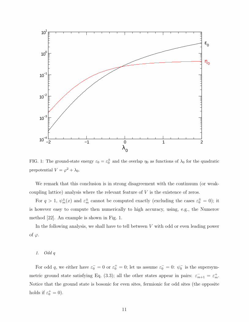
FIG. 1: The ground-state energy ε0 = ε±0 and the overlap η0 as functions of λ0 for the quadratic

prepotential V = ϕ2 + λ0.

We remark that this conclusion is in strong disagreement with the continuum (or weak-

coupling lattice) analysis where the relevant feature of V is the existence of zeros.

For q > 1, ψ±m(x) and ε±m cannot be computed exactly (excluding the cases ε±0 = 0); it

is however easy to compute then numerically to high accuracy, using, e.g., the Numerov

method [22]. An example is shown in Fig. 1.

In the following analysis, we shall have to tell between V with odd or even leading power

of ϕ.

1. Odd q

For odd q, we either have ε−0 = 0 or ε+0 = 0; let us assume ε−0 = 0: ψ−

0 is the supersym-

metric ground state satisfying Eq. (3.3); all the other states appear in pairs: ε−m+1 = ε+m.

Notice that the ground state is bosonic for even sites, fermionic for odd sites (the opposite

holds if ε+0 = 0).

11

A strong argument against supersymmetry breaking is given by the Witten index

IW ≡ Tr(−1)Nf [23]; in the strong-coupling limit, we clearly have IW = ±1; since IW 6= 0

implies unbroken SUSY, and IW is invariant under regular perturbations (cf. Sect. IIIA 3),

supersymmetry can never be broken for odd q, not even in the L→ ∞ limit.

A simple check of this result can be given explicitely when V is linear and is discussed in

details in App. (A).

2. Even q

For even q, we have ε+m = ε−m; for m = 0, this corresponds to a degenerate ground state

with broken supersymmetry (ε±0 = ε0 > 0). The phases of the normalized states |ψ±n 〉 can

be chosen in order to satisfy

√2εn|ψ−

n 〉 = [−ip + V (ϕ)] |ψ+n 〉, (3.5)

√2εn|ψ+

n 〉 = [ip+ V (ϕ)] |ψ−n 〉; (3.6)

Introducing the notation

〈O〉± = 〈ψ±0 |O|ψ±

0 〉,

〈ψ+0 |ψ−

0 〉 = η0,

we can prove the important relations

〈V 〉± =√

2ε0 η0, (3.7)

〈ϕ〉− − 〈ϕ〉+ = frac1√

2ε0 η0. (3.8)

η0 can be computed numerically from ψ±0 (ϕ), cf. Fig. 1. The proof of Eq. (3.7) is very simple:

just take the scalar product of Eq. (3.5) with 〈ψ+0 | and of Eq. (3.5) with 〈ψ−

0 |, and observe

that 〈p〉± = 0. The proof of Eq. (3.8) is also immediate:

√2ε0 〈ψ+

0 |ϕ|ψ+0 〉 = 〈ψ+

0 |ϕ(ip+ V )|ψ−0 〉 = 〈ψ+

0 |(ip+ V )ϕ|ψ−0 〉 + 〈ψ+

0 |i[ϕ, p]|ψ−0 〉 =

√2ε0 〈ψ−

0 |ϕ|ψ−0 〉 − 〈ψ+

0 |ψ−0 〉,

Several simplifications can be exploited when V (ϕ) is even. For an asymptotically positive

12

summing the two equations

√2(√εn(−1)n +

√εm(−1)m)〈ψn|ϕ|ψm〉 = 〈ψni[ϕ, p]I|ψm〉 = −〈ψn|I|ψm〉

and (exploiting parity)

〈ψ±n |ϕ|ψ±

m〉 = ∓ 1√2

1√εn + (−1)n+m

√εm

〈ψ∓n |ψ±

m〉 (3.14)

Of course, for n = m = 0, Eqs. (3.11), (3.14) agree with the previous general results.

3. On the convergence of the perturbative expansion

The Rayleigh-Schrodinger perturbation theory of a Hamiltonian of the form H = H0 +

βH1 is regular (i.e., it has a finite radius of convergence in β) if [24]

‖H1Ψ‖ ≤ a‖H0Ψ‖ + b‖Ψ‖ (3.15)

uniformly for all state vectors Ψ; in our case, Eq. (3.15) clearly holds, for both H(2) and

H(4), except for the trivial cases q ≤ 1.

B. First order

At first order (subleading) in the strong-coupling expansion we consider again the two

cases of even or odd q.

1. Odd q

In the case of unbroken supersymmetry (odd q), the subleading correction to the ground-

state energy in the strong-coupling expansion is zero: the fermionic contribution iψ1l+1ψ

2l +

iψ2l+1ψ

1l has clearly zero diagonal matrix elements, and the bosonic contribution ϕl+1V (ϕl)−

ϕlV (ϕl+1) is zero because it factorizes into 〈ϕ〉〈V 〉 − 〈ϕ〉〈V 〉; strictly speaking, this is true

for periodic and free boundary conditions, but it could be false, e.g., for fixed boundary

conditions.

14

2. Even q

Due to the structure of the Hamiltonian, it is convenient to describe states in the mixed

form∑

n1,...,nL

ψn1,...,nL(ϕ1, . . . , ϕL)|n1, . . . , nL〉 (3.16)

where ψn1,...,nL(ϕ1, . . . , ϕL) is a wave function depending on the bosonic degrees of free-

dom and |n1, . . . , nL〉 is the fermionic component of the state defined in terms of the state

annihilated by all χ

χi|0〉 = 0, (3.17)

according to the canonical ordering of the Fermi operators:

|n1, . . . , nL〉 = (χ†1)

n1 · · · (χ†L)nL |0〉. (3.18)

Of course ni = 0, 1 and |n1, . . . , nL〉 describes a state with ni fermions at site i. In the case

of broken supersymmetry (even q), the subspace B of lowest leading-order energy is spanned

by the states

|n〉 = ψσ1

0 (ϕ1) · · ·ψσL0 (ϕL) |n1, . . . , nL〉, (3.19)

where σl = (−1)l+nl and ψ±10 ≡ ψ±

0 . We have adopted open boundary conditions, corre-

sponding in our notations to setting ϕ0 = ϕL+1 = 0 and ψa0 = ψa

L+1 = 0 (and therefore

χ0 = χL+1 = 0).

Since the number of fermions∑

l nl is conserved, we can impose an additional constraint

on B and define

BN = |n〉,∑

l

nl = N, B = B0 ⊕ . . .⊕ BL.

We will now prove that, for even L, the ground state is doubly degenerate and lies in the

sectors with N = L/2, L/2 − 1.

At first order, we have to diagonalize the operator H(2) over BN . Let us split

H(2) = H(2)B +H

(2)F (3.20)

H(2)B =

1

2

L∑

l=1

V (ϕl)(ϕl+1 − ϕl−1) (3.21)

H(2)F = −1

2

L∑

l=1

(χ†lχl+1 + χ†

l+1χl) (3.22)

15

Since

〈n′|H(2)B |n〉 =

1

2

√2ε0 η0 δn,n′

∑

l

(〈ϕl+1〉 − 〈ϕl−1〉) (3.23)

we have

〈n′|H(2)B |n〉 = −1

4η2

0δn,n′ [(−1)n1 + (−1)nL] (3.24)

where we have exploited

〈ϕl〉 = −(−1)l+nlη0√2ε0

, (3.25)

that holds for even V . Since n = 0, 1 we can use (−1)n = 1 − 2n and write

〈n′|H(2)B |n〉 =

1

2η2

0δn,n′ (−1 + n1 + nL) (3.26)

The matrix elements of H(2)F are

〈n′|H(2)F |n〉 = −1

2η2

0 hn,n′ (3.27)

where hn,n′ = 1 if n and n′ are connected by H(2)F (i.e. a hopping of one fermion) and 0

otherwise.

Thus, we can hide the bosonic wave functions and write an effective perturbation acting

on purely fermionic states as

H(2)eff =

η20

2

L∑

i,j=1

χ†iMijχj − 1

(3.28)

where 1 is the identity operator and

Mij =

−1 |i− j| = 1

1 i = j = 1 or L

0 otherwise

(3.29)

Since H(2)eff is quadratic, it is convenient to change operator basis. Let v

(p)i be the p-th

eigenvector of M with eigenvalue λ(p):

v(p)n =

√2 − δp,L

Lsin

[pπ

L

(n− 1

2

)](3.30)

λ(p) = −2 cospπ

L(3.31)

They define a (real) unitary matrix

L∑

p=1

v(p)i v

(p)j = δij ,

L∑

i=1

v(p)i v

(q)i = δpq

16

We can replace the operators χi by the operators ai defined by

χi =L∑

p=1

v(p)i ap, ap =

L∑

i=1

v(p)i χi

with

ap, a†q = δpq

The new form of H(2)eff is

H(2)eff =

η20

2

L∑

p=1

λ(p)a†pap − 1

(3.32)

The eigenvalues λ(1), . . . , λ(L/2−1) are negative and λ(L/2) = 0; there are thus two degenerate

ground states with L/2 − 1 and L/2 fermions. This is required by supersymmetry: since

H(2) restricted to B commutes with Q(0), all the states must be paired in doublets with N

differing by 1. The ground state with L/2 fermions is

|Ψ(1)0 〉 = ψσ1

0 (ϕ1) · · ·ψσL0 (ϕL) a†1 · · ·a†L/2|0 > (3.33)

To conclude, the shift of the ground state energy due to the perturbation is

E1 =η2

0

2

−1 − 2

L/2∑

n=1

cosπn

L

= −η

20

2cot

π

2L(3.34)

In the L→ ∞ limit we haveE1

L= −η

20

π+ O(1/L) (3.35)

In summary, the first order perturbation in the strong-coupling expansion removes the large

degeneracy of the ground state and determines a doublet of eigenstates with L/2 − 1 and

L/2 fermions with minimum energy

E

L= ε0 −

1

λ2

η20

π+ O

(1

λ2L,

1

λ4

)(3.36)

A similar calculation at first order for 〈ϕk〉 and 〈ϕkϕl〉c is discussed in App. (B). The second-

order correction to the ground state energy can also be computed with a reasonable effort

and the result is described in App. (C). However, we remark that the results drawn from

the first order corrections are not qualitatively changed.

17

C. Discussion

From the analysis of the strong-coupling expansion of the model we can draw the following

conclusion. For polynomial V (ϕ), the relevant parameter is just its degree q.

For odd q, the strong coupling analysis and the tree-level results agree and supersymmetry

is expected to be unbroken. This conclusion gains further support from the nonvanishing

value of the Witten index at strong coupling.

For even q, in strong coupling, the ground state (at least in the sector with half filling)

has a positive energy density also for L → ∞ and supersymmetry appears to be broken.

Of course, this can be in disagreement with weak coupling. A specific case that we shall

analyze numerically in great detail is

V (ϕ) = λ2ϕ2 + λ0. (3.37)

For λ0 < 0, weak coupling predicts unbroken SUSY, whereas the strong coupling prediction

gives broken SUSY for all λ0. For this specific model, as we already discussed, the strong

coupling analysis agrees with Ref. [23] in the sense that it reproduces the continuum physics

in finite volume.

For large expansion parameter, the strong coupling results can be compared with explicit

simulations (that we shall fully discuss in Sec. V). Let us consider for instance the quadratic

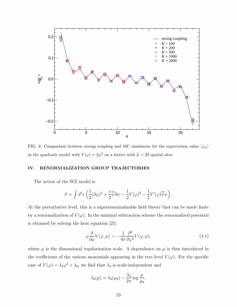
model with λ0 = 0 on a lattice with L = 22 spatial sites. In Fig. 2, we show the expectation

value 〈ϕn〉 computed at λ2 = 2. The agreement is quite good apart from the points on

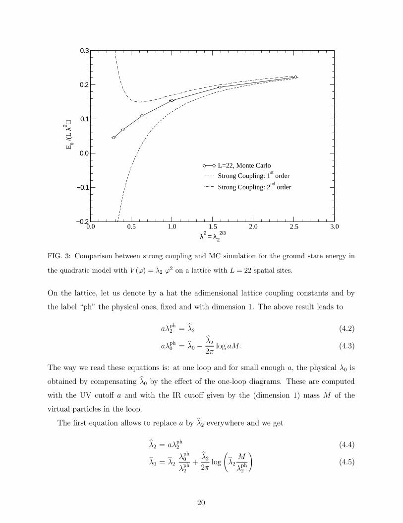
the border where the convergence seems to be slower. To check the validity of the strong

coupling expansion at smaller couplings, we show in Fig. 3 the ground state energy from

MC simulation compared with the first and second order strong coupling expansion. The

scaled variables on the plot axes are discussed in App. (C). The second order gives better

results at large values of the expansion parameter, but is unreliable below λ2 ≃ 0.35.

In the next Section, we shall see that the continuum limit is in the region of small λ2.

Thus, for even q, it seems difficult to gain additional insight from strong coupling and some

kind of transition can happen as the continuum limit is reached. For this reason, a full

simulation of the model appears to be the only way to answer the question of symmetry

breaking.

18

0 5 10 15 20n

−0.2

−0.1

0.0

0.1

0.2<φ

n>strong couplingK = 100K = 200K = 500K = 1000K = 2000

FIG. 2: Comparison between strong coupling and MC simulation for the expectation value 〈ϕn〉

in the quadratic model with V (ϕ) = 2ϕ2 on a lattice with L = 22 spatial sites.

IV. RENORMALIZATION GROUP TRAJECTORIES

The action of the WZ model is

S =∫d2x

(1

2(∂ϕ)2 +

i

2ψ∂ψ − 1

2V (ϕ)2 − 1

2V ′(ϕ)ψψ

).

At the perturbative level, this is a superrenormalizable field theory that can be made finite

by a renormalization of V (ϕ). In the minimal subtraction scheme the renormalized potential

is obtained by solving the heat equation [25]

µ∂

∂µV (ϕ, µ) = − 1

4π

∂2

∂ϕ2V (ϕ, µ), (4.1)

where µ is the dimensional regularization scale. A dependence on µ is thus introduced in

the coefficients of the various monomials appearing in the tree level V (ϕ). For the specific

case of V (ϕ) = λ2ϕ2 + λ0, we find that λ2 is scale-independent and

λ0(µ) = λ0(µ0) −λ2

2πlog

µ

µ0.

19

0.0 0.5 1.0 1.5 2.0 2.5 3.0

λ2 = λ22/3

−0.2

−0.1

0.0

0.1

0.2

0.3

E0 /(

L λ2 )

L=22, Monte Carlo

Strong Coupling: 1st order

Strong Coupling: 2nd

order

FIG. 3: Comparison between strong coupling and MC simulation for the ground state energy in

the quadratic model with V (ϕ) = λ2 ϕ2 on a lattice with L = 22 spatial sites.

On the lattice, let us denote by a hat the adimensional lattice coupling constants and by

the label “ph” the physical ones, fixed and with dimension 1. The above result leads to

aλph2 = λ2 (4.2)

aλph0 = λ0 −

λ2

2πlog aM. (4.3)

The way we read these equations is: at one loop and for small enough a, the physical λ0 is

obtained by compensating λ0 by the effect of the one-loop diagrams. These are computed

with the UV cutoff a and with the IR cutoff given by the (dimension 1) mass M of the

virtual particles in the loop.

The first equation allows to replace a by λ2 everywhere and we get

λ2 = aλph2 (4.4)

λ0 = λ2λph

0

λph2

+λ2

2πlog

(λ2M

λph2

)(4.5)

20

This seems to show that the continuum limit can be reached with λ2 → 0 and

λ0

λ2

λ2→0∼ A+1

2πlog λ2 (4.6)

where A contains the ratio λph2 /λ

ph0 and the details of the physical mass generation.

V. SIMULATION ALGORITHM

A. Green Function Monte Carlo: general considerations

In this Section, we review the Green Function Monte Carlo approach to the study of the

ground state of a general quantum model. To this aim, we consider the simple case of 0 + 1

dimensional quantum mechanics in order to illustrate the basic ideas without unnecessary

details hiding the essential features of the algorithm.

For a canonical spinless quantum particle, the Hamiltonian is

H =1

2p2 + V (q), [qi, pj] = iδi,j . (5.1)

The ground state |Ψ0〉 of H can be projected out of any initial state |i〉 with non zero overlap

〈Ψ0|i〉 6= 0. The projection is performed by applying the evolution semigroup exp(−tH)t≥0

and going to asymptotically large times.

Focusing on the ground state energy E0, this procedure leads to the following simple

formula

E0 = limt→+∞

〈f |He−tH|i〉〈f |e−tH |i〉 ; (5.2)

the final state |f〉 is in principle arbitrary, as long as it is not orthogonal to |Ψ0; in practice,

it must be chosen with care, to avoid numerical instability.

The vacuum expectation value of a generic observable O can be computed as

〈Ψ0|O|Ψ0〉 = limt,τ→∞

〈f |e−τH O e−tH |i〉〈f |e−(τ+t)H |i〉 ; (5.3)

this procedure is known as forward walking.

To translate the above formula into a stable numerical algorithm, it is necessary to find

a basis such that the Hamiltonian H has non positive off-diagonal matrix elements. By the

way, this is true for the Hamiltonian (5.1) in the basis |q〉 of position eigenstates. If such

a basis is found, it is possible to identify matrix elements of e−tH as probability transitions

21

defining a Markov random process in the state space. For instance, in the simple case when

|f〉 is chosen to be a zero momentum state, p|f〉 = 0, we have (Feynman-Kac formula)

E0 = limt→+∞

〈f |V e−tH |i〉〈f |e−tH |i〉 = lim

t→+∞

∫Dq(τ) V (q(t))e−

∫ t

0V (q(τ))dτ

∫ Dq(τ) e−∫ t

0V (q(τ))dτ

, (5.4)

where Dq(τ) is the Wiener measure.

The probabilistic interpretation of the above equation is as follows: E0 (as well as other

observables) can be computed by taking the average over weighted walkers which diffuse

according to the Wiener process. Each path is weighted by the following functional of the

trajectory

W [q(τ)] = exp−∫ t

0V (q(τ))dτ. (5.5)

In the numerical implementation, an estimate of E0 is obtained by computing

limt→+∞

E(V (qt)Wt

)

E(Wt

) , (5.6)

where qt is a numerical discretization of the Wiener process, Wt its associated weight com-

puted by properly approximating Eq. (5.5) and, finally, E (·) denotes the average with respect

to the realizations of qt. In practice, after the choice of a particular approximation qt, one

works with a large number K of walkers and extrapolates numerically to K → ∞. The

control of the approximations involved in this strategy requires some discussion that we

defer to the Section devoted to results.

A point that is worth mentioning regards the possibility of introducing a guidance in the

walkers diffusion. To improve the convergence to ground state it is customary to define the

unitarily equivalent Hamiltonian

H = eSHe−S =1

2p2 + ip · F + V (q), (5.7)

where S is an arbitrary (real) function and

F = ∇S, (5.8)

V = V − 1

2(∇S)2 − 1

2∆S.

It can be shown that the derivation of expressions like (5.4) can be easily generalized to this

case and the required modifications can be summarized as: (i) the potential V is replaced

22

by with V , (ii) the Wiener process is replaced by a deformed process guided by the drift F .

In the following, we shall call Importance Sampling the trick of exploiting a non zero S.

In the following Sections, we describe in full details the algorithm for the model un-

der study considering first the bosonic and fermionic sectors separately and finally the full

Hamiltonian.

B. Bosonic sector

The bosonic sector of the lattice model is a canonical quantum mechanical one with many

degrees of freedom. The algorithm is the one described in the previous Section. Given the

transformed Hamiltonian H of Eq. (5.7), we write

exp(−εHB) = exp(−ε

2V)

exp

(−ε

2

p2

2

)e−iεp·F exp

(−ε

2

p2

2

)exp

(−ε

2V)

+ O(ε3). (5.9)

The function V depends on the bosonic state, i.e. the set of values of the scalar fields that

we collectively denote by Q.

The update rule for the weighted walker (Q,W ) is built, step by step, following the

approximate operator factorization (5.9) and reads (see [26] for similar calculations in the

solution of the Langevin equation)

(Q′,W ′) → (Q′′′,W ′′′), (5.10)

where Q′′′ and W ′′′ are built according to

W ′′ = W ′ exp(−ε

2V (Q′)

), (5.11)

Q′′ = Q′ +

√ε

2ξ′,

z = Q′ +ε

2F (Q′),

Q′′ = Q′ + εF (z),

Q′′′ = Q′′ +

√ε

2ξ′′,

W ′′′ = W ′′ exp(−ε

2V (Q′′′)

),

and ξ′, ξ′′ are independent sets of Gaussian random numbers. In the above update, the

integration of the equations of motion associated with the driving force F has been solved

23

at second order. In the end a systematic error O(ε3) with respect to the evolution time has

been introduced.

An estimate of the energy in the bosonic sector is obtained by taking the weighted average

of V over several realizations of the walker path

Ebosonic0 = lim

t→+∞

E(V (Qt) Wt

)

E (Wt). (5.12)

C. Fermionic sector

In the fermionic sector, the spirit of the algorithm is the same, but there are important

technical differences that we want to emphasize. At fixed scalar fields configuration, the

remaining state space is purely fermionic and, on a finite lattice, it is both discrete and

finite dimensional.

To simplify notation, in this Section we denote H ≡ HF . The Hamiltonian can be

thought as a large sparse matrix H = ‖Hss′‖ with s and s′ denoting fermionic states. We

now show that a similar construction like the one exploited with HB can be repeated here.

The Gaussian random noise that was the building block in the simulation of the Wiener

process is replaced here by a discrete jump process.

Again, the problem is that of giving a probabilistic representation for the evolution semi-

group Ω = e−tHt≥0. To this aim, we define a Markov process that describes diffusion in

the discrete state space and also provide a rule for the update of a walker weight. We finally

show that suitable averages over weighted walkers reconstruct the evolution governed by H

and project a given initial state onto the ground state.

For each pair s, s′ in the state space S such that s 6= s′ and Hs′s 6= 0 we define Γs′s =

−Hs′s. We assume that all Γs′s > 0 (no sign problem) and build a S-valued Markov stochastic

process st by identifying Γs′s as the rate for the transition s → s′. Hence, the average

occupation Ps(t) = E (δs,st) , with E (·) denoting the average with respect to st, obeys the

Master Equation Ps(β) =∑

s′ 6=s(Γss′Ps′ − Γs′sPs).

Related to st, we also define the real valued stochastic process Wt = exp(− ∫ t

0 ωstdt),

with ωs =∑

s′∈S Hs′s. It can be shown that the weighted expectation value ψs(t) =

E (δs,stWt) reconstructs Ω:

d

dtψs(t) = −

∑

s′∈S

Hss′ψs′(t),

24

with ψs(0) = Prob(s0 = s). Matrix elements of Ω can be identified with certain expectation

values. In particular, the ground state energy E0 (in the purely fermionic sector) can be

obtained by

E0 = limt→+∞

E (ωstWt)

E (Wt). (5.13)

The actual construction of the process is straightforward. A realization of st is a piece-wise

constant map R → S with isolated jumps at times t = t0, t1, . . ., with t0 < t1 < t2 < · · ·.The algorithm that computes the triples tn, stn ,Wtn is the following:

1. We denote stn ≡ s and define the set Ts of target states connected to s: Ts = s′,Γs′s >

0. We also define the total width Γs =∑

s′∈TsΓs′s.

2. Extract τ ≥ 0 with probability density ps(τ) = Γse−Γsτ . In other words, τ = − 1

Γslog ξ

with ξ uniformly distributed in [0, 1].

3. Extract a new state s′ ∈ Ts with probability ps′ = Γs′s/Γs.

4. Define tn+1 = tn + τ , stn+1= s′ and Wtn+1

= Wtn · e−ωsτ .

In this sector there is no systematic error due to a finite evolution time. The semigroup

dynamics is in fact reproduced exactly by the above stochastic process (st,Wt).

About Importance Sampling, we remark that in the discrete case, the inclusion of a trial

wave function amounts to the redefinition

Hs′s = ΨTs′Hs′s

1

ΨTs

, (5.14)

where ΨTs = 〈s|ΨT

0 〉 are the components of the trial ground state |ΨT0 〉. The new Hamil-

tonian H is not symmetric, but the above formulas works as well with no need for further

modifications: actually, they have been derived without requiring any symmetry condition

H = HT .

Some final comments are in order about the choice of the basis for the fermionic states. As

we mentioned in the general discussion, we want to have zero or negative off-diagonal matrix

elements of H . The simplest choice amounts to consider eigenstates |n〉 of the occupation

numbers χ†iχi and with a relative phase fixed by the natural choice

|n〉 =L∏

i=1

(χ†)ni|0〉, χi|0〉 = 0. (5.15)

25

This does not guarantee that the above sign problems are absent. In fact, in weak-coupling

perturbation theory, the choice of periodic boundary conditions does not break supersym-

metry when Lmod4 = 0 as can be checked, e.g., in the free model. However, under this

condition, there is an even number of fermions, L/2, in the ground state and a sign prob-

lem arises due to boundary crossings of a fermion, since such a transition involves an odd

number of fermion exchanges. To avoid such a difficulty, we shall adopt open boundary

conditions. With this choice, L needs just to be even to assure a supersymmetric weak

coupling ground state. Also, we shall restrict to the case Lmod 4 = 2 and to the sector with

L/2 fermions that contains a non-degenerate ground state, with zero energy at all orders in

a weak-coupling expansion.

D. Algorithm for the full model

To study the full Hamiltonian of the Wess Zumino model, the simplest attitude is to

perform an approximate splitting of the bosonic and fermionic sectors. For instance, with

second order precision, we can write

exp (−εH) = exp(−1

2εHB

)exp (−εHF ) exp

(−1

2εHB

)+ O(ε3), (5.16)

and consider separately the evolution related to HB and HF freezing the fermionic or bosonic

fields respectively. In the end, an extrapolation to the ε → 0 limit must be performed.

Eq. (5.16) has been approximated to the same order as Eq. (5.9); if necessary, both can be

improved.

E. Variance control

A straightforward implementation of the above formulae fails because of a numerical

instability: the variance of the walker weights Wt computed over the walkers ensemble

grows exponentially with t and forbids the projection onto the ground state [27]. A good

trial wave function can certainly reduce the growth rate, but the problem disappears only

in the ideal case when the trial wave function is exact. To bypass this problem, some kind

of branching procedure must be applied in order to delete trajectories (walkers) with low

weight and replicate those with larger weight.

26

In practice, we introduce an ensemble, i.e., a collection of K independent walkers s(n)

each one carrying its own weight W (n):

E = (s(n)(t),W (n)(t)), 1 ≤ n ≤ K. (5.17)

When the variance of the weights in the ensemble becomes too large, E is transformed in

a new ensemble E ′ that reproduces the same expectation values (at least in the K → ∞limit) and has a smaller variance. We adopted the branching procedure of Ref. [28]: for each

walker s(n) we compute a multiplicity

M (n) = ⌊cW (n) + ξ⌋, c =K

∑nW (n)

, (5.18)

where ξ is a random number uniformly distributed in [0, 1], K is the desired number of

walkers, and ⌊x⌋ is the maximum integer not greater than x; the new ensemble E ′ contains

M (n) copies of each configuration s(n) in E and all the weights are set to 1; the actual number

of walkers K will oscillate around K. This procedure has the advantage that there is no

harmful effect from its repeated application; therefore we apply it at each Monte Carlo

iteration, after all the fields have been updated.

F. Choice and dynamical optimization of the trial wave function ΨT

About the choice of the trial wave function, we propose the factorized form

|ΨT0 〉 = eSB(ϕ)+SF (ϕ,χ,χ†)|Ψ0〉B ⊗ |Ψ0〉F , (5.19)

where |Ψ0〉B ⊗ |Ψ0〉F is the ground state of the free model given explicitely in App. (D) and

SB =∑

n

dB∑

k=1

αBk ϕ

kn, SF =

∑

n

(−1)n(χ†

nχn − 1

2

) dF∑

k=1

αFk ϕ

kn.

Since the trial wave function is a modification of the free ground-state wave function, we

expect that importance sampling will improve as we approach the continuum limit.

The degrees dB and dF must be chosen carefully to achieve a balance between the accuracy

of the trial wave function on one hand, and convergence of the adaptive determination of

the parameters α and computation time on the other hand. We chose dB = dF = 4, except

for situations very close to the continuum limit, e.g., V = λ2ϕ2 +λ0 with λ2 < 0.2, for which

we chose dB = dF = 2 (cf. Sect. VID).

27

The trial wave function should of course respect the symmetries of the model; a Z2

symmetry possessed by the model for specific forms of V is very helpful to reduce the number

of parameters that we must optimize. For odd V , the model enjoys the exact symmetry

ϕn → −ϕn, and therefore odd αBk and αF

k can be set to zero. For even V , the model enjoys

the approximate symmetry ϕn → −ϕn, χn ↔ χ†n (it is broken by irrelevant terms and by

boundary terms), and we verified that odd αBk and even αF

k can be set to zero.

Let us denote by α = αB, αF the collective set of free parameters appearing in the

trial wave function. A possible approach consists in performing simulations of moderate

size at fixed α in order to optimize their choice. However, as shown in [29], the trial wave

function |ΨT0 〉 can also be optimized dynamically within Monte Carlo evolution with a better

performance of the full procedure.

The idea is again simple: consider the ground state energy as a typical observable; for a

given choice of α, after N Monte Carlo steps, a simulation with an average population of

K walkers furnishes a biased estimator E0(N,K,α). If we denote by 〈·〉 the average with

respect to Monte Carlo realizations, E0 is a random variable such that

limN→∞

〈E0(N,K,α)〉 = E0 + δE0(α, K), (5.20)

where δE0(α, K) depends on α, but vanishes asK → ∞. Besides, the size of the fluctuations

is measured by

Var E0(N,K,α)N→∞∼ c2(K,α)√

N. (5.21)

In the K → ∞ limit, 〈E0〉 is exact and independent on α. The constant c2(K,α) is related

to the fluctuations of the effective potential V and is strongly dependent on α. The problem

of finding the optimal trial wave function can be translated in the minimization of c2(K,α)

with respect to α.

The algorithm we propose performs this task by interlacing a Stochastic Gradient steepest

descent with the Monte Carlo evolution of the walkers ensemble. At each Monte Carlo step,

we update αn → αn+1 according to the simple law

αn+1 = αn − ηn∇αVarEnV (5.22)

where En is the ensemble at step n and η is a suitable sequence, asymptotically vanishing;

to keep things simple, we use the same η for all components αk of α, although in principle

we could use a different ηk for each αk.

28

A non-linear feedback is thus established between the trial wave function and the evolution

of the walkers. The convergence of the method can not be easily investigated by analytical

methods and explicit numerical simulations are required to understand the stability of the

algorithm. In [29], examples of applications of the method with purely bosonic or fermionic

degrees of freedom can be found. Here, we apply the method for the first time to a model

with both kinds of fields.

In practice, the choice of the initial values of α is important: it is clear that, if we have a

good guess of the optimal values (e.g., from runs at the same V but for smaller values of L or

K), starting from them makes the convergence much faster. We also noticed that, starting

e.g. from α0 = 0, the steepest descent at times fails and αn oscillates wildly; this never

happens if most of the starting values have at least the right sign and order of magnitude.

We found it useful to determine η dynamically as well. The basic idea is that we wish to

decrease η when all the αk have reached the optimal value and they are oscillating at random

around it: in this situation, a smaller η means less noise on α. On the other hand, we wish

to increase η when one or more αk is drifting: a larger η now means a faster approach toward

the optimal value. To monitor the trend of α, we use the quantity

τ = maxkτk, τk =

N |ak|vk

− 3, (5.23)

where N = n1 − n0 is the number of iterations in the interval of Monte Carlo iterations

(n0, n1] we are considering, vk is the variance of αk in the interval, and ak is the slope

of the linear least-squares fit to αk,n vs. n. τk is invariant under translations and scale

transformations; it is positive if αk is drifting and it is negative if αk is oscillating.

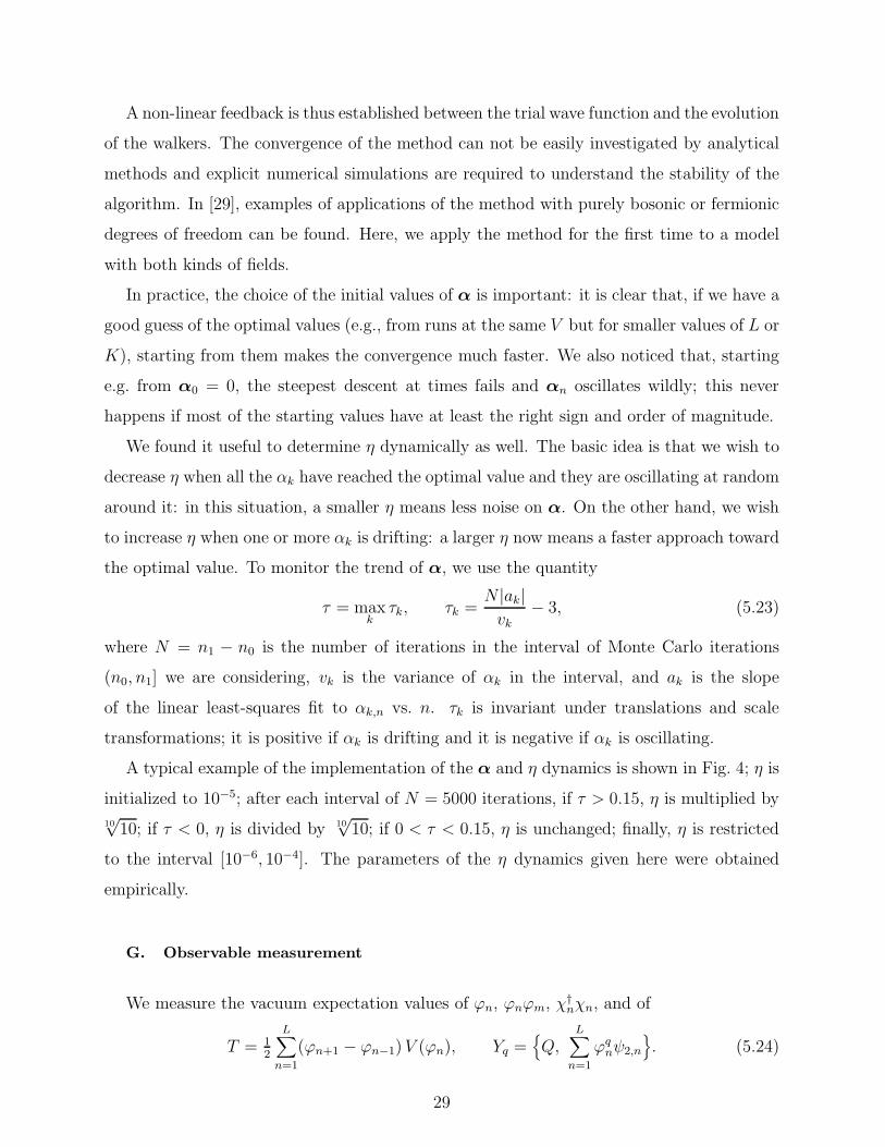
A typical example of the implementation of the α and η dynamics is shown in Fig. 4; η is

initialized to 10−5; after each interval of N = 5000 iterations, if τ > 0.15, η is multiplied by

10√

10; if τ < 0, η is divided by 10√

10; if 0 < τ < 0.15, η is unchanged; finally, η is restricted

to the interval [10−6, 10−4]. The parameters of the η dynamics given here were obtained

empirically.

G. Observable measurement

We measure the vacuum expectation values of ϕn, ϕnϕm, χ†nχn, and of

T = 12

L∑

n=1

(ϕn+1 − ϕn−1)V (ϕn), Yq =Q,

L∑

n=1

ϕqnψ2,n

. (5.24)

29

0 100 k 200 k 300 kiter

−0.2

0.0

0.2

0.4

α

10−6

10−5

10−4

η

αF

1

αB

2

αF

3

αB

4

FIG. 4: α and η dynamics from a run at V = 0.5ϕ2 − 0.55, L = 34 and K = 100.

Note that, with our choice of boundary conditions, we don’t have translation invariance and,

e.g., 〈ϕn〉 will depend on i; however, the dependence is sizable only within a few correlation

lengths from the border; therefore we typically average site-dependent quantities excluding

sites closer than a suitable Lmin from the border; in the case of 〈ϕnϕm〉, we average over all

pairs with fixed distance r = |n−m|, excluding the cases when n or m is closer than Lmin

from the border.

The ground-state energy is measured simply by averaging the measured values of E0 over

the ensembles E(t), discarding a suitable thermalization interval (0, t0):

E0∼= 1

t1 − t0

t1∑

t=t0+1

∑Kt

i=1Ei,twi,t∑Kt

i=1wi,t

, Ei,t =〈si,t|H|si,t〉〈si,t|si,t〉

, (5.25)

cf. Eq. (5.2). The vacuum expectation value of a generic observable is computed implement-

ing the forward-walking formula (5.3) as

〈O〉 ∼= 1

t1 − t0

t1∑

t=t0+1

∑Kt

i=1Oi,twi,t+∆t∑Kt

i=1wi,t+∆t

, Oi,t =〈si,t|O|si,t〉〈si,t|si,t〉

; (5.26)

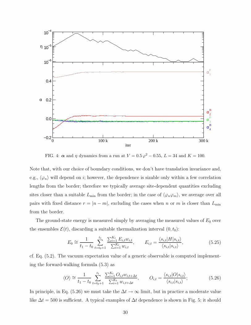
In principle, in Eq. (5.26) we must take the ∆t→ ∞ limit, but in practice a moderate value

like ∆t = 500 is sufficient. A typical examples of ∆t dependence is shown in Fig. 5; it should

30

0 100 200 300 400 500∆ t

−0.9

−0.8

−0.7

−0.6

−0.5

−0.4

T

K = 100K = 200K = 500

FIG. 5: The central charge T (cf. Eq. (5.24)) vs. ∆t from runs at V = 0.5ϕ2 and L = 34.

be noticed that the error bars grow with ∆t but very slowly.

VI. NUMERICAL RESULTS

A. Review of previous lattice studies

The class of models that we study in this paper has been previously considered in [18]

with a Monte Carlo approach that determine the ground state energy by using

E0 = limβ→∞

Tr(He−βH)

Tr(e−βH), (6.1)

and working numerically with a large fixed β. This is in the spirit of the usual Lagrangian

algorithms to be compared with the Green Function Monte Carlo method where β can be

identified with the simulation time and is thus taken to infinity by the very nature of the

algorithm.

The analysis of [18] is performed on 12 × 100 lattice, hence with a rather coarse spatial

mesh. In the model with V (ϕ) = λ3ϕ3 supersymmetry appears to be unbroken in full

31

0.000 0.001 0.002 0.003 0.004 0.0051/K

0.0000

0.0002

0.0004

0.0006

E0/L

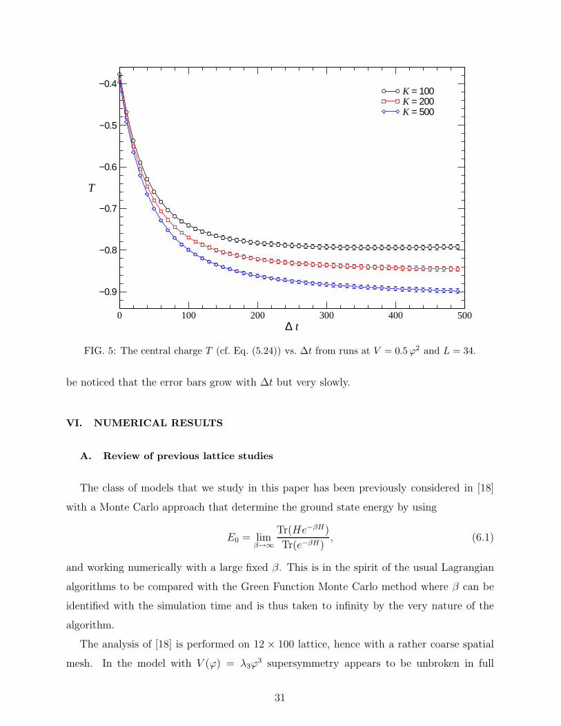
FIG. 6: The ground-state energy density E0/L vs. 1/K at V = ϕ3, L = 22, with statistics of 1 M

iterations for K < 5000, 500 k iterations at K = 5000, and 300 k iterations at K = 10000.

agreement with our analysis. In the quadratic model with V (ϕ) = λ2ϕ2 + λ0, the authors

of Ref. [18] find rather strong signals for supersymmetry breaking with λ0 bigger that the

critical value λ0 ≃ −0.5 and have numerical results showing a very small ground state energy

for λ0 < −0.5. No discussion of the continuum limit is attempted.

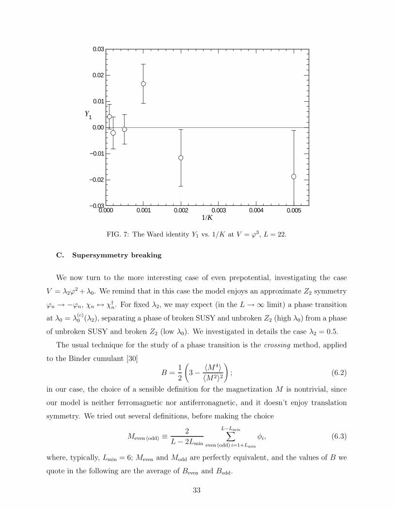
B. Odd V

As an example of odd prepotential, we study the case V = ϕ3. We plot the ground-state

energy vs. K in Fig. 6 and the Ward identity Y1 vs. K in Fig. 7. Both give a very convincing

evidence for unbroken SUSY; all the other Ward identities are consistent with zero, but more

noisy. It should be noticed that the bosonic and fermionic contribution to E0 are ≃ ±7.4:

we are observing a cancellation of four orders of magnitude.

32

0.000 0.001 0.002 0.003 0.004 0.0051/K

−0.03

−0.02

−0.01

0.00

0.01

0.02

0.03

Y1

FIG. 7: The Ward identity Y1 vs. 1/K at V = ϕ3, L = 22.

C. Supersymmetry breaking

We now turn to the more interesting case of even prepotential, investigating the case

V = λ2ϕ2 +λ0. We remind that in this case the model enjoys an approximate Z2 symmetry

ϕn → −ϕn, χn ↔ χ†n. For fixed λ2, we may expect (in the L→ ∞ limit) a phase transition

at λ0 = λ(c)0 (λ2), separating a phase of broken SUSY and unbroken Z2 (high λ0) from a phase

of unbroken SUSY and broken Z2 (low λ0). We investigated in details the case λ2 = 0.5.

The usual technique for the study of a phase transition is the crossing method, applied

to the Binder cumulant [30]

B =1

2

(3 − 〈M4〉

〈M2〉2)

; (6.2)

in our case, the choice of a sensible definition for the magnetization M is nontrivial, since

our model is neither ferromagnetic nor antiferronagnetic, and it doesn’t enjoy translation

symmetry. We tried out several definitions, before making the choice

Meven (odd) ≡2

L− 2Lmin

L−Lmin∑

even (odd) i=1+Lmin

φi, (6.3)

where, typically, Lmin = 6; Meven and Modd are perfectly equivalent, and the values of B we

quote in the following are the average of Beven and Bodd.

33

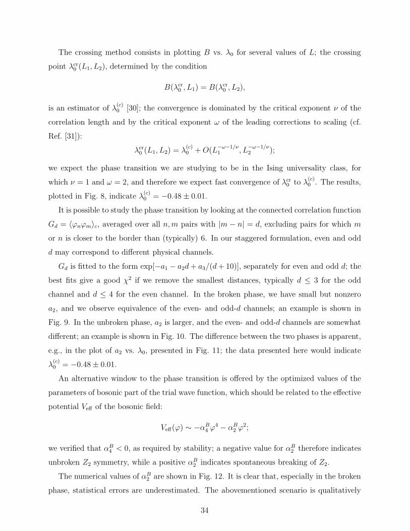
The crossing method consists in plotting B vs. λ0 for several values of L; the crossing

point λcr0 (L1, L2), determined by the condition

B(λcr0 , L1) = B(λcr

0 , L2),

is an estimator of λ(c)0 [30]; the convergence is dominated by the critical exponent ν of the

correlation length and by the critical exponent ω of the leading corrections to scaling (cf.

Ref. [31]):

λcr0 (L1, L2) = λ

(c)0 +O(L

−ω−1/ν1 , L

−ω−1/ν2 );

we expect the phase transition we are studying to be in the Ising universality class, for

which ν = 1 and ω = 2, and therefore we expect fast convergence of λcr0 to λ

(c)0 . The results,

plotted in Fig. 8, indicate λ(c)0 = −0.48 ± 0.01.

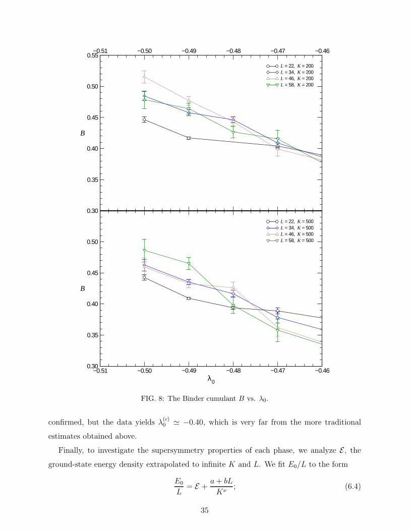
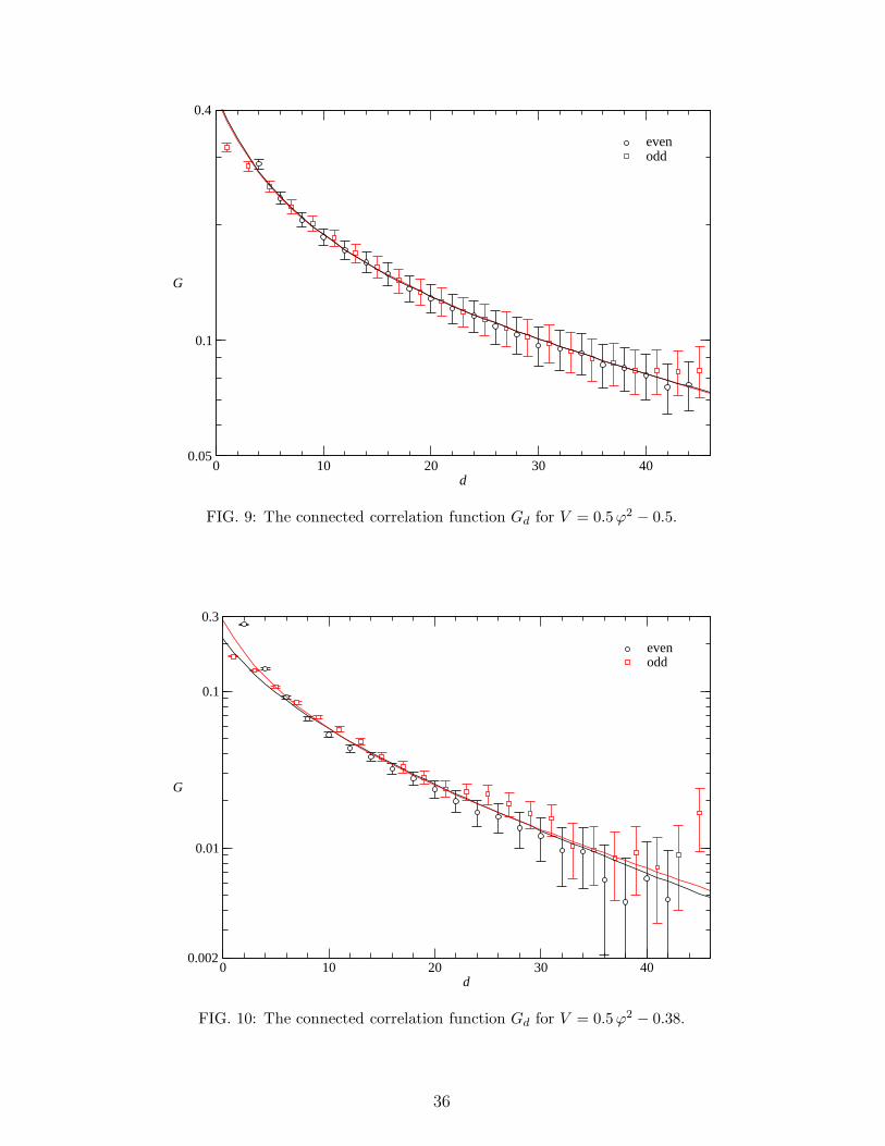
It is possible to study the phase transition by looking at the connected correlation function

Gd = 〈ϕnϕm〉c, averaged over all n,m pairs with |m − n| = d, excluding pairs for which m

or n is closer to the border than (typically) 6. In our staggered formulation, even and odd

d may correspond to different physical channels.

Gd is fitted to the form exp[−a1 − a2d+ a3/(d+ 10)], separately for even and odd d; the

best fits give a good χ2 if we remove the smallest distances, typically d ≤ 3 for the odd

channel and d ≤ 4 for the even channel. In the broken phase, we have small but nonzero

a2, and we observe equivalence of the even- and odd-d channels; an example is shown in

Fig. 9. In the unbroken phase, a2 is larger, and the even- and odd-d channels are somewhat

different; an example is shown in Fig. 10. The difference between the two phases is apparent,

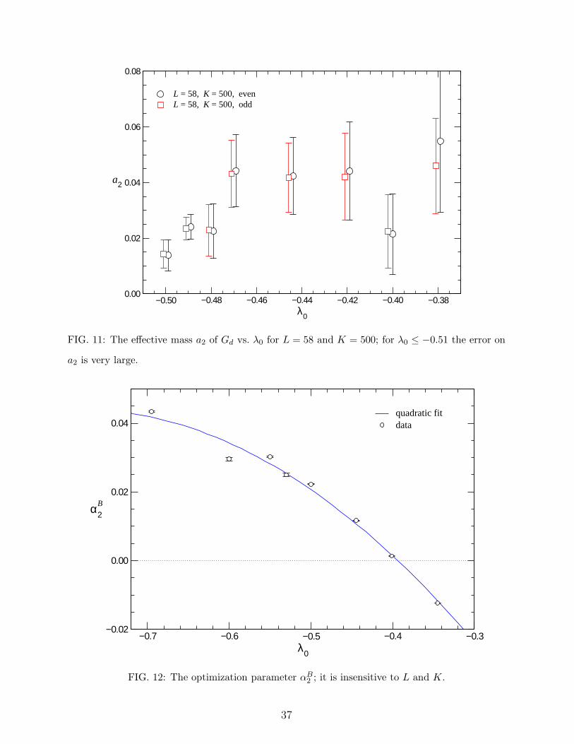
e.g., in the plot of a2 vs. λ0, presented in Fig. 11; the data presented here would indicate

λ(c)0 = −0.48 ± 0.01.

An alternative window to the phase transition is offered by the optimized values of the

parameters of bosonic part of the trial wave function, which should be related to the effective

potential Veff of the bosonic field:

Veff(ϕ) ∼ −αB4 ϕ

4 − αB2 ϕ

2;

we verified that αB4 < 0, as required by stability; a negative value for αB

2 therefore indicates

unbroken Z2 symmetry, while a positive αB2 indicates spontaneous breaking of Z2.

The numerical values of αB2 are shown in Fig. 12. It is clear that, especially in the broken

phase, statistical errors are underestimated. The abovementioned scenario is qualitatively

34

−0.51 −0.50 −0.49 −0.48 −0.47 −0.46

0.30

0.35

0.40

0.45

0.50

0.55

B

L = 22, K = 200L = 34, K = 200L = 46, K = 200L = 58, K = 200

−0.51 −0.50 −0.49 −0.48 −0.47 −0.46λ0

0.30

0.35

0.40

0.45

0.50

B

L = 22, K = 500L = 34, K = 500L = 46, K = 500L = 58, K = 500

FIG. 8: The Binder cumulant B vs. λ0.

confirmed, but the data yields λ(c)0 ≃ −0.40, which is very far from the more traditional

estimates obtained above.

Finally, to investigate the supersymmetry properties of each phase, we analyze E , the

ground-state energy density extrapolated to infinite K and L. We fit E0/L to the form

E0

L= E +

a+ bL

Kν; (6.4)

35

0 10 20 30 40d

0.05

0.1

0.4

G

evenodd

FIG. 9: The connected correlation function Gd for V = 0.5ϕ2 − 0.5.

0 10 20 30 40d

0.002

0.01

0.1

0.3

G

evenodd

FIG. 10: The connected correlation function Gd for V = 0.5ϕ2 − 0.38.

36

−0.50 −0.48 −0.46 −0.44 −0.42 −0.40 −0.38λ0

0.00

0.02

0.04

0.06

0.08

a2

L = 58, K = 500, evenL = 58, K = 500, odd

FIG. 11: The effective mass a2 of Gd vs. λ0 for L = 58 and K = 500; for λ0 ≤ −0.51 the error on

a2 is very large.

−0.7 −0.6 −0.5 −0.4 −0.3λ0

−0.02

0.00

0.02

0.04

α2B

quadratic fitdata

FIG. 12: The optimization parameter αB2 ; it is insensitive to L and K.

37

−0.52 −0.50 −0.48 −0.46 −0.44 −0.42λ0

0.000

0.001

0.002

0.003

0.004

0.005

E0/L

0.01289 (λ0 + 0.5276)1/2

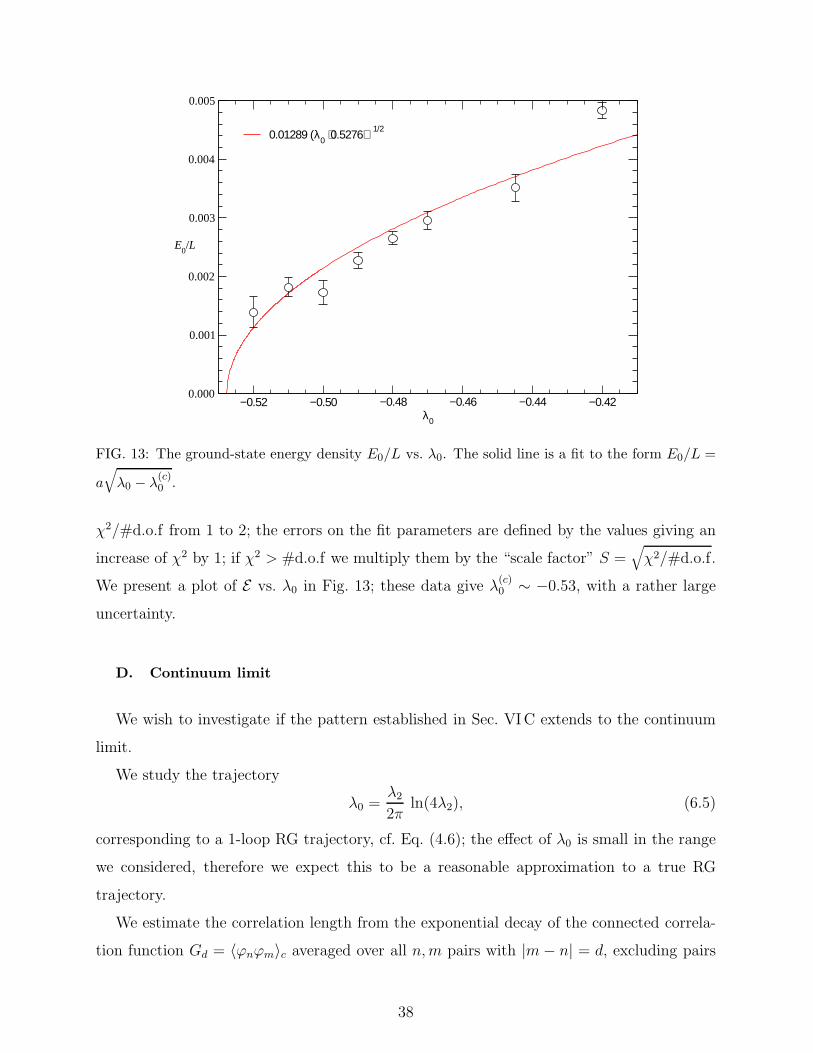
FIG. 13: The ground-state energy density E0/L vs. λ0. The solid line is a fit to the form E0/L =

a√λ0 − λ

(c)0 .

χ2/#d.o.f from 1 to 2; the errors on the fit parameters are defined by the values giving an

increase of χ2 by 1; if χ2 > #d.o.f we multiply them by the “scale factor” S =√χ2/#d.o.f.

We present a plot of E vs. λ0 in Fig. 13; these data give λ(c)0 ∼ −0.53, with a rather large

uncertainty.

D. Continuum limit

We wish to investigate if the pattern established in Sec. VIC extends to the continuum

limit.

We study the trajectory

λ0 =λ2

2πln(4λ2), (6.5)

corresponding to a 1-loop RG trajectory, cf. Eq. (4.6); the effect of λ0 is small in the range

we considered, therefore we expect this to be a reasonable approximation to a true RG

trajectory.

We estimate the correlation length from the exponential decay of the connected correla-

tion function Gd = 〈ϕnϕm〉c averaged over all n,m pairs with |m− n| = d, excluding pairs

38

for which m or n is closer to the border than (typically) 8. In our staggered formulation,

even and odd d correspond to different physical channels.

We performed runs for values of λ2 spaced by a factor of√

2, with a statistics of 4×106

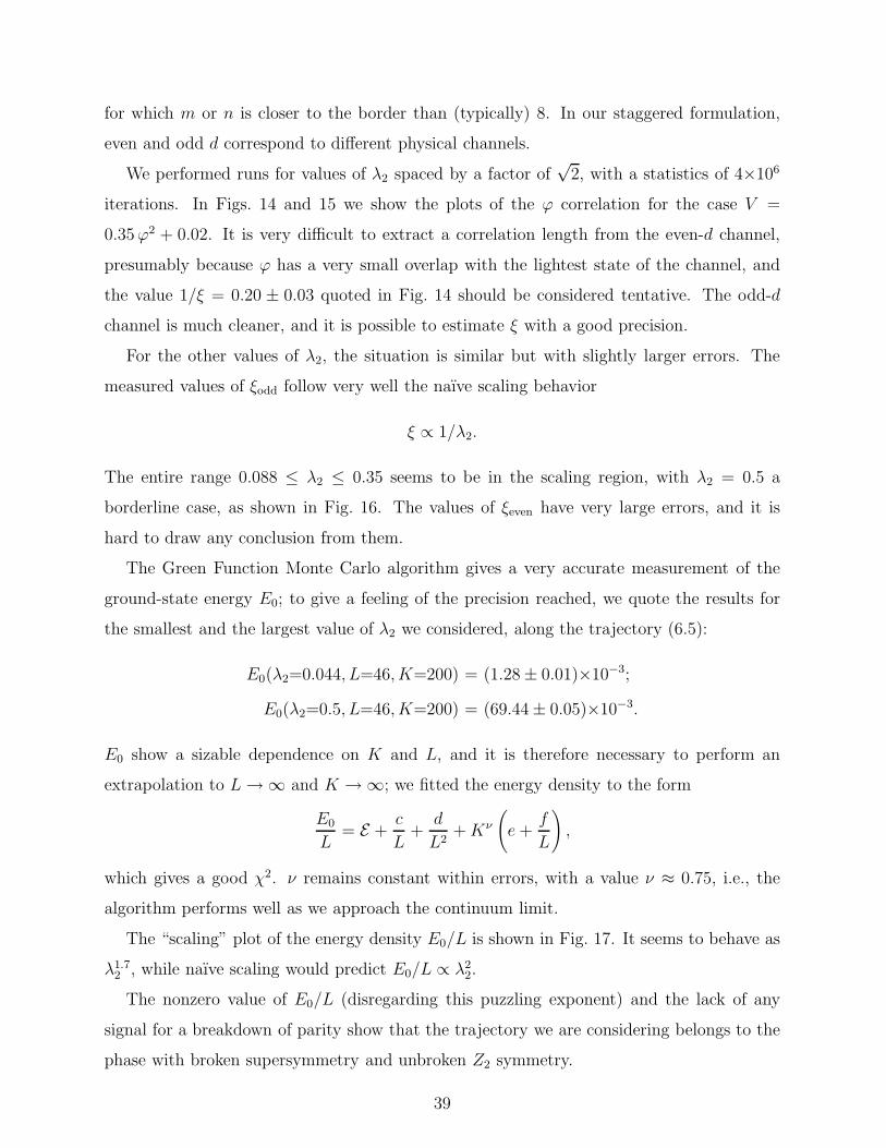
iterations. In Figs. 14 and 15 we show the plots of the ϕ correlation for the case V =

0.35ϕ2 + 0.02. It is very difficult to extract a correlation length from the even-d channel,

presumably because ϕ has a very small overlap with the lightest state of the channel, and

the value 1/ξ = 0.20 ± 0.03 quoted in Fig. 14 should be considered tentative. The odd-d

channel is much cleaner, and it is possible to estimate ξ with a good precision.

For the other values of λ2, the situation is similar but with slightly larger errors. The

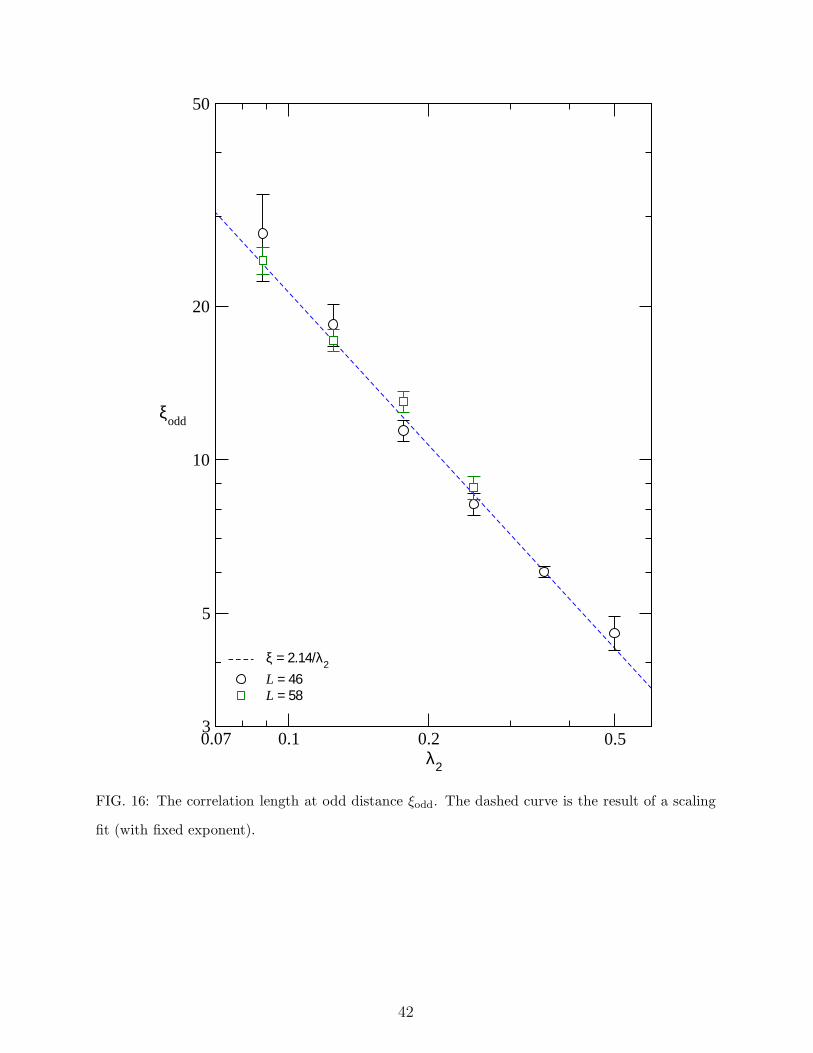
measured values of ξodd follow very well the naıve scaling behavior

ξ ∝ 1/λ2.

The entire range 0.088 ≤ λ2 ≤ 0.35 seems to be in the scaling region, with λ2 = 0.5 a

borderline case, as shown in Fig. 16. The values of ξeven have very large errors, and it is

hard to draw any conclusion from them.

The Green Function Monte Carlo algorithm gives a very accurate measurement of the

ground-state energy E0; to give a feeling of the precision reached, we quote the results for

the smallest and the largest value of λ2 we considered, along the trajectory (6.5):

E0(λ2=0.044, L=46, K=200) = (1.28 ± 0.01)×10−3;

E0(λ2=0.5, L=46, K=200) = (69.44 ± 0.05)×10−3.

E0 show a sizable dependence on K and L, and it is therefore necessary to perform an

extrapolation to L→ ∞ and K → ∞; we fitted the energy density to the form

E0

L= E +

c

L+

d

L2+Kν

(e+

f

L

),

which gives a good χ2. ν remains constant within errors, with a value ν ≈ 0.75, i.e., the

algorithm performs well as we approach the continuum limit.

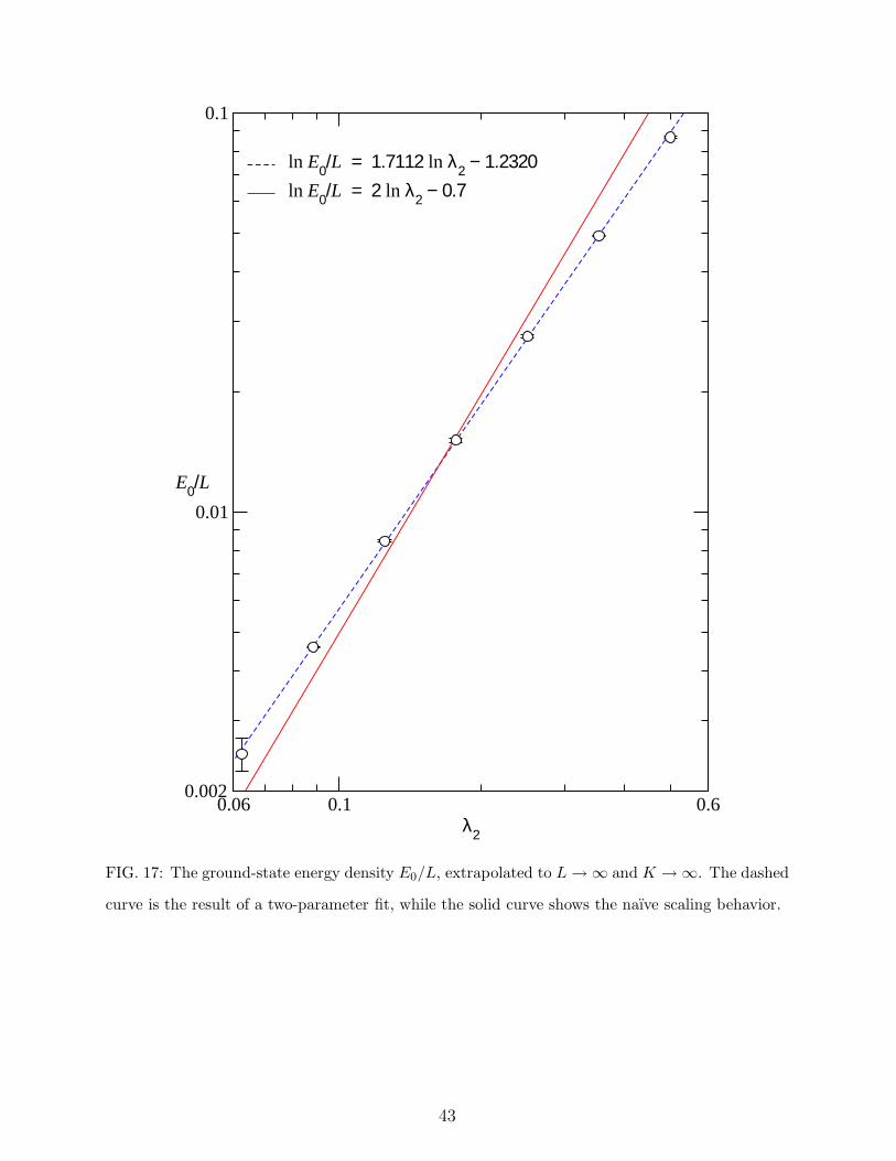
The “scaling” plot of the energy density E0/L is shown in Fig. 17. It seems to behave as

λ1.72 , while naıve scaling would predict E0/L ∝ λ2

2.

The nonzero value of E0/L (disregarding this puzzling exponent) and the lack of any

signal for a breakdown of parity show that the trajectory we are considering belongs to the

phase with broken supersymmetry and unbroken Z2 symmetry.

39

0 5 10 15 20d

4×10−4

10−3

10−2

6×10−2

Gd

K = 100, L = 34K = 200, L = 34K = 100, L = 46K = 200, L = 46

1/ξ = 0.20(3)

FIG. 14: The connected correlation function Gd at even distance for V = 0.353553ϕ2 + 0.019502;

the curve and value of 1/ξ quoted are the result of an exponential fit for 10 ≤ d ≤ 18 to the L = 46,

K = 200 data.

VII. CONCLUSION

In this paper, we investigated a class of two-dimensional N = 1 Wess-Zumino models

by non-perturbative lattice Hamiltonian techniques. The key property of the formulation

is the exact preservation of a SUSY subalgebra at finite lattice spacing. Our main tool are

numerical simulations using the Green Function Monte Carlo algorithm; we also performed

strong-coupling expansions.

All our results for the model with cubic prepotential indicate unbroken supersymmetry.

40

0 5 10 15 20d

3×10−3

10−2

6×10−2

Gd

K = 100, L = 34K = 200, L = 34K = 100, L = 46K = 200, L = 46

1/ξ = 0.166(4)

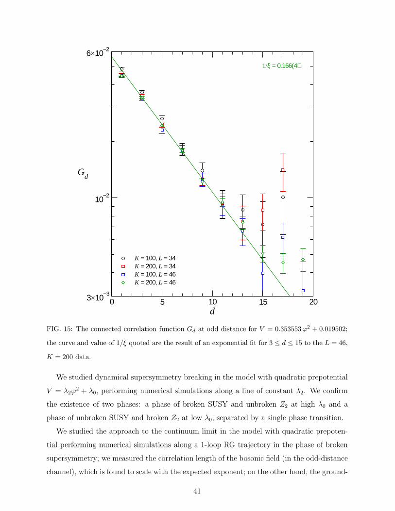
FIG. 15: The connected correlation function Gd at odd distance for V = 0.353553ϕ2 + 0.019502;

the curve and value of 1/ξ quoted are the result of an exponential fit for 3 ≤ d ≤ 15 to the L = 46,

K = 200 data.

We studied dynamical supersymmetry breaking in the model with quadratic prepotential

V = λ2ϕ2 + λ0, performing numerical simulations along a line of constant λ2. We confirm

the existence of two phases: a phase of broken SUSY and unbroken Z2 at high λ0 and a

phase of unbroken SUSY and broken Z2 at low λ0, separated by a single phase transition.

We studied the approach to the continuum limit in the model with quadratic prepoten-

tial performing numerical simulations along a 1-loop RG trajectory in the phase of broken

supersymmetry; we measured the correlation length of the bosonic field (in the odd-distance

channel), which is found to scale with the expected exponent; on the other hand, the ground-

41

0.07 0.1 0.2 0.5λ2

3

5

10

20

50

ξodd

ξ = 2.14/λ2L = 46L = 58

FIG. 16: The correlation length at odd distance ξodd. The dashed curve is the result of a scaling

fit (with fixed exponent).

42

0.06 0.1 0.6λ2

0.002

0.01

0.1

E0/L

ln E0/L = 1.7112 ln λ2 − 1.2320ln E0/L = 2 ln λ2 − 0.7

FIG. 17: The ground-state energy density E0/L, extrapolated to L→ ∞ and K → ∞. The dashed

curve is the result of a two-parameter fit, while the solid curve shows the naıve scaling behavior.

43

state energy density scales with an exponent clearly different from the expected exponent.

In many instances, the simulation algorithm suffers from slow convergence in the number

of walkers K.

Acknowledgments

It is a pleasure to thank Camillo Imbimbo, Ken Konishi, Gianni Morchio, and Ettore

Vicari for many helpful discussions and suggestions.

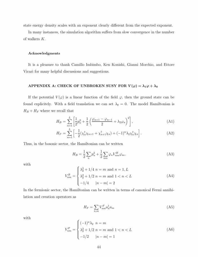
APPENDIX A: CHECK OF UNBROKEN SUSY FOR V (ϕ) = λ1ϕ + λ0

If the potential V (ϕ) is a linear function of the field ϕ, then the ground state can be

found explicitely. With a field translation we can set λ0 = 0. The model Hamiltonian is

HB +HF where we recall that

HB =L∑

n=1

[1

2p2

n +1

2

(ϕn+1 − ϕn−1

2+ λ2ϕn

)2], (A1)

HF =L∑

n=1

[−1

2(χ†

nχn+1 + χ†n+1χn) + (−1)nλ2χ

†nχn

]. (A2)

Thus, in the bosonic sector, the Hamiltonian can be written

HB =1

2

∑

n

p2n +

1

2

∑

nm

ϕnVBnmϕm, (A3)

with

V Bnm =

λ22 + 1/4 n = m and n = 1, L

λ22 + 1/2 n = m and 1 < n < L

−1/4 |n−m| = 2

(A4)

In the fermionic sector, the Hamiltonian can be written in terms of canonical Fermi annihi-

lation and creation operators as

HF =∑

n,m

V Fnma

†nam (A5)

with

V Fnm =

(−1)nλ2 n = m

λ22 + 1/2 n = m and 1 < n < L

−1/2 |n−m| = 1

(A6)

44

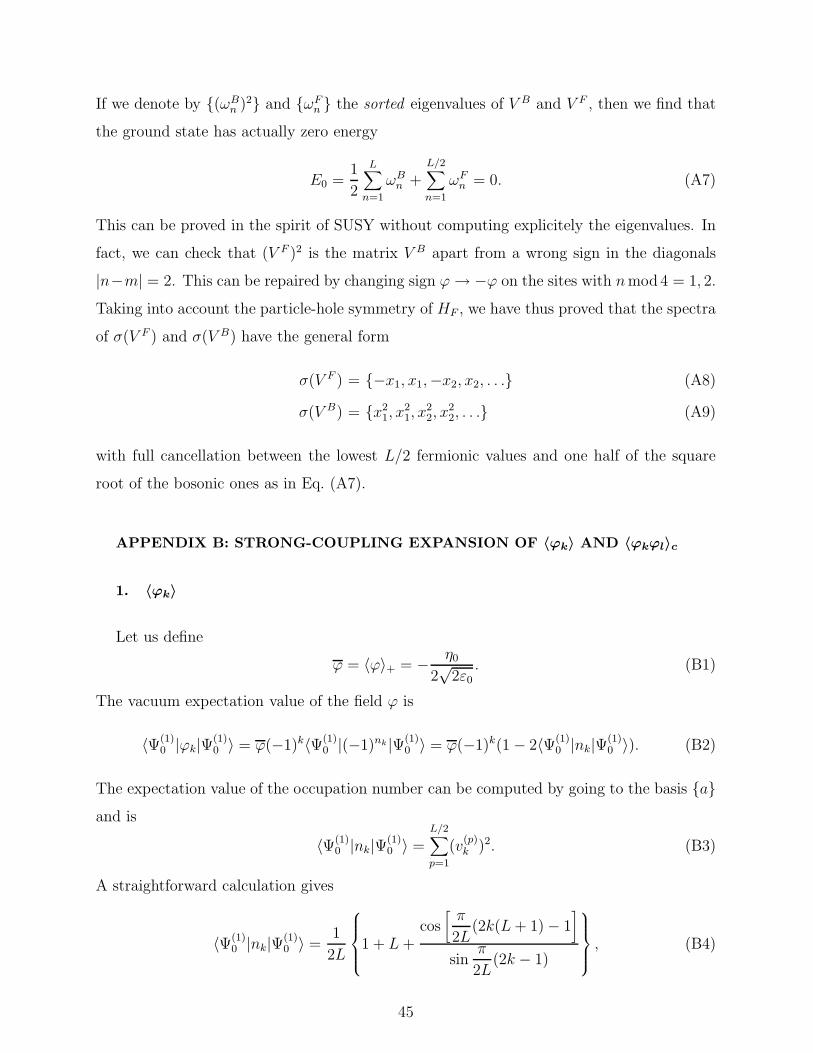
If we denote by (ωBn )2 and ωF

n the sorted eigenvalues of V B and V F , then we find that

the ground state has actually zero energy

E0 =1

2

L∑

n=1

ωBn +

L/2∑

n=1

ωFn = 0. (A7)

This can be proved in the spirit of SUSY without computing explicitely the eigenvalues. In

fact, we can check that (V F )2 is the matrix V B apart from a wrong sign in the diagonals

|n−m| = 2. This can be repaired by changing sign ϕ→ −ϕ on the sites with nmod4 = 1, 2.

Taking into account the particle-hole symmetry of HF , we have thus proved that the spectra

of σ(V F ) and σ(V B) have the general form

σ(V F ) = −x1, x1,−x2, x2, . . . (A8)

σ(V B) = x21, x

21, x

22, x

22, . . . (A9)

with full cancellation between the lowest L/2 fermionic values and one half of the square

root of the bosonic ones as in Eq. (A7).

APPENDIX B: STRONG-COUPLING EXPANSION OF 〈ϕk〉 AND 〈ϕkϕl〉c

1. 〈ϕk〉

Let us define

ϕ = 〈ϕ〉+ = − η0

2√

2ε0

. (B1)

The vacuum expectation value of the field ϕ is

〈Ψ(1)0 |ϕk|Ψ(1)

0 〉 = ϕ(−1)k〈Ψ(1)0 |(−1)nk |Ψ(1)

0 〉 = ϕ(−1)k(1 − 2〈Ψ(1)0 |nk|Ψ(1)

0 〉). (B2)

The expectation value of the occupation number can be computed by going to the basis aand is

〈Ψ(1)0 |nk|Ψ(1)

0 〉 =L/2∑

p=1

(v(p)k )2. (B3)

A straightforward calculation gives

〈Ψ(1)0 |nk|Ψ(1)

0 〉 =1

2L

1 + L+cos

[π

2L(2k(L+ 1) − 1

]

sinπ

2L(2k − 1)

, (B4)

45

and therefore

〈Ψ(1)0 |ϕk|Ψ(1)

0 〉 =η0

2√

2ε0

(−1)k 1

L

1 +cos

[π

2L(2k(L+ 1) − 1

]

sinπ

2L(2k − 1)

. (B5)

It is interesting to consider the limit L → ∞ of this expression after a rescaling k → xL

where 0 < x < 1. The result is

〈Ψ(1)0 |ϕxL|Ψ(1)

0 〉 =η0

2√

2ε0

1

L(±1 + cot(πx)) +

π

2L2

1

sin2(πx)+ O

(1

L3

)(B6)

where the sign is +1 for even k = xL and −1 for odd k.

2. 〈ϕkϕl〉c

Let us denote briefly

〈A〉 ≡ 〈Ψ(1)0 |A|Ψ(1)

0 〉, (B7)

and

〈AB〉c = 〈AB〉 − 〈A〉〈B〉. (B8)

The 2-point correlation is, for k 6= l,

〈ϕkϕl〉 = (ϕ)2(−1)k+l〈(−1)nk+nl〉 = (ϕ)2(−1)k+l(1 − 〈nk + nk〉 + 4〈nknl〉). (B9)

Going to the a basis, we immediately obtain

〈nknl〉c =∑

1≤A≤L/2

vAk v

Al ·

∑

L/2+1≤B≤L

vBk v

Bl , (B10)

and, for k 6= l,

〈ϕkϕl〉c = 4(ϕ)2(−1)k+l〈nknl〉c. (B11)

The two sums over eigenvalues can be evaluated analytically thanks to the simple form of

the eigenvectors v(p)l . The explicit result is

L

2

L/2∑

p=1

v(p)n v(p)

m =L

4δn,m +

1

4Zn,m, (B12)

L

2

L∑

p=1+L/2

v(p)n v(p)

m =L

4δn,m +

1

2(−1)n+m − 1

4Zn,m, (B13)

46

where

Zn,m =

n even, m even : (−1)n+m

2

[1 + cot

π

2L(m+ n− 1)

]

n even, m odd : (−1)n+m+1

2

[1 + cot

π

2L(n−m)

]

n odd, m even : (−1)n+m+1

2

[1 + cot

π

2L(m− n)

]

n odd, m odd : (−1)n+m

2

[−1 + cot

π

2L(m+ n− 1)

]

, (B14)

that can be used to compute the connected correlation on a finite lattice.

It is interesting to note that the limit L → ∞ can be taken without rescaling n and m.

For instance, we have

limL→∞

〈Ψ(1)0 |ϕ1 ϕn|Ψ(1)

0 〉c =4(ϕ)2

π2(−1)n

n even :1

(n− 1)2

n odd :1

n2

. (B15)

APPENDIX C: SECOND-ORDER EXPANSION FOR E0, EVEN q

The general formula for the second order contribution to the ground state energy is

E2 = E2,1 + E2,2 (C1)

E2,1 = 〈Ψ(1)0 |H(4)|Ψ(1)

0 〉 (C2)

E2,2 =∑

Ψ′

〈Ψ(1)0 |H(2)|Ψ′〉〈Ψ′|H(2)|Ψ(1)

0 〉E0 −E ′

(C3)

The states |Ψ′〉 are excited states of the form

|Ψ′〉 = ψσ1

k1(ϕ1) · · ·ψσL

kL(ϕL)|n1, . . . nL〉

where k1 + · · · kL = ν > 0 (integer) and σl = (−1)nl+l. For such a state we have

E ′ =∑

l

εkl

A first important remark is that H(2) can be restricted to its H(2)B part. In fact, the fermionic

part of H(2) can be written as H(2)eff plus terms that are only functions of the occupation

numbers. These operators acting on |Ψ(1)0 〉 give states that are orthogonal to the subspace

of excited unperturbed states |Ψ′〉.

47

The first term in E2 is simple and can be computed straightforwardly exploiting the fact

that the expectation value of ϕ2l over |Ψ(1)〉 does not depend on l:

E2,1 =L− 1

4ϕ2 − 1

4

L−2∑

l=1

〈Ψ(1)0 |ϕlϕl+2|Ψ(1)

0 〉 =L− 1

4ϕ2 − 1

4(ϕ)2c0(L) (C4)

where

ϕ2 =∫ ∞

−∞ϕ2[ψ±

0 (ϕ)]2dϕ

and

c0(L) =L−2∑

l=1

(1 − 〈nl〉 − 〈nl+2〉 + 4〈nlnl+2〉) (C5)

About E2,2, it can be computed by considering states with an excited single-site wave func-

tion in one or two distinct sites. Summing the two contributions we find

E2 =L− 1

4ϕ2 − 1

4(ϕ)2c0(L)

−∑

s>0

1

εs − ε0

(1

2

(Φ(1)

s

)2 (V (0)

)2+ c1(L) Φ(1)

s V (1)s ϕ V (0) + c2(L) (ϕ)2

(V (1)

s

)2)

−∑

s>0, t>0

1

εs + εt − 2ε0

1

4(L− 1)

[(Φ(1)

s

)2 (V

(1)t

)2+(Φ

(1)t

)2 (V (1)

s

)2]

+ c3(L)Φ(1)s Φ

(1)t V (1)

s V(1)t

(C6)

The symbols appearing in the above equations are defined as follows

V (0) = 〈ψ±0 |V (ϕ)|ψ±

0 〉 =√

2ε0η0 (C7)

V (1)s =

1√2(√ε0 + (−1)s√εs)〈ψ−

0 |ψ+s 〉, (C8)

Φ(1)s = − 1√

2

1√ε0 + (−1)s

√εs

〈ψ−0 |ψ+

s 〉 (C9)

The functions c0,1,2,3(L) can be fitted with a few powers of L and the numerical result is

c0(L) = L− 1.495 − 2.610

L+ · · · (C10)

c1(L) = −0.540 − 1.698

L+

1.787

L2+ · · · (C11)

c2(L) =1

2L− 0.540 +

0.301

L+

1.788

L2+ · · · (C12)

c3(L) = − 2

π2L− 0.167

L+ · · · (C13)

48

The full expression for E2 has thus the following simpler asymptotic expression

limL→∞

E2

L=

1

4(ϕ2 − ϕ2) − 1

2(ϕ)2

∑

s>0

(V (1)

s

)2

εs − ε0+

−∑

s>0,t>0

1

εs + εt − 2ε0

1

4

[(Φ(1)

s

)2 (V

(1)t

)2+(Φ

(1)t

)2 (V (1)

s

)2]+

− 2

π2Φ(1)

s Φ(1)t V (1)

s V(1)t

. (C14)

As an example, we find for the model with V (ϕ) = ϕ2:

E(λ2, 22) = 0.2811 − 0.160

λ2+

0.0481

λ4, and E(λ2,∞) = 0.2811 − 0.160

λ2+

0.0488

λ4

If we are interested in a comparison with an actual simulation, some trivial rescaling is

necessary. For instance, in the case of a purely quadratic V (ϕ) = λ2 ϕ2 we must compare

the expansion and the results for λ−2/32 E0/L and identify λ = λ

1/32 as the strong-coupling

expansion parameter.

APPENDIX D: FACTORIZED WAVE FUNCTION FOR THE FREE MODEL

In the free case V ≡ 0, with even L, we have

H(0) = HB +HF , (D1)

where (ϕ0 = ϕL+1 ≡ 0, the same for fermions)

HB =L∑

n=1

1

2p2

n +1

8(ϕn+1 − ϕn−1)

2, (D2)

HF = −1

2

L∑

n=1

(χ†nχn+1 + χ†

n+1χn). (D3)

The two HamiltoniansHB andHF are decoupled and the ground state takes the factorized

form

|Ψ(0)〉 = |Ψ(0)B 〉 ⊗ |Ψ(0)

F 〉. (D4)

We now determine |Ψ(0)B,F 〉 separately, assuming Lmod4 = 2 in order to have a unique ground

state in the decoupled V ≡ 0 model.

49

1. Bosonic sector

Let us write HB in the form

HB =1

2

L∑

n=1

p2n +

1

2

L∑

n,m=1

Vnmϕnϕm. (D5)

Let λ2k be the eigenvalues of the L × L matrix V and let z(k)

n be the corresponding (real)

eigenvectors satisfying

z(k) · z(l) = δk,l. (D6)

The ground state is

〈ϕ|Ψ(0)B 〉 = exp

−1

2

L∑

n,m=1

Rnmϕnϕm

, (D7)

where

Rnm =L∑

k=1

λkz(k)n z(k)

m (D8)

The explicit form of λk is

λk = sin(

2i− 1

L+ 1

π

2

), i = ⌊1

2(k + 1)⌋ (i = 1, . . . , 1

2L); (D9)

the dimension of each eigenspace is 2. The ground state energy of HB is

E0,B =L∑

k=1

12λk =

L/2∑

i=1

sin(

2i− 1

L+ 1

π

2

). (D10)

We adopt for the two orthogonal eigenvectors the choice

z(2i−1)n =

2√L+ 1

0 (n even)

sin(

2i− 1

L+ 1

π

2(L− n + 1)

)(n odd)

(D11)

z(2i)n =

2√L+ 1

sin(

2i− 1

L+ 1

π

2n)

(n even)

0 (n odd)(D12)

2. Fermionic sector

In the free case, the Hamiltonian in the fermionic sector is diagonalized by the orthogonal

change of basis

χx =

√2

L+ 1

L∑

n=1

sinnπx

L+ 1an, (D13)

50

and takes the form

HF = −L∑

n=1

cosnπ

L+ 1a†nan, (D14)

Hence the one-fermion energies are

− cosnπ

L+ 1, n = 1, . . . , L. (D15)

The fermionic component of the (supersymmetric) ground state is

|Ψ(0)F 〉 =

L/2∏

n=1

a†n|0〉; (D16)

the ground state energy of HF is

E0,F = −L/2∑

i=1

cosnπ

L+ 1; (D17)

we can easily check that

E0,F = −E0,B =1

2

1 − 1

sinπ

2(L+ 1)

, (D18)

and therefore E0 = E0,B + E0,F = 0.

[1] P. Langacker, in Proceedings of the PASCOS90 Symposium, Eds. P. Nath and S. Reucroft,

(World Scientific, Singapore 1990);

J. Ellis, S. Kelley, and D. Nanopoulos, Phys. Lett. B260, 131 (1991);

U. Amaldi, W. de Boer, and H. Furstenau, Phys. Lett. B260, 447 (1991);

P. Langacker and M. Luo, Phys. Rev. D44, 817 (1991);

C. Giunti, C.W. Kim and U. W. Lee, Mod. Phys. Lett. A6, 1745 (1991).

[2] E. Witten, Quest for Unification, Lectures given at 10th International Conference on Super-

symmetry and Unification of Fundamental Interactions (SUSY02), Hamburg, Germany, 17-23

Jun 2002; hep-ph/0207124.

[3] S. Weinberg, Phys. Rev. D13, 974 (1976);

Phys. Rev. D19, 1277 (1979);

L. Susskind, Phys. Rev. D20, 2619 (1979);

G. ’t Hooft, in Recent developments in gauge theories, Proceedings of the NATO Advanced

Summer Institute, Cargese 1979, ed. G. ’t Hooft et al. (Plenum, New York 1980).

51

[4] M. Beccaria, M. Campostrini, A. Feo, Adaptive Optimization of Wave Functions for Lattice

Field Models, Contributed to ECT* Collaboration Meeting on Quantum Monte Carlo: Recent

Advances and Common Problems in Condensed Matter and Field Theory, Trento, Italy, 3-7

Jul 2001, hep-lat/0109005;

M. Beccaria, M. Campostrini, A. Feo, Nucl. Phys. B (Proc. Suppl.) 106, (2002) 944;

M. Beccaria, M. Campostrini, A. Feo, Nucl. Phys. B (Proc. Suppl.) 119, (2003) 891;

M. Beccaria, M. Campostrini, A. Feo, hep-lat/0309054.

[5] S. Catterall, JHEP 0305:038, (2003);

S. Catterall and S. Karamov, Phys. Rev. D68 014503 (2003).

[6] K. Wilson, Phys. Rev. D10 (1974), 2445.

[7] J. Kogut, L. I. Susskind, Phys. Rev. D11 (1975), 395;

J. Kogut, Rev. Mod. Phys. 51 (1979), 659.

[8] M. Harada and S. Pinsky, Phys. Lett. B567 (2003) 277.

[9] D. M. Ceperley, M. H. Kalos, “Monte Carlo Methods in Statistical Physics”, edited by

K. Binder, Springer-Verlag, Heidelberg (1992).

[10] I. Montvay and G. Munster, Quantum Fields on a Lattice, Cambridge University Press, 1994.

[11] A. Feo, Nucl. Phys. Proc. Suppl. 119 (2003) 198.

[12] E. Y. Loh, J. E. Gubernatis, R. T. Scalettar, S. R. White, D. J. Scalapino and R. L. Sugar,

Phys. Rev. B41, 9301, (1990).

[13] S. Coleman, Phys. Rev. D 22, 2088, (1975);

S. Mandelstam, Phys. Rev. D 11, 3026, (1975).

[14] Mandelstam, Phys. Rev. D11 (1975) 3026.

[15] W. Von der Linden, Phys. Rep. 220, 53 (1992). For an interesting complete solution of the

sign problem in a class of models in 2 + 1 and 3 + 1 dimensions, see S. Chandrasekharan and

J. Osborn, Springer Proc. Phys. 86, 28 (2000).

[16] E. Witten and D. Olive, Phys. Lett. 78B, 97 (1978).

[17] S. Elitzur, E. Rabinovici, A. Schwimmer, Phys. Lett. B119 (1982), 165.

[18] J. Ranft, A. Schiller, Phys. Lett. B138 (1984), 166; for a theoretical discussion see also

[19] S. Elitzur and A. Schwimmer, Nucl. Phys. B 226 (1983) 109.

[20] A. Schiller, J. Ranft, J. Phys. G12 (1986), 935.

[21] E. Witten, Nucl. Phys. B 188 (1981) 513; F. Cooper, A. Khare, U. Sukhatme, Phys. Rept.

52

251 (1995) 267.

[22] B. R. Johnson, J. Chem. Phys. 67 (1977) 4086.

[23] E. Witten, Nucl. Phys. B 202 (1982) 253.

[24] M. Reed and B. Simon, Methods of modern mathematical physics, Vol IV: Analysis of opera-

tors, Academic press, New York (1978).

[25] L. Alvarez-Gaume, D. Z. Freedman, M. T. Grisaru, Spontaneous breakdown of supersymmetry

in two-dimensions, Brandeis U. preprint HUTMP 81/B111, unpublished.

[26] S. A. Chin, Proc. of 1988 Symp. on Lattice Field Theory, Batavia, IL, Sept. 22-25 (1988),

Nucl. Phys. (Proc. Suppl.) 9 (1989) 498.

[27] J. H. Hetherington, Phys. Rev. A30 (1984) 2713.

[28] N. Trivedi and D. M. Ceperley, Phys. Rev. B41, (1990) 4552.

[29] M. Beccaria, Europhys. Journal C13 (2000), 357;

M. Beccaria, Phys. Rev. D61 (2000), 114503;

M. Beccaria, Phys. Rev. D62 (2000), 34510;

M. Beccaria, A. Moro, Phys. Rev. D64 (2001), 077502.

[30] K. Binder, Z. Phys. B 43 (1981) 119.

[31] A. Pelissetto, E. Vicari, Phys. Rept. 368 (2002) 549.

53

Supersymmetry breaking in two dimensions: The lattice N=1 Wess-Zumino model

Documents

Transcript of Supersymmetry breaking in two dimensions: The lattice N=1 Wess-Zumino model