hep-ph/0305212

CERN–TH/2003-107

UMN–TH–2201/03

FTPI–MINN–03/12

Phenomenological Constraints on Patterns of Supersymmetry

Breaking

John Ellis1, Keith A. Olive2, Yudi Santoso2 and Vassilis C. Spanos2

1TH Division, CERN, Geneva, Switzerland

2William I. Fine Theoretical Physics Institute,

University of Minnesota, Minneapolis, MN 55455, USA

Abstract

Specific models of supersymmetry breaking predict relations between the trilinear and

bilinear soft supersymmetry breaking parameters A0 and B0 at the input scale. In such

models, the value of tan β can be calculated as a function of the scalar masses m0 and the

gaugino masses m1/2, which we assume to be universal. The experimental constraints on

sparticle and Higgs masses, b → sγ decay and the cold dark matter density ΩCDMh2 can then

be used to constrain tan β in such specific models of supersymmetry breaking. In the simplest

Polonyi model with A0 = (3−√3)m0 = B0 +m0, we find 11 <∼ tan β <∼ 20 (tan β ' 4.15) for

µ > 0 (µ < 0). We also discuss other models with A0 = B0 +m0, finding that only the range

−1.9 <∼ A0/m0 <∼ 2.5 is allowed for µ > 0, and the range 1.25 <∼ A0/m0 <∼ 4.8 for µ < 0. In

these models, we find no solutions in the rapid-annihilation ‘funnels’ or in the ‘focus-point’

region. We also discuss the allowed range of tanβ in the no-scale model with A0 = B0 = 0.

In all these models, most of the allowed regions are in the χ− τ1 coannihilation ‘tail’.

CERN–TH/2003-107

May 2003

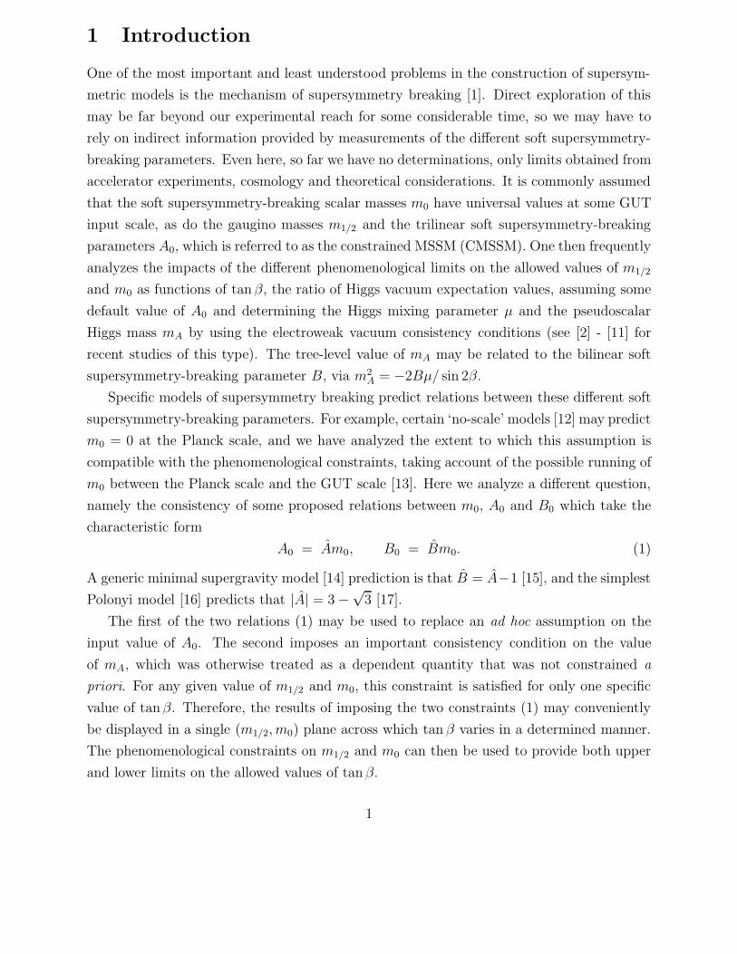
1 Introduction

One of the most important and least understood problems in the construction of supersym-

metric models is the mechanism of supersymmetry breaking [1]. Direct exploration of this

may be far beyond our experimental reach for some considerable time, so we may have to

rely on indirect information provided by measurements of the different soft supersymmetry-

breaking parameters. Even here, so far we have no determinations, only limits obtained from

accelerator experiments, cosmology and theoretical considerations. It is commonly assumed

that the soft supersymmetry-breaking scalar masses m0 have universal values at some GUT

input scale, as do the gaugino masses m1/2 and the trilinear soft supersymmetry-breaking

parameters A0, which is referred to as the constrained MSSM (CMSSM). One then frequently

analyzes the impacts of the different phenomenological limits on the allowed values of m1/2

and m0 as functions of tanβ, the ratio of Higgs vacuum expectation values, assuming some

default value of A0 and determining the Higgs mixing parameter µ and the pseudoscalar

Higgs mass mA by using the electroweak vacuum consistency conditions (see [2] - [11] for

recent studies of this type). The tree-level value of mA may be related to the bilinear soft

supersymmetry-breaking parameter B, via m2A = −2Bµ/ sin 2β.

Specific models of supersymmetry breaking predict relations between these different soft

supersymmetry-breaking parameters. For example, certain ‘no-scale’ models [12] may predict

m0 = 0 at the Planck scale, and we have analyzed the extent to which this assumption is

compatible with the phenomenological constraints, taking account of the possible running of

m0 between the Planck scale and the GUT scale [13]. Here we analyze a different question,

namely the consistency of some proposed relations between m0, A0 and B0 which take the

characteristic form

A0 = Am0, B0 = Bm0. (1)

A generic minimal supergravity model [14] prediction is that B = A−1 [15], and the simplest

Polonyi model [16] predicts that |A| = 3−√3 [17].

The first of the two relations (1) may be used to replace an ad hoc assumption on the

input value of A0. The second imposes an important consistency condition on the value

of mA, which was otherwise treated as a dependent quantity that was not constrained a

priori. For any given value of m1/2 and m0, this constraint is satisfied for only one specific

value of tanβ. Therefore, the results of imposing the two constraints (1) may conveniently

be displayed in a single (m1/2, m0) plane across which tan β varies in a determined manner.

The phenomenological constraints on m1/2 and m0 can then be used to provide both upper

and lower limits on the allowed values of tanβ.

1

In this paper, we analyze these constraints on tanβ as functions of A in the generic

scenario (1), including the Polonyi case A = 3 − √3 and other models with A = B + 1.

In the Polonyi case, we find that 11 <∼ tanβ <∼ 20 for µ > 0, with only a small area in

the m1/2 −m0 plane with tanβ ' 4.15 surviving for µ < 0. In general, we find consistent

solutions for −1.9 <∼ A <∼ 2.25 for µ > 0 and 1.25 <∼ A <∼ 4.8 for µ < 0. We also explore the

range of tan β that is allowed in a no-scale scenario with A0 = B0 = 0 at the GUT scale.

It should, however, be recalled that the no-scale boundary conditions [12] were originally

proposed to hold at the supergravity scale, which might be significantly above the GUT

scale. In this case, renormalization-group running between these scales would generate A

and B 6= 0 at the GUT scale.

2 Models of Supersymmetry Breaking

In this Section, we review briefly models that yield the characteristic patterns of supersym-

metry breaking whose phenomenology we study later in the paper. We assume an N = 1

supergravity framework, interpreted as a low-energy effective field theory. This may be

characterized by a Kahler function K that describes the kinetic terms for the chiral super-

multiplets Φ ≡ (ζ, φ), where the ζ represent hidden-sector fields and the φi observable-sector

fields, a holomorphic function f(Φ) that yields kinetic terms for the gauge supermultiplets

Aa as well as gauge couplings, and a holomorphic superpotential W (Φ). We assume the form

of the gauge kinetic function f to be such that the gaugino masses m1/2 are universal at the

GUT input scale, as are the gauge couplings.

So-called minimal supergravity theories have K = Σi|Φi|2, whereas no-scale models have

non-trivial Kahler functions such as K = −3ln(ζ + ζ† − Σj |φj|2). The scalar potential

(neglecting any gauge contributions) is in general [14]

V (φ, φ∗) = eK[Ki(K−1)j

iKj − 3]

(2)

where we are working in Planck units. For minimal supergravity, we have Ki = φi∗+W i/W ,

Ki = φi + W ∗i /W ∗, and (K−1)j

i = δji , and the resulting scalar potential is

V (φ, φ∗) = eφiφi∗ [|W i + φi∗W |2 − 3|W |2

]. (3)

In this minimal case, the soft supersymmetry-breaking scalar masses m0 are universal at the

input GUT scale, with [1]

m20 = m2

3/2 + Λ, (4)

2

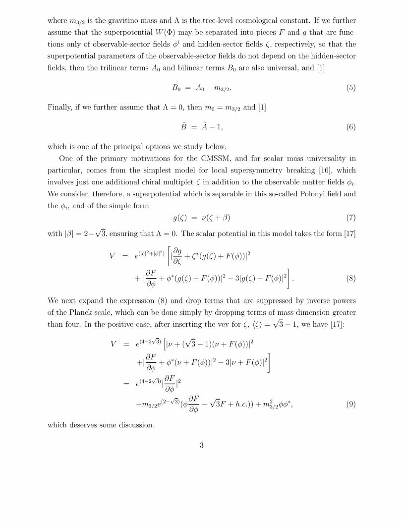
where m3/2 is the gravitino mass and Λ is the tree-level cosmological constant. If we further

assume that the superpotential W (Φ) may be separated into pieces F and g that are func-

tions only of observable-sector fields φi and hidden-sector fields ζ , respectively, so that the

superpotential parameters of the observable-sector fields do not depend on the hidden-sector

fields, then the trilinear terms A0 and bilinear terms B0 are also universal, and [1]

B0 = A0 −m3/2. (5)

Finally, if we further assume that Λ = 0, then m0 = m3/2 and [1]

B = A− 1, (6)

which is one of the principal options we study below.

One of the primary motivations for the CMSSM, and for scalar mass universality in

particular, comes from the simplest model for local supersymmetry breaking [16], which

involves just one additional chiral multiplet ζ in addition to the observable matter fields φi.

We consider, therefore, a superpotential which is separable in this so-called Polonyi field and

the φi, and of the simple form

g(ζ) = ν(ζ + β) (7)

with |β| = 2−√3, ensuring that Λ = 0. The scalar potential in this model takes the form [17]

V = e(|ζ|2+|φ|2)[|∂g

∂ζ+ ζ∗(g(ζ) + F (φ))|2

+ |∂F

∂φ+ φ∗(g(ζ) + F (φ))|2 − 3|g(ζ) + F (φ)|2

]. (8)

We next expand the expression (8) and drop terms that are suppressed by inverse powers

of the Planck scale, which can be done simply by dropping terms of mass dimension greater

than four. In the positive case, after inserting the vev for ζ , 〈ζ〉 =√

3− 1, we have [17]:

V = e(4−2√

3)[|ν + (

√3− 1)(ν + F (φ))|2

+|∂F

∂φ+ φ∗(ν + F (φ))|2 − 3|ν + F (φ)|2

]

= e(4−2√

3)|∂F

∂φ|2

+m3/2e(2−√3)(φ

∂F

∂φ−√

3F + h.c.)) + m23/2φφ∗, (9)

which deserves some discussion.

3

First, up to an overall rescaling of the superpotential, F → e√

3−2F , the first term is

the ordinary F -term part of the scalar potential of global supersymmetry. The next term,

which is proportional to m3/2, provides universal trilinear soft supersymmetry-breaking terms

A = (3−√3)m3/2 and bilinear soft supersymmetry-breaking terms B = (2−√3)m3/2, i.e.,

a special case of the general relation (5) above between B and A. Finally, the last term

represents a universal scalar mass of the type advocated in the CMSSM, with m20 = m2

3/2,

since the cosmological constant Λ vanishes in this model, by construction.

As we have seen above, the generation of such soft terms is a rather generic property

of low-energy supergravity models [15] and many of these conclusions persist when one

generalizes the Polonyi potential. For example, if we choose g(ζ) so that 1 〈g〉 = ν, 〈∂g/∂ζ〉 =

a∗ν, and 〈ζ〉 = b, the condition that Λ = 0 at ζ = b implies |a + b|2 = 3. Substituting these

expectation values in (8), we find [15] that A = b∗(a + b)ν and once again B = A − ν, but

now with A free. The constant ν determines the gravitino mass, and hence m0, through:

m0 = m3/2 = e12bb∗ν.

Another broad option for supersymmetry breaking is that provided by no-scale models

[12], of which the simplest example is

K = −3ln(ζ + ζ† − Σi|φi|2

). (10)

No-scale models have the universal values

m20 = 0, A0 = 0, B0 = 0 (11)

at the input supergravity scale. The possibility that m0 = 0 at the GUT scale has re-

cently been studied [13, 18], and shown to be excluded by the phenomenological constraints.

However, it was recalled that the input supergravity scale could be somewhat higher than

the GUT scale, in which case one might find m0 6= 0 already at the GUT scale. Clearly

the same could also be true for A0 and B0. However, the deviations from (11) are model-

dependent, and we think it important to be aware of the phenomenological fate of the

clear-cut A0 = B0 = 0 option for supersymmetry breaking.

3 Electroweak Vacuum Conditions

Before discussing the phenomenological constraints on this model, we first show more pre-

cisely how the relation between A and B can be used to determine tanβ when the radiative

electroweak symmetry breaking conditions are applied.

1One could also consider models in which several fields ζi contribute to supersymmetry breaking.

4

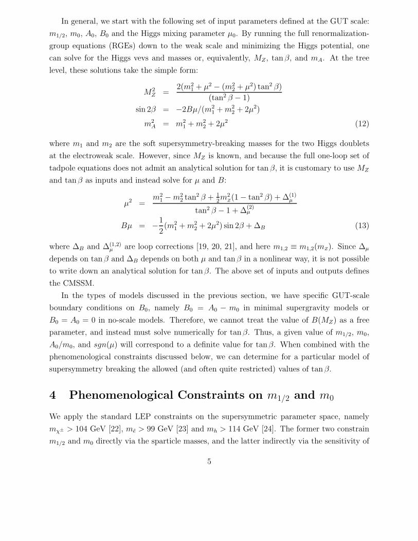
In general, we start with the following set of input parameters defined at the GUT scale:

m1/2, m0, A0, B0 and the Higgs mixing parameter µ0. By running the full renormalization-

group equations (RGEs) down to the weak scale and minimizing the Higgs potential, one

can solve for the Higgs vevs and masses or, equivalently, MZ , tanβ, and mA. At the tree

level, these solutions take the simple form:

M2Z =

2(m21 + µ2 − (m2

2 + µ2) tan2 β)

(tan2 β − 1)

sin 2β = −2Bµ/(m21 + m2

2 + 2µ2)

m2A = m2

1 + m22 + 2µ2 (12)

where m1 and m2 are the soft supersymmetry-breaking masses for the two Higgs doublets

at the electroweak scale. However, since MZ is known, and because the full one-loop set of

tadpole equations does not admit an analytical solution for tan β, it is customary to use MZ

and tanβ as inputs and instead solve for µ and B:

µ2 =m2

1 −m22 tan2 β + 1

2m2

Z(1− tan2 β) + ∆(1)

µ

tan2 β − 1 + ∆(2)µ

Bµ = −1

2(m2

1 + m22 + 2µ2) sin 2β + ∆B (13)

where ∆B and ∆(1,2)µ are loop corrections [19, 20, 21], and here m1,2 ≡ m1,2(mZ). Since ∆µ

depends on tanβ and ∆B depends on both µ and tanβ in a nonlinear way, it is not possible

to write down an analytical solution for tanβ. The above set of inputs and outputs defines

the CMSSM.

In the types of models discussed in the previous section, we have specific GUT-scale

boundary conditions on B0, namely B0 = A0 − m0 in minimal supergravity models or

B0 = A0 = 0 in no-scale models. Therefore, we cannot treat the value of B(MZ) as a free

parameter, and instead must solve numerically for tanβ. Thus, a given value of m1/2, m0,

A0/m0, and sgn(µ) will correspond to a definite value for tanβ. When combined with the

phenomenological constraints discussed below, we can determine for a particular model of

supersymmetry breaking the allowed (and often quite restricted) values of tan β.

4 Phenomenological Constraints on m1/2 and m0

We apply the standard LEP constraints on the supersymmetric parameter space, namely

mχ± > 104 GeV [22], me > 99 GeV [23] and mh > 114 GeV [24]. The former two constrain

m1/2 and m0 directly via the sparticle masses, and the latter indirectly via the sensitivity of

5

radiative corrections to the Higgs mass to the sparticle masses, principally mt,b2. We use the

latest version of FeynHiggs [25] for the calculation of mh. We require the branching ratio

for b → sγ to be consistent with the experimental measurements [26]. We also indicate the

regions of the (m1/2, m0) plane that are favoured by the BNL measurement [27] of gµ− 2 at

the 2-σ level, corresponding to a deviation of (33.9±11.2)×10−10 from the Standard Model

calculation of [28] using e+e− data. We are however aware that this constraint is still under

discussion and do not use it to constrain tanβ. All the µ > 0 planes would be consistent

with gµ− 2 at the 3-σ level, whereas µ < 0 is disfavoured even if one takes a relaxed view of

the gµ − 2 constraint.

Finally, we impose the following requirement on the relic density of neutralinos χ: 0.094 ≤Ωχh2 ≤ 0.129, as suggested by the recent WMAP data [29], in agreement with earlier

indications. We recall that several cosmologically-allowed domains of the (m1/2, m0) planes

for different values of tanβ have been discussed previously in the general CMSSM framework

[2] - [4], [6] - [11]. One is a ‘bulk’ region at low m1/2 and m0, which has been squeezed

considerably by the WMAP constraint on Ωχh2. A second region is the χ− τ1 coannihilation

‘tail’ [7, 8], which stretches to larger m1/2, close to the boundary of the acceptable region

where mχ ≤ mτ1 . In the wake of WMAP, this ‘tail’ is now much narrower - because of the

smaller range of Ωχh2 - and shorter - because of the more stringent upper limit on Ωχh2

[5, 30]. A third region is the ‘funnel’ due to rapid χχ → H, A annihilation that occurs at

larger m0 and m1/2 [4, 9]. Finally, the fourth domain is the ‘focus-point’ region at large

m0, close to the boundary where radiative breaking of electroweak symmetry is no longer

possible [10, 11].

We see in the next Section that the ‘funnel’ and ‘focus-point’ regions are not present in

the simple models of supersymmetry breaking introduced earlier, whilst the ‘bulk’ region is

possible only for a very restricted range of tanβ. On the other hand, the coannihilation ‘tail’

generally remains permitted.

5 Examples of (m1/2, m0) Planes

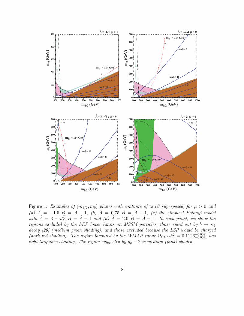
We display in Fig. 1 the contours of tanβ (solid blue lines) in the (m1/2, m0) planes for

selected values of A, B and the sign of µ. Also shown are the contours where mχ± > 104 GeV

(near-vertical black dashed lines) and mh > 114 GeV (diagonal red dash-dotted lines). The

excluded regions where mχ > mτ1 have dark (red) shading, those excluded by b → sγ have

medium (green) shading, and those where the relic density of neutralinos lies within the

2We assume as our default that mt = 175 GeV.

6

WMAP range 0.094 ≤ Ωχh2 ≤ 0.129 have light (turquoise) shading. Finally, the regions

favoured by gµ − 2 at the 2-σ level are medium (pink) shaded.

As seen in panel (a) of Fig. 1, when µ > 0 and A = −1.5, close to its minimum possible

value, the contours of tan β rise diagonally from low values of (m1/2, m0) to higher values, with

higher values of tanβ having lower values of m0 for a given value of m1/2. The mh = 114 GeV

contour rises in a similar way, and regions above and to the left of this contour have mh < 114

GeV and are excluded. Therefore, only a very limited range of tanβ ∼ 4 is compatible with

the mh and ΩCDMh2 constraints. At lower values of A, the slope of the Higgs contour softens

and even less of the parameter space is allowed. Below A ' −1.9, the entire m1/2−m0 plane

is excluded. When A is increased to 0.75, as seen in panel (b) of Fig. 1, both the tan β and

mh contours rise more rapidly with m1/2, and a larger range 9 <∼ tan β <∼ 14 is allowed 3.

In the simplest Polonyi model with A = 3 − √3 shown in panel (c) of Fig. 1, we see that

the tanβ contours have noticeable curvature. In this case, the Higgs constraint combined

with the relic density requires tan β >∼ 11, whilst the relic density also enforces tanβ <∼ 20 4.

Finally, in panel (d) of Fig. 1, when A = 2.0, close to its maximal value for µ > 0, the tanβ

contours turn over towards smaller m1/2, and only relatively large values 25 <∼ tan β <∼ 35

are allowed by the b → sγ and ΩCDMh2 constraints, respectively.

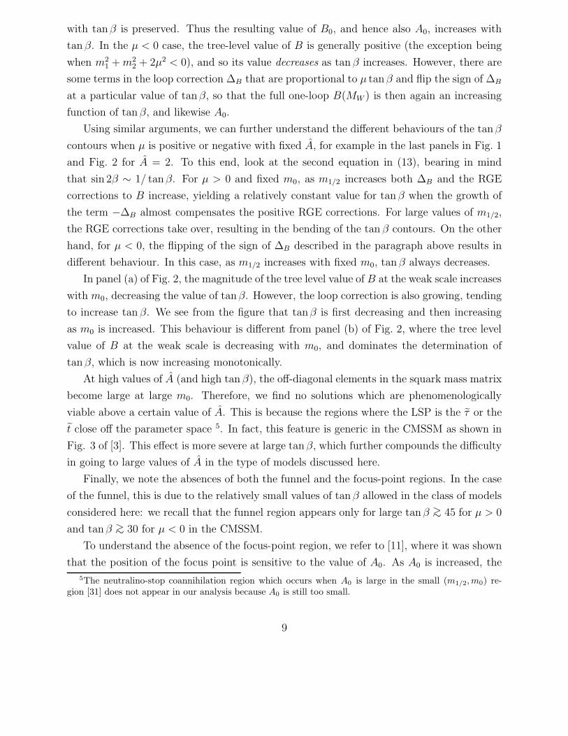
In the case of µ < 0, negative values of A are not allowed, and only a tiny area in the

(m1/2, m0) plane near the end point of the coannihilation tail around m1/2 = 1000 GeV is

allowed in the positive Polonyi case A = 3 − √3, as seen in panel (a) of Fig. 2. This is

because the Higgs and ΩCDMh2 constraints are barely compatible in this case, and allow

only tan β ' 4.15. At larger values of A, the allowed region is extended, as exemplified in

panel (b) of Fig. 2 for the case A = 2.0, where a small region around tan β ' 5.5 − 5.7 is

allowed. This panel shows that, approximately, the value of tanβ depends only on the ratio

m1/2/m0 [32].

There are several generic patterns in the results above that can be explained qualitatively,

as follows. First, we notice that for any given value of (m1/2, m0), tan β increases as A

increases. The reason for this can be found by looking at the second equation of (12), and

setting A0 = B0 + m0. For large tanβ, sin 2β ∼ 1/ tanβ, so B at the weak scale is inversely

proportional to tanβ, at the tree level. In the µ > 0 case, this tree-level value of B is

negative, so its value grows as tan β increases. While loop corrections are generally negative

for µ > 0, and RGE corrections to obtain B(MX) are positive, the monotonic growth of B0

3Note that the contours for given values of tanβ always intersect the axis m0 = 0 at the same value ofm1/2.

4The other Polonyi case with A = −3 +√

3 (not shown) is very similar to panel (a) for A = −1.5, andhas a very narrow allowed range of tanβ ∼ 4.5.

7

100 200 300 400 500 600 700 800 900 10000

100

200

300

400

500

100 200 300 400 500 600 700 800 900 10000

100

200

300

400

500

tan β = 5

m0

(GeV

)

m1/2 (GeV)

mh = 114 GeV

tan β = 10 = 15

A = -1.5; µ > 0^

100 200 300 400 500 600 700 800 900 10000

100

200

300

400

500

600

700

800

100 200 300 400 500 600 700 800 900 10000

100

200

300

400

500

600

700

800

tan β = 5

m0

(GeV

)

m1/2 (GeV)

mh = 114 GeV

tan β = 10

= 15

A = 0.75; µ > 0^

100 200 300 400 500 600 700 800 900 10000

100

200

300

400

500

600

700

800

100 200 300 400 500 600 700 800 900 10000

100

200

300

400

500

600

700

800

tan β = 15

m0

(GeV

)

m1/2 (GeV)

mh = 114 GeV

tan β = 10

= 10

tan β = 20

= 25

A = 3 - √3 ; µ > 0^

100 200 300 400 500 600 700 800 900 10000

100

200

300

400

500

600

700

800

100 200 300 400 500 600 700 800 900 10000

100

200

300

400

500

600

700

800

tan β = 25

m0

(GeV

)

m1/2 (GeV)

mh = 114 GeV

tan β = 30

= 35

tan β = 20 = 15

A = 2; µ > 0^

Figure 1: Examples of (m1/2, m0) planes with contours of tan β superposed, for µ > 0 and

(a) A = −1.5, B = A − 1, (b) A = 0.75, B = A − 1, (c) the simplest Polonyi modelwith A = 3 − √

3, B = A − 1 and (d) A = 2.0, B = A − 1. In each panel, we show theregions excluded by the LEP lower limits on MSSM particles, those ruled out by b → sγdecay [26] (medium green shading), and those excluded because the LSP would be charged(dark red shading). The region favoured by the WMAP range ΩCDMh2 = 0.1126+0.0081

−0.0091 haslight turquoise shading. The region suggested by gµ − 2 is medium (pink) shaded.

8

with tanβ is preserved. Thus the resulting value of B0, and hence also A0, increases with

tan β. In the µ < 0 case, the tree-level value of B is generally positive (the exception being

when m21 + m2

2 + 2µ2 < 0), and so its value decreases as tan β increases. However, there are

some terms in the loop correction ∆B that are proportional to µ tanβ and flip the sign of ∆B

at a particular value of tanβ, so that the full one-loop B(MW ) is then again an increasing

function of tanβ, and likewise A0.

Using similar arguments, we can further understand the different behaviours of the tanβ

contours when µ is positive or negative with fixed A, for example in the last panels in Fig. 1

and Fig. 2 for A = 2. To this end, look at the second equation in (13), bearing in mind

that sin 2β ∼ 1/ tanβ. For µ > 0 and fixed m0, as m1/2 increases both ∆B and the RGE

corrections to B increase, yielding a relatively constant value for tan β when the growth of

the term −∆B almost compensates the positive RGE corrections. For large values of m1/2,

the RGE corrections take over, resulting in the bending of the tan β contours. On the other

hand, for µ < 0, the flipping of the sign of ∆B described in the paragraph above results in

different behaviour. In this case, as m1/2 increases with fixed m0, tan β always decreases.

In panel (a) of Fig. 2, the magnitude of the tree level value of B at the weak scale increases

with m0, decreasing the value of tanβ. However, the loop correction is also growing, tending

to increase tan β. We see from the figure that tanβ is first decreasing and then increasing

as m0 is increased. This behaviour is different from panel (b) of Fig. 2, where the tree level

value of B at the weak scale is decreasing with m0, and dominates the determination of

tan β, which is now increasing monotonically.

At high values of A (and high tan β), the off-diagonal elements in the squark mass matrix

become large at large m0. Therefore, we find no solutions which are phenomenologically

viable above a certain value of A. This is because the regions where the LSP is the τ or the

t close off the parameter space 5. In fact, this feature is generic in the CMSSM as shown in

Fig. 3 of [3]. This effect is more severe at large tanβ, which further compounds the difficulty

in going to large values of A in the type of models discussed here.

Finally, we note the absences of both the funnel and the focus-point regions. In the case

of the funnel, this is due to the relatively small values of tanβ allowed in the class of models

considered here: we recall that the funnel region appears only for large tanβ >∼ 45 for µ > 0

and tanβ >∼ 30 for µ < 0 in the CMSSM.

To understand the absence of the focus-point region, we refer to [11], where it was shown

that the position of the focus point is sensitive to the value of A0. As A0 is increased, the

5The neutralino-stop coannihilation region which occurs when A0 is large in the small (m1/2, m0) re-gion [31] does not appear in our analysis because A0 is still too small.

9

100 200 300 400 500 600 700 800 900 10000

100

200

300

400

500

600

700

800

100 200 300 400 500 600 700 800 900 10000

100

200

300

400

500

600

700

800

tan β = 5

m0

(GeV

)

m1/2 (GeV)

tan β = 4

= 6

A = 3 - √3 ; µ < 0^

100 200 300 400 500 600 700 800 900 10000

100

200

300

400

500

600

700

800

100 200 300 400 500 600 700 800 900 10000

100

200

300

400

500

600

700

800

tan β = 8

m0

(GeV

)

m1/2 (GeV)

mh = 114 GeV

tan β = 10

= 20

tan β = 6

= 15

tan β = 5

A = 2; µ < 0^

Figure 2: As in Fig. 1, but now for µ < 0 and the choices (a) A = 3−√3, B = A − 1 and(b) A = 2, B = A− 1 and µ < 0.

focus point is pushed up to higher values of m0. Here, with A0 ∝ m0, the focus-point region

recedes faster than m0 if A is large enough, and is therefore never encountered. For small A,

tan β is small at large m0, as shown in panel (b) of Fig. 1, so we do not find a focus point in

this case, either. In addition, as can be inferred from the small disconnected segment of the

tan β = 10 contour in the top left corner of panel (c), all the tan β contours loop back down

to lower m0 before reaching the focus-point region.

The above analysis shows that the ‘bulk’ ΩCDMh2 region is almost completely excluded

by the Higgs constraint, but a larger fraction would be allowed if we allowed a 2-GeV error

in the CMSSM Higgs mass calculation, or if mt turns out to be significantly greater than

175 GeV. Almost all the coannihilation ‘tail’ region is allowed. As remarked on above, there

is no ‘funnel’ region at large m1/2 and m0, nor any ‘focus-point’ region at large m0.

6 Bounds on tan β

It is clear from the previous figures that only limited ranges of tan β are consistent with

the phenomenological constraints within any given pattern of supersymmetry breaking. We

display in Fig. 3 the ranges of tanβ allowed as a function of A. For B = A− 1 and µ > 0,

as shown by the solid lines, we see that the upper and lower limits on tanβ both increase

monotonically with A. We find consistent solutions to all the phenomenological constraints

10

only for

−1.9 < A < 2.5, (14)

over which range

3.7 < tanβ <∼ 46. (15)

Generally speaking, the range of tan β for any fixed value of A < 0 is very restricted, with

larger ranges of tan β becoming allowed for A > 0. In the specific case of the simplest Polonyi

model with positive A = 3−√3, we find

11 < tan β < 20, (16)

whereas the range in tan β for the negative Polonyi model with A =√

3 − 3, is 4.4 – 4.6.

Furthermore, the difference between the upper and lower limits on tan β never exceeds ∼ 14

for any fixed value of A.

The corresponding results for µ < 0 are

1.2 < A < 4.8, (17)

over which range

4 < tanβ <∼ 26. (18)

The range of A is shifted, and the range of tan β reduced, as compared to the case of µ > 0.

In particular, the negative Polonyi model is disallowed and the positive version is allowed

only for tan β ∼ 4.15.

7 No-Scale Models

We display in Fig. 4 the results of a similar analysis for the no-scale case A = B = 0. For

µ > 0, the allowed range of tanβ is

16 < tan β < 30, (19)

where the lower limit is provided by the Higgs search, and the upper limit is at the tip of

the coannihilation ‘tail’. For µ < 0, the same constraints allow just a small range around

tan β ∼ 4.8. These two ranges are both shown as ‘error bars’ in Fig. 3.

However, the other no-scale condition m0 = 0 is not allowed for either sign of µ, the

minimum being m0 ' 62 GeV for µ > 0 and tanβ ' 16. The fact that m0 6= 0 is no surprise,

since the same conclusion was reached previously without imposing the supplementary no-

scale conditions A = B = 0 [13]. However, as we have already pointed out, the no-scale

11

-2 -1 0 1 2 3 4 51

10

20

30

40

50ta

n β

A = A0/m0

µ > 0

µ < 0

^

Figure 3: The ranges of tanβ allowed if B = A−1 for µ > 0 (solid lines) and µ < 0 (dashedlines). The Polonyi model corresponds to A ' ±1.3. Also shown as ‘error bars’ are theranges of tan β allowed in the no-scale case A = B = 0 for µ > 0 (upper) and µ < 0 (lower).

12

100 200 300 400 500 600 700 800 900 10000

100

200

300

400

500

600

700

800

100 200 300 400 500 600 700 800 900 10000

100

200

300

400

500

600

700

800

tan β = 30

m0

(GeV

)

m1/2 (GeV)

µ > 0

mh = 114 GeV

tan β = 25

= 35

tan β = 20

= 15

100 200 300 400 500 600 700 800 900 10000

100

200

300

400

500

600

700

800

100 200 300 400 500 600 700 800 900 10000

100

200

300

400

500

600

700

800

tan β = 10

m0

(GeV

)

m1/2 (GeV)

µ < 0

mh = 114 GeV

= 15

tan β = 5

= 20

Figure 4: As in Fig. 1, for the no-scale cases A = 0, B = 0 and (a) µ > 0, (b) µ < 0.

boundary conditions should be interpreted as applying at the supergravity scale, so it is

possible that m0, A, B all 6= 0, albeit small, at the GUT scale. We note that in this case,

there is in fact a focus-point region at roughly the same position as in the CMSSM with

A0 = 0.

8 Conclusions

We have shown in this paper that only a restricted range of tan β is allowed in any specific

pattern of supersymmetry breaking. We have illustrated this point by discussions of minimal

supergravity models with A = B + 1 and no-scale models with A = B = 0, but the same

comment would apply to other models of supersymmetry breaking not discussed here. Within

the class of minimal supergravity models, we have selected in particular the simplest Polonyi

model with |A| = 3−√3, but also discussed models with other values of A, finding a rather

restricted range, in particular for µ < 0.

One inference from our analysis is that an experimental determination of tanβ could be

a useful discriminator between different models of supersymmetry breaking. To understand

the potential scope of this analysis tool, it would be necessary to study a wider class of

models of supersymmetry breaking than those discussed here.

13

Acknowledgments

The work of K.A.O., Y.S., and V.C.S. was supported in part by DOE grant DE–FG02–

94ER–40823.

References

[1] For reviews, see: H. P. Nilles, Phys. Rep. 110 (1984) 1; A. Brignole, L. E. Ibanez

and C. Munoz, arXiv:hep-ph/9707209, published in Perspectives on supersymmetry, ed.

G. L. Kane, pp. 125-148.

[2] J. Ellis, T. Falk, G. Ganis, K. A. Olive and M. Schmitt, Phys. Rev. D58 (1998) 095002

[arXiv:hep-ph/9801445].; J. R. Ellis, K. A. Olive and Y. Santoso, New J. Phys. 4 (2002)

32 [arXiv:hep-ph/0202110].

[3] J. R. Ellis, T. Falk, G. Ganis and K. A. Olive, Phys. Rev. D 62 (2000) 075010 [arXiv:hep-

ph/0004169].

[4] J. R. Ellis, T. Falk, G. Ganis, K. A. Olive and M. Srednicki, Phys. Lett. B 510 (2001)

236 [arXiv:hep-ph/0102098].

[5] J. R. Ellis, K. A. Olive, Y. Santoso and V. C. Spanos, arXiv:hep-ph/0303043.

[6] A. B. Lahanas, D. V. Nanopoulos and V. C. Spanos, Phys. Rev. D 62 (2000) 023515

[arXiv:hep-ph/9909497]; V. Barger and C. Kao, Phys. Lett. B518 (2001) 117 [arXiv:hep-

ph/0106189]; L. Roszkowski, R. Ruiz de Austri and T. Nihei, JHEP 0108 (2001) 024

[arXiv:hep-ph/0106334]; A. Djouadi, M. Drees and J. L. Kneur, JHEP 0108 (2001) 055

[arXiv:hep-ph/0107316]; R. Arnowitt and B. Dutta, arXiv:hep-ph/0211417; H. Baer,

C. Balazs and A. Belyaev, JHEP 0203 (2002) 042 [arXiv:hep-ph/0202076]; T. Kamon,

R. Arnowitt, B. Dutta and V. Khotilovich, arXiv:hep-ph/0302249; H. Baer, C. Balazs,

A. Belyaev, T. Krupovnickas and X. Tata, arXiv:hep-ph/0304303.

[7] J. R. Ellis, T. Falk and K. A. Olive, Phys. Lett. B 444 (1998) 367 [arXiv:hep-

ph/9810360]; J. R. Ellis, T. Falk, K. A. Olive and M. Srednicki, Astropart. Phys.

13 (2000) 181 [Erratum-ibid. 15 (2001) 413] [arXiv:hep-ph/9905481]; R. Arnowitt,

B. Dutta and Y. Santoso, Nucl. Phys. B 606 (2001) 59 [arXiv:hep-ph/0102181].

[8] M. E. Gomez, G. Lazarides and C. Pallis, Phys. Rev. D D61 (2000) 123512 [arXiv:hep-

ph/9907261]; Phys. Lett. B487 (2000) 313 [arXiv:hep-ph/0004028]; Nucl. Phys. B B638

14

(2002) 165 [arXiv:hep-ph/0203131]; T. Nihei, L. Roszkowski and R. Ruiz de Austri,

JHEP 0207 (2002) 024 [arXiv:hep-ph/0206266].

[9] M. Drees and M. M. Nojiri, Phys. Rev. D 47 (1993) 376 [arXiv:hep-ph/9207234]; H. Baer

and M. Brhlik, Phys. Rev. D 53 (1996) 597 [arXiv:hep-ph/9508321]; H. Baer, M. Brhlik,

M. A. Diaz, J. Ferrandis, P. Mercadante, P. Quintana and X. Tata, Phys. Rev. D 63

(2001) 015007 [arXiv:hep-ph/0005027]; A. B. Lahanas and V. C. Spanos, Eur. Phys. J.

C 23 (2002) 185 [arXiv:hep-ph/0106345].

[10] J. L. Feng, K. T. Matchev and T. Moroi, Phys. Rev. Lett. 84 (2000) 2322; J. L. Feng,

K. T. Matchev and T. Moroi, Phys. Rev. D61 (2000) 075005; J. L. Feng, K. T. Matchev

and F. Wilczek, Phys. Lett. B482 (2000) 388.

[11] K. L. Chan, U. Chattopadhyay and P. Nath, Phys. Rev. D 58 (1998) 096004 [arXiv:hep-

ph/9710473].

[12] E. Cremmer, S. Ferrara, C. Kounnas and D. V. Nanopoulos, Phys. Lett. B 133 (1983)

61; J. R. Ellis, A. B. Lahanas, D. V. Nanopoulos and K. Tamvakis, Phys. Lett. B 134

(1984) 429; A. B. Lahanas and D. V. Nanopoulos, Phys. Rept. 145 (1987) 1.

[13] J. R. Ellis, D. V. Nanopoulos and K. A. Olive, Phys. Lett. B 525 (2002) 308 [arXiv:hep-

ph/0109288].

[14] E. Cremmer, B. Julia, J. Scherk, S. Ferrara, L. Girardello and P. Van Nieuwenhuizen,

Phys. Lett. 79B (1978) 231; and Nucl. Phys. B147 (1979) 105; E. Cremmer, S. Ferrara,

L. Girardello and A. Van Proeyen, Phys. Lett. 116B (1982) 231; and Nucl. Phys. B212

(1983) 413; R. Arnowitt, A.H. Chamseddine and P. Nath, Phys. Rev. Lett. 49 (1982)

970; 50 (1983) 232 and Phys. Lett. 121B (1983) 33; J. Bagger and E. Witten, Phys.

Lett. 115B (1982) 202 and 118B (1982) 103; J. Bagger, Nucl. Phys. B211 (1983) 302.

[15] H.-P. Nilles, M. Srednicki and D. Wyler, Phys. Lett. 120B (1983) 345; L.J. Hall, J.

Lykken and S. Weinberg, Phys. Rev. D27 (1983) 2359.

[16] J. Polonyi, Budapest preprint KFKI-1977-93 (1977).

[17] R. Barbieri, S. Ferrara and C.A. Savoy, Phys. Lett. 119B (1982) 343.

[18] M. Endo, M. Matsumura and M. Yamaguchi, Phys. Lett. B 544 (2002) 161 [arXiv:hep-

ph/0204349].

15

[19] R. Arnowitt and P. Nath, Phys. Rev. D 46 (1992) 3981; V. D. Barger, M. S. Berger

and P. Ohmann, Phys. Rev. D 49 (1994) 4908 [arXiv:hep-ph/9311269].

[20] W. de Boer, R. Ehret and D. I. Kazakov, Z. Phys. C 67 (1995) 647 [arXiv:hep-

ph/9405342]; D. M. Pierce, J. A. Bagger, K. T. Matchev and R. J. Zhang, Nucl. Phys.

B 491 (1997) 3 [arXiv:hep-ph/9606211].

[21] M. Carena, J. R. Ellis, A. Pilaftsis and C. E. Wagner, Nucl. Phys. B 625 (2002) 345

[arXiv:hep-ph/0111245].

[22] Joint LEP 2 Supersymmetry Working Group, Combined LEP Chargino Results, up to

208 GeV,

http://lepsusy.web.cern.ch/lepsusy/www/inos moriond01/charginos pub.html.

[23] Joint LEP 2 Supersymmetry Working Group, Combined LEP Selectron/Smuon/Stau

Results, 183-208 GeV,

http://lepsusy.web.cern.ch/lepsusy/www/sleptons summer02/slep 2002.html.

[24] LEP Higgs Working Group for Higgs boson searches, OPAL Collaboration, ALEPH

Collaboration, DELPHI Collaboration and L3 Collaboration, Search for the Standard

Model Higgs Boson at LEP, CERN-EP/2003-011, available from

http://lephiggs.web.cern.ch/LEPHIGGS/papers/index.html.

[25] S. Heinemeyer, W. Hollik and G. Weiglein, Comput. Phys. Commun. 124 (2000) 76

[arXiv:hep-ph/9812320]; S. Heinemeyer, W. Hollik and G. Weiglein, Eur. Phys. J. C 9

(1999) 343 [arXiv:hep-ph/9812472].

[26] M.S. Alam et al., [CLEO Collaboration], Phys. Rev. Lett. 74 (1995) 2885 as updated

in S. Ahmed et al., CLEO CONF 99-10; BELLE Collaboration, BELLE-CONF-0003,

contribution to the 30th International conference on High-Energy Physics, Osaka, 2000.

See also K. Abe et al., [Belle Collaboration], [arXiv:hep-ex/0107065]; L. Lista [BaBar

Collaboration], [arXiv:hep-ex/0110010]; C. Degrassi, P. Gambino and G. F. Giudice,

JHEP 0012 (2000) 009 [arXiv:hep-ph/0009337]; M. Carena, D. Garcia, U. Nierste and

C. E. Wagner, Phys. Lett. B 499 (2001) 141 [arXiv:hep-ph/0010003]; P. Gambino and

M. Misiak, Nucl. Phys. B 611 (2001) 338; D. A. Demir and K. A. Olive, Phys. Rev. D

65 (2002) 034007 [arXiv:hep-ph/0107329]; T. Hurth, arXiv:hep-ph/0212304.

[27] G. W. Bennett et al. [Muon g-2 Collaboration], Phys. Rev. Lett. 89 (2002) 101804

[Erratum-ibid. 89 (2002) 129903] [arXiv:hep-ex/0208001].

16

[28] M. Davier, S. Eidelman, A. Hocker and Z. Zhang, arXiv:hep-ph/0208177; see also

K. Hagiwara, A. D. Martin, D. Nomura and T. Teubner, arXiv:hep-ph/0209187;

F. Jegerlehner, unpublished, as reported in M. Krawczyk, arXiv:hep-ph/0208076.

[29] C. L. Bennett et al., arXiv:astro-ph/0302207; D. N. Spergel et al., arXiv:astro-

ph/0302209.

[30] U. Chattopadhyay, A. Corsetti and P. Nath, arXiv:hep-ph/0303201; H. Baer and

C. Balazs, arXiv:hep-ph/0303114; A. B. Lahanas and D. V. Nanopoulos, arXiv:hep-

ph/0303130.

[31] J. R. Ellis, K. A. Olive and Y. Santoso, Astropart. Phys. 18 (2003) 395 [arXiv:hep-

ph/0112113]; C. Boehm, A. Djouadi and M. Drees, Phys. Rev. D 62 (2000) 035012

[arXiv:hep-ph/9911496].

[32] J. Tabei and H. Hotta, arXiv:hep-ph/0208039.

17