arX

iv:h

ep-l

at/0

2060

29v1

25

Jun

2002

Oxford preprint OUTP-02-28P

The deconfinement transition in SU(N) gauge theories

Biagio Lucini, Michael Teper and Urs Wenger

Theoretical Physics, University of Oxford,1 Keble Road, Oxford, OX1 3NP, U.K.

Abstract

We investigate the properties of the deconfinement transition in SU(4) and SU(6) gaugetheories. We find that it is a ‘normal’ first order transition in both cases, from which weconclude that the transition is first order in the N → ∞ limit. Comparing our prelimi-nary estimates of the continuum values of Tc/

√σ with existing values for SU(2) and SU(3)

demonstrates a weak dependence on N for all values of N .

1 Introduction

The dependence of QCD and SU(N) gauge theories on the number of colours, N , is of greatinterest [1, 2]. Through a number of recent lattice calculations [2, 3, 4, 5, 6, 7] we havelearned a great deal about the mass spectrum, various string tensions and the topologicalproperties of SU(N) gauge theories at finite and infinite N . These calculations confirm theusual diagrammatic expectation that a smooth large-N physics limit is achieved by keepingfixed the ’t Hooft coupling g2N . In addition there is some good evidence from very accuratecalculations of the string tension, σ, in 2+1 dimensional gauge theories [8], that the leadingcorrections are O(1/N2) – again as expected. (Note however that there is room for a violationof this [2], but the evidence is equivocal as yet.)

An interesting question concerns the order of the deconfining phase transition at N = ∞.It has been argued [9] that the difference between the SU(3) gauge theory and QCD with lightquarks (see [10] for recent reviews) can be reconciled with both being ‘close to’ large-N if infact the SU(N) transition becomes second order at large-N . (See [11] for some more recentreflections on this.) This has prompted lattice studies [12, 13] of deconfinement in SU(4)which claim that the transition is first order there. However it is only in SU(6), or largergroups, that all possible escape routes close [9]. Thus we hope that the calculations in bothSU(4) and SU(6) gauge theories [14] that we shall briefly report upon in this paper will serveto settle this question. (See also [15] for calculations at very large N , performed in a twistedEguchi-Kawai single-site reduced model [16].)

In this letter we focus upon the order of the transition and upon our preliminary deter-mination of how the critical temperature, Tc, varies with N . There are of course many otherinteresting aspects of the transition, some of which we are studying. We will mention someof these in the concluding section, and will present our detailed results in a longer publi-cation [14]. There we will also discuss and compare several different methods for locatingand analysing the deconfining phase transition. We will, in addition, apply these methods tothe case of SU(2), where the transition is known to be 2nd order [17], and SU(3), where itis known to be weakly 1st order [18]. At the same time we will have higher statistics whichshould allow us to considerably improve upon the preliminary continuum values of Tc/

√σ that

we present in this paper. However, we believe that we already have unambiguous evidence forthe first order nature of the SU(4) and SU(6) phase transitions and this is what we wish tocommunicate in this letter.

2 Strategy and technical details

Our lattices are hyper-cubic with periodic boundary conditions and with lattice spacing a.We use the standard plaquette action

S = β∑

p

{1 − 1

NReTrUp} (1)

1

where the ordered product of the SU(N) matrices around the boundary of the plaquette p isrepresented by Up. In the continuum limit this becomes the usual Yang-Mills action with

β =2N

g2. (2)

The simulations are performed with a combination of heat bath and over-relaxation updates,as described in [4, 3]. Our SU(4) and SU(6) updates involve 6 and 15 SU(2) subgroupsrespectively.

Consider a lattice whose size is L3Lt in lattice units. This may be regarded as a systemat temperature

a(β)T =1

Lt

. (3)

We require L ≫ Lt, so that it makes sense to discuss thermodynamics. We study the decon-fining transition by fixing Lt and varying β so that T passes through Tc.

For T < Tc we are in the confining phase, while for T > Tc we will be in one of N equivalentdeconfined phases. To distinguish all these phases we define the Polyakov loop

lp(~x) = Tr∏

t

Ut(~x, t) (4)

and denote by lp its average over ~x for a given field configuration. For T < Tc we will havelp ≃ 0 while for T > Tc the N deconfined vacua will be characterised by values lp ≃ czn wherezn is one of the N ’th roots of unity and c > 0 will depend on β, Lt, N etc. For L large enoughthe fluctuations of lp become small enough that a field configuration can be unambiguouslycategorised into one of the phases by its value of lp. Near Tc there may be tunnelling betweenthese phases. This process will involve field configurations that contain a mix of phases andwill have intermediate values of lp. Note that the usual characteristic of first order latticetransitions, a clear double peak structure when one plots a histogram of the number of fieldsagainst the action (energy) is not so useful here. This is because we are dealing with a physicalrather than a bulk transition. Any difference in the action will therefore be O(a4) and thisis extremely small compared to the O(1/β) value of the action. It is only on the very largestlattices that the fluctuations in the latter, which are also O(1/

√L3), become small enough

for the beginnings of a double peak structure to appear. By contrast, clear multiple peakstructures in histograms of lp already appear on small lattices.

In a finite spatial volume V the phase transition is smeared over a finite range of T . Oneneeds to choose a value for Tc(V ) in this range and then to extrapolate this to V = ∞ toobtain the value of Tc in the thermodynamic limit. Different criteria will differ at finite V butshould extrapolate to the same value of Tc at V = ∞. Good criteria will be ones with finite-Vcorrections that are simple, small and have a known functional form. We have performedcalculations with a number of criteria which produce consistent results. In this paper wepresent values of βc obtained from the value of β at which the Polyakov loop susceptibilityhas a peak. To obtain the susceptibility as a continuous function of β we use a standardreweighting technique [19] applied to those calculations that lie close enough to Tc. This willbe described in some more detail in the next Section.

2

Tunnelling between the confined and deconfined vacua is a first sign that the phase tran-sition is first order. However its observation at T 6= Tc and/or on small volumes may bemisleading. Equally a lack of tunnelling on small volumes may be misleading; for example,the transition may be weakly first order. It is therefore crucial to perform a finite volumestudy to identify what volumes are large enough to be useful. Given that near Tc the impor-tant length scale is aLt = 1/Tc one would expect that one needs at least L ≃ 3Lt in orderthat the periodic spatial volume can accommodate two phases and some intervening surfacein a realistic fashion. In a finite volume study a first order transition would be characterised,at large V , by a latent heat that stays non-zero, a mass gap that does not vanish (i.e. acorrelation length that does not diverge), an appropriately behaved susceptibility, and cleartunnelling that becomes exponentially rare as V grows.

The computational cost will clearly be minimised by using the smallest possible valuesof Lt. It is however well known that with the standard plaquette lattice action there is across-over in the strong-to-weak coupling transition region which becomes a strong first-orderphase transition at larger N . (See e.g. [4] for a discussion.) For SU(4) this appears to besmooth cross-over [4] but by SU(6) it is certainly a strongly first order bulk phase transition[5]. This presents some problems. In particular any calculations that are going to be useful forcontinuum extrapolations will need to be made on the weak-coupling side of this transition.For SU(4) deconfinement this means that we have to use Lt ≥ 5. For SU(6) the finite-Ttransition for Lt = 5 is quite close to the strongly first order bulk phase transition and sothis would not be a good place to address the delicate question of whether the former is alsofirst order or not. For that we will use Lt = 6. However the computational expense of SU(6)calculations at Lt = 6 is such that we will not be able to perform the kind of finite sizestudy that distinguishes most unambiguously between 1st and 2nd order phase transitions.Fortunately the phase transition turns out to be reasonably strong first order, rather thanbeing weak first order as in SU(3). This makes it relatively easy to study, even within ourtight constraints.

Our strategy will therefore be as follows. We start with SU(4) where we perform a detailedfinite size study of the deconfining transition for lattices with Lt = 5. We shall establish thatit is first order and will quantify its dependence on the spatial volume. We then perform astudy of the SU(6) phase transition on a 1636 lattice, using our earlier finite-size study toextrapolate it to the thermodynamic limit. We also have begun calculations in SU(4) forLt = 6 and in SU(6) for Lt = 5; these enable us to make some preliminary estimates of Tc/

√σ

in the continuum limit. At the same time the Lt = 6 SU(4) calculations provide for a directcomparison with the SU(6) calculations at Lt = 6.

3 Tc in SU(4)

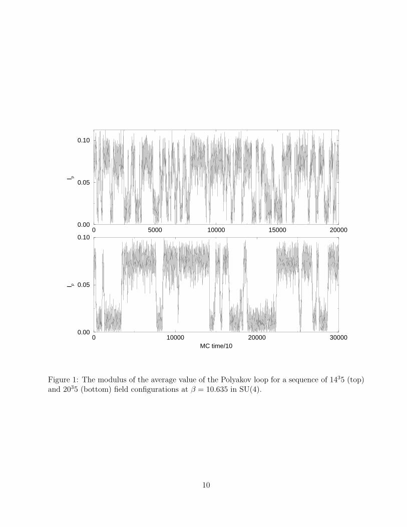
Our Lt = 5 study has been performed on L = 12, 14, 16, 18, 20 lattices, with between 200000to 300000 sweeps at each value of β and L. For β in a narrow region around β = 10.635we find very clear tunnelling transitions on all lattice sizes. These become more rare as L ↑,just as one would expect for a first order transition. In Fig.1 we illustrate this with the time

3

histories of |lp| on the L = 14 and L = 20 lattices at β = 10.635.We define a normalised Polyakov loop susceptibility

χl

V= 〈|lp|2〉 − 〈|lp|〉2 (5)

where we expect

limT→Tc

χlV →∞∝

{

V, if 1’st orderV γ, if 2’nd order

(6)

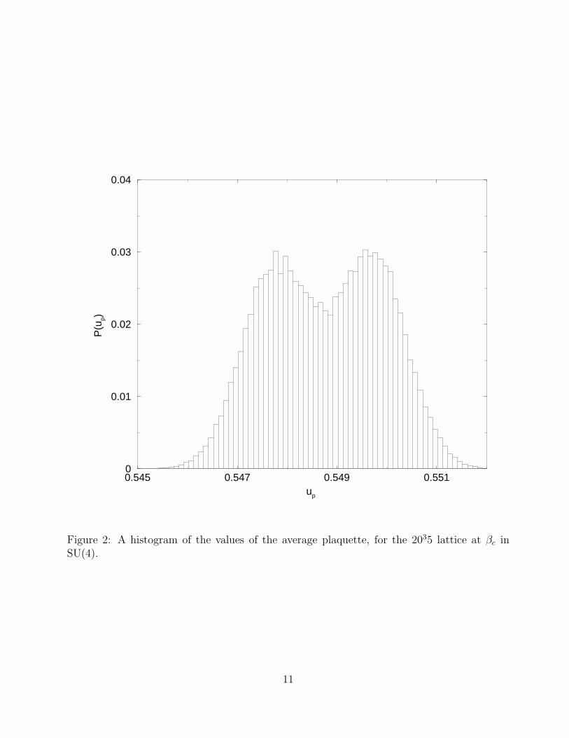
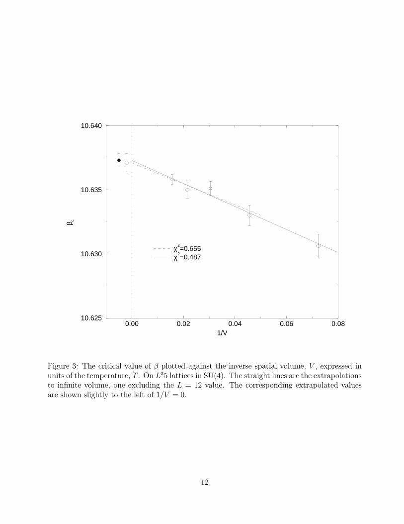
with γ a constant that depends on both the space-time dimension and the critical exponentsof the transition. For each value of L we calculate χl as a function of β, determine the valueat which it has a maximum and use that as our estimate of βc, and hence Tc. This is a good,although not unique, criterion irrespective of whether the transition is first or second order.To identify the maximum we interpolate between the values of β at which we have performedcalculations (usually there are three that have sufficient tunnellings to be useful) using astandard reweighting technique [19]. Fig.2 shows a histogram of the plaquette, averaged overthe lattice volume, for the 2035 lattices reweighted to the critical beta-value. It clearly showsthe double peaking that is characteristic of a first order transition. In Fig.3 we plot our valuesof βc against the inverse volume expressed in units of T . We note that if the transition is firstorder, as our’s clearly is, then there exist arguments [18] that with this way of determining βc

the leading finite-V correction should be

βc(V ) = βc(∞) − h

V T 3. (7)

Here h is independent of the lattice action and of the lattice spacing a up to lattice correctionsthat will be small if a is small. We observe from Fig.3 that all our values of βc are consistentwith eqn(7). Moreover the value of h we thus extract

h = 0.09 ± 0.02 (8)

is close to the SU(3) value, h ≃ 0.1 [18]. We take this to imply that h depends weakly on Nand will use the value in eqn(8) to extrapolate to V = ∞ in the SU(6) case where we do notperform an explicit finite volume study. We remark that if h is indeed independent of N , thenthis implies that the volume dependence of Tc(V )/Tc(∞) is O(1/N2), i.e. there is no volumedependence in the N → ∞ limit.

A quantity analogous to χl, but with plaquettes replacing the Polyakov loop, is the specificheat C(β):

1

β2C(β) =

∂

∂β〈up〉 = Np〈u2

p〉 − Np〈up〉2 (9)

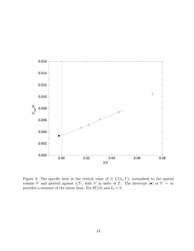
where up is the average value for a given lattice field of the plaquette up ≡ ReTrUp/N , andNp = 6L3Lt is the total number of plaquettes. In Fig.4 we plot C(βc)/V against 1/V . Weobserve that it is certainly consistent with going to a finite value as V → ∞, as one wouldexpect for a first order transition. We show in Fig.4 a fit with a leading linear correctionin 1/V of the kind that one would expect irrespective of whether the transition was first or

4

second order. For a first order transition, as we appear to have here, we can obtain the latentheat, Lh, from the intercept

limV →∞

1

β2c Np

C(βc) =1

4(〈up,c〉 − 〈up,d〉)2 =

1

4L2

h (10)

where up,c and up,d are the average plaquette values at β = βc in the confined and deconfinedphases respectively. From the fit in Fig.4 we obtain

Lh = 0.00197(5). (11)

We note that if we take the Lt = 4 SU(3) latent heat in [20] and naively scale it to Lt = 5, weobtain Lh(N = 3) ≃ 0.0013 which is substantially smaller than our above SU(4) value. Thisshows explicitly that the SU(4) transition is more strongly first-order than the SU(3) one.

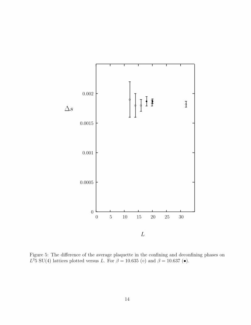
We have seen in Fig.1 that the value of lp allows us to label the phase of a field configurationalmost unambiguously. So for values of β close to βc, where all phases are sampled, we cancalculate the average plaquette in each phase separately and hence the difference ∆s betweenthe confined and deconfined phases. Calculated at βc this is the finite-V latent heat of thetransition. There is some uncertainty in separating configurations in a single phase from thosethat are tunnelling. This is a systematic error that we can estimate by varying the cuts on lp,and we include it in our final error estimates. In Fig.5 we show how ∆s varies with the spatialsize, L, for those of our calculations that are closest to βc (see Fig.3). We see that the latentheat is at most weakly dependent on the spatial volume and appears to have a finite V = ∞limit, confirming once again that this is a first order phase transition. The value is pleasinglyclose to that in eqn(11), which has been obtained under very different assumptions.

The value of ∆s provides a measure of how strong is the transition. To express it inphysical units we note that if one separates the plaquette into an ultraviolet perturbativepiece and the gluon condensate [21], then the lattice renormalisation factor multiplying thelatter is Z ≃ 1. Thus we can express ∆s ≡ a4m4

s where ms is a physical scale. Noting thatfor β ≃ βc we have ∆s ≃ 0.002 and that aTc = 1/Lt = 0.2 we see that ms ≃ Tc; that isto say, a typical dynamical scale indicating that the strength of this first order transition isquite ordinary. We remark that our preliminary calculations with Lt = 6 indicate that latticecorrections are small and that this statement holds in the continuum limit.

From the fit in Fig.3 we obtain the V = ∞ critical value βc = 10.63709(72). Interpolatingpreviously calculated values of the string tension [4] to βc, and using Tc = 1/5a(βc), we obtain

Tc√σ

= 0.6024 ± 0.0045 at a = 1/5Tc (12)

where the bulk of the error comes from the string tension. If lattice corrections are very small,as is found to be the case in SU(3) [18], then eqn(12) should provide a good estimate of thevalue in the continuum limit. In fact our very preliminary Lt = 6 calculations give a V = ∞value βc = 10.780(10) which translates to Tc/

√σ = 0.597(8), where the major part of the

error comes from the uncertainty in βc. This, taken together with the value in eqn(11), gives

5

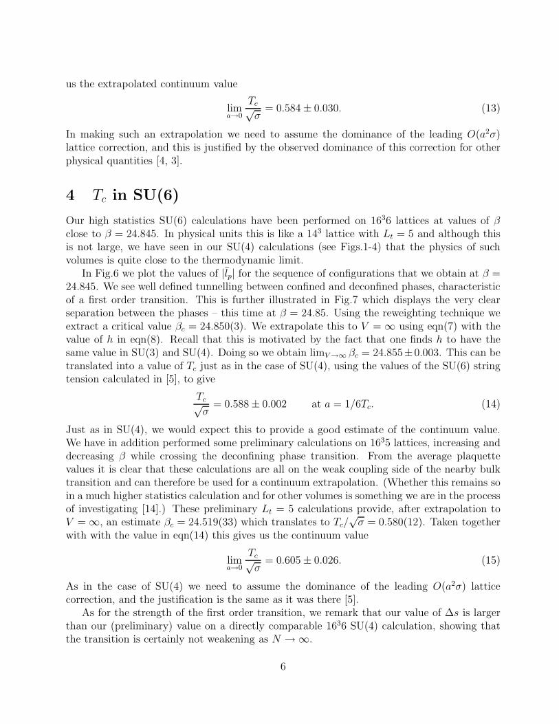
us the extrapolated continuum value

lima→0

Tc√σ

= 0.584 ± 0.030. (13)

In making such an extrapolation we need to assume the dominance of the leading O(a2σ)lattice correction, and this is justified by the observed dominance of this correction for otherphysical quantities [4, 3].

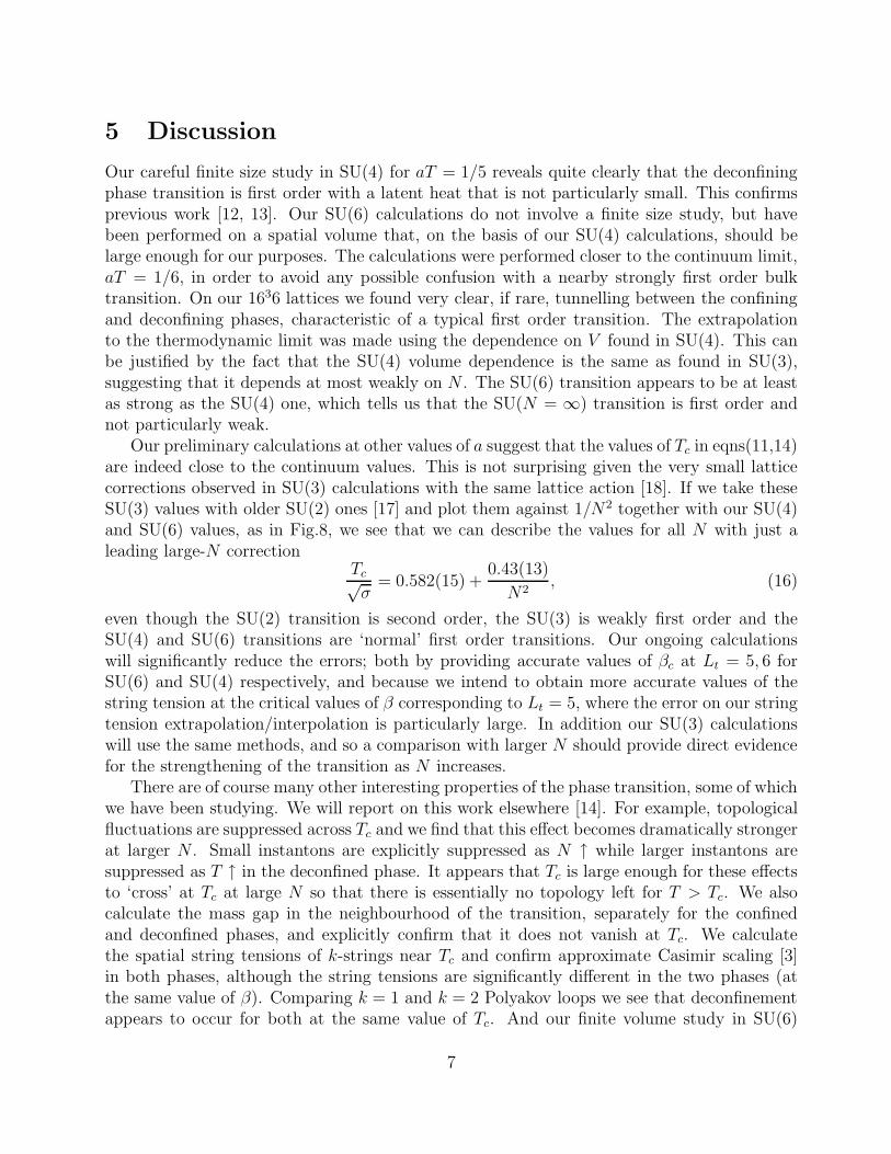
4 Tc in SU(6)

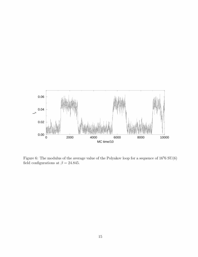
Our high statistics SU(6) calculations have been performed on 1636 lattices at values of βclose to β = 24.845. In physical units this is like a 143 lattice with Lt = 5 and although thisis not large, we have seen in our SU(4) calculations (see Figs.1-4) that the physics of suchvolumes is quite close to the thermodynamic limit.

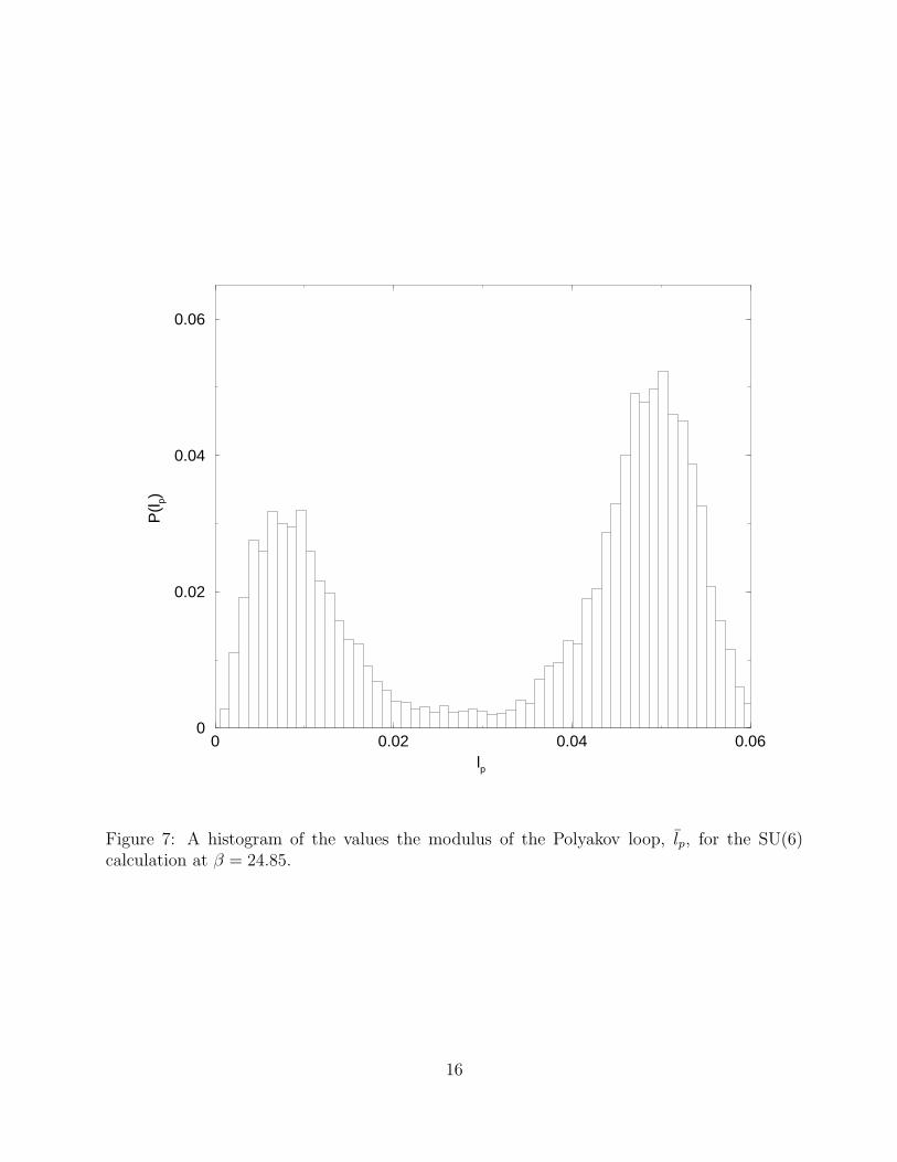
In Fig.6 we plot the values of |lp| for the sequence of configurations that we obtain at β =24.845. We see well defined tunnelling between confined and deconfined phases, characteristicof a first order transition. This is further illustrated in Fig.7 which displays the very clearseparation between the phases – this time at β = 24.85. Using the reweighting technique weextract a critical value βc = 24.850(3). We extrapolate this to V = ∞ using eqn(7) with thevalue of h in eqn(8). Recall that this is motivated by the fact that one finds h to have thesame value in SU(3) and SU(4). Doing so we obtain limV →∞

βc = 24.855±0.003. This can betranslated into a value of Tc just as in the case of SU(4), using the values of the SU(6) stringtension calculated in [5], to give

Tc√σ

= 0.588 ± 0.002 at a = 1/6Tc. (14)

Just as in SU(4), we would expect this to provide a good estimate of the continuum value.We have in addition performed some preliminary calculations on 1635 lattices, increasing anddecreasing β while crossing the deconfining phase transition. From the average plaquettevalues it is clear that these calculations are all on the weak coupling side of the nearby bulktransition and can therefore be used for a continuum extrapolation. (Whether this remains soin a much higher statistics calculation and for other volumes is something we are in the processof investigating [14].) These preliminary Lt = 5 calculations provide, after extrapolation toV = ∞, an estimate βc = 24.519(33) which translates to Tc/

√σ = 0.580(12). Taken together

with with the value in eqn(14) this gives us the continuum value

lima→0

Tc√σ

= 0.605 ± 0.026. (15)

As in the case of SU(4) we need to assume the dominance of the leading O(a2σ) latticecorrection, and the justification is the same as it was there [5].

As for the strength of the first order transition, we remark that our value of ∆s is largerthan our (preliminary) value on a directly comparable 1636 SU(4) calculation, showing thatthe transition is certainly not weakening as N → ∞.

6

5 Discussion

Our careful finite size study in SU(4) for aT = 1/5 reveals quite clearly that the deconfiningphase transition is first order with a latent heat that is not particularly small. This confirmsprevious work [12, 13]. Our SU(6) calculations do not involve a finite size study, but havebeen performed on a spatial volume that, on the basis of our SU(4) calculations, should belarge enough for our purposes. The calculations were performed closer to the continuum limit,aT = 1/6, in order to avoid any possible confusion with a nearby strongly first order bulktransition. On our 1636 lattices we found very clear, if rare, tunnelling between the confiningand deconfining phases, characteristic of a typical first order transition. The extrapolationto the thermodynamic limit was made using the dependence on V found in SU(4). This canbe justified by the fact that the SU(4) volume dependence is the same as found in SU(3),suggesting that it depends at most weakly on N . The SU(6) transition appears to be at leastas strong as the SU(4) one, which tells us that the SU(N = ∞) transition is first order andnot particularly weak.

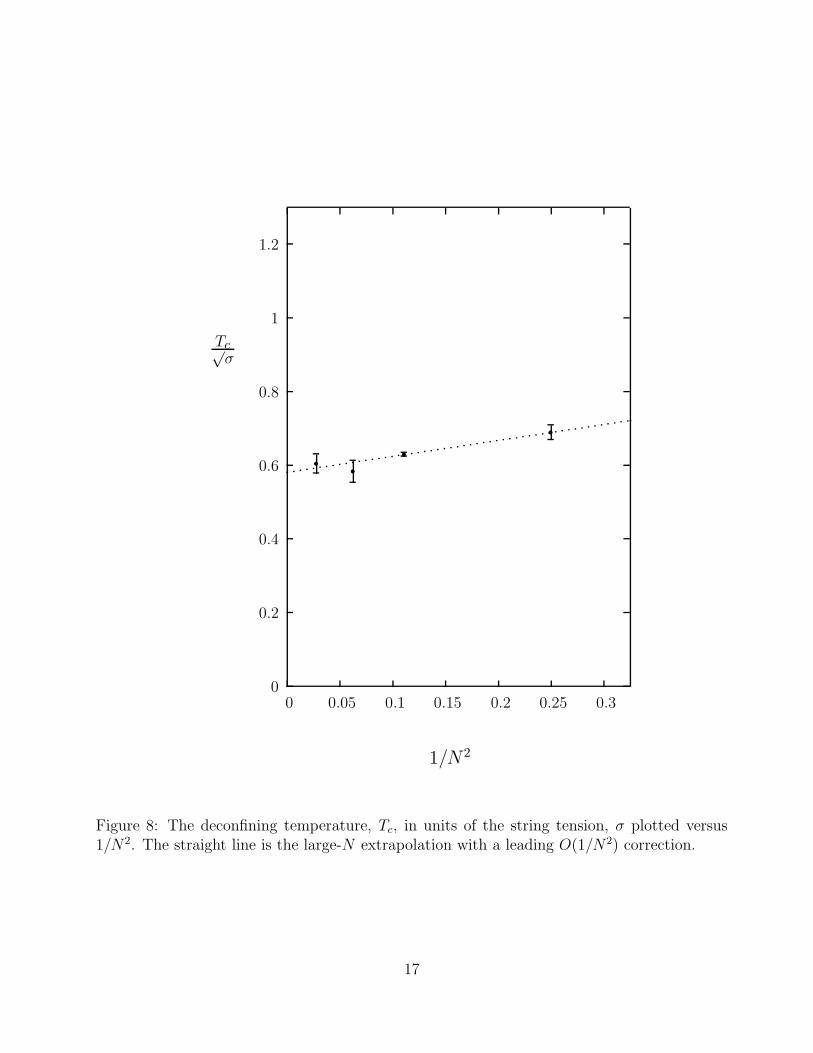
Our preliminary calculations at other values of a suggest that the values of Tc in eqns(11,14)are indeed close to the continuum values. This is not surprising given the very small latticecorrections observed in SU(3) calculations with the same lattice action [18]. If we take theseSU(3) values with older SU(2) ones [17] and plot them against 1/N2 together with our SU(4)and SU(6) values, as in Fig.8, we see that we can describe the values for all N with just aleading large-N correction

Tc√σ

= 0.582(15) +0.43(13)

N2, (16)

even though the SU(2) transition is second order, the SU(3) is weakly first order and theSU(4) and SU(6) transitions are ‘normal’ first order transitions. Our ongoing calculationswill significantly reduce the errors; both by providing accurate values of βc at Lt = 5, 6 forSU(6) and SU(4) respectively, and because we intend to obtain more accurate values of thestring tension at the critical values of β corresponding to Lt = 5, where the error on our stringtension extrapolation/interpolation is particularly large. In addition our SU(3) calculationswill use the same methods, and so a comparison with larger N should provide direct evidencefor the strengthening of the transition as N increases.

There are of course many other interesting properties of the phase transition, some of whichwe have been studying. We will report on this work elsewhere [14]. For example, topologicalfluctuations are suppressed across Tc and we find that this effect becomes dramatically strongerat larger N . Small instantons are explicitly suppressed as N ↑ while larger instantons aresuppressed as T ↑ in the deconfined phase. It appears that Tc is large enough for these effectsto ‘cross’ at Tc at large N so that there is essentially no topology left for T > Tc. We alsocalculate the mass gap in the neighbourhood of the transition, separately for the confinedand deconfined phases, and explicitly confirm that it does not vanish at Tc. We calculatethe spatial string tensions of k-strings near Tc and confirm approximate Casimir scaling [3]in both phases, although the string tensions are significantly different in the two phases (atthe same value of β). Comparing k = 1 and k = 2 Polyakov loops we see that deconfinementappears to occur for both at the same value of Tc. And our finite volume study in SU(6)

7

should determine whether our claim in this paper, that finite volume effects disappear as1/N2, is indeed correct. Finally our extra calculations at other other values of a will enableus to improve upon the calculations reported herein.

Acknowledgments

These calculations were carried out on Alpha Compaq workstations in Oxford TheoreticalPhysics, funded by PPARC and EPSRC grants. UW has been supported by a PPARC fel-lowship, and BL by a EU Marie Sklodowska-Curie postdoctoral fellowship.

References

[1] G. ’t Hooft, Nucl. Phys. B72 (1974) 461.E. Witten, Nucl. Phys. B160 (1979) 57.S. Coleman, 1979 Erice Lectures.A. Manohar, 1997 Les Houches Lectures, hep-ph/9802419.S.R. Das, Rev. Mod. Phys. 59(1987)235.

[2] M. Teper, hep-ph/0203203.

[3] B. Lucini and M. Teper, Phys. Rev. D64 (2001) 105019 (hep-lat/0107007);Phys.Lett. B501 (2001) 128 (hep-lat/0012025).

[4] B. Lucini and M. Teper, JHEP 0106 (2001) 050 (hep-lat/0103027).

[5] L. Del Debbio, H. Panagopoulos, P. Rossi and E. Vicari, JHEP 0201 (2002) 009 (hep-th/0111090); Phys.Rev. D65 (2002) 021501 (hep-th/0106185).

[6] L. Del Debbio, H. Panagopoulos and E. Vicari, hep-th/0204125.L. Del Debbio, A. Di Giacomo, B. Lucini and G. Paffuti hep-lat/0203023.

[7] N. Cundy, M.Teper and U. Wenger, hep-lat/0203030.

[8] M. Teper, Phys. Rev. D59 (1999) 014512 (hep-lat/9804008).B. Lucini and M. Teper, hep-lat/0206027.

[9] R. Pisarski and M. Tytgat, hep-ph/9702340.

[10] F. Karsch, Nucl. Phys. A698 (2002) 199 (hep-ph/0103314); hep-lat/0106019.

[11] R. Pisarski, hep-ph/0203271.

[12] M. Wingate and S. Ohta, Phys. Rev. D63 (2001) 094502 (hep-lat/0006016).

[13] R. Gavai, Nucl. Phys. B633 (2002) 127 (hep-lat/0203015); Nucl. Phys. Proc. Suppl. 106(2002) 480 (hep-lat/0110054).

8

[14] B. Lucini, M. Teper and U. Wenger, in progress.

[15] M. Campostrini, Nucl. Phys. Proc. Suppl. 73 (1999) 724 (hep-lat/9809072).

[16] A. Gonzales-Arroyo and M. Okawa, Phys. lett. 120B (1983) 174.

[17] F. Fingberg, U. Heller and F. Karsch, Nucl.Phys. B392 (1993) 493 (hep-lat/9208012).

[18] B. Beinlich, F. Karsch, E. Laermann and A. Peikert, Eur. Phys. J. C6 (1999) 133 (hep-lat/9707023).

[19] A. M. Ferrenberg and R. H. Swendsen, Phys. Rev. Lett. 63, 1195 (1989); ibid. 61, 2635(1988).M. Falcioni, E. Mariniari, M. L. Paciello, G. Parisi and B. Taglienti, Phys. Lett. B108(1982) 331.

[20] N. Alves, B. Berg and S. Sanielevici, Nucl. Phys. B376 (1992) 218 (hep-lat/9107002).

[21] M. Campostrini, A. Di Giacomo and Y. Gunduc, Phys. Lett. B225 (1989) 393.

9

0 10000 20000 30000MC time/10

0.00

0.05

0.10

l p

0 5000 10000 15000 200000.00

0.05

0.10

l p

Figure 1: The modulus of the average value of the Polyakov loop for a sequence of 1435 (top)and 2035 (bottom) field configurations at β = 10.635 in SU(4).

10

0.545 0.547 0.549 0.551up

0

0.01

0.02

0.03

0.04

P(u

p)

Figure 2: A histogram of the values of the average plaquette, for the 2035 lattice at βc inSU(4).

11

0.00 0.02 0.04 0.06 0.081/V

10.625

10.630

10.635

10.640

β c

χ2=0.655

χ2=0.487

Figure 3: The critical value of β plotted against the inverse spatial volume, V , expressed inunits of the temperature, T . On L35 lattices in SU(4). The straight lines are the extrapolationsto infinite volume, one excluding the L = 12 value. The corresponding extrapolated valuesare shown slightly to the left of 1/V = 0.

12

0.00 0.02 0.04 0.06 0.081/V

0.000

0.002

0.004

0.006

0.008

0.010

0.012

0.014

0.016

Cm

ax/V

Figure 4: The specific heat at the critical value of β, C(βc, V ), normalised to the spatialvolume V and plotted against 1/V , with V in units of T . The intercept (•) at V = ∞provides a measure of the latent heat. For SU(4) and Lt = 5.

13

0

0.0005

0.001

0.0015

0.002

0 5 10 15 20 25 30

∆s

L

c

c c

cc

s s

Figure 5: The difference of the average plaquette in the confining and deconfining phases onL35 SU(4) lattices plotted versus L. For β = 10.635 (◦) and β = 10.637 (•).

14

0 2000 4000 6000 8000 10000MC time/10

0.00

0.02

0.04

0.06

l p

Figure 6: The modulus of the average value of the Polyakov loop for a sequence of 1636 SU(6)field configurations at β = 24.845.

15

0 0.02 0.04 0.06lp

0

0.02

0.04

0.06

P(l p)

Figure 7: A histogram of the values the modulus of the Polyakov loop, lp, for the SU(6)calculation at β = 24.85.

16

0

0.2

0.4

0.6

0.8

1

1.2

0 0.05 0.1 0.15 0.2 0.25 0.3

Tc√σ

1/N2

r

r

r

r

Figure 8: The deconfining temperature, Tc, in units of the string tension, σ plotted versus1/N2. The straight line is the large-N extrapolation with a leading O(1/N2) correction.

17