arX

iv:0

711.

0115

v2 [

gr-q

c] 1

5 N

ov 2

009

Manifestly Gauge-Invariant General Relativistic

Perturbation Theory : I. Foundations

K. Giesel1∗, S. Hofmann2,3†, T. Thiemann1,2‡, O. Winkler2§

1 MPI f. Gravitationsphysik, Albert-Einstein-Institut,

Am Muhlenberg 1, 14476 Potsdam, Germany

2 Perimeter Institute for Theoretical Physics,

31 Caroline Street N, Waterloo, ON N2L 2Y5, Canada

3 NORDITA,

Roslagstullsbacken 23, SE–10691 Stockholm, Sweden

Preprint AEI-2007-150

Abstract

Linear cosmological perturbation theory is pivotal to a theoretical understanding of current cosmologicalexperimental data provided e.g. by cosmic microwave anisotropy probes. A key issue in that theory is to extractthe gauge invariant degrees of freedom which allow unambiguous comparison between theory and experiment.

When one goes beyond first (linear) order, the task of writing the Einstein equations expanded to n’th orderin terms of quantities that are gauge invariant up to terms of higher orders becomes highly non-trivial andcumbersome. This fact has prevented progress for instance on the issue of the stability of linear perturbationtheory and is a subject of current debate in the literature.

In this series of papers we circumvent these difficulties by passing to a manifestly gauge invariant framework.In other words, we only perturb gauge invariant, i.e. measurable quantities, rather than gauge variant ones.Thus, gauge invariance is preserved non perturbatively while we construct the perturbation theory for theequations of motion for the gauge invariant observables to all orders.

In this first paper we develop the general framework which is based on a seminal paper due to Brownand Kuchar as well as the realtional formalism due to Rovelli. In the second, companion, paper we apply ourgeneral theory to FRW cosmologies and derive the deviations from the standard treatment in linear order. As itturns out, these deviations are negligible in the late universe, thus our theory is in agreement with the standardtreatment. However, the real strength of our formalism is that it admits a straightforward and unambiguous,gauge invariant generalisation to higher orders. This will also allow us to settle the stability issue in a futurepublication.

∗gieskri@aei.mpg.de†stefan@nordita.org‡thiemann@aei.mpg.de,tthiemann@perimeterinstitute.ca§owinkler@perimeterinstitute.ca

1

Contents

1 Introduction 3

2 The Brown – Kuchar formalism 11

2.1 Lagrangian Analysis . . . . . . . . . . . . . . . . . . . . . . . . . . . . . . . . . . . . . . . . . 112.2 Hamiltonian Analysis . . . . . . . . . . . . . . . . . . . . . . . . . . . . . . . . . . . . . . . . 122.3 The Brown – Kuchar Mechanism for Dust . . . . . . . . . . . . . . . . . . . . . . . . . . . . . 16

2.3.1 Deparametrisation: General Theory . . . . . . . . . . . . . . . . . . . . . . . . . . . . 162.3.2 Deparametrisation: Scalar Fields . . . . . . . . . . . . . . . . . . . . . . . . . . . . . . 172.3.3 Deparametrisation: Dust . . . . . . . . . . . . . . . . . . . . . . . . . . . . . . . . . . 172.3.4 Deparametrisation for Dust: Sign Issues . . . . . . . . . . . . . . . . . . . . . . . . . . 18

2.4 Dust Interpretation . . . . . . . . . . . . . . . . . . . . . . . . . . . . . . . . . . . . . . . . . . 20

3 Relational Observables and Physical Hamiltonian 22

3.1 Implementing spatial diffeomorphism invariance . . . . . . . . . . . . . . . . . . . . . . . . . . 253.2 Implementing invariance with respect to the Hamiltonian constraint . . . . . . . . . . . . . . 273.3 Constants of the physical Motion . . . . . . . . . . . . . . . . . . . . . . . . . . . . . . . . . . 28

4 Physical Equations of Motion 31

4.1 First Order (Hamiltonian) Formulation . . . . . . . . . . . . . . . . . . . . . . . . . . . . . . . 314.2 Second Order (Lagrangian) Formulation . . . . . . . . . . . . . . . . . . . . . . . . . . . . . . 334.3 Derivation of the Second Order Equations of Motion . . . . . . . . . . . . . . . . . . . . . . . 334.4 Summary of Second Order Equations of Motion . . . . . . . . . . . . . . . . . . . . . . . . . . 35

5 Physical Hamiltonian, Boundary Term and ADM Hamiltonian 36

6 Linear, Manifestly Gauge Invariant Perturbation Theory 38

6.1 Derivation of the Equation of Motion for δΞ . . . . . . . . . . . . . . . . . . . . . . . . . . . . 386.2 Derivation of the Equation of Motion for δQjk . . . . . . . . . . . . . . . . . . . . . . . . . . 426.3 Summary of the Equations of Motion for δΞ and δQjk . . . . . . . . . . . . . . . . . . . . . . 47

7 Comparison with Other Frameworks 50

8 Conclusions and Open Questions 52

A Second Class Constraints of the Brown – Kuchar Theory 55

B Comparison with Symplectic reduction 60

C Effective Action and Fixed Point Equation 62

D Two Routes to Second Time Derivatives of Linear Perturbations 64

E Constants of the Motion of n’th Order Perturbation Theory 65

F Generalisation to Other Deparametrising Matter 69

G Linear Perturbation Theory: Some Calculations in More Detail 74

H Gauge Invariant Versus Gauge Fixed Formalism 76

2

1 Introduction

General relativity is our best theory for gravitational physics and, sofar, has stood the test of time andexperiments. Its complicated, highly nonlinear equations of motion, however, mean that the calculation ofmany gravitational processes of interest has to rely on the use of approximations. One important class ofsuch approximations is given by perturbation theory, where, generally speaking, one perturbs quantities ofinterest, such as the metric and matter degrees of freedom around an exact, known solution which, typically,displays a high degree of symmetry.

It is well-known that perturbation techniques in general relativity pose challenges above and beyondthose typically associated with them in other areas of physics, such as stability, convergence issues etc.The reason is that general relativity is a gauge theory, the gauge group being the diffeomorphism groupDiff(M) of the spacetime manifold M . As a result, all metric and matter variables transform non-triviallyunder gauge transformations. This creates the problem of differentiating between (physical) perturbationsof a given variable and the effect of a gauge-transformation on the latter. The obvious solution to thissituation would be to calculate only with observables and perturb those. It has proved extremely difficult,however, to find observables in the full theory, with the exception of a few special situations, such as forasymptotically flat spacetimes. As a way out of this conundrum, one usually resorts to calculating in aspecific gauge, carefully ensuring that all calculated quantities are gauge-independent. Alternatively, onetries to construct quantities that are observables up to a certain order. In the cosmological standard modelthis has been successfully done in linear order and forms an integral part of the modern lore of cosmology.In fact, there have been attempts to extend this even to second order and beyond, see, e.g., [1, 2, 3, 4]. Thesheer complexity of those calculations, however, shows that there is a natural limit to how far that approachcan be pushed. Furthermore, it is not clear whether it will succeed for other backgrounds, such as a blackhole spacetime etc.

This clearly makes the search for a more general framework for perturbation theory of observable quan-tities highly desirable. Another motivation comes from the prospects of developing perturbation methodsfor non-perturbative quantum gravity approaches, such as loop quantum gravity [5]. It is clear that thestandard methods mentioned earlier will be extremely difficult, if not impossible to implement.

This paper, the first in a series dedicated to this challenge, lays the foundations at the level of the fulltheory. Subsequent papers will deal with simplified cases of particular interest, such as perturbations aroundan FRW background.

After this brief overview of the motivations behind our paper, let us now discuss some of these issues inmore detail. The crucial ingredient in our undertaking is the construction of observables for the full theory.To that end let us first recall the counting of the true degrees of freedom of general relativity: The temporal-temporal as well as the temporal-spatial components of the Einstein equations do not contain temporalderivatives of four metric functions (known as lapse and shift). Thus, in the Lagrangean picture, these foursets of equations can be used, in principle, in order to eliminate the temporal-temporal and temporal-spatialcomponents of the metric in terms of the spatial-spatial components1. In addition, diffeomorphism gaugeinvariance displays four additional degrees of freedom as pure gauge2. This is why general relativity invacuum (without matter) has only two true (configuration) degrees of freedom (gravitons).

In the canonical picture, the ten equations split into four plus six equations. The four equations are theafore mentioned constraints which canonically generate spacetime diffeomorphisms, that is, gauge transfor-mations. The other six equations are canonically generated by a canonical “Hamiltonian” which is actuallya linear combination of these constraints, and thus also generates gauge transformations and even is con-strained to vanish. It is customary not to call it a Hamiltonian but rather a Hamiltonian constraint. The

1In the Hamiltonian picture, these equations relate canonical momenta to canonical configuration coordinates. There arefour additional (so called primary) constraints which impose that the momenta conjugate to lapse and shift vanish which leavesonly two independent momenta. These eight constraints are of the first class type in Dirac’s terminology [6].

2In the Hamiltonian picture, the eight constraints canonically generate gauge transformations which displays eight out often configuration variables as pure gauge.

3

interpretation of Einstein’s equations as evolution equations is therefore unconvincing. Instead, the correctinterpretation seems to be that they actually describe the flow of unphysical degrees of freedom under gaugetransformations. Thus we contend that their primary use is to extract the true degrees of freedom in theway described below. These true degrees of freedom are gauge invariant and thus have trivial evolution withrespect to the canonical Hamiltonian (constraint). This is the famous problem of time of General Relativity[8]: There is no true Hamiltonian, only a Hamiltonian constraint and the observable quantities do not moveunder its flow. Nothing seems to move, everything is frozen, in obvious contradiction to our experience.This begs, of course, the question of what determines the time evolution of the true physical observables.

In [9] a possible answer was proposed. Namely, it was shown that the problem of time can be resolvedwithout affecting the interpretation of Einstein’s equations as evolution equations by adding certain matterto the system. The method for doing this is based on Rovelli’s relational formalism [10], which was recentlyextended considerably by Dittrich [11], as well as on the Brown – Kuchar mechanism [12]. This necessarilyuses a canonical approach. Furthermore, it was shown in [9] that this in one stroke provides the true degreesof freedom and provides us with a true (physical) Hamiltonian which generates a non trivial evolution of thegauge invariant degrees of freedom. Remarkably, these evolution equations look very similar to Einstein’sequations for the type of matter considered. The type of matter originally used in [9] was chosen somewhatad hoc and guided more by mathematical convenience rather than physical arguments 3. Furthermore, itseems desirable to find the optimal matter which would minimally affect the standard interpretation ofEinstein’s equations as evolution equations while increasing the number of true degrees of freedom by four.As it turns out, there is a natural candidate, which we will use for our purposes: Pressure free dust asintroduced in the seminal paper by Brown and Kuchar [12] cited before. The dust particles fill time andspace, they are present everywhere and at every instant of time. They follow geodesics with respect to thedynamical four metric under consideration. However, they only interact gravitationally, not with the othermatter and not with itself. The dust serves as a dynamical reference frame solving Einstein’s hole problem[14]. It can be used to build gauge invariant versions of all the other degrees of freedom.

The dust supplies the physically meaningless spacetime coordinates with a dynamical field interpretationand thus solves the “problem of time” of General Relativity as outlined above. This is its only purpose. Forevery non – dust variable in the usual formalism without dust there is unique gauge invariant substitutein our theory. Once these observables, that is gauge invariant matter and geometry modes, have beenconstructed as complicated aggregates made out of the non gauge invariant matter, geometry and dustmodes, the dust itself completely disappears from the screen. The observable matter and geometry modesare now no longer subject to constraints, rather, the constraints are replaced by conservation laws of agauge invariant energy momentum density. This energy momentum density is the only trace that the dustleaves on the system, it can be arbitrarily small but must not vanish in order that the dust fulfills its roleas a material reference frame of “clocks and rods”. The evolution equations of the observables is generatedby a physical Hamiltonian which is simply the spatial integral of the energy density. These evolutionequations, under proper field identifications, can be mapped exactly to the six of the Einstein equations forthe unobservable matter and geometry modes without dust, up to modifications proportional to the energymomentum density. Thus again the influence of the dust can be tuned away arbitrarily and so it plays aperfect role as a “test observer”. It is interesting that in contrast to [12] the dust must be a “phantom dust”,for the same reason that the phantom scalars apperared in [9]: If we would use usual dust as in [12] thenthe physical Hamiltonian would come out negative definite rather than positive definite. Or equivalently,physical time would run backwards rather than forward. Notice that general relativistic energy conditionsfor the gauge invariant energy momentum tensor are not violated because it does not contain the dustvariables and it is the dust free and gauge invariant energy momentum tensor that the positive physicalHamiltonian generates. Hence, while the energy conditions for the phantom dust species are violated atthe gauge variant level, at the gauge invariant level there is no problem because the dust has disappeared.Notice also that even at the gauge variant level the energy conditions for the total energy momentum tensor

3Also, apart from cosmological settings, the consequences of the deviations of these evolution equations from Einstein’sequations was not analysed.

4

are still satisfied if there is sufficient additional, observable matter present.Based on these constructions we will develop a general relativistic perturbation theory in this series of

papers. In the current work we treat the case of a general background, in the follow-up papers we discussspecial cases of particular interest.

The plan of this paper is as follows:In section 2 we review the seminal work of Brown and Kuchar [12]. We start from their Lagrangian

(with opposite sign in order to get phantom dust) and then perform the Legendre transform. This leads tosecond class constraints which were not discussed in [12] and which we solve in appendix A. After havingsolved the second class constraints the further analysis agrees with [12]. The Brown – Kuchar mechanismcan now be applied to the dust plus geometry plus other matter system and enables us to rewrite the fourinitial value constraints of General Relativity in an equivalent way such that these constraints are not onlymutually Poisson commuting but also that the system deparametrises. That is, they can be solved for thefour dust momentum densities, and the Hamiltonian densities to which they are equal no longer depend onthe dust variables.

In section 3 we pass to the gauge invariant observables and the physical Hamiltonian. In situationssuch as ours where the system deparametrises, the general framework of [11] drastically simplifies andone readily obtains the Dirac observables and the physical Hamiltonian. Due to general properties of therelational approach, the Poisson algebra among the observables remains simple. More precisely, for everygauge variant non – dust variable we obtain a gauge invariant analog and the gauge variant and gaugeinvariant observables satisfy the same Poisson algebra. This is also proved for part of the gauge invarianceby independent methods in appendix B. The physical time evolution of these observables is generated by aunique, positive Hamiltonian.

In section 4 we derive the equations of motion generated by the physical Hamiltonian for the physicalconfiguration and momentum observables. We also derive the second order in time equations of motionfor the configuration observables. Interestingly, these equations can be seen of almost precisely the usualform that they have in the canonical approach [26] if one identifies lapse and shift with certain functions ofthe canonical variables. Hence we obtain a dynamical lapse and shift. The system of evolution equationsis supplemented by four sets of conservation laws which follow from the mutual commutativity of theconstraints. They play a role quite similar to the initial value constraints for the system without dustwritten in gauge variant variables but now the constraint functions do not vanish bur rather are constantsof the motion.

In section 5 we treat the case of asymptotically flat spacetimes and derive the necessary boundary termsto make the Hamiltonian functionally differentiable in that case. Not surprisingly, the boundary term isjust the ADM Hamiltonian. However, while in the usual formalism the bulk term is a linear combinationof constraints, in our formalism the bulk term does not vanish on the constraint surface, it represents thetotal dust energy.

In appendix C we perform the inverse Legendre transform from the physical Hamiltonian to an action.This cannot be done in closed form, however, we can write the transform in the form of a fix point equationwhich can be treated iteratively. The zeroth iteration precisely becomes the Einstein – Hilbert actionfor geometry and non – dust matter. Including higher orders generates a more complicated “effective”action which contains arbitrarily high spatial derivatives of the gauge invariant variables but only first timederivatives.

In section 6 we perturb the equations of motion about a general exact solution to first order, both in thefirst time derivative order form and the second time derivative order form. Notice that our perturbationsare fully gauge invariant. In appendix D we show that one can get the second time derivative equation ofmotion for the perturbations in two equivalent ways: Perturbing the second time derivative equations ofmotion to first order or deriving the second time order equation from the perturbations to first order of thefirst time order equations. This is an important check when one derives the equations of motion for theperturbations on a general background and the second avenue is easier at linear order. However, the first

5

avenue is more economic at higher orders. In appendix E we show that the equations of motion up to n’thorder are generated by the physical Hamiltonian expanded up to (n+1)th order. Moreover we show thatthe invariants expanded to n’th order remain constants of the motion under the (n+1)th order Hamiltonianup to terms of at least order n+1. This is important in order to actually derive the second time derivativeequations of motion because we can drop otherwise complicated expressions.

In section eight we compare our new approach to general-relativistic perturbation theory with someother approaches that can be found in the literature.

Finally, in section nine we conclude and discuss the implications and open problems raised by the presentpaper.

In appendix F we ask the question whether the qualitative conclusions of the present paper are generic orwhether they are special for the dust we chose. In order to test this question we sketch the repetition of theanalysis carried out for the phantom dust for the phantom scalar field of [9]. It seems that qualitatively notmuch changes, although the dust comes closer than the phantom scalar to reproducing Einstein’s equationsof motion. This indicates that the Brown – Kuchar mechanism generically leads to equations of motionfor gauge invariant observables which completely resemble the equations of motion of their gauge variantcounter parts.

Appendix G contains more details concerning some calculations in section seven.Appendix H derives the connection between our manifestly gauge invariant formalism and a correspond-

ing gauge fixed version of it.

Finally, our rather involved notation is listed, for the convenience of the reader, on the next page.

6

Notation

As a rule of thumb, gauge non invariant quantities are denoted by lower case letters, gauge invariantquantities by capital letters. The only exceptions from this rule are the dust fields T, Sj , ρ,Wj , their conju-gate momenta P,Pj , I, I

j and their associated primary constraints Zj , Z, Zj which however disappear in the

final picture. Partially gauge invariant quantities (with respect to spatial diffeomorphisms) carry a tilde.Background quantities carry a bar. Our signature convention is that of relativists, that is, mostly plus.

7

symbol meaning

GN Newton constantκ = 16πGN gravitational coupling constant

λ scalar coupling constantΛ cosmological constantM spacetime manifoldX spatial manifoldT dust time manifoldS dust space manifold

µ, ν, ρ, .. = 0, .., 3 tensor indices on Ma, b, c, .. = 1, 2, 3 tensor indices on Xi, j, k, .. = 1, 2, 3 tensor indices on S

Xµ coordinates on Mxa coordinates on Xσj coordinates on St foliation parameterτ dust time coordinateY µ

t one parameter family of embeddings X →MXt = Yt(X ) leaves of the foliation

gµν metric on Mqab (pullback) metric on Xqij (pullback) metric on SQij Dirac observable associated to qab

pab momentum conjugate to qab

pij momentum conjugate to qijP ij momentum conjugate to Qij

ζ scalar field on Mξ scalar field on Xξ pullback scalar field on SΞ Dirac observable associated to ξπ momentum conjugate to ξ

π momentum conjugate to ξΠ momentum conjugate to Ξ

v potential of ζ, ξ, ξ, ΞT dust time field on XT dust time field on SSj dust space fields on Xρ dust energy density on M, XWj dust Lagrange multiplier field on M,X

U = −dT +WjdSj dust deformation covector field on M

J = det(∂S/∂x) dust field spatial density on XP momentum conjugate to T

P momentum conjugate to TPj momentum conjugate to Sj

I momentum conjugate to ρIj momentum conjugate to Wj

Zj , Z, Zj dust primary constraints on X

µj , µ, µj dust primary constraint Lagrange multipliers on X

8

ϕ diffeomorphism of Xnµ unit normal of spacelike hypersurface on Mn coordinate lapse function on Xna coordinate shift function on Xp momentum conjugate to npa momentum conjugate to na

z, za primary constraint for lapse, shiftν, νa lapse and shift primary constraint Lagrange multipliers

φ,ψ,B,E MFB scalars on X , SSa, Fa MFB transversal vectors on XSj, Fj MFB transversal vectors on Shab MFB transverse tracefree tensor on Xhjk MFB transverse tracefree tensor on SΦ,Ψ linear gauge invariant completions of φ,ψVa linear gauge invariant completions of Fa

Vj linear gauge invariant completions of Fj

ctota total spatial diffeomorphism constraint on Xctotj = Sa

j ctota total spatial diffeomorphism constraint on X

ctot total Hamiltonian constraint on Xca non – dust contribution to spatial diffeomorphism constraint on X

cj = Saj ca non – dust contribution to spatial diffeomorphism constraint on X

cj non – dust contribution to spatial diffeomorphism constraint on SCj 6= cj momentum density: Dirac observable associated to cj

c non – dust contribution to Hamiltonian constraint on Xc non – dust contribution to Hamiltonian constraint on S

C 6= c Dirac observable associated to ch energy density on Xh energy density on S

H = h energy density: Dirac observable associated to hhj = ctotj − Pj auxiliary density on X

ǫ numerical energy density on Sǫj numerical momentum density on S

H =∫S d3σ H physical Hamiltonian, energyL Lagrange density associated to H

L =∫S d3σ L physical LagrangianVjk velocity associated to Qjk

Υ velocity associated to ΞN = C/H dynamical lapse function on S

Nj = −Cj/H dynamical shift function on SN j = QjkNk dynamical shift function on S

∇µ gµν compatible covariant differential on MDa qab compatible covariant differential on XDj qjk compatible covariant differential on SDj Qjk compatible covariant differential on SQjk background spatial metricP jk background momentum conjugate to Qjk

Ξ background scalar fieldΠ background momentum conjugate to Ξ

ρ = 12λ

[ ˙Ξ2 + v(Ξ)] background scalar energy density

p = 12λ

[ ˙Ξ2 − v(Ξ)] background scalar pressure

9

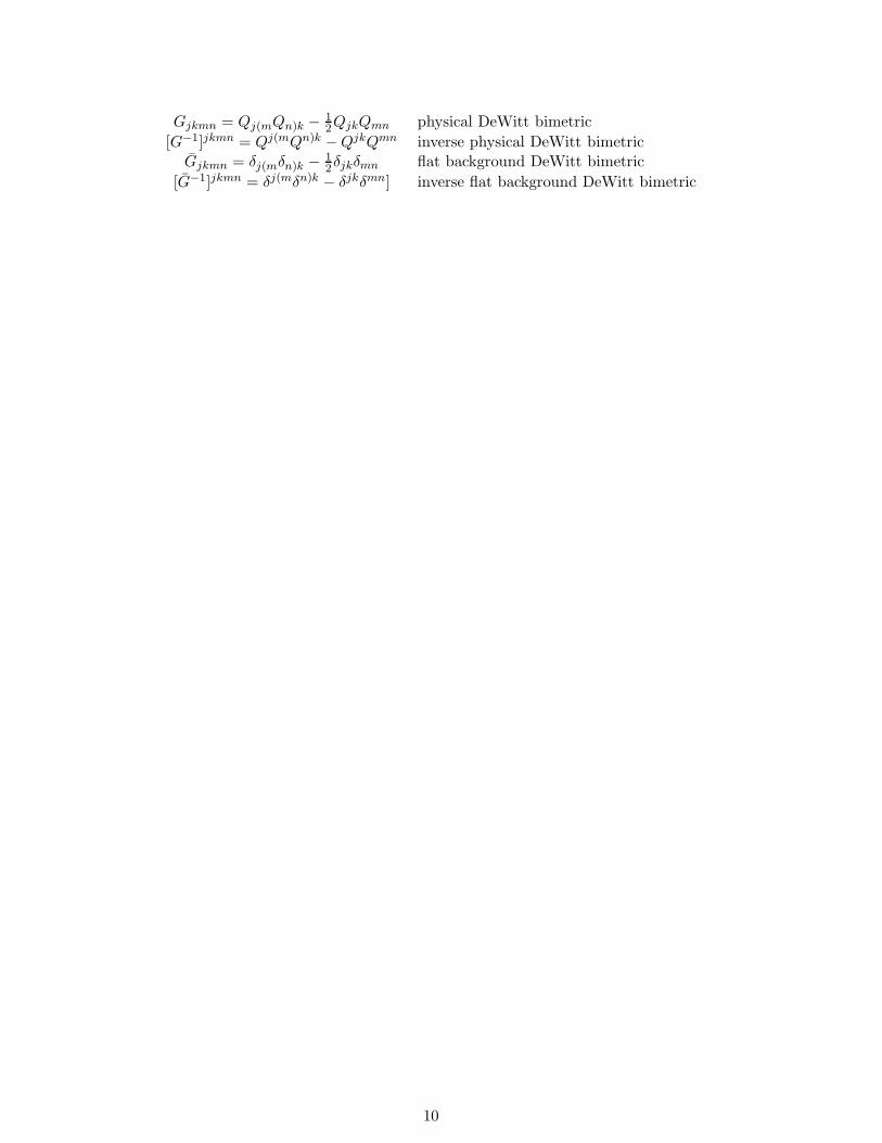
Gjkmn = Qj(mQn)k − 12QjkQmn physical DeWitt bimetric

[G−1]jkmn = Qj(mQn)k −QjkQmn inverse physical DeWitt bimetricGjkmn = δj(mδn)k − 1

2δjkδmn flat background DeWitt bimetric

[G−1]jkmn = δj(mδn)k − δjkδmn] inverse flat background DeWitt bimetric

10

2 The Brown – Kuchar formalism

In this section we review those elements of the Brown – Kuchar formalism [12] that are most relevant to us.Furthermore, we present an explicit constraint analysis for the system where gravity is coupled to a genericscalar field and the Brown – Kuchar dust, based on a canonical analysis using the full arsenal of Dirac’salgorithm for constrained Hamiltonian systems.

For concreteness, we employ dust to deparametrise a system consisting of a generic scalar field ζ ona four-dimensional hyperbolic spacetime (M,g). The corresponding action, Sgeo + Smatter, is given by theEinstein – Hilbert action

Sgeo =1

κ

∫

Md4X

√|det(g)| [R(4) + 2Λ] (2.1)

where κ ≡ 16πGN, with GN denoting Newton’s constant, R(4) is the Ricci scalar of g and Λ denotes thecosmological constant, and the scalar field action

Smatter =1

2λ

∫

Md4X

√det(g)| [−gµνζ,µζ,ν − v(ζ)] (2.2)

with λ denoting a coupling constant allowing for a dimensionless ζ and v is a potential term.

2.1 Lagrangian Analysis

In their seminal paper [12] Brown and Kuchar introduced the following dust action4

Sdust = −1

2

∫

Md4X

√|det(g)| ρ [gµν UµUν + 1] . (2.3)

Here, g denotes the four-metric on the spacetime manifold M. The dust velocity field is defined by U =−dT +WjdS

j (j ∈ 1, 2, 3. The action Sdust is a functional of the fields ρ, gµν , T, Sj , Wj

5. The physicalinterpretation of the action will now be given in a series of steps.

First of all, the energy momentum of the dust reads

T dustµν = − 2√

|det(g)|δSdust

δgµν= ρ UµUν − ρ

2gµν [gλσUλUσ + 1] . (2.4)

By the Euler–Lagrange equation for ρ

δSdust

δρ= gλσUλUσ + 1 = 0 (2.5)

the second term in (2.4) vanishes on shell. Hence, U is unit timelike on shell. Comparing with the energymomentum tensor of a perfect fluid with energy density ρ, pressure p and unit (timelike) velocity field U

T pfµν = ρ UµUν + p (gµν + UµUν) (2.6)

shows that the action (2.3) gives an energy-momentum tensor for a perfect fluid with vanishing pressure.For ρ 6= 0, variation with respect to Wj yields an equation equivalent to

LUSj = 0 (2.7)

where L denotes the Lie derivative. Hence, the fields Sj are constant along the integral curves of U . Equation(2.7) implies

LUT = UµT,µ = Uµ[T,µ −WjSj,µ] = −UµUµ = +1 (2.8)

4A classical particle interpretation of this action will be given in section 2.4.5Here, T, Sj have dimension of length, Wj is dimensionless and, thus, ρ has dimension length−4. The notation used here is

suggestive: T stands for time, Sj for space and ρ for dust energy density.

11

so that T defines proper time along the dust flow lines.Variation with respect to T results in

∂µ[ρ√

|det(g)|Uµ] =√

|det(g)|∇µ[ρUµ] = 0 (2.9)

while variation with respect to Sj gives

∂µ[ρ√

|det(g)|UµWj ] =√

|det(g)|∇µ[ρUµWj ] = 0 . (2.10)

Using (2.9), (2.10) reduces to (assuming ρ 6= 0)

∇UWj = 0 . (2.11)

Thus, ∇UUµ = 0, and, as a consequence, the integral curves of U are affinely parametrised geodesics. Thephysical interpretation of the fields T, Sj is complete: the vector field U is geodesic with proper time T ,and each integral curve is completely determined by a constant value of Sj. This determines a dynamicalfoliation of M, with leaves characterized by constant values of T . A given integral curve intersects each leaveat the same value of Sj.

2.2 Hamiltonian Analysis

In this section we derive the constraints that restrict the phase space of the system of a generic scalar fieldon a spacetime (M, g), extended by the Brown – Kuchar dust. The reader not interested in the details ofthe derivation, which uses the full arsenal of Dirac’s algorithm for constrained systems, may directly referto the result (2.32–2.34).

We assume (M, g) to be globally hyperbolic in order to guarantee a well posed initial value problem. As aconsequence, M is diffeomorphic to R×X , where X is a three-manifold of arbitrary topology. The spacelikeleaves Xt of the corresponding foliation are obtained as images of a one parameter family of embeddingst 7→ Yt, see e.g. [26] for more details and our notation table for ranges of indices etc. The timelike unitnormals to the leaves may be written6 as nµ = [Y µ

,t − naY µ,a]/n, where n, na are called lapse and shift

functions, respectively. Throughout, nµ is assumed to be future oriented with respect to the parameter t,which requires n > 0.

The three metric on X is the pull back of the spacetime metric under the embeddings, that is, qab(x, t) =Y µ

,aY ν,bgµν . Denoting the inverse of qab by qab it is not difficult to see that

gµν = −nµnν + qab Y µ,aY

ν,b . (2.12)

It follows that the dust action can be written as

Sdust = −1

2

∫

R

dt

∫

Xd3x

√det(q) n ρ

(−U2

n + qabUaUb + 1)

(2.13)

with Un ≡ nµUµ, Ua ≡ Y µ,aUµ.

The form (2.13) is useful to derive the momentum fields canonically conjugate to T, Sj , respectively, as

P :=δSdust

δT,t= −

√det(q) ρ Un

Pj :=δSdust

δSj,t

=√

det(q) ρ UnWj . (2.14)

The second relation in (2.14) shows that the Legendre transform is singular, and we obtain the primary

constraint (Zwangsbedingung)Zj := Pj +WjP = 0 . (2.15)

6We have written Y (t, x) ≡ Yt(x).

12

Additional primary constraints arise when we compute the momenta conjugate to ρ and Wj

I := Z :=δSdust

δρ,t= 0

Ij := Zj :=δSdust

δWj,t= 0 . (2.16)

Considering the total action S ≡ Sgeo+Smatter+Sdust, further primary constraint follow from the calculationof the canonical momentum fields conjugate to lapse and shift n, na, respectively,

p := z :=δS

δn,t= 0

pa := za :=δS

δna,t

= 0 (2.17)

The primary constraints signify the fact that we cannot solve for the velocities Sj,t, ρ,t, Wj ,t, n,t, n

a,t,

respectively, in terms of the momenta and configuration variables. Therefore, all primary constraints mustbe included in the canonical action, together with appropriate Lagrange multipliers

µj, µ, µj, ν, ν

a, in

order to reproduce the Euler – Lagrange equations.It is straightforward to solve for T,t and ζ,t, qab ,t. For instance,

T,t = nTn + naT,a = n[−Un +WjS

jn

]+ naT,a = n

1

ρ

P√det(q)

+ Sj,tWj + na

[T,a −WjS

j,a

]. (2.18)

How to eliminate the velocities of the scalar field and the three-metric is well known,e.g. [26], and will notbe repeated here.

The resulting Hamiltonian constraint for the extended system, ctot ≡ cgeo + cmatter + cdust, is explicitlygiven by

κ cgeo =1√

det(q)

[qacqbd −

1

2qabqcd

]pabpcd −

√det(q) R(3) + 2Λ

√det(q)

λ cmatter =1

2

[π2

√det(q)

+√

det(q)(qabξ,aξ,b + v(ξ)

)]

cdust =1

2

[P 2/ρ√det(q)

+√

det(q) ρ(qabUaUb + 1

)](2.19)

with Ua ≡ −T,a + Wj Sj,a. The spatial diffeomorphism constraints for the extended system, ctota ≡ cgeoa +

cmattera + cdust

a , are explicitly given by

κ cgeoa = −2 qacDb pbc

λ cmattera = π ξ,a

cdusta = P

[T,a −Wj S

j,a

]. (2.20)

The total action in canonical form reads

S =

∫

R

dt

∫

Xd3x

(PT,t + Pj S

j,t + I ρ,t + Ij Wj,t + p n,t + pa n

a,t +

1

κpab qab,t +

1

λπ ξ,t

)

−∫

R

dt Hprimary (2.21)

with pab denoting the momentum field conjugate to qab, ξ denoting the pullback of ζ to X , π denoting itscanonical momentum and D is the covariant differential compatible with qab. Furthermore, the Hamiltonian

13

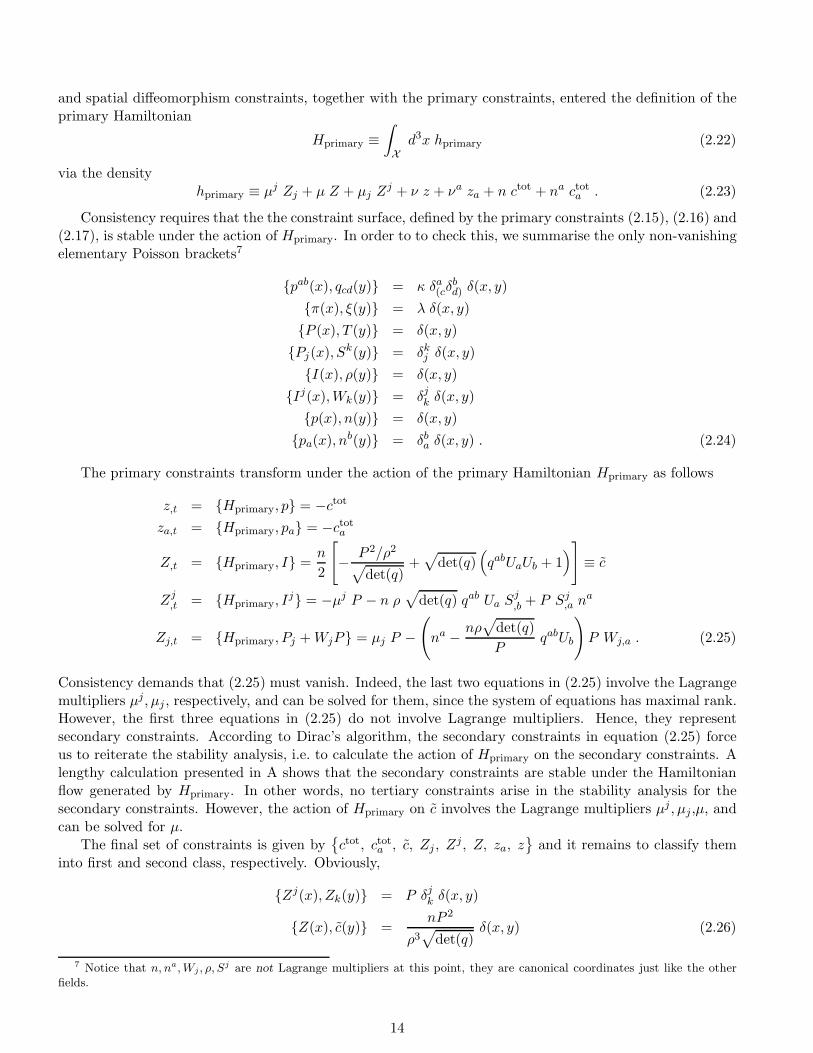
and spatial diffeomorphism constraints, together with the primary constraints, entered the definition of theprimary Hamiltonian

Hprimary ≡∫

Xd3x hprimary (2.22)

via the densityhprimary ≡ µj Zj + µ Z + µj Z

j + ν z + νa za + n ctot + na ctota . (2.23)

Consistency requires that the the constraint surface, defined by the primary constraints (2.15), (2.16) and(2.17), is stable under the action of Hprimary. In order to to check this, we summarise the only non-vanishingelementary Poisson brackets7

pab(x), qcd(y) = κ δa(cδ

bd) δ(x, y)

π(x), ξ(y) = λ δ(x, y)

P (x), T (y) = δ(x, y)

Pj(x), Sk(y) = δk

j δ(x, y)

I(x), ρ(y) = δ(x, y)

Ij(x),Wk(y) = δjk δ(x, y)

p(x), n(y) = δ(x, y)

pa(x), nb(y) = δb

a δ(x, y) . (2.24)

The primary constraints transform under the action of the primary Hamiltonian Hprimary as follows

z,t = Hprimary, p = −ctot

za,t = Hprimary, pa = −ctota

Z,t = Hprimary, I =n

2

[− P 2/ρ2

√det(q)

+√

det(q)(qabUaUb + 1

)]≡ c

Zj,t = Hprimary, I

j = −µj P − n ρ√

det(q) qab Ua Sj,b + P Sj

,a na

Zj,t = Hprimary, Pj +WjP = µj P −(na − nρ

√det(q)

PqabUb

)P Wj,a . (2.25)

Consistency demands that (2.25) must vanish. Indeed, the last two equations in (2.25) involve the Lagrangemultipliers µj, µj , respectively, and can be solved for them, since the system of equations has maximal rank.However, the first three equations in (2.25) do not involve Lagrange multipliers. Hence, they representsecondary constraints. According to Dirac’s algorithm, the secondary constraints in equation (2.25) forceus to reiterate the stability analysis, i.e. to calculate the action of Hprimary on the secondary constraints. Alengthy calculation presented in A shows that the secondary constraints are stable under the Hamiltonianflow generated by Hprimary. In other words, no tertiary constraints arise in the stability analysis for thesecondary constraints. However, the action of Hprimary on c involves the Lagrange multipliers µj , µj,µ, andcan be solved for µ.

The final set of constraints is given byctot, ctota , c, Zj , Z

j, Z, za, z

and it remains to classify theminto first and second class, respectively. Obviously,

Zj(x), Zk(y) = P δjk δ(x, y)

Z(x), c(y) =nP 2

ρ3√

det(q)δ(x, y) (2.26)

7 Notice that n, na, Wj , ρ, Sj are not Lagrange multipliers at this point, they are canonical coordinates just like the otherfields.

14

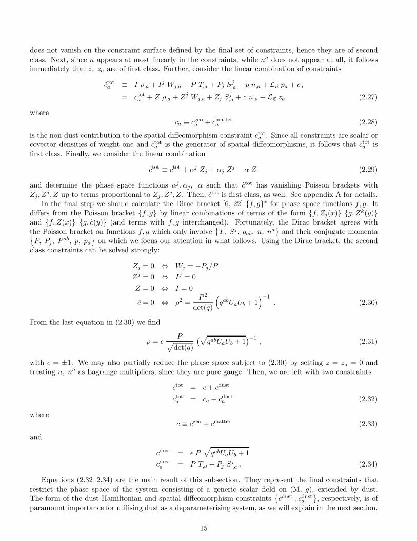
does not vanish on the constraint surface defined by the final set of constraints, hence they are of secondclass. Next, since n appears at most linearly in the constraints, while na does not appear at all, it followsimmediately that z, za are of first class. Further, consider the linear combination of constraints

ctota ≡ I ρ,a + Ij Wj,a + P T,a + Pj Sj,a + p n,a + L~n pa + ca

= ctota + Z ρ,a + Zj Wj,a + Zj Sj,a + z n,a + L~n za (2.27)

whereca ≡ cgeoa + cmatter

a (2.28)

is the non-dust contribution to the spatial diffeomorphism constraint ctota . Since all constraints are scalar orcovector densities of weight one and ctota is the generator of spatial diffeomorphisms, it follows that ctota isfirst class. Finally, we consider the linear combination

ctot ≡ ctot + αj Zj + αj Zj + α Z (2.29)

and determine the phase space functions αj , αj , α such that ctot has vanishing Poisson brackets withZj, Z

j , Z up to terms proportional to Zj , Zj, Z. Then, ctot is first class, as well. See appendix A for details.

In the final step we should calculate the Dirac bracket [6, 22] f, g∗ for phase space functions f, g. Itdiffers from the Poisson bracket f, g by linear combinations of terms of the form f, Zj(x) g, Zk(y)and f, Z(x) g, c(y) (and terms with f, g interchanged). Fortunately, the Dirac bracket agrees withthe Poisson bracket on functions f, g which only involve

T, Sj, qab, n, n

a

and their conjugate momentaP, Pj , P

ab, p, pa

on which we focus our attention in what follows. Using the Dirac bracket, the second

class constraints can be solved strongly:

Zj = 0 ⇔ Wj = −Pj/P

Zj = 0 ⇔ Ij = 0

Z = 0 ⇔ I = 0

c = 0 ⇔ ρ2 =P 2

det(q)

(qabUaUb + 1

)−1. (2.30)

From the last equation in (2.30) we find

ρ = ǫP√

det(q)

(√qabUaUb + 1

)−1, (2.31)

with ǫ = ±1. We may also partially reduce the phase space subject to (2.30) by setting z = za = 0 andtreating n, na as Lagrange multipliers, since they are pure gauge. Then, we are left with two constraints

ctot = c+ cdust

ctota = ca + cdusta (2.32)

wherec ≡ cgeo + cmatter (2.33)

and

cdust = ǫ P√qabUaUb + 1

cdusta = P T,a + Pj S

j,a . (2.34)

Equations (2.32–2.34) are the main result of this subsection. They represent the final constraints thatrestrict the phase space of the system consisting of a generic scalar field on (M, g), extended by dust.The form of the dust Hamiltonian and spatial diffeomorphism constraints

cdust , cdust

a

, respectively, is of

paramount importance for utilising dust as a deparameterising system, as we will explain in the next section.

15

2.3 The Brown – Kuchar Mechanism for Dust

In the previous section we have shown that the canonical formulation of a classical system, originallydescribed by General Relativity and a generic scalar field theory, then extended by a specific dust model,results in a phase space subject to the Hamiltonian and spatial diffeomorphism constraints (2.32–2.34). Theprimary Hamiltonian, after having solved the second class constraints, is a linear combination of those finalfirst class constraints (2.32–2.34) and, thus, is constrained to vanish. This holds in general, independentlyof the matter content, and is a direct consequence of the underlying spacetime diffeomorphism invariance.

Now, observable quantities are special phase space functions, distinguished by their invariance undergauge transformations. In other words, their Poisson brackets with the constraints must vanish when theconstraints hold. In particular, they have vanishing Poisson brackets with the primary Hamiltonian Hprimary

on the constraint surface. This is one of the many facets of the problem of time: observable quantities do notmove with respect to the primary Hamiltonian, because the latter generates gauge transformations ratherthan physical evolution. It follows that physical evolution must be generated by a true Hamiltonian (notconstrained to vanish, but still gauge invariant).

In this section we address the questions how to construct a true Hamiltonian from a given Hamiltonianconstraint, and, how to construct observable quantities (gauge invariant phase space functions).

2.3.1 Deparametrisation: General Theory

The manifest gauge invariant construction of a true Hamiltonian, generating physical evolution as opposedto mere gauge transformations, becomes particular simple when the original system under consideration canbe extended to a system with constraints in deparametrised form.

Consider first a general system subject to first class constraints cI . The set of canonical pairs on phasespace split into two sets of canonical pairs (qa, pa) and (T I , πI), respectively, such that the constraints canbe solved, at least locally in phase space, for the πI . In other words,

cI = 0 ⇔ cI = πI + hI(TJ ; qa, pa) = 0 . (2.35)

Notice that, in general, the functions hI do depend on the T J . The first class property guarantees that thecI are mutually Poisson commuting [36].

A system that deparametrises allows to split the set of canonical pairs into two sets of canonical pairssuch that (1) equation (2.35) holds globally on phase space8, and (2) the functions hI are independent ofthe T J .

Property (2) implies that the functions hI are gauge invariant. Hence, any linear combination of thehI that is bounded from below is a suitable candidate for a true Hamiltonian in the following sense: letcτ ≡ τ I cI be such a linear combination, with real coefficients τ I in the range of T I , and consider for anyphase space function f the expression

Of (τ) ≡[

∞∑

n=0

1

n!cτ , f(n)

]

τI→(τ−T )I

. (2.36)

Here9, the iterated Poisson bracket is inductively defined by cτ , f(0) = f, cτ , f(n+1) = cτ , cτ , f(n).Then, Of (τ) is an observable quantity. More precisely, it is a gauge invariant extension of the phase spacefunction f. Furthermore, physical time translations of Of (τ) are generated by the functions hI :

∂Of (τ)

∂τ I= hI , Of (τ) (2.37)

provided that f only10 depends on (qa, pa).

8This is not the case for Klein – Gordon fields and many other scalar field theories with a canonical action that is at leastquadratic in the πI .

9Notice that the substitution of the phase space independent numbers τ I by the phase space dependent combination (τ −T )I

is performed only after the series has been calculated.10This is no restriction, since the πI can be expressed in terms of the (qa, pa) (using (2.35)), and the T I are pure gauge.

16

The observable quantities Of (τ) can also be interpreted from the point of view of choosing a physical

gauge. Indeed, Of (τ) can be interpreted as representing the value of f in the gauge T I = τ I .

2.3.2 Deparametrisation: Scalar Fields

The Brown – Kuchar mechanism relies on the observation that free scalar fields lead to deparametrisationof General Relativity, as we sketch below (see [9] for a detailed discussion).

A free scalar field contributes to the spatial diffeomorphism constraint a term of the form

cscalara = πφ,a (2.38)

and to the Hamiltonian constraint a function of π2 and qabφ,aφ,b, in the absence of a potential. On theconstraint surface, defined by the spatial diffeomorphism constraint, we have the identity

qabφ,aφ,b =qab cscalara cscalarb

π2=qab cacbπ2

(2.39)

with ca denoting the contribution to the total spatial diffeomorphism constraint that is independent of thefree scalar field. Substitution of (2.39) into the total Hamiltonian and spatial diffeomorphism constraintsyields the same constraint surface and gauge flow than before. In other words, the constraints with thesubstitution (2.39) are equivalent to the original ones. However, the new total Hamiltonian constraint doesnot depend on the free scalar field φ any more. Therefore, at least locally in phase space, we can solve thenew total Hamiltonian constraint for the momentum field π and write locally

ctot(x) = π(x) + h(x) (2.40)

where the scalar density h of weight one is independent of π, φ and, typically, positive definite, see [9] fordetails.

As mentioned above, the constraint (2.40) and h(x) are mutually Poisson commuting, which guaranteesthat the physical Hamiltonian

H :=

∫

Xd3x h(x) (2.41)

is observable (it has vanishing Poisson brackets with the spatial diffeomorphism constraint, because h hasdensity weight one).

This is as much as the general theory goes. There are two remaining caveats: first of all, the constructionis only local in phase space. Secondly, the construction based on a single free scalar field requires phasespace functions that are already invariant under spatial diffeomorphisms. Only those can be completed tofully gauge invariant quantities11.

2.3.3 Deparametrisation: Dust

Dust described by the action (2.3) does not entirely fit into the classification scheme given in [9] and sketchedin the last section. It is not simply based on four free scalar fields T, Sj , but in addition leads to secondclass constraints. However, it has a clear interpretation as a system of test observers in geodesic motion,and circumvents the remaining caveats mentioned at the end of the last subsection as we will see.

Recall the final form of the Hamiltonian constraint (2.32–2.32) derived in the previous section:

ctot = c+ ǫP√

1 + qabUaUb (2.42)

with Ua = −T,a + Wj Sj,a. Solving the second class constraint Zj = 0 for Wj, we find Ua = −cdust

a /P .Inserting the first class spatial diffeomorphism constraint ctota = ca + cdust

a , we arrive at the equivalentHamiltonian constraint

ctot ′ = c+ ǫP

√1 +

qabcacbP 2

(2.43)

11 This can be circumvented by employing e.g. three more free scalars but this would be somewhat ad hoc.

17

which is already independent of T, Sj and Pj , but still not of the form ctot = P +h, as required for a systemthat deparametrises.

2.3.4 Deparametrisation for Dust: Sign Issues

In order to bring (2.43) into the form ctot = P + h, we have to solve a quadratic equation. Each rootdescribes only one sheet of the constraint surface, unless the sign of P is somehow fixed. As we argue below,this freedom will be fixed by our interpretation of the dust system as a physical reference system.

Recall that P = −ρ√

det(q)Un and Uµ T,µ = 1, Uµ Sj,µ = 0. In accordance with our interpretation,

we identify T with proper time along the dust flow lines. Thus, U is timelike and future pointing, henceUn < 0. It follows that sgn(P ) =sgn(ρ), so ǫ = 1 in (2.31).

In [12] the authors assume ρ > 0, as it is appropriate for observable dust12. In our case, however, thedust serves only as a tool to deparametrise the system and is, by construction, only pure gauge. Therefore,we relax the restriction ρ > 0, when solving (2.43) for P :

P 2 = c2 − qabcacb . (2.44)

The right hand side of (2.44) is constrained to be non – negative, albeit it is not manifestly non – negative.But this causes no problem, since it is sufficient to analyse the system in an arbitrarily small neighborhoodof the constraint surface, where c2 − qabcacb ≥ 0. Then,

ctot = P − sgn(P ) h, h =√c2 − qabcacb (2.45)

is the general solution, globally defined on (the physically interesting portion of) the full phase space.However, ctot is not yet of the form required by a successful deparametrisation, because of the sign functionwhich also renders the constraint non – differentiable.

In order to utilise dust for deparametrisation, the choice P < 0 is required. Before presenting reasonsfor this choice, we stress again that the dust itself is not observable. There are three related arguments forthe choice of P < 0:

1. Dynamics

The deparametrisation mechanism supplies us with a physical Hamiltonian of the form

H =

∫

Xd3x h . (2.46)

In the case where dust is chosen as the clock of the system, the variation of the physical Hamiltonianis given by

δH =

∫

Xd3x

(c

hδc− qab cb

hδca +

1

2hqacqbdcccd δqab

). (2.47)

For P 6= 0, then h 6= 0 (in a sufficiently small neighbourhood of the constraint surface). Hence, thecoefficients of the variations on the right hand side of (2.47) are non singular. Moreover, for P 6= 0,also c 6= 0, as we see from (2.43). In fact, using sgn(c) = −sgn(P ) (from (2.43)) in a neighborhood ofthe constraint surface,

c

h= −sgn(P )

√1 + qab

cah

cbh

(2.48)

has absolute value no less than one.

12 This would be required by the usual energy conditions if the dust would be the only observable matter. However, noticethat only the total energy momentum is subject to the energy conditions, not the individual contributions from various matterspecies.

18

Let us now compare (2.47) with the differential of the primary Hamiltonian constraint in the absenceof dust:

Hprimary =

∫

Xd3x (nc+ naca) (2.49)

which is given by (lapse and shift functions are considered as Lagrange multipliers, i.e. are phase spaceindependent)

dHprimary =

∫

Xd3x (ndc+ nadca) . (2.50)

Comparison between (2.47) and (2.50) reveals that the differentials coincide, up to the additionalterm proportional to δqab, provided we identify n := c/h as dynamical lapse and na := −qabcb/h asdynamical shift. This is promising in our aim to derive physical equations of motions for observablequantities which nevertheless come close to the usual Einstein equations for gauge dependent quantities.However, in the standard framework the lapse function is always positive, guaranteeing that the normalvector field is future oriented. This fact is correctly reflected in our framework only if P < 0.

2. Kinematics

The identification n ≡ c/h and na ≡ −qabcb/h can also be motivated as follows:Consider a spacetime diffeomorphism defined by Xµ 7→ (τ, σj) := (T (X), Sj(X)) =: Y µ(X) and let(τ, σj) → Zµ(τ, σ) be its inverse. We can define a dynamical foliation of M by T (X) = τ =const.hypersurfaces. The leaves Sτ of that foliation are the images of S (which is the range of the Sj) underthe map Z at constant τ . Using the identity

δµν = Zµ

,τ T,ν + Zµ,j S

j,ν (2.51)

and Uµ T,µ = 1 , Uµ Sj,µ = 0, we find Uµ = Zµ

,τ . Thus, as expected, the foliation is generated by thevector field U = ∂/∂τ , which is unit timelike.

It is useful to decompose the deformation vector field U with respect to the arbitrary coordinatefoliation that we used before:

Uµ = gµνUν = −nµUn +Xµ,a q

ab Ub . (2.52)

From (2.13) and (2.31) with ǫ = 1 we find Un = −√

1 + qabUaUb. Next,

Ua = −cdusta

P=caP. (2.53)

On the other hand n ≡ c/h = sgn(P )Un and na ≡ −ca/h = −sgn(P ) Ua. Therefore, (2.52) can bewritten

Uµ = −sgn(P )(n nµ +Xµ

,a na). (2.54)

Hence, the sign for which n is positive yields the correct decomposition of the deformation vector fieldU in terms of lapse and shift. This calculation reveals also the geometrical origin of the identificationn ≡ c/h and na ≡ −qabcb/h.

As a side remark: the identity −n2 + qabnanb = −1 is an immediate consequence of the normalisationof the deformation vector field, gµνU

µUν = −1. That is, the deformation vector field is timelike, futureoriented and normalised, but not normal to the leaves of the foliation that it defines.

3. Stability and flat spacetime limit

Of course, we could choose P > 0 and use −h instead of h in order to obtain equations of motion.However, in that case the physical Hamiltonian would be unbounded from below, leading to an unstabletheory. Alternatively, we could stick to +h for the equations of motion, but then the τ evolution wouldrun backwards.

19

Moreover, since ctot = c + P√

1 + qabUaUb = 0 on the constraint surface, we would have c < 0 forP > 0. Since c = cgeo + cmatter and cmatter > 0, this would enforce cgeo < 0. Hence, flat space wouldnot be a solution.

As a side remark: for ca/h ≪ 1 and P < 0, h ≈ c, while h ≈ −c for P > 0. Thus, the physicalHamiltonian density, with respect to dust as a physical reference system, approximates the standardmodel Hamiltonian density cmatter only for P < 0.

We emphasise again that the dust used for deperametrisation is not observable, and should not be confusedwith observable matter. It solely provides a dynamical reference frame.

2.4 Dust Interpretation

In this section we derive a physical interpretation of the Brown – Kuchar action based on the geodesicmotion of otherwise free particles [12].

Consider first the action for a single relativistic particle with mass m on a background g:

Sm = −m∫

R

ds

√−gµν Xµ Xν . (2.55)

The momentum conjugate to the configuration variable Xµ is given by

Pµ =δSm

δXµ= m

gµνXν

√−gρσXρXσ

, (2.56)

rendering the Legendre transformation singular. This is a consequence of the reparametrisation invarianceof the action (2.55). Hence, the system exhibits no physical Hamiltonian, but instead a primary Hamiltonianconstraint enforcing the mass shell condition:

C =1

2m

(m2 + gµνPµPν

). (2.57)

Let us proceed to the canonical formulation. In terms of the embeddings X ≡ Yt(x), the particletrajectory reads X(s) = Yt(s)(x(s)), so that

X(s) = t(s) Y,t + xa(s) Y,a (2.58)

where the overdot refers to differentiation with respect to the trajectory parameter s. The momenta arethen given by

pa ≡ Y µ,aPµ =

m√−gρσXρXσ

qab

(t nb + xb

)

pt ≡ Y µ,t Pµ =

m√−gρσXρXσ

(t gtt + qab n

bxa)

(2.59)

where gtt = −n2 + qabnanb. We can only eliminate the spatial velocities xa. To do this set A ≡ gtax

a =qabn

bxa and B ≡ qabxaxb. Then,

w ≡ gµνXµXν = gtt t

2 + 2A t+B . (2.60)

On the other hand,

− w

m2qabpapb = B + 2At+ qabn

anbt2 . (2.61)

20

Substituting w from (2.60) and collecting coefficients of A,B, t2 yields

0 = B + 2A t+ t2gtt

qabpapb

m2 + qabnanb

1 + qabpapb

m2

= w +t2 n2

1 + qabpapb

m2

. (2.62)

Now we can solve the first equation in (2.59) for xa:

xa = t

(−na ±

√1 +

qabpapb

m2

). (2.63)

Inserting this into the second equation in (2.59) leads to a constraint of the form C ≡ ps + h:

C = ps − napa ± n√m2 + qabpapb (2.64)

while the canonical Hamiltonian is obtained from the Lagrangian in (2.55) as

Hcanon = PµXµ − L = t C . (2.65)

Since the constraint (2.64) is in deparametrised form, the phase space can easily be reduced, leading to thereduced action

Sreduced =

∫ds (pax

a − h) . (2.66)

We extend this phase space by adding a canonical pair (τ,m) and consider the extended action

Sextended =

∫ds (mτ + pax

a − h) (2.67)

where the particle mass m is now considered as a dynamical variable. The equations of motion for m, τ givem = 0 and τ = t

√−w. Thus, the mass is constant and τ is the proper time (in the gauge s = t).We generalize our results now to the case of many particles. More precisely, let S be a label set and

consider a relativistic particle for each label σ ∈ S. This amounts to provide each variable appearing in theextended action with a corresponding label, i.e. xa

σ, pσa , τσ, m

σ, and the total action for those particles isthen just the sum over the corresponding actions Sσ

extended

Sextended =∑

σ∈S

Sσextended . (2.68)

Next we consider the limit in which S becomes a three – manifold, with the labels σ becoming coordinateson this manifold. In this limit, we introduce the following fields:

T (σ) ≡ τσ

P (σ) d3σ ≡ mσ

Sa(σ) ≡ xaσ

pa(σ)d3σ ≡ pa(xσ)

n(σ) ≡ n(xσ)

na(σ) ≡ na(xσ)

qab(σ) ≡ qab(xσ). (2.69)

21

Then, in the specified limit, the extended action (2.68) becomes

Sextended =

∫dt

∫d3σ

(˙T P + ˙SaPa + naPa ∓ n

√P 2 + qabPaPb

). (2.70)

Finally, we perform a canonical transformation: instead of the fields Sa(σ) with values in X , we wouldlike to consider the inverse fields Sj(x) with values in S, that is Sj(S(σ)) = σj, Sa(S(x)) = xa. This is atthe same time a diffeomorphism and we can transform the other fields as well. For instance (T is a scalarand P is a scalar density),

T (x) = T (S(x)) =

∫

Sd3σ δ

(x, S(σ)

) ∣∣∣det(∂S/∂σ)∣∣∣ T (σ)

P (x) =P

|det(∂S/∂σ)|(S(x)) =

∫

Sd3σ δ

(x, S(σ)

)P (σ)

Sj(x) =

∫

Sd3σ σj δ(x, S(σ))

∣∣∣det(∂S/∂σ)∣∣∣ . (2.71)

Calculating the time derivatives and performing integrations by parts, we find∫

Sd3σ ˙T P =

∫

Xd3x

(T P − SjSa

j PT,a

)(2.72)

with Saj denoting the inverse of the matrix Sj

,a. Using

˙Sa(σ) = −[SjSa

j

]S(x)=σ

(2.73)

and defining Pj(x) implicitly through

Pa = −[PT,a + PjS

j,a

|det(∂S/∂x)|

]

S(x)=σ

(2.74)

we find that Sextended precisely turns into the dust action on X with the second class constraints eliminated13.

3 Relational Observables and Physical Hamiltonian

In this section we present an explicit prescription for constructing gauge invariant completions of arbitraryphase space functions. The construction is non – perturbative and technically involved, but the physicalpicture behind it will become crystal clear. Furthermore, the formal expressions are only required to establishcertain properties of the construction, but are not required for the calculation of physical properties. Thisis a great strength of the relational formalism.

Let us summarise the situation. After having solved the second class constraints and having identifiedlapse and shift fields as Lagrange multipliers, we are left with the following canonical pairs

(qab, pab), (ξ, π), (T, P ), (Sj , Pj) , (3.1)

subject to the following first class constraints

ctota = ca + cdusta , cdust

a = P T,a + Pj Sj,a

ctot = c+ cdust , cdust = −√P 2 + qabcdust

a cdustb (3.2)

13The metric field has to be pulled back by the dynamical spatial diffeomorphism, as well. For details, see next section.

22

where ca, c are independent of the dust variablesT, P, Sj , Pj

. We already used P < 0.

As explained in 2.3, we aim at deparametrisation of the theory and therefore solve (3.2) for the dustmomenta, leading to the equivalent form of the constraints

ctot = P + h , h =√c2 − qabcacb

ctotj = Pj + hj , hj = Saj (−hT,a + ca) (3.3)

with Saj S

k,a = δk

j , Saj Sj

,b = δab , hence Sa

j is the inverse of Sj,a (assuming, as before, that S : X →

S is a diffeomorphism). These constraints are mutually Poisson commuting14. However, only ctot is indeparametrised form (i.e. h is independent of T, Sj), but ctotj is not. In particular, we can only conclude

that the h(x) are mutually Poisson commuting. Still, this will be enough for our purposes15.Following the works [9, 10, 11], we describe the construction of fully gauge invariant completions of phase

space functions. Consider the smeared constraint

Kβ ≡∫

Xd3x

[β(x)ctot(x) + βj(x)ctotj (x)

](3.4)

where β(x), βj(x) are phase space independent smearing functions in the range of T (x), Sj(x). Under agauge transformation generated by this constraint, an arbitrary phase space function f is mapped to:

αβ(f) ≡∞∑

n=0

1

n!Kβ, f(n) . (3.5)

The fully gauge invariant completion of f is given by

Of [τ, σ] ≡[αβ(f)

]β→τ−T

βj→σj−Sj

. (3.6)

Here, the functions τ(x), σj(x) are also in the range of T (x), Sj(x), respectively16. It is important tofirst calculate the Poisson brackets appearing in (3.5) with the phase space independent functions β, βj ,and afterwards to replace them with the phase space dependent functions τ − T, σj − Sj, respectively.This connection can be established based on the gauge transformation properties of T, Sj: αβ(T ) = T +β, αβ(Sj) = Sj + βj . Hence,

Of [τ, σ] ≡[αβ(f)

]αβ (T )=τ

αβ(Sj)=σj

. (3.7)

Indeed, (3.7) motivates the following interpretation: Of [τ, σ] is the gauge invariant completion of f , whichin the gauge T = τ, Sj = σj takes the value f . This is not the only interpretation we entertain a differentone below.

For the purpose of this paper it suffices to consider the infinite series appearing in the gauge invariantcompletions as expressions useful for formal manipulations. There is no need to actually calculate theseseries for any physical problem.

Further important properties [36, 20] of the completion are:

Of [τ, σ], Of ′ [τ, σ] = Of [τ, σ], Of ′ [τ, σ]∗ = Of,f ′∗ [τ, σ] (3.8)

Of+f ′ [τ, σ] = Of [τ, σ] +Of ′ [τ, σ] , Of ·f ′ [τ, σ] = Of [τ, σ] ·Of ′ [τ, σ] . (3.9)

14One can either prove this by direct calculation, or one uses the following simple argument: the Poisson bracket between theconstraints must be proportional to a linear combination of constraints, because the constraint algebra is first class. Since theconstraints are linear in the dust momenta, the result of the Poisson bracket calculation no longer depends on them. Therefore,the coefficients of proportionality must vanish.

15 In what follows we will drop the tilde in noting the constraints for notational simplicity.16We denote the functional dependence of (3.6) on the functions τ (x), σj(x) by square brackets. Below we show that it is

sufficient to choose those functions to be constant and replace the square brackets by round ones for notational convenience.

23

Here, ., .∗ is the Dirac bracket17 [6] associated with the constraints and the gauge fixing functions T, Sj.Relations (3.8) and (3.9) show that the map f 7→ Of [τ, σ] is a Poisson homomorphism of the algebraof functions on phase space with pointwise multiplication, equipped with the Dirac bracket18 as Poissonstructure.

In particular, for a general functional f = f [qab(x), Pab(x), ξ(x), π(x), T (x), P (x), Sj (x), Pj(x)] the fol-

lowing useful identity holds:

Of = f[Oqab(x), OP ab(x), Oξ(x), Oπ(x), OT (x), OP (x), OSj(x), OPj(x)

](τ, σ) . (3.11)

This has important consequences: (3.11) ensures that it suffices to know the completions of the elementaryphase space variables. In fact, we are only interested in those functions that are independent of the dustvariables

T, Sj , P, Pj

. The reason for this is that, first of all, P,Pj are expressible in terms of all other

variables on the constraint surface. Alternatively, since the constraints are mutually Poisson commuting,we have

OP (x) = Octot(x) +Oh(x) = ctot(x) +Oh(x) , OPj(x) = Octotj (x) +Ohj(x) = ctotj (x) +Ohj(x) . (3.12)

Hence, these functions are known, once we know the completion of the remaining variables. Secondly,

OT (x)[τ, σ] = τ(x) , OSj(x)[τ, σ] = σj(x) (3.13)

are phase space independent. Thus, the only interesting variables to consider areqab, P

ab, ξ, π.

In what follows we consider only dust – independent functions f . For those (3.8) simplifies to

Of [τ, σ], Of ′ [τ, σ] = Of,f ′[τ, σ] . (3.14)

Equations (3.9) and (3.8) imply that f 7→ Of [τ, σ] is a Poisson automorphism of the Poisson subalgebra offunctions that do not depend on the dust variables with the ordinary Poisson bracket as Poisson structure.This will be absolutely crucial for all what follows.

Further useful properties of the completion are:

Of [τ, σ] = O(2)

O(1)f

[σ][τ ] (3.15)

where (recall (3.4), (3.5) and (3.6))

O(1)f [σ] =

[αβ(f)

]β→0

βj→σj−Sj

O(2)f [τ ] = [αβ(f)]β→τ−T

βj→0

. (3.16)

This follows from the fact that the constraints are mutually Poisson commuting and ctot(x), Sj(y) = 0.The important consequence of (3.15) is that we can accomplish full gauge invariance in two stages: weestablish first invariance under the action of the spatial diffeomorphism constraint, and afterwards achieveinvariance with respect to gauge transformations generated by the Hamiltonian constraint. This holds evenunder more general circumstances [11], i.e. when the constraints can not be deparametrised.

17 For completeness, we note the definition of the Dirac bracket:

f, f ′∗ ≡ f, f ′ −

Z

X

d3x3

X

µ=0

ˆ

f, ctotµ (x)f ′, Sµ(x) − f ′, ctot

µ (x)f, Sµ(x)˜

(3.10)

where ctot0 ≡ ctot, S0 := T . The Dirac bracket is antisymmetric and f, ctot

µ (x)∗ = f, Sµ(x)∗ = 0 everywhere. This followsfrom the fact that ctot

µ (x) and Sµ(x) are mutually Poisson commuting, and that ctotµ (x), Sν(y) = δ(x, y)δν

µ.18The Dirac bracket coincides with the Poisson bracket on gauge invariant functions. It is degenerate, since it annihilates

coinstraints and gauge fixing functions. Hence, it defines only a Poisson structure, but not a symplectic structure on the fullphase space.

24

3.1 Implementing spatial diffeomorphism invariance

Keeping the physical interpretation of the completion in mind, the map f 7→ O(1)f [σ] can be worked out

explicitly. In the first stage of the construction, the corresponding smeared constraint reads

Kβ =

∫

Xd3x βj(x) ctotj (x) . (3.17)

Given a phase space function f , its completion O(1)f with respect to gauge transformations generated by Kβ

becomes

O(1)f [σ] =

∞∑

n=0

1

n!

[Kβ , f(n)

]βj→σj−Sj

= f +∞∑

n=1

1

n!

∫

Xd3x1 [σj1(x1) − Sj1(x1)] . . .

∫

Xd3xn [σjn(xn) − Sjn(xn)]

×ctotj1

(x1),ctotj2

(x2), . . . ,ctotjn

(xn), f. . .

. (3.18)

Let us begin with f = ξ(x). We claim that

Kβ, ξ(x)(n) =[βj1 . . . βjn vj1 . . . vjn · ξ

](x) (3.19)

where vj is the vector field defined by

vj · ξ(x) := Saj (x) ξ,a(x) . (3.20)

In fact the vectors vj are mutually commuting.

[vj , vk] = Saj S

bk,a∂b − j ↔ k

= −Saj S

bl S

l,caS

ck∂b − j ↔ k

= −Saj S

bl S

l,acS

ck∂b − j ↔ k

= Saj S

bl,cS

l,aS

ck∂b − j ↔ k

= Sbj,cS

ck∂b − j ↔ k

= SakS

bj,a∂b − j ↔ k

= 0 (3.21)

To prove (3.19) by induction over n we need

Kβ , Saj (x) = −Sa

k(x)Kβ , Sk,b(x)Sb

j (x) = −Sak(x)βk

,b(x)Sbj (x) = −[vj · βk]Sa

k (3.22)

For n = 1 we haveKβ , ξ(x)(1) = [βjSa

j ξ,a](x) = βjvj · ξ (3.23)

which coincides with (3.19). Suppose that (3.19) is correct up to n, then

Kβ , ξ(n+1) = βj1 . . . βjn Kβ , vj1 . . . vjn · ξ

= βj1 . . . βjn

[vj1 . . . vjn · Kβ, ξ +

n∑

l=1

vj1 . . . vjl−1

Kβ, S

ajl

∂avjl+1

. . . vjn · ξ]

= βj1 . . . βjn

[vj1 . . . vjn · βjn+1vjn+1 · ξ −

n∑

l=1

vj1 . . . vjl−1

[vjlβjn+1

]vjn+1vjl+1

. . . vjn · ξ]

= βj1 . . . βjn

[vj1 . . . vjn · βjn+1vjn+1 · ξ −

n∑

l=1

vj1 . . . vjl−1

[vjlβjn+1

]vjl+1

. . . vjn+1 · ξ]

= βj1 . . . βjn[vj1 . . . vjn · βjn+1vjn+1 · ξ −

(vj1 . . . vjnβ

jn+1 − βjn+1vj1 . . . vjn

)vjn+1 · ξ

]

= βj1 . . . βjn+1 vj1 . . . vjn+1 · ξ . (3.24)

25

where we used commutativity of the vj and the Leibniz rule.It follows that

O(1)ξ(x)[σ] = ξ(x) +

∞∑

n=1

1

n!

[σj1(x) − Sj1(x)

]. . .[σjn(x) − Sjn(x)

]vj1 . . . vjn · ξ(x) . (3.25)

Using vj · Sk = δkj and commutativity of the vj , we find with βj := σj − Sj that

vk ·O(1)ξ(x)[σ] = vk · ξ +

∞∑

n=1

[1

(n− 1)!

[vk · βj

]βj1 . . . βjn−1 vjvj1 . . . vjn−1 · ξ +

1

n!βj1 . . . βjn vkvj1 . . . vjn · ξ

]

= vk · ξ +[vk · βj

]vj · ξ +

∞∑

n=1

1

n!βj1 . . . βjn

[[vk · βj

]vjvj1 . . . vjn · ξ + vkvj1 . . . vjn · ξ

]

=∞∑

n=0

1

(n)!βj1 . . . βjn

[vk · σj

]vjvj1 . . . vjn · ξ . (3.26)

The interpretation of (3.25) becomes clear for the choice σj(x) = σj =const., for which (3.26) vanishes

identically. In other words, the completion O(1)ξ(x)[σ] does not depend on x at all. Hence, for this choice

of σj , we are free to choose x in O(1)ξ(x)[σ] in order to simplify (3.25). Since (3.25) is a power expansion

in(σj(x) − Sj

)(x), and Sj is a diffeomorphism, we choose x = xσ, with xσ being the unique solution of

Sj(x) = σj . Then19,

O(1)ξ(x)(σ) = ξ(xσ) = [ξ(x)]Sj(x)=σj . (3.27)

The completion O(1)ξ(x)(σ) of ξ(x) has also a simple integral representation:

O(1)ξ(x)(σ) =

∫

Xd3x |det(∂S(x)/∂x)| δ (S(x), σ) ξ(x) . (3.28)

The significance of choosing σj =const is the following: Clearly, the choice σj(x) = const. is not in the

range of Sj(x), which is supposed to be a diffeomorphism. Thus, the interpretation of O(1)f (σ) as the value

of f in the gauge Sj = σj is obsolete. However, given a function σj(x), instead of solving Sj(x) = σj(x)for the values of the function Sj for all x, we could solve it for x, while keeping the function Sj arbitrary.

This is the appropriate interpretation of O(1)f (σ). This is possible because O

(1)f [σ] is (at least formally)

gauge invariant, whether or not Sj = σj is a good choice of gauge. It is fully sufficient to do this because,as shown in [12] and as we will show in appendix B, the partially reduced phase space (with respect to

the spatial diffeomorphism constraint) is completely determined by the O(1)f (σ), hence the O

(1)f [σ] must be

hugely redundant.We can now compute the spatially diffeomorphism invariant extensions for the remaining phase space

variables without any additional effort, by switching first to variables which are spatial scalars on X , usingJ := det(∂S/∂x), which we assume to be positive (orientation preserving diffeomorphism):

(ξ, π/J) , (T, P/J) ,(qjk ≡ qab S

aj S

bk , p

jk ≡ Sj,aS

k,b p

ab/J). (3.29)

The image of these quantities, evaluated at x, under the completion O(1)f (σ) simply consists in replacing x by

xσ, where xσ solves Sj(x) = σj, just as in (3.27). The scalars (3.29) on X are the pull backs of the originaltensor (densities) under the diffeomorphism σ 7→ xσ evaluated at σ. Thus, they are tensor (densities) of thesame type, but live now on the dust space manifold S.

19We switched to the notation O(1)f (σ) to indicate the choice σj(x) = σj =const.

26

This statement sounds contradictory because of the following subtlety: We have e.g. the three quantitiesP (x), P (x) = P (x)/J(x), P (σ) = P (xσ). On X , P (x) is a scalar density while P (x) is a scalar. Pullingback P (x) to S = S(X ) by the diffeomorphism σ 7→ S−1(σ) results in P (σ). But pulling back P (x) back toS results in the same quantity P (σ). Since a diffeomorphism does not change the density weight, we wouldget the contradiction that P (σ) has both density weights zero and one on S. The resolution of the puzzleis that what determines the density weight of P (x) on X is its transformation behaviour under canonicaltransformations generated by the total spatial diffeomorphism constraint ctota = cdust

a +ca where cdusta , ca are

the dust and non dust contributions respectively. After the reduction of ctota , what determines the densityweight of P (σ) on S is its transformation behaviour under ([ca + PT,a]S

aj /J)(xσ) = cj(σ) + P (σ)T,j(σ) and

this shows that P (σ) has density weight one20.

We will denote the images under f 7→ O(1)f (σ) by

(ξ(σ), π(σ)

),(T (σ), P (σ)

),(qij(σ)pij(σ)

). (3.30)

In appendix B we show that the quantities (3.30) can be also obtained through symplectic reduction whichis an alternative method to show that the pairs in (3.30) are conjugate and as it was done in [12].

3.2 Implementing invariance with respect to the Hamiltonian constraint

Having completed the elementary phase space variables with respect to the spatial diffeomorphism constraint,it remains to render those variables invariant under the action of the Hamiltonian constraint. This amountsto calculate the image of those variables under the map f 7→ O

(2)f [σ], for any f in (3.30). For f independent

of T, P , the completion of f with respect to the Hamiltonian constraint is given by

O(2)f [τ ] =

∞∑

n=0

1

n!h[τ ], f(n) , h[τ ] =

∫

Xd3x (τ(x) − T (x)) h(x) . (3.31)

Only if we choose τ(x) = τ = const. (3.31) is invariant under diffeomorphisms. Hence we choose τ(x) = τ =const. which allows to rewrite (3.31) entirely in terms of the variables (3.30). As a reminder of this choice,

we denote the completion by O(2)f (τ). In this case (3.31) can be written as

O(2)f (τ) =

∞∑

n=0

1

n!h(τ), f(n) , h(τ) =

∫

Sd3σ (τ − T (σ)) h(σ) (3.32)

with h(σ) denoting the image of h(x) under the replacement21 ofξ(x), π(x), qab(x), p

ab(x)

byξ(σ), π(σ), qjk(σ), pjk(σ)

, respectively. Explicitly, denoting

c(σ) ≡[c(x)

J(x)

]

S(x)=σ

cj(σ) ≡[cj(x)

J(x)

]

S(x)=σ

, (3.33)

where, as before, cj(x) = Saj (x) ca(x), we find

h(σ) =√c2 − qjk cj ck(σ) . (3.34)

20 In order to avoid confusion of the reader we mention that any quantity f on X which has positive density weight is mappedto zero under f 7→ O

(1)f (σ). Let us again consider the example f = P . We have P (σ) = P (xσ) det(∂S−1(σ)/∂σ) which is

perfectly finite. However by the Poisson automorphism formula O(1)

P (x) = O(1)

J(x) P (x)= O

(1)

J(x) P (σ) = det(∂σ/∂x) P (σ) = 0 since

σ =const.21 The proof of this statement is based on the fact that the replacement corresponds to a diffeomorphism and that h(τ ) is

the integral of a scalar density of weight on, for τ =const.

27

It is easy to see thatd

dτO

(2)f (τ) = H, O(2)

f (τ) (3.35)

with

H :=

∫

Sd3σ h(σ) (3.36)

is the physical Hamiltonian (not Hamiltonian density) of the deparametrised system.We denote the fully gauge invariant completions of the Hamiltonian constraint, the spatial diffeomor-

phism constraints22 and the physical Hamilton density, respectively, as

C(τ, σ) ≡ O(2)c(σ)(τ) Cj(τ, σ) ≡ O

(2)cj(σ)(τ) ,

H(τ, σ) ≡ O(2)

h(σ)(τ) . (3.37)

It is worth emphasising again that H(τ, σ) is the physical energy density associated to the physical Hamil-tonian when the dust fields are considered as clocks of the system. The fully gauge invariant completions ofthe phase space variables for matter and gravity are denoted by

Ξ(τ, σ) ≡ O(2)

ξ(σ)(τ) Π(τ, σ) ≡ O

(2)π(σ)(τ), ,

Qij(τ, σ) ≡ O(2)qij(σ)(τ) P ij(τ, σ) ≡ O

(2)pij(σ)

(τ) . (3.38)

The matter scalar field Ξ(τ, σ) and its conjugate momentum Π(τ, σ) are observable quantities since gaugeinvariant. The same applies to the three-metric Qij(τ, σ) and its canonical momentum field P ij(τ, σ).Moreover, the completion is non – perturbative, i.e. full non-Abelian gauge invariance has been accomplished.

3.3 Constants of the physical Motion

In the previous section we successfully constructed fully gauge invariant quantities for a specific deparmetris-ing system. In some sense, the construction frees the true degrees of freedom from the constraints, replacingthem by conservation laws which govern the physical motion of observable quantities. Indeed, we have thefollowing first integrals of physical motion (conservation laws):

d

dτCj(τ, σ) = 0 ,

d

dτH(τ, σ) = 0 . (3.39)

These equations express invariance under the physical evolution generated by H, as opposed to gaugeinvariance. The functions Cj, H, representing physical three – momentum and energy, are already gaugeinvariant.

We proceed the proof of (3.39). Recall that the original constraints ctot(x) , ctotj (x) are mutually Poissoncommuting. Using (3.3), this means in particular,

ctot(x), ctot(y)

= P (x) + h(x), P (y) + h(y) = h(x), h(y) = 0 (3.40)

where we used that the P (x) are mutually Poisson commuting and that h(x) is independent of the dustvariables. Next, consider the smeared spatial diffeomorphism generator

c(u) ≡∫

Xd3x ua(x) ca(x) . (3.41)

The smeared constraint acts on h(y) as it should,

c(u), h(y) = [uah],a (y) (3.42)

22Explicit expression for the constraints in terms of the fully gauge invariant phase space variables are given in the nextsection, see (3.56).

28

or, after functional differentiation with respect to the smearing functions ua:

ca(x), h(y) = ∂ya (δ(x, y)h(y)) . (3.43)

This follows from the properties of ca, generating spatial diffeomorphims on the matter and gravity variables,and h, being a scalar density of weight one and only depending on the non – dust variables. Furthermore, thespatial diffeomorphsims form an algebra with c(u), c(u′) = c([u′, u]). From this follows again by functionaldifferentiation

ca(x), cb(y) =[∂ybδ(x, y)

]ca(y) − [∂xaδ(y, x)] cb(x) . (3.44)

Let us investigate the implications of (3.40–3.44) for

h(σ) =

[h(x)

J(x)

]

S(x)=σ

=

∫

Xd3x δ (S(x), σ) h(x)

cj(σ) =

[ca(x) S

aj (x)

J(x)

]

S(x)=σ

=

∫

Xd3x δ (S(x), σ) Sa

j (x)ca(x) . (3.45)

First of all, h(σ), h(σ′)

=

∫

Xd3x

∫

Xd3y δ (S(x), σ) δ

(S(y), σ′

)h(x), h(y) = 0 (3.46)

where we used that the Sj(x) are mutually commuting, as well as with the h(y). Second, denoting thepullback of the smeared diffeomorphism generator with c(u) for some smearing functions uj(σ), we have

c(u), h(σ′)

=

∫

Sd3σ uj(σ)

∫

Xd3x

∫

Xd3y δ

(S(x), σ) δ(S(y), σ′

)Sa

j (x) ca(x), h(y)

=

∫

Sd3σ uj(σ)

∫

Xd3x

∫

Xd3y δ (S(x), σ) δ

(S(y), σ′

)Sa

j (x) ∂ya (δ(x, y)h(y))

= −∫

Sd3σ uj(σ)

∫

Xd3x δ (S(x), σ)

[∂xaδ

(S(x), σ′

)]Sa

j (x)h(x)

= −∫

Sd3σ uj(σ)

∫

Xd3xδ (S(x), σ)

[∂σkδ

(σ, σ′

)]σ=S(x)

Sk,a(x)S

aj (x) h(x)

= −∫

Sd3σ uj(σ)

∫

Sd3σ1 δ (σ1, σ)

[∂

σj1δ(σ1, σ

′)] [h(x)

J(x)

]

S(x)=σ1

= −∫

Sd3σ1 u

j(σ1)[δ(σ1, σ

′)]

,σj1h(σ1)

=

∫

Sd3σ1

[uj(σ1) h(σ1)

],σ

j1

δ(σ1, σ

′)

=[uj(σ′) h(σ′)

],σ′j

. (3.47)

The last implication follows from

c(u) = c(uS) , uaS(x) = Sa

j (x)uj(S(x)) (3.48)

where the vector fields uS are phase space dependent (they depend on S) and using the fact that the Sj(x)

29

and ca(y) are mutually Poisson commuting. Then,

c(u), c(u′)

= c

([u′S , uS

])

=

∫

Xd3x

[u′bS(x)ua

S,b(x) − ubS(x)u′aS,b(x)

]ca(x)

=

∫

Xd3x Sb

j (x)

[u′j(S(x))

(Sa

k(x)Sl,b(x) u

k,l(S(x)) − Sa

l (x)Sl,cb(x)S

ck(x)u

k(S(x)))

−uj(S(x))(Sa

k(x)u′k,l (S(x)) − Sal (x)Sl

,cb(x)Sck(x)u′k(S(x))

) ]ca(x)

=

∫

Xd3x

[u′j(S(x))uk

,j(S(x)) − uj(S(x))u′k,j (S(x))]ca(x)S

ak(x)

=

∫

Sd3σ

∫

Xd3x δ (S(x), σ)

[u′j(σ)uk

,j(σ) − uj(σ)u′k,j (σ)]ca(x)S

ak(x)

= c([u′, u

]). (3.49)

Hence, equations (3.40–3.44) are exactly reproduced by (3.46), (3.47) and (3.49).We can now easily finish the proof of (3.39). In (3.32) we introduced h(τ). From (3.46) follows that

h(τ), h(σ)

= 0 . (3.50)

This implies in particular that

h(σ) = H(σ) = O(2)

h(σ)(τ) (3.51)

is already an observable quantity23. Hence, from the definition of H and (3.46) we find H, h(σ) = 0.Furthermore,

H, Cj(τ, σ) = O(2)H

(τ), O(2)cj (σ)(τ) = O

(2)H,cj(σ)(τ) = 0 . (3.52)

Alternatively, a more direct way to understand this result is to make use of the series representation(3.32) and of

h(τ) = τ H−h[T ] h[T ] =

∫

Sd3σ T (σ) h(σ) . (3.53)

Since the Hamiltonian vector fields X1, X2 of H and h[T ], respectively, are commuting, we may write for(3.32)

Cj(σ, τ) = exp(τX1 −X2) · cj(σ) = exp(−X2) · [exp(τX1) · cj(σ)]

= exp(−X2) · cj(σ) =

∞∑

n=0

(−1)n

n!h[T ], σj(σ)(n) (3.54)

which is clearly τ – independent.We end this section by giving an explicit expressions for the physical Hamiltonian in terms of purely

gauge invariant quantities:

H(σ) =√C(τ, σ)2 −Qjk(τ, σ) Cj(σ) Ck(σ) (3.55)

Note that C, Qjk are not independent of the physical time τ . Of course, C(τ, σ), Cj(σ) are obtained from

c(σ), cj(σ) simply by replacing everywhere the functional dependence onξ(σ), π(σ), qjk(σ), pjk(σ)

by

23Note, however, although H(σ) = h(σ), this is not true for the corresponding spatial diffeomorphism constraints, cj(σ) 6=Cj(σ)!

30

that onΞ(τ, σ),Π(τ, σ), Qjk(τ, σ), P jk(τ, σ)

. In greater detail,

Cj(σ) =[−2Qjk(DkP

kl) + Π(DjΞ)](τ, σ)

C(τ, σ) =1

κ

[1√

det(Q)

(QjmQkn − 1

2QjkQmn

)P jkPmn −

√det(Q)R(3)[Q] + 2Λ

√det(Q)

](τ, σ)

+1

2λ

[Π2

√det(Q)

+√

det(Q)(Qjk (DjΞ) (DkΞ) + v(Ξ)

)](τ, σ)

≡ Cgeo(τ, σ) + Cmatter(τ, σ) (3.56)

with Dj denoting the covariant differential compatible with Qjk.

4 Physical Equations of Motion

In this section24 we derive the physical evolution of the gauge invariant functions Ξ, Π, Qjk, P jk,generated by the true Hamiltonian H, in the first order (Hamilton) and second order (Lagrange) formulation.In other words, we study the true evolution of matter degrees of freedom and gravity with respect to thephysical reference system (dust).

4.1 First Order (Hamiltonian) Formulation

For a generic observable F , we denote25 its τ–derivative simply by an overdot, F . Then,

F = H, F =

∫

Sd3σ H(σ), F (4.1)

=

∫

Sd3σ

1

H(σ)

(C(σ) C(σ), F −Qjk(σ)Ck(σ) Cj(σ), F +

1

2Qim(σ)Cm(σ)Qjn(σ)Cn(σ) Qij(σ), F

).

Let us introduce dynamical shift and dynamical lapse fields by

Nj ≡ −Cj/H

N ≡ C/H =√

1 +QjkNjNk . (4.2)

Notice that Nj is a constant of the physical motion, but neither are N nor N j = QjkNk. Then (4.1) can berewritten in the familiar looking form

F =

∫

Sd3σ

(N(σ) C(σ), F +N j(σ) Cj(σ), F +

1

2H(σ)N i(σ)N j(σ) Qij(σ), F

). (4.3)

The first two terms in (4.3) are exactly the same as those in the gauge variant derivation of the equation ofmotion, derived with respect the primary Hamiltonian

Hprimary(N, ~N ) =

∫

Sd3σ

(N(σ)C(σ) +N j(σ)Cj(σ)

). (4.4)

24 For the purposes of this section we assume that X and, equivalently, S have no boundary. In order to allow for moregeneral topologies, we consider boundary terms in the next section. The calculations of the present section are not affected bythe presence of such a boundary term, because it only cancels the boundary term that would appear in the calculation of thissection.

25 Furthermore, for notational ease we drop the dependence on (τ, σ) when no confusions can arise.

31

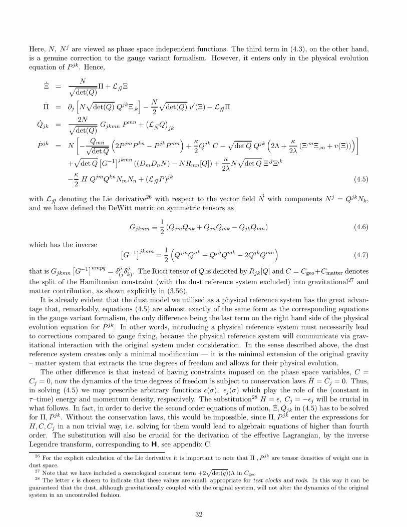
Here, N, N j are viewed as phase space independent functions. The third term in (4.3), on the other hand,is a genuine correction to the gauge variant formalism. However, it enters only in the physical evolutionequation of P jk. Hence,

Ξ =N√

det(Q)Π + L ~N

Ξ

Π = ∂j

[N√

det(Q) QjkΞ,k

]− N

2

√det(Q) v′(Ξ) + L ~N

Π

Qjk =2N√det(Q)

Gjkmn Pmn +

(L ~N

Q)jk

P jk = N

[− Qmn√

detQ

(2P jmP kn − P jkPmn

)+κ

2Qjk C −

√detQ Qjk

(2Λ +

κ

2λ(Ξ,mΞ,m + v(Ξ))

)]

+√

detQ[G−1

]jkmn((DmDnN) −NRmn[Q]) +

κ

2λN√

detQ Ξ,jΞ,k

−κ2H QjmQknNmNn + (L ~N

P )jk (4.5)

with L ~Ndenoting the Lie derivative26 with respect to the vector field ~N with components N j = QjkNk,

and we have defined the DeWitt metric on symmetric tensors as

Gjkmn ≡ 1

2(QjmQnk +QjnQmk −QjkQmn) (4.6)

which has the inverse [G−1

]jkmn=

1

2

(QjmQnk +QjnQmk − 2QjkQmn

)(4.7)

that is Gjkmn

[G−1

]nmpq= δp

(jδq

k). The Ricci tensor of Q is denoted by Rjk[Q] and C = Cgeo+Cmatter denotes

the split of the Hamiltonian constraint (with the dust reference system excluded) into gravitational27 andmatter contribution, as shown explicitly in (3.56).

It is already evident that the dust model we utilised as a physical reference system has the great advan-tage that, remarkably, equations (4.5) are almost exactly of the same form as the corresponding equationsin the gauge variant formalism, the only difference being the last term on the right hand side of the physicalevolution equation for P jk. In other words, introducing a physical reference system must necessarily leadto corrections compared to gauge fixing, because the physical reference system will communicate via grav-itational interaction with the original system under consideration. In the sense described above, the dustreference system creates only a minimal modification — it is the minimal extension of the original gravity– matter system that extracts the true degrees of freedom and allows for their physical evolution.

The other difference is that instead of having constraints imposed on the phase space variables, C =Cj = 0, now the dynamics of the true degrees of freedom is subject to conservation laws H = Cj = 0. Thus,in solving (4.5) we may prescribe arbitrary functions ǫ(σ), ǫj(σ) which play the role of the (constant inτ–time) energy and momentum density, respectively. The substitution28 H = ǫ, Cj = −ǫj will be crucial inwhat follows. In fact, in order to derive the second order equations of motion, Ξ, Qjk in (4.5) has to be solvedfor Π, P jk. Without the conservation laws, this would be impossible, since Π, P jk enter the expressions forH,C,Cj in a non trivial way, i.e. solving for them would lead to algebraic equations of higher than fourthorder. The substitution will also be crucial for the derivation of the effective Lagrangian, by the inverseLegendre transform, corresponding to H, see appendix C.

26 For the explicit calculation of the Lie derivative it is important to note that Π , P jk are tensor densities of weight one indust space.

27 Note that we have included a cosmological constant term +2p

det(q))Λ in Cgeo28 The letter ǫ is chosen to indicate that these values are small, appropriate for test clocks and rods. In this way it can be

guaranteed that the dust, although gravitationally coupled with the original system, will not alter the dynamics of the originalsystem in an uncontrolled fashion.

32

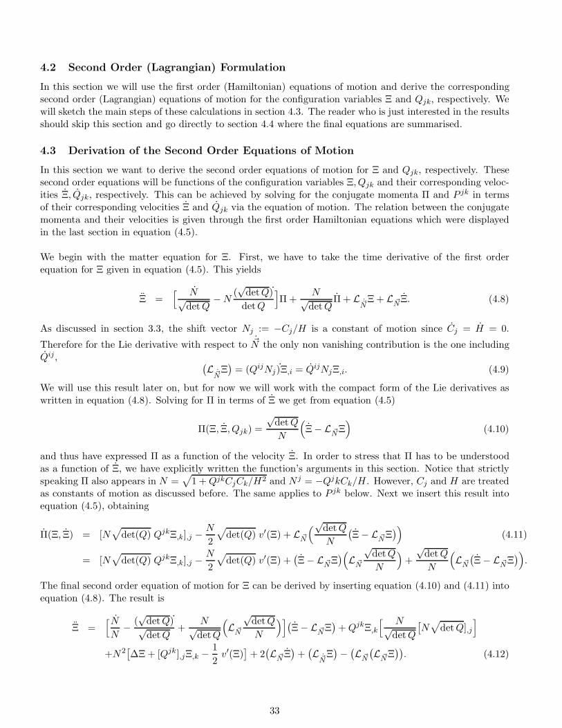
4.2 Second Order (Lagrangian) Formulation

In this section we will use the first order (Hamiltonian) equations of motion and derive the correspondingsecond order (Lagrangian) equations of motion for the configuration variables Ξ and Qjk, respectively. Wewill sketch the main steps of these calculations in section 4.3. The reader who is just interested in the resultsshould skip this section and go directly to section 4.4 where the final equations are summarised.

4.3 Derivation of the Second Order Equations of Motion

In this section we want to derive the second order equations of motion for Ξ and Qjk, respectively. Thesesecond order equations will be functions of the configuration variables Ξ, Qjk and their corresponding veloc-ities Ξ, Qjk, respectively. This can be achieved by solving for the conjugate momenta Π and P jk in termsof their corresponding velocities Ξ and Qjk via the equation of motion. The relation between the conjugatemomenta and their velocities is given through the first order Hamiltonian equations which were displayedin the last section in equation (4.5).

We begin with the matter equation for Ξ. First, we have to take the time derivative of the first orderequation for Ξ given in equation (4.5). This yields

Ξ =[ N√

detQ−N

(√

detQ)˙

detQ

]Π +

N√detQ

Π + L~NΞ + L ~N

Ξ. (4.8)

As discussed in section 3.3, the shift vector Nj := −Cj/H is a constant of motion since Cj = H = 0.

Therefore for the Lie derivative with respect to ~N the only non vanishing contribution is the one includingQij, (

L~NΞ)

= (QijNj)˙Ξ,i = QijNjΞ,i. (4.9)

We will use this result later on, but for now we will work with the compact form of the Lie derivatives aswritten in equation (4.8). Solving for Π in terms of Ξ we get from equation (4.5)

Π(Ξ, Ξ, Qjk) =

√detQ

N

(Ξ − L ~N

Ξ)

(4.10)

and thus have expressed Π as a function of the velocity Ξ. In order to stress that Π has to be understoodas a function of Ξ, we have explicitly written the function’s arguments in this section. Notice that strictlyspeaking Π also appears in N =

√1 +QjkCjCk/H2 and N j = −QjkCk/H. However, Cj and H are treated

as constants of motion as discussed before. The same applies to P jk below. Next we insert this result intoequation (4.5), obtaining

Π(Ξ, Ξ) = [N√

det(Q) QjkΞ,k],j −N

2

√det(Q) v′(Ξ) + L ~N

(√detQ

N

(Ξ − L ~N

Ξ))

(4.11)

= [N√

det(Q) QjkΞ,k],j −N

2

√det(Q) v′(Ξ) +

(Ξ − L ~N

Ξ)(

L ~N

√detQ

N

)+

√detQ

N

(L ~N

(Ξ − L ~N

Ξ)).

The final second order equation of motion for Ξ can be derived by inserting equation (4.10) and (4.11) intoequation (4.8). The result is

Ξ =[NN

− (√

detQ)˙√detQ

+N√detQ

(L ~N

√detQ

N

)](Ξ − L ~N

Ξ)

+QjkΞ,k

[ N√detQ

[N√

detQ],j

]

+N2[∆Ξ + [Qjk],jΞ,k −

1

2v′(Ξ)

]+ 2(L ~N

Ξ)

+(L

~NΞ)−(L ~N

(L ~N

Ξ)). (4.12)

33

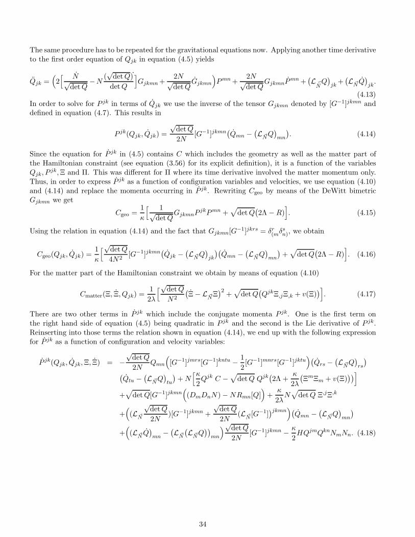
The same procedure has to be repeated for the gravitational equations now. Applying another time derivativeto the first order equation of Qjk in equation (4.5) yields

Qjk =(2[ N√

detQ−N (

√detQ)˙

detQ

]Gjkmn +

2N√detQ

Gjkmn

)Pmn +

2N√detQ

GjkmnPmn +

(L ~

NQ)jk

+(L ~N

Q)jk.

(4.13)In order to solve for P jk in terms of Qjk we use the inverse of the tensor Gjkmn denoted by [G−1]jkmn anddefined in equation (4.7). This results in

P jk(Qjk, Qjk) =

√detQ

2N[G−1]jkmn

(Qmn −

(L ~N

Q)mn

). (4.14)

Since the equation for P jk in (4.5) contains C which includes the geometry as well as the matter part ofthe Hamiltonian constraint (see equation (3.56) for its explicit definition), it is a function of the variablesQjk, P

jk,Ξ and Π. This was different for Π where its time derivative involved the matter momentum only.Thus, in order to express P jk as a function of configuration variables and velocities, we use equation (4.10)and (4.14) and replace the momenta occurring in P jk. Rewriting Cgeo by means of the DeWitt bimetricGjkmn we get

Cgeo =1

κ

[ 1√detQ

GjkmnPjkPmn +

√detQ

(2Λ −R)

]. (4.15)

Using the relation in equation (4.14) and the fact that Gjkmn[G−1]jkrs = δr(mδ

sn), we obtain

Cgeo(Qjk, Qjk) =1

κ

[√detQ

4N2[G−1]jkmn

(Qjk −

(L ~N

Q)jk

)(Qmn −

(L ~N

Q)mn

)+√

detQ(2Λ −R)

]. (4.16)

For the matter part of the Hamiltonian constraint we obtain by means of equation (4.10)

Cmatter(Ξ, Ξ, Qjk) =1

2λ

[√detQ

N2

(Ξ − L ~N

Ξ)2

+√

detQ(QjkΞ,jΞ,k + v(Ξ)

)]. (4.17)

There are two other terms in P jk which include the conjugate momenta P jk. One is the first term onthe right hand side of equation (4.5) being quadratic in P jk and the second is the Lie derivative of P jk.Reinserting into those terms the relation shown in equation (4.14), we end up with the following expressionfor P jk as a function of configuration and velocity variables:

P jk(Qjk, Qjk,Ξ, Ξ) = −√

detQ

2NQmn

([G−1]jmrs[G−1]kntu − 1

2[G−1]mnrs[G−1]jktu

)(Qrs −

(L ~N

Q)rs

)

(Qtu −

(L ~N

Q)tu

)+N

[κ2Qjk C −

√detQ Qjk

(2Λ +

κ

2λ

(ΞmΞm + v(Ξ)

))]

+√

detQ[G−1]jkmn((DmDnN) −NRmn[Q]

)+

κ

2λN√

detQ Ξ,jΞ,k

+((L ~N

√detQ

2N)[G−1]jkmn +

√detQ

2N(L ~N

[G−1])jkmn

)(Qmn −

(L ~N

Q)mn

)

+((L ~N

Q)mn

−(L ~N

(L ~N

Q))

mn

)√detQ

2N[G−1]jkmn − κ

2HQjmQknNmNn. (4.18)

34

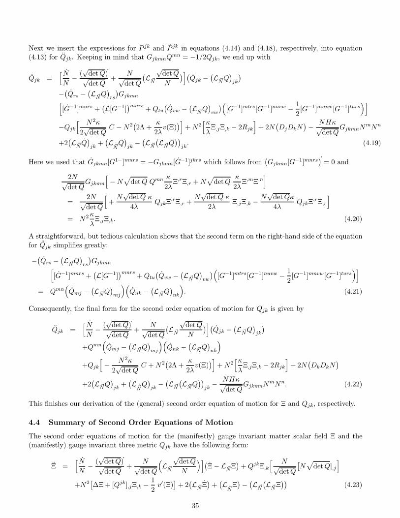
Next we insert the expressions for P jk and P jk in equations (4.14) and (4.18), respectively, into equation(4.13) for Qjk. Keeping in mind that GjkmnQ

mn = −1/2Qjk, we end up with

Qjk =[NN

− (√

detQ)˙√detQ

+N√detQ

(L ~N

√detQ

N

)](Qjk −

(L ~N

Q)jk

)

−(Qrs −

(L ~N

Q)rs

)Gjkmn

[[G−1]mnrs +

(L[G−1]

)mnrs+Qtu

(Qvw −

(L ~N

Q)vw

)([G−1]mtrs[G−1]nuvw − 1

2[G−1]mnvw[G−1]turs

)]

−Qjk

[ N2κ

2√

detQC −N2

(2Λ +

κ

2λv(Ξ)

)]+N2

[κλ

Ξ,jΞ,k − 2Rjk

]+ 2N

(DjDkN

)− NHκ√

detQGjkmnN

mNn

+2(L ~N

Q)jk

+(L

~NQ)jk

−(L ~N

(L ~N

Q))

jk. (4.19)

Here we used that Gjkmn[G1−]mnrs = −Gjkmn[G−1]jkrs which follows from(Gjkmn[G−1]mnrs

)= 0 and

2N√detQ

Gjkmn

[−N

√detQ Qmn κ

2λΞ,rΞ,r +N

√detQ

κ

2λΞ,mΞ,n

]

=2N√detQ

[+N√

detQ κ

4λQjkΞ

,rΞ,r +N√

detQ κ

2λΞ,jΞ,k −

N√

detQκ

4λQjkΞ

,rΞ,r

]

= N2κ

λΞ,jΞ,k. (4.20)

A straightforward, but tedious calculation shows that the second term on the right-hand side of the equationfor Qjk simplifies greatly:

−(Qrs −

(L ~N

Q)rs

)Gjkmn

[[G−1]mnrs +

(L[G−1]

)mnrs+Qtu

(Qvw −

(L ~N

Q)vw

)([G−1]mtrs[G−1]nuvw − 1

2[G−1]mnvw[G−1]turs

)]

= Qmn(Qmj −

(L ~N

Q)mj

)(Qnk −

(L ~N

Q)nk

). (4.21)

Consequently, the final form for the second order equation of motion for Qjk is given by

Qjk =[NN

− (√

detQ)˙√detQ

+N√detQ

(L ~N

√detQ

N

)](Qjk −

(L ~N

Q)jk

)

+Qmn(Qmj −

(L ~N

Q)mj

)(Qnk −

(L ~N

Q)nk

)

+Qjk

[− N2κ

2√

detQC +N2

(2Λ +

κ

2λv(Ξ)

)]+N2

[κλ

Ξ,jΞ,k − 2Rjk

]+ 2N

(DkDkN

)

+2(L ~N

Q)jk

+(L

~NQ)jk

−(L ~N

(L ~N

Q))

jk− NHκ√

detQGjkmnN

mNn. (4.22)

This finishes our derivation of the (general) second order equation of motion for Ξ and Qjk, respectively.

4.4 Summary of Second Order Equations of Motion

The second order equations of motion for the (manifestly) gauge invariant matter scalar field Ξ and the(manifestly) gauge invariant three metric Qjk have the following form:

Ξ =[NN

− (√

detQ)˙√detQ

+N√detQ

(L ~N

√detQ

N

)](Ξ − L ~N

Ξ)

+QjkΞ,k

[ N√detQ

[N√

detQ],j

]

+N2[∆Ξ + [Qjk],jΞ,k −

1

2v′(Ξ)

]+ 2(L ~N

Ξ)

+(L

~NΞ)−(L ~N

(L ~N

Ξ))

(4.23)

35

and

Qjk =[NN

− (√

detQ)˙√detQ

+N√detQ

(L ~N

√detQ

N

)](Qjk −

(L ~N

Q)jk

)

+Qmn(Qmj −

(L ~N

Q)mj

)(Qnk −

(L ~N

Q)nk

)

+Qjk

[− N2κ

2√

detQC +N2

(2Λ +

κ

2λv(Ξ)

)]+N2

[κλ

Ξ,jΞ,k − 2Rjk

]+ 2N

(DjDkN

)

+2(L ~N

Q)jk

+(L

~NQ)jk

−(L ~N

(L ~N

Q))

jk− NHκ√

detQGjkmnN

mNn. (4.24)

The term C = Cgeo + Cmatter occurring in the equation for Qjk has to be understood as a function ofconfiguration and velocity variables and is explicitly given by

Cgeo =1

κ

[√detQ

4N2[G−1]jkmn

(Qjk −

(L ~N

Q)jk

)(Qmn −

(L ~N

Q)mn

)+√

detQ(2Λ −R)

]

Cmatter =1

2λ

[√detQ

N2

(Ξ − L ~N

Ξ)2

+√

detQ(QjkΞ,jΞ,k + v(Ξ)

)]. (4.25)

Apart from the fact that we have a dynamical lapse function given by N = C/H, as well as a dynamicalshift vector defined as Nj = −Cj/H, the only deviation from the standard Einstein equations in canonicalform is the last term on the right-hand side in equation (4.24). This term, being quadratic in Nj andtherefore quadratic in Cj = Cgeo

j + Cmatterj , vanishes for instance when FRW spacetimes are considered. In

our companion paper [15], we specialize these equations precisely to this context and show that the equationsabove reproduce the correct FRW equations.

5 Physical Hamiltonian, Boundary Term and ADM Hamiltonian

As long as the dust space S (and therefore X ) has no boundary, H is functionally differentiable, which wealways assumed so far. However, for more general topologies we are forced to consider boundary conditions.In this section we show how to deal with asymptotically flat boundary conditions for illustrative purposes.More general situations can be considered analogously.

Recall [37] that asymptotically flat initial data are subject to the following boundary conditions

qab(x) = δab +fab(Ω)

r+ O(r−2) ,

pab(x) =gab(Ω)

r+ O(r−3) ,

ξ(x) =f(Ω)

r2+ O(r−3) ,

π(x) =g(Ω)

r2+ O(r−3) . (5.1)

Here, xa is an asymptotic coordinate system, r2 ≡ δabxaxb and Ω denotes the angular dependence of the

unit vector xa/r (on the asymptotic sphere). The functions fab, f, gab, g are assumed to be smooth.

Moreover, fab is an even function under reflection at spatial infinity on the sphere, while gab is odd (f, gdo not underly parity restrictions). Notice that these boundary conditions directly translate into analogousones for the substitutions Qjk ↔ qab, P

jk ↔ pab, Ξ ↔ ξ, Π ↔ π, because switching from X to S is just adiffeomorphism.

The part of the differential of H that gives rise to a boundary term is

δboundary H =

∫

Sd3σ

[NδboundaryC +N jδboundaryCj

], (5.2)

36

which coincides precisely with the boundary terms produced by the canonical Hamiltonian29

Hcanonical =

∫

Xd3x [nc+ naca] (5.3)

without dust. Here, the lapse and shift functions n, na are Lagrange multiplier rather than dynamical quan-tities like N,N j . Therefore, the usual boundary terms [37] can be adopted, once the asymptotic behaviourof the dynamical lapse and shift functions N,N j have been determined, which, in turn, is completely spec-ified by Nj because N j = QjkNk, N =

√1 +QjkNjNk. The scalar field contribution to C,Cj decays as

1/r4, thus it is sufficient to consider the geometrical contribution. Cgeoj = −2DkP

kj decays as 1/r3 and is

even asymptotically. The term quadratic in P jk and the term quadratic in the Christoffel symbols in Cgeo

decays as 1/r4, while the term linear in the Cristoffel symbols decays as 1/r3 and is even. We conclude that

Nj = −Cj

H(with H =

√C2 −QjkCjCk) is asymptotically constant and even. The same is true for N , which

is anyway bounded from below by unity. The usual computation [22, 37] yields

δboundary H = −δB′(N) − δ ~B′( ~N ′)

κδB′(N) =

∫

S2

√det(Q)QjkQmn [(DjN)dSkδ(Qmn − δmn) − (DmN)dSnδ (Qjk − δjk)]

+

∫

S2

√det(Q)QjkN

[−dSjδΓ

mmk + SkδΓ

kjk

]

κδ ~B′( ~N ) = 2

∫

S2

dSj NkδP j

k , (5.4)

where dSj = xj/rdΩ , dΩ the volume element of S2. The prime is to indicate that, contrary to whatthe notation suggests, the terms shown are, a priori, not total differentials. In the usual formalism theyare, because lapse and shift functions are Lagrange multipliers and do not depend on phase space. Here,however, they are dynamical and we must worry about the variation δNj .

It turns out that the boundary conditions need to be refined in order to make H differentiable. Wewill not analyze the most general boundary conditions in this paper, but just make a specific choice thatwill be sufficient for our purposes. Namely, we will impose in addition that Cgeo

j = −2DkPkj decays as

1/r3+ǫ, (ǫ > 0) at spatial infinity. Then also Cj falls off as 1/r3+ǫ. Since C decays like 1/r3, it follows thatalso H =

√C2 −QjkCjCk decays as 1/r3, whence Nj = −Cj/H decays as 1/rǫ. This implies that δNj

decays as 30 1/rǫ. Thus, δN = [QjkNkδNj +NjNkδQjk/2]/N decays as 31 1/r2ǫ.

It follows that δ ~B′( ~N) = 0 and

κδB′(N) = κδEADM, EADM =

∫

S2

√det(Q)Qjk

[−dSj Γm

mk + SkδΓkjk

](5.5)

reduces to the variation of the ADM energy. The correct Hamiltonian is given by

H = EADM +

∫

Sd3σ H(σ) . (5.6)

It is reassuring that in the asymptotically flat context, we have automatically a boundary term in the Hamil-tonian, which is just the ADM energy. The additional bulk term comes from the dust energy density anddoes not vanish on the constraint surface.

29With the substitutions S ↔ X , Qjk ↔ qab, P jk ↔ pab, Ξ ↔ ξ, Π ↔ π implied.30We could more generally have imposed that δNj falls off like 1/rǫ at spatial infinity.31The choice ǫ = 1/2 seems to be appropriate in order to reproduce the asymptotic Schwarzschild decay for dynamical lapse

and shift. However, this is not the case here, because we are automatically in a freely falling (dust) frame and τ is eigentime.Hence, gττ = −N2 + QjkNjNk − 1, whatever choice for Nj is made, it is independent of τ .

37

Before we close this section, let us also mention the physical Hamiltonian system under considerationthere exists a Lagrangian from which derives by Legendre transformation on the phase space defined by thephysical observables. Curiously, the corresponding effective action turns out to be non-local in dust spacebut local in dust time. It can be computed via a fixed point equation to any order in the spatial derivativesof the fields. Details can be found in appendix C.

6 Linear, Manifestly Gauge Invariant Perturbation Theory

In section 4 we derived the (manifestly) gauge invariant second order equation of motion for the scalar fieldΞ and the three metric Qjk. Now we want to consider small perturbations around a given background whosecorresponding quantities will be denoted by a bar, namely Ξ, Qjk. The linear perturbations are then defined

as δΞ := Ξ − Ξ and δQjk := Qjk − Qjk, respectively. Note that these perturbations are also (manifestly)gauge invariant because they are defined as a difference of two gauge invariant quantities. Consequently,any power of δΞ and δQjk will also be a (manifestly) gauge invariant quantity such that in the frameworkintroduced in this paper gauge invariant perturbation theory up to arbitrary order is not only possible, butalso straightforward. This is a definite strength of our approach compared to the traditional one, see section7 for a detailed discussion.

However, in this section we will restrict ourselves to linear (manifestly) gauge invariant perturbation theory.That is any function F (Qjk,Ξ) will be expanded up to linear order in the perturbations δΞ and δQjk. Wedenote by δF the linear order term in the Taylor expansion of the expression F (Qjk,Ξ) − F (Qjk,Ξ). Acalculation of higher order terms will be the content of a future publication. Usually, in cosmological per-turbation theory one chooses an FRW background and considers small perturbations around it. Here wewill derive the equations of motion for the linear perturbations assuming an arbitrary background. In ourcompanion paper, we will specialise the results derived here to the case of an FRW background and showthat we can reproduce the standard results as presented, e.g., in [7]. The reader who is only interested inthe final form of the perturbed equation of motions should go directly to section 6.3, where a summary ofthe results is provided.

6.1 Derivation of the Equation of Motion for δΞ

Let us go back to the second order equation of motion for Ξ shown in equation (4.23). Since its perturbationinvolves several terms we will, for reasons of book keeping, split this equation into several parts and considerthe perturbation of those parts separately. Comparing the equation of Ξ with the one for Qij in equation(4.24), we realise that in both equations the first term on the right-hand side includes an identical term,namely the expression in the square brackets. Therefore it is convenient to derive its perturbation in aclosed form such that the result can then also be used for the derivation of the equation of motion of δQij .Throughout this section we will repeatedly need the perturbation of

√detQ and its inverse, given by

δ√

detQ =1

2

√detQ Q

ijδQij

δ( 1√

detQ

)= −1

2

1√detQ

QijδQij . (6.1)

Next, considering the definition of the lapse functions given by N = C/H and the definition of H =√C2 −QijCiCj we obtain N =

√1 +QijNiNj . Thus, as mentioned before, N is not an independent

variable, but can be expressed in terms of Qij and the shift vector, which itself is a function of the elementaryvariables Ξ, Qij. However, as shown in our companion paper [15], the perturbation of Nj is again a constantof motion, that is δNj = 0. For this reason it is convenient to work with δQjk, δΞ and δNj , although, strictly

38

speaking, δNj is not an independent perturbation. Keeping this in mind the perturbation of N yields

δN =[− N

2

(N jN

k

N2

)]δQjk +

[NN

j

N2

]δNj . (6.2)

From the explicit form of δN and δ√

detQ we can derive the following expressions which we will need below:

δ(NN

)=

[− ∂

∂τ

1

2

(N jN

k

N2

)]δQjk +

[(N j

N2

) ]δNj (6.3)

δ(−(√

detQ)

√detQ

)=

[− ∂

∂τ

1

2Q

jk]δQjk.

Here the derivative with respect to τ is understood to act on everything to its right, including the perturba-tions. We also used that δNj is a constant of motion, so the term proportional to δNj does not contribute.In order to calculate the perturbation of the Lie derivative term occurring in the square brackets in eqn.(4.23), we compute

δ( N√

detQ

)=

[−( N√

detQ

)1

2

(Q

jk+N

jN

k

N2

)]δQjk +

[N j

N2

]δNj

δ(√detQ

N

)=

[(√detQ

N

)1

2

(Q

jk+N

jN

k

N2

)]δQjk +

[−√

detQ

N

Nj

N2

]δNj . (6.4)

The Lie derivative term yields then

δ((

L ~N

√detQ

N

))=

[L~

N

(√detQ

N

1

2

(Q

jk+N

jN

k

N2

))]δQjk

+[− L~

N

√detQ

N

(N j

N2

)]δNj

+(L

δ ~N

√detQ

N

). (6.5)

Similar to the τ -derivative, the Lie derivative L ~Nacts on all terms to its right, including the linear pertur-

bations. For the moment we keep the Lie derivative with respect to δ ~N in the compact form above. At alater stage we will write down these terms explicitly and express them in terms of δQjk and δNj . Havingcalculated the variations of all components of the first square bracket in eqn. (4.23), we can now give thefinal result:

δ[NN

− (√

detQ)˙√detQ

+N√detQ

(L ~N

√detQ

N

)]=

[−( ∂∂τ

− L~N

)(1

2

(Q

jk+N

jN

k

N2

))]δQjk

+[( ∂∂τ

− L~N

)N j

N2

]δNj

+N√detQ

(L

δ ~N

√detQ

N

). (6.6)

The last term in this equation can be written explicitly in terms of δQmn and δNm as

N√detQ

(L

δ ~N

√detQ

N

)=

[− N√

detQ

∂

∂xm

(√detQ

NQ

jmN

k)]δQjk

+[ N√

detQ

∂

∂xk

(√detQ

NQ

jk)]δNj . (6.7)

39

As the terms in equation (6.6) are multiplied by (Ξ−(L ~NΞ)) in equation (4.23), we also need the perturbation

of the latter term. It is given by

δ(Ξ −

(L ~N

Ξ))

=( ∂∂τ

− L~N

)δΞ −

(L

δ ~NΞ). (6.8)

Next we determine the perturbation of QjkΞ,k which enters the second term on the right-hand side ofequation (4.23):

δ(QjkΞ,k

)=

[−Q

jmQ

knΞ,k

]δQmn +

[Q

jk ∂

∂xk

]δΞ. (6.9)

The perturbation of the term that is multiplied with QjkΞ,k yields

δ[ N√

detQ

(N√

detQ),j

](6.10)

=[− N√

detQ

1

2

(Q

jk+N

jN

k

N2

)[N

√detQ],j +

N√detQ

∂

∂xj

(1

2

(Q

jk − NjN

k

N2

)N

√detQ

)]δQjk

+[ N√

detQ

Nj

N2

[N

√detQ],j +

N√detQ

∂

∂xj

(N j

N2N

√detQ

)]δNj .

We will split the third term occurring on the right-hand side of equation (4.23) into N2 and the remainingpart given by (∆Ξ + [Qjk],jΞ,k − 1

2v′(Ξ)). Their respective perturbations are

δN2 = 2NδN =[−N

jN

k]δQjk +

[2N

j]δNj (6.11)

δ(∆Ξ + [Qjk],jΞ,k −

1

2v′(Ξ)

)=

[− ∂

∂xn

(Q

jmQ

knΞ,m

)]δQjk

+[∆ + [Q

mn],n

∂

∂xm− 1

2v′′(Ξ)

]δΞ.

Finally, we have to calculate the perturbation of the last three terms in equation (4.23), involving Liederivatives of Ξ and Ξ, respectively. We obtain

δ(2(L ~N

Ξ)

+(L

~NΞ)−(L ~N

(L ~N

Ξ)))

=[L~

N

( ∂∂τ

− L~N

)+

∂

∂τL~

N

]δΞ (6.12)

+(LδN

( ∂∂τ

− L~N

)+( ∂∂τ

− L~N

)LδN

)[Ξ].

40

Adding up all the contributions and factoring out the linear perturbations δΞ, δQjk and δNj , we can rewritethe second order EOM as

δΞ =[[NN

− (√

detQ)˙√detQ

+N√detQ

(L~

N

√detQ

N

)]( ∂∂τ

− L~N

)+Q

jk[ N√

detQ

(N

√detQ),j

] ∂

∂xk(6.13)

+N2(∆ + [Q

mn],n

∂

∂xm− 1

2v′′(Ξ)

)+(L~

N

( ∂∂τ

− L~N

)+

∂

∂τL~

N

)]δΞ

+[−(Ξ −

(L~

NΞ))[( ∂

∂τ− L~

N

)(1

2

(Q

jk+N

jN

k

N2

))+

N√detQ

∂

∂xm

(√detQ

NQ

jmN

k)]

−QjmQ

knΞ,n

[ N√detQ

(N√

detQ),m]+[NN

− (√

detQ)˙√detQ

+N√detQ

(L~

N

√detQ

N

)](Q

jmΞ,mN

k))

+(Q

mnΞ,n

)(− N√

detQ

1

2

(Q

jk+N

jN

k

N2

)[N

√detQ],m

+N√detQ

∂

∂xm

(1

2

(Q

jk − NjN

k

N2

)N

√detQ

))

−N2(∆Ξ + [Q

mn],mΞ,n − 1

2v′(Ξ)

)(N jN

k

N2

)−N

2 ∂

∂xn

(Q

jmQ

knΞ,m

)

−QjmQ

knNm

[Ξ −

(L~

NΞ)]

,n−( ∂∂τ

− L~N

)(Q

jmQ

knNmΞ,n

)]δQjk

+[(

Ξ −(L~

NΞ))[( ∂

∂τ− L~

N

)N j

N2 +

N√detQ

∂

∂xk

(√detQ

NQ

jk)]

+2N2(∆Ξ + [Q

mn],mΞ,n − 1

2v′(Ξ)

)N j

N2

+(Q

mnΞ,n

)( N√detQ

Nj

N2

[N

√detQ],m +

N√detQ

∂

∂xj

(N j

N2N

√detQ

))

−[NN

− (√

detQ)˙√detQ

+N√detQ

(L~

N

√detQ

N

)](Q

jkΞ,k

)

+Qjk[

Ξ −(L~

NΞ)]

,k+( ∂∂τ

− L~N

)(Q

jkΞ,k

)]δNj .

Here we used that the last term occurring in equation (4.23), which involves the Lie derivative with respectto δ ~N , can again be expressed in terms of the perturbations δQjk and δNj , explicitly given by

(LδN

( ∂∂τ

− L~N

)+( ∂∂τ

− L~N

)LδN

)[Ξ]

(6.14)

=[Q

jk[Ξ −

(L~

NΞ)]

,k+( ∂∂τ

− L~N

)(Q

jkΞ,k

)]δNj

[−Q

jmQ

knNm

[Ξ −

(L~

NΞ)]

,n−( ∂∂τ

− L~N

)(Q

jmQ

knNmΞ,n

)]δQjk.

Analogously, the last term on the right hand side of equation (6.6), which also involves a Lie derivative withrespect to δ ~N , can be expressed as

N√detQ

(L

δ ~N

√detQ

N

)=[− N√

detQ

∂

∂xm

(√detQ

NQ

jmN

k)]δQjk +

[ N√detQ

∂

∂xk

(√detQ

NQ

jk)]δNj .

(6.15)

41

Moreover(L

δ ~NΞ)

occurring in equation (6.8) is given by

(L

δ ~NΞ)

=[−Q

jmΞ,mN

k]δQjk +

[Q

jkΞ,k

]δNj . (6.16)

We would like to emphasise again that the partial and Lie derivatives act on everything to their right andtherefore also on the perturbations. That is the reason why for instance δΞ and δQjk have not been factoredout separately. This finishes our derivation of the second order equation of motion for the scalar fieldperturbation δΞ. In the next section we will discuss the corresponding equation for the metric perturbationδQjk.

6.2 Derivation of the Equation of Motion for δQjk

Similar to the derivation of the second order equation of motion for δΞ we will also split the equation for Qjk

in equation (4.24) into several terms whose perturbations are then considered separately. More precisely,we will split the equation into seven separate terms, with the three terms involving Lie derivatives in thelast line counted as one. Starting with the first term on the right-hand side, we recall that the perturbationof the sum of terms in the square brackets has already been computed during the derivation of the equationfor δΞ. Thus, we can take over those results, as shown in equation (6.6). The perturbation of the term(Qjk − (L ~N

Q)jk) is given by

δ(Qjk −

(L ~N

Q)jk

)=

( ∂∂τ

− L~N

)δQjk −

(LδNQ

)jk, (6.17)

whereby

(LδNQ

)jk

=[−Q

mrN

n[Qjk

],r−Qkm

∂

∂xj

(Q

mrN

n)−Qjm

∂

∂xk

(Q

mrN

n)]δQmn (6.18)

+[Q

mn[Qjk

],n

+Qkn

∂

∂xj

(Q

mn)

+Qjn

∂

∂xk

(Q

mn)]δNm.

Consequently, we have all ingredients needed for the perturbation of the first term. However, we will notpresent the final expression in the main text since it is quite lengthly. Nevertheless, the interested readercan find the explicit form in appendix G in equation (6.17). The perturbation of the second term on theright-hand side yields

δ(Qmn

(Qmj −

(L ~N

Q)mj

)(Qnk −

(L ~N

Q)nk

))(6.19)

=[−Q

mrQ

ns(Qrj −

(L~

NQ)rj

)(Qsk −

(L~

NQ)sk

)]δQmn +

[2Q

mn(Qn(k −

(L~

NQ)n(k

)( ∂∂τ

− L~N

)]δQj)m

+[− 2Q

mn(Qn(k −

(L~

NQ)n(k

)](LδNQ

)j)m

.

The perturbation of the third term occurring on the right-hand side requires a bit more work, because itinvolves C = Cgeo + Cmatter. Thus we will perform this calculation in two steps. First we will ignore theexplicit form of δC in terms of δQjk, δΞ and δNj . The resulting expression looks like

δ(Qjk

[− N2κ

2√

detQC +N2

(2Λ +

κ

2λv(Ξ)

)])(6.20)

=[Qjk

[12

(Q

mn+N

mN

n

N2

) κN2

2√

detQC +

NmN

n

2N2 N

2( κ

2√

detQC − 2

(2Λ +

κ

2λv(Ξ)

)))]]δQmn

+[N

2(− κ

2√

detQC + 2Λ +

κ

2λv(Ξ)

)]δQjk +

[2QjkN

2(− κ

2√

detQC + 2Λ +

κ

2λv(Ξ)

)(Nm

N2

)]δNm

+[−QjkN

2 κ

2√

detQ

]δC +

[QjkN

2 κ

2λv′(Ξ)

]δΞ.

42

Due to its length, the explicit calculation of δC can be found in appendix G. However, when actuallyinserting the expression of δC into equation (6.20), some of the terms in the expression for δC cancel withexisting terms in equation (6.20). As a result, the final expression for the perturbation of the third term inequation (6.21) is slightly less involved. It is given by

δ(Qjk

[− N2κ

2√

detQC +N2

(2Λ +

κ

2λv(Ξ)

)])(6.21)

=[−Qjk

(1

2

NmN

n

N2 N

2(2Λ −R+

κ

2λ

(v(Ξ) −Q

rsΞ,rΞ,s

))+N

2

2

(R

mn − [G−1

]mnrsDrDs

)

+κ

2λQ

mrQ

ns(Ξ −

(L~

NΞ))N rΞ,s −

κN2

2λQ

rmQ

snΞ,rΞ,s

+1

4

(Qrs −

(L~

NQ)rs

)[[G

−1]mnrs

( ∂∂τ

− L~N

)−(Qtu −

(L~

NQ)tu

)Q

sn[G

−1]turm

]

+1

4

(Qrs −

(L~

NQ)rs

)[G

−1]rsvw

[Q

mtN

n[Qvw],t + 2Qtw

∂

∂xv

(Q

mtN

n)])]

δQmn

[−Qjk

(− N

m

N2 N

2(2Λ −R− κ

2λ

(v(Ξ) −Q

rsΞ,rΞ,s

))− κ

2λ

(Ξ −

(L~

NΞ))Q

mnΞ,n

−1

4

(Qrs −

(L~

NQ)rs

)[G

−1]rsvw

[Q

mt[Qvw],t + 2Qtw

∂

∂xv

(Q

mt)])

δNm

+[−Qjk

(N2κ

2λ

( 1

N2

(Ξ −

(L~

NΞ))( ∂

∂τ− L~

N

)+Q

mnΞ,n

∂

∂xm− 1

2v′(Ξ)

))]δΞ

+[N

2(− κ

2√

detQC + 2Λ +

κ

2λv(Ξ)

)]δQjk.

Proceeding with the next term on the right-hand side of equation (4.24), we obtain for its perturbation thefollowing result:

δ(N2(κλ

Ξ,jΞ,k − 2Rjk

))=

[12

NmN

n

N2

(− 2N

2(κλ

Ξ,jΞ,k − 2Rjk

))+N

2DjDkQ

mn]δQmn (6.22)

+[N

2DmDnQ

mn]δQjk +

[− 2N

2DnD(kQ

mn]δQj)m

+[Nm

N2

(2N

2(κλ

Ξ,jΞ,k − 2Rjk

))]δNm +

[4N

2κ

λΞ(,k

∂

∂xj)

]δΞ.

For this calculation we used the fact that the perturbation of the Ricci tensor can be expressed in terms ofthe perturbations δQjk. The explicit relation reads

δRjk =[− 1

2DmDnQ

mn]δQjk +

[− 1

2DjDkQ

mn]δQmn +

[DnD(kQ

mn]δQj)m. (6.23)

The next term in equation (4.24) includes covariant derivatives. Therefore we will have to consider theperturbation of the Christoffel symbols Γm

jk. These can again be written in terms of metric perturbations asshown below

δΓmjk =

Qmn

2

((DjδQnk

)+(DkδQjn

)−(DnδQjk

)). (6.24)

Using this we end up with

δ(2NDjDkN) =

[12

NmN

n

N2

(− 4N

(DjDkN

))− 2N

2DjDk

(1

2

NmN

n

N2

)]δQmn (6.25)

+[Nm

N2

(4N(DjDkN

))+ 2N

2DjDk

(Nm

N2

)]δNm

+[2N(DnN

)D(kQ

mn]δQj),m +

[−N

2(DnN

)DmQ

mn]δQjk.

43

Note that covariant derivatives surrounded by round bracket such as (DjDk...) act on the elements inside theround brackets only. By contrast, covariant derivatives not surrounded by round brackets act on everythingto their right, including also the perturbations.

Next we deal with the three terms on the right-hand side of equation (4.24) that include Lie derivativeswith respect to δ ~N . Those Lie derivatives are again functions of δQjk, δNj , and partial derivatives thereof,because we have δNm = −Qmr

QnsN sδQrn + Q

mnδNn. In this section, however, we will work with the

following compact form only:

δ(2(L ~N

Q)jk

+(L

~NQ)jk

−(L ~N

(L ~N

Q))

jk

)=

[L~

N

( ∂∂τ

−L~N

)+

∂

∂τL~

N

]δQjk (6.26)

+(LδN

( ∂∂τ

− L~N

)+( ∂∂τ

− L~N

)LδN

)[Qjk

].

In the next section, we will rewrite the second order equation of motion in a more concise form, usingcoefficient functions. That will allow us to include the Lie derivative term with respect to δ ~N in thefollowing, more explicit form:

(LδN

( ∂∂τ

− L~N

)+( ∂∂τ

− L~N

)LδN

)[Qjk

](6.27)

=[−Q

mrN

n[Qjk −

(L~

NQ)jk

],r−(Qkm −

(L~

NQ)kr

) ∂

∂xj

(Q

mrN

n)−(Qjm −

(L~

NQ)jr

) ∂

∂xk

(Q

mrN

n)

+( ∂∂τ

− L~N

)(−Q

mrN

n[Qjk

],r−Qkm

∂

∂xj

(Q

mrN

n)−Qjm

∂

∂xk

(Q

mrN

n))]

δQmn

+[Q

mn[Qjk −

(L~

NQ)jk

],n

+(Qkn −

(L~

NQ)kn

) ∂

∂xj

(Q

mn)

+(Qjn −

(L~

NQ)jn

) ∂

∂xk

(Q

mn)

+( ∂∂τ

− L~N

)(Q

mn[Qjk

],n

+Qkn

∂

∂xj

(Q

mn)

+Qjn

∂

∂xk

(Q

mn))]

δNm

Another term which includes Lie derivatives with respect to δ ~N appeared previously as part of equation(6.19). Performing the Lie derivative also in this case, we end up with

[− 2Q

mn(Qn(k −

(L~

NQ)n(k

)](LδNQ

)j)m

(6.28)

=[(

− 2Qtu(Qt(k −

(L~

NQ)t(k

))(−Q

mrN

n[Qj)u

]

,r−Qum

∂

∂xj)

(Q

mrN

n)−Qj)m

∂

∂xu

(Q

mrN

n))]

δQmn

[(− 2Q

tu(Qt(k −

(L~

NQ)t(k

))(Q

mn[Qj)u

]

,n+Qun

∂

∂xj)

(Q

mn)

+Qj)n∂

∂xu

(Q

mn))]

δNm.

The other two terms that include Lie derivatives with respect to δ ~N are parts of the perturbation of thefirst term. Their explicit expressions are given in equation (6.7) and equation (6.18), respectively. Note thatthese terms are written out explicitly in appendix G, where the final form of the perturbation of the firstterm is calculated.Finally, we consider the last remaining term from equation (4.24). It involves the Hamiltonian density H,which we found out to be a constant of motion in section (3.4). In our companion paper [15] we show thatalso δNj and δH are constants of motion. Therefore, in complete analogy to the case of δNj , we will factor

44

out δH. We thus obtain

δ(− Nκ√

detQHGjkmnN

mNn)

=[− Nκ√

detQN

nN

mGjkmn

]δH +

[− Nκ√

detQHQ

rmN

nN

sGsnr(k

]δQj)m

+[12

(Q

mn+N

mN

n

N2

) Nκ√detQ

HNrN

sGjkrs

+Nκ√detQ

HQsmN

rN

nGjkrs

]δQmn

+[− N

m

N2

Nκ√detQ

HNrN

sGjkrs

]δNm. (6.29)

Here we used thatδGjkmn = −GjkrsGmntuδ[G

−1]rstu. (6.30)

Now we have finally derived all the individual parts that are needed in order to write down the equation ofmotion for δQjk. However, by just looking at the various individual terms, it is clear that they are alreadyconsiderably more complicated than for the corresponding case of the matter equation of motion for δΞ.Nevertheless, we decided to present the final equation in detailed form on the next page, in particular toconvey a sense of how much more involved the geometrical part of the perturbed equations is compared tothe matter part. In the next section we will rewrite both equations of motion, the one for δΞ as well as theone for δQjk, in a more transparent form where all the complicated background coefficients in front of theperturbations are hidden in certain coefficient functions. In our companion paper, we will then specialisethose coefficient functions to the case of an FRW spacetime and show that the general equations derivedin the last two subsection are (up to small correction caused by our dust clock) in agreement with thewell-known perturbation equations as discussed, e.g., in [7]. Note that we still kept the compact form ofthe Lie derivative with respect to δN in equation (6.31), because we wanted to present this equation on onepage only.

45

δQjk =[−Qjk

(N2κ

2λ

( 1

N2

(Ξ −

(L~

NΞ))( ∂

∂τ− L~

N

)+Q

mnΞ,n

∂

∂xm− 1

2v′(Ξ)

))+(4N

2κ

λΞ(,k

∂

∂xj)

)]δΞ

[[NN

− (√

detQ)˙√detQ

+N√detQ

(L~

N

√detQ

N

)](Q

rnNn[Qjk],r +Qrk

∂

∂xj

(Q

rnN

m)

+Qrj

∂

∂xk

(Q

rnN

m))

−(Qjk −

(L~

NQ)jk

)(( ∂∂τ

− L~N

)(1

2

(Q

mn+N

mN

n

N2

))+

N√detQ

∂

∂xk

(√

detQ

NN

mQ

rn))

+(−Q

mrQ

ns(Qrj −

(L~

NQ)rj

)(Qsk −

(L~

NQ)sk

))

+(−Qjk

[12

NmN

n

N2 N

2(2Λ −R+

κ

2λ

(v(Ξ) −Q

rsΞ,rΞ,s

))+N

2

2

(R

mn − [G−1

]mnrsDrDs

)

+κ

2λQ

mrQ

ns(Ξ −

(L~

NΞ))N rΞ,s −

κN2

2λQ

rmQ

snΞ,rΞ,s

+1

4

(Qrs −

(L~

NQ)rs

)[[G

−1]mnrs

( ∂∂τ

− L~N

)−(Qtu −

(L~

NQ)tu

)Q

sn[G

−1]turm

]

+1

4

(Qrs −

(L~

NQ)rs

)[G

−1]rsvw

[Q

mtN

n[Qvw],t + 2Qtw

∂

∂xv

(Q

mtN

n)]])

+(1

2

NmN

n

N2

(− 2N

2(κλ

Ξ,jΞ,k − 2Rjk

)− 4N

(DjDkN

))+N

2DjDkQ

mn − 2N2DjDk

1

2

NmN

n

N2

)

+(1

2

(Q

mn+N

mN

n

N2

) Nκ√detQ

HNrN

sGjkrs +

Nκ√detQ

HQsmN

rN

nGjkrs

)]δQmn

+[−[NN

− (√

detQ)˙√detQ

+N√detQ

(L~

N

√detQ

N

)](Q

mn[Qjk],n +Qnk

∂

∂xj

(Q

mn)

+Qnj

∂

∂xk

(Q

mn)

+(Qjk −

(L~

NQ)jk

)(( ∂∂τ

− L~N

)(Nm

N2

)+

N√detQ

∂

∂xn

(√

detQ

NQ

mn))

+(−Qjk

[− N

m

N2 N

2(2Λ −R− κ

2λ

(v(Ξ) −Q

rsΞ,rΞ,s

))− κ

2λ

(Ξ −

(L~

NΞ))Q

mnΞ,n

−1

4

(Qrs −

(L~

NQ)rs

)[G

−1]rsvw

[Q

mt[Qvw],t + 2Qtw

∂

∂xv

(Q

mt)]])

+(− N

m

N2

Nκ√detQ

HNrN

sGjkrs

)

+(Nm

N2

(2N

2(κλ

Ξ,jΞ,k − 2Rjk

)+ 4N

(DjDkN

))+ 2N

2DjDk

(Nm

N2

)]δNm

+[[NN

− (√

detQ)˙√detQ

+N√detQ

(L~

N

√detQ

N

)]( ∂∂τ

− L~N

)+(N

2(− κ

2√

detQC + 2Λ +

κ

2λv(Ξ)

))

+(N

2DmDnQ

mn)

+(−N

2(DnN

)DmQ

mn)

+((

L~N

( ∂∂τ

− L~N

)+

∂

∂τL~

N

)]δQjk

+[(

2Qmn(Qn(k −

(L~

NQ)n(k

)( ∂∂τ

− L~N

))+(− 2N

2DnD(kQ

mn)

+(2N(DnN

)D(kQ

mn)

+(− Nκ√

detQHQ

rmN

nN

sGsnr(k

)]δQj)m +

[− Nκ√

detQN

nN

mGjkmn

]δH

+(LδN

( ∂∂τ

− L~N

)+( ∂∂τ

− L~N

)LδN

)[Qjk

]+[− 2Q

mn(Qn(k −

(L~

NQ)n(k

)](LδNQ

)j)m

. (6.31)

46

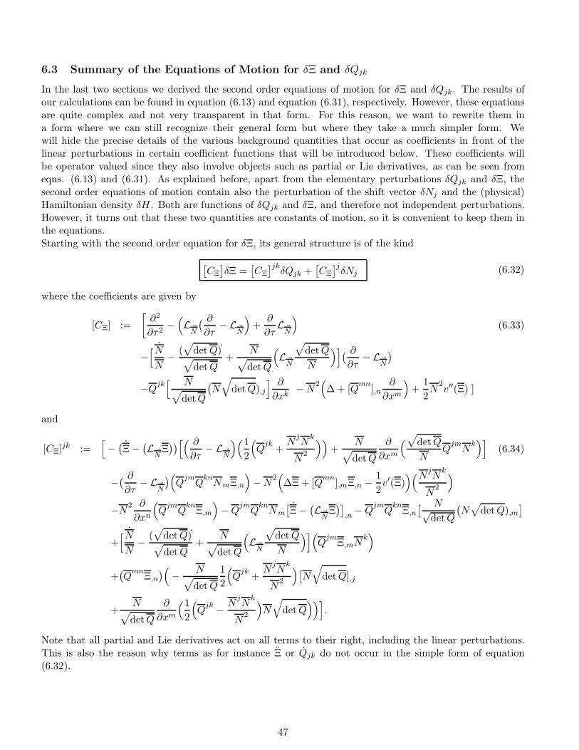
6.3 Summary of the Equations of Motion for δΞ and δQjk

In the last two sections we derived the second order equations of motion for δΞ and δQjk. The results ofour calculations can be found in equation (6.13) and equation (6.31), respectively. However, these equationsare quite complex and not very transparent in that form. For this reason, we want to rewrite them ina form where we can still recognize their general form but where they take a much simpler form. Wewill hide the precise details of the various background quantities that occur as coefficients in front of thelinear perturbations in certain coefficient functions that will be introduced below. These coefficients willbe operator valued since they also involve objects such as partial or Lie derivatives, as can be seen fromeqns. (6.13) and (6.31). As explained before, apart from the elementary perturbations δQjk and δΞ, thesecond order equations of motion contain also the perturbation of the shift vector δNj and the (physical)Hamiltonian density δH. Both are functions of δQjk and δΞ, and therefore not independent perturbations.However, it turns out that these two quantities are constants of motion, so it is convenient to keep them inthe equations.Starting with the second order equation for δΞ, its general structure is of the kind

[CΞ

]δΞ =

[CΞ

]jkδQjk +

[CΞ

]jδNj (6.32)

where the coefficients are given by

[CΞ] :=

[∂2

∂τ2−(L~

N

( ∂∂τ

−L~N

)+

∂

∂τL~

N

)(6.33)

−[NN

− (√

detQ)˙√detQ

+N√detQ

(L~

N

√detQ

N

)]( ∂∂τ

− L~N

)

−Qjk[ N√

detQ

(N

√detQ),j

] ∂

∂xk−N

2(∆ + [Q

mn],n

∂

∂xm

)+

1

2N

2v′′(Ξ) ]

and

[CΞ]jk :=[−(Ξ −

(L~

NΞ))[( ∂

∂τ− L~

N

)(1

2

(Q

jk+N

jN

k

N2

))+

N√detQ

∂

∂xm

(√detQ

NQ

jmN

k)]

(6.34)

−( ∂∂τ

− L~N

)(Q

jmQ

knNmΞ,n

)−N

2(∆Ξ + [Q

mn],mΞ,n − 1

2v′(Ξ)

)(N jN

k

N2

)

−N2 ∂

∂xn

(Q

jmQ

knΞ,m

)−Q

jmQ

knNm

[Ξ −

(L~

NΞ)]

,n−Q

jmQ

knΞ,n

[ N√detQ

(N√

detQ),m]

+[NN

− (√

detQ)˙√detQ

+N√detQ

(L~

N

√detQ

N

)](Q

jmΞ,mN

k)

+(Q

mnΞ,n

)(− N√

detQ

1

2

(Q

jk+N

jN

k

N2

)[N

√detQ],j

+N√detQ

∂

∂xm

(1

2

(Q

jk − NjN

k

N2

)N

√detQ

))].

Note that all partial and Lie derivatives act on all terms to their right, including the linear perturbations.This is also the reason why terms as for instance Ξ or Qjk do not occur in the simple form of equation(6.32).

47

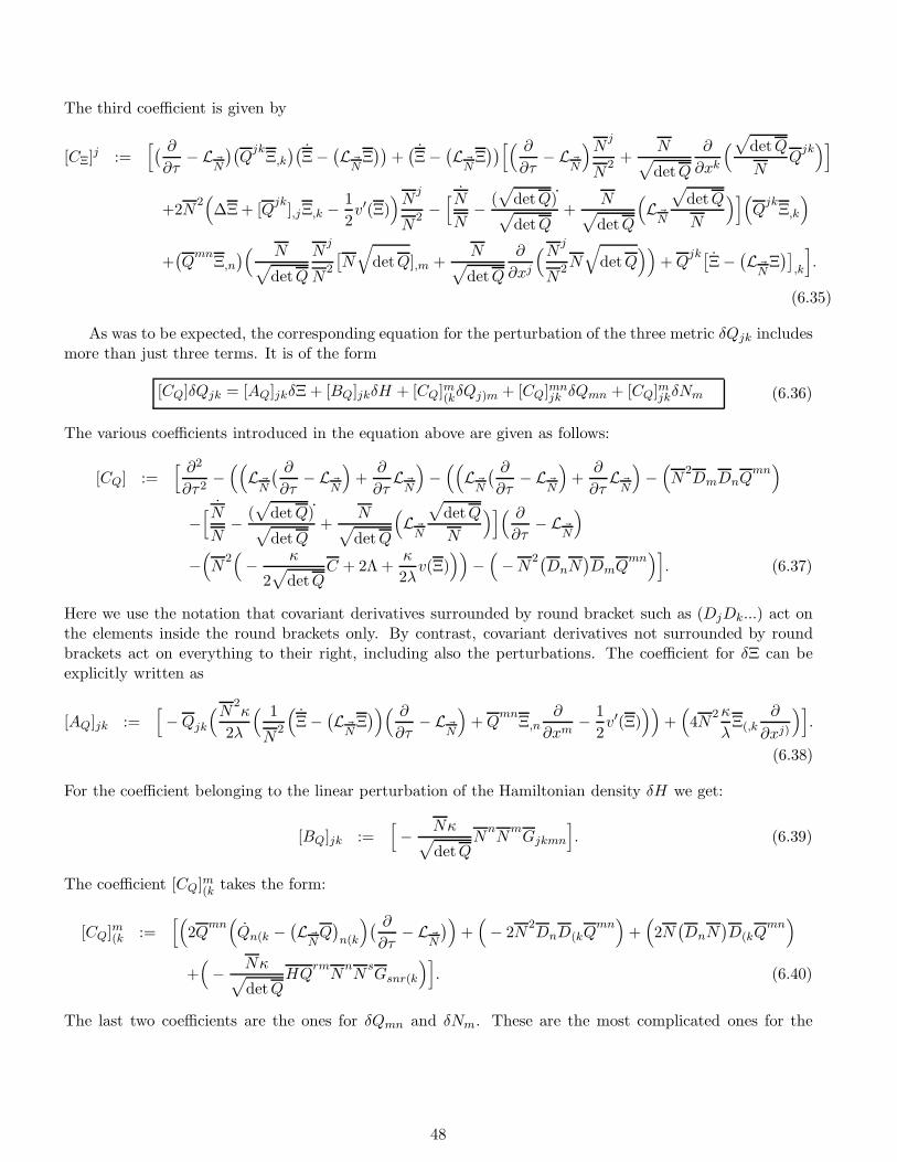
The third coefficient is given by

[CΞ]j :=[( ∂∂τ

− L~N

)(Q

jkΞ,k

)(Ξ −

(L~

NΞ))

+(Ξ −

(L~

NΞ))[( ∂

∂τ− L~

N

)N j

N2 +

N√detQ

∂

∂xk

(√detQ

NQ

jk)]

+2N2(∆Ξ + [Q

jk],jΞ,k − 1

2v′(Ξ)

)N j

N2 −

[NN

− (√

detQ)˙√detQ

+N√detQ

(L~

N

√detQ

N

)](Q

jkΞ,k

)

+(Q

mnΞ,n

)( N√detQ

Nj

N2

[N

√detQ],m +

N√detQ

∂

∂xj

(N j

N2N

√detQ

))+Q

jk[Ξ −

(L~

NΞ)]

,k

].

(6.35)

As was to be expected, the corresponding equation for the perturbation of the three metric δQjk includesmore than just three terms. It is of the form

[CQ]δQjk = [AQ]jkδΞ + [BQ]jkδH + [CQ]m(kδQj)m + [CQ]mnjk δQmn + [CQ]mjkδNm (6.36)

The various coefficients introduced in the equation above are given as follows:

[CQ] :=[ ∂2

∂τ2−((

L~N

( ∂∂τ

− L~N

)+

∂

∂τL~

N

)−((

L~N

( ∂∂τ

− L~N

)+

∂

∂τL~

N

)−(N

2DmDnQ

mn)

−[NN

− (√

detQ)˙√detQ

+N√detQ

(L~

N

√detQ

N

)]( ∂∂τ

− L~N

)

−(N

2(− κ

2√

detQC + 2Λ +

κ

2λv(Ξ)

))−(−N

2(DnN

)DmQ

mn)]. (6.37)

Here we use the notation that covariant derivatives surrounded by round bracket such as (DjDk...) act onthe elements inside the round brackets only. By contrast, covariant derivatives not surrounded by roundbrackets act on everything to their right, including also the perturbations. The coefficient for δΞ can beexplicitly written as

[AQ]jk :=[−Qjk

(N2κ

2λ

( 1

N2

(Ξ −

(L~

NΞ))( ∂

∂τ− L~

N

)+Q

mnΞ,n

∂

∂xm− 1

2v′(Ξ)

))+(4N

2κ

λΞ(,k

∂

∂xj)

)].

(6.38)

For the coefficient belonging to the linear perturbation of the Hamiltonian density δH we get:

[BQ]jk :=[− Nκ√

detQN

nN

mGjkmn

]. (6.39)

The coefficient [CQ]m(k takes the form:

[CQ]m(k :=[(

2Qmn(Qn(k −

(L~

NQ)n(k

)( ∂∂τ

− L~N

))+(− 2N

2DnD(kQ

mn)

+(2N(DnN

)D(kQ

mn)

+(− Nκ√

detQHQ

rmN

nN

sGsnr(k

)]. (6.40)

The last two coefficients are the ones for δQmn and δNm. These are the most complicated ones for the

48

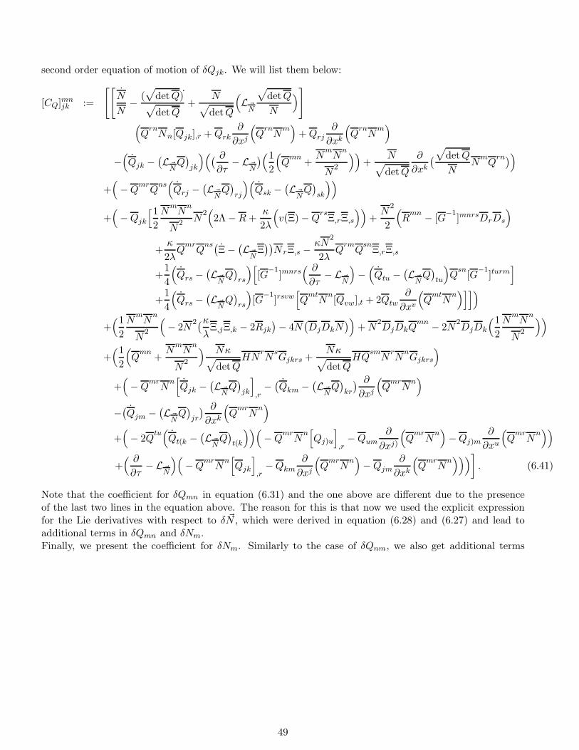
second order equation of motion of δQjk. We will list them below:

[CQ]mnjk :=

[[N

N− (√

detQ)˙√detQ

+N√detQ

(L~

N

√detQ

N

)]

(Q

rnNn[Qjk],r +Qrk

∂

∂xj

(Q

rnN

m)

+Qrj

∂

∂xk

(Q

rnN

m)

−(Qjk −

(L~

NQ)jk

)(( ∂∂τ

− L~N

)(1

2

(Q

mn+N

mN

n

N2

))+

N√detQ

∂

∂xk

(√

detQ

NN

mQ

rn))

+(−Q

mrQ

ns(Qrj −

(L~

NQ)rj

)(Qsk −

(L~

NQ)sk

))

+(−Qjk

[12

NmN

n

N2 N

2(2Λ −R+

κ

2λ

(v(Ξ) −Q

rsΞ,rΞ,s

))+N

2

2

(R

mn − [G−1

]mnrsDrDs

)

+κ

2λQ

mrQ

ns(Ξ −

(L~

NΞ))N rΞ,s −

κN2

2λQ

rmQ

snΞ,rΞ,s

+1

4

(Qrs −

(L~

NQ)rs

)[[G

−1]mnrs

( ∂∂τ

− L~N

)−(Qtu −

(L~

NQ)tu

)Q

sn[G

−1]turm

]

+1

4

(Qrs −

(L~

NQ)rs

)[G

−1]rsvw

[Q

mtN

n[Qvw],t + 2Qtw

∂

∂xv

(Q

mtN

n)]])

+(1

2

NmN

n

N2

(− 2N

2(κλ

Ξ,jΞ,k − 2Rjk

)− 4N

(DjDkN

))+N

2DjDkQ

mn − 2N2DjDk

(1

2

NmN

n

N2

))

+(1

2

(Q

mn+N

mN

n

N2

) Nκ√detQ

HNrN

sGjkrs +

Nκ√detQ

HQsmN

rN

nGjkrs

)

+(−Q

mrN

n[Qjk −

(L~

NQ)jk

]

,r−(Qkm −

(L~

NQ)kr

) ∂

∂xj

(Q

mrN

n)

−(Qjm −

(L~

NQ)jr

) ∂

∂xk

(Q

mrN

n)

+(− 2Q

tu(Qt(k −

(L~

NQ)t(k

))(−Q

mrN

n[Qj)u

],r−Qum

∂

∂xj)

(Q

mrN

n)−Qj)m

∂

∂xu

(Q

mrN

n))

+( ∂∂τ

− L~N

)(−Q

mrN

n[Qjk

],r−Qkm

∂

∂xj

(Q

mrN

n)−Qjm

∂

∂xk

(Q

mrN

n)))]

. (6.41)

Note that the coefficient for δQmn in equation (6.31) and the one above are different due to the presenceof the last two lines in the equation above. The reason for this is that now we used the explicit expressionfor the Lie derivatives with respect to δ ~N , which were derived in equation (6.28) and (6.27) and lead toadditional terms in δQmn and δNm.Finally, we present the coefficient for δNm. Similarly to the case of δQnm, we also get additional terms

49

coming from the Lie derivatives in the last line of equation (6.31).

[CQ]mjk :=[−[NN

− (√

detQ)˙√detQ

+N√detQ

(L~

N

√detQ

N

)](Q

mn[Qjk],n +Qnk

∂

∂xj

(Q

mn)

+Qnj

∂

∂xk

(Q

mn))

+(Qjk −

(L~

NQ)jk

)(( ∂∂τ

− L~N

)(Nm

N2

)+

N√detQ

∂

∂xn

(√

detQ

NQ

mn))

+(−Qjk

[− N

m

N2 N

2(2Λ −R− κ

2λ

(v(Ξ) −Q

rsΞ,rΞ,s

))− κ

2λ

(Ξ −

(L~

NΞ))Q

mnΞ,n

−1

4

(Qrs −

(L~

NQ)rs

)[G

−1]rsvw

[Q

mt[Qvw],t + 2Qtw

∂

∂xv

(Q

mt)]])

+(− N

m

N2

Nκ√detQ

HNrN

sGjkrs

)

+(Nm

N2

(2N

2(κλ

Ξ,jΞ,k − 2Rjk

)+ 4N

(DjDkN

))+ 2N

2DjDk

(Nm

N2

))

+(Q

mn[Qjk −

(L~

NQ)jk

],n

+(Qkn −

(L~

NQ)kn

) ∂

∂xj

(Q

mn)

+(Qjn −

(L~

NQ)jn

) ∂

∂xk

(Q

mn))

+( ∂∂τ

− L~N

)(Q

mn[Qjk

],n

+Qkn

∂

∂xj

(Q

mn)

+Qjn

∂

∂xk

(Q

mn))

+(− 2Q

tu(Qt(k −

(L~

NQ)t(k

))(Q

mn[Qj)u

],n

+Qun

∂

∂xj)

(Q

mn)

+Qj)n∂

∂xu

(Q

mn))]

. (6.42)

Although the form of the perturbed equations is quite complicated, they simplify drastically for specialbackgrounds of interest. For the case of FRW, for instance, all terms proportional to N j vanish, sinceN j = −Cj/H = 0 for FRW. This is due to the geometry and matter parts of the diffeomorphism constraintvanishing both separately in that case. Furthermore, all terms in the coefficients that contain spatial deriva-tives applied to background quantities vanish also. Other backgrounds where considerable simplificationwill occur include Schwarzschild spacetime.

7 Comparison with Other Frameworks

We now proceed to compare our work with other approaches to general relativistic perturbation theory foundin the literature. In the following we will restrict ourselves to discussing works that treat perturbation theoryaround general backgrounds. Approaches which deal exclusively with cosmological perturbation theory willbe looked at in our second paper, specifically dedicated to that topic.

The central point of comparison is how gauge-invariance is handled in the various approaches. As thatnotion often acquires different meanings, especially in the context of general-relativistic perturbation theory,it seems prudent to recall the precise mathematical setting underlying most works. It was developed bySachs [27] and Stewart and Walker [28], and recently given a very general and elegant formulation by Bruni,Sonego and collaborators [29, 30, 31]. The starting point consists of two spacetime manifolds M0 and M ,which represent the background spacetime around which one perturbs and the actual physical spacetime,respectively. It is important to keep in mind that M0 is only an artificial construct. Perturbations ofgeometric quantities are then defined by comparing their values in M0 and M , respectively. This procedureis highly ambiguous, however, in that there is a great freedom inherent in the choice of points where onecompares background and ”real” quantities to define the perturbations. Note that this freedom is in additionto the usual coordinate gauge freedom in general relativity. For that reason, Sachs termed it gauge invarianceof the second type [27]. Making such a choice, which mathematically amounts to choosing a so-called pointidentification map between M0 and M , is therefore nothing but a choice of gauge. Correspondingly, gauge-invariant perturbations are those quantities whose values do not depend on the choice of point identification

50

map. The actual condition for a perturbed quantity to be gauge-invariant to first order in this sense wasalready derived in [27], fully proved in [28] and finally generalized to arbitrary order n in [29]. The resultcan be succinctly summarised as follows: a geometric quantity T - such as a tensor - is invariant to order niff all its perturbations to order n− 1 are either vanishing, (spacetime) constant scalars or a combination ofKronecker deltas. This result is often known as the Stewart&Walker lemma. Clearly, the only case of actualinterest is the first. An example is given by curvature tensors in linear perturbation theory around Minkowskispace. As they vanish in the background, they are gauge-invariant to first order. These insights have beenthe backbone of most attempts to construct gauge-invariant quantities to various orders in perturbationtheory or even non-perturbatively. We will now discuss two of them.

In a series of papers [2, 3, 4] Nakamura has used these principles to develop formulas for gauge-invariantquantities to second and third order around an arbitrary background. They encompass the invariant parts ofvarious metric and curvature, as well as matter perturbations. These general formulas are, however, implicitonly to the extent that Nakamura derives them from the assumption that the corresponding linear orderperturbations can be decomposed into gauge-invariant and gauge-variant parts. Consequently, while theconstruction is, in principle, valid for arbitrary backgrounds, in practice only backgrounds with sufficientsymmetries to perform that split at linear order explicitly can be used. Luckily, that applies, of course, toseveral cases of great interest, such as cosmological and spherically symmetric backgrounds. The latter caseis explicitly treated in [4].

A distinctly different approach - let us call it the EB approach - is based on seminal work by Ellis andBruni [32], which has since inspired a multitude of other works [33, 34, 35]. Although the discussions inthese papers is geared towards applications in cosmology, the framework itself can be applied to arbitraryspacetimes, in principle, which is why we decided to discuss it here. The basic idea is to use a 1 + 3-approach by employing covariant quantities connected to a family of flow lines or ”fundamental observers”.The prime reason is that these quantities are much more closely related to what one actually measures inastrophysics. Furthermore, by a simple application of the Stewart-Walker lemma, they are automaticallygauge-invariant if the corresponding quantities in the background spacetime vanish. Unlike in the morecommon metric-based formalism, these quantities are defined in the physical, perturbed spacetime. As aresult, they are fully non-perturbative and in that sense their gauge-invariance extends to all orders. Theconnection to the standard perturbative approach based on perturbations in the background spacetime canbe made by suitably expanding the physical quantities to the desired order, see [33]. This approach enjoysa clear geometric and physical interpretation of the quantities used, as well as the advantage of basingperturbation theory on non-perturbative variables.

Comparing the works mentioned so far to ours, a first obvious difference is that we work in a canonicalsetting versus the covariant setting used by the others. The motivation is first that gauge issues becomeparticularly clear in the canonical picture and second our view towards quantization. The more importantdifference, however, is our use of dust as a dynamically implemented coordinate system. Our dust clocksserve a twofold purpose: on the one hand they enable us to construct background observables and thereforeto solve the standard gauge problem in general relativity. On the other hand they also serve as the pointidentification map and thus eliminate the gauge freedom of ”second type”. In that sense they represent alogical extension to perturbation theory of the initial conceptual idea by Brown and Kuchar [12] to use dustas a physical and therefore preferred coordinate system.

We should also point out that while our framework employs the metric and its perturbations as funda-mental variables, we could equally well use the dust clocks to build a gauge-invariant perturbation theorybased on the same variables used in the EB approach. In fact, it seems worthwhile to look a bit more closelyat the relationship between the two approaches. Both are non-perturbative in the following sense: they con-struct quantities which are gauge-invariant (with respect to gauge transformations of the second type). Onlythen perturbation theory is applied, which means that gauge-invariance is then automatically guaranteedin each order of perturbation. The difference arises when one looks at the role of gauge transformations ofthe first kind. The EB approach uses idealized observers that are comoving with the physical matter in themodel. Thus the theory is not deparametrized and gauge freedom with respect to the background spacetime

51

remains, as illustrated by the presence of constraints as part of the equations of motion. In our case, theobservers are represented by the dust, a component added to the physical matter content of the theory.They are thus dynamically included in the theory via the dust contribution to the Lagrangian, in additionto all the other matter. This allows for a complete deparametrization of the non-dust system with respectto the dust. Time evolution for this subsystem becomes unconstrained and a physical Hamiltonian emerges.The price to pay for this is that the dust contributes to the energy-momentum tensor of the deparametrizedsystem, the size of which is small, however. One might well argue that, for practical purposes at the classicallevel, the choice between the two approaches is a matter of taste. Our approach, however, offers a clearadvantage if one is interested in quantization, eventually. All programs aiming at a quantization of gravitythat have been pursued, so far, use the metric as a fundamental building block. It is not obvious to us howto attempt a quantization based on the covariant variables used in the EB approach.Another argument in favour of our framework is the following: A test observer which by definition doesnot have any impact is only a mathematical idealisation. Physically much more realistic is a dynamicallycoupled observer fluid like the dust considered here which in particular takes into account the gravitationalbackreaction.

To summarise: the crucial difference between our approach and the others discussed here is that the latterdeal only with gauge freedom of the second type. This can be seen from the fact that they use backgroundvariables which are not gauge-invariant and is evidenced, e.g., by the presence of constraint equations inaddition to evolution equations. Our treatment, by contrast, deals with all variables at all orders in a unifiedmanner. Furthermore, in our opinion the framework developed here allows for a much more straightforwardimplementation at higher orders. Another advantage is that it allows to treat arbitrary backgrounds inpractice, without the high degree of symmetry necessary for approaches based on the Stewart-Walker lemmato work. Recall that the latter require finding non-trivial quantities that vanish in the background manifold.Only in symmetric backgrounds such as homogeneous spacetimes is that a fairly tractable problem.

Finally, we should briefly discuss the recent work in [25], which is close to ours in terms of motivationand conceptual underpinnings. The authors there also use the general gauge invariant framework of [11],however, with two differences: First of all, they do not use dust matter to achieve gauge invariant completionsof geometry and matter variables. This prevents them from bringing the constraints into a deparametrisedform [9] and thus there is no time independent physical Hamiltonian. Secondly, while they can develophigher order cosmological perturbation theory, their perturbations of gauge invariant quantities are stillexpanded in terms of the perturbations of the the gauge variant quantities which is what we never do.Therefore the basic perturbation variables are different in the two schemes: In our scheme we never carehow our gauge invariant variables are assembled from gauge variant ones, they and their perturbations arefundamental for us and n’th order quantities are n’th order expressions in those. In contrast, in [25] n’thorder means n’th order in the gauge variant quantities. In particular, the n’th order perturbed variablesare only invariant with respect to the n’th order constraints up to terms of higher order. In contrast, ourperturbed variables are always first order and always fully gauge invariant, it is only in the Hamiltonian thathigher orders of gauge invariant variables appear. It would no doubt be fruitful to translate the schemesinto each other and to see which differences and similarities arise.

8 Conclusions and Open Questions

This is a long and technically involved paper. The reader rightfully will ask why one should dive into itsdetails and what exactly is novel as compared to the existing literature. The following remarks are in order:

1. Non perturbative gauge invarianceTo the best of our knowledge, there exists no generally accepted notion of gauge invariance at n-thorder of perturbation theory in General Relativity. Moreover, at each order of perturbation theoryone has to repeat the analysis for how to preserve gauge invariance to the given order. Given thosedifficulties, it is natural to try to invent a scheme which separates the issue of gauge invariance from

52

the perturbation theory. Hence, one must treat gauge invariance non perturbatively. This is exactlywhat we managed to do in this paper.

Thus, one only deals with the exact observables of the theory. All the equations of the theory have tobe written in terms of those gauge invariant quantities. Given such a gauge invariant function O onthe full phase space, we evaluate it on a certain background (data) which is an exact solution to ourequations of motion and get a certain value O0. The perturbation of O is then defined as δO = O−O0.We never care to expand δO in terms of the perturbations of the gauge variant degrees of freedom(although we could). However, all the equations are expanded directly in terms of the perturbationsof those physical observables.

2. Material reference systemIn General Relativity it is well known that in order to meaningfully talk about the Einstein equationsand to have them describe something observable or measurable, one has to suppose that spacetime isinhabited by (geodesic) test observers. By definition, a test observer has no effect whatsoever on thesystem. This is of course mathematically convenient but physically worrysome because a test observeris a mathematical idealisation. Every real observer interacts at least gravitationally and does leaveits fingerprint on the system. One of the achievements of the seminal work [12] of Brown & Kuchar,which in our mind is insufficiently appreciated in the literature, is to have overcome this shortcoming.The authors of [12] have identified a generally covariant Lagrangian which comes as close as possibleto describing a non – self interacting, perfect and geodesically moving fluid that fills out spacetime(congruence). It does leave its fingerprint on the system and thus is physically more realistic than thetest observer fluid.

In this paper we have driven the work of [12] to its logical frontier and have asked the questionwhether the dust when added to the geometry – matter system really accomplishes the goal of keepingthe approximate validity of the usual interpretation of the Einstein equations. We have verified thatit does which in our mind is an intriguing result.

3. Solving the Problem of TimeSince General Relativity is a generally covariant or reparametrisation invariant theory, it is notequipped with a natural Hamiltonian. Rather, the “dynamics” of the non observables is describedby a linear combination of constraints which really generate gauge transformations rather than phys-ical evolution. Observable quantities are gauge invariant and therefore do not evolve with respect tothe “gauge dynamics”. Therefore it is conceptually unclear what to do with those observables. Theachievement of [10, 11] is to have invented a scheme that in principle unfreezes the observables fromtheir non motion. However, in general that physical motion is far from uniquely selected, there arein general infinitely many such physical notions of time and none of them is preferred. Moreover, theassociated Hamiltonians are generically neither preserved nor positive or at least bounded from below.

When combining the frameworks of [12] and [10, 11] we find the remarkable result that there isa preferred Hamiltonian which is manifestly positive, not explicitly dependent on physical time andgauge invariant. It maps a conceptually complicated gauge systems into the safe realm of a conservativeHamiltonian system. The physical Hamiltonian drives the evolution of the physical observables. Itreproduces the Einstein equations for the gauge invariant observables up to corrections which describethe influence of the dust.

4. Counting of the Physical Degrees of FreedomThe price to pay is that one has to assume the existence of the dust as an additional matter speciesnext to those of the standard model32. It would maybe be more desirable to have matter species of

32 Curiously, what we have done in this paper bears some resemblance with the Stueckelberg formalism. There one also addsadditional matter to Maxwell theory. One can then make the longitudinal mode gauge invariant and thus finds a theory withone more degree of freedom. This is one way to arrive at the Proca theory and more generally at massive vector boson theoriesvia the Higgs mechanism.

53

the standard model or geometry modes playing the role of a dynamical test observer33 . In principlethis is possible, however, the resulting formalism is much more complicated and it does not leadto deparametrisation. Thus a conserved physical Hamiltonian would then not be available and theequations of motion would become intractable.

It is true that the dust variables disappear in the final description of the observables which are com-plicated aggregates built out of all fields. However, the theory has fundamentally four more physicaldegrees of freedom than without dust and that might eventually rule out our theory if those additionaldegrees of freedom are not observed.

The truly remarkable feature of the dust is that it replaces the initial value constraints of GeneralRelativity which are reponsible for having less physical degrees of freedom than one would naivelyexpect, by four conservation laws. That is, in any given solution of our equations of motion, thephysical observables must physically evolve with respect to each other in such a way that the conservedquantities do not change. This effectively acts like a constraint and therefore reduces the number ofindependently evolving observables by four, in agreement with the counting of the degrees of freedomwithout dust. Thus, at least as long as the value of those conserved quantities is sufficiently small, wewill not be able to see those additional degrees of freedom. It is this fact which makes it possible thatone effectively does not see more degrees of freedom than in the standard treatment.

As a final objection against our formalism one might raise the fact that the dust contributes with thewrong sign to the matter energy momentum tensor. However, the formalism not only forces us to dothis as we would otherwise have a negative definite Hamiltonian, moreover, as already remarked inthe introduction, it is completely acceptable since here we talk about the energy momentum tensor ofnon observables. The energy momentum tensor of the observables in the final Einstein equations doessatisfy the usual energy conditions.

5. Complexity of the Equations of MotionSince General Relativity is a highly non linear, complicated self – interacting theory, experience frommuch less complicated integrable systems suggests that its Invariants, that is, the gauge invariantobservables, satisfy a tremendously complicated Poisson algebra and that the equations of motion areintractable. Surprisingly, this is not at all the case. The observable algebra is almost as simple as thealgebra of non observables and the equations of motion can be solved almost as easily as in the usualgauge variant formalism. Key to that is the presence of the already mentioned conserved current.

In this first paper we have developed the general gauge invariant formalism and linear perturbation theoryabout general backgrounds. In the companion paper we apply the general results to flat and FRW back-grounds and find agreement with usual linear perturbation theory for linearly invariant observables. Thisis a first consistency test that our theory has passed. Thus we hope to have convinced the reader that thepresent framework has conceptual advantages over previous ones and that it is nonetheless technically notmuch more complicated. Actually, the pay – off for having a manifestly gauge invariant approach will reallycome in at higher order where we believe that our equations of motion will be simpler.

There are many lines of investigations that one can follow from here. An obvious one, the specializationto the all-important case of an FRW background is presented in a companion paper as already mentioned.Investigating perturbations around backgrounds of astrophysical interest, such as Schwarzschild spacetime,is also valuable. Again, for all these cases it should also prove very interesting to go beyond the linear tohigher orders. Predictions from second-order perturbation theory, e.g. the issue of non-Gaussianity in cos-mological perturbations, are the topic of current research and could soon be testable by future experimentssuch as PLANCK, see [38]. On a more technical and conceptual level, our framework might prove usefulto settle the issue of under what conditions general-relativistic perturbation theory is consistent and stable.

33This would be similar to technicolour theories which declare the Higgs scalar field not as an independent degree of freedombut as a compound object built from the bosons of the electroweak theory. Here one would build four independent scalars e.g.from the geometry field.

54

Finally, with a view towards facilitating the search for physically relevant predictions from approaches toquantum gravity, a quantization of our gauge-invariant formulation of general relativity, together with thedevelopment of the corresponding perturbation theory at the quantum level strikes us as a highly desirablegoal. See [24] for first steps.

Acknowledgements

K.G. is grateful to Perimeter Institute for hospitality and financial support. Research performed at Perime-ter Institute Theoretical Physics is supported in part by the Government of Canada through NSERC andby the Province of Ontario through MRI. O.W. was partially supported by the Province of Ontario throughan ERA award, ER06-02-298.

A Second Class Constraints of the Brown – Kuchar Theory

In this section we provide the calculational details of the constraint analysis of the Brown – Kuchar theorydiscussed in section 2. In particular we want to show that no tertiary constraints arise. Our starting pointis equation (2.25) which we display once again below for the convenience of the reader

z,t = Hprimary, p = −ctot

za,t = Hprimary, pa = −ctota

Z,t = Hprimary, I =n

2[− P 2

√det(q)ρ2

+√

det(q)(qabUaUb + 1)] =: c

Zj,t = Hprimary, I

j = −µjP − nρ√

det(q)qabUaSj,b + PSj

,ana

Zj,t = Hprimary, Pj +WjP = µjP − (na − nρ√

det(q)

PqabUb)PWj,a (A.1)

The last two equations involve the Lagrange multipliers µj and µj and can be solved for them. In contrastwe observe that the first three equation are independent of the Lagrange multipliers, they are secondaryconstraints. We will now proceed with the constraint analysis and show that when the Poisson bracketsbetween the primary Hamiltonian Hprimary and the secondary constraints are consideres no new constraintsare generated. Recall that the primary Hamiltonian density was given by

hprimary = µjZj + µZ + µjZj + νz + νaza + n′ctot + n′actota (A.2)

55

whereby the single constraints are shown below

ctot = cgeo + cmatter + cD

ctota = cgeoa + cmattera + cDa

κcgeo =1√

det(q)[P abPab −

1

2(P a

a )2] −√

det(q) R(3) + 2Λ√

det(q)

λcmatter =1

2[

π2

√det(q)

+√

det(q)(qabξ,aξ,b + v(ξ)

)]

cD =1

2[

P 2

√det(q)ρ

+√

det(q)ρ(qabUaUb + 1)]

κcgeoa = −2DbPba

λcmattera = πξ,a

cDa = P [T,a −WjSj,a] (A.3)

We begin with the calculation of the Poisson bracket of Hprimary and the smeared constraint

~ctot(~n) :=

∫d3x na(x)ctota (x) (A.4)

Hprimary,~ctot(~n) =

∫d3x

∫d3y(µj(y)Zj(y), n

a(x)ctota (x) + µ(y)Z(y), na(x)ctota (x)

+µj(y)Zj(y), na(x)ctota (x) + ν(y)z(y), na(x)ctota (x) + νb(y)zb(y), n

a(x)ctota (x)+n′(y)ctot(y), na(x)ctota (x) + n′b(y)ctotb (y), na(x)ctota (x)

)(A.5)

For the single Poisson brackets that occur in the equation above we obtain the following result:

∫d3x

∫d3yµj(y)Zj(y), n

a(x)ctota (x) =

∫d3xnaPµjWj,a (A.6)

∫d3x

∫d3yµ(y)Z(y), na(x)ctota (x) = 0

∫d3x

∫d3yµj(y)Z

j(y), na(x)ctota (x) = −∫d3xPµjS

j,an

a

∫d3x

∫d3yν(y)z(y), na(x)ctota (x) = 0

∫d3x

∫d3yνb(y)zb(y), n

a(x)ctota (x) = ~ctot(~ν)∫d3x

∫d3yn′(y)ctot(y), na(x)ctota (x) = ctot(L~nn

′) + c(L~n′ρ) +

∫d3xρn′ na

√det(q)qbcUb

(Wj,aS

jc −Wj,cS

j,a

)

∫d3x

∫d3yn′b(y)ctotb (y), na(x)ctota (x) = ~c(L~n~n

′) −∫d3x(n′anb − nan′b

)PSj

,aWj,b

56

Consequently we can rewrite equation (A.5) as

Hprimary,~ctot(~n) = ctot(L~nn

′) + c(L~nρ) +

∫d3xρnna

√det(q)qbcUb

(Wj,aS

jc − wj,cS

ja

)

−∫d3xµjPS

jan

a +

∫d3xµjPwj,an

a + ~c(L~n~n′) + ~ctot(~ν)

−∫d3x(n′bna − n′anb

)PWj,aS

j,b

≈∫d3xna

(Sj

a

(Pn′bWj,b − ρn

√det(q)qbcUbwj,c − µjP

)

+Wj,a

(− Pn′bSj

,b + ρn√

det(q)qbcUbSj,c + µjP

))(A.7)

Hence, the result above involves the Langrange multipliers µj and µj and can be solved for them such thatno new constraints arise from ctota . Proceeding with ctot whereby the smeared constraint is given by

ctot(n) :=

∫d3xn(x)ctot(x) (A.8)

Thus we get

Hprimary, ctot(n) =

∫d3x

∫d3y(µj(y)Zj(y), n(x)ctot(x) + µ(y)Z(y), n(x)c(x)

+µj(y)Zj(y), n(x)ctot(x) + ν(y)z(y), n(x)ctot(x) + νb(y)zb(y), n(x)ctot(x)

+n′(y)ctot(y), n(x)ctot(x) + n′b(y)ctotb (y), n(x)ctot(x))

(A.9)

For the single Poisson brackets that occur in the equation above we obtain the following result

∫d3x

∫d3yµj(y)Zj(y), n(x)ctot(x) = −

∫d3x√

det(q)n ρµjqabUbWj,a (A.10)∫d3x

∫d3yµ(y)Z(y), n(x)ctot(x) =

∫d3xµ

n

n′c

∫d3x

∫d3yµj(y)Z

j(y), n(x)ctot(x) =

∫d3xµjρn

√det(q)qbcUbS

j,c

∫d3x

∫d3yν(y)z(y), n(x)ctot(x) = ctot(ν)

∫d3x

∫d3yνb(y)zb(y), n(x)ctot(x) = 0

∫d3x

∫d3yn′(y)ctot(y), n(x)ctot(x) = ~ctot(q−1[n′dn− ndn′])

∫d3x

∫d3yn′b(y)ctotb (y), n(x)ctot(x) = −ctot(L~n′n) − c(L~n′ρ)

−∫d3xρnn′a

√det(q)qbcUb

(Wj,aS

jc −Wj,cS

j,a

)

57

Reinserting these results into equation (A.9) yields

Hprimary, ctot(n) = −

∫d3x√

det(q)nρµjqabUbWj,a +

∫d3xµ

n

n′c+

∫d3xρnµj

√det(q)qbcUbS

j,c

+ctot(ν) + ~ctot[q−1(n′dn− ndn′]) − ctot(L~n′n) − c(L~n′ρ)

−∫d3xρnn′a

√det(q)qbcUb

(Wj,aS

jc −Wj,cS

j,a

)

≈∫d3x√

det(q)nρqbcUb

(Wj,c

(n′aSj

,a − µj − ρn′

P

√det(q)qdeUdS

j,e

)

Sj,c

(µj −Wj,an

′a +ρn′

PqdeUdWj,e

))

+

∫d3x√

det(q)nρqbcUbρn′

P

√det(q)qdeUd

(Wj,cS

j,e −Wj,eS

j,c

)

=

∫d3x√

det(q)nρqbcUb

(Wj,c

(n′aSj

,a − µj − ρn′

P

√det(q)qdeUdS

j,e

)

Sj,c

(µj −Wj,an

′a +ρn′

PqdeUdWj,e

))(A.11)

Here we used in the last step that the last integral in the line before the last line one vanishes, becauseWj,cS

j,e −Wj,eS

j,c is antisymmetric in e, c and multiplied by qbcqdeUbUd which is symmetric in the indeces

c, e.These are again the equation involving the Lagrange multipliers that we have seen before in the calculationsfor ctota .

Finally, let us consider the Poisson bracket of Hprimary and the secondary constraint c whose smearedversion is given by

c(u) :=

∫d3xu(x)c(x) (A.12)

where u is an appropiate smearing function. We obtain

Hprimary, c(u) =

∫d3x

∫d3y(µj(y)Zj(y), u(x)c(x) + µ(y)Z(y), u(x)c(x)

+µj(y)Zj(y), u(x)c(x) + ν(y)z(y), u(x)c(x) + νb(y)zb(y), u(x)c(x)

+n′(y)ctot(y), u(x)c(x) + n′b(y)ctotb (y), u(x)c(x))

(A.13)

In this case we do not need to compute all the individual Poisson bracket in order to convince ourselves thatno constraints arise, because the Poisson bracket of Z(µ) and c(u) yields

∫d3x

∫d3yµ(y)Z(y), u(x)c(x) =

∫d3xµu

nP 2

ρ3√

det(q)(A.14)

which is a new term invloving the Lagrange multiplier µ. Thus, we can solve the equation Hprimary, c(u) = 0for µ.It follows that no new terms are produced not involving µj, µj , µ in this second iteration step. Consequently,the full set of (primary and secondary) constraints is given by ctot, ctota , c, Zj , Z

j , Z, za and z and it remainsto classify them into first and second class. Obviously,

Zj(x), Zk(y) = P δjk δ(x, y) ,

Z(x), c(y) =

nP 2

ρ3√det(q)

δ(x, y) , (A.15)

58

does not vanish on the constraint surface defined by the final set of constraints, hence they are second classconstraints. Since n appears only linearly in c and na does not appear at all, it follows that z, za are firstclass.Let us consider the linear combination

ctota ≡ I ρ,a + Ij Wj,a + P T,a + Pj Sj,a + p n,a + L~n pa + ca

= ctota + Z ρ,a + Zj Wj,a + Zj Sj,a + z n,a + L~n za (A.16)

whereca ≡ cgeoa + cmatter

a (A.17)

is the non-dust contribution to the spatial diffeomorphism constraint ctota . Since all constraints are scalar orcovector densities of weight one and ctota is the generator of spatial diffeomorphisms, it follows that ctota isfirst class. Finally, we consider as an Ansatz the linear combination

ctot ≡ ctot + αj Zj + αj Zj + α Z , (A.18)

and determine the phase space functions αj , αj , α such that ctot has vanishing Poisson brackets withZj, Z

j , Z up to terms proportional to Zj , Zj, Z.

We have

ctot(x), Zj(y) = ctot(x), Zj(y) + αk(x)Zk(x), Zk(y)= ctot(x), Zj(y) + αj(x)P (x)δ3(x, y). (A.19)

where we used equation (A.15) in the last line. Solving this equation for αj we end up with

αj(x) = −∫d3y

1

P (y)ctot(x), Zj(y) =

(1

P

√det(q) ρ qabUbWj,a

)(x) (A.20)

which is a sensible expression since ctot(x), Zk(y) ∼ δ3(x, y). For the Poisson bracket involving Zj we get

ctot(x), Zj(y) = ctot(x), Zj(y) + αk(x)Zk(x), Zj(y)= ctot(x), Zj(y) − αj(x)P (x)δ3(x, y) (A.21)

such that this equation can be solved for αj explicitly given by

αj(x) =

∫d3y

1

P (y)ctot(x), Zj(y) =

(1

Pρ√

det(q)qbcUbSj,c

)(x). (A.22)

Finally, for Z we obtain

ctot(x), Z(y) = ctot(x), Z(y) ∼ c ≈ 0 (A.23)

Hence this Poisson bracket vanishes weakly. Considering now the Poisson bracket between c and ctot we get

ctot(x), c(y) = ctot(x), c(y) + αj(x)Zj(x), c(y) + αj(x)Zj(x), c(y) + α(x)Z(x), c(y)(A.24)

The results of the last three individual Poisson brackets occurring above are listed below

Zj(x), c(y) =(n√

det(q)qabUaWjP)(y)

∂

∂ybδ3(x, y) (A.25)

Zj(x), c(y) = −(n√

det(q)qabUaPSj,b

)(y)δ3(x, y)

Z(x), c(y) =

(nP 2

ρ3√

det(q)

)(y)δ3(x, y)

59

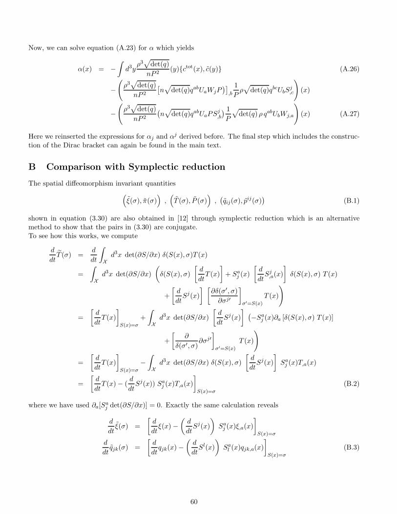
Now, we can solve equation (A.23) for α which yields

α(x) = −∫d3y

ρ3√

det(q)

nP 2(y)ctot(x), c(y) (A.26)

−(ρ3√

det(q)

nP 2

[n√

det(q)qabUaWjP)]

,b

1

Pρ√

det(q)qbcUbSj,c

)(x)

−(ρ3√

det(q)

nP 2

(n√

det(q)qabUaPSj,b

) 1

P

√det(q) ρ qabUbWj,a

)(x) (A.27)

Here we reinserted the expressions for αj and αj derived before. The final step which includes the construc-tion of the Dirac bracket can again be found in the main text.

B Comparison with Symplectic reduction

The spatial diffeomorphism invariant quantities

(ξ(σ), π(σ)

),(T (σ), P (σ)

),(qij(σ), pij(σ)

)(B.1)

shown in equation (3.30) are also obtained in [12] through symplectic reduction which is an alternativemethod to show that the pairs in (3.30) are conjugate.To see how this works, we compute

d

dtT (σ) =

d

dt

∫

Xd3x det(∂S/∂x) δ(S(x), σ)T (x)

=

∫

Xd3x det(∂S/∂x)

(δ(S(x), σ)

[d

dtT (x)

]+ Sa

j (x)

[d

dtSj

,a(x)

]δ(S(x), σ) T (x)

+

[d

dtSj(x)

] [∂δ(σ′, σ)

∂σj′

]

σ′=S(x)

T (x)

)

=

[d

dtT (x)

]

S(x)=σ

+

∫

Xd3x det(∂S/∂x)

[d

dtSj(x)

] (−Sa

j (x)∂a [δ(S(x), σ) T (x)]

+

[∂

δ(σ′, σ)∂σj′

]

σ′=S(x)

T (x)

)

=

[d

dtT (x)

]

S(x)=σ

−∫

Xd3x det(∂S/∂x) δ(S(x), σ)

[d

dtSj(x)

]Sa

j (x)T,a(x)

=

[d

dtT (x) − (

d

dtSj(x)) Sa

j (x)T,a(x)

]

S(x)=σ

(B.2)

where we have used ∂a[Saj det(∂S/∂x)] = 0. Exactly the same calculation reveals

d

dtξ(σ) =

[d

dtξ(x) −

(d

dtSj(x)

)Sa

j (x)ξ,a(x)

]

S(x)=σ

d

dtqjk(σ) =

[d

dtqjk(x) −

(d

dtSl(x)

)Sa

l (x)qjk,a(x)

]

S(x)=σ

(B.3)

60

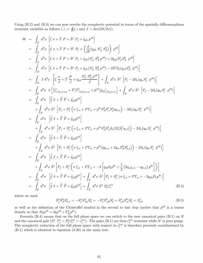
Using (B.2) and (B.3) we can now rewrite the symplectic potential in terms of the spatially diffeomorphisminvariant variables as follows ˙(.) := d

dt(.) and J = det(∂S/∂x))

Θ =

∫

Xd3x

[ξ π + T P + Sj Pj + qab p

ab]

=

∫

Xd3x

[ξ π + T P + Sj Pj +

(d

dt

(qjk S

j,a S

k,b

))pab

]

=

∫

Xd3x

[ξ π + T P + Sj Pj + qjk(S

j,a S

k,b p

ab) + 2qjkSj,aS

k,b pab

]

=

∫

Xd3x

[ξ π + T P + Sj Pj + qjk(S

j,a S

k,b p

ab) − 2Sj∂a(qjkSk,b pab)

]

=

∫

XJ d3x

[ξπ

J+ T

P

J+ qjk

Sj,a Sk

,b pab

J

]+

∫

Xd3x Sj

[Pj − 2∂a(qbcS

cj pab)

]

=

∫

Sd3σ π

[[ξ]S(x)=σ

+ P[T]S(x)=σ

+ pjk[qjk]S(x)=σ

]+

∫

Xd3x Sj

[Pj − 2∂a(qbcS

cj pab)

]

=

∫

Sd3σ

[˙ξ π +

˙T P + ˙qjkp

jk]

+

∫

Xd3x Sj

[Pj + Sa

j

(π ξ,a + PT,a + pbcSk

,bSl,cS

aj qkl,a

)− 2∂a(qbcS

cj pab)

]

=

∫

Sd3σ

[˙ξ π +

˙T P + ˙qjkp

jk]

+

∫

Xd3x Sj

[Pj + Sa

j

(π ξ,a + PT,a + pbcSk

,bSl,c∂a

(Se

kSfl qef

))− 2∂a

(qbcS

cj pab

)]

=

∫

Sd3σ

[˙ξ π +

˙T P + ˙qjkp

jk]

+

∫

Xd3x Sj

[Pj + Sa

j

(π ξ,a + PT,a + pbc

(qbc,a + 2qecS

k,bS

ek,a

))− 2∂a

(qbcS

cj pab

)]

=

∫

Sd3σ

[˙ξ π +

˙T P + ˙qjkp

jk]

+

∫

Xd3x Sj

[Pj + Sa

j

(π ξ,a + PT,a + −2

[qab∂cp

bc +1

2

(2qa(b,c) − qbc,a

)pbc

])]

=

∫

Sd3σ

[˙ξ π +

˙T P + ˙qjkp

jk]

+

∫

Xd3x Sj

[Pj + Sa

j (π ξ,a + PT,a + −2qabDcpbc)]

=

∫

Sd3σ

[˙ξ π +

˙T P + ˙qjkp

jk]

+

∫

Xd3x Sj Sj

actota (B.4)

where we usedSa

j Sk,bS

ek,a = −Sa

j Sk,baS

ek = −Sa

j Sk,abS

ek = Sa

j,bSk,aS

ek = Se

j,b (B.5)

as well as the definition of the Christoffel symbol in the second to last step (notice that pab is a tensordensity so that Dbp

ab = ∂bpab + Γa

bcpbc).

Formula (B.4) means that on the full phase space we can switch to the new canonical pairs (B.1) on Xand the canonical pair (Sj , P ′

j = Saj c

tota = ctotj ). The pairs (B.1) are thus ctotj invariant while Sj is pure gauge.

The symplectic reduction of the full phase space with respect to ctotj is therefore precisely coordinatised by(B.1) which is identical to equation (3.30) in the main text.

61

C Effective Action and Fixed Point Equation

The aim of the present section is to derive, at least in implicit form, the Lagrangian that correspondscanonically to the physical Hamiltonian. This can be done by calculating the inverse Legendre transform34

and leads to a fixed point equation, which can be solved order by order, in principle. Interestingly, theLagrangian turns out to be local in dust time, but will be non–local in dust space. However, the Hamiltoniandescription is completely local.

The inverse Legendre transform requires to solve for the momenta P jk(σ), Π(σ) in terms of the corre-sponding velocities Vjk(σ), Υ(σ), respectively, defined by 35

Vjk(σ) ≡ Qjk(σ) = H, Qjk(σ)Υ(σ) ≡ Ξ(σ) = H,Ξ(σ) . (C.1)

This can be done by using the first order equations of motion for Qjk(σ), Ξ(σ), derived from the physicalHamiltonian H. From the physical Hamiltonian H we obtain the Lagrangian

L[Q,V ; Ξ,Υ] =

∫

Sd3σ L(σ) =

∫

Sd3σ

[(1

κP jkVjk +

1

λΠΥ

)− H[Q,P ; Ξ,Π]

]

(C.1)

(C.2)

where it it is understood that the solution of (C.1) for P jk, Π has to be inserted.With the dynamical lapse and shift given by N = C/H, Nj = −Cj/H, respectively, we obtain for P jk

P jk =

√det(Q)

2N[G−1]jkmn

(Qmn − (L ~N

Q)mn

)=√

det(Q)[G−1]jkmnKmn , (C.3)

with Kmn denoting the extrinsic curvature. This leads to the following expression for the velocities Vjk andΥ:

Vjk = 2[N Kjk +D(jNk)

]and Υ =

N√det(Q)

Π +QjkNj DkΞ . (C.4)

We conclude

L =

∫

Sd3σ

[1

κVjkP

jk +1

λΥΠ −H

](C.5)

=

∫

Sd3σ

[2

κ

(NKjk +D(jNk)

)P jk +

(N

Π

λ√

det(Q)+N jDj

Ξ

λ

)Π −H

]

=

∫

Sd3σ

[N( 2

κKjkP

jk +Π2

λ√

det(Q)

)+N jCj −H

]

=

∫

Sd3σ

1

H

[C

(2

κKjkP

jk +Π2

λ√

det(Q)

)−QjkCjCk −H2

]

=

∫

Sd3σ

C

H

[2

κKjkP

jk +Π2

λ√

det(Q)− C

]

=

∫

Sd3σ N

[2

κ

√det(Q)(KjkK

jk − (Kjj )

2) +Π2

λ√

det(Q)− C

]

=

∫

Sd3σ N

√det(Q)

[1

κ

(KjkK

jk − (Kjj )

2 +R(3)[Q] − 2Λ)

+1

2λ

(Π2

det(Q)− [QjkΞ,jΞ,k + v(Ξ)]

)]

=

∫

Sd3σ N

√det(Q)

[1

κ

(KjkK

jk − (Kjj )2 +R(3)[Q] − 2Λ

)+

1

2λ

((∇uΞ)2 − (QjkΞ,jΞ,k + v(Ξ))

)].

34 This is possible because the Legendre transform is regular.35 Note that Qjk and Ξ must be treated as independent variables in addition to Qjk and Ξ.

62

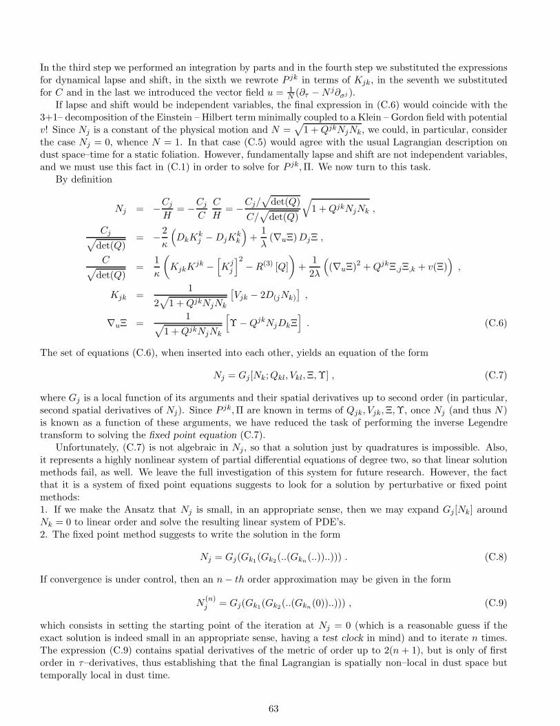
In the third step we performed an integration by parts and in the fourth step we substituted the expressionsfor dynamical lapse and shift, in the sixth we rewrote P jk in terms of Kjk, in the seventh we substitutedfor C and in the last we introduced the vector field u = 1

N(∂τ −N j∂σj ).

If lapse and shift would be independent variables, the final expression in (C.6) would coincide with the3+1– decomposition of the Einstein – Hilbert term minimally coupled to a Klein – Gordon field with potentialv! Since Nj is a constant of the physical motion and N =

√1 +QjkNjNk, we could, in particular, consider

the case Nj = 0, whence N = 1. In that case (C.5) would agree with the usual Lagrangian description ondust space–time for a static foliation. However, fundamentally lapse and shift are not independent variables,and we must use this fact in (C.1) in order to solve for P jk,Π. We now turn to this task.

By definition

Nj = −Cj

H= −Cj

C

C

H= −Cj/

√det(Q)

C/√

det(Q)

√1 +QjkNjNk ,

Cj√det(Q)

= −2

κ

(DkK

kj −DjK

kk

)+

1

λ(∇uΞ)DjΞ ,

C√det(Q)

=1

κ

(KjkK

jk −[Kj

j

]2−R(3) [Q]

)+

1

2λ

((∇uΞ)2 +QjkΞ,jΞ,k + v(Ξ)

),

Kjk =1

2√

1 +QjkNjNk

[Vjk − 2D(jNk)

],

∇uΞ =1√

1 +QjkNjNk

[Υ −QjkNjDkΞ

]. (C.6)

The set of equations (C.6), when inserted into each other, yields an equation of the form

Nj = Gj [Nk;Qkl, Vkl,Ξ,Υ] , (C.7)

where Gj is a local function of its arguments and their spatial derivatives up to second order (in particular,second spatial derivatives of Nj). Since P jk,Π are known in terms of Qjk, Vjk,Ξ,Υ, once Nj (and thus N)is known as a function of these arguments, we have reduced the task of performing the inverse Legendretransform to solving the fixed point equation (C.7).

Unfortunately, (C.7) is not algebraic in Nj , so that a solution just by quadratures is impossible. Also,it represents a highly nonlinear system of partial differential equations of degree two, so that linear solutionmethods fail, as well. We leave the full investigation of this system for future research. However, the factthat it is a system of fixed point equations suggests to look for a solution by perturbative or fixed pointmethods:1. If we make the Ansatz that Nj is small, in an appropriate sense, then we may expand Gj [Nk] aroundNk = 0 to linear order and solve the resulting linear system of PDE’s.2. The fixed point method suggests to write the solution in the form

Nj = Gj(Gk1(Gk2(..(Gkn(..))..))) . (C.8)

If convergence is under control, then an n− th order approximation may be given in the form

N(n)j = Gj(Gk1(Gk2(..(Gkn(0))..))) , (C.9)

which consists in setting the starting point of the iteration at Nj = 0 (which is a reasonable guess if theexact solution is indeed small in an appropriate sense, having a test clock in mind) and to iterate n times.The expression (C.9) contains spatial derivatives of the metric of order up to 2(n + 1), but is only of firstorder in τ–derivatives, thus establishing that the final Lagrangian is spatially non–local in dust space buttemporally local in dust time.

63

D Two Routes to Second Time Derivatives of Linear Perturbations

In this appendix we consider a general Hamiltonian system with canonical coordinates (q, p) and standardPoisson brackets p, q = 1 and a Hamiltonian function H(q, p). We will consider only one degree of freedombut everything generalises to an arbitrary number of degrees of freedom.

Lemma D.1. Let (q0(τ), p0(τ)) be an exact solution of the Hamiltonian equations of motion

q0(τ) =[H, q(q, p)

]q=q0(τ)p=p0(τ)

p0(τ) =[H, p(q, p)

]q=q0(τ)p=p0(τ)

(D.1)

Define the perturbations δq := q − q0(τ), δp := p − p0(τ). Let H(q, p) =∑∞

n=0H(n) be the expansion of

H(q, p) around q0(τ), p0(τ) in terms of the perturbations where H(n) is the n-th order term in terms of theperturbations. Then(i.) Expanding the full Hamiltonian equations of motion for q, p to linear order is equivalent to using thefunction H(2) as a Hamiltonian for the perturbations.(ii.) Expanding the equation for q to linear order is equivalent to the equations for δq = δq, δp = δp to linearorder.

Proof. Notice that q0(τ), p0(τ) do not carry any phase space dependence in contrast to δq, δp. Thereforeδq, δq = δp, δp = 0 and δp, δq = 1.(i.)Consider the full Hamiltonian equations of motion for a general solution (q(τ), p(τ))

q(τ) = H,p(q(τ), p(τ)) and p(τ) = −H,p(q(τ), p(τ)) (D.2)

where H,q = ∂H/∂q, H,p = ∂H/∂p. We set δq(τ) = q(τ) − q0(τ) and δp(τ) = p(τ) − p0(τ). Subtractingfrom (D.2) the equations for (q0(τ), p0(τ)) we obtain

δq(τ) = H,p(q(τ), p(τ)) −H,p(q0(τ), p0(τ))

δp(τ) = −H,q(q(τ), p(τ)) +H,q(q0(τ), p0(τ)) (D.3)

which is still exact. Expanding the right hand side of (D.3) to first order in δq(τ), δp(τ) we find

δq(τ) = H,pq(q0(τ), p0(τ))δq(τ) +H,pp(q0(τ), p0(τ))δp(τ)

δp(τ) = −H,qq(q0(τ), p0(τ))δq(τ) −H,qp(q0(τ), p0(τ))δp(τ) (D.4)

On the other hand we have

H(2) =1

2H,qq(q0(τ), p0(τ))

[δq]2

+1

2H,pp(q0(τ), p0(τ))

[δp]2

+H,qp(q0(τ), p0(τ))[δq] [δp]

(D.5)

Then it is trivial to check that (D.4) is reproduced by

δq(τ) = H(2), δq δq=δq(τ)δp=δp(τ)

and δp(τ) = H(2), δp δq=δq(τ)δp=δp(τ)

(D.6)

(ii.)Let p(τ) = F (q(τ), q(τ)) be the solution of solving q(τ) = H,p(q(τ), p(τ)) for p(τ). Then

q(τ) = H,pq

(q(τ), p(τ)

)q(τ) +H,pp

(q(τ), p(τ)

)p(τ)

= H,pq

(q(τ), p(τ)

)q(τ) −H,pp

(q(τ), p(τ)

)H,q

(q(τ), p(τ)

)

= H,pq

(q(τ), F (q(τ), q(τ))

)q(τ) −H,pp

(q(τ), F (q(τ), q(τ))

)H,q

(q(τ), F (q(τ), q(τ))

)

=: G(q(τ), q(τ)

)(D.7)

64

Equation (D.7) is what we mean by the q(τ) form of the quations of motion, i.e an equation only involvingq, q, q but no longer the momentum. Subtracting from (D.7) the corresponding equation for q0(τ) andexpanding the right hand side to first order we obtain with G = G(q, v)

δq(τ) = G,q(q0(τ), q0(τ))δq(τ) +G,v(q0(τ), q0(τ))δq(τ) (D.8)

Now

G,q(q, v) =[H,pqq(q, p)v −H,ppq(q, p)H,q(q, p) −

[H,pp(q, p)H,qq(q, p)

]p=F (q,v)

+[H,ppq(q, p)v −H,ppp(q, p)H,q(q, p) −H,pp(q, p)H,pq(q, p)

]p=F (q,v)

F,q(q, v) (D.9)

G,v(q, v) = H,pq(q, p) +[H,ppq(q, p)v −H,ppp(q, p)H,q(q, p) −H,pp(q, p)H,pq(q, p)

]p=F (q,v)

F,v(q, v)

Since v = H,p(q, F (q, v)) is an identity we obtain

1 = H,pp(q, F (q, v))F,v(q, v) and 0 = H,pq(q, F (q, v)) +H,pp(q, F (q, v))F,q(q, v) (D.10)

by taking the derivative with respect to the independent variables v, q respectively. This way we can eliminatethe derivatives of F

F,v(q, v) =1

H,pp(q, F (q, v))and F,q(q, v) = −H,pq(q, F (q, v))

H,pp(q, F (q, v))(D.11)

Substituting (D.11) into (D.9) we obtain the simplified expressions

G,v(q, v) =

[(H,ppqv −H,pppH,q

H,pp

)(q, p)

]

p=F (q,v)

G,q(q, v) =[H,pqq(q, p)v −H,ppq(q, p)H,q(q, p) −H,pp(q, p)H,qq(q, p)

]p=F (q,v)

−[H,ppq(q, p)v −H,ppp(q, p)H,q(q, p) −H,pp(q, p)H,pq(q, p)

]p=F (q,v)

H,pq

H,pp(D.12)

Now we invert the second equation in (D.4) for δp and obtain

δp(τ) =δq(τ) −H,pq(q0(τ), p0(τ))δq(τ)

H,pp(q0(τ), p0(τ)(D.13)

Taking the time derivative of the first equation in (D.4) and using (D.13) yields after some algebra

δq(τ) =

[H,pq −H,ppH,qq −

H,pq(H,pp −H,ppH,pq)

H,pp

](q0(τ), p0(τ)) δq(τ)

+

[H,pp

H,pp

](q0(τ), p0(τ)) δq(τ) (D.14)

where e.g. H,pp(q0(τ), p0(τ) := ddτH,pp(q0(τ), p0(τ). Carrying out the remaining time derivatives in (D.14)

and comparing with (D.8) evaluated with the help of (D.12) at q = q0(τ), v = q0(τ) = H,p(q0(τ), p0(τ) wesee that the expressions coincide.

E Constants of the Motion of n’th Order Perturbation Theory

In this section we will show that for any fully conserved quantity F of a Hamiltonian sytem with HamiltonianH, when expanding both the equations of motion and F to order n then F is still a constant of motion upto terms of order n+ 1.

65

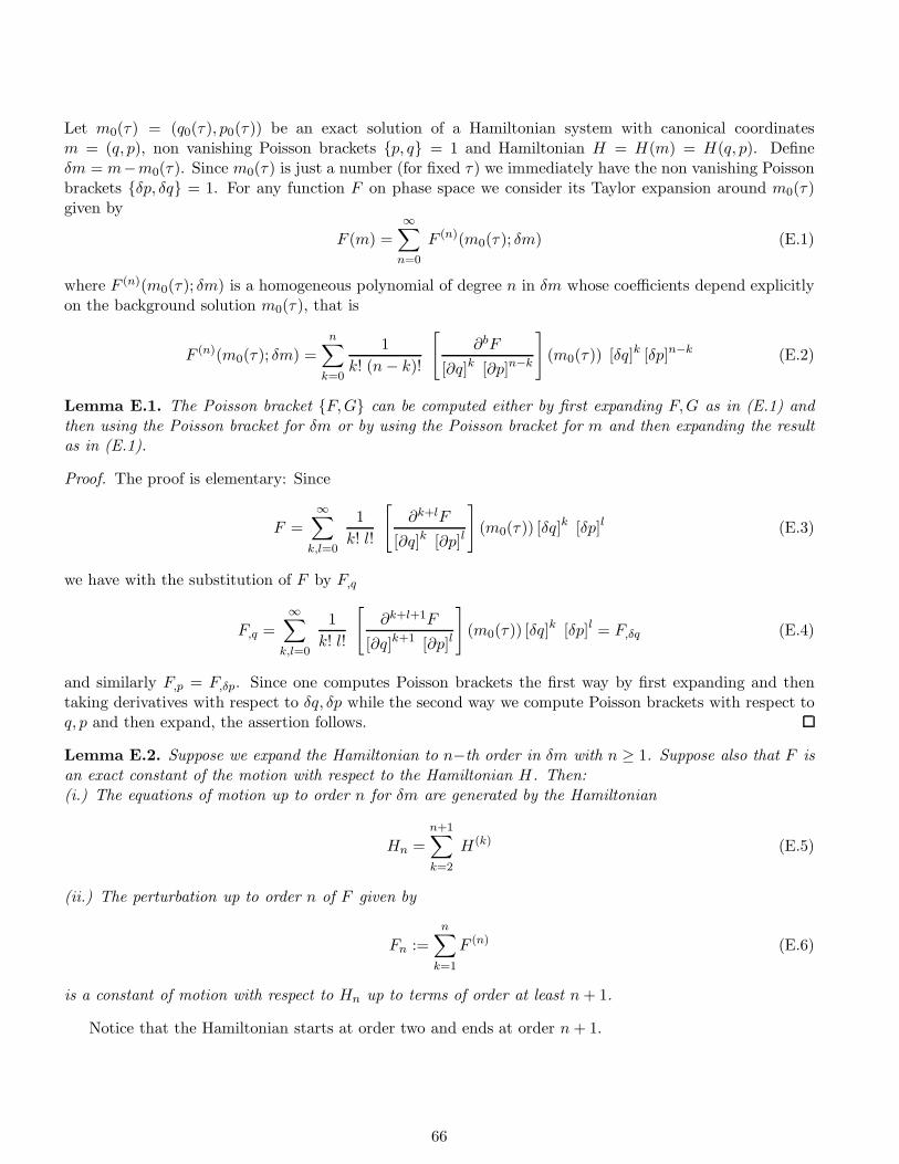
Let m0(τ) = (q0(τ), p0(τ)) be an exact solution of a Hamiltonian system with canonical coordinatesm = (q, p), non vanishing Poisson brackets p, q = 1 and Hamiltonian H = H(m) = H(q, p). Defineδm = m−m0(τ). Since m0(τ) is just a number (for fixed τ) we immediately have the non vanishing Poissonbrackets δp, δq = 1. For any function F on phase space we consider its Taylor expansion around m0(τ)given by

F (m) =

∞∑

n=0

F (n)(m0(τ); δm) (E.1)

where F (n)(m0(τ); δm) is a homogeneous polynomial of degree n in δm whose coefficients depend explicitlyon the background solution m0(τ), that is

F (n)(m0(τ); δm) =n∑

k=0

1

k! (n− k)!

[∂bF

[∂q]k [∂p]n−k

](m0(τ)) [δq]k [δp]n−k (E.2)

Lemma E.1. The Poisson bracket F,G can be computed either by first expanding F,G as in (E.1) andthen using the Poisson bracket for δm or by using the Poisson bracket for m and then expanding the resultas in (E.1).

Proof. The proof is elementary: Since

F =

∞∑

k,l=0

1

k! l!

[∂k+lF

[∂q]k [∂p]l

](m0(τ)) [δq]k [δp]l (E.3)

we have with the substitution of F by F,q

F,q =

∞∑

k,l=0

1

k! l!

[∂k+l+1F

[∂q]k+1 [∂p]l

](m0(τ)) [δq]k [δp]l = F,δq (E.4)

and similarly F,p = F,δp. Since one computes Poisson brackets the first way by first expanding and thentaking derivatives with respect to δq, δp while the second way we compute Poisson brackets with respect toq, p and then expand, the assertion follows.

Lemma E.2. Suppose we expand the Hamiltonian to n−th order in δm with n ≥ 1. Suppose also that F isan exact constant of the motion with respect to the Hamiltonian H. Then:(i.) The equations of motion up to order n for δm are generated by the Hamiltonian

Hn =

n+1∑

k=2

H(k) (E.5)

(ii.) The perturbation up to order n of F given by

Fn :=

n∑

k=1

F (n) (E.6)

is a constant of motion with respect to Hn up to terms of order at least n+ 1.

Notice that the Hamiltonian starts at order two and ends at order n+ 1.

66

Proof.(i.)Let m(t) be any solution of the exact equation of motion. We have for example

q(τ) = [H, q]m=m(τ) (E.7)

Subtracting the same equation for m0(τ) and setting δq(τ) = q(τ) − q0(τ) we find

δq(τ) = [H, q]m=m(τ) − [H, q]m=m0(τ) =∞∑

k=2

H(k),δp (E.8)

from which the assertion follows immediately (the proof for δp is identical).(ii.)Using the explicit background dependence of F (k) = F (k)(m0(τ); δm(τ)) we have

d

dτF (k) =

∂F (k)

∂q0q0(τ) +

∂F (k)

∂p0p0(τ) +

∂F (k)

∂δqδq(τ) +

∂F (k)

∂δpδp(τ)

=∂F (k)

∂q0

∂H(1)

∂δp− ∂F (k)

∂p0

∂H(1)

∂δq+∂F (k)

∂δq

∂Hn

∂δp− ∂F (k)

∂δp

∂Hn

∂δq(E.9)

where we used the first part of the lemma as well as the fact that H,q(m0) = H(1),δq , H,p(m0) = H

(1),δp . All

Poisson brackets are with respect to the coordinates δq, δp.Now observe the important fact

F (k),q0

=

k∑

l=0

1

l!(k − l)!

∂k+1F

[∂q]l+1 [∂p](k+1)−(l+1)[δq]l [δp](k+1)−(l+1)

=∂

∂δq

k∑

l=0

1

(l + 1)!((k + 1) − (l + 1))!

∂k+1F

[∂q]l+1 [∂p](k+1)−(l+1)[δq]l+1 [δp](k+1)−(l+1)

=∂

∂δq

k+1∑

l=1

1

l!(k + 1 − l)!

∂k+1F

[∂q]l [∂p]k+1−l[δq]l [δp]k+1−l

=∂

∂δq

[F (k+1) − 1

(k + 1)!

∂k+1F

[∂p]k+1[δp]k+1

]

= F(k+1),δq (E.10)

and similarly F(k),p0 = F

(k+1),δp .

Combining (E.9) and (E.10) we see that

dF (k)

dτ= H(1), F (k+1) + Hn, F

(k) (E.11)

HencedFn

dτ=

n∑

k=1

[H(1), F (k+1) +

n+1∑

l=2

H(l), F (k)]

(E.12)

We would like to show that the terms up to order n in (E.12) vanish identically. Since H(l), F (k) is oforder k + l − 2, for given k we can restrict the sum over l from l = 2 until n + 2 − k up to terms of order

67

O(δn+1). Notice that n + 2 − k is at least 2 (for k = n) and at most n + 1 (for k = 1) for all values of kwhich is the allowed range of l. It follows

dFn

dτ+O(δn+1) =

n∑

k=1

[H(1), F (k+1) +

n+2−k∑

l=2

H(l), F (k)]

=

n∑

k=1

[H(1), F (k+1) +

n∑

r=k

H(r−k+2), F (k)]

=

n∑

r=1

[H(1), F (r+1) +

r∑

k=1

H(r−k+2), F (k)]

=

n∑

r=1

r+1∑

k=1

H(r−k+2), F (k) (E.13)

where in the second step we have introduced the summation variable r = k + l − 2 which for given k takesrange in k, .., n (lowest value for l = 2 and highest value for l = n + 2 − k) whence l = r − k + 2, in thethird step we have changed the order of the k and r summation in the second term (keeping in mind theconstraint 1 ≤ k ≤ r ≤ n) while the summation variable k was renamed by r in the first term and in thefourth step we noticed that the first and second term can be combined by having the k summation extendto r + 1.

Now we exploit the fact that F is an exact invariant, that is

0 = H,F =

∞∑

k,l=1

H(l), F (k) =

∞∑

r=0

[r+1∑

k=1

H(r−k+2), F (k)]

(E.14)

where in the second step we collected all terms of order r (notice that l = r − k + 2 ≥ 1 as required).Since (E.13) is an identity on the entire phase space, the Taylor coefficients of [δq]k [δp]l have to vanishseparately for all k, l ≥ 0. The term corresponding to order r in (E.13) contains all terms of the form[δq]s[δp]r−s, s = 0, .., r. Therefore we conclude

r+1∑

k=1

H(r−k+2), F (k) = 0 (E.15)

identically for all r. In particular, (E.13) implies

dFn

dτ= O(δn+1) (E.16)

The only n for which the term O(δn+1) vanishes is for n = 1 as one can see from (E.12) since thenk = 1, l = 2 can only take one value which already contributes to order r = 1. Thus for n = 1 we even have

dF1

dτ= 0 (E.17)

It is instructive to see how the background equations find their way into demonstrating the important result(E.16) which ensures that an exact invariant expanded up to order n remains an invariant up to higherorders for the equations of motion expanded up to order n, thus simplifying the task to integrate thoseequations of motion.

68

F Generalisation to Other Deparametrising Matter

In this work dust was used as a reference frame in order to define a physical time evolution. We chosedust because then, for the case of no perturbations, the induced physical Hamiltonian yields the exact FRWequations used in standard cosmology. However, when perturbations of the metric and the scalar field areconsidered, deviations from the standard FRW framework occur, which are, however, still in agreement withobservational data. Since General Relativity does not tell us which is the right clock to use for cosmology,we chose a clock such that the resulting physical Hamiltonian is as close as possible to the FRW-Hamiltonianin standard cosmology, where one uses the Hamiltonian constraint c as a true Hamiltonian. The physicalHamiltonian used here, Hdust =

√C2 −QijCiCj , reduces to HFRW

dust = C for an FRW universe, namely tothe gauge invariant version of the Hamiltonian constraint. However, the question arises how generic are theresults obtained from a dust clock and what changes do we expect when choosing other matter than dustto reparametrise or even deparametrise the constraints of General Relativity. To illustrate this issue, let usdiscuss the phantom clock introduced in [9] which leads to a physical Hamiltonian of the form

Hphan =

∫

χ

d3σHphan(σ), (F.1)

with the Hamiltonian density Hphan defined as

Hphan(σ) =

√1

2(F (C,Ci, Qij)) +

√1

4(F (C,Ci, Qij))

2 − α2Qij(σ, τ)CiCj(σ)Q(σ, τ) (F.2)

whereF (C,Ci, Qij) := C2(σ, τ) −Qij(σ, τ)CiCj(σ) − α2Q(σ, τ). (F.3)

Above we introduced the abbreviation Q = det(Qij), and α > 0 is for the moment an arbitrary constantof dimension cm−2 that enters the phantom field action as a free parameter. Recall that the expressionsfor C and Cj were given by the geometry and matter part of the total Hamiltonian and diffeomorphismconstraint, respectively, that is

C(σ, τ) = Cgeo(σ, τ) + Cmatter(σ, τ) and Cj(σ) = Cgeoj (σ) + Cmatter

j (σ). (F.4)

From now on we will drop the τ dependence of C(σ, τ) and Qij(σ, τ) in the expression for Hphan and writethem explicitly only when confusion could arise otherwise.

For the dust Hamiltonian we saw that the first order equations of motion obtained for Ξ,Π and Qij , Pij

look similar to the standard cosmological equations apart from the fact that in the case of a dust clockwe obtain a dynamical, that is phase space dependent, lapse function Ndust = C/Hdust and shift vectorN i

dust = N i/Hdust. Moreover, in the general equations there occurs a term proportional to N idustN

jdust.

With respect to Hphan, we want to analyse now whether it produces a similar effect and leads to possi-bly more serious deviations from the standard equations. Starting with the first order equation for Ξ weobtain

Ξ(σ, τ) = Hphan,Ξ(σ, τ) (F.5)

=

∫

χ

d3σ′[ C

Hphan(σ′)

1

2+

(C2 −QijCiCj − α2Q)(σ′)

4√

(14 (C2 −QijCiCj − α2Q)2 − α2QijCiCjQ)(σ′)

Cmatter(σ′),Ξ(σ, τ)

−QijCj

Hphan(σ′)

1

2+

(C2 −QijCiCj + α2Q)(σ′)

4√

(14(C2 −QijCiCj − α2Q)2 − α2QijCiCjQ)(σ′)

Cmatter(σ′),Ξ(σ, τ)i

].

69

Introducing the dynamical lapse function Nphan and the dynamical shift covector N iphan as

Nphan(σ) :=C

Hphan(σ)

1

2+

(C2 −QijCiCj − α2Q)(σ)

4√

(14(C2 −QijCiCj − α2Q)2 − α2QijCiCjQ)(σ)

N iphan(σ) := −Q

ijCj

Hphan(σ)

1

2+

(C2 −QijCiCj + α2Q)(σ)

4√

(14(C2 −QijCiCj − α2Q)2 − α2QijCiCjQ)(σ)

, (F.6)

we can rewrite the first order equation of motion for Ξ as

Ξ(σ, τ) = Hphan,Ξ(σ, τ) =

∫

χ

d3σ′(Nphan(σ′)Cmatter(σ′),Ξ(σ, τ) +N i

phanCmatteri (σ′),Ξ(σ, τ)

). (F.7)

Hence, we realise that, similarly to the case of the dust clock, the effect of the phantom clock results inthe appearance of a dynamical lapse function and a dynamical shift vector. However, due to the morecomplicated structure of Hphan as compared to Hdust, Nphan and N i

phan are not simply given in terms ofC/Hphan and −Cj/Hphan respectively. Now also terms occur which include higher than linear powers ofthe constraints in the nominator and denominator. Since the quantities Π and obviously Qij also Poissoncommute with any function that does depend on Qij only, the calculation works analogously in these casesand we obtain

Π(σ, τ) = Hphan,Π(σ, τ) =

∫

χ

d3σ′(Nphan(σ′)Cmatter(σ′),Ξ(σ) +N i

phanCmatteri (σ′),Π(σ, τ)

)(F.8)

and

Qij(σ, τ) = Hphan, Qij(σ) =

∫

χ

d3σ′(Nphan(σ′)Cgeo(σ′), Qij(σ, τ) +N i

phanCgeoi (σ′), Qij(σ, τ)

). (F.9)

For the dynamical variable P ij things look slightly different, because P ij does not Poisson commute withfunctions depending on Qij. Therefore we get, as in the dust case, an additional contribution proportional tothe Poisson bracket Qkl(σ′), P ij(σ, τ). Furthermore, since Hphan includes a term of the form α2Q, we alsoobtain a term proportional to the Poisson bracket Q(σ′), P ij(σ, τ). The explicit results for these Poissonbrackets are

Qkl(σ′), P ij(σ, τ) =κ

2(QikQlj +QjkQil)(σ′, τ)δ3(σ′, σ)

Q(σ′), P ij(σ, τ) = −κ(QQij)(σ′, τ)δ3(σ′, σ). (F.10)

Inserting this back into the eqn. for P ij, we end up with

P ij(σ, τ) = Hphan, Pij(σ, τ)

=

∫

χ

d3σ′(Nphan(σ′)Cgeo(σ′), P ij(σ, τ) +N i

phanCgeoi (σ′), P ij(σ, τ)

)

−κ2

HphanN

iphanN

jphan

1

2+

(C2 −QijCiCj + α2Q)

4√

(14(C2 −QijCiCj − α2Q)2 − α2QijCiCjQ)

−1 (σ, τ)

+κ

2

α

2QijQ

Hphan

1

2+

C2 +QijCiCj − α2Q

4√

14(C2 −QijCiCj − α2Q)2 − α2QQijCiCj

(σ, τ). (F.11)

70

The remaining Poisson brackets in the first order equations for the dynamical variables are the same Poissonbrackets that occur when Hdust is used as a Hamiltonian. Inserting the results obtained there into thecorresponding equations for the case of Hphan, we obtain the following final form of the first order equations:

Ξ(σ, τ) =NphanΠ

Q(σ, τ) +

(L ~NphanΞ

)(σ, τ)

Π(σ, τ) =[NphanQQ

ijΞ, i],j

(σ, τ) − 1

2(NphanQV

′(Ξ))(σ, τ) +(L ~Nphan

Π)

(σ, τ)

Qij(σ, τ) =2Nphan

Q(σ, τ) (GijmnP

mn) (σ, τ) +(L ~Nphan

Q)

ij(σ, τ), (F.12)

where

Gijmn :=1

2(QimQjn +QinQjm −QijQmn) , (F.13)

with its inverse given by

[G−1]ijmn :=1

2

(QimQjn +QinQjm − 2QijQmn

). (F.14)

For the gravitational momentum we have

P ij(σ, τ) =(Nphan

[− Qmn√

detQ

(2P jmP kn − P jkPmn

)+κ

2Qjk C −

√detQ Qjk

(2Λ +

κ

2λ

(Ξ,mΞ,m + v(Ξ)

))]

+√

detQ[G−1]jkmn((DmDnNphan) −NphanRmn[Q]

)+

κ

2λNphan

√detQ Ξ,jΞ,k + (L ~Nphan

P )jk)(σ, τ)

−κ2

HphanN

iphanN

jphan

1

2+

(C2 −QijCiCj + α2Q)

4√

(14 (C2 −QijCiCj − α2Q)2 − α2QijCiCjQ)

−1 (σ, τ)

+κ

2

α

2QijQ

Hphan

1

2+

C2 +QijCiCj − α2Q

4√

14(C2 −QijCiCj − α2Q)2 − α2QQijCiCj

(σ, τ). (F.15)

One can see that the first order equations for Ξ,Π and Qij in equation (F.12) are identical to those forthe dust Hamiltonian Hdust, apart from the different definitions of the dynamical lapse function Nphan

and shift vector N iphan in equation (F.6). However, the equation for P ij differs from the corresponding

dust Hamiltonian equation. The term in the second last line in equation (F.15) corresponds to the term−κ

2 (HdustNidustN

jdust)(σ) in the equation for P ij derived from Hdust. In the present case this term looks a

bit more complicated, since we have to divide the whole expression by the term in the square brackets whichis identical to one in case of Hdust. The additional term in the last line of equation (F.15) comes from theterms α2Q and α2QijCiCj in Hphan, which are absent in Hdust. Since in this term we cannot factor out C orCi but only α2, we are also not able to reexpress this term by means of the dynamical lapse function Nphan

and the dynamical shift vector N iphan, respectively, as it was possible for the term in the second last line.

In summary, when using a phantom scalar field as a clock we also obtain deviations from the standardtreatment in which the Hamiltonian constraint is used as a true Hamiltonian. These deviations manifestthemselves in the appearance of a dynamical lapse function Nphan and a dynamical shift vector N i

phan, anal-

ogous to the case where dust is used as a clock. However, the explicit dependence of Nphan and N iphan on the

dynamical variables is more complicated than for the corresponding quantities Ndust and N idust. Another

modification occurs in the equation for the gravitational momentum P ij . While it contains a term thatis second order in N i

phan, in complete analogy with the case of Hdust, it also features an additional term

proportional to α2.

71

The Special Case of an FRW Universe

It is interesting to study the special case of FRW also for Hphan. Recall from [15] that by assuminghomogeneity and isotropy, Hdust, Ndust and N i

dust reduce to the following quantities

Ndust(σ)FRW−→ 1, N i

dust(σ)FRW−→ 0, Hdust(σ)

FRW−→ CFRW(σ), (F.16)

where

CFRWdust (τ) = A3(τ)

( 1

κ

(− 6( AA

)2+ 2Λ

)+

1

2λ

(Ξ2 + V (Ξ)

))(τ). (F.17)

Here A = A(τ) is a function of dust time τ and the dot refers to a derivative with respect to dust time. Inparticular A(τ) can be understood as the gauge invariant extension of the ordinary scale factor a(t) usedin standard cosmology. The difference between the two is that A is gauge invariant and thus a physicalobservable whereas a is not, since it does not commute with the Hamiltonian constraint of FRW.The gravitational canonical variables are given by Qij = A2(τ)δij and P ij = −2A(τ)δij . We mentionedpreviously that a consequence of this behaviour is that the unperturbed equations of motion for (Ξ,Π) and(Qij , P

ij) agree with the FRW equations used in standard cosmology. In particular, the deviation from thegeneral standard equation of motion for P ij vanishes in the case of FRW, because it is quadratic in N i

dust.For the phantom Hamiltonian Hphan things look slightly different. Here we have the following behaviour ofHphan, Nphan and N i

phan, when a homogenous and isotropic universe is considered:

Nphan(σ)FRW−→ NFRW

phan :=

(CFRW

phan

HFRWphan

)(σ), N i

phan(σ)FRW−→ 0, Hphan(σ)

FRW−→ HFRWphan :=

√(CFRW

phan)2 − α2A6(σ)

(F.18)with

CFRWphan(τ) =

A3

(NFRWphan)2

(τ)( 1

κ

(− 6( AA

)2+ 2Λ(NFRW

phan)2)

+1

2λ

(Ξ2 + V (Ξ)(NFRW

phan)2))

(τ). (F.19)

Hence, the dust clock and the phantom scalar field clock agree only if the parameter α is chosen to be tinycompared to the Hamiltonian constraint CFRW

phan, e.g. αA3 ≪ CFRWphan. Consequently, the equations of motion

generated by Hphan also deviate from the standard FRW equations. The significance of this deviation againdepends on the specific value of the parameter α, as was discussed in detail in [9]. For completeness we alsolist the first order equations of motion here

Ξ(τ) =(NFRW

phan

Π√Q

)(τ) (F.20)

Π(τ) = −(NFRW

phan

√Q

2V ′(Ξ)

)(τ)

Qij =(NFRW

phan

2√QGijmnP

mn)(τ)

P ij = NFRWphan(τ)

(−Qmn√

Q

(2P imP jn − P ijPmn

)+κ

2QijCFRW

phan −Qij√Q(2Λ +

κ

2λV (Ξ)) +

α2κ

2

Q

CFRWQij

)(τ).

Taking into account that Qij = A2δij and using the first order equation for Qij, we solve for the momentaP ij = −2A/NFRW

phanδij in terms of Qjk = 2AA. In order to derive the corresponding FRW equation with

respect to the time generated by HFRWphan, we take the time derivative of the equation for Qij and insert into

the resulting equation for Qij the expression for P ij and P ij given above. This yields

(AA

)= −1

2

(AA

)2+

1

2(NFRW

phan)2Λ− κ

4λ

(12Ξ2 − 1

2(NFRW

phan)2V (Ξ))

+NFRW

phan

NFRWphan

( AA

)− κ

4(NFRW

phan)2( α2A3

CFRWphan

). (F.21)

72

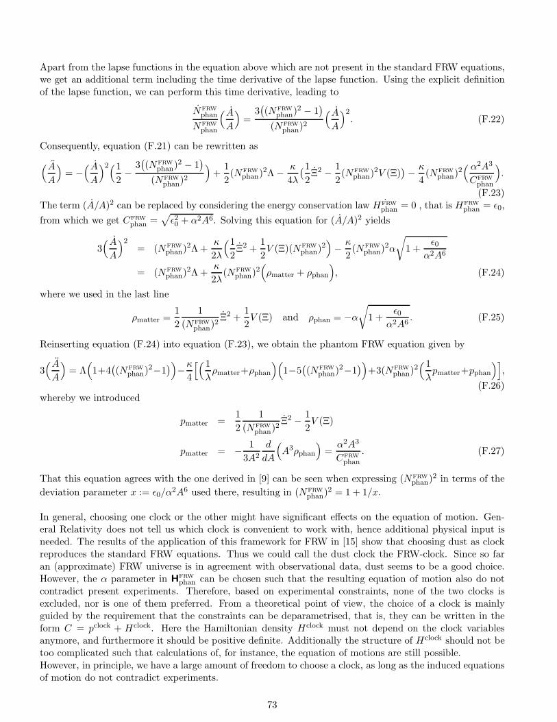
Apart from the lapse functions in the equation above which are not present in the standard FRW equations,we get an additional term including the time derivative of the lapse function. Using the explicit definitionof the lapse function, we can perform this time derivative, leading to

NFRWphan

NFRWphan

( AA

)=

3((NFRW

phan)2 − 1)

(NFRWphan)2

(AA

)2. (F.22)

Consequently, equation (F.21) can be rewritten as

(AA

)= −

(AA

)2(1

2−

3((NFRW

phan)2 − 1)

(NFRWphan)2

)+

1

2(NFRW

phan)2Λ − κ

4λ

(12Ξ2 − 1

2(NFRW

phan)2V (Ξ))− κ

4(NFRW

phan)2( α2A3

CFRWphan

).

(F.23)The term (A/A)2 can be replaced by considering the energy conservation law ˙HFRW

phan = 0 , that is HFRWphan = ǫ0,

from which we get CFRWphan =

√ǫ20 + α2A6. Solving this equation for (A/A)2 yields

3( AA

)2= (NFRW

phan)2Λ +κ

2λ

(1

2Ξ2 +

1

2V (Ξ)(NFRW

phan)2)− κ

2(NFRW

phan)2α

√1 +

ǫ0α2A6

= (NFRWphan)2Λ +

κ

2λ(NFRW

phan)2(ρmatter + ρphan

), (F.24)

where we used in the last line

ρmatter =1

2

1

(NFRWphan)2

Ξ2 +1

2V (Ξ) and ρphan = −α

√1 +

ǫ0α2A6

. (F.25)

Reinserting equation (F.24) into equation (F.23), we obtain the phantom FRW equation given by

3(AA

)= Λ

(1+4

((NFRW

phan)2−1))

−κ4

[( 1

λρmatter+ρphan

)(1−5

((NFRW

phan)2−1))

+3(NFRWphan)2

( 1

λpmatter+pphan

)],

(F.26)whereby we introduced

pmatter =1

2

1

(NFRWphan)2

Ξ2 − 1

2V (Ξ)

pmatter = − 1

3A2

d

dA

(A3ρphan

)=α2A3

CFRWphan

. (F.27)

That this equation agrees with the one derived in [9] can be seen when expressing (NFRWphan)2 in terms of the

deviation parameter x := ǫ0/α2A6 used there, resulting in (NFRW

phan)2 = 1 + 1/x.

In general, choosing one clock or the other might have significant effects on the equation of motion. Gen-eral Relativity does not tell us which clock is convenient to work with, hence additional physical input isneeded. The results of the application of this framework for FRW in [15] show that choosing dust as clockreproduces the standard FRW equations. Thus we could call the dust clock the FRW-clock. Since so faran (approximate) FRW universe is in agreement with observational data, dust seems to be a good choice.However, the α parameter in H

FRWphan can be chosen such that the resulting equation of motion also do not

contradict present experiments. Therefore, based on experimental constraints, none of the two clocks isexcluded, nor is one of them preferred. From a theoretical point of view, the choice of a clock is mainlyguided by the requirement that the constraints can be deparametrised, that is, they can be written in theform C = pclock + Hclock. Here the Hamiltonian density Hclock must not depend on the clock variablesanymore, and furthermore it should be positive definite. Additionally the structure of Hclock should not betoo complicated such that calculations of, for instance, the equation of motions are still possible.However, in principle, we have a large amount of freedom to choose a clock, as long as the induced equationsof motion do not contradict experiments.

73

G Linear Perturbation Theory: Some Calculations in More Detail

In section 6.2 we derived the second order equation of motion for the linear perturbation of the (manifestly)gauge invariant three metric δQjk. For that we needed the perturbation of the geometry and matter partof the gauge invariant Hamiltonian constraint, denoted by Cgeo and Cmatter, respectively, as these termsoccur in the third term on the right-hand side of the unperturbed equation of motion for Qjk, equation(4.24). We omitted the details in the main text due to their length, and also because it turns out thatseveral terms cancel when inserted back into the expression of the perturbation of the third term, shown inequation (6.20). For the interested reader, however, the detailed perturbations of the constraints are givenbelow.The perturbed geometry constraint δCgeo is given by

δCgeo =[12

(Q

jk+N

jN

k

N2

)C

geo+

1

2

NjN

k

N2

(C

geo − 2

√detQ

κ

(2Λ −R

))+

√detQ

κ

(R

jk − [G−1

]jkmnDmDn

)

+

√detQ

2N2κ

(Qmn −

(L~

NQ)mn

)[[G

−1]jkmn

( ∂∂τ

− L~N

)−(Qrs −

(L~

NQ)rs

)Q

nk[G

−1]rsmj

]

+

√detQ

2N2κ

(Qrs −

(L~

NQ)rs

)[G

−1]rsmn

[Q

jtN

k[Qmn],t + 2Qtn

∂

∂xm

(Q

jtN

k)]]

δQjk

+[− 2

Nj

N2

(C

geo −√

detQ

κ

(2Λ −R

))

−√

detQ

2N2κ

(Qrs −

(L~

NQ)rs

)[G

−1]rsmn

[Q

jt[Qrs],t + 2Qts

∂

∂xk

(Q

jt)]]

δNj . (G.1)

Here we used that the perturbation of the Ricci scalar can be written as

δR =[[G

−1]jkmnDmDn −R

jk]δQjk. (G.2)

For the perturbed matter part of the constraint δCmatter we obtain

δCmatter =[12

(Q

jk+N

jN

k

N2

)C

matter+

1

2

NjN

k

N2

(C

matter −√

detQ

λ

(Q

jkΞ,jΞ,k + v(Ξ)

))(G.3)

+

√detQ

N2λ

QjmQ

kn(Ξ −

(L~

NΞ))NmΞ,n −

√detQ

2λQ

jmQ

jkΞ,mΞ,n

]δQjk

+[−√

detQ

N2λ

(Ξ −

(L~

NΞ))Q

jkΞ,k − 2

Nj

N2

(C

matter −√

detQ

2λ

(Q

jkΞ,jΞ,k + v(Ξ)

))]δNj

+[√detQ

λ

( 1

N2

(Ξ −

(L~

NΞ))( ∂

∂τ− L~

N

)+Q

jkΞ,k

∂

∂xj+

1

2v′(Ξ)

)]δΞ.

74

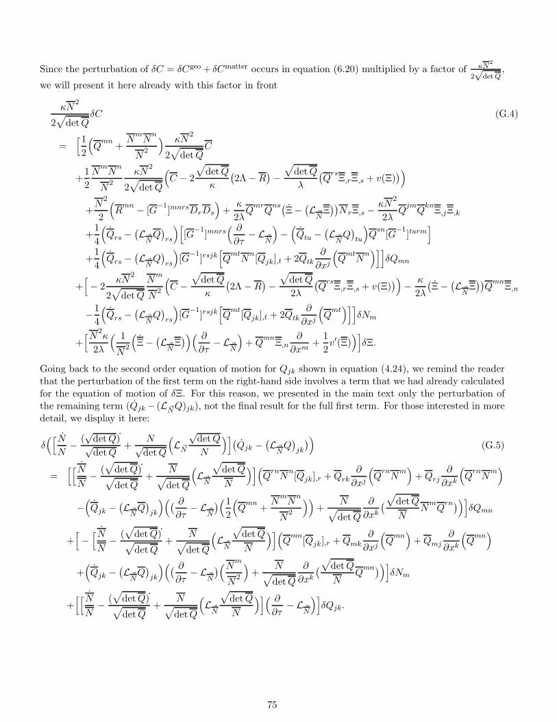
Since the perturbation of δC = δCgeo + δCmatter occurs in equation (6.20) multiplied by a factor of κN2

2√

det Q,

we will present it here already with this factor in front

κN2

2√

detQδC (G.4)

=[12

(Q

mn+N

mN

n

N2

) κN2

2√

detQC

+1

2

NmN

n

N2

κN2

2√

detQ

(C − 2

√detQ

κ

(2Λ −R

)−√

detQ

λ

(Q

rsΞ,rΞ,s + v(Ξ)

))

+N

2

2

(R

mn − [G−1

]mnrsDrDs

)+

κ

2λQ

mrQ

ns(Ξ −

(L~

NΞ))N rΞ,s −

κN2

2λQ

jmQ

knΞ,jΞ,k

+1

4

(Qrs −

(L~

NQ)rs

)[[G

−1]mnrs

( ∂∂τ

− L~N

)−(Qtu −

(L~

NQ)tu

)Q

sn[G

−1]turm

]

+1

4

(Qrs −

(L~

NQ)rs

)[G

−1]rsjk

[Q

mtN

n[Qjk],t + 2Qtk

∂

∂xj

(Q

mtN

n)]]

δQmn

+[− 2

κN2

2√

detQ

Nm

N2

(C −

√detQ

κ

(2Λ −R

)−√

detQ

2λ

(Q

rsΞ,rΞ,s + v(Ξ)

))− κ

2λ

(Ξ −

(L~

NΞ))Q

mnΞ,n

−1

4

(Qrs −

(L~

NQ)rs

)[G

−1]rsjk

[Q

mt[Qjk],t + 2Qtk

∂

∂xj

(Q

mt)]]

δNm

+[N2

κ

2λ

( 1

N2

(Ξ −

(L~

NΞ))( ∂

∂τ− L~

N

)+Q

mnΞ,n

∂

∂xm+

1

2v′(Ξ)

)]δΞ.

Going back to the second order equation of motion for Qjk shown in equation (4.24), we remind the readerthat the perturbation of the first term on the right-hand side involves a term that we had already calculatedfor the equation of motion of δΞ. For this reason, we presented in the main text only the perturbation ofthe remaining term (Qjk − (L ~N

Q)jk), not the final result for the full first term. For those interested in moredetail, we display it here:

δ([NN

− (√

detQ)˙√detQ

+N√detQ

(L ~N

√detQ

N

)](Qjk −

(L~

NQ)jk

))(G.5)

=[[NN

− (√

detQ)˙√detQ

+N√detQ

(L~

N

√detQ

N

)](Q

rnN

n[Qjk],r +Qrk

∂

∂xj

(Q

rnN

m)

+Qrj

∂

∂xk

(Q

rnN

m)

−(Qjk −

(L~

NQ)jk

)(( ∂∂τ

− L~N

)(1

2

(Q

mn+N

mN

n

N2

))+

N√detQ

∂

∂xk

(√

detQ

NN

mQ

rn))]δQmn

+[−[NN

− (√

detQ)˙√detQ

+N√detQ

(L~

N

√detQ

N

)](Q

mn[Qjk],r +Qmk

∂

∂xj

(Q

mn)

+Qmj

∂

∂xk

(Q

mn)

+(Qjk −

(L~

NQ)jk

)(( ∂∂τ

− L~N

)(Nm

N2

)+

N√detQ

∂

∂xk

(√

detQ

NQ

mn))]δNm

+[[NN

− (√

detQ)˙√detQ

+N√detQ

(L~

N

√detQ

N

)]( ∂∂τ

− L~N

)]δQjk.

75

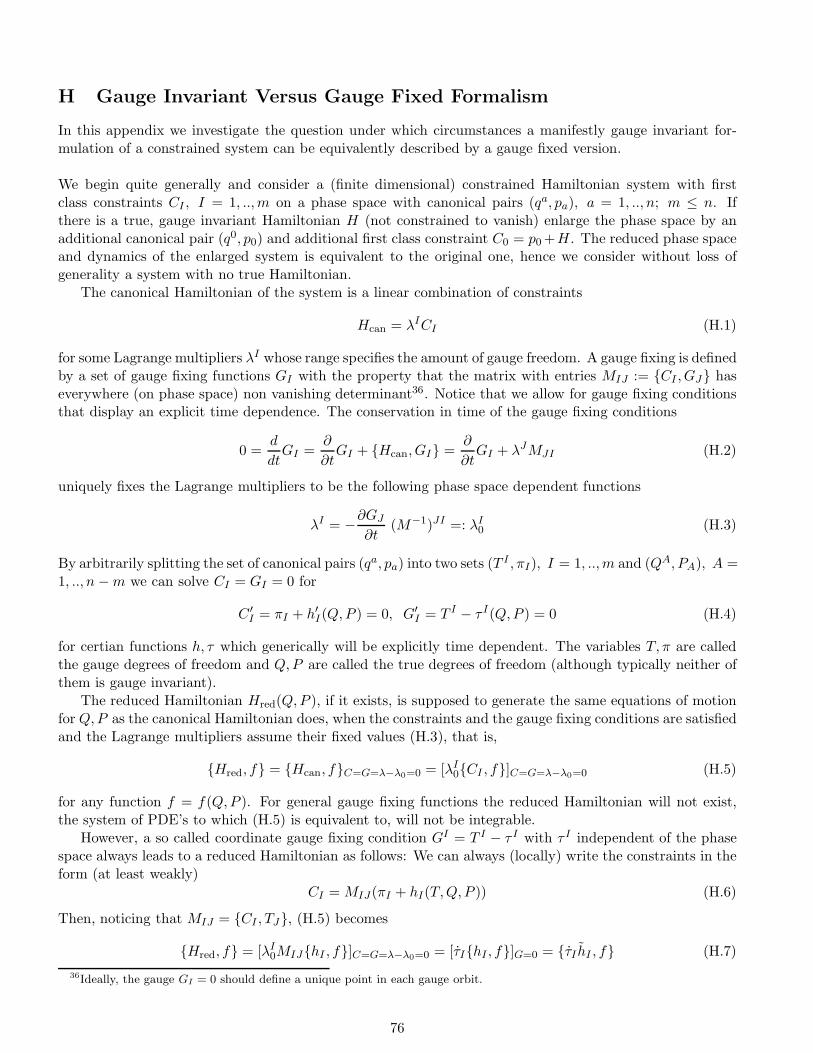
H Gauge Invariant Versus Gauge Fixed Formalism

In this appendix we investigate the question under which circumstances a manifestly gauge invariant for-mulation of a constrained system can be equivalently described by a gauge fixed version.

We begin quite generally and consider a (finite dimensional) constrained Hamiltonian system with firstclass constraints CI , I = 1, ..,m on a phase space with canonical pairs (qa, pa), a = 1, .., n; m ≤ n. Ifthere is a true, gauge invariant Hamiltonian H (not constrained to vanish) enlarge the phase space by anadditional canonical pair (q0, p0) and additional first class constraint C0 = p0 +H. The reduced phase spaceand dynamics of the enlarged system is equivalent to the original one, hence we consider without loss ofgenerality a system with no true Hamiltonian.

The canonical Hamiltonian of the system is a linear combination of constraints

Hcan = λICI (H.1)

for some Lagrange multipliers λI whose range specifies the amount of gauge freedom. A gauge fixing is definedby a set of gauge fixing functions GI with the property that the matrix with entries MIJ := CI , GJ haseverywhere (on phase space) non vanishing determinant36. Notice that we allow for gauge fixing conditionsthat display an explicit time dependence. The conservation in time of the gauge fixing conditions

0 =d

dtGI =

∂

∂tGI + Hcan, GI =

∂

∂tGI + λJMJI (H.2)

uniquely fixes the Lagrange multipliers to be the following phase space dependent functions

λI = −∂GJ

∂t(M−1)JI =: λI

0 (H.3)

By arbitrarily splitting the set of canonical pairs (qa, pa) into two sets (T I , πI), I = 1, ..,m and (QA, PA), A =1, .., n −m we can solve CI = GI = 0 for

C ′I = πI + h′I(Q,P ) = 0, G′

I = T I − τ I(Q,P ) = 0 (H.4)

for certian functions h, τ which generically will be explicitly time dependent. The variables T, π are calledthe gauge degrees of freedom and Q,P are called the true degrees of freedom (although typically neither ofthem is gauge invariant).

The reduced Hamiltonian Hred(Q,P ), if it exists, is supposed to generate the same equations of motionfor Q,P as the canonical Hamiltonian does, when the constraints and the gauge fixing conditions are satisfiedand the Lagrange multipliers assume their fixed values (H.3), that is,

Hred, f = Hcan, fC=G=λ−λ0=0 = [λI0CI , f]C=G=λ−λ0=0 (H.5)

for any function f = f(Q,P ). For general gauge fixing functions the reduced Hamiltonian will not exist,the system of PDE’s to which (H.5) is equivalent to, will not be integrable.

However, a so called coordinate gauge fixing condition GI = T I − τ I with τ I independent of the phasespace always leads to a reduced Hamiltonian as follows: We can always (locally) write the constraints in theform (at least weakly)

CI = MIJ(πI + hI(T,Q,P )) (H.6)

Then, noticing that MIJ = CI , TJ, (H.5) becomes

Hred, f = [λI0MIJhI , f]C=G=λ−λ0=0 = [τIhI , f]G=0 = τI hI , f (H.7)

36Ideally, the gauge GI = 0 should define a unique point in each gauge orbit.

76

with hI = hI(T = τ,Q, P ) and we used that f only depends on Q,P . This displays the reduced Hamiltonianas

Hred(Q,P ; t) = τI(t)hI(T = τ(t), Q, P )) (H.8)

It will be explicitly time dependent unless τI is time independent and hI is independent of T , that is, unlessthose constraints can be deparametrised for which τI 6= 0. Hence, deparametrisation is crucial for having aconserved Hamiltonian system.

On the other hand, let us consider the gauge invariant point of view. The observables associated withf(Q,P ) are given by

Of (τ) = [exp(βIXI) · f ]β=τ−T (H.9)

where we have denoted the Abelian Hamiltonian vector fields XI by XI := πI + hI , .. Consider a oneparameter family of flows t 7→ τ I(t) then with Of (t) := Of (τ(t)) we find

d

dtOf (t) = τ I(t)

∞∑

n=0

βJ1..βJn

n!XIXJ1 ..XJn · f (H.10)

On the other hand, consider HI(t) := OhI(τ(t)), then

HI(t), Of (t) = = OhI ,f∗(τ(t)) = OhI ,f(τ(t)) = OXI ·f (τ(t))

= τ I(t)

∞∑

n=0

βJ1 ..βJn

n!XIXJ1..XJn · f (H.11)

where in the second step we used that neither hI nor f depend on πJ , in the third we used that f does notdepend on T J and in the last we used the commutativity of the XJ . Thus the physical Hamiltonian thatdrives the time evolution of the observables is simply given by

H(t) := τ I(t)hI(τ(t), OQ(t), OP (t)) (H.12)

This is exactly the same as (H.8) under the identification f ↔ Of (0). Hence we have shown that for suitablegauge fixings the reduced and the gauge invariant frameworks are equivalent. Notice that it was crucial inthe derivation that (T I , πI) and (QA, PA) are two sets of canonical pairs. If that would not be the case,then it would be unclear whether the time evolution of the observables has a canonical generator.

The power of a manifestly gauge invariant framework lies therefore not in the gauge invariance itself.Rather, it relies on whether the gauge fixing can be achieved globally, whether it can be phrased in termsof separate canonical pairs, whether the observer clocks TI are such that reduced Hamiltonian system isconserved and whether they do display the time evolution of observables as viewed by a realistic observer.In particular, the reduced Hamiltonian by construction only depends on (QA, PA). In application to gravity,if one would not add an additional matter component such as the dust, then the true degrees of freedomwould sit in two of the six canonical pairs (qab, p

ab). However, notice that it is not obvious how to splitthese pairs into gauge and true degrees of freedom in an at least spatially covariant way and moreover it isnot possible to solve for four of the pab algebraically because the spatial diffeomorphism constraint involvestheir derivatives. Hence the physical or reduced Hamiltonian would become non-local. Furthermore, if oneuses gravitational degrees of freedom for reduction then it is clear that onbe does not get the full set ofEinstein’s equations as evolution equations which is something that one may want to keep. Finally, thereduced Hamiltonian will not reduce to the standard model Hamiltonian in the flat space limit (i.e. withunit lapse) nor will it be necessarily positive. Of course, when adding matter like our dust, then similarto the Higgs mechanism the four dust degrees of freedom get absorbed by the metric which develops fouradditional Goldstone modes. These modes should decouple and they do as we showed explicitly in this paperbecause of the existence of an infinite number of conserved charges, however, it is not granted to happenwhen adding arbitrary matter.

77

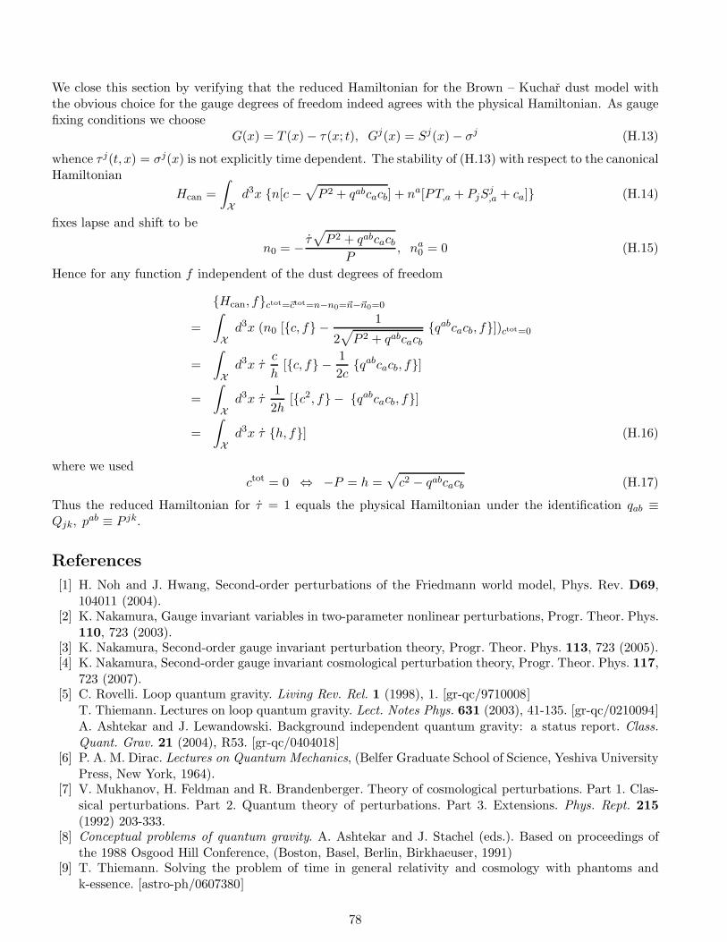
We close this section by verifying that the reduced Hamiltonian for the Brown – Kuchar dust model withthe obvious choice for the gauge degrees of freedom indeed agrees with the physical Hamiltonian. As gaugefixing conditions we choose

G(x) = T (x) − τ(x; t), Gj(x) = Sj(x) − σj (H.13)

whence τ j(t, x) = σj(x) is not explicitly time dependent. The stability of (H.13) with respect to the canonicalHamiltonian

Hcan =

∫

Xd3x n[c−

√P 2 + qabcacb] + na[PT,a + PjS

j,a + ca] (H.14)

fixes lapse and shift to be

n0 = − τ√P 2 + qabcacb

P, na

0 = 0 (H.15)

Hence for any function f independent of the dust degrees of freedom

Hcan, fctot=~ctot=n−n0=~n−~n0=0

=

∫

Xd3x (n0 [c, f − 1

2√P 2 + qabcacb

qabcacb, f])ctot=0

=

∫

Xd3x τ

c

h[c, f − 1

2cqabcacb, f]

=

∫

Xd3x τ

1

2h[c2, f − qabcacb, f]

=

∫

Xd3x τ h, f] (H.16)

where we usedctot = 0 ⇔ −P = h =

√c2 − qabcacb (H.17)

Thus the reduced Hamiltonian for τ = 1 equals the physical Hamiltonian under the identification qab ≡Qjk, p

ab ≡ P jk.

References

[1] H. Noh and J. Hwang, Second-order perturbations of the Friedmann world model, Phys. Rev. D69,104011 (2004).

[2] K. Nakamura, Gauge invariant variables in two-parameter nonlinear perturbations, Progr. Theor. Phys.110, 723 (2003).

[3] K. Nakamura, Second-order gauge invariant perturbation theory, Progr. Theor. Phys. 113, 723 (2005).[4] K. Nakamura, Second-order gauge invariant cosmological perturbation theory, Progr. Theor. Phys. 117,

723 (2007).[5] C. Rovelli. Loop quantum gravity. Living Rev. Rel. 1 (1998), 1. [gr-qc/9710008]

T. Thiemann. Lectures on loop quantum gravity. Lect. Notes Phys. 631 (2003), 41-135. [gr-qc/0210094]A. Ashtekar and J. Lewandowski. Background independent quantum gravity: a status report. Class.Quant. Grav. 21 (2004), R53. [gr-qc/0404018]

[6] P. A. M. Dirac. Lectures on Quantum Mechanics, (Belfer Graduate School of Science, Yeshiva UniversityPress, New York, 1964).

[7] V. Mukhanov, H. Feldman and R. Brandenberger. Theory of cosmological perturbations. Part 1. Clas-sical perturbations. Part 2. Quantum theory of perturbations. Part 3. Extensions. Phys. Rept. 215

(1992) 203-333.[8] Conceptual problems of quantum gravity. A. Ashtekar and J. Stachel (eds.). Based on proceedings of

the 1988 Osgood Hill Conference, (Boston, Basel, Berlin, Birkhaeuser, 1991)[9] T. Thiemann. Solving the problem of time in general relativity and cosmology with phantoms and

k-essence. [astro-ph/0607380]

78

[10] C. Rovelli. What is observable in classical and quantum gravity? Class. Quantum Grav. 8 (1991),297-316.C. Rovelli. Quantum reference systems. Class. Quantum Grav. 8 (1991), 317-332.C. Rovelli. Time in quantum gravity: physics beyond the Schrodinger regime. Phys. Rev. D43 (1991),442-456.C. Rovelli. Quantum mechanics without time: a model. Phys. Rev. D42 (1990), 2638-2646.

[11] B. Dittrich. Partial and complete observables for Hamiltonian constrained systems, Gen. Rel. Grav. 39

(2007) 1891 [gr-qc/0411013].B. Dittrich. Partial and complete observables for canonical general relativity. Class. Quant. Grav. 23

(2006),6155-6184. [gr-qc/0507106][12] J. Brown and K. Kuchar. Dust as a standard of space and time in canonical quantum gravity. Phys.

Rev. D51 (1995), 5600-5629. [gr-qc/9409001][13] D. Langlois. Hamiltonian formalism and gauge invariance for linear perturbations in inflation. Class.

Quant. Grav. (1994) 11 389-407.[14] M. Iftime and J. Stachel. The hole argument for covariant theories. Gen. Rel. Grav. 38 (2006) 1241-1252.[15] K. Giesel, S. Hofmann, T. Thiemann and O. Winkler. Manifestly gauge-invariant general relativistic

perturbation theory: II. FRW Background and First Order. [arXiv:0711.0117 [gr-qc]][16] N. Straumann. From primordial quantum fluctuations to the anisotropies of the cosmic microwave

background radiation. Annalen Phys. 15 (2006) 701-847. [hep-ph/0505249][17] V. Mukhanov. Physical foundations of cosmology, (Cambridge, Cambridge University Press, 2006).[18] V. I. Arnold. Mathematical methods of classical mechanics, (New York, Berlin, Heidelberg, Springer-

Verlag, 1989).[19] K. Giesel, S. Hofmann, T. Thiemann and O. Winkler. Manifestly gauge-invariant general relativistic

perturbation theory: III. FRW background and Second Order. In preparation.[20] T. Thiemann. Reduced phase space quantization and Dirac observables. Class. Quant. Grav. 23 (2006),

1163-1180. [gr-qc/0411031][21] C. Rovelli. Quantum Gravity, (Cambridge University Press, Cambridge, 2004).[22] Thiemann. Modern Canonical Quantum General Relativity, (Cambridge University Press, Cambridge,

2007). [gr-qc/0110034][23] K. Giesel and T. Thiemann. Algebraic quantum gravity (AQG) I. Conceptual setup. Class. Quant.

Grav. 24 (2007) 2465-2498. [gr-qc/0607099]K. Giesel and T. Thiemann. Algebraic quantum gravity (AQG) II. Semiclassical analysis. Class. Quant.Grav. 24 (2007) 2499-2564. [gr-qc/0607100]K. Giesel and T. Thiemann. Algebraic quantum gravity (AQG) III. Semiclassical perturbation theory.Class. Quant. Grav. 24 (2007) 2565-2588. [gr-qc/0607101]

[24] K. Giesel and T. Thiemann. Algebraic quantum gravity (AQG) IV. Reduced phase space quantisationof Loop Quantum Gravity. [arXiv:0711.0119 [gr-qc]]

[25] B. Dittrich and J. Tambornino. A perturbative approach to Dirac observables and their spacetime al-gebra. Class. Quant. Grav. 24 (2007) 757. [arXiv:gr-qc/0610060]B. Dittrich and J. Tambornino. Gauge invariant perturbations around symmetry reduced sec-tors of general relativity: Applications to cosmology. Class. Quant. Grav. 24 (2007) 4543-4586.[arXiv:gr-qc/0702093].

[26] R. M. Wald. General Relativity, (The University of Chicago Press, Chicago, 1989).[27] R.K. Sachs, in Relativity, Groups and Topology, ed. B. De Witt & C. De Witt (Gordon&Breach, London,

1964), p. 523.[28] J.M. Stewart and M. Walker, Perturbations of spacetime in general relativity, Proc.R.Soc.London A341,

49 (1974).[29] M. Bruni, S. Matarrese, S. Mollerach and S. Sonego, Perturbations of spacetime: gauge transformations

and gauge invariance at second order and beyond, Class. Quantum Grav. 14, 2585 (1997).[30] S. Sonego and M. Bruni, Gauge dependence in the theory of non-linear spacetime perturbations, Com-

mun. Math. Phys. 193, 209 (1998).

79

[31] M. Bruni and S. Sonego, Observables and gauge invariance in the theory of nonlinear spacetime per-turbations, Class. Quantum Grav. 16, L29 (1999).

[32] G. F. R. Ellis and M. Bruni, Covariant and gauge-invariant approach to cosmological density fluctua-tions, Phys. Rev. D 40, 1804 (1989).

[33] M. Bruni, P. K. S. Dunsby and G. F. R. Ellis, Cosmological perturbations and the physical meaning ofgauge-invariant variables, Astrophys. J. 395, 34 (1992).

[34] C. Clarkson, Cosmological density fluctuations and gravity waves: A covariant approach to gauge-invariant nonlinear perturbation theory, Phys. Rev. D 70, 103524 (2004).

[35] D. Langlois and F. Vernizzi, Evolution of nonlinear cosmological perturbations, Phys. Rev. Lett. 95,091303 (2005).

[36] M. Henneaux and C. Teitelboim. Quantization of Gauge Systems, (Princeton University Press, Prince-ton, 1992).

[37] R. Beig and B. G. Schmidt. Einstein’s equations near spatial infinity. Commun. Math. Phys. 87 (1982),65.

[38] N. Bartolo, S. Matarrese and A. Riotto, The full second-order radiation transfer function for large-scaleCMB anisotropies, JCAP 05, 010 (2006).

80