arX

iv:1

002.

2358

v2 [

hep-

th]

13

May

201

0

Preprint typeset in JHEP style - HYPER VERSION La Plata Th-09/01

February, 2010

Gauge invariant perturbation theory and non-critical

string models of Yang-Mills theories

Adrian R. Lugo, Mauricio B. Sturla

Instituto de Fısica de La Plata (IFLP) - Departamento de Fısica

Facultad de Ciencias Exactas, Universidad Nacional de La Plata

C. C. 67, (1900) La Plata, Argentina.

E-mail: lugo@fisica.unlp.edu.ar, sturla@fisica.unlp.edu.ar

Abstract: We carry out a gauge invariant analysis of certain perturbations of D − 2-

branes solutions of low energy string theories. We get generically a system of second order

coupled differential equations, and show that only in very particular cases it is possible

to reduce it to just one differential equation. Later, we apply it to a multi-parameter,

generically singular family of constant dilaton solutions of non-critical string theories in D

dimensions, a generalization of that recently found in arXiv:0709.0471 [hep-th]. According

to arguments coming from the holographic gauge theory-gravity correspondence, and at

least in some region of the parameters space, we obtain glue-ball spectra of Yang-Mills

theories in diverse dimensions, putting special emphasis in the scalar metric perturbations

not considered previously in the literature in the non critical setup. We compare our

numerical results to those studied previously and to lattice results, finding qualitative and

in some cases, tuning properly the parameters, quantitative agreement. These results seem

to show some kind of universality of the models, as well as an irrelevance of the singular

character of the solutions. We also develop the analysis for the T-dual, non trivial dilaton

family of solutions, showing perfect agreement between them.

Keywords: Non-critical supergravity, AdS/CFT correspondence.

Contents

1. Introduction 2

2. The family of solutions 3

3. Wilson loops and confinement 5

4. The gauge-invariant perturbative setup 8

4.1 The equation for dilatonic fluctuations 11

4.2 The equation for RR one-form fluctuations 12

4.3 The equation for the metric fluctuations 13

5. Holographic models of d dimensional Yang-Mills theories 14

5.1 Dilatonic fluctuations 14

5.2 RR gauge field: transverse fluctuations 14

5.3 RR gauge field: longitudinal fluctuations 14

5.4 Metric: transverse fluctuations 15

5.5 Metric: longitudinal fluctuations 15

5.6 Metric: scalar fluctuations 15

6. Glue-ball spectra of 3D Yang-Mills theories. 18

6.1 Spectrum from dilatonic fluctuations. 20

6.2 Spectra from RR 1-form fluctuations. 21

6.3 Glueball spectra from metric perturbations 22

7. Glueball spectra of 4D Yang-Mills theories. 23

7.1 Spectrum from dilatonic fluctuations. 25

7.2 Spectra from RR 1-form fluctuations. 25

7.3 Glueball spectra from metric perturbations 26

8. Summary of results and discussion 28

A. Some useful formulae. 33

A.1 Computation of the tensor AAB 34

A.2 A short derivation of the solutions. 35

B. The fluctuations in the T-dual solutions. 36

B.1 The family of solutions. 36

B.2 The equations for the fluctuations in e-frame 37

B.3 Holographic models of d dimensional Yang-Mills theories 40

B.4 Metric: transverse fluctuations 40

B.5 Metric: longitudinal fluctuations 40

– 1 –

B.6 Scalar fluctuations 40

1. Introduction

Since the equivalence between type IIB superstring theory on AdS1,4 × S5 and N = 4

superconformal Yang-Mills theory in four dimensions was put on firm grounds [1] [2] [3],

many works has been devoted to possible extensions of this gauge/gravity correspondence

to general conformal setups, and non conformal (even confining) and less supersymmetric

ones [4] [5]. In particular, soon after Maldacena’ s work, Witten proposed a possible path

to study non-supersymmetric, pure Yang-Mills (Y-M) theories at large number of colors N ,

starting from finite temperature field theories and their conjectured gravity duals, i.e. AdS

black holes like solutions [6]. Among other things, he showed in a general context properties

like confinement and the existence of a mass gap, and how to compute the spectrum of

bound states of gluons (“glue-balls”) (see also [7]). Since then, many papers were devoted

to the calculation of these spectra, mainly in three and four dimensions [8] [9] [10] [11] [12]

[13] [14].

In most of these cases two main related problems are present. On one hand, the validity

of supergravity computations breaks down when we attempt to reach the field theory limit,

and so we must content ourselves with calculations at finite cut-off. On the other hand, the

spectra of glue-balls, whose masses should be of the order of the typical scale of the theory

(ΛQCD), result “contaminated” by the presence of Kaluza-Klein modes with masses of the

same order coming from the extra dimensions of 10-dimensional superstring theories, that

certainly are not present in pure Y-M. An attempt to overcome these problems (or part of

them) could be to study holographic duals in the context of string theories in dimensions

less that ten [15]. More that a decade ago, Kutasov and Seiberg constructed tachyon-

free superstring theories in even dimensions D < 10, the so-called type II non-critical

superstrings (NCS) [16] [17]. Recently, in reference [18] Kuperstein and Sonnenschein (K-S)

investigated the supergravity equations of motion associated with these non-critical string

theories that incorporate RR forms, and derived several classes of solutions. In particular,

they found analytic backgrounds with a structure of AdS1,p+1×Sk, and numerical solutions

that asymptote a linear dilaton with a topology of ℜ1,D−3 × ℜ × S1. Unfortunately, for

all these solutions the curvature in string units is proportional to c = 10 − D and it

cannot be reduced by taking a large N limit like in the critical case. This means that the

supergravity approximation can not be fully justifiable. They conjectured however, that

higher order corrections would modify the radii, while leaving the geometrical structure

of the background unchanged. In the light of the by now well-established gauge-gravity

correspondence, they took one step forward and used the near extremal AdS1,5 background

to extract dynamical properties of four dimensional confining theories [19]. This AdS1,5

model, which is a member of the family of solutions mentioned above, includes a zero form

field strength that may be associated with a D4 brane in a similar way to the D8 brane

– 2 –

of the critical type IIA superstring theory. The counterpart on the gauge theory side of

the introduction of near extremality, i.e. the incorporation of a black hole, is given by

the compactification of the euclidean time coordinate on a circle and the imposition of

anti-periodic boundary conditions on the fermions, that is, to consider the five dimensional

theory living on the brane at finite temperature [6].

Later on, it was discovered in reference [21] a whole family of AdS black hole-like solu-

tions in arbitrary dimension D that includes the K-S solution previously mentioned. These

families present a constant dilaton, includes a D ≡ p + 2 form field strength proportional

to an integer N associated with the presence of N Dp branes, and are parameterized by

certain exponents that satisfy a set of constraints. Although these solutions are Einstein

spaces, they present a singularity. It was conjectured in [21] to be T-dual to solutions

of N black D(p − 1) branes placed in the N = 2 superconformal linear dilaton vacuum

ℜ1,p−1 × ℜ × S1 (a fact proved by numerical analysis in [18] in the case of the T-dual

solution to the AdS1,D−1 background).

In the spirit of [6], and along the lines of [19], we consider in this paper holographic

models of d = 3, 4 dimensional gauge theories based on these families of solutions. After

analyzing the issue of confinement, we devote our efforts to the extraction of the glue-

ball spectra associated with the fluctuations of the dilaton, the graviton and the R-R

one form. For carrying out this task, and at difference of computations usually found in

the literature, we prefer to develop a gauge-invariant framework to analyze numerically

the resulting, generically coupled, second order systems of differential equations. We put

special emphasis in the dependence of the results on the set of exponents that label the

families.

The organization of the paper is as follows. In Section 2 we present the non-critical

families to be analyzed along the paper, and discuss the salient features of them. In Section

3 we briefly describe the Wilson loop computation, and discuss the issue of confinement for

these models. Section 4 is devoted to present the gauge-invariant perturbative formalism.

In Section 5 we discuss the models to be considered. In Section 6 we present the results of

the calculation of the glue-ball spectra in three-dimensional gauge theory in the context of

non-critical supergravity, while that in Section 7 we carry out a similar analysis for models

of four-dimensional gauge theory. In Section 8 we present a discussion of our results. We

make an analysis of the spectra obtained and compare them with the lattice YM3 and

YM4 calculations. We find that there is qualitative and quantitative agreement between

both results. Two appendices are added. In Appendix A we collect relevant formulae as

well as a derivation of the family of constant dilaton solutions considered in the paper. In

Appendix B we present an analysis of the perturbations for the T-dual, non trivial dilaton

family, showing perfect agreement with the spectra obtained in the constant dilaton family

case analyzed in the main of the paper.

2. The family of solutions

Let us consider the bosonic part of the low energy effective action of non critical (super)

– 3 –

strings in D dimensions, that in string frame reads,

S[G,Φ, Aq+1] =1

2κD2

∫

ǫG

(

e−2Φ(

R[G] + 4 (DΦ)2 +Λ2)

− 1

2

∑

q

e2 bq Φ (Fq+2)2

)

(2.1)

where Fq+2 = dAq+1 is the field strength of the gauge field form Aq+1, bq = 0 (−1) for

RR (NSNS) forms, and the possible q’s depend on the theory. The volume element is

ǫG = ω0 ∧ · · · ∧ ωD−1 = dDx√− detG , with ωA the vielbein.

The cosmological constant Λ2(> 0) is identified in (super) string theories with (10−Dα′ )

2 (26−D)3α′ , where Ts = (2π α′)−1 is the string tension, while that the D-dimensional Newton

constant κD2 ∼ α′D

2−1.

It is possible to show that the equations of motion that follow from (2.1) are solved by,

l0−2G =

D−2∑

a=0

u2 f(u)aa dxa2 +du2

u2 f(u); f(u) ≡ 1−

(u0u

)D−1

eΦ =2√D

Λ

|QD−2|FD = (−)D QD−2 ǫG ⇐⇒ ∗FD = (−)D−1 QD−2 (2.2)

where l0 =√

D (D − 1) Λ−1 , u0 is an arbitrary scale, and the following constraints on the

exponents must hold,D−2∑

a=0

aa = 1 ,D−2∑

a=0

aa2 = 1 (2.3)

A short derivation is given in Appendix A.

This is a generalized version of the constant dilaton family obtained in [21] by perform-

ing a T-duality transformation of a non trivial dilaton family. In this paper we will focus

on these solutions; an analysis of the non trivial dilaton ones is presented in Appendix

B. The solutions can be interpreted as the near horizon limit of a D-(D − 2) black-brane

extended along the x-coordinates. They are Einstein spaces with Ricci tensor,

RAB = −D − 1

l02GAB , R = −Λ2 (2.4)

Furthermore, all of them are asymptotic at large u≫ u0 to AdS1,D−1 space. However, the

only solution strictly regular also in the IR region u→ u0+, corresponds to take one of the

a′as equal to one, the other ones zero. Explicitly,

l0−2G = u2

(

η1,D−3 + f(u) dτ2)

+du2

u2 f(u)(2.5)

This can be verified from the computation of the fourth order invariant,

(

l0D − 1

)4

ℜABCD ℜABCD =1

8(4 (1 − s3)− 1 + s4) f(u)

−2

+1

2

(

− 2D

D − 1(1− s3) + 1− s4

)

f(u)−1

– 4 –

+9

(D − 1)2+

1

2

(

1− 12

D − 1+

6

D − 1(1− s3)−

3

2(1− s4)

)

+ o(f(u)) (2.6)

where sn ≡∑

a aan. Clearly, the only way of cancelling the dangerous terms is to impose

s3 = s4 = 1; together with the constraints s1 = s2 = 1 we get the solution (2.5) as the only

possibility. It is the AdS1,D−1 Schwarzchild black hole recently derived in [18], and used in

[19] as a model (for D = 6) of four dimensional Y-M theory. A further imposition to avoid

a conical singularity in the IR is to impose the periodicity condition,

τ ∼ τ + β , β ≡ 4π

D − 1

1

u0(2.7)

This periodicity is usual in solutions that we associate to field theories at finite temperature

β−1 [6].

What about the other solutions? As discussed in the introduction, the IR behavior of

the curvature make the solutions not to be under control anyway, as it happens in critical

string theories, For any member of the constant dilaton family yields an effective string

coupling constant,

gs = eΦ =

√

10

D− 1

4π

|Qp|∼ 1

N(2.8)

where N is the number of D(D−2)-branes; then it will be small, and so perturbative string

theory will be valid for any solution of the family, provided that we take a large N limit.

Furthermore, following [18] the computation on the gravity side of the number of degrees

of freedom (“entropy”) in the UV region yields,

Sgravity ∼N2

δD−2(2.9)

where δ is an IR cutoff; this is exactly the result we expect for a D − 1 dimensional U(N)

gauge theory with UV cutoff δ−1 [26]. So, we will consider the general case with arbitrary

exponents (subject to the constraints (2.3)), and therefore we will have free parameters as

well as additional Kaluza-Klein (KK) directions. Among the objectives of the paper is to

studying the dependence of the spectra on the exponents.

3. Wilson loops and confinement

It is known since some time ago [27], [28] that the stringy description of a Wilson loop is

in terms of a string whose end-points are attached at two points on the boundary of the

AdS-like black hole space-time, that represent a quark anti-quark pair from the point of

view of the gauge theory. Then, we will be interested in strings that end at u = u∞(→∞), x1 = ±L/2, where x1 denotes one of the p spatial directions. In [29] the classical

energy of the Wilson loop associated with a background metric of the form,

G = G00 dx02 +

p∑

i,j=1

Gii δij dxi dxj + C(u)2 du2 +G⊥ (3.1)

– 5 –

with a general dependence on the radial direction was written down, whereG⊥ is orthogonal

to the (x0, xi, u)-directions. Let us briefly sketch the computation.

Let (σα) = (t, σ) parameterize the string world-sheet. In the static gauge X0(t, σ) =

t ∈ ℜ , X1(t, σ) = σ ∈ [−L2 ,

L2 ] , let us consider the static configuration of a string defined

by u(t, σ) = u(σ) = u(−σ) ∈ [u0, u∞], and the rest of the coordinates fixed. The Nambu-

Goto lagrangian is,

L[X] = Ts

∫ L2

−L2

dσ√

− det hαβ(σ) = Ts

∫ L2

−L2

dσ√

F (u)2 +G(u)2 u′(σ)2 (3.2)

Here hαβ(σ) ≡ GMN (X) ∂αXM (σ)∂βX

N (σ) is the induced metric, and the functions F

and G are defined by,

F (u) ≡ |G00 Gii|12 , G(u) ≡ |G00 C

2| 12 (3.3)

For a minimal action configuration,

F (u)∂uF (u) +G(u)∂uG(u)u′(σ)√

F (u)2 +G(u)2 u′(σ)2=

(

G(u)2 u′(σ)2√

F (u)2 +G(u)2 u′(σ)2

)′

(3.4)

The separation between quarks and energy that follow from (3.2), (3.4) are,

L = 2

∫ u∞

um

duG(u)

F (u)

(

F (u)2

F (um)2− 1

)− 12

E = Ts

(

F (um)L+ 2

∫ u∞

um

du G(u)

√

1− F (um)2

F (u)2

)

(3.5)

where um = u(σm) ≥ u0 for (admitting it is unique) σm such that u′(σm) = 0 (σm =

0 , um = u(0) , for our configuration), and F (u) ≥ F (um). However the expression for the

energy diverges for u∞ → ∞ due to the contribution of the self-energy (mass) of the two

quarks [27], each one represented for long strings puncturing the boundary u = u∞ at

x1 = ±L2 and extended along the u-direction,

mq = Ts

∫ u∞

u0

du G(u) (3.6)

By subtracting the masses we get the binding energy as,

V (L) ≡ E − 2mq = Ts (F (um)L− 2K(L))

K(L) =

∫ u∞

um

du G(u)

(

1−√

1− F (um)2

F (u)2

)

+

∫ um

u0

du G(u) (3.7)

From the analysis of (3.7) it follows that sufficient condition for an area law behavior is

that F (u) has a minimum at u = umin ≥ u0 and F (umin) > 0, or that G(u) diverges at

– 6 –

some udiv ≥ u0 and F (udiv) > 0 1. In this case the quark anti-quark potential of the dual

gauge theory results linear in the separation distance L; it follows from (3.7) that,

limL→∞

V (L)

L= σs , σs = Ts F (umin) or Ts F (udiv) (3.8)

where σs is the (YM) string tension. Specializing to our family of solutions, it is not difficult

to see that F (u) = (l0 u0)2 h(x)|

x= u2

u02

presents a minimum at u = umin if

γ ≡ −1

2(a+ a) > 0 =⇒ umin = u0

(

1 +D − 1

2γ

) 1D−1

(3.9)

The function h(x) = x(

1− x−D−12

)−γ

is displayed in Figure (1) for different values of γ

and D.

1.5 2.0 2.5 3.0x

2.0

2.5

3.0

3.5

4.0

hHxLhHxL for different values of Γ and D = 6.

Figure 1: The plot shows h(x) as a function of x, where γ is between 1/8 and 1/2. The dotted

line corresponds to γ = 1/8, while the solid line corresponds to γ = 1/2.

We conclude that if we restrict the space of parameters to the region γ > 0, then the

dual gauge theory should be (classically) confining, with a string tension given by,

σs ≡ σs u02 , σs =

(

D − 1

2

)D+1D−1 D

π (10−D)

(

γ + 2D−1

)γ+ 2D−1

γγ(3.10)

1We refer the reader to [22] for the complete statement of the theorem, that includes other hypothesis

about the behavior on F and G (that are fulfilled by our family of solutions). We remark that in (3.5) the

separation L should be considered as fixed, and um though as a function of it. Moreover, umin certainly

does not depend on um, but um ≥ umin must hold for the configuration to exist. It is not difficult to show

for (3.3) that to taking um → umin+ is equivalent to taking the limit L → ∞, which is just that condition

that leads to the definition of the string tension σs in (3.8).

– 7 –

Conditions (3.9) corresponds to consider confinement in a p+1 dimensional theory at

finite temperature. Because we are interested in the p-dimensional theory at zero tempera-

ture, we should consider both directions among the p ones. In this case we have (3.3) with

the replacement of a with a; the confinement condition (3.9) now reads,

γ ≡ −a > 0 =⇒ umin = u0

(

1 +D − 1

2|a|) 1

D−1

(3.11)

For a = 0, we get that udiv = u0 gives also confinement, with a string tension,

σs = Ts F (udiv) = Ts l02 u0

2 =D (D − 1)

2π (10 −D)u0

2 (3.12)

This is the case analyzed by K-S. Finally, for a > 0 there is no confinement.

It is important to note that, in contrast to what happens in critical superstring models,

the string tension is given by the scale u02 up to a numerical constant; therefore in the

non-critical set-up, u0 always results fixed to the typical scale of the theory,

u0 ∼ ΛQCD (3.13)

4. The gauge-invariant perturbative setup

According to the gauge/gravity correspondence, in order to determine the glue-ball mass

spectra we must solve the linearized supergravity equations of motion in the background

(2.2) [6], [7]. The fields present in the low energy effective actions are the metric G, the

antisymmetric Kalb-Ramond tensor, the dilaton Φ and the RR q+1-forms Aq+1, with the

values of q depending on the theory.

We will analyze consistent perturbations that leads to the equations to be considered

in the next Sections. As noted in [19], in the string frame exists a complicated mixing

between graviton perturbations and the rest. Fortunately as we will show, that does not

occur in the Einstein frame for the family (2.2) in almost all the fluctuations; only the

scalars from the metric perturbations lead to coupled systems. Then, since now on we

switch to it in order to perform the computations, recalling that the metric tensors in both

frames are related by G|s-f = e4

D−2ΦG|e-f.

The low energy effective action for non critical strings in Einstein frame is, 2,

S[G,Φ, Aq+1] =1

2κD2

∫

ǫG

(

R[G]− 4

D − 2(D(Φ))2 + Λ2 e

4D−2

Φ − 1

2

∑

q

e2αq Φ (Fq+2)2

)

2We use the compact notation,

(Ω · Λ)A1...Ap;B1...Bp ≡1

q!G

C1D1 . . . GCqDq ΩC1...CqA1...Ap ΛD1...DqB1...Bp (4.1)

where Ω and Λ are arbitrary (p+ q)−forms.

– 8 –

αq =D − 2 q − 4

D − 2− 0 (1) , RR (NSNS) forms (4.2)

where Fq+2 = dAq+1 is the field strength of the gauge field form Aq+1, and the possible q’s

depend on the theory. The volume element is ǫG = ω0 ∧ · · · ∧ ωD−1 = dDxE , with ωAthe vielbein.

The equations of motion that follows from (4.2) are,

RAB =4

D − 2DAΦDBΦ−

Λ2

D − 2e

4D−2

Φ GAB

+1

2

∑

q

e2αq Φ

(

(Fq+2)2A;B −

q + 1

D − 2(Fq+2)

2 GAB

)

0 = D2(Φ) +Λ2

2e

4D−2

Φ − D − 2

8

∑

q

αq e2αq Φ (Fq+2)

2

d(

e2αq Φ ∗ Fq+2

)

= (−)q Qq ∗ Jq+1 , Qq ≡ 2κD2 µq (4.3)

where we have introduced a current Jq+1 of q-brane source with tension µq.

The perturbations around a classical solution (G,Φ, Aq) are written as,

metric→ GAB + hAB , dilaton→ Φ+ ξ , q-form→ Aq + aq (4.4)

The linear equations for the perturbations (h, ξ, aq) that follows from (4.3) are,

h-equations

0 = AAB(h) −(

2Λ2

D − 2e

4D−2

Φ +∑

q

q + 1

D − 2e2αq Φ (Fq+2)

2

)

hAB

+∑

q

e2αq Φ

((

−(Fq+2)2CA;DB +

q + 1

D − 2GAB (Fq+2)

2C;D

)

hCD

+ (Fq+2 · fq+2)A;B + (Fq+2 · fq+2)B;A − 2q + 1

D − 2GAB Fq+2 · fq+2

)

+

(

∑

q

2αq e2αq Φ

(

(Fq+2)2A;B −

q + 1

D − 2(Fq+2)

2 GAB

)

− 8Λ2

(D − 2)2e

4D−2

ΦGAB

)

ξ

+8

D − 2(DAΦDBξ +DBΦDAξ) (4.5)

where AAB(h) is worked out in Appendix A.

ξ-equation

0 = D2(ξ) +

(

2Λ2

D − 2e

4D−2

Φ − D − 2

4

∑

q

αq2 e2αqΦ (Fq+2)

2

)

ξ

+

(

−DADB(Φ) +D − 2

16

∑

q

αq eαqΦ (Fq+2)

2A;B

)

hAB

− DC(Φ)

(

DDhCD −1

2DCh

DD

)

− D − 2

4

∑

q

αq e2αqΦ Fq+2 · fq+2 (4.6)

– 9 –

aq+1-equations

0 = −e−2αqΦDB(

e2αqΦ (fq+2)A1...Aq+1B

)

− 2αq e−2αqΦDB

(

e2αqΦ (Fq+2)A1...Aq+1B ξ)

+ e−αqΦDB(

eαqΦ (Fq+2)A1...Aq+1C hBC

)

− 1

2(Fq+2)A1...Aq+1

B DBhCC

+(

(Fq+2)A1A2...Aq

BCDChBAq+1 + · · · − (Fq+2)Aq+1A2...Aq

BCDChBA1

)

(4.7)

We remark that, for general backgrounds, the diagonalization is not possible. However, for

the backgrounds (2.2) (and working in Einstein frame), we will see that it results rather

simply.

The system of equations (4.3) is of course invariant under re-parameterizations, in par-

ticular under infinitesimal ones, xM → xM − ǫM(x)+ o(ǫ2), with the fields transforming as

tensors. On the other hand, (4.5) can be seen as a system of equations for fields (h, ξ, aq+1)

in a background (G,Φ, Aq+1). Diffeomorphism invariance translates as invariance under,

h→ h+ Lǫ(G) , ξ → ξ + Lǫ(Φ) , aq → aq + Lǫ(Aq) (4.8)

where Lǫ(...) stands for the Lie derivative w.r.t. the vector field ǫ = ǫM (x)∂M = ǫA(x)eA.

More explicitly, it is not difficult to show that (4.5)-(4.7) are left invariant under the field

transformations 3 ,

ǫhAB = hAB +DAǫB +DBǫAǫξ = ξ + ǫADAΦ

ǫaqA1...Aq = aqA1...Aq + ǫB DBAqA1...Aq +DA1ǫB AqBA2...Aq + · · ·+DAqǫ

B AqA1...Aq−1B

(4.9)

As the system is linear, it follows that (Lǫ(G), Lǫ(Φ), Lǫ(Aq)) is solution for any ǫ, the pure

gauge, trivial, solution. In contrast to ordinary gauge theories where the transformations

are non linear, in the case at hand of linear perturbation theory it should be possible to

define explicitly gauge invariant quantities, and to express the equations for the perturba-

tions (4.5) in terms of them in a manifest gauge invariant way. It is worth to remark here

that, since the pioneer work by J.M. Bardeen [32], gauge-invariant perturbation theory

was developed in the last decades mainly in cosmological contexts 4 . For the family that

will concern in this paper we can do it as follows. First, we introduce the fluctuation χ

according to,

fD ≡ χFD , ǫχ = χ+DAǫA (4.10)

where the gauge transformation of χ follows from (4.9). Next we observe that,

Iξ ≡ ξ , Iχ ≡ χ− 1

2hAA (4.11)

3This is a generalization of the usual perturbative treatment around flat space in the context of General

Relativity, see for example [31], chapter 6.4For the extension to second order perturbation theory, see [33].

– 10 –

are both gauge invariant, together with the q + 1-form fields aq+1 , q 6= D − 2. In terms of

them, the fluctuation equations (4.5)-(4.7) are written in a manifest gauge invariant way,

0 = AAB(h)−2Λ2

De

4D−2

Φ hAB −8Λ2e

4D−2

Φ

D(D − 2)GAB

(

2D

D − 2Iξ − Iχ

)

0 = D2(Iξ) +D + 2

D − 2Λ2 e

4D−2

Φ Iξ − Λ2 e4

D−2Φ Iχ

0 = DB(

e2αq Φ (fq+2)A1...Aq+1B

)

, q 6= D − 2

0 = DA

(

2D

D − 2Iξ − Iχ

)

(4.12)

From the last, aD−1-equation, it follows the relation,

Iχ =2D

D − 2Iξ (4.13)

Hence we get a partially decoupled system,

0 = AAB(h)−2Λ2

De

4D−2

Φ hAB

0 = D2(Iξ)−Λ2

D − 2e

4D−2

Φ Iξ

0 = DB(

e2αq Φ (fq+2)A1...Aq+1B

)

, q 6= D − 2 (4.14)

All the perturbative spectrum comes from these equations. It is worth to note that the

metric equation is gauge invariant, as can be checked by using the general property,

AAB(ǫh)−AAB(h) = −2

(

DCRAB ǫC +RAC DBǫC +RBC DAǫ

C)

(4.15)

and the background field equations of motion (4.3). Later in Subsection 4.3 further gauge

invariant fields will be constructed from the metric fluctuations, for the particular ansatz

to be considered.

4.1 The equation for dilatonic fluctuations

They correspond to take 5,

hAB = 0 ; fq+2 ≡ daq+1 =

0 , q 6= D − 2

(−)p+1 2DD−2 QD−2 e

2DD−2

Φ ǫG Iξ , q = D − 2(4.16)

with Iξ satisfying the second equation in (4.14). As usual, we Fourier decompose the

perturbation,

Iξ(x, u) = χ(u) eipa xa

(4.17)

From the translational symmetries in the xa-coordinates of the background, the modes do

not mix. In Section 5 we will consider some of them compactified.

5With the no gauge-invariant statement hAB = 0, we really mean that we put to zero the possible gauge

invariant metric fluctuations constructed from hAB , see subsection 4.3.

– 11 –

By introducing (4.17) in (4.14), Iξ-equation, we get,

1

E∂u

(

E

C2∂uχ(u)

)

−(

∑

a

pa paAa

2+ Λ2

)

χ(u) = 0 (4.18)

where the metric functions are those in the string frame (2.2). The following change of

variable and definition,(

u

u0

)D−1

= 1 + ex ≡ g(x) , x ∈ ℜ

χ(u) ≡ g(x)−12 H(x) (4.19)

puts (4.18) in the Schrodinger form for H(x),

0 = −H ′′(x) + V (x)H(x) (4.20)

with the potential,

V (x) =1

4− 1

4 g(x)2+∑

a

papae(1−aa)x

g(x)1−aa+2

D−1

+D

D − 1(1 + e−x)−1 (4.21)

where pa ≡ 1(D−1) u0

pa.

4.2 The equation for RR one-form fluctuations

Among the possible (q + 1)-forms fluctuations, we will consider the RR a1 field that it is

always present in D-dimensional type IIA NCST 6 . According to (4.14), the fluctuation

obtained by switching on only aq+1, for any q 6= D − 2 is consistent if aq+1 satisfy the

generalized Maxwell equations in the background metric. In particular, for the a1 form,

DB(

e2αq Φ DA(a1B))

−DB(

e2αq ΦDB(a1A))

= 0 (4.22)

The general Fourier form is,

aA(x, u) = χA(u) eipa xa

(4.23)

By using the results collected in Appendix A we get,

DBFaB e−ipc xc

=∑

c

pcpcAc

2Pa

bχb +C Aa

Een

(

E

C Aa

(

ipa

Aaχn − en(χa)− σa χa

))

DBFnB e−ipc xc

=∑

b

pbpbAb

2χn + i

∑

b

pb

Ab(en(χb) + σb χb) (4.24)

where Pab ≡ δa

b −(

∑

cpcpcAc

2

)−1paAa

pb

Ab. The second equation (in the u-polarization) is just

a constraint that gives χn in terms of the χb’s. By plugging it in the first equation we get,

C Aa

Een

(

E

C AaPa

b (en(χb) + σb χb)

)

−∑

c

pcpcAc

2Pa

bχb = 0 (4.25)

We will reduce this coupled system in the next section by using standard ansatz in each of

the models to be considered.6In D = 8 it is also present a3, and of course the Kalb-Ramond field B2AB from the NS-NS sector in

any dimension, but they will not be considered in this paper.

– 12 –

4.3 The equation for the metric fluctuations

From (4.14),

Iξ = Iχ = 0 ; fq+2 ≡ daq+1 =

0 , q 6= D − 2(−)D

2 QD−2 e2DD−2

Φ ǫG hCC , q = D − 2(4.26)

is consistent if the metric perturbation satisfy,

AAB(h) ≡ DADBhCC +D2hAB −DCDAhCB −DCDBhAC =

2Λ2

De

4D−2

Φ hAB (4.27)

In order to write it in manifest gauge invariant way, we introduce the fields (g, ga, Iab) by,

en(g) ≡ hnn

Aa en

(

gaAa

)

≡ han −1

2ea(g)

Iab ≡ hab − ea(gb)− eb(ga)− ηab σa g (4.28)

that under gauge transformations go to,

δǫg = 2 ǫn , δǫga = ǫa , δǫIab = 0 (4.29)

The equations that follow from (4.27) and (A.10) are,

0 = eAeA(Iab) + eaeb(Icc )− ecea(Ibc)− eceb(Iac) + σ en(Iab)− (σa − σb)

2 Iab+ ηab σa en(I

cc )

0 = ecen(Iac)− eaen(Icc ) + (σc − σa) (e

c(Iac)− ea(Icc ))

0 = en2(Icc ) + 2σc en(I

cc ) (4.30)

where the sum over the “c” index is understood in the last two equations. The dependence

on g and ga has fallen down leaving all the equations expressed in terms of the gauge

invariant fluctuation fields Iab. The Fourier modes are introduced as usual,

Iab(x, u) = χab(u) eipa xa

(4.31)

The equations for χAB(u) that follow from (4.30) results,

0 = en2(χab) + σ en(χab) + ηab σa en(χ

cc)−

pa pbAaAb

χcc +

(

−pc pcAc

2− (σa − σb)

2

)

χab

+paAa

pc

Acχbc +

pbAb

pc

Acχac

0 =pc

Acen(χac)−

paAa

en(χcc) + (σc − σa)

(

pc

Acχac −

paAa

χcc

)

0 =∑

c

1

Ac2en(

Ac2 en(χ

cc))

(4.32)

– 13 –

5. Holographic models of d dimensional Yang-Mills theories

Let us take, among the xa coordinates, d non compact, equivalent, xµ-coordinates, µ =

0, 1, . . . , d − 1, and D − d − 1 compact and non equivalent τ i, i = 1, . . . D − d − 1, τi ≡τi + 2π Ri. We will denote with a˜quantities associated with the non-compact directions

(Aµ = A , aµa , σµ = σ , etc). The metric and constraints (2.3) are,

l0−2 G = u2

(

f(u)a ηµν dxµ dxν +

∑

i

f(u)ai dτ i2

)

+du2

u2 f(u)

d a+∑

i

ai = 1 , d a2 +∑

i

ai2 = 1 (5.1)

We stress that D − d− 2 exponents remain free.

5.1 Dilatonic fluctuations

From (4.21), the equation to solve is,

0 = −H ′′(x) + V (x)H(x)

V (x) =1

4− 1

4 g(x)2+

D

D − 1

ex

g(x)− M2 e(1−a)x

g(x)1−a+ 2D−1

+∑

i

pi2 e(1−ai)x

g(x)1−ai+2

D−1

(5.2)

where M ≡ (D − 1)u0 M is the d-dimensional mass. The terms with momentum in the

compact directions are quantized in units of Ri−1, and represent Kaluza-Klein modes, and

decouple for Ri → 0;

5.2 RR gauge field: transverse fluctuations

The consistent ansatz includes the transverse condition,

χµ(u) = ǫµ(p) χ(u) ; ǫµ(p) pµ = 0 (5.3)

From (4.25), (4.19), we obtain,

0 = −H ′′(x) + V (x)H(x)

V (x) =1

4 g(x)2

(

(

D − 3

D − 1ex − a

)2

+ 2

(

D − 3

D − 1+ a

)

ex

)

− M2 e(1−a)x

g(x)1−a+ 2D−1

+∑

i

pi2 e(1−ai)x

g(x)1−ai+2

D−1

(5.4)

5.3 RR gauge field: longitudinal fluctuations

The consistent ansatz is, at fixed i (but for any i = 1, . . . ,D − d− 1),

χi(u) = χ(u) ; pi = 0 (5.5)

From (4.25), (4.19), we get,

0 = −H ′′(x) + V (x)H(x)

– 14 –

V (x) =1

4 g(x)2

(

(

D − 3

D − 1ex − ai

)2

+ 2

(

D − 3

D − 1+ ai

)

ex

)

− M2 e(1−a)x

g(x)1−a+ 2D−1

+∑

j 6=i

pj2 e(1−aj )x

g(x)1−aj+2

D−1

(5.6)

5.4 Metric: transverse fluctuations

They correspond to take the ansatz,

χµν(u) = ǫµν(p) χ(u) ; ǫρρ = 0 , ǫµν pν = 0 (5.7)

and the rest zero. Equations (4.32) are satisfied if, after making the change in (4.19), H

obeys the equation,

0 = −H ′′(x) + V (x)H(x)

V (x) =1

4− 1

4 g(x)2− M2 e(1−a)x

g(x)1−a+ 2D−1

+∑

i

pi2 e(1−ai)x

g(x)1−ai+2

D−1

(5.8)

5.5 Metric: longitudinal fluctuations

They correspond to take the ansatz, at fixed i (but for any i),

χiµ(u) = ǫµ(p) χ(u) ; pi = 0 , ǫµ pµ = 0 (5.9)

and the rest zero. It obeys the equations (4.32) if, after making the change in (4.19), H

satisfy the equation,

0 = −H ′′(x) + V (x)H(x)

V (x) =1

4− 1− (a− ai)

2

4 g(x)2− M2 e(1−a)x

g(x)1−a+ 2D−1

+∑

j 6=i

pj2 e(1−aj )x

g(x)1−aj+2

D−1

(5.10)

5.6 Metric: scalar fluctuations

This is the more complicated case, because it involves in general a coupled system. Only in

the case analyzed in [34], that we review below, the system can be reduced to one equation

of the type (4.21) for some potential, as it happened with the perturbations analyzed so

far. So we think it is worth to present a somewhat detailed analysis of this case.

Let us consider the ansatz,

χµν(u) = a(u) ηµν + b(u) pµ pν , χij(u) = ai(u) δij , χµi(u) = 0 (5.11)

We note that this ansatz depends on D − d + 1 invariant functions (a, ai, b). We would

like to stress that, at difference of [34], these functions are gauge invariant, and then all of

them are relevant. It results convenient to introduce the following invariant fluctuations,

F = a− σ A2 en(b)

Fi = ai − σi A2 en(b)

Fn = −en(

A2 en(b))

(5.12)

– 15 –

In terms of them, equations (4.32) are written as,

0 = en2(F ) + σ en(F ) + σ en (dF + Fτ − Fn) +

M2

A2F − 2Λ2

De

4D−2

Φ Fn

0 = en2(Fi) + σ en(Fi) + σi en (dF + Fτ − Fn) +

M2

A2Fi −

2Λ2

De

4D−2

ΦFn

0 = en2 (dF + Fτ ) + 2 d σ en(F ) + 2

∑

i

σi en(Fi)− σ en(Fn) +

(

M2

A2− 2Λ2

De

4D−2

Φ

)

Fn

0 = en ((d− 1)F + Fτ ) +∑

i

(σi − σ)Fi − (σ − σ)Fn

0 = (d− 2)F + Fτ + Fn (5.13)

where Fτ ≡∑

i Fi . The last equation clearly is a constraint, that we trivially solve for

Fn = −(d− 2)F − Fτ . The remaining equations take the form,

0 = en2(F ) + σ en(F ) + 2 σ en ((d− 1)F + Fτ ) +

M2

A2F +

2Λ2

De

4D−2

Φ ((d− 2)F + Fτ )

0 = en2(Fi) + σ en(Fi) + 2σi en ((d− 1)F + Fτ ) +

M2

A2Fi +

2Λ2

De

4D−2

Φ ((d− 2)F + Fτ )

0 = en2 (dF + Fτ ) + σ en (dF + Fτ ) + 2

∑

i

σi en(Fi − F )

+

(

−M2

A2+

2Λ2

De

4D−2

Φ

)

((d− 2)F + Fτ )

0 = en ((d− 1)F + Fτ ) + (d− 2) (σ − σ)F +∑

i

(σi + σ − 2 σ)Fi (5.14)

At this point we note three facts,

• There are D−d unknowns (F,Fi) andD−d+2 differential equations; this is obviously

related with the fixed gauge invariance;

• The en ((d− 1)F + Fτ ) terms in the first two equations in (5.13) can be eliminated

by using the last one;

• The third equation can be transformed in a first order one by using the first two

equations.

By taking into account all these facts, the system (5.13) can be partitioned in two sets,

a second order system of D − d equations with D − d unknowns,

0 = en2(F ) + σ en(F ) +

(

M2

A2+ 2 (d − 2)

(

Λ2

De

4D−2

Φ − σ (σ − σ)

))

F

+ 2∑

i

(

Λ2

De

4D−2

Φ − σ (σi + σ − 2 σ)

)

Fi

0 = en2(Fi) + σ en(Fi) + 2 (d− 2)

(

Λ2

De

4D−2

Φ − σi (σ − σ)

)

F

+∑

j

(

M2

A2δij +

2Λ2

De

4D−2

Φ − 2σi (σj + σ − 2 σ)

)

Fj (5.15)

– 16 –

and two first order equations,

0 =∑

i

σi en (F − Fi) +

(

(d− 1)M2

A2+ (d− 2)

∑

i

σi (σ − σi)

)

F

+∑

i

M2

A2+∑

j

σj (σ − σj) + σ (σ − σi)

Fi

0 = en ((d− 1)F + Fτ ) + (d− 2) (σ − σ)F +∑

i

(σi + σ − 2 σ)Fi (5.16)

Let us first concentrate on the second order system (5.15). According to (4.19), we intro-

duce the variable x and the fields (H,Hi) by,

F (u) ≡ g(x)−12 H(x) , Fi(u) ≡ g(x)−

12 Hi(x) (5.17)

After some computations, (5.15) can be put in the form,

~0 = − ~H ′′(x) +V(x) ~H(x)

V(x) ≡ v(x)1+

(

m(x) ~m(1)t(x)

~m(2)(x) m(x)

)

(5.18)

where ~H(x) ≡ (H(x),H1(x), . . . ,HD−d−1(x)). The elements that define the potential ma-

trix V(x) are given by,

v(x) =1

4− 1

4 g(x)2− M2 e(1−a)x

g(x)1−a+ 2D−1

m(x) =D − 4

g(x)2

(

a

2(1− a) +

(D − 3) a − 1

D − 1ex − 2

(D − 1)2e2x)

m(1)i (x) =

1

g(x)2

(

a

2(1 + ai − 2 a) +

(D − 4) a+ ai − 1

D − 1ex − 2

(D − 1)2e2x)

m(2)i (x) =

D − 4

g(x)2

(

ai2(1− a) +

(D − 2) ai − a− 1

D − 1ex − 2

(D − 1)2e2 x)

mij(x) =1

g(x)2

(

ai2(1 + aj − 2 a) +

(D − 2) ai + aj − 2 a− 1

D − 1ex − 2

(D − 1)2e2 x)

(5.19)

This is the system to be analyzed thorough in the computation of the respective spectra.

The case d = D − 2

What about the linear equations (5.16)? For d = D − 2 there is just one compact

dimension τ i ≡ τ , and consequently we introduce ai ≡ aτ , etc. There exist two solutions

in this case, corresponding to the values of the exponents given by (a = 0, aτ = 1) ,

and (a = 2D−1 , aτ = −D−3

D−1). The first one is just the AdS Schwarzchild black hole in

D dimensions; the period of τ is usually fixed as in (2.7) requiring absence of a conical

singularity in the plane τ −u and is regular, while the second one is not regular anyway in

the IR, and what is more important for us, it is not confining solution according to (3.11)

– 17 –

and will not be considered. What this case has of particular is that, having two unknowns

F and Fτ , the equations (5.16) constitute themselves a system of two first order equations

with two unknowns. After the change (5.17), (5.16) becomes,

0 =

(

H(x)

Hτ (x)

)′

−U(x)

(

H(x)

Hτ (x)

)

U(x) ≡ ex

2 g(x)1 +

(

u11(x) u12(x)

u21(x) u22(x)

)

(5.20)

where the elements that define U(x) are given by,

u11 = −(D − 3) (D − 1)

D − 2M2 e(1−a)x

g(x)1−a+ 2D−1

g(x)D−12 aτ + ex

− D − 4

D − 1

D−12 a+ ex

g(x)

u12 = −D − 1

D − 2M2 e(1−a)x

g(x)1−a+ 2D−1

g(x)D−12 aτ + ex

− 1

D − 1

(

D−12 a+ ex

)2

g(x)(

D−12 aτ + ex

)

u21 =(D − 3)2 (D − 1)

D − 2M2 e(1−a)x

g(x)1−a+ 2D−1

g(x)D−12 aτ + ex

− D − 4

D − 1

D−12 aτ + ex

g(x)

u22 =(D − 3) (D − 1)

D − 2M2 e(1−a)x

g(x)1−a+ 2D−1

g(x)D−12 aτ + ex

+1

g(x)

(

D − 3

D − 1

(

D−12 a+ ex

)2

D−12 aτ + ex

+ a− 1 + aτ2− D − 2

D − 1ex

)

(5.21)

Now, it is easy to prove that (5.20) implies the second order system (5.18) if and only if

the identity,

V(x) = U′(x) +U(x)2 (5.22)

holds. We have verified this relation of compatibility by direct computation. Moreover,

the equivalence of the whole set of equations to the linear system (5.20) also allows to

attack the problem by just solving one second order equation in, for example, the field H,

obtained by plugging in the second equation of (5.20) the value of Hτ obtained from the

first one in terms of H and H ′. In the general case D− d− 1 > 1, the linear equations acts

presumably as constraints, and we must solve (5.18) and verify a posteriori (5.20). 7 We

will follow this strategy in the next section, presenting also results related to this particular

case, compatible with those found in [34].

6. Glue-ball spectra of 3D Yang-Mills theories.

We will consider in this section non critical IIA superstrings in D = 6 dimensions. The RR

forms present are A1 (with A3 as its Hodge dual) and A5, with field strengths F2 = dA1

7Conversely, if as we will do, we assume that (5.18) holds, then if we find a matrix U that verify (5.22),

it follows that,

( ~H ′(x)−U(x) ~H(x))′ +U(x) ( ~H ′(x)−U(x) ~H(x)) = 0 (5.23)

We believe that with a convenient choice of U (and maybe, determined boundary conditions), ~H ′(x) =

U(x) ~H(x), thing that certainly happens for d = D − 2. This would leave us with a (D − d)-dimensional

linear system that presumably implies the two equations (5.18), but we have not verified this due to the

non triviality of (5.22)

– 18 –

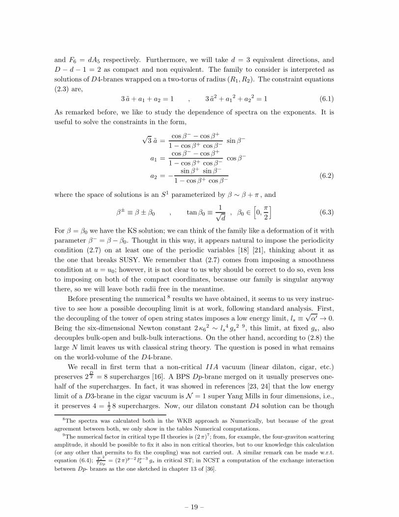
and F6 = dA5 respectively. Furthermore, we will take d = 3 equivalent directions, and

D − d − 1 = 2 as compact and non equivalent. The family to consider is interpreted as

solutions ofD4-branes wrapped on a two-torus of radius (R1, R2). The constraint equations

(2.3) are,

3 a+ a1 + a2 = 1 , 3 a2 + a12 + a2

2 = 1 (6.1)

As remarked before, we like to study the dependence of spectra on the exponents. It is

useful to solve the constraints in the form,

√3 a =

cos β− − cos β+

1− cos β+ cos β−sin β−

a1 =cos β− − cos β+

1− cos β+ cos β−cos β−

a2 = − sin β+ sin β−

1− cosβ+ cos β−(6.2)

where the space of solutions is an S1 parameterized by β ∼ β + π , and

β± ≡ β ± β0 , tan β0 ≡1√d

, β0 ∈[

0,π

2

]

(6.3)

For β = β0 we have the KS solution; we can think of the family like a deformation of it with

parameter β− = β − β0. Thought in this way, it appears natural to impose the periodicity

condition (2.7) on at least one of the periodic variables [18] [21], thinking about it as

the one that breaks SUSY. We remember that (2.7) comes from imposing a smoothness

condition at u = u0; however, it is not clear to us why should be correct to do so, even less

to imposing on both of the compact coordinates, because our family is singular anyway

there, so we will leave both radii free in the meantime.

Before presenting the numerical 8 results we have obtained, it seems to us very instruc-

tive to see how a possible decoupling limit is at work, following standard analysis. First,

the decoupling of the tower of open string states imposes a low energy limit, ls ≡√α′ → 0.

Being the six-dimensional Newton constant 2κ62 ∼ ls

4 gs2 9, this limit, at fixed gs, also

decouples bulk-open and bulk-bulk interactions. On the other hand, according to (2.8) the

large N limit leaves us with classical string theory. The question is posed in what remains

on the world-volume of the D4-brane.

We recall in first term that a non-critical IIA vacuum (linear dilaton, cigar, etc.)

preserves 2D2 = 8 supercharges [16]. A BPS Dp-brane merged on it usually preserves one-

half of the supercharges. In fact, it was showed in references [23, 24] that the low energy

limit of a D3-brane in the cigar vacuum is N = 1 super Yang Mills in four dimensions, i.e.,

it preserves 4 = 12 8 supercharges. Now, our dilaton constant D4 solution can be though

8The spectra was calculated both in the WKB approach as Numerically, but because of the great

agreement between both, we only show in the tables Numerical computations.9The numerical factor in critical type II theories is (2π)7; from, for example, the four-graviton scattering

amplitude, it should be possible to fix it also in non critical theories, but to our knowledge this calculation

(or any other that permits to fix the coupling) was not carried out. A similar remark can be made w.r.t.

equation (6.4); Ts2

TDp= (2π)p−2 lp−3

s gs in critical ST; in NCST a computation of the exchange interaction

between Dp- branes as the one sketched in chapter 13 of [36].

– 19 –

as the black version of a BPS (u0 = 0) D4 in the near horizon limit, that is T-dual to a

BPS D3 brane living in the linear dilaton vacuum, which is the large u limit of the cigar

vacuum. So we could argue that our family describes in the UV some (unknown) CFT in

five dimensions, the completion of the five dimensional YM theory whose coupling constant

at scale Λs ≡ ls−1 is,

gYM52 =

Ts2

TD4∼ ls gs (6.4)

The t’Hooft coupling at such scale, and the dimensionless effective coupling constant

at scale E are,

λ52 ≡ gYM5

2 N ∼ ls ; λeff5 (E)2 ≡ λ5

2E ∼ E

Λs(6.5)

where we have used (2.8). From (6.5) two well-known facts follow; for E << Λs, λeff5 << 1

and perturbative YM theory is valid at low energies. On the other hand it is clear that

gYM5 can not be fixed for ls → 0, and therefore no decoupling limit exists; this fact can be

interpreted as a manifestation of the non-renormalizability of YM theories in dimensions

higher that four [37]. However we are interested in the three-dimensional theory that we

get below the compactification scale Λc ≡ (4π2 R1 R2)− 1

2 ; the t’Hooft coupling at such

scale is,

λ32 =

λ52

4π2 R1 R2∼ Λc

2

Λs(6.6)

Then, following Witten’s argument [6], the compactification should break supersymmetry,

giving masses to both fermions and bosons at tree and one-loop level respectively, the large

compactification scale limit should decouple them, and three-dimensional YM should be

reached in the limit [4],

λ32 Λc→∞−−−−→

Λs→∞ΛQCD ∼ u0 ←→ Λc

2

Λs∼ u0 (6.7)

where (3.13) was taken into account.

We will use the usual notation that assigns for every kind of perturbation the corre-

sponding dual glueball notation JPC . The spin J , parity P and charge conjugation C,

are deduced from the quantum numbers of the boundary operator that couples to the

perturbation under consideration, we refer the reader to the literature [8, 13]

In the following sections we compute the spectra corresponding to every kind of per-

turbation.

6.1 Spectrum from dilatonic fluctuations.

The Schroedinger like equation to solve for zero energy corresponds to the potential,

V (x) =1

4− 1

4 g(x)2+

6

5

ex

g(x)− M2 e(1−a)x

g(x)75−a

+

2∑

i=1

pi2 e(1−ai)x

g(x)75−ai

(6.8)

The corresponding 0++ mass spectrum is showed in Table 1.

– 20 –

0 π6

π12

7.59 7.59 4.80

10.40 10.40 7.81

13.08 13.08 10.19

15.71 15.71 12.41

18.30 18.30 14.56

Table 1: The table shows the values of M0++ mass, corresponding to dilatonic perturbations, for

values β = 0, β = π

6and β = π

12with d = 3.

6.2 Spectra from RR 1-form fluctuations.

It is straightforward to verify that the perturbation defined by switching on only fq+2, for

any q 6= D − 2 is consistent, and it is governed by the generalized Maxwell equations in

(4.12). In particular, for D = 6 we have just a1 from the RR form sector. 10.

From the Section 5, we analyze,

• Longitudinal polarizations: 0−+ glueballs

By carrying out the same steps as in (4.19) we arrive to the Schrodinger form (4.21),

with the potential,

V (x) =1

4 g(x)2

(

9

25e2x +

2

5(3 + 2 ai) e

x + ai2

)

− M2 e(1−a)x

g(x)75−a

+∑

j 6=i

pj2 e(1−aj )x

g(x)75−aj

(6.9)

In Tables 2 we show the 0−+ masses spectra for different polarizations.

0 π

6

π

12

2.96 4.06 3.97

5.55 6.69 6.67

8.09 9.25 9.31

10.61 11.78 11.94

13.13 14.30 14.57

15.64 16.82 17.18

0 π

6

π

12

4.06 2.96 3.79

6.69 5.55 6.45

9.25 8.09 9.08

11.78 10.61 11.70

14.31 13.12 14.32

16.83 15.64 16.93

Table 2: In the table on the left, we show the values of M0−+ corresponding to longitudinal

1-form perturbation, polarized along direction characterized by a1. The parameter takes values

β = 0, β = π

6and β = π

12. In the table on the right, we show these values for longitudinal

polarization characterized by a2. In both of them d = 3.

• Transverse polarizations: 1++ glueballs

10We would like to alert the reader that we work in a local basis, not in a coordinate one; therefore our

tensor components differ from those in [19] by metric factors.

– 21 –

The potential is,

V (x) =1

4 g(x)2

(

9

25e2x +

2

5(3 + 2 a) ex + a2

)

− M2 e(1−a)x

g(x)75−a

+∑

j

pj2 e(1−aj)x

g(x)75−aj

(6.10)

We show in Table 3 the 1++ mass spectra.

0 π6

π12

2.96 2.96 3.10

5.55 5.55 5.82

8.09 8.09 8.47

10.61 10.61 11.10

13.12 13.12 13.72

Table 3: The table shows the values of M1++ , of transverse 1-form perturbation corresponding

β = 0, β = π

6and β = π

12for d = 3.

6.3 Glueball spectra from metric perturbations

From the proposed metric ansatz in the section 5 we analyze, in the d = 3, the following

cases:

• Transverse polarizations: 2++ glueballs

The potential,

V (x) =1

4− 1

4 g(x)2− M2 e(1−a)x

g(x)75−a

(6.11)

We notice that there is no degeneration with the 0++ spectrum as it happens in the

critical case, a fact noted in [19] and that is valid for all the solutions of our family.

The corresponding 2++ spectra is shown in Table 4.

0 π6

π12

4.06 4.06 4.28

6.69 6.69 7.00

9.25 9.25 9.66

11.79 11.79 12.31

14.31 14.3 14.94

Table 4: In the table above, we show the values of M2++ , corresponding to transverse metric

perturbation, with β = 0, β = π

6and β = π

12. All of them were calculated with d = 3.

– 22 –

• Longitudinal polarizations: 1−+ glueballs

The potential is,

V (x) =1

4− 1− (ai − a)2

4 g(x)2− M2 e(1−a)x

g(x)75−a

(6.12)

In Tables 5 we show the 1−+ masses spectra for different polarizations.

0 π

6

π

12

4.06 5.00 5.06

6.69 7.73 7.88

9.25 10.34 10.59

11.79 12.91 13.25

14.31 15.45 15.90

16.83 17.99 18.54

0 π

6

π

12

5.00 4.06 4.92

7.73 6.69 7.70

10.34 9.25 10.39

12.91 11.79 13.051

15.45 14.31 15.69

17.99 16.83 18.33

Table 5: In the table on the left, we show the values of M1−+ , corresponding to longitudinal

metric polarization along the direction characterized by a1, for parameter values β = 0, β = π

6

and β = π

12. In the table on the right, we show these values for polarization characterized by a2.

In both of them d = 3.

• Scalars: 0++ glueballs

The system (5.18) is such that the element (5.19) of the potential reduce to:

v(x) =1

4− 1

4 g(x)2− M2 e(1−a)x

g(x)1−a+ 25

m(x) =2

g(x)2

(

a

2(1− a) +

3 a− 1

5ex − 2

25e2 x)

m(1)i (x) =

1

g(x)2

(

a

2(1 + ai − 2 a) +

2 a+ ai − 1

5ex − 2

25e2x)

m(2)i (x) =

2

g(x)2

(

ai2(1− a) +

4 ai − a− 1

5ex − 2

25e2x)

mij(x) =1

g(x)2

(

ai2(1 + aj − 2 a) +

4 ai + aj − 2 a− 1

5ex − 2

25e2 x)

(6.13)

In Table 6, we show the 0++ spectra corresponding to metric pertubations.

7. Glueball spectra of 4D Yang-Mills theories.

We consider non critical IIA superstrings in D = 8, in the background (2.2) of black D6-

branes. We will take d = 4 equivalent directions, and D − d− 1 = 3 as compact and non

equivalent. The constraint equations (2.3) are,

4 a+ a1 + a2 + a3 = 1 , 4 a2 + a12 + a2

2 + a32 = 1 (7.1)

– 23 –

0 π6

π12

3.97 3.97 3.22

6.67 6.67 6.36

9.26 9.26 9.25

11.81 11.81 12.04

14.45 14.45 14.78

Table 6: The table shows the values of M0++ , corresponding to scalar metric perturbation for

β = 0, β = π

6and β = π

12, and d = 3.

They are explicitly solved by,

a1 =1

7

(√21x+

√15 z + 1

)

a2 =1

7

(

−√21x+

√15 z + 1

)

a3 =1

7

(

−2√

42

5y −

√

12

5z + 1

)

2 a =1

7

(

√

42

5y − 2

√

12

5z + 2

)

(7.2)

where

x2 + y2 + z2 = 1 (7.3)

The parameter space results a two dimensional sphere characterized for example by stan-

dard angular variables θ and φ.

As we made in the precedent section for the three dimensional models, let us look at

the decoupling limit in this four dimensional case. The eight-dimensional Newton constant

is 2κ82 ∼ ls

6 gs2, and then the decoupling of the tower of open string states as well as

the bulk-open and bulk-bulk interactions requires the low energy limit ls → 0. And the

question is focalized again on what remains on the world-volume of the D6-brane. The

non-critical vacuum preserves 2D2 = 16 supercharges, and the BPS D6-branes merged on it

will preserve eight of them, as it can be argued following similar reasoning as in Section 7

from the knowledge that the low energy limit of a D5-brane in the cigar vacuum is minimal

N = (0, 1) super Yang Mills in six dimensions, i.e., it preserves 8 = 12 16 supercharges [23].

So we could argue that our family is holographic in the to UV some (unknown) CFT

in seven dimensions, the completion of the seven dimensional YM theory whose coupling

constant at scale Λs ≡ ls−1 is,

gYM72 =

Ts2

TD6∼ ls

3 gs (7.4)

The t’Hooft coupling at such scale, and the dimensionless effective coupling constant at

– 24 –

scale E are,

λ72 ≡ gYM7

2 N ∼ ls3 ; λeff

7 (E)2 ≡ λ72 E3 ∼

(

E

Λs

)3

(7.5)

from where the validity of the perturbative description in the region E << Λs and the

absence of the decoupling limit follow [37]. The t’Hooft coupling at the compactification

scale Λc ≡ (8π3 R1R2 R1)− 1

3 of the four-dimensional theory we are interested in is,

λ42 =

λ72

8π3 R1 R2 R3∼(

Λc

Λs

)3

(7.6)

To make contact with four dimensional pure YM we should take the scaling limit [6] [7],

Λc e− 1

B λ4(Λc)Λc→∞−−−−→Λs→∞

ΛQCD ∼ u0 ←→ lnΛc

u0∼(

Λs

Λc

)32

(7.7)

where B is the coefficient of the one-loop beta function defined by, β(λ4) ≡ µ∂µλ4(µ) =

−B λ42 + . . . (B = 23

48π2 for SU(N) pure YM).

We will not consider the A+3 perturbation.

7.1 Spectrum from dilatonic fluctuations.

The Schroedinger like equation to solve for zero energy corresponds to the potential,

V (x) =1

4− 1

4 g(x)2+

8

7

ex

g(x)− M2 e(1−a)x

g(x)97−a

+

3∑

i=1

pi2 e(1−ai)x

g(x)97−ai

(7.8)

The corresponding mass spectra is shown in Table 7.

P1 P2 P3

10.69 11.15 11.43

13.80 14.96 15.17

16.78 18.4 18.68

19.68 21.85 22.08

22.54 25.18 25.67

Table 7: The table shows the values of M0++ mass, corresponding to dilatonic perturbations, in

the parameter space points P1 = (π6, 7π

6), P2 = (π

2, 4π

3) and P3 = (π

3, 9π

6) of the d = 4 case.

7.2 Spectra from RR 1-form fluctuations.

It is straightforward to verify that the perturbation defined by switching on only fq+2, for

any q 6= p+1 is consistent, giving the generalized Maxwell equations (4.12). In particular,

for D = 6 we have just a1 from the RR form sector. 11.

From the Section 5, we analyze,

11We would like to alert the reader that we work in a local basis, not in a coordinate one; therefore our

tensor components differ from those in [19] by metric factors.

– 25 –

P1 P2 P3

4.84 5.36 4.58

7.68 8.25 7.43

10.46 11.06 10.20

13.21 13.84 12.95

P1 P2 P3

4.44 4.925 5.26

7.29 7.74 8.12

10.04 10.47 10.89

12.75 13.19 13.62

P1 P2 P3

4.96 4.96 5.24

7.85 7.85 , 8.17

10.66 10.66 11.00

13.45 13.45 , 13.80

Table 8: In the table on the left, we show the values of M0−+ , corresponding to longitudinal 1-

form perturbation polarized along direction characterized by a1. The parameters take values on the

2-dimensional parameter space associated with d = 4, named P1, P2 and P3. In the tables on the

center and on the right, we show these values for longitudinal polarization a2 and a3, respectively.

• Longitudinal polarizations: 0−+ glueballs

By carrying out the same steps as in (4.19) we arrive to the Schrodinger form (4.20),

with the potential,

V (x) =1

4 g(x)2

(

25

49e2x +

2

7(5 + 2 ai) e

x + ai2

)

− M2 e(1−a)x

g(x)97−a

+∑

j 6=i

pj2 e(1−aj )x

g(x)97−aj

(7.9)

In Tables 8 we show the 0−+ masses spectra for different polarizations.

• Transverse polarizations: 1++ glueballs

The potential is,

V (x) =1

4 g(x)2

(

25

49e2x +

2

7(5 + 2 a) ex + a2

)

− M2 e(1−a)x

g(x)97−a

+∑

j

pj2 e(1−aj)x

g(x)97−aj

(7.10)

The corresponding 1++ spectrum is shown in Table 9.

P1 P2 P3

4.42 4.31 4.52

7.31 7.14 7.44

10.10 9.89 10.27

12.86 1260 13.06

15.61 15.30 15.83

Table 9: The table shows M1++ values, of transverse 1-form perturbation at the points P1, P2

and P3 of the parameter space corresponding to d = 4.

7.3 Glueball spectra from metric perturbations

From the proposed metric ansatz in the section 5 we analyze, in the d = 4, the following

cases:

– 26 –

• Transverse polarizations: 2++ glueballs

The potential,

V (x) =1

4− 1

4 g(x)2− M2 e(1−a)x

g(x)97−a

(7.11)

We notice that there is no degeneration with the 0++ spectrum as it happens in the

critical case, a fact noted in [19] and that is valid for all the solutions of our family.

The corresponding 2++ mass spectrum is shown in Table 10.

P1 P2 P3

5.52 5.40 5.60

8.45 8.29 8.55

11.27 11.07 11.40

14.05 13.80 14.21

16.81 16.52 17.00

Table 10: In the table above, we show the values of M2++ , corresponding to transverse metric

perturbation. The values correspond to P1, P2 and P3. All of them were calculated with d = 4.

• Longitudinal polarizations: 1−+ glueballs

The potential is,

V (x) =1

4− 1− (ai − a)2

4 g(x)2− M2 e(1−a)x

g(x)97−a

(7.12)

In Tables 11 we show the 1−+ masses spectra for different polarizations.

P1 P2 P3

5.97 6.39 5.79

8.93 9.42 8.72

11.76 12.30 11.54

14.55 15.12 14.32

P1 P2 P3

5.54, 5.96 6.26

8.41 8.87 9.23

11.19 11.66 12.06

13.92 14.41 14.82

P1 P2 P3

6.14 6.14 6.36

9.14 9.14 9.41

12.00 12.00 12.31

14.83 14.83 15.15

Table 11: In the tables above we show the values M1−+ , of the longitudinal metric perturbation,

along the three different directions associated with a1, a2 and a3. The values correspond to points

of parameter space that we have called P1, P2, and P3 for d = 4.

• Scalars: 0++ glueballs

The system (5.18) is such that the element (5.19) of the potential reduce to:

v(x) =1

4− 1

4 g(x)2− M2 e(1−a)x

g(x)1−a+ 27

– 27 –

m(x) =4

g(x)2

(

a

2(1− a) +

5 a− 1

7ex − 2

49e2 x)

m(1)i (x) =

1

g(x)2

(

a

2(1 + ai − 2 a) +

4 a+ ai − 1

7ex − 2

49e2x)

m(2)i (x) =

4

g(x)2

(

ai2(1− a) +

6 ai − a− 1

7ex − 2

49e2x)

mij(x) =1

g(x)2

(

ai2(1 + aj − 2 a) +

6 ai + aj − 2 a− 1

7ex − 2

49e2 x)

(7.13)

The corresponding 0++ spectrum is shown in Table 12.

P1 P2 P3

6.44 6.37 6.50

9.12 9.00 9.20

11.62 11.47 11.72

14.06 13.87 14.18

Table 12: The table shows values of M0++ , corresponding to scalar metric perturbation for three

different points of the parameter space P1, P2, and P3 with d = 4.

8. Summary of results and discussion

We believe that is worth to start with some general remarks. First, it is an open question if

such a thing like a low energy effective field theory associated to a non critical superstring

theory, commonly referred in the literature as non critical supergravity, can be well defined.

If it were so, presumably a scalar field (what would be a tachyon in the critical case,

although in the present framework is just a misnomer) should also be present [30]. The

existence of non critical superstrings lead us to conjecture that a manifestly supersymmetric

action, maybe with infinite terms could be constructed. We think however that, from the

results existing in the literature as well as those presented in this paper, the truncated action

(2.1) usually considered is physically sensible. A further support to this statement is the

existence, showed in [35], of a highly non trivial solution localized both in the Minkowski

and cigar spaces, that was identified as the fundamental non critical string. Second, we

think that the gauge-invariant, first order perturbation approach developed here in Section

4 is a very interesting and useful tool because it is free of gauge dependencies and mixings,

once a background is given.

Now let us go to the analysis of the results obtained in Section 6 and 7. We note that,

for the case d = 3 we have two contributions to longitudinal polarizations, one coming

from the direction associated with a1 and the other from the one associated with a2. These

contributions are not KK-modes, but they are a consequence of the polarization along the

two non-equivalent compact directions. Because of that, we have twice the states 0−+

– 28 –

and 1−+ than those found in [19]. In general these modes are split (Figure 2), but for a

few particular values of the parameter β that labels the solutions (see (6.3)), they appear

degenerated. The slightly splitting in mass is a direct consequence of the constraint (2.3).

0-+ 1++ 0++dilaton 1-+ 0++metric 2++0

1

2

Glueball spectra HΒ=0L

Figure 2: The plot shows the glueballs spectra normalized by the lightest mass of 0++ of the

metric perturbation in d = 3, for β = 0.

Even though we had hoped to reproduce the spectra obtained in [19] when the param-

eter β becomes π/6 (except for the splitting in longitudinal modes), this never happens.

This is due to the difference between our lightest 0++ mode related to metric perturbation

and that obtained in [19]. We have found a better agreement than in [19] between the

numerical and the WKB computations, and in virtue of this fact, we assume as a correct

value for the lightest 0++ mode of the scalar perturbation of the metric the one obtained

here. Below, in the plot of Figure 3, we show the spectra obtained in [19] and the spectra

obtained by us in the case β = π6 , each one normalized by their own lightest value of metric

0++. In the plot of Figure 4, we show the same spectra, but now both are normalized by

our lightest value of metric 0++. The agreement is perfect.

It is important to note that the expected qualitative aspect of the glueballs spectra is

not that appearing in the previous plots for the particular values of β that we have shown.

In general it is widely assumed, and checked in some cases in Lattice QCD, that the lightest

glueball corresponds to the operator 0++. Clearly, that is not the case for Figures 2, 3 y

4. Nevertheless, because of the freedom in choosing the values of β, it is possible to tune

the parameter to obtain a better agreement with the desired spectra.

Although it is not the aim of this paper to perform a systematic exploration of the confining

sectors of the theories parametrized by β, it is possible to observe that some particular

values of the parameter give a better agreement with the values obtained in Lattice QCD

[41] (see Figure 6).

Finally, it is interesting to note that the same value of the parameter that provides the

best agreement with Lattice QCD spectra (in the sense that the relative ratios between

masses are more similar) is also the one for which the splitting in longitudinal polarized

modes is smaller. We believe that a more accurate value of β should be able to erase such

splitting, leaving us with qualitatively and quantitatively more similar spectra to Lattice

– 29 –

0-+ 1++ 0++dilaton 1-+ 0++metric 2++0

1

2

3

4

Glueballs Β=Π6 and KS normalized by H0++LΒ=Π6 and H0++LKS

Figure 3: In this plot we compare the spectra obtained by Kuperstein and Sonnenschein [19](@)

to our case for β = π

6(), each one normalized by their corresponding lowest 0++. In principle,

this two spectra should be the same except for the splitting in the longitudinal polarized modes

0−+ and 1−+.

ð

ð

ð

ð

ð

ð

ð

ð

ð

ð

ð

ð

0-+ 1++ 0++dilaton 1-+ 0++metric 2++0

1

2

Glueballs Β=Π6 and KS normalized by H0++LΒ=Π6

Figure 4: In this plot we compare the spectra obtained by Kuperstein and Sonnenschein [19](♯) to

our case for β = π

6(), each one normalized by our lowest value of 0++. The agreement between

the two spectra is perfect, except for the splitting in 0−+ and 1−+.

QCD.

In the case of d = 4 (Figure 7), our solutions have three non equivalent compact

directions, and thus, three states with the same quantum numbers but different masses.

As in the d = 3 case, the splitting in the masses of longitudinal polarized modes appears

as a consequence of the freedom in choosing the longitudinal direction along which to

polarize the perturbation. In this case, we have two free parameters that characterize the

solution (see (7.3)), and again this freedom enables us to obtain different spectra that we

can compare with the results of Lattice QCD. Although it is very difficult to compute

the entire spectrum for every point of the confining sector of the theory, that now is a

2-dimensional manifold, we think that a systematic exploration of the parameter space can

be achieved with some numerical techniques, like Markov Chain Monte Carlo for example,

– 30 –

ðð

ð

ð

ð

ðð

0-+ 1++ 0++dilaton 1-+ 0++metric 2++0

1

2

Glueballs Β=Π6 and Lattice QCD HTeperL

Figure 5: In this plot we compare our spectrum for β = π/6 () to the Lattice QCD (♯) spectrum

obtained by Teper [41], for d = 3.

ðð

ð

ð

ð

ðð

0-+ 1++ 0++dilaton 1-+ 0++metric 2++0

1

2

Glueballs Β=Π12 and Lattice QCD HTeperL

Figure 6: In this plot we compare our obtained spectrum for β = π/12 () with the Lattice QCD

(♯) obtained by Teper for d = 3 ([41]).

and we hope that a better agreement with Lattice QCD can be obtained. In the present

case, we selected in a random way the points in the confining sector of the parameter space

of the theory (see Figure (8)).

We would like to remark as a very important fact that, although singular in the IR, all

the solutions lead to a well-defined problem and spectra, without needing of extra boundary

conditions at the singularity; results exist even when the solutions are singular in the IR

limit. It is like if there were some mechanism at work, i.e. a barrier for string propagation

in the backgrounds before the deep infrared region can be reached, as the Wilson loop

computation in Section 3 seems to indicate. Furthermore, both families (2.2) and (B.1)

yield exactly the same spectra as showed in Appendix (B), as one could guess from T-

duality arguments 12 ; however it results striking that while the string approximation for

all the constant dilaton solutions in the family are under control in the large N limit, the

T-dual family analysis seems to be restricted to the region aθ < 0 due to the blow-up of

12We thank J. M. Maldacena for a discussion on this point.

– 31 –

0-+ 1++ 0++dilaton 1-+ 0++metric 2++

1

Glueball spectra HΘ=Π2 , Φ=4Π3L

Figure 7: In this plot we show the glueballs spectra for d = 4 normalized by the lowest masses of

0++ for the point of the parameter space called P2 that corresponds to θ = π

2and φ = 4π

3.

ð

ð

ð

ð

ð

ð

ð

ð

ð

ð

ð

ð

ð

ð

ð

ð

ð

ð

ðÌ

Ì

Ì

ÌÌ

0-+ 1++ 0++dilaton 1-+ 0++metric 2++

1

Glueballs P1, P2, P3, and Lattice normailzed by 0++

Figure 8: In the plot we show the glueballs spectra for d = 4, computed for three different points

of the parameter space P1(©), P2(), P3(♯) and we compare them with the Lattice QCD spectra

() obtained by Morningstar and Peardon [42].

the effective string coupling gs ≡ eΦ in the infrared region u → u0+. We take this fact as

a further sign of the effective irrelevance of the singularity. The repulsive character of IR

singularities was noted in [43] (see [44] for a review).

It is possible that there exist exact solutions which approach our family in the UV

but that are regular in the IR, maybe even at the level of the low energy effective ac-

tion i.e. through a non trivial θ-dependence, as much as it happens with the Klebanov-

Tseytlin background [39] that presents a naked IR singularity that results regularized by

the Klebanov-Strassler solution [40], but that modify in a mild way the spectra. Of course,

a proof of this conjecture seems to be very far by now. 13.

13An example of this that is not close to our set-up but similar in spirit is the Maldacena-Nunez solution

[38], that regularize in the IR the back-reaction of D5- branes at the origin of the resolved conifold.

– 32 –

Acknowledgments

We would like to thank Raul Arias, Nicolas Grandi, Sameer Murthy, and Guillermo Silva

for useful discussions, and the Abdus Salam ICTP of Trieste for kindly hospitality during

part of this work.

A. Some useful formulae.

In this appendix we resume the conventions and formulae relevant in the computations

carried out in the paper, Unless specified on the contrary, we work in a local basis with

indices A,B,C, · · · = 0, 1, . . . ,D − 1.

Let us consider a metric of the form,

G = ηAB ωA ωB = ηab ωa ωb + ωn2 , a, b = 0, 1, . . . ,D − 2 (A.1)

where the vielbein ωA, dual vector fields eA, eA(ωB) = δBA , and volume element are,

ωa = Aa(u) dxa , ea = Aa(u)

−1 ∂aωn = C(u) du , en = C(u)−1 ∂uǫG = ω0 ∧ · · · ∧ ωn = dx0 ∧ · · · ∧ dxD−2 ∧ duE , E =

∏

a

Aa C (A.2)

The pseudo-riemmanian connections, ωAB = −ωBA : dωA + ωAB ∧ ωB = 0 are,

ωab = 0 , ωan = σa ωa

σa ≡ en(lnAa) , σ ≡∑

a

σa = en

(

lnE

C

)

(A.3)

The relevant covariant derivatives on a scalar field φ(x, u) are,

DA(φ) = eA(φ) , ∀ADaDb(φ) = eaeb(φ) + σa en(φ) ηabDaDn(φ) = eaen(φ)− σa ea(φ)

DnDa(φ) = enea(φ) = DaDn(φ)

Dn2(φ) = en

2(φ)

D2(φ) = eaea(φ) + en2(φ) + σ en(φ) =

∑

a

∂a∂aφ

Aa2

+1

E∂u

(

E

C2∂uφ

)

(A.4)

with σ defined in (A.3).

The relevant covariant derivatives on a one-form A = AA(x, u)ωA are,

DbAa = eb(Aa) + σbAn ηabDnAa = en(Aa)

DaAn = ea(An)− σaAa

DnAn = en(An)

DcDaAb = ecea(Ab) + σc en(Ab) ηca − σc σaAa ηcb + σb (ec(An) ηab + ea(An) ηcb)

DnDaAb = enea(Ab) + en(σaAn) ηab

– 33 –

DaDnAb = eaen(Ab)− σa ea(Ab) + σb (en(An)− σb An) ηabDnDnAb = en

2(Ab)

DcDaAn = ecea(An)− σa ec(Aa)− σc ea(Ac) + σa (en(An)− σaAn) ηacDnDaAn = enea(An)− en(σaAa)

DaDnAn = eaen(An)− σa (ea(An) + en(Aa)− σaAa)

DnDnAn = en2(An) (A.5)

The relevant covariant derivatives on symmetric two-tensors h = hAB(x, u)ωA ωB are,

Dchab = ec(hab) + σc (ηac hbn + ηbc han)

Dchan = ec(han) + σc (ηac hnn − hac)

Dchnn = ec(hnn)− 2σc hcnDnhAB = en(hAB) , ∀ A,B

DdDchab = edec(hab) + σc σd ((ηbc ηad + ηac ηbd)hnn − ηad hbc − ηbd hac)

+ σc (ηcd en(hab) + ηac ed(hbn) + ηbc ed(han) + σd (ηad ec(hbn) + ηbd ec(han))

DnDchab = enec(hab) + ηac en(σc hbn) + ηbc en(σc han)

DcDnhab = ecen(hab) + σc (ηac en(hbn) + ηbc en(han)− ec(hab))− σc2 (ηac hbn + ηbc han)

DdDchan = edec(han)− σc σd (ηac hdn + 2 ηad hcn) + σc (ηac ed(hnn)− ed(hac))

+ σd (ηad ec(hnn)− ec(had) + σd ηcd (en(han)− σc han)

DnDchan = enec(han) + ηac en(σa hnn)− en(σc hac)

DcDnhan = ecen(han) + σc (ηac en(hnn)− en(hac)− ec(han))− σc2 (ηac hnn − hac)

DdDchnn = edec(hnn)− 2σc σd (ηcd hnn − hcd) + σc ηcd en(hnn)

− 2 (σc ed(hcn) + σd ec(hdn))

DnDchnn = enec(hnn)− 2 en(σc hcn)

DcDnhnn = ecen(hnn)− σc (ec(hnn) + 2 (en(hcn)− σc hcn))

DnDnhAB = en2(hAB) , ∀ A,B (A.6)

The curvature tensor ℜAB ≡ dωAB + ωAC ∧ ωCB is,

ℜab = −σa σb ωa ∧ ωb

ℜan = − 1

Aaen

2(Aa) ωa ∧ ωn (A.7)

and the Ricci tensor and scalar are,

Rab = −D2(lnAa) ηab

Rnn = −∑

a

1

Aaen

2(Aa) = −(

en(σ) +∑

a

σa2

)

R = −2D2

(

lnE

C

)

+ σ2 −∑

a

σa2 (A.8)

A.1 Computation of the tensor AAB

The following symmetric two-tensor,

AAB(h) ≡ DADBhCC +D2hAB −DCDAhCB −DCDBhAC (A.9)

– 34 –

naturally arises in the metric perturbation theory. With the help of (A.6) we get the

expressions,

Aab(h) = eAeA(hab) + eaeb(hCC)− eaen(hbn)− eben(han)− ecea(hbc)− eceb(hac)

+ σ en(hab) +(

en(σa + σb) + σ (σa + σb)− (σa − σb)2)

hab+ (2σa − σb − σ) ea(hbn) + (2σb − σa − σ) eb(han)

+ ηab (−2 (en(σa) + σ σa) hnn + σa (en(hcc)− en(hnn)− 2 ec(hcn))

Aan(h) = ecec(han)− ecen(hac)− ecea(hcn) + enea(hcc) + 2 (en(σa) + σ σa)han

− (σ − σa) ea(hnn) + (σa − σc) ec(hac) + σc ea(h

cc)

Ann(h) = ecec(hnn)− σ en(hnn)− 2 ecen(hcn)− 2σc ec(hcn) + en

2(hcc) + 2σc en(hcc)

(A.10)

Under the gauge transformation in (4.9),

Aab(δǫh) = (en(σa) + σ σa + en(σb) + σ σb) δǫhab + 2 en (en(σa) + σ σa) ǫn ηab+ (en(σb) + σ σb − en(σa)− σ σa) (ea(ǫb)− eb(ǫa))

Aan(δǫh) = 2 (en(σa) + σ σa) δǫhan + 2

(

∑

c

(

en(σc) + σc2)

− en(σa)− σ σa

)

ea(ǫn)

Ann(δǫh) = 2∑

c

(

en(σc) + σc2)

δǫhnn + 2 en

(

∑

c

(

en(σc) + σc2)

)

ǫn (A.11)

A.2 A short derivation of the solutions.

Here we sketch the obtention of the family of solutions (2.2) considered in the paper. Let

us consider an ansatz for the metric of the form (A.1), together with,

Φ(u) = Φ = constant

FD = (−)D QD−2 ǫG ⇐⇒ ∗FD = (−)D−1 QD−2 (A.12)

The strength field tensor in (A.12) leads to,

(FD)2AB = (FD)

2 ηAB , (FD)2 = −

(

C en(E)

E

)2

(A.13)

The equations of motion in string frame read (we consider D-branes, bD−2 = 0),

RAB =1

4e2Φ (FD)

2 ηAB

Λ2 = −D

4e2Φ (FD)

2

d (∗FD) = (−)D QD−2 ∗ JD−1 , QD−2 ≡ 2κD2 µD−2 (A.14)

where κD2 = 8πGD is the gravitational coupling and µD−2 the D(D − 2)-brane tension.

The last two equations are solved by,

C en(E)

E= −QD−2 , e2Φ =

4

D

Λ2

QD−22

(A.15)

– 35 –

while that the metric equations reduce to,

D2(lnAa) ≡ en(σa) + σ σa =Λ2

D, ∀a

∑

a

(

en(σa) + σa2)

=Λ2

D(A.16)

By following steps similar to those in reference [21], the general solution to (A.16) can be

written,

Aa(u) = l0 u f(u)aa2 ; C(u) = l0 u

−1 f(u)−12 (A.17)

with f(u) as in (2.2), and the constraints on the exponents given in (2.3).

B. The fluctuations in the T-dual solutions.

In this appendix we present the analysis of the perturbations around the backgrounds T-

dual to those considered in the main of the paper. It results more involved due to the

presence of a non constant dilaton, however yields the same spectra.

B.1 The family of solutions.

The family of solutions (in string frame) obtained from (2.2) by performing a T-duality

transformation in, i.e. xD−2− coordinate reads,

l0−2 G = u2 f(u)aµ ηµν dx

µ dxν +du2

u2 f(u)+ u1

2 dθ2

u2 f(u)aθ, Λ2 l0

2 = D (D − 1)

eΦ =4π√D − 1

|QD−3|u1u

f(u)−aθ2

FD−1 =QD−3 l0

D−2

2π u1uD−2 du ∧ dx0 ∧ · · · ∧ dxD−3 ↔ ∗FD−1 = (−)D−1 QD−3

dθ

2π(B.1)

where µ, ν = 0, 1, . . . ,D − 3 , the coordinate θ is 2π-periodic, and the identifications

f(u) = 1−(u0u

)D−1(B.2)

The scales u0 and u1 are arbitrary, and Furthermore, the following constraints on the

exponents must hold,

∑

µ

aµ + aθ = 1 ,∑

µ

aµ2 + aθ

2 = 1 (B.3)

These solutions could be interpreted as the near horizon of D(D-3)-branes in a linear

dilaton background.

Some useful relations are,

en(σµ) + σ σµ =Λ2

D − 2e

4D−2

Φ

– 36 –

en(σθ) + σ σθ = − D − 4

D(D − 2)Λ2 e

4D−2

Φ

∑

a

(

en(σa) + σa2)

=Λ2

D − 2e

4D−2

Φ − 4 (D − 2)

(D − 4)2σθ

2

σ2 −∑

a

σa2 =

D − 2

DΛ2 e

4D−2

Φ +4 (D − 2)

(D − 4)2σθ

2

en2(Φ) + σ en(Φ) = −Λ2

De

4D−2

Φ

en(Φ) =D − 2

D − 4σθ (B.4)

B.2 The equations for the fluctuations in e-frame

As remarked in Section 4, since the system for the fluctuations is linear, it should be

possible to write it in a manifest gauge invariant way under (4.9). For the family (B.1)

that will concern us here we can do it as follows. First, we restrict ourselves to fluctuations

such that,

fD−1 ≡ χFD−1 , ǫχ = χ+Daǫa +

D

D − 4σθ ǫn (B.5)

Consistency with the Bianchi identity imposes θ-independence of χ, and therefore on all

the fluctuations; moreover the gauge transformation of χ follows from (4.9). In second

term, following (4.28) we introduce the fields (g, ga, Iab, Iξ, Iχ) by,

hnn ≡ 2 en(g) , δǫg = ǫn

han ≡ Aa en

(

gaAa

)

+ ea(g) , δǫga = ǫa

hab ≡ Iab + ea(gb) + eb(ga) + 2 ηab σa g , δǫIab = 0

ξ ≡ Iξ +D − 2

D − 4σθ g , δǫIξ = 0

χ ≡ Iχ + eµ(gµ) + en(g) +

(

σ +4

D − 4σθ

)

g , δǫIχ = 0 (B.6)

where again the gauge transformations follows from (4.9). In terms of these variables (A.10)

is written as,

Aab(h) = A(i)ab (I) + 2 (en(σb) + σ σb) ea(gb) + 2 (en(σa) + σ σa) eb(ga)

+ 2 ηab (en (en(σa) + σ σa) + 2σa (en(σa) + σ σa)) g

A(i)ab (I) ≡ eAeA(Iab) + eaeb(I

cc )− eae

c(Ibc)− ebec(Iac) + σ en(Iab)

+(

en(σa + σb) + σ (σa + σb)− (σa − σb)2)

Iab + ηab σa en (Icc )

Aan(h) = A(i)an(I) + 2 (en(σa) + σ σa) (en(ga)− σa ga) + 2

∑

c

(

en(σc) + σc2)

ea(g)

A(i)an(I) ≡ −ecen(Iac) + eaen(I

cc ) + (σa − σc) (e

c(Iac)− ea(Icc ))

Ann(h) = A(i)nn(I) + 4

∑

c

(

en(σc) + σc2)

en(g) + 2 en

(

∑

c

(

en(σc) + σc2)

)

g

A(i)nn(I) ≡ en

2(Icc ) + 2σc en(Icc ) (B.7)

– 37 –

where the A(i)AB(I)’ s are manifest gauge invariant; we remark that these expressions are

valid for any metric of the form in (A.1). After a lengthy but straightforward computation

equations (4.5), (4.6), (4.7) in our backgrounds (B.1) result,

h-equations

0 = eAeA(Iµν) + eµeν(Icc )− eµe

c(Iνc)− eνec(Iµc) + σ en(Iµν)

+ ηµν σµ en (Icc )− (σµ − σν)

2 Iµν −8Λ2

(D − 2)2ηµν e

4D−2

Φ Iξ

0 = −ecen(Iµc) + eµen(Icc ) + (σµ − σc) (e

c(Iµc)− eµ(Icc )) +

8

D − 4σθ eµ(Iξ)

0 = en2(Icc ) + 2σc en(I

cc ) +

16

D − 4σθ en(Iξ)−

8Λ2

(D − 2)2e

4D−2

Φ Iξ

0 = eAeA(Iθθ) + σ en(Iθθ) + σθ en(Icc ) +

8Λ2

De

4D−2

Φ

(

Iχ −1

2Iµµ −

D2 − 3D + 4

(D − 2)2Iξ

)

0 = eAeA(Iµθ) + σ en(Iµθ)− eµec(Icθ) +

(

2Λ2

De

4D−2

Φ − (σµ − σθ)2

)

Iµθ

0 = ec (en(Icθ) + (σc − σθ) Icθ) (B.8)

ξ-equation

0 = eAeA(Iξ) + σ en(Iξ) +D − 2

2(D − 4)σθ en(I

cc )

+D − 2

DΛ2 e

4D−2

Φ

(

−Iχ +1

2Iµµ +

D2 − 2D + 4

(D − 2)2Iξ

)

(B.9)

aq+1 -equation , q 6= D − 3

0 = −e−αqΦ DB(

eαqΦ (fq+2)A1...Aq+1B

)

(B.10)

aD−2 -equation

From (4.7) we get an equation with (D − 2) antisymmetric indices that leads to the

following equations,

0 = eµ(Iνθ)− eν(Iµθ) , ∀µ, ν0 = en

(

Aµ

AθIµθ

)

, ∀µ

0 = ea

(

2 Iξ − Iχ +1

2(Iµµ − Iθθ)

)

, ∀ a (B.11)

with solution,

Iµθ = 0 , ∀µIχ = 2 Iξ +

1

2(Iµµ − Iθθ) (B.12)

– 38 –

The fluctuations aq+1 with q 6= D− 3 are gauge invariant and decoupled from the rest

of the fluctuations; we focus on these last ones. By using the relations (B.11) in (B.8),

(B.9) we get the following system,

0 = en2(Iµν) + σ en(Iµν) + eρeρ(Iµν) + eµeν(I

cc )− eµe

ρ(Iνρ)− eνeρ(Iµρ)− (σµ − σν)

2 Iµν

+ ηµν σµ en (Icc )−

8Λ2

(D − 2)2ηµν e

4D−2

Φ Iξ

0 = en2(Iθθ) + σ en(Iθθ) + eρeρ(Iθθ) + σθ en(I

cc )

+8Λ2

De

4D−2

Φ

(

(D − 1)(D − 4)

(D − 2)2Iξ −

1

2Iθθ

)

0 = −eρen(Iµρ) + eµen(Icc ) + (σµ − σρ) e

ρ(Iµρ) + (σc − σµ) eµ(Icc ) +

8

D − 4σθ eµ(Iξ)

0 = en2(Icc ) + 2σc en(I

cc ) +

16

D − 4σθ en(Iξ)−

8Λ2

(D − 2)2e

4D−2

Φ Iξ

0 = D2(Iξ) +D − 2

2(D − 4)σθ en(I

cc )−

(D − 2)Λ2

De

4D−2

Φ

(

D2 − 6D + 4

(D − 2)2Iξ −

1

2Iθθ

)

(B.13)

Now we introduce the modes in momenta,

Iµν = χµν(u) eip·x ; Iθθ = χθ(u) e

ip·x ; Iξ = χξ(u) eip·x (B.14)

where p · x ≡ pρ xρ . With the definition pµ ≡ Aµ pµ , we get the system in the form,

0 = en2(χµν) + σ en(χµν)−

(

pρ pρ + (σµ − σν)2)

χµν + pµ pρ χνρ + pν p

ρ χµρ

− pµ pν (χρρ + χθ) + ηµν σµ en

(

χρρ + χθ

)

− 8Λ2

(D − 2)2ηµν e

4D−2

Φ χξ

0 = en2(χθ) + σ en(χθ)−

(

pρpρ +4Λ2

De

4D−2

Φ

)

χθ + σθ en(χρρ + χθ)

+8(D − 1)(D − 4)

D(D − 2)2Λ2 e

4D−2

Φ χξ

0 = en2(χξ) + σ en(χξ)−

(

p2 +D2 − 6D + 4

D(D − 2)Λ2 e

4D−2

Φ χξ

)

+D − 2

2(D − 4)σθ en(χ

ρρ + χθ)

+D − 2

2DΛ2e

4D−2

Φ χθ

0 = pµ(

en(χρρ + χθ) + (σρ − σµ)χ

ρρ + (σθ − σµ)χθ +

8

D − 4σθ χξ

)

− pρ (en(χµρ) + (σρ − σµ)χµρ)

0 = en2(χρ

ρ + χθ) + 2σρ en(χρρ) + 2σθ en(χθ) +

16

D − 4σθ en(χξ)−

8Λ2

(D − 2)2e

4D−2

Φ χξ

(B.15)

We note that we have left with the unknowns (χµν , χθθ, χξ), whose system of coupled, sec-

ond order differential equations is given by the first three equations; the last two equations

should work as constraints 14.

14The first one of them is of first order, while that the second one can be put in first order form by using

the first two equations in (B.15).

– 39 –

B.3 Holographic models of d dimensional Yang-Mills theories

Let us take, among the xµ coordinates, d non compact, equivalent, xα-coordinates, α =

0, 1, . . . , d − 1, and D − d − 2 compact and non equivalent τ i, i = 1, . . . D − d − 2, τi ≡τi + 2π Ri. We will denote with a˜quantities associated with the non-compact directions

(Aα = A , aα = a , σα = σ , etc). The metric and constraints (2.3) are,

l0−2 G = u2

(

f(u)a ηµν dxµ dxν +

∑

i

f(u)ai dτ i2

)

+du2

u2 f(u)+ u1

2 dθ2

u2 f(u)aθ

d a+∑

i

ai + aθ = 1 , d a2 +∑

i

ai2 + aθ

2 = 1 (B.16)

We stress that D − d− 2 exponents remain free.

B.4 Metric: transverse fluctuations

They correspond to take the ansatz,

χαβ(u) = ǫαβ(p) χ(u) ; ǫαα = 0 , ǫαβ pβ = 0 (B.17)

and the rest of the fluctuations zero. This ansatz solves (B.15) if χ satisfies,

en2(χ) + σ en(χ) +

(

M2

A2−∑

i

pi2

)

χ = 0 (B.18)

where M2 ≡ −pαpα is the d-dimensional mass. By making the change (4.19), it turns out

that H satisfy exactly the equation (5.8).

B.5 Metric: longitudinal fluctuations

They correspond to take the ansatz, at fixed i (but for any i),

χiα(u) = ǫα(p) χ(u) ; pi = 0 , ǫα pα = 0 (B.19)

and the rest of the fluctuations zero. It is consistent with (B.15) if χ(u) obeys,

en2(χ) + σ en(χ) +

(

M2

A2−∑

i

pi2 − (σ − σi)

2

)

χ = 0 (B.20)

By making the change (4.19), it turns out that H satisfy exactly the equation (5.10).

B.6 Scalar fluctuations

We expect that they come from the dilaton and the metric. However, at difference of the

case worked out in references [34], [18], they do not disentangle, in the sense that putting

to zero the metric fluctuations is not consistent. So we start with the ansatz for the metric,

χµν(u) = aµ(u) ηµν + bµν(u) pµ pν (B.21)

– 40 –

which at difference of the cases treated above, is not transverse neither traceless. It results

convenient to introduce the following variables,

χµ ≡ aµ − σµχθ

σθ

χµν ≡ AµAν bµν −1

2(Aµ

2 bµµ +Aν2 bνν)

χµ ≡ Aµ2 en(bµµ)−

χθ

σθ

χθ ≡ en

(

χθ

σθ

)

χξ ≡ χξ −D − 2

2(D − 4)χθ (B.22)

We note that bµν is replaced by χµν and χµ (by construction, χµµ ≡ 0 for any µ). With

them, and combining equations in (B.15), we can rearrange the system in the following

way,

0 = en2(χµ) + σ en(χµ)− pρ pρ χµ +

2Λ2

D − 2e

4D−2

Φ

(

1 +D − 4

D

σµσθ

)

χθ

− 8Λ2

(D − 2)2e

4D−2

Φ

(

1 + (D − 1)D − 4

D

σµσθ

)

χξ

0 = en2(χµν) + (σ − 2(σµ + σν)) en(χµν) +

∑

ρ

pρ pρ (χµρ + χνρ − χµν)

+

(

4σµ σν −2Λ2

D − 2e

4D−2

Φ

)

χµν + χθ + χµ + χν −∑

ρ

χρ

+1

2(en(χµ + χν) + σ (χµ + χν))− σµ χν − σν χµ

0 = en2(χξ) + σ en(χξ)−

(

p2 + Λ2 e4

D−2Φ)

χξ

0 = σθ en(χθ) + 2D2(lnAθ) χθ + σθ en(∑

ρ

χρ) + σθ∑

ρ

pρ pρ χρ

+8(D − 1)(D − 4)

D(D − 2)2Λ2 e

4D−2

Φ χξ

0 =∑

ρ

(en(χρ) + (σρ − σµ)χρ)− en(χµ) + (σ − σµ) χθ +8

D − 4σθ χξ

−∑

ρ

pρ pρ

(

1

2(χµ − χρ) + en(χµρ)− 2σµ χµρ

)

0 =∑

ρ

pρ pρ

(

χρ + (σ − σρ) χρ +∑

σ

pσ pσ χρσ

)

+D − 2

DΛ2 e

4D−2

Φ

(

χθ −8

(D − 2)2χξ

)

(B.23)

We observe that the equation for χξ gets decoupled from the rest of the fluctuations, so we

can divide the scalar fluctuations in two disjoint cases.

χξ 6= 0

If so, the equation that defines the spectra is just,

0 = en2(χξ) + σ en(χξ)−

(

p2 + Λ2 e4

D−2Φ)

χξ (B.24)

– 41 –

By making the change (4.19), it turns out that H satisfy exactly the equation (4.20)-(4.21)

corresponding to the dilatonic fluctuations. We stress here that, obtained the solution to

(B.24) for χξ, one should put it in the remaining equations in (B.23) and solve for the

rest of the perturbations that define this fluctuation, because putting them to zero is not

consistent.

χξ = 0

The equation (B.24) is trivially satisfied, and we remain with a couple set ofequations obtained by putting χξ = 0 in (B.23). This system should be equivalent to(5.15)-(5.16) that defines the scalar fluctuation of the metric; the analysis of thisequivalence becomes cumbersome and we have not verified it.

References

[1] J. M. Maldacena, Adv. Theor. Math. Phys. 2, 231 (1998) [Int. J. Theor. Phys. 38, 1113

(1999)] [arXiv:hep-th/9711200].

[2] S. S. Gubser, I. R. Klebanov and A. M. Polyakov, Phys. Lett. B 428, 105 (1998)

[arXiv:hep-th/9802109].

[3] E. Witten, Adv. Theor. Math. Phys. 2, 253 (1998) [arXiv:hep-th/9802150].

[4] O. Aharony, S. S. Gubser, J. M. Maldacena, H. Ooguri and Y. Oz, Phys. Rept. 323, 183

(2000) [arXiv:hep-th/9905111], and references therein.

[5] E. Imeroni, arXiv:hep-th/0312070. and references therein.

[6] E. Witten, “Anti-de Sitter space, thermal phase transition, and confinement in gauge

theories,” Adv. Theor. Math. Phys. 2, 505 (1998) [arXiv:hep-th/9803131].

[7] D. J. Gross and H. Ooguri, Phys. Rev. D 58, 106002 (1998) [arXiv:hep-th/9805129].

[8] C. Csaki, H. Ooguri, Y. Oz and J. Terning, JHEP 9901, 017 (1999) [arXiv:hep-th/9806021].

[9] R. de Mello Koch, A. Jevicki, M. Mihailescu and J. P. Nunes, Phys. Rev. D 58, 105009

(1998) [arXiv:hep-th/9806125].

[10] A. Hashimoto and Y. Oz, Nucl. Phys. B 548, 167 (1999) [arXiv:hep-th/9809106].

[11] J. A. Minahan, JHEP 9901, 020 (1999) [arXiv:hep-th/9811156].

[12] R. C. Brower, S. D. Mathur and C. I. Tan, Nucl. Phys. B 574, 219 (2000)

[arXiv:hep-th/9908196].

[13] R. C. Brower, S. D. Mathur and C. I. Tan, Nucl. Phys. B 587, 249 (2000)

[arXiv:hep-th/0003115].

[14] E. Caceres and R. Hernandez, Phys. Lett. B 504, 64 (2001) [arXiv:hep-th/0011204].

[15] A. M. Polyakov, Nucl. Phys. Proc. Suppl. 68, 1 (1998) [arXiv:hep-th/9711002].

[16] D. Kutasov and N. Seiberg, Phys. Lett. B 251, 67 (1990).

[17] D. Kutasov, arXiv:hep-th/9110041.

[18] S. Kuperstein and J. Sonnenschein, JHEP 0407, 049 (2004) [arXiv:hep-th/0403254].

[19] S. Kuperstein and J. Sonnenschein, JHEP 0411, 026 (2004) [arXiv:hep-th/0411009].

– 42 –

[20] A. M. Polyakov, Int. J. Mod. Phys. A 14, 645 (1999) [arXiv:hep-th/9809057].

[21] A. R. Lugo and M. B. Sturla, Nucl. Phys. B 792, 136 (2008) [arXiv:0709.0471 [hep-th]].

[22] J. Sonnenschein, arXiv:hep-th/0003032.

[23] S. K. Ashok, S. Murthy and J. Troost, Nucl. Phys. B 749, 172 (2006) [arXiv:hep-th/0504079].

[24] A. Fotopoulos, V. Niarchos, N. Prezas, JHEP 0510, 081 (2005). arxiv:hep-th/0504010

[25] See for example, C. V. Johnson, arXiv:hep-th/0007170, and references therein.

[26] L. Susskind and E. Witten, arXiv:hep-th/9805114.

[27] J. M. Maldacena, Phys. Rev. Lett. 80, 4859 (1998) [arXiv:hep-th/9803002].

[28] S. J. Rey and J. T. Yee, Eur. Phys. J. C 22, 379 (2001) [arXiv:hep-th/9803001].

[29] Y. Kinar, E. Schreiber and J. Sonnenschein, Nucl. Phys. B 566, 103 (2000)

[arXiv:hep-th/9811192].

[30] S. Murthy, JHEP 0311, 056 (2003) [arXiv:hep-th/0305197].

[31] S. M. Carroll, “Lecture notes on General Relativity,” arXiv:gr-qc/9712019.

[32] J. M. Bardeen, Phys. Rev. D 22, 1882 (1980).

[33] K. Nakamura, Prog. Theor. Phys. 117, 17 (2007) [arXiv:gr-qc/0605108].

[34] N. R. Constable and R. C. Myers, JHEP 9910, 037 (1999) [arXiv:hep-th/9908175].

[35] A. R. Lugo and M. B. Sturla, Phys. Lett. B 637, 338 (2006) [arXiv:hep-th/0604202].

[36] J. Polchinski, “String theory, vol. 1 and 2”, Cambridge University Press, Cambridge (1998).

[37] N. Itzhaki, J. M. Maldacena, J. Sonnenschein and S. Yankielowicz, Phys. Rev. D 58, 046004

(1998) [arXiv:hep-th/9802042].

[38] J. M. Maldacena and C. Nunez, Phys. Rev. Lett. 86, 588 (2001) [arXiv:hep-th/0008001].

[39] I. R. Klebanov and A. A. Tseytlin, Nucl. Phys. B 578, 123 (2000) [arXiv:hep-th/0002159].

[40] I. R. Klebanov and M. J. Strassler, JHEP 0008, 052 (2000) [arXiv:hep-th/0007191].

[41] M. J. Teper, Phys. Rev. D 59, 014512 (1999) [arXiv:hep-lat/9804008].

[42] C. J. Morningstar and M. J. Peardon, Phys. Rev. D 60 (1999) 034509

[arXiv:hep-lat/9901004].

[43] U. Gursoy, E. Kiritsis and F. Nitti, JHEP 0802, 019 (2008) [arXiv:0707.1349 [hep-th]].

[44] E. Kiritsis, arXiv:0901.1772 [hep-th], and references therein.

– 43 –