Perturbation Theory and Biomedical Application

Light Transport in Inhomogeneous Scattering

Media: Perturbation Theory and Biomedical

Application

Vom Fachbereich Physik der Universitat Hannover

zur Erlangung des Grades

Doktor der Naturwissenschaften

Dr. rer. nat.

genehmigte Dissertation

von

Dipl. Phys. Martin Ostermeyer

geboren am 15.3.1965 in Hannover

1999

Referent: Prof. Dr. W. Ertmer

Korreferent: Prof. Dr. A. Tunnermann

Tag der Promotion: 24.7.1998

Datum der Veroffentlichung: 23.7.1999

Zusammenfassung der Arbeit

Die biomedizinische Optik hat sich in den letzten Jahren sturmisch entwickelt.Im fur viele diagnostische wie auch therapeutische Anwendungen besondersinteressanten nahinfraroten Spektralbereich wird die Lichtausbreitung in bio-logischem Gewebe von Streuung dominiert und kann als ein Diffusionsprozeßvon Photonen beschrieben werden. Wahrend die Theorie fur homogene Modell-systeme inzwischen gut verstanden ist, stellt die Optik in den aus medizinischerSicht besonders relevanten inhomogenen Medien gegenwartig ein Forschungs-schwerpunkt im Bereich der biomedizinischen Optik dar. Als Anwendungensind neben der Detektion und Therapie von Tumoren insbesondere die to-mographische Darstellung physiologischer Parameter, wie etwa der Blut– undZelloxygenierung, zu nennen.

In dieser Arbeit wird eine umfassende Theorie der Lichtausbreitung in inhomo-genen stark streuenden Medien entwickelt. Sie beschreibt kontinuierlich einge-strahltes Licht, wie auch die Ausbreitung von sogenannten diffusen Photonen–Dichtewellen bei amplitudenmodulierter Einstrahlung. Es werden zwei kom-plementare storungstheoretische Ansatze verfolgt. Die erste Methode beruhtauf der Losung der differentiellen Form der Strahlungs–Diffusionsgleichung furein spharisches Objekt. Es werden grundlegende Eigenschaften von kleinenstreuenden und absorbierenden Storungen diskutiert und deren Einfluß aufMessungen untersucht. Die zweite Methode basiert auf der integralen For-mulierung der Diffusionstheorie. Zur Beschreibung von Inhomogenitaten wirddazu der Formalismus der ‘virtuellen Quellen’ eingefuhrt, die mittels der Green-schen Funktion des ungestorten Mediums auf das Lichtfeld wirken. Mit derformalen Losung laßt sich erstmals ein detailliertes und zugleich physikalischintuitives Verstandnis der Wirkung von makroskopischen Storungen erlangen.Die eigentliche Losung ist jedoch ein iterativer Prozeß. Mit der dazu entwickel-ten numerischen Implementation lassen sich nun Gewebe mit Objekten beliebigkomplexer Geometrie flexibel und schnell modellieren.

Abschließend wird die optische Detektion von Hirnblutungen bei Unfallopfernuntersucht. Da eine dunne Schicht klarer Gehirnflussigkeit zwischen Schadelund Gehirn die Anwendung der Diffusionstheorie nicht zulaßt, wird die Licht-ausbreitung hier mit Monte Carlo Simulationen modelliert. Die Ergebnissezeigen, daß Blutungen trotz unterschiedlicher anatomischer Verhaltnisse durchAbsorptionsmessungen bei Optodenabstanden großer als 4 cm sicher nach-weisbar sein sollten. Daraufhin wurde ein tragbarer optischer Sensor fur denEinsatz direkt am Unfallort entwickelt. Die hohe Sensitivitat und der großeDynamikbereich erlauben bei gesunden Probanden einen Optodenabstand von5,5 cm, bei dem die erfolgreiche Detektion von schadelnahen Hamatomen beiUnfallopfern sicher scheint. Ein klinischer Test steht unmittelbar bevor.

Schlagworter: Gewebeoptik, Storungstheorie, Hirnblutungen

Abstract

Biomedical optics has developed rapidly in recent years. In the near infrared

spectral range, which is of special interest for diagnostic as well as therapeutic

applications, light propagation in biological tissues is dominated by scattering,

and can be described as a diffusion process of photons. While by now the theory

for homogeneous model systems is well understood, the optics of the medically

most relevant inhomogeneous media is currently an active area of biomedical

research. Prominent applications are the therapy and detection of tumors and

the tomographic reconstruction of physiological parameters like blood and cell

oxygenation.

In this work a comprehensive theory of light propagation in inhomogeneous

strongly scattering media is developed. It describes the propagation of contin-

uous light as well as diffuse photon density waves due to amplitude modulated

illumination. Two complementary approaches are used. The first method is

based on a solution of the differential form of the photon diffusion equation

for a spherical object. Basic properties of small absorbing and scattering per-

turbations and their influence on measurements are investigated. The second

method utilizes the integral formulation of diffusion theory. To describe inho-

mogeneities the concept of virtual sources is introduced. The virtual sources

affect the light field through the Green’s functions of the unperturbed medium.

With the formal solution it is possible for the first time to gain a detailed and

at the same time physically intuitive understanding of the effects of macro-

scopic perturbations. The actual solution, however, is an iterative process.

With the numerical implementation it is now possible to rapidly model tissues

with inclusions of arbitrary complexity.

Finally the optical detection of traumatic brain hematoma in accident victims

is investigated. The light propagation is modeled with Monte Carlo simulations

because a clear layer of cerebrospinal fluid between skull and brain prevents

the use of diffusion theory. The results show that despite anatomical variations

brain hematomas should be securely detectable with absorption measurements

using optode separations greater than 4 cm. Based on these results a portable

optical probe for application directly at the accident site is developed. The

high sensitivity and dynamic range allow for an optode separation of 5.5 cm

on healthy volunteers. For this separation the successful detection of shallow

hematomas seems certain. A clinical test is impendent.

Key words: tissue optics, perturbation theory, brain hematoma

Acknowledgements

The research for this work was conducted at the Laser Biology Research Lab-

oratory of the University of Texas M. D. Anderson Cancer Center in Houston,

Texas, USA, as well as in the Institute for Quantum Optics of the University

of Hannover in Hannover, Germany. It has thus been my privilege to enjoy

the guidance of two advisors. Prof. Steven Jacques, PhD supported me, sent

me to conferences, introduced me to the biomedical community, taught me

tissue optics, and showed me how far one can get with some math and a deep

physical intuition. Prof. Dr. Wolfgang Ertmer adopted me to his group when I

came back to Germany and supported me from his Leibniz price funds, which

I consider a special honor. His encouragement, advice, and deep scientific

insight securely guided me through this work. I want to express my sincere

appreciation to both of them.

In both locations many people have contributed to the success of this work.

This makes it hard to arrange the acknowledgements in the order of impor-

tance, I therefore chose to roughly use the order of appearance in this almost

never ending story. I thank:

Andreas Hielscher, PhD for invaluable scientific discourse and a deep friend-

ship. I want to thank him especially for taking me by the hand during the

first time in Houston. With his continuing support he has helped me to avoid

a lot of pitfalls.

Mrs. Aline Ray for her help in visa and administrative issues. Without her I

wouldn’t have made it to the US.

Prof. Lihong Wang, PhD for patiently answering my endless questions about

optics, Monte Carlo, UNIX, and countless other things.

Prof. Sharon Thomsen, MD who filled the self proclaimed role as mother of

the lab perfectly. I always admired her sarcastic but never cynical humor. I

owe her thanks for lots of good advice in medical issues as well as almost any

other aspect of life, and also for drawing some stitches.

Beop-Min Kim, PhD for too much to mention, but especially for a rewarding

collaboration on the prostate project and the exposure to the Korean cuisine.

Prof. Alexander Oraevsky, PhD for a fruitful collaboration and for many dis-

cussions about the russian and american way of life. The excitement with

which he approaches science and life in general was always inspiring.

David Levy, MD, who has greatly inspired my interest in medical issues. In

M. D. Andersons pathology he showed me that freshly excised organs are not

only yucky, but in fact rather interesting. I am still grateful that he didn’t try

the optical prostrate measurements on me, but rather took me to mountain

bike tours.

Jon Schwartz for his constant support in the lab. He is one of the most polite

and helpful persons I know.

Shao Lin, Rinat Esenaliev, PhD, Jeff Ellards, and Tom Rodriguez for keeping

up the spirit in the lab.

David Boas, PhD and Maureen O’Leary, PhD for many very fruitful discussions

about tissue optics, their great hospitality, and a terrific week of nerdy software

development.

Volkart Abraham for ‘discovering’ me on a SPIE meeting.

Dr. Holger Lubatschowski for recruiting me on that same meeting. He involved

me in the hematoma project and supported me in every possible way. He has

my highest respect for leading the ‘medi’ group in a unique way: I have never

before experienced such an atmosphere of mutual trust.

Christoph Schmitz and Stefan Lohmann, the ultimate couple, for the continued

very open discussion of the really important physical issues in life. Thanks for

all your support, scientifically and socially, and here I only have to exclude the

repeated recitation of Helge Schneider songs.

Sebastian Bartel for his help with the Monte Carlo simulations. It was a

pleasure to work on the polarization project with a student as brilliant as him.

Special thanks for proving that it is possible to be fussier than I am.

Gerd Horbe for being himself and for remarkable acoustic effects, Dr. Andreas

Olmes for the proof that project management really does work, Guido Wokurka

for strategic advice and good friendship, and Carsten Ziolek for some nice

electronic sparrings.

Mrs. Kramer and Mrs. Griese for smoothing the way and generally for putting

up with me.

All members of the institute for the pleasant atmosphere and a thousand little

and not so little things, but especially Uwe Oberheide, Michael Zacher, Thomas

Hantzko, Thomas Kleine–Besten, Christine Ruff, Maike Busemann, Martin

Brand, Martin Raible, Alexander Heisterkamp, Stefan Hiller, Kai Bongs, Dr.

Rudi Gaul, Mr. Heidekruger, and Matthias Scholz.

Prof. Dr. Weinrich for initiating and fostering the hematoma project.

Dr. Eckhard Ludwig and Dr. Stefan Zander, who taught me some basics of

neurology and spent much of their free time with me on the hematoma project.

Special thanks to Dr. Zander for proof reading the medical part of this thesis

and to Dr. Stefan Randzio for providing the CT scans.

My wife Heidrun Kupka for unconditional support and a great deal of en-

durance during some tough times in Houston as well as in Hannover.

My family for their back up and especially my parents and my brother Eckhard

for providing a firm home base during our stay in the US.

Navigating the Electronic Version of this Document

This document is available in electronic form as a PDF file. One of the advan-

tages of this format for online viewing is the availability of hyperlinks, which

allow for elegant navigation through the document.

In order to help the reader to recognize hyperlinks they are often emphasized,

for example by using special fonts or colors, understriking, or bounding boxes.

While this is convenient when reading the electronic document, all of these

methods have the disadvantage that they yield unsatisfying results if the doc-

ument is printed. I therefore chose not to emphasize hyperlinks.

But then, how can a reader recognize a hyperlink? As a rule, whenever the

reader feels it would be convenient to have a hyperlink, there usually is one.

Specifically, hyperlinks are available in the following contexts:

• References in the text or in the table of contents to chapters or sections

• References in the text to figures, tables, and equations

• References to specific pages

• Citations are hyperlinks to the bibliography

• Back references from the bibliography to all citations in the text

Generally the number associated with the linked target (e.g. page number,

equation number) is the active element of the hyperlink, except for the table

of contents, where the title of the chapter or section is the active element.

Depending on the program used for viewing, a change of the cursor indicates

an active hyperlink.

Contents

1 Introduction 1

2 Light Propagation in Biological Tissues 7

2.1 Radiative Transfer Theory . . . . . . . . . . . . . . . . . . . . . 10

2.2 Monte Carlo Simulation . . . . . . . . . . . . . . . . . . . . . . 11

2.3 Diffusion Theory . . . . . . . . . . . . . . . . . . . . . . . . . . 13

2.3.1 Diffuse Photon Density Waves . . . . . . . . . . . . . . . 17

2.3.2 Exterior Boundaries to Non–Scattering Media . . . . . . 19

3 Perturbation Theory for Spherical and Small Objects 27

3.1 Analytical Solution for a Spherical Object . . . . . . . . . . . . 29

3.2 Pointlike Perturbations . . . . . . . . . . . . . . . . . . . . . . . 31

3.2.1 Small Object and Weak Perturbation . . . . . . . . . . . 32

3.2.2 Small Object and Strong Perturbation . . . . . . . . . . 36

3.3 Sensitivity Maps . . . . . . . . . . . . . . . . . . . . . . . . . . 40

3.3.1 Sensitivity Maps for Absorption Perturbations . . . . . . 44

3.3.2 Sensitivity Maps for Scattering Perturbations . . . . . . 49

3.4 Design Example for Detection of Buried Absorbers . . . . . . . 52

i

ii

4 General Perturbation Theory for Complex Extended Objects 57

4.1 The Virtual Source Formalism . . . . . . . . . . . . . . . . . . . 59

4.2 Iterative Solution and Born Approximation . . . . . . . . . . . . 62

4.3 Sharp Boundaries . . . . . . . . . . . . . . . . . . . . . . . . . . 63

4.4 Scattering and Absorbing Inhomogeneities . . . . . . . . . . . . 64

4.5 Weak and Small Perturbations . . . . . . . . . . . . . . . . . . . 67

4.6 Ambiguity of Scattering and Absorption . . . . . . . . . . . . . 70

5 Numerical Implementation of the Virtual Source Formalism 75

5.1 Discretization . . . . . . . . . . . . . . . . . . . . . . . . . . . . 76

5.2 Self Interaction Term . . . . . . . . . . . . . . . . . . . . . . . . 78

5.3 Iteration . . . . . . . . . . . . . . . . . . . . . . . . . . . . . . . 80

5.4 Optimized Iteration for Strong Absorbers . . . . . . . . . . . . . 83

5.5 Boundaries to Non–Scattering Media . . . . . . . . . . . . . . . 87

5.6 Surface Effects and Discretization Errors . . . . . . . . . . . . . 88

5.7 Software for Light Transport in Complex Inhomogeneous Systems 90

5.7.1 The SVS Software Package . . . . . . . . . . . . . . . . . 90

5.7.2 The PMI Software Package . . . . . . . . . . . . . . . . . 102

5.7.3 Comparison With Other Numerical Methods . . . . . . . 103

iii

6 Optical Detection of Brain Hematoma 109

6.1 Introduction . . . . . . . . . . . . . . . . . . . . . . . . . . . . . 110

6.1.1 Overview over Traumatic Head Injury . . . . . . . . . . 110

6.1.2 Optical Diagnosis of the Brain . . . . . . . . . . . . . . 113

6.1.3 A New Application: Optical Detection of Brain Hematomasfor Emergency Medicine . . . . . . . . . . . . . . . . . . 114

6.2 Brain Hematoma . . . . . . . . . . . . . . . . . . . . . . . . . . 115

6.2.1 Normal Anatomy . . . . . . . . . . . . . . . . . . . . . . 115

6.2.2 Pathology of Intracranial Hematomas . . . . . . . . . . . 117

6.3 Head Optics . . . . . . . . . . . . . . . . . . . . . . . . . . . . . 120

6.3.1 Optical Properties . . . . . . . . . . . . . . . . . . . . . 122

6.3.2 Simulation of Light Propagation in the Head . . . . . . . 124

6.4 Design of a Portable Optical Hematoma Detector . . . . . . . . 134

6.4.1 Choosing the Measurement Modality . . . . . . . . . . . 134

6.4.2 Detection Electronics . . . . . . . . . . . . . . . . . . . . 136

6.5 First Results . . . . . . . . . . . . . . . . . . . . . . . . . . . . . 140

7 Conclusion 143

Bibliography 149

A List of Symbols 161

iv

B The PMI Online Help File 163

C List of Publications 191

D Resume 195

Chapter 1

Introduction

During the last years the use of light, and especially lasers, in medicine and

biology has increased significantly. Medical lasers are now available with a wide

range of parameters, be it wavelength, power, or pulse length. They continually

become smaller and more economic and are used for an ever growing variety of

applications, ranging from precise surgical ablation with ultrashort pulses over

photodynamic therapy of tumors to the spectroscopic imaging of metabolic

information.

The success of these applications ultimately depends on the understanding of

the interaction of light with biological tissues. Consequently considerable re-

search efforts have been devoted to this complex field, and by now biomedical

optics has established itself as a scientific discipline of its own right. A central

task of biomedical optics is to describe how light propagates in tissue. This is

the prerequisite for any further analysis of the thermal, mechanical, or photo-

chemical processes of laser tissue interactions in therapeutic applications, and

it naturally is the main point of interest in diagnostic applications. Biomedical

optics is complicated by the fact that in tissue light is not only absorbed and

diffracted, but generally also strongly scattered. The random nature of scat-

tering causes light to quickly loose its original direction. This leads to a broad

1

2 Chapter 1. Introduction

10-3

10-2

10-1

100

101

102

103

104

500 1000 1500

µ a, µs'

[cm

-1]

λ [nm]

optical window

H2O

HbO

H b

µs' typical

Figure 1.1: In the visible and near infrared spectral range water [1] and

hemoglobin are the dominant absorbers in biological tissues. The curves for

oxy-hemoglobin (HbO) and deoxy-hemoglobin (Hb) [2] are scaled for 3% blood

volume and 45% hematocrit, which are typical values for tissue. Also shown

is the typical wavelength dependence of the reduced scattering coefficient µ′s,

which is a measure for the macroscopic effects of the forward directed small

angle scattering in tissue (a precise definition will be given in section 2.3).

Note that the absolute value of µ′s can differ by about an order of magnitude,

depending on the tissue type.

distribution even if the light enters the tissue as a collimated or focused beam.

Therefore conventional ray optics is not applicable to tissues. Instead it is

appropriate to model the light propagation as a transport process of radiation.

The details of the light transport depend on the relative strength of absorption

and scattering. In tissue this varies strongly with the wavelength. Figure 1.1

shows the spectrum of the absorption coefficient µa for the two most important

chromophores in tissue, hemoglobin and water. Both have a low absorption in

3

the near infrared spectral range, especially between about 600 nm and 1300 nm.

This region is commonly referred to as the ‘optical window’, because here light

can penetrate deep into the tissue. Clearly this is very convenient for both

therapeutic and diagnostic applications.

The figure also shows that in the optical window the scattering dominates

the absorption. On one hand this is a serious drawback because the strong

scattering prevents focusing of light into the tissue and effectively renders

conventional transillumination imaging impossible. On the other hand there

is also an advantage: In the strong scattering regime light propagation can

be described with a diffusion theory. The simplicity of this description has

led to various applications in biomedical optics. Unfortunately simple analytic

solutions for diffusion theory exist only for homogeneous media.

However, biological tissues are optically inhomogeneous not only on the micro-

scopic scale, which is the cause for the light scattering, but also on a mesoscopic

and macroscopic scale. The encountered structures range from agglomerations

of organs on a centimeter scale, over cellular structures like blood vessels in

the surrounding tissue on a millimeter scale, to cells in their extracellular fluid

on the scale of a few micrometers. Especially the chromophores are not evenly

distributed. Hemoglobin is the dominant absorber in the visible and near in-

frared spectral range. It is well known that blood is distributed in a fractal

tree of vessels with diameters ranging from about 10 µm for capillaries up to

almost a centimeter for big veins.

To some extend the averaging nature of diffuse light transport allows to neglect

the smaller inhomogeneities and to model tissue as a homogeneous medium

with the average optical properties of the real tissue. Larger inhomogeneities,

however, are the main obstacle for an accurate theoretical description of light

propagation in tissues. At the same time they are often the focus of interest in

biomedical applications. An important example are tumors. For their treat-


ment it is necessary to predict the light distribution in and around the tumor

in order to plan the dosimetry. This type of calculation is known as forward

modeling, since the distribution of the light field is calculated from the known

(or assumed) distribution of optical properties in the tissue. In order to de-

tect tumors it is necessary to know how different optical properties inside the

medium affect the measurements on the outside. The actual reconstruction

of the optical properties mapping is known as the inverse problem. However,

inverse algorithms are always based on forward models and depend on their

accuracy. It is thus apparent that an accurate forward theory is of the highest

practical interest for both diagnostic and therapeutic applications.

The aim of this work is to give a comprehensive account of the forward theory

for the propagation of steady state and amplitude modulated light in inhomo-

geneous tissues.

After a brief summary of transport and diffusion theory for homogeneous media

in chapter 2 the following chapters discuss different aspects of inhomogeneous

tissue optics.

In chapter 3 an analytic multipole solution of the differential diffusion the-

ory for a spherical inclusion is used to formulate a perturbation theory for

small inhomogeneities. It is used to investigate the sensitivity of reflection

mode measurements to the presence of perturbations. Thereby the concept

of the sensitivity map for absorbing perturbations is extended to scattering

perturbations, the differences are discussed.

In chapter 4 we develop a new perturbation approach that is based on the

integral formulation of the diffusion theory. The concept of virtual sources

is introduced. This approach has several advantages. Extended objects of

arbitrary geometry can be modeled. An iteration scheme allows to account for

the inherent nonlinearity of the problem and thus allows to model situations

5

with strong perturbations, were the usual first order approximations fail. Most

important, the virtual source formalism for the first time provides an intuitive

understanding of light propagation in media with scattering perturbations.

Chapter 5 discusses the implementation of the virtual source formalism as

a numerical algorithm. This yields valuable information for the accuracy of

forward as well as inverse algorithms. The resulting software package is a

versatile tool for the rapid three dimensional modeling of tissues with inclusions

of arbitrary complexity.

In chapter 6 we discuss a practical biomedical application: the optical detection

of brain hematomas. In this case the perturbation concepts we have developed

so far cannot be applied, because diffusion theory fails in the non–scattering

layer of cerebrospinal fluid between skull and brain. Nevertheless the use of

Monte Carlo simulations as a numerical forward model allows to determine the

appropriate measurement modality. Based on these results a prototype of the

optical hematoma detector is build and tested.

Chapter 2

Light Propagation in Biological

Tissues

In this work the propagation of light in biological tissues is approximated with

transport theory, also called radiative transfer theory. This theory simplifies

the light propagation as well as the description of the medium light interacts

with.

It is possible to include coherence and polarization effects in transport theory

[3]. We have shown that polarization causes fascinating effects with potential

diagnostic applications [4, 5] and are currently refining the theoretical descrip-

tion [6]. However, for this work we restrict ourselves to scalar transport theory

which neglects the wave nature of light completely (except for a wavelength

dependence of the optical properties of the tissue) and thus treats light as a

stream of uncorrelated, unpolarized, point-like photons. This approximation

allows to use the same tools that were developed for other particle transport

processes like kinetic gas theory and neutron scattering in nuclear reactor the-

ory. Although the underlying particle picture of transport theory is naturally

discrete and discontinuous, its basic equation, the radiative transfer equation

7

8 Chapter 2. Light propagation in biological tissues

(RTE), is a macroscopic, continuous energy balance equation that averages

over many scattering events.

A consequence of this macroscopic and averaging nature of the RTE is that

the scattering medium can be described with only four averaged bulk opti-

cal properties: the absorption coefficient µa, the scattering coefficient µs, the

refractive index n, and the scattering phase function p(s, s′), which accounts

for the angle dependence of a scattering process between the incoming and

outgoing directions. Thus the scattering coefficient and the scattering phase

function account for the microscopic inhomogeneities that cause the scatter-

ing, but macroscopically the medium is considered to be homogeneous and

continuous.

For some simple scattering media this is a very good description. An important

example are suspensions of latex or glass spheres or of lipid emulsions with

spherical droplets. They are used routinely as optical phantoms to mimic

biological tissues in the laboratory. For these media the bulk optical properties

can be calculated with Mie theory [7]. This is a satisfactory situation since

the macroscopic effects of light transport can be deduced from the microscopic

properties of the medium with a chain of rigorous theories that are ultimately

based on Maxwell’s equations.

Unfortunately, light propagation in biological tissues cannot be treated that

rigorously, because they are too complex. Beuthan et al [8] attempted to

calculate the scattering properties of cells using Fraunhofer diffraction of the

measured phase profile as well as Rayleigh-Gans scattering of cell components.

These calculations underestimated typical real scattering coefficients of tissue

by about an order of magnitude. This is not surprising in light of a study by

Schmitt et al [9], who have recently shown that on the cellular and sub cellu-

lar scale the spatial variation of the refractive index in tissues is of turbulent

nature. Thus the basic optical properties cannot be deduced from the phys-

9

iologically most interesting microscopic makeup of the tissue, but have to be

measured as bulk quantities. In this sense radiative transfer theory for tissues

is essentially a heuristic theory.

In the introduction we have pointed out that biological tissues are inhomoge-

neous on a wide range of length scales. Thus the question arises what scale we

should use to define the ‘macroscopic’ optical properties? At the same time

this determines the resolution of the description, i.e. the minimal extension

we can attribute to an inhomogeneity. The answer is a rather practical one:

It depends on the volume our experimental setup samples and on the spatial

resolution and accuracy we want to (and can principally) achieve.

In this work we are interested in diagnostic applications in the near infrared

optical window, where light can penetrate deep into the tissue. At 800 nm the

1/e–penetration depth is about 4 mm. Reasonable diagnostic measurements

are limited to about 5 to 8 cm source detector separation, the resolution limit

is on the order of some millimeters. Typical for measuring bulk optical prop-

erties in vivo are about 2 cm separation, the sampled tissue volume is then

on the order of a cubic centimeter. Considering this, the near infrared in vivo

optical parameters in tissues are practically defined only down to a length scale

of some millimeters. This means that variations below this length scale are

averaged out and we can treat a medium with such variations as macroscop-

ically homogeneous in the practical sense of transport theory. Consequently,

variations above this length scale should be considered as inhomogeneities.

After this careful definition of homogeneous and inhomogeneous biological me-

dia we can now turn to a discussion of the light propagation in such media. In

this chapter we first give a summary of transport theory and then outline the

derivation of the homogeneous diffusion theory. We discuss the basic solutions

for infinite and semi–infinite media. This lays the foundation for the discussion

of inhomogeneous light propagation in the following chapters.


2.1 Radiative Transfer Theory

The fundamental quantity of radiation transfer is the radiance L(r, s, t), also

referred to as specific intensity. Radiance is the power density that reaches the

position r from a direction s at time t, its units are power per area per solid

angle [W/sr/cm2].

Light transport can be described by the radiative transfer equation(RTE):

1

c

∂

∂tL(r, t, s) = −s·∇L(r, t, s)−µtL(r, t, s)+µs

∫ds′p(s, s′)L(r, t, s′)+S(r, t, s).

(2.1)

Here c is the speed of light in the medium and µt = µs +µa is the total interac-

tion coefficient, where µs and µa are the scattering and absorption coefficient.

S(r, t, s) is the source distribution. p(s, s′) is the normalized phase function,

which represents the probability of scattering from direction s into direction

s′, or vice versa.

The radiative transfer equation is an energy balance equation [10, 3]. This can

be seen best if the whole equation is integrated over a small volume dV . Then

the change of the radiance on the left hand side is the net sum of losses and

gains on the right hand side of the equation. They are from left to right: loss

due to flow out of the volume, loss due to absorption and due to scattering

out of the direction s, gain due to scattering from all other directions s′ into

direction s, and gain due to light sources in the volume.

The phase function p is a quantity that is directly related to the microscopic

structure of the medium. For simple scatterers it can be calculated e.g. with

Mie theory [7]. For biological tissues, however, a heuristic model has to be

used. Jacques et al [11] have shown experimentally that the Henyey–Greenstein

phase function, which was originally proposed for light scattering in interstellar

2.2. Monte Carlo simulation 11

clouds [12], describes scattering in biological tissues adequately. The Henyey–

Greenstein phase function is defined as

pHG(s′ · s) = pHG(cos θ) =1 − g2

4π(1 + g2 − 2g cos θ)(2.2)

where θ is the scattering angle. The mean cosine of the scattering angle

g =

∫ds cos θ pHG(cos θ) (2.3)

is in turn the only parameter that defines the Henyey–Greenstein phase func-

tion. Note that the phase function is normalized, i.e.∫

ds pHG(s′ · s) = 1.

Analytical solutions to the RTE are only known for the simplest geometries

and are of little practical use [3, 13]. Numerically, the RTE can be solved

with discrete ordinate methods, where not only the spatial coordinates and

the time, but also the solid angle are discretized [13]. However, in this work

we will specialize on two methods that are widely used in biomedical optics to

obtain approximate solutions of the RTE: diffusion theory and Monte Carlo

simulation. Both are complimentary in several ways.

2.2 Monte Carlo Simulation

Monte Carlo simulation is a statistical method to obtain approximate solutions

of the RTE. The basic idea is to simulate the propagation of single photons

as close to the physical process as possible. The distance between consecu-

tive scattering events, the scattering angle at each scattering event, and the

pathlength before the photon is absorbed are determined by random variables.

The sampling of the random variables is thereby chosen in such a way that for

many scattering events the optical properties are on average reproduced. The

light distribution in the medium can be obtained as a histogram of absorbed

photons. Also, the path histories of photons can be analyzed.


One advantage of the method is the great flexibility. It is for example easy to

model inhomogeneities, including clear regions, or Fresnel reflection at refrac-

tive index mismatches. The other advantage is that Monte Carlo simulations

yield exact solutions of the RTE in the sense that no approximations beyond

those of radiative transport theory are made. The drawback is that the so-

lution is only a statistical one and that the method is slow. Often a large

number of simulated photons is required to give a sufficiently low variance.

The reason is that the statistical error of the results is inverse proportional

to the square of the number of simulated photons. Depending on the optical

properties of the medium it takes about a day to simulate 106 photon packets

on workstations, with supercomputers 108 are tractable, which gives about a

tenfold decrease in the statistical errors. This is still many orders of magnitude

below the number of photons typical light sources emit in a second. Because of

the high computational costs Monte Carlo simulations are usually used only if

diffusion theory cannot be applied. We will encounter such a case in chapter 6,

where the diffusion approximation fails because of a clear layer of cerebrospinal

fluid between skull and brain.

The Monte Carlo code we use is based on the MCML–code by Wang and

Jacques [14, 15], which simulates light propagation in multi–layered media. To

reduce the computational cost it implements a variance reduction technique

[16] and uses so called weighted photon packets instead of single photons. A

photon packet is started with a certain photon weight. While propagating the

packet through the medium a fraction of the weight is dropped at each inter-

action site according to the ratio of absorption and scattering. The dropped

weight is stored in a collection grid for histogramming the light distribution.

The advantage is that on average the photon packages penetrate deeper into

the medium as single photons before they are terminated, and this improves

the statistic away from the source. We rewrote the code for parallel process-

ing on a Cray T3E supercomputer and added time resolved collection of the

2.3. Diffusion theory 13

photons. We also store the individual photon paths in order to analyze the

light propagation specifically between a source and a detector. In chapter 6

we use the resulting sensitivity maps to analyze the measurement of brain

hematomas.

2.3 Diffusion Theory

The main advantage of diffusion theory is that it is much simpler than radiative

transfer theory. Analytic solutions can be obtained for practically relevant

cases, see section 3.1. The Green’s function formalism can be used to develop

a general perturbation theory (see section 4). Even numerically the diffusion

equation is much more tractable than the RTE. However, diffusion theory

is only an approximation to the radiative transfer theory. It describes light

transport accurately only in the strong scattering regime where the scattering

coefficient is much larger than the absorption coefficient (µa (1 − g)µs). It

also fails near sources and boundaries and it cannot describe clear regions in

the medium as we will see in chapter 6.

In the strong scattering regime photons survive many scattering events before

they are absorbed. Scattering is a random process, and after many scattering

events the direction of a photon has lost any correlation to the direction it was

launched in. The angular distribution of the radiance is then almost isotropic

and can be described by the first few moments of a multipole expansion. This

is known as the PN or spherical harmonic method [13, 17, 18]. We will outline

the general procedure only briefly and then proceed with a simplified method

to derive the diffusion equation.

For the PN approximation the radiance, the source distribution, and the phase

function are expanded in a series of spherical harmonic functions Yl,m(s) and


inserted into the RTE. The RTE is then multiplied with Y ∗l′,m′ (s) and inte-

grated over s. Using the orthogonality relations for the spherical harmonic

functions the RTE is transformed into a set of (2N + 1)2 coupled first order

differential equations. Truncation of the expansion at the N th moment results

in the PN approximation. The P1 approximation is also known as the diffusion

approximation and the resulting four coupled equations can be combined in

the diffusion equation.

Instead of dealing with spherical harmonics we use the integral definition of

the first two angular moments for radiance, source distribution, and phase

function. The fluence rate φ is the isotropic part of the radiance and is obtained

by integration of the radiance over the whole solid angle

φ(r, t) =

∫4π

ds L(r, t, s). (2.4)

The net flux vector J

J(r, t) =

∫4π

ds L(r, t, s) s (2.5)

is the first angular moment of the radiance. Both have units of [W/cm2]. In

the diffusion approximation the expansion is aborted here and the radiance is

represented as

L(r, t, s) =1

4πφ(r, t) +

3

4πJ(r, t) · s. (2.6)

The first moments of the source distribution S0 and S1 are defined in the same

way as fluence rate and net flux. The phase function, however, is normalized,

therefore

p0 =

∫4π

ds p(s, s′) ≡ 1, (2.7)

and the first moment is the average cosine g

p1 =

∫4π

ds p(s, s′) s ≡ g. (2.8)


Equation (2.6) is now inserted in the radiative transfer equation (2.1). Inte-

grating the whole equation over s gives

1

c

∂

∂tφ(r, t) + µaφ(r, t) + ∇J(r, t) = S0(r, t), (2.9)

while multiplying the equation with s and then integrating over s gives

1

c

∂

∂tJ(r, t) + (µa + µ′

s)J(r, t) +1

3∇φ(r, t) = S1(r, t), (2.10)

where

µ′s = µs(1 − g) (2.11)

is defined as the reduced scattering coefficient. Combining Eqs. (2.9, 2.10) and

defining D = 1/(µa + µ′s) we obtain

1

c

∂

∂tφ(r, t) + µaφ(r, t) − ∇(D∇φ(r, t)) − S0(r, t) = (2.12)

−3∇(DS1(r, t)) +3D

c

(∂

∂tS0(r, t) − µa

∂

∂tφ(r, t) − 1

c

∂2

∂t2φ(r, t)

).

The terms on the right hand side are all dropped. The term with the dipole

moment of the source S1 is omitted because it is of little practical use. While

many applications involve collimated light sources, the dipole moment is not

sufficient to describe this directionality. Instead, a collimated source is mim-

icked with a point source that is placed one reduced scattering length 1/µ′s

away from the actual collimated source (see section 2.3.2.2). The remaining

terms can be neglected because they are usually small. To see this we fourier

transform the equation to change from time domain to frequency domain. The

time derivatives are thus replaced by −iω, where f = ω/(2π) is the modulation

frequency of an amplitude modulated source. We get a common factor 3Dω/c

in the remaining terms. For typical reduced scattering coefficients of tissue in

the near infrared spectral range µ′s ≈ 10 cm−1 this factor is small if f 3

GHz and the remaining terms can therefore be neglected.

Before we write down the diffusion equation we have to address a rather pe-

culiar issue. The coefficient D = 1/(3(µa + µ′s)) in Eqs. (2.9–2.12) has long


been known as the diffusion coefficient. Because diffusion theory is limited to

strongly scattering media, i.e. µa µ′s, the absorption coefficient was some-

times dropped, but this was thought to be a further approximation to diffusion

theory. However, Furutsu et al [19] and Yamada [20] have derived the diffusion

equation with a diffusion coefficient which is independent of absorption:

D =1

3µ′s

. (2.13)

Recently, this has been verified with Monte Carlo simulations [21] and also

experimentally [22]. We therefore adopt Eq. (2.13) as the definition of the

diffusion coefficient. While this change in the definition of D will have only

small quantitative effects for most experiments if µa µ′s, it has qualitative

consequences for the theory of absorbing and scattering inhomogeneities as we

will see in section 4.4.

Up to now we have only implicitly assumed that the optical properties can

vary spatially. Now we write the spatial dependence explicitly and finally get

the diffusion equation for inhomogeneous media in the frequency domain

−∇D(r) ·∇φ(r, ω)−D(r)∇2φ(r, ω)+ µa(r) φ(r, ω)− iω

c(r)φ(r, ω) = S0(r, ω).

(2.14)

From Eq. (2.10) we also get Fick’s law

J(r, ω) = −D(r) ∇φ(r, ω). (2.15)

We will discuss the diffusion equation for inhomogeneous media extensively

in chapter 4 and show that the first term in Eq. (2.14) is responsible for the

dipole characteristic of a scattering perturbation.

For the rest of this chapter we will concentrate on a homogeneous medium,

where the optical properties and especially the diffusion coefficient D = 1/(3µ′s)

are constant. Then the first term in Eq. (2.14) vanishes and the resulting

diffusion equation for homogeneous media can be brought in the form of a


Helmholtz equation

(∇2 + k2) φ(r, ω) = −3µ′s S0(r, ω), (2.16)

where k is the wave vector with the definition

k2 = −3µ′s

(µa − iω

c

). (2.17)

2.3.1 Diffuse Photon Density Waves

In an infinite medium the Green’s function for the Helmholtz equation, i.e. the

solution of the equation (∇2 + k2) φ(r, ω) = −δ(r − rs) is

G(|r − rs|, ω) =1

4π|r− rs|eik|r−rs|, (2.18)

where rs is the position of a mathematical point source. Since in the diffusion

equation the source term is scaled by 3µ′s = 1/D it is practical to define the

impulse response to a physical point source for the diffusion equation as

G(|r − rs|, ω) = 3µ′sG(|r− rs|, ω). (2.19)

In the following we will mostly use G instead of G because it simplifies the

formulas. Note that G has units of [cm−1].

The nature of the solution of a Helmholtz equation depends on the constant k.

From Eq. (2.17) we see that k is purely imaginary for steady state light (ω = 0)

and the solution is then a simple diffusion process similar to heat diffusion. For

amplitude modulated light k = kr+iki is complex and the solution is a damped

wave. Noting that the fluence is proportional to the photon number density

N = φ/(chν), where hν is the photon energy, the wave can be recognized as a

diffuse photon density wave (DPDW). It is important to stress that DPDWs

have nothing to do with the wave nature of light since in radiative transfer

theory this is completely neglected. Also they do not describe the movement


of individual photons but their collective behavior, just as thermal waves do

not describe the brownian motion of single molecules.

For a detailed analysis of DPDWs see e.g. Tromberg et al [23], here we give

only the basic properties. The imaginary part ki determines the attenuation

and the real part kr the phase.1

Two regimes can be distinguished. In the low frequency regime, where ω µac, the imaginary part of the wave vector ki approaches the DC effective

attenuation coefficient µeff = 1δ, where

δ =

√D

µa

=1√

3µaµ′s

(2.20)

is the penetration depth.2 And kr ≈ ω/(2µacδ) so that the phase velocity

becomes vp = ω/kr ≈ 2µacδ. Since both the attenuation and the phase velocity

are approximately independent from ω this regime is called the dispersionless

limit. In the high frequency regime ω µac and kr ≈ ki ≈√

ω/(cD) thus the

phase velocity as well as the attenuation are proportional to√

ω and we have

dispersion. We see that DPDWs are strongly damped. In the low frequency

regime the wave or AC part has the same strong attenuation as the DC part but

in the high frequency regime the AC attenuation even increases with frequency

and over the distance of one wavelength the amplitude drops to 0.2% of the

initial value. Typical values for the wavelength λ = 2π/kr are 5 cm for 500

MHz modulation frequency.

1 Note that Tromberg et al define the wave vector differently. Their ki is our kr and vice

versa.2The old definition of the diffusion coefficient D = 1/(3(µa+µ′

s)) yields the (now obsolete)

definiton of the penetration depth δ = 1√3µa(µa+µ′

s).


2.3.2 Exterior Boundaries to Non–Scattering Media

A main advantage of optical methods is the prospect for non–invasive and

minimal invasive applications, where light sources as well as detectors are

attached to the surface of the body. From an optical point of view this situation

is described as a boundary between a scattering medium and a non–scattering

(clear) medium. There can also be a mismatch of the refractive indices of

the tissue and the adjacent medium. Because of the high water content of

tissue the refractive index is usually close to that of water. Most researchers

use ntissue = 1.4 in the near infrared spectral region. However, one should be

aware that the refractive index does vary for different tissue types. Li and Xie

[24] have measured values from ntissue = 1.34 to 1.49 at 633 nm. In endoscopic

applications the adjacent clear medium is usually a fluid, either water or a

body fluid with high water content. The refractive index mismatch to the

tissue is small and Fresnel reflection of light at the boundary can usually be

neglected. We speak of a matched boundary. But in most cases the boundary

is the outside surface of the body and the adjacent clear medium is air. The

relative refractive index is then about nrel = ntissue/nair ≈ 1.4 and there is a

significant reflection at the boundary.

Several studies have been devoted to the analysis of a boundary to a clear

medium in terms of diffusion theory [25, 26, 27, 28, 29, 30, 21]. Solutions

for other geometries than the semi–infinite half space have been summarized

by Arridge et al [31]. Here we follow mostly Haskell et al [29] to derive the

boundary conditions for a semi–infinite medium.

The basic assumption is that photons that once escape the scattering medium

cannot re–enter the medium and are lost for the diffusion process. For a

matched boundary this means that L(r, s)|s·n>0 = 0, where n is the surface

normal vector, pointing from the scattering to the clear medium, and r is


a point on the boundary. Diffusion theory has no means to treat individual

directions s, therefore the radiance is integrated over the hemispheres, yielding

the hemispherical fluxes3

Jn±(r) =

∫s·n?0

ds L(r, s)(s · n). (2.21)

Using the diffusion approximation of the radiance Eq. (2.6) this becomes

Jn±(r) =1

4φ(r) ± 1

2J(r) · n. (2.22)

Note that the definition of the spherical fluxes is independent of the presence of

a boundary. In a homogeneous medium the relations φ(r) = 2(Jn+(r)+Jn−(r))

and J(r) · n = Jn+(r) − Jn−(r) hold.

At a matched boundary the hemispherical flux into the scattering medium

Jn−(r) must be zero and the boundary condition thus becomes

φ(r) − 2J(r) · n = 0 (2.23)

For a mismatched boundary a fraction of the outgoing radiance in direction s

is reflected back into the scattering medium according to the Fresnel reflection

coefficient for unpolarized light R(s · n)[29]. In diffusion theory we can again

only set the integrated quantities in relation∫s·n>0

ds L(r, s)(s · n) =

∫s·n<0

ds R(s · n)L(r, s)|s · n|, (2.24)

and Eq. (2.6) yields

1

2φ(r) + J(r) · n = Rφ

1

2φ(r) + RjJ(r) · n, (2.25)

where Rφ and Rj are the reflection coefficients for fluence and flux. With

cos θ = s · n they are given by

Rφ = 2

∫ π/2

0

dθ sin θ cos θR(cos θ) (2.26)

Rj = 3

∫ π/2

0

dθ sin θ cos2 θR(cos θ) (2.27)

3 The boundary conditions involve only spatial dependencies and are therefore identical

for steady state, time domain and frequency domain. For simplicity we give the derivation

for the steady state.


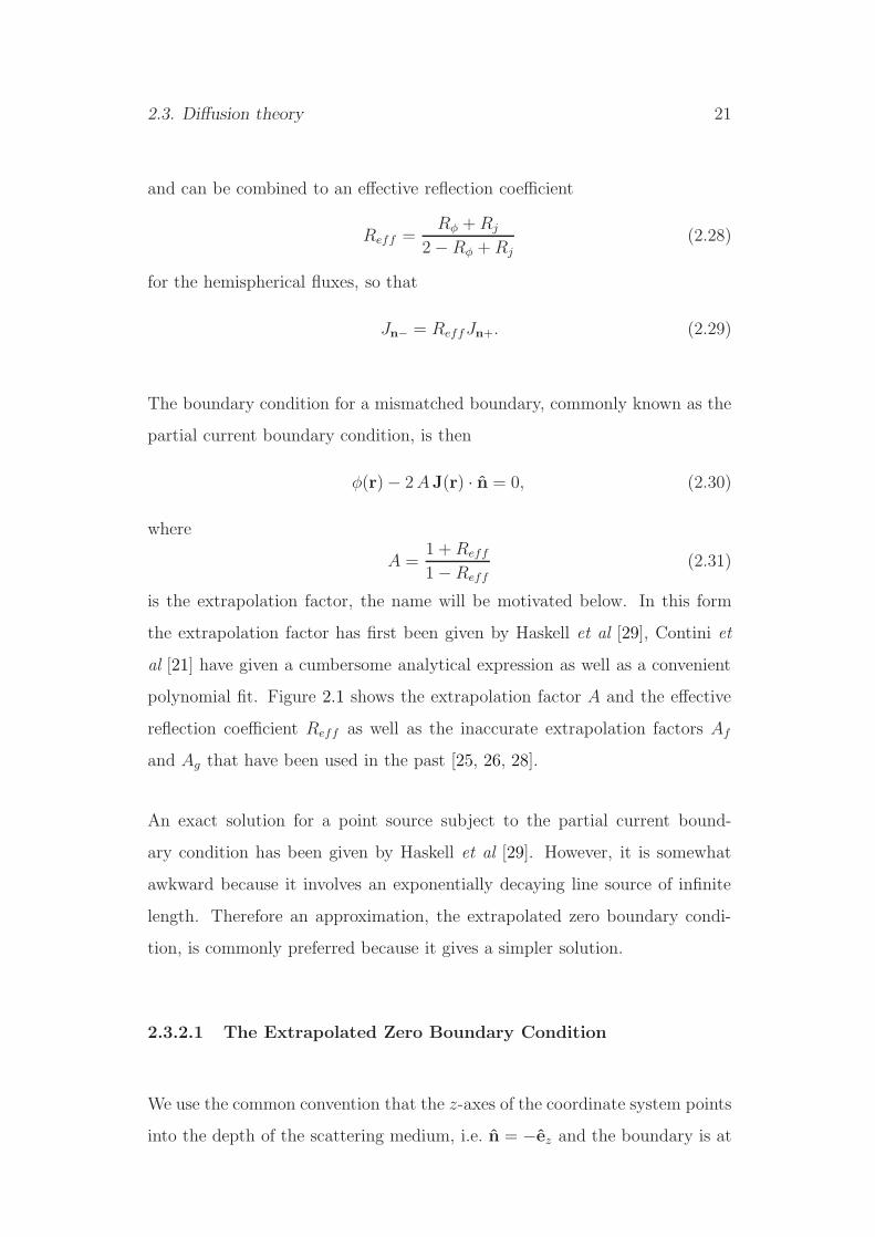
and can be combined to an effective reflection coefficient

Reff =Rφ + Rj

2 − Rφ + Rj(2.28)

for the hemispherical fluxes, so that

Jn− = ReffJn+. (2.29)

The boundary condition for a mismatched boundary, commonly known as the

partial current boundary condition, is then

φ(r) − 2 AJ(r) · n = 0, (2.30)

where

A =1 + Reff

1 − Reff(2.31)

is the extrapolation factor, the name will be motivated below. In this form

the extrapolation factor has first been given by Haskell et al [29], Contini et

al [21] have given a cumbersome analytical expression as well as a convenient

polynomial fit. Figure 2.1 shows the extrapolation factor A and the effective

reflection coefficient Reff as well as the inaccurate extrapolation factors Af

and Ag that have been used in the past [25, 26, 28].

An exact solution for a point source subject to the partial current bound-

ary condition has been given by Haskell et al [29]. However, it is somewhat

awkward because it involves an exponentially decaying line source of infinite

length. Therefore an approximation, the extrapolated zero boundary condi-

tion, is commonly preferred because it gives a simpler solution.

2.3.2.1 The Extrapolated Zero Boundary Condition

We use the common convention that the z-axes of the coordinate system points

into the depth of the scattering medium, i.e. n = −ez and the boundary is at


0

0.1

0.2

0.3

0.4

0.5

0.6

1 1.1 1.2 1.3 1.4 1.5 1.6

AA

g

Af

0

1

2

3

4

5

6

A

nrel

Ref

f

Reff

Figure 2.1: Effective reflection coefficient Reff and extrapolation factor A.

The inaccurate extrapolation factors Ag used by Groenhuis et al [25], and Af

used by Keijzer et al [26] and Farrell et al [28] are plotted for comparison.

z = 0. With Jz = −D∂φ/∂z the partial current boundary condition Eq. (2.30)

is then

φ(z = 0) + 2AD∂φ

∂z(z = 0) = 0. (2.32)

To simplify this boundary condition it is assumed that in the neighborhood

of the boundary the fluence varies linearly in the z–direction. The fluence is

then linearly extrapolated to the outside of the medium and becomes zero at

the extrapolation distance le = 2AD. Note that the extrapolation distance is

determined by the effective reflectivity of the boundary via the extrapolation

factor A, as well as by the reduced scattering coefficient of the medium via

D = 1/(3µ′s). Thus the extrapolated zero boundary condition is

φ(z = −le) = 0 with le = 2AD. (2.33)

This Dirichlet boundary condition is trivially solved with the method of image

sources (see Figure 2.2): any source in the scattering medium is mirrored at the

extrapolated boundary. More precisely, a semi–infinite scattering medium with


z

z

image -1

z=0

z

z

extrapolatedboundary e

s

i = z + 4AD

= 2AD

s

source +1

Figure 2.2: Image source configuration for the extrapolated zero boundary

condition.

a point source at rs = (x, y, zs) is replaced by an infinite medium with a point

source at rs and a negative image source at ri = (x, y,−zs − 2le). For these

sources in a now infinite medium the Green’s function of the homogeneous

diffusion equation applies and thus the Green’s function for the semi–infinite

medium is

Gsemi(r, rs) = G(|r − rs|) − G(|r − ri|). (2.34)

We will use this Green’s function in chapter 3 and 4 for the treatment of

perturbations in inhomogeneous semi–infinite media.

2.3.2.2 Collimated Light Sources

With the Green’s function we have a solution for a diffuse point source. How-

ever, the light sources most often used in biomedical optics, free laser beams

and optical fibers, are best described as collimated pencil beams. For the

case of isotropic scattering (g = 0) the description with Green’s functions is


straightforward: the collimated beam is attenuated exponentially due to scat-

tering and absorption, and the scattered part directly forms the source distri-

bution for the diffusion problem. For the strongly forward peaked scattering

in tissues (g ≈ 0.9) the situation is more complicated. Photons that leave the

collimated beam due to the first scattering event are not yet diffuse, and when

they have become diffuse they have already left the collimated beam by about

a reduced scattering length 1/µ′s. These complications are usually avoided by

mimicking the collimated beam with a single diffuse point source, placed one

reduced scattering length away from the entrance of the collimated beam. This

approximation gives good results at distances greater than a few reduced scat-

tering lengths. In non–invasive applications the light enters the medium at the

surface. This means that the point source is at a depth zs = 1/µ′s = 3D and

the image source is consequently at zi = −4AD − 3D, according to Fig. 2.2.

2.3.2.3 Detection of Diffuse Light

After considering light sources we now turn to light detection. Within the

diffusion approximation, the power received by a detector is

P =1

4π

∫Adet

dr

∫ds T (s) [φ(r) + 3J(r) · s] (s · n) (2.35)

where Adet is the active area and T (s) is the aperture function of the detec-

tor. Often the aperture function T (s) is symmetric around the surface normal

vector. Then the component of the flux perpendicular to the surface normal

vector gives no contribution to the integral and thus J(r) can be replaced by

Jn(r). According to the partial current boundary condition in Eq. (2.30) the

fluence and the normal component of the net flux are proportional, φ = 2AJn.

Therefore the detected power can be expressed either in terms of the fluence

or of the normal component of the net flux [29]. For some reason it is common

in the literature [28, 31, 32, 27, 33, 21] to use the normal component of the net

flux as the detector signal, although this complicates the formulas. We prefer


the simpler forms obtained with the fluence and thus adopt that the detec-

tor signal is proportional to the Green’s function of the semi–infinite medium

Eq. (2.34).

It is instructive to address the common case of detection with multimode

optical fibers. The radius of the fiber is usually small enough to assume that

the integrand is independent of r. The aperture function is approximately

unity within the acceptance angle θmax, that is s · n < θmax. Then Eq. (2.35)

becomes

P = Adet1

2φ

[∫ θmax

0

dθ sin θ cos θ +3

2A

∫ θmax

0

dθ sin θ cos2 θ

]

= Adet φ1

4

(sin2 θmax +

1

A(1 − cos3 θmax)

)︸︷︷︸

β

. (2.36)

For direct coupling of the fiber to the medium the acceptance angle is θmax =

arcsin(NA/nmedium), where NA is the numerical aperture in air. We assume

nmedium = 1.4 → A ≈ 3 and consider two common fiber types:

• A 1000 µm fiber with a high numerical aperture NA = 0.4 is typical for

detection systems with large area detectors like photo multipliers. We

get β = 0.03, Adet = 8 · 10−3 cm2 and thus

P = 2.4 · 10−3[cm2] · φ. (2.37)

• A 100 µm fiber with a numerical aperture NA = 0.25 is typical for

detection systems with fast small area photo diodes. We get β = 0.012,

Adet = 8 · 10−5 cm2 and

P = 1 · 10−6[cm2] · φ. (2.38)

Chapter 3

Perturbation Theory for

Spherical and Small Objects

As we have outlined in the introduction of chapter 2, inhomogeneities are of

prime interest in biomedical optics. We saw that biological tissues are optically

inhomogeneous on a large range of scales. With the use of transport theory

and the diffusion approximation we sacrifice the microscopic variations by us-

ing average optical properties, but the variations on the range of millimeters

and centimeters remain. In the scattering dominated regime, i.e. in the near

infrared spectral range, this means that the diffusion equation (2.14) has to be

solved for spatially varying D(r) and k(r).

One way to tackle this problem is to resort to numerical brute force approaches

like finite element and finite difference methods. These powerful and well es-

tablished techniques are the methods of choice if the medium is very inho-

mogeneous. They have, however, some drawbacks. As all purely numerical

methods they cannot offer the physical understanding an analytical descrip-

tion provides. Moreover, the computational cost for calculations in three di-

mensional geometries is high, and biological systems usually lack symmetry

27

28 Chapter 3. Perturbation Theory for Small and Spherical Objects

properties that would allow to reduce the dimensionality.

An elegant way to avoid these drawbacks is to describe light propagation in

terms of perturbation theory. This approach is appropriate if the system can

be approximated as a background medium with some included objects of dif-

ferent optical properties. The light field is splitted into the solution for the

unperturbed background medium φ0 and a perturbation φpert that is caused by

the presence of the objects. Note that this approach does not work always. It

fails if the perturbation is too strong, i.e. if the optical properties of the objects

are too different from the background and/or if the objects are too large. It

can also happen that the ansatz to split the fluence in background and pertur-

bation part is simply not practical because the background, or unperturbed,

medium is too complicated. Then neither the solution for the background part

nor for the perturbation part can be readily obtained. We will encounter such

a situation in chapter 6, where a clear layer in the background medium even

precludes the use of the diffusion approximation. This will force us to resort

to Monte Carlo simulations.

However, for rather homogeneous organs like breast, prostrate, or muscle, per-

turbation theory does work and is often the method of choice to analyze the

light propagation. For example, all tomographic reconstruction strategies are

based upon a perturbation ansatz.

We start this chapter with a discussion of an analytical solution of the diffu-

sion equation for a spherical object in a homogeneous medium. By itself, this

solution has only limited practical value because inclusions in biological tissues

are usually not spherically. We will therefore take the limits for small objects

and weak perturbations to obtain a simple solution for pointlike perturba-

tions and discuss the basic differences for absorption and scattering changes.

The solution for pointlike perturbations is then used to address the spatial

sensitivity of reflection mode measurements for absorbing and scattering inho-

29

mogeneities. A design study for an optical probe for the detection of buried

absorbers concludes the chapter.

3.1 Analytical Solution for a Spherical Object

Analytical solutions of the inhomogeneous diffusion equation are only available

for simple piece wise homogeneous geometries. In this section we discuss the

solution for a spherical object in an otherwise homogeneous infinite medium,

illuminated by a single point source. Inside, the sphere has constant optical

properties µa1, µ′s1, but they are different from the µa0, µ′

s0 on the outside. It

is convenient to define the differences ∆µa = µa1 − µa0 and ∆µ′s = µ′

s1 − µ′s0.

Since the optical properties are constant inside each region, the homogeneous

diffusion equation (2.16) is valid in each region. The solution is then deter-

mined by the boundary conditions at the interface of the two media and by

the restriction that the fluence must vanish at infinity.

Outside the sphere the general solution is a superposition of the incoming flu-

ence φ0 and the scattered fluence φPert, while inside the sphere we have φIns.

All three functions are now expanded in a suitable system of basis functions.

The spherical symmetry suggests a multipole expansion of the Helmholtz equa-

tion as it is known from Electrodynamics [34]. The expansion coefficients are

determined using boundary conditions at the surface of the sphere. For the ra-

dial part spherical Bessel and Hankel functions are used. For the angular part,

Boas et al [35] and Hielscher et al [36] have originally used the most general

approach of a spherical harmonics expansion. However, using the azimuthal

symmetry around the axes between source and center of the sphere, one can

immediately use Legendre polynomials [37].


The center of the sphere is set at the origin of the coordinate system, the

illuminating point source of strength S is at the position rs, and the detector

is at r. From Eq. (2.19) in section 2.3.1 we recall that the incoming fluence φ0

is simply described by the impulse response G scaled by the source strength S

φ0 = SG(|r − rs| , ω) =S

4πD0 |r − rs| exp(ik0 |r − rs|), (3.1)

where k0 is the wave vector (see Eq. (2.17)), and D0 = 1/(3µ′s0) is the diffusion

coefficient for the surrounding medium (see Eq. (2.13)). Note that the fre-

quency dependence is hidden in the wave vector k0. We then get the multipole

expansion

φ0 = Sik0

D0

∞∑l=0

jl(k0r<)h(1)l (k0r>)

(2l + 1)

4πPl(cos α) (3.2)

where jl are spherical Bessel functions, h(1)l are spherical Hankel functions of

the first kind, Pl are Legendre polynomials, α is the angle between r and rs,

r< is the smaller and r> is the larger of |r| and |rs|. For the evaluation of

the boundary conditions at the surface of the sphere we have r< = |r| and

r> = |rs|.

The perturbed fluence φPert and the fluence inside the sphere φIns are expanded

with the same angular part. φPert has to be an outgoing wave, thus the radial

part must be described with spherical Hankel functions of the first kind and

we get

φPert =

∞∑l=0

Al h(1)l (k0r)

(2l + 1)

4πPl(cos α), (3.3)

where the Al are expansion coefficients for the perturbed fluence. For φIns

standing wave solutions have to be used for the radial part, i.e. spherical Bessel

and Neumann functions. The condition that φIns has to be finite inside the

sphere rules out spherical Neumann functions and we get

φIns =

∞∑l=0

Bl jl(k1r)(2l + 1)

4πPl(cos α), (3.4)

31

where k1 is the wave vector for the medium inside the sphere and the Bl are

expansion coefficients for the fluence inside the sphere.

To determine the expansion coefficients Al and Bl we employ the boundary

conditions at the surface of the sphere at r = |r| = a. They state that the

fluence φ as well as the normal component of the net flux Jr = −D∂φ/∂r must

be continuous:

φ0(a) + φPert(a) = φIns(a)

D0∂φ0

∂r(a) + D0

∂φPert

∂r(a) = D1

∂φIns

∂r(a). (3.5)

With the abbreviations x = k0a and y = k1a we get

Al = −Sik0

D0h

(1)l (k0rs)

D0xj′l(x)jl(y) − D1yjl(x)j′l(y)

D0xh(1)′l (x)jl(y) − D1yh

(1)l (x)j′l(y)

(3.6)

and

Bl = Sik0

D0h

(1)l (k0rs)

D0xh(1)′l (x)jl(x) − D0xh

(1)l (x)j′l(x)


(1)l (x)j′l(y)

, (3.7)

where the prime denotes the derivative of the function with respect to its

argument x or y respectively. The series converges for x < 1 [35].

An implementation of this solution as MATHEMATICA code can be found in

[38]. A numerical implementation in ANSI C by D. Boas [18] is available as

part of the software package PMI, which will be discussed in section 5.7.2. We

will use it as a verification for the iterative perturbation approach we develop

in chapter 4.

3.2 Pointlike Perturbations

Although the solution from the last section is analytical it is too awkward to

gain real insight in the nature of the solution. In this section we will therefore


develop an approximation for small spheres which allows to discuss some basic

properties of scattering and absorbing perturbations.

We concentrate on the perturbed fluence φPert outside the sphere. Regrouping

the terms in Eqs. (3.3) and (3.6) the perturbed fluence becomes

φPert = Sk0

4πD0

∞∑l=0

h(1)l (k0rs) h

(1)l (k0r)Pl(cos α) fl (3.8)

with

fl = −i (2l + 1)D0xj′l(x)jl(y) − D1yjl(x)j′l(y)


(1)l (x)j′l(y)

. (3.9)

The size and optical properties of the sphere contribute only to fl.

3.2.1 Small Object and Weak Perturbation

To simplify Eq. (3.9) we will assume that the sphere is small and the perturba-

tion is weak. Small means that the dimension of the inclusion is optically thin

for the surrounding medium, i.e. the unperturbed fluence φ0 does not change

significantly over the radius of the sphere a. This is the case if x = k0a 1.

Weak means that the object itself is optically thin, i.e. the total (perturbed)

fluence φ does not change significantly over the object. This is the case if

y = k1a 1.

We can then use the limiting forms of the spherical Bessel and Hankel functions

for small arguments x (and y)

h(1)l (x) → −i

(2l − 1)!!

xl+1

h(1)′l (x) → i (l + 1)

(2l − 1)!!

xl+2

jl(x) → xl

(2l + 1)!!

j′l(x) → −1

3x : l = 0

l(2l+1)!!

xl−1 : l > 0(3.10)

33

where the double factorial (n)!! = n(n−2)(n−4) · · · (1). For l = 0 the limiting

form of the derivative of the spherical Bessel function j′0 has to be derived

from the explicit form j0(x) = sin x/x. We will see that this exception has an

interesting consequence for the behavior of the solution. With Eq. (3.10) fl

becomes:

fl>0 =−x2l+1

((2l − 1)!!)2

l ∆µ′s

(l + 1) ∆µ′s + (2l + 1) µ′

s0

(3.11)

fl=0 =k0

3D0

a3 ∆µa, (3.12)

where the dipole term is explicitly:

fl=1 = −k30 a3 ∆µ′

s

3µ′s0 + 2∆µ′

s

. (3.13)

Thus we have the remarkable result that for a small and weak perturbation

the monopole term of the perturbed fluence depends only on the difference

in the absorption coefficients ∆µa, while all higher orders depend only on the

difference in the reduced scattering coefficient ∆µ′s. Both the monopole and the

dipole term are of the order a3 and are thus proportional to the volume of the

sphere. Higher terms drop quickly because of the double factorial and higher

powers in x = k0a. Using the explicit forms of the spherical Hankel function

h(1)0 (x) = −i exp(ix)/x and h

(1)1 (x) = − exp(ix)(1/x + i/x2) in Eq. (3.8) the

perturbed fluence becomes

φPert = −S4π

3a3 eik0r

4πD0r

eik0rs

4πD0rs

∆µa (3.14)

+ S4π

3a3 eik0r

4πD0r(ik0 − 1

r)

eik0rs

4πD0rs

(ik0 − 1

rs

) cos α D03∆µ′

s

3µ′s0 + 2∆µ′

s

.

Recognizing the Green’s function Eq. (2.19) and its gradient we can express

Eq. (3.14) as

φPert = −S4π

3a3 G(rs) G(r) ∆µa

+ S4π

3a3 ∇G(rs) · ∇G(r) D0

3∆µ′s

3µ′s0 + 2∆µ′

s

. (3.15)


This is an important result. Small absorbing objects cause a monopole per-

turbation. If the absorption in the object is higher than in the background

medium the light field is depleted. Thus the increased absorption is modeled

with a negative monopole source. To distinguish it from the real light sources

we call this a virtual source. Small scattering objects behave different. For

increased scattering they cause a dipole virtual source which reflects fluence

back into the direction of the real source and depletes the light field on the far

side.

In chapter 4 we will extend the concept of virtual sources to discuss extended

perturbations of arbitrary shape. This approach will provide more insight in

the different behavior of scattering and absorbing perturbations and will show

that the basic difference is caused by a surface term that is only caused by a

scattering change.

Before we proceed to use Eq. (3.15) we have to address the validity of the ap-

proximation: How small and how weak must a perturbation be for Eq. (3.15)

to hold? For what size do we have to resort to the theory for extended per-

turbations? In Figure 3.1 the behavior of the first moments is exemplified for

some practically relevant parameter sets. Shown are the exact solutions of the

expansion coefficient fl obtained with Eq. (3.9) as solid lines and the approx-

imation for small and weak perturbations Eqs. (3.11, 3.12) as dashed lines.

From the top row to the bottom row the optical thickness of the inclusion

for the surrounding medium |ak0| increases as the size and/or the modulation

frequency increases, and is 0.35, 0.46, 0.87, and 1.15 respectively.

The left column shows the expansion coefficients fl for an absorbing object

with ∆µa 6= 0, the right column for a scattering object with ∆µ′s 6= 0. In order

to compare how the expansion coefficients vary with changing µa1 and µ′s1 it is

convenient to normalize these parameters to their background values µa0 and

35

0 1 2 3 4 5contrast ratio

0.10.20.30.40.50.60.70.8

fl

f=0.5GHz, a=5mm

0

1

20 1 2 3 4 5

contrast ratio

0.10.20.30.40.50.60.70.8

fl

f=0.5GHz, a=5mm

1

2

0

0 1 2 3 4 5

0.10.20.30.40.50.60.70.8

fl

DC, a=5mm

0

1

0 1 2 3 4 5

0.10.20.30.40.50.60.70.8

fl

DC, a=5mm

1

2

0 1 2 3 4 5

0.01

0.02

0.03

0.04

fl

f=0.5GHz, a=2mm

0

1

0 1 2 3 4 5

0.01

0.02

0.03

0.04

fl

f=0.5GHz, a=2mm

1

2

0 1 2 3 4 5

0.01

0.02

0.03

0.04

fl

DC, a=2mm

0

10 1 2 3 4 5

0.01

0.02

0.03

0.04

fl

DC, a=2mm

1

2

Figure 3.1: Absolute values of the coefficients fl of the multipole expansion as

a function of the contrast ratio γ. Results for spheres with a = 2 mm and a

= 5 mm radius, for steady state light (DC), and for amplitude modulated light

with modulation frequency f = 500 MHz. Left column: absorbing object with

µa1 = γµa0; right column: scattering object with µ′s1 = γµ′

s0. The background

optical properties are µa0 =0.1 cm−1, µ′s0 = 10 cm−1. Solid lines were computed

with the exact solution Eq. (3.9), dashed lines with the limit for pointlike weak

perturbations Eqs. (3.11, 3.12). The order of the moments are indicated at the

lines.


µ′s0 by means of a contrast ratio parameter γ

µa1 = γµa0 (3.16)

µ′s1 = γµ′

s0

which signifies the relative strength of the perturbation. Note that the optical

thickness |ak1| of the object itself scales with the contrast ratio γ. Conse-

quently, for γ > 1 the weak perturbation condition |ak1| 1, is fulfilled worse

than the small object condition |ak0| 1.

Figure 3.1 shows that for a radius a = 5 mm the small object approximation is

violated both for the absorbing and the scattering sphere, as could be expected

from the high |ak0| values. For the scattering sphere with a modulation fre-

quency f = 500 MHz this results in a significant monopole moment (which is

even larger than the quadrupole moment), in clear contradiction to Eq. (3.12).

For the absorbing sphere the appearance of the dipole moment indicates the

violation of the small object approximation.

3.2.2 Small Object and Strong Perturbation

The behavior for stronger perturbations is different for scattering and absorb-

ing spheres.

For the scattering sphere the approximation for dipole and higher moments

is surprisingly robust for large contrast ratios γ, even for the large sphere

with a = 5 mm radius. In biological tissues the scattering coefficient does

not vary too strongly, a scattering contrast up to five, as in Fig. 3.1, should

cover most cases. The dipole approximation of Eq. (3.15) is therefore limited

by the size of the object, with an upper limit of at least 2 mm radius. The

situation is different for inclusions with lower scattering than the background

37

medium. While in ‘normal tissues’ the contrast ratio for lower scattering is

not very pronounced there is an important exception: regions with clear, non–

scattering fluids like the ventricular system with cerebrospinal fluid in the brain

(see chapter 6). In these cases the diffusion approximation breaks down and

one has to resort to Monte Carlo simulations.

For an absorbing sphere Fig. 3.1 shows that the monopole moment begins to

deviate from the approximate form for contrast ratios γ & 2.5 and starts to

saturate. Since for µa1 → ∞ the conservation of energy forces the strength

of the perturbation to saturate eventually, it is clear that Eq. (3.12) with its

linear dependence on ∆µa must fail for large µa1. However, it is remarkable

that even for the relatively small sphere with a = 2 mm the deviation starts

already at an absorption contrast of only three. Absorption contrasts can be

high in biomedical applications, examples are tumors marked with contrast

agents and, more common, blood vessels and hemorrhages. The typical vol-

ume concentration of blood in tissue is about 3%. Most of it is distributed in

the tissue quasi continuously in small capillaries and thus determines the ab-

sorption coefficient of tissues in the visible NIR spectral range. Larger regions

of whole blood will therefore have an absorption contrast to the surrounding

of about γ = 33. The scattering is close to that of many tissue types. A

practically relevant question is therefore: How large may a bleeding or a vessel

be to be described accurately with the simple monopole perturbation model

Eq. (3.15)? Figure 3.2 shows that the simple approximation deviates from the

exact solution for radii greater than about 0.7 mm due to saturation. The

dipole moment essentially plays no role.

Note that diffusion theory is not expected to work properly inside such a

strong absorber as whole blood (µa ≈ 15 cm−1 µ′s ≈ 8 cm−1 @ λ = 760 nm

[39]). But the boundary condition of continuous flux and fluence we used to

derive the exact solution relies on diffusion theory to work inside the object.

One approach to overcome this limitation is to approximate blood as a perfect


0 0.05 0.1 0.15 0.2 0.25a

0.05

0.1

0.15

0.2

0.25

0.3

0.35

0.4

fl0

0

1

Figure 3.2: Absolute value of the first moments for a strongly absorbing sphere

and steady state light as a function of the radius a[cm]. The contrast ratio

γ = 33 is typical for blood aggregations in the surrounding tissue. Shown are

the monopole moments (0) and dipole moments (1) of the exact solution (solid

line) and the perfect absorber (dashed line), and the approximation for small

and weak perturbation (dotted line).

absorber and to use the boundary condition of no outgoing partial flux Jr− = 0,

where no assumptions are made for the inside of the object. The expansion

coefficient fl becomes:

fabsl = −i(2l + 1)

3µ′s0 jl(x) − 2k0j

′l(x)

3µ′s0 h

(1)l (x) − 2k0h

(1)′l (x)

. (3.17)

Figure 3.2 shows that the monopole moment for a perfect absorber fabs0 (dashed

line) does not agree at all with the exact solution for small objects, but for a

radius a & 1.7 mm the agreement is at least better than with the small and

weak approximation, which diverges quickly.

Thus the small and weak approximation should not be expected to quantita-

tively describe blood volumes larger than about 3 mm in diameter. However,

we see that the dipole moment can be neglected for the perfect absorber too.

This means that although the approximation for small and weak perturbations

39

overestimates the strength of strong absorbing perturbations it can neverthe-

less be used to explore the spatial behavior of absorbing perturbations.

In summary, absorbing perturbations cause a perturbation with a dominant

monopole moment, while for scattering perturbations the dipole moment is

dominant. For perturbations smaller than 4 mm in diameter higher multi-

pole terms can be neglected. This means that the shape of such small objects

does not influence the perturbation outside the objects, they can therefore be

treated as pointlike perturbations. Both leading moments scale with the vol-

ume of the perturbation. For pointlike absorbing perturbations with a contrast

ratio less than about three the perturbation is linear in ∆µa. For higher con-

trast the perturbation begins to saturate and can be described with Eq. (3.9),

the limiting form for perfect absorbers is Eq. (3.17). Although scattering per-

turbations are linear only for ∆µ′s µ′

s0 the simple form in Eq. (3.14) holds

for all practically relevant contrast ratios in tissues, except for clear, non–

scattering regions.


3.3 Sensitivity Maps

Sensitivity maps visualize the spatial distribution of the sensitivity of a mea-

surement for the presence of perturbations. The idea is to keep the source and

detector position fixed and to calculate the change of the detector response a

perturbation at different positions would cause. The knowledge of this sen-

sitivity for all volume elements of interest is the basis of most tomographic

approaches to reconstruct the optical properties from measurements on the

outside of the medium. It is also of great interest for applications that do not

aim for a full tomographic reconstruction, as for example local measurements

of the averaged optical properties. Here sensitivity maps can be used to as-

sess the errors inhomogeneities cause in algorithms that assume homogeneous

media. We will use sensitivity maps in section 3.4 for a design study for an

optical probe to detect surface near brain hematomas. Here we proceed with

the definition of the formalism and thereafter specialize on sensitivity maps

for absorbing perturbations in section 3.3.1 and for scattering perturbations

in section 3.3.2.

For absorbing perturbations the sensitivity has been described as ‘photon–

hitting density’ [40], ‘photon sampling volume’ [41], ‘weighting function’ [42],

and ‘photon visit probability’ [33]. These names are inspired by an intuitive

physical interpretation of the nature of the perturbed measurement. Con-

sider photons which actually travel from source to detector in the unperturbed

medium and monitor the volume were we will put the test perturbation. The

change of the detector signal due to a change of the absorption must depend

on the average pathlength these photons spend in the volume of interest. This

can be computed directly with Monte Carlo simulations by recording and an-

alyzing the photon paths. We will use this approach in chapter 6 to obtain

sensitivity maps for measurements on the head, because diffusion theory can-

not be applied there.

41

source

test volume

with virtual source

detector

source detector

a)

b)

G(|r -r|)sG(|r -r|)d

Figure 3.3: Principle of the sensitivity map.

In the framework of diffusion theory the sensitivity for a small absorption

change in a small volume can be described with the monopole approximation

we have developed in the last section (Eq. 3.15)

φPert = −S4π

3a3 G(|rs − r|) G(|r − rd|) ∆µa, (3.18)

where rs, r, and rd are the positions of source, test volume, and detector re-

spectively, S is the source strength, and a is the radius of the test volume, see

Fig. 3.3a. The first Green’s function determines how much light gets from the

source to the test volume. The virtual source strength determines how much

the perturbation changes the light propagation, for the absorption perturba-

tion this is simply the product of the volume and the change in absorption

V ∆µa. Then the second Green’s function determines how this change prop-

agates to the detector. The product of both Green’s functions is sometimes

referred to as ‘three point Green’s function’ G(rs, r, rd) = G(|rs−r|) G(|r−rd|).When the sensitivity is plotted for varying r the region with high sensitivity

spans between source and detector in a shape that resembles a banana, as is

schematically shown in Fig. 3.3b. For this reason the sensitivity maps are also

called ‘photon bananas’. Arridge et al [32, 43] have refined the photon ba-

nana concept (and coined the term ‘photon measurement density functions’)


to distinguish between the different measurement modalities, viz. integrated

intensity for DC measurements, amplitude ratio and phase difference for fre-

quency domain measurements, and the temporal moments for time domain

measurements.

Although originally developed for absorption perturbations, the concept of the

sensitivity maps or photon bananas can naturally be extended to scattering

perturbations simply by replacing the absorbing test perturbation with a scat-

tering test perturbation. We use of the dipole approximation in Eq. (3.15),

i.e.

φPert = S4π

3a3 ∇G(|rs − r|) · ∇G(|r − rd|) D0

3∆µ′s

3µ′s0 + 2∆µ′

s

, (3.19)

to describe the effect of the scattering perturbation on the detector signal.

However, the physical interpretation is not as straightforward as for the ab-

sorption change. Principally, due to the different scattering in the perturbation

the paths of the photons which pass through this volume are altered. But the

multipole expansion formalism does not facilitate an intuitive explanation why

this is mediated by the gradient of the Green’s functions, not the Green’s func-

tions themselves. We have to delay an interpretation until the virtual source

approach is fully developed in section 4.

Generally, sensitivity maps can be obtained for all measurement geometries.

For tomographic applications mostly measurements in transmission mode or on

the circumference of a cylindrical medium were investigated. The curved pho-

ton bananas can be used in backprojection image reconstruction approaches

[44]. However, because of the high attenuation in biological tissue source–

detector separations are limited to about 5 to 10 cm, depending on the optical

properties. Practically, this means that for some important applications, like

imaging of breast cancer [45, 46, 47, 44] and brain imaging in neonates [48],

transmission measurements can be used. But in this work we are especially in-

terested in optical measurements on the adult head, where the larger diameter

43

and high scattering coefficient of the brain make transmission measurements

impossible. Any optical diagnostic methods on the adult head are thus re-

stricted to the reflection mode. In the following we will therefore concentrate

on the discussion of sensitivity maps for reflection mode measurements in a

semi–infinite geometry. One could argue that it would be more appropriate to

use a spherical or cylindrical geometry with the average diameter of a head,

but the curvature on a human head is actually quite variable. On the tempo-

ral lobe the scull is rather flat, even with some concave regions, while on the

frontal lobe the curvature is pronounced. Thus there is no typical curvature

and for the sake of simplicity we can as well choose the semi–infinite case.

In section 2.3.2 we showed that the extrapolated zero boundary condition can

be satisfied by adding an image source on the outside of the medium for each

real source in the medium. This principle applies as well to virtual sources

which are caused by a perturbation. Thus the form of the monopole and

dipole terms in Eq. (3.15) is unchanged except that the Green’s functions for

source +1

image -1

extrapolatedboundary

virtual source

image

detector

Figure 3.4: Image source configuration for a perturbation in a semi–infinite

geometry.


homogeneous media are now replaced by the Green’s functions for semi–infinite

media according to Eq. (2.34), that is by a sum of the Green’s functions for

the source and its image source. This situation is depicted in Figure 3.4. Note

that for the scattering perturbation the gradient of the sum has to be taken.

In the following two sections we will discuss the properties of sensitivity maps

for scattering and absorbing perturbations for steady state and for frequency

domain measurements. The results will be used for the design study of an

optical probe in section 3.4.

3.3.1 Sensitivity Maps for Absorption Perturbations

The form and strength of the sensitivity maps depends on the values of the

optical properties of the background medium, the source–detector distance,

the modulation frequency, and of course on the measurement modality. We

consider the amplitude ratio φ/φ0 and the phase difference arg(φ)−arg(φ0) of

the detected diffuse photon density wave φ in the perturbed medium relative

to the DPDW φ0 in the unperturbed background medium . To get an overview

over the principal behavior of the photon bananas we choose a typical example

of a reflection mode measurement and then vary the modulation frequency and

the source–detector distance.

Figure 3.5 shows the geometry of our example sensitivity map. The light enters

the background medium (µa0 = 0.1 cm−1, µ′s0 = 10 cm−1) at the surface of the

medium at (0,0,0). The equivalent diffuse point source is therefore placed at a

depth of one mean free path below the surface at rs = (0, 0, 0.1) (all distances

are given in cm). The detector is placed in 2 cm distance at rd = (2, 0, 0).

In order to appreciate the practically achievable signals we use a reasonably

macroscopic absorbing test perturbation of a = 2 mm radius and a contrast

45

x0 2

z

0.1

Figure 3.5: Geometry for sensitivity maps in semi–infinite media.

ratio γ = 2, that is µa1 = γµa0 = 0.2 cm−1 and consequently ∆µa = 0.1 cm−1.

From section 3.2.1 we know that such a perturbation can still accurately be

described with the monopole approximation. In Figs. 3.6, 3.7, and 3.8 the

sensitivity is shown for different modulation frequencies. The contour plots

in Fig. 3.6 together with the surface plots in Fig. 3.7 give a good qualitative

impression of the photon bananas, while the line plots in Fig. 3.8 for a cut

through the y = 0 plane half way between source and detector are useful for a

quantitative comparison.

We see that for increasing modulation frequency the photon bananas for the

amplitude ratio as well as for the phase difference move nearer to the sur-

face. Also, the extrema become stronger and sharper. Consequently, high

modulation frequencies are appropriate for high resolution measurements near

the surface, while lower modulation frequencies are better suited for deeper

measurements. While these trends hold for both amplitude ratio and phase

difference there are also differences. The photon bananas for the phase dif-

ference generally penetrates deeper into the medium than for the amplitude

ratio. Figure 3.7 shows that the strength of the banana for phase difference is

relatively uniform over its way from source to detector, while the banana for

amplitude ratio is strongly peaked near source and detector. This suggests to

use phase measurements for the detection of buried absorbers since they are

relatively insensitive to variations of the optical properties at source and detec-

tor, and to use relatively low modulation frequencies for a deep penetration of


Amplitude Ratio

-0.5 0 0.5 1 1.5 2 2.5x

00.20.40.60.8

11.21.4

z

300 MHz

-0.5 0 0.5 1 1.5 2 2.5x

00.20.40.60.8

11.21.4

z

1000 MHz

-0.5 0 0.5 1 1.5 2 2.5x

00.20.40.60.8

11.21.4

z

DC

-0.5 0 0.5 1 1.5 2 2.5x

00.20.40.60.8

11.21.4

z

100 MHz

Phase Difference

-0.5 0 0.5 1 1.5 2 2.5x

00.20.40.60.8

11.21.4

z

300 MHz

-0.5 0 0.5 1 1.5 2 2.5x

00.20.40.60.8

11.21.4

z

1000 MHz

-0.5 0 0.5 1 1.5 2 2.5x

00.20.40.60.8

11.21.4

z

30 MHz

-0.5 0 0.5 1 1.5 2 2.5x

00.20.40.60.8

11.21.4

z

100 MHz

Figure 3.6: Photon bananas for absorbing perturbations in the x–z–plane be-

tween source and detector (dimensions in cm), for DC light and for modulation

frequencies from 30 MHz to 1 GHz. The plot range for all amplitude ratios is

0.96 to 1.01. For the phase difference the plot ranges in degree are -0.18 to 0.1

for 30 MHz, -0.45 to 0.3 for 100 MHz, -0.8 to 0.4 for 300 MHz, and -1.1 to

0.5 for 1 GHz.

47

0

1

2

x

0

0.5

1

1.5

z

0.96

0.98

1

A

0

1

2

x

0

1

2

x

0

0.5

1

1.5

z

0.96

0.98

1

A

0

1

2

x

0

1

2

x

0

0.5

1

1.5

z

-0.5-0.25

00.25

Phase

0

1

2

x

0

1

2

x

0

0.5

1

1.5

z

-0.75-0.5

-0.250

0.25

Phase

0

1

2

x

Figure 3.7: Photon bananas for absorbing perturbations. Top row: amplitude

ratio; bottom row: phase difference in degrees. Left column: f = 100 MHz;

right column: f = 1000 MHz.

the sensitive region. However, Fig. 3.8 shows that the maximum phase differ-

ence strongly decreases for lower frequencies. The phase errors of the detection

system will therefore limit the use of lower frequencies. Currently, about 0.05

degree phase accuracy are realistically for shot noise limited systems [49].

Note that the phase difference has a dominant region with a negative phase

difference, but also a less pronounced positive region near the surface. This is

caused by the distribution of the pathlength of the photons. Photons with a

shorter total pathlength travel on average nearer to the surface, while photons

with a longer total pathlength travel on average deeper in the medium. Thus


0 0.2 0.4 0.6 0.8 1 1.2 1.4z

0.975

0.98

0.985

0.99

0.995

1

amplitude

ratio

DC1003001000

0 0.2 0.4 0.6 0.8 1 1.2 1.4z

-0.6

-0.4

-0.2

0

0.2

phase

difference

30

100

300

1000

Figure 3.8: Sensitivity for absorbing perturbations versus depth half way be-

tween source and detector, i.e. on a line from (1,0,0) to (1,0,1.5).

an absorber near to the surface dampens predominantly the ‘fast’ photons and

the total phase is delayed, while an absorber deeper in the medium dampens

the ‘slow’ photons and the phase is advanced.

The second parameter which can be varied in reflection mode measurements

is the source–detector distance. Figure 3.9 shows that for increasing source–

detector distance the maximum of the sensitivity moves deeper into the medium

while the sensitivity drops. Note that the sensitivity decrease of the phase dif-

ference is less pronounced than for the amplitude ratio.

0 0.2 0.4 0.6 0.8 1 1.2 1.4z

0.96

0.97

0.98

0.99

1

amplituderatio

1

2

3

5

0 0.2 0.4 0.6 0.8 1 1.2 1.4z

-0.4

-0.3

-0.2

-0.1

0

0.1

0.2

phasedifference

1

2

35

Figure 3.9: Sensitivity for absorbing perturbations, source–detector separa-

tions between 1 and 5 cm, f = 100 MHz.

49

Amplitude Ratio

-0.5 0 0.5 1 1.5 2 2.5x

00.20.40.60.81

1.21.4

z

300 MHz

-0.5 0 0.5 1 1.5 2 2.5x

00.20.40.60.81

1.21.4

z

1000 MHz

-0.5 0 0.5 1 1.5 2 2.5x

00.20.40.60.81

1.21.4

zDC

-0.5 0 0.5 1 1.5 2 2.5x

00.20.40.60.81

1.21.4

z

100 MHz

Phase Difference

-0.5 0 0.5 1 1.5 2 2.5x

00.20.40.60.8

11.21.4

z

300 MHz

-0.5 0 0.5 1 1.5 2 2.5x

00.20.40.60.81

1.21.4

z

1000 MHz

-0.5 0 0.5 1 1.5 2 2.5x

00.20.40.60.8

11.21.4

z

30 MHz

-0.5 0 0.5 1 1.5 2 2.5x

00.20.40.60.81

1.21.4

z

100 MHz

Figure 3.10: Photon bananas for scattering perturbations in the x–z–plane be-

tween source and detector (dimensions in cm), for DC light and for modulation

frequencies from 30 MHz to 1 GHz. The plot range for all amplitude ratios is

0.91 to 1.01. For the phase difference the plot ranges in degree are ± 0.4 for

30 MHz, ± 1 for 100 MHz, ± 3 for 300 MHz, and ± 8 for 1 GHz.

3.3.2 Sensitivity Maps for Scattering Perturbations

To compare the effects of absorption and scattering perturbations we now

consider a scattering perturbation with the same strength and size as the


0

1

2

x

0

0.5

1

1.5

z

0.920.940.960.98

11.02

A

0

1

2

x

0

1

2

x

0

0.5

1

1.5

z

0.920.940.960.98

11.02

A

0

1

2

x

0

1

2

x

0

0.5

1

1.5

z

-2-10123

Phase0

1

2

x

--01

0

1

2

x

0

0.5

1

1.5

z

0

5

10

Phase0

1

2

x

0

5

Figure 3.11: Photon bananas for scattering perturbations. Top row: amplitude

ratio; bottom row: phase difference in degrees. Left column: f = 100 MHz;

right column: f = 1000 MHz.

absorption perturbation in the last section, i.e. radius a = 2 mm and contrast

ratio γ = 2, therefore µ′s1 = γµ′

s0 = 20 cm−1 and ∆µ′s = 10 cm−1. Consequently,

Figures 3.12 to 3.13 show sensitivity maps for the same parameters as were

used for the absorption perturbation.

The sensitivity maps for scattering objects also have the typical banana shape

and one might be surprised that the dipole character of the scattering pertur-

bation (Eq. 3.19) does not cause more discrepancies. However, a closer inspec-

tion of the shape in Figs. 3.10 and 3.11 reveals several differences. Contrary

to the absorption case, the sign of the phase difference is positive through-

51

0 0.2 0.4 0.6 0.8 1 1.2 1.4z

0.94

0.96

0.98

1

amplitude

ratio

DC

100

300

1000

0 0.2 0.4 0.6 0.8 1 1.2 1.4z

0

2

4

6

8

phase

difference

30

100

300

1000

Figure 3.12: Sensitivity for scattering perturbations versus depth half way

between source and detector, i.e. on a line from (1,0,0) to (1,0,1.5).

out the region between source and detector. This means that an increase in

scattering on the relatively direct paths between source and detector always

delays the photon propagation. In the sensitivity maps for amplitude ratio

as well as for phase difference we see small regions of opposite sign directly

besides the source and detector on the outside. These features are caused by

the dipole character of the scattering perturbation. Because here the angle

between r− rs and r− rd is larger than π/2 the detector sees the front lobe of

the dipole perturbation, where light is scattered back into the direction of the

source.

Figure 3.12 shows the behavior halfway between source and detector in more

detail; compare it to Fig. 3.8 for the absorbing perturbation. We see that,

contrary to the absorption case, the depth of the maximal sensitivity does

not shift significantly for different modulation frequencies, but therefore the

strength of the sensitivity increases drastically with the frequency. Note that

for the scattering perturbation the phase delay for 1 GHz modulation frequency

is about an order of magnitude higher than for an absorbing perturbation of

the same relative strength.

In Fig. 3.13 the sensitivity for different source–detector distances is shown.

As for the absorption case (Fig. 3.9) the sensitivity moves deeper into the


0 0.2 0.4 0.6 0.8 1 1.2 1.4z

0.94

0.95

0.96

0.97

0.98

0.99

1

amplitude

ratio

1

2

35

0 0.2 0.4 0.6 0.8 1 1.2 1.4z

0

0.5

1

1.5

2

phase

difference

1

2

3

5

Figure 3.13: Sensitivity for scattering perturbations, source–detector separa-

tions between 1 and 5 cm, f = 100MHz.

medium for increasing source–detector separation and the strength decreases.

Thus for scattering perturbations the source–detector distance determines the

sampling depth, while the modulation frequency determines the strength of

the sensitivity.

3.4 Design Example for Detection of Buried

Absorbers

The general discussion of the sensitivity of reflection mode measurements to

absorbing and scattering perturbations in the last two sections has highlighted

the basic trends for variations of the source–detector separation and the mod-

ulation frequency. In this section we show how the sensitivity analysis can be

utilized for the design of a detection system.

In chapter 6 we will discuss the detection of epidural and subdural brain

hematomas, which are located just below the skull. We will show that the

light propagation is dominated by a tunneling effect in the clear layer of cere-

brospinal fluid between skull and brain and thus cannot be described by dif-

fusion theory.

53

However, we expect that in cases of a local volume expansion in the brain due

to intracranial bleeding, brain tumor, or edema the brain is pressed against the

skull, thereby squeezing the cerebrospinal fluid out of the arachnoidea. The

DC system we discuss in chapter 6 is not expected to distinguish between this

situation and a bleeding because both essentially block the tunneling effect.

It is therefore worth exploring frequency domain measurements for this case.

Without the layer of cerebrospinal fluid the head can be approximated as an

optically quasi homogeneous medium since the optical properties of the skull

and the gray brain matter are very similar. In such a simplified model the

task is simply to detect an increase of absorption at a fixed depth of about one

centimeter.

We consider a simple system with one source and one detector. The opti-

cal properties for skull and brain are assumed to be µa0 = 0.3 cm−1 and

µ′s0 = 20 cm−1. From section 3.3.1 we know that the photon banana for the

phase difference penetrates deeper than that for the amplitude ratio, and is

also not so strongly peaked in the vicinity of source and detector. We will

therefore concentrate on phase measurements. But what are the best modula-

tion frequency and source–detector separation? To address this issue we have

plotted in Fig. 3.14 the phase difference for our standard pointlike absorbing

perturbation (a = 0.2 cm and γ = 1), located in one centimeter depth halfway

between source and detector, as a function of frequency and source–detector

separation. As expected, the highest sensitivity for the phase difference oc-

curs at large separations and at high frequencies. But this is also the region

of high attenuation of the diffuse photon density waves. A low amplitude of

the detector signal eventually limits the achievable phase accuracy of the sys-

tem. In order to optimize this tradeoff Fig. 3.14 also shows the amplitude

of the total signal (not the amplitude ratio!). More precisely, we have plot-

ted logarithmic contours for the Green’s function G(rs − rd, f) in dB, that is

10 log10(G(rs − rd, f) · [cm2]). Once we choose the detector aperture and size


0 5·107 1·108 1.5·108 2·108 2.5·108 3·108

frequency

0

1

2

3

4

5

6

separation

A

B

0

-20

-40

-60

-80

-100

-120

Figure 3.14: Total amplitude and phase difference for different source–detector

separations in cm and modulation frequencies in Hertz. The values for the

contours of the phase difference (solid lines) in degrees are marked on the

right side of the frame. The dashed contours are for the logarithmic amplitude

in dB, details see text.

and the source power we can use Eq. (2.36) to calculate the detector signal. In

Fig. 3.14 the combinations of separation and frequency witch yield the largest

phase difference with the largest detector signal are marked with a thick solid

line. On first glance this line should mark the optimal parameter combina-

tions from a signal–to–noise point of view. However, this also depends on the

detection system.

Detection with normal photomultipliers like the Hamamatsu R928 is limited

to about 100 MHz. Since lower frequencies bring no advantage for phase

sensitivity or total amplitude we can restrict our attention to the thick dashed

line in Fig. 3.14. We discuss two situations: point A at 100 MHz and 2.5 cm

55

-0.5 0 0.5 1 1.5 2 2.5 3x

00.20.40.60.81

1.21.4

z

Absorbing Perturbation

-0.5 0 0.5 1 1.5 2 2.5 3x

00.20.40.60.81

1.21.4

z

Scattering Perturbation

Figure 3.15: Sensitivity maps for parameters at point A in Fig. 3.14, i.e.

modulation frequency f = 100 MHz, 2.5 cm separation.

separation close to the -60 dB contour line; and point B at 100 MHz and

4 cm separation close to the -90 dB contour line. One advantage of photo

multipliers is the large detection area which permits to use large optical fibers.

Using a 1000 µm diameter multimode fiber with a high numerical aperture

of NA = 0.4 and a 1 mW light source Eq. (2.37) in section 2.3.2.3 predicts a

detectable power of P = G · 2.4 ·10−6 [Wcm2]. Thus the -60 dB contour line in

Fig. 3.14 corresponds to a power of 2.4 pW, which can be detected with such a

PMT with sufficient signal–to–noise ratio to make phase measurements with an

accuracy of about 0.1 [50]. Note that Fig. 3.14 shows the phase sensitivity for

a fixed depth of 1 cm, midway between source and detector. Figure 3.15 shows

the complete sensitivity maps for these parameters, for absorption changes and

scattering changes. We see that both photon bananas have their maximum

sensitivity much closer to the surface, which means that the measurement will

be rather susceptible to inhomogeneities in the sub surface layer.

Consider now point B with f = 100 MHz and 4 cm separation. Figure 3.16

shows that the photon banana for the phase difference reaches now deeper.


0 1 2 3 4x

00.20.40.60.81

1.21.4

z

Absorbing Perturbation

0 1 2 3 4x

00.20.40.60.81

1.21.4

z

Scattering Perturbation

Figure 3.16: Sensitivity maps for parameters at point B in Fig. 3.14, i.e.

modulation frequency f = 100 MHz, 4 cm separation.

Additionally the increased source–detector separation gives a small gain of

0.2 phase difference. But the drawback is a 30 dB loss of amplitude, down

to some fW of detectable power, which will reduce the phase accuracy. A

further increase in source–detector separation will yield no improvement in

the phase sensitivity and only marginally deeper penetration of the photon

banana. Therefore we conclude that a detection system based on standard

photomultipliers should use a modulation frequency of 100 MHz and a source–

detector separation between 2.5 cm and 4 cm, depending on the noise of the

phase detector and the expected inhomogeneities in the sub surface layer.

Chapter 4

General Perturbation Theory

for Complex Extended Objects

While the multipole expansion method from the previous chapter is quite useful

for the investigation of the basic properties of light propagation in inhomoge-

neous systems, it has a fundamental limitation: The inhomogeneity must be

either of spherical geometry, or it must be so small that the higher order mul-

tipole terms, which are sensitive to the shape of the object, can be neglected.

For many practical biomedical applications these restrictions render the mul-

tipole expansion approach useless because the inhomogeneities of interest, like

tumors, vessel systems, hematomas, or regions of hypoxia, are neither small

nor spherical.

A straightforward way to model extended objects is to divide them into small

volume elements or voxels, use simple perturbation solutions for each voxel,

and obtain a solution for the extended object as a sum of the contributions

from all voxels. To this end, Boas et al [18] and Feng et al [51] have used

limiting forms of the multipole expansion approach, similar to the result we

have discussed in section 3.2.1. Barbour and Graber et al [52, 42] have obtained

57

58 Chapter 4. General Perturbation Theory for Complex Extended Objects

‘weight functions’ based on Monte Carlo simulations. Pogue et al [53], Kaschke

et al [46], and Arridge et al [54] have used direct Green’s function approaches.

O’Leary et al [55] have used an approximated integral approach. Only [54, 55,

18] treat scattering objects correctly.

All these approaches, however, have a fundamental limitation: they linearize

the problem, i.e. they neglect the interaction of objects or, for large objects,

of different parts of the objects. They are therefore not suited for extended

inhomogeneities with stronger perturbations.

The objective of this chapter is to overcome these limitations and to develop a

comprehensive and coherent theory for diffuse light transport in heterogeneous

turbid media, based on an integral perturbation approach. The theory covers

steady state and modulated light, is applicable to absorbing and scattering

inhomogeneities of arbitrary size and shape, and accounts for the nonlinear

interaction between inhomogeneities. We have developed and used the theory

in [56, 57, 58, 59, 60], this and the next chapter are based on - and extend

beyond - these publications.

In section 4.1 we give a rigorous derivation of the integral formulation of the

optical diffusion equation starting from the differential formulation. Thereby

we introduce the virtual source formalism, which is a conceptually simple yet

powerful tool. For one, it establishes the framework for a very versatile iterative

numerical perturbation method. We sketch the iterative solution only briefly

in section 4.2 and postpone the detailed discussion to the next chapter. But,

equally important, the virtual source formalism also facilitates an intuitive and

deep insight into the nature of light propagation in heterogeneous systems. We

therefore devote the remainder of this chapter to the discussion of the virtual

source formalism. In section 4.3 we specialize on sharply bounded objects

and in section 4.4 this special case is used to discuss the principal behavior of

scattering and absorption perturbations. In section 4.5 we develop the limiting

59

form of the virtual source formalism for small and weak perturbations. This

permits us to draw a connection to the multipole approach from the previous

chapter as well as to the first order approximations which are the basis for an

important class of inverse algorithms [55]. In section 4.6 we use the virtual

source formalism to show that weak scattering and absorption perturbations

can be ambiguous and may result in the same light field. We draw conclusions

for the source and detector placement in inverse problems.

4.1 The Virtual Source Formalism

We recall the frequency dependent diffusion equation (2.14) for an inhomoge-

neous medium from section 2.3:

∇D(r) · ∇φ(r, ω) + D(r)∇2φ(r, ω)− µa(r) φ(r, ω) +iω

c(r)φ(r, ω) = −S0(r, ω).

(4.1)

For a homogeneous medium the first term vanishes because D = D0 is constant

and we get the homogeneous diffusion equation

D0∇2φ(r) − µa0φ(r) +iω

cφ(r) = −S(r). (4.2)

We will show below that this term determines the dipole-like perturbation

that dominates the effect of small scattering perturbations. Therefore any

perturbation theory that starts with homogeneous diffusion equation cannot

describe scattering objects.

In the following we will drop (r) in the formulas and implicitly assume that

all quantities vary spatially, unless otherwise noted. It is advantageous to

reformulate Eq. (4.1) in terms of the net flux vector J = − D∇φ and the

reduced scattering coefficient µ′s = 1/(3D). We also employ the definition of

the square of the wave number k2 = − 3µ′s(µa − iω/c) to obtain

3∇µ′s · J + ∇2φ + k2φ = −3µ′

sS. (4.3)


The advantage of using the net flux J instead of the gradient of the fluence is

that the net flux is continuous at boundaries between different media while ∇φ

is not. This will be helpful for the discussion of objects with sharp boundaries

in section 4.3.

To separate the effect of the objects from that of the background medium the

optical properties are written as µa = µa0 + ∆µa and µ′s = µ′

s0 + ∆µ′s, where

µa0 and µ′s0 are the constant parts due to the background medium, and ∆µa

and ∆µ′s are the absorption and scattering perturbations due to the objects.

With this we write k2 = k20 + ∆k2, where

k20 = −3µ′

s0(µa0 − iω

c), (4.4)

∆k2 = −3(∆µaµ′s0 + ∆µ′

s(µa0 − iω/c) + ∆µa∆µ′s), (4.5)

and extract the Helmholtz operator of the background medium, (∇2 + k20), to

obtain:

(∇2 + k20)φ = −3µ′

sS − 3∇µ′s · J − ∆k2φ. (4.6)

We rewrite this as

(∇2 + k20)φ = −3µ′

s0

(µ′

s

µ′s0

S + SV irt[φ]

), (4.7)

where the virtual source density SV irt[φ] is defined as,

SV irt[φ] = SV irtφ + SV irt

J (4.8)

SV irtφ =

1

3µ′s0

∆k2φ, (4.9)

SV irtJ =

∇µ′s

µ′s0

· J, (4.10)

which depends on both the fluence and its gradient, since J = − D∇φ.

In this form we can see how the presence of the objects affects the light field.

The strength of the real source density S is scaled according to the actual

optical properties at its location. Note that in the common case where S is

61

located entirely in the background medium its strength remains unchanged.

Additionally, the objects cause a virtual source density SV irt[φ] that depends

on the optical properties of the objects and the light field at the objects.

We now change to the integral formulation. With Green’s vector theorem [37],

Eq. (4.7) can be transformed into an equivalent integral equation,

φ(r) = φ0(r) + φPert(r), (4.11)

φ0(r) =

∫Vs

dr′ (µ′s(r

′)/µ′s0)S(r′) G(|r − r′|), (4.12)

φPert(r) =

∫Vobj

dr′ SV irt[φ(r′)] G(|r − r′|) (4.13)

=

∫Vobj

dr′(

1

3µ′s0

∆k2φ(r′) +∇µ′

s

µ′s0

· J(r′))

G(|r − r′|),

where G(|r − r′|) = 3µ′s0G(|r− r′|) is the impulse response to a physical point

source and G(|r − r′|) = exp(ik0 |r − r′|)/(4π |r − r′|) is the Green’s function

of the Helmholtz equation for the background medium, see Eqs. (2.18, 2.19).

φ0 is a convolution of the scaled real source density with the impulse response.

If the volume Vs of the source density is located entirely in the background

medium, φ0 becomes the background fluence, that is the fluence in the homo-

geneous background medium without objects. The perturbation fluence φPert

is a convolution integral of similar form. The virtual source density SV irt[φ]

contributes to the light field like the real source density S, but its strength

in turn depends on the light field within the objects. Once SV irt[φ] is deter-

mined by solving the integral equation inside the objects, the light field at an

arbitrary position, inside or outside the objects, can be calculated as a simple

integration over the virtual and real source densities. Due to the fundamental

role of the virtual source density we will refer to this approach as the virtual

source formalism.

While the transformation of the differential equation into an integral equation

by itself does not solve the problem, the virtual source formalism is the ap-


propriate form for a perturbation approach. In the following section we will

briefly outline how the integral equation can be solved iteratively, but a de-

tailed description of the numerical implementation is postponed to chapter 5.

Once we principally know how to obtain a solution we will use the virtual

source formalism to discuss the basic properties of the solution.

4.2 Iterative Solution and Born Approxima-

tion

Formally, the integral equation of the virtual source formalism (4.11–4.13) is

a Fredholm equation of the second kind in three dimensions. It can be solved

with the iterative approach of successive approximation [37]. The first order

approximation φ1 is obtained by using the background solution φ0 to calculate

the perturbation integral in Eq. (4.13), which yields:

φ1(r) = φ0(r) +

∫Vobj

dr′SV irt[φ0(r′)] G(|r− r′|) (4.14)

= φ0(r) +

∫Vobj

dr′(

1

3µ′s0

∆k2φ0(r′) +

∇µ′s

µ′s0

· J0(r′))

G(|r − r′|).

This is known as the Born approximation. Some imaging reconstruction

schemes [55, 61] are based on the inversion of a different formulation of this

equation, which we will discuss in section 4.5. The second order is calculated by

using φ1 in the perturbation integral, etc., which leads to the general recursion

formula

φn(r) = φ0(r) +

∫Vobj

dr′ SV irt[φn−1(r′)] G(|r − r′|). (4.15)

By repeated application of this equation to itself one can transform it into a

Neumann series [37]

φn = φ0 +

∫dV GSV irt φ0 +

∫dV GSV irt

∫dV GSV irt φ0

63

+ · · · +

[∫dV GSV irt

]n

φ0, (4.16)

where we have used a shorthand notation where the integration as well as SV irt

have to be understood as operators acting on everything on their right hand

side. However, for numerical evaluation (chapter 5) we prefer the recursive

form.

4.3 Sharp Boundaries

Objects with sharp boundaries are a special but important case. Compared

with a typical length scale of resolution in imaging of a few millimeters, blood

vessels, bones, hematoma, some tumors, and most inclusions in tissue phan-

toms can be considered as sharply bounded. Both the integral and the differ-

ential formulation given so far rely on a smoothly varying reduced scattering

coefficient µ′s, because they contain ∇µ′

s in the term SV irtJ (Eq. 4.10). If objects

have sharp boundaries the reduced scattering coefficient µ′s is discontinuous at

their surface and ∇µ′s(rsurf) has a singularity. In the differential formulation,

the boundary conditions of continuous fluence and net flux have to be applied

at the surfaces and solved together with the diffusion equation. The integral

formulation requires no additional boundary conditions. At the surface of a

sharp object, ∇µ′s(r) = −∆µ′

s(r)n(r) δ(r − rsurf), where δ is Dirac’s delta

function and n is the outward pointing surface normal vector. This transforms

the volume integral (Eq. 4.13) over SV irtJ (Eq. 4.10) into a sum of an inte-

gral over the inner part of the volume Vobj−inside where µ′s(r) is smooth, and a

surface integral over the sharp transition:

1

µ′s0

∫Vobj

dr′∇µ′s(r

′)J(r′)G(|r− r′|)

→ 1

µ′s0

∫Vobj−inside

dr′∇µ′s(r

′)J(r′)G(|r − r′|)


− 1

µ′s0

∫Sobj

dA′∆µ′s(r

′)n(r′) · J(r′)G(|r− r′|). (4.17)

In the following discussion we will consider only sharply bounded objects with

constant optical properties inside, for which the volume integral over ∇µ′sJ

vanishes. For these objects the different effects of scattering and absorbing

perturbations are most pronounced and easy to interpret. With these simpli-

fications Eqs. (4.8–4.10, 4.13) become

φPert(r) = − ∆µ′s

µ′s0

∫Sobj

dA′ · J(r′)G(|r − r′|)

−(

∆µa + ∆µ′s

µa0 − iω/c

µ′s0

+∆µa∆µ′

s

µ′s0

)×

∫Vobj

dr′φ(r′)G(|r − r′|). (4.18)

Note that if ∆µa or ∆µ′s are small compared to the background value the

mixed term, ∆µa∆µ′s/µ

′s0, can be neglected and absorption and scattering

perturbations are approximately additive.

4.4 Scattering and Absorbing Inhomogeneities

To discuss the basic effects of scattering and absorption changes we investigate

the importance of the contributions from the surface and volume integrals. We

compare a scattering and an absorbing perturbation with the same relative

change ζ in scattering (∆µ′s = ζµ′

s0, ∆µa = 0) or absorption (∆µa = ζµa0,

∆µ′s = 0). For the absorbing perturbation Eq. (4.18) simplifies to:

φPert = −ζµa0

∫V

dV φG, (4.19)

for the scattering perturbation to:

φPert = −ζ

∫S

dA · JG − ζ(µa0 − iω/c)

∫V

dV φG. (4.20)

65

-0.02

-0.01

0

-0.8 -0.4 0 0.4 0.8

[ Wcm

-2 ]

x [cm]

sourceabsorbingsphere

φPe

rt

Figure 4.1: Perturbation of the diffuse light field in an infinite background

medium, caused by the doubled absorption in a sphere, calculated on a line

through point source and sphere. For comparison, results from the analytical

solution (section 3.1) are marked with symbols. (Sphere: radius = 0.2 cm, 739

voxels, µa = 0.2 cm−1, µ′s = 10 cm−1; background medium: µa = 0.1 cm−1,

µ′s = 10 cm−1; point source at x = -1 cm; S = 1 W.)

The result is shown in Fig. 4.1 for a sphere with doubled absorption (ζ = 1)

and in Fig. 4.2 for a sphere with doubled scattering relative to the background

medium, which has typical optical properties of biological tissues in the NIR

wavelength region. We chose unmodulated (DC) light because plots of the

real DC fluence yield a better understanding of the surface effect than the

amplitude of the AC fluence.

For the absorption change the volume integral causes a monopole pattern.

The virtual source density reduces to SV irt[φ] = −∆µaφ, thus an increase in

absorption simply depletes the light field as expected.

For the object with scattering change both the volume integral and the surface


-0.04

0

0.04

0.08

-0.8 -0.4 0 0.4 0.8

[ Wcm

-2 ]

x [cm]

sourcescatteringsphere

φPe

rt

Figure 4.2: Perturbation fluence from a sphere with increased scattering.

Same as Fig. 4.1, but the sphere has doubled scattering: µa = 0.1 cm−1,

µ′s = 20 cm−1. The total fluence perturbation φPert (solid line) is now a sum of

the contributions from the surface integral (dotted line) and the volume integral

(dashed line) in Eq. (4.18).

integral are important. It is remarkable that for DC light the volume integral

is the same as for an absorption perturbation with the same relative strength.

Why should an increase in scattering cause an absorption effect? The reason

is simply that because of the increased scattering the photons which enter

the object travel a longer path inside the object before they leave and there-

fore have a higher chance to be absorbed. Thus the scattering enhances the

effect of the absorption and the contribution from the volume integral can

be described as volume-induced scattering-enhanced absorption. In the sur-

face integral the dot product dA′ · J(r′) yields a distribution of virtual surface

sources with positive virtual sources on the side near to the point source and

negative virtual sources on the far side. This contribution can be described

as surface-induced back-scattering. However, because the magnitude of the

net flux vector drops quickly with increasing distance from the point source,

67

the virtual surface sources on the far side are considerably weaker than those

on the front. In Fig. 4.2 we have chosen an intermediate object size. In the

limit of a small sphere the surface-to-volume ratio is high, thus the surface-

induced back scattering dominates and φPert approaches a dipole field [51].

For large objects the surface-to-volume ratio is low, thus the volume-induced

scattering-enhanced absorption dominates. For comparison, we also plotted

the analytical solution from section 3.1 in Figs. 4.1 and 4.2. The agreement is

excellent.

We note that the definition of the diffusion coefficient D has an interesting

consequence for the qualitative effects of absorbing perturbations. In our paper

[56] we still used the old and inaccurate definition D = 1/(3(µa + µ′s)) instead

of the correct D = 1/(3µ′s) (see the paragraph around Eq. (2.13) on page 16).

The equivalent for Eq. (4.19) for absorbing perturbations is equation (16) in

that paper. It has a contribution from a surface integral just like in Eq. (4.20).

We had shown that this surface contribution was by a factor µa0/µ′s0 smaller

than the volume contribution and was thus negligible in the strong scattering

regime. It is satisfying that the use of the correct diffusion coefficient simplifies

the formalism and makes the fundamental difference between scattering and

absorbing perturbations even more obvious.

4.5 Weak and Small Perturbations

We have now two complementary approaches to describe inhomogeneities: the

virtual source formalism derived in the last sections, and the multipole expan-

sion from chapter 3. In this section we show that in the limiting case of small

and weak perturbations both approaches are equivalent, and then we com-

pare them. To prove the equivalence we have to transform the integral over

the virtual source density for the scattering perturbation SV irtJ with Green’s


first identity. It is possible to do this for the case of arbitrary and especially

smooth distributions of the scattering coefficient [50]. Here we follow a differ-

ent approach and start from the integral equation for sharply bounded objects

Eq. (4.18) because this yields the same result with less effort.

Consider the perturbed fluence for sharply bounded objects in Eq. (4.18). For

weak perturbations we can use the Born approximation, i.e. use the unper-

turbed background fluence in the integral, and with J0 = −1/(3µ′s0) ∇φ0 we

obtain

φPert(r) =∆µ′

s

3µ′2s0

∫Sobj

dA′ · ∇φ0(r′)G(|r− r′|)

−(

∆µa + ∆µ′s

µa0 − iω/c

µ′s0

+∆µa∆µ′

s

µ′s0

)×

∫Vobj

dr′φ0(r′)G(|r − r′|). (4.21)

The surface integral in this equation can be transformed into volume integrals

with Green’s first identity. This yields a term ∇2φ0 which can be transformed

according to the homogeneous Helmholtz equation ∇2φ0 = −k20φ0, and fur-

thermore with −k20/(3µ′

s0) = µa0 − iω/c. Note that for these two steps it is

essential to use the Born approximation in Eq. (4.21). The surface integral

then becomes

∆µ′s

3µ′2s0

∫Sobj

dA′ ·∇φ0G = ∆µ′s

µa0 − iω/c

µ′s0

∫Vobj

dr′ φ0G +∆µ′

s

3µ′2s0

∫Vobj

dr′ ∇φ0 ·∇G.

(4.22)

Inserting Eq. (4.22) in Eq. (4.21) we notice that the first volume integral on

the right hand side of Eq. (4.22) cancels with one in Eq. (4.21), so that we

finally have:

φPert(r) =∆µ′

s

3µ′2s0

∫Vobj

dr′∇φ0(r′) · ∇G(|r− r′|)

−(

∆µa +∆µa∆µ′

s

µ′s0

) ∫Vobj

dr′φ0(r′)G(|r − r′|). (4.23)

69

In order to make a direct connection to the multipole approach from chapter

3 we explicitly have to assume that the scattering change is small, that is

∆µ′s µ′

s0. Then the mixed term with ∆µ′s ∆µa in Eq. (4.23) can be neglected:

φPert(r) =∆µ′

s

3µ′2s0

∫Vobj

dr′∇φ0(r′) · ∇G(|r− r′|)

− ∆µa

∫Vobj

dr′φ0(r′)G(|r− r′|). (4.24)

For simplicity we will refer to this formulation as the ∇G–approach. Note

that this assumption is even more restrictive than the assumption that the

Born approximation holds, i.e. that the perturbed fluence does not differ too

much from the unperturbed fluence. If we additionally focus on small objects

we can approximate the integral and consequently Eq. (4.24) becomes

φPert(r) =∆µ′

s

3µ′2s0

Vobj∇φ0(r′) · ∇G(|r− r′|) − ∆µaVobjφ0(r

′)G(|r− r′|). (4.25)

For comparison consider now the limiting form of the multipole expansion for

small and weak perturbations Eq. (3.15) in chapter 3 on page 33. In the limit

∆µ′s µ′

s0 Eq. (3.15) becomes identical to Eq. (4.25). Thus the ∇G–approach

can be understood as a method to extend the limiting form of the multipole

approach to extended objects. A large object is simply modeled with many

small volume elements for which the limiting form of the multipole expansion

hold.

An advantage of the ∇G–approach is that it yields a simple linear dependence

in the perturbations ∆µ′s and ∆µa. For this reason it has been used as the

basis for some inverse algorithms in optical tomography [55].

The most important disadvantage of the ∇G–approach from a practical point

of view is that it is based on the Born approximation. As a consequence

it cannot be used to obtain higher order approximations with the method of

successive approximation. An attempt to repeat the derivation from Eq. (4.21)


to Eq. (4.22) for higher orders leads to awkward results1 with no practical

use. This severely limits the application of the ∇G–approach as a forward

algorithm, because it is limited to the Born approximation, while stronger

perturbations need to be modeled with higher orders.

A disadvantage of more philosophical nature but – in our opinion – equal

importance is that the ∇G–approach does not facilitate the physical inter-

pretation of extended scattering perturbations as well as the virtual source

formalism. From the first integral in Eq. (4.24) it is not immediately obvious

that the perturbation caused by a scattering change has a sharp peak at the

front and back surface. Of course one can understand this by noting that the

dipoles in the volume will almost cancel each other and leave ‘free’ dipoles at

the surface. But this means essentially to mentally apply Green’s first identity

to arrive at the virtual source concept. Therefore we believe it is more con-

venient to directly use the virtual source formalism. Another drawback of the

∇G–approach is that the effect of the scattering perturbation is propagated

to the detector position r not by the Green’s function, but by the gradient

of the Green’s function. Thus absorbing and scattering perturbations cannot

be compared directly, because of the different r–dependence of the Green’s

function and its gradient.

4.6 Ambiguity of Scattering and Absorption

In this section we will discuss an ambiguity of scattering and absorption per-

turbations which is of special importance for imaging applications with DC

or low-frequency modulated light. Typical source and detector configurations

in inverse problems are shown in Fig. 4.3. A general strategy is to distribute

1 The reason is that without the Born approximation the ∇2φ–term cannot be trans-

formed with the help of the homogeneous diffusion equation.

71

SD

DDD

DD

D SD

DDD

DD

S

DD

D

D

D

D

DDD

a b c

Figure 4.3: Measurement configurations for imaging.

sources and detectors as widely as the accessible surface of the sample al-

lows. Practical considerations will, however, limit the number and placement

of sources and detectors. It is therefore important to explore the impact of

different configurations. As an example, researchers have successfully used

phased arrays of few sources and detectors [62] to simplify object localization.

Although frequency domain measurements are superior to DC measurements

because of the additional phase information, the simplicity and low cost of the

equipment makes DC measurements attractive [45].

To discuss the ambiguity we will use the virtual source formalism because, con-

trary to the ∇G–approach from the last section, the virtual source formalism

is well suited to treat absorbing and scattering perturbations simultaneously.

The reason is that both absorbing and scattering perturbations simply yield

a distribution of virtual sources. After the virtual sources are obtained it is

unimportant whether they were caused by a scattering or an absorbing per-

turbation, because the perturbation light field is then generated by means of

the Green’s function in the same way as for normal real light sources.

If the modulation frequency is low enough (ω cµa0) the imaginary part of

the ∆k2 term (see Eq.( 4.4) on page 60) can be neglected. Our proposition

is that for a fixed source position, a scattering perturbation and an absorp-


tion perturbation can both yield the same virtual source distribution. Since

the virtual source distribution determines the perturbation fluence completely,

both situations are principally indistinguishable.

To illustrate this, we construct an example for the DC case, see Fig. 4.4.

We choose a rectangular object for numerical reasons because it is easier to

represent in a Cartesian voxel grid than a sphere. In this way we can rule

out errors due to a volume mismatch between the real and the discretized

object. The scattering object i in Fig. 4.4a is a 1x1x1 cm3 cube with increased

scattering µ′s = 12 cm−1 but the same absorption as the background medium

(µa0 = 0.1 cm−1, µ′s0 = 10 cm−1). The corresponding virtual source distribution

consists of a negative volume part which is spread over the cube, a positive

surface part on the front of the cube, and a smaller surface part on the back.

The resulting perturbation due to the scattering cube is shown as solid curve

in Fig. 4.4c.

To mimic the virtual source distribution of the scattering cube with an absorb-

ing perturbation (Fig. 4.4b) we model the volume distribution with a cube i

with increased absorption µa = 0.12 cm−1, the front surface part with a 0.1 cm

thick slab ii with decreased absorption µa = 0.002 cm−1, and the back surface

part with a 0.1 cm thick slab iii with increased absorption µa = 0.26 cm−1. The

scattering is the same as in the background. The resulting perturbation fluence

is shown as dashed curve in Fig. 4.4c. It differs slightly from the one for the

scattering perturbation because the equivalent absorber distribution is actually

more complicated than the simple three object model we used. Note also that

this scheme does not work for strong perturbations. The front virtual surface

source distribution has to be mimicked with a region of decreased absorption.

The constraint that ∆µa cannot be smaller than −µa puts a limitation on the

maximal accessible scattering perturbation that can be mimicked.

To distinguish between weak absorption and scattering perturbations with DC

73

0

10

scattering objectsource

i

sourceiii iii

00.10.2

a)

b)

c)

µ a[c

m-

]1µ

' s[c

m-

]1φP

ert[W

cm

-2]

absorbing objects

0

0.001

-2 -1 0 1 2

absorbingobjects b)

scatteringobject a)

x [cm]

Figure 4.4: Ambiguity between scattering and absorbing inhomogeneities for

DC light. a): Scattering cube with increased scattering but the same absorption

than the background medium. b): The equivalent absorbing object is composed

of the cube i with increased absorption, a thin slab ii with decreased absorp-

tion on the front side of i, and a thin slab iii with increased absorption on

the back side. For both situations: 1 W source at x = -2.5 cm, voxel length

1 mm. c): The perturbation for the scattering (solid curve) and the absorbing

inhomogeneities (dashed curve).


or low- frequency modulated light, it is necessary to take measurements with

different source positions in order to shift the position of the virtual surface

sources. This is easily achieved in applications like breast and brain imaging

where a measurement configuration like Fig. 4.3a allows for maximal flexibility.

Even in more restricted transmission measurements (Fig. 4.3b), i.e. in pros-

trate imaging between urethra and rectum, it is always possible to exchange

source and detector positions to get an illumination from the opposite side. For

measurements in reflection mode (Fig. 4.3c), however, movement of the source

will only cause a small change of the illumination angle for deep objects. We

conclude that in reflection mode measurements the ambiguity between scat-

tering and absorption should be avoided by using frequencies comparable or

higher than cµa.

Chapter 5

Numerical Implementation of

the Virtual Source Formalism

In the last chapter we have seen that the virtual source formalism is a valu-

able tool to analyze the basic properties of the solutions of the light diffusion

equation in inhomogeneous media. In this chapter we discuss how the vir-

tual source formalism can be implemented as a numerical method. We have

discussed this issue only briefly in conjunction with the theoretical aspects in

Refs. [56, 58, 59, 60], here we give a more detailed discussion. In the first two

sections the discretization of the recursive equation and the appearance of a

self interaction term are discussed. Section 5.3 describes the actual iteration

and section 5.4 introduces a technique to improve the convergence for strong

perturbations. Section 5.5 briefly covers the extension to semi infinite geome-

tries. In Section 5.6 we show that the surface effects due to sharp boundaries of

scattering objects can potentially increase the resolution of inverse algorithms,

but that this benefit is limited by a high sensitivity to discretization errors. In

Section 5.7 we describe the implementation of the algorithms in two software

packages.

75

76 Chapter 5. Numerical Implementation of the Virtual Source Formalism

5.1 Discretization

We recall the recursion formula Eq. (4.15) from section 4.2

φn(r) = φ0(r) +

∫Vobj

dr′SV irt[φn−1(r′)]G(|r− r′|) (5.1)

and the definition of the virtual source density Eq. (4.8–4.10) from section 4.1

SV irt[φ] =1

3µ′s0

∆k2φ +∇µ′

s

µ′s0

· J. (5.2)

For numerical evaluation the integral is discretized. The volume of the objects

is splitted into NV voxels of volume Vj with center points rj. For the fluence

at an arbitrary point r Eq. (5.1) becomes

φn(r) = φ0(r) +

NV∑j

VjSV irtj [φn−1(rj)]G(|r − rj|). (5.3)

During the iteration, however, the perturbed fluence φn is calculated only at

the voxel positions. Thus for a voxel at ri we get

φn,i = φ0,i +

NV∑j

VjSV irtj [φn−1,j]Gij, (5.4)

where φn,i = φn(ri) and Gij = G(|ri − rj|). The special case for i = j is

discussed in detail in the next section.

Note that the term for the virtual source strength SV irtj [φn−1,j] in Eq. (5.4)

is a symbolic notation and somewhat deceptive because it suggests that the

virtual source strength depends only on the fluence at the voxel j. However,

SV irtj [φn−1,j] has to be understood as an operator, acting on φn−1,j, because

for scattering perturbations SV irtj involves the gradient of the fluence via Jj =

−D∇φj (see Eq. (5.2)). The standard method to calculate a gradient on a

discrete grid is the centered difference quotient, which in three dimensions uses

77

: ∆µ'≠ 0, ∇µ'≠ 0s s

: ∆µ'= 0, ∇µ'≠ 0s s

: ∆µ'= 0, ∇µ'= 0s s

Figure 5.1: Discretization of scattering objects. The dark grey voxels belong to

the object, i.e. have a ∆µ′s 6= 0 and therefore carry a virtual source. The light

gray voxels have the optical properties of the background (∆µ′s = 0), but the

gradient of the scattering coefficient ∇µ′s 6= 0 because the centered difference

quotient uses values at neighboring voxels, which belong to the object. The

white voxels are only used to compute the centered difference quotient of the

fluence at the light gray voxels and carry no virtual source.

values at the six neighbor voxels. Therefore SV irtj depends on the fluence at

voxel j and the six neighbor voxels.

A similar issue arises from the discrete computation of the gradient of the

reduced scattering coefficient ∇µ′s in Eq. (5.2). Since the centered difference

quotient uses the difference of the values at the neighboring voxels, a voxel

just outside a scattering perturbation has a ∇µ′s 6= 0 and therefore a virtual

source. Since this virtual source also requires the computation of the gradient

of the fluence with the centered difference quotient, the fluence at an extra

voxel outside the object must be computed additionally. Thus scattering per-

turbations require two extra layers of voxels around the object. This situation

is depicted in Fig. 5.1.


5.2 Self Interaction Term

The discretization of Eq. (5.1), which yields Eq. (5.4), appears to be a trivial

step on first glance. However, consider the definition of Gij in Eq. (5.4). For

i = j the Green’s function G(|ri − rj|) = exp(ik0 |ri − rj|)/(4πD0 |ri − rj|) has

a singularity, which raises the question how Gii should be defined. Physically,

the question is if the perturbation at a voxel should affect the light field in the

voxel. In other words, should there be a self interaction term Gii, and if yes,

how can the singularity of the Green’s function be avoided?

Note that formally our approach has a close analogy to the multiple scattering

of waves on solid particles (see e.g. Ishimaru [3] section 14-1), where the self

interaction is excluded and thus Gii = 0. But in our case the diffuse photon

density wave is not scattered at a solid particle without penetrating it, instead

it traverses the voxel and thus gives rise to a virtual source density inside the

volume of the voxel. Therefore in our case the self interaction term Gii does

not vanish.

To see this formally, we take special care to derive the discretization of the

recursion formula Eq. (5.1). The volume of the objects is splitted into NV

voxels of volume Vi with center points ri and Eq. (5.1) becomes

φn(ri) = φ0(ri) +

NV∑j

∫Vj

dr′SV irt[φn−1(r′)]G(|ri − r′|). (5.5)

Up to now this is exact, we just splitted the integral and chose to evaluate the

fluence only at the ri’s. We now assume that the virtual source density SV irt

becomes approximately constant in each voxel Vj if we make the voxels small

enough1, so that it can be pulled out of the integral. However , for i = j the

1 For objects with sharp steps in the optical properties the virtual source density will

have discontinuities, but we assume that the volume elements can be chosen so that the

branch is along the boundaries of the volume elements.

79

0

2.5

5

7.5

10

12.5

15

0 0.5 1 1.5 2 2.5 3 hδnormalized voxel size

Gii

Gij

0

0.1

0.2

0.3

0.4

0.5

0 0.5 1 1.5 2 2.5 3

Gii

normalized voxel size

6

N=18

2 6

5 6

122

364

894

ΣGiji≠j

N

hδ

Figure 5.2: Contribution of the self interaction term Gii relative to the contri-

bution from neighboring voxels Gij for steady state light. Left: for the nearest

neighbor voxel. Right: for the sum of the N nearest neighbor voxels. The voxel

size is normalized to the DC penetration depth δ.

Green’s function has a singularity and can therefore not be pulled out of the

integral. Thus we get

φn,i = φ0,i +

NV∑j

VjSV irtj [φn−1,j]Gij, (5.6)

where we explicitly calculate the self interaction coefficient Gii as the integral

over the volume of the i-th voxel:

Gii =1

Vi

∫Vi

dr′G(|ri − r′|). (5.7)

To integrate this equation analytically we make a simplification: instead of

integrating over a voxel we integrate over a sphere with radius R that matches

the volume of the voxel. This yields

Gii =1 − (1 − ikR) exp(ikR)

Vi(µa0 − iω/c). (5.8)

How important is this self-contribution? To investigate this we compare the

self-contribution with the contribution from the nearest neighbor voxels. In


S

Vj

SVj

S

D

Vj

=> =>

Figure 5.3: Iterative solution of the discretized version of the virtual source

formalism. Left: illumination of the volume elements Vj of the perturbation

by the real source S. Center: iteration of the recursive equation (5.4) allows

for interaction of the volume elements. Right: after the iteration the real

and virtual sources contribute to the fluence at arbitrary detector positions D

according to Eq. (5.3).

Fig. 5.2a the ratio Gii/Gij is plotted, which compares the self-contribution

only with the nearest neighbor at a distance h (h/δ is the dimensionless voxel

length, normalized to the DC penetration depth δ). Fig. 5.2b shows the ratio

to the sum of the contributions from the N nearest neighbor voxels. Note

that this comparison does not allow to directly estimate the error which would

result from neglecting the self contribution in an actual simulation, because

the virtual source strength will generally be different for the different voxels of

a large object, due to the quick decrease of the incoming fluence over distance

from the source. However, two trends are clear: (i) the fewer voxels belong

to an object, the more important is the self contribution; (ii) the larger the

voxels, the more important is the self contribution.

5.3 Iteration

After the discretization of the integral equation has been thoroughly discussed

we turn now to the actual iteration. It is helpful to visualize the procedure of

the iteration, see Fig. 5.3. First, the background fluence due to the illumination

by the real source(s) is calculated (left picture). This determines the virtual

source strength SV irtj at the voxels. For the next higher order the fluence at

81

each voxel is calculated as the sum of contributions from the real sources and

the virtual sources at all voxels according to Eq. (5.4), and then the virtual

source strength is recalculated with the improved fluence (center picture). This

iteration is repeated until the relative change of the fluence at all voxels is

smaller than a given threshold. In this way the precision of the modeling can

be adjusted to the requirements of the application. After the virtual source

strength is thus obtained, the fluence can be computed at arbitrary positions,

e.g. at a detector, according to Eq. (5.3) by summing up the contributions

from the real and the virtual sources (right picture).

If the iteration, and equivalently the Neumann series (section 4.2), converges

it is assured that it converges to the right and unique solution. The reason for

this convenient quality is the fact that, contrary to the differential formulation,

the integral equation already includes the boundary conditions and thus leaves

no room for ambiguities. However, if the perturbation is too strong, that is if

the objects are too large and/or the optical properties are too different from

the background values, the iteration diverges. The Cauchy ratio criteria for

convergence of the Neumann series is not a convenient test because it is overly

restrictive [37]. In practice it will be preferable to start an iteration and see if

it converges.

Figure 5.4 shows an example for a relatively strong absorbing perturbation,

where several iteration steps are needed to reach a satisfying precision. To

illustrate the effect of the iteration the fluence on a line through the source

and the center of the object is shown for the first five iterations. The next

iterations are omitted for clarity. The fluence approaches the solution, and

after eleven iterations the fluence cannot be visibly distinguished from the

final result (solid curve) in the plot. We emphasize that the fluence outside the

object has been computed only for illustration purposes. During the iteration

it is only necessary to compute the fluence inside the object.


-0.4

-0.3

-0.2

-0.1

0

-0.8 -0.4 0 0.4 0.8

[ Wcm

-2 ]

x [cm]


φPe

rt

1

2

3

4

51 1

Figure 5.4: Normal iterative solution for a strongly absorbing object. The order

of the iteration is indicated at the curves, the final solution is plotted with a

thick line. The setup is similar to Fig. 4.1, but the absorption of the sphere

is tenfold stronger. (Sphere: radius = 0.2 cm, 251 voxels, µa = 2.0 cm−1,

µ′s = 10 cm−1; background medium: µa = 0.1 cm−1, µ′

s = 10 cm−1; point

source at x = -1 cm; S = 1 W.)

Note that the iterative solutions oscillate around the final solution. This can be

understood by considering the Neumann series Eq. (4.16). In our example the

absorbing perturbation has different but constant absorption, i.e. ∆µa(r) ≡∆µa, ∆µ′

s ≡ 0. The virtual source strength is then simply SV irt = −∆µaφ,

and the Neumann series simplifies to

φn = φ0 − ∆µa

∫dV G φ0 + ∆µ2

a

∫dV G

∫dV G φ0

+ · · · + (−∆µa)n

[∫dV G

]n

φ0. (5.9)

For an object with increased absorption ∆µa is positive, which results in an

alternating series. The alternating sign explains the oscillation.

83

5.4 Optimized Iteration for Strong Absorbers

We have mentioned before that it is not mandatory to start the iteration with

the background solution φ0 in the perturbation integral. If we can guess a

function that is closer to the actual solution φ we can certainly improve the

iteration. For absorbing perturbations with higher absorption, where the iter-

ation oscillates around the solution, it is straightforward to construct such an

improved function: as we know that the real solution must lie between con-

secutive approximations it is appropriate to use the mean of the two previous

order approximations to calculate the new virtual source strength. This can be

done for each order in the iteration except for the first, so that the improved

recursion formula for ∆µa > 0, ∆µ′s = 0 becomes:

φ1,i = φ0,i − ∆µa

NV∑j

Vj Gij φ0,j,

φn,i = φ0,i − ∆µa

NV∑j

Vj Gijφn−1,j + φn−2,j

2for n > 1. (5.10)

Figure 5.5 shows that this scheme indeed improves the convergence of the

iteration significantly: the solution is already reached after the third iteration.

The optimized iteration does not only improve the speed of convergence, but

even leads to convergence for strong perturbations which would be intractable,

i.e. divergent, with the normal iteration procedure. To show the practical

relevance we use an example which is inspired by an application from the

optical diagnosis of brain hematoma in neonates. Compared to the adult

head the head of a neonate is well suited for optical diagnostics. The main

advantage is that transmission measurements across the neonatal head are

possible, mainly because of the small diameter (≈ 8–10 cm), the thin and

transparent skull, and the relatively low scattering coefficient of the brain [48].

In Fig. 5.6 the setup for a frequency domain measurement on the neonatal


-0.4

-0.3

-0.2

-0.1

0

-0.8 -0.4 0 0.4 0.8

[ Wcm

-2 ]

x [cm]


φPe

rt

1

23

Figure 5.5: Optimized iterative solution for the same strongly absorbing object

as in Fig. 5.4.

head is shown. It is very simplified: the background medium is infinite and

the perturbation is spherical in order to be able to verify the results of the

iterative solution of the integral formalism with the multipole method from

chapter 3. The main purpose for this example is to show that the optimized

iteration scheme enables the integral formalism to model realistically strong

and large perturbations, such as hemorrhages.

Figure 5.7 shows that the first order Born approximation yields totally unac-

ceptable results. The part of the amplitude ratio around the forward direction

(α = 0) is folded up, which indicates that the perturbation φ1 is stronger

than the incoming background fluence φ0, which is of course unphysically.

With such a bad start the normal iteration scheme does not converge. How-

ever, the optimized iteration according to Eq. (5.10) does converge, and after

eight iterations the result cannot be distinguished from the multipole method,

which we use as a gold standard. Figure 5.8 shows in more detail how the

phase difference changes during the iterations. The images show the phase dif-

85

brain

sourcedetector line

blood filled ventricle

α

∅: 10 cm∅: 1.5 cm

200 MHz

Figure 5.6: Schematic of a transmission measurement on a neonatal head.

The optical properties of the brain are assumed as µa0 = 0.2 cm−1 and

µ′s0 = 10 cm−1. For simplicity the boundary conditions are neglected and an in-

finite background medium is assumed. The spherical perturbation in the center

is a model for a hemorrhage in a ventricle, the optical properties µa = 1 cm−1

and µ′s = 10 cm−1 mimic a mixture of cerebrospinal fluid and blood. The source

is amplitude modulated at f = 200 MHz.

0

0.2

0.4

0.6

0.8

1

- 9 0 - 4 5 0 4 5 9 0

|φ|

Angle α [deg]

Amplitude Ratio

|φ0|

- 4

- 3

- 2

- 1

0

1

2

- 9 0 - 4 5 0 4 5 9 0

∆ϕ [deg]

Angle α [deg]

Phase Difference

Figure 5.7: Simulated measurements on the circumfence of the neonatal head

as indicated in Fig. 5.6. The solid curves are the 8th order iteration, the dashed

curves are the first order Born approximation. For comparison, the symbols

represent calculations made with the multipole method from chapter 3.

ference in a plane cut through source and object. The phase oscillates wildly

for the first iterations, note the different range of the gray scale bar. Only for

the iterations of order 7, 8, and 9 the range is the same, and one can see that

the iteration now converges to a stable pattern.


-4 -2 0 2 4

-4

-2

0

2

4

z

x

-175 -150 -125 -100 -75 -50 -25 0

-4 -2 0 2 4

-4

-2

0

2

4

z

x0 5 10 15

-4 -2 0 2 4

-4

-2

0

2

4

z

x

-125 -100 -75 -50 -25 0

-4 -2 0 2 4

-4

-2

0

2

4

z

x

0 12 25 38

-4 -2 0 2 4

-4

-2

0

2

4

z

x

-62 -50 -38 -25 -12

-4 -2 0 2 4

-4

-2

0

2

4

zx

0 5 10 15 20 25

-4 -2 0 2 4

-4

-2

0

2

4

z

x

-6 -4 -2 0 2 4 6

-4 -2 0 2 4

-4

-2

0

2

4

z

x

-6 -4 -2 0 2 4 6

-4 -2 0 2 4

-4

-2

0

2

4

z

x

-6 -4 -2 0 2 4 6

Figure 5.8: Evolution of the phase difference for the simulated measurement

on the neonatal head for the first nine iterations with the optimized iteration

scheme. The first order is at top left, then the order increases from left to

right, and from top to bottom. Note that the geometry differs from Fig. 5.6,

here the source is located at the top center of each image. Observe that the

scale is only the same for the last three iterations.

87

0

z

-zb

tissue

air

extrapolatedboundary

(x’, y’, -z’-2z b)

(x’, y’, z’)(x, y, z)

-

+

Figure 5.9: Perturbations in semi–infinite media. The method of image

sources is applied to virtual sources as well as real sources.

5.5 Boundaries to Non–Scattering Media

The extension of the virtual source formalism to bounded systems is princi-

pally trivial. The only change with respect to the infinite background medium

is to use the appropriate Green’s function for the bounded medium. For semi–

infinite media the Green’s function for the extrapolated boundary condition

Eq. (2.34) from section 2.3.2 simply adds an image source for every source in

the medium, be it a real source or a virtual source. Thus the objects are effec-

tively mirrored at the extrapolated boundary, see Fig. 5.9. For slab geometries

the objects are consecutively mirrored at both boundaries, yielding a series

of image sources [27]. For cylindrical and spherical geometries Arridge et al

[31] have given analytical forms for Green’s functions, albeit they are cumber-

some series expansions involving Bessel functions. Note that the computation


of the Green’s functions enters the total computational cost of the iterative

solution only linearly. The reason is that the strength of the image sources is

coupled to their original sources, thus they do not take part in the iteration

independently.

5.6 Surface Effects and Discretization Errors

The sharp concentration of virtual sources at the surface of a scattering per-

turbation has the potential to increase the resolution of the inverse problem,

because it makes a direct detection of the surface possible. Experimental re-

constructions show indeed a higher resolution for scattering than for absorbing

inhomogeneities [55].

However, the discretization for numerical evaluation results in errors that are

most significant for the case of sharply bounded scattering inhomogeneities.

One aspect is the limited resolution of the object which leads to a volume

mismatch and also to a surface mismatch between the actual object and its

voxel representation. Because this effect is highly influenced by the actual

shape and position of the objects, we avoid it here by considering the cubic

object i from the last paragraph, which can be represented by voxels exactly,

i.e. without volume or surface mismatch. This allows us to concentrate on the

importance of the proper numerical treatment of the surface integral. For the

forward algorithm a separate evaluation of the surface integral is cumbersome

but not difficult. However, for inverse algorithms it is certainly appealing to

invert the basic equation for smooth optical properties, even if one knows a

priori that sharp boundaries occur. This causes an error, but for a fine enough

discretization, the error should become small. The question is then: what is a

fine enough discretization?

89

-0.001

0

0.001

0.002

-2 -1 0 1 2

1 mm2 mm3.3 mm5 mm

x [cm]

voxel size

[ Wcm

-2 ]

φPer

t

a)

-0.001

0

0.001

-2 -1 0 1 2x [cm]

[ Wcm

-2 ]

φPer

t

b)

Figure 5.10: a) Volume and surface contribution for the scattering object i

from Fig. 4.4, calculated with different discretizations. b) The total perturba-

tion is the sum of the volume and surface contribution in a).

Fig. 5.10 shows numerical results obtained with the algorithm for smooth op-

tical properties (Sec. 4.2). We compare four discretizations with a voxel size of

1, 2, 3.3, and 5 millimeters, which result in a representation of the 1 cm object

by 1000, 125, 27, and 8 voxels respectively. As expected, the surface contri-

bution is considerably more sensitive to discretization errors than the volume

contribution and dominates the error of the total perturbation effect. Interest-

ingly, the error is far more prominent in reflection than in transmission. This


can be explained by the different relative importance of both contributions:

in reflection the surface effect dominates, in transmission the volume effect

dominates (Fig. 5.10b. We infer that inversions based only on transmission

measurements can use a coarser discretization than those utilizing reflection

measurements, but therefore pay the price of a depleted surface resolution.

5.7 Software for Light Transport in Complex

Inhomogeneous Systems

The numerical algorithm we have discussed in the previous sections has been

implemented in two software packages, the ‘SVS’ and ‘PMI’ programmes.

While the SVS software has been developed by the author, the PMI package

is a joint project with researchers from the University of Pennsylvania. Both

programmes will be discussed in sequence. Examples for complex geometries

are given. Then a comparison with other numerical methods is drawn.

5.7.1 The SVS Software Package

SVS stands for ‘superposition of virtual sources’ and is the original imple-

mentation of the virtual source formalism. So far we have deliberately shown

numerical results of the SVS software only for examples with simple objects

as perturbations. We used either spheres in order to compare the results with

the analytical multipole solution from chapter 3, or cuboids in order to avoid

a volume mismatch due to the discretization of the object in a cartesian voxel

grid. However, one of the chief merits of the virtual source formalism is that

it can easily be applied to complex geometries with many objects of arbitrary

91

shape. In order to facilitate the use for such complex systems it was neces-

sary to provide the SVS software with a flexible user interface. We therefore

implemented an interpreter which executes the commands of a primitive pro-

gramming language. The commands can be given either in an input file or

interactively.

In a simulation three phases can be distinguished: the definition of the prob-

lem, then the actual solution of the integral equation, and finally the calcula-

tion of the detector signals. We now describe the commands for each phase

and also give some brief hints with regard to the implementation. Command

names and key words are printed in a typewriter font, parameters which have

to be replaced by actual values or key words are printed italic.

5.7.1.1 The Definition Phase

In the definition phase all information about the situation to be modeled, which

influences the light distribution, is specified. This includes the definition of the

geometry with the included objects, the optical properties of all regions, and

the definition of the light sources. It does not include the specification of the

detectors, since they are assumed to have negligible effect on the light field.

The geometry of the scattering medium is set with:

Geometry type

where type can be semi_infinite or infinite. An arbitrary number of

isotropic light sources can be defined. Each has its own name and can have

a different phase shift and strength (in W). All positions are given in cm:

Source name strength phase x y z

However, all sources must have the same modulation frequency because the

Green’s function is determined by the frequency. It is set for the whole simu-

lation with


Frequency value

where the valueis given in Hz.

The optical properties for the different media are specified with the command

Medium name mua mus g n

where mua is the absorption coefficient µa in cm−1, mus is the scattering

coefficient µs in cm−1, g is the scattering anisotropy2, and n is the refractive

index of the medium. The name of each media can be chosen freely (as long as

it contains no blanks), with one exception: there must always be a definition

of the background medium, which must have the name background.

The distribution of the different media, i.e. the definition of the perturbations

in the background medium, is accomplished by composing the perturbation of

simple geometrical objects, we have restricted ourselves to spheres, cylinders,

and rectangular boxes. Spheres are defined with the command

Sphere name x y z r

where (x, y, z) specify the position of the center of the sphere and r is the

radius. Cylinders are defined with

Cylinder name x1 y1 z1 x2 y2 z2 r

where (x1, y1, z1) and (x2, y2, z2) are the end points of the cylinder axes.

The axes can have arbitrary orientation. Rectangular objects are defined with

Box name x1 y1 z1 x2 y2 z2

where (x1, y1, z1) and (x2, y2, z2) specify opposite corner of the box, whose

sides are parallel to the coordinate axes. The objects can overlap, the rule is

that a new definition overrides an older one. In this way complex geometries

can be modeled, we will show an example in section 5.7.1.4.

Internally, the source, media, and object definitions are stored in linked lists of

data structures. Each time one of these commands is called, a new structure

2Recall from chapter 2 that g is defined as the mean cosine of the scattering angle, and

that the reduced scattering coefficient µ′s is defined as µ′

s = (1 − g)µs.

93

is allocated and appended to the appropriate list. In this way the number

of definitions is limited only by the available memory and thus very complex

geometries can be defined.

5.7.1.2 The Discretization and Iteration Phase

For the iterative solution of the integral equation the objects have to be dis-

cretized, i.e. divided into voxels. If several objects are disjunct it is principally

possible to use different voxel sizes for the objects. However, in the current

version of SVS we use, for simplicity, a uniform grid to divide the objects into

cubic voxels. It is defined with the command

Grid size

where size is the length of a voxel side in cm.

Now the iterative solution can be started with the command:

Run type max iterations accuracy

The type of the iteration can be either normal or optimized, where the latter

selects the optimized iteration scheme according to section 5.4. The last two

parameters control when the iteration should stop. The fluence at the voxels

of the objects is iterated until either the order of the iteration exceeds the

value given with max iterations, or until the maximal relative change of the

fluence between two consecutive iterations is below the threshold defined with

the parameter accuracy.

However, before Run starts the actual iteration, it first has to set up a dis-

cretized representation of the geometry and to create the appropriate data

structures. The object definitions in the object–list are processed and the ob-

jects are thereby divided into voxels. The usual way to discretize a volume

with a cartesian grid is to set up a three dimensional array of voxels, which

covers the whole region of interest, in our case this means: covers all objects.


For typical perturbation–type geometries with several objects this is often in-

efficient because most of the voxels in the array will not belong to objects

and are therefore not needed for the SVS algorithm. For this reason we use a

different approach. For each voxel which belongs to an object a data structure

for a virtual source is allocated and stored in a double linked list. It contains

all information needed at this voxel, like a pointer to the appropriate media

structure with the optical properties, the background and perturbation fluence

and the virtual source strength. If a virtual source already exists at this voxel

from a previously processed object definition, the information of the existing

structure is replaced by the properties of the new object. In this way it is pos-

sible to model delicate structures with a fine discretization even if the objects

cover a large volume.

However, the appearance of gradient terms in the virtual source strength for

scattering perturbations (Eq. 4.10) complicates this approach, because the cal-

culation of a gradient with a centered difference quotient requires the knowl-

edge of the quantity at neighboring voxels. But in the virtual source list the

neighbor voxel cannot be found by a simple index operation like in a carte-

sian array. Therefore the virtual sources in the list have to be interconnected

by pointers. A second problem arises at the surface of objects, where voxels

have no neighbors which belong to the virtual source list. In section 5.1 it is

explained that two extra layers of voxels are required around a scattering per-

turbation in order to calculate ∇µ′s and ∇φ numerically, see Fig. 5.1 on page

77. Therefore these extra voxels are added to the virtual source list as dummy

virtual sources and are also connected with their neighbors in the list3. After

the objects are thus discretized the actual iteration is performed according to

the algorithm described in section 5.3.

It is useful to have a means of checking the definition of the geometry and the

3Note that these extra dummies generally have ‘free neighbor places’, which are not filled

by adding new voxels to the list.

95

discretization. For this purpose the command

GeometryLog filename

writes lists of graphic primitives representing the discretized objects, which

can be directly read and displayed with the program MATHEMATICA. An

example will be shown below in Fig. 5.11.

5.7.1.3 The Detection Phase

After the iteration has determined the virtual source strength at the voxels the

fluence φ can be determined at any detector position by simply summing up

the contribution of all real and virtual sources. The commands of the detection

phase of a SVS run are used to define the position of the detectors and also to

define what quantity is actually used as output and what format is used. The

structure of most output commands is

command name what2print filename xlo ylo zlo xhi yhi zhi nx ny nz

The output is not displayed directly, but always written to a file specified

by the filename parameter. The command name determines for what graphic

program the output should be formatted. Currently available options are

• Gnuplot2D for line plots with Gnuplot, a popular public domain graphic

program on UNIX workstations

• Gnuplot3D for surface plots with Gnuplot

• Math3D for surface plots with MATHEMATICA

• OutputHDF for writing line, plane, or volume data to HDF files4.

4The Hierarchical Data Format, short HDF, is a file format devised at the National

Center for Supercomputing Applications NCSA in Urbana Champaign. It can be displayed

by a number of programs, e.g. ‘Spyglass’ from Fortner Reasearch Inc.


The parameters xlo ylo zlo xhi yhi zhi specify the coordinates of the line,

plane, or volume to be covered with detectors, and nx ny nz set the number of

detectors in each coordinate. An exception is the command Gnuplot2D with

only one parameter n for the number of detectors along the line.

The parameter what2print controls what kind of output is generated and can

have the following values:

• F : perturbed fluence φ

• B : background fluence φ0

• P : perturbation fluence φPert = φ − φ0

• PJ : component of φPert due to integral over SV irtφ

• PF : component of φPert due to integral over SV irtJ

Since these quantities have complex values they cannot be displayed by the

graphic programs directly. Therefore a prefix selects a real quantity:

• RE_ : real part

• IM_ : imaginary part

• AM_ : amplitude

• PH_ : phase

Some examples for valid combinations are:

• RE_B : real part of the background fluence

97

• PH_P : phase of the perturbation fluence

• AM_PJ : amplitude of the part of φPert that is due to SV irtJ .

There are also special keywords for three frequently used quantities:

• PH_DIF : phase difference between total and background fluence

• AM_RAT : amplitude ratio between total and background fluence

• AM_DIF : amplitude difference

5.7.1.4 Examples for Complex Inhomogeneous Systems

Before we consider a complex system it is useful to illustrate the typical use of

the commands for a simple case. We choose the scattering sphere from Fig. 4.2

on page 66. The SVS input script for this example is:

Geometry infiniteFrequency 0

# name mua mus g nMedium background 0.1 100 0.9 1.37Medium tumor 0.1 200 0.9 1.37

# name medium x y z rSphere o1 tumor 0 0 0 0.2

# name magn phase x y zSource s1 1 0 -1 0 0

Grid 0.05

# mode max_iteration accuracyRun normal 10 0.001

# type file x1 y1 z1 x2 y2 z2 nGnuplot2D RE_P scat.rp -1 0 0 1 0 0 100Gnuplot2D RE_PF scat.rpf -1 0 0 1 0 0 100Gnuplot2D RE_PJ scat.rpj -1 0 0 1 0 0 100


Note that everything after a ‘#’ character is a comment. When this script was

run, the sphere was discretized into 251 voxels, the volume mismatch between

the sphere of 2 mm radius and the sum of the voxels was 6 %. Four iterations

were performed to reach the desired accuracy, this took 1.7 CPU seconds on

an Apple PowerBook 5300cs with 100 MHz clock rate.

Now we come to an example with complex inhomogeneities. Figure 5.11 shows

the voxel representation of a situation with ramifying blood vessels and a

tumor, where one small vessel goes right through the tumor. This structure

was composed with Sphere and Cylinder commands in the SVS script in

Tab. 5.1. Figure 5.11 also shows the position of the illuminating amplitude

modulated source (f = 100 MHz) at rs = (0,0,0), and the location of three

detector planes, which were defined with the Math3D commands.

The graphic primitives for Fig. 5.11 were automatically created with the

GeometryLog command in the SVS script and then displayed with MATH-

EMATICA. Only the lines for the detector planes and the annotation for the

source was added manually. The GeometryLog command is very useful to

verify the correct placement of the objects. It also allows to judge if the dis-

cretization is fine enough to give a reasonable representation of the objects.

Figure 5.12 shows the results of the simulation at the three detector planes. In

the top graph on can see that the tumor with its increased scattering reflects

the light back and thus causes a maximum in the detector plane above the

tumor. In the bottom graph the detection plane is located beneath the tumor,

which therefore throws a shadow and thus depletes the light field. In the graph

in the center the detection plane cuts through the middle of the tumor. The

detection plane is thus halfway between the positive virtual sources at the top

surface and the negative virtual sources at the bottom surface. Therefore the

tumor has little effect on the light field. However, one can clearly see how the

small absorbing blood vessel, which leads through the tumor, causes a small

99

-0.5

-0.25

0

0.25

0.5

x

-0.5-0.25

00.25

0.5

y

-1

-0.8

-0.6

-0.4

-0.2

0

z

source

5

.25

0

0.25

0 5

x -1

-0

-

-

Figure 5.11: Example for the modeling of a complex inhomogeneous system

with the SVS program. Shown is the voxel representation of some blood vessels

and a tumor, note that one small vessel goes through the tumor. This scene

is illuminated by one amplitude modulated (f = 100 MHz) point source at

rs = (0,0,0). This graphical representation of the geometry and the discretized

objects was created by the SVS script in Fig. 5.1. The three thick rectangles

indicate the position of detector planes. The results at the detector planes are

shown in Fig. 5.12.

but distinctive valley in the surface plot.


Geometry infiniteFrequency 100e6

### define media #### name mua mus g nMedium background 0.1 100 0.9 1.37Medium tumor 0.1 500 0.9 1.37Medium blood 3.0 100 0.9 1.37

### define objects #### name medium xlo ylo zlo xhi yhi zhi rSphere t1 tumor -0.35 -0.2 -0.5 0.19Sphere t2 tumor -0.25 -0.2 -0.5 0.19Sphere t3 tumor -0.2 -0.2 -0.5 0.19Cylinder v1 blood 0.5 0.5 -0.6 0.2 0.25 -0.5 0.09Cylinder v2 blood 0.2 0.25 -0.5 -0.1 0.1 -0.4 0.07Cylinder v3 blood -0.1 0.1 -0.4 -0.5 0.15 -0.4 0.07Cylinder v4 blood 0.3 0.35 -0.5 0.2 -0.05 -0.6 0.06Cylinder v5 blood 0.2 -0.05 -0.6 0.2 -0.2 -0.6 0.06Cylinder v6 blood 0.2 -0.2 -0.6 0.3 -0.4 -0.65 0.05Cylinder v7 blood 0.3 -0.4 -0.65 0.5 -0.5 -0.7 0.04Cylinder v8 blood 0.1 0.2 -0.4 -0.1 0.25 -0.35 0.04Cylinder v9 blood -0.1 0.25 -0.35 -0.15 0.35 -0.3 0.04Cylinder v10 blood -0.15 0.35 -0.3 -0.05 0.4 -0.25 0.04Cylinder v11 blood -0.05 0.4 -0.25 0.2 0.5 -0.15 0.04Cylinder v12 blood -0.1 0.1 -0.4 -0.25 -0.2 -0.5 0.04Cylinder v13 blood -0.25 -0.2 -0.5 -0.25 -0.5 -0.5 0.04

# name magn phase x y zSource P 1 0 0 0 0

# define size of gridGrid 0.05

# mode max_iter accuracyRun optimized 10 0.01

# write graphical check how the virtual sources are placed.GeometryLog voxels.m

# 3D output for Mathematica.# what2print file xlo ylo zlo xhi yhi zhi nx ny nzMath3D AM_RAT ar1.m -0.5 -0.5 -0.3 0.5 0.5 -0.3 25 25 1Math3D AM_RAT ar2.m -0.5 -0.5 -0.5 0.5 0.5 -0.5 25 25 1Math3D AM_RAT ar3.m -0.5 -0.5 -0.7 0.5 0.5 -0.7 25 25 1

Table 5.1: SVS input script for modeling the complex geometry shown in

Fig. 5.11.

101

-0.5

-0.25

0

0.25

0.5

x

-0.5-0.25

00.25

0.5

y

0.8

0.9

1

A

0

0

-0.5

-0.25

0

0.25

0.5

x

-0.5-0.25

00.25

0.5

y

0.6

0.7

0.8

A

0

0

-0.5

-0.25

0

0.25

0.5

x

-0.5-0.25

00.25

0.5

y

0.6

0.7

0.8

A

0

0

Figure 5.12: The amplitude ratio A = φ/φ0 at the three detector planes from

Fig. 5.11. From top to bottom the graphs are for the planes at z = -0.3 cm,

-0.5 cm, and -0.7 cm.


5.7.2 The PMI Software Package

The PMI software started as a collaborative effort between the author, then

at the University of Texas in Houston, and Maureen O’Leary [50] and David

Boas [18] from the University of Pennsylvania in Philadelphia. ‘PMI’ stands for

‘photon migration imaging’. The basic idea was to merge the different software

modules from both groups in one program with a unified user interface and

common data structures. The basic structure of the SVS program was used as

the backbone of the PMI software because the flexibility of the concept allowed

for an efficient addition of other software modules.

The modules are:

• SVS Module: Implementation of the SVS algorithm

• Exact Module: Implementation of multipole solutions for spheres and

infinite cylinders

• Fluorescence Module: Analytic solutions for fluorescent diffuse pho-

ton density waves

• Fit Module: χ2 algorithm to fit simulated or measured data to a model

medium

• Reconstruction Module: Algorithms for reconstructing optical prop-

erties from measurements of the fluence

• MIE Module: Commands for calculation of the scattering coefficient

of microsphere suspensions based on Mie theory.

A convenient feature of the fusion of the different modules in one software

package is for example that the SVS method and the multipole expansion

103

solution for spheres (EXACT module) can now be compared in one program

run.

A further discussion of the PMI software is beyond the scope of this work.

To give an impression of the extensive features of the package a copy of the

online help file is provided in appendix B. It describes the general usage and

the commands of the different modules.

5.7.3 Comparison With Other Numerical Methods

The virtual source formalism is not the only numerical approach with the

ability to model complex geometries. In the following we compare Monte

Carlo simulations as well as finite difference and finite element solutions of the

diffusion equation with our SVS method. We cannot give a thorough com-

parison, but will highlight some of the benefits and drawbacks of the different

approaches with respect to their practical use for biomedical applications.

Monte Carlo simulations can be easily applied to heterogeneous media [14, 63].

The Monte Carlo simulation is regarded as the gold standard of the numerical

methods because it is directly based on radiative transfer theory. Therefore

it can model light propagation even in situations where diffusion theory fails.

However, for most practically relevant cases Monte Carlo simulations are very

time consuming. Especially for the computation of weak perturbations the

Monte Carlo method is of little use. As an example, consider Fig. 5.13. It

shows the amplitude ratio, i.e. φ/φ0, for an absorbing sphere computed with

the virtual source formalism SVS and with a Monte Carlo simulation. The

setup is similar to the one used in Fig. 4.1 in section 4.4, however, in order

to improve the statistics of the Monte Carlo simulation the absorption of the

background medium and the sphere were drastically increased and the source


0.6

0.7

0.8

0.9

1

1.1

- 1 - 0 . 8 - 0 . 6 - 0 . 4 - 0 . 2 0 0.2 0.4 0.6 0.8 1

am

plit

ud

e r

atio

φ /φ 0

x [cm]

source absorbing

sphere

Figure 5.13: Comparison of the SVS method (solid line) with a Monte Carlo

simulation (dashed line with symbols). The background optical properties are

µa0 = 1 cm−1 and µs0 = 12 cm−1, the sphere has the same reduced scattering

coefficient and an absorption coefficient µa1 = 3 cm−1.

was placed nearer to the object. Still, the statistical error of the Monte Carlo

simulation is unacceptably high, although the simulation took three days on

a SUN SparcStation 10. The iteration with the SVS program took only a few

seconds. This example makes clear that even with the rapid progress in com-

puter technology Monte Carlo simulations of typical perturbation situations

will remain unpractical for some time.

To avoid the high computational cost of the Monte Carlo simulation one usually

resorts to numerical solutions of the diffusion equation. Established numerical

techniques to solve differential equations are the finite difference and finite

element methods. Both have been used as forward algorithms to compute the

105

light distribution in complex scattering media.

A two dimensional implementation of the finite element approach has been

used by Arridge and Schweiger [43, 64] to simulate light propagation in the

human head. A high number of grid elements in a cross section of the two

dimensional head model allowed for a fine modeling of the detailed structure

of white and grey brain tissue. However, this high resolution is somewhat

deceptive, since a two dimensional model is of little practical use, and an

extension to three dimensions with the same resolution yields unacceptable

computational cost.

In three dimensional geometries standard finite difference algorithms have the

same principal problem of a high number of volume elements as finite element

methods. To illustrate this issue Fig. 5.14 juxtaposes schematical represen-

tations of the three discussed approaches, i.e. Monte Carlo simulation, our

solution of the integral formulation of the diffusion equation (SVS algorithm),

and finite element and finite difference solutions of the differential diffusion

equation. These graphics highlight the differences in the modeling of the ob-

jects and – equally important – the space between the objects for a typical

perturbation geometry.

In Monte Carlo simulations the simulated photons spend most of their path in

the background medium and are also concentrated near the source (Fig. 5.14

top left). Only seldom a photon passes through the objects and thus car-

ries information about the perturbation. As a consequence, the simulation of

the light propagation in the background medium is the reason for the high

computational cost.

In finite element and finite difference methods the situation is similar, because

the whole space between the objects has to be discretized (Fig. 5.14 bottom).


Figure 5.14: Schematics of the different modeling approaches of Monte Carlo

simulation (top left), SVS (top right), and finite difference and finite element

methods (bottom).

Furthermore, because these approaches are based on the differential formula-

tion of the diffusion equation it is necessary to specify boundary conditions on

the bounding surface of the modeled volume. Therefore the modeled volume

must be extended either to the real surface of the tissue, where the partial

current boundary condition can be applied, or the volume must be extended

far enough into the depth of the tissue to approximately use the boundary

condition of zero fluence. This means that the modeled volume will usually

extend beyond the objects considerably, which further increases the number

of volume elements and therefore the computational cost.

Contrary to these methods, the SVS approach (Fig. 5.14 top right) does not

need to discretize the volume of the background medium at all, because the

integral formulation of the diffusion equation needs to be solved only inside the

perturbations. This results in a comparably small number of volume elements

107

even for a fine discretization of the objects and thus leads to short computation

times. The accuracy of the solution can be directly controlled during the

iteration and can thus be adapted to the needs of the application. A specific

advantage of the SVS method for diagnostic applications is that it directly

computes the perturbation signal, while the other approaches have to subtract

the solution of the background medium from the solution of the perturbed

situation, which can lead to numerical problems since both solutions are very

similar if the perturbation is weak.

In summary, the SVS approach is favorable for applications which can be nat-

urally described in terms of perturbation theory, i.e. as objects in an otherwise

homogeneous background medium. This covers a large number of medically

interesting applications, like tumors or localized bleedings. However, the SVS

method does not converge in cases where the the perturbation is too severe.

In these cases it will generally be appropriate to use finite difference or finite

element methods. Monte Carlo simulations are computationally very expen-

sive and should therefore only be used if the other methods cannot be applied

because diffusion theory fails to describe the problem.

Chapter 6

Optical Detection of Brain

Hematoma

In this chapter we discuss the design and application of an optical probe for

the detection of brain hematomas in an early stage of the treatment of trauma

patients.

The aim of this project is directed towards a clinical application, it is therefore

important to consider the actual needs in the clinical practice very carefully.

This inevitably requires a collaborative effort of physicists and physicians. In

this case, a close cooperation with Dr. E. Ludwig, Dr. S. Zander, and Prof. Dr.

W. Weinrich from the Department of Neurology at the Nordstadt Krankenhaus

Hannover was established.

Motivated by the importance of the clinical aspects we begin this chapter with

a rather comprehensive introduction with an emphasis on the medical issues.

109

110 Chapter 6. Optical Detection of Brain Hematoma

6.1 Introduction

6.1.1 Overview over Traumatic Head Injury

6.1.1.1 Epidemiology

Traumatic brain injuries are the most common cause of disabilities among

young adults. Mostly these injuries are the result of traffic accidents, and

conversely about 60–70% of the lethal traffic accidents can be attributed to

brain injuries. In Germany, 200000 cases of traumatic brain injuries occur

every year, 50000 of them are severe brain injuries, and about 10000 have

a lethal outcome [65, 66, 67]. Still the mortality rate is high, although the

diagnostic and therapeutic means have improved significantly in the past.

6.1.1.2 Classification

Traumatic brain injuries can be divided into closed and open injuries. Open

injuries involve a fracture of the skull and a penetration of the outermost

brain membrane, the dura mater. However, they account only for about 3% of

the cases [66], we therefore concentrate on the closed injuries. Depending on

the nature of the applied forces, i.e. acceleration, deacceleration, rotation, or a

combination thereof, the type of injury varies. Diffuse injuries involve a damage

of neuronal structure of the brain tissue and obviously affect the brain function

directly. They also cause edema, i.e. a swelling of the brain as a secondary

effect. A second class of injuries are acute intracranial hematomas, that is

bleedings inside the skull. They can be divided in intracerebral hematomas

(bleeding inside the brain tissue), and extracerebral hematomas like epidural,

subdural, and subarachnoidal hematomas, which are located between the skull

and the brain. They will be described in more detail in section 6.2.

111

The most damaging and acute life–threatening effect of acute hematomas is

the resulting increase of the intracranial pressure, that is the pressure inside

the skull. The intracranial pressure (ICP) increases because the rigid com-

partment of the skull does not allow for an expansion of the brain, therefore

the additional volume of the bleeding compresses the brain tissue. As a result

the intracranial perfusion pressure, that is the difference of the arterial blood

pressure and the intracranial pressure, decreases, which can lead to an insuf-

ficient oxygen supply to the brain tissue (hypoxia). This causes a swelling of

the brain tissue which in turn increases the ICP even more [68]. If this cycle

is not stopped, a compression and damage of the brain stem, which controls

such vital functions as the breathing, will lead to death.

6.1.1.3 Initial Diagnosis and Treatment

The first task of emergency medicine at the accident site is to stabilize the

vital functions of the patient. This involves the stabilization of the cardiac

functions, shock treatment, and intubation of the patient, often the patient

is also sedated. Then the neurological status of the patient is assessed. The

neurological functions are usually rated with the Glasgow Coma Scale accord-

ing to the response of the patient to a standardized set of stimuli, like verbal

response, motoric response, and response and appearance of the eyes. Based

on the results a first diagnosis for brain injuries is established. Patients with a

significant brain injury have to be brought to a specialized clinic with a neu-

rosurgery unit and a computer tomograph, while others can be brought to the

nearest clinic with emergency and operating rooms.

For a favorable outcome after severe brain injuries the immediate begin of an

appropriate therapy is of utmost importance. Therefore the initial diagnosis at

the accident site plays a key role, because an admission to the wrong hospital,

that is a hospital without CT or neurosurgery, can cause an unacceptable


delay of a life saving surgery. Unfortunately, the initial diagnosis is not always

specific. Since it is based on the response of the patient the diagnosis can be

hindered by the intubation and sedation of the patient. Also, an intracranial

bleeding may still be too small to show significant neurological symptoms.

Neurological symptoms indicate that a damage of the brain is occurring or has

already occurred. Any prevention of a neurological symptom, and therefore

of the associated damage, is expected to improve the outcome in terms of

lethality and morbidity. It is therefore highly desirable to diagnose a hematoma

before the onset of neurological symptoms. Clearly, the initial diagnosis at the

accident site could significantly benefit from an easy to handle optical detection

system.

If the initial diagnosis suggested a brain injury, a computer tomography (CT)

scan will be performed immediately upon admission to the neurosurgery. Based

on the results the further therapy is planned. Intracranial hematomas above a

certain size are surgically removed. Acute hematomas can lead to a very quick

deterioration of the situation, the patient can die within minutes. Therefore

emergency surgery is sometimes performed immediately even without a CT

scan. For less acute cases with small hemorrhages surgery might not be needed

and the patients can be admitted to the intensive care unit. An increase of the

intracranial pressure can then be counteracted with hyperventilation, slight el-

evation of the head, a drainage for the cerebrospinal fluid, and pharmaceutical

means like osmotic therapy.

During intensive care the patients have to be monitored closely with respect

to their neurological status. Delayed hematoma can occur some hours or days

after an initial CT scan or after a surgical removal of a hematoma. This can

lead to a sudden neurological deterioration with an immediate need for a CT

scan and surgery. In other cases the delayed bleeding occurs slowly and is

difficult to detect with a neurological examination. However, CT scans cannot

be used as a means of monitoring due to both the high cost and the high

113

exposition of the patient to ionizing radiation. Here, we can again identify an

opportunity for optical diagnostics, because the low cost and the absence of

any radiation hazards allows for frequent examinations over extended periods

of time. Indeed, Gopinath et al [69] have recently investigated this approach.

We describe their work in the next section in the framework of other optical

techniques for head diagnostics.

6.1.2 Optical Diagnosis of the Brain

The head, or more precisely the brain, has been a target for optical diagnosis

for more than two decades. This work was pioneered by a study on the de-

termination of the cerebral oxygen saturation with near infrared spectroscopy

by Jobsis [70] in 1977. The vast majority of the investigations is still targeted

towards the noninvasive determination of metabolic information and especially

towards the oxygen supply of the brain. The reason is that the brain has a

high metabolic rate and is therefore especially vulnerable to even short periods

of hypoxia. Thus the cerebral oxygen supply is a valuable information for a

variety of applications, such as monitoring during birth [71] and neonatal in-

tensive care [48]. Other applications are the mapping of brain activity [72, 73]

and the diagnosis of Alzheimer’s Disease [74]. Time resolved [48, 75, 76] as well

as frequency domain [77, 78] and even DC techniques [79] have been employed.

An abundance of literature on this topic is available, an extensive collection of

references is, for example, given in [80]; reports on more recent developments

can be found in [81].

In view of the extensive research on the spectroscopic measurement of the brain

oxygenation status it is somewhat surprising that the optical detection of brain

hematomas has been investigated only recently. Gopinath et al [82, 69, 83] have

used near infrared light for the diagnosis of delayed brain hematoma starting in


1993. They employed a two wavelength device originally devised for portable

muscle oxygenation measurements but used only one wavelength to perform

simple absorption measurements. The anatomic variations from patient to

patient, as well as for different locations on the head of the same patient,

forced to use a symmetric measurement scheme. Measurements on the same

relative position on the right and left side of the head were taken. Thus the

resulting attenuation difference allowed to identify a hematoma on one side of

the head by comparison with the healthy other side of the head. With repeated

optical scans after the initial CT scan in the clinic it was possible to detect

the development of delayed hematomas prior to the appearance of neurological

symptoms.

6.1.3 A New Application: Optical Detection of Brain

Hematomas for Emergency Medicine

The work by Gopinath et al has demonstrated that the optical detection of

hematomas in a clinical setting is possible. On first thought it is therefore

tempting to use the same equipment and procedure for the detection of acute

brain hematomas in an emergency situation.

However, the application of an optical probe in emergency medicine puts high

demands on the design of the probe. Time is extremely precious at the accident

site. The decision about the destination of the emergency vehicle must be made

as early as possible. Therefore the time slot for an optical examination is short,

probably under five minutes. Thus the probe must be easy to handle, even

under stress conditions. It must be portable. While in an emergency vehicle a

design with a control unit and a separate sensor head might be acceptable, a

single, small hand–held device is strongly preferable.

115

To meet these requirements it is desirable to use simple DC techniques, be-

cause a probe based on frequency domain or time domain techniques would be

too bulky and also too expensive for this application. In the remainder of this

chapter we therefore concentrate on DC measurements. In order to optimize

the detection system for our specific application it is necessary to analyze the

light propagation in the head. In the next section we will therefore discuss

the anatomy of brain hematomas. Based on this information we then define

simplified yet realistic model systems and use them to model the light propa-

gation numerically in section 6.3. The results are then utilized in section 6.4

for the design of the probe. First results are presented in section 6.5.

6.2 Brain Hematoma

This section gives an introduction to the pathology of brain hematomas. We

first discuss the normal anatomy and then turn to the different types of brain

hematoma.

6.2.1 Normal Anatomy

Figure 6.1 shows a simplified schematic of the anatomy of the outer region of

the head, including the skull, the brain membranes, and the upper layers of

the brain. Special attention was paid to the brain membranes.

Directly below the skull is the outermost brain membrane, the dura mater.

Dura mater and skull are connected only at the sutures between the different

plates of the skull, elsewhere a thin space, the spatium subdurale, separates

skull and dura mater. Below the dura mater is the second brain membrane,


dura mater

skull

arachnoidea

pia mater

gray matter

white matter

cavumsubarachnoidale

spatium epidurale

spatium subdurale

scalp

suture

sulcus

Figure 6.1: Schematic anatomy of the brain membranes.

the arachnoidea, it is separated from the dura mater by the spatium subdu-

rale. Both spatium subdurale and spatium epidurale are normally very thin

capillary gaps. Below the arachnoidea is a relatively wide gap, the cavum sub-

arachnoidale, which is filled with cerebrospinal fluid (CSF). The brain floats in

this fluid and is held in a central position by fibrous structures, which connect

the arachnoidea with the third brain membrane, the pia mater. The pia mater

directly covers the brain and follows the complex geometry of the sulci, which

are slit–like indentations in the brain.

The dimensions of the different structures vary from patient to patient. The

width of the cavum subarachnoidale is typically on the order of 2 mm. How-

ever, the width is age dependent because the volume of the brain decreases

with age. The thickness of the skull varies not only individually, but also for

different locations on the head. Figure 6.2 on page 117 shows a computer to-

mography of a normal head. The exposure was chosen to show the details of

117

Figure 6.2: Computer tomography of the normal anatomy.

the bone structure, therefore the inner structures of the brain are not visible.

It can be seen that the bone thickness varies significantly, the markers show

thicknesses between 5 mm and 7 mm, as a typical value we can assume 6 mm.

A realistic value for the scalp thickness is about 4 mm, so that we can assume

1 cm as a typical value for the total thickness of the combined scalp and skull

layer.

6.2.2 Pathology of Intracranial Hematomas

Four types of intracranial hematomas can be distinguished: epidural, subdural,

subarachnoidal, and intracerebral hematomas. Figure 6.3 shows schematic

drawings of the anatomy and Fig. 6.4 shows typical CT scans. Now to a

description of the different hematoma types:


A B

C

Figure 6.3: Intracranial hematomas: A epidural, B subdural, C intracerebral.

For a legend of the structures see Fig. 6.1.

• Epidural hematomas

are located between the skull and the dura mater in the spatium epidu-

rale. They are mostly caused by ruptured arteries. Since the dura mater

is connected to the skull at the sutures between the bone plates the blood

cannot spread freely. This confinement often causes a typical biconvex

shape, as shown in Fig. 6.3 A. This can also be seen in the top left CT

119

Figure 6.4: Computer tomographies of the three most common types of trau-

matic brain hematomas. Top left: epidural hematoma; top right and lower left:

subdural hematoma; lower right: intracerebral hematoma

scan in Fig. 6.4.

• Subdural hematoma

are located between the dura mater and the arachnoidea in the spatium

subdurale. They are mostly caused by ruptured veins. The arach-

noidea is not connected to the skull at the sutures, the blood can spread

freely in the spatium subdurale. Subdural hematomas are therefore usu-


ally extended but relatively thin. If the blood volume is not too large

the hematoma has typically a convex–concave shape, as can be seen in

Fig. 6.3 B and in the top right CT scan in Fig. 6.4. For large blood

volumes, however, the shape can also be biconvex, as in the CT scan on

the lower left. The color separation in these relatively old hematomas is

caused by metabolic change and separation of the blood.

• Subarachnoidal hematomas

are located below the arachnoidea in the cavum subarachnoidale where

the blood can mix with the cerebrospinal fluid. The majority of trau-

matic subarachnoidal hematomas occur in conjunction with subdural and

epidural hematomas, we therefore do not treat them separately.

• Intracerebral hematomas

are located inside the parenchyma of the brain. A typical CT scan is

shown in the lower right image of Fig. 6.4. We expect that intracerebral

hematomas can squeeze the cerebrospinal fluid out of the subarachnoidal

cavity if the lesion is close enough to the skull and if the blood volume

of the hemorrhage is large enough. This situation is depicted in Fig. 6.3

C. Note that this is a (reasonable) hypothesis, since the subarachnoidal

space cannot be imaged with CT or magnetic resonance scans.

6.3 Head Optics

Based on the anatomical information from the last section we now model the

light propagation in the head. Several approaches have been used to pursue

this goal. The use of simple diffusion theory models is only appropriate for

basic feasibility studies, like our example for transillumination with photon

density waves in section 5.4. For the realistic quantitative modeling of light

propagation in the adult head it is essential to take into account the light

121

scalp and skull

cavum subarachnoidale

gray brain matter

white brain matter

x

z

Figure 6.5: Four layer model of the head.

piping effect through the clear cerebrospinal fluid (CSF) in the subarachnoidal

space. For this purpose Firbank et al have successfully employed Monte Carlo

simulations [84] and more recently a hybrid approach which uses diffusion

theory for the light propagation in the highly scattering tissues and a radiosity

approach for the clear CSF layer[85]. Okada et al [63] have used these numerical

techniques as well as experiments on phantoms to compare model systems for

the head of different sophistication. The most complex geometry even modeled

the sulci of the brain. The result was that this sophisticated model as well as

the simpler multi layer models gave very similar results as long as a layer of

the CSF was taken into account.

For our Monte Carlo simulations we therefore use a four layer model as depicted

in Fig. 6.5 and will adapt it to the anatomy of brain hematomas as discussed

in section 6.2. As standard values for the thickness of the layers we assume

the following: scalp and skull 1 cm, subarachnoidal space 0.2 cm, gray brain

matter 0.4 cm, and the white brain matter is, for simplicity, assumed to be

infinitely thick. We will also vary these values in section 6.3.2.3.


6.3.1 Optical Properties

For the modeling we obviously have to assign optical properties to the lay-

ers. Although many studies have been devoted to the measurement of optical

properties of biological tissues, it nevertheless still remains a challenging task

to obtain accurate values of these properties in inhomogeneous in vivo sys-

tems. The difficulties arise from the combination of the attributes ‘in vivo’

and ‘inhomogeneous’.

Optical properties of inhomogeneous systems can be relatively easy obtained

by making measurements, e.g. with the double integrating sphere method [86],

on small samples of the different tissue types. However, obviously the excision

of the samples automatically leads to in vitro measurements. The results

of in vitro measurements are significantly influenced by the preparation of

the samples. It is difficult to assure that the blood content, and with it the

absorption coefficient, of the sample is the same as for the corresponding in

vivo tissue. The scattering coefficient is also altered by the preparation, for

example by freezing or fixation of the samples. Moreover, cell death itself

alters the microstructure and thus the scattering coefficient. Experiments on

rats have shown that the scattering coefficient of brain tissue changes about

15% in the instant of death [87]. This can be explained by the refractive

index changes due to the depolarization of the axons. Thus values of in vitro

measurements can be regarded only as approximate.

On the other hand, in vivo experiments are hindered by inhomogeneities as

long as the algorithms for the estimation of the optical properties are based

on simplified tissue models. If, as usual, a homogeneous medium is assumed,

the deduced values can at best represent an average of the different tissue

types. Strong deviations from the average, like for the clear cerebrospinal

fluid, are expected to cause systematic errors. Another example for this type of

123

difficulties we have encountered in a study devoted to the in vivo measurement

of optical properties in human and canine prostates [88, 89, 90], where the

optical probe itself disturbed the light field and thus caused deviations.

When reviewing values given in the literature one also has to consider sys-

tematic deviations of different measurement types. For example, integrating

sphere measurements tend to significantly overestimate the absorption coef-

ficient of tissues with low absorption unless the integrating sphere losses are

carefully calculated with iterative inverse Monte Carlo simulations [86].

Above we have only discussed the uncertainties of the measured values due

to imperfect experimental or theoretical methods. But there are also varia-

tions of the real optical properties. It is known that the brains of neonates

have a much lower scattering coefficient, thus the optical properties are age

dependent, at least in the early childhood. How much the optical properties

vary from individual to individual is difficult to estimate since differences in the

measurements could also be explained by individual variations of the geometry.

Beyond that, it is known that the optical properties in a single individuum are

not constant. The optical detection of brain activity [72] is based on the fact

that thinking alters the oxygen saturation, and thus the absorption coefficient.

More relevant for our study is the reduction of the blood volume in the brain

of patients who suffer from shock, this reduces the absorption coefficient. The

scattering coefficient can also vary as a result of the administration of drugs

to counteract brain swelling, because solutes like mannitol induce changes in

refractive index and osmolarity [91].

In view of this multitude of difficulties it is not surprising that the values found

in the literature have a significant spread. For near infrared light absorption

coefficients between µa = 0.02 cm−1 and µa = 3 cm−1, and reduced scattering

coefficients between µ′s = 9 cm−1 and µ′

s = 60 cm−1 have been reported [85,

39, 75].


Tissue µa [cm−1] µ′s [cm−1]

Scalp and skull 0.3 20

Cerebrospinal fluid (CSF) 0.01 0.1

Gray matter 0.25 25

White matter 0.05 40

Whole blood 4 20

Table 6.1: Optical properties of the tissue types of the head.

For this study we use the values given in Tab. 6.1, (similar to those used by

Okada et al [63]) as standard values. The refractive index of all tissue types

as well as for CSF and blood is assumed to be n = 1.4. In section 6.3.2.3 we

will consider the effects of variations of the optical properties.

6.3.2 Simulation of Light Propagation in the Head

Before we can discuss variations of geometry or optical properties, we first have

to understand the basic contrast mechanism for the detection of hematomas.

To this end we investigate the light propagation by computing sensitivity maps,

or ‘photon bananas’.

6.3.2.1 Photon Bananas

We have mentioned before that the clear CSF layer does not allow to use

diffusion theory and the three point Green’s function derived in chapter 3.

We therefore resort to Monte Carlo simulations. To understand how photon

bananas can be computed with Monte Carlo simulations it is helpful to first

recall (see also section 2.2 on page 11) how a normal fluence distribution is

125

computed: The simulated photon–packets start with a certain photon weight

and are propagated through the medium. At every interaction site the portion

of the photon weight the packet has lost due to absorption on the small distance

from the last interaction site is dropped in the collection grid. In this way the

voxels of the collection grid accumulate photon weight, which is proportional

to the absorbed energy density and thus to the light fluence.

For the computation of photon bananas this scheme is modified. The geomet-

rical path of a photon package is intermediately stored in memory. Only the

paths of photon packets who actually reach the detector are further processed,

all other paths are discarded. When a photon packet reaches the detector its

remaining photon weight is proportional to the probability of a single photon

to survive this specific path without being absorbed. This probability is now

added to all voxels the photon packet has visited on its path. In this way the

collection grid accumulates the local visiting probability or photon hitting den-

sity of photons who actually do reach the detector. Note that a photon banana

calculated in this way is the result of a statistical process. Only the average of

many paths of detected photons yields a smooth probability distribution, for

few detected photons the photon banana will look cloudy. Since the photon

paths are smeared out over the whole volume of the photon banana but finally

concentrate at the detector, the statistical error of the detector signal is much

lower than the error at a volume element of the photon banana. Therefore, for

a satisfying simulation of a photon banana considerably more photon packets

are required than for the computation of the detector signal alone.

We had the opportunity to use a parallel Cray T3E supercomputer. Even with

this massive computer power at hand the simulation of a measurement at the

head is very demanding. To stay within reasonable computation time we used

a model of the head with a thickness of the scalp and skull of 7 mm and a

source detector separation of 3 cm. While these values are on the lower end

of the expected values for the real measurement, the resulting photon bananas


Figure 6.6: Photon bananas for a model of the normal head with the clear

layer of cerebrospinal fluid in the cavum subarachnoidale.

still give an accurate impression of the basic effects of the layered system on

the photon propagation. Even for this small model each of the photon bananas

we discuss below required the simulation of 60 million photon packets.

In the following we compare photon bananas for three different configurations.

Figure 6.6 shows the photon banana for our simplified model of the normal

adult head, that is the layered system as depicted in Fig. 6.5, where the cavum

subarachnoidale (z = 0.7 cm to 0.9 cm) is filled with cerebrospinal fluid. Fig-

ure 6.7 shows the photon banana for a subdural or epidural hematoma. For

simplicity we use the same layer model as for the normal head, except that the

CSF layer has been replaced by a layer of blood. Figure 6.8 shows the photon

banana for a head model without CSF or blood layer, where the scalp and skull

127

Figure 6.7: Photon bananas for a model system of a subdural or epidural

hematoma with a strongly absorbing layer of blood instead of the CSF layer in

Fig. 6.6.

layer is directly on top of the gray brain matter. This models the situation

in Fig. 6.3 C, where the pressure induced by an intracerebral hematoma has

pressed the cerebrospinal fluid out of the cavum subarachnoidale. We expect

that this might also happen for other pressure inducing pathologies, like brain

tumors or brain swelling after diffuse brain injury. As optical properties we

used the standard values from Tab. 6.1 on page 124 for all configurations.

The images in Figs. 6.8 – 6.7 show cuts through the photon bananas. In the

top left image the x–z–plane cuts through the photon banana at z = 0 cm and

thus contains the source at x = 0 cm and the detector at x = 3 cm. The y–z–

plane in the top right image cuts through the photon banana at x = 1.5 cm,

which is half way between the source and the detector. The lower left images

in Figs. 6.8 and 6.6 show the x–y–plane at a depth of z = 0.8 cm, which for

Fig. 6.6 is in the center of the CSF layer (z = 0.7 cm to 0.9 cm), and for Fig. 6.8

is in the first millimeter of the gray brain matter. In Fig. 6.7 this image is

missing since there were no photon paths in the highly absorbing blood layer.

The photon bananas show clearly how the presence of the clear CSF layer


Figure 6.8: Photon bananas for a homogeneous medium. The solid line at a

depth of z = 0.7 cm is intended to aid the comparison with the inhomogeneous

systems in Figs. 6.6 and 6.7, where the layer of cerebrospinal fluid or blood

begins at this depth.

in Fig. 6.6 results in a light piping effect with a high concentration of the

photon paths in the clear layer. On the other hand, the blood layer in Fig. 6.7

blocks the deeper penetration of photons and confines the photon banana to

the shallow region of the scalp and skull. Next we discuss how these different

photon paths affect the detector signal.

129

10-13

10-11

10-9

10-7

10-5

10-3

10-1

101

0 1 2 3 4 5 6

normal CSF layer

blood layer

no CSF or blood layer

φ [c

m-1

]

r [cm]

Figure 6.9: Simulated detector signals for the normal head model (solid line)

and the hematoma model (dashed line).

6.3.2.2 Light Piping

For a quantitative analysis of the light propagation in the three model ge-

ometries we have introduced in the last section it is necessary to consider the

detectable signal at the surface of the head. Since the computation of the sur-

face fluence is less demanding than the simulation of photon bananas we could

afford to use a realistic head model with the typical thickness of 1 cm for the

combined scalp and skull layer. The cavum subarachnoidale, either filled with

cerebrospinal fluid (CSF) or with blood, is 2 mm thick, and the gray brain

matter is 4 mm thick, below the white brain matter extends infinitely.

Figure 6.9 shows the surface fluence, which is proportional to the detector

signal, as a function of the source detector distance. The fluence is shown

for three situations, using the standard optical properties from Tab. 6.1: the

normal head model with CSF layer (solid curve), the hematoma model with a


blood layer ( dashed curve), and a setup without CSF or blood layer (dotted

curve). For small source detector distances all curves drop with a slope of two

and a half orders of magnitude per centimeter, i.e. 25 dB/cm. This behaviour

is expected and can be described by the normal diffusion theory solution for

semi–infinite media. Thus for small source detector separations the photon

banana does not reach deep enough into the medium to be influenced by the

presence of the CSF or blood layer. But at about 2 cm the signal for the

normal head model starts to deviate from the initial slope, and at distances

greater than 2.5 cm the light propagation is dominated by the light piping in

the clear CSF layer and the curve thus approaches a much shallower slope of

only 5 dB/cm. Contrary to this behaviour the signals for the hematoma model

as well as for the model without CSF or blood layer

For 3 cm source detector separation the curve for the normal head differs

already by an order of magnitude from the curves for the hematoma model as

well as and the difference increases rapidly with greater distance.

Thus according to our simple model the presence of a hematoma should be

detectable by simple DC absorption measurements provided that our assump-

tions about the geometry and the optical properties were correct. However, in

the last sections we have pointed out that both the geometry as well as the

optical properties are not well known and are expected to vary significantly.

Therefore the effects of these variations are discussed in the next section.

6.3.2.3 Variation of Optical Properties and Model Geometry

To explore the sensitivity of the detector signal to variations of the optical

properties we have repeated the simulations from the last section with different

optical properties of the tissue layers (i.e. scalp and skull, gray, and white

brain matter), while the optical properties of the CSF and blood layer were

131

10-12

10-10

10-8

10-6

10-4

10-2

100

102

0 1 2 3 4 5 6

CSF, +25%CSF, std.CSF, -25%

blood, +25%blood, std.blood, -25%

φ [c

m-1

]

r [cm]

Figure 6.10: Simulated detector signals for the normal head model (solid lines)

and the hematoma model (dashed lines). For each model the optical properties

were varied by ±25 % around the standard values, for details see text.

kept constant. One can go to considerable length by changing the absorption

coefficient and the reduced scattering coefficient individually for each layer.

For simplicity we restricted ourselves to two cases: the strong attenuation

scenario where in all tissue layers µa and µ′s were both increased by 25 %,

and the low attenuation scenario, where µa and µ′s were both decreased by

25 % with respect to the standard optical properties from Tab. 6.1. These

variations are not very realistically in the sense that it is not probable that

the measurement uncertainties and dynamic variations of both µa and µ′s go

uniformly in the same direction for all tissue types. Nevertheless, these two

extreme cases provide a reasonable estimation of the maximum spread in the

detector signal we can expect.

In Fig. 6.10 the results for both cases are shown together with the curves for the

standard optical properties. The main difference is the slope for small source


10-13

10-11

10-9

10-7

10-5

10-3

10-1

101

0 1 2 3 4 5 6

CSF, 7 mmCSF, 10 mmCSF, 15 mmblood, 7 mmblood, 10 mmblood, 15 mm

φ [c

m-1

]

r [cm]

Figure 6.11: Simulated detector signals for a scalp and skull layer of vary-

ing thickness. Solid lines indicate the normal head model, dashed lines the

hematoma model.

detector separations. This effect is expected since in this regime the photon

banana is confined to the scalp and skull layer and thus fully experiences the

different attenuation due to the changes in the optical properties. Somewhat

surprising, the shallow slope of the signal for large source detector separations

as well as the position of the transition is almost the same for all three sets

of optical properties, which suggests that the light piping effect is relatively

insensitive to variations of the tissue optical properties. Nevertheless, the

resulting spread of the signal at large source detector distances is 20 dB for

the normal head model and even greater for the hematoma model.

Next, we again use the standard optical properties, but vary the geometry of

the layer model. Figure 6.11 shows the results for a variation of the thickness

of the scalp and skull layer from 0.7 cm to 1.5 cm, which should cover the

natural variations for adult heads. This variation has remarkably little effect

133

10-13

10-11

10-9

10-7

10-5

10-3

10-1

101

0 1 2 3 4 5 6

CSF, 1 mmCSF, 2 mmCSF, 3 mmCSF, 7 mmblood, 2 mmno CSF

φ [c

m-1

]

r [cm]

Figure 6.12: Simulated detector signals for varying thickness of the CSF or

blood layer.

on the signal for the hematoma model. However, the signal for the normal

head model changes significantly. The position of the transition between the

steep and the shallow slope, indicating the onset of the light piping effect, is

shifted toward larger source detector separations for increasing thickness of the

upper scalp and skull layer. Effectively this results in a variation of the signal

of about 20 dB for large source detector separations above 3.5 cm.

In Fig. 6.12 the thickness of the scalp and skull layer is set to the standard

value of 1 cm and the thickness of the CSF layer is varied from zero to 0.7 cm.

The thickness of the CSF layer determines the shallow slope for large source

detector separations, while the position of the transition between the steep

and the shallow slope does not change. It is remarkable how effective the light

piping is, even the thin 1 mm CSF layer yields a 30 dB gain in signal at 5 cm

source detector distance. Compared to this dramatic increase the subsequent

change for thicker CSF layers is less pronounced.


6.4 Design of a Portable Optical Hematoma

Detector

6.4.1 Choosing the Measurement Modality

The discussion of head optics in the last section suggests that spatially resolved

measurements can be used to distinguish between the hematoma model and the

normal head model, because the ‘edge’ – that is the suddenly changing slope

– in the logarithmic plots is specific for the presence of the clear CSF layer.

This is true even for the cases where the optical properties or the thickness of

the scalp and skull layer have been changed, see Figs. 6.9 to 6.12. The ‘edge’

in the logarithmic plots can always be securely identified, regardless of the

drastic changes in the magnitude of the signals. This is appealing because on

first glance it suggests that the detection of hematomas will be independent

from anatomical variations as well as from calibration errors of the device.

In the real head, however, the thickness of the scalp and skull changes over

distances on the order of centimeters, see Fig. 6.2 on page 117. The influ-

ence of these changes on the detector signal would distort the different slopes

and thus hinder the clear identification of the ‘edge’. Beside these principal

difficulties there are also some major practical drawbacks. The secure identi-

fication of a slope requires many measurements and thus many optodes. The

head has a non–uniform curvature. Therefore a probe for spatially resolved

measurements must provide a firm contact of all its optodes with some kind

of elastic mounting or spring mechanism. This increases cost and complexity

considerably and also makes sterilization cumbersome. Due to these difficulties

we decided against a spatially resolved measurement mode.

Instead we employ attenuation measurements with a fixed source detector

135

distance. Figure 6.9 on page 129 shows that, for sufficiently large source de-

tector separations, the presence of the CSF layer in the normal head model

yields a dramatic increase in the detector signal, compared to the hematoma

models without clear layer. Under ideal conditions absolute measurements

with a source detector separation of, say, 4 cm could therefore easily identify

hematomas. However, the simulations in the previous section show that the

variations in geometry and optical properties we have to expect in practice

make the choice of a decision threshold difficult. Consider Fig. 6.10 on page

131. At 4 cm source detector distance the curve for the normal head model

with a 25% increase in optical properties and the curve for the hematoma

model with a 25% decrease in optical properties cross each other. A thicker

scalp and skull layer would push the intersection to even larger source detec-

tor distances. This makes clear that single absolute attenuation measurements

cannot be used for a reliable diagnosis of hematomas as long as the variations

of optical properties and anatomy cannot be taken into account.

Fortunately, these obstacles can be circumvented by taking symmetrical mea-

surements on the same relative position on opposite sides of the head. In this

approach we still cannot take the variations into account explicitly. Instead

we utilize the fact that the anatomy of the normal head has a high degree of

symmetry. This can be seen in the exemplary CT scan in Fig. 6.2 on page

117. Thus the difference of symmetrical measurements on a normal head is

usually small because the effects of the natural anatomical variations cancel.

We have verified this phenomenon with optical measurements on healthy vol-

unteers, which will be discussed in more detail in section 6.5. A hematoma on

one side of the head will break the symmetry and is therefore detectable with

symmetrical difference measurements.

The study by Gopinath et al has shown that this approach indeed works well

in a clinical setting. They used a relatively small source detector distances

of 3.5 cm and later 4 cm [83]. For extracerebral hematomas they reported


10e8 V/A

IR-LED

Photodiode

Shielding

Lock-In

Computer

Generator

Figure 6.13: Simplified schematics of the optical probe.

signal differences of usually one and at most two orders of magnitude. For

measurements under controlled conditions this margin is more than sufficient.

However, for our target application in an emergency situation at the accident

site we cannot assume controlled conditions. We anticipate that the restricted

time slot for the examination and the often difficult conditions will lead to a

less precise handling and positioning of the probe. This will cause increased

error margins due to non symmetric measurements and imperfect contact of

the probe. The design goal for our optical probe is therefore to increase the

signal contrast between normal head and hematoma by increasing the source

detector distance.

6.4.2 Detection Electronics

For large source detector distances very low light levels have to be detected.

To achieve the required sensitivity we used lock-in techniques. Figure 6.13

137

shows a schematic of our detection system.

As light source we use two high power infrared luminescent diodes (Siemens

SFH 485 P), which emit about 20 mW optical power at a wavelength of 880 nm.

The diode current and thus the optical power is modulated at a frequency of

25 Hz. Due to the wide angle beam profile of about ±20o the radiation does

not exceed the safety limits for skin and eye, the device is therefore safe for

the application on humans.

For the detector several options are available. Photomultipliers and avalanche

photodiodes are commonly used for low level light detection because their in-

trinsic low noise amplification allows for lower gain in the subsequent amplifier

stages and thus improves the overall signal to noise ratio. However, both pho-

tomultipliers and avalanche photodiodes need a high voltage power supply.

For our application this has two disadvantages. First, even a small high volt-

age module adds additional volume to the system, which is undesirable for a

battery driven hand held device. Second, high voltage in a device with direct

contact to the human body poses a potential risk. We therefore decided to use

a conventional silicon photodiode (Hamamatsu S2386-45K), which requires no

high voltage biasing. As a consequence of the lacking intrinsic amplification of

photodiodes the following preamplifier has to be very sensitive. We have built

a transimpedance amplifier with a transimpedance gain of 108 Ω. The spectral

noise density of the amplifier is 12 fA/√

Hz, which is the theoretical limit due

to the thermal noise of the feedback resistor. The capacitance of the photodi-

ode causes excess noise which yields an overall noise density of the combined

system of photodiode and preamplifier of about 20 fA/√

Hz at 25 Hz.


6.4.2.1 First Prototype

In our initial experiments a conventional lock-in amplifier (EG&G Model 5105)

was used. The system was controlled with a notebook computer, which also

recorded the results. The simulations have shown that a bleeding causes a

dramatic reduction of the signal. This can only be securely identified if the

signal to noise ratio is large enough for the smallest signal occurring for a

normal head. We therefore conducted measurements on healthy volunteers

in order to find the optimal source detector distance. As expected the signal

varied significantly depending on the position of the measurement. We found

that the smallest signal occurred at the occipital and parietal positions on

the rear head. At these positions a sufficiently large signal to noise ratio of

about 20 dB was obtained with a time constant of one second and a source

detector separation of 5.5 cm. While a larger time constant would allow for

an even larger source detector separation, the increased settling time would be

very inconvenient. We therefore chose a source detector separation of 5.5 cm

and incorporated the infrared LEDs, the photodiode, and the preamplifier in

a small sensor head. A black rubber pad was placed around the source and

extended to the detector in order to shield the detector from ambient light and

also to prevent a light leakage from source to detector. With this system we

made a series of measurements to test the handling of the probe and to asses

the repeatability of the difference signal, see section 6.5.

6.4.2.2 Second Prototype

Although the first system was already portable it required line power and was

also far too bulky for an application in an emergency situation. We therefore

built a prototype of a battery powered handheld device, which includes a

generator for the modulation of the LEDs, a single phase lock-in amplifier, a

139

17 cm

10 cm

Figure 6.14: The second prototype of the optical hematoma detector.

microcontroller, a small LCD display, and a keyboard. All components are self

designed, we employed the usual high precision low noise circuit techniques

[92]. The sensitivity is the same as with the commercial lock-in amplifier

we used in the first prototype. The measurements are directly displayed in

logarithmic units and are thus easy to interpret.

Figure 6.14 gives an impression of the device. The main unit has a size of

10 x 17 x 5 cm, the sensor head measures 6 x 7 x 2.5 cm. The system is easy

to handle, truly portable, and rugged. It thus meets all requirements for an

application in emergency medicine.


occipitalfrontal

parietaltemporal

symmetricalmeasurements

Figure 6.15: Measurement positions on the head.

6.5 First Results

We have used the probe on volunteers from our group in order to evaluate the

handling of the device, find the appropriate measurement procedure, and to

establish a signal range for measurements on normal heads.

We found that the probe is generally easy to handle and that the examination

caused no inconvenience. To achieve reproducible results it is important to

ensure a firm contact between optodes and skin. Since hair between either

optode and the skin significantly attenuates the signal it is important to care-

fully part the hair when placing the optodes. From a scientific point of view it

would be ideal to shave the measurement area. However, besides the fact that

this would prolong the examination, it is clear that the cosmetic implications

are not acceptable for patients who turn out to have no hematoma.

Even with firm contact of the probe and no interference from hair the signal still

varies significantly for different positions on the head. Figure 6.15 indicates the

measurement positions we used. There are also noticeable differences between

individuals. The signal range for our group of volunteers (male, caucasian skin

141

15

20

25

30

35

40

45

L R L R L R L R

Sig

nal [

dB]

frontal 1 frontal 2 temporal parietal

Figure 6.16: Typical symmetrical measurements on a healthy volunteer.

type, age 25–35) was between 15 and 40 dB. The decibel scale is referenced to

10−14 A, which marks a signal to noise ratio of one. Occasional tests on older

persons yielded even higher signals. This was expected, since the thickness of

the CSF layer becomes larger with age.

The large spread of the signal agrees with the results of our Monte Carlo

simulations in section 6.3.2.3 and thus supports the validity of our model.

As expected, symmetrical measurements can be used to reduce the variations

significantly. Figure 6.16 shows a typical measurement on the head of a volun-

teer. The differences between the measurements on the right and left side at

the same relative position do not exceed 5 dB. Such a small difference signal

for the normal head should easily allow for a secure detection of asymmetric

hematomas, which are expected to cause a decrease of the signal of at least

25 dB (see Fig. 6.11 on page 132).

However, consider the measurements for two different positions on the frontal


lobe of the head in Fig. 6.16. While the difference between the right and

left side of the same position is small, the signal for the two positions differs

by about 20 dB. The high signal for the ‘frontal 2’ position is caused by the

air filled sinus in the frontal head, which acts as a very effective light piping

mechanism. Contrary to that, position ‘frontal 1’ was higher on the head,

where the sinus had no influence. This drastic change in signal for only a

moderate variation of the measurement position emphasizes the need for a

careful examination with a precise placement of the optodes. Fortunately the

signal changes for other positions on the head are far less pronounced since

light piping in the sinus is a unique feature of the frontal lobe of the head.

Nevertheless we found that attention to the proper position and some practice

in the correct placement of the optodes significantly increase the precision of

the measurements.

Chapter 7

Conclusion

In the first part of this work we have given a comprehensive account of the

theory of diffusive light propagation in inhomogeneous scattering media like

biological tissues. It is applicable to frequency domain and steady state systems

and properly treats absorbing as well as scattering inhomogeneities.

In chapter 3 we have discussed the solution of the differential photon diffusion

equation for a spherical inclusion with a multipole expansion method. For ob-

jects smaller than about 4 mm in diameter it is usually appropriate to use the

limiting form of this solution for small inhomogeneities. It can efficiently be

used to explore the sensitivity of measurements to perturbations. The resulting

sensitivity maps, also called ‘photon bananas’, can be utilized for the design

of diagnostic methods. We have extended the concept of the sensitivity maps

to scattering perturbations. Since the penetration of light in tissue is limited

to about 5 cm, most diagnostic applications are restricted to reflection mode

measurements. We have therefore explored sensitivity maps for the reflection

mode. We found that despite the distinctive dipole pattern of scattering per-

turbations the shape of the sensitivity maps for scattering perturbations is

on first glance remarkably similar to those for absorbing perturbations. For

143

144 Chapter 7. Conclusion

absorption perturbations the sensitivity depends strongly on the modulation

frequency: the lower the frequency the further the sensitive region penetrates

into the tissue. Contrary to that, the maximum of the sensitivity for scatter-

ing perturbations only depends on the source detector distance, but not on the

modulation frequency.

Unfortunately, neither the exact solution for a spherical object nor the ap-

proximation for small objects are an adequate description for many biological

systems, because the encountered inhomogeneities are often extended but not

of spherical geometry. In chapter 4 we have therefore developed a perturba-

tion theory that overcomes the limitations of the multipole approach by using

the integral formulation of the photon diffusion equation. It can conveniently

be described in terms of a virtual source formalism. Absorbing perturbations

are described by a volume distribution of virtual sources which causes a per-

turbation with a dominant monopole pattern. Scattering perturbations have

an additional contribution that for sharply bounded objects is reduced to a

surface distribution of virtual sources. This causes a dipole-like virtual source

pattern, whose orientation is determined by the direction of the illuminating

light.

For weak perturbations the distribution of the virtual sources can be directly

computed form the distribution of the absorption and scattering perturba-

tions, and from the incoming unperturbed light field (Born approximation).

For small perturbations, the virtual source formalism is then equivalent to the

limiting form of the multipole expansion solution from chapter 3. For stronger

and extended perturbations, however, the problem becomes nonlinear. The

reason is that for strong perturbations it is no longer appropriate to use the

unperturbed light field to calculate the virtual sources. An iterative scheme is

then used to improve in turn the perturbed light field and the virtual source

distribution. Effectively, this takes the self shadowing of the objects into ac-

count.

145

An important property of the virtual source formalism is the fact that, al-

though the actual solution is an iterative procedure, the formal solution nev-

ertheless provides a deep insight into the nature of diffusive light transport.

This enabled us to address some issues of relevance for inverse problems. We

have found that for low modulation frequencies and a fixed source position, the

virtual source distributions for weak scattering and absorption perturbations

can be exactly the same. This result emphasizes the importance of different

source positions in measurements for tomographic reconstructions or, if that is

not possible, high modulation frequencies. Another result is that the detector

placement in measurements influences the detectability of object surfaces. To-

wards the light source the perturbation due to the surface is most pronounced.

As a consequence, reflection measurements are especially sensitive to the sur-

face of scattering objects.

In chapter 5 we have discussed the numerical implementation of the virtual

source formalism. The resulting ‘SVS’ algorithm (Superposition of Virtual

Sources) is a flexible tool for the fast simulation of light transport in systems

with complex and extended inhomogeneities. It is thus well suited for dosime-

try calculations in therapeutic applications. Besides this direct application of

the method as a forward algorithm our analysis also yielded interesting conse-

quences for the inverse problem, i.e. for tomographic reconstruction techniques.

We showed that the proper discretization of the integral equation yields a self

interaction term which accounts for the influence of a perturbation on its own

illumination. Currently this term is neglected in inversion algorithms. Our

analysis has shown, however, that for the often used coarse discretization grids

this term can yield an important contribution that should not be neglected.

Coarse discretization grids also cause special problems for the modeling and

reconstruction of scattering perturbations. In chapter 5 we had found that the

virtual sources on the surface of a scattering perturbation can principally lead

to a high edge contrast in reconstruction algorithms. But the same feature

146 Chapter 7. Conclusion

also poses a problem for the numerical accuracy, because the discretization of

the volume has to be fine enough to avoid large discretization errors. This

phenomenon is not unique to our forward algorithm, but applies as well to all

tomographic reconstruction algorithms for diffusive light transport.

For future work, three avenues seem promising: (i) The numerical efficiency

of the SVS algorithm can be improved by using a variable grid size, which

adapts to the geometry of the problem. Another possibility is to use several

grid sizes simultaneously, similar to the multigrid methods for finite difference

algorithms. The coarse grid is used for the long distance interaction, while the

fine grid mediates the short distance interaction and can model the details of

the light field in complex geometries. (ii) The SVS algorithm can be used as the

forward model in an iterative inversion algorithm for optical tomography. The

SVS algorithm is not restricted to the linear range of weak perturbations, but

can model the nonlinear interaction between stronger perturbations. Used as

part of an inversion algorithm this feature is expected to improve the accuracy

of tomographic reconstructions. (iii) Another interesting challenge for further

research will be to adapt the virtual source formalism to the time domain.

The second part of this work was devoted to the detection of traumatic brain

hematomas with optical reflection mode measurements. Diffusion theory can-

not be used to model the light propagation in the head because the presence of

the clear layer of cerebrospinal fluid (CSF) between skull and brain leads to a

light piping effect. We therefore could not use the virtual source formalism, but

had to resort to Monte Carlo simulations. Somewhat surprisingly, this showed

that the detector signal is not very sensitive to the presence of a hematoma

by itself. Instead the blockage of the light piping in the clear CSF layer is

the dominant contrast mechanism. This can be caused either by epidural and

subdural hematomas, which directly replace the CSF layer, or by intracranial

hematomas, which squeeze the CSF out of the cavum subarachnoidale due to

the locally increased intracranial pressure. The quantitative results of simula-

147

tions for variations of the geometry and the optical properties showed that it

is important to use symmetric measurements on both sides of the head. Fur-

thermore, for a secure identification of hematomas it is desirable to use the

source detector separation as large as possible. However, this requires a very

sensitive detection system with a wide dynamic range.

Based on these criteria we have built a prototype of an optical hematoma

detector. It incorporates a modulated infrared luminescence diode, a silicon

photodiode, a lock–in amplifier, and a microprocessor in a rugged, portable,

battery driven device. The device is easy to handle, which is important for an

application in emergency vehicles and at accident sites.

To validate the technique we plan to test our device in a clinical study at the

Department of Neurology at the Nordstadt Krankenhaus Hannover. In the

first phase of the study it is planned to use the probe in conjunction with CT

scans. In this controlled clinical environment the handling and reliability of

the probe can be tested and valuable information for further improvements

can be gathered. At this stage patients with a variety of conditions will be

included in the trial, i.e. patients with hematomas, diffuse brain injury, stroke,

and tumors. In this way the specificity of our approach can be assessed. We

expect that parallel to the first phase of the study the practical experience will

lead to further improvements of the device. In the second phase it is planned

to use the improved probe in emergency vehicles and directly at accident sites.

A proposal for the clinical trial has been submitted to the ethics committee of

the state of Lower Saxony, the approval is currently pending.

148 Bibliography

Bibliography

[1] G. M. Hale and M. R. Querry. Optical constants of water in the 200-nm

to 200-µm wavelength region. Applied Optics, 12:555, 1973. 2

[2] S. Wray, M. Cope, D.T. Delpy, J.S. Wyatt, and E. Reynolds. Char-

acterization of the near infrared absorption spectra of cytochrome aa3

and haemoglobin for the non-invasive monitoring of cerebral oxygenation.

Biochemica et Biophysica Acta, 933:184, 1988. 2

[3] A. Ishimaru. Wave Propagation and Scattering in Random Media. Aca-

demic Press, New York, 1978. Reissued by IEEE Press and Oxford Uni-

versity Press 1997. 7, 10, 11, 78

[4] M. Ostermeyer, D. V. Stephens, L. Wang, and S. L. Jacques. Nearfield

polarization effects on light propagation in random media. In E. Sevick-

Muraca and D. Benaron, editors, OSA TOPS on Biomedical Optical Spec-

troscopie and Diagnostics, volume 3, pages 20–25, 1996. 7

[5] S. L. Jacques, D. Stephens, M. Ostermeyer, and L. Wang. Polarized

light transmission through skin using video reflectometry: toward optical

tomography of superficial tissue layers. volume SPIE 2671, 1996. 7

[6] S. Bartel. Polarisationsabhangige Lichtausbreitung in stark streuenden

Medien. Diplomarbeit, Universitat Hannover, Germany, 1998. 7

[7] H. C. van de Hulst. Light Scattering by Small Particles. Dover Publica-

tions, Inc., New York, 1981. 8, 10

149

150 Bibliography

[8] J. Beuthan, O. Minet, J. Helfmann, M. Herring, and G. Muller. The

spatial variation of the refractive index in biological cells. Phys. Med.

Biol., 41:369–382, 1996. 8

[9] J. M. Schmitt and G. Kumar. Turbulent nature of refractive-index vari-

ations in biological tissue. Opt. Lett., 21:1310–1312, 1996. 8

[10] S. Chandrasekhar. Radiative Transfer. Oxford University Press, London,

New York and Dover, 1960. 10

[11] S. L. Jacques, C. A. Alter, and S. A. Prahl. Angular dependence of hene

laser light scattering by human dermis. Lasers Life Sci., 1:309, 1987. 10

[12] L. G. Henyey and J. L. Greenstein. Diffuse radiation in the galaxy. As-

trophys. J., 93:70, 1941. 11

[13] K. M. Case and P. F. Zweifel. Linear Transport Theory. Addison-Wesley,

Reading, Mass., 1967. 11, 11, 13

[14] L. Wang, S. L. Jacques, and L. Zheng. Mcml – monte carlo modeling of

light transport in multi–layered tissues. Computer Methods and Programs

in Biomedicine, 47:131, 1995. 12, 103

[15] S. L. Jacques and L. Wang. Monte carlo modeling of light transport in

tissues. In Optical–Thermal Response of Laser–Irradiated Tissue, chapter

four. Plenum Press, New York, 1995. 12

[16] I. Lux and L. Koblinger. Monte Carlo Particle Transport Methods: Neu-

tron and Photon Calculations. CRC Press, 1991. 12

[17] M. Keijzer. Light Transport for Medical Laser Treatments. PhD thesis,

Technical University Delft, The Netherlands, 1993. 13

[18] D. A. Boas. Diffuse Photon Probes of Structural and Dynamical Proper-

ties of Turbid Media: Theory and Biomedical Applications. PhD thesis,

University of Pennsylvania, USA, 1996. 13, 31, 57, 58, 102, 163

Bibliography 151

[19] K. Furutsu and Y. Yamada. Diffusion approximation for a dissipative

random medium and the applications. Physical Review E, 50(5):3634–

3640, 1994. 16

[20] Y. Yamada. Diffusion coefficient in the photon diffusion equation. In

Proc. SPIE, volume 2389, pages 87–97, 1995. 16

[21] D. Contini, F. Martelli, and G. Zaccanti. Photon migration through a

turbid slab described by a model based on diffusion approximation. 1.

theory. Applied Optics, 36(19):4587–4599, 1997. 16, 19, 21, 24

[22] M. Bassani, F. Martelli, and G. Zaccanti. Independence of the diffusion

coefficient from absorption: experimental and numerical evidence. Optics

Letters, 22(12):853, 1997. 16

[23] B. J. Tromberg, L. O. Svaasand, T. T. Tsay, and R. C. Haskell. Properties

of photon density waves in multiple–scattering media. Appl. Opt., 32:607,

1993. 18

[24] H. Li and S. Xie. Measurement of the refractive index of biotissue by total

internal reflection. Applied Optics, 35:1793, 1996. 19

[25] R. A. Groenhuis, H. A. Ferwerda, and J. J. ten Bosch. Scattering and

absorption of turbid materials determined from reflection measurements.

1. theory. Applied Optics, 22:2456, 1983. 19, 21, 22

[26] M. Keijzer, W. M. Star, and P. R. M. Storchi. Optical diffusion in layered

media. Applied Optics, 27:1820, 1988. 19, 21, 22

[27] M. S. Patterson, B. Chance, and B. C. Wilson. Time resolved reflectance

and transmittance for the noninvasive measurement of tissue optical prop-

erties. Appl. Opt., 28:2331, 1989. 19, 24, 87

[28] T. J. Farrell, M. S. Patterson, and B. Wilson. A diffusion theory model

of spatially resolved, steady-state diffuse reflectance for the noninvasive

152 Bibliography

determination of tissue optical properties in vivo. Med. Phys., 19:879,

1992. 19, 21, 22, 24

[29] R. C. Haskell, L. O. Svaasand, T.-T. Tsay, T.-C. Feng, M. S. McAdams,

and B. J. Tromberg. Boundary conditions for the diffusion equation in

radiative transfer. J. Opt. Soc. Am. A, 11:2727, 1994. 19, 19, 20, 21, 21,

24

[30] R. Aronson. Boundary conditions for diffusion of light. J. Opt. Soc. Am.

A, 12:2532, 1995. 19

[31] S. R. Arridge, M. Cope, and D. T. Delpy. The theoretical basis for the

determination of optical pathlengths in tissue: temporal and frequency

analysis. Phys. Med. Biol., 37:1531, 1992. 19, 24, 87

[32] S. R. Arridge. Photon–measurement density functions. part 1: Analytical

forms. Appl. Opt., 34:7359, 1995. 24, 41

[33] M. S. Patterson, S. Anderson-Engels, B. C. Wilson, and E. K. Osei. Ab-

sorption spectroscopy in tissue–simulating materials: a theoretical and

experimental study of photon paths. Appl. Opt., 34:22, 1995. 24, 40

[34] J. D. Jackson. Classical Electrodynamics. Wiley and Sons, Inc., New

York, 1975. 29

[35] D. A. Boas, M. A. O’Leary, B. Chance, and A. G. Yodh. Scattering of

diffuse photon density waves by spherical inhomogeneities within turbid

media: Analytic solution and applications. Proc. Natl. Acad. Sci. USA,

91:4887–4891, 1994. 29, 31, 163

[36] A. H. Hielscher, F. K. Tittel, and S. L. Jacques. Photon density wave

diffraction tomography. In R.R. Alfano, editor, OSA proceedings on Ad-

vances in Optical Imaging and Photon Migration, volume 21, pages 78–82,

1994. 29

Bibliography 153

[37] G. Arfken. Mathematical Methods for Physicists. Academic Press, San

Diego, Ca., fourth edition, 1995. 29, 61, 62, 62, 81

[38] A. H. Hielscher. Noninvasive Determination of Blood Oxigenation in the

Brain by Near–Infrared Reflectance Spectroscopy. PhD thesis, Rice Uni-

versity, USA, 1995. 31

[39] W.-F. Cheong. Appendix to chapter 8: Summary of optical properties. In

A. J. Welsh and M. J. C. van Gemert, editors, Optical-Thermal Response

of Laser-Irradiated Tissue. Plenum Press, New York, 1995. 37, 123

[40] J. C. Schotland, J. C. Haselgrove, and J. S. Leigh. Photon hitting density.

Appl. Opt., 32:448, 1993. 40

[41] E. M. Sevick, C. L. Burch, J. K. Frisoli, and J. R. Lakovicz. Locilization of

absorbers in scattering media by use of frequency–domain measurements

of time–dependent photon migration. Appl. Opt., 33:3562, 1994. 40

[42] H. L. Graber, J. Chang, R. Aronson, and R. L. Barbour. A perturbation

model for imaging in dense scattering media: Derivation and evaluation

of imaging operators. In G. Muller, editor, Medical Optical Tomography,

volume IS11, pages 121–143. SPIE Institutes, 1993. 40, 57

[43] S. R. Arridge and M. Schweiger. Photon–measurement density functions.

part 2: Finite–element–method calculations. Appl. Opt., 34:8026, 1995.

41, 105

[44] S. B. Colak, D. G. Papaioannou, G. W. ’t Hooft, M. B. van der Mark,

H. Schomberg, J. C. J. Paasschens, J. B. M. Melissen, and N. A. A. J.

van Asten. Tomographic image reconstruction from optical projections in

light–diffusing media. Appl. Opt., 36:180–213, 1997. 42, 42

[45] S. Zhao, M. A. O’Leary, S. Nioka, and B. Chance. Breast tumor detection

using continuous wave light sources. In B. Chance and R. Alfano, editors,

Optical Tomography, Photon Migration, and Spectroscopy of Tissue and

154 Bibliography

Model Media: Theory, Human Studies, and Instrumentation, pages 809–

817, 1995. 42, 71

[46] M. Kaschke, H. Jess, G. Gaida, J.-M. Kaltenbach, and W. Wrobel. Tran-

sillumination imaging of tissue by phase modulation techniques. In R.R.

Alfano, editor, OSA proceedings on Advances in Optical Imaging and Pho-

ton Migration, volume 21, pages 88–92, 1994. 42, 58

[47] H. Heusmann, J. Kolzer, R. Puls, J. Otto, S. Heywang-Kobrunner, and

W. Zinth. Spectral transillumination of human breast tissue. In B. Chance

and R. Alfano, editors, Optical Tomography, Photon Migration, and Spec-

troscopy of Tissue and Model Media: Theory, Human Studies, and Instru-

mentation, volume 2389, pages 798–808, 1995. 42

[48] D.A. Benaron, J. P. Van Houten, W. F. Cheong, E. L. Kermit, and R. A.

King. Early clinical results of time-of-flight optical tomography in a neona-

tal intensive care unit. In B. Chance and R. Alfano, editors, Optical To-

mography, Photon Migration, and Spectroscopy of Tissue and Model Me-

dia: Theory, Human Studies, and Instrumentation, volume 2389, pages

582–596. SPIE, 1995. 42, 83, 113, 113

[49] D. A. Boas, M. A. O’Leary, B. Chance, and A. G. Yodh. Detection

and charactization of optical inhomogeneities with diffuse photon density

waves: a signal–to–noise analysis. Appl. Opt., 36:75, 1997. 47

[50] Maureen A. Oleary. Imaging with Diffuse Photon Density Waves. PhD

thesis, University of Pennsylvania, USA, 1996. 55, 68, 102, 163

[51] S. Feng, F. A. Zeng, and B. Chance. Photon migration in the presence of

a single defect: a perturbation analysis. Appl. Opt., 34:3826, 1995. 57,

67

[52] R. L. Barbour, H. L. Graber, R. Aronson, and J. Lubovsky. Imaging of

subsurface regions of random media by remote sensing. In SPIE, volume

1431, pages 192–203, 1991. 57

Bibliography 155

[53] B. W. Pogue and M. S. Patterson. Perturbation calculations of photon

density waves in an inhomogeneous tissue-simulating medium. In R.R. Al-

fano, editor, OSA proceedings on Advances in Optical Imaging and Photon

Migration, volume 21, pages 74–77, 1994. 58

[54] S. R. Arridge, M. Schweiger, M. Hiraoka, and D. T. Delpy. Performance

of an iterative reconstruction algorithm for near infrared absorption and

scatter imaging. In SPIE, volume 1888, pages 360–371, 1993. 58, 58

[55] M. A. O’Leary, D. A. Boas, B. Chance, and A. G. Yodh. Experimental im-

ages of heterogeneous turbid media by frequency-domain diffusing-photon

tomography. Opt. Lett., 20:426–428, 1995. 58, 58, 59, 62, 69, 88, 163

[56] M. R. Ostermeyer and S. L. Jacques. Perturbation theory for diffuse light

transport in complex biological tissues. J. Opt. Soc. Am. A, 14:255–261,

1997. 58, 67, 75

[57] M. R. Ostermeyer and S. L. Jacques. Perturbation theory for optical

diffusion theory: a general approach for absorbing and scattering objects

in tissue. In B. Chance and R.R. Alfano, editors, Optical Tomography,

Photon Migration, and Spectroscopy of Tissue and Model Media: Theory,

Human Studies, and Instrumentation, volume SPIE 2389, pages 98–102,

1995. 58

[58] M. R. Ostermeyer, A. H. Hielscher, L. Wang, and S. L. Jacques. Accel-

erated modeling of light transport in heterogenous tissues using super-

position of virtual sources. In S. Avrillier, B. Chance, and G.J. Muller,

editors, Theoretical Study, Mathematical, Experimental Model for Photon

Transport in Scattering Tissue, volume SPIE 2326, pages 56–64, 1994.

58, 75

[59] S. L. Jacques, M. R. Ostermeyer, L. Wang, and A. H. Hielscher. Light

dosimetry in pdt using optical fiber delivery. In Optical Methods for Tumor

156 Bibliography

Treatment and detection: Mechanisms and Techniques in Photo-dynamic

Therapy III, volume SPIE 2133, pages 155–164, 1994. 58, 75

[60] S. L. Jacques, M. R. Ostermeyer, L. Wang, and A. H. Hielscher. Effects of

sources, boundaries, and heterogeneities on photon migration. In R.R. Al-

fano, editor, OSA proceedings on Advances in Optical Imaging and Photon

Migration, volume 21, pages 83–87, 1994. 58, 75

[61] M. A. O’Leary, D. A. Boas, B. Chance, and A. G. Yodh. Images of in-

homogeneous turbid media using diffuse photon density waves. In R.R.

Alfano, editor, OSA proceedings on Advances in Optical Imaging and Pho-

ton Migration, volume 21, pages 106–115, 1994. 62

[62] B. Chance, K. Kang, L. He, J. Weng, and E. Sevick. Highly sensitive

object location in tissue models with linear in-phase and anti-phase multi-

element optical arrays in one and two dimensions. Proc. Natl. Acad. Sci.

USA, 90:3423–3427, 1993. 71

[63] E. Okada, M. Firbank, M. Schweiger, S. R. Arridge, M. Cope, and D. T.

Delpy. Theoretical and exoerimental investigation of near–infrared light

propagation in a model of the adult head. Applied Optics, 36:21–31, 1997.

103, 121, 124

[64] M. Schweiger and S. R. Arridge. Near–infrared imaging: Photon mea-

surement density functions. In Proc. SPIE, volume 2389, pages 366–377,

1995. 105

[65] W. Poll. Traumen. In W. Froscher, editor, Lehrbuch der Neurologie mit

Repetitorium, chapter 12. Walter de Gruyter, Berlin, New York, 1991.

110

[66] K. F. Masuhr and M. Neumann. Neurologie. Hippokrates Verlag,

Stuttgart, 1989. 110, 110

Bibliography 157

[67] K. Kunze and H.-P. Neunzig. Neurotraumatologie. In K. Kunze, edi-

tor, Lehrbuch der Neurologie. Georg Thieme Verlag, Stuttgart, New York,

1992. 110

[68] M. Poremba. Schadelhirntrauma. In T. Brandt, J. Dichgans, and H. C.

Diener, editors, Therapie und Verlauf neurologischer Erkrankungen. Ver-

lag W. Kohlhammer, Stuttgart, Berlin, Koln, 1993. 111

[69] S. P. Gopinath, C. S. Robertson, C. F. Contant, R. K. Narayan, R. G.

Grossman, and B. Chance. Early detection of delayed traumatic in-

tracranial hematomas using near–infrared spectroscopy. Journal of Neu-

rosurgery, 83:438–444, 1995. 113, 113

[70] F. F. Jobsis. Noninvasive, infrared monitoring of cerebral and myocardial

oxygen sufficiency and circulatory parameters. Science, 19:1264–1267,

1977. 113

[71] C. J. Aldrich, J. S. Wyatt, J. A. Spencer, E. O. R. Reynolds, and D. T.

Delpy. The effect of maternal oxygen administration on human fetal cere-

bral oxygenation measured during labour by near infrared spectroscopy.

Br. J. Obstet. Gynaecol., 101:509–513, 1994. 113

[72] M. Fabiani, G. Gratton, and P. M. Corballis. Noninvasive near infrared

optical imaging of human brain function with subsecond temporal resolu-

tion. Journal of Biomedical Optics, 1:387–398, 1996. 113, 123

[73] C Hirth, H. Obrig, K. Villringer, A. Thiel, J. Bernarding, W. Muhlnickel,

H. Flor, U. Dirnagel, and A. Villringer. Non–invasive functional mapping

of the human motor cortex using near–infrared spectroscopy. NeuroRe-

port, 7:1977–1981, 1996. 113

[74] C Hock, K. Villringer, F. Muller–Spahn, M. Hofmann, S. Schuh–Hofer,

H. Heekeren, R. Wenzel, U. Dirnagel, and A. Villringer. Near infrared

spectroscopy in the diagnosis of alzheimer’s desease. Annals of the New

York Academy of Sciences, 777:22–29, 1996. 113

158 Bibliography

[75] E. M. Sevick, B. Chance, J. Leigh, S. Nioka, and M. Maris. Quantitation

of time- and frequency-resolved optical spectra for the determination of

tissue oxygenation. Analytical Biochemistry, 195:330–351, 1991. 113, 123

[76] M. Miwa, Y. Ueda, and B. Chance. Development of time resolved spec-

troscopy system for quantitative noninvasive tissue measurement. In

B. Chance and R. Alfano, editors, Optical Tomography, Photon Migra-

tion, and Spectroscopy of Tissue and Model Media: Theory, Human Stud-

ies, and Instrumentation, pages 142–149, 1995. 113

[77] M. Kohl, R. Watson, and M. Cope. Optical properties of highly scattering

media determined from changes in attenuation, phase, and modulation

depth. Appl. Opt., 36:105–115, 1997. 113

[78] S. Fantini, M. A. Franceschini–Fantini, J. S. Maier, S. A. Walker, B. Bar-

bieri, and E. Gratton. Frequency–domain multichannel optical detector

for noninvasive tissue spectroscopy and oxymetry. Opt. Eng., 34:32–42,

1995. 113

[79] H. Lui, D. A. Boas, Y. Zhang, A. Yodh, and B. Chance. Determination

of of optical properties and blood oxygenation in tissue using continuous

nir light. Phys. Med. Biol., 40:1983–1993, 1995. 113

[80] M. Cope. The Development of a Near Infrared Spectroscopy System and

its Application for Non Invasive Monitoring of Cerebral Blood and Tis-

sue Oxygenation in the Newborn Infant. PhD thesis, University College

London, 1991. 113

[81] Journal of Biomedical Optics, volume 1, Oct. 1996. 113

[82] S. P. Gopinath, C. S. Robertson, R. G. Grossman, and B. Chance. Near–

infrared spectroscopic localization of intracranial hematomas. Journal of

Neurosurgery, 79:43–47, 1993. 113

Bibliography 159

[83] C. S. Robertson, S. P. Gopinath, and B. Chance. Use of near–infrared

spectroscopy to identify traumatic intracranial hematomas. Journal of

Biomedical Optics, 2:31–41, 1997. 113, 135

[84] M. Firbank, M. Schweiger, and D. T. Delpy. Investigation of ’light piping’

through clear regions of scattering objects. In Proc. SPIE, volume 2389,

pages 167–173, 1995. 121

[85] M. Firbank, S. R. Arridge, M. Schweiger, and D. T. Delpy. An investi-

gation of light transport through scattering bodies with non–scattering

regions. Phys. Med. Biol., 41:767–783, 1996. 121, 123

[86] S. Spaniol. Gewebeoptische Untersuchungen zur Photodynamischen

Therapie von Tumoren. PhD thesis, Rheinische Friedrich–Wilhelms–

Universitat Bonn, 1996. 122, 123

[87] M. Kohl. Scattering change at the instant of brain death in rats. Private

communication, Nov. 1997. 122

[88] B.-M. Kim, M. Ostermeyer, S. L. Jacques, D. A. Levy, P. Chakrabarti,

J. H. Torres, A. C. von Eschenbach, S. Rastegar, and M. Motamedi. In

vivo optical property measurement using intraluminal fiber reflectometry:

Optical properties of canine and human prostates. In E. Sevick-Muraca

and D. Benaron, editors, OSA TOPS on Biomedical Optical Spectroscopie

and Diagnostics, volume 3, pages 55–58, 1996. 123

[89] B.-M. Kim, M. Ostermeyer, S. L. Jacques, D. A. Levy, P. Chakrabarti,

J. H. Torres, A. C. von Eschenbach, S. Rastegar, and M. Motamedi.

Transurethral fiber optics for in vivo optical property determination: Hu-

man and animal trials. In S. L. Jacques, editor, Laser-Tissue Interaction

VII, volume SPIE 2681, 1996. 123

[90] D. A. Levy, J. Schwartz, M. Ostermeyer, S. L. Jacques, and A. C. von Es-

chenbach. Transurethral in vivo optical porperties of the human prostate

gland. volume SPIE 2671, 1996. 123

160 Bibliography

[91] H. Liu, B. Beauvoit, M. Kimura, and B. Chance. Dependence of tis-

sue optical properties on solute–induced changes in refractive index and

osmolarity. Journal of Biomedical Optics, 1:200–211, 1996. 123

[92] P. Horowitz and W. Hill. The Art of Electronics. Cambridge University

Press, Cambridge, 2nd edition, 1989. 139

Appendix A

List of Symbols

Symbol Comment Page

L radiance [Wcm−2sr−1] 10

p scattering phase function [-] 10

g scattering anisotropy [-] 11, 14

µa absorption coefficient [cm−1] 8

µs scattering coefficient [cm−1] 8

µ′s reduced scattering coeff. µ′

s = (1 − g)µs [cm−1] 15

∆µa absorption difference ∆µa = µa1 − µa0 [cm−1] 29

∆µ′s scattering difference ∆µ′

s = µ′s1 − µ′

s0 [cm−1] 29

D diffusion coefficient D = 1/(3µ′s) [cm−1] 16

δ penetration depth δ = 1/√

3µaµ′s [cm] 18

k wave vektor of photon density wave [cm−1] 17

φ, φ0 total and background fluence [Wcm−2] 28

φPert perturbation fluence φPert = φ − φ0 [Wcm−2] 30, 61

φIns fluence inside sphere [Wcm−2] 30

G Green’s function of diffusion equation [-] 17

G Impulse response G = G/D [cm−1] 17

S source strength [W] 10

SV irt virtual source strength [W] 60

161

162 Appendix A. List of Symbols

Symbol Comment Page

f , ω modulation frequency, ω = 2πf [Hz] 15

J net flux [Wcm−2] 14

Jn+, Jn− hemispherical fluxes [Wcm−2] 20

A extrapolation factor [-] 21

le extrapolation distance le = 2AD [cm] 22

Al, Bl expansion coefficient for φPert, φIns [Wcm−2] 30

fl expansion coefficient for φPert [-] 32

Pl Legendre polynominals [-] 30

jl, h(1)l spherical Bessel, Hankel function [-] 30

a radius [cm] 31

γ, ζ contrast ratio [-] 36, 64

Appendix B

The PMI Online Help File

The Photon Migration Imaging software package (PMI) is an extensive collec-

tion of software modules for calculations related to the light propagation in

scattering media. In the version discussed here (V. 2.1), the package is the

result of a collaborative effort between Martin Ostermeyer, then at the Uni-

versity of Texas in Houston, and Maureen O’Leary and David Boas from the

University of Pennsylvania in Philadelphia.

A thorough description of the software is beyond the scope of this work. The

theory for the SVS module is discussed in chapter 4. Some hints about the

implementation of a stand–alone version of the SVS software are given in

section 5.7.1, the extension of the SVS to the PMI software is mentioned

in 5.7.2. Information about the modules concerned with inverse algorithms

and fluorescence can be found in [50, 55]. For the solution of the diffusion

equation with the multipole expansion method (EXACT module) see [18, 35]

and chapter 3.

To give an impression of the scope of the software this appendix lists a short

description of the commands of the different modules. The following sections

163

164 Appendix B. The PMI Online Help File

were converted directly from the help file of the PMI package (Version 2.1),

which is provided as a HTML file for convenient online use.

Format of the Input

The input is line oriented. Everything after a ’#’ is a comment. A line that is

not empty and does not begin with a ’#’ is a command line. A command line

starts with a keyword (leading blanks allowed), the rest of the line (up to an

eventual ’#’) are parameters of the command. This implies that there is only

one command per line and that a command can not continue on the next line.

Parameters are separated by one or more blanks or tabs.

The input can come either from an input file or from the standard input

(keyboard). Normally the input file is specified in the command line when the

program is started:

unixprompt> pmi [inputfilename]

The program will execute the commands in the input file and return to the Unix

prompt. If no input file is specified, the program switches to the interactive

mode and waits at its prompt for input. Now command after command can

be typed in, or an inputfile can be specified with the Include command:

|PMI> Include [inputfilename]

After the commands in the inputfile are executed, the program will return to

its prompt and wait for more commands.

165

PMI Command Summary

• General: General commands related to...

– Include, Prompt, Interactive, System, Bell, Echo, Exit, Quit, Help,

SetHTMLhelp, SetPMIdir, Pipes

• Programming: Script programming commands...

– For...Next Loops, Variables, Operations, While Blocks, If Blocks,

Functions, SetVariableVormat, Input, PassedArguments, String-

Compare

• Objects: Commands for defining inhomogeneities

– ObjectSphere, ObjectCylinder, ObjectBox, ObjectGauss, Apply-

Objects, ShowObject

• Medium: Commands for defining the properties of different turbid me-

dia.

– Medium, DefineMedium, DefineMediumDynamics, DefineMedium-

Flourescence, Background, ShowMedium, FreeMedium, Region-

Sphere, RegionCylinder, RegionBox

• Sources, Detectors, and Data: Commands for manipulating sets of

sources, detectors, and data.

– For automatic creation of whole SDLists: CreateSDList, SaveS-

DList, SaveDataListLoadSDDSet, LoadSDSet, FreeSourceList,

AddNoise

– For manual creation of SDDSets: OpenNewSDDSet, CloseNewS-

DDSet, AddSingleSource, AddDetectorLine, AddDetectorPlane,

AddDetectorVolume, PrintDetector


• Images: Commands for manipulating Images of the optical properties

and the fluence.

– InitImage, SaveImage, SaveDynamicImageLoadImage

• Boundaries: Commands for defining the boundaries of a system and

the boundary condition.

– Plane, BoxPlane, BoundaryCondition, Geometry

• Exact Module: Commands related to the EXACT module.

– Exact, Moments

• Fluorescence Module: Commands related to the Fluorescence mod-

ule.

– FLR Exact

• Fit Module: Commands related to running the FIT module.

– Fit, SetFitParam, FitToller, SetFitMaxIter

• Reconstruction Module: Commands for reconstructing optical prop-

erties from measurements of the fluence. Refer to the sample script

image1.pmi for an example.

– SetReconParams, NoSirtConstraints, PertData RytovData , Born-

Data, CreateWeights, SaveWeights, RunSirt, SirtConstraints,

NoSirtConstraints

• SVS Module: Commands related to the Superposition of Virtual

Sources module.

– SVSonSDDS, ContinueSVSonSDDS, SVSonImage, ContinueSV-

SonImage

167

• MIE Module: Commands for calculation of l* (random walk step) of

Polystyrene Spheres (microspheres) based on Mie Theory.

– Lambda, Mie, MiePoly

Examples can be found in the sample scripts. Check also the PMI home-

page.

General Commands

Following is a list of miscellaneous commands for PMI:

• Quit or Exit - to exit PMI.

• Include [filename] - Used to execute the commands in the script given

by [filename]. Included files may in turn use the Include command. If

[filename] could not be found it is searched for in the PMI directory.

• Interactive - switches the program to the interactive mode. This makes

only sense as a command in an input file. A single point in a line or ˆd

(Control d) terminates the interactive mode, the control of the program

returns to the superior file from which the Interactive command was

invoked. If the interactive mode was already the top control level, the

program terminates.

• System [unix command] or: ! [unix command] - launches a unix shell

command.

• Help [command] or ? [command]- gives help for the specified [com-

mand] or general help if [command] is missing. Gives HTML-help if a

browser and the help file have been specified properly with the command

SetHTMLhelp, or plain text help at the PMI-prompt otherwise.


• SetPMIdir [pmi dir] - Sets [pmi dir] as the PMI directory. It is con-

venient to use this command in the initialization file ”.pmi init” that is

executed at startup.

• SetHTMLhelp [browser] [file] - Sets the paths for a HTML-browser

(i.e. Mosaic or Netscape) which is used to display the HTML-help-file

(normally ”[pmi dir]/Help/PMI HELP.html”). It is convenient to use

this command in the initialization file ”.pmi init” that is executed at

startup.

• Bell - Rings a bell.

• Echo [text] - writes text on the screen and to the log file

• Prompt - The program waits for a ”RETURN”. If one types ”i” ”RE-

TURN”, the program executes the Interactive command.

• Pipes - Pipes are used to control command driven external programs

i.e. plot programs like gnuplot.

– OpenPipe [id] [prog name] - Start

∗ [id] - Identifies the pipe

∗ [prog name] - Name (with path) of the program to be executed

– ToPipe [id] [command] - Sends [command] to pipe [id]

– ClosePipe [id] - Closes pipe [id]

– CloseAllPipes - Closes all pipes. Normally obsolete since all pipes

are closed automatically when the program terminates.

Programming Commands

Following is a list of programming commands for use in scripts:

169

• For... Next Loops - For Next loops can be employed in scripts to repeat

a block of commands with an incrementing variable. Up to 9 nested loops

can be used.

– For [Variable Name] = [min] to [max] step [step] - Start of the

For Next loop

∗ [Variable Name] - Float variable to increment.

∗ [min] - Start the loop with a value of [min]

∗ [max] - End the loop with the value of [max]

∗ [step] - increment the value by [step]

– Next - marks the end of the For Next loop

• Variables There are two types of variables: float variables and string

variables. The name of a float variable is preceded by an & and the

name of a string variable is preceded by an $. Following are examples of

assignments:

– &musp = 10 Which gives the float variable &musp the value of

10.

– &$filename = foobar Which gives the string variable $filename

the value of foobar.

The values of these variables are used in other commands as follows

– Medium tumor 0.1 &&musp 0 1.333

– SaveDataList Normal Normal $$filename NoAppend

The format used for printing the values of these variables is set using the

SetVariableFormat command.

• Operations Simple mathematical operations are available. They are

addition(+), subtraction(-), multiplication(*), and division(/). These

operations are used in assignments. For example:


– &musp = &&musp + 5

– &D = 2.25e10 / 3 / &&mutr

– $filename = data + &&omega + .dat

NOTE that operations are performed from left to right. For string vari-

ables, only the addition operation is available.

• While Blocks - While blocks are used as conditional loops in scripts.

There can be 9 nested while blocks.

– While [value1] [condition] [value2] - Start of the While Block.

∗ [value1] and [value2] are the values being compared.

∗ [condition] - Six conditions are supported: less than (<), less

than or equal to (<=), greater than (>), greater than or equal

to (>=), equal to (=), and not equal to (!=).

– Wend - End the While Block.

• IF Blocks - If blocks are used to execute a set of commands depending

on the result of a condition. There is no limit to the number of nested

If Blocks.

– If [value1] [condition] [value2] - Start of the If Block.

∗ [value1] and [value2] are the values being compared.

∗ [condition] - Five conditions are supported: less than (<), less

than or equal to (<=), greater than (>), greater than or equal

to (>=), equal to (=), and not equal to (!=).

– IfEnd - End the If Block.

• Functions - Certain commands are capable of returning values to vari-

ables in the script, e.g. FIT. The usage is:

– COMMAND [parameters] -> &1 &2...

171

The -> indicates that the COMMAND will return values to the vari-

ables &1 &2.... The number of values returned depends on the COM-

MAND.

• SetVariableFormat [name] [format] - Used to set the format for print-

ing string and float variables.

– [name] is the name of a string or float variable. Remember to

precede the string (float) variable with a $ (&).

– [format] is the format string. Standard-C format strings are used.

Therefore, string variables must have a string format and float vari-

ables must have a float format. %s and %f are the default formats

for string and float variables respectively.

• Input [variable name] [text string] - Used to get input from the user and

place the result in a variable. For example,

– Input &musp What is the reduced scattering coef.?

• PassedArguments [var1] [var2]... - Used if arguments are passed to

an included file. There are two ways to pass arguments to an include

file: from the unix prompt you follow the format

– unixprompt> pmi [include file] [var1] [var2] ...

or from the PMI interactive mode

– —PMI> Include [include file] [var1] [var2] ...

The arguments are then passed to variables in the include file by using

this command in the include file. PassArguments can be used any-

where in the include file and can be used any number of times. For

example, if you have an include file that expects musp and mua to be

passed as arguments, then include the following line at the top of the

include file:


– PassedArguments &musp &mua

The float variable &argc is set equal to the number of passed arguments

when a new script is included.

• StringCompare [var1] = [var2] - This FUNCTION does a string com-

pare. It returns 0 if the strings are equal and 1 if they are not equal.

The compare is not case sensitive. Example:

– StringCompare $$FitWhat = MUSP -> &result

Object Commands

The following commands are used for defining different inhomogeneities:

• ObjectSphere [name] [medium] [x] [y] [z] [r] - Used to define a spherical

inhomogeneity.

– [name] - is the name of the sphere. The name may be exploited in

future versions of PMI.

– [medium] - is the name of the medium which fills the sphere, e.g. tu-

mor or hematoma. The medium must be defined prior to execution

of ObjectSphere using the command Medium

– [x] [y] [z] - define the position of the center of the sphere.

– [r] - is the radius of the sphere.

• ObjectCylinder [name] [medium] [x1] [y1] [z1] [x2] [y2] [z2] [r] - Used

to define a cylindrical inhomogeneity.

– [name] - is the name of the cylinder. The name may be exploited

in future versions of PMI.

173

– [medium] - is the name of the medium, see in ObjectSphere.

– [x1] [y1] [z1] - defines the position of the center of the bottom of

the cylinder.

– [x2] [y2] [z2] - defines the position of the center of the top of the

cylinder. Note that EXACT can only work with infinite cylinders

and thus only uses these positions to define the axis of the cylinder.

Presently, EXACT can only work with cylinders which have an axis

parallel to the z-axis. SVS, however, can use cylinders of finite

length and arbitrary orientation.

– [r] - is the radius of the cylinder.

• ObjectBox [name] [medium] [xlo] [ylo] [zlo] [xhi] [yhi] [zhi] - Used to

define a rectangular inhomogeneity with sides parallel to the coordinate

axes.

– [name] - is the name of the box. The name may be exploited in

future versions of PMI.

– [medium] - is the name of the medium, see in ObjectSphere.

– [xlo] [ylo] [zlo] - define the lower x, y, z values.

– [xhi] [yhi] [zhi] - define the upper x, y, z values.

Note that no EXACT solution is available for boxes, but SVS works with

it.

Medium Commands

The following commands are used to define the properties of different media:

• Medium [name] [mua] [mus] [g] [n] [LOTS OF STUFF] - Used to define

the properties of a new medium.


– [name] - is the name of the medium which is used by other parts of

the program to reference a particular medium.

– [mua] - is the absorption coefficient of the medium.

– [mus] - is the scattering coefficient of the medium.

– [g] - is the average cosine of the scattering angle.

– [n] - is the index of refraction.

• DefineMedium [name] [mua] [mus] [g] [n] - Used to define or change

the properties of a medium.



– [mua] - is the absorption coefficient of the medium.

– [mus] - is the scattering coefficient of the medium.

– [g] - is the average cosine of the scattering angle.

– [n] - is the index of refraction.

• DefineMediumDynamics [name] [Brownian] [Shear] - Used to define

or change the DYNAMICAL properties of a medium.



– [Brownian] - is the Brownian diffusion coefficient of the scattering

particles.

– [Shear] - is the rate of shear for the scattering particles.

• DefineMediumFluorescence [name] [tau] [mua f] [musp f] [fmua]

[fmusp] [fmua f] [fmusp f] - Used to define or change the FLUORES-

CENT properties of a medium.



175

– [tau] - is the fluorescence lifetime.

– [mua f] - is the absorption coefficient of the chromophore at the

fluorescence wavelength.

– [musp f] - is the reduced scattering coefficient of the chromophore

at the fluorescence wavelength.

– [fmua] - is the absorption coefficient of the fluorophore at the exci-

tation wavelength.

– [fmusp] - is the reduced scattering coefficient of the fluorophore at

the excitation wavelength.

– [fmua f] - is the absorption coefficient of the fluorophore at the

fluorescence wavelength.

– [fmusp f] - is the reduced scattering coefficient of the fluorophore

at the fluorescence wavelength.

• Background [medium name] - Used to set the background medium.

– [medium name] - is the name of the medium defined using the

Medium command.

Sources and Detectors

Several sources, each with its own amplitude and phase, and several detectors,

also with amplitude and phase, are organized in a Source-Detector-Data-Set

(SDDS). The modulation frequency and the correlation time are the same for

a SDDSet and all sources are ’on’ at the same time. The forward algorithms

(Exact, SVS, PertData) can operate on one SDDSet at a time. If one wants to

calculate situations with several modulation frequencies or correlation times or

with changed source or detector positions, one has to create several SDDSets.

All the SDDSets are stored in a list, the SDList.


Because inverse algorithms work with the SDList there is a group of commands

for creating, saving, and loading a whole SDList as well as saving and loading

the corresponding data in one step. For pure forward calculations it can be

more convenient to set a SDDSet ’by hand’, which is done by the second group

of commands.

Commands for SDLists

• CreateSDList [format] [parameters...] - Used to create a source-

detector set.

– [format]=GRID This format is used to create a set of detectors

for a spatially fixed source group. The modulation frequency and

correlation time of the source can be scanned as well as the X, Y,

and Z coordinates of the detector.

∗ [parameters...] =

∗ [number of Sources in Source Group]

∗ [Xs] [Ys] [Zs] [Amp] [Ph] ... Position and initial amplitude and

phase of each source in the source group.

∗ [Omega Min] [Omega Max] [Omega Step] Frequency given in

MHz

∗ [Tau Min] [Tau Max] [Tau Step] Correlation time in seconds

∗ [X Min] [X Max] [X Step] X coordinates of the detector

∗ [Y Min] [Y Max] [Y Step] Y coordinates of the detector

∗ [Z Min] [Z Max] [Z Step] Z coordinates of the detector

– [format]=TANDEM This format is used to scan a source group and

detector in tandem. A grid is defined and the position of the source

group and detector are given relative to the grid points.


177

∗ [number of Sources in Source Group]

∗ [Xs] [Ys] [Zs] [Amp] [Ph] ... Position and initial amplitude and

phase of each source in the source group. The position is given

relative to the grid points defined below.

∗ [Omega Min] [Omega Max] [Omega Step] Frequency given in

Mhz

∗ [X Min] [X Max] [X Step] X coordinates of the grid points

∗ [Y Min] [Y Max] [Y Step] Y coordinates of the grid points

∗ [Z Min] [Z Max] [Z Step] Z coordinates of the grid points

∗ [X det] [Y det] [Z det] Position of the detector relative to the

grid points

– [format]=CYLINDER2 This format is used to scan a source and

scan a detector around a cylinder. A grid is defined and the position

of the source group is given relative to the grid points. Next a

detector grid is defined relative to the source grid points. Thus, for

each source there are a grid of detectors.


∗ [Zmin] [Zmax] [Zstep] The z positions for the source grid.

∗ [Phis Min] [Phis Max] [Phis Step] The phi positions for the

source grid.

∗ [rho] This is the radius of the cylindrical scan.

∗ [omega] Modulation frequency

∗ [tau] Correlation time

∗ [Num Srcs] number of sources in the source group

∗ [Zsrc] [Phi src] [Amp] [Ph] ... Position and initial amplitude

and phase of each source in the source group. The position is

given relative to the source grid points.

∗ [Z det] [Phi Min Det] [Phi Max Det] [Phi Step Det] Definition

of the detector grid relative to the source grid.


• SaveSDList [filename] - Used to save a list of source-detector sets

– [filename] - is the filename for the output file. Note that .sd is

appended to the filename

• SaveDataList [FormatType] [DataType] [filename] [append] - Used to

save a list of data.

– [FormatType] One of the following:

∗ Normal - creates a data file with the standard PMI code for-

mat. [DataType] can have the following values:

· Normal - saves the incident and total amplitude and phase.

· Total/Incident - saves the ratio of the total to the inci-

dent.

∗ WWWstandard - uses the format designed for sharing data

over the WWW. [DataType] can have the following values:

· Normal - saves the incident and total amplitude and phase.

– [DataType] - determines what type of data is saved, e.g. save the

total amplitude and phase or relative to the incident amplitude

and phase. The value of this parameter depends on the chosen

[FormatType].

– [filename] - is the filename for the output file. Note that .dat is

appended to the filename

– [append] - if this equals APPEND then the output is appended to

[filename]

• AddNoise [shot noise] [position uncertainty] - Used to add noise to a

set of data.

– [shot noise] - When this is not equal to zero then shot noise is added

to the data, The noise is determined by taking the square-root of the

fluence multiplied by [shot noise]. [shot noise] is thus the product

179

of the source amplitude in units of photons per second, the signal

integration time in units of seconds, the detector area in units of

cmˆ2, and the quantum efficiency of the detector.

– [position uncertainty] - When this is not equal to zero then random

noise is added to the data as given by the uncertainty of the position

of the source and/or detector relative to each other and/or relative

to the sample. [position uncertainty] is given in units of cm.

Commands for individual SDDSets

• OpenNewSDDSet [name] [f ] [tau] - Used to create a new SDDSet with

the identification [name], the modulation frequency [f ] in Hz, and the

correlation time [tau] in ??. After this command sources and detectors

can be added until the SDDSet is closed with CloseSDDSet. Try also

the sample script svs demo1.pmi.

• CloseSDDSet [name] - Used to close the SDDSet with the name [name].

• AddSingleSource [amplitude] [phase] [x] [y] [z] - Adds a source to the

currently open SDDSet.

– [amplitude] in W

– [phase] in degree

– [x] [y] [z] position in cm

• AddDetectorLine [name] [amp] [ph] [x] [y] [z] [e1x] [e1y] [e1z] [lo1]

[hi1] [step1] - Adds a line of detectors with arbitrary orientation to the

currently open SDDSet.

– [amp] [ph] amplitude and phase for the whole line.

– [x] [y] [z] position


– [e1x] [e1y] [e1z] vector that specifies the direction of the line, start-

ing from (x,y,z).

– [lo1] [hi1] [step1] specifies distribution of detectors along the line.

The zero of the coordinate system is at (x,y,z), the direction is

specified by the vector e1.

• AddDetectorPlane [name] [amp] [ph] [x] [y] [z] [e1x] [e1y] [e1z] [lo1]

[hi1] [step1] [e2x] [e2y] [e2z] [lo2] [hi2] [step2] - Adds a plane of detectors

with arbitrary orientation to the currently open SDDSet.

– [amp] [ph] amplitude and phase for the whole plane.

– [x] [y] [z] position of the origin of the new coordinate system.

– [e1x] [e1y] [e1z] and [e2x] [e2y] [e2z] are two vectors e1 and e2 that

specify the axes of the new coordinate system. The zero of the new

coordinate system is at (x,y,z).

– [lo1] [hi1] [step1] and [lo2] [hi2] [step2] specify the sampling along

the axes of the coordinate system. The zero of the coordinate system

.

• AddDetectorVolume [name] [amp] [ph] [x] [y] [z] [e1x] [e1y] [e1z] [lo1]

[hi1] [step1] [e2x] [e2y] [e2z] [lo2] [hi2] [step2] [e3x] [e3y] [e3z] [lo3] [hi3]

[step3] - Adds a rectangular volume of detectors with arbitrary orienta-

tion to the currently open SDDSet. Syntax similar to AddDetectorPlane

but with an additional vector e3.

• PrintDetector [name] [printwhat] [style] [filename] - Writes values at

detectors.

– [name] name of a detector that was defined with AddDetectorLine

or AddDetectorPlane.

– [printwhat] ... sorry, no complete description yet, some of many

choices are:

181

∗ AM P - amplitude of perturbation fluence

∗ PH P - phase of perturbation fluence

∗ AM F - amplitude of total fluence

∗ PH F - phase of total fluence

∗ AM B - amplitude of background fluence

∗ PH B - phase of background fluence

∗ PH DIF - phase difference between total and background flu-

ence

∗ AM RAT - amplitude ratio between total and background flu-

ence

– [style] can be one of the following:

∗ GNU - file can be plotted directly with gnuplot.

∗ MATH - file can be plotted directly with Mathematica. In

Mathematica type: <<filename

– [filename] specifies the file. If no filename is given, PrintDetector

writes on the screen.

IMAGE Module Commands

The following commands are used for defining the image matrix of a finite

system. Each voxel in the image contains the optical properties defined by the

user by setting the background medium and the object list.

• InitImage [X min] [X max] [X step] [Y min] [Y max] [Y step] [Z min] [Z

max] [Z step] - sets area to be considered. The area to be reconstructed

should be a subset of this large cube. The corners on the cube and the

step define the region. When InitImage is called, then optical properties


of any objects which have been defined are inserted (voxel by voxel) into

the image.

• SaveImage [filename] [parameters] - save an image to the file filename.

The format of the image file is as follows:

– [number of x] [number of y] [number of z]

– [xmin] [xmax] [xstep]

– [ymin] [ymax] [ystep]

– [zmin] [zmax] [zstep]

– a list of the quantities that have been saved

– the background parameters for each or these quantities

Next, the columns of data are listed. The valid parameters are scattering

(MUSP), absorption (MUA), index of refraction (N), browninan diffusion

(DB), and shear (SHEAR). If NOHEADER is included in the parameter

list, then the first 6 rows are omitted. Note: You cannot use LoadImage

to read in a saved image if it is saved with the NOHEADER option.

• LoadImage [filename] - read a previously saved image into memory.

The image CANNOT have been saved with the headers disabled.

BOUNDARY Module Commands

The following commands are used for defining the boundaries of a finite system

and the boundary condition to be used in the calculations.

• Plane [a] [b] [c] [d] [n out] - Used to define a planar boundary.

183

– [a] [b] [c] [d] - The plane is defined by the equation [a] X + [b] Y

+ [c] Z + [d] = 0. Note that [a] [b] [c] is the normal vector to the

plane and must point towards the turbid medium.

– [n out] - is the index of refraction on the free-space side of the planar

boundary.

• BoxPlane [x1] [y1] [x2] [y2] - Used to define a BOX geometry. The

sides of the box are assumed parallel to the XZ and YZ planes. Opposite

corners of the box in the XY plane are given by [x1] [y1] and [x2] [y2].

Note that [x1] [y1] must be less than [x2] [y2]. The geometry type is

automatically set to BOX.

• BoundaryCondition [parameter] - Used to define the boundary condi-

tion. [parameter] is one of the following:

– Zero - uses the zero boundary condition in calculations.

– Extrapolated - uses the extrapolated boundary condition in calcula-

tions.

• Geometry [parameter] - Used to set the geometry type as given by

[parameter]. [parameter] is one of the following:

– Infinite - Calculations are performed for an INFINITE medium.

– Planar - for a medium with PLANAR boundaries.

EXACT Module Commands

These commands will calculate the incident, scattered, and total fluence for

the system defined using object, medium, and boundary commands.

• Exact - Used to calculate the analytic solution of the diffusion equation

for the defined system.


• Moments [file name] [number of moments] - Used to tell EXACT how

many moments to save to file name [file name] during the calculation of

the scattered wave. If [number of moments] is negative then the moments

are appended to the file.

FLUORESCENCE Module Commands

These commands will calculate the incident, scattered, and total FLUORES-

CENT fluence for the system defined using object, medium, and boundary

commands.

• FLR Exact - Used to calculate the analytic solution of the diffusion

equation for the defined FLUORESCENT system.

FIT Module Commands

Commands for fitting analytic solutions to experimental or simulated data

follow:

• Fit [FitWhat] - Used to initiate the fit. The source-detector list and

data must already be defined as well as all parameters which are known.

Refer to the sample script script fit1.pmi for an example.

– [FitWhat] - determines whether to fit the amplitude data (AMP),

the phase data (PHASE), or both amplitude and phase (BOTH).

For Example, Fit AMP or Fit PHASE or Fit BOTH

185

• SaveFitResult [filename] [DataFlag] [ParamFlag] [AppendFlag] - Saves

the results from the Fit command. Typically, the results of the fit are

written as the first line of the output file followed by a comparison of the

”experimental” and simulated data. Each line of the data corresponds

to a single source-detector pair.

– [filename] is the filename. An extension is added to [filename] indi-

cating what parameters where fitted.

– [DataFlag] determines what type of data is saved if any. [DataFlag]

can have the following parameters:

∗ NODATA - no data is saved.

∗ FREQ - each line of the data begins with the modulation freq.

in MHz of the source for that measurement.

– [ParamFlag] determines if the fitted parameters are saved to the

file. If [ParamFlag]=NOPARAM then no parameters are saved.

– [AppendFlag] determines if the new data starts a new file or is ap-

pended to the end of an existing file. If [AppendFlag]=APPEND

then the data is appended to the existing file.

• SetFitParam [parameter] [value] [uncertainty] - Used to set the initial

guess and uncertainty of an unknown parameter. If you wish to make an

unknown parameter known then set the [uncertainty] equal to zero.

– [parameter] - is one of the following

∗ mua back - absorption coefficient of the background

∗ musp back - scattering coefficient of the background

∗ db back - brownian diffusion coefficient of the background

∗ Xo - x position of the object center

∗ Yo - y position of the object center

∗ Zo - z position of the object center


∗ a - radius of the object

∗ mua obj - absorption coefficient of the object

∗ musp obj - scattering coefficient of the object

∗ db obj - brownian diffusion coefficient of the object

∗ tau f back - lifetime of fluorophore

∗ fmua back - absorption coefficient at excitation wavelength due

to fluorophore

∗ fmusp back - scattering coefficient at excitation wavelength due

to fluorophore

∗ mua f back- absorption coefficient at emission wavelength due

to chromophore

∗ musp f back- scattering coefficient at emission wavelength due

to chromophore

∗ fmua f back- absorption coefficient at emission wavelength due

to fluorophore

∗ fmusp f back- scattering coefficient at emission wavelength due

to fluorophore

– [value] - is the initial guess for the unknown parameter

– [uncertainty] - is an estimate of the uncertainty in the initial guess

• SetFitTolerance [tolerance] - Used to set the tolerance that must be

met when using the FIT module to determine unknown parameters.

• SetFitMaxIter [max] - Used to set the maximum number of iterations

for the AMOEBA fit.

187

RECONSTRUCTION Module Commands

The reconstruction module inverts the first order solution to the integral equa-

tion using either the Born or Rytov Expansion (see Kak and Slaney for de-

scriptions of the Bron and Rytov expansions for diffracting sources). The user

must define the quantities to be inverted (i.e. absorption, scattering), the grid

to reconstruct on, and the measurement geometry. The only inversion avail-

able here is the SIRT algorithm. Refer to the sample script image1.pmi for an

example.

• SetReconParams [Quantity] [Data Type] [Inverse Method] [Iterations]

[Foreward Method] - sets up the reconstruction.

– [Quantity] - can be Absorption or Scattering or Both or Brow-

nian or Shear.

– [Data Type] - can be Amplitude or Phase or Both.

– [Inverse Method] - can be Born or Rytov.

– [Iterations] - the number of SIRT iterations.

– [Foreward Method] - can be DPDW to calculate the green’s func-

tion for a homogeneous medium, exact to use the exact calculation

for a sphere or cylinder, or SVS to use a virtual source calculation

to calculate the green’s function. Note: exact uses the current ob-

ject list to determine what homogeneities are present, SVS uses the

current image matrix.

• RytovData [shot noise] [positional error] - divides the total measured

wave by the incident and takes the log of the results. This is for the

Rytov-type inversion. Shot noise and positional error are added to the

measurement before the division.


• BornData [shot noise] [positional error] - subtracts the incident wave

from the total measured wave. This is for the Born-type inversion. Shot

noise and positional error are added to the measurement before the sub-

traction.

• CreateWeights - uses either the Born or the Rytov approximation to

calculate the weights (also called photon hitting densities, or three point

green’s functions) to necessary for the inversion routines. WARNING:

You must have a source-detector list and an image matrix to create the

weights.

• SaveWeights [filename] - saves the weights to a file. This routine is only

recommended for debugging purposes as the weight matrix is generally

quite large.

• PertData [filename] - Multiplies the weights by the image to calculate

first order forward data. The data is written to filename.pert.dat. If

filename = none, then the data is saved in the internal source-detector-

data list for further use. WARNING: the weights and the image matrix

have to have been created before PertData is called.

• RunSirt [flag] - starts the iterative reconstruction routine. See Kak and

Slaney for details on SIRT. If the flag is set to be CALC WEIGHTS, then

the weights are created before SIRT is started.

• SirtConstraints [abs. min] [abs. max] [scat min] [scat. max] [lifetime

min] [lifetime max] [brownian min] [brownian max] [shearmin] [shear

max] - constrains the SIRT solutions for each voxel to be between some

minimum and maximum values. The reconstruction quantities that may

be constrained are absorption, scattering, fluorescence lifetime, brownian

diffusion, and shear flow.

• NoSirtConstraints - removes any/all constraints on reconstruction

quantities.

189

SVS Module Commands

SVS (Superposition of Virtual Sources) is a numerical method for the forward

problem. It solves the integral equation that is equivalent to the diffusion

equation in a two step process: (i) the integral equation is solved iteratively

only on the voxels of the Image which have different optical properties than

the background medium and are in the Region-of-interest. Each of these vox-

els is treated as a virtual source, where the strength of the virtual source

depends on the difference in the optical properties and on the fluence at each

voxel. Because the fluence at a voxel is a sum of the contributions from the real

sources and the virtual sources, the problem is iterated. (ii) As the strength

of the virtual sources is now known, the fluence at any other points is calcu-

lated directly as a superposition of the fluence from the normal sources and

the virtual sources. Step (i) is the same for both SVS commands, thus the

parameters are the same. The difference (in step (ii)) is where the fluence is

calculated.

• SVSonSDDS [mode] [max order] [precision] - calculates the fluence at

all the detectors of the SDDSet. Try the sample script svs demo1.pmi.

• SVSonImage [mode] [max order] [precision] - calculates the fluence at

all the voxels in the region of interest of the active Image.

– [mode] - can be normal or optimized. In normal-mode the Born-

series is computed straightforward. In optimized-mode, oscillation

around the correct solution is damped by taking the mean of the

fluence from the last two iterations as starting values for the next

iteration. Usually the optimized-mode converges faster than the

normal-mode and even for large and/or strong perturbations where

the normal-mode diverges.


– [max order] - at most max order orders are computed. If the desired

precision is reached earlier, the iteration stops.

– [precision] - the desired precision of the iteration. After each iter-

ation the change of the fluence at each voxel is normalized to the

background fluence. If this relative change is smaller than precision

at all voxels, the iteration stops.

Note that both commands require that an image has been created earlier with

the command InitImage.

MIE Module Commands

This command will calculate the l* (random walk step), which is in another

word the reciprocal of the scattering coefficient mus’ for polystyrene spheres

based on Mie Theory. It requires to get the wavelength Lambda first in

the units of cm. Then either one of the following commands can be chosen

depending upon the situation. A sample script can be found script mie.pmi.

• Mie [param] - Used to calculate the l* (cm) given the indices of re-

fraction of the polystyrene spheres and the solvent, the diameter of the

polystyrene sphere (um), and the volume fraction of polystyrene spheres

in the solvent.

• MiePoly [param] -Used to calculate the l* (cm) if the solvent is water,

given the temperature (K), the diameter of the polystyrene sphere (um),

and the volume fraction of polystyrene spheres in the solvent.

Incorporating with other PMI commands, you can use the returned value

(l*) and take advantage of the For...Next command. For details, please see

Functions for the usage of returned values and For...Next for the loops.

Appendix C

List of Publications

• M. R. Ostermeyer and S. L. Jacques, Perturbation theory for diffuse

light transport in complex biological tissues, J. Opt. Soc. Am. A 14, pp.

255–261, 1997

• M. Ostermeyer, D. V. Stephens, L. Wang, and S. L. Jacques, Nearfield

polarization effects on light propagation in random media, in OSA TOPS

on Biomedical Optical Spectroscopie and Diagnostics, editors E. Sevick-

Muraca and D. Benaron, 3, pp. 20–25, 1996

• S. L. Jacques, D. Stephens, M. Ostermeyer, and L. Wang, Polarized

light transmission through skin using video reflectometry: toward optical

tomography of superficial tissue layer, SPIE 2671, 1996

• B.-M. Kim, M. Ostermeyer, S. L. Jacques, D. A. Levy, P. Chakrabarti,

J. H. Torres, A. C. von Eschenbach, S. Rastegar, and M. Motamedi, In

vivo optical property measurement using intraluminal fiber reflectome-

try: Optical properties of canine and human prostates, in OSA TOPS

on Biomedical Optical Spectroscopie and Diagnostics, editors E. Sevick-

Muraca and D. Benaron, 3, pp. 55–58, 1996

191

192 Appendix C. List of Publications

• B.-M. Kim, M. Ostermeyer, S. L. Jacques, D. A. Levy, P. Chakrabarti,

J. H. Torres, A. C. von Eschenbach, S. Rastegar, and M. Motamedi,

Transurethral fiber optics for in vivo optical property determination:

Human and animal trials, in Laser-Tissue Interaction VII, editor S. L.

Jacques, SPIE 2681, 1996

• D. A. Levy, J. Schwartz, M. Ostermeyer, S. L. Jacques, and A. C. von

Eschenbach, Transurethral In Vivo Optical Porperties of the Human

Prostate Gland, SPIE 2671, 1996

• M. R. Ostermeyer and S. L. Jacques, Perturbation Theory for Opti-

cal Diffusion Theory: a general approach for absorbing and scattering

objects in tissue, in Optical Tomography, Photon Migration, and Spec-

troscopy of Tissue and Model Media: Theory, Human Studies, and In-

strumentation, Editors B. Chance and R. R. Alfano, SPIE 2389, pp.

98–102,1995

• M. R. Ostermeyer, A. H. Hielscher, L. Wang, and S. L. Jacques, Ac-

celerated modeling of light transport in heterogenous tissues using su-

perposition of virtual sources, in Theoretical Study, Mathematical, Ex-

perimental Model for Photon Transport in Scattering Tissue, Editors S.

Avrillier, B. Chance, and G. J. Muller, SPIE 2326, pp. 56–64, 1994

• S. L. Jacques, M. R. Ostermeyer, L. Wang, and A. H. Hielscher, Light

dosimetry in PDT using optical fiber delivery, in Optical Methods for

Tumor Treatment and detection: Mechanisms and Techniques in Photo-

dynamic Therapy III, SPIE 2133, pp. 155-164, 1994

• S. L. Jacques, M. R. Ostermeyer, L. Wang, and A. H. Hielscher, Effects

of Sources, Boundaries, and Heterogeneities on Photon Migration, in

OSA proceedings on Advances in Optical Imaging and Photon Migration,

editor R. R. Alfano, Optical Society of America, Washington, DC, 21,

pp. 83–87, 1994

Appendix C. List of Publications 193

• F. Mitschke, G. Steinmeyer, and M. Ostermeyer, Subpicosecond 1.9mm

Pulses from APM-pumped Color Center Laser, Quantum Electronics and

Laser Science Conference (QELS), paper QThH41, 1993

• F. Mitschke, G. Steinmeyer, M. Ostermeyer, C. Fallnich, and H. Welling,

Additive Pulse Mode-Locked Nd:YAG Laser: An Experimental Account,

Applied Physics B 56, p. 335, 1993

• G. Steinmeyer, U. Morgner, M. Ostermeyer, F. Mitschke, and H. Welling,

Subpicosecond pulses near 1.9mm from a synchronously pumped color-

center laser, Optics Letters 18, p. 1544, 1993

• G. Steinmeyer, U. Morgner, M. Ostermeyer, and F. Mitschke, Subpi-

cosecond Pulse Generation around 1.9mm by Synchronous Pumping of a

KCl:Na+:O2- Color Center Laser, Lietuvos Fizikos Zurnalas (Lithuanian

Journal of Physics) 33, p. 260, 1993

194 Appendix C. List of Publications

Appendix D

Resume

Name: Martin Ostermeyer

March 15, 1965 born in Hannover, Germany

parents: Erich Ostermeyer and Hannaliese Ostermeyer

married

1971 - 1975 Grundschule Grimsehlweg

1975 - 1984 Gymnasium Großburgwedel

1984 - 1993 University of Hannover

August 1993 Diplom (M.S) in Physics

1994 - 1996 Predoctoral Fellow at the University of Texas

M. D. Anderson Cancer Center

1996 - 1998 Graduate Student at the University of Hannover

since 4/1998 Research & Development at CeramOptec GmbH, Bonn

195

Perturbation Theory and Biomedical Application

Documents

Transcript of Perturbation Theory and Biomedical Application